Improving the Quality of Automatic DNA Sequence Assemblyusing Fluorescent Trace-Data Classifications

Carolyn F. Allext,2allex@ cs. wisc.edu

Schuyler E Baldwiwschuy@ d~mstar.com

Jude W. Shavliklshavlik @ c s. wise. edu

Frederick R. Blattner2,3fred@genetics, wisc.edu

IComputer Sciences Department, University of Wisconsin -Madison,1210 West Dayton St., Madison, WI 53706, Tel: (608) 262-1204, FAX: (608) 262-9777

2DNAStar Inc., 1228 South Park St., Madison, WI 53715,Tel: (608) 258-7420, FAX: (608) 258-7439

-k3enetics Department, University of Wisconsin - Madison, 445 Henry Mall, Madison, WI 53706,Tel: (608) 262-2534, FAX: (608) 262-2976

AbstractVirtually all large-scale sequencing projects use automaticsequence-assembly programs to aid in the determination ofDNA sequences. The computer-generated assembliesrequire substantial hand-editing to transform them intosubmissions for GenBank. As the size of sequencingprojects increases, it becomes essential to improve thequality of the automated assemblies so that this time-consuming hand-editing may be reduced. Current ABIsequencing technology uses base calls made fromfluoreseently-labeled DNA fragments run on gels. Wepresent a new representation for the fluorescent trace dataassociated with individual base calls. This representationcan be used before, during, and after fragment assembly toimprove the quality of assemblies. We demonstrate onesuch use - end-trimming of sub-optimal data - that resultsin a significant improvement in the quality of subsequentassemblies.

Introduction

A fundamental goal of the Human Genome Project is todetermine the sequence of bases in DNA molecules. Sincethe late 1970’s, researchers have been making progress insequencing human DNA as well as that of several modelorganisms (Maxam & Gilbert 1977, Sanger 1977). Theirmethods have evolved from painstaking manualgeneration and analysis of data to the incorporation ofautomated and computerized techniques (Ansorge et al.1986, Smith et al. 1986, Connell et al. 1987, Prober et al.1987, Dear & Staden 1991, Hunkapilleret al. 1991, Myers1994).

The key to the use of computers for analysis is thatDNA is most naturally represented as a discrete sequenceof bases. The sequence of bases can be thought of as astring over an alphabet of four symbols: A, G, C, and T.Algorithms for matching and aligning strings have beenwell-studied in computer science and can be applied to

problems in DNA sequencing (Waterman 1989, Kruskal1983). One critical application involves the alignment ofoverlapping sequences of bases among DNA fragments;this process is called sequence assembly. The sequences ofbases used for assembly are determined by an examinationof the fluorescent-dye intensity signal, called trace data,that is output by automatic sequencers.

We present amore descriptive representation of the tracedata that is output by Applied Biosystems Inc. (ABI)automatic sequencers. The output representation of ABItrace data is a sequence of discrete fluorescent-dyeintensities. Although the information contained in this datahas enormous potential for use in sequence assembly, therepresentation that is output by sequencers makes thedirect use of the data for automatic assembly almostimpossible. We believe that our new representation makestrace-data information directly accessible for automaticDNA sequence-assembly programs. To substantiate thisbelief, we present a case study in which our representationis used in an application that trims sub-optimal data fromsequences before assembly. Empirical results show thatthe inclusion of the trace-data information improves thequality of subsequent assemblies.

The following section of this paper presents a briefbackground of DNA sequencing and assembly for thosereaders who are unfamiliar. Next, our new representationfor trace data is detailed. This is followed by apresentation of our case study. Finally, ideas for futurework and conclusions complete the paper.

Background

In brief, the sequencing procedure consists of selecting alarge segment of DNA, producing overlapping fragmentsof this segment, sequencing each fragment, and finally

Allex 3

From: ISMB-96 Proceedings. Copyright © 1996, AAAI (www.aaai.org). All rights reserved.

aligning the overlapping areas of the fragments todetermine the overall sequence of the original segment ofinterest. With the ABI 377 sequencer, the large segmentsof DNA may be as long as several hundred kilobases (kb),and the fragments that can be sequenced are less than onekb long. Our work involves the sequencing and assemblyof individual fragments, so these aspects of the procedurewill be described in more detail.

Sequencing Fragments

The basic idea is that for each fragment, we need toproduce a set of complementary sub-fragments. The set iscomplementary since it is generated through replicationusing polymerase and a primer. At each replication stepdeoxynucleotides (A, G, C, and 7) and dideoxynucleotides(A*, G*, C*, and 7"*) compete for addition to the growingsequence. Deoxynucleotides permit elongation whereasdideoxynucleotides terminate replication (Prober et al.1987). The result is a set of sub-fragments thatencompasses all possible lengths (except those of theinitial primer).

Fragment:CTTGCTACCCTTCGGATTA+ primer (GAACG} + polymerase+A+G+C+T+ A* + G* + C* + T*

Complementary sub-fragments: GAACGA"GAACGAT*GAACGATG~

GAACGATGG*GAACGATGGG*GAACGATGGGA*GAACGATGGGAA~

GAACGATGGGAAG*GAACGATGGGAAGC*GAACGATGGGAAGCC*GAACGATGGGAAGCCT"GAACGATGGGAAGCCTA"GAACGATGGGAAGCCTAA*GAACGATGGGAAGCCTAAT*

Figure 1. The sequence of a fragment of DNA and thecnrresponding set of complementary sub-fragments forsequencing. Quantities of primer, polymerase, deoxynucleotides,and dye-labeled dideoxynucleotide terminators are added tocopies of the fragment to produce the set of complementary sub-fragments. The asterisks designate tluorescently-labeleddideoxynucleotide terminators.

Each dideoxynucleotide at the end of a sub-fragment islabeled with a fluorescent dye. Since a different dye labelseach of the the four bases, all sub-fragments of" a given

4 ISMB--96

length are labeled with the same dye. (Other methods oflabeling alsoexist, but will not be described in this paper.)Figure 1 shows a fragment and its corresponding set ofsub-fragments.

The set of labeled sub-fragments is placed on a plate ofpolyacrylamide gel and an electric current is applied. Thecurrent causes the migration of sub-fragments through thegel. Since smaller pieces of DNA migrate more quicklythan larger ones, the sub-fragments become separated bysize. The fluorescent labeling then provides the means fordetermination of the fragment sequence (Ansorge et al.1986, Smith et al. 1986).

The ABI sequencer reads the intensity trace of each o1"the four fluorescent dyes as the sub-fragments migratepast. This process is called reading the trace, and the dataproduced is called trace data. There is one set of trace datafor each of the four fluorescent dyes. Although each set oftrace data is composed of discrete measurements, thepoints can be interpolated to form a continuous curve.

Base Calling

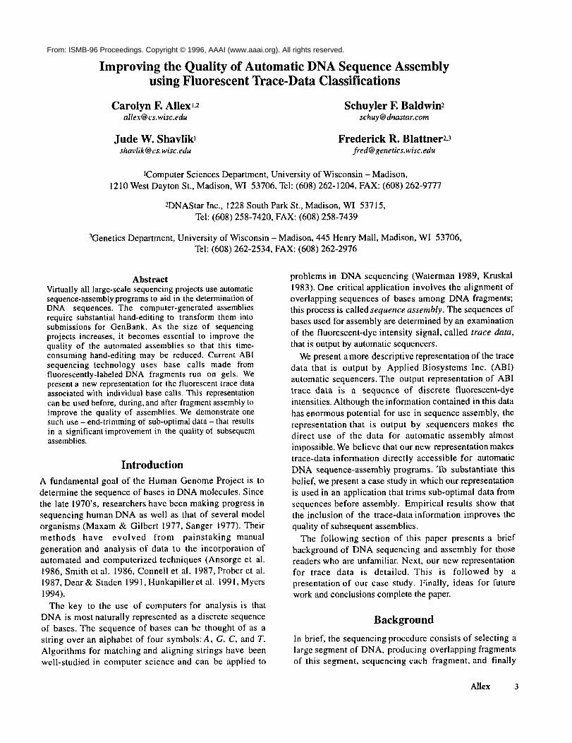
The sets of trace data are used to determine the sequenceof bases in the fragment; this is referred to as base calling.The four sets of trace data are kept synchronized as theyare scanned during base calling. The sequencer expects tocall a base at fairly regular intervals and calls exactly onebase for each of these intervals of trace data (Perkin Elmer1995). There are usually about ten trace-data points perinterval, and a record is kept ot" the points at which thecalls are made.

Trace

A

/\ _./\/

/\

_j"N

Figure 2. Sequence base calls and corresponding sets of tracedata. The sequencer calls the base with the highest trace valueunless two or more values are similar (in which case it calls anN). Gray lines indicate where base calls are made.

The sequencer calls the bases in order as it scans thetrace data. Calls are made by examining the values of thetrace data. Ideally, the trace values for one base aresubstantially higher than those for the other three. In thiscase, the base corresponding to that trace is the one that iscalled. Sometimes the trace values for two or morepossible bases are similar. In this case, the sequencermakes a no-call and labels the base with an N. The goal isto obtain the exact sequence of bases that is thecomplement of the fragment. In practice, the accuracy ofthe base calls made by modern sequencers is 98-99%(Chen 1994, Kelley 1994). A sequence of base calls andcorresponding trace data is depicted in Figure 2.

Sequence Assembly

When all the fragments of the original DNA segment ofinterest have been sequenced, we proceed to assemblingthe fragments into larger segments (McCombie & Martin-Gallardo 1994, Myers 1994, Rowen & Koop 1994). Thefragments overlap, so we can produce this assembly byaligning the overlapping regions of the sequences. Acomputer assembly program uses an approximate string-alignment algorithm to find the optimal alignment of thesequences of base calls (Needleman & Wunsch 1970,Martinez 1983). A consensus of the base calls iscomputed; this forms a contiguous sequence of DNA thatis known as a contig (Staden 1980). Figure 3 illustratesthis idea.

Sequence 1:Sequence 2:Sequence 3:

CCCGGGGCAATTGGGGCAATTAGCCCTTC

AATTAGCCCTTCCCACG

Consensus: CCCGGGGCAATTAGCCCTTCCCACG

Figure 3. Three overlapping fragments aligned to determinethe sequence of a larger segment of DNA. The base sequenceof this segment is the consensus of the aligned fragments.

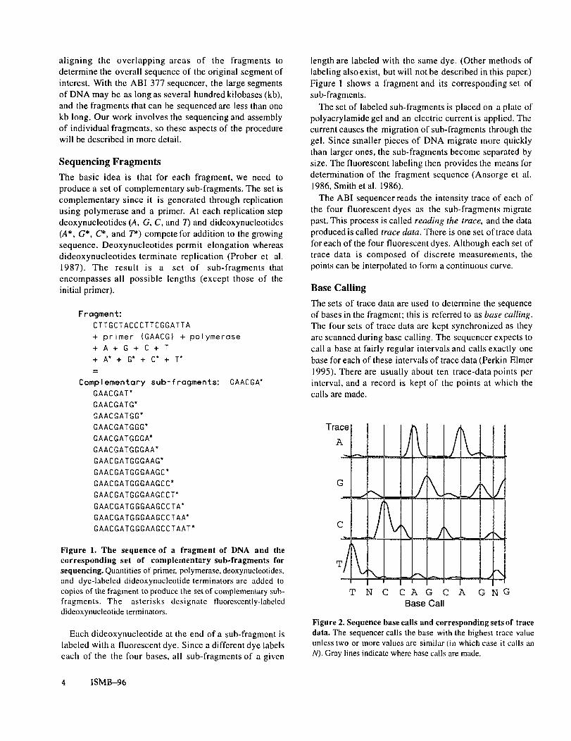
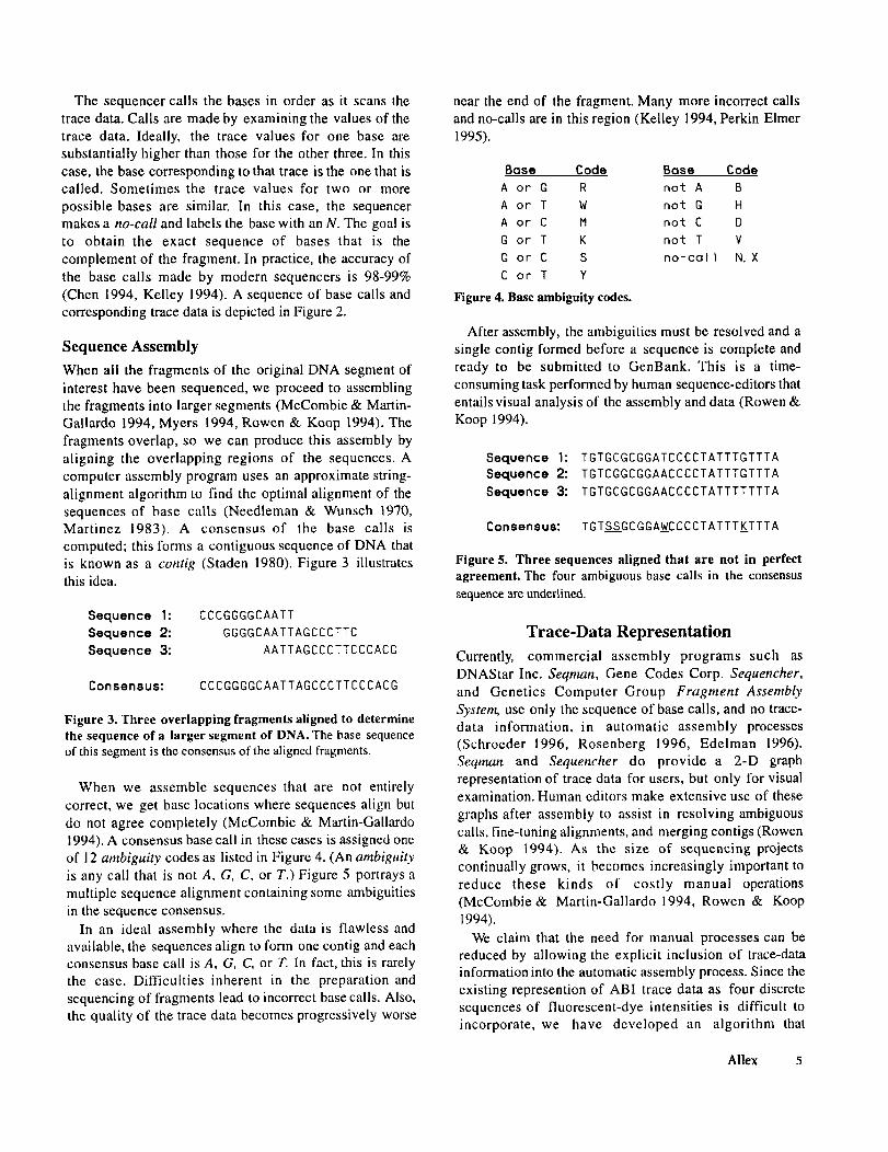
When we assemble sequences that are not entirelycorrect, we get base locations where sequences align butdo not agree completely (McCombie & Martin-Gallardo1994). A consensus base call in these cases is assigned oneof 12 ambigui~, codes as listed in Figure 4. (An ambigui~"is any call that is not A, G, C, or T.) Figure 5 portrays multiple sequence alignment containing some ambiguitiesin the sequence consensus.

In an ideal assembly where the data is flawless andavailable, the sequences align to form one contig and eachconsensus base call is A, G, C, or T. In fact, this is rarelythe case. Difficulties inherent in the preparation andsequencing of fragments lead to incorrect base calls. Also,the quality of the trace data becomes progressively worse

near the end of the fragment. Many more incorrect callsand no-calls are in this region (Kelley 1994, Perkin Elmer1995).

Base Code Base CodeA or G R not A BA or T W not g HA or C H not C Dg or T K not T VG or C S no-call N.XC or T Y

Figure 4. Base ambiguity codes.

After assembly, the ambiguities must be resolved and asingle contig formed before a sequence is complete andready to be submitted to GenBank. This is a time-consuming task performed by human sequence-editors thatentails visual analysis of the assembly and data (Rowen Koop 1994).

Sequence 1:Sequence 2:Sequence 3:

TGTGCGCGGATCCCCTATTTGTTTATGTCGGCGGAACCCCTATTTGTTTATGTGCGCGGAACCCCTATTTTTTTA

Consensus: TGTSSGCGGAWCCCCTATTTKTTTA

Figure 5. Three sequences aligned that are not in perfectagreement. The four ambiguous base calls in the consensussequence are underlined.

Trace-Data Representation

Currently, commercial assembly programs such asDNAStar Inc. Seqman, Gene Codes Corp. Sequencher,and Genetics Computer Group Fragment AssemblySysten~ use only the sequence of base calls, and no trace-data information, in automatic assembly processes(Schroeder 1996, Rosenberg 1996, Edelman 1996).Seqman and Sequencher do provide a 2-D graphrepresentation of trace data for users, but only for visualexamination. Human editors make extensive use of thesegraphs after assembly to assist in resolving ambiguouscalls, fine-tuning alignments, and merging contigs (Rowen& Koop 1994). As the size of sequencing projectscontinually grows, it becomes increasingly important toreduce these kinds of costly manual operations(McCombie & Martin-Gallardo 1994, Rowen & Koop1994).

We claim that the need for manual processes can bereduced by allowing the explicit inclusion of trace-datainformation into the automatic assembly process. Since theexisting represention of ABI trace data as four discretesequences of fluorescent-dye intensities is difficult toincorporate, we have developed an algorithm that

Allex 5

transforms the trace data into a visually-descriptiverepresentation that is usable in assembly programs.

The trace-data output from an ABI DNA sequencer isfound in the data files of the ABI Analysis program. Thereare four sets of data for a fragment of DNA - one for eachof the four fluorescent dyes. The trace data appears in twofl~rms; one is a sequence of raw intensities, and in theother, the data has been processed such that trace peaks aremore distinct and uniform. It is the processed data that isused to produce the graphs made available to users ofSeqman and Sequencher. While studying the graphs,sequence editors pay particular attention to the rclativeintensities and characteristic shapes of trace data. It is ameasure of these shapes and relative intensities found inthe graphs of processed data that we describe in ourrepresentation. By capturing this information, we canmake available to an assembly program the sameinformation that is available to editors.

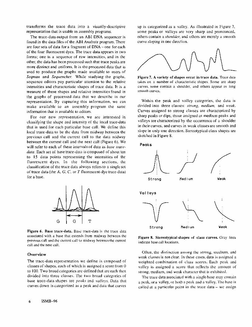
For our new rcpresentation, we are interested inclassifying the shape and intensity of the local trace-datathat is used for each particular base call. We define thislocal trace-data to be the data from midway between theprevious call and the current call to the data midwaybetween the current call and the next call (Figure 6). will refer to each of these intervals of data as base trace-data. Each set of base trace-data is composed of about tento 15 data points representing the intensities of thefluorescent dyes. In the following sections, thechtssification of the trace data always refers to a single setof trace data (the A, G, C, or T fluorescent-dye trace-data)for a base.

G G

Figure 6. Base trace-data. Base trace-data is the trace dataassociated with a base that extends from midway between theprevious call and the current call t~ midway between the currentcall and the next call.

Overview

The trace-data representation we define is composed ofclasses of shapes, each of which is assigned a score from 0to 100. Two broad categories are defined that arc each thendivided into three classes. The two broad categories ofbase trace-data shapes are peaks and valleys. Data thatcurves down is categorized as a peak and data that curves

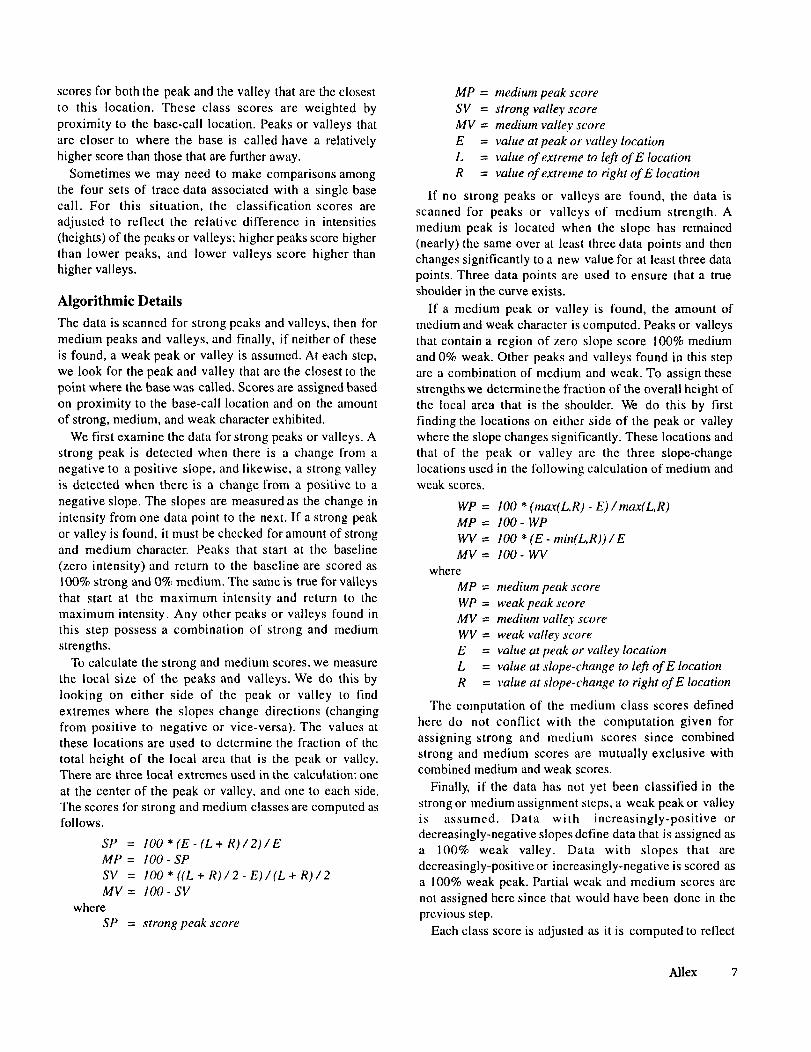
up is categorized as a valley. As illustrated in Figure 7,some peaks or valleys are very sharp and pronounced,others contain a shoulder, and others are merely a smoothcurve sloping in one direction.

Figure 7. A variety of shapes occur in trace data. Trace datatakes on a number of characteristic shapes. Some are sharpcurves, some contain a shoulder, and others appear as longsmooth curves.

Within the peak and valley categories, the data isdivided into three classes: strong, medium, and weak.Curves assigned Io strong classes are characterized bysharp peaks or dips, those assigned as medium peaks andvalleys are characterized by the occurrence of a shoulderin their curves, and curves in weak classes are smooth andslope in only one direction. Stereotypical class shapes aresketchedin Figum 8.

Peaks

i.

Strong Hed um Weak

Va I I eys

~,

Strong F1edl um Weak

Figure 8. Stereotypical shapes of class curves. Gray linesindicate base call locations.

Often, the distinction among the strong, medium, andweak classes is not clear. In these cases, data is assigned aweighted combination of class scores. Each peak andvalley is assigned a score that reflects the amount ofstrong, medium, and weak character that is exhibited.

The trace data associated with a single base may containa peak, era valley, or both a peak and a valley. The base iscalled at a particular point in the tracc data - wc assign

6 ISMB-96

scores for both the peak and the valley that are the closestto this location. These class scores are weighted byproximity to the base-call location. Peaks or valleys thatare closer to where the base is called have a relativelyhigher score than those that are further away.

Sometimes we may need to make comparisons amongthe four sets of trace data associated with a single basecall. For this situation, the classification scores areadjusted to reflect the relative difference in intensities(heights) of the peaks or valleys; higher peaks score higherthan lower peaks, and lower valleys score higher thanhigher valleys.

Algorithmic Details

The data is scanned for strong peaks and valleys, then formedium peaks and valleys, and finally, if neither of theseis found, a weak peak or valley is assumed. At each step,we look for the peak and valley that are the closest to thepoint where the base was called. Scores are assigned basedon proximity to the base-call location and on the amountof strong, medium, and weak character exhibited.

We first examine the data for strong peaks or valleys. Astrong peak is detected when there is a change from anegative to a positive slope, and likewise, a strong valleyis detected when there is a change from a positive to anegative slope. The slopes are measured as the change inintensity from one data point to the next. If a strong peakor valley is found, it must be checked for amount of strongand medium character. Peaks that start at the baseline(zero intensity) and return to the baseline are scored 100% strong and 0% medium. The same is true for valleysthat start at the maximum intensity and return to themaximum intensity. Any other peaks or valleys found inthis step possess a combination of strong and mediumstrengths.

To calculate the strong and medium scores, we measurethe local size of the peaks and valleys. We do this bylooking on either side of the peak or valley to findextremes where the slopes change directions (changingfrom positive to negative or vice-versa). The values atthese locations are used to determine the fraction of thetotal height of the local area that is the peak or valley.There are three local extremes used in the calculation: oneat the center of the peak or valley, and one to each side.The scores for strong and medium classes are computed asfollows.

SP = IO0*(E-(L+R)/2)/EMP = I00- SPSV = IO0*((L+R)/2-E)/(L+R)/2MV = I00 - SV

whereSP = strong peak score

MP = medium peak scoreSV = strong valley scoreMV = medium valley scoreE = value at peak or valley locationL = value of extreme to left of E locationR = value of extreme to right of E location

If no strong peaks or valleys are found, the data isscanned for peaks or valleys of medium strength. Amedium peak is located when the slope has remained(nearly) the same over at least three data points and thenchanges significantly to a new value for at least three datapoints. Three data points are used to ensure that a trueshoulder in the curve exists.

If a medium peak or valley is found, the amount ofmedium and weak character is computed. Peaks or valleysthat contain a region of zero slope score 100% mediumand 0% weak. Other peaks and valleys found in this stepare a combination of medium and weak. To assign thesestrengths we determine the fraction of the overall height ofthe local area that is the shoulder. We do this by firstfinding the locations on either side of the peak or valleywhere the slope changes significantly. These locations andthat of the peak or valley are the three slope-changelocations used in the following calculation of medium andweak scores.

100 * (n~(L.R) - E) / ma.~(L,R)I00- WP100 * (E- min(L,R)) I00- WV

WP =MP =~W =

MV =where

MP =WP =MV =WV =

E =L =R =

medium peak scoreweak peak scorenzedium valley scoreweak valley scorevalue at peak or valley locationvalue at slope-change to left of E locationvalue at slope-change to right of E location

The computation of the medium class scores definedhere do not conflict with the computation given forassigning strong and medium scores since combinedstrong and medium scores are mutually exclusive withcombined medium and weak scores.

Finally, if the data has not yet been classified in thestrong or medium assignment steps, a weak peak or valleyis assumed. Data with increasingly-positive ordecreasingly-negative slopes define data that is assigned asa 100% weak valley. Data with slopes that aredecreasingly-positive or increasingly-negative is scored asa 100% weak peak. Partial weak and medium scores arenot assigned here since that would have been done in theprevious step.

Each class score is adjusted as it is computed to reflect

AUex 7

the proximity of a peak or valley to the location where thebase was called. The scores are adjusted as follows.

Snew= Sold*(I-IE-BI/N)where

S = a class scoreE = location of peak or valleyB = location of base callN = number of base trace-data points

Peaks and valleys that are closer to where the base wascalled get higher scores.

(a) Existing Representation

Point Value1 392 143 q74 3755 4046 4647 7048 8339 702

10 57011 140112 1321

(b.) 2-D Graph Representation

8

7 ~ 9

%12

(c)New Representation

Base Trace-Data Classification ScoresSP MP WP SV MV WV60 32 0 0 74 17

(65) (35) (0) (0) (81) {19)

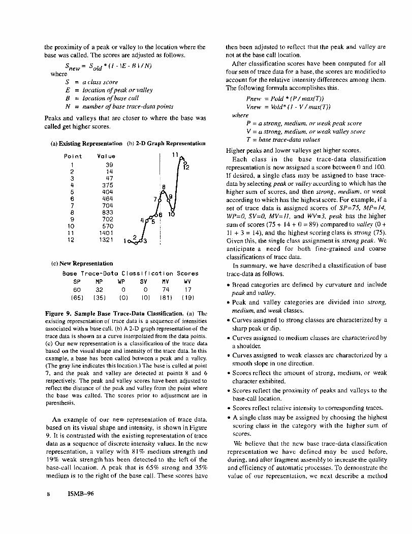
Figure 9. Sample Base Trace-Data Classification. (a) Theexisting representation of trace data is a sequence of intensitiesassociated with a base call. (b) A 2-D graph representation of thetrace data is shown as a curve interpolated from the data points.(c) Our new representation is a classification of the trace databased on the visual shape and intensity of the trace data. In thisexample, a base has been called between a peak and a valley.(The gray line indicates this location.) The base is called at point7, and the peak and valley are detected at points 8 and 6respectively. The peak and valley scores have been adjusted toreflect the distance of the peak and valley from the point wherethe base was called. The scores prior to adjustment are inparenthesis.

An example of our new representation of trace data,based on its visual shape and intensity, is shown in Figure9. It is contrasted with the existing representation of tracedata as a sequence of discrete intensity values. In the newrepresentation, a valley with 81% medium strength and19% weak strength has been detected to the left of thebase-call location. A peak that is 65% strong and 35%medium is to the right of the base call. These scores have

8 ISMB-96

then been adjusted to reflect that the peak and valley arenot at the base call location.

After classification scores have been computed for allfour sets of trace data for a base, the scores are modified toaccount for the relative intensity differences among them.The following formula accomplishes this.

Pnew = Pold * (P/max(T))Vnew = VoM* (1 - V/max(T))

whereP = a strong, medium, or weak peak scoreV = a strong, medium, or weak valley scoreT = base trace-data values

Higher peaks and lower valleys get higher scores.Each class in the base trace-data classification

representation is now assigned a score between 0 and 100.If desired, a single class may be assigned to base trace-data by selecting peak or valley according to which has thehigher sum of scores, and then strong, medium, or weakaccording to which has the highest score. For example, if aset of trace data is assigned scores of SP=75, MP=14,WP=O, SV=O, MV=I1, and WV=3, peak has the highersum of scores (75 + 14 + 0 = 89) compared to valley (0 I1 + 3 = 14), and the highest scoring class is strong (75).Given this, the single class assignment is strong peak. Weanticipate a need for both fine-grained and coarseclassifications of trace data.

In summary, we have dcscribed a classification of basetrace-data as follows.

¯ Broad categories are defined by curvature and includepeak and valley.

¯ Peak and valley categories are divided into strong,medium, and weak classes.

¯ Curves assigned to strong classes are characterized by asharp peak or dip.

¯ Curves assigned to medium classes are characterized bya shoulder.

¯ Curves assigned to weak classes are characterized by asmooth slope in one direction.

¯ Scores reflect the amount of strong, medium, or weakcharacter exhibited.

¯ Scores reflect the proximity of peaks and valleys to thebase-call location.

¯ Scores reflect relative intensity to corresponding traces.¯ A single class may be assigned by choosing the highest

scoring class in the category with the higher sum ofscores.

We believe that the new base trace-data classificationrepresentation we have defined may be used before,during, and after fragment assembly to increase the qualityand efficiency of automatic processes. To demonstrate thevalue of our representation, we next describe a method

that successfully uses base trace-data classifications in animportant pre-assembly step.

Case Study: End-Trimming

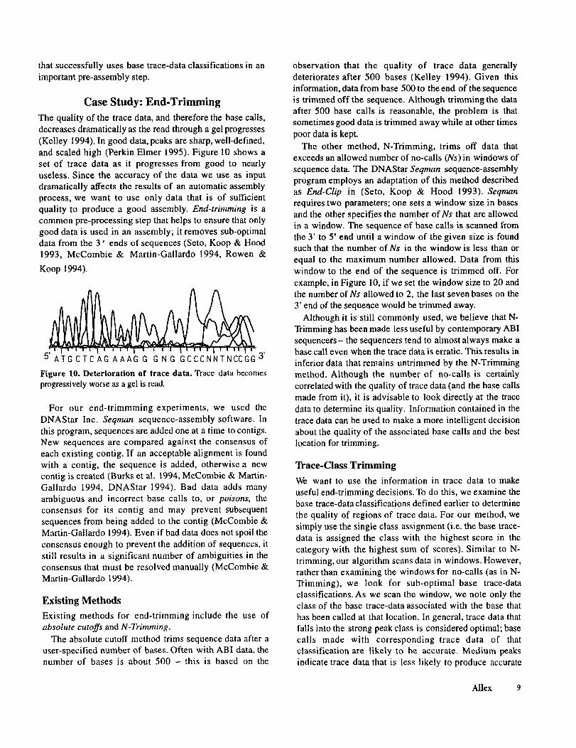
The quality of the trace data, and therefore the base calls,decreases dramatically as the read through a gel progresses(Kelley 1994). In good data, peaks arc sharp, well-defined,and scaled high (Perkin Elmer 1995). Figure 10 shows set of trace data as it progresses from good to nearlyuseless. Since the accuracy of the data we use as inputdramatically affects the results of an automatic assemblyprocess, we want to use only data that is of sufficientquality to produce a good assembly. End-trimming is acommon pre-processing step that helps to ensure that onlygood data is used in an assembly; it removes sub-optimaldata from the 3’ ends of sequences (Seto, Koop & Hood1993, McCombie & Martin-Gallardo 1994, Rowen &

Koop 1994).

5~-] F-,’,T, -I I I t 1~ ,,r l,lIIll,,,l,3,AI’IGCTCAG AAAG G GNG GCCCNNTNCCGG

Figure 10. Deterioration of trace data. Trace data becomesprogressively worse as a gel is read.

For our end-trimmming experiments, we used theDNAStar Inc. Seqman sequence-assembly software. Inthis program, sequences are added one at a time to contigs.New sequences are compared against the consensus ofeach existing contig. If an acceptable alignment is foundwith a contig, the sequence is added, otherwise a newcontig is created (Burks et al. 1994, McCombie & Martin-Gallardo 1994, DNAStar 1994). Bad data adds manyambiguous and incorrect base calls to, or poisons, theconsensus for its contig and may prevent subsequentsequences from being added to the contig (McCombie Martin-Gallardo 1994). Even if bad data does not spoil theconsensus enough to prevent the addition of sequences, itstill results in a significant number of ambiguities in theconsensus that must be resolved manually (McCombie Martin-Gallardo 1994).

Existing Methods

Existing methods for end-trimming include the use ofabsolute cutoffs and N-Trimming.

The absolute cutoff method trims sequence data after auser-specified number of bases. Often with ABI data, thenumber of bases is about 500 - this is based on the

observation that the quality of trace data generallydeteriorates after 500 bases (Kelley 1994). Given thisinformation, data from base 500 to the end of the sequenceis trimmed off the sequence. Although trimming the dataafter 500 base calls is reasonable, the problem is thatsometimes good data is trimmed away while at other timespoor data is kept.

The other method, N-Trimming, trims off data thatexceeds an allowed number of no-calls (Ns) in windows ofsequence data. The DNAStar Seqman sequence-assemblyprogram employs an adaptation of this method describedas End-Clip in (Seto, Koop & Hood 1993). Seqmanrequires two parameters; one sets a window size in basesand the other specifies the number of Ns that are allowedin a window. The sequence of base calls is scanned fromthe 3’ to 5’ end until a window of the given size is foundsuch that the number of Ns in the window is less than orequal to the maximum number allowed. Data from thiswindow to the end of the sequence is trimmed off. Forexample, in Figure 10, if we set the window size to 20 andthe number of Ns allowed to 2, the last seven bases on the3’ end of the sequence would be trimmed away.

Although it is still commonly used, we believe that N-Trimming has been made less useful by contemporary ABIsequencers- the sequencers tend to almost always make abase call even when the trace data is erratic. This results ininferior data that remains untrimmed by the N-Trimmingmethod. Although the number of no-calls is certainlycorrelated with the quality of trace data (and the base callsmade from it), it is advisable to look directly at the tracedata to determine its quality. Information contained in thetrace data can be used to make a more intelligent decisionabout the quality of the associated base calls and the bestlocation for trimming.

Trace-Class Trimming

We want to use the information in trace data to makeuseful end-trimming decisions. To do this, we examine thebase trace-data classifications defined earlier to determinethe quality of regions of trace data. For our method, wesimply use the single class assignment (i.e. the base trace-data is assigned the class with the highest score in thecategory with the highest sum of scores). Similar to N-trimming, our algorithm scans data in windows. However,rather than examining the windows for no-calls (as in N-Trimming), we look for sub-optimal base trace-dataclassifications. As we scan the window, we note only theclass of the base trace-data associated with the base thathas been called at that location. In general, trace data thatfalls into the strong peak class is considered optimal; basecalls made with corresponding trace data of thatclassification are likely to be accurate. Medium peaksindicate trace data that is less likely to produce accurate

Allex 9

base calls, and weak peaks and valleys indicate unreliablebase calls.

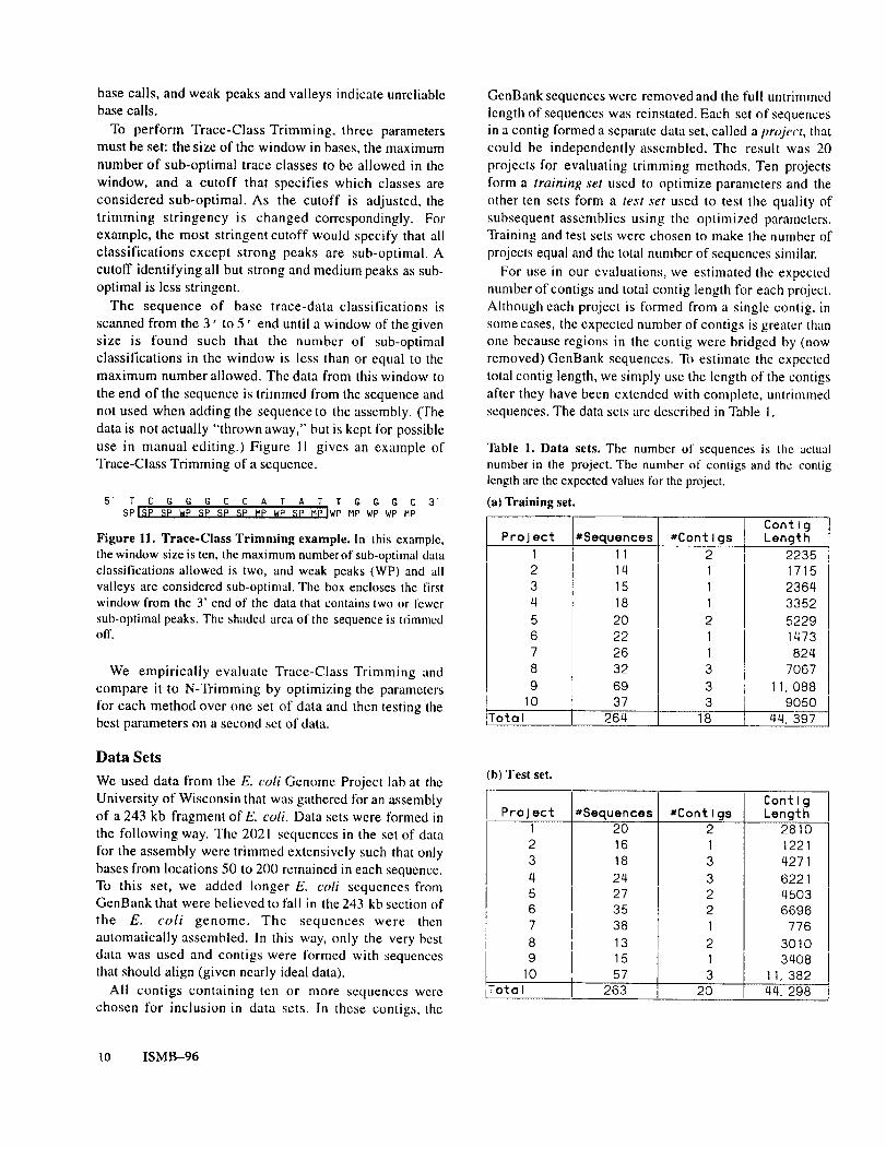
To perform Trace-Class Trimming, three parametersmust be set: the size of the window in bases, the maximumnumber of sub-optimal trace classes to be allowed in thewindow, and a cutoff that specifies which classes areconsidered sub-optimal. As the cutoff is adjusted, thetrimming stringency is changed correspondingly. Forexample, the most stringent cutoff would specify that allclassifications except strong peaks are sub-optimal. Acutoff identifying all but strong and medium peaks as sub-optimal is less stringent.

The sequence of base trace-data classifications isscanned from the 3’ to 5’ end until a window ofthegivensize is found such that the number of sub-optimalclassifications in the window is less than or equal to themaximum number allowed. The data from this window tothe end of the sequence is trimmed from the sequence andnot used when adding the sequence to the asscmbly. (Thedata is not actually "thrown away," but is kept lbr possibleuse in manual editing.) Figure 11 gives an example ofTrace-Class Trimming of a sequence.

5 T C G G G C C A T A T r (; (~ 11 C SP|SP SP WP SP SP SP MP WP ,SP ~PJWP MP WP WP i’IP

Figure II. Trace-Class Trimming example. In this example,the window size is ten. the maximum numberof sub-optimal dataclassifications allowed is two, and weak peaks (WP) and allvalleys are considered sub-optimal. The box encloses the firstwindow from the 3’ end of the data that contains two or fewersub-optimal peaks. The shaded area of the sequence is trimmedoff.

We empirically evaluate Trace-Class Trimming andcompare it to N-Trimming by optimizing the parametersfor each method over one set of data and then testing thebest parameters on a second set of data.

Data Sets

We used data from the E. coli Genome Project lab at theUniversity of Wisconsin that was gathered for an assemblyof a 243 kb fragment of E. coli. Data sets were formed inthe following way. The 2021 sequences in the set of datafor the assembly were trimmed extensively such that onlybases from locations 50 to 200 remained in each sequence.To this set, we addcd longer E. coli sequences fromGenBank that were believed to fall in the 243 kb section ofthe E. coli genome. The sequences were thenautomatically assembled. In this way, only the very bestdata was used and contigs were formed with sequencesthat should align (given ncarly ideal data).

All contigs containing ten or more sequences werechosen for inclusion in data sets. In these contigs, the

10 ISMB--96

GenBank sequences were removed and the full untrimmedlength of sequences was reinstated. Each set of sequencesin a contig formed a separate data set, called a project, thatcould be independently assembled. The result was 20projects for evaluating trimming methods. Ten projectsform a training set used to optimize parameters and theother ten sets form a test set used to test the quality ofsubsequent assemblies using the optimized parameters.Training and test sets were chosen to make the number ofprojects equal and the total numbcr of sequences similar.

For use in our evaluations, we estimated the expectednumber of contigs and total contig length for each project.Although each project is formed from a single contig, insome cases, the expected number of contigs is greater thanone because regions in the contig were bridged by (nowremoved) GenBank sequences. To estimate the expectedtotal contig length, we simply use the length of the contigsafter they have been extended with complete, untrimmedsequences. The data scts are described in Table 1.

Table 1. Data sets. The number of sequences is the actualnumber in the project. The number of contigs and the contiglength are the expected values for the project.

(a) Training set.

ContlgProJect #Sequences #Contlgs Length

1 11 2 I 22352 14 1 17153 15 1 23644 18 1 33525 20 2 52296 22 1 14737 26 1 8248 32 3 i 7o679 69 3 ; 11,088

lO 37 3 = 9050Total 264 18 44, 397

(b) "rest set.

ContlgProject #Sequences #Contlgs Length

1 20 2 28102 16 1 12213 18 3 42714 24 3 62215 27 2 45036 35 2 66967 38 1 7768 13 2 30109 15 1 3408

lo 57 3 11. 382Total 263 i 20 44, 298

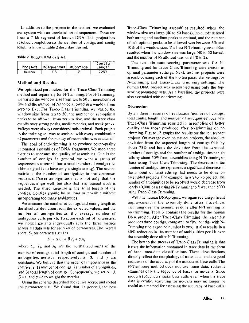
In addition to the projects in the test set, we evaluatedour system with an unrelated set of sequences. These arefrom a 7 kb segment of human DNA. This project hasreached completion so the number of contigs and contiglength is known. Table 2 describes this set.

Table 2. Human DNA data set.

ContlgProJect #Sequences #Contlgs Lengthhuman 98 2 7257

Method and Results

We optimized parameters for the Trace-Class Trimmingmethod and separately for N-Trimming. For N-Trimming,we varied the window size from ten to 50 in increments offive and the number of Ns to be allowed in a window fromzero to five. For Trace-Class Trimming, we varied thewindow size from ten to 50, the number of sub-optimalpeaks to be allowed from zero to five, and the trace classcutoffs over strong peaks, medium peaks, and weak peaks.Valleys were always considered sub-optimal. Each projectin the training set was assembled with every combinationof parameters and the quality of assemblies was evaluated.

The goal of end-trimming is to produce better-qualityautomated assemblies of DNA fragments. We used threemetrics to measure the quality of assemblies. One is thenumber of contigs. In general, we want a group ofsequences to assemble into a small number of contigs (theultimate goal is to have only a single contig). The secondmetric is the number of ambiguities in the consensussequence. Fewer ambiguities means not only that thesequences align well, but also that less manual work isneeded. The third measure is the total length of thecontigs. Contigs should be as long as possible withoutincorporating too many ambiguities.

We measure the number of contigs and contig length asthe absolute deviation from the expected values, and thenumber of ambiguities as the average number ofambiguous calls per kb. To score each set of parameters,we normalize and individually sum the three metricsacross all data sets for each set of parameters. The overallscore, Si, for parameter set i is

Si= otCi + ~Ti + YAiwhere Ci, Ti, and Ai are the normalized sums of the

number of contigs, total length of contigs, and number ofambiguities metrics, respectively; a, ~, and y areconstants. We believe that the order of importance of themetrics is: 1) number of contigs, 2) number of ambiguities,and 3) total length of contigs. Consequently, we set a =3.

=1, and y=2 to weight the metrics.Using the scheme described above, we scored and sorted

the parameter sets. We found that, in general, the best

Trace-Class Trimming assemblies resulted when thewindow size was large (40 to 50 bases), the cutoff definedboth strong and medium peaks as optimal, and the numberof sub-optimal peaks to be allowed was between 5% and10% of the window size. The best N-Trimming assembliesresulted when the window size was large (40 to 50 bases),and the number of Ns allowed was small (0 to 2).

The ten minimum scoring parameter sets for N-Trimming and for Trace-Class Trimming were chosen asoptimal parameter settings. Next, test set projects wereassembled using each of the top ten parameter settings tbrN-Trimming and Trace-Class Trimming settings. Thehuman DNA project was assembled using only the top-scoring parameter sets. As a baseline, the projects werealso assembled with no trimming.

Discussion

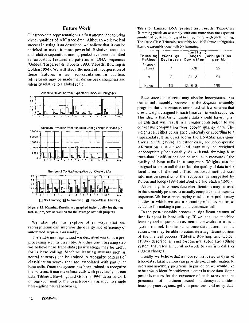
By all three measures of evaluation (number of contigs,total contig length, and number of ambiguities), our newTrace-Class Trimming resulted in assemblies of betterquality than those produced after N-Trimming or notrimming. Figure 12 graphs the results for the ten test-setprojects. On average over the test-set projects, the absolutedeviation from the expected length of contigs falls byabout 75% and both the deviation from the expectednumber of contigs and the number of ambiguities per kbfalls by about 50% from assemblies using N-Trimming tothose using Trace-Class Trimming. The decrease in thenumber of ambiguities represents a significant decrease inthe amount of hand editing that needs to be done onassembled projects. For example, in a 243 kb project, thenumber of ambiguities to be resolved would decrease fromnearly 10,000 bases using N-Trimming to fewer than 5000using Trace-Class Trimming.

With the human DNAproject, we again see a significantimprovement in the assembly done after Trace-ClassTrimming over the assemblies done after N-Trimming orno trimming. Table 3 contains the results for the humanDNA project. After Trace-Class Trimming, the assemblyproduces three contigs, compared to five contigs with N-Trimming (the expected number is two). It also results in 40% reduction in the number of ambiguities per kb overthe assembly done after N-Trimming.

The key to the success of Trace-ClassTrimming is thatit uses the information contained in trace data in the formof base trace-data classifications. These classificationsdirectly reflect the morphology of trace data, and are goodindicators of the accuracy of the associated base calls. TheN-Trimming method does not use trace data, rather itexamines only the sequence of bases for no-calls. Sincemodern sequencers make base calls even when the tracedata is erratic, searching for no-calls may no longer beuseful as a method for assessing the accuracy of base calls.

Allex 11

Future WorkOur trace-data representation is a first attempt at capturingvisual qualities of ABI trace data. Although we have hadsuccess in using it as described, we believe that it can beenriched to make it more powerful. Relative intensitiesand relative separations among peaks have been identifiedas important features in patterns of DNA sequences(Golden, Torgersen & Tibbetts 1993, Tibbetts, Bowling Golden 1994). We will study the merit of incorporation ofthese features in our representation. In addition,refinements may be made that define peak sharpness andintensity relative to a global scale.

Absolute Deviation from Expected Number el Contigs (C~)4o ~~] =| II ’

/ |__I |_ I~ L I [ 0r_T ....... .....20 ..... ~ .............

i~-

0 I 1 I 2 I :

Absolute Deviation from Expected Contig Length in Bases (Ti)25000 ~i

, [ i2oooo -~L .... --~ ...... ~ .... +--.

15000 "~

1000o -~

Number of Contig Ambiguities per Kilobase (A,)

[] No Trimming [] N-Trimming ~ Trace-Class Trimming

Figure 12. Results. Results are graphed individually for the tentest-set projects as well as for the average over all projects.

We also plan to explore other ways that ourrepresentation can improve the quality and efficiency ofautomated sequence-assembly.

The end-trimmingmethod we described works as a pre-processing step to assembly. Another pre-processing stepwe believe base trace-data classifications may be usefulfor is base calling. Machine learning systems such asneural networks can be trained to recognize patterns ofclassification scores that are associated with particularbase calls. Once the system has been trained to recognizethe patterns, it can make base calls with previously unseendata. Tibbetts, Bowling, and Golden (1994) describe workon one such method that uses trace data as input to simplebase-calling neural networks.

12 ISMB-96

Table 3. Human DNA project test results. Trace-ClassTrimming yields an assembly with one more than the expectednumber of contigs compared to three more with N-Trimming.The Trace-Class Trimming assembly had 40% fewer ambiguitiesthan the assembly done with N-Trimming.

ContlgTrimming #Contlgs Length Ambiguities

Method Deviation ~Devlatlon per kb

Troce-Class 1 576 32

N 3 3113 54

None 13 12. 818 149

Base trace-data classes may also be incorporated intothe actual assembly process. In the Seqman assemblyprogram, the consensus is computed with a scheme thatuses a weight assigned to each base call in each sequence.The idea is that better quality data should have higherweights that will result in a greater contribution to theconsensus computation than poorer quality data. Theweightscan either be assigned uniformly or according to atrapezoidal rule as described in the DNAStar LasergeneUser’s Guide (1994). In either case, sequence-specificinformation is not used and data may be weightedinappropriately for its quality. As with end-trimming, basetrace-data classifications can be used as a measure of thequality of base calls in a sequence. Weights can beassigned to a base call that reflect the quality of data in thelocal area of the call. This proposed method usesinformation specific to the sequence as suggested byRowen and Keep (1994) and Bonfield and Staden (1995).

Alternately, base trace-data classifications may be usedin the assembly process to actually compute the consensussequence. We have encouraging results from preliminarystudies in which we use a summing of class scores asevidence for making a particular consensus call.

In the post-assembly process, a significant amount oftime is spent in hand-editing. If we can use machinelearning techniques such as neural networks to train asystem to look for the same trace-data patterns as theeditors, we may be able to automate a significant portionof the manual process. Tibbetts, Bowling, and Golden(1994) describe a single-sequence automatic editingsystem that uses a neural network to confirm calls orsuggest changes.

Finally, we believe that a more sophisticated analysis oftrace-data classifications can provide useful information tousers and assembly programs. In particular, we would liketo be able to identify problematic areas in trace data. Somepossible causes for the existence of such areas are: thepresence of unincorporated dideoxynucleotides,homopolymer regions, gel compressions, and noisy data.

These regions are generally characterized by trace datathat exhibits concurrent significant intensities or peaksamong the four dye traces (Perkin Elmer 1995). Thisoccurrence can be detected with our trace-datarepresentation and the information gathered can be usedby hand-editors or in automatic processes requiring anassessment of data quality.

Conclusions

The quality and efficiency of automated DNA assembly ofABI-generated sequences can be increased by theincorporation of trace-data information into the process.The visually-oriented base trace-data classes we describeprovide a representation of trace data information thatmakes this incorporation possible. We have shown onesuch use, trimming of sub-optimal data before assembly,that results in better assemblies. Using the base trace-dataclassifications for trimming leads to a decrease in thenumber of contigs, a reduction in ambiguities, and a closerapproximation to the expected contig length. Refinementsof and other uses of our representation are underinvestigation.

Acknowledgments

We thank Mark Craven, Ernest Colantonio, and GuyPlunker for their useful comments on this document.

This research was supported in part by NationalResearch Service Award 5 T32 GM08349 from theNational Institute of General Medical Sciences, and in partby Small Business Innovation Research grant 1 R43GM51680-01 from the Department of Health and HumanServices.

References

Ansorge, W., Sproat, B.S., Stegemann, J., and Schwager,C. 1986. A non-radioactive automated method for DNAsequence determination. Journal of Biochemical andBiophysical Methods 13:315-323.

Burks, C., Engle, M.L., Forrest, S., Parsons, R.J.,Soderlund, C.A., and Stolorz, EE. 1994. Stochasticoptimization tools for genomic sequence assembly. InAdams, M.D., Fields, C., and Venter, J.C., eds.,Automated DNA Sequencing and Analysis 249-259. SanDiego, CA: Academic Press.

Chen, E.Y. t994. The efficiency of automated DNAsequencing. In Adams, M.D., Fields, C., and Venter, J.C.,eds., Automated DNA Sequencing and Analysis 3- I 0. SanDiego, CA: Academic Press.

Conneil, C., Fung, S., Heiner, C., Bridgham, J., Chakerian,

V., Heron, E., Jones, B., Menchen, S., Mordan, W., Raft,M., Recknor, M., Smith, L., Springer, J., Woo, S. andHunkapiller, M. 1987. Automated DNA sequence analysis.BioTechniques 5:342-348.

Dear, S. and Staden, R. 1991. A sequence assembly andediting program for efficient management of largeprojects. Nucleic Acids Research 19:3907-3911.

DNAStar. 1994. Lasergene User’s Guide, Madison, WI.

Edelman, I. 1996. Personal communication.

Golden, J.B. III, Torgersen, D. and "fibbetts, C. 1993.Pattern recognition for automated DNAsequencing: I. On-line signal conditioning and feature extraction forbasecalling. In Proceedings of the First InternationalConference on lntelligent Systems for Molecular Biology,136-134. Bethesda, MD: AAAI Press.

Hunkapiller, T., Kaiser, R.J., Koop, B.E and Hood, L.1991. Large-scale and automated DNA sequencedetermination. Science 254: 59-67.

Kelley, J.M. 1994. Automated dye-terminatorDNAsequencing. In Adams, M.D., Fields, C., and Venter, J.C.,eds., AutomatedDNA Sequencing and Analysis, 175-181.San Diego, CA: Academic Press.

Kruskal, J.B. 1983. An overview of sequence comparison.In Sankoff, D., Kruskal, J.B., eds., Time Warps, StringEdits, and Macromolecules: The Theory and Practice ofSequence Comparison 1-44. Reading, MA: Addison-Wesley Publishing Company, Inc.

Martinez, H.M. 1983. An efficient method for findingrepeats in molecular sequences. Nucleic Acids Research11:4629-4634.

Maxam, A.M. and Gilbert, W. 1977. A new method forsequencing DNA. Proceedings of the National Academyof Science USA 74:560-564.

McCombie, W.R., and Martin-Gallardo, A. 1994. Large-scale, automated sequencing of human chromosomalregions. In Adams, M.D., Fields, C., and Venter, J.C., eds.,Automated DNA Sequencing and Analysis 159-166. SanDiego, CA: Academic Press.

Myers, E.W. 1994. Advances in sequence assembly. InAdams, M.D., Fields, C., and Venter, J.C., eds.,Automated DNA Sequencing and Analys& 231-238. SanDiego, CA: Academic Press.

AUex 13

Needleman, S.B. and Wunsch, C.D. 1970. A generalmethod applicable to the search for similarities in theamino acid sequence of two proteins. Journal ofMolecular Biology 48:443-453.

Perkin Elmer. 1995. DNA Sequencing: Chemistry Guide.Foster City, CA.

Prober, J.M., Trainor, G.L., Dam, R.J., Hobbs, EW.,Robertson, C.W., Zagursky, R.J., Cocuzza, A.J., Jensen,M.A. and Baumeister, K. 1987. A system for rapid DNAsequencing with fluorescent chain-terminatingdideoxynucleotides. Science 238:336-34 I.

Rosenberg, D. 1996. Personal Communication.

Rowen, L., and Koop, B.E 1994. Zen and the art of large-scale genomic sequencing. In Automated DNA Sequencingand Anah,sis 167-174. San Diego, CA: Academic Press.

Schroeder, J. 1996. Personal communication.

Sanger, E, Nicklen, S. and Coulson, A.R. 1977. DNAsequencing with chain-terminating inhibitors. Proceedingsof the National Academy of Science USA 74:5463-5467.

Seto, D., Koop, B.E and Hood, L. 1993. Anexperimentally derived data set constructed for testinglarge-scale DNA sequence assembly algorithms.Genomics ! 5:673-676.

Smith, L.M., Sanders, J.Z., Kaiser, R.J., Hughes, P, Dodd,C., Connell, C.R., Heiner, C., Kent, S.B.H. and Hood, L.E.1986. Fluorescence detection in automated DNA sequenceanalysis. Nature 321:674-679.

Staden, R. 1980. A new computer method for the storageand manipulation of DNA gel reading data. Nucleic AcidsResearch 8:3673-3694.

Tibbetts, C., Bowling, J.M. and Golden, J.B. III. 1994.Neural networks for automated base-calling of gel-basedDNA sequencing laddcrs. In Adams, M.D., Ficlds, C., andVenter, J.C., eds., Automated DNA Sequencing andAnalysis 219-230. San Diego, CA: Academic Press,

Waterman, M.S. 1989. Sequence alignments. InWaterman, M.S., ed., Mathematical Methods for DNASequences 54-92. Boca Raton, FL: CRC Press.

14 ISMB-96