Automatic Model Transformation from UML Sequence Diagrams ... · Automatic Model Transformation from UML Sequence ... B.1 Automatic Model Transformation from UML Sequence ... 2.1

FACULDADE DE ENGENHARIA DA UNIVERSIDADE DO PORTO

Automatic Model Transformation fromUML Sequence Diagrams to Coloured

Petri Nets

João António Custódio Soares

Mestrado Integrado em Engenharia Informática e Computação

Supervisor: João Carlos Pascoal Faria

Co-Supervisor: Bruno Miguel Carvalhido Lima

July 19, 2017

Automatic Model Transformation from UML SequenceDiagrams to Coloured Petri Nets


Mestrado Integrado em Engenharia Informática e Computação

Approved in oral examination by the committee:

Chair: Ana Cristina Ramada PaivaExternal Examiner: Miguel Carlos Pacheco Afonso Goulão

Supervisor: João Carlos Pascoal Faria

July 19, 2017

Abstract

The dependence of our society on ever more complex software systems makes the task of test-ing and validating this software increasingly important and challenging. In many cases, multipleindependent and heterogeneous systems form a system of systems responsible for providing ser-vices to users, and the current testing automation tools and techniques provide little support forthe performance of this task.

This dissertation is part of a larger scale project that aims to produce a Model-based Testingtool that will automate the process of testing distributed systems, from UML sequence diagrams.These diagrams graphically define the interaction between the different modules of a system andits actors in a sequential way, facilitating the understanding of the system’s operation and allowingthe definition of critical sections of distributed systems such as situations of concurrency andparallelism.

The goal of this dissertation work is to develop one of the components of this project that isresponsible for the conversion of UML Sequence Diagrams, describing key system behaviours,into Coloured Petri Nets. Petri Nets are a modelling formalism that is indicated for describingdistributed systems by their ability to define communication and synchronization tasks, and by thepossibility of executing them in runtime using tools such as CPN Tools.

The objective is to define Model-to-Model translation rules that allow the conversion of mod-els, in order to allow integration with the target system, taking advantage of existing model trans-formation frameworks (EMF - Eclipse Modelling Framework) and model transformation tech-nologies (Epsilon). With this, we are able to hide the complexity of the system analysis to the user(Software Tester) introducing the possibility of automation, generation and execution of tests fromthe diagrams of test cases, and presenting the results visually.

The design of such transformation techniques has been the subject of multiple studies, al-though never fully implemented in a scalable and integrateable way, therefore, the challenge isto implement these rules in an solution that performs this automatic model transformation as astand-alone software component.

In the implemented solution, UML Sequence Diagrams created with the Papyrus visual mod-elling tool are converted to Coloured Petri Nets executable with CPN Tools. It were used existingverified meta models for both the input and output. The transformation rules were implemented inETL (Epsilon Tranformation Language). The most relevant features of UML Sequence Diagramsfor modelling distributed systems are transformed into equivalent Coloured Petri Nets that acceptthe same execution traces (event sequences) as the original models. A case study is also presentedto demonstrate and validate the approach.

i

ii

Resumo

A dependência da sociedade em sistemas de software cada vez mais complexos torna a tarefa detestar e validar estes sistemas cada vez mais importante e desafiante. Em vários casos, múltiplossistemas independentes e heterogéneos formam um sistema de sistemas responsável por providen-ciar serviços aos utilizadores e as ferramentas e técnicas atuais de automação de testes aos mesmosoferecem pouco suporte e apoio para para o desempenho desta tarefa.

Este trabalho está inserido num projeto de maior escala que tem como objetivo produzir umaferramenta de Model-based Testing que automatizará o processo de teste de sistemas distribuídos,a partir de diagramas de sequência UML. Estes diagramas definem graficamente a interação entreos diferentes módulos de um sistema e os seus atores de uma forma sequencial, facilitando acompreensão do funcionamento do sistema e possibilitando a definição de secções críticas dossistemas distribuídos como situações de concorrência e paralelismo.

O objetivo to trabalho desta dissertação é desenvolver um dos componentes deste projeto quetem como objetivo a conversão dos diagramas de sequência UML, que descrevem os comporta-mentos principais do sistema, em Coloured Petri Nets. Petri Nets são um formalismo de modelaçãoque é indicado para descrição de sistemas distribuídos pela sua capacidade de definição de tarefasde comunicação e de sincronização, e pela possibilidade de execução usando ferramentas comoCPN Tools.

O objetivo será a definição de regras de tradução Model-to-Model que permitirão a conver-são de modelos, de modo a possibilitar a integração com o sistema desejado, tirando partido deframeworks existentes de transformação de modelos (EMF - Eclipse Modeling Framework) e tec-nologias de transformação de modelos (Epsilon). Com isto conseguimos esconder a complexidadeda análise do sistema ao utilizador (Software Tester) introduzindo automatição, geração e execuçãode testes a partir dos diagramas de casos de teste, e apresentando os resultados visualmente.

A concepção destas técnicas de transformação de modelos foi alvo de muitos estudos, apesarde não haver uma solução implementada de uma forma escalável e de fácil integração, portanto, odesafio está em implementar uma solução que execute esta transformação automática de modelose que se comporte como um módulo de software independente.

Na solução implementada, diagramas de sequência UML criados com a ferramenta de mode-lação visual Papyrus são convertidos em Coloured Petri Nets capazes de ser executadas usando aferramenta CPN Tools. Foram usados meta modelos existentes e verificados tanto para os mod-elos de entrada como para os modelos de saída. As regras de transformação foram implemen-tadas recorrendo à tecnologia ETL (Epsilon Transformation Language). Os elementos relativosàs funcionalidades mais relevantes para a modelação de sistemas distribuídos dos diagramas desequência UML são tranformados em Coloured Petri Nets equivalentes que aceitam os mesmostraços de execução (sequência de eventos) que os modelos originais. Um caso de estudo é tambémapresentado para demonstrar o funcionamento da solução e validar a abordagem.

iii

iv

Agradecimentos

Após um período de quase um ano, finalmente chegou o dia de escrever os agradecimentos comoos últimos retoques na minha dissertação de Mestrado. Foi um período de aprendizagem inte-siva para mim, não só a nível científico, como também a um nível pessoal. Esta fase da minhaformação, que está agora no término, teve grande impacto na minha vida e, por isso, após muitareflexão e introspecção, gostaria de atribuir o devido reconhecimento a todas as pessoas que meapoiaram, suportaram e acima de tudo, me ajudaram a crescer ao longo deste período.

Em primeiro lugar, gostaria de agradecer ao meu orientador, o professor João Pascoal Faria,pelas ideias, disponibilidade, apoio e acompanhamento ao longo do desenvolvimento deste tra-balho.

Em segundo lugar, gostaria de agradecer ao meu co-orientador, o professor Bruno Lima, pelaajuda, pelas opiniões e, acima de tudo, pela dedicação que apresentou ao auxiliar-me com o de-senvolvimento deste trabalho.

Em terceiro lugar, gostaria de agradecer aos meus colegas que me acompanharam ao longodeste percurso pela companhia, companheirismo e paciência que apresentaram para comigo.

Por último, mas não menos importante, gostaria de agradecer ao meu irmão e aos meus paispor todo o amor, apoio incondicional, por tudo o que me ensinaram e por tudo o que fizeram pormim ao longo do meu percurso académico e da minha vida. Não teria sido possível sem vocês.


v

vi

“The beautiful thing about learningis nobody can take it away from you.”

B. B. King

vii

viii

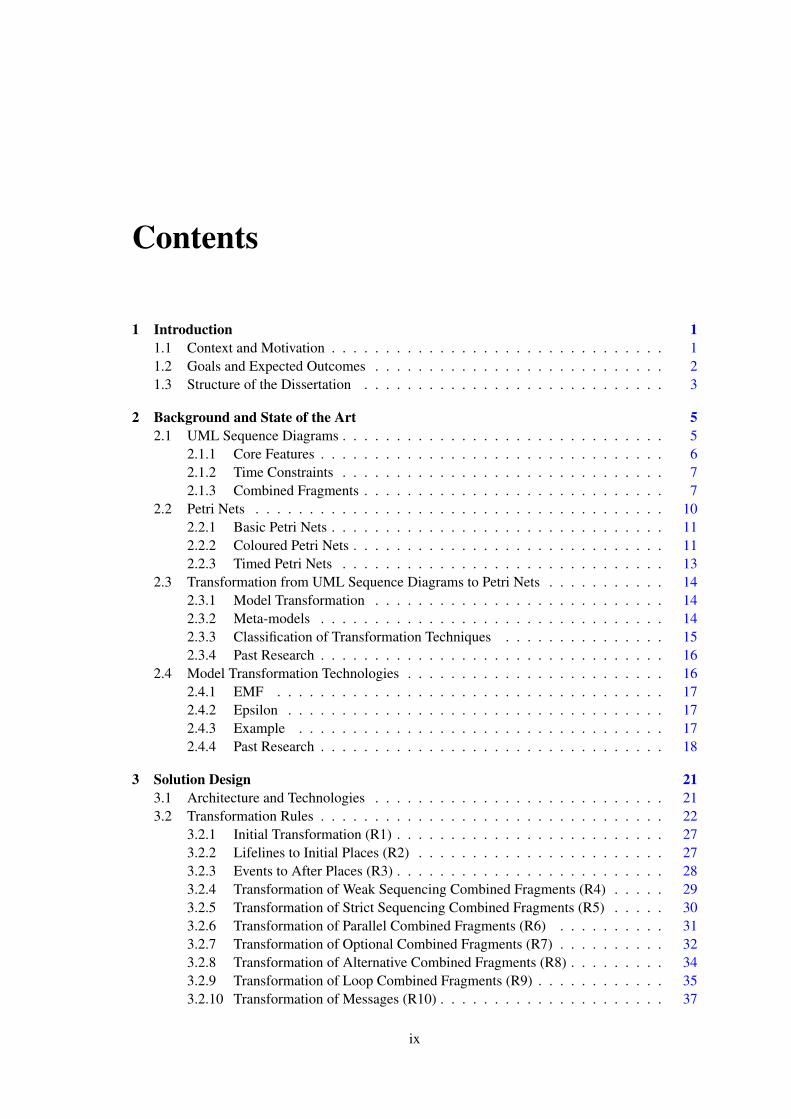
Contents

1 Introduction 11.1 Context and Motivation . . . . . . . . . . . . . . . . . . . . . . . . . . . . . . . 11.2 Goals and Expected Outcomes . . . . . . . . . . . . . . . . . . . . . . . . . . . 21.3 Structure of the Dissertation . . . . . . . . . . . . . . . . . . . . . . . . . . . . 3

2 Background and State of the Art 52.1 UML Sequence Diagrams . . . . . . . . . . . . . . . . . . . . . . . . . . . . . . 5

2.1.1 Core Features . . . . . . . . . . . . . . . . . . . . . . . . . . . . . . . . 62.1.2 Time Constraints . . . . . . . . . . . . . . . . . . . . . . . . . . . . . . 72.1.3 Combined Fragments . . . . . . . . . . . . . . . . . . . . . . . . . . . . 7

2.2 Petri Nets . . . . . . . . . . . . . . . . . . . . . . . . . . . . . . . . . . . . . . 102.2.1 Basic Petri Nets . . . . . . . . . . . . . . . . . . . . . . . . . . . . . . . 112.2.2 Coloured Petri Nets . . . . . . . . . . . . . . . . . . . . . . . . . . . . . 112.2.3 Timed Petri Nets . . . . . . . . . . . . . . . . . . . . . . . . . . . . . . 13

2.3 Transformation from UML Sequence Diagrams to Petri Nets . . . . . . . . . . . 142.3.1 Model Transformation . . . . . . . . . . . . . . . . . . . . . . . . . . . 142.3.2 Meta-models . . . . . . . . . . . . . . . . . . . . . . . . . . . . . . . . 142.3.3 Classification of Transformation Techniques . . . . . . . . . . . . . . . 152.3.4 Past Research . . . . . . . . . . . . . . . . . . . . . . . . . . . . . . . . 16

2.4 Model Transformation Technologies . . . . . . . . . . . . . . . . . . . . . . . . 162.4.1 EMF . . . . . . . . . . . . . . . . . . . . . . . . . . . . . . . . . . . . 172.4.2 Epsilon . . . . . . . . . . . . . . . . . . . . . . . . . . . . . . . . . . . 172.4.3 Example . . . . . . . . . . . . . . . . . . . . . . . . . . . . . . . . . . 172.4.4 Past Research . . . . . . . . . . . . . . . . . . . . . . . . . . . . . . . . 18

3 Solution Design 213.1 Architecture and Technologies . . . . . . . . . . . . . . . . . . . . . . . . . . . 213.2 Transformation Rules . . . . . . . . . . . . . . . . . . . . . . . . . . . . . . . . 22

3.2.1 Initial Transformation (R1) . . . . . . . . . . . . . . . . . . . . . . . . . 273.2.2 Lifelines to Initial Places (R2) . . . . . . . . . . . . . . . . . . . . . . . 273.2.3 Events to After Places (R3) . . . . . . . . . . . . . . . . . . . . . . . . . 283.2.4 Transformation of Weak Sequencing Combined Fragments (R4) . . . . . 293.2.5 Transformation of Strict Sequencing Combined Fragments (R5) . . . . . 303.2.6 Transformation of Parallel Combined Fragments (R6) . . . . . . . . . . 313.2.7 Transformation of Optional Combined Fragments (R7) . . . . . . . . . . 323.2.8 Transformation of Alternative Combined Fragments (R8) . . . . . . . . . 343.2.9 Transformation of Loop Combined Fragments (R9) . . . . . . . . . . . . 353.2.10 Transformation of Messages (R10) . . . . . . . . . . . . . . . . . . . . . 37

ix

CONTENTS

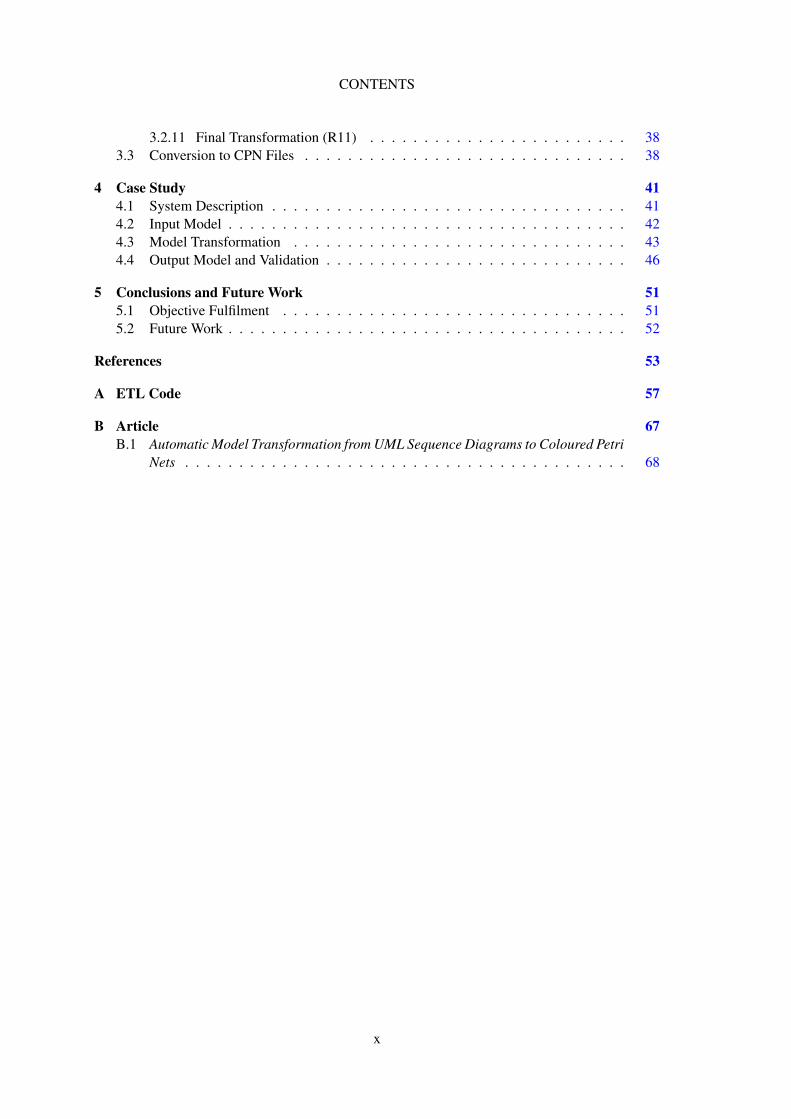
3.2.11 Final Transformation (R11) . . . . . . . . . . . . . . . . . . . . . . . . 383.3 Conversion to CPN Files . . . . . . . . . . . . . . . . . . . . . . . . . . . . . . 38

4 Case Study 414.1 System Description . . . . . . . . . . . . . . . . . . . . . . . . . . . . . . . . . 414.2 Input Model . . . . . . . . . . . . . . . . . . . . . . . . . . . . . . . . . . . . . 424.3 Model Transformation . . . . . . . . . . . . . . . . . . . . . . . . . . . . . . . 434.4 Output Model and Validation . . . . . . . . . . . . . . . . . . . . . . . . . . . . 46

5 Conclusions and Future Work 515.1 Objective Fulfilment . . . . . . . . . . . . . . . . . . . . . . . . . . . . . . . . 515.2 Future Work . . . . . . . . . . . . . . . . . . . . . . . . . . . . . . . . . . . . . 52

References 53

A ETL Code 57

B Article 67B.1 Automatic Model Transformation from UML Sequence Diagrams to Coloured Petri

Nets . . . . . . . . . . . . . . . . . . . . . . . . . . . . . . . . . . . . . . . . . 68

x

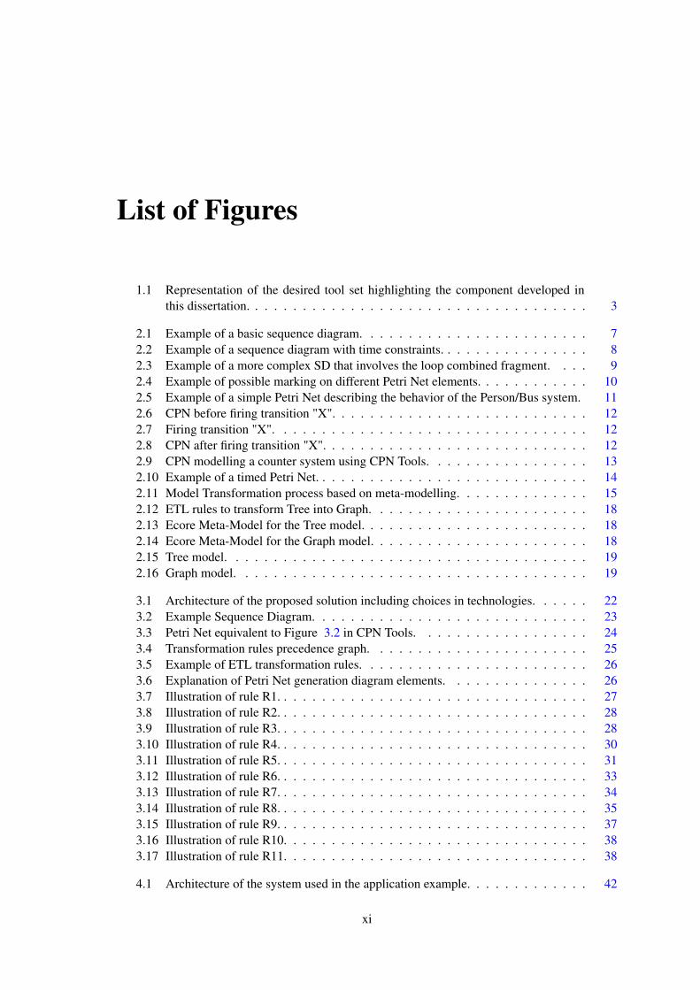
List of Figures

1.1 Representation of the desired tool set highlighting the component developed inthis dissertation. . . . . . . . . . . . . . . . . . . . . . . . . . . . . . . . . . . . 3

2.1 Example of a basic sequence diagram. . . . . . . . . . . . . . . . . . . . . . . . 72.2 Example of a sequence diagram with time constraints. . . . . . . . . . . . . . . . 82.3 Example of a more complex SD that involves the loop combined fragment. . . . 92.4 Example of possible marking on different Petri Net elements. . . . . . . . . . . . 102.5 Example of a simple Petri Net describing the behavior of the Person/Bus system. 112.6 CPN before firing transition "X". . . . . . . . . . . . . . . . . . . . . . . . . . . 122.7 Firing transition "X". . . . . . . . . . . . . . . . . . . . . . . . . . . . . . . . . 122.8 CPN after firing transition "X". . . . . . . . . . . . . . . . . . . . . . . . . . . . 122.9 CPN modelling a counter system using CPN Tools. . . . . . . . . . . . . . . . . 132.10 Example of a timed Petri Net. . . . . . . . . . . . . . . . . . . . . . . . . . . . . 142.11 Model Transformation process based on meta-modelling. . . . . . . . . . . . . . 152.12 ETL rules to transform Tree into Graph. . . . . . . . . . . . . . . . . . . . . . . 182.13 Ecore Meta-Model for the Tree model. . . . . . . . . . . . . . . . . . . . . . . . 182.14 Ecore Meta-Model for the Graph model. . . . . . . . . . . . . . . . . . . . . . . 182.15 Tree model. . . . . . . . . . . . . . . . . . . . . . . . . . . . . . . . . . . . . . 192.16 Graph model. . . . . . . . . . . . . . . . . . . . . . . . . . . . . . . . . . . . . 19

3.1 Architecture of the proposed solution including choices in technologies. . . . . . 223.2 Example Sequence Diagram. . . . . . . . . . . . . . . . . . . . . . . . . . . . . 233.3 Petri Net equivalent to Figure 3.2 in CPN Tools. . . . . . . . . . . . . . . . . . 243.4 Transformation rules precedence graph. . . . . . . . . . . . . . . . . . . . . . . 253.5 Example of ETL transformation rules. . . . . . . . . . . . . . . . . . . . . . . . 263.6 Explanation of Petri Net generation diagram elements. . . . . . . . . . . . . . . 263.7 Illustration of rule R1. . . . . . . . . . . . . . . . . . . . . . . . . . . . . . . . . 273.8 Illustration of rule R2. . . . . . . . . . . . . . . . . . . . . . . . . . . . . . . . . 283.9 Illustration of rule R3. . . . . . . . . . . . . . . . . . . . . . . . . . . . . . . . . 283.10 Illustration of rule R4. . . . . . . . . . . . . . . . . . . . . . . . . . . . . . . . . 303.11 Illustration of rule R5. . . . . . . . . . . . . . . . . . . . . . . . . . . . . . . . . 313.12 Illustration of rule R6. . . . . . . . . . . . . . . . . . . . . . . . . . . . . . . . . 333.13 Illustration of rule R7. . . . . . . . . . . . . . . . . . . . . . . . . . . . . . . . . 343.14 Illustration of rule R8. . . . . . . . . . . . . . . . . . . . . . . . . . . . . . . . . 353.15 Illustration of rule R9. . . . . . . . . . . . . . . . . . . . . . . . . . . . . . . . . 373.16 Illustration of rule R10. . . . . . . . . . . . . . . . . . . . . . . . . . . . . . . . 383.17 Illustration of rule R11. . . . . . . . . . . . . . . . . . . . . . . . . . . . . . . . 38

4.1 Architecture of the system used in the application example. . . . . . . . . . . . . 42

xi

LIST OF FIGURES

4.2 Input Sequence Diagram of the use case. . . . . . . . . . . . . . . . . . . . . . . 434.3 Result of the first step of the transformation process (R1). . . . . . . . . . . . . . 444.4 Result of the second step of the transformation process (R2) . . . . . . . . . . . 444.5 Result of the third step of the transformation process (R3). . . . . . . . . . . . . 454.6 Result of the fourth step of the transformation process (R7 and R8). . . . . . . . 474.7 Result of the fifth step of the transformation process (R10). . . . . . . . . . . . . 484.8 Result of the last step of the transformation process (R11). . . . . . . . . . . . . 494.9 Coloured Petri Net generated by the model transformation process. . . . . . . . . 50

A.1 ETL code for the implementation of R1. . . . . . . . . . . . . . . . . . . . . . . 58A.2 ETL code for the implementation of R2. . . . . . . . . . . . . . . . . . . . . . . 58A.3 ETL code for the implementation of R3. . . . . . . . . . . . . . . . . . . . . . . 58A.4 ETL code for the implementation of R4. . . . . . . . . . . . . . . . . . . . . . . 59A.5 ETL code for the implementation of R5. . . . . . . . . . . . . . . . . . . . . . . 59A.6 ETL code for the implementation of R6. . . . . . . . . . . . . . . . . . . . . . . 60A.7 ETL code for the implementation of R7. . . . . . . . . . . . . . . . . . . . . . . 61A.8 ETL code for the implementation of R7. . . . . . . . . . . . . . . . . . . . . . . 61A.9 ETL code for the implementation of R8. . . . . . . . . . . . . . . . . . . . . . . 62A.10 ETL code for the implementation of R8. . . . . . . . . . . . . . . . . . . . . . . 62A.11 ETL code for the implementation of R9. . . . . . . . . . . . . . . . . . . . . . . 63A.12 ETL code for the implementation of R9. . . . . . . . . . . . . . . . . . . . . . . 63A.13 ETL code for the implementation of R9. . . . . . . . . . . . . . . . . . . . . . . 64A.14 ETL code for the implementation of R10. . . . . . . . . . . . . . . . . . . . . . 64A.15 ETL code for the implementation of R11. . . . . . . . . . . . . . . . . . . . . . 65A.16 ETL code for the implementation of Combined Fragments Transformation. . . . 65A.17 ETL code for the implementation of getPreviousEvent(Lifeline lf) function. . . . 65A.18 ETL code for the implementation of getDecidingEvent() function. . . . . . . . . 65A.19 ETL code for the implementation of getLastEventPlace(Lifeline lf) function. . . . 66

xii

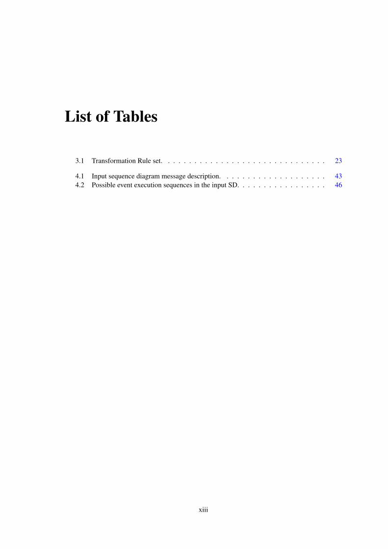
List of Tables

3.1 Transformation Rule set. . . . . . . . . . . . . . . . . . . . . . . . . . . . . . . 23

4.1 Input sequence diagram message description. . . . . . . . . . . . . . . . . . . . 434.2 Possible event execution sequences in the input SD. . . . . . . . . . . . . . . . . 46

xiii

LIST OF TABLES

xiv

Abbreviations

ATL Atlas Transformation LanguageCPN Coloured Petri NetsEMF Eclipse Modeling FrameworkETL Epsilon Transformation LanguageM2M Model-to-ModelMBT Model-based-TestingMDE Model Driven EngineeringMT Model TransformationOMG Object Management GroupPN Petri NetSD Sequence DiagramSwC Software ComponentsSwE Software EngineeringSwS Software SystemsSotA State of the ArtTPN Timed Petri NetsTR Transformation RuleUML Unified Modeling Language

xv

Chapter 1

Introduction

The Introductory chapter starts by giving context to this dissertation and explaining the need be-

hind it on Section 1.1. Section 1.2 defines the goals and expected artefacts to produce for this

dissertation work. Finally, Section 1.3 gives a brief explanation of how the dissertation is struc-

tured and what to expect in each chapter.

1.1 Context and Motivation

With Software Systems (SwS) taking a central role in current society and being responsible for

delivering many crucial services to users, ensuring quality of software is at its all time most im-

portance [FM08]. To ensure our SwS work as intended, it is necessary to verify it’s behaviour and

validate it, usually by the means of software testing. Normally in software projects, more than

between 5% and 50% of the development effort is being spent on testing [YHL+08].

Distributed systems are a combination of Software Components (SwC), divided into multiple

machines, that interact with each other to perform tasks and obtain a certain shared objective.

These SwC communicate by passing messages via a network. Each of these SwC has it’s own

behaviour and specifications, and are often developed using different technologies. Some of these

SwC can be independent systems, forming a system of systems with ever increasing complexity.

Since the parts of the SwS are heterogeneous and independent from each other, the behaviour of

each SwC must be as expected, as failure of one part can lead to the failure of the SwS as a whole.

Software Engineering (SwE) often relies on models to describe the behaviour of these SwC,

how they interact with each other and with the users for a better understanding of the desired

solution before the implementation. In the case of Distributed Systems, UML [DNN+15](Unified

Modelling Language) models, in particular, the Sequence Diagram (SD), is a standard for mapping

the communication and synchronization inside the system’s defined boundary, as it is capable of

representing this type of SwS most usual problems, such as concurrency and parallelism. Since it

is supposed to be a simplistic diagram by definition, it is not designed to be executed, making it a

1

Introduction

bad target to perform automated testing. Other types of models, such as Petri Nets [PR08] (PN),

can achieve the same objectives, but lack the simplicity, making them very hard to design, develop

and interpret. On the other hand, this particular type of modelling formalism has the advantage

of having an exact mathematical definition of their execution semantics, making it possible to use

engine type technologies to execute them, therefore making them suitable for executing automated

tests and generating test cases [JKW07a].

This dissertation is part of larger-scale project to create an approach and tool set to perform

model-based integration testing of distributed systems. In the approach outlined in [LF16], in-

tegration test scenarios are specified with UML SDs, because UML is an industry standard for

SwE, and SDs are adequate to describe interactions in distributed systems; the given input models

(UML SDs) need to be translated to a formal notation amenable for incremental execution at run-

time; Coloured Petri Nets (CPN) were chosen for that purpose because they can be executed (with

CPN Tools) and are adequate to model concurrency in systems. The final toolset should be able

to transform UML Sequence Diagrams into Coloured Petri Nets, automatically execute the trans-

formed model with a set of tests, and provide feedback (such as error occurrence and coverage of

different sequences of interactions) on the initial model.

1.2 Goals and Expected Outcomes

Hence, the main goal of this dissertation work is to develop a model transformation solution to

translate UML SDs into equivalent CPNs, taking advantage of existent model transformation tech-

niques to make the solution scalable, re-usable and easy to integrate and to be further developed

in the future. By equivalent, in this case, we mean a CPN that accepts the same possible execution

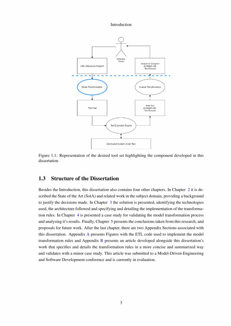
traces (event sequences) as the input model. The SwC to be developed is highlighted in blue in

image 1.1).

By hiding the task of Model Transformation (MT) from the tester (as represented by the sepa-

ration with the dashed blue line in figure 1.1), we can provide the benefits of Petri Nets (automated

testing) to the more perceivable and easy to interpret models for Distributed Systems (UML SD)

and, therefore, reduce the complexity and resources spent on testing.

As presented in Section 2, techniques for this MT have been previously studied, although never

fully implemented or taking advantage of integrated Model-Driven-Engineering (MDE) frame-

works like EMF [SBPM09]. A solution like this allows for further integration for the development

of the desired Model Based Testing (MBT) tool set.

This SwC was developed by the definition and implementation of a set of transformation rules

that allow mapping of elements of the source model into the elements of the target model. To

validate this technology, a case study is presented to demonstrate the MT possibilities with the

chosen tools and verify the correct behaviour and results for the MT.

2

Introduction

Figure 1.1: Representation of the desired tool set highlighting the component developed in thisdissertation.

1.3 Structure of the Dissertation

Besides the Introduction, this dissertation also contains four other chapters. In Chapter 2 it is de-

scribed the State of the Art (SotA) and related work in the subject domain, providing a background

to justify the decisions made. In Chapter 3 the solution is presented, identifying the technologies

used, the architecture followed and specifying and detailing the implementation of the transforma-

tion rules. In Chapter 4 is presented a case study for validating the model transformation process

and analysing it’s results. Finally, Chapter 5 presents the conclusions taken from this research, and

proposals for future work. After the last chapter, there are two Appendix Sections associated with

this dissertation. Appendix A presents Figures with the ETL code used to implement the model

transformation rules and Appendix B presents an article developed alongside this dissertation’s

work that specifies and details the transformation rules in a more concise and summarized way

and validates with a minor case study. This article was submitted to a Model-Driven-Engineering

and Software Development conference and is currently in evaluation.

3

Introduction

4

Chapter 2

Background and State of the Art

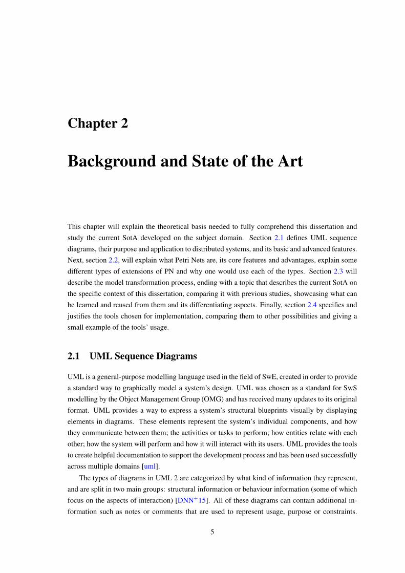
This chapter will explain the theoretical basis needed to fully comprehend this dissertation and

study the current SotA developed on the subject domain. Section 2.1 defines UML sequence

diagrams, their purpose and application to distributed systems, and its basic and advanced features.

Next, section 2.2, will explain what Petri Nets are, its core features and advantages, explain some

different types of extensions of PN and why one would use each of the types. Section 2.3 will

describe the model transformation process, ending with a topic that describes the current SotA on

the specific context of this dissertation, comparing it with previous studies, showcasing what can

be learned and reused from them and its differentiating aspects. Finally, section 2.4 specifies and

justifies the tools chosen for implementation, comparing them to other possibilities and giving a

small example of the tools’ usage.

2.1 UML Sequence Diagrams

UML is a general-purpose modelling language used in the field of SwE, created in order to provide

a standard way to graphically model a system’s design. UML was chosen as a standard for SwS

modelling by the Object Management Group (OMG) and has received many updates to its original

format. UML provides a way to express a system’s structural blueprints visually by displaying

elements in diagrams. These elements represent the system’s individual components, and how

they communicate between them; the activities or tasks to perform; how entities relate with each

other; how the system will perform and how it will interact with its users. UML provides the tools

to create helpful documentation to support the development process and has been used successfully

across multiple domains [uml].

The types of diagrams in UML 2 are categorized by what kind of information they represent,

and are split in two main groups: structural information or behaviour information (some of which

focus on the aspects of interaction) [DNN+15]. All of these diagrams can contain additional in-

formation such as notes or comments that are used to represent usage, purpose or constraints.

5


Structure diagrams describe the things that must be present in the system being modelled. Since

structure diagrams represent a sort of blueprint, they are mostly used to document the architecture

of SwS. Behaviour diagrams describe what must happen in the system. Since behaviour diagrams

represent the general behaviour of the system, they are mostly used to document the functionalities

of SwS. A subset of these, the Interaction diagrams, focus on the communication task, describing

how the SwC in the system interact with each other. A SD is an interaction diagram that focuses

on how objects in a SwS collaborate and synchronize with each other, and in what order. It is basi-

cally a message sequence chart, describing "who’s" turn it is to be sending "what" to "whom". SDs

show object interactions arranged in a time sequence. It depicts the objects and classes involved in

the scenario and the sequence of messages exchanged between the objects needed to carry out the

functionality of the scenario and fulfil its objective. This allows the specification of simple runtime

scenarios in a graphical manner and that is why SDs are generally used as use case realizations to

describe the logic of the distributed part of the system under development. These diagrams may

only serve as descriptive artefacts, not really contributing to optimize the development or testing

process, since they do not provide code generation or test automation capabilities by themselves.

But since they are so easily designed and understandable, and generally constructed in the con-

ception phase of the software project, there have been many attempts to incorporate them in later

phases. For example, by introducing more formalism and a more complete set of restrictions to

the system, these diagrams can be used to generate test cases (a process that would normally oc-

cupy many human and computational resources of the testing phase) automatically [LsLQC07], or

they can be combined with other modelling technologies to create an executable model that can be

used for automated testing of systems [FP16], granting this type of diagram an extra set of utilities.

Next in this section, the basic and advanced features of UML SDs relevant to this dissertation will

be presented.

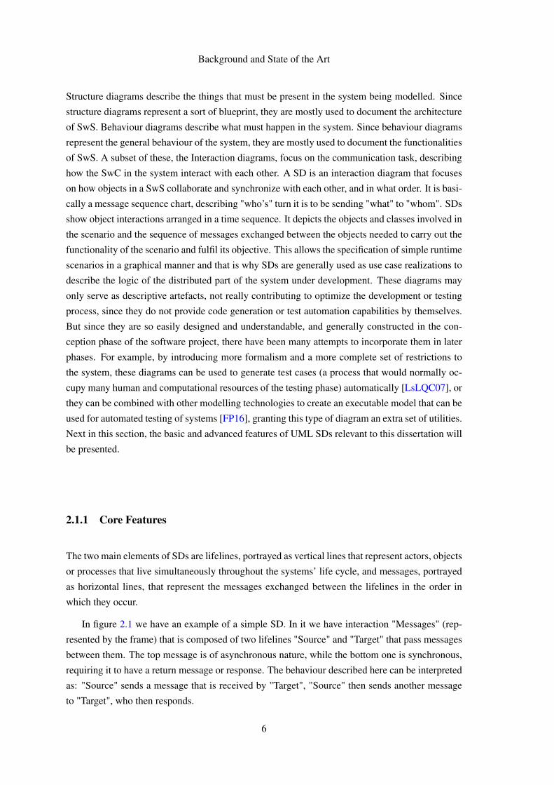
2.1.1 Core Features

The two main elements of SDs are lifelines, portrayed as vertical lines that represent actors, objects

or processes that live simultaneously throughout the systems’ life cycle, and messages, portrayed

as horizontal lines, that represent the messages exchanged between the lifelines in the order in

which they occur.

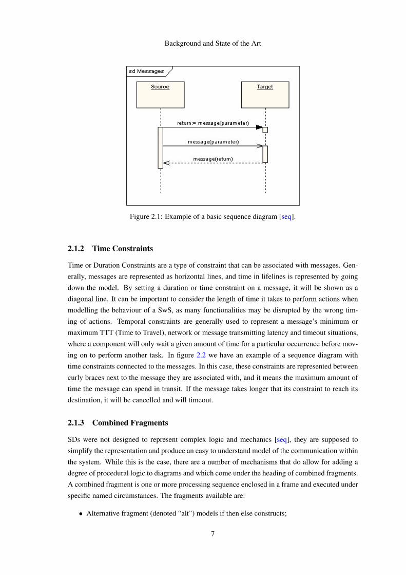
In figure 2.1 we have an example of a simple SD. In it we have interaction "Messages" (rep-

resented by the frame) that is composed of two lifelines "Source" and "Target" that pass messages

between them. The top message is of asynchronous nature, while the bottom one is synchronous,

requiring it to have a return message or response. The behaviour described here can be interpreted

as: "Source" sends a message that is received by "Target", "Source" then sends another message

to "Target", who then responds.

6


Figure 2.1: Example of a basic sequence diagram [seq].

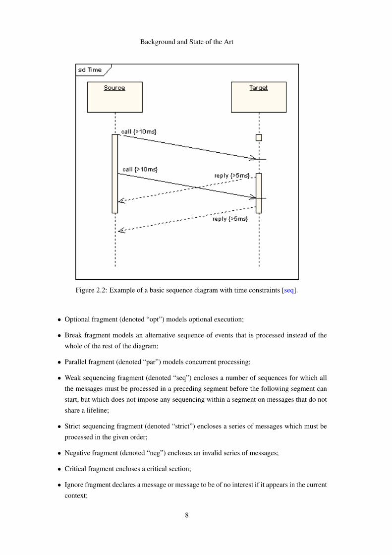
2.1.2 Time Constraints

Time or Duration Constraints are a type of constraint that can be associated with messages. Gen-

erally, messages are represented as horizontal lines, and time in lifelines is represented by going

down the model. By setting a duration or time constraint on a message, it will be shown as a

diagonal line. It can be important to consider the length of time it takes to perform actions when

modelling the behaviour of a SwS, as many functionalities may be disrupted by the wrong tim-

ing of actions. Temporal constraints are generally used to represent a message’s minimum or

maximum TTT (Time to Travel), network or message transmitting latency and timeout situations,

where a component will only wait a given amount of time for a particular occurrence before mov-

ing on to perform another task. In figure 2.2 we have an example of a sequence diagram with

time constraints connected to the messages. In this case, these constraints are represented between

curly braces next to the message they are associated with, and it means the maximum amount of

time the message can spend in transit. If the message takes longer that its constraint to reach its

destination, it will be cancelled and will timeout.

2.1.3 Combined Fragments

SDs were not designed to represent complex logic and mechanics [seq], they are supposed to

simplify the representation and produce an easy to understand model of the communication within

the system. While this is the case, there are a number of mechanisms that do allow for adding a

degree of procedural logic to diagrams and which come under the heading of combined fragments.

A combined fragment is one or more processing sequence enclosed in a frame and executed under

specific named circumstances. The fragments available are:

• Alternative fragment (denoted “alt”) models if then else constructs;

7


Figure 2.2: Example of a basic sequence diagram with time constraints [seq].

• Optional fragment (denoted “opt”) models optional execution;

• Break fragment models an alternative sequence of events that is processed instead of the

whole of the rest of the diagram;

• Parallel fragment (denoted “par”) models concurrent processing;

• Weak sequencing fragment (denoted “seq”) encloses a number of sequences for which all

the messages must be processed in a preceding segment before the following segment can

start, but which does not impose any sequencing within a segment on messages that do not

share a lifeline;

• Strict sequencing fragment (denoted “strict”) encloses a series of messages which must be

processed in the given order;

• Negative fragment (denoted “neg”) encloses an invalid series of messages;

• Critical fragment encloses a critical section;

• Ignore fragment declares a message or message to be of no interest if it appears in the current

context;

8


• Consider fragment is in effect the opposite of the ignore fragment: any message not included

in the consider fragment should be ignored;

• Assertion fragment (denoted “assert”) designates that any sequence not shown as an operand

of the assertion is invalid;

• Loop fragment encloses a series of messages which are repeated;

These combined fragments show different conditional paths that can be taken on a sequence

diagram, handling conditional flow. Nested diagrams are diagrams within diagrams, and can also

be seen as combined fragments, since they too can be framed and executed given the right con-

ditions, and they handle control flow. Instead of having the whole system encapsulated in one

diagram, multiple diagrams can be chained and nested in order to reduce the perceived complexity

and provide a clearer model for behavioural analysis.

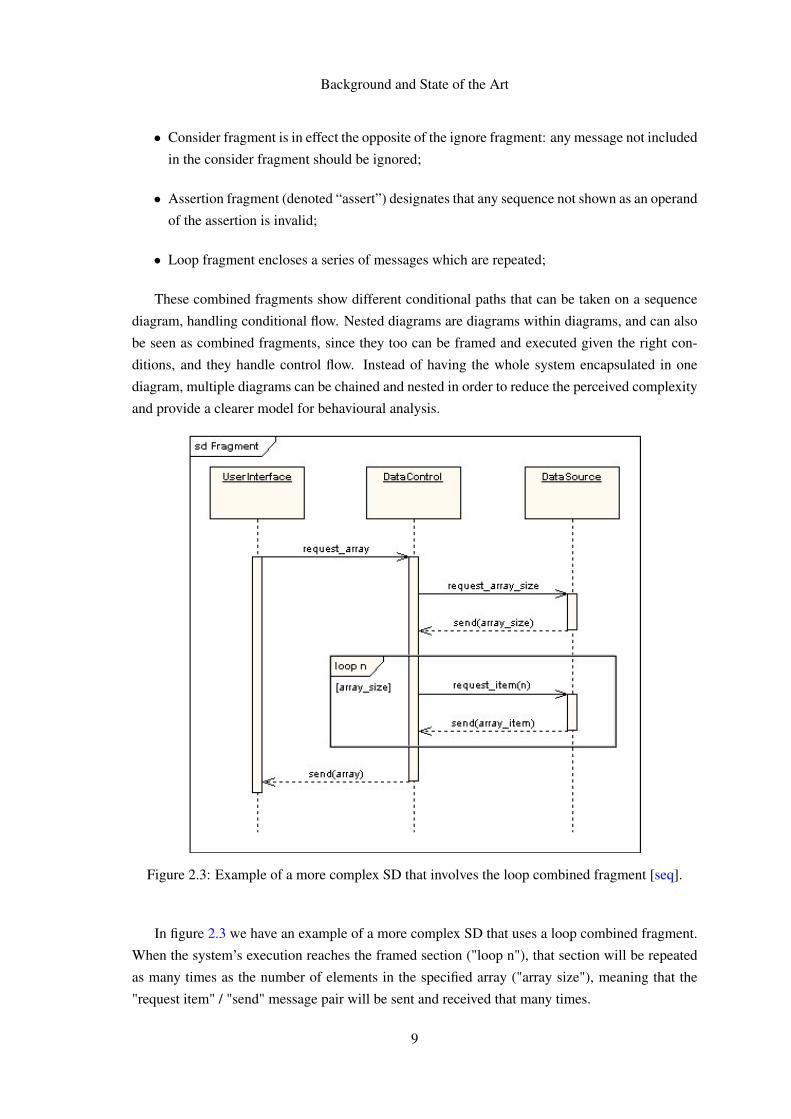
Figure 2.3: Example of a more complex SD that involves the loop combined fragment [seq].

In figure 2.3 we have an example of a more complex SD that uses a loop combined fragment.

When the system’s execution reaches the framed section ("loop n"), that section will be repeated

as many times as the number of elements in the specified array ("array size"), meaning that the

"request item" / "send" message pair will be sent and received that many times.

9


With this spectrum of tools, modelling the behaviour of a distributed system becomes a more

feasible task and produces a human interpretation friendly diagram, making SDs a powerful tool

for the software development process that requires minimal effort and resources (diagrams are

easy to learn, easy to use, re-usable and adaptable across domains and in-between very different

kinds of applications) and provides high return, either by themselves during the conception phase,

or in later stages when combined with other techniques and technologies.

2.2 Petri Nets

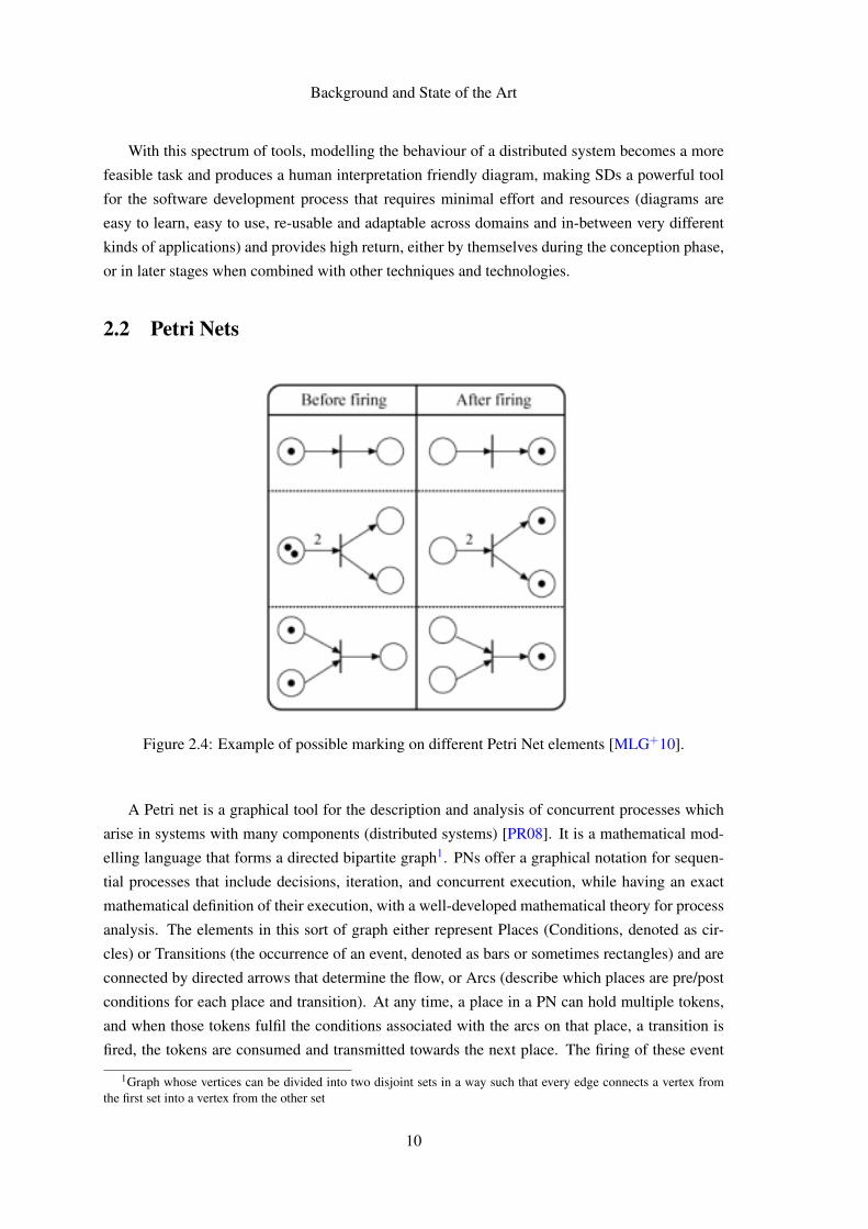
Figure 2.4: Example of possible marking on different Petri Net elements [MLG+10].

A Petri net is a graphical tool for the description and analysis of concurrent processes which

arise in systems with many components (distributed systems) [PR08]. It is a mathematical mod-

elling language that forms a directed bipartite graph1. PNs offer a graphical notation for sequen-

tial processes that include decisions, iteration, and concurrent execution, while having an exact

mathematical definition of their execution, with a well-developed mathematical theory for process

analysis. The elements in this sort of graph either represent Places (Conditions, denoted as cir-

cles) or Transitions (the occurrence of an event, denoted as bars or sometimes rectangles) and are

connected by directed arrows that determine the flow, or Arcs (describe which places are pre/post

conditions for each place and transition). At any time, a place in a PN can hold multiple tokens,

and when those tokens fulfil the conditions associated with the arcs on that place, a transition is

fired, the tokens are consumed and transmitted towards the next place. The firing of these event

1Graph whose vertices can be divided into two disjoint sets in a way such that every edge connects a vertex fromthe first set into a vertex from the other set

10


is of non-deterministic nature, given that it could occur at any time and that the tokens can be

anywhere in the net at any given moment, making them ideal to model the concurrent behaviour

of distributed systems. How the tokens are distributed between the places of the net is called the

marking, and it represents the configuration of a PN at a given time. In figure 2.4 we have example

of possible PN markings before and after the firing of a transition. The dots inside the places

represent the token that are to be consumed and transmitted to the next places.

2.2.1 Basic Petri Nets

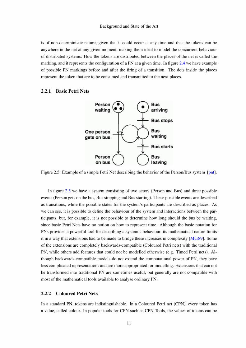
Figure 2.5: Example of a simple Petri Net describing the behavior of the Person/Bus system [pnt].

In figure 2.5 we have a system consisting of two actors (Person and Bus) and three possible

events (Person gets on the bus, Bus stopping and Bus starting). These possible events are described

as transitions, while the possible states for the system’s participants are described as places. As

we can see, it is possible to define the behaviour of the system and interactions between the par-

ticipants, but, for example, it is not possible to determine how long should the bus be waiting,

since basic Petri Nets have no notion on how to represent time. Although the basic notation for

PNs provides a powerful tool for describing a system’s behaviour, its mathematical nature limits

it in a way that extensions had to be made to bridge these increases in complexity [Mur89]. Some

of the extensions are completely backwards-compatible (Coloured Petri nets) with the traditional

PN, while others add features that could not be modelled otherwise (e.g. Timed Petri nets). Al-

though backwards-compatible models do not extend the computational power of PN, they have

less complicated representations and are more appropriated for modelling. Extensions that can not

be transformed into traditional PN are sometimes useful, but generally are not compatible with

most of the mathematical tools available to analyse ordinary PN.

2.2.2 Coloured Petri Nets

In a standard PN, tokens are indistinguishable. In a Coloured Petri net (CPN), every token has

a value, called colour. In popular tools for CPN such as CPN Tools, the values of tokens can be

11


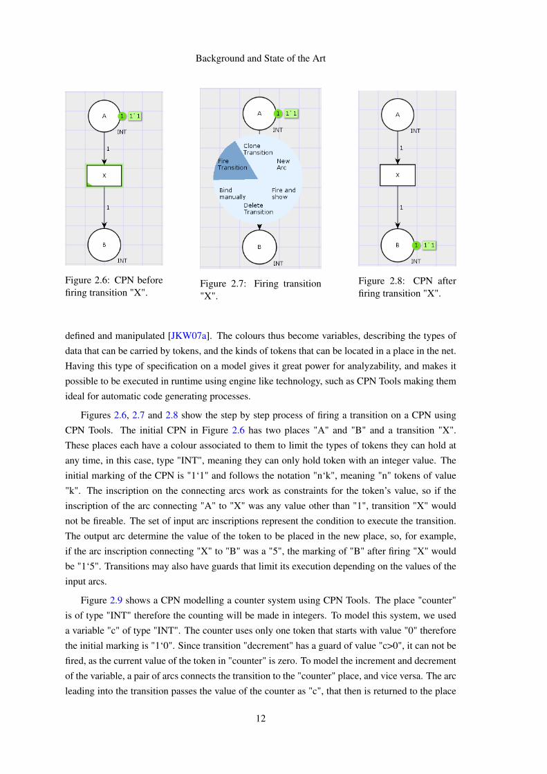
Figure 2.6: CPN beforefiring transition "X".

Figure 2.7: Firing transition"X".

Figure 2.8: CPN afterfiring transition "X".

defined and manipulated [JKW07a]. The colours thus become variables, describing the types of

data that can be carried by tokens, and the kinds of tokens that can be located in a place in the net.

Having this type of specification on a model gives it great power for analyzability, and makes it

possible to be executed in runtime using engine like technology, such as CPN Tools making them

ideal for automatic code generating processes.

Figures 2.6, 2.7 and 2.8 show the step by step process of firing a transition on a CPN using

CPN Tools. The initial CPN in Figure 2.6 has two places "A" and "B" and a transition "X".

These places each have a colour associated to them to limit the types of tokens they can hold at

any time, in this case, type "INT", meaning they can only hold token with an integer value. The

initial marking of the CPN is "1‘1" and follows the notation "n‘k", meaning "n" tokens of value

"k". The inscription on the connecting arcs work as constraints for the token’s value, so if the

inscription of the arc connecting "A" to "X" was any value other than "1", transition "X" would

not be fireable. The set of input arc inscriptions represent the condition to execute the transition.

The output arc determine the value of the token to be placed in the new place, so, for example,

if the arc inscription connecting "X" to "B" was a "5", the marking of "B" after firing "X" would

be "1‘5". Transitions may also have guards that limit its execution depending on the values of the

input arcs.

Figure 2.9 shows a CPN modelling a counter system using CPN Tools. The place "counter"

is of type "INT" therefore the counting will be made in integers. To model this system, we used

a variable "c" of type "INT". The counter uses only one token that starts with value "0" therefore

the initial marking is "1‘0". Since transition "decrement" has a guard of value "c>0", it can not be

fired, as the current value of the token in "counter" is zero. To model the increment and decrement

of the variable, a pair of arcs connects the transition to the "counter" place, and vice versa. The arc

leading into the transition passes the value of the counter as "c", that then is returned to the place

12


Figure 2.9: CPN modelling a counter system using CPN Tools.

by the firing of the transition with value "c+1" or "c-1". To reset the counter, the transition "reset"

places the value "0" in the token of "counter" upon firing.

2.2.3 Timed Petri Nets

Although non-determinism is convenient for this type of modelling, introducing the notion of

time in the transitions might be helpful to gain control over the timing of occurrences. Therefore,

Timed Petri Nets (TPN) [PZ13] were created, adding the option for transitions to either wait a

certain amount of time before firing, or limit the time the system has to fulfil the condition for

that firing to occur. With the tool set provided by basic PNs, combined with the powerful extra

features provided by its extensions, any behaviour found in a distributed system can be modelled,

having the only downside of its complexity to design, interpret and read. This makes these models

ideal for computational analysis, but very resource consuming for human analysis, and hiding

this complexity problem, while taking advantage of the whole potential of PNs, is the major idea

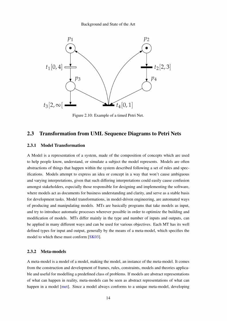
behind this dissertation. In figure 2.10 we have an example of a timed PN. The time constraints

associated with the transitions limit when these can be fired. In this case, t4 can only fire between

moment 0 and 1, while t2 can only fire between moment 2 and 3. These time units can be either

absolute (e.g. seconds) or relative, meaning the units will represent the order and the firing of a

transition increments it.

13


Figure 2.10: Example of a timed Petri Net.

2.3 Transformation from UML Sequence Diagrams to Petri Nets

2.3.1 Model Transformation

A Model is a representation of a system, made of the composition of concepts which are used

to help people know, understand, or simulate a subject the model represents. Models are often

abstractions of things that happen within the system described following a set of rules and spec-

ifications. Models attempt to express an idea or concept in a way that won’t cause ambiguous

and varying interpretations, given that such differing interpretations could easily cause confusion

amongst stakeholders, especially those responsible for designing and implementing the software,

where models act as documents for business understanding and clarity, and serve as a stable basis

for development tasks. Model transformations, in model-driven engineering, are automated ways

of producing and manipulating models. MTs are basically programs that take models as input,

and try to introduce automatic processes wherever possible in order to optimize the building and

modification of models. MTs differ mainly in the type and number of inputs and outputs, can

be applied in many different ways and can be used for various objectives. Each MT has its well

defined types for input and output, generally by the means of a meta-model, which specifies the

model to which these must conform [SK03].

2.3.2 Meta-models

A meta-model is a model of a model, making the model, an instance of the meta-model. It comes

from the construction and development of frames, rules, constraints, models and theories applica-

ble and useful for modelling a predefined class of problems. If models are abstract representations

of what can happen in reality, meta-models can be seen as abstract representations of what can

happen in a model [met]. Since a model always conforms to a unique meta-model, developing

14


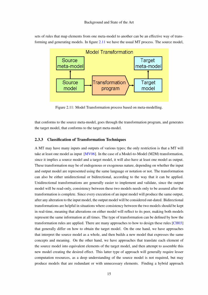
sets of rules that map elements from one meta-model to another can be an effective way of trans-

forming and generating models. In figure 2.11 we have the usual MT process. The source model,

Figure 2.11: Model Transformation process based on meta-modelling.

that conforms to the source meta-model, goes through the transformation program, and generates

the target model, that conforms to the target meta-model.

2.3.3 Classification of Transformation Techniques

A MT may have many inputs and outputs of various types; the only restriction is that a MT will

take at least one model as input [MV06]. In the case of a Model-to-Model (M2M) transformation,

since it implies a source model and a target model, it will also have at least one model as output.

These transformation may be of endogenous or exogenous nature, depending on whether the input

and output model are represented using the same language or notation or not. The transformation

can also be either unidirectional or bidirectional, according to the way that it can be applied.

Unidirectional transformations are generally easier to implement and validate, since the output

model will be read-only, consistency between these two models needs only to be assured after the

transformation is complete. Since every execution of an input model will produce the same output,

after any alteration to the input model, the output model will be considered out-dated. Bidirectional

transformations are helpful in situations where consistency between the two models should be kept

in real-time, meaning that alterations on either model will reflect to its peer, making both models

represent the same information at all times. The type of transformation can be defined by how the

transformation rules are applied. There are many approaches to how to design these rules [CH03]

that generally differ on how to obtain the target model. On the one hand, we have approaches

that interpret the source model as a whole, and then builds a new model that expresses the same

concepts and meaning. On the other hand, we have approaches that translate each element of

the source model into equivalent elements of the target model, and then attempt to assemble this

new model creating the desired effect. This latter type of approach will generally require lesser

computation resources, as a deep understanding of the source model is not required, but may

produce models that are redundant or with unnecessary elements. Finding a hybrid approach

15


adapted to the specific conditions of a case tends to be the most appropriate approach since there

are cases where a balance between direct mapping of elements combined with structural analysis

can be achieved to produce the most effective model transformation.

2.3.4 Past Research

The subject of applying model transformation from UML SDs to PNs has been the matter of many

previous studies. In [BM10] the authors’ have proven with formal methods that the model trans-

formation rules approach allows a one-to-one correspondence between the set of legal traces of

both models, that is, the languages are equivalent also known as strongly consistent. Although

the transformation rule based approach has been proven adequate, the design of these transforma-

tion rules may prove to be a challenge, given that SDs have no formal design rules. To surpass

this complexity problem, an example based heuristic search has been implemented in [KBSB10]

to produce results with 96% correctness, although requiring a knowledge base of many transfor-

mation examples with high detail on the execution trace of the most complex fragments. This

transformation rule generation approach would require the user to be experienced in CPNs to

evaluate the results of the transformation, or a validation system to check conformity and consis-

tency between the input and output model, therefore not being adaptable to this software module’s

requirements of hiding complexity from the user.

The meta model transformation approach was chosen since it was proven feasible with formal

methods by [OEPP06] and the transformation rules were derived from [ES09] and [Sta13]

that have conceptualized and validated them for specific scenarios, although not implementing

them in an automated process. The rules to produce the output CPNs were extended from the

transformation rules proposed, alongside the tool kit for conformance testing based on UML SDs

in [FP16]. These studies were developed and used as a base for designing transformation rules

for this type of model transformation for many application domains and have been adapted and

developed in order to increase the value of SDs. As proven in [JKW07b] CPNs and CPN Tools

can be used for automatic validation of systems, either by the means of creating animated system

simulation to be used as validation with clients [RF06] and acceptance testing, or by generating

automatic test cases and execution scenarios [LF16], therefore justifying the need for this software

module.

2.4 Model Transformation Technologies

Many tools and frameworks have been developed specifically for the task of MT, since it’s such

a nuclear component in Model Driven Engineering (MDE). This section will give an overview of

the possibilities to solve the problem at hand, while comparing them to the chosen ones.

16


2.4.1 EMF

Eclipse Modeling Framework (EMF) [SBPM09] is an Eclipse-based modeling and code gener-

ation framework integrated IDE for developing applications based on models of structured data.

From a model specification described in XMI [KH02], EMF provides execution support and tools

to generate Java [Gra97] classes, a set of adapter classes that enable viewing and command-based

editing of the model, and a basic editor that displays the elements of a model in an hierarchical

tree graph. Models can be designed in annotated Java, UML, XML [BPSM+97] documents, or

using modelling tools, and imported into EMF. Additionally, EMF provides interoperability with

other EMF-based applications, tools and frameworks. EMF uses Ecore [Sch09], its own imple-

mentation of EMOF (Essential Meta-Object Facility), a standardized way of defining meta-models

by OMG. Using Ecore as a foundation for meta modelling provides the necessary tools for M2M

transformations in an integrated solution, taking full advantage of EMF.

2.4.2 Epsilon

Epsilon [KPP08] is a family of languages and tools for code generation, M2M transformation,

model validation, comparison, migration and refactoring that work out of the box with EMF and

other types of models. ETL (Epsilon Transformation Language) is a rule-based M2M transfor-

mation specific language. ETL is used to query, navigate and modify source and target models,

having the capability for multiple input and output models, making it a perfect fit for this disser-

tation’s desired goal. Other transformation technologies could be integrated with EMF, such as

ATL (Atlas Transformation Language) [JABK08], a MT technology developed earlier that could

eventually reach the same purpose, although it does not offer the same array of choices as Epsilon,

such as the possibility for bidirectional rules [KPP06a]. Epsilon also provides a series of tutorials

on M2M transformation, facilitating the learning process, and also to serve as proof that a model,

expressed in XMI and compliant with a meta-model expressed in Ecore, can be transformed into

a whole different type of model, expressed in XMI and different meta-model expressed in Ecore,

by the application of simple TRs defined in ETL.

2.4.3 Example

ETL comes with a series of examples and tutorial on MT, showcasing how complete and simple to

use the EMF integrated solution really is [etl]. One of these tutorials defines MT rules to translate

Tree type models into Graph type models. The tutorial starts by explaining how to define the

Ecore model for the input Tree graph, as shown in figure 2.13. It only has one type of element

"Tree" that represents a node, and can reference its parent node or its many sibling nodes. Then,

an instance of this type of model must be created, and for that EMF offers the ".model" file, which

is a file format made to represent models within the EMF framework. It’s based on the XMI

file representing the diagram and constructs visual representations from it, and creates a file as

shown in 2.15. Next, we must define the output graph meta-model, such as in figure 2.14. This

meta-model has two type of elements: node and edge. Each node represents a node in the tree

17


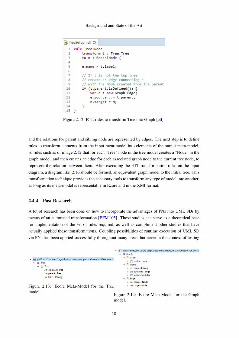
Figure 2.12: ETL rules to transform Tree into Graph [etl].

and the relations for parent and sibling node are represented by edges. The next step is to define

rules to transform elements from the input meta-model into elements of the output meta-model,

so rules such as of image 2.12 that for each "Tree" node in the tree model creates a "Node" in the

graph model, and then creates an edge for each associated graph node to the current tree node, to

represent the relation between them. After executing the ETL transformation rules on the input

diagram, a diagram like 2.16 should be formed, an equivalent graph model to the initial tree. This

transformation technique provides the necessary tools to transform any type of model into another,

as long as its meta-model is representable in Ecore and in the XMI format.

2.4.4 Past Research

A lot of research has been done on how to incorporate the advantages of PNs into UML SDs by

means of an automated transformation [EFM+05]. These studies can serve as a theoretical base

for implementation of the set of rules required, as well as compliment other studies that have

actually applied these transformations. Coupling possibilities of runtime execution of UML SD

via PNs has been applied successfully throughout many areas, but never in the context of testing

Figure 2.13: Ecore Meta-Model for the Treemodel.

Figure 2.14: Ecore Meta-Model for the Graphmodel.

18


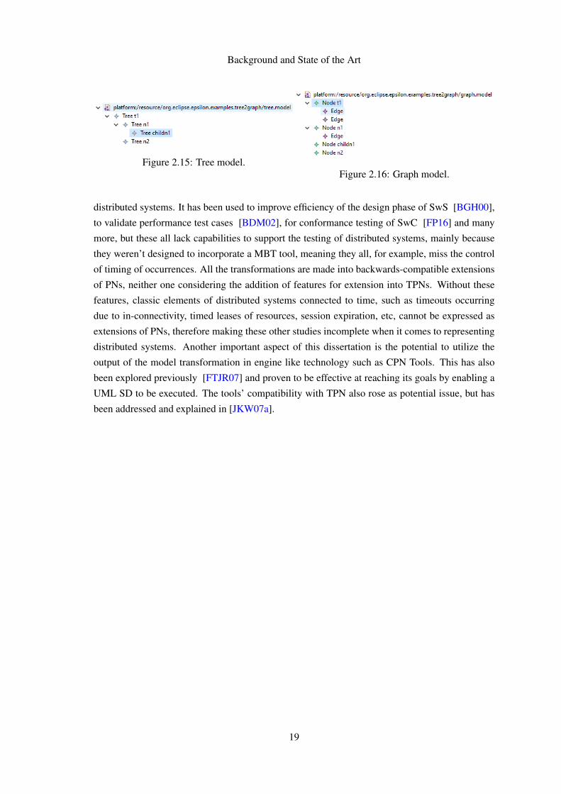
Figure 2.15: Tree model.Figure 2.16: Graph model.

distributed systems. It has been used to improve efficiency of the design phase of SwS [BGH00],

to validate performance test cases [BDM02], for conformance testing of SwC [FP16] and many

more, but these all lack capabilities to support the testing of distributed systems, mainly because

they weren’t designed to incorporate a MBT tool, meaning they all, for example, miss the control

of timing of occurrences. All the transformations are made into backwards-compatible extensions

of PNs, neither one considering the addition of features for extension into TPNs. Without these

features, classic elements of distributed systems connected to time, such as timeouts occurring

due to in-connectivity, timed leases of resources, session expiration, etc, cannot be expressed as

extensions of PNs, therefore making these other studies incomplete when it comes to representing

distributed systems. Another important aspect of this dissertation is the potential to utilize the

output of the model transformation in engine like technology such as CPN Tools. This has also

been explored previously [FTJR07] and proven to be effective at reaching its goals by enabling a

UML SD to be executed. The tools’ compatibility with TPN also rose as potential issue, but has

been addressed and explained in [JKW07a].

19


20

Chapter 3

Solution Design

This chapter describes the solution that was designed to transform UML SD to CPNs. It starts in

Section 3.1 by defining and explaining the solution’s architecture and the choices in technologies

to use. Section 3.2 describes the transformation rules, the core of the transformation process. In

this Section, each TR’s implementation is detailed and illustrated with explanatory diagrams. The

last Section 3.3 describes the additional SwC developed to convert the output of the transformation

process to a format acceptable by CPN Tools.

3.1 Architecture and Technologies

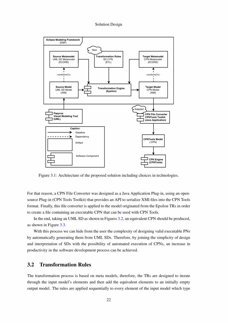
The transformation process was designed and implemented taking full advantage of the integrated

solutions provided by EMF. Figure 3.1 presents a dataflow view of the proposed model-to-model

transformation process and of the technologies used.

The TRs were implemented using the Epsilon Transformation Language (ETL), a state-of-the-

art tool for model-to-model transformation from Epsilon designed to pair with EMF. These rules

were designed to map elements from the source meta model to elements of the target meta model,

a meta model for CPNs that supports the features required by CPN Tools to create an executable

model. These TRs are then applied to an UML SD in order to create an equivalent model of a

CPN.

The visual modelling tool chosen was Papyrus, a visual modelling tool integrated in EMF, that

creates UML models in an XMI like format which can be used as input in the M2M transforma-

tions in ETL. These models are validated to conform with the source meta model provided by

EMF (UML meta model encoded in the ECORE format). The user only has to interact with the

visual modelling tool in order to create the input SD; then the transformation process produces an

executable CPN model that the user can execute with CPN Tools.

The generated CPN models are also in the EMF default format (XMI), and therefore need to

be converted into the CPN Tools format (.cpn) to successfully accomplish the goal of this solution.

21

Solution Design

Figure 3.1: Architecture of the proposed solution including choices in technologies.

For that reason, a CPN File Converter was designed as a Java Application Plug-in, using an open-

source Plug-in (CPN Tools Toolkit) that provides an API to serialize XMI files into the CPN Tools

format. Finally, this file converter is applied to the model originated from the Epsilon TRs in order

to create a file containing an executable CPN that can be used with CPN Tools.

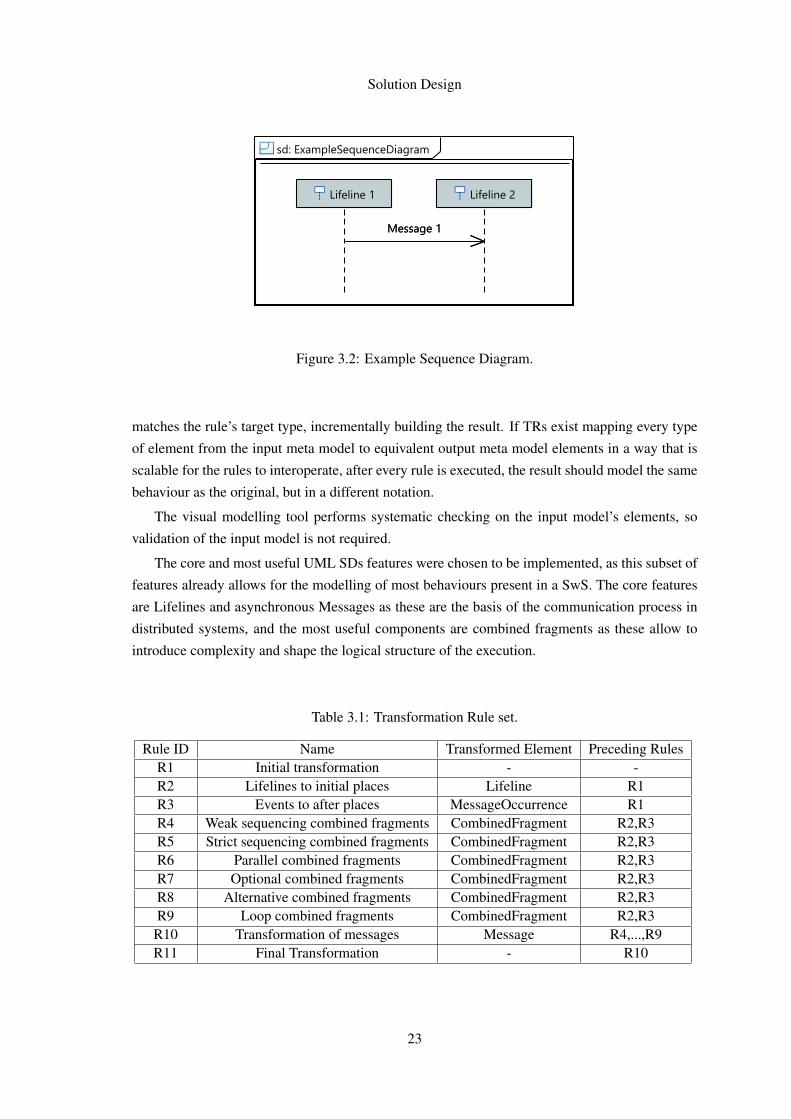
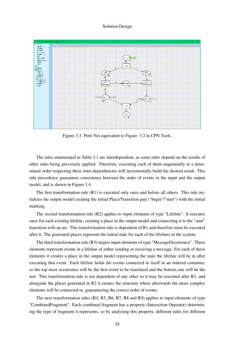
In the end, taking an UML SD as shown in Figures 3.2, an equivalent CPN should be produced,

as shown in Figure 3.3.

With this process we can hide from the user the complexity of designing valid executable PNs

by automatically generating them from UML SDs. Therefore, by joining the simplicity of design

and interpretation of SDs with the possibility of automated execution of CPNs, an increase in

productivity in the software development process can be achieved.

3.2 Transformation Rules

The transformation process is based on meta models, therefore, the TRs are designed to iterate

through the input model’s elements and then add the equivalent elements to an initially empty

output model. The rules are applied sequentially to every element of the input model which type

22

Solution Design

Figure 3.2: Example Sequence Diagram.

matches the rule’s target type, incrementally building the result. If TRs exist mapping every type

of element from the input meta model to equivalent output meta model elements in a way that is

scalable for the rules to interoperate, after every rule is executed, the result should model the same

behaviour as the original, but in a different notation.

The visual modelling tool performs systematic checking on the input model’s elements, so

validation of the input model is not required.

The core and most useful UML SDs features were chosen to be implemented, as this subset of

features already allows for the modelling of most behaviours present in a SwS. The core features

are Lifelines and asynchronous Messages as these are the basis of the communication process in

distributed systems, and the most useful components are combined fragments as these allow to

introduce complexity and shape the logical structure of the execution.

Table 3.1: Transformation Rule set.

Rule ID Name Transformed Element Preceding RulesR1 Initial transformation - -R2 Lifelines to initial places Lifeline R1R3 Events to after places MessageOccurrence R1R4 Weak sequencing combined fragments CombinedFragment R2,R3R5 Strict sequencing combined fragments CombinedFragment R2,R3R6 Parallel combined fragments CombinedFragment R2,R3R7 Optional combined fragments CombinedFragment R2,R3R8 Alternative combined fragments CombinedFragment R2,R3R9 Loop combined fragments CombinedFragment R2,R3R10 Transformation of messages Message R4,...,R9R11 Final Transformation - R10

23

Solution Design

Figure 3.3: Petri Net equivalent to Figure 3.2 in CPN Tools.

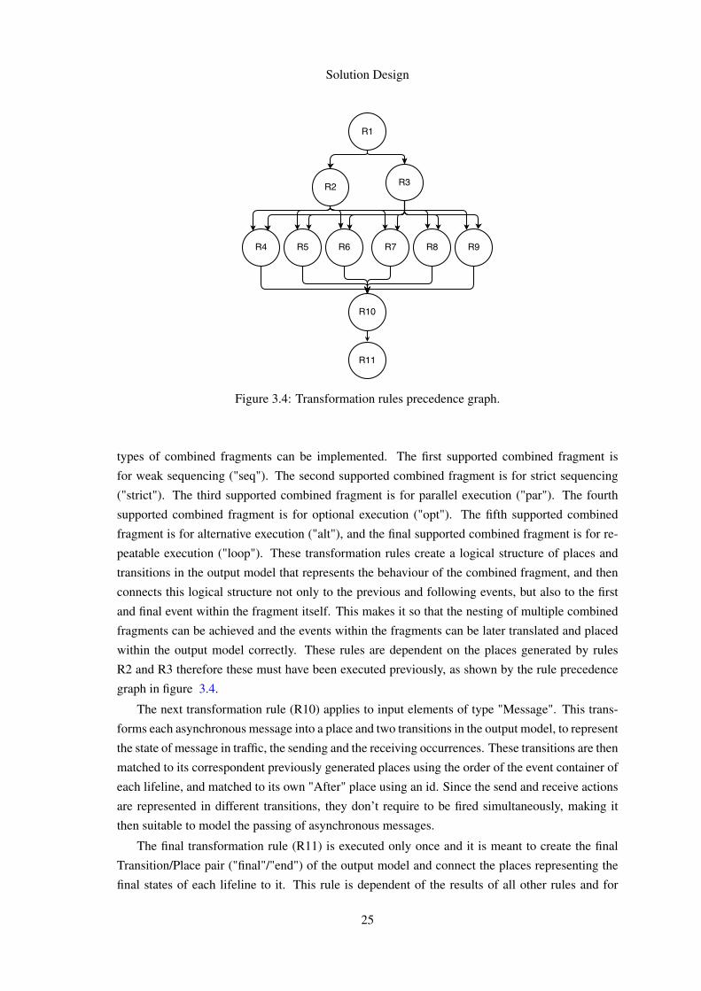
The rules enumerated in Table 3.1 are interdependent, as some rules depend on the results of

other rules being previously applied. Therefore, executing each of them sequentially in a deter-

mined order respecting these inter-dependencies will incrementally build the desired result. This

rule precedence guarantees consistency between the order of events in the input and the output

model, and is shown in Figure 3.4.

The first transformation rule (R1) is executed only once and before all others. This rule ini-

tializes the output model creating the initial Place/Transition pair ("begin"/"start") with the initial

marking.

The second transformation rule (R2) applies to input elements of type "Lifeline". It executes

once for each existing lifeline, creating a place in the output model and connecting it to the "start"

transition with an arc. This transformation rule is dependent of R1 and therefore must be executed

after it. The generated places represent the initial state for each of the lifelines in the system.

The third transformation rule (R3) targets input elements of type "MessageOccurrence". These

elements represent events in a lifeline of either sending or receiving a message. For each of these

elements it creates a place in the output model representing the state the lifeline will be in after

executing that event. Each lifeline holds the events connected to itself in an ordered container,

so the top most occurrence will be the first event to be translated and the bottom one will be the

last. This transformation rule is not dependent of any other so it may be executed after R1, and

alongside the places generated in R2 it creates the structure where afterwards the more complex

elements will be connected to, guaranteeing the correct order of events.

The next transformation rules (R4, R5, R6, R7, R8 and R9) applies to input elements of type

"CombinedFragment". Each combined fragment has a property (Interaction Operator) determin-

ing the type of fragment it represents, so by analysing this property, different rules for different

24

Solution Design

Figure 3.4: Transformation rules precedence graph.

types of combined fragments can be implemented. The first supported combined fragment is

for weak sequencing ("seq"). The second supported combined fragment is for strict sequencing

("strict"). The third supported combined fragment is for parallel execution ("par"). The fourth

supported combined fragment is for optional execution ("opt"). The fifth supported combined

fragment is for alternative execution ("alt"), and the final supported combined fragment is for re-

peatable execution ("loop"). These transformation rules create a logical structure of places and

transitions in the output model that represents the behaviour of the combined fragment, and then

connects this logical structure not only to the previous and following events, but also to the first

and final event within the fragment itself. This makes it so that the nesting of multiple combined

fragments can be achieved and the events within the fragments can be later translated and placed

within the output model correctly. These rules are dependent on the places generated by rules

R2 and R3 therefore these must have been executed previously, as shown by the rule precedence

graph in figure 3.4.

The next transformation rule (R10) applies to input elements of type "Message". This trans-

forms each asynchronous message into a place and two transitions in the output model, to represent

the state of message in traffic, the sending and the receiving occurrences. These transitions are then

matched to its correspondent previously generated places using the order of the event container of

each lifeline, and matched to its own "After" place using an id. Since the send and receive actions

are represented in different transitions, they don’t require to be fired simultaneously, making it

then suitable to model the passing of asynchronous messages.

The final transformation rule (R11) is executed only once and it is meant to create the final

Transition/Place pair ("final"/"end") of the output model and connect the places representing the

final states of each lifeline to it. This rule is dependent of the results of all other rules and for

25

Solution Design

that reason, it should only be executed after all others. At this point, every element of the input

model has been translated already, and because of the way the transformation rules were designed

to complement each other, there will only be one unconnected place in the output model for each

lifeline in the input model.

This process allows for scalable, consistent and deterministic results of the model-to-model

transformation, creating Coloured Petri Nets that are executable by CPN Tools, while still main-

taining behaviour that conforms to the UML specification.

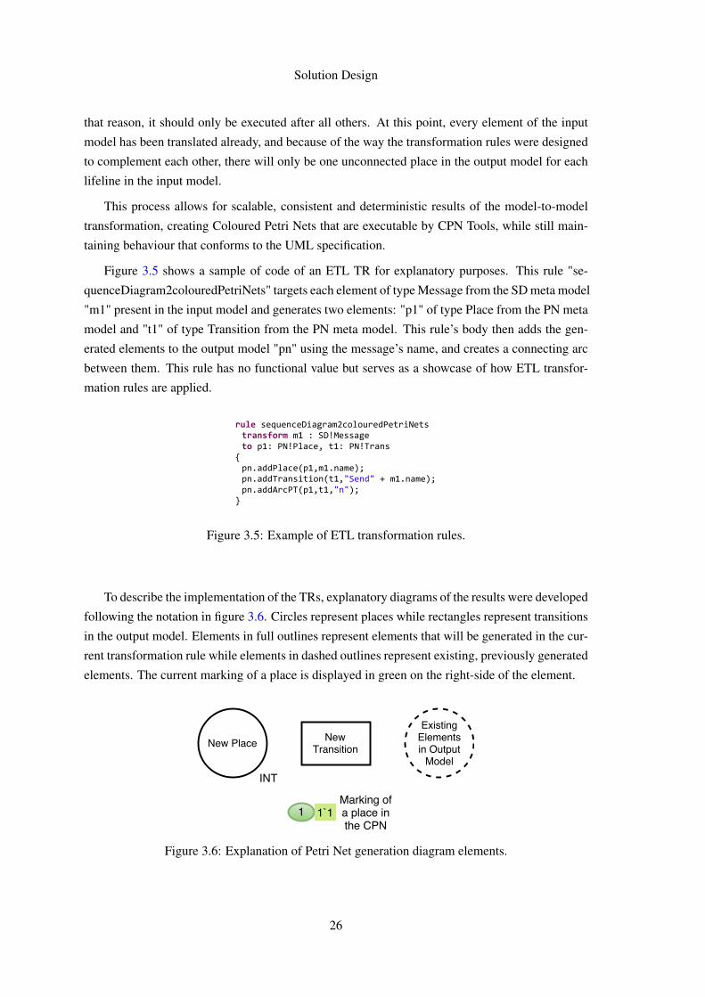
Figure 3.5 shows a sample of code of an ETL TR for explanatory purposes. This rule "se-

quenceDiagram2colouredPetriNets" targets each element of type Message from the SD meta model

"m1" present in the input model and generates two elements: "p1" of type Place from the PN meta

model and "t1" of type Transition from the PN meta model. This rule’s body then adds the gen-

erated elements to the output model "pn" using the message’s name, and creates a connecting arc

between them. This rule has no functional value but serves as a showcase of how ETL transfor-

mation rules are applied.

rule sequenceDiagram2colouredPetriNets transform m1 : SD!Message to p1: PN!Place, t1: PN!Trans { pn.addPlace(p1,m1.name); pn.addTransition(t1,"Send" + m1.name); pn.addArcPT(p1,t1,"n"); }

Figure 3.5: Example of ETL transformation rules.

To describe the implementation of the TRs, explanatory diagrams of the results were developed

following the notation in figure 3.6. Circles represent places while rectangles represent transitions

in the output model. Elements in full outlines represent elements that will be generated in the cur-

rent transformation rule while elements in dashed outlines represent existing, previously generated

elements. The current marking of a place is displayed in green on the right-side of the element.

Figure 3.6: Explanation of Petri Net generation diagram elements.

26

Solution Design

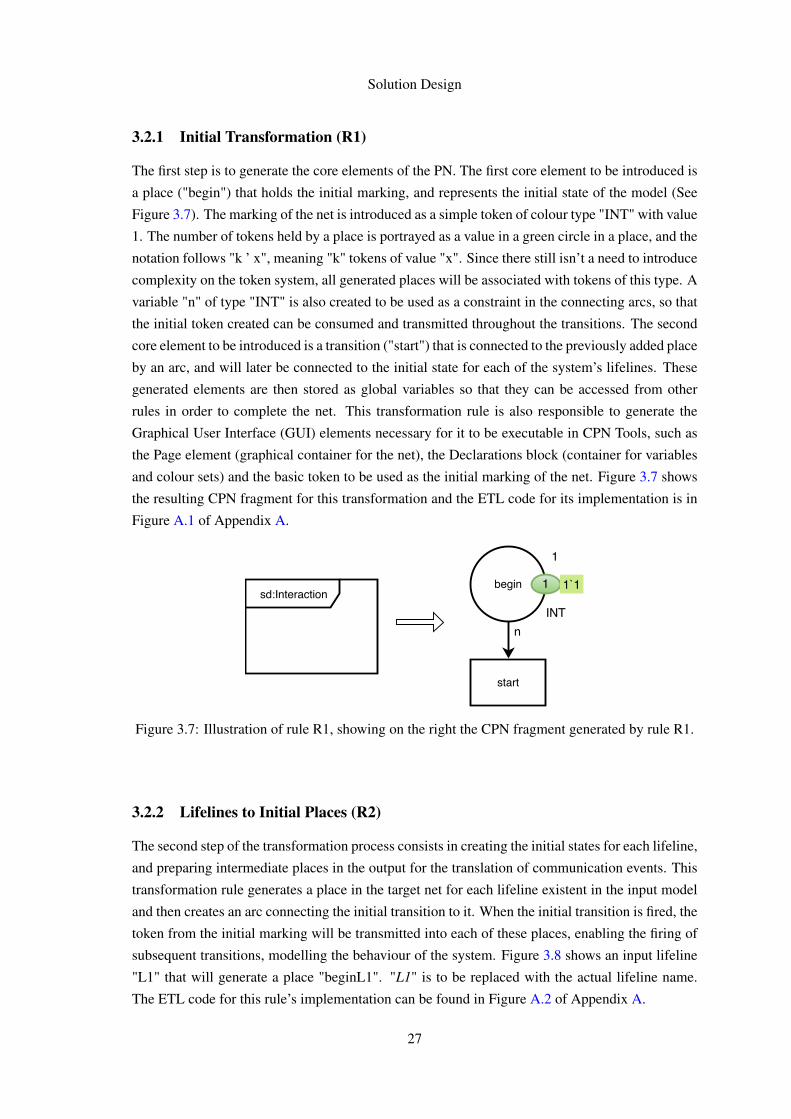
3.2.1 Initial Transformation (R1)

The first step is to generate the core elements of the PN. The first core element to be introduced is

a place ("begin") that holds the initial marking, and represents the initial state of the model (See

Figure 3.7). The marking of the net is introduced as a simple token of colour type "INT" with value

1. The number of tokens held by a place is portrayed as a value in a green circle in a place, and the

notation follows "k ’ x", meaning "k" tokens of value "x". Since there still isn’t a need to introduce

complexity on the token system, all generated places will be associated with tokens of this type. A

variable "n" of type "INT" is also created to be used as a constraint in the connecting arcs, so that

the initial token created can be consumed and transmitted throughout the transitions. The second

core element to be introduced is a transition ("start") that is connected to the previously added place

by an arc, and will later be connected to the initial state for each of the system’s lifelines. These

generated elements are then stored as global variables so that they can be accessed from other

rules in order to complete the net. This transformation rule is also responsible to generate the

Graphical User Interface (GUI) elements necessary for it to be executable in CPN Tools, such as

the Page element (graphical container for the net), the Declarations block (container for variables

and colour sets) and the basic token to be used as the initial marking of the net. Figure 3.7 shows

the resulting CPN fragment for this transformation and the ETL code for its implementation is in

Figure A.1 of Appendix A.

Figure 3.7: Illustration of rule R1, showing on the right the CPN fragment generated by rule R1.

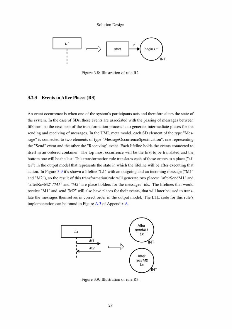
3.2.2 Lifelines to Initial Places (R2)

The second step of the transformation process consists in creating the initial states for each lifeline,

and preparing intermediate places in the output for the translation of communication events. This

transformation rule generates a place in the target net for each lifeline existent in the input model

and then creates an arc connecting the initial transition to it. When the initial transition is fired, the

token from the initial marking will be transmitted into each of these places, enabling the firing of

subsequent transitions, modelling the behaviour of the system. Figure 3.8 shows an input lifeline

"L1" that will generate a place "beginL1". "L1" is to be replaced with the actual lifeline name.

The ETL code for this rule’s implementation can be found in Figure A.2 of Appendix A.

27

Solution Design

Figure 3.8: Illustration of rule R2.

3.2.3 Events to After Places (R3)

An event occurrence is when one of the system’s participants acts and therefore alters the state of

the system. In the case of SDs, these events are associated with the passing of messages between

lifelines, so the next step of the transformation process is to generate intermediate places for the

sending and receiving of messages. In the UML meta model, each SD element of the type "Mes-

sage" is connected to two elements of type "MessageOccurrenceSpecification", one representing

the "Send" event and the other the "Receiving" event. Each lifeline holds the events connected to

itself in an ordered container. The top most occurrence will be the first to be translated and the

bottom one will be the last. This transformation rule translates each of these events to a place ("af-

ter") in the output model that represents the state in which the lifeline will be after executing that

action. In Figure 3.9 it’s shown a lifeline "L1" with an outgoing and an incoming message ("M1"

and "M2"), so the result of this transformation rule will generate two places: "afterSendM1" and

"afterRcvM2"."M1" and "M2" are place holders for the messages’ ids. The lifelines that would

receive "M1" and send "M2" will also have places for their events, that will later be used to trans-

late the messages themselves in correct order in the output model. The ETL code for this rule’s

implementation can be found in Figure A.3 of Appendix A.


28

Solution Design

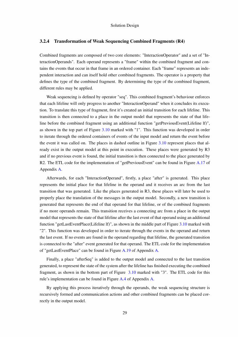
3.2.4 Transformation of Weak Sequencing Combined Fragments (R4)

Combined fragments are composed of two core elements: "InteractionOperator" and a set of "In-

teractionOperands". Each operand represents a "frame" within the combined fragment and con-

tains the events that occur in that frame in an ordered container. Each "frame" represents an inde-

pendent interaction and can itself hold other combined fragments. The operator is a property that

defines the type of the combined fragment. By determining the type of the combined fragment,

different rules may be applied.

Weak sequencing is defined by operator "seq". This combined fragment’s behaviour enforces

that each lifeline will only progress to another "InteractionOperand" when it concludes its execu-

tion. To translate this type of fragment, first it’s created an initial transition for each lifeline. This

transition is then connected to a place in the output model that represents the state of that life-

line before the combined fragment using an additional function "getPreviousEvent(Lifeline lf)",

as shown in the top part of Figure 3.10 marked with "1". This function was developed in order

to iterate through the ordered containers of events of the input model and return the event before

the event it was called on. The places in dashed outline in Figure 3.10 represent places that al-

ready exist in the output model at this point in execution. These places were generated by R3

and if no previous event is found, the initial transition is then connected to the place generated by

R2. The ETL code for the implementation of "getPreviousEvent" can be found in Figure A.17 of

Appendix A.

Afterwards, for each "InteractionOperand", firstly, a place "after" is generated. This place

represents the initial place for that lifeline in the operand and it receives an arc from the last

transition that was generated. Like the places generated in R3, these places will later be used to

properly place the translation of the messages in the output model. Secondly, a new transition is

generated that represents the end of that operand for that lifeline, or of the combined fragments

if no more operands remain. This transition receives a connecting arc from a place in the output

model that represents the state of that lifeline after the last event of that operand using an additional

function "getLastEventPlace(Lifeline lf)", as shown in the middle part of Figure 3.10 marked with

"2". This function was developed in order to iterate through the events in the operand and return

the last event. If no events are found in the operand regarding that lifeline, the generated transition

is connected to the "after" event generated for that operand. The ETL code for the implementation

of "getLastEventPlace" can be found in Figure A.19 of Appendix A.

Finally, a place "afterSeq" is added to the output model and connected to the last transition

generated, to represent the state of the system after the lifeline has finished executing the combined

fragment, as shown in the bottom part of Figure 3.10 marked with "3". The ETL code for this

rule’s implementation can be found in Figure A.4 of Appendix A.

By applying this process iteratively through the operands, the weak sequencing structure is

recursively formed and communication actions and other combined fragments can be placed cor-

rectly in the output model.

29

Solution Design


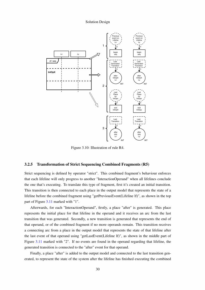
3.2.5 Transformation of Strict Sequencing Combined Fragments (R5)

Strict sequencing is defined by operator "strict". This combined fragment’s behaviour enforces

that each lifeline will only progress to another "InteractionOperand" when all lifelines conclude

the one that’s executing. To translate this type of fragment, first it’s created an initial transition.

This transition is then connected to each place in the output model that represents the state of a

lifeline before the combined fragment using "getPreviousEvent(Lifeline lf)", as shown in the top

part of Figure 3.11 marked with "1".


represents the initial place for that lifeline in the operand and it receives an arc from the last

transition that was generated. Secondly, a new transition is generated that represents the end of

that operand, or of the combined fragment if no more operands remain. This transition receives

a connecting arc from a place in the output model that represents the state of that lifeline after

the last event of that operand using "getLastEvent(Lifeline lf)", as shown in the middle part of

Figure 3.11 marked with "2". If no events are found in the operand regarding that lifeline, the

generated transition is connected to the "after" event for that operand.

Finally, a place "after" is added to the output model and connected to the last transition gen-

erated, to represent the state of the system after the lifeline has finished executing the combined

30

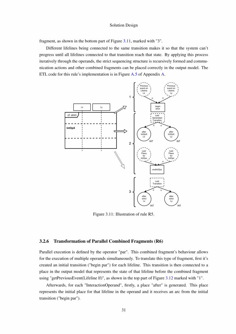
Solution Design

fragment, as shown in the bottom part of Figure 3.11, marked with "3".

Different lifelines being connected to the same transition makes it so that the system can’t

progress until all lifelines connected to that transition reach that state. By applying this process

iteratively through the operands, the strict sequencing structure is recursively formed and commu-

nication actions and other combined fragments can be placed correctly in the output model. The

ETL code for this rule’s implementation is in Figure A.5 of Appendix A.


3.2.6 Transformation of Parallel Combined Fragments (R6)

Parallel execution is defined by the operator "par". This combined fragment’s behaviour allows

for the execution of multiple operands simultaneously. To translate this type of fragment, first it’s

created an initial transition ("begin par") for each lifeline. This transition is then connected to a

place in the output model that represents the state of that lifeline before the combined fragment

using "getPreviousEvent(Lifeline lf)", as shown in the top part of Figure 3.12 marked with "1".


represents the initial place for that lifeline in the operand and it receives an arc from the initial

transition ("begin par").

31

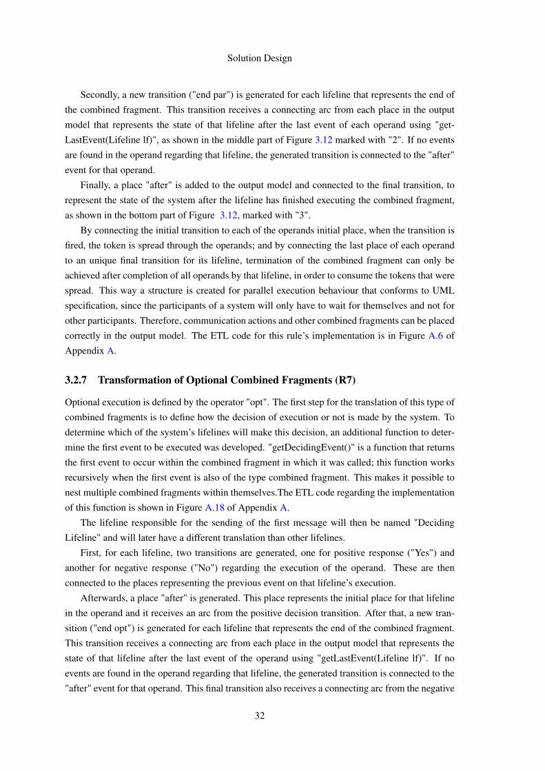
Solution Design

Secondly, a new transition ("end par") is generated for each lifeline that represents the end of

the combined fragment. This transition receives a connecting arc from each place in the output

model that represents the state of that lifeline after the last event of each operand using "get-

LastEvent(Lifeline lf)", as shown in the middle part of Figure 3.12 marked with "2". If no events

are found in the operand regarding that lifeline, the generated transition is connected to the "after"

event for that operand.

Finally, a place "after" is added to the output model and connected to the final transition, to

represent the state of the system after the lifeline has finished executing the combined fragment,

as shown in the bottom part of Figure 3.12, marked with "3".

By connecting the initial transition to each of the operands initial place, when the transition is

fired, the token is spread through the operands; and by connecting the last place of each operand

to an unique final transition for its lifeline, termination of the combined fragment can only be

achieved after completion of all operands by that lifeline, in order to consume the tokens that were

spread. This way a structure is created for parallel execution behaviour that conforms to UML

specification, since the participants of a system will only have to wait for themselves and not for

other participants. Therefore, communication actions and other combined fragments can be placed

correctly in the output model. The ETL code for this rule’s implementation is in Figure A.6 of

Appendix A.

3.2.7 Transformation of Optional Combined Fragments (R7)

Optional execution is defined by the operator "opt". The first step for the translation of this type of

combined fragments is to define how the decision of execution or not is made by the system. To

determine which of the system’s lifelines will make this decision, an additional function to deter-

mine the first event to be executed was developed. "getDecidingEvent()" is a function that returns

the first event to occur within the combined fragment in which it was called; this function works

recursively when the first event is also of the type combined fragment. This makes it possible to

nest multiple combined fragments within themselves.The ETL code regarding the implementation

of this function is shown in Figure A.18 of Appendix A.

The lifeline responsible for the sending of the first message will then be named "Deciding

Lifeline" and will later have a different translation than other lifelines.

First, for each lifeline, two transitions are generated, one for positive response ("Yes") and

another for negative response ("No") regarding the execution of the operand. These are then

connected to the places representing the previous event on that lifeline’s execution.

Afterwards, a place "after" is generated. This place represents the initial place for that lifeline

in the operand and it receives an arc from the positive decision transition. After that, a new tran-

sition ("end opt") is generated for each lifeline that represents the end of the combined fragment.

This transition receives a connecting arc from each place in the output model that represents the

state of that lifeline after the last event of the operand using "getLastEvent(Lifeline lf)". If no

events are found in the operand regarding that lifeline, the generated transition is connected to the

"after" event for that operand. This final transition also receives a connecting arc from the negative

32

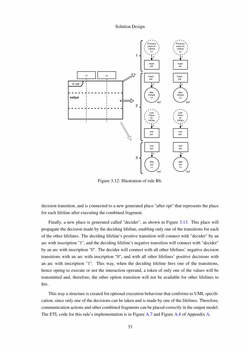
Solution Design


decision transition, and is connected to a new generated place "after opt" that represents the place

for each lifeline after executing the combined fragment.

Finally, a new place is generated called "decider", as shown in Figure 3.13. This place will

propagate the decision made by the deciding lifeline, enabling only one of the transitions for each

of the other lifelines. The deciding lifeline’s positive transition will connect with "decider" by an

arc with inscription "1", and the deciding lifeline’s negative transition will connect with "decider"

by an arc with inscription "0". The decider will connect with all other lifelines’ negative decision

transitions with an arc with inscription "0", and with all other lifelines’ positive decisions with

an arc with inscription "1". This way, when the deciding lifeline fires one of the transitions,

hence opting to execute or not the interaction operand, a token of only one of the values will be

transmitted and, therefore, the other option transition will not be available for other lifelines to

fire.

This way a structure is created for optional execution behaviour that conforms to UML specifi-

cation, since only one of the decisions can be taken and is made by one of the lifelines. Therefore,

communication actions and other combined fragments can be placed correctly in the output model.

The ETL code for this rule’s implementation is in Figure A.7 and Figure A.8 of Appendix A.

33

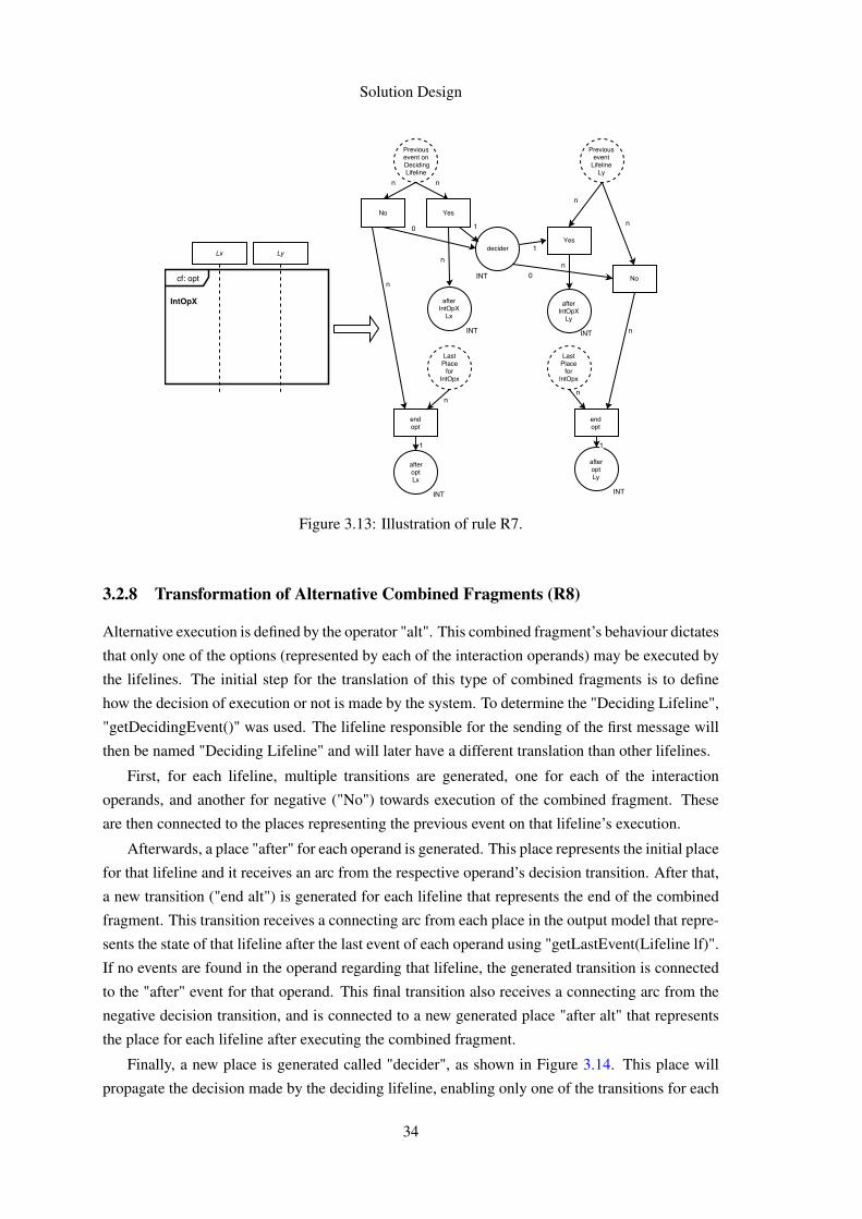
Solution Design


3.2.8 Transformation of Alternative Combined Fragments (R8)

Alternative execution is defined by the operator "alt". This combined fragment’s behaviour dictates

that only one of the options (represented by each of the interaction operands) may be executed by

the lifelines. The initial step for the translation of this type of combined fragments is to define

how the decision of execution or not is made by the system. To determine the "Deciding Lifeline",

"getDecidingEvent()" was used. The lifeline responsible for the sending of the first message will

then be named "Deciding Lifeline" and will later have a different translation than other lifelines.

First, for each lifeline, multiple transitions are generated, one for each of the interaction

operands, and another for negative ("No") towards execution of the combined fragment. These

are then connected to the places representing the previous event on that lifeline’s execution.

Afterwards, a place "after" for each operand is generated. This place represents the initial place

for that lifeline and it receives an arc from the respective operand’s decision transition. After that,

a new transition ("end alt") is generated for each lifeline that represents the end of the combined

fragment. This transition receives a connecting arc from each place in the output model that repre-

sents the state of that lifeline after the last event of each operand using "getLastEvent(Lifeline lf)".

If no events are found in the operand regarding that lifeline, the generated transition is connected

to the "after" event for that operand. This final transition also receives a connecting arc from the

negative decision transition, and is connected to a new generated place "after alt" that represents

the place for each lifeline after executing the combined fragment.

Finally, a new place is generated called "decider", as shown in Figure 3.14. This place will

propagate the decision made by the deciding lifeline, enabling only one of the transitions for each

34

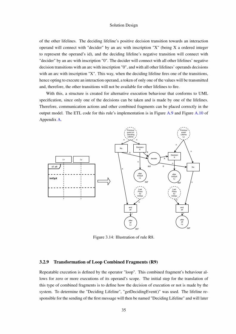
Solution Design

of the other lifelines. The deciding lifeline’s positive decision transition towards an interaction

operand will connect with "decider" by an arc with inscription "X" (being X a ordered integer

to represent the operand’s id), and the deciding lifeline’s negative transition will connect with

"decider" by an arc with inscription "0". The decider will connect with all other lifelines’ negative

decision transitions with an arc with inscription "0", and with all other lifelines’ operands decisions

with an arc with inscription "X". This way, when the deciding lifeline fires one of the transitions,

hence opting to execute an interaction operand, a token of only one of the values will be transmitted

and, therefore, the other transitions will not be available for other lifelines to fire.

With this, a structure is created for alternative execution behaviour that conforms to UML

specification, since only one of the decisions can be taken and is made by one of the lifelines.

Therefore, communication actions and other combined fragments can be placed correctly in the

output model. The ETL code for this rule’s implementation is in Figure A.9 and Figure A.10 of

Appendix A.


3.2.9 Transformation of Loop Combined Fragments (R9)

Repeatable execution is defined by the operator "loop". This combined fragment’s behaviour al-

lows for zero or more executions of its operand’s scope. The initial step for the translation of

this type of combined fragments is to define how the decision of execution or not is made by the

system. To determine the "Deciding Lifeline", "getDecidingEvent()" was used. The lifeline re-

sponsible for the sending of the first message will then be named "Deciding Lifeline" and will later

35

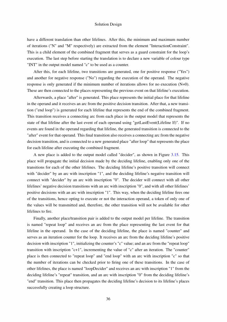
Solution Design

have a different translation than other lifelines. After this, the minimum and maximum number

of iterations ("N" and "M" respectively) are extracted from the element "InteractionConstraint".

This is a child element of the combined fragment that serves as a guard constraint for the loop’s

execution. The last step before starting the translation is to declare a new variable of colour type

"INT" in the output model named "c" to be used as a counter.

After this, for each lifeline, two transitions are generated, one for positive response ("Yes")

and another for negative response ("No") regarding the execution of the operand. The negative

response is only generated if the minimum number of iterations allows for no execution (N=0).

These are then connected to the places representing the previous event on that lifeline’s execution.

Afterwards, a place "after" is generated. This place represents the initial place for that lifeline

in the operand and it receives an arc from the positive decision transition. After that, a new transi-

tion ("end loop") is generated for each lifeline that represents the end of the combined fragment.

This transition receives a connecting arc from each place in the output model that represents the

state of that lifeline after the last event of each operand using "getLastEvent(Lifeline lf)". If no

events are found in the operand regarding that lifeline, the generated transition is connected to the

"after" event for that operand. This final transition also receives a connecting arc from the negative

decision transition, and is connected to a new generated place "after loop" that represents the place

for each lifeline after executing the combined fragment.

A new place is added to the output model called "decider", as shown in Figure 3.15. This

place will propagate the initial decision made by the deciding lifeline, enabling only one of the

transitions for each of the other lifelines. The deciding lifeline’s positive transition will connect

with "decider" by an arc with inscription "1", and the deciding lifeline’s negative transition will

connect with "decider" by an arc with inscription "0". The decider will connect with all other

lifelines’ negative decision transitions with an arc with inscription "0", and with all other lifelines’

positive decisions with an arc with inscription "1". This way, when the deciding lifeline fires one

of the transitions, hence opting to execute or not the interaction operand, a token of only one of

the values will be transmitted and, therefore, the other transition will not be available for other

lifelines to fire.

Finally, another place/transition pair is added to the output model per lifeline. The transition

is named "repeat loop" and receives an arc from the place representing the last event for that

lifeline in the operand. In the case of the deciding lifeline, the place is named "counter" and

serves as an iteration counter for the loop. It receives an arc from the deciding lifeline’s positive

decision with inscription "1", initializing the counter’s "c" value; and an arc from the "repeat loop"

transition with inscription "c+1", incrementing the value of "c" after an iteration. The "counter"

place is then connected to "repeat loop" and "end loop" with an arc with inscription "c" so that

the number of iterations can be checked prior to firing one of these transitions. In the case of

other lifelines, the place is named "loopDecider" and receives an arc with inscription "1" from the

deciding lifeline’s "repeat" transition, and an arc with inscription "0" from the deciding lifeline’s

"end" transition. This place then propagates the deciding lifeline’s decision to its lifeline’s places

successfully creating a loop structure.

36

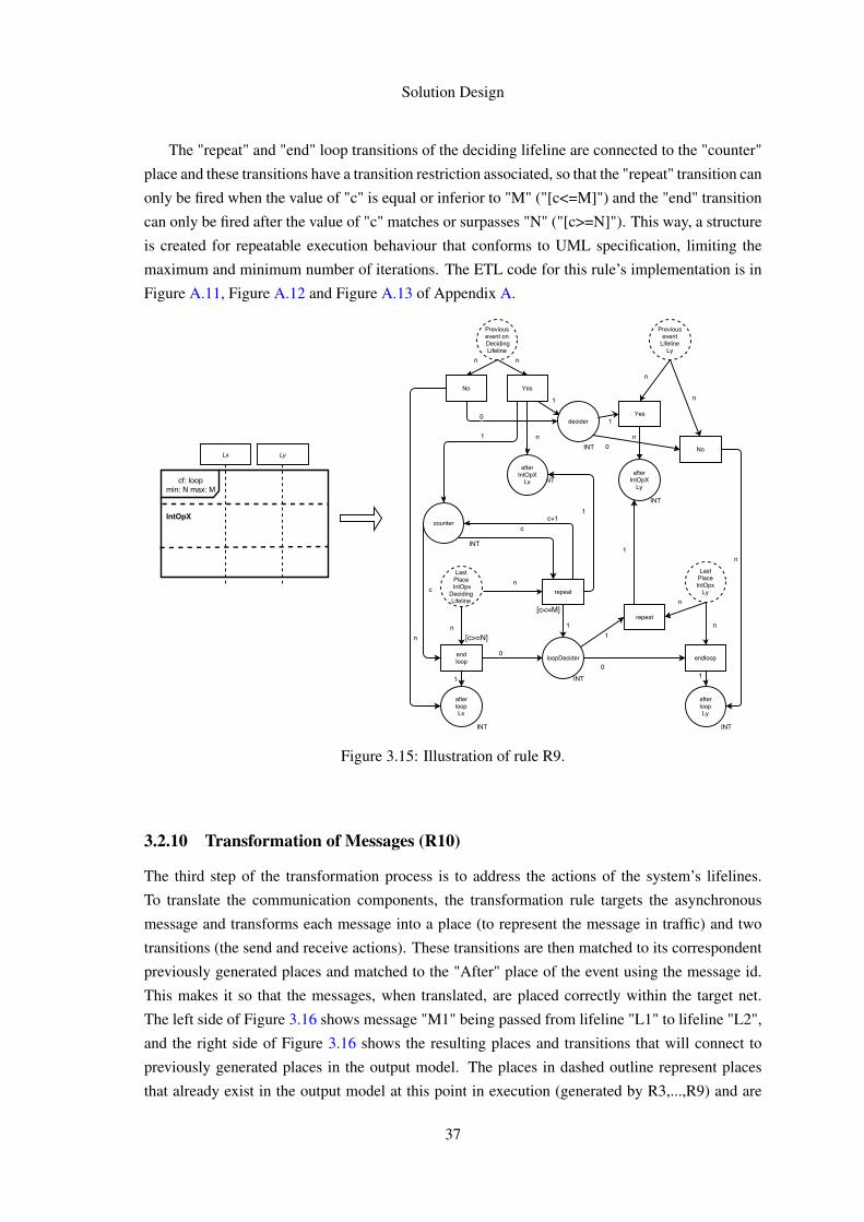
Solution Design

The "repeat" and "end" loop transitions of the deciding lifeline are connected to the "counter"

place and these transitions have a transition restriction associated, so that the "repeat" transition can

only be fired when the value of "c" is equal or inferior to "M" ("[c<=M]") and the "end" transition

can only be fired after the value of "c" matches or surpasses "N" ("[c>=N]"). This way, a structure

is created for repeatable execution behaviour that conforms to UML specification, limiting the

maximum and minimum number of iterations. The ETL code for this rule’s implementation is in

Figure A.11, Figure A.12 and Figure A.13 of Appendix A.


3.2.10 Transformation of Messages (R10)

The third step of the transformation process is to address the actions of the system’s lifelines.

To translate the communication components, the transformation rule targets the asynchronous

message and transforms each message into a place (to represent the message in traffic) and two

transitions (the send and receive actions). These transitions are then matched to its correspondent

previously generated places and matched to the "After" place of the event using the message id.

This makes it so that the messages, when translated, are placed correctly within the target net.

The left side of Figure 3.16 shows message "M1" being passed from lifeline "L1" to lifeline "L2",

and the right side of Figure 3.16 shows the resulting places and transitions that will connect to

previously generated places in the output model. The places in dashed outline represent places

that already exist in the output model at this point in execution (generated by R3,...,R9) and are

37

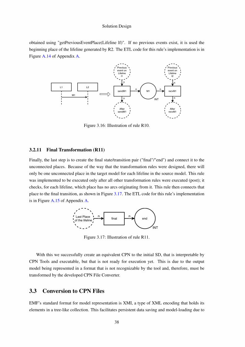
Solution Design

obtained using "getPreviousEventPlace(Lifeline lf)". If no previous events exist, it is used the

beginning place of the lifeline generated by R2. The ETL code for this rule’s implementation is in

Figure A.14 of Appendix A.


3.2.11 Final Transformation (R11)

Finally, the last step is to create the final state/transition pair ("final"/"end") and connect it to the

unconnected places. Because of the way that the transformation rules were designed, there will

only be one unconnected place in the target model for each lifeline in the source model. This rule

was implemented to be executed only after all other transformation rules were executed (post); it

checks, for each lifeline, which place has no arcs originating from it. This rule then connects that

place to the final transition, as shown in Figure 3.17. The ETL code for this rule’s implementation

is in Figure A.15 of Appendix A.


With this we successfully create an equivalent CPN to the initial SD, that is interpretable by

CPN Tools and executable, but that is not ready for execution yet. This is due to the output

model being represented in a format that is not recognizable by the tool and, therefore, must be

transformed by the developed CPN File Converter.

3.3 Conversion to CPN Files

EMF’s standard format for model representation is XMI, a type of XML encoding that holds its

elements in a tree-like collection. This facilitates persistent data saving and model-loading due to

38

Solution Design

the elements being represented as objects and in an organized structure (conforming to the meta

model it’s associated with). This type of file format is not supported by CPN Tools, therefore a

third party open-source software module had to be used to convert the generated files into files

that are ready to be executed with the tool. The used software is "CPN Tools Toolkit" [Gó16], a

collection of necessary Java plug-ins to create CPN Tools files from EMF. This plug-in provides

an ECORE meta model for CPNs executable with CPN Tools and Java functions to convert these

elements into the CPN Tools format. This plug-in was made to be used alongside EMF, therefore

conforms to the full EMF integrated solution approach.

39

Solution Design

40

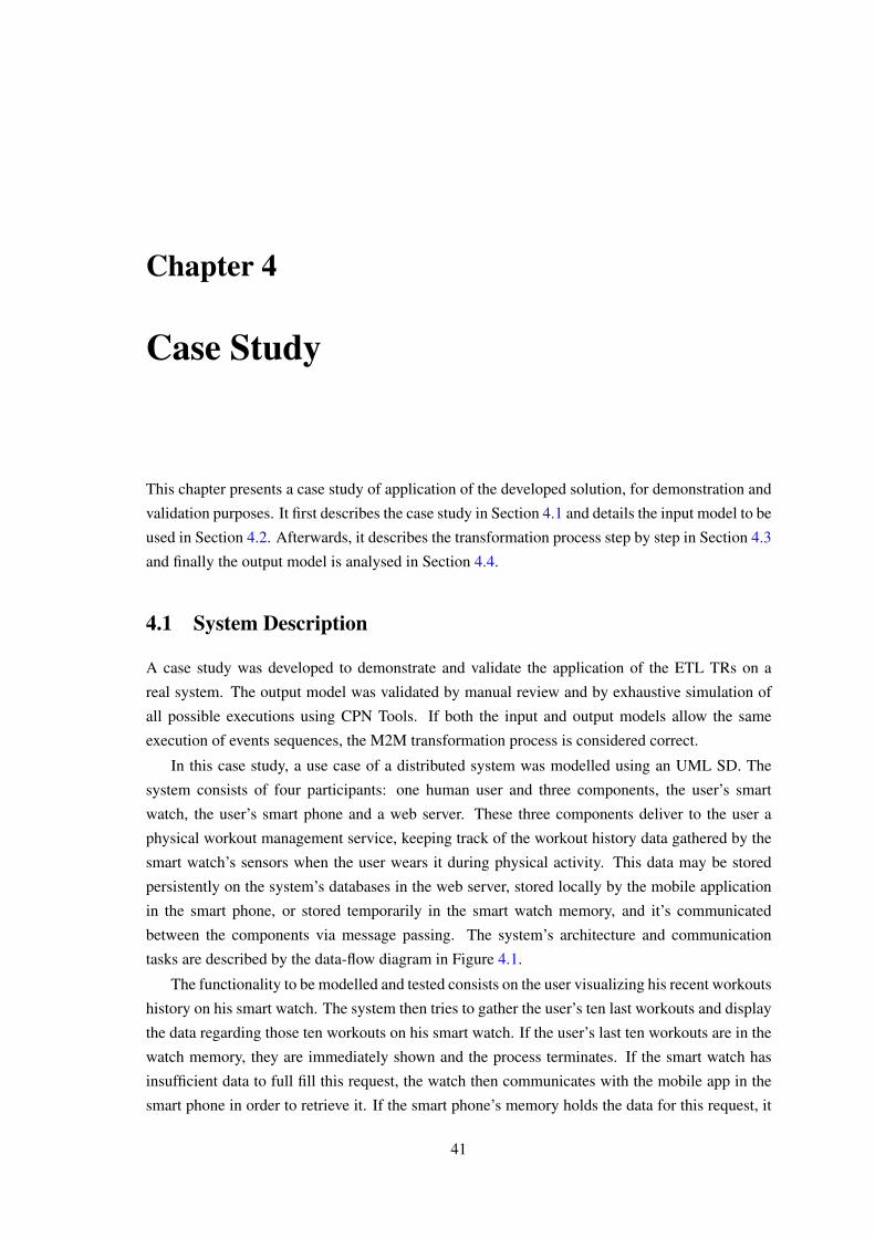
Chapter 4

Case Study

This chapter presents a case study of application of the developed solution, for demonstration and

validation purposes. It first describes the case study in Section 4.1 and details the input model to be

used in Section 4.2. Afterwards, it describes the transformation process step by step in Section 4.3

and finally the output model is analysed in Section 4.4.

4.1 System Description

A case study was developed to demonstrate and validate the application of the ETL TRs on a

real system. The output model was validated by manual review and by exhaustive simulation of

all possible executions using CPN Tools. If both the input and output models allow the same

execution of events sequences, the M2M transformation process is considered correct.

In this case study, a use case of a distributed system was modelled using an UML SD. The

system consists of four participants: one human user and three components, the user’s smart

watch, the user’s smart phone and a web server. These three components deliver to the user a

physical workout management service, keeping track of the workout history data gathered by the

smart watch’s sensors when the user wears it during physical activity. This data may be stored

persistently on the system’s databases in the web server, stored locally by the mobile application

in the smart phone, or stored temporarily in the smart watch memory, and it’s communicated

between the components via message passing. The system’s architecture and communication

tasks are described by the data-flow diagram in Figure 4.1.

The functionality to be modelled and tested consists on the user visualizing his recent workouts

history on his smart watch. The system then tries to gather the user’s ten last workouts and display

the data regarding those ten workouts on his smart watch. If the user’s last ten workouts are in the

watch memory, they are immediately shown and the process terminates. If the smart watch has

insufficient data to full fill this request, the watch then communicates with the mobile app in the

smart phone in order to retrieve it. If the smart phone’s memory holds the data for this request, it

41

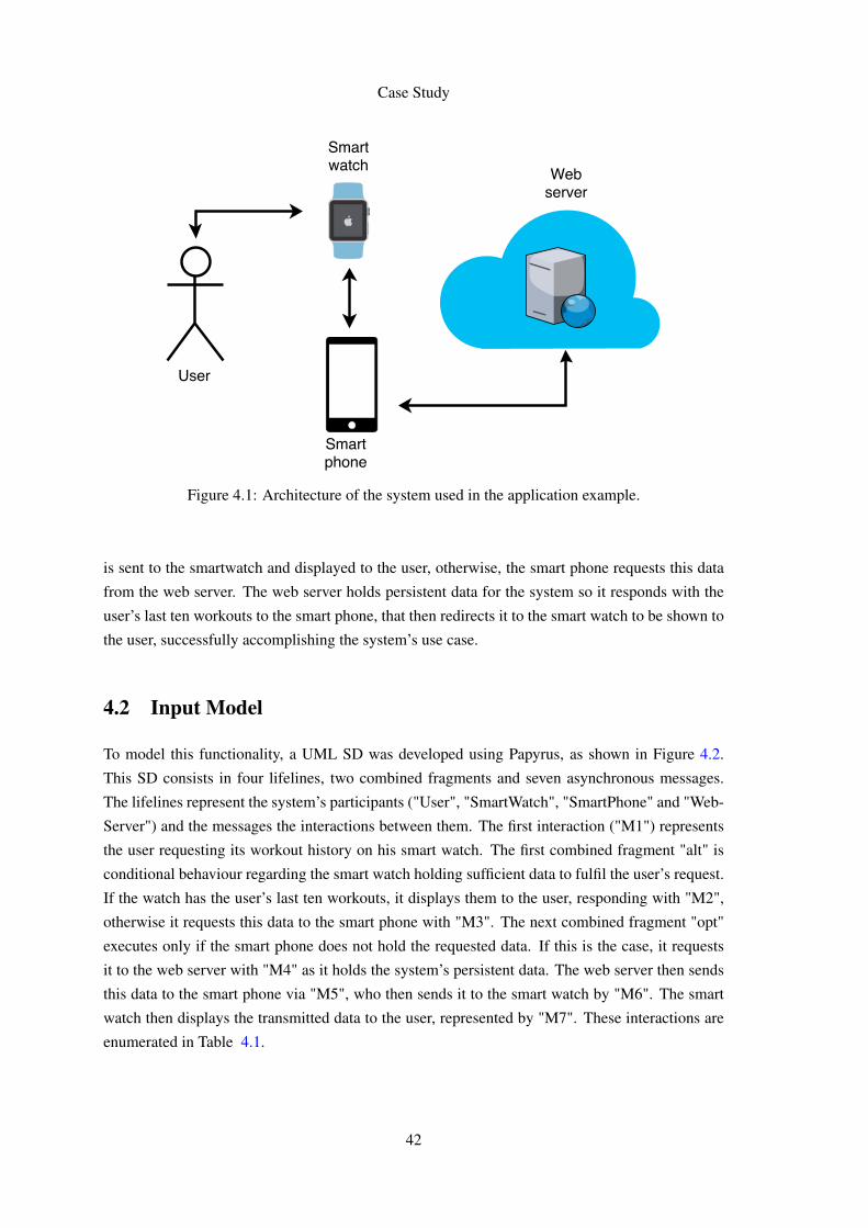
Case Study

Figure 4.1: Architecture of the system used in the application example.

is sent to the smartwatch and displayed to the user, otherwise, the smart phone requests this data

from the web server. The web server holds persistent data for the system so it responds with the

user’s last ten workouts to the smart phone, that then redirects it to the smart watch to be shown to

the user, successfully accomplishing the system’s use case.

4.2 Input Model

To model this functionality, a UML SD was developed using Papyrus, as shown in Figure 4.2.

This SD consists in four lifelines, two combined fragments and seven asynchronous messages.

The lifelines represent the system’s participants ("User", "SmartWatch", "SmartPhone" and "Web-

Server") and the messages the interactions between them. The first interaction ("M1") represents

the user requesting its workout history on his smart watch. The first combined fragment "alt" is

conditional behaviour regarding the smart watch holding sufficient data to fulfil the user’s request.

If the watch has the user’s last ten workouts, it displays them to the user, responding with "M2",

otherwise it requests this data to the smart phone with "M3". The next combined fragment "opt"

executes only if the smart phone does not hold the requested data. If this is the case, it requests

it to the web server with "M4" as it holds the system’s persistent data. The web server then sends

this data to the smart phone via "M5", who then sends it to the smart watch by "M6". The smart

watch then displays the transmitted data to the user, represented by "M7". These interactions are

enumerated in Table 4.1.

42

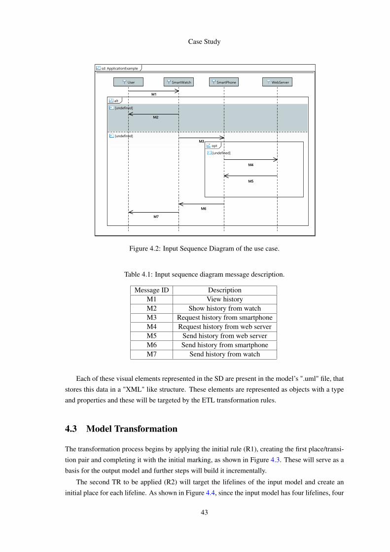
Case Study

Figure 4.2: Input Sequence Diagram of the use case.

Table 4.1: Input sequence diagram message description.

Message ID DescriptionM1 View historyM2 Show history from watchM3 Request history from smartphoneM4 Request history from web serverM5 Send history from web serverM6 Send history from smartphoneM7 Send history from watch

Each of these visual elements represented in the SD are present in the model’s ".uml" file, that

stores this data in a "XML" like structure. These elements are represented as objects with a type

and properties and these will be targeted by the ETL transformation rules.

4.3 Model Transformation

The transformation process begins by applying the initial rule (R1), creating the first place/transi-

tion pair and completing it with the initial marking, as shown in Figure 4.3. These will serve as a

basis for the output model and further steps will build it incrementally.

The second TR to be applied (R2) will target the lifelines of the input model and create an

initial place for each lifeline. As shown in Figure 4.4, since the input model has four lifelines, four

43

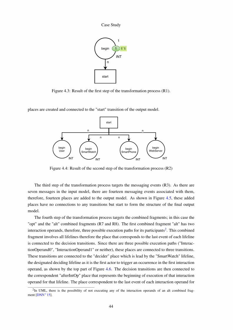
Case Study

Figure 4.3: Result of the first step of the transformation process (R1).

places are created and connected to the "start" transition of the output model.

Figure 4.4: Result of the second step of the transformation process (R2)

The third step of the transformation process targets the messaging events (R3). As there are

seven messages in the input model, there are fourteen messaging events associated with them,

therefore, fourteen places are added to the output model. As shown in Figure 4.5, these added

places have no connections to any transitions but start to form the structure of the final output

model.

The fourth step of the transformation process targets the combined fragments; in this case the

"opt" and the "alt" combined fragments (R7 and R8). The first combined fragment "alt" has two

interaction operands, therefore, three possible execution paths for its participants2. This combined

fragment involves all lifelines therefore the place that corresponds to the last event of each lifeline

is connected to the decision transitions. Since there are three possible execution paths ("Interac-

tionOperand0", "InteractionOperand1" or neither), these places are connected to three transitions.

These transitions are connected to the "decider" place which is lead by the "SmartWatch" lifeline,

the designated deciding lifeline as it is the first actor to trigger an occurrence in the first interaction

operand, as shown by the top part of Figure 4.6. The decision transitions are then connected to

the correspondent "afterIntOp" place that represents the beginning of execution of that interaction

operand for that lifeline. The place correspondent to the last event of each interaction operand for

2In UML, there is the possibility of not executing any of the interaction operands of an alt combined frag-ment [DNN+15].

44

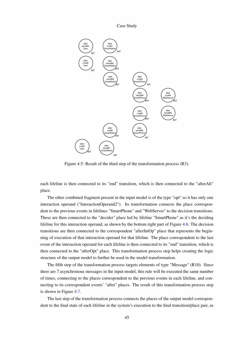
Case Study

Figure 4.5: Result of the third step of the transformation process (R3).

each lifeline is then connected to its "end" transition, which is then connected to the "afterAlt"

place.

The other combined fragment present in the input model is of the type "opt" so it has only one

interaction operand ("InteractionOperand2"). Its transformation connects the place correspon-

dent to the previous events in lifelines "SmartPhone" and "WebServer" to the decision transitions.

These are then connected to the "decider" place led by lifeline "SmartPhone" as it’s the deciding

lifeline for this interaction operand, as shown by the bottom right part of Figure 4.6. The decision

transitions are then connected to the correspondent "afterIntOp" place that represents the begin-

ning of execution of that interaction operand for that lifeline. The place correspondent to the last

event of the interaction operand for each lifeline is then connected to its "end" transition, which is

then connected to the "afterOpt" place. This transformation process step helps creating the logic

structure of the output model to further be used in the model transformation.

The fifth step of the transformation process targets elements of type "Message" (R10). Since

there are 7 asynchronous messages in the input model, this rule will be executed the same number

of times, connecting to the places correspondent to the previous events in each lifeline, and con-

necting to its correspondent events’ "after" places. The result of this transformation process step

is shown in Figure 4.7.

The last step of the transformation process connects the places of the output model correspon-

dent to the final state of each lifeline in the system’s execution to the final transition/place pair, as

45

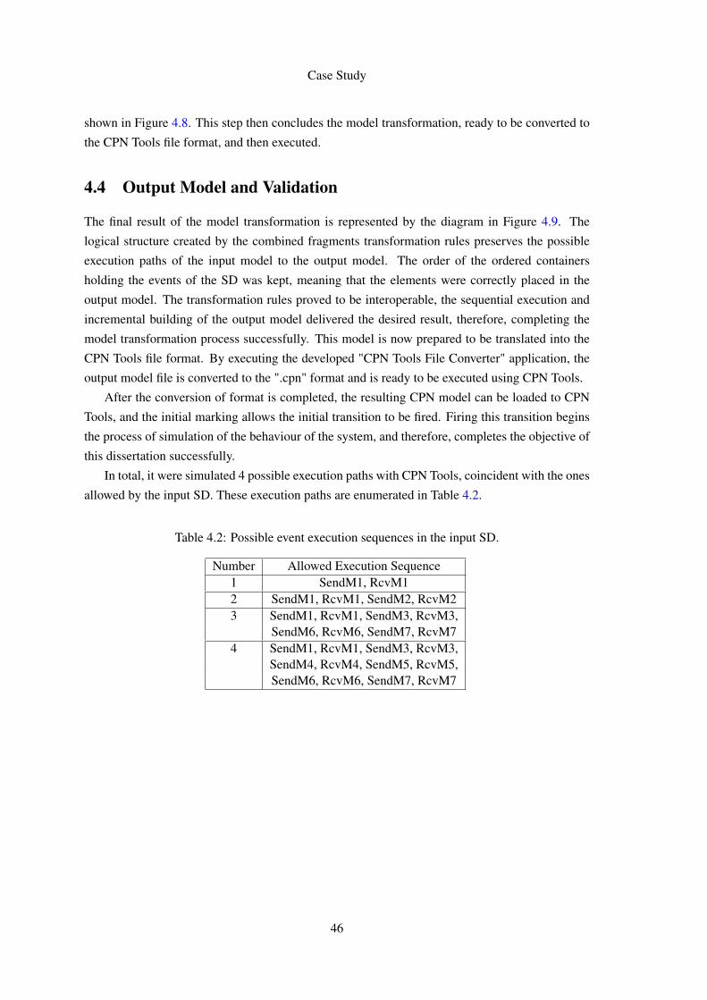
Case Study

shown in Figure 4.8. This step then concludes the model transformation, ready to be converted to

the CPN Tools file format, and then executed.

4.4 Output Model and Validation

The final result of the model transformation is represented by the diagram in Figure 4.9. The

logical structure created by the combined fragments transformation rules preserves the possible

execution paths of the input model to the output model. The order of the ordered containers

holding the events of the SD was kept, meaning that the elements were correctly placed in the

output model. The transformation rules proved to be interoperable, the sequential execution and

incremental building of the output model delivered the desired result, therefore, completing the

model transformation process successfully. This model is now prepared to be translated into the

CPN Tools file format. By executing the developed "CPN Tools File Converter" application, the

output model file is converted to the ".cpn" format and is ready to be executed using CPN Tools.

After the conversion of format is completed, the resulting CPN model can be loaded to CPN

Tools, and the initial marking allows the initial transition to be fired. Firing this transition begins

the process of simulation of the behaviour of the system, and therefore, completes the objective of

this dissertation successfully.

In total, it were simulated 4 possible execution paths with CPN Tools, coincident with the ones

allowed by the input SD. These execution paths are enumerated in Table 4.2.

Table 4.2: Possible event execution sequences in the input SD.

Number Allowed Execution Sequence1 SendM1, RcvM12 SendM1, RcvM1, SendM2, RcvM23 SendM1, RcvM1, SendM3, RcvM3,

SendM6, RcvM6, SendM7, RcvM74 SendM1, RcvM1, SendM3, RcvM3,

SendM4, RcvM4, SendM5, RcvM5,SendM6, RcvM6, SendM7, RcvM7

46

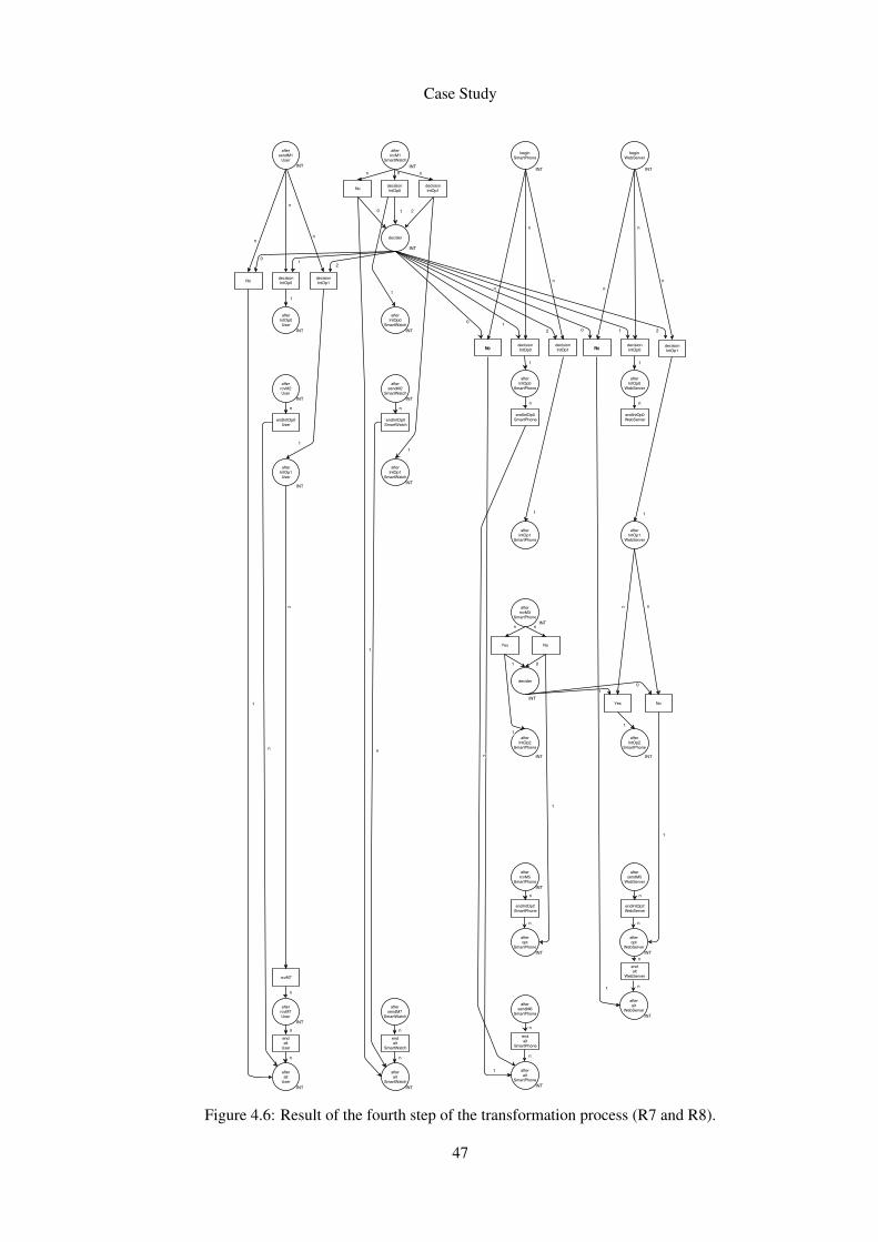
Case Study

Figure 4.6: Result of the fourth step of the transformation process (R7 and R8).

47

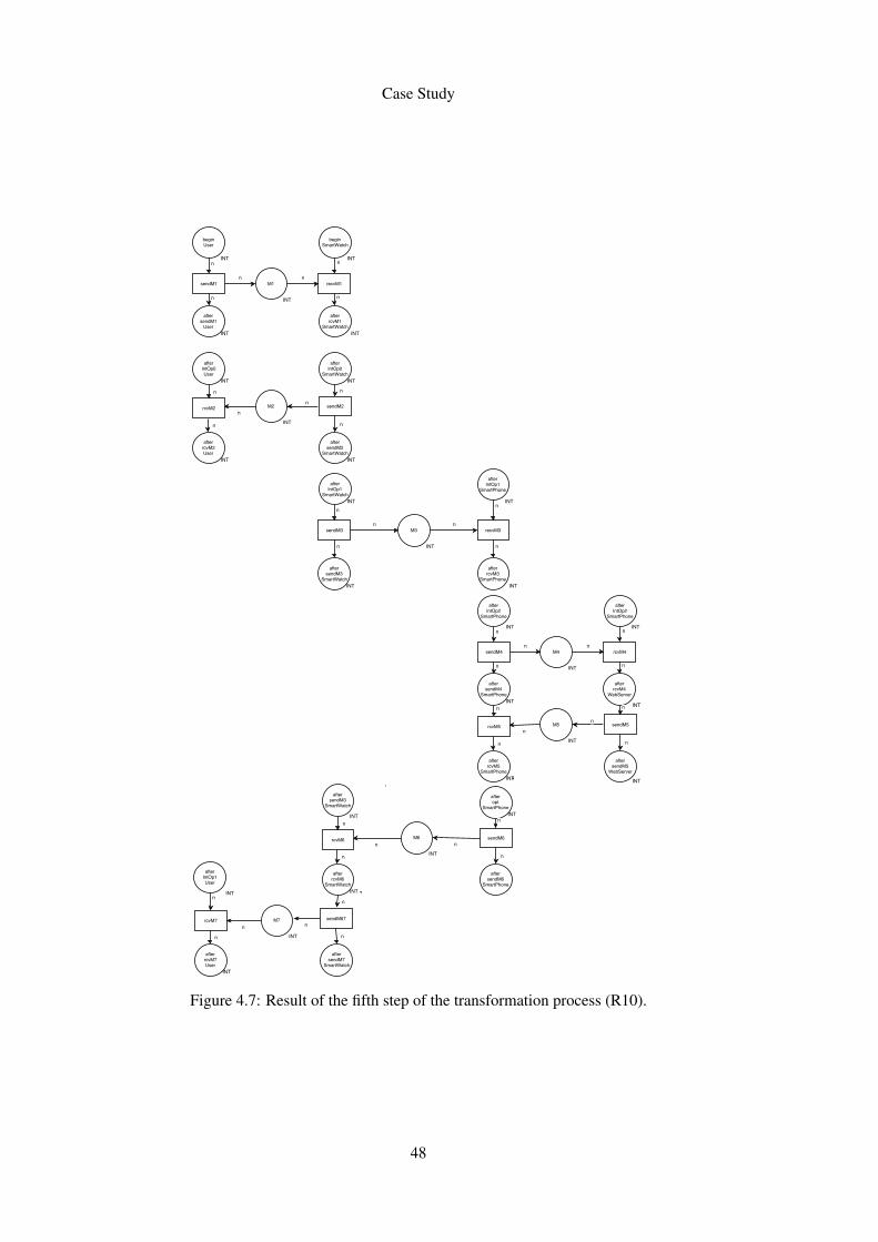
Case Study

Figure 4.7: Result of the fifth step of the transformation process (R10).

48

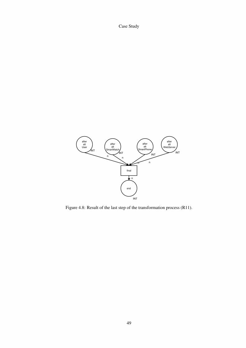
Case Study

Figure 4.8: Result of the last step of the transformation process (R11).

49

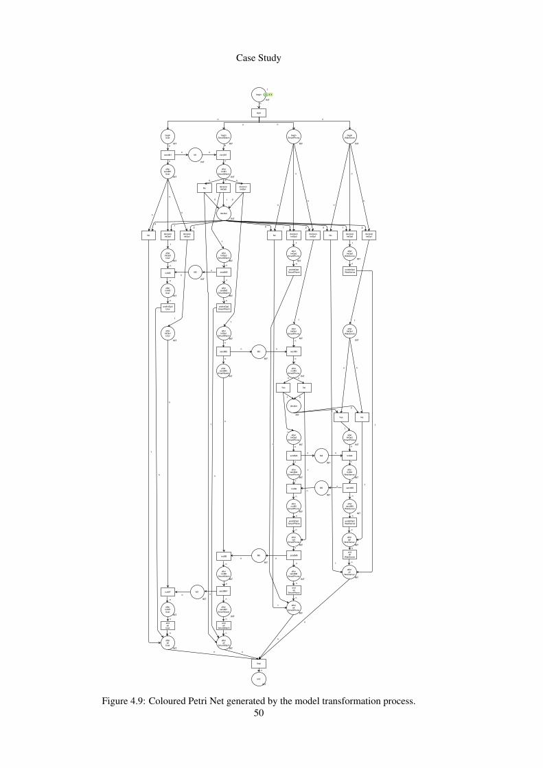
Case Study

Figure 4.9: Coloured Petri Net generated by the model transformation process.50

Chapter 5

Conclusions and Future Work

This ending chapter works as a summary of this dissertation, giving an overview in Section 5.1 of

the results and how these fulfil the desired objectives, and in Section 5.2 providing some sugges-

tions for further extension of the solution.

5.1 Objective Fulfilment

The main goal of this dissertation work was to develop a model transformation solution that trans-

forms UML SDs into equivalent CPNs executable by CPN Tools. The second main objective

was to implement this solution taking advantage of existent state of the art model transformation

frameworks, techniques and technologies. The third main objective was to make this solution in-

tegrateable with other model-driven-engineering solutions, scalable for an increase in complexity

and extendible for future implementations.

As seen from the analysis of the Case Study in Chapter 4, the developed solution successfully

generates CPNs executable with CPN Tools that are equivalent to the input UML SD, as long

as the input model is defined using only its main features selected for this dissertation work.

Therefore, the main goal was achieved correctly, although not entirely, as features from UML

SDs like synchronous messages and some combined fragments were not implemented due to their

lesser importance for the modelling of distributed systems. EMF and Epsilon proved to be efficient

tools for the development of the SwC as they provided a fully integrated solution to perform the

model transformation in a way that is possible to integrate with other model driven engineering

technologies. Finally, the TRs were designed and implemented in a way that facilitates future

extensions.

51

Conclusions and Future Work

5.2 Future Work

As future work it is intended to implement the remaining features of UML SDs like: synchronous

messages, action/behaviour specification, break combined fragments, negative combined frag-

ments, critical combined fragments, ignore combine fragment, consider combined fragments and

assertion combined fragments. These will be implemented as ETL transformation rules and are to

be inserted in the rule set precedence accordingly.

Further validation of the solution with more complex test case studies are also valuable as

future work to increase the certainty of the robustness of the solution.

Finally, as the whole purpose of this dissertation work is for it to be used in the development

of the Model Based Testing tool set, the final stage of maturity for this solution is for it to be

integrated with the remaining components of that project.

52

References

[BDM02] Simona Bernardi, Susanna Donatelli, and José Merseguer. From uml sequence di-agrams and statecharts to analysable petri net models. In Proceedings of the 3rdInternational Workshop on Software and Performance, WOSP ’02, pages 35–45,New York, NY, USA, 2002. ACM.

[BGH00] B. Bordbar, L. Giacomini, and D. J. Holding. Uml and petri nets for design and anal-ysis of distributed systems. In Proceedings of the 2000. IEEE International Confer-ence on Control Applications. Conference Proceedings (Cat. No.00CH37162), pages610–615, 2000.

[BM10] Juliana Bowles and Dulani Meedeniya. Formal transformation from sequence dia-grams to coloured petri nets. In Software Engineering Conference (APSEC), 201017th Asia Pacific, pages 216–225. IEEE, 2010.

[BPSM+97] Tim Bray, Jean Paoli, C Michael Sperberg-McQueen, Eve Maler, and FrançoisYergeau. Extensible markup language (XML). World Wide Web Journal, 2(4):27–66,1997.

[CH03] K Czarnecki and S Helsen. Classification of model transformation approaches. Procof the 2nd OOPSLA Workshop on Generative Techniques in the Context of the ModelDriven Architecture, pages 1–17, 2003.

[DNN+15] O M G Document, Number Normative, Associated Normative, Machine Consum-able, U M L Specification, and Simplification Rfp. OMG Unified Modeling Lan-guage TM ( OMG UML ). 05(March), 2015.

[EFM+05] Christoph Eichner, Hans Fleischhack, Roland Meyer, Ulrik Schrimpf, and ChristianStehno. Compositional Semantics for UML 2.0 Sequence Diagrams Using PetriNets, pages 133–148. Springer Berlin Heidelberg, Berlin, Heidelberg, 2005.

[ES09] Sima Emadi and Fereidoon Shams. Transformation of usecase and sequence di-agrams to petri nets. In Computing, Communication, Control, and Management,2009. CCCM 2009. ISECS International Colloquium on, volume 4, pages 399–403.IEEE, 2009.

[etl] Example: Transform a tree model to a graph model with etl. http://www.eclipse.org/epsilon/examples/index.php?example=org.eclipse.epsilon.examples.tree2graph. Accessed: 2017-02-09.

[FM08] Chlara Francalenei and Francesco Merlo. The Impact of Complexity on SoftwareDesign Quality and Costs: An Exploratory Empirical Analysis of Open Source Ap-plications. Ecis, (2008):201, 2008.

53

http://www.eclipse.org/epsilon/examples/index.php?example=org.eclipse.epsilon.examples.tree2graph



REFERENCES

[FP16] João Pascoal Faria and Ana C R Paiva. A toolset for conformance testing against umlsequence diagrams based on event-driven colored petri nets. International Journalon Software Tools for Technology Transfer, 18(3):285–304, 2016.

[FTJR07] J. M. Fernandes, S. Tjell, J. B. Jorgensen, and O. Ribeiro. Designing tool supportfor translating use cases and uml 2.0 sequence diagrams into a coloured petri net.In Scenarios and State Machines, 2007. SCESM ’07: ICSE Workshops 2007. SixthInternational Workshop on, pages 2–2, May 2007.

[Gó16] A. Gómez. CPN Tools Toolkit, 2016.

[Gra97] Mark Grand. Java Language Reference. O’Reilly & Associates, Inc., Sebastopol,CA, USA, 1997.

[JABK08] Frédéric Jouault, Freddy Allilaire, Jean Bézivin, and Ivan Kurtev. Atl: A modeltransformation tool. Science of Computer Programming, 72(1–2):31 – 39, 2008.Special Issue on Second issue of experimental software and toolkits (EST).

[JKW07a] Kurt Jensen, Lars Michael Kristensen, and Lisa Wells. Coloured Petri Nets and CPNTools for modelling and validation of concurrent systems. International Journal onSoftware Tools for Technology Transfer, 9(3):213–254, 2007.

[JKW07b] Kurt Jensen, Lars Michael Kristensen, and Lisa Wells. Coloured Petri Nets and CPNTools for modelling and validation of concurrent systems. International Journal onSoftware Tools for Technology Transfer, 9(3-4):213–254, 2007.

[KBSB10] Marouane Kessentini, Arbi Bouchoucha, Houari Sahraoui, and Mounir Boukadoum.Example-based sequence diagrams to colored petri nets transformation using heuris-tic Search. In European Conference on Modelling Foundations and Applications,pages 156–172. Springer, 2010.

[KH02] Jernej Kovse and Theo Härder. Generic XMI-Based UML Model Transformations,pages 192–198. Springer Berlin Heidelberg, Berlin, Heidelberg, 2002.

[KPP06a] Dimitrios S. Kolovos, Richard F. Paige, and Fiona A. C. Polack. Eclipse Develop-ment Tools for Epsilon. Eclipse Modeling Symposium on Eclipse Summit Europe,(October), 2006.

[KPP06b] Dimitrios S Kolovos, Richard F Paige, and Fiona AC Polack. Eclipse developmenttools for epsilon. In Eclipse Summit Europe, Eclipse Modeling Symposium, volume20062, page 200, 2006.

[KPP08] Dimitrios S. Kolovos, Richard F. Paige, and Fiona A. C. Polack. The Epsilon Trans-formation Language, pages 46–60. Springer Berlin Heidelberg, Berlin, Heidelberg,2008.

[LF16] Bruno Lima and João Pascoal Faria. Automated Testing of Distributed and Hetero-geneous Systems Based on UML Sequence Diagrams. Software Technologies: 10thInternational Joint Conference, ICSOFT 2015, Colmar, France, July 20-22, 2015,Revised Selected Papers, 586:380–396, 2016.

[LsLQC07] B. L. Li, Z. s. Li, L. Qing, and Y. H. Chen. Test case automate generation fromuml sequence diagram and ocl expression. In 2007 International Conference onComputational Intelligence and Security (CIS 2007), pages 1048–1052, Dec 2007.

54

REFERENCES

[LTE+09a] Agnes Lanusse, Yann Tanguy, Huascar Espinoza, Chokri Mraidha, Sebastien Ger-ard, Patrick Tessier, Remi Schnekenburger, Hubert Dubois, and François Terrier.Papyrus UML: an open source toolset for MDA. 5th ECMDA-FA: Proceedings ofthe Tools and Consultancy Track, pages 1–4, 2009.

[LTE+09b] Agnes Lanusse, Yann Tanguy, Huascar Espinoza, Chokri Mraidha, Sebastien Ger-ard, Patrick Tessier, Remi Schnekenburger, Hubert Dubois, and François Terrier.Papyrus UML: an open source toolset for MDA. In Proc. of the Fifth European Con-ference on Model-Driven Architecture Foundations and Applications (ECMDA-FA2009), pages 1–4, 2009.

[met] What is metamodeling, and what is it good for? = http://infogrid.org/trac/wiki/reference/whatismetamodeling. Accessed: 2017-02-09.

[MLG+10] Yoshimasa Miwa, Chen Li, Qi-Wei Ge, Hiroshi Matsuno, and Satoru Miyano. Ondetermining firing delay time of transitions for petri net based signaling pathways byintroducing stochastic decision rules. In silico biology, 10(1, 2):49–66, 2010.

[Mur89] T. Murata. Petri nets: Properties, analysis and applications. Proceedings of the IEEE,77(4):541–580, Apr 1989.

[MV06] Tom Mens and Pieter Van Gorp. A taxonomy of model transformation. ElectronicNotes in Theoretical Computer Science, 152(1-2):125–142, 2006.

[OEPP06] Adel Ouardani, Philippe Esteban, Mario Paludetto, and Jean-Claude Pascal. A Meta-modeling Approach for Sequence Diagrams to Petri Nets Transformation within therequirements validation process. In Proceedings of the European Simulation andModeling Conference, pages 345–349, 2006.

[pnt] Interactive tutorials on petri nets. http://www.informatik.uni-hamburg.de/TGI/PetriNets/introductions/aalst/. Accessed: 2017-02-01.

[PR08] C. Adam Petri and W. Reisig. Petri net. Scholarpedia, 3(4):6477, 2008. revision91646.

[PZ13] Louchka Popova-Zeugmann. Time Petri Nets, pages 31–137. Springer Berlin Hei-delberg, Berlin, Heidelberg, 2013.

[RF06] Óscar Rafael Silva Ferreira Ribeiro and João M Fernandes. Some rules to transformsequence diagrams into coloured Petri nets. In 7th Workshop and Tutorial on Prac-tical Use of Coloured Petri Nets and the CPN Tools (CPN 2006), pages 237–256,2006.

[SBPM09] David Steinberg, Frank Budinsky, Marcelo Paternostro, and Ed Merks. EMF:Eclipse Modeling Framework 2.0. Addison-Wesley Professional, 2nd edition, 2009.

[SC04] N. Serrano and I. Ciordia. Ant: automating the process of building applications.IEEE Software, 21(6):89–91, Nov 2004.

[Sch08] Bernhard Schätz. Formalization and rule-based transformation of EMF Ecore-basedmodels. In International Conference on Software Language Engineering, pages227–244. Springer, 2008.

55

http://infogrid.org/trac/wiki/reference/whatismetamodeling

http://infogrid.org/trac/wiki/reference/whatismetamodeling

http://www.informatik.uni-hamburg.de/TGI/PetriNets/introductions/aalst/

http://www.informatik.uni-hamburg.de/TGI/PetriNets/introductions/aalst/

REFERENCES

[Sch09] Bernhard Schätz. Formalization and Rule-Based Transformation of EMF Ecore-Based Models, pages 227–244. Springer Berlin Heidelberg, Berlin, Heidelberg,2009.

[seq] Uml 2 sequence diagram. https://http://www.sparxsystems.com/resources/uml2_tutorial/uml2_sequencediagram.html/. Accessed:2017-02-09.

[SK03] S. Sendall and W. Kozaczynski. Model transformation: the heart and soul of model-driven software development. IEEE Software, 20(5):42–45, Sept 2003.

[Sta13] Tony Spiteri Staines. Transforming UML sequence diagrams into Petri Net. Journalof communication and computer, 10(1):72–81, 2013.

[uml] Uml: Success stories. https://www.uml.org/uml_success_stories/.Accessed: 2017-02-05.

[WLL09] Lee W. Wagenhals, Stewart W. Liles, and Alexander H. Levis. Toward executablearchitectures to support evaluation. 2009 International Symposium on CollaborativeTechnologies and Systems, CTS 2009, (June 2009):502–511, 2009.

[YHL+08] Ye Yang, Mei He, Mingshu Li, Q Wang, and Barry W. Boehm. Phase distributionof software development effort. Int. Symp. on Empirical Software Engineering andMeasurement, pages 61–69, 2008.

56

https://http://www.sparxsystems.com/resources/uml2_tutorial/uml2_sequencediagram.html/

https://http://www.sparxsystems.com/resources/uml2_tutorial/uml2_sequencediagram.html/

https://www.uml.org/uml_success_stories/

Appendix A

ETL Code

This appendix presents Figures of the implementation of the ETL transformation rules and addi-

tional functions developed for this solution.

57

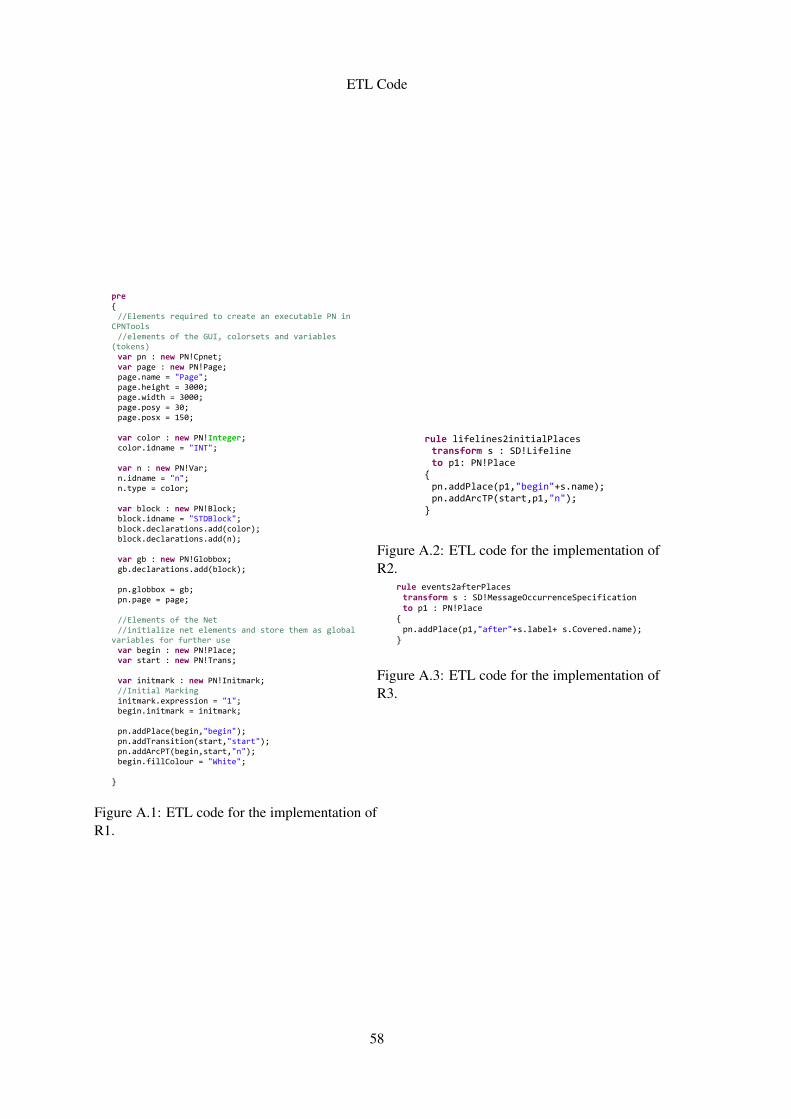
ETL Code

pre { //Elements required to create an executable PN in CPNTools //elements of the GUI, colorsets and variables (tokens) var pn : new PN!Cpnet; var page : new PN!Page; page.name = "Page"; page.height = 3000; page.width = 3000; page.posy = 30; page.posx = 150; var color : new PN!Integer; color.idname = "INT"; var n : new PN!Var; n.idname = "n"; n.type = color; var block : new PN!Block; block.idname = "STDBlock"; block.declarations.add(color); block.declarations.add(n); var gb : new PN!Globbox; gb.declarations.add(block); pn.globbox = gb; pn.page = page; //Elements of the Net //initialize net elements and store them as global variables for further use var begin : new PN!Place; var start : new PN!Trans; var initmark : new PN!Initmark; //Initial Marking initmark.expression = "1"; begin.initmark = initmark; pn.addPlace(begin,"begin"); pn.addTransition(start,"start"); pn.addArcPT(begin,start,"n"); begin.fillColour = "White"; }

Figure A.1: ETL code for the implementation ofR1.

rule lifelines2initialPlaces transform s : SD!Lifeline to p1: PN!Place { pn.addPlace(p1,"begin"+s.name); pn.addArcTP(start,p1,"n"); }


rule events2afterPlaces transform s : SD!MessageOccurrenceSpecification to p1 : PN!Place { pn.addPlace(p1,"after"+s.label+ s.Covered.name); }


58

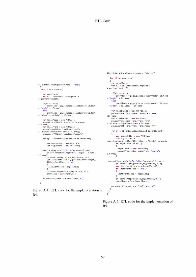
ETL Code

if(s.interactionOperator.name = "seq") { for(lf in s.covered) { var prevPlace; var e1 : SD!InteractionFragment = s.getPrevEvent(lf); if(e1 == null) prevPlace = page.places.selectOne(it|it.text = "begin" + lf.name); else prevPlace = page.places.selectOne(it|it.text = "after" + e1.label + lf.name); var finalPlace : new PN!Place; pn.addPlace(finalPlace,"after"+ s.name +lf.name); var finalTrans : new PN!Trans; pn.addTransition(finalTrans,"end"+ s.interactionOperator.name + lf.name); pn.addArcTP(finalTrans,finalPlace,"n"); for (y : SD!InteractionOperand in IntOpCont) { var beginIntOp : new PN!Place; var beginTrans : new PN!Trans; pn.addPlace(beginIntOp,"after"+y.name+lf.name); pn.addTransition(beginTrans,"begin"+ y.name + lf.name); pn.addArcTP(beginTrans,beginIntOp,"n"); var lastEventPlace = y.getLastEventPlace(lf); if(lastEventPlace == null) { lastEventPlace = beginIntOp; } pn.addArcPT(prevPlace,beginTrans,"n"); prevPlace = lastEventPlace; } pn.addArcPT(prevPlace,finalTrans,"n"); } }


if(s.interactionOperator.name = "strict") { for(lf in s.covered) { var prevPlace; var e1 : SD!InteractionFragment = s.getPrevEvent(lf); if(e1 == null) prevPlace = page.places.selectOne(it|it.text = "begin" + lf.name); else prevPlace = page.places.selectOne(it|it.text = "after" + e1.label + lf.name); var finalPlace : new PN!Place; pn.addPlace(finalPlace,"after"+ s.name +lf.name); var finalTrans : new PN!Trans; pn.addTransition(finalTrans,"end"+ s.interactionOperator.name + lf.name); pn.addArcTP(finalTrans,finalPlace,"n"); for (y : SD!InteractionOperand in IntOpCont) { var beginIntOp : new PN!Place; var beginTrans = page.transs.selectOne(it|it.text = "begin"+y.name); if(beginTrans == null) { beginTrans = new PN!Trans; pn.addTransition(beginTrans,"begin"+ y.name); } pn.addPlace(beginIntOp,"after"+y.name+lf.name); pn.addArcTP(beginTrans,beginIntOp,"n"); var lastEventPlace = y.EventPlace(lf); if(lastEventPlace == null) { lastEventPlace = beginIntOp; } pn.addArcPT(prevPlace,beginTrans,"n"); prevPlace = lastEventPlace; } pn.addArcPT(prevPlace,finalTrans,"n"); } } }


59

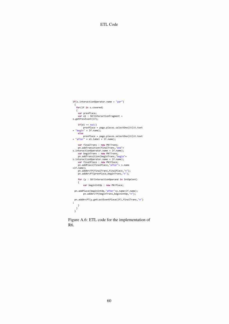
ETL Code

if(s.interactionOperator.name = "par") { for(lf in s.covered) { var prevPlace; var e1 : SD!InteractionFragment = s.getPrevEvent(lf); if(e1 == null) prevPlace = page.places.selectOne(it|it.text = "begin" + lf.name); else prevPlace = page.places.selectOne(it|it.text = "after" + e1.label + lf.name); var finalTrans : new PN!Trans; pn.addTransition(finalTrans,"end"+ s.interactionOperator.name + lf.name); var beginTrans : new PN!Trans; pn.addTransition(beginTrans,"begin"+ s.interactionOperator.name + lf.name); var finalPlace : new PN!Place; pn.addPlace(finalPlace,"after"+ s.name +lf.name); pn.addArcTP(finalTrans,finalPlace,"n"); pn.addArcPT(prevPlace,beginTrans,"n"); for (y : SD!InteractionOperand in IntOpCont) { var beginIntOp : new PN!Place; pn.addPlace(beginIntOp,"after"+y.name+lf.name); pn.addArcTP(beginTrans,beginIntOp,"n"); pn.addArcPT(y.getLastEventPlace(lf),finalTrans,"n"); } } }


60

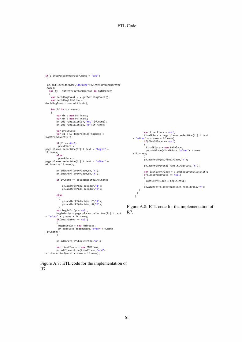
ETL Code

if(s.interactionOperator.name = "opt") { pn.addPlace(decider,"decider"+s.interactionOperator.name); for (y : SD!InteractionOperand in IntOpCont) { var decidingEvent = y.getDecidingEvent(); var decidingLifeline = decidingEvent.covered.first(); for(lf in s.covered) { var dY : new PN!Trans; var dN : new PN!Trans; pn.addTransition(dY,"Yes"+lf.name); pn.addTransition(dN,"No"+lf.name); var prevPlace; var e1 : SD!InteractionFragment = s.getPrevEvent(lf); if(e1 == null) prevPlace = page.places.selectOne(it|it.text = "begin" + lf.name); else prevPlace = page.places.selectOne(it|it.text = "after" + e1.label + lf.name); pn.addArcPT(prevPlace,dY,"n"); pn.addArcPT(prevPlace,dN,"n"); if(lf.name == decidingLifeline.name) { pn.addArcTP(dY,decider,"1"); pn.addArcTP(dN,decider,"0"); } else { pn.addArcPT(decider,dY,"1"); pn.addArcPT(decider,dN,"0"); } var beginIntOp = null; beginIntOp = page.places.selectOne(it|it.text = "after" + y.name + lf.name); if(beginIntOp == null) { beginIntOp = new PN!Place; pn.addPlace(beginIntOp,"after"+ y.name +lf.name); } pn.addArcTP(dY,beginIntOp,"n"); var finalTrans : new PN!Trans; pn.addTransition(finalTrans,"end"+ s.interactionOperator.name + lf.name);


var finalPlace = null; finalPlace = page.places.selectOne(it|it.text = "after" + s.name + lf.name); if(finalPlace == null) { finalPlace = new PN!Place; pn.addPlace(finalPlace,"after"+ s.name +lf.name); } pn.addArcTP(dN,finalPlace,"n"); pn.addArcTP(finalTrans,finalPlace,"n"); var lastEventPlace = y.getLastEventPlace(lf); if(lastEventPlace == null) { lastEventPlace = beginIntOp; } pn.addArcPT(lastEventPlace,finalTrans,"n"); } } }


61

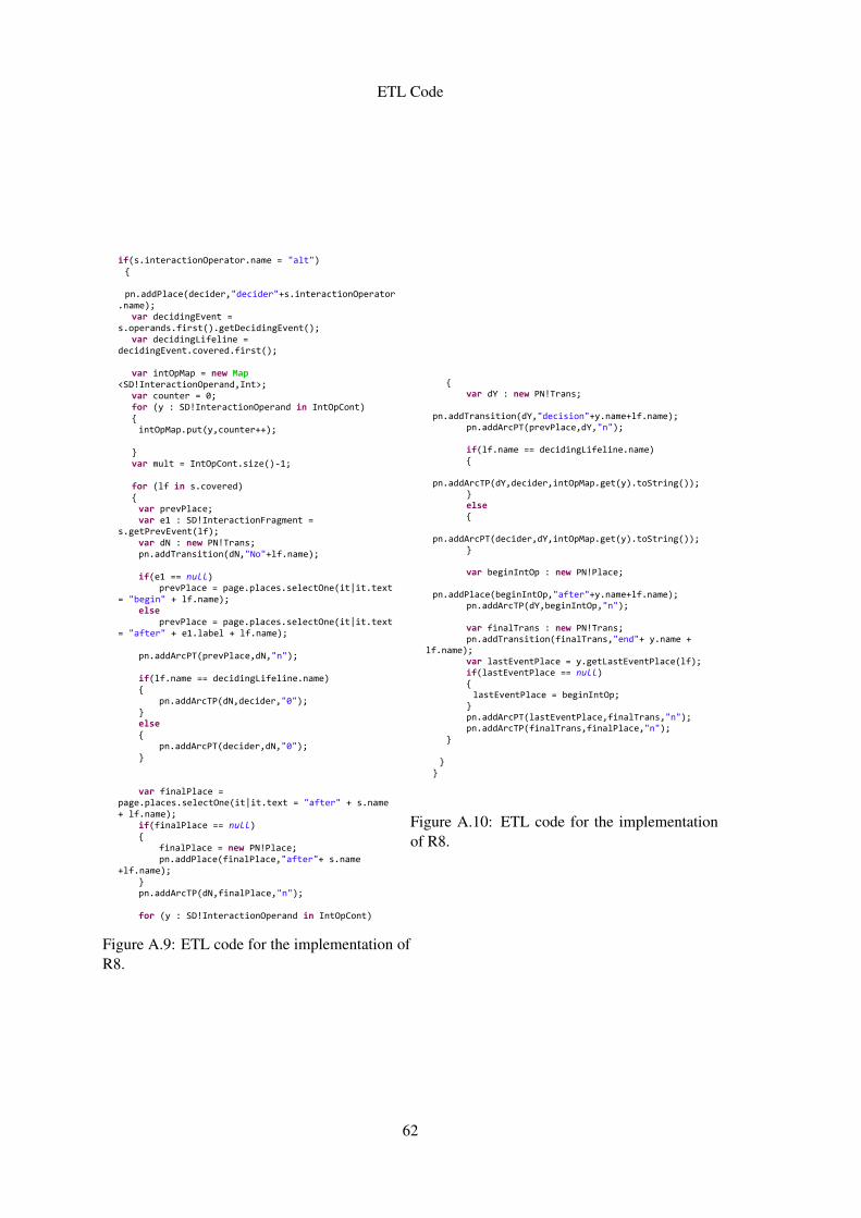
ETL Code

if(s.interactionOperator.name = "alt") { pn.addPlace(decider,"decider"+s.interactionOperator.name); var decidingEvent = s.operands.first().getDecidingEvent(); var decidingLifeline = decidingEvent.covered.first(); var intOpMap = new Map <SD!InteractionOperand,Int>; var counter = 0; for (y : SD!InteractionOperand in IntOpCont) { intOpMap.put(y,counter++); } var mult = IntOpCont.size()-1; for (lf in s.covered) { var prevPlace; var e1 : SD!InteractionFragment = s.getPrevEvent(lf); var dN : new PN!Trans; pn.addTransition(dN,"No"+lf.name); if(e1 == null) prevPlace = page.places.selectOne(it|it.text = "begin" + lf.name); else prevPlace = page.places.selectOne(it|it.text = "after" + e1.label + lf.name); pn.addArcPT(prevPlace,dN,"n"); if(lf.name == decidingLifeline.name) { pn.addArcTP(dN,decider,"0"); } else { pn.addArcPT(decider,dN,"0"); } var finalPlace = page.places.selectOne(it|it.text = "after" + s.name + lf.name); if(finalPlace == null) { finalPlace = new PN!Place; pn.addPlace(finalPlace,"after"+ s.name +lf.name); } pn.addArcTP(dN,finalPlace,"n"); for (y : SD!InteractionOperand in IntOpCont)


{ var dY : new PN!Trans; pn.addTransition(dY,"decision"+y.name+lf.name); pn.addArcPT(prevPlace,dY,"n"); if(lf.name == decidingLifeline.name) { pn.addArcTP(dY,decider,intOpMap.get(y).toString()); } else { pn.addArcPT(decider,dY,intOpMap.get(y).toString()); } var beginIntOp : new PN!Place; pn.addPlace(beginIntOp,"after"+y.name+lf.name); pn.addArcTP(dY,beginIntOp,"n"); var finalTrans : new PN!Trans; pn.addTransition(finalTrans,"end"+ y.name + lf.name); var lastEventPlace = y.getLastEventPlace(lf); if(lastEventPlace == null) { lastEventPlace = beginIntOp; } pn.addArcPT(lastEventPlace,finalTrans,"n"); pn.addArcTP(finalTrans,finalPlace,"n"); } } }

Figure A.10: ETL code for the implementationof R8.

62

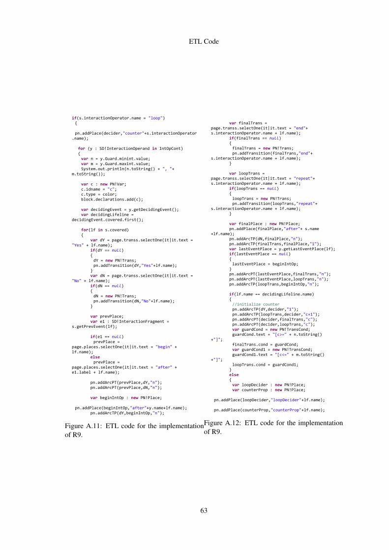
ETL Code

if(s.interactionOperator.name = "loop") { pn.addPlace(decider,"counter"+s.interactionOperator.name); for (y : SD!InteractionOperand in IntOpCont) { var n = y.Guard.minint.value; var m = y.Guard.maxint.value; System.out.println(n.toString() + ", "+ m.toString()); var c : new PN!Var; c.idname = "c"; c.type = color; block.declarations.add(c); var decidingEvent = y.getDecidingEvent(); var decidingLifeline = decidingEvent.covered.first(); for(lf in s.covered) { var dY = page.transs.selectOne(it|it.text = "Yes" + lf.name); if(dY == null) { dY = new PN!Trans; pn.addTransition(dY,"Yes"+lf.name); } var dN = page.transs.selectOne(it|it.text = "No" + lf.name); if(dN == null) { dN = new PN!Trans; pn.addTransition(dN,"No"+lf.name); } var prevPlace; var e1 : SD!InteractionFragment = s.getPrevEvent(lf); if(e1 == null) prevPlace = page.places.selectOne(it|it.text = "begin" + lf.name); else prevPlace = page.places.selectOne(it|it.text = "after" + e1.label + lf.name); pn.addArcPT(prevPlace,dY,"n"); pn.addArcPT(prevPlace,dN,"n"); var beginIntOp : new PN!Place; pn.addPlace(beginIntOp,"after"+y.name+lf.name); pn.addArcTP(dY,beginIntOp,"n");


var finalTrans = page.transs.selectOne(it|it.text = "end"+ s.interactionOperator.name + lf.name); if(finalTrans == null) { finalTrans = new PN!Trans; pn.addTransition(finalTrans,"end"+ s.interactionOperator.name + lf.name); } var loopTrans = page.transs.selectOne(it|it.text = "repeat"+ s.interactionOperator.name + lf.name); if(loopTrans == null) { loopTrans = new PN!Trans; pn.addTransition(loopTrans,"repeat"+ s.interactionOperator.name + lf.name); } var finalPlace : new PN!Place; pn.addPlace(finalPlace,"after"+ s.name +lf.name); pn.addArcTP(dN,finalPlace,"n"); pn.addArcTP(finalTrans,finalPlace,"1"); var lastEventPlace = y.getLastEventPlace(lf); if(lastEventPlace == null) { lastEventPlace = beginIntOp; } pn.addArcPT(lastEventPlace,finalTrans,"n"); pn.addArcPT(lastEventPlace,loopTrans,"n"); pn.addArcTP(loopTrans,beginIntOp,"n"); if(lf.name == decidingLifeline.name) { //initialize counter pn.addArcTP(dY,decider,"1"); pn.addArcTP(loopTrans,decider,"c+1"); pn.addArcPT(decider,finalTrans,"c"); pn.addArcPT(decider,loopTrans,"c"); var guardCond = new PN!TransCond; guardCond.text = "[c>=" + n.toString() +"]"; finalTrans.cond = guardCond; var guardCond1 = new PN!TransCond; guardCond1.text = "[c<=" + m.toString() +"]"; loopTrans.cond = guardCond1; } else { var loopDecider : new PN!Place; var counterProp : new PN!Place; pn.addPlace(loopDecider,"loopDecider"+lf.name); pn.addPlace(counterProp,"counterProp"+lf.name);


63

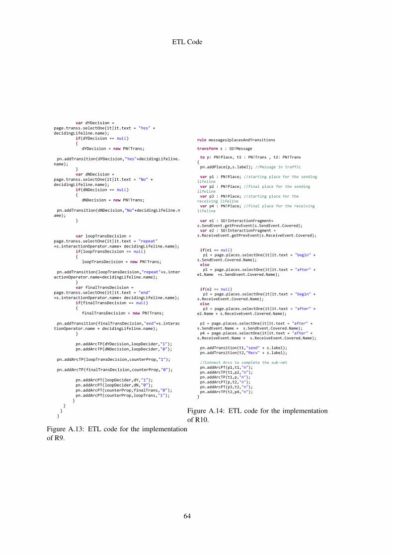
ETL Code

var dYDecision = page.transs.selectOne(it|it.text = "Yes" + decidingLifeline.name); if(dYDecision == null) { dYDecision = new PN!Trans; pn.addTransition(dYDecision,"Yes"+decidingLifeline.name); } var dNDecision = page.transs.selectOne(it|it.text = "No" + decidingLifeline.name); if(dNDecision == null) { dNDecision = new PN!Trans; pn.addTransition(dNDecision,"No"+decidingLifeline.name); } var loopTransDecision = page.transs.selectOne(it|it.text = "repeat" +s.interactionOperator.name+ decidingLifeline.name); if(loopTransDecision == null) { loopTransDecision = new PN!Trans; pn.addTransition(loopTransDecision,"repeat"+s.interactionOperator.name+decidingLifeline.name); } var finalTransDecision = page.transs.selectOne(it|it.text = "end" +s.interactionOperator.name+ decidingLifeline.name); if(finalTransDecision == null) { finalTransDecision = new PN!Trans; pn.addTransition(finalTransDecision,"end"+s.interactionOperator.name + decidingLifeline.name); } pn.addArcTP(dYDecision,loopDecider,"1"); pn.addArcTP(dNDecision,loopDecider,"0"); pn.addArcTP(loopTransDecision,counterProp,"1"); pn.addArcTP(finalTransDecision,counterProp,"0"); pn.addArcPT(loopDecider,dY,"1"); pn.addArcPT(loopDecider,dN,"0"); pn.addArcPT(counterProp,finalTrans,"0"); pn.addArcPT(counterProp,loopTrans,"1"); } } } }


rule messages2placesAndTransitions

transform s : SD!Message

to p: PN!Place, t1 : PN!Trans , t2: PN!Trans { pn.addPlace(p,s.label); //Message in traffic var p1 : PN!Place; //starting place for the sending lifeline var p2 : PN!Place; //final place for the sending lifeline var p3 : PN!Place; //starting place for the receiving lifeline var p4 : PN!Place; //final place for the receiving lifeline var e1 : SD!InteractionFragment= s.SendEvent.getPrevEvent(s.SendEvent.Covered); var e2 : SD!InteractionFragment = s.ReceiveEvent.getPrevEvent(s.ReceiveEvent.Covered); if(e1 == null) p1 = page.places.selectOne(it|it.text = "begin" + s.SendEvent.Covered.Name); else p1 = page.places.selectOne(it|it.text = "after" + e1.Name +s.SendEvent.Covered.Name); if(e2 == null) p3 = page.places.selectOne(it|it.text = "begin" + s.ReceiveEvent.Covered.Name); else p3 = page.places.selectOne(it|it.text = "after" + e2.Name + s.ReceiveEvent.Covered.Name); p2 = page.places.selectOne(it|it.text = "after" + s.SendEvent.Name + s.SendEvent.Covered.Name); p4 = page.places.selectOne(it|it.text = "after" + s.ReceiveEvent.Name + s.ReceiveEvent.Covered.Name); pn.addTransition(t1,"send" + s.label); pn.addTransition(t2,"Recv" + s.label); //Connect Arcs to complete the sub-net pn.addArcPT(p1,t1,"n"); pn.addArcTP(t1,p2,"n"); pn.addArcTP(t1,p,"n"); pn.addArcPT(p,t2,"n"); pn.addArcPT(p3,t2,"n"); pn.addArcTP(t2,p4,"n"); }


64

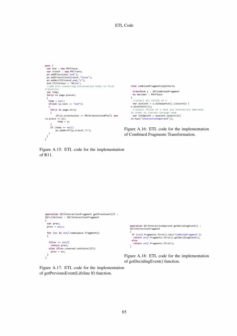
ETL Code

post { var end : new PN!Place; var transF : new PN!Trans; pn.addPlace(end,"end"); pn.addTransition(transF,"final"); pn.addArcTP(transF,end,"n"); end.fillColour = "White"; //add arcs connecting disconnected nodes to final transition var temp; for(p in page.places) { temp = null; if(not (p.text == "end")) { for(a in page.arcs) { if((a.orientation == PN!Orientation#PtoT) and (a.place == p)) temp = a; } if (temp == null) pn.addArcPT(p,transF,"n"); } } }


rule combinedFragments2patterns

transform s : SD!CombinedFragment to decider : PN!Place { //select all childs of s var auxCont = s.asSequence().closure(x | x.eContents()); //select childs of s that are Interaction Operands in order to iterate through them var IntOpCont = auxCont.select(it| it.has("InteractionOperand")); Figure A.16: ETL code for the implementation

of Combined Fragments Transformation.

operation SD!InteractionFragment getPrevEvent(lf : SD!Lifeline) : SD!InteractionFragment { var prev; prev = null; for (ev in self.namespace.fragments) { if(ev == self) return prev; else if(ev.covered.contains(lf)) prev = ev; } }

Figure A.17: ETL code for the implementationof getPreviousEvent(Lifeline lf) function.

operation SD!InteractionOperand getDecidingEvent() : SD!InteractionFragment { if (self.fragments.first().has("CombinedFragment")) return self.fragments.first().getDecidingEvent(); else return self.fragments.first(); } Figure A.18: ETL code for the implementation

of getDecidingEvent() function.

65

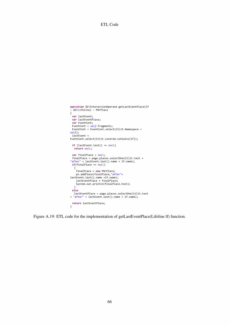
ETL Code

operation SD!InteractionOperand getLastEventPlace(lf : SD!Lifeline) : PN!Place { var lastEvent; var lastEventPlace; var EventCont; EventCont = self.fragments; EventCont = EventCont.select(it|it.Namespace = self); lastEvent = EventCont.select(it|it.covered.contains(lf)); if (lastEvent.last() == null) return null; var finalPlace = null; finalPlace = page.places.selectOne(it|it.text = "after" + lastEvent.last().name + lf.name); if(finalPlace == null) { finalPlace = new PN!Place; pn.addPlace(finalPlace,"after"+ lastEvent.last().name +lf.name); lastEventPlace = finalPlace; System.out.println(finalPlace.text); } else lastEventPlace = page.places.selectOne(it|it.text = "after" + lastEvent.last().name + lf.name); return lastEventPlace; }

Figure A.19: ETL code for the implementation of getLastEventPlace(Lifeline lf) function.

66

Appendix B

Article

During the development of this dissertation work, a scientific paper named Automatic Model

Transformation from UML Sequence Diagrams to Coloured Petri Nets was produced and sub-

mitted to the International Conference on Model-Driven Engineering and Software Development,

MODELSWARD 2018, and is currently awaiting evaluation.

67

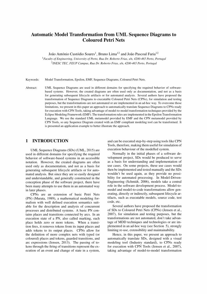
Automatic Model Transformation from UML Sequence Diagrams toColoured Petri Nets

Joao Antonio Custodio Soares1, Bruno Lima12 and Joao Pascoal Faria12

1Faculty of Engineering, University of Porto, Rua Dr. Roberto Frias, s/n, 4200-465 Porto, Portugal2INESC TEC, FEUP Campus, Rua Dr. Roberto Frias, s/n, 4200-465 Porto, Portugal

Keywords: Model Transformation, Epsilon, EMF, Sequence Diagrams, Coloured Petri Nets.

Abstract: UML Sequence Diagrams are used in different domains for specifying the required behavior of software-based systems. However, the created diagrams are often used only as documentation, and not as a basisfor generating subsequent lifecycle artifacts or for automated analysis. Several authors have proposed thetransformation of Sequence Diagrams to executable Coloured Petri Nets (CPNs), for simulation and testingpurposes, but the transformations are not automated or are implemented in an ad-hoc way. To overcome thoselimitations, we present in this paper an approach to automatically translate Sequence Diagrams to CPNs readyfor execution with CPN Tools, taking advantage of model-to-model transformation techniques provided by theEclipse Modeling Framework (EMF). The transformation rules are implemented in the Epsilon TransformationLanguage. We use the standard UML metamodel provided by EMF and the CPN metamodel provided byCPN Tools, so any Sequence Diagram created with an EMF compliant modeling tool can be transformed. Itis presented an application example to better illustrate the approach.

1 INTRODUCTION

UML Sequence Diagrams (SDs) (UML, 2015) areused in different domains for specifying the requiredbehavior of software-based systems in an accessiblenotation. However, the created diagrams are oftenused only as documentation, and not as a basis forgenerating subsequent lifecycle artifacts or for auto-mated analysis. But since they are so easily designedand understandable, and generally constructed in theconception phase of the software project, there havebeen many attempts to use them in an automated wayin later phases.

CPNs are an extension of basic Petri Nets(PN) (Murata, 1989), a mathematical modeling for-malism with well defined execution semantics suit-able for the description and analysis of concurrentprocesses and distributed systems. A basic PN con-tains places and transitions connected by arcs. In anexecution state of a PN, also called marking, eachplace holds zero or more tokens. When a transi-tion fires, it removes tokens from its input places andadds tokens to its output places. CPNs allow forthe definition of more complex nets with typed (orcoloured) places and tokens, guarded transitions, andarc expressions (Jensen, 2013). The passing of to-kens through the firing of transitions represent the ex-ecution of an event and change of state in a system,

and can be executed step-by-step using tools like CPNTools, therefore, making them useful for simulation ofexecution behaviour of the modelled system.

Normally in the initial phases of a software de-velopment project, SDs would be produced to serveas a basis for understanding and implementation ofuse cases. On some projects, these use cases wouldthen be implemented and tested manually and the SDswouldn’t be used again, as they provide no possi-bility for automated processing. In Model-Driven-Engineering (Schmidt, 2006), models take a centralrole in the software development process. Model-to-model and model-to-code transformations allow gen-erating, directly or indirectly, subsequent lifecycle ar-tifacts, such as executable models, source code, testcode, etc.

Several authors have proposed the transformationof SDs to Coloured Petri Nets (CPNs) (Jensen et al.,2007), for simulation and testing purposes, but thetransformations are not automated, don’t take advan-tage of MDD techniques and technologies or are im-plemented in an ad-hoc way (see Section 5), stronglylimiting re-use, extensibility and maintainability.

Hence, in this paper, we present an approach toautomatically translate SDs, designed with a visualmodeling tool (Industry standard), to CPNs readyfor execution with CPN Tools (Jensen et al., 2007),taking advantage of model-to-model transformation

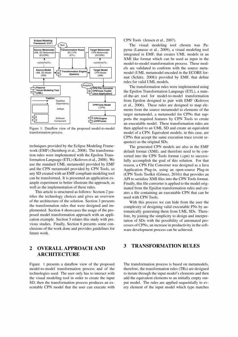
Figure 1: Dataflow view of the proposed model-to-modeltransformation process.

techniques provided by the Eclipse Modeling Frame-work (EMF) (Steinberg et al., 2008). The transforma-tion rules were implemented with the Epsilon Trans-formation Language (ETL) (Kolovos et al., 2008). Weuse the standard UML metamodel provided by EMFand the CPN metamodel provided by CPN Tools, soany SD created with an EMF compliant modeling toolcan be transformed. It is presented an application ex-ample experiment to better illustrate the approach, aswell as the implementation of these rules.

This article is structured as follows: Section 2 jus-tifies the technology choices and gives an overviewof the architecture of the solution. Section 3 presentsthe transformation rules that were designed and im-plemented. Section 4 showcases the usage of the pro-posed model transformation approach with an appli-cation example. Section 5 relates this study with pre-vious studies. Finally, Section 6 presents some con-clusions of the work done and provides guidelines forfuture work.

2 OVERALL APPROACH ANDARCHITECTURE

Figure 1 presents a dataflow view of the proposedmodel-to-model transformation process and of thetechnologies used. The user only has to interact withthe visual modeling tool in order to create the inputSD; then the transformation process produces an ex-ecutable CPN model that the user can execute with

CPN Tools (Jensen et al., 2007).The visual modeling tool chosen was Pa-

pyrus (Lanusse et al., 2009), a visual modeling toolintegrated in EMF, that creates UML models in anXMI like format which can be used as input in themodel-to-model transformation process. These mod-els are validated to conform with the source meta-model (UML metamodel encoded in the ECORE for-mat (Schatz, 2008)) provided by EMF, that definerules for valid UML models.

The transformation rules were implemented usingthe Epsilon Transformation Language (ETL), a state-of-the-art tool for model-to-model transformationfrom Epsilon designed to pair with EMF (Kolovoset al., 2006). These rules are designed to map ele-ments from the source metamodel to elements of thetarget metamodel, a metamodel for CPNs that sup-ports the required features by CPN Tools to createan executable model. These transformation rules arethen applied to an UML SD and create an equivalentmodel of a CPN. Equivalent models, in this case, areCPNs that accept the same execution trace (event se-quence) as the original SDs.

The generated CPN models are also in the EMFdefault format (XMI), and therefore need to be con-verted into the CPN Tools format (.cpn) to success-fully accomplish the goal of this solution. For thatreason, a CPN File Converter was designed as a JavaApplication Plug-in, using an open-source Plug-in(CPN Tools Toolkit (Gomez, 2016)) that provides anAPI to serialize XMI files into the CPN Tools format.Finally, this file converter is applied to the model orig-inated from the Epsilon transformation rules and cre-ates a file containing an executable CPN that can beused with CPN Tools.

With this process we can hide from the user thecomplexity of designing valid executable PNs by au-tomatically generating them from UML SDs. There-fore, by joining the simplicity to design and interpre-tation of SDs with the possibility of automated pro-cesses of CPNs, an increase in productivity in the soft-ware development process can be achieved.

3 TRANSFORMATION RULES

The transformation process is based on metamodels,therefore, the transformation rules (TRs) are designedto iterate through the input model’s elements and thenadd the equivalent elements to an initially empty out-put model. The rules are applied sequentially to ev-ery element of the input model which type matches

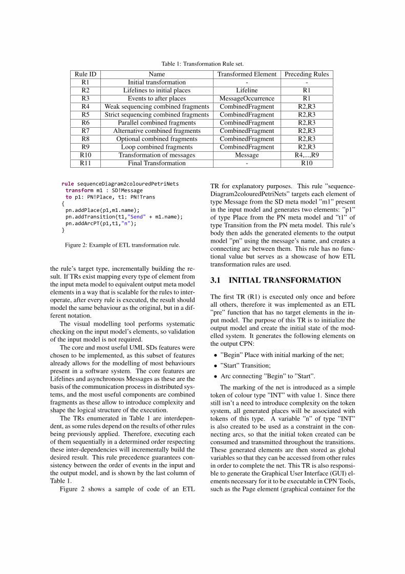
Table 1: Transformation Rule set.

Rule ID Name Transformed Element Preceding RulesR1 Initial transformation - -R2 Lifelines to initial places Lifeline R1R3 Events to after places MessageOccurrence R1R4 Weak sequencing combined fragments CombinedFragment R2,R3R5 Strict sequencing combined fragments CombinedFragment R2,R3R6 Parallel combined fragments CombinedFragment R2,R3R7 Alternative combined fragments CombinedFragment R2,R3R8 Optional combined fragments CombinedFragment R2,R3R9 Loop combined fragments CombinedFragment R2,R3

R10 Transformation of messages Message R4,...,R9R11 Final Transformation - R10

rule sequenceDiagram2colouredPetriNets transform m1 : SD!Message to p1: PN!Place, t1: PN!Trans { pn.addPlace(p1,m1.name); pn.addTransition(t1,"Send" + m1.name); pn.addArcPT(p1,t1,"n"); }

Figure 2: Example of ETL transformation rule.

the rule’s target type, incrementally building the re-sult. If TRs exist mapping every type of element fromthe input meta model to equivalent output meta modelelements in a way that is scalable for the rules to inter-operate, after every rule is executed, the result shouldmodel the same behaviour as the original, but in a dif-ferent notation.

The visual modelling tool performs systematicchecking on the input model’s elements, so validationof the input model is not required.

The core and most useful UML SDs features werechosen to be implemented, as this subset of featuresalready allows for the modelling of most behaviourspresent in a software system. The core features areLifelines and asynchronous Messages as these are thebasis of the communication process in distributed sys-tems, and the most useful components are combinedfragments as these allow to introduce complexity andshape the logical structure of the execution.

The TRs enumerated in Table 1 are interdepen-dent, as some rules depend on the results of other rulesbeing previously applied. Therefore, executing eachof them sequentially in a determined order respectingthese inter-dependencies will incrementally build thedesired result. This rule precedence guarantees con-sistency between the order of events in the input andthe output model, and is shown by the last column ofTable 1.

Figure 2 shows a sample of code of an ETL

TR for explanatory purposes. This rule ”sequence-Diagram2colouredPetriNets” targets each element oftype Message from the SD meta model ”m1” presentin the input model and generates two elements: ”p1”of type Place from the PN meta model and ”t1” oftype Transition from the PN meta model. This rule’sbody then adds the generated elements to the outputmodel ”pn” using the message’s name, and creates aconnecting arc between them. This rule has no func-tional value but serves as a showcase of how ETLtransformation rules are used.

3.1 INITIAL TRANSFORMATION

The first TR (R1) is executed only once and beforeall others, therefore it was implemented as an ETL”pre” function that has no target elements in the in-put model. The purpose of this TR is to initialize theoutput model and create the initial state of the mod-elled system. It generates the following elements onthe output CPN:

• ”Begin” Place with initial marking of the net;

• ”Start” Transition;

• Arc connecting ”Begin” to ”Start”.

The marking of the net is introduced as a simpletoken of colour type ”INT” with value 1. Since therestill isn’t a need to introduce complexity on the tokensystem, all generated places will be associated withtokens of this type. A variable ”n” of type ”INT”is also created to be used as a constraint in the con-necting arcs, so that the initial token created can beconsumed and transmitted throughout the transitions.These generated elements are then stored as globalvariables so that they can be accessed from other rulesin order to complete the net. This TR is also responsi-ble to generate the Graphical User Interface (GUI) el-ements necessary for it to be executable in CPN Tools,such as the Page element (graphical container for the

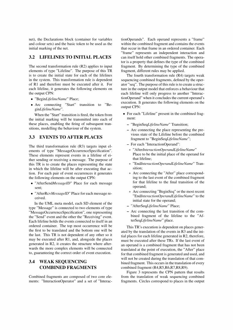
net), the Declarations block (container for variablesand colour sets) and the basic token to be used as theinitial marking of the net.

3.2 LIFELINES TO INITIAL PLACES

The second transformation rule (R2) applies to inputelements of type ”Lifeline”. The purpose of this TRis to create the initial state for each of the lifelinesin the system. This transformation rule is dependentof R1 and therefore must be executed after it. Foreach lifeline, it generates the following elements onthe output CPN:• ”BeginLifelineName” Place;• Arc connecting ”Start” transition to ”Be-

ginLifelineName”.When the ”Start” transition is fired, the token from

the initial marking will be transmitted into each ofthese places, enabling the firing of subsequent tran-sitions, modelling the behaviour of the system.

3.3 EVENTS TO AFTER PLACES

The third transformation rule (R3) targets input el-ements of type ”MessageOccurrenceSpecification”.These elements represent events in a lifeline of ei-ther sending or receiving a message. The purpose ofthis TR is to create the places representing the statein which the lifeline will be after executing that ac-tion. For each pair of event occurrences it generatesthe following elements on the output CPN:• ”AfterSendMessageID” Place for each message

sent;• ”AfterRcvMessageID” Place for each message re-

ceived.In the UML meta model, each SD element of the

type ”Message” is connected to two elements of type”MessageOccurrenceSpecification”, one representingthe ”Send” event and the other the ”Receiving” event.Each lifeline holds the events connected to itself in anordered container. The top most occurrence will bethe first to be translated and the bottom one will bethe last. This TR is not dependent of any other so itmay be executed after R1, and, alongside the placesgenerated in R2, it creates the structure where after-wards the more complex elements will be connectedto, guaranteeing the correct order of event execution.

3.4 WEAK SEQUENCINGCOMBINED FRAGMENTS

Combined fragments are composed of two core ele-ments: ”InteractionOperator” and a set of ”Interac-

tionOperands”. Each operand represents a ”frame”within the combined fragment and contains the eventsthat occur in that frame in an ordered container. Each”frame” represents an independent interaction andcan itself hold other combined fragments. The opera-tor is a property that defines the type of the combinedfragment. By determining the type of the combinedfragment, different rules may be applied.

The fourth transformation rule (R4) targets weaksequencing combined fragments, defined by the oper-ator ”seq”. The purpose of this rule is to create a struc-ture in the output model that enforces a behaviour thateach lifeline will only progress to another ”Interac-tionOperand” when it concludes the current operand’sexecution. It generates the following elements on theoutput CPN:

• For each ”Lifeline” present in the combined frag-ment:

– ”BeginSeqLifelineName” Transition;– Arc connecting the place representing the pre-

vious state of the Lifeline before the combinedfragment to ”BeginSeqLifelineName”;

– For each ”InteractionOperand”:∗ ”AfterInteractionOperandLifelineName”

Place to be the initial place of the operand forthat lifeline;

∗ ”EndInteractionOperandLifelineName” Tran-sition;

∗ Arc connecting the ”After” place correspond-ing to the last event of the combined fragmentfor that lifeline to the final transition of theoperand;

∗ Arc connecting ”BeginSeq” or the most recent”EndInteractionOperandLifelineName” to theinitial state for the operand;

– ”AfterSeqLifelineName” Place;– Arc connecting the last transition of the com-

bined fragment of the lifeline to the ”Af-terSeqLifelineName” place.

This TR’s execution is dependent on places gener-ated by the translation of the events in R3 and the ini-tial places for each lifeline generated in R2, therefore,must be executed after these TRs. If the last event ofan operand is a combined fragment that has not beentranslated at the point of execution, the ”After” placefor that combined fragment is generated and used, andwill not be created during the translation of that com-bined fragment. This occurs in the translation of everycombined fragment (R4,R5,R6,R7,R8,R9).

Figure 3 represents the CPN pattern that resultsfrom the translation of weak sequencing combinedfragments. Circles correspond to places in the output

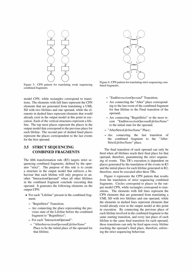
Figure 3: CPN pattern for translating weak sequencingcombined fragments.

model CPN, while rectangles correspond to transi-tions. The elements with full lines represent the CPNelements that are generated from translating a UMLSD with two lifelines and one operand, while the el-ements in dashed lines represent elements that wouldalready exist in the output model at this point in exe-cution. Each of the vertical structures represent a life-line. The top most places represent the places in theoutput model that correspond to the previous place foreach lifeline. The second pair of dashed lined placesrepresent the places correspondent to the last eventsfor the first operand.

3.5 STRICT SEQUENCINGCOMBINED FRAGMENTS

The fifth transformation rule (R5) targets strict se-quencing combined fragments, defined by the oper-ator ”strict”. The purpose of this rule is to createa structure in the output model that enforces a be-haviour that each lifeline will only progress to an-other ”InteractionOperand” when all other lifelinesin the combined fragment conclude executing thatoperand. It generates the following elements on theoutput CPN:


– ”BeginStrict” Transition;– Arc connecting the place representing the pre-

vious state of the Lifeline before the combinedfragment to ”BeginStrict”;

– For each ”InteractionOperand”:∗ ”AfterInteractionOperandLifelineName”


Figure 4: CPN pattern for translating strict sequencing com-bined fragments.

∗ ”EndInteractionOperand” Transition;∗ Arc connecting the ”After” place correspond-

ing to the last event of the combined fragmentfor that lifeline to the Final transition of theoperand;

∗ Arc connecting ”BeginStrict” or the most re-cent ”EndInteractionOperandLifelineName”to the initial state for the operand;

– ”AfterStrictLifelineName” Place;

– Arc connecting the last transition ofthe combined fragment to the ”After-StrictLifelineName” place.

The final transition of each operand can only befired when all lifelines reach their final place for thatoperand, therefore, guaranteeing the strict sequenc-ing of events. This TR’s execution is dependent onplaces generated by the translation of the events in R3and the initial places for each lifeline generated in R2,therefore, must be executed after these TRs.

Figure 4 represents the CPN pattern that resultsfrom the translation of strict sequencing combinedfragments. Circles correspond to places in the out-put model CPN, while rectangles correspond to tran-sitions. The elements with full lines represent theCPN elements that are generated from translating aUML SD with two lifelines and one operand, whilethe elements in dashed lines represent elements thatwould already exist in the output model at this pointin execution. By connecting the previous place ofeach lifeline involved in the combined fragment to thesame starting transition, and every last place of eachlifeline to the same final transition for each operand,these transitions can only be fired upon every lifelinereaching the operand’s final place, therefore, enforc-ing the strict sequencing behaviour.

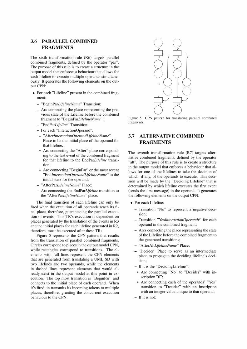
3.6 PARALLEL COMBINEDFRAGMENTS

The sixth transformation rule (R6) targets parallelcombined fragments, defined by the operator ”par”.The purpose of this rule is to create a structure in theoutput model that enforces a behaviour that allows foreach lifeline to execute multiple operands simultane-ously. It generates the following elements on the out-put CPN:


– ”BeginParLifelineName” Transition;– Arc connecting the place representing the pre-

vious state of the Lifeline before the combinedfragment to ”BeginParLifelineName”;

– ”EndParLifeline” Transition;– For each ”InteractionOperand”:∗ ”AfterInteractionOperandLifelineName”


∗ Arc connecting the ”After” place correspond-ing to the last event of the combined fragmentfor that lifeline to the EndParLifeline transi-tion;

∗ Arc connecting ”BeginPar” or the most recent”EndInteractionOperandLifelineName” to theinitial state for the operand;

– ”AfterParLifelineName” Place;– Arc connecting the EndParLifeline transition to

the ”AfterParLifelineName” place.

The final transition of each lifeline can only befired when the execution of all operands reach its fi-nal place, therefore, guaranteeing the parallel execu-tion of events. This TR’s execution is dependent onplaces generated by the translation of the events in R3and the initial places for each lifeline generated in R2,therefore, must be executed after these TRs.

Figure 5 represents the CPN pattern that resultsfrom the translation of parallel combined fragments.Circles correspond to places in the output model CPN,while rectangles correspond to transitions. The el-ements with full lines represent the CPN elementsthat are generated from translating a UML SD withtwo lifelines and two operands, while the elementsin dashed lines represent elements that would al-ready exist in the output model at this point in ex-ecution. The top most transition is ”BeginPar” andconnects to the initial place of each operand. Whenit’s fired, in transmits its incoming tokens to multipleplaces, therefore, granting the concurrent executionbehaviour to the CPN.

Figure 5: CPN pattern for translating parallel combinedfragments.

3.7 ALTERNATIVE COMBINEDFRAGMENTS

The seventh transformation rule (R7) targets alter-native combined fragments, defined by the operator”alt”. The purpose of this rule is to create a structurein the output model that enforces a behaviour that al-lows for one of the lifelines to take the decision ofwhich, if any, of the operands to execute. This deci-sion will be made by the ”Deciding Lifeline” that isdetermined by which lifeline executes the first event(sends the first message) in the operand. It generatesthe following elements on the output CPN:

• For each Lifeline:

– Transition ”No” to represent a negative deci-sion;

– Transition ”YesInteractionOperandr” for eachoperand in the combined fragment;

– Arcs connecting the place representing the stateof the Lifeline before the combined fragment tothe generated transitions;

– ”AfterAltLifelineName” Place;– ”Decider” Place to serve as an intermediate

place to propagate the deciding lifeline’s deci-sion;

– If it is the ”DecidingLifeline”:∗ Arc connecting ”No” to ”Decider” with in-

scription ”0”;∗ Arc connecting each of the operands’ ”Yes”

transition to ”Decider” with an inscriptionwith an integer value unique to that operand;

– If it is not:

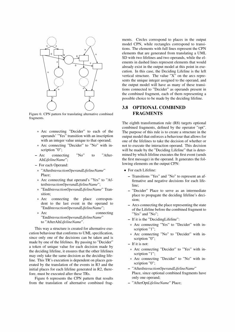
Figure 6: CPN pattern for translating alternative combinedfragments.

∗ Arc connecting ”Decider” to each of theoperands’ ”Yes” transition with an inscriptionwith an integer value unique to that operand;

∗ Arc connecting ”Decider” to ”No” with in-scription ”0”;

– Arc connecting ”No” to ”After-AltLifelineName”;

– For each Operand:∗ ”AfterInteractionOperandLifelineName”

Place;∗ Arc connecting that operand’s ”Yes” to ”Af-

terInteractionOperandLifelineName”;∗ ”EndInteractionOperandLifelineName” Tran-

sition;∗ Arc connecting the place correspon-

dent to the last event in the operand to”EndInteractionOperandLifelineName”;

∗ Arc connecting”EndInteractionOperandLifelineName”to ”AfterAltLifelineName”.

This way a structure is created for alternative exe-cution behaviour that conforms to UML specification,since only one of the decisions can be taken and ismade by one of the lifelines. By passing to ”Decider”a token of unique value for each decision made bythe deciding lifeline, it ensures that the other lifelinesmay only take the same decision as the deciding life-line. This TR’s execution is dependent on places gen-erated by the translation of the events in R3 and theinitial places for each lifeline generated in R2, there-fore, must be executed after these TRs.

Figure 6 represents the CPN pattern that resultsfrom the translation of alternative combined frag-

ments. Circles correspond to places in the outputmodel CPN, while rectangles correspond to transi-tions. The elements with full lines represent the CPNelements that are generated from translating a UMLSD with two lifelines and two operands, while the el-ements in dashed lines represent elements that wouldalready exist in the output model at this point in exe-cution. In this case, the Deciding Lifeline is the leftvertical structure. The value ”X” on the arcs repre-sents the unique integer assigned to the operand, andthe output model will have as many of these transi-tions connected to ”Decider” as operands present inthe combined fragment, each of them representing apossible choice to be made by the deciding lifeline.

3.8 OPTIONAL COMBINEDFRAGMENTS

The eighth transformation rule (R8) targets optionalcombined fragments, defined by the operator ”opt”.The purpose of this rule is to create a structure in theoutput model that enforces a behaviour that allows forone of the lifelines to take the decision of whether ornot to execute the interaction operand. This decisionwill be made by the ”Deciding Lifeline” that is deter-mined by which lifeline executes the first event (sendsthe first message) in the operand. It generates the fol-lowing elements on the output CPN:

• For each Lifeline:

– Transitions ”Yes” and ”No” to represent an af-firmative and negative decisions for each life-line;

– ”Decider” Place to serve as an intermediateplace to propagate the deciding lifeline’s deci-sion;

– Arcs connecting the place representing the stateof the Lifeline before the combined fragment to”Yes” and ”No”;

– If it is the ”DecidingLifeline”:∗ Arc connecting ”Yes” to ”Decider” with in-

scription ”1”;∗ Arc connecting ”No” to ”Decider” with in-

scription ”0”;– If it is not:∗ Arc connecting ”Decider” to ”Yes” with in-

scription ”1”;∗ Arc connecting ”Decider” to ”No” with in-

scription ”0”;– ”AfterInteractionOperandLifelineName”

Place, since optional combined fragments haveonly one operand;

– ”AfterOptLifelineName” Place;

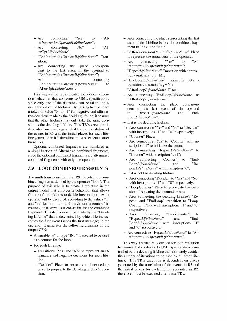
– Arc connecting ”Yes” to ”Af-terInteractionOperandLifelineName”;

– Arc connecting ”No” to ”Af-terOptLifelineName”;

– ”EndInteractionOperandLifelineName” Tran-sition;

– Arc connecting the place correspon-dent to the last event in the operand to”EndInteractionOperandLifelineName”;

– Arc connecting”EndInteractionOperandLifelineName” to”AfterOptLifelineName”.

This way a structure is created for optional execu-tion behaviour that conforms to UML specification,since only one of the decisions can be taken and ismade by one of the lifelines. By passing to ”Decider”a token of value ”0” or ”1” for negative and affirma-tive decisions made by the deciding lifeline, it ensuresthat the other lifelines may only take the same deci-sion as the deciding lifeline. This TR’s execution isdependent on places generated by the translation ofthe events in R3 and the initial places for each life-line generated in R2, therefore, must be executed afterthese TRs.

Optional combined fragments are translated asa simplification of Alternative combined fragments,since the optional combined fragments are alternativecombined fragments with only one operand.

3.9 LOOP COMBINED FRAGMENTS

The ninth transformation rule (R9) targets loop com-bined fragments, defined by the operator ”loop”. Thepurpose of this rule is to create a structure in theoutput model that enforces a behaviour that allowsfor one of the lifelines to decide how many times anoperand will be executed, according to the values ”n”and ”m” for minimum and maximum amount of it-erations, that serve as a constraint for the combinedfragment. This decision will be made by the ”Decid-ing Lifeline” that is determined by which lifeline ex-ecutes the first event (sends the first message) in theoperand. It generates the following elements on theoutput CPN:• A variable ”c” of type ”INT” is created to be used

as a counter for the loop;• For each Lifeline:

– Transitions ”Yes” and ”No” to represent an af-firmative and negative decisions for each life-line;

– ”Decider” Place to serve as an intermediateplace to propagate the deciding lifeline’s deci-sion;

– Arcs connecting the place representing the laststate of the Lifeline before the combined frag-ment to ”Yes” and ”No”;

– ”AfterInteractionOperandLifelineName” Placeto represent the initial state of the operand;

– Arc connecting ”Yes” to ”Af-terInteractionOperandLifelineName”;

– ”RepeatLifelineName” Transition with a transi-tion constraint ”c ¡= M”;

– ”EndLoopLifelineName” Transition with atransition constraint ”c ¿= N”;

– ”AfterLoopLifelineName” Place;– Arc connecting ”EndLoopLifelineName” to

”AfterLoopLifelineName”;– Arcs connecting the place correspon-

dent to the last event of the operandto ”RepeatLifelineName” and ”End-LoopLifelineName”;

– If it is the deciding lifeline:∗ Arcs connecting ”Yes” and ”No” to ”Decider”

with inscriptions ”1” and ”0” respectively;∗ ”Counter” Place;∗ Arc connecting ”Yes” to ”Counter” with in-

scription ”1” to initialize the count;∗ Arc connecting ”RepeatLifelineName” to

”Counter” with inscription ”c+1”;∗ Arc connecting ”Counter” to ”End-

LoopLifelineName” and ”Re-peatLifelineName” with inscription ”c”;

– If it is not the deciding lifeline:∗ Arcs connecting ”Decider” to ”Yes” and ”No”

with inscriptions ”1” and ”0” respectively;∗ ”LoopCounter” Place to propagate the deci-

sion of repeating the operand or not;∗ Arcs connecting the deciding lifeline’s ”Re-

peat” and ”EndLoop” transition to ”Loop-Counter” Place with inscriptions ”1” and ”0”respectively;

∗ Arcs connecting ”LoopCounter” to”RepeatLifelineName” and ”End-LoopLifelineName” with inscriptions ”1”and ”0” respectively;

– Arc connecting ”RepeatLifelineName” to ”Af-terInteractionOperandLifelineName”.

This way a structure is created for loop executionbehaviour that conforms to UML specification, con-trolled by the deciding lifeline that ultimately decidesthe number of iterations to be used by all other life-lines. This TR’s execution is dependent on placesgenerated by the translation of the events in R3 andthe initial places for each lifeline generated in R2,therefore, must be executed after these TRs.

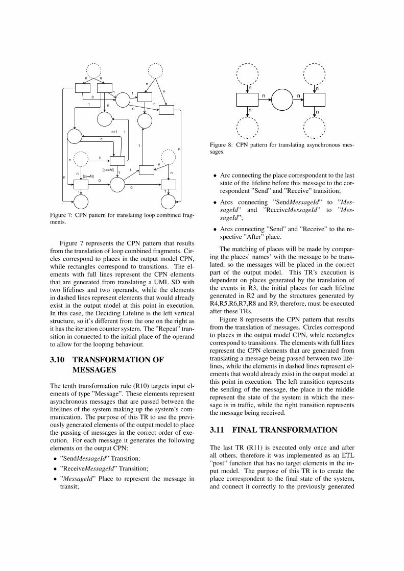
Figure 7: CPN pattern for translating loop combined frag-ments.

Figure 7 represents the CPN pattern that resultsfrom the translation of loop combined fragments. Cir-cles correspond to places in the output model CPN,while rectangles correspond to transitions. The el-ements with full lines represent the CPN elementsthat are generated from translating a UML SD withtwo lifelines and two operands, while the elementsin dashed lines represent elements that would alreadyexist in the output model at this point in execution.In this case, the Deciding Lifeline is the left verticalstructure, so it’s different from the one on the right asit has the iteration counter system. The ”Repeat” tran-sition in connected to the initial place of the operandto allow for the looping behaviour.

3.10 TRANSFORMATION OFMESSAGES

The tenth transformation rule (R10) targets input el-ements of type ”Message”. These elements representasynchronous messages that are passed between thelifelines of the system making up the system’s com-munication. The purpose of this TR to use the previ-ously generated elements of the output model to placethe passing of messages in the correct order of exe-cution. For each message it generates the followingelements on the output CPN:

• ”SendMessageId” Transition;• ”ReceiveMessageId” Transition;• ”MessageId” Place to represent the message in

transit;

Figure 8: CPN pattern for translating asynchronous mes-sages.

• Arc connecting the place correspondent to the laststate of the lifeline before this message to the cor-respondent ”Send” and ”Receive” transition;

• Arcs connecting ”SendMessageId” to ”Mes-sageId” and ”ReceiveMessageId” to ”Mes-sageId”;

• Arcs connecting ”Send” and ”Receive” to the re-spective ”After” place.

The matching of places will be made by compar-ing the places’ names’ with the message to be trans-lated, so the messages will be placed in the correctpart of the output model. This TR’s execution isdependent on places generated by the translation ofthe events in R3, the initial places for each lifelinegenerated in R2 and by the structures generated byR4,R5,R6,R7,R8 and R9, therefore, must be executedafter these TRs.

Figure 8 represents the CPN pattern that resultsfrom the translation of messages. Circles correspondto places in the output model CPN, while rectanglescorrespond to transitions. The elements with full linesrepresent the CPN elements that are generated fromtranslating a message being passed between two life-lines, while the elements in dashed lines represent el-ements that would already exist in the output model atthis point in execution. The left transition representsthe sending of the message, the place in the middlerepresent the state of the system in which the mes-sage is in traffic, while the right transition representsthe message being received.

3.11 FINAL TRANSFORMATION

The last TR (R11) is executed only once and afterall others, therefore it was implemented as an ETL”post” function that has no target elements in the in-put model. The purpose of this TR is to create theplace correspondent to the final state of the system,and connect it correctly to the previously generated

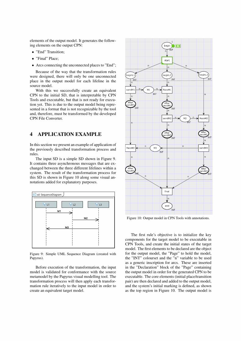
elements of the output model. It generates the follow-ing elements on the output CPN:

• ”End” Transition;

• ”Final” Place;

• Arcs connecting the unconnected places to ”End”;

Because of the way that the transformation ruleswere designed, there will only be one unconnectedplace in the output model for each lifeline in thesource model.

With this we successfully create an equivalentCPN to the initial SD, that is interpretable by CPNTools and executable, but that is not ready for execu-tion yet. This is due to the output model being repre-sented in a format that is not recognizable by the tooland, therefore, must be transformed by the developedCPN File Converter.

4 APPLICATION EXAMPLE

In this section we present an example of application ofthe previously described transformation process andrules.

The input SD is a simple SD shown in Figure 9.It contains three asynchronous messages that are ex-changed between the three different lifelines within asystem. The result of the transformation process forthis SD is shown in Figure 10 along some visual an-notations added for explanatory purposes.

Figure 9: Simple UML Sequence Diagram (created withPapyrus).

Before execution of the transformation, the inputmodel is validated for conformance with the sourcemetamodel by the Papyrus visual modelling tool. Thetransformation process will then apply each transfor-mation rule iteratively to the input model in order tocreate an equivalent target model.

R1

R2

R3+R4

R5

Figure 10: Output model in CPN Tools with annotations.

The first rule’s objective is to initialize the keycomponents for the target model to be executable inCPN Tools, and create the initial states of the targetmodel. The first elements to be declared are the objectfor the output model, the ”Page” to hold the model,the ”INT” colourset and the ”n” variable to be usedas a generic inscription for arcs. These are insertedin the ”Declaration” block of the ”Page” containingthe output model in order for the generated CPN to beexecutable. The core elements (initial place/transitionpair) are then declared and added to the output model,and the system’s initial marking is defined, as shownas the top region in Figure 10. The output model is

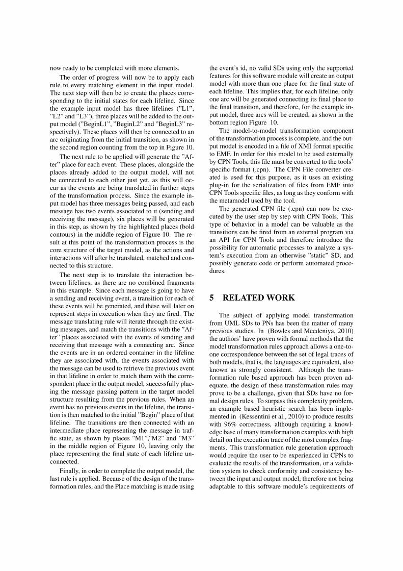
now ready to be completed with more elements.The order of progress will now be to apply each

rule to every matching element in the input model.The next step will then be to create the places corre-sponding to the initial states for each lifeline. Sincethe example input model has three lifelines (”L1”,”L2” and ”L3”), three places will be added to the out-put model (”BeginL1”, ”BeginL2” and ”BeginL3” re-spectively). These places will then be connected to anarc originating from the initial transition, as shown inthe second region counting from the top in Figure 10.

The next rule to be applied will generate the ”Af-ter” place for each event. These places, alongside theplaces already added to the output model, will notbe connected to each other just yet, as this will oc-cur as the events are being translated in further stepsof the transformation process. Since the example in-put model has three messages being passed, and eachmessage has two events associated to it (sending andreceiving the message), six places will be generatedin this step, as shown by the highlighted places (boldcontours) in the middle region of Figure 10. The re-sult at this point of the transformation process is thecore structure of the target model, as the actions andinteractions will after be translated, matched and con-nected to this structure.

The next step is to translate the interaction be-tween lifelines, as there are no combined fragmentsin this example. Since each message is going to havea sending and receiving event, a transition for each ofthese events will be generated, and these will later onrepresent steps in execution when they are fired. Themessage translating rule will iterate through the exist-ing messages, and match the transitions with the ”Af-ter” places associated with the events of sending andreceiving that message with a connecting arc. Sincethe events are in an ordered container in the lifelinethey are associated with, the events associated withthe message can be used to retrieve the previous eventin that lifeline in order to match them with the corre-spondent place in the output model, successfully plac-ing the message passing pattern in the target modelstructure resulting from the previous rules. When anevent has no previous events in the lifeline, the transi-tion is then matched to the initial ”Begin” place of thatlifeline. The transitions are then connected with anintermediate place representing the message in traf-fic state, as shown by places ”M1”,”M2” and ”M3”in the middle region of Figure 10, leaving only theplace representing the final state of each lifeline un-connected.

Finally, in order to complete the output model, thelast rule is applied. Because of the design of the trans-formation rules, and the Place matching is made using

the event’s id, no valid SDs using only the supportedfeatures for this software module will create an outputmodel with more than one place for the final state ofeach lifeline. This implies that, for each lifeline, onlyone arc will be generated connecting its final place tothe final transition, and therefore, for the example in-put model, three arcs will be created, as shown in thebottom region Figure 10.

The model-to-model transformation componentof the transformation process is complete, and the out-put model is encoded in a file of XMI format specificto EMF. In order for this model to be used externallyby CPN Tools, this file must be converted to the tools’specific format (.cpn). The CPN File converter cre-ated is used for this purpose, as it uses an existingplug-in for the serialization of files from EMF intoCPN Tools specific files, as long as they conform withthe metamodel used by the tool.

The generated CPN file (.cpn) can now be exe-cuted by the user step by step with CPN Tools. Thistype of behavior in a model can be valuable as thetransitions can be fired from an external program viaan API for CPN Tools and therefore introduce thepossibility for automatic processes to analyze a sys-tem’s execution from an otherwise ”static” SD, andpossibly generate code or perform automated proce-dures.

5 RELATED WORK

The subject of applying model transformationfrom UML SDs to PNs has been the matter of manyprevious studies. In (Bowles and Meedeniya, 2010)the authors’ have proven with formal methods that themodel transformation rules approach allows a one-to-one correspondence between the set of legal traces ofboth models, that is, the languages are equivalent, alsoknown as strongly consistent. Although the trans-formation rule based approach has been proven ad-equate, the design of these transformation rules mayprove to be a challenge, given that SDs have no for-mal design rules. To surpass this complexity problem,an example based heuristic search has been imple-mented in (Kessentini et al., 2010) to produce resultswith 96% correctness, although requiring a knowl-edge base of many transformation examples with highdetail on the execution trace of the most complex frag-ments. This transformation rule generation approachwould require the user to be experienced in CPNs toevaluate the results of the transformation, or a valida-tion system to check conformity and consistency be-tween the input and output model, therefore not beingadaptable to this software module’s requirements of

hiding complexity from the user.The metamodel transformation approach was cho-

sen since it was proven feasible with formal methodsby (Ouardani et al., 2006) and the transformationrules were derived from (Emadi and Shams, 2009)and (Staines, 2013) that have conceptualized and val-idated them for specific scenarios, although not im-plementing them in an automated process. The rulesto produce the output CPNs were extended from thetransformation rules proposed, alongside the toolkitfor conformance testing based on UML SDs in (Fariaand Paiva, 2016). These studies were developed andused as a base for designing transformation rules forthis type of model transformation for many applica-tion domains and have been adapted and developedin order to increase the value of SDs. As proven in(Jensen et al., 2007) CPNs and CPN Tools can beused for automatic validation of systems, either by themeans of creating animated system simulation to beused as validation with clients (Ribeiro and Fernan-des, 2006) and acceptance testing, or by generatingautomatic test cases and execution scenarios (Limaand Faria, 2015), therefore justifying the need for thissoftware module.

6 CONCLUSIONS AND FUTUREWORK

It was presented an automated model-to-modeltransformation approach from UML SDs to CPNs.Our approach was successfully implemented based onstate-of-the-art model-transformation techniques andtools, namely, EMF and ETL, and an experiment wasconducted to validate and illustrate the approach. Toour knowledge, there is no other previous approachable to automatically perform the end-to-end trans-formation, from SDs created with a visual modelingtool to CPNs executable with CPN Tools, without anymanual step. ETL allowed us to define the transfor-mations in a declarative and extensible way.

As future work it is intended to implement the re-maining features of UML SDs such as: synchronousmessages, action/behaviour specification, break com-bined fragments, negative combined fragments, crit-ical combined fragments, ignore combine fragment,consider combined fragments and assertion combinedfragments. These will be implemented as ETL trans-formation rules and are to be inserted in the rule setprecedence accordingly.

Further validation of the solution with more com-plex test case studies are also valuable as future workto increase the certainty of the robustness of the solu-tion and ensure scalability.

REFERENCES

Bowles, J. and Meedeniya, D. (2010). Formal transforma-tion from sequence diagrams to coloured petri nets.In Software Engineering Conference (APSEC), 201017th Asia Pacific, pages 216–225. IEEE.

Emadi, S. and Shams, F. (2009). Transformation of use-case and sequence diagrams to petri nets. In Com-puting, Communication, Control, and Management,2009. CCCM 2009. ISECS International Colloquiumon, volume 4, pages 399–403. IEEE.

Faria, J. P. and Paiva, A. C. (2016). A toolset for con-formance testing against UML sequence diagramsbased on event-driven colored Petri nets. InternationalJournal on Software Tools for Technology Transfer,18(3):285–304.

Gomez, A. (2016). CPN Tools Toolkit.Jensen, K. (2013). Coloured Petri nets: basic con-

cepts, analysis methods and practical use, volume 1.Springer Science & Business Media.

Jensen, K., Kristensen, L. M., and Wells, L. (2007).Coloured Petri Nets and CPN Tools for modelling andvalidation of concurrent systems. International Jour-nal on Software Tools for Technology Transfer, 9(3-4):213–254.

Kessentini, M., Bouchoucha, A., Sahraoui, H., andBoukadoum, M. (2010). Example-based sequencediagrams to colored petri nets transformation usingheuristic Search. In European Conference on Mod-elling Foundations and Applications, pages 156–172.Springer.

Kolovos, D. S., Paige, R. F., and Polack, F. A. (2006).Eclipse development tools for epsilon. In EclipseSummit Europe, Eclipse Modeling Symposium, vol-ume 20062, page 200.

Kolovos, D. S., Paige, R. F., and Polack, F. A. (2008).The epsilon transformation language. In InternationalConference on Theory and Practice of Model Trans-formations, pages 46–60. Springer.

Lanusse, A., Tanguy, Y., Espinoza, H., Mraidha, C., Ger-ard, S., Tessier, P., Schnekenburger, R., Dubois, H.,and Terrier, F. (2009). Papyrus UML: an open sourcetoolset for MDA. In Proc. of the Fifth European Con-ference on Model-Driven Architecture Foundationsand Applications (ECMDA-FA 2009), pages 1–4.

Lima, B. and Faria, J. P. (2015). Automated Testing of Dis-tributed and Heterogeneous Systems Based on UMLSequence Diagrams. In International Conference onSoftware Technologies, pages 380–396. Springer.

Murata, T. (1989). Petri nets: Properties, analysis and ap-plications. Proceedings of the IEEE, 77(4):541–580.

Ouardani, A., Esteban, P., Paludetto, M., and Pascal, J.-C. (2006). A Meta-modeling Approach for SequenceDiagrams to Petri Nets Transformation within the re-quirements validation process. In Proceedings ofthe European Simulation and Modeling Conference,pages 345–349.

Ribeiro, O. R. S. F. and Fernandes, J. M. (2006). Somerules to transform sequence diagrams into colouredPetri nets. In 7th Workshop and Tutorial on Practical

Use of Coloured Petri Nets and the CPN Tools (CPN2006), pages 237–256.

Schatz, B. (2008). Formalization and rule-based trans-formation of EMF Ecore-based models. In Interna-tional Conference on Software Language Engineer-ing, pages 227–244. Springer.

Schmidt, D. C. (2006). Guest Editor’s Introduction: Model-Driven Engineering. Computer, 39(2):25–31.

Staines, T. S. (2013). Transforming UML sequence dia-grams into Petri Net. Journal of communication andcomputer, 10(1):72–81.

Steinberg, D., Budinsky, F., Merks, E., and Paternostro, M.(2008). EMF: eclipse modeling framework. PearsonEducation.

UML, O. (2015). Unified Modeling LanguageTM(UML R©) Version 2.5.

Documents

Automatic Model Transformation from UML Sequence Diagrams ... · Automatic Model Transformation from UML Sequence ... B.1 Automatic Model Transformation from UML Sequence ... 2.1