In-Core Neutron Noise Analysis for Diagnosis of Fuel

THESIS FOR THE DEGREE OF MASTER OF SCIENCE

CTH-NT-218 September 2008

In-Core Neutron NoiseAnalysis for Diagnosis ofFuel Assembly Vibrations

PETTY BERNITT

Nuclear EngineeringDepartment of Applied Physics

Chalmers University of TechnologyS-412 96 Goteborg, Sweden 2008

II

Abstract

This thesis deals with the analysis of in-core neutron noise measurements inorder to diagnose fuel assembly vibrations in the PWR unit R4 of the nuclearpower plant Ringhals in Southern Sweden. With the help of noise diagnos-tic methods the vibrational frequencies of the core and fuel components aswell as the axial distribution of the neutron noise, induced by the fuel ele-ment vibrations, are determined. After evaluating the obtained auto powerspectral density (APSD) plots, the maximum amplitudes of the peaks corre-sponding to the various vibration frequencies of interest are determined andone can plot their axial distribution. The fundamental vibration mode of thefuel assemblies was found at 1.8 Hz, their second bending mode at 6.8 Hz.The core barrel beam mode vibration has a frequency of 7.8 Hz although thereliability of this interpretation suffers from a lack of information. The shellmode vibration could be found at 19 Hz which is an interesting outcomefrom an in-core measurement. There were at least two forced vibrations ofthe fuel assemblies at 9.9 and 10.8 Hz but due to too few measurement datait was not possible to identify the origin of those vibrations in more detail.Furthermore the pump frequency of the primary coolant system could bedetermined and was found to be 24.9 Hz, i.e. approximately 25 Hz.

III

IV

CONTENTS

1 Introduction 1

1.1 Nuclear Power . . . . . . . . . . . . . . . . . . . . . . . . . . . . 1

1.2 Nuclear Power in Sweden . . . . . . . . . . . . . . . . . . . . . 2

2 General Background 5

2.1 Description of the Problem . . . . . . . . . . . . . . . . . . . . . 5

2.2 Pressurized Water Reactor . . . . . . . . . . . . . . . . . . . . . 6

2.2.1 Reactor Core Internals . . . . . . . . . . . . . . . . . . . 7

2.3 Noise . . . . . . . . . . . . . . . . . . . . . . . . . . . . . . . . . 9

2.3.1 Noise Sources in a Nuclear Reactor . . . . . . . . . . . . 10

2.3.2 Zero Power Reactor Noise . . . . . . . . . . . . . . . . . 11

2.3.3 Power Reactor Noise . . . . . . . . . . . . . . . . . . . . 12

2.4 Reactor Vibrations . . . . . . . . . . . . . . . . . . . . . . . . . . 14

2.4.1 Modes of Vibration . . . . . . . . . . . . . . . . . . . . . 17

2.5 In-Core Detectors . . . . . . . . . . . . . . . . . . . . . . . . . . 19

2.5.1 Fission Chambers . . . . . . . . . . . . . . . . . . . . . . 19

2.6 Computational Method and Theoretical Aspects . . . . . . . . 21

3 In-Core Measurements 25

3.1 Measurement Setup . . . . . . . . . . . . . . . . . . . . . . . . . 25

3.2 Technical Data of R4 . . . . . . . . . . . . . . . . . . . . . . . . 27

4 Data Analysis and Results 31

V

4.1 Measurement Data . . . . . . . . . . . . . . . . . . . . . . . . . 31

4.2 Power Spectra . . . . . . . . . . . . . . . . . . . . . . . . . . . . 33

4.3 Vibrational Frequencies . . . . . . . . . . . . . . . . . . . . . . 36

4.4 Axial Amplitude Distribution . . . . . . . . . . . . . . . . . . . 38

5 Discussion and Conclusions 41

5.1 Classification of Frequencies . . . . . . . . . . . . . . . . . . . . 41

5.1.1 The Fundamental Bending Mode - 1.8 Hz . . . . . . . . 42

5.1.2 The 2nd Order Bending Mode - 6.8 Hz . . . . . . . . . . 42

5.1.3 The Beam Mode - 7.8 Hz . . . . . . . . . . . . . . . . . . 42

5.1.4 Unclassified Vibrations - 9.9, 10.8, 12, 15.5 Hz . . . . . . 44

5.1.5 The Shell Mode - 19 Hz . . . . . . . . . . . . . . . . . . 48

5.1.6 The Pump Frequency - 24.9 Hz . . . . . . . . . . . . . . 48

6 Summary 49

Acknowledgements 53

References 57

VI

”Anyone

who expects a source of power

from the transformation of the atom

is talking moonshine.”

ERNEST RUTHERFORD(1871 - 1937)

VII

VIII

CHAPTER 1

Introduction

This thesis will investigate the vibrations that occur in an operating nuclearreactor. The measurements needed for this purpose were carried out at oneof the pressurized water reactors (PWRs) of the Ringhals power plant closeto Varberg, Sweden. Noise diagnostics will be used to analyze the obtaineddata in order to find the frequencies of the vibrations of the core internals.

This chapter will give a short overview of some few important facts onnuclear power and its status worldwide as well as in Sweden.

1.1 Nuclear Power

There exist several types of nuclear reactors in the world that have the pur-pose of producing electrical power. At present 441 nuclear power plantsoperate with the capacity of about 370 GWe, which amounts to about 15%of the electricity need worldwide. If one considers the increasing energydemand of mankind, as well as the fact that fossil fuel supply will be termi-nated, those numbers will most probably increase in the coming years.

The most common reactor types in operation today are based on lightwater as reactor coolant and neutron moderator but new units, i.e. differentin construction, so-called generation III and IV reactors are being developedon the drawing board as well as in real life and have a significant chance tobecome the electricity suppliers of the near future. Until then the alreadyexisting units have to serve this purpose and in consideration of the highsafety standards they have to be checked and upgraded all the time.

1

Chapter 1. Introduction

1.2 Nuclear Power in Sweden

Regarding pure statistics Sweden takes the first place in the world rankingon ”nuclear energy per capita”. Table 1.1 is an excerpt from this ranking andshows a few interesting numbers for some of the leading countries regard-ing nuclear energy.

MWe/inhabitant Number of Reactors Net Output [GWe]

SWEDEN 0.98 10 9

FRANCE 0.97 59 63

FINLAND 0.51 4 5.3

JAPAN 0.38 55 48

USA 0.32 104 97

GERMANY 0.24 17 20

Table 1.1: Excerpt from ”Nuclear energy per capita”.

The first Swedish reactor, the boiling water reactor (BWR) O1 in Oskars-hamn, started operating in 1972 and has a net capacity of 491 MWe. Un-til 1985 Sweden built 11 additional reactors which can be found along theSwedish coast line.

In 1999 and 2005 the two units in Barseback were shut down, c.f. Table1.2. Nevertheless, Sweden generates about 50% of its electricity with the 10remaining units, c.f. Figs. 1.1 and 1.2.

Figure 1.1: Electricity in Sweden is mostly produced in nuclear or hydro powerstations.

2

1.2. Nuclear Power in Sweden

OskarshamnBWR O1 (1972)BWR O2 (1974)BWR O3 (1985)

BarsebackBWR B1 (1975 - 1999)BWR B2 (1977 - 2005)

Ringhals

BWR R1 (1976)PWR R2 (1975)PWR R3 (1981)PWR R4 (1983)

ForsmarkBWR F1 (1980)BWR F2 (1981)BWR F3 (1985)

Table 1.2: List over the Swedish power reactors.

The Ringhals power plant, which is of special interest in the following work,is owned and run by Vattenfall Sweden AB. With its electricity generationof 3.7 GWe, 20% of Sweden’s energy demand, it is both the most productivenuclear facility in Northern Europe and the biggest power plant in Sweden.Furthermore one can claim that Ringhals is one of the biggest nuclear powerplants worldwide since it produces about 1% of all the nuclear energy on theplanet.

Figure 1.2: Net power in MWe of each Swedish reactor in operation.

3

Chapter 1. Introduction

4

CHAPTER 2

General Background

This chapter tries to summarize the knowledge needed to understand theimportance and resulting possibilities of neutron noise diagnostics.

First the topics of this thesis are described briefly to get an overview ofwhat was done. Afterwards some basic concepts, which make the frame-work of this thesis, will be explained in detail.

2.1 Description of the Problem

Due to the construction of a PWR and its core, flow-induced mechanical vi-brations can occur, which most likely lead to vibrations of other core inter-nals. Those vibrations are difficult to detect but usually of minor importancefor the reactor operation. However, noise diagnostics has the capability todetect them, and hence makes it possible to find normal, i.e. harmless vi-brations, and also probable unwanted, anomalous vibrations.

One example of unwanted vibrations can be found in the vibration ofsingle fuel pins which might be due to loose bounds that can even lead tofuel damage, although this kind of event is a rather rare one. It is more com-mon that core vibrations effect the reactor materials such as grids, supportplates and surrounding walls. Those parts are constantly exposed to strongradiation which already causes changes in the materials’ properties but theadditional impacting that follows from the vibrating motion leads, on thelong run, to fatigue, wear and even fretting of the core internals.

As long as these kinds of changes in the reactor materials are observedand monitored it is no problem to guarantee the safe operation of a powerreactor. One method of doing this is the measurement of neutron noise.

5

Chapter 2. General Background

The vibrations that influence the system are very small and do not con-tribute much to the neutron flux but mathematical tools can help to extractthose weak signals in order to obtain detailed information on the reactorinternals.

2.2 Pressurized Water Reactor

The aim of this section is to explain how electricity is generated from a mi-croscopic chain reaction so that it finally can reach the customer. Fig. 2.1 isa simplified image of a PWR. It shall help to visualize the following expla-nation of how a nuclear power station works.

Figure 2.1: Simplified layout of a PWR.

Light water enters the reactor vessel at a temperature of about 280◦C. Sinceboiling inside of the reactor is not allowed, a pressurizer is used to keep thewater in the liquid phase. The pressure of this so-called primary coolantloop (reactor coolant system) is around 150 bar. A pump in the bottom ofthe core forces the water to stream upwards the fuel assemblies where it isheated up to about 310◦C - this is less than half the inside-temperature of afuel pin.

After passing the reactor core, the water is pumped to a system of steamgenerators. Here is where the secondary coolant loop starts. A steam gen-erator contains light water and works as a heat exchanger - the hot waterfrom the primary coolant loop heats the water inside of the steam generatorso that saturated steam at a pressure of circa 65 bar and a temperature ofabout 280◦C is created. The primary coolant cools down and is recirculated

6

2.2. Pressurized Water Reactor

into the reactor vessel. Since the hot steam from the steam generator is wet(saturated) it needs to be dried before passing on to a system of several highand low pressure turbines.

The turbines are connected to an electric generator where electricity isproduced ready for delivery to the electric grid. While the steam passes theturbines it turns into a mixture of steam and liquid water which is due tothe cooling down and pressure drop that occurs in the turbine system.

This mixture of steam and water is transported to the condenser wherethe coolant is liquefied so that it can be re-pumped into the high-pressuresteam-generator and the cycle can start again.

One very important characteristic of a PWR is that the two coolant loopsare separated from each other and contaminated water therefore remainsin the reactor vessel whereas in a BWR radioactive steam is directly trans-ported from the reactor vessel to the turbines.

2.2.1 Reactor Core Internals

The heart of a PWR, the reactor core, is a near-cylindrical arrangement offuel assemblies. Each fuel assembly contains 264 fuel pins (Westinghouse17x17 design) which are bundled with a number of grids and spacers, andis furthermore equipped with a top and a bottom nozzle. The materialsused here are either stainless steel or Zircaloy since these materials onlyhave small cross-sections for the absorption of neutrons. Zircaloy is a metalthat contains small amounts of tin (Sn), iron (Fe), chromium (Cr) and nickel(Ni).

The fuel pin is a long tube and is made of stainless steel or Zircaloy.It contains many cylindrical pellets of uranium dioxide UO2 with a 3-5 %enrichment of the fissile nuclide U-235.

Fig. 2.2 tries to summarize this: in the upper left corner one can see a setof fuel assemblies getting ready for delivery or being loaded in the core. Inthe subfigure below one finds the layout of a single fuel assembly includingthe description of some basic parts. Furthermore, one finds an illustrationof a fuel pin and a fuel pellet.

Fig. 2.3 shows a horizontal cross section of a single fuel assembly. Thegrey squares represent the fuel pin positions whereas the white circles sym-bolize the control rod guide tubes. The orange circle right in the middleis the instrumentation guide tube which cannot really be seen in Fig. 2.2 -more about its function will be explained in the sections below.

7


Figure 2.2: The fuel assemblies are lined up, a close look at a single fuel assemblyand the fuel pin with pellet.

Figure 2.3: Horizontal cross section of a Westinghouse 17x17 fuel assembly.

8

2.3. Noise

Finally Fig. 2.4 shows how all fuel assemblies are arranged in the core. Inthe case of a 15x15 core design one uses 157 fuel assemblies for optimalreactor operation.

Figure 2.4: Simple image of the Westinghouse 15x15 core layout including the ex-core detectors N41...44.

2.3 Noise

The word noise can stand for a number of different phenomena, especiallyregarding sound or video applications, so that it is important to state what”noise” means in the special case of reactor operation. Generally one can saythat noise is the irregular variation of a measurable variable which changesits characteristics randomly in time. This process can be divided into twocategories: stationary and non-stationary noise. Stationary noise remainsrelatively constant over a long period of time and does not change its char-acter very much whereas non-stationary noise occurs instantly.

In most physical applications noise is regarded as distracting since itmakes the determination of the mean value of a variable more difficult.

9


Many methods of experimental and computational nature have been devel-oped to get rid of unwanted background noise in the signals. However, incertain cases, such as noise analysis in reactor cores, the noise, i.e. the fluc-tuation of the neutron flux, can carry important information that otherwisewould get lost in surroundings of strong signals.

A helpful tool that filters out weak and probably informative signalsfrom a dominant signal environment is noise analysis which for examplein reactor physics is used to determine basic physical properties as well astechnological and dynamical processes. One of the advantageous character-istics of noise analysis is that the system does not need to be disturbed ex-ternally because here the fluctuations, that occur completely naturally, areused to determine some of the dynamic relationships between process vari-ables without the need of adding external noise.

2.3.1 Noise Sources in a Nuclear Reactor

The transport of neutrons in an amorphous medium is a random processsince many related variables such as neutron flight path, scattering angleand number of neutrons per fission event are also random. As mentioned, inmany physical processes the variations around the mean can be neglected.In a multiplying medium, like a reactor, fluctuations should not be neglectedsince they carry interesting information on several parameters such as reac-tivity, cross sections and time constants.

The decay of a radioactive substance is an exponential process wherethe nuclei of the sample decay independently from each other. Hence thedifferent events cannot be correlated to each other and the process itself issaid to follow Poisson statistics. Fluctuation measurements become a usefultool when correlations exist between several events and system parameters.Such a case is the development of a neutron chain in a multiplying medium.Here the thermal fission of U-235 causes the nucleus to decay into two fis-sion fragments and 2 or 3 neutrons (ν(U-235) = 2.418 where ν is the averagenumber of neutrons per fission). Those neutrons slow down while travel-ling through the moderator and each of them has the possibility to inducefurther thermal fissions in the fuel. This way a neutron chain develops andall events are time correlated to each other.

There are basically two principles which create correlations between sin-gle events and system fluctuations. These two principles lead to noise phe-nomena which are called zero reactor noise and power reactor noise, respec-tively.

10

2.3. Noise

2.3.2 Zero Power Reactor Noise

Zero power reactor noise describes the neutronic fluctuations in a steadymultiplying medium. In such a medium, usually a very low power reac-tor or critical assembly, all material properties are constant in time, i.e. thematerials itself do not fluctuate or vibrate as well as moderator boiling isabsent. Hence the reason for the occurrence of the fluctuations lies only inthe random nature of neutron transport, c.f. first paragraph of section 2.3.1.The term zero power reactor noise is also based on the assumption that thereactor power is so low that effects on the reactivity due to changes in tem-perature, pressure or density can be neglected.

Since there are no external perturbations, the dynamic behavior of theneutrons in the reactor is only characterized by the neutron source and theneutron chains, including the correlated processes fission, moderation, ab-sorption and leakage.

In reactor theory this is completely described by neutron kinetic equa-tions such as the forward and backward master equations. Those mas-ter equations are based on probability theory and by introducing the zeropower reactor transfer function G0 as a function of frequency, one can plotthe neutron noise spectrum for a zero power reactor. A closer look on thiswill be taken in the following section on power reactor noise, 2.3.3.

One important property of zero power reactor noise is the direct pro-portionality between the variance and the static mean neutron flux, i.e. theaverage power.

σ2

Z ∼ Z ·(

1 + ǫ · A[

1 −1 − e−αt

αt

])

(2.1)

Here Z resembles the number of neutrons, i.e. the neutron flux, α and A areconstants that describe the neutron decay.

Any deviation from the Poisson variance, which is Λ, gives rise to thecorrelations that lead to the information ”hidden” in a fluctuation measure-ment like nuclear parameters or criticality.

11


2.3.3 Power Reactor Noise

The second principle that is associated with correlations between severalevents and the system’s fluctuations is called power reactor noise. The be-havior of a power reactor is different from that of a zero power reactor andtherefore one has to treat the mechanisms in another way.

In a power reactor neutron flux fluctuations are directly induced by theoscillation of reactor materials like coolant boiling, control rod and core vi-brations as well as temperature and density variations of moderator andfuel. Any of those arbitrary oscillations causes the corresponding cross sec-tions to fluctuate randomly and the number of neutrons is instantly affected.Since the cross sections are the determining coefficients in the transport anddiffusion equations, the effects of the initial perturbation are carried throughthe entire process of neutron transport and diffusion.

Power reactor noise can be described by stochastic differential equationswhere the coefficients are treated as random processes, cf. ”cross sections[...] fluctuate randomly”. This leads to a randomly distributed time- andspace-dependent fluctuation in the neutron flux. One method to extract in-formation on the perturbations that generate noise is called the Langevintechnique. This technique neglects zero power reactor noise. As alreadymentioned before, cf. last paragraph of section 2.3.2, the variance of zeroreactor noise is a linear function of the power. The variance of power re-actor noise is proportional to the squared mean of the neutron flux so thatneglecting zero power noise is justified.

APSDδφ = φ2

0APSDρ|G(ω)|2 (2.2)

Power reactor noise is widely used in reactor or neutron noise diagnosticssince it is possible to observe changes in the noise which in turn might indi-cate anomalies in the system.

Around 1950 scientists started to use signals from neutron detectors formeasuring reactor kinetics and dynamics. Applying a sufficiently high sam-pling rate and knowing the frequency dependence of the neutron flux, cf.equations 2.3 and 2.2, make it possible to calculate the auto power spectraldensity (APSD) via fast Fourier transform (FFT).

A simple example for this can be seen in fig. 2.5 which was obtainedfrom measurements at the High Flux Isotope Reactor (HFIR) at the OakRidge National Laboratory (ORNL) in the USA.

12

2.3. Noise

Figure 2.5: NPSD of neutron noise at HFIR before and after control rod bearingbreak.

The undisturbed system is characterized by the crosses in Fig. 2.5 whereasthe dotted curve shows the effect of a perturbation. The peak that occursat approximately 5 Hz is caused by anomalous vibrations since one of thecontrol rod bearings broke during the measurements.

This event shows clearly that neutron noise measurements can be usedto detect probable irregularities and changes in the reactor’s behavior. Moretechniques regarding noise analysis have been developed ever since and arewidely used in reactor operation because they improve reactor safety.

The transfer function G0 that is introduced here describes the undis-turbed system and arises from the theory on zero reactor noise. Equation2.3 is a simplified version of the formula given by Thie (1981, pg. 92):

G0(ω) =1

iω ·(

Λ + β

iω+λ

) (2.3)

Fig. 2.6 is the graphical interpretation of equation 2.3 and shows the neutronnoise spectrum for an undisturbed zero power reactor. It furthermore canbe compared with the crossed curve in Fig. 2.5 and helps to imagine whathappens to the spectrum when external perturbations act on the system.

13


Power reactor noise becomes especially interesting in the so-called ”plateau-region” which lies between 0.1 and 100 rad/s, where the amplitude of theneutron physical transfer of the reactor is constant, since periodic move-ments are mostly observed here.

10−3

10−2

10−1

100

101

102

103

101

102

103

104

|G0 (f)|

frequency [rad/s]

ampl

itude

[a.u

.]

Figure 2.6: Frequency dependence of the amplitude of the neutron noise spectrumfor a U-235 zero power reactor with a neutron lifetime of 0.1 ms.

2.4 Reactor Vibrations

This section tries to explain how vibrations in a PWR are generated, suchthat the need for power reactor noise measurements as a tool for reactordiagnostics is understood. Besides noise that occurs because of reactivityeffects or other primary processes, one finds vibrations as a noise source ina PWR.

14

2.4. Reactor Vibrations

As one could see in Fig. 2.1 the containment building encloses the reactorvessel, steam generators and the pressurizer. Fig. 2.7a shows how thoseelements are connected with each other and Fig. 2.7b makes clear that thereactor vessel is more or less held up by the junctions of pressurizer andsteam generators. One concludes now that the reactor vessel is an objectthat is only fixed in the top so that it is able to move in a random and evenpendulum-like manner.

a) b)

Figure 2.7: This model shows the setup of a Westinghouse PWR. In a) one seeshow the different components in the containment building are connected. b) isa magnification of a) in order to see the junctions between core, pressurizer andsteam generators.

The core barrel is clamped in the top of the reactor vessel and so the vessel’smotion causes the barrel itself and its internal parts to move as well. Oneexample for this might be the lateral movement of the lower and uppercore support plate since their motions excite fuel elements and control rods,respectively. This might be clearer when looking at Figs. 2.8 and 2.9 that tryto show how several core elements are connected with each other.

Furthermore the strong forces that act on the vessel and the core barrelplay an important role for the occurrence of vibrations of the reactor in-ternals. The piping between reactor vessel and steam generator, the inletnozzle, forces the primary coolant to make a 90◦ turn in order to streamdownwards which causes the water to hit the core barrel’s outer surfacestrongly. This impingement and the high hydraulic pressure of the coolantforces the core barrel to move.

15


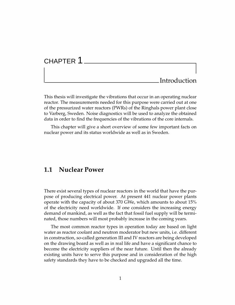
Another reason for fuel elements to move, in addition to the excitationthrough core barrel or support plate motion, is the coolant’s upward streamto the outlet nozzle. The speed the coolant obtains here is so high that singlefuel elements start to vibrate slightly even if they are fixed in several axialpositions.

Figure 2.8: Construction drawing of the Westinghouse PWR reactor vessel includ-ing labels on several parts.

16

2.4. Reactor Vibrations

Figure 2.9: Model of the Westinghouse PWR reactor vessel with the core barrelhosting support plates, fuel assemblies and control rods.

2.4.1 Modes of Vibration

The most obvious mode of vibration is the reactor vessel’s pendular move-ment, also known as beam mode vibration. The frequency of this vibrationusually lies around 8 Hz whereas another mode of vibration, the shell modevibration, occurs at about 20 Hz. Those two kinds of core barrel vibrationscan easily be recorded by neutron detectors that are positioned outside ofthe reactor vessel, so-called ex-core detectors. The R4 reactor has 8 of thosedetectors, 4 positioned in the top and 4 positioned in the bottom, to recordthe external neutron flux, see also Fig. 2.2b.

As already explained in the introduction of this section, ”outer” vibra-tions influence the ”inner” life of the reactor vessel and most likely propa-gate to the core barrel and its internals where for example fuel rod vibrationsmight develop.

17


Single fuel rods have the chance to vibrate at the frequencies mentionedabove, i.e. at their eigenfrequencies, or to evolve vibrations at completelydifferent frequencies, which correspond to resonances of the driving force.The latter kind of fuel rod vibrations can usually not be measured by theex-core detectors since their contribution to the total neutron flux might betoo small. Therefore one uses detectors inside of the core barrel so that lo-calized fluctuations have a chance to be found. Fuel vibrations are usuallyconsidered as a combination of local fuel rod movements and global coremovements. Hence, recording in-core noise on a regular basis is one possi-bility to detect construction defects within the core, as for example a weaklyfixed or even loose fuel pin.

Figure 2.10: Simplified illustration of the dominating core barrel vibration modes,beam and shell mode.

18

2.5. In-Core Detectors

2.5 In-Core Detectors

Controlling a power reactor and assuring the fulfilment of high safety de-mands requires a number of measurements regarding temperature and pres-sure, neutron flux, radiation and power level, coolant flow and many more.The essential reaction in a PWR, the fission, is induced by thermal neutronswhich is why nuclear sensors have to be based on detectors that mostlyrespond to low-energy neutrons and, furthermore, are very resistant to ra-diation damage.

There are two categories of nuclear sensors in order to measure the neu-tron flux: in-core and ex-core detectors.

As already mentioned before, ex-core detectors are situated outside ofthe reactor core and simply measure the flux of neutrons that leak out of thecore. In a PWR one finds a number of fix ex-core detectors which are placedin the top and bottom of the reactor. Fig. 2.4 indicates their approximatepositions.

In-core detectors on the other hand are located in narrow detector-guidetubes in the middle of a fuel assembly, cf. Fig. 2.2, where detailed knowl-edge on the flux shape can be provided since local variations of the neutronflux might be found. In-core detectors are equipped with a drive mecha-nism so that they can be moved vertically in the tube they are positioned inwith the aim of measuring axial flux distributions. Considering the limitedspace inside of the fuel assembly, in-core detectors have to be very small -their diameter is in the range of 10mm.

2.5.1 Fission Chambers

The detectors used in the in-core neutron noise measurement at R4 are minia-turized fission chambers. Fission chambers or fission counters are gas coun-ters which are coated interiorly with a fissile isotope in order to measurethe number of neutrons arriving at the detector. A common filling gas forthe chamber is argon Ar. Its pressure shall make sure that the range of theemitted fission fragments does not exceed the dimensions of the detector.When a neutron hits the coating, fission takes place and the resulting fissionfragments move apart from each other. On their way through the counterion-pairs will be created in the gas since the ionizing density of the fissionfragments is very high. Due to the electric field which is applied to thecounter, the ion-pairs will drift to the electrodes where they generate an

19


electric pulse. This signal is directly related to the fission rate which in turnis proportional to the neutron flux.

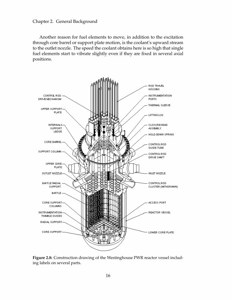
In order to make the fission chamber work properly, it is of particularimportance to know the dependence between the coating material and theneutron energy. The fission cross-section for U-235 is much higher for low-energy (slow) neutrons than it is for high-energy (fast) neutrons and there-fore fission of U-235 happens with a much higher probability when the nu-clei are hit by thermal neutrons. At higher neutron energies the cross-sectionfor inelastic scattering is higher than the one for fission which makes U-235”blind” to the much less probable process of fast fission. One conclusion ofthis is that if U-235 is used in fission chambers, the detection of thermal neu-trons is possible. Fig. 2.11 shows the cross sections for absorption, scatteringand fission with respect to the neutron energy.

When using U-238 instead of U-235 in a fission chamber, fast neutronscan be counted since U-238 fissions at high neutron energies. Taking forexample a mixture of U-235 and U-238 as coating for the fission chamber isone reliable method to measure the thermal as well as the fast neutron flux.

Figure 2.11: Neutron cross sections for U-235 vs. neutron energy. (blue - total; red- fission; green - elastic; black - inelastic; purple - caption)

20

2.6. Computational Method and Theoretical Aspects

Figure 2.12: Neutron cross sections for U-238 vs. neutron energy. (blue - total; red- fission; green - elastic; black - inelastic; purple - caption)

2.6 Computational Method and Theoretical Aspects

This part of the thesis describes a method for finding the different vibra-tional frequencies from the measured detector signal. Generally speakingthe data taken contains the noise of the system, i.e. a superposition of ran-dom processes of different character. In order to obtain information on thenoise component of interest, one has to perform spectral analysis, that is todescribe the distribution over frequency of the power contained in a signal.

To estimate the auto power spectral density (APSD) in this specific caseWelch’s method is used: the signal is divided into several segments (blocks)of equal length and the computed periodograms (digital Fourier transforms)- one per segment - are averaged.

The length of a block is determined by the amount of points that willlater on be used for the FFT. A window function is applied to each segmentin order to generate a filter, ”which tapers the ideal impulse response” andin turn results in an increasing resolution of the amplitude.

21


Windowing in this context means to multiply the data sequence in the blockwith the corresponding values of the window function. The window func-tion used for this specific case is called a Hanning function and is definedas

hann(N) = 0.5(

1 − cos( 2πN

n − 1

))

N = 0...n − 1 (2.4)

A graphical interpretation of this can be found in Fig. 2.13.

Figure 2.13: The Hanning window.

The windowed data is subsequently put together. It is important to men-tion that the blocks are used more than once such that each block overlapswith the preceding and consecutive block by 50%. It is easy to see that thisenhances the effectiveness of the use of the data.

The periodograms, which are needed for averaging the squared magni-tude of the spectral density, are computed by using FFT. Fourier’s theoremstates that every periodic function of time can be written as a superposi-tion of several sine waves of specified frequency, amplitude and phase andtherefore can be transformed into a function of frequency which makes it bymeans of physics easier to analyse and interpret.

22

2.6. Computational Method and Theoretical Aspects

A periodic function of time, in this case the measured signal, is expressedin form of a Fourier series:

x(t) =

∞∑

j=−∞

Xj · exp[

i2πj

Tt]

(2.5)

Here Xj is the Fourier amplitude at the frequency j

Tand can be obtained by:

Xj =1

T

∫ T

2

−T

2

x(t) · exp[

−i2πj

Tt]

dt (2.6)

Since x(t) is real, the results for Xj, where j is both positive and negative, arerelated through the condition

X−j = X∗

j (2.7)

so that all parts of Xj , real and imaginary, are obtained by:

{

Re

Im

}

Xj =1

T

∫ T

2

−T

2

x(t) ·{

cos

−sin

}2πj

Tdt (2.8)

Expressing equation 2.8 as a sum of N=T/∆ t makes it transform to

{

Re

Im

}

Xj =1

N

N∑

k=1

x(k · ∆t) ·{

cos

−sin

}2πjk

N(2.9)

and is defined as the FFT. It is important that N is a power of 2 because thisthis condition is the ”fast” in FFT.

Now that we transformed the data in the time domain to the frequencydomain, it is possible to plot the PSD with respect to frequency in Hz. Thiswill reveal several peaks, some of which can be interpreted as frequenciesof vibrations in the reactor core.

23


24

CHAPTER 3

In-Core Measurements

The in-core neutron noise measurements were performed at the youngestunit of the 4 Ringhals reactors, which is R4. The reason for this decisionlies in the outcome of earlier ex-core measurements, which were performedin order to monitor and diagnose the core-barrel vibrations. Such measure-ments show the beam-mode and shell-mode vibrations as correspondingpeaks in the neutron noise spectra. Due to the symmetries of the variousmodes with respect to the positions of the ex-core detectors, the auto- andcross-spectra, coherence and phase between different detector pairs shouldobey certain conditions. Further, the auto-spectra of all four ex-core detec-tors should show a similar shape at the vibration frequencies at the sameaxial level. However, in earlier measurements deviations from the expectedgeneral properties were observed mostly in R4, and to a lesser extent in R3.Hence the hypothesis was set up that in the measurements a combined ef-fect of the core-barrel and the fuel assembly vibrations is observed, whichcan lend a possible explanation for the irregularities observed in the ex-coredetector signals. Thus it was thought that additional in-core measurementsmight help to answer some of the questions on this problem.

The in-core measurements at R4 were executed on March, 4th in 2008with the help of Bjorn Severinsson and Martin Bengtsson.

3.1 Measurement Setup

Five in-core detectors were used to measure the neutron flux at 6 differentaxial positions such that every detector was kept in each of those axial posi-tions for 15 minutes. After inserting the detectors at the bottom of the corethey were firstly moved to the very top of the core and then taken out inseveral steps. The first axial position was situated 30 cm below the top of

25

Chapter 3. In-Core Measurements

the reactor core from where each detector was moved in steps of 60 cm untilposition 6, situated 30 cm above the bottom of the reactor core, was reached.A graphical interpretation of the above can be seen in Figs. 3.1 and 3.2. Allin all the in-core measurement took 2 hours.

Furthermore the 8 ex-core detectors, 4 positioned in the bottom and theother 4 in the reactor’s top, were used to measure the ex-core noise, althoughthe analysis of this measurement belongs to another project and is not in-cluded in the present thesis.

a) b)

Figure 3.1: a) Axial positions of the in-core detectors. b) Detector positions in thecore.

26

3.2. Technical Data of R4

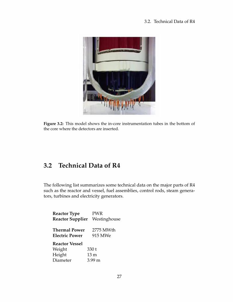
Figure 3.2: This model shows the in-core instrumentation tubes in the bottom ofthe core where the detectors are inserted.

3.2 Technical Data of R4

The following list summarizes some technical data on the major parts of R4such as the reactor and vessel, fuel assemblies, control rods, steam genera-tors, turbines and electricity generators.

Reactor Type PWRReactor Supplier Westinghouse

Thermal Power 2775 MWthElectric Power 915 MWe

Reactor VesselWeight 330 tHeight 13 mDiameter 3.99 m

27


Primary Coolant CycleNumber of cooling circuits 3Operating Pressure 15.5 MPaInlet Temperature 284◦COutlet Temperature 323◦C

Secondary Coolant CycleOperating Pressure 6 MPaSteam Temperature 276◦CSteam Flow Rate 1521 kg/s

Fuel AssembliesCladding Material Zircaloy-4Fuel Weight per Assembly 523 kg UO2

Total Number in Core 157Number of Fuel Pins 264 (17x17 type)

Fuel Pin Length 3.66 mFuel Pellet Diameter 0.819 cm

Control RodsNumber 48

Steam GeneratorSupplier WestinghouseNumber 3Steam Flow Rate 507 kg/s

Weight 308 tHeight 20.6 m

Electricity GeneratorSupplier ASEA Stal ABNumber 2Voltage 21.5 kVLine Voltage 438.5 kV

28

3.2. Technical Data of R4

TurbineSupplier ASEA Stal ABEfficiency 32.3%Speed 3000 rpm

Number of High Pressure Turbines (HPT) 2x1Steam Temperature before HPT 275◦CSteam Pressure before HPT 5.9 MPaSteam Temperature after HPT 163◦CSteam Pressure after HPT 0.7 MPa

Number of Low Pressure Turbines (LPT) 2x3Steam Temperature before LPT 260◦CSteam Pressure before LPT 0.46 MPaSteam Temperature after LPT 29◦CSteam Pressure after LPT 0.004 MPa

29


30

CHAPTER 4

Data Analysis and Results

To analyze the data obtained from the R4 in-core measurement, a short Mat-Lab code was written. Its aim is to show the axial distribution of the autopower spectral density (APSD) at all axial positions for each of the five de-tectors.

4.1 Measurement Data

The original data file from the Ringhals measurement, ”r4exin c.txt”, con-tains information on both the in-core and ex-core detectors. This txt-filestarts with a header of 17 lines that contains some general information onthe measurement as for example total measuring time and sampling fre-quency. It is followed by an array filled with ASCII entries only which rep-resent all detector signals at the different measurement points.

Due to a total measuring time of 10 882.56 s and a sampling frequency fsof 62.5 Hz the array consists of 680 180 lines. The time increases in steps of0.016 s (=1/fs).

The number of columns arises from the number of detectors plus onecolumn, the first one, that represents the different measurement points. Thecolumns 2 to 17 now contain the measurement data of the 13 detectors thatwhere used to obtain information on the vibrations of the system:

• column 2...4: DC signal of the upper ex-core detectors N41, N42, andN43

• column 5...9: AC signal of the in-core detectors

• column 10...17: AC signal of all 8 ex-core detectors.

31

Chapter 4. Data Analysis and Results

All this makes the file quite big with regard to its txt-format. Thus, inorder to cut down on calculation time and to avoid confusion with all thedifferent detector signals, a short code called ”detectordata.m” was written.This code splits up the original txt-file and creates one mat-file for the timeand one for each detector signal. Here it is important to consider that themeasuring time for the in-core detectors was about 1 hour shorter than forthe ex-core detectors which makes the in-core mat-files just 400 000 lineslong.

Since this thesis mostly pays attention to in-core phenomena it will notcontain the ex-core measurements, so the data used in the following arebased on the shortened measurement files. All complete ex-core data are ofcourse available for further noise diagnostics.

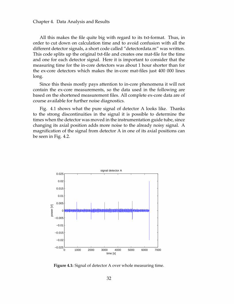
Fig. 4.1 shows what the pure signal of detector A looks like. Thanksto the strong discontinuities in the signal it is possible to determine thetimes when the detector was moved in the instrumentation guide tube, sincechanging its axial position adds more noise to the already noisy signal. Amagnification of the signal from detector A in one of its axial positions canbe seen in Fig. 4.2.

0 1000 2000 3000 4000 5000 6000 7000−0.025

−0.02

−0.015

−0.01

−0.005

0

0.005

0.01

0.015

0.02

0.025

time [s]

pow

er [V

]

signal detector A

Figure 4.1: Signal of detector A over whole measuring time.

32

4.2. Power Spectra

1220 1240 1260 1280 1300 1320 1340

−1

−0.5

0

0.5

1

x 10−3

time [s]

pow

er [V

]

magnification of signal from detector A in position 2

Figure 4.2: Signal of detector A in position 2 scaled up by a factor of 50.

4.2 Power Spectra

By using the 5 mat-files that contain information on the in-core detectorsA through E, the auto power spectra for the different detectors and posi-tions are calculated by running the MatLab code named ”spetra*.m” whichwas written for this specific purpose. Here the pre-installed MatLab func-tion ”pwelch”, named after Welch’s method, was used. The algorithm wasexplained in the previous theoretical part of this work. The output of ”spec-tra*.m” is a set of figures that show the APSD vs. frequency for all measuredsignals.

The ”*” in the program’s name stands for the number of FFT points usedwhen calculating the APSD. This number varies between 512, 1024 and 2048and is a crucial factor for the smoothness of the spectrum. A low but ade-quate number of FFT points results in a rather smooth curve but causeslosses in the precision of the frequency and peak height. A higher numberincludes more measurement points which results in a noise-like spectrumbut at the same time increases the accuracy of the APSD amplitude regard-ing the reconstruction of the peaks of interest.

33


Therefore a combination of the spectra obtained with 512 and 2048 pointswas the optimal method to find the different vibrational frequencies andtheir maximum amplitudes. The ”512-version” was used to find a roughestimate of the frequency while the ”2048-version” gave the magnitudesused in the further analysis. Figs. 4.3 and 4.4 show the signal for detectorA in position 1 with 512 and 2048 FFT points, respectively, and shall help tostress this explanation.

Figure 4.3: APSD vs. frequency when 512 data points per block (”512-version”) areused for the FFT procedure.

Figure 4.4: APSD vs. frequency when 2048 data points per block (”2048-version”)are used for the FFT procedure.

34

4.2. Power Spectra

As it can be seen in Figs. 4.3 and 4.4, the number of FFT points does notinfluence the general shape of the APSD spectra. The following figures aregoing to contain several APSD curves in one plot so that, for the conve-nience of finding probable similarities or differences between all detectorsignals, the ”512-version” of the spectra will be used.

a) b)

0 5 10 15 20 25 30 3510

−13

10−12

10−11

10−10

10−9

10−8

10−7

10−6

Position 1

frequency [Hz]

PS

D

detector Adetector Bdetector Cdetector Ddetector E

0 5 10 15 20 25 30 3510

−13

10−12

10−11

10−10

10−9

10−8

10−7

10−6

Position 2

frequency [Hz]

PS

D


c) d)

0 5 10 15 20 25 30 3510

−13

10−12

10−11

10−10

10−9

10−8

10−7

10−6

Position 3

frequency [Hz]

PS

D


0 5 10 15 20 25 30 3510

−13

10−12

10−11

10−10

10−9

10−8

10−7

10−6

Position 4

frequency [Hz]

PS

D


e) f)

0 5 10 15 20 25 30 3510

−13

10−12

10−11

10−10

10−9

10−8

10−7

10−6

Position 5

frequency [Hz]

PS

D


0 5 10 15 20 25 30 3510

−13

10−12

10−11

10−10

10−9

10−8

10−7

Position 6

frequency [Hz]

PS

D


Figure 4.5: APSD vs. frequency of the different detectors for all 6 axial positions.

35


Each subplot in Fig. 4.5 shows the APSD plots for all 5 detectors in one ofthe axial positions. Comparing those graphs with each other helps to iden-tify the frequencies of vibration which will be done in the subsequent sec-tion. Furthermore the comparison of the graphs might indicate whether thedifferent detectors behave similarly, and generally measure the same phe-nomenon, or whether some vibrations depend on the detector’s insertionposition in the core or even on the measurement time.

4.3 Vibrational Frequencies

For the purpose of creating plots that describe the axial behavior of the max-imum APSD amplitudes at the vibrational frequencies it is first of all impor-tant to find those frequencies.

Comparing Figs. 4.3, 4.4 and 4.5 with the one in section 2.3.2, Fig. 2.6,makes clear that the APSD plots obtained from the measurements followthe general tendency of the zero noise spectrum whereas the obvious peaksin the spectra indicate the frequencies of vibration. First of all the ”512-version” of the APSD plots helped to find a rough estimate of the differentfrequency values. The result from this analysis was then used to determinethe ”true” frequency values and the amplitude height of the APSD by eval-uating the ”2048-version” of the 30 processed signals.

The outcome of this is a number of frequencies which occurred in most ofthe APSD plots. Table 4.1 summarizes the frequencies found as well as thepercentage value of their clear appearance. The reason for mentioning howoften a peak occurs lies in the fact that it becomes easier to decide whethera peak found at a special frequency can be interpreted as a vibration or not.

Frequency 1.8 Hz 6.7 Hz 7.8 Hz 9.9 Hz 10.8 Hz 24.9 Hz

Fraction in % 50 100 70 70 60 80

Frequency 12 Hz 15.5 Hz 19 Hz

Fraction in % 30 40 40

Table 4.1: Summary over frequencies of vibration.

36

4.3. Vibrational Frequencies

Due to the high fraction of the peaks found at 6.7, 7.8, 9.9 and 24.9 Hz it ispossible to classify those frequencies as vibrational ones.

In 60% of all detector signals one finds a strong peak at 10.8 Hz andin 50% there is a distinct peak at 1.8 Hz. In order to be sure that thosefrequencies are interesting for the purpose of analyzing core vibrations onehas to find out in which spectra those peaks are very low or even missing.

The 10.8 Hz peak is measured by detectors A and B in every positionand detector D reveals it in 4 of the 6 positions whereas detectors C and Edo not show it clearly at all. Here it is important to point out that detectorsC and E measure a high peak at 12 Hz instead, which might interfere withthe 10.8 Hz top so that its strength could be weakened and therefore cannotbe seen clearly. An important question that arises here is whether it couldbe possible that the 10.8 Hz is shifted to 12 Hz or whether both frequenciesreally have to be regarded separately. The conclusions regarding this willbe drawn in chapter 5. For the purpose of studying the axial amplitudedistribution in section 4.4 it is assumed that the two frequencies are separatefrom each other.

The peak at 1.8 Hz shows a somewhat different behavior. It is measuredby all 5 detectors but only appears really clear in the upper positions. For theremaining positions 4 to 6 one observes that the beginning of each spectrumis broadened which might be due to the 1.8 Hz peak which is containedhere and just too weak to be seen in a distinct manner. Furthermore it wasobserved that, in position 1 only, the frequency always lies slightly below1.8 Hz, namely at 1.6 Hz. Since exactly this behavior was found numer-ous times before the measurement discussed here, it is treated as a typicalbehavior of the vibration at 1.8 Hz.

Even though the top around 19 Hz is only found in 2 out of 5 signals,one can be rather sure that it really is one of the vibrational frequencies ofinterest. From earlier measurements it is known that the shell mode vibra-tion occurs at approximately 20 Hz. The 19 Hz top was found for everydetector in at least one of the axial positions but the fact that it occurredin 5 out of 6 cases for the outermost detector C, is a reliable indicator thatthis particular frequency represents the shell mode vibration. This modeof vibration reminds on a ”fluctuating crunch” of the core, c.f. Fig. 2.10 inchapter 2, and influences the neutron flux strongest on the outside of thecore. Since there are almost no changes inside of the core for this type ofvibration, ex-core detectors are most sensitive to this vibration mode, butouter in-core detectors could recognize this vibration, too. Detector C ispositioned in a fuel assembly which sits on the edge of the core and with re-gard to the discussion above the shell mode can probably be measured by it.

37


Furthermore the fuel assembly has less possibilities to move since it is re-strained by two core walls and it could be that this limitation is transferredto the detector so that wall vibrations might be recognized.

Even if strong tops were found at 15.5 Hz in 40% of the cases and fur-thermore every detector measured this frequency at least once, it was notpossible to make out any trend behavior regarding their occurrence.

At the end of this section it is maybe important to mention that the phe-nomena observed, especially regarding the frequencies that only occur witha relatively low fraction, are not very strange to experts in the field of reac-tor diagnostics. Indeed they have been seen in several earlier measurementsbut could not be explained in detail yet.

4.4 Axial Amplitude Distribution

With the help of the APSDs calculated and shown above and by classify-ing the frequencies of interest, bold-marked in Table 4.1, it was possible togenerate lists that contain information on the maximum amplitude for eachdetector and position. In the beginning those tables are of the format ”ax-ial*.xls” but later on their entries are transformed to matrices that are savedas mat-files. Finally those files are used as input data for the MatLab code”axial*.m” which plots the axial distribution of the APSDs for all vibrationalfrequencies identified above.

The 6 resulting plots are summarized in Fig. 4.6. Here each subplotrepresents one of the vibrational frequencies and shows its maximum am-plitude with respect to the reactor height for each detector.

Furthermore it was of interest to follow the amplitude distribution forthose frequencies that are difficult to classify. For the purpose of creatingplots that hopefully help to prove the assumptions made above or reveal theorigin of the peaks that occur at 12, 15.5 and 19 Hz, another MatLab codewas written. This short program, named ”axialextra.m”, works in the samemanner as ”axial*.m” with the only difference that the vectors that result inthe axial amplitude distribution of the chosen frequencies were generatedmanually. Of course the resolution is not as good as in Fig. 4.6 since thenumber of peaks that were identified in a definite manner is substantiallylower than for the other frequencies. However, comparisons between thedifferent graphs might help to understand the nature of some of the unex-plained phenomena anyway.

38

4.4. Axial Amplitude Distribution

a) b)

0 1 2 3 4 5 6 7 8 9

x 10−8

0

50

100

150

200

250

300

350frequency 1.8 Hz

PSD amplitude [a.u.]

reac

tor

heig

ht [c

m]

incore Aincore Bincore Cincore Dincore E

0 0.5 1 1.5 2 2.5 3 3.5 4 4.5

x 10−8

0

50

100

150

200

250

300

350frequency 6.8 Hz


reac

tor

heig

ht [c

m]


c) d)

0 0.2 0.4 0.6 0.8 1 1.2 1.4 1.6 1.8

x 10−8

0

50

100

150

200

250

300

350frequency 7.9 Hz


reac

tor

heig

ht [c

m]


0 0.5 1 1.5

x 10−9

0

50

100

150

200

250

300

350frequency 9.9 Hz


reac

tor

heig

ht [c

m]


e) f)

1 2 3 4 5 6 7 8 9

x 10−10

0

50

100

150

200

250

300

350frequency 10.8 Hz


reac

tor

heig

ht [c

m]


0 0.2 0.4 0.6 0.8 1 1.2 1.4 1.6 1.8

x 10−10

0

50

100

150

200

250

300

350frequency 24.9 Hz


reac

tor

heig

ht [c

m]


Figure 4.6: Amplitude vs. height for each vibrational frequency.

39


a)

3 4 5 6 7 8 9

x 10−10

50

100

150

200

250

300

350frequency 12 Hz, detector C and E


reat

or h

eigh

t [cm

]

detector Cdetector E

b)

0 0.2 0.4 0.6 0.8 1 1.2

x 10−9

0

50

100

150

200

250

300frequency 15.5 Hz, detector C


reat

or h

eigh

t [cm

]

detector Adetector Bdetector C

c)

1 2 3 4 5 6 7 8

x 10−10

0

50

100

150

200

250

300

350frequency 19 Hz, detector C


reat

or h

eigh

t [cm

]

Figure 4.7: Amplitudes vs. height for 12, 15.5 and 19 Hz.

40

CHAPTER 5

Discussion and Conclusions

The aim of this chapter is to summarize the main results of the measure-ments and to draw conclusions from the plots obtained in chapter 4. Herethe frequencies will be classified regarding their origin and type so that char-acteristics on the system can be found.

5.1 Classification of Frequencies

Classifying the frequencies by their shape will partly be done by the helpof a work on in-core measurements at R4 in 1998 (Demaziere et al, 1999)which showed theoretical mode shapes in an abstract manner. The plots thatwere created in that report are shown in Fig. 5.1 and include the boundaryconditions of the occurring vibrations.

Figure 5.1: Theoretical mode shapes.

41

Chapter 5. Discussion and Conclusions

5.1.1 The Fundamental Bending Mode - 1.8 Hz

From the literature on earlier in-core measurements it was found that thevibration at 1.8 Hz corresponds to the fundamental, or first order, bendingmode vibration of the fuel assembly. Comparing the measured axial am-plitude distribution at this frequency in Fig. 4.6a with Fig. 5.1 leads to theinsight that the 1.8 Hz vibration has fixed conditions in both ends of the fuelassembly. This makes perfectly sense since the fuel assemblies are in prin-ciple attached between the upper and lower core support plate so that theirvibrations most likely generate the fundamental fuel assembly vibration at1.8 Hz.

All 5 in-core detector data show that the APSD amplitude increases toits maximum in the middle of the core and then decreases again to a valueslightly smaller than the one in the first axial position.

5.1.2 The 2nd Order Bending Mode - 6.8 Hz

The rather strong vibration at 6.8 Hz is classified as the second order bend-ing mode vibration of the fuel assemblies with fixed conditions in the topand free conditions in the bottom. The amplitude increases much in thelower part of the core which indicates that the vibrations here are strongerthan in the upper part of the core. That specific behavior was measured byall 5 detectors whereas the signal from detector C is again dominating.

With regard to the results obtained from vibration measurements at theSequoyah-1 reactor in 1985 one can conclude that the vibration at 6.8 Hz isa result of the movement of the lower core support plate which is triggeredby the pendulum movement of the core barrel.

5.1.3 The Beam Mode - 7.8 Hz

The vibration at 7.8 Hz is assumed to originate from the classical beam modevibration with a fixed end in the top and a free end in the bottom. Evenif there is, according to Fig. 5.1, no theoretical mode shape that shows abehavior similar to the experimental one, the vibration is classified as thefuel assemblies following the pendulum movement of the core barrel. Un-fortunately there are not many references that stress this interpretation butcomparing the in-core with the ex-core spectra might help to prove this as-sumption.

42

5.1. Classification of Frequencies

The ex-core measurements used here were made simultaneously withthe in-core measurements and the analysis was made by A. Hernandez-Solisat the Department of Nuclear Engineering of Chalmers. Fig. 5.2 shows theNAPSD (Normalized Auto Power Spectral Density) vs. frequency of thebeam mode component for the upper and lower ex-core detectors.

a)

0 5 10 15 20 25 30 3510

−2

10−1

100

101

102

103

104

NA

PS

D

Frequency [Hz]

beam mode component of the signal from upper ex−core detectors

b)

0 5 10 15 20 25 30 3510

−2

10−1

100

101

102

103

104

NAP

SD

Frequency [Hz]

beam mode component of the signal for lower ex−core detectors

Figure 5.2: NAPSD vs. frequency for the upper and the lower ex-core detectors.

43


The frequencies of interest in the 6 - 8 Hz region agree almost exactly withthe frequencies measured in the in-core measurement. The upper part of thecore vibrates at 6.7 and 7.9 Hz, whereas the vibrations found in the lowerpart are 6.8 and 7.9 Hz. So the double peak that was observed in 70% ofthe in-core measurements also occurs in the ex-core noise spectra with oneimportant difference. In the case of the in-core spectra the top at 7.8 Hz wasalways lower than the one at 6.8 Hz. But as one can see in Fig. 5.2, thisis only true in the upper half of the core in the ex-core measurements. Inthe lower part the vibration at 7.9 Hz dominates over the peak at 6.8 Hz,and it is still difficult to determine the ”real” frequency of the beam modevibration.

One fact that is consistent between the in-core and ex-core measurementsis that the NAPSD amplitude increases in the lower part of the core and thiswas also observed in the amplitude shapes of all 5 in-core detectors.

Even if the consideration of the ex-core measurements might be moreconfusing than enlightening it is suggested that the vibration at 7.8 Hz cor-responds to the beam mode since there were at least two more referencesthat stated a frequency around 8 Hz for the beam mode vibration.

An additional comment regarding the double peak in the 6 - 8 Hz re-gion will follow in the summarizing chapter of this thesis since the correctclassification of the two peaks is still unclear.

5.1.4 Unclassified Vibrations - 9.9, 10.8, 12, 15.5 Hz

The classification of the vibrations at 9.9, 10.8, 12 and 15.5 Hz is far morecomplicated than for the other frequencies found. All detectors behave dif-ferently, the resolution of the axial amplitude distribution for 12 and 15.5 Hzis not sufficient and references from literature could not be found.

The two last reasons above make it impossible to categorize the 15.5 Hzvibration. By looking at the shape created by detector C one can state thatthe vibration has fixed end conditions, cf. Fig. 4.7b, but this information isnot even enough to prove that the resonance found is a real fuel vibrationor just an unexplained perturbation that could result from wall movements.Remember that detector C is the outermost one and due to this might showa behavior different from the other in-core detectors. The observed shapereminds of a higher order vibration mode and could be traced back to walleffects but its definite origin remains unclear so far.

44


In the following the different curves for the 5 detectors in Fig. 4.6d willbe discussed. Here one observes that the vibration has fixed conditions inboth ends in all cases except for detector E which has fixed conditions in thetop and free conditions in the bottom.

The shapes of the curves for detectors B and D remind to some extent ofthe fundamental mode shape since the maxima of the amplitudes are foundin the middle of the reactor but drawing concrete conclusions from this doesnot appear possible, mostly since the signals of the other detectors behavein a different manner.

The shape for detector C might be interpreted as a higher order vibrationmode shape whereas the shape created by detector A could be somethinglike a superposition of C and D. Here the question appears whether it is pos-sible that the different in-core detectors can actually measure the individualbehavior of the fuel assembly they are placed in so that one is able to finddetails on the vibrations of a single fuel assembly.

At last the shape of detector E is similar to the theoretical one that rep-resents the beam mode. Hence one reasonable argument here could be thatit resembles the probable swinging movement of the fuel assembly in coreposition L9. It might also be of interest that the shape of detector E behavesin exactly the same way as for the 10.8 Hz resonance, cf. Fig. 4.6e. It is al-most unfortunate that the amplitude for detector E in the case of the 12 Hzresonance misses measurement points in the uppermost and lowest axialposition and therefore makes the resolution of Fig. 4.7a poor. This makesit difficult to state that the frequency at 10.8 Hz is really shifted to 12 Hz.Assuming now that the vibration of a fuel assembly might be due to a loosefixing in the lower core support plate remains unjustified. Fig. 5.3 is a com-parison of the axial amplitude distributions for detector E at the resonancesat 9.9, 10.8 and 12 Hz and shall help to stress the statements made above.

45


2 4 6 8 10

x 10−10

0

50

100

150

200

250

300

350comparison of axial amplitude distribution for detector E


reac

tor

heig

ht [c

m]

9.9 Hz10.8 Hz12 Hz

Figure 5.3: Comparison of the mode shapes for detector E in the range of 10 - 12Hz.

Analyzing Fig. 4.6e in the same manner as Fig. 4.6d does not lead to bet-ter insights. The amplitudes for detector A in both figures behave in princi-ple alike as it can be seen in Fig. 5.4a. However, classifying this vibration asa fundamental one seems unreasonable. One could interpret the resonancesat 9.9 and 10.8 Hz as forced first order vibrations, again with fixed end con-ditions, of the fuel assembly in core position G7 caused by outer vibrationsor by the coolant flow.

The shape for the vibration at 10.8 Hz for detector B reminds of a secondorder vibration with fixed end conditions. Due to the fact that the shapes for9.9 and 10.8 Hz do not look similar, cf. Fig. 5.4b, it is assumed that these twofrequencies represent two different vibrations. The one at 9.9 Hz predicts astrong vibration due to the lateral movement of the lower core support platewhich particularly acts on the fuel assembly in core position F6, whereas theresonance at 10.8 Hz might be a higher order vibration.

Fig. 5.4c compares the axial amplitude distributions for detector C andthe resonances found at 9.9, 10.8 and 12 Hz. The curves for the two lowerfrequencies look very much alike and are most likely interpreted as higherorder vibrations with fixed end conditions. As well as in the case for de-tector E, the 12 Hz resonance has a poor resolution. The idea that the 12Hz resonance is a shift of the vibration at 10.8 Hz is still valid because the

46


12 Hz amplitudes are generally bigger and follow the trend of the curve at10.8 Hz. It is assumed that the resonances at 9.9 and 10.8 Hz resemble higherorder vibrations whereas the 10.8 Hz resonance is shifted to 12 Hz. The phe-nomenon of a shift in frequency was observed before but has not found anexplanation yet. Unfortunately no publications could be found that discussthe occurrence of something like a shifted frequency.

Finally one has to judge the behavior of the curves created through thein-core measurement by detector D. The 9.9 Hz shape reminds of the shapeof the fundamental mode whereas the 10.8 Hz shape reminds of the beammode, cf. Fig. 5.4d. The maximum amplitude is found in the middle or inthe lower part of the core, respectively, and classifying the vibrations apartfrom their fixed end conditions is not possible due to the lack of informationfrom the literature.

a) b)

1 1.5 2 2.5 3 3.5 4

x 10−10

0

50

100

150

200

250

300

350comparison of axial amplitude distribution for detector A


reac

tor

heig

ht [c

m]

9.9 Hz10.8 Hz

2 2.5 3 3.5 4

x 10−10

0

50

100

150

200

250

300

350comparison of axial amplitude distribution for detector B


reac

tor

heig

ht [c

m]

9.9 Hz10.8 Hz

c) d)

0 0.2 0.4 0.6 0.8 1 1.2 1.4

x 10−9

0

50

100

150

200

250

300

350comparison of axial amplitude distribution for detector C


reac

tor

heig

ht [c

m]

9.9 Hz10.8 Hz12 Hz

1 1.5 2 2.5 3

x 10−10

0

50

100

150

200

250

300

350comparison of axial amplitude distribution for detector D


reac

tor

heig

ht [c

m]

9.9 Hz10.8 Hz

Figure 5.4: Comparison of the mode shapes in the range of 10 - 12 Hz for detectorsA, B, C and D.

47


As a final conclusion here one can say that with the limited amount of mea-surement data and references it is impossible to fully classify the vibrationsafter their origin. Anyhow it is assumed that the resonances found at 9.9,10.8 and 12 Hz are forced higher order vibrations of the fuel assemblies. Thefuel assemblies furthermore might behave in various different manners dueto mechanical properties or fuel content and radial fixings. The 15.5 Hz vi-bration could not even be classified as a real vibration and this is why it isneglected in the further consideration.

5.1.5 The Shell Mode - 19 Hz

From earlier works on the vibration modes of the core barrel it is well knownthat the shell mode vibration is found at about 20 Hz. As already mentionedin section 4.3 of the previous chapter, the resonance at 19 Hz could be mea-sured in 40% of the signals, whereas only detector C allows plotting the axialamplitude distribution with a sufficient resolution. The shape observed inFig. 4.7c does not apply to any of the theoretical mode shapes shown in thebeginning of this chapter but since the amplitude has its maximum in thetop of the core the vibration is assumed to have free conditions in the topand fixed conditions in the bottom.

5.1.6 The Pump Frequency - 24.9 Hz

When examining the shapes for the axial amplitude distribution of all 5 de-tectors at 24.9 Hz it becomes obvious that it is impossible to find any trendbehavior. Detectors A and D are the only ones that have similar characteris-tics but C and E for example behave in an opposite manner.

One noticeable property of the resonance at 24.9 Hz observed in almostevery spectrum was that the peak was particularly sharp and precise. Know-ing that the revolution per minute of the pump that accelerates the primarycoolant is 1500, one can easily conclude that the resonance at 25 Hz trans-lates to a mechanical vibration caused by the pump frequency. It arises fromthe rotor blades that cause the coolant to flow upwards through the reactorcore and is identified as the pump frequency.

48

CHAPTER 6

Summary

The in-core measurement at R4 used 5 in-core fission chambers at 6 axialpositions to evaluate the mode shapes of the core and fuel vibrations. Thepurpose of this task was to find possible reasons for the unusual behaviorof the reactor which was observed in earlier ex-core measurements. Sincethose results were of internal nature it was not possible to get hold of them.Analyzing the noise spectra obtained from the measurements made at R4in 2008 via typical noise diagnostic methods led to the following results.The APSDs revealed 5 frequencies that could be classified after their type ofvibration:

The top at 1.8 Hz could be found in a definite manner in 50 % of themeasurements and was identified as the fundamental bending mode of thefuel assemblies.

It was found that the double peak in the 6 - 8 Hz range represents twodifferent vibrations which unfortunately can be interpreted in two differentmanners.

The first interpretation states that the resonance at 6.8 Hz, whichoccurs in all measurement positions as a very strong peak, re-sembles the second bending mode of the fuel assemblies. At 7.8Hz one finds that the APSD amplitude increases much in thelower part of the core, i.e. the vibrations here are stronger thanin the upper part of the core. This behavior might originate fromthe pendulum movement of the core which also affects the coreinternals, hence the beam mode vibration can be observed within-core instrumentation.

The second interpretation of the double peak is the contrary ofthe above. Previous in-core measurements at R4 (Karlsson, 1998)as well as the consideration of the analysis done in this work, cf.Fig. 4.6b, lead to the idea that the vibration at 6.8 Hz is caused by

49

Chapter 6. Summary

the pendulum movement of the core and, in turn, is interpretedas the beam mode vibration. This interpretation is intensified byconsidering the results of the three ex-core measurements donein the previous fuel cycle (Hernandez-Solis, 2008). Here it wasobserved that the higher resonance at around 8 Hz changed itsvalue during the fuel cycle whereas the 6.8 Hz peak remainedrelatively constant. Generally it can be assumed that the beammode vibration is more constant than the individual movementof fuel assemblies since they change their properties with timeso that one could claim that the vibration at 7.9 Hz is associatedwith the eigenfrequency, or higher order bending mode, of thefuel assemblies which is induced by the coolant flow. This state-ment is again stressed by the results found in this, cf. Fig. 4.6c,and previous analyses. Furthermore one could see that the 6.8Hz peak dominates over the 7.9 Hz peak when getting closer tothe bottom of the core. This indicates that the beam mode vi-bration is stronger than the fuel assembly vibration with an owneigenfrequency which is a logical consequence when consider-ing the construction of core and fuel assemblies.

In order to prove or disprove the interpretations made above additionalmeasurements are necessary - so far, both ideas are just hypothetical.

Another resonance was found at 19 Hz. Even if this frequency was onlymeasured in 40 % of the cases it could be identified as the shell mode vibra-tion.

At 24.9 Hz, which is approximated to 25 Hz, the pump frequency wasfound.

Furthermore there are 2 forced vibration modes at 9.9 and 10.8 Hz wherethe latter one is assumed to be shifted to 12.8 Hz in the cases of detectors Cand E. Detailed knowledge on those frequencies is not available yet but ad-ditional in-core measurements could help to analyze those resonances pre-cisely and maybe even find their true origin.

The results obtained from this thesis can be corroborated by further in-core measurements. Unfortunately it was not possible to identify some ofthe vibrations more specifically, but additional noise diagnostics, also forthe Ringhals reactor R3 which is similar in construction, would definitelyimprove the outcome of this thesis. As a final statement one can mentionthat noise diagnostics and the analysis of reactor vibrations is definitely ahelpful tool to find typical core characteristics as well as probable anomalies.If there was not a lack of earlier measurement data and results it would

50

have been easier to assign those frequencies that have not found a specificexplanation yet.

51

Chapter 6. Summary

52

Acknowledgements

It is difficult to know where to start since there were so many people in-volved in helping me on my journey so I hope that it is accepted if I startwith the 3 people who mean the world to me.

Five years ago not even I believed that I will finish my studies,especially in physics, in the regular time. Studying was not al-ways fun and definitely not easy but I am grateful that I stoodout. Of course this would not have been possible without theunlimited support of my Mum and Dad. Therefore I thank mybeloved parents first - without your love, trust and constant be-lief in me I could not have got through my life so far.

Secondly, I have to admit that Sweden as the choice for my for-eign studies would have never been an option if I had not lost myheart to the ”love of my life”. After the two year long struggleof a relationship based on phone calls, e-mail and travelling be-tween Germany and Sweden once every sixth week I was finallyable to move to Gothenburg which I consider as ”home!” today.Henrik, words cannot describe how much I love you and howthankful I am for letting me share my past, present and futurewith you.

A big ”Thank you!” goes to Imre Pazsit for being the supervisor of this the-sis and helping me with the difficult questions I had to face. Thanks foralways making time for me and ending up in interesting discussions apartfrom physics.Since the measurements were performed at the Ringhals Power Plant I wouldalso like to thank Bjorn Severinsson, Martin Bengtsson, Tell Andersson andthe staff behind the scenes for taking care of me and making this thesis pos-sible.

53

Furthermore I send my regards to Anders Nordlund and Christophe De-maziere for offering the education in Nuclear Engineering and being mylecturers. I am not sure whether my educational path would have guidedme into the field of Nuclear Technique without the interesting course on”Reactor Physics” in the autumn term of 2006.

Thanks to my friend and roommate Katti as well as Davide, Augusto,Lennard and of course everyone else at the Department for Nuclear Engi-neering. I hope I do not have to leave you so soon!

Another very special thanks goes to Elisabeth Ericsson who helped meto fix all the paper work regarding me being a foreign student. Thank youfor always giving me hope, acting quickly when I was in trouble with mycourse choice and being there when I just needed someone to talk to.

It is of course important to mention that I would have not gotten myscholarships without the help of Karin Robel and Jutta Wagler from theAAA at my home university BTU Cottbus.

And here we are back to where we started - in Cottbus. Big thanks to allmy professors, lecturers and fellow students from BTU Cottbus. The threeyears of basic physics education were hard and sweaty but we had muchfun together. I hope that I will have the chance to join you in the futurewhen it is time for another ”Paddeln & Grillen mit den Physikern”.

Last but not least I have to thank all family members and friends - Ger-man and Swedish, old and new - who unfortunately find no name in thislist of acknowledgements since I am running out of space: thank you foralways being there when I need to escape from my routines!

54

WO WORTE NICHT AUSREICHEN

Nicht fur den sußen Duft des feuchten Waldbodens

oder den warmenden Sonnenstrahl, der meine Haut kitzelt;

nicht fur den herrlich-salzigen Geschmack auf den Lippen nach einemSpaziergang am Meer

oder den lieblichen Ton, der durch Musik erzeugt;

bin ich so dankbar, wie fur das Erblicken des Glanzes in euren Augen, derwortlos Liebe spricht.

Jede Sekunde seid ihr mit mir, bin ich mit euch

doch dieses eine Wort scheint viel zu klein

um allumschreibend fur meine Gefuhle zu sein:

(ich) LIEBE (euch)!

55

56

References

Arzhanov, V., Pazsit, I. ”Diagnostics of Core Barrel Vibrations by In-Coreand Ex-Core Neutron Noise”, 2003, Progress in Nuclear Energy 43, 151-158

Demaziere, C., Arzhanov, V., Karlsson, J. K.-H., Pazsit, I. ”Final Report onthe Research Project Ringhals Diagnostics and Monitoring, Stage 4”, 1999,CTH-RF-145/RR-6

Hernandez-Solis, A. ”Diagnosis of centrifugal pumps”, 2006 (Master The-sis), Department of Electrical Machines and Power Electronics, Royal Insti-tute of Technology (KTH)

Kim, H. K., Kim, M. S. ”Vibration analysis of PWR fuel rod”, 2005, Journalof Sound and Vibration 282, 553-572

Kim, T.-R., Jung, S.-H., Park, J.-H., Choi, S. ”Reactor Internals VibrationMonitoring in Korean Nuclear Power Plant”, 1996, Proceedings of a Spe-cialists’ Meeting on In-Core Instrumentation and Core Assessmenthttp://www.nea.fr/html/science/rsd/ic96/, accessed 27.06.08

Lamarsh, J. R. ”Introduction to Nuclear Reactor Theory”, 2002, AmericanNuclear Society

Pazsit, I. ”Transport Theory and Stochastic Processes”, 2007 (lecture notes),Department of Nuclear Engineering, Chalmers University of Technology

Pazsit, I., Kuang, Z. F., Prinja, A. K. ”A unified theory of zero power andpower reactor noise via backward master equations”, 2002, Annals of Nu-clear Energy 29, 169-170

Pazsit, I., Demaziere, C., Sunde, C., Hernandez-Solis, A., Bernitt, P. ”FinalReport on the Research Project Ringhals Diagnostics and Monitoring, Stage12”, 2008, CTH-RF-194/RR-14

Smith, J. O. ”Mathematics of the discrete Fourier Transform (DFT) with Au-dio Applications”, 2007 (online book), Second Editionhttp://ccrma.stanford.edu/∼jos/mdft/, accessed 30.04.08

57

Sunde, C. ”Noise Diagnostics of Stationary and Non-Stationary ReactorProcesses”, 2007 (PhD Thesis), Department of Nuclear Engineering,Chalmers University of Technology

Sunde, C., Wright, J., Demaziere, C., Pazsit, I. ”Final Report on the Re-search Project Ringhals Diagnostics and Monitoring, Stage 10”, 2005, CTH-RF-194/RR-12, 30

Sweeney, F. J., March-Leuba, J., Wood, R. T. ”Excitation Sources for Fuel As-sembly Vibrations in a PWR”, 1985, Transactions of the American NuclearSociety 49, 334-335

Thie, J. A. ”Power Reactor Noise”, 1981, American Nuclear Society

Tsoulfanidis, N. ”Measurement and Detection of Radiation”, 1983, McGraw-Hill Book Company, 432-433

Weisstein, E. W. ”Hanning Function” from MathWorld-A Wolfram WebRessourcehttp://mathworld.wolfram.com/HanningFunction.html, accessed 29.04.08

Yun, W.-Y. ”On-Line Vibration Monitoring of Core Support Barrel in Ko-rean NPP”, 2005 (ppt-presentation), IAEA Meeting on On-line ConditionMonitoring of Equipment and Process in Nuclear Plants Using AdvancedDiagnostic Systems

58

INTERNET-REFERENCES

www.barseback-kraft.net, accessed 16.06.08: ”Technical Description of R4”

www.energimyndigheten.se, accessed 21.05.08: ”Energy in Sweden Factsand Figures”, 2007, Swedish Energy Agency

www.iaea.org, accessed 20.05.08: ”Nuclear Technology Review 2007”, 2007,International Atomic Energy Agency

www.mnf.co.jp, accessed 26.05.08

www.nndc.bnl.gov, accessed 15.06.08: ”NNDC Database: ENDF”, NationalNuclear Data Center (Brookhaven National Laboratory)

www.nrc.gov, accessed 26.05.08: ”Nuclear Reactors”, U.S. Nuclear Regula-tory Commission

www.vattenfall.com, accessed 20.05.08: ”Ringhals Annual Report 2006”,2006, Vattenfall

www.westinghouse.com, accessed 26.05.08

www.world-nuclear.org, accessed 10.06.08: ”Nuclear Power Information Pa-pers Worldwide”, World Nuclear Association

59

Documents

In-Core Neutron Noise Analysis for Diagnosis of Fuel