Embed Size (px)
Citation preview
IN SILICO INTERACTION
OF ADAPTIVE TISSUES AND DEVICES
A DISSERTATION
SUBMITTED TO THE DEPARTMENT OF MECHANICAL ENGINEERING
AND THE COMMITTEE ON GRADUATE STUDIES
OF STANFORD UNIVERSITY
IN PARTIAL FULFILLMENT OF THE REQUIREMENTS
FOR THE DEGREE OF
DOCTOR OF PHILOSOPHY
Alexander M Zollner
March 2016

This dissertation is online at: http://purl.stanford.edu/wt951gn6092
© 2016 by Alexander Martin Zoellner. All Rights Reserved.
Re-distributed by Stanford University under license with the author.
ii
I certify that I have read this dissertation and that, in my opinion, it is fully adequatein scope and quality as a dissertation for the degree of Doctor of Philosophy.
Ellen Kuhl, Primary Adviser
I certify that I have read this dissertation and that, in my opinion, it is fully adequatein scope and quality as a dissertation for the degree of Doctor of Philosophy.
Marc Levenston
I certify that I have read this dissertation and that, in my opinion, it is fully adequatein scope and quality as a dissertation for the degree of Doctor of Philosophy.
Charles Steele
Approved for the Stanford University Committee on Graduate Studies.
Patricia J. Gumport, Vice Provost for Graduate Education
This signature page was generated electronically upon submission of this dissertation in electronic format. An original signed hard copy of the signature page is on file inUniversity Archives.
iii
Abstract
Finite element simulations were introduced in the aviation industry in the 1970s and soon found their
way into other industries as well as biomedical research. Since then, constitutive laws have been
developed with the goal of building realistic organ level models and ultimately creating a whole
human model. The attempts to model the fibrous soft tissue in the human body has led to the
development of anisotropic models as conceived by Fung or Holzapfel and active muscle models as
developed by Hill. These models have led to a better understanding of the underlying biomechanics in
both passive and active systems and their interaction with devices or changing boundary conditions
during disease. However, the human body’s ability to adapt to boundary conditions, particularly
in conjunction with devices or disease, has been ignored in most of these models. Here, I present
constitutive laws for soft tissue adaptation, their implementation into general purpose finite element
codes, and applications to clinically relevant problems. I applied a continuum mechanics framework
to model the in-plane area growth of skin upon overstretch, the adaptation of skeletal muscle to
changes in its mechanical environment, and the e↵ect of annuloplasty ring sizes during mitral valve
repair surgery. Our results demonstrate how the finite element method can be applied to model
the interaction of adapting soft tissue with medical devices and changing mechanical changes in ite
environment. We anticipate our models to open new avenues in surgical planning and to enhance the
treatment of patients in both plastic and cardiovascular surgery. Furthermore, I expect these models
to be used by medical device manufacturers as part of their computer-aided engineering pipelines.
iv

Acknowledgements
I would like to take this opportunity to thank the people who have contributed to this thesis in
many di↵erent ways.
Firstly, I would like to thank my advisor Prof. Ellen Kuhl for her continuous support of my PhD
research, for her patience, motivation, and immense knowledge. Her guidance has helped me during
my time at Stanford and I could not imagine a better advisor, mentor, and teacher.
Besides my advisor, I would like to thank Prof. Marc Levenston and Prof. Charles Steele for
being members of my reading committee as well as Prof. Sunil Puria and Prof. John Lipa for being
part of my defense committee.
I also want to thank my co-authors for their help and contribution to my published research
work. Special thanks go to Uwe Raaz and Oscar Abilez for the opportunity to transduce theory into
practice.
I thank the former and current living matter lab members Manuel Rausch, Jonathan Wong,
Adrian Buganza, Corey Murphy, Maria Holland, Mona Eskandari, Annette Bohmer, Jaqi Pok, Mar-
tin Genet, Jacob Gowan, Rijk de Rooij, Francisco Sahli, Moritz Mangold, Johannes Weickenmeier,
Caitlin Ploch, and Doreen Wood.
Thanks to Jan and Annette Hennigs and Kiril Penov for your medical expertise and patience
answering every single one of my questions.
Last but not the least, I would like to thank my family. Thank you to my parents Armin and
Heidi Zollner for their unconditional support and patience. Finally, I want to thank my brother
Andreas Zollner who has always been my best friend for his help and opinion over more than 20
years.
v
Contents
Abstract iv
Acknowledgements v
Introduction 1
1 Tissue expansion in Lagrangian Formulation 4
1.1 Motivation . . . . . . . . . . . . . . . . . . . . . . . . . . . . . . . . . . . . . . . . . 4
1.2 Methods . . . . . . . . . . . . . . . . . . . . . . . . . . . . . . . . . . . . . . . . . . . 7
1.3 Results . . . . . . . . . . . . . . . . . . . . . . . . . . . . . . . . . . . . . . . . . . . . 15
1.4 Discussion . . . . . . . . . . . . . . . . . . . . . . . . . . . . . . . . . . . . . . . . . . 18
2 Tissue expansion in Eulerian formulation 25
2.1 Motivation . . . . . . . . . . . . . . . . . . . . . . . . . . . . . . . . . . . . . . . . . 26
2.2 Methods . . . . . . . . . . . . . . . . . . . . . . . . . . . . . . . . . . . . . . . . . . . 29
2.3 Results . . . . . . . . . . . . . . . . . . . . . . . . . . . . . . . . . . . . . . . . . . . . 32
2.4 Discussion . . . . . . . . . . . . . . . . . . . . . . . . . . . . . . . . . . . . . . . . . . 38
2.5 Conclusion . . . . . . . . . . . . . . . . . . . . . . . . . . . . . . . . . . . . . . . . . 44
3 Realistic, volume controlled skin expander model 45
3.1 Mechanobiology Of Growing Skin . . . . . . . . . . . . . . . . . . . . . . . . . . . . . 46
3.2 Histology Of Growing Skin . . . . . . . . . . . . . . . . . . . . . . . . . . . . . . . . 51
3.3 Continuum Modeling Of Growing Skin . . . . . . . . . . . . . . . . . . . . . . . . . . 52
3.4 Computational Modeling Of Growing Skin . . . . . . . . . . . . . . . . . . . . . . . . 54
3.5 Simulation Of Growing Skin . . . . . . . . . . . . . . . . . . . . . . . . . . . . . . . . 56
3.6 Discussion . . . . . . . . . . . . . . . . . . . . . . . . . . . . . . . . . . . . . . . . . . 64
3.7 Conclusion . . . . . . . . . . . . . . . . . . . . . . . . . . . . . . . . . . . . . . . . . 68
vi
4 Chronic muscle lengthening through sarcomerogenesis 70
4.1 Introduction . . . . . . . . . . . . . . . . . . . . . . . . . . . . . . . . . . . . . . . . . 71
4.2 Methods . . . . . . . . . . . . . . . . . . . . . . . . . . . . . . . . . . . . . . . . . . . 73
4.3 Results . . . . . . . . . . . . . . . . . . . . . . . . . . . . . . . . . . . . . . . . . . . . 77
4.4 Discussion . . . . . . . . . . . . . . . . . . . . . . . . . . . . . . . . . . . . . . . . . . 87
4.5 Conclusion . . . . . . . . . . . . . . . . . . . . . . . . . . . . . . . . . . . . . . . . . 88
4.6 Acknowledgments . . . . . . . . . . . . . . . . . . . . . . . . . . . . . . . . . . . . . . 89
5 A multiscale model for sarcomere loss 90
5.1 Motivation . . . . . . . . . . . . . . . . . . . . . . . . . . . . . . . . . . . . . . . . . 91
5.2 Methods . . . . . . . . . . . . . . . . . . . . . . . . . . . . . . . . . . . . . . . . . . . 93
5.3 Results . . . . . . . . . . . . . . . . . . . . . . . . . . . . . . . . . . . . . . . . . . . . 101
5.4 Discussion . . . . . . . . . . . . . . . . . . . . . . . . . . . . . . . . . . . . . . . . . . 107
5.5 Concluding remarks . . . . . . . . . . . . . . . . . . . . . . . . . . . . . . . . . . . . 109
6 A virtual sizing tool for mitral valve annuloplasty 111
6.1 Motivation . . . . . . . . . . . . . . . . . . . . . . . . . . . . . . . . . . . . . . . . . 111
6.2 Methods . . . . . . . . . . . . . . . . . . . . . . . . . . . . . . . . . . . . . . . . . . . 114
6.3 Results . . . . . . . . . . . . . . . . . . . . . . . . . . . . . . . . . . . . . . . . . . . . 117
6.4 Discussion . . . . . . . . . . . . . . . . . . . . . . . . . . . . . . . . . . . . . . . . . . 121
Conclusions 125
Bibliography 128
vii
List of Tables
1.1 Algorithmic flowchart for strain-driven transversely isotropic area growth . . . . . . 14
4.1 Material parameters for elastic model and growth model . . . . . . . . . . . . . . . . 77
4.2 Sarcomere lengths in chronically stretched skeletal muscle . . . . . . . . . . . . . . . 79
5.1 Dimensions of muscle tendon unit in flat foot and high heel positions . . . . . . . . . 99
5.2 Muscle fiber orientations in the gastrocnemius muscle . . . . . . . . . . . . . . . . . 100
6.1 Annular dimensions of healthy and dilated annulus . . . . . . . . . . . . . . . . . . . 118
6.2 Annular dimensions with 24mm, 28mm, and 32mm diameter Physio rings implanted 121
6.3 Suture forces upon ring implantation . . . . . . . . . . . . . . . . . . . . . . . . . . . 122
viii
List of Figures
1.1 Tissue expansion for pediatric forehead reconstruction . . . . . . . . . . . . . . . . . 5
1.2 Schematic sequence of tissue expander inflation . . . . . . . . . . . . . . . . . . . . . 6
1.3 Tissue expander to grow skin for defect correction in reconstructive surgery . . . . . 7
1.4 Tissue expansion in equi-biaxial stretch . . . . . . . . . . . . . . . . . . . . . . . . . 11
1.5 Three-dimensional computer tomography scans from the skull of a one-year old child 14
1.6 Mesh generation from clinical images . . . . . . . . . . . . . . . . . . . . . . . . . . . 16
1.7 Temporal evolution of tissue expansion in the scalp . . . . . . . . . . . . . . . . . . . 17
1.8 Spatio-temporal evolution of tissue expansion in the scalp . . . . . . . . . . . . . . . 18
1.9 Remaining deformation after tissue expansion in the scalp . . . . . . . . . . . . . . . 19
1.10 Temporal evolution of tissue expansion in the forehead . . . . . . . . . . . . . . . . . 19
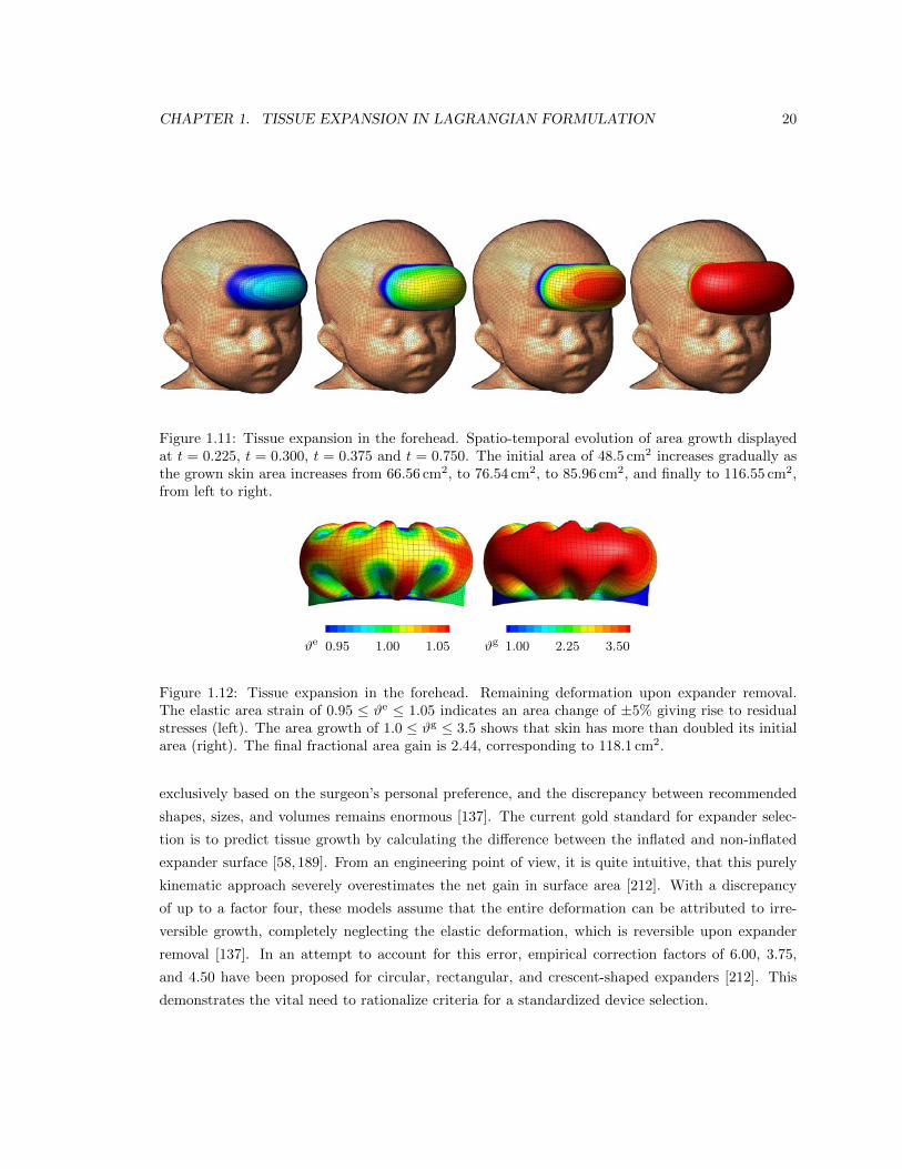
1.11 Spatio-temporal evolution of tissue expansion in the forehead . . . . . . . . . . . . . 20
1.12 Remaining deformation after issue expansion in the forehead . . . . . . . . . . . . . 20
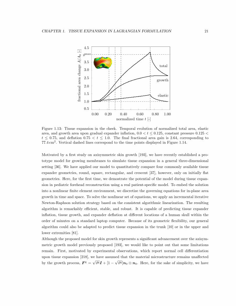
1.13 Temporal evolution of tissue expansion in the cheek . . . . . . . . . . . . . . . . . . 21
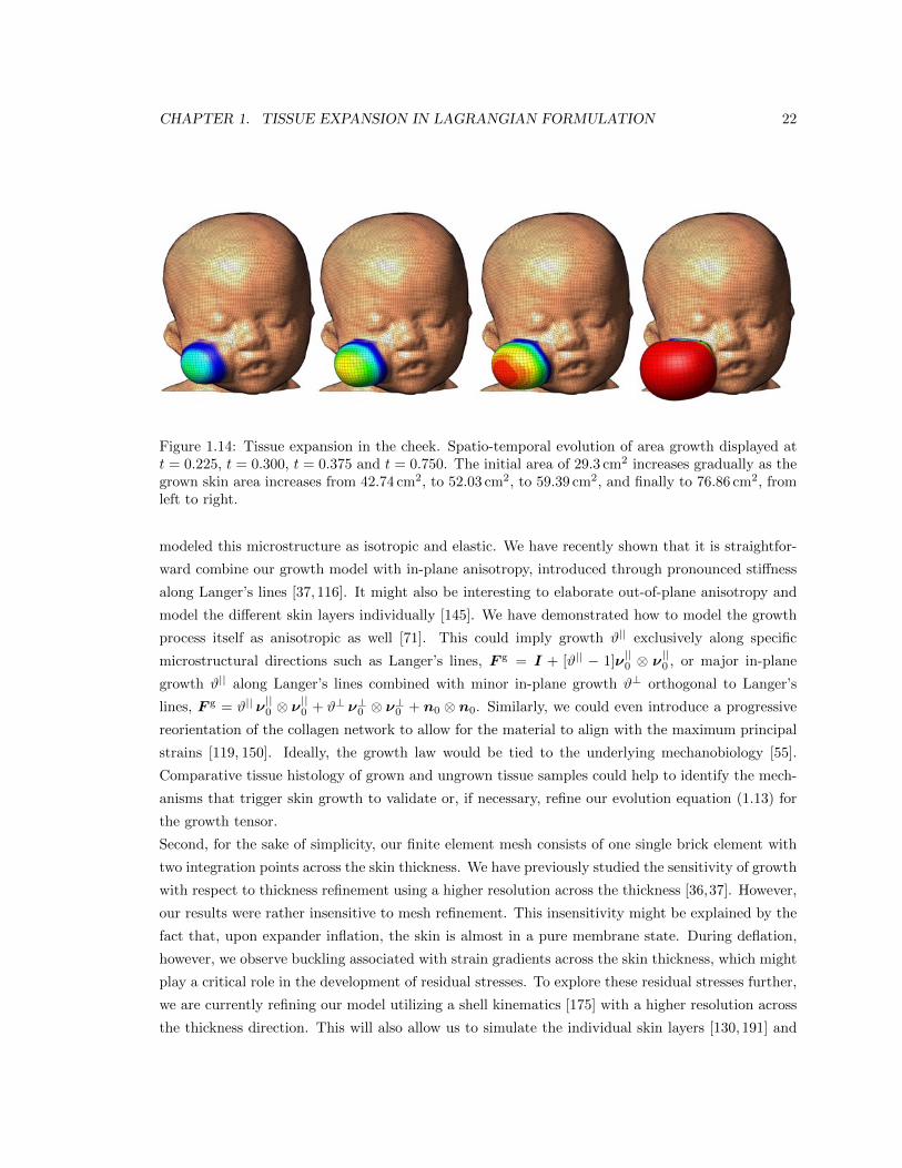
1.14 Spatio-temporal evolution of tissue expansion in the cheek . . . . . . . . . . . . . . . 22
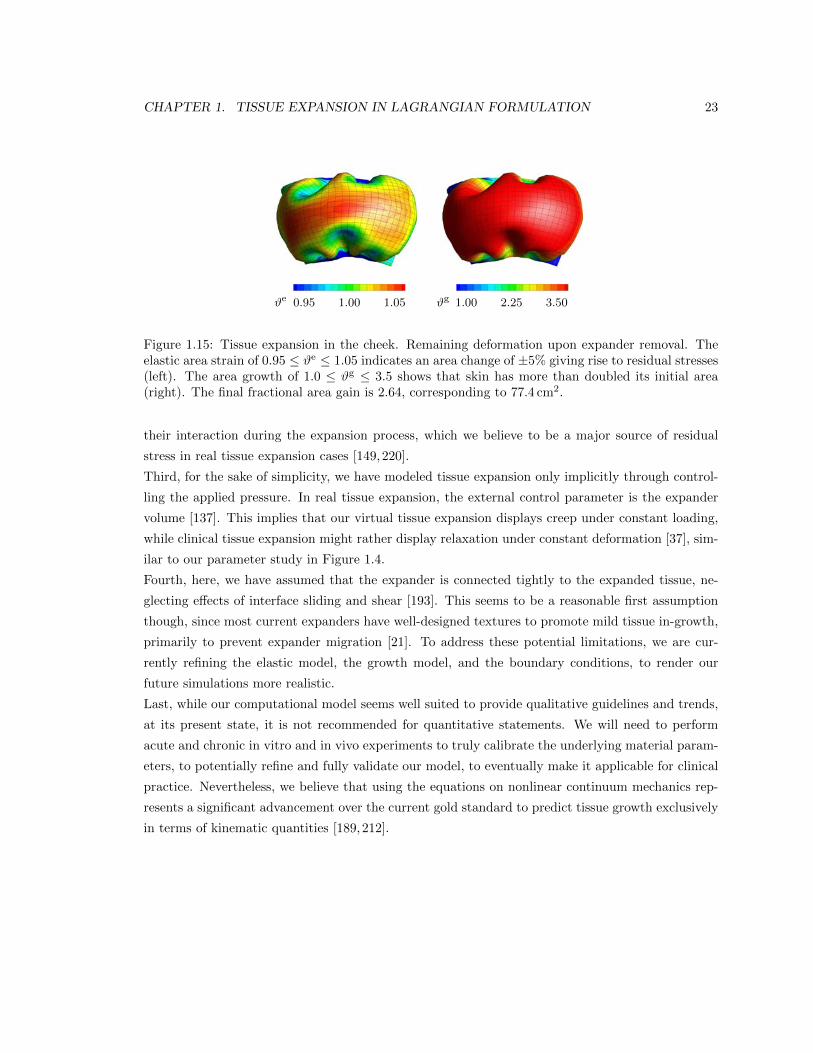
1.15 Remaining deformation tissue expansion in the cheek . . . . . . . . . . . . . . . . . . 23
2.1 Mechanotransduction of growing skin . . . . . . . . . . . . . . . . . . . . . . . . . . . 26
2.2 Biomechanics of growing skin . . . . . . . . . . . . . . . . . . . . . . . . . . . . . . . 28
2.3 Temporal evolution of total area for displacement driven skin expansion . . . . . . . 33
2.4 Temporal evolution of skin thickness t for displacement driven skin expansion . . . . 34
2.5 Skin expansion in pediatric forehead reconstruction . . . . . . . . . . . . . . . . . . . 36
2.6 Skin expansion in pediatric forehead reconstruction . . . . . . . . . . . . . . . . . . . 37
2.7 Spatio-temporal evolution of area for case study I . . . . . . . . . . . . . . . . . . . . 38
2.8 Temporal evolution of normalized area for case study II . . . . . . . . . . . . . . . . 39
2.9 Spatio-temporal evolution of area for case study II . . . . . . . . . . . . . . . . . . . 40
3.1 Skin expansion in pediatric scalp reconstruction . . . . . . . . . . . . . . . . . . . . . 46
3.2 Histological cross section of human skin . . . . . . . . . . . . . . . . . . . . . . . . . 48
3.3 Mechanotransduction of growing skin . . . . . . . . . . . . . . . . . . . . . . . . . . . 50
ix
3.4 Histological sections of expanded and non-expanded skin . . . . . . . . . . . . . . . . 51
3.5 Filling volume of skin expanders over time . . . . . . . . . . . . . . . . . . . . . . . . 57
3.6 Skin growth over time . . . . . . . . . . . . . . . . . . . . . . . . . . . . . . . . . . . 58
3.7 Expander pressure during skin expansion . . . . . . . . . . . . . . . . . . . . . . . . 59
3.8 Spatio-temporal evolution of skin growth upon tissue expansion . . . . . . . . . . . . 60
3.9 Spatio-temporal evolution of von Mises stress during skin growth upon tissue expansion 61
3.10 Spatio-temporal evolution of growth multiplier during skin growth upon tissue expansion 63
4.1 Sarcomere units in striated muscle . . . . . . . . . . . . . . . . . . . . . . . . . . . . 71
4.2 Stretching skeletal muscle . . . . . . . . . . . . . . . . . . . . . . . . . . . . . . . . . 72
4.3 Temporal evolution of sarcomere length ls in stretched skeletal muscle . . . . . . . . 78
4.4 Temporal evolution of serial sarcomere number # in stretched skeletal muscle . . . . 79
4.5 Single-step stretching vs multi-step stretching of skeletal muscle . . . . . . . . . . . . 80
4.6 Temporal evolution of muscle stretch �, muscle stress �/�0, serial sarcomere number
#, and sarcomere length ls in chronically stretched skeletal muscle . . . . . . . . . . 81
4.7 Finite element model of biceps brachii muscle . . . . . . . . . . . . . . . . . . . . . . 82
4.8 Spatio-temporal evolution of sarcomere length ls/lo . . . . . . . . . . . . . . . . . . . 83
4.9 Spatio-temporal evolution of serial sarcomere number # . . . . . . . . . . . . . . . . 84
4.10 Temporal evolution of average sarcomere length ls/lo . . . . . . . . . . . . . . . . . . 85
4.11 Temporal evolution of serial sarcomere number # . . . . . . . . . . . . . . . . . . . . 86
5.1 Chronic muscle adaptation across the scales . . . . . . . . . . . . . . . . . . . . . . . 91
5.2 Chronic muscle adaptation on the sarcomere scale . . . . . . . . . . . . . . . . . . . 92
5.3 Sagittal magnetic resonance images of the right lower limb of a healthy 20-year old
female subject . . . . . . . . . . . . . . . . . . . . . . . . . . . . . . . . . . . . . . . . 97
5.4 Generation of finite element model from magnetic resonance images of the lower limb 97
5.5 Finite element model of the lower limb . . . . . . . . . . . . . . . . . . . . . . . . . . 98
5.6 Muscle fiber orientation model of the gastrocnemius muscle . . . . . . . . . . . . . . 100
5.7 Finite element model of muscle shortening in response to frequent high heel use . . . 101
5.8 Acute decrease in sarcomere length when switching from flat footwear to high heels . 103
5.9 Chronic increase in sarcomere length when frequently wearing high-heeled footwear . 104
5.10 Chronic decrease in sarcomere number when frequently wearing high-heeled footwear 104
5.11 Chronic increase in sarcomere length when switching from flat footwear to high heels 105
5.12 Chronic decrease in sarcomere number when switching from flat footwear to high heels105
5.13 Acute increase in sarcomere length when switching from high heels to flat footwear . 106
6.1 Mitral annuloplasty . . . . . . . . . . . . . . . . . . . . . . . . . . . . . . . . . . . . . 112
6.2 The Living Heart model . . . . . . . . . . . . . . . . . . . . . . . . . . . . . . . . . . 113
x
6.3 Using the Living Heart model as virtual sizing tool for mitral annuloplasty . . . . . 117
6.4 Two chamber and four chamber views of the heart before and after ventricular re-
modeling in response to diastolic overload . . . . . . . . . . . . . . . . . . . . . . . . 118
6.5 Two chamber and four chamber views of the heart before and after annular dilation
in response to diastolic overload . . . . . . . . . . . . . . . . . . . . . . . . . . . . . . 119
6.6 Two chamber and four chamber views of the heart after virtual ring implantation . . 120
6.7 Annular stretch in the healthy and dilated annulus, and after ring-implantation . . . 121
xi
Introduction
Motivation
What if surgical outcomes and medical device performance could be predicted in the same way that
crash test simulations predict the crashworthiness of automobiles? The human body and its organs,
despite being more familiar to most of us than for example cars, are infathomably complex systems
that are much less understood than designed engineering systems [153]. A layer of complexity
unknown to engineering systems and materials is the ability of tissue and organs to heal, grow, and
regenerate [197]. When living tissue is damaged, it is automatically repaired through an orchestrated
cascade of inflammation, tissue growth, and tissue remodeling. Similarly, when living tissue is
overstretched or overstressed, a cascade of biochemical events forms new tissue. In the extreme,
some species like the axolotl are capable of regenerating entire lost limbs [35]. While the human
body adapts to a variety of thermal, radiological, electrical, biochemical, or mechanical boundary
conditions and loads, mechanical changes are the most relevant for surgical procedures and medical
device development [185]. Typical phenomena observed in healthcare include cardiac growth upon
hypertension or dilation, sarcomerogenesis or sarcomere loss upon chronic muscle over or under
stretch, and skin growth through controlled tissue expansion. All these applications are highly
nonlinear in terms of the underlying elasticity model, the growth model, geometry, and boundary
conditions. Common options to characterize the baseline elasticity of these biological tissues are
neo-Hookean, Fung type, or Holtzapfel material models [90]. In addition to the baseline elasticity,
a suitable material model needs to include a growth component to describe the addition or loss of
sarcomeres, skin area, or more generally mass. The choice of growth model depends on the clinically
observed phenomena [197]. In addition to influence of the di↵erent boundary conditions, it is import
to note that wide range of tissue and their mechanical responses. Overstretched skeletal muscle is,
for example, typically associated with one dimensional grotwh along a preferred fiber direction while
skin growth is typically linked to growth in two dimensions, normal to the skin surface.
1
2
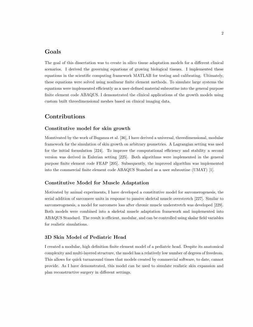
Goals
The goal of this dissertation was to create in silico tissue adaptation models for a di↵erent clinical
scenarios. I derived the governing equations of growing biological tissues. I implemented these
equations in the scientific computing framework MATLAB for testing and calibrating. Ultimately,
these equations were solved using nonlinear finite element methods. To simulate large systems the
equations were implemented e�ciently as a user-defined material subroutine into the general purpose
finite element code ABAQUS. I demonstrated the clinical applications of the growth models using
custom built threedimensional meshes based on clinical imaging data.
Contributions
Constitutive model for skin growth
Momtivated by the work of Buganza et al. [36], I have derived a universal, threedimensional, modular
framework for the simulation of skin growth on arbitrary geometries. A Lagrangian setting was used
for the initial formulation [224]. To improve the computational e�ciency and stability a second
version was derived in Eulerian setting [225]. Both algorithms were implemented in the general
purpose finite element code FEAP [205]. Subsequently, the improved algorithm was implemented
into the commercial finite element code ABAQUS Standard as a user subroutine (UMAT) [1].
Constitutive Model for Muscle Adaptation
Motivated by animal experiments, I have developed a constitutive model for sarcomerogenesis, the
serial addition of sarcomere units in response to passive skeletal muscle overstretch [227]. Similar to
sarcomerogenesis, a model for sarcomere loss after chronic muscle understretch was developed [229].
Both models were combined into a skeletal muscle adaptation framework and implemented into
ABAQUS Standard. The result is e�cient, modular, and can be controlled using skalar field variables
for realistic simulations.
3D Skin Model of Pediatric Head
I created a modular, high definition finite element model of a pediatric head. Despite its anatomical
complexity and multi-layered structure, the model has a relatively low number of degrees of freedeom.
This allows for quick turnaround times that models created by commercial software, to date, cannot
provide. As I have demonstrated, this model can be used to simulate realistic skin expansion and
plan reconstructive surgery in di↵erent settings.
3
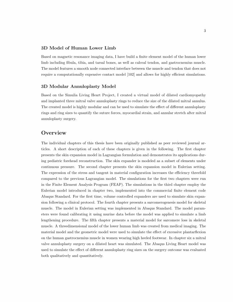
3D Model of Human Lower Limb
Based on magnetic resonance imaging data, I have build a finite element model of the human lower
limb including fibula, tibia, and tarsal bones, as well as calceal tendon, and gastrocnemius muscle.
The model features a smooth node connected interface between the muscle and tendon that does not
require a computationally expensive contact model [102] and allows for highly e�cient simulations.
3D Modular Annuloplasty Model
Based on the Simulia Living Heart Project, I created a virtual model of dilated cardiomyopathy
and implanted three mitral valve annuloplasty rings to reduce the size of the dilated mitral annulus.
The created model is highly modular and can be used to simulate the e↵ect of di↵erent annuloplasty
rings and ring sizes to quantify the suture forces, myocardial strain, and annular stretch after mitral
annuloplasty surgery.
Overview
The individual chapters of this thesis have been originally published as peer reviewed journal ar-
ticles. A short description of each of these chapters is given in the following. The first chapter
presents the skin expansion model in Lagrangian formulation and demonstrates its applications dur-
ing pediatric forehead reconstruction. The skin expander is modeled as a subset of elements under
continuous pressure. The second chapter presents the skin expansion model in Eulerian setting.
The expression of the stress and tangent in material configuration increases the e�ciency threefold
compared to the previous Lagrangian model. The simulations for the first two chapters were run
in the Finite Element Analysis Program (FEAP). The simulations in the third chapter employ the
Eulerian model introduced in chapter two, implemented into the commercial finite element code
Abaqus Standard. For the first time, volume controlled expanders are used to simulate skin expan-
sion following a clinical protocol. The fourth chapter presents a sarcomerogenesis model for skeletal
muscle. The model in Eulerian setting was implemented in Abaqus Standard. The model param-
eters were found calibrating it using murine data before the model was applied to simulate a limb
lengthening procedure. The fifth chapter presents a material model for sarcomere loss in skeletal
muscle. A threedimensional model of the lower human limb was created from medical imaging. The
material model and the geometric model were used to simulate the e↵ect of excessive plantarflexion
on the human gastrocnemius muscle in women wearing high heeled footwear. In chapter six a mitral
valve annuloplasty surgery on a dilated heart was simulated. The Abaqus Living Heart model was
used to simulate the e↵ect of di↵erent annuloplasty ring sizes on the surgery outcome was evaluated
both qualitatively and quantitatively.
Chapter 1
Tissue expansion in Lagrangian
Formulation
Abstract
Tissue expansion is a common surgical procedure to grow extra skin through controlled
mechanical over-stretch. It creates skin that matches the color, texture, and thickness of the
surrounding tissue, while minimizing scars and risk of rejection. Despite intense research in tissue
expansion and skin growth, there is a clear knowledge gap between heuristic observation and
mechanistic understanding of the key phenomena that drive the growth process. Here, we show
that a continuum mechanics approach, embedded in a custom-designed finite element model,
informed by medical imaging, provides valuable insight into the biomechanics of skin growth. In
particular, we model skin growth using the concept of an incompatible growth configuration. We
characterize its evolution in time using a second-order growth tensor parameterized in terms
of a scalar-valued internal variable, the in-plane area growth. When stretched beyond the
physiological level, new skin is created, and the in-plane area growth increases. For the first
time, we simulate tissue expansion on a patient-specific geometric model, and predict stress,
strain, and area gain at three expanded locations in a pediatric skull: in the scalp, in the
forehead, and in the cheek. Our results may help the surgeon to prevent tissue over-stretch and
make informed decisions about expander geometry, size, placement, and inflation. We anticipate
our study to open new avenues in reconstructive surgery, and enhance treatment for patients
with birth defects, burn injuries, or breast tumor removal.
1.1 Motivation
One percent of neonates is born with congenital melanocytic nevi, dark-colored surface lesions present
at birth [45]. Congenital nevi may vary in size, shape, texture, color, hairiness, and location, but
they have one thing in common: their high malignant potential [100]. Birthmarks larger than 10 cm
4
CHAPTER 1. TISSUE EXPANSION IN LAGRANGIAN FORMULATION 5
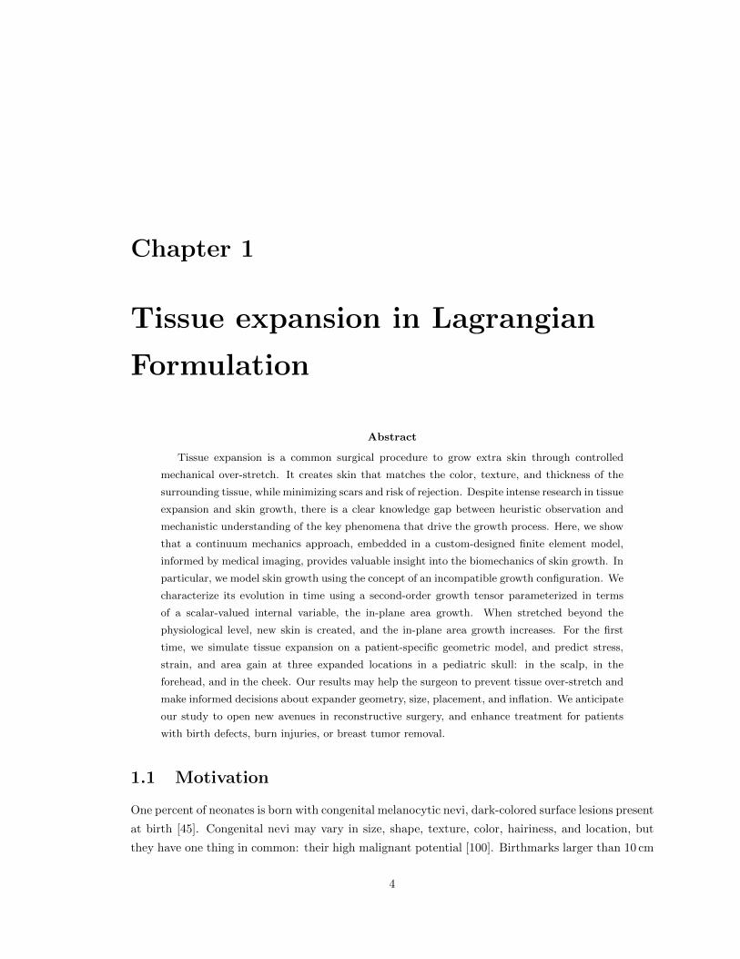
Figure 1.1: Tissue expansion for pediatric forehead reconstruction. The patient, a one-year old boypresented with a giant congenital nevus involving 25 percent of his forehead, extending to the righttemporal scalp and cheek. Simultaneous forehead, cheek, and scalp expanders were implanted forin situ skin growth. This technique allows to resurface large anatomical areas with skin of similarcolor, quality, and texture. The follow-up photograph shows the boy at age three, after completedforehead, scalp, and cheek reconstruction.
in diameter are classified as giant congenital nevi and have a prevalence of one in 20,000 infants [172].
Because giant congenital nevi place the child at an increased risk to develop skin cancer, surgical
excision remains the standard treatment option [81]. Cosmetic deformity, significant aesthetic dis-
figurement, and severe psychological distress are additional compelling reasons for nevus removal,
especially in the craniofacial region [100].
To reconstruct the defect, preserve function, and maintain aesthetic appearance, tissue expansion
has become a major treatment modality in the management of giant congenital nevi [137]. Tis-
sue expansion was first proposed more than half a century ago to reconstruct a traumatic ear and
has since then revolutionized reconstructive surgery [154]. Today it is widely used to repair birth
defects [11], correct burn injuries [9], and reconstruct breasts after tumor removal [173]. Tissue
expansion is the ideal strategy to grow skin that matches the color, texture, hair bearance, and
thickness of the surrounding healthy skin, while minimizing scars and risk of rejection [181].
Figure 1.1, left, shows a one-year old boy who presented with a giant congenital nevus concerning 25
percent of his forehead, extending to the right temporal scalp and cheek [83]. To resurface the nevus
region and stimulate in situ skin growth, three simultaneous forehead, cheek, and scalp expanders
are used. They are implanted in subcutaneous pockets adjacent to the defect, where they are grad-
ually filled with saline solution. The amount of filling is controlled by visual inspection of skin color
and capillary refill [181]. Multiple serial inflations stretch the skin and stimulate tissue growth over
a period of several weeks [222]. Once enough skin is created, the expanders are removed, the nevus
CHAPTER 1. TISSUE EXPANSION IN LAGRANGIAN FORMULATION 6
unloaded - ungrown
loaded - ungrown loaded - grown
unloaded - grown
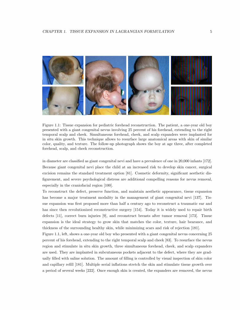
Figure 1.2: Schematic sequence of tissue expander inflation. At biological equilibrium, the skin isin a physiological state of resting tension, unloaded and ungrown. When an expander is implantedand inflated, the skin is stretched, loaded and ungrown. Mechanical stretch beyond a critical leveltriggers a series of signaling pathways eventually leading to the creation of new skin to restore thestate of resting tension, loaded and grown. Upon expander removal, elastic deformations retract andinelastic deformations remain, unloaded and grown.
is excised, and the newly grown skin flaps are advanced to close the defect zone. Figure 1.1, right,
shows the boy at age three, after completed forehead, scalp, and cheek reconstruction.
Figure 1.2 shows a schematic sequence of the mechanical processes during tissue expansion. Initially,
at biological equilibrium, the skin is in a natural state of resting tension [191]. When the expander
is implanted and inflated, skin is loaded in tension. Stretch beyond a critical level triggers a series
of signaling pathways eventually leading to the creation of new skin [203]. On the cellular level,
mechanotransduction a↵ects a network of several integrated cascades including growth factors, cy-
toskeletal rearrangement, and protein kinases [55]. On the tissue level, skin growth induces stress
relaxation and restores the state of resting tension [191]. The cycle of expander inflation, stretch,
growth, and relaxation is repeated multiple times, typically on a weekly basis [222]. As demonstrated
by immunocytochemistry, the expanded tissue undergoes normal cell di↵erentiation and maintains
its characteristic phenotype [218]. Skin initially displays thickness changes upon expansion, how-
ever, these changes are fully reversible upon expander removal [210]. When the expander is removed,
the skin retracts and reveals the irreversible nature of skin growth, associated with growth-induced
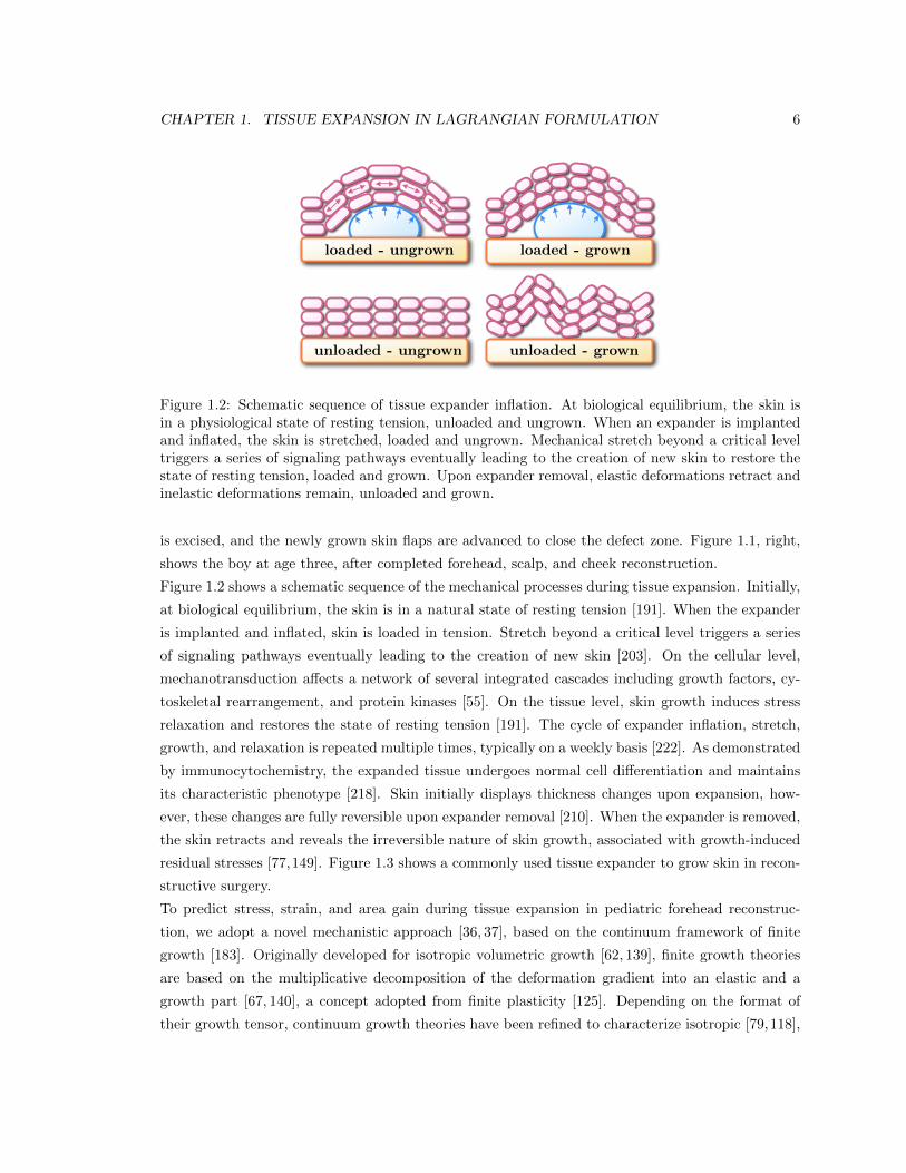
residual stresses [77,149]. Figure 1.3 shows a commonly used tissue expander to grow skin in recon-
structive surgery.
To predict stress, strain, and area gain during tissue expansion in pediatric forehead reconstruc-
tion, we adopt a novel mechanistic approach [36, 37], based on the continuum framework of finite
growth [183]. Originally developed for isotropic volumetric growth [62, 139], finite growth theories
are based on the multiplicative decomposition of the deformation gradient into an elastic and a
growth part [67, 140], a concept adopted from finite plasticity [125]. Depending on the format of
their growth tensor, continuum growth theories have been refined to characterize isotropic [79,118],
CHAPTER 1. TISSUE EXPANSION IN LAGRANGIAN FORMULATION 7
Figure 1.3: Tissue expander to grow skin for defect correction in reconstructive surgery. Typicalapplications are birth defects, burn injuries, and breast reconstruction. Devices consist of a siliconeelastomer inflatable expander with a reinforced base for directional expansion, and a remote siliconeelastomer injection dome. Courtesy of Mentor Worldwide LLC.
transversely isotropic [176, 197], orthotropic [72], or generally anisotropic growth [148, 150], either
compressible [148] or incompressible [186]. Recent trends focus on the computational modeling of
finite growth [87], typically by introducing the growth tensor as an internal variable within a finite
element framework [71,110], a strategy that we also adopt here. A recent monograph that compares
di↵erent approaches to growth and summarizes the essential findings, trends, and open questions in
this progressively evolving new field [6]. Despite ongoing research in growing biological systems, the
growth of thin biological membranes remains severely understudied. Only few attempts address the
growth of thin biological plates [56] and membranes [148]. Motivated by a first study on axisym-
metric skin growth [193], we have recently established a prototype model for growing membranes to
predict skin expansion in a general three-dimensional setting [36]. This study capitalizes on recent
developments in reconstructive surgery, continuum mechanics of growing tissues, and computational
modeling, supplemented by medical image analysis. It documents our first attempts to model and
simulate skin expansion in pediatric forehead reconstruction using a real patient-specific geometry.
1.2 Methods
1.2.1 Continuum modeling of skin growth
We adopt the kinematics of finite deformations and introduce the deformation map ', which, at any
given time t maps the material placement X of a physical particle in the material configuration to
its spatial placement x in the spatial configuration, x = ' (X, t). We choose a formulation which is
entirely related to the material frame of reference, and use r{�} = @X{�}|t
and Div {�} = @X{�}|t
:
I to denote the gradient and the divergence of any field {�} (X, t) with respect to the material
placement X at fixed time t. Here, I is the material identity tensor. To characterize finite growth,
we introduce an incompatible growth configuration, and adopt the multiplicative decomposition of
the deformation gradient
F = rX' = F
e · F g (1.1)
CHAPTER 1. TISSUE EXPANSION IN LAGRANGIAN FORMULATION 8
into a reversible elastic part F e and an irreversible growth part F g. This multiplicative decomposi-
tion, reminiscent of the decomposition of the elastoplastic deformation gradient [125], was first used
to describe growth of biologial tissues in [183]. Similarly, we can then decompose the total Jacobian
J = det (F ) = Je Jg (1.2)
into an elastic part Je = det (F e) and a growth part Jg = det (F g). We idealize skin as a thin layer
characterized through the unit normal n0 in the undeformed reference configuration. The length of
the deformed skin normal n = cof(F ) · n0 = J F
�t · n0 introduces the area stretch
# = || cof(F ) · n0 || = #e #g (1.3)
which we can again decompose into an elastic area stretch #e = || cof(F e) ·ng/||ng|| || and a growth
area stretch #g = || cof(F g) · n0 || [36]. Here, ng = cof(F g) · n0 = JgF
g � t · n0 denotes the
grown skin normal, and cof(�) = det(�) (�)�t denotes the cofactor of the second order tensor (�).As characteristic deformation measures, we introduce the right Cauchy Green tensor C in the
undeformed reference configuration
C = F
t · F = F
gt · F et · F e · F g (1.4)
and its elastic counterpart C
e = F
et · F e = F
g � t · C · F g � 1 in the intermediate configuration.
This allows us to rephrase the total area stretch as # = J [n0 ·C�1 · n0 ]1/2. Finally, we introduce
the pull back of the spatial velocity gradient l = F · F�1 to the intermediate configuration,
F
e � 1 · l · F e = L
e +L
g (1.5)
which obeys the additive decomposition into the elastic velocity gradient L
e = F
e�1 · F eand the
growth velocity gradient Lg = F
g ·F g�1. Here, {�} = @t
{�}|X denotes the material time derivative
of any field {�} (X, t) at fixed material placement X.
We characterize growing tissue using the framework of open system thermodynamics in which the
material density ⇢0 is allowed to change as a consequence of growth [112,114]. The balance of mass
for open systems balances its rate of change ⇢0 with a possible in- or outflux of mass R and mass
source R0 [115,165].
⇢0 = Div (R) +R0 (1.6)
Similarly, the balance of linear momentum balances the density-weighted rate of change of the
velocity ⇢0 v = ⇢0 ', with the momentum flux P = F · S, and the momentum source ⇢0 b,
⇢0 v = Div (F · S) + ⇢0 b (1.7)
CHAPTER 1. TISSUE EXPANSION IN LAGRANGIAN FORMULATION 9
here stated in its mass-specific form [113]. P and S are the first and second Piola-Kirchho↵ stress
tensors. Last, we would like to point out that the dissipation inequality for open systems
⇢0 D = S : 12C � ⇢0 � ⇢0 S � 0 (1.8)
typically contains an extra entropy source ⇢0 S to account for the growing nature of living biological
systems [112, 149]. Equations (1.7) and (1.8) represent the mass-specific versions of the balance of
momentum and of the dissipation inequality which are particularly useful in the context of growth
since they contains no explicit dependencies on the changes in mass [113].
To close the set of equations, we introduce the constitutive equations for the mass source R0, for
the momentum flux S, and for the growth tensor F
g, assuming that the mass flux R = 0, the
momentum source b = 0, and the acceleration v = 0 are negligibly small. On the cellular level,
immunocytochemistry has shown that expanded tissue undergoes normal epidermal cell di↵erentia-
tion [218]. On the organ level, mechanical testing has confirmed that the newly grown skin has the
same material properties as the initial tissue [222]. Accordingly, we assume that the newly grown
skin has the same density as the initial tissue. This implies that the mass source
R0 = ⇢0 tr (Lg) (1.9)
can be expressed as the density-weighted trace of the growth velocity gradient tr (Lg) = F
g: F g � t
[87]. We model skin as a hyperelastic material characterized through the Helmholtz free energy
= (C,F g), which we use to evaluate the dissipation inequality (1.8).
⇢0D=
S�⇢0
@
@C
�: 12C +M
e : Lg � ⇢0@
@⇢0R0 � ⇢0S0 � 0 (1.10)
We observe that the Mandel stress of the intermediate configuration M
e = C
e · Se is energetically
conjugate to the growth velocity gradient Lg = F
g · F g � 1. From the dissipation inequality (1.10),
we obtain the definition of the second Piola Kirchho↵ stress S as thermodynamically conjugate
quantity to the right Cauchy Green deformation tensor C.
S = 2 ⇢0@
@C= 2
@
@Ce:@Ce
@C= F
g � 1 · Se · F g � t (1.11)
According to this definition, the first derivative of the Helmholtz free energy with respect to the
elastic right Cauchy Green tensor Ce introduces the elastic second Piola Kirchho↵ stress Se, while
the second derivative defines the elastic constitutive moduli Le.
S
e = 2 ⇢0@
@Ceand L
e = 2@Se
@Ce= 4 ⇢0
@2
@Ce ⌦ @Ce(1.12)
CHAPTER 1. TISSUE EXPANSION IN LAGRANGIAN FORMULATION 10
To focus on the impact of growth, rather than adopting a sophisticated anisotropic material model
for skin [37, 116], we assume a classical Neo-Hookean free energy ⇢0 = 12 � ln2(Je) + 1
2 µ [Ce :
I�3�2 ln(Je) ], introducing the elastic second Piola Kirchho↵ stress Se = [� ln(Je)�µ ]Ce�1+µ I,
and the elastic constitutive moduli Le = �Ce�1 ⌦ C
e�1 + [µ � � ln(Je) ] [Ce⌦Ce + C
e⌦Ce ].
Motivated by clinical observations [181], we classify skin growth as a strain-driven, transversely
isotropic, irreversible process. It is characterized through one single growth multiplier #g that
reflects the irreversible area increase perpendicular to the skin normal n0.
F
g =p#g I + [ 1�
p#g ] n0 ⌦ n0 (1.13)
For this particular type of transversely isotropic growth, for which all thickness changes are reversibly
elastic [210], area growth is identical to volume growth, i.e., #g = det(F g) = Jg. Because of the
simple rank-one update structure in (1.13), we can invert the growth tensor explicitly, F g � 1 =
1/p#g I + [ 1� 1/
p#g ]n0 ⌦n0, using the Sherman-Morrison formula. This explicit representation
introduces the following simple expression for the growth velocity gradient,
L
g =p#g/p#gI + [ 1�
p#g/p#g]n0 ⌦ n0 (1.14)
which proves convenient to explicitly evaluate the mass source in equation (1.9) as R0 = ⇢0 [ 1 +
2p#g/p#g ]. Motivated by physiological observations of stretch-induced skin expansion [83], we
adopt the following evolution equation for the growth multiplier,
#g = kg(#g)�g(#e) (1.15)
which follows a well-established functional form [139], but is now rephrased in a strain-driven format
[72]. To control unbounded growth, we introduce the weighting function
kg =1
⌧
#max � #g
#max � 1
��
(1.16)
where 1/⌧ controls the adaptation speed, the exponent � calibrates the shape of the growth curve,
and #max > 1 is the maximum area growth [87,139]. The growth criterion
�g =⌦#e � #crit
↵=
⌦#/#g � #crit
↵(1.17)
is driven by the elastic area stretch #e = #/#g, such that growth is activated only if the elastic area
stretch exceeds a critical physiological stretch limit #crit. Here, h�i denote the Macaulay brackets.
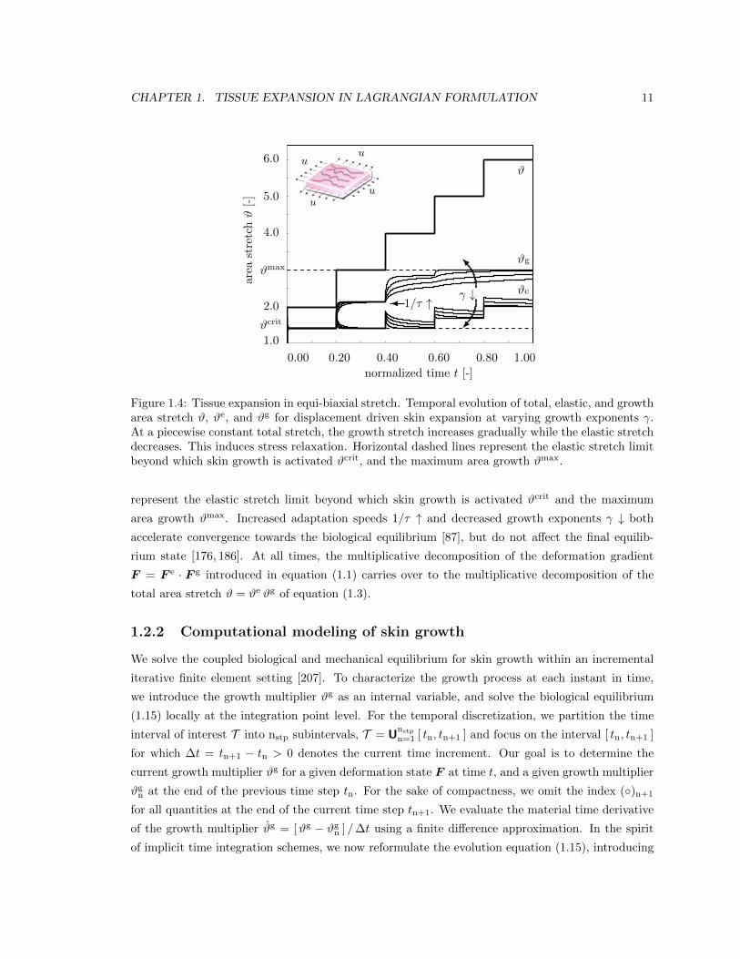
Figure 1.4 displays the constitutive response of the four-parameter growth model in equi-biaxial
stretch. At a prescribed piecewise constant total stretch #, the growth stretch #g increases grad-
ually while the elastic stretch #edecreases. This induces stress relaxation. Horizontal dashed lines
CHAPTER 1. TISSUE EXPANSION IN LAGRANGIAN FORMULATION 11
0 0.1 0.2 0.3 0.4 0.5 0.6 0.7 0.8 0.9 1
1
1.5
2
2.5
3
3.5
4
4.5
5
5.5
6
#
#g
#e
u
uu
u
normalized time t [-]0.00 0.20 0.40 0.60 0.80 1.00
area
stretch#[-]
1.0#crit2.0
#max
4.0
5.0
6.0
I
� #�1/⌧ "
Figure 1.4: Tissue expansion in equi-biaxial stretch. Temporal evolution of total, elastic, and growtharea stretch #, #e, and #g for displacement driven skin expansion at varying growth exponents �.At a piecewise constant total stretch, the growth stretch increases gradually while the elastic stretchdecreases. This induces stress relaxation. Horizontal dashed lines represent the elastic stretch limitbeyond which skin growth is activated #crit, and the maximum area growth #max.
represent the elastic stretch limit beyond which skin growth is activated #crit and the maximum
area growth #max. Increased adaptation speeds 1/⌧ " and decreased growth exponents � # both
accelerate convergence towards the biological equilibrium [87], but do not a↵ect the final equilib-
rium state [176, 186]. At all times, the multiplicative decomposition of the deformation gradient
F = F
e · F g introduced in equation (1.1) carries over to the multiplicative decomposition of the
total area stretch # = #e #g of equation (1.3).
1.2.2 Computational modeling of skin growth
We solve the coupled biological and mechanical equilibrium for skin growth within an incremental
iterative finite element setting [207]. To characterize the growth process at each instant in time,
we introduce the growth multiplier #g as an internal variable, and solve the biological equilibrium
(1.15) locally at the integration point level. For the temporal discretization, we partition the time
interval of interest T into nstp subintervals, T = U
nstp
n=1 [ tn, tn+1 ] and focus on the interval [ tn, tn+1 ]
for which �t = tn+1 � tn > 0 denotes the current time increment. Our goal is to determine the
current growth multiplier #g for a given deformation state F at time t, and a given growth multiplier
#gn at the end of the previous time step tn. For the sake of compactness, we omit the index (�)n+1
for all quantities at the end of the current time step tn+1. We evaluate the material time derivative
of the growth multiplier #g = [#g � #gn ] /�t using a finite di↵erence approximation. In the spirit
of implicit time integration schemes, we now reformulate the evolution equation (1.15), introducing
CHAPTER 1. TISSUE EXPANSION IN LAGRANGIAN FORMULATION 12
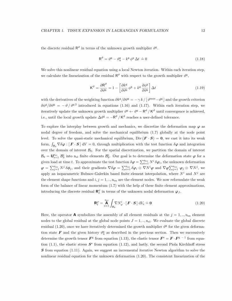
the discrete residual R# in terms of the unknown growth multiplier #g.
R# = #g � #gn � kg �g �t.= 0 (1.18)
We solve this nonlinear residual equation using a local Newton iteration. Within each iteration step,
we calculate the linearization of the residual R# with respect to the growth multiplier #g,
K# =@R#
@#g= 1�
@kg
@#g�g + kg
@�g
@#g
��t (1.19)
with the derivatives of the weighting function @kg/@#g = � � k / [#max�#g ] and the growth criterion
@�g/@#g = �# /#g 2 introduced in equations (1.16) and (1.17). Within each iteration step, we
iteratively update the unknown growth multiplier #g #g � R# /K# until convergence is achieved,
i.e., until the local growth update �#g = �R# /K# reaches a user-defined tolerance.
To explore the interplay between growth and mechanics, we discretize the deformation map ' as
nodal degree of freedom, and solve the mechanical equilibrium (1.7) globally at the node point
level. To solve the quasi-static mechanical equilibrium, Div (F · S) = 0, we cast it into its weak
form,RB0r�' : [F · S ] dV = 0, through multiplication with the test function �' and integration
over the domain of interest B0. For the spatial discretization, we partition the domain of interest
B0 = U
nele=1 Be
0 into nel finite elements Be0. Our goal is to determine the deformation state ' for a
given load at time t. To approximate the test function �' =Pnen
i=1 Ni �'
i
, the unknown deformation
' =Pnen
j=1 Nj ��
j
, and their gradients r�' =Pnen
i=1 �'i
⌦ rN i
' and r'Pnen
j=1 '
j
⌦ rN j , we
apply an isoparametric Bubnov-Galerkin based finite element interpolation, where N i and N j are
the element shape functions and i, j = 1, .., nen are the element nodes. We now reformulate the weak
form of the balance of linear momentum (1.7) with the help of these finite element approximations,
introducing the discrete residual R'
I
in terms of the unknown nodal deformation '
J
.
R
'
I
=nel
A
e=1
Z
Be
rN i
'
· [F · S ] dVe.= 0 (1.20)
Here, the operator A symbolizes the assembly of all element residuals at the j = 1, .., nen element
nodes to the global residual at the global node points J = 1, .., nel. We evaluate the global discrete
residual (1.20), once we have iteratively determined the growth multiplier #g for the given deforma-
tion state F and the given history #gn as described in the previous section. Then we successively
determine the growth tensor F g from equation (1.13), the elastic tensor F e = F ·F g � 1 from equa-
tion (1.1), the elastic stress S
e from equation (1.12), and lastly, the second Piola Kirchho↵ stress
S from equation (1.11). Again, we suggest an incremental iterative Newton algorithm to solve the
nonlinear residual equation for the unknown deformation (1.20). The consistent linearization of the
CHAPTER 1. TISSUE EXPANSION IN LAGRANGIAN FORMULATION 13
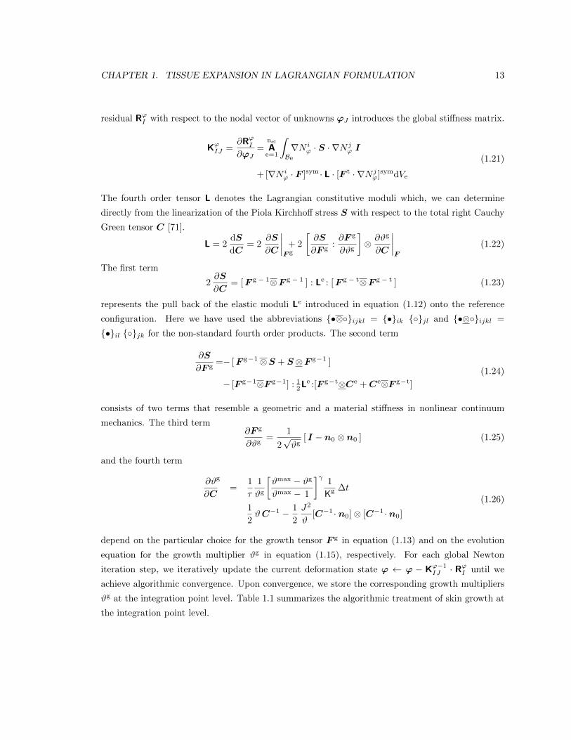
residual R'
I
with respect to the nodal vector of unknowns 'J
introduces the global sti↵ness matrix.
K
'
IJ
=@R'
I
@'J
=nel
A
e=1
Z
Be
rN i
'
· S ·rN j
'
I
+[rN i
'
· F ]sym · L · [F t ·rN j
'
]symdVe
(1.21)
The fourth order tensor L denotes the Lagrangian constitutive moduli which, we can determine
directly from the linearization of the Piola Kirchho↵ stress S with respect to the total right Cauchy
Green tensor C [71].
L = 2dS
dC= 2
@S
@C
����F g+ 2
@S
@F g:@F g
@#g
�⌦ @#g
@C
����F
(1.22)
The first term
2@S
@C= [F g � 1⌦F
g � 1 ] : Le : [F g � t⌦F
g � t ] (1.23)
represents the pull back of the elastic moduli Le introduced in equation (1.12) onto the reference
configuration. Here we have used the abbreviations {•⌦�}ijkl
= {•}ik
{�}jl
and {•⌦�}ijkl
=
{•}il
{�}jk
for the non-standard fourth order products. The second term
@S
@F g=� [F g�1⌦S + S⌦F
g�1 ]
� [F g�1⌦F g�1] : 12Le :[F g�t⌦Ce +C
e⌦F g�t]
(1.24)
consists of two terms that resemble a geometric and a material sti↵ness in nonlinear continuum
mechanics. The third term@F g
@#g=
1
2p#g
[ I � n0 ⌦ n0 ] (1.25)
and the fourth term
@#
@C
g
=1
⌧
1
#g
#max � #g
#max � 1
�� 1
Kg �t
1
2#C�1 � 1
2
J2
#[C�1 · n0]⌦ [C�1 · n0]
(1.26)
depend on the particular choice for the growth tensor F
g in equation (1.13) and on the evolution
equation for the growth multiplier #g in equation (1.15), respectively. For each global Newton
iteration step, we iteratively update the current deformation state ' ' � K
'�1IJ
· R'
I
until we
achieve algorithmic convergence. Upon convergence, we store the corresponding growth multipliers
#g at the integration point level. Table 1.1 summarizes the algorithmic treatment of skin growth at
the integration point level.
CHAPTER 1. TISSUE EXPANSION IN LAGRANGIAN FORMULATION 14
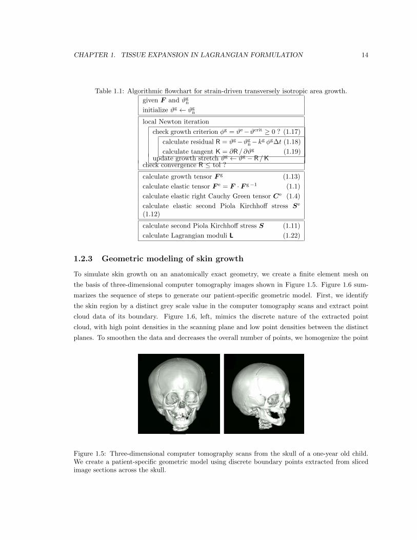
Table 1.1: Algorithmic flowchart for strain-driven transversely isotropic area growth.
given F and #gninitialize #g #gn
local Newton iteration
check growth criterion �g = #e�#crit � 0 ? (1.17)
calculate residual R = #g�#gn�kg �g�t (1.18)
calculate tangent K = @R / @#g (1.19)update growth stretch #g #g � R /K
check convergence R tol ?
calculate growth tensor F g (1.13)
calculate elastic tensor F e = F · F g�1 (1.1)
calculate elastic right Cauchy Green tensor Ce (1.4)
calculate elastic second Piola Kirchho↵ stress S
e
(1.12)
calculate second Piola Kirchho↵ stress S (1.11)
calculate Lagrangian moduli L (1.22)
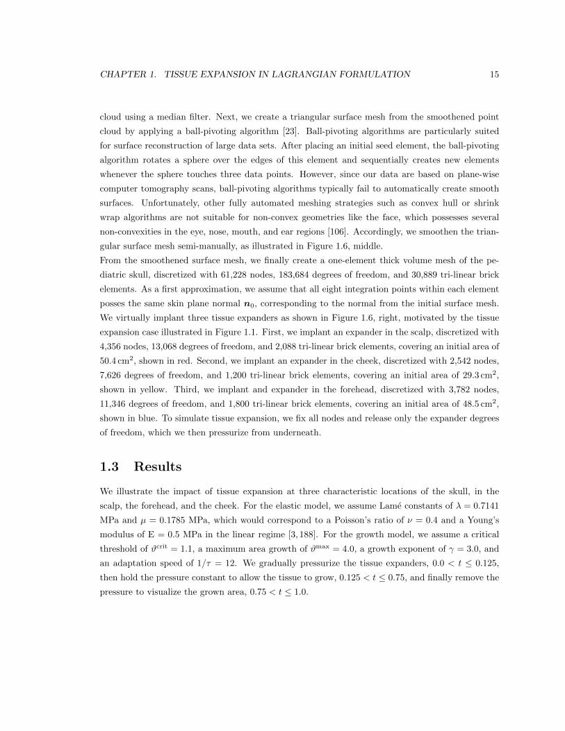
1.2.3 Geometric modeling of skin growth
To simulate skin growth on an anatomically exact geometry, we create a finite element mesh on
the basis of three-dimensional computer tomography images shown in Figure 1.5. Figure 1.6 sum-
marizes the sequence of steps to generate our patient-specific geometric model. First, we identify
the skin region by a distinct grey scale value in the computer tomography scans and extract point
cloud data of its boundary. Figure 1.6, left, mimics the discrete nature of the extracted point
cloud, with high point densities in the scanning plane and low point densities between the distinct
planes. To smoothen the data and decreases the overall number of points, we homogenize the point
Figure 1.5: Three-dimensional computer tomography scans from the skull of a one-year old child.We create a patient-specific geometric model using discrete boundary points extracted from slicedimage sections across the skull.
CHAPTER 1. TISSUE EXPANSION IN LAGRANGIAN FORMULATION 15
cloud using a median filter. Next, we create a triangular surface mesh from the smoothened point
cloud by applying a ball-pivoting algorithm [23]. Ball-pivoting algorithms are particularly suited
for surface reconstruction of large data sets. After placing an initial seed element, the ball-pivoting
algorithm rotates a sphere over the edges of this element and sequentially creates new elements
whenever the sphere touches three data points. However, since our data are based on plane-wise
computer tomography scans, ball-pivoting algorithms typically fail to automatically create smooth
surfaces. Unfortunately, other fully automated meshing strategies such as convex hull or shrink
wrap algorithms are not suitable for non-convex geometries like the face, which possesses several
non-convexities in the eye, nose, mouth, and ear regions [106]. Accordingly, we smoothen the trian-
gular surface mesh semi-manually, as illustrated in Figure 1.6, middle.
From the smoothened surface mesh, we finally create a one-element thick volume mesh of the pe-
diatric skull, discretized with 61,228 nodes, 183,684 degrees of freedom, and 30,889 tri-linear brick
elements. As a first approximation, we assume that all eight integration points within each element
posses the same skin plane normal n0, corresponding to the normal from the initial surface mesh.
We virtually implant three tissue expanders as shown in Figure 1.6, right, motivated by the tissue
expansion case illustrated in Figure 1.1. First, we implant an expander in the scalp, discretized with
4,356 nodes, 13,068 degrees of freedom, and 2,088 tri-linear brick elements, covering an initial area of
50.4 cm2, shown in red. Second, we implant an expander in the cheek, discretized with 2,542 nodes,
7,626 degrees of freedom, and 1,200 tri-linear brick elements, covering an initial area of 29.3 cm2,
shown in yellow. Third, we implant and expander in the forehead, discretized with 3,782 nodes,
11,346 degrees of freedom, and 1,800 tri-linear brick elements, covering an initial area of 48.5 cm2,
shown in blue. To simulate tissue expansion, we fix all nodes and release only the expander degrees
of freedom, which we then pressurize from underneath.
1.3 Results
We illustrate the impact of tissue expansion at three characteristic locations of the skull, in the
scalp, the forehead, and the cheek. For the elastic model, we assume Lame constants of � = 0.7141
MPa and µ = 0.1785 MPa, which would correspond to a Poisson’s ratio of ⌫ = 0.4 and a Young’s
modulus of E = 0.5 MPa in the linear regime [3, 188]. For the growth model, we assume a critical
threshold of #crit = 1.1, a maximum area growth of #max = 4.0, a growth exponent of � = 3.0, and
an adaptation speed of 1/⌧ = 12. We gradually pressurize the tissue expanders, 0.0 < t 0.125,
then hold the pressure constant to allow the tissue to grow, 0.125 < t 0.75, and finally remove the
pressure to visualize the grown area, 0.75 < t 1.0.
CHAPTER 1. TISSUE EXPANSION IN LAGRANGIAN FORMULATION 16
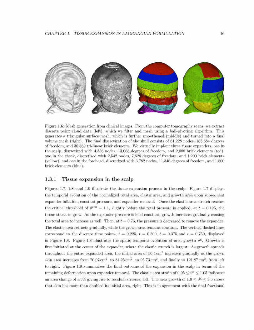
Figure 1.6: Mesh generation from clinical images. From the computer tomography scans, we extractdiscrete point cloud data (left), which we filter and mesh using a ball-pivoting algorithm. Thisgenerates a triangular surface mesh, which is further smoothened (middle) and turned into a finalvolume mesh (right). The final discretization of the skull consists of 61,228 nodes, 183,684 degreesof freedom, and 30,889 tri-linear brick elements. We virtually implant three tissue expanders, one inthe scalp, discretized with 4,356 nodes, 13,068 degrees of freedom, and 2,088 brick elements (red),one in the cheek, discretized with 2,542 nodes, 7,626 degrees of freedom, and 1,200 brick elements(yellow), and one in the forehead, discretized with 3,782 nodes, 11,346 degrees of freedom, and 1,800brick elements (blue).
1.3.1 Tissue expansion in the scalp
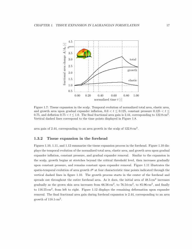
Figures 1.7, 1.8, and 1.9 illustrate the tissue expansion process in the scalp. Figure 1.7 displays
the temporal evolution of the normalized total area, elastic area, and growth area upon subsequent
expander inflation, constant pressure, and expander removal. Once the elastic area stretch reaches
the critical threshold of #crit = 1.1, slightly before the total pressure is applied, at t = 0.125, the
tissue starts to grow. As the expander pressure is held constant, growth increases gradually causing
the total area to increase as well. Then, at t = 0.75, the pressure is decreased to remove the expander.
The elastic area retracts gradually, while the grown area remains constant. The vertical dashed lines
correspond to the discrete time points, t = 0.225, t = 0.300, t = 0.375 and t = 0.750, displayed
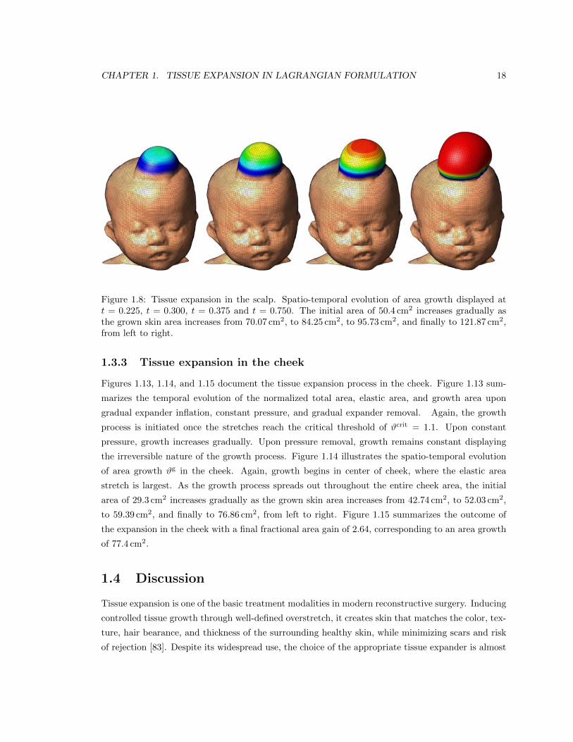
in Figure 1.8. Figure 1.8 illustrates the spatio-temporal evolution of area growth #g. Growth is
first initiated at the center of the expander, where the elastic stretch is largest. As growth spreads
throughout the entire expanded area, the initial area of 50.4 cm2 increases gradually as the grown
skin area increases from 70.07 cm2, to 84.25 cm2, to 95.73 cm2, and finally to 121.87 cm2, from left
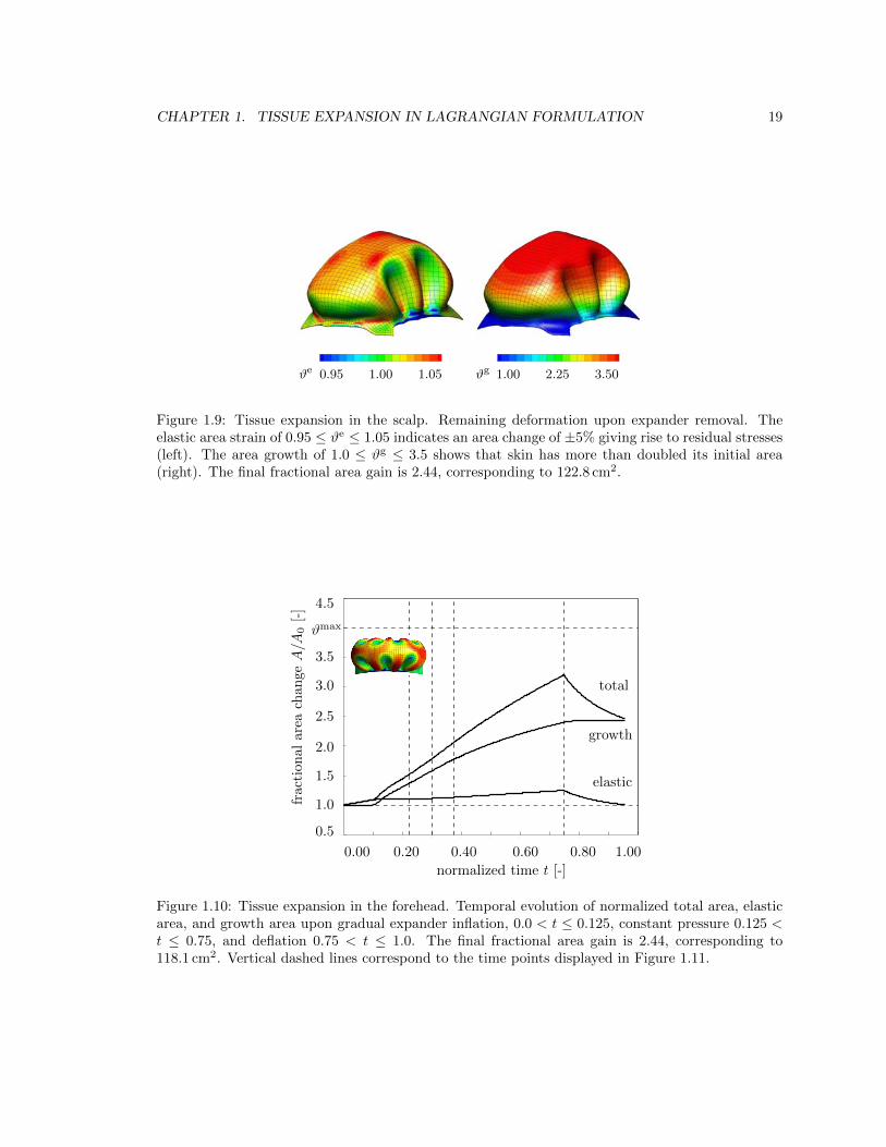
to right. Figure 1.9 summarizes the final outcome of the expansion in the scalp in terms of the
remaining deformation upon expander removal. The elastic area strain of 0.95 #e 1.05 indicates
an area change of ±5% giving rise to residual stresses, left. The area growth of 1.0 #g 3.5 shows
that skin has more than doubled its initial area, right. This is in agreement with the final fractional
CHAPTER 1. TISSUE EXPANSION IN LAGRANGIAN FORMULATION 17
0 0.1 0.2 0.3 0.4 0.5 0.6 0.7 0.8 0.9 1
0.5
1
1.5
2
2.5
3
3.5
4
4.5
total
growth
elastic
normalized time t [-]0.00 0.20 0.40 0.60 0.80 1.00
fraction
alarea
chan
geA/A
0[-]
0.5
1.0
1.5
2.0
2.5
3.0
3.5
#max
4.5
Figure 1.7: Tissue expansion in the scalp. Temporal evolution of normalized total area, elastic area,and growth area upon gradual expander inflation, 0.0 < t 0.125, constant pressure 0.125 < t 0.75, and deflation 0.75 < t 1.0. The final fractional area gain is 2.44, corresponding to 122.8 cm2.Vertical dashed lines correspond to the time points displayed in Figure 1.8.
area gain of 2.44, corresponding to an area growth in the scalp of 122.8 cm2.
1.3.2 Tissue expansion in the forehead
Figures 1.10, 1.11, and 1.12 summarize the tissue expansion process in the forehead. Figure 1.10 dis-
plays the temporal evolution of the normalized total area, elastic area, and growth area upon gradual
expander inflation, constant pressure, and gradual expander removal. Similar to the expansion in
the scalp, growth begins at stretches beyond the critical threshold level, then increases gradually
upon constant pressure, and remains constant upon expander removal. Figure 1.11 illustrates the
spatio-temporal evolution of area growth #g at four characteristic time points indicated through the
vertical dashed lines in figure 1.10. The growth process starts in the center of the forehead and
spreads out throughout the entire forehead area. As it does, the initial area of 48.5 cm2 increases
gradually as the grown skin area increases from 66.56 cm2, to 76.54 cm2, to 85.96 cm2, and finally
to 116.55 cm2, from left to right. Figure 1.12 displays the remaining deformation upon expander
removal. The final fractional area gain during forehead expansion is 2.44, corresponding to an area
growth of 118.1 cm2.
CHAPTER 1. TISSUE EXPANSION IN LAGRANGIAN FORMULATION 18
14 Alexander M. Zoellner, Adrian Buganza Tepole, Arun K. Gosain, Ellen Kuhl
Fig. 16 Tissue expansion in the scalp. Spatio-temporal evolution of area growth displayed at t = 0.225, t = 0.300, t = 0.375and t = 0.750. The initial area of 50.4 cm2 increases gradually as the grown skin area increases from 70.07 cm2, to 84.25 cm2,to 95.73 cm2, and finally to 121.87 cm2, from left to right.Figure 1.8: Tissue expansion in the scalp. Spatio-temporal evolution of area growth displayed att = 0.225, t = 0.300, t = 0.375 and t = 0.750. The initial area of 50.4 cm2 increases gradually asthe grown skin area increases from 70.07 cm2, to 84.25 cm2, to 95.73 cm2, and finally to 121.87 cm2,from left to right.
1.3.3 Tissue expansion in the cheek
Figures 1.13, 1.14, and 1.15 document the tissue expansion process in the cheek. Figure 1.13 sum-
marizes the temporal evolution of the normalized total area, elastic area, and growth area upon
gradual expander inflation, constant pressure, and gradual expander removal. Again, the growth
process is initiated once the stretches reach the critical threshold of #crit = 1.1. Upon constant
pressure, growth increases gradually. Upon pressure removal, growth remains constant displaying
the irreversible nature of the growth process. Figure 1.14 illustrates the spatio-temporal evolution
of area growth #g in the cheek. Again, growth begins in center of cheek, where the elastic area
stretch is largest. As the growth process spreads out throughout the entire cheek area, the initial
area of 29.3 cm2 increases gradually as the grown skin area increases from 42.74 cm2, to 52.03 cm2,
to 59.39 cm2, and finally to 76.86 cm2, from left to right. Figure 1.15 summarizes the outcome of
the expansion in the cheek with a final fractional area gain of 2.64, corresponding to an area growth
of 77.4 cm2.
1.4 Discussion
Tissue expansion is one of the basic treatment modalities in modern reconstructive surgery. Inducing
controlled tissue growth through well-defined overstretch, it creates skin that matches the color, tex-
ture, hair bearance, and thickness of the surrounding healthy skin, while minimizing scars and risk
of rejection [83]. Despite its widespread use, the choice of the appropriate tissue expander is almost
CHAPTER 1. TISSUE EXPANSION IN LAGRANGIAN FORMULATION 19
#e 0.95 1.00 1.05 #g 1.00 2.25 3.50
Figure 1.9: Tissue expansion in the scalp. Remaining deformation upon expander removal. Theelastic area strain of 0.95 #e 1.05 indicates an area change of ±5% giving rise to residual stresses(left). The area growth of 1.0 #g 3.5 shows that skin has more than doubled its initial area(right). The final fractional area gain is 2.44, corresponding to 122.8 cm2.
0 0.1 0.2 0.3 0.4 0.5 0.6 0.7 0.8 0.9 1
0.5
1
1.5
2
2.5
3
3.5
4
4.5
total
growth
elastic
normalized time t [-]0.00 0.20 0.40 0.60 0.80 1.00
fraction
alarea
chan
geA/A
0[-]
0.5
1.0
1.5
2.0
2.5
3.0
3.5
#max
4.5
Figure 1.10: Tissue expansion in the forehead. Temporal evolution of normalized total area, elasticarea, and growth area upon gradual expander inflation, 0.0 < t 0.125, constant pressure 0.125 <t 0.75, and deflation 0.75 < t 1.0. The final fractional area gain is 2.44, corresponding to118.1 cm2. Vertical dashed lines correspond to the time points displayed in Figure 1.11.
CHAPTER 1. TISSUE EXPANSION IN LAGRANGIAN FORMULATION 20
Growing skin: Tissue expansion in pediatric forehead reconstruction 15
Fig. 17 Tissue expansion in the forehead. Spatio-temporal evolution of area growth displayed at t = 0.225, t = 0.300,t = 0.375 and t = 0.750. The initial area of 48.5 cm2 increases gradually as the grown skin area increases from 66.56 cm2, to76.54 cm2, to 85.96 cm2, and finally to 116.55 cm2, from left to right.Figure 1.11: Tissue expansion in the forehead. Spatio-temporal evolution of area growth displayedat t = 0.225, t = 0.300, t = 0.375 and t = 0.750. The initial area of 48.5 cm2 increases gradually asthe grown skin area increases from 66.56 cm2, to 76.54 cm2, to 85.96 cm2, and finally to 116.55 cm2,from left to right.
#e 0.95 1.00 1.05 #g 1.00 2.25 3.50
Figure 1.12: Tissue expansion in the forehead. Remaining deformation upon expander removal.The elastic area strain of 0.95 #e 1.05 indicates an area change of ±5% giving rise to residualstresses (left). The area growth of 1.0 #g 3.5 shows that skin has more than doubled its initialarea (right). The final fractional area gain is 2.44, corresponding to 118.1 cm2.
exclusively based on the surgeon’s personal preference, and the discrepancy between recommended
shapes, sizes, and volumes remains enormous [137]. The current gold standard for expander selec-
tion is to predict tissue growth by calculating the di↵erence between the inflated and non-inflated
expander surface [58, 189]. From an engineering point of view, it is quite intuitive, that this purely
kinematic approach severely overestimates the net gain in surface area [212]. With a discrepancy
of up to a factor four, these models assume that the entire deformation can be attributed to irre-
versible growth, completely neglecting the elastic deformation, which is reversible upon expander
removal [137]. In an attempt to account for this error, empirical correction factors of 6.00, 3.75,
and 4.50 have been proposed for circular, rectangular, and crescent-shaped expanders [212]. This
demonstrates the vital need to rationalize criteria for a standardized device selection.
CHAPTER 1. TISSUE EXPANSION IN LAGRANGIAN FORMULATION 21
0 0.1 0.2 0.3 0.4 0.5 0.6 0.7 0.8 0.9 1
0.5
1
1.5
2
2.5
3
3.5
4
4.5
total
growth
elastic
normalized time t [-]0.00 0.20 0.40 0.60 0.80 1.00
fraction
alarea
chan
geA/A
0[-]
0.5
1.0
1.5
2.0
2.5
3.0
3.5
#max
4.5
Figure 1.13: Tissue expansion in the cheek. Temporal evolution of normalized total area, elasticarea, and growth area upon gradual expander inflation, 0.0 < t 0.125, constant pressure 0.125 <t 0.75, and deflation 0.75 < t 1.0. The final fractional area gain is 2.64, corresponding to77.4 cm2. Vertical dashed lines correspond to the time points displayed in Figure 1.14.
Motivated by a first study on axisymmetric skin growth [193], we have recently established a pro-
totype model for growing membranes to simulate tissue expansion in a general three-dimensional
setting [36]. We have applied our model to quantitatively compare four commonly available tissue
expander geometries, round, square, rectangular, and crescent [37], however, only on initially flat
geometries. Here, for the first time, we demostrate the potential of the model during tissue expan-
sion in pediatric forehead reconstruction using a real patient-specific model. To embed the solution
into a nonlinear finite element environment, we discretize the governing equations for in-plane area
growth in time and space. To solve the nonlinear set of equations, we apply an incremental iterative
Newton-Raphson solution strategy based on the consistent algorithmic linearization. The resulting
algorithm is remarkably e�cient, stable, and robust. It is capable of predicting tissue expander
inflation, tissue growth, and expander deflation at di↵erent locations of a human skull within the
order of minutes on a standard laptop computer. Because of its geometric flexibility, our general
algorithm could also be adapted to predict tissue expansion in the trunk [10] or in the upper and
lower extremities [81].
Although the proposed model for skin growth represents a significant advancement over the axisym-
metric growth model previously proposed [193], we would like to point out that some limitations
remain. First, motivated by experimental observations, which report normal cell di↵erentiation
upon tissue expansion [218], we have assumed that the material microstructure remains una↵ected
by the growth process, F g =p#gI + [1 �
p#g]n0 ⌦ n0. Here, for the sake of simplicity, we have
CHAPTER 1. TISSUE EXPANSION IN LAGRANGIAN FORMULATION 22
16 Alexander M. Zoellner, Adrian Buganza Tepole, Arun K. Gosain, Ellen Kuhl
Fig. 18 Tissue expansion in the cheek. Spatio-temporal evolution of area growth displayed at t = 0.225, t = 0.300, t = 0.375and t = 0.750. The initial area of 29.3 cm2 increases gradually as the grown skin area increases from 42.74 cm2, to 52.03 cm2,to 59.39 cm2, and finally to 76.86 cm2, from left to right.Figure 1.14: Tissue expansion in the cheek. Spatio-temporal evolution of area growth displayed att = 0.225, t = 0.300, t = 0.375 and t = 0.750. The initial area of 29.3 cm2 increases gradually as thegrown skin area increases from 42.74 cm2, to 52.03 cm2, to 59.39 cm2, and finally to 76.86 cm2, fromleft to right.
modeled this microstructure as isotropic and elastic. We have recently shown that it is straightfor-
ward combine our growth model with in-plane anisotropy, introduced through pronounced sti↵ness
along Langer’s lines [37, 116]. It might also be interesting to elaborate out-of-plane anisotropy and
model the di↵erent skin layers individually [145]. We have demonstrated how to model the growth
process itself as anisotropic as well [71]. This could imply growth #|| exclusively along specific
microstructural directions such as Langer’s lines, F
g = I + [#|| � 1]⌫||0 ⌦ ⌫
||0 , or major in-plane
growth #|| along Langer’s lines combined with minor in-plane growth #? orthogonal to Langer’s
lines, F g = #|| ⌫||0 ⌦ ⌫
||0 + #? ⌫
?0 ⌦ ⌫
?0 + n0 ⌦ n0. Similarly, we could even introduce a progressive
reorientation of the collagen network to allow for the material to align with the maximum principal
strains [119, 150]. Ideally, the growth law would be tied to the underlying mechanobiology [55].
Comparative tissue histology of grown and ungrown tissue samples could help to identify the mech-
anisms that trigger skin growth to validate or, if necessary, refine our evolution equation (1.13) for
the growth tensor.
Second, for the sake of simplicity, our finite element mesh consists of one single brick element with
two integration points across the skin thickness. We have previously studied the sensitivity of growth
with respect to thickness refinement using a higher resolution across the thickness [36,37]. However,
our results were rather insensitive to mesh refinement. This insensitivity might be explained by the
fact that, upon expander inflation, the skin is almost in a pure membrane state. During deflation,
however, we observe buckling associated with strain gradients across the skin thickness, which might
play a critical role in the development of residual stresses. To explore these residual stresses further,
we are currently refining our model utilizing a shell kinematics [175] with a higher resolution across
the thickness direction. This will also allow us to simulate the individual skin layers [130, 191] and
CHAPTER 1. TISSUE EXPANSION IN LAGRANGIAN FORMULATION 23
#e 0.95 1.00 1.05 #g 1.00 2.25 3.50
Figure 1.15: Tissue expansion in the cheek. Remaining deformation upon expander removal. Theelastic area strain of 0.95 #e 1.05 indicates an area change of ±5% giving rise to residual stresses(left). The area growth of 1.0 #g 3.5 shows that skin has more than doubled its initial area(right). The final fractional area gain is 2.64, corresponding to 77.4 cm2.
their interaction during the expansion process, which we believe to be a major source of residual
stress in real tissue expansion cases [149,220].
Third, for the sake of simplicity, we have modeled tissue expansion only implicitly through control-
ling the applied pressure. In real tissue expansion, the external control parameter is the expander
volume [137]. This implies that our virtual tissue expansion displays creep under constant loading,
while clinical tissue expansion might rather display relaxation under constant deformation [37], sim-
ilar to our parameter study in Figure 1.4.
Fourth, here, we have assumed that the expander is connected tightly to the expanded tissue, ne-
glecting e↵ects of interface sliding and shear [193]. This seems to be a reasonable first assumption
though, since most current expanders have well-designed textures to promote mild tissue in-growth,
primarily to prevent expander migration [21]. To address these potential limitations, we are cur-
rently refining the elastic model, the growth model, and the boundary conditions, to render our
future simulations more realistic.
Last, while our computational model seems well suited to provide qualitative guidelines and trends,
at its present state, it is not recommended for quantitative statements. We will need to perform
acute and chronic in vitro and in vivo experiments to truly calibrate the underlying material param-
eters, to potentially refine and fully validate our model, to eventually make it applicable for clinical
practice. Nevertheless, we believe that using the equations on nonlinear continuum mechanics rep-
resents a significant advancement over the current gold standard to predict tissue growth exclusively
in terms of kinematic quantities [189,212].
CHAPTER 1. TISSUE EXPANSION IN LAGRANGIAN FORMULATION 24
Conclusion
We have presented a novel computational model to predict the chronic adaptation of thin biological
membranes when stretched beyond their physiological limit. Here, to illustrate the features of
this model, we have demonstrated its performance during tissue expansion in pediatric forehead
reconstruction. We have quantified reversibly elastic and irreversibly grown area changes in response
to skin expansion in the scalp, the forehead, and the cheek of a one-year-old child. In general, our
generic computational model is applicable to arbitrary skin geometries, and has the potential to
predict area gain in skin expansion during various common procedures in reconstructive surgery.
A comprehensive understanding of the gradually evolving stress and strain fields in growing skin
may help the surgeon to prevent tissue damage and optimize clinical process parameters such as
expander geometry, expander size, expander placement, and inflation timing. Ultimately, through
inverse modeling, computational tools like ours have the potential to rationalize these parameters
to create skin flaps of desired size and shape. Overall, we believe that predictive computational
modeling might open new avenues in reconstructive surgery and enhance treatment for patients
with birth defects, burn injuries, or breast tumor removal.
Acknowledgements
This work was supported by the Claudio X. Gonzalez Fellowship CVU 358668 and the Stanford
Graduate Fellowship to Adrian Buganza Tepole and by the National Science Foundation CAREER
award CMMI-0952021 and the National Institutes of Health Grant U54 GM072970 to Ellen Kuhl.
Chapter 2
Tissue expansion in Eulerian
formulation
Abstract
Skin displays an impressive functional plasticity, which allows it to adapt gradually to en-
vironmental changes. Tissue expansion takes advantage of this adaptation, and induces a con-
trolled in situ skin growth for defect correction in plastic and reconstructive surgery. Stretches
beyond the skin’s physiological limit invoke several mechanotransduction pathways, which in-
crease mitotic activity and collagen synthesis, ultimately resulting in a net gain in skin surface
area. However, the interplay between mechanics and biology during tissue expansion remains
unquantified. Here we present a continuum model for skin growth that summarizes the un-
derlying mechanotransduction pathways collectively in a single phenomenological variable, the
strain-driven area growth. We illustrate the governing equations for growing biological mem-
branes, and demonstrate their computational solution within a nonlinear finite element setting.
In displacement-controlled equi-biaxial extension tests, the model accurately predicts the ex-
perimentally observed histological, mechanical, and structural features of growing skin, both
qualitatively and quantitatively. Acute and chronic elastic uniaxial stretches are 25% and 10%,
compared to 36% and 10% reported in the literature. Acute and chronic thickness changes are
-28% and -12%, compared to -22% and -7% reported in the literature. Chronic fractional weight
gain is 3.3, compared to 2.7 for wet weight and 3.3 for dry weight reported in the literature.
In two clinical cases of skin expansion in pediatric forehead reconstruction, the model captures
the clinically observed mechanical and structural responses, both acutely and chronically. Our
results demonstrate that the field theories of continuum mechanics can reliably predict the me-
chanical manipulation of thin biological membranes by controlling their mechanotransduction
pathways through mechanical overstretch. We anticipate that the proposed skin growth model
can be generalized to arbitrary biological membranes, and that it can serve as a valuable tool to
virtually manipulate living tissues, simply by means of changes in the mechanical environment.
25
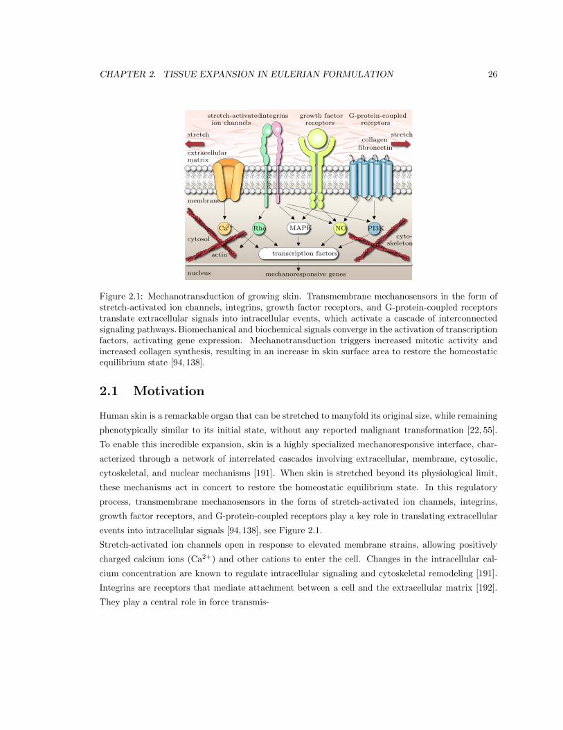
CHAPTER 2. TISSUE EXPANSION IN EULERIAN FORMULATION 26
transcription factors
mechanoresponsive genes
Ca2+ Rho MAPK NO PI3K
stretch-activatedion channels
integrins growth factorreceptors
G-protein-coupledreceptors
collagenfibronectin
extracellularmatrix
stretch stretch
membrane
cytosol
nucleus
actin
cyto-skeleton
Figure 2.1: Mechanotransduction of growing skin. Transmembrane mechanosensors in the form ofstretch-activated ion channels, integrins, growth factor receptors, and G-protein-coupled receptorstranslate extracellular signals into intracellular events, which activate a cascade of interconnectedsignaling pathways. Biomechanical and biochemical signals converge in the activation of transcriptionfactors, activating gene expression. Mechanotransduction triggers increased mitotic activity andincreased collagen synthesis, resulting in an increase in skin surface area to restore the homeostaticequilibrium state [94, 138].
2.1 Motivation
Human skin is a remarkable organ that can be stretched to manyfold its original size, while remaining
phenotypically similar to its initial state, without any reported malignant transformation [22, 55].
To enable this incredible expansion, skin is a highly specialized mechanoresponsive interface, char-
acterized through a network of interrelated cascades involving extracellular, membrane, cytosolic,
cytoskeletal, and nuclear mechanisms [191]. When skin is stretched beyond its physiological limit,
these mechanisms act in concert to restore the homeostatic equilibrium state. In this regulatory
process, transmembrane mechanosensors in the form of stretch-activated ion channels, integrins,
growth factor receptors, and G-protein-coupled receptors play a key role in translating extracellular
events into intracellular signals [94, 138], see Figure 2.1.
Stretch-activated ion channels open in response to elevated membrane strains, allowing positively
charged calcium ions (Ca2+) and other cations to enter the cell. Changes in the intracellular cal-
cium concentration are known to regulate intracellular signaling and cytoskeletal remodeling [191].
Integrins are receptors that mediate attachment between a cell and the extracellular matrix [192].
They play a central role in force transmis-
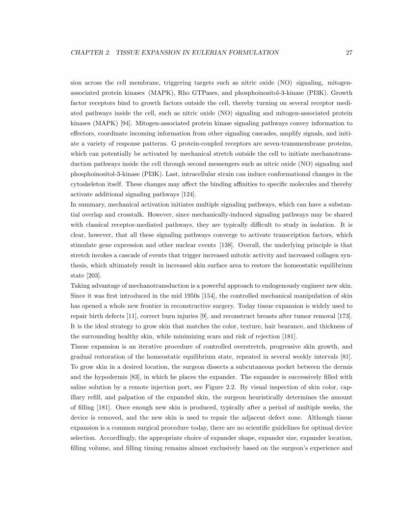
CHAPTER 2. TISSUE EXPANSION IN EULERIAN FORMULATION 27
sion across the cell membrane, triggering targets such as nitric oxide (NO) signaling, mitogen-
associated protein kinases (MAPK), Rho GTPases, and phosphoinositol-3-kinase (PI3K). Growth
factor receptors bind to growth factors outside the cell, thereby turning on several receptor medi-
ated pathways inside the cell, such as nitric oxide (NO) signaling and mitogen-associated protein
kinases (MAPK) [94]. Mitogen-associated protein kinase signaling pathways convey information to
e↵ectors, coordinate incoming information from other signaling cascades, amplify signals, and initi-
ate a variety of response patterns. G protein-coupled receptors are seven-transmembrane proteins,
which can potentially be activated by mechanical stretch outside the cell to initiate mechanotrans-
duction pathways inside the cell through second messengers such as nitric oxide (NO) signaling and
phosphoinositol-3-kinase (PI3K). Last, intracellular strain can induce conformational changes in the
cytoskeleton itself. These changes may a↵ect the binding a�nities to specific molecules and thereby
activate additional signaling pathways [124].
In summary, mechanical activation initiates multiple signaling pathways, which can have a substan-
tial overlap and crosstalk. However, since mechanically-induced signaling pathways may be shared
with classical receptor-mediated pathways, they are typically di�cult to study in isolation. It is
clear, however, that all these signaling pathways converge to activate transcription factors, which
stimulate gene expression and other nuclear events [138]. Overall, the underlying principle is that
stretch invokes a cascade of events that trigger increased mitotic activity and increased collagen syn-
thesis, which ultimately result in increased skin surface area to restore the homeostatic equilibrium
state [203].
Taking advantage of mechanotransduction is a powerful approach to endogenously engineer new skin.
Since it was first introduced in the mid 1950s [154], the controlled mechanical manipulation of skin
has opened a whole new frontier in reconstructive surgery. Today tissue expansion is widely used to
repair birth defects [11], correct burn injuries [9], and reconstruct breasts after tumor removal [173].
It is the ideal strategy to grow skin that matches the color, texture, hair bearance, and thickness of
the surrounding healthy skin, while minimizing scars and risk of rejection [181].
Tissue expansion is an iterative procedure of controlled overstretch, progressive skin growth, and
gradual restoration of the homeostatic equilibrium state, repeated in several weekly intervals [81].
To grow skin in a desired location, the surgeon dissects a subcutaneous pocket between the dermis
and the hypodermis [83], in which he places the expander. The expander is successively filled with
saline solution by a remote injection port, see Figure 2.2. By visual inspection of skin color, cap-
illary refill, and palpation of the expanded skin, the surgeon heuristically determines the amount
of filling [181]. Once enough new skin is produced, typically after a period of multiple weeks, the
device is removed, and the new skin is used to repair the adjacent defect zone. Although tissue
expansion is a common surgical procedure today, there are no scientific guidelines for optimal device
selection. Accordlingly, the appropriate choice of expander shape, expander size, expander location,
filling volume, and filling timing remains almost exclusively based on the surgeon’s experience and
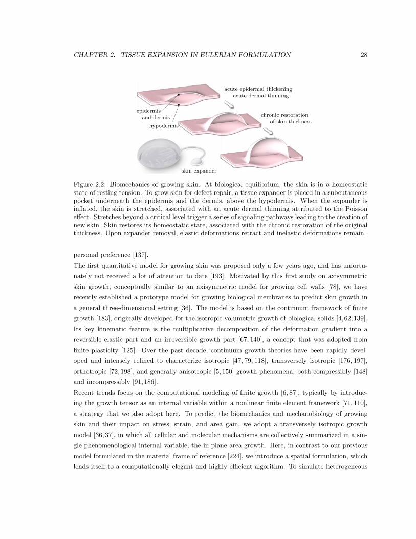
CHAPTER 2. TISSUE EXPANSION IN EULERIAN FORMULATION 28
skin expander
epidermis
and dermis
hypodermis
acute epidermal thickening
acute dermal thinning
chronic restoration
of skin thickness
Figure 2.2: Biomechanics of growing skin. At biological equilibrium, the skin is in a homeostaticstate of resting tension. To grow skin for defect repair, a tissue expander is placed in a subcutaneouspocket underneath the epidermis and the dermis, above the hypodermis. When the expander isinflated, the skin is stretched, associated with an acute dermal thinning attributed to the Poissone↵ect. Stretches beyond a critical level trigger a series of signaling pathways leading to the creation ofnew skin. Skin restores its homeostatic state, associated with the chronic restoration of the originalthickness. Upon expander removal, elastic deformations retract and inelastic deformations remain.
personal preference [137].
The first quantitative model for growing skin was proposed only a few years ago, and has unfortu-
nately not received a lot of attention to date [193]. Motivated by this first study on axisymmetric
skin growth, conceptually similar to an axisymmetric model for growing cell walls [78], we have
recently established a prototype model for growing biological membranes to predict skin growth in
a general three-dimensional setting [36]. The model is based on the continuum framework of finite
growth [183], originally developed for the isotropic volumetric growth of biological solids [4,62,139].
Its key kinematic feature is the multiplicative decomposition of the deformation gradient into a
reversible elastic part and an irreversible growth part [67, 140], a concept that was adopted from
finite plasticity [125]. Over the past decade, continuum growth theories have been rapidly devel-
oped and intensely refined to characterize isotropic [47, 79, 118], transversely isotropic [176, 197],
orthotropic [72, 198], and generally anisotropic [5, 150] growth phenomena, both compressibly [148]
and incompressibly [91, 186].
Recent trends focus on the computational modeling of finite growth [6, 87], typically by introduc-
ing the growth tensor as an internal variable within a nonlinear finite element framework [71, 110],
a strategy that we also adopt here. To predict the biomechanics and mechanobiology of growing
skin and their impact on stress, strain, and area gain, we adopt a transversely isotropic growth
model [36,37], in which all cellular and molecular mechanisms are collectively summarized in a sin-
gle phenomenological internal variable, the in-plane area growth. Here, in contrast to our previous
model formulated in the material frame of reference [224], we introduce a spatial formulation, which
lends itself to a computationally elegant and highly e�cient algorithm. To simulate heterogeneous
CHAPTER 2. TISSUE EXPANSION IN EULERIAN FORMULATION 29
growth phenomena on anatomically realistic geometries, we integrate the growth model into a multi-
purpose nonlinear finite element program [205]. We illustrate its features by means of the simple
model problem of equi-biaxial extension and through two clinical cases of skin expansion in pediatric
forehead reconstruction.
2.2 Methods
2.2.1 Continuum model of growing skin
To accurately represent the finite deformations during skin expansion, we adopt the kinematics of
finite growth, and introduce the deformation map ', which, at any given time t, maps the material
placement X of a physical particle onto its spatial placement x = ' (X, t). We then introduce the
multiplicative decomposition of the deformation gradient [183],
F = rX' = F
e · F g (2.1)
into a reversible elastic part F e and an irreversible growth part F g, in agreement with experimental
findings [212]. Here, r{�} = @X{�}|t
denotes the gradient of a field {�} (X, t) with respect to the
material placement X at fixed time t. Its Jacobian defines the overall change in tissue volume,
J = det (F ) = Je Jg (2.2)
which we can equivalently decompose into a reversibly elastic volume change Je = det (F e) and
an irreversibly grown volume change Jg = det (F g). Skin is a composite material consisting of a
0.1-1.0mm thick, waterproof, protective outer layer, the epidermis, and a 1.0-4.0mm thick, load
bearing inner layer, the dermis [191], which we idealize jointly as a single layer. We characterize its
area stretch through Nanson’s formula
# = || cof(F ) · n0 || = #e #g (2.3)
in terms of the skin plane normal n0 in the undeformed reference configuration, where cof(�) =
det (�) (�)�t denotes the cofactor of a second order tensor (�). The area stretch obeys the multi-
plicative decomposition into a reversibly elastic area stretch #e and an irreversibly grown area stretch
#g = || cof(F g) · n0 ||. To model stretch-induced skin growth, we collectively summarize the e↵ects
of mechanotransduction in a single scalar-valued variable #g, which characterizes the evolution of
the in-plane area growth, while the response in the thickness direction n0 is assumed to be purely
elastic [22]. Accordingly, we can express the growth tensor F g in the following simple format.
F
g =p#g I + [ 1�
p#g ] n0 ⌦ n0 (2.4)
CHAPTER 2. TISSUE EXPANSION IN EULERIAN FORMULATION 30
Since the material is not assumed to grow in the thickness direction n0 [181,210], its area growth is
identical to its volume growth, i.e., #g = det(F g) = Jg. Using the simple rank-one update structure
of F g, we can apply the Sherman-Morrison formula to invert the growth tensor explicitly,
F
g � 1 =1p#g
I +
1� 1p
#g
�n0 ⌦ n0 (2.5)
and obtain an explicit representation of the elastic tensor F e,
F
e =1p#g
F +
1� 1p
#g
�n⌦ n0 (2.6)
in terms of the spatial normal n = F ·n0. From the push forward of the contravariant material and
intermediate metric tensors G�1 and G
g�1, we obtain the left Cauchy Green tensor b = F ·G�1 ·F t
and its counterpart be in the deformed, current configuration.
b
e = F
e ·Gg�1· F et =1
#gb+
1� 1
#g
�n⌦ n (2.7)
To focus on the impact of growth, we assume skin to behave isotropically elastic within the in vivo
loading range of interest. Accordingly, we introduce the following Helmholtz free energy
= 12 � ln2(Je) + 1
2 µ [ g : be � 3� 2 ln(Je) ] (2.8)
to evaluate the standard dissipation inequality, which defines the Kirchho↵ stress ⌧ as thermody-
namically conjugate to covariant spatial metric g.
⌧ = 2@
@g= [� ln(Je)� µ ] g�1 + µ b
e (2.9)
This implies that the newly created skin will have the same microstructure, density, and sti↵ness,
as the original, native tissue [22, 36]. We model skin growth as a strain-driven process [83], and
introduce the following evolution equation for the area growth,
#g = kg(#g)�g(#e) (2.10)
in which kg(#g) is a weighting function and �g(#e) is a growth criterion similar to a yield function in
the theory of plasticity. For the weighting function, we adopt a well-established functional form [139],
which we rephrase here in a strain-driven format [71, 72], to control unbounded growth.
kg =1
⌧
#max � #g
#max � 1
��
(2.11)
CHAPTER 2. TISSUE EXPANSION IN EULERIAN FORMULATION 31
The adaptation speed ⌧ and the shape parameter for the adaptation curve � control the speed of
adaptation, whereas the maximum area growth #max defines the biological equilibrium state [87,139].
For the growth criterion, we assume that growth is driven by the elastic area stretch #e,
�g =⌦#e � #crit
↵=
⌦#/#g � #crit
↵(2.12)
and that it is activated only if the elastic area stretch exceeds a critical physiological limit #crit,
where h�i denote the Macaulay brackets.
2.2.2 Computational model of growing skin
To solve the nonlinear finite element equations of stretch-induced skin growth, we implement the
growth model in a custom-designed version of the multipurpose nonlinear finite element program
FEAP [205]. To characterize the growth process at each instant in time, we introduce the area
growth #g as an internal variable, and solve the biological equilibrium equation (2.10) locally at
the integration point level. At each discrete time step t, we determine the current area growth #g
for a given current deformation state F and a given area growth #gn from the previous time step
tn. Accordingly, we introduce the following finite di↵erence approximation for the material time
derivative of the area growth,
#g = [#g � #gn ] /�t (2.13)
where �t = t�tn denotes the current time increment. In the spirit of implicit time stepping schemes,
we now reformulate the evolution equation (2.10) with the help of equation (2.13), introducing the
discrete residual R# in terms of the unknown area growth #g.
R# = #g � #gn � kg �g �t.= 0 (2.14)
We solve this nonlinear equation using a local Newton iteration. Within each iteration step, we
calculate the linearization of the residual R# with respect to the area growth #g,
K# =@R#
@#g= 1�
@kg
@#g�g + kg
@�g
@#g
��t (2.15)
in terms of the linearizations of the weighting function @kg / @#g = �� kg / [#max � #g ] and the
growth criterion @�g / @#g = �# /#g2 introduced in equations (2.11) and (2.12). We update the
unknown area growth iteratively,
#g #g � R# /K# (2.16)
until we achieve convergence, i.e., until the absolute value of the local growth update�#g = �R# /K#
is below a user-defined threshold value. Once we have iteratively determined the current area growth
#g, we can successively determine the growth tensor F
g from equation (2.4), the elastic tensor
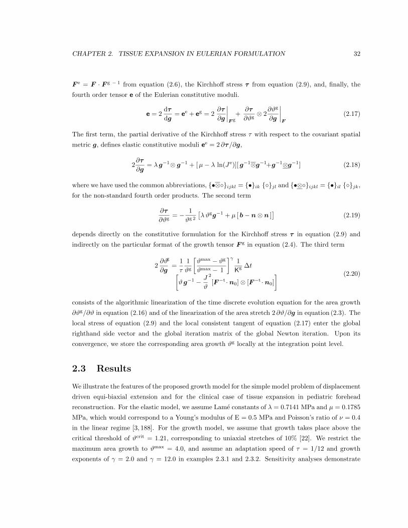
CHAPTER 2. TISSUE EXPANSION IN EULERIAN FORMULATION 32
F
e = F · F g � 1 from equation (2.6), the Kirchho↵ stress ⌧ from equation (2.9), and, finally, the
fourth order tensor e of the Eulerian constitutive moduli.
e = 2d⌧
dg= e
e + e
g = 2@⌧
@g
����F g
+@⌧
@#g⌦ 2
@#g
@g
����F
(2.17)
The first term, the partial derivative of the Kirchho↵ stress ⌧ with respect to the covariant spatial
metric g, defines elastic constitutive moduli ee = 2 @⌧/@g,
2@⌧
@g= � g�1⌦ g
�1 + [µ� � ln(Je)][ g�1⌦g�1+g
�1⌦g�1] (2.18)
where we have used the common abbreviations, {•⌦�}ijkl
= {•}ik
{�}jl
and {•⌦�}ijkl
= {•}il
{�}jk
,
for the non-standard fourth order products. The second term
@⌧
@#g= � 1
#g 2
⇥�#gg�1 + µ [ b� n⌦ n ]
⇤(2.19)
depends directly on the constitutive formulation for the Kirchho↵ stress ⌧ in equation (2.9) and
indirectly on the particular format of the growth tensor F g in equation (2.4). The third term
2@#
@g
g
=1
⌧
1
#g
#max � #g
#max � 1
�� 1
Kg �t# g�1 � J
#
2
[F�t · n0]⌦ [F�t · n0]
� (2.20)
consists of the algorithmic linearization of the time discrete evolution equation for the area growth
@#g/@# in equation (2.16) and of the linearization of the area stretch 2 @#/@g in equation (2.3). The
local stress of equation (2.9) and the local consistent tangent of equation (2.17) enter the global
righthand side vector and the global iteration matrix of the global Newton iteration. Upon its
convergence, we store the corresponding area growth #g locally at the integration point level.
2.3 Results
We illustrate the features of the proposed growth model for the simple model problem of displacement
driven equi-biaxial extension and for the clinical case of tissue expansion in pediatric forehead
reconstruction. For the elastic model, we assume Lame constants of � = 0.7141 MPa and µ = 0.1785
MPa, which would correspond to a Young’s modulus of E = 0.5 MPa and Poisson’s ratio of ⌫ = 0.4
in the linear regime [3, 188]. For the growth model, we assume that growth takes place above the
critical threshold of #crit = 1.21, corresponding to uniaxial stretches of 10% [22]. We restrict the
maximum area growth to #max = 4.0, and assume an adaptation speed of ⌧ = 1/12 and growth
exponents of � = 2.0 and � = 12.0 in examples 2.3.1 and 2.3.2. Sensitivity analyses demonstrate
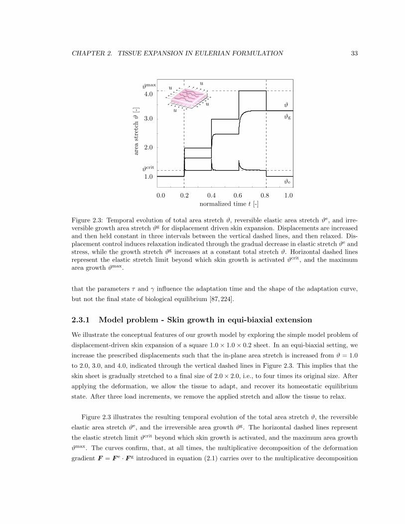
CHAPTER 2. TISSUE EXPANSION IN EULERIAN FORMULATION 33
0 0.1 0.2 0.3 0.4 0.5 0.6 0.7 0.8 0.9 1
1
1.5
2
2.5
3
3.5
4
#
#g
#e
u
uu
u
normalized time t [-]0.0 0.2 0.4 0.6 0.8 1.0
area
stretch#[-]
1.0#crit
2.0
3.0
4.0#max
Figure 2.3: Temporal evolution of total area stretch #, reversible elastic area stretch #e, and irre-versible growth area stretch #g for displacement driven skin expansion. Displacements are increasedand then held constant in three intervals between the vertical dashed lines, and then relaxed. Dis-placement control induces relaxation indicated through the gradual decrease in elastic stretch #e andstress, while the growth stretch #g increases at a constant total stretch #. Horizontal dashed linesrepresent the elastic stretch limit beyond which skin growth is activated #crit, and the maximumarea growth #max.
that the parameters ⌧ and � influence the adaptation time and the shape of the adaptation curve,
but not the final state of biological equilibrium [87,224].
2.3.1 Model problem - Skin growth in equi-biaxial extension
We illustrate the conceptual features of our growth model by exploring the simple model problem of
displacement-driven skin expansion of a square 1.0⇥ 1.0⇥ 0.2 sheet. In an equi-biaxial setting, we
increase the prescribed displacements such that the in-plane area stretch is increased from # = 1.0
to 2.0, 3.0, and 4.0, indicated through the vertical dashed lines in Figure 2.3. This implies that the
skin sheet is gradually stretched to a final size of 2.0⇥ 2.0, i.e., to four times its original size. After
applying the deformation, we allow the tissue to adapt, and recover its homeostatic equilibrium
state. After three load increments, we remove the applied stretch and allow the tissue to relax.
Figure 2.3 illustrates the resulting temporal evolution of the total area stretch #, the reversible
elastic area stretch #e, and the irreversible area growth #g. The horizontal dashed lines represent
the elastic stretch limit #crit beyond which skin growth is activated, and the maximum area growth
#max. The curves confirm, that, at all times, the multiplicative decomposition of the deformation
gradient F = F
e · F g introduced in equation (2.1) carries over to the multiplicative decomposition
CHAPTER 2. TISSUE EXPANSION IN EULERIAN FORMULATION 34
0 0.1 0.2 0.3 0.4 0.5 0.6 0.7 0.8 0.9 1
0.65
0.7
0.75
0.8
0.85
0.9
0.95
1
1.05
1.1
t
u
uu
u
normalized time t [-]0.0 0.2 0.4 0.6 0.8 1.0
normalized
thickn
esst[-]
0.7
0.8
0.9
1.0
1.1
Figure 2.4: Temporal evolution of skin thickness t for displacement driven skin expansion. Displace-ments are increased and then held constant in three intervals between the vertical dashed lines, andthen relaxed. Upon stretching, the skin thickness decreases acutely to 0.72, but then returns chron-ically to the homeostatic equilibrium thickness of 0.88 indicated through the lower horizontal line.This value is smaller than the original thickness because of the Poisson e↵ect. Upon displacementrelaxation, however, the skin thickness immediately returns to its original value of 1.0, indicatedthrough the upper horizontal line.
of the total area stretch # = #e #g of equation (2.3). Convergence towards the homeostatic state
manifests itself through a gradual increase of growth #g at a constant total stretch #, while the elastic
stretch #e, and, accordingly the stresses, decrease. Upon removal of the applied displacements, the
elastic stretch instantaneously returns to its baseline value of one, #e = 1. Since the growth process
is assumed to be irreversible, the growth stretch remains constant, #g = const. The total stretch
instantaneously adapts the value of the growth stretch, # = #g.
Figure 2.4 shows the temporal evolution of the skin thickness. Upon loading, the thickness decreases
acutely from 1.0 to 0.72, but then returns chronically to its loaded baseline value of 0.88. This value,
indicated through the lower horizontal line, is slightly smaller than the original thickness because
of the Poisson e↵ect. Upon removal of the applied displacements, the skin thickness immediately
returns to its original value of t = 1.0, indicated through the upper horizontal line. Since the model
assumes no growth in thickness direction, tg = 1.0, all thickness changes are fully reversible, te = t.
2.3.2 Clinical problem - Skin growth in pediatric forehead reconstruction
To illustrate the full potential of our model, we simulate skin expansion in pediatric forehead re-
construction for two clinical cases, a one-year old girl in case study I [82], and a one-year old boy
in case study II [83], both born with giant congenital nevi a↵ecting almost half of their foreheads,
CHAPTER 2. TISSUE EXPANSION IN EULERIAN FORMULATION 35
see Figure 2.5. Because giant congenital nevi place the child at an increased risk of skin cancer, the
nevus is typically removed in the early childhood [81]. To reconstruct the defect, preserve function,
and maintain aesthetic appearance, both children underwent conrolled tissue expansion [137]. To
simulate the process of tissue expansion in an anatomically exact geometry, we create a finite ele-
ment mesh from three-dimensional computer tomography images of a child of similar age following
the procedure outlined in [224]. We identify the skin region by its distinct grey scale value in the
computer tomography scans to create a triangular surface mesh, which we further smoothen semi-
manually. From the smoothened surface mesh, we create a volume mesh of the skin layer, discretized
with 61,228 nodes, 183,684 degrees of freedom, and 30,889 tri-linear brick elements. Last, we assign
each element a skin plane normal n0, corresponding to the normal of the initial surface mesh.
Case study I:
Simultaneous forehead, anterior and posterior scalp expansion
The first case study mimics the case of a one-year old girl, whose nevus covered her left posterior
forehead [82]. To grow extra skin to cover the defect area, she underwent simultaneous tissue ex-
pansion in the forehead and in the anterior and posterior scalp as shown in Figure 2.5, top row. To
model her case, we virtually implant three expanders. First, we implant an expander in the posterior
scalp, discretized with 4,726 nodes, 14,178 degrees of freedom, and 2,270 tri-linear brick elements,
covering an initial area of 53.1 cm2. Second, we implant two closely connected expanders in the
forehead and in the scalp, discretized together with 7,954 nodes, 23,862 degrees of freedom, and
3,820 tri-linear brick elements, covering an initial area of 96.3 cm2. To simulate tissue expansion,
we fix all nodes and release only the expander degrees of freedom, which we then pressurize from
underneath. We assume that the adjacent dermis and hypodermis remain closely connected [193].
Figure 2.6 displays the temporal evolution of the normalized total area, elastic area, and growth
area upon gradual expander inflation, constant pressure, and gradual expander removal. Once the
elastic area stretch reaches the critical threshold of #crit = 1.21, slightly before the total pressure is
applied, at t = 0.125, the tissue starts to grow. As the expander pressure is held constant, growth
increases gradually causing the total area to increase. Then, at t = 0.75, the pressure is decreased
to remove the expander. The elastic area retracts gradually, while the grown area remains constant.
The vertical dashed lines correspond to the discrete time points, t = 0.24, t = 0.33, t = 0.42 and
t = 0.75, displayed in Figure 2.7.
Figure 2.7 illustrates the spatio-temporal evolution of the area growth #g. Growth is first initiated
at the center of the expanders, where the elastic stretch is largest. As growth spreads throughout
the entire expanded areas, the initial area of 149.4 cm2 increases gradually as the grown skin area
increases to 190.2 cm2, 207.4 cm2, 220.4 cm2, and finally 251.2 cm2, displayed from left to right. In
detail, we observe that the final area in the posterior scalp region is 91.5 cm2, corresponding to a
fractional area gain of 1.73. In the combined forehead and anterior scalp regions, the final area
is 159.6 cm2, corresponding to a slightly lower fractional area gain of 1.66. Area growth displays
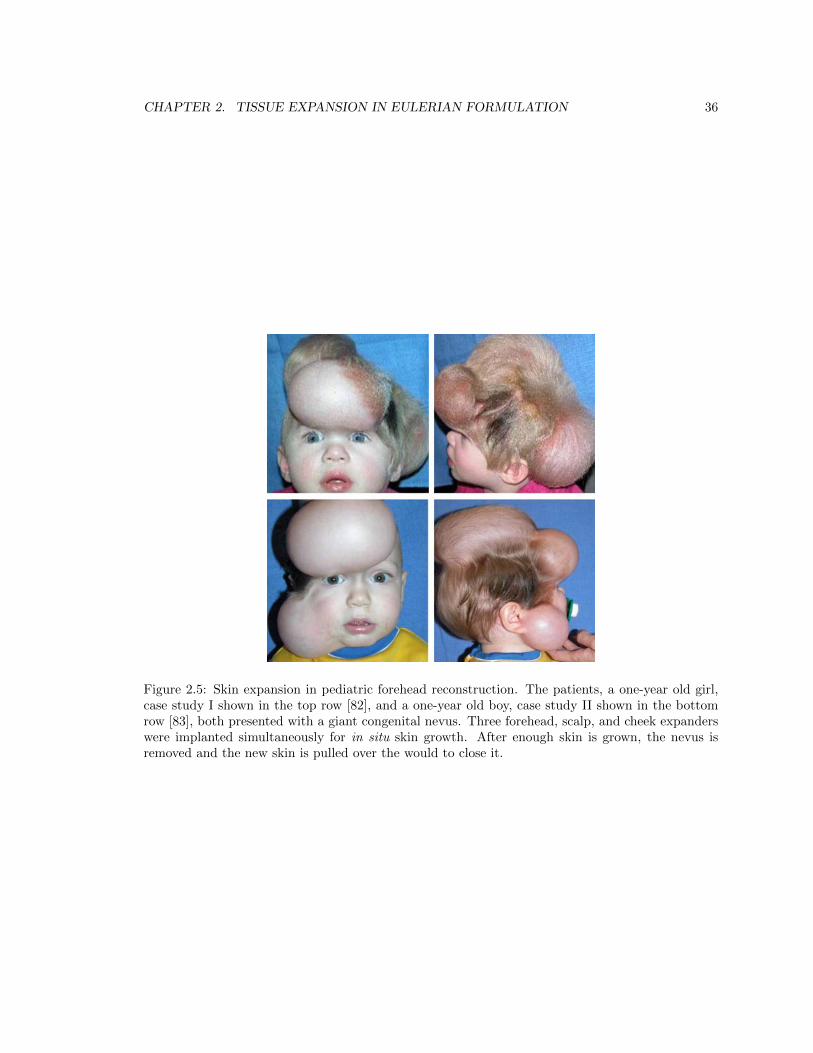
CHAPTER 2. TISSUE EXPANSION IN EULERIAN FORMULATION 36
Figure 2.5: Skin expansion in pediatric forehead reconstruction. The patients, a one-year old girl,case study I shown in the top row [82], and a one-year old boy, case study II shown in the bottomrow [83], both presented with a giant congenital nevus. Three forehead, scalp, and cheek expanderswere implanted simultaneously for in situ skin growth. After enough skin is grown, the nevus isremoved and the new skin is pulled over the would to close it.
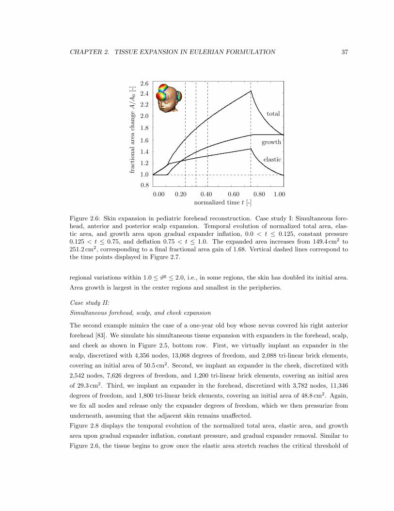
CHAPTER 2. TISSUE EXPANSION IN EULERIAN FORMULATION 37
0 0.1 0.2 0.3 0.4 0.5 0.6 0.7 0.8 0.9 1
0.8
1
1.2
1.4
1.6
1.8
2
2.2
2.4
2.6
total
growth
elastic
normalized time t [-]0.00 0.20 0.40 0.60 0.80 1.00
fraction
alarea
chan
geA/A
0[-]
0.8
1.0
1.2
1.4
1.6
1.8
2.0
2.2
2.4
2.6
Figure 2.6: Skin expansion in pediatric forehead reconstruction. Case study I: Simultaneous fore-head, anterior and posterior scalp expansion. Temporal evolution of normalized total area, elas-tic area, and growth area upon gradual expander inflation, 0.0 < t 0.125, constant pressure0.125 < t 0.75, and deflation 0.75 < t 1.0. The expanded area increases from 149.4 cm2 to251.2 cm2, corresponding to a final fractional area gain of 1.68. Vertical dashed lines correspond tothe time points displayed in Figure 2.7.
regional variations within 1.0 #g 2.0, i.e., in some regions, the skin has doubled its initial area.
Area growth is largest in the center regions and smallest in the peripheries.
Case study II:
Simultaneous forehead, scalp, and cheek expansion
The second example mimics the case of a one-year old boy whose nevus covered his right anterior
forehead [83]. We simulate his simultaneous tissue expansion with expanders in the forehead, scalp,
and cheek as shown in Figure 2.5, bottom row. First, we virtually implant an expander in the
scalp, discretized with 4,356 nodes, 13,068 degrees of freedom, and 2,088 tri-linear brick elements,
covering an initial area of 50.5 cm2. Second, we implant an expander in the cheek, discretized with
2,542 nodes, 7,626 degrees of freedom, and 1,200 tri-linear brick elements, covering an initial area
of 29.3 cm2. Third, we implant an expander in the forehead, discretized with 3,782 nodes, 11,346
degrees of freedom, and 1,800 tri-linear brick elements, covering an initial area of 48.8 cm2. Again,
we fix all nodes and release only the expander degrees of freedom, which we then pressurize from
underneath, assuming that the adjacent skin remains una↵ected.
Figure 2.8 displays the temporal evolution of the normalized total area, elastic area, and growth
area upon gradual expander inflation, constant pressure, and gradual expander removal. Similar to
Figure 2.6, the tissue begins to grow once the elastic area stretch reaches the critical threshold of
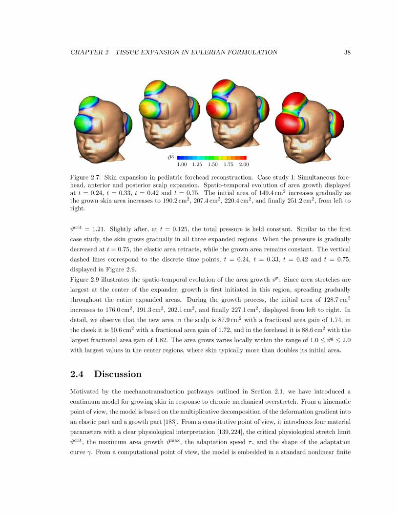
CHAPTER 2. TISSUE EXPANSION IN EULERIAN FORMULATION 38
#g
1.00 1.25 1.50 1.75 2.00
Figure 2.7: Skin expansion in pediatric forehead reconstruction. Case study I: Simultaneous fore-head, anterior and posterior scalp expansion. Spatio-temporal evolution of area growth displayedat t = 0.24, t = 0.33, t = 0.42 and t = 0.75. The initial area of 149.4 cm2 increases gradually asthe grown skin area increases to 190.2 cm2, 207.4 cm2, 220.4 cm2, and finally 251.2 cm2, from left toright.
#crit = 1.21. Slightly after, at t = 0.125, the total pressure is held constant. Similar to the first
case study, the skin grows gradually in all three expanded regions. When the pressure is gradually
decreased at t = 0.75, the elastic area retracts, while the grown area remains constant. The vertical
dashed lines correspond to the discrete time points, t = 0.24, t = 0.33, t = 0.42 and t = 0.75,
displayed in Figure 2.9.
Figure 2.9 illustrates the spatio-temporal evolution of the area growth #g. Since area stretches are
largest at the center of the expander, growth is first initiated in this region, spreading gradually
throughout the entire expanded areas. During the growth process, the initial area of 128.7 cm2
increases to 176.0 cm2, 191.3 cm2, 202.1 cm2, and finally 227.1 cm2, displayed from left to right. In
detail, we observe that the new area in the scalp is 87.9 cm2 with a fractional area gain of 1.74, in
the cheek it is 50.6 cm2 with a fractional area gain of 1.72, and in the forehead it is 88.6 cm2 with the
largest fractional area gain of 1.82. The area grows varies locally within the range of 1.0 #g 2.0
with largest values in the center regions, where skin typically more than doubles its initial area.
2.4 Discussion
Motivated by the mechanotransduction pathways outlined in Section 2.1, we have introduced a
continuum model for growing skin in response to chronic mechanical overstretch. From a kinematic
point of view, the model is based on the multiplicative decomposition of the deformation gradient into
an elastic part and a growth part [183]. From a constitutive point of view, it introduces four material
parameters with a clear physiological interpretation [139,224], the critical physiological stretch limit
#crit, the maximum area growth #max, the adaptation speed ⌧ , and the shape of the adaptation
curve �. From a computational point of view, the model is embedded in a standard nonlinear finite
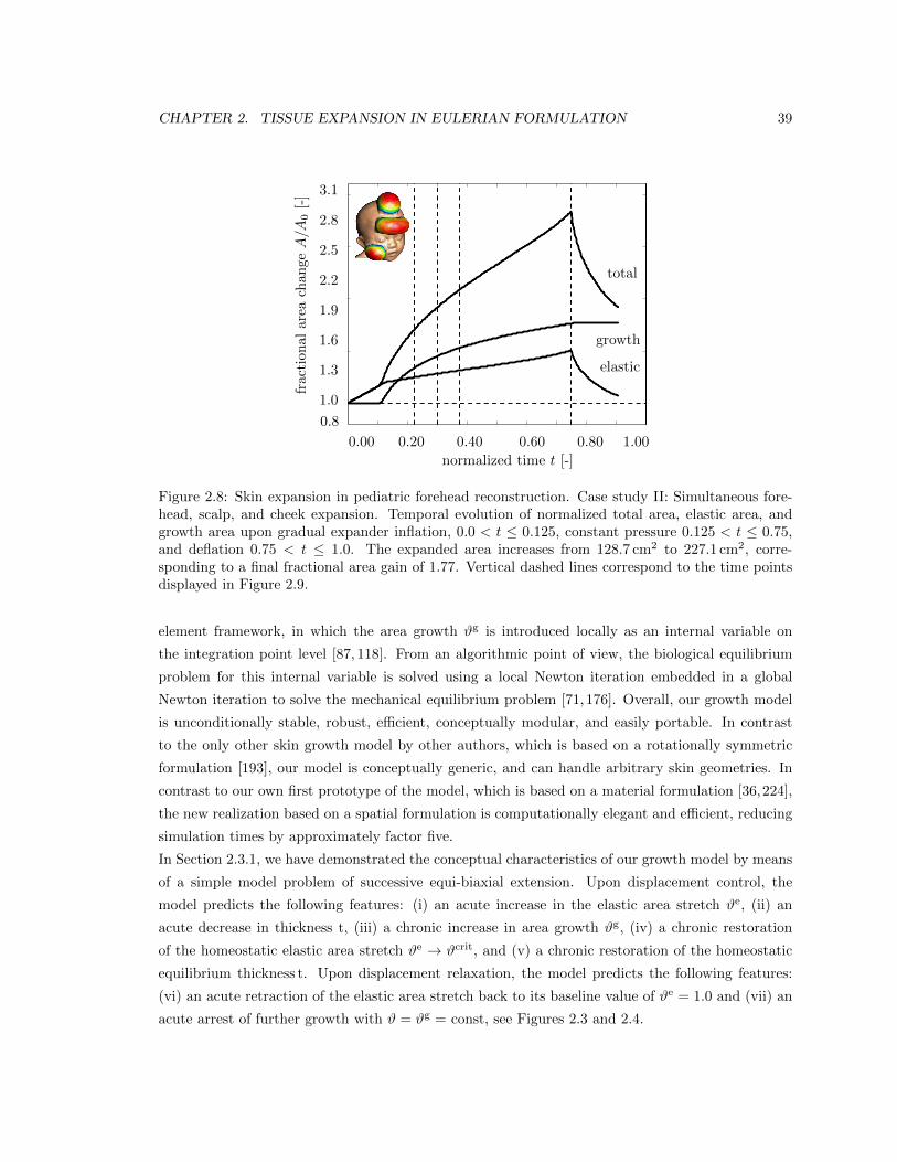
CHAPTER 2. TISSUE EXPANSION IN EULERIAN FORMULATION 39
0 0.1 0.2 0.3 0.4 0.5 0.6 0.7 0.8 0.9 1
1
1.5
2
2.5
3
total
growth
elastic
normalized time t [-]0.00 0.20 0.40 0.60 0.80 1.00
fraction
alarea
chan
geA/A
0[-]
0.8
1.0
1.3
1.6
1.9
2.2
2.5
2.8
3.1
Figure 2.8: Skin expansion in pediatric forehead reconstruction. Case study II: Simultaneous fore-head, scalp, and cheek expansion. Temporal evolution of normalized total area, elastic area, andgrowth area upon gradual expander inflation, 0.0 < t 0.125, constant pressure 0.125 < t 0.75,and deflation 0.75 < t 1.0. The expanded area increases from 128.7 cm2 to 227.1 cm2, corre-sponding to a final fractional area gain of 1.77. Vertical dashed lines correspond to the time pointsdisplayed in Figure 2.9.
element framework, in which the area growth #g is introduced locally as an internal variable on
the integration point level [87, 118]. From an algorithmic point of view, the biological equilibrium
problem for this internal variable is solved using a local Newton iteration embedded in a global
Newton iteration to solve the mechanical equilibrium problem [71, 176]. Overall, our growth model
is unconditionally stable, robust, e�cient, conceptually modular, and easily portable. In contrast
to the only other skin growth model by other authors, which is based on a rotationally symmetric
formulation [193], our model is conceptually generic, and can handle arbitrary skin geometries. In
contrast to our own first prototype of the model, which is based on a material formulation [36,224],
the new realization based on a spatial formulation is computationally elegant and e�cient, reducing
simulation times by approximately factor five.
In Section 2.3.1, we have demonstrated the conceptual characteristics of our growth model by means
of a simple model problem of successive equi-biaxial extension. Upon displacement control, the
model predicts the following features: (i) an acute increase in the elastic area stretch #e, (ii) an
acute decrease in thickness t, (iii) a chronic increase in area growth #g, (iv) a chronic restoration
of the homeostatic elastic area stretch #e ! #crit, and (v) a chronic restoration of the homeostatic
equilibrium thickness t. Upon displacement relaxation, the model predicts the following features:
(vi) an acute retraction of the elastic area stretch back to its baseline value of #e = 1.0 and (vii) an
acute arrest of further growth with # = #g = const, see Figures 2.3 and 2.4.
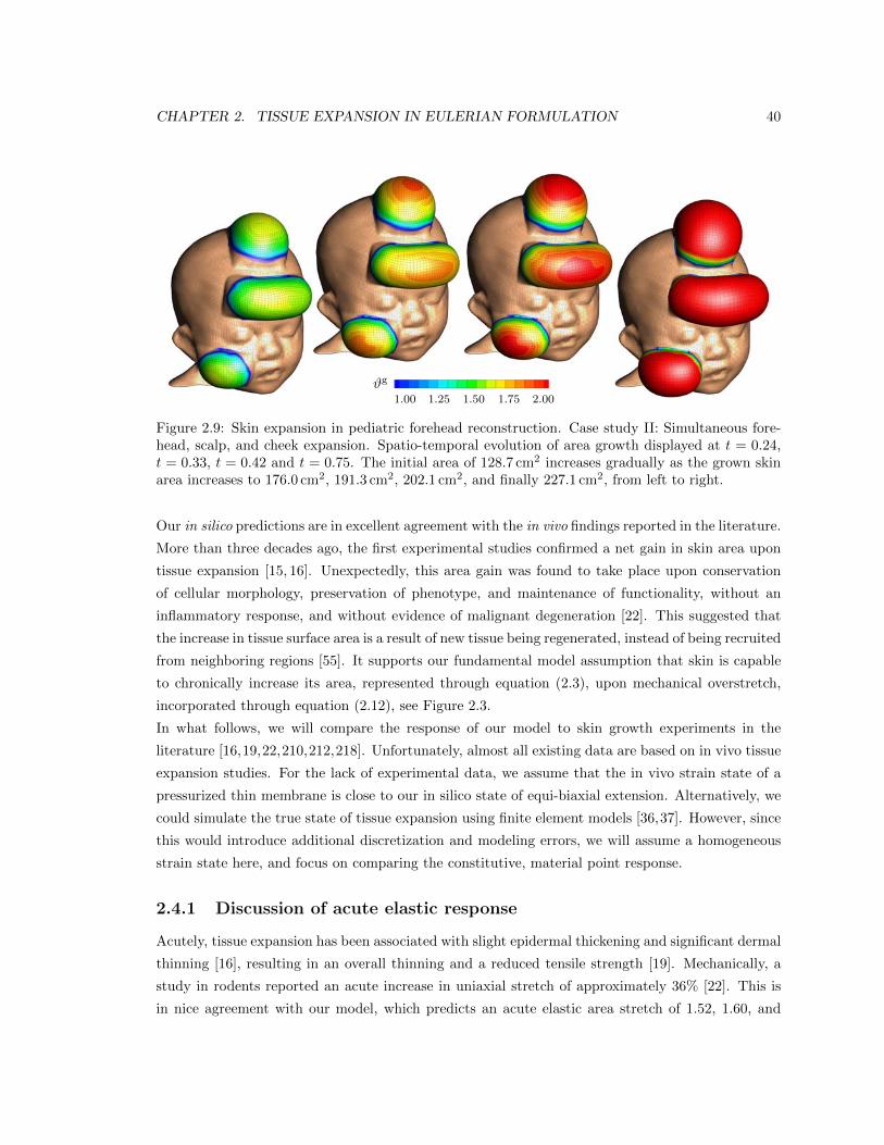
CHAPTER 2. TISSUE EXPANSION IN EULERIAN FORMULATION 40
#g
1.00 1.25 1.50 1.75 2.00
Figure 2.9: Skin expansion in pediatric forehead reconstruction. Case study II: Simultaneous fore-head, scalp, and cheek expansion. Spatio-temporal evolution of area growth displayed at t = 0.24,t = 0.33, t = 0.42 and t = 0.75. The initial area of 128.7 cm2 increases gradually as the grown skinarea increases to 176.0 cm2, 191.3 cm2, 202.1 cm2, and finally 227.1 cm2, from left to right.
Our in silico predictions are in excellent agreement with the in vivo findings reported in the literature.
More than three decades ago, the first experimental studies confirmed a net gain in skin area upon
tissue expansion [15, 16]. Unexpectedly, this area gain was found to take place upon conservation
of cellular morphology, preservation of phenotype, and maintenance of functionality, without an
inflammatory response, and without evidence of malignant degeneration [22]. This suggested that
the increase in tissue surface area is a result of new tissue being regenerated, instead of being recruited
from neighboring regions [55]. It supports our fundamental model assumption that skin is capable
to chronically increase its area, represented through equation (2.3), upon mechanical overstretch,
incorporated through equation (2.12), see Figure 2.3.
In what follows, we will compare the response of our model to skin growth experiments in the
literature [16,19,22,210,212,218]. Unfortunately, almost all existing data are based on in vivo tissue
expansion studies. For the lack of experimental data, we assume that the in vivo strain state of a
pressurized thin membrane is close to our in silico state of equi-biaxial extension. Alternatively, we
could simulate the true state of tissue expansion using finite element models [36,37]. However, since
this would introduce additional discretization and modeling errors, we will assume a homogeneous
strain state here, and focus on comparing the constitutive, material point response.
2.4.1 Discussion of acute elastic response
Acutely, tissue expansion has been associated with slight epidermal thickening and significant dermal
thinning [16], resulting in an overall thinning and a reduced tensile strength [19]. Mechanically, a
study in rodents reported an acute increase in uniaxial stretch of approximately 36% [22]. This is
in nice agreement with our model, which predicts an acute elastic area stretch of 1.52, 1.60, and
CHAPTER 2. TISSUE EXPANSION IN EULERIAN FORMULATION 41
1.56, corresponding to an average increase in uniaxial stretch of 25%, see Figure 2.3. Structurally,
the same study identified an initial acute decrease in skin thickness from 407 ± 3µm to 317 ±4µm corresponding to an acute thickness reduction of 22% [22]. Again, this is in good quantitative
agreement with our model, which predicts an acute average normalized thickness of 0.74, 0.71, and
0.72 corresponding to an acute average thickness decrease of 28%, see Figure 2.4. Since these acute
thickness changes can be attributed primarily to the Poisson e↵ect, they can be utilized to calibrate
the elastic material parameters, in particular Poisson’s ratio.
2.4.2 Discussion of chronic growth response
Chronically, tissue expansion is associated with the gradual restoration of baseline histology, baseline
mechanics, and baseline structure [19]. Histologically, a comparison of piglet tissue in expanded and
non-expanded regions demonstrated a chronic restoration of the number of epidermal cell layers and
a chronic restoration of the epidermal thickness [210]. In addition, immunocytochemistry confirmed
that the expanded tissue maintains its phenotypical characteristics and native program of cellular
di↵erentiation [218]. Mechanically, in a multiple time-point study in rodents, an acutely increased
uniaxial stretch of 36% was reduced chronically to approximately 10% 32 days post expansion [22].
This is in excellent agreement with our model, which predicts an acutely increased uniaxial stretch
of 25% and a chronic reduction to 10%, see Figure 2.3. A uniaxial stretch of 10% would corresponds
to an area stretch of #crit = 1.21. In our model, the model parameter #crit takes the interpretation
of the physiological threshold value, to which the elastic area stretch tends to return during adaptive
skin growth, see equation (2.12). Structurally, after an initial acute thickness decrease of 22%, the
same study reports a chronic restoration of the homeostatic equilibrium thickness from initially 425±4µm to 398 ± 3µm, corresponding to a chronic thickness reduction of 7% [22]. This agrees well with
our model, which predicts a normalized homeostatic equilibrium thickness of 0.88, corresponding to
a chronic thickness reduction 12%, see Figure 2.4. The chronic rodent study also reported that the
overall weight of the tissue sample almost tripled, with a fractional weight gain of approximately
2.7 for wet weight and 3.3 for dry weight [22]. In our model, the fractional weight gain is directly
proportional to the fractional area gain of #g = 3.3 which agrees nicely with these experimental
findings, see Figure 2.3. Finally, the study found a conservation of the mechanical properties, for
example, a constant breaking strength acutely right after expansion and chronically long term [22].
These findings support our model assumption that ultimately, the newly created skin will have the
same microstructure, density, and sti↵ness, as the original, native tissue [36, 37].
2.4.3 Discussion of elastic retraction
Acutely, upon expander removal, an instantaneous retraction of the elastic deformation significantly
reduces the overall skin area. In controlled in vivo experiments in pigs, the ratio between the
reversible elastic deformation to irreversible growth was almost 2:1 [212]. Since our model assumes
CHAPTER 2. TISSUE EXPANSION IN EULERIAN FORMULATION 42
that the overall deformation gradient can be multiplicatively decomposed into an elastic and growth
part, represented through equation (2.1), it is perfectly capable of reproducing the e↵ect of elastic
retraction upon expander removal, see Figures 2.3, 2.6, and 2.8.
2.4.4 Discussion of growth heterogeneity
Figures 2.7 and 2.9 clearly indicate the heterogeneity of the growth process with larger values in the
center region and smaller values in the periphery. This is in agreement with in vivo studies, which
report a fractional area gain of 3.14, i.e., 50% above average, in the center region, and 2.06, i.e.,
25% below average, in the periphery [22]. The authors hypothesized that larger strains in the center
region would trigger larger growth. This is in agreement with our model in equation (2.10), where
the evolution of area growth is directly correlated to the amount of overstretch through the growth
criterion defined in equation (2.12).
2.4.5 Limitations
Although we have presented both qualitative and quantitative comparisons of the proposed model
with acute and chronic tissue expansion experiments from the literature, several limitations remain.
First and foremost, the most challenging aspect would be to tie the growth law in equation (2.4)
more closely to the underlying mechanobiology described in detail in the introduction section. Com-
parative gene expression assays and immunohistochemistry of grown versus ungrown tissue samples
could help to identify the mechanisms that trigger skin growth on the molecular and cellular level.
Similar approaches have been proposed for amelogenesis [49] and tumorigenesis [14,170] in the past
and could also be adopted here. Ideally, this would help to specify our evolution equation for the
growth tensor (2.4) in terms of discrete mechanotransduction cascades through selected extracellular
and intracellular events. To this end, we are currently designing a test setup to stretch and grow
explanted tissue samples ex vivo. Since most existing data sets on skin growth are based on in
vivo measurements of inflated membranes, an ex vivo setting will allow us to create well-defined
geometries and boundary conditions such as the equi-biaxial extension test suggested here.
Second, since our goal was to focus primarily on the kinematic characterization of the growth pro-
cess, the constitutive modeling of the elastic baseline properties of skin has played a minor role.
However, the proposed model is inherently modular and the incorporation of more sophisticated
constitutive models [213] is relatively straightforward. A typical candidate is a multiple-constituent
anisotropic skin model with in-plane anisotropy introduced through a pronounced sti↵ness along
Langer’s lines [116, 117], which we have successfully combined with the proposed growth model in
the past [37]. In addition, the growth process itself could be modeled as anisotropic [72], e.g., at-
tributed to a pronounced growth along specific microstructural directions. Similarly, through the
deposition of large bundles of compacted immature collagen [19, 109], the underlying collagen net-
work could reorient itself, e.g., to align with the maximum principal strains [88,119]. Here, we model
CHAPTER 2. TISSUE EXPANSION IN EULERIAN FORMULATION 43
growth as a strain driven process. This implies that the elastic material parameters, or, accordingly,
the corresponding stresses, play a less important role than in stress-driven growth, e.g., in hyperten-
sion [118,176]. In other words, when using the same model with di↵erent Lame constants or di↵erent
constitutive models, we would require di↵erent expander pressures to obtain the same deformation
pattern, but the growth process itself would still be a↵ected by kinematical quantities only. Along
the same lines, we have assumed that the e↵ects of resting tension and residual stress are negligible.
Both play a critical role when studying instabilities and buckling [77, 211]. In a previous study,
we have explored these phenomena in more detail [36]. Within the context of finite deformations,
resting tension and residual stress could be incorporated through another second order tensor, which
would mimic the mapping to a pre-strained or residually stressed configuration [150,200].
Third, for the sake of simplicity, we have modeled skin as homogeneous across the thickness, ne-
glecting its individual layers and their potential interaction. We are currently refining our model
utilizing shell kinematics with a higher resolution across the thickness direction. This will facilitate
to model the individual skin layers [191], which we believe to be a major source of heterogeneities
and residual stresses in real tissue expansion cases [149]. Alternatively, to explore the biomechanical
interaction between the growing dermis and the underlying hypodermis during tissue expansion, we
could even model growing skin through its own boundary energy [95].
Fourth, at this stage, the chronic response of our model is not yet calibrated in time. We have as-
sumed that chronic growth takes place within a normalized time interval from zero to one. In reality,
growth periods range from the order of days in rodents [22] to weeks in pigs [212] and humans [83].
However, with the appropriate experimental data, the duration of the adaptation process can be
calibrated easily through the adaptation speed ⌧ [224].
Fifth, we have modeled the tissue expander only implicitly through controlling the expander pres-
sure. In real tissue expansion, the external control parameter is the expander volume [137]. This
implies that our simulation displays creep under constant loading, while clinical tissue expansion
might rather display relaxation under constant deformation [37]. Moreover, we have assumed that
the expander is connected tightly to the expanded tissue, neglecting e↵ects of interface sliding and
shear [193]. However, this seems to be a reasonable first assumption, since most current expanders
have well-designed textures to promote mild tissue in-growth, primarily to prevent expander migra-
tion [21].
Last, while our computational model seems well suited to provide qualitative guidelines and trends,
in its present state, it is not recommended for quantitative statements. We will need to perform
acute and chronic in vitro and in vivo experiments to truly identify the underling mechanisms which
have, up until now, only been represented phenomenologically. Nevertheless, we believe that using
the equations of nonlinear continuum mechanics to characterize skin growth represents a significant
advancement over the current gold standard to predict tissue growth exclusively in terms of areas,
volumes, and empiric correction factors [189,212].
CHAPTER 2. TISSUE EXPANSION IN EULERIAN FORMULATION 44
2.5 Conclusion
We have presented a continuum model for growing biological membranes in which the underlying
mechanobiology is collectively summarized in a single pheonomenological internal variable, the in-
plane area growth. The model can reliably predict the characteristic histological, mechanical, and
structural features of controlled overstretch-induced skin growth, both acutely and chronically. We
anticipate that the proposed skin growth model can be generalized to arbitrary biological membranes,
and that it can serve as a valuable tool to virtually manipulate membrane area simply by means of
changes in the mechanical environment.
Acknowledgements
We acknowledge the support by Professor Arun K. Gosain, Department of Plastic Surgery, Case
Western Reserve University, Cleveland, Ohio, for stimulating discussions, and for providing the
computer tomography images of the pediatric skulls. This work was supported by the Stanford
Graduate Fellowship to Adrian Buganza Tepole and by the National Science Foundation CAREER
award CMMI-0952021 and the National Institutes of Health Grant U54 GM072970 to Ellen Kuhl.
Chapter 3
Realistic, volume controlled skin
expander model
Abstract
Skin is a highly dynamic, autoregulated, living system that responds to mechanical stretch
through a net gain in skin surface area. Tissue expansion uses the concept of controlled over-
stretch to grow extra skin for defect repair in situ. While the short-term mechanics of stretched
skin have been studied intensely by testing explanted tissue samples ex vivo, we know very little
about the long-term biomechanics and mechanobiology of living skin in vivo. Here we explore
the long-term e↵ects of mechanical stretch on the characteristics of living skin using a mathe-
matical model for skin growth. We review the molecular mechanisms by which skin responds
to mechanical loading and model their e↵ects collectively in a single scalar-valued internal vari-
able, the surface area growth. This allows us to adopt a continuum model for growing skin
based on the multiplicative decomposition of the deformation gradient into a reversible elastic
and an irreversible growth part. To demonstrate the inherent modularity of this approach, we
implement growth as a user-defined constitutive subroutine into the general purpose implicit
finite element program Abaqus/Standard. To illustrate the features of the model, we simulate
the controlled area growth of skin in response to tissue expansion with multiple filling points
in time. Our results demonstrate that the field theories of continuum mechanics can reliably
predict the manipulation of thin biological membranes through mechanical overstretch. Our
model could serve as a valuable tool to rationalize clinical process parameters such as expander
geometry, expander size, filling volume, filling pressure, and inflation timing to minimize tissue
necrosis and maximize patient comfort in plastic and reconstructive surgery. While initially de-
veloped for growing skin, our model can easily be generalized to arbitrary biological structures
to explore the physiology and pathology of stretch-induced growth of other living systems such
as hearts, arteries, bladders, intestines, ureters, muscles, and nerves.
45
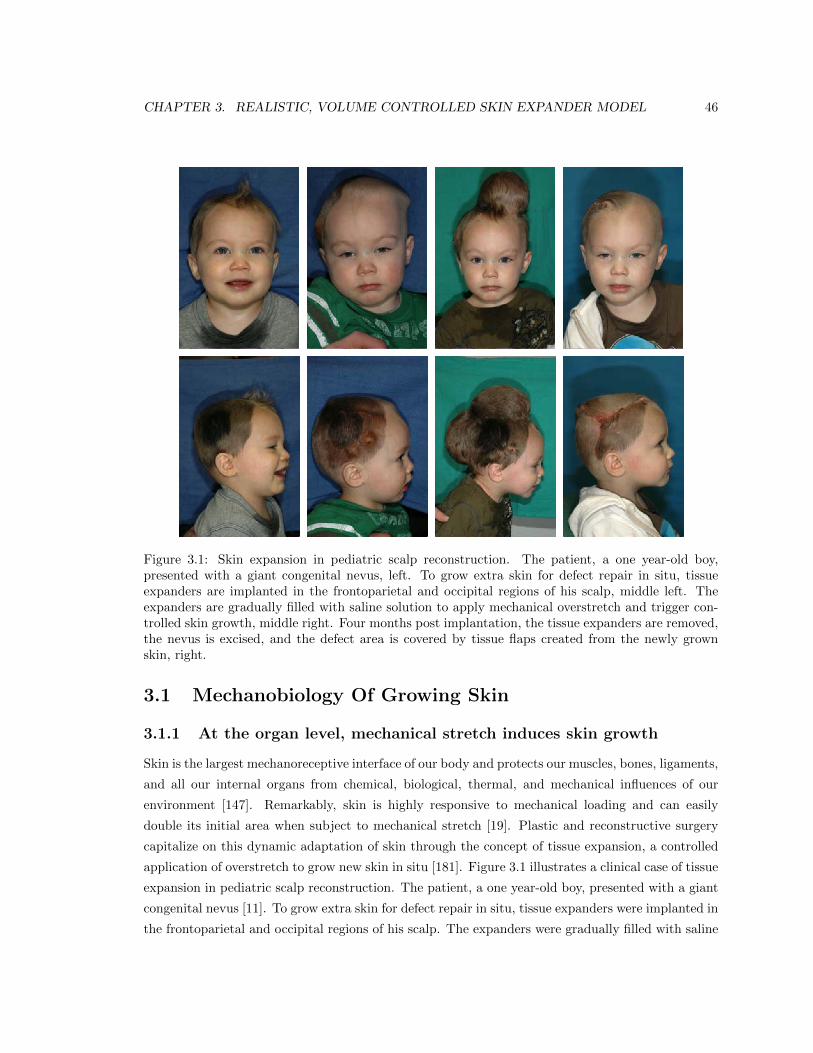
CHAPTER 3. REALISTIC, VOLUME CONTROLLED SKIN EXPANDER MODEL 46
Figure 1: Skin expansion in pediatric scalp reconstruction. The patient, a one year-old boy, presented with a giant congenital nevus, left. To grow extra skin fordefect repair in situ, tissue expanders are implanted in the frontoparietal and occipital regions of his scalp, middle left. The expanders are gradually filled with salinesolution to apply mechanical overstretch and trigger controlled skin growth, middle right. Four months post implantation, the tissue expanders are removed, thenevus is excised, and the defect area is covered by tissue flaps created from the newly grown skin, right.
overinflation, which causes skin thinning, necrosis, sloughing,and trauma through excessive tissue tension and compromisedvascularization [40]. While it is virtually impossible to measuretissue tension in the living skin in vivo, mathematical modelingprovides a safe and cheap alternative to estimate stress, strain,and area gain and avoid overstretch [11]. Personalized com-putational simulations have the potential to optimize the set ofclinical process parameters with the ultimate goal of maximiz-ing surface area gain while minimizing stress, tissue necrosis,inflation timing, and patient discomfort [72].
1.2. At the tissue level, mechanical stretch initiates cell-celland cell-matrix signaling
Skin is a composite microstructural material consisting of twodistinct layers, the epidermis and the dermis [14], see Figure 2.The epidermis, shown in dark purple in Figure 2, is the 0.1-1.0 mm-thick, waterproof, protective, outer layer. It consists ofan approximately four-cell-thick layer of densely packed ker-atinocytes, which constitute 95% of all cells in the epidermis[43]. Cells of the innermost epidermis, the basal keratinocytes,have a brick-type shape and are joined together tightly bydesmosomal junctions. Basal keratinocytes are attached to thebasement membrane, the 200 µm-thick divider between the epi-dermis and the dermis, via a complex network of proteins andglycoproteins including hemidesmosomes and integrin recep-tors [62]. Mechanical continuity at the basement membrane iskey for appropriate force transfer between the epidermis and
the dermis. The dermis, shown in pink in Figure 2,, is the 0.5-5.0 mm-thick, load-bearing inner layer. In contrast to the epi-dermis, the dermis is largely acellular and consists of 60% wa-ter. Of its remaining dry weight, 80-85% consists of looselyinterwoven, wavy, randomly oriented collagen fibers, supple-mented by 2-4% of elastin [43]. At low mechanical strains, theelastin fibers are stretched out, while the wavy collagen fibersuncrimp and do not contribute markedly to the overall skin sti↵-ness [37]. At higher strains, the stretched, crosslinked collagennetwork is the main load-carrying element responsible for thecharacteristic strain locking [32]. Fibroblasts, the major celltype in the dermis, are responsible for the synthesis of extracel-lular matrix proteins and regulate the collagen content. Frombelow, the dermis is demarcated by the hypodermis, shownin white in Figure 2, a subcutaneous fatty layer that connectsskin to bone and muscle. The hypodermis consists primarily ofadipocytes. Its major functions are to provide insulation, me-chanical cushioning, and energy storage [43]. When exposed totension, for example internally-generated during wound heal-ing [13] or externally-applied during tissue expansion [16],forces need to be transferred between the di↵erent layers of skin[62]. In the epidermis, stretching of keratinocyte-keratinocytejunctions and of the keratinocyte-basement-membrane inter-face initiates active cell-cell crosstalk and cell-matrix interac-tion. In the dermis, stretching of fibroblast-fibroblast junctionsand of the fibroblast-collagen interface triggers active cell-cellcrosstalk and cell-matrix interaction. In the following two sub-
2
Figure 3.1: Skin expansion in pediatric scalp reconstruction. The patient, a one year-old boy,presented with a giant congenital nevus, left. To grow extra skin for defect repair in situ, tissueexpanders are implanted in the frontoparietal and occipital regions of his scalp, middle left. Theexpanders are gradually filled with saline solution to apply mechanical overstretch and trigger con-trolled skin growth, middle right. Four months post implantation, the tissue expanders are removed,the nevus is excised, and the defect area is covered by tissue flaps created from the newly grownskin, right.
3.1 Mechanobiology Of Growing Skin
3.1.1 At the organ level, mechanical stretch induces skin growth
Skin is the largest mechanoreceptive interface of our body and protects our muscles, bones, ligaments,
and all our internal organs from chemical, biological, thermal, and mechanical influences of our
environment [147]. Remarkably, skin is highly responsive to mechanical loading and can easily
double its initial area when subject to mechanical stretch [19]. Plastic and reconstructive surgery
capitalize on this dynamic adaptation of skin through the concept of tissue expansion, a controlled
application of overstretch to grow new skin in situ [181]. Figure 3.1 illustrates a clinical case of tissue
expansion in pediatric scalp reconstruction. The patient, a one year-old boy, presented with a giant
congenital nevus [11]. To grow extra skin for defect repair in situ, tissue expanders were implanted in
the frontoparietal and occipital regions of his scalp. The expanders were gradually filled with saline
CHAPTER 3. REALISTIC, VOLUME CONTROLLED SKIN EXPANDER MODEL 47
solution to create mechanical overstretch and initiate controlled skin growth [81]. Four months post
implantation, the tissue expanders were removed, the nevus was excised, and the defect area was
covered by tissue flaps created from the newly grown skin [83]. When the concept of tissue expansion
was first introduced, the stretched skin was believed to simply redistribute its mass by increasing its
area while reducing its thickness [16]. We now know that skin actually grows in mass; it increases its
area while its thickness remains virtually unchanged [168]. Macroscopically, the newly grown skin
not only has the same thickness, but also the same mechanical properties as the native tissue [22].
Microscopically, it displays the same surface waviness and possesses a similar cell-to-matrix volume
fraction as the original tissue [203]. While tissue expansion has become a widely used procedure in
plastic and reconstructive surgery since it was first introduce more than half a century ago [154],
there are still no quantitative, mechanistic criteria for the appropriate selection of the relevant clinical
process parameters such as expander geometry, expander size, filling volume, filling pressure, and
inflation timing [212]. The success of the procedure almost exclusively relies on the skills and
experience of the surgeon and on his personal judgement [81]. A common complication associated
with the lack of experience is overinflation, which causes skin thinning, necrosis, sloughing, and
trauma through excessive tissue tension and compromised vascularization [137]. While it is virtually
impossible to measure tissue tension in the living skin in vivo, mathematical modeling provides
a safe and cheap alternative to estimate stress, strain, and area gain and avoid overstretch [36].
Personalized computational simulations have the potential to optimize the set of clinical process
parameters with the ultimate goal of maximizing surface area gain while minimizing stress, tissue
necrosis, inflation timing, and patient discomfort [225].
3.1.2 At the tissue level, mechanical stretch initiates cell-cell and cell-
matrix signaling
Skin is a composite microstructural material consisting of two distinct layers, the epidermis and the
dermis [47], see Figure 3.2. The epidermis, shown in dark purple in Figure 3.2, is the 0.1-1.0mm-
thick, waterproof, protective, outer layer. It consists of an approximately four-cell-thick layer of
densely packed keratinocytes, which constitute 95% of all cells in the epidermis [147]. Cells of
the innermost epidermis, the basal keratinocytes, have a brick-type shape and are joined together
tightly by desmosomal junctions. Basal keratinocytes are attached to the basement membrane, the
200µm-thick divider between the epidermis and the dermis, via a complex network of proteins and
glycoproteins including hemidesmosomes and integrin receptors [191]. Mechanical continuity at the
basement membrane is key for appropriate force transfer between the epidermis and the dermis. The
dermis, shown in pink in Figure 3.2, is the 0.5-5.0mm-thick, load-bearing inner layer. In contrast to
the epidermis, the dermis is largely acellular and consists of 60% water. Of its remaining dry weight,
80-85% consists of loosely interwoven, wavy, randomly oriented collagen fibers, supplemented by
2-4% of elastin [147]. At low mechanical strains, the elastin fibers are stretched out, while the wavy
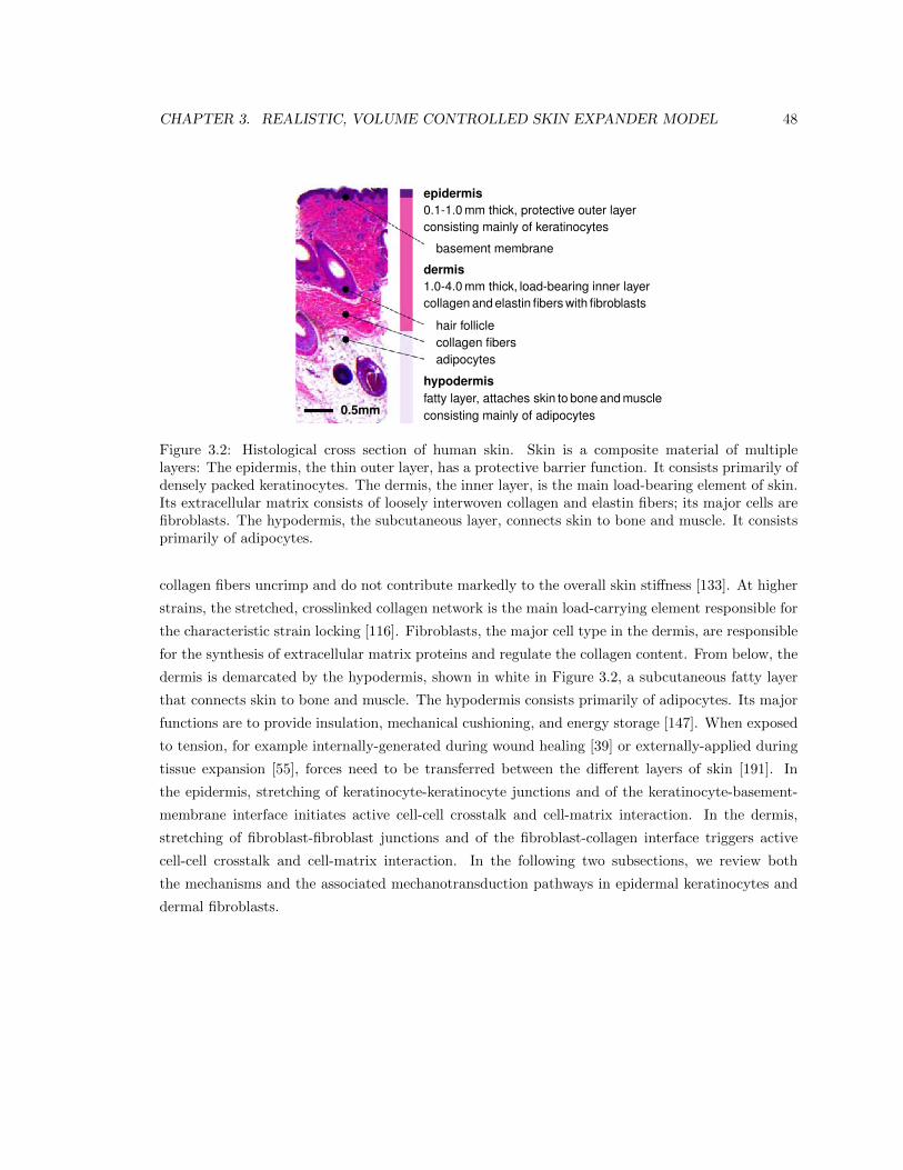
CHAPTER 3. REALISTIC, VOLUME CONTROLLED SKIN EXPANDER MODEL 48
epidermis0.1-1.0 mm thick, protective outer layer
consisting mainly of keratinocytes
basement membrane
dermis1.0-4.0 mm thick, load-bearing inner layer
collagen and elastin fibers with fibroblasts
hair follicle
collagen fibers
adipocytes
hypodermisfatty layer, attaches skin to bone and muscle
consisting mainly of adipocytes
0.5mm
Figure 2: Histological cross section of human skin. Skin is a composite materialof multiple layers: The epidermis, the thin outer layer, has a protective barrierfunction. It consists primarily of densely packed keratinocytes. The dermis, theinner layer, is the main load-bearing element of skin. Its extracellular matrixconsists of loosely interwoven collagen and elastin fibers; its major cells arefibroblasts. The hypodermis, the subcutaneous layer, connects skin to bone andmuscle. It consists primarily of adipocytes.
3
Figure 3.2: Histological cross section of human skin. Skin is a composite material of multiplelayers: The epidermis, the thin outer layer, has a protective barrier function. It consists primarily ofdensely packed keratinocytes. The dermis, the inner layer, is the main load-bearing element of skin.Its extracellular matrix consists of loosely interwoven collagen and elastin fibers; its major cells arefibroblasts. The hypodermis, the subcutaneous layer, connects skin to bone and muscle. It consistsprimarily of adipocytes.
collagen fibers uncrimp and do not contribute markedly to the overall skin sti↵ness [133]. At higher
strains, the stretched, crosslinked collagen network is the main load-carrying element responsible for
the characteristic strain locking [116]. Fibroblasts, the major cell type in the dermis, are responsible
for the synthesis of extracellular matrix proteins and regulate the collagen content. From below, the
dermis is demarcated by the hypodermis, shown in white in Figure 3.2, a subcutaneous fatty layer
that connects skin to bone and muscle. The hypodermis consists primarily of adipocytes. Its major
functions are to provide insulation, mechanical cushioning, and energy storage [147]. When exposed
to tension, for example internally-generated during wound healing [39] or externally-applied during
tissue expansion [55], forces need to be transferred between the di↵erent layers of skin [191]. In
the epidermis, stretching of keratinocyte-keratinocyte junctions and of the keratinocyte-basement-
membrane interface initiates active cell-cell crosstalk and cell-matrix interaction. In the dermis,
stretching of fibroblast-fibroblast junctions and of the fibroblast-collagen interface triggers active
cell-cell crosstalk and cell-matrix interaction. In the following two subsections, we review both
the mechanisms and the associated mechanotransduction pathways in epidermal keratinocytes and
dermal fibroblasts.
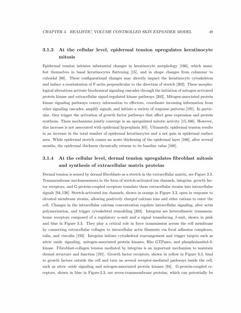
CHAPTER 3. REALISTIC, VOLUME CONTROLLED SKIN EXPANDER MODEL 49
3.1.3 At the cellular level, epidermal tension upregulates keratinocyte
mitosis
Epidermal tension initiates substantial changes in keratinocyte morphology [166], which mani-
fest themselves in basal keratinocytes flattening [15], and in shape changes from columnar to
cuboidal [98]. These configurational changes may directly impact the keratinocyte cytoskeleton
and induce a reorientation of F-actin perpendicular to the direction of stretch [202]. These morpho-
logical alterations activate biochemical signaling cascades through the initiation of mitogen-activated
protein kinase and extracellular signal-regulated kinase pathways [203]. Mitogen-associated protein
kinase signaling pathways convey information to e↵ectors, coordinate incoming information from
other signaling cascades, amplify signals, and initiate a variety of response patterns [191]. In partic-
ular, they trigger the activation of growth factor pathways that a↵ect gene expression and protein
synthesis. These mechanisms jointly converge in an upregulated mitotic activity [15,166]. However,
this increase is not associated with epidermal hyperplasia [65]. Ultimately, epidermal tension results
in an increase in the total number of epidermal keratinocytes and a net gain in epidermal surface
area. While epidermal stretch causes an acute thickening of the epidermal layer [166], after several
months, the epidermal thickness chronically returns to its baseline value [168].
3.1.4 At the cellular level, dermal tension upregulates fibroblast mitosis
and synthesis of extracellular matrix proteins
Dermal tension is sensed by dermal fibroblasts as a stretch in the extracellular matrix, see Figure 3.3.
Transmembrane mechanosensors in the form of stretch-activated ion channels, integrins, growth fac-
tor receptors, and G-protein-coupled receptors translate these extracellular strains into intracellular
signals [94, 138]. Stretch-activated ion channels, shown in orange in Figure 3.3, open in response to
elevated membrane strains, allowing positively charged calcium ions and other cations to enter the
cell. Changes in the intracellular calcium concentration regulate intracellular signaling, alter actin
polymerization, and trigger cytoskeletal remodeling [203]. Integrins are heterodimeric transmem-
brane receptors composed of a regulatory ↵-unit and a signal transducing �-unit, shown in pink
and blue in Figure 3.3. They play a critical role in force transmission across the cell membrane
by connecting extracellular collagen to intracellular actin filaments via focal adhesion complexes,
talin, and vinculin [192]. Integrins initiate cytoskeletal rearrangement and trigger targets such as
nitric oxide signaling, mitogen-associated protein kinases, Rho GTPases, and phosphoinositol-3-
kinase. Fibroblast-collagen tension mediated by integrins is an important mechanism to maintain
dermal structure and function [191]. Growth factor receptors, shown in yellow in Figure 3.3, bind
to growth factors outside the cell and turn on several receptor-mediated pathways inside the cell,
such as nitric oxide signaling and mitogen-associated protein kinases [94]. G-protein-coupled re-
ceptors, shown in blue in Figure 3.3, are seven-transmembrane proteins, which can potentially be
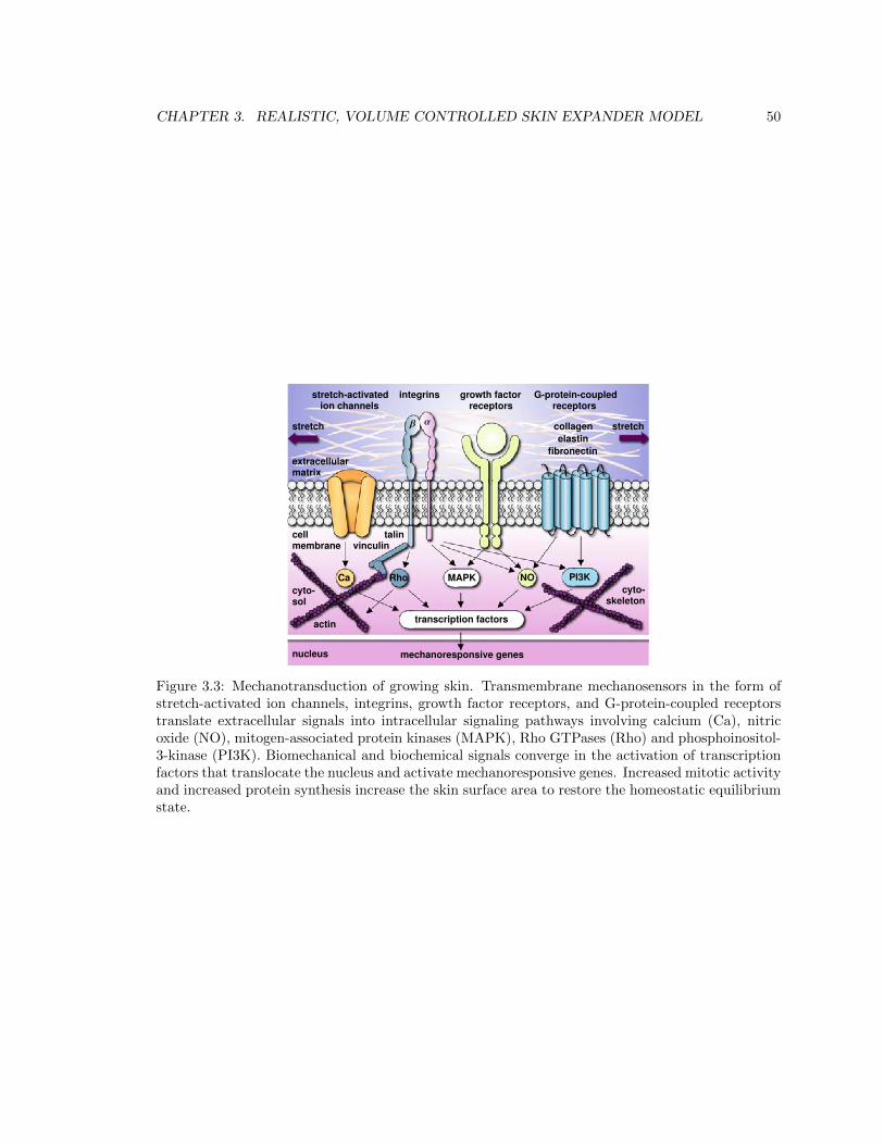
CHAPTER 3. REALISTIC, VOLUME CONTROLLED SKIN EXPANDER MODEL 50
When exposed to tension, for example internally-generated dur-ing wound healing [13] or externally-applied during tissue ex-pansion [16], forces need to be transferred between the dif-ferent layers of skin [62]. In the epidermis, stretching ofkeratinocyte-keratinocyte junctions and of the keratinocyte-basement-membrane interface initiates active cell-cell crosstalkand cell-matrix interaction. In the dermis, stretching offibroblast-fibroblast junctions and of the fibroblast-collagen in-terface triggers active cell-cell crosstalk and cell-matrix inter-action. In the following two subsections, we review both themechanisms and the associated mechanotransduction pathwaysin epidermal keratinocytes and dermal fibroblasts.
1.3. At the cellular level, epidermal tension upregulates ker-atinocyte mitosis
Epidermal tension initiates substantial changes in keratinocytemorphology [52], which manifest themselves in basal ker-atinocytes flattening [6], and in shape changes from columnarto cuboidal [29]. These configurational changes may directlyimpact the keratinocyte cytoskeleton and induce a reorienta-tion of F-actin perpendicular to the direction of stretch [66].These morphological alterations activate biochemical signalingcascades through the initiation of mitogen-activated protein ki-nase and extracellular signal-regulated kinase pathways [67].Mitogen-associated protein kinase signaling pathways conveyinformation to e↵ectors, coordinate incoming information fromother signaling cascades, amplify signals, and initiate a varietyof response patterns [62]. In particular, they trigger the activa-tion of growth factor pathways that a↵ect gene expression andprotein synthesis. These mechanisms jointly converge in an up-regulated mitotic activity [6, 52]. However, this increase is notassociated with epidermal hyperplasia [18]. Ultimately, epider-mal tension results in an increase in the total number of epi-dermal keratinocytes and a net gain in epidermal surface area.While epidermal stretch causes an acute thickening of the epi-dermal layer [52], after several months, the epidermal thicknesschronically returns to its baseline value [54].
1.4. At the cellular level, dermal tension upregulates fibroblastmitosis and synthesis of extracellular matrix proteins
Dermal tension is sensed by dermal fibroblasts as a stretchin the extracellular matrix, see Figure 3. Transmembranemechanosensors in the form of stretch-activated ion channels,integrins, growth factor receptors, and G-protein-coupled re-ceptors translate these extracellular strains into intracellular sig-nals [28, 71]. Stretch-activated ion channels, shown in orangein Figure 3, open in response to elevated membrane strains,allowing positively charged calcium ions and other cations toenter the cell. Changes in the intracellular calcium concen-tration regulate intracellular signaling, alter actin polymeriza-tion, and trigger cytoskeletal remodeling [67]. Integrins areheterodimeric transmembrane receptors composed of a regu-latory ↵-unit and a signal transducing �-unit, shown in pinkand blue in Figure 3. They play a critical role in force trans-mission across the cell membrane by connecting extracellu-lar collagen to intracellular actin filaments via focal adhe-
transcription factors
mechanoresponsive genes
Ca Rho MAPK NO PI3K
stretch-activatedion channels
integrins
↵�
growth factorreceptors
G-protein-coupledreceptors
collagenelastin
fibronectinextracellularmatrix
stretch stretch
cellmembrane
talinvinculin
cyto-sol
nucleus
actin
cyto-skeleton
Figure 3: Mechanotransduction of growing skin. Transmembrane mechanosen-sors in the form of stretch-activated ion channels, integrins, growth factor recep-tors, and G-protein-coupled receptors translate extracellular signals into intra-cellular signaling pathways involving calcium (Ca), nitric oxide (NO), mitogen-associated protein kinases (MAPK), Rho GTPases (Rho) and phosphoinositol-3-kinase (PI3K). Biomechanical and biochemical signals converge in the activa-tion of transcription factors that translocate the nucleus and activate mechanore-sponsive genes. Increased mitotic activity and increased protein synthesis in-crease the skin surface area to restore the homeostatic equilibrium state.
sion complexes, talin, and vinculin [63]. Integrins initiate cy-toskeletal rearrangement and trigger targets such as nitric oxidesignaling, mitogen-associated protein kinases, Rho GTPases,and phosphoinositol-3-kinase. Fibroblast-collagen tension me-diated by integrins is an important mechanism to maintain der-mal structure and function [62]. Growth factor receptors, shownin yellow in Figure 3, bind to growth factors outside the cell andturn on several receptor-mediated pathways inside the cell, suchas nitric oxide signaling and mitogen-associated protein ki-nases [28]. G-protein-coupled receptors, shown in blue in Fig-ure 3,, are seven-transmembrane proteins, which can potentiallybe activated by mechanical stretch outside the cell to initiatemechanotransduction pathways inside the cell. Their stretch-induced conformational changes initiate second messenger cas-cades such as nitric oxide signaling and phosphoinositol-3-kinase [67]. Last, the cytoskeleton itself serves as an impor-tant internal signaling mechanism. It undergoes highly dynamicconformational changes induced by intracellular strain. Thesechanges may a↵ect the binding a�nities to specific moleculesand activate additional signaling pathways involving the pro-tein kinase family, second messengers, and nuclear proteins[36]. In summary, dermal tension initiates multiple signalingpathways, which can have a substantial overlap and crosstalk.Since biomechanical signaling pathways are typically sharedwith biochemical receptor-mediated pathways, it is virtuallyimpossible to study individual pathways in complete isolation.We know, however, that all these signaling pathways convergein the activation of transcription factors, which stimulate geneexpression and other nuclear events [28, 71]. Ultimately, der-mal tension causes an increase in extracellular matrix proteins
4
Figure 3.3: Mechanotransduction of growing skin. Transmembrane mechanosensors in the form ofstretch-activated ion channels, integrins, growth factor receptors, and G-protein-coupled receptorstranslate extracellular signals into intracellular signaling pathways involving calcium (Ca), nitricoxide (NO), mitogen-associated protein kinases (MAPK), Rho GTPases (Rho) and phosphoinositol-3-kinase (PI3K). Biomechanical and biochemical signals converge in the activation of transcriptionfactors that translocate the nucleus and activate mechanoresponsive genes. Increased mitotic activityand increased protein synthesis increase the skin surface area to restore the homeostatic equilibriumstate.
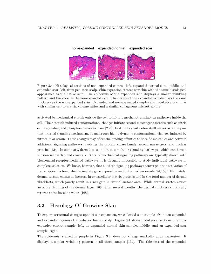
CHAPTER 3. REALISTIC, VOLUME CONTROLLED SKIN EXPANDER MODEL 51
and in the total number of dermal fibroblasts, which jointly re-sult in a net gain in dermal surface area. While dermal stretchcauses an acute thinning of the dermal layer [52], after severalmonths, the dermal thickness chronically returns to its baselinevalue [54].
2. HISTOLOGY OF GROWING SKIN
To explore structural changes upon tissue expansion, we col-lected skin samples from non-expanded and expanded regionsof a pediatric human scalp. Figure 4 shows histological sec-tions of a non-expanded control sample, left, an expanded nor-mal skin sample, middle, and an expanded scar sample, right.
non-expanded expanded normal expanded scar
Figure 4: Histological sections of non-expanded control, left, expanded nor-mal skin, middle, and expanded scar, left, from pediatric scalp. Skin expansioncreates new skin with the same histological appearance as the native skin: Theepidermis of the expanded skin displays a similar wrinkling pattern and thick-ness as the non-expanded skin. The dermis of the expanded skin displays thesame thickness as the non-expanded skin. Expanded and non-expanded sam-ples are histologically similar with similar cell-to-matrix volume ratios and asimilar collagenous microstructure.
The epidermis, stained in purple in Figure 4, does not changemarkedly upon expansion. It displays a similar wrinkling pat-tern in all three samples [38]. The thickness of the expandedepidermis is similar to the non-expanded epidermis. The ex-panded epidermis shows no evidence of necrosis, inflammation,or epidermal hyperplasia. Overall, we conclude that tissue ex-pansion initiates an increase in epidermal surface area at con-stant epidermal thickness through increased keratinocyte mito-sis. These observations are in excellent agreement with findingsreported in the literature [6, 18, 54]. Histological analyses in theliterature report that, long-term, neither the epidermal thicknessnor the number of epidermal layers undergo statistically signif-icant changes after tissue expansion [68, 70].Similar to the epidermis, the dermis, stained in pink in Figure4, does not change noticeably upon tissue expansion. The av-erage dermal thickness is 2.0 mm in the non-expanded sampleand 2.05 mm in the expanded samples. However, the expandeddermal thickness varies locally depending on the presence ofsubcutaneous adipocytes. The expanded dermis is histologi-cally similar to the non-expanded dermis with similar cell-to-matrix volume ratios and a similar loosely interwoven, wavy,randomly-oriented collagenous microstructure. It shows no ev-idence of inflammation, no evidence of malignant degenera-tion, and no loss of microstructural organization. Overall, weconclude that tissue expansion initiates an increase in dermal
surface area at constant dermal thickness through increased fi-broblast mitosis and increased collagen synthesis. These obser-vations are in agreement with findings reported in the literatureboth in animals [6, 52] and in humans [59].Unlike the epidermis and the dermis, the subcutaneous hypo-dermis undergoes significant changes upon tissue expansion.Subcutaneous adipocytes are compressed and diminished insize. This results in a significant net thinning of the sub-cutaneous layer. The expanded region itself undergoes sub-cutaneous fibrosis with a host inflammatory response. Subcuta-neous collagen fibers and fibroblasts reorient themselves paral-lel to the expander, which becomes surrounded by a thin layerof histiocytes. These observations agree nicely with findings inthe literature [6, 18, 52]. Histological analyses in the literaturereport flattening, shrinkage, and atrophy of adipocytes as wellas an acute thinning of the subcutaneous layer, which graduallyreturns to its baseline thickness within two years after comple-tion of the procedure [53].These histological observations have important consequenceswhen modeling skin growth: First, we can confidently assumethat the thickness of the epidermal and dermal layers does notchange when skin is subjected to controlled chronic overstretch.Second, we can assume that the newly grown skin has the samemicrostructure and the same mechanical properties as the orig-inal native tissue. Third, since the skin area increases and thethickness remains constant, skin undergoes significant changesin mass and can be modeled thermodynamically as an open sys-tem.
3. CONTINUUM MODELING OF GROWING SKIN
Motivated by the mechanobiology of growing skin summa-rized in Section 1 and by our histological study in Section 2,we now formulate a continuum model for controlled stretch-induced skin growth. To characterize the large deformationswhen stretching skin, we introduce the deformation map ',which maps points X from the undeformed configuration totheir new positions x = ' (X, t) in the deformed configuration.We can then characterize changes of infinitesimal line elementsthrough the deformation gradient,
F = rX
' = F
e · Fg , (1)
which we decompose multiplicatively into an elastic part F
e
and a growth part F
g [19, 60]. Similarly, we can characterizechanges in skin volume through the Jacobian,
J = det (F) = Je Jg , (2)
which we decompose into a reversibly elastic volume changeJe = det (F
e) and an irreversibly grown volume change Jg =det (F
g). Motivated by our histological analysis in Section 2,we assume that the response in the thickness direction n0 ispurely reversible and elastic. In the skin plane, orthogonal ton0, we characterize skin growth through a single scalar-valuedvariable, the surface area growth #g. This allows us to charac-terize changes in skin area through the area stretch,
# = || J F
�t · n0 || = #e #g , (3)
5
Figure 3.4: Histological sections of non-expanded control, left, expanded normal skin, middle, andexpanded scar, left, from pediatric scalp. Skin expansion creates new skin with the same histologicalappearance as the native skin: The epidermis of the expanded skin displays a similar wrinklingpattern and thickness as the non-expanded skin. The dermis of the expanded skin displays the samethickness as the non-expanded skin. Expanded and non-expanded samples are histologically similarwith similar cell-to-matrix volume ratios and a similar collagenous microstructure.
activated by mechanical stretch outside the cell to initiate mechanotransduction pathways inside the
cell. Their stretch-induced conformational changes initiate second messenger cascades such as nitric
oxide signaling and phosphoinositol-3-kinase [203]. Last, the cytoskeleton itself serves as an impor-
tant internal signaling mechanism. It undergoes highly dynamic conformational changes induced by
intracellular strain. These changes may a↵ect the binding a�nities to specific molecules and activate
additional signaling pathways involving the protein kinase family, second messengers, and nuclear
proteins [124]. In summary, dermal tension initiates multiple signaling pathways, which can have a
substantial overlap and crosstalk. Since biomechanical signaling pathways are typically shared with
biochemical receptor-mediated pathways, it is virtually impossible to study individual pathways in
complete isolation. We know, however, that all these signaling pathways converge in the activation of
transcription factors, which stimulate gene expression and other nuclear events [94,138]. Ultimately,
dermal tension causes an increase in extracellular matrix proteins and in the total number of dermal
fibroblasts, which jointly result in a net gain in dermal surface area. While dermal stretch causes
an acute thinning of the dermal layer [166], after several months, the dermal thickness chronically
returns to its baseline value [168].
3.2 Histology Of Growing Skin
To explore structural changes upon tissue expansion, we collected skin samples from non-expanded
and expanded regions of a pediatric human scalp. Figure 3.4 shows histological sections of a non-
expanded control sample, left, an expanded normal skin sample, middle, and an expanded scar
sample, right.
The epidermis, stained in purple in Figure 3.4, does not change markedly upon expansion. It
displays a similar wrinkling pattern in all three samples [134]. The thickness of the expanded
CHAPTER 3. REALISTIC, VOLUME CONTROLLED SKIN EXPANDER MODEL 52
epidermis is similar to the non-expanded epidermis. The expanded epidermis shows no evidence
of necrosis, inflammation, or epidermal hyperplasia. Overall, we conclude that tissue expansion
initiates an increase in epidermal surface area at constant epidermal thickness through increased
keratinocyte mitosis. These observations are in excellent agreement with findings reported in the
literature [15, 65, 168]. Histological analyses in the literature report that, long-term, neither the
epidermal thickness nor the number of epidermal layers undergo statistically significant changes
after tissue expansion [210,218].
Similar to the epidermis, the dermis, stained in pink in Figure 3.4, does not change noticeably upon
tissue expansion. The average dermal thickness is 2.0mm in the non-expanded sample and 2.05mm
in the expanded samples. However, the expanded dermal thickness varies locally depending on the
presence of subcutaneous adipocytes. The expanded dermis is histologically similar to the non-
expanded dermis with similar cell-to-matrix volume ratios and a similar loosely interwoven, wavy,
randomly-oriented collagenous microstructure. It shows no evidence of inflammation, no evidence
of malignant degeneration, and no loss of microstructural organization. Overall, we conclude that
tissue expansion initiates an increase in dermal surface area at constant dermal thickness through
increased fibroblast mitosis and increased collagen synthesis. These observations are in agreement
with findings reported in the literature both in animals [15, 166] and in humans [181].
Unlike the epidermis and the dermis, the subcutaneous hypodermis undergoes significant changes
upon tissue expansion. Subcutaneous adipocytes are compressed and diminished in size. This results
in a significant net thinning of the subcutaneous layer. The expanded region itself undergoes sub-
cutaneous fibrosis with a host inflammatory response. Subcutaneous collagen fibers and fibroblasts
reorient themselves parallel to the expander, which becomes surrounded by a thin layer of histiocytes.
These observations agree nicely with findings in the literature [15, 65, 166]. Histological analyses in
the literature report flattening, shrinkage, and atrophy of adipocytes as well as an acute thinning
of the subcutaneous layer, which gradually returns to its baseline thickness within two years after
completion of the procedure [167].
These histological observations have important consequences when modeling skin growth: First, we
can confidently assume that the thickness of the epidermal and dermal layers does not change when
skin is subjected to controlled chronic overstretch. Second, we can assume that the newly grown
skin has the same microstructure and the same mechanical properties as the original native tissue.
Third, since the skin area increases and the thickness remains constant, skin undergoes significant
changes in mass and can be modeled thermodynamically as an open system.
3.3 Continuum Modeling Of Growing Skin
Motivated by the mechanobiology of growing skin summarized in Section 3.1 and by our histological
study in Section 3.2, we now formulate a continuum model for controlled stretch-induced skin growth.
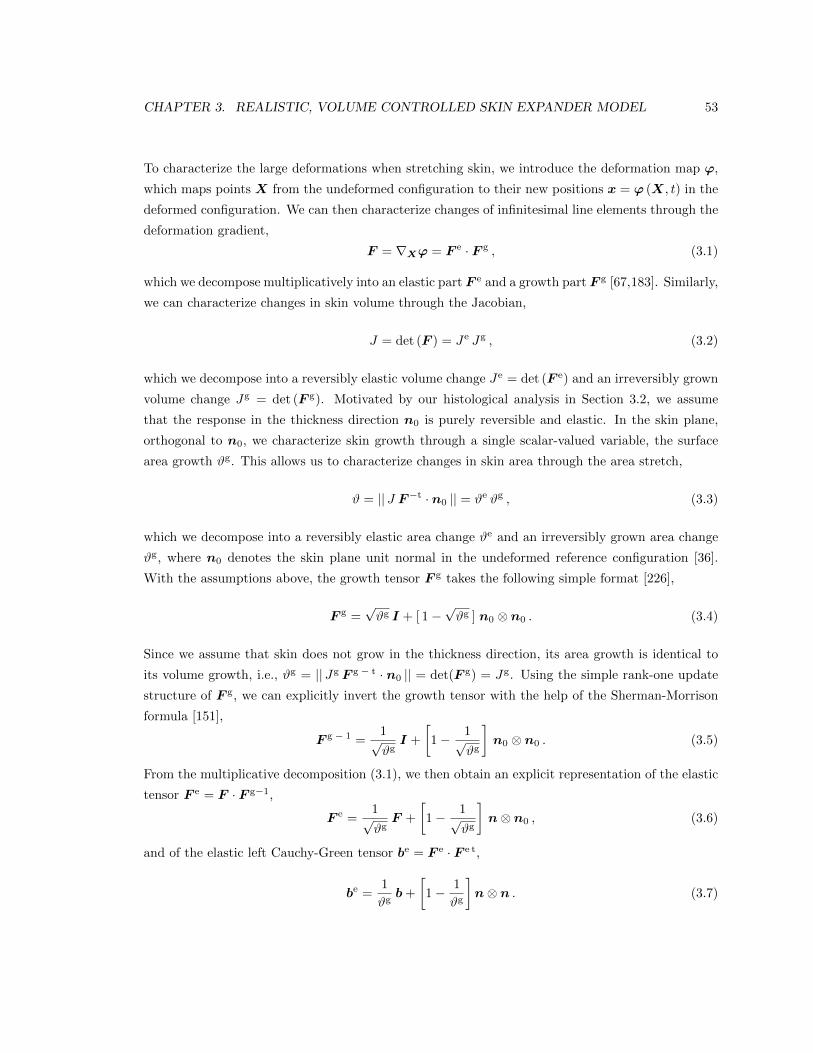
CHAPTER 3. REALISTIC, VOLUME CONTROLLED SKIN EXPANDER MODEL 53
To characterize the large deformations when stretching skin, we introduce the deformation map ',
which maps points X from the undeformed configuration to their new positions x = ' (X, t) in the
deformed configuration. We can then characterize changes of infinitesimal line elements through the
deformation gradient,
F = rX' = F
e · F g , (3.1)
which we decompose multiplicatively into an elastic part F e and a growth part F g [67,183]. Similarly,
we can characterize changes in skin volume through the Jacobian,
J = det (F ) = Je Jg , (3.2)
which we decompose into a reversibly elastic volume change Je = det (F e) and an irreversibly grown
volume change Jg = det (F g). Motivated by our histological analysis in Section 3.2, we assume
that the response in the thickness direction n0 is purely reversible and elastic. In the skin plane,
orthogonal to n0, we characterize skin growth through a single scalar-valued variable, the surface
area growth #g. This allows us to characterize changes in skin area through the area stretch,
# = || J F
�t · n0 || = #e #g , (3.3)
which we decompose into a reversibly elastic area change #e and an irreversibly grown area change
#g, where n0 denotes the skin plane unit normal in the undeformed reference configuration [36].
With the assumptions above, the growth tensor F g takes the following simple format [226],
F
g =p#g I + [ 1�
p#g ] n0 ⌦ n0 . (3.4)
Since we assume that skin does not grow in the thickness direction, its area growth is identical to
its volume growth, i.e., #g = || JgF
g � t · n0 || = det(F g) = Jg. Using the simple rank-one update
structure of F g, we can explicitly invert the growth tensor with the help of the Sherman-Morrison
formula [151],
F
g � 1 =1p#g
I +
1� 1p
#g
�n0 ⌦ n0 . (3.5)
From the multiplicative decomposition (3.1), we then obtain an explicit representation of the elastic
tensor F e = F · F g�1,
F
e =1p#g
F +
1� 1p
#g
�n⌦ n0 , (3.6)
and of the elastic left Cauchy-Green tensor be = F
e · F e t,
b
e =1
#gb+
1� 1
#g
�n⌦ n . (3.7)
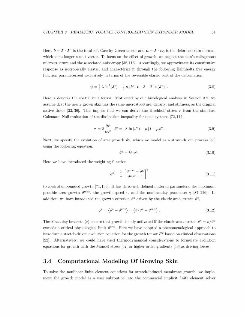
CHAPTER 3. REALISTIC, VOLUME CONTROLLED SKIN EXPANDER MODEL 54
Here, b = F ·F t is the total left Cauchy-Green tensor and n = F ·n0 is the deformed skin normal,
which is no longer a unit vector. To focus on the e↵ect of growth, we neglect the skin’s collagenous
microstructure and the associated anisotropy [38,116]. Accordingly, we approximate its constitutive
response as isotropically elastic, and characterize it through the following Helmholtz free energy
function parameterized exclusively in terms of the reversible elastic part of the deformation,
= 12 � ln2(Je) + 1
2 µ [ be : i� 3� 2 ln (Je) ] . (3.8)
Here, i denotes the spatial unit tensor. Motivated by our histological analysis in Section 3.2, we
assume that the newly grown skin has the same microstructure, density, and sti↵ness, as the original
native tissue [22, 36]. This implies that we can derive the Kirchho↵ stress ⌧ from the standard
Colemann-Noll evaluation of the dissipation inequality for open systems [72,112],
⌧ = 2@
@be· be = [� ln (Je)� µ ] i+ µ b
e . (3.9)
Next, we specify the evolution of area growth #g, which we model as a strain-driven process [83]
using the following equation,
#g = kg �g . (3.10)
Here we have introduced the weighting function
kg =1
⌧
#max � #g
#max � 1
��
(3.11)
to control unbounded growth [71,139]. It has three well-defined material parameters, the maximum
possible area growth #max, the growth speed ⌧ , and the nonlinearity parameter � [87, 226]. In
addition, we have introduced the growth criterion �g driven by the elastic area stretch #e,
�g =⌦#e � #crit
↵=
⌦#/#g � #crit
↵. (3.12)
The Macaulay brackets h�i ensure that growth is only activated if the elastic area stretch #e = #/#g
exceeds a critical physiological limit #crit. Here we have adopted a phenomenological approach to
introduce a stretch-driven evolution equation for the growth tensor F g based on clinical observations
[22]. Alternatively, we could have used thermodynamical considerations to formulate evolution
equations for growth with the Mandel stress [62] or higher order gradients [48] as driving forces.
3.4 Computational Modeling Of Growing Skin
To solve the nonlinear finite element equations for stretch-induced membrane growth, we imple-
ment the growth model as a user subroutine into the commercial implicit finite element solver
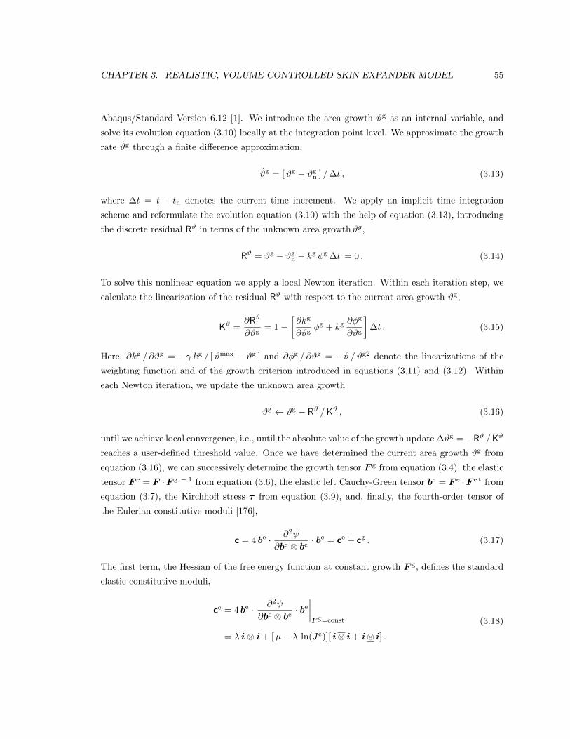
CHAPTER 3. REALISTIC, VOLUME CONTROLLED SKIN EXPANDER MODEL 55
Abaqus/Standard Version 6.12 [1]. We introduce the area growth #g as an internal variable, and
solve its evolution equation (3.10) locally at the integration point level. We approximate the growth
rate #g through a finite di↵erence approximation,
#g = [#g � #gn ] /�t , (3.13)
where �t = t � tn denotes the current time increment. We apply an implicit time integration
scheme and reformulate the evolution equation (3.10) with the help of equation (3.13), introducing
the discrete residual R# in terms of the unknown area growth#g,
R# = #g � #gn � kg �g �t.= 0 . (3.14)
To solve this nonlinear equation we apply a local Newton iteration. Within each iteration step, we
calculate the linearization of the residual R# with respect to the current area growth #g,
K# =@R#
@#g= 1�
@kg
@#g�g + kg
@�g
@#g
��t . (3.15)
Here, @kg / @#g = �� kg / [#max � #g ] and @�g / @#g = �# /#g2 denote the linearizations of the
weighting function and of the growth criterion introduced in equations (3.11) and (3.12). Within
each Newton iteration, we update the unknown area growth
#g #g � R# /K# , (3.16)
until we achieve local convergence, i.e., until the absolute value of the growth update�#g = �R# /K#
reaches a user-defined threshold value. Once we have determined the current area growth #g from
equation (3.16), we can successively determine the growth tensor F g from equation (3.4), the elastic
tensor F e = F ·F g � 1 from equation (3.6), the elastic left Cauchy-Green tensor be = F
e ·F e t from
equation (3.7), the Kirchho↵ stress ⌧ from equation (3.9), and, finally, the fourth-order tensor of
the Eulerian constitutive moduli [176],
c = 4 be · @2
@be ⌦ b
e· be = c
e + c
g . (3.17)
The first term, the Hessian of the free energy function at constant growth F
g, defines the standard
elastic constitutive moduli,
c
e = 4 be · @2
@be ⌦ b
e· be
����F g=const
= � i⌦ i+ [µ� � ln(Je)][ i⌦ i+ i⌦ i] .
(3.18)
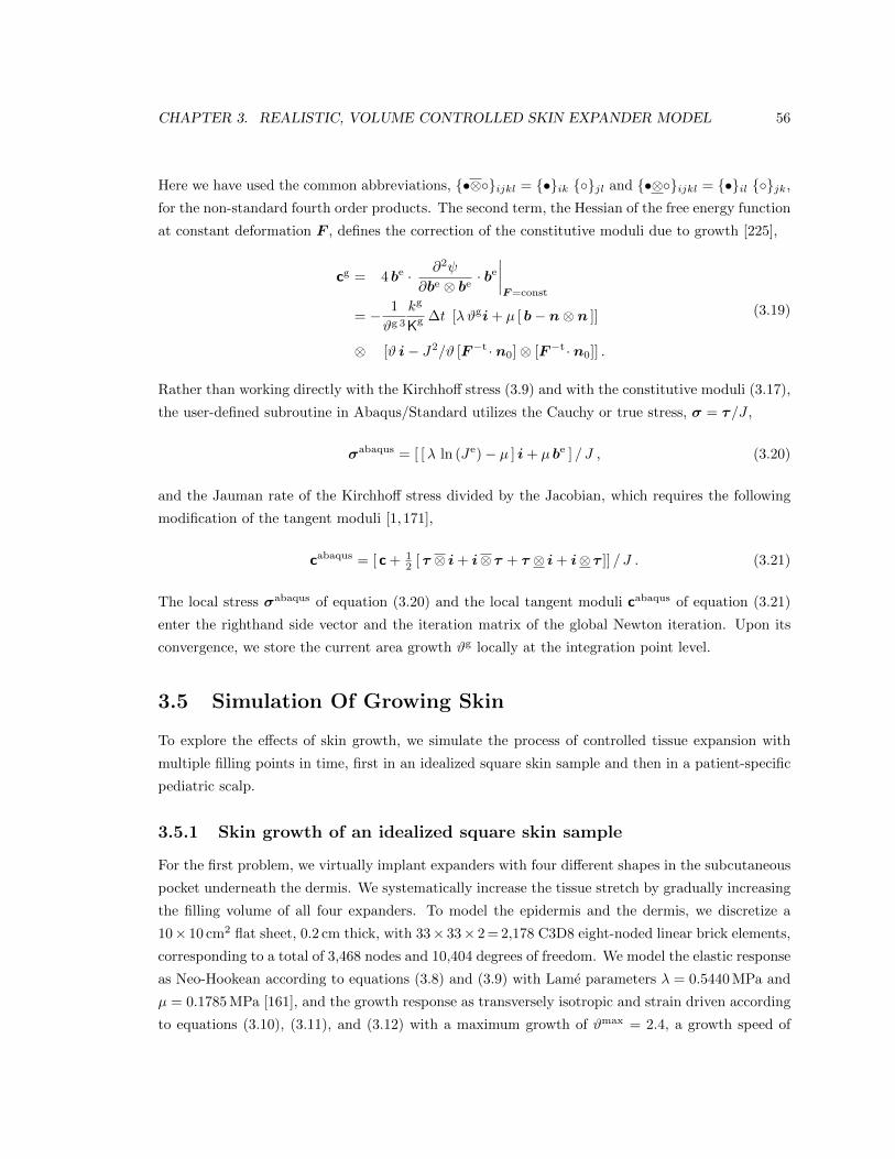
CHAPTER 3. REALISTIC, VOLUME CONTROLLED SKIN EXPANDER MODEL 56
Here we have used the common abbreviations, {•⌦�}ijkl
= {•}ik
{�}jl
and {•⌦�}ijkl
= {•}il
{�}jk
,
for the non-standard fourth order products. The second term, the Hessian of the free energy function
at constant deformation F , defines the correction of the constitutive moduli due to growth [225],
c
g = 4 be · @2
@be ⌦ b
e· be
����F=const
= � 1
#g 3
kg
Kg �t [�#gi+ µ [ b� n⌦ n ]]
⌦ [# i� J2/# [F�t · n0]⌦ [F�t · n0]] .
(3.19)
Rather than working directly with the Kirchho↵ stress (3.9) and with the constitutive moduli (3.17),
the user-defined subroutine in Abaqus/Standard utilizes the Cauchy or true stress, � = ⌧/J ,
�
abaqus = [ [� ln (Je)� µ ] i+ µ b
e ] / J , (3.20)
and the Jauman rate of the Kirchho↵ stress divided by the Jacobian, which requires the following
modification of the tangent moduli [1, 171],
c
abaqus = [ c+ 12 [ ⌧ ⌦ i+ i⌦ ⌧ + ⌧ ⌦ i+ i⌦ ⌧ ]] / J . (3.21)
The local stress �
abaqus of equation (3.20) and the local tangent moduli cabaqus of equation (3.21)
enter the righthand side vector and the iteration matrix of the global Newton iteration. Upon its
convergence, we store the current area growth #g locally at the integration point level.
3.5 Simulation Of Growing Skin
To explore the e↵ects of skin growth, we simulate the process of controlled tissue expansion with
multiple filling points in time, first in an idealized square skin sample and then in a patient-specific
pediatric scalp.
3.5.1 Skin growth of an idealized square skin sample
For the first problem, we virtually implant expanders with four di↵erent shapes in the subcutaneous
pocket underneath the dermis. We systematically increase the tissue stretch by gradually increasing
the filling volume of all four expanders. To model the epidermis and the dermis, we discretize a
10⇥ 10 cm2 flat sheet, 0.2 cm thick, with 33⇥ 33⇥ 2=2,178 C3D8 eight-noded linear brick elements,
corresponding to a total of 3,468 nodes and 10,404 degrees of freedom. We model the elastic response
as Neo-Hookean according to equations (3.8) and (3.9) with Lame parameters � = 0.5440MPa and
µ = 0.1785MPa [161], and the growth response as transversely isotropic and strain driven according
to equations (3.10), (3.11), and (3.12) with a maximum growth of #max = 2.4, a growth speed of
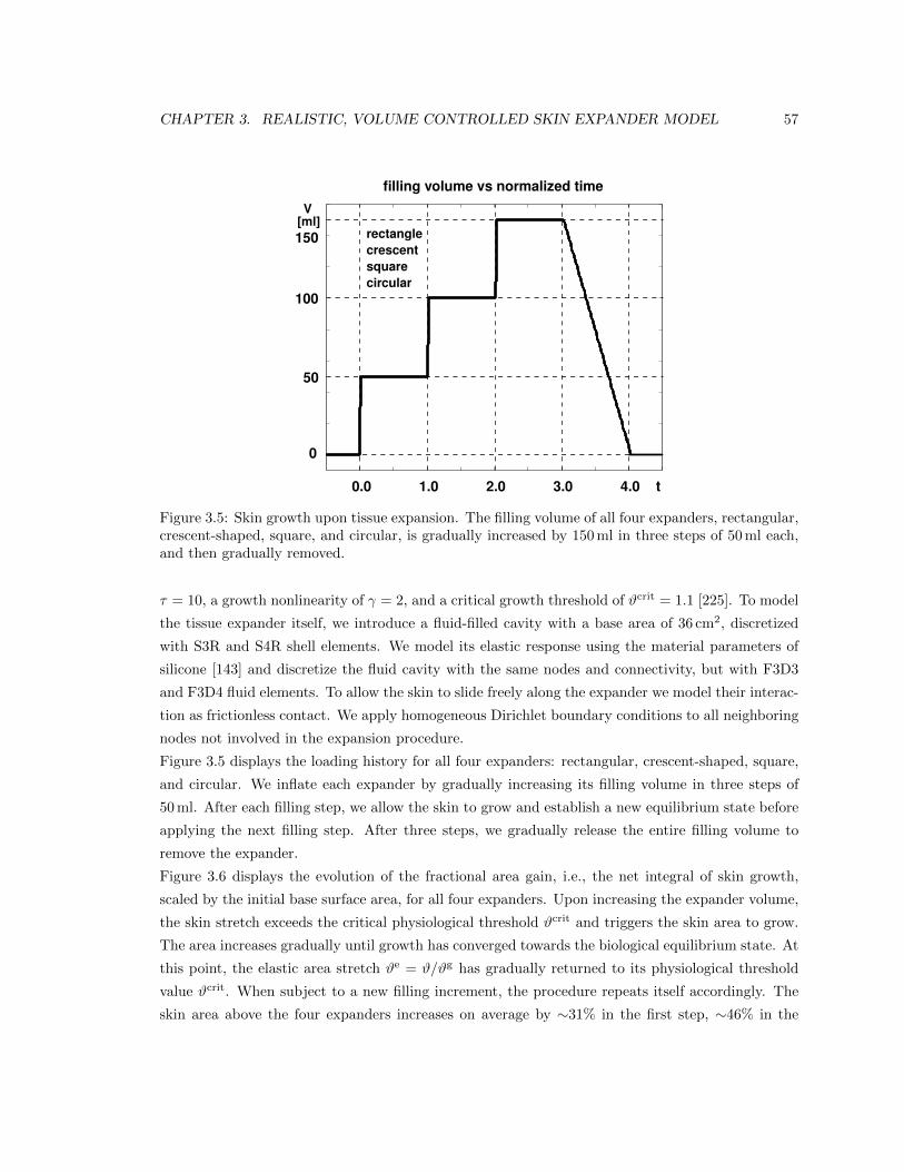
CHAPTER 3. REALISTIC, VOLUME CONTROLLED SKIN EXPANDER MODEL 57
The first term, the Hessian of the free energy function at con-stant growth F
g, defines the standard elastic constitutive mod-uli,
ce = 4 b
e · @2
@b
e ⌦ b
e · be
������F
g=const
= � i ⌦ i + [ µ � � ln(Je)][ i⌦ i + i⌦ i] .
(18)
Here we have used the common abbreviations, {•⌦�}i jkl ={•}ik {�} jl and {•⌦�}i jkl = {•}il {�} jk, for the non-standard fourthorder products. The second term, the Hessian of the free en-ergy function at constant deformation F, defines the correctionof the constitutive moduli due to growth [72],
cg = 4 b
e · @2
@b
e ⌦ b
e · be
������F=const
= � 1#g 3
kg
K
g �t⇥�#g
i + µ [ b � n⌦ n ]⇤
⌦ [# i � J2/# [F
�t · n0] ⌦ [F
�t · n0]] .
(19)
Rather than working directly with the Kirchho↵ stress (9) andwith the constitutive moduli (17), the user-defined subroutinein Abaqus/Standard utilizes the Cauchy or true stress, � = ⌧/J,
�abaqus = [ [ � ln (Je) � µ ] i + µ b
e ] / J , (20)
and the Jauman rate of the Kirchho↵ stress divided by the Jaco-bian, which requires the following modification of the tangentmoduli [1, 55],
cabaqus = [ c + 12 [ ⌧⌦ i + i⌦ ⌧ + ⌧⌦ i + i⌦ ⌧]] / J . (21)
The local stress �abaqus of equation (20) and the local tangentmoduli cabaqus of equation (21) enter the righthand side vectorand the iteration matrix of the global Newton iteration. Uponits convergence, we store the current area growth #g locally atthe integration point level.
5. SIMULATION OF GROWING SKIN
To explore the e↵ects of skin growth, we simulate the process ofcontrolled tissue expansion with multiple filling points in time,first in an idealized square skin sample and then in a patient-specific pediatric scalp.
5.1. Skin growth of an idealized square skin sampleFor the first problem, we virtually implant expanders with fourdi↵erent shapes in the subcutaneous pocket underneath the der-mis. We systematically increase the tissue stretch by graduallyincreasing the filling volume of all four expanders. To modelthe epidermis and the dermis, we discretize a 10⇥ 10 cm2 flatsheet, 0.2 cm thick, with 33⇥ 33⇥ 2= 2,178 C3D8 eight-nodedlinear brick elements, corresponding to a total of 3,468 nodesand 10,404 degrees of freedom. We model the elastic responseas Neo-Hookean according to equations (8) and (9) with Lameparameters � = 0.5440 MPa and µ = 0.1785 MPa [48], andthe growth response as transversely isotropic and strain drivenaccording to equations (10), (11), and (12) with a maximum
growth of #max = 2.4, a growth speed of ⌧ = 10, a growth non-linearity of � = 2, and a critical growth threshold of #crit = 1.1[72]. To model the tissue expander itself, we introduce a fluid-filled cavity with a base area of 36 cm2, discretized with S3Rand S4R shell elements. We model its elastic response usingthe material parameters of silicone [42] and discretize the fluidcavity with the same nodes and connectivity, but with F3D3 andF3D4 fluid elements. To allow the skin to slide freely along theexpander we model their interaction as frictionless contact. Weapply homogeneous Dirichlet boundary conditions to all neigh-boring nodes not involved in the expansion procedure.
filling volume vs normalized time
0.5 1 1.5 2 2.5 3 3.5 4 4.5 5 5.5
0
20
40
60
80
100
120
140
160
V[ml]150
100
50
0
0.0 1.0 2.0 3.0 4.0 t
rectanglecrescentsquarecircular
Figure 5: Skin growth upon tissue expansion. The filling volume of all fourexpanders, rectangular, crescent-shaped, square, and circular, is gradually in-creased by 150 ml in three steps of 50 ml each, and then gradually removed.
Figure 5 displays the loading history for all four expanders:rectangular, crescent-shaped, square, and circular. We inflateeach expander by gradually increasing its filling volume in threesteps of 50 ml. After each filling step, we allow the skin to growand establish a new equilibrium state before applying the nextfilling step. After three steps, we gradually release the entirefilling volume to remove the expander.Figure 6 displays the evolution of the fractional area gain, i.e.,the net integral of skin growth, scaled by the initial base sur-face area, for all four expanders. Upon increasing the ex-pander volume, the skin stretch exceeds the critical physiolog-ical threshold #crit and triggers the skin area to grow. The areaincreases gradually until growth has converged towards the bi-ological equilibrium state. At this point, the elastic area stretch#e = #/#g has gradually returned to its physiological thresholdvalue #crit. When subject to a new filling increment, the pro-cedure repeats itself accordingly. The skin area above the fourexpanders increases on average by ⇠31% in the first step, ⇠46%in the second step, and ⇠25% in the third step. This illustratesthe nonlinear nature of the growth process. When the fillingvolume is removed, the fractional area gain remains constant.This illustrates the irreversible nature of the growth process. Atthe end of the procedure, the rectangular expander has initiated
7
Figure 3.5: Skin growth upon tissue expansion. The filling volume of all four expanders, rectangular,crescent-shaped, square, and circular, is gradually increased by 150ml in three steps of 50ml each,and then gradually removed.
⌧ = 10, a growth nonlinearity of � = 2, and a critical growth threshold of #crit = 1.1 [225]. To model
the tissue expander itself, we introduce a fluid-filled cavity with a base area of 36 cm2, discretized
with S3R and S4R shell elements. We model its elastic response using the material parameters of
silicone [143] and discretize the fluid cavity with the same nodes and connectivity, but with F3D3
and F3D4 fluid elements. To allow the skin to slide freely along the expander we model their interac-
tion as frictionless contact. We apply homogeneous Dirichlet boundary conditions to all neighboring
nodes not involved in the expansion procedure.
Figure 3.5 displays the loading history for all four expanders: rectangular, crescent-shaped, square,
and circular. We inflate each expander by gradually increasing its filling volume in three steps of
50ml. After each filling step, we allow the skin to grow and establish a new equilibrium state before
applying the next filling step. After three steps, we gradually release the entire filling volume to
remove the expander.
Figure 3.6 displays the evolution of the fractional area gain, i.e., the net integral of skin growth,
scaled by the initial base surface area, for all four expanders. Upon increasing the expander volume,
the skin stretch exceeds the critical physiological threshold #crit and triggers the skin area to grow.
The area increases gradually until growth has converged towards the biological equilibrium state. At
this point, the elastic area stretch #e = #/#g has gradually returned to its physiological threshold
value #crit. When subject to a new filling increment, the procedure repeats itself accordingly. The
skin area above the four expanders increases on average by ⇠31% in the first step, ⇠46% in the
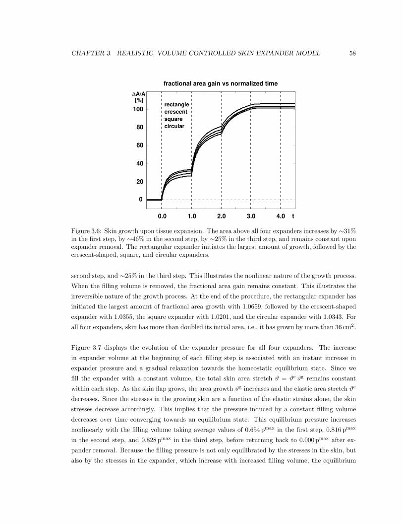
CHAPTER 3. REALISTIC, VOLUME CONTROLLED SKIN EXPANDER MODEL 58
fractional area gain vs normalized time
0.5 1 1.5 2 2.5 3 3.5 4 4.5 5 5.5
1
1.2
1.4
1.6
1.8
2
2.2
�A/A[%]
100
80
60
40
20
0
0.0 1.0 2.0 3.0 4.0 t
rectanglecrescentsquarecircular
Figure 6: Skin growth upon tissue expansion. The area above all four expandersincreases by ⇠31% in the first step, by ⇠46% in the second step, by ⇠25% in thethird step, and remains constant upon expander removal. The rectangular ex-pander initiates the largest amount of growth, followed by the crescent-shaped,square, and circular expanders.
the largest amount of fractional area growth with 1.0659, fol-lowed by the crescent-shaped expander with 1.0355, the squareexpander with 1.0201, and the circular expander with 1.0343.For all four expanders, skin has more than doubled its initialarea, i.e., it has grown by more than 36 cm2.Figure 7 displays the evolution of the expander pressure for allfour expanders. The increase in expander volume at the begin-ning of each filling step is associated with an instant increase inexpander pressure and a gradual relaxation towards the homeo-static equilibrium state. Since we fill the expander with a con-stant volume, the total skin area stretch # = #e #g remains con-stant within each step. As the skin flap grows, the area growth#g increases and the elastic area stretch #e decreases. Since thestresses in the growing skin are a function of the elastic strainsalone, the skin stresses decrease accordingly. This implies thatthe pressure induced by a constant filling volume decreases overtime converging towards an equilibrium state. This equilibriumpressure increases nonlinearly with the filling volume taking av-erage values of 0.654 pmax in the first step, 0.816 pmax in the sec-ond step, and 0.828 pmax in the third step, before returning backto 0.000 pmax after expander removal. Because the filling pres-sure is not only equilibrated by the stresses in the skin, but alsoby the stresses in the expander, which increase with increasedfilling volume, the equilibrium pressure increases with volume.The rectangular expander is subject to the largest pressure witha maximum value of 0.3752 MPa, followed by the crescent-shaped expander with 0.3637 MPa, the square expander with0.3087 MPa, and circular expander with 0.2879 MPa.Figure 8 displays the spatio-temporal evolution of the growthmultiplier #g for the rectangular, crescent-shaped, square, andcircular expanders, from top to bottom. The individual snap-shots correspond to the converged equilibrium states for filling
normalized expander pressure vs normalized time
p/pmax
[%]
80
60
40
20
0
0.0 1.0 2.0 3.0 4.0 t
rectanglecrescentsquarecircular
Figure 7: Skin growth upon tissue expansion. The expander pressure of allfour expanders increases instantly upon inflation and relaxes gradually as skingrows in area and the elastic strain decreases. The rectangular expander issubject to the largest pressured, followed by the crescent-shaped, square, andcircular expanders.
volumes of 50 ml, 100 ml, and 150 ml, and to the deflated statewith the filling volume reduced to 0 ml, from left to right. Skingrowth displays significant regional variations. Largest growthtakes place in the center region with values up to #g = 2.25,shown in red, indicating that the initial area has more than dou-bled in size. Smallest growth takes place along the expanderedges with values of #g = 1.00, shown in blue, indicating thatno growth has taken place at all.Figure 9 displays the spatio-temporal evolution of the normal-ized von Mises stress �/�max for the rectangular, crescent-shaped, square, and circular expanders, from top to bottom. Theindividual snapshots correspond to the converged equilibriumstates for filling volumes of 50 ml, 100 ml, and 150 ml, and tothe deflated state with the filling volume reduced to 0 ml, fromleft to right. To illustrate the individual skin expanders, we havevirtually removed the lower corner of the skin patch. For thesame filling volume and the same base surface area, the rect-angular expander initiates the largest stresses, followed by thecrescent-shaped, square, and circular expanders. Stresses dis-play significant regional variations. Largest stresses are locatedin the center region and along the expander edges, shown inred. Moderate stresses are located at the expander sides, shownin green. No stresses occur in the unexpanded regions, shownin blue.
5.2. Skin growth of a pediatric scalp
For the second problem, we closely follow a clinical tissue ex-pansion protocol and simulate skin growth in the scalp of thepediatric patient shown in Figure 1. We virtually insert a rect-angular expander with a base surface area of 14 ⇥ 10 cm2 in asubcutaneous pocket of the frontoparietal scalp. The expanderhas a filling capacity of 450 ml, which we reach gradually by in-
8
Figure 3.6: Skin growth upon tissue expansion. The area above all four expanders increases by ⇠31%in the first step, by ⇠46% in the second step, by ⇠25% in the third step, and remains constant uponexpander removal. The rectangular expander initiates the largest amount of growth, followed by thecrescent-shaped, square, and circular expanders.
second step, and ⇠25% in the third step. This illustrates the nonlinear nature of the growth process.
When the filling volume is removed, the fractional area gain remains constant. This illustrates the
irreversible nature of the growth process. At the end of the procedure, the rectangular expander has
initiated the largest amount of fractional area growth with 1.0659, followed by the crescent-shaped
expander with 1.0355, the square expander with 1.0201, and the circular expander with 1.0343. For
all four expanders, skin has more than doubled its initial area, i.e., it has grown by more than 36 cm2.
Figure 3.7 displays the evolution of the expander pressure for all four expanders. The increase
in expander volume at the beginning of each filling step is associated with an instant increase in
expander pressure and a gradual relaxation towards the homeostatic equilibrium state. Since we
fill the expander with a constant volume, the total skin area stretch # = #e #g remains constant
within each step. As the skin flap grows, the area growth #g increases and the elastic area stretch #e
decreases. Since the stresses in the growing skin are a function of the elastic strains alone, the skin
stresses decrease accordingly. This implies that the pressure induced by a constant filling volume
decreases over time converging towards an equilibrium state. This equilibrium pressure increases
nonlinearly with the filling volume taking average values of 0.654 pmax in the first step, 0.816 pmax
in the second step, and 0.828 pmax in the third step, before returning back to 0.000 pmax after ex-
pander removal. Because the filling pressure is not only equilibrated by the stresses in the skin, but
also by the stresses in the expander, which increase with increased filling volume, the equilibrium
CHAPTER 3. REALISTIC, VOLUME CONTROLLED SKIN EXPANDER MODEL 59
fractional area gain vs normalized time�A/A[%]
100
80
60
40
20
0
0.0 1.0 2.0 3.0 4.0 t
rectanglecrescentsquarecircular
Figure 6: Skin growth upon tissue expansion. The area above all four expandersincreases by ⇠31% in the first step, by ⇠46% in the second step, by ⇠25% in thethird step, and remains constant upon expander removal. The rectangular ex-pander initiates the largest amount of growth, followed by the crescent-shaped,square, and circular expanders.
the largest amount of fractional area growth with 1.0659, fol-lowed by the crescent-shaped expander with 1.0355, the squareexpander with 1.0201, and the circular expander with 1.0343.For all four expanders, skin has more than doubled its initialarea, i.e., it has grown by more than 36 cm2.Figure 7 displays the evolution of the expander pressure for allfour expanders. The increase in expander volume at the begin-ning of each filling step is associated with an instant increase inexpander pressure and a gradual relaxation towards the homeo-static equilibrium state. Since we fill the expander with a con-stant volume, the total skin area stretch # = #e #g remains con-stant within each step. As the skin flap grows, the area growth#g increases and the elastic area stretch #e decreases. Since thestresses in the growing skin are a function of the elastic strainsalone, the skin stresses decrease accordingly. This implies thatthe pressure induced by a constant filling volume decreases overtime converging towards an equilibrium state. This equilibriumpressure increases nonlinearly with the filling volume taking av-erage values of 0.654 pmax in the first step, 0.816 pmax in the sec-ond step, and 0.828 pmax in the third step, before returning backto 0.000 pmax after expander removal. Because the filling pres-sure is not only equilibrated by the stresses in the skin, but alsoby the stresses in the expander, which increase with increasedfilling volume, the equilibrium pressure increases with volume.The rectangular expander is subject to the largest pressure witha maximum value of 0.3752 MPa, followed by the crescent-shaped expander with 0.3637 MPa, the square expander with0.3087 MPa, and circular expander with 0.2879 MPa.Figure 8 displays the spatio-temporal evolution of the growthmultiplier #g for the rectangular, crescent-shaped, square, andcircular expanders, from top to bottom. The individual snap-shots correspond to the converged equilibrium states for filling
normalized expander pressure vs normalized time
0.5 1 1.5 2 2.5 3 3.5 4 4.5 5 5.5
0
0.1
0.2
0.3
0.4
0.5
0.6
0.7
0.8
0.9
1
p/pmax
[%]
80
60
40
20
0
0.0 1.0 2.0 3.0 4.0 t
rectanglecrescentsquarecircular
Figure 7: Skin growth upon tissue expansion. The expander pressure of allfour expanders increases instantly upon inflation and relaxes gradually as skingrows in area and the elastic strain decreases. The rectangular expander issubject to the largest pressured, followed by the crescent-shaped, square, andcircular expanders.
volumes of 50 ml, 100 ml, and 150 ml, and to the deflated statewith the filling volume reduced to 0 ml, from left to right. Skingrowth displays significant regional variations. Largest growthtakes place in the center region with values up to #g = 2.25,shown in red, indicating that the initial area has more than dou-bled in size. Smallest growth takes place along the expanderedges with values of #g = 1.00, shown in blue, indicating thatno growth has taken place at all.Figure 9 displays the spatio-temporal evolution of the normal-ized von Mises stress �/�max for the rectangular, crescent-shaped, square, and circular expanders, from top to bottom. Theindividual snapshots correspond to the converged equilibriumstates for filling volumes of 50 ml, 100 ml, and 150 ml, and tothe deflated state with the filling volume reduced to 0 ml, fromleft to right. To illustrate the individual skin expanders, we havevirtually removed the lower corner of the skin patch. For thesame filling volume and the same base surface area, the rect-angular expander initiates the largest stresses, followed by thecrescent-shaped, square, and circular expanders. Stresses dis-play significant regional variations. Largest stresses are locatedin the center region and along the expander edges, shown inred. Moderate stresses are located at the expander sides, shownin green. No stresses occur in the unexpanded regions, shownin blue.
5.2. Skin growth of a pediatric scalp
For the second problem, we closely follow a clinical tissue ex-pansion protocol and simulate skin growth in the scalp of thepediatric patient shown in Figure 1. We virtually insert a rect-angular expander with a base surface area of 14 ⇥ 10 cm2 in asubcutaneous pocket of the frontoparietal scalp. The expanderhas a filling capacity of 450 ml, which we reach gradually by in-
8
Figure 3.7: Skin growth upon tissue expansion. The expander pressure of all four expanders increasesinstantly upon inflation and relaxes gradually as skin grows in area and the elastic strain decreases.The rectangular expander is subject to the largest pressured, followed by the crescent-shaped, square,and circular expanders.
pressure increases with volume. The rectangular expander is subject to the largest pressure with
a maximum value of 0.3752MPa, followed by the crescent-shaped expander with 0.3637MPa, the
square expander with 0.3087MPa, and circular expander with 0.2879MPa.
Figure 3.8 displays the spatio-temporal evolution of the growth multiplier #g for the rectangular,
crescent-shaped, square, and circular expanders, from top to bottom. The individual snapshots
correspond to the converged equilibrium states for filling volumes of 50ml, 100ml, and 150ml, and
to the deflated state with the filling volume reduced to 0ml, from left to right. Skin growth displays
significant regional variations. Largest growth takes place in the center region with values up to
#g = 2.25, shown in red, indicating that the initial area has more than doubled in size. Smallest
growth takes place along the expander edges with values of #g = 1.00, shown in blue, indicating
that no growth has taken place at all.
Figure 3.9 displays the spatio-temporal evolution of the normalized von Mises stress �/�max for the
rectangular, crescent-shaped, square, and circular expanders, from top to bottom. The individual
snapshots correspond to the converged equilibrium states for filling volumes of 50ml, 100ml, and
150ml, and to the deflated state with the filling volume reduced to 0ml, from left to right. To illus-
trate the individual skin expanders, we have virtually removed the lower corner of the skin patch.
For the same filling volume and the same base surface area, the rectangular expander initiates the
largest stresses, followed by the crescent-shaped, square, and circular expanders. Stresses display
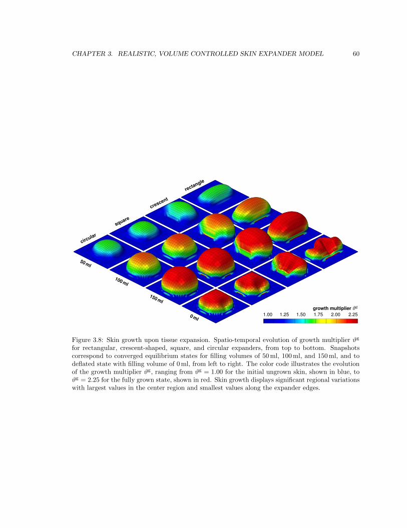
CHAPTER 3. REALISTIC, VOLUME CONTROLLED SKIN EXPANDER MODEL 60
growth multiplier #g
1.00 1.25 1.50 1.75 2.00 2.25
circular
square
crescent
rectangle
50 ml
100 ml
150 ml
0 ml
Figure 8: Skin growth upon tissue expansion. Spatio-temporal evolution of growth multiplier #g for rectangular, crescent-shaped, square, and circular expanders,from top to bottom. Snapshots correspond to converged equilibrium states for filling volumes of 50 ml, 100 ml, and 150 ml, and to deflated state with filling volumeof 0 ml, from left to right. The color code illustrates the evolution of the growth multiplier #g, ranging from #g = 1.00 for the initial ungrown skin, shown in blue,to #g = 2.25 for the fully grown state, shown in red. Skin growth displays significant regional variations with largest values in the center region and smallest valuesalong the expander edges.
creasing the filling volume in three consecutive steps of 150 mleach. To model the epidermis and the dermis, we discretizethe skin on top of the expander as a 14 ⇥ 10 cm2 large, 0.2cmthick layer with 45⇥ 32⇥ 2= 2,880 C3D8 eight-noded linearbrick elements, corresponding to a total of 4,554 nodes and13,662 degrees of freedom. Similar to the idealized squareskin sample in Section 5.1, we model the elastic response asNeo-Hookean according to equations (8) and (9) with Lameparameters � = 0.5440 MPa and µ = 0.1785 MPa [48], andthe growth response as transversely isotropic and strain drivenaccording to equations (10), (11), and (12) with a maximumgrowth of #max = 2.4, a growth speed of ⌧ = 10, a growth non-linearity of � = 2, and a critical growth threshold of #crit = 1.1[72]. We model the skin expander as a fluid-filled cavity with abase area of 14 ⇥ 10 cm2, discretized with 638 S4R shell ele-ments, corresponding to a total of 640 nodes and 1,920 degreesof freedom. We model its elastic response using the materialparameters of silicone [42] and discretize the fluid cavity withthe same nodes and connectivity, but with F3D4 fluid elements.We allow the skin to slide freely along the expander and modelthe skin-expander interaction as frictionless contact. We fix allnodes that are not involved in the expansion procedure usinghomogeneous Dirichlet boundary conditions.Figure 10 displays the spatio-temporal evolution of the growthmultiplier #g immediately after filling, bottom row, and afterconverged growth, top row. The individual snapshots corre-spond to the initial filled states and the converged homeostaticequilibrium states for filling volumes of 150 ml, 300 ml, and450 ml, and to deflated state with filling volume of 0 ml, from
left to right. Similar to the idealized square skin sample in Sec-tion 5.1, skin growth displays regional variations in magnitudewith largest values in the center region, shown in red, and small-est values along the expander edges, shown in blue.
6. DISCUSSION
6.1. Discussion of results
We have presented a constitutive model for overstretch-inducedskin growth, which allows us to predict chronic changes instress, strain, and area gain in thin biological membranes. Uponexpander inflation, our model predicts an acute increase in thetotal area stretch # = #e#g, associated with an acute decreasein skin thickness. Inititally, in the absence of growth #g = 0,the total stretch is carried exclusively by the elastic stretch#e = #, which increases acutely. Since the skin stress ⌧ (b
e) isa function of the elastic part of the deformation only, the acuteincrease in elastic stretch induces an acute increase in tissuestress, and accordingly, an acute increase in the expander pres-sure, see Figure 7.Over time, our model predicts a chronic increase in area growth#g, see Figures 6, 9, and 10. Since we drive expander inflationby controlling the filling volume, as shown in Figure 5, the to-tal area stretch # = #e#g remains constant between two fillingsessions. Accordingly, a chronic increase of the area growth#g " implies a chronic decrease of the elastic area stretch #e #,which gradually returns to its homeostatic equilibrium value#e ! #crit. Similarly, the model predicts a gradual return of
9
Figure 3.8: Skin growth upon tissue expansion. Spatio-temporal evolution of growth multiplier #g
for rectangular, crescent-shaped, square, and circular expanders, from top to bottom. Snapshotscorrespond to converged equilibrium states for filling volumes of 50ml, 100ml, and 150ml, and todeflated state with filling volume of 0ml, from left to right. The color code illustrates the evolutionof the growth multiplier #g, ranging from #g = 1.00 for the initial ungrown skin, shown in blue, to#g = 2.25 for the fully grown state, shown in red. Skin growth displays significant regional variationswith largest values in the center region and smallest values along the expander edges.
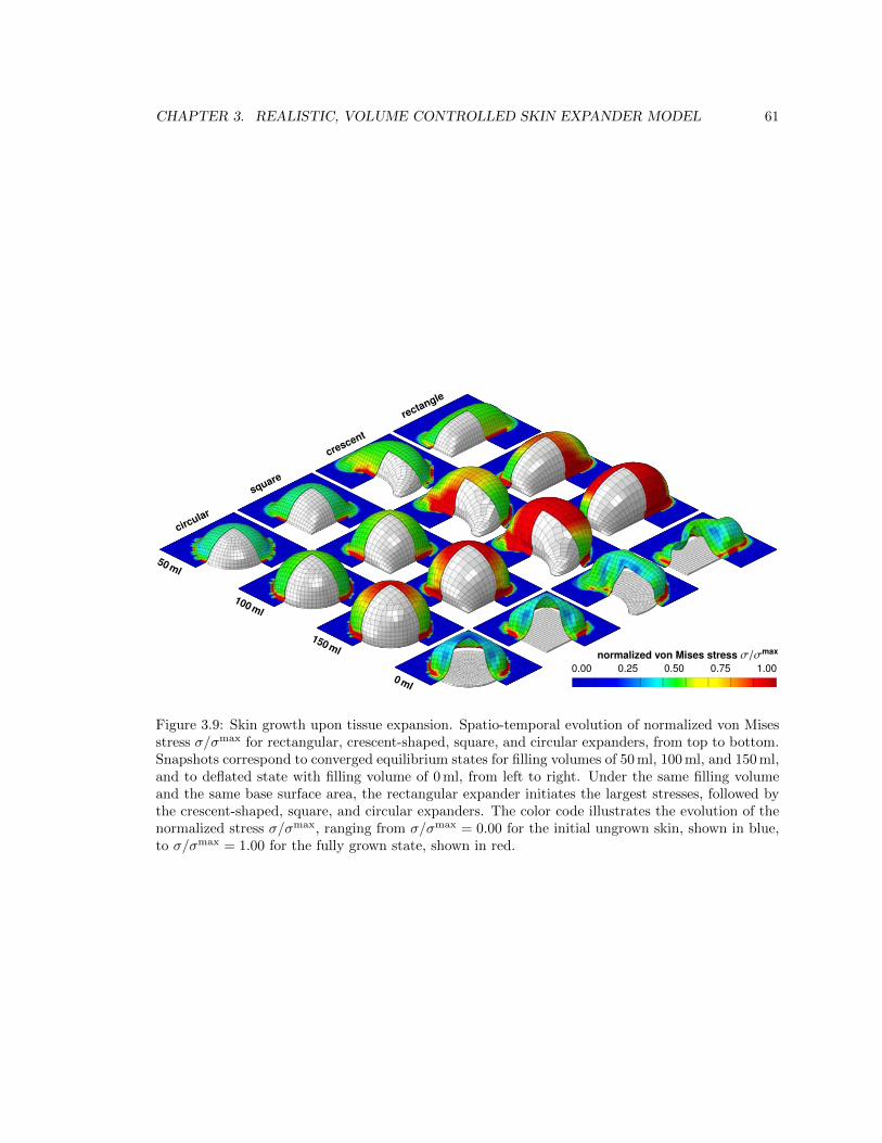
CHAPTER 3. REALISTIC, VOLUME CONTROLLED SKIN EXPANDER MODEL 61
normalized von Mises stress �/�max
0.00 0.25 0.50 0.75 1.00
circular
square
crescent
rectangle
50 ml
100 ml
150 ml
0 ml
Figure 9: Skin growth upon tissue expansion. Spatio-temporal evolution of normalized von Mises stress �/�max for rectangular, crescent-shaped, square, andcircular expanders, from top to bottom. Snapshots correspond to converged equilibrium states for filling volumes of 50 ml, 100 ml, and 150 ml, and to deflatedstate with filling volume of 0 ml, from left to right. Under the same filling volume and the same base surface area, the rectangular expander initiates the largeststresses, followed by the crescent-shaped, square, and circular expanders. The color code illustrates the evolution of the normalized stress �/�max, ranging from�/�max = 0.00 for the initial ungrown skin, shown in blue, to �/�max = 1.00 for the fully grown state, shown in red.
the skin thickness to its initial baseline value. The chronic de-crease of the elastic stretch induces a chronic decrease in theskin stress ⌧ (b
e), which manifests itself in a decrease in ex-pander pressure, see Figure 7. Rheologically, this chronic re-sponse resembles the phenomenon of relaxation. However, theexpander pressure p/pmax never fully returns to zero because ofthe inherent resistance of the silicone expander itself.Upon expander deflation, the elastic strain decreases below thecritical threshold value #e < #crit associated with an acute arrestof further growth #g = const, see Figures 6 and 10, bottom right.Deflation is associated with an acute retraction of the reversibleelastic area stretch back to its initial baseline value of #e ! 1.0and an acute release of the expander pressure p/pmax ! 0, seeFigure 7. Although the expander volume is fully released at theend of the procedure, the heterogeneity of the growth processleaves some residual elastic deformation, which manifests itselfin residual stresses upon expander removal, see Figure 9, right,and Figure 10, bottom right.In space, our model predicts regional variations in the amountof growth with larger values in the center region and smallervalues in the periphery, see Figures 8 and 10. Expander infla-tion causes largest area strains in the center region. This trig-gers a heterogeneity of the growth process. In the center region,skin more than doubles its initial area with #g ! #max, whilethe amount of growth gradually decays towards the expanderedges.
6.2. Comparison with the literature
The characteristic features predicted by our model are in ex-cellent agreement with the observed phenomena during tissueexpansion in animals [9, 10] and in humans [24, 49]. In thetissue expansion literature, our decomposition of the deforma-tion gradient into reversible and irreversible parts F = F
e · Fg
is referred to as mechanical creep and biological creep [29] or,more illustratively, as loan and dividend [7]. What is referredto as stretch back in the tissue engineering literature [69] isassociated with the reversible elastic part of the deformation,which is released upon expander removal. To account for thisreversible deformation, empirical guidelines suggest to selectan expander size with a base surface area which is 2.5 largerthan the defect area to be closed [29]. A quantitative study ofskin growth in pigs recommends to multiply the required sur-face area with an empirical correction factor. Recommendedcorrection factors range from 6.00 to 4.50 and 3.75 for the cir-cular, crescent shaped, and rectangular expanders, respectively[69]. In agreement with our findings in Figures 6 and 8, thesecorrection factors suggest that the net area gain is greatest forthe rectangular expander, followed by the crescent-shaped andcircular expanders [10, 69]. A comparison of the fractional areagain �A/A revealed values ranging from 35% to 137% [29].Our fractional area gain between 100% and 110% as displayedin Figure 6 is well within this range.In one of the earliest quantitative studies of controlled tissue ex-pansion in guinea pigs, it was argued that stretching skin stim-ulates cell proliferation just su�cient to relieve tension [18].This is in agreement with the rheological analogy of stress re-
10
Figure 3.9: Skin growth upon tissue expansion. Spatio-temporal evolution of normalized von Misesstress �/�max for rectangular, crescent-shaped, square, and circular expanders, from top to bottom.Snapshots correspond to converged equilibrium states for filling volumes of 50ml, 100ml, and 150ml,and to deflated state with filling volume of 0ml, from left to right. Under the same filling volumeand the same base surface area, the rectangular expander initiates the largest stresses, followed bythe crescent-shaped, square, and circular expanders. The color code illustrates the evolution of thenormalized stress �/�max, ranging from �/�max = 0.00 for the initial ungrown skin, shown in blue,to �/�max = 1.00 for the fully grown state, shown in red.
CHAPTER 3. REALISTIC, VOLUME CONTROLLED SKIN EXPANDER MODEL 62
significant regional variations. Largest stresses are located in the center region and along the ex-
pander edges, shown in red. Moderate stresses are located at the expander sides, shown in green.
No stresses occur in the unexpanded regions, shown in blue.
3.5.2 Skin growth of a pediatric scalp
For the second problem, we closely follow a clinical tissue expansion protocol and simulate skin
growth in the scalp of the pediatric patient shown in Figure 3.1. We virtually insert a rectangular
expander with a base surface area of 14 ⇥ 10 cm2 in a subcutaneous pocket of the frontoparietal
scalp. The expander has a filling capacity of 450ml, which we reach gradually by increasing the
filling volume in three consecutive steps of 150ml each. To model the epidermis and the dermis,
we discretize the skin on top of the expander as a 14 ⇥ 10 cm2 large, 0.2cm thick layer with
45⇥ 32⇥ 2=2,880 C3D8 eight-noded linear brick elements, corresponding to a total of 4,554 nodes
and 13,662 degrees of freedom. Similar to the idealized square skin sample in Section 3.5.1, we model
the elastic response as Neo-Hookean according to equations (3.8) and (3.9) with Lame parameters
� = 0.5440MPa and µ = 0.1785MPa citepamplona09, and the growth response as transversely
isotropic and strain driven according to equations (3.10), (3.11), and (3.12) with a maximum growth
of #max = 2.4, a growth speed of ⌧ = 10, a growth nonlinearity of � = 2, and a critical growth
threshold of #crit = 1.1 [225]. We model the skin expander as a fluid-filled cavity with a base
area of 14 ⇥ 10 cm2, discretized with 638 S4R shell elements, corresponding to a total of 640
nodes and 1,920 degrees of freedom. We model its elastic response using the material parameters of
silicone [143] and discretize the fluid cavity with the same nodes and connectivity, but with F3D4
fluid elements. We allow the skin to slide freely along the expander and model the skin-expander
interaction as frictionless contact. We fix all nodes that are not involved in the expansion procedure
using homogeneous Dirichlet boundary conditions.
Figure 3.10 displays the spatio-temporal evolution of the growth multiplier #g immediately after
filling, bottom row, and after converged growth, top row. The individual snapshots correspond to
the initial filled states and the converged homeostatic equilibrium states for filling volumes of 150ml,
300ml, and 450ml, and to deflated state with filling volume of 0ml, from left to right. Similar to the
idealized square skin sample in Section 3.5.1, skin growth displays regional variations in magnitude
with largest values in the center region, shown in red, and smallest values along the expander edges,
shown in blue.
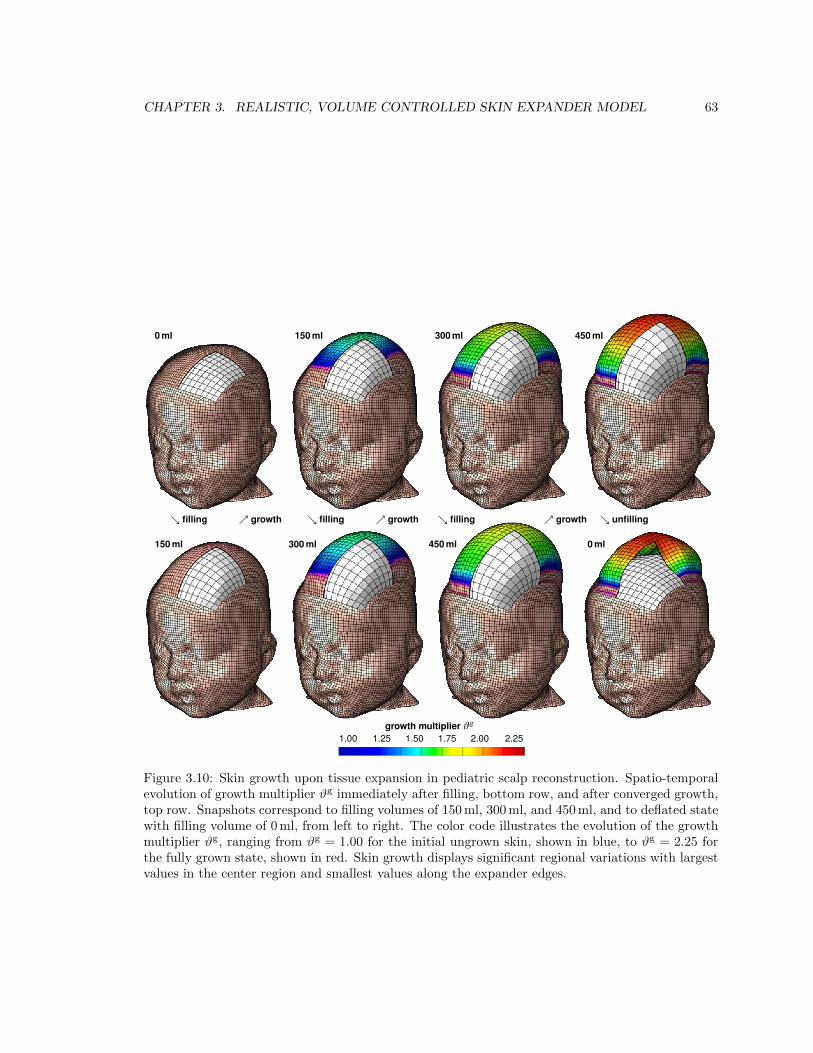
CHAPTER 3. REALISTIC, VOLUME CONTROLLED SKIN EXPANDER MODEL 63
growth multiplier #g
1.00 1.25 1.50 1.75 2.00 2.25
0 ml
150 ml
150 ml
300 ml
300 ml
450 ml
450 ml
0 ml
& filling % growth & filling % growth & filling % growth & unfilling
Figure 10: Skin growth upon tissue expansion in pediatric scalp reconstruction. Spatio-temporal evolution of growth multiplier #g immediately after filling, bottomrow, and after converged growth, top row. Snapshots correspond to filling volumes of 150 ml, 300 ml, and 450 ml, and to deflated state with filling volume of 0 ml,from left to right. The color code illustrates the evolution of the growth multiplier #g, ranging from #g = 1.00 for the initial ungrown skin, shown in blue, to#g = 2.25 for the fully grown state, shown in red. Skin growth displays significant regional variations with largest values in the center region and smallest valuesalong the expander edges.
laxation [12], which we observed in Figure 7. In a chronicporcine model, the expander pressure was found to increaseacutely, but returned to its homeostatic equilibrium state aftera period of a few days [10]. The fact that this equilibrium statechanges nonlinearly with the amount of filling was attributedto nonlinearities in the constitutive responses of both the ex-panded skin and the silicone expander itself [10]. This is in ex-cellent agreement with our observations in Figure 7. Along thesame lines, detailed thickness studies of expanded human skinrevealed an initial epidermal thickening, dermal thinning, andand subcutaneous thinning five months after expansion. How-ever, the thicknesses of all three layers returned to their pre-expansion baseline values two years after the procedure hadbeen completed [53, 54]. This is in agreement with the acuteand chronic features predicted by our model, see Figure 7.Controlled tissue expansion studies in rodents revealed a re-
gional variation of skin growth with largest growth in the centerregion and smallest growth in the periphery [9]. The authors hy-pothesized that larger strains in the center region would triggerlarger growth. This feature is nicely reflected by our model, inwhich the evolution of area growth in equation (10) is directlycorrelated to the amount of overstretch through the growth cri-terion in equation (12). Figures 8 and 10 clearly support theexperimental observations of a heterogeneous growth processwith larger values in the center region and smaller values in theperiphery [9].We have implemented our growth model as user-defined con-stitutive subroutine into the general purpose finite element pro-gram Abaqus/Standard Version 6.12 [1]. Instead of using theexplicit version Abaqus/Explicit, as previously proposed fortissue expansion in breast reconstruction [47], we have usedthe implicit version of the program. To ensure optimal conver-
11
Figure 3.10: Skin growth upon tissue expansion in pediatric scalp reconstruction. Spatio-temporalevolution of growth multiplier #g immediately after filling, bottom row, and after converged growth,top row. Snapshots correspond to filling volumes of 150ml, 300ml, and 450ml, and to deflated statewith filling volume of 0ml, from left to right. The color code illustrates the evolution of the growthmultiplier #g, ranging from #g = 1.00 for the initial ungrown skin, shown in blue, to #g = 2.25 forthe fully grown state, shown in red. Skin growth displays significant regional variations with largestvalues in the center region and smallest values along the expander edges.
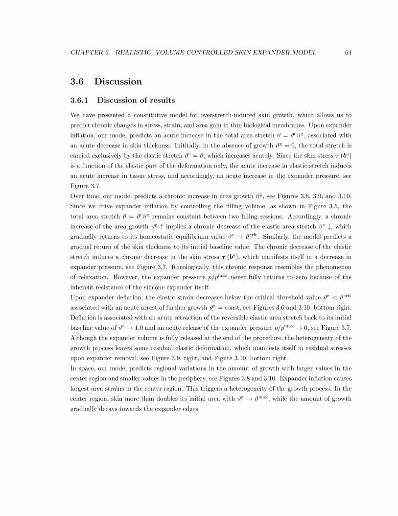
CHAPTER 3. REALISTIC, VOLUME CONTROLLED SKIN EXPANDER MODEL 64
3.6 Discussion
3.6.1 Discussion of results
We have presented a constitutive model for overstretch-induced skin growth, which allows us to
predict chronic changes in stress, strain, and area gain in thin biological membranes. Upon expander
inflation, our model predicts an acute increase in the total area stretch # = #e#g, associated with
an acute decrease in skin thickness. Inititally, in the absence of growth #g = 0, the total stretch is
carried exclusively by the elastic stretch #e = #, which increases acutely. Since the skin stress ⌧ (be)
is a function of the elastic part of the deformation only, the acute increase in elastic stretch induces
an acute increase in tissue stress, and accordingly, an acute increase in the expander pressure, see
Figure 3.7.
Over time, our model predicts a chronic increase in area growth #g, see Figures 3.6, 3.9, and 3.10.
Since we drive expander inflation by controlling the filling volume, as shown in Figure 3.5, the
total area stretch # = #e#g remains constant between two filling sessions. Accordingly, a chronic
increase of the area growth #g " implies a chronic decrease of the elastic area stretch #e #, whichgradually returns to its homeostatic equilibrium value #e ! #crit. Similarly, the model predicts a
gradual return of the skin thickness to its initial baseline value. The chronic decrease of the elastic
stretch induces a chronic decrease in the skin stress ⌧ (be), which manifests itself in a decrease in
expander pressure, see Figure 3.7. Rheologically, this chronic response resembles the phenomenon
of relaxation. However, the expander pressure p/pmax never fully returns to zero because of the
inherent resistance of the silicone expander itself.
Upon expander deflation, the elastic strain decreases below the critical threshold value #e < #crit
associated with an acute arrest of further growth #g = const, see Figures 3.6 and 3.10, bottom right.
Deflation is associated with an acute retraction of the reversible elastic area stretch back to its initial
baseline value of #e ! 1.0 and an acute release of the expander pressure p/pmax ! 0, see Figure 3.7.
Although the expander volume is fully released at the end of the procedure, the heterogeneity of the
growth process leaves some residual elastic deformation, which manifests itself in residual stresses
upon expander removal, see Figure 3.9, right, and Figure 3.10, bottom right.
In space, our model predicts regional variations in the amount of growth with larger values in the
center region and smaller values in the periphery, see Figures 3.8 and 3.10. Expander inflation causes
largest area strains in the center region. This triggers a heterogeneity of the growth process. In the
center region, skin more than doubles its initial area with #g ! #max, while the amount of growth
gradually decays towards the expander edges.
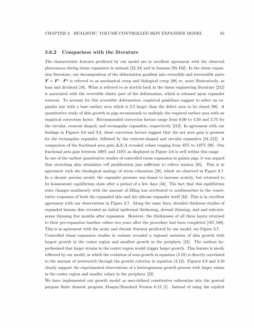
CHAPTER 3. REALISTIC, VOLUME CONTROLLED SKIN EXPANDER MODEL 65
3.6.2 Comparison with the literature
The characteristic features predicted by our model are in excellent agreement with the observed
phenomena during tissue expansion in animals [22,34] and in humans [83,162]. In the tissue expan-
sion literature, our decomposition of the deformation gradient into reversible and irreversible parts
F = F
e · F g is referred to as mechanical creep and biological creep [98] or, more illustratively, as
loan and dividend [16]. What is referred to as stretch back in the tissue engineering literature [212]
is associated with the reversible elastic part of the deformation, which is released upon expander
removal. To account for this reversible deformation, empirical guidelines suggest to select an ex-
pander size with a base surface area which is 2.5 larger than the defect area to be closed [98]. A
quantitative study of skin growth in pigs recommends to multiply the required surface area with an
empirical correction factor. Recommended correction factors range from 6.00 to 4.50 and 3.75 for
the circular, crescent shaped, and rectangular expanders, respectively [212]. In agreement with our
findings in Figures 3.6 and 3.8, these correction factors suggest that the net area gain is greatest
for the rectangular expander, followed by the crescent-shaped and circular expanders [34, 212]. A
comparison of the fractional area gain �A/A revealed values ranging from 35% to 137% [98]. Our
fractional area gain between 100% and 110% as displayed in Figure 3.6 is well within this range.
In one of the earliest quantitative studies of controlled tissue expansion in guinea pigs, it was argued
that stretching skin stimulates cell proliferation just su�cient to relieve tension [65]. This is in
agreement with the rheological analogy of stress relaxation [38], which we observed in Figure 3.7.
In a chronic porcine model, the expander pressure was found to increase acutely, but returned to
its homeostatic equilibrium state after a period of a few days [34]. The fact that this equilibrium
state changes nonlinearly with the amount of filling was attributed to nonlinearities in the consti-
tutive responses of both the expanded skin and the silicone expander itself [34]. This is in excellent
agreement with our observations in Figure 3.7. Along the same lines, detailed thickness studies of
expanded human skin revealed an initial epidermal thickening, dermal thinning, and and subcuta-
neous thinning five months after expansion. However, the thicknesses of all three layers returned
to their pre-expansion baseline values two years after the procedure had been completed [167, 168].
This is in agreement with the acute and chronic features predicted by our model, see Figure 3.7.
Controlled tissue expansion studies in rodents revealed a regional variation of skin growth with
largest growth in the center region and smallest growth in the periphery [22]. The authors hy-
pothesized that larger strains in the center region would trigger larger growth. This feature is nicely
reflected by our model, in which the evolution of area growth in equation (3.10) is directly correlated
to the amount of overstretch through the growth criterion in equation (3.12). Figures 3.8 and 3.10
clearly support the experimental observations of a heterogeneous growth process with larger values
in the center region and smaller values in the periphery [22].
We have implemented our growth model as user-defined constitutive subroutine into the general
purpose finite element program Abaqus/Standard Version 6.12 [1]. Instead of using the explicit
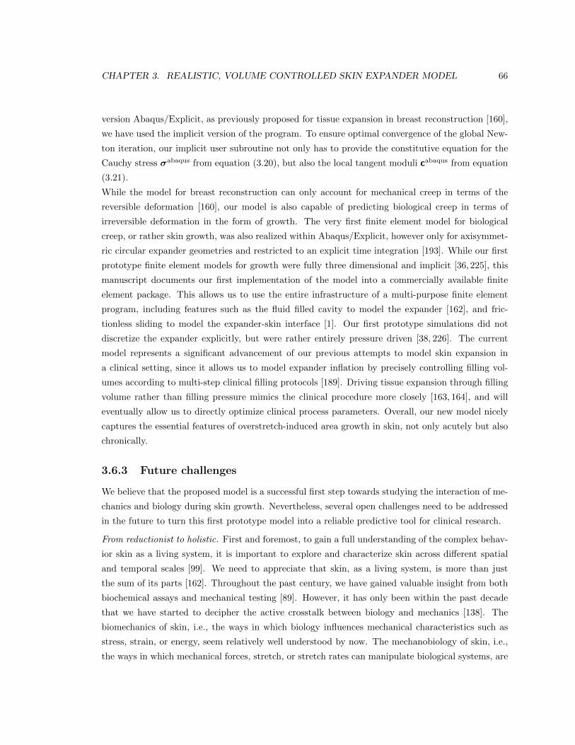
CHAPTER 3. REALISTIC, VOLUME CONTROLLED SKIN EXPANDER MODEL 66
version Abaqus/Explicit, as previously proposed for tissue expansion in breast reconstruction [160],
we have used the implicit version of the program. To ensure optimal convergence of the global New-
ton iteration, our implicit user subroutine not only has to provide the constitutive equation for the
Cauchy stress �abaqus from equation (3.20), but also the local tangent moduli cabaqus from equation
(3.21).
While the model for breast reconstruction can only account for mechanical creep in terms of the
reversible deformation [160], our model is also capable of predicting biological creep in terms of
irreversible deformation in the form of growth. The very first finite element model for biological
creep, or rather skin growth, was also realized within Abaqus/Explicit, however only for axisymmet-
ric circular expander geometries and restricted to an explicit time integration [193]. While our first
prototype finite element models for growth were fully three dimensional and implicit [36, 225], this
manuscript documents our first implementation of the model into a commercially available finite
element package. This allows us to use the entire infrastructure of a multi-purpose finite element
program, including features such as the fluid filled cavity to model the expander [162], and fric-
tionless sliding to model the expander-skin interface [1]. Our first prototype simulations did not
discretize the expander explicitly, but were rather entirely pressure driven [38, 226]. The current
model represents a significant advancement of our previous attempts to model skin expansion in
a clinical setting, since it allows us to model expander inflation by precisely controlling filling vol-
umes according to multi-step clinical filling protocols [189]. Driving tissue expansion through filling
volume rather than filling pressure mimics the clinical procedure more closely [163, 164], and will
eventually allow us to directly optimize clinical process parameters. Overall, our new model nicely
captures the essential features of overstretch-induced area growth in skin, not only acutely but also
chronically.
3.6.3 Future challenges
We believe that the proposed model is a successful first step towards studying the interaction of me-
chanics and biology during skin growth. Nevertheless, several open challenges need to be addressed
in the future to turn this first prototype model into a reliable predictive tool for clinical research.
From reductionist to holistic. First and foremost, to gain a full understanding of the complex behav-
ior skin as a living system, it is important to explore and characterize skin across di↵erent spatial
and temporal scales [99]. We need to appreciate that skin, as a living system, is more than just
the sum of its parts [162]. Throughout the past century, we have gained valuable insight from both
biochemical assays and mechanical testing [89]. However, it has only been within the past decade
that we have started to decipher the active crosstalk between biology and mechanics [138]. The
biomechanics of skin, i.e., the ways in which biology influences mechanical characteristics such as
stress, strain, or energy, seem relatively well understood by now. The mechanobiology of skin, i.e.,
the ways in which mechanical forces, stretch, or stretch rates can manipulate biological systems, are
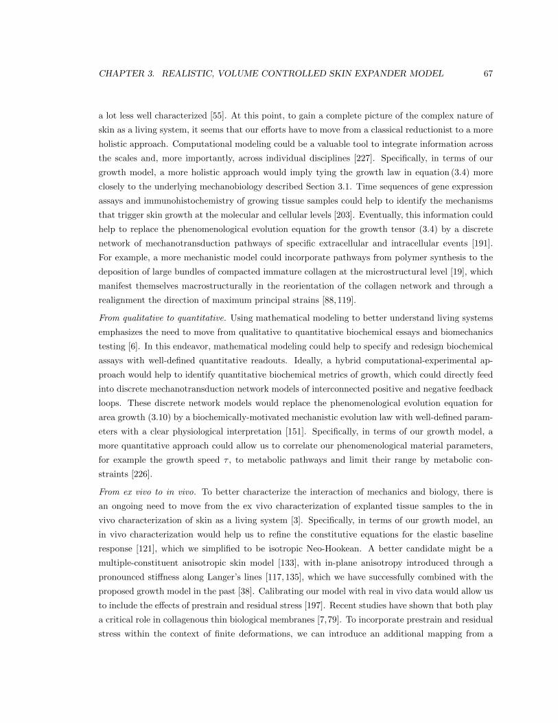
CHAPTER 3. REALISTIC, VOLUME CONTROLLED SKIN EXPANDER MODEL 67
a lot less well characterized [55]. At this point, to gain a complete picture of the complex nature of
skin as a living system, it seems that our e↵orts have to move from a classical reductionist to a more
holistic approach. Computational modeling could be a valuable tool to integrate information across
the scales and, more importantly, across individual disciplines [227]. Specifically, in terms of our
growth model, a more holistic approach would imply tying the growth law in equation (3.4) more
closely to the underlying mechanobiology described Section 3.1. Time sequences of gene expression
assays and immunohistochemistry of growing tissue samples could help to identify the mechanisms
that trigger skin growth at the molecular and cellular levels [203]. Eventually, this information could
help to replace the phenomenological evolution equation for the growth tensor (3.4) by a discrete
network of mechanotransduction pathways of specific extracellular and intracellular events [191].
For example, a more mechanistic model could incorporate pathways from polymer synthesis to the
deposition of large bundles of compacted immature collagen at the microstructural level [19], which
manifest themselves macrostructurally in the reorientation of the collagen network and through a
realignment the direction of maximum principal strains [88, 119].
From qualitative to quantitative. Using mathematical modeling to better understand living systems
emphasizes the need to move from qualitative to quantitative biochemical essays and biomechanics
testing [6]. In this endeavor, mathematical modeling could help to specify and redesign biochemical
assays with well-defined quantitative readouts. Ideally, a hybrid computational-experimental ap-
proach would help to identify quantitative biochemical metrics of growth, which could directly feed
into discrete mechanotransduction network models of interconnected positive and negative feedback
loops. These discrete network models would replace the phenomenological evolution equation for
area growth (3.10) by a biochemically-motivated mechanistic evolution law with well-defined param-
eters with a clear physiological interpretation [151]. Specifically, in terms of our growth model, a
more quantitative approach could allow us to correlate our phenomenological material parameters,
for example the growth speed ⌧ , to metabolic pathways and limit their range by metabolic con-
straints [226].
From ex vivo to in vivo. To better characterize the interaction of mechanics and biology, there is
an ongoing need to move from the ex vivo characterization of explanted tissue samples to the in
vivo characterization of skin as a living system [3]. Specifically, in terms of our growth model, an
in vivo characterization would help us to refine the constitutive equations for the elastic baseline
response [121], which we simplified to be isotropic Neo-Hookean. A better candidate might be a
multiple-constituent anisotropic skin model [133], with in-plane anisotropy introduced through a
pronounced sti↵ness along Langer’s lines [117, 135], which we have successfully combined with the
proposed growth model in the past [38]. Calibrating our model with real in vivo data would allow us
to include the e↵ects of prestrain and residual stress [197]. Recent studies have shown that both play
a critical role in collagenous thin biological membranes [7,79]. To incorporate prestrain and residual
stress within the context of finite deformations, we can introduce an additional mapping from a
CHAPTER 3. REALISTIC, VOLUME CONTROLLED SKIN EXPANDER MODEL 68
relaxed ex vivo to the prestrained in vivo configuration through another second-order tensor [150].
We have recently shown that incorporating prestrain of only 20% to 30% can decrease the in vivo
tissue sti↵ness by three to four orders of magnitude [178].
From acute to chronic. In the current model, the long-term response growing of skin is not yet
calibrated in time. We have assumed that chronic growth between two filling increments takes place
within a normalized time interval from zero to one. In reality, growth periods range from the order
of days in rodents [22] to weeks in pigs [212] and humans [83]. In an ideal experimental setting,
data would be acquired not only acutely but also chronically [177], and the relevant growth metrics
would be quantified at multiple points in time [162]. Specifically, in terms of our growth model,
quantitative chronic studies would allow us to calibrate the adaptation speed ⌧ and the shape of the
growth curve � [225, 226], or the corresponding time parameters of more mechanistic biochemically
driven evolution equations.
3.7 Conclusion
We have demonstrated the mathematical modeling and computational simulation of skin growth
by mechanical overstretch. Previous models of skin growth have controlled overstretch by directly
applying the expander pressure without discretizing the expander itself. Here, we have controlled
the amount of overstretch by gradually filling a virtually implanted tissue expander. In contrast
to previous models, this allows us now to predict the rheological e↵ect of stress relaxation, i.e.,
a chronic increase in skin area at constant stretch, associated with a chronic decrease in elastic
stretch, stress, and pressure. While it is virtually impossible to measure stresses in living biological
membrane in vivo, the precise knowledge of skin stress and expander pressure is clinically critical to
optimize capillary refill, minimize tissue necrosis, and maximize patient comfort. Once calibrated
with long-term in vivo data, our model will be capable of predicting stress, pressure, strain, and area
gain in thin biological membranes exposed to mechanical overstretch. It can serve as a valuable tool
to rationalize clinical process parameters such as expander geometry, expander size, filling volume,
filling pressure, and inflation timing. The proposed model for skin growth can easily be generalized
to explore the physiology and pathology of stretch-induced growth in other living systems such as
the bladder, intestine, ureter, blood vessels, muscles, and nerves, which display similar structural
characteristics.
Acknowledgements
We gratefully acknowledge the Holland family for proofreading the manuscript. This study was
supported by the National Science Foundation CAREER award CMMI 0952021, by the National
Science Foundation INSPIRE grant 1233054, and by the National Institutes of Health grant U54

CHAPTER 3. REALISTIC, VOLUME CONTROLLED SKIN EXPANDER MODEL 69
GM072970.

Chapter 4
Chronic muscle lengthening
through sarcomerogenesis
Abstract
Skeletal muscle responds to passive overstretch through sarcomerogenesis, the creation and
serial deposition of new sarcomere units. Sarcomerogenesis is critical to muscle function: It
gradually re-positions the muscle back into its optimal operating regime. Animal models of
immobilization, limb lengthening, and tendon transfer have provided significant insight into
muscle adaptation in vivo. Yet, to date, there is no mathematical model that allows us to predict
how skeletal muscle adapts to mechanical stretch in silico. Here we propose a novel mechanistic
model for chronic longitudinal muscle growth in response to passive mechanical stretch. We
characterize growth through a single scalar-valued internal variable, the serial sarcomere number.
Sarcomerogenesis, the evolution of this variable, is driven by the elastic mechanical stretch. To
analyze realistic three-dimensional muscle geometries, we embed our model into a nonlinear
finite element framework. In a chronic limb lengthening study with a muscle stretch of 1.14,
the model predicts an acute sarcomere lengthening from 3.09µm to 3.51µm, and a chronic
gradual return to the initial sarcomere length within two weeks. Compared to the experiment,
the acute model error was 0.00% by design of the model; the chronic model error was 2.13%,
which lies within the rage of the experimental standard deviation. Our model explains, from
a mechanistic point of view, why gradual multi-step muscle lengthening is less invasive than
single-step lengthening. It also explains regional variations in sarcomere length, shorter close
to and longer away from the muscle-tendon interface. Once calibrated with a richer data set,
our model may help surgeons to prevent muscle overstretch and make informed decisions about
optimal stretch increments, stretch timing, and stretch amplitudes. We anticipate our study to
open new avenues in orthopedic and reconstructive surgery and enhance treatment for patients
with ill proportioned limbs, tendon lengthening, tendon transfer, tendon tear, and chronically
retracted muscles.
70
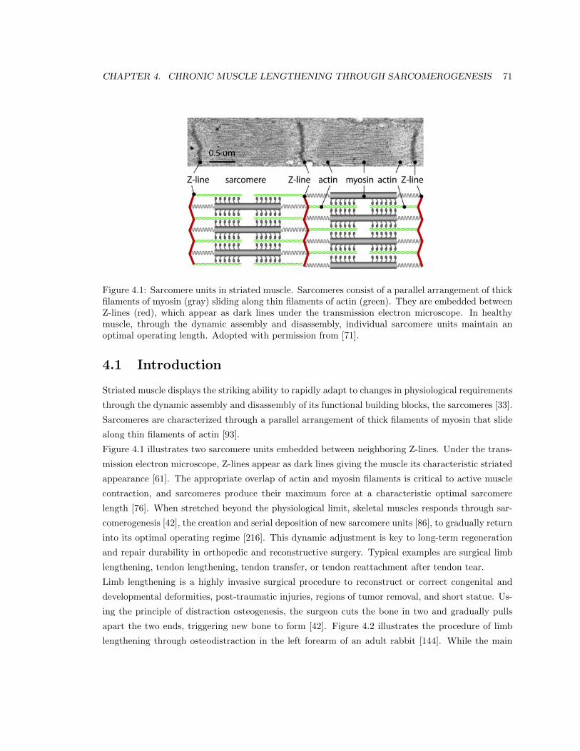
CHAPTER 4. CHRONIC MUSCLE LENGTHENING THROUGH SARCOMEROGENESIS 71
Figure 4.1: Sarcomere units in striated muscle. Sarcomeres consist of a parallel arrangement of thickfilaments of myosin (gray) sliding along thin filaments of actin (green). They are embedded betweenZ-lines (red), which appear as dark lines under the transmission electron microscope. In healthymuscle, through the dynamic assembly and disassembly, individual sarcomere units maintain anoptimal operating length. Adopted with permission from [71].
4.1 Introduction
Striated muscle displays the striking ability to rapidly adapt to changes in physiological requirements
through the dynamic assembly and disassembly of its functional building blocks, the sarcomeres [33].
Sarcomeres are characterized through a parallel arrangement of thick filaments of myosin that slide
along thin filaments of actin [93].
Figure 4.1 illustrates two sarcomere units embedded between neighboring Z-lines. Under the trans-
mission electron microscope, Z-lines appear as dark lines giving the muscle its characteristic striated
appearance [61]. The appropriate overlap of actin and myosin filaments is critical to active muscle
contraction, and sarcomeres produce their maximum force at a characteristic optimal sarcomere
length [76]. When stretched beyond the physiological limit, skeletal muscles responds through sar-
comerogenesis [42], the creation and serial deposition of new sarcomere units [86], to gradually return
into its optimal operating regime [216]. This dynamic adjustment is key to long-term regeneration
and repair durability in orthopedic and reconstructive surgery. Typical examples are surgical limb
lengthening, tendon lengthening, tendon transfer, or tendon reattachment after tendon tear.
Limb lengthening is a highly invasive surgical procedure to reconstruct or correct congenital and
developmental deformities, post-traumatic injuries, regions of tumor removal, and short statue. Us-
ing the principle of distraction osteogenesis, the surgeon cuts the bone in two and gradually pulls
apart the two ends, triggering new bone to form [42]. Figure 4.2 illustrates the procedure of limb
lengthening through osteodistraction in the left forearm of an adult rabbit [144]. While the main
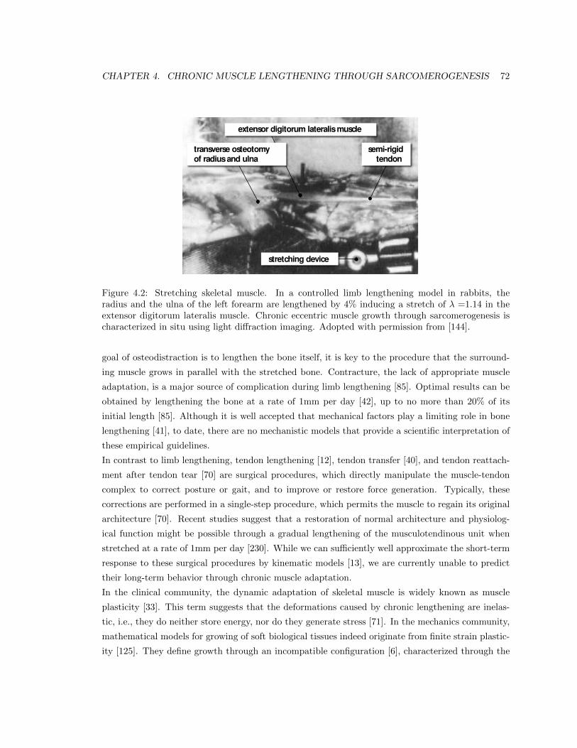
CHAPTER 4. CHRONIC MUSCLE LENGTHENING THROUGH SARCOMEROGENESIS 72
extensor digitorum lateralis muscle
stretching device
transverse osteotomyof radius and ulna
semi-rigidtendon
extensor digitorum lateralismuscle
transverse osteotomyof radiusand ulna
semi-rigidtendon
stretching device
Figure 4.2: Stretching skeletal muscle. In a controlled limb lengthening model in rabbits, theradius and the ulna of the left forearm are lengthened by 4% inducing a stretch of � =1.14 in theextensor digitorum lateralis muscle. Chronic eccentric muscle growth through sarcomerogenesis ischaracterized in situ using light di↵raction imaging. Adopted with permission from [144].
goal of osteodistraction is to lengthen the bone itself, it is key to the procedure that the surround-
ing muscle grows in parallel with the stretched bone. Contracture, the lack of appropriate muscle
adaptation, is a major source of complication during limb lengthening [85]. Optimal results can be
obtained by lengthening the bone at a rate of 1mm per day [42], up to no more than 20% of its
initial length [85]. Although it is well accepted that mechanical factors play a limiting role in bone
lengthening [41], to date, there are no mechanistic models that provide a scientific interpretation of
these empirical guidelines.
In contrast to limb lengthening, tendon lengthening [12], tendon transfer [40], and tendon reattach-
ment after tendon tear [70] are surgical procedures, which directly manipulate the muscle-tendon
complex to correct posture or gait, and to improve or restore force generation. Typically, these
corrections are performed in a single-step procedure, which permits the muscle to regain its original
architecture [70]. Recent studies suggest that a restoration of normal architecture and physiolog-
ical function might be possible through a gradual lengthening of the musculotendinous unit when
stretched at a rate of 1mm per day [230]. While we can su�ciently well approximate the short-term
response to these surgical procedures by kinematic models [13], we are currently unable to predict
their long-term behavior through chronic muscle adaptation.
In the clinical community, the dynamic adaptation of skeletal muscle is widely known as muscle
plasticity [33]. This term suggests that the deformations caused by chronic lengthening are inelas-
tic, i.e., they do neither store energy, nor do they generate stress [71]. In the mechanics community,
mathematical models for growing of soft biological tissues indeed originate from finite strain plastic-
ity [125]. They define growth through an incompatible configuration [6], characterized through the
CHAPTER 4. CHRONIC MUSCLE LENGTHENING THROUGH SARCOMEROGENESIS 73
multiplicative decomposition of the overall deformation into a reversible elastic and an irreversible
inelastic part [67, 183]. The irreversible part is represented through a second order growth ten-
sor [151], which can be isotropic [87], transversely isotropic [36, 104], orthotropic [72], or generally
anisotropic [149, 209] depending on the particular type of tissue. Its evolution can be driven by
stress [118] or strain [225] again depending on the particular type of growth. Similar to cardiac mus-
cle, skeletal muscle grows in a transversely isotropic pattern, along the fiber direction in response to
passive mechanical stretch [72] and orthogonal to the fiber direction in response to active mechan-
ical stress [176]. On the macroscopic scale, a passively stretched muscle grows eccentrically, i.e., it
becomes longer, while an actively stressed muscle grows concentrically, i.e., it becomes thicker [197].
On the microscopic scale, passive stretch induces sarcomerogenesis, the serial deposition of sarcomere
units, while active stress induces myofibrillogenesis, the parallel deposition of sarcomeres arranged
in myofibrils [71, 101]. We have previously modeled both forms of growth in cardiac muscle [72]
using generalized continuum theories with internal variables [62, 151]. However, to date, there is
no mechanistic model to characterize growth in skeletal muscle using the nonlinear field theories of
continuum mechanics.
Here we establish a mechanistic mathematical model for overstretch-induced eccentric skeletal mus-
cle growth. The model is inherently multiscale, since it links macroscopic changes in elastic and
inelastic muscle stretch to microscopic changes in sarcomere length and number. We illustrate the
continuum theory of finite growth, adapt it to sarcomerogenesis, and embed it into a nonlinear finite
element framework. We demonstrate that the model shows an excellent qualitative and quanti-
tative agreement with experimentally measured sarcomere lengths and numbers in a chronic limb
lengthening experiment.
4.2 Methods
In this section, we briefly summarize the continuum modeling of sarcomerogenesis and its computa-
tional realization within a nonlinear finite element environment.
Continuum modeling of sarcomerogenesis
To accurately represent the finite deformations during muscle stretching, we adopt the kinematics of
finite growth, and introduce the deformation map ', which, at any given time t, maps the material
placement X of a physical particle onto its spatial placement x = ' (X, t). We then introduce the
multiplicative decomposition of the deformation gradient [125],
F = rX' = F
e · F g (4.1)
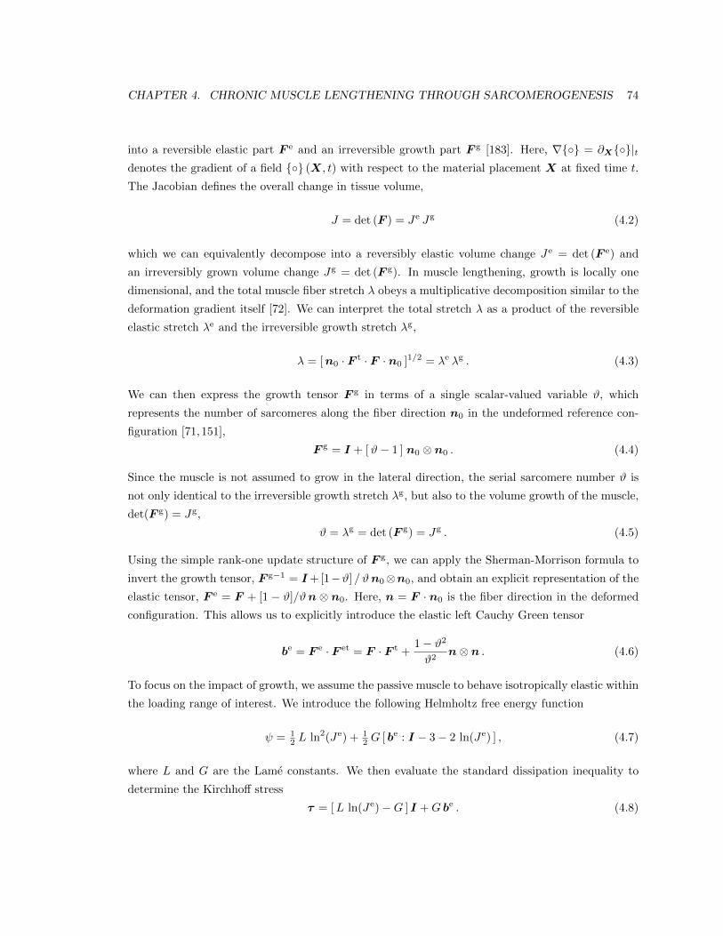
CHAPTER 4. CHRONIC MUSCLE LENGTHENING THROUGH SARCOMEROGENESIS 74
into a reversible elastic part F
e and an irreversible growth part F
g [183]. Here, r{�} = @X{�}|t
denotes the gradient of a field {�} (X, t) with respect to the material placement X at fixed time t.
The Jacobian defines the overall change in tissue volume,
J = det (F ) = Je Jg (4.2)
which we can equivalently decompose into a reversibly elastic volume change Je = det (F e) and
an irreversibly grown volume change Jg = det (F g). In muscle lengthening, growth is locally one
dimensional, and the total muscle fiber stretch � obeys a multiplicative decomposition similar to the
deformation gradient itself [72]. We can interpret the total stretch � as a product of the reversible
elastic stretch �e and the irreversible growth stretch �g,
� = [n0 · F t · F · n0 ]1/2 = �e �g . (4.3)
We can then express the growth tensor F
g in terms of a single scalar-valued variable #, which
represents the number of sarcomeres along the fiber direction n0 in the undeformed reference con-
figuration [71,151],
F
g = I + [#� 1 ] n0 ⌦ n0 . (4.4)
Since the muscle is not assumed to grow in the lateral direction, the serial sarcomere number # is
not only identical to the irreversible growth stretch �g, but also to the volume growth of the muscle,
det(F g) = Jg,
# = �g = det (F g) = Jg . (4.5)
Using the simple rank-one update structure of F g, we can apply the Sherman-Morrison formula to
invert the growth tensor, F g�1 = I+[1�#] /#n0⌦n0, and obtain an explicit representation of the
elastic tensor, F e = F + [1 � #]/#n ⌦ n0. Here, n = F · n0 is the fiber direction in the deformed
configuration. This allows us to explicitly introduce the elastic left Cauchy Green tensor
b
e = F
e · F et = F · F t +1� #2
#2n⌦ n . (4.6)
To focus on the impact of growth, we assume the passive muscle to behave isotropically elastic within
the loading range of interest. We introduce the following Helmholtz free energy function
= 12 L ln2(Je) + 1
2 G [ be : I � 3� 2 ln(Je) ] , (4.7)
where L and G are the Lame constants. We then evaluate the standard dissipation inequality to
determine the Kirchho↵ stress
⌧ = [L ln(Je)�G ] I +G b
e . (4.8)
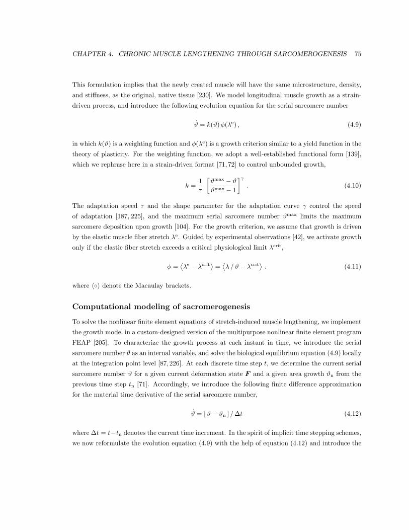
CHAPTER 4. CHRONIC MUSCLE LENGTHENING THROUGH SARCOMEROGENESIS 75
This formulation implies that the newly created muscle will have the same microstructure, density,
and sti↵ness, as the original, native tissue [230]. We model longitudinal muscle growth as a strain-
driven process, and introduce the following evolution equation for the serial sarcomere number
# = k(#)�(�e) , (4.9)
in which k(#) is a weighting function and �(�e) is a growth criterion similar to a yield function in the
theory of plasticity. For the weighting function, we adopt a well-established functional form [139],
which we rephrase here in a strain-driven format [71, 72] to control unbounded growth,
k =1
⌧
#max � ##max � 1
��
. (4.10)
The adaptation speed ⌧ and the shape parameter for the adaptation curve � control the speed
of adaptation [187, 225], and the maximum serial sarcomere number #max limits the maximum
sarcomere deposition upon growth [104]. For the growth criterion, we assume that growth is driven
by the elastic muscle fiber stretch �e. Guided by experimental observations [42], we activate growth
only if the elastic fiber stretch exceeds a critical physiological limit �crit,
� =⌦�e � �crit
↵=
⌦� /#� �crit
↵. (4.11)
where h�i denote the Macaulay brackets.
Computational modeling of sacromerogenesis
To solve the nonlinear finite element equations of stretch-induced muscle lengthening, we implement
the growth model in a custom-designed version of the multipurpose nonlinear finite element program
FEAP [205]. To characterize the growth process at each instant in time, we introduce the serial
sarcomere number # as an internal variable, and solve the biological equilibrium equation (4.9) locally
at the integration point level [87,226]. At each discrete time step t, we determine the current serial
sarcomere number # for a given current deformation state F and a given area growth #n from the
previous time step tn [71]. Accordingly, we introduce the following finite di↵erence approximation
for the material time derivative of the serial sarcomere number,
# = [#� #n ] /�t (4.12)
where �t = t�tn denotes the current time increment. In the spirit of implicit time stepping schemes,
we now reformulate the evolution equation (4.9) with the help of equation (4.12) and introduce the
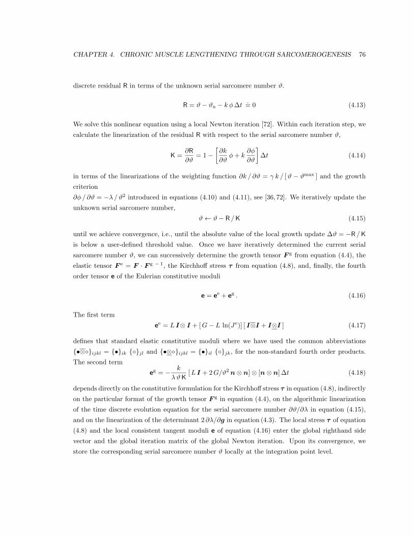
CHAPTER 4. CHRONIC MUSCLE LENGTHENING THROUGH SARCOMEROGENESIS 76
discrete residual R in terms of the unknown serial sarcomere number #.
R = #� #n � k ��t.= 0 (4.13)
We solve this nonlinear equation using a local Newton iteration [72]. Within each iteration step, we
calculate the linearization of the residual R with respect to the serial sarcomere number #,
K =@R
@#= 1�
@k
@#�+ k
@�
@#
��t (4.14)
in terms of the linearizations of the weighting function @k / @# = � k / [# � #max ] and the growth
criterion
@� / @# = �� /#2 introduced in equations (4.10) and (4.11), see [36, 72]. We iteratively update the
unknown serial sarcomere number,
# #� R /K (4.15)
until we achieve convergence, i.e., until the absolute value of the local growth update �# = �R /K
is below a user-defined threshold value. Once we have iteratively determined the current serial
sarcomere number #, we can successively determine the growth tensor F g from equation (4.4), the
elastic tensor F
e = F · F g � 1, the Kirchho↵ stress ⌧ from equation (4.8), and, finally, the fourth
order tensor e of the Eulerian constitutive moduli
e = e
e + e
g . (4.16)
The first term
e
e = L I⌦ I + [G� L ln(Je)] [ I⌦I + I⌦I ] (4.17)
defines that standard elastic constitutive moduli where we have used the common abbreviations
{•⌦�}ijkl
= {•}ik
{�}jl
and {•⌦�}ijkl
= {•}il
{�}jk
, for the non-standard fourth order products.
The second term
e
g = � k
�#K[L I + 2G/#2 n⌦ n]⌦ [n⌦ n]�t (4.18)
depends directly on the constitutive formulation for the Kirchho↵ stress ⌧ in equation (4.8), indirectly
on the particular format of the growth tensor F g in equation (4.4), on the algorithmic linearization
of the time discrete evolution equation for the serial sarcomere number @#/@� in equation (4.15),
and on the linearization of the determinant 2 @�/@g in equation (4.3). The local stress ⌧ of equation
(4.8) and the local consistent tangent moduli e of equation (4.16) enter the global righthand side
vector and the global iteration matrix of the global Newton iteration. Upon its convergence, we
store the corresponding serial sarcomere number # locally at the integration point level.
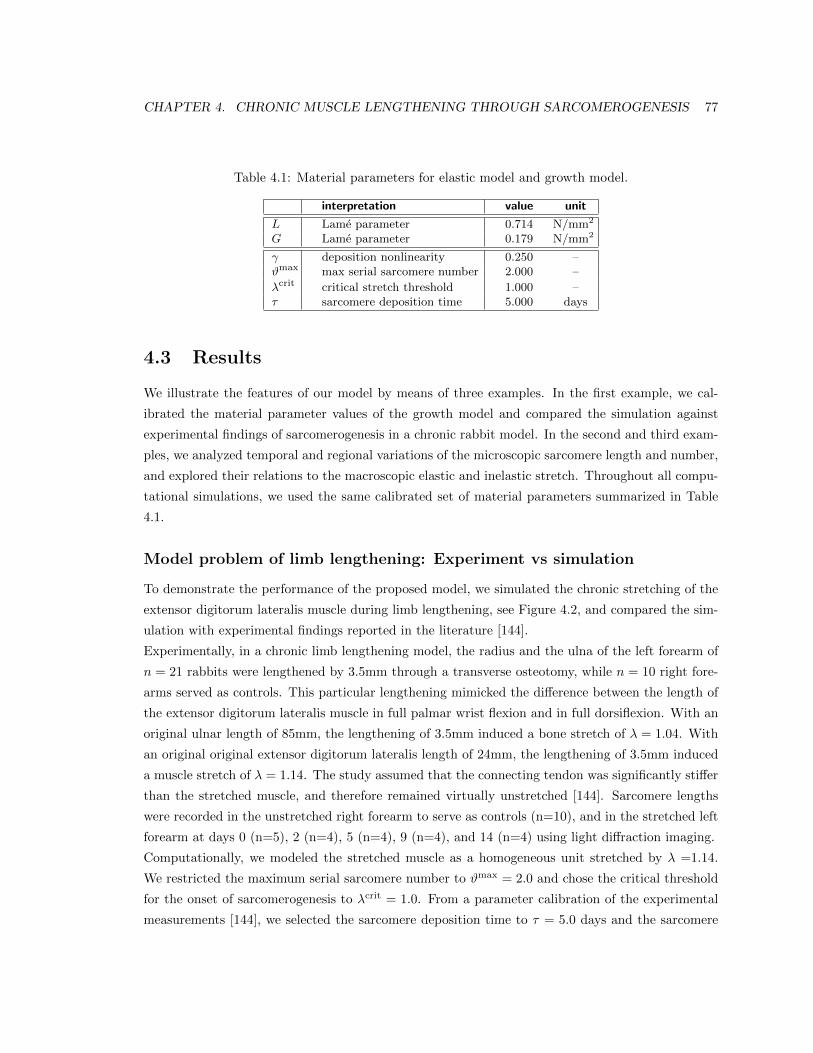
CHAPTER 4. CHRONIC MUSCLE LENGTHENING THROUGH SARCOMEROGENESIS 77
Table 4.1: Material parameters for elastic model and growth model.
interpretation value unit
L Lame parameter 0.714 N/mm2
G Lame parameter 0.179 N/mm2
� deposition nonlinearity 0.250 –#max max serial sarcomere number 2.000 –�crit critical stretch threshold 1.000 –⌧ sarcomere deposition time 5.000 days
4.3 Results
We illustrate the features of our model by means of three examples. In the first example, we cal-
ibrated the material parameter values of the growth model and compared the simulation against
experimental findings of sarcomerogenesis in a chronic rabbit model. In the second and third exam-
ples, we analyzed temporal and regional variations of the microscopic sarcomere length and number,
and explored their relations to the macroscopic elastic and inelastic stretch. Throughout all compu-
tational simulations, we used the same calibrated set of material parameters summarized in Table
4.1.
Model problem of limb lengthening: Experiment vs simulation
To demonstrate the performance of the proposed model, we simulated the chronic stretching of the
extensor digitorum lateralis muscle during limb lengthening, see Figure 4.2, and compared the sim-
ulation with experimental findings reported in the literature [144].
Experimentally, in a chronic limb lengthening model, the radius and the ulna of the left forearm of
n = 21 rabbits were lengthened by 3.5mm through a transverse osteotomy, while n = 10 right fore-
arms served as controls. This particular lengthening mimicked the di↵erence between the length of
the extensor digitorum lateralis muscle in full palmar wrist flexion and in full dorsiflexion. With an
original ulnar length of 85mm, the lengthening of 3.5mm induced a bone stretch of � = 1.04. With
an original original extensor digitorum lateralis length of 24mm, the lengthening of 3.5mm induced
a muscle stretch of � = 1.14. The study assumed that the connecting tendon was significantly sti↵er
than the stretched muscle, and therefore remained virtually unstretched [144]. Sarcomere lengths
were recorded in the unstretched right forearm to serve as controls (n=10), and in the stretched left
forearm at days 0 (n=5), 2 (n=4), 5 (n=4), 9 (n=4), and 14 (n=4) using light di↵raction imaging.
Computationally, we modeled the stretched muscle as a homogeneous unit stretched by � =1.14.
We restricted the maximum serial sarcomere number to #max = 2.0 and chose the critical threshold
for the onset of sarcomerogenesis to �crit = 1.0. From a parameter calibration of the experimental
measurements [144], we selected the sarcomere deposition time to ⌧ = 5.0 days and the sarcomere
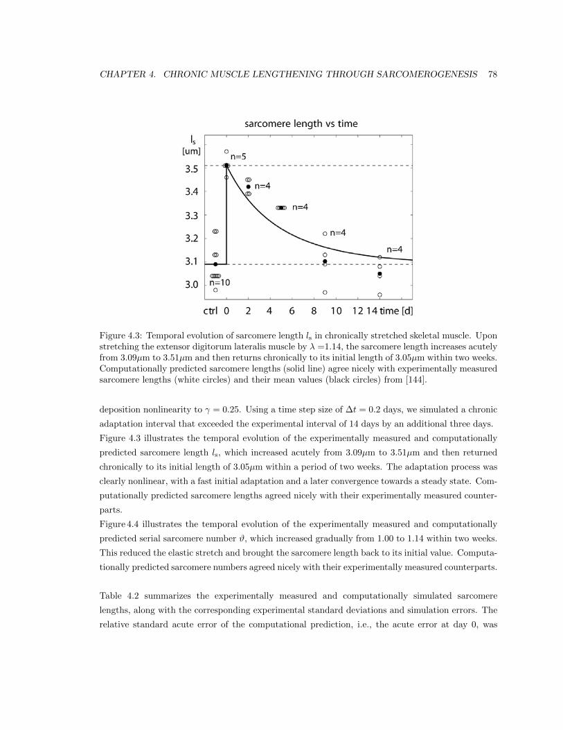
CHAPTER 4. CHRONIC MUSCLE LENGTHENING THROUGH SARCOMEROGENESIS 78
Figure 4.3: Temporal evolution of sarcomere length ls in chronically stretched skeletal muscle. Uponstretching the extensor digitorum lateralis muscle by � =1.14, the sarcomere length increases acutelyfrom 3.09µm to 3.51µm and then returns chronically to its initial length of 3.05µm within two weeks.Computationally predicted sarcomere lengths (solid line) agree nicely with experimentally measuredsarcomere lengths (white circles) and their mean values (black circles) from [144].
deposition nonlinearity to � = 0.25. Using a time step size of �t = 0.2 days, we simulated a chronic
adaptation interval that exceeded the experimental interval of 14 days by an additional three days.
Figure 4.3 illustrates the temporal evolution of the experimentally measured and computationally
predicted sarcomere length ls, which increased acutely from 3.09µm to 3.51µm and then returned
chronically to its initial length of 3.05µm within a period of two weeks. The adaptation process was
clearly nonlinear, with a fast initial adaptation and a later convergence towards a steady state. Com-
putationally predicted sarcomere lengths agreed nicely with their experimentally measured counter-
parts.
Figure 4.4 illustrates the temporal evolution of the experimentally measured and computationally
predicted serial sarcomere number #, which increased gradually from 1.00 to 1.14 within two weeks.
This reduced the elastic stretch and brought the sarcomere length back to its initial value. Computa-
tionally predicted sarcomere numbers agreed nicely with their experimentally measured counterparts.
Table 4.2 summarizes the experimentally measured and computationally simulated sarcomere
lengths, along with the corresponding experimental standard deviations and simulation errors. The
relative standard acute error of the computational prediction, i.e., the acute error at day 0, was
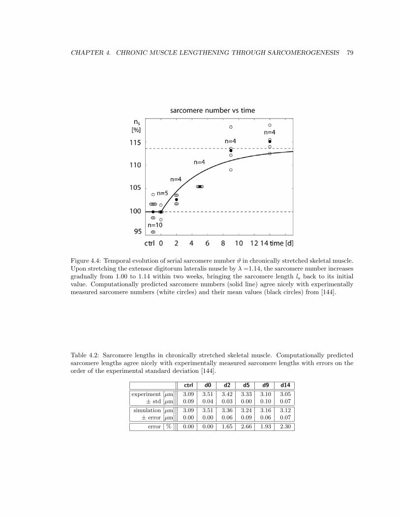
CHAPTER 4. CHRONIC MUSCLE LENGTHENING THROUGH SARCOMEROGENESIS 79
Figure 4.4: Temporal evolution of serial sarcomere number # in chronically stretched skeletal muscle.Upon stretching the extensor digitorum lateralis muscle by � =1.14, the sarcomere number increasesgradually from 1.00 to 1.14 within two weeks, bringing the sarcomere length ls back to its initialvalue. Computationally predicted sarcomere numbers (solid line) agree nicely with experimentallymeasured sarcomere numbers (white circles) and their mean values (black circles) from [144].
Table 4.2: Sarcomere lengths in chronically stretched skeletal muscle. Computationally predictedsarcomere lengths agree nicely with experimentally measured sarcomere lengths with errors on theorder of the experimental standard deviation [144].
ctrl d0 d2 d5 d9 d14
experiment [µm] 3.09 3.51 3.42 3.33 3.10 3.05± std [µm] 0.09 0.04 0.03 0.00 0.10 0.07
simulation [µm] 3.09 3.51 3.36 3.24 3.16 3.12± error [µm] 0.00 0.00 0.06 0.09 0.06 0.07
error [ % ] 0.00 0.00 1.65 2.66 1.93 2.30
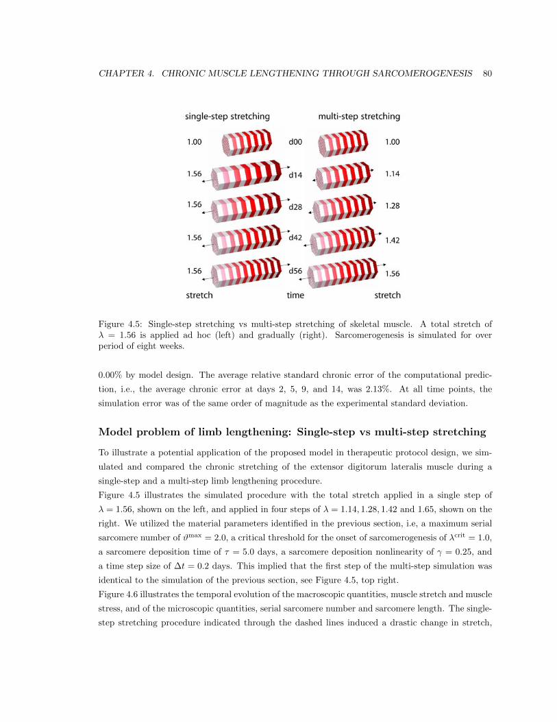
CHAPTER 4. CHRONIC MUSCLE LENGTHENING THROUGH SARCOMEROGENESIS 80
Figure 4.5: Single-step stretching vs multi-step stretching of skeletal muscle. A total stretch of� = 1.56 is applied ad hoc (left) and gradually (right). Sarcomerogenesis is simulated for overperiod of eight weeks.
0.00% by model design. The average relative standard chronic error of the computational predic-
tion, i.e., the average chronic error at days 2, 5, 9, and 14, was 2.13%. At all time points, the
simulation error was of the same order of magnitude as the experimental standard deviation.
Model problem of limb lengthening: Single-step vs multi-step stretching
To illustrate a potential application of the proposed model in therapeutic protocol design, we sim-
ulated and compared the chronic stretching of the extensor digitorum lateralis muscle during a
single-step and a multi-step limb lengthening procedure.
Figure 4.5 illustrates the simulated procedure with the total stretch applied in a single step of
� = 1.56, shown on the left, and applied in four steps of � = 1.14, 1.28, 1.42 and 1.65, shown on the
right. We utilized the material parameters identified in the previous section, i.e, a maximum serial
sarcomere number of #max = 2.0, a critical threshold for the onset of sarcomerogenesis of �crit = 1.0,
a sarcomere deposition time of ⌧ = 5.0 days, a sarcomere deposition nonlinearity of � = 0.25, and
a time step size of �t = 0.2 days. This implied that the first step of the multi-step simulation was
identical to the simulation of the previous section, see Figure 4.5, top right.
Figure 4.6 illustrates the temporal evolution of the macroscopic quantities, muscle stretch and muscle
stress, and of the microscopic quantities, serial sarcomere number and sarcomere length. The single-
step stretching procedure indicated through the dashed lines induced a drastic change in stretch,
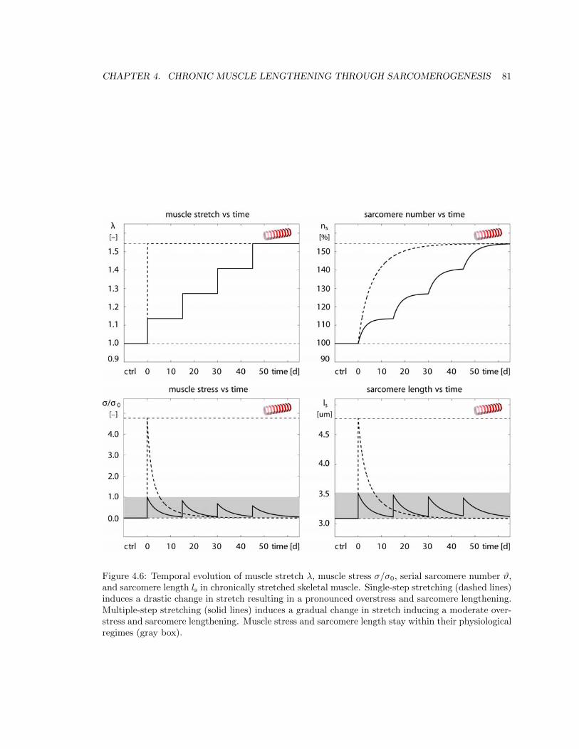
CHAPTER 4. CHRONIC MUSCLE LENGTHENING THROUGH SARCOMEROGENESIS 81
Figure 4.6: Temporal evolution of muscle stretch �, muscle stress �/�0, serial sarcomere number #,and sarcomere length ls in chronically stretched skeletal muscle. Single-step stretching (dashed lines)induces a drastic change in stretch resulting in a pronounced overstress and sarcomere lengthening.Multiple-step stretching (solid lines) induces a gradual change in stretch inducing a moderate over-stress and sarcomere lengthening. Muscle stress and sarcomere length stay within their physiologicalregimes (gray box).
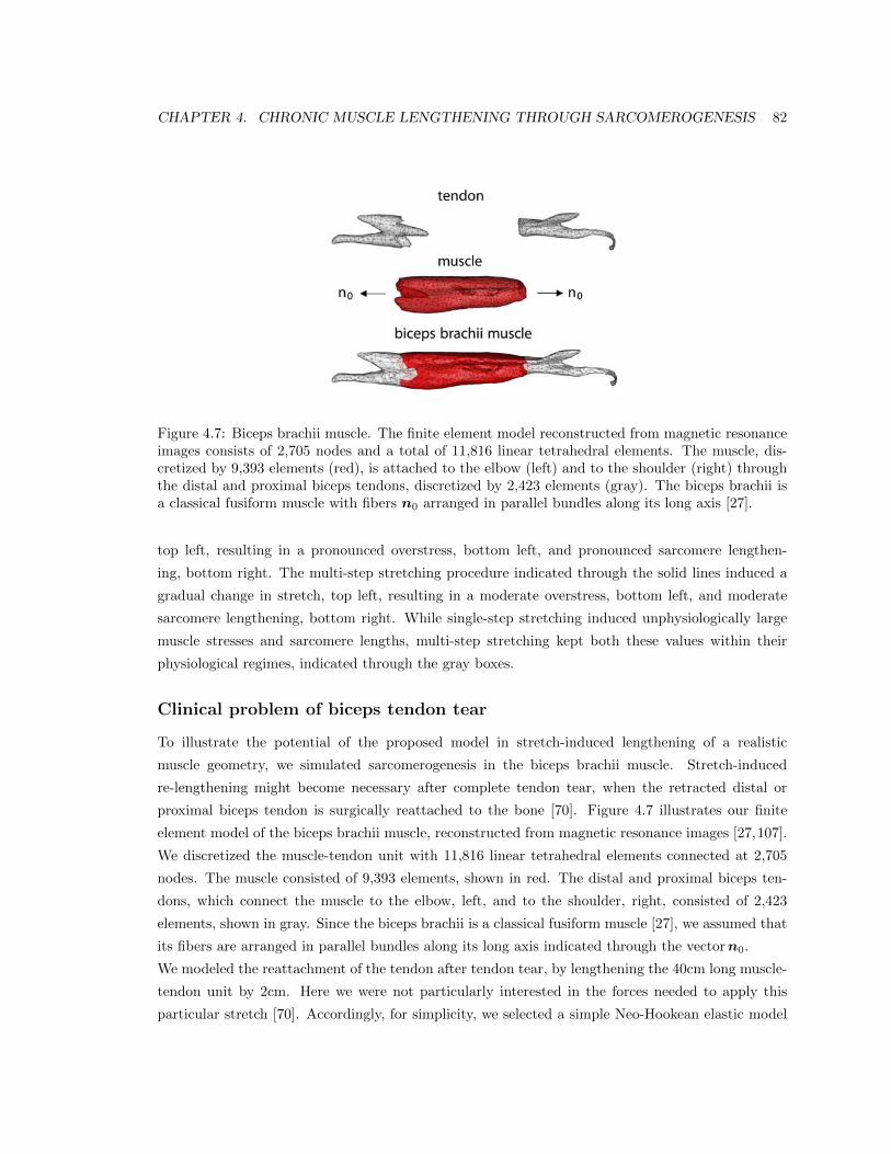
CHAPTER 4. CHRONIC MUSCLE LENGTHENING THROUGH SARCOMEROGENESIS 82
Figure 4.7: Biceps brachii muscle. The finite element model reconstructed from magnetic resonanceimages consists of 2,705 nodes and a total of 11,816 linear tetrahedral elements. The muscle, dis-cretized by 9,393 elements (red), is attached to the elbow (left) and to the shoulder (right) throughthe distal and proximal biceps tendons, discretized by 2,423 elements (gray). The biceps brachii isa classical fusiform muscle with fibers n0 arranged in parallel bundles along its long axis [27].
top left, resulting in a pronounced overstress, bottom left, and pronounced sarcomere lengthen-
ing, bottom right. The multi-step stretching procedure indicated through the solid lines induced a
gradual change in stretch, top left, resulting in a moderate overstress, bottom left, and moderate
sarcomere lengthening, bottom right. While single-step stretching induced unphysiologically large
muscle stresses and sarcomere lengths, multi-step stretching kept both these values within their
physiological regimes, indicated through the gray boxes.
Clinical problem of biceps tendon tear
To illustrate the potential of the proposed model in stretch-induced lengthening of a realistic
muscle geometry, we simulated sarcomerogenesis in the biceps brachii muscle. Stretch-induced
re-lengthening might become necessary after complete tendon tear, when the retracted distal or
proximal biceps tendon is surgically reattached to the bone [70]. Figure 4.7 illustrates our finite
element model of the biceps brachii muscle, reconstructed from magnetic resonance images [27,107].
We discretized the muscle-tendon unit with 11,816 linear tetrahedral elements connected at 2,705
nodes. The muscle consisted of 9,393 elements, shown in red. The distal and proximal biceps ten-
dons, which connect the muscle to the elbow, left, and to the shoulder, right, consisted of 2,423
elements, shown in gray. Since the biceps brachii is a classical fusiform muscle [27], we assumed that
its fibers are arranged in parallel bundles along its long axis indicated through the vectorn0.
We modeled the reattachment of the tendon after tendon tear, by lengthening the 40cm long muscle-
tendon unit by 2cm. Here we were not particularly interested in the forces needed to apply this
particular stretch [70]. Accordingly, for simplicity, we selected a simple Neo-Hookean elastic model
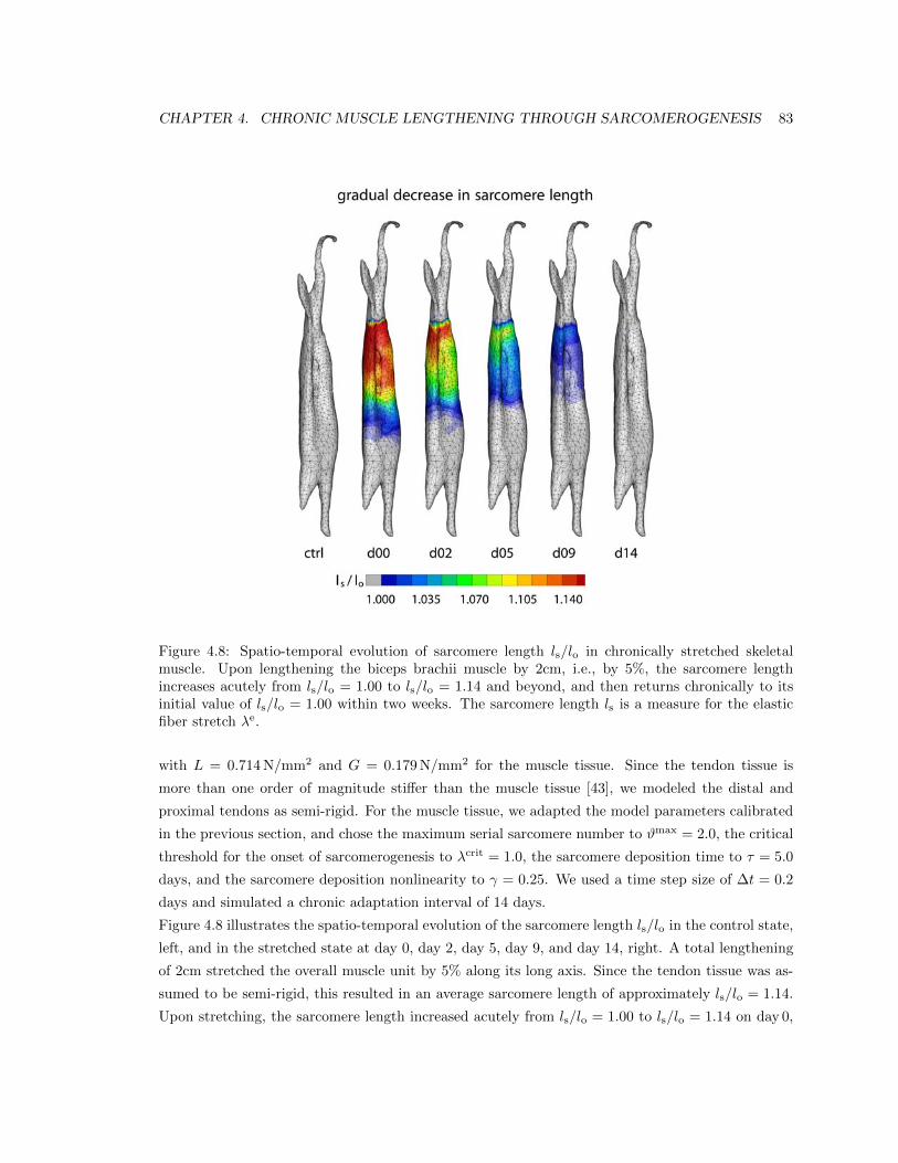
CHAPTER 4. CHRONIC MUSCLE LENGTHENING THROUGH SARCOMEROGENESIS 83
Figure 4.8: Spatio-temporal evolution of sarcomere length ls/lo in chronically stretched skeletalmuscle. Upon lengthening the biceps brachii muscle by 2cm, i.e., by 5%, the sarcomere lengthincreases acutely from ls/lo = 1.00 to ls/lo = 1.14 and beyond, and then returns chronically to itsinitial value of ls/lo = 1.00 within two weeks. The sarcomere length ls is a measure for the elasticfiber stretch �e.
with L = 0.714N/mm2 and G = 0.179N/mm2 for the muscle tissue. Since the tendon tissue is
more than one order of magnitude sti↵er than the muscle tissue [43], we modeled the distal and
proximal tendons as semi-rigid. For the muscle tissue, we adapted the model parameters calibrated
in the previous section, and chose the maximum serial sarcomere number to #max = 2.0, the critical
threshold for the onset of sarcomerogenesis to �crit = 1.0, the sarcomere deposition time to ⌧ = 5.0
days, and the sarcomere deposition nonlinearity to � = 0.25. We used a time step size of �t = 0.2
days and simulated a chronic adaptation interval of 14 days.
Figure 4.8 illustrates the spatio-temporal evolution of the sarcomere length ls/lo in the control state,
left, and in the stretched state at day 0, day 2, day 5, day 9, and day 14, right. A total lengthening
of 2cm stretched the overall muscle unit by 5% along its long axis. Since the tendon tissue was as-
sumed to be semi-rigid, this resulted in an average sarcomere length of approximately ls/lo = 1.14.
Upon stretching, the sarcomere length increased acutely from ls/lo = 1.00 to ls/lo = 1.14 on day 0,
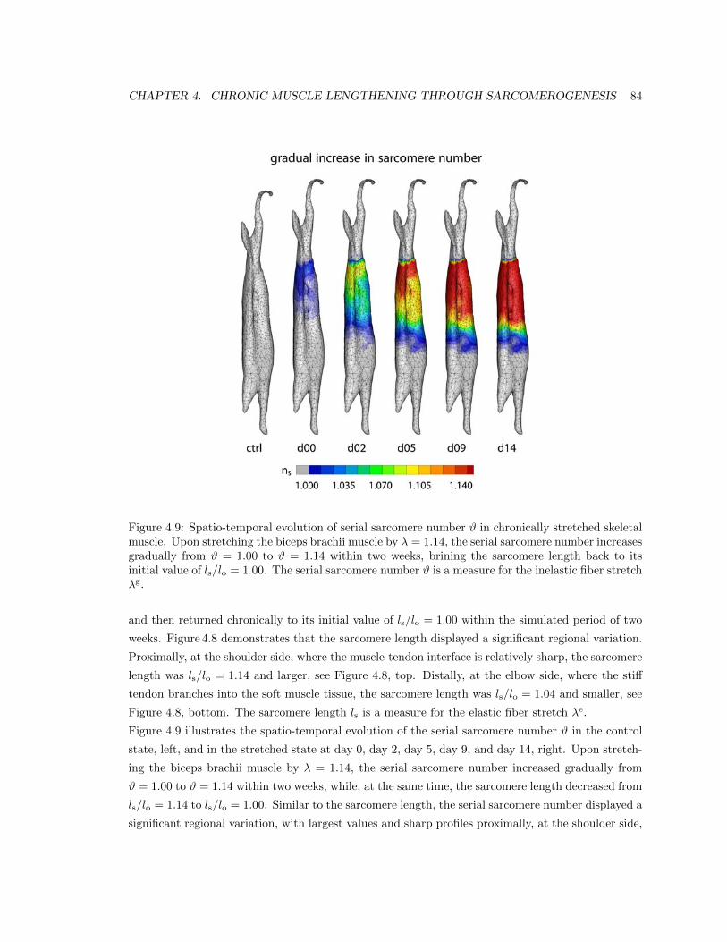
CHAPTER 4. CHRONIC MUSCLE LENGTHENING THROUGH SARCOMEROGENESIS 84
Figure 4.9: Spatio-temporal evolution of serial sarcomere number # in chronically stretched skeletalmuscle. Upon stretching the biceps brachii muscle by � = 1.14, the serial sarcomere number increasesgradually from # = 1.00 to # = 1.14 within two weeks, brining the sarcomere length back to itsinitial value of ls/lo = 1.00. The serial sarcomere number # is a measure for the inelastic fiber stretch�g.
and then returned chronically to its initial value of ls/lo = 1.00 within the simulated period of two
weeks. Figure 4.8 demonstrates that the sarcomere length displayed a significant regional variation.
Proximally, at the shoulder side, where the muscle-tendon interface is relatively sharp, the sarcomere
length was ls/lo = 1.14 and larger, see Figure 4.8, top. Distally, at the elbow side, where the sti↵
tendon branches into the soft muscle tissue, the sarcomere length was ls/lo = 1.04 and smaller, see
Figure 4.8, bottom. The sarcomere length ls is a measure for the elastic fiber stretch �e.
Figure 4.9 illustrates the spatio-temporal evolution of the serial sarcomere number # in the control
state, left, and in the stretched state at day 0, day 2, day 5, day 9, and day 14, right. Upon stretch-
ing the biceps brachii muscle by � = 1.14, the serial sarcomere number increased gradually from
# = 1.00 to # = 1.14 within two weeks, while, at the same time, the sarcomere length decreased from
ls/lo = 1.14 to ls/lo = 1.00. Similar to the sarcomere length, the serial sarcomere number displayed a
significant regional variation, with largest values and sharp profiles proximally, at the shoulder side,
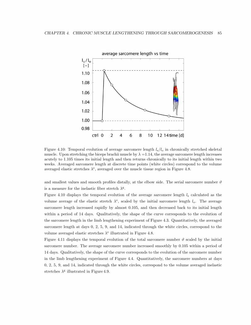
CHAPTER 4. CHRONIC MUSCLE LENGTHENING THROUGH SARCOMEROGENESIS 85
Figure 4.10: Temporal evolution of average sarcomere length ls/lo in chronically stretched skeletalmuscle. Upon stretching the biceps brachii muscle by � =1.14, the average sarcomere length increasesacutely to 1.105 times its initial length and then returns chronically to its initial length within twoweeks. Averaged sarcomere length at discrete time points (white circles) correspond to the volumeaveraged elastic stretches �e, averaged over the muscle tissue region in Figure 4.8.
and smallest values and smooth profiles distally, at the elbow side. The serial sarcomere number #
is a measure for the inelastic fiber stretch �g.
Figure 4.10 displays the temporal evolution of the average sarcomere length ls calculated as the
volume average of the elastic stretch �e, scaled by the initial sarcomere length lo. The average
sarcomere length increased rapidly by almost 0.105, and then decreased back to its initial length
within a period of 14 days. Qualitatively, the shape of the curve corresponds to the evolution of
the sarcomere length in the limb lengthening experiment of Figure 4.3. Quantitatively, the averaged
sarcomere length at days 0, 2, 5, 9, and 14, indicated through the white circles, correspond to the
volume averaged elastic stretches �e illustrated in Figure 4.8.
Figure 4.11 displays the temporal evolution of the total sarcomere number # scaled by the initial
sarcomere number. The average sarcomere number increased smoothly by 0.105 within a period of
14 days. Qualitatively, the shape of the curve corresponds to the evolution of the sarcomere number
in the limb lengthening experiment of Figure 4.4. Quantitatively, the sarcomere numbers at days
0, 2, 5, 9, and 14, indicated through the white circles, correspond to the volume averaged inelastic
stretches �g illustrated in Figure 4.9.
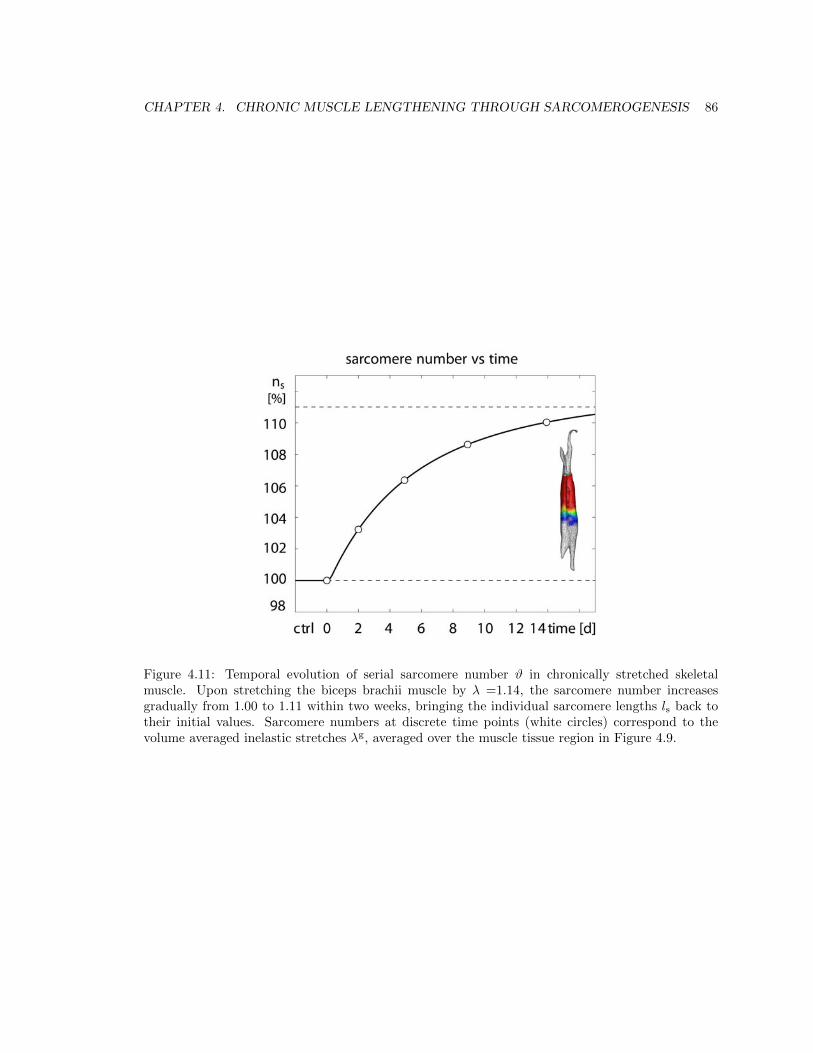
CHAPTER 4. CHRONIC MUSCLE LENGTHENING THROUGH SARCOMEROGENESIS 86
Figure 4.11: Temporal evolution of serial sarcomere number # in chronically stretched skeletalmuscle. Upon stretching the biceps brachii muscle by � =1.14, the sarcomere number increasesgradually from 1.00 to 1.11 within two weeks, bringing the individual sarcomere lengths ls back totheir initial values. Sarcomere numbers at discrete time points (white circles) correspond to thevolume averaged inelastic stretches �g, averaged over the muscle tissue region in Figure 4.9.
CHAPTER 4. CHRONIC MUSCLE LENGTHENING THROUGH SARCOMEROGENESIS 87
4.4 Discussion
We have proposed, for the first time, a mechanistic multiscale model for stretch-induced sarcom-
erogenesis, in which chronic muscle lengthening is characterized through a scalar-valued internal
variable, the serial sarcomere number. The model interprets the macroscopic elastic and inelastic
fiber stretches �e and �g as metrics for the microscopic sarcomere length and sarcomere number ls
and #. It is in excellent qualitative and quantitative agreement with the sarcomere lengths observed
in a chronic limb lengthening experiment.
Limitations
Although our first prototype model agrees nicely with experimental findings, a few limitations re-
main to be addressed in future model refinements. First, for the sake of simplicity, we have chosen
a relatively straightforward baseline elastic model, see equation (4.7). Since we model the growth
process as strain-driven [36] and not stress-driven [87], the choice of the constitutive model a↵ects
the growth process only indirectly. An appropriate muscle model would become important though
if we wanted to predict limit stresses and forces required to apply the desired stretch [70]. However,
as our approach is inherently modular, it would be relatively straightforward to integrate a more
physiological constitutive model [24,29]. Second, since tendon tissue is more than one order of mag-
nitude sti↵er than muscle tissue [27, 43], we have modeled the tendon as semi-rigid. This approach
provides quick insight into overall characteristics and trends. Extending the model towards a tendon
with a finite sti↵ness should not pose additional complexity, provided the tendon model parameters
are known [43]. Third, we have assumed that muscle lengthening translates directly into sarcomere
lengthening, i.e., that the elastic fiber stretch is directly correlated to the sarcomere length [75]. This
approach is relatively common in the skeletal muscle literature [13, 144], although potential second
order e↵ects could possibly contribute to additional muscle lengthening. Fourth, we have adopted
a simple functional form for the evolution of the sarcomere number in equations (4.9) and (4.10).
This particular format is conceptually well-understood since it has been applied to model growth of
other soft biological tissues, first in a stress-driven [118,139] then in a strain-driven [72,176] version.
Although this format seems to yield an excellent agreement with experimental findings, alternative
evolution equations might be possible and could be integrated in a relatively straightforward fashion.
Along the same lines, we could further enhance the model to integrate sarcomere disassembly upon
chronically reduced stretch [40], a phenomenon that has been studied intensely during immobiliza-
tion [194, 216] and tendon retraction [70]. Last, to better calibrate the model, a richer data set
would be desirable. Here we have based our model calibration on a two-week long limb lengthening
study in rabbits [144]. At this point, it is unclear whether the adaptation speed observed in small
animals translates directly to humans. Currently, the lack of chronic experiments with multiple
well-defined time points still limits the clinical use of the model. However, recent developments in
CHAPTER 4. CHRONIC MUSCLE LENGTHENING THROUGH SARCOMEROGENESIS 88
second harmonic generation microendoscopy [136] now allow us to measure local sarcomere length
non-invasively in humans, to precisely quantify spatial and temporal sarcomere variations in vivo.
Significance
Our model is the first mechanistic model to link macroscopic elastic and inelastic stretch to micro-
scopic sarcomere length and number using nonlinear continuum theories of finite growth. On the
microscopic scale, chronic muscle stretching beyond the physiological limit creates unphysiologically
large sarcomere lengths [20], which, in turn, induce a serial sarcomere deposition [42]. The resulting
increase in sarcomere number causes a chronic restoration of the initial sarcomere length [86]. On
the macroscopic scale, the serial sarcomere deposition induces a chronic reduction of the macroscopic
elastic stretch, gradually reducing the passive stress [71], a phenomenon similar to classical stress
relaxation [38]. Our model provides a mechanistic understanding of the underlying mechanisms
accompanying chronic muscle stretch and sarcomerogenesis [104]. At this point, it does not describe
the mechanobiology and the mechanotransduction pathways associated with sarcomerogenesis [61].
However, ultimately, it would be desirable to tie the mechanical response to mechanoreception, in-
tracellular signaling pathways, and target activation [41].
We have shown that our model can explain why gradual multi-step stretching is less invasive than
single-step stretching [85]. It also explains regional variation in sarcomere lengths [182], shorter close
to and longer away from the muscle-tendon interface, where the sti↵ tendon provides additional sup-
port to stretch [75]. Acutely, our model could serve as a design tool to prevent short-term muscle
damage caused by mechanical overstretch. Macroscopically for a given limit stress, or equivalently,
microscopically for a given limit sarcomere length, we could optimize temporal stretching sequences
that predict the maximum possible stretch within acceptable limits [230]. The ultimate goal would
be to maximize stretch-induced muscle growth, such that the muscle always stays within a physio-
logically reasonable operating range. Chronically, our model could serve as a design tool to predict
long-term muscle adaptation. We could easily integrate it into existing skeletal muscle models to
optimize muscle lengthening in response to eccentric training [195] or to predict di↵erent surgical
procedures such as tendon transfer, tendon reattachment, or tendon lengthening [12]. The ultimate
goal would be to guarantee optimal regeneration and long-term repair durability.
4.5 Conclusion
Striated muscle adapts to chronic mechanical stretch through the creation and serial deposition of
new sarcomere units. The phenomenon of sarcomerogenesis has been quantified in chronic animal
experiments, but it has never been modeled computationally. Here we have presented a mathemat-
ical model for chronic muscle growth through sarcomerogenesis and illustrated its computational
realization. Acutely, upon 14% lengthening of the extensor digitorum lateralis muscle, the model
CHAPTER 4. CHRONIC MUSCLE LENGTHENING THROUGH SARCOMEROGENESIS 89
predicts a sarcomere lengthening from 3.09µm to 3.51µm with a model error of 0.00%. Chronically,
the model predicts the gradual return to the initial sarcomere length within two weeks with a model
error of 2.13%, which is within the rage of the experimental standard deviation. Once calibrated
with a richer data set, our model may be used to help surgeons to make informed decisions about
optimal stretch increments, stretch timing, and stretch amplitudes. Our study might to open new
avenues in orthopedic and reconstructive surgery and enhance muscle adaptation, repair, and regen-
eration for patients with ill proportioned limbs, tendon lengthening, tendon transfer, tendon tear,
or chronically retracted muscles.
4.6 Acknowledgments
This material is part of a final project for the Stanford graduate course ME337 Mechanics of Growth.
This work was supported by the National Science Foundation CAREER award CMMI-0952021 and
by the National Institutes of Health Grant U54 GM072970.
Chapter 5
A multiscale model for sarcomere
loss
Abstract
High heels are a major source of chronic lower limb pain. Yet, more than one third of all
women compromise health for looks and wear high heels on a daily basis. Changing from flat
footwear to high heels induces chronic muscle shortening associated with discomfort, fatigue, re-
duced shock absorption, and increased injury risk. However, the long-term e↵ects of high-heeled
footwear on the musculoskeletal kinematics of the lower extremities remain poorly understood.
Here we create a multiscale computational model for chronic muscle adaptation to characterize
the acute and chronic e↵ects of global muscle shortening on local sarcomere lengths. We perform
a case study of a healthy female subject and show that raising the heel by 13 cm shortens the
gastrocnemius muscle by 5% while the Achilles tendon remains virtually una↵ected. Our com-
putational simulation indicates that muscle shortening displays significant regional variations
with extreme values of 22% in the central gastrocnemius. Our model suggests that the muscle
gradually adjusts to its new functional length by a chronic loss of sarcomeres in series. Sarcom-
ere loss varies significantly across the muscle with an average loss of 9%, virtually no loss at
the proximal and distal ends, and a maximum loss of 39% in the central region. These changes
reposition the remaining sarcomeres back into their optimal operating regime. Computational
modeling of chronic muscle shortening provides a valuable tool to shape our understanding of
the underlying mechanisms of muscle adaptation. Our study could open new avenues in or-
thopedic surgery and enhance treatment for patients with muscle contracture caused by other
conditions than high heel wear such as paralysis, muscular atrophy, and muscular dystrophy.
90
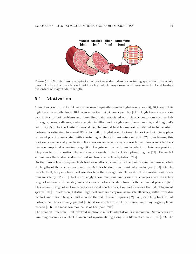
CHAPTER 5. A MULTISCALE MODEL FOR SARCOMERE LOSS 91
sarcomerefiberfasciclemuscle[um][mm][cm][dm]
Figure 5.1: Chronic muscle adaptation across the scales. Muscle shortening spans from the wholemuscle level via the fascicle level and fiber level all the way down to the sarcomere level and bridgesfive orders of magnitude in length.
5.1 Motivation
More than two thirds of all American women frequently dress in high-heeled shoes [8], 40% wear their
high heels on a daily basis, 10% even more than eight hours per day [221]. High heels are a major
contributor to foot problems and lower limb pain, associated with chronic conditions such as hal-
lux vagus, corns, callusses, metatarsalgia, Achilles tendon tightness, planar fasciitis, and Haglund’s
deformity [53]. In the United States alone, the annual health care cost attributed to high-fashion
footwear is estimated to exceed $3 billion [208]. High-heeled footwear forces the foot into a plan-
tarflexed position associated with shortening of the calf muscle-tendon unit [52]. Short-term, this
position is energetically ine�cient: It causes excessive actin-myosin overlap and forces muscle fibers
into a non-optimal operating range [60]. Long-term, our calf muscles adapt to their new position:
They shorten to reposition the actin-myosin overlap into back its optimal regime [53]. Figure 5.1
summarizes the spatial scales involved in chronic muscle adaptation [217].
On the muscle level, frequent high heel wear a↵ects primarily in the gastrocnemuius muscle, while
the lengths of the soleus muscle and the Achilles tendon remain virtually unchanged [103]. On the
fascicle level, frequent high heel use shortens the average fascicle length of the medial gastrocne-
mius muscle by 12% [51]. Not surprisingly, these functional and structural changes a↵ect the active
range of motion of the ankle joint and cause a noticeable shift towards the supinated position [53].
This reduced range of motion decreases e�cient shock absorption and increases the risk of ligament
sprains [103]. In addition, habitual high heel wearers compromise muscle e�ciency, su↵er from dis-
comfort and muscle fatigue, and increase the risk of strain injuries [52]. Yet, switching back to flat
footwear can be extremely painful [105]; it overstretches the triceps surae and may trigger planar
fasciitis [156], the most common cause of heel pain [206].
The smallest functional unit involved in chronic muscle adaptation is a sarcomere. Sarcomeres are
3um long assemblies of thick filaments of myosin sliding along thin filaments of actin [132]. On the
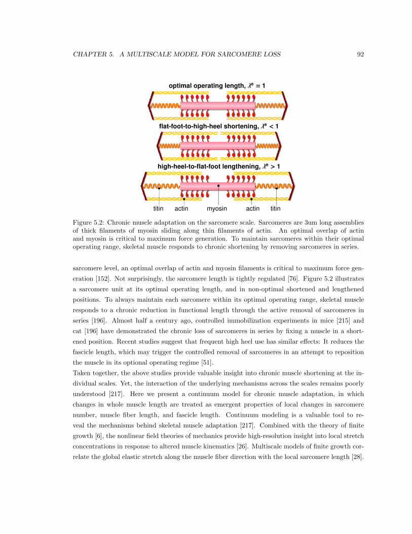
CHAPTER 5. A MULTISCALE MODEL FOR SARCOMERE LOSS 92
titin actin myosin actin titin
optimal operating length, �e = 1
flat-foot-to-high-heel shortening, �e < 1
high-heel-to-flat-foot lengthening, �e > 1
Figure 5.2: Chronic muscle adaptation on the sarcomere scale. Sarcomeres are 3um long assembliesof thick filaments of myosin sliding along thin filaments of actin. An optimal overlap of actinand myosin is critical to maximum force generation. To maintain sarcomeres within their optimaloperating range, skeletal muscle responds to chronic shortening by removing sarcomeres in series.
sarcomere level, an optimal overlap of actin and myosin filaments is critical to maximum force gen-
eration [152]. Not surprisingly, the sarcomere length is tightly regulated [76]. Figure 5.2 illustrates
a sarcomere unit at its optimal operating length, and in non-optimal shortened and lengthened
positions. To always maintain each sarcomere within its optimal operating range, skeletal muscle
responds to a chronic reduction in functional length through the active removal of sarcomeres in
series [196]. Almost half a century ago, controlled immobilization experiments in mice [215] and
cat [196] have demonstrated the chronic loss of sarcomeres in series by fixing a muscle in a short-
ened position. Recent studies suggest that frequent high heel use has similar e↵ects: It reduces the
fascicle length, which may trigger the controlled removal of sarcomeres in an attempt to reposition
the muscle in its optional operating regime [51].
Taken together, the above studies provide valuable insight into chronic muscle shortening at the in-
dividual scales. Yet, the interaction of the underlying mechanisms across the scales remains poorly
understood [217]. Here we present a continuum model for chronic muscle adaptation, in which
changes in whole muscle length are treated as emergent properties of local changes in sarcomere
number, muscle fiber length, and fascicle length. Continuum modeling is a valuable tool to re-
veal the mechanisms behind skeletal muscle adaptation [217]. Combined with the theory of finite
growth [6], the nonlinear field theories of mechanics provide high-resolution insight into local stretch
concentrations in response to altered muscle kinematics [26]. Multiscale models of finite growth cor-
relate the global elastic stretch along the muscle fiber direction with the local sarcomere length [28].
CHAPTER 5. A MULTISCALE MODEL FOR SARCOMERE LOSS 93
To maintain this length within its physiologically optimal regime, the local sarcomere number un-
dergoes dynamic change, which translates globally into an inelastic stretch or growth [72]. Previous
models for cardiac muscle, the extensor digitorum, and the biceps brachii have successfully applied
this concept to model positive growth associated with chronic muscle lengthening in dilated car-
diomyopathy [73], limb lengthening, and tendon tear [225]. Here we adopt the same paradigm to
model negative growth associated with chronic muscle shortening in frequent high heel wear.
5.2 Methods
To simulate the short- and long-term e↵ects of high-heeled footwear, we create a subject-specific
model of the lower limb using magnetic resonance images in flat foot and high heel positions. We
perform a finite element analysis of acute and chronic muscle shortening using the continuum theory
of finite growth.
5.2.1 Continuum model
To represent large muscle deformations, we adopt the kinematics of finite growth, and introduce the
deformation map '(X, t) mapping particlesX from the initial configuration to particles x = '(X, t)
in the new configuration. We multiplicatively decompose its gradient F = rX
' into an elastic
contribution F
e and an inelastic contribution F
g [183], which we associate with chronic muscle
adaptation [225],
F = rX
' = F
e · F g . (5.1)
The Jacobian J = det(F ) defines the change in muscle volume,
J = det(F ) = JeJg , (5.2)
which we decompose into an elastic volume change Je = det(F e) and an inelastic volume change Jg =
det(F g) attributed to muscle adaptation. Similar to the deformation gradient and the Jacobian, we
interpret the total stretch � along the fiber direction of the initial configuration n0 as the product
of the elastic stretch �e and the inelastic stretch �g associated with chronic changes in muscle
length [151],
� = [n0 · F t · F · n0 ]1/2 = �e�g . (5.3)
We model chronic muscle shortening as the removal of sarcomeres in series. This implies that we
can express the muscle adaptation tensor F g as rank-one update of the identity tensor I [225],
F
g = I + [#� 1] n0 ⌦ n0 , (5.4)
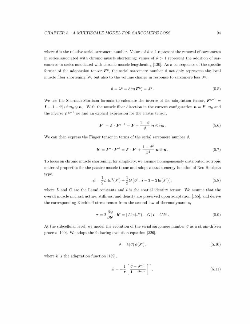
CHAPTER 5. A MULTISCALE MODEL FOR SARCOMERE LOSS 94
where # is the relative serial sarcomere number. Values of # < 1 represent the removal of sarcomeres
in series associated with chronic muscle shortening; values of # > 1 represent the addition of sar-
comeres in series associated with chronic muscle lengthening [120]. As a consequence of the specific
format of the adaptation tensor F
g, the serial sarcomere number # not only represents the local
muscle fiber shortening �g, but also to the volume change in response to sarcomere loss Jg,
# = �g = det(F g) = Jg . (5.5)
We use the Sherman-Morrison formula to calculate the inverse of the adaptation tensor, F g�1 =
I + [1� #] /#n0 ⌦n0. With the muscle fiber direction in the current configuration n = F ·n0 and
the inverse F
g�1 we find an explicit expression for the elastic tensor,
F
e = F · F g�1 = F +1� ##
n⌦ n0 . (5.6)
We can then express the Finger tensor in terms of the serial sarcomere number #,
b
e = F
e · F et = F · F t +1� #2
#2n⌦ n . (5.7)
To focus on chronic muscle shortening, for simplicity, we assume homogeneously distributed isotropic
material properties for the passive muscle tissue and adopt a strain energy function of Neo-Hookean
type,
=1
2L ln2(Je) +
1
2G [ be : i� 3� 2 ln(Je) ] , (5.8)
where L and G are the Lame constants and i is the spatial identity tensor. We assume that the
overall muscle microstructure, sti↵ness, and density are preserved upon adaptation [155], and derive
the corresponding Kirchho↵ stress tensor from the second law of thermodynamics,
⌧ = 2@
@be· be = [L ln(Je)�G ] i+G b
e . (5.9)
At the subcellular level, we model the evolution of the serial sarcomere number # as a strain-driven
process [199]. We adopt the following evolution equation [226],
# = k(#)�(�e) , (5.10)
where k is the adaptation function [139],
k = �1
⌧
#� #min
1� #min
��
, (5.11)
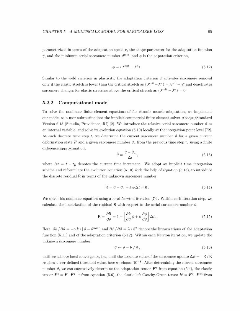
CHAPTER 5. A MULTISCALE MODEL FOR SARCOMERE LOSS 95
parameterized in terms of the adaptation speed ⌧ , the shape parameter for the adaptation function
�, and the minimum serial sarcomere number #min, and � is the adpatation criterion,
� = h�crit � �e i . (5.12)
Similar to the yield criterion in plasticity, the adaptation criterion � activates sarcomere removal
only if the elastic stretch is lower than the critical stretch as h�crit��e i = �crit��e and deactivates
sarcomere changes for elastic stretches above the critical stretch as h�crit � �e i = 0.
5.2.2 Computational model
To solve the nonlinear finite element equations of for chronic muscle adaptation, we implement
our model as a user subroutine into the implicit commercial finite element solver Abaqus/Standard
Version 6.13 (Simulia, Providence, RI) [2]. We introduce the relative serial sarcomere number # as
an internal variable, and solve its evolution equation (5.10) locally at the integration point level [72].
At each discrete time step t, we determine the current sarcomere number # for a given current
deformation state F and a given sarcomere number #n from the previous time step tn using a finite
di↵erence approximation,
# =#� #n�t
, (5.13)
where �t = t � tn denotes the current time increment. We adopt an implicit time integration
scheme and reformulate the evolution equation (5.10) with the help of equation (5.13), to introduce
the discrete residual R in terms of the unknown sarcomere number,
R = #� #n + k ��t.= 0 . (5.14)
We solve this nonlinear equation using a local Newton iteration [73]. Within each iteration step, we
calculate the linearization of the residual R with respect to the serial sarcomere number #,
K =@R
@#= 1�
@k
@#�+ k
@�
@#
��t . (5.15)
Here, @k / @# = �� k / [# � #min ] and @� / @# = � /#2 denote the linearizations of the adaptation
function (5.11) and of the adaptation criterion (5.12). Within each Newton iteration, we update the
unknown sarcomere number,
# #� R /K , (5.16)
until we achieve local convergence, i.e., until the absolute value of the sarcomere update�# = �R /K
reaches a user-defined threshold value, here we choose 10�8. After determining the current sarcomere
number #, we can successively determine the adaptation tensor F g from equation (5.4), the elastic
tensor F e = F · F g�1 from equation (5.6), the elastic left Cauchy-Green tensor be = F
e · F e t from
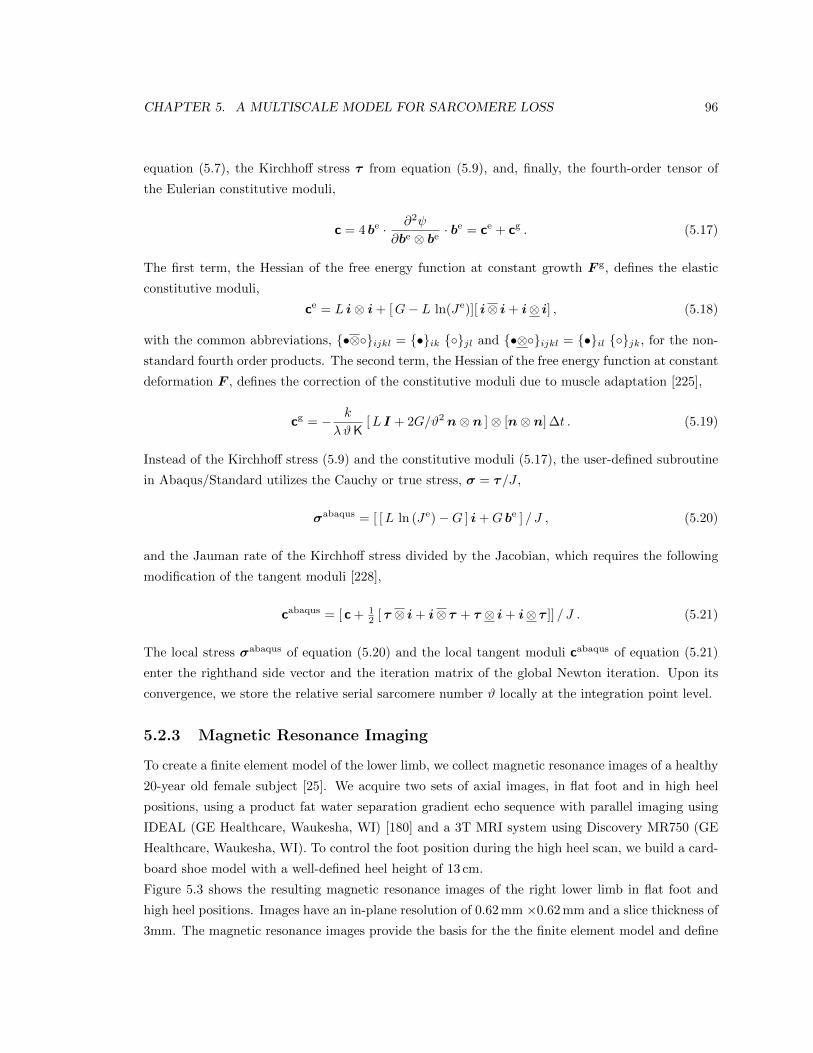
CHAPTER 5. A MULTISCALE MODEL FOR SARCOMERE LOSS 96
equation (5.7), the Kirchho↵ stress ⌧ from equation (5.9), and, finally, the fourth-order tensor of
the Eulerian constitutive moduli,
c = 4 be · @2
@be ⌦ b
e· be = c
e + c
g . (5.17)
The first term, the Hessian of the free energy function at constant growth F
g, defines the elastic
constitutive moduli,
c
e = L i⌦ i+ [G� L ln(Je)][ i⌦ i+ i⌦ i] , (5.18)
with the common abbreviations, {•⌦�}ijkl
= {•}ik
{�}jl
and {•⌦�}ijkl
= {•}il
{�}jk
, for the non-
standard fourth order products. The second term, the Hessian of the free energy function at constant
deformation F , defines the correction of the constitutive moduli due to muscle adaptation [225],
c
g = � k
�#K[L I + 2G/#2 n⌦ n ]⌦ [n⌦ n]�t . (5.19)
Instead of the Kirchho↵ stress (5.9) and the constitutive moduli (5.17), the user-defined subroutine
in Abaqus/Standard utilizes the Cauchy or true stress, � = ⌧/J ,
�
abaqus = [ [L ln (Je)�G ] i+G b
e ] / J , (5.20)
and the Jauman rate of the Kirchho↵ stress divided by the Jacobian, which requires the following
modification of the tangent moduli [228],
c
abaqus = [ c+ 12 [ ⌧ ⌦ i+ i⌦ ⌧ + ⌧ ⌦ i+ i⌦ ⌧ ]] / J . (5.21)
The local stress �
abaqus of equation (5.20) and the local tangent moduli cabaqus of equation (5.21)
enter the righthand side vector and the iteration matrix of the global Newton iteration. Upon its
convergence, we store the relative serial sarcomere number # locally at the integration point level.
5.2.3 Magnetic Resonance Imaging
To create a finite element model of the lower limb, we collect magnetic resonance images of a healthy
20-year old female subject [25]. We acquire two sets of axial images, in flat foot and in high heel
positions, using a product fat water separation gradient echo sequence with parallel imaging using
IDEAL (GE Healthcare, Waukesha, WI) [180] and a 3T MRI system using Discovery MR750 (GE
Healthcare, Waukesha, WI). To control the foot position during the high heel scan, we build a card-
board shoe model with a well-defined heel height of 13 cm.
Figure 5.3 shows the resulting magnetic resonance images of the right lower limb in flat foot and
high heel positions. Images have an in-plane resolution of 0.62mm ⇥0.62mm and a slice thickness of
3mm. The magnetic resonance images provide the basis for the the finite element model and define
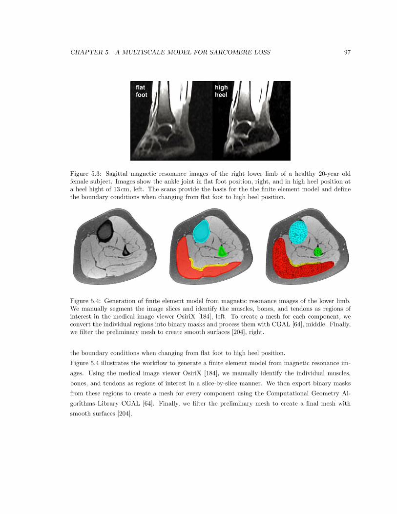
CHAPTER 5. A MULTISCALE MODEL FOR SARCOMERE LOSS 97
and the Jauman rate of the Kirchho↵ stress divided by the Jaco-bian, which requires the following modification of the tangentmoduli [49],
cabaqus = [ c + 12 [ ⌧⌦ i + i⌦ ⌧ + ⌧⌦ i + i⌦ ⌧]] / J . (21)
The local stress �abaqus of equation (20) and the local tangentmoduli cabaqus of equation (21) enter the righthand side vectorand the iteration matrix of the global Newton iteration. Uponits convergence, we store the relative serial sarcomere number# locally at the integration point level.
2.3. Magnetic Resonance ImagingTo create a finite element model of the lower limb, we collectmagnetic resonance images of a healthy 20-year old femalesubject [4]. We acquire two sets of axial images, in flat footand in high heel positions, using a product fat water separationgradient echo sequence with parallel imaging using IDEAL(GE Healthcare, Waukesha, WI) [34] and a 3T MRI systemusing Discovery MR750 (GE Healthcare, Waukesha, WI). Tocontrol the foot position during the high heel scan, we build acardboard shoe model with a well-defined heel height of 13 cm.
flatfoot
highheel
Figure 3: Sagittal magnetic resonance images of the right lower limb of ahealthy 20-year old female subject. Images show the ankle joint in flat footposition, right, and in high heel position at a heel hight of 13 cm, left. Thescans provide the basis for the the finite element model and define the bound-ary conditions when changing from flat foot to high heel position.
4
Figure 5.3: Sagittal magnetic resonance images of the right lower limb of a healthy 20-year oldfemale subject. Images show the ankle joint in flat foot position, right, and in high heel position ata heel hight of 13 cm, left. The scans provide the basis for the the finite element model and definethe boundary conditions when changing from flat foot to high heel position.
Figure 4: Generation of finite element model from magnetic resonance imagesof the lower limb. We manually segment the image slices and identify the mus-cles, bones, and tendons as regions of interest in the medical image viewerOsiriX [36], left. To create a mesh for each component, we convert the indi-vidual regions into binary masks and process them with CGAL [16], middle.Finally, we filter the preliminary mesh to create smooth surfaces [39], right.
5
Figure 5.4: Generation of finite element model from magnetic resonance images of the lower limb.We manually segment the image slices and identify the muscles, bones, and tendons as regions ofinterest in the medical image viewer OsiriX [184], left. To create a mesh for each component, weconvert the individual regions into binary masks and process them with CGAL [64], middle. Finally,we filter the preliminary mesh to create smooth surfaces [204], right.
the boundary conditions when changing from flat foot to high heel position.
Figure 5.4 illustrates the workflow to generate a finite element model from magnetic resonance im-
ages. Using the medical image viewer OsiriX [184], we manually identify the individual muscles,
bones, and tendons as regions of interest in a slice-by-slice manner. We then export binary masks
from these regions to create a mesh for every component using the Computational Geometry Al-
gorithms Library CGAL [64]. Finally, we filter the preliminary mesh to create a final mesh with
smooth surfaces [204].
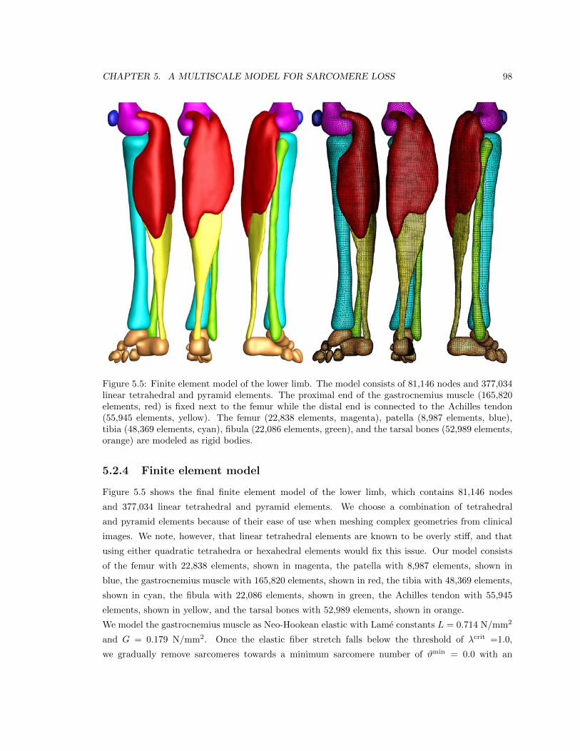
CHAPTER 5. A MULTISCALE MODEL FOR SARCOMERE LOSS 98
Figure 5: Finite element model of the lower limb. The model consists of 81,146nodes and 377,034 linear tetrahedral and pyramid elements. The proximal endof the gastrocnemius muscle (165,820 elements, red) is fixed next to the femurwhile the distal end is connected to the Achilles tendon (55,945 elements, yel-low). The femur (22,838 elements, magenta), patella (8,987 elements, blue),tibia (48,369 elements, cyan), fibula (22,086 elements, green), and the tarsalbones (52,989 elements, orange) are modeled as rigid bodies.
7
Figure 5.5: Finite element model of the lower limb. The model consists of 81,146 nodes and 377,034linear tetrahedral and pyramid elements. The proximal end of the gastrocnemius muscle (165,820elements, red) is fixed next to the femur while the distal end is connected to the Achilles tendon(55,945 elements, yellow). The femur (22,838 elements, magenta), patella (8,987 elements, blue),tibia (48,369 elements, cyan), fibula (22,086 elements, green), and the tarsal bones (52,989 elements,orange) are modeled as rigid bodies.
5.2.4 Finite element model
Figure 5.5 shows the final finite element model of the lower limb, which contains 81,146 nodes
and 377,034 linear tetrahedral and pyramid elements. We choose a combination of tetrahedral
and pyramid elements because of their ease of use when meshing complex geometries from clinical
images. We note, however, that linear tetrahedral elements are known to be overly sti↵, and that
using either quadratic tetrahedra or hexahedral elements would fix this issue. Our model consists
of the femur with 22,838 elements, shown in magenta, the patella with 8,987 elements, shown in
blue, the gastrocnemius muscle with 165,820 elements, shown in red, the tibia with 48,369 elements,
shown in cyan, the fibula with 22,086 elements, shown in green, the Achilles tendon with 55,945
elements, shown in yellow, and the tarsal bones with 52,989 elements, shown in orange.
We model the gastrocnemius muscle as Neo-Hookean elastic with Lame constants L = 0.714 N/mm2
and G = 0.179 N/mm2. Once the elastic fiber stretch falls below the threshold of �crit =1.0,
we gradually remove sarcomeres towards a minimum sarcomere number of #min = 0.0 with an
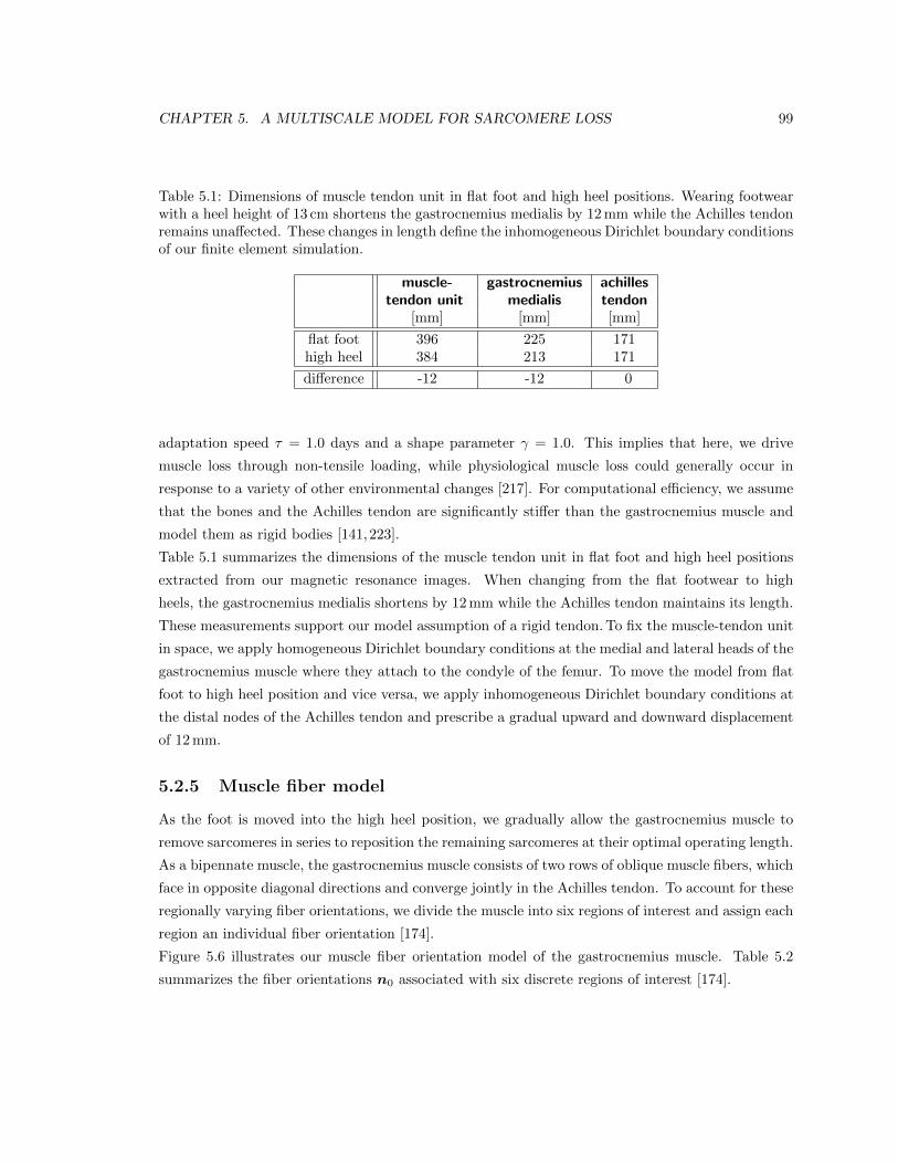
CHAPTER 5. A MULTISCALE MODEL FOR SARCOMERE LOSS 99
Table 5.1: Dimensions of muscle tendon unit in flat foot and high heel positions. Wearing footwearwith a heel height of 13 cm shortens the gastrocnemius medialis by 12mm while the Achilles tendonremains una↵ected. These changes in length define the inhomogeneous Dirichlet boundary conditionsof our finite element simulation.
muscle- gastrocnemius achilles
tendon unit medialis tendon
[mm] [mm] [mm]
flat foot 396 225 171high heel 384 213 171
di↵erence -12 -12 0
adaptation speed ⌧ = 1.0 days and a shape parameter � = 1.0. This implies that here, we drive
muscle loss through non-tensile loading, while physiological muscle loss could generally occur in
response to a variety of other environmental changes [217]. For computational e�ciency, we assume
that the bones and the Achilles tendon are significantly sti↵er than the gastrocnemius muscle and
model them as rigid bodies [141,223].
Table 5.1 summarizes the dimensions of the muscle tendon unit in flat foot and high heel positions
extracted from our magnetic resonance images. When changing from the flat footwear to high
heels, the gastrocnemius medialis shortens by 12mm while the Achilles tendon maintains its length.
These measurements support our model assumption of a rigid tendon.To fix the muscle-tendon unit
in space, we apply homogeneous Dirichlet boundary conditions at the medial and lateral heads of the
gastrocnemius muscle where they attach to the condyle of the femur. To move the model from flat
foot to high heel position and vice versa, we apply inhomogeneous Dirichlet boundary conditions at
the distal nodes of the Achilles tendon and prescribe a gradual upward and downward displacement
of 12mm.
5.2.5 Muscle fiber model
As the foot is moved into the high heel position, we gradually allow the gastrocnemius muscle to
remove sarcomeres in series to reposition the remaining sarcomeres at their optimal operating length.
As a bipennate muscle, the gastrocnemius muscle consists of two rows of oblique muscle fibers, which
face in opposite diagonal directions and converge jointly in the Achilles tendon. To account for these
regionally varying fiber orientations, we divide the muscle into six regions of interest and assign each
region an individual fiber orientation [174].
Figure 5.6 illustrates our muscle fiber orientation model of the gastrocnemius muscle. Table 5.2
summarizes the fiber orientations n0 associated with six discrete regions of interest [174].
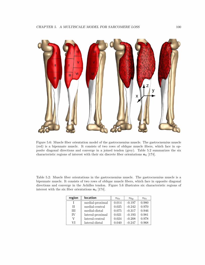
CHAPTER 5. A MULTISCALE MODEL FOR SARCOMERE LOSS 100
-6
�� x
y
z
Figure 5.6: Muscle fiber orientation model of the gastrocnemius muscle. The gastrocnemius muscle(red) is a bipennate muscle. It consists of two rows of oblique muscle fibers, which face in op-posite diagonal directions and converge in a joined tendon (grey). Table 5.2 summarizes the sixcharacteristic regions of interest with their six discrete fiber orientations n0 [174].
Table 5.2: Muscle fiber orientations in the gastrocnemius muscle. The gastrocnemius muscle is abipennate muscle. It consists of two rows of oblique muscle fibers, which face in opposite diagonaldirections and converge in the Achilles tendon. Figure 5.6 illustrates six characteristic regions ofinterest with the six fiber orientations n0 [174].
region location n0x n0y n0z
I medial-proximal 0.014 -0.197 0.980II medial-central 0.025 -0.242 0.970III medial-distal 0.075 -0.317 0.946IV lateral-proximal 0.021 -0.193 0.981V lateral-central 0.024 -0.208 0.978VI lateral-distal 0.040 -0.247 0.968
CHAPTER 5. A MULTISCALE MODEL FOR SARCOMERE LOSS 101
Figure 7: Finite element model of muscle shortening in response to frequent high heel use. The left model shows the baseline state created from magnetic resonanceimages in flat foot position. The right model shows the shortened state created from images in high heel position. To move the flat foot into the high heel position,we apply inhomogeneous Dirichlet boundary conditions by prescribing a 12 mm upward displacement of the distal end of the Achilles tendon. Then we maintainthe foot in this position to allow the muscle to adapt to its new physiological length.
8
Figure 5.7: Finite element model of muscle shortening in response to frequent high heel use. Theleft model shows the baseline state created from magnetic resonance images in flat foot position.The right model shows the shortened state created from images in high heel position. To movethe flat foot into the high heel position, we apply inhomogeneous Dirichlet boundary conditions byprescribing a 12mm upward displacement of the distal end of the Achilles tendon. Then we maintainthe foot in this position to allow the muscle to adapt to its new physiological length.
5.2.6 Boundary conditions
To explore the acute and chronic e↵ects of global muscle shortening on local sarcomere lengths, we
simulate three scenarios: (i) acute e↵ects when changing from flat foot to high heel position, (ii)
chronic e↵ects when maintaining the high heel position, and (iii) acute e↵ects when changing back
from high heel to flat foot position.
Figure 5.7 illustrates our finite element model of the lower limb. The left model shows the baseline
state created from magnetic resonance images in flat foot position. The right model shows the
shortened state created from images in high heel position. First, we move the model from flat foot
to high heel position by prescribing an upward displacement on the distal nodes of the Achilles
tendon. Then, we keep the foot in this position and allow the gastrocnemius to shorten and adapt
to its new physiological length. Last, after the muscle has adapted, we move the foot back into the
flat foot position.
5.3 Results
All three simulations run robustly, converge quadratically, and generate conceptually feasible results,
which we discuss in detail in the following three subsections.
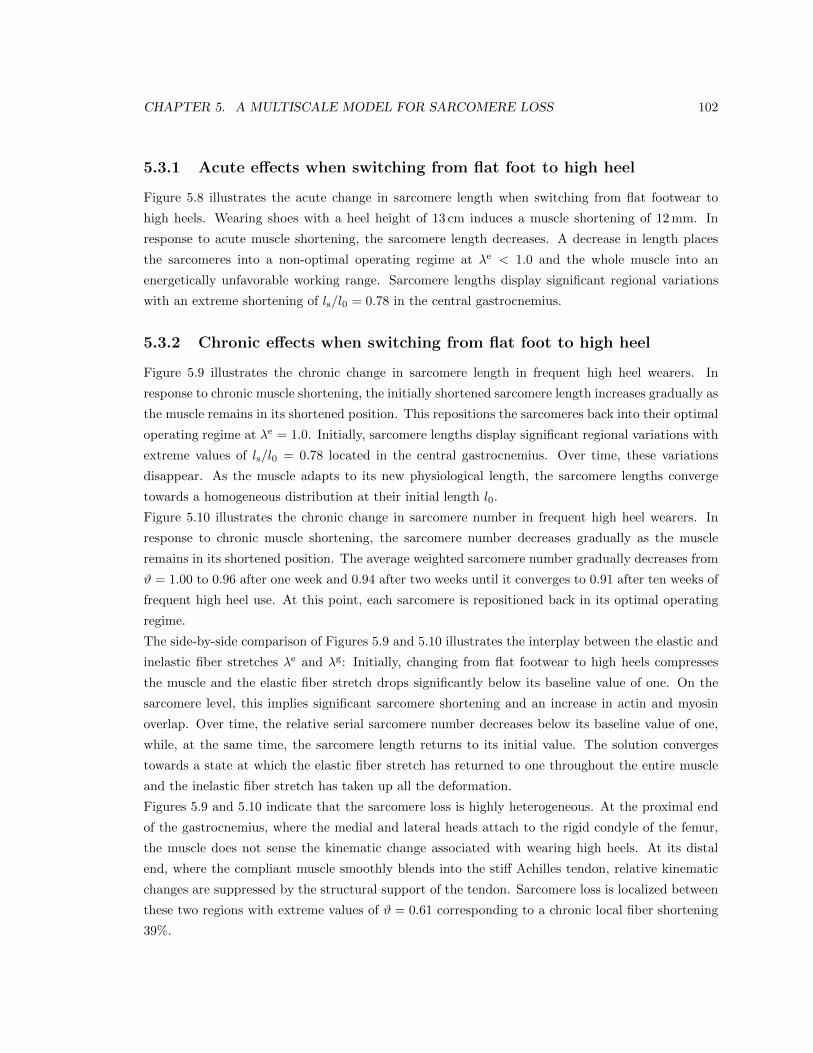
CHAPTER 5. A MULTISCALE MODEL FOR SARCOMERE LOSS 102
5.3.1 Acute e↵ects when switching from flat foot to high heel
Figure 5.8 illustrates the acute change in sarcomere length when switching from flat footwear to
high heels. Wearing shoes with a heel height of 13 cm induces a muscle shortening of 12mm. In
response to acute muscle shortening, the sarcomere length decreases. A decrease in length places
the sarcomeres into a non-optimal operating regime at �e < 1.0 and the whole muscle into an
energetically unfavorable working range. Sarcomere lengths display significant regional variations
with an extreme shortening of ls/l0 = 0.78 in the central gastrocnemius.
5.3.2 Chronic e↵ects when switching from flat foot to high heel
Figure 5.9 illustrates the chronic change in sarcomere length in frequent high heel wearers. In
response to chronic muscle shortening, the initially shortened sarcomere length increases gradually as
the muscle remains in its shortened position. This repositions the sarcomeres back into their optimal
operating regime at �e = 1.0. Initially, sarcomere lengths display significant regional variations with
extreme values of ls/l0 = 0.78 located in the central gastrocnemius. Over time, these variations
disappear. As the muscle adapts to its new physiological length, the sarcomere lengths converge
towards a homogeneous distribution at their initial length l0.
Figure 5.10 illustrates the chronic change in sarcomere number in frequent high heel wearers. In
response to chronic muscle shortening, the sarcomere number decreases gradually as the muscle
remains in its shortened position. The average weighted sarcomere number gradually decreases from
# = 1.00 to 0.96 after one week and 0.94 after two weeks until it converges to 0.91 after ten weeks of
frequent high heel use. At this point, each sarcomere is repositioned back in its optimal operating
regime.
The side-by-side comparison of Figures 5.9 and 5.10 illustrates the interplay between the elastic and
inelastic fiber stretches �e and �g: Initially, changing from flat footwear to high heels compresses
the muscle and the elastic fiber stretch drops significantly below its baseline value of one. On the
sarcomere level, this implies significant sarcomere shortening and an increase in actin and myosin
overlap. Over time, the relative serial sarcomere number decreases below its baseline value of one,
while, at the same time, the sarcomere length returns to its initial value. The solution converges
towards a state at which the elastic fiber stretch has returned to one throughout the entire muscle
and the inelastic fiber stretch has taken up all the deformation.
Figures 5.9 and 5.10 indicate that the sarcomere loss is highly heterogeneous. At the proximal end
of the gastrocnemius, where the medial and lateral heads attach to the rigid condyle of the femur,
the muscle does not sense the kinematic change associated with wearing high heels. At its distal
end, where the compliant muscle smoothly blends into the sti↵ Achilles tendon, relative kinematic
changes are suppressed by the structural support of the tendon. Sarcomere loss is localized between
these two regions with extreme values of # = 0.61 corresponding to a chronic local fiber shortening
39%.
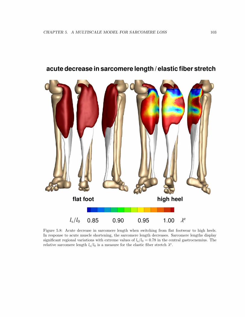
CHAPTER 5. A MULTISCALE MODEL FOR SARCOMERE LOSS 103
acute decrease in sarcomere length / elastic fiber stretch
flat foot high heel
ls/l0 0.85 0.90 0.95 1.00
�e
Figure 5.8: Acute decrease in sarcomere length when switching from flat footwear to high heels.In response to acute muscle shortening, the sarcomere length decreases. Sarcomere lengths displaysignificant regional variations with extreme values of ls/l0 = 0.78 in the central gastrocnemius. Therelative sarcomere length ls/l0 is a measure for the elastic fiber stretch �e.
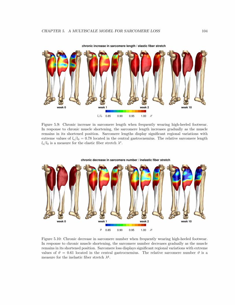
CHAPTER 5. A MULTISCALE MODEL FOR SARCOMERE LOSS 104
chronic increase in sarcomere length / elastic fiber stretch
week 0 week 1 week 2 week 10
ls/l0 0.85 0.90 0.95 1.00
�e
Figure 9: Chronic increase in sarcomere length when frequently wearing high-heeled footwear. In response to chronic muscle shortening, the sarcomere lengthincreases gradually as the muscle remains in its shortened position. Sarcomere lengths display significant regional variations with extreme values of ls/l0 = 0.78located in the central gastrocnemius. The relative sarcomere length ls/l0 is a measure for the elastic fiber stretch �e.
7
Figure 5.9: Chronic increase in sarcomere length when frequently wearing high-heeled footwear.In response to chronic muscle shortening, the sarcomere length increases gradually as the muscleremains in its shortened position. Sarcomere lengths display significant regional variations withextreme values of ls/l0 = 0.78 located in the central gastrocnemius. The relative sarcomere lengthls/l0 is a measure for the elastic fiber stretch �e.
chronic decrease in sarcomere number / inelastic fiber stretch
week 0 week 1 week 2 week 10
#0.85 0.90 0.95 1.00
�g
Figure 10: Chronic decrease in sarcomere number when frequently wearing high-heeled footwear. In response to chronic muscle shortening, the sarcomere numberdecreases gradually as the muscle remains in its shortened position. Sarcomere loss displays significant regional variations with extreme values of # = 0.61 locatedin the central gastrocnemius. The relative sarcomere number # is a measure for the inelastic fiber stretch �g.
9
Figure 5.10: Chronic decrease in sarcomere number when frequently wearing high-heeled footwear.In response to chronic muscle shortening, the sarcomere number decreases gradually as the muscleremains in its shortened position. Sarcomere loss displays significant regional variations with extremevalues of # = 0.61 located in the central gastrocnemius. The relative sarcomere number # is ameasure for the inelastic fiber stretch �g.
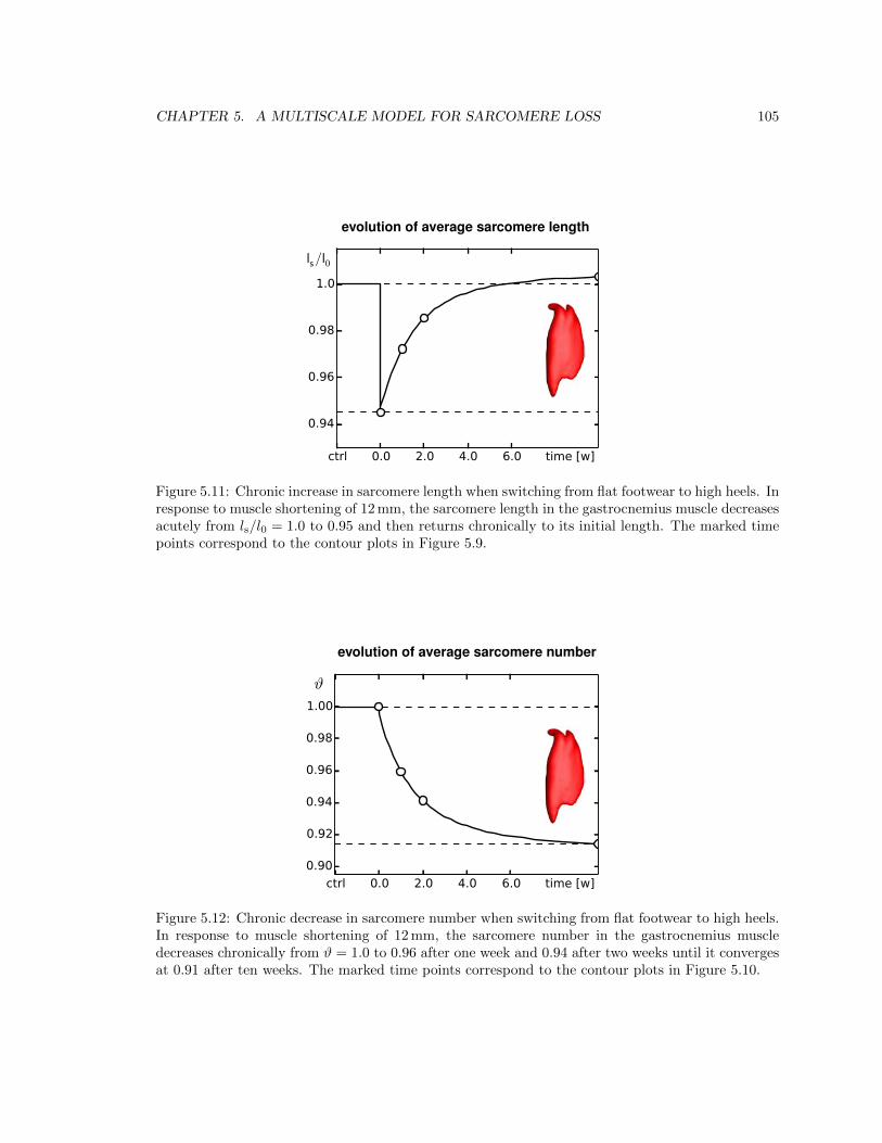
CHAPTER 5. A MULTISCALE MODEL FOR SARCOMERE LOSS 105
evolution of average sarcomere length
Figure 11: Chronic increase in sarcomere length when switching from flatfootwear to high heels. In response to muscle shortening of 12 mm, the sar-comere length in the gastrocnemius muscle decreases acutely from ls/l0 = 1.0to 0.95 and then returns chronically to its initial length. The marked time pointscorrespond to the contour plots in Figure 9.
11
Figure 5.11: Chronic increase in sarcomere length when switching from flat footwear to high heels. Inresponse to muscle shortening of 12mm, the sarcomere length in the gastrocnemius muscle decreasesacutely from ls/l0 = 1.0 to 0.95 and then returns chronically to its initial length. The marked timepoints correspond to the contour plots in Figure 5.9.
evolution of average sarcomere number
Figure 12: Chronic decrease in sarcomere number when switching from flatfootwear to high heels. In response to muscle shortening of 12 mm, the sarcom-ere number in the gastrocnemius muscle decreases chronically from # = 1.0 to0.96 after one week and 0.94 after two weeks until it converges at 0.91 after tenweeks. The marked time points correspond to the contour plots in Figure 10.
12
Figure 5.12: Chronic decrease in sarcomere number when switching from flat footwear to high heels.In response to muscle shortening of 12mm, the sarcomere number in the gastrocnemius muscledecreases chronically from # = 1.0 to 0.96 after one week and 0.94 after two weeks until it convergesat 0.91 after ten weeks. The marked time points correspond to the contour plots in Figure 5.10.
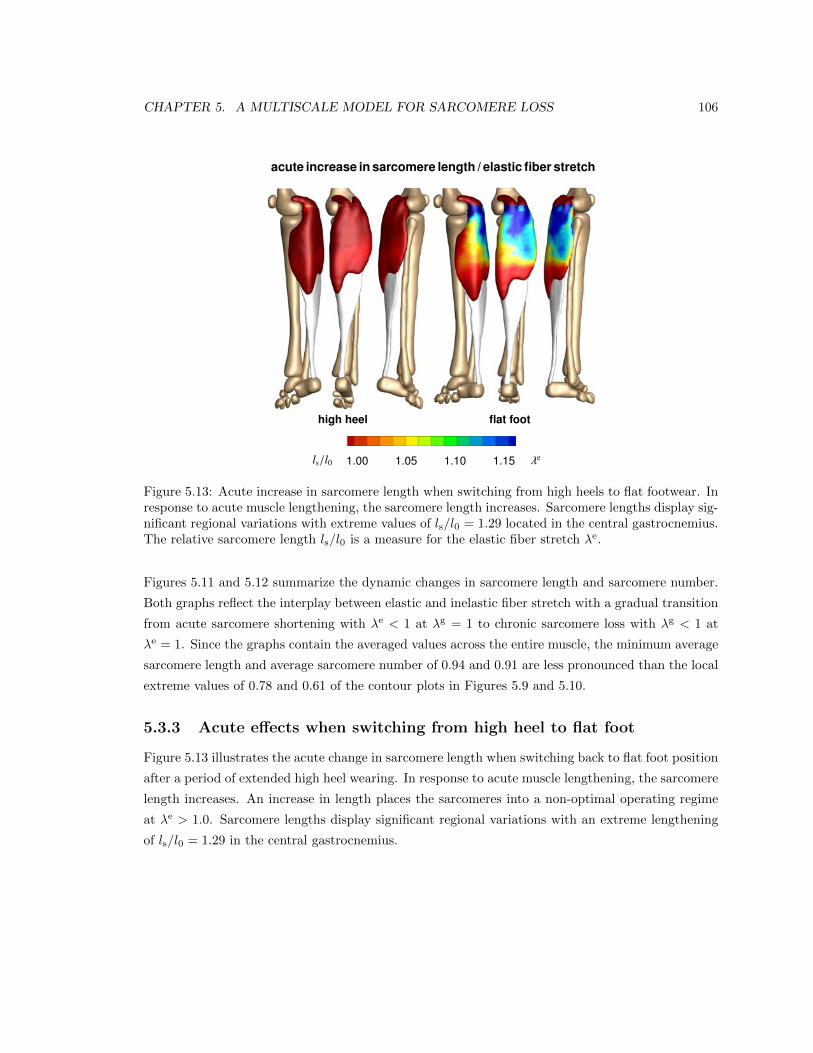
CHAPTER 5. A MULTISCALE MODEL FOR SARCOMERE LOSS 106
acute increase in sarcomere length / elastic fiber stretch
high heel flat foot
ls/l0 1.00 1.05 1.10 1.15
�e
Figure 13: Acute increase in sarcomere length when switching from high heelsto flat footwear. In response to acute muscle lengthening, the sarcomere lengthincreases. Sarcomere lengths display significant regional variations with ex-treme values of ls/l0 = 1.29 located in the central gastrocnemius. The relativesarcomere length ls/l0 is a measure for the elastic fiber stretch �e.
the same study, in agreement with our measurements and simu-lations, the length of the Achilles tendon was almost identical inboth groups with 18.69 cm in the flat foot group and 18.91 cmin the high heel group [10].Chronically, skeletal muscle adapts to its new physiologicallength by removing sarcomeres in series to reposition its sar-comeres back into their optimal regime [42], see Figure 2.When maintaining the foot in the high heel position, our simu-lations predict a chronic average reduction in serial sarcomerenumber by 9%, see Figure 12, with local maxima of sarcomereloss of 31% in the central gastrocnemius, see Figure 10. Thesevalues lie within the range of the reported sarcomere loss dur-ing immobilization experiments in mice, where the serial sar-comere number decreased by 10% from 2,200 to 1,975 in thesoleus after four weeks of immobilization [43] and by 9% from3,200 to 2,900 in the tibialis anterior after two weeks of immo-bilization [7]. These values are slightly lower than the reportedsarcomere loss in cat, where the serial sarcomere number de-creased by 40% from 13,844 to 8,258 in the soleus after fourweeks of immobilization [37]. Undoubtably, these immobiliza-tion experiments impose a more drastic kinematic constraintthan frequent high heel wearing [13]. Nonetheless, the chronicsarcomere loss reported upon immobilization represents a valu-able upper limit for the sarcomere loss we can expect in womenwho frequently wear high-heeled shoes.Acutely, switching back from frequent high heel use to flatfootwear causes a drastic reduction in actin-myosin overlap andforces the muscle to operate in a non-optimal operating regime[20], see Figure 2. When moving from the foot from high heelto flat, our simulations predict an acute sarcomere lengtheningwith local extrema of 29% in the central gastrocnemius, see
Figure 13. Our large regional variations in sarcomere lengthare in agreement with previous studies, which have reportedsignificant regional variations in fascicle lengths and sarcom-ere lengths in the stretched cat biceps femoris muscle [8]. Oursarcomere lengths agree with common observation that switch-ing back from high heels to flat footwear induces muscle over-stretch associated with muscle pain [22] and increased risk ofstrain injuries [11].While our study provides valuable insight into the mechanismsof chronic muscle shortening on the muscle and sarcomere lev-els, our current model has a few limitations: First, to illustratethe conceptual feasibility of our method, we have only pro-totyped the study for a single heel height and a single studysubject. It would be interesting to explore the dimensions ofthe muscle-tendon unit in Table 1 for flat foot and high heelpositions with varying heel heights in di↵erent study subjects[14]. Second, for simplicity, in equation (8), we have mod-eled skeletal muscle as isotropic Neo-Hookean material. Whilean isotropic model might be a su�cient approximation un-der compressive loading when switching from flat foot to highheel, a more sophisticated anisotropic model that takes into ac-count strain sti↵ening might be more appropriate under tensileloading when switching from high heel to flat foot [5, 19].Since we have only reported strains and stretches, here, so-phisticated constitutive modeling might not be critical; yet, itwould be worth considering in future studies, especially whenaddressing chronic force alterations in muscle [21] and ten-don [15, 28]. Third, the model presented here only accountsfor sarcomere removal upon chronic understretch. To add sar-comeres in series upon chronic overstretch [44], we wouldneed to modify the adaptation function in equation (11) tok = [[#max � #]/[#max � 1]]�/⌧ and activate it through the mod-ified adaptation criterion in equation (12) as � = h�e � �criti us-ing the generic approach [26] adopted for skeletal muscle [47].Last, until now, we have only compared our model qualitativelyagainst animal immobilization models in mice [43] and cat [37].Recent developments in microendoscopy now enable the non-invasive sarcomere imaging in vivo [24]. We have designed ourmodel with these new technologies in mind [9]. We are cur-rently in the process of measuring sarcomere lengths in flat footand high heel positions in di↵erent regions of the gastrocnemiusmuscle to validate our model with in vivo human data.What can we learn from this study? First and foremost, ourresults support the hypothesis that frequent use of high-heeledfootwear alters the natural position of the calf muscle-tendoncomplex. We have seen that this change could initiate a chainreaction of negative e↵ects [12]: Acutely, it creates excessiveactin-myosin overlap associated with energetically ine�cientmuscle use [14]. Chronically, it initiates an adaptation processassociated with the loss of sarcomeres and significant muscleshortening [10]. A major concern is that these changes arechronic. Changing back to flat footwear does not provide im-mediate cure; quite the contrary: For most frequent high heelwearers, switching to the flat foot position can be extremelypainful. It overstretched the triceps surae [22], which mightcause muscle pain and planar fasciitis [32]. To ensure comfortand reduce risk of injury [11], recent recommendations suggest
12
Figure 5.13: Acute increase in sarcomere length when switching from high heels to flat footwear. Inresponse to acute muscle lengthening, the sarcomere length increases. Sarcomere lengths display sig-nificant regional variations with extreme values of ls/l0 = 1.29 located in the central gastrocnemius.The relative sarcomere length ls/l0 is a measure for the elastic fiber stretch �e.
Figures 5.11 and 5.12 summarize the dynamic changes in sarcomere length and sarcomere number.
Both graphs reflect the interplay between elastic and inelastic fiber stretch with a gradual transition
from acute sarcomere shortening with �e < 1 at �g = 1 to chronic sarcomere loss with �g < 1 at
�e = 1. Since the graphs contain the averaged values across the entire muscle, the minimum average
sarcomere length and average sarcomere number of 0.94 and 0.91 are less pronounced than the local
extreme values of 0.78 and 0.61 of the contour plots in Figures 5.9 and 5.10.
5.3.3 Acute e↵ects when switching from high heel to flat foot
Figure 5.13 illustrates the acute change in sarcomere length when switching back to flat foot position
after a period of extended high heel wearing. In response to acute muscle lengthening, the sarcomere
length increases. An increase in length places the sarcomeres into a non-optimal operating regime
at �e > 1.0. Sarcomere lengths display significant regional variations with an extreme lengthening
of ls/l0 = 1.29 in the central gastrocnemius.
CHAPTER 5. A MULTISCALE MODEL FOR SARCOMERE LOSS 107
5.4 Discussion
Even though high heels are known to be a major source of chronic lower limb pain, more than one
third of American women wear high heels on a daily basis. To characterize the e↵ects of high-heeled
footwear on muscle adaptation in the lower limb, we created a multiscale computational model for
chronic muscle shortening. To calibrate the model, we performed a case study of a healthy female
subject and created two lower limb models using magnetic resonance images, one in flat foot and
one in high heel position. Surprisingly, when moving the foot from flat position to a heel height of
13 cm, the length of the calf muscle-tendon unit changes only marginally from 396mm to 384mm
corresponding to a stretch of � = 0.97. However, a closer look reveals two essential characteristics:
The Achilles tendon remains at a constant length of 171mm with � = 1.00, while the gastrocnemius
experiences the entire length change of 12mm from 225mm to 213mm corresponding to a stretch
of � = 0.95. More importantly, the finite element simulation suggests that this stretch is not dis-
tributed homogeneously across the gastrocnemius muscle: In the proximal and distal regions, where
the muscle is structurally supported by the sti↵er femur and Achilles tendon, the muscle experience
virtually no stretch; in the central muscle region, local stretches take extreme values of � = 0.78.
Acutely, switching from flat footwear to high heels causes excessive actin-myosin overlap and forces
the muscle to operate in a non-optimal operating regime [52], see Figure 5.2. When moving from
the flat to the high heel position, our simulations predict an acute average reduction in sarcomere
length by 5%, see Figure 5.11, with local extrema of sarcomere shortening of 22% in the central
gastrocnemius, see Figure 5.9. These values are in excellent agreement with recent studies, which
have reported a fascicle length di↵erence of 12% in the medial gastrocnemius muscle, with lengths
of 56.0±7.7mm in the flat foot group compared to 49.6±5.7mm in the high heel group [51]. In the
same study, in agreement with our measurements and simulations, the length of the Achilles tendon
was almost identical in both groups with 18.69 cm in the flat foot group and 18.91 cm in the high
heel group [51].
Chronically, skeletal muscle adapts to its new physiological length by removing sarcomeres in series
to reposition its sarcomeres back into their optimal regime [214], see Figure 5.2. When maintaining
the foot in the high heel position, our simulations predict a chronic average reduction in serial sar-
comere number by 9%, see Figure 5.12, with local maxima of sarcomere loss of 31% in the central
gastrocnemius, see Figure 5.10. These values lie within the range of the reported sarcomere loss
during immobilization experiments in mice, where the serial sarcomere number decreased by 10%
from 2,200 to 1,975 in the soleus after four weeks of immobilization [215] and by 9% from 3,200 to
2,900 in the tibialis anterior after two weeks of immobilization [40]. These values are slightly lower
than the reported sarcomere loss in cat, where the serial sarcomere number decreased by 40% from
13,844 to 8,258 in the soleus after four weeks of immobilization [196]. Undoubtably, these immobi-
lization experiments impose a more drastic kinematic constraint than frequent high heel wearing [59].
Nonetheless, the chronic sarcomere loss reported upon immobilization represents a valuable upper
CHAPTER 5. A MULTISCALE MODEL FOR SARCOMERE LOSS 108
limit for the sarcomere loss we can expect in women who frequently wear high-heeled shoes.
Acutely, switching back from frequent high heel use to flat footwear causes a drastic reduction in
actin-myosin overlap and forces the muscle to operate in a non-optimal operating regime [76], see
Figure 5.2. When moving from the foot from high heel to flat, our simulations predict an acute
sarcomere lengthening with local extrema of 29% in the central gastrocnemius, see Figure 5.13. Our
large regional variations in sarcomere length are in agreement with previous studies, which have
reported significant regional variations in fascicle lengths and sarcomere lengths in the stretched cat
biceps femoris muscle [46]. Our sarcomere lengths agree with common observation that switching
back from high heels to flat footwear induces muscle overstretch associated with muscle pain [105]
and increased risk of strain injuries [52].
While our study provides valuable insight into the mechanisms of chronic muscle shortening on the
muscle and sarcomere levels, our current model has a few limitations: First, to illustrate the concep-
tual feasibility of our method, we have only prototyped the study for a single heel height and a single
study subject. It would be interesting to explore the dimensions of the muscle-tendon unit in Table
5.1 for flat foot and high heel positions with varying heel heights in di↵erent study subjects [60].
Second, for simplicity, in equation (5.8), we have modeled skeletal muscle as isotropic Neo-Hookean
material. While an isotropic model might be a su�cient approximation under compressive loading
when switching from flat foot to high heel, a more sophisticated anisotropic model that takes into
account strain sti↵ening might be more appropriate under tensile loading when switching from high
heel to flat foot [26, 74]. Since we have only reported strains and stretches, here, sophisticated
constitutive modeling might not be critical; yet, it would be worth considering in future studies,
especially when addressing chronic force alterations in muscle [103] and tendon [63, 142]. Third,
the model presented here only accounts for sarcomere removal upon chronic understretch. To add
sarcomeres in series upon chronic overstretch [217], we would need to modify the adaptation function
in equation (5.11) to k = [[#max�#]/[#max�1]]�/⌧ and activate it through the modified adaptation
criterion in equation (5.12) as � = h�e � �criti using the generic approach [139] adopted for skele-
tal muscle [225]. Last, until now, we have only compared our model qualitatively against animal
immobilization models in mice [215] and cat [196]. Recent developments in microendoscopy now
enable the non-invasive sarcomere imaging in vivo [136]. We have designed our model with these
new technologies in mind [50]. We are currently in the process of measuring sarcomere lengths in flat
foot and high heel positions in di↵erent regions of the gastrocnemius muscle to validate our model
with in vivo human data.
What can we learn from this study? First and foremost, we have seen that we can interpret chronic
changes in whole muscle length as emergent properties of local changes in sarcomere number, muscle
fiber length, and fascicle length. This has allowed us to create multiscale computational models,
which strongly support the hypothesis that frequent high-heel use alters the natural position of the
calf muscle-tendon complex. Our results suggest that this change could initiate a chain reaction of
CHAPTER 5. A MULTISCALE MODEL FOR SARCOMERE LOSS 109
negative e↵ects [53]: Acutely, it creates excessive actin-myosin overlap associated with energetically
ine�cient muscle use [60]. Chronically, it initiates an adaptation process associated with the loss
of sarcomeres and significant muscle shortening [51]. A major concern is that these changes are
chronic. Changing back to flat footwear does not provide immediate cure; quite the contrary: For
most frequent high heel wearers, switching to the flat foot position can be extremely painful. It
overstretched the triceps surae [105], which might cause muscle pain and planar fasciitis [156]. To
ensure comfort and reduce risk of injury [52], recent recommendations suggest limiting the heel hight
to 5 cm or less [60]. To maintain muscle fiber lengths and ankle range of motion [105], recent studies
recommend intensive passive stretching exercise with long frequent stretching times in dorsiflexion
direction [103]. Our study strongly supports these recommendations.
5.5 Concluding remarks
We have created a computational model of the lower limb to study the acute and chronic e↵ects of
high-heeled footwear on the kinematics of the calf muscle-tendon unit. Through the case study of
a healthy female subject, we have shown that raising the heel by 13 cm reduces the length of the
muscle-tendon unit by 12mm or 3%. Notably, this change a↵ects almost exclusively the gastrocne-
mius muscle, which experiences an average shortening of 5%, while the length of the Achilles tendon
remains virtually unchanged. Our computational simulations indicate that muscle shortening dis-
plays significant regional variations with extreme values of 22% in the central gastrocnemius. Our
model suggests that the muscle gradually adjusts to its new functional length by a chronic loss of
sarcomeres in series. Sarcomere loss varies regionally with virtually no loss at the proximal and distal
ends and a maximum loss of 39% in the central muscle region. Collectively, these changes result
in chronic muscle shortening associated with discomfort, compromised muscle e�ciency, increased
fatigue, reduced shock absorption, and increased risk of strain injuries. Computational modeling
of chronic muscle shortening provides a valuable tool to shape our understanding of the interacting
mechanisms in skeletal muscle adaptation. Our study could open new avenues in orthopedic surgery
and enhance treatment in patients with muscle contracture caused by other conditions than high
heel wear such as paralysis, muscular atrophy, and muscular dystrophy.
Acknowledgments
We thank Professor Gerald E. Loeb for stimulating discussions that initiated this study. This
research was supported by the Stanford Graduate Fellowship to Alexander Zollner, by the Stanford
Mechanical Engineering SURI support to Jacquelynn Pok, by the NSERC PDF Fellowship to Emily
McWalter, by GE Healthcare, by the NIH grant NIH EB002524, and by the NIH grant AR062068 to
Garry Gold, and by the NSF CAREER award CMMI 0952021, by the NSF INSPIRE grant 1233054,

CHAPTER 5. A MULTISCALE MODEL FOR SARCOMERE LOSS 110
and by the NIH grant U01 HL119578 to Ellen Kuhl.
Chapter 6
A virtual sizing tool for mitral
valve annuloplasty
Abstract
Functional mitral regurgitation, a backward leakage of the mitral valve, is a result of left
ventricular growth and mitral annular dilatation. Its gold standard treatment is mitral annulo-
plasty, the surgical reduction in mitral annular area through the implantation of annuloplasty
rings. Recurrent regurgitation rates may, however, be as high as 30% and more. While the
degree of annular downsizing has been linked to improved long-term outcomes, too aggressive
downsizing increases the risk of ring dehiscences and significantly impairs repair durability. Here
we prototype a virtual sizing tool to quantify changes in annular dimensions, surgically-induced
tissue strains, mitral annular stretches, and suture forces in response to mitral annuloplasty.
We create a computational model of dilated cardiomyopathy onto which we virtually implant
annuloplasty rings of di↵erent sizes. Our simulations confirm the common intuition that smaller
rings are more invasive to the surrounding tissue, induce higher strains, and require larger suture
forces than larger rings: The total suture force was 2.2N for a 24mm ring, 1.9N for a 28mm
ring, and 0.8N for a 32mm ring. Our model predicts the highest risk of dehiscence in the septal
and postero-lateral annulus where suture forces are maximal. These regions co-localize with
regional peaks in myocardial strain and annular stretch. Our study illustrates the potential of
realistic predictive simulations in cardiac surgery to identify areas at risk for dehiscence, guide
the selection of ring size and shape, rationalize the design of smart annuloplasty rings and,
ultimately, improve long-term outcomes after surgical mitral annuloplasty.
6.1 Motivation
Functional mitral regurgitation is a backward leakage of the mitral valve in the absence of any
disease to the valve itself [122,157,179]. A major cause of functional mitral regurgitation is dilated
111
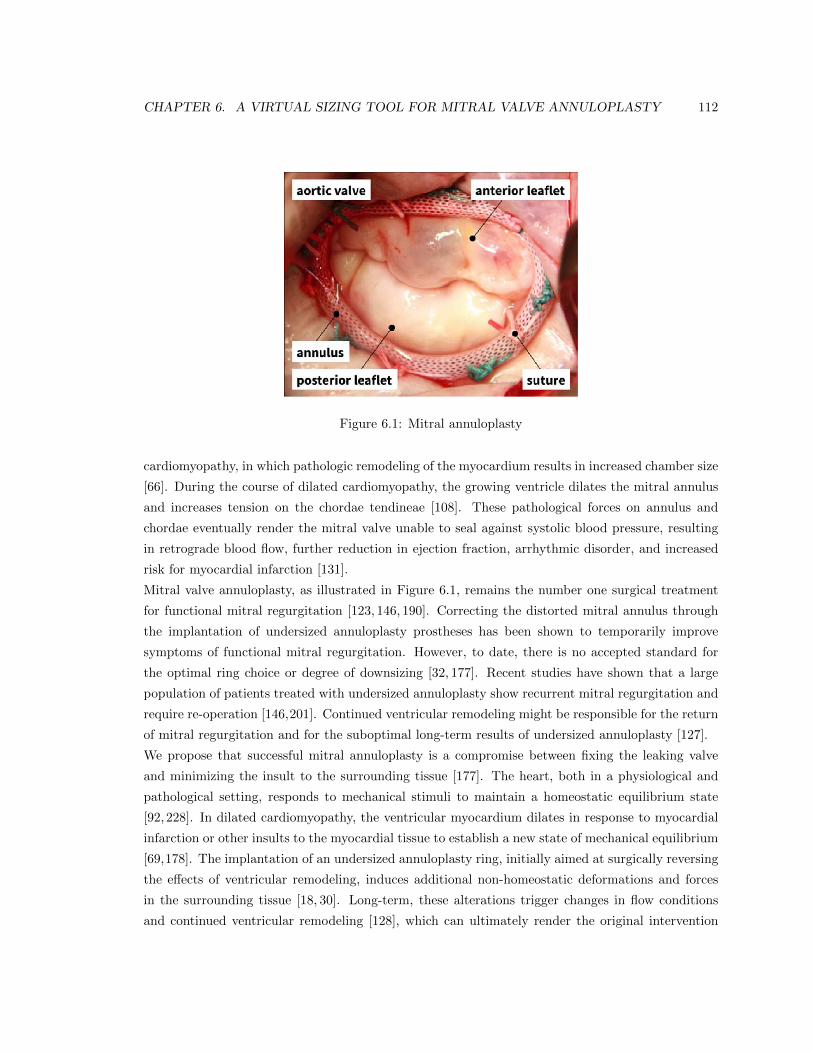
CHAPTER 6. A VIRTUAL SIZING TOOL FOR MITRAL VALVE ANNULOPLASTY 112
Figure 6.1: Mitral annuloplasty
cardiomyopathy, in which pathologic remodeling of the myocardium results in increased chamber size
[66]. During the course of dilated cardiomyopathy, the growing ventricle dilates the mitral annulus
and increases tension on the chordae tendineae [108]. These pathological forces on annulus and
chordae eventually render the mitral valve unable to seal against systolic blood pressure, resulting
in retrograde blood flow, further reduction in ejection fraction, arrhythmic disorder, and increased
risk for myocardial infarction [131].
Mitral valve annuloplasty, as illustrated in Figure 6.1, remains the number one surgical treatment
for functional mitral regurgitation [123, 146, 190]. Correcting the distorted mitral annulus through
the implantation of undersized annuloplasty prostheses has been shown to temporarily improve
symptoms of functional mitral regurgitation. However, to date, there is no accepted standard for
the optimal ring choice or degree of downsizing [32, 177]. Recent studies have shown that a large
population of patients treated with undersized annuloplasty show recurrent mitral regurgitation and
require re-operation [146,201]. Continued ventricular remodeling might be responsible for the return
of mitral regurgitation and for the suboptimal long-term results of undersized annuloplasty [127].
We propose that successful mitral annuloplasty is a compromise between fixing the leaking valve
and minimizing the insult to the surrounding tissue [177]. The heart, both in a physiological and
pathological setting, responds to mechanical stimuli to maintain a homeostatic equilibrium state
[92, 228]. In dilated cardiomyopathy, the ventricular myocardium dilates in response to myocardial
infarction or other insults to the myocardial tissue to establish a new state of mechanical equilibrium
[69,178]. The implantation of an undersized annuloplasty ring, initially aimed at surgically reversing
the e↵ects of ventricular remodeling, induces additional non-homeostatic deformations and forces
in the surrounding tissue [18, 30]. Long-term, these alterations trigger changes in flow conditions
and continued ventricular remodeling [128], which can ultimately render the original intervention
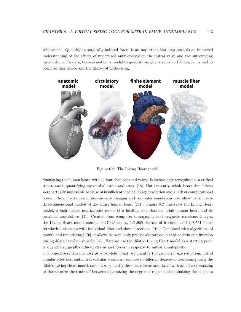
CHAPTER 6. A VIRTUAL SIZING TOOL FOR MITRAL VALVE ANNULOPLASTY 113
suboptimal. Quantifying surgically-induced forces is an important first step towards an improved
understanding of the e↵ects of undersized annuloplasty on the mitral valve and the surrounding
myocardium. To date, there is neither a model to quantify surgical strains and forces, nor a tool to
optimize ring choice and the degree of undersizing.
finite element model
muscle fiber model
anatomic model
circulatory model
Figure 6.2: The Living Heart model
Simulating the human heart–with all four chambers and valves–is increasingly recognized as a critical
step towards quantifying myocardial strain and stress [18]. Until recently, whole heart simulations
were virtually impossible because of insu�cient medical image resolution and a lack of computational
power. Recent advances in non-invasive imaging and computer simulation now allow us to create
three-dimensional models of the entire human heart [231]. Figure 6.2 illustrates the Living Heart
model, a high-fidelity multiphysics model of a healthy, four-chamber adult human heart and its
proximal vasculature [17]. Created from computer tomography and magnetic resonance images,
the Living Heart model consist of 47,323 nodes, 141,969 degrees of freedom, and 208,561 linear
tetrahedral elements with individual fiber and sheet directions [219]. Combined with algorithms of
growth and remodeling [176], it allows us to reliably predict alterations in cardiac form and function
during dilated cardiomyopathy [69]. Here we use the dilated Living Heart model as a starting point
to quantify surgically-induced strains and forces in response to mitral annuloplasty.
The objective of this manuscript is two-fold: First, we quantify the geometric size reduction, mitral
annular stretches, and mitral valvular strains in response to di↵erent degrees of downsizing using the
dilated Living Heart model; second, we quantify the suture forces associated with annular downsizing
to characterize the trade-o↵ between maximizing the degree of repair and minimizing the insult to
CHAPTER 6. A VIRTUAL SIZING TOOL FOR MITRAL VALVE ANNULOPLASTY 114
the surrounding tissue. Our overall goal is to prototype a virtual surgical tool for the optimal design
and selection of cardiovascular devices using predictive computational simulation.
6.2 Methods
6.2.1 Cardiac Growth Model
To create the geometry of dilated cardiomyopathy, we multiplicatively decompose the deformation
gradient F , the spatial gradient of the deformation map ', into an elastic part F
e and a growth
part F g [183],
F = F
e · F g with F = rX'. (6.1)
To account for quasi-incompressibility of the elastic tissue response, we further decompose the elastic
tensor F e into volumetric and isochoric parts,
F
e = F
evol · F e with F
evol = (Je)1/3I and F
e = (Je)�1/3F
e . (6.2)
Here I denotes the second-order unit tensor, Je = det(F e) = Jevol is the elastic Jacobian and
Je = det(F e) = 1 is the isochoric Jacobian [90]. We can now characterize the elastic deformation in
terms of the elastic Jacobian Je and the isochoric elastic Green-Lagrange strain tensor Ee,
Je = det(F e) and E
e = 12 [ (Je)�2/3 (F e)t · F e � I ] . (6.3)
The underlying principle of the theory of finite growth is that only elastic deformations generate
stress. We thus introduce the following strain energy function (Je,Ee),
(Je,Ee) = U(Je) + (Ee) , (6.4)
which we decompose additively into a volumetric part U(Je) and an isochoric part (Ee),
U(Je) =1
2K0
⇥(Je)2 � 2 ln(Je)
⇤and (Ee) =
1
2C0
⇥exp(Ee : B0 : Ee)� 1
⇤. (6.5)
Here K0 and C0 are the volumetric and isochoric elastic sti↵nesses, and the fourth-order tensor
B0 contains the weighting factors of the orthotropic Fung-type model for myocardial tissue [84].
In Voigt notation, B0 takes a diagonal representation, cB0 = diag {B↵ , Bss, Bnn, 2Bfs, 2Bfn, 2Bsn},
where the individual entries are the weights of the normal and shear strains in the fiber, sheet, and
normal directions. According to the standard arguments of thermodynamics, the Piola-Kirchho↵
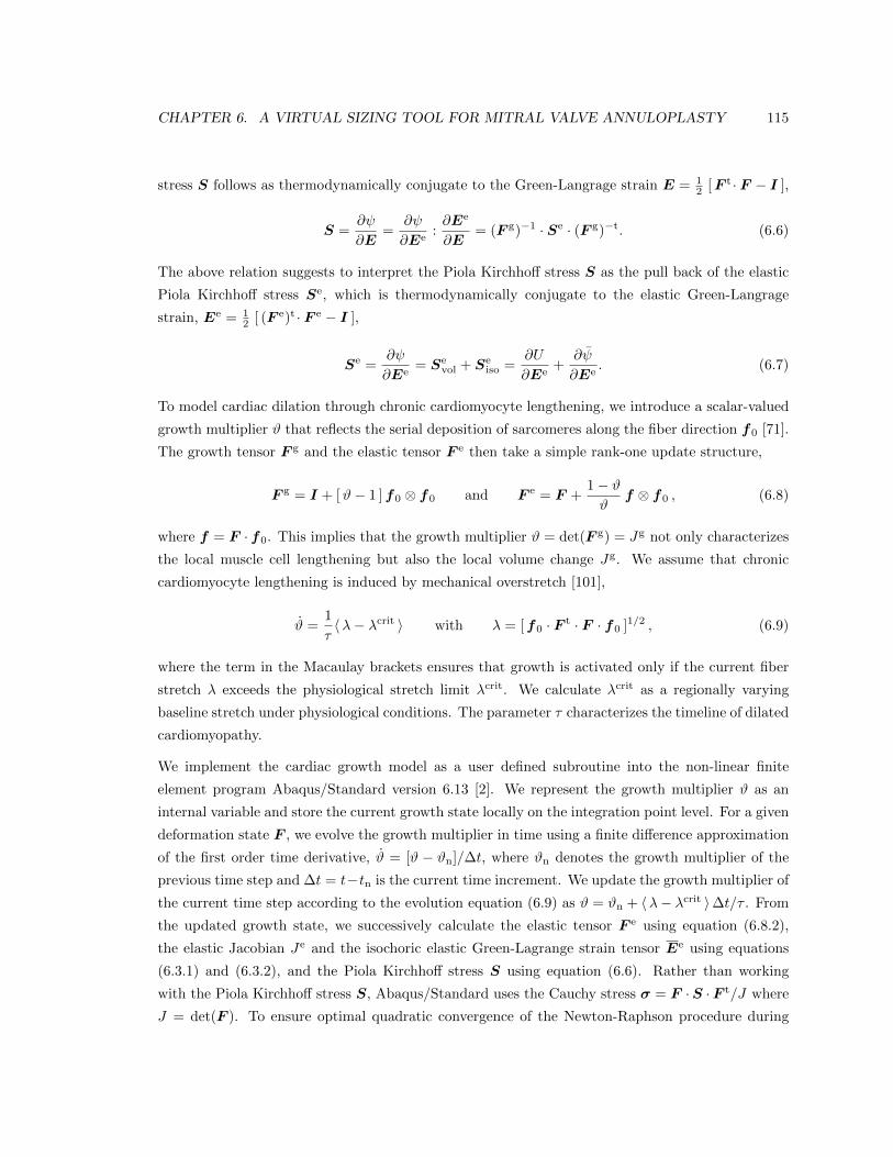
CHAPTER 6. A VIRTUAL SIZING TOOL FOR MITRAL VALVE ANNULOPLASTY 115
stress S follows as thermodynamically conjugate to the Green-Langrage strain E = 12 [F t · F � I ],
S =@
@E=
@
@Ee:@Ee
@E= (F g)�1 · Se · (F g)�t. (6.6)
The above relation suggests to interpret the Piola Kirchho↵ stress S as the pull back of the elastic
Piola Kirchho↵ stress S
e, which is thermodynamically conjugate to the elastic Green-Langrage
strain, Ee = 12 [ (F e)t · F e � I ],
S
e =@
@Ee= S
evol + S
eiso =
@U
@Ee+
@
@Ee. (6.7)
To model cardiac dilation through chronic cardiomyocyte lengthening, we introduce a scalar-valued
growth multiplier # that reflects the serial deposition of sarcomeres along the fiber direction f0 [71].
The growth tensor F g and the elastic tensor F e then take a simple rank-one update structure,
F
g = I + [#� 1 ]f0 ⌦ f0 and F
e = F +1� ##
f ⌦ f0 , (6.8)
where f = F · f0. This implies that the growth multiplier # = det(F g) = Jg not only characterizes
the local muscle cell lengthening but also the local volume change Jg. We assume that chronic
cardiomyocyte lengthening is induced by mechanical overstretch [101],
# =1
⌧h�� �crit i with � = [f0 · F t · F · f0 ]
1/2 , (6.9)
where the term in the Macaulay brackets ensures that growth is activated only if the current fiber
stretch � exceeds the physiological stretch limit �crit. We calculate �crit as a regionally varying
baseline stretch under physiological conditions. The parameter ⌧ characterizes the timeline of dilated
cardiomyopathy.
We implement the cardiac growth model as a user defined subroutine into the non-linear finite
element program Abaqus/Standard version 6.13 [2]. We represent the growth multiplier # as an
internal variable and store the current growth state locally on the integration point level. For a given
deformation state F , we evolve the growth multiplier in time using a finite di↵erence approximation
of the first order time derivative, # = [# � #n]/�t, where #n denotes the growth multiplier of the
previous time step and �t = t�tn is the current time increment. We update the growth multiplier of
the current time step according to the evolution equation (6.9) as # = #n + h�� �crit i�t/⌧ . From
the updated growth state, we successively calculate the elastic tensor F
e using equation (6.8.2),
the elastic Jacobian Je and the isochoric elastic Green-Lagrange strain tensor E
e using equations
(6.3.1) and (6.3.2), and the Piola Kirchho↵ stress S using equation (6.6). Rather than working
with the Piola Kirchho↵ stress S, Abaqus/Standard uses the Cauchy stress � = F ·S ·F t/J where
J = det(F ). To ensure optimal quadratic convergence of the Newton-Raphson procedure during
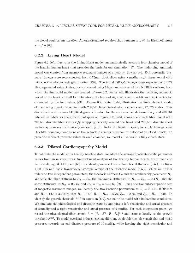
CHAPTER 6. A VIRTUAL SIZING TOOL FOR MITRAL VALVE ANNULOPLASTY 116
the global equilibrium iteration, Abaqus/Standard requires the Jaumann rate of the Kirchho↵ stress
⌧ = J � [69].
6.2.2 Living Heart Model
Figure 6.2, left, illustrates the Living Heart model, an anatomically accurate four-chamber model of
the healthy human heart that provides the basis for our simulation [17]. The underlying anatomic
model was created from magnetic resonance images of a healthy, 21-year old, 50th percentile U.S.
male. Images were reconstructed from 0.75mm thick slices using a medium soft-tissue kernel with
retrospective electrocardiogram gating [232]. The initial DICOM images were exported as JPEG
files, segmented using Amira, post-processed using Maya, and converted into NURBS surfaces, from
which the final solid model was created. Figure 6.2, center left, illustrates the resulting geometric
model of the heart with all four chambers, the left and right atria and the left and right ventricles,
connected by the four valves [231]. Figure 6.2, center right, illustrates the finite element model
of the Living Heart discretized with 208,561 linear tetrahedral elements and 47,323 nodes. This
discretization introduces 141,969 degrees of freedom for the vector-valued deformation ' and 208,561
internal variables for the growth multiplier #. Figure 6.2, right, shows the muscle fiber model with
208,561 discrete fiber vectors f0 wrapping helically around the heart and 208,561 discrete sheet
vectors s0 pointing transmurally outward [219]. To fix the heart in space, we apply homogeneous
Dirichlet boundary conditions at the geometric centers of the in- or outlets of all blood vessels. To
prescribe di↵erent pressure values in each chamber, we model all valves in a fully closed state.
6.2.3 Dilated Cardiomyopathy Model
To calibrate the model at its healthy baseline state, we adopt the averaged patient-specific parameter
values from an in vivo inverse finite element analysis of five healthy human hearts, three male and
two female, age 36±11 years [68]. Specifically, we select the volumetric sti↵ness in (6.5.1) to K0 =
1, 000 kPa and use a transversely isotropic version of the isochoric model (6.5.2), which we further
reduce to two independent parameters, the isochoric sti↵ness C0 and the nonlinearity parameter B0.
We scale the fiber sti↵ness to B↵ = B0, the transverse sti↵nesses to Bss = Bnn = 0.4B0, and the
shear sti↵nesses to Bsn = 0.2B0 and Bfs = Bfn = 0.35B0 [68]. Using the five subject-specific sets
of magnetic resonance images, we identify the two isochoric parameters to C0 = 0.115 ± 0.008 kPa
and B0 = 14.4± 3.2 such that B↵ = 14.4, Bss = Bnn = 5.76, Bsn = 2.88, and Bfs = Bfn = 5.04. To
identify the growth threshold �crit in equation (6.9), we train the model with its baseline conditions.
We simulate the physiological end-diastolic state by applying a left ventricular and atrial pressure
of 5mmHg and a right ventricular and atrial pressure of 2mmHg. For each integration point, we
record the physiological fiber stretch � = [f0 · F t · F · f0 ]1/2 and store it locally as the growth
threshold �crit. To model overload-induced cardiac dilation, we double the left ventricular and atrial
pressures towards an end-diastolic pressure of 10mmHg, while keeping the right ventricular and
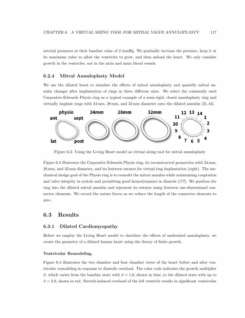
CHAPTER 6. A VIRTUAL SIZING TOOL FOR MITRAL VALVE ANNULOPLASTY 117
arterial pressures at their baseline value of 2 mmHg. We gradually increase the pressure, keep it at
its maximum value to allow the ventricles to grow, and then unload the heart. We only consider
growth in the ventricles, not in the atria and main blood vessels.
6.2.4 Mitral Annuloplasty Model
We use the dilated heart to simulate the e↵ects of mitral annuloplasty and quantify mitral an-
nular changes after implantation of rings in three di↵erent sizes. We select the commonly used
Carpentier-Edwards Physio ring as a typical example of a semi-rigid, closed annuloplasty ring and
virtually implant rings with 24mm, 28mm, and 32mm diameter onto the dilated annulus [31, 44].
Figure 6.3: Using the Living Heart model as virtual sizing tool for mitral annuloplasty
Figure 6.3 illustrates the Carpentier-Edwards Physio ring, its reconstructed geometries with 24mm,
28mm, and 32mm diameter, and its fourteen sutures for virtual ring implantation (right). The me-
chanical design goal of the Physio ring is to remodel the mitral annulus while maintaining coaptation
and valve integrity in systole and permitting good hemodynamics in diastole [177]. We position the
ring into the dilated mitral annulus and represent its sutures using fourteen one-dimensional con-
nector elements. We record the suture forces as we reduce the length of the connector elements to
zero.
6.3 Results
6.3.1 Dilated Cardiomyopathy
Before we employ the Living Heart model to elucidate the e↵ects of undersized annuloplasty, we
create the geometry of a dilated human heart using the theory of finite growth.
Ventricular Remodeling.
Figure 6.4 illustrates the two chamber and four chamber views of the heart before and after ven-
tricular remodeling in response to diastolic overload. The color code indicates the growth multiplier
#, which varies from the baseline state with # = 1.0, shown in blue, to the dilated state with up to
# = 2.0, shown in red. Stretch-induced overload of the left ventricle results in significant ventricular
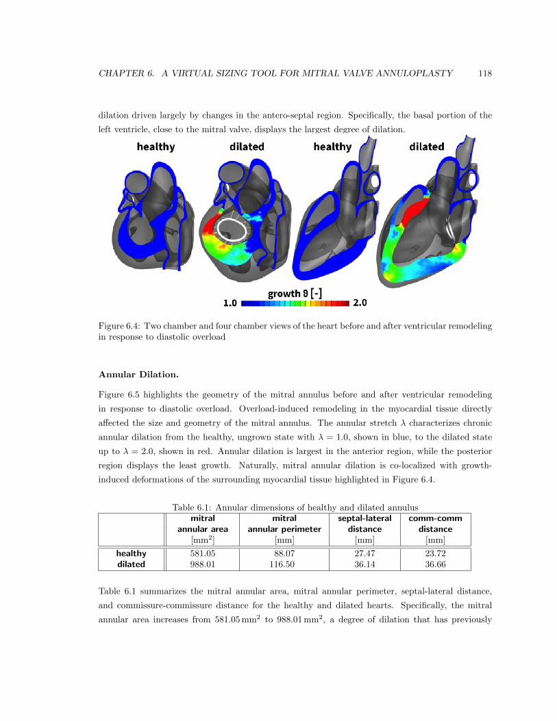
CHAPTER 6. A VIRTUAL SIZING TOOL FOR MITRAL VALVE ANNULOPLASTY 118
dilation driven largely by changes in the antero-septal region. Specifically, the basal portion of the
left ventricle, close to the mitral valve, displays the largest degree of dilation.
Figure 6.4: Two chamber and four chamber views of the heart before and after ventricular remodelingin response to diastolic overload
Annular Dilation.
Figure 6.5 highlights the geometry of the mitral annulus before and after ventricular remodeling
in response to diastolic overload. Overload-induced remodeling in the myocardial tissue directly
a↵ected the size and geometry of the mitral annulus. The annular stretch � characterizes chronic
annular dilation from the healthy, ungrown state with � = 1.0, shown in blue, to the dilated state
up to � = 2.0, shown in red. Annular dilation is largest in the anterior region, while the posterior
region displays the least growth. Naturally, mitral annular dilation is co-localized with growth-
induced deformations of the surrounding myocardial tissue highlighted in Figure 6.4.
Table 6.1: Annular dimensions of healthy and dilated annulusmitral mitral septal-lateral comm-comm
annular area annular perimeter distance distance
[mm2] [mm] [mm] [mm]
healthy 581.05 88.07 27.47 23.72dilated 988.01 116.50 36.14 36.66
Table 6.1 summarizes the mitral annular area, mitral annular perimeter, septal-lateral distance,
and commissure-commissure distance for the healthy and dilated hearts. Specifically, the mitral
annular area increases from 581.05mm2 to 988.01mm2, a degree of dilation that has previously
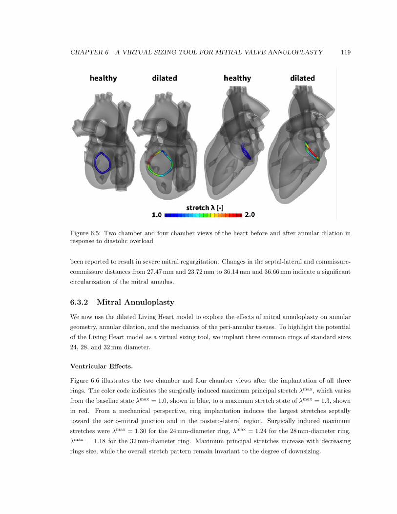
CHAPTER 6. A VIRTUAL SIZING TOOL FOR MITRAL VALVE ANNULOPLASTY 119
Figure 6.5: Two chamber and four chamber views of the heart before and after annular dilation inresponse to diastolic overload
been reported to result in severe mitral regurgitation. Changes in the septal-lateral and commissure-
commissure distances from 27.47mm and 23.72mm to 36.14mm and 36.66mm indicate a significant
circularization of the mitral annulus.
6.3.2 Mitral Annuloplasty
We now use the dilated Living Heart model to explore the e↵ects of mitral annuloplasty on annular
geometry, annular dilation, and the mechanics of the peri-annular tissues. To highlight the potential
of the Living Heart model as a virtual sizing tool, we implant three common rings of standard sizes
24, 28, and 32mm diameter.
Ventricular E↵ects.
Figure 6.6 illustrates the two chamber and four chamber views after the implantation of all three
rings. The color code indicates the surgically induced maximum principal stretch �max, which varies
from the baseline state �max = 1.0, shown in blue, to a maximum stretch state of �max = 1.3, shown
in red. From a mechanical perspective, ring implantation induces the largest stretches septally
toward the aorto-mitral junction and in the postero-lateral region. Surgically induced maximum
stretches were �max = 1.30 for the 24mm-diameter ring, �max = 1.24 for the 28mm-diameter ring,
�max = 1.18 for the 32mm-diameter ring. Maximum principal stretches increase with decreasing
rings size, while the overall stretch pattern remain invariant to the degree of downsizing.
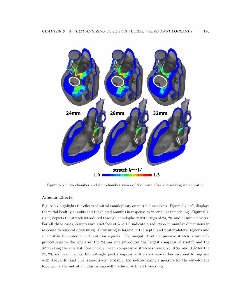
CHAPTER 6. A VIRTUAL SIZING TOOL FOR MITRAL VALVE ANNULOPLASTY 120
Figure 6.6: Two chamber and four chamber views of the heart after virtual ring implantation
Annular E↵ects.
Figure 6.7 highlights the e↵ects of mitral annuloplasty on mitral dimensions. Figure 6.7, left, displays
the initial healthy annulus and the dilated annulus in response to ventricular remodeling. Figure 6.7,
right, depicts the stretch introduced through annuloplasty with rings of 24, 28, and 32mm diameter.
For all three cases, compressive stretches of � < 1.0 indicate a reduction in annular dimensions in
response to surgical downsizing. Downsizing is largest in the septal and postero-lateral regions and
smallest in the anterior and posterior regions. The magnitude of compressive stretch is inversely
proportional to the ring size; the 24mm ring introduces the largest compressive stretch and the
32mm ring the smallest. Specifically, mean compressive stretches were 0.75, 0.85, and 0.92 for the
24, 28, and 32mm rings. Interestingly, peak compressive stretches were rather invariant to ring size
with 0.51, 0.46, and 0.54, respectively. Notably, the saddle-height, a measure for the out-of-plane
topology of the mitral annulus, is markedly reduced with all three rings.
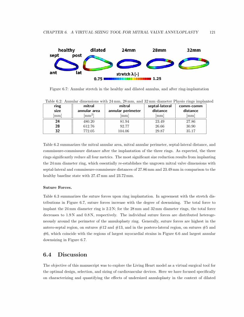
CHAPTER 6. A VIRTUAL SIZING TOOL FOR MITRAL VALVE ANNULOPLASTY 121
Figure 6.7: Annular stretch in the healthy and dilated annulus, and after ring-implantation
Table 6.2: Annular dimensions with 24mm, 28mm, and 32mm diameter Physio rings implantedring mitral mitral septal-lateral comm-comm
size annular area annular perimeter distance distance
[mm] [mm2] [mm] [mm] [mm]
24 480.20 81.94 23.49 27.8628 612.76 92.77 26.66 30.9032 772.05 104.06 29.87 35.17
Table 6.2 summarizes the mitral annular area, mitral annular perimeter, septal-lateral distance, and
commissure-commissure distance after the implantation of the three rings. As expected, the three
rings significantly reduce all four metrics. The most significant size reduction results from implanting
the 24mm diameter ring, which essentially re-establishes the ungrown mitral valve dimensions with
septal-lateral and commissure-commissure distances of 27.86mm and 23.49mm in comparison to the
healthy baseline state with 27.47mm and 23.72mm.
Suture Forces.
Table 6.3 summarizes the suture forces upon ring implantation. In agreement with the stretch dis-
tributions in Figure 6.7, suture forces increase with the degree of downsizing. The total force to
implant the 24mm diameter ring is 2.2N; for the 28mm and 32mm diameter rings, the total force
decreases to 1.9N and 0.8N, respectively. The individual suture forces are distributed heteroge-
neously around the perimeter of the annuloplasty ring. Generally, suture forces are highest in the
antero-septal region, on sutures #12 and #13, and in the postero-lateral region, on sutures #5 and
#6, which coincide with the regions of largest myocardial strains in Figure 6.6 and largest annular
downsizing in Figure 6.7.
6.4 Discussion
The objective of this manuscript was to explore the Living Heart model as a virtual surgical tool for
the optimal design, selection, and sizing of cardiovascular devices. Here we have focused specifically
on characterizing and quantifying the e↵ects of undersized annuloplasty in the context of dilated
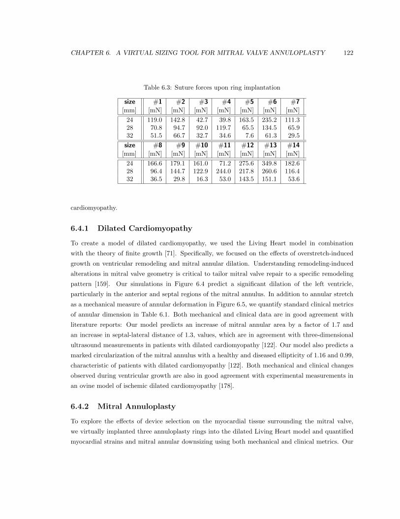
CHAPTER 6. A VIRTUAL SIZING TOOL FOR MITRAL VALVE ANNULOPLASTY 122
Table 6.3: Suture forces upon ring implantation
size #1 #2 #3 #4 #5 #6 #7
[mm] [mN] [mN] [mN] [mN] [mN] [mN] [mN]
24 119.0 142.8 42.7 39.8 163.5 235.2 111.328 70.8 94.7 92.0 119.7 65.5 134.5 65.932 51.5 66.7 32.7 34.6 7.6 61.3 29.5
size #8 #9 #10 #11 #12 #13 #14
[mm] [mN] [mN] [mN] [mN] [mN] [mN] [mN]
24 166.6 179.1 161.0 71.2 275.6 349.8 182.628 96.4 144.7 122.9 244.0 217.8 260.6 116.432 36.5 29.8 16.3 53.0 143.5 151.1 53.6
cardiomyopathy.
6.4.1 Dilated Cardiomyopathy
To create a model of dilated cardiomyopathy, we used the Living Heart model in combination
with the theory of finite growth [71]. Specifically, we focused on the e↵ects of overstretch-induced
growth on ventricular remodeling and mitral annular dilation. Understanding remodeling-induced
alterations in mitral valve geometry is critical to tailor mitral valve repair to a specific remodeling
pattern [159]. Our simulations in Figure 6.4 predict a significant dilation of the left ventricle,
particularly in the anterior and septal regions of the mitral annulus. In addition to annular stretch
as a mechanical measure of annular deformation in Figure 6.5, we quantify standard clinical metrics
of annular dimension in Table 6.1. Both mechanical and clinical data are in good agreement with
literature reports: Our model predicts an increase of mitral annular area by a factor of 1.7 and
an increase in septal-lateral distance of 1.3, values, which are in agreement with three-dimensional
ultrasound measurements in patients with dilated cardiomyopathy [122]. Our model also predicts a
marked circularization of the mitral annulus with a healthy and diseased ellipticity of 1.16 and 0.99,
characteristic of patients with dilated cardiomyopathy [122]. Both mechanical and clinical changes
observed during ventricular growth are also in good agreement with experimental measurements in
an ovine model of ischemic dilated cardiomyopathy [178].
6.4.2 Mitral Annuloplasty
To explore the e↵ects of device selection on the myocardial tissue surrounding the mitral valve,
we virtually implanted three annuloplasty rings into the dilated Living Heart model and quantified
myocardial strains and mitral annular downsizing using both mechanical and clinical metrics. Our
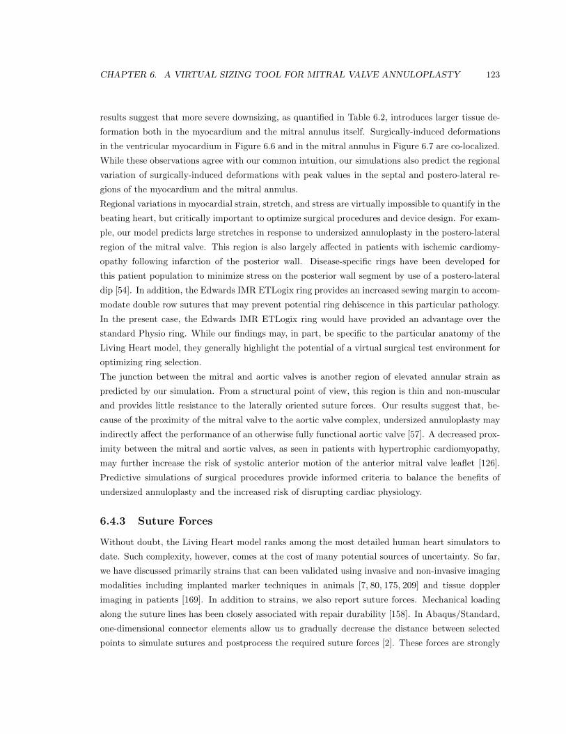
CHAPTER 6. A VIRTUAL SIZING TOOL FOR MITRAL VALVE ANNULOPLASTY 123
results suggest that more severe downsizing, as quantified in Table 6.2, introduces larger tissue de-
formation both in the myocardium and the mitral annulus itself. Surgically-induced deformations
in the ventricular myocardium in Figure 6.6 and in the mitral annulus in Figure 6.7 are co-localized.
While these observations agree with our common intuition, our simulations also predict the regional
variation of surgically-induced deformations with peak values in the septal and postero-lateral re-
gions of the myocardium and the mitral annulus.
Regional variations in myocardial strain, stretch, and stress are virtually impossible to quantify in the
beating heart, but critically important to optimize surgical procedures and device design. For exam-
ple, our model predicts large stretches in response to undersized annuloplasty in the postero-lateral
region of the mitral valve. This region is also largely a↵ected in patients with ischemic cardiomy-
opathy following infarction of the posterior wall. Disease-specific rings have been developed for
this patient population to minimize stress on the posterior wall segment by use of a postero-lateral
dip [54]. In addition, the Edwards IMR ETLogix ring provides an increased sewing margin to accom-
modate double row sutures that may prevent potential ring dehiscence in this particular pathology.
In the present case, the Edwards IMR ETLogix ring would have provided an advantage over the
standard Physio ring. While our findings may, in part, be specific to the particular anatomy of the
Living Heart model, they generally highlight the potential of a virtual surgical test environment for
optimizing ring selection.
The junction between the mitral and aortic valves is another region of elevated annular strain as
predicted by our simulation. From a structural point of view, this region is thin and non-muscular
and provides little resistance to the laterally oriented suture forces. Our results suggest that, be-
cause of the proximity of the mitral valve to the aortic valve complex, undersized annuloplasty may
indirectly a↵ect the performance of an otherwise fully functional aortic valve [57]. A decreased prox-
imity between the mitral and aortic valves, as seen in patients with hypertrophic cardiomyopathy,
may further increase the risk of systolic anterior motion of the anterior mitral valve leaflet [126].
Predictive simulations of surgical procedures provide informed criteria to balance the benefits of
undersized annuloplasty and the increased risk of disrupting cardiac physiology.
6.4.3 Suture Forces
Without doubt, the Living Heart model ranks among the most detailed human heart simulators to
date. Such complexity, however, comes at the cost of many potential sources of uncertainty. So far,
we have discussed primarily strains that can been validated using invasive and non-invasive imaging
modalities including implanted marker techniques in animals [7, 80, 175, 209] and tissue doppler
imaging in patients [169]. In addition to strains, we also report suture forces. Mechanical loading
along the suture lines has been closely associated with repair durability [158]. In Abaqus/Standard,
one-dimensional connector elements allow us to gradually decrease the distance between selected
points to simulate sutures and postprocess the required suture forces [2]. These forces are strongly
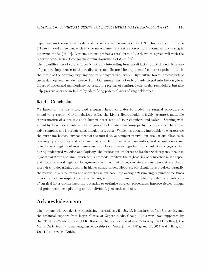
CHAPTER 6. A VIRTUAL SIZING TOOL FOR MITRAL VALVE ANNULOPLASTY 124
dependent on the material model and its associated parameters [129, 179]. Our results from Table
6.3 are in good agreement with in vivo measurements of suture forces during annular downsizing in
a porcine model [96, 97]. Our simulations predict a total force of 2.2N, which agrees well with the
reported total suture force for maximum downsizing of 3.5N [97].
The quantification of suture forces is not only interesting from a validation point of view, it is also
of practical importance to the cardiac surgeon. Suture bites represent focal stress points both in
the fabric of the annuloplasty ring and in the myocardial tissue. High suture forces indicate risk of
tissue damage and ring dehiscence [111]. Our simulations not only provide insight into the long-term
failure of undersized annuloplasty by predicting regions of continued ventricular remodeling, but also
help prevent short-term failure by identifying potential sites of ring dehiscence.
6.4.4 Conclusion
We have, for the first time, used a human heart simulator to model the surgical procedure of
mitral valve repair. Our simulations utilize the Living Heart model, a highly accurate, anatomic
representation of a healthy adult human heart with all four chambers and valves. Starting with
a healthy heart, we simulated the progression of dilated cardiomyopathy, its impact on the mitral
valve complex, and its repair using annuloplasty rings. While it is virtually impossible to characterize
the entire mechanical environment of the mitral valve complex in vivo, our simulations allow us to
precisely quantify tissue strains, annular stretch, mitral valve kinematics, and suture forces and
identify local regions of maximum stretch or force. Taken together, our simulations suggests that
during undersized valvular annuloplasty, the highest suture forces co-localize with regional peaks in
myocardial strain and annular stretch. Our model predicts the highest risk of dehiscence in the septal
and postero-lateral regions. In agreement with our intuition, our simulations demonstrate that a
more drastic downsizing results in higher suture forces. However, our simulations precisely quantify
the individual suture forces and show that in our case, implanting a 24mm ring requires three times
larger forces than implanting the same ring with 32mm diameter. Realistic predictive simulations
of surgical intervention have the potential to optimize surgical procedures, improve device design,
and guide treatment planning on an individual, personalized basis.
Acknowledgements
The authors acknowledge the stimulating discussions with Jay D. Humphrey at Yale University and
the technical support from Roger Clarke at Zygote Media Group. This work was supported by
the 5T32HL007974-14 grant (M.K. Rausch), the Stanford Graduate Fellowship (A.M. Zollner), the
Marie-Curie international outgoing fellowship (M. Genet), the NSF grant 1233054 and NIH grant
U01-HL119578 (E. Kuhl).
Conclusions
In the scope of this thesis, I have successfully created and run patient specific simulations of adaptive
tissue. I have successfully derived and calibrated constitutive models for adaptive tissue. To put
our constitutive framework to practice in realistic scenarios I have created patient specific geometry
models from medical imaging data. Our tool of choice to solve the created system of partial di↵er-
ential equations was the finite element method. The main advantage of the finite element method
over analytical models is its natural ability to capture geometries that are di�cult or impossible to
describe using analytical models, but can be subdivided into smaller, finite elements. In particular,
accurate patient specific models are virtually impossible to realize using analytical models. The same
holds for the modeling of physical contact between one or more bodies. Again, the finite element
method can be applied using small or finite sliding contact models to create realistic simulations
of the interaction. However, all these features and the flexibility compared to analytical mathe-
matical models do not come free. Compared to their analytical counterparts, finite element models
are typically computationally expensive and cumbersome to create. Therefore, in addition to the
concluding remarks, the opportunities and obstacles of using the finite element method to model
adaptive tissues and their interaction with devices and changing boundary conditions are presented
in the following.
Skin Expansion
I have presented a novel computational model for growing biological membranes in which I have
summarized the underlying mechanobiology in a single pheonomenological internal variable, the in-
plane area growth. To demonstrate the model performance, I have simulated tissue expansion in
pediatric forehead reconstruction. Driven by the clinical interest for a mechanistic model for skin
expansion, I have continuously improved our model. Without altering the key equations for skin
growth, I have transformed the model into a more e�cient spatial formulation and implemented it
into the general purpose finite code ABAQUS/Standard. This allowed for more realistic simulations
of the expander device itself and its interaction with the skin. The resulting model in its latest version
is applicable to arbitrary skin geometries derived from medical imaging and can use a discrete volume
125
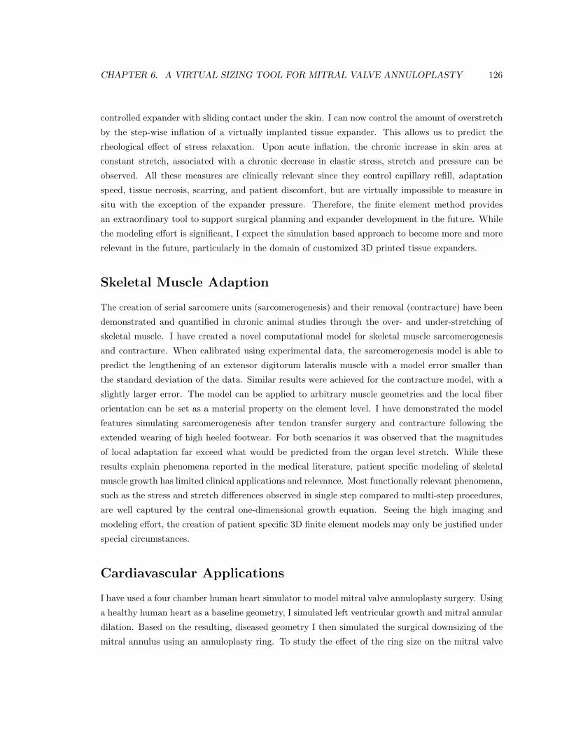
CHAPTER 6. A VIRTUAL SIZING TOOL FOR MITRAL VALVE ANNULOPLASTY 126
controlled expander with sliding contact under the skin. I can now control the amount of overstretch
by the step-wise inflation of a virtually implanted tissue expander. This allows us to predict the
rheological e↵ect of stress relaxation. Upon acute inflation, the chronic increase in skin area at
constant stretch, associated with a chronic decrease in elastic stress, stretch and pressure can be
observed. All these measures are clinically relevant since they control capillary refill, adaptation
speed, tissue necrosis, scarring, and patient discomfort, but are virtually impossible to measure in
situ with the exception of the expander pressure. Therefore, the finite element method provides
an extraordinary tool to support surgical planning and expander development in the future. While
the modeling e↵ort is significant, I expect the simulation based approach to become more and more
relevant in the future, particularly in the domain of customized 3D printed tissue expanders.
Skeletal Muscle Adaption
The creation of serial sarcomere units (sarcomerogenesis) and their removal (contracture) have been
demonstrated and quantified in chronic animal studies through the over- and under-stretching of
skeletal muscle. I have created a novel computational model for skeletal muscle sarcomerogenesis
and contracture. When calibrated using experimental data, the sarcomerogenesis model is able to
predict the lengthening of an extensor digitorum lateralis muscle with a model error smaller than
the standard deviation of the data. Similar results were achieved for the contracture model, with a
slightly larger error. The model can be applied to arbitrary muscle geometries and the local fiber
orientation can be set as a material property on the element level. I have demonstrated the model
features simulating sarcomerogenesis after tendon transfer surgery and contracture following the
extended wearing of high heeled footwear. For both scenarios it was observed that the magnitudes
of local adaptation far exceed what would be predicted from the organ level stretch. While these
results explain phenomena reported in the medical literature, patient specific modeling of skeletal
muscle growth has limited clinical applications and relevance. Most functionally relevant phenomena,
such as the stress and stretch di↵erences observed in single step compared to multi-step procedures,
are well captured by the central one-dimensional growth equation. Seeing the high imaging and
modeling e↵ort, the creation of patient specific 3D finite element models may only be justified under
special circumstances.
Cardiavascular Applications
I have used a four chamber human heart simulator to model mitral valve annuloplasty surgery. Using
a healthy human heart as a baseline geometry, I simulated left ventricular growth and mitral annular
dilation. Based on the resulting, diseased geometry I then simulated the surgical downsizing of the
mitral annulus using an annuloplasty ring. To study the e↵ect of the ring size on the mitral valve
CHAPTER 6. A VIRTUAL SIZING TOOL FOR MITRAL VALVE ANNULOPLASTY 127
kinematics I virtually implanted 3D reconstructed Carpentier Edwards Physio II rings with three
di↵erent diameters. To quantify the surgery outcome, I then virtually measured the septal-lateral
and commissure-commissure distances, the strain in the surrounding tissue, and the suture forces. In
agreement with findings reported in the medical literature, the smallest ring size provided the best
reconstruction of the original mitral valve geometry, but also caused the highest suture forces and
strains in the surrounding tissue. As expected, increasing the ring size reduced the invasiveness of the
procedure, but resulted in larger annular areas and a less e↵ective reonstruction overall. While the
measurement of most of these values in vivo is virtually impossible for just one ring, there is no way to
implant and compare multiple options at all. Finite element simulations provide a way to virtually
test di↵erent ring sizes and shapes and quantify their e↵ect before surgery. Performing virtual
annuloplasty surgery can help the surgeon to pick a ring size and type that e↵ectively reconstructs
the annular geometry while optimizing for low suture forces and tissue strains. In addition to
applications in surgical planning, finite element simulations can help to guide the development of
new implants or create better sizing guidelines.
Concluding Remarks
Patient specific finite element simulation is a promising tool in biomedical research, surgical plan-
ning, and medical device development. However, as I have discussed previously in this chapter,
applications should be selected carefully due to the computational and modeling resources needed.
In summary, it can be stated that finite element simulations of adaptive tissue are well suited for
applications in plastic surgery as for example skin expansion procedures. The superficial position
of the skin and its primarily two-dimensional nature allow for fast and e�cient geometry model-
ing. In addition, access to measure mechanical parameters is easily available and the measurement
procedures are typically non-invasive. In contrast, applications for simulations of skeletal muscle
adaptation show limited benefits compared to the extensive modeling e↵ort. While the geometry
modeling requires expensive image acquisition using CT or MRI scanning, the addition of clini-
cally useful information from these 3D simulations is minimal compared to one-dimensional models.
Lastly, the finite element method is an excellent tool for cardiovascular surgery planning. Proce-
dures such as mitral valve repair surgery are performed on high risk, high cost patient populations
with major comorbidities and comortalities. The benefits of tools like the virtual ring sizing tool
presented in this thesis promise to far outweigh their additional cost. Overall, after careful cost
benefit analyses, finite element models of adapting soft tissue are a promising tool for applications
in surgery planning and fast paced medical device R&D environments. I envision current trends in
medicine like customized 3D printed implants to accelerate the development and adaptation of these
models in the future.
Bibliography
[1] Abaqus 6.12. Analysis User’s Manual. SIMULIA. Dassault Systemes. 2012.
[2] Abaqus 6.13. Analysis User’s Manual. 2013. Simulia. Dassault Systemes.
[3] Agache PG, Monneur C, Leveque JL, DeRigal J. Mechanical properties and Young’s modulus
of human skin in vivo. Arch Dermatol Res. 1980;269:221-232.
[4] Ambrosi D, Mollica F. On the mechanics of a growing tumor. Int J Eng Sci. 2002;40:1297-1316.
[5] Ambrosi D, Preziosi L, Vitale G. The insight of mixtures theory for growth and remodeling.
ZAMP. 2010;61:177-191.
[6] Ambrosi D, Ateshian GA, Arruda EM, Cowin SC, Dumais J, Goriely A, Holzapfel GA,
Humphrey JD, Kemkemer R, Kuhl E, Olberding JE, Taber LA, Garikipati K. Perspectives
on biological growth and remodeling. J Mech Phys Solids. 2011;59:863-883.
[7] Amini, R., Eckert, C.E., Koomalsingh, K., McGarvey, J., Minakawa, M., Gorman, J.H., Gor-
man, R.C., Sacks, M.S. On the in vivo deformation of the mitral valve anterior leaflet: E↵ects of
annular geometry and referential configuration. Annals of Biomedical Engineering 2012;40:1455-
1467.
[8] American Podiatric Medical Association. 2003. High Heels Survey.
[9] Argenta LC, Watanabe MJ, Grabb WC. The use of tissue expansion in head and neck recon-
struction. Annals Plast Surg. 1983;11:31-37.
[10] Arneja JS, Gosain AK. Giant congenital melanocytic nevi of the trunk and an algorithm for
treatment. J Craniofac Surg. 2005;16:886-893.
[11] Arneja JS, Gosain AK. Giant congenital melanocytic nevi. Plast Reconstr Surg. 2007;120:26e-
40e.
[12] Arnold AS, Liu MQ, Schwartz MH, Ounpuu S, Delp SL. The role of estimating muscle-tendon
lengths and velocities of the hamstrings in the evaluation and treatment of crouch gait. Gait
Posture. 2006;23:273-281.
128
BIBLIOGRAPHY 129
[13] Arnold EM, Delp SL. Fibre operating lengths of human lower limb muscles during walking. Phil
Trans R Soc London B Biol Sci. 2011;366:1530-1539.
[14] Astanin S, Preziosi L. Mathematical modelling of the Warburg e↵ect in tumour cords. J Theor
Bio. 2009;258:578-590.
[15] Austad ED, Pasyk KA, McClatchey KD, Cheery GW. Histomorphologic evaluation of guinea
pig skin and soft tissue after controlled tissue expansion. Plast Reconstr Surg. 1982;70:704-710.
[16] Austad ED, Thomas SB, Pasyk KA. Tissue expansion: Divided or loan? Plast Reconstr Surg.
1982;78:63-67.
[17] Baillargeon, B., Rebelo, N., Fox, D.D., Taylor, R.L., Kuhl, E., 2014. The Living Heart Project:
A robust and integrative simulator for human heart function. European Journal of Mechanics
A/Solids, 48, 38-47.
[18] Baillargeon, B., Costa, I., Leach, J.R., Lee, L.C., Genet, M., Toutain, A., Wenk, J.F., Rausch,
M.K., Rebelo, N., Acevedo-Bolton, G., Kuhl, E., Navia, J.L., Guccione, J.M., 2015. Human
cardiac function simulator for the optimal design of a novel annuloplasty ring with a sub-
valvular element for correction of ischemic mitral regurgitation. Cardiovascular Engineering
and Technology 6(2), 105-116.
[19] Baker SR. Fundamentals of expanded tissue. Head & Neck. 1991;13:327-333.
[20] Barnett JG, Holly RG, Ashmore CR. Stretch-induced growth in chicken wing muscles: bio-
chemical and morphological characterization. Am J Physiol. 1980;239:C39-C46.
[21] Barone FE, Perry L, Keller T, Maxwell GP. The biomechanical and histopathologic e↵ect of
surface texturing with silicone and polyurethane in tissue implantation and expansion. Plast
Reconstr Surg. 1992;90:77-86.
[22] Beauchenne JG, Chambers MM, Peterson AE, Scott PG. Biochemical, biomechanical, and
physical changes in the skin in an experimental animal model of therapeutic tissue expansion.
J Surg Res. 1989;47:507-514.
[23] Bernardini F, Mittleman J, Rushmeiner H, Silva C, Taubin G. The ball-pivoting algorithm for
surface reconstruction. IEEE Trans Vis Comp Graph. 1999;5:349-359.
[24] Bol M, Reese S, Parker KK, Kuhl E. Computational modeling of muscular thin films for cardiac
repair. Comp Mech. 2009;43:535-544.
[25] Blemker SS, Asakawa DS, Gold GE, Delp SL. 2007. Image-based musculoskeletal modeling:
Applications, advances, and future opportunities. J Magn Res Img. 25:441–451.
BIBLIOGRAPHY 130
[26] Bol M, Reese S. 2008. Micromechanical modelling of skeletal muscles based on the finite element
method. Comp Meth Biom Biomed Eng. 11:489–504.
[27] Bol M, Sturmat M, Weichert C, Kober C. A new approach for the validation of skeletal muscle
modeling using MRI data. Comp Mech. 2011;47:591-601.
[28] Bol M, Stark H, Schilling N. 2011. On a phenomenological model for fatigue e↵ects in skeletal
muscles. J Theor Bio. 281:122–132.
[29] Bol M, Abilez OJ, Assar AN, Zarins CK, Kuhl E. In vitro / in silico characterization of active
and passive stresses in cardiac muscle. Int J Multiscale Comp Eng. 2012;10:171-188.
[30] Bothe, W., Kuhl, E., Kvitting, J.P., Rausch, M.K., Goktepe, S., Swanson, J.C., Farahmandnia,
S., Ingels, N.B., Miller, D.C., 2011. Rigid, complete annuloplasty rings increase anterior mitral
leaflet strains in the normal beating ovine heart. Circulation 124, S81-S96.
[31] Bothe, W., Rausch, M.K., Kvitting, J.P., Echtner, D.K., Walther, M., Ingels, N.B., Kuhl, E.,
Miller, D.C. 2012. How do annuloplasty rings a↵ect mitral annular strains in the normal beating
ovine heart? Circulation, 126, S231-S238.
[32] Bothe, W., Miller, D.C., Doenst, T., 2013. Sizing for mitral annuloplasty: where does science
stop and voodoo begin?, The Annals of Thoracic Surgery 95(4), 1475-1483.
[33] Bottinelli R, Reggiani C. Skeletal muscle plasticity in health and disease. Advances in Muscle
Research. 2002; Volume 2, Springer.
[34] Brobmann GF, Huber J. E↵ects of di↵erent shaped tissue expanders on transluminal pres-
sure, oxygen tension, histopathologic changes, and skin expansion in pigs. Plast Reconstr Surg.
1985;76:731-736.
[35] Brockes, JP Amphibian limb regeneration: Rebuilding a complex structure. Science.
1997;276:81-87
[36] Buganza Tepole A, Ploch CJ, Wong J, Gosain AK, Kuhl E. Growing skin - A computational
model for skin expansion in reconstructive surgery. J Mech Phys Solids. 2011;59:2177-2190.
[37] Buganza Tepole A, Gosain AK, Kuhl E. Stretching skin: The physiological limit and beyond.
Int J Nonlin Mech. doi: 10.1016/j.ijnonlinmec.2011.07.006.
[38] Buganza Tepole A, Gosain AK, Kuhl E. Stretching skin: The physiological limit and beyond.
Int J Nonlin Mech. 2012;47:938-949.
[39] Buganza Tepole A, Kuhl E. Systems-based approaches towards wound healing. Pediatric Res.
2013;doi:10.1038/pr.2013.3.
BIBLIOGRAPHY 131
[40] Burkholder TJ, Lieber RL. Sarcomere number adaptation after retinaculum transection in adult
mice. J Exp Bio. 1998;201:309-316.
[41] Burkholder TJ. Mechanotransduction in skeletal muscle. Front Biosci. 2007;12:174-191.
[42] Caiozzo VJ, Utkan A, Chou R, Khalafi A, Chandra H, Baker M, Rourke B, Adams G, Baldwin
K, Green S. E↵ects of distraction on muscle length: Mechanisms involved in sarcomerogenesis.
Clin Orthop Rel Res. 2002;403S:S133-S145.
[43] Calvo B, Ramirez A, Alonso A, Grasa J, Soteras F, Osta R, Munoz MJ. Passive nonlinear
elastic behavior of skeletal muscle: Experimental results and model formulation J Biomech.
2010;43:133-145.
[44] Carpentier, A.F., Lessana, A., Relland, J.Y., Belli, E., Mihaileanu, S., Berrebi, A.J., Palsky,
E., Loulmet, D.F., 1995. The“Physio-Ring”: an advanced concept in mitral valve annuloplasty.
Annals of Thoracic Surgery 60, 1177-1186.
[45] Castilla EE, da Graca Dutra M, Orioli-Parreiras IM. Epidermiology of congenital pigmented
naevi: I. Incidence rates and relative frequencies. Br J Dermatol. 1981;104:307-315.
[46] Chanaud CM, Pratt CA, Loeb GE. 1991. Functionally complex muscles of the cat hindlimb. II.
Mechanical and architectural heterogenity within the biceps femoris. Exp Brain Res. 85:257-270.
[47] Ciarletta P., Ben Amar M. Papillary networks in the dermal-epidermal junction of skin: a
biomechanical model. Mech Res Comm. in press.
[48] Ciarletta P, Ambrosi D, Maugin GA. Mass transport in morphogenetic processes: A second gra-
dient theory for volumetric growth and material remodeling. J Mech Phys Solids. 2012;60:432-
450.
[49] Cox B. A multi-scale, discrete-cell simulation of organogenesis: Application to the e↵ects
of strain stimulus on collective cell behavior during ameloblast migration. J Theor Bio.
2010;262:58-72.
[50] Cromie MJ, Sanchez GN, Schnitzer MJ, Delp SL. 2013. Sarcomere lengths in human extensor
carpi radials brevis measured by microendoscropy. Muscle & Nerve 48:286-292.
[51] Csapo R, Maganaris CN, Seynnes OR, Narici MV. 2010. On muscle, tendon and high heels. J
Exp Bio. 213:2582–2588.
[52] Cronin NJ, Barrett RS, Carty CP. 2012. Long-term use of high-heeled shoes alters the neu-
romechanics of human walking. J Appl Physiol. 112:1054–1058.
[53] Cronin NJ. 2014. The e↵ects of high heeled shoes on female gait: A review. J Electr Kinesiol.
24:258–263.
BIBLIOGRAPHY 132
[54] Daimon, M., Fukuda, S., Adams, D.H., McCarthy, P.M., Gillinov, A.M., Carpentier, A., Fil-
soufi, F., Abascal, V.M., Rigolin, V.H., Salzberg, S., Huskin, A., Langenfeld, M., Shiota, T.,
2006. Mitral valve repair with Carpentier-McCarthy-Adams IMR ETlogix annuloplasty ring
for ischemic mitral regurgitation. Early echocardiographic results from a multi-center study.
Circulation 114(1 suppl), I588-I593.
[55] De Filippo RE, Atala A. Stretch and growth: the molecular and physiologic influences of tissue
expansion. Plast Reconstr Surg. 2002;109:2450-2462.
[56] Dervaux J, Ciarletta P, Ben Amar M. Morphogenesis of thin hyperelastic plates: A constitutive
theory of biological growth in the Foppl-von Karman limit. J Mech Phys Solids. 2009;57:458-
471.
[57] Ducharme, A., Courval, J.F., Dore, A., Leclerc, Y., Tardif, J.C., 1999. Severe aortic regurgita-
tion immediately after mitral valve annuloplasty. Annals of Thoracic Surgery 67(5), 1487-1489.
[58] Duits EHA, Molenaar J, van Rappard JHA. The modeling of skin expanders. Plast Reconstr
Surg. 1989;83:362-367.
[59] Dupont Salter AC, Richmond FJR, Loeb GE. 2011. E↵ects of muscle immobilization at di↵erent
lengths on tetrodotoxin-induced disuse atrophy. IEEE Trans Neur Sys Reha Eng. 11:209-217.
[60] Ebbeling CJ, Hamill J, Crussemeyer JA. 1994. Lower extremity mechanics and energy cost of
walking in high-heeled shoes. J Orth Sports Phys Therapy. 19:190-196.
[61] Ehler E, Gautel M. The sarcomere and sarcomerogenesis. In: The Sarcomere and Skeletal
Muscle Disease. edited by Laing NG. 2008. Springer.
[62] Epstein M, Maugin GA. Thermomechanics of volumetric growth in uniform bodies. Int J Plast.
2000;16:951-978.
[63] Eurviriyanukul S, Askes H. 2011. Tendon layout optimization through configurational force
equilibration in plane stress analysis of prestressed concrete structures. Comp Struct. 89:1673-
1680.
[64] Fabri A, Pion S. 2009. CGAL: the Computational Geometry Algorithms Library. In: 17th ACM
SIGSPATIAL Int Conf. pp. 538–539. ACM Press, New York, New York, USA.
[65] Francis AJ, Marks R. Skin stretching and epidermopoiesis. Br J Exp Pathol. 1977;58:35-39.
[66] Fuster, V., Gersh, B.J., Giuliani, E.R., Tajik, A.J., Brandenburg, R.O., Frye, R.L., 1981. The
natural history of idiopathic dilated cardiomyopathy. American Journal of Cardiology 47(3),
525-531.
BIBLIOGRAPHY 133
[67] Garikipati K. The kinematics of biological growth. Appl Mech Rev. 2009;62:030801.1-030801.7.
[68] Genet, M., Lee, L.C., Nguyen, R., Haraldsson, H., Acevedo-Bolton, G., Zhang, Z., Ge, L.,
Ordovas, K., Kozerke, S., Guccione, J.M., 2014. Distribution of normal human left ventricu-
lar myofiber stress at end-diastole and end-systole - A target for in silico studies of cardiac
procedures. Journal of Applied Physiology 117, 142-152.
[69] Genet, M., Lee, L.C., Baillargeon, B., Guccione, J.M., Kuhl, E., 2015. Modeling pathologies of
systolic and diastolic heart failure. Annals of Biomedical Engineering doi: 10.1007/s10439-015-
1351-2.
[70] Gerber C, Meyer DC, Frey E, von Rechenberg B, Hoppeler H, Frigg R, Jost B, Zumstein MA.
Reversion of structural muscle changes caused by chronic rotator cu↵ tears using continuous
muscolotendinous traction. J Shoulder Elbow Surg. 2009;18:163-171.
[71] Goktepe S, Abilez OJ, Parker KK, Kuhl E. A multiscale model for eccentric and concentric
cardiac growth through sarcomerogenesis. J Theor Bio. 2010;265:433-442.
[72] Goktepe S, Abilez OJ, Kuhl E. A generic approach towards finite growth with examples of
athlete’s heart, cardiac dilation, and cardiac wall thickening. J Mech Phys Solids. 2010;58:1661-
1680.
[73] Goktepe S, Abilez OJ, Parker KK, Kuhl E. 2010. A multiscale model for eccentric and concentric
cardiac growth through sarcomerogenesis. J Theor Bio. 265:433-442.
[74] Goktepe S, Menzel A, Kuhl E. 2014. The generalized Hill model: A kinematic approach towards
active muscle contraction. J Mech Phys Solids. 72:20-39.
[75] Goldspink G. Sarcomere length during post-natal growth of mammalian muscle fibers. J Cell
Sci. 1968;3:539-548.
[76] Gordon AM, Huxley AF, Julian FJ. The variation in isometric tension with sarcomere length
in vertebrate muscle fibers. J Physiol. 1966;184:170-192.
[77] Goriely A, BenAmar M. Di↵erential growth and instability in elastic shells. Phys Rev Letters.
2005;94:198103.
[78] Goriely A, Tabor M. Biomechanical models of hyphal growth in actinomycetes. J Theor Bio.
2003;222:211218.
[79] Goriely A, BenAmar M. On the definition and modeling of incremental, cumulative, and con-
tinuous growth laws in morphoelasticity. Biomech Model Mechanobio. 2007;6:289296.
BIBLIOGRAPHY 134
[80] Gorman III, J.H., Gupta, K.B., Streicher, J.T., Gorman, R.C., Jackson, B.M., Ratcli↵e, M.B.,
Bogen, D.K., Edmunds, L.H., 1996. Dynamic three-diomensional maging of the mitral valve
and left ventricle by rapid sonomicrometry array localization. Journal of Thoracic and Cardio-
vascular Surgery 112, 712-726.
[81] Gosain AK, Santoro TD, Larson DL, Gingrass RP. Giant congenital nevi: A 20-year experience
and an algorithm for their management. Plast Reconstr Surg. 2001;108:622-636.
[82] Gosain AK, Cortes W. Pediatric tissue expansion for forehead reconstruction: A 13-year review
and an algorithm for its use. Am Soc Plast Surg. Baltimore, 2007; Abstract 13288.
[83] Gosain AK, Zochowski CG, Cortes W. Refinements of tissue expansion for pediatric forehead
reconstruction: A 13-year experience. Plast Reconstr Surg. 2009;124:1559-1570.
[84] Guccione, J.M., McCulloch, A.D., Waldman, L.K., 1991. Passive material properties of in-
tact ventricular myocardium determined from a cylindrical model. Journal of Biomechanical
Engineering 113, 42-55.
[85] Hayatsu K, De Deyne PG. Muscle adaptation during distraction osteogenesis in skeletally im-
mature and mature rabbits. J Orth Res. 2001;19:897-905.
[86] Herring SW, Grimm AF, Grimm BR. Regulation of sarcomere number in skeletal muscle: A
comparison of hypotheses. Muscle & Nerve. 1984;7:161-173.
[87] Himpel G, Kuhl E, Menzel A, Steinmann P. Computational modeling of isotropic multiplicative
growth. Comp Mod Eng Sci. 2005;8:119-134.
[88] Himpel G, Menzel A, Kuhl E, Steinmann P. Time-dependent fiber reorientation of transversely
isotropic continua - Finite element formulation and consistent linearization. Int J Num Meth
Eng. 2008;73:1413-1433.
[89] Hollenstein M, Ehret AE, Itskov M, Mazza E. A novel experimental procedure based on pure
shear testing of dermatome-cut samples applied to porcine skin. Biomech Model Mechanobio.
2011;10:651-661.
[90] Holzapfel, GA, 2000. Nonlinear Solid Mechanics: A Continuum Approach for Engineering. John
Wiley & Sons.
[91] Humphrey J. Cardiovascular tissue mechanics: Cells, tissues, and organs. Springer. 2002.
[92] Humphrey, J.D., Holzapfel, G.A., 2012. Mechanics, mechanobiology, and modeling of human
abdominal aorta and aneurysms. Journal of Biomechanics 45(5), 805-814.
[93] Huxley H, Hanson J. Changes in the cross-striations of muscle during contraction and stretch
and their structural interpretation. Nature. 1994;173:973-976.
BIBLIOGRAPHY 135
[94] Jaalouk DE, Lammerding J. Mechanotransduction gone awry. Nature Rev Mol Cell Bio.
2009;10:63-73.
[95] Javili A, Steinmann P. On the thermodynamics of solids with boundary structures. Int J Solids
& Structures. 2010;47:3245-3253.
[96] Jensen, M.O., Jensen, H., Nielsen, S.L., Smerup, M., Johansen, P., Yoganathan, A.P., Nygaard,
H., Hasenkam, J.M. 2008. What forces act on a flat rigid mitral annuloplasty ring? Journal of
Heart Valve Disease 17(3), 267-275.
[97] Jensen, M.O., Honge, J.L., Benediktsson, J.A., Siefert, A.W., Jensen, H., Yoganathan, A.P.,
Snow, T.K., Hasenkam, J.M. Nygaard, H., Nielsen, S.L., 2014 Mitral valve annular downsizing
forces: Implications for annuloplasty device development. Journal of Thoracic and Cardiovas-
cular Surgery 148(1), 83-89.
[98] Johnson TM, Lowe L, Brown MD, Sullivan MJ, Nelson BR. Histology and physiology of tissue
expansion. J Dermatol Surg Oncol. 1993;19:1074-1078.
[99] Jor JWY, Nash MP, Nielsen PMF, Hunter PJ. Estimating material parameters of a structurally
based constitutive relation for skin mechanics. Biomech Model Mechanobio. 2011;10:767-778.
[100] Kaplan EN. The risk of malignancy in large congenital nevi. Plast Reconstr Surg. 1974;53:421-
428.
[101] Kerckho↵s RCP, Omens JH, McCulloch AD. A single strain-based growth law predicts con-
centric and eccentric cardiac growth during pressure and volume overload. Mech Res Comm.
2012;42:40-50.
[102] Kikuchi N, Oden JT, 1988. Contact Problems in Elasticity: A Study of Variational Inequali-
ties and Finite Element Methods. Studies in Applied Mathematics, Society for Industrial and
Applied Mathematics.
[103] Kim Y, Lim JM, Yoon BC. 2013. Changes in ankle range of motion and muscle strength in
habitual wearers of high-heeled shoes. Foot Ankle Int. 34:414-419.
[104] Klepach D, Lee LC, Wenk JF, Ratcli↵e MB, Zohdi TI, Navia JA, Kassab GS, Kuhl E, Guccione
JM. Growth and remodeling of the left ventricle. Mech Res Comm. 2012;42:134-141.
[105] Knight K. 2010. Why walking flat-footed hurts after high heels. J Exp Bio. 213: Insight JEB
i.
[106] Kobbelt LP, Vorsatz J, Labsik U, Seidel HP. A shrink wrapping approach to remeshing polyg-
onal surfaces. Comp Graph Forum. 1999;18:119-130.
BIBLIOGRAPHY 136
[107] Kober C, Berg BI, Sturmat M, Rieger J, Gallo, L, Bol M, Mack M, Zeilhofer HF, Sader R.
Macroscopic muscular modeling based on in vivo 4d radiology. Int J Multiscale Comp Eng.
2012;2:131-142.
[108] Kono, T., Sabbah, Hani, N., Rosman, H., Alam, M., Jafri, S., Goldstein, S., 1992. Left
ventricular shape is the primary determinant of functional mitral regurgitation in heart failure.
Journal of the American College of Cardiology 20(7), 1594-1598.
[109] Kroon M, Holzapfel GA. A model for saccular cerebral aneurysm growth by collagen fibre
remodelling. J Theor Bio. 2007;247:775-787.
[110] Kroon W, Delhaas T, Arts T, Bovendeerd P. Computational modeling of volumetric soft tissue
growth: Application to the cardiac left ventricle. Biomech Model Mechanobio. 2009;8:301-309.
[111] Kronzon, I., Sugeng, L., Perk, G., Hirsh, D., Weinert, L., Fernandez, M.A.G., Lang, R.M.,
2009. Real-time 3-dimensional transesophageal echocardiography in the evaluation of post-
operative mitral annuloplasty ring and prosthetic valve dehiscence. Journal of the American
College of Cardiology 53(17), 1543-1547.
[112] Kuhl E, Steinmann P. Mass- and volume specific views on thermodynamics for open systems.
Proc Royal Soc. 2003;459:2547-2568.
[113] Kuhl E, Steinmann P. On spatial and material settings of thermohyperelstodynamics for open
systems. Acta Mech. 2003;160:179-217.
[114] Kuhl E, Menzel A, Steinmann P. Computational modeling of growth - A critical review, a
classification of concepts and two new consistent approaches. Comp Mech. 2003;32:71-88.
[115] Kuhl E, Steinmann P. Computational modeling of healing - An application of the material
force method. Biomech Model Mechanobio. 2004;2:187-203.
[116] Kuhl E, Garikipati K, Arruda EM, Grosh K. Remodeling of biological tissue: Mechanically in-
duced reorientation of a transversely isotropic chain network. J Mech Phys Solids. 2005;53:1552-
1573.
[117] Kuhl E, Menzel A, Garikipati K. On the convexity of transversely isotropic chain network
models. Phil Mag. 2006;86:3241-3258.
[118] Kuhl E, Maas R, Himpel G, Menzel A. Computational modeling of arterial wall growth:
Attempts towards patient-specific simulations based on computer tomography. Biomech Model
Mechanobio. 2007;6:321-331.
[119] Kuhl E, Holzapfel GA. A continuum model for remodeling in living structures. J Mat Sci.
2007;2:8811-8823.
BIBLIOGRAPHY 137
[120] Kuhl E. 2014. Growing matter - A review of growth in living systems. J Mech Behavior Biomed
Mat. 29:529-543.
[121] Kvistedal YA, Nielsen PMF. Estimating material parameters of human skin in vivo. Biomech
Model Mechanobio. 2009;8:1-8.
[122] Kwan, J., Shiota, T., Agler, D.A., Popovic, Z.B., Qin, J.X., Gillinov, M.A., Stewart, W.J.,
Cosgrove, D.M., McCarthy, P.M., Thomas, J.D., 2003. Geometric di↵erences of the mitral
apparatus between ischemic and dilated cardiomyopathy with significant mitral regurgitation
real-time three-dimensional echocardiography study. Circulation 107(8), 1135-1140.
[123] Lachmann, J., Shirani, J., Plestis, K.A., Frater, R.W.M., LeJemtel, T.H., 2001. Mitral ring
annuloplasty: an incomplete correction of functional mitral regurgitation associated with left
ventricular remodeling. Current Cardiology Reports 3(3), 241-246.
[124] Langevin HM, Bou↵ard NA, Badger GJ, Iatridis JC, Howe AK. Dynamic fibroblast cytoskele-
tal response to subcutaneous tissue stretch ex vivo and in vivo. Am J Physiol Cell Physiol.
2005;288:C747C756.
[125] Lee EH. Elastic-plastic deformation at finite strains. J Appl Mech. 1969;36:1-6.
[126] Lee, K.S., Stewart, W.J., Lever, H.M., Underwood, P.L., Cosgrove, D.M., 1993. Mechanism
of outflow tract obstruction causing failed mitral valve repair. Anterior displacement of leaflet
coaptation. Circulation 88(5), II24–II29.
[127] Lee, A.P.W., and Acker, M., Kubo, S.H., Bolling, S.F., Park, S.W., Bruce, C.J., Oh, J.K.,
2009. Mechanisms of recurrent functional mitral regurgitation after mitral valve repair in non-
ischemic dilated cardiomyopathy importance of distal anterior leaflet tethering. Circulation
119(19), 2606-2614.
[128] Lee, C.H., Oomens, P.J., Rabbah, J.P., Yoganathan, A., Gorman, R.C., Gorman, J.H., Amini,
R., Sacks, M.S., 2013. A high-fidelity and micro-anatomically accurate 3D finite element model
for simulations of functional mitral valve. Lecture Notes in Computer Science 7945, 416424.
[129] Lee, C.H., Amini, R., Gorman, R.C., Gorman III, J.H., Sacks, M.S., 2014. An inverse modeling
approach for stress estimation in mitral valve biomaterial assessment. Journal of Biomechanics
47, 2055-2063.
[130] Levi K, Kwan A, Rhines AS, Gorcea M, Moore DJ, Dauskardt RH. Emollient molecule e↵ects
on the drying stresses in human stratum corneum. Brit J Dermatol. 2010;163:695-703.
[131] Levine, R.A., Hung, J., Otsuji, Y., Messas, E., Liel-Cohen, N., Nathan, N., Handschumacher,
M.D., Guerrero, J.L., He, S., Yoganathan, A.P., Vlahakes, G.J., 2002. Mechanistic insights into
functional mitral regurgitation. Current Cardiology Reports 4(2), 125–129.
BIBLIOGRAPHY 138
[132] Lieber RL. 2009. Skeletal Muscle Structure, Function, and Plasticity. Lippincott Williams&
Wilkins, Baltimore.
[133] Limbert G, Taylor M. On the constitutive modeling of biological soft connective tissues. Int J
Solids & Structures. 2002;39:2343-2358.
[134] Limbert G. Dynamic skin wrinkles: Geometry or Mechanics? A probabilistic finite element
approach. ASME. Proc STLE/ASME Int Joint Tribology Conf 2010:45-47.
[135] Limbert G. A mesostructurally-based anisotropic continuum model for biological soft tissues
- Decoupled invariant formulation. J Mech Behavior Biomed Mat. 2011;4:1637-1657.
[136] Lewellyn ME, Barretto RP, Delp SL, Schnitzer MJ. Minimally invasive high-speed imaging of
sarcomere contractile dynamics in mice and humans. Nature. 2008;454:784-788.
[137] LoGiudice J, Gosain AK. Pediatric tissue expansion: Indications and complications. J Cran-
iofac Surg. 2003;14:866-872.
[138] Wong VW, Akaishi S, Longaker MT, Gurtner GC. Pushing back: Wound mechanotransduction
in repair and regeneration. J Invest Dermatol. in press. doi:10.1038/jid.201.212.
[139] Lubarda VA, Hoger A. On the mechanics of solids with a growing mass. Int J Solids & Struc-
tures. 2002;39:4627-4664.
[140] Lubarda VA. Constitutive theories based on the multiplicative decomposition of deformation
gradient: Thermoelasticity, elastoplasticity and biomechanics. Appl Mech Rev. 2004:57;95108.
[141] Maganaris CN, Paul JP. 2002. Tensile properties of the in vivo human gastrocnemius tendon.
J Biomech. 35:1639–1646.
[142] Magnusson SP, Varici MV, Maganaris CN, Kjaer M. 2008. Human tendon behavior and adap-
tation, in vivo. J Physiol. 586:71–81.
[143] Martins PALS, Natal Jorge RM, Ferreira AJM. A comparative study of several material models
for prediction of hyper elastic properties: Application to silicone-rubber and soft tissues. Strain.
2006:42:135-147.
[144] Matano T, Tamai K, Kurokawa T. Adaptation of skeletal muscle in limb lengthening: a light
di↵raction study on the sarcomere length in situ. J Orthop Res. 1994;12:193-196.
[145] Mazza E, Papes O, Rubin MB, Bodner SR, Binur NS. Nonlinear elastic-viscoplastic constitu-
tive equations for aging facial tissues. Biomech Model Mechanobiol. 2005;4:178-189.
BIBLIOGRAPHY 139
[146] McGee, E.C., Gillinov, A.M., Blackstone, E.H., Rajeswaran, J., Cohen, G., Najam, F., Shiota,
T., Sabik, J.F., Lytle, B.W., McCarthy, McCarthy PM, Cosgrove DM, 2004. Recurrent mitral
regurgitation after annuloplasty for functional ischemic mitral regurgitation. Journal of Thoracic
and Cardiovascular Surgery 128(6), 916-924.
[147] McGrath JA, Uitto J. Anatomy and organization of human skin. Chapter 3 in: Burns T,
Breathnach S, Cox N, Gri�ths C. Rook’s Textbook of Dermatology. Volume 1, Eighth Edition;
Blackwell Publishing. 2010.
[148] McMahon J, Goriely A. Spontaneous cavitation in growing elastic membranes. Math Mech
Solids. 2010;15:57-77.
[149] Menzel A. Modelling of anisotropic growth in biological tissues - A new approach and compu-
tational aspects. Biomech Model Mechanobiol. 2005;3:147-171.
[150] Menzel A. A fibre reorientation model for orthotropic multiplicative growth. Biomech Model
Mechanobiol. 2007;6:303-320.
[151] Menzel A, Kuhl E. Frontiers in growth and remodeling. Mech Res Comm. 2012;42,1-14.
[152] Murtada SC, Arner A, Holzapfel GA. 2012. Experiments and mechanochemical modeling of
smooth muscle contraction. Significance of filament overlap. J Thero Bio. 297:176–186.
[153] Neal ML, Kerckho↵s, R. 2009. Current progress in patient-specific modeling. Brief Bioinform
(2010) 11 (1): 111-126.
[154] Neumann CG. The expansion of an area of skin by progressive distension of a subcutaneous
balloon; use of the method for securing skin for subtotal reconstruction of the ear. Plast Reconstr
Surg. 1959;19:124-130.
[155] O’Dwyer NJ, Neilson PD, Nash J. 1989. Mechanisms of muscle growth related to muscle
contracture in cerebral palsy. Dev Med Child Neuro. 31:543–547.
[156] Opila KA, Wagner SS, Schiowitz S, Chen J. 1988. Postural alignment in barefoot and high-
heeled stance. Spine. 13:542–547.
[157] Otsuji, Y., Handschumacher, M.D., Schwammenthal, E., Jiang, L., Song, J.K. Guerrero, J.L.,
Vlahakes, G.J., Levine, R.A., 1997. Insights from three-dimensional echocardiography into the
mechanism of functional mitral regurgitation direct in vivo demonstration of altered leaflet
tethering geometry. Circulation 96(6), 1999-2008.
[158] Padala, M., Hutchinson, R.A., Croft, L.R., Jimenez, J.H., Gorman, R.C., Gorman III, J.H.,
Sacks, M.S., Yoganathan, A.P., 2009. Saddle shape of the mitral annulus reduces systolic strains
on the P2 segment of the posterior mitral leaflet. Annals of Thoracic Surgery 88, 1499-1505.
BIBLIOGRAPHY 140
[159] Padala, M., Gyoneva, L.I., Thourani, V.H., Yoganathan, A.P., 2014. Impact of mitral valve
geometry on hemodynamic e�cacy of surgical repair in secondary mitral regurgitation. Journal
of Heart Valve Disease 23, 79-87.
[160] Pamplona DC, de Abreu Alvim C. Breast reconstruction with expanders and implants. A
numerical analysis. Artificial Organs. 2004;28:353-356.
[161] Pamplona DC, Carvalho CR, Radwasnki H, Pitanguy I. Changes in the characterization of
the human scalp due to the process of successive skin expansion. Proc Mech Solids Brazil. Eds:
da Costa Mattos HS, Alves M. 2009;426-436.
[162] Pamplona DC, Carvalho C. Characterization of human skin through skin expansion. J Mech
Mat Structures. 2012;7:641-655.
[163] Pamplona DC, Mota DEJS. Numerical and experimental analysis of inflating a circular hy-
perelastic membrane over a rigid and elastic foundation. Int J Mech Sci. 2012;65:18-23.
[164] Pamplona DC, Velloso RQ, Radwanski HN. On skin expansion. J Mech Behavior Biomed Mat.
2013; accepted for publication.
[165] Pang H, Shiwalkar AP, Madormo CM, Taylor RE, Andriacchi TP, Kuhl E. Computational
modeling of bone density profiles in response to gait: A subject-specific approach. Biomech
Model Mechanobio. doi: 10.1007/s10237-011-0318-y.
[166] Pasyk KA, Austad ED, McClatchey KD, Cherry GW. Electron microscopic evaluation of
guinea pig and soft tissue expanded with a self-inflating silicone implant. Plast Reconstr Surg.
1982;70:37-45.
[167] Pasyk KA, Argenta LC. Histopathology of human expanded tissue. Clinics Plast Surg.
1987;14:435-445.
[168] Pasyk KA, Argenta LC, Hassett C. Quantitative analysis of the thickness of human skin and
subcutaneous tissue following controlled expansion with a silicone implant. Plast Reconstr Surg.
1988;81:516-523.
[169] Pellerin, D., Sharma, R., Elliott, P., Veyrat, C., 2003. Tissue Doppler, strain, and strain rate
echocardiography for the assessment of left and right systolic ventricular function. Heart 89
(Suppl III), iii9-iii17.
[170] Preziosi L, Tosin AR. Multiphase modelling of tumour growth and extracellular matrix inter-
action: Mathematical tools and applications. J Math Bio. 2009;58:625-656.
BIBLIOGRAPHY 141
[171] Prot V, Skallerud B, Holzapfel GA. Transversely isotropic membrane shells with application
to mitral valve mechanics. Constitutive modeling and finite element implementation. Int J Num
Meth Eng 2007;71:987-1008.
[172] Quaba AA, Wallace AF. The incidence of malignant melanoma (0 to 15 years of age) arising
in large congenital nevocellular nevi. Plast Reconstr Surg. 1986;78:174-178.
[173] Radovan C. Breast reconstruction after mastectomy using the temporary expander. Plast Re-
constr Surg. 1982;69:195-208.
[174] Rana M, Hamarneh G, Wakeling JM. 2013. 3D fascicle orientations in triceps surae. J Appl
Physiol. 115:116–125.
[175] Rausch MK, Bothe W, Kvitting JP, Goktepe S, Miller DC, Kuhl E. In vivo dynamic strains
of the ovine anterior mitral valve leaflet. J Biomech. 2011;44:1149-1157.
[176] Rausch MK, Dam A, Goktepe S, Abilez OJ, Kuhl E. Computational modeling of
growth: Systemic and pulmonary hypertension in the heart. Biomech Model Mechanobiol.
doi:10.1007/s10237-010-0275-x.
[177] Rausch MK, Tibayan FA, Miller DC, Kuhl E. Evidence of adaptive mitral leaflet growth. J
Mech Behavior Biomed Mat. 2012;15:208-217.
[178] Rausch MK, Famaey N, O’Brien Shultz T, Bothe W, Miller DC, Kuhl E. Mechanics of the
mitral valve: A critical review, an in vivo parameter identification, and the e↵ect of prestrain.
Biomech Model Mechanobiol. doi:10.1007/s10237-012-0462-z.
[179] Rausch, M.K., Tibayan, F.A., Ingels, N.B., Miller, D.C., Kuhl E., 2013. Mechanics of the
mitral annulus in chronic ischemic cardiomyopathy. Annals of Biomedical Engineering 41(10),
2171-2180.
[180] Reeder SB, Wen Z, Yu H, Pineda AR, Gold GE, Markl M, Pelc NJ. 2004. Multicoil Dixon
chemical species separation with an iterative least-squares estimation method. Magn Reson
Med. 51:35-45.
[181] Rivera R, LoGiudice J, Gosain AK. Tissue expansion in pediatric patients. Clin Plast Surg.
2005;32:35-44.
[182] Rodriguez EK, Omens JH, Waldman LK, McCulloch AD. E↵ect of residual stress on trans-
mural sarcomere length distributions in rat left ventricle. Am J Phys. 1993;264:H1048-H1056.
[183] Rodriguez EK, Hoger A, McCulloch AD. Stress-dependent finite growth in soft elastic tissues.
J Biomech. 1994;27:455-467.
BIBLIOGRAPHY 142
[184] Rosset A, Spadola L, Ratib O. 2004. OsiriX: An open-source software for navigating in mul-
tidimensional DICOM images. J Digit Img. 17:205–216.
[185] Ryan, JM, Humphrey, JD”, Finite Element Based Predictions of Preferred Material Symme-
tries in Saccular Aneurysms Annals of Biomedical Engineering1999;27:641-647.
[186] Schmid H, Pauli L, Paulus A, Kuhl E, Itskov M. How to utilise the kinematic constraint of
incompressibility for modelling adaptation of soft tissues. Comp Meth Biomech Biomed Eng.
doi: 10.1080/10255842.2010.548325.
[187] Schmid H, Pauli L, Paulus A, Kuhl E, Itskov M. Consistent formulation of the growth process
at the kinematic and constitutive level for soft tissues composed of multiple constituents. Comp
Meth Biomech Biomed Eng. 2012;15:547-561.
[188] Serup J, Jemec GBE, Grove GL. Handbook of Non-Invasive Methods and the Skin. Informa
Healthcare. 2003.
[189] Shively RE. Skin expander volume estimator. Plast Reconstr Surg. 1986;77:482-483.
[190] Siefert, A.W., Touchton, S.A., McGarvey, J.R., Takebayashi, S., Rabbah, J.P., Jimenez, J.H.,
Saikrishnan, N., Gorman, R.C., Gorman, J.H., Yoganathan, A.P., 2013. In-vivo mitral an-
nuloplasty ring transducer: Implications for implantation and annular downsizing. Journal of
Biomechanics 46(14), 2550–2553.
[191] Silver FH, Siperko LM, Seehra GP. Mechanobiology of force transduction in dermal tissue.
Skin Res Tech. 2003;9:3-23.
[192] Simpson CL, Patel DM, Green KJ. Deconstructing the skin. Cytoarchitectural determinants
of epidermal morphogenesis. Nature Rev Mol Cell Bio. 2011;12:565-580.
[193] Socci L, Pennati G, Gervaso F, Vena P. An axisymmetric computational model of skin expan-
sion and growth. Biomech Model Mechanobiol. 2007;6:177-188.
[194] Spector SA, Simard CP, Fournier M, Sternlicht E, Edgerton VR. Architectural alterations of
rat hind-limb skeletal muscles immobilized at di↵erent lengths. Exp Neurol. 1982;76:94-110.
[195] O’Sullivan K, McAuli↵e S, DeBurca N. The e↵ects of eccentric training on lower limb flexibility:
A systematic review. Brit J Sports Medicine. 2012;doi:10.1136/bjsports-2011-090835.
[196] Tabary JC, Tabary C, Tardieu C, Tardieu G, Goldspink G. 1972. Physiological and structural
changes in the cat’s soles muscle due to immobilization at di↵erent lengths by plaster casts. J
Physiol. 224:231–244.
[197] Taber LA. Biomechanics of growth, remodeling and morphogenesis. Appl Mech Rev.
1995;48:487-545.
BIBLIOGRAPHY 143
[198] Taber LA, Eggers DW. Theoretical study of stress-modulated growth in the aorta. J Theor
Bio. 1996;180:343-357.
[199] Taber LA. 1998. Biomechanical growth laws for muscle tissue. J Theor Bio. 193:201–213.
[200] Taber LA, Humphrey JD. Stress-modulated growth, residual stress, and vascular heterogeneity.
J Biomech Eng. 2001;123:528-535.
[201] Tahta, S.A., Oury, J.H., Maxwell, J.M., Hiro, S.P., Duran, C.M., 2002. Outcome after mitral
valve repair for functional ischemic mitral regurgitation. Journal of Heart Valve Disease 11(1),
11-18.
[202] Takei T, Rivas-Gotz C, Delling CA, Koo JT, Mills I, McCarthy TL, Centrella M, Sumpio BE.
E↵ects of strain on human keratinocytes. J Cell Physiol. 1997;173:64-72.
[203] Takei T, Mills I, Arai K, Sumpio BE. Molecular basis for tissue expansion: Clinical implications
for the surgeon. Plast Reconstr Surg. 1998;102:247-258.
[204] Taubin G, Zhang T, Golub G. 1996 Optimal surface smoothing as filter design. In: Lecture
Notes in Computer Science. eds. B. Buxton, R. Cipolla. pp. 283–292. Springer Berlin Heidelberg.
[205] Taylor RL. FEAP - A Finite Element Analysis Program. User Manual, Version 8.2, University
of California at Berkeley, 2008.
[206] Theodorou DJ, Theodorou SJ, Kakitsubata U, Lektrakul N, Gold GE, Roger B, Resnick D.
Plantar fasciitis and fascial rupture: MR imaging findings in 26 patients supplemented with
anatomic data in cadavers. Radiograpics. 20:S181–S197.
[207] Taylor RL. FEAP - A Finite Element Analysis Program. Version 8.3, User Manual, University
of California at Berkeley, 2011.
[208] Thompson FM, Coughlin MJ. 1994. The high price of high-fashion footwear. J Bone Joint
Surg. 76:1586-1593.
[209] Tsamis A, Cheng A, Nguyen TC, Langer F, Miller DC, Kuhl E. Kinematics of cardiac growth -
In vivo characterization of growth tensors and strains. J Mech Behavior Biomed Mat. 2012;8:165-
177.
[210] van der Kolk CA, McCann JJ, Knight KR, O’Brien BM. Some further characteristics of ex-
panded tissue. Clin Plast Surg. 1987;14:447-453.
[211] Vandiver R, Goriely A. Di↵erential growth and residual stress in cylindrical elastic structures.
Phil Trans R Soc A. 2009;367:3607-3630.
BIBLIOGRAPHY 144
[212] van Rappard JHA, Molenaar J, van Doorn K, Sonneveld GJ, Borghouts JMHM. Surface-area
increase in tissue expansion. Plast Reconstr Surg. 1988;82:833-839.
[213] Verdier C, Etienne J, Duperray A, Preziosi L. Review: Rheological properties of biological
materials. Comptes Rendus Phys. 2009;10:790-811.
[214] Williams PE, Goldspink G. 1971. Longitudinal growth of striated muscle fibres. J Cell Sci.
9:751-767.
[215] Williams PE, Goldspink G. 1971. The e↵ect of immobilization on the longitudinal growth of
striated muscle fibres. J Anat. 116:45-55.
[216] Williams PE, Goldspink G. Changes in sarcomere lengths and physiological properties in
immobilized muscle. J Anat. 1978;127:459-468.
[217] Wisdom KM, Delp SL, Kuhl E. 2014. Review. Use it or lose it: Multiscale skeletal
muscle adaptation to mechanical stimuli. Biomech Mod Mechanobio. available online first.
doi:10.1007/s10237-014-0607-3.
[218] Wollina U, Berger U, Stolle C, Stolle H, Schubert H, Zieger M, Hipler C, Schumann D. Tissue
expansion in pig skin - A histochemical approach. Anat Histol Embryol. 1992;21:101-11.
[219] Wong, J., Kuhl, E., 2014. Generating fibre orientation maps in human heart models using
Poisson interpolation. Computer Methodes in Biomechanics and Biomedical Engineering 17,
1217-1226.
[220] Wu KS, van Osdol WW, Dauskardt RH. Mechanical properties of human stratum corneum:
E↵ects of temperature, hydration, and chemical treatment. Biomaterials. 2006;27:785-795.
[221] Yoon JY, An DH, Yoo WG, Kwon YR. 2009. Di↵erences in activities of the lower extremity
muscles with and without heel contact during stair ascent by young women wearing high-heeled
shoes. J Orth Surg. 14:418-422.
[222] Zeng Y, Xu C, Yang J, Sun G, Xu X. Biomechanical comparison between conventional and
rapid expansion of skin. Brit Assoc Plast Surg. 2003;56:660-666.
[223] Zioupos P, Currey JD. 1998. Changes in the sti↵ness, strength, and toughness of human
cortical bone with age. Bone. 22:57-66.
[224] Zollner AM, Buganza Tepole A, Gosain AK, Kuhl E. Growing skin - Tissue expansion in
pediatric forehead reconstruction. Biomech Mod Mechanobio. in press. doi:10.1007/s10237-011-
0357-4.
[225] Zollner AM, Buganza Tepole A, Kuhl E. On the biomechanics and mechanobiology of growing
skin. J Theor Bio. 2012;297:166-175.
BIBLIOGRAPHY 145
[226] Zollner AM, Buganza Tepole A, Gosain AK, Kuhl E. Growing skin - Tissue expansion in
pediatric forehead reconstruction. Biomech Mod Mechanobio. 2012;11:855-867.
[227] Zollner AM, Abilez OJ, Bl M, Kuhl E. Stretching skeletal muscle - Chronic muscle lengthening
through sarcomerogenesis. PLoS ONE. 2012;7(10):e45661.
[228] Zollner AM, Holland MA, Honda KS, Gosain AK, Kuhl E. 2013. Growth on demand - Re-
viewing the mechanobiology of stretched skin. J Mech Behavior Biomed Mat. 28:495-509.
[229] Zollner AM, Pok JM, McWalter EJ, Gold GE, Kuhl E. On high heels and short muscles: A
multiscale model for sarcomere loss in the gastrocnemius muscle. J Theor Bio. 2015;365:301310.
[230] Zumstein MA, Frey E, von Rechenberg B, Frigg R, Gerber C, Meyer DC. Device for lengthening
of a musculotendinous unit by direct continuous traction in the sheep. BMC Vet Res. 2012;
doi:10.1186/1746-6148-8-50.
[231] Zygote Media Group, Inc. The Zygote Solid 3D Heart Model, 2014.
[232] Zygote Media Group, Inc. Zygote Solid 3d Heart Generations I & II Development Report.
Technical Development of 3D Anatomical Systems, 2014.