Incentive-Centered Design ofMoney-Free Mechanisms

by

Vasileios Gkatzelis

A dissertation submitted in partial fulfillment

of the requirements for the degree of

Doctor of Philosophy

Department of Computer Science

New York University

September 2013

Professor Richard J. Cole

c© Vasileios Gkatzelis

All rights reserved, 2013

Dedication

This work is dedicated to my family:

My sister Maria, my parents Giannis and Sofia, my brother Giorgos, and my wife Maria.

iv

Acknowledgements

First and foremost I would like to thank my research advisor, Professor Richard

Cole. Richard was always there for me throughout these five years at Courant; he

provided me with the flexibility to define my own research agenda, but at the same

time he worked very closely with me on both a technical and a conceptual level.

He helped me improve my writing skills and offered his enlightening perspective

on the problems that we worked on, but he also spent hours with me discussing

non-technical issues regarding career and life related choices. As the years flew by,

our brainstorming sessions became more and more enjoyable and these sessions are

one of the things that I will miss the most.

Second, I would like to thank Dr. Gagan Goel and Dr. Vahab Mirrokni. Not all

Ph.D. students have the good fortune to collaborate with two people as laid back

and fun to work with as Gagan and Vahab. Gagan quickly infused me with his

inspirational approach toward research problems, always keeping the bigger picture

in mind and seeking for the right questions to ask. Our research discussions took

place in different New York coffee shops every time, making each one of them

memorable. Vahab introduced me to coordination mechanisms and he regularly

impressed me with his ability to take deep theoretical notions, simplify them, and

provide me with exactly the information I needed in order to approach a problem.

I also had the luck to work with both Gagan and Vahab as a Google intern.

Before acknowledging more of my collaborators and colleagues, I would like to

first thank my department’s Assistant Director, Rosemary Amico, and the Director

of Graduate Studies, Margaret Wright. It would not have been as easy to focus

on research without the work of Rosemary and Margaret, who dealt with virtually

v

any problem that came up. I especially want to thank Rosemary for always being

very efficient, friendly, and almost too helpful. I would also like to thank the Ph.D.

Program Administrator, Santiago Pizzini.

I would now like to express my gratitude to Christina Aperjis and Bernardo

Huberman for hosting my internship at HP Labs as well as to Samuel Ieong and

Rakesh Agrawal for hosting my internship at Microsoft Research. To my great

co-authors and collaborators: Xi Chen, Jose R. Correa, Dimitris Fotakis, Alexis

C. Kaporis, Neil Olver, Jay Sethuraman, and Paul G. Spirakis, as well as to my

thesis committee members Oded Regev and Steven Brams.

I owe this work to my friends, both in New York and back in Greece, and to

my family all of who provided me with the love, the support, and the peace of

mind that made this journey as much fun as it was.

Finally, I would like to acknowledge the sources that provided me with finan-

cial support during these years: the NYU Graduate School of Arts and Science

that supported me through both the “MacCracken Fellowship” and the “Dean’s

Dissertation Fellowship”, and the University of Patras that awarded me with the

“Andreas Mentzelopoulos Scholarship”.

vi

Abstract

This thesis serves as a step toward a better understanding of how to design fair

and efficient multiagent resource allocation systems by bringing the incentives of

the participating agents to the center of the design process. As the quality of these

systems critically depends on the ways in which the participants interact with

each other and with the system, an ill-designed set of incentives can lead to severe

inefficiencies. The special focus of this work is on the problems that arise when the

use of monetary exchanges between the system and the participants is prohibited.

This is a common restriction that substantially complicates the designer’s task; we

nevertheless provide a sequence of positive results in the form of mechanisms that

maximize efficiency or fairness despite the possibly self-interested behavior of the

participating agents.

The first part of this work is a contribution to the literature on approximate

mechanism design without money. Given a set of divisible resources, our goal is to

design a mechanism that allocates them among the agents. The main complication

here is due to the fact that the agents’ preferences over different allocations may

not be known to the system. Therefore, the mechanism needs to be designed in

such a way that it is in the best interest of every agent to report the truth about her

preferences; since monetary rewards and penalties cannot be used in order to elicit

the truth, a much more delicate regulation of the resource allocation is necessary.

The second part of this work concerns the design of money-free resource alloca-

tion mechanisms for decentralized multiagent systems. As the world has become

increasingly interconnected, such systems are using more and more resources that

are geographically dispersed; to provide scalability in these systems, the mecha-

vii

nisms need to be decentralized. That is, the allocation decisions for any given

resource should not assume global information regarding the system’s resources

or participants. We approach this restriction by using coordination mechanisms:

simple resource allocation policies, each of which controls only one of the resources

and uses only local information regarding the state of the system.

viii

Contents

Dedication . . . . . . . . . . . . . . . . . . . . . . . . . . . . . . . . . . . iv

Acknowledgements . . . . . . . . . . . . . . . . . . . . . . . . . . . . . . v

Abstract . . . . . . . . . . . . . . . . . . . . . . . . . . . . . . . . . . . . vii

List of Figures xi

1 Introduction 1

1.1 Incentive-Centered Design . . . . . . . . . . . . . . . . . . . . . . . 1

1.2 Mechanism Design without Payments . . . . . . . . . . . . . . . . . 4

1.3 Coordination Mechanisms and the Price of Anarchy . . . . . . . . . 6

2 Centralized Mechanisms for Efficiency 11

2.1 Introduction . . . . . . . . . . . . . . . . . . . . . . . . . . . . . . . 11

2.2 Preliminaries . . . . . . . . . . . . . . . . . . . . . . . . . . . . . . 16

2.3 Proportional Fairness . . . . . . . . . . . . . . . . . . . . . . . . . . 17

2.4 Truthful Mechanisms . . . . . . . . . . . . . . . . . . . . . . . . . . 22

2.5 Combining the Mechanisms . . . . . . . . . . . . . . . . . . . . . . 24

2.6 Concluding Remarks . . . . . . . . . . . . . . . . . . . . . . . . . . 27

3 Centralized Mechanisms for Fairness 29

3.1 Introduction . . . . . . . . . . . . . . . . . . . . . . . . . . . . . . . 29

ix

3.2 Preliminaries . . . . . . . . . . . . . . . . . . . . . . . . . . . . . . 36

3.3 The Partial Allocation Mechanism . . . . . . . . . . . . . . . . . . . 39

3.4 The Strong Demand Matching Mechanism . . . . . . . . . . . . . . 56

3.5 Connections to Mechanism Design with Money . . . . . . . . . . . . 64

3.6 Concluding Remarks . . . . . . . . . . . . . . . . . . . . . . . . . . 68

4 Decentralized Welfare-Optimizing Mechanisms 70

4.1 Introduction . . . . . . . . . . . . . . . . . . . . . . . . . . . . . . . 70

4.2 Preliminaries . . . . . . . . . . . . . . . . . . . . . . . . . . . . . . 78

4.3 Smith’s Rule . . . . . . . . . . . . . . . . . . . . . . . . . . . . . . . 82

4.4 Improvements with Preemption and Randomization . . . . . . . . . 87

4.5 Potential Games and an Algorithmic Application . . . . . . . . . . 102

4.6 Concluding Remarks . . . . . . . . . . . . . . . . . . . . . . . . . . 110

A Appendix: Omitted Proofs 112

A.1 Proofs Omitted from Chapter 3 . . . . . . . . . . . . . . . . . . . . 112

A.2 Proofs Omitted from Chapter 4 . . . . . . . . . . . . . . . . . . . . 117

5 Bibliography 123

x

List of Figures

2.1 The Partial Allocation mechanism for two agents. . . . . . . . . . . 23

2.2 The Max mechanism. . . . . . . . . . . . . . . . . . . . . . . . . . . 24

2.3 The approximation factor of Max . . . . . . . . . . . . . . . . . . . 26

3.1 The Partial Allocation mechanism. . . . . . . . . . . . . . . . . . . 40

3.2 The Approximate Partial Allocation mechanism. . . . . . . . . . . . 54

3.3 The Strong Demand Matching mechanism. . . . . . . . . . . . . . . 59

4.1 Jobs scheduled by SmithRule and by ProportionalSharing. . . . . . . 87

4.2 A factor 2 + ε approximation algorithm . . . . . . . . . . . . . . . . 107

A.1 A machine scheduling problem instance exhibiting how inefficient a

Nash equilibrium of a fixed ordering policy can become. . . . . . . . 118

xi

Chapter 1

Introduction

1.1 Incentive-Centered Design

The rise of the internet during the previous decade enabled the development of

systems with vast numbers of interacting users. This soon led to the realization

that without a proper coordination of the resulting interactions such systems may

face severe inefficiencies. As an example, the peer-to-peer networking revolution

revealed that the incentives users face when choosing how much of their resources

(bandwidth, storage space, or computing power) to share with others can make

or break a system as the number of participants grows [82, Chapter 23]. The

ongoing paradigm shift from personal computers to cloud computing complicates

these interactions even further since more and more services that used to be run

on isolated machines are now being migrated to shared computing clusters. As a

result, the way the users choose to interact with such services affects how these

shared resources are allocated among them, thus emphasizing the need for higher

quality incentive design in the form of protocols or mechanisms.

One of the most common objectives of these systems is the fair and efficient

1

allocation of resources, which has long been one of the main goals of Economics,

Operations Research, and Computer Science. The increasing importance of the

role that incentives play in the efficacy of resource allocation mechanisms is now

concentrating a significant amount of attention on the study of multiagent resource

allocation [23]. Here the incentives of the users (agents) are at the center of the

design process, making game theory the natural tool for designing and analyz-

ing these systems. Specifically, the goal is to create mechanisms that optimize

the allocation of resources among a set of self-interested agents. Different types

of resources, agent preferences, measures of efficiency or fairness, and allocation

procedures give rise to different settings; from a theoretical standpoint though,

one can model any such setting using game theory: the ways in which the agent

can interact with the system define a set of agent strategies, and a combination

of strategic choices by the agents, known as a strategy profile, yields an outcome.

In other words, the mechanism can be thought of as inducing a game among the

agents. Since each agent may have different preferences over the possible out-

comes, she will choose her strategy so as to yield an outcome that she prefers.

Moreoever, instead of just human users, one now also finds automated agents that

are programmed to seek resources strategically on a user’s behalf; such agents, if

well designed, can be expected to exhibit rational strategic behavior, exactly the

behavior assume in game theory-based mechanism design and analysis.

This thesis contributes a collection of positive results in the form of mechanisms

that manage to better align the incentives of the agents with the social objectives

that the mechanism designer wishes to optimize; that is, despite the fact that

the agents may be self-interest with no regard for the designer’s objectives, we

still manage to implement outcomes that approximately optimize these objectives

2

via carefully designed mechanisms. The first part of this thesis, which consists of

Chapters 2 and 3, addresses incentive-centered problems whose allocation proce-

dures can be centralized in nature, while the second part, which corresponds to

Chapter 4, studies allocation procedures that need to be decentralized.

Traditionally, it is the centralized approach that has been followed, especially

in Computer Science and Operations Research. Here, all related information is

gathered by one entity which then aims to compute an allocation that optimizes

some social objective. Research along these lines has attempted to understand the

computational complexity of such processes, drawing the boundary between what

is tractable and what is not. It is very often the case though, as we explain in

Section 1.2 below, that the information that needs to be considered by the alloca-

tion procedure is private to the agents. In this case, apart from the computational

tractability of the allocation procedure the designer may also need to elicit the

true information from the agents.

On the other hand, as the world becomes increasingly interconnected, a much

more (geographically) distributed set of resources has become available, leading

to a rising need for decentralized allocation processes. One of the main reasons

is that centralized control in such distributed systems, examples of which include

the Grid [53] and PlanetLab [85], severely impacts their scalability. The obvious

drawback of decentralization, besides the limited communication among the allo-

cation processes which may lead to inefficient solutions, is that such systems are

more prone to strategic manipulation by the agents. In Section 1.3 we review the

definition of coordination mechanisms; they provide an elegant solution for the

decentralized manipulation of the agents’ incentives which we will be using in the

second part of this thesis.

3

1.2 Mechanism Design without Payments

Even when the resource allocation can be implemented in a centralized fashion,

achieving efficiency or fairness is not a trivial task. Most natural measures of

efficiency and fairness depend directly on the agents’ preferences over different

allocations, and it is very often the case that these preferences are private infor-

mation of the agent. For example, if the mechanism designer’s objective is to

maximize the efficiency of the allocation, she might wish to allocate each resource

to the agent who desires it the most. Not knowing how much each agent values a

resource, the mechanism designer may ask them to report these values; but with-

out establishing an appropriate payment scheme the designer cannot be sure that

the agents are not misreporting their valuations for the resources. If, for instance,

the mechanism just allocates each resource to the agent that reported the high-

est valuation for it without requesting a payment, then an agent may report a

higher valuation for any resource that she desires, thus hampering the designer’s

goal of achieving efficiency. Mechanism Design is the sub-field of economic theory

whose purpose is to design games with private information in a way that allows

the designer to achieve her goals despite the agents’ self-interested behavior. One

of the most significant positive results in the mechanism design literature is the

Vickrey-Clarke-Groves (VCG) mechanism [82, Chapter 9]. This mechanism defines

a set of monetary payments that incentivize the agents to report their true values

while the resources are allocated in a way that maximizes the sum of the agents’

valuations for the bundle of resources that they are allocated. Unfortunately, the

applicability of this method is restricted to this specific measure of efficiency and

to settings where monetary payments are an option that the designer can use.

4

There are many settings though, especially in computing, where the mecha-

nisms need to eschew monetary transfers completely, often due to ethical, legal, or

even practical considerations [82, Chapter 10]. For instance, agents could repre-

sent internal teams in an internet company which are competing for resources. The

inability to use monetary rewards or penalties, of course, severely limits what the

mechanism designer can achieve since the exchange of payments is the most ver-

satile method for affecting the incentives of the agents. In light of this restriction,

the only available tool for aligning the agents’ incentives with the objectives of

the system is what Hartline and Roughgarden referred to as money burning [61].

This means that the system can choose to intentionally degrade the quality of

its services in order to influence the preferences of the agents. This degradation

of service can often be interpreted as an implicit form of “payment”, but since

these payments do not correspond to actual trades, they are essentially burned;

for example, money burning might correspond to resources not being allocated to

anyone. It is therefore not very surprising that the domain of mechanism design

without money is dominated by negative results [82, Chapter 10].

Contribution. This thesis contributes to the literature on mechanism design

without payments, and more specifically to the research agenda of approximate

mechanism design without money [87], by providing money-free mechanisms that

improve upon the best previously known efficiency and fairness guarantees. Chap-

ter 2 considers a measure of efficiency for which previous research provided no

non-trivial positive results. In contrast, we provide a truthful mechanism that

guarantees a non-trivial worst-case approximation of this objective [35]. More

significantly, in Chapter 3 we revisit the problem of fair division: one very well

5

studied problem for which the restriction to payment-free mechanisms is most rel-

evant. Our goal is to design truthful mechanisms for the fair allocation of multiple

heterogenous divisible goods. As a benchmark for fairness we use the proportion-

ally fair solution, which is widely recognized as the most desirable notion of fairness

when allocating divisible resources. We then define the Partial Allocation mecha-

nism, which first computes this proportionally fair allocation, but then allocates to

each agent only a fraction of her share, a fraction which depends on how much her

presence inconveniences the other agents. This elegant mechanism guarantees that

every agent’s value for the outcome is at most a small constant factor away from

the benchmark while guaranteeing that no agent has an incentive to misreport her

preferences. We also reveal an interesting economic interpretation of the discarded

resources as Vickrey-Clarke-Groves (VCG) payments, which provides some insight

regarding the truthfulness of this mechanism. Finally, we also define the Strong

Demand Matching mechanism which, for a well motivated set of problem instances,

guarantees that every agent will receive a resource of value very close to her value

as prescribed by the benchmark [34].

1.3 Coordination Mechanisms and the Price of Anarchy

Having described the difficulties that the mechanism designer might face even

when the allocation mechanism can be centralized, one can extrapolate that her

ability to achieve efficiency is limited even further in distributed systems. The

agent interactions that arise within large-scale distributed systems can take differ-

ent forms but it is well known that strategic behavior by the agents often leads

to significant inefficiencies in the final allocation. Since there is no centralized

“benevolent dictator” to enforce the good behavior of the participating agents,

6

decentralized incentive-centered design becomes a critical tool for alleviating inef-

ficiencies. To this end, several approaches have been proposed in the literature,

including some approaches enforcing strategies on a fraction of agents as a Stackel-

berg strategy [11, 73, 89, 101] and others using monetary transfers [13, 33, 51, 20].

The primary drawback of these methods is the need for global knowledge of the

system: the mechanism itself is still centralized and this can compromise the scal-

ability of the system.

In an attempt to address precisely this restriction, Chistodoulou, Koutsoupias,

and Nanavati [28] proposed a different approach, which they called coordination

mechanisms. They consider settings where agents can strategically choose which

resource they are going to share. A combination of strategies then corresponds

to an assignment of agents to resources and a coordination mechanism aims to

provide the incentives that lead to more efficient allocations. What makes coor-

dination mechanisms a purely decentralized solution for this setting is that they

consist of several independent and decentralized allocation processes, one for each

of the available resources. That is, each resource has its own decentralized policy

which decides how the resource will be allocated to the agents that seek it. These

policies prohibit any form of monetary side payment and thus the manipulation

of the agents’ incentives is instead achieved only through appropriate regulation

of how much of her chosen resource an agent is allocated. This means that, for

example, instead of requiring a player to contribute some form of payment, the

policy would choose to provide a less valuable allocation of the resource it con-

trols; in other words, these mechanisms apply money burning in a decentralized

fashion. More importantly, these policies only consider local information, i.e. the

decision regarding how a resource will be allocated among the agents assigned to

7

it may only depend on properties of these agents, disregarding what other agents

or resources are currently active elsewhere in the system. As a result, the com-

munication complexity of the system becomes insignificant, and the addition of a

new resource does not affect the rest of the system in any way.

The abstract definition of coordination mechanisms provides a simple model

of a cloud computing environment, so the power of these mechanisms has mostly

been analyzed for a machine scheduling setting where each resource corresponds to

a computing machine. These resources can be thought of as computing servers of

some distributed system offering a service that the system’s users need. Each agent

then seeks to be allocated time on such a machine in order to process some com-

puting task. A coordination mechanism for this setting defines one local scheduling

policy for each machine, and this scheduling policy chooses the order in which any

given set of tasks will be scheduled. The agents may then select which machine

they prefer but their cost is proportional to the completion time of their task, and

it therefore depends directly on which other agents select the same machine, as

well as on the scheduling policy of that machine. The goal of this line of research

is to study the extent to which simple local policies can significantly improve the

efficiency of the outcomes that arise as a result of the strategic interactions of the

agents.

In order to analyze the efficiency of these coordination mechanisms though,

one needs to define what the final outcome is expected to be given the incentives

that the participating agents face. This expected outcome is assumed to be an

equilibrium, which has been one of the central concepts of game theory since its

inception. A configuration of a game is called an equilibrium when it is stable

with respect to strategic deviations by the agents. The assumption is that, if some

8

self-interested agent can unilaterally change her strategy leading to an outcome

that she prefers, then she will do so. Therefore, if the agents behave rationally

and are well informed about the game, no unstable configuration should arise

as an outcome. Based on this assumption, the inefficiency of the outcome of

a game will never be worse than that of its least efficient equilibrium outcome;

following this line of thought, Koutsoupias and Papadimitriou defined the Price

of Anarchy [74], which is now the standard measure of a game’s efficiency within

the algorithmic game theory literature [82, Chapter 17]. Given a game and some

social objective, the price of anarchy is simply the worst case ratio of the social

cost at an equilibrium of the game to that at the social optimum. As its name

implies, this measure provides a way to quantify the deterioration with respect

to the social objective that is suffered due to the self-interested mindset of the

participants. In the case of coordination mechanisms, apart from this mindset,

the designer also faces the lack of centralized control; the definition of the price of

anarchy for these mechanisms therefore corresponds to the worst case ratio of the

social cost in equilibrium compared to the optimal social cost that could possibly

be achieved via the centralized optimization approach. We will sometimes use the

synonym coordination ratio as a reminder of this distinction.

Contribution. Chapter 4 of this thesis provides an extensive study of different

coordination mechanisms for a very general machine scheduling model. We focus

on the social objective of minimizing the sum over all agents of the cost that the

agent suffers, and we prove that our mechanisms guarantee a social cost which is

close to the optimal social cost that could be achieved by a centralized allocation

mechanism that could enforce any possible outcome. We also provide an analysis

9

showing that a counter-intuitive coordination mechanism that delays the release

of tasks beyond their completion time (thus causing an increase in the social cost)

outperforms the one that avoids these, otherwise unnecessary, delays. To explain

this phenomenon, we provide an economic interpretation of the delays, showing

that they correspond to well motivated incentive design using money burning.

Finally, using the intuition obtained from these mechanisms we provide a novel

combinatorial approximation algorithm for the underlying well-studied machine

scheduling problem; this provides evidence that a game theoretic viewpoint can

contribute to optimization [32].

10

Chapter 2

Centralized Mechanisms for Efficiency

2.1 Introduction

How does one allocate a collection of resources to a set of strategic agents without

using money? This is a fundamental problem with many applications since in many

scenarios payments cannot be solicited from agents; for instance, different teams

compete for a set of shared resources in a firm, and the firm cannot solicit payments

from the teams to make allocation decisions. Another motivating example is the

division of a married couple’s assets if they choose to divorce. Allowing monetary

payments could introduce unwanted inequalities as the two members of the couple

may be facing different budgets.

The lack of monetary rewards or penalties causes several problems to arise,

making the design of useful allocation processes much more difficult. As a result,

despite the applicability of mechanism design without money, much of the work in

the broader area of multiagent resource allocation [24] relies on enforcing payments.

Two of the most significant obstacles for mechanism design without money are

the difficulty of enforcing truthfulness on behalf of the strategic agents, and the

11

inability to compare these agents’ reported valuations.

To avoid the first obstacle the mechanism designer must ensure that there is

no way for an agent to misreport her valuations in order to receive an allocation

which she prefers. Not surprisingly, the most useful tool in designing such truthful

mechanisms has been the use of payments or rewards that can help make undesir-

able allocations seem less appealing to the agents. When monetary exchanges are

prohibited, the number and possibly also the quality of the outcomes that can be

implemented in a truthful manner is restricted. In this work, we discard part of

the resources and use this approach as an indirect way of enforcing truthful be-

havior by the agents. Discarding resources leads to inefficiencies but, as we show,

it nonetheless allows us to improve upon the best previously known worst-case

efficiency guarantees.

The other obstacle that arises in mechanism design without money is that the

valuations of the agents need to be put on a common scale. For example, happiness

could mean different things to different people and cannot be compared as such.

When payments can be used, a standard approach is to measure valuations in

terms of money. In the absence of money, one way to overcome this difficulty is to

look for scale-free solutions, i.e. if an agent scales her valuations up or down, the

solution should remain the same. When seeking to maximize social welfare (SW),

one can define an appropriate scale-free solution by first normalizing the valuations

of the agents so that every agent has some common value for the bundle containing

all the resources (1 say); then, using these normalized valuations, the goal is to

allocate the resources so as to maximize the sum of the agents’ valuations. In

this chapter we will be using this solution as the benchmark that we wish to

approximately implement in a truthful manner. Another interesting scale-free

12

solution, which is well regarded for its fairness properties, is the proportionally fair

(PF) solution. In brief, a PF allocation is a Pareto optimal allocation x∗ which

compares favorably to any other Pareto optimal allocation x in the sense that, when

switching from x to x∗, the aggregate percentage gain in happiness of the agents

outweighs the aggregate percentage loss. The PF solution was first proposed in the

TCP literature and is used widely in many practical scenarios [69]. In this chapter,

instead of fairness maximization, our objective is to maximize efficiency (or social

welfare). Nevertheless, we will be using the PF allocation as an intermediate tool

in designing a mechanism aiming to maximize social welfare; in Chapter 3 the PF

allocation plays an even more important role, as we focus on fairness maximization

and use this allocation as a benchmark as well. It is often the case that achieving

efficiency comes at a great cost in terms of fairness and vice-versa but, as we

show in this chapter, the two scale-free solutions mentioned above are actually

well aligned, at least for two-agent instances.

The problem of maximizing the social welfare with normalized valuations using

truthful mechanisms was first studied by Guo and Conitzer [57]. Their goal was

to allocate a collection of divisible resources among two strategic agents, and they

measured the competitiveness of their mechanisms by comparing the social welfare

that they guarantee with the best possible social welfare. They mainly focused on

the special case of two items and two agents for which they presented a truthful

mechanism that achieves a 0.829 worst-case approximation; they also showed that

no truthful mechanism can achieve better than a 0.841 approximation, even for

this very restricted setting. For the more general setting of many items and two

bidders they showed that no mechanism from a class of increasing price mecha-

nisms (mechanisms using artificial currency for both linear and non-linear pricing)

13

can guarantee an approximation factor better than 0.5; they left it as an open ques-

tion to overcome this bound. Subsequent work of Han et al. [60] extended these

negative results, showing that even for the more general class of swap-dictatorial

mechanisms, no mechanism can guarantee an approximation factor better than 0.5

when the number of items is unbounded. The class of swap-dictatorial mechanisms

contains all mechanisms that first (randomly) choose one of the two bidders and

then allow her to choose her preferred bundle of items from a predefined set; the

other bidder receives the remaining items1. Finally, another negative result from

the work of Han et al. [60] showed that if both the number of agents and the

number of items are unbounded, then no non-trivial approximation factor of the

optimal SW can be achieved. Therefore, the main open question that remains in

this setting is whether interesting truthful mechanisms for the two-bidder case ex-

ist beyond the class of swap-dictatorial mechanisms and whether such mechanisms

can achieve an approximation factor better than 0.5. We provide a positive answer

to this open question by presenting an interesting non-swap-dictatorial mechanism

that breaks this bound of 0.5. Our main contribution here is to show a connection

between the PF and SW maximizing allocations; then we exploit this connection

in order to define our mechanism.

Our results. We start Section 2.3 by providing a simple algorithm for com-

puting the PF allocation and then we prove that this solution is actually highly

competitive with respect to social welfare. More specifically, we show that for any

instance with two agents and many items, the social welfare of the PF solution is

at least 0.933 times the optimal social welfare. This result shows that maximizing

1For further discussion on swap-dictatorial mechanisms and their importance in money-freemechanism design, see [57] and references therein.

14

social welfare and achieving fairness need not be two conflicting objectives for this

setting. In addition to this, the fact that the PF solution is efficient implies that it

can serve as an intermediate step towards maximizing social welfare, so we actually

use it to define our mechanism.

In Section 2.4 we present two truthful mechanisms: The first is a simple swap-

dictatorial one that splits all items in half and gives each agent a different half. The

second is a novel non-swap-dictatorial mechanism, a generalization of which we will

be studying in Chapter 3. This mechanism, which we call the Partial Allocation

mechanism, first computes the PF solution and then uses this solution in order

to define the final allocation. More specifically, it allocates to each agent only a

fraction of her PF allocation; the size of this fraction depends on how satisfied the

other agent is regarding her own PF allocation; the remaining fractions are not

allocated to any agent.

Finally, in Section 2.5 we combine the two truthful mechanisms of the previous

section in order to define our main mechanism. This mechanism is based on the

observation that the agents either both prefer the output of the dictatorial mecha-

nism or they both prefer the allocation of the Partial Allocation mechanism. The

fact that their preferences agree for all problem instances allows us to create a

new mechanism, called the Max mechanism that outputs the best allocation of the

two without sacrificing truthfulness. The Max mechanism therefore combines the

best properties of each one of the initial two mechanisms and surpasses the trivial

approximation factor of 0.5 which, as mentioned above, had been the best factor

known for the case of two agents and many items. The Max mechanism guarantees

a 2/3 approximation and it is therefore essentially the first general positive result

for this setting.

15

2.2 Preliminaries

Let M denote the set of m items and N the set of n bidders. Each bidder i ∈ N

has a valuation vij for each item j ∈M and each item is divisible, meaning that it

can be cut into arbitrarily small pieces and then allocated to different bidders. All

the solutions that we will be discussing in this work are scale-free, i.e. multiplying

some agents’ reported valuations by some factor does not change that solution;

the bidder valuations can therefore be scaled so that∑

j vij = 1 for each bidder

i. In this chapter we restrict our attention to bidders that have additive linear

valuations; this means that, if bidder i is allocated a fraction xij of each item j,

then her valuation for that allocation x will be vi(x) =∑

j xijvij.

Given a valuation bid vector from each bidder (one bid for each item), we

want to design a mechanism that outputs an allocation of items to bidders. We

restrict ourselves to truthful mechanisms, i.e. mechanisms which never return a

more valuable allocation to a bidder who reports a false bid instead of the truth.

In designing such mechanisms we consider the objective which aims to output

an allocation x (approximately) maximizing the social welfare, denoted SW (x) =∑i∈N vi(x). Since maximizing this objective via truthful mechanisms is infeasible

in our setting [57], we will measure the performance of our mechanisms based on

the extent to which they approximate it. More specifically, when referring to an

approximation factor of a mechanism in this chapter, this will be the minimum

value of the ratio SW (x)/SW (x) across all the relevant problem instances, where

x is the output of the mechanism and x is the allocation that maximizes SW.

An allocation x is Pareto Efficient if there exists no other allocation x′ that both

agents weakly prefer and at least one of them strictly prefers to x. Formally, there

16

exists no allocation x′ such that vi(x′) ≥ vi(x) for all i ∈ N and vi′(x

′) > vi′(x) for

some i′ ∈ N . An allocation x∗ is Proportionally Fair (PF) if it is Pareto efficient

and additionally, for any other allocation x′ the aggregate proportional change to

the valuations is not positive, i.e.:

∑i∈N

vi(x′)− vi(x∗)vi(x∗)

≤ 0.

In this chapter we will be focusing on problem instances with two agents (n = 2),

which we will refer to as agent A, and agent B. The two agents’ valuations for

some item j will therefore be denoted as vAj and vBj. It will also be useful to define

the valuation ratio rj =vAjvBj

of item j, which we assume, without loss of generality,

to be distinct for each item; if two items had the same valuation ratio, we could

treat them as a single item that would still have the same valuation ratio.

2.3 Proportional Fairness

The notion of Proportional Fairness (PF) plays a central role in this chapter so in

what follows we first provide a sketch of a very simple algorithm that computes

this allocation for instances involving two agents. Then we prove that the social

welfare of this allocation is highly competitive with respect to the optimal social

welfare.

Computing the PF Allocation. As we also discuss in Chapter 3, the PF

solution coincides with the market equilibrium allocation when each agent has a

unit budget of some artificial currency. This is captured via the Eisenberg-Gale

program [46, 42, 68], and it can be computed in polynomial time for any number of

17

items and agents. For the two-agent case though, we provide a much more efficient

algorithm for computing it.

A useful thing to note is that an allocation is Pareto efficient if and only if there

exists an item e such that any item with a greater valuation ratio than e is fully

allocated to agent A and any item with a smaller valuation ratio is fully allocated to

agent B. To verify this fact, assume that some Pareto efficient allocation does not

satisfy this property. This implies that there exist two items j, j′ withvAjvBj

>vAj′

vBj′

such that the allocation assigns to agent B a fraction xBj > 0 of item j and to

agent A a fraction xAj′ > 0 of item j′. Clearly, if agent A exchanges a piece of item

j′ for a piece of item j which she values equally, the valuation of agent A remains

unchanged, while the valuation of agent B strictly increases. The same argument

implies that all allocations that satisfy this property are Pareto efficient.

An implication of this characterization is that both the social welfare maximiz-

ing allocation, as well as the PF allocation must have some item e that satisfies

this property since they are both Pareto efficient. Therefore, computing the PF

allocation reduces to finding the item e that corresponds to that allocation, along

with how the two agents should share that item e. The algorithm begins by order-

ing all the items in a decreasing order of their valuation ratios and assuming that

all the items are initially fully allocated to agent B. Then, starting from the first

item, the algorithm checks whether reallocating this item from agent B to agent

A leads to a higher relative increase of A’s valuation than the relative decrease of

B’s valuation. While this is true, the algorithm continues by considering the next

item in the ordering. To be more precise, let v−A(e) be the valuation of agent A

for the bundle of items that precede item e in the ordering, and similarly let v+B(e)

be the valuation of agent B for the bundle of items that come after item e in the

18

ordering. Starting from the first item in the ordering, the following predicate is

checked:

vAev−A(e)

>vBe

v+B(e) + vBe

.

If this predicate is satisfied by item e, then this item should be fully allocated to

agent A according to the PF solution. The algorithm continues with the next item

in the ordering until it finds an item e that does not satisfy this predicate. Then,

the algorithm checks whether

vAev−A(e) + vAe

<vBev+B(e)

.

If this new predicate is true, then the item e at hand including all the ones following

it are allocated to agent B and the remaining items are allocated to agent A. If

on the other hand this predicate is not satisfied, this means that this item e will

be shared between the two agents. To compute how to share, the algorithm scales

both the agents’ valuations so that they both have a scaled valuation of 1 for that

item. This means that the valuation vector of agent A is multiplied by 1/vAe and

similarly the valuation of agent B is multiplied by 1/vBe. Then, agent A receives

a fraction fA of this item and agent B receives a fraction fB = 1− fA such that

1

vAev−a (e) + fA =

1

vBev+B(e) + (1− fA).

It is not hard to check that this equation yields the appropriate values for fA and

fB and an allocation which is the market equilibrium when the agents both have

unit budgets.

19

Social Welfare of PF Allocations. We now show that the social welfare of

the PF allocation x∗ is a very good approximation of the social welfare achieved

by x, the social welfare maximizing allocation. Specifically:

Theorem 2.3.1. For problem instances with two agents and multiple items, the

PF social welfare satisfies:

SW (x∗)

SW (x)≥ 2√

3 + 3

4√

3≈ 0.933.

Proof. The social welfare maximizing allocation x allocates each item j either to

agent A, or to agent B, depending on whether vAj or vBj is greater. We assume

that items valued equally by both are allocated to agent B.

As we discussed above, each one of the allocations x∗ and x defines an item such

e that all items with a valuation ratio greater than re are fully allocated to agent

A, and those with a valuation ratio less than that are fully allocated to agent B.

Without loss of generality, we assume that after ordering the items in a decreasing

order of their valuation ratios, the item defined by x∗ precedes the one defined by

x in the ordering. These two items separate the ordered set of items into three

groups. Group 1 is the set of item fractions that both x∗ and x allocate to agent

A, and group 3 is the set of item fractions that both x∗ and x allocate to agent

B. Group 2 corresponds to the item fractions in the middle of the ordering for

the allocation on which x∗ and x disagree: allocation x∗ assigns them to agent B,

while x assigns them to agent A. Slightly abusing notation, let vAg and vBg denote

the valuations of agents A and B respectively for the bundle of item fractions in

group g ∈ 1, 2, 3. Note that vA1/vB1 ≥ vA2/vB2, and vA2/vB2 ≥ vA3/vB3. The

ratio that we are studying can thus be rewritten as follows:

20

SW (x∗)

SW (x)=

vA1 + vB2 + vB3

vA1 + vA2 + vB3

= 1− vA2 − vB2

vA1 + vA2 + vB3

. (2.1)

Let k = vA2/vB2, which implies that k > 1 since these item fractions are

allocated to agent A in x. Then, vA1 ≥ kvB1. Thus k(vB1 + vB2) ≤ vA1 + vA2 ≤ 1,

or k(1 − vB3) ≤ 1, which yields that vB3 ≥ (k − 1)/k. Also, by the definition

of PF, since the PF solution allocates the second group of items to agent B,

vA2

vA1≤ vB2

vB2+vB3which, after substituting for vA2, yields vA1 ≥ k(vB2 + vB3). Since

vB2 + vB3 = 1− vB1, this inequality can be rewritten as vA1 ≥ k(1− vB1). Adding

this inequality to vA1 ≥ kvB1 yields vA1 ≥ k/2. Using these lower bounds for vA1

and vB3 in Equation (2.1), we get:

SW (x∗)

SW (x)≥ 1− (k − 1)vB2

k2

+ kvB2 + k−1k

= 1− 2k(k − 1)vB2

2k2vB2 + k2 + 2k − 2. (2.2)

The lower bound implied by this inequality is minimized when the fraction on

the right hand side is maximized. Assuming that vB2 is fixed, we take the partial

derivative w.r.t. k, which is equal to:

(2k(k − 1)vB2

2k2vB2 + k2 + 2k − 2

)′k

=(2k2vB2 + 3k2 − 4k + 2) 2vB2

(2k2vB2 + k2 + 2k − 2)2.

It is easy to verify that this is positive because 3k2− 4k+ 2 > 0 for any value of k.

This means that for any value of vB2, the fraction is maximized when k is as large

as possible. But we know that kvB2 = vA2 ≤ 1 − vA1, and since vA1 ≥ k/2, this

yields k ≤ 1vB2+0.5

. Thus to maximize the fraction we let k = 1vB2+0.5

, or vB2 = 2−k2k

.

21

Substituting for vB2 in Inequality (2.2) yields:

SW (x∗)

SW (x)≥ 1− −k

2 + 3k − 2

4k − 2, (2.3)

and the right hand side of this inequality is minimized when k = 1+√

32

. Substituting

this value for k in Inequality (2.3) proves the theorem.

2.4 Truthful Mechanisms

Swap-Dictatorial Mechanism. Consider the simple swap-dictatorial mecha-

nism that cuts each item in half and, for each item, allocates one half to agent A

and the other half to agent B. This mechanism is clearly truthful since the final

allocation is independent of the agents’ reported values, and it is competitive with

respect to the social welfare for instances where both agents value many, or all

the items (almost) equally. On the other hand, this mechanism performs poorly

for instances where the agents have disjoint interests. To make this more precise,

note that this mechanism always yields a valuation of exactly 0.5 for each agent

(half of her total valuation for all items, which is 1). The social welfare induced

by this mechanism is therefore always equal to 1. Note that the maximum value

that the optimal social welfare may take is 2, which can happen when each item is

positively valued by only one of the agents; allocating each item to the agent that

values is then leads to a value of 1 for each agent. As a result, this mechanism is

a 0.5-approximation of the optimal social welfare, which is to be expected since

it is a swap-dictatorial mechanism. On the other hand, using this same insight,

when the agents have similar interests, the optimal social welfare will not be much

higher than 1.

22

Partial Allocation Mechanism. We now present an interesting non-swap-

dictatorial truthful mechanism which we call the Partial Allocation (PA) mech-

anism. For notational simplicity, let vA = vA(x∗) and vB = vB(x∗) denote the

valuations of agent A and agent B respectively for the PF allocation. Note that

since the total valuation of the agents for all items is 1, both these values will lie

in the interval [0, 1]. The mechanism allocates Bidder A a fraction vB of each of

the items in her PF allocation and, similarly, Bidder B a fraction vA of each of the

items in her PF allocation.2

1 Compute the PF allocation: x∗.2 Let vA and vB be the agents’ valuations for x∗.3 Agent A receives a fraction vB of her PF allocation.4 Agent B receives a fraction vA of her PF allocation.

Figure 2.1: The Partial Allocation mechanism for two agents.

In contrast to the previous mechanism, the types of instances for which this

mechanism performs poorly are the ones where, for example, both bidders value

all items equally. To verify this fact in a more precise way, note that the final

valuation of both agents for the allocation that this mechanism produces will be

exactly vAvB; one agent gets a fraction vA of items of value vB and the other gets

a fraction vB of items of value vA. If they both value all items equally, then the

PF solution would allocate each one of them half the items and this would lead to

vA = vB = 0.5 for a social welfare of 2vAvB = 0.5. On the other hand the optimal

social welfare would be 1.

Maybe the most surprising fact about this mechanism is that it is truthful.

In Chapter 3 we generalize this mechanism so that it can deal with an arbitrary

2We can split an item in two in order to avoid any sharing in the PF allocation.

23

number of players whose valuations may be more general than additive linear, and

Theorem 3.3.2 proves that this generalization is indeed truthful. This proof shows

that, even if some agent had the power to dictate what the allocation should be,

the fraction of that allocation that she would eventually receive depends on the

satisfaction of the other agent and it incentivizes her to choose allocations based

on the true PF allocation.

2.5 Combining the Mechanisms

We now provide a non-swap-dictatorial truthful mechanism that outperforms all

swap-dictatorial mechanisms, giving a 2/3 approximation of the SW objective.

Our mechanism is the following combination of the swap-dictatorial and the PA

mechanisms described in the previous section:

1 Compute the allocation of the PA mechanism.2 Compute the allocation of the dictatorial mechanism.3 Output the allocation that both agents would prefer.

Figure 2.2: The Max mechanism.

The truthfulness of this mechanism depends on the fact that both agents receive

the exact same value from each one of the mechanisms. More specifically, the swap-

dictatorial mechanism always gives both of them a valuation of 0.5, while the PA

mechanism gives both of them a valuation of vA · vB, where vA and vB are the

valuations of these agents for their PF allocations. Therefore this Max mechanism

is also truthful since both agents agree on which mechanism they prefer; otherwise

one could lie in order to effectively choose which of the two mechanisms will be

used.

24

Lemma 2.5.1. The Max mechanism is truthful.

Proof. Suppose that some agent chooses to lie and the outcome comes from the

dictatorial mechanism. Then, this outcome is the same as the outcome that the

dictatorial mechanism would yield if that agent were truthful, and the Max mecha-

nism does at least as well for that agent; thus, there is no room for improvement by

lying in this case. Now suppose that the outcome comes from the PA mechanism.

The outcome that the PA mechanism would yield if that agent were truthful would

be at least as valuable for her; this holds because the PA mechanism is truthful.

Once again, the Max mechanism does at least as well for that agent, so there is no

room for improvement by lying in this case either.

The benefit of combining the two mechanisms comes from the fact that one

performs well when the other one does not. The following theorem parameterizes

the approximation factor that the Max mechanism guarantees using the optimal

social welfare value of the instances. As a corollary of this theorem we get that this

mechanism will always yield an allocation with social welfare at least 2/3 times

the optimal social welfare.

Theorem 2.5.2. For problem instances with two agents and multiple items the

Max mechanism outputs an allocation xm that satisfies the following tight bounds

(see Figure 2.3):

SW (xm)

SW (x)≥

1

SW (x)when SW (x) ≤ 3/2

2− 2SW (x)

when SW (x) > 3/2.

Proof. Since the swap-dictatorial mechanism always provides a social welfare of

1 and the PA mechanism provides a social welfare of 2vAvB, we can express the

25

Figure 2.3: The approximation factor of Max as a function of the optimal socialwelfare.

social welfare of an allocation xm that is the outcome of the Max mechanism as

SW (xm) = max1, 2vAvB. Since SW (xm) ≥ 1, the first case of the theorem is

clearly true.

For notational simplicity let vA = vA(x) and vB = vB(x) denote the valuations

of players A and B respectively for allocation x, so that SW (x) = vA + vB. We first

note that, since the PF allocation maximizes the product of the agents’ valuations,

vAvB ≥ vAvB; this in turn implies that SW (xm)SW (x)

≥ 2vAvBvA+vB

. Since vA ≤ 1 and vB ≤ 1,

one can quickly verify that the right hand side of this inequality is minimized when

vA = 1, or vB = 1. This yields SW (xm)SW (x)

≥ 2(SW (x)−1)SW (x)

, which proves the second case.

One can also show that these bounds are tight, using instances with just two

items. For the first case let agent A see the same value in both items, i.e. vA1 =

vA2 = 0.5. Then, consider the family of instances that arise for different values

of vB2 ∈ [0.5, 1]. Both the PF allocation and the social welfare maximizing one

allocate item 1 to agent A and item 2 to agent B. The social welfare of the PA

mechanism does not exceed 1 (so the dictatorial mechanism is used), while the

26

optimal social welfare ranges from 1 to 1.5; we conclude that the bound of the first

case is tight. For the second case let agent A see no value in item 2, i.e. vA1 = 1 and

vA2 = 0; the values of vB2 once again come from the interval [0.5, 1]. Again, both

the PF allocation and the social welfare maximizing one allocate item 1 to agent

A and item 2 to agent B. The social welfare of the PA mechanism will therefore

equal 2(SW (x)− 1), which proves that the second case is also tight.

The bounds of Theorem 2.5.2 imply that the worst approximation factor that

the Max mechanism can guarantee arises with instances whose optimal social wel-

fare value is 3/2. Even for these instances though the approximation factor guar-

anteed is 2/3.

Corollary 2.5.3. For problem instances with two agents and multiple items the

Max mechanism satisfies SW (xm)SW (x)

≥ 23.

It is worth noting that, apart from the improved approximation guarantees in

terms of social welfare, the Max mechanism also satisfies or approximates some

basic fairness properties. For example, since the final valuation of both agents

will always be the same, the induced allocations satisfy equitability; also, they

satisfy envy-freeness. Finally, both agents will receive at least a 0.5 fraction of the

valuation that the PF solution dictates they should be receiving.

2.6 Concluding Remarks

The main remaining open problem in this setting is to close the gap between 2/3,

the approximation factor guaranteed in this chapter, and 0.841 the best currently

known upper bound regarding the achievable approximation ratios; note that this

upper bound comes from the very special case of two items and two agents. Another

27

interesting direction is to try to combine good approximation factors for social

welfare with guarantees regarding fairness. As we have shown, these two goals

appear to be well aligned, so it would be interesting to see the extent to which

both can be approximated simultaneously.

28

Chapter 3

Centralized Mechanisms for Fairness

3.1 Introduction

In the previous chapter, we focused on the problem of maximizing efficiency with-

out the use of monetary exchanges within a multiagent resource allocation system

comprised of self-motivated agents; in this chapter we approach multiagent re-

source allocation from the perspective of fairness maximization. From inheritance

and land dispute resolution to treaty negotiations and divorce settlements, the

problem of fair division of diverse resources has troubled man since antiquity. Not

surprisingly, it has now also found its way into the highly automated, large scale

world of computing. The goal of the resulting systems is to find solutions that are

fair to the agents without introducing unnecessary inefficiencies. In achieving this

goal though, the system designer needs to ensure that the agents report their true

preferences.

But even before dealing with the fact that the participating agents may behave

strategically, one first needs to ask what is the right objective for fairness. This

question alone has been the subject of long debates, in both social science and

29

game theory, leading to a very rich literature. At the time of writing this thesis,

there are at least five academic books [103, 15, 88, 79, 12] written on the topic of

fair division, providing an overview of various proposed solutions for fairness. In

this chapter we will be focusing on resources that are divisible; for such settings,

the most attractive solution for efficient and fair allocation is the Proportionally

Fair solution (PF), which we also discussed in Chapter 2. The notion of PF was

first introduced in the seminal work of Kelly [70] in the context of TCP congestion

control. Since then it has become the de facto solution for bandwidth sharing in

the networking community, and is in fact the most widely implemented solution in

practice (for instance see [4])1. The wide adoption of PF as the solution for fairness

is not a fluke, but is grounded in the fact that PF is equivalent to the Nash

bargaining solution [80], and to the Competitive Equilibria with Equal Incomes

(CEEI) [100, 45] for a large class of valuation functions. Both Nash bargaining

and the CEEI are well regarded solutions in microeconomics for bargaining and

fairness.

A notable property of the PF solution is that it gives a good tradeoff between

fairness and efficiency. One extreme notion of fairness is the Rawlsian notion of the

egalitarian social welfare that aims to maximize the quality of service of the least

satisfied agent irrespective of how much inefficiency this might be causing. At the

other extreme, the utilitarian social welfare approach aims to maximize efficiency

while disregarding how unsatisfied some agents might become. The PF allocation

lies between these two extremes by providing a significant fairness guarantee with-

out neglecting efficiency. As we showed in the previous chapter, for instances with

1We note that some of the earlier work on Proportional Fairness such as [70] and [71] have2000+ and 3900+ citations respectively in google scholar, suggesting the importance and usageof this solution.

30

just two players who have affine valuation functions, the PF allocation has a social

welfare of at least 0.933 times the optimal one.

Unfortunately, the PF allocation has one significant drawback: it cannot be

implemented using truthful mechanisms without the use of payments; even for

simple instances involving just two agents and two items, it is not difficult to show

that no truthful mechanism can obtain a PF solution. This motivates the following

natural question: can one design truthful mechanisms that yield a good approxi-

mation to the PF solution? Since our goal is to obtain a fair division, we seek a

strong notion of approximation in which every agent gets a good approximation of

her PF valuation. One of our main results is to give a truthful mechanism which

guarantees that every agent will receive at least a 1/e fraction of her PF valuation

for a very large class of valuation functions. We note that this is one of the very

few positive results in multi-dimensional mechanism design without payments. We

demonstrate the hardness of achieving such truthful approximations by providing

an almost matching negative result for a restricted class of valuations.

While a 1/e approximation factor is quite surprising for such a general setting,

in some circumstances one would prefer to restrict the setting in order to achieve a

ratio much closer to 1. Our final result concerns such a scenario, which is motivated

by the real-world privatization auctions that took place in Czechoslovakia in the

early 90s. At that time, the Czech government sought to privatize the state owned

firms dating from the then recently ended communist era. The government’s goal

was two-fold — first, to distribute shares of these companies to their citizens in a

fair manner, and second, to calculate the market prices of these companies so that

the shares could be traded in the open market after the initial allocation. To this

end, they ran an auction, as described in [3]. Citizens could choose to participate

31

by buying 1000 vouchers at a cost of 1,000 Czech Crowns, about $35, a fifth of the

average monthly salary. Over 90% of those eligible participated. These vouchers

were then used to bid for shares in the available 1,491 firms. We believe that the PF

allocation provides a very appropriate solution for this example, both to calculate

a fair allocation and to compute market prices. Our second mechanism solves the

problem of finding allocations very close to the PF allocation in a truthful fashion

for such natural scenarios where there is high demand for each resource.

3.1.1 Our results

In this work we provide some surprising positive results for the problem of multi-

dimensional mechanism design without payments. We focus on allocating divisible

items and we use the widely accepted solution of proportional fairness as the

benchmark specifying the valuation that each participating player deserves. In

this setting, we undertake the design of truthful mechanisms that approximate

this solution; we consider a strong notion of approximation, requiring that every

player receives a good fraction of the valuation that she deserves according to the

proportionally fair solution of the instance at hand.

The main contribution of this chapter is the general version of the Partial

Allocation mechanism. In Section 3.3 we analyze this mechanism and we prove

that it is truthful and that it guarantees that every player will receive at least a

1/e fraction of her proportionally fair valuation. These results hold for the very

general class of instances with players having arbitrary homogeneous valuation

functions of degree one. This includes a wide range of well studied valuation

functions, from additive linear and Leontief, to Constant Elasticity of Substitution

and Cobb-Douglas [76]. We later extend these results to homogeneous valuations

32

of any degree. To complement this positive result, we provide a negative result

showing that no truthful mechanism can guarantee to every player an allocation

with value greater than 0.5 of the value of the PF allocation, even if the mechanism

is restricted to the class of additive linear valuations. In proving the truthfulness

of the Partial Allocation mechanism we reveal a connection between the amount of

resources that the mechanism discards and the payments in VCG mechanisms. In

a nutshell, multiplicative reductions in allocations are analogous to payments. As

a result, we anticipate that this approach may have a significant impact on other

problems in mechanism design without money. Indeed, in Chapter 2, we applied

this approach to the problem of maximizing social welfare without payments.

In Section 3.4 we show that, restricting the set of possible instances to ones

involving players with additive linear valuations2 and items with high prices in the

competitive equilibrium from equal incomes3, will actually allow for the design of

even more efficient and useful mechanisms. We present the Strong Demand Match-

ing (SDM) mechanism, a truthful mechanism that performs increasingly well as

the competitive equilibrium prices increase. More specifically, if p∗j is the price

of item j, then the approximation factor guaranteed by this mechanism is equal

to minj(p∗j/⌈p∗j⌉)

. It is interesting to note that scenarios such as the privatiza-

tion auction mentioned above involve a number of bidders much larger than the

number of items; as a rule, we expect this to lead to high prices and a very good

approximation of the participants’ PF valuations.

2Note that our negative results imply that the restriction to additive linear valuations alonewould not be enough to allow for significantly better approximation factors.

3The prices induced by the market equilibrium when all bidders have a unit of scrip money;also referred to as PF prices.

33

3.1.2 Related Work

Our setting is closely related to the large topic of fair division or cake-cutting [103,

15, 88, 79, 12], which has been studied since the 1940’s, using the [0, 1] interval as

the standard representation of a cake. Each agent’s preferences take the form of a

valuation function over this interval, with the valuations of unions of subintervals

being additive. Note that the class of homogeneous valuation functions of degree

one takes us beyond this standard cake-cutting model. Leontief valuations, for

example, allow for complementarities in the valuations, and then the valuations of

unions of subintervals need not be additive. On the other hand, the additive linear

valuations setting that we focus on in Section 3.4 is equivalent to cake-cutting

with piecewise constant valuation functions over the [0, 1] interval. Other common

notions of fairness that have been studied in this literature are, proportionality4,

envy-freeness, and equitability [103, 15, 88, 79, 12].

Despite the extensive work on fair resource allocation, truthfulness consider-

ations have not played a major role in this literature. Most results related to

truthfulness were weakened by the assumption that each agent would be truth-

ful in reporting her valuations unless this strategy was dominated. Very recent

work [22, 78, 104, 77] studies truthful cake cutting variations using the standard

notion of truthfulness according to which an agent need not be truthful unless

doing so is a dominant strategy. Chen et al. [22] study truthful cake-cutting with

agents having piecewise uniform valuations and they provide a polynomial-time

mechanism that is truthful, proportional, and envy-free. They also design ran-

domized mechanisms for more general families of valuation functions, while Mossel

4It is worth distinguishing the notion of PF from that of proportionality by noting that thelatter is a much weaker notion, directly implied by the former.

34

and Tamuz [78] prove the existence of truthful (in expectation) mechanisms satis-

fying proportionality in expectation for general valuations. Zivan et al. [104] aim

to achieve envy-free Pareto optimal allocations of multiple divisible goods while

reducing, but not eliminating, the agents’ incentives to lie. The extent to which

untruthfulness is reduced by their proposed mechanism is only evaluated empiri-

cally and depends critically on their assumption that the resource limitations are

soft constraints. Very recent work by Maya and Nisan [77] provides evidence that

truthfulness comes at a significant cost in terms of efficiency.

The resource allocation literature has seen a resurgence of work studying fair

and efficient allocation for Leontief valuations [55, 43, 84, 58]. These valuations

exhibit perfect complements and they are considered to be natural valuation ab-

stractions for computing settings where jobs need resources in fixed ratios. Ghodsi

et al. [55] defined the notion of Dominant Resource Fairness (DRF), which is a

generalization of the egalitarian social welfare to multiple types of resources. This

solution has the advantage that it can be implemented truthfully for this specific

class of valuations; as the authors acknowledge, the CEEI solution would be the

preferred fair division mechanism in that setting as well, and its main drawback

is the fact that it cannot be implemented truthfully. Parkes et al. [84] assessed

DRF in terms of the resulting efficiency, showing that it performs poorly. Dolev et

al. [43] proposed an alternate fairness criterion called Bottleneck Based Fairness,

which Gutman and Nisan [58] subsequently showed is satisfied by the proportion-

ally fair allocation. Gutman and Nisan [58] also posed the study of incentives

related to this latter notion as an interesting open problem. Our results could po-

tentially have significant impact on this line of work as we are providing a truthful

way to approximate a solution which is recognized as a good benchmark. It would

35

also be interesting to study the extent to which the Partial Allocation mechanism

can outperform the existing ones in terms of efficiency.

Most of the papers mentioned above contribute to our understanding of the

trade-offs between either truthfulness and fairness, or truthfulness and social wel-

fare. Another direction that has been actively pursued is to understand and quan-

tify the interplay between fairness and social welfare. Caragiannis et al. [21] mea-

sured the deterioration of the social welfare caused by different fairness restrictions,

the price of fairness. More recently, Cohler et al. [31] designed algorithms for com-

puting allocations that (approximately) maximize social welfare while satisfying

envy-freeness.

Our results fit into the general agenda of approximate mechanism design with-

out money, explicitly initiated by Procaccia and Tennenholtz [87]. More interest-

ingly, the underlying connection with VCG payments proposes a framework for

designing truthful mechanisms without money and we anticipate that this might

have a significant impact on this literature.

3.2 Preliminaries

Let M denote the set of m items and N the set of n bidders. Each item is di-

visible, meaning that it can be divided into arbitrarily small pieces, which are

then allocated to different bidders. An allocation x of these items to the bid-

ders defines the fraction xij of each item j that each bidder i will be receiving;

let F = x | xij ≥ 0 and∑

i xij ≤ 1 denote the set of feasible allocations. Each

bidder is assigned a weight bi ≥ 1 which allows for interpersonal comparison of

valuations, and can serve as priority in computing applications, as clout in bar-

gaining applications, or as a budget for the market equilibrium interpretation of

36

our results. We assume that bi is defined by the mechanism as it cannot be truth-

fully elicited from the bidders. The preferences of each bidder i ∈ N take the form

of a valuation function vi(·), that assigns nonnegative values to every allocation in

F . We assume that every player’s valuation for a given allocation x only depends

on the bundle of items that she will be receiving.

We will present our results assuming that the valuation functions are homoge-

neous of degree one, i.e. player i’s valuation for an allocation x′ = f · x satisfies

vi(x′) = f · vi(x), for any scalar f > 0. We later discuss how to extend these

results to general homogeneous valuations of degree d for which vi(x′) = fd · vi(x).

A couple of interesting examples of homogeneous valuations functions of degree

one are additive linear valuations and Leontief valuations; according to the for-

mer, every player has a valuation vij for each item j and vi(x) =∑

j xijvij, and

according to the latter, each player i’s type corresponds to a set of values aij, one

for each item, and vi(x) = minj xij/aij. (i.e. player i desires the items in the

ratio ai1 : ai2 : . . . : aim.)

An allocation x∗ ∈ F is Proportionally Fair (PF) if, for any other allocation x′ ∈

F the (weighted) aggregate proportional change to the valuations after replacing

x∗ with x′ is not positive, i.e.:

∑i∈N

bi[vi(x′)− vi(x∗)]vi(x∗)

≤ 0. (3.1)

This allocation rule is a strong refinement of Pareto efficiency, since Pareto effi-

ciency only guarantees that if some player’s proportional change is strictly posi-

tive, then there must be some player whose proportional change is negative. The

Proportionally Fair solution can also be defined as an allocation x ∈ F that

37

maximizes∏

i [vi(x)]bi , or equivalently (after taking a logarithm), that maximizes∑i bi log vi(x); we will refer to these two equivalent objectives as the PF objectives.

Note that, although the PF allocation need not be unique for a given instance, it

does provide unique bidder valuations [46].

We also note that the PF solution is equivalent to the Nash bargaining solution.

John Nash in his seminal paper [80] considered an axiomatic approach to bargain-

ing and gave four axioms that any bargaining solution must satisfy. He showed that

these four axioms yield a unique solution which is captured by a convex program;

this convex program is equivalent to the one defined above for the PF solution.

Another well-studied allocation rule which is equivalent to the PF allocation is the

Competitive Equilibrium. Eisenberg [45] showed that if all agents have valuation

functions that are quasi-concave and homogeneous of degree 1, then the compet-

itive equilibrium is also captured by the same convex program as the one for the

PF solution. The Competitive Equilibrium with Equal Incomes (CEEI) has been

proposed as the ideal allocation rule for fairness in microeconomics [100, 17, 83].

Given a valuation function reported from each bidder, we want to design mech-

anisms that output an allocation of items to bidders. We restrict ourselves to

truthful mechanisms, i.e. mechanisms such that any false report from a bidder will

never return her a more valuable allocation. Since proportional fairness cannot

be implemented via truthful mechanisms, we will measure the performance of our

mechanisms based on the extent to which they approximate this benchmark. More

specifically, the approximation factor, or competitive factor of a mechanism will

correspond to the minimum value of ρ(I) across all relevant instances I, where

ρ(I) = mini∈N

vi(x)

vi(x∗)

,

38

with x being the allocation generated by the mechanism for instance I, and x∗ the

PF allocation of I.

3.3 The Partial Allocation Mechanism

In this section, we define the Partial Allocation (PA) mechanism as a novel way

to allocate divisible items to bidders with homogeneous valuation functions of

degree one. We subsequently prove that this non-dictatorial mechanism not only

achieves truthfulness, but also guarantees that every bidder will receive at least

a 1/e fraction of the valuation that she deserves, according to the PF solution.

This mechanism depends on a subroutine that computes the PF allocation for

the problem instance at hand; we therefore later study the running time of this

subroutine, as well as the robustness of our results in case this subroutine returns

only approximate solutions.

The PA mechanism elicits the valuation function vi(·) from each player i and

it computes the PF allocation x∗ considering all the players’ valuations. The final

allocation x output by the mechanism gives each player i only a fraction fi of her

PF bundle x∗i , i.e. for every item j of which the PF allocation assigned to her

a portion of size x∗ij, the PA mechanism instead assigns to her a portion of size

fi · x∗ij, where fi ∈ [0, 1] depends on the extent to which the presence of player i

inconveniences the other players; the value of fi may therefore vary across different

players. The following steps give a more precise description of the mechanism.

Lemma 3.3.1. The allocation x produced by the PA mechanism is feasible.

Proof. Since the PF allocation x∗ is feasible, to verify that the allocation pro-

duced by the PA mechanism is also feasible, it suffices to show that fi ∈ [0, 1] for

39

1 Compute the PF allocation x∗ based on the reported bids.2 For each player i, remove her and compute the PF allocation x∗−i that would arise in

her absence.3 Allocate to each player i a fraction fi of everything that she receives according to x∗,

where

fi =

( ∏i′ 6=i [vi′(x

∗)]bi′∏i′ 6=i [vi′(x

∗−i)]

bi′

)1/bi

. (3.2)

Figure 3.1: The Partial Allocation mechanism.

every bidder i. The fact that fi ≥ 0 is clear since both the numerator and the

denominator are non-negative. To show that fi ≤ 1, note that

x∗−i = arg maxx′∈F

∏i′ 6=i

vi′(x′)

.

Since x∗ remains a feasible allocation (x∗ ∈ F) after removing bidder i (we can

just discard bidder i’s share), this implies

∏i′ 6=i

vi′(x∗) ≤

∏i′ 6=i

vi′(x∗−i).

3.3.1 Truthfulness

We now show that, despite the fact that this mechanism is not dictatorial and does

not use monetary payments, it is still in the best interest of every player to report

her true valuation function, irrespective of what the other players do.

Theorem 3.3.2. The PA mechanism is truthful.

Proof. In order to prove this theorem, we approach the PA mechanism from the

40

perspective of some arbitrary player i. Let vi′(·) denote the valuation function that

each player i′ 6= i reports to the PA mechanism. We assume that the valuation

functions reported by these players may differ from their true ones, vi′(·). Player

i is faced with the options of, either reporting her true valuation function vi(·), or

reporting some false valuation function vi(·). After every player has reported some

valuation function, the PA mechanism computes the PF allocation with respect

to these valuation functions; let xT denote the PF allocation that arises if player

i reports the truth and xL otherwise. Finally, player i receives a fraction of what

the computed PF allocation assigned to her, and how big or small this fraction

will be depends on the computed PF allocation. Let fT denote the fraction of her

allocation that player i will receive if xT is the computed PF allocation and fL

otherwise. Since the players have homogeneous valuation functions of degree one,

what we need to show is that fT vi(xT) ≥ fL vi(xL), or equivalently that

[fT vi(xT)]bi ≥ [fL vi(xL)]bi .

Note that the denominators of both fractions fT and fL, as given by Equation (3.2),

will be the same since they are independent of the valuation function reported by

player i. Our problem therefore reduces to proving that

[vi(xT)]bi ·∏i′ 6=i

[vi′(xT)]bi′ ≥ [vi(xL)]bi ·∏i′ 6=i

[vi′(xL)]bi′ . (3.3)

To verify that this inequality holds we use the fact that the PF allocation is the

one that maximizes the product of the corresponding reported valuations. This

41

means that

xT = arg maxx∈F

[vi(x)]bi ·

∏i′ 6=i

[vi′(x)]bi′

,

and since xL ∈ F , this implies that Inequality (3.3) holds, and therefore reporting

her true valuation function is a dominant strategy for every player i.

The arguments used in the proof of Theorem 3.3.2 imply that, given the val-

uation functions reported by all the other players i′ 6= i, player i can effectively

choose any bundle that she wishes, but for each bundle the mechanism defines

what fraction player i can keep. One can therefore think of the fraction of the

bundle thrown away as a form of non-monetary “payment” that the player must

suffer in exchange for that bundle, with different bundles matched to different pay-

ments. The fact that the PA mechanism is truthful implies that these payments,

in the form of fractions, make the bundle allocated to her by allocation x∗ the

most desirable one. We revisit this interpretation later on in this section.

3.3.2 Approximation

Before studying the approximation factor of the PA mechanism, we first state a

lemma which will be useful for proving Theorem 3.3.4 (its proof is deferred to

Appendix A.1).

Lemma 3.3.3. For any set of pairs (δi, βi) with βi ≥ 1 and∑

i βi · δi ≤ b the

following holds (where B =∑

i βi)

∏i

(1 + δi)βi ≤

(1 +

b

B

)B.

Using this lemma we can now prove tight bounds for the approximation factor

42

of the Partial Allocation mechanism. As we show in this proof, the approximation

factor depends directly on the relative weights of the players. For simplicity in

expressing the approximation factor, let bmin denote the smallest value of bi across

all bidders of an instance and let B =(∑

i∈N bi)− bmin be the sum of the bi values

of all the other bidders. Finally, let ψ = B/bmin denote the ratio of these two

values.

Theorem 3.3.4. The approximation factor of the Partial Allocation mechanism

for the class of problem instances of some given ψ value is exactly

(1 +

1

ψ

)−ψ.

Proof. The PA mechanism allocates to each player i a fraction fi of her PF alloca-

tion, and for the class of homogeneous valuation functions of degree one this means

that the final valuation of player i will be vi(x) = fi · vi(x∗). The approximation

factor guaranteed by the mechanism is therefore equal to minifi. Without loss

of generality, let player i be the one with the minimum value of fi. In the PF allo-

cation x∗−i that the PA mechanism computes after removing player i, every other

player i′ experiences a value of vi′(x∗−i). Let di′ denote the proportional change

between the valuation of player i′ for allocation x∗ and allocation x∗−i, i.e.

vi′(x∗−i) = (1 + di′)vi′(x

∗).

Substituting for vi′(x∗−i) in Equation (3.2) yields:

fi =

(1∏

i′ 6=i(1 + di′)bi′

)1/bi

. (3.4)

43

Since x∗ is a PF allocation, Inequality (3.1) implies that

∑i′∈N

bi′ [vi′(x∗−i)− vi′(x∗)]vi′(x∗)

≤ 0 ⇐⇒

∑i′ 6=i

bi′di′ +bi[vi(x

∗−i)− vi(x∗)]vi(x∗)

≤ 0 ⇐⇒

∑i′ 6=i

bi′di′ ≤ bi. (3.5)

The last equivalence holds due to the fact that vi(x∗−i) = 0, since allocation x∗−i

clearly assigns nothing to player i.

Let B−i =∑

i′ 6=i bi′ ; using Inequality (3.5) and Lemma 3.3.3 (on substituting

bi for b, di′ for δi, bi′ for βi, and B−i for B), it follows from Equation (3.4) that

fi ≥(

1 +biB−i

)−B−ibi

. (3.6)

To verify that this bound is tight, consider any instance with just one item and

the given ψ value. The PF solution dictates that each player should be receiving

a fraction of the item proportional to the player’s bi value. The removal of a

player i therefore leads to a proportional increase of exactly bi/B−i for each of

the other players’ PF valuation. The PA mechanism therefore assigns to every

player i a fraction of her PF allocation which is equal to the right hand side

of Inequality (3.6). The player with the smallest bi value receives the smallest

fraction.

The approximation factor of Theorem 3.3.4 implies that fi ≥ 1/2 for instances

with two players having equal bi values, and fi ≥ 1/e even when ψ goes to infinity;

we therefore get the following corollary.

44

Corollary 3.3.5. The Partial Allocation mechanism always yields an allocation x

such that for every participating player i

vi(x) ≥ 1

e· vi(x∗).

To complement this approximation factor, we now provide a negative result

showing that, even for the special case of additive linear valuations, no truthful

mechanism can guarantee an approximation factor better than n+12n

for problem

instances with n players.

Theorem 3.3.6. There is no truthful mechanism that can guarantee an approxi-

mation factor greater than n+12n

+ ε for any constant ε > 0 for all n-player problem

instances, even if the valuations are restricted to being additive linear.

Proof. For an arbitrary real value of n > 1, let ρ = n+12n

, and assume that Q is

a truthful resource allocation mechanism that guarantees a (ρ+ ε) approximation

for all n-player problem instances, where ε is a positive constant. This mechanism

receives as input the bidders’ valuations and it returns a valid (fractional) allocation

of the items. We will define n + 1 different input instances for this mechanism,

each of which will consist of n bidders and m = (k + 1)n items, where k > 2ε

will take very large values. In order to prove the theorem, we will then show

that Q cannot simultaneously achieve this approximation guarantee for all these

instances, leading to a contradiction. For simplicity we will refer to each bidder

with a number from 1 to n, to each item with a number from 1 to (k + 1)n, and

to each problem instance with a number from 1 to n+ 1.

We start by defining the first n problem instances. For i ≤ n, let problem

instance i be as follows: Every bidder i′ 6= i has a valuation of kn + 1 for item

45

i′ and a valuation of 1 for every other item; bidder i has a valuation of 1 for all

items. In other words, all bidders except bidder i have a strong preference for

just one item, which is different for each one of them. The PF allocation for such

additive linear valuations dictates that every bidder i′ 6= i is allocated only item i′,

while bidder i is allocated all the remaining kn+ 1 items. Since Q achieves a ρ+ ε

approximation for this instance, it needs to provide bidder i with an allocation

which the bidder values at least at (ρ+ ε) (kn + 1). In order to achieve this,

mechanism Q can assign to this bidder fractions of the set M−i of the n− 1 items

that the PF solution allocates to the other bidders as well as fractions of the set Mi

of the kn+ 1 items that the PF allocation allocates to bidder i. Even if all of the

n−1 items of M−i were fully allocated to bidder i, the mechanism would still need

to assign to this bidder an allocation of value at least (ρ+ ε) (kn+1)−(n−1) using

items from Mi. Since k > 2ε, n − 1 < ε

2(kn + 1), and therefore mechanism Q will

need to allocate to bidder i a fractional assignment of items in Mi that the bidder

values at least at(ρ+ ε

2

)(kn+ 1). This implies that there must exist at least one

item in Mi of which bidder i is allocated a fraction of size at least(ρ+ ε

2

). Since

all the items in Mi are identical and the numbering of the items is arbitrary, we

can, without loss of generality, assume that this item is item i. We have therefore

shown that, for every instance i ≤ n mechanism Q will have to assign to bidder i

at least(ρ+ ε

2

)of item i, and an allocation of items in Mi that guarantees her a

valuation of at least(ρ+ ε

2

)(kn+ 1).

We now define problem instance n+ 1, in which every bidder i has a valuation

of kn + 1 for item i and a valuation of 1 for all other items. The PF solution for

this instance would allocate to each bidder i all of item i, as well as k items from

the set n+ 1, ..., (k + 1)n (or more generally, fractions of these items that add

46

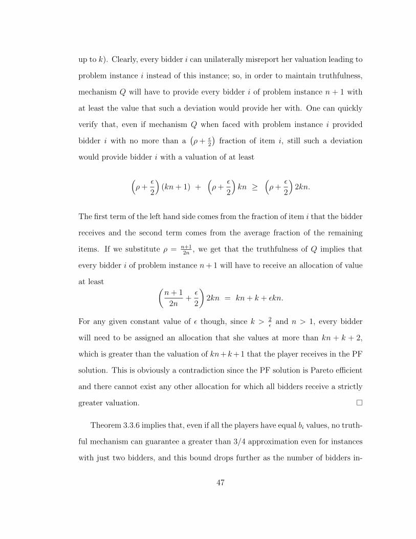
up to k). Clearly, every bidder i can unilaterally misreport her valuation leading to

problem instance i instead of this instance; so, in order to maintain truthfulness,

mechanism Q will have to provide every bidder i of problem instance n + 1 with

at least the value that such a deviation would provide her with. One can quickly

verify that, even if mechanism Q when faced with problem instance i provided

bidder i with no more than a(ρ+ ε

2

)fraction of item i, still such a deviation

would provide bidder i with a valuation of at least

(ρ+

ε

2

)(kn+ 1) +

(ρ+

ε

2

)kn ≥

(ρ+

ε

2

)2kn.

The first term of the left hand side comes from the fraction of item i that the bidder

receives and the second term comes from the average fraction of the remaining

items. If we substitute ρ = n+12n

, we get that the truthfulness of Q implies that

every bidder i of problem instance n+ 1 will have to receive an allocation of value

at least (n+ 1

2n+ε

2

)2kn = kn+ k + εkn.

For any given constant value of ε though, since k > 2ε

and n > 1, every bidder

will need to be assigned an allocation that she values at more than kn + k + 2,

which is greater than the valuation of kn+k+ 1 that the player receives in the PF

solution. This is obviously a contradiction since the PF solution is Pareto efficient

and there cannot exist any other allocation for which all bidders receive a strictly

greater valuation.

Theorem 3.3.6 implies that, even if all the players have equal bi values, no truth-

ful mechanism can guarantee a greater than 3/4 approximation even for instances

with just two bidders, and this bound drops further as the number of bidders in-

47

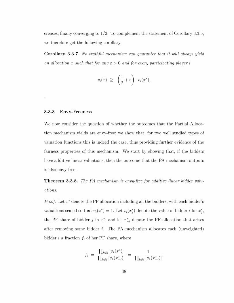
creases, finally converging to 1/2. To complement the statement of Corollary 3.3.5,

we therefore get the following corollary.

Corollary 3.3.7. No truthful mechanism can guarantee that it will always yield

an allocation x such that for any ε > 0 and for every participating player i

vi(x) ≥(

1

2+ ε

)· vi(x∗).

.

3.3.3 Envy-Freeness

We now consider the question of whether the outcomes that the Partial Alloca-

tion mechanism yields are envy-free; we show that, for two well studied types of

valuation functions this is indeed the case, thus providing further evidence of the

fairness properties of this mechanism. We start by showing that, if the bidders

have additive linear valuations, then the outcome that the PA mechanism outputs

is also envy-free.

Theorem 3.3.8. The PA mechanism is envy-free for additive linear bidder valu-

ations.

Proof. Let x∗ denote the PF allocation including all the bidders, with each bidder’s

valuations scaled so that vi(x∗) = 1. Let vi(x

∗j) denote the value of bidder i for x∗j ,

the PF share of bidder j in x∗, and let x∗−i denote the PF allocation that arises

after removing some bidder i. The PA mechanism allocates each (unweighted)

bidder i a fraction fi of her PF share, where

fi =

∏k 6=i [vk(x

∗)]∏k 6=i [vk(x

∗−i)]

=1∏

k 6=i [vk(x∗−i)]

.

48

In order to prove that the PA mechanism is envy-free, we need to show that

for every bidder i, and for all j 6= i, fivi(x∗) ≥ fjvi(x

∗j), or equivalently

1∏k 6=i [vk(x

∗−i)]

≥vi(x

∗j)∏

k 6=j [vk(x∗−j)]⇔

∏k 6=j

[vk(x∗−j)] ≥ vi(x

∗j)∏k 6=i

[vk(x∗−i)]. (3.7)

To prove the above inequality, we will modify allocation x∗−i so as to create an

allocation x−j such that

∏k 6=j

[vk(x−j)] ≥ vi(x∗j)∏k 6=i

[vk(x∗−i)]. (3.8)

Clearly, for any feasible allocation x−j it must be the case that

∏k 6=j

[vk(x∗−j)] ≥

∏k 6=j

[vk(x−j)], (3.9)

since x∗−j is, by definition, the feasible allocation that maximizes this product.

Therefore, combining Inequalities (3.8) and (3.9) implies Inequality (3.7).

To construct allocation x−j, we use allocation x∗−i and we define the following

weighted directed graph G based on x∗−i: the set of vertices corresponds to the set

of bidders, and a directed edge from the vertex for bidder j to that for bidder k

exists if and only if x∗−i allocates to bidder j portions of items that were instead

allocated to bidder k in x∗. The weight of such an edge is equal to the total value

that bidder j sees in all these portions. Since the valuations of all bidders are scaled

so that vj(x∗) = 1 for all j, this implies that, if the weight of some edge (j, k) is

v (w.r.t. these scaled valuations), then the total value of bidder k for those same

portions that bidder j values at v, is at least v. If that were not the case, then x∗

would not have allocated those portions to bidder k; allocating them to bidder j

49

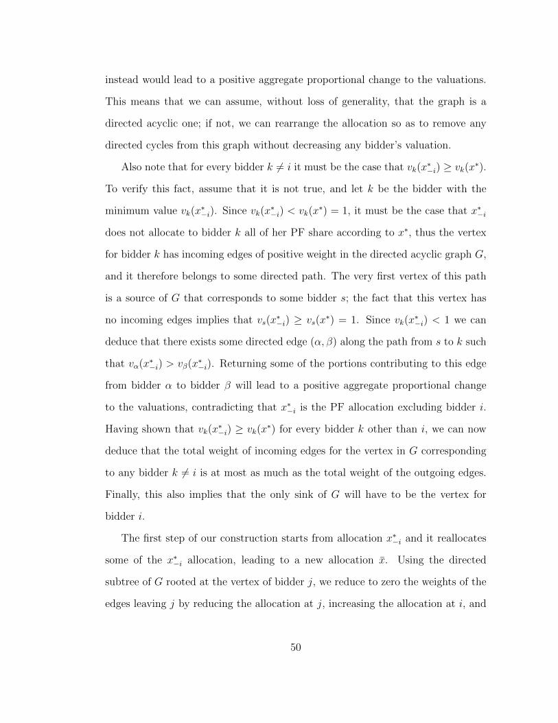
instead would lead to a positive aggregate proportional change to the valuations.

This means that we can assume, without loss of generality, that the graph is a

directed acyclic one; if not, we can rearrange the allocation so as to remove any

directed cycles from this graph without decreasing any bidder’s valuation.

Also note that for every bidder k 6= i it must be the case that vk(x∗−i) ≥ vk(x

∗).

To verify this fact, assume that it is not true, and let k be the bidder with the

minimum value vk(x∗−i). Since vk(x

∗−i) < vk(x

∗) = 1, it must be the case that x∗−i

does not allocate to bidder k all of her PF share according to x∗, thus the vertex

for bidder k has incoming edges of positive weight in the directed acyclic graph G,

and it therefore belongs to some directed path. The very first vertex of this path

is a source of G that corresponds to some bidder s; the fact that this vertex has

no incoming edges implies that vs(x∗−i) ≥ vs(x

∗) = 1. Since vk(x∗−i) < 1 we can

deduce that there exists some directed edge (α, β) along the path from s to k such

that vα(x∗−i) > vβ(x∗−i). Returning some of the portions contributing to this edge

from bidder α to bidder β will lead to a positive aggregate proportional change

to the valuations, contradicting that x∗−i is the PF allocation excluding bidder i.

Having shown that vk(x∗−i) ≥ vk(x

∗) for every bidder k other than i, we can now

deduce that the total weight of incoming edges for the vertex in G corresponding

to any bidder k 6= i is at most as much as the total weight of the outgoing edges.

Finally, this also implies that the only sink of G will have to be the vertex for

bidder i.

The first step of our construction starts from allocation x∗−i and it reallocates

some of the x∗−i allocation, leading to a new allocation x. Using the directed

subtree of G rooted at the vertex of bidder j, we reduce to zero the weights of the

edges leaving j by reducing the allocation at j, increasing the allocation at i, and

50

suitably changing the allocation of other bidders. More specifically, we start by

returning all the portions that bidder j was allocated in x∗−i but not in x∗, back

to the bidders who were allocated these portions in x∗. These bidders to whom

some portions were returned then return portions of equal value that they too were

allocated in x∗−i but not in x∗; this is possible since, for each such bidder, the total

incoming edge weight of its vertex is outweighed by the total outgoing edge weight.

We repeat this process until the sink, the vertex for bidder i, is reached. One can

quickly verify that

vi(x) ≥ vj(x∗−i)− vj(x); (3.10)

in words, the value that bidder i gained in this transition from x∗−i to x is at least as

large as the value that bidder j lost in that same transition. Finally, in allocation

x, whatever value vj(x) bidder j is left with comes only from portions that were

part of her PF share in x∗.

Bidder j’s total valuation for any portions of her PF share in x∗ that are

allocated to other bidders in x∗−i is equal to 1 − vj(x). Thus, bidder i’s valuation

for those same portions will be at most 1 − vj(x); otherwise modifying x∗ by

allocating these portions to i would lead to a positive aggregate change to the

valuations. This means that for bidder i the portions remaining with bidder j in

allocation x have value at least vi(x∗j)− (1− vj(x)). We conclude the construction

of allocation x−j by allocating all the remaining portions allocated to bidder j in

51

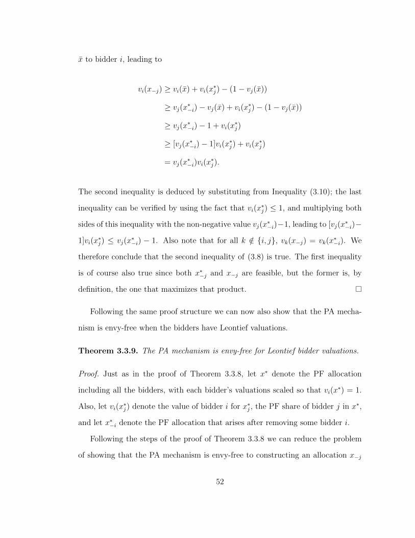
x to bidder i, leading to

vi(x−j) ≥ vi(x) + vi(x∗j)− (1− vj(x))

≥ vj(x∗−i)− vj(x) + vi(x

∗j)− (1− vj(x))

≥ vj(x∗−i)− 1 + vi(x

∗j)

≥ [vj(x∗−i)− 1]vi(x

∗j) + vi(x

∗j)

= vj(x∗−i)vi(x

∗j).

The second inequality is deduced by substituting from Inequality (3.10); the last

inequality can be verified by using the fact that vi(x∗j) ≤ 1, and multiplying both

sides of this inequality with the non-negative value vj(x∗−i)−1, leading to [vj(x

∗−i)−

1]vi(x∗j) ≤ vj(x

∗−i) − 1. Also note that for all k /∈ i, j, vk(x−j) = vk(x

∗−i). We

therefore conclude that the second inequality of (3.8) is true. The first inequality

is of course also true since both x∗−j and x−j are feasible, but the former is, by

definition, the one that maximizes that product.

Following the same proof structure we can now also show that the PA mecha-

nism is envy-free when the bidders have Leontief valuations.

Theorem 3.3.9. The PA mechanism is envy-free for Leontief bidder valuations.

Proof. Just as in the proof of Theorem 3.3.8, let x∗ denote the PF allocation

including all the bidders, with each bidder’s valuations scaled so that vi(x∗) = 1.

Also, let vi(x∗j) denote the value of bidder i for x∗j , the PF share of bidder j in x∗,

and let x∗−i denote the PF allocation that arises after removing some bidder i.

Following the steps of the proof of Theorem 3.3.8 we can reduce the problem

of showing that the PA mechanism is envy-free to constructing an allocation x−j

52

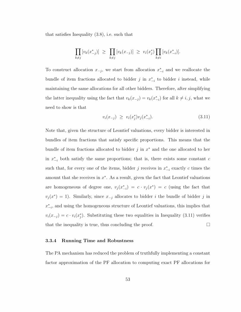
that satisfies Inequality (3.8), i.e. such that

∏k 6=j

[vk(x∗−j)] ≥

∏k 6=j

[vk(x−j)] ≥ vi(x∗j)∏k 6=i

[vk(x∗−i)].

To construct allocation x−j, we start from allocation x∗−i and we reallocate the

bundle of item fractions allocated to bidder j in x∗−i to bidder i instead, while

maintaining the same allocations for all other bidders. Therefore, after simplifying

the latter inequality using the fact that vk(x−j) = vk(x∗−i) for all k 6= i, j, what we

need to show is that

vi(x−j) ≥ vi(x∗j)vj(x

∗−i). (3.11)

Note that, given the structure of Leontief valuations, every bidder is interested in

bundles of item fractions that satisfy specific proportions. This means that the

bundle of item fractions allocated to bidder j in x∗ and the one allocated to her

in x∗−i both satisfy the same proportions; that is, there exists some constant c

such that, for every one of the items, bidder j receives in x∗−i exactly c times the

amount that she receives in x∗. As a result, given the fact that Leontief valuations

are homogeneous of degree one, vj(x∗−i) = c · vj(x∗) = c (using the fact that

vj(x∗) = 1). Similarly, since x−j allocates to bidder i the bundle of bidder j in

x∗−i, and using the homogeneous structure of Leontief valuations, this implies that

vi(x−j) = c · vi(x∗j). Substituting these two equalities in Inequality (3.11) verifies

that the inequality is true, thus concluding the proof.

3.3.4 Running Time and Robustness

The PA mechanism has reduced the problem of truthfully implementing a constant

factor approximation of the PF allocation to computing exact PF allocations for

53

several different problem instances, as this is the only subroutine that the mech-

anism calls. If the valuation functions of the players are affine, then there is a

polynomial time algorithm to compute the exact PF allocation [42, 68].

We now show that, even if the PF solution can be only approximately computed

in polynomial time, our truthfulness and approximation related statements are

robust with respect to such approximations (all the proofs of this subsection are

deferred to Appendix A.1). More specifically, we assume that the PA mechanism

uses a polynomial time algorithm that computes a feasible allocation x instead of

x∗ such that

[∏i

[vi(x)]bi

]1/B

≥

[(1− ε)

∏i

[vi(x∗)]bi

]1/B

, where B =n∑i=1

bi.

Using this algorithm, the PA mechanism can be adapted as follows:

1 Compute the approximate PF allocation x based on the reported bids.2 For each player i, remove her and compute the approximate PF allocation x−i that

would arise in her absence.

3 Allocate to each player i a fraction fi of everything that she receives according to x,where

fi = min

1 ,

( ∏i′ 6=i [vi′(x)]bi′∏i′ 6=i [vi′(x−i)]bi′

)1/bi . (3.12)

Figure 3.2: The Approximate Partial Allocation mechanism.

For this adapted version of the PA mechanism to remain feasible, we need

to make sure that fi remains less than or equal to 1. Even if, for some reason,

the allocation x−i computed by the approximation algorithm does not satisfy this

property, the adapted mechanism will then choose fi = 1 instead.

We start by showing two lemmas verifying that this adapted version of the PA

54

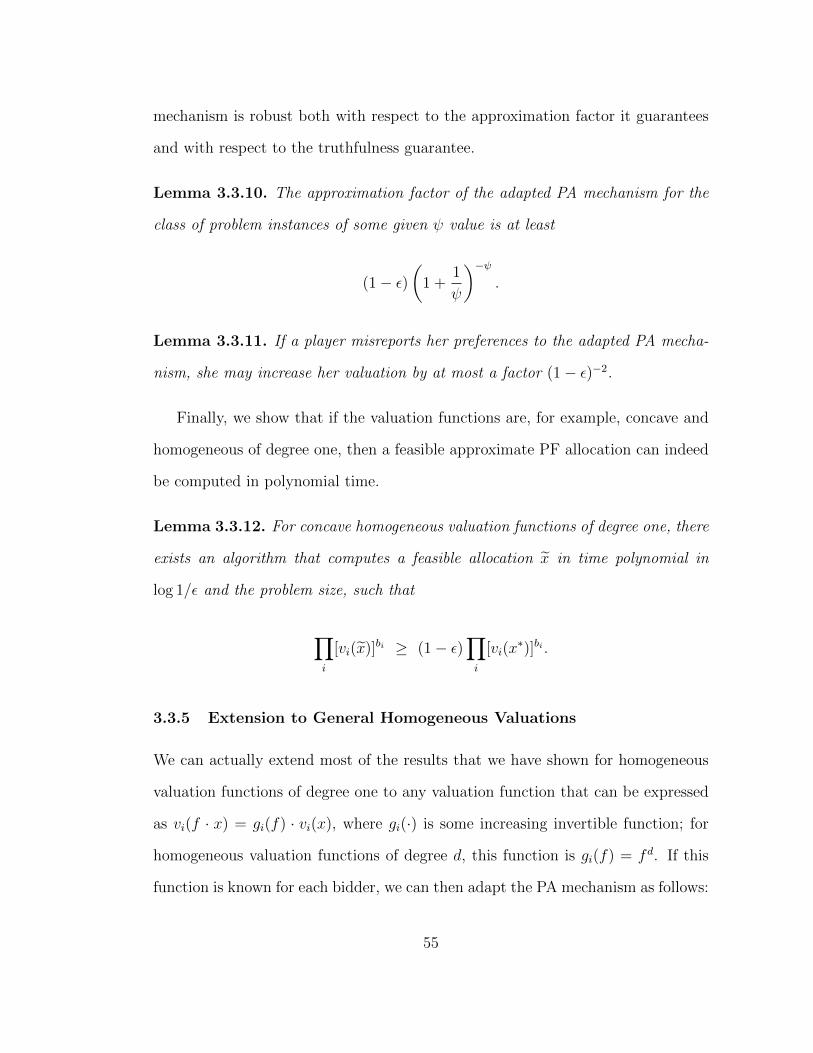
mechanism is robust both with respect to the approximation factor it guarantees

and with respect to the truthfulness guarantee.

Lemma 3.3.10. The approximation factor of the adapted PA mechanism for the

class of problem instances of some given ψ value is at least

(1− ε)(

1 +1

ψ

)−ψ.

Lemma 3.3.11. If a player misreports her preferences to the adapted PA mecha-

nism, she may increase her valuation by at most a factor (1− ε)−2.

Finally, we show that if the valuation functions are, for example, concave and

homogeneous of degree one, then a feasible approximate PF allocation can indeed

be computed in polynomial time.

Lemma 3.3.12. For concave homogeneous valuation functions of degree one, there

exists an algorithm that computes a feasible allocation x in time polynomial in

log 1/ε and the problem size, such that

∏i

[vi(x)]bi ≥ (1− ε)∏i

[vi(x∗)]bi .

3.3.5 Extension to General Homogeneous Valuations

We can actually extend most of the results that we have shown for homogeneous

valuation functions of degree one to any valuation function that can be expressed

as vi(f · x) = gi(f) · vi(x), where gi(·) is some increasing invertible function; for

homogeneous valuation functions of degree d, this function is gi(f) = fd. If this

function is known for each bidder, we can then adapt the PA mechanism as follows:

55

instead of allocating to bidder i a fraction fi of her allocation according to x∗ as

defined in Equation (3.2), we instead allocate to this bidder a fraction g−1i (fi),

where g−1i (·) is the inverse function of gi(·). If, for example, some bidder has a

homogeneous valuation function of degree d, then allocating her a fraction f1/di

of her PF allocation has the desired effect and both truthfulness and the same

approximation factor guarantees still hold. The idea behind this transformation is

that all that we need in order to achieve truthfulness and the approximation factor

is to be able to discard some fraction of a bidder’s allocation knowing exactly what

fraction of her valuation this will correspond to.

3.4 The Strong Demand Matching Mechanism

The main result of the previous section shows that one can guarantee a good

constant factor approximation for any problem instance within a very large class

of bidder valuations. The subsequent impossibility result shows that, even if we

restrict ourselves to problem instances with additive linear bidder valuations, no

truthful mechanism can guarantee more than a 1/2 approximation.

In this section we study the question of whether one can achieve even better

factors when restricted to some well-motivated class of instances. We focus on

additive linear valuations, and we provide a positive answer to this question for

problem instances where every item is highly demanded. More formally, we con-

sider problem instances for which the PF price (or equivalently the competitive

equilibrium price) of every item is large when the budget of every player is fixed

to one unit of scrip money5. The motivation behind this class of instances comes

5Remark: Our mechanism does not make this assumption, but the approximation guaranteesare much better with this assumption.

56

from problems such as the one that arose with the Czech privatization auctions [3].

For such instances, where the number of players is much higher than the number

of items, one naturally anticipates that all item prices will be high in equilibrium.

For the rest of the chapter we assume that the weights of all players are equal

and that their valuations are additive linear. Let p∗j denote the PF price of item

j when every bidder i’s budget bi is equal to 1. Our main result in this section is

the following:

Theorem 3.4.1. For additive linear valuations there exists a truthful mechanism

that achieves an approximation factor of minjp∗j/dp∗je

.

Note that if k = minj p∗j , this is an approximation factor of at least k/(k + 1).

We now describe our solution which we call the Strong Demand Matching mech-

anism (SDM). Informally speaking, SDM starts by giving every bidder a unit

amount of scrip money. It then aims to discover minimal item prices such that the

demand of each bidder at these prices can be satisfied using (a fraction of) just one

item. In essense, our mechanism is restricted to computing allocations that assign

each bidder to just one item, and this restriction of the output space renders the

mechanism truthful and gives an approximation guarantee much better than that

of the PA mechanism for instances where every item is highly demanded.

The procedure used by our mechanism is reminiscent of the method utilized by

Demange et al. for multi-unit auctions [41]. Recall that this method increases the

prices of all over-demanded items uniformly until the set R of over-demanded items

changes, iterating this process until R becomes empty. At that point, bidders are

matched to preferred items. For our setting, each bidder will seek to spend all

her money, and we employ an analogous rising price methodology, again making

allocations when the set of over-demanded items is empty. In our setting, the price

57

increases are multiplicative rather than additive, however. This approach also has

some commonality with the algorithm of Devanur et al. [42] for computing the com-

petitive equilibrium for divisible items and bidders with additive linear valuations.

Their algorithm also proceeds by increasing the prices of over-demanded items

multiplicatively. Of course, their algorithm does not yield a truthful mechanism.

Also, in order to achieve polynomial running time in computing the competitive

equilibrium, their algorithm needs, at any one time, to be increasing the prices

of a carefully selected subset of these items; this appears to make their algorithm

quite dissimilar to ours. Next we specify our mechanism in more detail.

Let pj denote the price of item j, and let the bang per buck that bidder i gets

from item j equal vij/pj. We say that item j is an MBB item of bidder i if she

gets the maximum bang per buck from that item6. For a given price vector p, let

the demand graph D(p) be a bipartite graph with bidders on one side and items

on the other, such that there is an edge between bidder i and item j if and only

if j is an MBB item of bidder i. We call cj = bpjc the capacity of item j when

its price is pj, and we say an assignment of bidders to items is valid if it matches

each bidder to one of her MBB items and no item j is matched to more than cj

bidders. Given a valid assignment A, we say an item j is reachable from bidder

i if there exists an alternating path (i, j1, i1, j2, i2, · · · , jk, ik, j) in the graph D(p)

such that edges (i1, j1), · · · , (ik, jk) lie in the assignment A. Finally, let d(R) be

the collection of bidders with all their MBB items in set R. Using these notions,

we define the Strong Demand Matching mechanism in Figure 3.3.

6Note that for each bidder there could be multiple MBB items and that in the PF solutionbidders are only allocated such MBB items.

58

1 Initialize the price of every item j to pj = 1.2 Find a valid assignment that maximizes the number of matched bidders.3 if all the bidders are matched then4 conclude with Step 15.5 Let U be the set of bidders who are not matched in Step 2.6 Let R be the set of all items reachable from bidders in the set U .7 Increase the price of each item j in R from pj to r · pj ,

where r ≥ 1 is the minimum value for which one of the following events takes place:8 if the price of an item in R reaches an integral value then9 continue with Step 2.

10 if for some bidder i ∈ d(R), her set of MBB items increases, causing R to grow then11 if for each item j added to R, the number of bidders already matched to it equals cj

then12 continue with Step 6.13 if some item j added to R has cj greater than the number of bidders matched to it

then14 continue with Step 2.

15 Every bidder matched to some item j is allocated a fraction 1/pj of that item.

Figure 3.3: The Strong Demand Matching mechanism.

3.4.1 Running time

We first explain how to carry out Steps 6-14. Set R can be computed using a

breadth-first-search like algorithm. To determine when the event of Step 8 takes

place, we just need to know the smallest dpje/pj ratio over all items whose price is

being increased. For the event of Step 10, we need to calculate, for each bidder in

d(R), the ratio of the bang per buck for her MBB items and for the items outside

the set R.

In terms of running time, if c(R) =∑

j∈R cj denotes the total capacity in R,

it is not difficult to see that if U is non-empty, |d(R)| > c(R). Note that each

time either the event of Step 8 or the event of Step 13 occurs, c(R) increases by

at least 1, and thus, using the alternating path from a bidder in the set U to the

corresponding item, we can increase the number of matched bidders by at least

59

1; this means that this can occur at most n times. The only other events are the

unions (of connected components in graph D(p)) resulting from the event of Step

11. Between successive iterations of either Step 8 or 13, there can be at most

min(n,m) iterations of Step 11. Thus there are O(n ·min(n,m)) iterations of Step

11 overall and O(n) iterations of Steps 8 and 13.

3.4.2 Truthfulness and Approximation

The proofs of the truthfulness and the approximation of the SDM mechanism use

the following lemma which states that the prices computed by the mechanism are

the minimum prices supporting a valid assignment. An analogous result was shown

in [41] for a multi-unit auction of non-divisible items. We provide an algorithmic

argument.

Lemma 3.4.2. For any problem instance, if p ≥ 1 is a set of prices for which

there exists a valid assignment, then the prices q computed by the SDM mechanism

will satisfy q ≤ p.

Proof. Aiming for a contradiction, assume that qj > pj for some item j, and let

q be the maximal price vector that the SDM mechanism reaches before increasing

the price of some item j′ beyond pj′ for the first time. In other words, q ≤ p and

qj′ = pj′ . Also, let S = j ∈M | qj = pj, which implies that qj < pj for all j /∈ S.

Clearly, any bidder i who has MBB items in S at prices q will not be interested

in any other item at prices p. This implies that the valid assignment that exists

for prices p assigns every such bidder to one of her MBB items j ∈ S. Therefore,

the total capacity of items in S at prices q is large enough to support all these

bidders and hence no item in S will be over-demanded at prices q. As a result, the

60

SDM mechanism will not increase the price of any item in S, which leads us to a

contradiction.

Using this lemma we can now prove the statements regarding the truthfulness

and the approximation factor of SDM; the following two lemmata imply Theo-

rem 3.4.1.

Lemma 3.4.3. The SDM mechanism is truthful.

Proof. Given a problem instance, fix some bidder i and let x′ and q′ denote the

assignment and the prices that the SDM mechanism outputs instead of x and q

when this bidder reports a valuation vector v′i instead of her true valuation vector

vi.

If the item j to which bidder i is assigned in x′ is one of her MBB items w.r.t.

her true valuations vi and prices q′, then x′ would be a valid assignment for prices

q′ even if the bidder had not lied. Lemma 3.4.2 therefore implies that q ≤ q′. Since

the item to which bidder i is assigned by x is an MBB item and q ≤ q′, we can

conclude that vi(x) ≥ vi(x′).

If on the other hand item j is not an MBB item w.r.t. the true valuations

of bidder i and prices q′, we consider an alternative valid assignment and prices.

Starting from prices q′, we run the steps of the SDM mechanism assuming bidder i

has reported her true valuations vi, and we consider the assignment x and the prices

q that the mechanism would yield upon termination. Assignment x would clearly

be valid for prices q if bidder i had reported the truth; therefore Lemma 3.4.2

implies q ≤ q and thus vi(x) ≥ vi(x). As a result, to conclude the proof it suffices

to show that vi(x) ≥ vi(x′). To verify this fact, we show that q′j = qj, implying

that x allocates to i (a fraction of) some item which she values at least as much

61

as a 1/q′j fraction of item j.

Consider the assignment x′−i that matches all bidders i′ 6= i according to x′ and

leaves bidder i unmatched. In the graph D(q′), if item j is reachable from bidder

i given the valid assignment x′−i, then all bidders would be matched by the very

first execution of Step 1 of the mechanism. This is true because the capacity of

item j according to prices q′ is greater than the number of bidders matched to it in

x′−i. The alternating path (i, j1, i1, j2, i2, · · · , jk, ik, j) implied by the reachability

can therefore be used to ensure that bidder i is matched to an MBB item as well;

this is achieved by matching i to j1, i1 to j2 and so on. Otherwise, if not all bidders

can be matched in that very first step of the SDM mechanism, the mechanism can

instead match the bidders according to x′−i and set U = i.7 Before the price of

item j can be increased, Step 10 must add this item to the set R. If this happens

though, item j becomes reachable from bidder i thus causing an alternating path to

form, and the next execution of Step 1 of the mechanism yields a valid assignment

before q′j is ever increased.

Lemma 3.4.4. The SDM mechanism achieves an approximation of minjp∗j/dp∗je

.

Proof. We start by showing that there must exist a valid assignment at prices

fp∗, where p∗ corresponds to the PF prices and f = maxjdp∗je/p∗j . Given any PF

allocation x∗, we consider the bipartite graph on items and bidders that has an

edge between a bidder and an item if and only if x∗ assigns a portion of the item

to that bidder. If there exists a cycle in this graph, one can remove an edge in

this cycle by reallocating along the cycle while maintaining the valuation of every

bidder. To verify that this is possible, note that all the items that a bidder is

7Note that this may not be the only way in which the SDM mechanism can proceed but, sincethe bidders’ valuations for the final outcome are unique, this is without loss of generality.

62

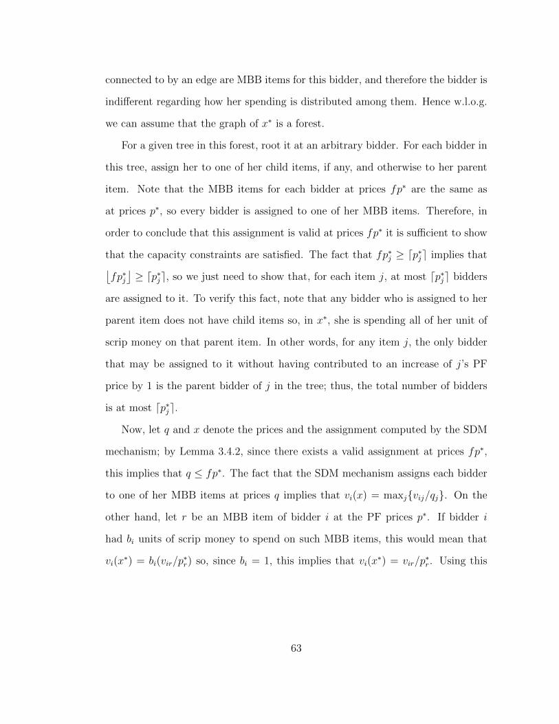
connected to by an edge are MBB items for this bidder, and therefore the bidder is

indifferent regarding how her spending is distributed among them. Hence w.l.o.g.

we can assume that the graph of x∗ is a forest.

For a given tree in this forest, root it at an arbitrary bidder. For each bidder in

this tree, assign her to one of her child items, if any, and otherwise to her parent

item. Note that the MBB items for each bidder at prices fp∗ are the same as

at prices p∗, so every bidder is assigned to one of her MBB items. Therefore, in

order to conclude that this assignment is valid at prices fp∗ it is sufficient to show

that the capacity constraints are satisfied. The fact that fp∗j ≥ dp∗je implies that⌊fp∗j⌋≥ dp∗je, so we just need to show that, for each item j, at most dp∗je bidders

are assigned to it. To verify this fact, note that any bidder who is assigned to her

parent item does not have child items so, in x∗, she is spending all of her unit of

scrip money on that parent item. In other words, for any item j, the only bidder

that may be assigned to it without having contributed to an increase of j’s PF

price by 1 is the parent bidder of j in the tree; thus, the total number of bidders

is at most dp∗je.

Now, let q and x denote the prices and the assignment computed by the SDM

mechanism; by Lemma 3.4.2, since there exists a valid assignment at prices fp∗,

this implies that q ≤ fp∗. The fact that the SDM mechanism assigns each bidder

to one of her MBB items at prices q implies that vi(x) = maxjvij/qj. On the

other hand, let r be an MBB item of bidder i at the PF prices p∗. If bidder i

had bi units of scrip money to spend on such MBB items, this would mean that

vi(x∗) = bi(vir/p

∗r) so, since bi = 1, this implies that vi(x

∗) = vir/p∗r. Using this

63

inequality along with the fact that qj ≤ fp∗j for all items j, we can show that

vi(x) = maxj

vijqj

≥ vir

qr≥ vir

fp∗r=

1

f· vi(x∗),

from which we conclude that vi(x) ≥ minjp∗j/dp∗je · vi(x∗) for any bidder i.

3.5 Connections to Mechanism Design with Money

In hindsight, a closer look at the mechanisms of this chapter reveals an interesting

connection between our work and known results from the literature on mechanism

design with money. What we show in this section is that one can uncover useful

interpretations of money-free mechanisms as mechanisms with actual monetary

payments by instead considering appropriate logarithmic transformations of the

bidders’ valuations. In what follows, we expand on this connection for the two

mechanisms that we have proposed.

Partial Allocation Mechanism. We begin by showing that one can actually

interpret the item fractions discarded by the Partial Allocation mechanism as VCG

payments. The valuation of player i for the PA mechanism outcome is vi(x) =

fi · vi(x∗), or

vi(x) =

( ∏i′ 6=i [vi′(x

∗)]bi′∏i′ 6=i [vi′(x

∗−i)]

bi′

)1/bi

· vi(x∗). (3.13)

Taking a logarithm on both sides of Equation (3.13) and then multiplying them

by bi yields

bi log vi(x) = bi log vi(x∗)−

(∑i′ 6=i

bi′ log vi′(x∗−i) −

∑i′ 6=i

bi′ log vi′(x∗)

). (3.14)

64

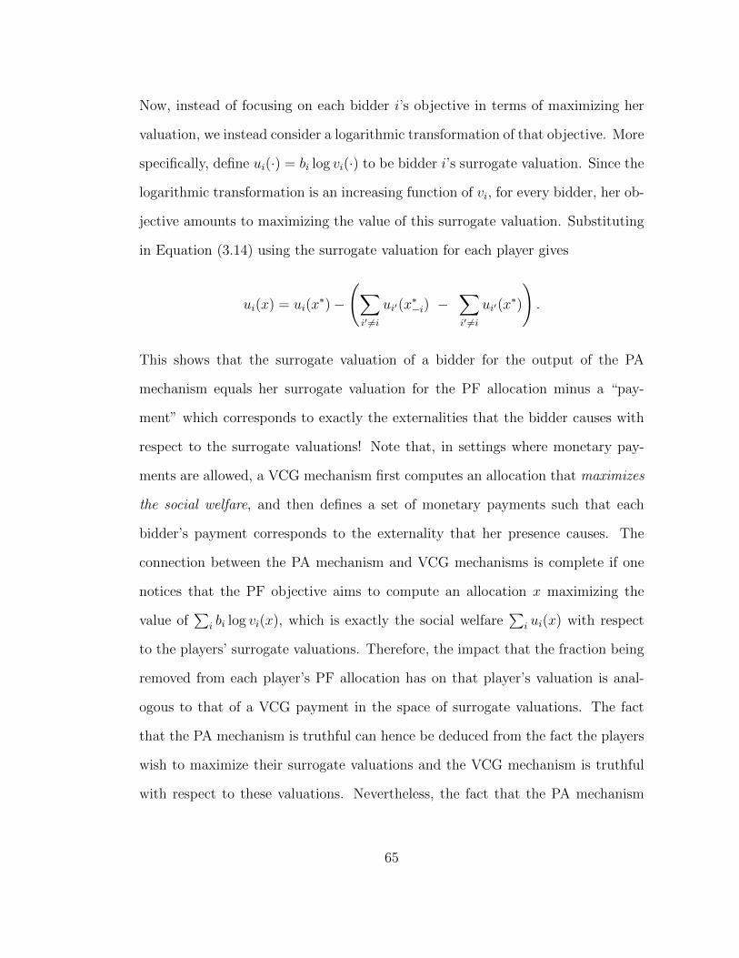
Now, instead of focusing on each bidder i’s objective in terms of maximizing her

valuation, we instead consider a logarithmic transformation of that objective. More

specifically, define ui(·) = bi log vi(·) to be bidder i’s surrogate valuation. Since the

logarithmic transformation is an increasing function of vi, for every bidder, her ob-

jective amounts to maximizing the value of this surrogate valuation. Substituting

in Equation (3.14) using the surrogate valuation for each player gives

ui(x) = ui(x∗)−

(∑i′ 6=i

ui′(x∗−i) −

∑i′ 6=i

ui′(x∗)

).

This shows that the surrogate valuation of a bidder for the output of the PA

mechanism equals her surrogate valuation for the PF allocation minus a “pay-

ment” which corresponds to exactly the externalities that the bidder causes with

respect to the surrogate valuations! Note that, in settings where monetary pay-

ments are allowed, a VCG mechanism first computes an allocation that maximizes

the social welfare, and then defines a set of monetary payments such that each

bidder’s payment corresponds to the externality that her presence causes. The

connection between the PA mechanism and VCG mechanisms is complete if one

notices that the PF objective aims to compute an allocation x maximizing the

value of∑

i bi log vi(x), which is exactly the social welfare∑

i ui(x) with respect

to the players’ surrogate valuations. Therefore, the impact that the fraction being

removed from each player’s PF allocation has on that player’s valuation is anal-

ogous to that of a VCG payment in the space of surrogate valuations. The fact

that the PA mechanism is truthful can hence be deduced from the fact the players

wish to maximize their surrogate valuations and the VCG mechanism is truthful

with respect to these valuations. Nevertheless, the fact that the PA mechanism

65

guarantees such a strong approximation of the PF solution remains surprising even

after revealing this reduction.

Also note that VCG mechanisms do not, in general, guarantee envy-freeness.

The connection between the PA mechanism and VCG mechanisms that we pro-

vide above, combined with the envy-freeness results that we proved for the PA

mechanism for both additive linear and Leontief valuations, implies that the VCG

mechanism is actually envy-free for settings with money and bidders having the

corresponding surrogate valuations. Therefore, these results also contribute to the

recent work on finding truthful, envy-free, and efficient mechanisms [30, 49].

Strong Demand Matching Mechanism. We now provide an even less obvi-

ous connection between the SDM mechanism and existing literature on mechanism

design with money; this time we illustrate how one can interpret the SDM mech-

anism as a stable matching mechanism. In order to facilitate this connection, we

begin by reducing the problem of computing a valid assignment to the problem of

computing a “stable” matching: we first scale each bidder’s valuations so that her

minimum non-zero valuation for an item is equal to n, and then, for each item j

we create n copies of that item such that the k-th copy (where k ∈ 1, 2, . . . , n)

of item j has a reserve price rjk = k. Given some price for each item copy, every

buyer is seeking to be matched to one copy with a price that maximizes her valua-

tion to price ratio, i.e. an MBB copy. A matching of each bidder to a distinct item

copy in this new problem instance is stable if and only if every bidder is matched

to an MBB copy; it is easy to verify that such a stable matching will always exist

since there are n copies of each item. Note that in a stable matching any two

copies of the same item, each of which is being matched to some bidder, need to

66

have exactly the same price, otherwise the more expensive copy cannot be an MBB

choice for the bidder matched to it.

Now, a valid assignment of the initial input of the SDM mechanism implies a

stable matching in the new problem instance: set the price pjk of the k-th copy

of item j to be equal to the price pj of item j in the valid assignment, unless

this violates its reserve price, i.e. pjk = maxpj, rjk, and match each bidder to

a distinct copy of the item that she was assigned to by the valid assignment; the

validity of the assignment implies that, for each item j, the number of bidders

assigned to it is at most bpjc, and hence the number of item copies for which

pjk ≥ rjk, i.e. pjk = pj is enough to support all these bidders. Similarly, a stable

matching of the item copies implies a valid assignment of the actual items of

the initial problem instance: the price pj of each item j is set to be equal to

the minimum price over all its copies (pj = minkpjk), and each bidder who is

matched to one of these copies is allocated a fraction 1/pj of the corresponding

actual item.

Using this reduction, we can now focus on the problem of computing such a

stable matching of each bidder to just one distinct copy of some item; that is, we

wish to define a price pjk ≥ rjk for each one of the m · n item copies, as well as a

matching of each bidder to a distinct copy such that every bidder is matched to one

of her MBB copies for the given prices. If we consider the same surrogate valuations

ui(·) = log vi(·), the objective of each bidder i to be matched to a copy of some item

j that maximizes the ratio vij/pjk is translated to the objective of maximizing the

difference log vij − log pjk. If one therefore replaces the values vij of the valuation

vector reported by each bidder i with the values log vij, then the initial problem is

reduced to the problem of computing stable prices for these transformed valuations,

67

assuming that monetary payments are allowed. This problem has received a lot

of attention in the matching literature, building upon the assignment model of

Shapley and Shubik [95]. Having revealed this connection, we know that we can

truthfully compute a bidder optimal matching that does not violate the reserve

prices using, for example, the mechanism of Aggarwal et al. [2]; one can verify

that these are exactly the logarithmic transformations of the prices of the SDM

mechanism, and also that this is the matching the SDM mechanism computes.

Note that increasing the surrogate prices of overdemanded item copies by some

additive constant corresponds to increasing the corresponding actual prices by a

multiplicative constant. Therefore, this transformation also sheds some light on

why the SDM mechanism uses multiplicative increases of the item prices.

3.6 Concluding Remarks

Our work was motivated by the fact that no incentive compatible mechanisms

were known for the natural and widely used fairness concept of Proportional Fair-

ness. In hindsight our work provides several new contributions. First, the class

of bidder valuation functions for which our results apply is surpringly large and

it contains several well studied functions; previous truthful mechanisms for fair-

ness were studied for much more restricted classes of valuation functions. Second,

to the best of our knowledge, this is first work that defines and gives guarantees

for a strong notion of approximation for fairness, where one desires to approxi-

mate the valuation of every bidder. Last, our Partial Allocation mechanism can

be seen as a framework for designing truthful mechanims without money. This

mechanism can be generalized further by restricting the range of the outcomes

(similar to maximal-in-range mechanisms when one can use money). We believe

68

that this generalization is a powerful one, and might allow for new solutions to

other mechanism design problems without money.

69

Chapter 4

Decentralized Welfare-Optimizing Mech-

anisms

4.1 Introduction

In this chapter we study decentralized methods for the efficient allocation of a type

of resource aiming to model machines or servers of some distributed system. Each

user of this system needs to have some computational task completed and she is

therefore seeking to have her task served by one of the machines. Since the users

are competing for time on these servers, without proper coordination the resulting

allocation would likely suffer from substantial delays in servicing their demands. In

order to formally study this problem we use the model of machine scheduling [86]

which has been extensively studied since the 1950s and is generally considered a

canonical model for studying settings related to job scheduling and processing.

70

4.1.1 Machine scheduling

In this model there are n jobs and m machines; each job must be assigned to a

single machine. The processing time of a job can differ depending on the machine

it is executed on; let pij denote the processing time of job j on machine i. Each

job can also have an associated weight, which may be interpreted as a measure of

importance. A resource allocation for such a problem instance (a schedule) consists

of an assignment of jobs to machines, and a specification of the order in which the

jobs on each machine will be processed. For any such assignment and ordering, the

completion time of each job is now determined; if on machine i the assigned jobs

are in the order j1, . . . , jr, then the completion time of job j1 is pij1 , the completion

time of job j2 is pij1 + pij2 , and so on.

The most basic model is that of identical machines, where the processing time

of any job is the same on all of the machines. In the more general model of related

machines each machine has a speed, and the processing time of a job on a machine

is inversely proportional to the speed of that machine. The main scheduling model

that we study is unrelated machine scheduling in which the processing times are

arbitrary, thus capturing all the above models as special cases.

In this work we consider the scheduling game that is induced due to the lack

of centralized control. Each job is a fully informed player wanting to minimize

its individual completion time, and its set of strategies correspond to the set of

machines. A job’s completion time on a machine depends not only on the strategies

chosen by other players (in particular, which other players chose that machine),

but also on the order that the jobs are run on the machine1; in other words, this is

1Actually, we will allow schedules that are more general than just executing the jobs in someorder, but this simplifies the discussion for now.

71

a setting with externalities. The cost of a job will be its weighted completion time;

its completion time multiplied by its weight. The objective function that research

on this setting has mostly focused on is the makespan, i.e. the maximum completion

time over all jobs, which, for unweighted jobs, corresponds to the egalitarian social

cost (see Section 4.1.3). This chapter studies the utilitarian social cost instead, i.e.

the unweighted or weighted sums of completion times.

A coordination mechanism for this setting is a set of local policies, one per

machine, specifying how the jobs choosing that machine are scheduled. We will

actually consider the slightly more restrictive class of strongly local policies. For

such policies the schedule on machine i must be a function of only the processing

times pij and weights wj of the jobs assigned to the machine. In contrast, in simply

local policies the schedule on machine i may also depend on the full processing

times vector pj = (p1j, p2j, . . . , pmj) of each job j assigned to the machine. This is

a somewhat weaker notion of locality, providing the policies with more information

about the given problem instance.

4.1.2 Our Results

We begin by studying Smith’s Rule, the policy prescribing that machines process

jobs in increasing order of their processing time to weight ratio. This is a natural

first candidate to analyze since it is known that, for any given assignment of jobs

to machines, this is the policy that minimizes our social cost function [99]. We

prove that the coordination ratio for this policy is exactly 4, improving upon a

result by Correa and Queyranne [38], who showed the same bound but for the

less general model of restricted related machines (see Section 4.2). The constant

coordination ratio for the weighted sum of completion times is in sharp contrast to

72

the negative results that have been shown for the makespan objective, for which

no natural coordination mechanism can achieve a constant coordination ratio [1]

(See Section 4.1.3).

We also show that if we restrict ourselves to deterministic policies which always

run jobs one after the other in some order, regardless of how this ordering depends

on the weights and processing times of the assigned jobs—then this factor of 4 can-

not be improved. We overcome this barrier in two ways; the first is deterministic,

and adds artificial delays; the second is randomized, and achieves an even better

total welfare.

Among them, the deterministic policy is most naturally described as a pre-

emptive one. In our context, preemption really refers to time multiplexing: the

machine runs the jobs “in parallel”, dividing its processing resources among the

active jobs. The preemptive policy that we consider (ProportionalSharing) splits

the processing capacity of a machine among its uncompleted jobs in proportion

to their weights. This generalizes the EqualSharing policy [44], which splits the

processing capacity equally amongst the jobs and which is what ProportionalShar-

ing does in the unweighted case. We uncover a close connection of this policy to

Smith’s Rule, allowing us to apply a similar proof strategy, but yielding a signifi-

cantly improved coordination factor of 2.618. This improvement using preemption

is somewhat counter-intuitive if one considers the fact that, for any preemptive

policy, there is a non-preemptive policy that Pareto dominates it for any given

assignment of jobs to machines. This result is also in contrast to the makespan

case, where even in the unweighted case the EqualSharing policy achieves a coor-

dination ratio of Θ(m) [44], no better than Smith’s rule. To make sense of this

phenomenon we show that, for a fixed assignment, the cost that each job suffers

73

according to this very natural preemptive policy actually equals the cost that it

would suffer if Smith’s Rule were instead being used, plus the externalities that

this job would cause to the jobs that would have been scheduled after it. Each job

is therefore forced to internalize externalities that it causes to jobs on the same

machine, leading to improved incentives. We also show an improved bound of 2.5

for the coordination ratio in the unweighted case.

On the other hand, we show that, under some restrictions, no deterministic pol-

icy can achieve a factor better than 2.166. To break this new barrier we consider

a policy we call Rand, in which jobs are randomly (but non-uniformly) ordered,

based on their processing time to weight ratio. This randomized policy also forces

jobs which have a higher priority according to Smith’s Rule to suffer delays due to

externalities that they cause, again leading to better incentives and even more effi-

cient equilibrium allocations. One of the benefits of randomization is that although

the jobs are made to suffer for (part of) their externalities, the schedule that the

policy produces is always Pareto efficient. We give a bound of 32/15 ≈ 2.133 for

the coordination ratio of this policy, a significant improvement over Proportional-

Sharing. In addition, in the case where the weighted sum of processing times is

negligible compared to the total cost, our randomized policy has a much better

coordination ratio of π/2, which is tight. The proofs here are perhaps the most

interesting, involving a connection to the classical Hilbert matrix.

We prove all of the upper bound results in a common framework that brings out

the structure in the scheduling games we consider. Once the framework has been

set up, our proofs become short and elegant, and we anticipate that the approach

may prove useful elsewhere too. We are able to relate the games induced by each

of the policies we consider to certain inner product spaces. Proving upper bounds

74

on the price of anarchy then becomes much simpler, in most cases involving an

application of Cauchy-Schwartz and some form of “norm distortion” inequality to

relate back to the Smith’s rule cost. While we present our proofs for pure strategies

and pure Nash equilibria, we observe that all the results can be stated within the

smoothness framework of Roughgarden [90] (see Section 4.2). This implies that

all the bounds hold for more general equilibrium concepts including mixed Nash

equilibria and correlated equilibria.

The game obtained when using Smith’s rule as the policy has a defect: it

does not necessarily possess pure Nash equilibria [38]. Nevertheless, we show that

the other policies we consider all induce exact potential games, giving another

indication that ProportionalSharing and Rand are very natural policies. In fact, we

can use these properties, along with other game-theoretic insights we have gained

to give a result for the underlying centralized optimization problem.

From a purely centralized optimization perspective, the problem of minimizing

the weighted sum of completion times has been extensively studied. The prob-

lem is APX-hard [64] on unrelated machines, and the current best polynomial

time algorithm has an approximation factor of 32

[94, 97]. All previous constant-

factor approximation algorithms are based on rounding linear or convex programs.

Complementing all these known non-combinatorial approximation algorithms, we

design a new combinatorial (2 + ε)-approximation algorithm for optimizing the

weighted sum of completion times on unrelated machines.

In designing our approximation algorithm we take advantage of the fact that

the best-response dynamics of the induced game are related to local search algo-

rithms. Starting from an initial solution, a local search algorithm iteratively moves

to neighboring solutions which improve the global objective. This is based on a

75

neighborhood relation that is defined on the set of solutions. Now, if one considers

the strategy profiles of the game induced by the coordination mechanism as solu-

tions, the best-response moves of the users in this game implicitly define the set of

possible local moves. The speed of convergence and the approximation factor of

local search algorithms for scheduling problems have been studied mainly for the

makespan objective function [40, 47, 50, 66, 91, 93, 102, 5, 10]. Our combinatorial

approximation algorithm for the weighted sum of completion times is the first lo-

cal search algorithm for this problem, and is different from the previously studied

algorithms for the makespan objective. The neighborhood implicitly defined by

the coordination mechanism at hand is non-trivial and it seems unlikely that such

a simple algorithm could be designed without the initial game-theoretic intuition.

4.1.3 Related Work

Previous work on scheduling games mainly concerned the makespan social cost.

One of the first such games to be considered was the one induced by the Makespan

policy [74], according to which all jobs are released at the same time; each job’s

completion time is equal to the sum of the processing times of the jobs assigned

to its machine. This scheduling game gathered significant attention, eventually

leading to a sequence of tight price of anarchy bounds for different machine mod-

els [39, 54, 8]. The games induced by Makespan are also known as load bal-

ancing games. In their paper introducing coordination mechanism design [28],

Christodoulou, Koutsoupias and Nanavati analyzed mechanisms for identical ma-

chines using the ShortestFirst and LongestFirst policies, which process jobs in non-

decreasing and non-increasing order of their processing times respectively. Immor-

lica et al. [67] studied these three coordination mechanisms, along with a random-

76

ized one which orders jobs randomly in a uniform fashion, for several different

machine scheduling models. They surveyed the known results for these settings,

uncovering connections of these local policies with greedy and local search algo-

rithms [66, 50, 91, 40, 5, 10, 14, 102]. Apart from price of anarchy related results,

they also studied the speed of convergence to equilibria and the existence of pure

Nash equilibria for the ShortestFirst and LongestFirst policies. Azar, Jain, and

Mirrokni [9] showed that the ShortestFirst policy and in fact any strongly local

fixed ordering policy (defined in Section 4.2) does not achieve a coordination ra-

tio better than Ω(m). Additionally, they presented a non-preemptive local policy

that achieves a coordination ratio of O(logm) and a policy that induces potential

games and gives a coordination ratio of O(log2m). Caragiannis [18], among other

results, showed an alternative coordination mechanism that guaranteed a coor-

dination ratio of O(logm) for unrelated machines, while still inducing potential

games. Fleischer and Svitkina [52] showed a lower bound of Ω(logm) for all local

fixed ordering policies, thus proving that Caragiannis’ mechanism is optimal with

respect to the price of anarchy within this class. This bound had already been

overcome by Caragiannis [18] who presented a local preemptive policy with an

approximation factor of O(logm/ log logm). Recent work by Abed and Huang [1]

showed that this factor is the best that can be achieved by any natural policy,

including preemptive and randomized ones.

Our work concerns the utilitarian social cost, or (weighted) sum of completion

times. For this objective, Correa and Queyranne [38] studied Smith’s rule for

the restricted related machine model and they exhibited an instance for which

the induced game does not possess a pure Nash equilibrium. They also presented

bounds for the price of anarchy of SmithRule in this model. Finally, Hoeksma and

77

Uetz [63] showed better price of anarchy bounds for the less general setting of

unweighted jobs and related machines using ShortestFirst; the unweighted variant

of SmithRule.

4.2 Preliminaries

Throughout this chapter, let J be a set of n jobs to be scheduled on a set I of m

machines. Let pij denote the processing time of job j ∈ J on machine i ∈ I and wj

denote its weight (or importance). The shorthand notation ρij will be used for the

ratio pij/wj. Jobs that have both the same processing time and the same weight

can be distinguished from one another only if they have been assigned a unique

ID; otherwise, the jobs are said to be anonymous.

We will refer to the following standard scheduling models:

Identical machines. All machines are identical, meaning each job needs the same

processing time on each machine: pij = pi′j for all i, i′ ∈ I. The model of

restricted identical machines is a variant according to which each job can be

run only on some specified subset of machines.

Related machines. The machines may have different speeds, and the processing

time of a job is inversely proportional to the speed: pij = pj/σi, where σi

represents the speed of machine i, and pj the processing requirement of job

j. The restricted related machines variant is again obtained by possibly

restricting the set of machines to which each job can be assigned.

Unrelated machines. The processing times are arbitrary. This is the most gen-

eral of these models. There is no need to distinguish between restricted and

78

unrestricted variants, since we allow specifying that a job takes infinite time

on a machine.

A coordination mechanism for this setting is a set of local policies, one for each

machine. Each such policy determines how to schedule the set of jobs assigned

to the machine it controls, thus defining the completion time cj of each job j in

that set. A coordination mechanism thereby gives rise to a scheduling game in

which there are n agents (jobs) and each agent’s strategy set is the set of machines

I. A strategy profile (or configuration) corresponds to an assignment of jobs to

machines, represented by a vector x, where xj gives the machine to which job

j assigns itself. Given such an assignment x, the cost of job j is its weighted

completion time, as determined by the policy on machine xj. We let wjcαj (x) and

Cα(x) denote the cost for player j and the social cost respectively, where α ∈

SR, PS, SF,ES,R denotes the policy, namely SmithRule, ProportionalSharing,

ShortestFirst, EqualSharing and Rand, respectively.2 The agent controlling each

job aims to choose a strategy (i.e., a machine) that minimizes its cost or, in the

case of randomized policies, its expected cost. The mechanisms that we analyze

are designed with the goal of minimizing the utilitarian social cost, i.e. Cα(x) =∑j∈J wjc

αj (x).

A strategy profile x of a scheduling game instance is a pure Nash equilibrium

(PNE) if no player has an incentive to unilaterally change its strategy. Formally,

if this instance is induced by coordination mechanism α, then for all j ∈ J and all

i ∈ I we get cαj (x) ≤ cαj (x−j, i), where (x−j, i) denotes the assignment x, except

modified so that job j chooses machine i.

2The coordination mechanisms we study in this chapter use the same local policy on eachmachine, so henceforth we refer to a coordination mechanism using the name of the policy.

79

In order to measure the efficiency of a coordination mechanism α for a given

scheduling game instance, we study its social cost in PNE assignments. We are

interested in the worst case ratio of the social cost in a PNE assignment divided by

the optimal social cost achievable from a centralized optimization approach. It is

known that the optimal solution of the centralized optimization problem schedules

jobs on machines according to SmithRule [99], so the optimal social cost can be

expressed as CSR(x∗), where x∗ = arg minx′ CSR(x′). If we also let E(α) be

the set of equilibria induced by α, and x = arg maxx′∈E(α)Cα(x′) be the worst

equilibrium assignment with respect to the social cost induced by α, then this ratio

is equal to Cα(x)/CSR(x∗) for the given game instance. Following the definition

of [28] the (pure) price of anarchy or coordination ratio of coordination mechanism

α is defined to be the maximum such ratio, taken over all the scheduling game

instances that the mechanism may induce. Slightly abusing notation, we use Xi =

j ∈ J | xj = i to denote the set of jobs allocated to machine i in configuration

x, and define X∗i analogously for x∗.

Adapting the work of Roughgarden [90] to this setting, we define a coordination

mechanism α to be (λ, µ)-smooth if for any two configurations x and x′,

∑j∈J

wjcαj (x−j, x

′j) ≤ λCSR(x′) + µCα(x).

If a coordination mechanism is (λ, µ) smooth, then this yields an upper bound of

λ1−µ for its pure price of anarchy, and also for its robust price of anarchy. This,

among other things, implies that it is not only the social cost of PNE that is bound

to be at most λ1−µ times the optimal social cost, but also the social cost of any

correlated equilibrium [90].

80

A game is a potential game if there exists a potential function over the set of

strategy profiles such that any player’s unilateral deviation leads to a drop of the

potential function if and only if that player’s cost drops. A potential game is exact

if after each move, the changes to the potential function and to the player’s cost

are equal. It is easy to see that a potential game always possesses a pure Nash

equilibrium, corresponding to a local minimum of the potential function.

4.2.1 Classification of policies

It will be useful (particularly for discussing lower bounds) to identify the main

classes of strongly local policies that will concern us in this work.

Fixed ordering policies .3 These policies assign an order on all jobs, based on

the jobs’ characteristics on the machine (processing time, weight, and possibly

ID). Then, for a given assignment, the jobs assigned to the machine are executed

according to this order. One motivation for these policies is that they satisfy

the independence of irrelevant alternatives (IIA) property: for any pair of jobs,

their relative ordering is independent of which other jobs are assigned to the ma-

chine. This property appears as an axiom in voting theory, bargaining theory and

logic [96].

Flexible ordering policies. In this class, policies still execute jobs in some fixed

order, but that order may depend arbitrarily on the set of jobs assigned to the

machine. Here we require that the jobs on a machine are executed consecutively in

some deterministic order. Moreover, we require that there be no idle time between

jobs, and that jobs are released immediately upon completion. The reason for this

3These were called simply ordering policies in [9], but we wish to emphasize the distinctionwith the superset of flexible ordering policies, defined next.

81

restriction is to distinguish from the next case.

Preemptive policies. Preemption refers to the ability to suspend a job before it

completes in order to execute another job.4 The initial job can then be resumed

later. Preemption allows for time multiplexing : by switching between a number of

jobs very quickly, the illusion is given that the jobs are being run simultaneously

on the machine. Preemptive policies can also introduce idle time intervals dur-

ing which no job is being processed (e.g. [18]); we call the ones without idle time

prompt. In fact, any preemptive policy yields a schedule which is Pareto domi-

nated by the schedule of some policy that does not use preemption. Thus, as we

explain in more detail in Section 4.4, such policies can equally well be considered

as flexible ordering policies, but where jobs may be held back after completion.

Randomized policies. Here, the policy may schedule the jobs randomly, accord-

ing to a distribution depending only on the processing times and weights of the

jobs on the machine. While more general schedules are possible, it’s helpful to

think of simply a random ordering of the jobs.

We also call, e.g., a coordination mechanism consisting of fixed ordering policies a

“fixed ordering coordination mechanism”.

4.3 Smith’s Rule

Smith’s rule is a fixed ordering policy that schedules jobs on machine i in increasing

order of ρij = pij/wj. In the unweighted case, this reduces to the ShortestFirst

policy. It is known that given an assignment of jobs to machines, in order to

4Note that, unlike in some literature on machine scheduling, preemption here does not implythat a job can be processed on a different machine after it is suspended.

82

minimize the weighted sum of completion times, using Smith’s rule is optimal [99].

It is therefore natural to consider this policy as a good first candidate to study.

Our first theorem shows that using this rule will result in Nash equilibria with

social cost at most a constant factor of 4 away from the optimum.

Our price of anarchy related proofs will use a common framework. The proof

for Smith’s rule is the simplest, but it will introduce a number of aspects of this

framework. In the following two proofs, for notational simplicity we assume that

all jobs assigned to the same machine have distinct ratios (of processing time to

weight) on that machine.5 Also, we index some of the intermediate inequalities in

the derivations of these proofs in order to refer to them in subsequent discussion.

We will construct a mapping from the set of configurations to a certain inner

product space, such that the norm of the mapping will closely correspond to the

cost of the configuration. To wit, define the map ϕ : IJ → L2([0,∞))I , which

maps every strategy profile x to a vector of functions (one for each machine) as

follows. If f = ϕ(x), then for each i ∈ I

fi(y) =∑

j∈Xi:ρij≥y

wj (recall that ρij = pij/wj).

Notice that fi(ρij), multiplied by pij, is simply the marginal social cost due to

job j, i.e., its own cost plus the cost it induces on other jobs. We let 〈f, g〉 :=∫∞0f(y)g(y)dy denote the usual inner product on L2, and in addition define 〈f , g〉 :=∑

i∈I〈fi, gi〉. In both cases, ‖·‖ refers to the induced norm. Next, define η(x) to

5The proofs can be adapted to the case of non-distinct ratios by replacing the conditionρik < ρij that appears in the terms of sums with the condition ρik ≤ ρij , and introducing a tiebreaking rule.

83

be the weighted processing time of all the jobs:

η(x) =∑j∈J

wjpxjj.

We can then write the cost of a configuration in terms of ϕ(x) and η(x):

Lemma 4.3.1. For any configuration x, CSR(x) = 12‖ϕ(x)‖2 + 1

2η(x).

Proof. Let f = ϕ(x). We have

‖ϕ(x)‖2 =∑i∈I

∫ ∞0

fi(y)2dy

=∑i∈I

∫ ∞0

∑j∈Xiρij≥y

wj∑k∈Xiρik≥y

wkdy

=∑i∈I

∑j∈Xi

∑k∈Xi

wjwk

∫ ∞0

1ρij≥y1ρik≥ydy

=∑i∈I

∑j∈Xi

∑k∈Xi

wjwk minρij, ρik (4.1)

=∑i∈I

∑j∈Xi

wj

(2∑k∈Xiρik<ρij

wkρik + wjρij

)

=∑i∈I

∑j∈Xi

wj

(2∑k∈Xiρik≤ρij

pik − pij

)

= 2CSR(x)− η(x).

The result follows.

Theorem 4.3.2. The price of anarchy of SmithRule for unrelated machines is at

most 4.

Proof. Let x and x∗ be two assignments, with x being a Nash equilibrium, and

84

write f = ϕ(x), and f∗ = ϕ(x∗). We first calculate a job j’s completion time

according to x, and then we use the Nash condition that cSRj (x) ≤ cSRj (x−j, x∗j)

for every job j.

cSRj (x) =∑

k∈J : xk=xjρxjk<ρxjj

pxjk + pxjj ≤∑

k∈J : xk=x∗jρx∗jk<ρx∗

jj

px∗jk + px∗j j.

So

CSR(x) =∑j∈J

wjcSRj (x) ≤

∑i∈I

∑j∈X∗i

wj

( ∑k∈Xiρik<ρij

pik + pij

)

≤∑i∈I

∑j∈X∗i

( ∑k∈Xiρik<ρij

wjwkρik + wjpij

)

≤∑i∈I

∑j∈X∗i

∑k∈Xi

wjwk minρik, ρij +∑i∈I

∑j∈X∗i

wjpij (4.2)

=∑i∈I

∑j∈X∗i

∑k∈Xi

wjwk

∫ ∞0

1ρij≥y1ρik≥ydy + η(x∗)

=∑i∈I

∫ ∞0

∑j∈X∗iρij≥y

wj∑k∈Xiρik≥y

wkdy + η(x∗)

=∑i∈I

∫ ∞0

fi(y)f ∗i (y)dy + η(x∗)

= 〈f ,f∗〉 + η(x∗). (4.3)

Now applying Cauchy-Schwartz, followed by the inequality ab ≤ a2 + b2/4 for

85

a, b ≥ 0, we obtain

CSR(x) ≤ ‖f‖‖f∗‖ + η(x∗)

≤ ‖f∗‖2 + 14‖f‖2 + η(x∗)

≤ 2CSR(x∗) + 12CSR(x) by Lemma 4.3.1.

Hence CSR(x) ≤ 4CSR(x∗).

Notice that in this proof, the cost CSR(x) of an assignment x is closely related

to the norm of ϕ(x), and the inequality obtained from the Nash condition is

bounded by a term involving the inner product 〈ϕ(x), ϕ(x∗)〉. This will be a

common feature of all our proofs.

For simplicity, the proof above was written as a pure price of anarchy bound;

x was taken to be a pure Nash equilibrium. However, it is clear that the proof in

fact yields a robust price of anarchy bound, as defined by Roughgarden [90]. More

precisely, the above proof shows that SmithRule is (2, 1/2)-smooth.

The following result, proved in Appendix A.2, shows that no fixed ordering

coordination mechanism can do better than SmithRule. (In fact, the result can be

extended to all flexible ordering coordination mechanisms, but we will not discuss

this here.) This also implies that the bound of Theorem 4.3.2 is tight.

Theorem 4.3.3. The pure price of anarchy of any set of fixed ordering policies

is at least 4. This is true even for the case of restricted identical machines with

unweighted jobs.

We note that for the unit weight case, a constant upper bound on the coor-

dination ratio of Smith’s rule can be obtained via a reduction from the priority

86

ProportionalSharing

SmithRule

Figure 4.1: Three jobs scheduled on some machine i, which uses SmithRule in thefirst case and ProportionalSharing in the second. Their processing times and weightsare pi1 = 4 and w1 = 7 for the first job, pi2 = 2 and w2 = 3 for the second, andpi3 = 2 and w3 = 2 for the third.

routing model of Farzad et al. [48]. However, the resulting bound is not optimal.

4.4 Improvements with Preemption and Randomization

4.4.1 Preemptive Coordination Mechanism

In this section, we study the power of preemption (or equivalently, delays) and

present the following preemptive policy, named ProportionalSharing. Jobs are

scheduled in parallel using time-multiplexing, and, at any moment in time, each

uncompleted assigned job receives a fraction of the processor time equal to its

weight divided by the total weight of uncompleted jobs on the machine. In the

unweighted case, this gives the EqualSharing policy.

We will show that ProportionalSharing has a better coordination ratio than any

fixed ordering policy. These results create a clear dichotomy between such policies

and ProportionalSharing. This may seem counter-intuitive at first, since, given an

assignment of jobs to machines, the schedule produced by ProportionalSharing is

Pareto dominated by that of SmithRule. To be more precise, on each machine,

87

every job apart from the one that SmithRule would schedule last, strictly prefers

SmithRule to ProportionalSharing; the one scheduled last is indifferent between the

two schedules. This can also be seen in Figure 1 which compares how the two

policies would schedule a given set of jobs on the same machine.

Lemma 4.4.1. Given an assignment x, the weighted completion time of a job j

on some machine i using ProportionalSharing (whether currently assigned there or

not) is

wjcPSj (x−j, i) =

∑k∈Xi\j

wjwk minρij, ρik + wjpij.

Proof. First, observe that for two jobs k and k′ with ρik ≤ ρik′ , job k will complete

before (or at the same time as) job k′ when ProportionalSharing is used. To see this,

consider the situation at the time when the earlier of the two jobs is completed.

Let q and q′ be the amount of processing time that has been allocated to k and

k′ by this time. Then q′ =wk′wkq. If k is not completed, then q < wkρik, and so

q′ < wk′ρik ≤ pik′ , and k′ is not completed either.

Let t be the time when job j is completed. All jobs k with ρik ≤ ρij have

completed by this time; thus each such job has received pik units of processing

time. On the other hand, all jobs k with ρik > ρij are not yet complete at time

t, and for each wj units of processing time job j receives, job k receives wk units.

Thus by time t, the processing time spent on any such job k will be exactlypijwkwj

.

Since the total processing time is the sum of the processing times allocated to all

the jobs, we have that

t =∑

k∈Xi\jρik≤ρij

pik +∑k∈Xiρik>ρij

wkwjpij + pij

88

Thus

wjcPSj (x−j, i) =

∑k∈Xi\jρik≤ρij

wjpik +∑k∈Xiρik>ρij

wkpij + wjpij

=∑

k∈Xi\j

wjwk minρij, ρik + wjpij.

A better understanding of why ProportionalSharing performs better despite the

Pareto inefficiency of the schedules it produces can be obtained by examining the

following corollary of Lemma 4.4.1.

Corollary 4.4.2. Given an assignment x, the weighted completion time of a job

j on some machine i using ProportionalSharing is

wjcPSj (x−j, i) = wjc

SRj (x−j, i) +

∑k∈Xiρik>ρij

wkpij.

This corollary precisely quantifies what cost, in addition to the SmithRule cost,

this job is forced to suffer. A closer look reveals that this additional cost (the

rightmost term) is exactly equal to externalities that job j would cause if the

assignment of jobs to machines remained the same but SmithRule was used in-

stead. That is, the sum for each job k that would have been scheduled after job

j (ρik > ρij), of the cost increase that job j causes to that job (wkpij). From

this perspective, ProportionalSharing can be thought of (and also implemented) as

using SmithRule to determine the processing order, but then delaying the release

of each job after it is completed until the additional cost equals these externalities.

Since we already know that, for any given assignment, SmithRule would produce

89

the social welfare maximizing schedule, one may expect that our preemptive pol-

icy exactly “internalizes the externalities” of the players and should therefore lead

to the optimal assignment in equilibrium. The reason why this is not the case is

that the participation of job j in the game does not cause externalities only to

jobs that are assigned to its machine. Nevertheless, our policies are necessarily

oblivious to what the state of the system is beyond the machine they control, so

these “local externalities” may be the best possible alternative. By taking these

local externalities into consideration, ProportionalSharing better aligns the interests

of a player with those of the system, leading not only to better assignments than

SmithRule but also to a better social cost, despite the (otherwise unnecessary) de-

lays suffered. Another perspective on the delays is that they are a form of money

that the players are forced to pay, but this is money that can only be “burned”

and not transferred. From this perspective, our setting is similar to that of money

burning mechanisms [61], with the added restriction that the “payments” have

to be a function of local information alone. These two restrictions preclude the

implementation of welfare-maximizing mechanisms like VCG, but nonetheless our

mechanisms define payments that lead to surprisingly low social cost.

From Lemma 4.4.1 and (4.1) we also immediately obtain the following corollary

(note the factor 2 difference compared to the main term in the cost of Smith’s rule

in Lemma 4.3.1), which will be used in proving the two subsequent theorems:

Corollary 4.4.3. For any assignment x, CPS(x) = ‖ϕ(x)‖2.

Theorem 4.4.4. The price of anarchy of ProportionalSharing for unrelated ma-

chines is at most φ+ 1 = 3+√

52≈ 2.618. Moreover, this bound is tight even for the

restricted related machines model.

90

Proof. Let x be an equilibrium assignment, and x∗ any arbitrary assignment.

From the Nash condition,

CPS(x) ≤∑j∈J

wjcPS(x−j, x

∗j)

≤∑i∈I

∑j∈X∗i

(∑k∈Xi

wjwk minρij, ρik + wjpij

)

= 〈ϕ(x), ϕ(x∗)〉+ η(x∗) (4.4)

The second inequality is true because of Lemma 4.4.1, and the last equation can

be verified by following steps (4.2)-(4.3). Following the same method of analysis

as for Smith’s Rule, we obtain

CPS(x) ≤ ‖ϕ(x)‖‖ϕ(x∗)‖ + η(x∗)

≤ α‖ϕ(x∗)‖2 + 14α‖ϕ(x)‖2 + η(x∗)

≤ 2αCSR(x∗) + 14αCPS(x) + (1− α)η(x∗)

≤ (1 + α)CSR(x∗) + 14αCPS(x),

using the Cauchy-Schwartz inequality and the fact that η(x∗) ≤ CSR(x∗). Setting

α = (1 +√

5)/4 yields CPS(x)/CSR(x∗) ≤ 3+√

52

.

The tightness of this bound follows from a construction in [19], where in fact

they show that even if CPS is used as the benchmark, i.e., we consider the ratio

CPS(x)/CPS(x∗), this can be arbitrarily close to 1 + φ.

The reader will observe how similar the proof above was to the proof of The-

orem 4.3.2, once the relevant costs have been described in terms of the inner

product. In particular, (4.4) is obtained by following precisely the same steps as

91

in the proof of Theorem 4.3.2 to get from (4.2) to (4.3). In that proof, (4.2) can

be interpreted as a kind of symmetrization step, which is needed since the inner

product 〈ϕ(x), ϕ(x∗)〉 is symmetric. ProportionalSharing is already symmetric in

the appropriate sense, and so there is a tighter connection between the Nash con-

dition and the inner product. This same symmetry property will be shared in the

randomized policy we consider in the next section.

Notice also that since SmithRule and ProportionalSharing were described in terms

of the same mapping and inner product, it was very easy to relate ‖ϕ(x∗)‖ back to

the cost of SmithRule. This will be less straightforward for the randomized policy

discussed in the next section.

The coordination ratio obtained may remind the reader of similar bounds for

weighted congestion games [6]. It is important to stress that our bounds do not

follow from these results. What can be deduced by applying the arguments of Azar

et al. [6] to our setting is that CPS(x)/CPS(x∗) ≤ φ+ 1 for any Nash assignment

x for the very restricted set of instances in which every pair of jobs j, j′ satisfy

ρij = ρij′ on each machine i, or in other words, all jobs scheduled on the same

machine face the same completion time. Our result shows that, for arbitrary ρij

values, the ratio does not get any worse even when we compare against the stronger

benchmark of CSR(x∗).

In the case of equal weights, we obtain a slightly improved bound using the fol-

lowing lemma instead of the Cauchy-Schwartz inequality. This is a tighter version

of an inequality initially used by Christodoulou and Koutsoupias [27]:

Lemma 4.4.5. For every pair of nonnegative integers k and k∗,

k∗(k + 1) ≤ 1

3k2 +

5

6k∗(k∗ + 1).

92

Proof. This translates to showing that for all nonnegative integers k and k∗,

5k∗2 + 2k2 − 6k∗k − k∗ ≥ 0.

Rewriting the left hand side as 2(k− 32k∗)2 + 1

2k∗2−k∗, we see immediately that the

inequality holds for k∗ ≥ 2 and k∗ = 0. In the case k∗ = 1, the required inequality

simplifies to k2 − 3k + 2 ≥ 0 which is true for all integral k.

Theorem 4.4.6. The price of anarchy of EqualSharing for unrelated machines is

at most 2.5. This bound is tight even for the restricted related machines model.

Proof. Let x be any some assignment, and let f = ϕ(x). Since wj = 1 for all j,

fi(y) = |j ∈ J : xj = i and pij ≥ y|,

and also

η(x) =∑i

∑j∈Xi

pij

=∑i∈I

∫ ∞0

∑j∈Xi

1y≤pijdy

=∑i∈I

∫ ∞0

fi(y)dy.

For the unweighted case, just as ProportionalSharing reduces to EqualSharing, SmithRule

reduces to ShortestFirst. Adapting Corollary 4.4.3 and Lemma 4.3.1 to these un-

weighted counterparts, we get

CES(x) =

∫ ∞0

f 2i (y)dy and CSF (x) = 1

2

∫ ∞0

fi(y)(fi(y) + 1)dy. (4.5)

93

Now suppose x is a Nash equilibrium; take x∗ to be any assignment, with f∗ =

ϕ(x∗). We continue from (4.4):

CES(x) ≤ 〈f ,f∗〉+ η(x∗)

=

∫ ∞0

fi(y)(f ∗i (y) + 1)dy

≤∫ ∞

0

13f 2i (y)) + 5

6f ∗i (y)(f ∗i (y) + 1)dy by Lemma 4.4.5

= 13CES(x) + 5

3CSF (x∗) by (4.5).

This gives a price of anarchy bound of 2.5.

The tightness of the bound follows from Theorem 3 of [19]. The authors present

a load balancing game lower bound, which is equivalent to assuming that all jobs

have unit processing times and the machines are using EqualSharing; thus the same

proof yields a (pure) price of anarchy lower bound for restricted related machines

and unweighted jobs.

Once again, all of the upper bounds also hold for the robust price of anarchy.

On the negative side, we have the following (the proof of which can be found

in Appendix A.2). Recall that a coordination mechanism is prompt if, on any

machine, the completion time of every job assigned to the machine is never larger

than the sum of processing times of jobs on the machine. Equivalently, each

machine uses its full capacity and does not delay the release of a job after its

completion.

Proposition 4.4.7. When jobs are anonymous, the coordination ratio of any de-

terministic prompt coordination mechanism is at least 13/6.

94

4.4.2 Randomized Coordination Mechanism

In this section we examine the power of randomization and present Rand, a random-

ized policy that satisfies the following property: if two jobs j and j′ are assigned

to machine i, then

Pj precedes j′ in the ordering =ρij′

ρij + ρij′. (4.6)

Recall ρij = pij/wj. A distribution over orderings with this property can be

constructed as follows. Starting from the set of jobs Xi assigned to machine i ∈ I,

select job j ∈ Xi with probability ρij/∑

k∈Xi ρik, and schedule j at the end. Then

remove j from the list of jobs, and repeat this process. Note that this policy is

different from a simple randomized policy that orders jobs uniformly at random.

In fact, this simpler policy is known to give an Ω(m) price of anarchy bound for

the makespan objective [67], and the same family of examples developed in [67]

gives an Ω(m) lower bound for this policy in our setting.

As we show below, this randomized policy outperforms any deterministic strongly

local policy that has the “prompt” property defined above. In an attempt to ex-

plain this success, it is straightforward to verify that, unlike ProportionalSharing,

this policy produces Pareto efficient schedules. One can actually show that it

Pareto dominates ProportionalSharing. Yet, contrary to SmithRule, for any pair of

jobs assigned to the same machine, there is positive probability that any one of the

two is scheduled later, thus suffering a delay because of the other. In this sense,

Rand gives high priority jobs the incentive to avoid crowded machines if they have

better alternatives, but it does so without introducing very long delays.

Theorem 4.4.8. The price of anarchy when using the Rand policy is at most

95

32/15 = 2.133 · · · . Moreover, if the sum of the processing times of the jobs

is negligible compared to the social cost of the optimal solution—more precisely,

η(x∗) = o(CSR(x∗))—this bound improves to π/2 + o(1), which is tight.

The high level approach for obtaining these upper bounds is in exactly the same

spirit as the previous section: find an appropriate mapping ϕ from an assignment

into a convenient inner product space. To make the mapping and inner product

space easier to describe, we assume in this section that the processing times have

been scaled so that the ratios ρij are all integral. We also take κ large enough

so that, except for infinite processing times, ρij ≤ κ for all i ∈ I, j ∈ J . These

assumptions are inessential and easily removed.

An inner product space. The map ϕ we use gives the signature for each

machine: in the unweighted case, this simply describes how many jobs of each size

are assigned to the machine.

Definition 4.4.9. Given an assignment x, its signature ϕ(x) ∈ Rm×κ+ is a vector

indexed by a machine i and a processing time over weight ratio r; we denote this

component by ϕ(x)ir. Its value is then defined as

ϕ(x)ir :=∑j∈Xiρij=r

wj.

We also let ϕ(x)i denote the vector (ϕ(x)i0, ϕ(x)i1, . . . , ϕ(x)iκ).

Let M be the κ× κ matrix given by

Mrs =rs

r + s.

96

Lemma 4.4.10. Let x be some assignment, and let u = ϕ(x). If job j is assigned

to machine i, its expected completion time is given by

cRj (x) = (Mui)ρij + 12pij. (i)

If j is not assigned to i, then its expected completion time upon switching to i would

be

cRj (x) = (Mui)ρij + pij. (ii)

Proof. We consider case (i); case (ii) is similar. So xj = i. The expected completion

time of job j on machine i is

cRj (x) =∑

k∈Xi\j

pikPjob k ahead of job j + pij

=∑

k∈Xi\j

pikρij

ρij + ρik+ pij

=∑k∈Xi

pikρij

ρij + ρik+ 1

2pij.

We can rewrite this in terms of the signature as

cRj (x) =∑s

uisMρijs + 12pij = (Mui)ρij + 1

2pij.

A crucial observation is the following:

Lemma 4.4.11. The matrix M is positive definite.

Proof. Let D be the diagonal matrix with Drr = r. Then we have M = DHD,

where the κ×κ matrix H is given by Hrs = 1r+s

. This is a submatrix of the infinite

Hilbert matrix(

1r+s−1

)r,s∈N

. The Hilbert matrix has the property that it is totally

97

positive [26], meaning that the determinant of any submatrix is positive. It follows

that H is positive definite, and hence so is M .

Thus we may define an inner product by

〈u,v〉R :=∑i∈I

(ui)TMvi, (4.7)

with an associated norm ‖·‖R. In addition, the total cost∑

j wjcRj (x) of an assign-

ment x may be written in the convenient form

CR(x) = ‖ϕ(x)‖2R

+ 12

∑j∈J

wjpxjj

= ‖ϕ(x)‖2R

+ 12η(x).

Competitiveness of Rand on a single machine. An interesting extra com-

plication that occurs with this policy is that, unlike with ProportionalSharing, the

inner product describing the cost of Rand is quite different to the one describing

SmithRule. Since we ultimately need to compare against CSR(x∗), we need to re-

late the cost of Rand and SmithRule. For this reason, the performance of Rand on

even a single machine, compared to SmithRule, plays an important role.

So suppose we have n jobs with processing times pj and weight wj, for j ≤ n.

The signature u is given by just ur =∑

j:pj/wj=rwj. By considering (4.1), it follows

that the weighted sum of completion times according to SmithRule is

uTSu +1

2

∑j

wjpj,

98

where Srs = 12

minr, s. Compare this to the corresponding formula for Rand:

uTMu +1

2

∑j

wjpj.

The extra∑

j wjpj terms only help, and in fact turn out to be negligible in the

worst case example; ignoring them, the goal is to determine supu≥0uTMuuTSu

. So the

question is closely related to the worst-case distortion between two norms (not

quite, because of the nonnegativity constraint).

Interestingly, it turns out that this problem has been considered, and solved,

in a different context. In [29], Chung, Hajela and Seymour consider the problem

of self-organizing sequential search. In order to prove a tight bound on the per-

formance of the “move-to-front” heuristic compared to the optimal ordering, they

show:

Theorem 4.4.12 ([29]). For any sequence u1, u2, . . . , uk with ur > 0 for all r,

∑r,s

urusrs

r + s<π

4

∑r,s

urus minr, s.

(We also present a quite different proof of the theorem in Appendix A.2.) Thus

on a single machine, Rand costs at most a factor π2

more than SmithRule. Moreover,

this is tight [56] (take pj = 1/j2, wj = 1, and let n → ∞). Of course, it follows

immediately that for any number of machines and any assignment x,

CR(x) ≤ π

2CSR(x). (4.8)

All in all, we find that π/2 is a tight upper bound on the competitiveness of Rand

on a single machine. The following lemma (which may also be cast as a norm

99

distortion question), is much more easily demonstrated:

Lemma 4.4.13. For any assignment x, we have CR(x) ≤ 2CSR(x)− η(x).

Proof. Consider a particular machine i. We have

∑j,k∈Xi

wjwkρijρikρij + ρik

=∑

j 6=k∈Xi

wjwkρijρikρij + ρik

+ 12

∑j∈Xi

wjpij

≤∑

j 6=k∈Xi

wjwk minρij, ρik+ 12

∑j∈Xi

wjpij

=∑j,k∈Xi

wjwk minρij, ρik − 12

∑j∈Xi

wjpij.

Summing over all machines gives

CR(x)− 12η(x) ≤ 2

(CSR(x)− 1

2η(x)

)− 1

2η(x)

from which the bound is immediate.

The upper bound. We are now ready to prove the main theorem of this section.

Proof of Theorem 4.4.8. Let x be the assignment at a Nash equilibrium, and x∗

be any arbitrary assignment, and let u = ϕ(x) and u∗ = ϕ(x∗).

100

From the Nash condition and Lemma 4.4.10, we obtain

CR(x) ≤∑j∈J

wjcRj (x−j, x

∗j)

≤∑i∈I

∑j∈X∗i

wjM(ui)ρij + η(x∗)

=∑i∈I

(u∗i)TMui + η(x∗)

= 〈u∗,u〉R + η(x∗).

Applying the Cauchy-Schwartz inequality,

CR(x) ≤ ‖u∗‖R‖u‖R + η(x∗) (4.9)

≤ 23‖u∗‖2

R+ 3

8‖u‖2

R+ η(x∗),

Now recalling the definition of ϕ and applying Lemma 4.4.13, we obtain

CR(x) ≤ 23(CR(x∗)− 1

2η(x∗)) + 3

8(CR(x)− 1

2η(x)) + η(x∗)

≤ 23(2CSR(x∗)− 3

2η(x∗)) + 3

8(CR(x)− 1

2η(x)) + η(x∗)

≤ 43CSR(x∗) + 3

8CR(x).

This gives a coordination ratio of 32/15.

Suppose now that η(x∗) is very small; η(x∗) ≤ εCSR(x∗) for some ε > 0. Then

we may continue from (4.9):

CR(x) ≤ ‖u∗‖R‖u‖R + εCSR(x∗)

≤√CR(x∗) · CR(x) + ε

√CR(x∗) · CR(x).

101

Thus

CR(x)/CR(x∗) ≤ (1 + ε)2.

So if η(x∗) = o(CSR(x)), we obtain from (4.8) that CR(x)/CSR(x∗) ≤ π/2 +

o(1).

As noted in Appendix A.2, a slight modification of the construction used to

prove Proposition 4.4.7 can be used to show that the worst-case price of anarchy

of Rand is at least 5/3.

4.5 Potential Games and an Algorithmic Application

Potential games. Under SmithRule it may happen that no pure Nash equilib-

rium exists [38]. Here we show that ProportionalSharing and Rand both induce

exact potential games, which hence always have pure Nash equilibria. This also

implies that certain natural best response dynamics quickly converge to solutions

whose social cost is not much worse than the social cost in equilibrium; we discuss

this in more detail at the end of this section.

The following theorem generalizes [44, Theorem 3], which addresses EqualShar-

ing (i.e., the unweighted case).

Theorem 4.5.1. The ProportionalSharing mechanism induces exact potential games,

with potential

ΦPS(x) = 12CPS(x) + 1

2η(x). (4.10)

Likewise, the Rand mechanism yields exact potential games with potential

ΦR(x) = 12CR(x) + 1

2η(x). (4.11)

102

Proof. We give the proof for ProportionalSharing; the proof for Rand is similar.

Consider an assignment x and a job j ∈ J , and let i be the machine to which j

is assigned. Define x′ as the assignment differing from x only in that job j moves

to some machine i′ 6= i.

We may write the change in the potential function as

ΦPS(x′)− ΦPS(x) =∑k∈J

Dk + 12wj(pi′j − pij), (4.12)

where

Dk = 12wk(cPSk (x′)− cPSk (x)

).

Consider a job k 6= j on machine i. Since only job j left the machine, we have

from Lemma 4.4.1 that

cPSk (x′)− cPSk (x) = −wj minρij, ρik.

Thus

∑k∈Xi\j

Dk = −12wj

∑k∈Xi\j

wk minρij, ρik

= −12wj(c

PSj (x)− pij).

103

Similarly, considering jobs on i′ yields

∑k∈Xi′

Dk = 12wj∑k∈Xi′

wk minρi′j, ρi′k

= 12wj(c

PSj (x′)− pi′j).

All other jobs are unaffected by the change, and so do not contribute to (4.12).

Summing all terms (including Dj), we obtain

ΦPS(x′)− ΦPS(x) = wj(cPSj (x′)− cPSj (x)),

exactly the change in the cost of job j.

A combinatorial approximation algorithm. Minimizing the unweighted sum

of completion times is polynomial time solvable, even for unrelated machines [65,

16]. For identical parallel machines, the ShortestFirst policy leads to an optimal

schedule at any pure Nash equilibrium [37, 67]. On the other hand, minimizing the

weighted sum of completion times is NP-complete even for identical machines [75].

This special case does admit a polynomial time approximation scheme (PTAS)

however: for any ε > 0, a solution only a factor 1 + ε more expensive than the

optimal one can be found in polynomial time [98]. Recall that the cost of the

optimal solution, which we will denote by OPT , is simply CSR(x∗).

By contrast, the general case of unrelated machines is APX-hard [64]—no PTAS

is possible. A sequence of papers gave improving constant-factor approximation

algorithms, all based on rounding a linear or convex programming relaxation. The

first was a 16/3-approximation algorithm [59], based on rounding an appropri-

104

ate linear programming relaxation. An improvement to 32

+ ε, again based on

linear programming, was given in [92]. Finally the best currently known factor,

a 32-approximation, was obtained based on a convex quadratic relaxation of the

problem [94, 97].

In this section, we will give a very simple and combinatorial approximation

algorithm. While it does not quite match the best factor of 32, it achieves a factor

of 2 + ε, for any ε > 0.

The basic idea is as follows. If we could compute a Nash equilibrium of the

game induced by a policy with a coordination ratio of γ, this Nash equilibrium

schedule would have a social cost at most γ times the optimum. The algorithm

computing this Nash equilibrium would therefore be a γ-approximation algorithm

for the optimization problem. Of course, there is no longer any need to keep to the

suboptimal scheduling that any policy apart from SmithRule would yield. Once we

have the Nash assignment x, we can switch to using SmithRule, as this step will

always decrease the social cost. In what follows we carefully choose a policy that

has a small coordination ratio, but at the same time guarantees that the cost will

decrease by half after switching to SmithRule. In this way, we can guarantee an

approximation factor that is better than the best price of anarchy bound that we

managed to achieve.

The policy we use, which we call Approx, is a variation of ProportionalSharing

with some additional delays. Schedule the jobs exactly as in ProportionalSharing,

but hold each job j back by an additional duration equal to its processing time.

In other words, the completion time of any job j under an assignment x is

cAj (x) = cPSj (x) + pxjj.

105

Comparing Lemma 4.3.1 and Corollary 4.4.3, we see that

CPS(x) = 2CSR(x)− η(x).

Thus

CA(x) = CPS(x) + η(x) = 2CSR(x).

This will give us a saving of a factor of 2 when we switch from using the Approx

policy to SmithRule. It turns out that Approx has a coordination ratio of 4; thus

for any Nash equilibrium x with respect to this policy, CSR(x) ≤ 2OPT .

Unfortunately we do not know how to compute an equilibrium allocation to

this game (similarly for ProportionalSharing and Rand, in fact). Despite this, we

will show that a natural best response dynamics will converge in polynomial time

to some assignment of cost at most (2 + ε)OPT for any ε > 0. This will follow

from general results on the robust price of anarchy proved by Roughgarden [90],

drawing on work by Awerbuch et al. [7] and Chien and Sinclar [25]. We will

actually prove everything we need, primarily in order to be able to give a precise

stopping condition for our algorithm, something which is not quite explicit in [90].

It also demonstrates that there is no difficulty in extending the proofs to price of

anarchy bounds on coordination mechanisms rather than games, although this is

fairly immediate from a consideration of the original proofs.

Consider the following natural best response dynamics: simply pick the job

which can improve its disutility (weighted completion time) the most by deviating,

and allow that job to move. Following [90] we will call this the maximum-gain best

response dynamics. Given some coordination mechanism α and configuration x,

106

let

∆αj = wj

(cαj (x)− cαj (x−j, x

′j))

for any j ∈ J,

where x′j is the best response move for player j. Also let

∆α(x) =∑j∈J

∆αj .

Definition 4.5.2. An assignment x is an ε-equilibrium if ∆α(x) < εCα(x).

The full algorithm using these dynamics is described in Algorithm 4.2. Note

that this is nothing more than a local search algorithm, and it could have been

stated without reference to any game theoretic notions. However, the cost structure

is defined by the Approx coordination mechanism; this choice is based heavily on

the game theoretic intuition explained in previous sections. It is not clear how

such an algorithm could be discovered without the game theoretic perspective.

1 Assign each job to a machine on which it has minimum processing time.2 Using the Approx policy, run basic dynamics until an ε/4-equilibrium x is obtained.3 Return assignment x, scheduled according to SmithRule.

Figure 4.2: A factor 2+ε approximation algorithm for minimizing∑

j∈J wjcSRj (x).

In order to bound the running time of our local-search algorithm we use the

following theorem, slightly adapted from [90, Proposition 2.6], which is in turn

based on [7].

Proposition 4.5.3. [90] Let α be a (λ, µ)-smooth coordination mechanism, let x0

be any initial configuration, and let x be the global minimizer of Φα. Then for any

ε > 0, maximum-gain best response dynamics generates an ε-equilibrium x in at

most O(nε

log(

Φα(x0)Φα(x)

))steps, and this assignment satisfies Cα(x) ≤ λ

1−µ−εOPT .

107

Proof. By the definition of (λ, µ)-smooth, we have

∑j∈J

wjcαj (x−j, x

∗j) ≤ µCα(x) + λOPT .

Thus ∆α(x) ≥ (1− µ)Cα(x)− λOPT , and so if x is an ε-equilibrium,

εCα(x) ≥ ∆α(x) ≥ (1− µ)Cα(x)− λOPT ,

implying the required cost bound.

Let xt be the assignment after t steps of basic dynamics. Suppose that xt is

not an ε-equilibrium, so ∆α(xt) > εCα(xt). Then if j is the player which can

improve the most, we must have ∆αj (xt) ≥ ε

nCα(xt). Then since Cα(xt) ≤ Φα(xt)

and Φα(xt+1) = Φα(xt)−∆αj (xt), we have

Φα(xt+1) ≤ (1− εn)Φα(xt).

Thus if no ε-equilibrium is found in the first T steps,

Φα(x) ≤ Φα(xT ) ≤ (1− εn)TΦα(x0).

This yields the required bound on the number of steps.

We omit the proofs of the following two lemmas, which are essentially identical

to those of Theorem 4.5.1 and Theorem 4.4.4 respectively:

Lemma 4.5.4. The Approx coordination mechanism induces an exact potential

108

game, with potential function

ΦA(x) = 12CA(x) + η(x).

Lemma 4.5.5. The Approx coordination mechanism is (3, 1/4)-smooth.

We may now prove the main result of this section.

Theorem 4.5.6. For any 0 < ε < 1, Algorithm 4.2 runs in polynomial time, and

returns a schedule of cost at most (2 + ε)OPT .

Proof. We first argue that ΦA(x0) ≤ (n+ 1)ΦA(x), where x is a global minimizer

of ΦA. Consider two jobs j and k assigned to some machine i under x0, such that

j is processed before k under Smith’s rule. Then ρij ≤ ρik. The total contribution

to the cost CSR(x0) due to the delay of job k by job j is wkpij. But we have

wkpij = wjwkρij ≤ 12(w2

j + w2k)ρij ≤ 1

2(wjpij + wkpik).

Summing over all pairs of jobs processed on the same machine, the total contribu-

tion to CSR(x0) due to delays is at most

∑i∈I

∑j 6=k∈X0

i

12(wjpij + wkpik) ≤ (n− 1)

∑i∈I

∑j∈X0

i

wjpij = (n− 1)η(x0).

109

Hence CSR(x0) ≤ nη(x0), and so

ΦA(x0) ≤ CSR(x0) + η(x0)

≤ (n+ 1)η(x0)

≤ (n+ 1)η(x) (since x0 minimizes η)

≤ (n+ 1)ΦA(x).

Since Approx is (3, 1/4)-smooth, by Proposition 4.5.3 the algorithm returns an

assignment x of cost CA(x) ≤ 31−1/4−ε/4OPT in O(n logn

ε) steps of best response

dynamics. Thus the algorithm runs in polynomial time, and simplifying, CSR(x) ≤

(2 + ε)OPT .

Since we also have robust price of anarchy bounds for ProportionalSharing and

Rand, and these both induce exact potential games, fast convergence statements

can be made for these policies as well. As well as the maximum-gain best response

dynamics used in Algorithm 4.2, best response dynamics where a random player

is chosen at each round also leads to convergence, with high probability [90].

4.6 Concluding Remarks

On mapping machines to edges of a parallel link network, the machine scheduling

problem for the case of related machines becomes a special case of general selfish

routing games. In this context, the ordering policies on machines correspond to

local queuing policies at the edges of the network. From this perspective, it would

be interesting to generalize our results to network routing games. Designing such

local queuing policies would be an important step toward more realistic models

110

of selfish routing games when the routing happens over time [62, 48, 72, 36]. We

hope that our new technique along with the policies proposed in this chapter could

serve as a building block toward this challenging problem.

All the mechanisms discussed here are strongly local. For the case of the

makespan objective, one can improve the coordination ratio from Θ(m) to Θ(logm)

by using local policies instead of just strongly local policies. It remains open

whether there are local policies that perform even better than our strongly local

ones. In particular, we do not know of any local policy that does better than Rand.

111

Appendix A

Appendix: Omitted Proofs

In what follows, we provide the proofs that were omitted from the main body of

the thesis.

A.1 Proofs Omitted from Chapter 3

Proof of Lemma 3.3.3. We first prove that this lemma is true for any number k of

pairs when βi = 1 for every pair. For this special case we need to show that, if∑ki=1 δi ≤ b, then

k∏i=1

(1 + δi) ≤(

1 +b

k

)k.

Let δi denote the values that actually maximize the left hand side of this in-

equality and ∆k′ =∑k′

i=1 δi denote the sum of these values up to δk′ . Note that it

suffices to show that δi = b/k for all i since we have

k∏i=1

(1 + δi) ≤k∏i=1

(1 + δi),

and replacing δi with b/k yields the inequality that we want to prove.

112

To prove that δi = b/k we first prove that for any k′ ≤ k and any i ≤ k′ we

get δi = ∆k′/k′; we prove this fact by induction on k′: For the basis step (k′ = 2)

we show that δ1 = ∆2/2. For any given value of ∆2 we know that any choice of δ1

will yield2∏i=1

(1 + δi) = (1 + δ1)(1 + ∆2 − δ1).

Taking the partial derivative with respect to δ1 readily shows that this is max-

imized when δ1 = ∆2/2, thus δ1 = ∆2/2. For the inductive step we assume that

δi = ∆k′−1/(k′ − 1) for all i ≤ k′ − 1. This implies that for any given value of ∆k′ ,

given a choice of δk′ the remaining product is maximized if the following holds

k′∏i=1

(1 + δi) =

(1 +

∆k′ − δk′k′ − 1

)k′−1

(1 + δk′).

Once again, taking the partial derivative of this last formula with respect to δk′

for any given ∆k′ shows that this is maximized when δk′ = ∆k′/k′. This of course

implies that ∆k′−1 = k′−1k′

∆k′ so δi = ∆k′/k′ for all i ≤ k′.

This property of the δi that we just proved, along with the fact that ∆k ≤ b

impliesk∏i=1

(1 + δi) ≤(

1 +∆k

k

)k≤(

1 +b

k

)k.

We now use what we proved above in order to prove the lemma for any rational

δi using a proof by contradiction. Assume that there exists a multiset A of pairs

(δi, βi) with βi ≥ 1 and∑

i βi · δi ≤ b such that

∏i

(1 + δi)βi >

(1 +

b

B

)B, (A.1)

where B =∑

i βi. Let M be an arbitrarily large value such that β′i = Mβi

113

is a natural number for all i. Also, let b′ = Mb. Then∑

i β′i · δi ≤ b′, and

B′ = M ·B =∑

i β′i. Raising both sides of Inequality A.1 to the power of M yields

∏i

(1 + δi)β′i >

(1 +

b′

B′

)B′.

To verify that this is a contradiction, we create a multiset to which, for any pair

(δi, βi) of multiset A, we add β′i pairs (δi, 1). This multiset contradicts what we

showed above for the special case of pairs with βi = 1.

Extending the result to real valued δi just requires approximating the δi closely

enough with rational valued terms. Specifically, let δi = δ′i + εi, where εi ≥ 0 and

δ′i is rational. Then∑

i δ′iβi ≤ b, and by the result for rational δ,

∏i

(1 + δ′i)βi ≤

(1 +

b

B

)B.

But then

∏i

(1 + δi)βi ≤

∏i

(1 + δ′i + εi)βi

≤∏i

[(1 + δ′i)

(1 +

εi1 + δ′i

)]βi≤

(1 +

b

B

)B∏i

(1 +

εi1 + δ′i

)βi.

As εi can be chosen to be arbitrarily small, it follows that even for real valued δi

∏i

(1 + δi)βi ≤

(1 +

b

B

)B.

114

Proof of Lemma 3.3.10. For any given approximate PF allocation x, one can quickly

verify that the valuation of bidder i for her final allocation only decreases as the

value of∏

i′ 6=i [vi′(x−i)]bi′ increases. We can therefore assume that the approxi-

mation factor is minimized when the denominator of Equation (3.12) takes on its

maximum value, i.e. x−i = x∗−i. This implies that the fraction in this equation will

always be less than or equal to 1, and the valuation of bidder i will therefore equal

fi · vi(x) ≥

( ∏i′ [vi′(x)]bi′∏

i′ 6=i [vi′(x∗−i)]

bi′

)1/bi

≥ (1− ε)

( ∏i′ [vi′(x

∗)]bi′∏i′ 6=i [vi′(x

∗−i)]

bi′

)1/bi

= (1− ε)fi · vi(x∗).

The first inequality holds because the right hand side is minimized when x−i = x∗−i,

and the second inequality holds because x is defined to be an allocation that

approximates x∗. The result follows on using Theorem 3.3.4 to lower bound

fi.

Proof of Lemma 3.3.11. In the proof of the previous lemma we showed that, if

bidder i is truthful, then her valuation in the final allocation produced by the

adapted PA mechanism will always be at least (1−ε) times the valuation fi ·vi(x∗)

that she would receive if all the PF allocations could be computed optimally rather

than approximately. We now show that her valuation cannot be more than (1−ε)−1

times greater than fi · vi(x∗), even if she misreports her preferences. Upon proving

this statement, the theorem follows from the fact that, even if bidder i being

truthful results in the worst possible approximation for this bidder, still any lie

can increase her valuation by a factor of at most (1− ε)−2.

115

For any allocation x we know that∏

i′ [vi′(x)]bi′ ≤∏

i′ [vi′(x∗)]bi′ , by definition

of PF. Also, any allocation x−i that the approximation algorithm may compute

instead of x∗−i will satisfy

∏i′ 6=i

[vi′(x)]bi′ ≥ (1− ε)∏i′ 6=i

[vi′(x∗)]bi′ .

Using Equation (3.12) we can therefore infer that no matter what the computed

allocations x and x−i are, bidder i will experience a valuation of at most

( ∏i′ [vi′(x)]bi′∏

i′ 6=i [vi′(x−i)]bi′

)1/bi

≤

( ∏i′ [vi′(x

∗)]bi′∏i′ 6=i [vi′(x−i)]

bi′

)1/bi

≤ (1− ε)

( ∏i′ [vi′(x

∗)]bi′∏i′ 6=i [vi′(x

∗−i)]

bi′

)1/bi

≤ (1− ε) fi · vi(x∗).

Proof of Lemma 3.3.12. As the valuation functions are all concave and homoge-

neous of degree one, so is the following product,

(∏i

[vi(x)]bi

)1/B

.

Also, note that this product has the same optima as the PF objective. Conse-

quently the above optimization is an instance of convex programming with linear

constraints, which can be solved approximately in polynomial time. More pre-

cisely, an approximation with an additive error of ε to the optimal product of

the valuations can be found in time polynomial in the problem instance size and

116

log(1/ε) [81]. In addition, the approximation is a feasible allocation.

We normalize the individual valuations to have a value 1 for an allocation of

everything. If B =∑

i bi is the sum of the bidders’ weights then, at the optimum,

bidder i has valuation at least bi/B. To verify that this is true, just note that the

sum of the prices of all goods in the competitive equilibrium will be B and bidder

i will have a budget of bi. Since each bidder will spend all her budget on the items

she values the most for the prices at hand, her valuation for her bundle will have

to be at least bi/B. This implies that the optimum product valuation is at least∏i(bi/B)bi/B ≥ mini bi/B; this can be approximated to within an additive factor

ε ·mini bi/B in time polynomial in log 1/ε+ logB, and this is an approximation to

within a multiplicative factor of 1− ε.

A.2 Proofs Omitted from Chapter 4

Proof of Theorem 4.3.3. We begin by presenting the family of game instances that

leads to a pure price of anarchy approaching 4 for games induced by SmithRule in

the restricted identical machines model [38], and then show how to generalize the

lower bound based on this construction.

There are m machines and k groups of unweighted unit-length jobs g1, . . . , gk,

where group gr has m/r2 jobs. We assume that m is such that all groups have

integer size and let jrs denote the s-th job of the r-th group. A job jrs can be

assigned to machines 1, . . . , s, and we assume that for two jobs jrs and jr′s′ with

s < s′, jr′s′ has higher priority than jrs (if s = s′, the ordering can be arbitrary).

If every job jrs is assigned to machine s, there are exactly m/r2 jobs with

completion time r (1 ≤ r ≤ k), which leads to a total cost of m∑k

r=1 1/r. On the

other hand, consider the following assignment. Process the jobs in order of priority,

117

highest to lowest. For each, consider the set of machines which minimizes its

completion time (given the already assigned jobs), and assign it to the machine in

this set with smallest index. This gives a (pure) Nash equilibrium by construction,

since the completion time at the point when a job is assigned is unaffected by the

assignment of later jobs. In [38], it is shown that this assignment has total cost

Ω(4m∑k

r=1 1/r). Figure A.1 demonstrates the case k = 2.

j11

j12

j13

j14

j21

Optimal assignment Nash equilibrium

1

2

3

4

1

2

3

4

j14

j13

j12 j21j11

Figure A.1: A machine scheduling problem instance for m = 4, k = 2, showing theoptimal solution and a Nash equilibrium with high social cost.

Fixed ordering policies. Let I denote an arbitrary instance of the family defined

above, and let x and x∗ denote its pure Nash equilibrium assignment and its

optimal assignment respectively, as described above. We seek to reproduce instance

I in a setting in which each machine has its own ordering of the jobs. We will

think of each job j of I as defining a job slot ; then, for any given set of fixed

ordering policies of the machines we construct an instance I ′ by matching jobs

to these slots. We conclude by showing that the pure price of anarchy of I ′ with

respect to the given fixed ordering policies is at least as high as that of I with

respect to SmithRule.

Given a set of ordering policies, each machine has its own strictly ordered list

of all n jobs. We start from the job slot j of I with the greatest machine index

118

xj; in case of a tie, that is if there is more than one job with the same xj, we first

consider the slot with greater x∗j machine index. We match the first job in the

ordered list of machine xj to this slot. Denote the job matched to slot j by j′, and

restrict this job j′ so that it can be assigned only to either machine xj or x∗j . We

then erase job j′ from all the machines’ lists and we repeat this process until all

jobs have been matched; we denote the induced problem instance by I ′.

Note that if each job j′ is assigned to machine x∗j , then the social cost of this

assignment in I ′ is equal to that of assignment x∗ in I; similarly, if each job j′ is

assigned to machine xj, the social cost of the assignment in I ′ is equal to that of

assignment x in I. Therefore, to conclude the proof we only need to show that

the latter assignment is a pure Nash equilibium in I ′. To do this, it is sufficient

to argue that the cost of each job j′ in this assignment is the same as that of job

j in x, and that the cost of j′ if it deviates from this assignment to machine x∗j is

the same as that of job j if it deviates from assignment x by selecting x∗j instead.

It therefore suffices to show that for any machine i, and any pair of jobs j and

k of I, each of which is assigned to i in either the pure Nash equilibrium or the

optimal assignment, the relative ordering of j and k on i according to SmithRule

is the same as that of the corresponding jobs j′ and k′ of I ′ according to the fixed

ordering of machine i. Considering the structure of instance I, this reduces to

showing that if x∗j < x∗k, then k′ has higher priority than j′ on i. If i = xj = xk,

then this holds by the tie-breaking rule of the job to slot matching. Otherwise,

since xj ≤ x∗j (again due to the structure of I)1, the only other possibility is that

i = x∗j = xk. But then either xj < xk, or xj = xk and x∗j < x∗k; once again k′ will

1According to the equilibrium assignment of instance I, each job j is assigned to a machinewith an index (xj) which is less than or equal to that of the machine to which job j is assignedin the optimal assignment (x∗j ).

119

be assigned before j′, ensuring that k′ has higher priority on i.

Proof of Proposition 4.4.7. The construction is a slight variant of one given in

Caragiannis et al. [19] for load balancing games. We define the construction in

terms of the game graph; a directed graph, with nodes corresponding to machines,

and arcs corresponding to jobs. The interpretation of an arc (i∗, i) is that the

corresponding job is run on i at the Nash equilibrium, and i∗ in the optimal

solution (all jobs can only be run on at most two machines in the instance we

construct).

Our graph consists of a binary tree of depth `, with a path of length ` appended

to each leaf of the tree. In addition, there is a loop at the endpoint of each path.

All arcs are directed towards the root; the root is considered to be at depth zero.

In the binary tree, on a machine at depth i, the processing time of any job that

can run on that machine is (3/2)`−i. In the chain, on a machine at distance k from

the tree leaves all processing times are (1/2)k.

By slightly perturbing the processing times of jobs on different machines, it is

easily checked that if every job is run on the machine pointed to by its correspond-

ing arc, the assignment is a pure Nash equilibrium. The latter holds for arbitrary

prompt strongly local coordination mechanisms so long as jobs are anonymous. On

the other hand, if all jobs choose their alternative strategy, we obtain the optimal

solution. A straightforward calculation shows that, in the limit `→∞, the ratio of

the cost of the Nash equilibrium to the optimal cost converges to 13/6 > 2.166.

Rand. The previous instance can be easily modified to give a lower bound on the

performance of Rand. Simply take the same instance but replace 3/2 by 4/3 and

1/2 by 2/3. The same assignment then gives a Nash equilibrium, and in this case

120

the ratio of interest approaches 5/3.

Proof of Theorem 4.4.12. We want to prove that for any sequence u1, . . . , uk, ui ≥

0, the following inequality holds:

∑i

∑j

uiujij

i+ j≤ π

4

∑i

∑j

uiuj mini, j.

We will in fact prove that for any sequence x1, x2, . . . , xn, xi ∈ N,

∑i

∑j

xixjxi + xj

<π

4

∑i

∑j

minxi, xj. (A.2)

This implies the inequality in the statement, for the choice ur = |i : xi = r|,

and hence clearly for any integer sequence (ui). An obvious scaling argument then

gives it for general nonnegative ui.

Since both summations in (A.2) are symmetric, we may assume without loss of

generality that x1 ≥ · · · ≥ xn ≥ 0. Then, we note that∑n

i=1

∑nj=1 minxi, xj =

2∑n

i=1 xi(i−1/2). Also, observe that the inequality is homogeneous so that proving

the inequality is equivalent to proving that the optimal value of the following

concave optimization problem is less than π/2:

z = max

n∑i=1

n∑j=1

xixjxi + xj

: s.t.n∑i=1

xi(i− 1/2) = 1, x1 ≥ · · · ≥ xn ≥ 0

.

Clearly z ≤ z′, where

z′ = max

n∑i=1

n∑j=1

xixjxi + xj

: s.t.n∑i=1

xi(i− 1/2) = 1, xi ≥ 0 for all i = 1, . . . , n

.

Furthermore, we may assume that in an optimal solution all variables satisfy xi > 0.

121

Otherwise, we could consider the problem in a smaller dimension. Thus, the KKT

optimality conditions state that for all i = 1, . . . , n we have

µ(i− 1/2) = 2n∑j=1

(xj

xi + xj

)2

. (A.3)

Multiplying by xi, summing over all i, and using∑n

i=1 xi(i− 1/2) = 1, we obtain:

µ = 2n∑i=1

n∑j=1

xi

(xj

xi + xj

)2

=n∑i=1

n∑j=1

xixj(xi + xj)2

(xi + xj) = z′.

Now consider (A.3) with i∗ = arg maxi xi(i− 1/2)2. We have that

z′ =2

i∗ − 1/2

n∑j=1

(xj

xi∗ + xj

)2

≤ 2(i∗ − 1/2)3

∞∑j=1

(1

(i∗ − 1/2)2 + (j − 1/2)2

)2

.

Using standard complex analysis it can be shown that the latter summation equals

(π/2)((i∗ − 1/2)π tanh(π(i∗ − 1/2))2 + tanh(π(i∗ − 1/2))− π(i∗ − 1/2)

),

which is less than π/2.

122

Chapter 5

Bibliography

[1] F. Abed and C.-C. Huang. Preemptive coordination mechanisms for unre-

lated machines. In ESA, pages 12–23, 2012.

[2] G. Aggarwal, S. Muthukrishnan, D. Pal, and M. Pal. General auction mech-

anism for search advertising. In WWW, pages 241–250, 2009.

[3] R. Aggarwal and J.T. Harper. Equity valuation in the czech voucher priva-

tization auctions. Financial Management, pages 77–100, Winter 2000.

[4] M. Andrews, L. Qian, and A. L. Stolyar. Optimal utility based multi-user

throughput allocation subject to throughput constraints. In INFOCOM,

pages 2415–2424, 2005.

[5] J. Aspnes, Y. Azar, A. Fiat, S.A. Plotkin, and O. Waarts. On-line routing of

virtual circuits with applications to load balancing and machine scheduling.

J. ACM, 44(3):486–504, 1997.

[6] B. Awerbuch, Y. Azar, and A. Epstein. The price of routing unsplittable

flow. In STOC, pages 57–66, 2005.

123

[7] B. Awerbuch, Y. Azar, A. Epstein, V.S. Mirrokni, and A. Skopalik. Fast con-

vergence to nearly optimal solutions in potential games. In ACM Conference

on Electronic Commerce, pages 264–273, 2008.

[8] B. Awerbuch, Y. Azar, Y. Richter, and D. Tsur. Tradeoffs in worst-case

equilibria. Theor. Comput. Sci., 361(2-3):200–209, 2006.

[9] Y. Azar, K. Jain, and V.S. Mirrokni. (Almost) optimal coordination mech-

anisms for unrelated machine scheduling. In SODA, pages 323–332, 2008.

[10] Y. Azar, J. Naor, and R. Rom. The competitiveness of on-line assignments.

Journal of Algorithms, 18:221–237, 1995.

[11] A. Bagchi. Stackelberg differential games in economic models. Springer-

Verlag, 1984.

[12] J.B. Barbanel. The Geometry of Efficient Fair Division. Cambridge Univer-

sity Press, 2004.

[13] M. Beckman, C.B. McGuire, and C.B. Winsten. Studies in the Economics

of Transportation. Yale University Press, 1956.

[14] A. Borodin, M.N. Nielsen, and C. Rackoff. (Incremental) priority algorithms.

Algorithmica, 37:295–326, 2003. 10.1007/s00453-003-1036-3.

[15] S. Brams and A. Taylor. Fair Division: from cake cutting to dispute resolu-

tion. Cambridge University Press, Cambridge, 1996.

[16] J. Bruno, E.G. Coffman, and R. Sethi. Scheduling independent tasks to

reduce mean finishing time. Communications of the ACM, 17:382–387, 1974.

124

[17] E. Budish. The combinatorial assignment problem: approximate competitive

equilibrium from equal incomes. BQGT ’10, pages 74:1–74:1, New York, NY,

USA, 2010. ACM.

[18] I. Caragiannis. Efficient coordination mechanisms for unrelated machine

scheduling. Algorithmica, pages 1–29, April 2012.

[19] I. Caragiannis, M. Flammini, C. Kaklamanis, P. Kanellopoulos, and

L. Moscardelli. Tight bounds for selfish and greedy load balancing. Al-

gorithmica, 61(3):606–637, 2011.

[20] I. Caragiannis, C. Kaklamanis, and P. Kanellopoulos. Taxes for linear atomic

congestion games. ACM Transactions on Algorithms, 7(1):13, 2010.

[21] I. Caragiannis, C. Kaklamanis, P. Kanellopoulos, and M. Kyropoulou. The

efficiency of fair division. Theory Comput. Syst., 50(4):589–610, 2012.

[22] Y. Chen, J.K. Lai, D.C. Parkes, and A.D. Procaccia. Truth, justice, and

cake cutting. In AAAI, 2010.

[23] Y. Chevaleyre, P.E. Dunne, U. Endriss, J. Lang, M. Lemaıtre, N. Maudet,

J.A. Padget, S. Phelps, J.A. Rodrıguez-Aguilar, and P. Sousa. Issues in

multiagent resource allocation. Informatica (Slovenia), 30(1):3–31, 2006.

[24] Y. Chevaleyre, P.E. Dunne, U. Endriss, J. Lang, M. Lemaıtre, N. Maudet,

J.A. Padget, S. Phelps, J.A. Rodrıguez-Aguilar, and P. Sousa. Issues in

multiagent resource allocation. Informatica (Slovenia), 30(1):3–31, 2006.

[25] S. Chien and A. Sinclair. Convergence to approximate Nash equilibria in

congestion games. Games and Economic Behavior, 71(2):315–327, 2011.

125

[26] M.-D. Choi. Tricks or treats with the Hilbert matrix. The American Math-

ematical Monthly, 90(5):301–312, May 1983.

[27] G. Christodoulou and E. Koutsoupias. The price of anarchy of finite conges-

tion games. In STOC, pages 67–73, 2005.

[28] G. Christodoulou, E. Koutsoupias, and A. Nanavati. Coordination mecha-

nisms. Theor. Comput. Sci., 410(36):3327–3336, 2009.

[29] F. Chung, D. Hajela, and P. D. Seymour. Self-organizing sequential search

and Hilbert’s inequalities. Journal of Computer and System Sciences,

36(2):148–157, April 1988.

[30] E. Cohen, M. Feldman, A. Fiat, H. Kaplan, and S. Olonetsky. Truth, envy,

and truthful market clearing bundle pricing. In WINE, pages 97–108, 2011.

[31] Y.J. Cohler, J.K. Lai, D.C. Parkes, and A.D. Procaccia. Optimal envy-free

cake cutting. In AAAI, 2011.

[32] R. Cole, J.R. Correa, V. Gkatzelis, V. Mirrokni, and N. Olver. Decentralized

utilitarian mechanisms for scheduling games. Games and Economic Behav-

ior, (0):–, 2013.

[33] R. Cole, Y. Dodis, and T. Roughgarden. How much can taxes help selfish

routing? J. Comput. Syst. Sci., 72(3):444–467, 2006.

[34] R. Cole, V. Gkatzelis, and G. Goel. Mechanism design for fair division: allo-

cating divisible items without payments. In ACM Conference on Electronic

Commerce, pages 251–268, 2013.

126

[35] R. Cole, V. Gkatzelis, and G. Goel. Positive results for mechanism design

without money. In AAMAS, 2013.

[36] R. Cominetti, J.R. Correa, and O. Larre. Existence and uniqueness of equi-

libria for flows over time. In ICALP (part II), pages 552–563, 2011.

[37] R.W. Conway, W.L. Maxwell, and L.W. Miller. Theory of Scheduling.

Addison-Wesley, Reading, MA, 1967.

[38] J.R. Correa and M. Queyranne. Efficiency of equilibria in restricted uniform

machine scheduling with total weighted completion time as social cost. Naval

Research Logistics, 59(5):384–395, 2012.

[39] A. Czumaj and B. Vocking. Tight bounds for worst-case equilibria. ACM

Trans. Algorithms, 3(1):4:1–4:17, February 2007.

[40] E. Davis and J.M. Jaffe. Algorithms for scheduling tasks on unrelated pro-

cessors. J. ACM, 28(4):721–736, 1981.

[41] G. Demange, D. Gale, and M Sotomayor. Multi-item auctions. J. Political

Economy, 94(4):863–872, 1986.

[42] N.R. Devanur, C.H. Papadimitriou, A. Saberi, and V.V. Vazirani. Mar-

ket equilibrium via a primal-dual algorithm for a convex program. JACM.,

55(5):1–22, 2008.

[43] D. Dolev, D.G. Feitelson, J.Y. Halpern, R. Kupferman, and N. Linial. No

justified complaints: on fair sharing of multiple resources. In ITCS, pages

68–75, 2012.

127

[44] C. Durr and N.K. Thang. Non-clairvoyant scheduling games. In SAGT,

pages 135–146, 2009.

[45] E. Eisenberg. Aggregation of utility functions. Management Science,

7(4):337–350, 1961.

[46] E. Eisenberg and D. Gale. Consensus of subjective probabilities: The pari-

mutuel method. Ann. Math. Stat., 30:165–168, 1959.

[47] E. Even-Dar, A. Kesselman, and Y. Mansour. Convergence time to Nash

equilibrium in load balancing. ACM Trans. Algorithms, 3(3), August 2007.

[48] B. Farzad, N. Olver, and A. Vetta. A priority-based model of routing.

Chicago J. Theor. Comput. Sci., 2008, 2008.

[49] M. Feldman and J.K. Lai. Mechanisms and impossibilities for truthful, envy-

free allocations. In SAGT, pages 120–131, 2012.

[50] G. Finn and E. Horowitz. A linear time approximation algorithm for multi-

processor scheduling. BIT, 19:312–320, 1979.

[51] L. Fleischer, K. Jain, and M. Mahdian. Tolls for heterogeneous selfish users

in multicommodity networks and generalized congestion games. In FOCS,

pages 277–285, 2004.

[52] L. Fleischer and Z. Svitkina. Preference-constrained oriented matching. In

ANALCO, pages 56–65, 2010.

[53] I. Foster and C. Kesselman. The Grid: Blueprint for a New Computing

Infrastructure. Morgan Kaufmann Publishers, nov 1998.

128

[54] M. Gairing, T. Lucking, M. Mavronicolas, and B. Monien. Computing nash

equilibria for scheduling on restricted parallel links. Theory Comput. Syst.,

47(2):405–432, 2010.

[55] A. Ghodsi, M. Zaharia, B. Hindman, A. Konwinski, S. Shenker, and I. Sto-

ica. Dominant resource fairness: fair allocation of multiple resource types.

NSDI’11, pages 24–24, 2011.

[56] G.H. Gonnet, J.I. Munro, and H. Suwanda. Exegesis of self-organizing linear

search. SIAM Journal on Computing, 10(3):613–637, 1981.

[57] M. Guo and V. Conitzer. Strategy-proof allocation of multiple items between

two agents without payments or priors. In AAMAS, pages 881–888, 2010.

[58] A. Gutman and N. Nisan. Fair allocation without trade. In AAMAS, pages

719–728, 2012.

[59] L.A. Hall, A.S. Schulz, D.B. Shmoys, and J. Wein. Scheduling to minimize av-

erage completion time: Off-line and on-line approximation algorithms. Math.

Oper. Res., 22(3):513–544, 1997.

[60] L. Han, C. Su, L. Tang, and H. Zhang. On strategy-proof allocation without

payments or priors. In WINE, pages 182–193, 2011.

[61] J.D. Hartline and T. Roughgarden. Optimal mechanism design and money

burning. In STOC, pages 75–84, 2008.

[62] M. Hoefer, V.S. Mirrokni, H. Roglin, and S.-H. Teng. Competitive routing

over time. Theoretical Computer Science, 412(39):5420–5432, 2011.

129

[63] R. Hoeksma and M. Uetz. The price of anarchy for minsum related machine

scheduling. In WAOA, pages 261–273, 2011.

[64] H. Hoogeveen, P. Schuurman, and G.J. Woeginger. Non-approximability

results for scheduling problems with minsum criteria. INFORMS J. Comput.,

13(2):157–168, 2001.

[65] W.A. Horn. Minimizing average flow time with parallel machines. Operations

Research, 21(3):846–847, 1973.

[66] O.H. Ibarra and C.E. Kim. Heuristic algorithms for scheduling independent

tasks on nonidentical processors. J. ACM, 24(2):280–289, 1977.

[67] N. Immorlica, L. Li, V.S. Mirrokni, and A.S. Schulz. Coordination mecha-

nisms for selfish scheduling. Theor. Comput. Sci., 410(17):1589–1598, 2009.

[68] K. Jain and V.V. Vazirani. Eisenberg-gale markets: algorithms and struc-

tural properties. In STOC, pages 364–373, 2007.

[69] F. P. Kelly. Proportional fairness. www.statslab.cam.ac.uk/˜frank/pf/.

[70] F. P. Kelly. Charging and rate control for elastic traffic. European Transac-

tions on Telecommunications, 8:33–37, 1997.

[71] F. P. Kelly, A. K. Maulloo, and D. K. H. Tan. Rate control in communica-

tion networks: shadow prices, proportional fairness and stability. Journal of

Operational Research Society, 49:237–252, 1998.

[72] R. Koch and M. Skutella. Nash equilibria and the price of anarchy for flows

over time. Theor. Comp. Sys., 49(1):71–97, July 2011.

130

[73] Y.A. Korilis, A.A. Lazar, and A. Orda. Achieving network optima using

Stackelberg routing strategies. IEEE/ACM Transactions on Networking,

5(1):161–173, 1997.

[74] E. Koutsoupias and C.H. Papadimitriou. Worst-case equilibria. Computer

Science Review, 3(2):65–69, 2009.

[75] J.K. Lenstra, A.H.G. Rinnooy Kan, and P. Brucker. Complexity of machine

scheduling problems. Ann. Discrete Math., 4:281–300, 1977.

[76] A. Mas-Colell, M. Whinston, and J. Green. Microeconomic Theory. Oxford,

1995.

[77] A. Maya and N. Nisan. Incentive compatible two player cake cutting. In

WINE, 2012.

[78] E. Mossel and O. Tamuz. Truthful fair division. In SAGT, pages 288–299,

2010.

[79] H. Moulin. Fair Division and Collective Welfare. The MIT Press, 2003.

[80] J. F. Nash. Equilibrium points in N-person games. In Proceedings of NAS,

1950.

[81] A. Nemirovski. Advances in convex optimization: conic programming. In

Proceedings oh the International Congress of Mathematicians, pages 413–444,

2006.

[82] N. Nisan, T. Roughgarden, E. Tardos, and V.V. Vazirani. Algorithmic Game

Theory. Cambridge University Press, New York, NY, USA, 2007.

131

[83] A. Othman, T. Sandholm, and E. Budish. Finding approximate competitive

equilibria: efficient and fair course allocation. AAMAS ’10, pages 873–880,

Richland, SC, 2010.

[84] D.C. Parkes, A.D. Procaccia, and N. Shah. Beyond dominant resource fair-

ness: extensions, limitations, and indivisibilities. In ACM Conference on

Electronic Commerce, pages 808–825, 2012.

[85] L.L. Peterson, T.E. Anderson, D.E. Culler, and T. Roscoe. A blueprint for

introducing disruptive technology into the internet. Computer Communica-

tion Review, 33(1):59–64, 2003.

[86] M. Pinedo. Scheduling: Theory, Algorithms and Systems. Springer, third

edition, 2008.

[87] A.D. Procaccia and M. Tennenholtz. Approximate mechanism design with-

out money. In ACM Conference on Electronic Commerce, pages 177–186,

2009.

[88] J.M. Robertson and W.A. Webb. Cake-cutting algorithms - be fair if you

can. A K Peters, 1998.

[89] T. Roughgarden. Stackelberg scheduling strategies. SIAM Journal on Com-

puting, 33(2):332–350, 2004.

[90] T. Roughgarden. Intrinsic robustness of the price of anarchy. In STOC,

pages 513–522, 2009. Expository version published in C. ACM, July 2012.

[91] S. Sahni and Y. Cho. Bounds for list schedules on uniform processors. Siam

J. of Computing, 9:91–103, 1980.

132

[92] A.S. Schulz and M. Skutella. Scheduling unrelated machines by randomized

rounding. SIAM J. Discrete Math., 15(4):450–469, 2002.

[93] P. Schuurman and T. Vredeveld. Performance guarantees of local search for

multiprocessor scheduling. INFORMS J. Comput., 19(1):52–63, 2007.

[94] J. Sethuraman and M.S. Squillante. Optimal scheduling of multiclass parallel

machines. In SODA, pages 963–964, 1999.

[95] L.S. Shapley and M. Shubik. The assignment game i: The core. International

Journal of Game Theory, 1(1):111–130, 1971.

[96] Y. Shoham and K. Leyton-Brown. Multiagent Systems: Algorithmic, Game-

Theoretic, and Logical Foundations. Cambridge University Press, December

2008.

[97] M. Skutella. Convex quadratic and semidefinite programming relaxations in

scheduling. J. ACM, 48(2):206–242, 2001.

[98] M. Skutella and G.J. Woeginger. A PTAS for minimizing the total weighted

completion time on identical parallel machines. Math. Oper. Res., 25(1):63–

75, 2000.

[99] W. Smith. Various optimizers for single stage production. Naval Res. Logist.

Quart., 3(1-2):59–66, 1956.

[100] H.R. Varian. Equity, envy, and efficiency. Journal of Economic Theory,

9(1):63–91, 1974.

[101] H. von Stackelberg. Marktform und Gleichgewicht. Springer-Verlag, 1934.

English translation entitled The Theory of the Market Economy.

133

[102] T. Vredeveld. Combinatorial approximation algorithms. Guaranteed versus

experimental performance. 2002. Ph.D. thesis.

[103] H.P. Young. Equity. Princeton University Press, 1995.

[104] R. Zivan, M. Dudık, S. Okamoto, and K.P. Sycara. Reducing untruthful

manipulation in envy-free pareto optimal resource allocation. In IAT, pages

391–398, 2010.

134