Including the lateral redistribution of soil moisture in a

HAL Id: hal-01515220https://hal.archives-ouvertes.fr/hal-01515220

Submitted on 4 Apr 2018

HAL is a multi-disciplinary open accessarchive for the deposit and dissemination of sci-entific research documents, whether they are pub-lished or not. The documents may come fromteaching and research institutions in France orabroad, or from public or private research centers.

L’archive ouverte pluridisciplinaire HAL, estdestinée au dépôt et à la diffusion de documentsscientifiques de niveau recherche, publiés ou non,émanant des établissements d’enseignement et derecherche français ou étrangers, des laboratoirespublics ou privés.

Distributed under a Creative Commons Attribution - ShareAlike| 4.0 InternationalLicense

Including the lateral redistribution of soil moisture in asupra regional water balance model to better identify

suitable areas for tree speciesIan Ondo, Janice Burns, Christian Piedallu

To cite this version:Ian Ondo, Janice Burns, Christian Piedallu. Including the lateral redistribution of soil moisture ina supra regional water balance model to better identify suitable areas for tree species. CATENA,Elsevier, 2017, 153, pp.207-218. �10.1016/j.catena.2017.01.032�. �hal-01515220�

https://hal.archives-ouvertes.fr/hal-01515220

http://creativecommons.org/licenses/by-sa/4.0/



https://hal.archives-ouvertes.fr

1

Catena 153 (2017) 207–218 http://dx.doi.org/10.1016/j.catena.2017.01.032

Including the lateral redistribution of soil moisture in a supra regional

water balance model to better identify suitable areas for tree species

Ian Ondo , Janice Burns, Christian Piedallu *,

LERFoB, AgroParisTech, INRA, F-54000, Nancy, France

*corresponding author : [email protected]

2

Abstract

To assess suitable areas for species, plant ecologists need accurate spatial information about available water for plants. Despite the recognized importance of topography in controlling soil moisture patterns, existing maps do not account for the redistribution of water through lateral fluxes. We included lateral fluxes in a GIS-based soil water balance model with the aim of evaluating the influence of lateral fluxes on soil moisture patterns and their importance to explain tree species distribution at regional scale. We used hydrological knowledge about lateral fluxes to map the distribution of monthly average soil moisture over the 1961-1990 period, for a 43,000-km² area in northeastern France. We then compared the ability of soil water estimated with or without lateral fluxes to explain the distribution of 19 common tree species. Spatial patterns significantly change when lateral fluxes are included in the model, with both large-scale effects due to variations in climate and soil properties, and local effects due to topography. The lateral redistribution given by the model revealed from 5% to 25% less water on the crests compared to in the valleys for metamorphic, sand and sedimentary bedrocks. Most of the tree species distributions studied were better explained when lateral fluxes were taken into account. Estimating soil moisture dynamics improves the ability to determine suitable areas for species at the landscape scale. It has major implications in the current climate change context owing to the potential to delineate topographic refugia or areas where species could colonize.

Highlights

• Contribution of lateral redistribution of water was included in soil moisture maps. • Lateral runoff leads to 5 to 25% less water available for plants on the crests

compared to the valleys. • Tree species distribution was better explained when taking lateral fluxes into

account.

Keywords

Water balance, lateral flux, soil moisture, topography, digital map, species distribution model.

3

1 Introduction

Soil moisture is both recognized as one of the major determinants for plant composition and ecological processes, and one of the most difficult to estimate due to its high variability in space and time (Porporato et al., 2004). The evaluation of the fine-scale spatial variability of available water for plants over large geographic areas and for long periods of time is crucial for plant ecologists in order to improve their understanding of species ecology and to adapt vegetation management to local conditions (Barbour and Billings, 2000; Botkin and Keller, 1995; Chabot and Mooney, 1985). This knowledge is particularly important in the current climate change context, with an expected decrease in water availability in large parts of the world (Bates et al., 2008). The important spatial variability of soil moisture and the difficulties to obtain relevant datasets at the landscape scale make its estimation particularly difficult. It is often evaluated using the soil water balance (SWB, see table 1 for abbreviations), which estimates the amount of plant available water (PAW) for a defined period. Its calculation, based on the principle of the conservation of water contained in a volume of soil (Choisnel, 1992), states that the amount of water entering is equal to the amount of water leaving, plus the change in the amount of water stored.

The variables involved are related to climate, soils and vegetation (Dyck, 1985; Saxton, 1985). Climate includes both precipitation (P) and potential evapotranspiration (PET), defined as the water demand of the atmosphere that would be possible under ideal conditions of moisture supply (Thornthwaite, 1948). The soil-related components are linked to soil water holding capacity (SWHC), actual evapotranspiration (AET), and soil water runoff processes. The SWHC represents the maximum amount of water that plants can extract from the soil (Granier et al., 1999), corresponding to the difference between the water contents at field capacity (Θfc) and the permanent wilting point (Θpwp). It depends on soil physical properties such as soil depth, texture, density and organic matter content, and the prospectable soil volume (Bruand et al., 2003). AET represents the amount of soil water delivered to the atmosphere both by evaporation and transpiration. Soil water runoff processes concern the surface runoff (water that flows at the ground surface), subsurface lateral fluxes (soil water that moves laterally) and percolation (soil water that flows downwards). Vegetation plays a significant role in the processes of interception and influences evapotranspiration through the transpiration of plants and the evaporation of soil and foliage (Thornthwaite, 1948).

Numerous water balance models have been developed at various time scales (e.g., hourly, daily, monthly and yearly) and to varying degrees of complexity (Xu and Singh, 1998, Schwärzel et al 2011). Most existing PAW maps available over broad areas have been comprised using simplified equations (Van der Schrier et al., 2006; Zierl, 2001). They are often based on models at the monthly scale pioneered in the middle of the last century by Thornthwaite and Palmer (Palmer, 1965; Thornthwaite and Mather, 1955). They do not take hydrological fluxes into account, despite their importance in influencing soil moisture patterns at the toposcale. Indeed, many hydrological studies showed a redistribution of the soil moisture gradient along the hillslope gradient (Brocca et al., 2007; Ticehurst et al., 2003), with large variations depending on the season and precipitation (Weyman, 1973). The effect of topographical position has also been observed on vegetation. Several studies attributed changes in species composition (Deblauwe et al., 2008; Johnson et al., 2007) and productivity (Berges et al., 2005; Curt et al., 1996; Kobal et al., 2015) along the topographical gradient to

4

variations in soil moisture, suggesting that lateral fluxes could be an important consideration in the study of plant ecology.

Abbreviation Description Units SWB soil water balance mm P precipitation mm PET potential evapotranspiration mm AET actual evapotranspiration mm DE deficit of evapotranspiration mm RAW runoff available soil water mm PAW plant available water mm D soil thickness m SWDC soil water draining capacity (Θsat - Θfc) * D mm SWHC soil water holding capacity (Θfc- Θpwp) * D mm SWC soil water content (PAW + RAW) mm Volumetric SWC volumetric SWC (SWC/D) cm3/cm3 FC soil water content at field capacity mm SAT soil water content at saturation mm Ksat hydraulic conductivity at saturation m.d-1 Θ volumetric soil water content cm3/cm3 Θpwp volumetric water contents at permanent wilting point cm3/cm3 Θfc volumetric water contents at field capacity cm3/cm3 Θsat volumetric water content at saturation cm3/cm3 Qsurf surface runoff mm Qsub lateral subsurface runoff mm Ia initial abstraction mm S potential retention mm Smax maximum potential retention mm CN curve number --- V flow velocity (0. 02 m.s-1 <V< 2 m.s-1) m.s-1 Qout,surf surface runoff discharge m3.s-1 or mm n Manning’s roughness coefficient s.m-1/3 R hydraulic radius at cell i m Slope slope at ground surface m.m-1 B flow width (cell width) m Ai upstream drainage area at cell i m² a network constant (2.4 10-4) --- b geometric scaling exponent (0.5) --- Ds saturated depth area m w flow width (dimension of the cell) m tan β land slope m/m di fraction of the discharge from a particular cell --- Li effective contour length of cell i: 0.5 and 0.354 for

downslope cells in cardinal directions and diagonal directions, respectively

e maximum downslope gradient DTW depth-to-water index m Σ (dz/dx) the cumulative slope (sum of slope values) along the

least cost path connecting any point of the landscape to a watercourse

m

a a is a multiplier equal to 1 when the path is in the cardinal direction, and 1.414214 when it is diagonal

---

wc grid cell size m

Table 1: List of abbreviations.

Lateral fluxes can be estimated by hydrological models such as TOPMODEL (Beven and Kirkby, 1979), TOPOG (Oloughlin, 1981), WET (Moore et al., 1993) and SMR (Frankenberger et al., 1999), using soil hydraulic conductivity at saturation (Ksat: maximum

5

rate at which a soil can transmit water) and the shape of the surface topography as data inputs. Most of them aim to determine where the runoff takes place in the catchment to reproduce river discharge at the basin outlet (Beven, 1991; Xu and Singh, 1998). They are not suitable to study plant distribution over large areas for different reasons:

- they do not describe PAW spatial variation. Moreover, many of them are semi-distributed, which means that hydrologically similar portions of the watershed are lumped together and are characterized by averaged ecological conditions, which do not provide precise estimation of soil moisture;

- they are based on fine time step calculations, estimating PAW for long periods of time and over broad areas can be too time-consuming and data is not always available;

- some parameters should be calibrated at the catchment scale and cannot be extrapolated.

The aim of this study was to include lateral fluxes in a simple GIS-based soil water balance model at regional scale, to improve the estimation of available water for trees and evaluate the importance of lateral fluxes to explain tree species distribution. By building a program that could easily use available input data and that does not need calibration, we estimated the monthly time step average soil moisture for the 1961-1990 reference period, accounting or not for the lateral fluxes, in a 43,000-km² area in northeastern France. We used the model outputs to evaluate the influence of lateral fluxes in SWB, and determined their ability to explain the distribution of the most common tree species present in the study area.

2 Materials and Methods

To estimate available water for plants, we developed a fully-distributed water balance model coupled with a Geographic Information System (GIS) that requires easily available variables. To account for runoff that usually occurs at daily or shorter time scales, the model uses a daily subroutine whose soil water balance components are aggregated on a monthly basis to provide average monthly values of PAW that are representative of a long period of time in order to be related to tree species distribution. The routine was implemented and launched from R statistics software and executed in the environment of GRASS GIS through the R interface library for GRASS 6.4 spgrass6.

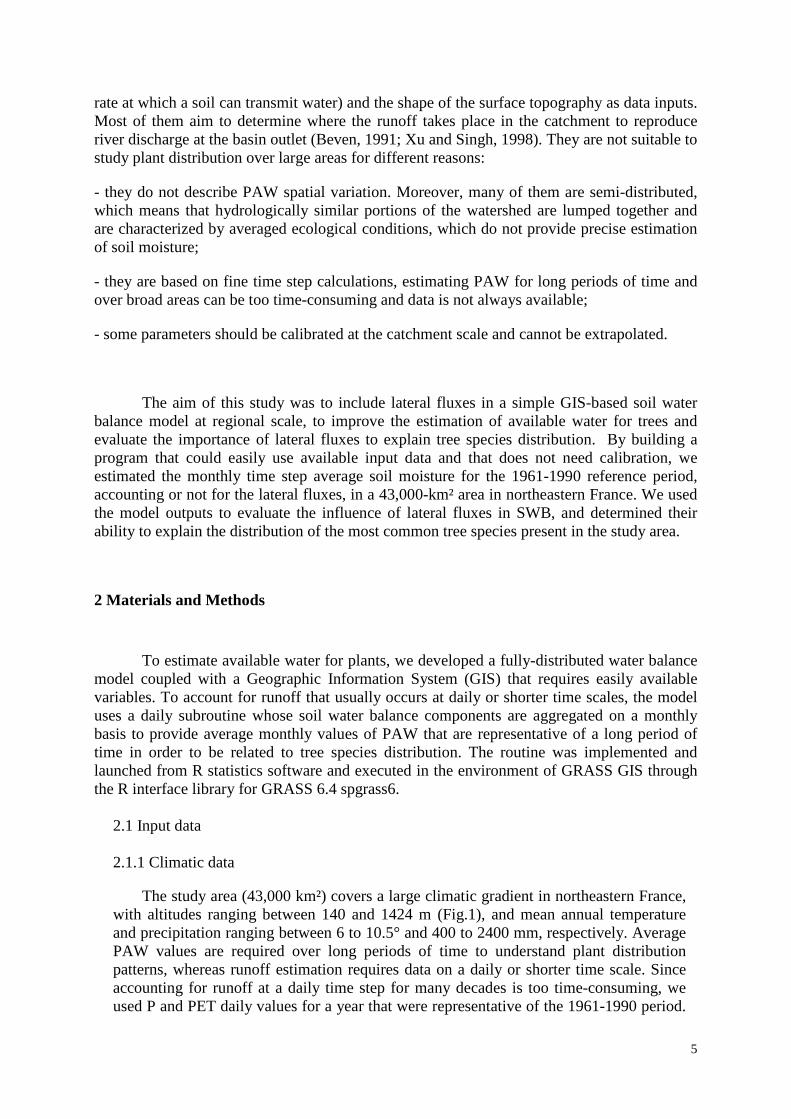
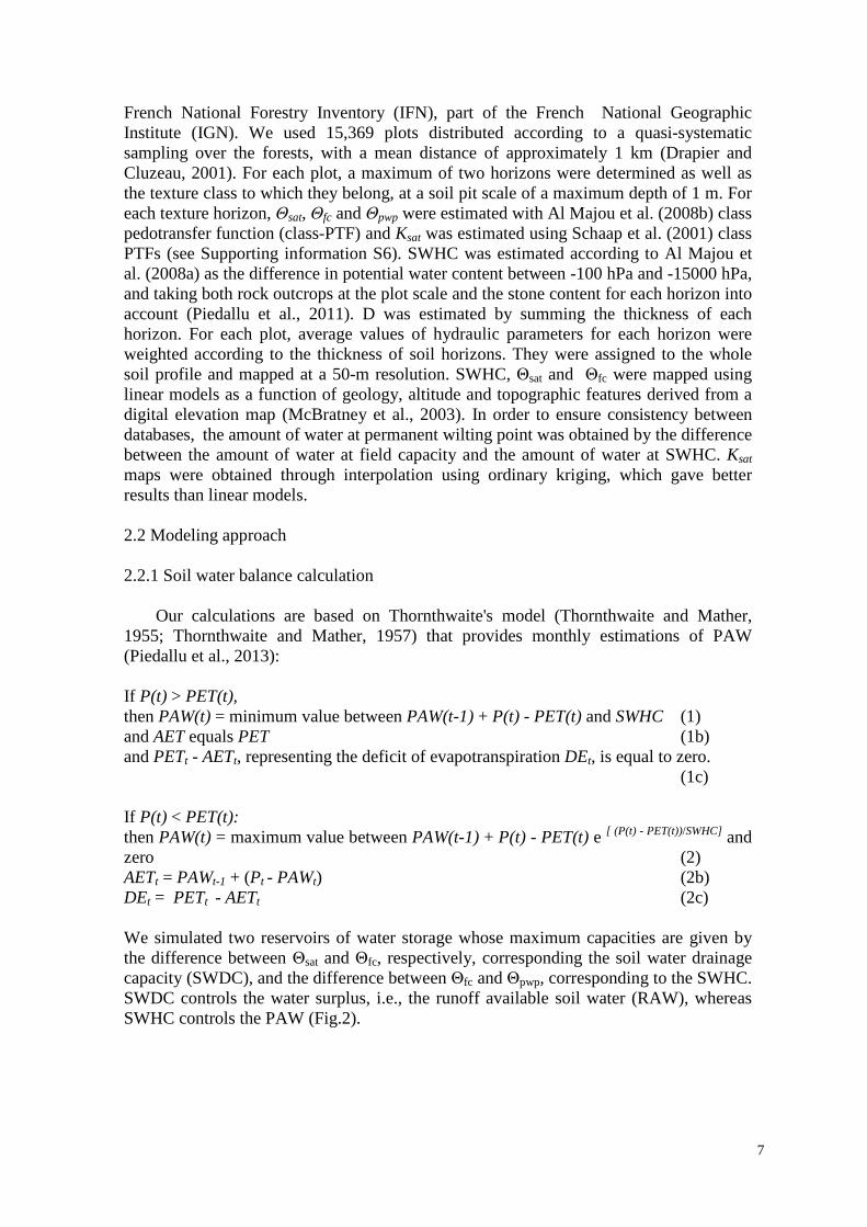
2.1 Input data 2.1.1 Climatic data The study area (43,000 km²) covers a large climatic gradient in northeastern France, with altitudes ranging between 140 and 1424 m (Fig.1), and mean annual temperature and precipitation ranging between 6 to 10.5° and 400 to 2400 mm, respectively. Average PAW values are required over long periods of time to understand plant distribution patterns, whereas runoff estimation requires data on a daily or shorter time scale. Since accounting for runoff at a daily time step for many decades is too time-consuming, we used P and PET daily values for a year that were representative of the 1961-1990 period.

6

Because averaging P over this time period will result in an unrealistic sequence, we disaggregated monthly average P for the 1961-1990 period into the most likely sequence of daily rainfall events (Supporting information S1). Daily PET were obtained using the Turc formula (Turc, 1961). This requires solar radiation obtained by dividing monthly 1961-1990 values by the number of days in the month, and temperature obtained by averaging daily values over the 1961-1990 period for each Julian day of the year.

Fig.1: Elevation of the study area (m).

Mean temperatures were extracted from the SAFRAN model (Quintana-Seguí et al., 2008; Vidal et al., 2010) and solar radiation from the Helios model (Piedallu and Gégout, 2007). For P, we extracted averaged monthly values over the period 1961-1990 from a 1-km resolution map (Bertrand et al., 2011) and occurrences of daily rainfall events used for disaggregation from SAFRAN data (Quintana-Seguí et al., 2008). 2.1.2 Soil properties The model requires knowledge about the soil thickness (D), SWHC, hydraulic conductivity (Ksat) and volumetric water content at saturation (Θsat), field capacity (Θfc) and wilting point (Θpwp). All these data were gathered from plots monitored by the

7

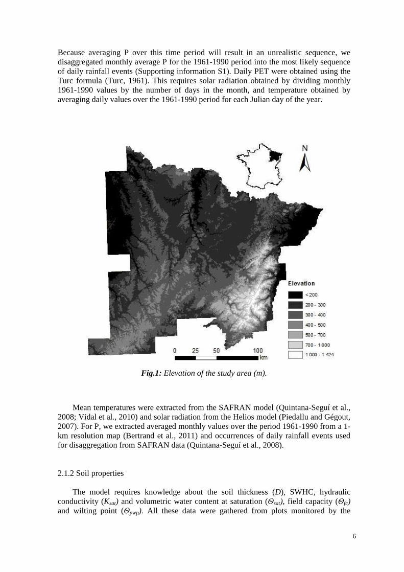
French National Forestry Inventory (IFN), part of the French National Geographic Institute (IGN). We used 15,369 plots distributed according to a quasi-systematic sampling over the forests, with a mean distance of approximately 1 km (Drapier and Cluzeau, 2001). For each plot, a maximum of two horizons were determined as well as the texture class to which they belong, at a soil pit scale of a maximum depth of 1 m. For each texture horizon, Θsat, Θfc and Θpwp were estimated with Al Majou et al. (2008b) class pedotransfer function (class-PTF) and Ksat was estimated using Schaap et al. (2001) class PTFs (see Supporting information S6). SWHC was estimated according to Al Majou et al. (2008a) as the difference in potential water content between -100 hPa and -15000 hPa, and taking both rock outcrops at the plot scale and the stone content for each horizon into account (Piedallu et al., 2011). D was estimated by summing the thickness of each horizon. For each plot, average values of hydraulic parameters for each horizon were weighted according to the thickness of soil horizons. They were assigned to the whole soil profile and mapped at a 50-m resolution. SWHC, Θsat and Θfc were mapped using linear models as a function of geology, altitude and topographic features derived from a digital elevation map (McBratney et al., 2003). In order to ensure consistency between databases, the amount of water at permanent wilting point was obtained by the difference between the amount of water at field capacity and the amount of water at SWHC. Ksat maps were obtained through interpolation using ordinary kriging, which gave better results than linear models. 2.2 Modeling approach 2.2.1 Soil water balance calculation Our calculations are based on Thornthwaite's model (Thornthwaite and Mather, 1955; Thornthwaite and Mather, 1957) that provides monthly estimations of PAW (Piedallu et al., 2013): If P(t) > PET(t), then PAW(t) = minimum value between PAW(t-1) + P(t) - PET(t) and SWHC (1) and AET equals PET (1b) and PETt - AETt, representing the deficit of evapotranspiration DEt, is equal to zero. (1c) If P(t) < PET(t): then PAW(t) = maximum value between PAW(t-1) + P(t) - PET(t) e [ (P(t) - PET(t))/SWHC] and zero (2) AETt = PAWt-1 + (Pt - PAWt) (2b) DEt = PETt - AETt (2c) We simulated two reservoirs of water storage whose maximum capacities are given by the difference between Θsat and Θfc, respectively, corresponding the soil water drainage capacity (SWDC), and the difference between Θfc and Θpwp, corresponding to the SWHC. SWDC controls the water surplus, i.e., the runoff available soil water (RAW), whereas SWHC controls the PAW (Fig.2).

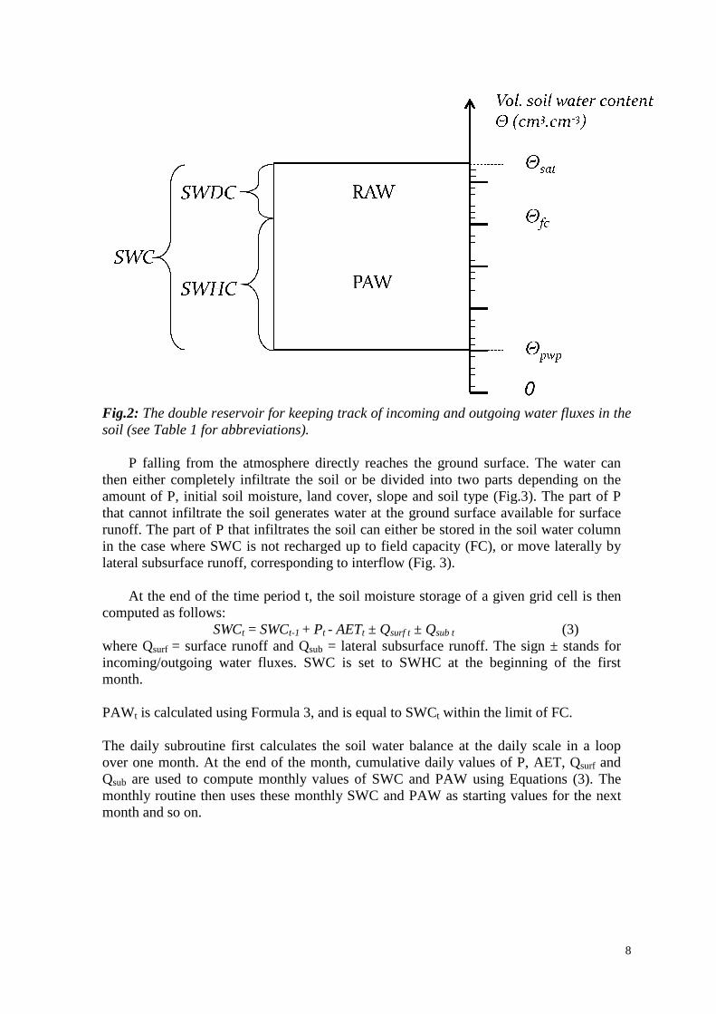
Fig.2: The double reservoir for keeping track of incoming and outgoing water fluxes in the soil (see Table 1 for abbreviations). P falling from the atmosphere directly reaches the ground surface. The water can then either completely infiltrate the soil or be divided into two parts depending on the amount of P, initial soil moisture, land cover, slope and soil type that cannot infiltrate the soil generates water at the ground surface available for surface runoff. The part of P that infiltrates the soil can either be stored in the soil water column in the case where SWC is not recharged up to lateral subsurface runoff, corresponding to At the end of the time period t, the soil moisture storage of a given grid cell is then computed as follows:

SWCt = where Qsurf = surface runoff and incoming/outgoing water fluxes. SWC is set to SWHC at the beginning of the first month. PAWt is calculated using Formula 3, and is equal to SWC The daily subroutine first calculates the soil water balance at the daily scale in a loop over one month. At the end of the month, cumulative daily values of P, AET, QQsub are used to compute monthly values of SWC and PAW using Equations (3)monthly routine then uses these monthly SWC and PAW as starting values for the next month and so on.

The double reservoir for keeping track of incoming and outgoing water fluxes in the soil (see Table 1 for abbreviations).

P falling from the atmosphere directly reaches the ground surface. The water can then either completely infiltrate the soil or be divided into two parts depending on the amount of P, initial soil moisture, land cover, slope and soil type (Fig.3).that cannot infiltrate the soil generates water at the ground surface available for surface runoff. The part of P that infiltrates the soil can either be stored in the soil water column in the case where SWC is not recharged up to field capacity (FC), or move laterally by

, corresponding to interflow (Fig. 3).

At the end of the time period t, the soil moisture storage of a given grid cell is then

= SWCt-1 + Pt - AETt ± Qsurf t ± Qsub t

surface runoff and Qsub = lateral subsurface runoff. The sign ± stands for incoming/outgoing water fluxes. SWC is set to SWHC at the beginning of the first

is calculated using Formula 3, and is equal to SWCt within the limit of

The daily subroutine first calculates the soil water balance at the daily scale in a loop over one month. At the end of the month, cumulative daily values of P, AET, Q

are used to compute monthly values of SWC and PAW using Equations (3)monthly routine then uses these monthly SWC and PAW as starting values for the next

8

The double reservoir for keeping track of incoming and outgoing water fluxes in the

P falling from the atmosphere directly reaches the ground surface. The water can then either completely infiltrate the soil or be divided into two parts depending on the

(Fig.3). The part of P that cannot infiltrate the soil generates water at the ground surface available for surface runoff. The part of P that infiltrates the soil can either be stored in the soil water column

or move laterally by

At the end of the time period t, the soil moisture storage of a given grid cell is then

(3) = lateral subsurface runoff. The sign ± stands for

incoming/outgoing water fluxes. SWC is set to SWHC at the beginning of the first

within the limit of FC.

The daily subroutine first calculates the soil water balance at the daily scale in a loop over one month. At the end of the month, cumulative daily values of P, AET, Qsurf and

are used to compute monthly values of SWC and PAW using Equations (3). The monthly routine then uses these monthly SWC and PAW as starting values for the next

9

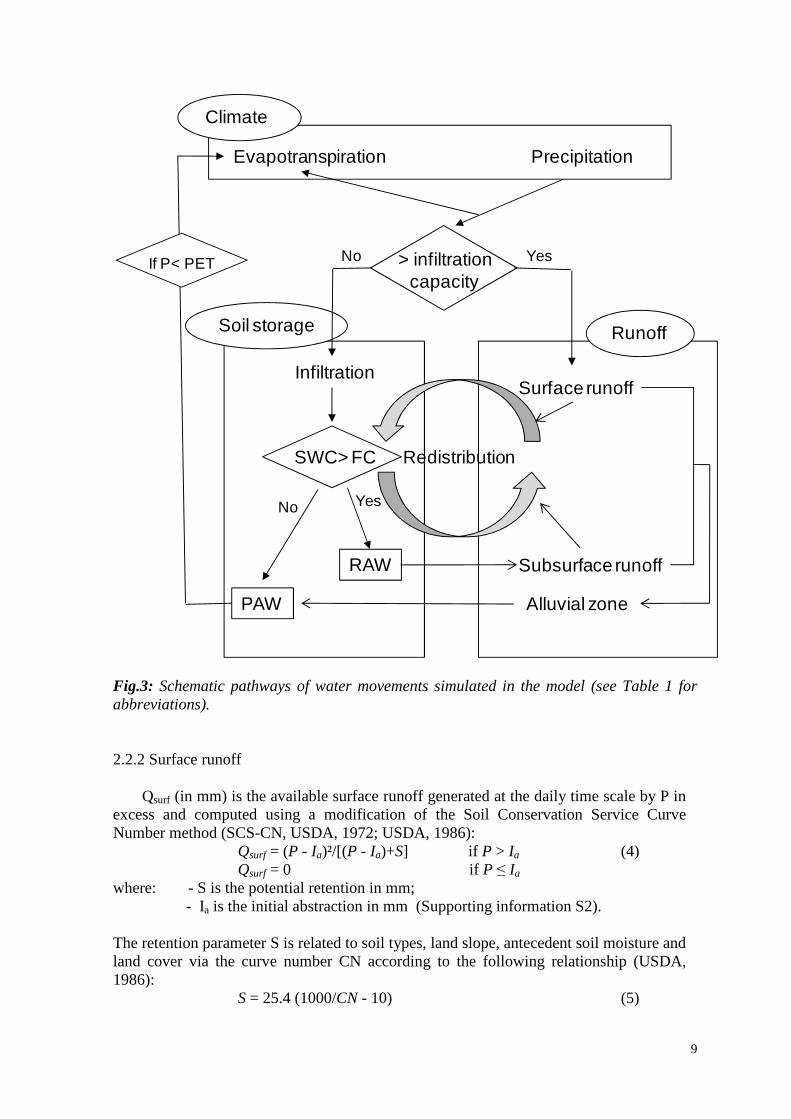
Fig.3: Schematic pathways of water movements simulated in the model (see Table 1 for abbreviations). 2.2.2 Surface runoff Qsurf (in mm) is the available surface runoff generated at the daily time scale by P in excess and computed using a modification of the Soil Conservation Service Curve Number method (SCS-CN, USDA, 1972; USDA, 1986): Qsurf = (P - Ia)²/[(P - Ia)+S] if P > Ia (4) Qsurf = 0 if P ≤ Ia where: - S is the potential retention in mm; - Ia is the initial abstraction in mm (Supporting information S2). The retention parameter S is related to soil types, land slope, antecedent soil moisture and land cover via the curve number CN according to the following relationship (USDA, 1986): S = 25.4 (1000/CN - 10) (5)

Evapotranspiration Precipitation

Climate

> infiltration capacity

YesNo

Soil storage Runoff

Redistribution

Infiltration

SWC> FC

No Yes

RAW

PAW

Surface runoff

Subsurface runoff

Alluvial zone

If P< PET

10

where CN ranges from 0 under totally dry conditions, to 100 under water-ponded conditions (Supporting information S2). Once Qsurf is calculated, it is discharged downslope using Manning's formula: V = 1/n R2/3 Slope1/2 (6a) Qout,surf = V B Qsurf (6b) Ri = a (Ai)

b (6c)

where: - V is flow velocity (m.s-1), limited between 0.02 m.s-1 to 2 m.s-1, corresponding to a speed range that occurs naturally across a hillslope (Grimaldi et al., 2010; Maidment et al., 1996), - Qout,surf is the surface runoff discharge (m3.s-1), - n is the Manning roughness coefficient (s.m-1/3) (Supporting information S7), - Ri is the hydraulic radius at cell i (m), - Slope is the slope at ground surface (m.m-1), - B is the flow width (cell width) (m), - Ai is the upstream drainage area at cell i (m²), - a is a network constant (2.4 x 10-4) and b a geometric scaling exponent (0.5),

empirically estimated with respect with flow velocity boundaries imposed. The quantity of surface water moving laterally as a sheet flow is limited by Qsurf, and is equal to: Qsurf (mm) = minimum value between Qout,surf and Qsurf (7) 2.2.3 Lateral subsurface runoff The lateral subsurface runoff is calculated from a simple relationship for saturated flow based on Darcy’s law (Darcy, 1856) and a kinematic approximation of hydraulic gradient i.e., the hydraulic gradient is equal to the land slope at the site (Beven, 1981; Frankenberger et al., 1999). Under saturated flow conditions, the pores of the soil layer are full of water and flow discharge depends on hydraulic conductivity at saturation and the contributing saturated depth of the soil layer: Qout,sub = Ksat Ds w tan β (10-3/Area of cell) (8) where: - Qout,sub is the subsurface lateral discharge (mm), - Ksat is the (horizontal) hydraulic conductivity at saturation (m.d-1), - Ds is the saturated depth area (m), - w is the flow width (dimension of the cell in m), - tan β is the tangent of the land slope (m/m or unitless) and 10-3/(Area of cell) is a factor of conversion to convert discharge from m3.d-1 to mm. As the soil layer dries, a saturated area is assumed to build up at its bottom because of the tendency of water to accumulate downwards. Therefore, Ds is assumed to be a function of the total soil layer depth D and relative soil water content storage: Ds = D (Θ - Θfc / Θsat - Θfc), Θ > Θfc , (9) Ds = 0, Θ ≤ Θfc , where: - Ds is the saturated depth of soil layer, - Θ is the actual soil water content (cm3/cm3),

11

- the term (Θ - Θfc/Θsat - Θfc) determines the fraction of the soil layer contributing

to saturated flow. The quantity of subsurface water draining laterally is limited by RAW and is equal to: Qout,sub = minimum value between Qout,sub and RAW (10) 2.2.4 Lateral redistribution of fluxes The lateral redistribution of surface flow and lateral subsurface flow is processed by an automatic drainage path algorithm that divides the discharge of a particular cell among its downhill neighbors, based on the maximum downslope gradient (MFD-md) proposed by Qin et al. (2007): di = tanβi

f(e) Li / ∑ (tanβjf(e) Lj) (11)

Each cell is potentially surrounded by eight cells, and MFD-md allocates a fraction di of the discharge from a particular cell into its ith neighboring cell; tanβi is the directional slope with the ith neighbor (the difference in elevation divided by the horizontal distance between the centers of the cells); Li is the ‘‘effective contour length’’ of cell i (0.5 and 0.354 for downslope cells in cardinal directions and diagonal directions, respectively, and 0 for non-downslope (Quinn et al., 1991). The function f(e) is used for modeling the flow (Qin et al., 2007): f(e) = 8.9 min(e,1) + 1.1 (12) where e refers to the maximum downslope gradient. The lateral inflow that a cell receives from its surrounding upslope neighbors is defined as: Qsurf in = ∑ di Qsurf out,i Or, Qsub in = ∑ di Qsub,i (13) where Qsurf in/Qsub in is the quantity of runoff that enters the given cell and is equal to the cumulative contributions of water flow from neighbors that drain it. According to our flow velocity calculations, we allowed the subsurface water to flow from one cell to another in one day. In agreement with the USDA (1972), surface flow was restricted to a maximum of six cells per day. 2.2.5 Alluvial zone delineation In the model, we accounted for fluvial processes that operate in the alluvial zone, subjected to variations in the water table. We delineated areas where Θ is always considered greater or equal to Θfc using the depth-to-water (DTW, in m.) index at site i (Murphy et al., 2009): DTWi = [Σ (dz/dx)a]wc (14) where [Σ (dz/dx)a] is the cumulative slope (sum of slope values) along the least cost path connecting any point of the landscape to a watercourse (m); a is a multiplier that is equal to 1 when the path is in the cardinal direction, and 1.414214 when it is diagonal; wc is the grid cell size (m).

12

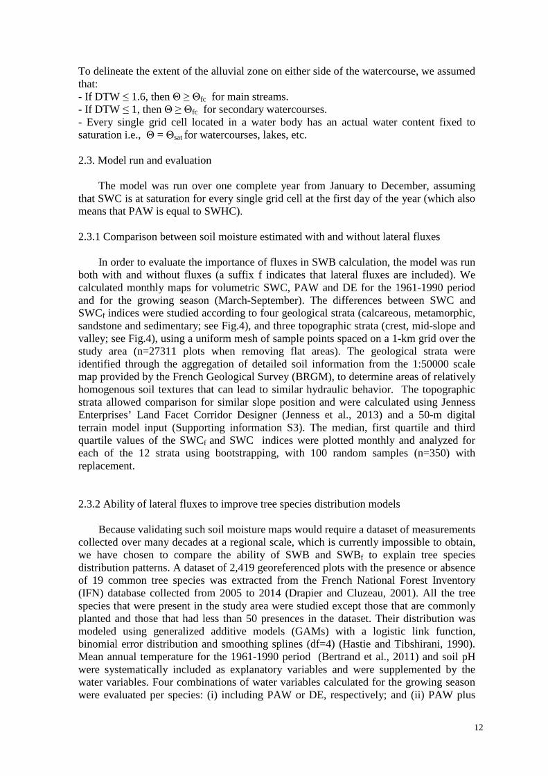
To delineate the extent of the alluvial zone on either side of the watercourse, we assumed that: - If DTW ≤ 1.6, then Θ ≥ Θfc for main streams. - If DTW ≤ 1, then Θ ≥ Θfc for secondary watercourses. - Every single grid cell located in a water body has an actual water content fixed to saturation i.e., Θ = Θsat for watercourses, lakes, etc. 2.3. Model run and evaluation The model was run over one complete year from January to December, assuming that SWC is at saturation for every single grid cell at the first day of the year (which also means that PAW is equal to SWHC). 2.3.1 Comparison between soil moisture estimated with and without lateral fluxes In order to evaluate the importance of fluxes in SWB calculation, the model was run both with and without fluxes (a suffix f indicates that lateral fluxes are included). We calculated monthly maps for volumetric SWC, PAW and DE for the 1961-1990 period and for the growing season (March-September). The differences between SWC and SWCf indices were studied according to four geological strata (calcareous, metamorphic, sandstone and sedimentary; see Fig.4), and three topographic strata (crest, mid-slope and valley; see Fig.4), using a uniform mesh of sample points spaced on a 1-km grid over the study area (n=27311 plots when removing flat areas). The geological strata were identified through the aggregation of detailed soil information from the 1:50000 scale map provided by the French Geological Survey (BRGM), to determine areas of relatively homogenous soil textures that can lead to similar hydraulic behavior. The topographic strata allowed comparison for similar slope position and were calculated using Jenness Enterprises’ Land Facet Corridor Designer (Jenness et al., 2013) and a 50-m digital terrain model input (Supporting information S3). The median, first quartile and third quartile values of the SWCf and SWC indices were plotted monthly and analyzed for each of the 12 strata using bootstrapping, with 100 random samples (n=350) with replacement. 2.3.2 Ability of lateral fluxes to improve tree species distribution models Because validating such soil moisture maps would require a dataset of measurements collected over many decades at a regional scale, which is currently impossible to obtain, we have chosen to compare the ability of SWB and SWBf to explain tree species distribution patterns. A dataset of 2,419 georeferenced plots with the presence or absence of 19 common tree species was extracted from the French National Forest Inventory (IFN) database collected from 2005 to 2014 (Drapier and Cluzeau, 2001). All the tree species that were present in the study area were studied except those that are commonly planted and those that had less than 50 presences in the dataset. Their distribution was modeled using generalized additive models (GAMs) with a logistic link function, binomial error distribution and smoothing splines (df=4) (Hastie and Tibshirani, 1990). Mean annual temperature for the 1961-1990 period (Bertrand et al., 2011) and soil pH were systematically included as explanatory variables and were supplemented by the water variables. Four combinations of water variables calculated for the growing season were evaluated per species: (i) including PAW or DE, respectively; and (ii) PAW plus

13

the difference between PAWf and PAW (DiffPAW-PAWf) or DE plus the difference between DEf and DE (DiffDE-DEf). Each model was evaluated using the explained deviance (D²). The difference in D² between models including or not including DiffPAW-PAWf and Diff DE-

DEf was evaluated, and its significance was estimated using an ANOVA with a Chi-square test. Fig.4: Delineation of the four geological strata (on the left) and the three topographical strata (on the right)

3 Results 3.1 Comparison between SWB and SWB SWB and SWBf indices representative for the 1961monthly and mapped at a 50calcareous soils in winter, to 25% for sandstone in PAWf shows considerable spatial variations both at the global and local scale, with lower values in mountains and in calcareous plateaus and near steep areas (Fig.6). Lateral redistribution along the topography content near the crests than differences occur between SWC and SWCP (during the winter) since the effects of lateral fluxes appear when sbetween Θs and Θfc (Supporting information S5)globally decreases the amount of water available to plants (for the metamorphic or sand strata where Ks is the hlateral fluxes were amplified by the high precipitation rates and steep slopes of the Vosges Mountains (Table 3). Calcareous areas show little difference between SWC and SWCto the similar values for Θs

Fig.5: Monthly SWC (%) calculated with SWB and SWBaccording to geological and topographic strata. The median is represented by a solid line, while the transparent area illustrates the range from the 1each strata.

3.1 Comparison between SWB and SWBF maps

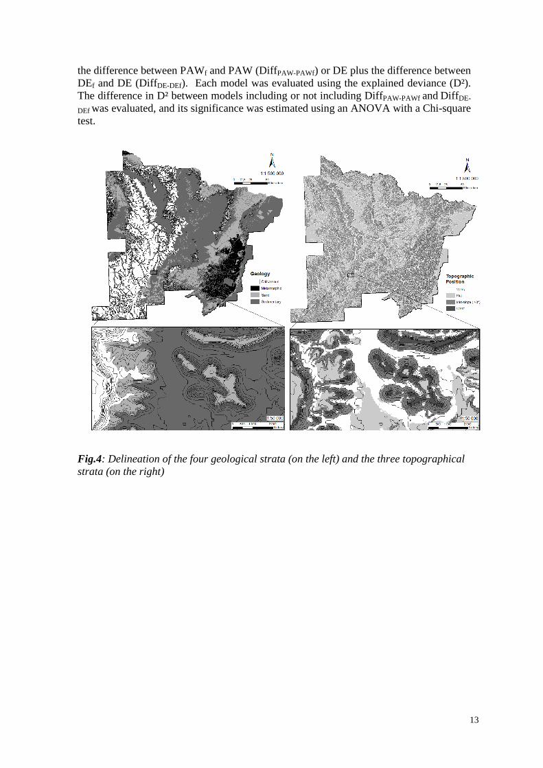
indices representative for the 1961-1990 period were calculated monthly and mapped at a 50-m resolution. Average SWC values vary from 45% for calcareous soils in winter, to 25% for sandstone in summer (Fig.5). The distribution of

shows considerable spatial variations both at the global and local scale, with lower values in mountains and in calcareous plateaus and near steep areas (Fig.6). Lateral redistribution along the topography logically leads to a more important decrease of

than in the valleys (Table 3, Fig.5, Supporting information S5differences occur between SWC and SWCf when the soil is saturated and PET is lower than P (during the winter) since the effects of lateral fluxes appear when s

Supporting information S5). Including lateral fluxes in the calculation globally decreases the amount of water available to plants (Table 3, Figs. 5 and 7), mainly for the metamorphic or sand strata where Ks is the highest (Table 2). For these two strata, lateral fluxes were amplified by the high precipitation rates and steep slopes of the Vosges

. Calcareous areas show little difference between SWC and SWCs and Θfc and the low Ks that does not allow large fluxes (Table 2

Monthly SWC (%) calculated with SWB and SWBf models for the period 1961according to geological and topographic strata. The median is represented by a solid line, while the transparent area illustrates the range from the 1st to the 3

14

1990 period were calculated m resolution. Average SWC values vary from 45% for

summer (Fig.5). The distribution of shows considerable spatial variations both at the global and local scale, with lower

values in mountains and in calcareous plateaus and near steep areas (Fig.6). Lateral a more important decrease of water

Supporting information S5). No when the soil is saturated and PET is lower than

P (during the winter) since the effects of lateral fluxes appear when soil moisture ranges . Including lateral fluxes in the calculation

Figs. 5 and 7), mainly ighest (Table 2). For these two strata,

lateral fluxes were amplified by the high precipitation rates and steep slopes of the Vosges . Calcareous areas show little difference between SWC and SWCf due

that does not allow large fluxes (Table 2).

models for the period 1961-1990, according to geological and topographic strata. The median is represented by a solid line,

to the 3rd quartile; n=350 for

15

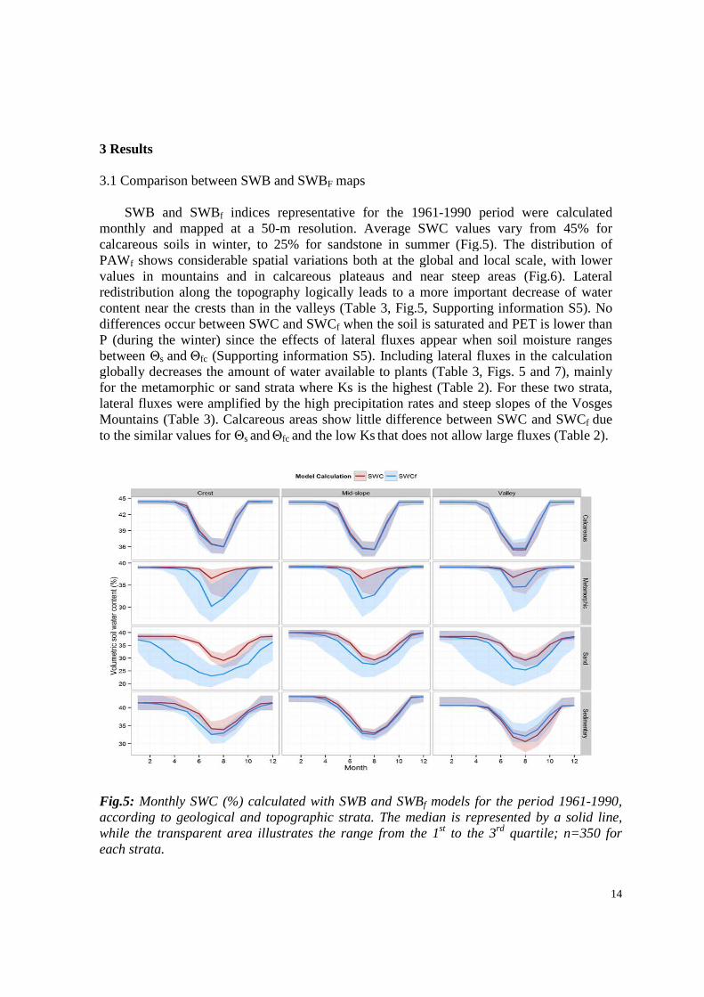
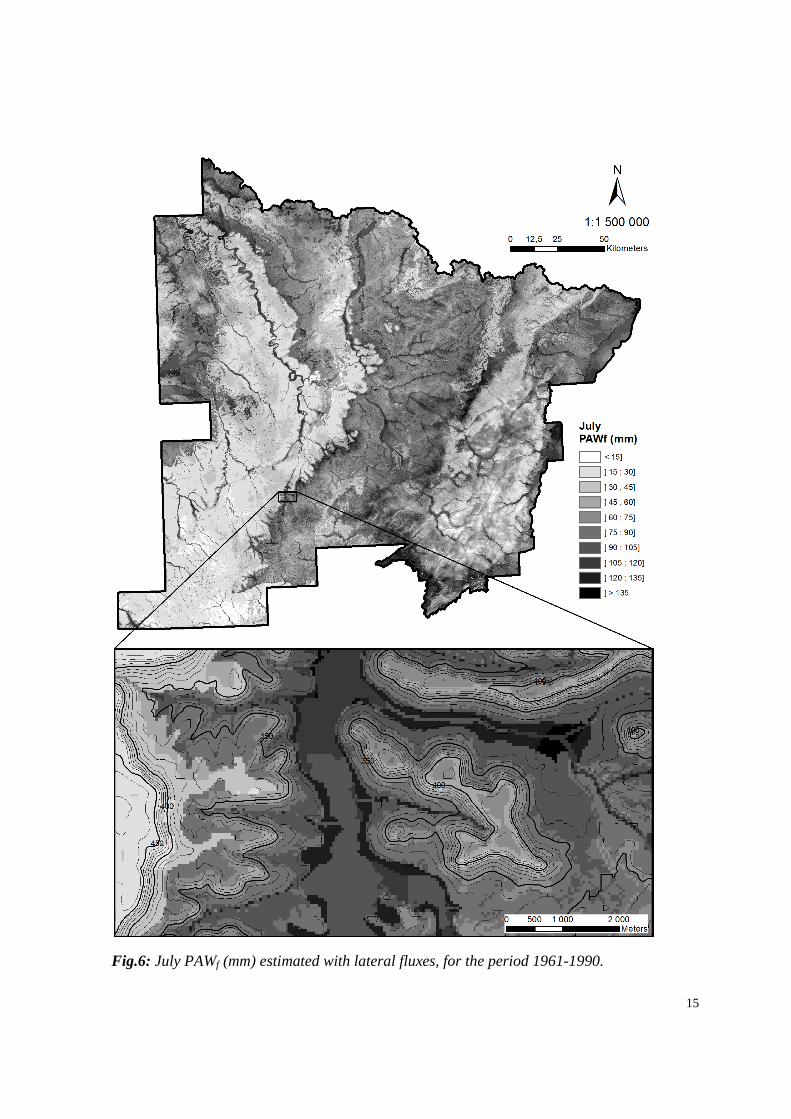
Fig.6: July PAWf (mm) estimated with lateral fluxes, for the period 1961-1990.

16

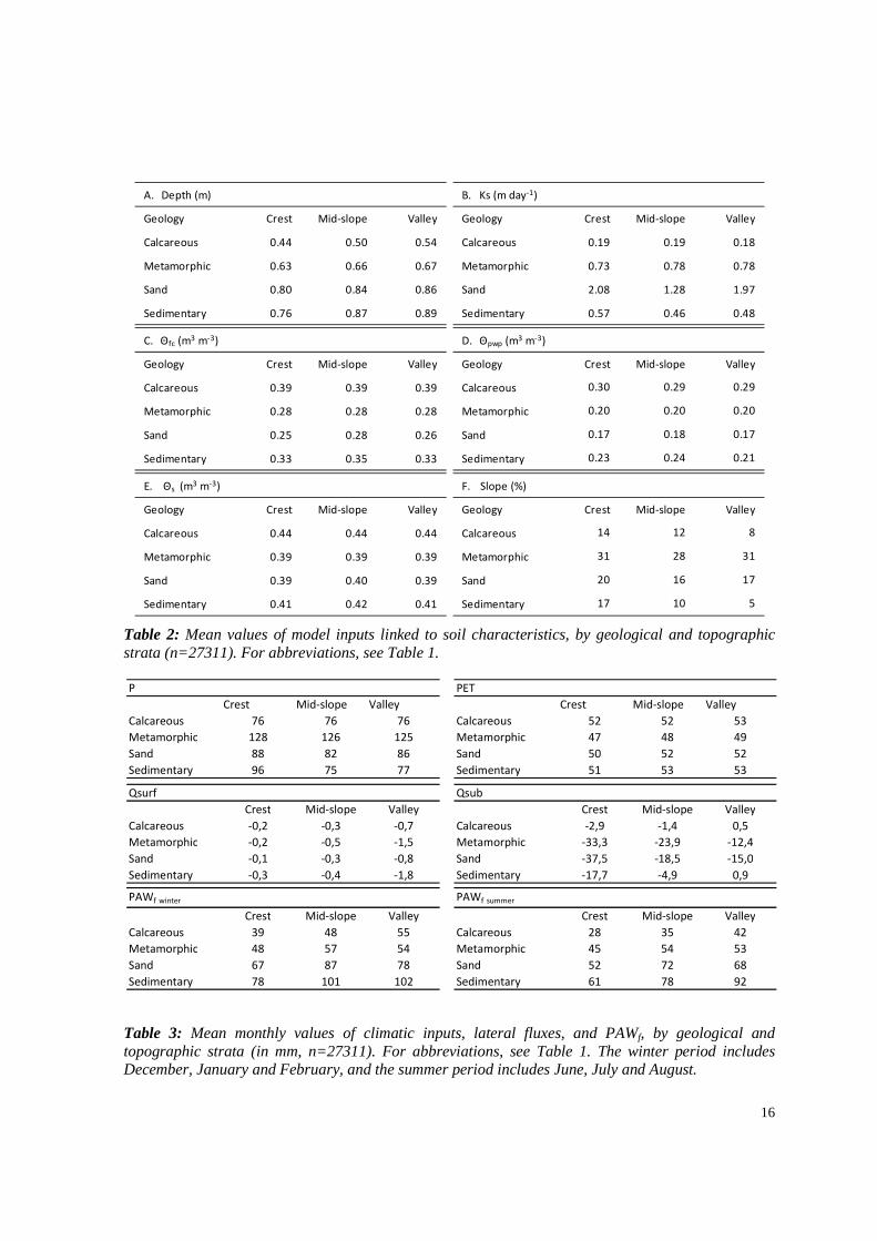
Table 2: Mean values of model inputs linked to soil characteristics, by geological and topographic strata (n=27311). For abbreviations, see Table 1.

Table 3: Mean monthly values of climatic inputs, lateral fluxes, and PAWf, by geological and topographic strata (in mm, n=27311). For abbreviations, see Table 1. The winter period includes December, January and February, and the summer period includes June, July and August.

B. Ks (m day-1)

Geology Crest Mid-slope Valley

Calcareous 0.19 0.19 0.18

Metamorphic 0.73 0.78 0.78

Sand 2.08 1.28 1.97

Sedimentary 0.57 0.46 0.48

E. Θs (m3 m-3)




Sand 0.39 0.40 0.39


A. Depth (m)




Sand 0.80 0.84 0.86


C. Θfc (m3 m-3)




Sand 0.25 0.28 0.26


D. Θpwp (m3 m-3)




Sand 0.17 0.18 0.17


F. Slope (%)


Calcareous 14 12 8

Metamorphic 31 28 31

Sand 20 16 17

Sedimentary 17 10 5

P PET

Crest Mid-slope Valley Crest Mid-slope Valley

Calcareous 76 76 76 Calcareous 52 52 53

Metamorphic 128 126 125 Metamorphic 47 48 49

Sand 88 82 86 Sand 50 52 52

Sedimentary 96 75 77 Sedimentary 51 53 53

Qsurf Qsub


Calcareous -0,2 -0,3 -0,7 Calcareous -2,9 -1,4 0,5

Metamorphic -0,2 -0,5 -1,5 Metamorphic -33,3 -23,9 -12,4

Sand -0,1 -0,3 -0,8 Sand -37,5 -18,5 -15,0

Sedimentary -0,3 -0,4 -1,8 Sedimentary -17,7 -4,9 0,9

PAWf winter PAWf summer


Calcareous 39 48 55 Calcareous 28 35 42

Metamorphic 48 57 54 Metamorphic 45 54 53

Sand 67 87 78 Sand 52 72 68

Sedimentary 78 101 102 Sedimentary 61 78 92

17

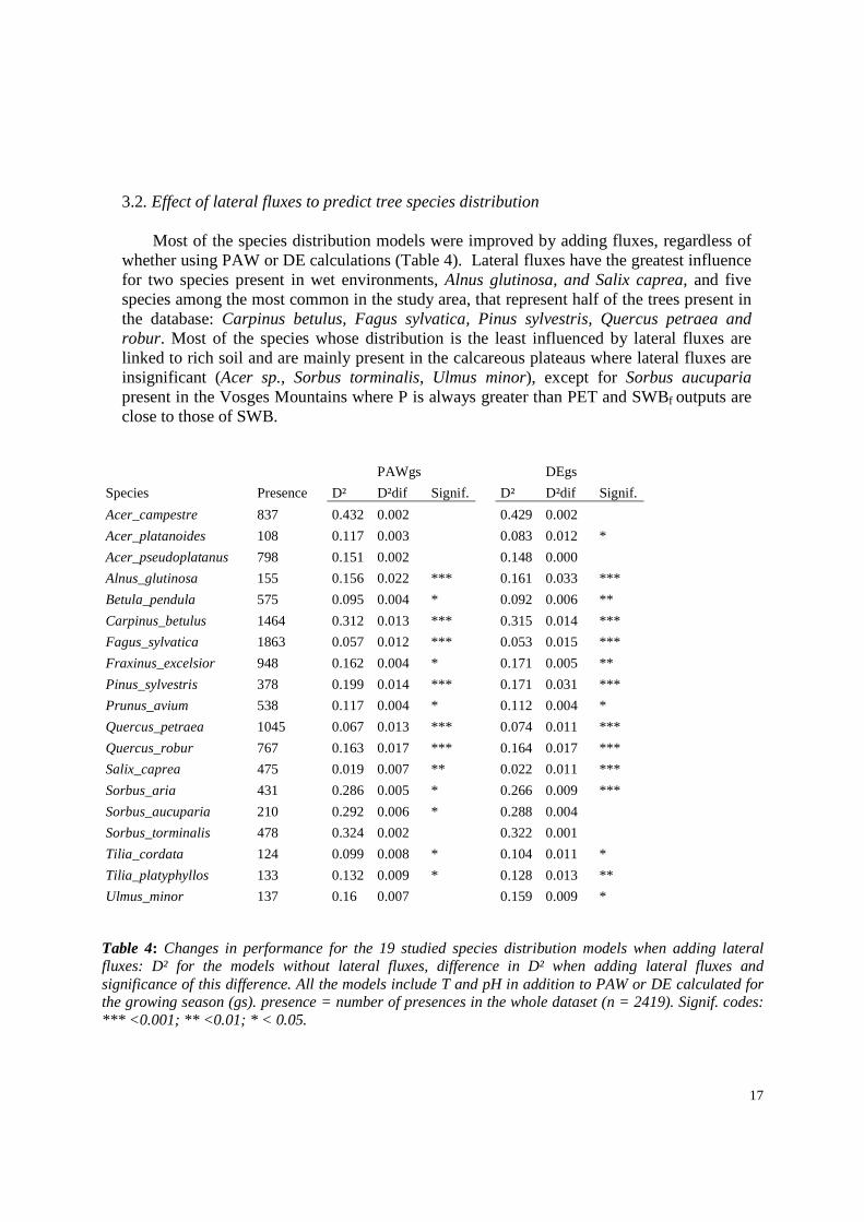
3.2. Effect of lateral fluxes to predict tree species distribution Most of the species distribution models were improved by adding fluxes, regardless of whether using PAW or DE calculations (Table 4). Lateral fluxes have the greatest influence for two species present in wet environments, Alnus glutinosa, and Salix caprea, and five species among the most common in the study area, that represent half of the trees present in the database: Carpinus betulus, Fagus sylvatica, Pinus sylvestris, Quercus petraea and robur. Most of the species whose distribution is the least influenced by lateral fluxes are linked to rich soil and are mainly present in the calcareous plateaus where lateral fluxes are insignificant (Acer sp., Sorbus torminalis, Ulmus minor), except for Sorbus aucuparia present in the Vosges Mountains where P is always greater than PET and SWBf outputs are close to those of SWB.

PAWgs DEgs

Species Presence D² D²dif Signif. D² D²dif Signif.

Acer_campestre 837 0.432 0.002 0.429 0.002

Acer_platanoides 108 0.117 0.003 0.083 0.012 *

Acer_pseudoplatanus 798 0.151 0.002 0.148 0.000

Alnus_glutinosa 155 0.156 0.022 *** 0.161 0.033 ***

Betula_pendula 575 0.095 0.004 * 0.092 0.006 **

Carpinus_betulus 1464 0.312 0.013 *** 0.315 0.014 ***

Fagus_sylvatica 1863 0.057 0.012 *** 0.053 0.015 ***

Fraxinus_excelsior 948 0.162 0.004 * 0.171 0.005 **

Pinus_sylvestris 378 0.199 0.014 *** 0.171 0.031 ***

Prunus_avium 538 0.117 0.004 * 0.112 0.004 *

Quercus_petraea 1045 0.067 0.013 *** 0.074 0.011 ***

Quercus_robur 767 0.163 0.017 *** 0.164 0.017 ***

Salix_caprea 475 0.019 0.007 ** 0.022 0.011 ***

Sorbus_aria 431 0.286 0.005 * 0.266 0.009 ***

Sorbus_aucuparia 210 0.292 0.006 * 0.288 0.004

Sorbus_torminalis 478 0.324 0.002 0.322 0.001

Tilia_cordata 124 0.099 0.008 * 0.104 0.011 *

Tilia_platyphyllos 133 0.132 0.009 * 0.128 0.013 **

Ulmus_minor 137 0.16 0.007 0.159 0.009 *

Table 4: Changes in performance for the 19 studied species distribution models when adding lateral fluxes: D² for the models without lateral fluxes, difference in D² when adding lateral fluxes and significance of this difference. All the models include T and pH in addition to PAW or DE calculated for the growing season (gs). presence = number of presences in the whole dataset (n = 2419). Signif. codes: *** <0.001; ** <0.01; * < 0.05.

18

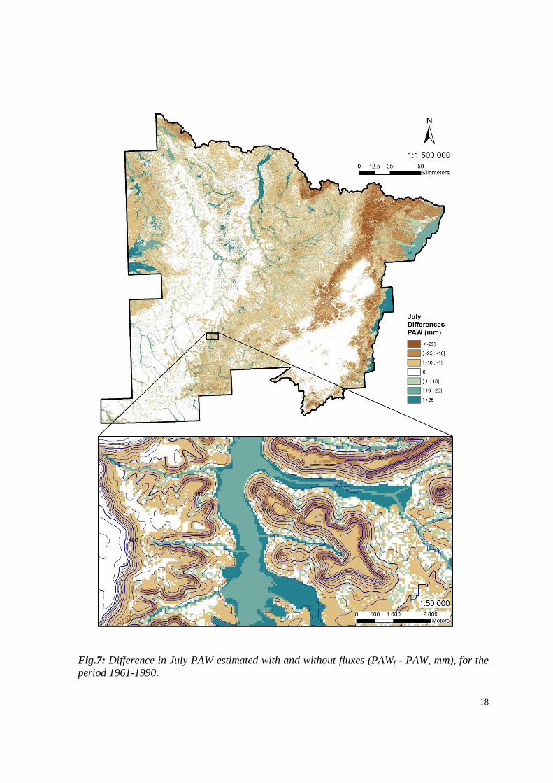
Fig.7: Difference in July PAW estimated with and without fluxes (PAWf - PAW, mm), for the period 1961-1990.

19

4 Discussion

For the first time, a large-scale study combined fine resolution water balance and lateral fluxes to estimate water available to plants. The simulated soil moisture values seem to be in agreement compared to measurements provided by other studies. For example, Ali et al. (2010) found volumetric SWC values between 10 and 45% in Canada, and Brocca et al. (2007) between 13 and 52% in central Italy, while the majority of our simulations range between 19 and 45%. By accounting for soil moisture dynamics, we refined existing maps and improved the estimate of the spatial distribution of water available for plants. We showed that including lateral fluxes in SWB significantly changes the soil moisture patterns, with both a large area effect due to climate and soil properties, and a local effect due to the topography. We also showed that the intensity of fluxes differs according to the location and the period, with few changes when the soil water reserve is full (e.g., in the wet mountains), or when soil characteristics do not allow for large fluxes (e.g., on calcareous plateaus). This little lateral redistribution of soil moisture along hillslopes in chalky catchments has already been observed in previous studies (Blyth et al., 2004). Spatial redistribution is also meaningless when available water is low (< Θfc), mainly during dry periods in summer (Supporting information S4), in agreement with existing studies showing that the effects of topography become negligible when soil moisture decreases (Ridolfi et al., 2003; Western et al., 2002).

We logically observe a decrease in soil water content during summer, but with a lower intensity, as can be expected. Compared to winter, soil moisture is reduced by 10-40% for the driest month, compared to the 50-80% reduction reported in different studies in the same area (Granier et al., 2007; Lebourgeois et al., 2005). This difference can be due to the water that is stored between ϴfc and ϴs in our model, making it available for infiltration the following day, or because precipitation intercepted by vegetation and percolation are not accounted for. Improvements in the model’s outputs could probably be obtained by further investigating the partitioning between vertical fluxes and lateral fluxes since the importance of vertical fluxes is frequently reported in the literature (Grayson and Western, 2001; Selby, 1993). However, these values should be compared with caution because soil moisture in our study is averaged over 30 years, includes different soil layers up to 1 m, and is compared to plot measurements or estimations at a specific place, over a short time period and at a specific soil depth. As a follow-up to this work, the model should be validated with ground measurements that could be made at a more local scale and considering shorter time steps.

In contrast to SWC, SWCf shows a large gradient in water content along hillslopes, with between 5 to 25% less SWCf in the crests than in the valleys for metamorphic, sand and sedimentary bedrocks (Fig.7). This soil moisture gradient was expected because it was already reported in numerous studies (Famiglietti et al., 1998; Lookingbill and Urban, 2004). The amount of water redistributed along the topographical gradient is difficult to

20

compare between studies due to the considerable heterogeneity in climate, soils, topography, periods of the year, time step and measurement methods. Different authors reported that SWC is 15 to 90% lower in the crests compared to the valleys at the same period, with values higher than 40% for wet areas or wet periods (Blyth et al., 2004; Western et al., 2004), and ranging between 15 and 25% when the climate is dry (Blyth et al., 2004; Famiglietti et al., 1998). Compared to the literature, the differences we observed seem relatively small, despite the fact that they are probably a bit underestimated in Fig.7 by the averaging of SWCf values from many plots with different environmental characteristics. Locally, differences exceeding 50% can be observed on steep slopes or sand strata, but they concern limited areas. These discrepancies may be caused by differences between our estimates based on the entire soil profile, and the shallow measurement depths (0-15 cm) used in some studies since the topographic control on SWC is greater near the surface than at greater depths (Famiglietti et al., 1998; Grayson and Western, 2001; Wilson et al., 2004). Additionally, our model provides monthly time step data, whereas studies of spatial patterns in soil moisture are often characterized by daily or hourly measurements of SWC during storm events or intensive rains. Finally, the disaggregation method used to generate daily data for P that is representative of the 1961-1990 period leads to obtaining a representative number of days with rainfall events of the same intensity. By reducing the likelihood of exceeding the thresholds that trigger lateral flow, we probably limit the intensity of runoff. Further work should evaluate the results obtained by using observed sequences of rainfall. The largest magnitude of subsurface fluxes and the strongest effects of topographic gradients in SWCf are observed in the sand strata that have the highest transmissivity values. This result highlights the model outputs' sensitivity to soil textural assumptions and corresponding PTFs. The range of available PTFs is highly variable among similar soil textural classes, and different PTFs for any given soil texture could result in very different outcomes. For example, the Ks value we used for sand is provided by Rosetta and is 3.739 m day-1 (Schaap et al., 2001), but other PTFs use Ks values for sand of 5.315 m day-1 (Carsel and Parrish, 1988) and 0.690 m day-1 (Hypres, Wosten et al., 1999). Running the model using the Carsel and Parrish database should consequently increase the lateral fluxes in the sand strata, although they will be significantly decreased using the Hypres database. The limited fluxes observed in the calcareous strata are also explained by PTFs (mainly Ks, Θs

and Θfc ), and using different PTFs will change their magnitude in this area. This comparison emphasizes the importance of the PTF selection and the high variability that can be generated according to the database used (Loosvelt et al., 2011). Using local PFT and improving the models' inputs by using continuous PTFs should be a solution for reducing these uncertainties (Nemes et al., 2003). Despite the fact that numerous studies have focused on the effects of hydrologic processes on plants (Porporato et al., 2001), very few of them were interested in evaluating the effect of lateral fluxes on vegetation over broad areas (Berges and Balandier, 2010; Hwang et al., 2012). The studied tree species distributions were better explained when accounting for the lateral fluxes, demonstrating that soil moisture dynamics contribute to shaping species distribution patterns at a regional scale. The importance of topographical position on vegetation has been recognized for a long time by practitioners, and is commonly linked both to changes in soil depth, water or nutrient fluxes, and local climates

21

(Cajander, 1926). By controlling changes in soil depth, soil nutrition or temperature, we showed that the observed model improvement is not induced by these three environmental gradients, that can be linked with the topographical position (Burke et al., 1999; Dyer, 2009). The better performance of models accounting for the lateral fluxes can probably be attributed to the redistribution of water from the alluvial zone for the species that occur in wet areas, like Alnus glutinosa or Salix caprea. For the other species, soil moisture dynamics along hillslopes are probably the best explanation for these results. The species whose distributions are the least improved are mainly distributed on calcareous bedrocks where lateral fluxes are weak, or in mountains where water availability is not a limiting factor. We can expect that the importance of runoff in shaping species distribution would be underestimated in this study. A large proportion of the studied area is flat (35% is less than 3˚, and 92% is less than 10˚), and most of the steep slopes are located in the Vosges Mountains where little difference exists between SWB and SWBf. Moreover, water constraint is relatively low in this area, and we can expect lateral runoff to have a greater effect on plants in arid or Mediterranean ecosystems (Porporato et al., 2001). Identifying the driest and the wettest areas at the landscape scale is of crucial interest for plant ecologists and natural resources managers. We provided a new tool that makes it possible to study the redistribution of water along hillslopes over large areas. The program, that does not need calibration at the catchment scale, requires only readily available data. It can be used to characterize the spatial distribution in available water over long periods, or to simulate the evolution of soil moisture distribution among years. This information can be used for a wide variety of applications: to refine the delineation of areas with favorable ecological conditions for species, to better predict species composition, to improve our knowledge about species ecology, and to better understand tree growth dynamics, plant health and forest fire risks. It also has important implications for assessing ecosystem responses to climate change by determining topographic refugia where species could persist locally despite regional climatic conditions that may be unfavorable in the future or local areas where species could colonize (Ashcroft and Gollan, 2013).

Acknowledgments

This work was supported by the French National Research Agency through the Laboratory of Excellence ARBRE , the GIP ECOFOR and the RMT AFORCE , the Regional Council of Lorraine , and the Direction Régionale de l'Alimentation, de l'Agriculture et de la Forêt of the Lorraine region. We also thanks François Ridremont for its proofreading and Bruno Ambroise for its help.

22

References

Al Majou, H., A. Bruand, and O. Duval , 2008. The use of in situ volumetric water content at field capacity to improve the prediction of soil water retention properties, Canadian Journal of Soil Science, 88(4), 533-541.

Al Majou, H., A. Bruand, O. Duval, C. Le Bas, and A. Vautier , 2008. Prediction of soil water retention properties after stratification by combining texture, bulk density and the type of horizon, Soil Use and Management, 24(4), 383-391.

Ali, G. A., A. G. Roy, and P. Legendre , 2010. Spatial relationships between soil moisture patterns and topographic variables at multiple scales in a humid temperate forested catchment, Water Resources Research, 46(10).

Ashcroft, M. B., and J. R. Gollan , 2013. Moisture, thermal inertia, and the spatial distributions of near-surface soil and air temperatures: Understanding factors that promote microrefugia, Agricultural and Forest Meteorology, 176, 77-89.

Barbour, M. G., and W. D. Billings, 2000. North American terrestrial vegetation, Cambridge University Press, Cambridge, UK.

Bates, B. C., Z. W. Kundzewicz, S. Wu, and J. P. Palutikof , 2008. Climate Change and Water. Technical Paper of the Intergovernmental Panel on Climate ChangeRep., 210 pp pp, Geneva.

Berges, L., and P. Balandier, 2010. Revisiting the use of soil water budget assessment to predict site productivity of sessile oak (Quercus petraea Liebl.) in the perspective of climate change, European Journal of Forest Research, 129(2), 199-208.

Berges, L., R. Chevalier, Y. Dumas, A. Franc, and J. M. Gilbert, 2005. Sessile oak (Quercus petraea) site index variations in relation to climate, topography and soil in even-aged high-forest stands in northern France, Annals of Forest Science, 62(5), 391-402.

Bertrand, R., J. Lenoir, C. Piedallu, G. Riofrío-Dillon, P. d. Ruffray, C. Vidal, J.-C. Pierrat, and J.-C. Gégout, 2011. Changes in plant community composition lag behind climate warming in lowland forests, Nature, 479(7374), 517.

Beven, K., 1981. kinematic subsurface stormflow, Water Resources Research, 17(5), 1419-1424.

Beven, K. (1991), Spatially distributed modeling: conceptual approach to runoff prediction, 373-387 pp.

Beven, K. J., and M. J. Kirkby (1979), A physically based, variable contributing area model of basin hydrology, Hydrological Sciences -Bulletin- des Sciences Hydrologiques, 24, 43 - 69.

Blyth, E. M., J. Finch, M. Robinson, and P. Rosier (2004), Can soil moisture be mapped onto the terrain?, Hydrology and Earth System Sciences, 8(5), 923-930.

23

Botkin, D., and E. Keller (1995), Environmental Science: Earth as a Living Planet, John Wiley & Sons, Inc., Canada.

Brocca, L., R. Morbidelli, F. Melone, and T. Moramarco (2007), Soil moisture spatial variability in experimental areas of central Italy, Journal of Hydrology, 333(2), 356-373.

Bruand, A., P. N. Fernandez, and O. Duval (2003), Use of class pedotransfer functions based on texture and bulk density of clods to generate water retention curves, Soil Use and Management, 19(3), 232-242.

Burke, I. C., W. K. Lauenroth, R. Riggle, P. Brannen, B. Madigan, and S. Beard (1999), Spatial variability of soil properties in the shortgrass steppe: The relative importance of topography, grazing, microsite and plant species in controlling spatial patterns, Ecosystems, 2, 422-438.

Cajander, A. K. (1926), The theory of forest types, Acta For. Fenn., 29(3), 1:108.

Carsel, R. F., and R. S. Parrish (1988), Developing joint probability distributions of soil water retention characteristics, Water Resources Research, 24(5), 755-769.

Chabot, B. F., and H. A. Mooney (1985), Physiological ecology of North American plant communities, Chapman and Hall, New York.

Choisnel, E. (1992), Le calcul du bilan hydrique du sol : options de modélisation et niveaux de complexité, science du sol,, 30, 1, 15-31.

Curt, S., S. Dole, and G. Marmeys (1996), Alimentation en eau et production forestière, application d'indicateurs simples pour les résineux dans le massif central., Etude et gestion des sols, 3,2, 81-96.

Darcy, H. (1856), Les fontaines publiques de la ville de Dijon, V. Dalmont.

Deblauwe, V., N. Barbier, P. Couteron, O. Lejeune, and J. Bogaert, 2008. The global biogeography of semi-arid periodic vegetation patterns, Global Ecology and Biogeography, 17(6), 715-723.

Drapier, J., and C. Cluzeau, 2001. La base de données écologiques de l'IFN, Revue forestière française, 53(3-4), 365-371.

Dyck, S., 1985. Overview on the present status of the concepts of water balance models, IAHS Publication(148), 3-19.

Dyer, J., 2009. Assessing topographic patterns in moisture use and stress using a water balance approach, Landscape Ecology, 24(3), 391-403.

Famiglietti, J. S., J. W. Rudnicki, and M. Rodell , 1998. Variability in surface moisture content along a hillslope transect: Rattlesnake Hill, Texas, Journal of Hydrology, 210(1–4), 259-281.

Frankenberger, J. R., E. S. Brooks, M. T. Walter, M. F. Walter, and T. S. Steenhuis , 1999. A GIS-based variable source area hydrology model, Hydrological Processes, 13(6), 805-822.

Granier, A., N. Breda, P. Biron, and S. Villette, 1999. A lumped water balance model to evaluate duration and intensity of drought constraints in forest stands, Ecological Modelling, 116(2-3), 269-283.

24

Granier, A., et al., 2007. Evidence for soil water control on carbon and water dynamics in European forests during the extremely dry year: 2003, Agricultural and Forest Meteorology, 143(1-2), 123-145.

Grayson, R., and A. Western , 2001. Terrain and the distribution of soil moisture, Hydrological Processes, 15(13), 2689-2690.

Grimaldi, S., A. Petroselli, G. Alonso, and F. Nardi, 2010. Flow time estimation with spatially variable hillslope velocity in ungauged basins, Advances in Water Resources, 33(10), 1216-1223.

Hastie, T. J., and R. Tibshirani, 1990. Generalized additive models, Chapman and Hall, London.

Hwang, T., L. E. Band, J. M. Vose, and C. Tague (2012), Ecosystem processes at the watershed scale: Hydrologic vegetation gradient as an indicator for lateral hydrologic connectivity of headwater catchments, Water Resources Research, 48.

Jenness, J., B. Brost, and P. Beier (2013), Land Facet Corridor Designer: Extension for ArcGIS., Jenness Enterprises.

Johnson, E. A., K. Miyanishi, and C. Ebrary Academic Complete Subscription (2007), Plant disturbance ecology: the process and the response, Elsevier/AP, Amsterdam; Boston.

Kobal, M., H. Grčman, M. Zupan, T. Levanič, P. Simončič, A. Kadunc, and D. Hladnik (2015), Influence of soil properties on silver fir (Abies alba Mill.) growth in the Dinaric Mountains, Forest Ecology and Management, 337(Journal Article), 77-87.

Lebourgeois, F., Bréda N., Ulrich E., and G. A (2005), Climate-tree-growth relationships of European beech(Fagus sylvatica L.) in the French Permanent Plot Network (RENECOFOR), Trees Structure and Function, 19, 385-401.

Lookingbill, T., and D. Urban (2004), An empirical approach towards improved spatial estimates of soil moisture for vegetation analysis, Landscape ecology, 19(4), 417-433.

Loosvelt, L., V. R. N. Pauwels, W. M. Cornelis, G. J. M. De Lannoy, and N. E. C. Verhoest (2011), Impact of soil hydraulic parameter uncertainty on soil moisture modeling, Water Resources Research, 47.

Maidment, D., F. Olivera, A. Calver, A. Eatherall, and W. Fraczek (1996), Unit hydrograph derived from a spatially distributed velocity field, Hydrological processes, 10(6), 831-844.

McBratney, A. B., M. L. Mendonca Santos, and B. Minasny (2003), On digital soil mapping, geoderma, 117(1), 3-52.

Moore, I. D., A. K. Turner, J. P. Wilson, S. K. Jenson, and L. E. Band (1993), GIS and land-surface-subsurface modeling, 196-230 pp.

Murphy, P., J. Ogilvie, and P. Arp (2009), Topographic modelling of soil moisture conditions: a comparison and verification of two models, European journal of soil science, 60(1), 94-109.

Nemes, A., M. G. Schaap, and J. H. M. Wosten, 2003. Functional evaluation of pedotransfer functions derived from different scales of data collection, Soil Science Society of America Journal, 67(4), 1093-1102.

25

Oloughlin, E. M., 1981. Saturation regions in catchments and their relations to soil and topographic properties, Journal of Hydrology, 53(3-4), 229-246.

Palmer, W. C., 1965. Meteorological drought, US Department of Commerce, Weather Bureau Washington, DC, USA.

Piedallu, C., and J.-C. Gégout, 2007. Multiscale computation of solar radiation for predictive vegetation modelling, Annals of forest science, 64(8), 899-909.

Piedallu, C., J. C. Gegout, A. Bruand, and I. Seynave, 2011. Mapping soil water holding capacity over large areas to predict potential production of forest stands, Geoderma, 160(3-4), 355-366.

Piedallu, C., J. C. Gegout, V. Perez, and F. Lebourgeois , 2013. Soil water balance performs better than climatic water variables in tree species distribution modelling, Global Ecology and Biogeography, 22(4), 470-482.

Porporato, A., E. Daly, and I. Rodriguez-Iturbe, 2004. Soil water balance and ecosystem response to climate change, AMerican Naturalist, 164(5), 625-632.

Porporato, A., F. Laio, L. Ridolfi, and I. Rodriguez-Iturbe , 2001. Plants in water-controlled ecosystems: active role in hydrologic processes and response to water stress - III. Vegetation water stress, Advances in Water Resources, 24(7), 725-744.

Qin, C., A. X. Zhu, T. Pei, B. Li, C. Zhou, and L. Yang , 2007. An adaptive approach to selecting a flow-partition exponent for a multiple-flow-direction algorithm, International Journal of Geographical Information Science, 21(4), 443-458.

Quinn, P., K. Beven, P. Chevallier, and O. Planchon ,1991. The prediction of hillslope flow paths for distributed hydrological modeling using digital terrain models, Hydrological Processes, 5(1), 59-79.

Quintana-Seguí, P., P. Le Moigne, Y. Durand, E. Martin, F. Habets, M. Baillon, C. Canellas, L. Franchisteguy, and S. Morel ,2008. Analysis of near-surface atmospheric variables: Validation of the SAFRAN analysis over France, Journal of applied meteorology and climatology, 47(1), 92-107.

Ridolfi, L., P. D'Odorico, A. Porporato, and I. Rodriguez-Iturbe (2003), Stochastic soil moisture dynamics along a hillslope, Journal of hydrology, 272(1-4), 264-275.

Saxton, K. E. (1985), Soil water hydrology: simulation for water balance computations, IAHS Publication(148), 47-59.

Schaap, M. G., F. J. Leij, and M. T. van Genuchten (2001), rosetta: a computer program for estimating soil hydraulic parameters with hierarchical pedotransfer functions, Journal of Hydrology, 251(3–4), 163-176.

Schwärzel, K., Peters, R., Petzold, R., Häntzschel, J, Menzer, A., Clausnitzer, F., Spank, U., Köstner, B., Bernhofer, C., Feger, K.H., (2011). Räumlich-differenzierte Berechnung und Bewertung des Standortswasserhaushaltes von Wäldern des Mittelgebirges. - Waldökologie, Landschaftsforschung und Naturschutz, 12,119-126

Selby, M. J. (1993), Hillslope Materials and Processes, Oxford University Press.

26

Thornthwaite, C., and J. Mather (1955), The water balance. Centerton: Drexel Institute of Technology, 1955. 104 p, Publications in climatology, 8(1).

Thornthwaite, C. W. (1948), An approach toward a rational classification of climate, Geographical Review, 38, 55-94.

Thornthwaite, C. W., and J. R. Mather (1955), The water balance, Laboratory of Climatology, Publication in Climatology., n°8, 1-86.

Thornthwaite, C. W., and J. R. Mather (1957), Instructions and Tables for Computing Potential Evapotranspiration and the water balance., Laboratory of Climatology, Publication in Climatology,Volume X (n°3).

Ticehurst, J. L., H. P. Cresswell, and A. J. Jakeman (2003), Using a physically based model to conduct a sensitivity analysis of subsurface lateral flow in south-east Australia, Environmental Modelling & Software, 18(8-9), 729-740.

Turc, L. (1961), Estimation of irrigation water requirements, potential evapotranspiration: a simple climatic formula evolved up to date, Ann Agron, 12(1), 13-49.

USDA (1972), SCS (Soil Conservation Service).National Engineering Handbook. Section 4, hydrology, Washington, DC, USDA.

USDA (1986), Urban hydrology for small watersheds . Technical Release 55 (TR-55) Rep., Natural Resources Conservation Service, Conservation Engineering Division.

Van der Schrier, G., K. Briffa, P. Jones, and T. Osborn (2006), Summer moisture variability across Europe, Journal of Climate, 19(12), 2818-2834.

Vidal, J. P., E. Martin, L. Franchistéguy, M. Baillon, and J. M. Soubeyroux , 2010. A 50‐year high‐resolution atmospheric reanalysis over France with the Safran system, International Journal of Climatology, 30(11), 1627-1644.

Western, A. W., R. B. Grayson, and G. Bloschl , 2002. Scaling of soil moisture: A hydrologic perspective, Annual Review of Earth and Planetary Sciences, 30, 149-180.

Western, A. W., S.-L. Zhou, R. B. Grayson, T. A. McMahon, G. Blöschl, and D. J. Wilson, 2004. Spatial correlation of soil moisture in small catchments and its relationship to dominant spatial hydrological processes, Journal of Hydrology, 286(1), 113-134.

Weyman, D. R., 1973. Measurements of the downslope flow of water in a soil, Journal of Hydrology, 20(3), 267-288.

Williams, J. R., and V. Singh, 1995. The EPIC model, Computer models of watershed hydrology., 909-1000.

Wilson, D. J., A. W. Western, and R. B. Grayson, 2004. Identifying and quantifying sources of variability in temporal and spatial soil moisture observations, Water Resources Research, 40(2).

Woodward, D. E., R. H. Hawkins, R. Jiang, A. T. Hjelmfelt, J. A. Van Mullem, and Q. D. Quan , 2003. Runoff curve number method: examination of the initial abstraction ratio, paper presented at World Water & Environmental Resources Congress 2003, American Society of Civil Engineers, Philadelphia, Pennsylvania, United States, June 23-26, 2003.

27

Wosten, J. H. M., A. Lilly, A. Nemes, and C. l. Bas , 1999. Development and use of a database of hydraulic properties of European soils, Geoderma, 90(3/4).

Xu, C. Y., and V. P. Singh, 1998. A Review on Monthly Water Balance Models for Water Resources Investigations, Water Resources Management, 12(1), 31-50.

Zierl, B., 2001. A water balance model to simulate drought in forested ecosystems and its application to the entire forested area in Switzerland, Journal of Hydrology, 242(1), 115-136.

28

Supporting Information for

Including the lateral redistribution of soil moisture in a supra regional

water balance model to better identify suitable areas for tree species

Contents of this file

Text S1: Temporal disaggregation of monthly rainfall

Text S2: The Curve Number calculation

Text S3: Topographic strata calculation

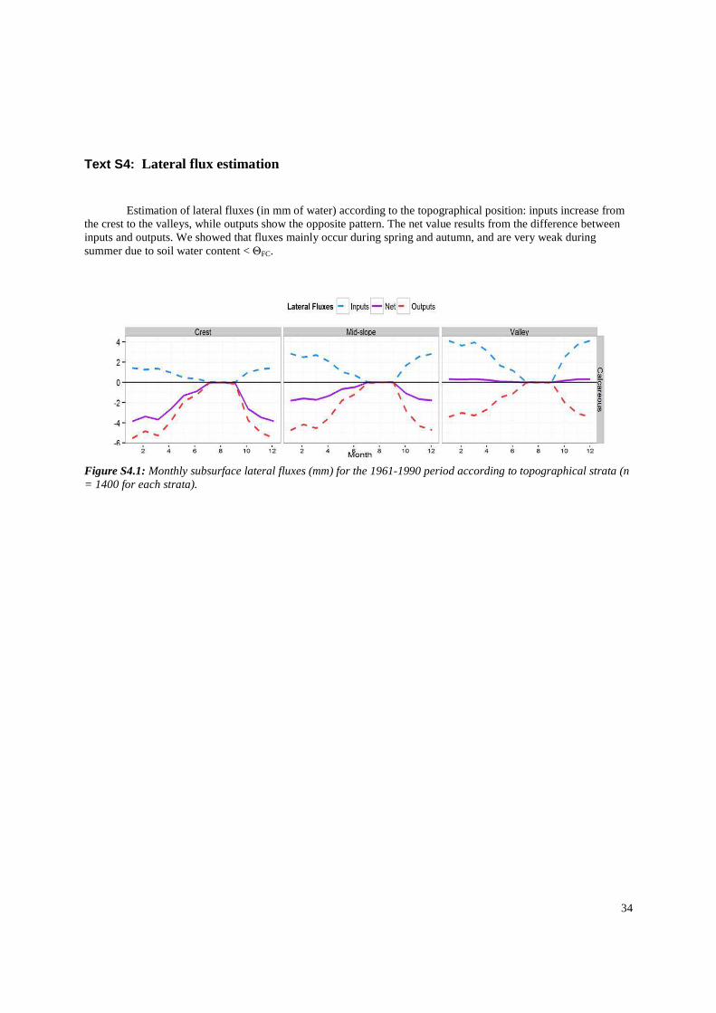
Text S4: Lateral flux estimation

Figure S5: Difference between DE and DEf

Table S6: Θsat, Θfc and Ksat class PTF values calculated for the nine NFI soil textures

Table S7: Look-up table between land cover and roughness coefficient n used in Equation 6a.

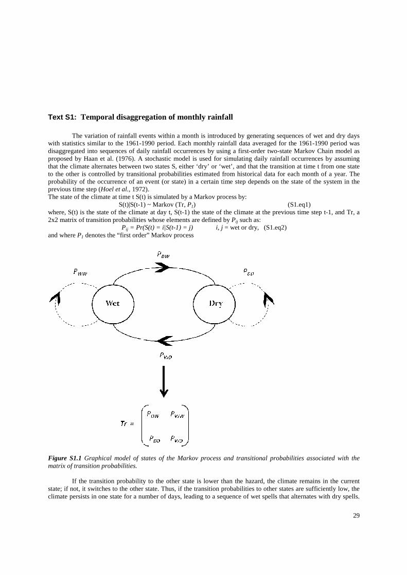
Text S1: Temporal disaggregation of monthly rainfall The variation of rainfall eventwith statistics similar to the 1961-1990 perioddisaggregated into sequences of daily rainfall occurrences by proposed by Haan et al. (1976). A that the climate alternates between two states Sto the other is controlled by transitional probabilities estimated from historical data for each month of a year. probability of the occurrence of an event (or state) in a certain time step depends on the state oprevious time step (Hoel et al., 1972)The state of the climate at time t S(t) is simulated by a Markov process by:

S(t)|S(t-1) ~ Markov (Tr, where, S(t) is the state of the climate at day t, S(t2x2 matrix of transition probabilities whose elements are defined by Pij = Pr(S(t) = i|S(tand where P1 denotes the “first order” Markov process

Figure S1.1 Graphical model of states of the Markov process and transitional probabilities associated matrix of transition probabilities. If the transition probability to the state; if not, it switches to the other state. Thus, if the transition probabilities to other states are sufficiently low, the climate persists in one state for a number of days,

Temporal disaggregation of monthly rainfall

events within a month is introduced by generating sequences of wet and dry days 1990 period. Each monthly rainfall data averaged for the 1961

disaggregated into sequences of daily rainfall occurrences by using a first-order two-state Markov Chain model as stochastic model is used for simulating daily rainfall occurrences by assuming

that the climate alternates between two states S, either ‘dry’ or ‘wet’, and that the transition at time t from one state to the other is controlled by transitional probabilities estimated from historical data for each month of a year.

occurrence of an event (or state) in a certain time step depends on the state o, 1972).

The state of the climate at time t S(t) is simulated by a Markov process by: 1) ~ Markov (Tr, P1)

here, S(t) is the state of the climate at day t, S(t-1) the state of the climate at the previous time step t2x2 matrix of transition probabilities whose elements are defined by Pij such as:

= Pr(S(t) = i|S(t-1) = j) i, j = wet or dry, (S1.eq2) denotes the “first order” Markov process

Graphical model of states of the Markov process and transitional probabilities associated

If the transition probability to the other state is lower than the hazard, the climate remains in the current if not, it switches to the other state. Thus, if the transition probabilities to other states are sufficiently low, the

climate persists in one state for a number of days, leading to a sequence of wet spells that

29

by generating sequences of wet and dry days Each monthly rainfall data averaged for the 1961-1990 period was

state Markov Chain model as stochastic model is used for simulating daily rainfall occurrences by assuming

the transition at time t from one state to the other is controlled by transitional probabilities estimated from historical data for each month of a year. The

occurrence of an event (or state) in a certain time step depends on the state of the system in the

(S1.eq1) 1) the state of the climate at the previous time step t-1, and Tr, a

Graphical model of states of the Markov process and transitional probabilities associated with the

other state is lower than the hazard, the climate remains in the current if not, it switches to the other state. Thus, if the transition probabilities to other states are sufficiently low, the

that alternates with dry spells.

30

The amount of rainfall on rainy days is assumed to be constant and simply equal to monthly rainfall P divided by the number of simulated wet days within the month. The Markov model requires knowledge of two monthly conditional probabilities to simulate sequences of rainy and no-rain days over a month: the probability PDW that a wet day occurs at time t, knowing that a dry day occurred at the precedent time t-1, and the probability PWD that a dry day occurs at time t, knowing that a wet day occurred at the precedent time t-1. Both can be estimated from the monthly probability density function (PDF) fM (t) of times of inter-arrivals, where the subscript M refers to the month considered, and t represents the time of inter-arrivals, i.e., the time elapsed between two successive events of interest. In our case, events are either rainy days PDW = fM (1) or dry days, PWD = fM (1). In order to estimate the PDF fM (t), we used available daily precipitation, and for each month M of the year over the period 1961-90, the within-month distribution of the time elapsed between two successive rainy days or dry days was fitted by testing three PDF: Exponential, Gamma and Weibull using a two-sample Kolmogorov-Smirnov test. Whenever the exponential law proved to be in agreement with the data distribution, it was selected because of its ease of use. For each month, PDW and PWD were computed according to its corresponding PDF, and mapped at a 50-m resolution by kriging. Then, for a given month and for each unique couple of transition probabilities PDW and PWD, 5,000 first-order Markov chain models produced 5,000 sequences of states of the Markov model. Each sequence of observations consisting of successive weather, i.e., “wet, wet, dry” (two successive rainy days followed by a day with no rain), has a probability to be observed, which is calculated as:

P(WWD..) = P(W(t)) * P(W(t)|W(t-1)) * P(D(t)|W(t-1)) … (S1.eq3) The most likely sequence is defined as the sequence with the highest probability (to occur), and is used for generating daily maps of precipitation.

Text S2: The Curve Number calculation. The curve number CN used in

(i) Dividing the soils into four classes or hydrologic groups according to their infiltration capacity: A - high capacity [low runoff potential B - medium capacity [moderate runoff potential] (0.09 C - low capacity [high runoff potential] (0.02 m D - very low capacity [very high runoff potential] (K(ii) Assigning specific values to each of the previous classes with respect to land cover. Land cover data was extracted from the CORINE project

The CN values for normal moisture conditioncover are given in Table S2.1.

Table S2.1: Look-up table between curve number and land cover for the the USDA Soil Conservation Service, 1972 This classical SCS-CN calculation was modified according to the purpose of the study, to facilitate the calculation, to account for the high variability in topography and land use, and to be linked CN adjustment for AMC For changes in soil moisture conditions, CNCondition indices (AMC-index): AMCreferring to normal and wet conditionsdepending on the quantity of precipitation calculation we used the following converTable S2.1 (USDA Soil Conservation Service

CNI = (4.2 * CNII

The Curve Number calculation.

The curve number CN used in Equation 5 (USDA, 1972) is estimated by: i) Dividing the soils into four classes or hydrologic groups according to their infiltration capacity:

low runoff potential] (Ksat > 0.18 m-d); medium capacity [moderate runoff potential] (0.09 m-d < Ksat < 0.18 m-d);

apacity [high runoff potential] (0.02 m-d < Ksat < 0.09 m-d); and very low capacity [very high runoff potential] (Ksat < 0.02 m-d).

ii) Assigning specific values to each of the previous classes with respect to land cover. Land cover data was CORINE project (European Environment Agency, 2000).

The CN values for normal moisture conditions (CNII) used for the four soil classes and the different land

up table between curve number and land cover for the four hydrologic soil groups Conservation Service, 1972).

CN calculation was modified according to the purpose of the study, to facilitate the variability in topography and land use, and to be linked

For changes in soil moisture conditions, CNII values are adjusted depending on AMC-I referring to dry conditions; and AMC-II (Table

referring to normal and wet conditions, respectively. In the traditional method, CN is adjustedon the quantity of precipitation that fell in the last five days and the season. In order to simplify this

calculation we used the following conversion formulas, making it possible to use only the CN values displayed in Conservation Service, 1972):

II) / (10 - 0.058 * CNII) (S2.eq1)

31

i) Dividing the soils into four classes or hydrologic groups according to their infiltration capacity:

ii) Assigning specific values to each of the previous classes with respect to land cover. Land cover data was

for the four soil classes and the different land

hydrologic soil groups (adapted from

CN calculation was modified according to the purpose of the study, to facilitate the variability in topography and land use, and to be linked to soil moisture.

adjusted depending on Antecedent Moisture (Table S2.1) and AMC-III

is adjusted for a particular AMC days and the season. In order to simplify this

to use only the CN values displayed in

32

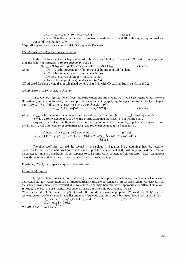
CNIII = (23 * CNII) / (10 + 0.13 * CNII) (S2.eq2) where CN is the curve number for moisture conditions I, II and III, referring to dry, normal and

wet conditions, respectively. CNI and CNIII values were used to calculate S in Equation (S2.eq4). CN adjustment for different slope conditions

In the traditional method, CNII is assumed to be used for 5% slopes. To adjust CN for different slopes, we used the following equation (Williams and Singh, 1995):

CNII slope = (CNIII – CNII) /3*(1-2*exp(-13.86*Slope)) + CNII (S2.eq3) where: - CNII slope is the curve number for normal conditions adjusted for slope, - CNII is the curve number for normal conditions, - CNIII is the curve number for wet conditions,

- Slope is the slope at the ground surface (in %), CN adjusted for slopes were then recalculated by replacing CNII with CNII slope in Equations C.1 and C.2. CN adjustment for soil moisture changes Once CN are adjusted for different moisture conditions and slopes, we allowed the retention parameter S (Equation 5) to vary continuously with soil profile water content by applying the equation used in the hydrological model SWAT (Soil and Water Assessment Tool) (Arnold et al., 1998):

S = Smax * (1 - SW/[SW + exp(w1 - w2 * SW)] ) (S2.eq4)

where: - Smax is the maximum potential retention solved for dry conditions (i.e., CNI slope) using equation 5, - SW is the soil water content of the entire profile excluding the water held at wilting point, - w1 and w2 are shape coefficients related to maximum potential retention Smax, potential retention for wet conditions S3, soil water content at saturation SAT, and soil water content at field capacity FC:

w1 = ln[ FC/(1 - S3 * Smax

-1) - FC] + w2 * FC (S2.eq5) w2 = (ln[ FC/(1 - S3*Smax

-1) - FC] - ln[ SAT/(1 - 2.54*Smax-1) - SAT] ) / (SAT – FC)

(S2.eq6) The first coefficient w1 and the second w2 are solved in Equation 5 by assuming that: the retention parameter for moisture conditions I corresponds to soil profile water content at the wilting point; and the retention parameter for moisture conditions III corresponds to soil profile water content at field capacity. These assumptions make the water retention parameter more dependent on soil water storage. Equation (S2.eq4) then replaces Equation 5 to estimate S. Ia/S ratio adjustment Ia represents all losses before runoff begins such as interception by vegetation, water retained in surface depression storage, evaporation and infiltration. Historically, the percentage of initial abstraction was derived from the study of many small, experimental U.S. watersheds, and may therefore not be appropriate in different situations. If needed, the SCS-CN user manual recommends using a relationship other than Ia = 0.2S. Woodward et al. (2003) found that Ia/S ratios of 0.05 would seem more appropriate. We used this 5% Ia/S ratio to generate (more) surface runoff for smaller amounts of precipitation. Equation 4 becomes (Woodward et al., 2003): Qsurf = (P - 0.05S0.05)²/(P - 0.95S0.05), if P > 0.05S (S2.eq7) Qsurf = 0, if P ≤ 0.05S where S0.05 = 1.33S0.20

1 .15

33

Text S3: Topographic strata calculation

Four topographic strata, including “crest”, “mid-slope”, “valley”, and “flat”, were calculated using Jenness Enterprises’ Land Facet Corridor Designer (Jenness et al., 2013) for ArcGIS 10 Four-category Topographic Position Tool and a 50-m digital terrain model input. The tool uses a topographic position index (TPI), which is calculated as the difference between the elevation of a pixel and the average elevation of all the pixels in the surrounding neighborhood to assign pixels to different topographic positions (Jenness et al., 2013). Positive TPI values indicate that the pixel elevation is higher than the surrounding neighborhood, and negative values indicate that the elevation is lower than the surrounding neighborhood. If the TPI of a pixel is greater than a given crest threshold or lower than a given valley threshold, it will be classified as a crest or valley. If the TPI is near zero, the elevation of the pixel is similar to that of the surrounding cells and may be located in a flat area or mid-slope. The slope of the pixel is used to differentiate the two situations, and the slope threshold is the minimum slope required for a pixel to be considered mid-slope. Pixels with slopes lower than the slope threshold can be classified as flat, crest or valley. Each pixel in our study area was assigned a topographic position based on its classification calculated using a 300-m circular neighborhood with crest and valley thresholds of +10 m and -10 m, respectively, and a 3° slope threshold (Class1), and also using its classification based on a 1000-m neighborhood with thresholds of ±5 m and a 3° slope (Class2). Pixels were assigned to crest and mid-slope positions based on their classification in Class1 and to valley and flat positions based on their classification in Class2, given that crest and mid-slope classifications from Class1 took priority, and Class2 could only be used to classify remaining pixels as flat or valley. Class2 was calculated with a larger neighborhood and more sensitive valley threshold so that pixels in broad valleys, which are in a water receiving position at the catchment scale but have a relatively similar elevation to their neighboring pixels within 300 m (and are thus classified as flat in Class1), would be assigned to the valley classification (rather than flat). Areas classified as “flat” were not considered because the elevation in the surrounding neighborhood was so similar that flat pixels were not expected to generate or receive lateral fluxes.

34

Text S4: Lateral flux estimation Estimation of lateral fluxes (in mm of water) according to the topographical position: inputs increase from the crest to the valleys, while outputs show the opposite pattern. The net value results from the difference between inputs and outputs. We showed that fluxes mainly occur during spring and autumn, and are very weak during summer due to soil water content < ΘFC.

Figure S4.1: Monthly subsurface lateral fluxes (mm) for the 1961-1990 period according to topographical strata (n = 1400 for each strata).

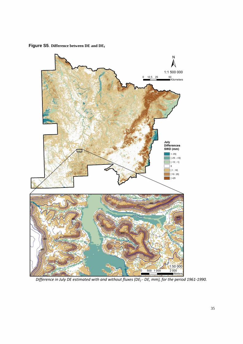
35

Figure S5. Difference between DE and DEf

Difference in July DE estimated with and without fluxes (DEf - DE, mm), for the period 1961-1990.

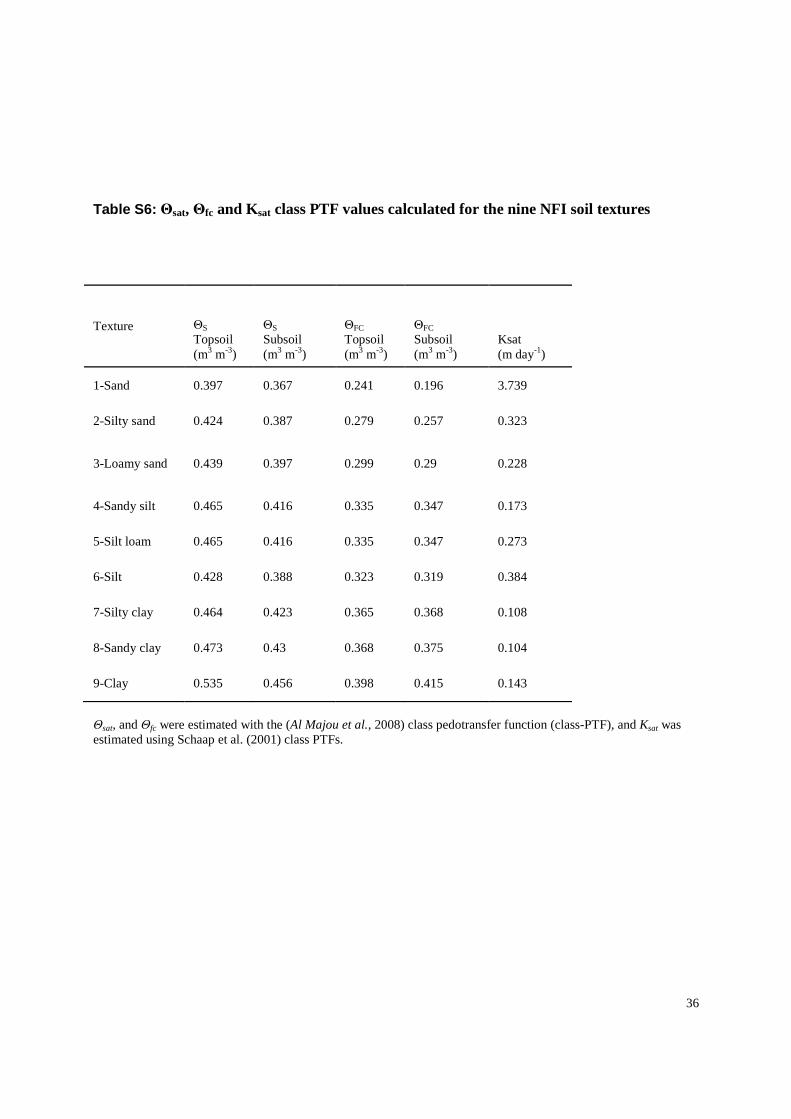
36

Table S6: Θsat, Θfc and Ksat class PTF values calculated for the nine NFI soil textures

Texture ΘS Topsoil (m3 m-3)

ΘS Subsoil (m3 m-3)

ΘFC Topsoil (m3 m-3)

ΘFC Subsoil (m3 m-3)

Ksat (m day-1)

1-Sand 0.397 0.367 0.241 0.196 3.739

2-Silty sand 0.424 0.387 0.279 0.257 0.323

3-Loamy sand 0.439 0.397 0.299 0.29 0.228

4-Sandy silt 0.465 0.416 0.335 0.347 0.173

5-Silt loam 0.465 0.416 0.335 0.347 0.273

6-Silt 0.428 0.388 0.323 0.319 0.384

7-Silty clay 0.464 0.423 0.365 0.368 0.108

8-Sandy clay 0.473 0.43 0.368 0.375 0.104

9-Clay 0.535 0.456 0.398 0.415 0.143

Θsat, and Θfc were estimated with the (Al Majou et al., 2008) class pedotransfer function (class-PTF), and Ksat was estimated using Schaap et al. (2001) class PTFs.

Table S7: Look-up table between land cover and roughness coefficient n used in

Manning’s roughness coefficient (n, s.mtables reported in the literature (Chow et al., 1988;

up table between land cover and roughness coefficient n used in Equation 6a.

Manning’s roughness coefficient (n, s.m-1/3) obtained for Corine Land cover codes, by combining multiple value (Chow et al., 1988; Grimaldi et al., 2010).

37

quation 6a.

) obtained for Corine Land cover codes, by combining multiple value

38

References Arnold, J. G., R. Srinivasan, R. S. Muttiah, and J. R. Williams (1998), Large area hydrologic

modeling and assessment part I: Model development1, edited, Wiley Online Library.

Chow VT, Maidment DR, Mays LW. Applied Hydrology. (1988): McGraw-Hill International Editions

European Environment Agency (2000), Corine Land Cover, Copenhagen (CORINE (Coordination of Information on Environment) Database, a key database for European integrated environmental assessment. Programme of the European Commission, European Environmental Agency (EEA).

Grimaldi, S., A. Petroselli, G. Alonso, and F. Nardi (2010), Flow time estimation with spatially variable hillslope velocity in ungauged basins, Advances in Water Resources, 33(10), 1216-1223.

Haan, C., D. M. Allen, and J. Street (1976), A Markov chain model of daily rainfall, Water Resources Research, 12(3), 443-449.

Hoel, P., S. Port, and C. Stone (1972), Introduction to stochastic processes, Houghton Mifflin, Boston, USA.

Jenness, J., B. Brost, and P. Beier (2013), Land Facet Corridor Designer: Extension for ArcGIS., Jenness Enterprises.

Schaap, M. G., F. J. Leij, and M. T. van Genuchten (2001), rosetta: a computer program for estimating soil hydraulic parameters with hierarchical pedotransfer functions, Journal of Hydrology, 251(3–4), 163-176.

USDA (1972), SCS (Soil Conservation Service).National Engineering Handbook. Section 4, hydrology, Washington, DC, USDA.

Documents

Including the lateral redistribution of soil moisture in a