Incorporating Macroeconomic and Firm-Level Uncertainties ... · PDF fileIncorporating Macroeconomic and Firm-Level Uncertainties in Stochastic Pro-Forma Financial Modeling ... Our

Incorporating Macroeconomic and Firm-Level Uncertainties in Stochastic Pro-Forma Financial Modeling

John T. Cuddington

W.J. Coulter Professor of Mineral Economics Colorado School of Mines

Irina Khindanova

University of Denver

This paper demonstrates how to incorporate macroeconomic and firm-level uncertainties into stochastic pro-forma financial modeling using EViews. A recent paper by Cuddington and Khindanova (CK) showed how to link a simple univariate sales forecasting equation with a pro forma financial statement model to perform stochastic simulations of financial statements. This study extends the CK analysis to include a multivariate sales forecasting equation with macroeconomic factors. In addition, key ratio equations are estimated and treated as stochastic. The integration of macroeconomic forecasting and financial projections should be especially useful for an analysis of companies in highly cyclical industries. INTRODUCTION

Spreadsheet program like Excel are a common tool for pro forma statement modeling. Using scenario or ‘what-if’ analysis, such models can be used to informally study various risks facing a business entity. Add-In programs such as @Risk or Crystal Ball can be used to formally introduce stochastic considerations for a detailed statistical analysis of multiple sources of uncertainty.1 Cuddington and Khindanova (CK, 2011) recently proposed an alternative tool for carrying out stochastic simulation analysis in financial models, namely the MODEL object in the EViews econometrics program. EViews is not widely used in financial analysis circles, but is a highly regarded platform for estimating small to very large-scale macroeconomic models. It allows for the individual or system estimation of dynamic equations. These estimated stochastic difference equations are then put into EViews’ powerful solver called the MODEL object so that they may be solved forward using Monte Carlo simulation to calculate expected future values with confidence bands.

EViews offers several advantages over Excel for financial modeling, as CK (2011) highlight. First, the model equations are written out explicitly rather than being embedded in spreadsheet cell formulas. This makes financial models more transparent and hence easier to audit and debug. Second, EViews’ tools can be then used to carry out forecasting with confidence bands for a wide variety of interdependent variables, where the variance-covariance matrix for the error terms in the model is estimated from historical data. Third, there are a number of macroeconomic and industry-level models that use the EViews software (e.g. the IHS Global Insight U.S. macro model and the Fair model). Thus, it is, in

24 Journal of Accounting and Finance vol. 12(3) 2012

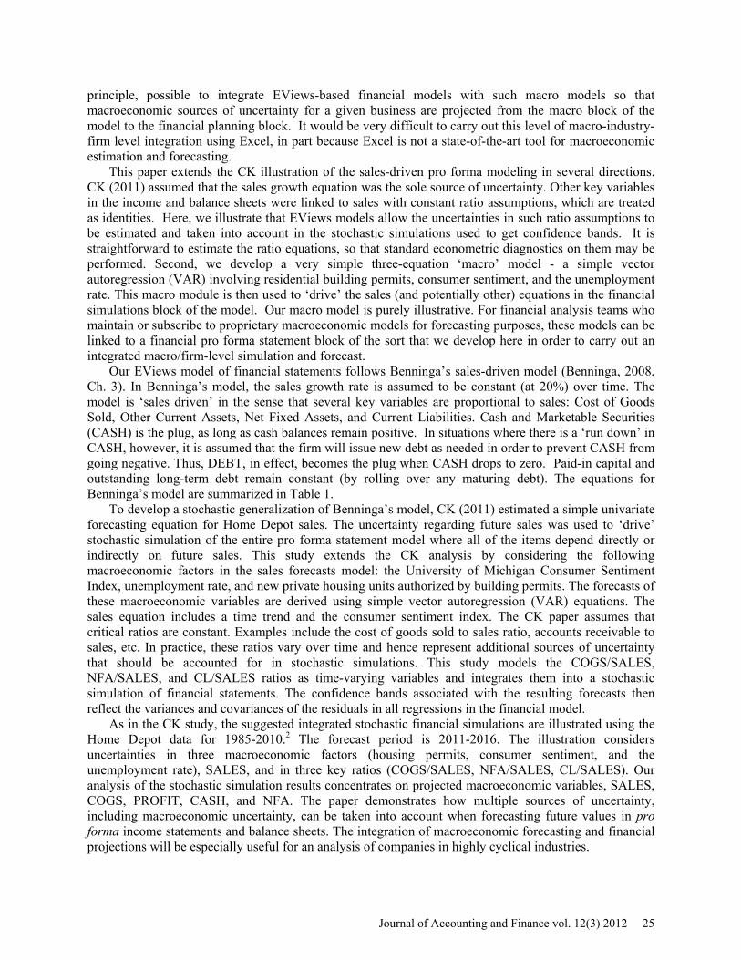
principle, possible to integrate EViews-based financial models with such macro models so that macroeconomic sources of uncertainty for a given business are projected from the macro block of the model to the financial planning block. It would be very difficult to carry out this level of macro-industry-firm level integration using Excel, in part because Excel is not a state-of-the-art tool for macroeconomic estimation and forecasting.

This paper extends the CK illustration of the sales-driven pro forma modeling in several directions. CK (2011) assumed that the sales growth equation was the sole source of uncertainty. Other key variables in the income and balance sheets were linked to sales with constant ratio assumptions, which are treated as identities. Here, we illustrate that EViews models allow the uncertainties in such ratio assumptions to be estimated and taken into account in the stochastic simulations used to get confidence bands. It is straightforward to estimate the ratio equations, so that standard econometric diagnostics on them may be performed. Second, we develop a very simple three-equation ‘macro’ model - a simple vector autoregression (VAR) involving residential building permits, consumer sentiment, and the unemployment rate. This macro module is then used to ‘drive’ the sales (and potentially other) equations in the financial simulations block of the model. Our macro model is purely illustrative. For financial analysis teams who maintain or subscribe to proprietary macroeconomic models for forecasting purposes, these models can be linked to a financial pro forma statement block of the sort that we develop here in order to carry out an integrated macro/firm-level simulation and forecast.

Our EViews model of financial statements follows Benninga’s sales-driven model (Benninga, 2008, Ch. 3). In Benninga’s model, the sales growth rate is assumed to be constant (at 20%) over time. The model is ‘sales driven’ in the sense that several key variables are proportional to sales: Cost of Goods Sold, Other Current Assets, Net Fixed Assets, and Current Liabilities. Cash and Marketable Securities (CASH) is the plug, as long as cash balances remain positive. In situations where there is a ‘run down’ in CASH, however, it is assumed that the firm will issue new debt as needed in order to prevent CASH from going negative. Thus, DEBT, in effect, becomes the plug when CASH drops to zero. Paid-in capital and outstanding long-term debt remain constant (by rolling over any maturing debt). The equations for Benninga’s model are summarized in Table 1.

To develop a stochastic generalization of Benninga’s model, CK (2011) estimated a simple univariate forecasting equation for Home Depot sales. The uncertainty regarding future sales was used to ‘drive’ stochastic simulation of the entire pro forma statement model where all of the items depend directly or indirectly on future sales. This study extends the CK analysis by considering the following macroeconomic factors in the sales forecasts model: the University of Michigan Consumer Sentiment Index, unemployment rate, and new private housing units authorized by building permits. The forecasts of these macroeconomic variables are derived using simple vector autoregression (VAR) equations. The sales equation includes a time trend and the consumer sentiment index. The CK paper assumes that critical ratios are constant. Examples include the cost of goods sold to sales ratio, accounts receivable to sales, etc. In practice, these ratios vary over time and hence represent additional sources of uncertainty that should be accounted for in stochastic simulations. This study models the COGS/SALES, NFA/SALES, and CL/SALES ratios as time-varying variables and integrates them into a stochastic simulation of financial statements. The confidence bands associated with the resulting forecasts then reflect the variances and covariances of the residuals in all regressions in the financial model.

As in the CK study, the suggested integrated stochastic financial simulations are illustrated using the Home Depot data for 1985-2010.2 The forecast period is 2011-2016. The illustration considers uncertainties in three macroeconomic factors (housing permits, consumer sentiment, and the unemployment rate), SALES, and in three key ratios (COGS/SALES, NFA/SALES, CL/SALES). Our analysis of the stochastic simulation results concentrates on projected macroeconomic variables, SALES, COGS, PROFIT, CASH, and NFA. The paper demonstrates how multiple sources of uncertainty, including macroeconomic uncertainty, can be taken into account when forecasting future values in pro forma income statements and balance sheets. The integration of macroeconomic forecasting and financial projections will be especially useful for an analysis of companies in highly cyclical industries.

Journal of Accounting and Finance vol. 12(3) 2012 25

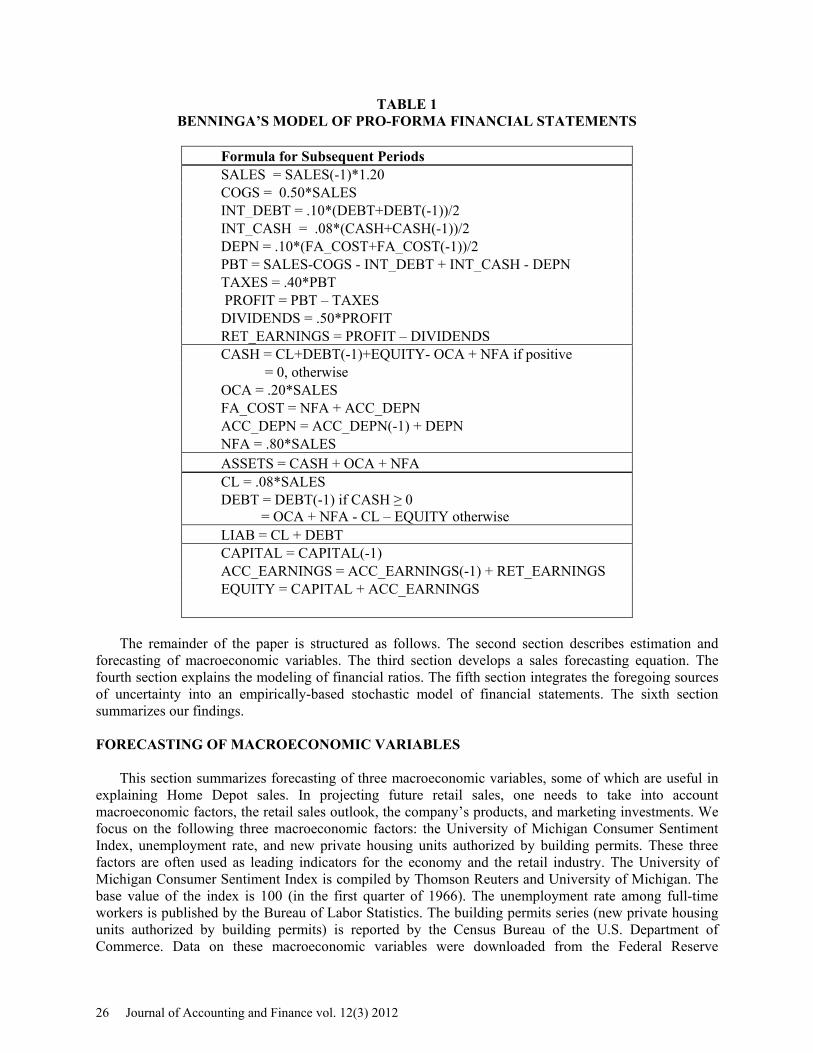
TABLE 1 BENNINGA’S MODEL OF PRO-FORMA FINANCIAL STATEMENTS

Formula for Subsequent Periods SALES = SALES(-1)*1.20 COGS = 0.50*SALES INT_DEBT = .10*(DEBT+DEBT(-1))/2 INT_CASH = .08*(CASH+CASH(-1))/2 DEPN = .10*(FA_COST+FA_COST(-1))/2 PBT = SALES-COGS - INT_DEBT + INT_CASH - DEPN TAXES = .40*PBT PROFIT = PBT – TAXES DIVIDENDS = .50*PROFIT RET_EARNINGS = PROFIT – DIVIDENDS CASH = CL+DEBT(-1)+EQUITY- OCA + NFA if positive = 0, otherwise OCA = .20*SALES FA_COST = NFA + ACC_DEPN ACC_DEPN = ACC_DEPN(-1) + DEPN NFA = .80*SALES ASSETS = CASH + OCA + NFA CL = .08*SALES DEBT = DEBT(-1) if CASH ≥ 0 = OCA + NFA - CL – EQUITY otherwise LIAB = CL + DEBT CAPITAL = CAPITAL(-1) ACC_EARNINGS = ACC_EARNINGS(-1) + RET_EARNINGS EQUITY = CAPITAL + ACC_EARNINGS

The remainder of the paper is structured as follows. The second section describes estimation and forecasting of macroeconomic variables. The third section develops a sales forecasting equation. The fourth section explains the modeling of financial ratios. The fifth section integrates the foregoing sources of uncertainty into an empirically-based stochastic model of financial statements. The sixth section summarizes our findings. FORECASTING OF MACROECONOMIC VARIABLES

This section summarizes forecasting of three macroeconomic variables, some of which are useful in explaining Home Depot sales. In projecting future retail sales, one needs to take into account macroeconomic factors, the retail sales outlook, the company’s products, and marketing investments. We focus on the following three macroeconomic factors: the University of Michigan Consumer Sentiment Index, unemployment rate, and new private housing units authorized by building permits. These three factors are often used as leading indicators for the economy and the retail industry. The University of Michigan Consumer Sentiment Index is compiled by Thomson Reuters and University of Michigan. The base value of the index is 100 (in the first quarter of 1966). The unemployment rate among full-time workers is published by the Bureau of Labor Statistics. The building permits series (new private housing units authorized by building permits) is reported by the Census Bureau of the U.S. Department of Commerce. Data on these macroeconomic variables were downloaded from the Federal Reserve


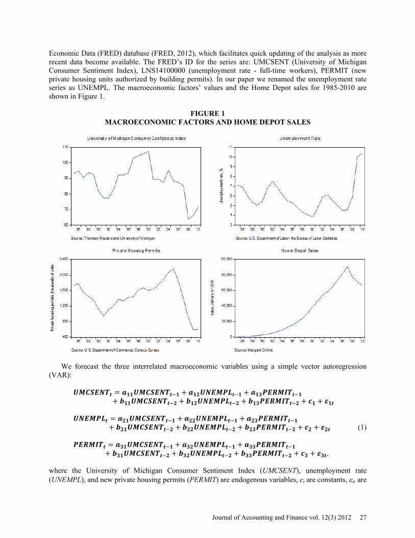
Economic Data (FRED) database (FRED, 2012), which facilitates quick updating of the analysis as more recent data become available. The FRED’s ID for the series are: UMCSENT (University of Michigan Consumer Sentiment Index), LNS14100000 (unemployment rate - full-time workers), PERMIT (new private housing units authorized by building permits). In our paper we renamed the unemployment rate series as UNEMPL. The macroeconomic factors’ values and the Home Depot sales for 1985-2010 are shown in Figure 1.

FIGURE 1

MACROECONOMIC FACTORS AND HOME DEPOT SALES

We forecast the three interrelated macroeconomic variables using a simple vector autoregression

(VAR): 𝑼𝑴𝑪𝑺𝑬𝑵𝑻𝒕 = 𝒂𝟏𝟏𝑼𝑴𝑪𝑺𝑬𝑵𝑻𝒕−𝟏 + 𝒂𝟏𝟐𝑼𝑵𝑬𝑴𝑷𝑳𝒕−𝟏 + 𝒂𝟏𝟑𝑷𝑬𝑹𝑴𝑰𝑻𝒕−𝟏 + 𝒃𝟏𝟏𝑼𝑴𝑪𝑺𝑬𝑵𝑻𝒕−𝟐 + 𝒃𝟏𝟐𝑼𝑵𝑬𝑴𝑷𝑳𝒕−𝟐 + 𝒃𝟏𝟑𝑷𝑬𝑹𝑴𝑰𝑻𝒕−𝟐 + 𝒄𝟏 + 𝜺𝟏𝒕 𝑼𝑵𝑬𝑴𝑷𝑳𝒕 = 𝒂𝟐𝟏𝑼𝑴𝑪𝑺𝑬𝑵𝑻𝒕−𝟏 + 𝒂𝟐𝟐𝑼𝑵𝑬𝑴𝑷𝑳𝒕−𝟏 + 𝒂𝟐𝟑𝑷𝑬𝑹𝑴𝑰𝑻𝒕−𝟏 + 𝒃𝟐𝟏𝑼𝑴𝑪𝑺𝑬𝑵𝑻𝒕−𝟐 + 𝒃𝟐𝟐𝑼𝑵𝑬𝑴𝑷𝑳𝒕−𝟐 + 𝒃𝟐𝟑𝑷𝑬𝑹𝑴𝑰𝑻𝒕−𝟐 + 𝒄𝟐 + 𝜺𝟐𝒕 (1) 𝑷𝑬𝑹𝑴𝑰𝑻𝒕 = 𝒂𝟑𝟏𝑼𝑴𝑪𝑺𝑬𝑵𝑻𝒕−𝟏 + 𝒂𝟑𝟐𝑼𝑵𝑬𝑴𝑷𝑳𝒕−𝟏 + 𝒂𝟑𝟑𝑷𝑬𝑹𝑴𝑰𝑻𝒕−𝟏 + 𝒃𝟑𝟏𝑼𝑴𝑪𝑺𝑬𝑵𝑻𝒕−𝟐 + 𝒃𝟑𝟐𝑼𝑵𝑬𝑴𝑷𝑳𝒕−𝟐 + 𝒃𝟑𝟑𝑷𝑬𝑹𝑴𝑰𝑻𝒕−𝟐 + 𝒄𝟑 + 𝜺𝟑𝒕,

where the University of Michigan Consumer Sentiment Index (UMCSENT), unemployment rate (UNEMPL), and new private housing permits (PERMIT) are endogenous variables, ci are constants, εit are


innovations, i =1, 2, 3, t = 1985,…, 2010. Each endogenous variable is a function of lagged values of all three endogenous variables. The estimation results are displayed in Table 2. Each column in the table represents an equation in the VAR system (1). The reported numbers are estimated coefficients and the t-statistics (in square brackets). In the Consumer Sentiment Index equation, the coefficients of the first lag

TABLE 2 VAR COEFFICIENT ESTIMATES FOR MACROECONOMIC FACTORS

Explanatory Variables (Lagged Dependent Variables)

Dependent Variables

UMCSENT UNEMPL PERMIT UMCSENT(-1) 0.568 -0.077 3.819 [ 2.290] [-4.248] [ 0.737] UMCSENT(-2) 0.297 0.036 1.729 [ 0.960] [ 1.584] [ 0.268] UNEMPL(-1) 0.574 0.716 63.000 [ 0.240] [ 4.092] [ 1.265] UNEMPL(-2) 1.955 -0.372 -54.261 [ 0.962] [-2.498] [-1.279] PERMIT(-1) 0.018 -0.002 1.585 [ 1.926] [-2.365] [ 7.983] PERMIT(-2) -0.023 0.001 -0.844 [-2.342] [ 1.121] [-4.055] C 5.178 8.652 -181.789 [ 0.124] [ 2.824] [-0.208] Adjusted R-squared 0.68 0.91 0.89

of the index and the second lag of private housing permits are statistically significant. In the unemployment rate equation, the coefficients of first lag of the Consumer Sentiment Index, the first and second lags of the unemployment rate, the first lag of the housing permits, and the constant are statistically significant. In the private housing permits equation, the coefficients of its first and second lag are statistically significant. The adjusted R2 values for each equation are provided in the bottom row. Granger causality test results are provided in Table 3. The test results show that housing permits and unemployment rate Granger cause the Consumer Sentiment Index, the Consumer Sentiment Index and housing permits Granger cause the unemployment rate, the unemployment rate and the Consumer Sentiment Index do not Granger cause the housing permits.

The next section takes into account impacts of the macroeconomic variables (Consumer Confidence Index, unemployment factor, and housing permits) on the Home Depot sales forecasts.


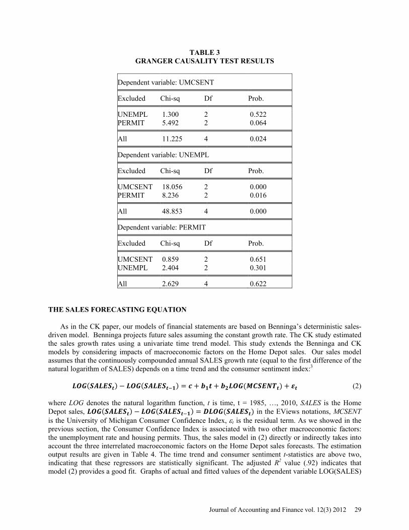
TABLE 3 GRANGER CAUSALITY TEST RESULTS

Dependent variable: UMCSENT Excluded Chi-sq Df Prob. UNEMPL 1.300 2 0.522 PERMIT 5.492 2 0.064 All 11.225 4 0.024 Dependent variable: UNEMPL Excluded Chi-sq Df Prob. UMCSENT 18.056 2 0.000 PERMIT 8.236 2 0.016 All 48.853 4 0.000 Dependent variable: PERMIT Excluded Chi-sq Df Prob. UMCSENT 0.859 2 0.651 UNEMPL 2.404 2 0.301 All 2.629 4 0.622

THE SALES FORECASTING EQUATION

As in the CK paper, our models of financial statements are based on Benninga’s deterministic sales-driven model. Benninga projects future sales assuming the constant growth rate. The CK study estimated the sales growth rates using a univariate time trend model. This study extends the Benninga and CK models by considering impacts of macroeconomic factors on the Home Depot sales. Our sales model assumes that the continuously compounded annual SALES growth rate (equal to the first difference of the natural logarithm of SALES) depends on a time trend and the consumer sentiment index:3

𝑳𝑶𝑮(𝑺𝑨𝑳𝑬𝑺𝒕) − 𝑳𝑶𝑮(𝑺𝑨𝑳𝑬𝑺𝒕−𝟏) = 𝒄 + 𝒃𝟏𝒕 + 𝒃𝟐𝑳𝑶𝑮(𝑴𝑪𝑺𝑬𝑵𝑻𝒕) + 𝜺𝒕 (2) where LOG denotes the natural logarithm function, t is time, t = 1985, …, 2010, SALES is the Home Depot sales, 𝑳𝑶𝑮(𝑺𝑨𝑳𝑬𝑺𝒕) − 𝑳𝑶𝑮(𝑺𝑨𝑳𝑬𝑺𝒕−𝟏) = 𝑫𝑳𝑶𝑮(𝑺𝑨𝑳𝑬𝑺𝒕) in the EViews notations, MCSENT is the University of Michigan Consumer Confidence Index, εt is the residual term. As we showed in the previous section, the Consumer Confidence Index is associated with two other macroeconomic factors: the unemployment rate and housing permits. Thus, the sales model in (2) directly or indirectly takes into account the three interrelated macroeconomic factors on the Home Depot sales forecasts. The estimation output results are given in Table 4. The time trend and consumer sentiment t-statistics are above two, indicating that these regressors are statistically significant. The adjusted R2 value (.92) indicates that model (2) provides a good fit. Graphs of actual and fitted values of the dependent variable LOG(SALES)


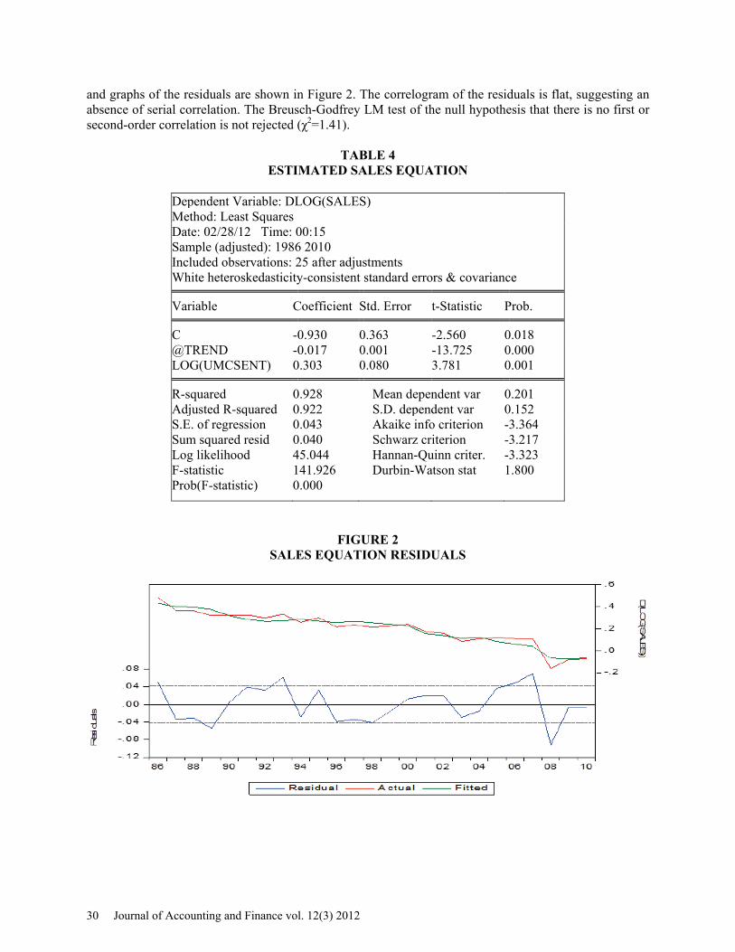
and graphs of the residuals are shown in Figure 2. The correlogram of the residuals is flat, suggesting an absence of serial correlation. The Breusch-Godfrey LM test of the null hypothesis that there is no first or second-order correlation is not rejected (χ2=1.41).

TABLE 4 ESTIMATED SALES EQUATION

Dependent Variable: DLOG(SALES) Method: Least Squares Date: 02/28/12 Time: 00:15 Sample (adjusted): 1986 2010 Included observations: 25 after adjustments White heteroskedasticity-consistent standard errors & covariance Variable Coefficient Std. Error t-Statistic Prob. C -0.930 0.363 -2.560 0.018 @TREND -0.017 0.001 -13.725 0.000 LOG(UMCSENT) 0.303 0.080 3.781 0.001 R-squared 0.928 Mean dependent var 0.201 Adjusted R-squared 0.922 S.D. dependent var 0.152 S.E. of regression 0.043 Akaike info criterion -3.364 Sum squared resid 0.040 Schwarz criterion -3.217 Log likelihood 45.044 Hannan-Quinn criter. -3.323 F-statistic 141.926 Durbin-Watson stat 1.800 Prob(F-statistic) 0.000

FIGURE 2 SALES EQUATION RESIDUALS


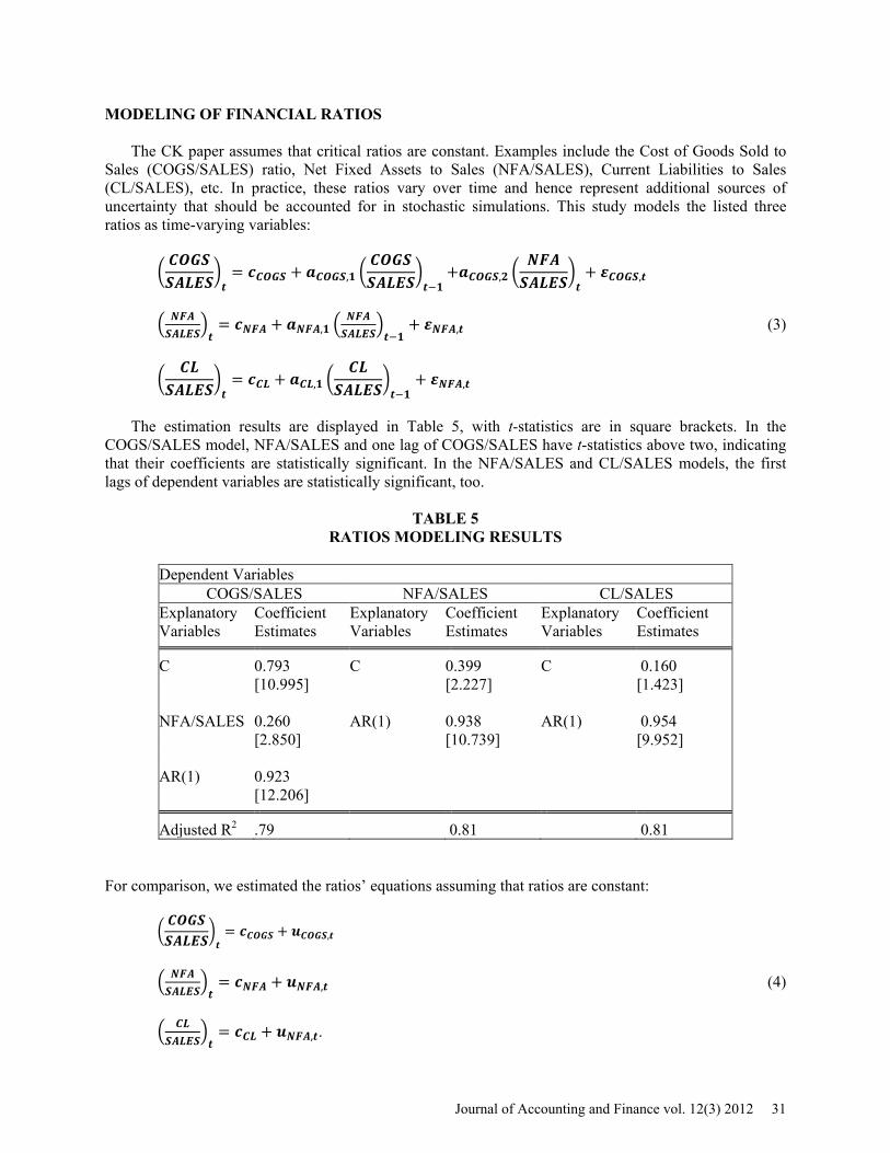
MODELING OF FINANCIAL RATIOS The CK paper assumes that critical ratios are constant. Examples include the Cost of Goods Sold to

Sales (COGS/SALES) ratio, Net Fixed Assets to Sales (NFA/SALES), Current Liabilities to Sales (CL/SALES), etc. In practice, these ratios vary over time and hence represent additional sources of uncertainty that should be accounted for in stochastic simulations. This study models the listed three ratios as time-varying variables:

�𝑪𝑶𝑮𝑺𝑺𝑨𝑳𝑬𝑺

�𝒕

= 𝒄𝑪𝑶𝑮𝑺 + 𝒂𝑪𝑶𝑮𝑺,𝟏 �𝑪𝑶𝑮𝑺𝑺𝑨𝑳𝑬𝑺

�𝒕−𝟏

+𝒂𝑪𝑶𝑮𝑺,𝟐 �𝑵𝑭𝑨𝑺𝑨𝑳𝑬𝑺

�𝒕

+ 𝜺𝑪𝑶𝑮𝑺,𝒕

� 𝑵𝑭𝑨𝑺𝑨𝑳𝑬𝑺

�𝒕

= 𝒄𝑵𝑭𝑨 + 𝒂𝑵𝑭𝑨,𝟏 �𝑵𝑭𝑨𝑺𝑨𝑳𝑬𝑺

�𝒕−𝟏

+ 𝜺𝑵𝑭𝑨,𝒕 (3)

�𝑪𝑳

𝑺𝑨𝑳𝑬𝑺�𝒕

= 𝒄𝑪𝑳 + 𝒂𝑪𝑳,𝟏 �𝑪𝑳

𝑺𝑨𝑳𝑬𝑺�𝒕−𝟏

+ 𝜺𝑵𝑭𝑨,𝒕

The estimation results are displayed in Table 5, with t-statistics are in square brackets. In the

COGS/SALES model, NFA/SALES and one lag of COGS/SALES have t-statistics above two, indicating that their coefficients are statistically significant. In the NFA/SALES and CL/SALES models, the first lags of dependent variables are statistically significant, too.

TABLE 5 RATIOS MODELING RESULTS

Dependent Variables

COGS/SALES NFA/SALES CL/SALES Explanatory Variables

Coefficient Estimates

Explanatory Variables


Explanatory Variables


C 0.793 C 0.399 C 0.160 [10.995] [2.227] [1.423] NFA/SALES 0.260 AR(1) 0.938 AR(1) 0.954 [2.850] [10.739] [9.952] AR(1) 0.923 [12.206] Adjusted R2 .79 0.81 0.81

For comparison, we estimated the ratios’ equations assuming that ratios are constant:

�𝑪𝑶𝑮𝑺𝑺𝑨𝑳𝑬𝑺

�𝒕

= 𝒄𝑪𝑶𝑮𝑺 + 𝒖𝑪𝑶𝑮𝑺,𝒕

� 𝑵𝑭𝑨𝑺𝑨𝑳𝑬𝑺

�𝒕

= 𝒄𝑵𝑭𝑨 + 𝒖𝑵𝑭𝑨,𝒕 (4) � 𝑪𝑳𝑺𝑨𝑳𝑬𝑺

�𝒕

= 𝒄𝑪𝑳 + 𝒖𝑵𝑭𝑨,𝒕.


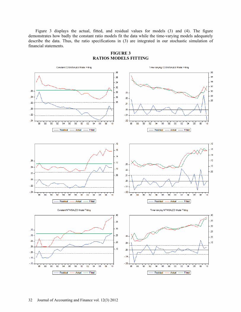
Figure 3 displays the actual, fitted, and residual values for models (3) and (4). The figure demonstrates how badly the constant ratio models fit the data while the time-varying models adequately describe the data. Thus, the ratio specifications in (3) are integrated in our stochastic simulation of financial statements.

FIGURE 3 RATIOS MODELS FITTING


INTEGRATED STOCHASTIC MODEL OF FINANCIAL STATEMENTS This section describes integration of the macroeconomic forecasts, sales forecasts, the ratios’ models,

and the financial statement model. We wrote a program that automates the EViews implementation of the integrated stochastic financial modeling for Home Depot. The program creates an annual frequency workfile with the time range 1985-2016 (the historical and forecast periods), fetches the macroeconomic series from the Federal Reserve Economic Data (FRED) database, imports the balance sheet and the income statement for 1985-2010 from Excel spreadsheets, runs a vector autoregression (VAR) for the macroeconomic factors, estimates equations for uncertain financial variables (SALES, COGS, NFA, CL), creates and solves the stochastic financial statement model. The model integrates forecasts for the Consumer Sentiment Index, unemployment rate, and housing permits by adding a link to their vector autoregression in the workfile (type in the model text a colon followed by a name of a vector autoregression. For example, :VAR_MACRO). The stochastic model has links to sales and ratios’ forecasting equations (type in the model text a colon followed by a name of the regression. For example, :EQ_SALES, :EQ_COGS, :EQ_NFA, :EQ_CL). We add the @IDENTITY specification to other equations in the MODEL object, which are not estimated. (Otherwise, EViews will attempt to include these equations’ uncertainty in the stochastic forecast, even when the equations are not explicitly estimated.) The integrated model equations are provided in Table 6. Our solution of the model uses the stochastic simulation features in the EViews MODEL to forecast macroeconomic factors, sales and all of the other income and balance sheet items into the future. Through Monte Carlo simulation methods (using 10,000 stochastic repetitions), the means and the 67% confidence bands for each variable at each future dates are obtained.

TABLE 6 EVIEWS MODEL EQUATIONS

' Macroeconomic Variables :VAR_MACRO ' Income Statement :EQ_SALES :EQ_COGS @IDENTITY INT_DEBT = (DEBT(-1) + DEBT) / 2 * 0.07 @IDENTITY INT_CASH = (CASH(-1) + CASH) / 2 * 0.01 @IDENTITY PBT = SALES - COGS - INT_DEBT + INT_CASH - DEPN @IDENTITY TAXES = 0.36 * PBT @IDENTITY PROFIT = PBT - TAXES @IDENTITY DIVIDENDS = 0.58 * PROFIT @IDENTITY RET_EARNINGS = PROFIT - DIVIDENDS ' Balance Sheet ' create a dummy variable that is 1 if CASH would be negative in the absence of additional debt, and zero otherwise. ' Using EViews syntax, everything after the equal sign is treated as a logical condition. If it holds, DUM is 1; zero otherwise. @IDENTITY DUM = - OCA - NFA + CL + DEBT(-1) + EQUITY < 0 ' define CASH as the balance sheet plug, if positive, and ZERO otherwise by creative use of the dummy: @IDENTITY CASH = (- OCA - NFA + CL + DEBT(-1) + EQUITY) * (1 - DUM) @IDENTITY OCA = 0.18 * SALES :EQ_NFA @IDENTITY DEPN = 0.05 * (FA_COST(-1) + FA_COST) / 2 @IDENTITY ACC_DEPN = ACC_DEPN(-1) + DEPN @IDENTITY FA_COST = NFA + ACC_DEPN


@IDENTITY ASSETS = CASH + OCA + NFA :EQ_CL ' when DUM=1, cash is negative, so DEBT is the plug; when DUM=0, cash is positive, so debt is unchanged from the previous period @IDENTITY DEBT = (OCA + NFA - CL - EQUITY) * DUM + DEBT(-1) * (1 - DUM) @IDENTITY LIAB = DEBT + CL @IDENTITY CAPITAL = CAPITAL(-1) @IDENTITY MINORITY = MINORITY(-1) @IDENTITY TSTOCK = TSTOCK(-1) @IDENTITY ACC_EARNINGS = ACC_EARNINGS (-1) + RET_EARNINGS @IDENTITY EQUITY = CAPITAL + ACC_EARNINGS + MINORITY + TSTOCK

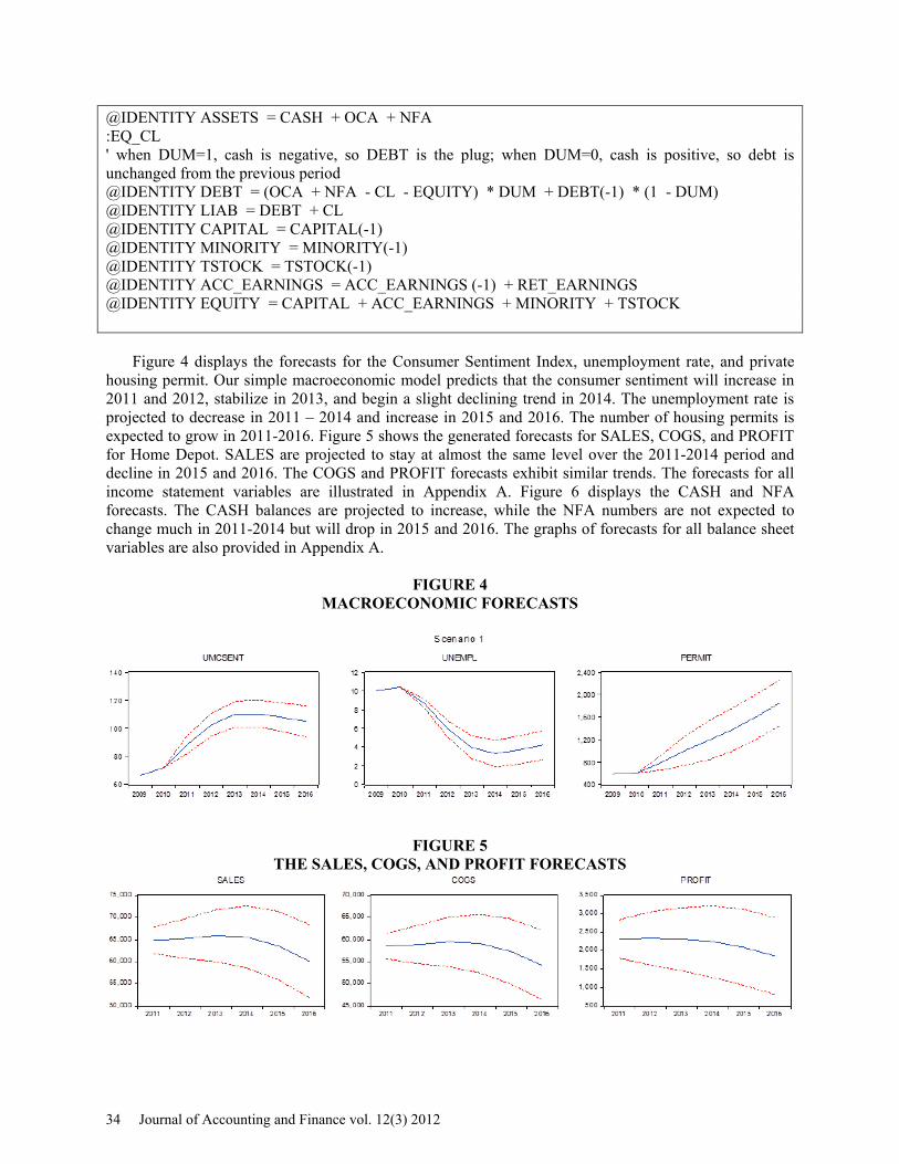
Figure 4 displays the forecasts for the Consumer Sentiment Index, unemployment rate, and private housing permit. Our simple macroeconomic model predicts that the consumer sentiment will increase in 2011 and 2012, stabilize in 2013, and begin a slight declining trend in 2014. The unemployment rate is projected to decrease in 2011 – 2014 and increase in 2015 and 2016. The number of housing permits is expected to grow in 2011-2016. Figure 5 shows the generated forecasts for SALES, COGS, and PROFIT for Home Depot. SALES are projected to stay at almost the same level over the 2011-2014 period and decline in 2015 and 2016. The COGS and PROFIT forecasts exhibit similar trends. The forecasts for all income statement variables are illustrated in Appendix A. Figure 6 displays the CASH and NFA forecasts. The CASH balances are projected to increase, while the NFA numbers are not expected to change much in 2011-2014 but will drop in 2015 and 2016. The graphs of forecasts for all balance sheet variables are also provided in Appendix A.

FIGURE 4 MACROECONOMIC FORECASTS

FIGURE 5

THE SALES, COGS, AND PROFIT FORECASTS


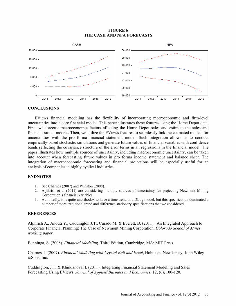
FIGURE 6 THE CASH AND NFA FORECASTS

CONCLUSIONS

EViews financial modeling has the flexibility of incorporating macroeconomic and firm-level uncertainties into a core financial model. This paper illustrates these features using the Home Depot data. First, we forecast macroeconomic factors affecting the Home Depot sales and estimate the sales and financial ratios’ models. Then, we utilize the EViews features to seamlessly link the estimated models for uncertainties with the pro forma financial statement model. Such integration allows us to conduct empirically-based stochastic simulations and generate future values of financial variables with confidence bands reflecting the covariance structure of the error terms in all regressions in the financial model. The paper illustrates how multiple sources of uncertainty, including macroeconomic uncertainty, can be taken into account when forecasting future values in pro forma income statement and balance sheet. The integration of macroeconomic forecasting and financial projections will be especially useful for an analysis of companies in highly cyclical industries. ENDNOTES

1. See Charnes (2007) and Winston (2008). 2. Aljihrish et al (2011) are considering multiple sources of uncertainty for projecting Newmont Mining

Corporation’s financial variables. 3. Admittedly, it is quite unorthodox to have a time trend in a DLog model, but this specification dominated a

number of more traditional trend and difference stationary specifications that we considered. REFERENCES Aljihrish A., Anouti Y., Cuddington J.T., Curado M. & Everett, B. (2011). An Integrated Approach to Corporate Financial Planning: The Case of Newmont Mining Corporation. Colorado School of Mines working paper. Benninga, S. (2008). Financial Modeling. Third Edition, Cambridge, MA: MIT Press. Charnes, J. (2007). Financial Modeling with Crystal Ball and Excel, Hoboken, New Jersey: John Wiley &Sons, Inc. Cuddington, J.T. & Khindanova, I. (2011). Integrating Financial Statement Modeling and Sales Forecasting Using EViews. Journal of Applied Business and Economics, 12, (6), 100-120.


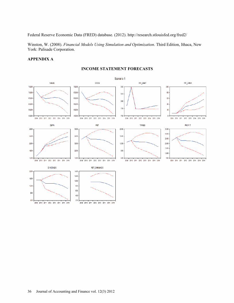
Federal Reserve Economic Data (FRED) database. (2012). http://research.stlouisfed.org/fred2/ Winston, W. (2008). Financial Models Using Simulation and Optimization. Third Edition, Ithaca, New York: Palisade Corporation. APPENDIX A

INCOME STATEMENT FORECASTS


THE BALANCE SHEET FORECASTS


Documents

Incorporating Macroeconomic and Firm-Level Uncertainties ... · PDF fileIncorporating Macroeconomic and Firm-Level Uncertainties in Stochastic Pro-Forma Financial Modeling ... Our