Incorporating Satellite Precipitation Estimates into a

Article

Incorporating Satellite Precipitation Estimates into a Radar-Gage Multi-Sensor Precipitation Estimation Algorithm Yuxiang He 1,2, *, Yu Zhang 1, Robert Kuligowski 3, Robert Cifelli 4 and David Kitzmiller 1

1 National Water Center (NWC), National Weather Service (NWS), NOAA, Silver Spring, ML 20910, USA; [email protected] (Y.Z.); [email protected] (D.K.)

2 University Corporation for Atmospheric Research (UCAR), Boulder, CO 80307, USA 3 NOAA/NESDIS/Center for Satellite Applications and Research, College Park, ML 20740, USA;

[email protected] 4 Physical Sciences Division, NOAA/Earth System Research Laboratory, Boulder, CO 80305, USA;

[email protected] * Correspondence: [email protected]; Tel.: +1-301-427-9519

Abstract: This paper presents a new and enhanced fusion module for the Multi-Sensor Precipitation Estimator (MPE) that would objectively blend real-time satellite quantitative precipitation estimates (SQPE) with radar and gauge estimates. This module consists of a preprocessor that mitigates systematic bias in SQPE, and a two-way blending routine that statistically fuses adjusted SQPE with radar estimates. The preprocessor not only corrects systematic bias in SQPE, but also improves the spatial distribution of precipitation based on SQPE and makes it closely resemble that of radar-based observations. It uses a more sophisticated radar-satellite merging technique to blend preprocessed datasets, and provides a better overall QPE product. The performance of the new satellite-radar-gauge blending module is assessed using independent rain gauge data over a 5-year period between 2003-2007, and the assessment evaluates the accuracy of newly developed satellite-radar-gauge (SRG) blended products versus that of radar-gauge products (which represents MPE algorithm currently used in the NWS operations) over two regions: I) inside radar effective coverage and II) immediately outside radar coverage. The outcomes of the evaluation indicate a) ingest of SQPE over areas within effective radar coverage improve the quality of QPE by mitigating the errors in radar estimates in region I; and b) blending of radar, gauge, and satellite estimates over region II leads to reduction of errors relative to bias-corrected SQPE. In addition, the new module alleviates the discontinuities along the boundaries of radar effective coverage otherwise seen when SQPE is used directly to fill the areas outside of effective radar coverage.

Keywords: multi-sensor fusion; satellite; radar; precipitation

1. Introduction

Precipitation estimation is critical in hydrology and weather forecasting over a wide range of spatiotemporal scales. For example, in the National Oceanic and Atmospheric Administration (NOAA)/National Weather Service’s (NWS) flash flood and river forecast operations, quantitative precipitation estimates (QPEs) are one of the major inputs to the models and serve as a basis for watches and warnings[1,2]. At present, operational QPEs are produced at NWS River Forecast Centers (RFCs) based primarily on rain gauge reports and the observations of Weather Surveillance Radars-1988 Doppler (WSR-88D) through the Multi-sensor Precipitation Estimator (MPE)[3]. MPE consists of an interactive interface and a suite of automated algorithms, including those for correcting mean-field and range-dependent errors in radar, and one for blending radar and point gauge data.

Over the past two decades, a number of satellite-based QPE (SQPE) algorithms have been developed for applications in many areas of hydrology. Satellite-based precipitation estimates have both advantages and disadvantages compared to ground-based estimates. On the negative side,

Preprints (www.preprints.org) | NOT PEER-REVIEWED | Posted: 27 September 2017 doi:10.20944/preprints201709.0134.v1

© 2017 by the author(s). Distributed under a Creative Commons CC BY license.

Peer-reviewed version available at Remote Sens. 2018, 10, 106; doi:10.3390/rs10010106

http://dx.doi.org/10.20944/preprints201709.0134.v1

http://creativecommons.org/licenses/by/4.0/

http://dx.doi.org/10.3390/rs10010106

2 of 25

SQPE is limited by overpass frequency for microwave-based retrievals and a lack of robust correlation between cloud top brightness temperature and surface rainfall for geostationary platforms. However, satellite platforms also have inherent advantages compared to ground-based sensors because their views are not subject to terrain-based blockages or discontinuities along political boundaries due to lack of data, instrumentation differences or data embargo. In particular, The Geostationary Operational Environmental Satellite-R Series (GOES-R) products will improve precipitation estimation quality utilizing Lightning Imaging Sensor(LIS) and/or the higher temporal resolution that can fill in gaps between microwave overpasses. As a result, SQPEs are particularly useful in areas with few ground gauges, under radar gaps, and along national borders. Some of the most widely used algorithms retrieved rain rate using (IR) brightness temperature observations from geostationary platforms, which have short latency and wide spatial-temporal coverage, and more accurate estimates from microwave sensors onboard lower-orbit satellites. These include the Climate Prediction C-Morphing (CMORPH)[4,5], TRMM Multi-Sensor Precipitation Analysis (TMPA) and Global Precipitation Measurement Integrated Multi-satellitE Retrievals for GPM (IMERG)[6,7]; and the Self-Calibrating Multivariate Precipitation Retrieval (SCAMPR)[8-11]. Recent advances in precipitation retrieval and calibration algorithms have led to substantial improvements to the latency, resolution and accuracy of SQPEs. For example, the recently launched Geostationary Operational Environmental Satellite (GOES)-16 satellite tripled the number of spectral bands offered by the previous GOES, which has the potential to further enhance the detection of precipitation. These enhancements offer new opportunities of using SQPEs to address the quality issue of radar QPE arising from factors such as overshooting, beam widening, and partial beam blockage.

In order to address inadequacies in the coverage of radar and gauges, the MPE has the capability to display the SQPE as a separate field for qualitative comparison, or SQPE field can be cut and pasted into any other MPE products through the Graphical User Interface, also the satellite QPE based on the Hydro-Estimator (H-E) algorithm[12] has been introduced to NWS operations[13], which however was limited by SQPE quality and the uneven radar errors’ distribution, it needs to be further improved and enhanced. As forecasting missions require seamless precipitation maps, a new module was developed for the MPE to bias-correct SQPE and to use the results to fill the radar gaps. The resulting products have been used operationally in a few NWS RFCs, most notably the West Gulf RFC (WGRFC) whose service area covers the drainage of the Rio Grande and requires SQPE for filling the radar-gauge gaps across the Mexico-US border. Though this MPE satellite-radar-gauge (SRG) module has been found to be overall satisfactory by forecasters, it is limited by design for filling radar coverage gaps and unable to fully harness the complementary skill of SQPE within the areas of the effective radar coverage. In addition, simple gap-filling operations often create discontinuities along the borders of the effective radar coverage areas due to dissimilarities in the storm configurations as seen by satellite-borne sensors and ground-based radar.

In this work, we develop an enhanced SRG fusion module that goes beyond simple gap filling, and seeks to blend the radar, gauge and satellite QPE over regions within the effective radar coverage and over areas immediately outside the effective radar coverage. In this way, the algorithm more effectively takes advantage of the different sensor inputs when and where they are available. This module consists of a preprocessor that employs local bias correction to mitigate systematic biases in the SQPE, and an advanced double two-way co-Kriging mechanism to objectively blend radar, gauge and satellite using an RQI-like (RQI: Radar Quality Index) mechanism to determine weighting of satellite data over locations. This new module is written in object-oriented C++ programming language and can run in standalone mode. It can be easily adopted for real-time integration of radar, gauge and satellite observations.

The remainder of the paper is structured as follows. Section 2 reviews the existing MPE SQPE module and describes the new module and its underlying mechanisms. Section 3 describes the evaluation methodology for assessing the merits of the enhanced module. Section 4 presents the experimental design and data. Section 5 discusses the findings and discussions. Section 6 is the summary and conclusions of this work.




http://dx.doi.org/10.3390/rs10010106

3 of 25

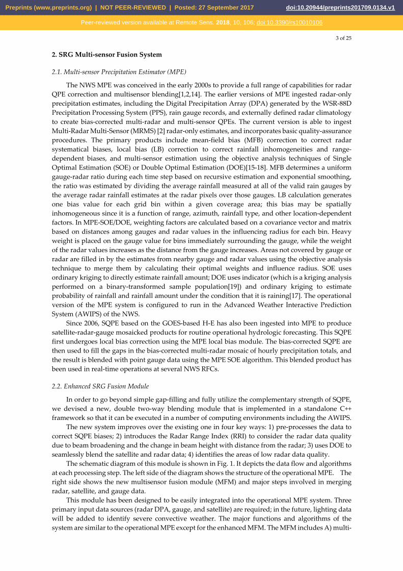
2. SRG Multi-sensor Fusion System

2.1. Multi-sensor Precipitation Estimator (MPE)

The NWS MPE was conceived in the early 2000s to provide a full range of capabilities for radar QPE correction and multisensor blending[1,2,14]. The earlier versions of MPE ingested radar-only precipitation estimates, including the Digital Precipitation Array (DPA) generated by the WSR-88D Precipitation Processing System (PPS), rain gauge records, and externally defined radar climatology to create bias-corrected multi-radar and multi-sensor QPEs. The current version is able to ingest Multi-Radar Multi-Sensor (MRMS) [2] radar-only estimates, and incorporates basic quality-assurance procedures. The primary products include mean-field bias (MFB) correction to correct radar systematical biases, local bias (LB) correction to correct rainfall inhomogeneities and range-dependent biases, and multi-sensor estimation using the objective analysis techniques of Single Optimal Estimation (SOE) or Double Optimal Estimation (DOE)[15-18]. MFB determines a uniform gauge-radar ratio during each time step based on recursive estimation and exponential smoothing, the ratio was estimated by dividing the average rainfall measured at all of the valid rain gauges by the average radar rainfall estimates at the radar pixels over those gauges. LB calculation generates one bias value for each grid bin within a given coverage area; this bias may be spatially inhomogeneous since it is a function of range, azimuth, rainfall type, and other location-dependent factors. In MPE-SOE/DOE, weighting factors are calculated based on a covariance vector and matrix based on distances among gauges and radar values in the influencing radius for each bin. Heavy weight is placed on the gauge value for bins immediately surrounding the gauge, while the weight of the radar values increases as the distance from the gauge increases. Areas not covered by gauge or radar are filled in by the estimates from nearby gauge and radar values using the objective analysis technique to merge them by calculating their optimal weights and influence radius. SOE uses ordinary kriging to directly estimate rainfall amount; DOE uses indicator (which is a kriging analysis performed on a binary-transformed sample population[19]) and ordinary kriging to estimate probability of rainfall and rainfall amount under the condition that it is raining[17]. The operational version of the MPE system is configured to run in the Advanced Weather Interactive Prediction System (AWIPS) of the NWS.

Since 2006, SQPE based on the GOES-based H-E has also been ingested into MPE to produce satellite-radar-gauge mosaicked products for routine operational hydrologic forecasting. This SQPE first undergoes local bias correction using the MPE local bias module. The bias-corrected SQPE are then used to fill the gaps in the bias-corrected multi-radar mosaic of hourly precipitation totals, and the result is blended with point gauge data using the MPE SOE algorithm. This blended product has been used in real-time operations at several NWS RFCs.

2.2. Enhanced SRG Fusion Module

In order to go beyond simple gap-filling and fully utilize the complementary strength of SQPE, we devised a new, double two-way blending module that is implemented in a standalone C++ framework so that it can be executed in a number of computing environments including the AWIPS.

The new system improves over the existing one in four key ways: 1) pre-processes the data to correct SQPE biases; 2) introduces the Radar Range Index (RRI) to consider the radar data quality due to beam broadening and the change in beam height with distance from the radar; 3) uses DOE to seamlessly blend the satellite and radar data; 4) identifies the areas of low radar data quality.

The schematic diagram of this module is shown in Fig. 1. It depicts the data flow and algorithms at each processing step. The left side of the diagram shows the structure of the operational MPE. The right side shows the new multisensor fusion module (MFM) and major steps involved in merging radar, satellite, and gauge data.

This module has been designed to be easily integrated into the operational MPE system. Three primary input data sources (radar DPA, gauge, and satellite) are required; in the future, lighting data will be added to identify severe convective weather. The major functions and algorithms of the system are similar to the operational MPE except for the enhanced MFM. The MFM includes A) multi-




http://dx.doi.org/10.3390/rs10010106

4 of 25

radar mosaicking, B) mean field bias correction, C) local bias correction, and D) double two-way multisensor blending. The enhanced MFM includes a procedure to identify whether radar echoes are inside or outside the area where the radar beam is below the melting layer. If the echoes are outside this area, it determines how far away they are from the area where the radar beam is below the melting layer and computes the radar range index (RRI). RRI can be considered as a simplified version of radar quality index (RQI) which integrates additional information (e.g., blockages, depth of the bright band layer) to determine radar quality[20]. The reason we employ RRI is that the method can be applied to existing DPA products, for which RQI is not available.

After computing the RRI, the modified double optimal estimation (MDOE) is used to blend radar and satellite QPE. Before this step, local bias correction is used to correct satellite data (Fig. 1. E). MDOE, the local bias correction, and the RRI method are described in the following section.

2.3. Local Bias Correction of Satellite Quantitative Precipitation

Before blending the satellite rainfall with the radar-gauge MPE fusion products as described above, the satellite rainfall needs to be corrected with respect to in-situ gauge data. This is done using a local bias correction algorithm in [15]. The correction problem is formulated as a space-time estimation procedure in the radius of influence of the gauge. The correction is computed as soon as the corresponding satellite rainfall QPEs and bin-averaged gauge rain rates are available, and the correction is calculated sub-optimally via exponential smoothing to minimize processing time.

2.4. RRI calculation

Satellite rainfall QPEs are more spatially coherent and temporally consistent than radar QPEs, so they are potentially useful in the region of poor radar data quality. Generally, they are less accurate than radar-derived precipitation, and therefore just considered as a useful supplement and not a replacement for radar. The RRI was developed to indicate the quality of radar QPEs as a function of beam height, with values calculated for each radar bin ranging from 0 (bad quality) to 1 (good quality). The RRI is based on concepts from the Italian Regional Environmental Protection Agency (APRA-SMR)[21], the German Aerospace Center (DLR)[22] and[20]. It is based primarily on radar beam height and width, as shown in Fig. 2. The first circle O1 is the radar coverage and the second circle O2 represents the area of influence of the satellite QPE; their area of intersection is used to determine the RRI. To calculate it is actually a crop circle problem. So,

= 1 ( + ), − < < cos1 ( + − ), cos < < +

With = asin − ( − )( − ) , = asin − ( − )( − ) , = , = , and = (− + + )( − + )( + − )( + + ). D is the distance between radar site O1 and satellite data point location O2. R1 and R2 are the radar QPE coverage radius and satellite QPE influence radius. Figure 2b shows the resulting RRI values as a function of distance from the radar, where R1 and R2 are set at 65 and 12 Hydrologic Rainfall Analysis Project (HRAP) grid boxes (approximately 4.7 km each), respectively. This is because WSR-88D level III precipitation products are on the Hydrologic Rainfall Analysis Project (HRAP) coordinate grid system, in which each radar has 131*131 grid, and the default value of R2 is 12 which depends on the satellite data influence radius.

2.5. Double Optimal Estimation (DOE) for Radar and Satellite

The problem of optimally estimating the spatial distribution of rainfall using satellite (S) and radar (R) rainfall may be stated as determining the rainfall at a location using the radar and satellite rainfall data within the estimation domain . Assuming isotropy in the correlation structure of rainfall, we define the estimation domain to be a circle centered at the point of estimation whose radius equals the spatial correlation scale of rainfall. Our goal is to estimate the expected




http://dx.doi.org/10.3390/rs10010106

5 of 25

amount of rainfall at this ungauged location , given the radar estimates of rainfall directly over and/or near , through , and the satellite estimates near , through , [ | , … , , , … , ], where the upper- and lowercase letters signify random variables and their observed values, respectively. Mathematical notation we used follows[16].

Similar to radar-gauge estimation, the first step in DOE to fuse the radar and satellite data is to rewrite the conditional expectation and variance, [ | , ] and [ | , ], as follows: [ | , ] = [ | , , > 0] × Pr[ > 0| , ], (1)

[ | , ] = [Z | , , > 0] × Pr[ > 0| , ] + [ | , , > 0] ×Pr[ > 0| , ] 1 − Pr[ > 0| , ] , (2) Where Pr[ > 0| , ] is the conditional probability, and the next step is then to

estimate Pr[ > 0| , ] , E[ | , , > 0] and [ | , , > 0] . Interested readers are referred to Seo [16] for the full derivations.

Simply following the original DOE in the work of Seo [16]would weigh the radar and satellite data equally within the domain A, since the weighting is based only on the distance between each radar or satellite observation and the location . However, the errors in the satellite rain rates are generally higher than radar estimates. Furthermore, the quality of the radar QPE varies in space and time due to a number of factors; e.g., the range dependence[20]. In order to generate an optimal merged precipitation field, a weighting coefficient is introduced to allocate the contribution for each dataset in domain ; in our study, it is determined by the radar range index and indicated by for radar and by for satellite. Here is a function of the distance of from the radar site and the radar effective sampling volume above , its value is determined by the RRI, i.e. = , and + = 1; the satellite contribution is 1 − for each data point in the estimation domain . If the radar beam is below the melting layer at , = 0; if is far outside the region where the radar beam is below the melting layer, we assume radar data no contribution to this region, and errors in satellite QPE is constant everywhere, so = 1.0.

Since the weight coefficient does not impact the conditional probability estimation, the conditional probabilityPr[ > 0| , ] is estimated via the indicator kriging estimator based on conditional-probability approximation of the conditional expectation of indicator random variable, which is similar to [1]. However, since SQPEs have a very high false alarm ratio, in the radar-satellite overlay region the conditional probabilityPr[ > 0| , ] is simplified to Pr[ > 0| ].

The conditional expectation [ | , , > 0] in Eqs.1 and 2 is influenced by the new parameter RRI which is estimated using the following linear estimator: ∗[ | , , > 0] = [ | > 0] + ∑ Γ ( − [ | > 0]) + ∑ Γ − | >0 (3)

Where, [ | > 0] is the expected positive rainfall estimate at , [ | > 0] is the expected radar rainfall at given that it rained at , and [ | > 0] is the expected satellite rainfall at given that it rained at . The optimal weights, Γ and Γ are obtained by minimizing the conditional error variance [( − ∗[ | , , > 0]) | > 0]. The optimal weights not only are function of radar and satellite data, but also function of , , and are determined by RRI:

( , … , , , … , ) = (4)

Where , (= ), and are the × , × , and × conditional matrices, whose entries are given by , | > 0 , , > 0 , and , > 0 ,

respectively, and and are the 1 × and 1 × conditional covariance vectors, whose and entries are given by [ , | > 0] and , | > 0 , respectively. The estimation variance is given by:

∗[ | , , > 0] = [ | > 0] − (5)




http://dx.doi.org/10.3390/rs10010106

6 of 25

The values of [ | , , > 0] and [ | , , > 0] are estimated as in [16], but have different weighting coefficients which are assigned to the radar and satellite dataset covariance matrix/vector according to the value of RRI in the domain A.

3. Evaluation method

The hourly rainfall estimates on the HRAP grid are evaluated to understand the accuracy and limitations of the new SRG-MSF algorithm, as shown in the following sections. The surface rain gauges are considered to be the ground truth for the HRAP grid boxes in which they are located; if there are multiple gauges in one grid box, the values of all the gauges within the HRAP grid box are averaged. Several continuous verification and categorical metrics are used in this study, as described below.

3.1. Continuous verification statistics

The percentage bias(PBIAS)[9], mean absolute error (MAE) Root Mean Square Error (RMSE), and correlation coefficient (r) are defined as follows: = 100 ∑ E∑ − 1

= 1 | − | = 1 ( − )

= ∑ ( − ) ( − )∑ ( − ) ∑ ( − )

where E is the MPE estimate, O is the gauge observation, and N is the number of pair numbers of matched gauge and MPE estimates.

3.2. Categorical verification statistics

Categorical verification statistics measure the correspondence between the estimated and observed occurrences of precipitation ≥ 0.254 mm/hour. They can be derived from a 2 × 2 contingency table which is constructed using dichotomous (rain-no rain) values from MPE estimates and independent gauge observations [23] . In this table, the entries in each “cell” represent the number of hits, misses, false alarms and correct rejections. From the table values can be computed for bias score (BIAS), Probability of Detection (POD), False Alarm Ratio (FAR), and Critical Success Index (CSI) as follows: = ℎ + ℎ + = ℎℎ + = ℎ + = ℎℎ + +

For BIAS, the valid range: 0 to infinity, the perfect score is 1. For POD, FAR, and CSI, their valid ranges: 0 (bad) to 1 (good).

4. Experimental Design and Data

The experimental region is focused around Texas, where the climate varies from semi-arid in the west to humid in the east, with fewer gauges available in the west than in the east. As shown in Fig 3, the primary source of hourly rain gauge data is the Hydro-meteorological Automated Data System




http://dx.doi.org/10.3390/rs10010106

7 of 25

(HADS), which was reprocessed by Kim, et al. [24]. It is based on the historical archive of the real-time data collected and distributed by the HADS Program in the NWS Office of Hydrologic Development (OHD), now the Office of Water Prediction (OWP). Data loss and quality issues with HADS and possible biases with respect to neighboring COOP gauges have previously been investigated[24]. The available gauge sites are shown in Fig. 3 as yellow dots. In order to make the validation independent, the total available gauge sites (~800) were split into two groups--one for MPE bias correction, the other for validation.

The DPA products were operationally produced by WSR-88D and stored in the Level III data suite. The DPA are on the HRAP grid and cover the area within 230 km of the radar site, in each individual DPA product, reflectivity was converted to rain rate using one of several Z-R relationships, the choice being made at the supporting Weather Forecast Office based on the weather situation[25]. The locations of the 22 NEXRAD radars used in this study are indicated by red stars in Fig. 3. SCaMPR is used in SRG-MSF as satellite QPE. SCaMPR rain rates are derived from IR brightness temperatures and derived quantities after being calibrated against microwave rain rates[8,10,11] in an effort to capture the accuracy of microwave rain rates along with the rapid refresh of GOES data.

5. Results and discussion

Precipitation estimations over the study area from satellite only (SQPE), satellite-gauge local bias correction (LSQPE), radar-gauge multi-sensor fusion (RG-MSF), and the new satellite-radar-gauge multi-sensor fusion (SRG-MSF) are compared and analyzed in this section, starting with a case study and then with an analysis of the 5 years of warm seasons (April-October) from 2003 to 2007.

5.1. Case study

The case study is a summertime heavy rain event on 27 June 2007 that was part of an unusually wet weather pattern that began in May and lasted into early August. During that time, a trough of low pressure in the middle and upper atmosphere over Texas was surrounded by ridges of high pressure to the east and west. Atmospheric disturbances tracking south from the Plains states interacted with a rich supply of moisture from the Gulf of Mexico. On 26 June, a complex of thunderstorms developed in the unstable atmosphere over central Texas. The storms entrained a very warm, moist flow of air off the Gulf of Mexico (low-level jet). The intersection of the jet with outflow in the upper atmosphere caused the storm complex to stall. Rainfall intensity increased as individual storms repeatedly moved over the same areas. The highest rain total measured during the event was 19.06 inches (484 mm) at the Hydro-met station near Marble Falls, Texas. Approximately 18 inches (457 mm) of rain fell in a six-hour period, exceeding the 500-year return frequency of central Texas. This case was chosen in order to illustrate errors rising from assumed Z-R relationships in estimating radar rain rates.

Figure 4 shows the hourly results during 00:00:00 to 23:59:59 on June 27th 2007 with the four different algorithms in the MPE software package, (a) SQPE, (b) LSQPE, (c) RG-MSF, and (d) SRG-MSF. The rain map of SQPE is very different from the radar QPE distribution in terms of resolution and distribution pattern (Figs 4a,b vs. Fig4c,d) because satellite QPE is retrieved from cloud-top properties tuned using infrequent microwave-based precipitation estimates. Figure 4b shows the SQPE after the local bias correction, which has a greater similarity with RG-MSF than with the unadjusted SQPE with respect to the main precipitation core distribution. The locations of the mesoscale convective centers in the LSQPE in Fig. 4b corresponded reasonably well with the maxima in the RG-MSF and SRG-MSF in Fig 4c,d, the heavy precipitation in Fig. 4a is obvious overestimated; however, even after local bias correction the LSQPE still places too much precipitation in northeast Texas and the Texas panhandle compared to the radar QPE products in 4c, d. The LSQPE product also does not contain the spatial detail of the RG-MSF (Fig 4d). However, the LSQPE did fill the gaps and/or extended rainfall region on the radar-gauge MSF in the western portion of Texas (left bottom region in Fig 4c,d) and improved the quality of the estimates where the radar beam was above the freezing level. In addition, the rainfall distribution smoothly extends from radar coverage to satellite-only region, but the discontinuity in the LSQPE over western Texas that also carries over into MSF,




http://dx.doi.org/10.3390/rs10010106

8 of 25

it appears to be a problem, actually the artifacts around radar site KMAF is appeared in the uncorrected satellite QPE map, after local bias correction, it became more conspicuous because the rain gauge distribution is sparse around this region, even there is no gauge record during the event on the far western region, so satellite data quality needs to be increased, and more high quality dense gauge observations are needed in this region to get better local bias corrected satellite QPE.

The impact of the various stages of multisensor merging can be evaluated objectively using partition biases into hit, false alarm, miss and correct null. So, an analysis of biases within the sample of hourly precipitation gauge observations and remote sensor estimates were carried out (Table 1). Biases were calculated for various criteria. These included the cases in which both the estimate and gauge were greater than 0.254 (hit cases), either was greater than 0.254(false alarm and missed event cases), and where the estimate or gauge value were greater than zero (total cases).

The hit and total bias are very similar in Table 1. For total biases (either gauge or MPE estimate was nonzero), the MPE estimates had biases between 0.9 and 1.1 except for the uncorrected satellite (SQPE). It apparently overestimates rain rate, which had a highest bias of 1.54. Applying the LB correction to the SQPE (for LSQPE), the systematical bias is corrected, the bias was reduced to 0.90, and also reduced the RMSE by 13% (Table 1. Total). While the RG-MSF is significantly better than the SQPE even after the local bias correction, blending the LSQPE with the RG-MSF still produces a slight improvement in correlation coefficient (CC) and reduces the RMSE, producing the best estimates for this case ( =0.62 and RMSE=4.99).

As might be expected, given their generally lower skill, the satellite estimates produced appreciably more missed events and false alarms than did the radar-gauge and radar-gauge-satellite estimates. The number of hits increases and the numbers of false alarm and misses decrease when radar data is blended in RG-MSF and SRG-MSF. Both SQPE and LSQPE had approximately 40% more false alarms and over 100% more missed events than did either RG-MSF or SRG-MSF. Also, SQPE and LSQPE mean precipitation were nearly 400% higher in their false alarm cases than were the RG-MSF and SRG-MSF.

However, we noted that there was little difference in skill between the RG-MSF and SRG-MSF for this case, indicating that the incorporation of satellite QPE information did not adversely affect the information from radar and gauge networks, while the addition of SQPE did increase the effective spatial coverage of precipitation detection, and improves correlation considerably within the radar effective coverage.

5.2. Statistical Verification

In addition to the case study, multisensor estimates were derived throughout 5 consecutive warm seasons (April through October 2003-07) and evaluated using the continuous and categorical verification metrics. The verification dataset was divided into two subsets of gauge reports: one within the radar coverage but including areas where the radar beam is above the melting level (Region I), and the other outside the radar coverage, but close enough for the SRG-MSF to still be influenced by radar (Region II). The continuous and categorical verification statistics for the 1-hour totals of the four products for Region I and Region II are compared in the following section respectively.

A total of about 392 rainfall gauges and 125,016 hourly reports are considered here, in which about 40,000 hours located in the region I, 10,000 hours located in the region II. It should be noted that the statistical sample contains sites and hours at which the verifying gauge or MPE products reported measurable precipitation and therefore False Alarm Ratio (FAR) is a fairly high due to the extended light rain effect which is lower than rain gauge minimum records (<0.254mm/hour).

Region I:

Table 2 shows the results for Region I. As expected, satellite QPE performs worse than radar, though the local bias correction significantly improves every continuous statistical measure except correlation coefficient which has no substantial change. The RG-MSF is significantly better than LSQPE, with the notable exception of percent bias. The SRG-MSF performs best of all, with a 10%




http://dx.doi.org/10.3390/rs10010106

9 of 25

reduction in RMSE from adding the satellite component. However, the correlation coefficient is essentially unchanged from the RG-MSF and a significant wet bias remains from the radar component even after the addition of satellite QPE. The categorical verification statistics (which focus on rain / no rain identification without any information about rainfall amount) are consistent with the continuous validation statistics, the RG-MSF and SRG-MSF have a significant wet bias, which appears to indicate that the radar estimates have a wet bias in areas where rainfall is correctly identified and the algorithm extended the light rain under the gauge measurable records.

To look at the differences in more detail, the continuous and categorical metrics for each of the warm months (April-October) are shown in Figs. 6 and 7 respectively. The month by month variability in the following comparison reflects the most dominant type of events sampled in each month (e.g. deep convective or stratiform precipitation). Figure 6a indicates that most of the wet bias of the SQPE occurs in August and October, and that in the other months it generally has less of a wet bias than the RG-MSF. The local bias correction reduces the SQPE bias to near zero in every month except for October in those cases, the adjustment causes the LSQPE to be a little bit dry. This indicates that the local bias correction algorithm is very useful and robust for satellite QPE bias correction in most months. Meanwhile, the RG-MSF has a wet bias every month, with peaks in June and August (Fig. 6a), possible reason of overestimating rain rate in radar is likely due to inappropriate Z-R for the types of storms that are sampled in this region. For all months, there is less bias in the SRG-MSF than for the RG-MSF (Fig. 6a), which shows the value in using satellite rainfall information is useful to improve rain rates estimation in the new algorithm. Comparison of MAE and RMSE statistics for the four estimates (Figs. 6b and 6c) reveals that LSQPE has the largest MAE and RMSE almost for all months, even after the local bias correction; however, the SRG-MSF still has a lower MAE and RMSE than the SG-MSF. Since the addition of satellite rain rates to the RG-MSF has a largely neutral impact on correlation coefficient (Fig. 6d and table 2.) it appears that the reduction in MAE and RMSE is entirely due to bias reduction.

Figure 7 contains a similar comparison of the categorical metrics. They show that the tendency of radar to over-estimate the spatial coverage of rainfall is persistent throughout the warm season, but satellite bias shows variation with the most overestimation in May and the most underestimation in October (Fig. 7a), but that while the satellite significantly under-detects rainfall relative to radar (Fig. 7b), it generally does produce significantly more false alarms than radar (Fig. 7c). However, the addition of satellite, while improving detection slightly (Fig. 7b) also increases false alarms somewhat (Fig. 7c), resulting in a generally neutral impact on CSI (Fig. 7d and Table 3.). Carefully reviewed SRG-MSF products and compared with RG-MSF, the increased false alarms and other categorical metrics underperforms due to the drizzle, which usually are found on the edge of rain regions, its influence over percentage bias is negligible, but the addition of satellites in the region I the wet bias in the radar data is corrected along with the improvement of percentage bias.

Region II:

Region II is the area outside the radar coverage area (so there is no RG-MSF), but close enough to it for the SRG-MSF to still contain a radar component. Table 4 shows the continuous statistics of Region II corresponding to the time period in Table 2. As in Region I, the LB correction actually overcorrects the wet bias in the SQPE, and integrating the radar data exacerbates the dry bias, though it does reduce the MAE and RMSE. The correlation coefficient of the SQPE is actually degraded slightly by the LB correction but is identical to the SQPE value for the SRG-MSF. The categorical validation statistics in Table 5 show a dry rainfall detection bias for the SQPE that is similar to that within the radar coverage umbrella (Table 3), and as in Region I it is made slightly worse by the LB correction. However, in Region II the radar is unable to correct the dry bias to the degree that it does in Region I, which would be expected since the radar has less weight in the SRG-MSF in Region II. The slight drying by the LB correction reduces the POD of the satellite somewhat, but merging with radar produces the best POD but one that is still significantly below that of Region I. Since the FAR is essentially very close for all three fields, the improved POD leads to the CSI of the SRG-MSF being the best of the three fields.




http://dx.doi.org/10.3390/rs10010106

10 of 25

Figure 8 shows the continuous statistical metrics for Region II, analogous to Fig. 6 for Region I. The general patterns of behavior are similar, with the notable exception that the LB correction more frequently turns a wet bias in the SPE into a dry bias in the LSPE (Fig. 8a), and once again the weaker radar adjustment in the SRG-MSF in Region II is unable to address this (and in some months the dry bias becomes even worse when radar data are included). The LB generally reduces the MAE of the LSPE relative to the SPE (with the interesting exception of April), and the SRG-MSF consistently has the lowest MAE and RMSE of the three (Figs. 8b, c). The LB also appears to degrade the correlation significantly in April but has a more neutral impact in other months, while after blending with radar, the SRG-MSF product generally has better correlation than LB does (Fig. 8d and Table 4.).

The categorical metrics in Fig. 9 for Region II are analogous to Fig. 7 for Region I, and they again show similar results. The LB makes a dry rain detection bias in the SQPE slightly worse, and the addition of radar data is less able to remove this bias in Region II than in Region I because it has relatively less influence in the RG-MSF. This is driven by changes in the POD, since the FAR is not affected significantly by the additional blending in most months. The result is that the CSI is still better for the SRG-MSF than for the LSQPE, but the improvement is smaller outside the radar coverage umbrella than within it.

6. Summary and Conclusions

In this paper, we describe an enhanced module that objectively blends QPEs from gauge, radar and satellite on the basis of radar range, availability of radar data, and distance of gauge and available radar data to the location of interest. This MFM exploits the complementary accuracy of satellite, radar and gauge QPE, and expands the use of GOES-R satellite QPE within radar coverage where quality of radar product is considered low. The basic mechanism of the MFM is the DOE algorithm from the original MPE, which is a form of co-Kriging. The MFM not only utilizes satellite QPE within radar range, but also allows radar QPE to be used immediately outside of radar range so to improve the accuracy of blended product and mitigate discontinuities along the radar boundary due to differences in radar and satellite QPEs.

To evaluate and demonstrate the value of the new algorithm SRG-MSF, we compared the various rain rate products with HADS gauge data over Texas for a test case and for a 5-year warm-season longitudinal study. The major findings are as follows:

1) The satellite-radar-gauge SRG MSF improves over using satellite-gauge or radar-gauge alone, mainly because the estimates of radar and satellite are corrected consulting with gauge before merging them together, this procedure makes SRG-MSF less biased than the radar and more highly correlated with gauges.

2) Within the radar coverage region (Region I) the merging of satellite data with radar and gauges improves the data quality during the warm season, apparently by compensating for degradation of the radar data in regions where the beam is at or above the melting level (See, Fig. 6a, b, c, d). Outside the radar coverage region (Region II) nearby radar rain rates can be used via SOE and DOE to create a merged field that improves over the LB-adjusted satellite rain rates.

3) Introducing the parameter RRI to express the degradation of radar data quality with distance from the radar (beam height) provides an effective strategy for merging satellite and radar data in the framework of MPE. The smooth transition, as well as BP and other improved evaluation metrics between radar and satellite in the final product map reveal that the new fusing algorithm is reliable and robust.

4) Although the MPE and the enhanced satellite data fusion software package are reliable, the quality of the merged fields is directly influenced by the quality of each component dataset; e.g., some errors in the individual component data set (particularly satellite) will propagate into the merged fields. Consequently, pre-processing the component data to reduce its errors (e.g., using local bias correction based on gauge values) is necessary to minimize the final product errors. This study demonstrates the value of LB correction of the satellite QPEs used in this framework.




http://dx.doi.org/10.3390/rs10010106

11 of 25

It should be noted that some of the errors identified during the evaluation are because of the mismatch in spatial scale between the point gauge values and the areal averages represented by the multisensor products; i.e., the right tail of the distribution of the point values will tend to be higher than the tail of the distribution of the corresponding areal averages. Furthermore, since the MSF algorithm is trying to find the optimal weights for gauge and radar to blend them by minimizing the conditional error variance[16], the fields will tend to be smoothed and thus will tend to underestimate the small-scale heaviest rain rates.

The algorithm in this work is a procedure to blend different sources of information which represent the same physical quantity. It is based on the idea that the merging result of multiple source of rainfall rates can provide a better quantity of interest than any single source. This is particularly the case when the errors from the different methods are complementary, in the sense that radar rain rates tend to perform well where satellite rain rates are weak. So SRG-MSF algorithm has potential benefits to estimate rain rates in/above the radar melting layer where radar data quality is very low, pretty closing to the quality of satellite observations, and also satellite provides additional information for the convective precipitation system, it is a good practice to combine them, therefore the convective and stratiform precipitation classification information is needed to get more precise rain-rate estimates. So, future work will integrate the lightning detection information to identify different precipitation types to get more robust and accurate rain-rate estimate.

Acknowledgments: This project was supported in part by NOAA GOES-R Risk Reduction, and in part by the NOAA US Weather Research Program. These supports are acknowledged here. The work benefits from discussions with J. J Gourley at NOAA NSSL. Paul Tilles at NWS Office of Water Prediction helped with the operational MPE software and tools. Bob Corby at NWS WGRFC helped in providing the DPA data.

Copyright: ©2017, University Corporation for Atmospheric Research. All Rights Reserved. This journal article was developed by the CPAESS Program of the University Corporation for Atmospheric Research (UCAR), sponsored in part through a cooperative agreement number NA16NWS4620043, Years 2017 - 2021, with the National Oceanic and Atmospheric Administration (NOAA), U.S. Department of Commerce (DOC). The views expressed in this (abstract/website/journal article/publication) are those of the author(s) and do not necessarily reflect the view of DOC, any of its sub-agencies, or any other Sponsors of CPAESS and/or UCAR.

Author Contributions: Y. Zhang conceived the development of the new module; Y. He and Y. Zhang designed the module and performed the validation experiments. K. Kuligowski provided the satellite QPE data. Y. He, Y. Zhang, R. Kuligowski, R. Cifelli and D. Kitzmiller collaborated in developing the manuscripts.

Conflicts of Interest: The authors declare no conflict of interest.

References

1. Kitzmiller, D.; Miller, D.; Fulton, R.; Ding, F. Radar and multisensor precipitation estimation

techniques in national weather service hydrologic operations. Journal of Hydrologic Engineering 2013,

18, 133-142.

2. Zhang, Y.; Reed, S.; Kitzmiller, D. Effects of retrospective gauge-based readjustment of multisensor

precipitation estimates on hydrologic simulations. Journal of Hydrometeorology 2010, 12, 429-443.

3. Seo, D.-J.; Seed, A.; Delrieu, G. Radar and multisensor rainfall estimation for hydrologic applications.

In Rainfall: State of the science, American Geophysical Union: 2013; pp 79-104.

4. Joyce, R.J.; Janowiak, J.E.; Arkin, P.A.; Xie, P. Cmorph: A method that produces global precipitation

estimates from passive microwave and infrared data at high spatial and temporal resolution. Journal

of Hydrometeorology 2004, 5, 487-503.

5. Joyce, R.J.; Xie, P. Kalman filter–based cmorph. Journal of Hydrometeorology 2011, 12, 1547-1563.

6. Huffman, G.J.; Bolvin, D.T.; Nelkin, E.J.; Wolff, D.B.; Adler, R.F.; Gu, G.; Hong, Y.; Bowman, K.P.;

Stocker, E.F. The trmm multisatellite precipitation analysis (tmpa): Quasi-global, multiyear,

combined-sensor precipitation estimates at fine scales. Journal of Hydrometeorology 2007, 8, 38-55.




http://dx.doi.org/10.3390/rs10010106

12 of 25

7. Huffman, G.J.; Bolvin, D.T.; Braithwaite, D.; Hsu, K.; Joyce, R.; Xie, P.; Yoo, S.-H. Nasa global

precipitation measurement (gpm) integrated multi-satellite retrievals for gpm (imerg). Algorithm

theoretical basis document, version 4.5 2015, [Available online at pmm. nasa. gov/ sites/ default/ files/

document_files /IMERG_ ATBD_ V4.5_0. pdf. ].

8. Kuligowski, R.J. A self-calibrating real-time goes rainfall algorithm for short-term rainfall estimates.

Journal of Hydrometeorology 2002, 3, 112-130.

9. Zhang, Y.; Seo, D.-J.; Kitzmiller, D.; Lee, H.; Kuligowski, R.J.; Kim, D.; Kondragunta, C.R.

Comparative strengths of scampr satellite qpes with and without trmm ingest versus gridded gauge-

only analyses. Journal of Hydrometeorology 2012, 14, 153-170.

10. Kuligowski, R.J.; Li, Y.; Zhang, Y. Impact of trmm data on a low-latency, high-resolution precipitation

algorithm for flash-flood forecasting. Journal of Applied Meteorology and Climatology 2013, 52, 1379-1393.

11. Kuligowski, R.J.; Li, Y.; Hao, Y.; Zhang, Y. Improvements to the goes-r rainfall rate algorithm. Journal

of Hydrometeorology 2016, 17, 1693-1704.

12. Scofield, R.A.; Kuligowski, R.J. Status and outlook of operational satellite precipitation algorithms for

extreme-precipitation events. Weather and Forecasting 2003, 18, 1037-1051.

13. Kondragunta, C.; Kitzmiller, D.; Seo, D.-J.; Shrestha, K. In Objective integration of satellite, rain gauge,

and radar precipitation estimates in the multi-sensor precipitation estimator algorithm, Poster presented at

the 19 th Conference on Hydrology, 2005 AMS conference in San Diego, Ca, 2005.

14. Zhang, J.; Howard, K.; Langston, C.; Vasiloff, S.; Kaney, B.; Arthur, A.; Van Cooten, S.; Kelleher, K.;

Kitzmiller, D.; Ding, F., et al. National mosaic and multi-sensor qpe (nmq) system: Description,

results, and future plans. Bulletin of the American Meteorological Society 2011, 92, 1321-1338.

15. Seo, D.-J.; Breidenbach, J.P. Real-time correction of spatially nonuniform bias in radar rainfall data

using rain gauge measurements. Journal of Hydrometeorology 2002, 3, 93-111.

16. Seo, D.J. Real-time estimation of rainfall fields using radar rainfall and rain gage data. Journal of

Hydrology 1998, 208, 37-52.

17. Seo, D.J. Real-time estimation of rainfall fields using rain gage data under fractional coverage

conditions. Journal of Hydrology 1998, 208, 25-36.

18. Seo, D.J.; Breidenbach, J.P.; Johnson, E.R. Real-time estimation of mean field bias in radar rainfall data.

Journal of Hydrology 1999, 223, 131-147.

19. Journel, A.G. Nonparametric estimation of spatial distributions. Mathematical Geology 1983, 15, 445-

468.

20. Zhang, J.; Qi, Y.; Howard, K.; Langston, C.; Kaney, B. In Radar quality index (rqi)—a combined measure of

beam blockage and vpr effects in a national network, Proc. Eighth Int. Symp. on Weather Radar and

Hydrology, 2011; pp 388-393.

21. Fornasiero, A.; Amorati, R.; Alberoni, P.; Ferraris, L.; Taramasso, A. In Impact of combined beam blocking

and anomalous propagation correction algorithms on radar data quality, Proceedings of ERAD, 2004.

22. Friedrich, K.; Hagen, M.; Einfalt, T. A quality control concept for radar reflectivity, polarimetric

parameters, and doppler velocity. Journal of Atmospheric and Oceanic Technology 2006, 23, 865-887.

23. Roebber, P.J. Visualizing multiple measures of forecast quality. Weather and Forecasting 2009, 24, 601-608.

24. Kim, D.; Nelson, B.; Seo, D.-J. Characteristics of reprocessed hydrometeorological automated data

system (hads) hourly precipitation data. Weather and Forecasting 2009, 24, 1287-1296.

25. Fulton, R.A.; Breidenbach, J.P.; Seo, D.-J.; Miller, D.A.; O’Bannon, T. The wsr-88d rainfall algorithm.

Weather and Forecasting 1998, 13, 377-395.




http://dx.doi.org/10.3390/rs10010106

13 of 25

Figure 1. The new Multi-Sensor Fusion System, showing the existing MPE on the left, and new developed Multi-Sensor Fusion System on the right. Major features include the Radar Range Index (RRI) to quantify the radar data quality based on beam broadening and increase in beam height with distance from the radar, the Modified-Sensor Estimator which uses Double Optimal Estimation (DOE) to blend the satellite and radar data, and pre-processing to identify regions of low radar data quality region and to correct SQPE biases, here A: radar mosaic(RM), B: mean field bias correction (MB), C: local bias correction (LB), D: radar-gage fusion (RG-MSF), E: satellite local bias correction (LSQPE), H: satellite-radar-gage multi-sensor fusion (SRG-MSF).




http://dx.doi.org/10.3390/rs10010106

14 of 25

(a) (b) Figure 2. Illustration of the RRI calculation. On the left, (a) shows radar and satellite relative location, O1 is the radar location, O2 is the location for which the rain rate will be estimated, R1 is the radar coverage radius, and R2 is the range of influence of satellite QPE. On the right, (b) shows an example of calculated radar range index as a function of distance from radar, the solid line is the Radar Range Index and the dashed line is the satellite supplemental index, the distance D between O1 and O2 on the left is same as the x-axis on the right.

D

R1R2

O1 O2




http://dx.doi.org/10.3390/rs10010106

15 of 25

Figure 3. Test area of offline MPE. The red stars are radar sites and the yellow points are HADS gauge locations. There are approximately 800 gauges in the study area. Half of them are used for MPE bias correction, the rest of them serve as independent validation gauge.




http://dx.doi.org/10.3390/rs10010106

16 of 25

(a) (b)

(c) (d) Figure 4. Estimates of total rainfall during 00:00:00 to 23:59:59 on June 27th 2007 from different algorithms in the MPE software package, (a) satellite only (SQPE), (b)satellite-gauge local bias correction (LSQPE), (c) radar-gauge multi-sensor fusion (RG-MSF), and (d) satellite-radar-gauge multi-sensor fusion (SRG-MSF)

K S H VK S H V

K S J TK S J T

K T L XK T L X

K L I XK L I XK M A FK M A F

K L B BK L B B

K L Z KK L Z K

K D F XK D F X

K L C HK L C H

K J A NK J A N

K H G XK H G X

K F D RK F D R

K S R XK S R X

K P O EK P O E

K G R KK G R K

K D Y XK D Y XK F W SK F W S

K C R PK C R P

K F D XK F D X

K E W XK E W X

K A M AK A M A

mm/day 0.0 - 0.5 0.6 - 3.5 3.6 - 6.5 6.6 - 10.5 10.6 - 14.5 14.6 - 18.5 18.6 - 23.5 23.6 - 29.0 29.1 - 35.0 35.1 - 42.0 42.1 - 51.0 51.1 - 63.0 63.1 - 78.5 78.6 - 103.0 103.1 - 163.0 163.1 - 312.0

(a) Satellite QPE

K S H VK S H V

K S J TK S J T

K T L XK T L X


K L B BK L B B

K L Z KK L Z K

K D F XK D F X

K L C HK L C H

K J A NK J A N

K H G XK H G X

K F D RK F D R

K S R XK S R X

K P O EK P O E

K G R KK G R K


K C R PK C R P

K F D XK F D X

K E W XK E W X

K A M AK A M A

(b) Satellite-Gauge LB

K S H VK S H V

K S J TK S J T

K T L XK T L X


K L B BK L B B

K L Z KK L Z K

K D F XK D F X

K L C HK L C H

K J A NK J A N

K H G XK H G X

K F D RK F D R

K S R XK S R X

K P O EK P O E

K G R KK G R K


K C R PK C R P

K F D XK F D X

K E W XK E W X

K A M AK A M A

(c) Radar-Gauge MSF

mm/day 0.0 - 0.5 0.6 - 3.5 3.6 - 6.5 6.6 - 10.5 10.6 - 14.5 14.6 - 18.5 18.6 - 23.5 23.6 - 29.0 29.1 - 35.0 35.1 - 42.0 42.1 - 51.0 51.1 - 63.0 63.1 - 78.5 78.6 - 103.0 103.1 - 163.0 163.1 - 312.0

Marble Falls

K S H VK S H V

K S J TK S J T

K T L XK T L X


K L B BK L B B

K L Z KK L Z K

K D F XK D F X

K L C HK L C H

K J A NK J A N

K H G XK H G X

K F D RK F D R

K S R XK S R X

K P O EK P O E

K G R KK G R K


K C R PK C R P

K F D XK F D X

K E W XK E W X

K A M AK A M A

(d) Satellite-Radar-Gauge MSF




http://dx.doi.org/10.3390/rs10010106

17 of 25

Table 1. Area average and bias for estimated hourly rainfall from June 26th to June 28th, 2007 vs the amounts of the independent gauges from different algorithm in the MPE software package, (a) SQPE, (b) LSQPE, (c) RG-MSF, and (d) SRG-MSF, last two rows are correlation coefficient and RMSE, where and are hourly rain rate of offline-MPE products and independent gauge, respectively.

Hit QMPE ≥0.254

and QGauge≥0.254

(a)SQPE (b)LSQPE (c)RG-MSF (d)SRG-MSF QMPE 8.20 4.87 4.90 4.88

QGauge 5.37 5.44 4.32 4.36 R= QMPE/ QGauge 1.53 0.89 1.13 1.12

Pairs 294 283 446 443

False Alarm

QMPE ≥0.254 and

QGauge<0.254

QMPE 3.98 2.94 0.67 0.77 QGauge 0.00 0.00 0.00 0.00

R= QMPE/ QGauge NA NA NA NA Pairs 185 159 119 119

Miss QMPE <0.254

and QGauge≥0.254

QMPE 0.01 0.01 0.01 0.01 QGauge 1.68 1.74 0.95 0.90

R= QMPE/ QGauge 0.01 0.01 0.01 0.01 Pairs 283 294 131 134

Correct Null

QMPE <0.254 and

QGauge<0.254

QMPE 0.10 0.11 0.23 0.21 QGauge 0.00 0.00 0.00 0.00

R= QMPE/ QGauge NA NA NA NA Pairs 49 69 47 58

Total

QMPE >0.0 or

QGauge>0.0

QMPE 3.89 2.31 3.07 3.00 QGauge 2.53 2.55 2.76 2.72

R= QMPE/ QGauge 1.54 0.90 1.11 1.10 Pairs 811 805 743 754

0.36 0.30 0.61 0.62 RMSE 6.29 5.56 5.29 4.99




http://dx.doi.org/10.3390/rs10010106

18 of 25

Table 2. Percentage bias (PB%), mean average error(MAE), root mean square error(RMSE), and correlation(r) between hourly rainfall from four different algorithms in the MPE software package vs. rain gauge for all of Region I during 2003 to 2007 from April to October.

PB (%) MAE RMSE r SQPE 22.04 4.78 7.28 0.57 LSQPE -2.75 4.33 6.98 0.55 RG-MSF 27.63 3.01 5.81 0.75 SRG-MSF 16.49 2.83 5.15 0.74

Table 3. Same as Table 2, but area bias (BIAS), Probability of Detection (POD), False Alarm Ration (FAR), and Critical Success Index (CSI) for rain/no rain discrimination (the cut off threshold is 0.254 mm/hour).

BIAS POD FAR CSI SQPE 0.99 0.42 0.58 0.27 LSQPE 0.92 0.40 0.56 0.27 RG-MSF 1.36 0.77 0.44 0.48 SRG-MSF 1.47 0.77 0.48 0.45




http://dx.doi.org/10.3390/rs10010106

19 of 25

Table 4. Same as Table 2, but for Region II.

PB (%) MAE RMSE r SQPE 14.56 4.76 7.15 0.56 LSQPE -2.26 4.45 7.02 0.54 SRG-MSF -10.72 4.04 6.48 0.56

Table 5. Same as Table 3, but for Region II.

BIAS POD FAR CSI SQPE 1.01 0.40 0.60 0.25 LSQPE 0.93 0.38 0.59 0.25 SRG-MSF 1.07 0.47 0.56 0.29




http://dx.doi.org/10.3390/rs10010106

20 of 25

(a)

(b)

April May June July August September October

-30

0

30

60

90

120

Per

cent

age

Bia

s (%

)

Month

Satellite QPE Satellite-Gauge LB Radar-Gauge MSF Satellite-Radar-Gauge MSF

April May June July August September October0

1

2

3

4

5

6

7

Mea

n A

bsol

ute

Erro

r (m

m/h

our)

Month





http://dx.doi.org/10.3390/rs10010106

21 of 25

(c)

(d) Figure 6: Monthly average continuous statistical metrics from four different algorithms in the MPE software package vs. gauges over Region I for April through October of 2003-2007: (a) percentage bias; (b) mean absolute error, (c) root mean square error, and (d) correlation coefficient.


2

4

6

8

10

12

Roo

t Mea

n S

quar

e E

rror(m

m2 /h

our)

Month


April May June July August September October0.0

0.2

0.4

0.6

0.8

1.0

1.2

Cor

rela

tion

Coe

ffici

ent

Month





http://dx.doi.org/10.3390/rs10010106

22 of 25

(a)

(b)


0.4

0.8

1.2

1.6

2.0

Bia

s S

core

Month



0.2

0.4

0.6

0.8

1.0

1.2

Pro

babi

lity

of D

etec

tion

(PO

D)

Month





http://dx.doi.org/10.3390/rs10010106

23 of 25

(c)

(d) Figure 7: Same as Fig. 6 but for categorical metrics (Bias score, POD, FAR, and CSI).


0.1

0.2

0.3

0.4

0.5

0.6

0.7

0.8

Fals

e A

larm

Rat

io (F

AR

)

Month



0.1

0.2

0.3

0.4

0.5

0.6

0.7

0.8

Crit

ical

Suc

cess

Inde

x (C

SI)

Month





http://dx.doi.org/10.3390/rs10010106

24 of 25

(a) (b)

(c) (d)Figure 8: Same as Fig. 6 but for Region II.

April May June July August September October

-30

0

30

60

90

120

Per

cent

age

Bia

s (%

)

Month

Satellite QPE Satellite-Gauge LB Satellite-Radar-Gauge MSF


1

2

3

4

5

6

7

Mea

n A

bsol

ute

Erro

r (m

m/h

our)

Month



2

4

6

8

10

12

Roo

t Mea

n S

quar

e E

rror

Month



0.2

0.4

0.6

0.8

1.0

1.2

Cor

rela

tion

Coe

ffici

ent

Month





http://dx.doi.org/10.3390/rs10010106

25 of 25

(a) (b)

(c) (d)Figure 9: Same as Fig. 7 but for Region II.


0.4

0.8

1.2

1.6

2.0

Bia

s Sc

ore

Month



0.2

0.4

0.6

0.8

1.0

1.2

Prob

abilit

y of

Det

ectio

n (P

OD

)

Month



0.1

0.2

0.3

0.4

0.5

0.6

0.7

0.8

Fals

e A

larm

Rat

io (F

AR

)

Month



0.1

0.2

0.3

0.4

0.5

0.6

0.7

0.8

Crit

ical

Suc

cess

Inde

x (C

SI)

Month





http://dx.doi.org/10.3390/rs10010106

Documents

Incorporating Satellite Precipitation Estimates into a