Embed Size (px)
Citation preview

remote sensing
Article
Increasing Precision for French Forest InventoryEstimates using the k-NN Technique with Opticaland Photogrammetric Data andModel-Assisted Estimators
Dinesh Babu Irulappa-Pillai-Vijayakumar 1, Jean-Pierre Renaud 2 , François Morneau 3 ,Ronald E. McRoberts 4,5 and Cédric Vega 1,*
1 Institut National de l’Information Géographique et Forestière, Laboratoire d’Inventaire Forestier,54000 Nancy, France; [email protected]
2 Office National des Forêts, Pôle Recherche Développement Innovation, Site de Nancy-Brabois,8 allée de Longchamp, 54600 Nancy, France; [email protected]
3 Institut National de l’Information Géographique et Forestière, Service de l’Inventaire Forestier etEnvironmental, 45290 Nogent-sur-Vernisson, France; [email protected]
4 Department of Forest Resources, University of Minnesota, Saint Paul, MN 55108, USA; [email protected] Northern Research Station, U.S. Forest Service, Saint Paul, MN 55108, USA* Correspondence: [email protected]; Tel.: +33-143-98-62-68
Received: 14 March 2019; Accepted: 18 April 2019; Published: 25 April 2019�����������������
Abstract: Multisource forest inventory methods were developed to improve the precision of nationalforest inventory estimates. These methods rely on the combination of inventory data and auxiliaryinformation correlated with forest attributes of interest. As these methods have been predominantlytested over coniferous forests, the present study used this approach for heterogeneous and complexdeciduous forests in the center of France. The auxiliary data considered included a forest typemap, Landsat 8 spectral bands and derived vegetation indexes, and 3D variables derived fromphotogrammetric canopy height models. On a subset area, changes in canopy height estimated fromtwo successive photogrammetric models were also used. A model-assisted inference framework,using a k nearest-neighbors approach, was used to predict 11 field inventory variables simultaneously.The results showed that among the auxiliary variables tested, 3D metrics improved the precision ofdendrometric estimates more than other auxiliary variables. Relative efficiencies (RE) varying from2.15 for volume to 1.04 for stand density were obtained using all auxiliary variables. Canopy heightchanges also increased RE from 3% to 26%. Our results confirmed the importance of 3D metricsas auxiliary variables and demonstrated the value of canopy change variables for increasing theprecision of estimates of forest structural attributes such as density and quadratic mean diameter.
Keywords: multisource forest inventory; national forest inventory; non-parametric models; statisticalinference; digital photogrammetry
1. Introduction
French forests, as with their European counterparts, undergo rapid changes, mainly due to theabandonment of agricultural lands [1]. In France, forests are defined as land areas of at least 0.5 hawith a minimum average width of 20 m, and a canopy cover of trees capable of reaching a height of5 m in situ of more than 10% [2]. French forest area expanded by around 100,000 ha per year duringthe last century, and the phenomenon is showing no signs of diminishing. Similarly, forest-growingstock experienced the same trend with a time lag, and even doubled during the last 50 years [3].
Remote Sens. 2019, 11, 991; doi:10.3390/rs11080991 www.mdpi.com/journal/remotesensing

Remote Sens. 2019, 11, 991 2 of 19
As the French National Forest Inventory (NFI) is continuous, with a new sample generated eachyear, such an expansion is handled with a sample size adapted yearly to these new conditions [4].Nevertheless, a large proportion of these new resources are located in areas where the intensity of forestmanagement practices has been historically limited. These new resources have different propertiescompared to ancient forests [3], and remain largely unknown by local stakeholders. Support for actionby territorial decision-makers, forest industry, and local administrations, requires precise estimation offorest resources at larger spatial scales for establishing forest management strategies under sustainabledevelopment. As the number of NFI plots at those scales is usually limited, alternative solutions mustbe developed.
Multisource national forest inventory (MSNFI) methods have been applied (e.g., [5–7]) to improvethe precision of forest resource estimates without increasing inventory costs or sampling intensities forsmaller areas than normally possible using NFI field data alone [8]. MSNFI relies on the combinationof field inventory data with wall-to-wall auxiliary variables derived from thematic maps and remotelysensed data. The objective of MSNFI methods is to infer population parameters [6,9]. Design-basedestimators [10] are well adapted to NFI data because they rely on probability sampling designs as thebasis for inference and are nearly design-unbiased [11–14]. A model-based approach is an alternativewhich assumes that the population under study is a random realization of a “super-population”,but is subject to bias [15] and requires the use of a correctly specified model form [16,17]. Eachmethod has its advantages and drawbacks [11], and the appropriate inference approach should beselected according to the objectives of interest because the respective estimators are based on differentunderlying assumptions [18–20].
MSNFIs have been implemented using either parametric or non-parametric models [21–24],including co-kriging, universal kriging, Bayesian regression model, geographically weighted regression,and k nearest neighbors (k-NN) [8,25–28]. Among these methods k-NN approaches have gainedpopularity in MSNFIs because of their multivariate properties [24,29], allowing simultaneous predictionof multiple forest attributes with a single model, and the absence of assumptions regarding thedistributions of both response and auxiliary variables. A strong argument for k-NN relies on its ease ofuse and the fact that predictions better preserve the covariances among the observed forest responsevariable observations [24]. Overall, the performance of k-NN relies on the number of neighbors, k,the distance metric, the weights used for individual neighbors, and the auxiliary variables to buildthe model [30,31]. The optimal value of k is a trade-off between accuracy and variance. Singlenearest neighbor (k = 1) uses only a single sample plot value in the imputations [15,32,33], and avoidsextrapolation beyond bounds of reality [34], but at the cost of a reduced prediction accuracy [35].A greater k value (>3 to 10 or much greater) selected based on an optimization criterion (e.g., predictionerror) using the leave-one-out technique generally improves predictive accuracy [20,36].
In terms of variables, the majority of MSNFIs rely on freely available medium (i.e., Landsat TM)or coarse (i.e., MODIS) resolution optical images [8,37] due to their availability over large territoriesand their frequent renewal [38]. However, the correlation between optical variables and major forestattributes such as volume or biomass may be weak due to signal saturation problems [39]. Haapanenand Tuominen [40] combined Landsat TM data with textural features extracted from aerial photographsand reported that the combination of variables from both data sources provided the greatest predictiveaccuracies. The development of three-dimensional remote sensing from both spaceborne and airborneplatforms provides information related to canopy height and structure that is well-correlated withsome of the major forest attributes measured in the field [19,31,41], and is expected to provide greateraccuracies for forest attribute estimates [42]. Studies have been conducted using Airborne LaserScanning (ALS) data [43,44], Digital Aerial Photography (DAP) [41,45,46], and even InterferometricSynthetic Aperture Radar (InSAR) [47]. Estimates obtained using auxiliary variables derived fromimage matching techniques were found to be in good agreement with estimates obtained usingALS-derived variables [48,49]. The availability and affordability of aerial photographs at frequentintervals make them a viable alternative for forest inventory applications for updating or retrospective

Remote Sens. 2019, 11, 991 3 of 19
analysis compared to ALS or InSAR data [45,50,51]. Furthermore, multi-temporal aerial photographsalso facilitate estimation of growth increment or canopy change detection that may improve theprecision of MSNFI estimates. Typically, studies have employed simple height-related metrics (e.g.,mean height, percentiles, maximum height) for forest attribute estimation (e.g., [52]). Other studiesfocus on more complex descriptors of canopy structure and heterogeneity at the plot-level [53–55].The proliferation of auxiliary information poses the issue of the curse of dimensionality [56] and therelated noise introduced by variables unrelated to response attributes of interest. For k-NN, the valueof k can then be large when the relationship between field attributes and auxiliary variables is weak,and the selection of nearest neighbors may become difficult [20].
According to [57], more than 35% of studies involving k-NN approaches focused on borealconiferous forests, and most of the studies on temperate continental and temperate mountain forestswere for the USA. Despite the multivariate capabilities of k-NN, many researchers focused on a singleresponse variable [20,58,59]. In this context, the objective of this paper was to test the performanceof MSNFI based on multivariate k-NN imputations for improving the precision of estimates beyondwhat could be obtained by NFI field data alone in a broadleaved-dominated forest, which is complexin terms of composition, structure, and fragmentation. The secondary objectives were: 1) to assess theinfluence of auxiliary data (Landsat images, 3D models from aerial images and forest type map) on theprecision of the MSNFI estimates, and 2) to further evaluate the potential of diachronic 3D data fromtwo successive aerial data coverages on the precision of MSNFI estimates. The performance of MSNFIwas evaluated in a multivariate context with 11 forest attributes as response variables: growing stockvolume, production volume, basal area, density, quadratic mean diameter, and the volume respectivelyof broadleaved, conifers, oak, Scots pine, other broadleaved, and other conifers.
2. Materials and Methods
2.1. Study Site
The study site is located in Central France (48◦6′ N to 48◦5′ N and 1◦50′ E to 1◦30′ E) and coversthe Sologne and Orléans forests, an area of 7335 km2, of which 48% consists of forests (3600 km2)(Figure 1). The area is representative of western oak-dominated broadleaved French forests withrespect to landscape heterogeneity, forest habitats, and diversity in forest management practices [60].The area is influenced by a degraded oceanic climate and is marked by a greater temperature rangecompared with the littoral area. Mean annual temperature and precipitation are 10.9 ◦C and 731 mm,respectively. The slowly undulating relief ranges from 70 to 180 m elevations, and bears hydromorphic(58%), brown (23%), and podzolized (17%) soils made of sand and clay, and resulting from the erosionof the Massif Central. The forests are dominated by broadleaved (75.3%) mainly oaks (i.e., Quercus roburL. and Quercus petraea Mill.). Coniferous stands represent 15.5% of the forest area and are dominatedby maritime (Pinus pinaster Ait.) and Scots pines (Pinus sylvestris L.). The remaining area of the forestsis covered by mixed stands consisting mostly of oak and Scots pine. The forests are characterized bydifferent management strategies related to forest ownership. While the southern part of the area isdominated by private forests (90%) with various intensities of management, the northern part is moreintensely managed and includes the largest state forest of France, which covers around 34,600 ha.
2.2. National Forest Inventory Data
The French NFI is a continuous countrywide inventory [1,61]. The two-phase sampling plan isbased on a permanent systematic 1-kilometer-square unit grid. The first-phase annual sample is drawnrandomly for one-tenth of the grid (10 km2). For each 1-kilometer square grid cell one to four pointsmay be drawn, thus constructing an annual sample of ~80,000 points. The first phase points are photointerpreted on 0.5 m resolution infrared aerial photographs for land cover and land use, and produceresults for land cover. The second phase is a subsample of the first taken in different proportions. Forforests, the standard second phase sample is obtained by taking one point out of two (~6500 points)

Remote Sens. 2019, 11, 991 4 of 19
that are visited in the field. Field observations are obtained from concentric plots of 6, 9, 15, and25 m radius. The stand description in terms of land cover and use, as well as composition, structure,age, etc. is assessed for the 25 m plot. Trees are measured on the three smallest concentric plots,according to their circumference at a height of 1.3 m: trees in the 23.5–70.5 cm circumference range aremeasured on the 6 m radius plot, trees in the 70.5–117.5 cm circumference range are measured on the9 m radius plots, and the trees with a circumference of at least 117.5 m are measured on the 15 m radiusplot. Dendrometric measurements include species, diameter at 0.1 and 1.3 m, total height, as wellas diameter increment during the last five years. Additional measurements including timber height,mid-diameter and mid-timber diameter are taken on a subsample of plots to fit volume models [1].
For the purpose of this research, data from 775 plots measured during the 5-year period 2010–2014were used. This period has been selected to match the acquisition date of the remotely sensed datawhose reference year was 2014. A total of 11 forest attributes were considered as response variables:growing stock volume, basal area, density, and quadratic mean diameter, production volume (estimatedbased on measurements of the last 5 growth rings), volumes of broadleaved, conifers, oak, Scots pine,other broadleaved and other conifers. Summary statistics for the plot variables are provided in Table 1.Two photogrammetric elevation models (2008 and 2014) are available for a subset (~44%) of the studyarea (N = 346 plots, Table 1), and were used to assess the effect of canopy height changes on theprecision of estimates.
Remote Sens. 2018, 10, x FOR PEER REVIEW 4 of 20
structure, age, etc. is assessed for the 25 m plot. Trees are measured on the three smallest concentric plots, according to their circumference at a height of 1.3 m: trees in the 23.5–70.5 cm circumference range are measured on the 6 m radius plot, trees in the 70.5–117.5 cm circumference range are measured on the 9 m radius plots, and the trees with a circumference of at least 117.5 m are measured on the 15 m radius plot. Dendrometric measurements include species, diameter at 0.1 and 1.3 m, total height, as well as diameter increment during the last five years. Additional measurements including timber height, mid-diameter and mid-timber diameter are taken on a subsample of plots to fit volume models [1].
For the purpose of this research, data from 775 plots measured during the 5-year period 2010-2014 were used. This period has been selected to match the acquisition date of the remotely sensed data whose reference year was 2014. A total of 11 forest attributes were considered as response variables: growing stock volume, basal area, density, and quadratic mean diameter, production volume (estimated based on measurements of the last 5 growth rings), volumes of broadleaved, conifers, oak, Scots pine, other broadleaved and other conifers. Summary statistics for the plot variables are provided in Table 1. Two photogrammetric elevation models (2008 and 2014) are available for a subset (~44%) of the study area (N = 346 plots, Table 1), and were used to assess the effect of canopy height changes on the precision of estimates.
(a)
(b)
(c) (d)
(e)
Figure 1. Localization of the study area (a), showing (b) the forest mask and the 775 national forest inventory plots in the main and the subset (southwestern part below dotted line) areas; 1 km2 tiles of (c) the forest type map; (d) a 30 m resolution Landsat color composition (bands 4,3,2); and (e) a 1 m resolution photogrammetric canopy height model. The position of the tile used to illustrate is shown as a black rectangle in (b).
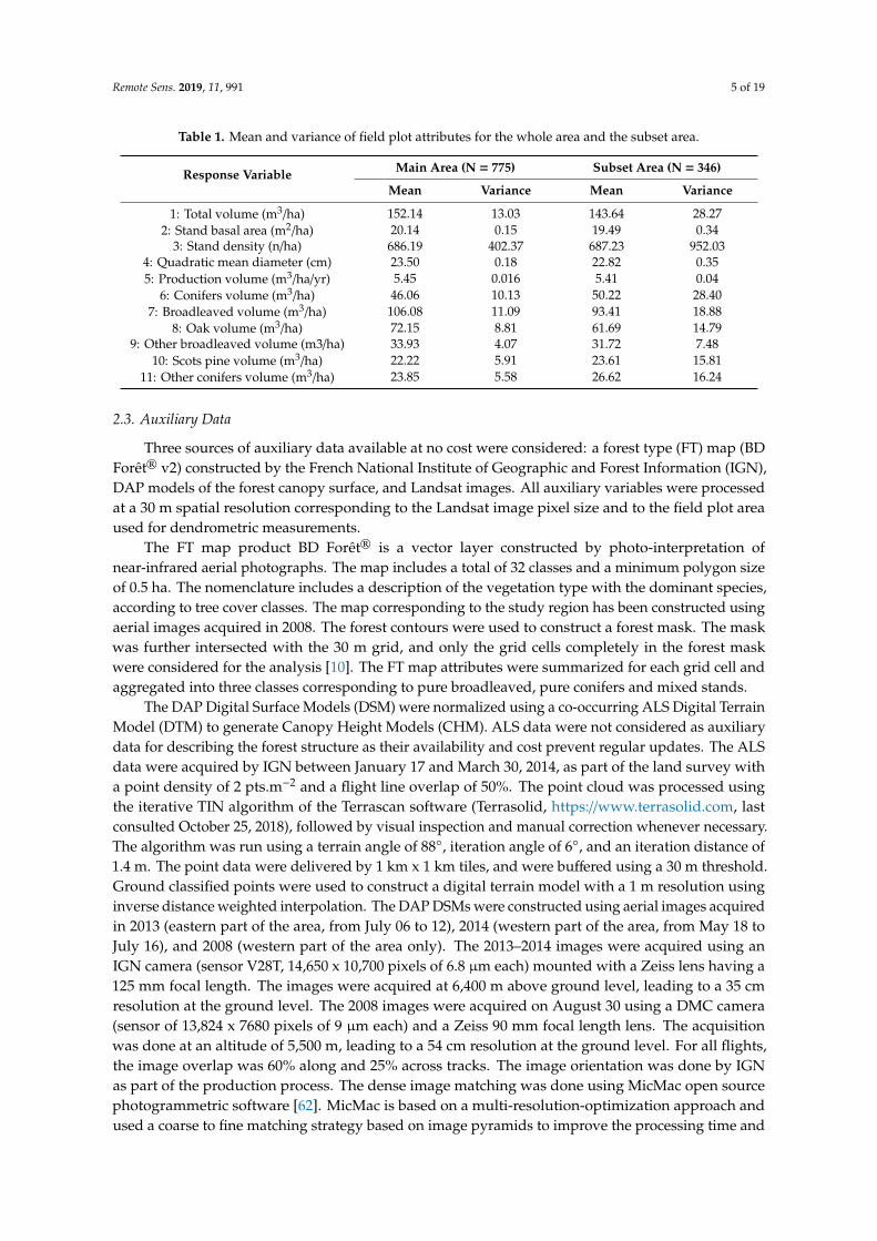
Table 1. Mean and variance of field plot attributes for the whole area and the subset area.
Response variable Main area (N = 775) Subset area (N = 346) Mean Variance Mean Variance
1: Total volume (m3/ha) 152.14 13.03 143.64 28.27 2: Stand basal area (m2/ha) 20.14 0.15 19.49 0.34
3: Stand density (n/ha) 686.19 402.37 687.23 952.03 4: Quadratic mean diameter (cm) 23.50 0.18 22.82 0.35
Figure 1. Localization of the study area (a), showing (b) the forest mask and the 775 national forestinventory plots in the main and the subset (southwestern part below dotted line) areas; 1 km2 tiles of(c) the forest type map; (d) a 30 m resolution Landsat color composition (bands 4,3,2); and (e) a 1 mresolution photogrammetric canopy height model. The position of the tile used to illustrate is shown asa black rectangle in (b).
Remote Sens. 2019, 11, 991 5 of 19
Table 1. Mean and variance of field plot attributes for the whole area and the subset area.
Response Variable Main Area (N = 775) Subset Area (N = 346)
Mean Variance Mean Variance
1: Total volume (m3/ha) 152.14 13.03 143.64 28.272: Stand basal area (m2/ha) 20.14 0.15 19.49 0.34
3: Stand density (n/ha) 686.19 402.37 687.23 952.034: Quadratic mean diameter (cm) 23.50 0.18 22.82 0.355: Production volume (m3/ha/yr) 5.45 0.016 5.41 0.04
6: Conifers volume (m3/ha) 46.06 10.13 50.22 28.407: Broadleaved volume (m3/ha) 106.08 11.09 93.41 18.88
8: Oak volume (m3/ha) 72.15 8.81 61.69 14.799: Other broadleaved volume (m3/ha) 33.93 4.07 31.72 7.48
10: Scots pine volume (m3/ha) 22.22 5.91 23.61 15.8111: Other conifers volume (m3/ha) 23.85 5.58 26.62 16.24
2.3. Auxiliary Data
Three sources of auxiliary data available at no cost were considered: a forest type (FT) map (BDForêt® v2) constructed by the French National Institute of Geographic and Forest Information (IGN),DAP models of the forest canopy surface, and Landsat images. All auxiliary variables were processedat a 30 m spatial resolution corresponding to the Landsat image pixel size and to the field plot areaused for dendrometric measurements.
The FT map product BD Forêt® is a vector layer constructed by photo-interpretation ofnear-infrared aerial photographs. The map includes a total of 32 classes and a minimum polygon sizeof 0.5 ha. The nomenclature includes a description of the vegetation type with the dominant species,according to tree cover classes. The map corresponding to the study region has been constructed usingaerial images acquired in 2008. The forest contours were used to construct a forest mask. The maskwas further intersected with the 30 m grid, and only the grid cells completely in the forest maskwere considered for the analysis [10]. The FT map attributes were summarized for each grid cell andaggregated into three classes corresponding to pure broadleaved, pure conifers and mixed stands.
The DAP Digital Surface Models (DSM) were normalized using a co-occurring ALS Digital TerrainModel (DTM) to generate Canopy Height Models (CHM). ALS data were not considered as auxiliarydata for describing the forest structure as their availability and cost prevent regular updates. The ALSdata were acquired by IGN between January 17 and March 30, 2014, as part of the land survey witha point density of 2 pts.m−2 and a flight line overlap of 50%. The point cloud was processed usingthe iterative TIN algorithm of the Terrascan software (Terrasolid, https://www.terrasolid.com, lastconsulted October 25, 2018), followed by visual inspection and manual correction whenever necessary.The algorithm was run using a terrain angle of 88◦, iteration angle of 6◦, and an iteration distance of1.4 m. The point data were delivered by 1 km x 1 km tiles, and were buffered using a 30 m threshold.Ground classified points were used to construct a digital terrain model with a 1 m resolution usinginverse distance weighted interpolation. The DAP DSMs were constructed using aerial images acquiredin 2013 (eastern part of the area, from July 06 to 12), 2014 (western part of the area, from May 18 toJuly 16), and 2008 (western part of the area only). The 2013–2014 images were acquired using anIGN camera (sensor V28T, 14,650 x 10,700 pixels of 6.8 µm each) mounted with a Zeiss lens having a125 mm focal length. The images were acquired at 6,400 m above ground level, leading to a 35 cmresolution at the ground level. The 2008 images were acquired on August 30 using a DMC camera(sensor of 13,824 x 7680 pixels of 9 µm each) and a Zeiss 90 mm focal length lens. The acquisitionwas done at an altitude of 5,500 m, leading to a 54 cm resolution at the ground level. For all flights,the image overlap was 60% along and 25% across tracks. The image orientation was done by IGNas part of the production process. The dense image matching was done using MicMac open sourcephotogrammetric software [62]. MicMac is based on a multi-resolution-optimization approach andused a coarse to fine matching strategy based on image pyramids to improve the processing time and

Remote Sens. 2019, 11, 991 6 of 19
control the similarity of matches between levels. The dense matching was performed using a PerImages Matching approach (PIMs mode) in image geometry and rely on tie points generated using the‘Scale-Invariant-Feature Transform’ (SIFT) detector [63]. The matching approach produces a depthmap for each image pair. The depth maps are then merged together and converted into a dense pointcloud. The resulting point clouds were converted into a 1 m DSM using the maximum height perpixels. Empty pixels were not interpolated. The DSM was further converted into a canopy heightmodel (CHM) by subtracting the ALS DTM. Two categories of metrics were derived from the CHM toserve as auxiliary variables for each cell of the 30 m grid: distribution metrics above a height thresholdfixed at 5 m to match with the definition of forest and structure metrics [53]. The distributional metricsincluded the percentiles 0 to 100 by steps of 10 (p0 to p100), as well as upper percentiles 95 and 99 (p95,p99), the mean (hmean), standard deviation (hstd), variance (hvar), and the mean absolute deviation(hmad) of heights. The structure metrics (Table A1), included the gap area ratio (Ga), the mean innercanopy volume (Vi), the mean outer canopy volume (Vo), the mean inner canopy volume above agiven threshold value (Th) fixed here at 5 m (Vci), the mean outer canopy volume above Th (Vco),defined as the complement of the canopy volume to the maximum height, the mean inner canopyvolume within gaps (Vgi) and its outer complement (Vgo), the standard rumple area (Ra) [55], orthe ones defined with respect to Vi (Ra1) and Vci (Ra2), as well as the number of empty pixels (NA).Over the subset area, various difference metrics were computed, including changes in gap area (dGa),in volume differences (e.g., dVi, dVo), mean, minimum and maximum heights (dhmean, dp0, dp100),as well as in the upper percentiles (dp95, dp99).
Four Landsat 8 images acquired on September 8, 2014 were downloaded from the Theiaplatform (https://theia-landsat.cnes.fr) with the processing level 2A, including orthorectification,atmospheric correction and cloud detection [64]. The reflectance images were used to computevarious indices (Table A2): the simple ratio (SR), the normalized difference vegetation index (NDVI),the Specific Leaf Area Vegetation Index (SLAVI), the Soil Adjusted Vegetation Index (SAVI), theModified Soil Adjusted Vegetation Index (MSAVI), the enhance vegetation index (EVI) the green NDVI(GNDVI), the Normalized Difference Moisture Index (NDMI), Normalized Difference Water Index(NDWI) [65,66], as well as brightness (Br), greenness (Gr), and wetness (We) derived from TasseledCap transformation [67]. In addition to computed spectral reflectance indices, we also included theseven reflectance bands of Landsat 8: Ultra Blue (UB), Blue (B), Green (G), Red (R), Near Infrared (NIR),Shortwave Infrared (SWIR) 1, and Shortwave Infrared (SWIR) 2. The Landsat metrics were assigned tothe grid cells by intersecting the grid with the coordinate of the center of the Landsat pixels.
2.4. Optimization of the k-NN Model
MSNFI performance depends on: (1) the modeling framework, and (2) the correlation betweenthe surveyed forest attributes and the auxiliary information.
As indicated above, a non-parametric multivariate k-NN approach was adopted to constructwall-to-wall predictions of forest attributes. The k-NN parameters include the number of neighbors(k), the distance metric used to search the variable space, and a weighting function to computepredictions [57]. In k-NN, the population units for which both response and auxiliary variables areavailable are termed the reference set and the units for which predictions of response variables aresought are termed the target set. The auxiliary variables are also termed feature variables and thespace defined by them is termed the feature space.
Based on a literature survey [57,68] and preliminary results, two distance metrics were compared:Euclidean and Canonical Correlation Analysis (CCA) [69]. The Euclidean distance is computed in anormalized space of auxiliary variables. The CCA distance is defined by Equation (1):
d =√
Γ ∧2 ΓT (1)

Remote Sens. 2019, 11, 991 7 of 19
where Γ is the matrix of canonical vectors corresponding to the X’s found by canonical correlationanalysis between X and Y, ΓT the transposed matrix, and ∧ is the canonical correlation matrix.
Values of k in the range of 1 to 20 were tested to optimize model performance. The weight of theneighbors used to compute the imputed values for the continuous variables according to Equation (2):
wj = 1/(1 + dij) (2)
where dij is the distance between target pixel i and reference pixel j in the feature space.k-NN models were generated using six different combinations of auxiliary variables: (1) Landsat
variables alone, (2) Landsat variables and FT from the forest map, 3() 3D metrics from DAP CHMs,(4) 3D metrics from DAP CHMs with FT from the forest map, (5) Landsat variables and 3D metrics fromDAP CHMs, and (6) all auxiliary variables. On the subset area, the introduction of change detectionvariables was also tested. Only two combinations of auxiliary variables were considered: all formerauxiliary variables used alone, or with the change detection variables.
Note that preliminary analyses revealed estimation accuracy issues due to auxiliary variableshaving weak correlations with the response variables, which has also been reported in [30,31]. Theproblem was solved by filtering out auxiliary variables that have maximum correlation values lessthan 0.2 with the response variable considered. A total of four auxiliary variables were discarded fromanalysis, including three Landsat bands (UB, B, R), and one volume metric (Vco).
The performance of the k-NN models was evaluated using a leave-one-out cross-validationapproach (LOOCV). Model accuracy was evaluated using the Root Mean Squared Difference (RMSD)between observed and imputed values [70]. For comparing imputation models across multipleresponse variables with different measurement units, RMSD value was standardized by dividingRMSD by the standard deviation of the observations of the response variable (i.e., Scaled RMSD =
RMSD/Standard deviation of the response variable) [71]. Optimal k values were selected as those forwhich mean RMSD across multiple response variables did not differ more than 5% from the minimalmean RMSD value [20].
k-NN optimization was conducted using R open source software with the yaImpute package [71].
2.5. Statistical Inference
Using field data only, the design-based, simple expansion (Exp) estimators of the populationmean and variance were defined by Equations (3) and (4).
µExp =1n
n∑i=1
yi (3)
Var(µExp
)=
1n · (n− 1)
n∑i=1
(yi−µExp)2 (4)
where n is the number of sample plots, and yi is the observed value of plot i.The inference of population parameters from the k-NN predictions across the study area was
assessed using model-assisted generalized regression (GREG) estimators of means and variances [72].Despite using the term regression in the label characterizing GREG estimators, multiple predictiontechniques other than regression models, and particularly other than linear regression models, havebeen used with the GREG estimators [73–75]. The GREG estimator of the mean is the differencebetween the mean of the k-NN predictions across population units and the estimated bias, as shown inEquation (5):
µGREG =1N
N∑i=1
yi −1n
n∑i=1
εi (5)

Remote Sens. 2019, 11, 991 8 of 19
where εi = (yi − yi) is the difference between k-NN prediction and the observed response variable(estimate of bias), N is the number of population units or pixels, and n is the number of field sampleplots. The associated variance estimator is computed using Equation (6):
Var(µGREG
)=
1n · (n− 1)
·
n∑i=1
(εi−ε)2 (6)
where ε =(
1n
)·∑n
i=1 εi.The performance of k-NN was evaluated through a measure of relative efficiency (RE =
Var(µExp
)/Var
(µGREG
). RE provides an estimate of the gain in precision resulting from the use
of the auxiliary information that is incorporated into the model-assisted estimators in comparisonwith pure field-based estimates. RE values greater than 1 indicate increased precision. The primaryadvantage of the GREG estimators is that they take advantage of the relationship between theprobability based sample plot data and their corresponding predictions to reduce the variance of theestimated population mean [20] and thereby increase RE. For each combination of auxiliary variables:µGREG,Var
(µGREG
), and RE were calculated for all 11 response variables.
2.6. External Validation
Internal models are recognized to underestimate variance [12,13]. To account for this issue, acomplementary analysis was conducted. Both the main and subset areas were divided into threesub-areas having approximately the same number of field plots (i.e., 258 (~775/3) and 115 (~346/3)plots for the main and the subset areas, respectively). Each sub-area was used to build a k-NN modelfollowing the methods presented in Sections 2.4 and 2.5. The models were then applied to the twoother sub-areas as external models. The mean REs obtained with both approaches were compared toassess the underestimation associated with the internal model.
3. Results
3.1. k-NN Optimization
Table 2 shows the mean RMSD values for the various combinations of auxiliary variables anddistance metrics. The smaller the RMSD, the greater the similarity between the reference and theimputed observations. Using Euclidean distance, mean RMSD values ranged from 1.00 for the Landsatmetrics alone to 0.84 for the overall metrics. The k values selected were relatively stable, rangingfrom 4 to 8. Interestingly, the combination of 3D metrics with the FT map performed well with amean RMSD of 0.85, which was only 0.01 greater than for the combination having smaller RMSDwith a 37.5% decrease in the number of auxiliary variables. By comparison, the combination of 3Dmetrics with Landsat metrics (39 variables) performed slightly less well with mean RMSD of 0.86, anda greater range of individual RMSD values. Slightly smaller RMSD values were obtained using CCAdistance, with mean RMSD values ranging from 0.99 for the Landsat metrics alone to 0.84 with the fullset of metrics. The optimal k value was also rather stable, ranging from 5 to 6. With both distancemetrics, the introduction of canopy change auxiliary variables contributed to greater mean RMSDvalues. The improvement was more pronounced using the Euclidean distance metric, with a gain inmean RMSD of 0.02.

Remote Sens. 2019, 11, 991 9 of 19
Table 2. Cross-validated Root Mean Squared Differences (RMSD) of the imputation, for the optimalk-NN models. Numbers in parenthesis are minimum and maximum values of the 11 forest attributes.
Euclidean CCA
Auxiliary VariableCombination Domain No. of Variables k RMSD k RMSD
Landsat Main 15 6 1.00(0.84;1.08) 6 0.99
(0.83;1.07)
Landsat & Forest types Main 16 6 0.98(0.73;1.09) 6 0.97
(0.71;1.07)
3D metrics Main 24 6 0.91(0.72;1.04) 6 0.91
(0.71;1.03)
3D metrics and Forest types Main 25 5 0.85(0.69;0.98) 5 0.84
(0.67,1.00)
3D metrics and Landsat Main 39 8 0.86(0.68;1.00) 5 0.86
(0.71;0.99)
All Main 40 5 0.84(0.67;1.00) 5 0.84
(0.64;0.97)
All Subset 41 4 0.87(0.66;1.02) 5 0.86
(0.66;1.01)
All and change Subset 45 5 0.85(0.65;1.00) 6 0.85
(0.64;1.01)
3.2. Statistical Inference
Tables 3 and 4 show the estimated means and corresponding REs for the 11 field response attributesfor the whole area computed using Euclidean and CCA distances, respectively. Using Euclideandistance (Table 3), the greatest RE was obtained for total volume, with a value of 2.18. The smallestRE was obtained for the volume of other broadleaved, with a value of 1.03. For nine out of the11 forest attributes, the greatest RE was achieved with all auxiliary variables combined. The standdensity was most accurately estimated using the 3D metrics alone (RE = 1.21). For the volume of otherbroadleaved, the most accurate auxiliary variable combination included the 3D metrics and the foresttypes, and produced RE of 1.03. With CCA distance (Table 4), the greatest RE was obtained for thevolume of other conifers with a value of 2.37. As for Euclidean distance, the least accurate results wereobtained for the volume of other broadleaved, reaching a RE of 1.06. The greatest REs were achievedusing all auxiliary variables combined for only six of the 11 forest attributes. The greatest REs fortotal volume (2.04), stand basal area (1.44), broadleaved volume (2.15), and oak volume (1.65) wereobtained using as the 3D metrics and the FT. For stand density, the greatest RE was obtained withthe 3D metrics only (1.14). On average, Euclidean distance was more accurate for six of the 11 forestattributes. But CCA distance tended to be more accurate for those field attributes showing the smallestREs, namely the production volume, the Scots pine volume and the volume of other conifers.
Table 3. Mean, standard error (SE), and relative efficiencies (RE) computed on the main area for thedifferent combination of auxiliary variables using Euclidean distance. The greatest RE for each forestattributes appears in bold.
Landsat Landsat and Forest Types 3D Metrics
Forest Attributes 1 Mean SE RE Mean SE RE Mean SE RE
1 155.02 3.63 0.99 154.82 3.59 1.01 153.83 2.62 1.902 20.47 0.13 0.98 20.42 0.39 1.00 20.10 0.33 1.393 692.67 21.27 0.89 690.32 21.48 0.87 686.65 18.27 1.214 23.55 0.46 0.85 23.55 0.46 0.84 23.59 0.38 1.235 5.57 0.13 0.96 5.57 0.13 0.98 5.45 0.12 1.096 48.92 2.68 1.41 49.61 2.35 1.83 45.74 3.13 1.047 106.09 3.15 1.12 105.22 3.07 1.18 108.09 2.70 1.528 72.04 2.84 1.09 71.07 2.83 1.10 72.65 2.55 1.359 34.06 2.14 0.89 34.15 2.13 0.90 35.43 2.04 0.97
10 23.52 2.39 1.04 25.08 2.27 1.14 21.84 2.49 0.9511 25.40 2.38 0.98 24.52 2.33 1.03 24.21 2.46 0.93

Remote Sens. 2019, 11, 991 10 of 19
Table 3. Cont.
3D Metrics and Forest Types Landsat and 3D Metrics All
Forest Attributes 1 Mean SE RE Mean SE RE Mean SE RE
1 155.28 2.55 2.00 153.60 2.48 2.12 153.24 2.44 2.182 20.33 0.32 1.43 20.00 0.31 1.54 19.98 0.31 1.563 691.73 18.37 1.19 673.84 19.07 1.11 678.00 19.17 1.104 23.54 0.39 1.20 23.64 0.38 1.22 23.48 0.38 1.235 5.49 0.12 1.16 5.45 0.12 1.18 5.47 0.12 1.196 47.66 2.19 2.10 48.69 2.44 1.70 47.91 2.18 2.137 107.62 2.31 2.07 104.91 2.39 1.93 105.33 2.29 2.118 72.12 2.41 1.52 72.20 2.33 1.63 72.29 2.28 1.699 35.50 1.99 1.03 32.71 2.02 0.99 33.05 2.02 1.00
10 22.72 2.15 1.28 24.40 2.27 1.14 23.68 2.15 1.2811 24.94 2.32 1.04 24.28 2.36 1.01 24.23 2.27 1.08
1: forest attributes: 1: total volume (m3/ha); 2: stand basal area (m2/ha); 3: stand density (stem/ha); 4: quadraticmean diameter (cm); 5: production volume (m3/ha/yr), 6: conifers volume (m3/ha); 7: broadleaved volume (m3/ha);8: Oak volume (m3/ha), 9: other broadleaved volume (m3/ha); 10: Scots pine volume (m3/ha); 11: other conifersvolume (m3/ha).
Table 4. Mean, standard error (SE) and relative efficiencies (RE) computed on the main area for thedifferent combinations of auxiliary variables using Canonical Correlation Analysis distance. The greatestRE for each forest attribute appears in bold.
Landsat Landsat and Forest Types 3D Metrics
Forest Attributes 1 Mean SE RE Mean SE RE Mean SE RE
1 152.67 3.65 0.97 153.85 3.56 1.02 154.83 2.58 1.962 20.23 0.39 0.97 20.32 0.39 1.00 20.23 0.33 1.383 701.32 21.31 0.88 697.03 21.65 0.86 683.02 18.77 1.144 23.19 0.45 0.87 23.49 0.45 0.88 23.73 0.38 1.215 5.53 0.13 1.00 5.55 0.13 1.01 5.44 0.13 1.056 47.27 2.67 1.42 48.73 2.26 1.97 49.10 3.08 1.067 105.40 3.22 1.07 105.11 3.07 1.17 105.73 2.68 1.548 72.04 2.84 1.08 72.04 2.82 1.11 72.02 2.48 1.429 33.35 2.15 0.88 33.07 2.13 0.90 34.70 2.03 0.99
10 22.23 2.31 1.11 23.18 2.24 1.18 24.11 2.51 0.9411 25.04 2.38 0.99 25.55 2.22 1.13 24.98 2.38 0.98
3D Metrics and Forest Types Landsat and 3D Metrics All
Forest Attributes 1 Mean SE RE Mean SE RE Mean SE RE
1 154.79 2.53 2.04 153.43 2.56 1.98 154.95 2.53 2.032 20.21 0.32 1.44 20.03 0.33 1.41 20.24 0.32 1.433 679.82 18.91 1.12 676.87 19.50 1.05 685.17 19.43 1.074 23.74 0.40 1.15 23.76 0.38 1.21 23.77 0.38 1.215 5.44 0.12 1.12 5.43 0.12 1.16 5.44 0.11 1.216 48.95 2.14 2.21 50.34 2.38 1.78 50.04 2.07 2.377 105.84 2.27 2.15 103.10 2.50 1.78 104.90 3.39 1.958 71.25 2.31 1.65 68.77 2.41 1.52 70.61 2.38 1.569 35.59 2.01 1.00 34.33 1.99 1.01 34.30 1.95 1.0610 23.78 2.13 1.31 25.43 2.15 1.27 24.92 2.10 1.3411 25.17 2.19 1.16 24.90 2.21 1.14 25.13 2.19 1.16
1: forest attributes: 1: total volume (m3/ha); 2: stand basal area (m2/ha); 3: stand density (stem/ha); 4: quadraticmean diameter (cm); 5: production volume (m3/ha/yr), 6: conifers volume (m3/ha); 7: broadleaved volume (m3/ha);8: Oak volume (m3/ha), 9: other broadleaved volume (m3/ha); 10: Scots pine volume (m3/ha); 11: other conifersvolume (m3/ha).
Table 5 shows the RE achieved on the subset area after including 3D change detection metrics.Using Euclidean distance, REs increased for nine of the 11 field attributes, with an average RE differenceof 0.05. The greatest increase was obtained for the production volume with a RE increase of 0.17. REwas most degraded for the volume of other conifers, with a difference of −0.06. Using CCA distance,the mean RE difference was 0.04. However, the introduction of 3D change detection metrics contributedto increased RE for six forest attributes only. The greatest increases were achieved for conifer volumeand production volume, with RE differences of 0.17 and 0.15, respectively. On the contrary, RE values

Remote Sens. 2019, 11, 991 11 of 19
were degraded for the volume of other conifers (−0.06), the broadleaved volume (−0.03), and the standbasal area (−0.02). Overall the greatest RE values were obtained using a CCA distance for seven out ofthe 11 field attributes.
Table 5. Effect of the inclusion of diachronic variables on the mean, standard error (SE), and relativeefficiencies (RE) over the subset area, for both distance metrics. The greatest RE for each forest attributeand distance metric appears in bold.
Euclidean CCA
All All and Change All All and Change
ForestAttributes 1 Mean SE RE Mean SE RE Mean SE RE Mean SE RE
1 142.60 3.62 2.15 144.0 3.57 2.21 146.15 3.78 1.97 146.27 3.79 1.972 19.23 0.48 1.50 19.36 0.47 1.57 19.63 0.49 1.41 19.59 0.50 1.393 682.13 30.63 1.01 680.01 29.47 1.10 693.18 31.19 0.98 683.96 31.22 0.984 22.80 0.56 1.11 22.88 0.55 1.16 22.89 0.56 1.12 22.74 0.54 1.215 5.33 0.20 1.07 5.43 0.18 1.24 5.52 0.19 1.09 5.52 0.18 1.246 51.52 3.55 2.25 54.27 3.49 2.33 54.37 3.57 2.23 54.81 3.44 2.407 91.07 3.27 1.77 89.72 3.24 1.80 91.78 3.12 1.94 91.46 3.14 1.918 59.65 3.18 1.46 60.18 3.10 1.54 60.89 3.12 1.52 60.87 3.05 1.599 31.42 2.80 0.95 29.54 2.76 0.98 30.90 2.72 1.01 30.59 268 1.0410 26.18 3.74 1.13 28.20 3.73 1.13 26.53 3.74 1.13 25.52 3.69 1.1611 25.34 3.82 1.11 26.08 3.92 1.05 27.84 3.39 1.42 29.29 3.45 1.36
1: forest attributes: 1: total volume (m3/ha); 2: stand basal area (m2/ha); 3: stand density (stem/ha); 4: quadraticmean diameter (cm); 5: production volume (m3/ha/yr), 6: conifers volume (m3/ha); 7: broadleaved volume (m3/ha);8: Oak volume (m3/ha), 9: other broadleaved volume (m3/ha); 10: Scots pine volume (m3/ha); 11: other conifersvolume (m3/ha).
3.3. External Validation
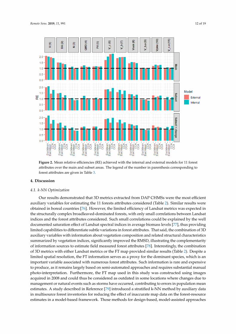
The results of the external validation are presented in Figure 2. Over the main area, the mean REobtained with the Euclidean distance was 1.45 for the internal model and 1.38 for the external model.REs obtained with the CCA distance were of the same magnitude, with an internal RE of 1.41 and anexternal one slightly greater with a value of 1.42. The results obtained over the subset area showedthe limitation of CCA distance associated with respect to the number of field sample units. Using theEuclidean distance, the greatest REs were obtained using the change detection metrics, with values of1.41 and 1.35 for the internal and external models, respectively. This is 0.04 and 0.05 greater than theRE achieved without considering change metrics. By comparison, the greatest RE output with theCCA distance were almost similar to the two sets of metrics, reaching 1.27 with the internal modelsand 1.16 and 1.15 with the external models with and without change metrics, respectively.
Figure 2 also highlights the differences between forest attributes. Volume attributes were estimatedwith the greatest RE, provided these attributes were well represented within the field sampling plots,and were not rare events. Indeed, the total volume, total volume of conifers and of broadleavedwere estimated with RE above 1.5. Those volumes with smaller frequencies like the volume of otherbroadleaved than oaks and the volume of other conifers than scot pines were estimated with REaround 1. The introduction of change detection metrics with the Euclidean distance mostly benefitsestimation of production volume, a flux variable, and stand density to a lesser extent. RE for theformer increased by 0.13 from 1.08 to 1.21 for the internal model, and by 0.2 (i.e., from 1.01 to 1.21)for the external model. The latter showed a gain in RE of 0.09 and 0.08 for the internal and externalmodels, respectively.
Remote Sens. 2019, 11, 991 12 of 19
Remote Sens. 2018, 10, x FOR PEER REVIEW 12 of 20
Figure 2. Mean relative efficiencies (RE) achieved with the internal and external models for 11 forest attributes over the main and subset areas. The legend of the number in parenthesis corresponding to forest attributes are given in Table 3.
4. Discussion
4.1. k-NN Optimization
Our results demonstrated that 3D metrics extracted from DAP CHMSs were the most efficient auxiliary variables for estimating the 11 forests attributes considered (Table 2). Similar results were obtained in boreal countries [76]. However, the limited efficiency of Landsat metrics was expected in the structurally complex broadleaved-dominated forests, with only small correlations between Landsat indices and the forest attributes considered. Such small correlations could be explained by the well documented saturation effect of Landsat spectral indices in average biomass levels [77], thus providing limited capabilities to differentiate subtle variations in forest attributes. That said, the combination of 3D auxiliary variables with information about vegetation composition and related structural characteristics summarized by vegetation indices, significantly improved the RMSD, illustrating the complementarity of information sources to estimate field measured forest attributes [78]. Interestingly, the combination of 3D metrics with either Landsat metrics or the FT map provided similar results (Table 2). Despite a limited spatial resolution, the FT information serves as a proxy for the dominant species, which is an important variable associated with numerous forest attributes. Such information is rare and expensive to produce, as it remains largely based on semi-automated approaches and requires substantial manual photo-interpretation. Furthermore, the FT map used in this study was constructed using images acquired in 2008 and could thus be considered as outdated in some locations where changes due to management or natural events such as storms have occurred, contributing to errors in population mean estimates. A study described in Reference [79] introduced a stratified k-NN method by auxiliary data in multisource forest inventories for reducing the effect of inaccurate map data on the forest-resource estimates in a model-based framework. Those methods for design-based, model-assisted approaches should be investigated. However, considering the
Figure 2. Mean relative efficiencies (RE) achieved with the internal and external models for 11 forestattributes over the main and subset areas. The legend of the number in parenthesis corresponding toforest attributes are given in Table 3.
4. Discussion
4.1. k-NN Optimization
Our results demonstrated that 3D metrics extracted from DAP CHMSs were the most efficientauxiliary variables for estimating the 11 forests attributes considered (Table 2). Similar results wereobtained in boreal countries [76]. However, the limited efficiency of Landsat metrics was expected inthe structurally complex broadleaved-dominated forests, with only small correlations between Landsatindices and the forest attributes considered. Such small correlations could be explained by the welldocumented saturation effect of Landsat spectral indices in average biomass levels [77], thus providinglimited capabilities to differentiate subtle variations in forest attributes. That said, the combination of 3Dauxiliary variables with information about vegetation composition and related structural characteristicssummarized by vegetation indices, significantly improved the RMSD, illustrating the complementarityof information sources to estimate field measured forest attributes [78]. Interestingly, the combinationof 3D metrics with either Landsat metrics or the FT map provided similar results (Table 2). Despite alimited spatial resolution, the FT information serves as a proxy for the dominant species, which is animportant variable associated with numerous forest attributes. Such information is rare and expensiveto produce, as it remains largely based on semi-automated approaches and requires substantial manualphoto-interpretation. Furthermore, the FT map used in this study was constructed using imagesacquired in 2008 and could thus be considered as outdated in some locations where changes due tomanagement or natural events such as storms have occurred, contributing to errors in population meanestimates. A study described in Reference [79] introduced a stratified k-NN method by auxiliary datain multisource forest inventories for reducing the effect of inaccurate map data on the forest-resourceestimates in a model-based framework. Those methods for design-based, model-assisted approaches

Remote Sens. 2019, 11, 991 13 of 19
should be investigated. However, considering the importance of the auxiliary variable, there is aninterest for NFIs to automate construction/updating of those maps to account for variations in forestsurfaces and types in a k-NN framework.
The introduction of variables based on 3D changes contributed to the reduction of RMSD,demonstrating the importance of this kind of metric for increasing the precision of estimates and fordeveloping monitoring systems. This result further points out the potential of time-series of opticalimageries to improve neighbor selection within the k-NN method and to contribute to improvedestimations [80]. Long-term times-series including decades of observations might provide insights intoforest management [78], especially clear and partial cuts, and could be used to update forest maps [7].Short-term time-series, built using images collected over a year, might also provide information aboutphenology and further improve neighbor selection [33]. Apart from time-series data, texture metricsextracted from aerial images or very high-resolution satellites data need to be further considered,as they were found to provide information about forest structure and composition [81,82] and did notappear to saturate with increases in biomass levels [82].
In terms of k-NN setup, the optimal number of neighbors, defined according to [20] was relativelyconstant, despite a large variation in the number of auxiliary variables. Our results are in agreementwith the literature, with optimal k values ranging between 1 and 10, with five as a most often selectedvalue [57]. CCA distance, despite using both auxiliary and field data in the k-NN construction onlymarginally improved the mean RMSD with respect to Euclidean Distance. This makes Euclideandistance appealing since additional field attributes could be estimated without a requirement tore-compute a new k-NN model. This is particularly attractive for NFIs that collect hundreds ofvariables and could also compute additional information from those field measured attributes.
4.2. Statistical Inference
The estimated means and REs confirmed the trends observed with the RMSD values.The combination of field and Landsat data provided limited precision gain, and even generatedgreater variance than the one obtained using field data alone for a majority of field attributes. All butone of the REs were greater than 1.0 when the auxiliary variable set included the 3D metrics and eitherLandsat metrics or FT map. The greatest REs were obtained for volume-related field attributes, to thedegree that the attributes were not rare events and were well-represented by the field data. Such aresult was expected, since volume is a function of the canopy height and is thus well correlated withthe auxiliary variables describing canopy surface height and structure [53]. The degraded precision ofvolume attributes having small frequencies in our field sample such as the volume of other broadleavedtrees, or the volume of other conifers showing a limited precision gain, which has also been reportedby others [68]. Indeed, forest attributes with few observations from rare populations are expected tocontribute to large standard errors [83]. Other structural metrics were estimated with RE ranging from1.14 (stand density) to 1.58 (basal area). Those results are of the same magnitude as reported by [29] fora forest area in north central Minnesota in the USA, with values ranging from 1.23 to 1.35 for six forestattributes including volume. The moderate precision gain achieved here for stand density and to someextent to production volume and the QMD could be explained by the smaller correlations of thosefield attributes with both 3D and 2D metrics [84]. Even though some studies did not report the sametrends [29,85] the smaller precision gains reported here for density and QMD could be attributed tothe complexity of the forest, characterized by two dominant forest structures made of regular stands(~55%) and of coppice-with-standards (~40%).
An important result was the performance gains achieved with the introduction of variablesassociated with 3D changes (Table 5). RE increased on average by 0.06 and 0.04 using the Euclideanand CCA distance, respectively. Using both distance metrics, the most substantial precision gainwas obtained for the production volume (0.17 and 0.15, respectively), which is a flux variable andthus benefited from the inclusion of 3D variables related to canopy dynamics. Other field attributesbenefiting from the inclusion of change detection variables with both distance metrics were the conifer

Remote Sens. 2019, 11, 991 14 of 19
and oak volumes. While the QMD also showed a substantial precision gain with CCA distance (0.09),the stand density (0.09), the stand basal area (0.07), and the total volume (0.06) exhibit among thelargest gain in RE based on Euclidean distance. This indicated that changes in canopy height andstructure provide additional and pertinent information about traditional field measurements of foreststructure that are difficult to estimate from remote sensing means [86]. The differences achieved in thek-NN setup have been reported by others [68,86]. The study described in Reference [86] reported thatMSN was sensitive the choice of the response variables.
4.3. External Validation
The external validation showed limited RE differences between internal and external models,indicating that the results achieved over the whole area with internal models are not as overlyoptimistic as reported in other studies [13]. That said, the study highlights a limitation of the CCAdistance metric when an internal model is used. As CCA uses both X and Y variables to set-up thek-NN, it tends to generate a reduced variance as compared to Euclidean distance. However, in anexternal validation context, CCA-based predictions appear to have more limited capabilities to predictattributes outside the geographical domain used to train the k-NN model [87]. Furthermore, the studyconducted in Reference [68] reported that CCA distance tended to have decreased accuracy comparedto other distance metrics when no variable selection is performed, probably highlighting a curse ofdimensionality issue while both X and Y variables are considered in the feature space [56]. Furthermore,the study described in Reference [29] strongly advised using variable selection approach for the CCAdistance metric despite its capability to weight auxiliary variables according to their explanatory power,because multicollinearity degrades the predictive power and the estimation of canonical weightsrapidly becomes more complex leading to instability figure [88]. This result therefore indicates thatmodel-assisted inference without variable selection should avoid using CCA distance metric, at thebenefit of a distance metric independent of the response variables, such as the Euclidean one.
5. Conclusions
Five principal conclusions could be drawn from this research: (1) provided a sufficient numberof sample plots, design-based model-assisted inference performs well with large dimension data, asfar as the data sources are related to the forest attributes considered. In such situation, the diversityand complementary of the auxiliary data are expected to improve precision (produce larger REs) andreduce RMSD; (2) a substantial increase in precision of the forest attribute estimates was brought by3D metrics and the addition of canopy change metrics. The latter contributed to improve markedlythe estimations in production volumes; (3) the optimal k value was stable with respect to the k-NNconfiguration tested; (4) the CCA distance metric involving both feature and response variables couldbe affected by dimensionality problems. Euclidean distance should be preferred when no variableselection is performed; and (5) the k-NN technique in conjunction with model-assisted estimatorsproduced a significant improvement in precision of inventory parameter estimates.
This work demonstrated the potential of MSNFI approaches in complex broadleaved dominatedforests such as those found in France. This opens up the possibilities of more forest attribute estimationfor smaller spatial domains. Future work will focus on a downscaling approach involving bothmodel-assisted and model-based approaches.
Author Contributions: conceptualization, C.V. and J.-P.R.; methodology, C.V., J.-P.R., and D.B.I.P.V.; validation,C.V., J.-P.R., D.B.I.P.V., R.McR., and F.M.; formal analysis, C.V., J.-P.R., and D.B.I.P.V.; investigation, C.V., J.-P.R.,and D.B.I.P.V.; data curation, C.V., J.-P.R., and D.B.I.P.V.; writing—original draft preparation, D.B.I.P.V., C.V., andJ.-PR; writing—review and editing, D.B.I.P.V., C.V., J.-P.R., R.McR., and F.M.; visualization, C.V.; supervision, C.V.;project administration, C.V.; funding acquisition, C.V.
Funding: This research was funded by The French Environmental Management Agency (ADEME), grant number16-60-C0007. The methods and algorithms for processing photogrammetric data were supported by DIABOLOproject from the European Union’s Horizon 2020 research and innovation program under grant agreement

Remote Sens. 2019, 11, 991 15 of 19
No 633464, as well as CHM-ERA project from the French National Research Agency (ANR) as part of the“Investissements d’Avenir” program (ANR-11-LABX-0002-01, Lab of Excellence ARBRE).
Acknowledgments: The authors would like to acknowledge Maryem Fadili and Thibaud Souter for theircontribution to the photogrammetric data processing.
Conflicts of Interest: The authors declare no conflict of interest. The funders had no role in the design of thestudy; in the collection, analyses, or interpretation of data; in the writing of the manuscript, or in the decision topublish the results.
Appendix A
Table A1. Structure metrics derived from the photogrammetric canopy height model. N is the totalnumber of pixels, P is a given pixel, and PS is the pixel size.
Metric Name Acronym Equation
Gap area Ga∑n
i CHMi<thPS2
Mean inner canopy volume Vi 1n∑n
i CHMi>thPS2
Mean outer canopy volume Vo 1n∑n
i (PixelCHMi>th ∗Max(CHM) ∗ PS2) −ViMean inner gap canopy volume Vgi 1
n∑n
i CHMi<thPS2
Mean outer gap canopy volume Vgo 1n∑n
i (PCHMi<th ∗Max(CHM) ∗ PS2) −Vgi
Rumple area Ra ∑CHM>th ||
−−−−−−−→Pl,cPl+1,c ∧
−−−−−−−→Pl,cPl,c+1)
2 +−−−−−−−→
Pl+1,c+1Pl,c+1∧−−−−−−−→
Pl+1,c+1+Pl,c+1)
2 ∗ PS2||/
∑CHM>th PS2
No data NA∑n
i PCHMi=NA
Table A2. Landsat spectral indices. Acronyms B, R, NIR stand for blue, red, and near infra-red bands,respectively. SWIR stands for the shortwave Infrared bands. Ls and Lc are sol brightness correctionfactor and canopy background value, respectively. Ls is by default equal to 0.5 (Ls = 0 means NDVI =
SAVI), and Lc is equal to 1.
Indice Name Acronym Equation
Simple Ratio SR NIR/RNormalized Difference vegetation index NDVI (NIR − R)/(NIR + R)
Specific Leaf Area Vegetation Index SLAVI NIR/(R + SWIR1)Soil Adjusted Vegetation Index SAVI ((NIR − R)/(NIR + R+Ls)) * (1+Ls)
Modified Soil Adjusted Vegetation Index MSAVI (2 * NIR + 1 −√(2 ∗ NIR + 1)2
− 8 ∗ (NIR − R))/2Enhance Vegetation Index EVI 2.5 * ((NIR − R)/(NIR + 6 * R − 7.5 * B + Lc))
Normalized Difference Moisture Index NDMI (R − NIR)/(R + NIR)Normalized Difference Water Index NDWI (NIR − SWIR1)/(NIR + SWIR1)
Green NDVI GNDVI (NIR − G)/(NIR + G)
Brightness Br 0.3029 B + 0.2786 G + 0.4733 R + 0.5599 NIR +0.508 SWIR1 + 0.1872 SWIR2
Greenness Gr −0.2941 B − 0.243 G − 0.5424 R + 0.7276 NIR −0.0713 SWIR1 − 0.1608 SWIR2
Wetness We 0.1511 B + 0.1973 G + 0.3283 R + 0.3707 NIR −0.7117 SWIR1 − 0.4559 SWIR2
References
1. Hervé, J.-C.; Wurpillot, S.; Vidal, C.; Roman-Amat, B. L’inventaire des ressources forestières en France:Un nouveau regard sur de nouvelles forêts. RFF 2014, 3, 247–260. [CrossRef]
2. Tomppo, E.; Gschwantner, T.; Lawrence, M.; McRoberts, R.E. National Forest Inventories: Pathways for CommonReporting; Springer: Berlin, Germany, 2010; 612p.
3. Denardou, A.; Hervé, J.-C.; Dupouey, J.-L.; Bir, J.; Audinot, T.; Bontemps, J.-D. L’expansion séculaire desforêts françaises est dominée par l’accroissement du stock sur pied et ne sature pas dans le temps. RFF 2017,4–5, 319–339. [CrossRef]
4. McRoberts, R.E.; Tomppo, E.O.; Czaplewski, R.L. Sampling designs for national forest assessments.In Knowledge Reference for National Forest Assessments; FAO: Rome, Italy, 2015; pp. 23–40.
5. Magnussen, S.; Nord-Larsen, T.; Riis-Nielsen, T. Lidar supported estimators of wood volume and abovegroundbiomass from the Danish national forest inventory (2012–2016). Remote Sens. Environ. 2018, 211, 146–153.[CrossRef]

Remote Sens. 2019, 11, 991 16 of 19
6. McRoberts, R.E.; Chen, Q.; Gormanson, D.D.; Walters, B.F. The shelf-life of airborne laser scanning data forenhancing forest inventory inferences. Remote Sens. Environ. 2018, 206, 254–259. [CrossRef]
7. Nilsson, M.; Nordkvist, K.; Jonzén, J.; Lindgren, N.; Axensten, P.; Wallerman, J.; Egberth, M.; Nilsson, L.;Eriksson, J.; Olsson, H. A nationwide forest attribute map of Sweden predicted using airborne laser scanningdata and field data from the National Forest Inventory. Remote Sens. Environ. 2017, 194, 447–454. [CrossRef]
8. Tomppo, E.; Olsson, H.; Ståhl, G.; Nilsson, M.; Hagner, O.; Katila, M. Combining national forest inventoryfield plots and remote sensing data for forest databases. Remote Sens. Environ. 2008, 112, 1982–1999.[CrossRef]
9. Ene, L.T.; Næsset, E.; Gobakken, T.; Bollandsås, O.M.; Mauya, E.W.; Zahabu, E. Large-scale estimation ofchange in aboveground biomass in miombo woodlands using airborne laser scanning and national forestinventory data. Remote Sens. Environ. 2017, 188, 188. [CrossRef]
10. Särndal, C.-E.; Thomsen, I.; Hoem, J.M.; Barndorff-Nielsen, O.; Dalenius, T. Design-Based and Model-BasedInference in Survey Sampling. Scand. J. Stat. 1978, 5, 27–52. [CrossRef]
11. Gregoire, T.G.; Næsset, E.; McRoberts, R.E.; Ståhl, G.; Andersen, H.-E.; Gobakken, T.; Ene, L.; Nelson, R.Statistical rigor in LiDAR-assisted estimation of aboveground forest biomass. Remote Sens. Environ. 2016,173, 98–108. [CrossRef]
12. Kangas, A.; Myllymäki, M.; Gobakken, T.; Næsset, E. Model-assisted forest inventory with parametric,semiparametric, and nonparametric models. Can. J. For. Res. 2016, 46, 855–868. [CrossRef]
13. Massey, A.; Mandallaz, D.; Lanz, A. Integrating remote sensing and past inventory data under the newannual design of the Swiss National Forest Inventory using three-phase design-based regression estimation.Can. J. For. Res. 2014, 44, 1177–1186. [CrossRef]
14. Magnussen, S.; Tomppo, E. Model-calibrated k-nearest neighbor estimators. Scand. J. For. Res. 2016, 183–193.[CrossRef]
15. Magnussen, S.; Mandallaz, D.; Breidenbach, J.; Lanz, A.; Ginzler, C. National forest inventories in the serviceof small area estimation of stem volume. Can. J. For. Res. 2014, 44, 1079–1090. [CrossRef]
16. Longford, N.T. Editorial: Model selection and efficiency—is ‘Which model . . . ?’ the right question? J. R. Stat.Soc. Series A 2005, 168, 469–472. [CrossRef]
17. Rao, J.N.K.; Molina, I. Small Area Estimation, 2nd ed.; John Wiley & Sons: Hoboken, NJ, USA, 2015;ISBN 9780471722182.
18. Baffetta, F.; Fattorini, L.; Franceschi, S.; Corona, P. Design-based approach to k-nearest neighbours techniquefor coupling field and remotely sensed data in forest surveys. Remote Sens. Environ. 2009, 113, 463–475.[CrossRef]
19. McRoberts, R.E.; Naesset, E.; Gobakken, T. Accuracy and Precision for Remote Sensing Applications ofNonlinear Model-Based Inference. IEEE J.-STARS 2013, 6, 27–34. [CrossRef]
20. McRoberts, R.E.; Næsset, E.; Gobakken, T. Optimizing the k-Nearest Neighbors technique for estimatingforest aboveground biomass using airborne laser scanning data. Remote Sens. Environ. 2015, 163, 13–22.[CrossRef]
21. Gagliasso, D.; Hummel, S.; Temesgen, H. A Comparison of Selected Parametric and Non-ParametricImputation Methods for Estimating Forest Biomass and Basal Area. Open J. For. 2014, 4, 42. [CrossRef]
22. Gregoire, T.G.; Ståhl, G.; Næsset, E.; Gobakken, T.; Nelson, R.; Holm, S. Model assisted estimation of biomassin a LiDAR sample survey in Hedmark County, Norway. Can. J. For. Res. 2011, 41, 83–95. [CrossRef]
23. Opsomer, J.D.; Breidt, F.J.; Moisen, G.G.; Kauermann, G. Model-Assisted Estimation of Forest ResourcesWith Generalized Additive Models. J. Am. Stat. Assoc. 2007, 102, 400–409. [CrossRef]
24. Kim, H.-J.; Tomppo, E. Model-based prediction error uncertainty estimation for k-nn method.Remote Sens. Environ. 2006, 104, 257–263. [CrossRef]
25. Wallerman, J.; Joyce, S.; Vencatasawmy, C.P.; Olsson, H. Prediction of forest stem volume using krigingadapted to detected edges. Can. J. For. Res. 2002, 32, 509–518. [CrossRef]
26. Hoef, J.M.V.; Temesgen, H. A Comparison of the Spatial Linear Model to Nearest Neighbor (k-NN) Methodsfor Forestry Applications. PLoS ONE 2013, 8, e59129. [CrossRef]
27. Nieschulze, J.; Sabrowski, J. Regionalisation of Point Information: A Comparison of Parameter EstimationTechniques for Universal Kriging. Proceedings of IUFRO 4.11 Conference; Rennolls, K., Ed.; University ofGreenwich: London, UK, 2003.

Remote Sens. 2019, 11, 991 17 of 19
28. Salvati, N.; Tzavidis, N.; Pratesi, M.; Chambers, R. Small area estimation via M-quantile geographicallyweighted regression. TEST 2012, 21, 1–28. [CrossRef]
29. McRoberts, R.E.; Chen, Q.; Walters, B.F. Multivariate inference for forest inventories using auxiliary airbornelaser scanning data. For. Ecol. Manag. 2017, 401, 295–303. [CrossRef]
30. Beaudoin, A.; Bernier, P.Y.; Guindon, L.; Villemaire, P.; Guo, X.J.; Stinson, G.; Bergeron, T.; Magnussen, S.;Hall, R.J. Mapping attributes of Canada’s forests at moderate resolution through kNN and MODIS imagery.Can. J. For. Res. 2014, 44, 521–532. [CrossRef]
31. McRoberts, R.E. Estimating forest attribute parameters for small areas using nearest neighbors techniques.For. Ecol. Manag. 2012, 272, 3–12. [CrossRef]
32. Muinonen, E.; Maltamo, M.; Hyppänen, H.; Vainikainen, V. Forest stand characteristics estimation using amost similar neighbor approach and image spatial structure information. Remote Sens. Environ. 2001, 78,223–228. [CrossRef]
33. Franco-Lopez, H.; Ek, A.R.; Bauer, M.E. Estimation and mapping of forest stand density, volume, and covertype using the k-nearest neighbors method. Remote Sens. Environ. 2001, 77, 251–274. [CrossRef]
34. LeMay, V.; Temesgen, H. Comparison of Nearest Neighbor Methods for Estimating Basal Area and Stems perHectare Using Aerial Auxiliary Variables. For. Sci. 2005, 51, 109–119. [CrossRef]
35. Ohmann, J.L.; Gregory, M.J.; Roberts, H.M. Scale considerations for integrating forest inventory plot dataand satellite image data for regional forest mapping. Remote Sens. Environ. 2014, 151, 3–15. [CrossRef]
36. Eskelson, B.; Barrett, T.; Temesgen, H. Imputing mean annual change to estimate current forest attributes.Silva Fenn. 2009, 43, 185. [CrossRef]
37. Muinonen, E.; Parikka, H.; Pokharel, Y.P.; Shrestha, S.M.; Eerikäinen, K. (2012) Utilizing a Multi-SourceForest Inventory Technique, MODIS Data and Landsat TM Images in the Production of Forest Cover andVolume Maps for the Terai Physiographic Zone in Nepal. Remote Sens. 2012, 4, 3920–3947. [CrossRef]
38. McRoberts, R.E.; Tomppo, E.O. Remote sensing support for national forest inventories. Remote Sens. Environ.2007, 110, 412–419. [CrossRef]
39. Vastaranta, M.; Niemi, M.; Karjalainen, M.; Peuhkurinen, J.; Kankare, V.; Hyyppä, J.; Holopainen, M.Prediction of Forest Stand Attributes Using TerraSAR-X Stereo Imagery. Remote Sens. 2014, 6, 3227–3246.[CrossRef]
40. Haapanen, R.; Tuominen, S. Data Combination and Feature Selection for Multisource Forest Inventory.Photogramm. Eng. Remote Sens. 2008, 74, 869–880. [CrossRef]
41. Breidenbach, J.; Astrup, R. Small area estimation of forest attributes in the Norwegian National ForestInventory. Eur. J. For. Res. 2012, 131, 1255–1267. [CrossRef]
42. Kangas, A.; Astrup, R.; Breidenbach, J.; Fridman, J.; Gobakken, T.; Korhonen, K.T.; Maltamo, M.; Nilsson, M.;Nord-Larsen, T.; Næsset, E.; Olsson, H. Remote sensing and forest inventories in Nordic countries – roadmapfor the future. Scand. J. For. Res. 2018, 33, 397–412. [CrossRef]
43. Goerndt, M.E.; Monleon, V.J.; Temesgen, H. Small-Area Estimation of County-Level Forest Attributes UsingGround Data and Remote Sensed Auxiliary Information. For. Sci. 2013, 59, 536–548. [CrossRef]
44. Hudak, A.T.; Crookston, N.L.; Evans, J.S.; Hall, D.E.; Falkowski, M.J. Nearest neighbor imputation ofspecies-level, plot-scale forest structure attributes from LiDAR data. Remote Sens. Environ. 2008, 112,2232–2245. [CrossRef]
45. Bohlin, J.; Wallerman, J.; Fransson, J.E.S. Forest variable estimation using photogrammetric matching ofdigital aerial images in combination with a high-resolution DEM. Scand. J. For. Res. 2012, 27, 692–699.[CrossRef]
46. Waser, L.T.; Baltsavias, E.; Ecker, K.; Eisenbeiss, H.; Feldmeyer-Christe, E.; Ginzler, C.; Küchler, M.; Zhang, L.Assessing changes of forest area and shrub encroachment in a mire ecosystem using digital surface modelsand CIR aerial images. Remote Sens. Environ. 2008, 112, 1956–1968. [CrossRef]
47. Askne, J.; Santoto, M.; Smith, G.; Fransson, E.S. Multitemporal repeat-pass SAR interferometry of borealforests. IEEE Trans. Geosci. Remote Sens. 2003, 41, 1540–1550. [CrossRef]
48. St-Onge, B.; Véga, C.; Fournier, R.; Hu, Y. Mapping canopy height using a combination of digitalphotogrammetry and lidar. Int. J. Remote Sens. 2008, 29, 3343–3364. [CrossRef]
49. Rahlf, J.; Breidenbach, J.; Solberg, S.; Næsset, E.; Astrup, R. Digital aerial photogrammetry can efficientlysupport large-area forest inventories in Norway. Forestry (Lond) 2017, 90, 710–718. [CrossRef]

Remote Sens. 2019, 11, 991 18 of 19
50. Véga, C.; St-Onge, B. Height Growth Reconstruction of a Boreal Forest Canopy Over a Period of 58 YearsUsing a Combination of Photogrammetric and Lidar Models. Remote Sens. Environ. 2008, 112, 1784–1794.[CrossRef]
51. Granholm, A.-H.; Olsson, H.; Nilsson, M.; Allard, A.; Holgren, J. The potential of digital surface models basedon aerial images for automated vegetation mapping. Int. J. Remote Sens. 2015, 36, 1855–1870. [CrossRef]
52. Falkowski, M.J.; Hudak, A.T.; Crookston, N.L.; Gessler, P.E.; Uebler, E.H.; Smith, A.M.S. Landscape-scaleparameterization of a tree-level forest growth model: A k-nearest neighbor imputation approach incorporatingLiDAR data. Can. J. For. Res. 2010, 40, 184–199. [CrossRef]
53. Véga, C.; Renaud, J.-P.; Durrieu, S.; Bouvier, M. On the interest of penetration depth, canopy area andvolume metrics to improve Lidar-based models of forest parameters. Remote Sens. Environ. 2016, 175, 32–42.[CrossRef]
54. Bouvier, M.; Durrieu, S.; Fournier, R.A.; Renaud, J.-P. Generalizing predictive models of forest inventoryattributes using an area-based approach with airborne LiDAR data. Remote Sens. Environ. 2015, 156, 322–334.[CrossRef]
55. Kane, V.R.; McGaughey, R.J.; Bakker, J.D.; Gersonde, R.F.; Lutz, J.A.; Franklin, J.F. Comparisons between field-and LiDAR-based measures of stand structural complexity. Can. J. For. Res. 2010, 40, 761–773. [CrossRef]
56. Pestov, V. Is the k-NN classifier in high dimensions affected by the curse of dimensionality? Comput. Math. Appl.2013, 65, 1427–1437. [CrossRef]
57. Chirici, G.; Mura, M.; McInerney, D.; Py, N.; Tomppo, E.O.; Waser, L.T.; Travaglini, D.; McRoberts, R.E.A meta-analysis and review of the literature on the k-Nearest Neighbors technique for forestry applicationsthat use remotely sensed data. Remote Sens. Environ. 2016, 176, 282–294. [CrossRef]
58. Moser, P.; Vibrans, A.C.; McRoberts, R.E.; Næsset, E.; Gobakken, T.; Chirici, G.; Mura, M.; Marchetti, M.Methods for variable selection in LiDAR-assisted forest inventories. Forestry (Lond) 2017, 90, 112–124.[CrossRef]
59. Saarela, S.; Andersen, H.-E.; Grafström, A.; Schnell, S.; Gobakken, T.; Næsset, E.; Nelson, R.F.; McRoberts, R.E.;Gregoire, T.G.; Ståhl, G. A new prediction-based variance estimator for two-stage model-assisted surveys offorest resources. Remote Sens. Environ. 2017, 192, 1–11. [CrossRef]
60. Jarret, P. Guide des Sylvicultures: Chênaie Atlantique; Office National des Forêts: Paris, France, 2004.61. Vidal, C.; Bélouard, T.; Hervé, J.-C.; Robert, N.; Wolsack, J. A New Flexible Forest Inventory in France.
In Proceedings of the seventh annual forest inventory and analysis symposium, Portland, OR, USA,3–6 October 2005.
62. Rupnik, E.; Daakir, M.; Pierrot Deseilligny, M. MicMac—A free, open-source solution for photogrammetry.Open Geospat. Data Softw. Stand. 2017, 2, 14. [CrossRef]
63. Lowe, D.G. Distinctive image features from scale-invariant keypoints. Int. J. Comput. Vis. 2004, 60, 91–110.[CrossRef]
64. Hagolle, O.; Huc, M.; Villa Pascual, D.; Dedieu, G. A Multi-Temporal and Multi-Spectral Method to EstimateAerosol Optical Thickness over Land, for the Atmospheric Correction of FormoSat-2, LandSat, VENµS andSentinel-2 Images. Remote Sens. 2015, 2668–2691. [CrossRef]
65. Barati, S.; Rayegani, B.; Saati, M.; Sharifi, A.; Nasri, M. Comparison the accuracies of different spectral indicesfor estimation of vegetation cover fraction in sparse vegetated areas. Egypt. J. Remote Sens. Space Sci. 2011,14, 49–56. [CrossRef]
66. USGS Land Surface Reflectance-Derived Spectral Indices. Product Guide, Version 3.6. Available online:https://landsat.usgs.gov/documents/si_product_guide.pdf (accessed on 22 April 2019).
67. Baig MHA, Zhang L, Shuai T, Tong Q (2014) Derivation of a tasselled cap transformation based on Landsat 8at-satellite reflectance. Remote Sens. Lett. 2014, 5, 423–431. [CrossRef]
68. Packalén, P.; Temesgen, H.; Maltamo, M. Variable selection strategies for nearest neighbor imputationmethods used in remote sensing based forest inventory. Can. J. Remote. Sens. 2012, 38, 557–569. [CrossRef]
69. Moeur, M.; Stage, A.R. Most Similar Neighbor: An Improved Sampling Inference Procedure for NaturalResource Planning. For. Sci. 1995, 41, 337–359. [CrossRef]
70. Stage, A.R.; Crookston, N.L. Partitioning Error Components for Accuracy-Assessment of Near-NeighborMethods of Imputation. For. Sci. 2007, 53, 62–72. [CrossRef]
71. Crookston, N.L.; Finley, A.O. yaImpute: An R package for k-NN imputation. J. Stat. Softw. 2008, 23, 16.[CrossRef]

Remote Sens. 2019, 11, 991 19 of 19
72. Särndal, C.-E.; Swensson, B.; Wretman, J.H. Model Assisted Survey Sampling; Springer Series in Statistics;Springer: New York, NY, USA, 1992; 695p, ISBN 978-0-387-40620-6.
73. Breidt, F.J.; Opsomer, J.D. Model-Assisted Survey Estimation with Modern Prediction Techniques. Stat. Sci.2017, 32, 190–205. [CrossRef]
74. Lehtonen, R.; Särndal, C.-E.; Veijanen, A. Does the model matter? Comparing model-assisted andmodel-dependent estimators of class frequencies for domains. Stat. Transit. 2005, 7, 649–673.
75. Särndal, C.-E. Combined inference in survey sampling. Pak. J. Stat. 2011, 27, 359–370.76. Tuominen, S.; Pitkänen, T.; Balázs, A.; Kangas, A. Improving Finnish Multi-Source National Forest Inventory
by 3D aerial imaging. Silva Fenn. 2017, 51, 7743. [CrossRef]77. Lu, D. Aboveground biomass estimation using Landsat TM data in the Brazilian Amazon. Int. J. Remote Sens.
2005, 26, 2509–2525. [CrossRef]78. Matasci, G.; Hermosilla, T.; Wulder, M.A.; White, J.C.; Coops, N.C.; Hobart, G.W.; Bolton, D.K.; Tompalski, P.;
Bater, C.W. Three decades of forest structural dynamics over Canada’s forested ecosystems using Landsattime-series and lidar plots. Remote Sens. Environ. 2018, 216, 697–714. [CrossRef]
79. Katila, M.; Tomppo, E. Stratification by ancillary data in multisource forest inventories employingk-nearest-neighbour estimation. Can. J. For. Res. 2002, 32, 1548–1561. [CrossRef]
80. Wilson, B.T.; Knight, J.F.; McRoberts, R.E. Harmonic regression of Landsat time series for modeling attributesfrom national forest inventory data. ISPRS J. Photogramm. Remote Sens. 2018, 137, 29–46. [CrossRef]
81. Tuominen, S.; Balazs, A.; Honkavaara, E.; Pölönen, I.; Saari, H.; Hakala, T.; Viljanen, N. HyperspectralUAV-imagery and photogrammetric canopy height model in estimating forest stand variables. Silva Fenn.2017, 51, 7721. [CrossRef]
82. Véga, C.; Vepakomma, U.; Morel, J.; Bader, J.-L.; Rajashekar, G.; Jha, C.S.; Ferêt, J.; Proisy, C.; Pélissier, R.;Dadhwal„ V.K. Aboveground-Biomass Estimation of a Complex Tropical Forest in India Using Lidar.Remote Sens. 2015, 7, 10607–10625. [CrossRef]
83. Kangas, A. Sampling rare populations. In Forest Inventory—Methodology and Applications; Kangas, A.,Maltamo, M., Eds.; Springer: Berlin, Germany, 2006; pp. 119–139. ISBN 978-1-4020-4381-9.
84. Hudak, A.T.; Crookston, N.L.; Evans, J.S.; Falkovski, M.J.; Smith, A.M.S.; Gessler, P.E.; Morgan, P. Regressionmodeling and mapping of coniferous forest basal area and tree density from discrete-return lidar andmultispectral satellite data. Can. J. Remote Sens. 2006, 32, 126–138. [CrossRef]
85. Dash, J.P.; Marshall, H.M.; Rawley, B. Methods for estimating multivariate stand yields and errors usingk-NN and aerial laser scanning. Forestry (Lond) 2015, 88, 237–247. [CrossRef]
86. Strunk, J.; Gould, P.; Packalen, P.; Poudel, K.; Andersen, H.-E.; Temesgen, H. An Examination of DiameterDensity Prediction with k-NN and Airborne Lidar. Forests 2017, 8, 444. [CrossRef]
87. Hou, Z.; Xu, Q.; McRoberts, R.E.; Greenberg, J.A.; Liu, J.; Heiskanen, J.; Pitkänen, S.; Packalen, P. Effectsof temporally external auxiliary data on model-based inference. Remote Sens. Environ. 2017, 198, 150–159.[CrossRef]
88. Gittins, R. Canonical Analysis: A Review with Applications in Ecology; Springer: Berlin/Heidelberg, Germany,1985; 352p, ISBN 978-3-642-69878-1.
© 2019 by the authors. Licensee MDPI, Basel, Switzerland. This article is an open accessarticle distributed under the terms and conditions of the Creative Commons Attribution(CC BY) license (http://creativecommons.org/licenses/by/4.0/).