Increasing the quantity and value of energy delivered from

i

Department of Mechanical and Aerospace Engineering

Increasing the quantity and value of energy delivered

from a tidal current resource by integration with energy

storage

Author: Gary McAleer

Supervisor: Cameron Johnstone

A thesis submitted in partial fulfilment for the requirement of the degree

Master of Science

Sustainable Engineering: Renewable Energy Systems and the Environment

2016

ii

Copyright Declaration

This thesis is the result of the author’s original research. It has been composed by the author

and has not been previously submitted for examination which has led to the award of a

degree.

The copyright of this thesis belongs to the author under the terms of the United Kingdom

Copyright Acts as qualified by University of Strathclyde Regulation 3.50. Due

acknowledgement must always be made of the use of any material contained in, or derived

from, this thesis.

Signed: Gary McAleer Date: 31/08/2016

iii

Abstract

The global tidal current energy resource is huge, with resource in the UK alone being

estimated at up to 94TWh per year. As a result, tidal current energy technologies have the

potential to make significant contributions to overall renewable energy production and help

bring about reductions in global carbon emissions. However, tidal energy sites are often

located in areas with weak grid connections, a restriction which could limit the amount of

electricity produced from the resource which can be exported to the grid.

A conceptual model was constructed to investigate the feasibility of coupling a tidal current

turbine with an energy storage technology to provide firm power, as this could increase the

quantity of energy delivered from a site while mitigating the need to increase connection

capacity. The power output of a tidal turbine was modelled as a function of the tidal stream

velocity, which in turn was modelled as the sum of the primary two tidal harmonic

constituents. The energy storage system model took account of its energy capacity, round-

trip efficiency and rate of self-discharge. The relationship between the storage and turbine

systems was modelled such that their combined power outputs equalled a defined value of

grid export.

The results of the simulations performed showed that most storage technologies are

theoretically capable of smoothing tidal turbine power fluctuations to provide firm power;

however, required storage capacities and resultant levelised costs of energy varied widely.

Pumped hydro storage would technically be able to provide firm power at the lowest

levelised cost, but hydrogen storage, power to gas and flow batteries would all be viable

options. In future, hydrogen is likely to become competitive with pumped hydro in certain

situations. Flow batteries are likely to be the next best option, but they are not capable of

providing energy at the same cost.

iv

Acknowledgements

I would like to thank my supervisor, Cameron Johnstone, for his guidance throughout this

project and availability from the outset.

I would also like to thank Dr Paul Strachan for his continuous support throughout the

duration of my studies.

Special thanks go to my friends and family; for their logistical support, moral support, and

most of all for being there.

v

Table of contents

Copyright Declaration ................................................................................................................ ii

Abstract .................................................................................................................................... iii

Acknowledgements ................................................................................................................... iv

Table of contents ........................................................................................................................ v

List of figures ......................................................................................................................... viii

List of tables ............................................................................................................................... x

Nomenclature ............................................................................................................................ xi

1. Introduction ........................................................................................................................ 1

1.1. Background ................................................................................................................ 1

1.2. Objectives and scope .................................................................................................. 2

2. Literature review ................................................................................................................. 3

2.1. Tidal current energy ................................................................................................... 3

2.1.1. Definition ............................................................................................................. 3

2.1.2. Spring-neap cycle................................................................................................. 3

2.1.3. Forecasting ........................................................................................................... 5

2.1.4. Technology .......................................................................................................... 6

2.1.5. Status and role in future energy supply................................................................ 7

2.1.6. Cost ...................................................................................................................... 8

2.1.7. Grid connection and integration ........................................................................... 9

2.1.8. Environmental and social impacts ....................................................................... 9

2.2. Tidal energy with storage ......................................................................................... 10

2.3. Energy storage ......................................................................................................... 12

2.3.1. Overview ............................................................................................................ 12

2.3.2. Applications ....................................................................................................... 13

2.3.3. Technologies ...................................................................................................... 15

3. Methodology ..................................................................................................................... 33

3.1. Model construction .................................................................................................. 34

3.1.1. Tidal module ...................................................................................................... 34

3.1.2. Turbine module .................................................................................................. 37

3.1.3. Storage module .................................................................................................. 38

3.1.4. Cost module ....................................................................................................... 45

3.2. Model validation ...................................................................................................... 48

vi

3.2.1. Step 1 ................................................................................................................. 48

3.2.2. Step 2 ................................................................................................................. 49

3.2.3. Step 3 ................................................................................................................. 50

3.2.4. Step 4 ................................................................................................................. 50

4. Simulation performed ....................................................................................................... 52

4.1. Time constant simulations ....................................................................................... 52

4.2. Storage capacity simulations .................................................................................... 52

4.3. Storage capacity simulation parameters ................................................................... 52

4.3.1. Tidal parameters................................................................................................. 52

4.3.2. Turbine parameters ............................................................................................ 53

4.3.3. Storage parameters ............................................................................................. 54

5. Results .............................................................................................................................. 56

5.1. Time constant simulations ....................................................................................... 56

5.2. Capacity requirement simulations – Present Day .................................................... 58

5.2.1. Power output to grid........................................................................................... 58

5.2.2. Energy capacity .................................................................................................. 59

5.2.3. Power capacity ................................................................................................... 62

5.2.4. Land requirements ............................................................................................. 62

5.2.5. Levelised cost..................................................................................................... 63

5.3. Capacity requirement simulations – Year 2030 ....................................................... 67

5.3.1. Energy capacity .................................................................................................. 67

5.3.2. Land requirements ............................................................................................. 68

5.3.3. Levelised cost..................................................................................................... 69

6. Discussion ......................................................................................................................... 71

6.1. Storage system performance requirements .............................................................. 71

6.2. Storage benefits ........................................................................................................ 71

6.3. Turbine-storage system LCOE ................................................................................ 73

6.4. Storage system land requirements ........................................................................... 76

7. Conclusions and further work........................................................................................... 77

7.1. General conclusions ................................................................................................. 77

7.2. Turbine-storage system benefits .............................................................................. 78

7.3. Cost savings with energy storage ............................................................................. 78

7.4. Recommendations .................................................................................................... 79

7.5. Further work ............................................................................................................. 80

vii

References ................................................................................................................................ 82

viii

List of figures

Figure 1 - High and low tides (Cheng, 2014) ............................................................................ 3

Figure 2 - Spring and neap tides ................................................................................................ 4

Figure 3 - Spring-neap cycle ...................................................................................................... 5

Figure 4 - Horizontal axis turbine (Lewis, et al., 2014) ............................................................. 6

Figure 5 - Vertical axis turbine (Lewis, et al., 2014) ................................................................. 6

Figure 6 - Cross flow turbine (Lewis, et al., 2014) .................................................................... 7

Figure 7 – Global installed grid-connected storage capacity (MW) (IEA, 2014) ................... 13

Figure 8 - Storage system classification (Fuchs, et al., 2012) ................................................. 16

Figure 9 - Pumped hydro storage (Fuchs, et al., 2012) ............................................................ 17

Figure 10 – Compressed air storage (Fuchs, et al., 2012)........................................................ 18

Figure 11 – Hydrogen storage (Fuchs, et al., 2012)................................................................. 19

Figure 12 - (Fuchs, et al., 2012) ............................................................................................... 21

Figure 13 – Lead-acid batteries (Fuchs, et al., 2012) ............................................................... 22

Figure 14 – Lithium-ion batteries (Fuchs, et al., 2012) ........................................................... 24

Figure 15 – High-temperature batteries (Fuchs, et al., 2012) .................................................. 25

Figure 16 – Flow batteries (Fuchs, et al., 2012) ...................................................................... 26

Figure 17 – Flywheels (Fuchs, et al., 2012) ............................................................................. 28

Figure 18 – Supercapacitor (Fuchs, et al., 2012) ..................................................................... 29

Figure 19 - (Fuchs, et al., 2012) ............................................................................................... 30

Figure 20 – High-temperature thermoelectric storage (Fuchs, et al., 2012) ............................ 32

Figure 21 - Model architecture ................................................................................................ 34

Figure 22 - Constituent flow velocities .................................................................................... 35

Figure 23 - Total flow velocity ................................................................................................ 35

Figure 24 - Spring-neap cycle .................................................................................................. 35

Figure 25 – Turbine power profile ........................................................................................... 38

Figure 26 - System schematic (Barbour & Bryden, 2011) ...................................................... 39

Figure 27 - Stored energy ........................................................................................................ 43

Figure 28 - Final energy stored profile .................................................................................... 44

Figure 29 - Model validation Step 1 ........................................................................................ 49




ix

Figure 33 - Modelled Turbine Power Profile ........................................................................... 53

Figure 34 - Seagen Power Profile (Barbour & Bryden, 2011)) ............................................... 53

Figure 35 - Minimum time constant v PRC ............................................................................. 56

Figure 36 – Time constant v round-trip efficiency .................................................................. 57

Figure 37 - Power output to grid .............................................................................................. 58

Figure 38 – Curtailed LCOE .................................................................................................... 59

Figure 39 - Energy capacity v PRC ......................................................................................... 60

Figure 40 – 100% DOD energy capacity vs PRC .................................................................... 61

Figure 41 - Power capacity v PRC ........................................................................................... 62

Figure 42 - Land requirements (present day) ........................................................................... 63

Figure 43 - LCOE v PRC ......................................................................................................... 64

Figure 44 - LCOE v PRC (no supercapacitors) ....................................................................... 65

Figure 45 - LCOE v PRC (viable options only) ...................................................................... 66

Figure 46 - Energy installation cost v power installation cost ................................................. 67

Figure 47 - Energy capacity v PRC (Year 2030) ..................................................................... 68

Figure 48 - Land reqiirements (year 2030) .............................................................................. 69

Figure 49 - LCOE v PRC (Year 2030) .................................................................................... 70

Figure 50 - Best LCOE v PRC ................................................................................................. 75

Figure 51 - Land Requirements (present day/year 2030) ........................................................ 76

x

List of tables

Table 1 - Tidal Costs (DECC, 2013) ......................................................................................... 8

Table 2 – Pumped hydro storage (Fuchs, et al., 2012) ............................................................ 17

Table 3 – Compressed air storage (Fuchs, et al., 2012) ........................................................... 18

Table 4 – Hydrogen storage ..................................................................................................... 20

Table 5 – Power to gas (Fuchs, et al., 2012) ............................................................................ 21

Table 6 – Lead-acid batteries (Fuchs, et al., 2012) .................................................................. 23

Table 7 - Lithium-ion batteries (Fuchs, et al., 2012) ............................................................... 24

Table 8 – High-temperature batteries (Fuchs, et al., 2012) ..................................................... 25

Table 9 – Flow batteries (Fuchs, et al., 2012) .......................................................................... 27

Table 10 – Flywheels (Fuchs, et al., 2012) .............................................................................. 28

Table 11 – Supercapacitors (Fuchs, et al., 2012) ..................................................................... 29

Table 12 - Superconductive magnetic energy storage (Fuchs, et al., 2012) ............................ 31

Table 13 - Fixed storage parameters ........................................................................................ 42

Table 14 - Variable storage parameters ................................................................................... 43

Table 15 – Simulation target values......................................................................................... 43

Table 16 - Optimised storage parameters ................................................................................ 44

Table 17 - Optimised target storage values .............................................................................. 44

Table 18 - Validation parameters ............................................................................................. 48

Table 19 - Validation simulation results .................................................................................. 51

Table 20 - Turbine tarameters .................................................................................................. 53

Table 21 - Turbine cost parameters ......................................................................................... 53

Table 22 - Simulation storage parameters ............................................................................... 54

Table 23 - Simulation storage parameters for year 2030 ......................................................... 55

Table 24 - Minimum time constant requirements .................................................................... 56

Table 25 – Power output to grid .............................................................................................. 58

xi

Nomenclature

𝐴 turbine cross-sectional area, m2

𝐶𝑝 turbine coefficient of performance

𝐷 turbine blade diameter, m

𝑑𝑡 time step

𝐸0 energy stored at time t=0, kWh

𝐸1 energy stored at time corresponding to t=0 in following spring neap

cycle, kWh

𝐸(𝑡) energy stored at time t, kWh

𝐸𝑔𝑟𝑖𝑑(𝑡) energy exported to grid over time step t, kWh

𝐸𝑚𝑖𝑛 minimum value of energy stored over simulation period, kWh

𝐸𝑠−𝑑𝑖𝑠𝑐ℎ𝑎𝑟𝑔𝑒(𝑡) energy discharged from store over time step t, kWh

𝐸𝑠−𝑟𝑎𝑡𝑒𝑑 rated energy capacity of storage system, kWh

𝐸𝑠−𝑤𝑜𝑟𝑘𝑖𝑛𝑔 working energy capacity of storage system, kWh

𝐸𝑡𝑢𝑟𝑏𝑖𝑛𝑒(𝑡) energy produced by turbine over time step t, kWh

𝐼(𝑡) energy system investment cost over time step t, £

𝐼𝑠𝑡𝑜𝑟𝑒(𝑡) storage system investment cost over time step t, £

𝐼𝑡𝑢𝑟𝑏𝑖𝑛𝑒(𝑡) turbine investment cost over time step t, £

𝑖𝐸−𝑠𝑡𝑜𝑟𝑒 storage system relative energy investment cost, £/kWh

𝑖𝑝−𝑠𝑡𝑜𝑟𝑒 storage system relative power investment cost, £/kW

𝑖𝑡𝑢𝑟𝑏𝑖𝑛𝑒 turbine relative investment cost, £/kW

𝐿𝑠−𝑒𝑓𝑓. effective lifespan of storage system, years

𝐿𝑡 lifespan of turbine, years

𝑀(𝑡) energy system maintenance cost over time step t, £

𝑀𝑓𝑖𝑥𝑒𝑑(𝑡) fixed maintenance cost, £/yr

𝑀𝑠𝑡𝑜𝑟𝑎𝑔𝑒(𝑡) storage system maintenance cost, £/yr

𝑀𝑡𝑢𝑟𝑏𝑖𝑛𝑒(𝑡) turbine maintenance cost, £/yr

𝑀𝑣𝑎𝑟𝑖𝑎𝑏𝑙𝑒(𝑡) variable maintenance cost, £/kWh

𝑚𝑠−𝑓𝑖𝑥𝑒𝑑 storage system relative fixed maintenance cost, £/kW/yr

𝑚𝑠−𝑣𝑎𝑟𝑖𝑎𝑏𝑙𝑒 storage system relative variable maintenance cost, £/kWh/yr

𝑚𝑡−𝑓𝑖𝑥𝑒𝑑 turbine relative fixed maintenance cost, £/kW/yr

𝑚𝑡−𝑣𝑎𝑟𝑖𝑎𝑏𝑙𝑒 turbine relative variable maintenance cost, £/kWh/yr

𝑁𝑚𝑎𝑥 storage system maximum number of charge/discharge cycles

𝑁𝑦𝑒𝑎𝑟 number of storage system charge/discharge cycles per year

𝑛 number of time steps in simulation

𝑃 turbine power

𝑃𝑔𝑟𝑖𝑑(𝑡) power exported to grid at time t, kW

𝑃𝑚𝑎𝑥−𝑐ℎ𝑎𝑟𝑔𝑒 maximum charging power of storage system, kW

𝑃𝑚𝑎𝑥−𝑑𝑖𝑠𝑐ℎ𝑎𝑟𝑔𝑒 maximum discharging power of storage system, kW

𝑃𝑠−𝑟𝑎𝑡𝑒𝑑 rated power capacity of storage system, kW

𝑃𝑠𝑡𝑜𝑟𝑒(𝑡) power transferred to store at time t, kW

𝑃𝑡−𝑟𝑎𝑡𝑒𝑑 rated power capacity of turbine, kW

𝑃𝑡𝑢𝑟𝑏𝑖𝑛𝑒(𝑡) power produced by turbine at time t, kW

𝑟 annual discount rate, %

𝑇𝐴 period of harmonic constituent A, hours

𝑇𝑀2 period of lunar semi-diurnal harmonic constituent, 12.4206h

xii

𝑇𝑆2 period of solar semi-diurnal harmonic constituent, 12h

𝑡1 first time step of simulation

𝑡𝑛 nth time step of simulation

𝑣(𝑡) tidal current velocity at time t, ms-1

𝑣𝐴 velocity of harmonic constituent A, ms-1

𝑣𝑐𝑢𝑡−𝑖𝑛 turbine cut-in speed, ms-1

𝑣𝑀2 velocity of lunar semi-diurnal harmonic constituent, ms-1

𝑣𝑛𝑒𝑎𝑝 mean neap peak current velocity, ms-1

𝑣𝑆2 velocity of solar semi-diurnal harmonic constituent, ms-1

𝑣𝑠𝑝𝑟𝑖𝑛𝑔 mean spring peak current velocity, ms-1

𝜂𝑇 storage system round-trip efficiency

𝜂𝑐ℎ𝑎𝑟𝑔𝑒 storage system charging efficiency

𝜂𝑑𝑖𝑠𝑐ℎ𝑎𝑟𝑔𝑒 storage system discharging efficiency

𝜌𝐴 density of fluid involved in tidal harmonic constituent A, kg/m3

𝜌 density of sea water, 1025kg/m3

𝜏 energy storage system time constant, hours

𝐿𝐶𝑂𝐸 levelised cost of energy, £/kWh

𝑃𝑅𝐶 percentage of rated capacity, %

DOD energy storage system depth of discharge, %

1

1. Introduction

1.1. Background

Tidal current energy technologies have the potential to make a significant contribution to

overall renewable energy production and, consequently, reduce carbon emissions. The

technical resource potential within the UK alone has been estimated at up to 94TWh per year

(Lewis, et al., 2014), roughly 30% of annual electricity consumption (DECC, 2014) and 6%

of overall final energy consumption (DBEIS, 2016). To capitalise of this huge resource, the

UK government has set an ambitious target of 20GW installed ocean energy capacity, which

includes tidal energy, by 2020 (Mueller and Jeffrey, 2008).

However, most tidal resources, both in the UK and throughout the world, are situated at

remote locations some distance from population centres. Consequently, the available grid

connection is often weak or absent, meaning that high expenditure would likely be required

to connect the resource for widespread use (Magagna & Uihlein, 2015). This issue

compounds the already present problem which affects the integration of all intermittent and

fluctuating renewable energy sources into the electricity grid; namely, the impact they have

on grid stability (Magagna, et al., 2014). This impact could potentially limit the amount of

electricity produced from a tidal resource which can be delivered to the grid (Mueller &

Wallace, 2008)

Energy storage technologies are seen as one means by which the variability of this resource

can be accommodated within the grid – particularly in areas where grid connection is weak –

and grid connection can be made easier (Huckerby, et al., 2011) (Lewis, et al., 2014). This

applies generally to all variable and intermittent renewable energy sources; however, there

are additional and unique opportunities for energy storage when applied specifically to tidal

energy.

These unique opportunities are a result of the highly predictable nature of tidal currents.

Since the gravitational interaction of the earth, moon and sun – the interaction which gives

rise to the tides – are well understood, tidal currents can be forecast well into the future. This

forecasting capability presents the opportunity to use energy storage to smooth the

2

predictable fluctuations in power output from a tidal energy array and produce firm power.

The result of this would not only be that the resource and grid connection would be more

fully exploited, but any need to upgrade the capacity of the grid connection would be

mitigated. There is therefore potential to enhance the economic viability of some tidal energy

projects.

There is presently limited research in this area, presumably due to the relative immaturity of

tidal energy technology and the consequent lack of operational deployments; however,

several studies have shown that benefits of integrating these two technologies exist. These

studies have generally focused on the feasibility of integration from a theoretical perspective

and, consequently, there is a lack of information available on the suitability of particular

technologies for the application. Furthermore, no studies could be found in the literature

which made any effort to calculate the levelised cost of electricity which would result from

such installations. This study aims to fill that gap.

1.2. Objectives and scope

The overall objective of this study was to investigate the feasibility of integrating a tidal

current turbine with a real world energy storage technology. More specifically, the objectives

were as follows:

1. To determine the minimum performance characteristics required of an energy storage

technology to provide firm power.

2. To determine the energy capacity requirements for each viable technology.

3. To determine the associated levelised cost of energy produced from each combined

installation.

4. To give a recommendation on the most suitable storage technology for the

application.

The scope of the study covered those technologies for which sufficient information could be

obtained to carry out the simulations.

3

2. Literature review

2.1. Tidal current energy

2.1.1. Definition

Tidal currents result from the rise and fall of the tide caused by the gravitational influence of

the moon and sun. The forces that these bodies exert on the ocean cause it to deform around

the earth, resulting in high tides at the points on the earth’s surface in line with the force

vector and low tides at the points 90° out of phase with it (see Figure 1).

Figure 1 - High and low tides (Cheng, 2014)

Logically, these vertical displacements of large volumes of water give rise to corresponding

horizontal displacements, and it is these horizontal displacements which, in turn, give rise to

tidal currents. The currents do not typically reach high velocities in most ocean regions;

however, the flows are accelerated by constrictions to their movement from seabed

bathymetry in coastal regions, particularly in estuaries and channels (Hardisty, 2009). Since

the power contained within a tidal current is proportional to the cube its velocity, even small

increases in velocity can cause a substantial increase in power (Lewis, et al., 2014).

2.1.2. Spring-neap cycle

The earth’s rotation on its axis with respect to the sun and moon results in each point on its

surface experiencing two high tides and two low tides each day. However, since the period

of the earth’s rotation with respect to the sun is not the same as it is to the moon, the exact

tidal height at high tide is different on each day throughout the lunar cycle (see Figure 2).

During the new and full moon phases of the lunar cycle the gravitational influences of the sun

4

and moon combine and give rise to spring tides, while during the first and third quarter of the

lunar cycle their gravitational influences oppose and give rise to neap tides. The result is that

spring high tides are much greater than neap high tides.

Figure 2 - Spring and neap tides

This variation in tidal range throughout the lunar cycle is referred to the spring-neap cycle

and its effects on current velocity can be seen in Figure 3.

5

Figure 3 - Spring-neap cycle

2.1.3. Forecasting

Since the gravitational interaction of the earth, moon and sun are well understood, accurate

forecasting of tidal currents is possible; this is especially the case in coastal regions (Hardisty,

2009). One means by which they can be predicted is harmonic analysis.

In this analysis, the periodic oscillation of the tide is resolved into the sum of a series of

simpler harmonic motions (Hardisty, 2009). This can be expressed in the form of the

harmonic current equation, shown in equation (1).

𝑣(𝑡) = ∑ [𝑣𝐴𝑐𝑜𝑠 (2𝜋𝑡

𝑇𝐴+ 𝜌𝐴)] (1)

If the velocities and periods of each harmonic constituent are known, it is possible to

accurately predict the currently velocity for a particular site well into the future. However, in

practice it is difficult to know the velocities of each of these constituents. Nevertheless,

knowledge of even only the two primary constituent velocities provides some degree of

forecasting capability (Adock, et al., 2013). These constituents are the principle lunar semi-

diurnal constituent, which accounts for the rotation of the moon with respect to the earth, and

the principle solar semi-diurnal constituent, which accounts for the rotation of the sun with

respect to the earth.

Spring tides Neap tides

6

2.1.4. Technology

The turbines which are designed to harness the power of the currents share a lot of

characteristics with wind turbines, these being the technology upon which they are broadly

based; however, their design is optimised to suit reversing flows and harsh underwater

conditions, and also to minimise cavitation. These more stringent criteria are not required of

wind turbines (Lewis, et al., 2014).

As with wind turbines, the power output of a tidal turbine can be express as a function of the

kinetic energy of the fluid stream in which it is situated and its coefficient of performance

(Barbour & Bryden, 2011), as shown in equation (2).

𝑃 =1

2𝐶𝑝𝜌𝐴𝑣3 (2)

The devices are usually classified based on their principal of operation. Axial flow devices

(Figure 4) share the most in common with wind turbines, but other types are also in

development; for example, vertical axis (Figure 5), cross flow (Figure 6) and reciprocating

(not shown) types. Cross-flow turbines, in a sense, offer the greatest amount of flexibility,

since they can operate regardless of current direction, whereas axial-flow turbines must be

designed to either reverse nacelle direction or accept flow in either direction (Lewis, et al.,

2014).

Figure 4 - Horizontal axis turbine (Lewis, et al., 2014)

Figure 5 - Vertical axis turbine (Lewis, et al., 2014)

7

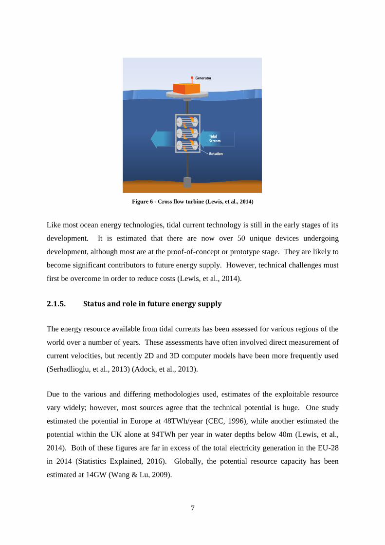
Figure 6 - Cross flow turbine (Lewis, et al., 2014)

Like most ocean energy technologies, tidal current technology is still in the early stages of its

development. It is estimated that there are now over 50 unique devices undergoing

development, although most are at the proof-of-concept or prototype stage. They are likely to

become significant contributors to future energy supply. However, technical challenges must

first be overcome in order to reduce costs (Lewis, et al., 2014).

2.1.5. Status and role in future energy supply

The energy resource available from tidal currents has been assessed for various regions of the

world over a number of years. These assessments have often involved direct measurement of

current velocities, but recently 2D and 3D computer models have been more frequently used

(Serhadlioglu, et al., 2013) (Adock, et al., 2013).

Due to the various and differing methodologies used, estimates of the exploitable resource

vary widely; however, most sources agree that the technical potential is huge. One study

estimated the potential in Europe at 48TWh/year (CEC, 1996), while another estimated the

potential within the UK alone at 94TWh per year in water depths below 40m (Lewis, et al.,

2014). Both of these figures are far in excess of the total electricity generation in the EU-28

in 2014 (Statistics Explained, 2016). Globally, the potential resource capacity has been

estimated at 14GW (Wang & Lu, 2009).

8

Most sources agree that within Europe the greatest potential is in the UK (Lewis, et al.,

2014), and to capitalise of this huge resource the UK government has set a target of 20GW

installed capacity of ocean energy (including wave) by 2020 (Mueller and Jeffrey, 2008).

However, significant deployments of devices are not expected globally until 2030, and

widespread deployment may be prevented by site availability (Lewis, et al., 2014).

2.1.6. Cost

Due to the immaturity of tidal energy technology, and the consequent limited experience of

commercial scale installations, there is a general lack of data on costs (Uihlein & Magagna,

2016). Future costs are therefore highly speculative, but have been predicted, for example,

by SI-Ocean through the application of “learning rates”, which are derived from empirical

studies of broadly similar technologies (SI-Ocean, 2013).

In general, installation cost estimates vary widely. A study published by the Carbon Trust in

2006 gave estimates ranging from £1,400/kW to £3,000/kW for the first tidal stream farms

(Callaghan, 2006), while another study gave figures of between £2,500/kW and £4,200/kW

(IEA OES, 2015). Different estimates are given by (DECC, 2013) (shown in Table 1), but

these are generally within the same range.

Table 1 - Tidal Costs (DECC, 2013)

Construction Costs (£/kW)

High £3,100

Medium £2,700

Low £2,000

Fixed O&M Costs (£/MW/yr)

Medium £143,000

Variable O&M Costs (£/MWh)

Medium £1

Similar to installation costs, LCOE estimates vary between studies. For example, the same

Carbon Trust report calculated it to be in the range between £0.09/kWh to £0.18/kWh

(Callaghan, 2006), while another estimated it to be as low as $0.01/kWh (Klein, 2009) (in

(Lewis, et al., 2014)). One cost-benefit analysis has even shown that the net present value of

tidal energy projects is negative due to high capital expenditure (Houde, 2012) (in (Uihlein &

Magagna, 2016)).

9

2.1.7. Grid connection and integration

Although sophisticated modelling systems now enable accurate and robust resource

assessment for most ocean regions, much work has still to be done on the assessment of

limitations on resource accessibility due to conflicting agendas, i.e. fishing, shipping,

offshore wind, etc. Furthermore, the possibility of connecting an exploited resource to the

grid must also be considered (Uihlein & Magagna, 2016).

Integrating any intermittent and fluctuating energy source into the electricity grid increases

the difficulty of stabilising the grid; in the case of tidal energy this will be particularly

challenging. This is primarily because connection to the grid will likely to be very expensive,

even in the rare cases where a grid connection is available in reasonable proximity to the

array (Magagna, et al., 2014). In reality, most tidal resources are in fact remote from

population centres, where grid connection is weak or absent; this will undoubtedly further

increase costs and lead to high expenditure (Magagna & Uihlein, 2015).

In general, TEC grid integration could contribute to grid congestion, weak grids and voltage

stability problems due to the variable nature of their output (Uihlein & Magagna, 2016).

Issues with supply quality could also potentially limit the amount of electricity delivered to

the grid (Mueller & Wallace, 2008) (Kiprakis & Wallace, 2004). This will especially be the

case in future, when demands on power quality will likely be more stringent for renewable

energy producers (IEC, 2012). The cost of intermittent energy penetration has been

estimated at between £5 and £8 per MWh (Gross, et al., 2007).

2.1.8. Environmental and social impacts

Due to the immaturity of tidal energy technology, the environmental impacts of turbine arrays

are currently unknown (Uihlein & Magagna, 2016). It is likely, though, that benthic habitats

will be affected due to changes in water flows, substrate composition and sediment dynamics

(Frid, et al., 2012) (in (Uihlein & Magagna, 2016)). There is also the potential for fish and

marine mammals to be killed by blade strikes (Frid, et al., 2012) (Boehlert & Gill, 2010) (in

(Uihlein & Magagna, 2016)) and for distress to be caused to marine mammals by noise

disruption in turbulent waters (Polagye, et al., 2011) (in (Uihlein & Magagna, 2016)).

10

As with environmental impacts, social impacts are unknown due to the immaturity of the

technology, but negative impacts will likely be related to visual impacts and access

restrictions to the occupied space for other users of the environment (Uihlein & Magagna,

2016).

2.2. Tidal energy with storage

There is presently limited published research on the use of energy storage systems with tidal

electricity generation, presumably due to the relative immaturity of tidal energy technology.

Nevertheless, a few studies were found which suggest there are likely to be some benefits to

combining the two technologies. In general, energy storage is seen as one means by which

the variability of any renewable resource can be accommodated (Uihlein & Magagna, 2016).

In the case of tidal turbines, this may make connection and integration into the electricity grid

easier by influencing how well their power output can be forecast and matched to demand

(Huckerby, et al., 2011) (Lewis, et al., 2014).

A study published by Clarke, et al. (2006) looked at the viability of combining the power

output of three geographically separated tidal sites to provide firm power. They suggested

that pumped hydro storage would be a potential solution to enhance power smoothing within

the daily timescale, but performed no simulation or analysis in support of this. Nor did they

give justification for ruling out other technologies.

In contrast, other studies have made efforts to model the coupling of tidal and storage

technologies with the aim of quantifying the specific storage characteristics required to meet

demand. One such study by Bryden & Macfarlane (2000) investigated the possibility of them

being used to ensure demand was always met, and to provide firm capacity electricity. In this

study, a simple model was constructed in which the energy storage capacity was varied while

the other variables were held constant, while further simulations varied the time constant and

fixed the other variables. The results showed that a storage capacity capable of ensuring that

consumption could always be met was achievable, even for a ‘leaky system’ with a time

constant of approximately 23h. The analysis of base load power capabilities found that even

a small storage capacity could have a substantial influence on the system’s ability to provide

steady supply; however, the benefits of increasing the storage capacity were not attractive

unless to time constant was also increased. Although this study provided some useful

11

information and analysis on the storage characteristics required, it did so from a purely

theoretical perspective, making no reference to any particular storage or turbine technologies.

Its findings are therefore not broadly applicable to real world applications, nor could they

even be used for preliminary feasibility analyses.

Later work by Barbour & Bryden (2011), however, performed very similary analyses but

used a commercial tidal turbine as the power source. While this work is largely derivative of

the earlier study by Bryden & Macfarlane (2000), its methodology was slightly improved and

its use of a real world example turbine make its findings more meaningful. Nevertheless, it

was not without fault, as its modelling of the turbine used incorrect values of turbine diameter

– it mistakenly modelled the turbine as having a total cross-sectional flow area equivalent to a

single 15m diameter turbine rather than as two 16m diameter turbines. This resulted in an

underestimation of the turbine’s power output, as with these parameters it would not achieve

its rated capacity until flow velocities of 3.3m/s were reached rather than 2.4m/s. This again

affects the usefulness of the results, especially since no specific storage technologies which

met the defined criteria were highlighted. Their results did show, however, that storage could

be used to increase exported power under certain circumstances and consequently increase

revenue. They recommended that further cost analysis be done to ascertain levelised costs

for such coupled systems.

Unlike in the aforementioned studies, Testa, et al. (2009) modelled a real world turbine in

conjunction with a specific energy storage system (although the ESS performance

characteristics were hypothetical). They modelled an 18kW Kobold turbine in conjunction

with a vanadium redox flow battery and found that a 35kWh, 10kW battery would be

sufficient to provide uninterrupted power supply to three residential households, provided

that the turbine never ceased to operate; however, 12 hours of autonomy would require more

than double this capacity. While these results are encouraging, the very small scale of this

study (considering only three households) leaves questions about the scalability of energy

storage in this type of application, meaning further work is required in this area.

Furthermore, the study’s narrow scope in terms of storage technologies leaves questions

unanswered about potential other technologies that may also be suitable.

The only study found in the literature which looked at a real life case where tidal and storage

technologies may be installed together was that conducted by Manchester, et al. (2013). The

12

study modelled and analysed an ESS for a 0.5MW tidal turbine in the Bay of Fundy, Canada,

where local policy limited the installed renewable capacity to the minimum annual demand of

0.9MW. This demand was at the time serviced by a wind turbine; however, additional

renewable capacity could be installed if an ESS could ensure that the total renewable output

did not exceed 0.9MW. In the model, the discharge rate and storage capacity were varied and

the additional amount of saleable energy resultant from each combination was quantified.

The results showed that the most energy efficient solution would perhaps not be the most

profitable one, with a 35 year payback period for the storage option required to avoid all

curtailment. Although this study highlights the relevance of one of the key applications of

storage with tidal energy, its lack of consideration of a specific storage technology leave it

unknown if any specific technology would be suitable for the job. Furthermore, the study did

not appear to model the storage system self-discharge, which can have a profound effect on

system performance.

Further studies conducted have found that storage can be used with tidal energy in a number

of applications other than those so far mentioned. For example, Wang, et al. (2011) looked at

the use of a flywheel to maintain active power delivered to the grid at a constant value under

steady state conditions, to suppress bus voltage variations, and to mitigate active power

fluctuations.

2.3. Energy storage

2.3.1. Overview

Energy storage technologies are seen as one of many that could contribute to a reduction in

GHG emissions (IEA, 2014). They are able to provide the flexibility required in energy

systems with high renewable penetrations by enabling energy supply to be decoupled from

demand (Fuchs, et al., 2012). This means that the intermittency and variability of renewable

energy sources can be more easily accommodated, which makes higher renewable

penetrations possible (IEA, 2014).

However, they also have applications within traditional energy systems where renewable

penetrations are low. In these systems, peaks in demand are typically met by ‘cycling’ or

‘intermediate’ generating equipment, which are usually older and less efficient. These plants

13

generate electricity at higher cost than base-load plants, and rising fuel costs are making them

less economically attractive (Ter-Gazarian, 2011, p25). As an alternative, energy storage

systems could be used to smooth the peaks and troughs of daily demand, enabling base load

plants to operate at higher loads and efficiencies.

Presently, the global installed capacity of grid connected electricity is estimated at 140GW,

the majority of which is pumped hydro storage (see Figure 7). It is estimated that 310GW of

installed capacity will be required in the US, Europe, China and India to support

decarbonisation of the electricity sector (IEA, 2014).

Figure 7 – Global installed grid-connected storage capacity (MW) (IEA, 2014)

2.3.2. Applications

Energy storage systems can be used in a number of applications within an energy storage

system. Each of the functions which they might be required to perform, taken from (Fuchs,

et al., 2012), are summarised in the following sections.

2.3.2.1. Ancillary Services

Ancillary services refer to the services required to maintain the integrity, stability and quality

of power delivered in the transmission and distribution network. These services are:

frequency control, voltage control, spinning reserve, and standing reserve. The requirement

for these services increases with renewable penetrations and energy storage systems are able

to perform them all (Fuchs, et al., 2012).

14

2.3.2.2. Peak Shaving

Energy storage systems sighted close to areas of demand could reduce the costs associated

with peak loads by mitigating the need for transmission and distribution lines required to

carry these loads, in addition to possibly replacing peak-load power plants (Fuchs, et al.,

2012).

2.3.2.3. Load Levelling

Energy storage in the form of pumped hydro storage already performs a key load-levelling

function by shifting energy demand from day to night. This is necessary due to the non-

dispatchable nature of base-load thermal – typically nuclear – power plants. When demand

drops in the evening below the plant’s level output the surplus energy is stored in the pumped

hydro reservoir. When demand increases during the day this stored energy can be dispatched

to meet it. As renewable penetration increases and power production becomes increasingly

intermittent, this specific role will largely become obsolete; however, load-levelling on the

scale of a few hours will still be required. Furthermore, load-levelling batteries and PV

installations are likely to become more prevalent (Fuchs, et al., 2012).

2.3.2.4. Long-term Storage

Long-term energy storage will become increasingly necessary with high renewable

penetrations to overcome periods when challenging weather conditions hinder renewable

energy production. This could be due to low winds in the case of wind generation or high fog

or snow cover in the case of solar generation. In the high demand periods of winter these

conditions could pose a significant challenge. To overcome these periods an energy storage

system should be able to provide full power for up to three weeks, the longest typical

duration of one of these weather periods (Fuchs, et al., 2012).

2.3.2.5. Seasonal Storage

Energy storage could be used to overcome seasonal fluctuations in energy productions, for

example by storing the excess energy produced by solar panels during summer and

discharging it during the high demand period of winter. This type of storage is likely to be

15

very expensive; however, it could become competitive in energy systems which have high

penetration of particular types of renewables (Fuchs, et al., 2012).

2.3.2.6. Island Grids

Energy storage can be used in remote communities and areas disconnected from the

electricity grid to supplement either renewable generators or the diesel generators

traditionally used. The addition of storage could not only improve security of supply but also

help to reduce generator operational costs by reducing fuel consumption and wear and tear

brought about by cycling required to meet varying demand. Reductions in emission would

also result (Fuchs, et al., 2012).

2.3.2.7. Uninterruptible Power Supply

Energy storage can be used to provide uninterruptible power, which is typically necessary in

hospital and IT centres. This function is normally performed by backup diesel generators, but

a storage system of sufficient capacity could perform the same function, with the diesel

generator only there for back up once the reserves are depleted (Fuchs, et al., 2012).

2.3.3. Technologies

Energy storage systems all contain the same three essential parts: a power transformation

system; a central store; and charge-discharge control system. They are generally classified by

the storage medium of their central store and fall into a few distinct categories (Ter-Gazarian,

2011). These can be seen in Figure 8.

16

Figure 8 - Storage system classification (Fuchs, et al., 2012)

The timescales shown in Figure 8 give a general indication of the field of application of each

different type of storage. Those with short timescales are typically used for frequency control

and will be required to perform a high number of cycles; those with medium timescales are

typically used to smooth the fluctuations in load between day and night; and those with long

timescales are typically used for supplying power over a number of days or week (Fuchs, et

al., 2012).

A summary of each of the main storage technologies, taken from (Fuchs, et al., 2012), is

given in the following sections.

2.3.3.1. Pumped hydro

17

Figure 9 - Pumped hydro storage (Fuchs, et al., 2012)

Roughly 99% of installed electrical energy storage worldwide is in the form of pumped hydro

storage (IEA, 2014). The general principle involves pumping water from a lower reservoir to

a higher reservoir. The energy is thus stored in the water’s potential energy and can be

recovered by allowing it to flow in the opposite direction and power a turbine to generate

electricity. PHS is a mature technology, having been around since the end of the 19th century.

Discharge times are in the range of a several hours to a few days and efficiencies range from

70-85%. It has the advantage of a long lifetime and high cycle-life, the latter being

practically unlimited. However, its reliance on topographical features limits its use to certain

locations (IEC, 2011).

All the pumped hydro schemes developed so far exploit suitably located reservoirs of water,

but consideration has been given to alternative configurations that may extend the range of

possible sites, such as using the sea as a lower reservoir with an upper reservoir located in

high coastal ground. These schemes are more expensive due to corrosion protection costs

and prevention of water leakage. Underground pumped hydro storage is another option, as is

a combination of the two (Ter-Gazarian, 2011).

Table 2 – Pumped hydro storage (Fuchs, et al., 2012)

2010 2030

Round trip efficiency 75 – 82%

Energy density 0.27Wh/l (100m head) to 1.5Wh/l (550m

head)

Power density n/a

Cycle life n/a

Calendar life 80 years

Depth of discharge 80 – 100%

Self-discharge 0.005%/day to 0.02%/day

Power installation cost 500€/kW to 1,000€/kW

Energy installation cost 5€/kWh to 20€/kWh

Deployment time Approximately 3 minutes

Site requirements Two reservoirs at significantly different

heights

Main applications Frequency control, voltage control, peak

shaving, load levelling, standing reserve,

black start

18

Pumped hydro storage has the strengths of being an established technology with high

efficiency, low self-discharge and long calendar life. However, its costs are high leading to a

long payback period and its energy density is low resulting in large installations being

necessary to be economical. It is also limited by its reliance on specific geological features

(Fuchs, et al., 2012).

2.3.3.2. Compressed air

Figure 10 – Compressed air storage (Fuchs, et al., 2012)

Compressed air energy storage involves using surplus energy to drive a motor which, in turn,

powers a compressor to compress air and store it in a cavern. The heat produced in the

process is removed by a cooler. As the air is discharged from the cavern it cools down,

necessitating the use of a fuel to heat it up before using it to power a turbine-generator to

produce power. An alternative to using a fuel to heat the air is to store heat extracted during

compression and then use it to expand the air through the turbine-generator. The required

heat storage systems for this type of storage are still under development, however (Fuchs, et

al., 2012).

It is used as a medium-term storage solution and could be an alternative to pumped hydro.

However, there are presently very few plants in operation. Like pumped hydro, CAES

requires specific geological features to store the air; for example, salt caverns (Fuchs, et al.,

2012).

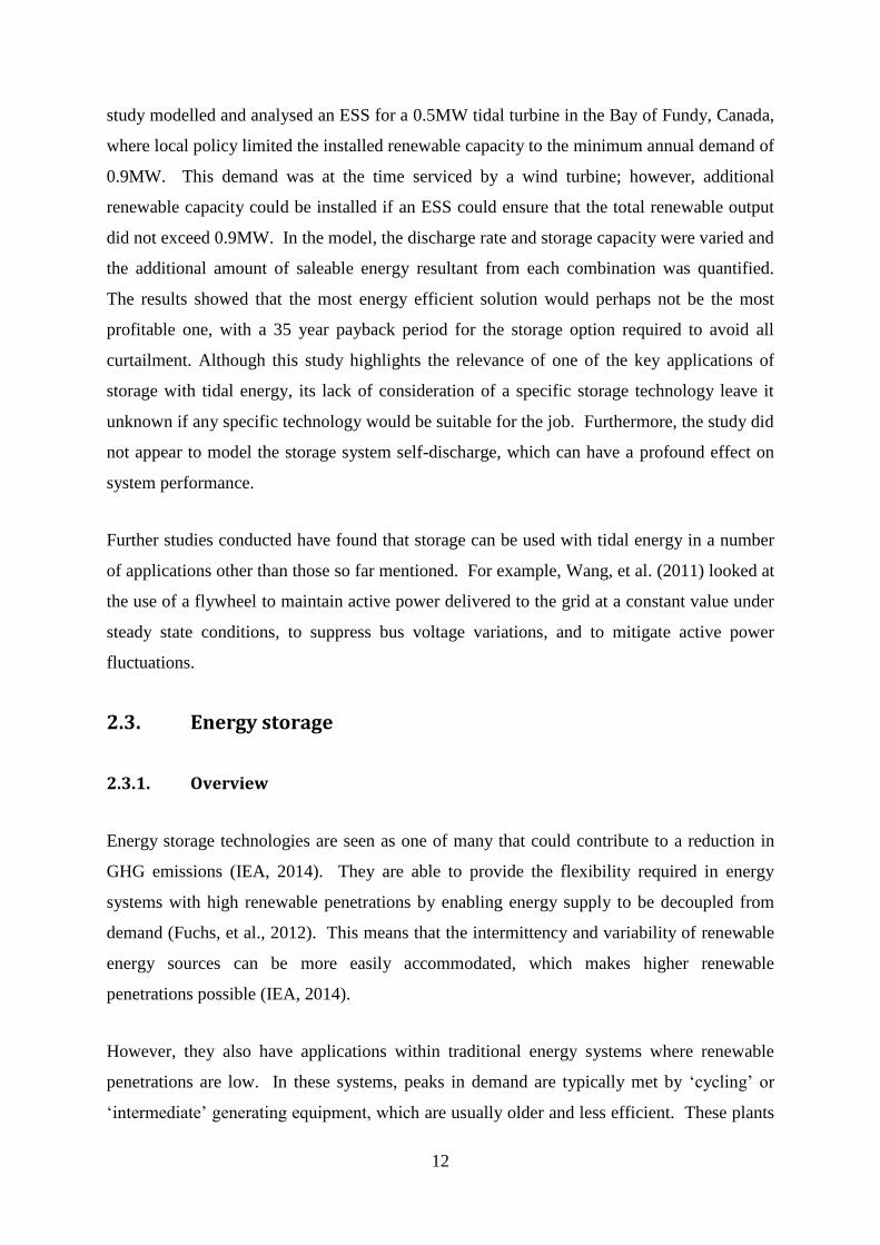
Table 3 – Compressed air storage (Fuchs, et al., 2012)

2010 2030

Round trip efficiency 60 – 70%

Energy density 3Wh/l (100bar) to 6Wh/l (200bar)

19

2010 2030

Power density n/a

Cycle life Not limiting



Self-discharge 0.5%/day to 1%/day

Power installation cost 1,000€/kW 700€/kW

Energy installation cost 40€/kWh to 80€/kWh

Deployment time Approximately 3 to 10 minutes

Site requirements Cavern

Main applications Frequency control, voltage control, peak

shaving, load levelling, standing reserve,

black start

CAES has the strengths of being relatively low storage cost, low self-discharge, long calendar

life and low surface footprint. However, it requires high investment cost resulting in long

payback periods. It also relies on specific geological features and the higher efficiency

adiabatic type is an immature technology that has yet to be demonstrated full-scale (Fuchs, et

al., 2012).

2.3.3.3. Hydrogen

Figure 11 – Hydrogen storage (Fuchs, et al., 2012)

In hydrogen storage systems, surplus energy is used to power an electrolyser to produce

hydrogen which is then compressed and stored. The stored hydrogen can then be used to

drive a turbine or a fuel cell to generate electricity. It can also be used in cars with fuel cells

or special internal combustion engines. The volumetric energy density of compressed

20

hydrogen is very high, leading to low energy storage costs. However, efficiency is very low.

Additionally, energy storage costs are significantly higher for small and midsize systems

which do not utilise large salt caverns. There is scope to use the natural gas grid as a large

reservoir for hydrogen storage. Its most likely field of application is in large, long-term

energy storage, on timescales of weeks, months or seasonal. Present utilisation is low as it is

cheaper to use conventional backup or long distance transmission; however, as renewable

penetrations reach 80-100% it is likely to become more important (Fuchs, et al., 2012).

Although fuel cells exist for the conversion of chemical energy to electrical energy, due to

their expense, combustion remains the primary means by which power is extracted.

Hydrogen is therefore most likely to be used in combustion engines in vehicles as a substitute

for fossil fuels. It is also most likely to be used in existing thermal power plants to

supplement power production (Ter-Gazarian, 2011).

Table 4 – Hydrogen storage

2010 2030

Round trip efficiency 34 – 40% 40 – 50%

Energy density 3Wh/l (1bar) 750Wh/l (250bar) 2,400Wh/l (liquid)

Power density n/a

Cycle life n/a

Calendar life n/a



Power installation cost 1,500 €/kW to 2,000 €/kW 500 €/kW to 800 €/kW

Energy installation cost 0.3 €/kW to 0.6 €/kW

Deployment time 10 minutes

Site requirements Underground cavern

Main applications Seasonal storage, island grid

Hydrogen storage has the strengths of a low surface footprint due to the reservoir being

underground, being able to store large amounts of energy, and utilising the abundant source

of water. However, efficiency is low, as is storage density. Electrolyser costs are also high


21

2.3.3.4. Power to gas

Figure 12 - (Fuchs, et al., 2012)

Power to gas can be considered an alternative to hydrogen storage by storing the energy in

synthetic natural gas (methane). Methane is produced by the Fischer-Tropsch process, an

exothermic reaction between hydrogen and carbon dioxide. The methane produced can be

stored in the natural gas grid using existing infrastructure, eliminating storage costs.

However, efficiencies are lower still than hydrogen, with additional cost. An external source

of carbon dioxide is required and, unless a heat load is nearby, the produced heat is wasted


Table 5 – Power to gas (Fuchs, et al., 2012)

2010 2030


Energy density Approximately three times that of

hydrogen

Power density n/a

Cycle life n/a

Calendar life n/a



Power installation cost 1,000 €/kW to 2,000 €/kW

Energy installation cost No additional cost if stored in gas grid

Deployment time 10 minutes

Site requirements Cavern or gas grid access, carbon

dioxide source, heat demand

22

2010 2030

Main applications Seasonal storage, island grid

Power to gas has the strengths of high energy density and being suitable for long-term

storage. However, its efficiency is low and it requires an external source of carbon dioxide.

If this were to be extracted from the air its efficiency would reduce further (Fuchs, et al.,

2012).

2.3.3.5. Batteries

Batteries are considered a type of chemical storage with internal storage. Energy and power

capacity are dependent on each other such that high energy content leads to high power

capability. This contrasts with chemical storage with external storage, in which energy and

power capacities are independent of each other (Fuchs, et al., 2012).

2.3.3.5.1. Lead-acid batteries

Figure 13 – Lead-acid batteries (Fuchs, et al., 2012)

Lead acid batteries have the largest installed capacity of all battery technologies and are the

most mature; some systems have been in operation for up to 20 years. They are mainly used

for short-term and medium-term storage; for example, in car batteries and for UPS in

telecommunications and island grids. Increased production quantities and design

optimisation for stationary applications could lead to cost reductions and lifetime

23

improvements. Their low investment and life-cycle costs make them an important

technology for the near and mid-term future, but they are often disregarded due to the

publicity of higher performance batteries such as lithium-ion (Fuchs, et al., 2012).

Table 6 – Lead-acid batteries (Fuchs, et al., 2012)

2010 2030


Energy density 50Wh/l to 100Wh/l 50Wh/l to 130Wh/l

Power density 10W/l to 500W/l 10W/l to 1,000W/l

Cycle life 500 to 2,000 1,500 to 5,000

Calendar life 5 to 15 years 10 to 20 years

Depth of discharge 70% 80%

Self-discharge 0.1%/day to 0.4%/day 0.05%/day to

0.2%/day

Power installation cost 150 €/kW to 200 €/kW 35 €/kW to 65 €/kW

Energy installation cost 100 €/kWh to 250

€/kWh

50 €/kWh to 80

€/kWh

Deployment time 3 to 5ms

Site requirements Ventilation due to gassing

Main applications Frequency control, peak shaving, load levelling,

island grids, residential storage, UPS

Lead acid batteries have the strengths of acceptable energy and power densities, no

requirement for complex cell management, there being experience with this technology and a

relatively low investment cost leading to a short payback period. However, charging and

discharging abilities are not symmetrical, ventilation is required and they have a limited cycle

life (Fuchs, et al., 2012).

2.3.3.5.2. Lithium-ion batteries

24

Figure 14 – Lithium-ion batteries (Fuchs, et al., 2012)

Lithium-ion batteries consist of lithiated metal-oxide and layered graphitic carbon electrodes.

Lithium salts dissolved in organic carbonates make up the electrolyte. The lithium ions are

transferred from the positive, lithiated metal oxide electrode to the negative carbon one and

during discharge the process is reversed. They are primarily used for medium-term storage

but can also be used for short-term storage. They are used most widely in portable

applications – for example, laptops and mobile phones – however, they can also be used in

static applications. High development activity is still present for this technology. The main

challenge will be to reduce cost (Fuchs, et al., 2012).

Table 7 - Lithium-ion batteries (Fuchs, et al., 2012)

2010 2030


Energy density 200Wh/l to 350Wh/l 250Wh/l to 550Wh/l

Power density 100W/l to 3,500W/l 100W/l to 5,000W/l

Cycle life 1,000 to 5,000 (full

cycles)

3,000 to 10,000 (full

cycles)


Depth of discharge Up to 100% Up to 100%

Self-discharge 5%/month 1%/month

Power installation cost 150 €/kW to 200 €/kW 35 €/kW to 65€/kW

Energy installation cost 300 €/kWh to 800

€/kWh

150 €/kWh to 300 €/kWh


Site requirements None

Main applications Frequency control, voltage control, peak shaving,

load levelling, electromobility, residential storage

Lithium-ion batteries have the strengths of high energy density and long lifetime. However,

costs are high and sophisticated battery management systems are required. Packaging and

cooling requirements are also costly (Fuchs, et al., 2012).

25

2.3.3.5.3. High temperature batteries

Figure 15 – High-temperature batteries (Fuchs, et al., 2012)

High temperature batteries have a solid state electrolyte and thus are required to operate at

temperatures in the region of 270 - 350°C to achieve high ion conductivity with the active

components in a fluid condition. These high temperatures can be maintained by the heat

generated by the battery during charging and discharging. They are therefore suitable for

applications with daily cycling but would not be suitable for applications with long periods

between charging and discharging since this would allow them to cool down. They are

typically used for medium-term energy storage. Raw materials are cheap, so increased

deployment is likely in future (Fuchs, et al., 2012).

Table 8 – High-temperature batteries (Fuchs, et al., 2012)

2010 2030

Round trip efficiency

75 – 80% 80 – 90%

Energy density 150Wh/l to 250Wh/l n/a

Power density n/a n/a

Cycle life 5,000 to 10,000


Depth of discharge 100%

Self-discharge 10%/day n/a

Power installation cost

150 €/kW to 200

€/kW

35 €/kW to 65 €/kW

Energy installation cost

500 €/kW to 700

€/kW

80 €/kW to 150

€/kW



Main applications Frequency control, peak shaving, load

levelling, island grids, electromobility, UPS

26

High temperature batteries have the strengths of high specific energy, high cycle and calendar

life and cheap raw materials. However, they have high thermal losses and are potentially

hazardous due to their high operating temperature (Fuchs, et al., 2012).

2.3.3.5.4. Flow batteries

Figure 16 – Flow batteries (Fuchs, et al., 2012)

In flow batteries, surplus energy is used to apply current to a central reaction unit through

which the electrolyte is pumped. Energy deficits are met during discharging by the current

delivered from the same reaction unit when the process is reversed. Energy capacity is

determined by the volume of electrolyte while the central reaction unit determines the power

capacity. They are well suited to large and medium scale technical operations since the

construction of larger tanks is easily possible (Fuchs, et al., 2012) and are generally used in

high energy applications (Zhou, et al., 2012). They could potentially bridge the gap between

medium-term storage – with timescales in the region of 1 to 10 hours – and long-term storage

– with timescales in the region of several weeks. They are likely to be suitable for storage of

marine energy (Zhou, et al., 2012). The vanadium redox-flow type are the most important

commercially available. Zinc-bromine is an alternative. It has the advantage, as an example

of chemical storage with external storage, of power and energy capacities being independent

of each other (Zhou, et al., 2012). Vanadium and zinc-bromine are presently too expensive to

be competitive, so further investigation of redox pairs is required. Maintenance costs are

high due to leaks caused by acidic liquids (Fuchs, et al., 2012).

27

Table 9 – Flow batteries (Fuchs, et al., 2012)

2010 2030


Energy density 20Wh/l to 70Wh/l >100Wh/l

Power density n/a

Cycle life >10,000



Self-discharge 0.1% /day to

0.4%/day

0.05%/day to

0.2%/day

Power installation cost 1,000 €/kW to 1,500

€/kW

600 €/kW to 1,000

€/kW

Energy installation cost 300 €/kW to 500

€/kW

70 €/kW to 150

€/kW

Deployment time Seconds


Main applications Secondary/tertiary frequency control, long-

term storage, island grids

Flow batteries have the strengths of their power and energy capacity ratings being

independent of each other and a high cycle life. However, the acidic liquids used cause

leakage and the life span of the cell stack is short. Additionally, vanadium redox solution

costs are high and the necessary valves and pumps are prone errors increasing maintenance

costs (Fuchs, et al., 2012).

2.3.3.6. Flywheels

28

Figure 17 – Flywheels (Fuchs, et al., 2012)

Flywheel storage uses surplus power to drive a motor which accelerates a rotating mass. The

energy is thus stored as rotating kinetic energy. Those which rotate at speeds below

10,000rpm are termed ‘low-speed’ (Zhou, et al., 2012). Energy deficits can then be met by

reversing the process, i.e. using the rotating mass to drive a generator to produce power. To

maintain the angular velocity of the rotating mass, losses must be low. Low friction magnetic

bearings and vacuum chambers are therefore used to keep resistance to a minimum. Power

density and cycle life are typically high, but energy density is typically average and self-

discharge is high. They are therefore typically used for short-term storage in applications

which demand very high power. The high cost components required to reduce losses lead to

considerable investment costs. They are unlikely to be a relied upon technology for higher

renewable penetrations (Fuchs, et al., 2012).

Table 10 – Flywheels (Fuchs, et al., 2012)

2010 2030


80 – 95%

No data available

Energy density 80Wh/l to 200Wh/l

Power density 10kW/l

Cycle life Several millions



Self-discharge 5 – 15%/hour


300€/kW


1,000€/kW

Deployment time Approximately 10ms


Main applications Primary frequency control, voltage control,

peak shaving, UPS

Flywheels have the strengths of a long cycle life, low maintenance costs and high charge

capability. However, energy density is low and self-discharge is high. Vacuum chamber and

cooling system requirements also lead to high costs (Fuchs, et al., 2012).

29

2.3.3.7. Supercapacitors

Figure 18 – Supercapacitor (Fuchs, et al., 2012)

Super-capacitors use surplus energy to move ions in an electrolyte from one electrode of the

capacitor to the other. The energy is thus stored in the electric field between the two. Power

and energy densities lie in the region between regular capacitors and batteries. Their cycle

life and power density is very high when compared with batteries, but energy densities are

low. They are therefore typically used for short-term storage applications which require high

power, but can also be used in hybrid systems with batteries to increase their lifetime. Costs

are high, but there is scope for this to decrease if they are adopted for hybrid vehicles which

would lead to high production quantities. However, they are likely to still be used in

specialist fields to store energy for timescales in the region of 10 seconds (Fuchs, et al., 2012)

(Zhou, et al., 2012).

Table 11 – Supercapacitors (Fuchs, et al., 2012)

2010 2030


90 – 94% No data available

30

2010 2030

Energy density 2Wh/l to 10Wh/l

Power density Up to 15kW/l

Cycle life Up to one million



Self-discharge 25% in first 48

hours, very low

thereafter


10€/kW to 20€/kW


10,000€/kWh to

20,000€/kWh

Deployment time <10ms


Main applications Primary frequency control, voltage

control, peak shaving, UPS

Super-capacitors have the benefit of high efficiency, high power capability and long cycle

life. However, energy density is low leading to high energy installation costs (Fuchs, et al.,

2012).

2.3.3.8. Superconductive magnetic energy

Figure 19 - (Fuchs, et al., 2012)

SMES systems use surplus power that is inverted to DC and supplied to a superconducting

coil. The current in the coil induces a constant magnetic field in which the energy is stored.

31

The stored energy is discharged by connecting the coil to a load, reducing its magnetic field

and current. To maintain zero losses in the coil it must be maintained at -260°C, resulting in

high self-discharge due to cooling requirements. They are used for short-term storage which

requires high power. This technology is unlikely to become competitive with others and is

primarily used in niche applications (Fuchs, et al., 2012).

Table 12 - Superconductive magnetic energy storage (Fuchs, et al., 2012)

2010 2030


80 – 90% No data

Energy density 0.5Wh/l to 10Wh/l

Power density 1kW/l to 4kW/l

Cycle life Not limiting


Depth of discharge n/a

Self-discharge 10%/day to

15%/day


n/a


n/a

Deployment time Approximately 1 – 10ms

Site requirements Refrigeration/ switching & inverter

systems

Main applications Primary frequency control, voltage

control, peak shaving, UPS

SMES has the strengths of high power capability and high cycle life. However, self-

discharge losses are high due to the high cooling demand and costs are high. System design

is also very complicated.

32

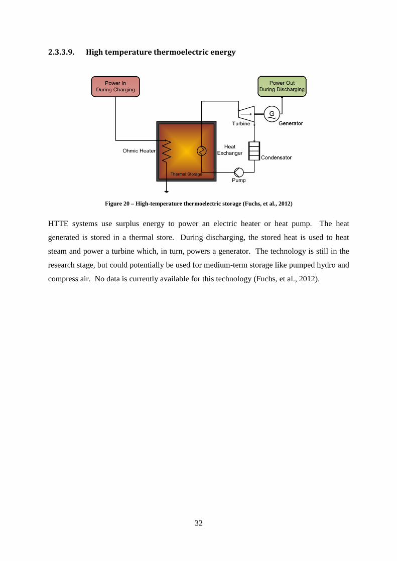
2.3.3.9. High temperature thermoelectric energy

Figure 20 – High-temperature thermoelectric storage (Fuchs, et al., 2012)

HTTE systems use surplus energy to power an electric heater or heat pump. The heat

generated is stored in a thermal store. During discharging, the stored heat is used to heat

steam and power a turbine which, in turn, powers a generator. The technology is still in the

research stage, but could potentially be used for medium-term storage like pumped hydro and

compress air. No data is currently available for this technology (Fuchs, et al., 2012).

33

3. Methodology

To meet the project objectives, the methodology employed involved carrying out the

following sequential steps.

1. Literature review

2. Model construction

3. Model validation

4. Simulation parameter definition

5. Simulation

6. Results analysis

7. Recommendation

First, a literature review was conducted to obtain the knowledge required to build the

simulation model. The model was then constructed and tested for robustness by validation

against the results of an existing study. The parameters of the simulation were set based

information found in the literature and the required number of simulations was performed.

The results of the simulations were then analysed and interpreted in order to give a final

recommendation.

34

3.1. Model construction

The simulation model was created in Microsoft Excel and was comprised of four integrated

modules. Three of these modules – the tidal, turbine and storage modules – together

described the essential physical characteristics of the system. The fourth module calculated

the levelised cost of energy (LCOE). The overall architecture of the system can be seen in

Figure 21.

Figure 21 - Model architecture

A detailed description of each module is given in the following sections.

3.1.1. Tidal module

The flow velocity of the tides was modelled using a simplified version of the harmonic

current equation (1) in which only the primary two tidal harmonic constituents were

considered. These constituents are M2, the principle lunar semi-diurnal constituent, and S2,

the principle solar semi-diurnal constituent. This simplified version of the equation can be

seen in equation (3):

35

𝒗(𝒕) = 𝒗𝑴𝟐𝒄𝒐𝒔 (

𝟐𝝅𝒕

𝑻𝑴𝟐

) + 𝒗𝑺𝟐𝒄𝒐𝒔 (

𝟐𝝅𝒕

𝑻𝑺𝟐

) (3)

The principle lunar semi-diurnal constituent, M2, in this equation represents the rotation of

the earth with respect to the moon and has a period of 12.4206 hours. The principle solar

semi-diurnal constituent, S2, represents the rotation of the earth with respect to the sun and

has a period of 12 hours. The asynchronicity of these two constituents is what causes the

spring-neap cycle, so the modelling of only these is sufficient to capture the most significant

variations in output throughout the cycle. A characteristic example of this variation produced

by the model can be seen in Figure 22, Figure 23 and Figure 24 for symbolic lunar and solar

flow velocities of 3.5ms-1 and 1.5ms-1, respectively.

Figure 22 - Constituent flow velocities

Figure 23 - Total flow velocity

Figure 24 - Spring-neap cycle

36

Figure 22 shows the constituent flow velocities while Figure 23 shows the resultant total flow

velocity. The approximate 12 hour period of the variation in total velocity produced by the

model, which mimics the twice daily variation in tidal height, can be clearly observed in

Figure 23. Figure 24 shows the entire spring-neap cycle produced by the model, lasting

approximately 14.75 days. The high flow velocities at spring tides and low flow velocities at

neap tides can be clearly observed.

Although the modelling of only these two constituents will not give an entirely accurate

representation of the varying flow characteristics throughout the cycle – some of the more

nuanced harmonic constituents having been ignored – it is sufficient for the purposes of this

study. Furthermore, use of this relatively simple model is not without precedent, it being the

method used to give some preliminary resource estimates in various studies; for example, by

(Adock, et al., 2013).

The magnitudes of the constituent velocities required to calculate the resultant flow velocity

using equation (3) are not widely available; however, mean spring and neap velocities are

relatively easily obtainable from published sources. Admiralty tidal diamonds, for example,

contain mean spring and mean neap flow velocities in addition to tidal range data. From the

mean spring and neap velocities, the constituent velocities can be easily calculated using

equations (4) and (5), taken from (Hardisty, 2009):

𝒗𝑴𝟐=

𝒗𝒔𝒑𝒓𝒊𝒏𝒈 + 𝒗𝒏𝒆𝒂𝒑

𝟐 (4)

𝒗𝑺𝟐=

𝒗𝒔𝒑𝒓𝒊𝒏𝒈 − 𝒗𝒏𝒆𝒂𝒑

𝟐 (5)

The result of modelling the tidal flow as described above was that the only data which was

required to be defined by the user to create a flow profile were the mean spring and neap flow

velocities, which are easily obtainable. This flow profile could then be fed into the tidal

module in order to create a power profile.

37

3.1.2. Turbine module

The power produced by the tidal turbine was modelled from the kinetic energy flux of the

fluid stream and the power coefficient of the turbine, shown in equation (6).

𝑷𝑻𝒖𝒓𝒃𝒊𝒏𝒆(𝒕) =𝟏

𝟐𝑪𝒑𝝆𝝅

𝑫𝟐

𝟒𝒗(𝒕)𝟑 (6)

The turbine’s performance envelope, dictated by its cut-in velocity and rated capacity, was

modelled such that it only produced power when the flow velocity was above its cut-in

velocity and the maximum power it produced was set to never exceed the rated capacity.

These restrictions are expressed in equations (7) and (8).

𝑰𝑭 𝒗(𝒕) ≥ 𝒗𝒄𝒖𝒕−𝒊𝒏, 𝑻𝑯𝑬𝑵 𝑷𝑻𝒖𝒓𝒃𝒊𝒏𝒆(𝒕) =𝟏

𝟐𝑪𝒑𝝆𝑨𝒗(𝒕)𝟑

𝑬𝑳𝑺𝑬 𝑷𝑻𝒖𝒓𝒃𝒊𝒏𝒆(𝒕) = 𝟎 (7)

𝑰𝑭 𝑷𝑻𝒖𝒓𝒃𝒊𝒏𝒆(𝒕) ≥ 𝑷𝒕−𝒓𝒂𝒕𝒆𝒅, 𝑻𝑯𝑬𝑵 𝑷𝑻𝒖𝒓𝒃𝒊𝒏𝒆(𝒕) = 𝑷𝒕−𝒓𝒂𝒕𝒆𝒅

𝑬𝑳𝑺𝑬 𝑷𝑻𝒖𝒓𝒃𝒊𝒏𝒆(𝒕) =𝟏

𝟐𝑪𝒑𝝆𝑨𝒗(𝒕)𝟑

(8)

A power profile produced by the model for a commercially operated turbine during spring

tides can be seen in Figure 25. The turbine considered has a coefficient of performance of

0.42, a cut-in velocity of 1ms-1 and a rated capacity of 1.2MW. The mean spring peak

velocity of the flow is 5ms-1. The variation of the turbine power output in line with flow

velocity produced by the model can be clearly seen. Due to the bi-directionality of the

turbine, power is produced when the flow velocity is either positive or negative. The only

time the turbine produces no power is when the magnitude of the flow velocity drops below

the turbine’s cut-in velocity. When the magnitude of the flow velocity reaches the turbine’s

rated velocity, the power output is maintained at the rated capacity.

38

Figure 25 – Turbine power profile

The result of modelling the turbine power output as described above was that a power profile

could be produced by the user defining the turbine diameter, coefficient of performance, cut-

in velocity and rated capacity. To give the additional attribute of scalability, a provision was

also made for specifying the total number of turbines installed. This power profile could then

be fed into the storage module to in order to create a stored energy profile.

3.1.3. Storage module

The storage system was modelled using the same general method employed by (Barbour &

Bryden, 2011). A simple schematic of the combined tidal-storage system modelled in that

study can be seen in Figure 26. In the model, all power produced by the turbine goes through

the power transfer control system, whose control parameters determine how much of the

power is transferred to the grid and how much to the storage system. The control parameters

of the PTCS also determine how much power is extracted from the storage system and

exported to the grid.

39

Figure 26 - System schematic (Barbour & Bryden, 2011)

For this study, the PTCS was included as part of the storage module. A detailed description

of both the PTCS and the storage system is given in the following sections.

3.1.3.1. Power Transfer Control System

3.1.3.1.1. Power transferred to store

It can be seen from Figure 26 that the power transferred to the store, neglecting efficiencies,

is simply the difference between the power produced by the turbine and the power exported

to the grid. Using a positive sign convention for power transferred to the store, this can be

expressed using equation (9).

𝑷𝒔𝒕𝒐𝒓𝒆(𝒕) = 𝑷𝒕𝒖𝒓𝒃𝒊𝒏𝒆(𝒕) − 𝑷𝒈𝒓𝒊𝒅(𝒕) (9)

However, due to charging and discharging efficiencies, the energy increase of the store over

time will be less than surplus energy produced by the turbine over the same period and,

similarly, the energy decrease of the store over time will be greater than the energy deficit it

is required to fill over the same period. To take account of this, the charging and discharging

efficiencies were modelled by first assuming that the efficiency was equal in both directions,

as shown in equation (10).

𝜼𝒄𝒉𝒂𝒓𝒈𝒆 = 𝜼𝒅𝒊𝒔𝒄𝒉𝒂𝒓𝒈𝒆 = √𝜼𝑻 (10)

The effective power transfer to the store was then modelled using equations (11), (12) and

(13).

𝑰𝑭 𝑷𝒕𝒖𝒓𝒃𝒊𝒏𝒆(𝒕) > 𝑷𝒈𝒓𝒊𝒅(𝒕),

𝑻𝑯𝑬𝑵 𝑷𝒔𝒕𝒐𝒓𝒆(𝒕) = √𝜼𝑻 × (𝑷𝒕𝒖𝒓𝒃𝒊𝒏𝒆(𝒕) − 𝑷𝒈𝒓𝒊𝒅(𝒕)) (11)

𝑰𝑭 𝑷𝒕𝒖𝒓𝒃𝒊𝒏𝒆(𝒕) < 𝑷𝒈𝒓𝒊𝒅(𝒕),

𝑻𝑯𝑬𝑵 𝑷𝒔𝒕𝒐𝒓𝒆(𝒕) =𝑷𝒕𝒖𝒓𝒃𝒊𝒏𝒆(𝒕) − 𝑷𝒈𝒓𝒊𝒅(𝒕)

√𝜼𝑻

(12)

40

𝑰𝑭 𝑷𝒕𝒖𝒓𝒃𝒊𝒏𝒆(𝒕) = 𝑷𝒈𝒓𝒊𝒅(𝒕),

𝑻𝑯𝑬𝑵 𝑷𝒔𝒕𝒐𝒓𝒆(𝒕) = 𝟎 (13)

3.1.3.1.2. Power exported to grid

It can be seen from Figure 26 that, in order to model the power transferred to the store, the

power exported to the grid must first be modelled. This was done by first defining a

percentage of rated capacity (PRC), shown in equation (14).

𝑷𝑹𝑪 =∫ 𝑷𝒈𝒓𝒊𝒅𝒅𝒕

𝒕𝒏

𝒕𝟏

∫ 𝑷𝒕𝒖𝒓𝒃𝒊𝒏𝒆𝒅𝒕𝒕𝒏

𝒕𝟏

(14)

That is to say, the ratio of the total energy exported to the grid to the total energy produced by

the turbine within the same period.

By rearranging equation (14), the power exported to the grid could then be modelled using

equation (15).

𝑷𝒈𝒓𝒊𝒅(𝒕) =∫ 𝑷𝒕𝒖𝒓𝒃𝒊𝒏𝒆𝒅𝒕

𝒕𝒏

𝒕𝟏

𝒏× 𝑷𝑹𝑪 (15)

If PRC was set to 100%, the power exported to the grid would simply be the average power

produced by the turbine. However, due to energy losses during charging and discharging the

storage system, in addition to self-discharge losses, PRC will always be less than 100%.

3.1.3.2. Storage system

The energy contained within the store at any moment in time, neglecting self-discharge, can

be expressed using equation (16).

𝐸(𝑡) = 𝐸0 + ∫ 𝑃𝑠𝑡𝑜𝑟𝑒(𝑡)𝑑𝑡𝑡𝑛

𝑡1

(16)

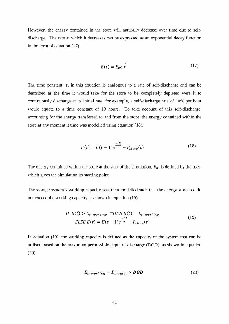
41

However, the energy contained in the store will naturally decrease over time due to self-

discharge. The rate at which it decreases can be expressed as an exponential decay function

in the form of equation (17).

𝐸(𝑡) = 𝐸0𝑒−𝑡𝜏 (17)

The time constant, 𝜏, in this equation is analogous to a rate of self-discharge and can be

described as the time it would take for the store to be completely depleted were it to

continuously discharge at its initial rate; for example, a self-discharge rate of 10% per hour

would equate to a time constant of 10 hours. To take account of this self-discharge,

accounting for the energy transferred to and from the store, the energy contained within the

store at any moment it time was modelled using equation (18).

𝐸(𝑡) = 𝐸(𝑡 − 1)𝑒−𝑑𝑡

𝜏 + 𝑃𝑠𝑡𝑜𝑟𝑒(𝑡) (18)

The energy contained within the store at the start of the simulation, 𝐸0, is defined by the user,

which gives the simulation its starting point.

The storage system’s working capacity was then modelled such that the energy stored could

not exceed the working capacity, as shown in equation (19).

𝐼𝐹 𝐸(𝑡) > 𝐸𝑠−𝑤𝑜𝑟𝑘𝑖𝑛𝑔 𝑇𝐻𝐸𝑁 𝐸(𝑡) = 𝐸𝑠−𝑤𝑜𝑟𝑘𝑖𝑛𝑔

𝐸𝐿𝑆𝐸 𝐸(𝑡) = 𝐸(𝑡 − 1)𝑒−𝑑𝑡

𝜏 + 𝑃𝑠𝑡𝑜𝑟𝑒(𝑡) (19)

In equation (19), the working capacity is defined as the capacity of the system that can be

utilised based on the maximum permissible depth of discharge (DOD), as shown in equation

(20).

𝑬𝒔−𝒘𝒐𝒓𝒌𝒊𝒏𝒈 = 𝑬𝒔−𝒓𝒂𝒕𝒆𝒅 × 𝑫𝑶𝑫 (20)

42

No lower limit for stored energy was imposed, meaning that the energy contained within the

store at any moment in time could drop below zero. This was an important feature of the

model which was used during the optimisation simulations.

3.1.3.3. Storage system optimisation

The result of modelling the energy storage system in the manner described was that a stored

energy profile could be obtained by the user defining only five system parameters: the PRC

to be produced, the round-trip efficiency, the time-constant, the working energy capacity, and

the value of the energy stored at the start of the simulation. Since the round-trip efficiency

and time constant are properties of the storage system used, it was possible to optimise the

energy capacity of a particular storage system for a defined PRC by simply varying the

working energy capacity and the initial stored energy. The optimal system would be the one

with the smallest energy capacity capable of ensuring that the value of the energy stored

never dropped below zero.

The procedure for the optimisation was as follows:

3.1.3.3.1. Step 1

The parameters of the storage system under consideration were set within the storage module

(Table 13).

Table 13 - Fixed storage parameters

3.1.3.3.2. Step 2

Start values were set for the working energy capacity of the system and the initial energy

stored (Table 14). The values chosen to start are of little consequence as they will be

changed later.

Fixed Storage Parameters

PRC 60%

Round Trip Efficiency 80%

Time Constant (h) 240

43

Table 14 - Variable storage parameters

3.1.3.3.3. Step 3

The suitability of the start values was evaluated by consideration of ‘target values’ (Table

15). The target ‘Initial Stored Energy’ value, 𝐸1, was measured as the energy contained

within the store at the point corresponding to 𝐸0 in the following spring-neap cycle. The

target ‘Min. Stored Energy’, 𝐸𝑚𝑖𝑛, was measured as the lowest value of energy stored over a

six month period. Both of these values are shown in Figure 27.

Table 15 – Simulation target values

Figure 27 - Stored energy

For an optimal system, 𝐸𝑚𝑖𝑛 should be as close to zero as possible while still being above

zero. This will ensure that all of the working capacity is being utilised throughout the cycle.

Furthermore, for the system to be truly sustainable 𝐸1 should be equal to 𝐸0, as any

discrepancy indicates that the system is either gaining or losing energy over each cycle. For

the system depicted, the working capacity should therefore be reduced until 𝐸𝑚𝑖𝑛 is close to

zero and 𝐸0 should be adjusted to equal 𝐸1.

Variable Storage Parameters

Working Capacity (kWh) 14000

Initial Energy Stored (kWh) 8000

Target Values

Initial Stored Energy (kWh) 14000

Min. Stored Energy (kWh) 2827.52

𝐸0 𝐸1

𝐸𝑚𝑖𝑛

44

3.1.3.3.4. Step 4

The working energy capacity of the system and the initial stored energy were then adjusted in

an iterative manner until the working capacity of the system was optimal and the system was

sustainable (Table 16, Table 17 & Figure 28).

Table 16 - Optimised storage parameters

Table 17 - Optimised target storage values

Figure 28 - Final energy stored profile

The rated energy capacity of the system was then calculated by the user defining the DOD for

the system, as shown in equation (21).

𝑬𝒔−𝒓𝒂𝒕𝒆𝒅 =𝑬𝒔−𝒘𝒐𝒓𝒌𝒊𝒏𝒈

𝑫𝑶𝑫 (21)

Variable Storage Parameters

Working Capacity (kWh) 10215

Initial Energy Stored (kWh) 10215

Target Values

Initial Stored Energy (kWh) 10215

Min. Stored Energy (kWh) 0.18

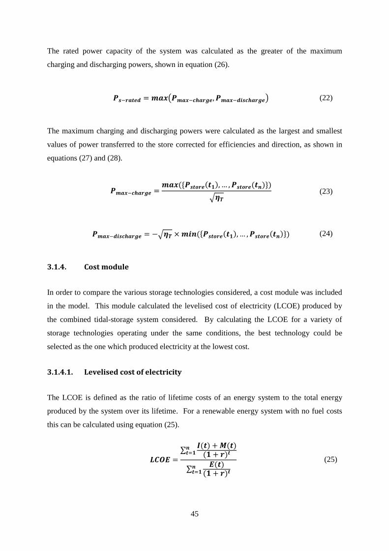
45

The rated power capacity of the system was calculated as the greater of the maximum

charging and discharging powers, shown in equation (26).

𝑷𝒔−𝒓𝒂𝒕𝒆𝒅 = 𝒎𝒂𝒙 (𝑷𝒎𝒂𝒙−𝒄𝒉𝒂𝒓𝒈𝒆, 𝑷𝒎𝒂𝒙−𝒅𝒊𝒔𝒄𝒉𝒂𝒓𝒈𝒆) (22)

The maximum charging and discharging powers were calculated as the largest and smallest

values of power transferred to the store corrected for efficiencies and direction, as shown in

equations (27) and (28).

𝑷𝒎𝒂𝒙−𝒄𝒉𝒂𝒓𝒈𝒆 =𝒎𝒂𝒙 ({𝑷𝒔𝒕𝒐𝒓𝒆(𝒕𝟏), … , 𝑷𝒔𝒕𝒐𝒓𝒆(𝒕𝒏)})

√𝜼𝑻

(23)

𝑷𝒎𝒂𝒙−𝒅𝒊𝒔𝒄𝒉𝒂𝒓𝒈𝒆 = −√𝜼𝑻 × 𝒎𝒊𝒏 ({𝑷𝒔𝒕𝒐𝒓𝒆(𝒕𝟏), … , 𝑷𝒔𝒕𝒐𝒓𝒆(𝒕𝒏)}) (24)

3.1.4. Cost module

In order to compare the various storage technologies considered, a cost module was included

in the model. This module calculated the levelised cost of electricity (LCOE) produced by

the combined tidal-storage system considered. By calculating the LCOE for a variety of

storage technologies operating under the same conditions, the best technology could be

selected as the one which produced electricity at the lowest cost.

3.1.4.1. Levelised cost of electricity

The LCOE is defined as the ratio of lifetime costs of an energy system to the total energy

produced by the system over its lifetime. For a renewable energy system with no fuel costs

this can be calculated using equation (25).

𝑳𝑪𝑶𝑬 =∑

𝑰(𝒕) + 𝑴(𝒕)(𝟏 + 𝒓)𝒕

𝒏𝒕=𝟏

∑𝑬(𝒕)

(𝟏 + 𝒓)𝒕𝒏𝒕=𝟏

(25)

46

For the tidal-storage system considered, the LCOE can therefore be calculated using equation

(26).

𝑳𝑪𝑶𝑬 =∑

𝑰𝒕𝒖𝒓𝒃𝒊𝒏𝒆(𝒕) + 𝑰𝒔𝒕𝒐𝒓𝒂𝒈𝒆(𝒕) + 𝑴𝒕𝒖𝒓𝒃𝒊𝒏𝒆(𝒕) + 𝑴𝒔𝒕𝒐𝒓𝒂𝒈𝒆(𝒕)

(𝟏 + 𝒓)𝒕𝒏𝒕=𝟏

∑𝑬𝒈𝒓𝒊𝒅(𝒕)

(𝟏 + 𝒓)𝒕𝒏𝒕=𝟏

(26)

3.1.4.2. Investment costs

3.1.4.2.1. Tidal turbine investment costs

The investment cost of the tidal turbine was calculated by the model as the turbines rated

capacity multiplied by the investment cost in £/kW, as shown in equation (27).

𝑰𝒕𝒖𝒓𝒃𝒊𝒏𝒆(𝒕) = 𝑷𝒕−𝒓𝒂𝒕𝒆𝒅 × 𝒊𝒕𝒖𝒓𝒃𝒊𝒏𝒆 (27)

3.1.4.2.2. Storage system investment costs

The investment cost of the storage system was calculated by the model by first determining

the investment cost if one system were to be installed over the lifetime of the project. This

was calculated as the greater of the systems power capacity multiplied by its power

investment cost in £/kW and the systems energy capacity multiplied by its energy investment

cost in £/kWh, as shown in equation (28).

𝑰𝒔𝒕𝒐𝒓𝒆(𝒕) = 𝒎𝒂𝒙 (𝑷𝒔−𝒓𝒂𝒕𝒆𝒅 × 𝒊𝒑−𝒔𝒕𝒐𝒓𝒆, 𝑬𝒔−𝒓𝒂𝒕𝒆𝒅 × 𝒊𝑬−𝒔𝒕𝒐𝒓𝒆) (28)

This method was used because the investment cost of energy storage systems are given in the

literature as both a power investment cost and an energy investment cost, with the value of

each multiplied by its respective capacity always equalling the total cost of the system.

To take account of the fact that the lifespan of many energy storage systems would be less

than the lifespan of the tidal turbine, the effective lifespan of the storage system was first

defined as the number of years the system could feasibly operate based on its cycle life and

the number of equivalent full cycles it would perform each year, as shown in equation (29).

47

𝑳𝒔−𝒆𝒇𝒇. =𝑵𝒎𝒂𝒙

𝑵𝒚𝒆𝒂𝒓 (29)

The number of equivalent full cycles performed each year was calculated as the ratio of

energy discharged from the store to the system’s rated energy capacity. Since the simulation

was only run for a half year, the energy discharged from the store had to be multiplied by 2,

as shown in equation (30).

𝑵𝒚𝒆𝒂𝒓 =𝟐 × ∫ 𝑬𝒔−𝒅𝒊𝒔𝒄𝒉𝒂𝒓𝒈𝒆(𝒕)𝒅𝒕

𝒕𝒏

𝒕𝟏

𝑬𝒔−𝒓𝒂𝒕𝒆𝒅 (30)

The storage system investment cost was then modified by assuming that if the effective

lifespan of the storage system was less than lifespan of the turbine more than one storage

system would have to be installed over the lifetime of the project. This is expressed in

equation (31).

𝑰𝒔𝒕𝒐𝒓𝒆(𝒕) = 𝒎𝒂𝒙 (𝑷𝒔−𝒓𝒂𝒕𝒆𝒅 × 𝒊𝒑−𝒔𝒕𝒐𝒓𝒆, 𝑬𝒔−𝒓𝒂𝒕𝒆𝒅 × 𝒊𝑬−𝒔𝒕𝒐𝒓𝒆) × ⌈𝑳𝒕

𝑳𝒔−𝒆𝒇𝒇.⌉ (31)

The total storage system investment cost over the lifetime of the project was included within

the first initial investment cost.

3.1.4.3. Maintenance costs

The maintenance costs for both systems were split into fixed maintenance costs and variable

maintenance costs. The fixed maintenance costs were calculated for each year as the sum of

each systems rated power capacity multiplied by its respective fixed maintenance cost in

£/kW, as shown in equation (32).

𝑴𝒇𝒊𝒙𝒆𝒅(𝒕) = 𝑷𝒕−𝒓𝒂𝒕𝒆𝒅 × 𝒎𝒕−𝒇𝒊𝒙𝒆𝒅 + 𝑷𝒔−𝒓𝒂𝒕𝒆𝒅 × 𝒎𝒔−𝒇𝒊𝒙𝒆𝒅 (32)

The variable maintenance costs were calculated for each year as the sum of the energy

produced by the turbine in the year multiplied by its variable maintenance cost in £/kWh and

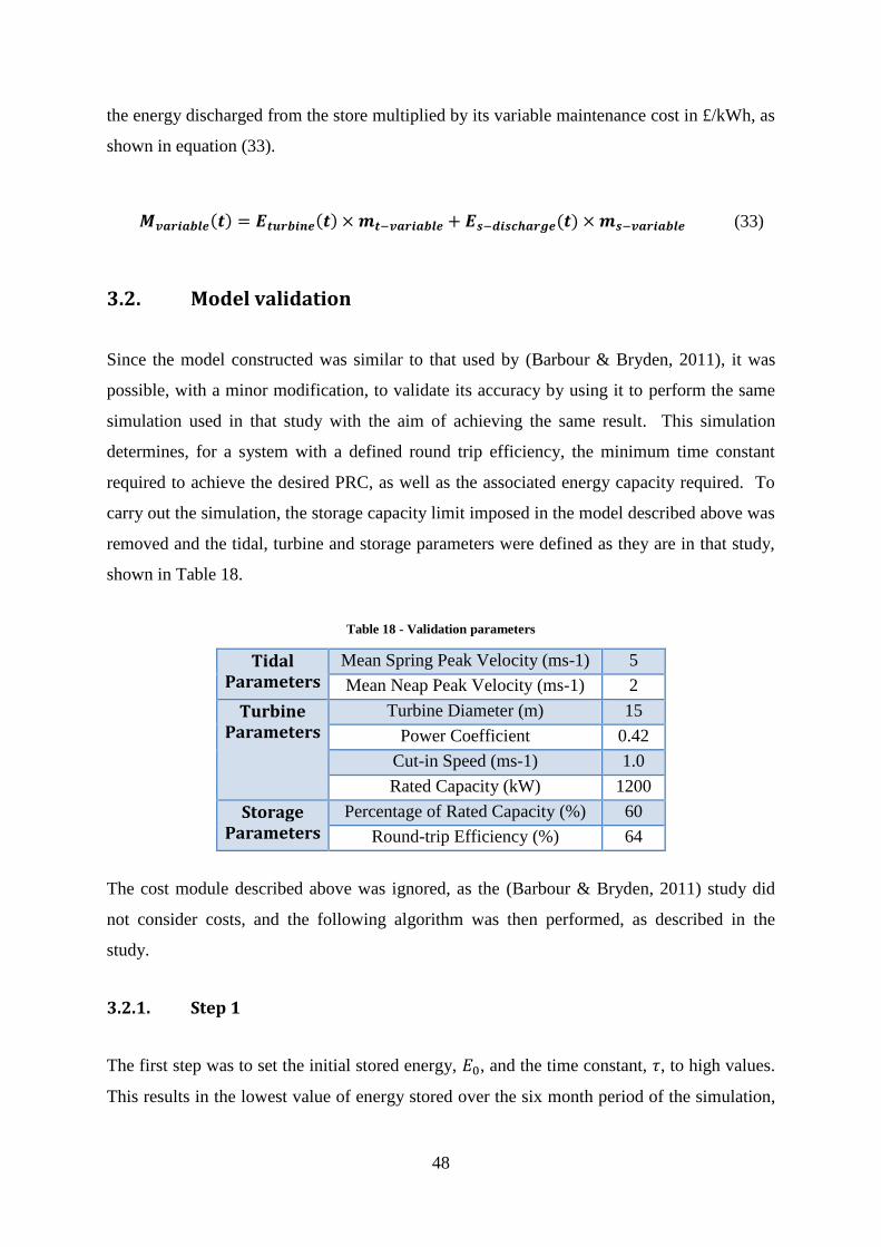
48

the energy discharged from the store multiplied by its variable maintenance cost in £/kWh, as

shown in equation (33).

𝑴𝒗𝒂𝒓𝒊𝒂𝒃𝒍𝒆(𝒕) = 𝑬𝒕𝒖𝒓𝒃𝒊𝒏𝒆(𝒕) × 𝒎𝒕−𝒗𝒂𝒓𝒊𝒂𝒃𝒍𝒆 + 𝑬𝒔−𝒅𝒊𝒔𝒄𝒉𝒂𝒓𝒈𝒆(𝒕) × 𝒎𝒔−𝒗𝒂𝒓𝒊𝒂𝒃𝒍𝒆 (33)

3.2. Model validation

Since the model constructed was similar to that used by (Barbour & Bryden, 2011), it was

possible, with a minor modification, to validate its accuracy by using it to perform the same

simulation used in that study with the aim of achieving the same result. This simulation

determines, for a system with a defined round trip efficiency, the minimum time constant

required to achieve the desired PRC, as well as the associated energy capacity required. To

carry out the simulation, the storage capacity limit imposed in the model described above was

removed and the tidal, turbine and storage parameters were defined as they are in that study,

shown in Table 18.

Table 18 - Validation parameters

Tidal Parameters

Mean Spring Peak Velocity (ms-1) 5

Mean Neap Peak Velocity (ms-1) 2

Turbine Parameters

Turbine Diameter (m) 15

Power Coefficient 0.42

Cut-in Speed (ms-1) 1.0

Rated Capacity (kW) 1200

Storage Parameters

Percentage of Rated Capacity (%) 60

Round-trip Efficiency (%) 64

The cost module described above was ignored, as the (Barbour & Bryden, 2011) study did

not consider costs, and the following algorithm was then performed, as described in the

study.

3.2.1. Step 1

The first step was to set the initial stored energy, 𝐸0, and the time constant, 𝜏, to high values.

This results in the lowest value of energy stored over the six month period of the simulation,

49

𝐸𝑚𝑖𝑛, being well above zero and the energy stored at the point corresponding to 𝐸0 in the

following spring-neap cycle, 𝐸1, being greater than 𝐸0:

Figure 29 - Model validation Step 1

3.2.2. Step 2

The second step was to reduce the time constant, 𝜏, until the minimum stored energy value

was close to but greater than zero. This will not necessarily occur over the first spring-neap

cycle, but if 𝐸1 is lower than 𝐸0 it generally indicates that system is not self-sustaining and

the value of energy stored will at some point drop below zero. This can be verified by

analysis of a later spring-neap cycle and highlights the key advantage of running the

simulation over a semi-annual period.


𝐸0

𝐸1 𝐸𝑚𝑖𝑛

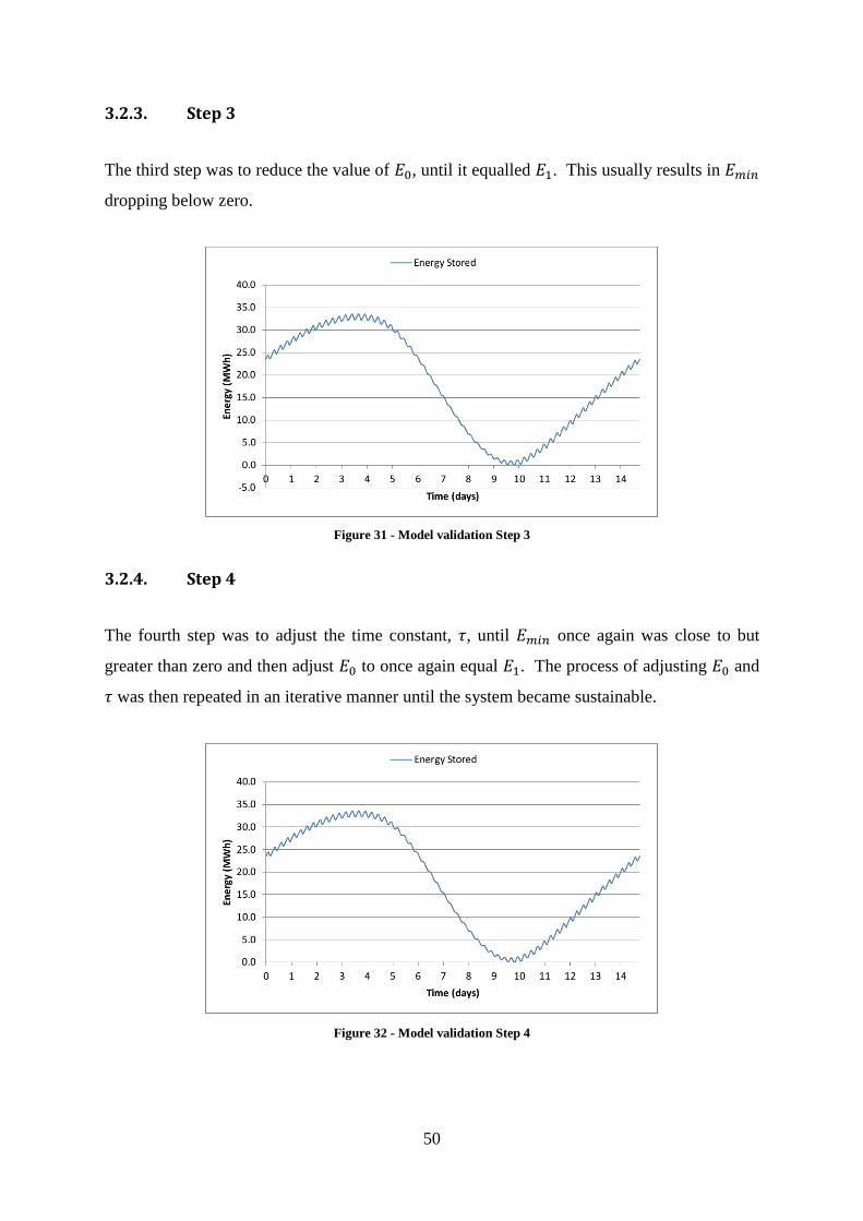
50

3.2.3. Step 3

The third step was to reduce the value of 𝐸0, until it equalled 𝐸1. This usually results in 𝐸𝑚𝑖𝑛

dropping below zero.


3.2.4. Step 4

The fourth step was to adjust the time constant, 𝜏, until 𝐸𝑚𝑖𝑛 once again was close to but

greater than zero and then adjust 𝐸0 to once again equal 𝐸1. The process of adjusting 𝐸0 and

𝜏 was then repeated in an iterative manner until the system became sustainable.


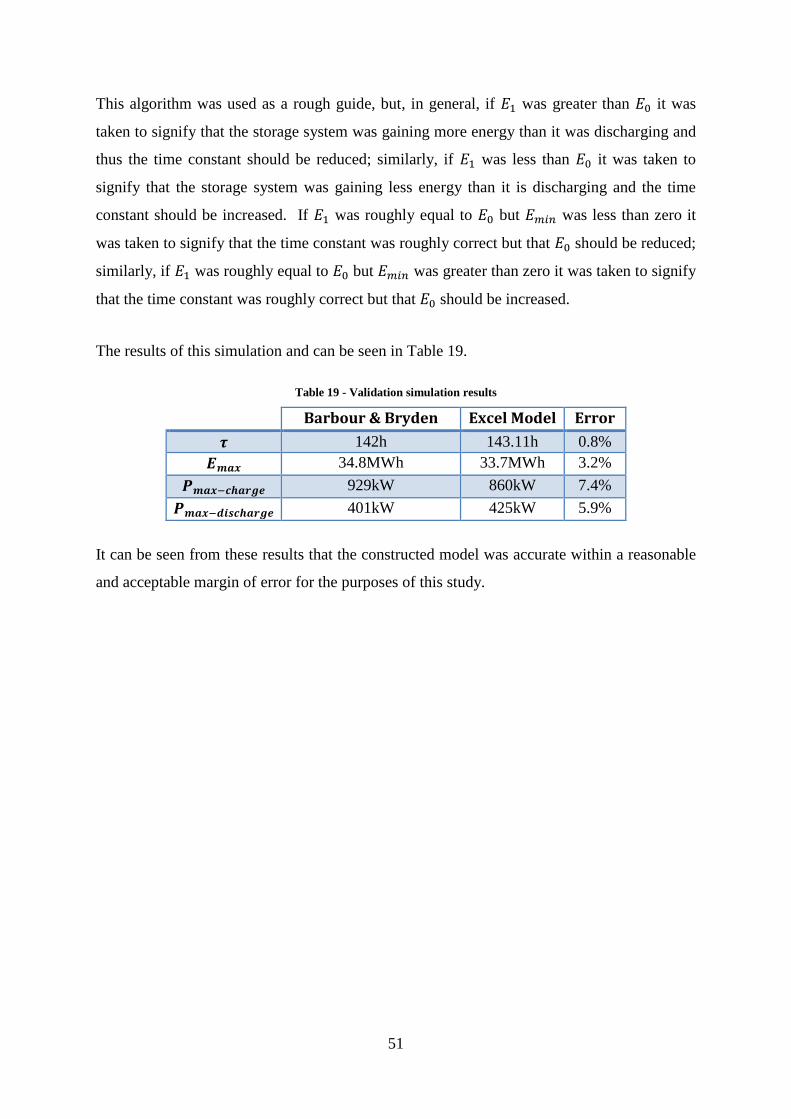
51

This algorithm was used as a rough guide, but, in general, if 𝐸1 was greater than 𝐸0 it was

taken to signify that the storage system was gaining more energy than it was discharging and

thus the time constant should be reduced; similarly, if 𝐸1 was less than 𝐸0 it was taken to

signify that the storage system was gaining less energy than it is discharging and the time

constant should be increased. If 𝐸1 was roughly equal to 𝐸0 but 𝐸𝑚𝑖𝑛 was less than zero it

was taken to signify that the time constant was roughly correct but that 𝐸0 should be reduced;

similarly, if 𝐸1 was roughly equal to 𝐸0 but 𝐸𝑚𝑖𝑛 was greater than zero it was taken to signify

that the time constant was roughly correct but that 𝐸0 should be increased.

The results of this simulation and can be seen in Table 19.

Table 19 - Validation simulation results

Barbour & Bryden (2011)

Excel Model Error

𝝉 142h 143.11h 0.8%

𝑬𝒎𝒂𝒙 34.8MWh 33.7MWh 3.2%

𝑷𝒎𝒂𝒙−𝒄𝒉𝒂𝒓𝒈𝒆 929kW 860kW 7.4%

𝑷𝒎𝒂𝒙−𝒅𝒊𝒔𝒄𝒉𝒂𝒓𝒈𝒆 401kW 425kW 5.9%

It can be seen from these results that the constructed model was accurate within a reasonable

and acceptable margin of error for the purposes of this study.

52

4. Simulation performed

4.1. Time constant simulations

The first objective of the study was to determine the minimum performance characteristics

required of the storage system to provide firm power. This was done by employing the same

method used to validate the model, as described in section 3.2.

This was carried out for the range of storage system round trip efficiencies found in the

literature, which range from 35% for power-to-gas to 95% for flywheels and supercapacitors.

To keep the number of simulations performed to a minimum, they were performed over this

range in increments of 10% and for 𝑃𝑅𝐶𝑠 ranging from 60% to 90% in increments of 10%.

4.2. Storage capacity simulations

Storage capacity optimisation simulations were run for the technologies which had the

required time constant determined from the time constant simulations. For each technology

considered, simulations were run to determine the storage and power capacity requirements

and associated costs for the system to achieve PRCs ranging from 60% to 90% in increments

of 10%. Where the technology was not able provide the specified PRC, the energy and

power capacity requirements for the highest PRC that it could feasibly provide was

determined instead.

4.3. Storage capacity simulation parameters

4.3.1. Tidal parameters

For all simulations performed, the mean spring peak and mean neap peak velocities were set

to 5ms-1 and 2ms-1, respectively. These are the same values as those used by (Barbour &

Bryden, 2011) and are fairly representative of a tidal current resource.

53

4.3.2. Turbine parameters

The turbine parameters used were those of the SeaGen S turbine manufactured by Marine

Current Turbines installed at Strangford Lough. This is the same turbine used by (Barbour &

Bryden, 2011); however, the parameters used for this study were corrected from those used

by (Barbour & Bryden, 2011) (one 15m diameter turbine with a rated capacity of 1.2MW) to

those published on the Marine Current Turbines website (with the exception of the power

coefficient, which was kept at 0.42) shown in Table 20. This resulted in a turbine power

profile which closely resembled that of the turbine, as see in Figure 33 and Figure 34.

Table 20 - Turbine tarameters

Number of Turbines 2

Turbine Diameter (m)

16

Power Coefficient 0.42

Cut-in Speed (ms-1) 1.0

Rated Capacity (kW) 600

Figure 33 - Modelled Turbine Power Profile

Figure 34 - Seagen Power Profile (Barbour &

Bryden, 2011))

The cost parameters used for the turbine were taken from (DECC, 2013) and can be seen in

Table 21.

Table 21 - Turbine cost parameters

Investment Cost (£/kW) 2,000

Fixed O &M Cost (£/MW/yr)

143,300

Variable O & M Cost (£/MWh)

1

54

4.3.3. Storage parameters

The storage technologies considered and the parameters used for the simulations can be seen

in Table 22, taken from (Fuchs, et al., 2012). Since the parameters published in the literature

often cover a range (i.e. a round-trip efficiency would be stated as 50-60%), the parameters

used were those which would portray the technology in the most positive light. Therefore,

the performance parameters used were those at the top of the published range and the cost

parameters used were those at the bottom end of the published range. For several of the

technologies, no data was available on its cycle life or lifespan. In these cases, nominal

values of 10,000 cycles and 25 years were used, which would result in the system being

operational for as long as the turbine.

Additional simulations were also run for those technologies for which data was available on

future performance improvements and cost reductions. These technologies and their

associated parameters can be seen in Table 23, taken from (Fuchs, et al., 2012).

Technologies which were considered for inclusion during the literature review but which

were not included in the simulations are super-conductive magnetic energy storage and high-

temperature thermoelectric energy storage. This was due to insufficient data being available

for these technologies due to their relative immaturity.

Table 22 - Simulation storage parameters

Technology 𝜼𝑻

(%) 𝑵𝒎𝒂𝒙

(cycles) 𝑳𝒎𝒂𝒙 (yrs)

𝑫𝑶𝑫𝒎𝒂𝒙 (%)

𝝉 (hours)

𝑼 (Wh/l)

𝒊𝒑−𝒔𝒕𝒐𝒓𝒆

(£/kW) 𝒊𝑬−𝒔𝒕𝒐𝒓𝒆

(£/kWh)

Flywheel 95 1,000,000 15 75 20 200 257 857

Super- capacitors

95 1,000,000 15 75 192 10 8.5 8,570

High-temp. Batteries

80 10,000 20 100 240 250 129 428

CAES 70 10,000 25 50 4,800 6 857 34

Li-ion Batteries

86 5,000 20 100 14,400 350 129 257

Lead-Acid Batteries

80 2,000 15 70 24,000 100 129 86

Flow Batteries

70 10,000 15 100 24,000 70 857 257

PHS 82 10,000 80 100 480,000 1.5 429 4.3

Hydrogen 40 10,000 25 60 800,000 750 1,285 0.25

55

Technology 𝜼𝑻




𝝉 (hours)

𝑼 (Wh/l)



(£/kWh)

Power to Gas

35 10,000 25 60 800,000 2250 857 0.0

Prices based on a £2011/€2011 exchange rate of 0.857 (XE, 2011)

Table 23 - Simulation storage parameters for year 2030

Technology 𝜼𝑻




𝝉 (hours)

𝑼 (Wh/l)



(£/kWh)

High-temp. Batteries

90 10,000 30 100 240 250 30 69

Li-ion Batteries

92 10,000 30 100 72,000 550 30 129

Flow Batteries

80 10,000 25 100 48,000 100 514.20 60

Lead-Acid Batteries

85 5,000 20 80 48,000 130 30 43

Power to Gas

40 10,000 25 60 800,000 2250 857 0.0

Hydrogen 50 10,000 25 60 800,000 750 429 0.25

Prices based on a £2011/€2011 exchange rate of 0.857 (XE, 2011)

56

5. Results

5.1. Time constant simulations

The results of the time constant simulations can be seen in Table 24, Figure 35 and Figure 36.

Table 24 - Minimum time constant requirements

PRC=60% PRC=70% PRC=80% PRC=90%

𝜼𝑻 = 𝟑𝟓% 329.7h - - -

𝜼𝑻 = 𝟒𝟓% 145.8h 556.9h - -

𝜼𝑻 = 𝟓𝟓% 100.3h 209.4h 18600h -

𝜼𝑻 = 𝟔𝟓% 78.7h 138.7h 391.6h -

𝜼𝑻 = 𝟕𝟓% 65.6h 107.5h 218.2h 9940h

𝜼𝑻 = 𝟖𝟓% 56.6h 89.1h 158.3h 519.5h

𝜼𝑻 = 𝟗𝟓% 50.1h 77.3h 127.2h 228.6h

It is clear from these results that there is a limit to the PRC which a system is able to achieve.

For example, a system with a round-trip efficiency of 35% would not be able to provide a

PRC of 70%, regardless of how high its time constant is. It is also clear that the required time

constant increases exponentially as PRC is increased and as system round-trip efficiency is

decreased, as can be seen in Figure 35 and Figure 36.

Figure 35 - Minimum time constant v PRC

57

Figure 36 – Time constant v round-trip efficiency

While this general increase is not in itself surprising, the extreme degree of the exponential

increase is. The rate of increase in time constant requirements to achieve a higher PRC are so

significant that, for example, a storage system with a round-tip efficiency of 35% is able to

provide a PRC of 60% with a moderate time constant of only 329.7 hours (equal to a self-

discharge rate of roughly 7% per day) yet is not able to provide a PRC of 70% at all.

Comparing the results in Table 24 with the performance parameters of the technologies

considered, shown in Table 22, it can be seen that a flywheel storage system would not be

able to perform the function required of it, since its time constant is only 20 hours and the

minimum time constant required by a system with the highest round-trip efficiency to a

achieve a PRC of 60% is 50.1 hours. Flywheel storage systems were therefore not included

within the energy capacity requirements simulations.

58

5.2. Capacity requirement simulations – Present Day

5.2.1. Power output to grid

The power output to the grid for each of the PRCs considered can be seen in Figure 37 and

Table 25. Table 25 also lists the power output for PRC=100% (i.e. the average turbine power

output) and the ‘turbine oversize’, defined as the ratio of the turbine’s rated capacity to the

output to the grid.

Figure 37 - Power output to grid

Table 25 – Power output to grid

PRC Output to Grid (kW)

Turbine Oversize

60% 438 274%

70% 511 235%

80% 584 205%

90% 657 183%

100% 730 164%

Here, it can be seen that the average power output of the turbine is 730kW. This average

power output reduces as PRC is reduced, as would be expected, down to 438kW for

PRC=60%. The effect of reducing the PRC on the oversizing of the turbine is clear; for

example, a tidal-storage system with PRC=60% results in the turbine having a rated capacity

274% larger than the output to the grid. Looked at another way, a tidal turbine could be

59

connected to a grid connection 274% smaller than its rated capacity if a storage system was

used to maintain its output to PRC=60%.

The LCOE that would result if no storage system was used and the turbine’s power output

was restricted to the PRC is shown in Figure 38. In this scenario, the power produced by the

turbine in excess of the PRC would be curtailed.

Figure 38 – Curtailed LCOE

Here, the increased LCOE as a result of curtailment can be seen. As would be expected, the

LCOE reduces as PRC increases, i.e. as less energy is curtailed. However, the LCOE figures

depicted represent a significant increase on the LCOE which would result if the turbine was

installed without storage and power output was not curtailed. This was calculated at only

£65/MWh by the model, highlighting the serious commercial implications of curtailment.

5.2.2. Energy capacity

The energy storage capacity requirements for each technology, as determined from the

simulations, can be seen in Figure 39.

60

Figure 39 - Energy capacity v PRC

Here, the relationship between storage system round-trip efficiency and the maximum PRC

achievable can be seen, most clearly in the cases of power to gas and hydrogen storage.

These technologies have the lowest round-trip efficiencies of the technologies considered -

35% for power to gas and 40% for hydrogen – which severely limits the PRCs which they are

able to achieve, power to gas only being capable of 65% and hydrogen 69%. This is in

contrast to pumped hydro storage, lead-acid batteries and lithium-ion batteries, which all have

round-trip efficiencies above 80% and are able to achieve 90% rated capacity.

High round-trip efficiencies are also clearly important to performance in terms of minimising

capacity requirements, again clearly illustrated in the cases of power to gas and hydrogen

storage. These technologies have the greatest capacity requirements, in spite of having the

highest time constant of all technologies considered at 800,000 hours, equal to a self-

discharge rate of only 0.003% per day. This indicates that high round-trip efficiencies are

more important for minimising capacity requirements than high time-constants.

However, this comparison ignores the maximum permissible discharge depth of the

technologies, which also has an impact on overall capacity requirements. Figure 40 shows

what the capacity requirements would be were each technology capable of discharging 100%.

This gives a slightly different picture from Figure 39; however, it still shows power to gas

and hydrogen performing the worst, despite their significant improvements. The technology

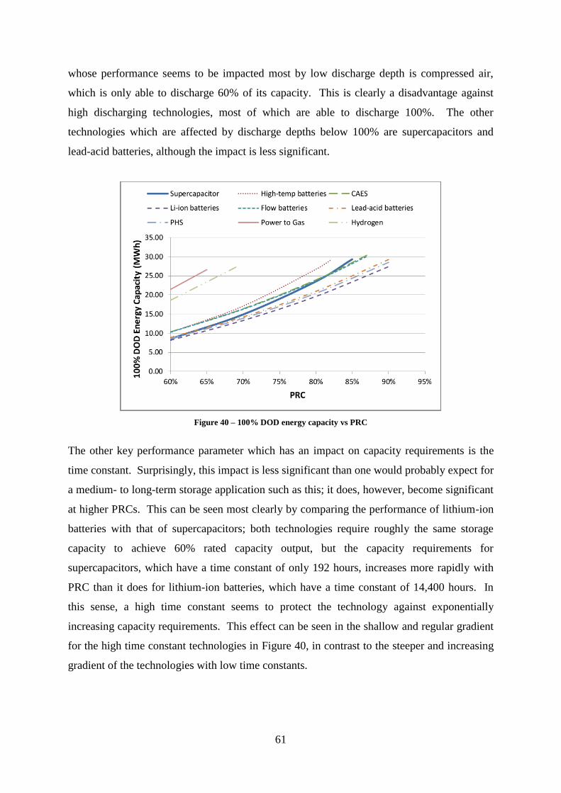
61

whose performance seems to be impacted most by low discharge depth is compressed air,

which is only able to discharge 60% of its capacity. This is clearly a disadvantage against

high discharging technologies, most of which are able to discharge 100%. The other

technologies which are affected by discharge depths below 100% are supercapacitors and

lead-acid batteries, although the impact is less significant.

Figure 40 – 100% DOD energy capacity vs PRC

The other key performance parameter which has an impact on capacity requirements is the

time constant. Surprisingly, this impact is less significant than one would probably expect for

a medium- to long-term storage application such as this; it does, however, become significant

at higher PRCs. This can be seen most clearly by comparing the performance of lithium-ion

batteries with that of supercapacitors; both technologies require roughly the same storage

capacity to achieve 60% rated capacity output, but the capacity requirements for

supercapacitors, which have a time constant of only 192 hours, increases more rapidly with

PRC than it does for lithium-ion batteries, which have a time constant of 14,400 hours. In

this sense, a high time constant seems to protect the technology against exponentially

increasing capacity requirements. This effect can be seen in the shallow and regular gradient

for the high time constant technologies in Figure 40, in contrast to the steeper and increasing

gradient of the technologies with low time constants.

62

5.2.3. Power capacity

The power storage capacity requirements for all technologies, as determined from the

simulations, can be seen in Figure 41. The power capacity requirements are the same for all

technologies, as it is determined solely by the power output of the turbine and the PRC.

Figure 41 - Power capacity v PRC

Here it can be seen that, in contrast to rated energy capacity, rated power capacity decreases

with PRC. This is due to the rate or power transfer to the store being calculated in equation

(9) as the difference between the power produced by the turbine and the power exported to

the grid. As the power exported to the grid increases, the power transferred to the store

during charging decreases, leading to lower power capacity requirements. At higher PRCs,

however, discharging power begins to exceed charging power, leading to increasing power

capacity requirements.

5.2.4. Land requirements

The land required for each technology to achieve a PRC of 60%, as determined from the


63

Figure 42 - Land requirements (present day)

Here it can be seen that PHS requires the greatest volume of land, despite having one of the

lowest energy capacity requirements. This is due to its very low energy density of only

1.5Wh/l. CAES requires almost as much land as PHS, primarily due to its higher capacity

requirements and only slightly improved energy density of 6Wh/l. Supercapacitors also stand

out as one of the technologies requiring high volumes of land, again due to its low energy

density of only 10Wh/l. Amongst the battery technologies, lithium-ion batteries stand out as

offering the best performance in terms of land use due to their high energy density of

350Wh/l. Hydrogen and power to gas are able to mitigate the impact of their high energy

capacity requirements since they have exceptionally high energy densities of 750Wh/l and

2250Wh/l, respectively.

5.2.5. Levelised cost

The resulting LCOE produced from each technology, as determined from the simulations, can

be seen in Figure 43.

64

Figure 43 - LCOE v PRC

Here it can be seen that there is little relationship between the energy capacity requirements

shown in Figure 39 and the resultant LCOE. This is not surprising, given the large variation

in installation costs between the technologies.

Supercapacitor storage results in the highest LCOE, more than a factor of 10 greater than the

next worst technology. This is solely due to its exceptionally high energy installation cost of

£8,570/kWh.

For clarity, Figure 44 shows the LCOE for all technologies excepting supercapacitors.

65

Figure 44 - LCOE v PRC (no supercapacitors)

Here, it can be seen that high-temperature batteries result in the next highest LCOE. This is

again due to their high energy installation cost of £428/kWh, the second highest after

supercapacitors. This extremely high cost is enough to result in what is one of the best

performing technologies in terms of energy capacity requirements becoming one of the worst

in terms of LCOE.

The remaining three battery technologies – flow batteries, lithium-ion batteries and lead-acid

batteries – result in a reduced LCOE relative to high-temperature batteries. This is due to

their lower energy installation costs of £257/kWh for flow and lithium-ion batteries and

£83/kWh for lead-acid batteries. Flow batteries and lithium-ion batteries both outperform

lead-acid batteries in terms of energy capacity requirements; however, the much lower cost of

lead-acid batteries is able to offset their performance limitations to result in them producing

energy at a lower levelised cost.

For clarity, Figure 45 shows the LCOE of the remaining four technologies to be discussed.

Also added for comparison is the LCOE that would result were no storage capacity installed,

as shown in Figure 38.

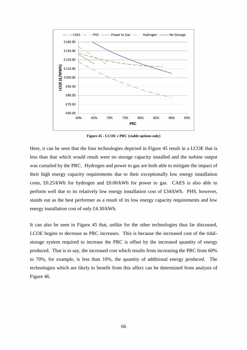
66

Figure 45 - LCOE v PRC (viable options only)

Here, it can be seen that the four technologies depicted in Figure 45 result in a LCOE that is

less than that which would result were no storage capacity installed and the turbine output

was curtailed by the PRC. Hydrogen and power to gas are both able to mitigate the impact of

their high energy capacity requirements due to their exceptionally low energy installation

costs, £0.25/kWh for hydrogen and £0.00/kWh for power to gas. CAES is also able to

perform well due to its relatively low energy installation cost of £34/kWh. PHS, however,

stands out as the best performer as a result of its low energy capacity requirements and low

energy installation cost of only £4.30/kWh.

It can also be seen in Figure 45 that, unlike for the other technologies thus far discussed,

LCOE begins to decrease as PRC increases. This is because the increased cost of the tidal-

storage system required to increase the PRC is offset by the increased quantity of energy

produced. That is to say, the increased cost which results from increasing the PRC from 60%

to 70%, for example, is less than 10%, the quantity of additional energy produced. The

technologies which are likely to benefit from this affect can be determined from analysis of

Figure 46.

67

Figure 46 - Energy installation cost v power installation cost

Those technologies for which the total power installation cost is greater than the total energy

installation cost, show here as having an energy/power ratio below 1, will result in a LCOE

that reduces as PRC increases, since power capacity decreases with PRC, as shown in Figure

41. This clearly explains why LCOE decreases for hydrogen, power to gas and PHS as PRC

increases. In the case of CAES, the cost increases are less than 10%, resulting in reducing

LCOE.

5.3. Capacity requirement simulations – Year 2030

5.3.1. Energy capacity

The energy storage capacity requirements for each technology whose performance is

predicted to improve can be seen for the year 2030, as determined from the simulations, in

Figure 47.

68

Figure 47 - Energy capacity v PRC (Year 2030)

Here, the relationship between capacity requirements and round-trip efficiency is still clear,

particularly in the cases of hydrogen and power to gas. However, it can be seen that both of

these technologies are predicted to improve their performance in terms of both the PRC they

are able to achieve and the energy capacity required. Slight reductions in capacity

requirements are also predicted for the other technologies, but these are less significant.

High-temperature batteries are predicted to be able to achieve higher PRCs, possibly up to

87%.

5.3.2. Land requirements

The land required for each technology to achieve a PRC of 60%, as determined from the


69

Figure 48 - Land reqiirements (year 2030)

It can be seen that improvements are predicted for all technologies. Flow and lead-acid

batteries are both predicted to slightly reduce their overall footprint due to improved

efficiency and increased energy density. The footprint of high-temperature batteries will

decrease slightly due to improved efficiency, but increased energy densities are not predicted.

Similarly, the energy density of hydrogen and power to gas are not predicted to increase, but

their overall footprint will reduce due to increased efficiencies. The technology which is

likely to see the most significant reductions in footprint is lithium-ion batteries, driven mostly

by predicted increase in energy density from 350Wh/l to 550Wh/l.

5.3.3. Levelised cost

The predicted LCOE produced by each technology, as determined from the simulations, can

be seen in Figure 49.

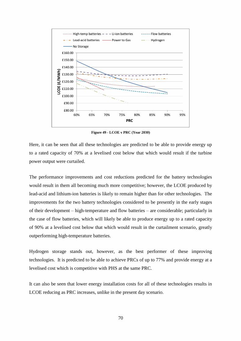
70

Figure 49 - LCOE v PRC (Year 2030)

Here, it can be seen that all these technologies are predicted to be able to provide energy up

to a rated capacity of 70% at a levelised cost below that which would result if the turbine

power output were curtailed.

The performance improvements and cost reductions predicted for the battery technologies

would result in them all becoming much more competitive; however, the LCOE produced by

lead-acid and lithium-ion batteries is likely to remain higher than for other technologies. The

improvements for the two battery technologies considered to be presently in the early stages

of their development – high-temperature and flow batteries – are considerable; particularly in

the case of flow batteries, which will likely be able to produce energy up to a rated capacity

of 90% at a levelised cost below that which would result in the curtailment scenario, greatly

outperforming high-temperature batteries.

Hydrogen storage stands out, however, as the best performer of these improving

technologies. It is predicted to be able to achieve PRCs of up to 77% and provide energy at a

levelised cost which is competitive with PHS at the same PRC.

It can also be seen that lower energy installation costs for all of these technologies results in

LCOE reducing as PRC increases, unlike in the present day scenario.

71

6. Discussion

6.1. Storage system performance requirements

Energy storage systems can be used in conjunction with tidal stream energy converters to

provide constant power output; however, not all energy storage technologies are capable of

doing so.

It was found through the time constant simulations carried out that the ability of a particular

technology to provide a defined value of steady output could be determined from two of its

key measures of performance: its round-trip efficiency and rate of self-discharge. As the

defined value of constant power output is increased, the required storage system round-trip

efficiency increases and the maximum permissible rate of self-discharge decreases. This

relationship can be seen in Figure 35 and Figure 36, which both show the rate of self-

discharge as an equivalent time constant. These minimum round-trip efficiency and time

constant requirements mean that some storage technologies are fundamentally incapable of

providing constant power output from a tidal resource.

In the analysis carried out, it was found that flywheel energy storage is one such technology.

This technology has a time constant far below the minimum required to provide a constant

power output equivalent to 60% of the average power produced from the tidal resource

(expressed as PRC=60%), the lowest value of power output considered. Its high self-

discharge, equivalent to roughly 5% per hour, is one of the main reasons why it is not

generally considered for applications requiring anything other than short-term power supply;

for example, for voltage and frequency control. The relatively low energy-to-power ratios

typical of flywheels also mean that they are best suited to applications requiring high power

for short periods of time, as is the case in the two aforementioned applications (Fuchs, et al.,

2012) (Zhou, et al., 2012).

6.2. Storage benefits

Since energy storage systems can be used in conjunction with tidal stream energy converters

to provide constant power, they present significant opportunities for maximising the amount

72

of energy that can be exploited from a tidal resource. It is not immediately clear, however,

that this is the case.

Considering the simulations performed as part of this study as an example, a glance at Table

25 might lead one to conclude that using a combined turbine-storage system configured for a

PRC of 60% in place of a tidal turbine on its own would result in a reduced average power

output (438kW as opposed to 730kW). In a sense, this is true; however, this conclusion

ignores the fact that the use of a combined turbine-storage system enables the installation of

more capacity on the same grid connection.

To illustrate this point, in the example given the turbine responsible for producing an average

power output of 730kW is rated at 1.2MW. Since the turbine does not produce constant

power – its output instead varying with the tides – it will at times produce 1.2MW of power

while at others producing none. So, although its average power output is only 730kW, the

capacity of the grid connection it is installed on must be rated at no less than 1.2MW. In

contrast, a combined tidal storage system which produces an average power output of 438kW

does so without any variation, meaning that the capacity of the grid connection it is installed

on need only be rated at 438kW. In other words, 2.74 times as many turbine-storage systems

can be installed on the 1.2MW connection as can individual turbines. The result of this

would be an average power output of 1.2MW, 1.64 times higher than for the turbine alone.

This increased energy production clearly comes at a cost. Although more energy is indeed

being produced, the cost per kilowatt-hour is greater since precisely 40% less energy is being

produced per unit turbine cost, on top of which the energy storage system cost has to be

added. However, this simple cost comparison in absolute terms does not give an accurate

indication of the relative benefits of using a combined turbine-storage system over a turbine

only system. A more detailed analysis is required to get an accurate picture.

This can be seen in the analysis carried out as part of this study. The simulations performed

calculated the LCOE produced in the turbine-only scenario at £65/MWh. However, it is

possible that this LCOE would only be achievable if a high level of turbine capacity was

installed; that is to say, it is unlikely that the cost of installing two turbines would be double

the cost of installing one. It is therefore foreseeable that circumstances might arise in which

the installed turbine capacity required to produce energy at the lowest levelised cost exceeds

73

the capacity of the grid connection the turbine array would be connected to. The LCOE that

would result in this scenario are shown in Figure 38.

Here it can be seen that the LCOE that would result if the installed turbine capacity was

274% greater than the capacity of the grid connection (i.e. the turbine’s output was capped at

PRC=60%) is much greater at nearly £150/MWh. Similarly, if the installed turbine capacity

was 183% greater than the connection capacity the LCOE would be approximately

£105/MWh.

This more detailed analysis highlights the extreme commercial cost of curtailed tidal energy

and shows where the key field of application for storage systems with tidal energy may lie. If

the combined turbine-storage system could produce energy at a levelised cost below that

which would result in the curtailment scenario, it could become a viable option. However,

the alternative option would be to simply upgrade the grid connection. Therefore, for the

combined turbine-storage system to be the preferred option it would have to produce energy

at a levelised cost below that which would result if the grid connection was upgraded.

6.3. Turbine-storage system LCOE

The simulations and analyses carried out highlight the fact that some storage technologies are

simply not well suited to providing constant power output with a tidal stream resource. It can

be seen in Figure 43 that the technology which most clearly falls into this category is

supercapacitors; however, all battery technologies at their present stage of development

would not be competitive either.

The reason for the extremely high LCOE for supercapacitors is that they have a very low

energy density compared to other technologies. It is for this reason that they are not typically

seen as a suitable option for applications requiring anything other than short-term power.

Since their power density is very high, they are particularly well suited to short-term high-

power applications; for example, primary frequency and voltage control (Fuchs, et al., 2012)

(Zhou, et al., 2012).

All of the battery technologies considered would not be able to provide energy at a levelised

cost below that which would result in the curtailment scenario, primarily due to their high

74

energy installation costs – high temperature batteries are particularly affected by this.

However, the poor performance of these technologies does not necessarily indicate that they

are not suitable for the application. Rather, the high cost gives an indication of the early

stages of their development.

High-temperature and flow batteries are the two which are considered to be in the earliest

stage of their development, although all of the battery technologies are predicted to improve

to some degree in the future in terms of both performance and cost. Figure 49 shows that, in

fact, all battery technologies are likely to become viable options by the year 2030.

For the year 2030, flow batteries stand out as the best performing battery technology, driven

mainly by the sharp fall in energy installation cost predicted. This low energy installation

cost, in addition to high cycle-life and high energy capacity, is why flow batteries are

considered to be well suited to medium- to long-term storage applications such as this. They

have the added benefit over other battery technologies of having independently scalable

energy and power capacities, which would be a particular advantage if applied to tidal energy

storage, since power capacity requirements were shown to vary little with increasing energy

capacity requirements. Although the other battery technologies perform well enough to be

economically viable, flow batteries would clearly be the best option.

Figure 45 shows that, in the present day, pumped hydro, compressed air, power to gas and

hydrogen storage are the only options which would be economically viable. This is not all

that surprising since all of these technologies are generally considered suitable options for

medium- to long-term storage applications (Fuchs, et al., 2012) (Zhou, et al., 2012).

PHS stands out as the best performer, which is not surprising given the maturity of this

technology. Not only is PHS able to provide energy at the lowest cost, but it is able to do so

over the broadest range of PRCs. CAES is the only other mature technology which would

presently be economically viable, but it is greatly outperformed by PHS.

Hydrogen storage and power to gas both appear to be economically viable, which is

encouraging given the early stage of development of these technologies. This low cost is

driven mainly by the exceptionally low energy installation costs. Predicted further

improvements in performance of these technologies, as well as the predicted reduced power

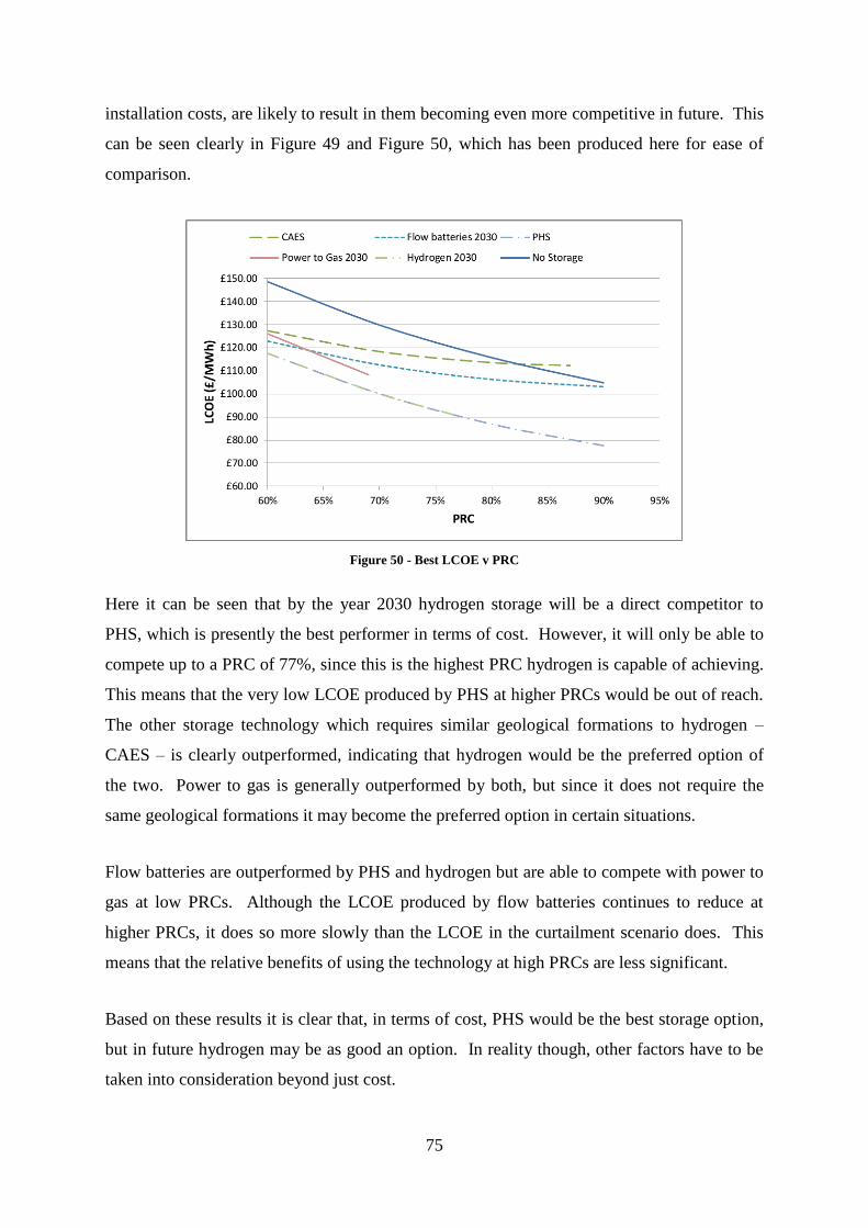
75

installation costs, are likely to result in them becoming even more competitive in future. This

can be seen clearly in Figure 49 and Figure 50, which has been produced here for ease of

comparison.

Figure 50 - Best LCOE v PRC

Here it can be seen that by the year 2030 hydrogen storage will be a direct competitor to

PHS, which is presently the best performer in terms of cost. However, it will only be able to

compete up to a PRC of 77%, since this is the highest PRC hydrogen is capable of achieving.

This means that the very low LCOE produced by PHS at higher PRCs would be out of reach.

The other storage technology which requires similar geological formations to hydrogen –

CAES – is clearly outperformed, indicating that hydrogen would be the preferred option of

the two. Power to gas is generally outperformed by both, but since it does not require the

same geological formations it may become the preferred option in certain situations.

Flow batteries are outperformed by PHS and hydrogen but are able to compete with power to

gas at low PRCs. Although the LCOE produced by flow batteries continues to reduce at

higher PRCs, it does so more slowly than the LCOE in the curtailment scenario does. This

means that the relative benefits of using the technology at high PRCs are less significant.

Based on these results it is clear that, in terms of cost, PHS would be the best storage option,

but in future hydrogen may be as good an option. In reality though, other factors have to be

taken into consideration beyond just cost.

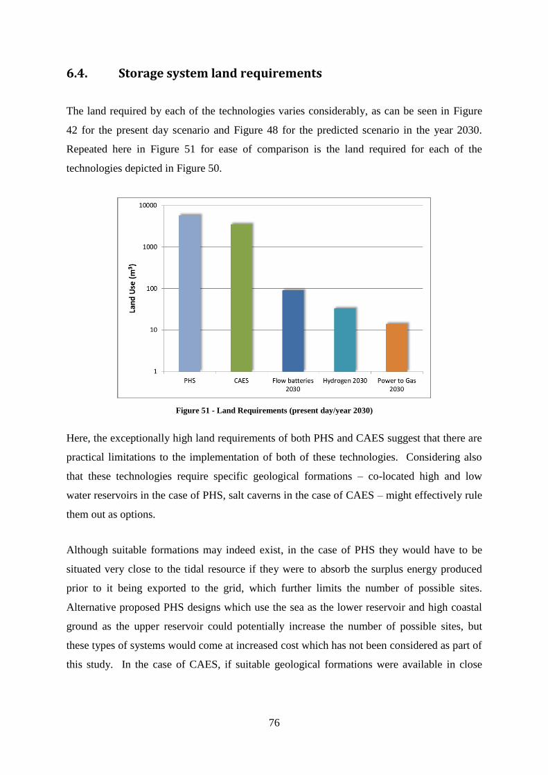
76

6.4. Storage system land requirements

The land required by each of the technologies varies considerably, as can be seen in Figure

42 for the present day scenario and Figure 48 for the predicted scenario in the year 2030.

Repeated here in Figure 51 for ease of comparison is the land required for each of the

technologies depicted in Figure 50.

Figure 51 - Land Requirements (present day/year 2030)

Here, the exceptionally high land requirements of both PHS and CAES suggest that there are

practical limitations to the implementation of both of these technologies. Considering also

that these technologies require specific geological formations – co-located high and low

water reservoirs in the case of PHS, salt caverns in the case of CAES – might effectively rule

them out as options.

Although suitable formations may indeed exist, in the case of PHS they would have to be

situated very close to the tidal resource if they were to absorb the surplus energy produced

prior to it being exported to the grid, which further limits the number of possible sites.

Alternative proposed PHS designs which use the sea as the lower reservoir and high coastal

ground as the upper reservoir could potentially increase the number of possible sites, but

these types of systems would come at increased cost which has not been considered as part of

this study. In the case of CAES, if suitable geological formations were available in close

77

proximity to the tidal resource, it would clearly be more sensible to use these for hydrogen

storage owing to its superior performance to CAES and higher energy density.

If suitable geological formations were not available for PHS or hydrogen, power to gas could

become a viable alternative at low PRCs. However, this option would require a gas-grid

connection to be situated close to the tidal resource, which may again effectively rule it out as

an option. It is possible that a gas-connection could be installed if this technology was

selected, but the cost of doing so has not been included within the analyses carried out in this

report, and this could have a significant impact on the overall LCOE.

Although the land requirements for flow batteries are considerable when compared with

hydrogen and power to gas, they are much lower than for both PHS and CAES. They do not

offer the same benefits as the gas storage technologies in terms of environmental impact since

they would be situated above ground and in plain sight, but they do offer enhanced flexibility.

Since they do not require any specific geological formations, they could be used in

conjunction with virtually any tidal resource. The economic benefits of using this technology

may be less significant than for the others, but they still offer some advantage over the

curtailment scenario.

7. Conclusions and further work

7.1. General conclusions

When considering any storage system for use with a tidal turbine array to provide firm power,

a number of factors which affect the performance of such a system have to be borne in mind.

The primary factor which effectively rules out some technologies is the rate of self-discharge.

This performance parameter must meet minimum criteria to ensure that such a system can be

self-sustaining; however, the criteria set a relatively low threshold, meaning that the majority

of technologies are in fact viable options in this respect.

The other factor which contributes most significantly to system performance is the storage

technology’s round-trip efficiency. Technologies with the highest round-trip efficiencies

78

generally offer the best overall performance, and higher efficiencies can also lower the self-

discharge criteria, effectively compensating for the ‘leakiness’ of the technology.

7.2. Turbine-storage system benefits

Energy storage systems coupled with tidal turbines present significant opportunities for

maximising the amount of energy exploited from a tidal resource. Where grid connection

capacity limitations exist, energy storage can be used to increase the amount of turbine

capacity which can be deployed at a tidal site while mitigating the need to upgrade the

capacity of the grid connection. The result of this increased capacity deployment would be

an overall increase in energy delivered.

The precise increase in quantity of energy delivered would vary depending on the flow

characteristics of the tidal site and the performance characteristics of the tidal turbine

installed, but the results of this study showed that any energy storage system capable of

providing steady power output from a tidal resource would increase the quantity of energy

delivered by 164%.

The increased turbine deployment required to provide this energy increase would vary

depending on the performance characteristics of the storage system. Those storage systems

only capable of providing constant power output equivalent to 60% of the average turbine

output would necessitate the installation of 274% more turbine capacity, while those capable

of providing constant power output equivalent to 90% of the average turbine output would

only necessitate the installation of 183% more turbine capacity.

7.3. Cost savings with energy storage

In some cases, trade-offs exist between the smaller increases in installed turbine capacity

required for high performance storage systems and the larger increases required for low

performance ones. This trade-off is primarily a function of the energy installation cost of the

storage system, with low performance storage systems providing energy at lower levelised

costs than high performance ones owing to their lower energy installation costs.

79

In the present day, only four storage technologies would be capable of providing energy at a

levelised cost below that which would result if a turbine array was connected to a grid

connection rated below its capacity and resulting in energy curtailment. These technologies

are: pumped hydro storage, hydrogen storage, compressed air storage, and power to gas.

Hydrogen storage and power to gas perform well in spite of their low round-trip efficiencies

– which necessitate the installation of more turbine capacity – since their energy installation

costs are exceptionally low. These results contrast with those for batteries which have higher

efficiencies – thus requiring the installation of less turbine capacity – but have higher energy

installation costs.

In the future, projected technological advances will result in lead-acid batteries, lithium-ion

batteries, flow batteries and high temperature batteries also being economically advantageous

compared with the curtailment scenario; however, flow batteries stand out as the best

performers. Additional technological advances and cost reductions for hydrogen storage and

power to gas will also result in these technologies becoming more competitive.

Pumped hydro storage will remain the best option into the future, being able to provide

electricity at a levelised cost of £77.60/MWh. The next best option is likely to be hydrogen,

but this technology will only be able to provide electricity at a levelised cost of £90.50/MWh;

the main reason for this is that hydrogen’s lower efficiency would necessitate the installation

of turbines with a rated capacity 203% greater than the grid connection, compared with only

183% for pumped hydro. Flow batteries would be able to provide energy at a levelised cost

of £103.16/MWh, marginally outperforming power to gas at £108.36/MWh. The reason for

the high cost of energy produced from power to gas is that its low efficiency would

necessitate the installation of turbines with a rated capacity 238% greater than the grid

connection. Compressed air will be able to provide energy at a levelised cost of

£112.35/MWh; however, to achieve this cost would be achieved by limiting the installed

turbine capacity to 183% of the grid capacity. In this scenario, the levelised cost of energy

produced if the surplus energy was curtailed would be less at roughly £108/MWh.

7.4. Recommendations

It is difficult to give a specific recommendation on the most suitable storage technology for

this application, as the best option depends on a number of factors. In general, pumped hydro

80

storage is going to be able to provide energy at the lowest levelised cost so would be the

preferred option. However, in situations where economies of scale dictate that the installed

turbine capacity be more than twice the capacity of the grid connection to obtain the best

turbine price, hydrogen also becomes a competitive option. The choice between the two

would be determined by consideration of the land requirements of each technology,

specifically the geological formations upon which they rely.

Where these requisite geological formations do not exist, power to gas storage should be

considered as an alternative option, particularly in situations where economies of scale dictate

that the installed turbine capacity be at least 238% greater than the grid connection.

However, consideration should be taken in this case of the availability of a local gas grid

connection.

In cases where the requisite geological formations do not exist for pumped hydro storage or

hydrogen storage and where a local gas grid connection is not available, flow batteries should

be the chosen storage option. These would also be the best option in cases where a gas grid

connection is available but the economies of scale dictate that the installed turbine capacity

need only be 183% greater than the capacity of the grid connection.

7.5. Further work

Further work is required to determine the applicability of the findings of this study to specific

tidal sights. Since the methodology that has been adopted relied upon a simple model of tidal

currents, it is unknown if its findings can be applied in practice at tidal sights where the flow

regime may differ significantly.

Further work is also required to quantify the trade-off between upgrading the capacity of a

grid connection and installing an energy storage system. This study did not try to quantify

how much a grid connection upgrade would cost, rather simply stating that an energy storage

system would only be the preferred option in cases where the grid connection upgrade would

result in a levelised cost greater than that which would result with the storage option.

Calculation of levelised costs for tidal turbines in which grid connection upgrades are also

included would be valuable in this sense.

81

Further work should also be carried out to determine if additional value could be added to the

storage system by oversizing it; that is to say, giving it a larger energy capacity than that

required to provide constant output. In this scenario, value could possibly be added operating

the combined turbine-storage system at a base load below the capacity of the grid connection.

This would introduce some ‘dispatchability’ into the system, enabling it to export more

power to the grid during times of high demand. The increased costs associated with the

increased energy capacity and reduced base-load power output could possibly be offset by the

higher energy prices obtained during times of high demand.

82

References

Adock, T. A. et al., 2013. The available power from tidal stream turbines in the Pentland

Firth. Proceedings of the Royal Society, A(469:20130072).

Anon., 2015. International levelised cost of energy for ocean energy technologies, Lisbon:

IEA-OES.

Barbour, E. & Bryden, I. G., 2011. Energy storage in association with tidal current generation

systems. Proceedings of the Institute of Mechanical Engineers, Part A: A Journal of Power

and Energy, Volume 225, pp. 443-445.

Boehlert, G. W. & Gill, A. B., 2010. Environmental and ecological effects of ocean

renewable energy development: A current synthesis. Oceanography, 23(2), pp. 68-81.

Brito e Melo, A. & Huckerby, J., 2012. Implement Agreement on Ocean Energy Systems,

Lisboa: IEA-OES.

Bryden, I. G. & Macfarlane, D. M., 2000. The utilisation of short term energy storage with

tidal current generation systems. Energy, Issue 25, pp. 893-907.

Callaghan, J., 2006. Future Marine Energy - Results of the Marine Energy Challenge: Cost

Competitiveness and Growth of Wave and Tidal Stream Energy, London: Carbon Trust.

CEC, 1996. Wave Energy Project Results: The Exploitation of Tidal Marine Currents. DGXII

- Report EUR16683EN, Luxembourg: Commission of the European Communities.

Cheng, H., 2014. Following the motion of the ocean. [Online]

Available at: http://feedthedatamonster.com/home/2014/9/12/following-the-motion-of-the-

ocean

[Accessed 29 August 2016].

83

Clarke, J. A., Connor, G., Grant, A. D. & Johnston, C. M., 2006. Regulating the output

characteristics of tidal current power stations to facilitate better base load matching over the

lunar cycle. Renewable Energy, Issue 31, pp. 173-180.

DBEIS, 2016. Energy Consumption in the UK (2016), London: Department for Business,

Energy and Industrial Action.

DECC, 2013. Electricity Generation Costs 2013, London: Department of Energy & Climate

Change.

DECC, 2014. Sub-national electricity and gas consumption statistics, London: DECC.

Frid, C. et al., 2012. The environmental impact of tidal and wave energy generation devices.

Environmental Impact Assessment Review, Volume 32, pp. 133-139.

Fuchs, G., Lunz, B., Leuthold, M. & Sauer, D. U., 2012. Technology Overview on Energy

Storage, Aachen: Institute for Power Electronics and Electrical Drives (ISEA), RWTH

Aachen University.

Gross, R. et al., 2007. Renewables and the grid: understanding intermittency. Proceedings of

the Institute of Civil Engineers: Energy, Volume 160, pp. 31-41.

Hardisty, J., 2009. The Analysis of Tidal Stream Power. Chichester: John Wiley & Sons.

Houde, J., 2012. Cost benefit analysis of tidal energy generation in Nova Scotia: A scenario

for a tidal farm with 300MW of installed capacity in the Minas passage in 2020, Halifax:

Dalhousie University.

Huckerby, J., Jeffrey, H. & Jay, B., 2011. An international vision for ocean energy. s.l.:Ocean

Energy Systems Implementing Agreement.

IEA OES, 2015. International Levelised Cost of Energy for Ocean Energy Technologies.

s.l.:Implementing Agreement on Ocean Energy Systems IEA OES.

IEA, 2009. World Energy Outlook 2009, Paris: International.

84

IEA, 2014. Technology Roadmap: Energy Storage, Paris: International Energy Agency -

IEA.

IEC, 2011. Electrical Energy Storage White Paper, Geneva: IEC.

IEC, 2012. Grid integration of large-capacity renewable energy sources and use of large-

capacity electrical energy storage, Geneva: International Electrotechnical Commission.

Kiprakis, A. & Wallace, A., 2004. Maximising energy capture from distributed generators in

weak networks. IEE Proc. -Gener. Transm. Distrib., 151(5), pp. 611-618.

Klein, J., 2009. Comparative Costs of California Central Station Electricity Generation

Technologies, Sacramento: California Energy Commission.

Lewis, A. et al., 2014. Renewable Energy Sources and Climate Change Mitigation, New

York: Cambridge University Press.

Lopez, J. et al., 2010. Preliminary economic assessment and analysis of grid connection

schemes for ocean energy arrays. Bilbao, s.n.

Lynn, P. A., 2014. Electricity from Wave and Tide. Chichester: John Wiley & Sons.

Magagna, D. et al., 2014. Wave and tidal energy strategic technology agenda, s.l.: SI Ocean.

Magagna, D. & Uihlein, A., 2015. JRC Ocean energy status report: Technology, market and

economic aspects of ocean energy in Europe, Luxembourg: Publication Office of the

European Union.

Manchester, S., Barzegar, B., Swan, L. & Groulx, D., 2013. Energy storage requirements for

in-stream tidal generation on a limited capacity electricity grid. Energy, Issue 61, pp. 283-

290.

Morandeau, M., Walker, R. T., Argall, R. & Nicholls-Lee, R. F., 2013. Optimisation of

marine energy installation operations. International Journal of Marine Energy, Volume 3-4,

pp. 14-26.

85

Mueller, M. & Wallace, R., 2008. Enabling science and technology for marine renewable

energy. Energy Policy, Volume 36, pp. 4376-4382.

O'Conner, M., Lewis, T. & Dalton, G., 2013. Weather window analysis of Irish and

Portuguese wave data with relevance to operations and maintenance of marine renewables.

Nantes, s.n.

Polagye, B., Cleve, B. V., Copping, A. & Kirkendall, K., 2011. Environmental Effects of

Tidal Enegy Development: Proceedings of a Scientific Workshop. Seattle: National Oceanic

and Atmospheric Administration (NOAA).

Santos, M. et al., 2011. Integrating wave and tidal current power: Case studies through

modelling and simulation, s.l.: IEA-OES.

Serhadlioglu, S. et al., 2013. Tidal stream energy resource assessment of the Anglesey

Skerries. International Journal of Marine Energy, 3-4(e), pp. 98-111.

SI-Ocean, 2013. Ocean Energy: Cost of Energy and Cost Reduction Opportunities, s.l.:

Strategic Initiative for Ocean Energy (SI-Ocean).

Statistics Explained, 2016. Electricity production, consumption and market overview.

[Online]

Available at: http://ec.europa.eu/eurostat/statistics-

explained/index.php/Electricity_production,_consumption_and_market_overview

[Accessed 28 Aug 2016].

Ter-Gazarian, A. G., 2011. Energy Storage for Power Systems. 2nd ed. London: The

Institution of Engineering and Technology.

Testa, A., De Caro, S. & Scimone, T., 2009. Analysis of a VRB energy storage system for a

tidal turbine generator. s.l., Power Electronics and Applications, 2009. EPE '09, 13th

European Conference on.

86

Treillant, B., Costello, R., Weber, J. & Ringwood, J., 2012. Productivity and economic

assessment of wave energy projects through operational simulations. Renewable Energy,

Volume 48, pp. 220-230.

Uihlein, A. & Magagna, D., 2016. Wave and tidal current energy - A review of the current

state of research beyond technology. Renewable and Sustainable Energy Reviews, Volume

58, pp. 1070-1081.

UKERC, 2007. Electricity Generation Costs and Investment Decisions: A Review, s.l.: UK

Energy Research Centre.

Wang, C. & Lu, W., 2009. Analysis Method and Reserves Estimation on Ocean Energy

Resources. Beijing: Ocean Press.

Wang, L. et al., 2011. Analysis of a Hybrid Offshore Wind and Tidal Farm Connected to a

Power Grid Using a Flywheel Energy Storage System. 2011 IEEE Power and Energy Society

General Meeting, pp. 1-8.

Wang, L., Yu, J. Y. & Chen, Y. T., 2011. Dynamic stability improvement of an integrated

offshore wind and marine-current farm using a flywheel energy-storage system. IET

Renewable Power Generation, 5(5), pp. 387-396.

XE, 2011. XE Currency Table: Euro. [Online]

Available at: http://www.xe.com/currencytables/?from=EUR&date=2011-01-01

[Accessed 7 July 2016].

Zhou, Z. et al., 2012. Energy Storage Technologies for Smoothing Power Fluctuations in

Marine Current Turbines. IEEE International Symposium on Industrial Electronics (ISIE),

2012, pp. 1425-1430.

Documents

Increasing the quantity and value of energy delivered from