Embed Size (px)
Citation preview

ww
w.inl.gov
Increasing Transmission Capacities with Dynamic Monitoring Systems
Kurt S. Myers
Jake P. Gentle
March 22, 2012
INL/MIS-11-22167
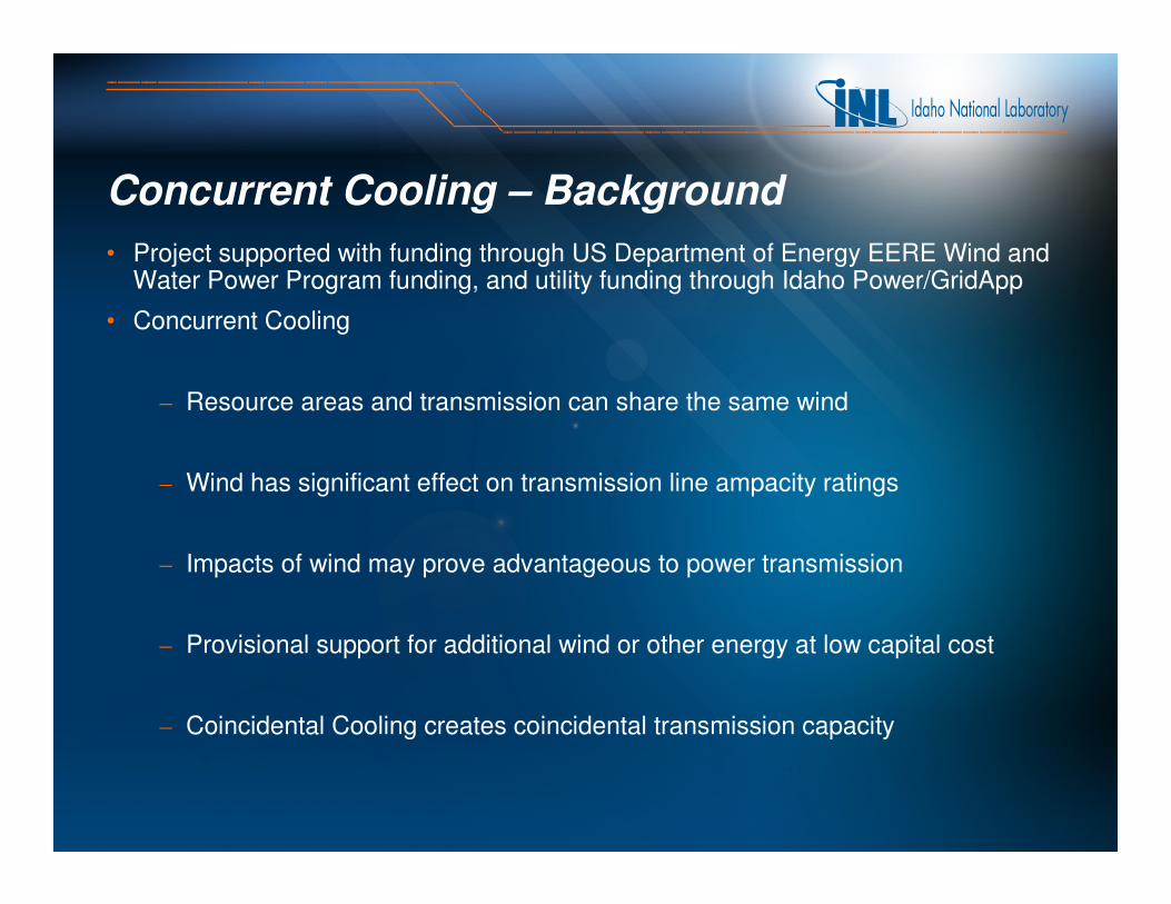
Concurrent Cooling – Background
• Project supported with funding through US Department of Energy EERE Wind and Water Power Program funding, and utility funding through Idaho Power/GridApp
• Concurrent Cooling
– Resource areas and transmission can share the same wind
– Wind has significant effect on transmission line ampacity ratings
– Impacts of wind may prove advantageous to power transmission
– Provisional support for additional wind or other energy at low capital cost
– Coincidental Cooling creates coincidental transmission capacity
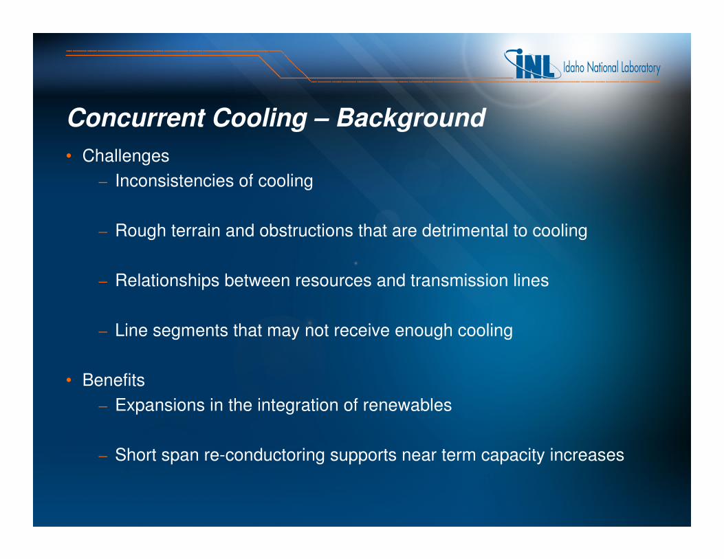
Concurrent Cooling – Background
• Challenges
– Inconsistencies of cooling
– Rough terrain and obstructions that are detrimental to cooling
– Relationships between resources and transmission lines
– Line segments that may not receive enough cooling
• Benefits
– Expansions in the integration of renewables
– Short span re-conductoring supports near term capacity increases
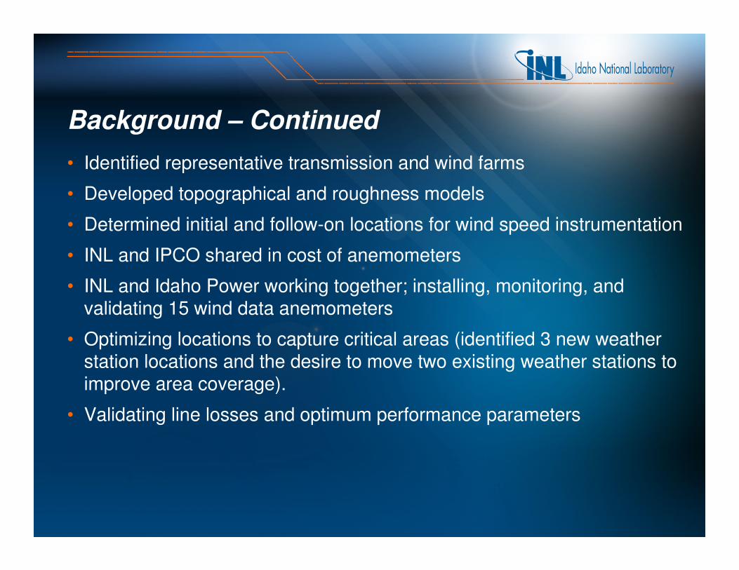
Background – Continued
• Identified representative transmission and wind farms
• Developed topographical and roughness models
• Determined initial and follow-on locations for wind speed instrumentation
• INL and IPCO shared in cost of anemometers
• INL and Idaho Power working together; installing, monitoring, and validating 15 wind data anemometers
• Optimizing locations to capture critical areas (identified 3 new weather station locations and the desire to move two existing weather stations to improve area coverage).
• Validating line losses and optimum performance parameters

Background – Continued
• Real-time and historical data collected and used for research and validation
• Computational Fluid Dynamics (CFD) modeling software package, WindSim used to better understand the concurrent cooling effects
• Developing a historical database and understanding, freeing concurrent thermal ampacity ratings
• Various scenarios modeled to understand and determine field measurements and validity of CFD model
• Developing process and transition to IPCo planning and operations

Area of Interest
Approximately 1500km2

WindSim Model Verification Approach
• Input: 3 – minute averaged climatology data sets
– Wind speed
– Direction
• Various combinations
– Remove 1 – 3 input files
– Compare predicted at the removed location modeled in WindSim with the actual measured data.
• Investigate percent error results
– Develop historical/statistical database
– Look-up tables with weighting factors for speed and direction
– 500 – 1000 meter separation between modeled points

WindSim Terrain Conversion
48,000,000 cells

WindSim % Error – Layouts 1 & 2 (Original)
Weather Stations UsedAverage Wind Speed
(Actual)
Average Wind Speed
(WindSim-Adjusted)
% Error (Data actual vs.
WindSim-Adjusted)
Ave Wind Speed of
Missing WS (WindSim-
Predicted)
% Error (Data actual vs.
WindSim Predicted)
WS03 3.31 3.24 2.1148% 3.27 1.2085%
WS04 3.45 3.39 1.7391% 3.45 0.0000%
WS09 2.97 3.01 1.3468% 3.07 3.3670%
WS10 1.76 1.75 0.5682% 1.95 10.7955%
WS11 3.23 3.15 2.4768% 3.22 0.3096%
WS12 1.99 1.88 5.5276% 2.08 4.5226%
WS03 3.31 3.24 2.1148% 3.29 0.6042%
WS04 3.45 3.39 1.7391% 3.46 0.2899%
WS09 2.97 3.01 1.3468% 3.09 4.0404%
WS10 1.76 1.75 0.5682% 2.73 55.1136%
WS11 3.23 3.15 2.4768% 3.24 0.3096%
WS12 1.99 1.88 5.5276% 2.08 4.5226%
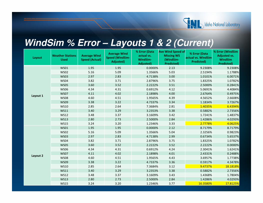
WindSim % Error – Layouts 1 & 2 (Current)
LayoutWeather Stations
Used
Average Wind
Speed (Actual)
Average Wind
Speed (WindSim-
Adjusted)
% Error (Data
actual vs.
WindSim-
Adjusted)
Ave Wind Speed of
Missing WS
(WindSim-
Predicted)
% Error (Data
actual vs. WindSim
Predicted)
% Error (WindSim
Adjusted vs.
WindSim
Predicted)
Layout 1
WS01 1.95 1.95 0.0000% 2.13 9.2308% 9.2308%
WS02 5.16 5.09 1.3566% 5.03 2.5194% 1.1788%
WS03 2.97 2.83 4.7138% 3.00 1.0101% 6.0071%
WS04 3.82 3.71 2.8796% 3.75 1.8325% 1.0782%
WS05 3.60 3.52 2.2222% 3.51 2.5000% 0.2841%
WS06 4.34 4.31 0.6912% 4.12 5.0691% 4.4084%
WS07 4.11 4.02 2.1898% 4.00 2.6764% 0.4975%
WS08 4.60 4.51 1.9565% 4.39 4.5652% 2.6608%
WS09 3.38 3.22 4.7337% 3.34 1.1834% 3.7267%
WS10 2.85 2.64 7.3684% 2.81 1.4035% 6.4394%
WS11 3.40 3.29 3.2353% 3.38 0.5882% 2.7356%
WS12 3.48 3.37 3.1609% 3.42 1.7241% 1.4837%
WS13 2.80 2.73 2.5000% 2.84 1.4286% 4.0293%
WS15 3.24 3.20 1.2346% 3.33 2.7778% 4.0625%
Layout 2
WS01 1.95 1.95 0.0000% 2.12 8.7179% 8.7179%
WS02 5.16 5.09 1.3566% 5.04 2.3256% 0.9823%
WS03 2.97 2.83 4.7138% 2.99 0.6734% 5.6537%
WS04 3.82 3.71 2.8796% 3.75 1.8325% 1.0782%
WS05 3.60 3.52 2.2222% 3.52 2.2222% 0.0000%
WS06 4.34 4.31 0.6912% 4.24 2.3041% 1.6241%
WS07 4.11 4.02 2.1898% 4.01 2.4331% 0.2488%
WS08 4.60 4.51 1.9565% 4.43 3.6957% 1.7738%
WS09 3.38 3.22 4.7337% 3.36 0.5917% 4.3478%
WS10 2.85 2.64 7.3684% 3.12 9.4737% 18.1818%
WS11 3.40 3.29 3.2353% 3.38 0.5882% 2.7356%
WS12 3.48 3.37 3.1609% 3.43 1.4368% 1.7804%
WS13 2.80 2.73 2.5000% 2.84 1.4286% 4.0293%
WS15 3.24 3.20 1.2346% 3.77 16.3580% 17.8125%

Look-up Tables

Average Wind Speed and Directions
• A map was created showing the high and low average wind speeds for each location (by line section).
• The transferred climatologies are color coordinated in accordance to their respective weather station.
• These values were then used to develop an average summary of thepotential Line Ampacity Ratings due to concurrent cooling on the four main transmission lines within the study Area of Interest.
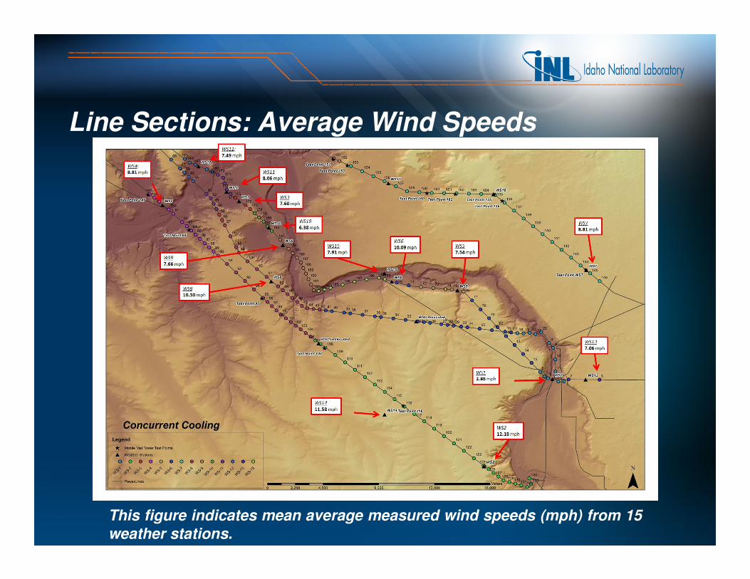
Line Sections: Average Wind Speeds
This figure indicates mean average measured wind speeds (mph) from 15
weather stations.

Concurrent Cooling – Wind Data Collection

Data Analysis 1

WS002 WS003 WS004 WS005 WS006 WS009 WS010 WS011 WS013 WS015
% Wind Speeds >= 3
mph91.58% 65.96% 79.86% 76.48% 87.71% 73.28% 56.34% 71.45% 71.20% 76.31%
% Wind Speeds >= 6
mph77.21% 51.59% 60.16% 55.26% 72.44% 50.34% 38.25% 52.58% 48.33% 59.00%
Jun-10 Jul-10 Aug-10 Sep-10 Oct-10 Nov-10 Dec-10 Jan-11 Feb-11 Mar-11 Apr-11
% Wind
Speeds >=
3 mph
53.71% 38.15% 30.95% 25.90% 21.87% 46.50% 33.19% 35.76% 34.91% 39.16% 49.56%
% Wind
Speeds >=
6 mph
30.92% 26.44% 19.12% 16.13% 14.59% 34.36% 21.41% 20.69% 20.67% 26.03% 35.83%
Total % Wind Speeds > 3 mph 35.9%
Total % Wind Speeds > 6 mph 23.6%
Data Analysis 1 - Continued

Data Analysis 1 - Continued

Data Analysis 1 - Continued
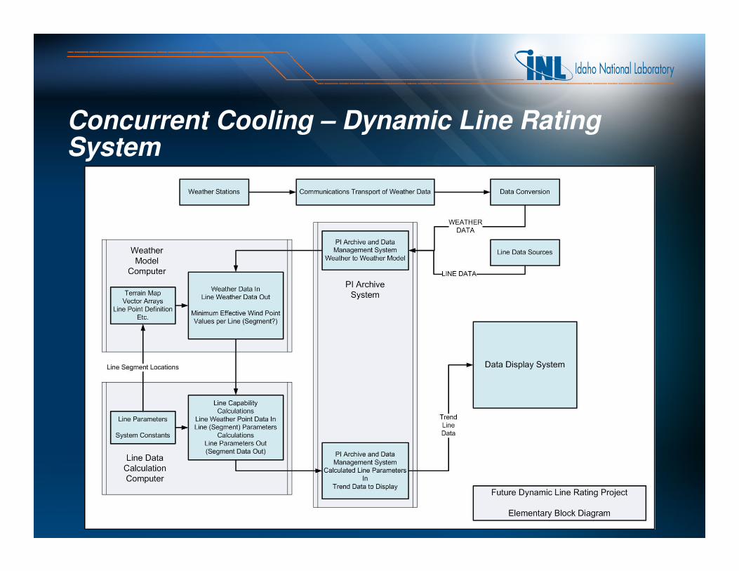
Concurrent Cooling – Dynamic Line Rating System

Dynamic Line Rating
• Equations describing cooling of bare overhead conductors were developed in the 1920’s.
• IEEE Standard for Calculating the Current-Temperature of Bare Overhead Conductors. IEEE Std. 738-2006.
– Blowing wind can provide significant additional capability over minimum wind conditions.
– The problem has always been knowing the weather conditions at all points along the transmission line.
– Substation equipment must also be rated for the additional capacity. That may require upgrades of station bus, switches and other equipment.
– Additional reactive support may be needed.
– The least capable line section or substation device determines the capability of the complete line.
Dynamic Line Rating – Continued
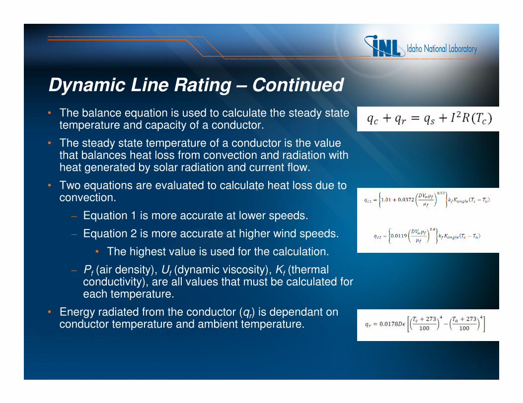
• The balance equation is used to calculate the steady state temperature and capacity of a conductor.
• The steady state temperature of a conductor is the value that balances heat loss from convection and radiation with heat generated by solar radiation and current flow.
• Two equations are evaluated to calculate heat loss due to convection.
– Equation 1 is more accurate at lower speeds.
– Equation 2 is more accurate at higher wind speeds.
• The highest value is used for the calculation.
– Pf (air density), Uf (dynamic viscosity), Kf (thermal conductivity), are all values that must be calculated for each temperature.
• Energy radiated from the conductor (qr) is dependant on conductor temperature and ambient temperature.

Dynamic Line Rating – Continued
• Conductor resistance (qR) is a function of conductor temperature (Tc).
– The change is nearly linear over the temperature range of interest.
• Heating of the conductor by solar energy is a function of sun angle (time of year and time of day), line angle, elevation, and conductor reflectivity.
– A’ in the equation is relationship between the line area, line angle and solar angle.
– Qse is either measured or calculated solar radiation.
• The steady state current capability of the conductor can be determined using maximum ambient temperature, conductor maximum temperature, and present wind conditions.
– Steady state conductor temperature is calculated from present weather conditions and line loading.
• After the present steady state line temperature and capacity arecalculated, the actual or dynamic line temperature and capacity are calculated using a (1-e^(-X)) relationship.
– X is the time step divided by the line thermal time constant.

Line Ampacity Calculations – Wind @ 0 degrees to the line. (Baseline – Worst case)
Columns 11 and 15 of Table 2 indicate that even higher ampacity ratings can be realized when baseline ampacity ratings are conservative (wind @ 0 degrees, or down-line).
Line
Point
Wind
Speed
(MPH)
Wind
Speed
(ft/sec)
Wind
Angle
Line
Azimuth
Line
Voltage
(kV) MVA Amps
Line
Voltage
(kV) MVA Amps
Percent
Change
Line
Voltage
(kV) MVA Amps
Percent
Change
230.0 433.4 1088.0 230.0 433.4 1088.0 0% 230.0 433.4 1088.0 0%
Ave High 161 9.48 13.94 30 90 230.0 1202.3 3018.0 177% 230.0 846.9 2126.0 95%
Ave High 161 9.48 13.94 15 90 230.0 1069.2 2684.0 147% 230.0 747.3 1876.0 72%
Ave High 161 9.48 13.94 0 90 230.0 888.4 2230.0 105% 230.0 609.5 1530.0 41%
Ave Low 160 8.306 12.21 30 90 230.0 1157.7 2906.0 167% 230.0 813.5 2042.0 88%
Ave Low 160 8.306 12.21 15 90 230.0 1030.2 2586.0 138% 230.0 717.9 1802.0 66%
Ave Low 160 8.306 12.21 0 90 230.0 857.3 2152.0 98% 230.0 584.8 1468.0 35%
Conductor
Respective
Weather
Station
Static Summer
Rating
Dynamic Winter Rating
5 deg C
Dynamic Summer Rating
40 deg C
ACSR - 715.5
Baseline
WS7
Bottom Lines
• Dynamic line rating is doable, but process is complex
• Wind modeling technology is good, and is getting even better with wind forecasting and other related research.
• Quality of model outputs depend on how it’s done, how much input data is used, time periods modeled, terrain complexity, quality of the data, etc.
• Real questions are how to keep costs manageable, have a fast enough process, and how much data is enough to stay within projected/validated error bands with enough granularity to see capacity improvements at good economic value.

Continuing Work
• Develop historical/statistical database through various scenarios
– Seasonal
– Time of day
– Times when all areas are receiving cooling (or need upgrades to achieve higher ampacity)
• Improve obstructions and surface roughness layers to improve modeling accuracy.
• Improve refinement grid for better resolution
• Investigate improvements with better resolution native map files
• Determine areas of highest interest for upgrades/reconductoring
• Determine upgrade costs of identified areas of interest to improve overall ampacity/capacity of the system
• Expand Area of Interest to include IPCo – INL proposal area

Mobile Met Tower – Modeled Point Validation

Mobile Met Tower Test Point Locations
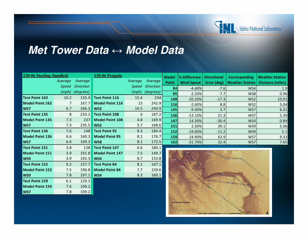
Met Tower Data ↔ Model Data
Average
Speed
(mph)
Average
Direction
(degrees)
Average
Speed
(mph)
Average
Direction
(degrees)
10.2 135.4 15.4 234
7 167.7 15 242.9
6.7 166.3 16.5 240.9
8 233.2 6 187.2
7.3 237 4.8 169.9
7.3 235.5 5.7 168.6
7.6 148 8.3 184.4
6.6 169.3 8.1 176.7
6.6 169.3 8.1 172.5
3.8 128 6.6 180.1
3.9 191.8 7.5 149.7
3.9 192.3 8.7 153.8
9.2 157.7 8.1 167.1
7.5 196.8 7.7 159.6
7.8 197.1 8.3 160.1
6.1 120.3
7.6 109.2
7.8 109.2
WS9 WS4
Test Point 159
Model Point 159
WS7
WS9 WS4
Test Point 152 Test Point 84
Model Point 152 Model Point 84
WS7 WS8
Test Point 151 Test Point 147
Model Point 151 Model Point 147
WS7 WS2
Test Point 136 Test Point 95
Model Point 136 Model Point 95
WS7 WS2
Test Point 135 Test Point 108
Model Point 135 Model Point 108
230-06 Starling (bundled) 138-06 Penguin
Test Point 162 Test Point 116
Model Point 162 Model Point 116
Model
Point
% Difference
Wind Speed
Directional
Error (deg)
Corresponding
Weather Station
Weather Station
Distance (miles)
84 -4.40% -7.6 WS4 1.9
95 -2.20% -7.7 WS8 0.96
108 -20.20% -17.3 WS2 10.01
116 -2.60% 8.8 WS2 5.04
135 -9.40% 3.7 WS7 6.01
136 -13.10% 21.3 WS7 5.39
147 14.30% -30.4 WS4 0.89
151 2.30% 39.1 WS9 5.06
152 -19.00% -11.2 WS9 5.1
159 24.90% 63.9 WS7 9.33
162 -31.70% 32.4 WS7 7.65

Test Point 147

Test Point 84

Future Items to Address
• Computer programming development for application to operations
– Utilizing look-up tables and/or other methods
– How to handle equipment or communication problems with particular monitoring equipment
– Calculation of all modeled point parameters, how to sort and which ones to display
– Best ways to handle line temps, thermal time constants, true-ups from specific line temp measurements, areas of darker/drier ground cover, etc.
• Other power system upgrades and modeling to handle effects of operating at higher ampacities

Power System Operators Control Board -Supplemental Screen

Questions?
INL Wind Website: http://www.inl.gov/wind
Questions? Contact:
Kurt Myers, MSEE, PE
Jake P. Gentle, MSMCE208-526-1753