Embed Size (px)
Citation preview
Int J Comput VisDOI 10.1007/s11263-010-0399-6
Incremental Tensor Subspace Learning and Its Applicationsto Foreground Segmentation and Tracking
Weiming Hu · Xi Li · Xiaoqin Zhang · Xinchu Shi ·Stephen Maybank · Zhongfei Zhang
Received: 28 September 2009 / Accepted: 1 October 2010© The Author(s) 2010. This article is published with open access at Springerlink.com
Abstract Appearance modeling is very important for back-ground modeling and object tracking. Subspace learning-based algorithms have been used to model the appear-ances of objects or scenes. Current vector subspace-basedalgorithms cannot effectively represent spatial correlationsbetween pixel values. Current tensor subspace-based al-gorithms construct an offline representation of image en-sembles, and current online tensor subspace learning al-gorithms cannot be applied to background modeling andobject tracking. In this paper, we propose an online ten-sor subspace learning algorithm which models appearance
Electronic supplementary material The online version of this article(doi:10.1007/s11263-010-0399-6) contains supplementary material,which is available to authorized users.
W. Hu (�) · X. Li · X. ShiNational Laboratory of Pattern Recognition, Institute ofAutomation, Chinese Academy of Sciences, Beijing 100190,Chinae-mail: [email protected]
X. Lie-mail: [email protected]
X. Shie-mail: [email protected]
X. ZhangCollege of Mathematics & Information Science, WenzhouUniversity, Wenzhou 325000, Zhejiang, Chinae-mail: [email protected]
S. MaybankDepartment of Computer Science and Information Systems,Birkbeck College, Malet Street, London WC1E 7HX, UKe-mail: [email protected]
Z. ZhangState University of New York, Binghamton, NY 13902, USAe-mail: [email protected]
changes by incrementally learning a tensor subspace repre-sentation through adaptively updating the sample mean andan eigenbasis for each unfolding matrix of the tensor. Theproposed incremental tensor subspace learning algorithmis applied to foreground segmentation and object trackingfor grayscale and color image sequences. The new back-ground models capture the intrinsic spatiotemporal charac-teristics of scenes. The new tracking algorithm captures theappearance characteristics of an object during tracking anduses a particle filter to estimate the optimal object state.Experimental evaluations against state-of-the-art algorithmsdemonstrate the promise and effectiveness of the proposedincremental tensor subspace learning algorithm, and its ap-plications to foreground segmentation and object tracking.
Keywords Incremental learning · Tensor subspace ·Foreground segmentation · Tracking
1 Introduction
Modeling the appearances of objects or scenes plays an im-portant role in computer vision applications such as back-ground modeling, tracking, and behavior analysis. Colorhistograms (Nummiaroa et al. 2003; Perez et al. 2002) ofregions are widely used for appearance modeling due totheir robustness to region scaling, rotation, and shape vari-ations. Their limitation is that they ignore the spatial distri-bution of pixel values. Kernel density estimation-based ap-pearance models (Elgammal et al. 2002; Yang et al. 2005)use spatial weighted kernels to represent the spatial distrib-ution of pixel values. Their limitation is their high compu-tational and memory complexities. GMM (Gaussian mix-ture model)-based appearance models (Zhou et al. 2004;Wu and Huang 2004) use a mixture of weighted Gaussian
Int J Comput Vis
distributions to learn a statistical model for colors. Theirlimitation is that they deal with each pixel independentlyand thus the relations between the values of nearby pixelsare not effectively characterized. Conditional random field-based appearance models (Wang et al. 2006) use Markovrandom fields to model the relations between the values ofneighboring pixels. Their limitations are that their trainingis very expensive and the global distributions of pixels arenot considered. Online subspace learning-based appearancemodels (Skocaj and Leonardis 2003; Ross et al. 2008) flat-ten appearance regions to vectors in order to describe globalstatistical information about pixel values. Their limitationis that spatial information, which is invariant under certainglobal appearance variations e.g. lighting changes and ro-bust to image noise, is missing due to the flattening.
Recently, multi-linear subspace analysis has attractedmuch attention and has been applied to image representa-tion and appearance modeling, etc. Yang et al. (2004) de-velop a 2-dimensional PCA (principal component analysis)for image representation. An image covariance matrix isconstructed. The eigenvectors of this matrix are derived forimage feature extraction. Ye et al. (2004a) present a learningmethod called 2-dimensional linear discriminant analysis inwhich classification is based on operations on image matri-ces. Ye (2005) propose an algorithm for low rank approxi-mations of a collection of matrices using an iterative algo-rithm which reduces the reconstruction error sequentially,and improves the resulting approximation during successiveiterations. Ye et al. (2004b) present a new dimension reduc-tion algorithm which constructs the low-order matrix repre-sentation of images directly by projecting the images to avector space that is the product of two lower-dimensionalvector spaces. Some pioneering methods use tensors to con-struct object models. Wang and Ahuja (2005) propose arank-R tensor approximation which can effectively capturespatiotemporal redundancies in the tensor entries. Yan etal. (2005) propose an algorithm for discriminant analysiswith tensor representation. This algorithm is derived fromthe popular vector-based linear discriminant analysis algo-rithm. Vasilescu and Terzopoulos (2002, 2003) apply the N -mode SVD (singular value decomposition), i.e. multi-linearsubspace analysis, to construct a compact representation offacial image ensembles factorized by different faces, expres-sions, viewpoints, and illuminations. He et al. (2005) presenta tensor subspace analysis algorithm, which learns a lowerdimensional tensor subspace, to characterize the intrinsiclocal geometric structure within the tensor space. Wang etal. (2007) give a convergent solution for general tensor-based subspace learning. Sun et al. (2006a, 2006b, 2008)propose three tensor subspace learning methods: DTA (dy-namic tensor analysis), STA (streaming tensor analysis), andWTA (window-based tensor analysis), for representing datastreams over time.
The above tensor analysis algorithms cannot be appliedto background modeling and object tracking directly. Wepoint out the following aspects:
1) Except for the DTA, STA, and WTA algorithms, theabove tensor analysis algorithms learn tensor subspaces of-fline, i.e. when new data arrives, the subspace model is re-trained using the new data and the previous data. This resultsin high memory and time costs, while spatiotemporal redun-dancies are substantially reduced. In the context of back-ground modeling and object tracking, it is necessary to usethe new data to online update the previously learned model.This is because appearance updating for background model-ing and object tracking is more effective if the recent framesin a video are weighted more heavily than previous frames.
2) The DTA, STA, and WTA algorithms include incre-mental tensor subspace learning which adaptively updatesthe subspaces. However, they cannot be applied to back-ground modeling and object tracking. These three algo-rithms use column spaces of the three unfolding matricesobtained from the corresponding three modes of the ten-sor. In fact, the column space of the unfolding matrix onthe third mode is of no use for background modeling andobject tracking, but the row space of this matrix is useful.Furthermore, DTA and WTA update the covariance matrixformed from the columns of each of the unfolding matricesand then obtain an eigenvector decomposition of the updatedcovariance matrix, assuming that the mean of the previousunfolding matrix is equal to the mean of the unfolding ma-trix of new data. As a result, the updating is not accurate ifthe mean changes. DTA and WTA have the small size prob-lem: the number of new samples is much less than the rankof the covariance matrix. STA applies the SPIRIT (stream-ing pattern discovery in multiple timeseries) iterative algo-rithm (Papadimitriou et al. 2005) to the new coming data toapproximate DTA without diagonalization. The tensor sub-spaces learned using STA are less accurate than the tensorsubspaces learned using DTA. (More descriptions to DTA,WTA, and STA are given in Sect. 3.3.6.)
In this paper, we develop a new incremental tensor sub-space learning algorithm, and apply it to foreground seg-mentation and object tracking. The main contributions ofour work are as follows:
• The proposed algorithm learns online a low dimensionaltensor subspace representation of the appearance of anobject or a scene by adaptively updating the sample meanand an eigenbasis for each unfolding matrix using ten-sor decomposition and incremental SVD. Compared withexisting vector subspace algorithms for appearance mod-eling, our algorithm more efficiently captures the intrinsicspatiotemporal characteristics of the appearance of an ob-ject and a scene. Furthermore, our method works online,resulting in much lower computational and memory com-plexities.
Int J Comput Vis
• Based on the proposed incremental subspace learning al-gorithm, two background models, one for grayscale im-age sequences and the other for color image sequences,are developed to capture the spatiotemporal characteris-tics of scenes based on a likelihood function which isconstructed from the learned tensor subspace model. Thebackground models are used to segment the foregroundfrom the background. The experimental results show thatour algorithm obtains more accurate foreground segmen-tation results than the vector subspace-based algorithm(Li 2004) and the GMM-based algorithm (Stauffer andGrimson 1999).
• We propose a visual object tracking algorithm in whichthe proposed incremental tensor subspace learning algo-rithm is used to capture the appearance of an object duringtracking (Li et al. 2007). Particle filtering is used to prop-agate the sample distributions over time. The experimen-tal results show that our algorithm tracks objects morerobustly than the vector subspace-based algorithm (Rosset al. 2008) and the Riemannian metric-based algorithm(Porikli et al. 2006).
The remainder of the paper is organized as follows:Sect. 2 discusses the related work. Section 3 describes ourincremental tensor subspace learning algorithm. Sections 4and 5 present our background segmentation algorithm andour object tracking algorithm respectively. Section 6 demon-strates experimental results. The last section summarizes thepaper.
2 Related Work
In Sect. 1, we reviewed the work closely related to tensor-based appearance modeling in order to strengthen the mo-tivation of this paper. For completeness, in the following,we briefly discuss the developments in foreground segmen-tation and visual object tracking.
2.1 Foreground Segmentation
Segmentation of foreground regions in an image sequenceis accomplished by comparing each new frame with thelearned background model. Effective modeling of the back-ground is crucial for foreground segmentation. However,changes in dynamic scenes, such as illumination variations,shadow movements, and tree swaying, make backgroundmodeling quite difficult.
Much work has been done in background modeling andforeground segmentation. Stauffer and Grimson (1999) pro-pose an online adaptive background model in which a GMMis used to model the sequence of values associated with eachpixel. Each pixel in a new frame is classified by matching thevalue of the pixel with one of the distributions in the GMM
associated with this pixel. Sheikh and Shah (2005) use non-parametric density estimation over a joint domain-range rep-resentation of image pixels to directly model multimodalspatial uncertainties and complex dependencies betweenpixel location and color. Jacques et al. (2006) present anadaptive background model for grayscale video sequences.The model utilizes local spatiotemporal statistics to de-tect shadows and highlights. It can adapt to illuminationchanges. Haritaoglu et al. (2000) build a statistical back-ground model which represents each pixel by three valueswhich are its minimum intensity value, its maximum inten-sity value, and the maximum intensity difference betweenconsecutive frames. Wang et al. (2005) present a proba-bilistic method for background subtraction and shadow re-moval. Their method detects shadows by a combined in-tensity and edge measure. Tian et al. (2005) propose anadaptive Gaussian mixture model based on a local normal-ized cross-correlation metric and a texture similarity metric.These two metrics are used for detecting shadows and il-lumination changes, respectively. Patwardhan et al. (2008)propose a framework for coarse scene modeling and fore-ground detection using pixel layers. The framework allowsfor integrated analysis and detection in a video scene. Wanget al. (2006) use a dynamic probabilistic framework basedon a conditional random field to capture spatial and tempo-ral statistics of pixels for foreground and shadow segmen-tation. Li (2004) constructs a subspace-based backgroundmodel. An online PCA is used to incrementally learn thebackground’s subspace representation.
The aforementioned methods for background modelingare unable to fully exploit the spatiotemporal redundancieswithin image ensembles. In particular, the vector subspacetechniques (Li 2004) lose local spatial information, perhapsleading to incorrect foreground segmentation results. Conse-quently, it is interesting to develop the tensor-based learningalgorithms to effectively capture the spatiotemporal charac-teristics of the background pixels.
2.2 Visual Object Tracking
The effective modeling of object appearance variations playsa critical role in visual object tracking. There are two typesof appearance variations: intrinsic appearance variations re-sulting from objects themselves such as object pose vari-ation or object shape deformation, and extrinsic appear-ance variations associated with the environment of the ob-jects, such as changes in illumination, camera motion, orocclusions. Much work has been done on modeling ob-ject appearance for visual tracking. Hager and Belhumeur(1996) propose a tracking algorithm which uses an extendedgradient-based optical flow method to track objects undervarying illumination. Black and Jepson (1998) present a nicesubspace learning-based tracking algorithm. A pre-trained,
Int J Comput Vis
view-based eigenbasis representation is used to model ap-pearance variations. Isard and Blake (1996) use curves orsplines to represent the boundary of an object and developthe Condensation algorithm for contour tracking. Black etal. (1998) employ a mixture model to represent and recoverobject appearance changes in consecutive frames, providingmore reliable estimates of image motion than traditional op-tical flow-based approaches. Jepson et al. (2003) develop arobust tracking algorithm using wavelet features which canbe used to model the spatial correlations in images directlyand are suited to multiple scales. They use a wavelet basisto decompose each image at two different scales. Each scalehas four orientations. In total, 8 filter masks are required.The extraction of wavelet features is time consuming andthe number of extracted features is large. Zhou et al. (2004)embed adaptive appearance models into a particle filter toachieve robust visual object tracking. Yu and Wu (2006)propose a non-rigid object tracking algorithm based on aspatial-appearance model which captures non-rigid appear-ance variations and recovers all the motion parameters effec-tively. Li et al. (2005) use a generalized geometric transformto handle object deformation, articulated objects, and occlu-sions. Wong et al. (2006) present a robust appearance-basedtracking algorithm using an online-updating Bayesian clas-sifier. Lee and Kriegman (2005) present a tracking methodbased on an online learning algorithm which incrementallylearns a generic appearance model from a video. Lim etal. (2006) present a human tracking framework using ro-bust identification of system dynamics and a nonlinear di-mension reduction technique. Ho et al. (2004) present a vi-sual tracking algorithm based on linear subspace learning.Ross et al. (2008) propose a generalized tracking frameworkbased on the incremental vector subspace learning methodwith sample mean updating. Han et al. (2009) apply con-tinuous density propagation in sequential Bayesian filteringto real-time object tracking. The techniques of density in-terpolation and density approximation are used to representthe likelihood and the posterior densities with Gaussian mix-tures. Gall et al. (2008) combine patch-based matching andregion-based matching to track both structured and homo-geneous object body parts. Nickel and Stiefelhagen (2008)propose a person tracker based on dynamic integration ofgeneralized cues. A layered sampling strategy is adoptedwhen particle filtering is applied to these cues. Chen andYang (2007) present a spatial bias appearance model whichexploits local region confidences for tracking objects un-der complex backgrounds and partial occlusions. Mahade-van and Vasconcelos (2009) propose an object tracking al-gorithm which combines a top-down saliency mode and abottom-up saliency mode to localize the object. Yang et al.(2009) propose an algorithm for tracking objects with non-stationary appearances. In this algorithm, negative data con-straints and bottom-up pair-wise data constraints are used
to dynamically adapt to the changes in the object appear-ance. Kwon and Lee (2009) track a non-rigid object using alocal patch-based appearance model which maintains rela-tions between local patches by online updating. Ramanan etal. (2007) propose a human body tracking algorithm whichmodels the appearance of each body part individually andrepresents the deformable assembly of parts by spring-likeconnections between pairs of parts. Matthews et al. (2004)propose an appearance template updating algorithm thatdoes not suffer from tracker drift. The template can be up-dated in every frame and yet still stay attached to the originalobject. The template is first updated at the current templatelocation. To eliminate drift, this updated template is thenaligned with the benchmark template extracted from the firstframe. Grabner et al. (2008) formulate the tracker updatingprocess in a semi-supervised fashion by combining the de-cisions obtained from a given prior classifier and an onlineclassifier. The prior classifier, which is trained using samplesextracted from the first frame, is used to deal with trackingdrift. Both the above two algorithms (Matthews et al. 2004;Grabner et al. 2008) use a fixed template, which is con-structed in the first frame, to significantly alleviate trackingdrift. The limitation of these two algorithms is that the tem-plate constructed in the first frame becomes unreliable if theobject appearance undergoes large changes.
It is noted that the above tracking algorithms do not fullyexploit the spatiotemporal information in the image ensem-bles obtained while tracking an object. This is particularlytrue for the vector subspace-based tracking algorithms (Rosset al. 2008) in which information about correlations betweenneighboring pixels is for the most part lost when the imagesare flattened into vectors. In order to achieve robust track-ing, it is necessary to develop the tensor-based learning al-gorithms for effective subspace analysis to more effectivelyutilize the spatiotemporal information about an object’s ap-pearance.
3 Incremental Tensor Subspace Learning
First, basic concepts of tensor algebra, as well as its nota-tions and symbols, are briefly introduced. Then, our onlinetensor subspace learning algorithm is described.
3.1 Tensor Algebra
Tensor algebra (Lathauwer et al. 2000) is the mathematicalfoundation of multi-linear analysis. A tensor can be regardedas a multi-order “array” lying in multiple vector spaces. Wedenote an N -order tensor as A ∈ RI1×I2×···In···×IN , whereIn (n = 1,2, . . . ,N) is a positive integer. Each element inthis tensor is represented as ai1...in...iN , where 1 ≤ in ≤ In.Each order of a tensor is associated with a “mode”. By un-folding a tensor along a mode, a tensor’s unfolding matrix
Int J Comput Vis
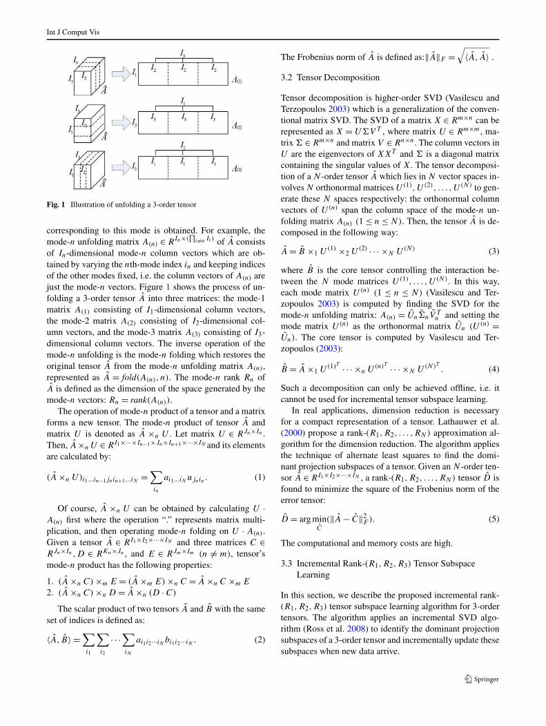
Fig. 1 Illustration of unfolding a 3-order tensor
corresponding to this mode is obtained. For example, themode-n unfolding matrix A(n) ∈ R
In×(∏
i �=n Ii ) of A consistsof In-dimensional mode-n column vectors which are ob-tained by varying the nth-mode index in and keeping indicesof the other modes fixed, i.e. the column vectors of A(n) arejust the mode-n vectors. Figure 1 shows the process of un-folding a 3-order tensor A into three matrices: the mode-1matrix A(1) consisting of I1-dimensional column vectors,the mode-2 matrix A(2) consisting of I2-dimensional col-umn vectors, and the mode-3 matrix A(3) consisting of I3-dimensional column vectors. The inverse operation of themode-n unfolding is the mode-n folding which restores theoriginal tensor A from the mode-n unfolding matrix A(n),represented as A = fold(A(n), n). The mode-n rank Rn ofA is defined as the dimension of the space generated by themode-n vectors: Rn = rank(A(n)).
The operation of mode-n product of a tensor and a matrixforms a new tensor. The mode-n product of tensor A andmatrix U is denoted as A ×n U . Let matrix U ∈ RJn×In .Then, A×n U ∈ RI1×···×In−1×Jn×In+1×···×IN and its elementsare calculated by:
(A ×n U)i1...in−1jnin+1...iN =∑
in
ai1...iN ujnin . (1)
Of course, A ×n U can be obtained by calculating U ·A(n) first where the operation “.” represents matrix multi-plication, and then operating mode-n folding on U · A(n).Given a tensor A ∈ RI1×I2×···×IN and three matrices C ∈RJn×In ,D ∈ RKn×Jn , and E ∈ RJm×Im (n �= m), tensor’smode-n product has the following properties:
1. (A ×n C) ×m E = (A ×m E) ×n C = A ×n C ×m E
2. (A ×n C) ×n D = A ×n (D · C)
The scalar product of two tensors A and B with the sameset of indices is defined as:
〈A, B〉 =∑
i1
∑
i2
· · ·∑
iN
ai1i2···iN bi1i2···iN . (2)
The Frobenius norm of A is defined as:‖A‖F =√
〈A, A〉 .
3.2 Tensor Decomposition
Tensor decomposition is higher-order SVD (Vasilescu andTerzopoulos 2003) which is a generalization of the conven-tional matrix SVD. The SVD of a matrix X ∈ Rm×n can berepresented as X = U�V T , where matrix U ∈ Rm×m, ma-trix � ∈ Rm×n and matrix V ∈ Rn×n. The column vectors inU are the eigenvectors of XXT and � is a diagonal matrixcontaining the singular values of X. The tensor decomposi-tion of a N -order tensor A which lies in N vector spaces in-volves N orthonormal matrices U(1),U(2), . . . ,U(N) to gen-erate these N spaces respectively: the orthonormal columnvectors of U(n) span the column space of the mode-n un-folding matrix A(n) (1 ≤ n ≤ N). Then, the tensor A is de-composed in the following way:
A = B ×1 U(1) ×2 U(2) · · · ×N U(N) (3)
where B is the core tensor controlling the interaction be-tween the N mode matrices U(1), . . . ,U(N). In this way,each mode matrix U(n) (1 ≤ n ≤ N) (Vasilescu and Ter-zopoulos 2003) is computed by finding the SVD for themode-n unfolding matrix: A(n) = Un�nV
Tn and setting the
mode matrix U(n) as the orthonormal matrix Un (U(n) =Un). The core tensor is computed by Vasilescu and Ter-zopoulos (2003):
B = A ×1 U(1)T · · · ×n U(n)T · · · ×N U(N)T . (4)
Such a decomposition can only be achieved offline, i.e. itcannot be used for incremental tensor subspace learning.
In real applications, dimension reduction is necessaryfor a compact representation of a tensor. Lathauwer et al.(2000) propose a rank-(R1,R2, . . . ,RN) approximation al-gorithm for the dimension reduction. The algorithm appliesthe technique of alternate least squares to find the domi-nant projection subspaces of a tensor. Given an N -order ten-sor A ∈ RI1×I2×···×IN , a rank-(R1,R2, . . . ,RN) tensor D isfound to minimize the square of the Frobenius norm of theerror tensor:
D = arg minC
(‖A − C‖2F ). (5)
The computational and memory costs are high.
3.3 Incremental Rank-(R1,R2,R3) Tensor SubspaceLearning
In this section, we describe the proposed incremental rank-(R1,R2,R3) tensor subspace learning algorithm for 3-ordertensors. The algorithm applies an incremental SVD algo-rithm (Ross et al. 2008) to identify the dominant projectionsubspaces of a 3-order tensor and incrementally update thesesubspaces when new data arrive.
Int J Comput Vis
3.3.1 Incremental SVD
Gu and Eisenstat (1995) propose an efficient and stable algo-rithm for finding the SVD of a matrix obtained by deletinga row from an original matrix. The algorithm updates theSVD of the original matrix. They (Gu and Eisenstat 1993)also propose a stable and fast algorithm for finding the SVDof a matrix obtained by appending a row to an original ma-trix with a known SVD. The techniques for downdating andupdating SVD are quite similar to each other. In incremen-tal SVD, the aim is to update a given SVD when new dataarrives. The SVD contains only a relatively small numberof non-zero singular values. Incremental SVD is suitable forbackground modeling and object tracking, as it emphasizesthe current observations and retains information about theprevious observations in the previous SVD. The algorithmin Ross et al. (2008) extends the classic incremental SVD(Levy and Lindenbaum 2000) by computing the subspace ofa dynamic matrix with the mean updating which removesthe assumption that the mean of the previous data is equal tothe mean of the new data. More accurate incremental SVDis obtained.
In this paper, we apply the incremental SVD algorithm inRoss et al. (2008) to our incremental tensor subspace learn-ing algorithm. In the following, this incremental SVD al-gorithm is briefly described. Let A′ be the previous datamatrix where the data are represented by column vectors.Let F ′ be a new data matrix. Let μA,μF , and μA∗ be thecolumn mean vectors of A′,F ′, and (A′|F ′) respectively,where the operation “|” merges the left and the right ma-trices. Let {UA,�A,VA} be the SVD of A′, where onlythe principal components with larger singular values are re-tained. The SVD {UA∗ ,�A∗ ,VA∗} of (A′|F ′) is estimatedfrom μA, {UA,�A,VA}, and F ′. This incremental updatingprocess is outlined as follows:
Step 1: Compute
μA∗ = IA
IA + IF
μA + IF
IA + IF
μF (6)
where IA is the number of the columns in A′ and IF is thenumber of columns in F ′.
Step 2: Construct a new matrix E:
E =(
(F ′ − μF l1×IF)|√
IAIF
IA + IF
(μA − μF )
)
(7)
where l1×IFis a IF -dimensional row vector whose elements
are all “1”, i.e.
IF︷ ︸︸ ︷1,1, . . . ,1.
Step 3: Compute the QR decomposition of E to obtainthe eigenbasis E of E. Let matrix U ′ be U ′ = (UA|E).
Step 4: Let matrix V ′ be
V ′ =(
VA 00 �IF
)
(8)
where �IFis the IF × IF identity matrix. Then, matrix �′
is defined as:
�′ =(
�A (UA)T E
0 ET E
)
. (9)
Step 5: Compute the SVD of �′ : �′ = U�V T . Then,the of SVD of (A′|F ′) is obtained: UA∗ = U ′U ,�A∗ = �,and (VA∗)T = (V )T (V ′)T .
The forgetting factor λ in Ross et al. (2008) is used toweight the data streams, in order that recent observations aregiven higher weights than historical ones. This is achievedby replacing the matrix A′ with λA′ in the incremental up-dating process described above.
As shown in Levy and Lindenbaum (2000), Ross et al.(2008), Golub and Van Loan (1996), the result of incremen-tal SVD for a matrix is the same as the result of the SVDfor the matrix in the batch mode if all the non-zero singularvalues at the previous step are retained and used for incre-mental SVD at the current step. The subspace obtained us-ing the incremental SVD in this way is very accurate. Exceptfor matrix SVD, there is no iterative process included in theincremental SVD algorithm. There are reliable, stable algo-rithms for the matrix SVD that converge rapidly to the cor-rect result. So, the incremental SVD avoids the convergenceproblem generally associated with iterative algorithms.
Let m be the number of rows in the data matrix and letn be the number of singular values retained in the SVDof the data matrix. In general, updates to the SVD requireO(mn2) operations in practice, although they can be donein O(mn log(n)) in theory. According to Ross et al. (2008),the above incremental SVD only requires O(mnIF ) opera-tions. As IF is a small integer, this incremental SVD is veryfast.
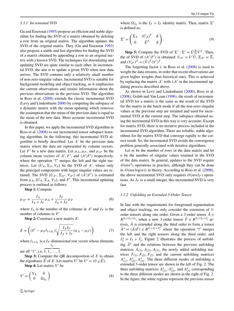
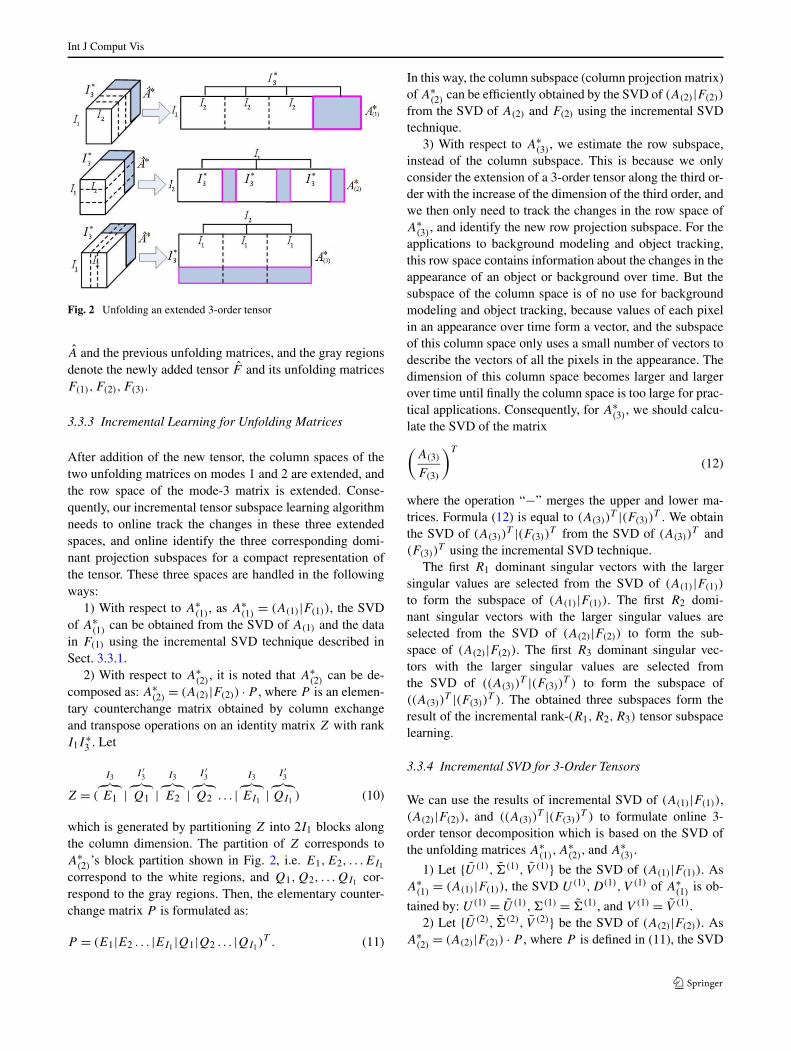
3.3.2 Unfolding an Extended 3-Order Tensor
In line with the requirements for foreground segmentationand object tracking, we only consider the extension of 3-order tensors along one order. Given a 3-order tensor A ∈RI1×I2×I3 , when a new 3-order tensor F ∈ RI1×I2×I ′
3 ar-rives, A is extended along the third order to form a tensorA∗ = (A|F ) ∈ RI1×I2×I∗
3 where the operation “|” mergesthe left and the right tensors along the third order, andI ∗
3 = I3 + I ′3. Figure 2 illustrates the process of unfold-
ing A∗ and the relations between the previous unfoldingmatrices A(1),A(2),A(3), the newly added unfolding ma-trices F(1),F(2),F(3) and the current unfolding matricesA∗
(1),A∗(2),A
∗(3). The three different modes of unfolding a
extended 3-order tensor are shown in the left of Fig. 2. Thethree unfolding matrices A∗
(1),A∗(2), and A∗
(3) correspondingto the three different modes are shown in the right of Fig. 2.In the figure, the white regions represent the previous tensor
Int J Comput Vis
Fig. 2 Unfolding an extended 3-order tensor
A and the previous unfolding matrices, and the gray regionsdenote the newly added tensor F and its unfolding matricesF(1),F(2),F(3).
3.3.3 Incremental Learning for Unfolding Matrices
After addition of the new tensor, the column spaces of thetwo unfolding matrices on modes 1 and 2 are extended, andthe row space of the mode-3 matrix is extended. Conse-quently, our incremental tensor subspace learning algorithmneeds to online track the changes in these three extendedspaces, and online identify the three corresponding domi-nant projection subspaces for a compact representation ofthe tensor. These three spaces are handled in the followingways:
1) With respect to A∗(1)
, as A∗(1)
= (A(1)|F(1)), the SVDof A∗
(1) can be obtained from the SVD of A(1) and the datain F(1) using the incremental SVD technique described inSect. 3.3.1.
2) With respect to A∗(2), it is noted that A∗
(2) can be de-composed as: A∗
(2) = (A(2)|F(2)) · P , where P is an elemen-tary counterchange matrix obtained by column exchangeand transpose operations on an identity matrix Z with rankI1I
∗3 . Let
Z = (
I3︷︸︸︷E1 |
I ′3
︷︸︸︷Q1 |
I3︷︸︸︷E2 |
I ′3
︷︸︸︷Q2 . . . |
I3︷︸︸︷EI1 |
I ′3
︷︸︸︷QI1 ) (10)
which is generated by partitioning Z into 2I1 blocks alongthe column dimension. The partition of Z corresponds toA∗
(2)’s block partition shown in Fig. 2, i.e. E1,E2, . . .EI1
correspond to the white regions, and Q1,Q2, . . .QI1 cor-respond to the gray regions. Then, the elementary counter-change matrix P is formulated as:
P = (E1|E2 . . . |EI1 |Q1|Q2 . . . |QI1)T . (11)
In this way, the column subspace (column projection matrix)of A∗
(2) can be efficiently obtained by the SVD of (A(2)|F(2))
from the SVD of A(2) and F(2) using the incremental SVDtechnique.
3) With respect to A∗(3), we estimate the row subspace,
instead of the column subspace. This is because we onlyconsider the extension of a 3-order tensor along the third or-der with the increase of the dimension of the third order, andwe then only need to track the changes in the row space ofA∗
(3), and identify the new row projection subspace. For theapplications to background modeling and object tracking,this row space contains information about the changes in theappearance of an object or background over time. But thesubspace of the column space is of no use for backgroundmodeling and object tracking, because values of each pixelin an appearance over time form a vector, and the subspaceof this column space only uses a small number of vectors todescribe the vectors of all the pixels in the appearance. Thedimension of this column space becomes larger and largerover time until finally the column space is too large for prac-tical applications. Consequently, for A∗
(3), we should calcu-late the SVD of the matrix(
A(3)
F(3)
)T
(12)
where the operation “−” merges the upper and lower ma-trices. Formula (12) is equal to (A(3))
T |(F(3))T . We obtain
the SVD of (A(3))T |(F(3))
T from the SVD of (A(3))T and
(F(3))T using the incremental SVD technique.
The first R1 dominant singular vectors with the largersingular values are selected from the SVD of (A(1)|F(1))
to form the subspace of (A(1)|F(1)). The first R2 domi-nant singular vectors with the larger singular values areselected from the SVD of (A(2)|F(2)) to form the sub-space of (A(2)|F(2)). The first R3 dominant singular vec-tors with the larger singular values are selected fromthe SVD of ((A(3))
T |(F(3))T ) to form the subspace of
((A(3))T |(F(3))
T ). The obtained three subspaces form theresult of the incremental rank-(R1,R2,R3) tensor subspacelearning.
3.3.4 Incremental SVD for 3-Order Tensors
We can use the results of incremental SVD of (A(1)|F(1)),(A(2)|F(2)), and ((A(3))
T |(F(3))T ) to formulate online 3-
order tensor decomposition which is based on the SVD ofthe unfolding matrices A∗
(1),A∗(2), and A∗
(3).
1) Let {U (1), �(1), V (1)} be the SVD of (A(1)|F(1)). AsA∗
(1) = (A(1)|F(1)), the SVD U(1),D(1), V (1) of A∗(1) is ob-
tained by: U(1) = U (1),�(1) = �(1), and V (1) = V (1).2) Let {U (2), �(2), V (2)} be the SVD of (A(2)|F(2)). As
A∗(2)
= (A(2)|F(2)) · P , where P is defined in (11), the SVD
Int J Comput Vis
U(2),D(2), V (2) of A∗(2) is obtained by: U(2) = U (2),�(2) =
�(2), and V (2) = P T · V (2).3) Let {U (3), �(3), V (3)} be the SVD of ((A(3))
T |(F(3))T ).
As A∗(3) = (
A(3)
F(3)), the SVD U(3),�(3), V (3) of A∗
(3) is ob-
tained by: U(3) = V (3),�(3) = (�(3))T ,V (3) = U (3).It is noted that our online 3-order tensor decomposition
is different from the offline tensor decomposition formulatedin (3) and (4) in that we use the row vectors in the mode-3unfolding matrix A∗
(3) rather than its column vectors. Thiscan be regarded as an extension of the offline tensor decom-position, because if column vectors are used for A∗
(3) theincremental subspace learning for A∗
(3)cannot be achieved.
The mode-3 unfolding matrix and its incremental subspacelearning just correspond to the vector subspace learning al-gorithm in Ross et al. (2008). In this way, the subspacelearned using the algorithm in Ross et al. (2008) is kept inour tensor subspace learning algorithm. This ensures, in the-ory, that our incremental tensor subspace learning algorithmcan obtain more accurate results than the incremental vectorsubspace learning algorithm.
3.3.5 Likelihood Evaluation
It is necessary for a subspace learning-based algorithm toevaluate the likelihood of the test sample given the learnedsubspace or subspaces. The likelihood evaluation methodwith respect to the proposed incremental 3-order tensor sub-space learning algorithm is described as follows: As we onlyconsider the increase of the dimension of the third order ofa 3-order tensor A ∈ RI1×I2×I3 with the dimensions of thefirst and second orders held constant, the learned subspacesof the tensor should be composed of the mode-1 column pro-jection matrix U(1) ∈ RI1×R1 , the mode-2 column projec-tion matrix U(2) ∈ RI2×R2 , and the mode-3 row projectionmatrix V (3) ∈ R(I1·I2)×R3 . Let μ(1) and μ(2) be the columnmean vectors of A(1) and A(2) respectively. Let μ(3) be therow mean vector of A(3). Tensors M1 and M2 are definedby:
M1 = (
I2︷ ︸︸ ︷μ(1), . . . ,μ(1)) ∈ RI1×I2×1
M2 = (μ(2), . . . ,μ(2)
︸ ︷︷ ︸I1
)T ∈ RI1×I2×1. (13)
The sum of the reconstruction error norms of a test sampleJ ∈ RI1×I2×1 corresponding to the three modes is computedby:
RE =(
2∑
i=1
∥∥(J − Mi) − (
(J − Mi) ×i (U(i) · U(i)T ))∥∥2
F
+ ∥∥(J(3) − μ(3))
− ((J(3) − μ(3)) · (V (3) · V (3)T )
)∥∥2
F
) 12
(14)
where J(3) is the mode-3 unfolding matrix ofJ , and the re-construction error for a mode represents the distance fromthe sample to the subspace corresponding to this mode. Thelikelihood of the test sample J given the learned tensor sub-spaces is computed by:
p(J |U(1),U(2), V (3)) ∝ exp
(
−RE2
2σ 2
)
(15)
where σ is a scale factor. The smaller the RE, the larger thelikelihood.
3.3.6 Theoretical Comparison
In the following, we compare our algorithm with DTA,WTA, and STA in Sun et al. (2006a, 2006b, 2008).
DTA: For DTA in Sun et al. (2006a, 2008), the incremen-tal updating of the subspace of the unfolding matrix of a ten-sor on each mode is performed by updating the covariancematrix formed from the columns of the unfolding matrix andthen obtaining an eigenvalue decomposition of the updatedcovariance matrix. The updating is achieved by:
Cd ← λCd + XT(d)X(d) (16)
where Cd on the right hand side of (16) is the covariancematrix of the unfolding matrix on mode d for the data ob-served at the previous steps, and Xd is the unfolding matrixon mode d for the incoming data at the current step. Accord-ing to Ross et al. (2008), this updating of the covariance ma-trix is based on the assumption that μd = μ′
d where μd is themean of the previous unfolding matrix, and μ′
d is the meanof Xd , i.e. any changes in the mean are not considered. So,this updating is not accurate if there are significant changesin the mean. If the updating is applied to background mod-eling and object tracking, the corresponding model cannotadapt to large appearance changes.
According to (Ross et al. 2008) the accurate updating ofthe covariance matrix with mean updating should be
Cd ← λCd +XT(d)X(d) + pq
p + q
(μd − μ′
d
) (μd − μ′
d
)T (17)
where p is the number of columns in the previous matrix andq is the number of columns in the new incoming data ma-trix. Even if we introduce (17) into DTA, the obtained sub-space is still not accurate for the applications to backgroundmodeling and object tracking, because DTA has the smallsize problem. For a 3-order tensor (RI1×I2×I3), the dimen-sion of the row vectors in the unfolding matrix on mode 3 isI1I2. The corresponding covariance matrix is a I1I2 × I1I2
Int J Comput Vis
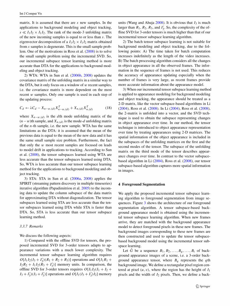
matrix. It is assumed that there are s new samples. In theapplications to background modeling and object tracking,s � I1I2 × I1I2. The rank of the mode-3 unfolding matrixof the new incoming samples is equal to or less than s. Theeigenvector decomposition of a I1I2 × I1I2 matrix obtainedfrom s samples is degenerate. This is the small sample prob-lem. One of the motivations in Ross et al. (2008) is to solvethe small sample problem using the incremental SVD. So,our incremental subspace tensor learning method is moreaccurate than DTA for the applications to background mod-eling and object tracking.
2) WTA: WTA in Sun et al. (2006b, 2008) updates thecovariance matrix of the unfolding matrix in a similar way tothe DTA, but it only focus on a window of w recent samples,i.e. the covariance matrix is more dependent on the mostrecent w samples. Only one sample is used in each step ofthe updating process:
Cd ← λCd − Xn−w,(d)XTn−w,(d) + Xn,(d)X
Tn,(d) (18)
where Xn−w,(d) is the d th mode unfolding matrix of the(n−w)th sample, and Xn,(d) is the mode-d unfolding matrixof the n-th sample, i.e. the new sample. WTA has the samelimitations as the DTA: it is assumed that the mean of theprevious data is equal to the mean of the new data and it hasthe same small sample size problem. Furthermore, the factthat only the w most recent samples are focused on leadsto model drift in applications to tracking. According to Sunet al. (2008), the tensor subspaces learned using WTA areless accurate than the tensor subspaces learned using DTA.So, WTA is less accurate than our tensor subspace learningmethod for the applications to background modeling and ob-ject tracking.
3) STA: STA in Sun et al. (2006a, 2008) applies theSPIRIT (streaming pattern discovery in multiple timeseries)iterative algorithm (Papadimitriou et al. 2005) to the incom-ing data to update the column subspace of the data matrixfor approximating DTA without diagonalization. The tensorsubspaces learned using STA are less accurate than the ten-sor subspaces learned using DTA while STA is faster thanDTA. So, STA is less accurate than our tensor subspacelearning method.
3.3.7 Remarks
We discuss the following aspects:1) Compared with the offline SVD for tensors, the pro-
posed incremental SVD for 3-order tensors adapts to ap-pearance variations with a much lower complexity. Theincremental tensor subspace learning algorithm requiresO[I1I2(I3 + I ′
3)(R1 + R2 + R3)] operations and O[I1R1 +I2R2 + I1I2(R3 + I ′
3)] memory units. In comparison, theoffline SVD for 3-order tensors requires O[I1I2(I1 + I2 +I3 + I ′
3)(I3 + I ′3)] operations and O[I1(I3 + I ′
3)I2] memory
units (Wang and Ahuja 2008). It is obvious that I3 is muchlarger than R1,R2,R3, and I ′
3. So, the complexity of the of-fline SVD for 3-order tensors is much higher than that of ourincremental tensor subspace learning algorithm.
2) The batch tensor subspace learning is not suitable forbackground modeling and object tracking, due to the fol-lowing points: A) The time taken for batch computationincreases indefinitely as the length of the video increases.B) The batch processing algorithm considers all the changesin object appearance in all the observed frames. The infor-mation in the sequence of frames is not used. This reducesthe accuracy of appearance updating especially when thenumber of frames is very large, as recent frames providemore accurate information about the appearance model.
3) When our incremental tensor subspace learning methodis applied to appearance modeling for background modelingand object tracking, the appearance should be treated as a2-D matrix, like the vector subspace-based algorithms in Li(2004), Ross et al. (2008). In Li (2004), Ross et al. (2008),the 2-matrix is unfolded into a vector, and the SVD tech-nique is used to obtain the subspace representing changesin object appearance over time. In our method, the tensortechnique is introduced to object appearance representationover time by treating appearances using 2-D matrices. Thespatial information of the object appearance is included inthe subspaces of the unfolding matrices on the first and thesecond modes of the tensor. The subspace of the unfoldingmatrix on the third mode of the tensor describes appear-ance changes over time. In contrast to the vector subspace-based algorithm in Li (2004), Ross et al. (2008), our tensorsubspace-based algorithm captures more spatial informationin images.
4 Foreground Segmentation
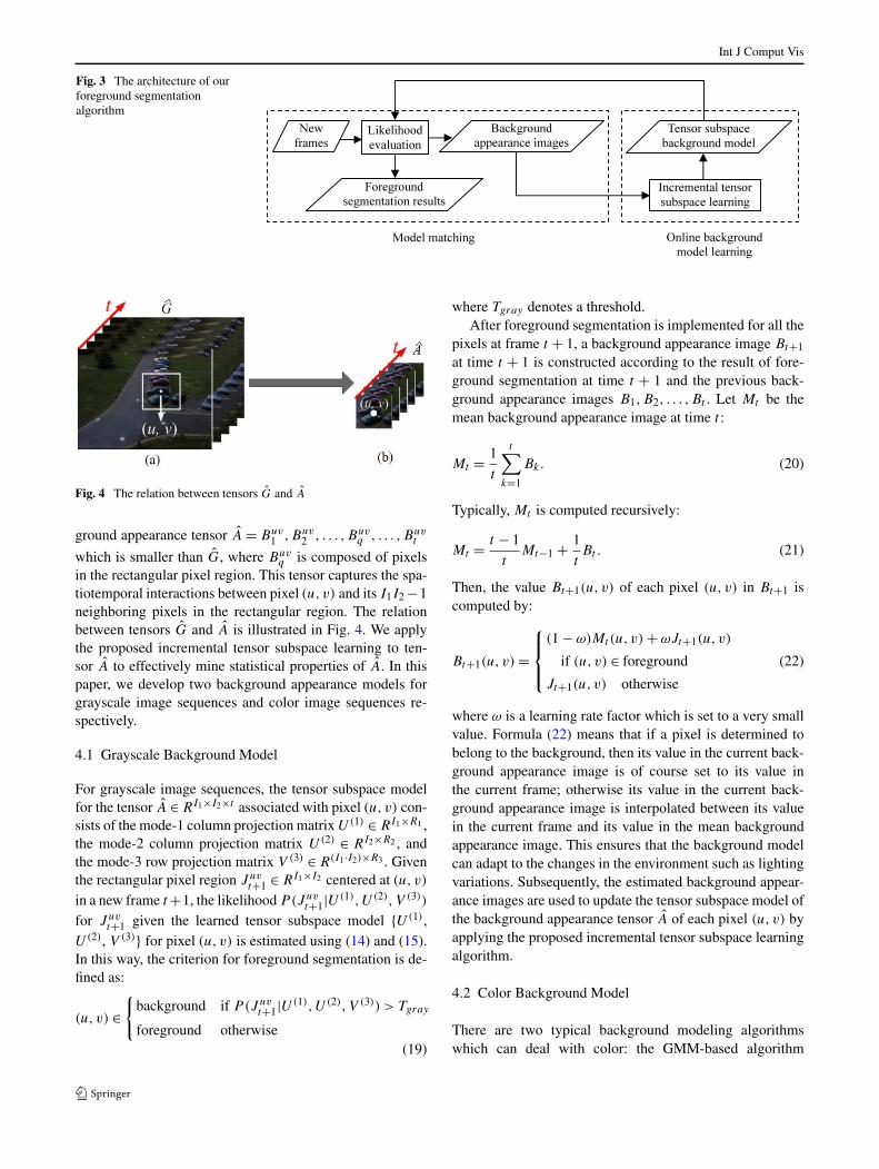
We apply the proposed incremental tensor subspace learn-ing algorithm to foreground segmentation from image se-quences. Figure 3 shows the architecture of our foregroundsegmentation algorithm. A tensor subspace-based back-ground appearance model is obtained using the incremen-tal tensor subspace learning algorithm. When new framesarrive, they are matched with the background appearancemodel to detect foreground pixels in these new frames. Thebackground images corresponding to these new frames arethen constructed and used to update the tensor subspace-based background model using the incremental tensor sub-space learning.
Let G be a sequence B1,B2, . . . ,Bq, . . . ,Bt of back-ground appearance images of a scene, i.e. a 3-order back-ground appearance tensor, where Bq represents the qthbackground image. We define a rectangular pixel region cen-tered at pixel (u,v), where the region has the height of I1
pixels and the width of I2 pixels. Then, we define a back-
Int J Comput Vis
Fig. 3 The architecture of ourforeground segmentationalgorithm
Fig. 4 The relation between tensors G and A
ground appearance tensor A = Buv1 ,Buv
2 , . . . ,Buvq , . . . ,Buv
t
which is smaller than G, where Buvq is composed of pixels
in the rectangular pixel region. This tensor captures the spa-tiotemporal interactions between pixel (u,v) and its I1I2 −1neighboring pixels in the rectangular region. The relationbetween tensors G and A is illustrated in Fig. 4. We applythe proposed incremental tensor subspace learning to ten-sor A to effectively mine statistical properties of A. In thispaper, we develop two background appearance models forgrayscale image sequences and color image sequences re-spectively.
4.1 Grayscale Background Model
For grayscale image sequences, the tensor subspace modelfor the tensor A ∈ RI1×I2×t associated with pixel (u,v) con-sists of the mode-1 column projection matrix U(1) ∈ RI1×R1 ,the mode-2 column projection matrix U(2) ∈ RI2×R2 , andthe mode-3 row projection matrix V (3) ∈ R(I1·I2)×R3 . Giventhe rectangular pixel region Juv
t+1 ∈ RI1×I2 centered at (u,v)
in a new frame t +1, the likelihood P(Juvt+1|U(1),U(2), V (3))
for Juvt+1 given the learned tensor subspace model {U(1),
U(2), V (3)} for pixel (u,v) is estimated using (14) and (15).In this way, the criterion for foreground segmentation is de-fined as:
(u, v) ∈{
background if P(J uvt+1|U(1),U(2), V (3)) > Tgray
foreground otherwise(19)
where Tgray denotes a threshold.After foreground segmentation is implemented for all the
pixels at frame t + 1, a background appearance image Bt+1
at time t + 1 is constructed according to the result of fore-ground segmentation at time t + 1 and the previous back-ground appearance images B1,B2, . . . ,Bt . Let Mt be themean background appearance image at time t :
Mt = 1
t
t∑
k=1
Bk. (20)
Typically, Mt is computed recursively:
Mt = t − 1
tMt−1 + 1
tBt . (21)
Then, the value Bt+1(u, v) of each pixel (u, v) in Bt+1 iscomputed by:
Bt+1(u, v) =
⎧⎪⎨
⎪⎩
(1 − ω)Mt(u, v) + ωJt+1(u, v)
if (u, v) ∈ foreground
Jt+1(u, v) otherwise
(22)
where ω is a learning rate factor which is set to a very smallvalue. Formula (22) means that if a pixel is determined tobelong to the background, then its value in the current back-ground appearance image is of course set to its value inthe current frame; otherwise its value in the current back-ground appearance image is interpolated between its valuein the current frame and its value in the mean backgroundappearance image. This ensures that the background modelcan adapt to the changes in the environment such as lightingvariations. Subsequently, the estimated background appear-ance images are used to update the tensor subspace model ofthe background appearance tensor A of each pixel (u, v) byapplying the proposed incremental tensor subspace learningalgorithm.
4.2 Color Background Model
There are two typical background modeling algorithmswhich can deal with color: the GMM-based algorithm
Int J Comput Vis
(Stauffer and Grimson 1999) and the kernel-based algo-rithm (Elgammal et al. 2002). In the GMM-based algorithm,each mixture component of the background model is a singleGaussian distribution in the RGB color space. The covari-ance matrix of each Gaussian is a diagonal matrix
∑ = σ 2I
where I is an identity matrix and σ is a standard deviation.The GMM-based algorithm deals with the RGB channelsseparately, and assumes the same standard deviation for eachchannel. Although dealing with color in this way is not con-sistent with real data distributions, it can greatly increasethe speed with only a slight loss of accuracy. The kerneldensity estimation-based background modeling algorithm(Elgammal et al. 2002) also deals with the color channelsseparately, i.e. the joint probability density of color pixels isdecomposed into the product of independent kernel densityfunctions of each color channel. In contrast to the GMM-based algorithm, the kernel-based algorithm uses differentGaussian kernel variances for each channel.
Referring to the GMM-based algorithm (Stauffer andGrimson 1999) and the Kernel-based algorithm (Elgammalet al. 2002), we extend the proposed background model forgrayscale sequences to the background model for color im-age sequences. In the color background model, we use the(r, g, s) color space which is defined in terms of the RGBcolor space by r = R/(R + G + B),g = G/(R + G + B),and s = (R +G+B)/3. The effects of shadows are reducedin the (r, g, s) color space (Elgammal et al. 2002).
Let Ar ∈ RI1×I2×t be a 3-order tensor Br1Br
2 . . .Brq . . .Br
t ,where Br
q is a matrix which is composed of the r-componentsof pixels in the rectangular appearance region centered atpixel (u,v) at time q . Similarly, we define tensors Ag ∈RI1×I2×t (B
g
1 Bg
2 . . .Bgt ) and As ∈ RI1×I2×t (Bs
1Bs2 . . .Bs
t )
for the g-components and the s-components of the pixelsin the region centered at (u,v). For each component’s ten-sor AC (C ∈ {r, g, s}), a tensor subspace model is incremen-tally learned using the proposed incremental tensor subspacelearning algorithm. In this way, three tensor subspace mod-els for each pixel are obtained corresponding to the threecolor components. The learning process for the tensor ofeach component is similar to that for the grayscale sequence.The subspace model for tensor AC (C ∈ {r, g, s}) consists ofthe following terms: 1) the maintained subspace dimensions(RC
1 ,RC
2 ,RC
3 ) corresponding to the three tensor unfolding
modes; 2) the column projection matrices U(1)C
∈ RI1×RC
1
and U(2)C
∈ RI2×RC
2 of modes 1 and 2, and the mode-3 row
projection matrix V(3)C
∈ R(I1·I2)×RC
3 ;3) the column mean
vectors μ(1)C
and μ(2)C
of the unfolding matrices AC
(1) and AC
(2)
of modes 1 and 2, and the row mean vector μ(3)C
of the mode-3 unfolding matrix AC
(3). Let J rt+1 ∈ RI1×I2, J
g
t+1 ∈ RI1×I2
and J st+1 ∈ RI1×I2 be, respectively, the matrices of r, g, s-
components of pixels in the appearance region centered at(u,v) at time t + 1. The distances RMr
uv,RMguv and RMs
uv
between {r, g, s}-components of pixels in the rectangularimage region Juv
t+1 centered at (u,v) at frame t + 1 andthe learned {r, g, s}-component tensor-based subspace mod-els are calculated, respectively, using (14). Then, the likeli-hood Puv for J uv
t+1 given the learned tensor subspace models
{U(1)r ,U
(2)r , V
(3)r }, {U(1)
g ,U(2)g ,V
(3)g }, and {U(1)
s ,U(2)s , V
(3)s }
for pixel (u,v) is estimated by:
Puv = exp
(
−1
2
(RMr
uv
σr
)2
− 1
2
(RM
guv
σg
)2
− 1
2
(RMs
uv
σs
)2)
(23)
where σr, σg , and σs are three scale factors. The criterion forforeground segmentation is defined as:
(u, v) ∈{
background if Puv > Tcolor
foreground otherwise(24)
where Tcolor is a threshold.Using the result of foreground segmentation at the cur-
rent time t + 1, we can estimate the current background ap-pearance image which consists of the (r, g, s)-componentbackground appearance matrices: Br
t+1 ∈ RI1×I2,Bg
t+1 ∈RI1×I2 , and Bs
t+1 ∈ RI1×I2 . The elements in these three ma-trices are estimated by:
BC
t+1(u, v) =
⎧⎪⎨
⎪⎩
(1 − ωC)MC
t+1(u, v) + ωCJC
t+1(u, v)
if (u, v) ∈ foreground
JC
t+1(u, v) otherwise
(25)
where C ∈ {r, g, s},ωC is a learning rate factor, and MCt is
the mean matrix of BC
1 ,BC
2 , . . . , and BCt at time t . As for-
mulated in (20) and (21), MCt is computed recursively.
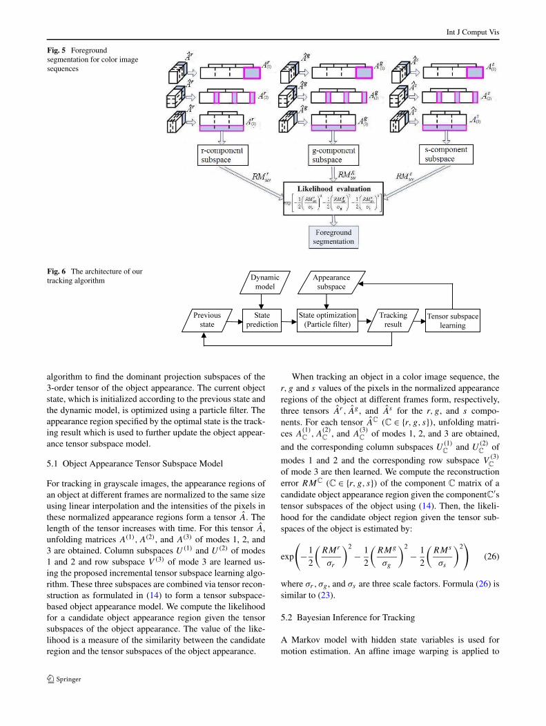
Subsequently, the newly estimated background appear-ance component matrices are used to incrementally updatethe subspace models of the component tensors of the colorbackground appearance region centered at each pixel by ap-plying the incremental tensor subspace learning algorithm.The tensor subspace model for each component is learnedand updated in the same way as the tensor subspace modelfor the grayscale sequences. Figure 5 is used to further illus-trate the foreground segmentation process for color imagesequences.
5 Visual Tracking
We apply the proposed incremental tensor subspace learn-ing algorithm to appearance-based object tracking. Figure 6shows the architecture of our object tracking algorithm. Inthe algorithm, a low dimensional subspace model for theappearance tensor of an object is learned. The model usesthe incremental rank-(R1,R2,R3) tensor subspace learning
Int J Comput Vis
Fig. 5 Foregroundsegmentation for color imagesequences
Fig. 6 The architecture of ourtracking algorithm
algorithm to find the dominant projection subspaces of the3-order tensor of the object appearance. The current objectstate, which is initialized according to the previous state andthe dynamic model, is optimized using a particle filter. Theappearance region specified by the optimal state is the track-ing result which is used to further update the object appear-ance tensor subspace model.
5.1 Object Appearance Tensor Subspace Model
For tracking in grayscale images, the appearance regions ofan object at different frames are normalized to the same sizeusing linear interpolation and the intensities of the pixels inthese normalized appearance regions form a tensor A. Thelength of the tensor increases with time. For this tensor A,unfolding matrices A(1),A(2), and A(3) of modes 1, 2, and3 are obtained. Column subspaces U(1) and U(2) of modes1 and 2 and row subspace V (3) of mode 3 are learned us-ing the proposed incremental tensor subspace learning algo-rithm. These three subspaces are combined via tensor recon-struction as formulated in (14) to form a tensor subspace-based object appearance model. We compute the likelihoodfor a candidate object appearance region given the tensorsubspaces of the object appearance. The value of the like-lihood is a measure of the similarity between the candidateregion and the tensor subspaces of the object appearance.
When tracking an object in a color image sequence, ther, g and s values of the pixels in the normalized appearanceregions of the object at different frames form, respectively,three tensors Ar , Ag , and As for the r, g, and s compo-nents. For each tensor AC (C ∈ {r, g, s}), unfolding matri-ces A
(1)C
,A(2)C
, and A(3)C
of modes 1, 2, and 3 are obtained,
and the corresponding column subspaces U(1)C
and U(2)C
of
modes 1 and 2 and the corresponding row subspace V(3)C
of mode 3 are then learned. We compute the reconstructionerror RMC (C ∈ {r, g, s}) of the component C matrix of acandidate object appearance region given the componentC′stensor subspaces of the object using (14). Then, the likeli-hood for the candidate object region given the tensor sub-spaces of the object is estimated by:
exp
(
−1
2
(RMr
σr
)2
− 1
2
(RMg
σg
)2
− 1
2
(RMs
σs
)2)
(26)
where σr, σg , and σs are three scale factors. Formula (26) issimilar to (23).
5.2 Bayesian Inference for Tracking
A Markov model with hidden state variables is used formotion estimation. An affine image warping is applied to
Int J Comput Vis
model the object motion between two consecutive frames.The object state variable vector Xt at time t is describedusing the six parameters of the affine motion transform:xt , yt , ηt , st , βt , and φt , which are respectively the transla-tion parameters of the x, y coordinates, the rotation angle,the scale, the aspect ratio, and the skew direction. The loca-tion, size and pose of the object are indicated in the affinemotion parameters. Given a set of observed image regionsO1,O2, . . . ,Ot , the posterior probability of the object stateis formulated by Bayes’ theorem:
p(Xt |O1,O2, . . . ,Ot )
∝ p(Ot |Xt)
∫
p(Xt |Xt−1)
× p(Xt−1|O1,O2, . . . ,Ot−1)dXt−1 (27)
where p(Ot |Xt) is the likelihood for the observation Ot
given the object state Xt , and p(Xt |Xt−1) is the probabil-ity model for the object state transition. The terms p(Ot |Xt)
and p(Xt |Xt−1) determine the tracking process. A Gaussiandistribution is employed to model the state transition distri-bution p(Xt |Xt−1):
p(Xt |Xt−1) = N(Xt : Xt−1,�) (28)
where � denotes a diagonal covariance matrix with six diag-onal elements σ 2
x , σ 2y , σ 2
η , σ 2s , σ 2
β , and σ 2φ . The observation
model p(Ot |Xt) is evaluated using the likelihood for a sam-ple image region given the learned appearance tensor sub-spaces. For grayscale image sequences, this probability isestimated using (15). For color image sequences, this prob-ability is estimated using (26).
A standard particle filter (Isard and Blake 1996) is usedto estimate the object motion state. The components of eachparticle correspond to the six affine motion parameters. Forthe maximum a posteriori estimate, the particle which max-imizes the observation model is selected as the optimal stateof the object in the current frame. The affinely warped im-age region associated with the optimal state of the object isused to incrementally update the tensor subspace-based ob-ject appearance model.
6 Experiments
The experimental results for the foreground segmentationare shown first, and then the experimental results for the vi-sual object tracking are shown. The runtimes are measuredon a computer with 3.25 GB RAM and Intel Core2 QuadCPU at 2.83 GHz.
6.1 Foreground Segmentation
In order to evaluate the performances of the proposed incre-mental tensor subspace learning-based algorithms for fore-ground segmentation for grayscale image sequences andfor color image sequences, four examples corresponding tofour videos are shown to demonstrate the claimed contribu-tions of our algorithms. The first two videos consist of 8-bit grayscale images while the two remaining videos consistof 24-bit color images. The first video is selected from thePETS2001 database, available on http://www.cvg.cs.rdg.ac.uk/slides/pets.html. It consists of 650 frames. In the video,a person walks along a road in a well lit scene, and ve-hicles enter or leave the scene every now and then. Thesecond video consists of 1012 frames. In the video, threepersons walk in a scene containing a side of a building,two lightly swaying trees, and two cars. In the middle ofthe video, these three people occlude each other. The thirdvideo consists of 89 frames. In the video, two cars are mov-ing in a dark and blurry traffic scene. The last video is se-lected from CAVIAR2, available on http://homepages.inf.ed.ac.uk/rbf/CAVIARDATA1/. It consists of 1000 frames.In the video, several people walk along a corridor, or en-ter or leave the corridor from time to time. The first twovideos are used to evaluate the foreground segmentationperformance of the proposed algorithm for grayscale im-age sequences, while the third and fourth videos are usedto evaluate the foreground segmentation for color imagesequences. The tensor subspace-based background mod-els for either grayscale image sequences or color imagesequences are updated every three frames. The rectangu-lar regions centered at each pixel are of size 5 × 5 pix-els, i.e. the values of I1 and I2 in Sect. 4 are both setto 5.
We compare our background modeling algorithm withthe representative incremental vector subspace learning-based algorithm in (Li 2004) and the standard GMM-basedalgorithm in Stauffer and Grimson (1999), with respect toaccuracy and speed. The competing algorithms are brieflydescribed below:
• The vector subspace-based algorithm in (Li 2004) incre-mentally constructs, using online PCA, a scene’s back-ground model represented by a low dimensional vectorsubspace. Although it uses a PCA model defined over thewhole image, information on each pixel is included in thePCA model and each pixel should be handled one by oneto detect foreground pixels using the learned PCA model.In the algorithm, each image is flattened into a vectorwhose dimension is equal to the product of the width andthe height of the image. In our algorithm the maximum ofthe lengths of the flattened vectors is only I1I2 which ismuch less than the number of pixels in the full image. Ouralgorithm can be applied to images which are in practice
Int J Comput Vis
too large for the vector subspace-based algorithm in Li(2004).
• For more fair comparison, we modify the original versionof the vector subspace-based algorithm in Li (2004) bydefining a separate PCA model for each I1 × I2 rectanglesampled from the image, and compare our algorithm withthe modified version of the vector subspace-based algo-rithm, besides the original version of the vector subspace-based algorithm.
• The GMM-based algorithm provides a very good trade-off between representational power and algorithmic com-plexity, allowing for good results in real time.
As the vector subspace-based algorithm in Li (2004) isonly available for grayscale image sequences, the grayscalevideos in Examples 1 and 2 are used to achieve the com-parisons between our algorithm and the vector subspace-based algorithms. The GMM-based algorithm is availablefor both grayscale and color image sequences, so results ofthe GMM-based algorithm for all the four videos are re-ported. In the following, the results of the examples are il-lustrated, and then the analysis of the results is given.
6.1.1 Example 1
In the first example, the subspace dimensions R1,R2, andR3 for the incremental tensor subspace learning algorithmare empirically set to 3, 3, and 10 respectively. The scalefactor σ in (15) is set to 15. The threshold Tgray in (19) isset to 0.8. The learning rate factor ω in (22) is set to 0.08.The parameters for the vector subspace-based algorithm arechosen to ensure that it performs as accurately as possible.The PCA subspace dimension p is 12; the updating rate α
in Li (2004) is 0.96; and the coefficient β in Li (2004) is11. The parameters for the GMM-based algorithm are set asdefaults in the OpenCV tool.
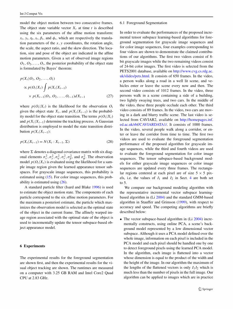
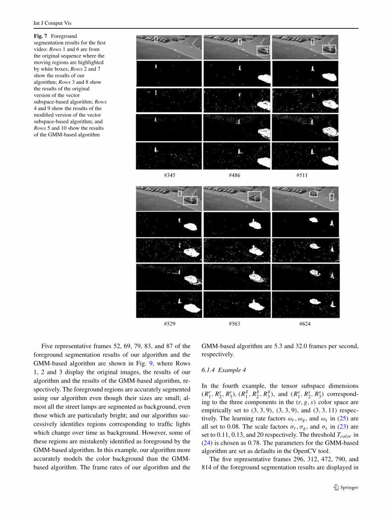
Six representative frames 345, 486, 511, 529, 563, and624 of the foreground segmentation results are shown inFig. 7, where the first and the sixth rows are from the orig-inal sequence, the second and the seventh rows show theresults of our algorithm, the third and the eighth rows showthe results of the original version of the vector subspace-based algorithm, the fourth and the ninth rows show the re-sults of the modified version of the vector subspace-basedalgorithm, and the fifth and the tenth rows show the resultsof the GMM-based algorithm. It can be seen that the seg-mentation results of our algorithm are clean, connected foreach object, and almost noiseless, and furthermore almostall of the associated shadows are omitted. Our algorithmobtains more accurate foreground segmentations than thevector subspace-based algorithms and the GMM-based al-gorithm.
The frame rate of our algorithm for this example is 1.2frames per second. The frame rate of the original version
of the vector subspace-based algorithm in Li (2004) is 8.3frames. The frame rate of the modified version of the vec-tor subspace-based algorithm is 2.3 frames. The frame rateof the GMM-based algorithm is 7.6 frames per second. Al-though our algorithm is slower than the vector subspace-based algorithms and the GMM-based algorithm, the speedof our algorithm is still acceptable.
6.1.2 Example 2
In the second example, the subspace dimensions R1,R2,and R3 for the incremental tensor subspace learning al-gorithm are empirically assigned as 3, 3, and 12 respec-tively. The scale factor α in (15) is set to 20. The thresh-old Tgray in (19) is chosen as 0.81. The learning rate fac-tor ω in (22) is assigned as 0.09. The parameters for thevector subspace-based algorithm are set as follows: thePCA subspace dimension p is 13; the updating rate α is0.95; and the coefficient β is 9. The parameters for theGMM-based algorithm are set as defaults in the OpenCVtool.
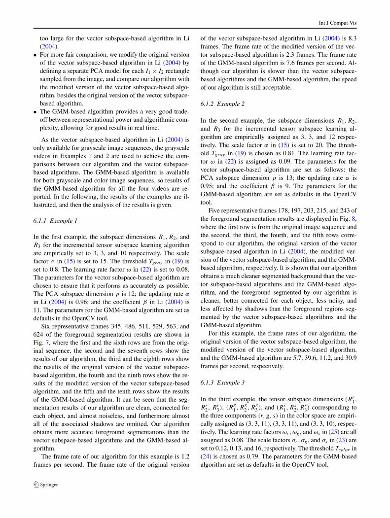
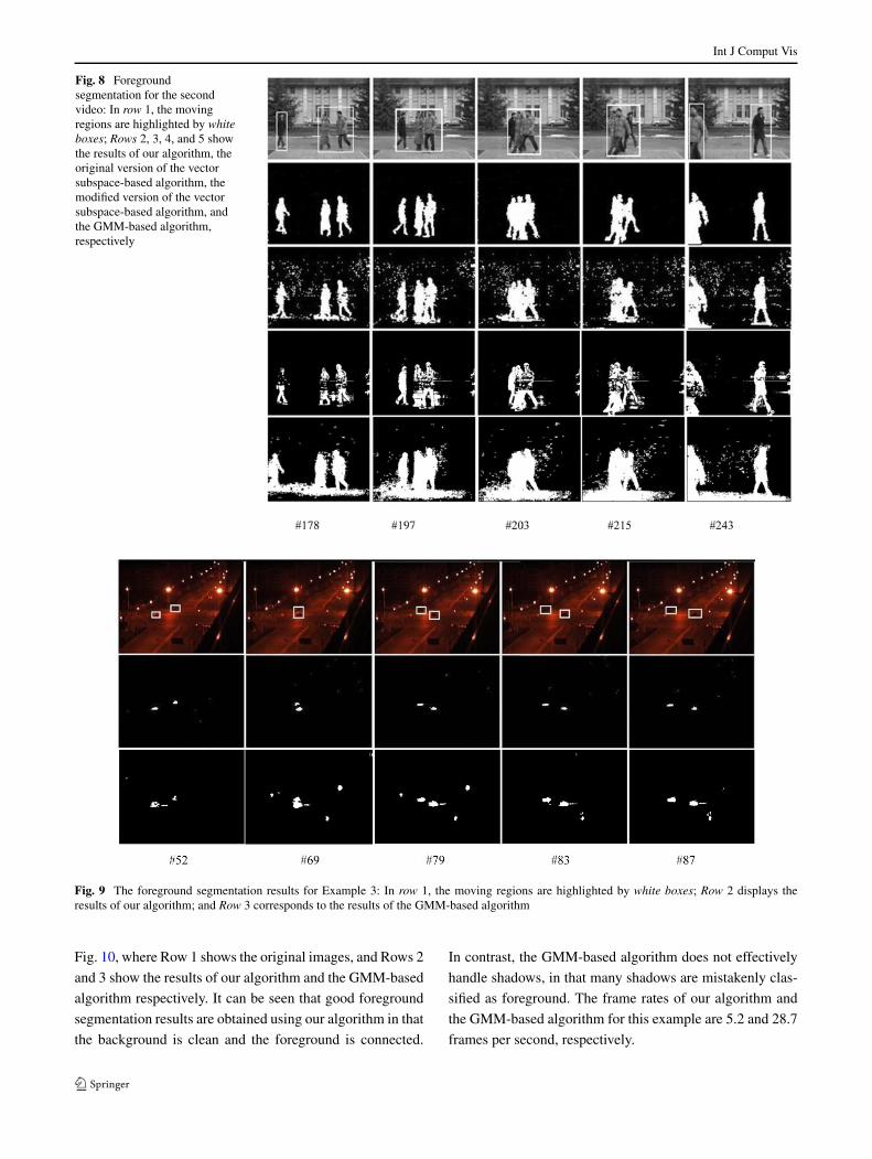
Five representative frames 178, 197, 203, 215, and 243 ofthe foreground segmentation results are displayed in Fig. 8,where the first row is from the original image sequence andthe second, the third, the fourth, and the fifth rows corre-spond to our algorithm, the original version of the vectorsubspace-based algorithm in Li (2004), the modified ver-sion of the vector subspace-based algorithm, and the GMM-based algorithm, respectively. It is shown that our algorithmobtains a much cleaner segmented background than the vec-tor subspace-based algorithms and the GMM-based algo-rithm, and the foreground segmented by our algorithm iscleaner, better connected for each object, less noisy, andless affected by shadows than the foreground regions seg-mented by the vector subspace-based algorithms and theGMM-based algorithm.
For this example, the frame rates of our algorithm, theoriginal version of the vector subspace-based algorithm, themodified version of the vector subspace-based algorithm,and the GMM-based algorithm are 5.7, 39.6, 11.2, and 30.9frames per second, respectively.
6.1.3 Example 3
In the third example, the tensor subspace dimensions (Rr1,
Rr2, Rr
3), (Rg
1 ,Rg
2 ,Rg
3 ), and (Rs1,R
s2,R
s3) corresponding to
the three components (r, g, s) in the color space are empiri-cally assigned as (3, 3, 11), (3, 3, 11), and (3, 3, 10), respec-tively. The learning rate factors ωr,ωg , and ωs in (25) are allassigned as 0.08. The scale factors σr, σg , and σs in (23) areset to 0.12, 0.13, and 16, respectively. The threshold Tcolor in(24) is chosen as 0.79. The parameters for the GMM-basedalgorithm are set as defaults in the OpenCV tool.
Int J Comput Vis
Fig. 7 Foregroundsegmentation results for the firstvideo: Rows 1 and 6 are fromthe original sequence where themoving regions are highlightedby white boxes; Rows 2 and 7show the results of ouralgorithm; Rows 3 and 8 showthe results of the originalversion of the vectorsubspace-based algorithm; Rows4 and 9 show the results of themodified version of the vectorsubspace-based algorithm; andRows 5 and 10 show the resultsof the GMM-based algorithm
Five representative frames 52, 69, 79, 83, and 87 of theforeground segmentation results of our algorithm and theGMM-based algorithm are shown in Fig. 9, where Rows1, 2 and 3 display the original images, the results of ouralgorithm and the results of the GMM-based algorithm, re-spectively. The foreground regions are accurately segmentedusing our algorithm even though their sizes are small; al-most all the street lamps are segmented as background, eventhose which are particularly bright; and our algorithm suc-cessively identifies regions corresponding to traffic lightswhich change over time as background. However, some ofthese regions are mistakenly identified as foreground by theGMM-based algorithm. In this example, our algorithm moreaccurately models the color background than the GMM-based algorithm. The frame rates of our algorithm and the
GMM-based algorithm are 5.3 and 32.0 frames per second,respectively.
6.1.4 Example 4
In the fourth example, the tensor subspace dimensions(Rr
1,Rr2,R
r3), (R
g
1 ,Rg
2 ,Rg
3 ), and (Rs1,R
s2,R
s3) correspond-
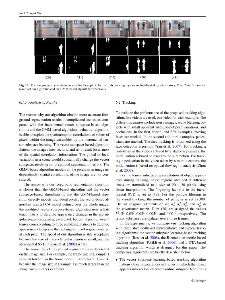
ing to the three components in the (r, g, s) color space areempirically set to (3,3,9), (3,3,9), and (3,3,11) respec-tively. The learning rate factors ωr,ωg , and ωs in (25) areall set to 0.08. The scale factors σr, σg , and σs in (23) areset to 0.11, 0.13, and 20 respectively. The threshold Tcolor in(24) is chosen as 0.78. The parameters for the GMM-basedalgorithm are set as defaults in the OpenCV tool.
The five representative frames 296, 312, 472, 790, and814 of the foreground segmentation results are displayed in
Int J Comput Vis
Fig. 8 Foregroundsegmentation for the secondvideo: In row 1, the movingregions are highlighted by whiteboxes; Rows 2, 3, 4, and 5 showthe results of our algorithm, theoriginal version of the vectorsubspace-based algorithm, themodified version of the vectorsubspace-based algorithm, andthe GMM-based algorithm,respectively
Fig. 9 The foreground segmentation results for Example 3: In row 1, the moving regions are highlighted by white boxes; Row 2 displays theresults of our algorithm; and Row 3 corresponds to the results of the GMM-based algorithm
Fig. 10, where Row 1 shows the original images, and Rows 2
and 3 show the results of our algorithm and the GMM-based
algorithm respectively. It can be seen that good foreground
segmentation results are obtained using our algorithm in that
the background is clean and the foreground is connected.
In contrast, the GMM-based algorithm does not effectively
handle shadows, in that many shadows are mistakenly clas-
sified as foreground. The frame rates of our algorithm and
the GMM-based algorithm for this example are 5.2 and 28.7
frames per second, respectively.
Int J Comput Vis
Fig. 10 The foreground segmentation results for Example 4: In row 1, the moving regions are highlighted by white boxes; Rows 2 and 3 show theresults of our algorithm and the GMM-based algorithm respectively
6.1.5 Analysis of Results
The reason why our algorithm obtains more accurate fore-ground segmentation results in complicated scenes, as com-pared with the incremental vector subspace-based algo-rithms and the GMM-based algorithm, is that our algorithmis able to exploit the spatiotemporal correlations of values ofpixels within the image ensembles by the incremental ten-sor subspace learning. The vector subspace-based algorithmflattens the images into vectors, and as a result loses mostof the spatial correlation information. The global or localvariations in a scene would substantially change the vectorsubspace, resulting in foreground segmentation errors. TheGMM-based algorithm models all the pixels in an image in-dependently: spatial correlations of the image are not con-sidered.
The reason why our foreground segmentation algorithmis slower than the GMM-based algorithm and the vectorsubspace-based algorithms is that the GMM-based algo-rithm directly models individual pixels; the vector-based al-gorithm uses a PCA model defined over the whole image;the modified vector subspace-based algorithm uses a flat-tened matrix to describe appearance changes in the rectan-gular region centered at each pixel; but our algorithm uses atensor corresponding to three unfolding matrices to describeappearance changes in the rectangular pixel region centeredat each pixel. The speed of our algorithm is still acceptablebecause the size of the rectangular region is small, and theincremental SVD in Ross et al. (2008) is fast.
The frame rate of foreground segmentation is dependenton the image size. For example, the frame rate in Example 1is much lower than the frame rates in Examples 2, 3, and 4,because the image size in Example 1 is much larger than theimage sizes in other examples.
6.2 Tracking
To evaluate the performance of the proposed tracking algo-rithm, five videos are used, one video for each example. Thedifferent scenarios include noisy images, scene blurring, ob-jects with small apparent sizes, object pose variations, andocclusions. In the first, fourth, and fifth examples, movingfaces are tracked. In the second and third examples, pedes-trians are tracked. The face tracking is initialized using theface detection algorithm (Yan et al. 2007). For tracking apedestrian in the video captured by a stationary camera, theinitialization is based on background subtraction. For track-ing a pedestrian in the video taken by a mobile camera, theinitialization is based on optical flow region analysis (Zhouet al. 2007).
For the tensor subspace representation of object appear-ance during tracking, object regions obtained at differenttimes are normalized to a size of 20 × 20 pixels usinglinear interpolation. The forgetting factor λ in the incre-mental SVD is set to 0.99. For the particle filtering inthe visual tracking, the number of particles is set to 300.The six diagonal elements σ 2
x , σ 2y , σ 2
η , σ 2s , σ 2
β , and σ 2φ in
the covariance matrix � in (28) are assigned the values52,52,0.032,0.032,0.0052, and 0.0012, respectively. Thetensor subspaces are updated every three frames.
In the experiments, we compare our tracking algorithmwith three state-of-the-art representative and typical track-ing algorithms: the vector subspace learning-based trackingalgorithm (Ross et al. 2008), the Riemannian metric-basedtracking algorithm (Porikli et al. 2006), and a DTA-basedtracking algorithm which is designed for this paper. Thecompeting algorithms are briefly described below:
• The vector subspace learning-based tracking algorithmflattens object appearances in frames in which the objectappears into vectors on which online subspace learning is
Int J Comput Vis
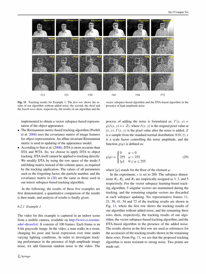
Fig. 11 Tracking results for Example 1: The first row shows the re-sults of our algorithm without added noise; the second, the third andthe fourth rows show, respectively, the results of our algorithm and the
vector subspace-based algorithm and the DTA-based algorithm in thepresence of high amplitude noise
implemented to obtain a vector subspace-based represen-tation of the object appearance.
• The Riemannian metric-based tracking algorithm (Porikliet al. 2006) uses the covariance matrix of image featuresfor object representation. An affine-invariant Riemannianmetric is used in updating of the appearance model.
• According to Sun et al. (2008), DTA is more accurate thanSTA and WTA. So, we choose to apply DTA to objecttracking. DTA itself cannot be applied to tracking directly.We modify DTA by using the row space of the mode-3unfolding matrix instead of the column space, as requiredby the tracking application. The values of all parameterssuch as the forgetting factor, the particle number, and thecovariance matrix in (28) are the same as those used inour tensor subspace-based tracking algorithm.
In the following, the results of these five examples arefirst demonstrated, a quantitative comparison of the resultsis then made, and analysis of results is finally given.
6.2.1 Example 1
The video for this example is captured in an indoor scenefrom a mobile camera, available on http://www.cs.toronto.edu/~dross/ivt/. It consists of 100 frames. Each frame is an8-bit grayscale image. In the video, a man walks in a room,changing his pose and facial expression over time undervarying lighting conditions. In order to investigate track-ing performance in the presence of high amplitude imagenoise, we add Gaussian random noise to the video. The
process of adding the noise is formulated as: I ′(x, y) =g(I (x, y)+s ·Z), where I (x, y) is the original pixel value at(x, y), I ′(x, y) is the pixel value after the noise is added, Z
is a sample from the standard normal distribution N(0,1), s
is a scale factor controlling the noise amplitude, and thefunction g(ϕ) is defined as:
g(ϕ) =⎧⎨
⎩
0 ϕ < 0255 ϕ > 255[ϕ] 0 ≤ ϕ ≤ 255
(29)
where [ϕ] stands for the floor of the element ϕ.In the experiment, s is set to 200. The subspace dimen-
sions R1,R2, and R3 are empirically assigned as 3, 3, and 5respectively. For the vector subspace learning-based track-ing algorithm, 5 singular vectors are maintained during thetracking, and the remaining singular vectors are discardedat each subspace updating. Six representative frames 11,21, 30, 41, 54 and 72 of the tracking results are shown inFig. 11, where the first row shows the tracking results ofour algorithm without added noise, and the remaining threerows show, respectively, the tracking results of our algo-rithm, the vector subspace-based tracking algorithm, and theDTA-based algorithm in the presence of the added noise.The results shown in the first row are used as references forthe accuracies of the tracking results shown in the remainingthree rows. From Fig. 11, we see that the proposed trackingalgorithm is more resistant to strong noise. Two points aremade out:
Int J Comput Vis
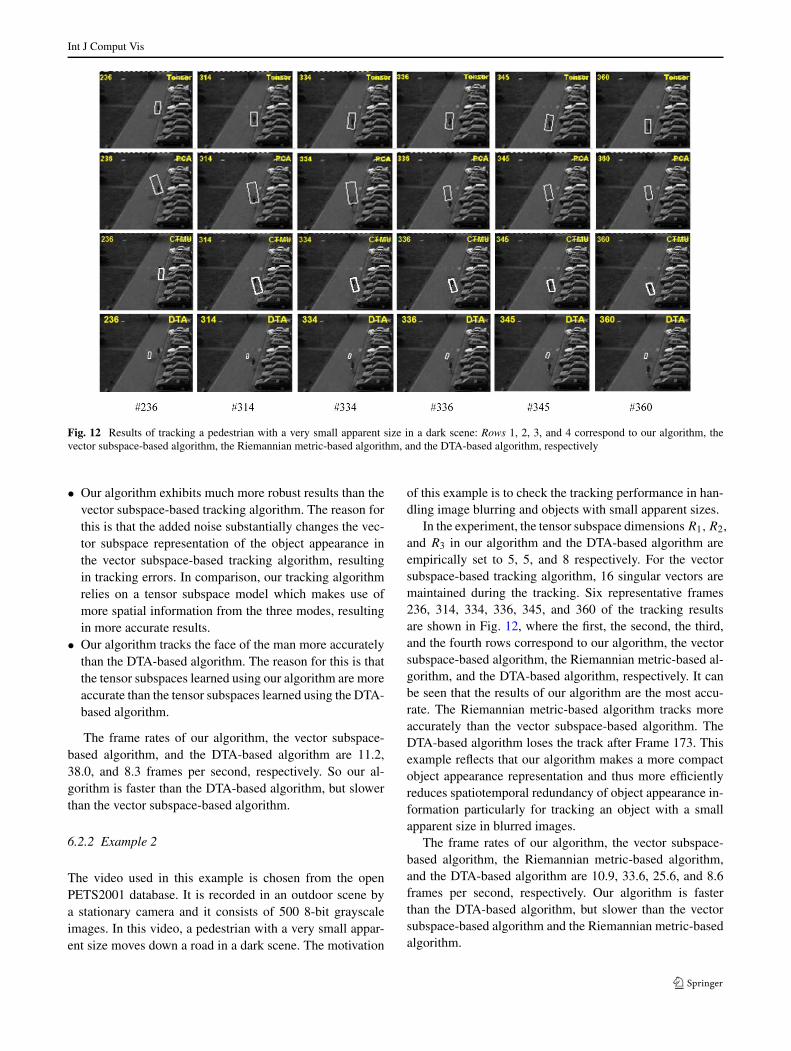
Fig. 12 Results of tracking a pedestrian with a very small apparent size in a dark scene: Rows 1, 2, 3, and 4 correspond to our algorithm, thevector subspace-based algorithm, the Riemannian metric-based algorithm, and the DTA-based algorithm, respectively
• Our algorithm exhibits much more robust results than thevector subspace-based tracking algorithm. The reason forthis is that the added noise substantially changes the vec-tor subspace representation of the object appearance inthe vector subspace-based tracking algorithm, resultingin tracking errors. In comparison, our tracking algorithmrelies on a tensor subspace model which makes use ofmore spatial information from the three modes, resultingin more accurate results.
• Our algorithm tracks the face of the man more accuratelythan the DTA-based algorithm. The reason for this is thatthe tensor subspaces learned using our algorithm are moreaccurate than the tensor subspaces learned using the DTA-based algorithm.
The frame rates of our algorithm, the vector subspace-based algorithm, and the DTA-based algorithm are 11.2,38.0, and 8.3 frames per second, respectively. So our al-gorithm is faster than the DTA-based algorithm, but slowerthan the vector subspace-based algorithm.
6.2.2 Example 2
The video used in this example is chosen from the openPETS2001 database. It is recorded in an outdoor scene bya stationary camera and it consists of 500 8-bit grayscaleimages. In this video, a pedestrian with a very small appar-ent size moves down a road in a dark scene. The motivation
of this example is to check the tracking performance in han-dling image blurring and objects with small apparent sizes.
In the experiment, the tensor subspace dimensions R1,R2,and R3 in our algorithm and the DTA-based algorithm areempirically set to 5, 5, and 8 respectively. For the vectorsubspace-based tracking algorithm, 16 singular vectors aremaintained during the tracking. Six representative frames236, 314, 334, 336, 345, and 360 of the tracking resultsare shown in Fig. 12, where the first, the second, the third,and the fourth rows correspond to our algorithm, the vectorsubspace-based algorithm, the Riemannian metric-based al-gorithm, and the DTA-based algorithm, respectively. It canbe seen that the results of our algorithm are the most accu-rate. The Riemannian metric-based algorithm tracks moreaccurately than the vector subspace-based algorithm. TheDTA-based algorithm loses the track after Frame 173. Thisexample reflects that our algorithm makes a more compactobject appearance representation and thus more efficientlyreduces spatiotemporal redundancy of object appearance in-formation particularly for tracking an object with a smallapparent size in blurred images.
The frame rates of our algorithm, the vector subspace-based algorithm, the Riemannian metric-based algorithm,and the DTA-based algorithm are 10.9, 33.6, 25.6, and 8.6frames per second, respectively. Our algorithm is fasterthan the DTA-based algorithm, but slower than the vectorsubspace-based algorithm and the Riemannian metric-basedalgorithm.
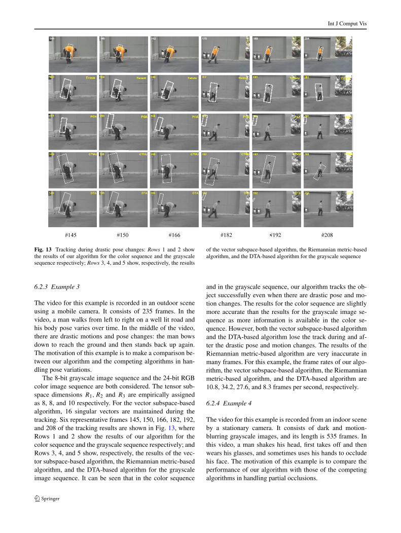
Int J Comput Vis
Fig. 13 Tracking during drastic pose changes: Rows 1 and 2 showthe results of our algorithm for the color sequence and the grayscalesequence respectively; Rows 3, 4, and 5 show, respectively, the results
of the vector subspace-based algorithm, the Riemannian metric-basedalgorithm, and the DTA-based algorithm for the grayscale sequence
6.2.3 Example 3
The video for this example is recorded in an outdoor sceneusing a mobile camera. It consists of 235 frames. In thevideo, a man walks from left to right on a well lit road andhis body pose varies over time. In the middle of the video,there are drastic motions and pose changes: the man bowsdown to reach the ground and then stands back up again.The motivation of this example is to make a comparison be-tween our algorithm and the competing algorithms in han-dling pose variations.
The 8-bit grayscale image sequence and the 24-bit RGBcolor image sequence are both considered. The tensor sub-space dimensions R1,R2 and R3 are empirically assignedas 8, 8, and 10 respectively. For the vector subspace-basedalgorithm, 16 singular vectors are maintained during thetracking. Six representative frames 145, 150, 166, 182, 192,and 208 of the tracking results are shown in Fig. 13, whereRows 1 and 2 show the results of our algorithm for thecolor sequence and the grayscale sequence respectively; andRows 3, 4, and 5 show, respectively, the results of the vec-tor subspace-based algorithm, the Riemannian metric-basedalgorithm, and the DTA-based algorithm for the grayscaleimage sequence. It can be seen that in the color sequence
and in the grayscale sequence, our algorithm tracks the ob-ject successfully even when there are drastic pose and mo-tion changes. The results for the color sequence are slightlymore accurate than the results for the grayscale image se-quence as more information is available in the color se-quence. However, both the vector subspace-based algorithmand the DTA-based algorithm lose the track during and af-ter the drastic pose and motion changes. The results of theRiemannian metric-based algorithm are very inaccurate inmany frames. For this example, the frame rates of our algo-rithm, the vector subspace-based algorithm, the Riemannianmetric-based algorithm, and the DTA-based algorithm are10.8, 34.2, 27.6, and 8.3 frames per second, respectively.
6.2.4 Example 4
The video for this example is recorded from an indoor sceneby a stationary camera. It consists of dark and motion-blurring grayscale images, and its length is 535 frames. Inthis video, a man shakes his head, first takes off and thenwears his glasses, and sometimes uses his hands to occludehis face. The motivation of this example is to compare theperformance of our algorithm with those of the competingalgorithms in handling partial occlusions.
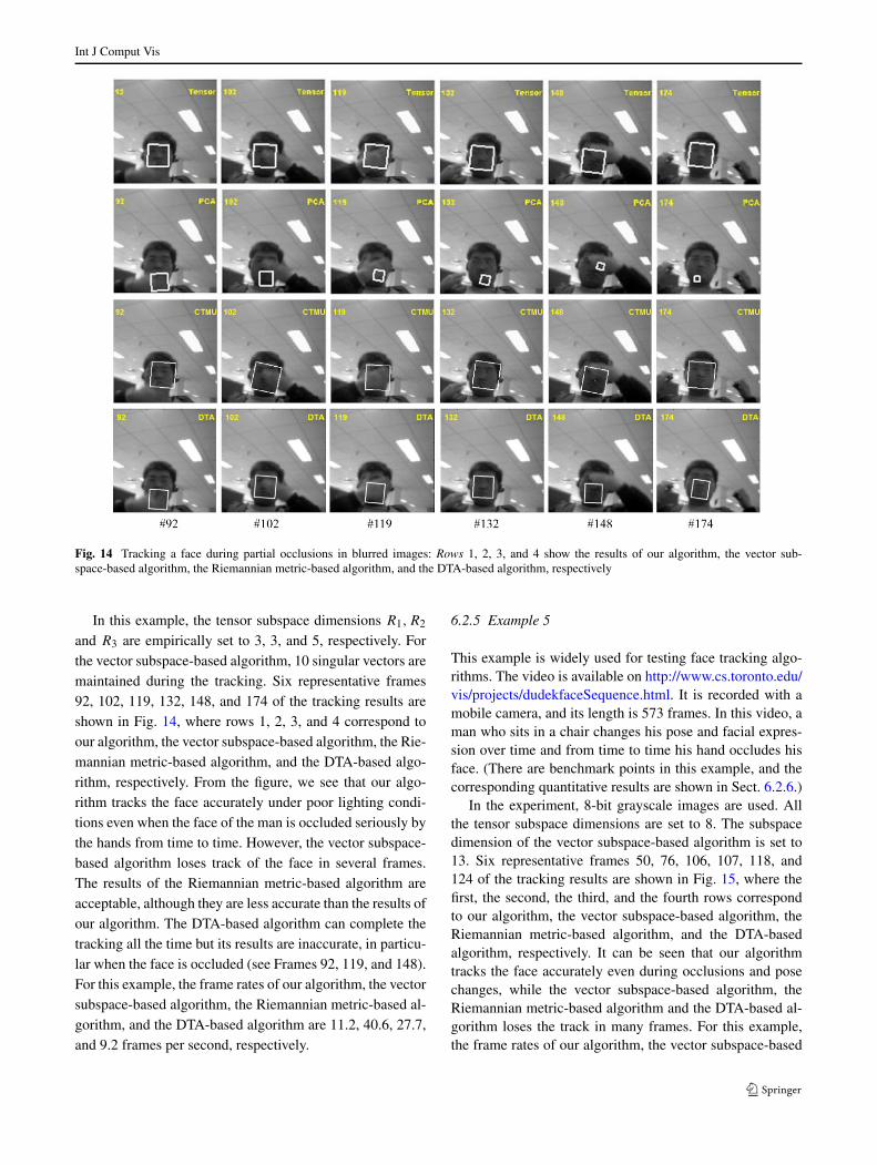
Int J Comput Vis
Fig. 14 Tracking a face during partial occlusions in blurred images: Rows 1, 2, 3, and 4 show the results of our algorithm, the vector sub-space-based algorithm, the Riemannian metric-based algorithm, and the DTA-based algorithm, respectively
In this example, the tensor subspace dimensions R1,R2
and R3 are empirically set to 3, 3, and 5, respectively. Forthe vector subspace-based algorithm, 10 singular vectors aremaintained during the tracking. Six representative frames92, 102, 119, 132, 148, and 174 of the tracking results areshown in Fig. 14, where rows 1, 2, 3, and 4 correspond toour algorithm, the vector subspace-based algorithm, the Rie-mannian metric-based algorithm, and the DTA-based algo-rithm, respectively. From the figure, we see that our algo-rithm tracks the face accurately under poor lighting condi-tions even when the face of the man is occluded seriously bythe hands from time to time. However, the vector subspace-based algorithm loses track of the face in several frames.The results of the Riemannian metric-based algorithm areacceptable, although they are less accurate than the results ofour algorithm. The DTA-based algorithm can complete thetracking all the time but its results are inaccurate, in particu-lar when the face is occluded (see Frames 92, 119, and 148).For this example, the frame rates of our algorithm, the vectorsubspace-based algorithm, the Riemannian metric-based al-gorithm, and the DTA-based algorithm are 11.2, 40.6, 27.7,and 9.2 frames per second, respectively.
6.2.5 Example 5
This example is widely used for testing face tracking algo-rithms. The video is available on http://www.cs.toronto.edu/vis/projects/dudekfaceSequence.html. It is recorded with amobile camera, and its length is 573 frames. In this video, aman who sits in a chair changes his pose and facial expres-sion over time and from time to time his hand occludes hisface. (There are benchmark points in this example, and thecorresponding quantitative results are shown in Sect. 6.2.6.)
In the experiment, 8-bit grayscale images are used. Allthe tensor subspace dimensions are set to 8. The subspacedimension of the vector subspace-based algorithm is set to13. Six representative frames 50, 76, 106, 107, 118, and124 of the tracking results are shown in Fig. 15, where thefirst, the second, the third, and the fourth rows correspondto our algorithm, the vector subspace-based algorithm, theRiemannian metric-based algorithm, and the DTA-basedalgorithm, respectively. It can be seen that our algorithmtracks the face accurately even during occlusions and posechanges, while the vector subspace-based algorithm, theRiemannian metric-based algorithm and the DTA-based al-gorithm loses the track in many frames. For this example,the frame rates of our algorithm, the vector subspace-based
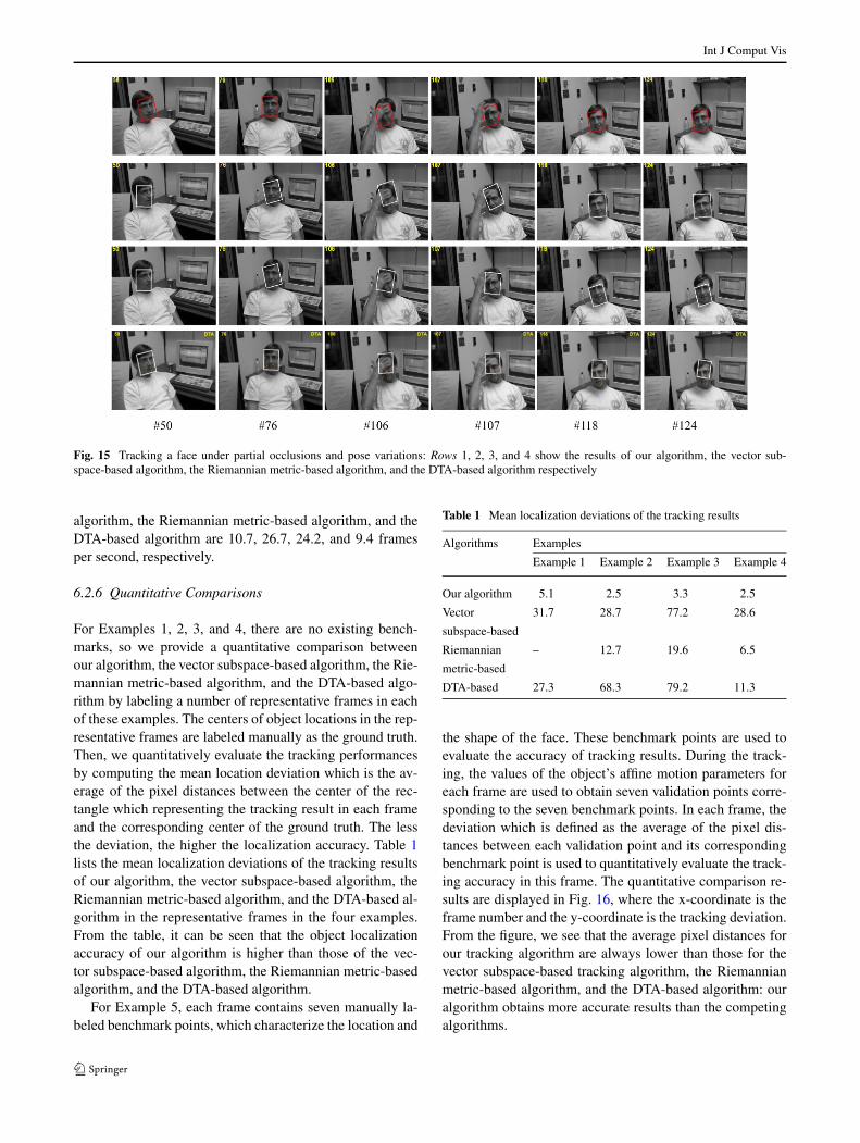
Int J Comput Vis
Fig. 15 Tracking a face under partial occlusions and pose variations: Rows 1, 2, 3, and 4 show the results of our algorithm, the vector sub-space-based algorithm, the Riemannian metric-based algorithm, and the DTA-based algorithm respectively
algorithm, the Riemannian metric-based algorithm, and theDTA-based algorithm are 10.7, 26.7, 24.2, and 9.4 framesper second, respectively.
6.2.6 Quantitative Comparisons
For Examples 1, 2, 3, and 4, there are no existing bench-marks, so we provide a quantitative comparison betweenour algorithm, the vector subspace-based algorithm, the Rie-mannian metric-based algorithm, and the DTA-based algo-rithm by labeling a number of representative frames in eachof these examples. The centers of object locations in the rep-resentative frames are labeled manually as the ground truth.Then, we quantitatively evaluate the tracking performancesby computing the mean location deviation which is the av-erage of the pixel distances between the center of the rec-tangle which representing the tracking result in each frameand the corresponding center of the ground truth. The lessthe deviation, the higher the localization accuracy. Table 1lists the mean localization deviations of the tracking resultsof our algorithm, the vector subspace-based algorithm, theRiemannian metric-based algorithm, and the DTA-based al-gorithm in the representative frames in the four examples.From the table, it can be seen that the object localizationaccuracy of our algorithm is higher than those of the vec-tor subspace-based algorithm, the Riemannian metric-basedalgorithm, and the DTA-based algorithm.
For Example 5, each frame contains seven manually la-beled benchmark points, which characterize the location and
Table 1 Mean localization deviations of the tracking results
Algorithms Examples
Example 1 Example 2 Example 3 Example 4
Our algorithm 5.1 2.5 3.3 2.5
Vector 31.7 28.7 77.2 28.6
subspace-based
Riemannian – 12.7 19.6 6.5
metric-based
DTA-based 27.3 68.3 79.2 11.3
the shape of the face. These benchmark points are used toevaluate the accuracy of tracking results. During the track-ing, the values of the object’s affine motion parameters foreach frame are used to obtain seven validation points corre-sponding to the seven benchmark points. In each frame, thedeviation which is defined as the average of the pixel dis-tances between each validation point and its correspondingbenchmark point is used to quantitatively evaluate the track-ing accuracy in this frame. The quantitative comparison re-sults are displayed in Fig. 16, where the x-coordinate is theframe number and the y-coordinate is the tracking deviation.From the figure, we see that the average pixel distances forour tracking algorithm are always lower than those for thevector subspace-based tracking algorithm, the Riemannianmetric-based algorithm, and the DTA-based algorithm: ouralgorithm obtains more accurate results than the competingalgorithms.
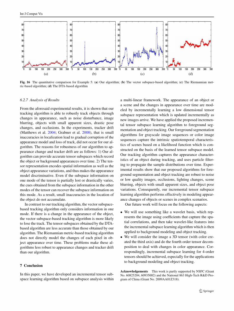
Int J Comput Vis
Fig. 16 The quantitative comparison for Example 5: (a) Our algorithm; (b) The vector subspace-based algorithm; (c) The Riemannian met-ric-based algorithm; (d) The DTA-based algorithm
6.2.7 Analysis of Results
From the aforesaid experimental results, it is shown that ourtracking algorithm is able to robustly track objects throughchanges in appearance, such as noise disturbance, imageblurring, objects with small apparent sizes, drastic posechanges, and occlusions. In the experiments, tracker drift(Matthews et al. 2004; Grabner et al. 2008), that is smallinaccuracies in localization lead to gradual corruption of theappearance model and loss of track, did not occur for our al-gorithm. The reasons for robustness of our algorithm to ap-pearance change and tracker drift are as follows: 1) Our al-gorithm can provide accurate tensor subspaces which recordthe object or background appearances over time. 2) The ten-sor representation encodes spatial information as well as theobject appearance variations, and thus makes the appearancemodel discriminative. Even if the subspace information onone mode of the tensor is partially lost or drastically varies,the cues obtained from the subspace information in the othermodes of the tensor can recover the subspace information onthis mode. As a result, small inaccuracies in the location ofthe object do not accumulate.
In contrast to our tracking algorithm, the vector subspace-based tracking algorithm only considers information in onemode. If there is a change in the appearance of the object,the vector subspace-based tracking algorithm is more likelyto lose the track. The tensor subspaces obtained by the DTA-based algorithm are less accurate than those obtained by ouralgorithm. The Riemannian metric-based tracking algorithmdoes not directly model the changes of each pixel in ob-ject appearance over time. These problems make these al-gorithms less robust to appearance changes and tracker driftthan our algorithm.
7 Conclusion
In this paper, we have developed an incremental tensor sub-space learning algorithm based on subspace analysis within
a multi-linear framework. The appearance of an object ora scene and the changes in appearance over time are mod-eled by incrementally learning a low dimensional tensorsubspace representation which is updated incrementally asnew images arrive. We have applied the proposed incremen-tal tensor subspace learning algorithm to foreground seg-mentation and object tracking. Our foreground segmentationalgorithms for grayscale image sequences or color imagesequences capture the intrinsic spatiotemporal characteris-tics of scenes based on a likelihood function which is con-structed on the basis of the learned tensor subspace model.Our tracking algorithm captures the appearance character-istics of an object during tracking, and uses particle filter-ing to propagate the sample distributions over time. Exper-imental results show that our proposed algorithms for fore-ground segmentation and object tracking are robust to noiseor low quality images, occlusions, lighting changes, sceneblurring, objects with small apparent sizes, and object posevariations. Consequently, our incremental tensor subspacelearning algorithm performs effectively in modeling appear-ance changes of objects or scenes in complex scenarios.
Our future work will focus on the following aspects:
• We will use something like a wavelet basis, which rep-resents the image using coefficients that capture the spa-tial correlations, and then take wavelet-like features intothe incremental subspace learning algorithm which is thenapplied to background modeling and object tracking.
• We will consider the image a 3D tensor (with color cre-ated the third axis) and do the fourth order tensor decom-position to deal with changes in color appearance. Cor-respondingly, incremental subspace learning for 4-ordertensors should be achieved, especially for the applicationsto background modeling and object tracking.
Acknowledgements This work is partly supported by NSFC (GrantNo. 60825204, 60935002) and the National 863 High-Tech R&D Pro-gram of China (Grant No. 2009AA01Z318).
Int J Comput Vis
Open Access This article is distributed under the terms of the Cre-ative Commons Attribution Noncommercial License which permitsany noncommercial use, distribution, and reproduction in any medium,provided the original author(s) and source are credited.
References
Black, M. J., & Jepson, A. D. (1998). EigenTracking: robust matchingand tracking of articulated objects using a view-based representa-tion. International Journal of Computer Vision, 26(1), 63–84.
Black, M. J., Fleet, D. J., & Yacoob, Y. (1998). A framework for model-ing appearance change in image sequence. In Proc. of IEEE inter-national conference on computer vision (pp. 660–667), Jan. 1998.
Chen, D., & Yang, J. (2007). Robust object tracking via online dy-namic spatial bias appearance models. IEEE Transactions on Pat-tern Analysis and Machine Intelligence, 29(12), 2157–2169.
Elgammal, A., Duraiswami, R., Harwood, M., & Davis, L. S. (2002).Background and foreground modeling using nonparametric ker-nel density estimation for visual surveillance. Proceedings of theIEEE, 99(7), 1151–1163.
Gall, J., Rosenhahn, B., & Seidel, H.-P. (2008). Drift-free tracking ofrigid and articulated objects. In Proc. of IEEE conference on com-puter vision and pattern recognition (pp. 1–8), June 2008.
Golub, G. H., & Van Loan, C. F. (1996). Matrix computations. Balti-more: Johns Hopkins University Press.
Grabner, H., Leistner, C., & Bischof, H. (2008). Semi-supervised on-line boosting for robust tracking. In Proc. of European conferenceon computer vision (pp. 234–247).
Gu, M., & Eisenstat, S. C. (1993). A stable and fast algorithmfor updating the singular value decomposition. Research reportYALEU/DCS/RR-966, Department of Computer Science, YaleUniversity, New Haven, June 1993.
Gu, M., & Eisenstat, S. C. (1995). Downdating the singular value de-composition. SIAM Journal on Matrix Analysis and Applications,16(3), 793–810.
Hager, G. D., & Belhumeur, P. N. (1996). Real-time tracking of imageregions with changes in geometry and illumination. In Proc. ofIEEE conference on computer vision and pattern recognition (pp.403–410), June 1996.
Han, B., Zhu, Y., Comaniciu, D., & Davis, L. S. (2009). Visual trackingby continuous density propagation in sequential bayesian filteringframework. IEEE Transactions on Pattern Analysis and MachineIntelligence, 31(5), 919–930.
Haritaoglu, I., Harwood, D., & Davis, L. S. (2000). W4: real-time sur-veillance of people and their activities. IEEE Transactions on Pat-tern Analysis and Machine Intelligence, 22(8), 809–830.
He, X., Cai, D., & Niyogi, P. (2005). Tensor subspace analysis. In Proc.of annual conference on neural information processing systemsDec. 2005 Cambridge: MIT Press.
Ho, J., Lee, K., Yang, M., & Kriegman, D. (2004). Visual trackingusing learned linear subspaces. In Proc. of IEEE conference oncomputer vision and pattern recognition (vol. 1, pp. 782–789).
Isard, M., & Blake, A. (1996). Contour tracking by stochastic propa-gation of conditional density. In Proc. of European conference oncomputer vision (vol. 2, pp. 343–356).
Jacques, J. C. S. Jr., Jung, C. R., & Musse, S. R. (2006). A backgroundsubtraction model adapted to illumination changes. In Proc. ofIEEE international conference on image processing (pp. 1817–1820), Oct. 2006.
Jepson, A. D., Fleet, D. J., & El-Maraghi, T. F. (2003). Robust onlineappearance models for visual tracking. IEEE Transactions on Pat-tern Analysis and Machine Intelligence, 25(10), 1296–1311.
Kwon, J., & Lee, K. M. (2009). Tracking of a non-rigid object viapatch-based dynamic appearance modeling and adaptive basin
hopping Monte Carlo sampling. In Proc. of IEEE conference oncomputer vision and pattern recognition workshops (pp. 1208–1215), June 2009.
Lathauwer, L. D., Moor, B. D., & Vandewalle, J. (2000). On the bestRank-1 and Rank-(R1,R2, . . . ,Rn) approximation of higher-order tensors. SIAM Journal of Matrix Analysis and Applications,21(4), 1324–1342.
Lee, K., & Kriegman, D. (2005). Online learning of probabilistic ap-pearance manifolds for video-based recognition and tracking. InProc. of IEEE conference on computer vision and pattern recog-nition (vol. 1, pp. 852–859).
Levy, A., & Lindenbaum, M. (2000). Sequential Karhunen-Loeve basisextraction and its application to images. IEEE Transactions onImage Processing, 9, 1371–1374.
Li, Y. (2004). On incremental and robust subspace learning. PatternRecognition, 37(7), 1509–1518.
Li, J., Zhou, S. K., & Chellappa, R. (2005). Appearance modeling un-der geometric context. In Proc. of IEEE international conferenceon computer vision (vol. 2, pp. 1252–1259).
Li, X., Hu, W. M., Zhang, Z. F., Zhang, X. Q., & Luo, G. (2007). Ro-bust visual tracking based on incremental tensor subspace learn-ing. In Proc. of IEEE international conference on computer vision(pp. 1–8), Oct. 2007.
Lim, H., Morariu, V. I., Camps, O. I., & Sznaier, M. (2006). Dynamicappearance modeling for human tracking. In Proc. of IEEE con-ference on computer vision and pattern recognition (vol. 1, pp.751–757).
Mahadevan, V., & Vasconcelos, N. (2009). Saliency-based discrimi-nant tracking. In Proc. of IEEE conference on computer visionand pattern recognition workshops (pp. 1007–1013), June 2009.
Matthews, I., Ishikawa, T., & Baker, S. (2004). The template updateproblem. IEEE Transactions on Pattern Analysis and Machine In-telligence, 26(4), 810–815.
Nickel, K., & Stiefelhagen, R. (2008). Dynamic integration of general-ized cues for person tracking. In Proc. of European conference oncomputer vision, Part IV. Lecture notes in computer science (vol.5305, pp. 514–526), Oct. 2008.
Nummiaroa, K., Koller-Meierb, E., & Gool, I. V. (2003). An adaptivecolor-based particle filter. Image and Vision Computing, 21(1),99–110.
Papadimitriou, S., Sun, J., & Faloutsos, C. (2005). Streaming patterndiscovery in multiple timeseries. In Proc. of international confer-ence on very large data bases (pp. 697–708).
Patwardhan, K., Morellas, V., & Sapiro, G. (2008). Robust foregrounddetection in video using pixel layers. IEEE Transactions on Pat-tern Analysis and Machine Intelligence, 30(4), 746–751.
Perez, P., Hue, C., Vermaak, J., & Gangnet, M. (2002). Color-basedprobabilistic tracking. In Proc. of European conference on com-puter vision, Part I. Lecture notes in computer science (vol. 2350,pp. 661–675).
Porikli, F., Tuzel, O., & Meer, P. (2006). Covariance tracking usingmodel update based on Lie algebra. In Proc. of IEEE conferenceon computer vision and pattern recognition (vol. 1, pp. 728–735).
Ramanan, D., Forsyth, D. A., & Zisserman, A. (2007). Tracking peo-ple by learning their appearance. IEEE Transactions on PatternAnalysis and Machine Intelligence, 29(1), 65–81.
Ross, D. A., Lim, J., Lin, R.-S., & Yang, M.-H. (2008). Incrementallearning for robust visual tracking. International Journal of Com-puter Vision, 77(2), 125–141.
Sheikh, Y., & Shah, M. (2005). Bayesian object detection in dynamicscenes. In Proc. of IEEE conference on computer vision and pat-tern recognition (vol. 1, pp. 74–79).
Skocaj, D., & Leonardis, A. (2003). Weighted and robust incrementalmethod for subspace learning. In Proc. of IEEE international con-ference on computer vision (vol. 2, pp. 1494–1501), Oct. 2003.
Int J Comput Vis
Stauffer, C., & Grimson, W. E. L. (1999). Adaptive background mix-ture models for real-time tracking. In Proc. of IEEE conference oncomputer vision and pattern recognition (vol. 2, pp. 246–252).
Sun, J., Tao, D., & Faloutsos, C. (2006a). Beyond streams and graphs:dynamic tensor analysis. In Proc. of ACM SIGKDD internationalconference on knowledge discovery and data mining (pp. 374–383), Aug. 2006.
Sun, J., Papadimitriou, S., & Yu, P. S. (2006b). Window-based tensoranalysis on high-dimensional and multi-aspect streams. In Proc.of international conference on data mining (pp. 1076–1080), Dec.2006.
Sun, J., Tao, D., Papadimitriou, S., Yu, P. S., & Faloutsos, C. (2008).Incremental tensor analysis: theory and applications. ACM Trans-actions on Knowledge Discovery from Data, 2(3), 1–37.
Tian, Y., Lu, M., & Hampapur, A. (2005). Robust and efficient fore-ground analysis for real-time video surveillance. In Proc. of IEEEconference on computer vision and pattern recognition (vol. 1, pp.1182–1187).
Vasilescu, M. A. O., & Terzopoulos, D. (2002). Multilinear subspaceanalysis of image ensembles: TensorFaces. In Proc. of Europeanconference on computer vision (pp. 447–460), May 2002.
Vasilescu, M. A. O., & Terzopoulos, D. (2003). Multilinear subspaceanalysis of image ensembles. In Proc. of IEEE conference oncomputer vision and pattern recognition (vol. 2, pp. 93–99), June2003.
Wang, H., & Ahuja, N. (2005). Rank-R approximation of tensors usingimage-as-matrix representation. In Proc. of IEEE conference oncomputer vision and pattern recognition (vol. 2, pp. 346–353).
Wang, H., & Ahuja, N. (2008). A tensor approximation approach todimensionality reduction. International Journal of Computer Vi-sion, 76(3), 217–229.
Wang, Y., Tan, T., Loe, K. F., & Wu, J. K. (2005). A probabilistic ap-proach for foreground and shadow segmentation in monocular im-age sequences. Pattern Recognition, 38(11), 1937–1946.
Wang, Y., Loe, K., & Wu, J. (2006). A dynamic conditional ran-dom field model for foreground and shadow segmentation. IEEETransactions on Pattern Analysis and Machine Intelligence,28(2), 279–289.
Wang, H., Yan, S., Huang, T., & Tang, X. (2007). A convergent so-lution to tensor subspace learning. In Proc. of international jointconference on artificial intelligence (pp. 629–634).
Wong, S., Wong, K. K., & Cipolla, R. (2006). Robust appearance-basedtracking using a sparse bayesian classifier. In Proc. of interna-tional conference on pattern recognition (vol. 3, pp. 47–50).
Wu, Y., & Huang, T. S. (2004). Robust visual tracking by integratingmultiple cues based on co-inference learning. International Jour-nal of Computer Vision, 58(1), 55–71.
Yan, S., Xu, D., Yang, Q., Zhang, L., Tang, X., & Zhang, H. (2005).Discriminant analysis with tensor representation. In Proc. of IEEEconference on computer vision and pattern recognition (vol. 1, pp.526–532), June 2005.
Yan, S., Shan, S., Chen, X., Gao, W., & Chen, J. (2007). Matrix-structural learning (MSL) of cascaded classifier from enormoustraining set. In Proc. of IEEE conference on computer vision andpattern recognition (pp. 1–7), June 2007.
Yang, J., Zhang, D., Frangi, A. F., & Yang, J. (2004). Two-dimensionalPCA a new approach to appearance-based face representation andrecognition. IEEE Transactions on Pattern Analysis and MachineIntelligence, 26(1), 131–137.
Yang, C., Duraiswami, R., & Davis, L. S. (2005). Efficient mean-shifttracking via a new similarity measure. In Proc. of IEEE confer-ence on computer vision and pattern recognition (vol. 1, pp. 176–183), June 2005.
Yang, M., Fan, Z., Fan, J., & Wu, Y. (2009). Tracking nonstationaryvisual appearances by data-driven adaptation. IEEE Transactionson Image Processing, 18(7), 1633–1644.
Ye, J. (2005). Generalized low rank approximations of matrices. Ma-chine Learning, 61(1–3), 167–191.
Ye, J., Janardan, R., & Li, Q. (2004a). Two-dimensional linear discrim-inant nalysis. In Proc. of neural information processing systemsconference (pp. 1569–1576). Cambridge: MIT Press.
Ye, J., Janardan, R., & Li, Q. (2004b). GPCA: an efficient dimensionreduction scheme for image compression and retrieval. In Proc. ofACM SIGKDD international conference on knowledge discoveryand data mining (pp. 354–363), Aug. 2004.
Yu, T., & Wu, Y. (2006). Differential tracking based on spatial-appearance model (SAM). In Proc. of IEEE conference on com-puter vision and pattern recognition (vol. 1, pp. 720–727), June2006.
Zhou, S. K., Chellappa, R., & Moghaddam, B. (2004). Visual track-ing and recognition using appearance-adaptive models in particlefilters. IEEE Transactions on Image Processing, 13(11), 1491–1506.
Zhou, X., Hu, W. M., Chen, Y., & Hu, W. (2007). Markov randomfield modeled level sets method for object tracking with movingcameras. In Proc. of Asian conference on computer vision, Part I(pp. 832–842).