EEccoonnoommiiccss PPrrooggrraamm WWoorrkkiinngg PPaappeerr SSeerriieess

India’s Demographic Transition: Boon

or Bane? A State-Level Perspective

Utsav Kumar

September 2010

EEPPWWPP ##1100 -- 0033

Economics Program 845 Third Avenue

New York, NY 10022-6679 Tel. 212-759-0900

www.conference-board.org/economics

India’s Demographic Transition: Boon or Bane?

A State-Level Perspective

Utsav Kumar

Abstract

Age structure and its dynamics are critical in understanding the impact of population

growth on a country‟s growth prospects. Using state-level data from India, I show that the

pace of demographic transition varies across states, and that these differences are likely to

be exacerbated over the period 2011-2026. I show that the so-called BIMARU states

(Bihar, Madhya Pradesh, Rajasthan, and Uttar Pradesh) are likely to see a continuing

increase in the share of the working-age population in total population. The BIMARU

states are expected to contribute 58% of the increase in India‟s working-age population.

The BIMARU states have traditionally been the slow-growing states and have performed

poorly on different accounts of social and physical infrastructure. Whether India can turn

demographic dividend into a boon or whether the dividend will become a bane will

critically depend on the ability of the BIMARU states to exploit the bulge in the working-

age population.

Keywords: Demographic dividend, economic growth, India, population growth,

working-age population

JEL Codes: J10, J11, J18, O53, R10, R11

A part of this paper was completed while the author was an economist at The Conference Board. I would

like to thank Bart van Ark, Judith Banister, Vivian Chen, and Gad Levanon for many helpful discussions

and comments. The views expressed here are those of the author and do not reflect the views of The

Conference Board. The responsibility for the results presented in this paper remains solely the individual

responsibility of the author. Corresponding e-mail address: kumarutsav@gmail.com.

1

1. Introduction

Social scientists have long argued over the impact of population growth on economic

growth. The debate has oscillated from the “pessimistic view,” which argued that the

population growth restricts economic development (credited largely to Malthus), to the

“optimistic view,” which argued that population growth fuels economic growth (for

example, Kuznets 1967). The debate seemed to have finally settled in favor of the

“neutralist view,” i.e., population growth does not matter for growth prospects.

Bloom and Williamson (1998) argued that the earlier debate missed a critical dimension

of the population dynamics, namely, the changing age structure. According to this view,

as countries pass through various phases of demographic transition from high fertility and

high mortality to low mortality and low fertility, the age composition of a country‟s

population changes. During this demographic transition, all countries have a demographic

“window of opportunity” when the growth in the working-age population is greater than

the growth in the total population. This bulge in the working-age population, i.e., the

increase in the share of the working-age population in total population, is referred to as

the “demographic dividend.”

Using cross-country data, Bloom and Williamson (1998), Bloom et al. (2002), among

others, show a positive relationship between the growth rate of the share of the working-

age population and economic growth.1 At some point, all countries are likely to

experience demographic transition. However, whether or not the window of opportunity

is utilized, as noted by Bloom et al. (2002), will depend on the policy environment. This

is the first strand of literature to which this paper relates, i.e., the studies examining the

role of the changing age structure of the population in economic growth. Change in the

age composition matters because different age groups have different economic behavior.

For example, a population with a greater share of the 0-14 age group will spend a greater

share of income on the upbringing of the young and will therefore save less. Similarly, a

population with a greater share of the elderly population, i.e. 65 and up, will see greater

spending on health care and pensions. On the other hand, a working-age (15-64 age

group) population in general tends to be more productive, supplies labor, saves more than

their consumption, and provides capital for investment. A differing share of the working-

age population across countries can have a differing impact on economic growth.

India has often been singled out as being in the midst of a demographic boom since the

1980s and one of the few countries expected to see an increase in the share of the

working-age population until about 2035 to 2040. In this paper, I go beneath the surface

and show that the aggregate picture masks significant differences in the demographic

1 Throughout this paper the share of the working-age population is discussed, it is with respect to the total

population, unless otherwise specified.

2

transition across states in India. I first investigate the relationship between economic

growth and growth in the share of the working-age population in the context of India

using state-level data. I find that, controlling for state characteristics and initial per capita

income, states with a higher growth in the share of the working-age population in total

population grow faster over time.

Using official population projections for the period 2001-2026, I show that differences in

demographic transition across states are likely to be exacerbated in the future. On the one

hand, some states such as Kerala and Tamil Nadu will start seeing a decline in the share

of the working-age population during the period 2011-2026. On the other hand, states

such as BIhar, MAdhya Pradesh, Rajasthan, and Uttar Pradesh (known collectively as the

BIMARU states), which are the slowest in their demographic transition, will continue to

see an increase in the share of the working-age population.2

There is lot of optimism about the potential of a huge labor supply, and rightly so.

However, Acharya (2004) notes that this represents only one side of the story, the supply

side. The other aspect is the demand side and the ability to provide additional labor

supply with gainful jobs. The BIMARU states have been the slowest in their

demographic transition and are among the slowest-growing states (as measured by

growth in per capita income). BIMARU states, as shown in this paper, are expected to

contribute as much as 58% of the increase in India‟s working-age population. I argue that

whether India will be able to make the most of the projected increase in labor supply will

rest critically on the ability of the BIMARU states to provide complementary conditions

for growth and generate gainful employment opportunities. The failure of these states to

create conducive conditions for providing the additional labor supply with gainful

employment has the potential to turn the demographic boon into a bane.

Though there is ample literature discussing cross-country experiences of demographic

transition and its implications for growth (see for example, Bloom and Williamson

(1998) and Bloom and Canning (2004)), there is little literature on differences in

demographic transition across regions within a country. However, there has been a keen

interest in the demographic trends across states in India (for example, Bose (1996), Bhat

(2001), Visaria and Visaria (2003), Mitra and Nagarajan (2005), Bose (2006),

Chandrashekhar et al. (2006), and James (2008)). This is the second strand of literature

with which this paper is closely connected. All these studies, as well as this paper, use

2 BIMARU is a variation of the Hindi word bimar, meaning ill. The BIMARU states are so nicknamed for

their lack of economic growth, high population growth rates, and their inability to undertake a successful

transition from high-birth and high-death rates to low-birth and low-death rates. Given that these states

accounted for 40% of India‟s population in the past, the poor economic performance in these states has

proved to be a drag on the overall growth performance.

3

historical data to bring out the imbalances in demographic transition across regions and

states in India, and draw policy implications. Bhat (2001) and Bose (2006) use

demographic projections to 2025 and 2026 respectively to show that the “north-south”

imbalance in the demographic transition is likely to continue. However, they do so only

at a very aggregate “region” level. In this paper, I use official projections to analyze

which states in India are expected to see an increase in the share of the working-age

population. I also show the contribution of each of the states to the expected increase in

India‟s working-age population. This will help identify the states that will account for a

lion‟s share of the increase in India‟s working-age population. I discuss whether these

states will be able to exploit the demographic window of opportunity.

Visaria and Visaria (2003), using the 1991 census as the base, provide population

projections for major states up to 2101. They argue that the difference in fertility and

mortality rates will manifest themselves in differences in the pace of demographic

transition and that the BIMARU states, Assam, Haryana, and Orissa will take 10 to 15

years longer to complete their demographic transition. They discuss the projected

differences in age composition of the population across states in terms of dependency

ratios—i.e., the ratio of number of dependents (those in the 0-14 and 65-plus age groups)

to the working-age population. In this paper, the focus is on the anticipated differences

across states in the share of working-age population and its growth, as well as the

contribution of different states to the overall increase in India‟s working-age population.

Finally, to the best of my knowledge, James (2008) is the only paper to have examined

this relationship between growth and population-age structure in the context of India.

However, James (2008) focuses on the growth in the working-age population and not the

growth in the share of the working-age population. The latter variable is what captures

the demographic dividend. I include this variable directly in my estimation.

The rest of the paper is organized as follows. Section 2 discusses the concept of

demographic dividend and the channels through which it affects economic growth.

Section 3 compares the demographic trends in India from an international perspective.

Section 4 provides a discussion of historical demographic trends in India and different

states. Section 5 examines the relationship between economic growth and growth in the

share of the working-age population. Section 6 discusses state-level population projection

trends in India and draws policy implications. Section 7 concludes.

2. Demography and economic growth

The relationship between population growth and economic growth has long interested

demographers, economists, and policymakers alike. Different strands of thought have

shaped the debate at different points of time. The early days of this debate were

4

dominated by the Malthusian view, according to which, population growth will impede

economic development. A rapidly growing population is likely to need more resources

and this could crowd out capital expenditure, resulting in lower capital per worker, which

will have an adverse impact on labor productivity and therefore, on living standards.

Another argument was that if the growth in population exceeds that of food production,

malnutrition will prevail and force many to live on a below-subsistence diet, which will

negatively affect the health of the workforce and therefore, their productivity. Also,

impoverishment may result in a high death rate, bringing an end to high population

growth.

Bloom et al. (2002) contend that the “starvation of millions” that was feared never

happened and, despite population growth, per capita incomes increased. This gave rise to

the second view in the debate on population growth and economic development. This

view argued that population growth assisted economic growth (Simon Kuznets, 1967).3

According to this school of thought, an increase in population comes with an increase in

the stock of human capital. This, combined with the pressure to invent when faced with

the possibility of dire outcomes, leads to population growth assisting economic

development.

At the same time, those arguing in favor of a positive impact of population growth on

economic growth were also mindful of the role of country-specific features that can have

an impact on growth. This paved the way for the middle path, according to which,

population change has no significant effect on economic growth. According to this view,

once country characteristics are taken into account, there is little evidence that population

growth has an adverse impact on economic growth.

More recently, Bloom and Williamson (1998), Bloom et al. (2002), and Bloom and

Canning (2004), argue that the debate on population growth and economic growth

seemed to have missed a critical dimension of population dynamics—the changing age

structure. They argue that population growth comes with a change in the age

composition, and this assumes importance because different age groups have different

economic behavior. All countries are likely to see this change in the age composition of

their population. This change in age structure will be magnified in some countries as

compared to other countries, which in turn will depend on the speed of demographic

transition.

Demographic transition is the shift from high mortality and fertility rates to low mortality

and fertility rates. This shift is commonly described in three phases. The first phase of the

demographic transition is characterized by high mortality and fertility rates.

3 Also see Simon (1981).

5

A decline in mortality marks the beginning of the second phase. Early mortality declines

are greatest among infants and children, thus causing a surge in the numbers of surviving

children and an increase in the proportion of the population in the childhood ages. The

population age structure at first becomes younger. A decline in mortality increases the

chances of survival of the young, as well as their life expectancy. With children more

likely to survive and live longer, parents are less likely to want to have more children,

leading to a decline in fertility, and instead, invest their resources in fewer children. In

other words, there is a decline in the “quantity” of children and an increase in the

“quality” of children.

However, in a typical demographic transition, fertility decline follows mortality

decline—but only after one generation or about two decades. Thus, the entry into the

third and the last phase of the demographic transition, to low mortality and fertility,

comes with a lag. The transition from the second to the third phase is accompanied by

rapid population growth. The second phase of the demographic transition sees major

changes in the age structure. Early on in the second phase, with mortality declining more

among the young, the proportion of the under-15 population in total population is very

large. After fertility begins to decline, the subsequent child cohorts start shrinking as a

proportion of the population. Meanwhile, as the earlier huge cohorts enter adult life, the

share of the working-age population (15-64) in the total population swells. This leads to a

baby-boom generation, which will have echo effects for several generations as they enter

the reproductive years. This increase in the share of the working-age population in total

population is referred to as the “demographic dividend.”

Delivering the demographic dividend

Age structure and its evolution over time are important because the economic behavior of

individuals varies over their life-cycle, which, when aggregated across the entire

population, has different implications for the overall growth of an economy. For example,

the young require intensive investment in education and health, working-age adults

supply labor and savings, and the aged require more health care and provision for

retirement. There are various channels through which a growing share of the working-age

population in total population can have a positive impact on an economy‟s growth

prospects.

The first channel through which an increase in the working-age population can positively

affect economic growth is through an increase in labor supply. As the demographic

transition shifts from the first stage to the second stage, the baby-boom generation enters

the working ages of 15-64, the number of people who would like to work increases, and

conditional on there being enough demand in the labor markets, per capita production

6

increases. Labor supply might also increase because of behavioral changes, though this is

to some extent dependent on cultural norms. This happens because of the possibility of a

higher entry of women into the workforce as the family size declines. Over time, the

probability of women themselves being brought up in small families and having an

education increases.4

Second, the demographic dividend provides an impetus to growth through savings in both

an accounting sense as well as in a behavioral way. An important difference in the

economic behavior of the various age groups is that while the young and the old consume

more than they produce, the reverse is true for the working-age population. As a result,

the working-age group also has a higher level of savings. The effect on savings is likely

to be more pronounced from 40 to 65, when the working-age group is less likely to be

investing in children, more likely to be engaged in preparing for retirement, and therefore

likely to be saving more. Improvements in public health and medicine, which increase

life expectancy, as well as a smaller family size, make savings more important. A higher

share of the population in the working-age group will therefore result in more savings,

which can provide capital to fund new investment.

The third is through an increase in the stock of human capital. An increase in the share of

the working-age population comes with a decline in mortality and fertility as well as a

higher life expectancy. With parents choosing to have fewer children who are likely to

live longer, they can afford to give more attention and invest more in fewer children.

They are more likely to invest in their children‟s education and health. A higher life

expectancy and a longer working life also translate into a higher probability of recovering

the investment. Bloom et al. (2002) note that the impact on growth through

improvements in human capital is the “most significant and is the least tangible.”

Increased educational investment translates into a more productive workforce as and

when the baby-boomers start working, which in turn results in higher wages and therefore

a higher standard of living.

The demographic window alone is not sufficient

It is inevitable that all countries that undergo demographic transition from high mortality

and fertility to low mortality and fertility will see an increase in the share of the working-

age population. However, this demographic window is at best an opportunity and does

not automatically guarantee that full use will be made of the opportunity. The presence of

complementary policies and institutions influences a country‟s ability to realize as well as

exploit the demographic dividend. These policies can be classified into various

4 Cultural norms themselves may change over time as family size becomes smaller, life expectancy

increases, and parents invest more in their children, both girls and boys. These factors may interact over a

long enough period of time to change cultural norms.

7

categories: health, population and family planning, labor markets, macroeconomic,

financial, and education.

A key determinant of when a country enters the demographic transition is the decline in

mortality, which depends on improvements in public health and medicine. The

importance of health, however, does not end here. There is increasing evidence showing

that health is a key determinant of economic outcomes. Along with public health,

population policy and family planning-related health policies can influence the timing of

the decline in fertility, and the speed with which a country enters and exits the

demographic transition. Investment in human capital is an important channel through

which the demographic dividends can be reaped. Transforming a youthful population into

a productive workforce will require investment in education at all levels.

The demographic dividend can be turned into real gains only if the working-age

population can find productive jobs or entrepreneurial opportunities to create jobs.

Government policies that help create conducive macroeconomic conditions are important

for the growth of productive and rewarding jobs. A healthy degree of flexibility in labor

markets and openness to trade are other policy areas that can help reap benefits from the

demographic dividend. A higher share of the working-age population, who save more

than they consume, can potentially lead to an increase in the savings of an economy and

provide the required financing for investment. However, to encourage savings and to

allocate them efficiently require a healthy macroeconomic environment, a sound financial

system, and good governance to ensure the safety and profitability of savings.

The demographic dividend along with the right policy environment can help create a

“virtuous cycle” of sustained growth. Policymakers in countries with demographic

dividend have a window of opportunity for exploiting the potential of the working-age

populations. However, this window is unlikely to be open for long. Not implementing the

right set of policies can potentially turn the demographic boon into a curse, in the form of

high unemployment and social unrest.

3. India’s window of opportunity: An international perspective

Before looking at the demographic transition across states in India, I examine how far

India is in the process of demographic transition when compared with other developed

and developing countries. Figure 1 shows the share of the working-age population, ages

15-64, in the total population from 1950 to 2050. The countries shown can be divided

into three groups.

8

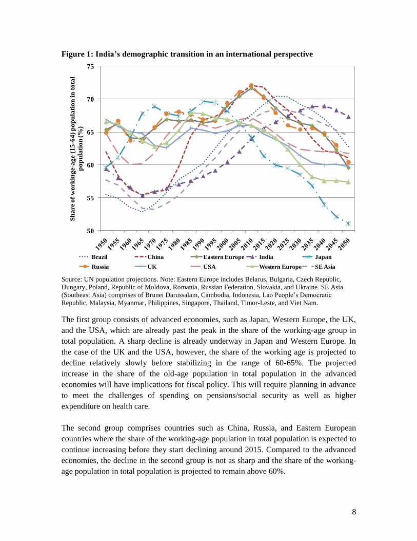
Figure 1: India’s demographic transition in an international perspective

Source: UN population projections. Note: Eastern Europe includes Belarus, Bulgaria, Czech Republic,

Hungary, Poland, Republic of Moldova, Romania, Russian Federation, Slovakia, and Ukraine. SE Asia

(Southeast Asia) comprises of Brunei Darussalam, Cambodia, Indonesia, Lao People‟s Democratic

Republic, Malaysia, Myanmar, Philippines, Singapore, Thailand, Timor-Leste, and Viet Nam.

The first group consists of advanced economies, such as Japan, Western Europe, the UK,

and the USA, which are already past the peak in the share of the working-age group in

total population. A sharp decline is already underway in Japan and Western Europe. In

the case of the UK and the USA, however, the share of the working age is projected to

decline relatively slowly before stabilizing in the range of 60-65%. The projected

increase in the share of the old-age population in total population in the advanced

economies will have implications for fiscal policy. This will require planning in advance

to meet the challenges of spending on pensions/social security as well as higher

expenditure on health care.

The second group comprises countries such as China, Russia, and Eastern European

countries where the share of the working-age population in total population is expected to

continue increasing before they start declining around 2015. Compared to the advanced

economies, the decline in the second group is not as sharp and the share of the working-

age population in total population is projected to remain above 60%.

50

55

60

65

70

75S

ha

re o

f w

ork

ing

e-a

ge

(15

-64

) p

op

ula

tio

n in

to

tal

po

pu

lati

on

(%

)

Brazil China Eastern Europe India Japan

Russia UK USA Western Europe SE Asia

9

The third group includes Brazil and other Latin American countries, and Southeast Asian

(SE Asia) countries along with Turkey (not shown), which are projected to see an

increase in the share of the working-age population until the mid-2020s before declining.

Like the countries in the second group, the decline is not as sharp and the share of the

working-age group in total population remains above 60%.

Lastly, there is India, where the share of the working-age population in total population is

expected to continue increasing until about 2035 to 2040, before starting a slow decline.

The share of the working-age population in India is expected to remain above 65% until

2050. India‟s window of opportunity to exploit the growing share of the working-age

population in total population is among the longest. India thus seems to be sitting on a

huge opportunity in terms of a boom in the share of the working-age population.

4. Demographic trends in India: A state-level perspective5

The previous section shows that India‟s demographic window of opportunity extends

until about 2035 to 2040. However, this masks differences in the pace of demographic

transition across states in India. I start with a discussion of key statistics at the all-India

level and then turn to discussing the differing pace of demographic transition across the

states in India.

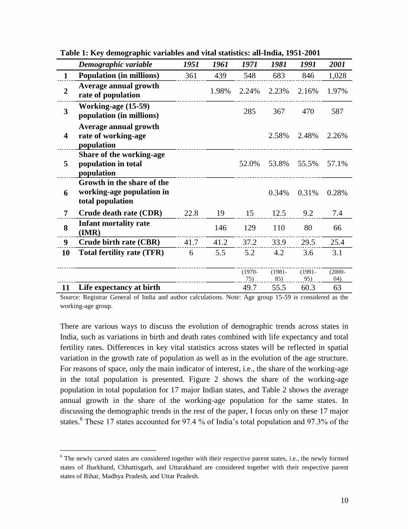
For purposes of consistency with the rest of the paper, which uses Census of India data,

Table 1 presents key demographic trends and vital statistics in India for the period 1951-

2001. The average annual growth rate of the total population was 2.24% during 1961-

1971, slowing down to 1.97% during the census period 1991-2001. Crude birth rate

(CBR) fell from 41.7 in 1951 to 37.2 in 1971, and to 25.4 in 2001. Crude death rate

(CDR) declined from 22.8 in 1951 to 15 in 1971, and to 7.4 in 2001. Total fertility rate

(TFR) declined from 5.2 in 1971 to 3.1 in 2001. Life expectancy at birth increased from

49.7 years over the period 1970-1975 to 63 years during 2000-2004. As discussed above,

a country‟s demographic transition is reflected in its changing age composition,

specifically in the share of the working-age population. Over the period 1971-2001, the

share of the working-age population in total population increased from 52% in 1971 to

55.5% in 1991, and further to 57.1% in 2001.

5This section onwards, the definition of the working-age group is ages 15-59.

10

Table 1: Key demographic variables and vital statistics: all-India, 1951-2001

Demographic variable 1951 1961 1971 1981 1991 2001

1 Population (in millions) 361 439 548 683 846 1,028

2 Average annual growth

rate of population 1.98% 2.24% 2.23% 2.16% 1.97%

3 Working-age (15-59)

population (in millions) 285 367 470 587

4

Average annual growth

rate of working-age

population

2.58% 2.48% 2.26%

5

Share of the working-age

population in total

population

52.0% 53.8% 55.5% 57.1%

6

Growth in the share of the

working-age population in

total population 0.34% 0.31% 0.28%

7 Crude death rate (CDR) 22.8 19 15 12.5 9.2 7.4

8 Infant mortality rate

(IMR) 146 129 110 80 66

9 Crude birth rate (CBR) 41.7 41.2 37.2 33.9 29.5 25.4

10 Total fertility rate (TFR) 6 5.5 5.2 4.2 3.6 3.1

(1970-

75)

(1981-

85)

(1991-

95)

(2000-

04)

11 Life expectancy at birth

49.7 55.5 60.3 63

Source: Registrar General of India and author calculations. Note: Age group 15-59 is considered as the

working-age group.

There are various ways to discuss the evolution of demographic trends across states in

India, such as variations in birth and death rates combined with life expectancy and total

fertility rates. Differences in key vital statistics across states will be reflected in spatial

variation in the growth rate of population as well as in the evolution of the age structure.

For reasons of space, only the main indicator of interest, i.e., the share of the working-age

in the total population is presented. Figure 2 shows the share of the working-age

population in total population for 17 major Indian states, and Table 2 shows the average

annual growth in the share of the working-age population for the same states. In

discussing the demographic trends in the rest of the paper, I focus only on these 17 major

states.6 These 17 states accounted for 97.4 % of India‟s total population and 97.3% of the

6 The newly carved states are considered together with their respective parent states, i.e., the newly formed

states of Jharkhand, Chhattisgarh, and Uttarakhand are considered together with their respective parent

states of Bihar, Madhya Pradesh, and Uttar Pradesh.

11

working-age population in 2001, and 93% of the increase in India‟s working-age

population between 1991 and 2001.

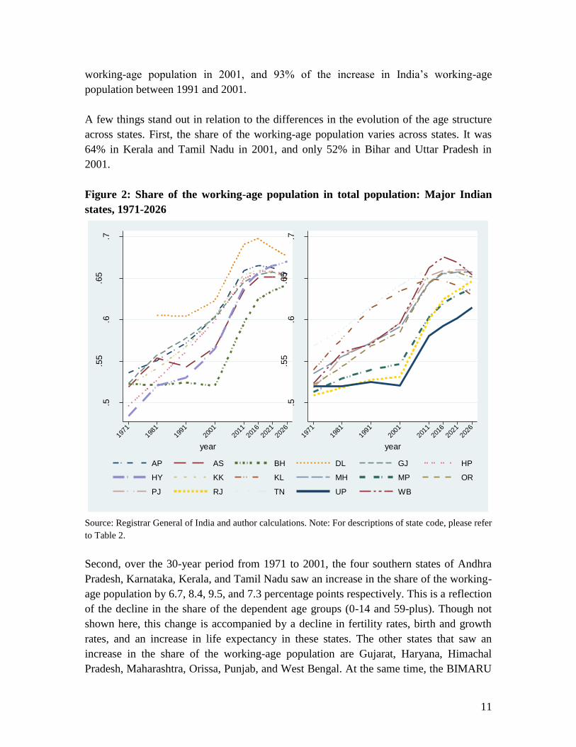
A few things stand out in relation to the differences in the evolution of the age structure

across states. First, the share of the working-age population varies across states. It was

64% in Kerala and Tamil Nadu in 2001, and only 52% in Bihar and Uttar Pradesh in

2001.

Figure 2: Share of the working-age population in total population: Major Indian

states, 1971-2026

Source: Registrar General of India and author calculations. Note: For descriptions of state code, please refer

to Table 2.

Second, over the 30-year period from 1971 to 2001, the four southern states of Andhra

Pradesh, Karnataka, Kerala, and Tamil Nadu saw an increase in the share of the working-

age population by 6.7, 8.4, 9.5, and 7.3 percentage points respectively. This is a reflection

of the decline in the share of the dependent age groups (0-14 and 59-plus). Though not

shown here, this change is accompanied by a decline in fertility rates, birth and growth

rates, and an increase in life expectancy in these states. The other states that saw an

increase in the share of the working-age population are Gujarat, Haryana, Himachal

Pradesh, Maharashtra, Orissa, Punjab, and West Bengal. At the same time, the BIMARU

.5.5

5.6

.65

.7

.5.5

5.6

.65

.7

1971

1981

1991

2001

2011

2016

2021

2026

year

1971

1981

1991

2001

2011

2016

2021

2026

year

AP AS BH DL GJ HP

HY KK KL MH MP OR

PJ RJ TN UP WB

sh

are

of w

ork

ing a

ge p

opu

lation

12

states saw a smaller increase in the share of the working-age population. There was only

a small increase in the share of the working-age population in Delhi, though in this case

the share of the working-age population in 1981 was already 61% (higher than any other

state).

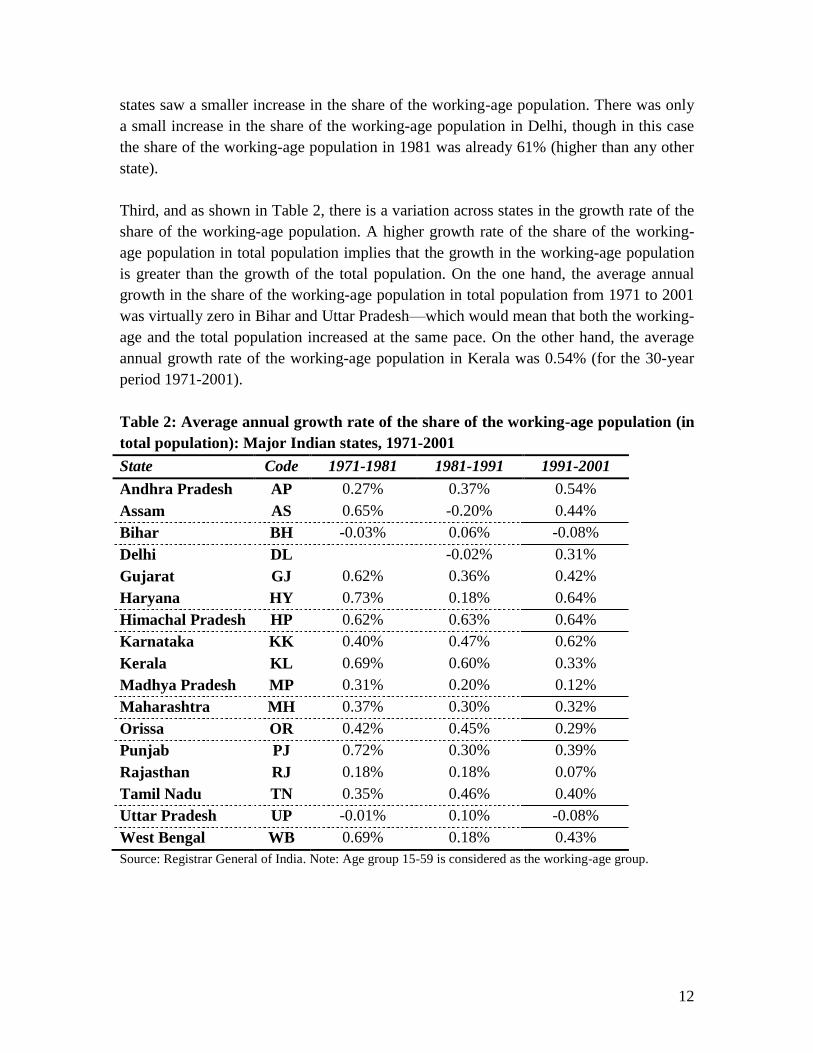
Third, and as shown in Table 2, there is a variation across states in the growth rate of the

share of the working-age population. A higher growth rate of the share of the working-

age population in total population implies that the growth in the working-age population

is greater than the growth of the total population. On the one hand, the average annual

growth in the share of the working-age population in total population from 1971 to 2001

was virtually zero in Bihar and Uttar Pradesh—which would mean that both the working-

age and the total population increased at the same pace. On the other hand, the average

annual growth rate of the working-age population in Kerala was 0.54% (for the 30-year

period 1971-2001).

Table 2: Average annual growth rate of the share of the working-age population (in

total population): Major Indian states, 1971-2001

State Code 1971-1981 1981-1991 1991-2001

Andhra Pradesh AP 0.27% 0.37% 0.54%

Assam AS 0.65% -0.20% 0.44%

Bihar BH -0.03% 0.06% -0.08%

Delhi DL -0.02% 0.31%

Gujarat GJ 0.62% 0.36% 0.42%

Haryana HY 0.73% 0.18% 0.64%

Himachal Pradesh HP 0.62% 0.63% 0.64%

Karnataka KK 0.40% 0.47% 0.62%

Kerala KL 0.69% 0.60% 0.33%

Madhya Pradesh MP 0.31% 0.20% 0.12%

Maharashtra MH 0.37% 0.30% 0.32%

Orissa OR 0.42% 0.45% 0.29%

Punjab PJ 0.72% 0.30% 0.39%

Rajasthan RJ 0.18% 0.18% 0.07%

Tamil Nadu TN 0.35% 0.46% 0.40%

Uttar Pradesh UP -0.01% 0.10% -0.08%

West Bengal WB 0.69% 0.18% 0.43%

Source: Registrar General of India. Note: Age group 15-59 is considered as the working-age group.

13

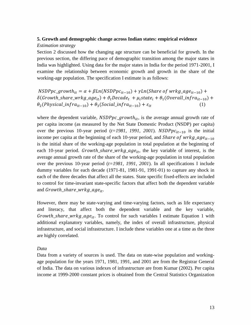
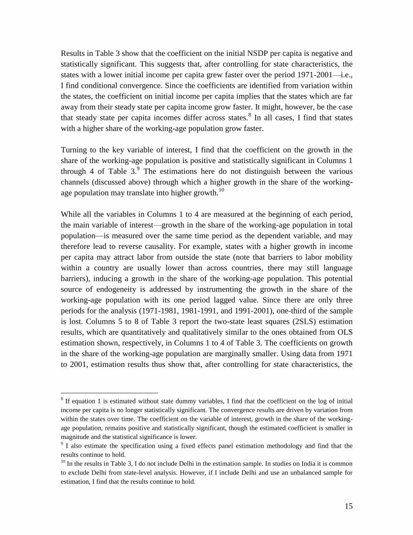
5. Growth and demographic change across Indian states: empirical evidence

Estimation strategy

Section 2 discussed how the changing age structure can be beneficial for growth. In the

previous section, the differing pace of demographic transition among the major states in

India was highlighted. Using data for the major states in India for the period 1971-2001, I

examine the relationship between economic growth and growth in the share of the

working-age population. The specification I estimate is as follows:

(1)

where the dependent variable, , is the average annual growth rate of

per capita income (as measured by the Net State Domestic Product (NSDP) per capita)

over the previous 10-year period (t=1981, 1991, 2001). is the initial

income per capita at the beginning of each 10-year period, and

is the initial share of the working-age population in total population at the beginning of

each 10-year period. , the key variable of interest, is the

average annual growth rate of the share of the working-age population in total population

over the previous 10-year period (t=1981, 1991, 2001). In all specifications I include

dummy variables for each decade (1971-81, 1981-91, 1991-01) to capture any shock in

each of the three decades that affect all the states. State specific fixed-effects are included

to control for time-invariant state-specific factors that affect both the dependent variable

and .

However, there may be state-varying and time-varying factors, such as life expectancy

and literacy, that affect both the dependent variable and the key variable,

. To control for such variables I estimate Equation 1 with

additional explanatory variables, namely, the index of overall infrastructure, physical

infrastructure, and social infrastructure. I include these variables one at a time as the three

are highly correlated.

Data

Data from a variety of sources is used. The data on state-wise population and working-

age population for the years 1971, 1981, 1991, and 2001 are from the Registrar General

of India. The data on various indexes of infrastructure are from Kumar (2002). Per capita

income at 1999-2000 constant prices is obtained from the Central Statistics Organization

14

(Government of India). Official data prior to 1993 and 1980 are indexed to different base

years and were spliced to 1999-2000 prices.7

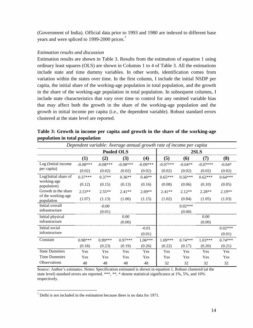
Estimation results and discussion

Estimation results are shown in Table 3. Results from the estimation of equation 1 using

ordinary least squares (OLS) are shown in Columns 1 to 4 of Table 3. All the estimations

include state and time dummy variables. In other words, identification comes from

variation within the states over time. In the first column, I include the initial NSDP per

capita, the initial share of the working-age population in total population, and the growth

in the share of the working-age population in total population. In subsequent columns, I

include state characteristics that vary over time to control for any omitted variable bias

that may affect both the growth in the share of the working-age population and the

growth in initial income per capita (i.e., the dependent variable). Robust standard errors

clustered at the state level are reported.

Table 3: Growth in income per capita and growth in the share of the working-age

population in total population

Dependent variable: Average annual growth rate of income per capita

Pooled OLS 2SLS (1) (2) (3) (4) (5) (6) (7) (8) Log (Initial income

per capita) -0.08*** -0.08*** -0.08*** -0.09*** -0.07*** -0.04** -0.07*** -0.04*

(0.02) (0.02) (0.02) (0.02) (0.02) (0.02) (0.02) (0.02)

Log(Initial share of

working-age

population)

0.37*** 0.37** 0.36** 0.40** 0.65*** 0.56*** 0.62*** 0.64***

(0.12) (0.15) (0.13) (0.16) (0.08) (0.06) (0.10) (0.05)

Growth in the share

of the working-age

population

2.53** 2.55** 2.41** 2.69** 2.41** 2.12** 2.28** 2.19**

(1.07) (1.13) (1.06) (1.15) (1.02) (0.84) (1.05) (1.03)

Initial overall

infrastructure -0.00

0.02***

(0.01)

(0.00)

Initial physical

infrastructure

0.00

0.00

(0.00)

(0.00)

Initial social

infrastructure

-0.01

0.02***

(0.01)

(0.01)

Constant 0.98*** 0.99*** 0.97*** 1.06*** 1.09*** 0.74*** 1.03*** 0.74***

(0.18) (0.23) (0.19) (0.26) (0.22) (0.17) (0.20) (0.21)

State Dummies Yes Yes Yes Yes Yes Yes Yes Yes

Time Dummies Yes Yes Yes Yes Yes Yes Yes Yes

Observations 48 48 48 48 32 32 32 32

Source: Author‟s estimates. Notes: Specification estimated is shown in equation 1. Robust clustered (at the

state level) standard errors are reported. ***, **, * denote statistical significance at 1%, 5%, and 10%

respectively.

7 Delhi is not included in the estimation because there is no data for 1971.

15

Results in Table 3 show that the coefficient on the initial NSDP per capita is negative and

statistically significant. This suggests that, after controlling for state characteristics, the

states with a lower initial income per capita grew faster over the period 1971-2001—i.e.,

I find conditional convergence. Since the coefficients are identified from variation within

the states, the coefficient on initial income per capita implies that the states which are far

away from their steady state per capita income grow faster. It might, however, be the case

that steady state per capita incomes differ across states.8 In all cases, I find that states

with a higher share of the working-age population grow faster.

Turning to the key variable of interest, I find that the coefficient on the growth in the

share of the working-age population is positive and statistically significant in Columns 1

through 4 of Table 3.9 The estimations here do not distinguish between the various

channels (discussed above) through which a higher growth in the share of the working-

age population may translate into higher growth.10

While all the variables in Columns 1 to 4 are measured at the beginning of each period,

the main variable of interest—growth in the share of the working-age population in total

population—is measured over the same time period as the dependent variable, and may

therefore lead to reverse causality. For example, states with a higher growth in income

per capita may attract labor from outside the state (note that barriers to labor mobility

within a country are usually lower than across countries, there may still language

barriers), inducing a growth in the share of the working-age population. This potential

source of endogeneity is addressed by instrumenting the growth in the share of the

working-age population with its one period lagged value. Since there are only three

periods for the analysis (1971-1981, 1981-1991, and 1991-2001), one-third of the sample

is lost. Columns 5 to 8 of Table 3 report the two-state least squares (2SLS) estimation

results, which are quantitatively and qualitatively similar to the ones obtained from OLS

estimation shown, respectively, in Columns 1 to 4 of Table 3. The coefficients on growth

in the share of the working-age population are marginally smaller. Using data from 1971

to 2001, estimation results thus show that, after controlling for state characteristics, the

8 If equation 1 is estimated without state dummy variables, I find that the coefficient on the log of initial

income per capita is no longer statistically significant. The convergence results are driven by variation from

within the states over time. The coefficient on the variable of interest, growth in the share of the working-

age population, remains positive and statistically significant, though the estimated coefficient is smaller in

magnitude and the statistical significance is lower. 9 I also estimate the specification using a fixed effects panel estimation methodology and find that the

results continue to hold. 10

In the results in Table 3, I do not include Delhi in the estimation sample. In studies on India it is common

to exclude Delhi from state-level analysis. However, if I include Delhi and use an unbalanced sample for

estimation, I find that the results continue to hold.

16

states with a higher growth in the share of the working-age population tend to grow

faster.

6. Regional variation in projected demographic changes

Based on historical data, the results in the previous section show that states with higher

growth in the share of the working-age population grow faster. This, however, does not

imply that the states projected to see a higher growth in the share of the working-age

population will grow faster. This is because favorable population dynamics at best

present an opportunity and do not guarantee higher future growth. Adequate provision of

health, education, physical infrastructure, and policies to generate gainful employment

opportunities are critical to reap the benefits of a growing share of the working-age

population and to attain a high growth trajectory. It is, therefore, important to know

which states are expected to see a higher growth in the share of the working-age

population, and if these states are in a position to reap the dividends. Demographic

projections lets the policymakers see the future and gauge the various phases of

demographic transition. This provides them with an opportunity to prepare for the

demographic changes and the economic challenges that are likely to accompany these

phases of transition. I turn to this next.

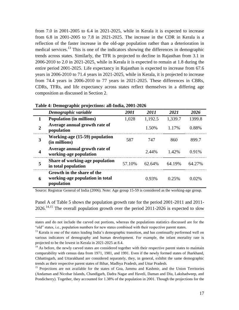
From 2001 to 2026, the total population in India is projected to grow at an average annual

rate of 1.2%—from 1.03 billion in 2001 to 1.4 billion in 2026 (Table 4).11

The CBR

(CDR) is projected to fall from 23.2 (7.5) during the period 2001-2005 to 16.0 (7.2)

during 2021-2025. The TFR is expected to fall from 3.2 in 1991-2001 to 2.6 in 2006-

2010, and further to 2.0 by 2026. The decline in the TFR and the CBR is expected to lead

to a fall in the share of the under-15 population, from 35.4% in 2001 to 29.1% in 2011

and to 23.4% by 2026. At the same time, the declining CDR combined with an increase

in life expectancy from 65 years for the period 2001-2005 to 71 years for 2021-2025, will

lead to an increase in the share of the population aged 60 and above, from 6.9% in 2001

to 8.3% in 2011 and to 12.4% by 2026. The rest of the projected increase in the total

population between 2001 and 2026 is accounted for by the working-age population,

whose share in the total population is projected to increase from 57.1% in 2001 to 64.3%

in 2026.

However, behind the overall changes in the demographic structure lie significant regional

differences in demographic trends. For example, the CBR is expected to decline in Kerala

to 12.3 in 2021-2025 from 16.3 in 2001-2005, and in Rajasthan from 27.1 in 2001-2005

to 16.7 in 2021-2025.12

On the other hand, the CDR is projected to decline in Rajasthan

11

All the statistics discussed in this section are from the Registrar General of India (2006). 12

The CBR in some states such as Uttar Pradesh, Madhya Pradesh, and Bihar are projected to be even

higher in 2021-2025 at 20.5, 18.0, and 17.4, respectively. However, these figures are for the newly formed

17

from 7.0 in 2001-2005 to 6.4 in 2021-2025, while in Kerala it is expected to increase

from 6.8 in 2001-2005 to 7.8 in 2021-2025. The increase in the CDR in Kerala is a

reflection of the faster increase in the old-age population rather than a deterioration in

medical services.13

This is one of the indicators showing the differences in demographic

trends across states. Similarly, the TFR is projected to decline in Rajasthan from 3.1 in

2006-2010 to 2.0 in 2021-2025, while in Kerala it is expected to remain at 1.8 during the

entire period 2001-2025. Life expectancy in Rajasthan is expected to increase from 67.6

years in 2006-2010 to 71.4 years in 2021-2025, while in Kerala, it is projected to increase

from 74.4 years in 2006-2010 to 77 years in 2021-2025. These differences in CBRs,

CDRs, TFRs, and life expectancy across states reflect themselves in a differing age

composition as discussed in Section 2.

Table 4: Demographic projections: all-India, 2001-2026

Demographic variable 2001 2011 2021 2026

1 Population (in millions) 1,028 1,192.5 1,339.7 1399.8

2 Average annual growth rate of

population 1.50% 1.17% 0.88%

3 Working-age (15-59) population

(in millions) 587 747 860 899.7

4 Average annual growth rate of

working-age population 2.44% 1.42% 0.91%

5 Share of working-age population

in total population 57.10% 62.64% 64.19% 64.27%

6

Growth in the share of the

working-age population in total

population

0.93% 0.25% 0.02%

Source: Registrar General of India (2006). Note: Age group 15-59 is considered as the working-age group.

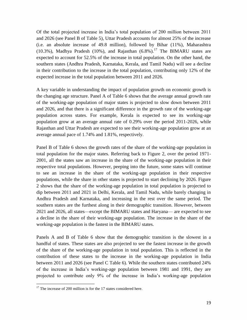
Panel A of Table 5 shows the population growth rate for the period 2001-2011 and 2011-

2026.14,15

The overall population growth over the period 2011-2026 is expected to slow

states and do not include the carved out portions, whereas the populations statistics discussed are for the

“old” states, i.e., population numbers for new states combined with their respective parent states. 13

Kerala is one of the states leading India‟s demographic transition, and has continually performed well on

various indicators of demography and human development. For example, the infant mortality rate is

projected to be the lowest in Kerala in 2021-2025 at 8.4. 14

As before, the newly carved states are considered together with their respective parent states to maintain

comparability with census data from 1971, 1981, and 1991. Even if the newly formed states of Jharkhand,

Chhattisgarh, and Uttarakhand are considered separately, they, in general, exhibit the same demographic

trends as their respective parent states of Bihar, Madhya Pradesh, and Uttar Pradesh. 15

Projections are not available for the states of Goa, Jammu and Kashmir, and the Union Territories

(Andaman and Nicobar Islands, Chandigarh, Dadra Nagar and Haveli, Daman and Diu, Lakshadweep, and

Pondicherry). Together, they accounted for 1.38% of the population in 2001. Though the projections for the

18

down in all the states compared with the population growth rates over the 10-year period

1991-2001. The states expected to see their population increase beyond the national

growth rate over the period 2011-2026 are Delhi, Haryana, Madhya Pradesh (undivided),

Maharashtra, Rajasthan, and Uttar Pradesh (undivided). The variation in average annual

growth rates of total population, as measured by the coefficient of variation, has been

increasing since 1971 and is projected to continue increasing until 2026.16

Table 5: Average annual growth rate of total population and contribution to

population increase: Major Indian states, 2001-2026

Panel A: Average annual growth

rate of total population

Panel B: Contribution to the

projected increase in India's

population

2001-

2011

2011-

2021

2021-

2026

2011-

2026 (overall)

2001-

2011

2011-

2021

2021-

2026

2011-

2026 (overall)

Andhra Pradesh 1.07% 0.78% 0.55% 0.70% 5.4% 4.8% 4.3% 4.7%

Assam 1.38% 1.12% 0.82% 1.02% 2.5% 2.5% 2.4% 2.5%

Bihar 1.63% 1.17% 0.83% 1.05% 12.1% 11.2% 10.5% 11.0%

Delhi 2.91% 2.87% 2.71% 2.82% 2.9% 4.3% 6.0% 4.8%

Gujarat 1.54% 1.15% 0.93% 1.07% 5.3% 5.0% 5.3% 5.1%

Haryana 1.87% 1.44% 1.15% 1.35% 2.7% 2.8% 3.0% 2.8%

Himachal Pradesh 1.12% 0.81% 0.57% 0.73% 0.4% 0.4% 0.4% 0.4%

Karnataka 1.18% 0.88% 0.63% 0.80% 4.1% 3.8% 3.6% 3.7%

Kerala 0.82% 0.57% 0.37% 0.50% 1.7% 1.4% 1.2% 1.3%

Madhya Pradesh 1.74% 1.37% 1.04% 1.26% 9.6% 9.9% 10.0% 9.9%

Maharashtra 1.52% 1.21% 0.96% 1.13% 9.9% 10.1% 10.7% 10.3%

Orissa 1.02% 0.79% 0.56% 0.71% 2.5% 2.3% 2.1% 2.3%

Punjab 1.29% 0.92% 0.67% 0.83% 2.1% 1.9% 1.7% 1.8%

Rajasthan 1.84% 1.36% 0.97% 1.23% 7.1% 6.9% 6.6% 6.8%

Tamil Nadu 0.78% 0.50% 0.28% 0.42% 3.2% 2.4% 1.7% 2.2%

Uttar Pradesh 1.89% 1.56% 1.16% 1.42% 22.7% 24.8% 25.1% 24.9%

West Bengal 1.11% 0.85% 0.64% 0.78% 5.9% 5.5% 5.4% 5.5%

Source: Registrar General of India (2006). Note: For purposes of calculating contribution to the increase in

India‟s total population, increase in total population considered is for the 17 major states shown above.

northeastern states (except Assam) as a group are available, they are not discussed here. The northeastern

states include Arunachal Pradesh, Manipur, Meghalaya, Mizoram, Nagaland, Sikkim, and Tripura. These

states together accounted for 1.2% of India‟s total population and 1.2% of India‟s total working-age

population in 2001, and 1.5% of the increase in India‟s working-age population between 1991 and 2001.

Thus, these states are very small in terms of their effect on overall population trends discussed here. 16

The coefficient of variation has increased from 26% for population growth over the period 1971-1981, to

34% for growth over the period 1991-2001, and to 50% for growth over the period 2011-2026.

19

Of the total projected increase in India‟s total population of 200 million between 2011

and 2026 (see Panel B of Table 5), Uttar Pradesh accounts for almost 25% of the increase

(i.e. an absolute increase of 49.8 million), followed by Bihar (11%), Maharashtra

(10.3%), Madhya Pradesh (10%), and Rajasthan (6.8%).17

The BIMARU states are

expected to account for 52.5% of the increase in total population. On the other hand, the

southern states (Andhra Pradesh, Karnataka, Kerala, and Tamil Nadu) will see a decline

in their contribution to the increase in the total population, contributing only 12% of the

expected increase in the total population between 2011 and 2026.

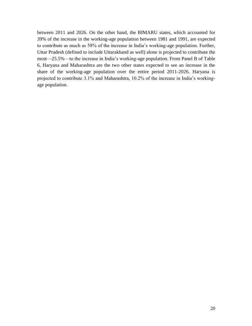
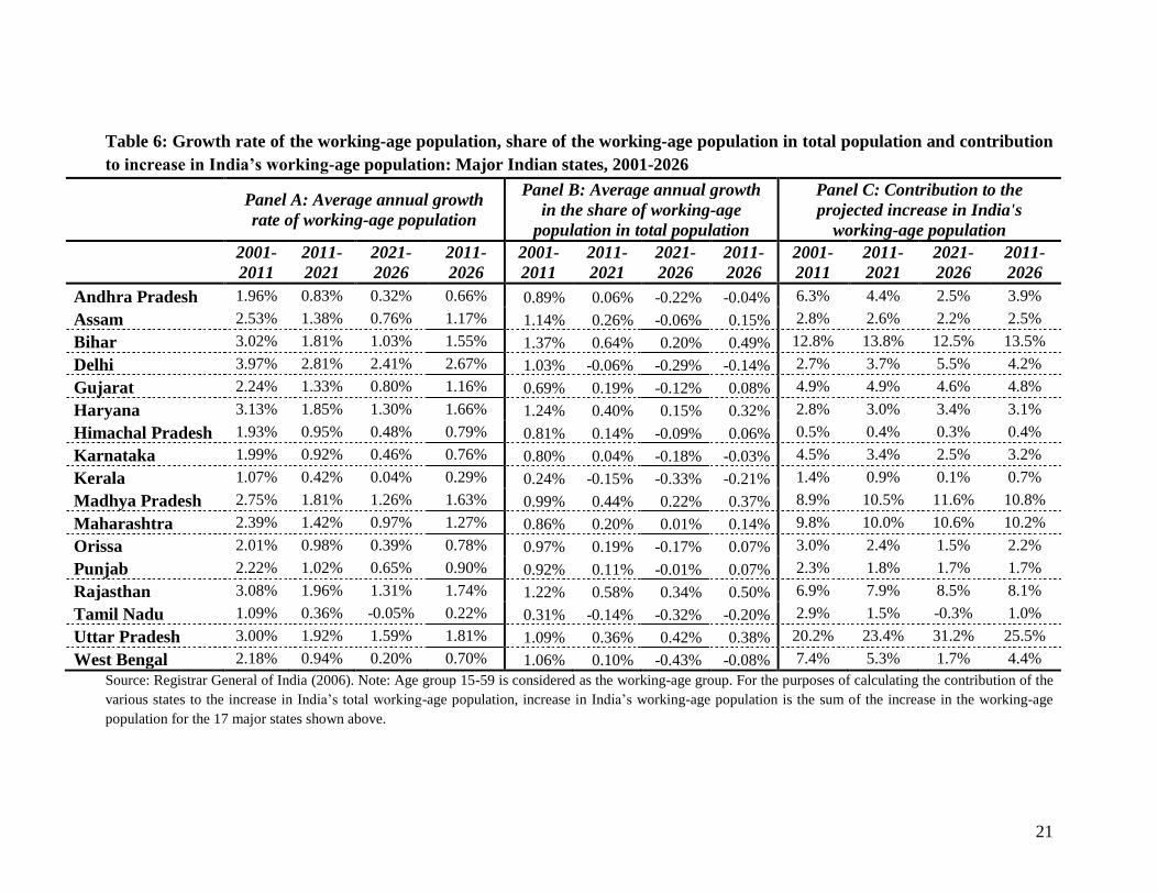
A key variable in understanding the impact of population growth on economic growth is

the changing age structure. Panel A of Table 6 shows that the average annual growth rate

of the working-age population of major states is projected to slow down between 2011

and 2026, and that there is a significant difference in the growth rate of the working-age

population across states. For example, Kerala is expected to see its working-age

population grow at an average annual rate of 0.29% over the period 2011-2026, while

Rajasthan and Uttar Pradesh are expected to see their working-age population grow at an

average annual pace of 1.74% and 1.81%, respectively.

Panel B of Table 6 shows the growth rates of the share of the working-age population in

total population for the major states. Referring back to Figure 2, over the period 1971-

2001, all the states saw an increase in the share of the working-age population in their

respective total populations. However, peeping into the future, some states will continue

to see an increase in the share of the working-age population in their respective

populations, while the share in other states is projected to start declining by 2026. Figure

2 shows that the share of the working-age population in total population is projected to

dip between 2011 and 2021 in Delhi, Kerala, and Tamil Nadu, while barely changing in

Andhra Pradesh and Karnataka, and increasing in the rest over the same period. The

southern states are the furthest along in their demographic transition. However, between

2021 and 2026, all states—except the BIMARU states and Haryana— are expected to see

a decline in the share of their working-age population. The increase in the share of the

working-age population is the fastest in the BIMARU states.

Panels A and B of Table 6 show that the demographic transition is the slowest in a

handful of states. These states are also projected to see the fastest increase in the growth

of the share of the working-age population in total population. This is reflected in the

contribution of these states to the increase in the working-age population in India

between 2011 and 2026 (see Panel C Table 6). While the southern states contributed 24%

of the increase in India‟s working-age population between 1981 and 1991, they are

projected to contribute only 9% of the increase in India‟s working-age population

17

The increase of 200 million is for the 17 states considered here.

20

between 2011 and 2026. On the other hand, the BIMARU states, which accounted for

39% of the increase in the working-age population between 1981 and 1991, are expected

to contribute as much as 58% of the increase in India‟s working-age population. Further,

Uttar Pradesh (defined to include Uttarakhand as well) alone is projected to contribute the

most—25.5%—to the increase in India‟s working-age population. From Panel B of Table

6, Haryana and Maharashtra are the two other states expected to see an increase in the

share of the working-age population over the entire period 2011-2026. Haryana is

projected to contribute 3.1% and Maharashtra, 10.2% of the increase in India‟s working-

age population.

21

Table 6: Growth rate of the working-age population, share of the working-age population in total population and contribution

to increase in India’s working-age population: Major Indian states, 2001-2026

Panel A: Average annual growth

rate of working-age population

Panel B: Average annual growth

in the share of working-age

population in total population

Panel C: Contribution to the

projected increase in India's

working-age population

2001-

2011

2011-

2021

2021-

2026

2011-

2026

2001-

2011

2011-

2021

2021-

2026

2011-

2026

2001-

2011

2011-

2021

2021-

2026

2011-

2026

Andhra Pradesh 1.96% 0.83% 0.32% 0.66% 0.89% 0.06% -0.22% -0.04% 6.3% 4.4% 2.5% 3.9%

Assam 2.53% 1.38% 0.76% 1.17% 1.14% 0.26% -0.06% 0.15% 2.8% 2.6% 2.2% 2.5%

Bihar 3.02% 1.81% 1.03% 1.55% 1.37% 0.64% 0.20% 0.49% 12.8% 13.8% 12.5% 13.5%

Delhi 3.97% 2.81% 2.41% 2.67% 1.03% -0.06% -0.29% -0.14% 2.7% 3.7% 5.5% 4.2%

Gujarat 2.24% 1.33% 0.80% 1.16% 0.69% 0.19% -0.12% 0.08% 4.9% 4.9% 4.6% 4.8%

Haryana 3.13% 1.85% 1.30% 1.66% 1.24% 0.40% 0.15% 0.32% 2.8% 3.0% 3.4% 3.1%

Himachal Pradesh 1.93% 0.95% 0.48% 0.79% 0.81% 0.14% -0.09% 0.06% 0.5% 0.4% 0.3% 0.4%

Karnataka 1.99% 0.92% 0.46% 0.76% 0.80% 0.04% -0.18% -0.03% 4.5% 3.4% 2.5% 3.2%

Kerala 1.07% 0.42% 0.04% 0.29% 0.24% -0.15% -0.33% -0.21% 1.4% 0.9% 0.1% 0.7%

Madhya Pradesh 2.75% 1.81% 1.26% 1.63% 0.99% 0.44% 0.22% 0.37% 8.9% 10.5% 11.6% 10.8%

Maharashtra 2.39% 1.42% 0.97% 1.27% 0.86% 0.20% 0.01% 0.14% 9.8% 10.0% 10.6% 10.2%

Orissa 2.01% 0.98% 0.39% 0.78% 0.97% 0.19% -0.17% 0.07% 3.0% 2.4% 1.5% 2.2%

Punjab 2.22% 1.02% 0.65% 0.90% 0.92% 0.11% -0.01% 0.07% 2.3% 1.8% 1.7% 1.7%

Rajasthan 3.08% 1.96% 1.31% 1.74% 1.22% 0.58% 0.34% 0.50% 6.9% 7.9% 8.5% 8.1%

Tamil Nadu 1.09% 0.36% -0.05% 0.22% 0.31% -0.14% -0.32% -0.20% 2.9% 1.5% -0.3% 1.0%

Uttar Pradesh 3.00% 1.92% 1.59% 1.81% 1.09% 0.36% 0.42% 0.38% 20.2% 23.4% 31.2% 25.5%

West Bengal 2.18% 0.94% 0.20% 0.70% 1.06% 0.10% -0.43% -0.08% 7.4% 5.3% 1.7% 4.4%

Source: Registrar General of India (2006). Note: Age group 15-59 is considered as the working-age group. For the purposes of calculating the contribution of the

various states to the increase in India‟s total working-age population, increase in India‟s working-age population is the sum of the increase in the working-age

population for the 17 major states shown above.

22

Table 7: State characteristics and demographic dividend

Source: Growth rate in the share of the working-age population is based on population projection data from Registrar General of India (2006). Per capita income and its growth

rate is based on data from Central Statistical Organization (Government of India). Literacy rate, life expectancy, and infant mortality rate are from various editions of Economic

Survey (Ministry of Finance, Government of India). Ranking of physical infrastructure is based on Kumar (2002). Investment Climate is from the 2002 edition of “How are the

States Doing?”. Labor force participation rate (LFPR) and Workforce participation rate (WFPR) are from the 61st round of NSS (National Sample Survey, 2004-2005).

Notes: Data on infant mortality rate for Delhi and Himachal Pradesh is for 2008. Data on life expectancy for Delhi is for 2001-2005 and Himachal Pradesh is for 2000-2004.

Investment climate is for the divided states in the case of Bihar, Madhya Pradesh, and Uttar Pradesh. LFPR and WFPR from the 61st round of household survey data are applied to

the 2006 population projections to get state level estimates which combine rural and urban as well male and female data and to combine new states with their parent states.

Average

annual growth

in the share of

the working-

age population

(2011-2026)

per capita

income

(2007-08,

current

prices in

Rupees)

Average

annual

growth in

per capita

income

(1971-2007)

Literacy

rate

(2001)

Life

expectancy

at birth (in

years)

Infant

mortality

Rate

(2007)

Rank-

physical

infrastructure

Investm-

ent climate LFPR

WFPR

narrow

WFPR

broad

Rajasthan 0.50% 23933 2.68% 61.0% 62 65 13 1.6 438 372 433

Bihar 0.49% 13279 1.75% 47.5% 61.6 58 16 0.4 340 304 333

Uttar Pradesh 0.38% 16862 1.99% 57.4% 60 69 12 1.4 370 308 366

Madhya Pradesh 0.37% 19923 1.61% 64.1% 58 72 15 1.8 446 415 441

Haryana 0.32% 58531 3.62% 68.6% 66.2 55 4 2.5 409 318 397

Assam 0.15% 21464 1.90% 64.3% 58.9 66 17 1.5 396 337 383

Maharashtra 0.14% 47051 3.77% 77.3% 67.2 34 2 2.3 470 435 460

Gujarat 0.08% 45773 3.73% 66.4% 64.1 52 5 2.4 466 415 460

Orissa 0.07% 23403 2.70% 63.6% 59.6 71 10 1.7 462 381 433

Punjab 0.07% 44923 2.83% 70.0% 69.4 41 1 2.9 432 318 413

Himachal

Pradesh 0.06% 40137 2.77% 76.5% 66.5 44 11 2.3 533 451 522

Karnataka -0.03% 36266 3.61% 67.0% 65.3 47 7 2.7 493 468 487

Andhra Pradesh -0.04% 35864 3.78% 61.1% 64.4 54 8 2.3 509 484 502

West Bengal -0.08% 31722 3.05% 69.2% 64.9 37 14 1.2 395 341 380

Delhi -0.14% 78690 3.05% 81.8% 72.2 35 9 3.1 349 327 333

Tamil Nadu -0.20% 40757 3.51% 73.5% 66.2 35 3 3.1 485 462 474

Kerala -0.21% 41814 3.33% 90.9% 74 13 6 2.8 446 339 393

23

Will India be able to reap the demographic dividend?

The BIMARU states, which together account for 40% of India‟s population, are projected

to contribute 52.5% of the increase in India‟s total population, and 58% of the increase in

India‟s working-age population. These four states are the slowest in their pace of

transition to low birth rates and low death rates. Using data for 1971-2001, I have shown

that the states with a higher growth in the share of the working-age population tend to

grow faster.

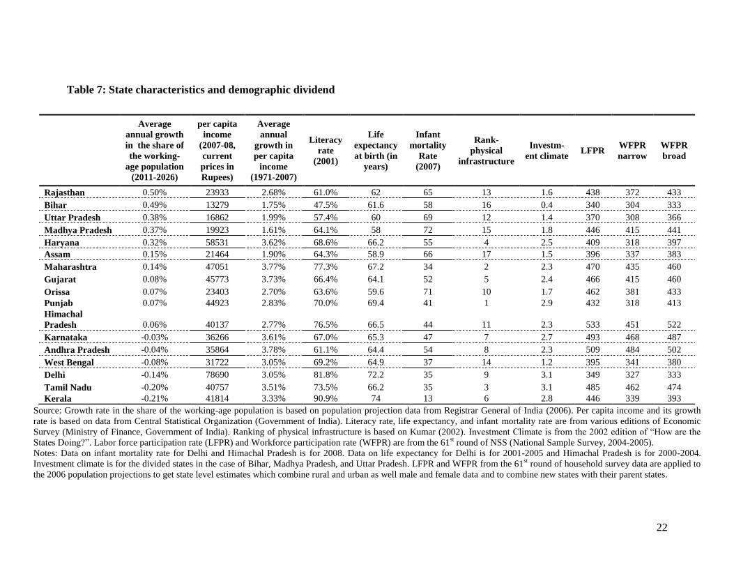
I use the past performance of Indian states, especially the BIMARU states, to reflect on

whether they will be able to deal with the challenge of a huge bulge in the working-age

population. I examine the performance of the 17 major states on various indicators such

as income per capita growth over the period 1971-2007, per capita income in 2007,

infrastructure, indicators of investment climate, and employment creation. Table 7

summarizes these indicators.

The states in Table 7 are ordered, from highest to lowest, according to the growth rate in

the share of the working-age population over the period 2011-2026. The BIMARU states

are at the top of the table, indicating that they are the ones expected to see a more

favorable change in the age structure of their populations from 2011 to 2026. As shown

in Table 7, the BIMARU states are also the ones with the lowest per capita income and

the slowest growth over the period 1971-2007. They are also the states that perform

poorly on various accounts of physical and social infrastructure, as well as rank low on

account of investment climate.

Table 7 also shows the labor force participation rate (LFPR) and workforce participation

rate (WFPR) for the major states using data from the 61st round of the National Sample

Survey. The officially reported statistics of employment includes those working full time

or part time. The WFPR based on both full-time workers (WFPR narrow) and full- and

part-time workers (WFPR broad) are shown. Bihar and Uttar Pradesh, two of the

BIMARU states, have the lowest LFPR. When considering full-time employment only

(WFPR narrow), which is a better indicator of full-time gainful employment

opportunities, Bihar and Uttar Pradesh have the lowest WFPR. A low WFPR (based on

the narrow definition of employment) is an indicator of the lack of full-time gainful

employment opportunities in these two states. It also shows that the two states—which

together are projected to contribute 39% of the increase in the working-age population—

face a daunting challenge in terms of putting the working-age population to work.

In short, the creation of gainful employment opportunities in the BIMARU states is

important to make the maximum use of the demographic dividend. Kochhar et al. (2006)

argue that policy reforms implemented since the 1980s have given way to multiple

24

Indias. They argue that in the post-1980s period, the performance across states has varied

with state characteristics such as institutional quality, investment climate, labor laws, and

product market regulations.

The slow-growing states face competition from the fast-growing states not only because

they are geographically disadvantaged by being landlocked, but also because the

footloose skilled labor in the slow-growing states—necessary in any labor-intensive

industry as well—could be absorbed by the fast-growing states. Rajan and Subramanian

(2006) call this the “Bangalore Bug,” akin to the “Dutch Disease,” with the skill-based

services playing the role of the natural resource sector. An increase in the demand for

skilled labor from the services sector causes the wages for skilled labor to go up in the

economy as a whole. This is likely to squeeze the profitability of the manufacturing

sector and, in a sector characterized by externalities, this may affect the overall growth of

the sector. This will also affect the laggard states disproportionately because these states

are in the hinterland and are behind in all the indicators of infrastructure. The fast-

growing states, with adequate provision of social and physical infrastructure as well as

institutional support, are the ones that are likely to attract both unskilled labor- intensive

and skilled labor-intensive manufacturing. The fast-growing states can potentially attract

whatever skilled labor is available in the laggard states, further hampering the growth of

manufacturing sector in these states. This will seriously inhibit the ability of the

BIMARU states to create employment for its working-age population.18

The fate of the laggard states, which are also expected to see a faster increase in the

working-age population, may very well lie in their own hands. The solution may lie in

implementing policies—such as product and labor market reforms, improving

institutional quality and governance, and the provision of adequate social (health and

education) and physical (electricity and roads) infrastructure—that will attract new

investment and help absorb the vast pool of the young population that will be available to

them in the coming years. The growing population in the four laggard states will also

require the implementation of appropriate family welfare programs and health policies

not only for the purposes of population control, but also to meet the needs of a young

population.

The ability of the BIMARU states—and therefore of India—to make the most of the

much talked about demographic dividend will critically depend on the ability of these

states to provide the right supporting environment that will help generate gainful job

18

Eichengreen and Gupta (2010) argue that it is no longer obvious that manufacturing is the main

destination for the vast majority of Indian labor moving into the modern sector or that modern services are

only a viable destination for the highly skilled few. In other words, services sector along with the

manufacturing sector has potential to absorb vast surplus labor and also provide jobs for the unskilled labor.

25

opportunities to absorb the young population. These states, as shown above, are likely to

account for 58% of the increase in India‟s working-age population. Whether the

BIMARU states will be able to create conducive conditions to provide the millions of the

young working-age population with jobs remains an open question. The discussion above

suggests that in their current form, the BIMARU states may impede India‟s ability to

make full use of the demographic window of opportunity. While sitting on a huge

dividend, these states also face the prospects of turning a boon into a bane, as

unemployment may in turn take the form of social unrest.

7. Conclusion

The impact of population growth on economic growth has always been of keen interest,

and the debate seemed to have settled in favor of no-impact of population growth on

economic development once other country characteristics are taken into account. Bloom

and William (1998), among others, however, argue that it is not population growth per se,

but the changing age structure that has an impact on the long-term economic prospects of

a country. According to this view, as a country passes through various phases of

demographic transition, there is an increase in the share of the working-age population in

total population. This bulge has the potential to enhance a country‟s growth prospects,

which could be realized if a suitable policy environment is provided.

This paper examines variations in the demographic transition across major sates in India.

I find that some states such as Karnataka and Kerala are well ahead of other states,

specifically the BIMARU states, in demographic transition. Using a cross-state database

on per capita income and the working-age population from 1971 to 2001, I find that, after

controlling for state fixed effects, states with a higher growth in the share of the working-

age population in total population grew faster over that period.

Using demographic projections until 2026, I show that differences in the pace of

demographic transition are likely to increase over the next few years. On the one hand,

some states such as Andhra Pradesh, Kerala, Karnataka, and Tamil Nadu are projected to

see a decline in their share of the working-age population in total population. On the

other hand, the BIMARU states are likely to see a continuing increase in the share of the

working-age population in total population, and will account for as much as 58% of the

increase in India‟s working-age population.

Therefore, India‟s ability to make full use of its demographic window of opportunity will

critically depend on the ability of the four BIMARU states to generate gainful

employment opportunities for the expected bulge in the working-age population in their

respective states. However, these four states are also the ones that have grown slowly,

have the lowest per capita income, as well as perform poorly on various accounts of

26

social and physical infrastructure, investment climate, and employment generation. The

fate of a significant proportion of India‟s working-age population may therefore depend

on how fast and to what extent the BIMARU states reform themselves. Failure of these

states to attract new investment and to generate new employment opportunities may turn

India‟s demographic boon into a bane.

Bibliography

Acharya, S., 2004, “India‟s Growth Prospects Revisited,” Economic and Political

Weekly, No. 39 (41), Oct. 9, pp. 1515-38.

Bhat, P. N. M., 2001, “Indian Demographic Scenario, 2025,” Population Research

Centre, Institute of Economic Growth, Delhi, mimeo.

Bose, A., 1996, “Demographic Transition and Demographic Imbalance in India,” Health

Transition Review, Supplement to Volume 6, pp. 89-99.

Bose, A., 2006, “Beyond Population Projections: Growing North-South Disparity,”

Economic and Political Weekly, No. 42(15), Apr. 14, pp. 1327-1329.

Bloom, D.E. and D. Canning, 2004, “Global Demographic Change: Dimensions and

Economic Significance,” NBER WP # 10817, Cambridge, MA.

Bloom, D.E., D. Canning and J. Sevilla, 2002, “The Demographic Dividend: A New

Perspective on the Economic Consequences of Population Change,” Santa Monica,

California: RAND, MR-1274.

Bloom, D. E. and J. G. Williamson, 1998, “Demographic Transitions and Economic

Miracles in Emerging Asia,” World Bank Economic Review, 12 (3), pp. 419-55.

Chandrashekhar, C. P., J. Ghosh, and A. Roychowdhury, 2006, “The „Demographic

Dividend‟ and Young India‟s Economic Future”, Economic and Political Weekly, No.

41(49), Dec. 9, pp. 5055-5064.

Eichengreen, B. and P. Gupta, 2010, “The Service Sector as India‟s Road to Economic

Growth?” Indian Council for Research on International Economic Relations Working

Paper No. 249.

James, K.S., 2008, “Glorifying Malthus: Current Debate on „Demographic Divident‟ in

India,” Economic and Political Weekly, No. 43(25), June 21, pp. 63-69.

Kochhar, K., U. Kumar, R. Rajan, A. Subramanian, and I. Tokatlidis, 2006, “India‟s

pattern of development: What happened, what follows?” Journal of Monetary

Economics, vol. 53, pp. 981-1019.

27

Kumar, T. R., 2002, “The Impact of Regional Infrastructure Investment in India,”

Regional Studies, 36(2), pp. 194-200.

Kuznets, S., 1967, “Population and Economic Growth,” Proceedings of the American

Philosophical Society, Vol. 111, pp. 170-193.

Mitra, S. and R. Nagarajan, 2005, “Making Use of the Window of Demographic

Opportunity, An Economic Perspective,” Economic and Political Weekly, No. 40(50),

Dec. 10, pp. 5327- 5332.

Rajan, R. and A. Subramanian, 2006, “The Bangalore Bug”, Financial Times, March 17

2006.

Registrar General of India, 2006, “Population Projections for India and the States 2001-

2026,” Office of the Registrar General of India and Census Commissioner, Government

of India, New Delhi.

Simon, J., 1981, The Ultimate Resource, Princeton University Press, Princeton, N.J.

Visaria, L. and P. Visaria, 2003, “Long term population projections for major

states, 1991-2101,” Economic and Political Weekly, No. 38(45), Nov. 8, pp.4763-4775.