Industry Choices and Social Interactions of Entrepreneurs:

Identification by Residential Addresses

Rocco R. Huang*

The World Bank, and the Tinbergen Institute

This draft: August 20th, 2005

Abstract:

This paper shows that industry choices of entrepreneurs are determined by their social networks. We establish the causality using residential addresses of entrepreneurs. In a large cross-section of London neighborhoods (about one squared mile each), we show that new generation of entrepreneurs are more likely to enter their residential neighbors’ popular industries. We further show that industry composition of a neighborhood is more persistent when social interactions are more intensive, as proxied by higher ethnic homogeneity, more sociable housing structures, or higher entrepreneurial population density. The effect is also stronger in industries that require more informational interactions, as proxied by higher geographic agglomeration of entrepreneurs.

The separation of residential and business addresses helps us identify the impacts of social interactions because we can safely argue that residential addresses determine social networks but do not directly affect industry choices. The median home-business distances in our sample is nearly six kilometers, thus the persistence of industry specializations is unlikely to be driven by unobservable common product market conditions. We also control for sectoral composition at borough level (each borough contains around 20 neighborhoods), to further remove the effects of unobservable factors. Finally, we also use various sub-groups of entrepreneurs to test for a series of alternative hypotheses, and we do not find support for them.

We do not find failure rates to be significantly different for entrepreneurs who follow their neighbors’ popular choices. Overall, the results suggest that entry of new entrepreneurs tend to reinforce agglomeration, while exits do not reverse it. These evidences (weakly) lend support to the existence of agglomeration economies.

Keyword: Social Interactions, Neighborhood Effects, Industry Choices JEL: Z13, M13, J24, R12

• Tinbergen Institute is the economic and management research branch of Erasmus University of

Rotterdam (EUR), Free University of Amsterdam, and University of Amsterdam • Current correspondence address: World Bank, 1818 H Street, Washington D.C. 20433,

E-mail: rhuang@worldbank.org

1

1. Introduction

1.1. Motivation

In London, entrepreneurs from certain neighborhoods, both the old generation

and the new generation, dominate certain industries for a long period of time. For

instance, a neighborhood called Garden Suburb supply disproportionate number of

entrepreneurs in real estate businesses. Why is it so? Given the free and convenient

mobility in London, why should neighbors and neighborhood matter? We suspect that

social interactions matter and social interactions determined individuals’ industry

choices.

Individuals are not considered as isolated entities but rather as being part of

networks of friends, relatives, neighbors, colleagues, that jointly provide cultural norms,

economic opportunities, information flows, social sanctions and so on (Topa, 2001). As

stated by Shiller (2000): “A fundamental observation about human society is that

people who communicate regularly with one another think similarly”. We suspect that

such social interaction effects exist not only when people pick their stocks, but also when

people make entrepreneurial decisions regarding which industries to enter. Residents

living a same neighborhood are more likely to social with one another, and they are thus

more likely to be familiar with what one another are working on.

There are two strands of literature both of which are compatible with such a

prediction. First, human beings have intrinsic desires to behave like certain others.

Hamilton (2000) and Moskovitz and Vissing-Jorgensen (2002) both show that

entrepreneurial decisions can be motivated by non-pecuniary benefits, which are mainly

acquired through social interactions. Social interactions may create social norms that

make certain industries more respectful, associated with social status, esteem, and

prestige and the like in some neighborhoods (Cole et al. 1992 and Bernheim 1994). An

individual, when assessing alternative behavioral choices, will find a given behavior

relatively more desirable if others have previously behaved or are currently behaving in

the same way. For instance, Giannetti and Simonov (2004) show that in social groups

2

where entrepreneurship is more widespread individuals are more likely to become

entrepreneurs, even though their entrepreneurial profits are lower. This suggests that

social norms create non-pecuniary benefits from entrepreneurial activities.

Second, agglomeration economy literature can also make the same empirical

predictions that entrepreneurs are more likely to enter industries in which their

residential neighbors are historically overrepresented. Individuals may learn how to run a

business by observing their neighbors. Geographic economists have shown that easy flow

of ideas explain why industries cluster into close quarters. Local accumulations of

knowledge, enhanced by long-term relationships and histories of interactions, will create

a stock of “local trade secrets” and informational externalities that benefit local firms

and entrepreneurs. On the empirical side, a vast and growing literature1 has attempted

to provide a statistical estimate of the magnitude of local interactions and neighborhood

effects.

1.2. Empirical Strategy and Summary of Findings

Manski (2000, pp. 128) (also known as “the Manski critique”) argues that

unobservable factors could create correlation of behaviors among members of a same

social group, absent social interactions. This creates difficulty for empirical research. To

address this problem, we use residential addresses of entrepreneurs to identify social

networks. A residential address determines an entrepreneur’s social network, but does

not directly affect his choice of industry, which is more likely to be affected by the

business location. Thus residential addresses become valid instrumental variables for

the availability of social contacts as well as the contacts’ industry backgrounds.

1 There are two sorts of externalities, as found by previous literature. The Marshall-Arrow-Romer (MAR) externality concerns knowledge spillover between firms within an same industry. A good example would be the Silicon Valley, where IT firms benefit from locating close to each other. Jacobs (1969), unlike MAR, believes that the most important knowledge transfers come from outside the core industry. He believes that, variety and diversity of geographically proximate industries rather than geographical specialization promote innovation and growth.Using city-industry data, Glaeser et al . (1992) show that local competition and urban variety , but not regional specialization, encourage employment growth in industries. Their evidences suggest that important knowledge spillovers might occur between rather than within industries, consistent with the theories of Jacobs. Henderson et al. (1995) however show that both MAR externalities and Jacobs externalities can affect industry growth positively. Jencks and Mayer (1990), Ioannides and Loury (2004) and Brock and Durlauf (2001) give excellent surveys of the empirical literature on agglomeration economy.

3

We implement our tests using government records of residential addresses of

London entrepreneurs. The administrative nature of the data set allows us to track down

the detailed location and industry background of virtually everyone in London. Our

results are based on a cross-section of neighborhood-industry pairs. We find that

entrepreneurs are more likely to enter industries in which their residential neighbors are

historically over-represented. We also find that the effect is stronger in neighborhoods

with more intensive social interactions, and in industries with higher agglomeration of

entrepreneurs. This provides an extra level of identification. The effects we find are not

likely to be driven by unobservable product market conditions (e.g., demand growth)

which are supposed to be determined by business addresses. The reasons are as follows.

First, we are examining an entrepreneur’s residential address rather than his

business address, and these two addresses are usually distant away from each other.

With the gazetteer dataset provided by the Royal Post, we find that, in our sample, the

median distance between an entrepreneur’s residential and business addresses is 5.45

kilometers, which is about one quarter of the radius of Greater London. More than 80 %

of entrepreneurs have their businesses operated outside the neighborhoods where they

reside, and nearly 70% outside the borough they reside. Furthermore, entrepreneurs

from a same residential neighborhood do not usually locate their businesses close to one

another2. We also run regressions based on sub-samples excluding entrepreneurs who

operate their businesses in their own residential neighborhoods or boroughs, and our

results remain robust. For these reasons, we argue that residential addresses only affect

social interactions, but do not directly affect industry choices.

Second, in all of our regressions, we also control for industry specialization at

borough level (each of which contains around 20 neighborhoods). This practice further

2 A median neighborhood (in terms of the number of neighborhood where its residents have business presence) has businesses operated in 104 other neighborhoods in London, which by the way are not concentrated in a particular part of London but can be found in 24 boroughs (a higher level of geographic unit than neighborhood) dispersed around London. For this same neighborhood, the Herfindahl-Hirschman Index (at neighborhood level) for the geographic concentration of businesses belonging to its residents is 1288, which is usually not considered as concentrated. This suggests that entrepreneurs of a neighborhood venture everywhere in London and do not cluster in a particular place (i.e. , this is not that sort of “China Town” story), and they are thus supposed not to share common product market factors.

4

takes care of the omitted variable problems, because we are actually examining the

within-borough variations across neighborhoods, which are mostly driven by difference in

circles of social interactions rather than in product markets. Positive sorting is unlikely

to happen in this context, as it is unlikely that entrepreneurs move to certain

neighborhoods in order to find industry peers. Finally, we can think of very few

residential neighborhood characteristics that can determine which neighborhoods must

do which industries.

The remainder of the paper is organized as follows. In Section 1.3, we briefly

review literature in relation to social interactions and individual choices. In Section 2, we

explain how we construct the data set and how we create industry specialization indices

for a large cross-section of neighborhood-industry pairs. In Section 3, we introduce the

empirical strategy. In Section 4, we report how new entrepreneurs’ industry choices are

influenced by the established entrepreneurs in their own residential neighborhoods. In

Section 5, we attempt to identify the channels through which established entrepreneurs

influence new entrepreneurs. In Section 6, we test for the agglomeration economy

hypothesis. We conclude in Section 7.

1. 3. Related Literature

Social interaction’s impacts on individual choices are also documented in other

lines of literature, mainly in relation to occupational choice and portfolio choice, among

many others. Here I mainly review papers in relation to multiple choices, but some

papers studying binary choices decisions are also covered when necessary.

The most relevant is on employees’ occupational choices. Labor economics

literature shows that workers’ occupational choices are positively affected by their

neighbors3. Bayer et al. (2004) find that neighbors in a same neighborhood block are 50%

more likely to work in a same place, which indicates some sorts of information sharing

3 Corcoran (1980), Montgomery (1991) and Granovertter (1995) show that from 24% to 74% of Americans found their jobs through friends, neighbors, and relatives. Bentolila et al. (2004) argue that people use personal contacts as referrals to find jobs, ending up working in the same occupations as their friends, but this usually create mismatch between occupations and their comparative productive advantage, and thus resulting in lower aggregate productivity.

5

among neighbors in the job searching process. Marmaros and Sacerdote (2002) find that

Dartmouth students’ occupational choice are heavily influenced by their randomly

assigned freshmen roommates, hallmates, and dormmates. Bertrand et al. (2000) find

that members of high welfare-using language groups are more likely to claim benefits if

living in neighborhoods with many people speaking the same languages. They interpret

this as a social interaction effect.

Literature on the portfolio choices of investors also suggests some sorts of “word-

of-mouth” effects. Hong, Kubik and Stein (2003) find that a mutual fund manager is

more likely to buy (or sell) a particular stock in any quarter if other managers in the

same city are buying (or selling) that same stock. Gamble (2003) finds similar effects

among individual investors. Lei and Seasholes (2004) find that purchases and sales are

highly correlated when we divide retail investors geographically.

There are applications in other fields as well. In relation to social interaction’s

effects on consumption behavior, Grinblatt et al. (2004) show that consumers’ purchase

of automobiles are strongly influenced by the purchases of his neighbors, particularly

those who are geographically most proximate. They also show that the choices on models

of automobiles are also affected by neighbors’ choices. In relation to social activities,

Sacerdote (2001) find that Dartmouth roommates and dormmates are more likely to join

the same fraternities or sororities. Glaeser, Sacerdote and Scheinkman (1996) show that

criminal behaviors are strongly shaped by peer groups.

2. Construction of Data Set and Industry Specialization Index

2.1. Entrepreneurs

Our data set is based on administrative record of United Kingdom’s incorporated

companies. Companies Act of U.K. requires that every limited liability company or

limited partnership must report to the Registrar of Companies House (the registration

authority) within 14 days after it makes changes to its board of directors, and failing to

6

do so will automatically result in penalties4. Thus we are able to collect information on

almost the whole universe of directors for U.K. limited liability companies and limited

partnerships for the past ten years.

We define entrepreneurs as those who are directors of limited liability companies

registered in UK (including public and private companies). We do not have data for

entrepreneurs who register as sole traders or unlimited partnerships. This exclusion

however is irrelevant to our results since we do not use total entrepreneur numbers as

regression variables. One assumption we need to make is that preference for

incorporation (as opposed to other legal forms) is industry-specific or neighborhood-

specific but not industry-neighborhood-pair –specific (that it is more popular to

incorporate as limited companies in some industries, or some neighborhoods, but not

some industry-neighborhood pairs). Under this assumption, we can measure industry

specialization without data on entrepreneurs who register as sole traders or partners.

Furthermore, given the low cost of incorporation in U.K., people undertaking truly

entrepreneurial ventures are most likely to have registered as limited liability companies

to take advantage of the limited liability protection.

Entrepreneurs in our sample are not likely to be those kind of non-

entrepreneurial directors we see in big corporations who only meet several times a year

for major decisions, as our sample are overwhelmed by small and micro enterprises5 and

presumably their directors personally should operate the businesses on a daily basis.

Moreover, the turnover of directors is low (80% of directors joined within half a year

since the companies’ incorporations), which suggests that most directors follow the

ventures from the beginning and can be safely defined as entrepreneurs. Last of all,

outside directors are also able to provide information to their residential neighbors.

4 The Companies House actively inform entrepreneurs on her web site that “Being Late is a Criminal Offence”, see www.companyhouse.gov.uk) . Certainly there are some companies which fail to update their information promptly. This however has minimal effects, because we do not see wide-spread incentives for which people would systematically provide false information on the identity of their directors. Thus we believe that these data are quite reliable (compared to accounting information). 5 According to UK Inland Revenue Department’s definition (43 Million GBP in total asset as a cut-off point), 98.2% of the companies in our sample are SMEs. As a matter of fact, among the SMEs, most are micro enterprises.

7

An entrepreneur is included in our sample if he meets the following two

conditions: (1) His company is registered and/or operated in Greater London; (2) He

resides in Greater London as well. By setting such restrictions, our results are cleaner as

the location decisions are less likely to be affected by transportation frictions or local

product market conditions. Greater London (the core of London Metropolitan Area) is a

single Travel-To-Work area with extensive and convenient public transportation

network, such that it is doable to commute within the area on a daily basis without

substantial costs, and thus most people who work in this area also live in this area.

2.2 Neighborhoods

Although people can travel conveniently in London, we believe that people still

interact more with neighbors in the same neighborhoods where they live. Our definition

of a neighborhood is the “electoral ward” in UK. Ward is the lowest level of geographic

and political unit for which representatives to local councils can be elected. In densely

populated area such as London, each ward has a population of around 10,000, which is

much smaller than electoral wards in the United States. In U.K. a ward is also

unofficially called a community or a neighborhood, and we will use the name

“neighborhood” throughout our paper, for convenience of presentation. There are more

than 600 such neighborhoods in Greater London. A map of Greater London, with

boundaries of boroughs and electoral wards is shown in Figure 1.

[insert Figure 1 about here]

The average area of a neighborhood is less than one square mile. The underlying

assumption of our paper is that the development and maintenance of social contacts is

limited to some extent by physical distance, and individuals are more likely to interact

with people who live physically close. This is strongly supported by previous findings,

which show that most social interactions happen within a one square mile area6.

6 Wellman (1996) using Toronto resident data finds that about 38% of yearly active contacts in all social networks take place between pairs of agents who live less than one mile apart. In a Detroit study, Connerly (1985) finds that 41% of the respondent had at least one third of their Detroit friends residing within one mile. Guest and Lee (1983) and Hunter (1974), using Seattle and Chicago data respectively, find that nearly half of the respondents say they have majority of their friends living in the same community (which actually have similar size as the electoral ward we use in this paper). Conley and Topa (2002) using

8

Furthermore, for political reasons, the boundaries of electoral wards are

intentionally drawn in a way that residents within an electoral ward level generally share

similar social-economic background as well as neighborhood identities, and are affected

by the same set of public service (e.g., public schools)7. Thus, residents living in the

same ward are more likely to meet, social, associate, and bond.

Thus, we sort entrepreneurs into their neighborhoods by using the a look-up

table provided by the Census Dissemination Unit (CDU) which use electoral wards

defined right before 2001 census, which is current with our base year 2000.

2.3. Industries

After matching entrepreneurs’ home address with neighborhoods, we also match

their industries with United Kingdom Standard Industrial Classification of Economic

Activities (1992) codes. UKSIC codes are used because they are grouped according to

the “similarity in the process used to produce goods or services”, and thus the exchange

of information and knowledge are presumably more valuable for entrepreneurs in the

same industry divisions. We use two-digit SIC industry divisions. Three-digit and four-

digit SIC industries may be distinct on the demand side, but less distinct in the

operation side. Within a two-digit industry, knowledge and “trade secrets” are generally

transferable. Furthermore, moving to a more finely disaggregated level creates

substantial difficulties with small number of entrepreneurs in each neighborhood-

industry pair.

In Table 1, we present the top twenty industries in London, in terms of their

shares of entrepreneurs in London. Virtually all of them are service industries. Only

Chicago data find that unemployment rates across census tract are weak, and suggest that most social interactions happen within census tracts (which correspond to our electoral wards). Rosenthal and Strange (2005) find that the amount of local employment in an entrepreneur’s own industry has positive effects on births of new ventures in this industry, but this effect beyond one mile is an order of magnitude smaller than the effect of the more immediate environment. The average population of an electoral ward is 10,000 residents, which is also commonly accepted as the size of neighborhood/community, e.g., Project on Human Development in Chicago Neighborhoods (PHDCN) documented by Sampson, Raudenbush and Earls (2003). Durlauf (2003) provides a good survey of the economics literature on neighborhood effects. 7 The criteria and guidelines for drawing neighborhood boundaries can be found on the website of U.K. government’s Boundary Committee (www.boundarycommittee.org.uk).

9

“manufacturing of furniture and manufacturing not elsewhere classified”8 narrowly makes

into top twenty. The top twenty industries however already host 95% of London’s

entrepreneurs. Entry requirements are low for these industries. GBP 20,000 -30,000 of

starting total asset is the norm for them, except “Real Estate Activities” industry which

requires some GBP 150,000. This explains why they are so popular in terms of number.

This also makes our later results more convincing, because financial constraints are not

of secondary importance for entrepreneurs’ industry choices. The top five industries in

year 2000 is other businesses services, real estate activities, residents property

management, computer and related activities, and other services. The industry

composition of London entrepreneurs is quite stable. Comparing the industry

composition of established entrepreneurs in year 2000 and that of the new entrants in

the next four years, we find that the ranking of industry share barely changed.

[insert Table 1 about here]

Arguably, an SIC industry division whose name starts by “Other....” (e.g., “Other

Business Activities” and “Other service activities”) or whose name includes “not else

classified” (e.g., “Manufacturing of Furniture and Manufacturing Not Else Classified” )

are less homogenous. This could affect our results. However, the results in this paper do

not rely on inclusion or exclusion of these industries. As a matter of fact, we also

estimate the model separately for each of the major industries, and find that our results

are not driven by any particular ones.

2.4. Calculation of Industry Specialization Index For a Cross-Section of

Neighborhood-Industry Pairs

8 In this case, it is certainly inappropriate to define a collection of “not else classified” manufacturing businesses as a homogenous industry. Nevertheless, in our analysis, this group happens to be the only manufacturing “industry” in the top twenty industries, thus the entry into this two-digit SIC industry sufficiently proxy for an industry choice of manufacturing as opposed to service. For that matter, this group of businesses is sharply distinct from the other industries, and in this special case we can accept it as a homogenous group. Finally, our results are not driven by this particular industry.

10

Following Glaeser et al. (1992), with the following formula we will create

“industry specialization (concentration) index” for each neighborhood-industry pair (i.e.,

industry i in neighborhood n), where i denotes industry and n denotes neighborhood. “#

Entrepreneurs” is short for “Number of Entrepreneurs”

Londonin ursEntreprene # Total / ursEntreprene #ursEntreprene # / ursEntreprene #

_n

in i,, =niIndextionSpecializa

This index is independent of the geographic distribution of total entrepreneurs,

which are controlled for by the denominator of the formula. Very intuitively, index

values greater than one indicate relative concentration/over-representation of industry i

in neighborhood n.

Using the formula mentioned above, for a cross-section of neighborhood-industry

pairs, we create industry specialization indices for two groups of entrepreneurs

respectively: (1) Old generation of established entrepreneurs on our base date January 1,

2000; (2) New generation of entrepreneurs who entered businesses in the next four-year

period between January 2, 2000 and January 1, 2004. For established entrepreneurs, we

also create index based on specializations at borough level.

Established entrepreneurs are defined as current directors of active companies on

the date of January 1, 2000. Constrained by data availability (company records which

have not been active for the past five years are routinely removed from the data set9),

year 2000 is the best choice if we want to obtain a complete snapshot of London

entrepreneurs active at a certain point in time.

We choose to end our investigation in 2004 because for companies incorporated

in most recent years UKSIC codes have not yet been assigned for them. We exclude

entrepreneurs who enter businesses by joining companies incorporated before January 1,

9 If a company can be located in the database, it is almost certain that it was still alive around year 2000. On the one hand, choosing earlier years would result in incomplete coverage, as those which ceased trading in 2000 (but still active before that) were dropped from the database already. On the other hand, choosing companies incorporated in later years would create another problem that we will not be able to identify whether a firm was active or not at a certain point in time, as the database only gives information on whether a company is active or not as of now (thus we may risk including directors for dead companies as active entrepreneurs).

11

2000, as that would create spurious correlation in our regressions (since replacement

directors are more likely to be drawn from the same neighborhoods).

During the period, the number of entrepreneurial entries is unprecedented. The

number of new entrepreneurs entering businesses in this merely four-year period is

already about half of the number of existing ones in year 2000. This exogenous shock to

the equilibrium provides us with a good opportunity to investigate the transition

dynamics. The surge of entrepreneurship in U.K. is argued to be the result of rising

prices of real estates, which can be used as collaterals to borrow against. Bank of

England states in its February 2004 inflation report that: “self-employment may simply

be more feasible than in the past, as sharp rises in house prices have increased the

collateral at workers’ disposal and so reduced the credit constraints they face.” In the

four-year period 2000-2004 we study, the house price in Greater London and Outer

Metropolitan Area appreciated by more than 50%, according to the house index

provided by Nationwide Co. The other favorable factors that contribute to the rise of

entrepreneurship includes among others the economic booms, loose monetary polices, tax

reform in 2002, and probably the drift of social norms toward entrepreneurship. We will

also show later that the major tax reform in 2002 is not creating spurious correlation in

our regressions.

2.5. Geography of London Entrepreneurs

Since we are using a new data set, it may be helpful to present a simple

description of the data.

Entrepreneurs are not evenly distributed in London. Neighborhoods vary in terms

of entrepreneurship. In Figure 2, we display a histogram of entrepreneurial densities in a

cross section of neighborhoods. We measure entrepreneurial density of a neighborhood by

the percentage of entrepreneurs in working age population. The median of

entrepreneurial densities is 3.6%, but we also have quite a few extremely entrepreneurial

neighborhoods with more than 30% of their working age residents running their own

businesses. We would not exploit this dimension of variation to examine why some

12

neighborhoods are more entrepreneurial because it is very difficult to address the

omitted variables problems.

[insert Figure 2 about here]

Neighborhoods in our sample also vary greatly in their industry specializations.

“Industry specialization” is defined on a relative term. A neighborhood will be defined

as a specialist of industry X if this neighborhood has disproportionate share of

entrepreneurs in industry X. In Figure 3, we present a histogram of “industry

specialization index” for a cross-section of neighborhood-industry pairs. In Table 2, we

also display the specialist industries by each of the top thirty most entrepreneurial

London neighborhoods. For each neighborhood we only present its top three specialist

industries. We notice that most of these neighborhoods specialize in real estate and

financial intermediation activities, which is not surprising as they demand a lot of social

interactions. Later we also show that these two industries are among the most

geographically agglomerated in terms of entrepreneurs’ residential addresses, and the

persistence of agglomeration is stronger in these industries. This correlation may suggest

to us the reason why entrepreneurs of certain industries crowd into a small number of

neighborhoods, while doing so certainly drive up real estate prices.

[insert Table 2 and Figure 3 about here]

Most entrepreneurs start their business outside their own residential

neighborhoods. In Table 1, we also present for each of the top twenty industries the

percentage of entrepreneurs operating businesses in their own residential neighborhoods,

as well as the median distance between their homes and their business sites. For the

whole population of entrepreneurs, only 20% of them locate their businesses in their own

residential neighborhoods, and the median distance between their homes and business

sites is nearly six kilometers. There are some industries where the two addresses are

relatively closer, such as residential management industry and computer industry, which

is not surprising considering the way these industries are operated.

3. Empirical Strategy

13

In this paper, we begins by first establishing to presence of a robust, positive

correlation between industry choices of old and new generations of neighbors. We then

proceed through a series of steps to rule out alternative hypotheses and to provide

stronger evidences in favor of the social interaction story.

In this section, I introduce how the correlation is established. Like most of the

existing literature (among others, Giannetti and Simonov 2004, Betrand, Luttmer and

Mullainathan 2000), we assume that social network are defined by administrative

boundaries (in our case neighborhood boundary) and can thus test only indirectly how

social interactions operate. For this reason, we base our analysis on a cross-section of

neighborhood-industry pairs instead of letting social network to vary across every

individual. I establish the correlation by testing whether, in a neighborhood, industry

backgrounds of old generation of entrepreneurs in year 2000 affect industry choices of

new entrepreneurs who start their businesses in the next four-year period. We estimate a

model as specified below10, with industry specializations of new entrepreneurs as

dependent variables, which reflect aggregate outcomes of a neighborhood’s industry

choices. Used as explanatory variables are industry specializations of old generation of

entrepreneurs in year 2000, which proxy for the industry background of a neighborhood’s

social network (i.e., for a would-be entrepreneur residing in neighborhood A, how likely

it is for him to meet a neighbor with entrepreneurial background in industry I). Later

we will also let the correlation to vary across neighborhoods and industries to provide

more direct evidence that social interactions are driving the correlation.

Specialization Index (at neighborhood level) of new entrepreneurs

= β1 [ Specialization Index (at neighborhood level) of old entrepreneurs ] + β2

[Specialization Index (at borough level) of old entrepreneurs] + Constant

We estimate the model with Tobit regressions (truncated at zero) instead of

OLS, because for substantial number of neighborhood-industry pairs we observe zero

10 There are certainly alternative ways to test for our hypothesis. For instance, Brock and Durlauf (2003) already develop an econometric method to estimate multinomial choice with social interactions. Their complicated method however is not necessary in our context, where we have separation of home and business addresses, as well as variation of social interactions across neighborhoods

14

values (i.e., absence of industry i in neighborhood c). In our baseline sample of 600

neighborhoods by 20 industries, 15% of the observations are zero (and even higher in

other samples).

We also run regressions separately for each of the individual industries, to make

sure that our results are not driven by an individual or a sub-group of industries. We

also use bootstrapping technique to address the concern that industry specialization

index within a neighborhood is mechanically correlated. Finally, neighborhood- or

industry-specific dummies are not necessary, as by construction the “industry

specialization index” does not contain any neighborhood- or industry-specific

components.

A statistically an economically significant β1 would indicate the persistence of

industry specialization over time. We also let β1 to vary across neighborhoods or

industries in order to detect the detailed channels through which social interactions

impact entrepreneurs’ industry choices. Theoretically, such effects should be stronger in

neighborhoods with more scope for social interactions, as well as in industries more

dependent on social interactions.

The specification is arguably very parsimonious. Undoubtedly, industry choice is

also influenced by many other factors. However, so long as these unobservable factors

are orthogonal to entrepreneurs’ residential choices, we are always able to obtain

unbiased estimates of the social interaction effects. Most importantly, we argue that our

null hypothesis of “entrepreneurs from a same neighborhood make their industry choices

independently” is very powerful, and it is hard to reject it unless there exist some sorts of

information interactions among neighbors. Below we will explain it in details.

Arguably, residential addresses should only affect social interactions, but do not

directly affect industry choices. First, entrepreneurs are facing a bigger market than their

own neighborhoods, and most of them operate their businesses far enough away from

where they reside and should not be affected by some unobservable common product

market factors. Second, we are regressing flow variables against stock variables in the

15

past, and we are not supposed to find correlations unless there exists word-of-mouth of

observational learnings among neighbors. Third, our basic unit of analysis is

neighborhood-industry pair, for which we can think of very few residential area

characteristics such as life style that can potentially affect the dependent variable in

such a systematic way (i.e., which neighborhoods must do which industries), although

certain life style may increase the density of entrepreneurial activities at aggregate level.

Most importantly, we also control for industry specializations at borough level.

Borough is the higher level of political/geographic unit than neighborhood. London is

composed of 33 boroughs (including City of London and City of Westminster). There are

around 20 neighborhoods within each borough. It is more convenient for people to travel

within a borough (because of shorter distances) than travel across boroughs in London,

thus entrepreneurs in the same borough may face similar product market conditions as

well as common circle of social interactions. Controlling for industry specializations at

borough level further restrict the scope for omitted variable problems, because the

coefficients on industry specialization index (at neighborhood level) will now only catch

the within-borough cross-neighborhood variations, which are not likely to be driven by

common market factors.

4. Persistence of Industry Specialization Index in a Cross Section of

Neighborhood-Industry Pairs

4.1. Is industry composition of a neighborhood persistent over time?

In Table 3 and Table 4, we report the results based on our basic regressions. We

are interested in the signs of the coefficients on the “industry specialization index” at

neighborhood level. If this coefficient turns out to be significantly positive, it indicates

that sectoral composition of a residential neighborhood is very persistent over time, and

that entrepreneurs are more likely to start businesses in industries where their neighbors

are overrepresented.

[insert Table 3 and Table 4 about here]

16

From the 633 neighborhoods for which we have data, we exclude from the

estimation the 33 least entrepreneurial ones, which account for less than 1% of all

entrepreneurs in our sample11. Each of these neighborhoods has on average only fifty

entrepreneurs (in all industries), and it is difficult to measure industry specialization

with such small number of entrepreneurs (we will explain in more details below). In

Table 3, readers can compare the regressions results in Row (1) which includes all 633

neighborhoods, and Row (2) which exclude the 33 least entrepreneurial ones. Two results

are quantitatively similar. Later in Section 5 we also show that social interactions among

entrepreneurial are the weaker in less entrepreneurial neighborhoods.

In the above regressions, we run regressions by pooling all industries together,

while in Table 4, we also run regressions separately for each industries and report results

of the top thirty industries. For regressions which pool all industries, we find that the

coefficients of interest are highly significant and positive, which supports the presence of

social interaction peer effects. The pseudo R2 however are close to zero, which suggests

that log-likelihoods for the full-model and the constant-only model are almost the same.

This is not surprising after we examine the industry-by-industry regressions in Table 4,

where we find that the persistence of a neighborhood’s sectoral composition is mainly

driven by the top twenty industries, which however already account for 95% of the

entrepreneurial population. This suggests that the low explanatory power is caused by

the outliers. The industry-by-industry regressions also address another concern: some

industries may require certain endowment that only residents of certain neighborhoods

possess, and as a result entrepreneurs of certain industries persistently come from certain

neighborhoods. Nevertheless, it is very hard to argue that this is true for all of the

twenty-three industries where we find very significant persistence of industry

specializations.

London heavily specializes in a small group of industries. Though theoretically

entrepreneurs have sixty SIC industries to choose from, nearly 95% of the entrepreneurs

11 The choice of 600 as a cut-off point is certainly arbitrary, but our results are not affected by alternative choices. We choose 600 simply because (1) it is a round number; (2) we do not want to drop too many observations, but it is equally unwise not to drop those very obvious outliers.

17

are in the top twenty industries, and the top thirty industries already account for more

than 98% of the entrepreneurs. Smaller industries outside top thirty attract so few

entrepreneurs per industry (not enough for one entrepreneur in each neighborhood, let

alone forming a social network) that specialization index will mechanically contain a lot

of measurement errors. Ellison and Glaeser (1997)’s “Dartboard” theory suggests that

simply by random chances small industries can be agglomerated geographically. For

instance, for an industry with only 300 entrepreneurs in London, simple by random

chance it is going to be agglomerated geographically because you can not divide one

person into two and assign half to each neighborhood. This generates large measurement

errors.

In Row (3) and Row (4) of Table 3, we report the regression results based on top

thirty and top twenty industries respectively and readers can compare the results. The

restriction to top twenty industries in analysis has minimal costs of sample selection (we

already include 95% of the entrepreneurs) while minimize the influences of outliers’

measurement errors. Bertrand et al. (2000) also adopt such a censoring by excluding

languages spoken by less than 2000 people in their sample. The results in Row (5) are

based on the “20 industries by 600 neighborhoods” sample. Using full sample would not

change our results, though reducing the size of pseudo R2. Unless otherwise indicated,

the results presented later are based on this main sample12.

By construction the values of industry specialization index within a neighborhood

are mechanically correlated (if neighborhood A is a relative specialist of industry X, it is

less likely to be a specialist in industry Y). This could inflate the t-statistics we obtain.

We use bootstrapping to adjust for the standard errors. We re-sample the dependent

variable for 10,000 times. The sample drawn during each replication is a bootstrap

sample of clusters by neighborhood. We report the bootstrapping adjusted standard

errors in brackets under Row (5). We find that the correlation of residuals is not very

12 The choice is certainly arbitrary. One can always ask why top 600 communities, but not 599 or 601. But for the brevity of the presentation, we have to make a choice.

18

serious because the unadjusted standard errors previously reported are only biased

downward by very small magnitude.

We also address this problem by reporting standard errors robust to potential

clustering of residuals by neighborhoods. This adjustment produces an upper bound of

the standard errors. Certainly the residuals can cluster by industries as well. This

however has much smaller impacts asymptotically. We have more than 600

neighborhoods, and relative concentration of industry X in any one of them presumably

should have minimal impact on the other neighborhoods. We cannot produce clustering-

robust standard errors in Tobit regressions, but only in OLS regressions. In Row (6) of

Table 3, we report the OLS results with standard errors robust to potential clustering of

residuals by neighborhoods, as well as un-adjusted standard errors. The results still hold

strongly, and by comparing the adjusted and unadjusted standard errors, we find that

the correlation of residuals within a neighborhood is actually minimal.

The coefficients on the borough “industry specialization index” are significantly

positive as well, which indicates that new entrepreneurs’ industry choices are also

correlated with those of the established entrepreneurs in the same borough. We are

however less confident in whether the correlation is due to social interaction or common

product market factors. The magnitude of the coefficients on neighborhood “industry

specialization index” is also a little bit smaller than those on borough “industry

specialization index”. This however does not mean that agglomeration at borough level is

more important, as we have to take into account the fact that standard deviation of

“industry specialization index” at borough level is only half of that at neighborhood

level.

4.2. Testing For Alternative Hypotheses Using Special Sub-Groups of

Entrepreneurs

In this sub-section, we use various sub-sample of entrepreneurs to test for

alternative hypotheses that may also explain our findings. We implement this by

constructing industry specialization index with only a certain sub-group of new

19

entrepreneurs, which is used to reflect aggregated choices of this sub-group of new

entrepreneurs. The industry specialization index of established entrepreneurs, on the

right hand side of the regression, remains the same because it is used to proxy for

contact availability.

4.2.1. Sample of “Commuters”

[insert Table 5 about here]

With “Manski critique” in mind, a very natural question reader may ask is

whether the correlation we find is the result of persistent and unobservable product

market factors, which determine industry specializations of both the established

entrepreneurs and the new entrepreneurs. We argue earlier that this is unlikely as we are

examining the residential addresses rather than business addresses of entrepreneurs, and

these two addresses are separate. In our sample, more than 80% of our entrepreneurs

operate their businesses outside the residential neighborhoods where they live. However,

it is still possible that our results are completely driven by the rest 20% who start

business in their own residential neighborhoods.

In Row (1) of Table 5, we formally address this concern by estimating a same

model but based on a sub-group of entrepreneurs who start businesses outside their

residential neighborhoods. In Row (2), we further exclude entrepreneurs who start their

businesses in the same boroughs where they live. The effects we find earlier are still

found in these two sub-groups of entrepreneurs. This safely rule out the common product

market factor concern, because it is hard to argue that entrepreneurs away from their

boroughs are still subject to the same product market conditions as their residential

neighbors.

4.2.2. Tax-Advantage-Induced Incorporations

There is concern that the tax reform in 2002 can cause the correlation we find.

The Budget Plan of 2002 cut the starting rate of corporate tax by 1%, and for the first

10,000 GBP of profit the tax rate is reduced from 10% to 0%. Thus, if a sole trader or

a partnership changes its legal form to an incorporated company and pay dividends to

shareholders, it can benefit from this scheme. This can create some spurious correlation,

20

if many of the newly incorporated companies have existed in a neighborhood for a long

time (thus their industry choices are affected by the same set of unobservable variables

that affects the existing companies). Critics attribute the unprecedented number of new

incorporations in 2002-2003 to this tax reform. Our analysis in the footnote shows that

tax-induced incorporations are not wide-spread13. Nevertheless, to directly address this

concern, we also run a regression for entrepreneurs who incorporated their companies

before April 2002 (when this drastic tax cut became effective). Between 2000 and 2002,

there were no changes to corporate tax rates, and thus we can argue that taxation-

induced incorporations are minimal. The results in Row (3) show that our results are not

driven by the group of potentially taxation-driven incorporations.

4.2.3. Sample of Founders

There is also concern that the entry of entrepreneurs can be inflated simply by

high turnover of directors. Some directors may join the businesses much later after

incorporation and they are not entrepreneurs at all but experienced locals (from the

same neighborhoods as the replaced directors) who get on board to help. In

neighborhoods where an industry is overrepresented, you are more likely to find some

neighboring friends who can help, i.e., the pool of talents are bigger, and thus either

higher turnover or building up of bigger board is more feasible. This could also create

13 For a company in our sample to incorporate for this incentive, it has to meet the following requirements. First, it has to be profitable, otherwise sole trader or partnership has better tax advantage as they can offset the loss against their personal income from other sources. The profit must also not be that high, as only the first 10,000 GBP of profit is eligible for tax relief. Second, the companies must pay dividends, otherwise the shareholders do not materially benefit from the schemes. U.K. corporation tax is an annual tax, which means it must be passed annually by parliament; otherwise there is no authority to collect it. The uncertainty on whether the scheme will be reversed is very high, and a company incorporated for tax purpose should pay back dividends as soon as possible. Third, such companies should not include non-shareholder directors. Generally, to prevent people from exploit this scheme, the taxman will require the dividends to be about equal to the salaries paid to directors, for businesses recently switch from other legal forms to corporations. In our sample, less than 10% of newly incorporated companies pay any dividends, and this percentage did not go up after April 2002. If many companies are incorporated to exploit this tax advantage, we should observe sharp rise of newly incorporated companies paying dividends. The Longitudinal Labour Force Survey also provide counter-evidence to the tax-reform-induced-incorporations argument. Although there has strong increase of sole director (of limited companies) since Spring 2002, this seems to be part of the general phenomenon of rise of entrepreneurship because we also see strong increase in freelancing and agency work. Independent data from Inter Departmental Business Register, using VAT registration numbers, also show that the rise of self-employed is a general trend not only present among incorporated companies. Thus it is hard to argue that taxation advantage provide a major incentive for incorporations.

21

the correlation we found. In Row (4), we only include those directors who join the

businesses within half a year since incorporation, and they are more likely to be

entrepreneurs in a strict sense. Our results still hold strongly.

4.2.4. Young Entrepreneurs

In Row (5), we include only young people who are under age 30 when they start

their ventures. There are two competing hypotheses as to whether young entrepreneurs

are more or less influenced by their neighbors. The “new generations” hypothesis

suggests that they would be less influenced by their neighbors. Residents of some

neighborhoods specialize in certain industries because they have the expertise in doing so

for historical reasons (for instance, immigrations), and since then stick to these trades.

Young entrepreneurs under the age of 30 are more likely to have grown up more

integrated with the world outside their neighborhoods, learn new skills and new

information, and should be able to do something different from what their parents do.

“Role model” hypothesis suggests the opposite. Young people may be less mature to

make their own carefully-thought-out decisions, and thus are more likely to be influenced

by their neighbors. This is called role model effects (Wilson, 1987), in which the behavior

of one individual in a neighborhood is influenced by the characteristics and earlier

behaviors of older members of his social group. Our results suggest that young

entrepreneurs are also influenced by the established entrepreneurs in their

neighborhoods.

4.2.5. Controlling For Board Size

It is also likely that residents of some neighborhoods prefer bigger boards of

directors for some industries. This would also create the correlation we find in the data,

as it constantly creates more entry of entrepreneurs in some neighborhood-industry

pairs. We formally address this concern in Row (6) and (7) , where we only count as

one observation if in a board there are multiple directors from the a same neighborhood

or sharing a same full postcode respectively. These only exclude 15% of the

entrepreneurs. Most directors who share a same neighborhood actually share a same

postcode. They are more likely to be family members or very close neighbors, as a full

22

postcode in London usually refer to one property or a very small group of dwellings.

Our results are robust to this alternative measure of entrepreneurial population.

5. Establishing Causality by Identifying Detailed Mechanisms of

Social Interactions

In Section 3 and 4, we establish that industry composition in a neighborhood is

usually very persistent over time. Correlation of industry choices between new and old

generations of entrepreneurs in a same neighborhood, however, is not necessarily the

result of social interactions. In order identify the roles of social interactions in such

correlation of industry choices, we need to document the detailed channels through

which social interactions impact industry choices. If we can show that the effects we

found are stronger in neighborhoods where social interactions are more intensive, we will

establish strong support to our story of social interactions. This approach is similar to

Bertrand et al. (2000), where they measure “Contact Availability” and examine whether

correlation of benefit claims are stronger when “contact availability” is stronger.

Furthermore, the role of social interactions will also be supported if the effects are found

stronger in industries where social interactions are more important.

We do not have any data directly measuring the social interaction intensity at

neighborhood level. But we find two proxies for it, the first is related to ethnic

composition of residents, and the second is related to housing structures. We are also

able to use Ellison-Glaeser index to proxy for industries’ dependence on social

interactions.

5.1. Ethnic Fragmentation and Social Interactions

Previous literature suggests that social interactions may be stratified along ethnic

lines. Marsden (1988) using General Value Survey data, finds that the chance of

observing a black-black friends tie is 4.2 times higher than that generated by pure

random matching, given the relative proportions of the different racial and ethnic

categories in the population. If people interact more with neighbors sharing similar

23

ethnic background, then we would expect residents in neighborhoods with more

homogenous ethnic background to interact more. Conley and Topa (2002) also find that

measure of ethnic distance seems to be the most salient dimension along which

neighborhoods exhibit spatial correlation.

We collect ethnic background data from UK Census 2001, which is the closest

survey to our base year. We divide UK population into several major ethnic groups: (1)

UK whites (British and Irish) (2) Other whites (Europeans) including mixed (3) South

Asian (India, Pakistan, etc) (4) Black (5) Chinese (6) Other. Following commonly-

accepted practice, we measure the ethnic fragmentation of a neighborhood by the

probability that two randomly drawn households belong to two different ethnic groups.

In London, we find large variations of ethnic homogeneity across neighborhoods,

from completely white-dominated ones, to neighborhoods not very different from a small

United Nations. In a median neighborhood in terms of ethnic homogeneity, you have

fifty percent chance of meeting people with different ethnic background than yours.

Even in the top 10% neighborhoods in terms of ethnic homogeneity, a resident still has

20% chance of randomly meeting a neighbor from different ethnic background.

[insert Table 6 about here]

In Column (1) of Table 6, we run the same regression but also include as

explanatory variables the ethnic fragmentation index as well as its interaction term with

industry specialization index. The interaction term enters significantly negative, which

suggest that persistence of industry specializations is stronger in neighborhoods where

ethnic composition is more homogenous.

5.2. Housing Structure and Social Interactions

Social interactions can be determined by architecture structure of a

neighborhood. Glaesser and Sacerdote (2000) examine the connection between housing

structure and social interactions. They find that neighbors in large apartment buildings

are more likely to be socially connected with one another, perhaps because distances

between neighbors are shorter, and because public spaces (traditional squares, piazzas,

coffer shops, bars, etc) create interactions between persons who don’t have natural

24

reasons to interact. This connection is not incompatible with the popular belief that

neighbors in apartment buildings develop weaker ties. Although they do not develop

very deep relationship with their neighbors as rural inhabitants do, they interact with a

larger set of neighbors because such neighborhoods are more densely populated. In our

context, what matters is how many neighbors you get to know, i.e., the scope of social

interactions, but not how well you know them, because you only need to know someone

a little bit to know something about his industry.

From UK 2001 Census data, we know the composition of accommodation type in

each neighborhood. We create a urbanization index by measuring the log difference

between the number of “Flat, maisonette or apartment” and the number of “Whole

house or bungalow” in a neighborhood. London neighborhoods are among the most

urbanized ones in U.K. However, within London, there is still a great deal of variations

of urbanization across neighborhoods.

We explore this variation to test for our hypothesis. In Column (2), we interact

the urbanization index with industry specialization index of established entrepreneurs.

We find that persistence of industry specializations is indeed stronger in neighborhoods

where the number of apartment buildings dominates that of detached houses.

5.3. Entrepreneurial Density and Social Interactions with Entrepreneurs

If there are very few entrepreneurs among residents of a neighborhood, a

potential entrepreneur is still less likely to meet and know an established entrepreneur

even when social interactions are very intensive. In these neighborhoods, industry choices

of start-up entrepreneurs are less likely to be influenced by neighbors, because not many

of them are entrepreneurs. In Column (3), we interact entrepreneurial density of a

neighborhood with industry specialization index of old generation of entrepreneurs. We

find that persistence of industry specializations is indeed weaker in neighborhoods where

people are less likely to meet an established entrepreneur.

5.4. Agglomeration of industries and information flows

Presumably, start-up entrepreneurs imitate their established counterparts

because they think they may benefit from information flows. As a result, we should

25

expect such herding to be stronger in industries where information interactions look

more important. We cannot directly quantify which industries require more information

interactions, although some previous research (e.g., Gordon and McCann 2000) make

subjective judgments by employing a panel of experts to evaluate the dependence on

social network for a small cross-section of industries. We instead measure it based on

outcomes. If based on residential addresses an industry’s entrepreneurs are historically

agglomerated geographically, we define that information interactions are more important

in this industry.

With the methodology proposed by Ellison and Glaeser (1997, page 899), we

create Ellison-Glaeser index (short as EG index) for industries in London. The EG index

was originally used to measures how much a certain industry’s employment is

agglomerated geographically, controlling for the agglomeration of total employment in

all industries, as well as the industrial organization of the industry (i.e., how

competitive the industry is). In other words, it measures, to what extent the geographic

distribution of employment deviate from randomness (“throwing darts toward a

dartboard”). In our context, the index however measures how much an industry’s

entrepreneurs (not plants) are relatively agglomerated based on their residential

addresses, controlling for industry size (in terms of entrepreneur population) and

geographic agglomeration of the whole entrepreneur population.

We present the indices in Table 1 for each of the top twenty industries. The unit

of analysis Ellison and Glaeser (1997) use is state in the U.S, while ours is neighborhood

in London, thus the absolute value of the indices are not comparable. Also, since we are

measuring the concentration of entrepreneurs in terms of where they live (which is quite a

“city-wide tradable goods”, we do not need to follow Ellison and Glaeser (1997) to restrict

the sample to manufacturing industries. Among the top twenty industries, the most

agglomerated industries are real estate activities industry and financial intermediation

industry. These industries act as intermediaries in business activities, and thus naturally

depend on social interactions and extensive exchange of information. The least

26

agglomerated industries are other services industry, and retail trade industry. Rosenthal

(2001) discuss why some industries are more agglomerated than others.

In Column (4), we interact Ellison-Glaeser index with industry specialization

index of established entrepreneurs. We find that persistence of geographic agglomeration

is indeed stronger among these geographically agglomerated industries. This may suggest

that geographic agglomeration is self-reinforcing.

5.5. Industry Specialization Based on Business Addresses

In Column (5), we formally address the question whether businesses set up in a

neighborhood can also influence local resident’s industry choice, and whether this effect

dominates the social interaction effect we find. Residents living in a neighborhood will

certainly get familiar with the businesses set up in their neighborhoods (which although

may be operated by residents from other neighborhoods). Although the residents

generally do not interact with these “immigrant” entrepreneurs as much as they interact

with their residential neighbors, we still expect there exist some sort of interactions of

information. To formally address this concern, we also create industry specialization

based on the business addresses of companies in our database. In Column (5), we control

for this as well in our regression. Indeed, start-up entrepreneurs are also influenced by

these “immigrant” entrepreneurs. The effects however are in a much smaller order of

magnitude. Thus our results suggest that entrepreneurs mainly imitate their residential

neighbors, not businesses established in their residential neighborhoods.

6. Testing for Agglomeration Economy Hypothesis

We are interested to know whether social interactions produce valuable

information to new entrepreneurs and create agglomeration economies. If an

entrepreneur who starts a business in his neighborhood’s specialized industry does fare

much better, this would suggest that the persistence of industry specialization we

observe in the data are the results of wise economic considerations (e.g. agglomeration

economies). For instance, Dumais et al. (2002) shows that plants in industry centers are

27

less likely to close, controlling for plant’s age and size. Even if these entrepreneurs do

only equally better compared with others, this will still be weak evidence in favor of

agglomeration economies, if we assume that: when a neighborhood is overrepresented in

a certain industry, the match between talent and industry is worse because the

distribution of industry talents are similar across neighborhoods. Finally, if the failure

rate is higher for them, we would say that these entrepreneurs make their industry

choices out of behavioral biases because their interactions with neighbors increase their

overconfidence in the odd of successes in their neighborhoods’ specialized industries,

which may even creates mismatch of talents across industries.

We collect data on a cohort of London entrepreneurs whose businesses got

started during year 2000. There are more than 50,000 of them. The first question we

have to address is how to measure the performance of the start-ups. A natural answer

would be to measure their profitability. However, UK law exempts small and medium

businesses from filing detailed Profit and Loss accounts to the Registrar of Companies

House. Furthermore, those which did not survive the first year certainly did not report

either. This will create large sample selection problems if we only examine those who

report.

To solve this problem, we find an alternative measure: the failures of start-ups.

The database provides information on whether a company is still alive, which are

available for each company without exception. Thus we are able to create a binary

variable “failure” for each entrepreneur, based on the fate of the businesses he keeps. The

reason why we only examine companies started in year 2000 is that from the database

we only know whether a company is alive or not by now, but do not know the exact

date when they started to cease trading. A safe decision is to include only companies

started 4-5 years ago, as we believe that if a company started then would fail (because of

lower quality), it should have failed now. The reason we examine start-up companies is

also that we want to achieve better comparability and initial homogeneity across

companies in our sample.

28

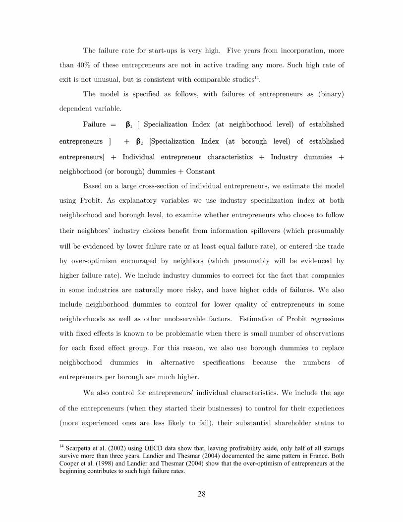
The failure rate for start-ups is very high. Five years from incorporation, more

than 40% of these entrepreneurs are not in active trading any more. Such high rate of

exit is not unusual, but is consistent with comparable studies14.

The model is specified as follows, with failures of entrepreneurs as (binary)

dependent variable.

Failure = β1 [ Specialization Index (at neighborhood level) of established

entrepreneurs ] + β2 [Specialization Index (at borough level) of established

entrepreneurs] + Individual entrepreneur characteristics + Industry dummies +

neighborhood (or borough) dummies + Constant

Based on a large cross-section of individual entrepreneurs, we estimate the model

using Probit. As explanatory variables we use industry specialization index at both

neighborhood and borough level, to examine whether entrepreneurs who choose to follow

their neighbors’ industry choices benefit from information spillovers (which presumably

will be evidenced by lower failure rate or at least equal failure rate), or entered the trade

by over-optimism encouraged by neighbors (which presumably will be evidenced by

higher failure rate). We include industry dummies to correct for the fact that companies

in some industries are naturally more risky, and have higher odds of failures. We also

include neighborhood dummies to control for lower quality of entrepreneurs in some

neighborhoods as well as other unobservable factors. Estimation of Probit regressions

with fixed effects is known to be problematic when there is small number of observations

for each fixed effect group. For this reason, we also use borough dummies to replace

neighborhood dummies in alternative specifications because the numbers of

entrepreneurs per borough are much higher.

We also control for entrepreneurs’ individual characteristics. We include the age

of the entrepreneurs (when they started their businesses) to control for their experiences

(more experienced ones are less likely to fail), their substantial shareholder status to

14 Scarpetta et al. (2002) using OECD data show that, leaving profitability aside, only half of all startups survive more than three years. Landier and Thesmar (2004) documented the same pattern in France. Both Cooper et al. (1998) and Landier and Thesmar (2004) show that the over-optimism of entrepreneurs at the beginning contributes to such high failure rates.

29

control for agency problems (entrepreneurs with small shares may act like employees and

prefer less risky projects), and their genders to control for differences of risk-aversion

(females are more risk averse and may pick less risky projects). The standard errors we

report are also robust for potential clustering of residuals at firm level, as many firms

have more than one entrepreneur from the same neighborhoods.

[insert Table 7 about here]

In Column (1) of Table 7, we control for neighborhood fixed effects, while in

Column (2) we control for borough fixed effects. The results do not favor the

agglomeration economy hypothesis, which should be reflected by a negative coefficient

value of β1. Entrepreneurs starting businesses in their neighbors’ popular sectors do not

have lower odds of failures. One reason we do not find imitators doing better could be

that: When there are something wrong with a company, new directors from where this

industry is overrepresented (and presumably who are equipped with better industry

expertise according to agglomeration economy theory) may join as “fire fighters”, and

this would offset the negative correlation between industry specialization and odds of

failure. To address this concern we use a sub-group of entrepreneurs who were appointed

as directors within half a year since the companies’ incorporations. They are more likely

to be “founders” than “fire fighters”. In Column (3) and (4), we run regressions for

“founders” who incorporate their companies during year 2000, controlling for

neighborhood and borough fixed effects respectively. We still do not find any significant

relationship between specialization and failure rates.

Although entrepreneurs who imitate their neighbors do not have lower failure

rates, they do not do significantly worse either. If we assume that (1) industry talents

are distributed similarly in populations of different neighborhoods; and (2) entrepreneurs

of lower quality (in terms of match of talents with industry) are also tempted into their

neighborhoods’ popular industries as a result of social interactions, then the fact that the

average failure rates do not significantly go up may suggest that agglomeration

economies are working in the opposite direction to offset the negative effects. This

30

indicates that social interactions promote entry in a neighborhood’s traditional specialty

without causing higher failure rates. In the future, we can shed more light on this

research question by controlling for observable quality of individual entrepreneurs. For

instance, we can control for individual-specific characteristics by using a special sub-

group of entrepreneurs who used to start more than two businesses in different

industries.

Overall, the results suggest that entry of new entrepreneurs tend to reinforce

agglomeration, while failures do not change the geographic concentration. This is in

contrast to Dumais et al. (2002)’s study on the dynamic process of geographic

concentration based on business addresses. Using U.S. manufacturing industries data,

they show that location choices of new firms play a de-agglomerating role, whereas plant

closures have tended to reinforce agglomeration. The two findings however are not

conflicting. When it comes to choosing locations to set up businesses, agglomeration

always results in rising costs for new entrants due to limited supply of commercial sites,

and entrepreneurs would have incentive to locate their businesses in new places. When it

comes to making decisions merely regarding which industries to enter, however,

entrepreneurs can choose any industries (e.g., industries that their neighbors specialize

in) without competing for resources with neighbors, because there are no known

constraints on how many people living in a residential neighborhood can enter certain

industries, so long as they do not go to the same places.

7. Conclusions

Why do entrepreneurs from certain neighborhoods consistently dominate certain

industries? In this paper, utilizing separations of home and business addresses, we find

evidences in support of social interactions’ impacts on entrepreneurs’ industry choices.

Based on a cross-section of neighborhood-industry pairs, we find that, new entrepreneurs

are more likely to enter their residential neighbors’ popular industries. This persistence of

industry specialization is stronger in neighborhoods with more intensive social

31

interactions, and stronger in industries which are more agglomerated geographically.

This effect is not likely to be driven by product market factors, as we are examining the

residential addresses but not business addresses of the entrepreneurs, and the two

addresses are generally distant from each other. We are able to identify the causality

because residential addresses only determine social interactions but do not directly affect

industry choices. Finally, we admit that, by aggregating our data from individual level

to neighborhood level, we remain somewhat agnostic as to the actual mechanism linking

neighborhoods to individual outcomes. Alternative strategies, especially those that allow

causal inferences to be drawn about particular channels and for broader populations,

have the potential to increase our understanding of the impact of neighborhoods on

individual outcomes.

32

References

Bayer, Patrick; Stephen L. Ross; Giorgio Topa. 2004. Place of Work and Place of

Residence: Informal Hiring Networks and Labor Market Outcomes. Working

Paper

Bentolila, Samuel; Claudio Michelacci; Javier Suarez. 2004. Social contacts and

occupational choice. Working Paper, CEMFI

Bernheim, B. Douglas (1994), A Theory of Conformity, The Journal of Political

Economy 102, 841-877.

Bertrand, Marianne; Sendhil Mullainathan and Erzo Luttmer. 2000. Network Effects and

Welfare Cultures, The Quarterly Journal of Economics, August

Brock, William A. and Steven N. Durlauf. 2003. Multinomial Choice with Social

Interactions. NBER technical Working Paper No. 288.

Brock, William A. and Steven N. Durlauf. 2001. Interactions-based model. In Handbook

of Econometrics, Volume 5, Chapter 54, pp. 3297-3380, Edited by J.J. Heckman

and E. Leamer, Elsevier Science B.V., 2001.

Cole, Harold L., George J. Mailath, and Andrew Postlewaite 1992. Social Norms, Saving

Behavior, and Growth, The ournal of Political Economy Vol. 100, 1092-1125.

Conley, Timothy G; Giorgio Topa. 2002. Socio-economic distance and spatial patterns

in unemployment. Journal of Applied Econometrics. Vol. 17: 303-327

Connerly, Charles E. 1985. The neighborhood question: an extension of Wellman and

Leighton. Urban Affairs Quarterly. Vol.20: 537-556

Cooper, Arnold C., Carolyn Y. Woo, and William C. Dunkelberg. 1988. Entrepreneurs’ perceived chances of success. Journal of Business Venturing 3: 97-108

Corcoran, M., L. Datcher and G. Duncan. 1980. ”Information and Influence Networks in

Labor Market” in G. Duncan and J. Morgan (eds.) Five Thousand American

Families: Patterns of Economic Progress. Vol. 7, 1-37.

Dumais, Guy; Glenn Ellison; Edward L. Glaeser. 2002. Geographic concentration as a

dynamic process. The Review of Economics and Statistics. May: 193-204

Durlauf, Steven N. 2003. Neighborhood Effects. In Handbook of Regional and Urban

Economics. Volumn 4, Economics, J.V. Henderson and J.-F. Thisse, eds.

Ellison, Glenn; Edward L. Glaeser. 1997. Geographic concentration in U.S.:

manufacturing industries: a dartboard approach. Journal of Political Economy.

Vol. 105(5)

Feng, Lei and Mark S. Seasholes, 2004, ”Correlated Trading and Location,” Journal of

Finance, LIX, 5, October, 2117-2144.

Gamble, Keith. 2003. Word-of-Mouth Influence on the Stock Holdings of Individual

Investors. Working Paper, UC Berkeley

33

Giannetti, Mariassunta and Andrei Simonov. 2004. Social interactions and

entrepreneurial activities. Working paper, Stockholm School of Economics.

Glaeser, Edward L.; Hedi D. Kallal; Jose A. Scheinkman; Andrei Shleifer. 1992. Growth

in cities. The Journal of Political Economy. Vol. 100. No. 6.

Glaeser, Edward L.; Bruce I. Sacerdote and Jose A. Scheinkman. 1996. Crime and social

interactions. Quarterly Journal of Economics. May

Glaesser, Edward L. and Bruce I. Sacerdote. 2000. The Social Consequences of Housing.

Journal of Housing Economics. Vol. 9

Gordon, Ian R. and Philip McCann. 2000. Industrial clusters: complexes, agglomeration

and /or social networks? Urban Studies. Vol. 37 (3): 513-532

Granovetter, Mark 1995. Getting a Job: a Study on Contacts and Careers (2nd

Ed).Chicago, Chicago University Press.

Grinblatt, Mark; Matti Keloharju; Seppo Ikaheimo. 2004. Interpersonal effects in

consumption: evidence from the automobile purchase of neighbors. Working

Paper. Helsinki School of Economics.

Guest, Avery M. and Barrett A. Lee. 1983. The social organization of local areas. Urban

Affairs Quarterly. Vol. 19-217-240

Hamilton, Barton H. 2000. Does entrepreneurship pay? An empirical analysis of the

returns to self-employment. Journal of Political Economy. Vol. 108: 604-631

Henderson, Vernon; Ari Kuncoro; Matt Turner. . 1995. Industrial Development in Cities.

Journal of Poltiical Economy. Vol. 105. No. 5

Hong, Harrsion; Jeffrey D. Kubik and Jeremy C. Stein. 2005. “Thy Neighbor’s Portfolio:

Word-of-Mouth Effects in the Holdings and Trades of Money Managers,” Journal

of Finance, forthcoming.

Hunter, Albert. 1974. Symbolic neighborhoods: the persistence and change of Chicago’s local neighborhoods. The University of Chicago Press: Chicago

Ioannides, Yannis M. and Datcher Loury. 2004. Job information networks, neighborhood

effects and inequality. Journal of Economic Literature. Vo. 42(4)

Jacob, Jane. 1969. The Economy of Cities. New York: Vintag

Jencks, Christopher and Susan Mayer. 1990. ”The Social Consequences of Growing Up

in a Poor Neighborhood.” In Laurence Lynn, Jr., and Michael G.H. McGeary

(eds) Inner City Poverty in the United States. Oxford: University Press.

Landier, Augustin, and David Thesmar. 2004. Financial contracting with optimistic

entrepeneurs: theory and evidence. NYU Stern working paper

Manski, Charles F. 2000. Economic Analysis of Social Interactions. Journal of Economic

Perspective. Vol. 14, No. 3, pp. 115-136.

Marsden Peter V. 1988. Homogeneity in confiding relations. Social Networks. Vol. 10:

57-76

34

Montgomery, James D. 1991. Social Network and labor-market outcomes: toward an

economic analysis. The American Economic Review Vol. 81(5)

Moskowitz, Tobias J. and Annette Vissing-Jorgensen. 2002. The private equity premium

puzzle. American Economic Review. Vol. 92: 745-778

Rosenthal, Stuart S. and William C. Strange. 2005. The geography of entrepreneurship

in the New York Metropolitan Area. Working Paper, Syracuse University and

University of Toronto

Rosenthal, Stuart S. 2001. The determinants of agglomeration. Journal of Urban

Economics. Vol. 50: 191-229

Sacerdote, Bruce I. 2001. Peer effects with random assignment: results for Dartmouth

roommates. Quarterly Journal of Economics. May

Sampson, Robert J.; Stephen W. Raudenbush; Felton Earls. 2003. Neighborhoods and

violent crime: a multilevel study of collective efficacy. Science. Vol. 277: 918-24

Scarpetta, Stefano, Philip Hemmings, Thierry Tressel, and Jaejoon Woo. 2002. The role

of policy and institutions for productivity and firm dynamics: evidence from

micro and industry data. OECD paper.

Shiller, Robert J. 2000. Irrational Exuberance. Broadway Books: New York

Topa, Giorgio; 2001. Social interactions, local spillovers and unemployment. Review of

Economic Studies. Vol. 68: 261-95

Wellman, Barru 1996. Are personal neighborhoods local? A dumptarian reconsideration.

Social Networks. Vol. 18: 347-354

Wilson, William J. 1987. The truly disadvantaged: the inner city, the underclass, and

public policy (Chicago: University of Chicago Press)

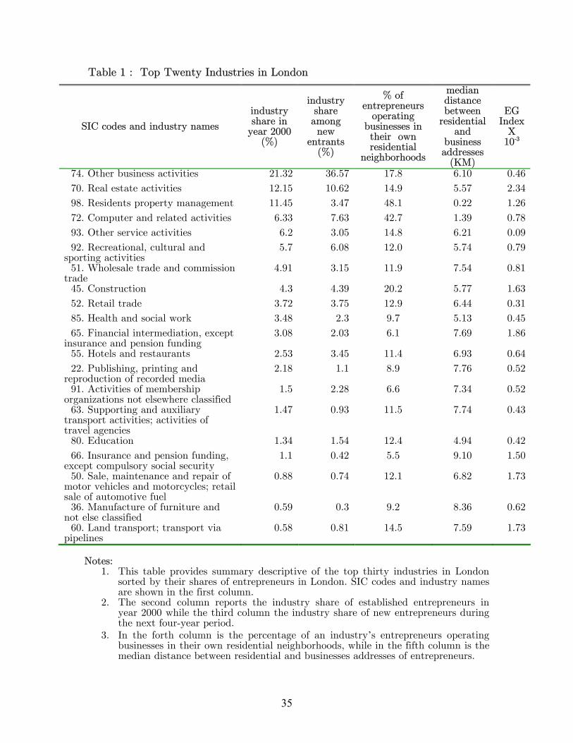
35

Table 1 : Top Twenty Industries in London

SIC codes and industry names

industry share in

year 2000 (%)

industry share among new

entrants (%)

% of entrepreneurs

operating businesses in their own residential

neighborhoods

median distance between

residential and

business addresses

(KM)

EG Index

X 10-3

74. Other business activities 21.32 36.57 17.8 6.10 0.46

70. Real estate activities 12.15 10.62 14.9 5.57 2.34

98. Residents property management 11.45 3.47 48.1 0.22 1.26

72. Computer and related activities 6.33 7.63 42.7 1.39 0.78

93. Other service activities 6.2 3.05 14.8 6.21 0.09

92. Recreational, cultural and sporting activities

5.7 6.08 12.0 5.74 0.79

51. Wholesale trade and commission trade

4.91 3.15 11.9 7.54 0.81

45. Construction 4.3 4.39 20.2 5.77 1.63

52. Retail trade 3.72 3.75 12.9 6.44 0.31

85. Health and social work 3.48 2.3 9.7 5.13 0.45

65. Financial intermediation, except insurance and pension funding

3.08 2.03 6.1 7.69 1.86

55. Hotels and restaurants 2.53 3.45 11.4 6.93 0.64

22. Publishing, printing and reproduction of recorded media

2.18 1.1 8.9 7.76 0.52

91. Activities of membership organizations not elsewhere classified

1.5 2.28 6.6 7.34 0.52

63. Supporting and auxiliary transport activities; activities of travel agencies

1.47 0.93 11.5 7.74 0.43

80. Education 1.34 1.54 12.4 4.94 0.42

66. Insurance and pension funding, except compulsory social security

1.1 0.42 5.5 9.10 1.50

50. Sale, maintenance and repair of motor vehicles and motorcycles; retail sale of automotive fuel

0.88 0.74 12.1 6.82 1.73

36. Manufacture of furniture and not else classified

0.59 0.3 9.2 8.36 0.62

60. Land transport; transport via pipelines

0.58 0.81 14.5 7.59 1.73

Notes:

1. This table provides summary descriptive of the top thirty industries in London sorted by their shares of entrepreneurs in London. SIC codes and industry names are shown in the first column.

2. The second column reports the industry share of established entrepreneurs in year 2000 while the third column the industry share of new entrepreneurs during the next four-year period.

3. In the forth column is the percentage of an industry’s entrepreneurs operating businesses in their own residential neighborhoods, while in the fifth column is the median distance between residential and businesses addresses of entrepreneurs.

36

4. The sixth column reports the Ellison-Glaeser index for each industry, scaled by 10-3. Higher values of this index indicate higher geographic agglomeration of entrepreneurs.

37

Table 2 : Specializations of the top thirty most entrepreneurial neighborhoods Neighborhoods First Specialty Second Specialty Third Specialty

Garden Suburb Real Estate Wholesale Trade Financial Intermediation

Edgware Other Business Activities Wholesale Trade Retail Trade

Frognal and Fitzjohns Real Estate Financial Intermediation Property Management

Knightsbridge and

Belgravia

Financial Intermediation Real Estate Insurance and pension

Abbey Road Real Estate Financial Intermediation Wholesale Trade

Hampstead Town Real Estate Recreational and Cultural Financial Intermediation

Finchley Church End Real Estate Wholesale Trade Manufacture

Holland Financial Intermediation Real Estate Supporting Transport

Totteridge Wholesale Trade Real Estate Manufacture

Childs Hill Real Estate Wholesale Trade Health and Social Work

Village Financial Intermediation Insurance and pension Education

Swiss Cottage Real Estate Property Management Financial Intermediation

Hendon Real Estate Wholesale Trade Manufacture

Regent’s Park Real Estate Wholesale Trade Financial Intermediation

Golders Green Real Estate Wholesale Trade Manufacture

Queen’s Gate Financial Intermediation Insurance and pension Hotels and Restaurants

Stanmore Park Real Estate Wholesale Trade Retail Trade

Little Venice Property Management Recreational and Cultural Supporting Transport

Brompton Financial Intermediation Hotels and Restaurants Retail Trade

Highgate Real Estate Financial Intermediation Property Management

Belsize Property Management Real Estate Recreational and Cultural

Cockfosters Wholesale Trade Insurance and pension Sales of Motor Vehicle

Mill Hill Wholesale Trade Real Estate Retail Trade

Marylebone High

Street

Real Estate Recreational and Cultural Hotels and Restaurants

West End Real Estate Financial Intermediation Hotels and Restaurants

Campden Financial Intermediation Insurance and pension Supporting Transport

Hyde Park Hotels and Restaurants Real Estate Publishing and Printing

Royal Hospital Financial Intermediation Insurance and pension Real Estate

Chislehurst Insurance and pension Sales of Motor Vehicle Construction

Hans Town Insurance and pension Financial Intermediation Real Estate

Note: This table reports the industry specializations of the top thirty most entrepreneurial neighborhoods in London. Neighborhood names are shown in the first column. In the second, third, and forth column we report the top three specialist industries of each neighborhood based on the “industry specialization index” we calculate.

38

Table 3: Persistence of industry specializations over time Dependent variable: industry specialization index of new entrepreneurs Unit of analysis: neighborhood-industry pair “industry

specialization” at neighborhood level

“industry specialization” at borough level

Pseudo R2 Obs.

(1) All 633 neighborhoods 0.053 1.220 0.00 37,980 (0.014)*** (0.061)*** (2) 0.058 1.182 0.00 36,000

Top 600 neighborhoods (0.015)*** (0.063)***

(3) 0.236 0.725 0.03 18,357

Top thirty industries (0.013)*** (0.028)***

(4) 0.318 0.513 0.07 12,660

Top twenty industries (0.012)*** (0.023)***

(5) 0.356 0.469 0.07 12,000 (0.012)*** (0.022)***

Top 20 Ind. / Top 600 Neighborhoods [0.023]*** [0.038]***

Bootstrapping adjusted standard errors are reported in brackets

(6) 0.329 0.440 0.20 12,000 (0.020)*** (0.031)***

OLS, robust to clustering by neighborhoods [0.022]*** [0.036]***

Standard errors robust to potential clustering of residuals at neighborhood level are reported in brackets

Notes: 1. The regression is specified as follows and estimated with Tobit unless otherwise indicated: Specialization (at neighborhood level) of new entrepreneurs = β1 [ Specialization (at neighborhood level) of established entrepreneurs ] + β2 [Specialization (at borough level) of established entrepreneurs] + Constant 2. The regressions are based on a cross section of neighborhood-industry pairs. On the left hand side is the neighborhood c’s specialization index in industry i of new entrepreneurs entering businesses between 2000 and 2004. On the right hand side we have two independent variables regarding the industry specializations of established entrepreneurs in year 2000. One variable is neighborhood c’s specialization index in industry i, while the other is borough b’s specialization in industry i, both are based on the established entrepreneurs in year 2000. 3. We present results based on varied sub-samples, to address the problem that industry specializations are estimated with large errors when there are too few entrepreneurs in a certain neighborhood or in a certain industry. Our full sample is consisted of 633 neighborhoods and 60 industries. Our main sample however is only consisted of 600 neighborhoods and 20 industries. This nevertheless does not affect our results. Top 600 neighborhoods already account fro 99% of the entrepreneurs, while top 20 industries account for 95%. Cut-off points for “top” neighborhoods and industries: Top 30 industries: >=595 entrepreneurs, Top 20 industries: >=1931 entrepreneurs, Top 600 neighborhoods: >=91 entrepreneurs.

39

4. In Row (5), bootstrapping (cluster by neighborhoods) adjusted standard errors are reported in brackets. 5. In Row (6), regression is estimated by OLS, with un-adjusted standard errors reported in parentheses. Standard errors robust to clustering by neighborhoods are reported in brackets

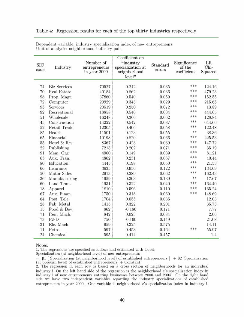
40

Table 4: Regression results for each of the top thirty industries respectively Dependent variable: industry specialization index of new entrepreneurs Unit of analysis: neighborhood-industry pair

SIC code Industry

Number of entrepreneurs in year 2000

Coefficient on “industry

specialization at neighborhood

level”

Standard errors

Significance of the

coefficient

LR Chi-

Squared

74 Biz Services 70527 0.242 0.035 *** 124.1670 Real Estate 40184 0.862 0.036 *** 479.2398 Prop. Magt. 37860 0.540 0.059 *** 152.5572 Computer 20929 0.343 0.029 *** 215.6593 Services 20519 0.250 0.072 *** 13.8992 Recreational 18858 0.546 0.034 *** 444.6551 Wholesale 16248 0.366 0.062 *** 128.8445 Construction 14222 0.542 0.037 *** 644.6652 Retail Trade 12305 0.406 0.058 *** 122.4885 Health 11501 0.123 0.055 ** 38.3665 Financial 10198 0.820 0.066 *** 225.5355 Hotel & Res 8367 0.423 0.039 *** 147.7222 Publishing 7215 0.202 0.071 *** 35.1991 Mem. Org. 4960 0.149 0.039 *** 81.2163 Aux. Tran. 4862 0.231 0.067 *** 40.4480 Education 4445 0.198 0.050 *** 21.5366 Insurance 3635 0.956 0.122 *** 134.6950 Motor Sales 2913 0.289 0.062 *** 162.4336 Manufacturing 1959 0.303 0.139 ** 17.6760 Land Tran. 1931 0.322 0.040 *** 164.4018 Apparel 1810 0.596 0.110 *** 135.2467 Aux. Finan. 1750 0.318 0.060 *** 148.6964 Post. Tele. 1704 0.055 0.036 12.0328 Fab. Metal 1415 0.322 0.201 35.7315 Food & Bev. 862 -0.186 0.171 7.7771 Rent Mach. 842 0.023 0.084 2.0673 R&D 750 -0.160 0.149 21.0831 Ele. Mach. 659 0.325 0.575 14.1111 Petro. 597 0.453 0.164 *** 55.9724 Chemical 595 0.414 0.457 1.4

Notes: 1. The regressions are specified as follows and estimated with Tobit: Specialization (at neighborhood level) of new entrepreneurs = β1 [ Specialization (at neighborhood level) of established entrepreneurs ] + β2 [Specialization (at borough level) of established entrepreneurs] + Constant 2. The regression in each row is based on a cross section of neighborhoods for an individual industry i. On the left hand side of the regression is the neighborhood c’s specialization index in industry i of new entrepreneurs entering businesses between 2000 and 2004. On the right hand side we have two independent variables regarding the industry specializations of established entrepreneurs in year 2000. One variable is neighborhood c’s specialization index in industry i,

41

while the other is borough b’s specialization in industry i, both are based on the established entrepreneurs in year 2000. For the brevity of presentation, we do not report in the table the coefficients on “borough industry specialization index”. 3. There are 600 neighborhoods in the sample. We run regressions for all the 60 industries but only report the results of the top thirty industries. We do not find significant results in the smaller industries. The SIC codes and abbreviation names for the industries are displayed in the first and second column. 4. *** indicates that the coefficients on “industry specialization index” is significantly different from zero at 1% level, ** denotes 5%, * denotes 10%

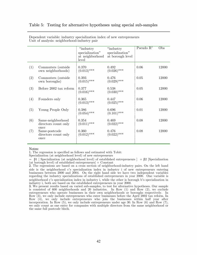
42

Table 5: Testing for alternative hypotheses using special sub-samples Dependent variable: industry specialization index of new entrepreneurs Unit of analysis: neighborhood-industry pair “industry

specialization” at neighborhood level

“industry specialization” at borough level

Pseudo R2 Obs

(1) 0.370 0.492 0.06 12000 (0.013)*** (0.026)***

Commuters (outside own neighborhoods)

(2) 0.393 0.476 0.05 12000 (0.015)*** (0.029)***

Commuters (outside own boroughs)

(3) Before 2002 tax reform 0.377 0.538 0.05 12000 (0.016)*** (0.030)*** (4) Founders only 0.365 0.447 0.06 12000 (0.013)*** (0.025)*** (5) Young People Only 0.386 0.696 0.01 12000 (0.054)*** (0.101)*** (6) 0.354 0.469 0.08 12000 (0.011)*** (0.022)***

Same-neighborhood directors count only once

(7) 0.360 0.476 0.08 12000 (0.012)*** (0.022)***

Same-postcode directors count only once

Notes: 1. The regression is specified as follows and estimated with Tobit: Specialization (at neighborhood level) of new entrepreneurs = β1 [ Specialization (at neighborhood level) of established entrepreneurs ] + β2 [Specialization (at borough level) of established entrepreneurs] + Constant 2. The regressions are based on a cross section of neighborhood-industry pairs. On the left hand side is the neighborhood c’s specialization index in industry i of new entrepreneurs entering businesses between 2000 and 2004. On the right hand side we have two independent variables regarding the industry specializations of established entrepreneurs in year 2000. One variable is neighborhood c’s specialization index in industry i, while the other is borough b’s specialization in industry i, both are based on the established entrepreneurs in year 2000. 3. We present results based on varied sub-samples, to test for alternative hypotheses. Our sample is consisted of 600 neighborhoods and 20 industries. In Row (1) and Row (2), we exclude entrepreneurs who operate businesses in their own neighborhoods or boroughs respectively. In Row (3), we only include entrepreneurs who enter businesses before the April 2002 tax reform. In Row (4), we only include entrepreneurs who join the businesses within half year after incorporation. In Row (5), we only include entrepreneurs under age 30. In Row (6) and Row (7), we only count as one entry for companies with multiple directors from the same neighborhood or the same full postcode block.

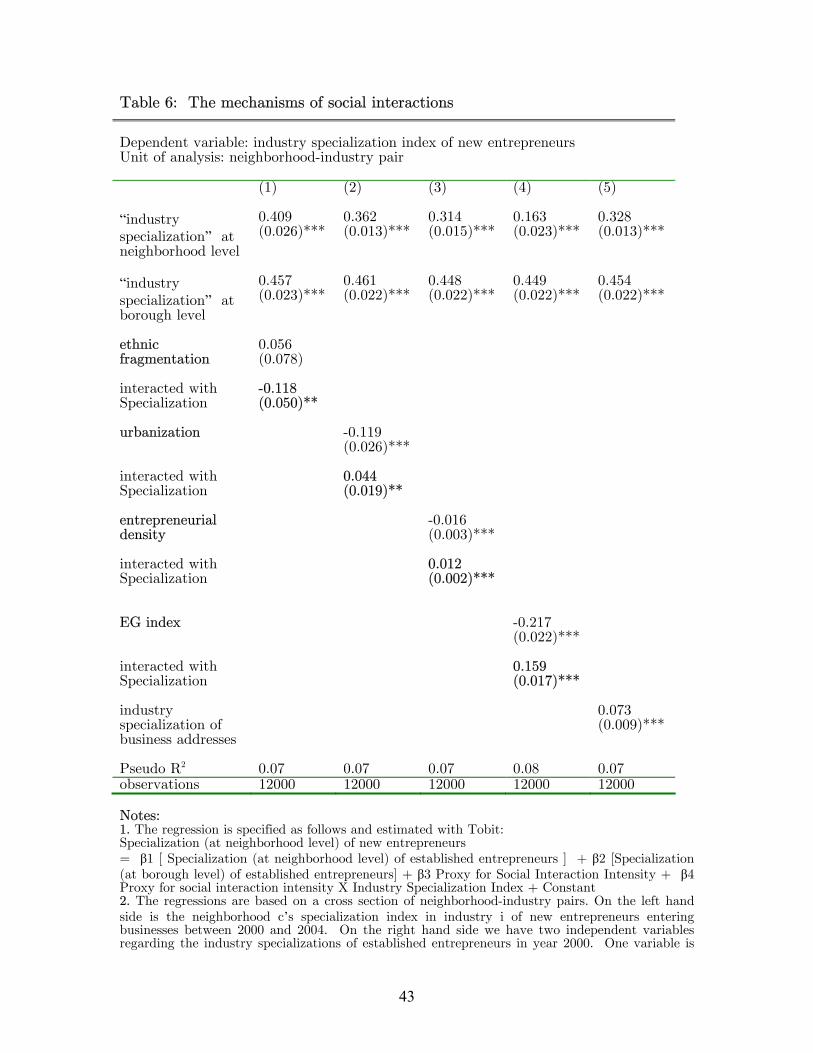
43

Table 6: The mechanisms of social interactions

Dependent variable: industry specialization index of new entrepreneurs Unit of analysis: neighborhood-industry pair (1) (2) (3) (4) (5)

0.409 0.362 0.314 0.163 0.328 (0.026)*** (0.013)*** (0.015)*** (0.023)*** (0.013)***

“industry specialization” at neighborhood level

0.457 0.461 0.448 0.449 0.454 (0.023)*** (0.022)*** (0.022)*** (0.022)*** (0.022)***

“industry specialization” at borough level

0.056 ethnic

fragmentation (0.078)

-0.118 (0.050)**

interacted with Specialization

urbanization -0.119 (0.026)***

0.044 (0.019)**

interacted with Specialization

-0.016 entrepreneurial

density (0.003)***

0.012 (0.002)***

interacted with Specialization

EG index -0.217 (0.022)***

0.159 (0.017)***

interacted with Specialization

0.073 (0.009)***

industry specialization of business addresses Pseudo R2 0.07 0.07 0.07 0.08 0.07 observations 12000 12000 12000 12000 12000 Notes: 1. The regression is specified as follows and estimated with Tobit: Specialization (at neighborhood level) of new entrepreneurs = β1 [ Specialization (at neighborhood level) of established entrepreneurs ] + β2 [Specialization (at borough level) of established entrepreneurs] + β3 Proxy for Social Interaction Intensity + β4 Proxy for social interaction intensity X Industry Specialization Index + Constant 2. The regressions are based on a cross section of neighborhood-industry pairs. On the left hand side is the neighborhood c’s specialization index in industry i of new entrepreneurs entering businesses between 2000 and 2004. On the right hand side we have two independent variables regarding the industry specializations of established entrepreneurs in year 2000. One variable is

44

neighborhood c’s specialization index in industry i, while the other is borough b’s specialization in industry i, both are based on the established entrepreneurs in year 2000. 3. In Column (1), we test whether persistence of industry specialization is stronger in neighborhoods with more homogeneous ethnic composition, by including on the right hand side of the regression the ethnic fragmentation index of a neighborhood as well as its interaction term with “industry specialization index” of the established entrepreneurs. In Column (2), we instead use housing structure as a proxy for intensity of social interactions. In Column (3), we test whether persistence is stronger in neighborhoods with higher entrepreneurial population density. In Column (4), we test whether persistence is stronger in industries which are more agglomerated geographically. In Column (5), we control for industry specialization based on business addresses.

45

Table 7: Determinants of entrepreneurs’ failures.

Dependent variable: an entrepreneur’s failure Unit of analysis: entrepreneur (1) (2) (3) (4) Full Sample Founders only Fixed Effects Neighborho

od Borough Neighborho

od Borough

Industry Specialization 0.002 0.017 -0.020 0.028 (at neighborhood level) (0.017) (0.016) (0.020) (0.017) Industry Specialization -0.008 -0.035 0.033 -0.050 (at borough level) (0.031) (0.030) (0.034) (0.032) Log of Ages -0.445 -0.451 -0.702 -0.531 (0.030)*** (0.030)*** (0.037)*** (0.034)*** Substantial Shareholder 0.450 0.452 0.827 0.407 (0.017)*** (0.017)*** (0.021)*** (0.018)*** Male 0.022 0.028 -0.015 0.026 (0.017) (0.017) (0.020) (0.019) Industry Fixed-Effects Y Y Y Y Location Fixed-Effects Y Y Y Y Pseudo R2 0.102 0.083 0.150 0.078 Obs. 49149 49171 35904 36405

Notes: 1. The regression is specified as follows and estimated with Probit: Failure = β1 [ Specialization (at neighborhood level) of established entrepreneurs ] + β2 [Specialization (at borough level) of established entrepreneurs] + individual entrepreneur characteristics + industry dummies + neighborhood (or borough) dummies + Constant 2. The regressions are based on a cross section of entrepreneurs who start their businesses during year 2000. On the left hand side is a binary variable with 1 indicating that the entrepreneur is out of business. On the right hand side we have two independent variables regarding industry specializations of established entrepreneurs in year 2000, as well as entrepreneur’s individual characteristics. Regarding industry specialization, one independent variable is neighborhood c’s specialization index in industry i, while the other is borough b’s specialization in industry i, both are based on the established entrepreneurs in year 200. Individual characteristics include age, shareholder status and gender. 3. In all regressions, we control for industry fixed-effects. In the meantime, in Column (1) and (3), we control for neighborhood fixed-effects, while in Column (2) and (4), we control for borough fixed-effects. 4. Standard errors are robust for clustering of entrepreneurs around firms

46

Figure 1: Maps of Greater London and Inner London

Borough boundaries (Greater London)

Ward Boundaries (Inner London only)

.

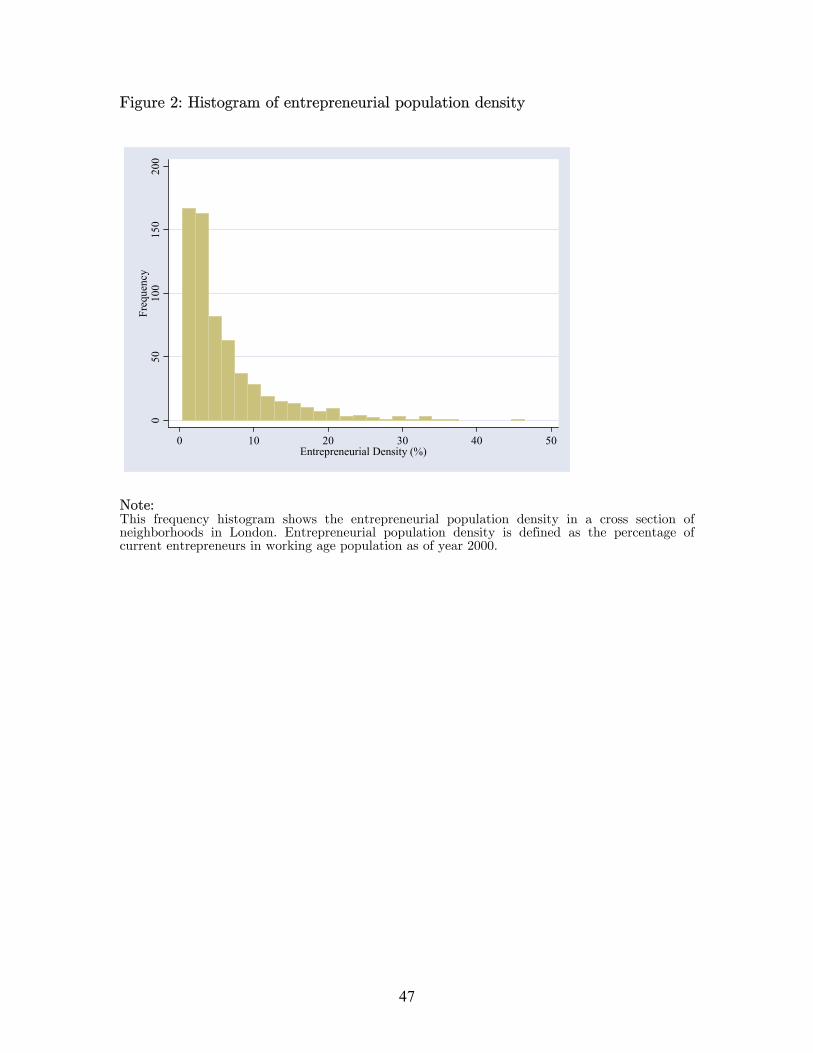
47

Figure 2: Histogram of entrepreneurial population density

050

100

150

200

Freq

uenc

y

0 10 20 30 40 50Entrepreneurial Density (%)

Note: This frequency histogram shows the entrepreneurial population density in a cross section of neighborhoods in London. Entrepreneurial population density is defined as the percentage of current entrepreneurs in working age population as of year 2000.

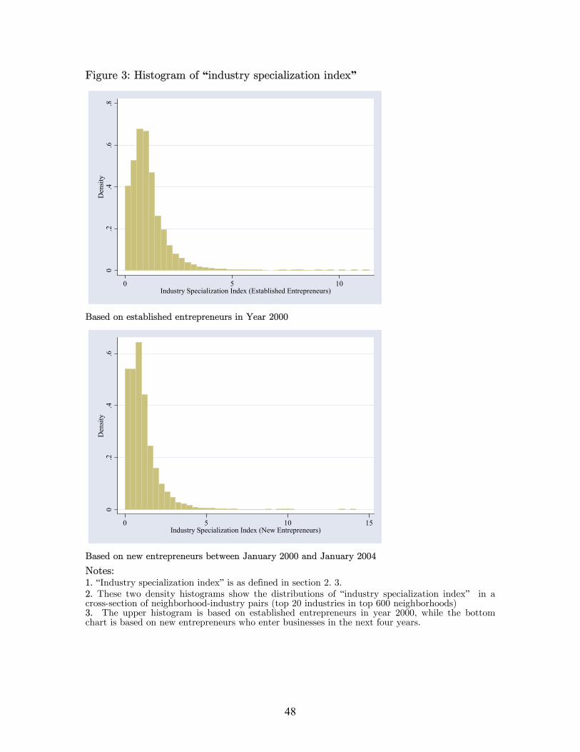
48

Figure 3: Histogram of “industry specialization index”

0.2

.4.6

.8D

ensit

y

0 5 10Industry Specialization Index (Established Entrepreneurs)

Based on established entrepreneurs in Year 2000

0.2

.4.6

Den

sity

0 5 10 15Industry Specialization Index (New Entrepreneurs)

Based on new entrepreneurs between January 2000 and January 2004

Notes: 1. “Industry specialization index” is as defined in section 2. 3. 2. These two density histograms show the distributions of “industry specialization index” in a cross-section of neighborhood-industry pairs (top 20 industries in top 600 neighborhoods) 3. The upper histogram is based on established entrepreneurs in year 2000, while the bottom chart is based on new entrepreneurs who enter businesses in the next four years.