Journal of Mathematical Economics 12 (1983) 103-118. North Holland

INEQUALITIES FOR THE GINI COEFFICIENT OF COMPOSITE POPULATIONS

Don ZAGIER

University of Bonn, 53 Bonn, West Germany

University of Maryland, College Park, MD 20742, USA

Received August 1981, revised version accepted November 1982

Unlike other popular measures of income inequality, the Gini coefficient is not decomposable, i.e., the coefficient G(Z) of a composite population %=!X^,u...uX, cannot be computed in terms of the sizes, mean incomes and Gini coefficients of the components Xi. In this paper upper and lower bounds (best possible for r=2) for G(T) in terms of these data are given. For example, G(ZI u . u a,) 2 1 ai G(.%Yi), where ai is the proportion of the population in Ti. One of the tools used, which may be of interest for other applications, is a lower bound for 1; f (x)g(x)dx (converse to Cauchy’s inequality) for monotone decreasing functions ,f and g.

1. Introduction

A very frequently used measure of the inequality of incomes in a

popuiation X is the Gini coejjkient,

G(X) = kitI jz, Ixidxjl*

(Here and in what follows we fix the following conventions: n denotes the

size of X, x1,..., x, are non-negative real numbers representing the individual

incomes, and X = XI= 1 xi and ,LJ = X/n are the total and mean incomes of the population, respectively.) In many situations, the population X is the union of several population groups X1,. . . , X‘, (e.g. male and female wage earners,

or the members of various racial or social groups) and one would like to know how much of the inequality of income distribution in X is due to the inequality within the separate groups Xi and how much to the disparateness of income between the groups. Such information might, for instance, be useful in gauging the effectiveness of a differentiated tax structure in reducing

‘Note that we are averaging Ixi-xjl over all nz pairs i,j with 1 si, jsn, not only over the n(n- 1)/2 pairs with i<j as is sometimes done.

0304-4068/83/$3.00 0 1983, Elsevier Science Publishers B.V. (North-Holland)

104 D. Zagier, The Gini coeficient of composite populations

inequality. To do this, one would like to know a priori bounds of the form

F,(n,, X,, G,; . . ; a,, X,, G,; Go) 5 G(X)

where F, and F, are universal functions of the sizes ni, total incomes Xi and Gini coefficients Gi of the individual population groups Xi and of the ‘between-group’ Gini coefficient G, (= the Gini coefficient of the hypothetical population X’ obtained from X by having the members of each subpopulation Xi share their incomes equally, so that they all have an income equal to ,U~ =X,/n,). This will describe the range of inequality possible for the composite population X, and then seeing in a given case whether G(X) is in fact closer to F, or F, will give us a feel for the nature of the sources of income inequality in X.

The purpose of this paper is to give such bounds. In section 3 we prove fve ;man,>~l;t;oo n;.r;nn lnnrer hnr,nAr far G(E). ipA oort;r\n A TX,P ohnw h-7 Il‘byu~ull”ir 6”“‘6 I”W”I ““UIIULI citiUCI”II -7 ““U Ull”“” “J

examples that the result of section 3 (i.e., the maximum of the live bounds) is the best possible universal lower bound F, in the case r = 2, and also establish the best possible universal upper bound F, in the same case. The simplest, though not the strongest, of the lower bounds in section 3 is the

elegant convexity property

(2)

which had been discovered experimentally by Sudhir Anand on the basis of

data on the income distribution in Maiaysia jAnand (i9S3)], the groups there being the Malay, Indian and Chinese populations. I would like to thank him for suggesting the problem of proving the inequality (2) and thereby stimulating my interest in the subject of this paper.

Note. This paper is part of the longer paper [Zagier (1982)], the rest of which is devoted to a complete classification of ‘decomposable’ indices of inequality, i.e., indices Z(X) which, as well as certain obviously desirable properties like the ‘Pigou-Dalton condition’ (see below), have the property that Z(X) for a composite population X=X, LJ . . . uX^, is given by an exact formula,

in terms of the sizes, incomes and indices of the component populations and the between-group index I,, where F is a universal function, assumed to be

D. Zagier, The Gini coefficient of composite populations 105

linear in the Ii (OS is I). [An example of such an index is the Theil index

T(x) =(l/n)~(x~/~) log(x,/p).] The classification showed that all such I are in certain respects less attractive measures of inequality than G, so that we are justified in using the popular Gini coefficient even though it is not decomposable. The original version of the paper, with the inequalities for the Gini coefficient and the classification of decomposable indices, was submitted in 1976 to another journal and held up for several years (so-called JET lag). In the meantime, as Professor Atkinson has kindly informed me, the classification theorem, or essentially equivalent results, has been published by Cowell (1980), Bourguignon (1979) and Shorrocks (1980); I have therefore suppressed it in the present paper.

2. Basic properties of the Gini coeffkient

The Gini coefficient is the best-known and most frequently used measure of inequality; its properties have been studied by many authors [Anand (1983, annex A), Atkinson (1970, 1975), David (1968), Fei-Ranis (1974), Gastwirth (1972, 1975), Kendall-Stuart (1963), Pyatt (1976), Rao (1969); for surveys of the literature see Bliimle (1975, 11.1.4), Sen (1973, ch. 2), Theil (1967), von Weizsacker (1967, part I, ch. II)]. In this section we review and re-prove some of its main properties and introduce a function t(t) which will play a basic role in this paper.

There are several equivalent definitions of the Gini coefficient. For

example, using the identity

la-b(=a+b--2min(a,b),

we can rewrite (1) in the form

If we order the incomes xi so that xi 2.. .2x,, then [since min(xi,xj) = x,,,,,(~, jj and there are 2k - 1 pairs (i, j) with max(i, j) = k] (3) becomes

This can be interpreted as saying that the Gini coefficient is based on a utility function which is a weighted sum of the individual income levels, the weight of the ith richest individual being proportional to i [cf. Sen (1973,

P. 3I)l.

106 D. Zagier, The Gini coejkient of composite populations

For very large populations 2E, one often uses a continuous rather than a discrete formalism and describes % by a continuous frequency distribution function f(x), where f(x)dx represents the proportion of the population with income between x and x+dx. Clearly

1 f(xW = 1, $xf(x)dx=p.

In terms of f(x), the eqs. (1) and (3) can be rewritten as

and

G = 1 - f i [ min (x, y)f(x)f(y) dxdy.

(4)

(3’)

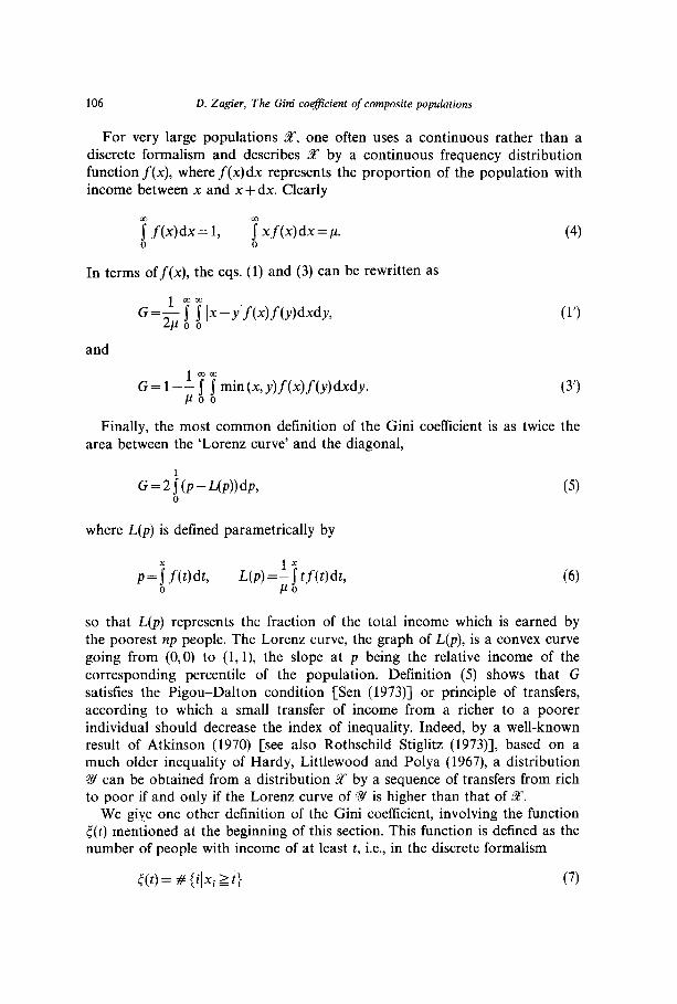
Finally, the most common definition of the Gini coefficient is as twice the area between the ‘Lorenz curve’ and the diagonal,

(5)

where L(p) is defined parametrically by

so that L(p) represents the fraction of the total income which is earned by the poorest np people. The Lorenz curve, the graph of L(p), is a convex curve going from (0,O) to (1, l), the slope at p being the relative income of the

corresponding percentile of the population. Definition (5) shows that G satisfies the Pigou-Dalton condition [Sen (1973)] or principle of transfers,

according to which a small transfer of income from a richer to a poorer individual should decrease the index of inequality. Indeed, by a well-known result of Atkinson (1970) [see also Rothschild-Stiglitz (1973)], based on a much older inequality of Hardy, Littlewood and Polya (1967), a distribution ?Y can be obtained from a distribution X by a sequence of transfers from rich to poor if and only if the Lorenz curve of g is higher than that of 2”‘.

We give one other definition of the Gini coefficient, involving the function c(t) mentioned at the beginning of this section. This function is defined as the number of people with income of at least t, i.e., in the discrete formalism

t(t)= # {ilXi 2t) (7)

D. Zagier, The Gini coejkient of composite populations 107

i 0

P 1

Fig. 1

(a step function), and in the continuous formalism

5(t) = n 7 f(x) dx f

(a differentiable function); it satisfies the properties

8t)20, t monotone decreasing,

W) = 4 i S(t)dt=X=np.

(7’)

(8)

Clearly the function 5 describes the income distribution % completely. WI now find with definition (7)

= [ C(t)‘dt,

108 D. Zagier, The Gini coefficient of composite populations

and similarly with definition (7’)

[ [ min (x, Af’(x)f(y)dxdy = [ g f(x) dx 9 f(y) dydt

Combining this with (3) or (3’) gives

G=l-$$(t)‘dl (9)

in both cases. This is the definition of G which will prove to be the most useful one for studying its decomposition properties. As a first application we give a short proof of the equivalence of formula (5) with the other definitions of the Gini coeffkient: using (7’) and the parametrization (6) of the Lorenz curve we find

2j(p-L(p))dp=1-2y Li f(t)dt f(x)dx 0 .Lot >

=1+-2&“(r)dl)d~(x)

= 1-;[ @x)xf(x) dx

(integration by parts)

=I-$$(x)‘dx

(integration by parts again), and this equals G by eq. (9).

With a similar calculation, one sees that the inequality index 2s: (1 -p) x (p-L(p))dp proposed by Mehran (1976) equals l- l/(n3p)Jr c(t)3dt [or, equivalently, 1 - l/(n3p)Ci, j,k min(xi, xjr xk)].

D. Zagier, The Gini coefficient of composite populations 109

3. Lower bounds for the Gini coeffkient of a many-component population

As in the introduction, consider a population X divided into Y smaller

groups X’i (i = 1,. . . , r),

x=x%^,u...vxr, (10)

and denote by ni, Xi and pi the size, total income and mean income of Xi, respectively. Thus

(11)

We are interested in relating the Gini coefficient of X to the Gini coefficients G(Xi) of the various population groups Xi and to the ‘between-group index’ G, (cf. section 1). By the Pigou-Dalton condition,

G(X) 2 Go; (12)

we wish to strengthen this lower bound.

Theorem 1. With the above notations, we have the following lower bounds for the Gini coefficient of the composite population X in terms of the individual Gini coefficients:

Prnnf Tt E~-GPPQ tn nm,,s= o,zeh nf thnoc= fnrml>lon fnr &“r.o 0*..1.,;..* 1 ‘““J. LC “Ulll”“U C” y’“.u lLL”ll “A CLLUJC L”llllUlLIJ 1”I 1=2, DIIIbC app,yu,g

the two-group formulas to the decomposition X=(X, v . . . v X^, _ J v X^, one then obtains the general results by induction on r.

To prove (a), (b) and (d), we use the definition (9) of the Gini coefficient,

where <(t) is defined by (7) or (7’). Let tl(t), t2(t) be the corresponding

110 D. Zagier, The Gini coefficient of composite populations

functions for the income distributions ?E1 and x2. Then clearly

nX(l - G(.%-)) = 7 &)‘dt 0

=n,X~(l-G,)+n,X,(l-C2)+2~51(t)52(t)dt, (13) 0

where we have written Gi for G(Z?“i). Using

0s 4 (tl(t>-X,(t))‘dt 0

= $ &(t)2dt+22 % 5,(02dt-2n %51(052(r)dr,

we find that

for any 1~0. With J =X,/X, we obtain inequality (a), with 2 = q/n2 we obtain (b), and with 1= {n,X,(l -G&,X2(1 -G,)>* we obtain (d). Indeed, in view of (13) the inequality (d) is nothing else than the Cauchy-Schwartz inequality

(14)

Another, more illuminating, argument to prove (b) is the following, which was suggested to me by Professor von Weizsacker. Assume for simplicity that X, and 5Y2 are of the same size m (so n, =n2 =m, n=2m), and order the members of each by income: x(,‘) 5.. . ix:), x$21 5.. . s x:). Now in the population !Z= $I u57’, let the jth members of the two populations !Z1 and X2 share their income, so that we get a new income distribution %* with xTj _ 1 = xzj =+(xjr) + xc2)) for j = 1 ,.. .,m. By the Pigou-Dalton condition, we have G(Z) zG(X*). dn the other hand, one easily checks that the Lorenz

D. Zagier, The Gini coefficient of composite populations

curves of X,, X2 and X* are related by

111

SC) the definition of the Gini coefhcient ____________ __ ____

G(X*) =$! G(X,) +% G(X,).

in terms of the Lorenz curve implies

If Xi and XZ have different sizes, say _

in the ratio ri: r2, and each income is

repeated rlr2 times in each population (which can be assumed by replicating the populations sufficiently often), one can carry out the same argument, defining X* by combining the incomes of rI members of X1 and r2 members

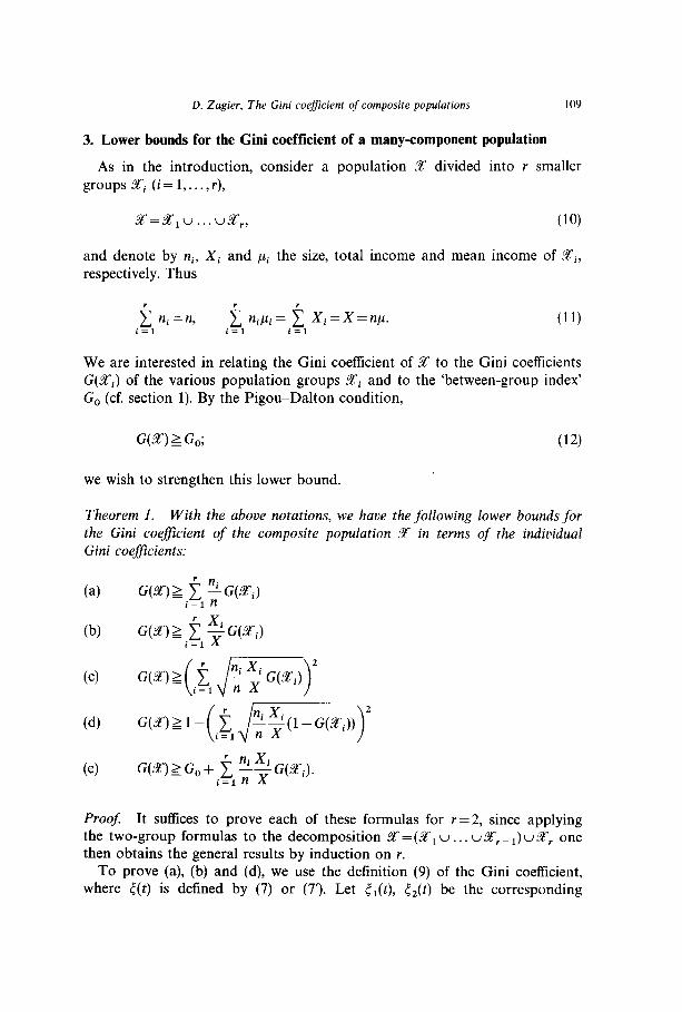
of X, at a time. The argument to prove (c) was pointed out to me by Professor Vind:

Consider the set of aii subpopuiations X’ CX and for each such X’ the point

(n’, X’) E R2, where n’ is the size and X’ the total income of X’. The convex hull of this set of points in R2 is the region of VCR (where R is the rectangle [0, n] x [0,X]), which is bounded below by the resealed Lorenz

curve

{(WXYp))IO5p5 11

(corresponding to choosing for X’ the poorest n’ members of X), and above

by the reflection of this curve in the center of R (corresponding to choosing for X the rirheft n’ mmnherc nf Q\ Rv cn (51 the Gip_i rndfirient ic the LllY ll”llVUI I. lll”lll”Vl” “1 w,. “, “1. \“,, “y.,l..-.~AA. .., . .._ ratio of the area of I/ to that of R. But it is clear from the definition that the region I/ for X=X1 u X, is the (vector) sum of the corresponding regions,

v,~LQ~,l x CO,X,l, v, = co, n21 x co, x21,

for X, and X2, so that (c) is a consequence of the Brunn-Minkowski theorem [see Griinbaum (1967, p. 338)], which states that for any two convex sets V,, I’, c R” the (n-dimensional) volume of the sum I’= I’, + V, is related to the volumes of Vi and V, by

[Conversely, one could interpret (d), which, as shown below, is stronger than (c), as an improvement of the Brunn-Minkowski theorem for the special case that II =2 and V,, V, are centrally symmetrical convex sets which are

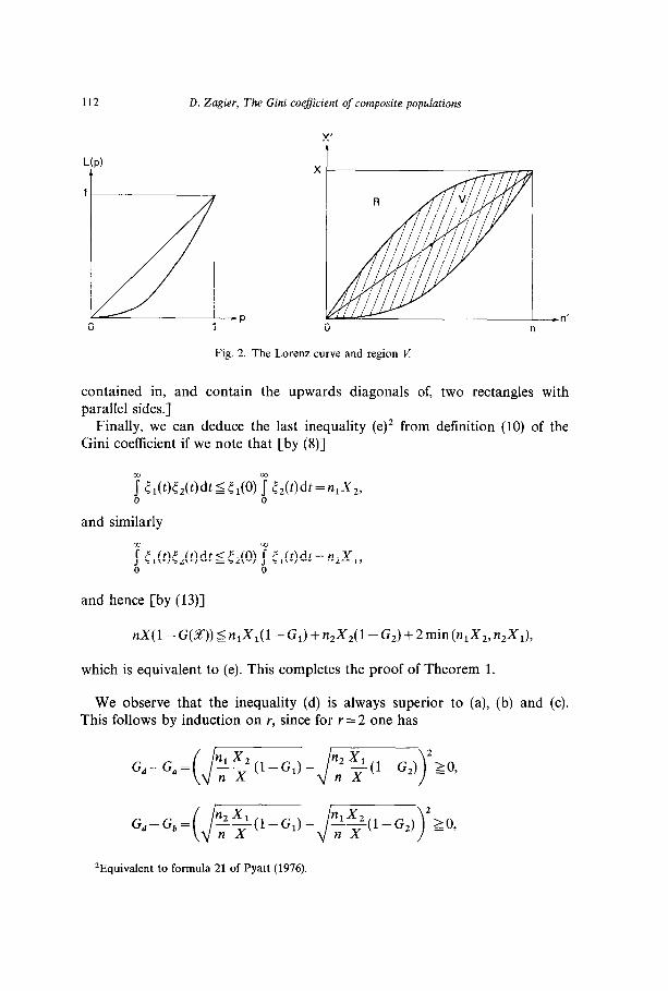
112

i /

0 ’ -P 1

D. Zagier, The Gini coefficient of composite popuiutions

0 ”

-n’

Fig. 2. The Lorenz curve and region V

contained in, and contain the upwards diagonals of, two rectangles with parallel sides.]

Finally, we can deduce the last inequality (e)2 from definition (10) of the Gini coefficient if we note that [by (S)]

% 5t(Otz(WStt(O) i lAW=n,X,,

and similarly

[ 5r(r)SAt)drSMO) $ tr(r)dr=n,X,,

and hence [by (13)]

nX(1 - G(X)) 5 n,X,( 1 - G,) + n2X2( 1 - G2) + 2 min (nIX2, n,X,),

which is equivalent to (e). This completes the proof of Theorem 1.

We observe that the inequality (d) is always superior to (a), (b) and (c). This follows by induction on r, since for r=2 one has

ZEquivalent to formula 21 of Pyatt (1976).

D. Zagier, The Gini coefficient of composite populations 113

~JG,(1-G,)-Jm=a2 >. X1+~~+~(l-G,)(l-GZ) = ’

where G,, . . . , G, denote the right-hand sides of (a), . . .,(d). We nevertheless have included all four bounds in our theorem because (a) and (b) are particularly simple and the proof of (c) involved an interesting idea. The lower bounds (d) and (e) are not comparable: if pL1 =,u2 (so that all inequality in X comes from inequality within the groups %‘J, then G, =0 and (e) is clearly worse than any of the other inequalities, while in the other extreme case G, = G2 =0 (when all the inequality in X is due to the disparity of inromp h~t~nl~~n the Q.b (~1 vive~ thp correct v&e G= Go and_ th_e other 1I1~V~l~” “I”,.__.. .--_ - ‘I, \-, b‘ .--

bounds all give something worse:

4. Best possible upper and lower bounds for the Gini coefficient of a two- component population

In this section we show that (d) and (e) of Theorem 1 together give the best possible lower bound for the Gini coefficient of 3’ in the case Y =2 and give the corresponding result for the upper bound.

Theorem 2. The Gini coefficient of a population X, consisting of two components Xl and X2, satisfies the inequalities

~G,+~$G,+~~G,+Zmin ~~ 33 (G,+G,-GrG,), (n X’n X)

114 D. Zagier, The Gini coefficient of composite populations

where ni, Xi and Gi denote the population sizes, total incomes and Gini coeficients of pi, respectively, n = n, + n2 and X=X, +X2 denote the size and total income of %, and

denotes the ‘between-group’ Gini coeficient. Both bounds are sharp for fixed values of q/n, n,/n, X,/X, X,/X, G, and G2.

Proof: The lower bound, which in the notation of the proof of Theorem 1 says that G(X) zmax(G,, G,), has already been proved. To show that it is sharp, we must find populations XI and XZ with given ni, Xi and G, and with G(X’, uX^,) arbitrarily close to max(G,, G,). We must distinguish two cases, according to the relative sizes of the mean incomes ,ui =X,/n, and of

the Gini coefficients Gi.

Case 1: mWl/~2,d~1)2(1 -GJl -GA

Here G, 2 G,, so we must construct populations Xi (i= 1,2) with the given values of ni, Xi and Gi such that G(X^, u XJ < G, +E. Choose an income x,, such that

pl(l-G&x,+- l-G,’

/L~(~-GJ&,~~ l-G,’

(this is possible by virtue of the assumption on pl, pLz, G,, GJ, and define Xi (i= 1,2) by giving an income x0 to a fraction (~~(1 -Gi)/x,)* of the population, an income 0 to a fraction 1 - {pi(l- Gi)/x,}* of the population, and the remaining income Xi(l- {x0(1 -Gi)/pi)*) to a fraction 0 of the population. [We are formulating everything for the limiting case of very large populations, i.e., ignoring indivisibilities. A more precise formulation for finite populations ni is that we give the income x0 to ni people, where ni 5

ni@i(l -Gi)lx~)* < ni + 1, an income 0 to ni -n; - 1 people, and the remaining income Xi -njxo to the last person; this gives a Gini coefficient Gi +O(l/ni), i.e., equal to Gi in the limit n, -+co.] One easily checks that with this distribution one has G(X-, u X,) = G, [respectively, G, + 0( l/n) in the case of a finite population].

Case 2: min h/h Ad < (1 - Gl)(l - GA Here G, > G,. Suppose for definiteness that ,u~ ipZ, so that pl,&l <

(1 - G,)(l- GJ. We define the distribution XI by assigning income 0 to a

D. Zagier, The Gini coefjicient of composite populations 115

fraction G, of the population, and income pi/(l-G,) to the remaining people. We define %‘z by giving the income pi/( 1 - G,) to a fraction

of the population, and the (larger) income

to the remaining fraction

of the population. Then everyone in the second population is richer than any one in the first, and one easily deduces that G(LE^, uLF^,) = G,.

We now turn to the upper bound. Using definition (9) of the Gini coefficient as in the proof of Theorem 1, we see that the upper bound is equivalent to the estimate

(15)

for monotone decreasing functions (i(t), c2(t) on [O, co), with

<i(O)=~zi, $ (fi(t)dt=X,y $5i(t)'dt=Ai=niXi(l_Gi).

Inequality (15), which can be thought of as a converse to the Cauchy- Schwarz inequality (14) for the class of monotone functions, is proved in Zagier (1977). However, since that paper is in Dutch, and since the proof of (15) is not very long and is actually simpler when formulated in terms of the standard definition (3) of the Gini coefftcient than when stated in terms of the function 5, we repeat the argument here. We have to show that

nX( 1 - G) 2 n,X,(l - G,) + n,X,( 1 - G,)

+ 2min(n,X,,n,X,)(l -G,)(l -G,).

By (3), this is equivalent to

116 D. Zagier, The Gini coefficient of composite populations

$, .z, min(xL:), xb:‘) L A,A,/max (n,X,, n,X,), 1 2

where xz’ (i= 1,2, 15~51~) are the elements of Zi and

A,=n,X,(l-G,)= f F min(xf),xf)), i= 1,2. a=lfl=l

For fixed a, and CQ (15 cli 5 ni) we have

(16)

(17)

By symmetry, the left-hand side of (17) is also bounded by

max(n,X,, n,X,)x!$, and hence in fact smaller than

max(n,X,, n,X,) . min (xi:), x Lz) ). Summing this inequality for c(i = 1,. . . ,nl and a,=1 , . . . , n2, we obtain (16). This proves the desired upper bound.

To show that it is the best possible, we take for X, and 3Yz the following distributions (assuming without loss of generality that p1 =X,/n, 5~1~ = X,/n,): in the first population we give a fraction G, of the total income to a fraction 0 of the population (say to one person) and distribute the remaining income X1( 1 - G,) equally among the remainder of the population [so that each person receives the income ~~(1 -G,)]; in the second

population we give an income 0 to a fraction G, of the population and income &(l - G2) to each of the other n,(l -G,) people. Then one easily checks [using the fact that &(l -G,) zpi(l -G,)] that the Gini coefficient of ?E1 u5?‘, is given exactly by the upper bound in Theorem 2. In other words, we obtain the largest degree of inequality for !Zt^, uX, by achieving the individual Gini coefficients Gi and G2 in as different ways as possible (in Z1 by having one millionaire and a large middle class, in X, by having no

very rich but a large percentage of paupers), whereas we obtained the lower bound by choosing the distributions 9-i and %‘2 to be as similar as possible within the limits permitted by their relative mean incomes and Gini coefficients.

Remark 1. By (a) or (b) of Theorem 1, the Gini coefficient of Z1 uX, can never be less than the individual Gini coefficients. It can, however, be quite a bit larger. For instance, for populations X, and x1, with n, = n2, X, =X2, G, = G, = y, we obtain from Theorem 2 the sharp estimates

D. Zagier, The Gini coefficient of composite populations 117

so that - even in the case of two population components of the same size and with the same mean incomes and Gini coefficients - the Gini coefficient of the combined population can be almost 50% greater than those of the individual components.

Remark 2. We observe that the Gini coefficient of a population made up of r components is given by

+ ni +n. xi +x. JI G(~i U Xj)

n X

[this follows easily from either (2) or (3) or (9)], so that one can always reduce to the case r=2. Thus Theorem 2 also implies upper and lower bounds for the Gini coefficient of a population made up of more than two components. In general, however, these bounds will not be the best possible.

References

Anand, S., 1983, Inequality and poverty in Malaysia: Measurement and decomposition (Oxford University Press, Oxford).

Atkinson, A.B., 1970, On the measurement of inequality, Journal of Economic Theory 2, 244 263.

Atkinson, A.B., 1975, The economics of inequality (Clarendon Press, Oxford). Bliimle, G., 1975, Theorie der Einkommensverteilung (Springer-Verlag, Berlin). Bourguignon, F., 1979, Decomposable income inequality measures, Econometrica 47, 901-920. Cowell. F.A., 1980, On the structure of additive inequality measures, Review of Economic

Studies 47, 521-531. David, H.A., 1968, Gini’s mean differences rediscovered, Biometrika 55, 573-575. Fei, J.C.H. and G. Ranis, 1974, Income inequality by additive factor components (Economic

Growth Center, Yale University, New Haven, CT). Gastwirth. J.L.. 1972. The estimation of the Lorenz curve and Gini index, Review of Economics

and Statistics 54, 306316. Gastwirth, J.L., 1975, The estimation of a family of measures of economic inequality, Journal of

Econometrics 3,61-70. Griinbaum, B., 1967, Convex polytopes (Interscience, London). Hardy, G.H., J.E. Littlewood and G. Polya, 1967, Inequalities (Cambridge University Press,

Cambridge). Kendall, M.G. and A. Stuart, 1963, The advanced theory of statistics (Griffin, London). Mehran, F., 1976, Linear measures of income inequality, Econometrica 44, 805-809. Pyatt, G., 1976, On the interpretation and disaggregation of Gini coefficients, Economic Journal

86, 243-255.

118 D. Zagier, The Gini coejkient of composite populations

Rao, V.M., 1969, Two decompositions of concentration ratio, Journal of the Royal Statistical Society A 132, 418-425.

Rothschild, M. and J.E. Stightz, 1973, Some further results on the measurement of inequality, Journal of Economic Theory 6, 188-204.

Sen, A., 1973, On economic inequality (Oxford University Press, Oxford). Shorrocks, A.F., The class of additively decomposable inequality measures, Econometrica 48,

613-625. The& H., 1967, Economics and information theory (North-Holland, Amsterdam). von Weizsacker, CC., 1976, Verteilungstheorie (Vorlesungsausarbeitung, University of Bonn,

Bonn). Zagier, D., 1977, Een ongelijkheid tegengesteld aan die van Cauchy, Indagationes Mathematicae

A 80, 3499351. Zagier, D., 1982, On the decomposability of the Gini coefftcient and other indices of inequality.

Discussion paper (Institut fiir Gesellschafts- und Wirtschaftswissenschaften, University of Bonn, Bonn).