Embed Size (px)
Citation preview

- 2 0 1 9 -- 2 0 1 9 -
XXVII INTERNATIONAL SCIENTIFIC CONFERENCEON TRANSPORT, ROAD-BUILDING, AGRICULTURAL,
HOISTING & HAULINGAND MILITARY TECHNICS AND TECHNOLOGIES
PROCEEDINGSISSN 1313-5031 (Print) ISSN 2535-0307 (Online)
SCIENTIFIC-TECHNICAL UNION OF MECHANICAL ENGINEERING - INDUSTRY 4.0
BULGARIA
17-20.06.2019, VARNA, BULGARIA

XXVII INTERNATIONAL SCIENTIFIC CONFERENCE
ttrraannss && MMOOTTAAUUTTOO ’’1199
PROCEEDINGS ISSN 1313-5031 (Print), ISSN 2535-0307(Online)
YEAR III, USSUE 1 (6), SOFIA, BULGARIA 2019
SECTION “TRANSPORT. SAFETY AND ECOLOGY. LOGISTICS AND MANAGEMENT. EDUCATION THEORY” SESSION “TRANSPORT TECHNIQUES. INVESTIGATION OF ELEMENTS. VEHICLE ENGINES”
17.06. – 20.06.2019
BURGAS, BULGARIA
Publisher: Scientific-technical union of mechanical engineering „Industry-4.0”

IINNEERRNNAATTIIOONNAALL EEDDIITTOORRIIAALL BBOOAARRDD CHAIRMAN: Dr.h.c. Prof. DSc PETAR KOLEV, BULGARIA Assoc. Prof. Aleksandar Kostikj NM Assoc. Prof. Andrey Ferenets RU Prof. Angel Dimitrov BG Assoc. Prof. Beti Angelevska NM Assoc. Prof. Boyko Gigov BG Prof. Dainis Berjoza LV Prof. Dan Scarpete RO Prof. Daniela Todorova BG Prof. Emilia Andreeva-Moschen AT Prof. Gordana Marunic HR Prof. Hristo Stanchev BG Assoc. Prof. Igor Penkov EE Prof. Igor Smirnov UA Prof. Igor Taratorkin RU Colonel Prof. Iliyan Lilov BG Prof. Jozef Majerčák SK Prof. Lech Sitnik PL Prof. Ljudmila Boyko UA Prof. Madaminjon Aripdzanov UZ Assoc. Prof. Martin Kendra SK
Prof. Massimo Borghi IT Prof. Miho Mihov BG Prof. Murat Dogruel TR Assoc. Prof. Naser Lajqi KO Assoc. Prof. Natalia Sidenko LV Assoc. Prof. Natasa Tomic-Petrovic RS Prof. Nikolay Georgiev BG Prof. Nikolay Ovchenkov RU Prof. Oleg Sharkov RU Assoc. Prof. Pepo Yordanov BG Acad. Polatbeg Zhunisbekov KZ Assoc. Prof. Rinat Kurmaev RU Prof. Rosen Ivanov BG Prof. Teymuraz Kochadze GE Prof. Vadim Zhmud RU Prof. Valyo Nikolov BG Prof. Wolfgang Fengler DE Assoc. Prof. Zoran Jovanovic RS Assoc. Prof. Ahmet H. Ertas TR
C O N T E N T S
SECTION TRANSPORT. SAFETY AND ECOLOGY. LOGISTICS AND MANAGEMENT. EDUCATION THEORY A NEW APPROACH TO THE HUMAN FACTOR’S ASSESSEMNT IN THE AUTOMATED CONTROL SYSTEM OF AVIATION SECURITY IN THE AIRPORT 1Filippov V.L., Elisov L.N., Ovchenkov N.I. ...................................................................................................................................................... 5 INFLUENCE OF LIBERALIZATION ON LONG-DISTANCE RAIL TRANSPORT IN THE CZECH REPUBLIC Ing. Vít Janoš, PhD., Ing. Milan Kříž ................................................................................................................................................................... 7 MODEL FOR ASSESSMENT OF POLLUTANT EMISSIONS FROM ROAD TRANSPORT ON NATIONAL ROADS OF THE REPUBLIC OF SERBIA Prof. Dr Manojlović A. M.Sc. Trifunović J., M.Sc. Milović M., Prof. Dr Kaplanović S. ................................................................................ 10 TRANSPORTATION OF LIQUEFIED FUEL GAS IN CONTAINERS Prof. Dr. Kochadze T., Doctoral candidate Gvarishvili B., Doctoral candidate Markelia B. ............................................................................ 15 TRANSIT CAPACITIES OF THE SOUTH CAUCASUS TRANSPORT CORRIDOR Prof. Dr. Kochadze T., Prof. Dr.Chabukiani R, Doctoral candidate Mikeladze I. , Master G.Iakobidze .......................................................... 18 DESIGN OF AN INNOVATIVE LUGGAGE STORAGE SYSTEM FOR PASSENGER TRAINS L.Cucu PhD. M. Stoica PhD., N. Crisan PhD., G.F. Stoica ............................................................................................................................... 21 USER INTERFACE OF AN INNOVATIVE EXTERNAL BAGGAGE STORAGE SYSTEM FOR PUBLIC TRANSPORTATIONS M. Stoica, L. Cucu, N. Crisan ............................................................................................................................................................................ 24 NEW VEHICLES AS OUR REALITY Prof dr Nataša Tomić-Petrović ........................................................................................................................................................................... 26 ENVIRONMENTAL IMPACT OF ELECTRIC VEHICLES Assistant Prof. Simeunović M. PhD., Associate Prof. Papić Z. PhD., Associate Prof. Simeunović M., M.Sc. Saulić N. ................................ 29 THEORY OF FACTOR EXPERIMENT (MATRIX OF IMPACT) OF GREENHOUSE AS A COMPOSITION SYSTEM FOR BIOGAS PRODUCTION AND REGULATION FOR PERMISSIBLE EMISSIONS OF HARMFUL MATERIALS IN ATMOSPHERE M.Sc. Veljanovski D., Prof. Jovanovska V. PhD., Jovanovska D., Prof. Hristovska E. PhD. ........................................................................... 33 SOCIAL DEVELOPMENT MANAGEMENT OF AIRLINES IN UKRAINE Zhavoronkova G., Doctor of Economic Sciences, Professor, Shkoda T. N., Doctor of Economic Sciences, Associate Professor, Zhavoronkov V., PhD (Economics), Associate Professor .................................................................................................................................. 36

FIRST AID TO THE VICTIMS OF ROAD ACCIDENTS IN THE EVACUATION PROCESS Prof. Dr. I. Nakashidze, Prof. Dr. P.GogiaShvili , Master of Medicine Sh. Potskhishvili, Resident A.Kochadze, Medicine student L.Chogovadze ........................................................................................................................................................................ 40 INCREASED RISKS OF IMPACT ON THE ENVIRONMENT OF POTI AND KULEVI SEA PORTS Assoc.Prof. N. Kamkamidze, Assoc.Prof A, Gobejishvili, Assoc.Prof, N. Khazaradze, Assoc.Prof. N.Tsutskiridze, Assoc.Prof. L. Gamkrelidze ............................................................................................................................................................................... 43 CO2 EMISSIONS OF E-MOBILITY Prof. Lech J. Sitnik DSc. PhD ........................................................................................................................................................................... 45 TYPES OF MATERIALS USED FOR WINTER MAINTENANCE OF ROADS, EFFICIENCY AND INFLUENCE ON CORROSION OF ROAD FACILITIES Еng. Kyuchukov N. ............................................................................................................................................................................................ 49 QUALITY CONTROL OF MULTI-PASS WELD BY MEANS OF ACOUSTIC EMISSION Dmitry S. Bals, M Sc. Eng. Education, Leonid A. Vinogradov, M Sc. Eng. Education Yulija Soldatova, M Sc. Eng. Education .................. 53 REDUCING THE ENERGY INTENSITY OF MULTI-PRODUCT MACHINERY PRODUCTION BY IMPROVING THE CORE PRODUCTION INFRASTRUCTURE V.G. Abrahamyan ............................................................................................................................................................................................... 56 THE RESEARCH PECULIERITIES OF PARAMETERS AND CHOICE OF AGRICULTURAL MACHINES IN PEDAGOGICAL TECHNOLOGIES FOR INNOVATIVE PROJECT ACTIVITY IN TRAINING AGROENGINEERS Candidate of Technical Sciences, Associate Professor Viktor Pryshliak ........................................................................................................... 58 SECTION TRANSPORT TECHNIQUES. INVESTIGATION OF ELEMENTS. VEHICLE ENGINES 1D SIMULATION-BASED DEVELOPMENT OF A SAFETY CONCEPT FOR THE INVESTIGATION OF A HIGH-PRESSURE GAS-DIESEL INJECTOR ON A SINGLE-CYLINDER RESEARCH ENGINE Dr. Dimitrov D., Dipl.-Ing. Aßmus K., Dr. Redtenbacher C., Dr. Schubert-Zallinger C. ................................................................................. 62 ANALYSIS OF THE EFFECT OF PERIODIC PULSATIONS OF LIQUIDS FLOW ON THE HEAT TRANSFERRING IN A CHANNEL WITH DISCRETE ROUGHNESS Dr. sc.ing. hab. prof. Dzelzitis E., Dr.sc.ing. Sidenko N. ................................................................................................................................... 66 MULTISCALE MODELING OF SHORT FIBRE REINFORCED COMPOSITES AND IT’S RELATIONSHIP TO MODAL ANALYSIS OF MACHINERY PARTS Eng. Jarmil Vlach., Eng. Jan Steklý Ph.D. ......................................................................................................................................................... 70 IDENTIFICATION OF THE MINOR CHEMICAL ELEMENTS IN THE EXHAUST EMISSIONS FROM DIESEL ENGINE VEHICLES Dr. Richard Viskup, M.Sc. Christoph Wolf, Prof. Dr. Werner Baumgartner .................................................................................................... 74 FINDING THE OPTIMAL COMPENSATOR CONTROL MATRIX IN THE LONGITUDINAL CHANEL FOR DEVELOPED MUAV M.Sc. Biliderov S. PhD. ..................................................................................................................................................................................... 78 APPROACH OF CALCULATING THE AUTOMOTIVE GASOLINE INJECTOR ELECTROMAGNETIC PARAMETERS Assoc.Prof. M.Sc. Bozhkov S. PhD. .................................................................................................................................................................. 82 СТАТИСТИЧЕСКАЯ ОЦЕНКА СТОЙКОСТЬИ БОКОВЫХ РАМ ТЕЛЕЖЕК ГРУЗОВЫХ ВАГОНОВ С КРИТИЧЕСКИМ ДЕФЕКТОМ доцент Элязов Исраил Шукур ......................................................................................................................................................................... 86 ELECTRONIC THROTTLE DEVELOPMENT FOR EXPERIMENTAL HYBRID-ELECTRIC VEHICLE Student Prodanović J. and Prof. Dr Stojić B. ..................................................................................................................................................... 89 EVALUATION OF THE EFFICIENCY OF THE VEHICLE WITH VARIOUS INTER-WHEELED DIFFERENTIALS FOR DIFFERENT CLUTCH CONDITIONS ON SIDES IN ACCELERATION REGIME Dr. Sci, (Tech), Professor, Volontsevych D., Cand. Sci, (Tech), Associate Professor, Veretennikov Ie., Phd. Student Eng. Mormylo Ia., Phd. Student Eng. Karpov V. ...................................................................................................................................................................................... 91 NUMERICAL ANALYSIS OF IN-CYLINDER PRESSURE AND TEMPERATURE CHANGE FOR NATURALLY ASPIRATED AND UPGRADED GASOLINE ENGINE PhD. Mrzljak Vedran, Eng. Žarković Božica, Prof. PhD. Prpić-Oršić Jasna, PhD Student Eng. Anđelić Nikola ............................................ 95

EXERGY ANALYSIS OF STEAM TURBINE GOVERNING VALVE FROM A SUPER CRITICAL THERMAL POWER PLANT PhD. Mrzljak Vedran, PhD. Orović Josip, PhD. Poljak Igor, PhD Student Lorencin Ivan ............................................................................... 99 NORMS AND LEGAL REGULATIONS TO LIMIT TOXIC EMISSIONS FROM INTERNAL COMBUSTION ENGINES WHEN USING ALTERNATIVE FUELS AS ENVIRONMENTALLY ELIGIBLE IN RELATION OF CONVENTIONAL FUELS M.Sc. Veljanovski D., Prof. Jovanovska V. PhD., Jovanovska D., Prof. Sovreski Z.V. PhD. ........................................................................ 103 OBJECTIFICATION AND DETERMINATION OF HAND-ARMD VIBRATIONS doc. Ing. Michaela Balážiková, PhD., doc. Ing. Marianna Tomašková, PhD. ................................................................................................. 108 FEATURES OF HYBRID ELECTRIC VEHICLE (HEV) TRANSMISSION Post-graduate student Tonkov G. ..................................................................................................................................................................... 112 A RESEARCH INTO THE EFFECT OF ATMOSPHERIC TURBULENCE ON THE MOTION OF A QUADROCOPTER WITH PID CONTROL M.Sc. Kambushev M. PhD. .............................................................................................................................................................................. 116 ANALYSIS OF THE RELIABILITY OF DC BRUSHLESS ELECTRIC MOTORS WITH POWER UP TO 200W USED IN MAVs M.Sc. Kambushev K.M. PhD. .......................................................................................................................................................................... 120 EXPERIMENTAL AND NUMERICAL ANALYSIS OF WIND TURBINE MODEL Biluš I. PhD., Lešnik L. PhD. ........................................................................................................................................................................... 122 SIMULATION OF THREE-DIMENSIONAL CAVITATION IN RADIAL DIVERGENT TEST SECTION USING DIFFERENT MASS TRANSFER MODELS Lešnik L. PhD., Biluš I. PhD. ........................................................................................................................................................................... 126 STUDY OF THE WORKFLOW OF A BUCKETLESS ROTARY LOADER BODY Нураков С., доктор технических наук, профессор; Мерзадинова Г.С., доктор технических наук, профессор; Тулебекова А.С., доктор PhD; Калиев А.Б., кандидат технических наук ............................................................................................................................... 130 МЕТОДЫ ПОВЫШЕНИЯ НАДЕЖНОСТИ И ЭФФЕКТИВНОСТИ СИСТЕМЫ УПРАВЛЕНИЯ ЭКСПЛУАТАЦИЯ АВТОМОБИЛЕЙ д.т.н. проф. Шатманов О.Т., д.т.н., проф Жанбиров Ж.Г., старший преподаватель Асаналиев Т.М., аспирант Кожогулов М.А. ..... 132 BASIS OF DESIGN TRAFFIC ROUTES UNMANNED TRACKED VEHICLE Prof. Dsc. Derzhanskii V., Prof. Dsc. Taratorkin I., Ph.D. Volkov A., postgraduate Yakovlev A. ................................................................. 137 ИЗПИТВАНЕ НА АВТОМАТИЗИРАНА СИСТЕМА ЗА КОМПЛЕКСЕН НЕРАЗРУШАВАЩ КОНТРОЛ НА МЕТАЛНИ МАТЕРИАЛИ Джуджев Б. д-р Ангелов В., д-р Златков М. , Костадинов П. .................................................................................................................... 141

A NEW APPROACH TO THE HUMAN FACTOR’S ASSESSEMNT IN THE
AUTOMATED CONTROL SYSTEM OF AVIATION SECURITY IN THE AIRPORT
1Filippov V.L., 1 Elisov L.N., 2 Ovchenkov N.I., 1State Research Institute of Civil Aviation, Moscow, Russian Federation
2 P.G.Demidov Yaroslavl State University, Yaroslavl, Russian Federation
Abstract: This report concludes a series of articles by the authors devoted to the human factor and published in scientific journals «Industry-
4.0» in 2017, 2018. The problem of the human factor is shown from a new point of view in the article, namely: the human factor is not only
the limited possibilities of professional activity, due to human physiology, it is, above all, the limited possibilities of technology that does not
take into account the characteristics of a person in the human-machine system. There are considered various aspects of this problem.
Keywords: Civil aviation, aviation security, human factor, integrated systems, harmonization of the human factor.
1. IntroductionThe human factor (HF) in many industries refers to one of
the most common concepts. This concept is especially widely
used in civil aviation. It has become a regular occurrence to
attribute the blame for most incidents to the human factor, while
the understanding of what is related to this factor is often
absolutely different. On the one hand, we can definitely consider
that the human component is present almost everywhere. On the
other hand, accusing the human factor of all the events essentially
complicates the situation, since we cannot get a real accident
picture, although this is not the purpose.
HF is a complex category with a fairly large number of
components, not all investigated in case of an incident. HF is an
inexhaustible field of research, even interdisciplinary. This is
especially important in civil aviation, where, nevertheless, the
main studies of the HF are concentrated in the field of flight
safety, and even more often in the study of crew teams.
There has not been carried out any scientific research
connected with the HF in the field of aviation security, although
the importance of the HF is equally important. This work
presents some approaches to the study of the HF in aviation
security.
2. The human factor and the personnel threatAviation security as a scientific area deals with the issues of
ensuring the protection of civil aviation from illegal interference
in its activities. The objective functional of the system solving
these problems is significantly different in its content from other
systems as part of the aviation transport system. This fact
determines the specifics of the means, methods and procedures
used in aviation security. The human factor in the structure of the
aviation security system occupies a particularly important place,
since up to 80% of negative events are connected with it.
In modern safety systems, including flight safety systems, it
is established that the causes of faulty actions of personnel are
associated not only with the level of professionally important
qualities of the individual, but also with the imperfection of the
means of activity and its organization. I.e. the question of
reducing the human factor’s negative role is determined by the
success in improving the parameters (characteristics) of a person
and technology.
It is more complicated in aviation security systems because
the procedures of personnel’s professional activities are poorly
formalized and algo-rhythmized, characterized by extreme
manifestations, have a high degree of ambiguity, and the tasks
are poorly structured and poorly formalized.
In terms of aviation security, it is proposed to consider the
human (personal) factor as an inevitable evil, excluding a useful
component, and all its negative manifestations are classified as
security threats. In this case, the methodologies developed to
protect the objects of the transport infrastructure can be used to
study the human factor in order to reduce and/or eliminate its
impact in aviation security, i.e. the well-known formula begins to
work: detection-reflection-elimination.
The conceptual construct can be the basis for this approach.
Indeed, the factor is the cause driving any process, determining
its nature or its individual features, where the cause is considered
as the basis for any action. The threat involves the possible, the
probable danger, the intention to cause harm. In this case, the
concept of factor can be replaced by the concept of threat, and the
actions of aircraft personnel in this part can be compared and
equated to the actions of the offender, agreeing that these actions
are not hostile, antagonistic, but are forced, random, often
independent of the intentions of the personnel. In this way the
concept of the personnel threat can be introduced.
The personnel threat (PT) in aviation security is a state of
inadequate professional readiness of the operator and the
situation’s parameters in the safety system, determined by the
limit level of the individual’s psychophysiological parameters,
allowing the appearance of a negative event. It should be noted
that deliberate actions of personnel provoking negative events,
even if it is an aviation security officer, automatically translate
the situation into an act of unlawful interference (AUI).
3. Some approaches to the study of HF in aviation
securityIn modern aviation security systems, a person is considered
as a source of threats, i.e. the security system should prevent and
neutralize the anthropogenic impact. These can be terrorist
threats, hooligan actions, negligence, theft, unauthorized photo
and video shooting, violations of the regime and labor discipline,
and much more. This is one category of threats. We consider
personnel threats from the perspective of the man’s imperfections
and poor adaptation of the characteristics of the personnel to the
protection parameters’ technical means when working with
personnel requirements can exceed the level of
psychophysiological opportunity of the human-operator.
Aviation management security system is a process of
rational behaviour of the system based on the measurement,
assessment and analysis of the situation (contingency
management) [10]. Contingency management is the process of
measuring the parameters of the system, transferring it from one
state to another in the interests of the target function, it is
contemplated that there is no stage-by-stage approach in the
solution of control problems, i.e. there may not be a solution
algorithm. In this case, the heuristic approach becomes relevant.
Heuristics can be understood as methods of solving
problems in conditions of uncertainty, which are opposed to
formal methods of solution. Heuristic methods should be
considered as having no prescriptive value, as in the case of using
algorithmic methods. A heuristic algorithm is an algorithm for
solving a problem, the correctness of which is not proved for all
possible cases, but it is known that it gives a fairly good solution
in most cases, i.e. it is not completely mathematically justified,
but at the same time it is a practically useful algorithm.
Heuristic algorithms and procedures give the greatest effect
in combination with the theory of decision-making [11, 12].
The decision-making procedure can be single-criteria and
multi-criteria, depending on the complexity of the problem.
If the control efficiency is characterized by some optimal
test F:
trans&MOTAUTO '19
5
F = F (X1, X2, …, Xl, A1, A2, …, Ap, Y1, Y2, …Yq, Z1, Z2, …,
Zr; t), (1)
where X is the control, A, Y,Z - the factors influencing the
decision, mathematically, the control objective is expressed in the
desire for the maximum possible increase (or decrease) in the
value of the criterion F: F → max (or min).
The person responsible for decision-making has a task: with
the given values and characteristics of the selected factors A1, ...,
Ap, Y1, ..., Yq , Z1, ..., Zl find the optimal values of X1, ..., X1,
controls X1, X2, ..., Xl of the set of their admissible values that
would convert to the maximum (minimum) of the optimality
criterion F.
For a multicriteria problem, the strategy of the operating
side X can be a scalar, a vector, a matrix, or an even more
complex formation, for example, n-dimensional vector, i.e. X =
(x1, x2, ...) = (xj), j Є l,n.
The means of achieving the management goal is the
appropriate choice of strategy X from the area of its permissible
values, i.e. it is necessary to find the optimal strategy X ,
determined by two conditions: strategy X must be admissible and
must be the best in the sense of the principle of the adopted
compromise in the task.
There are popular studies [6, 14, 15, 16], which present the
results of modeling separate processes of aviation security, which
investigated different types of models: linguistic, mathematical,
qualimetric, structural and logical, predictive, and some others.
The study [17] shows the principal possibility of
mathematical modeling of the tasks in the field of aviation
security, related to the human factor, in the format of
mathematical physics’ boundary value problems.
The boundary value problem for partial differential
equations is the problem of obtaining the solution of a partial
differential equation in a given domain under given additional
limitations on the solution at boundary points, edge or boundary
conditions. Partial differential equations are classified either
depending on their mathematical nature or depending on the
physical meaning of the problems they solve: second-order
equations, equations with two variables, linear equations, for
example, second-order equations with two independent variables
(3)
where A, B, C, D, E, F and G – constants or prescribed
functions of independent variables x and y, nonlinear, describing
a nonstationary process in three-dimensional space
(4)
The values of the function u are searched inside a certain
area S, and boundary conditions are set on the boundary:
, (5)
where and – prescribed functions of the boundary ,
– known function, possibly solution-dependent u, –
the derivative of the sought function by the normal to the
boundary .
There are also elliptic equations, Laplace equation, Poisson
equation, parabolic and hyperbolic equations, biharmonic
equation and others. The analytical solution of such equations is
almost impossible due to the insurmountable complexity of the
computational process, that is why numerical methods are used.
Brain-computer models are of particular interest, they reduce the
degree of uncertainty in the formation of the model due to the
procedure of training neurocomputer network [18,19].
The simulation prediction is a certain distribution of the
intensity of personnel threats on the topology of the transport
infrastructure object, which allows identifying extreme points of
impact of threats and including them in the list of priority when
monitoring the situation in the TF (transport facility).
The situation in the TF related to the security is assessed
through the dynamics of incidents, which represent threat
manifestation. It is through the incident that the negative impact
of personnel is manifested to the maximum extent, so the task is
to make a decision on the management of these personnel, i.e. to
exclude this negative impact. The control system should provide
the possibility of automated adjustment of the work’s algorithm
with the inclusion of tools for reconstruction of the structure of
the aviation security management system.
4. ConclusionThe problems in the field of aviation security related to the
human factor are multifaceted and quite complex. Classical
approaches to solving these problems have almost reached their
limits. There are needed new approaches, one of which you can
find in this report.
The idea of the new approach is a fundamental revision of
the human factor’s physical meaning, realizing that the HF in
rigorous definition is not a factor, but a much more complex and
multifaceted category relating to complex systems and having an
objective functional that is not amenable to the strict
mathematical investigation.
The authors introduce a new concept: the personnel threat,
by which we understand the state of inadequacy of the operator’s
professional readiness and the parameters of the situation in the
security system, determined by the limit level of the individual’s
psychophysiological parameters, allowing a negative event
appearance. Monitoring of this threat and its study involves the
use of known methods, mathematical or heuristic, with their
specific adaptation and limitations, subsequent measurement and
analysis in a quantitative format, which simplifies the procedure
for making decisions on personnel management.
The suggested approach increases the level of aviation
security of the transport infrastructure’s object by reducing the
level of negative impact from the aviation personnel.
5. REFERENCES1. Elisov L.N. Metodologiya I sredstva kvalimetrii
inzhenerno-tekhnicheskogo sostava grazhdanskoj aviatsii.
Aftoref.diss.dokt.tekhn.nauk [Methodology and means of
qualimetry of civil aviation engineering and technical staff. Dr.
techn. Sci. abstract of the thesis]. Moscow, 1995. (In Russian).
2. Elisov L.N., Ovchenkov N.I., Fadeev R.S.
Introduction to the theory of aviation security, Yaroslavl,
Filigran` Publ., 2016, 320 p. (In Russian).
3. Elisov L.N. To the question of the accuracy of
heuristic algorithms for solving optimization problems in
operation. Nauchnyj Vestnik MGTUGA=Scientific Bulletin of
MSTU CA, 2012, no. 179, pp. 123-126. (In Russian).
4. Filippov V. L., Ovchenkov N. Some problems of
automation of aviation security management procedures at the
airport / / Scientific Bulletin of the State Research Institute of
Civil Aviation. 2019. No. 24. P. 66-74.
5. Elisov L.N., Ovchenkov N.I. Aviation security as
an object of mathematical modeling. Nauchnyj Vestnik
MGTUGA=Scientific Bulletin of MSTU CA, 2017, vol.20, no. 3,
pp. 13-20. (In Russian).
6. Elisov, L. N., Ovchenkov N. Some of the
questions of the grid and neural network modeling task control of
aviation security of the airport. Scientific Bulletin of the Moscow
State Technical University of Civil Aviation, volume 20.
Moscow, 2017. No. 3. P. 21-29.
7. Elisov L. N., Gorbachenko V. I., Zhukov M. V.
Learning Radial Basis Function Networks with the Trust Region
Method for Boundary Problems // Automation and Remote
Control. - 2018, Vol. 79. - No. 9. - P. 1621-1629.
2 2 2
2 2
u u u u uA B C D E Fu G
x x y y x y
1 2 3
2
2
, , , , , , , , , , , ,
, , , , , , , , , , , ,
u u ux y z t u x y z t u x y z t u
x x y y z z
u ua x y z t u b x y z t u c x y z t u u d
t t
uu f
n
f u n
trans&MOTAUTO '19
6

INFLUENCE OF LIBERALIZATION ON LONG-DISTANCE RAIL TRANSPORT
IN THE CZECH REPUBLIC
Ing. Vít Janoš, PhD., Ing. Milan Kříž
Faculty of Transportation Sciences – Czech Technical University in Prague, Czech Republic
Abstract: In the Czech Republic, the rail transport market has been liberalized for several years - in addition to public services,
commercial services of individual rail carriers operate too. Public services in long-distance rail transport are ordered by the Czech Ministry
of Transport. In December 2019, the 10-year contract between Czech Ministry of Transport and Czech Railways will end. The approaching
end of this contract was connected with great interest of other rail carriers, which led to the fact, that the Czech Ministry of Transport
demanded individual long-distance rail lines in the form of so called "market consultations". Preparing of the operational performance of
individual long-distance rail lines for the needs of market consultations was a great challenge on the field of transport-planning. As a result,
from December 2019 there will operate 4 different rail carriers in ordered long-distance rail transport in The Czech Republic and this
situation is unique in its form and unparalleled throughout the EU.
Keywords: RAILWAY TRANSPORT, PUBLIC TRAFFIC, RAILWAY TECHNOLOGY, TIMETABLE DESIGNING, PERIODIC
TIMETABLE, OPEN-ACCESS, CAPACITY, LIBERALIZATION
1. Order of public rail services in the Czech
Republic
Since 2005, rail transport in the Czech Republic regionalised,
14 regions is responsible for ordering regional rail transport, the
Ministry of Transport is responsible for long-distance rail transport
order.
Public transport services in the Czech Republic are
characterized by the fact that they represent in general a
performance for which the sum of revenues is not sufficient to
cover costs associated with the services.
Order of the Ministry of Transport is focused on the fixed
interval connection between each regional capitals and other major
residential areas in the Czech Republic.
Overall, in 2018 in the Czech Republic, the total volume of
train-kilometers in ordered long-distance transport was about 35
million train km.
A feature of public rail services in the order of Ministry of
Transport and the Regions is also the fact, that it is an "open"
system, which works across the network unified fare system, so
there is time, space and tariff interconnection of services. A feature
of the system is not "denial of passengers" (i.e., inability due to lack
of transport capacity of lines), while no reservations required (no
link between a ticket and particular train). It is natural, that such a
generally high quality parameters of public services cannot be met
without compensation from national budget.
The total amount of payments from national budget for
compensation for ordering of long-distance transport rail passenger
transport was in 2018 CZK 4.1 billion (approximately EUR 158
million)
The main direct awarded 10-year public contract between Czech
Ministry of Transport and Czech railways ends in December 2019.
2. The liberalization of the rail market in the
Czech Republic
The current practice in the Czech Republic is still mostly
represented in rail passenger transport services by direct selecting of
the train operating company (TOC). In 2009, when Czech Ministry
of Transport signed the 10-year contract with Czech Railways to
provide transport services in long-distance traffic, followed
extensive criticism from another TOC´s. Czech private TOC´s have
criticized the closeness of the public service market and demanded
public procurement for rail through transparent selection.
Before 2009, contract award after competition of TOC´s was
made on long-distance lines Pardubice - Liberec and Plzeň - Most.
Both of these competitions were won in 2005 by Czech railways.
Despite the victory of the national carrier, these competitions led to
a reduction of compensation.
However, in 2009, there were timewise unable to prepare
further competitions into the process.
Despite the fact, that the majority of transport volume in long
distance rail transport has been selected directly, reported by the
Czech Republic to support the liberalization of rail transport.
This declaration liberalization of passenger rail market has two
specific implications:
1) official timetable for market opening in long-distance
transport, the opportunity to compete in selected
contracts
2) liberal access to railway infrastructure - Open Access
After closing of the 10-year contract between Czech Ministry of
Transport and Czech Railways, the private TOC´s in the Czech
Republic focused on developing open-access services.
2.1. Open-Access in the Czech Republic
In the Czech Republic, additionally to the public services, there
is a fully liberal approach to infrastructure – Open Access, without
any restriction. Each TOC can apply to the transport infrastructure
access authority (ÚPDI) and then may ask the infrastructure
manager (IM) for capacity and IM (Railway Infrastructure
Administration – RIA - SŽDC) will be required to allocate
infrastructure capacity.
The first project in the Czech railway network, which had
features of Open Access approach were the SC Pendolino trains
between Prague and Ostrava. These SC-trains operate Czech
Railways on their commercial risks, with mandatory reservation and
limited passenger capacity and costs for transportation of these
trains is significantly above the level of fares on trains, which are
ordered and form a public service.
The second Open Access project are the Regiojet trains of
(former) Student Agency company running on the route Praha –
Ostrava – Havířov (- Žilina). Again, these are trains to TOC
commercial risk, with mandatory reservation (seat reservation is
included in the ticket), with limited passenger capacity, but the price
for the carriage of these trains is comparable to fares on trains,
which are ordered and form a public service.
The third Open Access project is a LEO Express, i.e. Leo
Express trains again on the route Praha - Ostrava. As in the case of
trans&MOTAUTO '19
7

Regiojet, in this case, the connections to the commercial risk of the
TOC will have to provide mandatory seat reservation will have a
limited capacity for passengers.
All Open-Access projects began to develop. Czech Railways,
for example, has taken over the international night trains to their
commercial risk. Regiojet expanded its activities to include
connections Prague - Wien and Prague - Bratislava, Leo Express
expanded its range of services to include connections Prague -
Krakow and Prague - Staré Město u Uherského Hradiště.
This battle of TOCs in Open-access services is unprecedented in
the European railway area. Already less than one year of sharp
competition between three different TOC´s has been indicated, that
commercial Open-Access services are very unstable in time.
Changing time position of the trains, changing and different stops,
variable and unstable number of connections etc., such services
cannot be reasonably operationally integrated into the open
transport system and they can hardly serve as a fixed part of the
territory's transport service.
2.2. Market opening in long distance transport
Market opening in long-distance rail transport should solve as a
possibility to increase quality / price ratio in the Czech rail
transport. Ministry of Transport expects, that the current level of
compensation will be held and serve to reach higher quality or
higher range of passenger rail services performance. A prerequisite
is the case, it can maintain a stable long-term financing of the
railway sector and there will be no significant changes in the
amount of available financial performance.
After one-off competitions in the year 2005 (lines Pradubice -
Liberec and Plzeň - Most) has the Czech Ministry of Transport
already in 2011 published a schedule for market opening in long-
distance rail transport. In March 2012 have been published
specifications for the first competition (line Olomouc - Krnov -
Ostrava).
Although the tender for the line Olomouc - Krnov - Ostrava was
canceled for formal reasons in 2013, the competition trend
continued. In 2014, the preparation of the tender for the line Plzeň -
Most (where the contract from 2006 was to end in 2015) was
launched. Due to procedural delays, the contract from 2006 was
extended by 2 years - but the tender was in the end finally canceled
on the basis of objections from Czech Railways. However, there
occured a breakthrough situation, when the Ministry of Transport
used the possibility of direct awarding institute and assigned
directly to the winner of the canceled competition (TOC GWTR)
the operation on the line Plzeň - Most (with level of compensation
offered in the cancelled tender). It was a clear signal sent to the
market of rail operators, that the liberalization of the rail market
would not be stopped due to procedural obstruction.
For a main contract with Czech Railways from 2009, which
ends in December 2019, the Ministry of Transport prepared a
follow-up of direct assignment of the contract. The rules for access
to public services are laid down in the amendment to Regulation
(EC) No 1370/2007, which is part of the fourth railway package.
Applicability of direct award of the contract in the passenger rail
services is in force to 25. December 2023.
However, as the private TOC´s in the Czech Republic have
announced their relevant interest for participating in long-distance
rail-services, the Ministry of Transport has notified the order of
long-distance after 2019 transport in the Official journal of the EU
on a per-line basis, with a different duration, so that this
corresponds to the published schedule for competitions i rail public
services planned in years 2020 - 2034.
3. Procedure for concluding new contracts after
2019
The Ministry of Transport access is clear that the priority-driven
process in which is preserved the networked public rail transport (in
Czech and Central European scale) and will clearly set in advance
in market access conditions, including rules on mutual recognition
of travel documents and the use of station buildings.
The principle is, that the Czech Ministry of Transport published
in spring of 2017 in the Official journal of the EU, that all long-
distance lines from 12/2019 will be reassigned. Each line had its
own notification - all as a direct allocation for CD.
Until spring 2018 have The Ministry of Transport negotiated
with Czech Railways, what transport parameters (vehicles,
performance quality, timetable) of which lines is possible to offer
for next contract period.
Approximately in March / April 2018 got The Ministry of
Transport offer from Czech Railways on all lines and additionally
also offers on some lines from another TOC´s.
Than was necessary to sort, on which lines are the offers of
another operators nore favorable, than the offer from Czech
railways. Because the third operators have not previously negotiated
with The Ministry of Transport, were the offers not comparable.
The Ministry of Transport has then made operational "packages"
and asked with these packages new request to all interested TOC´s
(including Czech Railways) - for to update offer specification.
Content of each operational "package" was line (or more lines)
with such timetable and quality reqiurements, which was negotiated
with Czech Railways between 2017 - 2018. So the assignment of
each package was always direct assignment - only based "market
consultation". The requests to TOC´s for offers for operating these
"package" - so called "shoot-out" - ran between June - November
2018.
3.1. Technological structure of operational
"packages"
In order to formulate the content of each operational package, it
was necessary to set their structure, in particular the operational
closeness and consistency.
A task was the basic determination of number of trains and their
position in nodes (marketing timetable), defining the size of train-
sets including regular and seasonal capacity strengths and
timetabling (calculation of travel times).
Existing interconnected traffic provides a variety of synergies
(typically vehicle-to-line transitions) and it was not desirable to lose
these benefits.
For the operational separation of the lines and the arrangement
of the operating structure of the packages, it was necessary to reflect
the number of vehicles in relation to the timetable. On the
operational side, such lines were grouped into individual packages,
taking into account the operational background, necessary transport
capacities and traction.
From the timetable point of view, it was often necessary to add
new connection or links, for to isolate individual packages and close
them to the functional cycles. In this step, it was necessary to reflect
IPT nodes, bindings and schedule boundary conditions, transfer /
changing nodes and intended length intervals for peak-and-off-peak
hours.
The author´s team used their previously published approach,
which combines timetable proposal and operational concept with
cycles of vehicles, in mutual repeating iteration steps.
Approach to the timetable creating is as follows:
1) defining IPT nodes and intervals, calculate the number of
vehicles for "basic periodical operation"
trans&MOTAUTO '19
8

2) defining a specific operation in the peak hours and
minimizing the number of vehicles in peak period; ideally for the
number required in previous point 1
3) operational optimization and ensuring operational efficiency
(refueling, maintenance, cleaning...)
4) adaptation of timetables in the evening hours (to minimize
the number of vehicles, reduction of total working times)
The aim is to ensure maximum operational efficiency within a
defined operational file.
4. Conclusion
Based on so operationally and transportly defined content of
packages were made so called "shoots" - every interested TOC gave
its offer to the Ministry of Transport.
As first package, there was already in June 2018 direct assigned
a package including a line Pardubice - Liberec. The winner of this
"shoot-out" was Czech railways.
As second package, there was direct assigned a package
including lines Praha - Olomouc - Žilina and Praha - Olomouc -
Luhačovice. The winner of this "shoot-out" was Czech railways too.
As third package, there was direct assigned a package including
line Brno - Bohumín. The winner of this "shoot-out" was Czech
private railway operator Regiojet.
As fourth package, there were direct assigned a package
including large network of fast trains in diesel-traction in middle
Bohemia (Praha - Tanvald, Praha - Rakovník, Praha - Písek - České
Budějovice, Kolín - Nový Bor ). The winner of this "shoot-out" was
international operator Arriva.
Market opening in long-distance rail transport should solve as a
possibility to increase quality / price ratio in the Czech rail. The
whole money, which was saved by "shoot-outs" of these packages,
will be from December 2019 inserted in broad timetable extension -
and not only on the lines included in these packages, but nearly on
all lines in the fast-train network.
This way of liberalization of public rail services using direct
assignment has currently in Europe no analogy. Although there has
been a clear commitment to a functional operational arrangement, it
will be exciting to see, how this system will work in practice, with
the launch of a new timetable in Dezember 2019, and above all,
how passengers will react to this new system. A major challenge
will be the coordination of individual transport services in operation
to maintain the functionality and integrity of the rail transport
system.
REFERENCES
1. Drábek, M.; Pospíšil, J.: Fluctuations in Passenger Railway
Service Period In: Young Transportation Engineers
Conference 2018. Praha: CTU. Faculty of Transportation
Sciences, 2018. p. 1-8. ISBN 978-80-01-06464-1
2. Michl, Z.; Drábek, M.; Vávra, R.: Netgraph - an Efficient Tool
for Periodic Timetabling and Capacity Planning
In: Student Scientific Conference Modernization of Railway
IRICoN 2017. Praha: Czech Technical University in Prague,
2017. p. 43-48. ISSN 2336-5382. ISBN 978-80-01-06297-5
3. Janoš, V.; Baudyš, K.: TECHNOLOGICAL STRUCTURE
OF OPERATIONAL FILES IN REGIONAL BUS
TRANSPORT FOR THE NEEDS OF THE TENDER FOR
CARRIERS International journal for science, technics and
innovations for the industry MACHINES TECHNOLOGIES
MATERIALS. 2015, IX(10/2015), 57-60. ISSN 1313-0226
4. Janoš, V. - Baudyš, K.: TRANSPORT PLANNING ON THE
LIBERALIZED MARKET OF PUBLIC SERVICES. In
trans&MOTAUTO´14 XXII INTERNATIONAL
CONFERENCE PROCEEDINGS. Sofia: Scientific-technical
union of mechanical engineering, 2014, ISSN 1310-3946
5. Janoš, V. - Baudyš, K.: Transport Planning of Public Services.
In Proceedings of the 11th European Transport Congress.
Praha: České vysoké učení technické v Praze, Fakulta
dopravní, 2013, ISBN 978-80-01-05321-8
6. Janoš, V.; Baudyš, K.: ISSUES OF PERIODIC-TIMETABLE
CONSTRUCTION ON THE FULLY LIBERALIZED
RAILWAY MARKET Machines, Technologies, Materials.
2013, 7(6/2013), 54-56. ISSN 1313-0226
trans&MOTAUTO '19
9

MODEL FOR ASSESSMENT OF POLLUTANT EMISSIONS FROM ROAD
TRANSPORT ON NATIONAL ROADS OF THE REPUBLIC OF SERBIA
Prof. Dr Manojlović A.1 M.Sc. Trifunović J. 1, M.Sc. Milović M. 2, Prof. Dr Kaplanović S.1
University of Belgrade Faculty of Transport and Traffic Engineering, Belgrade. Republic of Serbia1
Intico ltd2, Belgrade, Republic of Serbia
[email protected], [email protected], [email protected], [email protected]
Abstract: Determination the annual quantities of pollutant emissions in road transport emitted into the atmosphere, with the timely
delivery of reliable information to all interested parties, conditions are created for raising the level of public awareness of environmental
protection. Determining the amount of pollutants emitted facilitates monitoring of trends in order to lower the level of risk from their
negative effect. This paper presents the results of calculating the amount of emitted pollutant emissions from road motor vehicles and
determining emissions of pollutants on state roads I and II in the Republic of Serbia for the period 2013 to 2015 using the current version of
COPERT 5 software. On the basis of the calculated emission of pollutants by shares and the belonging of the sections to the corresponding
squares, the spatial distribution according to the squares of the European Monitoring and Evaluation Program (EMEP) network is shown.
Keywords: ATMOSPHERIC POLLUTANT, COPERT 5, ROAD SECTION, EMEP NETWORK
1. Introduction
Determining emissions of pollutants in road transport is very
complex and requires the modeling of input parameters. In addition
to the pollution forecast, models and their results are used to make
decisions when creating strategies in order to reduce the negative
impact on the environment. With the help of the model, the effects
of the applied measures are evaluated. In order to apply the concept
of sustainable development to the road transport sector, it is
necessary to know the participation of road transport in air
pollution, which is provided by models for estimating emissions
from road transport. By determining the annual quantities of
pollutants from road transport in the atmosphere, with the timely
delivery of reliable information to all interested parties, conditions
for raising the level of public awareness of environmental
protection are created. Determining the amount of pollutants
emitted also facilitates the monitoring of trends in order to lower the
level of risk from their negative effect. All variables that affect the
amount of pollutant emissions in road transport is necessary to
accurately determine or evaluate in order to enable analysis of the
effects of stimulating and restrictive measures (cost-benefit
analysis, intangible effects, etc.) in order to achieve sustainability of
road transport. The assessment method presented in this paper
provides a good basis for assessing the feasibility of fiscal measures
to reduce emissions from road transport, or to increase its
sustainability, as well as to estimate pollutant emission generated by
vehicles on state roads I and II category. The subject of this paper is
to calculate the emissions of pollutants from road vehicles and to
determine emissions of pollutants on state roads I and II category
using the current version of COPERT 5 software for the period
from 2013 to 2015. The subject of research is also determining the
influence of the dominant exploitation conditions on the emission of
pollutants. On the basis of the estimated distance traveled, the
prevailing conditions of exploitation and the level of pollutant
emission standards of vehicles, it is determined the technical
condition of vehicles and the final value of vehicle emissions on
roads. For all sections of state roads I and II category based on data
from automatic counters or weighted data on average annual daily
traffic (AADT), structure of vehicle fleet, section length and
average speed on a section (measured or expertly assessed), the
emissions of a set of pollutants for individual sections by category
of vehicle are calculated. Based on the calculated emissions of
pollutants per road section and the affiliation of the section with the
corresponding squares, the spatial distribution is made according to
the squares of the European Monitoring and Evaluation Programme
(EMEP) network.
2. Model for assessment of pollutants emissions
In order to quantify the emission of gaseous pollutants derived
from road transport in this paper, the results obtained using the
COPERT 5 software tool (April, 2017) are presented. COPERT
(COmputer Program to calculate Emissions from Road Transport) is
one of the European tools for calculating emissions according to the
Convention on Long-Range Transboundary Air Pollution
(CLRTAP), in accordance with the requirements set by the
Cooperation Program for monitoring and evaluation of the EMEP
and the European Environment Agency (EEA), which financed the
development of COPERT within the activities of the European
Topic Center for Environmental Protection air and climate change
[1, 2].
In order to carry out the assessment of emissions from road
transport by using the COPERT 5 software tool, it is necessary to
collect extensive input data. Prior to any evaluation or use of the
software, it was necessary to collect data on:
weather (climatic) conditions during the year,
specific characteristics of all types of fuel in sales,
total (annual) consumption of all types of fuel,
a vehicle fleet classified according to the required
categories, subcategories and vehicle emission
technologies (number of vehicles)
the average distance traveled for each category of vehicle
(based on a special survey),
average speeds of vehicles by categories of vehicles and
roads,
participation of the mileage by categories of vehicles and
roads (urban, rural and highway) in percentages.
Input data for the Republic of Serbia, which were available in
official records or statistics of state institutions and bodies, were
collected from the Statistical Office of the Republic of Serbia (data
on sold / spent fuel in traffic and transport, data on border traffic of
passenger and freight vehicles, etc. .) and the Republic
Hydrometeorological Institute of Serbia (data on dominant weather
- hydrometeorological conditions). After analyzing the data, the
method of their correction, ie bringing in the form required by the
COPERT 5 model, has been determined.
Determination of the structure of the vehicle fleet on the first
and second road categories was done by adopting the relevant
national vehicle fleet structure, and according to the average annual
daily traffic (AADT) by category of vehicle.
trans&MOTAUTO '19
10

The only relevant source of data on hydrometeorological
(weather) conditions in the Republic of Serbia is the Meteorological
Yearbook issued by the Republic Hydrometeorological Service of
Serbia (RHSS). RHSS disposes of so-called "Climatological" data
from 1949 to 2015 with the exception of the period from 1980 to
1989. These reports contain data on average monthly minimum and
maximum temperatures, average monthly air pressure and relative
humidity.
Climatological data required for the calculation are:
mean maximum monthly temperature (°C),
mean minimum monthly temperature (°C),
air pressure (kPa) and
relative humidity (%).
These input data are necessary to obtain the average monthly
conditions in which vehicles are used. They are used to assess the
impact of a cold start on vehicle emissions, as well as air
conditioners, both for the purpose of cooling during the summer
(warmer months), as well as heating during winter, as well as
reducing air humidity (over the whole year).
Consumption or amount of spent fuel is one of the indicators of
transport activities. It is used as a control indicator for determining
and possibly correcting the average annual traveled route of certain
vehicle categories. Average fuel consumption is a measure of the
efficiency of fuel utilization as the ratio between the distance
traveled and the amount of fuel consumed. Given that spent fuel is
an important factor in air pollution, a large number of countries
have introduced strict fuel consumption related restrictions.
The COPERT 5 software tool calculates energy consumption
rather than the fuel consumption to facilitate the calculation of
energy consumption for new types of vehicles (hybrid vehicles -
plug-in vehicles with gasoline and hybrid vehicles powered by
diesel; electric vehicles drive - batteries and electricity, fuel cells
(N2) and electric drive).
Access to the COPERT 5 model implies that the following
information are entered for the vehicle: vehicle type, vehicle speed
(km / h), primary fuel consumption (TJ), primary fuel content (MJ /
kg), fuel mixture used, in a mixture of fuel (%). The COPERT 5
model compares the statistical and calculated energy consumption,
modifies the input data (for example, the traveled vehicle distance)
and repeats the procedure for calculating the amount of emitted
pollutants.
The source of data for determining size of the national vehicle
fleet is data on all national vehicles (excluding fleet of military and
police) located in the base, ie, records of registered vehicles. In
order to be able to use the data from registered vehicle records for
the calculation according to the COPERT 5 model, it is necessary to
adapt the existing vehicle classification to the categorization of the
vehicle defined in this model.
Sources that have been processed for the purpose of collecting
data on vehicle activities in the survey are as follows:
a) passenger car user survey conducted in 2017;
b) egular survey conducted in 2013 and 2016 in transport
companies for the transport of passengers (urban and
intercity buses) and for the transport of goods (delivery
and cargo vehicles);
c) average annual daily traffic on the roads of the first and
second category of the Republic of Serbia in the period
2013-2015.
All of the aforementioned and available data were used in terms
of obtaining the most reliable estimation, in the first place, the
number of vehicles on the road network of the Republic of Serbia,
and then the realized route of those vehicles. Values of certain input
data, for which there is no record, or not obtained through research,
were adopted according to the project recommendations [1].
According to this project the value of the average length of travel
should be in the range of 8 to 15 km, but in the absence of data, the
value is 12.4 km, which represents the average length of travel in
the EU Member States.
3. Emission of the national vehicle fleet
The total emissions of pollutants of the national vehicle fleet are
shown in Fig. 1and Fig. 2. Passenger vehicles mostly affect CO,
CO2, SO2 and Pb emissions, while commercial vehicles have the
largest share in NOX, PM2.5 and PM10 emissions (Fig. 3 - Fig. 5).
Fig. 1 The total emissions of carbon monoxide (CO), nitrogen oxides (NOx)
and carbon dioxide (CO2), 2013-2015 year [t]
Fig. 2 The total emission of suspended particles (PM2.5, PM10), sulphur
dioxide (SO2) and lead (Pb), 2013-2015 year [t]
trans&MOTAUTO '19
11

a) CO
b) NOX
Fig. 3 Cumulative emissions by category of vehicles 2013-2015 year: a)
carbon - monoxide (CO) [103 t] and b) nitrogen oxides (NOx) [103 t]
a) CO2
b) SO2
Fig.4 Cumulative emissions by category of vehicles 2013-2015 year: a)
carbon-dioxide (CO2) [106 t] andb) sulfur-dioxide (SO2) [kg]
a) PM2.5
b) PM10
Fig. 5 Cumulative emissions by category of vehicles 2013-2015 year:
a) particulate matters up to 2,5 m (PM2.5) [t] and b) particulate matters up
to 10 m (PM10) [t]
4. Emissions of pollutants on road sections of the I
and II category of the national roads
This paper presents the results of the Study on estimation of
emissions of pollutants in the atmosphere from transport on state
roads I and II category for the period from 2013 to 2015 [3].
The data on the vehicle fleet of the Republic of Serbia and the
emission factors from the COPERT 5 software tool have been used
for the calculation of the emissions of exhaust gases.
For all state roads (over 100 roads) and sections (over 1,000),
for each year of the observed period, 2013, 2014 and 2015, the
amount of pollutants emitted is calculated.
The following data were used for the calculation:
average annual daily traffic per vehicle category by road
section,
lenght of road section,
average speed of vehicles on road section and
emission of pollutants by vehicle category (g/km).
Based on the available data on the lengths of the road sections
and the average annual daily traffic, the total millage traveled by
road categories (in autocilometers) and road sections was
determined. The average speed of the vehicle on the sections are
calculated based on the available time travel speeds of the vehicles
read on the traffic counters. The unit emission of pollutants is
expressed in grams per autocilometer by category of vehicle
(passenger car, bus, light duty vehicle, medium freight vehicle,
heavy duty vehicle, articulated vehicle). In order to determine the
unit's emissions, the software tool COPERT 5 and the structure of
the fleet of the Republic of Serbia were used in 2013, 2014 and
2015.
trans&MOTAUTO '19
12

The total emission of pollutants on the road section during the
year is the product of the unit emission in the calculated
autokilometer and the total number of autokilometers per vehicle
category.
Total emissions of pollutants on state roads I and II category, by
category of vehicles, in the period from 2013 to 2015 is shown in
Table 1.
Table 1: Total emission of pollutants on state roads I and II category in the
period 2013-2015 2013 % 2014 % 2015 %
CAR 15,494.05 87.43 13,257.21 86.50 14,932.66 86.16
BUS 303.86 1.71 261.43 1.71 364.89 2.11
LDV 150.74 0.85 124.93 0.82 160.44 0.93
MHV 286.49 1.62 248.09 1.62 296.92 1.71
HDV 251.88 1.42 210.10 1.37 299.76 1.73
AV 1,234.05 6.96 1,224.39 7.99 1,276.54 7.37
Total 17,721.07 100 15,326.15 100 17,331.20 100
CAR 7,992.67 46.19 7,090.09 45.11 8,282.76 45.42
BUS 1,441.15 8.33 1,177.36 7.49 1,646.63 9.03
LDV 167.90 0.97 173.42 1.10 242.82 1.33
MHV 1,143.68 6.61 997.13 6.34 1,204.59 6.61
HDV 1,102.39 6.37 915.20 5.82 1,309.50 7.18
AV 5,454.68 31.53 5,365.39 34.13 5,548.09 30.43
Total 17,302.48 100 15,718.59 100 18,234.38 100
CAR 276.09 48.56 256.49 49.30 310.85 50.71
BUS 40.11 7.05 31.46 6.05 44.15 7.20
LDV 18.65 3.28 18.17 3.49 23.44 3.82
MHV 42.59 7.49 36.10 6.94 43.01 7.02
HDV 33.58 5.91 27.22 5.23 37.98 6.20
AV 157.56 27.71 150.80 28.99 153.56 25.05
Total 568.58 100 520.24 100 612.98 100
CAR 336.66 50.94 310.98 51.40 342.11 52.22
BUS 44.31 6.70 35.13 5.81 40.17 6.13
LDV 20.38 3.08 19.79 3.27 22.48 3.43
MHV 47.59 7.20 40.53 6.70 43.38 6.62
HDV 37.03 5.60 30.18 4.99 33.52 5.12
AV 174.98 26.47 168.39 27.83 173.47 26.48
Total 660.94 100 605.01 100 655.13 100
CAR 1,536,634.20 61.13 1,449,798.53 60.29 1,769,202.49 60.77
BUS 152,594.27 6.07 137,812.73 5.73 194,754.07 6.69
LDV 41,559.61 1.65 40,582.44 1.69 57,112.42 1.96
MHV 99,082.13 3.94 90,113.47 3.75 111,522.66 3.83
HDV 100,869.11 4.01 87,841.10 3.65 131,738.71 4.52
AV 583,000.46 23.19 598,699.95 24.90 647,201.86 22.23
Total 2,513,739.78 100 2,404,848.22 100 2,911,532.21 100
CAR 0.009 56.80 0.009 56.18 0.011 56.65
BUS 0.001 6.67 0.001 6.24 0.001 7.75
LDV 0.000 1.86 0.000 1.87 0.000 2.15
MHV 0.001 4.39 0.001 4.14 0.001 4.19
HDV 0.001 4.47 0.001 4.04 0.001 4.95
AV 0.004 25.82 0.004 27.52 0.005 24.30
Total 0.016 100 0.016 100 0.019 100
CAR 163.22 65.64 144.59 64.47 175.58 64.18
BUS 12.97 5.22 11.21 5.00 15.85 5.79
LDV 4.61 1.86 4.27 1.90 6.04 2.21
MHV 16.05 6.45 14.14 6.30 17.50 6.40
HDV 10.75 4.32 9.16 4.09 13.98 5.11
AV 41.05 16.51 40.89 18.23 44.63 16.31
Total 248.65 100 224.27 100 273.57 100
CO (t)
NOX (t)
SO2 (t)
PM2.5
(t)
PM10
(t)
CO2 (t)
Pb (kg)
5. Spatial distribution by squares of the EMEP
network
On the basis of the calculated emission of pollutants by road
sections and the belonging of the sections to the corresponding
squares, the spatial distribution according to the squares of the
Program of European Monitoring and Evaluation (EMEP) is made.
The emission level of the three selected pollutants according to
the EMEP network squares in 2015 are shown in the following
figures (Fig. 6 - Fig. 8). The highest emission of pollutants is in the
squares where the length of the road network is large and the high
value of the PGDS (squares 12.2, 12.1, 12.7, 12.8, etc.)
Fig. 6 Emission of CO per network squares, year 2015
Fig. 7 Emission of NOx per network square, 2015 year
trans&MOTAUTO '19
13

Fig. 8 Emission of CO2 per network square, 2015 year
6. Conclusion
In order to calculate the amount of pollutants emitted in this
study, the model and software tool of the European Environment
Agency - COPERT 5 was used.
For the purpose of the calculation of emissions, systematized
data on the fleet, mileage of the vehicle, climatological data and
other elements necessary for the calculation were collected. For the
observed period, the structure of the vehicle fleet was presented and
the average annual mileage by category of vehicles was presented.
Finally, as a result of using the COPERT 5 model, the quantities of
emitted pollutants from road transport at the national level for the
period from 2013 to 2015, as well as the quantities of emitted
pollutants on the first and second roads in 2013, 2014 and 2015, as
shown in the EMEP squares.
Depending on the quality and precision of the input data,
depends the level of quality of the results of the calculation. The
results of the calculation can serve as a basis for modeling different
scenarios of changing the structure of the vehicle fleet, transport
policy, ways of using roads and vehicles and the effects of these
changes on the environment and the impact of these changes on the
policy of taxation of the possession and use of roads and vehicles,
both at national and at the local level.
The basic effect of applying the results of this study should be
the creation of conditions for reducing the amount of pollutants
emitted for the realization of a certain amount of transport work in
order to reduce the adverse impact of vehicles on the environment.
7. References
[1] Ntziachristos, L. et al., (2008) European Database of Vehicle
Stock for the Calculation and Forecast of Pollutant and
Greenhouse Gases Emissions with TREMOVE and COPERT -
Final Report
[2] EEA, (2009). EMEP/EEA air pollutant emission inventory
guidebook 2009 - Technical guidance to prepare national
emission inventories, Copenhagen
[3] Manojlović, A., Momčilović, V., Milović, M., Trifunović, J.
(2018) Studija o proceni emisija zagađujućih materija u
atmosferu od saobraćaja na državnim putevima I i II reda za
period 2013-2015. godine, Intico d.o.o., Beograd
trans&MOTAUTO '19
14

TRANSPORTATION OF LIQUEFIED FUEL GAS IN CONTAINERS
Prof. Dr. Kochadze T., Doctoral candidate Gvarishvili B., Doctoral candidate Markelia B.
Akaki Tsereteli State University 1 - Kutaisi, Georgia
E-mail: [email protected], [email protected],[email protected]
Abstract: Transportation from receiving terminals and condensed fuel gas production plants is accomplished by sea, railway and road transport
using the standard (ISO) tank-containers, dedicated tanks and cryogenic semi-trailers.
Recently, the 20 ft and 40 ft tank containers, optimally adapted for multimodal transport have become commonplace.
The use of cryogenic semi-trailers with vacuum-perlite, polyurethane, multi-layer and combined insulation with a capacity of up to 54,000
liters of condensed fuel gas allows for creating a flexible and elastic delivery system to the market.
KEY WORDS: LAND TRANSPORT, SEA TRANSPORT, GAZ CARIER, EXPLOSION SAFETY.
1. Introduction Liquefied Natural Gas (LNG) represents the main alternative
to pipeline supplies of gas. In liquefied form, natural gas (methane)
can be stored and transported across long distances, contributing to
diversification of supply and enhancing energy security inEurope. The
gas market in the EU is characterised by gradually declining
domesticconsumption and more rapidly declining domestic
production. Import needs are likelyto increase in the short and
medium term, and remain broadly stable in the longerterm.
The International Energy Agency and the European Commission
expect this trend to continue in the coming years. Major new LNG
suppliers are emerging and the prospectof US shale gas being
exported as LNG could further reshape global gas markets. The
European Commission is developing an EU strategy for LNG and gas
storage, one of several measures under the Energy Union package to
improve energy security anddiversify sources of supply.
Infrastructural projects, often with EU funding, are helping several
Member States to access LNG supplies, while others have sufficient
importcapacity to meet expected future needs. A strategic emphasis on
LNG is consistent with the recommendations of the European Council
and the European Parliament.
Transportation from receiving terminals and condensed fuel
gas production plants is accomplished by sea, railway and road
transport using the standard (ISO) tank-containers, dedicated tanks
and cryogenic semi-trailers.
The first automobile transportations of liquefied natural gas in
the United States dates back to the mid-1960s. In this time period
there were not created the special designs of road tankers intended for
transportation of liquid gases. Transportations were mostly of an
experimental nature and were carried out in modernized vessels
engineered for transportation of liquid hydrogen and nitrogen.
A huge increase in the number of consumers and the volume of
deliveries of liquefied gas raised the question of creating specially
engineered road tankers for transportation of large quantities of liquid
gas. When developing the design of tanks, it was necessary to take
into account a number of conditions, for example, to fit within the
established dimensions for a trailer coupled with a towing vehicle. In
this regard, the maximum length of a truck with a trailer was required
to be less than 12.2 m, and the width - 2.44 m. The type of
transportation was also taken into account. In this case, the trace route
was taken into account, as well as whether the supplies are transit or
they are intended for a single consumer. In addition to that, the design
of a vehicle for transportation of liquefied gas must be approved by
the Ministry of Transport. The first road-tankers for transportation of
liquefied gas were limited both by the dimensions and weight [1].
Since the limitations on the dimensions and of road-tankers for
transportation of liquid gases were established, the tanks with the
increased working pressure (more than 2.8 kg/cm2) had been
considered to be the preferred option. The use of these tanks has
enabled to produce pouring the liquid gas without the use of the
special-purpose discharge pumps. However, automobile
transportations of liquefied gas remained low-efficient, since the
highly flammable and explosive cryogens required installing
expensive equipment, as well as the availability of fire-fighting
equipment.
One of the main factors that need to be resolved is the
determination of the optimal working pressure in the tank. In the light
of the accumulated operating experience, the pressure of about 4.9
kg/cm2 proved to be a most appropriate.
Liquefied gas is used for both covering the peaks in uneven gas
consumption, and as the buffer fuel and raw materials in the event of
temporary shutdown of gas pipeline.
In road transport of liquefied gas, great attention is paid to ensuring
their explosion safety and control systems during discharge, loading
and gas shipment. Two pressure gauges are installed on the tank, by
which the driver controls the pressure in the tank during transport. A
liquid level sensor, of the type of a differential pressure gauge, is
calibrated in inches of water gauge. On the pipelines block, there is a
table of conversion of readings of a differential pressure gauge into
gallons. A remote-control system for the filling and emptying of tanks
is provided.
When discharging liquid gas, part of it is skipped through the re-
gasifier, after which it is returned into the tank. The operator
maintains a constant control over the pressure in the tank, brings it to a
specified value, and then turns on the taps and discharges the liquid
gas.
A number of companies widely introduce computer engineering
in supply maintenance practice. In particular, a program has been
developed for calculating the operating schedule for preventive
maintenance of vehicles for transportation of liquefied gas.
When designing the road-tankers, it is advisable to take into
account the experience acquired with designing tanks for transport of
other liquid gases - hydrogen, nitrogen, oxygen, and argon. The
reliable thermal insulation of vehicles for fuel gas from the
environment is due to the fact that the ambient temperature is 200 °C
higher than the temperature of the liquid to be carried. The thermal
insulation reduces evaporative losses. Besides, according to standards
for occupational safety, the uncontrolled evaporation of gas during
transport is unacceptable. Good insulation is the key to the
economically optimal conditions for transportation of cryogenic
liquids.
Insulation of the first transport tanks was carried out by filling
the insulating space with powder, such as diatomite or magnesium
carbonate. There is a way to insulate the container with powder under
vacuum. The effectiveness of insulation by virtue of the provision of
vacuum in the insulation cavity between the outer shell and the inner
wall of the tank has increased 10 times. The thermal conductivity of
this insulation is about 10-3 kcal/m·hr·°C. In addition, the vacuum
insulation has the following advantages: the thickness of thermal
insulation is reduced; at the set maximum diameter of the tank, the
capacity of the latter increases due to the increase in the diameter of
its internal tank, the wall thickness of the internal tank might be small
due to a slight rise in pressure during transportation in the tank vapor
space above the liquid to be carried
trans&MOTAUTO '19
15

2. Preconditions and means for
resolving the problem
The outer shell of the tank is designed on the atmospheric
pressure. The dimensions of this shell, which is a cylindrical tank with
a big moment of resistance, allow for using it as a chassis of self-
supporting semi-trailer.
Experience shows that the price of the tank with the vacuum
powder insulation is only slightly higher, and sometimes is even lower
than the price of the tank insulated only with powder. For the life time
support of the vacuum powder insulation, it is necessary to exercise
the pilot-testing in the manufacture of the tank shell. The pilot-testing
includes the ultrasonic test of the cylinder and the bottoms, the X-ray
examination of the weld seams and leakage detection using helium by
means of a mass-spectrometer of both the inner and outer walls of the
tank, as well as the pipelines mounted between both tanks.
Switching of partial flow of cargo into the tank-containers is
considered to be a promising option for improving the rail transport
economy. This is a relatively new vehicle for transportation of
liquefied fuel gas. The tank-containers represent a modern and
effective way to transport liquefied fuel gases.
Advantages of transportation of fuel gases in tank-containers
are as follows:
- improvement of the rail transport economy;
- solving the problem of rolling stock deficit;
- shortening the time of transportation (time require for decanting of
cargo, car detention due to the limited power capacity of the decanting
stations);
- reducing dependence on the monopolized systems of storage and
transfer;- exclusion of losses of product in evaporation and
maintaining its chemical properties, owing to the exclusion of
repeated decanting of cargo (in places of transfer, along the joint of a
change of transport mode or the width of the railroad gauge);
- the geographical expansion of sales (door-to-door delivery to
consumers, even in the absence of traditional infrastructure for
transportation of fuel gases);
- additional opportunities to increase the number of fuel gas retail
outlets, since the tank-containers can be used as repository and
reservoirs.
Considering world practice and tendencies of market
development, experts regard as inevitable the development of tank-
container transportations. This view is supported by the fact that in the
world transportation containerization is a driving force behind the
development of logistics services. It should also be borne in mind that
a growth factor in demand for this means of transportation through the
South Caucasus transport corridor may be the implementation of the
gas program of Azerbaijan, Kazakhstan and Turkmenistan.
Tank-containers meet precisely all the requirements imposed on
them from the part of suppliers and consumers of liquefied fuel gas.
First of all, the tank-containers are designed to operate at low
temperatures. The temperature range, at which products retain their
properties makes up from - 500C to + 500C. Another advantage of the
modern container is the use of shut-off equipment, which reduces the
cost of products, and makes them maintainable.
Maritime shipping
Tank-container is a tank for transportation of liquid bulk and
gaseous cargo. Modules of this type are optimal for multimodal
transportation, because when changing the type of transport, they do
not require technically challenging repacking of contents. They are in
demand in the field of transportation and sale of fuel and energy
resources.
Structurally, the tank-container is a cylindrical metal cargo
block in a rectangular frame. Its capacity is 25-35 m3. The discharge
mechanism of the tank-container can be made either as a simple
gravitational discharge or as a system for pumping the contents under
the pressure using the pumps. Their bodies are made of chemically
resistant stainless steel. The hardness of the frames meets the ISO
requirements. The combination of these parameters ensures safe
transshipment and stacking of loaded equipment.
The tank container has unique advantages over the advanced
standard block:
It guarantees 100% safety of transportation of highly
combustible and explosive cargo, including different types of
fuel;
The original discharge system allows for unloading the
containers quickly and minimizing losses of the contents;
The tank-container fits 60% more liquid or gaseous substances,
compared to the similar standard block, and therefore provides
savings in logistics more than twice and increases the
profitability of business-projects.
The 20-foot tank-containers fall under the category of fast-payback
equipment with high profitability.
Transport of tank-containers is carried out on the railway platforms,
on decks and under decks of ships, by motor transport.
Maritime transport of containers is carried out on decks of
ships of an ordinary type and on decks and in the container
cells of specialized the container carriers.
During transport of tank-containers by public roads, there
are used the container-carriers and semi-trailers equipped
with the container mounting devices.
Tank containers are divided into several types, which in turn
mean suitability for transportation of goods of a certain kind, in
accordance with the specification in various categories, ranging from
IMO0 (food products) to IMO7 (cryogenic gases).
The IMO7 category covers tanks for transportation of
liquefied or pressurized gas, which typically has the operating
pressure more than 7 bar. The variety of gas transported in such tanks
is numerous, and there is no “standard” specification for such tanks
for the operating pressure. The type of tank will depend on the
technical characteristics of transported product. In all cases, the exact
nature of product to be transported must be known in advance in order
to determine the required operating pressures. These tanks are used for
products such as butane, propane, liquefied petroleum gas.
Tank-containers, being a multimodal vehicle for international
transportations, comply with international and national requirements
for vehicles carrying dangerous goods, and tank-containers, should not
be offered for carriage, if [2]:
In an ullage, the movement of liquid within the tank may
produce an unacceptable hydraulic force;
Tank is unpressurized;
Failures are such that the integrity of tank-container and its
lifting and mounting devices can be compromised;
Service equipment has not been examined and it has not
been established whether it is in proper operating
conditions.
In the process of transportation, tank containers should be
adequately protected from lateral and longitudinal impacts and from
overturning. If the hull and service equipment have such design,
which is able to withstand impacts or overturning, but such protection
is not required.
The examples for the protection of hull at collision:
side impact protection may consist, for example, of
longitudinal beams protecting the hull on both sides at the
centerline level;
the protection of hull from overturning may consist, for
example, of reinforcing rings or beams, fixed across the
frame;
back impact protection may consist of a collision bumper or
frame;
the external nozzles must be so designed or protected so that
they can prevent the release of contents on impact or if tank
was overturned onto the nozzles.
trans&MOTAUTO '19
16

Untreated and non-degassed empty tank-containers must meet
the same requirements as tank-containers filled with relevant
transported substances.
Displacement of container-tanks during an overload should be
made smoothly, without jolts. The collision of tank-containers with
vehicles, containers or other items shall be prohibited.
The carriage of tank-containers by motor transport is increasingly
demanded in the intermodal traffic, when different types of transport
interact with each other, when changing the rail gauges, or when
delivering to hard-to-reach areas, where there is no railway line and
where this container can be delivered by car.
Transportation in tank-containers is economically
beneficial for exporters and importers, since cargo is not overflowed
either when changing gauge or in ports when transshipping onto a
vessel, which rules out losses of cargo that inevitably occur from
spillover, and besides, transportation of containers by rail is
considerably cheaper than transportation by car.
The dimensions and coupling sizes of ISO-standard tank-
container fully coincide with the sizes of a dry cargo container. Due to
the aging of the rail car-tank fleet for transportation of dangerous
goods and the minimum production of new rolling stock, the
percentage of dangerous goods transported in tank-containers will
increase in the future.
Given the lack of the necessity of intermediate cargo
transshipment in multimodal transportation, tank containers are the
most economical and practical.
Advantages of tank-containers:
1. Tank-container – the means for safe transportation of
liquified gases. Safety of international transport is provided
by a well-developed world system of certification of tank-
containers, inspection, repairing, testing, and insurance of
containers and cargo;
2. The absence of additional overflow operations in the case of
combined carriage by several types of transport from the
manufacturer of cargo to the consumer, which makes it
possible to exclude operations transshipment of product
when changing the type of transport or crossing borders, in
order to maintain the product’s factory quality;
3. The possibility of international transportation under the
customs seals, applied during cargo shipping anywhere on
Earth crossing any number of state borders;
4. The possibility of warehousing and temporary storage of
goods in tank-containers without immediate unloading;
5. The solid structure of tank-containers that allows for
stacking in several tiers;
6. No need for special tracks leading to the places of discharge
and filling of product;
7. The possibility of direct inclusion in the technological
cycles of chemical, oil- and gas-processing enterprises and
so on.
Maritime transport of containers is carried out on decks of
ships of an ordinary type and on decks and in the container cells of
specialized the container carriers. The rules for the carriage of tank-
containers by sea, as well as the requirements for tank-containers are
regulated by the International Maritime Dangerous Goods Code in
maritime transportation, there are mostly used the ISO series
containers having a width of 2438 mm. Containers with a height of
2438 mm have designations 1C, 1B, 1A, 1D; containers with a height
of 2591 mm - 1CC, 1BB, 1AA; containers with a height of 2896 mm -
1BBB, 1AAA; and containers with a height less than 2438 mm have
designations - 1CX, 1BX, 1AX и 1DX.
According to ISO standards, tank-containers are divided into a number
of classes, the most common of which is IMO class 1 - for
transportation of dangerous chemical goods.
Fastening the tank to the frame elements or supporting elements
of container must withstand the inertia forces of the tank itself and its
load, arising during the movement of vehicle.
To prevent an increase in the internal pressure, each tank or
compartment is equipped with the pressure control devices. If
necessary, tanks are insulated, and also, there may be installed the
means of cargo heating or cooling. This includes the measures to
ensure safety of tank and its contents in the event of an excessive rise
in temperature and stresses.
3. Conclusion Today, in international practice, the use of
tank-containers having a number of design features (for example,
small capacity for transportation of viscous chemical goods, with a
special inner lining for transportation of acids and hydrogen peroxide),
refrigerated, heated for high-melting bituminous products, as well as
for bulk and powder cargo.
The general requirements for the design and operation of tank-
containers for maritime transportation are as follows [3]:
The bodies of tank-containers should be made of metal
suitable for profiling. For the welded bodies, it is allowed to
use only material whose weldability has been fully proven.
Seams must be performed in a workmanlike manner; they
are required to ensure complete safety. Materials for the
tank must be suitable for environmental conditions during
transportation, including the marine environment.
Use of aluminum as a construction material should be
restricted for tank-containers intended for land transport, but
its use is allowed for maritime transport if there is a special
permit on Part II of the UN Recommendations for certain
goods.
The coating of each tank, nozzles and pipelines must be
continuous and must cover the surface of any flange. The
coating material should not be significantly affected by
contents, be homogeneous, non-porous, and be no less
plastic than material of the pipelines of tank, and should
have the same coefficients of thermal expansion.
Tank materials, including any devices, gaskets and
equipment, must not be exposed to the harmful effects of
contents.
Tank-containers should be designed and manufactured with
a frame that provides reliable support during transportation,
as well as with the appropriate lifting and fastening device.
Tank-containers for dangerous goods of classes from 3 to 9
must be designed and manufactured so as to withstand a test
pressure exceeding at least 1.5 times the maximum
allowable working pressure. However, the test pressure
should never be less than 150 kPa (1.5 bar).
Tank-containers without a vacuum safety valve must be designed
in such a way as to withstand, without permanent deformation,
the external pressure exceeding at least 40 kPa (0.4 bar) the
internal pressure. Tanks equipped with a vacuum safety valve
must be designed to withstand, without permanent deformation,
an external pressure greater than the internal pressure by 21 kPa
(0.21 bar) or more; the valve must be adjusted to operate at a
gauge pressure of -21 kPa (-0.21 bar). 4. References 1. http://trans-nt.ru/konteinernyi-servis/tank-konteiner.htmlж
2. https://www.trajectus.ru/zheleznodorozhnye-perevozki
3. https://www.exsif.ru/tank-kontejnery-dlya-nalivnyh-gruzov/
o This work was supported by Shota Rustaveli National
Science Foundation (SRNSF) [DP 2016_5. Organization
and
management of transport processes]
trans&MOTAUTO '19
17

TRANSIT CAPACITIES OF THE SOUTH CAUCASUS TRANSPORT CORRIDOR
Prof. Dr. Kochadze T., Prof. Dr.Chabukiani R, Doctoral candidate Mikeladze I. , Master G.Iakobidze
AkakiTsereteli State University 1 - Kutaisi, Georgia
E-mail: [email protected] , [email protected] , [email protected], [email protected]
Abstract: The volume of trade between East and West of the Eurasian continent takes place on the numerous routes. However, the Europe-
Caucasus-Asia (TRACECA) transport corridor is most known to the world community.
The TRACECA program projects involve the integrated development of sea, railway and road transport. As the consolidating measures,
the central concern is the unification of transport legislation of the participating countries, the liberalization of regulation of shared services,
the solution of common market and social problems in the area of the environment, security and international integration.
Time of delivery, as well as transportation costs through the Europe-Caucasus-Asia corridor depend upon the successful solution
of these challenges.
KEY WORDS: RAIL FERRY CROSSING, MULTIMODAL TRANSPORTATION, LOGISTICAL SUPPORT.
1. Introduction
All transit routes that provide traffic flows by land,
maritime and in the mixed form, play a crucial role in trade and
economic relations between Europe and Asia. Over 50% of world
traffic flows goes to the carriage of goods between West and East.
Georgia is located in the most important and sensitive
geopolitical regions of the world, in key location of the Great Silk
Road that historically played a hige role in the development and
relations of Europe and Asia. Since late last century, due to its own
geographical space, historical past, political significance and
economic capacity, Georgia has become a new geo-economic center
between Europe and Asia, as well as between Russia and the
Middle East. Consequently, a growing interest has emerged in
Georgia as a new center of geo-economic attractiveness in regional
and international arenas. The main geopolitical task of the country
is integration into the European structures. Thus, the geopolitical
strategy is clearly declared, and for the creation a niche for itself in
the world economy, of utmost importance is to formulate and
implement a well-constructed geo-economic strategy in relevant
cooperation with local and international allies in the region. Thus,
Georgia's geo-economic positions are influenced by: the
intraregional level players (Armenia, Azerbaijan); in the case of the
interregional level - Russia, Turkey, Iran, Central Asia countries;
and such international level players as the EU, the United States and
China.
At the current stage, in the context o globalization, the geo-
economic role of Georgia, as a significant transit artery linking the
west and the east, north and south, becomes all the more relevant
and takes place in the geo-economic interests of big countries, such
as the USA, EU member states, China and neighboring states. This
transit artery is also important for the economic interests of Central
Asia countries. Thus, the geo-economic positioning of Georgia has
turned Georgia into a global interest. The developed countries have
started to actively cooperate with Georgia in order to maximize
their advantageous geo-economic significance.
In the center of the Caucasus transport corridor, the
railway line running through the territory of Azerbaijan and Georgia
connects the port of Baku in the Caspian Sea with the Black Sea
harbors in Batumi and Poti. Not so long ago, this line could pass 40
pairs of trains per day, was considered well-equipped and
electrified. However, the modernity has demanded reconstruction of
this and other rail routes. For example, Azerbaijan, on the basis of
free technical and financial assistance from Europeans, was able to
repair and reconstruct two large bridges on the state railway, carry
out major repairs of the track in some sections, as well as to buy
boiler installations for steam cleaning oil tankers, purchase spare
parts and so on. Within a short period, the country also succeeded in
creating its own base for major repairs of locomotives, freight and
passenger stocks.
Some projects are based on foreign loans. In Azerbaijan, over
$ 20 million from funds at the European Bank for Reconstruction
and Development was used for reconstruction of the railway
infrastructure, and in Georgia, the refurbishment of railways and
roads was carried out within the World Bank project ($ 11 million).
In order to ensure the reliable transmission of information on
the transportation of goods, the fiber-optic cable was laid along the
Baku-Tbilisi-Poti-Batumi railway. The work was carried out under
the TRACECA program, and $ 15 million was spent on it.
2. Preconditions and means for resolving the
problem
On the Caspian, one of the most important transport hubs
of the route is the Baku International Sea Port. It has several
mechanized berths that specialize in working the cargo and tank
vessels, as well as ferries and high-capacity containers. With the aid
of the grant, the port has purchased the modern cargo-handling
equipment. Rehabilitation of port using foreign investment is under
way.
In the east, within the TRASECA projects, the great bulk of
the cargo from Baku was to be transported by ferry across the
Caspian Sea to the far bank into the port of Turkmenbashi. Then,
the goods were to be transported through Turkmenistan by rail or
motor road. In recent years, humanitarian aid and goods have gone
on this route for economic recovery of Afghanistan. However, the
peculiar position of the leadership of this country in relation to the
transportation of goods, and the unpredictability of its position have
generally forced to search for alternative routes. This has become
the route of the north-east direction towards a new and rapidly
developing Kazakh port of Aktau. It was rehabilitated in a short
time with funds from EU, and this made it possible to significantly
increase the volume of cargo and passenger traffic through the
territory of Kazakhstan.
In the west, the Caucasian transport corridor is also divided
into the separate directions. The railway ferry service linked the
Georgian port of Poti to the Ukrainian port of Ilyichevsk and the
Bulgarian port of Varna. The European Union had to spend The
European Union had to spend more than 13 million euros on the
creation of a triple railway ferry link Varna-Ilyichevsk-Poti /
Batumi.
With increased cargo traffic, it is possible to open railway
ferry link to another Bulgarian port - Bourgas. Both Bulgarian ports
are well equipped, and they can receive and store the increasing
volumes of cargo, are linked by rail and motor roads to the most
important business centers of Europe.
According to the tripartite agreement between Bulgaria,
Georgia and Ukraine, the goods passing through their ports were
dispensed from paying the state duty.
The absence of a railway line to the east from Batumi and Poti
through Iran increases the importance of the motor road going in the
same direction and not crossing Azerbaijan and Turkey. A project
was proposed to transform the Armenian section of this road into a
highway. Thanks to flattening, the length of the road will be
noticeably reduced.
Azerbaijan and Georgia are also engaged in improving
their roads. The idea was put forward to build a toll Transcaucasian
highway Tbilisi-Baku, which will allow for reducing significantly
travel times from the Black Sea coast to the Caspian Sea.
trans&MOTAUTO '19
18

Fig.1. The Eurasian central transit routes
Georgia has access to Europe by land and sea routes. The
land route is part of the Trans-Caspian international transport route
(the middle corridor in Fig.1.). This route combines the Baku-
Tbilisi-Kars railway with the Yavuz Sultan Selim bridge over the
Bosporus Strait. The Baku-Tbilisi-Kars railway is a transport
corridor linking the railway networks of Azerbaijan, Georgia and
Turkey. It was opened on October 30, 2017. The projected traffic
for this route is 10 million tons, with a possible (theoretical)
increase up to 20 million tons [1]. The sea route can serve as a way
out to Europe through the Black Sea ports in Batumi, Poti and
Anaklia. Currently, there are three ports in Georgia: Batumi, Poti
and Kulevi. There is also a cargo terminal with liquid in Supsa.
However, the depth of the existing ports is insufficient to receive
medium-sized cargo ships or large carriers of crude oil. To deal this
constraint, the government of Georgia has decided to build a deep-
water port on the Black Sea coast in Anaklia. The depth of the
seaport is 20.5 meters (in Batumi - 14 meters, in Poti - 8.5 meters).
The port of Anaklia will be able to receive large-sized ships of the
Panamax and Postpanamax classes with a loading capacity of 50–
150 thousand tons [2]. It is expected that the new port will become
one of the main logistics centers in the South Caucasus and one of
the main sea gateways for Georgia. The expected throughput of the
port should reach 100 million tons per year [2].
Petroleum pipelines Baku-Tbilisi-Ceyhan and Baku-Tbilisi-
Supsa, as well as gas pipeline Baku-Tbilisi-Erzerum are routed via
Georgia, and Georgia is active in TRACECA (Transport Corridor
Europe Caucasus Asia) and INOGATE (Interstate Oil and GAs
Transportation to Europe) projects.
TRACECA is a program of international cooperation
between the European Union and the partner countries on the
organization of the Europe-Caucasus-Asia transport corridor. An
important role in TRACECA is played by Georgian Railway JSC,
which transports both liquid and dry cargo. Liquid cargo, consisting
of crude oil and petroleum products, amounted to 46% of total
goods traffic in 2016, while transit shipment - about 52% [3].
INOGATE is a program of international cooperation in the energy
sector between the European Union, the Black Sea and Caspian
states, as well as with their neighboring countries. The program was
founded in 1996, and it is being implemented on behalf of the
European Union [4]. For these pipelines and programs, an
appropriate infrastructure has already been created, which can be
used for the Belt and Road initiative.
Georgia has the free trade agreements with both EU and China.
The Free Trade Agreement, signed in May 2015 in Beijing, entered
into force on January 1, 2018. Prior to that, in 2014, the Deep and
Comprehensive Free Trade Agreement (DCFTA) was signed
between the European Union and Georgia, which has been entered
into force since 2016 [14]. Georgia has also signed a Free Trade
Agreement with Hong Kong. This Agreement was mutually agreed
in 2016, and it has several standard components, particularly:
elimination or reduction of tariffs; liberalization of non-tariff
barriers; flexibility regarding the rules of origin to facilitate bilateral
trade; procedures for simplifying customs procedures; investment
liberalization, promotion and protection; liberalization of trade in
services and the dispute settlement mechanism for a free-zone trade
[5].
In recent years, the bilateral relations between Georgia and China
have made rapid progress and obtained the positive results. Georgia
positively considers the Belt and Road initiative, and wants to
strengthen the cooperation with China in various fields.
3. Conclusion The analysis of the main challenges and development
opportunities of transport and logistics in Georgia indicate the need
for developing a single state strategy and a single legal regulatory
mechanism in this field, within which, it will be possible to
demonstrate the capacities of the overall transport logistics system.
In addition, full implementation of the transport and logistics
potential of Georgia is associated with the analysis of the following
issues in a common format: raising the quality of coordination
between the individual government agencies; contribution to the
development of a competitive environment among the carrier
business operators; facilitating the implementation of a common
tariff policy on cargo traffic; amendments to be implemented in the
tax and free industrial zones regulatory legislation ща Georgia;
activating economic diplomacy; improving the administrative,
technological and information space of transport and logistics
infrastructure and services.
The Belt and Road initiative contributes to the economic
development of many countries. Georgia expects that this initiative
will lead to an increase in transit shipments and a remarkable
recovery of the national economy. In general, the Belt and Road
initiative is beneficial both to Georgia and China. In this context,
the governments of both countries should make every effort to
further deepen their cooperation. Georgia has a chance to serve as a
trans&MOTAUTO '19
19

link between Europe and Asia and benefit from its geographical and
geopolitical position.
4. References 1. The Baku-Tbilisi-Kars railway. https://ru.wikipedia.org/wiki/
2. An international sea port of Anaklia. http://anaklia.travel/en/
news/novosti-anaklii/miezhdunarodnyimorskoi- port- anakliia.html
3. Georgian Railway. Annual report 2016.
http://www.railway.ge/files/q12012 /annual_report_2016.pdf
4. INOGATE. http://www.inogate.org/, https://ru.wikipedia
.org/wiki/INOGATE
5. Georgia-Hong Kong Free Trade Agreement Signed
http://georgiatoday.ge/news/ 11029/Georgia-Hong- Kong-Free-
Trade-Agreement-Signed
o This work was supported by Shota Rustaveli National
Science Foundation (SRNSF) [DP 2016_5. Organization and
management of transport processes]
.
trans&MOTAUTO '19
20

DESIGN OF AN INNOVATIVE LUGGAGE STORAGE SYSTEM FOR PASSENGER
TRAINS
L.Cucu PhD.1 M. Stoica PhD.1, N. Crisan PhD.2, G.F. Stoica1
Faculty of Mechanical Engineering and Mechatronics–University Politehnica of Bucarest, Romania 1
The Faculty of Engineering and Management of Technological Systems2 –University Politehnica of Bucarest, Romania 2
Abstract: Due to the small and strictly organized space of a train car, the internal dimensions offer limited possibilities to redesign and
extend the luggage storage space in order to accommodate a larger baggage. In order to have easy access and to be user friendly, the aim of
this paper is to design an external baggage storage system for passenger trains. The system proposed, has a chain transmission and it is
designed to accommodate the biggest size luggage commercially available.
Keywords: LUGGAGE STORAGE, TRANSPORT SERVICE, DESIGN
1. Introduction
Railway passenger transport ensures the movement of
passengers and their luggage, with a higher degree of safety. It is
done day and night and is carried out in a predefined schedule
system. This study is focused on an innovative luggage storage
system which can be a new direction for the railway industry,
applicable to other means of public transport. A solution to rethink
the luggage storage inside the wagon is presented in this paper. The
possibility of relocating the space storage outside of the wagon,
refers to the development of a modular design. This can solve the
deficiencies of storage spaces without affecting the operation of the
train and without making important structural changes to the
wagons.
An analysis has been done based on passanger-baggage
relationship on how to use the luggage storage space. Depending of
the nature of the goods transported by passengers, the design of the
wagon and the storage space has its limits.
2. Innovative luggage storage system description
The basic problems faced by the passanger while carrying a
luggage inside and outside the train are the following [1] : low or
non-existent storage space (number and size of luggages, placing
luggage under the seat) (figure 1a); climbing and descending on
stairs with hand luggage [2]; difficulty to perform basic movements
inside the wagon with the luggage in the hand due to width aisle of
only 60 cm (figure 1b)[3]; the lack of an adequate security system;
the presence of many pieces of luggage in the interior reduces
movement (figure 1b); damage of luggages due to inappropriate
transport (figure 2a) and to inappropriately handled (figure 2 b).
(a) (b)
Fig. 1 a) the aisle from passenger wagon; b) inappropriate storage space
for luggage
(a) (b)
Fig. 2 a) damaged wheel; b) damaged plastic luggage
Rail infrastructure is regulated by rigid safety requirements and
European standards. Due to this fact, this paper proposes two
solutions for extended luggage storage without altering the wagon
configuration. The first solution is a module that can be attached to
the wagon (Figure 3a). The second one, is placing the module in
another wagon especially designed only for luggage (figure 3b).
(a) (b)
Fig. 3 a) modulus that can be attached; b) wagon especially designed only
for luggage
In order to devise a new storage system an algorithm was
developed to take into account all variables (figure 4).
Fig. 4 Algorithm for designing a new luggage storage system
The analysis of the interior of the wagons and the general
configuration of the train leads to an optimal solution to place the
storage system modulus outside of the wagon. Thus, it becomes a
component that can be adaptable to different types of wagons.
The positioning of the storage system modulus outside the train
was designed in compliance with the standards of the maximum
permissible gauge on the railway tracks (figura 5) [4]. Also
elements of morphology and functionality, passanger interaction
trans&MOTAUTO '19
21

solutions were taken into account, resulting in a proposal that
complies with the safety requirements imposed by the standardized
passenger carriage system. The proposed solution is a fixed,
modular structure that can be attached to the ends of the train
wagons, making a common body with the wagon. The development
of such storage space is only allowed on the longitudinal axis of the
train. The positioning of the modulus can be seen in figure 6.
Fig. 5 Standards dimensions for train wagons
Fig. 6 Position of the storage luggage system
The storage modulus is composed of a metal structure frame
and capsules where the luggage can be placed (figures 7) . In figure
8 b can be seen how the metal frame of the modulus is positioned
on the wagon. This type of structure permits the existence of a
passage lane thought the storage modulus, allowing the movement
between wagons (figure 8a).
(a) (b)
Fig. 7 a) metal structure frame; b) metal structure frame with storage
capsules
(a) (b)
Fig. 8. a) Passage lane through the luggage storage module; b) Module coupling system, common to the wagon
This type of system involves low costs, having already all the
information in order to ensure its compliance with the UIC
regulations. The installation of the luggage storage system wagon
is the same as that of a standard wagon. The internal metallic
structure consists of metal beams, inside of which there is a set of
14 capsules mounted on a conveyor system, able to pick up and
deliver the luggage under different height conditions imposed by
the parking station architecture (train position according to
platform) (figure 7 b). The morphology of this structure allows the
allocation of a passage space between wagons, while also allowing
access to the inner capsules. At the bottom, below the passageway,
there is a channel that traverses the whole structure, making it
possible to fix the module through a clamping arm using the
original coupling architecture of the train (figure 8 b).
The module will not take over the loads resulting from the train
movement. The coupling is independent, without dispersion of the
forces, resulted from the dynamics of the train in its structure.
The 14-capsule assembly is driven mechanically by an electric
conveyor system capable of taking over and delivering the luggage
by repositioning the capsules on a required route. Each capsule has
the dimensions of 119cmx50cmx72 cm = length x height x width,
achieving an optimum volume that can receive the largest luggage
at this time in the market (figure 9).
(a) (b)
Fig. 9 a) Detail of storage capsules; b) Storage mode capsules views
The closing and opening system of the storage capsule provides
user access on both sides, depending on the position of the train to
the platform and consists of three elements: the frame that provides
the clamping of the module transport system, a drawer that can slide
50% on the outside, on both sides and the door which in the open
position forms a ramp to be able to place the luggage more easily
into the capsule.
3. Optimisation of the luggage storage system
The capsule system is developed in parallel with the structure of
the module influencing each other in terms of morphology and
functioning mechanics.
This has led to dimensioning the module around the capsule
gauge. For the construction of such a product, a material with
special properties is required which can withstand stress, vibration,
wear due to the loading and unloading of other products of different
density, weight and roughness, temperature changes depending on
the season, maintenance and the level of complexity for
manufacturing [5]. As a material, polycarbonate meets the
requirements so is the optimal choice due to its unique properties
[6].
The shape of the storage capsule results from the standard
baggage dimensions and the need for a required space, circulation
inside the module and end-user relationship. Due to the standard
market size of luggage, influenced by railways' rules, the capsule
had to adopt the highest standard size for accommodating all types
of luggage. The functional model of the capsule was determined by
the analysis of the movement space inside the module and the need
to be accessed on both sides by the user. The material chosen for the
construction of this capsule is also polycarbonate with outstanding
strength, low weight, ease of manufacture and maintenance and low
wear due to repeated luggage storage [7].
trans&MOTAUTO '19
22

The outer shell protects the capsules and the entire inner
mechanism from the outside (figure 10 b). On this cover are
mounted vertical sliding doors (figure 10 b) when the train is
stationary. Thus permitting access to the capsules and barcode
scanner which will forward the information to the requested capsule
a b c Fig. 10. a) clamping system for the outer shell; b)Outer shell for the
modulus;c)final design of the modulus.
The clamping system used to fix the outer shell does not involve
major structural changes for the wagons, retaining the same type of
standard coupling and a simple solution for mounting the module
(Figure 10 a)
Thus, the module represents an attachment that can be
dismantled if there is no need to use it, without the wagon requiring
modifications to be put back into operation as a result of the module
removal.
4. Conclusions
The design concept is a viable solution that aims to solve, even
partially, the issues raised based on user-baggage relationship on
how to use the luggage storage space.
The new storage system, in the given context, provides adequate
space for storage, easy access and independent use without auxiliary
staff.
The proposed system brings added comfort to passenger rail
transportation. The luggage storage system fluidizes passenger
traffic by allowing them to climb and descend more easily. The
proposed module offers a high level of safety for passengers due to
the innovative luggage storage system.
References
[1] Neufert and E. a. Peter, Architects' Data, vol. 3, pp. 426-
432.
[2] P. Coenen, I. Kingma, C. R. Boot, P. M. Bongers and J.
H. v. Dieen, Detailed assesment of low-back loads may not be
worth the effort: A comparison of two methods for exposure-
outcome assessment of low-back pain, Elsevier, Applied
Ergonomics.
[3] J. Drain, D. Billing, D. Neesham-Smith and B. Aisbett,
Predicting physiological capacity of human load carriage-A review,
Elsevier, Applied Ergonomics.
[4] E. a. P. Neufert, Architects' Data, Public Transport ed.,
vol. 3, pp. 426-432.
[5] M. F. Ashby, "Materials selection mechanical design in
second edition," 1999.
[6] D. Michelle and A. D. L., Smart materials and new
technologies for the architecture and design professions, Schodek
Harvard University.
[7] "www.sheffieldplastics.com," Bayer MaterialScience.
[Online].
trans&MOTAUTO '19
23

USER INTERFACE OF AN INNOVATIVE EXTERNAL BAGGAGE STORAGE
SYSTEM FOR PUBLIC TRANSPORTATIONS
M. Stoica1,L. Cucu1, N. Crisan 2
Faculty of Mechanical Engineering and Mechatronics–University Politehnica of Bucarest, Romania 1
The Faculty of Engineering and Management of Technological Systems2
Abstract: An innovative external baggage storage system for public transportation has been developed to ensure the ergonomic
requirements. This paper proposes, for this system, a user interface that increases the level of comfort and security for train passengers. The
interaction between the storage system and the final user it’s based on a complex scenario which includes the analysis of train stops time
frames, type of luggage, train station configuration and the user’s age..
Keywords: PUBLIC TRANSPORTATION, STORAGE SYSTEM, ERGONOMIC, USER INTERFACE
1. Introduction
The purpose of this study is to analyze the current state of
comfort and accessibility in public transport by rail and how they
interfere with passenger transport options and their comfort when
using these services. This study is based on surveys conducted in
Europe by various companies specialized in this field and on
statistical data recorded during simulations of passenger behavior
and time tables on various train routes in Romania in the last 3
years by studying [1].
The study shows that there are various situations in Europe in
terms of passenger comfort, accessibility and security, and areas
requiring improvements in rail transport services.
These surveys concluded that the major difficulties are
embarkation in train, finding the reserved place, acces to storage
spaces, reduced mobility inside trains, uncomfortable chairs and the
lack of security system.
The research is focused on the study of elderly people, people
with disabilities and tourists. The results of this work will be
relevant to future development and design, in terms of ergonomics,
accessibility and comfort, in the public transport area. This study is
aiming to optimize the flow between the passenger and luggage
module by using the same user interface.
A major concern in rail passenger services is to find and assess
the level of customer satisfaction. This level of satisfaction is
largely influenced by the following factors: comfort, accessibility
and security. Although these factors have been improved over the
past 20 years, there are still major problems that require resolution
and situations requiring improvement (figure 1), according to the
information presented in the following study.
The impact of passenger dissatisfaction with rail transport
services can lead to operational and financial costs. Also, this can
impact environment in terms of people preferring to use personal
transportation (greater pollution and more congested roads) [2].
Fig. 1 Global increasing of passenger using public transportation Грешка!
Източникът на препратката не е намерен..
In this study, the time required for different types of passengers
to embark and disembark from the train is measured. Passengers
aged between 15 to 70 years with heavy or light luggage are
considered. Data was also collected during several train journeys,
with a large baggage experimenting with the storage solutions
offered inside the train [3].
2. Ergonomic environment Грешка! Източникът на
препратката не е намерен.
The comfort or discomfort of train passengers vary according to
the purpose of the journey, the age of the passengers, the type of the
wagon and the length of the journey. The influence of these factors
increases when agglomeration exceeds a certain level, due to
inadequate baggage storage or exceeding the normal journey
capacity.
Human behavior has a special role in a properly constructed
ergonomic environment. Psychological, behavioral and physical
factors are needed to be analyzed in order to determine their
influence on passenger comfort. Ethnographic methods can also be
used to understand passengers behavior so that the user does not
feel constrained in any way when traveling.
The constant changing technology can be used to inform,
influence and direct passengers to make better use of the solutions
offered for travel. Besides that, it is very important how the design
impacts passenger behavior.
To determine the efficiency of accessibility and ergonomics
offered by the train's characteristics in relation to human behavior,
the time required for different passengers for boarding and
disembarking from the train was measured [4]. The time
measurement process was carried out during various hours of the
day, including peak hours. By analyzing these times, adjustments
can be made to the access routes and inside the train to achieve a
better flow of passengers during the embarkation and
disembarkation process.
Fig. 2 Time analysis for embarkation Грешка! Източникът на препратката не е намерен..
A wide range of metal powders (from light alloys through steels
to super-alloys and composites) is currently available for DMLS
trans&MOTAUTO '19
24

process and other new materials are under development. Table 1
lists mechanical properties of selected powder materials.
Fig. 3 Time analysis for disembarkation Грешка! Източникът на препратката не е
намерен..
Thus, in case of medium and large luggage, the average
disembarkation time for people aged from 20 to 35 was 4.54
seconds and for embarkation was 4.91 seconds. For the same type
of luggage the average time at disembarkation for people between
35-70 years was 8, 4 seconds, and 8.8 seconds for embarkation. For
younger people, boarding or disembarking time was about 2.5
seconds and for the elderly, between 7 and 15 seconds, depending
on their luggage.,
Figure 2 and 3 shows disembarkation and boarding times in
function of luggage volume for people of different ages was
analysed considering stationary times at different stops. An increase
in average time can be observed (highlighted in blue) for boarding
and disembarking in case of people with large luggage and the
elderly (respective of the size of their luggage).
3. User interface
The interaction between the user and the module is based on a
complex scenario. The module is mounted on a train wagon and
there is a live communication interface with the railway service
provider. The scenario takes into account stationary times, the type
of baggage and user age.
The user has access to a deposit space in the moment of buying
the ticket. This will probably require an additional cost (figure 4).
Fig. 4 Scenario: First step- Purchasing the ticket for deposit space Грешка!
Източникът на препратката не е намерен..
The allocation of a deposit space it is done by a software. This
software process the availability of spaces and destination stations.
Boundaries are put in place, to avoid overloading a module, using
methods to uniform the distributing of the seats for the entire train
wagon.
Access to the deposit space is possible by scanning the barcode
printed on the ticket at the time of purchase (figure 5). The ticket
scan sends a command to the module to select the allocated deposit
space [5], bringing it to the level of the user (figure 6).
Fig. 5 Scenario: Second step- Automatically assignment of deposit space
Грешка! Източникът на препратката не е намерен..
Fig. 6 Scenario: Third step- System pick up of the luggage.
The system takes the capsule with the luggage in, then prepares
another capsule for the next user (figure 6).
To access the baggage at the destination station, the user has to
scan the ticket on a device located inside the wagon in the
immediate vicinity of the access door (figure 7). The location of the
scanning device, is based on the intention of organizing and
fluidizing access to the module. The time required for pick up the
luggage from the deposit space is equivalent with the time needed
for the passenger to scan the ticket, disembark the train and arrive in
front of the module.
Fig. 7 Scenario: Fourth step- Pick up the luggage at destination.
4. Conclusions
The external baggage storage system presented in this paper
brings an increase in comfort and security for railway transportation
users.The system offers adequate storage for luggage and easy
access.
The storage dimensions are in total concordance with the
existing type of baggage. The module dimensions permit the
internal design, to be modified in case of changing the international
standards.
Implementation of this system doesn’t require administrative
staff and has a friendly user interface. Also, the system pick up
mechanism it’s easy to use, by elderly and people with disabilities.
From a security point of view, the system can be improved, by
adding special scanning device in the moment of the pick up.
The proposed concept represent a viable solution which can
partially resolve some of the current shortcomings in public
transportation.
References [1] T. G. Organization, "Survey on passengers'satisfaction with rail
services," vol. 326, 2011.
[2] N. A. Kruger, "Estimating traffic demand risk-A multiscale
analysis," Swedish National Road and Transportation Research Institute, 2012.
[3] L. Cucu, I. Simion, G. F. Stoica and S. Cănănău, "Ergonomics and
accessibility in passenger trains," Scientific Bulletin, vol. 77, no. 2, 2015. [4] L. Cucu, Studiu de caz efectuat pe trenurile Inter-Regio CFR, 2015.
[5] C. i. industry, "Measures and decision support," pp. 1-5, 2013.
trans&MOTAUTO '19
25

NEW VEHICLES AS OUR REALITY
Prof dr Nataša Tomić-Petrović, University of Belgrade, Serbia
Abstract: The world is changing very fast. The future already arrived in industry. Europe and China expel classic automobiles and
replace them with electrical. European Union predicts that till 2020 they will have 3,5 million electric cars and 800.000 stations for its
filling. In Serbia according to the Ministry of Internal Affairs from 2011. only 114 vehicles on electric power and 90 hybrids were registered.
The introduction of vehicles without a driver on the roads of the world will happen faster than lawmakers predicted. Recently, the
countries began to discuss laws regulating autonomous vehicles, but only a few of them actually adopted such laws. California, Nevada,
Michigan and Florida (USA) allow autonomous cars on the road, while their use on public roads in the states that have not enacted laws is
neither illegal, nor specifically allowed. Experts warn that it could take decades before legislators permit the production of vehicles without manual commands and it is
possible that during the transitional period when conventional and vehicles without a driver would share the road, security really could be
worse. In order to get a vehicle permit, with robots and electronics in them must also stand the man, as well as the system which in the case
of emergency enables taking control by man.
The first passenger drone in the world that can independently carry one person by air got permission for testing in Nevada. In the
race entered the Chinese, and the first flying car could have its first drive as soon as next year 2020. The Chinese company "Ehang" still in
2016 presented the model of unmanned aerial vehicle that can carry one person 30 kilometers by speed of 100 km/h. The "Airbus" vision of
taxi that solves the problem of traffic jam by throwing away of wheels at a special station and hooking on for the roof the massive drone, to
pick it up in the air at the critical moment, was presented.
Expectations are that in this type of traffic the number of accidents would decrease for at least 90%, what would save thousands of
human lives, while those who due to some limitations are not able to drive a car would not be discriminated, but could use self-driving
vehicles like everybody else.
KEYWORDS: AUTOMOBILES, LAW, WORLD, FUTURE, SERBIA
Introduction In the 18th century, on the streets of the metropolis
appeared vehicles using steam. The first vehicle driven on this drive
in Paris was constructed by the French explorer Nicholas Joseph
Kinjo. As the creator of the modern version of the car is considered
the inventor Karl Benz from Mannheim, who was the first who sold
in 1880 the vehicle that was working by its own power. Not until
the last decade of the 19th century the car with four wheels was
created.
There is a remarkable technology progres in the world, so
it is believed that by 2025 robots will take over more than half of
the jobs. The development of technology, automation and artificial
intelligence can cause a loss of 75 million jobs by 2022, but also the
creation of 133 million new job positions, according to a report
titled "The Future of jobs in 2018". The world is changing very fast.
The future already arrived in industry. Europe and China expel
classic automobiles and replace them with electrical. European
Union predicts that till 2020 they will have 3,5 million electric cars
and 800.000 stations for its filling. In Serbia according to the
Ministry of Internal Affairs from 2011. only 114 vehicles on
electric power and 90 hybrids were registered.
Vehicles for the future – World experience The homeland of the first modern electrical car is Greece.
Today in Europe for example, BMW has unveiled a redesigned
"series 7" and completely new look of the vehicle was obtained. For
a long time, "series 7" is the bestseller on the Chinese market. After
versions for Chinese and the US market "Volkswagen" has shown
also refreshed "Passat" (B 8), continuing the life of the eighth
generation of this popular model. It is planned that from May 2019
it will be offered to drivers, and it will be using the new technology
that allows partially autonomous driving up to the speed of 210
kilometer/h. This car was first presented in March on the Salon in
Genève. While the production of the new "Skoda" cars began,
company "Volvo" has announced a recall of 167,000 of its
automobiles. With the "Volvo" there was a long list of producers
who will not appear on the Motor Show in Geneva ("Ford", "Opel",
"Hyundai", "Land Rover Jaguar").
The introduction of vehicles without a driver on the roads
of the world will happen faster than lawmakers predicted. Recently,
the countries began to discuss laws regulating autonomous vehicles,
but only a few of them actually adopted such laws. California,
Nevada, Michigan and Florida (USA) allow autonomous cars on the
road, while their use on public roads in the states that have not
enacted laws is neither illegal, nor specifically allowed.
In 1999 Gehring et al. formulated that the autonomous car
(car without driver, self-driving car, robot car) is the vehicle that is
able to sense its environment and run without contribution of the
driver.1 There are more degrees of autonomy of self-driving
vehicles (Wood et al. 2012).
Experts warn that it could take decades before legislators
permit the production of vehicles without manual commands and it
is possible that during the transitional period when conventional and
vehicles without a driver would share the road, security really could
be worse. In order to get a vehicle permit, with robots and
electronics in them must also stand the man, as well as the system
which in the case of emergency enables taking control by man.
Since 2018, "Deutsche Bahn" that founded the branch
"Joki" dedicated to electric mobility and the transport of the future,
intends to test its station wagon in several German cities. Testing
was conducted in the spa Bad Birnbach, in Bavaria in southern
Germany, and this electric mini bus can carry 12 passengers and
this is a new era of public transportation.
For the next year “Mercedes“ announces the first self-
driving vehicle, so driving licenses will not be required. During last
year 1,3 million of these cars were sold in the world.
It is interesting that in 2018 /in April / US giant "Ford"
ceased to produce passenger cars in its plants in North America. US
factory produces only one old model, and it is focused on trucks and
SUVs. There is no sentimentality in business! However one model
maintained its position (while these models are not: "Fiesta",
"Taurus", “Galaxy“, “Fairline“, etc.) ... that is the famous
“Mustang“ 2. It survived all the cuts, the oil crisis of the seventies,
the transition to the SUV. It's been 54 years since the first
"Mustang" came from the production line - then this model was
presented as an alternative to expensive European sports cars. They
say "Mustang" represents freedom.
1 It is a motor vehicle that uses artificial intelligence, coordinates
and sensors of the global positioning system GPS /Global
Positioning System/ for driving without active intervention of the
driver. 2 At various tests this car is still passes better than "Porsche" 911.
During the year 2017, "Ford" has sold 126,000 in even 146
countries. That was the best-selling sports car in the world.
trans&MOTAUTO '19
26

At the Paris Motor Show opened on the 5th of October
2018, the 120 years of its existence was marked3, and all domestic
producers were present ("Renault", "Citroen", "Peugeot") as well as
"Mercedes-Benz", "BMW", while many important manufacturers
were absent. The French are planning to present 8 new electric cars
(record holder is the model "zoe"13, and soon the EV version of the
"Quid", a small SUV that is sold on developing markets should
join) before year 2022.
Japanese “Nissan” decided made a decision to abandon
production new generation of its model “X-Trail” in England, due
to the uncertainty related to Bregzit. New model will be produced
only in Japan.
In early 2019, at the Consumer Electronics Show in Las
Vegas "Mercedes" introduced a new generation of models, "CLA".
This small limousine the German manufacturer is now longer, wider
and lower than the previous one.4 This new generation of the
"CLA" model inherited all the best from the A and B class (new
digital instrument panel with two touch screen, and the drivers are
also offered seats with massage and cooling functions). At the fair
"CLA 250" is exposed, while the top version should be "Mercedes
CLA 45". The price has not yet been announced to the public.
It is significant that more and more manufacturers are
turning to modern technology and that the end of 2018 was marked
by hybrids. "Subaru" represented "kroster plug-in hybrid," and
"Honda" hybrid version of the model CR-V.5 Legend says that
every seven days somewhere in the world appears new SUV,
popular urban SUV. At the Fair in Los Angelos at the end of
November 2018 was presented a hybrid version of the "krostrek",
which will use innovative technology "Stardrive" that integrates an
electric motor, all-wheel drive, built-in lithium ion battery that
offers a range of only 27 kilometers (braking is regenerative, so the
braking energy is used for charging the battery, as well as on other
models).
Smart Mobility in the World Currently, at least 19 companies are working on the flying
cars, especially big ones like "Boeing" and "Airbus". We hope that
this idea will become a reality.
The first passenger drone in the world that can
independently carry one person by air got permission for testing in
Nevada. In the race entered the Chinese, and the first flying car
could have its first drive as soon as next year 2020. The Chinese
company "Ehang" still in 2016 presented the model of unmanned
aerial vehicle that can carry one person 30 kilometers by speed of
100 km/h. The "Airbus" vision of taxi that solves the problem of
traffic jam by throwing away of wheels at a special station and
hooking on for the roof the massive drone, to pick it up in the air at
the critical moment, was presented.
On the Fair in Las Vegas, in January 2019, the drone
"Ehang 184" was presented. The most notable at the show in Las
Vegas was "Bel nexus" with the hybrid system as the futuristic
vehicle. The drone at the fair in Las Vegas thrilled the
representatives of one biotechnological company, which announced
the collaboration with "Ehang" in order to adapt the vehicle for
transportation of organs for transplantation. "Ehang" is hoping to
start testing this year.6
State of Nevada was one of the first states to permit testing of
driverless cars. Last five years, Nevada has become the testing
3 In 1898. the first Motor Show was organized in Paris and it is held
every two years. 4 The distance between axis was increased for 30 millimeters and it
now amounts 2.729 mm. Trunk volume is 460 liters. 5 Hybrid CR-V can already be ordered, and delivery are planned to
begin in February 2019. 6 The Chinese company will have to prove to the US Federal
Aviation Agency that drones are safe for utilization in the air
space, before they start to use them in the larger capacity,
ground for advanced means of transport. It is one of the first
American states which have allowed test driving of cars without a
driver on public roads.
"Google" car does that running on the roads - with no driver at the
wheel. The idea is that the passenger simply enters the destination
on the screen (diagonal of 30 cm), a drone does everything else,
from navigation to communication with flight control. It would fly
at the altitudes of up to 3.5 kilometers, at speed up to 100
kilometers per hour, using eight propellers on four knobs. The
maximum flight length is currently 23 minutes.
However, since the completely autonomous land vehicles probably
will not be widely available until the middle of next decade, we
should not expect in the near future a taxi drones. “EHang” is
hoping the testing of their taxi drone will be the first step in making
the technology available to the masses. It’s an innovative jump in
drone technology.
At the time of law of obligations codification, special
rules were set out concerning the responsibility of the state. Rules
are also regulating causes of damage and compensation. The
question is how long will it take to get a report on the accident and
what will be the costs if the investigation takes months?
The “flying car” was produced in “Boing” to ensure that
passengers can fly over the street jam, successfully passed all the
tests, but the question is whether this will be the mean of transport
of the future. Fully autonomous prototype successfully passed
testing in the State of Virginia. For only one year, from concept to
flying model was passed the right way. In just one year the road
from concept to flying model was covered. The vehicle is electric,
and the idea is to fly on its own, without a pilot. The length of the
route for transportation of passengers will amount to 80 kilometers.
Almost all aviation companies compete in this production and by
the newest information the flying car should start with transportation of passengers already from 2020.
News from Serbia Serbia has made great progress in the area of
digitalization7, which is a great chance to be more efficient, with the
motto “Proudly made in Serbia”. New chance could be a new model
“Fiat Gardiniera”8 that will be produced in the factory in
Kragujevac in Serbia. Along with the classic version of this car in
Kragujevac will also begin the production of hybrid version of “Fiat
500”.
New industrial politics, the 4th industrial revolution
which meant development of the new technologies, digitalization,
production automation, smart factories and buildings, the
development of energy storage systems and advanced IT
technologies the future development of Serbia is based on. These
are our strategic aims and especially the development of the
infrastructural network (railway infra-structure and development of
the new railroad tracks Belgrade, Serbia – Budapest, Hungary) is of
the great importance. This fast railroad tracks should be open by
2023, with 60 road crossings what will significantly increase the
level of security and the maximal speed of train will be determined
by the computer at every moment.
We know that fulfilling the promises is difficult, but in these
conditions possible.
On the highway from the capital town Belgrade to Niš
were placed 56 cameras9 for those who escape from paying the toll
or exceed the prescribed speed. Public Enterprise "Roads of Serbia"
wants to increase the scope of toll payment from 99.92 to 100% and
so prevent arrogant drivers to break down fences and exit the
7 Programming was introduced as a compulsory subject in schools
in Serbia. 8 An extended version of the "Fiat 500" with places for 5 passengers
and a slightly larger luggage compartment.. 9 The cameras will be placed at the 28 existing portals in both
directions.
trans&MOTAUTO '19
27

highway without authorization on so-called "wild exits", as well as
the trucks that are overloaded more than it is allowed. The new
method of control on the highway will have the subsystem for
notification of drivers on the situation on the highway, toll stations,
border crossings, stoppages, as well as meteorological conditions.
"Fiat”10 remains in Serbia and is preparing the new model
of automobile “601”. The future of this company will be insured in
Serbia. In the sections of the factory in Kragujevac are already
ready for serial production of the model “550-L” with hybrid
power. The capacity of the factory in Kragujevac is more than
185.000 automobiles yearly. Till September 2018, only 2% of
"Fiat's 500 L" quota was sold in Serbia and the rest in Europe and
the United States.
With improved infrastructure and transport means Serbia
would be able to compete with the traffic of European countries. It
is a hybrid model with an electric motor. The new "B-SUV" would
be produced in Kragujevac in parallel with the existing model "500
L". And in this 2019 year Belgrade, our capital will be a candidate
for the green capital of Europe.
The World arrived in Belgrade in the period from 22 to
31st of March 2019 at the International Car Salon. It was one of the
most attractive fairs in the last ten or more years. The market of new
cars in Serbia is recovering, however, the number of premieres
depends on the Salon in Geneva, and more novelties of hybrid and
electric vehicles were confirmed. The main theme were electric
vehicles and hybrids, and the scientific meeting on electromobility
was organized too. There were 400 exhibitors from 30 countries,
and 48 premieres at the exhibition.
Conclusion Autonomous vehicles are considered to be the technology
that will change the city, public and private transportation, as well
as the concept of mobility in general. Besides the undisputed safer
driving, autonomous vehicles would be lighter than the existing and
would contribute to the reduction of average fuel consumption (if
the petroleum products would still be used to drive these cars).
Automobile Association of the Journalists of Serbia
proclaimed the " Peugeot 508" as the “Car of the year 2019“. The
best-selling car in the competition of hybrids during 2018 was the
"Toyota", and the best-selling electric car "model Wolkswagen
AP".
The expansion of autonomous vehicles will depend on the
belief of the public that are selfdriving cars are considerably safer
than those manually-controlled. Expectations are that in this type of
traffic the number of accidents would decrease for at least 90%,
what would save thousands of human lives, while those who due to
some limitations are not able to drive a car would not be
discriminated, but could use self-driving vehicles like everybody
else.
10 Today we have the museum for old timers, in which among other
exhibits there is also the one with motor of “Fiat“ popular “Fića“
constructed by domestic intellect in Rakovica (it did not achieve
to make a way through serial production, but on tests it showed
excellent performances, better than “Fiat’s“ original). Many years
ago our engineers M. Davidović, M.Popović and D. Koprivica
completed bolide, little motor of 850 cubic meters that will reach
speed of 160 km/h. Even to-day it is in excellent condition and
they made it as a hobby. The whole Museum was made with love,
old timers are today fixed up and all drivable. This Museum is
today interesting and valuable place in the center of Belgrade.
References 1. Slavnić, J. (2018). Insurance EU distribution directive, “Legal
life”(“Pravni život“), no.11, Belgrade, pp. 125-146.
2. Tomić-Petrović, N. (2018). Vehicles for the future – dilemmas
and perspectives, International Scientific Journal Trans&motoauto
World, published by Scientific technical Union of Mechanical
Engineering, year III, issue 4/2018, pp. 155-157.
3. Tomić-Petrović, N. (2018). Self-driving cars and liability in
traffic – reality or fiction? (Samoupravljajuća vozila i odgovornost
u saobraćaju - stvarnost ili fikcija?) Zbornik Matice Srpske, Novi
Sad, no.168, p. 769 - 776.
4. Tomić-Petrović, N. (2019). Modern tendencies intelligent
transport system as our reality - the case of Serbia and the world,
26th ITS World Congress, Singapore, 21-25 October 2019.
trans&MOTAUTO '19
28

ENVIRONMENTAL IMPACT OF ELECTRIC VEHICLES
Assistant Prof. Simeunović M. PhD.1, Associate Prof. Papić Z. PhD.1, Associate Prof. Simeunović M. 1, M.Sc. Saulić N.1
Faculty of Technical Sciences – University of Novi Sad, Novi Sad, Serbia 1
Abstract: The development of strategies for mitigating negative environmental impacts has been developed for a long period of time and it is
actually now also. At the European level, the DIRECTIVE 2014/94/EU of the European Parliament and of the Council has been adopted.
This the Directive has been in force since 2014. The main objective of the Directive is to reduce the use of oil and the adverse effects caused
by traffic, respectively the transition to alternative fuels. The idea of electric vehicles and theirs advantages is popularized because that. This
work will highlight the need for the use of electric vehicles, as well as the development of strategies for their use. Many of the leading
European and world countries already have a great deal of successful practice in sustainable development and can boast of positive results.
These countries emphasize the need of using natural resources and transforming them into energy that can be used, while minimizing
negative effects. Also, various innovations that influence the improvement of the quality of life and the possibilities of using electric vehicles
are being developed and projected. How and to what extent electric cars and the use of alternative fuel can contribute to a better and cleaner
environment has not yet been established, but it is certain that they can have a positive effect on the future.
Keywords: SUSTAINABLE MOBILITY, ELECTRIC CARS, CHARGING INFRASTRUCTURE
1. Introduction
A mobility of people and goods is necessary for a quality life,
business competitiveness, economic and social development, both
for developed and developing countries. On the other hand, increase
of mobility caused increase of motorization, development of new
transport infrastructure instead of green areas, increased traffic load,
increased pollution, increased noise, and creation of many other
negative effects on human society. Over time, negative effects were
increasing to such an extent that it was necessary find ways to
mitigate them. The idea of sustainable mobility which essentially
emphasized the importance of transport as an economic activity, has
developed at the global level. This idea was emphasing that traffic
safety, environmental protection, better and economically more
profitable transport should be addressed. Many countries began to
develop strategies and offer different solutions with this goal in the
20th century. One of the solutions, in an aspiration of sustainable
development, was transition to alternative fuel, because use of oil
began to exceed limits of supply capability. As a result, the idea of
electric vehicles and advantages it offers is popularized. Electric
vehicles are a mode of transport that can be considered sustainable
and which is get an increasing role within strategies developed by
many European and world countries. Electric vehicles offer great
potential to dramatically reduce local air pollution, greenhouse gas
emissions and resulting climate change impacts, and oil use from
the transport sector [1].
2. Sustainable development
Generally, sustainable development is a broad term that is
promoted in all segments of life, with a special emphasis on
providing safe, environmentally friendly and economically justified
services and activities. The World Commission on Environment and
Development (Brundtland Commission) established by the United
Nations in 1983 provided the following intergenerational definition
of sustainability: “Sustainable development is development that
meets the needs of the present without compromising the ability of
future generations to meet their own needs” [2].
Consequently, the concept of sustainability has become present
in all segments, as well as in the context of mobility, or transport.
Today, there are a lot of talk about the concept of sustainable
mobility. The transport is a key driver in attempts to increase the
degree of sustainability in our societies. It has a direct effect on all
the negative impacts that can be measured environmental impacts,
social impacts, economic impacts, etc. Sustainable transport, or
sustainable mobility, essentially implies a future vision of a society
that will enable economic development and normal functioning of
society, but in sustainable and acceptable frameworks.
In recent years, various strategies have been adopted with aim
of identifying and reducing harmful causative agents in air, soil and
water, and adjustments and harmonization of legislative policy have
been made, both at national and international level. The modes of
transport are potentiating who have equally positive influence on a
living space and possibility of providing efficient service. Special
emphasis is placed on reducing the use of conventional fuel and
promoting renewable energy sources. Such a policy also involves
encouraging and improving production of new vehicles that will use
biofuels or some other less harmful energy sources.
3.1. Basic recommendations at the EU level
The negative consequences of mobility, that society faces, are
most prominent in urban areas. Emission of harmful gases, energy
consumption, communal noise, taking up space in favor of traffic
infrastructure, etc. are just some of the consequences, which may be
most often highlighted as adverse effects of traffic.
The emission of harmful gases is increasing every year,
especially the amount of CO2. The main source of CO2 nascency is
burning of fossil fuels and it is in principle contributes to
greenhouse effect. According to the EU statistical data from 2011,
traffic activities resulted in approximately 20% of total greenhouse
gas emissions as a result of all activities (Figure 1). More than 70%
of CO2 is derived from road motor vehicles, observed in relation to
the total amount of CO2 generated from transport activities in EU
countries. [3]
Fig. 1 CO2 transport emissions, as a result of different activities in EU, 2011 [3].
Expressing concerns about overuse of oil and its diminishing
reserves, but also due to decarbonisation and combusting fuels
trans&MOTAUTO '19
29

harmful to environment as well, the EU has adopted a Directive that
seeks to encourages its members towards sustainable mobility and
healthier life. Better knows as Directive 2014/94 / EU of the
European Parliament and of the Council of 2014, this document
provides guidance and suggests the use of alternative fuels and
setting up of an infrastructure that will enable the supply of vehicles
to alternative fuels.
EU Member States were obliged to adopt infrastructure construction
plans for alternative fuels vehicles, where completion of
construction is planned for 2020 and 2025 respectively, all
depending on vehicles technologies. Within this strategy,
electromobility has also an important place with all its specific
recommendations are given regarding the development of charging
infrastructure, promotion of technological innovations in this field,
use of intelligent metering systems in order to contribute to stability
of the electricity system by recharging batteries from the grid at
times of low general electricity demand, etc. [4]
The European Commission also dealt with the reduction of
pollution within the White Paper. They have introduced a strategy
that generally predicted reduction in European dependence on oil
imports and reduction in carbon emissions in the transport sector for
60%, by 2050. In addition, use of cleaner cars and cleaner fuels is
envisaged for transport in urban areas. There is the plan that 50% of
cars with conventional fuel are replaced by cleaner cars by 2030,
and their complete abolishment is done by 2050 [5]. Within the
White Paper are presented construction infrastructure network
guidelines, financing through various funds and other sources,
adoption of new technologies (new technologies of traffic control,
new technologies for filling vehicles - new charging stations), etc.
During 2012, the European Commission has published a strategy
for clean transport systems, with specific details on measures to
encourage and facilitate introduction of clean vehicles and
development of standards across the EU for the application of clean
vehicles, with particular emphasis on electric vehicles.
CIVITAS Initiative, finansed by EU, also plays a significant
role in promoting and supporting cities which are introducing or
considering introduction of a strategic policy for sustainable urban
mobility. The Initiative started its work in 2002 launching the
CIVITAS I project, which included 19 cities. Development of
following projects also increased the number of participating cities,
so today this number reached a figure of 60 cities [6]. Among other
things, cities involved in the CIVITAS Initiative promote clean
fuels and vehicles using alternative fuels, including electric
vehicles.
As can be seen, previous experience shows that in Europe, and
of course at the world level, different strategies are developed that
result from today's conditions and today's real picture of state of the
environment. Most of strategies are based on preserving natural
environment, then maintaining human health and safety, meeting
needs of population for travel, supporting a good and efficient
economy, minimizing transport and infrastructure costs,
maintaining energy security and ensuring long-term sustainability
of the transport system. Within framework of strategies, measures
are proposed that offer solutions and improvement of situation.
Different directives and regulations have been adopted in the
framework of international and national regulations, all with unique
goal of promoting the sustainable mobility and the sustainable
transport.
3. Experience of individual countries
All developed world countries are constantly working on
developing strategies for the use of electric vehicles in accordance
with their capabilities and policies. Countries are developing
partnerships with companies involved in production of electric
vehicles and development of their filling infrastructure, striving
always with various innovations and improvements. Reviving
concept of sustainable mobility through the development of electric
vehicles and their infrastructure, is basically a costly investment.
However, many years of experience and practice, cooperation with
a clearly defined policy of functioning, can lead to fantastic results
that are useful and profitable for producers, governments and
consumers, and at same time there is a healthier environment.
United Kingdom
When it comes to electric vehicles and their infrastructure in the
United Kingdom, it can be said that the British with great care and
investment have dedicated themselves to this topic. There are
approximately 212000 electric vehicles registered in the UK, from
which 60000 were registered last year [7]. Research in the UK
shows that all monthly electric vehicle related costs are approximate
to costs required by conventional vehicles. Certain types of
subsidies and tax deductions for electric vehicles are certainly
contributed to this. The electric vehicles in the UK are free of toll
payments. In the UK, most of the charging electric vehicles is done
at home, with the government paying 75% of installation costs [8].
11837 electric vehicle chargers were registered on 4237 public
locations, of which 2173 were super fast chargers during 2017 [9].
The Highways England, the government organisation
responsible for road infrastructure maintenance, develops a project
that would allow enable to electric vehicles to be supplied with
electricity during their movement. Need for this project has arisen
due to lack of filling stations on highways, but also in order to
maintain continuity in driving. The aim of the project is a select
number of cars will be fitted with requisite wireless charging
technology, and a test road will be built to show how smaller sub-
stations, AC/AC converters, and power transfer loops can provide
inductive charging built into the road itself [10]. The UK
Government has provided a great deal of money to try this
technology with aim to create a more sustainable road network for
England.
Another of the most interesting innovations the British have
patented is electric busses. The testing of project was carried out in
the city of Milton Keynes, on bus line 7. The length of the line is 25
km. Fleet of 8 electric vehicles was inserted on the line 7 and their
testing is scheduled for the end of 2019. Since movement of
vehicles on a public transport line is organized so that buses operate
in a determined order of driving, it is very important to adjust filling
of vehicle to their movement on the line. It is therefore necessary to
use every little longer of their standing, which is usually at final
terminals. The bus timetable is not disturbed by this way of
charging which is an advantage of wireless charging.
Such a project has come up with positive reviews and there are
intentions to expand and promote it in the future. Financial
incentives for 11 new electric bus and charging infrastructure have
been approved [11].
Fig. 2 Wireless charging of electric buses [12].
trans&MOTAUTO '19
30

Germany
Germany is considered the leading country in production of
cars. Many major manufacturers come from this country. However,
the beginnings of development of idea about electric vehicles were
not optimistic, especially since the Government declared that they
would not provide subsidies. The Government has recognized many
positive things about the use of electric vehicles by time, and they
began to take part more and more in the promotion of electric
vehicles. 129246 electric vehicles were registered in Germany, in
2017. Targets are targeted towards 2020, when hopes are made to
increase the number of eletrical vehicles to as much as one million.
The charging infrastructure is still in the process of development
and progress. Germany owned 4800 public charging stations in
2014. All projects related to the development of the charging station
network were realized on basis of partnership relations between car
manufacturers and utility companies [13].
One of the main problems facing larger cities in Germany and
other countries is problem with an electricity network that is not
sufficiently equipped to support the development of electric
vehicles. Electric vehicles require the use of electricity whose
network is designed to meet conditions required by each city, but
not overloading caused by the charging of electric vehicles. This
automatically leads to the need to reconstruct the network in line
with increase in the number of cars in order to avoid collapse and
loss of electricity. Research in Germany has found that as much as
80% of electric vehicles are charged at home or at work, which
represents a large energy consumption [14]. It is necessary to
consider all possibilities and find the most adequate solution, since
overall idea about the development of electric vehicles is the best
option for the future. In Germany, the solution is sought through
common cooperation between industry, government and society, in
search of alternative sources of supply, such as solar energy.
Similar to the UK, in Germany, the city of Mannheim
developed the idea of electric buses and their use in city traffic. A
pilot project was carried out in 2013. The project involved
introduction of two electric buses on line 63 in the Mannheim
which can charging by wireless network on bus stops. This project
was implemented for 12 months, and similar ideas occurring in
other cities [15].
Norway
Norway is a country that stands out as a special example of
electric vehicles. It is the first country in which every electric car
was registered for every 100 passenger cars. The number of these
vehicles is the highest per capita in the world, and Oslo is
considered head of the city of electric vehicles. Figure 3 shows the
number of registered electric vehicles in Norway for period from
2004 to 2018 [16].
Fig. 3 Registration electric vehicles in Norway by year 2004-2018 [16].
Electric vehicles in Norway are considered the cleanest, as even
98% of the electricity used as a plant comes from hydropower. The
production and expansion of electric vehicles in this country has
influenced the Government to awaken awareness of welfare of
electric vehicles through a certain stimulus. This incentive consisted
in release of electric vehicles from all non-refundable charges,
including purchase taxes and 25% of VAT during purchase. Local
authorities have been given option of deciding whether electric
vehicles can be parked free of charge. All of these facilitation and
successful policies of Norway have led to accelerated growth of
electric vehicles on roads.
China
One of the largest and most populous countries in the world also
faced the problem of environmental pollution. China was the
world's largest car and fuel consumer in 2009. They imported large
quantities of oil that were consumed in the same amount as well.
For all of that, the Chinese government has understood this as a
serious invitation to do something in the field of reducing emissions
of harmful gases and oil imports. Their plans were aimed at two
goals: to reduce CO2, and to increase the use of electric vehicles.
The use and production of electric vehicles first came to life in the
major cities of China, where six cities were selected through a
single project to implement and subsidize the development of
electric vehicles, with a commitment to invest $ 9000 per vehicle. A
large number of manufacturers came in and presented their models
of electric vehicles and announced their mass production. Plans to
build the necessary infrastructure are also made. A concept was
developed to build 1700 charging stations and 3 million charging
points in 2015 [17]. Sales of electric vehicles in China increased by
53%, according to the data from 2017, and their tendencies are
aimed at selling 2 million electric vehicles annually by 2020, as
well as to completely prohibit the use of engines with internal
combustion [18].
The Chinese authorities saw three important benefits through
the expansion and promotion of electric vehicles:
1. Economic Opportunities
2. Energy security
3. Pure air [19].
4. Conclusion
Although the views regarding application of electric vehicles
are different and very often in complete mutual opposition,
increasingly massive use of electric vehicles in the future is
realistic. The development of infrastructure and the use of
alternative fuel vehicles has seen significant growth in recent years.
Technological innovations invested in significant investments and
pilot projects carried out within individual countries contribute to
accomplishment that the European Commission has set as a goal -
complete abolition of conventional vehicles by 2050. Many cities
encouraged by EU policies have implemented a number of
measures that have resulted in a reduction in dependence on
conventional fuel. Since the development and application of
renewable energy is becoming more and more current, it is
necessary to use this fact and work on co-ordination and creation of
common benefits in these areas at all national, European and world
levels. It is necessary to create such conditions in which despite the
many shortcomings prevailing advantages of using electric vehicles.
Disadvantages are time-consuming, studied, and strive to minimize
them.
trans&MOTAUTO '19
31

5. References
[1] Hall, D., N. Lutsey, Emerging best practices for electric vehicle
charging infrastructure, Washington, International Council on Clean
Transportation, 2017
[2] Perschon, J., Sustainable Mobility (Recommendations for
Future-Proof Transport Strategies), Bonn, Stiftung Entwicklung und
Frieden (SEF) / Development and Peace Foundation, 2012
[3]http://www.cold.org.gr/library/downloads/Docs/8.%20Intelligent
%20transport%20systems%20for%20the%20mitigation%20of%20c
limate%20change%20induced%20impacts.pdf (15.04.2019.)
[4]https://eur-lex.europa.eu/legal-
content/EN/TXT/?uri=celex%3A32014L0094 (24.06.2018)
[5] European Commission, White paper on transport, Luxembourg,
2011
[6] https://civitas.eu/sites/default/files/civitas_lflt_hr_web.pdf
(01.03.2019.)
[7] https://en.wikipedia.org/wiki/Plug-
in_electric_vehicles_in_the_United_Kingdom (16.09.2018.)
[8] https://www.telegraph.co.uk/cycling/tour-of-britain-2018/what-
its-like-owning-an-electric-car/ (16.09.2018.)
[9] https://en.wikipedia.org/wiki/Plug-
in_electric_vehicles_in_the_United_Kingdom#Charging_infrastruct
ure (12.06.2018.)
[10] https://www.sciencealert.com/the-uk-is-trialling-a-new-road-
surface-that-charges-your-electric-car-as-you-drive (06.06.2018.)
[11] http://www.cbi.org.uk/insight-and-analysis/milton-keynes-
wirelessly-charged-electric-buses/ (06.06.2018.)
[12]https://www.testsitesweden.com/sites/default/files/content/PDF/
electrified_public_transport_may_22_talbot_-_0687_efis_-
_presentation_template_may_2014.pdf (06.06.2018.)
[13] https://en.wikipedia.org/wiki/Plug-
in_electric_vehicles_in_Germany (12.06.2018.)
[14] https://global.handelsblatt.com/companies/electric-cars-
blackouts-german-cities-878678 (12.06.2018.)
[15] https://www.wired.com/2013/03/wireless-charging-bus-
germany/ (06.06.2018.)
[16]https://en.wikipedia.org/wiki/Plug-
in_electric_vehicles_in_Norway (10.05.2019.)
[17]Liu, J. (2012). Electric vehicle charging infrastructure
assignment and power grid impacts assessment in Beijing
[18]https://www.forbes.com/sites/energyinnovation/2018/05/30/chi
nas-all-in-on-electric-vehicles-heres-how-that-will-accelerate-sales-
in-other-nations/#3a836ff3e5c1 (10.05.2019.)
[19]https://www.forbes.com/sites/energyinnovation/2018/05/30/chi
nas-all-in-on-electric-vehicles-heres-how-that-will-accelerate-sales-
in-other-nations/#617c87c8e5c1 (10.05.2019.)
trans&MOTAUTO '19
32

THEORY OF FACTOR EXPERIMENT (MATRIX OF IMPACT) OF GREENHOUSE AS
A COMPOSITION SYSTEM FOR BIOGAS PRODUCTION AND REGULATION FOR
PERMISSIBLE EMISSIONS OF HARMFUL MATERIALS IN ATMOSPHERE
M.Sc. Veljanovski D., Prof. Jovanovska V. PhD., Jovanovska D., Prof. Hristovska E. PhD.
Faculty of Biotechnical Sciences – University St. Clement Ohridski – Bitola, the Republic of North Macedonia
Abstract: By applying a complex, exact and scientific approach, was performed the development, calculation and analysis of a complex
pilot installation (bioenergetics system consisting of the following elements: greenhouse for early vegetation crops, digester and internal
combustion engine powered by biogas). Using the factorial experiment, i.e. applying the matrix of influence, a complete optimization of the
internal combustion engine was performed in function of the other elements of the installation. An analysis is also made from the aspect of
the positive current EU regulations in the field of air pollution.
Keywords: greenhouse, digester, factor experiment, emissions, EU regulations.
1. Introduction
An intricate situation is elaborated, calculated and analyzed
(bioenergetics system consisting of a plastic garden for early
garden crops, a digester and an internal combustion engine). Here
we are talking about an environmentally friendly energy
production system, especially in terms of global warming,
because it is with zero carbon dioxide ejection in the atmosphere.
In the installation the producer of biogas is the digester in
which is performed continuous delivery of plant biomass from
the greenhouse, which ensures continuous production of biogas.
This gas is used by a motor generator that produces electricity to
illuminate the greenhouse, the needs of the system or the
agricultural economy. The waste heat energy from the engine's
cooling system is used to heat the greenhouse. The exhaust gases
of the engine are sprayed with clean and non-combustible
hydrocarbons and are directly used into the plastic garden. They
partly carry out the heating of the air and partly supplemental
CO2 yield, which increases the yield of products and biomass in
the greenhouse. After the completion of the production process in
the digest, there remains a high quality biological material that is
used in the greenhouse for the increase on the yield of the
production A software model for quick calculation of the
summarized production of biogas from the three-stage digester
and a corresponding diagram of the same was developed.
Analytical and numerical calculations have been verified
using experimental results from well-known researchers and
existing single-chamber digesters. Additional optimization of the
system with application of the impact matrix was made, with a
special review of the motor optimization.
2. Plastic garden and theory of factor
experiment (matrix of impact)
Picture 1. Plastic garden
Sun
radiation
atmosphere
radiati radiation
convection
convection
convection
convection
convection
convection
radiation from the
atmosphere
convection
evaporation
Radiation according to
the dround
evaporation
Radioation
according to the
enviroment
Emitted heat
according to
the ground
Emitted heat from
the ground water transport
Radiation
from the
enviroment
convection
Picture 2. Theory of factor experiment
With this theory of factor experiment presented, described and
planned in pictures number 1 and number 2, factors of action of
the three main elements in the installation are taken into account
on the resultant parameters.
To use this theory is necessary:
1. The correct selection of input-output factors for the
certain element;
2. Determining the magnitude of impact to a certain
factor;
3. Ability to determine the optimal variant of a given
element
4. The logical connection of the work of the elements,
especially those that can be applied indirectly.
In the given case, although the most distinguished elements
are the digester and the greenhouse, the greatest difficulty in
completing the matrix of influence is on the internal combustion
engine. The reason for this is the need to comment on parameters
that are influential or influenced, but not each of them can be
measured or visually determined. The point should be taken into
account that the internal combustion engine is a machine in
which numerous microprocesses take place.
Therefore, a great deal of knowledge and scientific
concealment of the researcher in the use of this theory is required
in order to determine the most optimal variant of the system.
Clean biogas
(removed more
than 99% of H2S
Purifying
container with H2S
purifier
Regenerative
container
H2S is
converting to
sulfur
Used biogas (filling with air)
Biogas (with
over than
10.000 ppmv
H2S)
Ejection of sulfur
Non-toxic and
non-risky
resistance
trans&MOTAUTO '19
33

3. The theory of factor experiment – matrix of
impact
Table 1. The theory of factor experiment – matrix of impact
DIGESTOR
1 2 3
D
4 5 6 7 8 9
Kind of
anaerobic
boiling
process
+2 - - 2 +9 +5 +6 +5 +6 +4 35
Size and
type of
material
+10 +8 +10 28 +9 +6 +6 +5 +6 +4 35
Temperatu
re of the
process
+10 -
+10 20 +9 +7 +7 +7 +7 +4 41
Pressure in
digester
+10 +9 +7 26 +10 +8 +8 +8 +6 +6 46
Acidity pH
+10 +10 +10 30 +7 +7 +7 +6 +6 +4 36
An
unbearable
atmospher
e in the
digester
+10 +10 +10 30 +9 +9 +8 +9 +7 +4 46
Quality of
methane
bacteria
+10 +10 +10 30 +6 +5 +5 +4 +5 +4 29
Time of
retaining
the
material
(substrate)
+7 -
+10 17 +3 +2 +2 +4 +3 +3 17
The ratio
of S and
N2 to the
material
that is
digested
+9 +9 +9 27 +6 +6 +5 +5 +4 +4 30
Mixing in
the
digester
+10 +8 +10 28 +4 +3 +3 +4 +3 +3 20
Removing
the swim
bark
+8 - +8 16 +4 +3 +4 +3 +4 +3 21
Relation to
dry
organic
matter and
water
+10 +10 +10 30 +5 +3 +5 +4 +5 +4 28
MOTOR
1 2 3 4 5 6 7 8 9 M
Q1 - total
amount of
heat from
fueled fuel
- - - - +10 +10 +10 +10 +10 - 50
Qe - the
amount of
heat
transforme
d into
effective
work
- - - - +10 +6 +6 +8 +10 - 40
Qw - the
amount of
heat taken
with the
cooling
medium
- - - - +10 +2 +2 +8 -
- 22
Qr -
quantity of
heat taken
with
combustio
n products
- - - - +8 +2 +2 +7 -
- 19
Qng -
quantity of
heat taken
with the
non-
combustibl
e fuel
product of
combustio
n
- - - - +6 +2 +3 +5 -
- 16
Oopt - the
difference
in the
amount of
heat input
and
consumpti
on
- - - - +9 +2 +2 +8 +3 - 24
n - number
of turns
- - - - +10 +10 +10 +10 +10 +10 60
-
coefficient
of excess
air
- - - - +10 +10 +10 +8 +8 +10 56
PLASTIC
GARDEN
1 2 3 4 5 6 7 8 9
Material
for making
pipes
- - - - - - - - - - -
Material
for making
a
glasshouse
- - - - - - - - - - -
Coefficient
for heat
transfer
- - - - - - - - - - -
Heated
fluid
- - - - - - - - - - -
Regulation
- - - - - - - - - - -
trans&MOTAUTO '19
34

Climate
change in
the
greenhous
e
- - - - - - - - - - -
Heat the
soil
- - - - - - - - - - -
Influence
on SO2
- - - - - - - - - - -
Influence
on
brightness
- - - - - - - - - - -
Influence
on
temperatur
e
- - - - - - - - - - -
1 – Biogas production
2 – Biogas quality
3 – Biogas quantity
4 – Pe – effective power
5 – Gh – hour consumption
6 – ge – Specific consumption
7 - pe – middle effective pressure
8 – torque
9 - v – charging coefficient
In accordance with EU air regulations, partial state
regulations should be compatible with the following directives:
The Directive (2008/50 / EC) for the quality of ambient air
and cleaner air for Europe, covers most of the existing legislation
(except for the fourth minor directive) without changing the
existing air quality targets set out in the old framework air quality
directive 96/62 / EC and the three minor directives. This
Directive sets new air quality targets for PM2.5 (fine particles),
including exposure concentration requirements and the objective
of reducing exposure (Official Journal of the European Union).
The Ambient Air Quality Standard (96/62 / EC) prescribes air
quality standards, while the four minor directives (the first
(1999/30 / EC), the second (2000/69 / EC), the third / 3 / EC) and
the fourth (2004/107 / EC), give limit values for specific
substances in ambient air. Decision of the Council (97/101 / EC)
for the exchange of information and data from networks and
individual measurement stations of ambient air pollution within
Member States.
Commission Decision:
- Commission Decision (2004/461 / EC), which sets out
the form and content of the Member States' annual
report on the quality of ambient air in their territories to
the Council;
- Directive 2008/1 / EC on Integrated Pollution
Prevention and Control;
- Directive 2001/80 / EC on the limitation of emissions of
certain pollutants into the air from large combustion
installations
- Directive 2001/81 / EC on national upper limits for
emissions of certain pollutants;
- Directive 1999/13 / EC on the limitation of emissions of
volatile organic compounds resulting from the use of
organic solvents in certain activities and installations;
(Section 3 - Handbook on the Implementation of EC
Environmental Legislation; Air quality – existing
legislation.)
4. Conclusion
In such a complex installation, its optimal operation is the
function of the optimal operation of each individual element. The
discontinuance of optimum work has only in the discontinuous
operation of one of the elements and its influence in the direction
of the subsequent element, but not in the reverse direction.
The type of material that digests most directly affects the
yield of biogas and the time of storage in the digester. Applied
plant biomass from early breeding production is a good choice
for that spa in the group of organic matter that is most frequently
digested in the technical practice. The reason for this is the high
numerical value this is obtained in the analyzing of the range of
biogas yields obtained from it. Namely, the minimum yield on
biogas ranges from 0.42-0.45 (m3 / kgOSM), and the maximum
yield on biogas is 0.520.55 (m3 / kgOSM). Therefore, the
average yield values for biogas for this type of plant biomass are
in the group of the maximum and amount to 0, 50 – 0,575 (m3 /
kgOSM). In the observed optimal conditions, the relation
between the amount of digested material and the daily inflow of
biogas is fairly proportional.
5. References
1. Section 3 – Handbook on the Implementation of EC
Environmental Legislation -
http://ec.europa.eu/environment/archives/enlarg/handbo
ok/air.pdf
2. Air Quality – Existing Legislation –
http://ec.europa.eu/environment/air/quality/existing_leg
.htm
3. Official Journal of the European Union - Directive
2008/50/ec of the European parliament and of the
council of 21 may 2008 on ambient air quality and
cleaner air for Europe – 11.6.2008 – https://eur-
lex.europa.eu/LexUriServ/LexUriServ.do?uri=OJ:L:20
08:152:0001:0044:EN:PDF
4. Biogas retention in high-rate anaerobic reactors, Proc.
of International Symposium on Anaerobic Digestion,
Hashelman S.J., James A., Bologna Italy, 1988
5. Biogas and natural gas fuel mixture for the future,
Jenesen J. K., Jensen A. B., World conference and
exhibition on biomass energy and industry, Sevilla,
2000
6. Development of Conversion Kits to promote the use of
Biogas in Existing Diesel Engines for Vaisable Load
Rural Applications, Govil G.P., Gaur R.R., Proceeding
of National Conference on Commercialization Aspect
of Renewable Energy Sources, New Delhi, 2000
7. Energy for Motor Vehicles, Bleviss D.L., Walzer P.,
Scientific American, 1990
8. Low-cost biodigesters as the epicenter of ecological
farming systems, Preston T.R., Rodriguez L., Univesity
of Tropical Agriculture Foundation, Cambodia, 2002
9. The Effects of Alternative Diesel Fuels on the
Composition of Organic Gas Emissions from Light-
Heavy-Duty Diesel Vehicles.Norbeck, J.M., Martis, D.,
Cocker, K., Durbin, T., Collins, J.F. (2001). 11th
Coordinating Research Council On-Road Vehicle
Emissions Workshop.. San Diego, CA, March.
trans&MOTAUTO '19
35

SOCIAL DEVELOPMENT MANAGEMENT OF AIRLINES
IN UKRAINE
УПРАВЛЕНИЕ СОЦИАЛЬНЫМ РАЗВИТИЕМ АВИАКОМПАНИЙ В УКРАИНЕ
Zhavoronkova G., Doctor of Economic Sciences, Professor,
National Aviation University,
Shkoda T. N., Doctor of Economic Sciences, Associate Professor
Kyiv National Economic University named after Vadym Hetman, Ukraine,
Zhavoronkov V., PhD (Economics), Associate Professor,
National Aviation University,
Kyiv, Ukraine.
Annotation. The purpose of this study is to determine the importance of influencing the effectiveness of social development management of
airlines in Ukraine on the economic indicators of their economic activity. The study was conducted on the example of 10 Ukrainian airlines,
whose financial statements are officially available during the analysed period of 2007-2017. The results of applying the statistical analysis
method showed that spending on social activities, as an indicator of social development is the largest by volume and the best in the positive
dynamics of the market leader, the UIA airline. However, the use of the method of analytical alignment to analyze the impact of spending on
social activities of the analyzed Ukrainian airlines on the profitability of their sales showed that the strongest impact of the results of social
development management on the efficiency of economic activity are in such airlines as Constanta, Artem-Avia, Kharkiv Airlines and
Dniproavia. Consequently, the main hypothesis of the study on the average importance of the impact of spending on social activities as an
indicator of the effectiveness of social development management on the economic performance of airlines in Ukraine was confirmed.
KEYWORDS: AIRLINE, MANAGEMENT, SOCIAL DEVELOPMENT, PROFITABILITY OF SALES, SPENDING ON SOCIAL ACTIVITIES.
1. Introduction
The research of problems and prospects of the development of
the air transport market in Ukraine was carried out by the authors in
the previous publication (G. Zhavoronkova, V. Zhavoronkov,
M. Volvach, 2018). However, the social security of this
development has not received adequate attention. Indeed, modern
trends in world development require airlines to be socially
responsible actors of societies in which they operate, and to use
social results as factors of their further economic growth. This has
become particularly relevant during the times of the socioeconomic
crisis that is taking place in Ukraine.
In our view, the practical management of Ukrainian airlines
underestimates the priority of social goals and often has a
stereotypical view of social issues as an object of exclusive
management of state bodies. However, today the harmonization of
social and economic goals is very important for the strategic
management of human capital of airlines in Ukraine, since the
components of the social-commercialization activity of the
reflexive-knowledge paradigm have the greatest impact on their
socio-economic development (Shkoda, 2018). Applied aspects of
managing the social development of airlines in Ukraine need further
research.
The purpose of this research is to determine the importance of
influencing the effectiveness of social development management of
airlines in Ukraine on the economic indicators of their economic
activity.
The main hypothesis of the research is that the importance of
influencing the spending on social activities as an indicator of the
effectiveness of social development management on the economic
performance of airlines in Ukraine is average.
2. Literature review Problems of social development of enterprises and their
management are researched in the works of the following scientists:
A. Babenko (2015), A. Kolot (2008), O. Martyakova (2011),
T. Nadtoka and G. Kakunina (2011), O. Novikova (2018),
L. Semenova (2016), N. Sychova (2015), etc.
In their study, T. Nadtoka and G. Kakunina (2011) note that
the key feature of the social development of the enterprise is a
certain type of change, which leads to a qualitatively new state of
all social processes and relations in the enterprise. N. Sychova
(2015) interprets the social development of the enterprise as
"progressive quantitative, qualitative and structural organizational
changes aimed at improving the social environment of the
enterprise and the sphere of social relations with the groups of those
interested in the activity of the enterprise such as owners, personnel,
consumers, public, business partners on principles of social
partnership and participatory approach in management". This author
also links social development with changes, and takes into account
the impact of the social environment and relationships with
stakeholders.
In our opinion, the social environment in Ukraine does not
contribute to the rapid social development of domestic airlines.
Unpopular social reforms, absence of Social Code, unconsciousness
of the priority of social goals solution by airlines delay practical and
theoretical understanding of social development. For the
transformation of the modern situation, changes are needed both in
applied and in the theoretical way. Ensuring appropriate changes
requires the development of a methodology for creating a
favourable internal and external social environment.
Social development covers a wide range of aspects that are
factors of the close social environment of the organization (Shkoda,
2012): organization potential, social infrastructure, working
conditions, occupational safety, leisure, material remuneration,
socio-psychological climate, social security. All these factors have a
full effect on the social development of airlines. For example,
according to O. Novikova and L. Logachova (2018), the reform of
the Ukrainian labour protection management system in Ukrainian
enterprises needs to improve the scientific and methodological
support for the analysis and evaluation of industrial safety and
occupational risk, the modernization of the system of benefits and
compensations under labour conditions on the basis of a risk-
oriented approach.
Thus, the social development of the airline can be
characterized as noticeable changes in the air transport company,
determined by the transition of all social relations and processes to a
qualitatively new state under the influence of factors of the internal
trans&MOTAUTO '19
36

and external environment. The social development of the airline's
employees as human capital carriers is a consequence of both the
targeted activity of the people who are the subjects of this process
and the indirect effect of production on the social groups of the
enterprise, the population of the region, and the consumers of the air
transport company's services.
According to N. Sychova (2015), the social development
management of the enterprise is a process of improving the internal
social environment and conditions for the implementation of labour
activities of the personnel, which allows enterprises to achieve high
results of economic activity. Agreeing in general with this
viewpoint, we consider it useful to add that in order to successfully
manage the social development of the airline it is necessary to
identify clearly the real goals of social development, the ways of
achieving which must be prescribed in the social policy of the air
transport enterprise and provided with the necessary resources. Of
course, the implementation of the developed social measures is
essential.
According to the authors’ point of view, the social policy of
the airlines represents the goals and measures related to the
provision of additional social benefits, services and benefits to
workers, which ensure the involvement of airline employees. At
most, enterprises, along with mandatory social programs, a large
number of voluntary programs are being implemented.
Implementation of compulsory and voluntary social programs is the
implementation of the social function of the airline.
According to L. Semenova & A. Shapoval (2016), A.
Babenko & A. Holodna (2015), the social policy of the enterprise
should be considered in conjunction with the social policy of the
state, since the activities of the enterprise in the social sphere are
determined by social policy and oriented on, it general laws and
contributes to the achievement of the main goals. In view of this,
the authors believe that the social policy of the enterprise and the
social policy of the state are influenced by the trends of world
development, which, in our opinion, should be supplemented with
the main components and presented in Table 1.
Table 1 Trends and the main components of global development
that affect social development of the enterprise
Main
components
Trends
Generally
civilizational
Economic Social
New
technologies
The development of
the Internet,
nanotechnology and biotechnology (in
general, NBICS
technologies)
E-business,
automation
and robotics
Social innovations,
mass communications
Organiza-
tional
structures
Adaptive, flexible
and network
organizational
structures
Virtual
(digital)
economy
The emergence of
the doctrine of
"social cohesion"
Socially responsible
business
Results Desynchronization Internationalization
Globalization and
ecologization
of the world economy
Mass consumer individualization
Changing the
demoseconomic characteristics of
human capital
Source: composed by the authors on the basis of (A. Kolot, 2008; O. Martyakova, V. Zubenko, 2011)
Indeed, it is evident that the economic realities and social
development of the country, and therefore the enterprises, correlate
with each other, the transformation of social and labour relations
and social expectations of airline employees and the airlines
themselves as employers is taking place.
At the large enterprise, social development management is
implemented by the social unit of the personnel management
department, while in the medium or small enterprise, the specified
functions are performed by individual employees of the personnel
management department or employer. The tasks and functions of
these employees have their own specifics. In the process of carrying
out work on social development of personnel, they must, by means
of justified provision of additional payments and benefits,
encourage the employees to their further development.
3. Research methodology
The research of determining the importance of influencing the
effectiveness of management of the social development of airlines
in Ukraine on the economic indicators of their economic activity
was conducted on the basis of available official data of the Stock
Market infrastructure development agency of Ukraine (SMIDA,
2019) for 2007-2017 for 10 airlines in Ukraine.
In the process of the research, statistical methods were used to
analyse the dynamics of spending on social activities in Ukrainian
airlines as a significant indicator of social development.
To analyse the impact of spending on social activities of
Ukrainian airlines on the profitability of sales, the method of
analytical alignment was applied by the authors. The trend model is
considered to be adequate to the process being studied and reflects
the tendency of its development in time, when the provided values
of R2 are close to 1.
An important problem that was solved with the application of
the method of analytical alignment was the selection of a
mathematical function for which the theoretical levels of a row are
calculated. The trend model, in which the determination coefficient
had the highest value, became the most adequate for each estimated
dependence.
Also, the correlation coefficient was determined, which made
it possible to measure the statistical dependence (the level of
influence of the argument x (spending on social activities of
Ukrainian airlines) on the function y (profitability of sales)). It is
taken into account that the correlation coefficient can range from -1
to +1. Therefore, based on the value of the calculated coefficient of
correlation on the Chaddock scale, the conclusion was reached on
the presence or absence of stochastic dependence: 1) from 0 till
±0,3 – absent; 2) from ±0,3 till ±0,5 – weak; 3) from ±0,5 till ±0,7 –
moderate (average); 4) from ±0,7 till ±1 – strong.
4. Research results
The success of measures to improve the social development of
airlines was analysed by assessing their spending on social activities
and analysing their impact on profitability of sales of Ukrainian
airlines for the period 2007-2017.
The results of the analysis of the dynamics of spending on
social activities for Ukrainian airlines are shown in Figure 1. It was
also used in the calculations the projected spending on social
activities of airlines in Ukraine for 2018-2019, as the official
statistical reporting for 2018 at the time of the research was not
available.
On the basis of the analysis of the obtained results (Fig. 1), it
is noted that in the social development of air transport enterprises,
several trends are outlined:
growth of rates of increase of spending on social activities of
the leader of the air transportation market, Ukrainian International
Airlines (UIA);
slight increase for airlines URGA and Ukrainian Helicopters;
a certain deceleration in the rate of increase of spending on social
activities for airlines Bukovina, Dniproavia;
saving at the same level for airlines Artem-Avia, Kharkiv
Airlines, Constanta, Spets-Avia, and Ukraine-Aeroalliance.
The increase in spending on social activities enables the
airline UIA: to increase the flexibility of social programs, to
strengthen the individual approach, to enrich the content of social
programs, due to the need to meet new social needs and problems.
All this confirms that the social function of this airline is developing
and strengthening, which contributes to the development of its
personnel, the formation of partnerships and increased efficiency of
work.
trans&MOTAUTO '19
37

Fig.1. Dynamics of spending on social activities for Ukrainian airlines, thousand UAH, 2007-2017 years Source: calculated by the authors on the basis of (SMIDA, 2019)
The results of analytical alignment for spending on social
activities of airlines are presented in Table 2.
As a mathematical model of the trend for all Ukrainian
airlines analysed, the second-order polynomial is chosen, since the
determination coefficient R2 has the highest value among the
proposed by the program Microsoft Excel.
Most of the existing polynomial dependencies indicate the
relative stability of the impact of the dynamics of costs on the social
measures of Ukrainian airlines on the profitability of sales with a
steady slight slowing down of their growth rates, as evidenced by
the small negative value of the coefficients a2 (Table 2).
Table 2 Impact of spending on social activities of Ukrainian airlines (х) on profitability of sales (у), 2007-2017 years
Source: calculated by the authors on the basis of (SMIDA, 2019)
The calculated correlation coefficient R (Table 2) indicates
the strong stochastic dependence of the profitability of sales of the
airline Constanta on the factor indicator of spending on social
activities for the relevant period. This means that in this airline,
social development has a significant impact on the economic
performance. Also, the influence of the factor character x on the
resulting indicator y should be taken into account in the social
development management of the analysed airline.
The moderate (average) value of the correlation coefficient R
occurs in the airlines Artem-Avia, Kharkiv Airlines and Dniproavia.
This also points to the very significant dependence of the
profitability of sales on the spending on social activities of these
airlines.
For the airlines of Bukovina, UIA, Spets-Avia, Ukraine-
Aeroalliance, Ukrainian Helicopters and URGA, no significant
stochastic dependence of the profitability of sales (y) on the factor
characteristic of deductions on social measures (x) was found
during the relevant period.
The evaluation of the constructed regressive economic and
mathematical models based on Student's t-criterion (Table 2)
confirms their adequacy under the following conditions (to define
critical values the appropriate statistical tables were used
(Vitlinskyj, 2008)):
Constanta – t″critic.value (σ/2; k) = 2,306 at the level of
significance α = 0,05 and degrees of freedom k = n - m - 1 = 8,
t′critic.value (σ/2; k) = -t″critic.value (σ/2; k) = -2,306;
Artem-Avia
Dniproavia
Spets-Avia
URGA
0,00
50000,00
100000,00
150000,00
200000,00
250000,00
Artem-Avia Kharkiv Airlines Bukovyna Dniproavia
Constanta UIA Spets-Avia Ukraine-Aeroalliance
Ukrainian Helicopters URGA
Airline Economic-mathematical model Determination coefficient (R2)
Correlation coefficient (R)
Student's t-criterion
Artem-Avia y = 0,0002x2 - 0,0261x + 0,7881 0,2843 0,5332 1,7827
Kharkiv Airlines y = -2E-08x2 + 0,0004x - 2,3803 0,2846 0,5335 1,7840
Bukovina y = 2E-05x2 - 0,0271x + 7,4101 0,1668 0,4084 1,2655
Dniproavia y = 3E-09x2 - 7E-05x - 0,9873 0,2791 0,5283 1,7599
Constanta y = -2E-06x2 + 0,0054x - 3,1131 0,8038 0,8965 5,7249
UIA y = 1E-11x2 - 3E-06x + 0,0819 0,1556 0,3945 1,2142
Spets-Avia y = -1E-05x2 + 0,0098x - 2,1016 0,0889 0,2982 0,8835
Ukraine-Aeroalliance y = -6E-08x2 + 9E-05x + 0,0185 0,0715 0,2674 0,7849
Ukrainian Helicopters y = 2E-10x2 - 7E-06x + 0,0309 0,0555 0,2356 0,6856
URGA y = 3E-10x2 - 1E-05x + 0,1371 0,1278 0,3575 1,0827
trans&MOTAUTO '19
38

Artem-Avia, Kharkiv Airlines and Dniproavia – t″critic.value
(σ/2; k) = 1,397 at the level of significance α = 0,2 and degrees of
freedom k = n - m - 1 = 8, moreover t′critic.value (σ/2; k) = -t″critic.value
(σ/2; k) = -1,397;
Bukovina – t″critic.value (σ/2; k) = 1,108 at the level of
significance α = 0,3 and degrees of freedom k = n - m - 1 = 8,
moreover t′critic.value (σ/2; k) = -t″critic.value (σ/2; k) = -1,108;
URGA – t″critic.value (σ/2; k) = 0,889 at the level of significance
α = 0,4 and degrees of freedom k = n - m - 1 = 8, moreover t′critic.value
(σ/2; k) = -t″critic.value (σ/2; k) = -0,889;
UIA, Spets-Avia, Ukraine-Aeroalliance – t″critic.value (σ/2; k) =
0,706 at the level of significance α = 0,5 and degrees of freedom k =
n - m - 1 = 8, moreover t′critic.value (σ/2; k) = -t″critic.value (σ/2; k) = -
0,706;
Ukrainian Helicopters – t″critic.value (σ/2; k) = 0,546 at the level
of significance α = 0,6 and degrees of freedom k = n - m - 1 = 8,
moreover t′critic.value (σ/2; k) = -t″critic.value (σ/2; k) = -0,546.
These obtained results also confirm the main hypothesis of
this research as the regressive economic and mathematical models
with strong and average values of the correlation coefficient have
the confirms their adequacy under the highest level of significance.
5. Conclusions
The results of applying the statistical analysis method showed
that spending on social activities as an indicator of social
development is the largest by volume and the best in the positive
dynamics of the market leader, the UIA airline. However, the use of
the method of analytical alignment to analyze the impact of
spending on social activities of the analyzed Ukrainian airlines on
the profitability of their sale showed that the most significant impact
of the results of social development management on the efficiency
of economic activity are in the airlines Constanta, Artem-Avia,
Kharkiv Airlines and Dniproavia. Consequently, the main
hypothesis of the research was confirmed on the average
importance of influencing the spending on social activities as an
indicator of the effectiveness of social development management on
the economic performance of airlines in Ukraine.
It is significant that the majority of airlines, whose spending
on social activities were stable during the analyzed period of 2007-
2017, also have the strong (airline Constanta) or the average
(airlines Artem-Avia, Kharkiv Airlines) importance of the impact of
this factor on the profitability of their sale.
7. References
Zhavoronkova G., Zhavoronkov V., Volvach N. (2018).
Development of the market of aviation transportation in Ukraine:
problems and prospects. TRANS & MOTAUTO WORD. №3. Р.
116-120.
Babenko A.G., Kholodna A.S. (2015). Analysis of the
enterprise social policy and directions of its improvement [Analiz
sotsialnoi polityky pidpryjemstva ta napriamy jiji vdoskonalennia].
http://www.economy.nayka.com.ua/pdf/11_2015/17.pdf (date of
access: 16.03.2019).
Kolot A. (2008). Genesis of social policy under the influence
of globalization and liberalization of economic relations [Genezys
sotsialnoi polityky pid vplyvom globalizatsii ta liberalizatsii
ekonomichnykh vidnosyn]. Ukraine: aspects of labor. № 1. Pp. 3-
11.
Martyakova O.V., Zubenko V.V. (2011). The vector of social
development of enterprises in modern conditions [Vektor
sotsialnogo razvitija predprijatij v sovremennykh uslovijakh].
Management technologies in solving contemporary problems of
social and economic systems development: Monograph / under the
general editorship of O.V. Martyakova. Donetsk: Publishing House
of SHEE “DonNTU”. Pp. 556-564.
Nadtoka T., Kakunina G. (2011). Social development of the
industrial enterprise and mechanisms of its management [Sotsialnyj
rozvytok promyslovogo pidpryjemstva ta mekhanizmy jogo
upravlinnia]. Management technologies in solving contemporary
problems of social and economic systems development: Monograph
/ under the general editorship of O.V. Martyakova. Donetsk:
Publishing House of SHEE “DonNTU”. Pp. 564–569.
Novikova O.F., Logachova L.M. (2018). Social guarantees for
employees in industry under labor conditions [Sotsialni garantii
pratsivnykam promyslovosti za umovamy pratsi]. Economy of
Industry. № 3 (83). Pp. 93-110. doi:
http://doi.org/10.15407/econindustry 2018.03.093
Semenova L.Yu., Shapoval A.Yu. (2016). Social policy of the
enterprise as a component of the social policy of the state [Sotsialna
polityka pidpryjemstva jak skladova sotsialnoi polityky derzhavy].
Young scientist. № 10 (37). Pp. 413-416.
Shkoda T.N. (2018). Strategic Management of Human Capital
of Air Transport Enterprises [Strategichne upravlinnia liudskym
kapitalom aviatransportnykh pidpryjemstv]: thesis of the doctoral
dissertation for the degree of Doctor of Economic Sciences by
specialties: 08.00.04, 08.00.07. Kyiv, SHEE “Kyiv National
Economic University named after Vadym Hetman”. 40 p.
Shkoda T. (2012). The essence of social development of the
enterprise [Sutnist sotsialnogo rozvytku pidpryjemstva]. Bulletin of
National Technical University «Kharkiv Polytechnic Institute».
Thematic issue: Technical progress and production efficiency. №
16. Pp. 69-74.
Stock market infrastructure development agency of Ukraine
(SMIDA). (2019). Financial reports of airlines 2007-2017. URL:
www.smida.gov.ua (date of access: 28.03.2019).
Sychova N. (2015). Social development management of an
enterprise [Upravlinnia sotsialnym rozvytkom pidpryjemstva].
Bulletin of KNTEU. 2015. № 4. Pp. 43-50.
Vitlinskyj V.V. (eds.) (2008). Economics and Mathematical
Modeling: Teaching manual [Ekonomiko-matematychne
modeliuvannia: navchalnyj posibnyk]. Kyiv, SHEE “Kyiv National
Economic University named after Vadym Hetman”. 536p.
trans&MOTAUTO '19
39

FIRST AID TO THE VICTIMS OF ROAD ACCIDENTS IN THE EVACUATION
PROCESS
Prof. Dr. I. Nakashidze 1 , Prof. Dr. P.GogiaShvili
2 , Master of Medicine Sh. Potskhishvili
3 , Resident A.Kochadze
4 ,
Medicine student L.Chogovadze 2
Batumi Shota Rustaveli State University 1 – Batumi, Georgia;
Akaki Tsereteli state University 2 - Kutaisi, Georgia;
Medical Center Medina 3 - Batumi, Georgia;
Tbilisi State Medical University 4 – Tbilisi, Georgia
[email protected], [email protected] , [email protected] , [email protected] , [email protected]
Abstract: The statistics demonstrate that giving the qualified first aid at the scene before admission is is significantly less frequently than
would be expected.
Medical care at the pre-hospital stage is of particular importance in cases of manifest circulatory and respiration disturbances, clinical
death, bleeding, fractures, when a failure or delay to render assistance quickly leads to a significant deterioration of the body condition and
even death.
The majority of the victims die at the pre-hospital stage, resulting in high importance of qualified first aid in the first moments after injury.
KEY WORDS: ROAD TRAFFIC INJURIES, URGENT CONDITIONS, RESUSCITATION .
1. Introduction The intensive development of transport communications has
exacerbated the problem of conflict with human flows in modern
society. Vehicles are distinguished by high power and speed. The
dynamics that accompany this development had naturally led to a
significant increase in trauma in people, the cause of which is a
conflict with the traffic flows. In recent years, among the causes of
mortality of people aged 5 to 45, road accidents ranked second [1].
In modern conditions, road accidents are characterized
predominantly by pelvic fractures, in combination with head
segments injuries and other bodily injuries. Soft-tissue damage and
ligamentous apparatus injury are often overlooked; attention often is
not paid to hidden injuries. In addition, the statistics demonstrate
that giving the qualified first aid at the scene before admission is
significantly less frequently than would be expected. For example,
first-aid assistance is provided by employees of the road patrol
service only in 1% of cases; assistance from the fellow travelers or
from drivers and travelers of other vehicles is provided in 10% of
cases. The reason for this is primarily a low level of skills of first
medical aid to people found at the accident site.
Numerous researches and tests have revealed that at a
frontal collision of the adapted bus, the angular speed and
acceleration of head of a traveler with restricted mobility, which is
much larger than of a common traveler, causes closed trauma, while
at a "collison from behind", cervical vertebrae are mostly damaged.
Therefore, during such road accident, it is necessary to take into
account the specificity of the mentioned injuries, as well as the
administration of first aid.
In the evacuation process from the accident site, the rapid
adminittration of first aid is of particular importance. In cases of
manifest circulatory and respiration disturbances, clinical death,
bleeding, open and closed fractures, thermal and chemical burns,
delay to render assistance quickly leads to a significant deterioration
of the body condition and even death.
Statistics confirm that the mortality rate in road accidents is
as follows: 50% of victims die in the first seconds and minutes of
accident, 30% of them lose their lives during the first two hours
after the injury, and 20% of victims - 5 days after. From this data, it
clearly appears that many victims of road accidents lose their lives
at the pre-hospital stage. More than half of them die at the accident
site before the arrival of a medical emergency team, which
emphasizes the importance of medical assistance from the first
moment after the injury.
According to the official statistics, more than 40 000 road
accidents occurred in Georgia in 2018. More than half of those who
lost their lives in road accidents are people of active working age
from 22 to 40. More than 20% of the injured are maimed. 9047
people were injured in road accidents occurred in 2018, and 459
people lost their lives. Of these, 13 were children under the age of 7.
According to the 2018 statistics, the number of road accidents
increased by 6% compared to the previous year, followed by the
increase in the number of the injured people.
The reasons for accdents with fatal consequences are as
follows:
- 27 % - of the rules for maneuvering;
- 26% - speeding;
- 19% - swerving into oncoming traffic;
- 9% - driving under the influence of alcohol;
-19% - different violations.
The mortality rate among children in road accidents is 4-6
times higher in comparison with the Nordic and economically
developed countries of Western Europe. According to expert
estimates, a significant number of victims lose their lives because
of incomplete and delayed medical care, although injuries
sustained in road accident were not fatal [2]. Lethality of injuries
sustained in road accidents largely depends on the level of
preparation of specialists of an ambulance team, their skills to
persons under life-threatening conditions, as well as on the
proper organization of life-saving and anesthesiological
treatment at the scene and in the evacuation process [3].
Experience gained in clinical practice in the world has clearly
demonstrated the important parts of these problems that have not
yet been resolved so far: belated diagnosis, imperfect assessment of
the severity of injuries sustained in road accidents, high frequency
of complications, high rates of injuries, the predominance of
injuries among people of working age. Most of the severe
consequences can be explained by belated and inadequate
diagnosis. Experience has shown that in the case of polytrauma, the
medical staff cannot reveal injuries in a timely manner, which leads
to the post-complication development and prolonging the treatment
duration, and often to patient's disability or fatal outcome. During
polytrauma, there is a variety of the injuries localization and
severities, as well as a multitude of their possible combinations for
the victims.
The complications of polytrauma diagnosis caused in road
accidents are caused by their pathogenesis, which often leads us to
typical symptoms that ultimately translate into to diagnostic pitfalls.
This is due to the fact that polytrauma sustained in road accident is
characterized by a number of peculiarities: there is exhibited a
syndrome of mutual complication of factors affecting the process;
often the process preceded by the less severe symptoms, but with
more pronounced pains. At this time, they eliminate the symptoms
of the main damages, which call an urgent operational intervention.
Many experts believe that there are distinctive features of
polytrauma:
- Syndrome of mutual aggravation;
- Atypical symptoms that complicate diagnosis;
- High likelihood of the development of traumatic shock and
massive loss of blood;
trans&MOTAUTO '19
40

- Instability of the compensation mechanisms, and a large
number of complications and fatalities.
Characteristic features of the assistance to the victims of road
accidents are represented by the reconciliation of the diagnostic
process and the immediate elimination of significant injuries.
Among them, the priority is given to the emergence evacuation
victims to hospital; the measures slowing the evacuation process are
undertaken only in accordance with vital indications. In addition, it
is necessary to strictly adhere the algorithm for action, which can
lead to serious diagnostic errors. First of all, this is the assessment
of the life-threatening disorders of the victim's respiratory and
circulatory systems.
Decision on the time of transportation of victim is made in
accordance with the life-threatening disorders, which is required for
ransferring patient the clinic. In case of the need for undertaking
medical reanimation measures, transportation can only be possible
after overcoming life-threatening situation [5].
2. Preconditions and means for resolving the
problem Primary medical examination (not more than three minutes):
1. Signs of respiratory distress: strongly-marked cyanosis, futile
attempt to breath in, chaotic arrhythmic breathing, inclusion of
auxiliary respiratory muscles.
Primary cause – full or partial obstruction of respiratory tract. In an
examination, it is necessary to exclude severe breast damage
through auscultation: open or pressure pneumothorax, hemothorax,
breast damages.
2. Hemodynamic assessment: it is necessary to measure heart rate
and blood pressure. The clinically significant tachycardia that
requires therapeutic intervention, among under 1 year old children,
is 220 bpm, among older children - more than 200 bpm, bradycardia
among under 1 year old children - less than 60 bpm, among older
children - less than 50 bpm.
Systolic pressure for children aged 1 year up can be calculated
according to the formula: 90+ (2 X age in years). Hypotension
among under 1 year old children is considered to be a reduction in
systolic pressure up to 70 Mmhg, and among children aged 1 to 10 -
70 + (2 in X age in years), for children aged 10 year up - less than
90. The pulse can be checked on a radial artery, if the blood
pressure is greater than 80 Mmhg, on a femoral artery -> 70 Mmhg,
on a carotid artery -> 60 Mmhg. For babies, it is recommended to
check the pulse on a brachial artery, and for older children - on a
carotid artery [3].
Bradycardia itself does not provide adequate perfusion, so the
treatment of deep bradycardia should be carried out in the same way
that treats asystolia.
1. Cardiopulmonary resuscitation
During the primary medical examination of the victims of
road accidents, special attention is paid to the signs of clinical death
and/or circulatory deficiency: pulselessness on the major veins, the
absence of spontaneous breathing, status of pupils, the absence of
heartbeats, considerable bradycardia ((heart rate below 60 among
under 1-year-old children, and below 50 bpm, among older
children, in case of the presence of circulatory failures).
The first stage of cardiopulmonary resuscitation involves:
- unblocking airways;
- breathing management and lung ventilation;
- preservation of blood circulation and stopping bleeding.
These factors in the process of cardiopulmonary resuscitation are
often denoted by the ABC abbreviation.
1.1. Airway breathing
In order to ensure airway breathing, it is necessary to open
the victim’s mouth. If clotted blood or foreign body were lodged in
the victim’s esophagus, it is necessary to clean up by means of the
aspirator or napkin. If obstruction is caused by tongue, it is
necessary to put the lower jaw forward. If the patient is
unconscious, then it is possible to install the S-type air duct in
his/her body. The dimension of this air duct should be adapted to
the patient’s age. The triangular method of covering (pushing back
the head, opening the mouth and putting the the lower jaw forward)
is considered to be the best method of post-traumatic recovery of
airway breathing [6] However, if there the reason to believe that the
backbone neck section is injured, then the victim’s head should be
pushed back not too far. In such a case, the head is pushed back
moderately (by stabilizing the neck section).
2. Pharmacological therapy
1 If there were signs of cardiac deficiency, the drug to be
chosen is an adrenaline (epinephrine). It is injected intravenously or
into the bone. The dosages are shown in Table 1 [3]. Table 1.
The doses of adrenaline for patients injured in road accidents
Patient’s
weight,
kg
An initial dose for
intravenous and intra-bone
injection
The second and
further injection
doses
10 0,1 mg
0,1 ml (1:1000)
1–2 mg
1–2 ml (1:1000)
20 0,2 mg
0,2 ml (1:1000)
2–4 mg
2–4 ml (1:1000)
30 0,3 mg
0,3 ml (1:1000)
3–6 mg
3–6 ml (1:1000)
Adults 1,0 mg (standard dose) Variation is
provided
It should be noted that in the resuscitation process,
adrenaline can be administered in every 3 minutes before the heart
rate is recovered.
After injecting any drug into the peripheral vein or bone, it
is necessary to immediately introduce 5-10 ml of isotonic solution,
in order to accelerate inclusion of drug into the central circulation
[7].
If it is not possible to enter the venous or intrabone channel,
and there is a need for injecting the drug externally, there is used the
intratracheal method of drug instillation: into the endotracheal tube
(if intubation was performed). At this time, the drug is doubled and
dissolved in 1-2 ml of physiological solution. The total volume of
one-time injected drugs can reach from 20 to 30 ml. Adrenaline
intake in the heart is used only when it is impossible to treat by
other methods.
In case of urgent need, prior to intravenous injection, we
can apply the method of sublingual injection of drug (into the
muscles of mouth cavity), which allows for urgent intravenous
injecting of the required drug dose, since there is no time for venous
puncture.
In this case, there is used the Three Deuces rule: the drug is
injected 2 cm from the front of chin, by means of the intramuscular
injection needle at a depth of 2 cm in sublingual muscles in the
direction towrards the crown, the total volume of which does not
exceed 2 ml (1 ml for children of up to age three). The drug dose
should be standard, without dilution.
The effectiveness of heart function for kids is mostly by
frequency of the pulse, so during bradycardia, it is treated as in the
case of asystolia. Along with adrenaline, there may also be selected
the atropine. It is administered by intravenous, intraosseous or
endotracheal injection at a dosage of 0,02 mg/kg, approximately 0,1
ml per year of child’s age, but no more than 0.6 milliliters. In
endotracheal injection, this dose is doubled. In case of a low
effectiveness, the repeat dose can be given to patient in 3 to 5
minutes. In the cases of prominent ventricular tachycardia or
fibrillation, the drug to be selected is lidocaine on 1-2 mg/kg
(intravenous, intraosseous or endotracheal) in every 3-5 minutes up
to the total dose (on 3 mg/kg).
3. Infusion therapy
Severe trauma is always accompanied by a shock
complication, so at the pre-hospital stage, it is necessary to provide
intravenous or intrabone injection of liquid. For this purpose, there
is mostly used by the Ringer’s balanced salt solution. At the initial
stage, it is injected at a dose of 20 ml/kg. Infusion is also done at the
rate of normal blood pressure.
The second bolus of infusion is repeated with the same
dose, and if the first bolus does not improve signs of tissue
trans&MOTAUTO '19
41

perfusion disorder: the light colored skin, capillary time ("white
spot") increases over 2 seconds.
If in the case of detecting the symptoms of internal
hemorrhage (suspicion of fracture of the pelvic and the long bones,
for intraperitoneal hemorrhage, it is expedient to initiate infusion
with colloidal solutions, among which the most recommended in the
pediatrics is hydroxyethylated starch 130/0,4, which can be injected
at a dose of 20 ml/kg. It has minimal side effects [3].
The next stage is a crystalloid infusion. There has been
confirmed the prospect for the use of method of a low-volume
infusion of the hypertonic solutions of sodium chloride at the victim
evacuation stage. Also, there have been registered the drug of a
mixed composition – Hyperhaese, which includes hydroxyethylated
starch 200/0,5 and a sodium chloride 7.2%-solution. The maximum
volume of its injection dose is 4 ml/kg. The anesthesiologist-
reanimatologists of the pediatric field have justified a high
effectiveness of using Hyperhaese at the evacuation stage, when
providing the first aid to children injured in road accident.
4. Analgo-sedation
Specific requirements are applied to analgetic and
sedative methods and agents for the victims of road accidents. They
should be distinguished by the technical simplicity, high
effectiveness, fast pain medication, they should not have a
depressing effect on the life-saving systems. Of these drugs, an
ambulance team must have a non-narcotic metamizol (analgin),
which must be injected into the vein or bone with a dose of with a
dose of 1 mg/kg. If it is impossible to inject this drug into the vein
or bone, it can be injected into the muscle at a dose of 4-5 mg/kg,
but in this case its action will start 4-5 minutes later. For sedation,
along with these analgesics, there are also injected into the vein
(bone) diazepam (seduxen, rilanium) with a dose of 0,3 mg/kg, or
into the muscle, at a dose of 0.5 mg/kg. Narcotic analgesics -
morphine or promedol - are allowed for newborns with a dose of
0,1 ml/per year, but not more than 1 ml, phentanyl, at a dose of 2
ml/kg. The narcotic analgesics are used with analgin. A good effect
is produced by the use of different blockings with local anesthetics.
5. Medical care in the process of evacuation of victims
Before we start the victims evacuation process from the
accident site to the hospital, it is necessary:
- to undertake all preparatory and preliminary measures
required for transportation (preparation of victim and vehicle,
providing opportunities for injections, sanitation of the mouth
cavity, esophagus and trachea, as well as cvonducting
oxygenotherapy and so on);
- to maintain all conditions for proper transportation for a
particular victim, in accordance with the severity level of his/her
state, taking into account the major pathological syndromes
(monitoring of vital functions of body, conducting the infusion
therapy, readiness for cardiopulmonary resuscitation, providing
artificial lung ventilation and so on);
- to pay special attention to the persons with restricted
mobility in the adapted bus, since in road accident, they are mostly
injured in the head and neck areas, which is not visible during the
visual inspection. Therefore, their above mentioned organs must be
fixated, so that their state won’t become even more severe in the
transportation process.
- to determine the complex of those treatment measures that
are necessary in the transportation process of the victims (infusion
therapy, artificial lung ventilation, the use of medicines for the
preservation of vital functions, and so on).
Prior to the start of transportation, the victims will be
provided with additional rapid physical examination of:
1. Head - skull bones and tissues, facial skeleton, eye damage,
hemorrhages, liquorrhea;
2. Neck – subcutaneous emphysema, trachea and backbone neck
section damage;
3. Breast bones – respiratory excursion, asymmetry, breast skeleton
damage;
4. Abdomen – we need to remember that in case of injury caused by
a sharp object, there are often damaged liver and kidney, which
leads to intra-abdominal hemorrhage;
5. Extremities – to assess the voluntary movements;
6. Skin – damage detection;
7. Additional neurological examination.
When starting the transfer of victim and during the
transportation process, it is necessary to maintain systolic blood
pressure at 90 Mmhg (80 Mmh for children of up to age three), and
the pulse rate should be within the 10%-deviation limits, according
to ages. Arterial hypertension should be eliminated as soon as
possible. In the case of hypertension maintenance and intravenous
or intra-bone active infusion therapy in the form of constant
infusion, there are used injection of dopamine with an average dose
of 6-8 mkg/kg/min. For this, 0,5 ml of a 4%-dopamine solution is
dissolved in 200 ml of physiological solution, and there is carried
out drip titration under blood pressure control. If there is no
dopamine, there is used adrenaline with a dose of 0,1 - 0,5
mkg/kg/min. In this case, 1 ml of a 0,1%-adrenaline solution is
dissolved in 200 ml of physiological solution, and titration is carried
out in the same way as with dopamine.
3. Conclusion A large number of complications and fatal consequences are
associated with the belated delivery of the victims of road accidents
to the hospital (the "golden hour" rule), insufficient fixation of
fractures, belated diagnosis and operative treatment of all injuries,
inconsistencies between the adequate rehabilitation and out-of-
hospital care.
The inevitability of road traffic injury conditions the need
for developing the uniform tactics of providing assistance to the
victims. Under great pressure of time, one of the methods for
excluding diagnostic and medicinal errors for the victims injured in
road accidents is a reasonable use of the algorithm and treatment
schemes for providing medical care. The right treatment-diagnostic
tactics by an ambulance team, timely hospitalization of victims with
providing the medical care at the accident site and during the
transportation process, as well as continuous retraining of medical
personnel for improving their practical skills, pertain to the reserves
in combatting the grave consequences of road accidents.
The use of the correct algorithm for providing medical care
to the victims of road accidents, dynamic observation and continuity
in the stages of treatment contribute to improving the health quality
by general and individual criteria (physical strength, positive
emotions, activity, workability, and fulfilling life in a social
environment).
4. References 1. World report on child injury prevention. - Geneva: World Health
Organization; New York: United Nations Children’s Fund, 2008. - 45
p. 2. Guidelines for essential trauma care. – Geneva: World Health
Organization, 2010. – 107 р.
3. Lekmanov A.U., Petlakh V.I. Emergency medical care for children injured in road accidents. Russian bulletin No 46, 2012. pp.79-86.
4. Afanasyeva N.V. Stage-by-stage provision of medical care to the
victims of road accidents. Doctoral thesis in Medicine. Ufa, 2017, BSMU. 186 p.
5. Standards on emergency medical care for children at the pre-hospital
stage / Under the editorship of A.G. Miroshnichenko, V.M. Shaytor. – St. Petersburg: BXV –Petersburg. Nevskiy Dialekt publishers, 2006.
– 128 p.
6. Modern emergency medical care for children: Practical manual / Under the general editorship of K. Mcway-Jones, E. Malineuks, B.
Philips, S. Viteski; translated from English; Under the general
editorship of Prof. N.P. Shabalov. – M.: MED press-inform, 2009. –464 p.
7. Rational pharmacotherapy of exigent conditions. M.: LITTERRA
publishers, 2007. – 648 p.
o This work was supported by Shota Rustaveli Georgian
National Science Foundation (SRNSF)
[№217764, Adaptation of persons with disabilities in
the logistics system of passenger transport].
trans&MOTAUTO '19
42

INCREASED RISKS OF IMPACT ON THE ENVIRONMENT OF POTI AND KULEVI
SEA PORTS
Assoc.Prof. N. Kamkamidze, Assoc.Prof A, Gobejishvili, Assoc.Prof, N. Khazaradze, Assoc.Prof. N.Tsutskiridze,
Assoc.Prof. L. Gamkrelidze
Akaki Tsereteli State University - Kutaisi, Georgia
E-mail: [email protected], [email protected], [email protected], [email protected] ge
Abstract: Based on the status of the maritime country of Georgia, we studied the increasing risks of the pollution by the ballast water and
wastewater volume increase in the sea caused by the volume of freight turnover of Poti and Kulevi sea ports. For this, we conducted
research in two directions: on the sensitive areas of Kulevi and Poti pipeline terminals and ships in the port. We first examined ecological
parameters: namely water relative temperature, water acidity (pH) and salinity (TDS) quantitative indicators as in the stationary, also in
non-stationary conditions. The results of the laboratory survey of water samples indicate that the relative temperature (t1 / t2) of Poti (t1 /
t2) 0,87 acidity (pH) 8.34, salinity (TDS) 15,60 Relative temperature of turbocharging (t1 / t2) 0,87, acidity (pH) 8.37, salinity (TDS) 15,12
Secondly, on the ships entered in the ports, we took as ballast and wastewater samples and analyzed in accordance with the legislation:
1. Ballast water analysis from tanker "Metin K" from Kulevi, shows that increased nitrogen +6 mg / l, oilseeds +0.7 mg / l, nitrates 1,3 mg / l
and nitrites- 0,35 mg / l
2Poti Port - N 5 Ventilation Examples of Weight Watchers Examples of Weighted Particles 4.0 mg / l, Ammonium 1,67 mg / l of ballast water
analysis shows that the total amount of oil nitrogen is 0.6 mg / l, + 0.7 mg / L, nitrates 1,3 mg / ld nitrites - 0,35 mg / l.
As a result of these two studies, based on reliability and risk theory of Kulevi, the mean value of salinity (TDS) is equal to: 10,85, for Poti
port, the mean value of salinity (TDS) is equal to 12,34.
In the theoretical and laboratory studies we have identified the risks of contamination of ports and waste water pollution.
KEYWORDS: WASTEWATER, BALLAST WATER, RELIABILITY, RISK.
1. Introduction The transport infrastructure of Georgia is unimaginable without the
development of marine ports, especially for the sea ports of Batumi,
Poti and Kulevi. They have a crucial role in shipping of marine
cargoes. The development of ports should be proportionate to other
transport infrastructure of Georgia. Therefore it is necessary to
develop a scientifically justified program for the development of
Marine Infrastructure of Georgia, which once again indicates the
goal of our research to study the risks of polluting the pollution of
the Poti and Kulevi sea ports by increasing the volume of cargo
turnover. 2. Preconditions and means for resolving the
problem It should be noted that the necessity to provide ecological safety of
marine ports under the strategic direction of the country, located on
the Black Sea, which is directly related to the scientific study and
prediction of the ecological problems of the Black Sea. In addition,
as it is known, the ecological environment of the Black Sea depends
mainly on the amount of oxygen (%) and bacteria, salinity (TDS),
water acidity (pH), air (t1) and sea temperature t2 (C0). Special
attention should be paid to the study of the number of oxygen in the
vertical layer of the sea (depth 100 m), where the photosynthesis
process is active and promotes the viability of the flora and fauna.
Taking into consideration all this, the scientific research of the
Black Sea ecological issues and its prediction allows us to evaluate
the main ecological parameters in the Black Sea, specify their
quantitative and qualitative characteristics, new vulnerable areas of
the sea coast, which at the next stage will allow us to fully evaluate
the Black Sea ecology problems and ecological safety measures of
coastal areas and surrounding areas are planned.
In the theoretical study of the thesis the study of the main
ecological parameters of the Black Sea are presented. The use of
conducted studies in practice will enable us to assess the ecological
security of Kulevi and Poti ports and adjacent territories located
within the boundaries of Georgia, which is one of the main strategic
and economic priorities of Georgia's economic and social
development. We conducted surveys in two directions: on the
sensitive areas of the Kulevi and Poti pipeline terminals and ships in
the port.
The aim of the first research carried out in 2015-2017 was to
take samples of water samples in the seaside zones and measuring
the main parameters:
1. Fixing the water (t1) and air (t2) temperature;
2. Water acidity (pH);
3. Determination of quantitative indicators of salts (TDS).
First of all, on ships arriving in ports, we took as ballast
and wastewater samples and analyzed in accordance with the
legislation:
Table 1. Analysis of Ballast Waters from the Tanker – "Metin K"
in Kulevi Port
N Showings sample Norm
1. Oxygen dissolved in
water
8,1 Mg/L 6,0 Mg/L
2. pH 7,9 6,5–8,5
3. Salinity 15,9 Mg/L 19,0–22,0‰
4. Weighted particles 2,0 Mg/L 30 Mg/L
5. copper 0,9 Mg/L 0,001 Mg/L
6. Iron 0,06 Mg/L 0,005 Mg/L
7. Nitrates 1,3 Mg/L 40 Mg/L
8. Nitrites 0,35 G/L 0,08 Mg/L
9. Ammonia 0,05 G/L 0,39 Mg/L
10. Common nitrogen 1,6 Mg/L 50 Mg/L
11. Common phosphorus 0,2 Mg/L 0,0001 Mg/L
12. Biochemical demand for
oxygen
5,7 Mg/L it must not be
3 Mg/L
13. Chemical demand for
oxygen
15 Mg/L 15 Mg/L –30
Mg/L
14. Oil pipelines 0,7 Mg/L 0,05 Mg/L
Table 2.Analysis of ballast waters taken from the tanker
"Seaespress" in the Kulevi port
N Showings Sample Norm
1. Oxygen dissolved in
water
8,4 Mg/L 6,0 Mg/L
2. pH 7,9 6,5–8,5
3. Salinity 16,7 Mg/L 19,0–22,0‰
4. Weighted particles 2,0 Mg/L 30 Mg/L
5. copper 0,7 Mg/L 0,001 Mg/L
6. Iron 0,09 Mg/L 0,005 Mg/L
7. Nitrates 1,35 Mg/L 40 Mg/L
8. Nitrites 0,4 Mg/L 0,08 Mg/L
9. Ammonia 0,07 Mg/L 0,39 Mg/L
10. Common nitrogen 1,9 Mg/L 50 Mg/L
11. Common phosphorus 0,21 Mg/L 0,0001 Mg/L
12. Biochemical demand
for oxygen
5,9 Mg/L it must not be
3 Mg/L
13. Chemical demand for
oxygen
15,8 Mg/L 15 Mg/L –30
Mg/L
14. Oil pipelines 0,5 Mg/L 0,05 Mg/L
trans&MOTAUTO '19
43

Table 3.Poti Port - N 5 Watershed Water Supply Sample 2017.04
Table 4. Poti Port- anker "Cassiopea Star"– Agricultural
fecal water sample taken from the
clearing plant from the pipe 2017. 02
water t◦ 12◦ C
Colour Colorless
smell 1 Bal
Sediment No
Transparency Transparent
Weighted particles 4,0 Mg/L
Dry balance –
Chlorides –
PH 8,5
Residual chlorine –
Ammonium 1,67 Mg/L
Nitrates –
Oxygen soluble in water 5,9 Mg/L
water t◦ 10◦ C
Colour yellow
smell 5 Ball
Sediment Yes
Transparency Turbid
Weighted particles 58 Mg/L
Dry balance –
Chlorides –
PH 5,3
Residual chlorine 13,0 Mg/L
Ammonium –
Nitrates –
Oxygen soluble in water 3,8 Mg/L
"Results of laboratory chemical research on Poti and Kulevi water
pollution are given in the following tables (1, 2, 3, 4). Pollution
indicators are comparable to international standard standards as well
as surface water pollution sanitary norms, with all metallic content
not exceeding the permissible concentration concentrations (black,
cold, water, cadmium, copper, bullet).
Secondly, the research of the "Poti (landing-stage) Water and Air
Relative Temperature Forecast" was carried out during the 4
seasons of 2017. The average value of relative temperature is equal
to:
1) 𝑡1 𝑡2 = (𝑡1 𝑡2)
𝑖𝑛𝑖−1
𝑁= 21.5450
𝑖−1
50=0,87
The average value of relative temperatures during the 4
seasons of 2017 for the Kulev berth is equal to:
2) 𝑡1 𝑡2 = (𝑡1 𝑡2)
𝑖𝑛𝑖−1
𝑁=0,87
"Water Potential (TDS) Forecast" - One of the most important
features of the Black Sea ecological parameters is the determination
of salinity of sea water, which basically determines the state of flora
and fauna. The statistical order obtained as a result of the survey
results in 50
points - the law of distribution of salinity change in the Black Sea
by using reliability and risk theory. "The mean value of salinity of
Poti berth (TDS) is equal to:
1) 𝑇𝐷𝑆 = (𝑇𝐷𝑆)𝑖
𝑛𝑖−1
𝑁=
(689.13)𝑖50𝑖−1
50= 15.60
The average value of salinity (TDS) during the 4 seasons of 2017 at
Kulev berth is equal to:
2) 𝑇𝐷𝑆 = (𝑇𝐷𝑆)𝑖
𝑛𝑖−1
𝑁= 15.12
"The prediction of sea water acidity (pH) of Poti (sea level)" -
The surveys carried out in the Black Sea waters of Georgia, whose
statistical rank has also been 50 points, allows for a sea water
acidity (pH), the mean value of which is:
1) 𝑝𝐻= (𝑝𝐻)𝑖
𝑛𝑖−1
𝑁= 396,2550
𝑖−1
50=8,37
During the 4 seasons of 2017 for the Kulevi berth. Acidity (pH), the
average value of which is equal to:
2) 𝑝𝐻= (𝑝𝐻)𝑖
𝑛𝑖−1
𝑁=8,34
3. Conclusion As a result of the works carried out by the reliability and
risk theory, the average value of salts (TDS) for the Kulevi berth is
equal to: 15,12 mg / dm3 and acidity - 8,34; For Poti Port, the
average value of salinity is 15,60 mg / dm3 and acidity - 8,37.
In the theoretical and laboratory studies we have found that the
risks of contamination of ports and ballast waters are expected to
increase.
4. References 1. Gavardashvili A. “The Program Software to Create United
Database of Black Sea Ecological Characteristics”. Collected
Papers of Water Management I institute of Geo rgian Technical
University, vol. 6 7 , Tbilisi, 2012, GEORGIA, p.p. 17-21.
2. Gavardashvili A. Results of Field Research in the Black Sea
Coast Line within the Borders of Georgia in April 2015. V
International Scientific and Technical Conference „ M o d e r n P r
o b l e m s o f W a t e r M a n a g e m e n t , E n v i r o n m e n t a l P
r o t e c t i o n , A r c h i t e c t u r e and Constru c tion “ . Tbilisi,
GEORGIA, 2015, pp. 13-29.
3. Gavardashvili A. Results of the field-and-scientific study in the
water area of the estuaries of the major rivers of the Black Sea and
sea ports on the territory of Georgia. 17th International conference
on „Environmental Sciences and Engineering“. Paris, FRANCE,
2015, pp. 2305-2309.
4. Surguladze, G., Topuria, N.,Gavardashvili, A., Kashibadze, M.
Automation of database design for the Black Sea ecological system.
Collection of GTU works N1(21). Tbilisi, 2016. p. 165-168.
5. Gavardashvili, A. Research on the Black Sea Water and Air
Relative Temperature using reliability and risk theory. Technical
University of Georgia Collection of Scientific Works of
Mirtskhulava Institute of Aquaculture #71, Tbilisi. 2016, p. 12-16.
6. Surguladze G., Topuria, N., Gavardashvili, A. Realization of web
services for the Black Sea River Survey Monitoring System.
Materials of Collections of GTU works N2(22). Tbilisi, 2016, p.
190-193.
6. Shotadze, A. Development of ships' ballast and wastewater
treatment systems Doctoral Thesis, Kutaisi 2018, 154 p.
7.Shotadze, A. Kamkamidze, N. Rukhadze, Sh.“MANAGEMENT
OF BALLAST WATERS AND THE SYSTEM OF THEIR
TREATMENT”, Proceedings of the international scientific-
practical conference “Innovation technology of food production
functional purpose”, Kutaisi, 2015
8.Rukhadze Sh.Sh., Apridonidze M.D., Tvalchrelidze A.K. "THE
MATHEMATICAL MODEL OF SEPARATION PROCESS IN
THE DUCTS OF ELECTROMEMBRANE APPARATUS" // IV
INTERNATIONAL CONFERENCE ON COLLOID CHEMISTRY
AND PHYSICOCHEMICAL MECHANICS. COLLECTION OF
WORKS, Moscow. -2013 P. 512-514
9.Apridonidze, M., "Improvement of Water Electrification of Water
Purification", Doctoral Thesis, Kutaisi, 2013, 150 p.
10. Rukhadze, Sh. Apridonidze, M. D. Mathematical modeling of
electromembrian processes, considering the gravitational
convection, Akaki Tsereteli State University “Moambe” №2,
2013, p.102-111.
trans&MOTAUTO '19
44

CO2 EMISSIONS OF E-MOBILITY
Prof. Lech J. Sitnik DSc. PhD
Faculty of Mechanical Engineering – Wroclaw University of Science and Technology, Poland
Abstract: E-mobility is generally regarded as a zero emission. This sentence can only be true in a very small scope, as only in relation to
selected parameters and in a very limited its dimension. An example of this is the measurement of CO2 emissions from BEV (battery electric
vehicle), which is known to be zero. The situation can change radically if it will be take into account the emissions in the production of
electricity that is necessary for the movement of this type of vehicles. This paper presents this problem, taking into account the energy mix in
various countries of the European Union. Simulation studies show that there are already countries in the EU in which the operation of elec-
tric vehicles makes sense. Especially when it concerns CO2 emissions. Emissions below the standards for 2025 can be obtained there. Unfor-
tunately, in most EU countries, the operation of BEV is associated with an increase (in relation to today) of CO2 emissions. Without the
change of energy policy, and in particular the energy mix, the introduction of e-mobility is problematic.
Keywords: E-MOBILITY, EMISSIONS, CO2
1. Introduction
E-mobility is treated as emission-free. Generally, this sentence
can only be true in a very small range. Namely, about selected
parameters and in a very limited using area. An example of this is
the measurement of CO2 emissions in the immediate vicinity of
BEV (battery electric vehicle) . The situation can change dramati-
cally if you take into account the emissions in the energy production
necessary for car traffic. This work presents this issue taking into
account the energy mix in the various countries of the European
Union.
In Figure 1 is the energy by sources in EU countries given.
Fig. 1 Energy by sources in some countries in Europe. (CT – conventional
thermal, NC – nuclear, HY – hydro, WD – wind, OR- other resources, based
on [1])
As can be seen in the European Union there is a strong diversi-
fication of sources of electricity. In some countries the dominant
role is played by conventional sources, while in others the acquisi-
tion of electricity from renewable resources is definitely more im-
portant.
But nowhere has such a state of affairs been achieved that all
electricity comes from renewable resources.
Today's electricity production covers today's needs. E-mobility
is "new" in energy demand. Hence the question arises from which
energy sources e-mobility will be powered, and in particular how it
will affect emissions.
When discussing emissions, the most common issues are global
emissions such as CO2 emissions. However, from the point of view
of people, also important are the emissions of PM – solid particles
(e.g. from grated tires or roadways), NOx – nitrogen oxides, SOx –
sulfur oxides or HC – hydrocarbons.
Generally, emissions are also divided into so-called low emis-
sions (smog) and high emissions.
Such a division may perhaps make sense , but each emission
has a negative impact on people and the environment, and unfortu-
nately there is no exception.
The problem of emission assessment is therefore multifaceted.
This work is devoted to the global approach to emission issues by
assessing CO2 emissions during the operation of electric vehicles. It
goes without saying that with the emission of CO2, the emission of
the above compounds will follow. These emissions are not linearly
correlated. This will have to be subjected to a deeper analysis, for
which it is also necessary to develop appropriate methods, and this
publication is also devoted this issue to .
The issue of emissions from e-mobility can be considered in
static terms (thus analyzing what is happening at a given moment)
or in dynamic terms, thus as a function of time (for example includ-
ing the increase in the number of electric vehicles).
In this work the issue was treated statically. But even in this
case there are issues that cannot be omitted.
Such issue is, for example, the issue of energy import and ex-
port between countries. In one country, more "pure" energy can be
produced and this energy is exported to a country that produces
"dirty" energy. Then, in the importing country, "more pure" energy
is used. Of course, the opposite is also possible. This undoubtedly
affects energy LCA in individual countries.
An important factor affecting energy LCA is also the use of
electricity, by BEVs, in individual countries. The issue here is a
way of assessing the use of electricity during the natural exploita-
tion of vehicles.
These issues are (somewhat) more accurately presented in this
publication.
2. Well-to-Wheels methodology The methodology presented here as chapter 2, 3 and 4 are on
basis of [2] The methodology considered in this article is Well-To-
Wheel (WTW) detailed in version 4a of the [3]
This approach allows quantifying the amount of energy required
for greenhouse gas emissions resulting from the production, trans-
port and distribution of conventional and alternative fuels for road
transport (Well-To-Tank, WTT), as well as for quantifying the
performance of various drive units (Tank- To-Wheels, TTW).
Compared to the Comprehensive Attribution Life Cycle As-
sessment (LCA) approach, WTW considers part of the LCA impact
category "energy consumption" and "greenhouse gas emissions".
In the WTW approach, emissions related to the construction of
equipment, maintenance and decommissioning of fuel and vehicle
production plants, including material cycles, are not taken into
account. Water pollution requirements or emissions are not taken
into account if they do not affect GHG emissions. GHG included is
carbon dioxide, methane and dinitrogen monoxide. The WTW
methodology can be seen as a simplified LCA, designed to assess
only energy consumption and greenhouse gas emissions from the
use of road transport fuels.
3. CI – Carbon intensity of electricity Carbon intensity of electricity can be defined as the GHG emit-
ted for producing or using a certain amount of electricity as shown
in equation (1):
trans&MOTAUTO '19
45

CI = GHG emissions/electricity amount (1)
Since GHG emissions are expressed in grams [g] of CO2 equiv-
alent and the electricity (e.g. produced or using) is expressed in
[kWh] the consequent carbon intensity (CI) is usually expressed in
[gCO2eq/kWh].
In this paper it will be report the carbon intensities for all the
following stages of the electricity pathway: gross production, net
production, electricity traded, supply post-trade, consumed at high
voltage after transmission, consumed at medium voltage after dis-
tribution and consumed (by the most of users) at low voltage.
The JEC WTW analysis considers GHG emissions occurring in
two main steps, that is: combustion emissions occurring when fuels
are burnt and upstream emissions.
The upstream emissions are caused by the extraction, refining
and transport of the fuels to the power plants. For other fuels and
renewables such as peat, municipal and industrial wastes, hydro-
power, geothermal, solar, wind and tidal power the upstream emis-
sion factors were considered equal to zero.
For nuclear power plants the approach in use by main interna-
tional statistical bodies (IEA, EUROSTAT, IAEA) has been
adopted. Converting the electric energy produced from nuclear or
renewables into an equivalent primary energy have a average ther-
mal efficiency (e.g. IAEA, 2007) equal 33%.
4. Electricity trade and carbon intensity The carbon intensity of the electricity consumed in a country
depends also on the CI and amount of electricity
traded with other countries. Logically, electricity imported in a
country embeds also the GHG necessary for its production, so a
WTW (or LCA) calculation aiming at realistically representing the
carbon intensity of electricity consumed, should also consider the
trade aspect, especially for countries having high electricity imports.
The electricity supplied (ElS) to a national network, considering
the trade, is defined by the IEA with the equation (2):
ElS = Elnet production−ElPumping + ELImports−ElExports (2)
For all these terms presented in equation (2) it can be used the
IEA statistical data.
In order to calculate the CI of the electricity supplied (post
trade) in a country it is possible to use equation (1), considering in
the denominator the result of equation (2), and in the numerator the
value of total GHG emissions embedded in the electricity supplied,
calculated according to equation (3):
GHGTotal = GHGCombustion+GHGUpstream−GHGExported+GHGImported (3)
Combustion and upstream GHG emissions are the same values
used to calculate the CI of electricity produced in each country, the
exported GHG is simply the product between the CI of electricity
traded multiplied by the Upstream and combustion emissions
Imported GHG emissions can be treated as
GHGImport = S(GHGImoirt from i-th Country x CIElproduction in i-th Counttry) (4)
where for each country it is necessary to consider the sum-
product of all the amount of electricity traded (El. Import from
Country “i”) and the respective Carbon Intensities (CI El traded
Country “i”).
Table 1 shows the results of calculations for the different values
of carbon intensity, calculated for each EU country (for the year
2013).
The order of the countries listed in Table 1 is the same as shown
in Figure 1. Countries were presented according to the decreasing
share of non-renewable sources in the generation of electricity.
Interesting are the results presented in Figure 2. The results
from Table 1 have been added to the results presented in Figure 1.
The percentage of electricity from combustion processes (in indi-
vidual EU countries) are compared as well with the CO2 mass
emissions (per kilowatt-hour) by electricity production and its use
(together with import) in every country.
The data primarily indicate that centralized electricity genera-
tion and distribution systems cause large losses in energy transmis-
sion - which means a significant increase in specific CO2 emissions
(in geq/kWh).
Electricity imports (especially if this energy is produced in the
exporter's country from non-renewable resources), can lead to a
significant increase in CO2 emissions "in the country that imports"
electricity.
Table 1 Carbon iintensity (CI) in EU countries in several steps of production trading and suplied
Country
CI of gross
electricity
Production
(combustion
only
CI of gross
electricity
production
(with
upstream)
CI of net
electricity
production
with
upstream
emissions)
CI of
electricity
traded (with
upstream)
CI of
electricity
supplied
(with
upstream)
Variation
of CI after
trade
CI of
electricity
consumed at
HV (with
upstream)
CI of
electricity
consumed at
MV (with
upstream)
CI of
electricity
consumed
at LV
(combustio
n only)
CI of
electricity
consumed at
LV (with
upstream)
[g/kWh] [g/kWh] [g/kWh] [g/kWh] [g/kWh] [%] [g/kWh] [g/kWh] [g/kWh] [g/kWh]
Austria 133 151 156 170 315 0.85 322 325 305 334
Belgium 188 224 233 239 257 0.08 261 262 224 267
Bulgaria 507 532 585 601 589 -0.02 618 628 636 669
Croatia 231 273 282 285 465 0.63 487 494 463 524
Cyprus 646 737 773 773 773 0.00 787 792 710 810
Czech Republic 518 545 587 596 640 0.07 657 663 643 685
Denmark 316 368 386 386 356 -0.08 364 367 328 377
Estonia 1020 1022 1152 1152 840 -0.27 878 891 931 944
Finland 171 200 209 209 204 -0.02 207 207 181 211
France 66 88 92 93 97 0.04 100 101 80 105
Germany 485 534 567 574 588 0.02 599 602 558 615
Greece 655 695 755 757 712 -0.06 732 739 723 767
Hungary 310 340 368 368 369 0.00 383 388 365 407
Ireland 459 533 555 568 570 0.00 588 594 530 617
Italy 358 427 444 448 402 -0.10 413 417 362 431
Latvia 134 173 185 185 1075 4.82 1110 1122 1140 1168
Lithuania 204 246 262 315 358 0.14 370 374 331 390
Luxembourg 236 283 283 585 505 -0.14 508 509 467 513
Malta 731 831 868 868 910 0.05 954 970 908 1032
Netherlands 479 559 582 582 547 -0.06 555 558 494 569
Poland 770 847 929 934 911 -0.03 937 946 890 980
Portugal 295 346 355 365 357 -0.02 372 378 340 400
Romania 356 379 413 416 425 0.02 449 457 460 492
Slovakia 173 199 211 215 407 0.90 412 414 383 420
Slovenia 315 329 351 361 302 -0.16 309 312 291 321
Spain 248 295 305 312 309 -0.01 321 325 287 341
Sweden 16 24 25 25 44 0.74 45 46 36 47
United Kingdom 469 555 584 591 576 -0.03 593 599 526 623
EU 28 average 340 387 407 413 417 0.01 428 432 393 447
Fig. 2 Carbon intensity by production and use of electricity in EU countries
5. Electricity use by BEV’s operation For the correct emission assessment related to the production
and use of energy in e-mobility, it is necessary to know the elec-
tricity demand of electric vehicles (BEVs)
Based on the assumption that the emission related to the supply
of electricity to the vehicle's charging point is known (Table 1), it is
necessary to assess how much of this energy must be used to drive
at a particular section of road.
The necessary data can be obtained from the appropriate tests
(in the EU previously NEDC test and currently WLTP [4]) but it is
known that the test results do not coincide with the data from natu-
ral exploitation [11]
Therefore, it is crucial to assess the operational energy “con-
sumption” in the natural exploitation of vehicles (energy cannot be
consumed – possible is the change of its form only – but as parallel
to the historical term "fuel consumption" in following will be the
term "energy consumption" used).
It seems that for assessing the energy consumption in natural
exploitation of BEVs in particular is the theory of cumulative ener-
gy consumption useful.
The theory of cumulative energy consumption was originally
developed (as author work) to assess the cumulative consumption of
fuel in the natural exploitation of ICE vehicles [5].
The usefulness of the theory has been repeatedly confirmed,
also when powering the engines with various fuels [6, 7, 8. 9]. The
main applications of the theory have been found in assessing the
fuel consumption of urban bus fleets. Special software has been
created for proper data collection (for obvious reasons, it will not be
described here).
trans&MOTAUTO '19
46

The energy consumption of a car in its natural exploitation is a
random process. Energy is consumed in the "quantum" model.
Energy quanta have a random size. Also, the time between the
quantum of energy consumed is random.
Total amount of quanta of energy supplied to the car engine in
the its operating period is called as cumulative energy consumption.
Energy quantum summation leads to determining the
cumulative energy consumption. Energy consumption caused by the
time t of the engine work. can be designated as
(5)
wherein:
- the cumulative energy consumption to the mileage
- mileage
- i-th quantum of energy
- the average size of the quantum of energy used to the
mileage
- number of the energy quantum used to the mileage
To know the cumulative energy consumption to the mileage
should be familiar with the average size of the quants and the num-
ber of quantum of consumed energy to that mileage.
The way to reach these values has been presented in [].
These publications also provide a way to obtain a mathematical
model describing the cumulative energy consumption as a function
of the vehicle's mileage.
The model has a form
𝐶𝐹𝐶𝑐 𝑡𝑑 = 𝑞𝑖 = 𝑛(𝑡𝑑)
𝑛(𝑡𝑑 )
𝑖=1
∙ 𝑞 𝑡𝑑 = 𝑐𝑡𝑑(𝑎+1)
(6)
The intensity of energy consumption is a mathematical
derivative from equation (6), so it has a form
𝐶𝐹𝐶 ′𝑐 = 𝐼𝐶𝐹𝐶𝑐 𝑡𝑑 =𝑑𝐶𝐹𝐶𝑐
𝑑𝑡= 𝑐(𝑎 + 1)𝑡𝑑
𝑎 (7)
wherein:
ICFCc(td)- the intensity of cumulative energy consumption to
the mileagetd..
c, a - coefficients
Constants “c” and “a” equations (6) can be derived from data
obtained from the use of vehicles in natural operation. Such data
are collected by various institutions and individuals. One of a good
database is from the website spritmonitor.de [11]. The advantage
of this database is not only the large amount of data collected there.
but also their widespread (and easy) availability. Data from this
database will be used in further consideration.
Figure 3 presents operation data of the SMART Fortwo car No
641784. To determine the coefficients “c” and “a”, data from the
operation are necessary and sufficient.
After calculations, the following results are obtained
c = 0.201467, a = -0.017827 (8)
and accordingly
𝐶𝐹𝐶𝑐 𝑡𝑑 = 𝑐𝑡𝑑 𝑎+1
= 0,201467𝑡𝑑0,982173
(9)
And
𝐼𝐶𝐹𝐶𝑐 = 𝑐 𝑎 + 1 𝑡𝑑𝑎 = 0.197874𝑡𝑑
−0.017827 (10)
Six decimal places of coefficient values look a bit shocking.
They were, however, deliberately entered. The author's experience
shows that the more accurately the value of coefficients is given, the
mathematical model is more adequate. On the other hand, in today's
computing calculations, the accuracy of calculations results from
the use of values with a much larger number of decimal places.
These values are stored in the computer's memory and it does not
matter how they are displayed on the screen.
Similarly, the results of the analysis but in the case of a TESLA
S85 car (No. 733036) lead to data
c = 0.212467 and a = - 0,003939 (11)
The models adequacy assessment (6) was carried out using the
analysis of variance. The results are as follows (Table 2).
Table 2. Results of the analysis of variance to determine the adequacy of the
model (6).
SMART Fortwo
(729182) TESLA S85 (733036)
Multiple R 0.999884 0.999922
Rsquare 0.999768 0.999844
Matched Rsquare 0.999766 0.999839
Standard error 0.010254 0.013717
Observations 83 35
The observations number is in this case the same as the charg-
ing number.
The results are amazingly good. It was not expected that the
correlation coefficients will be so high (it is worth recalling here
that the maximum theoretical value of, for example, the R square
(R2) coefficient is R2 = 1.
It is hardly surprising that the correlation coefficient has such a
high value since the "measuring" points lie almost perfectly on the
curve of the model.
A graphic illustration of the results obtained is shown in Figures
4 and 5. In this form presented results can be treated as a kind of
energy footprint of the defined vehicle.
Fig. 3. Energy footprint of SMART Fortwo car No. 729182
Both curves (CFCc and ICFCc) give the impression that they
are straight lines. However, when analyzing values of coefficients,
it must be clearly stated that they are curves, and only in some cases
(as presented here) quasi straight-lines.
Both drawings show that the average intensity of cumulated
electricity consumption (ICECc) can be reported relative to one
kilometer of the car's mileage. As you can see, the intensity of
cumulative energy consumption is not constant - therefore, for
example, the average value should be assumed as representative for
a particular car.
Fig. 4 Energy footprint of TESLA S car No. 733036
If the data on the ICECc for more cars are known, then can be
achieve the values for a given type of car. The relevant data are
shown in Table 4. Table 3 Intensity of cumulative energy consumption data for analyzed cars types
trans&MOTAUTO '19
47

Statistical parameter
SMART
Fortwo
(729182)
TESLA S85
(733036)
Average 0.1647 0.2083
Standard error 0.0039 0.0039
Median 0.1624 0.2093
Dominant 0.1554 0.2111
Standard deviation 0.0233 0.0315
The variance of the sample 0.0005 0.0010
Kurtosis 0.7362 3.1771
Slant 0.8955 0.4176
Range 0.1023 0.2177
Minimum 0.1250 0.1109
Maximum 0.2273 0.3286
Sum 5.9294 13.5366
Counter 36 65
Confidence level for the average (95.0%) 0.0079 0.0078
With the data from tables 1 and 3 is possible to achieve of
CO2 emission in each country of EU. The calculations results are
here in the Figure 5 given.
Fig. 5 CO2 emission in the operation of BEV’s in countries of EU and also
average for EU
For the comparison in Figure 5 are the maximum emission of
CO2 for car fleets in EU for next year‟s showing. These values are
correct for NEDC but for the WLTP test they are only slightly
lower.
The results of the calculations proved to be in line with expecta-
tions. On average, in the European Union it is already worthwhile to
use electro vehicles (BEV's) because CO2 emissions are within the
limits of the adopted standards for 2020. The use of small BEV's
already allows to meet the standards for 2025 today.
Figure 5 shows that in some countries, in order to get closer to
the standards for 2020, it would be necessary to reduce CO2 emis-
sions by at least a half. This means that although any action is
aimed at reducing energy consumption of vehicles have a sense,
then the main burden of change should concern the change in ener-
gy production and distribution.
6. Conclusions This paper presents two important methods for assessing the
emission of electric vehicles
an emission assessment method for generating and
supplying electricity to battery charging points,
a method of assessing energy consumption in the
natural use of vehicles. Both methods are shown in a static application - although there
are no contraindications to use them together in dynamic applica-
tions, including emission forecasting.
The method of using both methods is presented on the example
of CO2 emission assessment resulting from the operation of battery
electric vehicles.
Simulation research shows that there are already countries in the
EU where the operation of electric vehicles makes sense. Especially
when it concerns CO2 emissions. Emissions below the standards for
2025 can be obtained there. Unfortunately, in many EU countries,
the operation of BEV is associated with increased (in relation to
present day) CO2 emissions.
Because the high emission, in the first place, corresponds to the
use of energy coming from non-renewable resources, together with
excessive CO2 emissions probably occur excessive emissions of
nitrogen and sulfur oxides and a number of others, as well as heavy
and radioactive metals. Even if the plants are equipped with appro-
priate exhaust gas treatment systems, there are no systems operating
with 100% efficiency - therefore emissions cannot be avoided.
Without changing the energy policy, and in particular the ener-
gy mix, introducing e-mobility is problematic.
7. References
[1] 2018. Eurostat data base
http://ec.europa.eu/eurostat/data/database
[2] Moro A. Lonza L., Electricity carbon intensity in European Member States: Impacts on GHG emissions of electric vehicles,
European Commission, Joint Research Centre (JRC), Via Enrico
Fermi 2749, 21027 Ispra (VA), Italy
https://www.sciencedirect.com/science/article/pii/S13619209163
07933
[3] JEC WTW report (JEC, 2014a, b) https://ec.europa.eu/jrc/en/jec [4] WLTP for electric cars – what does the new test procedure mean?
https://www.mobilityhouse.com/int_en/magazine/e-
mobility/wltp-for-electric-car-new-test-procedure.html [5] Sitnik L., Skumulowane zużycie paliwa. Archiwum Motoryzacji.
2004, vol. 7, nr 3, pp. 227-254. 2004
http://yadda.icm.edu.pl/baztech/element/bwmeta1.element.baztech-article-BGPK-1003-3806?q=bwmeta1.element.baztech-
volume-1234-754X-archiwum_motoryzacji-2004-vol
[6] Sitnik L., Skumulowane zużycie LPG zasilającego silniki samochodów. Journal of KONES. 2009, vol. 16, nr 4, pp. 429-
434. 2009
http://yadda.icm.edu.pl/baztech/element/bwmeta1.element.baztech-journal-1231-4005-journal_of_kones
[7] Sitnik L., Teoria skumulowanego zużycia paliwa i jej aplikacja.
Transport Przemysłowy i Maszyny Robocze. 2014, nr 2, suppl.,
pp. 116-121. 2014
http://yadda.icm.edu.pl/yadda/element/bwmeta1.element.baztech-0567956a-6824-4dd1-a3bb-8392ff328b3d
[8] Sitnik L., Theory of cumulative fuel consumption and example
for its application. Trans & MOTAUTO' 14 : XXII international scientific-technical conference : proceedings, Varna, Bulgaria,
23-24.06.2014. Section I, Vehicle engines. Application of fuels
types. Efficiency. [Sofia] : Scientific-technical union of mechani-cal engineering, 2014. pp. 17-20. 2014 http://trans-
motauto.com/sbornik/2014-1.pdf
[9] Sitnik, L., 2015. Theory of cumulative fuel consumption by LPG powered cars. Journal of KONES. 2015, vol. 22, nr 4, pp. 275-
280.2015
http://yadda.icm.edu.pl/baztech/element/bwmeta1.element.baztech-journal-1231-4005-journal_of_kones
[10] Spritmonitor.de
https://www.spritmonitor.de/de/detailansicht/628759.html
[11] Tietge, U., Díaz, S., Mock, P., German, J., Bandivadekar, A.,
Ligterink, N., From laboratory to road. A 2016 update of official
and „real-world‟ fuel consumption and CO2 values for passenger cars in Europe WHITE PAPER November 2016 www.theicct.org
trans&MOTAUTO '19
48
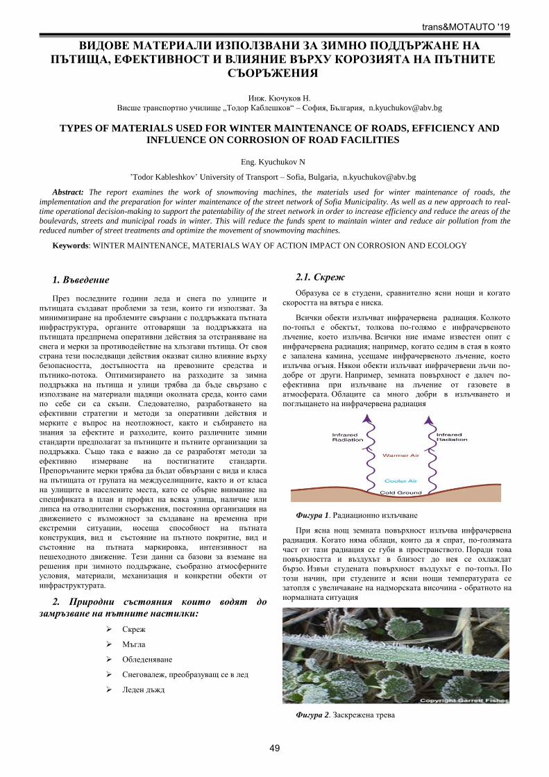
ВИДОВЕ МАТЕРИАЛИ ИЗПОЛЗВАНИ ЗА ЗИМНО ПОДДЪРЖАНЕ НА
ПЪТИЩА, ЕФЕКТИВНОСТ И ВЛИЯНИЕ ВЪРХУ КОРОЗИЯТА НА ПЪТНИТЕ
СЪОРЪЖЕНИЯ
Инж. Кючуков Н.
Висше транспортно училище „Тодор Каблешков“ – София, България, [email protected]
TYPES OF MATERIALS USED FOR WINTER MAINTENANCE OF ROADS, EFFICIENCY AND
INFLUENCE ON CORROSION OF ROAD FACILITIES
Еng. Kyuchukov N
’Todor Kableshkov’ University of Transport – Sofia, Bulgaria, [email protected]
Abstract: The report examines the work of snowmoving machines, the materials used for winter maintenance of roads, the
implementation and the preparation for winter maintenance of the street network of Sofia Municipality. As well as a new approach to real-
time operational decision-making to support the patentability of the street network in order to increase efficiency and reduce the areas of the
boulevards, streets and municipal roads in winter. This will reduce the funds spent to maintain winter and reduce air pollution from the
reduced number of street treatments and optimize the movement of snowmoving machines.
Keywords: WINTER MAINTENANCE, MATERIALS WAY OF ACTION IMPACT ON CORROSION AND ECOLOGY
1. Въведение
През последните години леда и снега по улиците и
пътищата създават проблеми за тези, които ги използват. За
минимизиране на проблемите свързани с поддръжката пътната
инфраструктура, органите отговарящи за поддръжката на
пътищата предприема оперативни действия за отстраняване на
снега и мерки за противодействие на хлъзгави пътища. От своя
страна тези последващи действия оказват силно влияние върху
безопасността, достъпността на превозните средства и
пътнико-потока. Оптимизирането на разходите за зимна
поддръжка на пътища и улици трябва да бъде свързано с
използване на материали щадящи околната среда, които сами
по себе си са скъпи. Следователно, разработването на
ефективни стратегии и методи за оперативни действия и
мерките е въпрос на неотложност, както и събирането на
знания за ефектите и разходите, които различните зимни
стандарти предполагат за пътниците и пътните организации за
поддръжка. Също така е важно да се разработят методи за
ефективно измерване на постигнатите стандарти.
Препоръчаните мерки трябва да бъдат обвързани с вида и класа
на пътищата от групата на междуселищните, както и от класа
на улищите в населените места, като се обърне внимание на
спецификата в план и профил на всяка улица, наличие или
липса на отводнителни съоръжения, постоянна организация на
движението с възможност за създаване на временна при
екстремни ситуации, носеща способност на пътната
конструкция, вид и състояние на пътното покритие, вид и
състояние на пътната маркировка, интензивност на
пешеходното движение. Тези данни са базови за вземане на
решения при зимното поддържане, съобразно атмосферните
условия, материали, механизация и конкретни обекти от
инфраструктурата.
2. Природни състояния които водят до
замръзване на пътните настилки:
Скреж
Мъгла
Обледеняване
Снеговалеж, преобразуващ се в лед
Леден дъжд
2.1. Скреж
Образува се в студени, сравнително ясни нощи и когато
скоростта на вятъра е ниска.
Всички обекти излъчват инфрачервена радиация. Колкото
по-топъл е обектът, толкова по-голямо е инфрачервеното
лъчение, което излъчва. Всички ние имаме известен опит с
инфрачервена радиация; например, когато седим в стая в която
е запалена камина, усещаме инфрачервеното лъчение, което
излъчва огъня. Някои обекти излъчват инфрачервени лъчи по-
добре от други. Например, земната повърхност е далеч по-
ефективна при излъчване на лъчение от газовете в
атмосферата. Облаците са много добри в излъчването и
поглъщането на инфрачервена радиация
Фигура 1. Радиационно излъчване
При ясна нощ земната повърхност излъчва инфрачервена
радиация. Когато няма облаци, които да я спрат, по-голямата
част от тази радиация се губи в пространството. Поради това
повърхността и въздухът в близост до нея се охлаждат
бързо. Извън студената повърхност въздухът е по-топъл. По
този начин, при студените и ясни нощи температурата се
затопля с увеличаване на надморската височина - обратното на
нормалната ситуация
Фигура 2. Заскрежена трева
trans&MOTAUTO '19
49

Когато температурата, се увеличава с повишаване на
надморската височина, това явление се нарича инверсия.
При облачни нощи, облаците действат като
метеорологични одеяла, които забавят или предотвратяват
загубата на инфрачервено лъчение (топлина) от повърхността и
по този начин охлаждането е далеч по-малко. Одеялата ни
затоплят, забавяйки загубата на топлина от нашите тела -
облаците работят по подобен начин, с изключение на това, че
намаляват количеството топлина, напускаща повърхността.
Силните ветрове също работят срещу повърхностното
охлаждане, тъй като ветровитите условия "разбуждат"
атмосферата и смесват част от по-топлия въздух на земята
надолу.
Във въздух се съдържа голямо количество водна пара.
Водната пара е невидим газ: водата може да се види само
когато се кондензира във водни капчици или ледени кристали.
Количеството на водната пара във въздуха, което може да се
задържи, варира в зависимост от температурата, като топлият
въздух има способността да задържи повече водни пари. Ако
охлаждаме достатъчно въздуха (до температурата на точката на
оросяване), той вече не може да задържи влагата в него и
водната пара кондензира във водни капчици или ледени
кристали.
През деня, когато слънцето изгрява и затопля повърхността,
температурите на въздуха в близост до повърхността
обикновено са над температурата на точката на оросяване, а
водата в атмосферата остава под формата на невидима пара.
Въпреки това, когато слънцето залязва при студени и ясни
нощи, температурата на повърхността се понижава (тъй като
земята излъчва топлина в пространството), а въздухът близо до
повърхността може да се охлади до температурата на точката
на оросяване. Ако температурата на пътната настилка и
температурата на точката на оросяване надхвърлят
температурата на замръзване, на повърхността се образува
роса, но ако температурата е под нула градуса повърхността на
настилката замръзва.
Явлението скреж се среща по често: в долини, водни
басейни и реки, където студеният въздух се задържа и
скоростта на вятъра обикновено е по-малка.
В обобщение, пътните настилки обикновено замръзват при
относително ясни нощи и слаби ветрове.
2.2. Мъгла
Често се образува при студени, ясни нощи, когато
температурите паднат до температурата на точката на
оросяване. Мъглата съдържа големи количества теч на вода,
която при преминаване върху път, който е охладен до
температура под температурата на замръзване, обледяването
може да бъде бързо и тежко, и дебел слой лед да се образува за
минути.
2.3. Обледеняване на пътните настилки
Появява се когато през деня температурата на пътната
настилка е над 0 С, същата е мокра от топящият се сняг, през
нощта температурата рязко пада под 0 С и се получава процеса
на обледеняване на настилката. Подобна ситуация може да се
получи и без сняг, ако водата се отича по пътя или от друг
водоизточник. През деня водата остава течна, но през нощта
замръзва на повърхността на пътя. Освен това влажните
пътища често замръзват много бързо, когато въздухът е
сух. Причината за това е охлаждането от изпаряване.
Особено опасен тип заледяване при снеговалеж се появява
в началото на зимния сезон или след период на топло време. В
такива случаи температурата на пътните повърхности са над 0
С. При понижаване на температурата и силен снеговалеж,
снегът първоначално се стопява и се превръща в киша от
топлия път. При продължително понижаване на температурата
на въздуха разтопеният се сняг се преобразува в лед.
2.4. Леденият дъжд
Образува се при валеж, падащ при отрицателни
температури на въздуха и наличие на температурна
инверсия. В долната тропосфера в близост до земната
повърхност въздуха е студен, а над него има слой от по-топъл
въздух. В топлия въздушен слой дъжда е под формата на малки
сфери пълни с вода, навлизайки в студения приземен въздух
водата в сферите се преохлажда и замръзва. Падайки върху
предмети, сферите се разбиват, водата изтича, замръзва веднага
и формира ледена покривка.
3. Предварителен анализ
Пред започването на зимата трябва да се направи обстоен
анализ на пътната инфраструктура която ще бъде поддържана.
В този анализ трябва да се имат в предвид:
3.1. Местата през които преминават
пътищата.
Изстиването на пътната настилка в началото на
зимата отнема дни или седмици, въпреки, че
температурата на въздуха може да е доста по-
ниска. Това се дължи на факта, че температурата
под основата на пътищата е по-висока и по-бавно
изстива. Което от своя страна, намалява нощните
температурни амплитуди и по този начин
намалява възможността за заледяване на
настилката.
Пътните настилки върху мостови конструкции са
много по-уязвими към заледяване от колкото
останалите настилки. Те изстиват много бързо,
защото под тях има въздух /който е добър
изолатор/ и до тях не достига температура от
земята. Ето защо студеният въздух бързо
изстудява мостовата конструкция. Чести са
случаите когато водачите на автомобили са били
неприятно изненадани когато при движение по
мокър път, влязат в заледена настилка на мост.
Фигура 3. Софийски околовръстен път – мост над
път III – 181
Засенчването на пътни настилки от дървета,
хълмове и други предмети значително влияе върху
образуването и трайността на лед върху
настилката. През нощта, надвисналите дървета
или други покрития над пътищата могат да
намалят възможността за замръзване, като
trans&MOTAUTO '19
50

блокират загубата на инфрачервена топлина в
пространството. Ето защо паркираните
автомобили под дървета рядко измръзват. От
друга страна, ако пътната настилка замръзне и се
покрие с лед, засенчването на дървета или
хълмове може да забави топенето до късно
сутринта или леда да се задържи и през
деня. Редица фатални злополуки са настъпили по
пътищата, когато шофьорите навлизат неочаквано
в заледени сенчести участъци. Критичното време
за заледяване на пътните настилки, засенчени от
хълмовете, /това е особено характерно за
високопланински пътища – пътища в ПП Витоша/
са часовете преди и след залез слънце.
Фигура 4. Сенчести участъци на пътна настилка
В участъците, в които пътя преминава над
магистрални водопроводи и газопроводи,
пътната настилка замръзва в резултат
ниската температура на движещите се през
съоръженията флуиди.
Фигура 5. Магистрален водопровод под улично платно
3.2. Топлинно картографиране
Необходимо е изготвяне на топлинно картографиране на
пътната инфраструктура, която ще бъде поддържана. Това се
прави с цел оптимизиране на използваните реагентни
материали при зимния период.
3.3. Оптимизация
Оптимизиране маршрутите на движението на
снегопочистващите машини от местостоянките (базите) до
участъците, които ще почистват. Това ще доведе до по-бързо
отстраняване на вредните последици от снеговалеж и/или
заледяване. Скъсяването на изминатото разстояние от базата до
участъка, който ще се обработва, ще доведе до намаляване на
вредните газове отделящи се от снегопочистващите машини.
Фигура 6. Графично изображение на топлинно
картографиране.
4. Материали използвани при зимно
поддържане.
4.1. Промит пясък – предимства: естествен и евтин
материал, особено полезен при замръзнала пътна настилка
(създава необходимото сцепление); недостатъци: не топи
снега и леда. Необходимо е почистване на пътната настилка от
пясъка използван през зимата. Утаяване в отводнителните
съоръжения на пътната инфраструктура, което води до
ограничаване на тяхната проводимост.
4.2. Натриев хлорид (NaCl) – предимства: евтино и
широкоразпространено средство за обезледяване;
недостатъци: не е достатъчно ефективно, особено при
температури под - 6°С, при които то спира своя ефект,
причинява сериозни щети на обкръжаващата пътна
растителност, може да замърси водната повърхност, както и
източниците за питейна вода и не на последно място - има
силно корозийно действие върху бетонови и метални
конструкции.
4.3 Калциев двухлорид СаСl 2 - предимства: по-
бързо първоначално топене на ледовете, по-дълго действие
като предотвратява повторно заледяване, ефективен също и
при по-ниски температури, увеличава ефективността на NaCl,
ако се използват заедно, намалява разходите, тъй като се
намалява използваният материал, по-ефективен при по-широка
гама от нива на влажност; недостатъци: по-скъп от
натриевият хлорид.
4.4 Магнезиев двухлорид (MgCl2) - предимства:
имат най-голяма способност да привлича и задържа влагата от
неговото обкръжение, ускорява процеса на разтваряне и
разтопяване, не изисква допълнително почистване на
настилката след прилагането му, не замърсява въздуха;
недостатъци: многобройни проучвания показват, че MgCl2,
когато е използван като деятел, причинява много по-тежко
влошаване на бетона, отколкото NaCl или CaCl2.
trans&MOTAUTO '19
51

Фигура 6. Корозия на пътно съоръжение
Таблица 1. Влияние на материалите използвани за зимно
поддържане
5. Заключение:
От направеното изследване се установи, че доброто
познаване на пътната инфраструктура, природните явления и
качествата на използваните реагенти води до:
1. Добро управление в реално време на снегопочистващите
машини, вида и количеството обработки.
2. Редуциране на разходите.
3. Намаляване на количеството отделяни фини прахови
частици от оптимизираното движение на снегопочистващите
машини и оптимално използване на химически реагенти.
6. Списък на използвана литература:
1. С.В.Алексиков, Г.И. Беликов, В.А.Пшеничкина,
С.В.Волченко. „Организация зимнего содержания городских
дорог“
2. А.К.Дюнин, Гр.В.Бялобжеский „Защита автомобильных
дорог от лавин“
3.„Мониторинг снегозаносимых участков“ проф. Т.
Самодурова, доц. О. Гладышева
4. prof. Cliff Mass „Weather Forecasting and Advanced
Synoptic Meteorology“
5. „Winter maintenance in Sweden“
6. Николов В., И. Гаджов, Текущо поддържане на улиците в
София, „Сборник от научна конференция с международно
участие Транспорт 2011“, ВТУ „Т. Каблешков“.
7. Николов В., И. Гаджов, „Ръководство за проектиране на
пътища“, ВТУ “Т. Каблешков“, 2010.
8. Николов В. „Проектиране и строителство на пътища“,
ВТУ „Т. Каблешков“, 2012.
Тип
Най-ниска
практическа
температура
на топене
Потенциал за
корозионно
увреждане
Въздействие върху околната среда
Корозия
на
металите
Корозия
на
бетона
Стомано-
бетон
Качество
на водата
Качество
на
въздуха
Почви Растител
-ност
Натриев
хлорид
NaCl
-9 °C Висок; ще
инициира
и ускори
корозията
Нисък /
умерен;
Висока:
предизвиква
корозия на
арматурата
Умерено:
Прекомерно
натоварване с
хлорид /
метални
замърсители;
Ниска: Води
до намалена
употреба на
абразиви
Умерено /
високо:
Натрупване
на натрий
нарушава
структурата
на почвата и
намалява
пропускли-
востта
Високо:
причинява
увреждане
на листата;
осмотичен
стрес
уврежда
корените,
Калциев
двухлорид
СаСl2
-28 °C Висок;
ускоряване
на
корозията;
Нисък /
умерен;
Висока: Ще
предизвика
корозия на
арматурата
Умерено:
Прекомерно
зареждане с
хлорид;
замърсяване с
тежки метали
Ниска: Води
до намалена
употреба на
абразиви
Ниска /
Средна:
Подобрява
структурата
на почвата;
увеличава
пропускливо
стта;
отлагане на
метали
Високо:
причинява
увреждане
на листата;
осмотичен
стрес
уврежда
корените
Магнезиев
двухлорид
MgCl2
-23 °C Високо;
ускорява
корозията
свързана с
хидроско-
пичните
свойства
Умерено /
високо:
Висока:
корозия на
арматурата,
изследвани
ята
показват, че
MgCl2 има
най-голям
потенциал
за корозия
Умерено:
Прекомерно
зареждане с
хлорид;
замърсяване с
тежки метали
Ниска: Води
до намалени
абразиви
Ниска /
Средна:
Подобрява
структурата
на почвата;
увеличава
пропусклив
остта;
Висока:
причинява
увреждане
на листата;
осмотичен
стрес
уврежда
корените,
trans&MOTAUTO '19
52

QUALITY CONTROL OF MULTI-PASS WELD BY MEANS OF ACOUSTIC EMISSION
Dmitry S. Bals, M Sc. Eng. Education1, Leonid A. Vinogradov, M Sc. Eng. Education2 Yulija Soldatova, M Sc. Eng. Education3
Chairman of the Board of TTS LNK INDUSTRIES, , RIGA, Latvija1, Riga Technical University Institute of Civil Aviation, RIGA, Latvija2,
Riga Technical University Institute of Civil Aviation, RIGA, Latvija3
e-mail: [email protected], [email protected], [email protected]
Abstract: The article proposes a method of assessing the quality of multi-pass weld by acoustic emission. The AE method involves the
identification of developing defects at the stage of stress changes in the material, as well as in the statically loaded state. In the process of
control two independent data collection systems were used, which worked in the process of testing synchronously. The selected method of
control of the object has a number of advantages over other methods of NDT. KEYWORDS: ACOUSTIC EMISSION, WELDING JOINTS, PROPAGATING DEFECTS, DATA ACQUISITION SYSTEM.
Introduction
Currently, it is more and more popular the NDT method of
welding structures elements technical condition assessing by the
physical principles of acoustic emission. The main advantage of this
method is its integrality without binding at the first stage to a
specific place and fixing the health as "there is a DEFECT-no
DEFECT" in a certain zone. After that, the decision is made quickly,
for example, in the control of multi-pass welds in thick-walled
structures, to eliminate defects with a minimum amount of metal
sampling. However, this method requires real-time analysis and
multy information that is coming in with high intensity, which is not
always feasible. So there is the risk of losing some data on the
further study of the defect, its nature, root cause and level of danger
(maintainability)[1].
Research technology
The object of the research is multi-pass welding seals as butt straight
joints of the bridge support pylon section (Fig. 1). The object of
study is made by welding cylindrical cones of steel grade S355NL -
analogues (USA A656, Russia 17Г1С, 17ГС). After welding, the
quality is usually controlled by traditional non-destructive testing:
visual, magnetic, ultrasonic, and radiographic.
Fig.1 Test Object
To compare the effectiveness of the NDT methods, we will
additionally check the object by the acoustic emission method. [1]
AE data acquisition system With the aim of obtaining acoustic emission data during the
checking, there are used two independent from each other data
acquisition systems, which operated simultaneously in the testing
process (see figure 2, 3): 1. AE data acquisition system Lel / A-Line 32D (DDM) / -
DIGITAL A-Line 32D. This is multi-channel AE data acquisition
modular system
Fig 2. Portable AE data acquisition system A-Line32D
2. Mobile data acquisition system Physical Acoustics
Pocket AE with outer preamplifiers 40dB
Fig 3. Portable АE-Station Pocket AE-2
The Pocket AE has only one recording line. The pickup gauge has
been installed on outer surface of test object. (Fig. 4/1, left). The A-Line System has two AE signals recording lines: the first
pickup gauge has been installed on the outer surface of test object
(Fig. 4/2), and the second - on the inner surface (Fig. 4/3), nearby
the welding seal. [3]
Fig 4. The pickup gauges disposition on the test object.
Each AE pickup gauge has its own channel line and has been
mounted on he surface by magnetic holder.
The test program included three stages
1.Lifting the object from the support with a crane
2.Keeping the object for 10-12 minutes
3. The descent of an object on a support
The AE method assumes the identification of propagated defects at
the stage of stress changes in the material, as well as in the
statically loaded state.[2]
Changing the load is occurred during the change in the direction of
deformation of the object. The test object has round in section,
mass near 2 tons. Under its dead weight the pressed and bending
loads are originated along the vertical axle.
(Fig 5.)
Fig. 5. The test object section deformation mode, then it sits on
surface (left) and hangs (right) .
trans&MOTAUTO '19
53

Then hang position the mode of load is changed. Under dead weight
the pressed and bending loads are originated in horizontal axle of
test object. Under the load changing any defects in existence
generate the AE signals. Inspecting the AE characteristics, such as
dynamics, amplitude etc., it is possible to reveal, identify and, if
necessary, to locate the defect in test object. After the lifting stage (12 sec), there is the static holding stage
during 600 sec. All the time AE signals have been recorded. Some
detected AE signals have proved the existence of probably AE
origins. During final checking stage the test object is moved down on
supports in horizontal state. The load changing occurs in opposite
order, than in the first stage. The unbend and spread stresses changes
the compressed and bending ones. Also the AE signals are recorded.
Results of AE NDT
The picture of AE impulses during the experiment #1 (until the
section of test object was rotated to 900), recorded by Mistras Pocket
AE-2, channel #1. The Test Results (the data line of Pocket AE)
Fig.6. Left: the AE intensity and amplitude versus time
Right-upper: AE-summing versus time; - center: AE impulses amplitudes frequency;
- down: AE intensity versus time
Fig. 7. The Test object loading and AE intensity. Experiment #1
The test program included three stages
1. Lifting the object from the support with a crane
2. Keeping the object
3. The descent of an object on a support
Fig. 8. The Test Object loading and AE intensity during Test Object
lifting (experiment #1)
From the first second the acceleration of the AE-intensity growth is
observed (-criteria) [5]. From the second 13 of the beginning of
test object holding-off two step-up stages of AE-intensity (Pocket
AE) are observed (secc. #640 and #670).
Fig. 9. The test object loading and AE-intensity during its
descending (experiment 1, Pocket AE).
After the first experiment, the test object was rotated by 90 grad
around the longitudinal axis and the tests were repeated. It is
necessary in order to identify possible defects that did not revealed
due to a possible difference of the mutual direction of the proposed
crack contour and the vector of the applied load. The test object checking results (A-Line System).
Fig. 10. Diagrams of AE data plots (A-line system, first experiment,
till test object rotation.).
Fig. 11. Diagrams of AE data plots (A-line system, second
experiment, after test object rotation.).
Fig 12. The Test object loading and AE intensity. Experiment #1
(A-Line).
Comparing the A-Line and Pocket AE sistems pickup data their
agreement is observed. During experiment following AE-signals data are registered.
amplitude,
intensity, AE impulses summing
At the stages of test object lifting and descending on the support
AE average (dozens of impulses per second) intensity was
observed. The nature of the total AE-summing is different. At the
stage of lifting, the total AE diagram has only one characteristic
pronounced break-point, while at the stage of descent — two
trans&MOTAUTO '19
54

stages. This may indicate the presence of fine heterogeneity in the
material of the object.
At the stage of test object holding no intense emission was observed.
Single events that occur within 600 seconds of the experiment do
not carry information about the presence of dangerous heterogeneity
that propagated over time. This emission is normal for a
homogeneous material.
Additionally the welded sample was checked by visual and
ultrasonic method
Results of visual and ultrasonic NDT checking
Under visual-measuring check of welded joint defects have been not
identified. Ultrasonic scanning was carried out along the entire
length of the weld, after the closing of welding within up 40 hours
[4]. The results were obtained by using USM 35 XS ultrasonic flaw
detector. Angle beam transducers of transverse waves are used to
scan, the dimensions of the piezo-element 14x14 mm, frequency 2
MHz, with input angles of 45º, 60º and 70º, and also the direct
transducers of longitudinal waves were used. The dimension of the
piezo-element 6х20мм, a frequency of 4 MHz and a piezo-element
with a diameter of 24 mm 2 MHz, the tuning was performed on the
lateral drilling with a diameter of 3 mm. In the zone specified by of
acoustic emission checking, the indication at a depth of 12 mm with
a signal amplitude +3 dB conditional length of 10 mm in the
analysis of the characteristics of the signal was revealed, it was
determined as the indication of the defect spherical shape
See Fig. 13.
Fig. 13. The pickup data of ultrasonic NDT Summary The proposed method of the object checking has some advantages
over methods of NDT. The time of preliminary assessment of the
technical state of the object practically coincides with the time of the
experiment. Taking into account the preparation and tuning of the
equipment, it took about 30 minutes to check the object. The method
does not require the use of dyes, powders, ionizing radiation. The
inspection process does not involve the use of consumables or
cleaning of the object after the experiment. At the same time, short-
term use of lifting or loading equipment (crane, Jack, etc.) is
required. Tests have shown the presence of heterogeneity of the material,
manifested under dynamic loads, but not detected in a static state.
To localize this heterogeneity a re-AE-experiment with the number
of sensors not less than 4 is required. Such experiment is possible
with the use of the A-Line 32D system and does not require
additional AE equipment. For classification of heterogeneity to the
class of hazardous or non-hazardous, other NDT methods are
required, which is confirmed by the data obtained as a result of
ultrasonic scanning.
Literature 1. Иванов В.И., Власов И.Э. Метод акустической эмиссии. – В
кн. неразрушающий контроль / Справочник в 7 т. // Под общ.
ред. В.В. Клюева. Т.7. Кн.1: - М.: Машиностроение, 2005 2. Г.С. Ельчанинов, В.В. Носов. Методика оценки ресурса
сложно нагруженных сварных соединений // Современное
машиностроение.Наука и образование: Материалы 1-ой
Международной науч.-практ.конференции под ред. М.М.
Радкевича и А.Н. Евграфова. – СПб.:Изд-во Политехн. ун-та,
2011. – С.212-218. 3. Баринов А.В., Федоров А.В., Кинжагулов И.Ю., Сергеев Д.С.,
Доренская А.В. Контроль качества сварных соединений в
процессе сварки с применением метода акустической эмиссии
// Науч.-техн.вестник ИТМО. 2013. №5(87), С.144 – 148.
4. ГОСТ Р 57351-2016/EN 1090-2:2008+A1:1011 Конструкции
стальные строительные. Общие технические условия. 5. Adrian A. Pollock. Acoustic Emission Inspection In: ASM
Metals Handbook Volume 17, Nondestructive Evaluation and
Quality Control (1997), pp. 593-628. 6. https://cloud.mail.ru/stock/gJSHVyob9HFL72fXDrg7ku1e
trans&MOTAUTO '19
55

REDUCING THE ENERGY INTENSITY OF MULTI-PRODUCT MACHINERY
PRODUCTION BY IMPROVING THE CORE PRODUCTION INFRASTRUCTURE
V.G. Abrahamyan
Russian-Armenian University
Ysrevan State University
Abstract: Multi-product machinery production forms a machine park of an industrial organization, so the finished products must provide
high-quality and economic indicators while using them in productions. The problem of increasing the level of production efficiency is
analysed in such organizations depending on the improvement of the basic production infrastructure. The new, quantitative indicators are
presented, which help justify the interrelations of material, labor and energy production costs. The necessity of implementation of innovative
technological processes at the preproduction phases is justified, which allows to reduce the level of material intensity, labor intensity and
energy intensity of production and increase the efficiency of the production organization.
KEY WORDS: MECHANICAL ENGINEERING, PRODUCTION PHASES, INFRASTRUCTURE, MATERIAL INTENSITY, LABOR
INTENSITY, ENERGY INTENSITY.
In order to create a powerful and efficient economy, it is
necessary to form a corresponding industry which will provide the
necessary basic resources to the other sectors of the economy and
form the appropriate material and technical base. The harmonious
implementation of these processes in space and through the time
enables to form a kind of structure which guarantees the balanced
development of all sectors of the economy and promotes the
effective solution of existing social and economic problems.It is
necessary to ensure the rapid and progressive development of multi-
product machinery production (machine-tool construction) as it
forms the basic tools of industrial enterprises and creates the
necessary mechanical assembly for the production and
technological processes. For the timely solution of the problems, it
is necessary to ensure the efficient and competitive activity of a
multi-product machinery production organization (hereinafter -
manufacturing company). For this reason, a manufacturing
company must systemise all the integrated processes that are
implemented from the formation and design of ideas (R&D,
technical and organizational preparation of production) to the
production and realization of new products.
For this purpose, the manufacturing company by using the
marketing division's instruments included in its logistic service,
studies the changes in the market on the basis of which the
necessary information base is formulated for innovation policy and
restructuring the manufacturingcompany's infrastructure.
In the framework of the innovation policy realization, in the
manufacturing company must be developed and realized the
upgrade of the range of the corresponding innovation programms'
products (improvement of manufacturing products, implementation
of new products) and introduction of new technological processes.
In order to implement the developed strategic plans, the
manufacturing company needs to carry out the reconstruction of
production and technological and organizational processes which
improve the existing production infrastructure and the new
technological processes and new production methods are
implemented very fast and efficiently.
Multi-product machinery production, being the main source for
the production of machinery and equipment, promotes the increase
of the level of labor productivity in the other sectors of the
economy. The technical re-equipment of production, the application
of new advanced production and working methods are the basis for
the increasing the manufacturing productivity and expanding the
segment of the manufacturing company in the market.
The improvementof the level of productivity and qualitative
indicators of the finished products, produced in multi-product
machinery production, is one of the main factors in reducing the
intensity and increasing the quality of products which are produced
in the practical production by using them.
The correct formation of the main production infrastructure has
the key role for increasing the productivity of multi-product
machinery production which is important in generating the
production costs. The improvement of the main production
infrastructure of manufacturing company gives an opportunity to
raise the level of production effectiveness by reducing of production
costs. In multi-product machinery production the efficient use of
material and labor resources and the reduction of their costs plays
the key role in reducing the production costs, as they have the major
share in total production costs.
The results of the conducted research show that in multi-
product machinery production, the full intensity has the following
structure: technological intensity is 60-65%, service intensity is 15-
20%, maintainance intensity is 15-20%: In multi-product machinery
production, first of all, it is necessary to accurately predict and
justify the value of technological laborintensity, as it is the main
strategy for increasing the labor and production productivity.
In multi-product machinery, the level of technological labor
intensity depends on the level of material intensityof production but
the level of the energy intensity of production in its turn depends on
the level of labor intensity of production. Therefore, in the
production should be used such kind of production and
technological processes which will first of all reduce the level of
material intensity of production.
The results of the conducted research show that in multi-
product machinery production the main production phases
technological intensity has the following structure: preproduction
phase - 15-20%, design - 45-55%, assembly - 20-25%, other
technological processes - up to 10%. Hence, the major share of
technological labor intensity (about 60-70%) has preproduction and
design labor intensity phases. So, we could say, that the value of
these phases directly depends on the level of material intensity of
production. The production phases that are mentioned in the
industrial organization are also energy intensity.
The level of labor intensity of design phase is determined by
the level of the technological processes progress, which are used in
the preproduction phase. At this stage the use of innovative
technological processes gives an opportunity to increase the degree
of accuracy of the preforms' output. As a result, their shape and size
is brought closer to the shape and size of the finished parts,
minimizing the volume of waste disposal. This helps to reduce the
level of material and labor intensity, which leads to the decrease of
energy costs in the manufacturing company.
The analysis shows that the level of labor intensity directly
depends on the level of material intensity and the level of material
intensity depends on the degree of accuracy of the used preforms. It
is justified by the modification of the well-known formula for
determining the labor intensity in the design phase which is
illustrated as follow:
Shbn
mmt
ijij
ij
0
1
1
(1),
where the numerator is the volume of waste disposal, the
denominator is a constant value for the given type of preform1.
1Abrahamyan V.Increasing the effectiveness of multi-product machinery
production through the management of the organizational and
innovative processes.Yerevan, 2010, p. 141
trans&MOTAUTO '19
56

We can conclude, that the value of technological labor intensity of
designing is directly proportional to the value of the preform mass
(or waste disposal).
It is necessary to use progressive technological processes for
reducing the value of material intensity in the preproduction phase,
which will give an opportunity o minimize the volume of waste
disposal. As a result, the mass of used materials will be reduced as
well as the level of energy and labor intensity in the design phase.
Labor intensity of each part of preform included in the finished
product structure in the preproduction phase can be determined by
the following formula2:
𝑡1𝑖𝑗 = 𝐴𝑖𝑗 𝑚 𝑖𝑗
𝐾𝑖𝑗𝑚
𝑥𝑖𝑗
𝐾1𝑖𝑗𝐾2𝑖𝑗 (2),
where ijt1 is technological labor intensity of i part of preform in
j production with technological process, ijm is the net mass of i
part, the preform of which is made by j technological process,
m
ijK is the coefficient of the use of material of i part in the case
of making the preform by j technological process, ijK1 is the
coefficient, which considers the impact of production volume at
ijt1 , ijK2 is the coefficient which considers the impact of
preform's degree of complexity at ijt1 .
The value of technological labor intensity of one machine set
of the manufactured finished product can be determined by the
following formula:
k
j
N
i
ijij
x
m
ij
ij
ij
k
j
N
i
ij
jij
j
KKK
mAtT
1 1
21
1 1
11 (3),
where Kj ,1 are the possible types of technological processes
for creating preforms, Ni ,1 is the quantity of parts included
in the structure of the finished product, the technological processes
of their preforms creating and designing are made in that
manufacturing company.
In the preproduction phase, the power energy cost per product
unit can be determined by the following formula:
𝐸1 = 𝑡1𝑖𝑗𝑁𝑗
𝑖=1𝑘𝑗=1 𝑁1𝑖𝑗 𝑘1𝑖𝑗 𝑎 (4),
where 𝑁1𝑖𝑗 isthe total nominal capacity of the engines in the
machinery and technological equipment used in production of
preforms of one machine set parts of finished product with the
various technological processes in the preproduction phase, 𝑘1𝑖𝑗 is
the coefficient of nominal capacity use of machinery and
technological equipment, 𝑎 is the tariff of electricity.
By determining the power energy cost before the
implementation of advanced technological processes, for creating
the preforms in the preproduction phase of production and after the
implementation of these processes, the change in the amount of
power energy cost caused by the use of innovative technological
processes can be determined.
,2
2
2
2
1 1
1
1 1
2 ПT
tz
y
t
b
l
xK
j
N
im
ij
ijaKe
NK
meT
j
(5),
The conducted research results show that in the design phase
of multi-product machinery production, the value of technological
labor intensity for one machine set of manufactured finished
product is determined by the following formula:
where the first component is the absolute term (2a
e , e=2,71828...),
2Abrahamyan V.Problems of Economics and Management of enterprises,
industries and complexes.Book 9. RF, Novosibirsk, 2009, p. 26.
222 ,, zyx are the power indicators, the second component
2
1 1
xK
j
N
im
ij
ijj
K
m
the total mass of preforms of one machine set parts of
finished product, which are designed in the manufacturing
company, the third component
2
1 1
1
y
t
b
l
N
is the coefficient of
technical saturation of the design phase of production, the fourth
component 2tze shows the impact of the product manufacturing
years in the manufacturing company (it is not taken into
consideration in the case of a new product), the fifth component
ПTK takes into account the level of used technological processes
progress due to the structure of the used machine assembly3.
In the design phase of the production, the value of
technological labor intensity made by the tehnological equipment of
group can be determined by the following formula:
βTt 22 (6)
where β is the specific weight of technological labor intensity
made by the tehnological equipment of group in the total
technological labor intensity of the production of one machine set of
one finished product.
In the design phase of the production, power energy cost per
product unit can be determined by the following formula:
𝐸2 = 𝑡2𝑖
𝑁𝑖=1
𝑘2
=1𝑁
2𝑖 𝑘2𝑖 𝑎 (7),
where 𝑁2𝑖 is total nominal capacity of the engines in the
technological equipment used in production of preforms of one
machine set parts of finished product in the designphase, 𝑘2𝑖 is
the coefficient of nominal capacity use of technological equipment,
𝑎 is the tariff of electricity.
In the design phase of production, by determining the value of
power energy costs before the implementation of progressive
technological processes for the preparation of the performers in the
preproduction phase and after these processes' realization we can
determine the value of power electricity costs' expected saving.
The implementation of new feasible progressive technological
processes in the preproduction phase for making high precision
preforms allows to reduce the level of material intensity, labor
intensity and energy intensity in the production, which provides the
cut in the value of production costs.
It is necessary to develop economic mathematical model for
economic feasibility of new technological processes
implementation, where the objective function is the value of
production costs of one machine set of the finished product in the
preproduction and design phases of production, and as limitations -
the level of material, labor and energy intensity.
The rebuilding of the core production infrastructure in the
preproduction and design phases of multi-product machinery
production gives an opportunity to use progressive technological
processes and high-performance machinery and technological
equipment, which enable to get high precision preforms for the
parts designed in the manufacturing company and included in the
finished product structure. Besides that, it increases the productivity
in the design phase of the production, providing the reduction in
material, labor and energy resources, and helps to raise the level of
efficiency of the manufacturing company.
3Abrahamyan V.Modern knowledge-based technology. Regional Annex. RF, Ivanovo, 2016/1, p. 104.
trans&MOTAUTO '19
57

THE RESEARCH PECULIERITIES OF PARAMETERS AND CHOICE OF
AGRICULTURAL MACHINES IN PEDAGOGICAL TECHNOLOGIES
FOR INNOVATIVE PROJECT ACTIVITY IN TRAINING
AGROENGINEERS
Candidate of Technical Sciences, Associate Professor Viktor Pryshliak
Ukraine, Vinnytsia National Agricultural University
Summary. The structural-logical model of training of future specialists in agroengineering for innovative project activity has been
developed on the basis of a systematic comprehensive study of the theoretical course of agricultural machines, the deepening of the students'
scientific work on the development of supporting and moving elements of machine-tractor units, including pneumatic tires. The samples of
individual fragments from the algorithm and the method of calculation of wheels used in the educational process are provided and the
general and professional competencies of the agroengineer are created, especially during the implementation of future specialists in agro-
industrial production of higher education courses in the course of master's and master's studies. It is noted that the training of agroengineers
for innovative project activities is carried out in accordance with the Law of Ukraine "On Higher Education" and the standards of higher
education of Ukraine. The influence of interdisciplinarity in the system of cross-cutting project preparation on the readiness for
implementation of production practical tasks is investigated. It is confirmed that the support-run elements of aggregates in the conditions of
complex terrain contributes to the development of erosion processes and negatively affect the soil fertility. Any tire better satisfies the
condition of permissible wheel pressure on the soil if the air pressure in the tire is low. Improving the technological process of
manufacturing tires for agricultural purposes allows them to ensure their quality, reliability and operational safety.
KEYWORDS: WHEEL TIRES, AGRICULTURAL MACHINERY, TECHNOLOGY, PROJECT TRAINING, PROJECT ACTIVITY,
STUDYING PROCESS, THEORY
Introduction.
Science and education are closely interconnected and able to
develop effectively in a single integrated system of scientific,
methodological and pedagogical activities. Educational process is an
intellectual, creative activity of scientific and pedagogical workers,
students, practitioners and other interested subjects in the sphere of
higher education and science [1].
The training of future agroengineers is based on the
formation of professional competences in a harmoniously developed
personality capable of solving various tasks of production activity.
The object of the study and activities of the agroengineer are the
phenomena and processes associated with the effective functioning
of agricultural machinery and mechanized technologies in agro-
industrial production [2]. The educational process of students of the
specialty "Agroengineering" is aimed at training specialists capable
of solving professional specialized tasks and applied problems
related to the use of agricultural machinery in mechanized
production technologies, primary processing, storage and
transportation of agricultural products, technical service of
mechanization facilities, etc.
In the structural and logical scheme of training future
agroengineers, the basic discipline is "Agricultural machines",
students learn about the structure and principle of operation of
agricultural machines, regulation and adjustment of them for
optimal modes of work, as well as the theoretical basis of
technological processes of working bodies, the method of
development and designing new and improving existing structures
[3]. Studying discipline in addition to classroom activities involves
the independent performance of course work, the purpose of which
is the technological development of the design of agricultural
machinery or its units, or the improvement of existing machines to
ensure the implementation of mechanized production processes of
growing crops and improving the operational, economic and
environmental performance.
The main scientific directions of the master's work in the
field of agroengineering are to increase the productivity of
aggregates, expand their versatility, combine energy resources with
other implements and ensure their reliable handling, minimize the
negative impact on the environment and soil, improve the working
conditions of machinery, as well as traffic safety. Agricultural
machine-tractor aggregates are driven across the field by
overwhelming majority by means of a wheeled driving system. The
processes that occur when the wheels interact with the soil, affect
not only the performance of the machines, but also the properties of
the soil, as the object of cultivation and the environment of
cultivating crops.
Practical, scientific and educational activities show that the
problem issues on the peculiarities of the substantiation of
parameters and the choice of tires of agricultural machinery wheels
in pedagogical technologies of agroengineering training for
innovative project activities are still insufficiently studied and
require further fundamental theoretical and experimental studies,
scientific substantiation and generalizations.
Prerequisites and means for solving the problem. For a long time, scientists have been engaged mainly in the
study of the processes of interaction of the running system with the
soil and traction-coupling properties of machines. Regarding the
deformation of pneumatic tires of agricultural wheels, these issues
are not sufficiently studied.
The problem issues related to the design of agricultural
machinery, preparation of agroengineering specialists for the project
activity, including the features of substantiation of parameters and
selection of tires of wheels, are not sufficiently studied.
In [4], the main components of the preparedness for the
project activity of the agroengineer as a specialist are presented,
which are united in physical and mathematical, general technical
and special blocks and general and professional competences, which
should be mastered by the bachelor of specialty 208
"Agroengineering". For example: to design equipment and
equipment of production areas, agricultural machines, their knots,
mechanisms, various connections; carry out standard design
calculations of knots and parts of machines and non-standard
equipment; rational assembly of machine aggregates in existing
production lines of crop and livestock production; to determine the
technical condition of tractors, cars and aggregates of complex
equipment [2], to optimize transport processes, etc.
In [5] presented an innovative system of scientific and
methodological developments that affect the formation of special
professional competencies of agroengineering. The basis of this
system is the latest textbooks, manuals, monographs, programs and
other teaching materials, as well as advanced pedagogical
technology of training, which is based on the progressive, phased
development of the future specialist's readiness for the project
activity. Such pedagogical technology of training provides a
comprehensive, comprehensive formation of professional
competencies of agroengineering in accordance with regulatory
requirements and standards of education, including [1, 2]. Students'
trans&MOTAUTO '19
58

scientific activity, which is based on the development and
modernization of agricultural machinery, plays an important role in
the design training. It was noted [5] that the first voluminous work
of the student in the educational process is the course work on the
discipline "Agricultural Machines". Its successful implementation is
a solid ground for effective and effective graduate design, writing
master's thesis.
The general issues of the theory of design training were
studied deeply by: Bryukhanova N.O. [6], Kolesnikova I.A. [7],
Gorchakov-Siberian M.P. [7], Nychalko N.G. [8], Zyazun I.A. [8],
Goncharenko S.U. [8] et al. The theory, methodology and practice
of design training for agroengineering, including in view of the
design of agricultural machinery, were studied and investigated:
Bendera I.M. [9, 10, 11], Duganets V.I. [12], Pryshliak V.M. [4, 5,
13] and others. Also, the questions of improving the methodology of
preparing future engineers are devoted to the work of A. Asherova,
O. Kovalenko, M. Lazareva, D. Chernilevsky, P. Yakovyshina, and
the methodological aspects of the future of agroengineering have
been reflected in the scientific researches of I. Buzik, A. Demin, S.
Daukilas, A. Esaulov, P. Luzan, V. Manke, I. Palamara, S.
Pastushenko, V. Yaroshenko, transformation of independent
educational activity into readiness for professional self-development
by means of technologies of personally oriented education − is
reflected in the monograph Bondar M.M., Zhuravsky L.M.,
Ostapenko E.O., Pryshliak V.M., Kutsenko A.G. [14].
Actual issues of studying the design, operation of tires,
reducing the harmful effects of the effect of running systems of the
machine tractor unit on the soil are devoted to the work [15, 16, 17,
18], and their production − [18, 19].
Solution of the examined problem.
As noted in [5], the theory and practice of project
preparation for future agroengineering involves the widespread use
of a scientific component in the educational process during
classroom classes, independent work of students. The scientifically
substantiated cross-cutting, interdisciplinary, sequential and phased
development of agricultural machinery involves achieving a high
quality learning outcomes and innovative technology development.
Apart from the fact that students during their studies at the
institution of higher education take part in research processes,
conferences, construct and model the means of mechanization, they
are to complete the term paper at the 3rd year, and in the master's
degree - a master's degree. Here, students mainly count, design and
study the working bodies of agricultural machines. However, there
are works in which auxiliary but very important nodes, mechanisms
or systems of machines are presented. The same applies to the
support and running elements of agricultural machines, including
wheel tires.
The type of wheel tires of agricultural machines should be
selected, taking into account the permissible action of the wheels on
the soil. Preferably the ecological pressure limit of the wheels on the
soil, depending on its type and state, is taken at a pressure of 0,1-
0,15 MPa.
First, for one of the circuits [3], it is necessary to determine
the radial load of the wheels on the soil (kN), which will correspond
to the required lifting capacity of the wheels of the machine, using
the formulas:
for front wheels
Ln/gQa10G 2м3
2
; (1)
for rear wheels
122м3
1 n/GnQg10G
, (2)
where a – center of gravity of the car relative to the rear axle, m
[3];
Qм – operating mass of the machine, kg [3];
g – acceleration of force weight, m/s2;
n2 – number of front wheels [3];
L – longitudinal base of the car, m [3];
n2 – number of rear wheels [3].
After receiving the radial load of the wheels on the
ground, you can proceed with the selection of the necessary tires,
following this sequence of actions. First, using the calculated
payload capacity of the rear and front wheels (G1 and G2), for tabl.
1 choose a tire capable of providing their payload, i.e.
1ш GG , 2ш GG
. (3)
Table 1
Load ratios and tire pressure to select a mode at 30 km / h.
Tire
designa-
tion
Air pressure in the tire chamber Рш, MPa
0,1 0,11 0,12 0,13 0,14 0,15 0,16 0,17 0,18
Permissible load on the bus Gд, kN
5,0-10 - - - 2,1 2,2 2,3 2,35 2,45
6-16 - - - 3,4 3,55 3,7 3,8 3,9
6,5-16 - - - 3,9 4,05 4,2 4,35 4,5
7,5-20 - - - 5,9 6,1 6,3 6,6 6,8
8,25-15 - - - 7,95 8,25 8,5 8,8 9,15
9,5-32 6,90 7,30 7,70 8,0 8,4 8,85 9,05 9,4 9,7
9-16 - - - - 8,5 8,85 9,5 9,8 10,45
12-16 - - - - 12,0 12,6 13,0 13,5 14,0
15,5-18 - - - - 13,6 13,9 14,8 15,4 16,4
It has been established that any tire will better satisfy the
achievement of permissible wheel pressure on the ground Р, if the
air pressure in the tire is low. After the previous choice of tires,
under its designation in the table. 2 linear sizes are selected: outer
diameter Dk and width of the tire вш. After that, it is checked
whether the selected tires are provided to the given ecologically
permissible pressure on the soil, using the formula
3шк23
кш2ш
22к
2ш
2шд вDр4DвР/DвРР12,0G
, (4)
where Рш – tire pressure, MPa (Table 1);
Р – permissible wheel pressure on the ground, MPa [3];
вш – width of the tire (for cars working in intermediate rows,
the width of the tire must be less than the width of the row), cm
(Table 2);
Dк – external diameter, cm (Table 2) ;
In tabl. 1 shows only data for air pressure in the chamber up
to 0,2 MPa. Tires with pressures greater than 0,2 MPa are not
recommended for use on field machines
Table 2
Characteristics of tires for agricultural machines
Brief
descript-
tion
Brief description
Model
Outer
diameter Dк,
cm
Tire
width
вш, cm
Mass,
kg
5,0-10 В-107 51,0 14,0 6,5
6-16 Л-225 75,0 17,5 17,5
6,5-16 Я-275Л 77,8 18,5 25
7,5-20 В-103 91,0 20,5 33
8,25-15 И-83 83,2 22,0 30
9,5-32 В-110 124,0 24,0 50
9-16 Я-324А 89,6 25,5 41
12-16 Л-163 93,0 32,5 44
15,5-18 КФ-105А 98,0 39,5 75
If after the calculations
1д GG , 2д GG
, (5)
then it is necessary to choose the bus with other parameters; and if
the tire could provide a condition
2,1д GG , (6)
it is impossible to pick up, the wheel must be taken with twin tires.
In this case, the number of tires for the wheel is determined from the
ratio
дG
GZ 2.1
. (7)
trans&MOTAUTO '19
59

Then repeat the same calculations for the second scheme
of the wheel drive of the car. The numbers for the tire, for example,
5.0-10, reflect: the first figure is the width of the profile of the tire in
inches, the second is the tire's diameter on the disc in inches.
As an example, according to such an algorithm, students of
the 3rd year of specialty 208 "Agroengineering" conduct
substantiation of parameters and choice of tires, performing course
work on the discipline "agricultural machines".
During the study in the magistracy, future specialists in
agroengineering conduct theoretical and experimental research at a
higher scientific level. Let's give an example of conducting such
researches for wheels of agricultural machines during their
movement in the field.
The processes of interaction of running systems with the soil
depend on its mechanical properties, that is, resistance, deformation
and destruction. A large amount of experimental data on the patterns
of deformation and destruction of soil has been accumulated. But
they are of a different nature due to the diversity of soil types,
conditions and methods of measurement, and the lack of
standardized methods for the integrated assessment of mechanical
properties. The use of this data to develop methods for forecasting
mechanical properties is not possible. This is due to the large
number of proposed empirical formulas and models of deformation
of soil [15].
In order to evaluate the interaction of the running system
with the soil, the regularity of its compression and displacement is
used, which implies the processes of formation of the trace (track)
and traction (traction) formation. These patterns are determined by
the corresponding displacement of the deformers (dies).
The diagram of the interaction of the rigid wheel with the
soil during rolling in a driven mode is shown in Figure 1.
Fig. 1. The scheme of deformation of the soil [15]
Observations show that the deformation of the soil by a
moving wheel at different time points extends predominantly to the
normal to the rim. Accordingly, the relative deformation є and the
rate of deformation є , elemental volumes in the sectors
corresponding to the corners, dφ to which all its array is divided into
angles φ° contact and thickness A of the active layer (deformed) can
be represented as follows [15]:
є =z0
l0 1 −
cos φ0
sin φ ; (8)
є = −ωz0
l0cosφ°
sin φ
cos 2 φ , (9)
where z0 і l0 – the dimensions are shown in the diagram; φ – the
value of the contact angle; ω – angle of rotation of the wheel.
Normal wheel load Q and longitudinal strength F, necessary
to overcome the rolling resistance, due to the processes of
interaction of the wheel with the soil, are equal to the sum of the
normal and tangential elementary soil reactions
Q = σ cosφBr0φ0
0dφ ; F = σ sin φ Br0
φ0
0dφ ,
where σ − contact voltage (elementary soil reaction)
В and r0 − contact width and wheel radius.
To solve these equations, it is necessary to use the analytical
relationship between voltage and deformation.
The deformation of the soil (its elementary volumes) is
completely reflected in the Kelvin model, to which the rheological
equation corresponds:
σ = Е2 ϵ + τ ϵ , (10)
where Е2 − deformation module; τ – time after action
viscosity ratio μ2 to the deformation module τ =μ2
Е2
Pattern of propagation resistance 𝜎𝑧 in depth z in the
direction of force Р Bussinesca formula is displayed [15]:
𝜎𝑧 = КР/𝑧2, (11)
where К − dimensionless multiplier.
To determine the effect of the solid reinforcing layer on the
nature of the propagation resistance used correction coefficient.
Also (using coefficients) the Bussineska formulas are
corrected with the aim of approximation of the calculated patterns of
propagation of resistance in soft soils to real
Deformation of pneumatic tires and soils adequately reflects
the three- and two-element rheological models, respectively. Using
the scheme of interaction of the elastic wheel with the soil and the
selected rheological models of contacting bodies, we find an
analytical description of the processes of simultaneous deformation
at wheel rolling. For this, the elementary sector of the scheme of
interaction (Fig. 2) will be presented in the form of sequentially
placed models of pneumatic tires and soil.
Fig 2. Interaction of rheological models of tires and soil
[15].
Determine what changes occur with the models when rolling
the wheel on the ground. If time t deduct from the moment when
𝜑 = 𝜑0, then on the front of the contact 𝜑 = 𝜑0 −𝜔𝑡, − and on
the back − 𝜑 = 𝜔𝑡 − 𝜑0 = − 𝜑0 − 𝜔𝑡 . Then for any t within
the angles of contact, the following relationship is valid [15]:
∆𝜌 + ∆𝑙 = ∆𝑅; (12) 𝑑𝜌
𝑑𝑡+
𝑑𝑙
𝑑𝑡=
𝑑𝑙
𝑑𝑡 ; (13)
𝜖1Е1 ± 𝜖 1𝜇1 ± 𝜈Е1𝑠𝑔𝑛𝜖1 = 𝜖2𝐸2 ± 𝜖 2𝜇2; (14)
𝑅0 𝑐𝑜𝑠 𝜑0 = 𝑅 𝑐𝑜𝑠 𝜑0 −𝜔𝑡 , 15
where 𝜌, 𝑙 і 𝑅0 − the sizes are shown in fig. 2, and R= 𝜌 + 𝑙. Indices 1 with designations indicate that they belong to the tire, and
2 to the ground. The "plus" signs correspond to the front of the
contact, and the "minus" is the rear.
The equation of correlation with respect to deformations and
their velocities is obtained after the time division of expressions (12)
and (13) into a product 𝐻𝑙0𝑅0, where 𝐻 – tire profile height
𝑙0 and 𝑅0 – initial values of sizes R and 𝑙. Can be recorded [15]
ϵ2 =∆R−ϵ1H
l0; ϵ 2 =
dR
dt−ϵ 1H
l0. (16)
Value ∆R and dR
dt can be found from equation (15), ie
trans&MOTAUTO '19
60

∆R = R0 1 −cosφ0
cos φ0 −ωt ;
dR
dt= −ωR0 cosφ0
sin φ0 − ωt
cos2 φ0 −ωt .
After substitution, expression (14) values ϵ2 and 𝜖 2,
represented by the calculation of formulas for ∆R and dR
dt, we obtain
the differential equation of the interaction of the elastic wheel with
the ground
±𝜖 1 𝜇1 +𝐻
𝑙0𝜇2 + 𝜖1 𝐸1 +
𝐻
𝑙0𝐸2
=𝑅0
𝑙0𝐸2 ± 𝜈Е1𝑠𝑔𝑛𝜖1 −
𝑅0
𝑙0𝐸2 𝑐𝑜𝑠𝜑0
1
𝑐𝑜𝑠 𝜑0 − 𝜔𝑡
±𝑅0
𝑙0𝜇2𝜔 𝑐𝑜𝑠𝜑0
𝑠𝑖𝑛 𝜑0 −𝜔𝑡
𝑐𝑜𝑠2 𝜑0 − 𝜔𝑡 . (17)
This equation does not have an exact solution, since
integrals are not expressed through elementary functions. Numerous
methods of integration and grounds for using Taylor series are used
for it. These methods do not allow (the second because it is large) to
add elementary soil reactions to represent the forces acting on the
wheel in the analytical form.
After conducting such an example of theoretical studies,
graduates begin to create a laboratory installation and conduct
experimental research in laboratory or field conditions.
As a result of scientific research, a pedagogical system was
developed, basing on the example of the interaction of the
supporting and moving elements of machine-tractor units with soil
and on the consistent study of topical production issues, contributes
to the improvement of the quality of training and the development of
design competencies of the agroengineer.
Results and discussion. The developed innovative system of
scientific and methodological training of future specialists is based
on a planned, cross-cutting, step-by-step growth of knowledge,
skills and abilities of future agroengineering. Course designing and
master's work provide a qualitative growth in the design
competencies of the graduate.
Conclusion. The obtained results of the conducted research
give grounds to conclude that an effective process of formation of
readiness for the project activity of future specialists in
agroengineering is possible on the basis of cross-cutting innovative
teaching technologies. Coursework and master's work contribute to
the development of scientific activities. It is important that they have
practical orientation, since this will substantially motivate the
students to complete them.
References
1. Law of Ukraine "On education" from 01.07.2014, №
1556-VII / Newspaper "Voice of Ukraine" dated 08.06.2014. − №
148.
2. The standard of higher education of Ukraine is the first
(Bachelor) level of education in higher education − bachelor, field
of knowledge − 20 Agrarian sciences and food specialties - 208
Agroengineering // Approved and put into effect by order of the
Ministry of Education and Science of Ukraine dated 12/5/2012, No.
1340. − Access mode:
https://mon.gov.ua/storage/app/media/vishcha-
osvita/zatverdzeni%20standarty/12/21/208-agroinzheneriya-
bakalavr.
3. Designing agricultural machines. Tutorial / І.М.
Bendera, A.V. Rud, Ya.V. Koziy and others; ed. І.М. Bendery, A.V.
Rudia, Ya.V. Kozia − Kamyanets-Podilsky: FOP Sysin O. V., 2010.
− 640 pp
4. Pryshliak Viktor. Role of project preparation in
formation professional competence of future specialists in
agroengineering / Viktor Pryshliak // TRANS MOTAUTO
WORLD: International scientific journal. – Sofia, Bulgaria: trans &
MOTAUTO WORLD, YEAR II, ISSUE 4/2017. – 162-165, ISSN
PRINT 2367-8399, ISSN WEB 2534-8493.
5. Pryshliak Viktor. Theory of project preparation of
agroengineers on the basis of scientific work on the development of
agricultural machinery / Viktor Pryshliak // SCIENCE. BUSINESS.
SOCIETY: International scientific journal. – Sofia, Bulgaria:
Scientific-technical union of mechanical engineering “Industry 4,0”,
National society «Industrial & national security», YEAR 3, ISSUE
4/2018. – 145-149, ISSN PRINT 2367-8380, ISSN WEB 2534-
8485.
6. Brukhanova N.O. Theory and methods of system
design teacher training future engineers-teachers: Dis. … Dr. ped.
Sciences: 13.00.04 – Kharkiv, 2011. − 594.
7. Kolesnikova I.A., Gorchakova-Sibirskaya M.P.
Pedagogical designing. − Moscow: Academy, 2007. − 288.
8. Designing the process of professional training in
vocational education institutions: monograph / [N.G. Nichkalo, IA
Zazyun, S.U. Goncharenko and others.]: Ed. N.G. Nobody. – K. –
Khmelnytsky: KhNU, 2010. – 335 p.
9. Bendera I.N. Full-time course and diploma designing
– a way to enhance the independent work of students of agrarian-
engineering specialties / Ivan Bender, Wojciech Tanas / Problemy
inzynierss rolnitsz w aspekcie rolnictwa zrownowazonego. – Lublin,
2005. – P. 180-192.
10. Graduate design in higher educational institutions of
the Ministry of Agrarian Policy of Ukraine: teaching method.
manual / [І.М. Bendera, O.V. Datsishin, O.V. Korolchuk et al.]; for
ed. T.D. Ishchenko, I.M. Bendery. − K.: Agrarian Education, 2006.
− 256 pp.
11. Benderа I.M. The theory and method of independent
work of future specialists in agricultural mechanization in higher
education: Dis. ... Dr. ped. Sciences: 13.00.04 − K., 2008. − 579.
12. Duganets V.I. Theory and practice of production
training of future specialists in agrarian-engineering direction: diss.
... doc. ped Sciences: 13.00.04 / Duganets Viktor Ivanovich. -
Kamenets-Podilsky, 2015 − 501.
13. Pryshliak Viktor. Method of projects in the theory
learning of a future agricultural engineer / Viktor Pryshliak //
TRANS MOTAUTO WORLD: International scientific journal. –
Sofia, Bulgaria: trans & MOTAUTO WORLD, YEAR I, ISSUE
4/2016. – 39-41, ISSN 2367
14. Transformation independent learning activities in
readiness for professional self-development by means of personal
technology based learning: Monograph / M.M. Bondar, L.M.
Zhuravska, E.A. Ostapenko, V.M. Pryshlyak, A.G. Kutsenko. –
Nizhin: LLC "Publishing" Aspect-Polygraph", 2016. − 760.
15. Vodyanik I.I. Processes of interaction of tractor
running systems with soil. − Chisinau, 1987. − 63 p.
16. Vodyanik I.I. Ways of reducing the harmful effects of
ITS running systems on soil in the conditions of the Southwest of
Ukraine. − Chisinau, 1987. − 63 p.
17. Vodyanik І.І. // Operational properties of tractors and
cars. − Kyiv: Harvest, 1994. −220 p.
18. Alixeychuk N.A., Budko Yu.V., Terekhov B.A. //
Increase of permeability of agricultural machines. − Minsk: Harvest,
1979. −135 p.
19. Bekin N.G., Petrov B.M. Equipment for
manufacturing pneumatic tires. − M.: Kolos. – 1998. − 479 p.
20. Gavrilov B.G. Tire production. − M.: Kolos. − 1998 −
379 p.
trans&MOTAUTO '19
61

1D SIMULATION-BASED DEVELOPMENT OF A SAFETY CONCEPT FOR THE
INVESTIGATION OF A HIGH-PRESSURE GAS-DIESEL INJECTOR ON A
SINGLE-CYLINDER RESEARCH ENGINE
Dr. Dimitrov D.1, Dipl.-Ing. Aßmus K.1, Dr. Redtenbacher C.1, Dr. Schubert-Zallinger C.2
LEC GmbH (Large Engines Competence Center), Graz, Austria 1
Graz University of Technology, Graz, Austria 2
Abstract: 1D simulation has significantly supported the process of developing a diesel ignited high-pressure gas direct injection
combustion concept, thus facilitating promising investigations at the SCE. It has been applied to a variety of tasks such as designing the
media supply system, pre-optimizing engine operating parameters and developing the safety concept discussed in this paper. Application
depends on two simulation models in particular: one validated MCE model and one SCE model enhanced in the course of the concept design
phase. Since the MCE model can reliably reproduce the behavior of a full engine with single-stage turbocharging, it played a critical role in
determining the boundary conditions for both the 3D-CFD simulation and the simulations with the SCE model. The SCE model, on the other
hand, includes all components relevant for the test bed and thus permits both a reliable design of the gas path and the development of a safety
concept, which is of remarkable importance for high-pressure gas applications. With regard to the safety concept, this paper presents and
discusses the difficulties in detecting injector malfunction and different detection strategies.
Keywords: DIESEL AND GAS FUELED ENGINES, 1D SIMULATION
1. Introduction
The potential for savings in greenhouse gas (GHG) by
substituting gases with high methane content (e.g., natural gas) for
conventional liquid fossil fuels is considerable due to the
comparatively low carbon dioxide emissions, cf. [1, 2].
Applications such as monovalent gas engines and diesel-gas engines
that operate on the Otto cycle already exploit this GHG saving
potential and are well known for their low emission of both
particulates and NOx as well as for high engine efficiencies, cf. [3,
4].
However, the feeding of a premixed gas-air mixture may result
in knocking combustion when gases with low methane numbers are
used as well as methane slip. Gas-diesel engines based on the diesel
cycle directly inject the gaseous fuel into the combustion chamber
during the high-pressure phase of the engine cycle. Ignition is
triggered by the injection of a small amount of diesel pilot fuel. The
resulting mixture-controlled combustion is not prone to knocking
and as a consequence, low-quality gases can be used at high
compression ratios and therefore high thermal efficiency.
Furthermore, these engines have the potential to avoid engine-out
methane emissions nearly entirely. Fully flexible gas-diesel
engines [4] can be operated either in dual fuel (DF) mode with
gaseous fuel as the main energy source or in diesel mode. This
redundancy is important in marine applications in particular where
fail-safe operation is critical. Application of these engines in
liquefied natural gas (LNG) tankers is economically advantageous
as the boil-off gas from the LNG storage system is effectively
transformed into propulsion energy, thereby increasing overall
efficiency, cf. [5, 6].
The development of a new dual fuel gas-diesel engine concept
requires the definition and pre-optimization of many parameters in
advance. Additionally, the system complexity resulting from having
to provide two fuels simultaneously is higher than with monovalent
engine concepts. Boundary conditions, knowledge of the
thermodynamic states in the combustion chamber during the engine
cycle as well as concept specific information on ignition and
combustion are all required in the development process. Therefore,
the 1D simulation that is part of LDM (LEC Development
Methodology) [10] is a good tool that meets the demands of this
type of investigation. This paper explains how 1D simulation is
applied to a variety of different tasks in the development of a DF
gas-diesel engine concept, focusing on a safety strategy for the
single-cylinder engine (SCE) test bed.
2. Fuel injection system for gas-diesel engines
One challenge of injecting fuel into gas-diesel engines is that
both diesel and gas must be provided at high pressure (HP) levels
when they are injected into the combustion chamber at the end of
the compression phase. For HP diesel generation, pressure control
and media guidance, standard systems can be used. In contrast, HP
gas applications for high-speed large engines are less common and
the subject of current development activities, cf. [9]. Furthermore, it
is particularly challenging to integrate more than one injection valve
into the cylinder head. With respect to slow-speed and medium-
speed large engines, systems with two or even more fuel injectors
are feasible, cf. [5, 7]. In high-speed large engines that feature high
power density, however, how the components are packaged within
the cylinder head is critical because available space is limited.
From investigations of diesel-gas engines with premixed
combustion, it is well-known that an off-center positioning of the
pilot diesel injector in the cylinder head has disadvantages over the
pilot diesel injector being situated in the center, cf. [4]. The off-
center ignition of the lean gas-air mixture results in asymmetrical
flame propagation, which in turn affects efficiency and combustion
stability. Similar disadvantages can also be expected with the gas-
diesel concept if the injectors are not arranged centrally.
Therefore, advanced injection systems use instead of a multi-
injector arrangement one combined gas-diesel injector installed in
the center of the cylinder head in which the diesel nozzle is
surrounded by the gas nozzle holes, cf. [8]. To obtain the best
engine performance possible while complying with stringent
emission legislation, the injector has to provide great flexibility in
terms of injection timing, multiple injection and injection pressure
with both diesel and gas injection. In order to ensure that the
injector is always supplied with the required gas pressure and
sufficient gas mass flow during the injection process as well, the gas
path must be designed accordingly.
3. Advanced high-pressure gas-diesel injector
A recently developed advanced combined HP gas-diesel
injector for large high-speed gas-diesel engines meets the
demanding requirements described in the previous section. By
applying common rail technology, the diesel fuel and the gaseous
fuel can be injected flexibly and independently of each other. The
trans&MOTAUTO '19
62
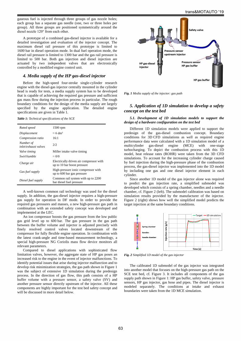
gaseous fuel is injected through three groups of gas nozzle holes;
each group has a separate gas needle (one, two or three holes per
group). All three groups are positioned symmetrically around the
diesel nozzle 120° from each other.
A prototype of a combined gas-diesel injector is available for a
detailed investigation and evaluation of the injector concept. The
maximum diesel rail pressure of this prototype is limited to
1600 bar in diesel operation mode. In dual fuel operation mode, the
diesel rail pressure is limited to 1300 bar and the gas rail pressure is
limited to 500 bar. Both gas injection and diesel injection are
actuated by two independent valves that are electronically
controlled by a modified engine control unit.
4. Media supply of the HP gas-diesel injector
Before the high-speed four-stroke single-cylinder research
engine with the diesel-gas injector centrally mounted in the cylinder
head is ready for tests, a media supply system has to be developed
that is capable of achieving the required gas pressure and sufficient
gas mass flow during the injection process in particular. The rough
boundary conditions for the design of the media supply are largely
specified by the engine application. The detailed engine
specifications are given in Table 1.
Table 1: Technical specifications of the SCE
Rated speed 1500 rpm
Displacement ≈ 6 dm³
Compression ratio 16:1
Number of
inlet/exhaust valves 2/2
Valve timing Miller intake valve timing
Swirl/tumble ≈ 0/0
Charge air Electrically driven air compressor with
up to 10 bar boost pressure
Gas fuel supply High-pressure ionic compressor with up to 600 bar gas pressure
Diesel fuel supply Common rail system with up to 2200
bar diesel fuel pressure
A well-known common rail technology was used for the diesel
supply. In addition, the gas-diesel injector requires a high-pressure
gas supply for operation in DF mode. In order to provide the
required gas pressures and masses, a new high-pressure gas path in
combination with an extended safety concept was developed and
implemented at the LEC.
An ion compressor boosts the gas pressure from the low public
gas grid level up to 600 bar. The gas pressure in the gas path
between the buffer volume and injector is adjusted precisely with
finely resolved control valves located downstream of the
compressor for fully flexible engine operation. In combination with
the latest crank-angle and time-based measurement technology, a
special high-pressure NG Coriolis mass flow device monitors all
relevant parameters.
Compared to diesel applications with sophisticated flow
limitation valves, however, the aggregate state of HP gas poses an
increased risk to the engine in the event of injector malfunctions. To
identify potential issues that arise during injector malfunction and to
develop risk minimization strategies, the gas path shown in Figure 1
was the subject of extensive 1D simulation during the predesign
process. In the direction of gas flow, this path consists of a HP
buffer volume with a pressure sensor, a safety valve (SV) and
another pressure sensor directly upstream of the injector. All these
components are highly important for the test bed safety concept and
will be discussed in more detail below.
Fig. 1 Media supply of the injector: gas path
5. Application of 1D simulation to develop a safety
concept on the test bed
5.1. Development of 1D simulation models to support the
design of a hardware configuration on the test bed
Different 1D simulation models were applied to support the
predesign of the gas-diesel combustion concept. Boundary
conditions for 3D CFD simulations as well as required engine
performance data were calculated with a 1D simulation model of a
multicylinder gas-diesel engine (MCE) with one-stage
turbocharging. To depict the combustion process with this 1D
model, heat release rates (ROHR) were taken from the 3D CFD
simulations. To account for the increasing cylinder charge caused
by fuel injection during the high-pressure phase of the combustion
process, the gas-diesel injector was implemented into the 1D model
by including one gas and one diesel injector element in each
cylinder.
Since another 1D model of the gas injector alone was required
to predict the gas injection rate, a simplified submodel was
developed which consists of a spring chamber, needles and a needle
chamber, cf. Figure 2 (left). The submodel calibration was based on
simulation results provided by the manufacturer of the injector.
Figure 2 (right) shows how well the simplified model predicts the
target injection at the same boundary conditions.
Fig. 2 Simplified 1D model of the gas injector
The calibrated 1D submodel of the gas injector was integrated
into another model that focuses on the high-pressure gas path on the
SCE test bed, cf. Figure 3. It includes all components of the gas
supply path shown in Figure 1: HP gas buffer, safety valve, pressure
sensors, HP gas injector, gas hose and pipes. The diesel injector is
modeled separately. The conditions at intake and exhaust
boundaries were taken from the 1D MCE simulation.
trans&MOTAUTO '19
63

Fig. 3 1D model with HP gas path
5.2. Development of a safety concept of a high-pressure gas-
diesel injector using 1D simulation
In the development of the reliable safety concept, the pressure
conditions within the gas supply path during standard operation
from engine start to stop were investigated with this 1D SCE model.
All 1D investigations of the gas path used the measurement
positions directly upstream of the injector and in the buffer volume.
Building on these results, the same model was used to simulate the
scenario of a stuck gas needle and its effect on the gas path
respectively on the engine at different engine loads while taking the
safety valve closing time into account. Finally, successful action
strategies were derived. These strategies will be discussed in more
detail below in the context of selected scenarios.
5.2.1. Malfunction due to the gas needle sticking during
standard engine operation
Figure 4 shows the pressure curves directly upstream of the
injector and in the buffer volume of two consecutive working cycles
in the event of an injector malfunction during standard engine
operation at part load (30%) and full load (100%). Irrespective of
the load and position, almost identical pressure curves can be
determined in the first working cycle (standard case) with a
characteristic pressure fluctuation for the gas injection close to the
specified pressure level. Compared to the second working cycle,
which represents the scenario of injector malfunction due to the gas
needle sticking, the gas pressure drops below the characteristic
pressure fluctuation; this is seen most clearly with regard to the
position upstream of the injector. In this case, a malfunction can be
detected with a threshold value, i.e. if the pressure upstream of the
injector falls below this threshold value, the closing process
(≈ 0.1 s) of the safety valve is triggered immediately and the diesel
injection is also switched off in parallel.
Fig. 4 1D simulation: detection of injector malfunction at different loads
Even if the safety valve closed immediately after the
malfunction was detected, it would not be possible to hinder the gas
remaining between the safety valve and the injector from expanding
into the combustion chamber. Figure 5 shows the impact of the gas
needle sticking on three subsequent combustion cycles considering
the valve closing time at 400 bar gas rail pressure. Combustion is
represented by one ROHR, which is calculated using 3D CFD
simulation for standard operation with the corresponding excess air
ratio (EAR), cf. working cycles 1 and 2 in Figure 5. The same
ROHR were used to simulate working cycles with injector
malfunction, cf. working cycles 3, 4 and 5 in Figure 5. The results
show that the gas remaining downstream of the safety valve
influences at least three further cycles and produces very rich air-
gas mixtures in the combustion chamber as well as an increased risk
of engine damage.
Fig. 5 Impact of injector malfunction on the cylinder charge
5.3. Malfunction due to the gas needle sticking at engine start
Even if an injector malfunction can be detected during standard
engine operation, the same approach does not work during engine
start. The following section reveals the difficulties in detection by
comparing a case in which injector malfunction occurs with a case
in which the injector work properly. In this case, the DF engine
starting procedure corresponds the one shown in Figure 6. First, the
engine is motored up to reference speed (not shown) and the
pressure in the gas buffer is raised to the target value of 400 bar
before pilot diesel injection occurs (1). In the next cycle, the safety
valve is opened (2) and the gas stored in the buffer volume is then
able to reach the injector. During this process, the pressure level
upstream of the injector increases and finally reaches the same
pressure rating as the buffer volume while the gas compressor
supplies additional HP gas until the target value of 400 bar is
restored throughout the entire gas path (3). Afterwards, the system
is ready for the additional gas injection to start the DF mode (4).
Fig. 6 Engine behavior without injector malfunction
Compared to the starting procedure discussed in Figure 6, the
difference in the case of injector malfunction (cf. Figure 7) becomes
clear after step (2).
trans&MOTAUTO '19
64

Fig. 7 Engine behavior with injector malfunction
Immediately after the safety valve is opened, the gas pressure
directly upstream of the injector rises quickly but cannot meet the
level of the buffer volume due to the stuck gas needle.
Subsequently, the high pressure gradient between the HP gas path
and comparatively low-pressure combustion chamber initiates an
unlimited gas flow directly into the combustion chamber, which
ultimately includes the previously mentioned dangers for the
engine.
Since error detection in the gas path via a threshold value
worked insufficiently in accordance to the simulation results,
further simulations were carried out to identify additional helpful
strategies. The indicated cylinder pressure signal was identified as a
promising parameter for much faster detection of injector
malfunction during both engine start and standard operation. In this
gas-diesel concept, air alone is compressed between inlet valve
closing (IVC) and start of injection (SOI) in standard operation
independent of gas pressure or engine load. As a result, the pressure
curve signal can be precalculated by a polytropic state change in
this time window and used in a real-time comparison with the
measured signal of the indicated pressure sensor, cf. Figure 8. If the
gas needle stuck, additional gas would flow into the combustion
chamber during this time window and the value of the measured
indicated pressure would deviate from the predicted curve without
delay. Thanks to this finely resolved monitoring, injector
malfunction is detected very quickly and has been successfully used
on the test bed in combination with error detection in the gas path
via a threshold, which facilitates additional monitoring of
malfunctions within the gas supply system.
Fig. 8 Injector malfunction at one gas needle during standard engine
operation
6. Summary
This paper presented the relevance of 1D simulations during the
development process to investigate gas-diesel injectors on a high-
speed large engine by taking different development issues into
account. 1D simulation models of different sizes and with different
levels of detail were discussed in relation to each specific issue.
Boundary conditions for 3D CFD simulations as well as additional
engine performance data were calculated with the MCE model with
one-stage turbocharging. In contrast to this extensive model, the
high-pressure gas injector was depicted by a simplified model that
simulates the required gas injection rates. As a consequence, it
became possible to support the design of the gas-fuel supply system
by optimizing the pipe and safety valve orifice diameters and
reducing the pressure drop in the system.
With regard to safety issues, critical cases caused by injector
malfunction were identified and simulated within various operating
scenarios. Derived safety strategies for detecting an injector
malfunction were discussed. The most promising strategy that was
identified involves monitoring the cylinder pressure signal within a
real-time comparison to a precalculated pressure curve in
combination with error detection in the gas path via a threshold.
7. References
[1] Beutler, M.; Naumann, M.: “Erdgas – Ein alternativer
Kraftstoff für den Verkehrssektor – Teil 1: Allgemeine technische
Aspekte, Kostenabschätzung und Energiekettenbetrachtung”, in: “ATZ
Automobiltechnische Zeitschrift”, Vol. 100, Issue No. 9, 1998, pp. 648-
656
[2] Kießling, C.; Tilz, A.; Nickl, A. et al.: “Evaluation of Gas
Injection Valves for Large Engines by Means of Spray Momentum
Measurement”, contribution at conference: “11. Tagung Einspritzung
und Kraftstoffe“, Berlin, 2018
[3] Redtenbacher, C.; Malin, M.; Kiesling, C. et al.: "Gas and
Dual Fuel Combustion Concepts: The Better Combustion Concepts for
Large Engines?", in: "16. FAD-Konferenz. Herausforderung –
Abgasnachbehandlung für Dieselmotoren. 7.11.-8.11.2018 in Dresden.
Beiträge", Dresden, 2018, pp. 201-226.
[4] Redtenbacher, C.; Kiesling, C.; Wimmer, A. et al.: "Dual
Fuel Brennverfahren – Ein zukunftsweisendes Konzept vom PKW- bis
zum Großmotorenbereich?", in: Lenz, H. P. (ed.): "37th International
Vienna Motor Symposium 28-29 April 2016. Volume 2: second day" (=
Fortschritt-Berichte VDI Reihe 12, Nr. 799), Düsseldorf, 2016, pp. 403-
428.
[5] Blöckhoff, N.; Hanenkamp, A.: “Der 51/60DF von MAN
Diesel SE – Der leistungsstärkste 4-Takt Dual Fuel Motor”, in: WTZ
Roßlau gGmbH (ed.): “Conference Proceedings, 5th Dessau Gas Engine
Conference”, Dessau, 2007, pp. 216-229
[6] Mohr, H.; Frobenius, M.: “Optimierung von Diesel-/Gas-
Großmotoren für unterschiedlichste Anwendungen”, in: Harndorf, H.
(ed.): “Die Zukunft der Großmotoren III, 3. Rostocker
Großmotorentagung”, Rostock, 2014, pp. 138-149
[7] Wärtsilä Corporation: “Wärtsilä 32GD Technology Review”,
2009. Accessible on the internet at:
http://www.wartsila.com/file/Wartsila/en/1270037664966a1267106724
867-W32GD_technology_review_2009_UK.pdf, accessed on: 2013-08-
02
[8] Järf, C.; Sutkowski, M.: "The Wärtsilä 32GD engine for
heavy gases", in: "Combustion Engines", Vol. 2, Issue 137, 2009, pp. 3-
11
[9] Aßmus, , K.; Redtenbacher, C.; Winter, H. et al.: "Simulation
Based Predesign and Validation of a Diesel Ignited High-pressure Gas
Direct Injection Combustion Concept", in: Leipertz, A. (ed.): "Engine
Combustion and Alternative Concepts – ENCOM 2019" (= Berichte zur
Energie- und Verfahrenstechnik (BEV), Vol. 19.1), Erlangen, 2019, pp.
83-94.
[10] Wimmer, A.; Golloch, R.; Auer, M.: "Großgasmotoren" in:
Merker, G. P.; Teichmann, R. (Hrsg.): "Grundlagen Verbrennungs-
motoren", 2018, pp. 241-244.
8. Acknowledgments
The authors would like to acknowledge the financial support of the
"COMET - Competence Centres for Excellent Technologies
Programme" of the Austrian Federal Ministry for Transport, Innovation
and Technology (BMVIT), the Austrian Federal Ministry of Science,
Research and Economy (BMWFW) and the Provinces of Styria, Tyrol
and Vienna for the K1-Centre LEC EvoLET. The COMET Programme
is managed by the Austrian Research Promotion Agency (FFG).
trans&MOTAUTO '19
65

ANALYSIS OF THE EFFECT OF PERIODIC PULSATIONS OF LIQUIDS FLOW ON
THE HEAT TRANSFERRING IN A CHANNEL WITH DISCRETE ROUGHNESS
АНАЛИЗ ВЛИЯНИЯ ПЕРИОДИЧЕСКИХ ПУЛЬСАЦИЙ ПОТОКА ЖИДКОСТИ НА ТЕПЛООБМЕН В
КАНАЛЕ С ДИСКРЕТНОЙ ШЕРОХОВАТОСТЬЮ
Dr. sc.ing. hab. prof. Dzelzitis E., Dr.sc.ing. Sidenko N.
Riga Technical University, Faculty of Building. Heat, Gas and Water Technology Institute.
[email protected], [email protected].
Abstract: At the present days the great attention is given to a problem of research of hydrodynamics and heat exchange in the pulsating
flows. Experimental studies for the flow in smooth channels show that the pulsation of fluids flow significantly affects to the heat transferring
and can be accompanied by both reduction and increasing in the intensity of the heat exchanging. This problem has a big practical
importance in the study of unstable processes in a various moving and power plants. The results showed that with unsteady fluid’s flow with
a alternating pulsations relative to the average velocity in a discretely rough channel is furthering to the intensification of the heat
transferring. It is shown that flow pulsations significantly affecting on the heat transferring coefficient, and its average values. This fact
opens up the possibility of using such currents to increase the energy efficiency of various technical devices.
KEYWORDS: HEAT TRANSFER ENHANCEMENT, DISCRETE ROUGHNESS, COMPUTER MODELING, NUMERICAL
CALCULATION.
1. Introduction Much attention has been paid to the problem of studying of the
effect of pulsating flows on hydrodynamics and heat transferring in
recent years. Experimental studies of unsteady flows at the present
day showed that such unsteady process can be accompanied by both
reduction and increasing in the intensity of the heat exchanging [1].
Known results of experimental and theoretical [2] studies are
often solutions for the specific problems and do not allow making
broad generalizations about the level of influence of superimposed
flow’s pulsations on the intensity of heat transferring. At this
moment, there is not enough reliable information about the
kinematic structure of the pulsating flow in the channels under the
conditions of superimposed nonstationarity.
Based on the reliability of information about the structure of the
pulsating flow in the channel, it is possible to estimate the effect of
superimposed pulsations on the heat transferring, as well as to
identify patterns of changing in flow’s characteristics under
considered conditions.
This fact opening up the possibility of using such flows to
increase energy efficiency in the studying of unstable processes in
various moving and energy equipment.
Thus, obtaining information about the structure of the pulsating
turbulent flow and identifying patterns of heat exchanging processes
of such flows in discretely rough channels is urgent task for the
present time.
The main goal of this work is to use computer simulation and
numerical analysis to investigate the effect of periodic flow
pulsations on the heat transferring in a channel with discrete
roughness in the shape of hemispherical concavities.
2. Prerequisites and means for solving the problem Analyzing of the existing literature has shown that there are
extensive reviews of hydrodynamics and heat transferring studies in
smooth and discretely rough channels with a stationary flow of
coolant [2-5].
The heat exchange of a hydraulically smooth circular channel
with a stationary developed turbulent flow has been studied in detail
and well described by the M.A. Mikheev dependence [12] for
various regimes of forced fluid flow in a smooth channel.
It is also known that increasing in the intensity of heat
exchanging between the coolant and the heat exchange surface is
provided, as a rule, with the help of discrete roughness, leading to
the partial or complete destruction of the boundary layer, in which
concentrated the greatest thermal resistance, as well as significant
turbulization of the flow. These effects are achieved by the
organization of flow’s separation and attachment areas, an increase
in the relative flow velocity near the wall, and generation of the
pressure pulsations in the flow and other ways of influencing to the
near-wall structure of the flow [6-8].
The experimental and theoretical results of the study of pulsating
flows that exist today are mainly obtained only for the boundary
layer and the flow in a smooth channel [9,10].
For the successful using of the detachable areas, it is necessary to
know the mechanism of their interaction with the main turbulent
pulsating flow and the mechanism of the processes in the detachable
area itself. These processes are very complex.
At this stage, numerical research methods using the latest
advances in the field of boundary layer diagnostics and
computerization are the most effective way in the modern theory of
heat and mass transferring.
In this work, in order to solve the heat transferring problem in a
channel with discrete roughness in the shape of concavities with
pulsating fluid motion, 3D modeling software complex CAD/CFD
of SolidWorks / Flow Simulation is used.
With using the SolidWorks CAD software calculating and
building three-dimensional geometric model of a discretely rough
channel.
The numerical solution of the problem is performing in the Flow
Simulation software, in which the motion and heat transferring of a
fluid is modeling with using the Navier – Stokes equations [11],
which describe in unsteady formulations the laws of conservation of
mass, momentum and energy of a given medium. In addition, using
equations of state of the components of the fluid, as well as the
empirical dependences of the viscosity and thermal conductivity of
these components of the medium on temperature.
Considering the complexity of the research task, the
insufficiency and inconsistency of the existing well-known research
results, it is necessary to determine the accuracy and reliability of
the results of numerical calculations. For this purposes two main
problems were solved:
- carried out series of calculations on the grids with different
resolution of the geometric features of the model and non-linearity
of the calculated physical parameters field to ensure that there is
grid convergence of the solution to the problem and to obtain the
final solution of the problem on the optimal (in terms of the
accuracy of the mathematical problem solving taking into account
computer resources and performance) of the computational grid.
- in a non-stationary problem formulation, perform time
discretization for each cell of the computational grid in the
computational area from the Kurant condition and determine the
allowable maximum time step depending both on the values of
physical quantities and the space discretization step in the cell area.
trans&MOTAUTO '19
66

3. Solution of the examined problem Computer simulation was carried out with using the CAD/CFD
complex software SolidWorks / Flow Simulation. In the
SolidWorks CAD software was constructed calculated three-
dimensional model of a circular channel with discrete roughness in
the shape of hemispherical recesses (concavities) with a sharp input
and output edges arranged in a corridor order.
The internal diameter of the channel is D = 0.018 m, the wall
thickness is δ = 0.002 m, the length is L = 1.6m. The relative pitch
S between the axes of the concavities is S / h = 10 (the h-radius of
the concavities), the concavity setting angle φ = 120 °. The walls of
the channel were modeled as aluminum and heated to a temperature
of twall=105°С. At the entrance of the channel supplied working
fluid - water, with a temperature tinlet= 20°С.
In this work using a model of a periodically pulsating internal
fluid flow (1) with a sinusoidal type speed pulses (Fig. 1.):
V(t) = 0.4 (1 + А sin (2πft)) m/s, (1)
Here t is time, V(t) is a flow rate, A = 1 is an amplitude of the
pulsations. The time-averaged flow rate for the all cases are the
same and equal V0 = 0,4 m/s.
For the velocity V0 = 0,4 m/s the average Reynolds number is
Re0 = V0D/ν = 7157, where ν =1,006·10-6 m2/s is the kinematic
coefficient of water viscosity at tinlet= 20°С.
With a changing in the average Reynolds number, the average
velocities changing accordingly. The instantaneous values of the
Reynolds numbers Ret = V(t)D/ν depend on time and for the case
(1) are described by the equitation
In the calculations, the range of the flow pulsation frequency 0
≤ f <130 Hz was investigated.
0
0,1
0,2
0,3
0,4
0,5
0,6
0,7
0,8
0,9
4 4,1 4,2 4,3 4,4 4,5 4,6 4,7 4,8 4,9 5
time(s)
V (m/s) V max
V min
V aver
Fig.1. Flow velocity profile: dashed line - average speed; smooth
line - speed, determined by equitation (1).
For mathematical modeling of the medium’s motion and heat
transferring, the unsteady Navier-Stokes equations are used. The
resulting open-loop system of equations is closed with using of the
additional equations for the kinetic energy of turbulence k and
dissipation of the energy of turbulence ε in accordance to the known
k - ε model of turbulence [11].
For the numerical solution of the Navier-Stokes system of
equations in Flow Simulation software using the finite volume
method with an adaptive rectangular grid [11]. In the calculation
process the initial grid of finite volumes in the computational area is
crushed automatically or according to a given law in the areas of
assumed large gradients of each of the dependent variables or in
areas of significant change in the curvature of the solid surface. For
a satisfactory accuracy of the results of the solution in this work
required about 1000000 - 1200000 liquid and solid elements.
Note that, in accordance to the calculation methodology, any
stationary problem is initially solved as non-stationary. The solution
is considered to be found after its establishment in time.
The results of numerical calculations, generalizing a series of
computer experiments, were processed in the dimensionless
Reynolds Re, Strouhal Sh, and Nu Nusselt criteria:
Re0 = V0D/ ν, Sh = f D/V0, Nu = α D/ λ , (3)
where Sh – the dimensionless frequency of flow pulsations, α
[В/(m2K)] – the heat transfer coefficient, λ [B/(m K)] – the heat
conduction coefficient of the liquid.
4. Results and discussion
The results showed that unlike to the stationary case with a unique
dependence Nu = φ(Re0) in a pulsating flow, the instantaneous
values of the coefficient Nu(t) = φ(Ret) changing with changing the
instantaneous values of the Reynolds numbers Ret (the Ret value is
determined by equitation (2)). Changes in the instant Reynolds
numbers are shown in Fig. 2. In the stationary case with V0 = 0,4
m/s, the Reynolds number is Re = 20000. For example, in a
pulsating flow at a pulsation frequency of f=20Hz (Strouhal number
Sh = 0.9) and an average speed of Vaver(t)=0,4 (m/s), the average
value of the Reynolds number increases to Re≈27000, as well as has
it’s minimum Re≈50000, and the maximum Re≈47000 value.
As a result for the each value of Ret corresponds to its own Nu
value and is limited to its minimum Numin and Numax maximum
values. This effect is due to the periodic change in the Reynolds
number and the inertia of the processes during unsteady fluid flow
in the channel.
0
5000
10000
15000
20000
25000
30000
35000
40000
45000
50000
1
1,0
1
1,0
2
1,0
3
1,0
4
1,0
5
1,0
6
1,0
7
1,0
8
1,0
9
1,1
1,1
1
1,1
2
1,1
3
1,1
4
1,1
5
1,1
6
1,1
7
1,1
8
1,1
9
1,2
Re
t(sek)
1
2
Fig. 2. Changing of the instant Reynolds numbers. Line 1 -
stationary flow V0 = 0,4 m/s; line 2 - pulsating flow f = 20Hz (Sh =
0.9) Vaver (t) = 0.4 (m/s).
For the dependence Nu = φ (Sh) can be selected conditionally
three characteristic areas (Fig. 3.). In the first zone, 0 <Sh <2, the
frequency of the flow velocity pulsations leads to the increasing in
the average values of the Nusselt Nuever numbers in relation to Nu0
for the stationary regime of the fluid flow.
0102030405060708090
100110120130140150160170180190200
0 1 2 3 4 5 6
Nu
Sh
Numax
Numin
NueverNu0
Zone 1 Zone 2 Zone 3
Fig.3. The dependence of the Nusselt number on the dimensionless
frequency of flow pulsations Nu = φ (Sh).
trans&MOTAUTO '19
67

In the second area 2 <Sh <4.3, the average values of the Nuever
numbers become lower relative to Nu0 by about 10-15%. In Fig. 2
can be noted that when the dimensionless Strouhal number Sh ≈ 2 is
reached (zone 2), the heat exchanging getting worse. In the third
zone, 4.3 <Sh <6, the average Nuever value in relation to Nu0
stabilizes and the value of Nu remains almost unchanged and the
flow pulsations have almost no effect on the heat transferring.
Fig. 4. shows visualization of a flow in a channel with a discrete
roughness (longitudinal section), in the case of stationary flow of a
fluid at average speed at the entrance to the channel Vinlet =0,4 m/s.
The flow under consideration can be conditionally divided into the
three areas: I – the outer boundary layer, II – the mixing region, and
III – the return flow.
The flow picture can be presented as follows. The incident flow
V at the exit from the concavity is turbulized, mixed with the
medium in the concavity, and carries particles of the liquid from the
mixing zone to the main flow. At the same time at an environ of the
outlet edge the flow is splitting. One part of the flow (laminar
sublayer) moves along the straight wall of the channel, the other
part goes around the surface of the concavity and when it reaches
the input edge of the concavity (inlet edge) it breaks down and
forming a vortex.
Fig.4. The flow pattern with a stationary flow Vinlet =0,4 (m/s)
concavities in the channel (longitudinal section).
The Fig. 5. shows the temperature distribution on the transverse
axis of the channel AB (r (mm)); the steady flow is Vinlet =0,4 m/s
line 1 – is a smooth channel and line 2 – is a discretely rough
channel.
404550556065707580859095
100105
0,00
0
0,00
1
0,00
2
0,00
3
0,00
4
0,00
5
0,00
6
0,00
7
0,00
8
0,00
9
0,01
0
0,01
1
0,01
2
0,01
3
0,01
4
0,01
5
0,01
6
r (mm)
T grad C
Wall
C
h
a
n
n
e
l
a
x
i
s
III II I
1
2
Fig.5. Temperature distribution along the transverse axis of the
channel AB.
In comparing with the stationary motion in the pulsating mode,
the flow patterns changing at time t(s).
Fig.6. The flow around the pulsating flow Vaver(t) (m/s) concavity in
the channel (longitudinal section) f = 20Hz (Sh = 0.9).
Unlike to the stationary flow, in the pulsating mode at an
average flow velocity of Vaver(t) (equation (1)), the pulsating
frequency f = 20Hz (Sh = 0.9) Fig. 6., the flow pattern are
changing. Here, the inlet flow Vaver moves along a straight channel
when the input edge of the concavity (inlet edge) is reached, the
flow is splitting: one part of the flow moves towards the output
edge (outlet edge), the other part towards the point 0, where it is
turbulized and mixed. So unlike to the stationary mode, it shifts
from the outlet edge (outlet edge) towards the axis AB by
approximately 45 °. In the same place, at point 0, one more splitting
of the flow occurs. One part of which (laminar sublayer) moves
along the surface of the concavity towards the outlet edge (outlet
edge) and then continues to move along the straight channel wall.
The other part flow around the surface of the concavity and when it
reaches point C, it breaks down and forming a vortex. At the same
time unlike to the stationary flow, the center of the vortex that was
on the axis AB, in the pulsating mode, the center of the vortex shifts
towards the input edge by a distance approximately equal to half of
the radius of the concavity.
When the maximum flow rate Fig.7. Vmax(t) is reached, the flow
pattern is simplified, the flow moves along the straight channel
wall, and when the input edge (inlet edge) is reached, part of the
flow moves in a straight line to the output edge (outlet edge), and a
part flow around the concavity and joins main flow around the exit
edge. At the same time, no flow separation or vortex zones are
observed in the concavity.
Fig.7. The flow around the pulsating flow Vmax(t) (m/s) concavity in
the channel (longitudinal section) f = 20Hz (Sh = 0.9).
The complex flow pattern is observed when the minimum flow
rate Vmin(t) is reached Fig.8.. Here the flow in the laminar sublayer
changes it’s direction to the opposite, in relation to the inlet flow
and moves from the output edge (outlet edge) to the input edge
(inlet edge). When reaching the entrance edge, the flow is splitting
and part of it moving along the straight wall of the channel, and part
trans&MOTAUTO '19
68

begins to move closer to the channel axis, where it merges with the
main fluid flow, and thus forms a vortex zone III. The center of the
vortex is located on the axis AB and at a distance approximately
equal to half the radius of the smooth part of the channel.
Fig.8. The flow around the pulsating flow Vmin (t) (m/s) concavity in
the channel (longitudinal section) f = 20Hz (Sh = 0.9).
So it can be assumed that the presence of vortex structures and
return flow zones on the heat exchanging surface leads to the
destruction of the boundary layer and, accordingly, intensifies the
heat exchange processes. And the occurrence of such disturbing
factors in the flow significantly affects both the hydrodynamics of
the flow and the heat transferring.
5. Conclusion.
In this work was established that nonstationary processes can be
accompanied by both an increase and a decrease in the intensity of
heat transferring.
It is shown that this is due to the presence of vortex structures
and backflow zones on the heat exchanging surface. Which lead to
the destruction of the boundary layer and, as a consequence, lead to
the intensification of heat exchanging processes.
It is revealed that the periodic pulsations of the flow velocity
of fluid in discretely rough channels have a significant effect on the
heat transferring coefficient Nu.
Unlike to the stationary case, in a pulsating flow, the
instantaneous values of the coefficient Nu changing as the
instantaneous values of the Reynolds numbers Ret.
The presence of the three characteristic zones of dependence
of the Nusselt number Nu on the dimensionless Strouhal number Sh
Nu = φ (Sh) is established. In the first zone (0 <Sh <2), the
pulsations of the fluid flow in the channels improve the average
intensity of the heat exchange. In the second zone (2 <Sh <4.3), the
average intensity of the heat exchange is accompanied by a
decreasing.
In the third zone (4.3 <Sh <6), the flow pulsations have practically
no effect on the average value of the heat exchanging, and the
average value of the Nusselt number becomes approximately the
same as for the stationary flow.
6. References
[1] Galicejskij B.M. Ryzhov YU.A., Yakush E.V. Thermal and
hydrodynamic processes in oscillating flows. Int:Mechanical
Engineering, 1977. 256 p.
[2] Халатов А.А. Теплообмен и гидродинамика около
поверхностных углублений (лунок) – Киев: НАН Украины,
Институт технической теплофизики, 2005. -59 с. [3] Mahmood G. I., Hill M. L., Nelson D. L., Ligrani P. M., Moon
H.-K., Glezer B. Local heat transfer and flow structure on and
above a dimpled surface in a channel. Transactions of the ASME.
Journal of Turbomachinery, 2001,vol. 123, iss. 1, pp. 115 - 123.
DOI: 10.1115/1.1333694
[4] Mahmood G. I., Ligrani P. M. Heat transfer in a dimpled
channel: Combined influences of aspect ratio, temperature ratio,
Reynolds number, and flow Structure. Intern. J. of Heat and
Mass Transfer, 2002, vol. 45, iss. 10, pp. 2011-2020.
[5]. Kiselev N.A., Burtsev S.A., Strongin M.M. A procedure for
determining the heat transfer coefficients of surfaces with regular
relief. Measurement Techniques, 2015, vol. 58, no. 9, pp. 1016-
1022. DOI: 10.1007/s11018-015-0835-7
[6]. Leontiev A.I., Dilevskaya E.V., Vinogradov Yu.A., Yermolaev
I.K., Strongin M.M., Bednov S.M., Golikov A.N. Effect of vortex
flows at surface with hollow-type relief on heat transfer coefficients
and equilibrium temperature in supersonic flow. Experimental
Thermal and Fluid Science, 2002, vol. 26, iss. 5, pp. 487-497. DOI:
10.1016/S0894-1777(02)00157-7
[7] А.Г. Лаптев, Н.А. Николаев, М.М. Башаров Методы
интенсификации и моделирования тепломассообменных
процесов.Справочное пособие.- М.: «Теплотехник», 2011 335 с.
[8] Д.Н. Попов, С.С. Панаиотти, М.В. Рябинин Гидромеханика,
Москва, Издательство МГТУ им.Н.Э. Баумана, 2002, 383 стр.
[9] Mizushina T., Maruyama T., Hirasava H. Strukture of the
turbulence in pulsating pipe flows. Eng. Japan -1975-Vol.8, Nr.3-
p.210-216.
[10] Chang P. Separation of Flow //New York, Pergamon Press,
1971.
[11] Алямовский А.А. и др. SolidWorks 2007/2008.
Компьютерное моделирование в инженерной практике.// БХВ–
Петербург, Санкт – Петербург, 2008.
[12] Михеев М.А. Михеева И.М. Основы теплопередачи. – М.:
Энергия.1977. 344с.
This work has been supported by the European Regional
Development Fund within the Activity 1.1.1.2 “Post-doctoral
Research Aid” of the Specific Aid Objective 1.1.1 “To increase the
research and innovative capacity of scientific institutions of Latvia
and the ability to attract external financing, investing in human
resources and infrastructure” of the Operational Programme
“Growth and Employment” (No Nr.1.1.1.2./VIAA/1/16/093).
trans&MOTAUTO '19
69

MULTISCALE MODELING OF SHORT FIBRE REINFORCED COMPOSITES
AND IT’S RELATIONSHIP
TO MODAL ANALYSIS OF MACHINERY PARTS
Eng. Jarmil Vlach., Eng. Jan Steklý Ph.D.
IDIADA CZ a. s., the Czech Republic
Abstract: Although molding of thermoplastics is very productive method of machinery manufacturing, pure plastics are almost not used
in so much quantity. Particle reinforced composites are more popular, because presence of solid inclusions reduces volume of organic
matrix and usually improve strength and stiffness. Final properties are strongly influenced by manufacturing process which affects inner
material structure. In composites where fibers are continuous in one direction or placed in layers, i.e. the fibers do not end inside the
composite and it`s length is close to the dimension of machinery parts, elastic [1] [2] and thermal properties [7] can be predicted quite
easily by Halpin-Tsai equations or derived simplified methods [2] with high accuracy. This paper is focused on prediction of density and
material stiffness of composites, which are reinforced with very short glass fibers in thermoplastic matrix. In the first part we define the field
of problem. Then we present simplified analytical calculus in compare to finite element method. We focus on ABAQUS 2018 and its features,
which can be used for solving those problems. Estimation approaches such as representative volume element method and mean field
homogenization are also studied. After this presented methods are confronted with selected material datasheet of Ultramid® A3WG6 [9] and
Zytel® 70G35HSLRA4 [12] composite material. The effect of fiber randomization on material stiffness is introduced [4]. At the end of thesis
we use previously calculated material data for modal analysis of real parts which are made from molded thermoplastic with short glass as
well.
Keywords: MODAL ANALYSIS, ELASTIC PROPERTIES, SHORT FIBER, THERMOPLASTIC, COMPOSITE
1. Introduction
In the case of large thin-walled and low-ragged composite
components, which are reinforced with long fibers, the volume
representation and orientation of the reinforcement are constant.
Prior to injection of the binder phase, the reinforcement is generally
positioned and fixed in the mold such that during the production
process to transfer the matrix was prevented from moving it. As the
reinforcement position is known in advance, the assumed properties
of actual products usually coincide well with the calculations and
correspond to our expectations. The problem of molding short fiber
reinforced composites stands on the opposite side of accuracy
interval, because the order of the system is much lower than in case
of long fiber composites.
In terms of access to the development process, it would be
optimal if separate injection simulations were made for each type of
material. In our article, we deal with the possibility that only one
simulation is performed and only small variations in elastic material
parameters would occur. We assume that fiber volume changes in
percentage order will not lead to fundamentally different
distribution and orientation results, while material parameters may
have a more significant effect.
Fig. 1 Schema of direct and indirect analysis procedure
In this work, we have considered the primary objective of
verifying the accuracy of material properties prediction in
connection with injection simulation, followed by experimental
modal analysis, because the problems of linear dynamics and elastic
wave propagation are closely related.
2. Injection simulation
The simulation results are sensitive to the quality of the FE
mesh and the type of used element. In this case, we consider the
analyses contains output mesh of the injection simulation from
Moldflow software. Because it is a flow problem where the mesh is
stable in the space (it does not deform), but the mass moves inside,
it is a description in Lagrange coordinates. The simulation provides
sufficient information on the distribution, concentration and
orientation of the material in the individual elements.
This type of mesh is often not suitable for distortion and stress
analysis when individual nodes move and structure deforms,
although in case of small strains, the model mesh can give
satisfying results. However if there are large deformations or strains
in the interval of plasticity, such a model can no longer be used,
because the intermediate results will no longer meet the
convergence criteria or give not good response to real problems.
Therefore, the next step of work usually is to create a model mesh
that would meet the least requirements. The flow model must then
meet the solvency criteria and the possibility of transmitting some
information so that the result is not affected.
3. Multiscale modelling of material properties
Each computational material model of composite material can
be divided in few basic parts. The first section at the macroscopic
level is usually a body or a machine component, consisting of a
discretized network of elements representing a particular region.
These are material properties that correspond to the microstructure
level scale of the unit characteristic. It is important to mention that
each of presented predictive theories reminded bellow works with
another type of this elementary cell and therefore the results of the
material characteristics differ from one another.
User input Mapping
Modal analysis inputs
Molding simulation
results
Material properties Orientation
Direct method No mapping
Indirect method
Original FV mesh
Original FV mesh
User created FE mesh
trans&MOTAUTO '19
70

4. Short fiber reinforced composite materials
Parameters that have a key effect on material characteristics are
fiber length (lf), fiber diameter (df), shape and volumetric fraction of
the reinforcements (vf). The most important describing parameter is
shape factor (ξ) [1]. Physical parameters are given by material
characteristics of components (Table 1). Since short fibers produced
in a special machine are shortened by cutting or milling of long
fibers and the length of each fiber is essentially unique, we must
work with it as a statistical variable. For this instance, we consider
the significant fiber length 120 µm ± 19 µm at 95% probability
level. Fiber diameter is considered as constant value which is 10
µm. The relevant prediction of mechanical properties is therefore a
rather complicated process where each of the variables we only
predict with a certain degree of accuracy.
Fig. 2 Elementary cell of single cylindrical fiber
Table 1: Component material description
Component ξ Density
Tensile
modulus
Poisson
ratio
[ - ] [ kg/m3 ] [ MPa ] [ - ]
Matrix PA66 - 1130 3000 0,4
Fiber E-Glass 12 2600 72500 0,2
In this work we mainly deal with elastic properties of binary
composites with polyamide matrix and reinforcement from E-glass.
We took the properties of the matrix from the material sheet
Ultramid A3W [8] and confronted with literature [2], glass
properties were taken from [2] a [3]. In all the calculations, we
consider the matrix as dry or low in moisture. We view both
components as homogeneous isotropic materials.
For prediction of the composite material properties [9] [12]
three basic methods were used. The traditional analytic method
(AM) represents Halpin-Tsai equations (HT). The second was
representative volume element method (RVE), which was applied
on three basic cells with cyllindrical and prolate reinforcement. It
shows Fig. 4, while the effect of connected and disconected front
boundary of cyllinder was studied [2]. The last approach was mean
field homohenization (MFH), when various formulations reminded
in Table 2 were used and the only ellipsoid-prolate inclusion was
considered. In case of (HT), the properties were directly calculated
by user written script. In case of (RVE) the ABAQUS CAE
Micromechanics plugin was used. Parameters from MFH and RVE
methods were derived from FE models when elementary
Fig. 3 Basic experiments applied on MFH and RVE models
tests applied and calculated. It shows Fig. 3. When we think
composite as continual phase (MFH), elastic properties can be
directly calculated from one element model following formulas
( 1 ), ( 2 ) and ( 3 ). When we consider material as separated entities
(RVE) formula ( 4 ) should be used.
( 1 ) 𝑬𝒊𝒊 =𝝈𝒊𝒊
𝝐𝒊𝒊; 𝒊, 𝒋 = 𝟏,𝟐, 𝟑
( 2 ) 𝑮𝒊𝒋 =𝝉𝒊𝒋
𝟐𝝐𝒊𝒋; 𝒊, 𝒋 = 𝟏,𝟐, 𝟑; 𝒊 ≠ 𝒋
( 3 ) 𝝂𝒊𝒋 = −𝝐𝒋𝒋
𝝐𝒊𝒊; 𝒊, 𝒋 = 𝟏,𝟐, 𝟑; 𝒊 ≠ 𝒋
Fig. 4 FE model of material cell with bonded and unbonded front part of fiber boundary
( 4 ) 𝑬𝒊𝒋𝑪 =
𝝈𝒊𝒋 𝒏 𝝐𝒊𝒋 𝒏
𝑽 𝒏𝑵𝟏
𝝐𝒄 𝟐 𝑽𝒄
Table 2: Results of predictive methods, Moduli E11
Method Formulation E11 [ GPa ]
Experiment Datasheet
Ult
ram
id®
A3
WG
6
vf =
0,1
6
10,0
Zy
tel®
70
G3
5H
SL
RA
4
vf =
0,1
9
11,0
RVE
Cell A 9,8 11,1
Cell B 7,9 8,7
Cell C 7,7 8,5
MFH
Balanced 10,1 11,4
Mori-Tanaka 9,7 11,0
Inversed Mori-Tanaka
Mori-Tanaka 14,1 16,2
AM Halpin-Tsai 9,2 10,5
Isotropic Halpin-Tsai 6,2 6,9
5. Results mapping and FE model creation
When comparison of material prediction methods was finished
and successful methods were selected, we created a trial workflow
how to prepare FE models of real parts, which shows Fig. 5.
Mesh o Mesh structure
From injection simulation User created mesh with mapped
orientation o Elements
2nd o. elements
Elasticity o From injection simulation o User defined
Analytic methods (Halpin-Tsai)
Mean Field Homogenization (Mori-Tanaka, Inversed Mori-Tanaka)
Material orientation o From injection simulation
Orientation tensor
Connected front boundary
RVE Cell A
Disconnected front boundary
RVE Cell B
Connected front boundary
RVE Cell C
i
j
i
j
σii τ
ij
a/2
a
a
lf
lc
trans&MOTAUTO '19
71

Fig. 5 Possible permutations of model creation
First variant deals with possibility that original finite volume
(FV) mesh generated by Moldflow is kept and directly used for past
analysis (Fig. 6).
Molflow output
job_mesh.inp
job_e11.xml
job_e22.xml
job_e33.xml
job_v12.xml
job_v13.xml
job_v23.xml
job_g12.xml
job_g13.xml
job_g23.xml
job_principal
Directions.xml
job_ltec_1.xml job_ltec_2.xml
job_ltec_3.xml
ABAQUS translator
for 3D solid simulations Model
(job-name.inp) file containing
list of nodes,
elements, boundary
conditions,
loads and step definition.
Material (job-name.mpt) file containing
orthotropic
material properties data
Orientation (job-name.opt)
file containing element
orientation data
Thermal
expansion (job-name.tpt)
file containing element thermal
expansion
coefficient data
ABAQUS solver
Fig. 6 Schema of extracting binary data
In second variant the successful (MFH) Mori-Tanaka was
applied on user created mesh, when FE model was simplified in
way that 9 elements thru thickness were reduced on 3 and the same
distribution of material given by orientation tensor which was
mapped on was used.
As third variant we considered the initially calculated
distribution of material from Moldflow valid again and just mapped
on user created mesh again, but this time material card was
generated by using (HT) method.
6. Modal analysis of real parts
6.1 Simulation
Task of this section was to verify the previously studied
assumptions for real products, which shows Fig. 7 a), b). Present
product, which consists of a two-piece assembly, was made by
injection technology of short-fiber reinforced thermoplastic material
[12]. The aim was to compare the results of modal analyses with
different model mesh settings and engineering elastic constants. In
this case, calculations have been performed in ways that were
recognized as effective. In total, modal analysis of individual
components were performed, then results were compared with the
experimentally determined values. Temperature of surroundings
was considered 23° C.
Fig. 7 Machinery parts, a) Cover, b) Housing
6.2 Experiment
Experimental modal analysis is the method which allows to
obtain mathematical model of the vibration properties and
behaviour of the structure by experimental means. The modal
parameters are established by measuring and processing of
frequency response function H(ω), given as
( 5 ) 𝑯(𝝎) =𝑯(𝝎)
𝑭(𝝎)
where F(ω) is excitation and X(ω) is response of the system, both in
frequency domain. In our case we tested parts freely suspended in
the center on rubber bands with low stiffness. For each part the
experiments were done at 11 different positions of actuator while
sensor position was fixed. Results were analyzed following
literature [13].
7. Results
List of performed simulation variants show Table 3. Results of
absolute values of modal frequencies for certain parts show Table 4
and Table 5. Eigen modal shapes show Fig. 8 and Fig. 9.
Table 3: List of performed analysis
Formulation
Material Experiment Moldflow Halpin-Tsai Mori-Tanaka
Method Experiment Direct Indirect Indirect
Mesh - Moldflow User User
Ori. tensor - Yes Yes Yes
Mapping - No Yes Yes
Table 4: Eigen modal frequency, Cover
Formulation
Frequency Experiment Moldflow Halpin-Tsai Mori-Tanaka
1st [Hz] 442.4 578.0 470.2 470.3
2nd [Hz] 492.2 586.7 481.7 482.1
3rd [Hz] 984.4 1300.0 1069.3 1072.7
4th [Hz] ≈ 3rd 1314.0 1073.4 1076.5
Fig. 8 Eigen modal shapes, Cover
Table 5: Eigen modal frequency, Housing
Formulation
Frequency Experiment Moldflow Halpin-Tsai Mori-Tanaka
1st [Hz] 424.8 562.7 492.5 484.9
2nd [Hz] 508.3 604.9 526.3 521.8
3rd [Hz] 1044.4 1295.2 1188.0 1144.0
4th [Hz] ≈ 3rd 1323.1 1207.4 1170.2
Fig. 9 Eigen modal shapes, Housing
1st
2nd
3rd
4th
1st
2nd
3rd
4th
a) b)
trans&MOTAUTO '19
72

8. Conclusion
Most of the methods did a well of predicting longitudinal
modulus. The worst results are provided by MFH Prolate Inversed
Mori-Tanaka method and whe we think material isotropic. Overall
result with deviation from -38% for Zytel and 46,8% for Ultramid is
unacceptable. Best deviation has been achieved using Prolate Mori-
Tanaka. Halpin-Tsai equations reaches the boundary of dev. -5 and
-8% for both materials. This can be considered also as sufficient.
Deviance of other properties was found lower or same orders but
not published.
Fig. 10 Deviance of E11 modulus from datasheet
Fig. 11 Deviance of modal frequency results to experimental, Cover
Fig. 12 Deviance of modal frequency results to experimental, Housing
Although the material settings of initial components were the
same, modal frequency determined from original Moldflow model
is influenced by largest error. The total average deviance from
experimental is 25,2% (housing) and 27,3% (cover). In case of
cover part the smallest deviance is obtained from model with user
defined material card, which was mapped on user mesh. It is 5,7%
in case of (HT) formulation. In instance of housing part the smallest
deviance is obtained from model with mean field homogenization
where Mori-Tanaka formulation was applied and which property
was also mapped on user mesh. Smallest deviance from
experimental was 8,8%. It was proofed that successful calibration of
material properties and proper choice of prediction method in a key
way influence results. Modal frequencies and modal shapes match
with experiment quite well although the prediction deviance of
natural frequencies is higher then material. It is caused by natural
distribution of fibers which is statistical value and low order of the
system.
References
[1] J. C. Halpin, J. L. Kardos; The Halpin-Tsai Equations: A
Review, Polymer engineering and science, 1976, v16, N5, pp
344-352.
[2] Agarwall B. D., Broutman L. J.; Analysis and performance of
fiber composites, Wiley, 2015.
[3] Berthelot J. M.; Composite materials, Mechanical behavior
and structural analysis. New York, Springer, 1999.
[4] Jacek Nabiałek; Modeling of fiber orientation during injection
molding process of polymer composites, Kompozyty 11: 4
(2011) 347-351.
[5] O. Pierard, C. Friebel, I. Doghri; Mean-field homogenization
of multi-phase thermo-elastic composites: a general
framework and its validation, Composites Science and
Technology 64 (2004) 1587–1603, Science Direct.
[6] N. Graupner, K. Albrecht, G. Ziegmann, H. Enzler, J. Müssig;
Influence of reprocessing on fibre length distribution, tensile
strength and impact strength of injection moulded cellulose
fibre-reinforced polyactide (PLA) composites, eXPRESS
Polymer Letters Vol.10, No. 8 (2016) 647-663.
[7] Christian Karch; Micromechanical Analysis of Thermal
Expansion Coefficients,
Airbus Group Innovations, Munich, Germany, Modeling and
Numerical Simulation of Material Science
Vol.4 No.3(2014), Article ID:47695.
[8] BASF Ultramid® A3W datasheet; CAMPUS® material
database, 2018.
[9] BASF Ultramid® A3WG6 datasheet; CAMPUS® material
database, 2018.
[10] ABAQUS online manual.
[11] J.C. Halpin and J. L. Kardos Halpin-Tsai equations:A review,
Polymer Engineering and Science, 1976, v16, N5, pp 344-
352.
[12] Zytel® 70G35HSLRA4; CAMPUS® material database, 2018.
[13] S. Miláček; Modální analýza mechanických kmitů,
Vydavatelství ČVUT, 2001.
0,9
-20,6
-23,1
3,4
0,1
46,8
-4,7
-37,3
-1,7
-20,6
-23,4
-0,5
-3,3
40,8
-7,8
-38,0
-40 -20 0 20 40 60
Cell A
Cell B
Cell C
Balanced
Mori-Tanaka
Inversed Mori-Tanaka
Halpin-Tsai
Isotropic Halpin-Tsai
Deviation [%]
Zytel® 70G35HSLRA4
Ultramid® A3WG6
30,7
6,3
6,3
19,2
-2,1
-2,1
32,1
8,6
9,0
27,3
5,7
5,8
-10 0 10 20 30 40
Moldflow
Halpin-Tsai
Mori-Tanaka
Deviance [ % ]
Average
3rd
2nd
1st
32,5
15,9
14,1
19,0
3,5
2,7
24,0
13,7
9,5
25,2
11,1
8,8
-10 0 10 20 30 40
Moldflow
Halpin-Tsai
Mori-Tanaka
Deviance [ % ]
Average
3rd
2nd
1st
trans&MOTAUTO '19
73

IDENTIFICATION OF THE MINOR CHEMICAL ELEMENTS IN THE EXHAUST
EMISSIONS FROM DIESEL ENGINE VEHICLES
Dr. Richard Viskup, M.Sc. Christoph Wolf, Prof. Dr. Werner Baumgartner
Institute of Biomedical Mechatronics – Johannes Kepler University Linz
Altenberger str. 69, 4040 Linz, Austria
Abstract: In this research we investigate the minor chemical elements contain in the particulate matter (PM) exhaust emissions,
generated from in - use light duty Diesel combustion engine vehicles. For this purpose we apply high resolution optical emission
spectroscopy technique, for precise spectrochemical analysis of Diesel particulate matter (DPM). By means of Laser Induced Breakdown
Spectroscopy analytical method we analyse PM from different on road Diesel engine vehicles. DPM were obtained from miscellaneous in-
use Diesel engine passenger vehicles of diverse types and models from major brand car producers in Europe.
Keywords: BLACK CARBON, DIESEL ENGINE, DIESEL EMISSIONS, PARTICULATE MATTER, SOOT, DIESEL VEHICLES
1. Introduction
The existing emission standards like Euro, Tier, or LEV, for
light-duty Diesel engine vehicles specify the maximum allowable
emissions of hydrocarbons, carbon monoxide, nitrogen oxides and
particulate matter (PM). PM is measured as the total number of all
generated particles from Diesel exhaust. On another hand, there are
no specific emission standards for additional compounds or
chemical elements contained in the exhaust emissions i.e. in exhaust
vapour, in Diesel particulate matter (DPM), in particulate matter
(PM), in black carbon / carbon black (BC/CB), or in the soot
formed by the Diesel combustion engine. Even though, the
chemical elements additional to carbonous particles, present a large
fraction of the total DPM or soot emission contents.
Generally, exhaust emissions from Diesel engine can form a
very complex mixture of gases, vapour and particles consisting of
countless elements and compounds. Gaseous compounds of Diesel
emission include carbon dioxide, oxygen, nitrogen, water vapour,
carbon monoxide, nitrogen compounds, sulphur compounds, and
numerous low molecular weight compounds 1]. The vapour phase
contains larger molecular weight compounds, located in unburned
tailpipe emissions. The Diesel exhaust particles are agglomerates of
many primary spherical particles that differ in size 2, composition
3 and solubility [4]. The particles in Diesel exhaust emission
consist of particulate matter - Diesel particulate matter. This is
further classified, depending on the size of particles to: particulates
of an aerodynamic diameter of less than 10 μm, fine particles of
diameters below 2,5 μm, ultra fine particles - below 0,1 μm and
nanoparticles - characterised by diameters less than 50 nm. DPM is
composed of elemental carbon in core and adsorbed compound. The
elemental carbon core has a high specific surface area and serves as
a nucleus for condensation of compounds with good adsorbtion
properties mainly from the unburned or incompletely burned Diesel,
particles or from crankcase oil volatilized metallic nano-particles
from the cylinder walls.
The aim of this research is to investigate the minor chemical
elements contained in the particulate matter exhaust emissions,
generated from standard in - use light duty Diesel combustion
engine vehicles. For this purpose we apply high resolution optical
emission spectroscopy technique for precise spectrochemical
analysis of DPM. By means of Laser Induced Breakdown
Spectroscopy analytical method we analyse PM from different on
road Diesel engine vehicles. DPM were obtained from
miscellaneous in-use Diesel engine passenger vehicles of diverse
types and models from major brand car producers in Europe.
2.Methodology
Laser induced breakdown spectroscopy (LIBS) 5, 6, 7 is an
optical measurement technique 8 for rapid qualitative 9 and
sensitive quantitative 10 compositional analysis of various forms
of materials like solids 11, liquids 12, gases 13, powders 14
or nanoparticles 15.
In Laser Induced Breakdown Spectroscopy a high power laser
radiation, with nanosecond or shorter pulse duration, is interacting
with the investigating material 16. This short light – matter
interaction generates a plasma, of which the optical emission
spectrum is collected by the optical spectrometer and then further
processed by computer. From LIBS spectra, the elemental chemical
composition of the examined sample can be obtained. The
qualitative spectral information can be further calibrated, to obtain
quantitative results. The LIBS technique provides very sensitive and
rapid analytical measurements, without sample pre-treatment, in the
range of ppm levels 17, almost instantaneously. This advantage
pushes the LIBS technique forward in many new research areas and
makes it also attractive for industrial applications 18.
The LIBS technique can almost instantly measure the minor
compounds of DPM and provide the qualitative results about the
chemical composition. The fingerprints of minor chemical elements
in PM exhaust emissions are related to different processes. These
are: fuel quality, fuel composition, additives, performance of
combustion, catalytic reaction, particulate filtering technique, or
wearing of the Diesel engine.
3. Experimental setup
3.1 Experimental LIBS setup
The experimental setup for LIBS measurement, consists of high
intensity pulsed laser system, experimental chamber, collection
optics and with high precision optical spectrometer. Laser beam is
guided via optical mirrors into the focusing lens. Plasma is
generated by focusing of laser radiation into the material. Schema
of LIBS experimental set-up is shown in Fig. 1.
Fig. 1 Layout of LIBS experimental setup..
For laser induced plasma we have used solid state Nd:YAG
laser from Quantel. The laser has 8.5 ns pulse duration, and
fundamental laser wavelength operating at 1064 nm in invisible
trans&MOTAUTO '19
74

infrared spectrum. For the measurements we have used the laser
energy of 300mJ per single pulse. Due to the large variations of
different DPM samples, we apply higher laser energy, to enhance
the plasma emission and ensure the gain in overall optical signal for
all spectra lines and samples. The laser radiation has been focused
with 10 cm focusing lens into the plane solid target surface to create
plasma. Optical emission from plasma has been collected
perpendicularly via optical telescope into the high resolution
Echelle spectrograph model Aryelle Butterfly from LTB Berlin
equipped with ICCD detector. Spectrometer consists of two
separate spectrographs, one part for UV range from 190 nm to 440
nm and the second part for VIS optical spectrum in range 440 nm to
800 nm. Spectral resolution capability is from 3 - 7 pm for VUV
part and 4 - 8 pm for VIS part, thus providing spectral information
of a broad spectral range with high resolution and variability. The
delay time 1s and gate width 2 s after the trigger signal has been
used. The LIBS emission has been recorded in open air atmosphere
under a atmospheric pressure at room temperature.
3.2 Particulate Matter collection and sample preparation
Sixty-seven different samples from in-use Diesel engine
passenger vehicles of major brand car producers in Europe have
been analysed by LIBS. Vehicles selected for the DPM sample
collection were from our daily life environment, as anyone is using
to drive to work, etc, no special driving test cycles vehicles or
engines were used. Diesel Particulate Matter has been collected and
extracted from the tail pipe at the end of the exhaust manifold, after
the Diesel Particulate Filter (DPF), if it was applied. Selections of
the vehicles were performed randomly and no company was given
preference. The collected DPM from Diesel engine vehicles exhaust
has been mechanically pressed into the small pellets with 6mm
diameter and with flat disc shape.
4. Results and discussion
4.1 Identification of the major elements in the DPM
Obtained signal from Laser Induced Breakdown Spectroscopy
measurements of Diesel Particulate Matter from three selected
samples, are shown in the Fig. 2. The strong optical emission is
characterise from Carbon, Iron, Magnesium, Aluminium,
Chromium, Zinc, Sodium and Calcium. These elements were
previously identified in PM as major components of Diesel
Particulate Matter [19].
Fig. 2 Optical emission LIBS spectra from three different
particulate matter samples. High intensity spectral lines are from
Carbon, Iron, Magnesium, Aluminium, Chromium, Zinc, Sodium and Calcium.
LIBS spectra generated from particulate matter collected from
in-used Diesel engine light-duty vehicles exhibits a characteristic
spikes - optical emissions lines with distinct of atomic, ionic and
molecular origin included in the signal.
4.2 Identification of the minor elements in the DPM
To identify the minor elements of DPM the state-of-the-art
laboratory Laser induced breakdown spectroscopy setup has been
used to obtain high resolution optical emission spectra image. The
qualitative LIBS results of these measurements are shown in Fig.
3(a-f). Obtained signal from minor chemical elements are
characterised by strong optical emissions from: a) Silicon, b)
Nickel, c) Titan, d) Potassium, e) Strontium and f) Molybdenum.
Minor elements of DPM matrices:
Silicon spectral line: atomic emission from Si I @ 288.15nm is
shown in the Fig. 3a. In this figure the raw spectral signal from
LIBS measurements of sixty-seven different samples of Diesel
particulate matter are shown. From this spectroscopical results one
can observe that the Silicon signal, mainly peak shape, peak
intensity and peak width at FWHM varies for each DPM sample.
The strength of the LIBS signal of particular atomic or ionic line is
basically proportional to the concentration of the analyte in studied
sample. Therefore for detail comparison we numerically calculated
the integral values of each signal peak to obtain qualitative
information about chemical composition of Diesel particulate
matter. The results from these calculations are shown in Fig. 4a.
Here one can easily compare the variations of Silicon signal /
concentrations (a.u.) within diverse DPM matrices. However for
detail quantitative analytical characterisation of Si in DPM, the
calibration of LIBS signal would be desirable. To compare; very
high content of Si is in the sample # 51, 31, 25, 55. From LIBS
analytical measurements and numerical calculations we can
conclude that Silicon is minor element and it has been measured in
63 from 67 different DPM samples.
Nickel spectral line: in Fig. 3b the comparisons of ionic
emission from Nickel, spectra line Ni II at 221.64nm is shown. One
can see, that this signal is quite strong. The calculation of signal
integral values is in Fig. 4(b). Samples with high content of Nickel
are #12, 4, 34, 5, 20. Nickel in DPM is present as minor element in
the 43 samples.
Titan spectral line: is compared in Figure 3c, where the ionic
spectra lines Ti II at 334.94nm is shown. From the numerical
calculation in Fig. 4c one can see, that optical emission from this
element is present in 32 DPM matrices. High content of Titan is
present in sample #51, 55 and 59.
Potassium spectral line: is shown in Fig. 3d, as atomic line K I
at 766.48nm in infrared spectral range. High content has been
measured in sample #51, 4, 26, 28, 25 and 8. The comparison of
integral spectral peak calculated values are shown in Fig. 4d.
Potassium is present in 50 different samples.
Strontium spectral line: the raw peak signal from sixty-seven
different DPM samples is shown in Fig. 3e. The Sr ionic line Sr II at
407.77nm, is present in visible spectral range. From numerical
calculation in Fig. 4e the Strontium as minor element has been
measured in 35 different DPM samples. Strong signal from Sr is in
sample #4 and 51.
Molybdenum spectral line: atomic emission Mo I @ 313.25nm
is shown in Fig. 3f. From the figure, higher content of molybdenum
is in two samples, #12 and 59. Molybdenum as minor element has
been measured in 17 different DPM. The comparison of integral
values are shown in Fig. 4f.
In Table 1 are summarised measured analytes, the spectral
atomic or ionic lines used for analytical LIBS measurements and
number of samples where the minor element has been successfully
detected.
trans&MOTAUTO '19
75

Fig. 3 Optical emissions spectrum from: a) Silicon, b) Nickel, c) Titan, d) Potassium, e) Strontium and f) Molybdenum signal,
measured by high resolution LIBS technique from Diesel particulate matter collected from in-use passenger Diesel engine vehicles.
Fig. 4 Comparison of calculated integral values from optical emissions spectrum of a) Silicon, b) Nickel, c) Titan, d) Potassium, e)
Strontium and f) Molybdenum minor chemical elements in Diesel Particulate Matter.
trans&MOTAUTO '19
76

Table 1: Spectral lines used for analytical measurements and number of samples with detected element.
Analyte
Spectral
line
Wavelength
(nm)
Detected in / total
number of samples
Si Si I 288.15 63 / 67
Ni Ni II 221.64 43 / 67
Ti Ti II 334.94 32 / 67
K K I 766.48 50 / 67
Sr Sr II 407.77 35 / 67
Mo Mo I 313.25 17 / 67
5. Conclusions
In this paper, we have investigated the minor chemical elements
present in Diesel Particulate Matter. The DPM have been collected
from sixty - seven different in-use Diesel engine passenger vehicles.
Selections of Diesel passenger vehicles have been performed
randomly, from daily life environment and from major brand car
producers in Europe. Particulate matter have been analysed
spectrochemicaly by means of a high resolution laser induced
breakdown spectroscopy (LIBS) technique. The qualitative
analytical results have shown the presence of minor chemical
elements: Silicon, Nickel, Titan, Potassium, Strontium and
Molybdenum in Diesel particulate matter. These elements were
measured by LIBS as strong spectral lines of atomic and ionic
emission in laser induced plasma. The spectral LIBS signal from
each minor element was further numerically processed. The integral
values of individual signal lines have been calculated to obtain
qualitative comparison of individual minor elements in different
Diesel particulate matter matrices. From analytical measurements
and numerical calculations we can conclude that Silicon as minor
element has been detected in 63 from 67 DPM samples. Nickel and
potassium have been detected in 43 and 50 samples, respectively.
Titan in 32 and Strontium in 35 samples of DPM. The Molybdenum
element have been detected in 17 DPM samples from different in-
use Diesel engine passenger vehicles.
Measured minor elements Si, Ni, Ti, K, Sr, Mo together with
major elements C, Fe, Mg, Al, Cr, Zn, Na and Ca are forming
important part of Diesel particulate matter composition. All these
elements are altogether contributing to overall exhaust emissions
from Diesel engine passenger vehicles.
We can conclude that the LIBS technique can almost instantly
measure the major and minor compounds of DPM to provide
qualitative information about the chemical composition. The
presence of these chemical elements in PM exhaust emissions are
related to different processes in Diesel combustion engine.
However in the future, a detail quantitative analytical
characterisation of minor elements, together with calibration
procedure would be necessary to obtain. This would help to
understand the minor element concentrations in Diesel particulate
matter.
Acknowledgements
The authors would like to thank to the Austrian Science Fund –
FWF (Fonds zur Förderung der wissenschaftlichen Forschung) for
providing financial support. Study was funded by the grant number:
FWF - P27967.
References
[1] Kittelson, D. B.; J. Aerosol Sci. 1998, 29, 575.
[2 Takahama, S.; Russell, L. M.,; Shores, C. A.; Marr, L. C.;
Zheng, J.; Levy, M.; Zhang, R.; Castillo, E.; Rodriguez-Ventura, J.
G.; Quintana, P. J. E.; Subramanian, R; Zavala, M.; Molina, L. T.;
Atmos. Environ. 2014, 88, 341.
[3 Kleeman, M. J.; Schauer, J. J.; Cass, G. R.; Environ. Sci.
Technol. 2000, 34, 1132.
[4] Burtscher, H.; J. Aerosol Sci. 2005, 36, 896.
[5] Noll, R.; Laser-Induced Breakdown Spectroscopy,
Fundamentals and Applications; Springer-Verlag Berlin
Heidelberg: Berlin, Germany, 2012.
[6] Miziolek, A. W.; Palleschi, V.; Schechter, I.; Laser-
Induced Breakdown Spectroscopy (LIBS):Fundamentals and
Application; Cambridge University Press: New York, USA, 2006.
[7] Cremers, D. A.; Radziemski, L. J.; Handbook of Laser-
Induced Breakdown Spectroscopy; John Wiley & Sons Inc.: New
Delhi, India, 2013.
[8] Hahn, D. W.; Omenetto, N.; Appl. Spectrosc. 2012, 66,
347.
[9] Noll, R.; Fricke-Begemann, C.; Brunk, M.; Connemann,
S.; Meinhardt, C.; Scharun, M.; Sturm, V.; Makowe, J.; Gehlen, C.;
Spectrochim. Acta. Part B At. Spectrosc. 2014, 93, 41.
[10] Wang, Z. Z.; Deguchi, Y.; Zhang, Z. Z.; Wang, Z.; Zeng,
X. Y.; Yan, J. J. ; Front. Phys. 2016, 11, 114213.
[11] Viskup, R.; Praher, B.; Linsmeyer, T.; Scherndl, H.;
Pedarnig, J. D.; Heitz, J.; Spectrochim. Acta. Part B At. Spectrosc.
2010, 65, 935.
[12] Samek, O. ; Beddows, D. C. S.; Kaiser, J.; Kukhlevsky, S.
V.; Liska, M.; Telle, H. H.; Young, J.; Opt. Eng. 2000, 39, 2248.
[13] Effenberger, A. J.; Scott, J. R.; Sensors (Basel) 2010, 10,
4907.
[14] Stehrer, T.; Praher, B.; Viskup, R.; Jasik, J.; Wolfmeir,
H.; Arenholz, E.; Heitz, J.; Pedarnig, J. D.; J. Anal. At. Spectrom.
2009, 24, 973.
[15] Viskup, R.; Praher, B.; Stehrer, T.; Jasik, J.; Wolfmeir,
H.; Arenholz, E.; Pedarnig, J. D.; Heitz, J.; Appl. Surf. Sci. 2008,
255, 5215.
[16] Aragón, C.; Aguilera, J.; Spectrochim. Acta. Part B At.
Spectrosc. 2008, 63, 893.
[17] Stepputat, M.; Noll, R.; Appl. Opt. 2003, 42, 6210.
[18] Noll, R.; Sturm, V.; Aydin, Ü.; Eilers, D.; Gehlen, C.;
Höhne, M.; Lamott, A.; Makowe, J.; Vrenegor, J.; Spectrochim.
Acta. Part B At. Spectrosc. 2008, 63, 1159.
[19] Viskup, R.; Baumgartner, W.; Proc SPIE, Optical Sensing
and Detection V, 2018, 10680, 1068017.
trans&MOTAUTO '19
77

FINDING THE OPTIMAL COMPENSATOR CONTROL MATRIX IN THE
LONGITUDINAL CHANEL FOR DEVELOPED MUAV
M.Sc. Biliderov S. PhD.1
Faculty of Aviation, Dolna Mitropolia – National Military University, Veliko Turnovo, Bulgaria 1
Abstract: The presented report examines the isolated longitudinal movement of a mini unmanned air vechicle type flying wing. The
overall dimensions and the mass characteristics are taked from the developed MUAV. These features are introduced into the software
environment of the virtual aerodynamic tunnel. The resulting mathematical model is statically balanced in the isolated longitudinal
movement and the openloop system has been stability examined. The received state matrix is introduced into the state space model of the
isolation longitudinal movement and the system is tested for stability and controlability. A matrix of the compensator is synthesized, and its
optimal coefficients are found by two methods.
Keywords: MUAVs, VIRTUAL WIND TUNEL, OPTIMAL COMPENSATOR CONTROL MATRIX
ОПРЕДЕЛЯНЕ НА ОПТИМАЛНАТА КОМПЕНСАТОРНА МАТРИЦА НА
УПРАВЛЕНИЕТО В НАДЛЪЖНИЯ КАНАЛ ЗА РАЗРАБОТЕН МБЛА
д-р, маг. инж. Билидеров С., д-р 1
Факултет “Авиационен”, Долна Митрополия – Национален Военен Университет, Велико Търново, България 1
1. Introduction
The safety is an important factor in the sustainable development
of the society [9]. The modern world has become more and more
insecure. This uncertainty leads to crises, whose analysis, risk
factors and characteristics become more and more diverse [4]. It is
particularly convenient to use aviation in operations in response to
large-scale disasters [3].
In this dynamic security environment, unmanned aerial vehicles
(UAVs) are increasingly finding their place and application. The
manufacturers of UAVs strive to make them more efficient and
reliable. For this purpose, a number of methods for forecasting the
technical condition of the aviation equipment installed on board are
used [5], [6].
In addition to the aviation equipment, UAVs efficiency and
reliability depend on the design methods of their construction [13],
the choice of a geometric schem with the suitable aerodynamic
quality [11] and the studies that are made in this direction with real
[14] and virtual [16] aerodynamic tunnels. The use of software
products to study the aerodynamic characteristics of the airfoils and
wings is growing. For this purpouse an appropriate free product is
XFLR5 [17].
Computer systems and software products shorten the time when
developing the mathematical models of the UAVs movement [7],
[18] and through them the synthesis of suitable autopilots and
automatic control systems are made. Especially important here are
real experiments as well as technical means and algorithms for
flight information processing [2]. The data from these experiments
are obtained from the on-board equipment and the ground control
station [1] using the sensors included therein [12].
The main purpose of this study is with the free software product
XFLR5 in its virtual aerodynamic tunnel environment to be made a
research of the developed mini UAV (MUAV) to produce the state
space matrix for isolated longitudinal motion. After that, a
mathematical model of the motion in the longitudinal channel to be
developed. Then, an appropriate control by optimizing the
compensation control matrix to be synthesize.
2. Тesting MUAV in a XFLR5 wind tunnel
A flying wing aircraft type was developed, from which the
shape of the airfoils and the overall dimensions of the planer were
taken. The airfoils from which the wing of the MUAV is made are
drawn in the XFLR5 software airfoil section environment. After
that, the airfoil aerodynamic characteristics have been investigated.
Using the downloaded dimensions of the MUAV and the previously
drawn aviation airfoils the whole sailplane was drawn in the aircraft
section environment of the same software product.
On the drawing MUAV, the locations of the main parts, such as
the battery, the autopilot, the steering gear, etc., have been defined,
and their mass characteristics are set. Based on mass features, the
XFLR5 software calculates the inertia moments and the center of
gravity of the MUAV.
For the purpose of the study, only the longitudinal channel of
the isolated longitudinal movement of the MUAV is considered.
Range of speeds and angles of attack were set and the aerodynamic
characteristics of the MUAV were taken. The experimental setting
of the study is shown in Figure 1.
Fig. 1 Testing MUAV in a XFLR5 wind tunnel environment.
A static balancing of the MUAV has been performed by
deviating the end portions of the airfoils where are the steering
wheels of the real aircraft. After the static balancing, the movement
trans&MOTAUTO '19
78

of the MUAV in the isolated longitudinal direction of the flight was
investigated at the specified frequency and the amplitude of the
disturbances.
In the event of atmospheric disturbances in the vertical plane, a
longitudinally-oriented horizontal flight of the MUAV is performed
by two types of movements: short periodic and long periodic [10].
The short period movement in the the XFLR5 environment is
shown in Figure 2. It is high frequency a vertical movement at the
same time with the angular velocity of the pitch. This movement is
well damped, but it is difficult for the operator of MUAVs because
it is invisible.
Fig. 2 Short time period movement in longitudinal chanel simulated in
XFLR5 environment.
The long-period movement is described by a figure called the
fugoid and is shown in Figure 3. In the execution of this movement,
the lift force is changed by converting the kinetic energy into
potential and vice versa when diving and climbing the MUAV.
Fig. 3 Long time period movement in longitudinal chanel simulated in
XFLR5 environment.
The two movements in the isolated longitudinal channel (long
and short periodical) are fluctuating in nature. The capabilities of
the XFLR5 software product include depicting the location of roots
of the characteristic equation for short-period and long-period
motion.
The rootlocus position in the complex plane is shown in Figure
4. In this figure, the roots of the short-period movement are far at
the left, while the long-periodic ones are close to the imaginary
axis.
The characteristic equation is obtained from the state space
matrix of the longitudinal isolated movement [15], composed by
expression (1):
(1)
Fig. 4 Openloop root locus of characteristic equation shown in XFLR5.
The numeric expression values (1) for the longitudinal state
matrixthe found in the XFLR5 software product are shown in (2):
А = [ -0.0222984 0.00822439 0 -9.81
-0.619111 -30.6397 26.6356 0
6.70861e-6 -79.5329 -33.6149 0
0 0 1 0 ] (2)
When the MUAV is subjected to disturbance, it has a physically
tends to respond to different flight modes. From a mathematical
point of view, these flight modes are called their own (natural)
modes and are described by:
1. eigenvalues – describing the flight mode frequency and its
damping;
2. eigenvectors – setting the shape of the figure in the
described movement reaction.
The numerical values of the eigenvalues and the eigenvectors of
this particular isolated longitudinal motion found by XFLR5 are
shown in Table 1.
Table 1: Eigenvalues and eigenvectors of state matrix.
Eigenvalues (собствени числа):
-32.13+ (-46i) -32.13+ (46i) -0.009611+
(-0.3916i)
-0.009611+ (0.3916i)
Eigenvectors (собствени вектори): 1+ (0i) 1+ (0i) 1+ (0i) 1+ (0i)
177.2+ (68.51i) 177.2+ (-68.51i) -0.00661+
(2.42e-5i)
-0.00661+
(-2.42e-5i) 108.4+ (-309.9i) 108.4+ (309.9i) 0.01564+
(0.000125i)
0.01564+
(-0.000125i) 3.421+(4.747i) 3.421+(-4.747i) -0.001299+
(0.03992i)
-0.001299+
(-0.03992i)
3. Optimizing the longitudinal channel compensator
control matrix
By the eigenvalues and the eigenvectors of the state matrix, it is
established whether the MUAV is resistant to the isolated
longitudinal movement. The study is drowned when all states in this
movement are observable.
Checking for observability and controlability is done in the
MATLAB environment. This is the first thing that needs to be done
when designing the system using the space space method. For the
states of the system to be fully observable and controlable, the rank
of the matrices of observation and control must be equal to the
number of independent rows (columns) of the state matrix. The
result of the MATLAB environment is shown in (3):
Controllability = 4; Observability = 4 (3)
which means that the system is observable and controlable.
The single step function reaction of the open system is shown in
Figure 5.
trans&MOTAUTO '19
79

Fig. 5 Openloop step function reaction.
Figure 5 shows that the openloop system can not reach the
desired state vector value. It is necessary to close the system with
feedback, so that when the system is entered in the desired state, the
system can reach it. Figure 6 shows a developed MATLAB-
Simulink model of the closedloop system.
Fig. 6 Closedloop system with compensator matrix K equal to one.
Initially, the values in the compensation matrix are set to ones.
The reaction of the closedloop system of the desired state is shown
in Figure 7. It is necessary to find such values in the compensator
matrix to control the MUAV in the isolated longitudinal movement
so as to reach the desired values of the state space.
Fig. 7 The result of the closedloop system with compensator matrix K equal
to one to a desired state.
In order to find the optimal values in the compensator matrix, a
linear-quadratic regulator (LQR) is used to build an LQR-based
compensator K.
0
T T
t t t tJ xQxuRudt
(3)
The idea is to minimize the function of the losses J in (3) by
optimally selecting the weight matrices Q and R [8].
(4)
The state is controling by error (4) where xd is the desired value.
The synthesized model with LQR compensator K is shown in
Figure 8, and in Figure 9 is the results of its operation.
Fig. 8 Closedloop system with LQR compensator matrix K.
Fig. 9 The result of the closedloop system with LQR compensator K.
Another method that is convenient to use when setting the
compensator coefficients is the MATLAB-Simulink-Control system
Tuner option. When entering the compensator coefficients from the
model in Figure 6 and determining the input and output signals in
the environment of the Control system Tuner, it is necessary to
select the aim of the system setting.
In this case, single step response response is selected in the
channels of the horizontal velocity and trajectory angle. The pre-set
reaction of the model in Figure 6 is shown in Figure 10.
Fig. 10 Reaction system to a step function in the control chanels.
After performing the automatic adjustment of the coefficients of
the compensator for the system reaction response in the control
channels, the results of Figure 11 are obtained.
trans&MOTAUTO '19
80

Fig. 11 The result of autotuning coeficients of the compensator.
Fig. 12 The model with tuning coeficients of the compensator.
The obtained compensator coefficients are entered in the model
of Figure 12 and its reaction to the desired state is shown in Figure
13.
Fig. 13 The reaction to the desired state space with tuning coeficients of the
compensator.
4. Conclusions and results
1. The longitudinal channel of the developed MUAV in its
isolated longitudinal motion was investigated.
2. The responses of the openloop and closedloop systems of a
single step signal and the desired state are compared.
3. Two methods are used to find compensator coefficients -
LQR and auto-tuning.
4. The results of the two using methods are similar.
5. Bibliography
[1] Георгиев Р. Бордови и наземни средства за контрол.
ISВN: 978-954-753-163-5, Факултет „Авиационен”, 2013г.
[2] Георгиев Р. Технически средства и алгоритми за
обработка на полетна информация. ISВN 954-713-063-3,
Факултет „Авиационен”, 2004г.
[3] Иванов И. Анализ на опита от използване на авиация
при операции в отговор на широкомащабни бедствия.
ISBN: 978-954-713-110-1, Факултет „Авиационен“, 2017г.
[4] Иванов И. Същност, характеристика и рискови фактори
на кризите от невоенен характер. ISBN: 978-954-713-109-5,
Факултет „Авиационен“, 2016г.
[5] Камбушев К. Особености при прогнозиране на
техническо състояние на авиационно оборудване. ISBN
978-954-713-110-1, Факултет „Авиационен“, 2017г.
[6] Камбушев К. Приложение на метода на оптималната
филтрация при прогнозиране на техническото състояние на
авиационното оборудване. ISSN-1310-3946, ТУ- София ,
“АДП – 2017”, 2017г.
[7] Камбушев М. Нелинеен модел на движение на
летателен апарат. ISSN: 1310-3946, ТУ- София , “АДП –
2009”, 2009г.
[8] Камбушев М. Определяне на тегловните матрици при
използване на линейно квадратичен регулатор, ISBN 978-
954-400-301-2, В. Търново, 2013г.
[9] Лазаров Л. Безопасността като фактор за устойчиво
развитие. НВУ „Васил Левски”, 2011 г.
[10] Лысенко Н. М. Динамика полета. София, 1977г.
[11] Маринов А. Влияние на схемата на самолета върху
аеродинамичното му качество. ISSN: 1314-1937, НВУ
„Васил Левски”, 2014г.
[12] Маринов А., Й. Георгиев. Сензори за отчитане на
параметрите на полета. ISBN: 978-954-713-123-1, Факултет
„Авиационен“, 2019г.
[13] Маринов И. Строителна механика на авиационните
конструкции, Част Първа. ISBN 978-954-713-105-7,
Факултет „Авиационен“, 2012г.
[14] Маринов И. С. Савов. Система за разлагане на
усилията за тензометрични везни на аеродинамична тръба
за малки дозвукови скорости. ISBN-13: 978-619-7246-19-3,
Факултет „Авиационен“, 2018г.
[15] Brain L. Stevens, Frank L. Lewis. Aircraft control and
simulation, 2nd Edition, Wiley (2003)
[16] About stability analysis using XFLR5. Available:
http://www.xflr5.com/docs/XFLR5_and_Stability_analysis.pdf.
(March 2019)
[17] Analysis of foils and wings operating at low Reynolds
numbers. Available: https://sourceforge.net/projects/xflr5/files/.
(March 2019)
[18] MATLAB - MathWorks - MATLAB & Simulink.
Available: https://uk.mathworks.com/products/matlab.html
(May 2019)
trans&MOTAUTO '19
81

APPROACH OF CALCULATING THE AUTOMOTIVE GASOLINE INJECTOR
ELECTROMAGNETIC PARAMETERS
Assoc.Prof. M.Sc. Bozhkov S. PhD.
Department of Transport Equipment, Todor Kableshkov University of Transport
Geo Milev str. 158, 1574 Sofia, Bulgaria
Abstract: The electromagnetic fuel injectors automotive are the gasoline injection systems main elements. The injectors perform the
gasoline injection and its time of open condition, i.e injection duration determines the fuel quantity per working cycle [1]. The injectors are
activated by solenoid and inject the gasoline in the engine manifold at the system pressure [2]. The gasoline injectors ensure precise fuel
metering according to engine work state. The injectors are controlled by control signals, whose parameters are defined by the engine
management system. The control devices are power transistors (drivers) in the electronic control unit (ECU). The injectors synchronizing
and speed activating has a special significance and influence upon the increasing of the power and efficiency and the decreasing of the
harmful emissions of the automotive engines. The synchronization of the electromagnetic gasoline injectors is connected by one hand of the
injection according engine work order and by the other – with equal fuel injection duration and injection quantity. Meanwhile the injectors
work at such conditions, which imposed constant compensation and adaptation activities by the ECU. This circumstance is connected with
requirements of speed activating, which is measured by indicators, such as minimal electromagnetic activating force and minimal opening
and closing time. This paper is considered the method of calculating the electromagnetic parameters of the automotive electromagnetic
gasoline injectors for manifold gasoline injection.
Keywords: AUTOMOTIVE, INJECTOR, PARAMETERS, INJECTION
1. Introduction
A general layout of a typical automobile electromagnetic
gasoline injestor is shown in Fig.1.
Fig.1. General layout of a electromagnetic gasoline injector: 1-Inlet port; 2-O-ring; 3-Filter; 4-Cover; 5-Terminal; 6-Coil holder; 7-Coil; 8-Upper
Housing; 9-Armature; 10-Spring; 11-Guide; 12-Needle; 13-Camera; 14-
Lower Housing; 15-Internal O-ring; 16-Spacer Washer
The fuel inlet port 1 and the lower housing 14 are sealed with
O-rings 2, respectively, to the fuel rail and the manifold. The filter 3
is located immediately after the inlet port in the cover 4. The cover
is provided with a housing for accommodating the electrical
terminals 5 connected to the winding 7 located on the ciol holder 6.
The upper housing 8 together with the lower housing closes the
magnetic circuit. The housings are made of steel with corresponding
strength, electromagnetic and anti-corrosion properties.
Upon feeding the control signal, the armature 9 draws the guide
11 and the associated needle 12 by collapsing the spring 10 and the
fuel passing through the injector interior and the open seat of the
chamber 13 is injected through two holes Ø 0.15 mm. When the
signal is interrupted, the spring returns the needle to the starting
position, whereby the needle seals the seat in the chamber with its
front head and interrupts fuel injection through the spraying holes.
Excess fuel that is at a higher pressure returns to the fuel rack. The
positioning and sealing between the upper and lower housing is via
the spacer washer 16 and the inner O-ring 15.
The ECU driver [2,5] (most commonly the Motronic system)
actuates the injector control signal (Fig. 2, diagram a). The current
in the winding of the electromagnet increases (diagram b) and this
leads to the needle lifting (diagram c). The maximum lift (full
stroke) of the needle is achieved after tpk (pickup time) [2]. The fuel
is injected as soon as the needle starts to rise from the sealing seat.
The total amount of injected fuel for one injection varies according
to the characteristic shown in diagram d.
Fig.2. [2] Activation characteristics: a-
trigger signal; b-current through the winding; c-
stroke of the needle; d-quantity of fuel injected The current through the winding decreases to zero when the
control signal is terminated. The inertia of the moving parts (guide,
needle, spring) causes the injector to close but with some delay. The
injector closes completely after tdr (drop-out time) [2]. When the
injector is fully open, the amount of spraying fuel is proportional to
time. The non-linear part of the injector opening and closing
characteristic (tpk and tdr times) must be compensated for the entire
injector actuation period (injection time tinj, injection duration). The
speed at which the needle is lifted also depends on the battery
voltage.
A stainless steel is used to produce metal elements that come in
contact with the fuel (i.e. gasoline) to ensure stable operation of the
nozzle [2].
2. Approach
The force P with which the electromagnet attracts the guide and
a related needle is determined by the formula [3]:
trans&MOTAUTO '19
82

(1) 2
5
2
4( )10
IW SР
, g,
where: IW is the number of amper-turns;
S – the cross section of the magnetic core, mm2;
– the distance between the guide and the core
(armature stroke), mm.
At a set force P, formula (1) is usually converted to determine the
required number of amper-turns:
(2) 50 10P
IWS
.
The cross section S of the automotive injectors is assumed to be
the cross section of the injector housing that closes the magnetic
circuit. The optimal value of S can be approximated by the
expression:
(3) 10
PS , mm2.
It can be seen from (3) that the cross section S is optimal,
whereby every square millimeter weighs 10 grams force of gravity.
After determination of the amper-turns IW to obtain the force P,
at the given working current I and voltage U, the number of
windings of the coil and its resistance R can be calculated:
(4) ( )IW
ni
,
(5) U
Ri
, .
According to the laws of theoretical electrical engineering [4],
the current through the winding is changed by the formula:
(6) 1
Rt
LU
i еR
, А,
where: L e is the inductance of the winding, H;
t – time, s.
The inductance L is related to the number of the turns of the coil
by the formula:
(7) n K L ,
where: K is a coefficient depending on the core material.
The coefficient K is taken from tables or nomograms [3].
Inductiveness can also be determined empirically by methodology
in the special literature.
To obtain the power in Newtons, formula (1) is converted,
according to a second law of Newton:
(8) 2
2
2
4( )10
IW SР g
, N,
where: g is the earth acceleration, m/s2.
3. Results
As a base model of the calculations an automotive
electromagnetic injector is used, the scheme of which is shown in
Fig.3.
Fig.3. Calculation scheme: 1-electromagnet; 2-winding; 3-armature; 4-
spring; 5-guide; 6-needle; 7-housing; 8-injection hole; d-diameter of the
injection hole; δ - stroke of the needle
The electromagnetic parameters of the injector are presented in
Table 1 together with the basic mechanical and hydraulic
parameters.
According to the above-mentioned dependencies calculations
were made for the determination of the electromagnetic parameters,
taking into account the influence of the voltage of the battery at the
start of the engine. The minimum, nominal and maximum values of
the voltage (Umin, Un, Umax), the current (Imin, In, Imax) and the
electromagnetic force (Pmin, Pn, Pmax) are given in Table 1.
Table 1: Calculation parameters
Parameter Design. Dim. Value
Electromagnetic Parameters
Operating Voltage U V
Umin Un Umax
9,00 14,20 15,40
Operating Current I A Imin In Imax
0,612 0,966 1,048
Resistance R 14,7
Inductance L H 0,060
Coil Turns n 1000
Needle Stroke mm 1,00
Electromagnetic
Force
P N Pmin Pn Pmax
25,97 64,70 76,15
Mechanical Parameters
Needle Mass mn g 0,7191
Guide Mass mg g 1,000
Spring Mass ms g 0,2151
Injection Hole
Diameter
d mm 0,15
Injection Hole
Number
m 2
Spring Force F N 10
Hydraulic Parameters
Fuel Type Gasoline A, B, C [7]
Работно
налягане на
горивото
pгориво bar 1,5 – 4,5
Плътност на горивото (250С)
гориво g/cm3 0,719
The calculation results for the electromagnetic force P in
dependence on the stroke of the needle õ are given in Table 2. Table
3 gives computational results for the electromagnetic force P
according to time t.
Figure 4 shows the change in working current I, A.
Фиг.4. Operating current characteristics
The value of the electromagnetic force P for the three voltage
values is calculated with a fully closed needle or maximum needle
stroke, i.e. at õ = 1,00 mm. This is done in order to determine a
force reserve for propelling the needle.
The maximum current value is reached for about t = 0.015 s,
which applies to all three characteristics.
trans&MOTAUTO '19
83

Table 2. Calculation results for electromagnetic force P depending on the stroke δ of the needle
δ, mm P, N Pmin, N Pn, N Pmax, N
1 57,42 25,97 64,7 76,15
0,98 59,79 27,04 67,37 79,29
0,96 62,3 28,18 70,21 82,63
0,94 64,98 29,39 73,23 86,19
0,92 67,84 30,68 76,44 89,97
0,9 70,89 32,06 79,88 94,02
0,88 74,15 33,54 83,55 98,34
0,86 77,63 35,11 87,48 102,97
0,84 81,37 36,81 91,7 107,93
0,82 85,39 38,62 96,23 113,26
0,8 89,72 40,58 101,1 118,99
0,78 94,38 42,69 106,35 125,17
0,76 99,41 44,96 112,02 131,84
0,74 104,85 47,42 118,16 139,07
0,72 110,76 50,1 124,81 146,9
0,7 117,18 53 132,05 155,41
0,68 124,17 56,16 139,93 164,69
0,66 131,81 59,62 148,54 174,82
0,64 140,18 63,4 157,96 185,92
0,62 149,37 67,56 168,32 198,11
0,6 159,49 72,14 179,73 211,54
0,58 170,68 77,2 192,34 226,38
0,56 183,09 82,81 206,32 242,84
0,54 196,91 89,06 221,89 261,16
0,52 212,34 96,04 239,28 281,63
0,5 229,67 103,88 258,81 304,61
0,48 249,21 112,72 280,83 330,53
0,46 271,35 122,73 305,78 359,89
0,44 296,58 134,14 334,21 393,35
0,42 325,5 147,22 366,79 431,71
0,4 358,86 162,31 404,39 475,96
0,38 397,63 179,85 448,08 527,38
0,36 443,04 200,38 499,25 587,6
0,34 496,7 224,65 559,71 658,76
0,32 560,72 253,61 631,86 743,68
0,3 637,98 288,55 718,91 846,15
0,28 732,37 331,25 825,28 971,34
0,26 849,38 384,17 957,13 1126,53
0,24 996,84 450,86 1123,3 1322,1
0,22 1186,32 536,57 1336,82 1573,41
0,2 1435,45 649,24 1617,56 1903,83
0,18 1772,16 801,54 1996,98 2350,41
0,16 2242,89 1014,44 2527,43 2974,73
0,14 2929,49 1324,99 3301,14 3885,37
0,12 3987,36 1803,46 4493,22 5288,42
0,1 5741,8 2596,98 6470,23 7615,32
0,08 8971,57 4057,78 10109,74 11898,94
0,06 15949,45 7213,83 17972,86 21153,66
0,04 35886,27 16231,12 40438,95 47595,75
0,02 143545,09 64924,47 161755,78 190382,98
0 ######## ######## ######## ########
At the beginning of the opening of the needle and the reduction
of the gap õ, the electromagnetic force P increases by exponential
law and theoretically bends to infinity at õ = 0,00 mm (fully open
needle) - fig.5.
Fig.5. Characteristics of electromagnetic force depending on the gap
(needle stroke)
The time to reach the maximum value of electromagnetic force
is shown in Figure 6. The maximum value of electromagnetic force
is reached for a time equal to that of the operating current, and has
the same nature of increase.
In this way, the specific value of the electromagnetic force P
can be determined for a particular interval and a period of time, as
well as determining the time tmin to reach the required minimum
value of the electromagnetic force Pmin for the opening of the
needle. Further it may be aligned with the frequency mode of the
engine and hence be recorded in the control algorithm of the
management system.
Fig.6. Characteristics of electromagnetic force depending on the time in a
fixed gap
Table 3. Calculation results for electromagnetic force depending on the time δ, mm Pmin, N Pn, N Pmax, N t, s
1 0 0 0 0
1 1,23 3,05 3,59 0,001
1 3,9 9,71 11,42 0,002
1 7,04 17,53 20,62 0,003
1 10,14 25,25 29,7 0,004
1 12,96 32,27 37,96 0,005
1 15,41 38,37 45,13 0,006
1 17,48 43,51 51,17 0,007
1 19,18 47,76 56,17 0,008
1 20,58 51,22 60,24 0,009
1 21,7 54,02 63,53 0,01
1 22,6 56,26 66,17 0,011
1 23,32 58,04 68,26 0,012
1 23,88 59,46 69,93 0,013
1 24,33 60,58 71,25 0,014
1 24,69 61,46 72,29 0,015
1 24,97 62,16 73,11 0,016
1 25,19 62,71 73,75 0,017
1 25,36 63,14 74,26 0,018
1 25,5 63,48 74,66 0,019
1 25,6 63,74 74,97 0,02
1 25,69 63,95 75,21 0,021
1 25,75 64,11 75,41 0,022
1 25,81 64,24 75,56 0,023
1 25,85 64,34 75,67 0,024
1 25,88 64,42 75,77 0,025
1 25,9 64,48 75,84 0,026
1 25,92 64,53 75,89 0,027
1 25,94 64,56 75,94 0,028
1 25,95 64,59 75,97 0,029
1 25,96 64,62 76 0,03
1 25,96 64,64 76,02 0,031
1 25,97 64,65 76,04 0,032
1 25,97 64,66 76,05 0,033
1 25,98 64,67 76,06 0,034
1 25,98 64,68 76,07 0,035
1 25,98 64,68 76,08 0,036
1 25,98 64,69 76,08 0,037
1 25,99 64,69 76,08 0,038
1 25,99 64,69 76,09 0,039
1 25,99 64,69 76,09 0,04
4. Parameters evaluation
It is of the utmost importance that the injector provides the
required cyclic fuel quantity at the right time and with the exact
predetermined angle of advance of the injection. In other words, the
performance of the injector defined by the minimum
electromagnetic force Pmin and the minimum trigger time tmin [5].
The minimum electromagnetic force is defined in the previous
section. The minimum trigger time is related to the needle
movement rate and is determined by the following dependencies.
The needle motion is determined by:
(9) 1
1i i
in n
n
P FV t V
m
, m/s,
where: Δt –time interval for needle motion, s;
inV – needle speed at i interval, m/s.
trans&MOTAUTO '19
84

The distance X traveled by the needle is determined of:
(10) 1
211i i
in i n
n
P FX t V t X
m
, m,
where: inX - distance traveled by the needle at i interval, m.
After replacing the values for the electromagnetic and spring
force and the needle mass, values of time t are set, the minimum
time tmin being defined as corresponding to that of Xn> 0 mm.
The calculated minimum trigger time tmin is compared to actual
oscillograms of the injetor operation along with the electronic
control unit of the engine test bench. Oscillograms were taken when
the engine was started (Fig.7), idle (Fig.8) and acceleration (Fig.9).
Fig.7. Oscillogram of the injector control signal at the engine start
Fig.8. Oscillogram of injector control signal at the engine idle speed
Fig.9. Oscillogram of injector control signal at the engine acceleration
According to the oscillograms the fuel injection time tinj is as
follows:
-start: tinj = 14 ms;
-idle: tinj = 3 ms;
-acceleration: tinj = 12ms.
It should be noted that the recorded oscillograms are at zero
engine load. When increasing the load on the engine, the value of
the tinj also increases.
It can be seen that tmin and tinj have comparable values only at
engine idle. In all other cases tmin << tinj, which means that the
calculations performed are of sufficient reliability.
5. Conclusion
An approach for calculating the electromagnetic parameters of
automotive electromagnetic gasoline injectors for manifold
injection (multi-point injection) is presented.
The criteria minimum trigger time tmin and minimum
electromagnetic force Pmin are proposed to assess the
electromagnetic parameters of automotive electromagnetic gasoline
injectors for manifold injection.
ACKNOLEDGEMENTS
The article is related to the implementation of the project
"Development of Mobile Laboratory Equipment for Measuring the
Energy Efficiency of Hybrid Electric Vehicles" under Contract №
131/25.04.2019, Todor Kableshkov University of Transport - Sofia.
RESOURCES
[1] Denton T. Automobile Electrical and Electronic Systems,
Elsevier Butterworth-Heinemann, Oxford, 2004.
[2] Konrad R. Gasoline Engine Management. ISBN 978-3-
658-03963-9, Springer Vieweg, 2015
[3] Рачев Д. Справочник на радиолюбителя, Техника,
София, 1990
[4] Генов Л. Теоретични основи на електротехниката,
Техника, София, 1991
[5] Slavcho Bozhkov, Method of Defining the Automotive
Gasoline Injector Electromagnetic Parameters, Научно списание
“Механика, транспорт, комуникации”, ISSN 1312-3823 (print),
ISSN 2367-6620 (online), том 17, брой 1, 2019 г., статия № 1742,
стр.VI-1-VI-6, ВТУ «Тодор Каблешков», София, 2019 (on
Bulgarian) https://mtc-aj.com/library/1742.pdf
[6] Slavcho Bozhkov, Ivan Milenov, Atanas Gozmanov,
Gergana Staneva and Penko Bozhkov, Researching the signals of
the automobile electromagnetic actuators, 12th International
Conference on Applied Electromagnetics - PEC 2015, ISBN 978-
86-6125-145-0, O5-5, Niš, Serbia, 2015
http://www.gbv.de/dms/ilmenau/toc/835329089.PDF
[7] Volpato Filho, Orlando. (2008). Gasoline C made with
hydrous ethanol, https://www.researchgate.net/publication/
trans&MOTAUTO '19
85

СТАТИСТИЧЕСКАЯ ОЦЕНКА СТОЙКОСТЬИ БОКОВЫХ РАМ ТЕЛЕЖЕК
ГРУЗОВЫХ ВАГОНОВ С КРИТИЧЕСКИМ ДЕФЕКТОМ
доцент Элязов Исраил Шукур,
Азербайджанский Технический Университет,
Аннотация. Для обеспечения безопасности движения поездов и увеличения межремонтного ресурса грузовых вагонов
необходимо не просто устранять причины допущенных нарушений безопасности, но и создавать эффективную систему ТО и Р
вагонов на основе глубокого анализа статической информации о дефектах. В этом статье проведено исследования для получения
закономерности распределения риска транс-портного происшествия, когда вагон эксплуатируется с боковой рамой, у которой
имеется критический дефект. Основные дефекты боковых рам, которые выявляется при техническим обслуживания и ремонта,
является трещины и износы. Поэтому выполнения по определению статистическая оценка стойкости боковых рам тележек
грузовых вагонов с критическим дефектом является актуальной задаче перед вагонном хозяйстве.
Ключевая слова: ТЕЛЕЖКА, БОКОВАЯ РАМА, ДЕФЕКТ, ОТКАЗ, ТРЕЩИНА, ИЗНОС, ЭКСПЛУАТАЦИЯ, ГАММА-
РАСПРЕДЕЛЕНИЯ, НАРАБОТКА, СРОК СЛУЖБА, НАГРУЗКА, ЖИВУЧЕСТЬ, СТОЙКОСТЬ.
Введение. Эксплуатационные испытания
подвижного состава в Азербайджан и в том числе странах СНГ
показали, что самым слабым звеном вагона является тележка.
Большинство выпускаемых вагоностроительными заводами
грузовых вагонов оборудовались тележкой ЦНИИ-Х3, модели
18-100. В проведенными исследованиями показали, что тележка
по многими параметрам не полностью отвечает
эксплуатационным требованиям.
Нагрузки, действующие на тележки в эксплуатации носят
случайный характер и зависят от многих факторов. Поэтому
неисправности и отказы также носят случайный характер [1,2].
Практика эксплуатации показывают, что около 20-22 %
грузовых вагонов поступают в текущий отцепочный ремонт по
отказам сборочных единиц тележек рис 1. Все неисправности
(дефекты) тележек в эксплуатации можно разбить на три
группы: дефекты усталостного происхождения, дефекты,
связанные с нарушениями условий эксплуатации, износы
трущихся поверхностей деталей тележек. Боковая рама и
надрессорная балка является основным базовым деталей тележек
вагонов и принимают все нагрузки от кузова вагона.
Рис 1.Распределение отцепок грузовых вагонов в текущий
отцепочный ремонт по неисправностям тележек.
Рис 2. Распределение неисправностей боковых рам по сроком
эксплуатации.
При техническом обслуживании грузовых вагонов
боковых рамах выявляется трещины в следующем порядке:
1-трещины в зонах наружных углов буксовых проемов,
2-трещины в зонах над буксовыми проемами,
3- трещины в зонах внутренних углов буксовых проемов,
4- трещины в зонах наклонных поясов,
5- трещины в зонах верхних углов рессорного проема,
6- трещины в зонах нижних углов рессорного проема,
Осмотр боковой раме при техническом обслуживании
производится в соответствии с руководством [3]. В боковой
раме грузовых вагонов трещины независимо от длины следющих
участков не допускаются и они с такими дефектами ремонту не
отправляются: в углах буксовых проемов, на горизонтальном
поясе буксовых проемов, в углах рессорных проемов, на
наклонном поясе, трещины (длиной более 7 cм) на верхном
поясе, на отбуртовах технологических окон.
В парке грузовых вагонов в настоящее время применяются
боковые рамы со сроком 35 лет и более. Распределение по
срокам эксплуатации представлена на рисунке 2. Основные
дефекты боковых рам, которые выявляется при техническом
обслуживании и ремонта, является трещины и износы, их
показание по зонам образование приведено на рисунке 3.
Рис 3.Дефекты в баковой раме, разрешенные ремонтировать
при плановых видах ремонта
В период с 2010 г. по настоящее время на сети дорог
произошло 142 случаев изломов боковых рам тележек , в том
числе изломы боковых рам тележек модели 18-100, повлекших за
собой сходы с рельсов подвижного состава, и эта цифра
продолжает расти (рис. 4).
Главной причиной указанных случаев стало несовершенство
технологии изготовления литых деталей тележек и, как
следствие, их низкое качество. В результате возникла серьезная
угроза безопасности движения поездов, а также возросли убытки
предприятиях железных дорог и других участников
перевозочного процесса. Под
безопасностью вагона следует понимать его свойство,
заключающееся в предсказуемости его переходов в процессе
эксплуатации в аварийные состояния, которые могут привести к
непоправимым последствиям для человека и природной среды
[4].
trans&MOTAUTO '19
86

Под опасным отказом вагона следует понимать событие,
состоящее в переходе его в аварийное состояние, которое при
наложении на него рокового сочетания обстоятельств может
немедленно привести к транспортному происшествию с весьма
тяжелыми последствиями - к аварии или крушению поезда.
Переход конструкций, в том числе вагонных, в это состояние
происходит из-за недостаточной прочности или ее исчерпании в
процессе эксплуатации, низкого качества и несвоевременности
ремонта и так далее.
Рис. 4 - Динамика изломов боковых рам грузовых
вагонов по сети дорог
Рис. 5. Количество изломов боковых рам со сроком
эксплуатации до шести лет в зависимости от завода-
изготовителя в период с 2010 по 2018 гг.
Под безопасностью вагона следует понимать его свойство,
заключающееся в предсказуемости его переходов в процессе
эксплуатации в аварийные состояния, которые могут привести к
непоправимым последствиям для человека и природной среды
[4].
Под опасным отказом вагона следует понимать событие,
состоящее в переходе его в аварийное состояние, которое при
наложении на него рокового сочетания обстоятельств может
немедленно привести к транспортному происшествию с весьма
тяжелыми последствиями - к аварии или крушению поезда.
Переход конструкций, в том числе вагонных, в это состояние
происходит из-за недостаточной прочности или ее исчерпании в
процессе эксплуатации, низкого качества и несвоевременности
ремонта и так далее.
Часть подобных причин является объективной. Например,
пока не существует технических средств контроля процесса
накопления усталостных повреждений в материале конструкции
вагона, следовательно, не существует и фиксации
предпредельного состояния. В результате наступает момент
времени, случайный для обслуживающего персонала, когда
вследствие цикличности нагружения запас прочности в
материале будет исчерпан - материал переходит в хрупкое
состояние, разрушение в этом смысле может наступить в любой
момент времени при напряжениях ниже допускаемых.
К тому же вагонные конструкции имеют один
существенный недостаток – ограниченную контроле пригодность
некоторых ответственных несущих узлов в условиях
эксплуатации относительно повреждений, имеющих внешние
признаки. Для грузовых вагонов упомянутый недостаток
особенно опасен из-за специфической формы их эксплуатации -
обезличенной.
Вследствие указанных выше причин присутствие брака в
работе осмотрщиков вагонов и определенной стойкости
конструкции вполне реальна ситуация, когда вагон какое-то
время находится в так называемом скрытом (для всех) аварийном
состоянии, но используется в перевозочном процессе как
исправный.
Пребывание вагона в скрытом аварийном состоянии может
завершиться постановкой его в плановый ремонт, обнаружением
опасного повреждения узла вагона с последующей отцепкой
вагона в текущий ремонт или переходом вагона в очевидное для
всех состояние полной потери работоспособности с
соответствующими последствиями той или иной тяжести.
Как правило, при разработке модели эксплуатационной
безопасности подвижного состава (вагон) выделяется три
основных этапа получения показателя риска аварии поезда.
Первый этап-получение данных о наработках грузовых
вагонов в скрытом аварийном состоянии в условиях нормальной
их эксплуатации на сети магистральных железных дорог.
Второй этап-обоснование типа порождающего закона
распределения вероятностей, то есть функции, с помощью
которой следует аппроксимировать полученные наработки
вагонов соответствующему закону распределения.
Третий этап - получение точечных оценок параметров
функции распределения.
В выполненным научным работе рассмотрена модель
стойкости боковой рамы грузового вагона, эксплуатирующейся
с наличием критического дефекта, а именно трещины (или
литейного дефекта), ставшей причиной ее излома в
организованном грузовом поезде. В соответствии с стандартом
[4] под критическим дефектом понимается дефект, при наличии
которого использование детали машин или продукции по
назначению практически невозможно или недопустимо.
В процессе формирования массива эмпирических данных
учитывались только те случаи изломов боковых рам тележек,
которые произошли из-за наличия дефекта, заложенного при
изготовлении, то есть по вине завода-изготовителя. Исчисления
наработки и фактического срока службы дефектной боковой
рамы до момента разрушения производились с момента начала
эксплуатации вагона и регистрировались только те случаи, когда
были достоверно известны рассматриваемые случайные
величины. В результате были проанализированы все случаи
изломов боковых рам тележек, произошедшие с 2010 по 2018 гг.
включительно. Массив данных принято «Массив эмпирических
данных по фактическому сроку службы и наработке боковых рам
тележек грузовых вагонов в странах СНГ» с наличием
критического дефекта до момента разрушения [5]
Рис.6 - Гистограмма распределения живучести боковых
рам с критическим дефектом по критерию наработки (км)
Проведено выравнивание эмпирических частот закону
гамма-распределения, функция плотности )(t которого при
ii xt 2 имеет вид:
i
ttt )
2exp(
)!1(2
1)( 1
Порядок выравнивания [6], а также значения теоретических
и эмпирических частот представлены в таблицах 2 и 3, в которых
использованы следующие обозначения: у - середина интервала
(наработки и фактический срок службы на момент излома), т-
trans&MOTAUTO '19
87

теоретическая частота, т'г- эмпирическая частота, - параметр
распределения. Гистограммы распределения фактического срока
службы и наработок боковых рам на момент излома показаны на
рисунках 6 и 7. Основные числовые характеристики
эмпирического гамма-распределения представлены в таблице 3.
Рис.7 - Гистограмма распределения стойкости боковых рам с
критическим дефектом по критерию срока службы (лет)
Таблица 1. Определение эмпирических данных - наработок
боковых рам с критическим дефектом до момента разрушения
по закону гамма-распределения
Таблица 2. Определение эмпирических данных -сроков службы
боковых рам с критическим дефектом до момента разрушения по
закону гамма - распределения.
Таблица 3.Основные технические характеристики эмпирического
гамма-распределения.
Таким образом, в результате проведенного исследования
получен закон распределения риска транспортного происшествия
для случаев, когда вагон эксплуатируется с боковой рамой, у
которой имеется критический дефект. Случайные величины -
фактический срок службы и наработка боковой рамы до излома -
подчиняются закону гамма - распределения.
Выводы. В статье показано основные неисправности тележек
грузовых вагонов. Проанализированы данные по изломам
боковых рам тележек грузовых вагонов в период с 2010 по 2017
гг., в результате полученных массив данных по живучести
боковых рам с критическим дефектом как по наработке, так и по
сроку службы. В результате аппроксимации эмпирических
данных установлено, что случайные величины - наработка и
фактический срок службы боковых рам с критическим дефектом
- подчиняются закону гамма - распределения. Определены
соответственно значения числовых характеристик параметров
гамма - распределения.
Список использованных источников
[1] Устич П.А. Вагонное хазяйство. [Текст]/ Устич П.А.,
Хаба И.И., Ивашов В.А. и др.// . - М.: «Маршурут», 2003. -
560 с.
[2] Особенности конструкции современных грузовых
вагонов [Текст]/под ред. В.Ф. Криворудченко.- Ростов н/Д,
2011- 403 с.
[3] Инструкция по ремонту тележек грузовых вагонов. РД32
ЦВ 052-99, от 13-14 мая 2010 г.-M.: Советом по ЖДТ государств
участников СНГ.
[4] ГОСТ 32400-2013. Межгосударственный стандарт.
Рама боковая и балка надрессорная литые тележек
железнодорожных грузовых вагонов.Техническая условия./
Стандартининформ, 2014, 50 с.
[5] Воронин Н.Н. Воронин Н.Н., Бударина О.Н. Основные
причины излома боковых рам тележки грузовых вагонов.
стр.34-37, Технология машиностроения. 2018 №4.
[6] Иванова Т.В. Статистическая оценка безопасной
эксплуатации боковых рам грузовых вагонов с критическим
дефектом [Текст] / Т.В. Иванова, Д.Г. Налабордин // Транспорт:
наука, техника, управление - 2011. - №7. С. 53-55
STATISTICAL ASSESSMENT OF THE RESISTANCE OF
THE LATERAL FRAMES OF THE CARTS OF TRUCK CARS
WITH CRITICAL DEFECT
Elyazov Israil Shukur oglu,
Azerbaican Techical
University, Az1073, Azerbaican, city Baku. Avenue G.Jaweed house
25, department «Operation of railway transport», cand.tech.scin.
associate prof., tel; +994(50) 664 42 71, E-mail: [email protected]
The article shows the main malfunctions of freight car trucks.
The data on the breaks of the side frames of freight car trucks in the
period from 2010 to 2017, as a result of the obtained data on the
survivability of side frames with a critical defect both in terms of
operating time and service life, are analyzed. The result of
aproximation of empirical data has been found accidental
development of the side frames with the critical defect are
subject to the low of the gamme distribution. Results of
numerical characterestics of the distribution parameters are
determined accordingly.
Key words: cart, side frame, defect, disclaimer, crack, wear,
explotation, gamma distributions, hours, service life, load, vitality,
resistance
trans&MOTAUTO '19
88

ELECTRONIC THROTTLE DEVELOPMENT FOR EXPERIMENTAL HYBRID-
ELECTRIC VEHICLE
Student Prodanović J. and Prof. Dr Stojić B.1,
University of Novi Sad, Faculty of Technical Sciences – Novi Sad, Republic of Serbia 1
Abstract: This paper presents a design proposal for an electronic throttle control system intended for the experimental light hybrid-
electric vehicle. This vehicle was made in the scope of ongoing student project of developing and creating a light hybrid-electric vehicle as a
platform for educational and research work. In the present case, ATV/quad-vehicle engine is used, where the throttle command of IC engine
was originally realized using mechanical linkages and cable. In order to fully exploit hybrid drive potentials, control of both IC engine and
electric hub motors had to be exerted by using single accelerator pedal. For this purpose, the original IC engine control system had to be
replaced by an electric motor actuator that uses control signal from accelerator pedal used for electric motors control. The prototype of
mechanism that converts rotation of electric motor actuator output shaft into linear displacement of the needle valve was also designed and
produced applying 3D printing technique.
Keywords: ELECTRONIC THROTTLE CONTROL, ELECTRIC DRIVE, HYBRID DRIVE, PROJECT-BASED LEARNING,
STUDENT PROJECT
1. Introduction
The aim of Electronic Throttle Control (ETC), alongside
improving vehicle’s performance, is reducing emissions and
improving fuel economy. Unlike traditional throttle system that uses
mechanical linkage between the acceleration pedal and the throttle,
ETC uses several sensors and actuators for regulating airflow in the
intake manifold [2]. This project implies a mechatronic approach as
it was designed as a combination of different engineering fields
(e.g. mechanics, electronics, and programming).
A vehicle that was developed through student project, is
configured as a parallel hybrid with IC engine power on the rear
axle and two electric hub-motors on the front axle. Such drivetrain
configuration enables different operating modes. For example, the
vehicle can be driven using either the IC engine or the electric drive
independent of each other. Further, these two power sources can
work simultaneously, whereby two different approaches can be
distinguished. One of them is the economic mode, where IC engine
operates around the most efficient energy conversion point, while
electric motors provide additional torque required for a smooth and
stable drive or moderate acceleration required by the driver. The
other one is achieving maximum torque, using full throttle control
for the IC engine and torque boost provided by the electric drive.
Finally, regenerative braking can be used to further improve the
overall fuel economy. Carburetor control is based on the needle
valve, so that special features of such a system had to be taken into
account in the scope of the designing process. For this purpose, the
original IC engine control system had to be replaced by an electric
motor actuator that uses control signal from accelerator pedal used
for electric motors control.
Design of such conversion is the main goal of this work.
Designing process for the prototype of the mechanism that converts
the rotation of electric motor actuator output shaft into linear
displacement of the needle valve will be described. 3D printing
technique has been utilized in realization of the project. The new
control system also uses the controller with the appropriate software
which converts the control signal to the actuator displacement.
2. Results and discussion
There are three types of hybrid drive structures
Serial
Parallel
Split power hybrid drive (has a combination of both
properties serial and parallel hybrid drives) [3]
The vehicle described in this paper is constructed as a parallel
hybrid drive gaining power from two different power sources. Two
in-wheels electric motors are controlling the front axle and the IC
engine is controlling the rear axle. By using parallel drive
configurations those two power sources can work either
simultaneously or independently. Both current vehicle and
powertrain components are shown in Figures 1, 2 and 3 [1].
Due to having two power sources, this vehicle contains two
separate acceleration pedals. This configuration is to be improved
by implementing ETC system that would result with usage of
conventional, driver-friendly single pedal system and so-called
throttle-by-wire control. ETC system’s task is to provide an
electronic connection from the acceleration pedal to a
microcontroller up to the electric motor actuator, which serves to
power the excenter mechanism that is directly connected to a
carburetor.
Fig.1 Current appearance of the vehicle [1]
trans&MOTAUTO '19
89

a) b)
Fig. 2 Front axle with in-wheel electric motors and batteries (a)
and Rear axle with the conventional passenger-car final drive,
driven by IC engine (b) [1]
There are various carburetor types, most common ones are with
the throttle valve, and however, carburetor described in this paper is
one with the needle valve, which makes it rare in the terms of
automatisation. The first approach was to model simplified models
of acceleration pedal and the carburetor which was done in Catia
V5 Student version (Fig. 3). The idea was to build a gear rack
mechanism that converts rotary to linear motion, but it was
eliminated due to printing difficulties. A mechanism that was
easiest to print, yet equally efficient, was an excenter mechanism
(Fig. 4). This mechanism only needs to overcome the spring force
because needle valve configuration is simpler than the throttle valve
configuration.
Electric motor actuator, suitable for this type of application was
a DC servo motor (model micro servo sg90 was used) because of
it’s a quick response to fast changing input signals. There was no
need for an additional sensor, like the linear potentiometer, because
chosen servo motor already has a potentiometer in its housing,
which acts as a sensor. Servo motor is controlled via PWM signal
through an Arduino microcontroller and signal gained from the
servo’s potentiometer is used as a feedback meaning this prototype
is controlled in a closed loop. Additionally, input signal was
received from the potentiometer (used as a substitution for the real
acceleration pedal) which determined acceleration pedal’s position
by giving the output voltage depending on a pedal’s angle i.e. force
made while stepping on a pedal.
Fig.3 Simplified models including needle valve carburetor and
acceleration pedal
Ultimaker 2 extended 3D printer was used for printing the
prototype (Fig. 4) using ABS (Acrylonitrile Butadiene Styrene)
filament and technology named fused filament fabrication (FFF).
Firstly the filament is extruded, heated to a working temperature
and then forced through the heated nozzle, which diameter is
smaller then 1 mm. While nozzle stays fixed, printer’s platform
beneath the nozzle is moving in X/Y/Z directions, allowing fresh
layers to fuze on top of the previous, cooled ones. All together,
aproximate time for printing the protoype was around four hours.
Fig. 4 3D printed excenter mechanism
3. Conclusion
Comparison of the working principles between the throttle and a
needle valve results with the conclusion that the needle valve
mechanism is much simpler meaning it requires simpler control.
The prototype used in this paper was controlled without any PID
controller unlike the one in [2], but adding the PID controller could
be accomplished in future development. Further improvements that
could be realised are adding more sensors for getting more reliable
output signals and designing a control logic in Matlab/Simulink by
using model-based technology. Additional tests could be done,
based on considering what external impacts could cause unwanted
mechanism behavior such as excessive vibrations, environmental
conditions, wear of materials, etc.
4. Acknowledgments
This paper was done as a part of the researches on the project
TR35041 – "Investigation of the safety of the vehicle as part of
cybernetic system: Driver-Vehicle-Environment" and the project
TR31046 " Improvement of the quality of tractors and mobile
systems with the aim of increasing competitiveness and preserving
soil and environment", supported by Serbian Ministry of Education,
Science and Technological Development.
5. References
[1] Stojić B, Ružić D, Ivanović Z, Adžić E, Ilanković N
2018. Light hybrid-electric vehicle as educational and
research platform. In Proc. International congress
Motor Vehicles and Motors. MVM2018-059
[2] Jiang S, Smith M, Kitchen J 2009. Optimization of
PID Control for Engine Electronic Throttle System
Using Iterative Feedback Tuning. SAE International
2009-01-0370
[3] Bosch R. GmbH: Bosch Automotive Electrics and
Automotive Electronics, Springer- Plochingen,
Germany, 2007.
trans&MOTAUTO '19
90

EVALUATION OF THE EFFICIENCY OF THE VEHICLE WITH VARIOUS
INTER-WHEELED DIFFERENTIALS FOR DIFFERENT CLUTCH CONDITIONS
ON SIDES IN ACCELERATION REGIME
ОЦЕНКА ЭФФЕКТИВНОСТИ РАЗГОНА АВТОМОБИЛЯ С РАЗЛИЧНЫМИ МЕЖКОЛЕСНЫМИ
ДИФФЕРЕНЦИАЛАМИ ПРИ НЕОДИНАКОВЫХ УСЛОВИЯХ СЦЕПЛЕНИЯ ПО БОРТАМ
Dr. Sci, (Tech), Professor, Volontsevych D., Cand. Sci, (Tech), Associate Professor, Veretennikov Ie.,
Phd. Student Eng. Mormylo Ia., Phd. Student Eng. Karpov V.,
Educational and Scientific Institute of Mechanical Engineering and Transport
of the National Technical University "Kharkiv Polytechnic Institute", Kharkiv, Ukraine
E-mail: [email protected], [email protected],
Abstract: In this paper, the dynamics of acceleration and energy costs for cars with various types of inter-wheeled differentials are
analyzed. The used dynamic models for drive with: a classical symmetric conical open differential, a fully locked differential, and limited-
slip differentials for which the locking torque depends on the load or the relative speed of rotation are described. During the study, the ratios
of the adhesion coefficients under the right and left sides were varied. As a result of the work, tasks are formulated for further more detailed
analysis of limited-slip differentials.
KEYWORDS: INTER-WHEELED DIFFERENTIALS, LIMITED-SLIP DIFFERENTIALS, ENERGY EFFICIENCY, ACCELERATION
DYNAMICS.
1. Introduction The need for inter-wheeled differentials arose immediately after
the appearance of the first vehicles with a two-wheel drive on the
same axle. The most noticeable this need was manifested when the
car turns and drives on roads with irregularities. The absence of an
inter-wheeled differential in transmissions leads to the appearance of
power circulation, unjustifiably large additional loads on the drive
axle and wheels, increased fuel consumption, and large tire wear.
With the invention of the classical conical symmetrical inter-wheeled
differential, these problems were solved. However, other problems
associated with the phenomenon of slippage in severe road conditions
are appeared. Naturally, there was a large number of technical
solutions to this challenge that somehow smoothed out the problem,
but did not solve it in a all-inclusive manner.
The simplest and chronologically the first solution to combat
slippage of one of the driving wheels was a complete interlock of
the differential on demand (manual control). As a rule, the locking
is effected by a gear or cam clutch. In this case, the process of
turning the clutch on or off requires a complete stop of the vehicle.
In severe road conditions, this requires the driver to activate the
described device in advance. Such a locking provides maximum
traction capabilities of the wheeled propeller, since it allows to
transmit up to 100% of the power to any of the wheels, which is
able to accept it under the conditions of adhesion to the supporting
surface. If the implementation of a complete locking is structurally
solved using a friction clutch, it no longer requires the vehicle to
stop. This design is relatively easy to automate, but is usually
associated with an increase in the size and weight of the differential
and the main gear, as well as a decrease in ground clearance. Full
locking of the differential requires mandatory shutdown after
entering to the road with a hard surface or a dry dirt road.
The second solution to the slip problem was the invention of a
whole group of self-locking differentials or limited-slip differentials.
Depending on the design, these may be Torque sensitive differentials
(HLSD) or Speed sensitive differentials. In recent decades, there have
been design solutions in which the degree of blocking is electronically
controlled by a given algorithm, as well as drives in which the
traction control system directly controls the torque applied to each
drive wheel. Especially effectively they work in the case of electric or
hydrostatic motor-wheels.
In the scientific and technical literature, the distribution of
power between wheels and axles in modern cars is given a lot of
attention. There are a large number of publications describing the
work of different types of differentials [1–6] and considering a
scientific approach to determining their optimal characteristics [7–
10]. However, in most cases when analyzing the differentials for
cars operating in difficult road conditions and off-road, the issues of
proper patency are considered.
The papers [11–14] also consider the efficiency of using
differential drives primarily for all-wheel drive vehicles. Especially
intensive in this direction works the scientific school headed by
Andrei Keller from the South Ural State University (Russian
Federation). However, the complex comparative analysis of the
dynamics of acceleration and losses on slippage for various types of
inter-wheeled differentials has not been found in the literature. This
issue, despite the rapid development of electronic control systems
and individual electric drives, remains relevant for military wheeled
vehicles and all-wheel drive vehicles of multi-purpose use, in which
the full lock of differentials with manually operating is still most
often used.
2. Materials research.
2.1 Formulation of the Problem In this paper, the authors posed the task of performing a
comparative analysis of the classical (open) conical symmetric
differentials, of the limited-slip differentials, of the traction control
systems (TCS) based on anti-lock brake systems (ABS) and of the
completely locked differentials, from the point of view of the
dynamics of the acceleration of the machine, the magnitude of the
slip losses and the magnitude of the moment of resistance to
turning. The study was carried out for vehicles under conditions
where dry and pure asphalt concrete is located under one of the
sides of the machine, and under other side the coupling properties of
the road surface change from dry asphalt to an icy road. The car was
considered as all-wheel driven, but the type of the inter-axle
differential and the method of power distribution between the axes
at this stage of the research was adopted rigid (blocked). In this
case, the wheel propeller on each of the axles can realize the
traction force proportional to the coupling weight. This was done to
assess the effect on the investigated factors of the imbalance of the
adhesion coefficients under the sides and the specific power for any
single axis.
2.2 The Description of the Mathematical Model of
the Vehicle Acceleration and the Calculation Assumptions Accepted Assumptions, Baseline Data and Variable
Parameters.
1) The entire weight of the all-wheel-drive vehicle is reduced to one
axis and is considered constant during the entire acceleration time.
Vibration processes in the suspension of the vehicle are not
considered.
2) We considered a plane model of vehicle rectilinear motion on a
horizontal surface during acceleration without lateral displacement
and skidding.
trans&MOTAUTO '19
91

3) The change in the instantaneous radius of the driving wheel with
respect to the static radius under the influence of the driving torque
and centrifugal forces is not taken into account.
4) The resistance of air during acceleration is not taken into
account, since acceleration is considered up to 10 m / s.
5) We accept that the left wheel is always in better conditions of
grip with the road than the right one.
The work examines the acceleration from the place of the all-
wheel drive wheeled armored personnel carrier BTR-4, which is in
conditions when the adhesion coefficient of wheels with the road
under left side meets the dry clean asphalt 8,0l , and under right
side the adhesion coefficient varies in different arrivals from dry
asphalt 8,0r to the icy road 1,0r .
The middle coefficient of resistance to movement (drag
coefficient) also changed in various races from dry clean asphalt
( 02,0mf for tires with adjustable pressure) to wet dirt road
08,0mf .
The drive to the differential was stepless with constant power,
which was limited to the maximum torque with a value providing a
specific traction force equal to unity. This limited the slippage of
both wheels during the acceleration process.
For carrying out the calculations, the data needed were taken
using the example of the wheeled armored personnel carrier BTR-4,
namely:
– armored vehicle weight G = 24 tons;
– static wheel radius at normal tire pressure Rw = 0,525 m;
– reduced moment of inertia of a wheel with a wheel gear and
a semiaxis Il(r)=1,5 kgm2;
– moment of inertia of the drive (engine and transmission) in
the first gear Iin=5 kgm2;
– the maximum torque on the differential case when the
specific thrust force is limited to unity maxinM 7275 Nm.
Structure of the Mathematical Model.
The calculation scheme for modeling the process of
accelerating the machine is shown in Fig. 1. Here the following
forces and torques are indicated:
GM – weight of the armored personnel carrier, per axle;
Nr= Nr= GM /2 – normal reaction of soil (road) in the contact spot of
one wheel;
PDl and PDr – The traction forces realized on the left and right
driving wheels that calculated as functions of the coefficients of
slipping and grip on each of the wheels PDi = f(i, i);
PRl and PRr – rolling resistance forces on the left and right driving
wheels, calculated as the product of the mean under the right and
left sides of the drag coefficient fm and normal ground reaction Ni:
PRl = PRr = Nifm, where fm = (fl+fr)/2;
Min – input (driving) torque on the differential case;
in – angular velocity of the input link (differential case);
Iin – the moment of inertia of the differential case and the associated
rotating parts of the drive;
Ml and Mr – torque on the left and right driving wheels;
l and r – angular speeds of rotation of the left and right driving
wheels;
Il and Ir – moment of inertia of the left and right driving wheels with
a wheel gear and a semiaxis;
VM – linear speed of the machine along the coordinate axis Х.
Three generalized speeds are identified in the model:
in – angular velocity of the input link (differential case);
– the difference between the angular velocities of the right and
left semi-axles or driving wheels (in the absence of wheel gears),
determined by formula = r – l;
VM – linear speed of the machine along the coordinate axis Х.
For these generalized velocities, according to the d'Alembert
principle (Newton's second law), differential equations are
constructed that describe the accelerated motion of these masses:
(1) rlin
rlinin
III
MMM
dt
d
;
(2)
rl
frcgrl
II
MMM
dt
d
2
;
(3) gG
PPPP
dt
dV
M
RrRlDrDlM
/
,
where cg – coefficient of efficiency of differential with conical
straight teeth ( 96,0...95,0cg ); frM – additional frictional
torque, formed on the limited-slip differentials or on brake
mechanisms of ABS to prevent intensive slippage.
Figure 1 – Calculation scheme for modeling the process of the
machine accelerating
Regardless of the type of modeled differential, the torque input
is applied to the system input, which is calculated according to the
following algorithm:
– for a specific power and current angular velocity given in a
particular experiment, the input torque is determined for one of the
four axes
in
MSin
GNM
4 ;
– if maxinin MM , then we accept max
inin MM ;
– to determine the traction forces PDl and PDr, we first
calculate the theoretical and actual speeds of the wheels along the
sides and the corresponding skid coefficients:
win
Mwinl
R
VR
5,0
5,0 and
win
Mwinr
R
VR
5,0
5,0,
and then, using known dependencies ),( fPD , we determine
the traction forces PDl and PDr as a function of the corresponding
skid coefficients and the current values of the adhesion coefficients
l and r ;
– then the torques on the wheels lM and rM are determined
by multiplying the corresponding traction forces by the radius of the
driving wheel wR .
In the simulation of the blocked inter-wheeled differential in
equation (2), it is assumed that 0 and 0
dt
d .
When modelling the limited-slip differentials, the additional
frictional moment is determined depending on the type of
differential or traction control systems as follows.
For differentials in which the degree of blockage depends on
the load (torque sensitive differentials):
rlMfrfr MMkMM 0 ,
where 0frM – initial value of additional locking torque; Mk –
coefficient of proportionality.
Min
in
l r
GM /2 GM /2
Ml Mr
Nl Nr
PDl PDr
PRl PRr
Iin
Il Ir
VM
X
trans&MOTAUTO '19
92

For differentials in which the degree of blockage depends on
the difference in the speed of the wheels rotation kM fr or
2 kM fr depending on the type of differential, where k –
corresponding coefficient of proportionality.
When using TCS based on ABS, the algorithm for determining
the additional frictional moment is as follows:
– if 0 , then 0frM ;
– if 0 and 0
dt
d , then there is an increase in the
frictional moment with a high speed in proportion to time
tkM tfr ;
– if 0 and 0
dt
d , then the value of the frictional
moment is fixed from the previous calculation step and does not
change.
It should be noted that when using TCS based on ABS, in
equation (1) the additional friction moment is also added, since it
additionally loads the drive:
rlin
frrlinin
III
MMMM
dt
d
.
The acceleration of the machine was carried out to a speed of
10 m/s, while at each step of solving the system of differential
equations the work performed by the drive was calculated, summing
over the entire period of acceleration.
2.3. Calculations results In fig. Figures 2-5 show the calculation results for the various
inter-wheeled differentials, described above, for the BTR-4 armored
personnel carrier. On all graphs, the horizontal scale is presented in
relative units 5,0;125,0l
r
, characterizing the balance of
adhesion coefficients under the sides. The right boundary of the
range was calculated to 1 , but due to the low information
content on this site was limited to 5,0 .
Calculations were carried out for the following types and
characteristics of differentials: w_10, w_20 and w_40 – differentials
in which the locking factor depends on the difference in wheel
speeds with coefficients, respectively: 40,20,10k Nms;
qw_05, qw_1, qw_15 and qw_2 – differentials in which the locking
factor depends on the square of the difference in wheel speeds with
coefficients, respectively: 0,2;5,1;0,1;5,0k Nms2; М_02,
М_04 and М_06 – differentials in which the locking factor depends
on the load with coefficients, respectively: 6,0;4,0;2,0Mk ;
TCS – traction control system based on ABS with 50 s-1,
20000tk Nm/s.
In all graphs, the results are presented in relative units relative
to the indicators obtained for the blocked differential. Since the
blocked differential has the best performance in straight-line
motion, all the values shown in the graphs are greater than one.
The graphs do not show curves for an open conic differential,
since they differ significantly from other indicators and have a bad
effect on the scale. For average coefficients of resistance to
movement 02,0mf and 08,0mf , the relative excess of the
acceleration time to 10 m/s with an open differential is 1,91 and
5,19 respectively. And the relative excess of energy costs for the
same conditions is 2.13 and 5.85 respectively.
All the charts in the work, as mentioned earlier, were built for
the wheeled armored personnel carrier BTR-4, which as standard
has a specific power of 14.58 kW / t (19.83 hp / t).
This moment is significant, since the change in specific power,
both in the smaller and in the larger direction, substantially distorts
the obtained graphical dependencies not only in absolute, but also in
relative dimension.
1
1,05
1,1
1,15
1,2
1,25
1,3
1,35
0,1 0,15 0,2 0,25 0,3 0,35 0,4 0,45 0,5
Clatch Balance
Rela
tiv
e A
ccele
ratio
n T
ime
w_10
w_20
w_40
qw_05
qw_1
qw_15
qw_2
M_02
M_04
M_06
TCS
Figure 2 – Comparison of the relative acceleration time during the
acceleration up to 10 m/s of armored personnel carriers with
different types of differentials on a road with an average drag
coefficient 02,0mf
1
1,1
1,2
1,3
1,4
1,5
1,6
1,7
1,8
1,9
0,1 0,15 0,2 0,25 0,3 0,35 0,4 0,45 0,5
Clutch Balance
Rela
tiv
e A
ccele
ratio
n T
ime
w_10
w_20
w_40
qw_05
qw_1
qw_15
qw_2
M_02
M_04
M_06
TCS
Figure 3 – Comparison of the relative acceleration time during the
acceleration up to 10 m/s of armored personnel carriers with
different types of differentials on a road with an average drag
coefficient 08,0mf
1
1,05
1,1
1,15
1,2
1,25
1,3
1,35
1,4
1,45
0,1 0,15 0,2 0,25 0,3 0,35 0,4 0,45 0,5
Clutch Balance
Rela
tiv
e S
pen
t E
nerg
y w_10
w_20
w_40
qw_05
qw_1
qw_15
qw_2
M_02
M_04
M_06
TCS
Figure 4 – Comparison of the relative spent energy during the
acceleration up to 10 m/s of armored personnel carriers with
different types of differentials on a road with an average drag
coefficient 02,0mf
11,11,21,31,41,51,61,71,81,92
0,1 0,15 0,2 0,25 0,3 0,35 0,4 0,45 0,5
Clutch Balance
Rela
tiv
e S
pen
t E
nerg
y w_10
w_20
w_40
qw_05
qw_1
qw_15
qw_2
M_02
M_04
M_06
TCS
Figure 5 – Comparison of the relative spent energy during the
acceleration up to 10 m/s of armored personnel carriers with
different types of differentials on a road with an average drag
coefficient 08,0mf
trans&MOTAUTO '19
93

3. CONCLUSIONS In accordance with the goals and objectives set for the results
of the work done, the following conclusions can be drawn:
1) Non-blocked open conic differentials and fully-locked
differentials were considered only to determine the boundaries of
the worst and best overclocking performance indicators.
2) The comparative data obtained are given for the average
values of the system adjustment factors. Therefore, for final
conclusions about the advisability of using a particular limited-slip
differentials or TCS based on ABS, taking into account the
influence of the differential on the controllability of the machine, it
is necessary to optimize by the setting factors.
3) From the preliminary consideration of the problem, it can
be stated that all the limited-slip differentials in terms of the
efficiency of straight-line acceleration are close to the
characteristics of the locked differential in the following sequence:
– fully-locked differentials;
– differentials in which the locking factor depends on the
difference in wheel speeds;
– differentials in which the locking factor depends on the
square of the difference in wheel speeds;
– differentials in which the locking factor depends on the load;
– TCS – traction control system based on ABS;
– open conic differentials.
4) Differentials with TCS based on ABS are most appropriate
for relatively small values of imbalance of adhesion coefficients
along the sides of the machine and to integrate them with systems
for maintaining directional stability, which allow, depending on the
situation, to change the values of the coefficients of the system
settings.
5) Limited-slip differentials, in which the blocking moment
depends on the square of the difference in the speed of rotation of
the wheels, can have high energy parameters during acceleration
with minimal negative impact on the controllability of the machine
and at the same time rely not on electronic control systems, but on
their own internal automatism.
4. LITERATURE [1] Afanasev B.A., Zheglov L.F., Zuzov V.N. and others,
Polungyan A.A. – editor. Design of all-wheel drive wheeled
vehicles: Textbook for high schools (in Russian) in 3 volumes, V.2.
Moscow: Publishing house of the MSTU named after N.E. Bauman.
2008.
[2] Pavlov V.V. Calculations for designing of the special
vehicles: Textbook (in Russian). Moscow: Publishing house of the
Moscow Automobile and Road Institute. 2014.
[3] Differential (mechanical device) from Wikipedia.
Retrieved from https://en.wikipedia.org/wiki/Differential_%28
mechanical_device%29; 28 January, 2018.
[4] Locking differential from Wikipedia. Retrieved from
https://en.wikipedia.org/wiki/Locking_differential; 22 July, 2017.
[5] Limited-slip differential from Wikipedia. Retrieved from
https://en.wikipedia.org/wiki/Limited-slip_differential; 10 February,
2018.
[6] Mihailidis A, Nerantzis I. Recent Developments in
Automotive Differential Design. In book: Power Transmissions.
Proceedings of the 4th International Conference, held at Sinaia,
Romania, June 20–23, 2012. – Volume 13 of the series Mechanisms
and Machine Science. –Р.Р. 125–140. DOI 10.1007/978-94-007-
6558-0_8.
[7] Volontsevych D.O., Mormylo Ia.M. On the determination
of insensitivity zone self-locking cross-axle differential with lock
ratio, speed-dependent relative rotation of wheels (in Russian).
Mechanics and mechanical engineering (Ukraine) 2016; №1: 30-35.
[8] Mattijs Klomp. Degree Project 2005: M025: Passenger
Car All-Wheel Drive Systems Analysis. University of Trollhättan /
Uddevalla, Department of Technology, Mathematics and Computer
Science. – 41 p. Retrieved from http://www.diva-portal.org/smash/
record.jsf?pid=diva2%3A215317&dswid=1997; 10 February, 2018.
[9] Annicchiaricom C., Rinchi M., Pellari S. and Capitani R.
Design of a Semi Active Differential to Improve the Vehicle
Dynamics, ASME 45837, vol.1, 2014.
[10] Keller A., Aliukov S. and Anchukov V. Studies of
Stability and Control of Movement of Multipurpose Vehicle.
Proceedings of the World Congress on Engineering 2017 Vol II
WCE 2017, July 5-7, 2017, London, U.K.
[11] Andreev A.F., Kabanau V., Vantsevich V. Driveline
Systems of Ground Vehicles: Theory and Design. 2010. CRC Press
(Series: Ground Vehicle Engineering).
[12] Pozin B.M., Troyanovskaya I.P., Yusupov A.A. Optimal
power distribution between the wheels of a mobile vehicle under
different soil conditions. International Conference on Industrial
Engineering. Procedia Engineering 129 (2015) 713–717.
[13] Keller A., Murog I. and Aliukov S, Comparative Analysis
of Methods of Power Distribution in Mechanical Transmissions and
Evaluation of their Effectiveness, SAE Technical Paper 2015-01-
1097, 2015, https://doi.org/10.4271/2015-01-1097.
[14] Keller A.V., Posin B.M., Troyanovskaya I.P.,
Bondar V.N., Yusupov A.A. For the Task of Distributing Power
Between the Mobile Vehicle Wheels. Tractors and Agricultural
Vehicles (RF). – 2015. – No. 3. – Р. 10-12.
trans&MOTAUTO '19
94

NUMERICAL ANALYSIS OF IN-CYLINDER PRESSURE AND TEMPERATURE CHANGE FOR NATURALLY ASPIRATED AND UPGRADED GASOLINE ENGINE
PhD. Mrzljak Vedran, Eng. Žarković Božica, Prof. PhD. Prpić-Oršić Jasna, PhD Student Eng. Anđelić Nikola
Faculty of Engineering, University of Rijeka, Vukovarska 58, 51000 Rijeka, Croatia E-mail: [email protected], [email protected], [email protected], [email protected]
Abstract: The paper presents numerical analysis of in-cylinder pressure and temperature change for naturally aspirated gasoline engine and two of its upgrades - upgrade with turbocharger only and upgrade with turbocharger along with air cooler. Numerical analysis was performed with 0D (zero-dimensional) numerical model. In-cylinder temperatures, for each engine rotational speed, are the highest for engine upgraded only with the turbocharger. The highest observed in-cylinder temperature of turbocharged engine was obtained at 5000 rpm and amounts 2542.4 °C. In-cylinder pressures are the highest for engine upgraded with turbocharger and air cooler for all rotational speeds except the highest one. The highest observed in-cylinder pressure of a turbocharged engine with air cooler was obtained at 5000 rpm and amounts 129.7 bars. Presented analysis showed that the selected air cooler can be improved at highest engine rotational speed. KEYWORDS: NUMERICAL SIMULATION, IN-CYLINDER PROCESS, GASOLINE ENGINE, ENGINE UPGRADE 1. Introduction
Gasoline engines with spark ignition are one of the known types of internal combustion engines [1]. Its characteristics and specifications are dependable on many parameters. Researchers are currently investigating various elements related to gasoline engines. Kilicarslan and Qatu [2] performed an exhaust gas analysis of gasoline engine based on engine speed. Elsemary et al. [3] investigated spark timing influence on the performance of a gasoline engine fueled with a mixture of hydrogen-gasoline. Control and regulation systems are essential elements of any gasoline engine, which ensures engine proper operation. Yar et al. [4] developed and presented first principle based control oriented model of a gasoline engine which includes multi-cylinder dynamics. Nonlinear constrained torque control system for a gasoline engine developed Kang et al. [5]. Alternative fuels for gasoline engines are investigated by many authors. Elfasakhany [6] performed gasoline engines performance evaluation and pollutant emissions analysis by using ternary bio-ethanol-iso-butanol-gasoline blends. Effect of addition of hydrogen and exhaust gas recirculation on characteristics of hydrogen gasoline engine investigated Du et al. [7]. Turbocharging process which uses the energy of engine exhaust gases is one of the best methods for improving naturally aspirated engine operating parameters and characteristics. Modeling and control of the air system for a turbocharged gasoline engine investigated Moulin and Chauvin [8]. An upgrade of turbocharging process involves air cooler after charger, in order to perform proper cooling of air which enters into the engine cylinders [9]. Air cooling allows an increase of engine volumetric efficiency and decrease of maximum in-cylinder temperature when compared to the engine which has only the turbocharger. In this paper is presented numerical analysis of in-cylinder pressure and temperature change for naturally aspirated gasoline engine and two of its upgrades - upgrade only with turbocharger and upgrade with turbocharger along with air cooler. Numerical analysis was performed with 0D (zero-dimensional) numerical model. It was obtained that in-cylinder temperatures, for each engine rotational speed, are the highest for engine upgraded only with the turbocharger. In-cylinder pressures are the highest for engine upgraded with turbocharger and air cooler for all rotational speeds except the highest one. Presented analysis showed that air cooler, selected in this analysis, can and should be improved at highest engine rotational speed.
2. Numerical model equations for in-cylinder temperature and pressure change calculation
Numerical model used for simulations is 0D (zero-dimensional) model presented by Medica [10]. 0D model is basically developed for simulation of diesel engines and after a while is upgraded on QD (quasi-dimensional) model [11] which results are presented in [12] and [13] for high-speed four-stroke diesel engine and in [14] for slow-speed two-stroke diesel engine.
To be able to simulate the operating parameters of a gasoline engine with the mentioned 0D model, the numerical model is modified in necessary elements which present differences in operating characteristics between gasoline and diesel engines. The modified 0D model is tested on several gasoline engines. For all analyzed gasoline engines and for its operating parameters were obtained deviations between producer specifications and numerical model results in the range of ± 3 %. Engine cylinder is presented as a separate control volume with periodical change of the volume. The shape is determined by the volume walls (cylinder, head and piston face). The differential equation for the temperature change related to the crank angle is:
∂∂
−−
−∑
+−∑
∂∂
=
ϕλ
λϕ
ϕϕϕ
ϕ
dd
dd
dd
dd
dd
1dd
c
cc
cc
j jc,
cc
i
ic,
cc
c
ummu
mhVpQ
Tum
T (1)
All indicated members of the equation (1) are related to the state in the cylinder. The work transmitted to the piston, as pressure forces to the moving boundary is:
ϕϕ dd
dd c
cc V
pW
= (2)
The heat exchange over cylinder boundaries (except the sensitive heat admitted by mass exchange) has the members in the heat of fuel combustion Qf and heat transferred to cylinder walls Qc,w [15]:
ϕϕϕ dd
dd
dd wc,f
i
ic, QQQ+=∑ (3)
The cylinder pressure is determined from the gas state equation:
c
cccc V
TRmp = (4)
The heat exchange between the working fluid and the cylinder walls was calculated by using an equation:
( )∑ −=i
cw,ic,iw,cwc,
dd
dd
ϕα
ϕtTTA
Q (5)
where the mean heat transfer coefficient αc is calculated by an empirical equation presented by Woschni [16]. The combustion process is described by the heat release rate:
combdf,1prff
dd
dd η
ϕϕ⋅⋅⋅= HmxQ (6)
where the relative amount of combusted fuel increment dxf/dφ is calculated by equation presented by Vibe [17]. In the above equations, used symbols are: T = temperature, φ = engine crankshaft angle, m = operating medium mass, u = operating
trans&MOTAUTO '19
95

medium specific internal energy, Q = heat amount, V = operating area volume, p = operating medium pressure, h = operating medium specific enthalpy, λ = excess air ratio, W = work, R = operating medium gas constant, A = control volume surface, t = time, x = relative amount of combusted fuel, Hd = fuel lower heating value, ηcomb = efficiency of the combustion process, 1pr = per one engine process, f = index for fuel, w = index for cylinder walls, c = index for engine cylinder. Calorific gas properties (u, h, ∂u/∂λ, ∂u/∂T) are modeled from the analytical expressions relating the temperature and gas composition [18], [19]. To make the simulation as fast as possible, it is assumed that in each engine cylinder happens the same change of pressure and temperature (phase-shifted).
3. Characteristics and specifications of base engine and both engine upgrades
The base engine is a four stroke, high speed, naturally aspirated gasoline engine with direct fuel injection. The engine is designed for the usage in automotive applications. Base engine does not have any upgrades. Main operating characteristics and parameters of the base, naturally aspirated engine are presented in Table 1. In Table 1 are also presented used cylinder materials and fuel basic specifications. Those data were the baseline for the correct heat exchange calculations in the engine cylinder.
Table 1. Analyzed naturally aspirated engine main operating characteristics
Fuel Gasoline Fuel lower calorific value 43 MJ/kg Fuel density 0.75 kg/l Number of cylinders 4 Ignition order 1-3-4-2 Compression ratio 11 Cylinder bore 84 mm Stroke 86 mm Cylinder clearance volume 0.0477 l Engine cooling Water Materials: Cylinder head Aluminum Piston Aluminum Cylinder liner Cast Iron
Numerical simulation was firstly performed for the base, naturally aspirated engine. For base engine, along with other operating parameters, was obtained curves of change in cylinder temperature and pressure. After simulation of base engine, it is performed the first base engine upgrade - inclusion of the turbocharger. Turbine and charger operating maps were described by polynomials and included in numerical simulation as a new subroutine along with equations for operating parameters calculation. During the engine upgrade with turbocharger engine base operating and geometrical characteristics remain unchanged, because one of the intentions was to investigate the possibility of engine proper operation with selected turbocharger without any base engine modifications. The main geometrical characteristics of selected turbocharger KKK 30.60/13.21 are presented in Table 2. Turbine and charger operating maps are obtained from the turbocharger producer.
Table 2. Geometry parameters of selected turbocharger KKK 30.60/13.21 [20]
Charger inlet diameter 0.0457 m Charger outlet diameter 0.0762 m Intake turbine flowing surface 0.0013 m2
Numerical simulation of engine with included turbocharger was performed and again, along with other operating parameters, was obtained curves of change in cylinder temperature and pressure. Second and final base engine upgrade was including air cooler after charger into engine simulation. Air cooler is air-air heat exchanger. In such heat exchanger numerical description, it is necessary to define heat exchanger cooling medium (air) mass flow, pressure loss and overall efficiency. For selected, standard charging
air cooler, according to producer specifications [21], air pressure loss and cooler overall efficiency were presented in relation to cooling air mass flow, Fig. 1.
Fig. 1. Air cooler pressure loss and overall efficiency in relation to cooling air mass flow
Final, third simulation was performed and along with other operating parameters, was obtained curves of change in cylinder temperature and pressure for the engine with both upgrades (turbocharger + air cooler).
4. Results of in-cylinder pressure and temperature change with discussion
Numerical model results of in-cylinder pressure and temperature change for all three simulated gasoline engine variants (base engine and two upgrades) are presented. Differences of analyzed engine variants are the most notable in high pressure and high temperature parts of in-cylinder process. In all the figures (from Fig. 2 to Fig. 7) it is presented the high temperature and high pressure part of in-cylinder process in relation to engine crank angle.
4.1. Cylinder temperature change for all simulated engine variants at different engine rotational speeds
At engine rotational speed of 3000 rpm, gasoline engine upgraded only with a turbocharger (without air cooler) gives the highest in-cylinder temperatures, with a peak value of 2491.2 °C. Engine upgraded with a turbocharger and air cooler at 3000 rpm gives lower in-cylinder temperatures than engine upgraded only with a turbocharger, but cylinder temperatures for engine with both upgrades are higher in comparison with a naturally aspirated engine. Peak in-cylinder temperature at 3000 rpm for the gasoline engine upgraded with a turbocharger and air cooler amounts 2471.8 °C. It can be concluded that air cooler causes notable decrease in cylinder temperature when compared to engine upgraded only with a turbocharger, Fig. 2. The lowest in-cylinder temperatures at 3000 rpm are achieved, as expected, for naturally aspirated engine. Peak in-cylinder temperature for naturally aspirated engine amounts 2443.8 °C at 3000 rpm.
Fig. 2. Cylinder temperature change for the analyzed engine at rotational speed of 3000 rpm
At engine rotational speed of 5000 rpm can be noticed significant differences in change of engine cylinder temperature for three simulated engine variants, Fig. 3. As before at 3000 rpm, at 5000 rpm the highest in-cylinder temperatures are obtained for the gasoline engine upgraded only with a turbocharger. Peak temperature value for engine upgraded with a turbocharger (without
trans&MOTAUTO '19
96

air cooler) at 5000 rpm amounts 2542.4 °C. Engine upgraded with a turbocharger and air cooler at 5000 rpm gives lower in-cylinder temperatures than engine upgraded only with a turbocharger, while at the same time in-cylinder temperatures for engine with both upgrades are higher in comparison with a naturally aspirated engine. Peak in-cylinder temperature at 5000 rpm for the engine upgraded with a turbocharger and air cooler amounts 2461.4 °C. Air cooler significantly decreases in-cylinder temperatures at 5000 rpm, because maximum in-cylinder temperature for the engine with two upgrades is lower at 5000 rpm than at 3000 rpm, Fig. 3. Again, as before, at 5000 rpm the lowest in-cylinder temperatures were achieved for naturally aspirated engine while temperature peak amounts 2431.1 °C, lower than at 3000 rpm.
Fig. 3. Cylinder temperature change for the analyzed engine at rotational speed of 5000 rpm
At the highest engine rotational speed (6000 rpm), some conclusions about engine in-cylinder temperature change for three simulated engine variants differ in comparison with the lower engine rotational speeds. The same conclusion as before can be seen for engine upgraded only with a turbocharger, which at 6000 rpm again gives the highest in-cylinder temperatures and the peak temperature amounts 2505.6 °C, Fig. 4. For the lower engine rotational speeds were valid a conclusion that engine with turbocharger and air cooler gives in-cylinder temperatures higher than naturally aspirated engine. At the highest engine rotational speed of 6000 rpm, in some parts on in-cylinder process, temperatures for engine with two upgrades are lower in comparison with a naturally aspirated engine. This conclusion leads to the fact that on the highest engine rotational speed, air cooler has the highest cooling medium mass flow and efficiency, so the temperature of air which enters into engine cylinders is much lower than on the lower rotational speeds. At the 6000 rpm peak in-cylinder temperature for the engine with turbocharger and air cooler amounts 2401.6 °C, while for naturally aspirated engine peak in-cylinder temperature amounts 2415.1 °C.
Fig. 4. Cylinder temperature change for the analyzed engine at rotational speed of 6000 rpm
4.2. Cylinder pressure change for all simulated engine variants at different engine rotational speeds
Naturally aspirated engine at 3000 rpm has significantly lower in-cylinder pressures when compared to engine with turbocharger or to an engine with turbocharger and air cooler, Fig. 5. Peak in-cylinder pressure for a naturally aspirated engine, at 3000 rpm, amounts 63.2 bars. Again, the highest values of in-cylinder pressures at 3000 rpm
has an engine with both upgrades and peak value of in-cylinder pressure for this engine variant amount 81.7 bars. An engine which is upgraded only with a turbocharger at 3000 rpm has in-cylinder pressure values slightly lower when compared to engine with both upgrades, while when this engine is compared with naturally aspirated one in-cylinder pressures are significantly higher. At the engine rotational speed of 3000 rpm, engine upgraded only with a turbocharger has peak in-cylinder pressure value equal to 77.4 bars.
Fig. 5. Cylinder pressure change for the analyzed engine at rotational speed of 3000 rpm
In general, the same conclusions for in-cylinder pressure change for all three simulated engine variants, which are valid for engine rotational speeds of 3000 rpm, are also valid for engine rotational speed of 5000 rpm. The only difference can be seen in Fig. 6 - engine with turbocharger or an engine with turbocharger and air cooler has much higher in-cylinder pressures in comparison to naturally aspirated engine at 5000 rpm. So, it can be concluded that turbocharging process causes a significant increase in engine in-cylinder pressure values especially at high engine rotational speeds. At the same high engine rotational speeds, with turbocharger and air cooler will be obtained the highest in-cylinder pressure values. At 5000 rpm, peak value of in-cylinder pressure for engine upgraded with turbocharger and air cooler amounts 129.7 bars, for engine upgraded only with a turbocharger it amounts 122.1 bars and for naturally aspirated engine amounts 72.3 bars.
Fig. 6. Cylinder pressure change for the analyzed engine at rotational speed of 5000 rpm
At the highest engine rotational speed (6000 rpm) engine with turbocharger or an engine with turbocharger and air cooler also has significant higher in-cylinder pressures in comparison with a naturally aspirated engine, Fig. 7. The only difference which occurs at the highest engine rotational speed (in comparison to lower rotational speeds) is that the highest in-cylinder pressures are obtained for the engine only with a turbocharger, not as before for the engine with a turbocharger and air cooler. The reason of this occurrence can be found in Fig. 4. Decrease in in-cylinder temperature at 6000 rpm caused by air cooler after the turbocharger is significant, therefore simultaneously with an in-cylinder temperature decrease occurs decrease of in-cylinder pressure. So, only at 6000 rpm, the highest values of in-cylinder pressure will be obtained with engine upgraded only with a turbocharger. This fact leads to conclusion that selected air cooler is not the best option for a simulated engine at the highest engine rotational speed. One of the future research directions of this engine and its
trans&MOTAUTO '19
97

upgrades will surely be to find or design a new air cooler, which will operate at 6000 rpm as at lower rotational speeds. The limit during an air cooler exchange will surely be not to exceed usual values of cylinder maximal pressures (usual values are from 150 bars to 170 bars). Peak values of in-cylinder pressure at 6000 rpm are: for naturally aspirated engine - 69.1 bars, for engine upgraded with turbocharger - 118.2 bars, and for engine upgraded with turbocharger and air cooler - 109.8 bars.
Fig. 7. Cylinder pressure change for the analyzed engine at rotational speed of 6000 rpm
5. Conclusions
This paper presents numerical analysis of in-cylinder pressure and temperature change for naturally aspirated gasoline engine and its upgrades - upgrade with turbocharger only and upgrade with turbocharger along with air cooler. It was analyzed by numerical 0D (zero-dimensional) model how engine upgrades influenced in-cylinder pressure and temperature change for the variety of engine rotational speeds. In-cylinder temperatures, for each engine rotational speed, are the highest for engine upgraded only with the turbocharger. Engine upgraded with turbocharger and air cooler has lower in-cylinder temperatures than engine upgraded only with a turbocharger, what is expected because of air cooling before its entrance into engine cylinders. At the highest engine rotational speed (6000 rpm) air cooler significantly reduces in-cylinder temperature, so at the highest rotational speed, in-cylinder temperatures for an engine with turbocharger and air cooler are lower in comparison with naturally aspirated engine. As expected, the lowest in-cylinder temperatures are obtained for a naturally aspirated engine, for all engine rotational speeds except the highest one. In-cylinder pressures are the highest for engine with two upgrades for all rotational speeds except the highest one. At 6000 rpm, air cooler after charger significantly reduces temperature of air which enters into engine cylinders and consequentially reduces the values of in-cylinder pressure. Engine upgraded only with a turbocharger has values of in-cylinder pressure slightly lower in comparison with an engine which has both upgrades, for each engine rotational speed except the highest one. When compared turbocharged engine with naturally aspirated - turbocharged engine has significantly higher values of in-cylinder pressure at each engine rotational speed. Presented analysis showed that selected air cooler (engine with both upgrades) can be improved at the highest engine rotational speed (6000 rpm) what will be the guideline for future research.
6. Acknowledgment
A retired professor Vladimir Medica, Faculty of Engineering, University of Rijeka is gratefully acknowledged for the ceded numerical model as well as for helpful suggestions and discussions. This work has been fully supported by the Croatian Science Foundation under the project IP-2018-01-3739.
7. References
[1] Stone, R.: Introduction to Internal Combustion Engines, Fourth edition, Palgrave Macmillan, 2012.
[2] Kilicarslan, A., Qatu, M.: Exhaust gas analysis of an eight cylinder gasoline engine based on engine speed, Energy Procedia 110, p. 459 – 464, 2017.
(doi:10.1016/j.egypro.2017.03.169) [3] Elsemary, I. M. M., Attia, A. A. A., Elnagar, K. H., Elsaleh, M.
S.: Spark timing effect on performance of gasoline engine fueled with mixture of hydrogen-gasoline, International Journal of Hydrogen Energy, In Press, 2017.
(doi:10.1016/j.ijhydene.2017.10.125) [4] Yar, A., Bhatti, A. I., Ahmed, Q.: First principle based control
oriented model of a gasoline engine including multi-cylinder dynamics, Control Engineering Practice 70, p. 63–76, 2018. (doi:10.1016/j.conengprac.2017.09.020)
[5] Kang, M., Alamir, M., Shen, T.: Nonlinear Constrained Torque Control For Gasoline Engines, IFAC-PapersOnLine, 49-18, p. 784-789, 2016. (doi:10.1016/j.ifacol.2016.10.261)
[6] Elfasakhany, A.: Engine performance evaluation and pollutant emissions analysis using ternary bio-ethanol-iso-butanol-gasoline blends in gasoline engines, Journal of Cleaner Production 139, p. 1057-1067, 2016.
(doi:10.1016/j.jclepro.2016.09.016) [7] Du, Y., Yu, X., Liu, L., Li, R., Zuo, X., Sun, Y.: Effect of
addition of hydrogen and exhaust gas recirculation on characteristics of hydrogen gasoline engine, International Journal of Hydrogen Energy 42, p. 8288-8298, 2017.
(doi:10.1016/j.ijhydene.2017.02.197) [8] Moulin, P., Chauvin, J.: Modeling and control of the air system
of a turbocharged gasoline engine, Control Engineering Practice 19, p. 287–297, 2011.
(doi:10.1016/j.conengprac.2009.11.006) [9] Garrett, T. K., Newton, K., Steeds, W.: The Motor Vehicle,
Thirteenth edition, Butterworth-Heinemann, 2001. [10] Medica, V.: Simulation of turbocharged diesel engine driving
electrical generator under dynamic working conditions, Doctoral Thesis, University of Rijeka, Rijeka, 1988.
[11] Mrzljak, V.: Quasi-dimensional model for numerical simulations of marine two-stroke diesel engine, Doctoral Thesis, University of Rijeka, Rijeka, 2015.
[12] Mrzljak, V., Medica, V., Bukovac, O.: Volume agglomeration process in quasi-dimensional direct injection diesel engine numerical model, Energy, 115, 2016, p. 658-667
(doi:10.1016/j.energy.2016.09.055) [13] Mrzljak, V., Medica, V., Bukovac, O.: Quasi-Dimensional
diesel engine model with direct calculation of cylinder temperature and pressure, Technical Gazette 24 (3), p. 681-686, 2017. (doi:10.17559/TV-20151116115801)
[14] Mrzljak, V., Medica, V., Bukovac, O.: Simulation of a Two-Stroke Slow Speed Diesel Engine Using a Quasi-Dimensional Model, Transactions of Famena 40 (2), p. 35-44, 2016. (doi:10.21278/TOF.40203)
[15] Senčić, T, Lucchini, T., Mrzljak, V.: Tuning and validation of a diesel spray model, Transactions of Famena 34 (4), p. 47-58, 2010.
[16]Woschni, G.: DIE BERCHNUNG DER WANDVERLUSTE UND DER THERMISCHEN BELASTUNG DER BAUTEILE
VON DIESELMOTOREN, MTZ 31, p. 491-499, 1970. [17] Vibe, I. I.: BRENNVERLAUF UND KREISPROZESS VON
VERBRENUNGSMOTOREN, VEB Verlag Technik, Berlin, 1970.
[18] Jankov, R.: Mathematical modeling of flow, thermodynamic processes and engine operation characteristics, Naučna knjiga, Beograd, Part 1 and Part 2, 1984.
[19] Mrzljak, V., Medica, V., Mrakovčić, T.: Simulation of diesel engine cylinder process using quasi-dimensional numerical model, Scientific Journal of Maritime Research 29, p. 165-169., 2015.
[20] Škifić, N.: Influence analysis of engine equipment parameters on diesel engine characteristics, Doctoral Thesis, Rijeka, University of Rijeka, 2003.
[21] http://www.mahle.com/en/ (accessed: 05.01.2019.)
trans&MOTAUTO '19
98

EXERGY ANALYSIS OF STEAM TURBINE GOVERNING VALVE FROM A SUPER CRITICAL THERMAL POWER PLANT
PhD. Mrzljak Vedran1, PhD. Orović Josip2, PhD. Poljak Igor2, PhD Student Lorencin Ivan1
1Faculty of Engineering, University of Rijeka, Vukovarska 58, 51000 Rijeka, Croatia 2University of Zadar, Maritime Department, M. Pavlinovića 1, 23000 Zadar, Croatia
E-mail: [email protected], [email protected], [email protected], [email protected]
Abstract: Exergy analysis of steam turbine governing valve from a super critical thermal power plant is presented in this paper. Governing valve was analyzed not only at the highest, but also on two partial steam system loads. The lowest valve exergy destruction is 3598 kW and is obtained at the highest steam system load, while at partial loads of 80% and 60% valve exergy destruction is 13550 kW and 21360 kW. Valve exergy efficiency increases with an increase in system load, from 95.58% at 60% of load to 97.87% at 80% of load. At the highest load, valve exergy efficiency is the highest and is 99.57%. Change in valve steam specific entropy increment (difference in steam specific entropy between valve outlet and inlet) can be used as a tool for quick assessment of valve losses change. The ambient temperature influence on governing valve exergy analysis is low, especially in the highest steam system load where the majority of valve operation can be expected. KEYWORDS: GOVERNING VALVE, EXERGY ANALYSIS, AMBIENT TEMPERATURE, SUPER CRITICAL POWER PLANT 1. Introduction
Governing valves were used in any type of power plants (land based or marine power plants) [1]. The main function of governing valves is to reduce pressure of operating medium [2]. When the governing valves are used in steam power plants (super critical or sub critical) their operating medium is superheated steam. Main operating characteristics of superheated steam governing valves are that with the pressure reduction the steam temperature also reduces. During the superheated steam pressure and temperature reduction, steam specific entropy increases [3]. As the governing valves are mounted before the turbine housing, its operation allows obtaining the desired superheated steam operating parameters at the turbine entrance [4], what is necessary for safe and reliable turbine operation. The essential rule for the governing valve operation is that before and after valve specific enthalpy of operating medium remains constant [5] (the negligible difference in specific enthalpy can occur only due to losses). In such way, operating medium pressure is reduced while the energy content remains unchanged [6]. It is irrelevant to investigate governing valves from the energy viewpoint, because without any operating medium mass flow leakage, governing valves have energy efficiency of 100 % and energy power losses equal to zero. In the scientific and professional literature analysis of any valve type is rare. After an extensive search, papers were found about the investigation of steam turbine control valves [7], or analysis of steam turbine control valve along with its actuation system [8]. In [9] authors analyzed compressible superheated steam flow rate through pressure reduction valves. This paper analyzed steam turbine governing valve mounted on the high pressure turbine inlet in a super critical thermal power plant, through three different steam system loads. Measurement results of governing valve operating parameters (steam pressures, temperatures and mass flow rates) at each steam system load enable calculation of valve exergy power inputs and outputs, as well as valve exergy destruction and exergy efficiency. At each steam system load the differences in steam specific entropy between governing valve outlet and inlet are also calculated and presented, which is a good indicator of system load and valve losses. Governing valve was also analyzed during the ambient temperature change.
2. Analyzed governing valve operating characteristics
The analyzed governing valve is mounted on the high pressure turbine inlet in a supercritical thermal power plant, Fig. 1. The main function of governing valve is steam pressure reducing before steam enters in the turbine. In the land-based steam power plant, steam generator (or more of them) will usually produce superheated steam with the highest possible pressure and temperature (defined by the steam generator producer) during the majority of plant operation.
The changeable variable is usually the steam mass flow rate, which is the most important parameter for defining the power plant load. Governing valves, which reduces steam pressure at the inlet of the first power plant turbine (high pressure turbine) are used for fine-tuning of power plant current load, while the steam energy content remains the same before and after the valve (the same steam specific enthalpy). Governing valves are important elements in any steam power plant, especially when plant operates at partial load.
Fig. 1. Analyzed governing valve position with marked inlet (1) and outlet (2) at the entrance of high pressure turbine from a super
critical thermal power plant [10] Steam turbine governing valves in thermal power plants are usually of Venturi type. Cross-section of the turbine steam chest along with governing valves and its main bar is presented in Fig. 2. The main bar mechanism is used for raising and lowering of the governing valves. All governing valves are not lifted at the same time equally, but periodically, one by one. Such opening regime is allowable by different lengths of each governing valve stem. The main bar lifting mechanism is usually driven by servomotor, as presented in Fig. 2.
Fig. 2. Venturi governing valves and bar lift mechanism [11]
trans&MOTAUTO '19
99

3. Exergy analysis of a control volume
3.1. Governing equations for exergy analysis
Mass flow balance for a control volume in steady state disregarding potential and kinetic energy is defined according to [12] by an equation:
∑=∑ OUTIN mm
(1)
Exergy analysis is based on the second law of thermodynamics [13]. The main exergy balance equation for a control volume in steady state [14] is:
Dex,ININOUTOUTheat EmmPX +∑ ⋅−⋅∑=− εε (2)
where the net exergy transfer by heat ( heatX ) at the temperature T can be defined, according to [15], by an following equation:
QTT
X ⋅∑ −= )1( 0heat (3)
Specific exergy is defined [16] by an equation:
)()( 000 ssThh −⋅−−=ε (4)
The exergy power of any flow stream [17,18] is defined as:
[ ])()( 000ex ssThhmmE −⋅−−⋅=⋅= ε (5)
The definition of control volume exergy efficiency depends on a control volume type and operation principle. In general, exergy efficiency of any control volume can be defined, according to [19,20], by an equation:
inputExergyoutputExergy
ex =η (6)
3.2. Exergy analysis of governing valve from a super critical thermal power plant
Necessary operating points for steam turbine governing valve exergy analysis are presented in Fig. 1. The required steam specific enthalpies and specific entropies are calculated by using measured steam pressures and temperatures from Table 1 with Nist-REFPROP 9.0 software [21]. Steam temperature and pressure change through the governing valve resulted with the change in steam specific entropy. Change in steam specific entropy resulted with a significant change of steam specific exergy, equation (4) and steam exergy power, equation (5). Change of governing valve outlet exergy power, in comparison with valve inlet, resulted with the change in the governing valve exergy destruction and exergy efficiency. Mass and exergy balances for the analyzed steam turbine governing valve, according to Fig. 1, are:
Governing valve mass flow balance:
21 mm = (7)
Governing valve exergy balance:
- Exergy power input:
11INex, ε⋅= mE (8)
- Exergy power output:
22OUTex, ε⋅= mE (9)
- Exergy destruction (exergy power loss):
2211OUTex,INex,Dex, εε ⋅−⋅=−= mmEEE (10)
- Exergy efficiency:
11
22
INex,
OUTex,ex ε
εη⋅⋅
==mm
EE
(11)
The ambient state in the plant during the measurements was: - pressure: p0 = 1 bar = 0.1 MPa, - temperature: T0 = 25 °C = 298 K.
4. Measurement of governing valve flow streams
Measurement results of governing valve flow streams (at valve inlet and outlet) were presented in [10] for three different thermal power plant loads (load of 60%, 80% and full load – 100%), Table 1. From Table 1 it can be seen that at any load steam pressure and temperature remain constant at governing valve inlet, while steam mass flow rates at valve inlet decreases with a decrease in plant load. The steam temperature at governing valve outlet depends on the pressure reduction. Higher pressure reduction (lower steam pressure at valve outlet) will result with lower steam temperature at the valve outlet.
Table 1. Measured data of steam flow streams at the governing valve inlet and outlet [10]
Load (%)
INLET (1*) OUTLET (2*)
Temp. (K)
Press. (bar)
Steam mass flow rate
(kg/s)
Temp. (K)
Press. (bar)
Steam mass flow rate
(kg/s) 100 810.1 242.2 562.2 805.1 229.2 562.2 80 810.1 242.2 435.7 787.0 183.0 435.7 60 810.1 242.2 327.6 766.5 138.1 327.6
* Streams numeration refers to Fig. 1
From Table 1 it can be seen that power plant (steam system) load is mostly influenced with steam mass flow rate, which is the lowest at the lowest load and then increases up to the highest load. Analyzed governing valve parameter which can also determine steam system load is the pressure reduction. The highest pressure reduction occurs at the lowest steam system load and for the analyzed valve it is 104.1 bar (reduction from 242.2 bar to 138.1 bar - load of 60%). Governing valve pressure reduction decreases with an increase in steam system load. It can be concluded that governing valve pressure reduction and steam system load are reverse proportional, while the steam mass flow rate and steam system load are directly proportional.
5. Governing valve exergy analysis results with the discussion
5.1. Governing valve exergy analysis - based on the measurement results
Analyzed governing valve exergy power input and output change during the change in steam system load is presented in Fig. 3. An increase in steam mass flow rate, according to Table 1 and equations (8) and (9), is the most important reason for the increase of valve exergy power input and output during the increase in steam system load. Governing valve exergy power input increases from 483538 kW at steam system load of 60%, to 643093 kW at a load of 80% and finally to 829807 kW at the highest steam system load of 100%, Fig. 3. Between the same steam system loads, valve exergy power output increases from 462178 kW to 629543 kW and finally it is 826209 kW at the highest steam system load. The difference between valve exergy power input and output at each load represents valve exergy destruction (valve exergy power losses). From Fig. 3 and from presented values of valve exergy power input and output at each load it can be seen that those differences become lower and lower as steam system load increases. Governing valve has an operation principle as the most of other steam power plant components - the lowest exergy destruction will be obtained at the highest system load.
Exergy destruction of the analyzed governing valve, as a difference between exergy power input and output - equation (10), is the lowest at the highest steam system load and is 3598 kW, Fig. 4. As the steam system load decreases, valve exergy destruction increases and is 13550 kW at steam system load of 80%, while at
trans&MOTAUTO '19
100

the lowest observed steam system load of 60% governing valve exergy destruction amounts 21360 kW. Governing valve exergy efficiency, calculated according to equation (11) is the highest at the highest steam system load (99.57%) and then decreases with a decrease in steam system load. At partial steam system load of 80% valve exergy efficiency is 97.87%, while at the lowest load valve exergy efficiency is equal to 95.58%. It should be concluded that governing valve exergy efficiency has a very high values, even at a partial steam system loads.
Fig. 3. Change of governing valve exergy power input and output during the change in steam system load
Fig. 4. Change of the governing valve exergy destruction and exergy efficiency during the change in steam system load
As mentioned before from the presented measurement results, pressure reduction on the analyzed governing valve and steam system load are reverse proportional. Additional operating parameter of the analyzed governing valve can be used for detecting the change in steam plant load. This operating parameter is steam specific entropy difference between valve outlet and inlet. Steam specific entropy at the governing valve outlet is higher than steam specific entropy at valve inlet due to pressure reduction and losses which can occur during this process. Pressure reduction on the governing valve and specific entropy difference (increment) on the same governing valve are directly proportional - they increase during the decrease in steam system load, Fig. 5.
Fig. 5. Change of steam specific entropy increment between governing valve outlet and inlet during the change in system load
Specific entropy increment of any steam plant component represents losses which occur during the component operation and therefore, it can also be the real indicator of the analyzed component operation. When comparing Fig. 4 and Fig. 5 it can be concluded that calculation of exergy destruction is not necessary for
governing valve loss assessment at different steam system loads - it is enough to calculate steam specific entropy increment. So, steam specific entropy increment can be used as a tool for quick assessment of valve losses, while a detailed analysis require calculation of valve exergy destruction. From Fig. 5 it can be seen that analyzed valve specific entropy increment decreases with an increase in steam system load from 0.224 kJ/kg·K at 60% of load to 0.112 kJ/kg·K at 80% of load. At the highest load, valve specific entropy increment amounts only 0.021 kJ/kg·K.
5.2. Governing valve exergy analysis - the ambient temperature variation
As for the most other steam plant components [22], it can be expected that the influence of the ambient temperature change on exergy analysis of governing valve will also have low impact. In this analysis, the ambient temperature was varied from 283 K to 313 K in the steps of 10 K, while the ambient pressure remains constant at the measurement state (1 bar) in each observed system load.
The change in analyzed governing valve exergy destruction for all observed steam system loads during the ambient temperature variation is presented in Fig. 6. It can clearly be seen that the ambient temperature change has as higher impact on valve exergy destruction as the steam system load decreases. At the highest steam system load, valve exergy destruction is the lowest and increase in the ambient temperature for 10 K causes a slight increase in valve exergy destruction for only 120 kW in average. The same increase in the ambient temperature resulted in an increase in valve exergy destruction for 500 kW in average at the steam system load of 80%. At the lowest steam system load of 60% increase in the ambient temperature for 10 K causes the highest increase in valve exergy destruction which is 740 kW in average. Several conclusions can be derived from Fig. 6. First of all, governing valve exergy destruction (exergy power losses) significantly increases during the decrease in steam system load. Second, the change in the ambient temperature more and more affects the valve exergy destruction as steam system load decreases.
Fig. 6. Change of governing valve exergy destruction during the variation in the ambient temperature
Analyzed governing valve exergy efficiency change during the ambient temperature variation is presented in Table 2. The ambient temperature increase causes decrease in governing valve exergy efficiency, but that decrease is low at all steam system loads. Still, the highest decrease in governing valve exergy efficiency during the ambient temperature increase is notable at the lowest system load.
Table 2. Governing valve exergy efficiency change during the ambient temperature variation
Load (%)
Exergy efficiency at the ambient temperature
283 K 293 K 303 K 313 K 100 99.62% 99.59% 99.55% 99.52% 80 98.11% 97.97% 97.80% 97.63% 60 96.05% 95.75% 95.42% 95.07%
trans&MOTAUTO '19
101

6. Conclusion
The paper presents exergy analysis of steam turbine governing valve mounted on the high pressure turbine inlet in a super critical thermal power plant. Governing valve was analyzed through three different steam system loads. Measurement results of steam operating parameters (pressures, temperatures and mass flow rates) at governing valve inlet and outlet enables calculation of valve exergy power inputs and outputs, as well as valve exergy destruction and exergy efficiency at each steam system load. Increase in steam mass flow rate is the most important reason for the increase of valve exergy power input and output during the increase in steam system load. The difference between valve exergy power input and output becomes lower as steam system load increases. That difference represents valve exergy destruction (valve exergy power losses) at each steam system load. The lowest valve exergy destruction which amounts 3598 kW and the highest valve exergy efficiency (99.57%) was obtained at the highest steam system load. Decrease in steam system load resulted in an increase in valve exergy destruction which is 13550 kW at 80% of load and 21360 kW at 60% of load, while at the same time valve exergy efficiency decreases (97.87% - 80% of load and 95.58% - 60% of load). Steam specific entropy difference (increment) between valve outlet and inlet is an additional operating parameter which can be used for detecting the change in steam plant load. Steam specific entropy increment of the analyzed valve can also be used as a tool for quick assessment of valve losses. The conclusion which follows from the ambient temperature variation is that the ambient temperature influence on analyzed governing valve exergy analysis is low, especially at the highest steam system load where the majority of valve operation can be expected.
7. Acknowledgment
This work has been fully supported by the Croatian Science Foundation under the project IP-2018-01-3739.
8. Nomenclature
Latin Symbols: Greek symbols: E stream flow power, kW ε specific exergy, kJ/kg h specific enthalpy, kJ/kg η efficiency, - m mass flow rate, kg/s p pressure, bar Subscripts: P power, kW 0 ambient state Q heat transfer, kW D destruction s specific entropy, kJ/kg·K ex exergy T temperature, K IN inlet (input)
heatX heat exergy transfer, kW OUT outlet (output)
9. References [1] Koroglu, T., Sogut, O. S.: Conventional and Advanced Exergy Analyses of a Marine Steam Power Plant, Energy 163, p. 392- 403, 2018. (doi:10.1016/j.energy.2018.08.119) [2] Kitto, J. B., Stultz, S. C.: Steam/its generation and use, 41st edition, The Babcock & Wilcox Company, Ohio, 2005. [3] Mrzljak, V., Poljak, I., Žarković, B.: Exergy Analysis of Steam Pressure Reduction Valve in Marine Propulsion Plant on Conventional LNG Carrier, International Journal of Maritime Science & Technology "Our Sea" 65(1), p. 24-31, 2018. (doi:10.17818/NM/2018/1.4) [4] Mrzljak, V.: Low power steam turbine energy efficiency and losses during the developed power variation, Technical Journal 12 (3), p. 174-180, 2018. (doi:10.31803/tg-20180201002943) [5] Tan, H., Shan, S., Nie, Y., Zhao, Q.: A new boil-off gas re liquefaction system for LNG carriers based on dual mixed refrigerant cycle, Cryogenics 92, p. 84–92, 2018. (doi:10.1016/j.cryogenics.2018.04.009)
[6] Cengel Y., Boles M.: Thermodynamics an engineering approach, Eighth edition, McGraw-Hill Education, 2015. [7] Wang, P., Liu, Y.: Influence of a circular strainer on unsteady flow behavior in steam turbine control valves, Applied Thermal Engineering, 115, p. 463–476, 2017. (doi:10.1016/j.applthermaleng.2016.12.073) [8] Pondini, M., Colla, V., Signorini, A.: Models of control valve and actuation system for dynamics analysis of steam turbines, Applied Energy 207, p. 208-217 , 2017. (doi:10.1016/j.apenergy.2017.05.117) [9] Qian, J. Y., Wei, L., Zhang, M., Chen, F. Q., Chen, L. L., Jiang, W. K., Jin, Z. J.: Flow rate analysis of compressible superheated steam through pressure reducing valves, Energy 135, p. 650-658, 2017. (doi:10.1016/j.energy.2017.06.170) [10] Adibhatla, S., Kaushik, S. C.: Energy and exergy analysis of a super critical thermal power plant at various load conditions under constant and pure sliding pressure operation, Applied Thermal Engineering, 73, p. 51-65, 2014. (doi:10.1016/j.applthermaleng.2014.07.030) [11] Bloch, H. P., Singh, M. P.: Steam Turbines - Design, Applications, and Re-rating, The McGraw-Hill Companies, Inc., Second Edition, 2009. [12] Mrzljak, V., Prpić-Oršić, J., Senčić, T.: Change in Steam Generators Main and Auxiliary Energy Flow Streams During the Load Increase of LNG Carrier Steam Propulsion System, Scientific Journal of Maritime Research 32 (1), p. 121-131, 2018. (doi:10.31217/p.32.1.15) [13] Mrzljak, V., Poljak, I., Medica-Viola, V.: Energy and Exergy Efficiency Analysis of Sealing Steam Condenser in Propulsion System of LNG Carrier, International Journal of Maritime Science & Technology "Our Sea" 64 (1), p. 20-25, 2017. (doi:10.17818/NM/2017/1.4) [14] Orović, J., Mrzljak, V., Poljak, I.: Efficiency and Losses Analysis of Steam Air Heater from Marine Steam Propulsion Plant, Energies 2018, 11 (11), 3019 (doi:10.3390/en11113019) [15] Mrzljak, V., Poljak, I., Prpić-Oršić, J.: Exergy analysis of the main propulsion steam turbine from marine propulsion plant, Shipbuilding Vol. 70., No. 1, p. 59-77, 2019. (doi:10.21278/brod70105) [16] Mrzljak, V., Poljak, I., Mrakovčić, T.: Energy and exergy analysis of the turbo-generators and steam turbine for the main feed water pump drive on LNG carrier, Energy Conversion and Management 140, p. 307–323, 2017. (doi:10.1016/j.enconman.2017.03.007) [17] Poljak, I., Orović, J., Mrzljak, V.: Energy and Exergy Analysis of the Condensate Pump During Internal Leakage from the Marine Steam Propulsion System, Scientific Journal of Maritime Research 32 (2), p. 268-280, 2018. (doi:10.31217/p.32.2.12) [18] Mrzljak, V., Poljak, I., Medica-Viola, V.: Dual fuel consumption and efficiency of marine steam generators for the propulsion of LNG carrier, Applied Thermal Engineering 119, p. 331–346, 2017. (doi:10.1016/j.applthermaleng.2017.03.078) [19] Mrzljak, V., Senčić, T., Žarković, B.: Turbogenerator Steam Turbine Variation in Developed Power: Analysis of Exergy Efficiency and Exergy Destruction Change, Modelling and Simulation in Engineering 2018. (doi:10.1155/2018/2945325) [20] Mrzljak, V., Poljak, I., Medica-Viola, V.: Thermodynamical analysis of high-pressure feed water heater in steam propulsion system during exploitation, Shipbuilding 68 (2), p. 45-61, 2017. (doi:10.21278/brod68204) [21] Lemmon, E. W., Huber, M. L., McLinden, M. O.: NIST Reference Fluid Thermodynamic and Transport Properties REFPROP, Version 9.0, User’s Guide, Colorado, 2010. [22] Mrzljak, V., Poljak, I., Medica-Viola, V.: Efficiency and losses analysis of low-pressure feed water heater in steam propulsion system during ship maneuvering period, Scientific Journal of Maritime Research 30, p. 133-140, 2016. (doi:10.31217/p.30.2.6)
trans&MOTAUTO '19
102

NORMS AND LEGAL REGULATIONS TO LIMIT TOXIC EMISSIONS FROM
INTERNAL COMBUSTION ENGINES WHEN USING ALTERNATIVE FUELS AS
ENVIRONMENTALLY ELIGIBLE IN RELATION OF CONVENTIONAL FUELS
M.Sc. Veljanovski D., Prof. Jovanovska V. PhD., Jovanovska D., Prof. Sovreski Z.V. PhD.
Faculty of Biotechnical Sciences – University St. Clement Ohridski – Bitola, the Republic of North Macedonia
Abstract: During the decades-long development of internal combustion engines, the main criteria for optimality were the increased
power, the low fuel consumption and the adjustment of the working process under non-stationary operating conditions. Even when the air
quality in some settlements was significantly worsening, due to the high degree of motorization, special attention has been paid to polluting
the atmosphere with exhaust gases from the engines. Problems that are created due to the increased environmental pollution significantly
influence the choice of providing minimal environmental conditions, they receive priority, especially in urban areas. As toxic components are
considered CO, CnNm, NOx, solid particles, etc. So if we know the conditions in which they are created then they can be the criterion for
optimality. The requirements also affect their reduction within certain permitted limits.
Keywords: norms, legal regulations, internal combustion engines, environmental criteria.
1. Introduction
The adoption of the legal regulations for limiting the emissions
of toxic components from the exhaust gases of internal combustion
engines initiated many extensive examinations mainly in the interior
of the engine and the additional treatment of exhaust gases through
thermal and catalytic reactors, contributed to the reduction of toxic
emissions.
The day-to-day development of internal combustion engines is
aimed at reducing the toxic emissions of exhaust gases at the barrier
level and reducing fuel consumption, while maintaining the good
engine characteristics.
Environmental pollution is a permanent process and it is a
complex phenomenon that is relatively slowly being explored and
the legitimacy of these are completely not defined. For many
occurrences, there are only hypotheses and assumptions, such as the
warming of the atmosphere in global proportions.
The biological existence of a human is inextricably linked to the
biosphere that is the main ecosystem of the country, which, with the
help of natural self-regulatory processes, is in the state of dynamic
equilibrium. Until the beginning of the rapid development of
industrialization, urbanization and motorization, which took place
in different countries at different times, it was considered that pure
air and water were in unlimited quantities, and the pollution that
occurred as a result of human activity was easily assimilated and
removed, as a result of the great power of self-awareness of these
media. Alongside with the increase in human activity in various
spheres, the first signs of degradation of the environment.
The more the man wanted to change the environment, the more
he burdened the country of the ball with various degradation
problems, seeking the most urgent solution. The degradation of the
environment gradually slowed down all over the environment in
which the human being lives, so it is difficult to determine its
dimensions and the consequences that it causes.
2. The efficiency of the internal combustion motors
in the aggregate pollution of the atmosphere
Due to the huge economy, the favorable specific power and the
favorable dimensions, the engines are accepted as the most suitable
source of thermal mechanical energy in many areas of application.
In road transport, they represent an exceptional means of
propulsion.
With combustion of 1 (t) fuel in the engine, depending on the
type of engine, the operating mode and regulation, can occur in the
exhaust gases: 150 – 800 kg CO, 7,5 – 40 kg NOx and 30 – 100 kg
CnHm .
Table 1. Air pollution in the US on an annual level
Harmful substance (106 t)
SOURCES CO Particles CO2 CnHm NOx
Transport 110.9 0.8 1.0 19.5 11.7
Combustion
in stationary
installations
0.8 6.0 21.5 0.6 9.4
Industry 11.4 13.3 6.4 5.5 0.2
Combustion
of waste
7.2 1.4 0.1 2.0 0.4
Rest 18.3 4.0 0.2 7.3 0.5
SUMMARY 148.6 25.5 29.2 34.9 22.2
The data for the participation of internal combustion engines as
aeronautics are very diverse. These data are in some ways one of
the main indicators for industrial development. In addition, the most
developed countries are the largest aerospace producers.
Observing the impact of internal combustion engines as
aeronautics, in Central Europe, was noted that their share in the CO
emission is 65%, the NOx emission is 55%, CnHm is 40%, and the
SO2 is 3%. The estimated impact of the main air pollutants in
relation to the emissions of wastes in R. of North Macedonia for the
end of the twentieth century is shown in the impact assessment.
Table 2 shows that the largest part of all emissions originated from
the combustion processes. The traffic is the largest emitter of
carbon monoxide, hydrogen peroxide and nitrogen oxides. On the
other hand, the largest part of the emitted sulfur originates from the
stationary power stations of the electric power station and from the
local and general consumption. This structure of issuers and
emissions is also valid for other countries, depending on their
degree of industrialization, urbanization and motorization
Table 2. The estimated impact of the main air pollutants in
relation to the emissions of wastes in R. of North Macedonia for the
end of the twentieth century is shown in the impact assessment.
HARMFUL SUBSTANCE (%)
POLLUTANTS
CO
CnHm
NOx
CO2
Solid particles
Electricity
distribution
1 1 28 43 27
Industrial 13 22 13 28 20
trans&MOTAUTO '19
103

pitches
Individual
pitches
21 28 4 20 33
Traffic 65 39 54 3 13
Total
combustion
processes
100 90 99 94 93
Other
industrial
process
0 10 1 6 7
In total 100 100 100 100 100
Engines with internal combustion, regardless of the degree of
combustion, emitted emissions which pose a potential danger to the
environment, while at the same time impairing the safety in traffic.
It was noted that when combining 1 l. petrol is obtained from
about 10 (m3) gas gases. Out of the total produced amount of lead
(which is about 2 million annual losses of about 50 thousand tons),
about 10% is spent on antidetonator additives, which the exhaust
gases are grounded in the environment.
The SO emission is most likely to emerge from the traffic and,
for example, in the past 1982.
In terms of SO2 emission, industrial facilities have a far-
reaching role, thermal power installations and the heaters
(installations in which the fuel oil is oil and coal). From these
pollutants it is assumed that SO2 plays, a decisive role in the
creation of the so-called "acid rains" that destroy the plants across
the length of the main roads in Europe.
The given data clearly indicate the gradual acceleration of the
pollution of the atmosphere on the planet's surface. The distribution
of the pollution is not uniform across the entire planet's surface, so
the pollutant has recorded more pollution (93% of the total
pollution) of the atmosphere relative to the southern hemisphere.
This is due to the uneven development of the industry, because the
developed industrial countries are located on the northern
hemisphere. About 90% of these pollutants pollute 8 - 10% of the
surface of the planet's surface (parts of Europe, North America and
Japan), or 3% of the total surface of the planets.
On this basis, an orientation assessment can be given for the
needs of the air for combustion of the planet's fuel. In 2000, they
amount to 22.1012 (m3 / year), which is 0.01% of the total mass of
the atmosphere.
For the calculation of the maximum terrestrial concentration of
harmful substances from conventional fuels as sources of pollution,
the known equation of Voeikov is used to calculate the maximum
ground concentration from precise sources of pollution, where:
- A - coefficient of temperature stratification of the
atmosphere, which depends on the meteorological
conditions;
- Es,p (g/s) – emissions of sulfur and nitrogen dioxide, or
solid particles from all vehicles at the intersection;
- Ff – without a dimensional coefficient that takes into
account the speed of road charges, which depends on the
level of clearance and in this case it can be taken Ff = 3;
- min – without dimensional coefficients which take into
account the exhaust outlet conditions and are calculated
according to the following expressions;
f – parameter that is calculated:
do (m) – the diameter of the exhaust pipe light;
wg (m/s) – the speed of the combustion products of the exhaust
pipe, which can be calculated according to the following level;
To compile,to calculate the coefficient “n”, it is necessary to
pre-calculate the Vm parameter:
at:
Vg (m3/s) – volume flow of combustion products reduced to a
condition that governs the exit of the exhaust pipe;
T = tg – tsrv (oC ) - the temperature difference between the
temperatures of the products of combustion (exhaust gases) on the
exit of the exhaust pipe and the medium temperature of the air.
The exhaust gas temperature of the exhaust pipe is different for
vehicles with internal combustion ( and diesel motors ( , so
because of that in this case, work with medium temperature of the
combustion products:
C
An important magnitude that is penetrated in the calculation is
the diametre of the adopted exhaust pipe which in this case is:
– number of vehicles at the intersection
(m) - diameter of the exhaust pipe of one vehicle (equivalent
vehicle).
The concentration of harmful substances in urban areas is
influenced by several factors:
a) Influence of meteorological factors
- Impact on the speed of air movement (wind);
- Impact on the temperature of the outdoor air;
- Impact on the direction of air movement (wind),
b) the impact of the factor taking into account the geographic
position of the urban environment;
c) impact of the factors that depend on the thermal power
plants in the urban environment.
Pi (%) – percentage representation of vehicles with internal
combustion and diesel engines (for internal combustion motors
much more in relation to Diesel engines), at intersections,
The volume flow of the combustion products (exhaust gases)
under normal conditions is calculated according to the expression:
trans&MOTAUTO '19
104

i = B, D
Bi (t/h) – fuel / diesel consumption
Vigi – volume of the products of the consumption during
consumption fuel or diesel
nei - number of equivalent vehicles with internal combustion and
diesel motors).
The volume flow of combustion products is reduced to the
conditions that the control of the exhaust pipe from the exhaust pipe
is calculated according to the expression:
C) - temperature of the products of combustion of the
exhaust from the exhaust pipe for the Oto or Diesel engine, which
varies, but is usually less than 100 ( C). By measuring the of
several vehicles idling on the engine, the following values were
obtained:
- for internal combustion motors
- for diesel motors
Measured temperatures are in accordance with the temperatures
of the combustion products in the cylinder at the end of the
extraction process, which move in the following borders:
- for internal combustion motors
- for diesel motors
The total volume flow of the combustion products is the sum of
the volume flows of the combustion products from internal
combustion and diesel motor respectively:
CO2 emission from vehicle with internal combustion or diesel
motor is calculated with the following expression:
i=B (petrol), D (diesel)
Bi (t/h) – petrol or diesel fuel consumption
Si (%) – content of petrol or diesel fuel
– coefficient that takes into account the percentage of SO2
retention in the exhaust part of the engine and runs for liquid fuels
(petrol and diesel) within the limits (0,0 – 0,2)
- a coefficient that takes into account the percentage of
SO2 in the purifier of solid particles and in the vehicle is zero at all
under the condition that there is no purifier of the combustion
products
The total SO2 emission of all vehicles at the intersection is
calculated according to the following expression:
– number of vehicles with internal combustion or diesel
motors at the intersection.
The NO2 emission from the vehicle with the internal
combustion and diesel engine is calculated according to the
expression:
(m) – the equivalent diameter of the combustion area
for internal combustion and diesel motor
(m2) – cross section of the cylinder for internal
combustion and diesel motor
– piston path for internal combustion and diesel motor
– the diameter of the cylinder for internal combustion and diesel
motor
For internal combustion motor
For diesel motor
We will get the values for from the cylinder displacement:
– number of cylinders at internal combustion and diesel
motors
The total NO2 emissions from all vehicles at the
intersection are calculated according to the following
expression:
– number of vehicles with internal combustion or
diesel motors at the intersection.
The emission of solid particles from a vehicle with internal
combustion or diesel engine is calculated according to the
expression:
(g/s)
Ai – ash content in petrol or diesel fuel
U4i % - heat loss due to chemically incomplete combustion, in
the vehicle with internal combustion or diesel engine that
moves:
– part of the ash, which comes out with the products of
combustion that the vehicles are carrying
The total emission of solid particles from all vehicles at
the intersection is calculated according to the following
expression:
– number of vehicles with internal combustion
and diesel motors at the intersection
The CO emissions from vehicles with internal combustion
or diesel engine are calculated according to the expression:
trans&MOTAUTO '19
105

Bi (t/h) – consumption of petrol i.e. diesel fuel
U4i (%) – heat loss due to chemically incomplete combustion, in the
vehicle with internal combustion or diesel engine that moves:
Hdi (kJ/kg) – lower thermal power on petrol or diesel fuel
(mᶾ) – volume of the CO2 combustion products at internal
combustion and diesel motors
(mᶾ)
Tgi (K) – temperature of the combustion products on the exit of the
exhaust pipe for internal combustion and diesel motors, usually
lower than 100 C.
- internal combustion motor
- diesel motor
– weight of CO2 in combustion products
– density CO2 of in combustion products at petrol and diesel
fuel
– gas constant for CO2 at internal combustion and diesel
motor
The total CO emissions from all vehicles on the intersection are
calculated according to the expression:
– number of vehicles with internal combustion and
diesel motor.
3. Alternative fuels and their ecological qualities in
relation to conventional fuels
Since it has been established that the utilized energy potential of
the Earth has been completed, the term "energy crisis" is emerging.
The energy crisis and knowledge of the limitations of natural
reserves for the production of conventional fuels, gasoline and
diesel fuel are increasingly given to them the significance of fuels
that can be produced from raw materials that are available in
practically unlimited quantities.
Resolving environmental problems also leads to research
focused on the selection of appropriate fuel as an alternative fuel,
which would be a worthwhile replacement of the used white
derivatives - gasoline and diesel fuel for internal combustion
engines.
In order to be able to be replaced accordingly, alternative fuels
are set to meet the requirements to be fulfilled. They should be
easily transported, maintained in the long-term storage, not
polluting the environment more than the existing fuels with the
exhaust emission gases, to be profitable and competitive.
Alternative fuels that could be alternatives to existing fuels
would be: different liquid hydrocarbons, methanol, ethanol, natural
gas, liquefied petroleum gas, water, etc.
Today, the most suitable source of energy in many areas,
especially in road transport, is internal combustion engines fueled
with petrol or diesel fuel. Accordingly to the researches of these
engines, they do not have a bright future ahead.
- Methanol – one kind of alternative fuel
Methanol (methyl alcohol - CH3OH) is a colorless, transparent,
low-viscosity liquid characterized by an alcoholic scent. It is made
of stone, coal, natural gas, purifier, organic waste or as a by –
product in the organic – chemical industry. Physical – chemical
characteristics of methanol, differ from commonly used fuels and
have a significant impact on the course of combustion and emission
of exhaust gases.
The following conclusions are important:
- Viscosity, density, as well as the heat in the mixture of
petrol and methanol, differ significantly.
- The presence of chemical oxygen in the alcohols reduces
the heat of combustion. That's why methanol has an
enlarged specific consumption.
- The optimum pre-ignition angle of the engine with
methanol is less often used when working with gasoline,
which indicates a change in the combustion engine, the
second and the faster progress of the combustion process.
- The effective degree of usefulness - when working with
methanol is higher because of the low heat losses and the
lower exhaust gas temperature.
- Methanol has a higher octane number, which is the reason
for increasing the compression ratio = 12 14: 1, and
thus increasing the effective power of the engine.
- When working with methanol, the limits of the
flammability of the mixture, especially in the context of
its impotence, are being sprayed.
- In the field of rich mixture in ( <1) when working with
methanol, the CO is significantly reduced in the exhaust
gases. The drive with methanol showed favorable
emissions of uncombusted gases. The methanol drive
showed a favorable emissions of both carbon dioxide CH,
in the whole field of interest in the high-air coefficient.
The values of the total quantities of undamaged hydrofoils
shown in the diagram are measured using a flame -
ionizing FID analyzer. Measured on FID - Regulations
showed confidence in the analysis of the products of
combustion. The sensitivity of FID alcohol analyzers is
considerably smaller than the usual components contained
in normal fuels: paraffins, olefins and aromatics. In this
way, a large part of the combusted hydrocarbons can not
be registered with the current common method of
measurement.
- The environmental indicators of the engine while working
on methanol are virtually identical and significantly
improved as they work on gasoline. The low pressure of
the saturated steam of the methanol impairs the initial
engine qualities, as it will be necessary to add to the
wood-volatile hydrocarbons. In winter conditions, electric
heating is necessary.
- Methanol mixing in any proportion with water is
successful, but the mixture of methanol and water causes
corrosion of the engine parts.
- The disadvantage of methanol as motor fuel is that there is
a large amount of aldehydes in the exhaust gases.
- Methanol vapors are often more harmful to human health
than petrol’s.
An interesting variant of the drive is the operation of the
internal combustion engine with a mixture of gasoline and
methanol. The conversion of 20% methanol in the fuel is
achieved, without any changes in the engine, the oscillation of
the mixture by 8.8% and that is so called M20 fuel. In this
way, the composition of the exhaust gases is significantly
trans&MOTAUTO '19
106

improved. Such a reduction was achieved by 75% SO, 30% for
HC and 22% for NO. Secondary problems are not recorded.
Conclusion
The day-to-day development of internal combustion engines is
aimed at reducing the toxic emissions of exhaust gases at the barrier
level and reducing fuel consumption, while maintaining the good
engine characteristics.
Engines with internal combustion, regardless of the degree of
combustion, emitted emissions which pose a potential danger to the
environment, while at the same time impairing the safety in traffic.
Resolving environmental problems leads to research focused on
the selection of appropriate fuel as an alternative fuel, which would
be a worthwhile replacement of the used white derivatives –
gasoline and diesel fuel for internal combustion engines.
Methanol is one kind of alternative fuel that is alternative to
existing fuels, it is a colorless, transparent, low-viscosity liquid
characterized by an alcoholic scent. The effective degree of
usefulness - when working with methanol is higher because of the
low heat losses and the lower exhaust gas temperature.
Methanol and other alternative fuels will be the new fuels which
are going to be use for motors with internal combustion.
Alternative fuels are healthier for the environment, cheaper for
the consumers and with better combustion than standard fuels.
References
1. Theory of motors with internal combustion, Dimitrovski
M., University "Sv.Kiril i Metodi", Skopje, 2002
2. Biogas, Gubic M., Technical book, Belgrade, 1996
3. Contribution to the study of influential quantities on the
performance characteristics of engines with biogas as a
basic fuel, Stefanovic A., Faculty of Mechanical
Engineering - Nis, 1988
4. Comparison of the start-up of a downflow anaerobic
sludge blanket reactor and a polyurethane carrier reactor,
Huub J. Gijzen, Frank Kansiime, 18th Biennial
Conference of the Intarnational Association on Water
Quality, Singapore, 1996
5. Aviation with passenger vehicles, Konjevic B., M.F. -
Belgrade, 1997
6. Dynamic Framework in Nature (Ecological
Observations), Dimovski I.I., Hydrometeorological
Institute - Ohrid, 1994
7. MSUS Exhaust Emission and Possibility of Its Reduction,
Petrovic S., Dimitrovski M., Council of DTM III, Skopje,
1991
8. Automobile transport and protection of the environment,
Ikubovskii IO., Moscow transport, 1997
9. BMW AG PRESSE Gaseous fuels and other alternative
fuels, G.S.Wedver, Socletu of Automotive Engineers,
August, 2000
10. Installation and performance of low-cost polyethylene
tube biodegesters on small-scale farms, Bui Xuan An,
Rodriguez L. Sarwatt S.V., Preston T.R., Dolberg F.,
World Animal Review Number 88, FAO Rome, 1997
11. Information technologies in ecology and environmentally
approved applications applied by computer program,
experiment and mathematical model for emission of
mobile efficiency emissions, Nikola Jovanovski, MSc
2005
trans&MOTAUTO '19
107

OBJECTIFICATION AND DETERMINATION OF HAND-ARMD VIBRATIONS
doc. Ing. Michaela Balážiková, PhD. 1, doc. Ing. Marianna Tomašková, PhD. 1
Technical University of Kosice, Letná 9, 042 00 Kosice, Slovakia , Faculty of Mechanical Engineering, Department of Safety and Quality,
Košice, Slovakia Republic 1
[email protected], [email protected]
Abstract: The paper is devoted to objectification and determination of the influence of hand-arm vibrations with selected machinery. We
permanently meet with vibrations, but especially when performing work activities. When working with machinery, a person is constantly
exposed to vibrations and they can very negatively affect the health of the person. The aim of the paper is to compare measured vibration
values with the manual of the device and then to determine the maximum time exposure for work activities to avoid the employee being at
risk of working with the device. Comparison of a final hand-arm vibration will be assessed by means of the hand-arm exposure calculator
and software for a specific measuring device - vibration analyzer of the 4447 type. The proposed method - an extended risk matrix - is used
to assess the risks of hand-arm vibration.
Keywords: VIBRATIONS, SAFETY, OCCUPATIONAL HEALTH PROTECTION
1. Introduction
Many work activities require regular and frequent use of
vibrating tools and equipment. The handling of vibrating materials
is also widely found in industries and provision of services. It is, for
example, civil engineering, building of roads and railways,
maintenance and improvement of real estate (maintenance of
terrain, parks, watercourses, roads and their adjacent green belts),
production of concrete products, forestry, foundry, heavy
engineering, mining and surface mining , production and repair of
automobiles, supply services to the public (works for water water
management companies, gas companies, power plants and
telecommunication companies), building and repair of ships and
other.
When in contact with work equipment and mechanical tools, a
person is often exposed to shocks and vibrations that are harmful to
human health when exceeding certain values. Vibrations increase
the fatigue of a person because a large amount of muscle is trying to
capture their effects. Damages caused by vibrations are dependent
on amplitude, frequency, acceleration, and vibration count. They are
caused in particular by chainsaws, drills, pneumatic hammers -
locally transmitted vibrations (hand-arm vibrations), vibrating
machines where the worker is sitting or standing - tractors, mobile
machines - whole body vibration, special transmission - carried on
the back. (OSHA, 2011)
2. Health risks associated with hand-arm vibration
exposure
Some hand tools produce high vibration acceleration levels that can
cause permanent damage to the hands and arms. This risk is caused
by the Hand-Arm Vibration Syndrome (HAVS) syndrome which
depends on the following factors:
• position and method of gripping tools,
• the length of time interval of work activity with tools,
• heat and cold load in the working environment,
• vibration level.
Exposure to hand-arm vibration syndrome could cause serious
health-damaging effects, circulatory disorders, such as vibration
white finger (VWF), sensitivity of the senses impairment, muscle,
bone and joint damage. The second and more serious manifestation
of the disease is the so-called Raynaud's syndrome, vibration white
finger disease may occur at frequencies between 5-2,000 Hz, but the
greatest risk is between 5-150 Hz. (OSHA, 2011)
3. Legal framework of the European Union related
to factors at work
Measurement, objectification, and assessment of vibrations
must firstly be in line with the applicable procedures and proposals
that are underpinned by relevant valid binding legislation. The main
legislative aspects used for the measurement and assessment of
hand-arm vibrations for which the different methods of exposure
determination are as follows:
Council Directive 2002/44/EC of 25 June 2002 on the minimum
health and safety requirements regarding the exposure of
workers to the risks arising from physical agents (vibration).
ISO 5349 - 1:2001 Mechanical vibration - Measurement and
evaluation of human exposure to hand-transmitted vibration -
Part 1: General requirements.
ISO 5349 - 2:2001 Mechanical vibration - Measurement and
evaluation of human exposure to hand-transmitted vibration -
Part 2: Practical guidance for measurement at the workplace.
This legislation sets out the limit and action values of vibration
that can not be exceeded during the work performed. It contains
methods for measuring and calculating the normalized vibration
acceleration by means of which representative vibration values are
obtained and then compared with the permissible values. This will
also include assignment to the appropriate category of work. Table
1 lists the respective action and limit values of hand-arm vibrations.
(Directive 2002/44/ EEC)
Table 1: Action and limit values for hand-arm-system
Transmission of vibration to the
hands
Resulting standardized
acceleration a) ahv,8h [ m/s2]
Limit value [ahv,8h,L] 5
Action value [ahv,8h,a] 2.5
Equivalent acceleration b) ahveq,a [ m/s2]
Action value – acting less than 20
minutes 12.25
Action value – acting less than 120
minutes -
Notes:
a) Equivalent weighted acceleration recalculated in terms of the normalized duration of work shift Tn=8h.
b) Effective acceleration value determined at time T.
4. Material and methods
Risk assessment procedure according to "Non-binding guide to
good practice with a view of implementation of Directive 2002/44/
EC (Vibrations at Work) issued by the European Commission (EC)
in 2009 is described in detail below.
The factors that govern the daily exposure of a person to
vibrations are the frequency weighted vibration force (level) and the
time of exposure of the person to this vibrational force. The greater
the force is or the longer the exposure lasts, the greater the exposure
of the person to the vibrations is.
The whole process can be modeled on the example of manual
grinding of metallic material - performed irregularly during the
work shift - profession of a locksmith.
To assess the threat rate, a representative sample value of 75%
of the instruments was selected, i.e., acceleration
trans&MOTAUTO '19
108

ahv = 7 m/s2 (1)
The estimation of daily vibration exposure A(8) can be based on
observation based on real work activities undertaken, i.e., on max.
length of exposure to vibrations transmitted to the worker´s hand
and arm (Hand-arm vibration exposure calculator, 2012), for
example,:
grinding and cutting with an electric angle grinder with
maximum duration 1 hour and duration 10 min.
Using the daily exposure estimation diagram A(8) - Fig. 1, it is
possible to determine the values for grinding and cutting on the
apparatus under consideration, i.e.:
grinding (7 m/s2 per 60 min.): A1(8) = 2.5 m/s2
cutting (7 m/s2 per 10 min.): A2(8) = 0.5 m/s2
Total exposure to vibration will be evaluated by relationship:
A(8) = (A1(8)2 + A2(8)2)1/2 (2)
i.e. after entering
A(8) = (2.52 + 0.52)1/2 = (6.25 + 0.25) 1/2 = 2.55 m/s2 (3)
When comparing graph limits, this calculated value of the total
vibration exposure resulting from the activity under consideration is
just above the action value of 2.55 m/s2, i.e., still within an
acceptable range but indicating the need for taking measures.
Fig. 1 Daily vibration exposure diagram according to EC Handbook
The rate of acceptability of the risk of exposure to vibrations:
A (8) < 2.5 m/s². The daily exposure to vibrations is lower than
the level during activity. There is no need to take special
measures to reduce exposure.
A (8) = 2.5 - 5.0 m/s². Daily vibration exceeds the level during
level. For users, there is an increased risk of the disease caused
by vibrations. Apply the manufacturer's recommendations and
the measures mentioned in Directive 2002/44 / EC to reduce the
risk of mechanical vibration.
A (8) > 5.0 m/s². Daily exposure to vibration exceeds the
exposure limit values. Shorten your daily working time or use a
machine with a lower equivalent vibration level.
The analyse and evaluate, the type 4447 hand-arm vibration
analyzer also includes appropriate software. A vibration sensor and
apparatus that is attached to it measures the vibrations stored in the
analyzer and can be transmitted to the computer and evaluated using
the software. The software evaluates and shows how many hours a
person can work with the device to avoid vibration values being
exceeded when operating with the device. (B&K)
5. Analysis and experiment evaluation
The aim of the experimental measurement was to assess
whether the indicated values of the transmission of vibration to the
hand and arm in the operating instructions comply with the
legislative requirements of Directive 2002/44/EEC. The hand-arm
vibration transmission measurement was performed using a 4447
vibration analyzer. The instrument meets the technical requirements
of EN ISO 8041 and allows measurement according to the
following standards:
ISO 5349 Hand-arm vibrations,
ISO 2631 Whole-body vibrations.
Vibrations were measured on three selected devices that were
used in selected work activities where measured vibrations were
evaluated and and it was determined whether the values were
exceeded according to the standard and according to the relevant
operating instructions beeing a part of each device.
Vibration values (measured and values mentioned in the
operating instructions) were compared and analyzed by the
following methods:
by software that is a part of the 4447 vibration analyzer,
by freely available hand-arm vibration evaluation calculator
developed by the Health and Safety Executive (HSE), also
subject to Directive 2002/44/EEC.
Measurement No. 1: Jigsaw
The jigsaw is used to cut wood. With special knives, it is also
possible to cut steel, plastic or aluminum.
Specifications of the jigsaw are recorded in Table 2.
Table 2: Specifications of the device – jigsaw
Perfor
mance
Number
of
strokes
Length of
stroke Inclined position Weight
550 W 31
000min-1 26 mm 45° on both sides 2.4 kg
Table 3 shows the values recorded in the manuals as well as the
values obtained by measuring the vibrations by the analyzer from
the device during activity - wood cutting.
Table 3: Vibration values in manuals and vibration analyzer 4447 - jigsaw
Activity
Vibration
value
in the
device
manuals
Vibration value measured by vibration
analyzer 4447 at time exposures
A(1) A(4) A(8)
Wood
cutting 7.0 m/s2 0.741 m/s2 1.482 m/s2 2.096 m/s2
Vibration measurement on the machinery was performed using
vibration analyzer 4447 according to ISO 5349-1: 2001 (ISO 5349-
1:2001). The vibration sensor was located on the device's handle.
By means of the device, sawing of 2 cm thick wood was carried
out. (ISO 5349-2: 2001).
During measurement of vibrations, the limit and action values
of vibrations were not exceeded. The measured vibration values
obtained from the vibration analyzer match with the HSE hand-arm
vibration exposure calculator aimed to evaluation of the hand-arm
vibration. Values from activities performed by means of the
machine device at time exposure A(1), i.e., 0.714 m/s2 and even A
(4), i. 1.482 m/s2 were minimum and did not exceed the set and
allowed values. Measured vibration values at 8 hour exposure were
2.096 m/s2. With this machine device it is possible to work 8 hours
or more because the vibrations should not be exceeded.
By means of the HSE hand-arm vibration exposure calculator, it
is possible to compare and find out whether the values in the
exposures fall within and do not exceed the action and limit value of
vibrations, and also determine how long it is possible to work with
the machine in order not to exceed the action and limit values. In
this case, on the HSE Calculator (EC Handbook, 2009) (Fig. 2), that
the values with this device are not exceeded and meet the action
and limit values of the vibrations for a given time exposure. From
the measured values, it has been found that with this device, it is
possible to work without problems even 8 hours or more.
According to the value mentioned in the operating instructions,
it is possible to work with the work equipment for only 1 hour and 1
minute so that the accelerating action is not exceeded and 4 hours
and 5 minutes in order not to exceed the limit value.
trans&MOTAUTO '19
109

Fig. 2: Measured values when working with a jigsaw
Measurement No.2: Angle grinder
This device is designed for cutting, planing metal or even stone
materials without the need for water. A special protection cover can
also be used when cutting. This machine can also be used for
grinding with grinding paper. The device specifications can be
found in Table 4.
Table 4: Specifications of the device – angle grinder
Weight Maximum
diameter of
grinding disc
Rated
power
input
Rated rpm
1.7 kg 115 mm 701 W 11 000 min-1
The vibrations on this machine were measured with a vibration
analyzer using a tri-axis sensor. Vibration measurement on the
device was done during iron grinding.
Table 5: Vibration values in manuals and vibration analyzer 4447 when
grinding with an angle grinder
Activity
Vibration
value
in the
device
manual
Vibration value measured by vibration
analyzer 4447 at time exposures
A(1) A(4) A(8)
Iron
grinding 8.0 m/s2 1.459 m/s2 2.918 m/s2 4.127 m/s2
The measured vibration value at exposure of 1 hour A(1) was
1.459 m/s2. The vibration value at exposure of 4 hours A(4) was
2.918 m/s2, it means that the vibration action value, which is 2.5 m /
s2, was exceeded.
Upon these values, it can be stated that the worker can work
with this device for 2 hours and 56 minutes to avoid exceeding the
values.
At the vibration value measured for the 8 hour A(8) time
exposure is 4.127 m/s2 which exceeds the action value
Fig. 3: Measured values when working with an angle grinder
According to the operating instructions, it is only possible to
work with the work equipment for 47 minutes, so that the
acceleration action value is not exceeded and 3 hours and 8 minutes
to avoid exceeding the limit value.
Measurement No.3 : Impact drill
The impact drill is used for drilling in various types of
materials. It can be drilled in wood, iron, concrete or steel. The
device specifications are listed in Table 6.
Table 6: Specifications of the device – impact drill
Weight Perfor
mance Idle speed
Without
impact Maximum chuck
capacity
1.6 kg 701 W 0-2800
min-1
0-47600
min-1 13 mm
We obtained the measured vibration by means of a hand
vibration analyzer 4447 on the machinery, i.e., an impact drill.
Table 7: Vibration values in a handbook and according to vibration
analyzer 4447 for drilling in wood with impact
Activity
Vibration
value
in the
device
manual
Vibration value measured by vibration
analyzer 4447 at time exposures
A(1) A(4) A(8)
Drilling
in wood
with the
impact
25.3 m/s2 1.673 m/s2 3.347 m/s2 4.734 m/s2
The value of vib rations at an hour work A(1) was measured as
1,673 m/s2. The value did not exceed either the action or limit
value.
The value of four-hour A(4) vibrations was 3.347 m/s2, and the
worker can only work 2 hours and 13 minutes at this value to avoid
exceeding the values according to the standard.
At work lasting eight hours A(8), the value of vibrations wwas
4.734 m/s2, exceeding the limit value.
The measured data in the above mentioned three time exposures
can be reassessed using the HSE hand-arm vibration calculator.
According to the calculator, the employee can work for 8 hours
without exceeding the HSE limit value (Handbook EC, 2009),
Fig.4.
Fig. 4: Measured values when working with an impact drill
According to the operating instructions, it is possible to work
with the work equipment only 5 minutes in order not to exceed the
acceleration action value and 19 minutes in order not to exceed the
limit value.
Suggestion of a method for estimation of a risk of hand-arm vibration
For management of risk of vibration transmission, by harmonizing
the risks of exposure to vibrations, it is possible to apply a standard
matrix of risks, e.g. with use of parameters of priod of exposure E
(duration of exposure), probability of health hazard caused by
exposure to vibrations resulting from work activities P and impacts
D, see the Tab. 8. (Pačaiová, 2014)
trans&MOTAUTO '19
110

Table 8: Suggestion of a method for estimation of risk of hand-arm vibrations (Pačaiová, 2014)
Impact (D) Risk value (E+P) x D Risk
management
1 – slight
damage 2 to 3 4 to 6 8 to 10
2 – 6 low
risk,
if A(8)< 2.5
m/s2, no measures are
needed
2 – serious
damage 4 to 6 8 to 10 12 to 15
8 – 10
medium risk,
if A(8)= 2.5–
5.0 m/s2, it is necessary to
take technical
or organizational
measures a
3 – very
serious
damage
8 to 10 12 to 5 15 to 18
10 – 18 high
risk, if
A(8)>5,0m/s2,
it is necessary to take
immediate
measures
1 – unlikely
2 –
possible 3 – sure
Probability
(P)
1 – short-term
(up to 20 min.)
2 –
average
(from 20
to 60
min.)
3 – long-
term Exposure (E)
Table 9 shows the vibration values mentioned in the operating
instructions as well as the vibration values measured by the
vibration analyzer. At recalculation to an 8-hour exposure, a freely
available HSE calculator was used. The values mentioned in the
operating instructions were recalculated to show how long it is
possible to work with the equipment in question so that the
vibration action or limit values given in the applicable legislation
are not exceeded. Subsequently, the table in the third column shows
the longest possible exposure with the device when calculated with
the values mentioned in the operating instructions. Based on the
results, it can be stated that the measured values are much lower
than those mentioned in the operating instruction for the devicel.
According to the measured values, the vibration action values
would be exceeded only in case of working with an impact drill so
it is possible to work with this device max. 4 hours to avoid health
damage.
The proposed method, based on Directive 89/391/EEC, was
also used to assess the risk of hand-arm vibration. (Dierective
89/391/EEC) Based on the assessment, it is possible to conclude
that the high risk is in the case of working with an angle grinder as
well as with an impact drill if the vibration value mentioned in the
operating instructions applies. Damage to the upper limbs due to
vibration may occur in these cases even if the time exposure is not
exceeded.
Table 9: Application of the method for estimating the risk of the hand-arm
vibration
Device av,T (m/s2)
Action value
[ahv,8h,a]
Limit value
[ahv,8h,L]
Ex
po
sure
Pro
ba
bil
ity
Imp
act
Ris
k
Jigsaw
(wood
sawing)
7
(in the
operating
instructions)
1 hour 1 minute
2 2 3 12 4 hours 5
minutes
2.096
(measured
values)
Limit and action
values not
exceeded
3 2 2 10
Angle
grinder
(iron
grinding)
8
(in the
operating
instructions)
47 minutes
2 3 3 15 3 hours 8
minutes
4.127
(measured
values)
Limit value
exceeded 3 2 2 10
Impact
drill
(drilling in
wood with
impact)
25.3
(in the
operating
instructions)
5 minutes
2 3 3 15 19 minutes
4.734 (measured
values)
Limit value
exceeded 3 2 2 10
Conclusion
There are several recommendations for minimizing the harmful
effects of vibration on the hand-arm system, while effectively
combining them according to the type of work:
replacing hand tools with a type that has a lower vibration level,
allowing rest breaks, work device cycling, wearing warm gloves
when working in cold environments or anti-vibration gloves,
regular tool maintenance, training staff not to hold hand tools
too firmly, advise workers to increase blood flow through
repeated hand and finger exercises, education of workers and
foremen regarding vibration hazard and encouraging them to
report signals and symptoms of hand-arm vibration syndrome
(HAVS).
According to the first recommendation, the use of tools with
reduced vibrations is the appropriate measure. The problem of
excessive vibration is widespread in most industrial plants using
hand tools and tools. Excessive vibration interferes to a great extent
with the working and living environment of the human being, thus
affecting his/her health, physical and mental well-being. Legislation
could also be more aware that by targeting vibration exposed
workplaces and by thoroughly training workers using hand tools
and tools during their working change, many negative effects of
excessive vibration would be avoided.
An article was elaborated within VEGA 1/0121/18 Development of
methods for implementing and verifying a comprehensive security
solution in Smart Factory as part of Industry Strategy 4.0
References
Directive 89/391/EEC of the european parliament and of the council
of 12 June 1989 on the introduction of measures to encourage
improvements in the safety and health of workers at work
ISO 5349-1:2001 Mechanical vibration - Measurement and
evaluation of human exposure to hand-transmitted vibration - Part
1: General requirements
ISO 5349-2:2001 Mechanical vibration - Measurement and
evaluation of human exposure to hand-transmitted vibration - Part
2: Practical guidance for measurement at the workplace
Directive 2002/44/EEC of the european parliament and of the
council of 25 June 2002 on the minimum health and safety
requirements regarding the exposure of workers to the risks
arising from physical agents (vibration)
B & K s.r.o.: Human Vibration Analyzer,
https://www.bruel.sk/File/files/bks/UL_4447.pdf
Pačaiová H.: Risk assessment of vibration exposure for small and
medium enterprises, In: Aktuálne otázky bezpečnosti práce, 2014,
Štrbské Pleso, Vysoké Tatry. - Košice : TU s. 1-7. ISBN 978-80-
553-1780-9
Hand-arm vibration exposure calculator:
http://www.hse.gov.uk/vibration/hav/vibrationcalc.htm
www.osha.gov/ SLTC/ etools/ sawmills / vibration.html, citované
15.07.2012
trans&MOTAUTO '19
111

FEATURES OF HYBRID ELECTRIC VEHICLE (HEV) TRANSMISSION
Post-graduate student Tonkov G.
Department of Transport Equipment, Todor Kableshkov University of Transport
Geo Milev str. 158, 1574 Sofia, Bulgaria
Abstract: The transmissions of HEVs or so-called hybrid transmissions (HT) are essentially power split transmissions, which almost always
require planetary gears to split or sum up power. An essential prerequisite for reading and studying hybrid transmissions is the knowledge of
planetary gear function and calculation. For example, the Toyota hybrid system can only be clarified using the principles of the planetary
mechanism. In addition to Toyota's decision, there are two modes of transmission (BMW, Daimler and GM) and many patent applications
with similar ideas. Technically speaking, these solutions are power split transmissions that turn into a hybrid system by adding an electric motor (EM), a
generator (G) and an electric storage battery (SB). These transmissions perform the functions required for vehicles with an internal
combustion engine, such as the HEV. These functions are launching, torque and speed conversion, reverse gear, and rapid gear-shifts in ascending or descending order. In
addition, the requirements for HT are realized with the help of electronic control. For parallel HEV, a conventional gearbox plus EM is
used. The automatic transmissions used in the mixed HEVs are designed with planetary gearboxes and are also known as automatic HTs. This article discusses the features of planetary gearboxes used in HEVs transmissions.
Keywords: HEV, TRANSMISSION, FEATURES
Introduction Almost all today's automatic transmissions use planetary gears for
torque conversion. Depending on the switching device of individual
planetary gears, both multi-disc brakes and multi-disc clutches
[1,2,3,4] are used.
There is another application for planetary gearboxes, suitable for
distribution of the power flow in HEV. Here, the possibility of
torque distribution and, in the case of HEV speed control, is used in
two branches - the internal combustion engine (ICE) and the electric
motor/generator (MG).
This allows to improve the efficiency of transmission components,
which may be mechanical, hydrostatic, hydrodynamic or electrical.
Such systems are increasingly being used today. Thus, this
application can be found in hybrid drives and stepless hydrostatic
gearboxes. Planetary gearboxes are flexible and suitable, especially
for power transmission gearboxes, because in this case they are a
central component.
Features of an 8-speed gearbox for a hybrid electric
vehicle
In order to better understand the characteristics of the HEV
gearboxes, the example of the 8-speed automatic transmission ZF
(Zahnradfabrik Friedrichshafen) [1,5] was used. This product can be
fitted as a "classic automatic transmission" (8 hp) as well as a
hybrid solution (8P). Several combinations can be selected. Figure 1
shows an embodiment as a hybrid transmission.
Fig. 1. Hybrid transmission box 8p70h from ZF [1]
With four planar rows and five friction elements, eight forward
gears and one rear gear are formed. This new structure is developed
using computer programs that create and compare all possible
connectivity options. Appropriate criteria, such as speed and torque
adjustments, determine variants for gear shifting.
A very large number of bindings must be examined, so only with
powerful computer systems. Top software products such as CATIA
V5, which is a leading product for almost all industrial enterprises
[6], and the high-end PTC Creo software development software [9]
apply. This includes design offices performing specialized activities
such as tolerance analysis, specialized strength calculations and so
on. [7]. Strong analysis and assessment of the load and the
dangerous sections and sections is a final stage and a verification of
the design results [8].
This gear box is a base for a series of power ranging from 140-300
kW and inputs from 300-1000 Nm with four planned dimensions.
The design of automatic transmissions for HEV depends on the
drive structure. In these cases, the hydrodynamic torque transformer
is no longer needed and in this transmission the multi-disc oil
trough clutch is offered as a source element in a neutral way. It is
also possible to install an MG to start the ICE and also transmit
power at parallel HEV between the ICE and the mechanical
transmission. The all-wheel drive variant is part of the scope of the
program in these transmissions, as the share of all-wheel drive
vehicles is growing among the more powerful HEVs.
Figure 2 shows a sectional view of this gearbox with all indications.
The brakes A and B, the clutchs C, D and E and the planet rows 1 to
4 are respectively indicated. Instead of the hydrodynamic
component, it is possible to integrate a multi-disc clutch into an oil
tank or, in a hybrid construction, to place the MG in the existing
installation space. This has the advantage that the manufacturer has
virtually no installation problems, as the hybrid version is almost
identical to the standard transmission.
Fig.2. A section of the 8-speed automatic transmission for HEV [1]
trans&MOTAUTO '19
112

Transmission technology requires an additional electric oil pump. It
is located parallel to the oil pump with mechanical drive. The
reason is that MG generates HEV zero torque (idle) and the
transmission has to drive the corresponding shifting gears. This is
advantageous for increasing the moment when starting in MG
mode.
The scheme of this automatic gearbox is shown in Figure 3.
Fig.3. ZF schematic 8-speed automatic transmission for HEV [1]
Using the scheme according to FIG. 3, a Wolf diagram is produced
(Fig. 4) and the number of teeth is entered.
Fig.4. Wolf ZF scheme for 8-speed automatic transmission for HEV [1]
The first gear (Fig. 5) is almost classic with the brakes A and B and
clutch C. The sun wheel on the fourth row is connected to the clutch
C. The advantage of this switching is about 2.5 times less torque
input the transmission for the brake B at a total gear ratio of 4.7.
1st gear: brakes A and B clutch C are engaged
i1 = - 4,7/1 = 4,7
Fig.5. ZF 8-speed automatic transmission for HEV - first gear [1]
The second gear is also formed by the brakes A and B, now the
clutch E is engaged and the ring wheel of the second row is
connected to the sun wheel the fourth row (Fig. 6).
2nd gear brakes A and B and clutch E are engaged
i2 = - 9,39 / 3 = 3,13
Fig. 6. ZF 8-speed automatic transmission for HEV - second gear [1]
In the third gear, brake A is off and clutch C is on. This leads to a
connecting shaft between the two sun wheels on the 1st and 2nd
planet rows. To offset the torque (-2) of the ring wheel of the
second row, the difference must be supplemented by the torque of
the engine to the sun wheel of the last row (+0.81) (Figure 7).
3rd gear brake B and clutches C and E are engaged
i3 = - 3,81 / (3 – 1,18) = 2,104
Fig.7. ZF 8-speed automatic transmission for HEV - third gear [1]
Determining the fourth gear with brake B and D and E is a bit more
difficult. Helping to know is the ratio of torque of the sun and ring
wheel of third row. This can be done by means of the clutch shaft
between the sun wheel of the first row and the ring wheel of the
second row. The fourth row determines the factor x, and hence the
moment of the arm on the third planet row (Figure 8).
The 4th gear brake B and the D and E clutches are engaged
i4 = - 4,998 / 3 = 1,667
Fig.8. ZF 8-speed automatic transmission for HEV - fourth gear [1]
The fifth gear is formed by changing the clutchs E and C. The
clutch C is switched on and the clutch E is off. All planet rows are
involved in this gear. In addition to the second planet row torque,
the engine must also maintain the torque applied to the clutch shaft
between the third row ring wheel and the fourth row sun wheel via
clutch C (Fig. 9).
trans&MOTAUTO '19
113

5th gear brake B and clutches C and D are engaged
i5 = - 9,027 / 7,029 = 1,284
Fig. 9. ZF 8-speed automatic transmission for HEV - fifth gear [1]
The sixth gear is the result of clutch E engaged and brake B
disengaged. Now all the clutches are engaged and a direct gear with
a ratio of i6 = 1 is obtained. In this case, the third planet row
operates, with the clutches C and D, transmitting the full torque of
the engine. Clutch E must absorb the proportional torque from the
sun wheel (on a third planet row). This is 38.3% of the input torque
(Figure 10).
The 6th gear clutches C, D and E are engaged
i6 = - 1 / 1 = 1
Fig.10. ZF 8-speed automatic transmission for HEV - sixth gear [1]
By disengaging the clutch E and engaging the brake A, the seventh
gear is obtained. Only second and third planet rows are used to
make this gear. Only the division of incoming torque through the
fixed connection (guided on 2nd and 3rd planar row) and the clutch
C (Fig. 11) should be taken into account here.
7th gear brake A and clutches C and D are engaged
i7 =– 5,217 / 6,217 = 0,839
Fig.11. ZF 8-speed automatic transmission for HEV - seventh gear [1]
The eighth and thus "fastest" driving speed is the result of the
switching of the clutches C and E, where C is disengaged and E is
engaged. In place of clutch C, clutch D is engaged. Like the fourth
gear, the clutch shaft between the second row sun wheel and the
third row sun wheel is critical. Since the relation between the sun
and ring wheels of the 3rd planet row is, the factor x and the output
torque can be determined (Figure 12).
8th gear brake A and clutchs D and E are on
i8 = – 2 / 3 = 0,667
Fig.12. ZF 8-speed automatic transmission for HEV - eighth gear
[1]
The required reverse gear - with the reversal of the direction of
rotation in the same direction of torque transmission - is formed by
both the brakes A and B and the clutch D. Starting from the drive
on the second planet row, respectively, the third and fourth planet
row perform the reverse gear (Figure 13).
R gear brakes A and B and clutch D engaged
iR = +9,891 / 3 = 3,297
Fig.13. ZF 8-speed automatic transmission for HEV - reverse gear [1]
Fig.14. ZF chart of the 8-speed automatic transmission for HEV [1]
The diagram in Fig. 14 shows the variants of ZF 8-speed automatic
transmission for HEV.
As shown in Figure 14, there are eight harmonic stepped ratios that
make sense for the modern vehicle transmission. The condition that
a switching element is always switched off and another is switched
on in ascending order with one gear is clearly visible in this
diagram. In principle, three of the five switching elements are
always included, and therefore only two elements are always
excluded.
trans&MOTAUTO '19
114

Conclusion
The mention above certainly has advantages in reducing
unavoidable idle losses. Together with this very "clever" clutch
structure and extended oil spreading, a 6% saving potential is
achieved compared to the 6-speed automatic transmission, this 8-
speed automatic transmission is no more severe than the 6-speed
automatic transmission. With this product, the number of planetary
rows and XPS planetary gearbox sizes will continue to grow. In
addition to this ZF product, an eight-speed Aisin gearbox has been
developed and Daimler AG already has a 9-speed automatic
transmission in its program. The management of these planetary
gearboxes is inextricably linked to actuators, which are essentially
electromagnetic devices [10] activated by the HEV electronic
control unit.
ACKNOWLEDGEMENT
Authors would like also to acknowledge the Todor Kableshkov
University of Transport for funding the project agreement №
131/25.04.2019.
LITERATURE
[1] Werner Klement. Hybridfahrzeuge Getriebtechnologie an
Beispielen, ISBN 978-3-446-43494-3, Fachbuchverlag Leipzig im
Carl Hanser Verlag, 2017
[2] Reif K., Noreikat K., Borgeest K. Kraftfahrzeug
Hybridantriebe, Springervieweg Verlag, 2012
[3] Hoffman P. Hybridfahrzeuge. 2.Auflage, Springer Verlag
Wien/Heidelberg/New York u.a., 2014
[4] Lang T. Hybrid. Zukunft, die heute schon fährt, Heel
Verlag Königswinter, 2007
[5] Looman J. Zahnradgetriebe. 3. neubearb und erweiterte
Auflage, Springer Verlag Berlin/Heidelberg u.a., 1996
[6] Slavcho Bozhkov, Lilo Kunchev, About the Features of
CATIA V5 Software in Automobile Engineering, BulTrans-2014,
ISSN 1313-955X, pp.191-194, Sozopol, 2014 http://www.tf-
tusofia.com/bultrans-2014.pdf
[7] А. Кичуков, А. Гозманов, С. Божков, Г. Станева,
Компютърно проектиране на автомобилен детайл, ІV
Национална студентска научна сесия по физика и инженерни
технологии, Научни трудове на ПУ”П.Хилендарски”, ISSN
0861-0029, том 39, кн.4, стр.160-165, Пловдив, 2015
http://nscp.uni-plovdiv.bg/files/NSCP-2015.pdf
[8] Ст. Гергьовски, Д. Данчев, Й. Петков, Сл. Божков, Г.
Станева. Компютърен анализ на автомобилен детайл, ІV
Национална студентска научна сесия по физика и инженерни
технологии, Научни трудове на ПУ”П.Хилендарски”, ISSN
0861-0029, том 39, кн.4, стр.166-171, Пловдив, 2015
http://nscp.uni-plovdiv.bg/files/NSCP-2015.pdf
[9] Славчо БОЖКОВ, Борислав РОМАНОВ, Васил
ВАСИЛЕВ. Методика за въвеждане на програмен продукт
CREO 2.0 за провеждане на лабораторни упражнения,
Национална конференция с международно участие “Сливен –
2015”, сп.”Механика на машините”, ISSN 1312-8612, год.Х,
кн.3, стр.12-14, Сливен, 2015
[10] Slavcho Bozhkov, Ivan Milenov, Atanas Gozmanov,
Gergana Staneva and Penko Bozhkov, Researching the signals of
the automobile electromagnetic actuators, 12th International
Conference on Applied Electromagnetics - PEC 2015, ISBN 978-
86-6125-145-0, O5-5, Niš, Serbia, 2015
http://www.gbv.de/dms/ilmenau/toc/835329089.PDF
trans&MOTAUTO '19
115

A RESEARCH INTO THE EFFECT OF ATMOSPHERIC TURBULENCE ON THE
MOTION OF A QUADROCOPTER WITH PID CONTROL
M.Sc. Kambushev M. PhD.1
Faculty of Aviation, Dolna Mitropolia – National Military University, Veliko Turnovo, Bulgaria 1
Abstract: This report looks at Dryden's atmospheric turbulence model. Applying the turbulent model to the motion of a quadrucopter
with PID control. Analysis of the impact of atmospheric disturbances on a quadrocopter flight.
Keywords: DRYDEN, ATMOSPHERIC TURBULENCE, QUADROCOPTER, PID CONTROL
1. Introduction
All types of aircraft are influenced by atmospheric turbulence
and air currents. Depending on the size, type and height of the
flight, atmospheric disturbances influence them differently. [5, 6].
One and the same disturbance, acting on a unmanned airplane
flying high altitude [2], for example UAV Predator, and on the
quadrocopter[4] flying several meters above the ground, will have
little or no impact on flight parameters in the first case, and from
there on the proper performance of the task, while in the case of the
quadrocopter it can lead to a collision with the ground or a nearby
obstacle (a building, a tree, etc.)[1]. This requires modeling and
research of the quadrocopter movement, using different control
methods in the presence of atmospheric disturbances.
2. Model of atmospheric turbulence.
In modeling the atmosphere, the most widely distributed model
is the International Standard Atmosphere [8].
The reason for the occurrence of air currents is the uneven
distribution of air pressure in the atmosphere. Depending on the
season, the place above the ground, the relief of the area and the
presence of vapors in the atmosphere, the air is heated differently by
the sun. What is more, significant differences in temperature
between the different layers in the horizontal and vertical directions
appear resulting in a change in the density and pressure. Therefore,
the solar-transmitted thermal energy is transformed into movement
of air particles. They move at different speeds in different
directions. If the particle speed exceeds a certain limit, the motion
becomes turbulent. Such movement is of a random nature and is
accompanied by significant vortexes forming [10, 13].
All air currents can be divided into two types: vertical and
horizontal.
Vertical currents include ascending and descending streams,
cloudy streams and vortices. The influence of these currents on the
flight depends on the size of the vertical component of the air
velocity, the spatial area occupied by the current, the velocity of the
flight, etc.
Horizontal currents include constant by size and direction
winds, wind strata, gusts, waves and whirlwinds.
Each air flow is accompanied by vortex generating. In this case,
the higher the flow velocity, the higher the speed of the vortex. The
formation of vortices is the result of the turbulent air movement.
Turbulence is caused by friction of the air with the surface of the
ground, heat movement, friction between the air layers, etc.
The whirlwinds accompanying the turbulent motion may have a
vertical or horizontal axis of rotation, and more commonly
encountered are the ones with a horizontal axis of rotation.
In an urban environment quadrocopter flight, the presence of an
air stream or a gust of wind may cause a strong turbulence to occur
in unexpected locations. The reason for this is the interaction of air
masses with different buildings [11].
Fig. 1 Turbulence in urban conditions [12].
In the modeling of turbulence, the Dryden and Karman models
are most commonly used [9].
There, the variable component of wind speed is described by
statistical methods. All of the models use, to a certant degree,
assumptions about: homogeneity, isotropy and stationarity. Under
these assumptions, the statistical characteristics depend only on the
distance between the points and the averaging interval.
The wind distribution in space is considered to be frozen and,
depending on the time, it is assumed that the airplane pierces this
distribution (Taylor hypothesis). For isotropic turbulence
estimation, two components of the random wind speed are used:
component of the tangent to the trajectory 𝑉𝑡 and the normal
component 𝑉𝑛 .
The statistical processing of experimental results is reduced to
approximation with empirical formulas, where spectral densities are
fractionally rational functions of the frequency. [3, 9]. Thus, wind
influences are represented as white noise that goes through linear
forming filters with a classical structure. The spectral density
functions are [9] :
(1) 𝑆𝑢 𝛺 = 𝜎2𝑢2𝐿𝑢
𝜋
1
1+ 𝐿𝑢𝛺 2;
(2) 𝑆𝑣 𝛺 = 𝜎2𝑣2𝐿𝑣
𝜋
1+12 𝐿𝑣𝛺 2
1+4 𝐿𝑣𝛺 2 2;
(3) 𝑆𝑤 𝛺 = 𝜎2𝑤2𝐿𝑤
𝜋
1+12 𝐿𝑤𝛺 2
1+4 𝐿𝑤𝛺 2 2,
where : σ - is the dispersion of the turbulent movement;
L - scale of turbulence;
Ω – spatial frequency;
S - a distance between two points of the
turbulence field.
3. Modeling of quadrocopter flight with PID
control in turbulent environment.
A mathematical model of a real class 500 quadrocopter was
made consisting of the following equations.
trans&MOTAUTO '19
116

The equations for the translational motion are obtained as a
consequence of the theorem of varying the amount of motion.
(4) 𝑚𝑑𝑉
𝑑𝑡= 𝐹
After substitution, the full differential equations for the
movement of the center of mass of the quadrocopter are obtained:
(5) 𝑉 𝑥 =𝑑 𝑉𝑥
𝑑𝑡=
𝐹𝑥
𝑚− 𝜔𝑦𝑉𝑧 + 𝜔𝑧𝑉𝑦 ;
(6) 𝑉 𝑦 =𝑑 𝑉𝑦
𝑑𝑡=
𝐹𝑦
𝑚− 𝜔𝑧𝑉𝑥 + 𝜔𝑥𝑉𝑧 ;
(7) 𝑉 𝑧 =𝑑 𝑉𝑧
𝑑𝑡=
𝐹𝑧
𝑚− 𝜔𝑥𝑉𝑦 + 𝜔𝑦𝑉𝑥 .
The external forces acting on the axis of the coupled coordinate
system of the quadrocopter are:
(8) 𝐹 =
𝐹𝑥𝐹𝑦𝐹𝑧
=
−𝐺𝑠𝑖𝑛 𝜗
𝜔21 + 𝜔2
2 +𝜔23 + 𝜔2
4 𝑘 − 𝐺𝑐𝑜𝑠 𝛾 𝑐𝑜𝑠 𝜗
𝐺𝑠𝑖𝑛 𝛾 𝑐𝑜𝑠 𝜗 ,
where 𝑓𝑖 = 𝑘𝜔2𝑖 is the thrust generated by the i-th engine;
𝐺𝑐𝑜𝑠 𝛾 𝑐𝑜𝑠 𝜗 is the force of gravity directed at the
local vertical.
Fig.2 The forces and the moments in quadrocopter flight.
The description of the movement around the center of mass is
carried out by integrating the derivative of the kinetic moment:
(9) 𝑑𝐾
𝑑𝑡= 𝑀
Complete equations for rotary motion around the center of the
mass are:
(10) 𝜔 𝑥 =1
𝐼𝑥 𝑀𝑥 − 𝐼𝑧 − 𝐼𝑦 𝜔𝑦𝜔𝑧 ;
(11) 𝜔 𝑦 =1
𝐼𝑦 𝑀𝑦 − 𝐼𝑥 − 𝐼𝑧 𝜔𝑥𝜔𝑧 ;
(12) 𝜔 𝑧 =1
𝐼𝑧 𝑀𝑧 − 𝐼𝑦 − 𝐼𝑥 𝜔𝑥𝜔𝑦 .
The quadrocopter has a symmetrical structure with four
propellers. Therefore, the cross inertia moments are very small and
can be ignored.
The angular velocity of the rotor i, designated 𝜔𝑖 , creates a
force 𝑓𝑖 in the direction of the axis of the rotor. The angular velocity
and the acceleration of the rotor also create a reactive moment 𝜏𝑀𝑖
around the axis of the rotor [7].
(13) 𝜏𝑀𝑖 = 𝑏𝜔2𝑖 + 𝐼𝑀𝜔 𝑖 ,
where: b is a constant, proportional to the reactive moment,
𝐼𝑀 is the inertia moment of the rotor.
Usually, the effect of the change in angular velocity is
considered to be small, and is therefore omitted.
External moments acting on the axis of the body-fixed frame
are:
(14) 𝑀 =
𝑀𝑥
𝑀𝑦
𝑀𝑧
= 𝑘 −𝜔2
1 − 𝜔22 +𝜔2
3 + 𝜔24
𝜏𝑀1 − 𝜏𝑀2 + 𝜏𝑀3 − 𝜏𝑀4𝑘 𝜔2
1 − 𝜔22 − 𝜔2
3 + 𝜔24
,
where - h is the distance between the rotor and the corresponding
axis of the body-fixed frame.
The angular position of the quadrocopter relative to the ground
coordinate system 𝑂𝑥1𝑦1𝑧1 is set by three angles: ψ - Yaw, γ -
Pitch, ϑ - Roll. The relationship between these angles and the
angular velocities around the axes of the body-fixed frame are given
by the following differential equations:
(15) 𝜓 =𝜔𝑦 𝑐𝑜𝑠𝛾+𝜔𝑧𝑠𝑖𝑛𝛾
𝑐𝑜𝑠𝜗,
(16) 𝛾 = 𝜔𝑥 + 𝑡𝑔𝜗 𝜔𝑦𝑐𝑜𝑠𝛾+𝜔𝑧𝑠𝑖𝑛𝛾 ,
(17) 𝜗 = 𝜔𝑦𝑠𝑖𝑛𝛾 + 𝜔𝑧𝑐𝑜𝑠𝛾.
The spatial displacement of the quadrocopter is described by
means of the guiding matrix of directing cosines and the linear
velocities in the body-fixed frame.
(18) 𝑋
𝑌
𝑍 = 𝐶 𝜓 ,𝜗 ,𝛾
𝑉𝑥𝑉𝑦𝑉𝑧
.
The system of equations (5 ÷ 8,10 ÷ 18) is realized in the
environment of Simulink. Four PID regulators are added to control
flight height and angles ψ, ϑ and γ. Atmospheric disturbances are
presented with a Dryden model [14] and are added to the closed
system (fig. 3).
Fig.3 Quadrocopter flight model with added atmospheric disturbance.
4. Results
Fig.4 shows the working of predetermined angles ψ, θ and γ
from the quadrocopter without atmospheric disturbance.
Fig.4 Angles of Yaw ψ,Pitch γ and Roll ϑ without added interference.
Figures 5 and 6 show the turbulent disturbances acting on the
axes of the body-fixed frame. They are generated under the
following conditions:
- Wind speed at the low-altitude – 8 (m/s);
- Probability of exceedance of high-altitude intensity: 10−2;
- Scale length at medium/high altitudes:533.4(m).
0 5 10 15 20 25 30 35 40 45 500
5
10
15
20
25
30
time
Psi, Gama, Tita
Psi
Gama
Tita
trans&MOTAUTO '19
117

Fig.5 Disturbances in the form of linear velocities on the axes of the body-
fixed frame, in meter per second.
Fig.6 Whirlwind disturbance on the axis of the body-fixed frame, in radians per second.
In fig. 7 is shown the influence of the disturbances on a
quadcopter flight without change in the setting of PID controller
shown in fig.5 and fig.6.
Fig.7 Angles of Yaw ψ, Pitch γ and Roll ϑ with added interference.
Fig.8 Angles of Yaw ψ, Pitch γ and Roll ϑ with added interference and
increased robustness of regulators.
Changing the setting of PID controllers by increasing the
robustness of the system reduces the impact of atmospheric
disturbances but reduces the speed of the system. Figure 8 shows
the change of the angles of Yaw ψ, Pitch γ and Roll ϑ under the
same initial conditions, with added disturbances and with the new
settings of the PID regulators.
Fig.9 Flight height variation at different wind intensities and increased
system robustness.
Figure 9 shows the variation in flight height at different wind
intensities and increased system robustness.
From Figures 7, 8 and 9 the following conclusions can be maid:
- Angles Yaw ψ, Pitch γ and Roll ϑ, defining the spatial position
and behavior of the quadrocopter, are influenced by the intensity of
the wind, but with increasing system robustness, this influence
weakens;
- The change in wind intensity has a greater effect on flight
height than its angular position, and increased robustness can not
compensate for atmospheric turbulence.
5. Conclusions
1. A mathematical model of a real quadrocopter is created;
2. The motion of a quadrocopter is modeled in the presence of
atmospheric disturbances;
3. From the results obtained, it is possible to determine the
upper limit of the atmospheric disturbances in which a quadrocopter
can be used;
4. The quadrocopter whose model has been studied can be used
in open spaces at winds up to 25 (m / s) and in urban environments
at winds up to 10 (m / s).
6. Bibliography
1. Билидеров С. Георгиев Р., Автоматично управление
на полета на малки и пределно малки височини. ЮНС на
Факултет „Авиационен“, том 2, Д. Митрополия, с.281-290,
ISBN 978-954-713-080-7 (т. 2). 2006г.
2. Билидеров С., Управление на автономен безпилотен
летателен апарат по зададена траектория. III национална
студентска научно-техническа конференция на ТУ-София, с.
79-86, ISBN 978-954-438-647-4. 2007г.
3. Георгиев Р. Ж. Технически средства и алгоритми за
обработка на полетна информация. Д. Митрополия –Факултет
“Авиационен”, 2004, 284стр.
4. Димитров Д. Увеличаване броя на пропорционалните
команди при апаратурите за радиоуправление на дистанционно
пилотируеми летателни апарати, Сборник от доклади на ЮНК,
Издателски комплекс на НВУ „В. Левски” – Факултет
„Авиационен”, 2014, с. 123-129, ISBN 978-954-713-216-8.
0 5 10 15 20 25 30 35 40 45 50-0.8
-0.6
-0.4
-0.2
0
0.2
0.4
0.6
time
m/s
Vwind (m/s)
0 5 10 15 20 25 30 35 40 45 50-0.04
-0.03
-0.02
-0.01
0
0.01
0.02
0.03
0.04
0.05
time
rad/s
Wwind (rad/s)
0 5 10 15 20 25 30 35 40 45 500
5
10
15
20
25
30
time
degre
e
Psi, Gama, Tita
Psi
Gama
Tita
0 5 10 15 20 25 30 35 40 45 500
5
10
15
20
25
time
degre
e
Psi, Gama, Tita
Psi
Gama
Tita
0 5 10 15 20 25 30 35 40 45 5020
22
24
26
28
30
32
34
36
time
Altitude (
m)
Wind=25(m/s)
Wind=0(m/s)
Wind=15(m/s)
trans&MOTAUTO '19
118

5. Маринов А. Влияние на турбулентния модел върху
аеродинамичните характеристики на профил NACA64A410 при
числено симулиране. НВУ „Васил Левски”, 2010 г. ISBN 978-
954-713-094-4.
6. Маринов А.А., Христов Т.М., Срез на вятъра в дадена
точка от траекторията на полета, Годишна международна
научна конференция на факултет „Авиационен“, 2019 г.,
сборник доклади, 62-69 стр., ISBN 978-954-713-123-1.
7. Salih1 A., Moghavvemi1 M, Mohamed H., Flight PID
controller design for a UAV quadrotor, Scientific Research and
Essays Vol. 5(23), pp. 3660-3667, 4 December, 2010, ISSN 1992-
2248.
8. Doc. 7488/2,. Manual of the ICAO Standard Atmosphere
9. “Military standard, flying qualities of piloted aircraft,”
MIL-STD-1797A, 1990
10.https://bg.wikipedia.org/wiki/%D0%A2%D1%83%D1%80
%D0%B1%D1%83%D0%BB%D0%B5%D0%BD%D1%82%D0%
BD%D0%BE%D1%81%D1%82 20.04.2019г.
11.https://skyvideo.wordpress.com/2015/12/31/understanding-
turbulence/ 20.04.2019г.
12. https://rheologic.net/en/urban-wind-assessment
20.04.2019г.
13. https://nauka.offnews.bg/news/Fizika_14/Zashto-
vnezapno-vaznikva-turbulentciia-dokato-se-vozim-sas-samolet-
v_81188.html 20.04.2019г.
14.https://www.mathworks.com/help/aeroblks/drydenwindturbu
lencemodelcontinuous.html 20.04.2019г.
trans&MOTAUTO '19
119

1
ANALYSIS OF THE RELIABILITY OF DC BRUSHLESS ELECTRIC MOTORS
WITH POWER UP TO 200W USED IN MAVs
M.Sc. Kambushev K.M. PhD.
Faculty of Aviation, Dolna Mitropolia – National Military University, Veliko Turnovo, Bulgaria
Abstract: This report analyzes the reliability of DC brushless electric motors up to 200W. Reliability is calculated in accordance with the
MIL-HDBK-217F Notice2 standard and NSWC-10 standard.
KEYWORDS: DC, BRUSHLESS, ELECTRIC MOTORS, RELIABILITY, 200W
1. Introduction Today's micro air vehicle (MAV), with the development of
technology and automatic control systems, are increasingly being
used for both military and civilian purposes. Nowadays, MAVs are
used for fun as well as important tasks such as:
- looking for injured in a distressed area;
- search and assessment in areas of disasters, accidents and
environmental catastrophes;
- monitoring of forests, agricultural crops, agricultural activities;
- a flying platform for conducting experiments;
- different types of security, control and monitoring;
- mapping and geodetic measurements;
- performing various military operations.
Modern MAVs are a complex set of information sensors [3],
automatic control systems [2], and powertrain assembled in the
corresponding aerodynamic circuit. In order for the tasks to be
performed, all elements of the MAVs must be highly reliable.
In MAVs are used brushless electric motors of up to 200W.
This type of DC motors has the following advantages:
- wide range of speed adjustment;
- lack of nodes that require frequent maintenance (collector);
- can be used in explosive environments (no irritation);
- high overload capacity for a short time;
- high energy efficiency (over 90%)
- long life and high reliability due to the lack of brushes.
One of the main disadvantages is the higher price due to the
more expensive materials.
2. Experimental part Reliability of an electric motor means the property of the object
to perform the assigned functions, preserving for a certain period of
time the values of the established operating parameters within
defined limits, corresponding to set modes and conditions of use,
maintenance, repairs, storage and servicing.
The function of the reliability P (t), expressing the probability
that the accidental processing of the motor to the failure τ will be no
less than the set work (0, t), at the failure intensity λ (t) = const is
calculated by [1]:
(1) 𝑃 𝑡 = 𝑒−𝜆𝑡
The probability of faultless operation of a small brushless
electric motor up to 200W can be calculated using the following
formula:
(2) 𝑃 𝑡 = 𝑃𝑏(𝑡)𝑃𝑤 (𝑡)
Where Pb is the probability of faultless operation of the
bearings, and Pw is the probability of faultless operation of the coils.
Under normal operating conditions (temperature, revolutions,
load and vibration), the bearing mounted in a small brushless motor
must operate on average 77 000h or MTBF (number of hours that
pass before a component, assembly, or system fails) = 77
000/(365×24) = 8.8 years. The probability of failure is λ = 1/77 000
= 1.3×10⁻⁵ 1/h. [4, 6]
The probability of faultless operation of the windings is
determined by (1), λ = λw. To find the failure rate, the average time
of service expectation
(3) 𝑡′ = 𝑇𝑤′ exp[−𝛼𝑡(𝜗 − 𝜗𝑚𝑎𝑥 )]
which, in principle, depends on the time of service expectation of
the winding. In eqn (3) 𝛼𝑡 is the temperature coefficient of time of
service expectation, ϑ is the temperature of the winding under
operation and 𝑇𝑤′ is the mean time of service expectation for the
winding at the permissible temperature ϑmax for a given class of
insulation and relative humidity from 40 to 60%,. The higher the
service temperature for the given class of insulation the longer the
time 𝑇𝑤′ .
Failures resulting from damaged soldered connections – due to
breakage or aging - are also possible. Failure rate of winding
including soldered connections is [4, 5]
Fig. 1 Brushless DC motor rotor
Fig. 2 Brushless DC motor stator
trans&MOTAUTO '19
120

2
Figures 1 and 2 show a rotor and stator of a 200W brushless DC
motor.
The thickness of the conductor from which the winding is made
is 0.25 mm. The maximum current for this engine is 16.7A.
Probability of failure-free operation of the motor within the time
period of 5000 h is P(t)=0.9467, i.e. if 100 such motors operate
within the time period t = 5000 h, 6 motors out of these 100 will
probably not survive.
The maximum current consumption of brushless electric motors
up to 200W is in the range of 1.8A to 27A.
Probability of failure-free operation of the motors within the
time period of 5000 h is from P(t)=0.9214 to P(t)=0.95117.
3 Conclusions From the calculations it can be deduced that the brushless DC
motors placed in normal operating conditions have very high
reliability. The bearings and windings used have a very long service
life. If a suitable engine is selected when designing MAVs, its
technical condition will mainly depend on the vibrations and
mechanical loads that will affect it in flight.
With proper operation and timely prophylaxis, including regular
bearing lubrication and dirt clearance, a high level of reliability can
be maintained for a very long time.
4. Literature 1. Йонков Х.Б., Валянов Д.Б. Техническа експлоатация на
авиационното оборудване – надеждност, контрол и
организация. ВВВУ “Георги Бенковски“, Долна Митрополия,
2000г, ISBN 954-713-041-2.
2. Kambushev M., Biliderov S. Defining the control law for
yaw mechanism control of a tricopter. TRANS’15 MOTAUTO,
Varna, р. 20-23, BULGARIA, 2015, ISSN: 1310-3946.
3. Маринов А., Йорданов Г. Сензори за отчитане на
параметрите на полета. Годишна международна научна
конференция на факултет „Авиационен“, НВУ „В. Левски”-
Долна Митрополия, 2019, ISSN 978-954-713-123-1, стр 69-75.
4. Gieras, Jacek F. Permanent magnet motor technology :
design and applications 3rd ed. Taylor and Francis Group, 2010,
ISBN 978-1-4200-6440-7.
5. MIL HDBK – 217F – Reliability Prediction of Electronic
system, USA .
6. NSWC-10, Handbook of Reliability Procedures for
Mechanical Equipment, Carderockdiv, January 2010.
trans&MOTAUTO '19
121

EXPERIMENTAL AND NUMERICAL ANALYSIS OF WIND TURBINE MODEL
Biluš I. PhD.1, Lešnik L. PhD.1
University of Maribor, Faculty of Mechanical Engineering, Slovenia 1
Abstract: Global demand for electric energy is predicted to increase in the coming decades. Following this, different approaches for
additional electricity production are analysed and tested worldwide. The EU supports the production and usage of electricity from
renewable energy sources, particularly wind energy, because it provides electricity without giving rise to any carbon dioxide emissions. The
presented work analysis the possibility for utilising of wind-generated electricity as a stand-alone system for small off grid cabin supply. The
very basic turbine geometry was designed and numerically simulated with commercial CFD software. After that, the turbine model was
printed using 3D printer and tested in laboratory environment. The comparison of numerically and experimentally obtained operating
characteristics show reasonable agreement and strong potential for system optimisation and improvements.
Keywords: wind turbine, CFD, experiment
1. Introduction
To obtain wind power, the kinetic energy of wind is used to
create mechanical power which is converted into electricity with
generator. This makes the wind as unlimited, free, renewable energy
resource with high economic value and low maintenance cost. The
wind turbines harmlessly generate electricity from wind passing by.
Wind energy is far more ecofriendly than the burning of fossil fuels
for electricity production. On the other side, the wind energy has
disadvantages as well. The two major disadvantages of wind power
include initial cost and technology immaturity.
Firstly, constructing turbines and wind facilities is extremely
expensive. The second disadvantage is technology immaturity,
which predominantly address the current technology limits for
offshore machines to shallow-water sites at a cost premium. New
technology is needed to lower costs, increase reliability and energy
production, expand the resource area and mitigate known
environmental impacts [1].
The land based wind turbine technology researches, on the other
side, addresses performance and reliability issues that wind power
plants experience throughout their life span and reduces system
costs through innovative technology development. Present study,
address the solution simplicity on the case of small off grid wind
power system. It was assumed, that area that have adequate wind, is
available. Therefore, the analysis started with search for a suitable
turbine geometry solution.
2. Wind turbine geometry
To determine the optimal wind turbine geometry, it is necessary
to select or define some parameters and quantities as speed,
Reynolds number, profile type and its span wise angle/length
distribution. The outer diameter limit was set to dmax<300 mm
according to the inner diameter of test section.
According to the diagram shown at Fig. 1 we selected the
SG6043 profile. The complete geometry of turbine blades was
defined using Betz and Schmitz's theory which provide the
equations for the length of the blade profile and its angle
distribution depending on the radius as follows [2].
Betz theory:
𝑐𝐵𝑒𝑡𝑧 (𝑟) ≈ 2𝜋𝑅1
𝑧
8
9𝑐𝐿
1
λ𝐷2
𝑟𝑅
𝛽𝐵𝑒𝑡𝑧 = 𝑎𝑟𝑐𝑡𝑎𝑛 2
3
𝑅
𝑟λ𝐷 − 𝛼𝐴
Schmitz theory:
𝑐𝑆𝑐ℎ𝑚𝑖𝑡𝑧 𝑟 =1
𝑧
16 𝜋 𝑟
𝑐𝐿sin
1
3 𝜑1
𝛽𝑆𝑐ℎ𝑚𝑖𝑡𝑧 = 𝑎𝑡𝑎𝑛 𝑅
𝑟λ𝐷 − 𝛼𝐴
Fig. 1. Cl /Cd ratio with angle of attack 𝛼𝐴
The blade profiles were designed as shown at Fig.2.
(a)
(b)
Fig. 2. Blade profile distribution for Betz (a) and Schmitz (b) theory
The commercial CAD program was used for modeling of both
turbine geometries. The Betz and Schmitz wind turbine runner
models are shown at Fig. 3.
trans&MOTAUTO '19
122

Fig. 3. Wind turbine runners according to Betz and Schmitz theory
3. Numerical simulation
Operating characteristics of wind turbines were simulated using
ANSYS- CFX. The simulation was set using Flow driven rigid
body approach, where different prescribed mechanical torque values
simulated the generator's electric load.
The used governing equations were based on the conservation
form of the Reynolds averaged Navier-Stokes (RANS) equations
system. The first equation is continuity equation, which can be
written as:
𝜕
𝜕𝑡𝜌 +
𝜕
𝜕𝑥𝑖
𝜌𝑢𝑖 = 0
The second equation presents the equation for conservation of
momentum:
𝜕
𝜕𝑡 𝜌𝑢 𝑖 +
𝜕
𝜕𝑥𝑗 𝜌𝑢𝑖 𝑢𝑗
= −𝜕
𝜕𝑥𝑖𝑝
+𝜕
𝜕𝑥𝑗 𝜇 + 𝜇𝑡
𝜕𝑢𝑖
𝜕𝑥𝑗+
𝜕𝑢𝑗
𝜕𝑥𝑖−
2
3𝛿𝑖𝑗
𝜕𝑢𝑘
𝜕𝑥𝑘
where 𝑝 denotes the pressure, 𝑢 is the velocity, 𝜇 and 𝜇𝑡 are
laminar and turbulent viscosity and 𝛿𝑖𝑗 is the Kronecker delta
function. Numerical modeling of turbulent flow is very complex
process in which turbulence model play a significant role. It is used
for calculation of fluctuating part of pressure and velocity in RANS
equations. The appropriate turbulence model must be applied in
order to accurately predict cavitation inception and detachment of
the cavity from solid surface. In present study, the standard 𝑘 − 휀
model was used. It is a two-equation model which includes two
extra transport equations which represent the turbulent properties of
the flow.
𝜕
𝜕𝑡 𝑘 +
𝜕
𝜕𝑥𝑖
𝑘𝑢𝑖 =𝜕
𝜕𝑥𝑗 𝜐 +
𝜐𝑡
𝜍𝑘
𝜕𝑘
𝜕𝑥𝑗 + 𝑃 − 휀
𝜕
𝜕𝑡 휀 +
𝜕
𝜕𝑥𝑖
휀𝑢𝑖 =𝜕
𝜕𝑥𝑗 𝜐 +
𝜇𝑡
𝜍휀
𝜕휀
𝜕𝑥𝑗 + 𝐶1휀
휀
𝑘𝑃 − 𝐶2휀
휀2
𝑘
Fig. 4. Computational mesh
The numerical domain was discretized by unstructured
tetragonal mesh (Fig. 4). Grid dependence study was made using
Richardson's extrapolation where three meshes with different mesh
densities were tested. The grid convergence index presenting the
calculated uncertainty was less than 5% for fine mesh and less than
7% for medium mesh. In order to assure minimal discretization
error, the finest mesh with total number of 1714660 elements was
used for numerical analysis.
Defining the right boundary conditions, it is a key to a
successful numerical simulation. The boundary conditions in pipe,
where turbine runners were mounted were prescribed as shown at
Fig. 5 and detailed in table 1.
Fig. 5. Computational domain and boundary conditions
Table 1: Boundary conditions.
Number Boundary
condition type Variable
1 Inlet Velocity
2 Outlet Pressure
3 Wall Free slip
4 Rotor Rotating, No slip
5 Interface Frozen Rotor Stator
3. Experimental setup
The wind turbine runners were mounted into the inlet pipe of
radial fan test section in laboratory. The wind was produced using
frequency regulated electric motor which power the fan, as shown
at Fig. 6.
Fig. 6. Test section and turbine runner
Wind turbine runners were directly connected to the axis of the
generator. For the production of electrical energy, we used the
permanent magnet brush DC motor, which operated in generator
mode. The basic characteristics of motor are summarized in the
table 2.
trans&MOTAUTO '19
123

Table 2: Generator characteristics.
Maximal voltage 12 V at 4700 rpm
Nominal power 60W
Maximal allowed current 5,85 A
Torque constant 100 mN/A
The wiring diagram of generator is shown at Fig. 7. The
induced voltage on generator equals
𝑈𝑖 = 𝑈𝑀 + 𝐼𝑅 𝑅𝑅
Where mechanical power depends on torque and constant 𝑘𝑚 as
foloows
𝑃 = 𝑀 𝜔 = 𝑘𝑚 𝐼𝑅 𝜔
Fig. 7. Wiring diagram
National instruments 9401 module on 9171 carrier on was used
for data acquisition. Optical encoder (5 V) was used for rotational
speed measurements.
4. Results
4.1. Numerical simulation results
We performed numerical simulations of the wind turbines using
both geometries and two different wind speeds. The simulations we
performed were transient. The angular velocity of rotor was zero at
the simulation start. The simulations were stopped at the moment
when rotor angular velocity become constant. In the continuation
results will be presented for the case of wind velocity 16 m/s.
Fig. 8 shows operating characteristics for Betz geometry at 16
m/s wind speed. We used normalized values of power, which means
that the power value is divided by the maximal power value. This
allows us to present results in values between 0 and 1, where value
1 stands for best efficiency.
Fig. 8. Operationg charateristics of Betz geometry at 16 m/s wind speed
CFD enables detailed analysis of flow variables and give us
deeper insight of flow characteristics of machinery Fig. 9 shows
velocity field and velocity vectors for Betz turbine at 16 m/s. The
point A represents a velocity field for lowest velocity ratio . As we
can see from the figure, the flow separation occurs in the point A.
On the other hand, we have points B and C, which both have higher
efficiency, and their velocity fields do not differ that much.
Fig. 10 shows operating characteristics for Schmitz geometry at
16 m/s wind speed. It is evident that characteristics show same trend
comparing to Betz turbine characteristics shown at Fig. 8. The
difference is at optimal value opt which is opt,Schmitz=3,3 and
opt,Betz=3,9. The reason for this is in different geometry of runners.
Fig. 9. Velocity field for Betz turbine geometry at 16 m/s wind speed
The velocity field and velocity vectors for Schmitz turbine are
shown on Fig. 11. As it follows from diagram, similar nature as
presented for the case of Betz turbine can be concluded.
Fig. 10. Operating characteristics of Schmitz geometry at 16 m/s wind
speed
4.2. Experiment results
The measurement of operating characteristics was performed
for both wind turbine runners. The “wind” velocity was increased
using frequency regulated electric motor. The Fig. 12 show the
turbine runner rotating frequency for different wind speeds and
mechanical power measured with the DAQ system.
It is evident, that turbine rotating frequency achieved more than
6000 rpm or 100 Hz at the wind speed of 10 m/s. At this operating
point, mechanical power of system equals 𝑃 = 20 𝑊.
Since both turbine runners were 3D printed from PLA filament,
wind velocity was not increased further due to the mechanical
0
0,25
0,5
0,75
1
1,25
0 1 2 3 4 5 6
P/P
max
A
BC
0
0,25
0,5
0,75
1
1,25
0 1 2 3 4
P/P
max
B
A
C
trans&MOTAUTO '19
124

properties (strength of material) limitation. According to this,
operating measured characteristics did not achieve the peak as
shown at Figs. 8 and 10, where velocity boundary condition was set
to the value of 16 m/s.
5. Discusion and conclusions
The CFD results presented clearly show, that wind turbines
have to be precisely designed for the area of operation. As we can
see the performance of the wind turbine rotor begins to increase, up
to the point where it reaches its peak at opt. This peak represents
the optimal operating point of the wind turbine. Past its peak, the
performance begins to deteriorate.
Fig. 11. Velocity field for Schmitz turbine geometry at 16 m/s wind speed
The quantitative analysis of CFD results show that geometry
according to the Schmitz theory performs a lot better. The
difference was more evident at wind of 16 m/s, where the power
output of the Schmitz geometry is 38.5W, while the Betz geometry
only produces 14.8W. On the other hand, we have the 8 m/s wind
where both geometries performed poorly, but still the Schmitz
geometry output was 4,7W, while the Betz geometry produced only
around 2,3W.
The reason for better characteristics of Schmitz runner
geometry is in surface area of runner. If we look at Fig. 3 we see
that the Schmitz geometry has a much larger surface area
comparing to the Betz geometry, which helps to extract more
energy from the wind.
Fig. 12. Measurement of operating characteristics for Schmitz turbine
The experimental analysis showed that used electric generator
characteristics and analyzed runners are not compatible for the case
of runners printed of PLA. To perform complete characteristics
measurement, the generator should be optimized or runner’s
material should be replaced with more rigid one.
In conclusion, we see that Schmitz geometry is more suitable,
because it produces twice as much power.
6. References
[1] W. Musial and B. Ram, "Large-Scale Offshore Wind
Power in the United States," U.S. National Renewable
Energy Laboratory, September 2010.
[2] Janič, "Design of geometry and numerical simulation of
the operating charateristics of the rotor of the air turbine,"
University of Maribor, 2018.
[3] W. Musial and B. Ram, "Large-Scale Offshore Wind
Power in the United States," U.S. National Renewable
Energy Laboratory, September 2010.
[4] A. Janič, "Design of geometry and numerical simulation
of the operating charateristics of the rotor of the air
turbine," University of Maribor, 2018.
[5] M. Ragheb. “Optimal rotor tip speed ratio.” 2014
Available:
http://mragheb.com/NPRE%20475%20Wind%20Power%
20Systems/Optimal%20Rotor%20Tip%20Speed%20Ratio
.pdf.
[6] R. Gasch, J. Twele, “Wind Power Plants: Fundamentals,
Design, Construction and Operation, second edition,”
Berlin, 2012.
[7] A. Hribernik, “Obnovljivi viri energije,” Fakulteta za
stojništvo, Maribor, 2012.
[8] H. Shah, N. Bhattarai, S. Mathew, C. M. Lim, “Low
Reynolds Number Airfoil for Small Horizontal Axis Wind
Turbine Blades, Sustainable Future Energy 2012 And
10th See Forum, 2012.
0
1000
2000
3000
4000
5000
6000
0,000
5,000
10,000
15,000
20,000
25,000
0,00 5,00 10,00 15,00
Wind speed [m/s]
Turb
ine
rota
tio
n [
rpm
]
Turb
ine
po
wer
[W]
Power Rotation frequency
trans&MOTAUTO '19
125

SIMULATION OF THREE-DIMENSIONAL CAVITATION IN RADIAL
DIVERGENT TEST SECTION USING DIFFERENT MASS TRANSFER MODELS
Lešnik L. PhD.1, Biluš I. PhD.1,
University of Maribor, Faculty of Mechanical Engineering, Slovenia 1
Abstract: Cavitation is a phenomenon of liquid transition to vapour which occur at sudden drop in pressure. It can be studied
experimentally using visualization techniques or numerically using numerical packages. In order to numerically predict cavitation Reynolds
Averaged Navier Stokes equations and an additional transport equation for the liquid volume fraction can be used. In the additional
transport equation mass transfer rate due to cavitation is modelled using different mass transfer models. In the presented paper cloud
cavitation in radial divergent test section was studied numerically using three different widespread mass transfer models. The models used
were Zwart, Kunz and Singhal mass transfer models. Zwart model is a native model of ANSYS CFX program while other two were
implemented to the program. Steady state and transient RANS simulations were performed using the simulation program, standard k-e
turbulence model and scalable wall functions. The results of numerical simulations were compared with the results of experimental
measurements performed at the University of Grenoble. Based on the presented results we concluded that all mass transfer models correctly
predict the area of cloud cavitation formation.
Keywords: Cavitation, mass transfer model, numerical simulations, radial divergent test section
1. Introduction
Cavitation is an unsteady, three dimensional, and periodic
phenomenon of liquid transition to the vapor and back to liquid. It
occurs at sudden drop in pressure. The positive effects of cavitation
are commonly used in medicine while its negative effects impact on
the operations of turbine and other machinery. Probable the most
common negative effect of cavitation is the cavitation erosion
caused by the implosion of vapor bubbles near a solid surface.
Cavitation can be studied experimentally like in [1] or numerically.
In recent years experimental testing are replaced using
numerical simulations (NS) which are used on several research and
engineering fields. Several numeric models have been developed to
investigate turbulent cavitating flows. The majority of developed
models base on the homogenous fluid approach which treats the
cavitation flow as a mixture of two fluids behaving as one fluid.
They are often used because of its simplicity despite that they are
not able to reproduce strong thermodynamic non equilibrium effects
[2-5].
In order to evaluate the variable density field several different
methods can be used. These methods usually imply a barotropic
law, [6-7], or a transport equations models for void ratio. The main
difficulty in these equations is related to the formulation of the
source term for vaporization and condensations process which can
be modeled using different mass transfer models [8-10].
In the presented paper we tested the ability of three different
mass transfer models to simulate 3D cavitation flow in radial
divergent test section. The tested models were native CFX mass
transfer model proposed by Zwart [8]. The model was compared
with models proposed in work of Singhal et al. [9] and Kunz et al.
[10]. All mass transfer models contain tunable parameters. The
parameter values were determined using DOE in order to ensure
congruent comparison or used models.
Obtained numerical results were compared with experimental
results obtained at the University of Grenoble. From the obtained
results we concluded that all mass transfer models correctly predict
the area of cavitation cloud. This indicates that used mass transfer
models can be used, with reasonable degree of confidence, for
prediction of cavitation and cavitation erosion prediction in radial
divergent test section.
2. Mathematical model
The governing continuity (1) and momentum equation (2) for a
homogeneous mixture multiphase flow can be written as:
𝜕𝜌
𝜕𝑡+
𝜕
𝜕𝑥𝑖
𝜌𝑣𝑖 = 0
𝜕(𝜌𝑣𝑖)
𝜕𝑡+
𝜕
𝜕𝑥𝑗
𝜌𝑣𝑖𝑣𝑗 = −𝜕𝑝
𝜕𝑥𝑖
+ 𝜇𝜕
𝜕𝑥𝑗
𝜕𝑣𝑖
𝜕𝑥𝑗
+𝜕𝑣𝑗
𝜕𝑥𝑖
+ 𝜌𝑓𝑚𝑖 = 0
Where 𝜌 is a mixture density, 𝑣 is a time averaged mixture
velocity, 𝑝 represents pressure, 𝜇 is a dynamic viscosity and 𝑓𝑚𝑖
volumetric forces. All phases are considered incompressible and
they share the same velocity. The volume fraction equation for the
liquid phase can be written as: 𝜕𝛾
𝜕𝑡+ ∇ ∙ 𝛾𝑣 =
𝑚
𝜌𝑙
In the above equation 𝑚 is the interphase mass transfer rate
due to cavitation, 𝜌𝑙 is liquid phase density and 𝛾 water volume
fraction defined as:
𝛾 =𝑣𝑜𝑙𝑢𝑚𝑒𝑛 𝑘𝑎𝑝𝑙𝑗𝑒𝑣𝑖𝑛𝑒
𝑐𝑒𝑙𝑜𝑡𝑛𝑖 𝑣𝑜𝑙𝑢𝑚𝑒𝑛
𝛾 + 𝛼 = 1
2. Mass transfer models
Zwart cavitation model
The mass transfer model proposed by Zwart is based on a
simplified Rayleigh-Plesset equation for bubble dynamics. The
model is a native mass transfer model of CFX program. Specific
mass transfer is formulated as:
𝑚 =
−𝐹𝑒
3𝑟𝑛𝑢𝑐 1 − 𝛼 𝜌𝑉
𝑟𝐵
2
3
𝑝𝑉 − 𝑝
𝜌𝐿
; 𝑝 < 𝑝𝑉
𝐹𝑐3𝛼𝜌𝑉
𝑟𝐵
2
3
𝑝𝑉 − 𝑝
𝜌𝐿
; 𝑝 > 𝑝𝑉
where 𝑝𝑣 presents vapor pressure, 𝑟𝑛𝑢𝑐 is the nucleation site
volumen fraction, 𝑟𝐵 is teh radius of a nucleation site, 𝐹𝑒 and 𝐹𝑐 are
empirical calibration coefficients for the evaporation and
condesation processes. The default values of the above mentioned
coefficients were used. They were set as follow: 𝑟𝑛𝑢𝑐 = 5,0 ∙ 10−4,
𝑟𝐵 = 1,0 ∙ 10−6, 𝐹𝑒 = 50 and 𝐹𝑐 = 0,01. 𝛼 present the vapour
volumen fraction.
trans&MOTAUTO '19
126

Singhal cavitation model
The Singhal mass transfer model, known also as Full
Cavitation Model, is also based on the reduced form of the
Rayleigh-Plesset equation for bubble dynamics. Specific mass
transfer model in simplified form can be formulated as follow:
𝑚 =
−𝐶𝑒
𝑘
𝑆𝜌𝐿𝜌𝑉
2
3
𝑝𝑉 − 𝑝
𝜌𝐿
1 − 𝑓𝑉 ; 𝑝 < 𝑝𝑉
𝐶𝑐
𝑘
𝑆𝜌𝐿𝜌𝑉
2
3
𝑝𝑉 − 𝑝
𝜌𝐿
𝑓𝑉 ; 𝑝 > 𝑝𝑉
In the above equation, 𝑓𝑉 is the vapor mass fraction, 𝑘 is the
turbulence kinetic energy, 𝑆 presents the surface tension. 𝐶𝑒 and
𝐶𝑐 are again empirical calibration coefficient with default values of
𝐶𝑒 = 0,02 and 𝐶𝑐 = 0,01, respective.
In the above formulation we replace the vapor mass fraction
by the vapor volume fraction 𝛼 as proposed by Huuva in [11].
Kunz cavitation model
The Kunz cavitation model is based on the work done by
Markle et al. [12]. The mass transfer in this model is based on two
different strategies for creation (𝑚 +) and destruction (𝑚 −) of
liquid. The amount of liquid, which transforms to vapor, is
proportional to the amount by which the pressure is below the vapor
pressure. The creation of liquid is based on third order polynomial
function of liquid volume fraction 𝛾. The specific mass transfer rate
is formulated as:
𝑚 + =
𝐶𝑝𝑟𝑜𝑑 𝜌𝑉𝛾2(1 − 𝛾)
𝑡∞
𝑚 − =𝐶𝑑𝑒𝑠𝑡 𝜌𝑉𝛾𝑚𝑖𝑛 0, 𝑝 − 𝑝𝑉
1 2𝜌𝐿𝑣∞2 𝑡∞
(
(5)
where v is the free stream velocity, t∞ = L v∞ is the mean
flow time scale, where L presents the characteristics length scale.
Cprod and Cdest are empirical coefficients with default values of
Cprod = 100 and Cdest = 100.
3. Numerical model
In the presented study we considered water flow in radial
divergent test section. The diameter of section test plates was 100
mm with 2.5 mm distance between plates. The inflow diameter was
16 mm with the radius of 1 mm at intake transition to test plate.
Only 45° section of whole test section was modeled in the presented
paper. The used geometry and mesh are presented in Fig. 1.
Fig. 1. Used geometry of test section
Grid convergence study was made using Richardson's
extrapolation where three meshes with different mesh densities
were teste. The selected mesh for further work has 7.21 million
elements with 5 layers of inflation at each wall. At the inlet and
outlet, we applied with normal speed of 31.08 m/s and static
pressure of 5.96 bars according to experimental study [13]. No-slip
condition was applied on solid walls. Water and vapor volume
fraction were set to 1 and 0, respective.
4. Experimental results
Experimental measurements are not part of the presented
work. The results from experimental measurements are taken from
work done at LEGI Institute University of Grenoble [13]. They are
used only for validation of numerical results. Test section is
schematically presented in Грешка! Източникът на
препратката не е намерен..
Fig. 2. Schematic presentation of test section
The cavitation cloud closing point obtained from experimental
results is at radial distance of 22.5 mm from central axis of inlet.
This is also the distance where maximal erosion of test plates was
observed. The erosion, caused by cavitation, is concentrated in a
ring of mean diameter similar to closing point of cavitation cloud
and thickness of 8 mm.
5. Parameter determination
As can be seen in section 2 all mass transfer models employ
some empirical parameters. The value of each parameter
significantly influence evaporation and condensation mass transfer
processes. The proper calibration of each parameter value is needed
in order to achieve the accuracy of used mass transfer model.
Based on experience from previous study [14] several
different optimization algorithms can be employed for
determination of parameter values. In presented study we used
Design of experiment (DOE) algorithm to explore influence of
parameters values variation on obtained numerical results.
The results of cavitation patterns of flow in test section
obtained using tuned and default values empirical parameters of
Kunz are presented in Fig. 3.
trans&MOTAUTO '19
127

Fig. 3. Cavitation patterns for default and tuned values of empirical parameters for Kunz model
The flowing Table shows default and calibrated values of
empirical parameters for all three mass transfer models.
Table 1: Default and tuned values of empirical parameters.
Zwart Singhal Kunz
Fe Fc Ce Cc Cprod Cdest
Default 50 0,01 0,02 0,01 100 100
Tuned 50 0,01 0,2 0,001 500 50
6. Results
In order to perform transient simulations steady simulations
were performed first. The results from steady simulations were
further used as initial conditions for transient simulations. Fig. 4
presents the numerical results of maximal flow velocity in test
section.
Numerical results of maximal flow velocity agree with
experimental one where velocity of 65 m/s was obtained. Fig. 5
present numerical results of vapor volume fraction.
Zwart
Singhal
Kunz
Fig. 4. Water velocity vectors and water vapor volume fraction (α=0,2)
Results of transient simulations
Transient simulations were perfumed with all three mass
transfer models and tuned values of empirical parameters. Time step
in all simulations was set at 1E-4 s. Convergence criteria was set at
RMS value 1E-4.
Figure presents results of cavitation pattern in test section at
different time steps.
Zwart Singhal Kunz
t = 0
s
t =
0.00
5 s
t =
0.01
s
t =
0.01
5 s
Fig. 5. cavitation pattern in test section at different time steps
7. Conclusions
From the obtained results we concluded that all mass transfer
models correctly predict the area of cavitation cloud. This indicates
that used mass transfer models can be used, with reasonable degree
of confidence, for prediction of cavitation and cavitation erosion
prediction in radial divergent test section.
The presented results are showing that two distinct areas of high
water velocity appear in radial divergent section. The first area
appears at change of water flow direction (90° turn), while the
second area appear behind cavitation cloud. The values of maximal
flow velocity inside test section agree with experimentally obtained
values. Behind the cavitation cloud the recirculation area is formed.
The recirculation flow causes the shedding which is usually related
to cavitaion erosion. The area of cavitation cloud formation
coincides with the low pressure area.
All cavitaion-mass transfer models correctly predict the area of
cavitation cloud formation. The front of cavitation cloud fluctuates
in area where maximal erosion was obtained experimentally.
The values of empirical parameters for mass transfer models
can be correctly determined using design of experiment algorithm.
8. References
[1] Biluš, I., Bombek, G, Hočevar, M., Širok, B., Cencič, T.,
Petkovšek, M. (2016) The experimental analysis of cavitating
structure fluctuations and pressure pulsations in the cavitation
station. Strojniški vestnik - Journal of Mechanical Engineering
60(2014)3, 147-157. DOI:10.5545/sv-jme.2013.1462
trans&MOTAUTO '19
128

[2] Liu, T., Khoo, B., Xie, W., (2004). Isentropic one-fluid
modelling of unsteady cavitating flow. J. Comp. Phys. 201 (1),
2004, 80-108.
[3] Sinibald, E., Beux, F., Salvetti, M., (2006). A numerical
method for 3D barotropic flows in turbomachinery. Flow Turbul.
Combust. 76, 2006, 371-381.
[4] Xie, W., Liu, T., Khoo, B., (2006). Application of a one-
fluid model for large scale homogeneous unsteady cavitation: the
modified Schmidt model. Compt. & Fluid 35, 2006, 1177-1192.
[5] Goncalves, E., Patella, R.F., (2009). Numerical
simulations of cavitating flows with homogeneous models. Comput.
& Fluids 38 (9), 2009, 1682-1696.
[6] Coutier-Delgosha, O., Reboud, J.L., Delannoy, Y.,
(2003). Numerical simulation of the unsteady behaviour of
cavitating flows. International Journal for Numerical Methods in
Fluids 42, 527–548
[7] Barre, S., Rolland, J., Boitel, G., Goncalves, E., Fortes
Patella, R., (2009). Experiments and modeling of cavitating flows in
venturi: attached sheet cavitation. European Journal of Mechanics
B/Fluids 28, 444–464.
[8] Zwart, P., Gerber, A.G., Belamri, T., (2004). A two-phase
model for predicting cavitation dynamics. In: ICMF 2004
International Conference on MultiphaseFlow, Yokohama, Japan.
[9] Singhal, A.K., Athavale, M.M., Li, H., Jiang, Y., (2002).
Mathematical basis and validation of the full cavitation model.
Journal of Fluids Engineering 124 (3),617–624.
[10] Kunz, R.F., Boger, D.A., Stinebring, D.R., Chyczewski,
T.S., Lindau, J.W., Gibeling, H.J., Venkateswaran, S., Govindan,
T.R., (2000). A preconditioned Navier–Stokes method for two-
phase flows with application to cavitation prediction. Computers
and Fluids, 29.
[11] Huuva, T. Large Eddy Simulation of Cavitating and Non-
cavitating Flow. Ph. D. thesis, Department of Shipping and Marine
Technology, Chalmers University of Technology, Gothenburg,
Sweden, 2008.
[12] Merkle, C.L., Feng, J., Buelow, P.E.O. Computational
modeling of the dynamics of sheet cavitation. Third International
Symposium on Cavitation, Grenoble, France, 1998.
[13] Kim, K.H., Chahine, G. Franc, J.P., Karim, A. Advanced
Experimental and Numerical Techniques for Cavitation Erosion
Prediction. 2014, XVII, 399 p. 290 illus., 220 illus. in color,
Hardcover ISBN: 978-94-017-8538-9.
[14] Morgut, M., Nobile, E., Biluš, I. Comparison of mass
transfer models for the numerical prediction of sheet cavitation
around a hydrofoil. International Journal of Multiphase Flow 37;
2011:620-626.
trans&MOTAUTO '19
129

STUDY OF THE WORKFLOW OF A BUCKETLESS ROTARY LOADER BODY
ИССЛЕДОВАНИЕ РАБОЧЕГО ПРОЦЕССА БЕСКОВШОВОГО РОТОРНОГО ЗАГРУЗОЧНОГО ОРГАНА
ПОГРУЗЧИКА
Нураков С.1, доктор технических наук, профессор; Мерзадинова Г.С.1, доктор технических наук, профессор; Тулебекова А.С.1,
доктор PhD; Калиев А.Б.1, кандидат технических наук 1Евразийский национальный университет им.Л.Н.Гумилева (Казахстан)
1. Введение.
Сыпучие строительные материалы, транспортируемые
погрузчиком, представляют собой разрыхленный грунт,
щебень, песок и т.п., которые штабелируются на складах
инертных материалов дорожных и строительных организаций и
формируются в виде призм с гранями с углами отсыпки,
которые различны для разных материалов и находятся в
пределах от 20 до 450 [1].
В таком случае рабочий орган погрузчика внедряется
в такую среду, сопротивление которой значительно меньше
сопротивления при разработке этих материалов в целике. При
этом основные энергозатраты загрузочного органа приходятся
на процесс транспортирования захваченного
транспортирующими элементами материала, а энергозатраты
на зачерпывание будут незначительными и могут быть
определены по широко известным зависимостям [2]. В связи с
этим рассмотрим особенности процесса транспортирования
сыпучего материала бесковшовым роторным загрузочным
органом (БРЗО) новых конструкций погрузчиков сыпучих
материалов [1, 3, 4, 5].
2. Основные результаты.
Для оценки транспортирующей способности БРЗО
составим расчетную схему, из которой видно, как материал
перемещается при вращательном движении загрузочного
органа (рисунок 1). БРЗО выполняет функции
транспортирования и разгрузки материала, взаимодействуя с
сыпучими материалом, обладающим свойствами трения и
сцепления. Качество выполнения им транспортных функций и
определяет его эффективность.
Рисунок 1 – Схема к определению транспортирующей
способности условного ковша БРЗО
Dр, dр - наружный и внутренний диаметры ротора, м; b р.ср. -
средняя ширина ротора (ковша); ε - угол на длине ковша; ψ -
угол на свободной поверхности материалов в ковше (возможны
случаи, когда ε = ψ); τ - угол точки В от оси Х относительно
оси О, определяемый положением передней грани ковша в
системе координат ХОУ, определяющих вращение ротора (т.е.
относительно оси О); υА, υВ - угловые координаты точек А и В
относительно оси Р; ρА, ρВ - полярные координаты точек А и В;
θ - угол между радиусом точки В и осью Х в полярной системе
координат (относительно Р)
Силовое поле, под воздействием которого находятся
куски сыпучего материала при вращательном движении БРЗО,
называется гравитационно-центробежным [6], т.к. любая
частица, находящаяся в рабочем органе, испытывает
одновременное активное воздействие силы тяжести и
центробежной силы. Поэтому рабочий процесс и параметры
рабочего органа, которые должны обеспечивать качественную
загрузку и разгрузку, должны определяться с учетом условий
движения материала с определенными свойствами по рабочим
поверхностям в гравитационно-центробежном силовом поле. С
позиции правильного учета всех факторов и расчета
параметров загрузочного органа необходимо рассмотреть
условия движения материала в плоскости вращения БРЗО.
Наиболее глубоко проанализированы условия
движения материала для роторов с горизонтальной осью
вращения в работах [6, 7]. В этих исследованиях установлено,
что в гравитационно-центробежном силовом поле движение
частиц сыпучего материала, обладающего трением и
сцеплением, происходит по поверхностям, описываемым
уравнением логарифмической спирали: еВ
, (1)
где υ - координата произвольной точки Т на спирали АВ в
полярной системе
координат с осью РВ и полюсом Р;
ρВ - радиус-вектор точки В;
μ=tgΔ - коэффициент, равный тангенсу угла - угла между
радиус-вектором точки Т и касательной к
спирали в полярной системе координат в
этой точке. Он равен углу внутреннего
трения транспортируемого сыпучего
материала.
Ось таких поверхностей Р проходит выше и
параллельно оси вращения ротора О и отстоит от нее на
величину полюсного расстояния (рис.1):
2
p
gh
, (2)
где g - ускорение свободного падения, м/с2;
ωр - угловая скорость вращения ротора, рад/с.
Для материалов, обладающих кроме свойства трения
еще и сцеплением, уравнение спиральных поверхностей будет: еВ , (3)
где μσ – коэффициент сопротивления внутреннему сдвигу,
который при малых давлениях, как в ковше или роторе,
определяется зависимостью:
)2
arctg4
(tgtg
, (4)
где υσ – угол сопротивления внутреннему сдвигу [8].
В таком силовом поле, характеризующимся
одинаковым силовым воздействием на частицы материала,
изобары представляют собой концентрические цилиндрические
поверхности с центральной осью, а силовые линии направлены
радиально и лежат в плоскости вращения [2].
Для исследования процесса транспортирования грунта
БРЗО положим в основу вышеприведенные теоретические
положения и рассмотрим положение свободной поверхности
trans&MOTAUTO '19
130

грунта в условном ковше на длине транспортирующих
элементов по направлению вращения ротора (рисунок 2).
Решая совместно геометрические и математические
задачи для ротора и свободной поверхности грунта в нем при
транспортировании, определим транспортирующую
способность БРЗО. Для этого на схеме (рисунок 2) показаны
основные общепринятые геометрические параметры ротора и
их обозначения.
Хотя роторное загрузочное устройство не имеет
ковшей, а только по две транспортирующие пластины [3, 4, 5],
введем понятие емкости условного ковша.
Рисунок 2 – Схема к определению полной выносной
способности БРЗО
εотк – угол естественного откоса; βн – угол начала заполнения
роторного загрузочного устройства транспортируемым
материалом; βр – угол разгрузки ротора; βл – угол,
характеризующий длину приемного лотка (принимается в
зависимости от конструкции узла)
Согласно рисунку 2, номинальная (полная,
конструктивная) емкость ковша VКН определяется из
выражения:
8
dDbV
22
ксркн
. (5)
Если свободная поверхность материала в ковше при
данном значении угла τ занимает предельное положение, тогда
получим максимальную полезную емкость условного ковша:
ABCDксркп Fb)(VV , (6)
где FABCD – площадь сектора ABCD, в который входит
уравнение свободной поверхности АВ (рисунок 1).
Следовательно, коэффициент транспортирующей
способности условного ковша БРЗО можно записать в виде [9]:
)dD(
F8
V
Vk
22
кн
кптрк
, (7)
при условии Vкн = Vк max,
где Vк max – максимальный объем условного ковша, м3.
Так как бесковшовое роторное загрузочное
устройство вращается с достаточно большой скоростью, и за
время его движения транспортируемый материал не
скатывается вдоль поверхности транспортирующих элементов,
то можно считать, что условные ковши перекрывают друг
друга без межковшового расстояния, т.е. поток материала,
перемещаемого роторным устройством, является
непрерывным. Исходя из этого, можно определить
транспортирующую способность всего роторного загрузочного
устройства. Для этого согласно схеме, изображенной на
рисунке 2, необходимо определить площадь поперечного
сечения роторного загрузочного устройства, занимаемую
транспортируемым материалом от начала транспортирования,
определяемого углом βн положения условного ковша, до
момента выгрузки, определяемого углом разгрузки βр. Тогда
объем материала в роторном устройстве будет определяться
как:
)(2
dDbFbV нp
22
рсррсррп
, (8)
где bр.ср – средняя ширина роторного загрузочного устройства,
м.
Угол разгрузки βр можно определить аналитически из
схемы (рисунок 2):
нллнр2
)2
(
, (9)
где βл – угол, характеризующий длину приемного лотка.
Значение угла начала захвата грунта
транспортирующими элементами βн определяется нахождением
точки пересечения угла естественного откоса εотк и радиуса
роторного загрузочного устройства.
Если принять, что момент встречи
транспортирующих элементов и откоса материала происходит
на уровне оси вращения ротора, что является наиболее
приемлемым условием заполнения ротора, то можно в
выражении (9) учесть, что βн = π/2.
Тогда лр
2
.
Отсюда полезная емкость БРЗО будет определяться из
выражения:
BABсрнл
22
рсррп Sb)2
(8
dDbV
,
где )dD(
22
DS 2
p
2
p
2
BAB
)dD(22
D)(
2
dDbFbV 2
p
2
p
2
нp
22
рсррсррп
.
(10)
Номинальная емкость загрузочного устройства
определяется как полный объем до сечения ВВ´:
)dD(22
D)
2(
8
dDbV 2
p
2
p
2
нл
22
рсррн
.
(11)
Тогда коэффициент транспортирующей способности
роторного загрузочного устройства будет определяться как:
)2
)(dD(
rb8
V
Vk
нл
22
рср
рн
рп
трр
.
(12)
3. Заключение.
Таким образом, с учетом особенностей конструкции
бесковшового роторного загрузочного устройства и его
заполнения сыпучим материалом выведено выражение для
определения коэффициента транспортирующей способности
БРЗО.
4. Литература 1 Нураков С. Экскавационно-погрузочные машины с
инерционным ротором нижней разгрузки. – Алматы: Гылым, 1995.
– 212 с.
2 Тарасов Ю.Д. Загрузочные и разгрузочные устройства
ленточных конвейеров. – М.: Недра, 1995. – 202 с.
3 Нураков С. Рабочий орган роторного экскаватора. Патент
СССР №1799413 от 8 октября 1993.
4 Нураков С. Роторно-ленточный погрузчик кусковых и сыпучих
материалов. Инновационный патент РК №19462 от 28.02.2008
5 Нураков С. Роторно-ленточный погрузчик с изменяемым углом
подъема. Инновационный патент на изобретение №27062 от
28.05.2013 по заявке №2012/1078.1
6 Трофимов В.К. Исследование условий движения сыпучего
материала с внутренним трением в гравитационно-центробежном
силовом поле. // Горные, строительные, дорожные и
мелиоративные машины. – 1985. - №38. – С.81-86.
7 Трофимов В.К., Ермаков М.В., Степаненко Н.И. Особенности
выгрузки малосвязной кусковатой породы из ковшей
центробежного и гравитационного рабочих органов. // Горные,
строительные, дорожные и мелиоративные машины. – 1991. - №44.
– С.58-62.
trans&MOTAUTO '19
131

МЕТОДЫ ПОВЫШЕНИЯ НАДЕЖНОСТИ И ЭФФЕКТИВНОСТИ СИСТЕМЫ
УПРАВЛЕНИЯ ЭКСПЛУАТАЦИЯ АВТОМОБИЛЕЙ
д.т.н. проф. Шатманов О.Т., д.т.н., проф Жанбиров Ж.Г., старший преподаватель Асаналиев Т.М., аспирант Кожогулов М.А. Кыргызский государственный университет строительства, транспорта и архитектуры имени Н. Исанова г. Бишкек. Кыргызстан
Казахская академия транспорта и коммуникаций имени М.Тынышпаева
г.Алматы. Казахстан
Предложен метод поиска оптимального системы управления эксплуатация автомобилей. Внедрение результатов
исследования по совершенствованию надежности системы управления эксплуатации автомобильного парка позволили
получить по предварительным расчетам экономический эффект более 10 млн тенге, рентабельность предприятия
составила 32,69% против 22,55 в 2017 году и повышение производительности на 12%.
Ключевые слова: автотранспорт, факторы, анализ, социально-экономика, повышение, надежность, эффективность, учет,
финансы.
METHODS TO IMPROVE THE RELIABILITY AND EFFICIENCY OF THE CONTROL SYSTEM
OPERATION OF VEHICLES
Ph. D. Prof. Shatmanov O. T., Ph. D. prof Ganbarov J. G., senior teacher T. M. Asanaliev, PhD student Kojogulov M. A.
Kyrgyz state University of construction, transport and architecture named after N. Isanova, Bishkek. Kyrgyzstan
Kazakh Academy of transport and communications named after M. Tynyshpaeva Almaty. Kazakhstan
The method of search of optimаl control system operation of cars is offered. The implementation of the results of the study to improve the
reliability of the fleet operation management system allowed to obtain according to preliminary calculations the economic effect of more
than 10 million tenge, the profitability of the enterprise amounted to 32.69% against 22.55 in 2017 and an increase in productivity by
12%.
Key words: motor transport, factors, analysis, social economy, increase, reliability, efficiency, accounting, Finance.
Введение. Повышение эффективности
эксплуатации автотранспорта, в связи с изменениями на
рыночном пространстве требует совершенствования
методов управления автотранспортных предприятий. Рынок
определяется тремя особенностями, указанных ниже [1]:
- формирование объема обслуживания для
потребителей;
- определение размера прибыли с любого вида
эксплаутации автотранспорта;
- наличие стратегии развития предприятия.
Для достижения цели эффективного выполнения
стратегического плана нужно планировать текущие
действия. Как перечислено выше, автотранспортное
предприятие для реализации своего стратегического плана
должно иметь планы пошаговых действий [2].
Совершенствования устойчивости управления цепи
эксплаутации автотранспорта является надежность
обслуживающих автомобилей, профессиональная
подготовка водителей и техническое состояние
автомобилей, «своевременное» и качественое выполнение
заказов.
Эффективность финансовой устойчивости
автотранспортных предприятий зависит от правильного
использования автомобилей в их списке. Поэтому
организационные работы следует начинать с
производительности работы автомобилей aW , а для этого
можно применить следующие уравнение [3]:
оборотtgab
W (1)
где g –грузоподъемность автомобилей;
-кратность использования грузоподъемности
автомобилей;
𝑡оборот - время для выполнения одного заказа
автомобилем или оборотный период.
Если для случая выполнения заказа используются
несколько или разные грузоподъемные автомобили, то в
качестве грузоподъемности используется их среднее
значение, то есть их грузоподъемность [4].
Например, для перевозки зерна значение кратности
0,9 можно принять так. Когда весь объем грузов равняется
жW , то количество необходимых автомобилей
определяется таким образом:
abWжW
abN (2)
А график передвижений автомобилей во время
выполнения заказа планируется в связи с
производительностью механизмов в местах загрузки и
разгрузки.
Особенности методики планирования эксплуатаций
автотранспорта. Точное время выполнения заказа t, то есть
время эксплаутации автотранспорта должно соотвествовать
этим условиям cb ttt , началу и окончанию работы
в местах принятия грузов. По этой причине, при
планировании эксплаутации автотранспорта, нужно
определить подготовку специального места разгрузки
грузов в местах принятия, для этого выполняются
процедуры расчета по нижеуказанным условиям [5,6]:
apTtД
T (3)
где 𝑇д –готовое время принятия груза, привезенного
автомобилем;
𝑇ар – периоды времени автомобилей с грузом.
trans&MOTAUTO '19
132

Если во время приезда автомобиля с грузом его
место для разгрузки не готово, то он может простоять,
такое время простоя һ – обозначают, и их можно
распланировать в качестве пошаговой таблицы
передвижений. Если такое условие соблюдается и
сохраняется, то план использования автомобилей можно
назвать оконченным а ctt . Если для оказания
транспортных услуг или выполнения работ используются
несколько автомобилей, то подготовка механизмов к
разгрузке товаров и их свободное состояние влияет на
эффективность эксплуатаций автотранспорта, поэтому
осуществляется рабочая таблица или график работы
автомобилей в зависимости от производительности труда
разгрузочных механизмов [7,8].
Для этого должны выполниться требования, указанные
ниже:
(4)
где 𝑡 ткд – готовое время для загрузки грузов загрузочных
устройств;
Т авж– время начиная с загрузки грузов автомобиля и
до места назначения;
𝑔𝑚𝑖𝑛 –самая низкая грузоподъемность участвующих
в работах эксплаутации автомобилей;
𝑊тк –производительность труда загрузочных
устройств;
𝑇кж – время, расходуемое на дополнительные работы
при загрузке груза.
После определения графика передвижения, в период
t-времени в зависимости от марки автомобиля готовятся
места для разгрузки и загрузки. Для этого с помощью этого
уравнения готовятся плащадки и места загрузки разгрузки
или выбирается вид и марка автомобиля в соотвествии с
шириной площадки [9]:
itавzTt
ЖT
dT
ТЖWg
авжiTt
it ,62
(5)
где 𝑡 𝑖– период последней разгрузки груза;
𝑇ж – время планируемого передвижения автомобиля
или эксплуатации автотранспорта;
𝑇 ав𝑧 - время передвижения автомобиля начиная от
постоянного места до мета загрузки груза;
it - время начала работы автомобиля.
Поэтому руководители и специалисты
автотранспортного предприятия в соответствии с видом
заказа, расстояния и подготовкой грузов, готовят
конкретные автомобили для обеспечения эффективного
выполнения заказа, принимают решение о том, чтобы взять
от их передвижения как можно больше пользы и прибыли.
Целью работы - исследование основных
требований, предъявлявшимся к таким системам являлась
их высокая управляемость в изменяющихся внешних
условиях функционирования при гарантированном
достижении заданного результата для автотранспортных
предприятий.
Исследование решений системы. К
надежности системы управления эксплуатации
автотранспорта влияют стоимость и изменение
тарифа на рынке транспортных услуг.
В основном установление тарифа в
зависимости от пройденного пути рассчитывается от
марки автомобилей и дальних дорог, от видов грузов
и грузоподъемности.
Установление тарифа в зависимости от
пройденного пути происходит путем двустороннего
заключения договора, после того, как заказчик
определил, какого вида автомобиль, для чего он
необходим. Тариф, устанавливаемый по времени,
назначается на 1 час, 2 часа или на 1 рабочий день.
Себестоимость эксплуатации автотранспорта
определяется по формуле:
𝐶𝑚 = 𝐶𝑜𝑐𝐿
𝑔+ 𝐶пост(
𝐿
𝑉𝑚+ 𝑡𝑚𝑚 ) /𝐺𝑠 (6)
где Сос –сумма оборотных средств
затрачиваемая на 1 км пробега автомобиля, тенге;
𝐿 - расстояние, км;
𝑔 – коэффициент использования пробега;
С пост– сумма постоянных средств
затрачиваемая на 1 км пробега автомобиля, тенге;
𝑉т-техническая скорость автомобиля, км/ч.;
𝑡тт-время простоя под погрузки и разгрузки
автомобиля, ч.;
𝐺 - грузоподъемность,т;
𝑆 - коэффициент использования
грузоподъемности автомобиля.
Рентабельность эксплуатации автотранспорта в
расчете на 1 тонну груза определяется по формуле:
𝑟𝑚 =𝑑𝑚−𝐶𝑚
𝐶𝑚∗ 100 (7)
где dт –тариф эксплуатации автотранспорта на 1
тонну груза.
Предварительно запланированный тариф
эксплуатации автотранспорта или рентабельности
рассчитывается таким образом:
𝑑𝑚 =𝐶𝑚 𝑟𝑚 +100
100 (8)
Как дано в уравнениях выше, объемы прибыли,
упущенной во время простоя автомобилей в процессе
эксплаутации автотранспорта восстанавливаются за
счет заказчика.Такое обстоятельство должно заранее
полностью оговорено заказчиком, а также обсудить
заранее стоимость услуг. Учитывая такие возможные
неожиданные случаи простоя, стоимость оказание
транспортных услуг определяется по формуле:
𝐵 = 𝐶𝑚𝑏 + 𝑇 ∗ 𝐶𝑚𝑚 + 𝑃 ∗ 𝐶𝑚км (9)
где 𝐶𝑚𝑏 – тариф заказа, тг;
𝑇 – время автомобиля, проведенное у
заказчика, час.;
𝐶𝑚𝑚 -тариф свободного простоя автомобиля на
1 час во время загрузочно-разрузочных работ тг/час.;
Р– выполненный объем работ, ткм;
𝐶𝑚км - тариф использования автомобиля за 1-
тг/ткм.
Тарифы являются задачей не только
хозяйственного производства и внутреннего
планирования автотранспортного предприятия.
Сокращает тариф или уменьшает стоимость
транспортных услуг за счет уменьшения расстояний
между постоянным местом расположений или
временной стоянкой автомобилей и мест загрузки
КЖT
TKWgавжTt
ТКДt
min
КЖT
TKWgавжTt
ТКДt
min
trans&MOTAUTO '19
133

грузов, однако, объем выделяемых средств на
организацию временной стоянки и материально-
технической базы должен обеспечить получение
запланированную сумму прибыли.
Поэтому для организации временной стоянки с
материально-технической базы автотранспортным
предприятиям необходимы многие специальные
процедуры организации, показанных ниже на
рисунке1.
Рис. 1- Схема организации материально-
технической базы временной автомобильной стоянки
эксплаутации автотранспортных предприятий
Как показано на рисунке 1, для эффективного
использования любых автомобилей нужна
специальная временная стоянка, средства и
устройства для их технического ремонта и
профилактических работ, места для хранения
запасных частей, места для питания и отдыха
водителей и работников. А также, путем заключения
точно определенного двустороннего договора между
заказчиком и эксплаутации автотранспортником,
также рассматривают дополнительные действия и
процедуры, выгодные обеим сторонам.
Общеизвестно, что все технологии и техники
требуют технического ремонта и профилактики,
замена запасных частей и инструментов автомобилей
в необходимый период. Поэтому для обеспечения
непрерывного повышения технической подготовки
автомобилей, необходимо чтобы поблизости была
специальная материально-техническая база. То есть
для обеспечения финансовой эффективности
автотранспортного предприятия, нужно уметь
сохранить условия его внутренних динамических
механизмов.
Внизу на рисунке 2 представлены
принципиальная схема организации и управления
грузовыми автомобилями на объекте.
где АП – автотранспортное предприятия; ПС
– производители сырья; ТТ – производители готовой
продукции; Д – готовая продукция; ШД –
месторасположение прозводителя необходимых
полуфабрикатов и сырья.
Рис. 2- Принципиальная схема организации на
объекте
График строительства конкретного объекта
расчитан таким образом, что строителям необходимо
своевременно в нужном объеме и количестве
доставить готовые строительные материалы. На
объекте отсутствует место или склады для хранения
строительных материалов. На обслуживание
строительного объекта привлечены 38 грузовых
автомобилей, в частности 20-самосвалов марки
КАМАЗ, 8-бортовых КАМАЗов, 5-автомобилей марки
ГАЗЕЛЬ, 3 самосвала марки Газ-53 и 2-автокрана на
базе Зил.
Однако, для организации временных стоянок и
пунктов требуется дополнительные затраты, сумма
которого определяется по формуле:
k
iij ALmP
1111
(10)
и интенсивность выполнения эксплаутации
автотранспортных процессов определяется по
следующей формуле:
k
itAt
ijLmI
1 1/
11/
11 (11)
где k -показатель необходимых материально-
технических ценностей для организации временных
стоянок и пунктов;
m - эксплаутации автотранспорта
возможность автотранспортного предприятия.
trans&MOTAUTO '19
134

где (Ai) –строительная компания (Bi)-
автотранспортное предприятие (Ci) – склад
строительных материалов и Li – расстояние между
объектами.
Рис.3- Предложенная схема организации
эксплуатации грузовых автомобилей
Таблица 1- Расчетная стоимость организаций
временных автостоянок
№ Приобретаемое на аренду
основное средство
(контейнерные)
Общая
стоимость в
расчете на
месяц,
долл.США
1 Блок питания (кухня,
столовая)
800,0
2 Общежитие на 15 человек 800,0
3 Ремонтный мастерской 800,0
4 Комната отдыха и совещание 800,0
5 Эл.станция 900,0
6 ГСМ для эл.станций (15л в
сутки-100 тг/л)
300,0
7 Постельное принадлежности 600,0
8 Продукты питания
(1000тг/сутки)
3000,0
9 Непредусмторенные затраты 800,0
ИТОГО 8 800,0
Общая месячная сумма затраты необходимых
для организаций и содержания временных
автостоянок составляет 11 050,0 долл.США.
Для сравнения рассмотрим затраты грузовых
автомобилей обслуживающих объектов заказчика в
зависимости от расстояние расположения
автотранспортной предприятий. Расход топлива -40
л/100 км, стоимость топлива 110 тг/л, другие затраты
автомобиля с учетом заработной платы водителя
принимаем в расчете 20% от стоимости топлива,
таким образом приведенная стоимость топлива равна
132 тг/л или 6,0 долл.США.
Таблица 2- Расчетная стоимость пробега
автомобилей по приведенной стоимости
№ Количес
тво
автомоб
илей
10
км
20
км
30
км
40
км
50
км
60
км
1 5 120,
0
240,
0
360,
0
480,
0
600,
0
720,
0
2 10 120
0,0
240
0,0
360
0,0
480
0,0
600
0,0
720
0,0
3 15 132
0,0
264
0,0
396
0,0
528
0,0
660
0,0
792
0,0
Если учесть, что расчет произведен на один
конец, общая стоимость умножается на два, тогда
график затраты холостого пробега автомобилей от
автотранспортного предприятия до объекта заказчика
выглядит таким образом.
1- Общая сумма затрат на временную стоянку
Рис. 4- Затраты грузовых автомобилей от
расстояния расположения АТП и объекта
Как видно их графика, если расстояние
превышает более 40 км руководству
автотранспортного предприятия экономический
выгодно организовать специальные пункты ТО и
ремонта автомобилей, пункт для отдыха и питания
водителей и ремонтников, а также других лиц
привлеченных на выполнение конкретного задания.
Организована в месте где расположено главное
автотранспортное предприятие и поблизости от
главной строительной площадки на расстоянии Lj
временная стоянка материально-технической базы.
Участвующие в работах эксплаутации
автотранспортаки все автомобили, водители и
технические работники располагаются в этой стоянке
и для них организовываются все жилищно-
социальные условия. Если место нужное для
строительства назвать (К), а место эксплаутации
автотранспортаки стройтельных материалов (Д), то их
расстояние не должно увеличивать объем свободного
простоя автомобилей.
Результаты внедрение предложенной
системы управления автотранспортными
эксплаутации грузовых автомобилей.
Нижепривепдены экономическеие показатели
ТОО «Бастау» за отчетный год доход от услуг
эксплуатации автотранспортаов уменьшился на
13 658, 0 тысяч тенге, то есть на 35, 3 %, а
себестоимость оказанных услуг, напротив, возросла
на 10 305, 5 тысяч тенге. Причину этого роста можно
объяснить ростом материальных расходов на 7684, 0
тысяч тенге. И если общий доход в 2017 году
составил 7601,0 тысячи тенге, то в 2015 году
предприятие получило убыток в 16 363,0 тысяч тенге.
Причина тому- в увеличении периодических
расходов на 2585,3 тысячи тенге, в результате чего
убыток от основной работы составил 21 674, 3 тысячи
тенге, а доход от неосновной работы в 2017 году
составил 16380,8 тысяч тенге. Общий доход по
результатам 2010 года показал убыток в 4 875,0 тысяч
тенге, а в 2017 году 5 293, 5 тысяч тенге.
Среднее количество сотрудников по списку
уменьшилось на 4 человека, а зарплатный фонд
уменьшился на 56,8 тысяч тенге, однако
среднегодовая зарплата сотрудников, напротив,
возросла на 1,9 тысяч тенге, что объясняется
1 $11050
trans&MOTAUTO '19
135

уменьшением персонала.
Среднегодовая стоимость основных фондов
возросла на 10 626,0 тысяч тенге, то есть на 62
процента, однако фонд отдачи уменьшилась на 1,25
тг\тг, то есть на 60 процентов.
Причина снижения связана с
уменьшением объема оказанных услуг. В связи
с этим проанализируем влияние основных
средств на объем оказания услуг
автомобильных эксплаутации автотранспортаок.
Объем прибыли в результате использования
предлагаемой системы управления превысил 10
000 000 тенге, рентабельность предприятия в
сравнении с 2015 годом, согласно отчету по итогам
2017 года, возросла с 22,55 до 32,69,
производительность труда возросла на 12 процентов.
Выводы. В соответствии с общей теорией
систем, локальная транспортная система может быть
определена, как расширенно - интегрированная
транзитная система. Произведенные исследования
позволяют сделать следующие основные выводы:
- Создание научных основ развития системы
организации и управления автотранспортного
предприятия и новые технологии дают экономике
Казахстана новый уровень качества
автотранспортных услуг, что приведет к снижению
уровня транспортных расходов в ВВП республики на
20-25%.
- Внедрение результатов исследования по
совершенствованию надежности системпы
управления эксплуатации автомобильного парка
позволили получить по предварительным расчетам
экономический эффект более 10 млн тенге,
рентабельность предприятия составила 32,69%
против 22,55 в 2017 году и повышение
производительности на 12%.
Литература
1 Автомобильный транспорт
Казахстана, 2005-2008 (Международный Союз
Автомобильного транспорта). - М., 2009.- 148 с.
2. Кенжегулова С.Б. Автокөлік логистикасын
тиімді басқару шарттары/ С.Б. Кенжегулова //
Научный журнал МОН РК “Поиск”. – Алматы, 2011. –
С. 289-293.
3. Джонсон Джеймс. Современная логистика:
учеб. пособие/ Джонсон Джеймс, Вуд Дональд, Л.
Дэниэл, Р. Поль. – М.: Вильямс, 2002.
4. Жанбиров Ж.Г. Эффективное использование
грузовых автомобилей в регионах: учеб. пособие/
Ж.Г. Жанбиров, Ж.У. Ибраев, Н. Аманов. -Алматы:
Нур-Принт, 2010. - 110с.
5. Кобдиков М.А., Карсыбаев Е.Е.
Систематизация материальных потоков и критерии
оптимизации грузопотоков/ М.А. Кобдиков, Е.Е.
Карсыбаев//Сб. ІІ –й межд. нау.-практ. конф.
«Транспорт Евразии: Взгляд в ХХIвек». Т.2.- Алматы:
КазАТК, 2002. – С.22-26.
6. Мартынов Л.М. Аспекты самоорганизации в
менеджменте: метод.пособие / Л.М. Мартынов. - М.:
МГТУ им.Н.Э.Баумана, 2007. - 36 с.
7. Рюли Э., Шмидт С. Исследование
стратегических процессов в организации: проблемы
теории и практики управления/ Э. Рюли, С. Шмидт. –
2000. - №5.
8. Zh. Zhanbirov, S. Kenzhegulova. Road factors
to align the economic conditions. Transport problems
international Scientific Journal. ISSN 1896-0596. The
Silrsian University Of Technologe.-2012
9. Жанбиров Ж.Г. Автокөлікпен тасымалдау
логистикасының ерекшеліктері/ Ж.Г. Жанбиров //
Вестник КазАТК: сб. науч.тр. – Алматы, 2007. -№6.-
С.45-49.
trans&MOTAUTO '19
136

ОСНОВЫ ПРОЕКТИРОВАНИЯ МАРШРУТА ДВИЖЕНИЯ БЕСПИЛОТНОГО ГУ-
СЕНИЧНОГО ТРАНСПОРТНОГО СРЕДСТВА
BASIS OF DESIGN TRAFFIC ROUTES UNMANNED TRACKED VEHICLE
Prof. Dsc. Derzhanskii V.1, Prof. Dsc. Taratorkin I.1, Ph.D. Volkov A1., postgraduate Yakovlev A.1 – Institute of Engineering Science of the
Ural Branch of the Russian Academy of Sciences (IES UB RAS), Russia
Corresponding author - Taratorkin I.
E-mail: [email protected]
Аннотация: В работе предлагается метод планирования маршрута движения БТС с учетом неголономности связи гусеничного
движителя с опорным основанием. Для этого уточняется математическая модель движения гусеничной машины, предлагается
метод определения коэффициента сопротивления боковому уводу в режиме реального времени, разрабатывается алгоритм пла-
нирования маршрута движения на основе диаграммы Вороного. Предложенные решения позволяют синтезировать корректи-
рующую матрицу управления, обеспечивающую повышение устойчивости движения
Ключевые слова: Гусеничное транспортное средство, диаграмма Вороного, траектория движения, математическая модель.
Abstract: The paper proposes a method for planning the route of movement of an unmanned vehicle (UTV), taking into account the nonho-
lonomic nature of the link between a tracked propulsion unit and a support base. To do this, a mathematical model of the tracked vehicle
movement is specified, a method is proposed for determining the lateral drag coefficient in real time, and an algorithm is developed for
planning the route of movement based on the Voronoi diagram. The proposed solutions allow you to synthesize a corrective control matrix
that provides improved motion stability.
Keywords: tracked transport vehicle, Voronoi graph, motion trajectory, mathematical model
Введение
Решение транспортных задач в условиях отсутствия ин-
фраструктуры наиболее эффективно с использованием быстро-
ходных гусеничных машин. Большая протяженность маршру-
тов, тяжелые погодные условия ставят вопрос о целесообраз-
ности применения автономных беспилотных систем управле-
ния. Задача создания автономной системы управления гусе-
ничной машиной осложняется недостаточной информативно-
стью существующей математической модели движения. Него-
лономность связей движителя с опорным основанием, пара-
метры и физико-механические свойства которого носят слу-
чайный характер и не позволяют достичь высокого качества
процесса управления гусеничной машиной. Таким образом,
требования к алгоритму беспилотного транспортного средства
должны включать в себя построение маршрута по предвари-
тельно заданным данным и корректировка его в соответствии с
окружающей обстановкой. Траектория движения должна учи-
тывать текущие параметры взаимодействия как внутри меха-
нической системы, так и взаимодействия ее с опорной поверх-
ностью. Также необходимо предусмотреть обеспечение гаран-
тированного зазора при обходе препятствий для обеспечения
безопасного движения.
Целью работы является создание автономной беспилотной
системы управления и для ее достижения необходимо решение
нескольких базовых задач. Первая – создание алгоритма по-
строения маршрута. Вторая – уточнение математической моде-
ли движения гусеничной машины. Третья – получение данных
о параметрах взаимодействия гусеничного движителя с опор-
ной поверхностью. В данной работе проводится анализ суще-
ствующих методов планирования маршрутов, выявляются со-
путствующие проблемы и предлагаются пути их решения.
1 Анализ существующих методов планирования маршрута
Для построения маршрута применяются различные
методы. Анализ опубликованных работ по этому направлению
позволяет выделить два подхода: вычисление траектории в
заранее известном статическом окружении и огибание обнару-
женных препятствий с учетом поступающей от датчиков ин-
формации. Наилучший результат наблюдается при совместном
использовании этих подходов [1].
Расчет траектории в статическом окружении позволя-
ет спланировать маршрут, отвечающий заданным параметрам,
например, кратчайший путь, определенная кривизна, наимень-
шее затраченное время и т.д. Задача нахождения пути между
начальной и конечной точками решается различными путями.
Наиболее часто упоминаются такие методы, как метод потен-
циальных полей, метод дорожной карты, генетический метод,
применение нейронной сети и другие [1].
Методы, основанные на том или ином виде «машин-
ного обучения» (генетический метод, нейронная сеть), заклю-
чаются в многократном проигрывании заданной ситуации со
случайным изменением параметров либо поведения объекта.
Вариант, дающий наилучшие результаты, становится базовым
для дальнейших мутаций. Высокий потенциал приспособляе-
мости является несомненным достоинством методов. Однако
высокая трудоемкость реализации и требования к мощности
вычислительных ресурсов затрудняет их практическое приме-
нение.
Широкое распространение получил метод потенци-
альных полей [2]. Робот и препятствия представляются в виде
положительных зарядов, а точка назначения – отрицательного.
Несмотря на простоту реализации данного метода, требуется
решение проблемы «ловушки локального минимума» [1] и
прохождения между двумя близко расположенными препятст-
виями.
Методы дорожной карты используют построенный на
известной карте вокруг препятствий каким-либо образом граф
(Roadmap). При этом предлагается множество способов по-
строения дорожной карты: граф видимости [3], клеточное раз-
биение [4], быстрорастущие случайные деревья (RRT) [4, 6] и
многие другие.
Ниже приводится пример реализации построения
маршрута на основе диаграммы (графа) Вороного [7, 8]. Дан-
ный граф обладает очень важной для навигации особенностью
– он проходит на наибольшем расстоянии от ближайших гра-
ней. Из приведенных данных следует, что маршрут, построен-
ный на основе графа Вороного, является наиболее безопасным
с точки зрения столкновения с препятствиями.
Движение безэкипажного транспортного средства в
естественном динамическом и/или неизвестном окружении
сопровождается появлением не учтенных препятствий на зара-
нее вычисленном маршруте. Для обеспечения безаварийного
движения необходимо вносить корректировки. Во многих слу-
чаях для этого применяются алгоритмы семейства Bug [1, 9].
Кроме того, существуют модификации различных методов,
например, потенциального поля, графа Вороного и т. п. [10,
11].
2 Формирование облика алгоритма планирования
маршрута
В качестве основы для маршрута будет использован граф
Вороного, преимущества данного метода описаны выше. На
рис. 1 представлено построение маршрута. Вначале (рис. 1, а)
trans&MOTAUTO '19
137

осуществляется построение графа, вокруг препятствий. На-
чальная и конечные точки отмечены символами «о» и «+» со-
ответственно. В дальнейшем происходит вычисление кратчай-
шего маршрута, основанного на линиях графа. Полученная
траектория показана на рис. 1 б) и выделена серым цветом.
а)
б)
Рис. 1 – Построение графа Вороного на области 20х20 с пре-
пятствиями (а) и нахождение кратчайшего маршрута от на-
чальной точки «о» к конечной «+» (б).
Стоит учесть, что перемещение реального транспорт-
ного средства в отличие от материальной точки осуществляет-
ся с ограничениями, обусловленными условиями взаимодейст-
вия как внутри механической системы, так и с опорной по-
верхностью. Поэтому данная траектория не обеспечивает оп-
тимального энергоэффективного движения и наименьшего
времени пути.
Следующий этап построения маршрута заключается в
анализе траектории с точки зрения математической модели
движения гусеничного транспортного средства. Кратчайшая
траектория не всегда может обеспечить движение с оптималь-
ной скоростью, а, следовательно, наименьшее время прохож-
дения пути. Ограничение минимального радиуса поворота в
зависимости от текущей скорости движения в определенных
условиях может привести к столкновению с огибаемым пре-
пятствием и для обеспечения безопасного движения потребу-
ется снизить скорость. Скорость движения реальной машины
может так же ограничиваться следующими факторами: обеспе-
чение проходимости машины, плавности хода при движении
по неровностям, энергоэффективности при вариации коэффи-
циентов сопротивления движению и повороту, а также обеспе-
чение тягово-сцепных свойств (ограничение буксования дви-
жителя, определяемое значением коэффициента сцепления). Из
приведенного следует, что маршрут должен корректироваться
в зависимости от значения физико-механических свойств
опорного основания, параметров взаимодействия с движите-
лем, измеряемых в режиме реального времени.
При проектировании маршрута необходима матема-
тическая модель движения машины. Известные модели требу-
ют корректировки, учитывающие дополнительные ограниче-
ния, определяемые алгоритмом функционирования системы
автономного управления. В связи с этим, в данной работе ис-
пользуется модель, новизна которой состоит в том, что учиты-
ваются упруго-инерционные свойства системы управления
поворотом (упруго-инерционные свойства системы «двигатель-
трансмиссия-движитель»). Это позволяет более точно модели-
ровать качество переходных процессов. Кроме того, в матема-
тической модели принято, что момент сопротивления форми-
руется силами бокового увода элементов движителя. При этом
функция коэффициента сопротивления уводу от угла скольже-
ния является нелинейной. Математическая модель представле-
на в виде системы дифференциальных уравнений (1).
Первые два уравнения системы описывают поступа-
тельное движение машины в продольном (х) и боковом (y)
направлениях. Третье уравнение определяет вращательное
движение машины относительно вертикальной оси (z) с учетом
действия центробежной силы. Четвертое уравнение определяет
колебательный процесс в приводе управления в системе «дви-
гатель-трансмиссия-машина».
В этих координатах плоскопараллельное движение машины
определяется следующей системой дифференциальных урав-
нений:
)ωf(μ(Cy
χ),V,f(ωθ
μ),ω,f(Vχ
fiff
M(f))ω(ωb)(CJω
)ω(ωb)(ClχθCy)l(χωmVJω
θСyωmVVm
ωV)fg(fδV
Zi
xZi
Zx
ПгрC
ДZdisMДtorДД
ДZdisДMtor
i
iiiц.мZXZZ
iiZxy
ZyСД
1
xx
(1)
где: m – масса машины; – продольная и попе-
речная скорости и ускорения соответственно; – угло-
вая скорость и ускорение двигателя соответственно, приведен-
ная к оси Z; g – ускорение свободного падения; – динами-
ческий фактор; – коэффициент сопротивления движению;
– коэффициент сопротивления уводу i-ой пары опорных
катков; χ – продольное смещение полюса поворота; – угол
увода оси i-ой пары опорных катков; – расстояние от оси
задней пары опорных катков до оси i-ой пары опорных катков;
– расстояние от оси задних опорных катков до центра
масс; – момент инерции машины; – момент инерции дви-
гателя, приведенный к оси Z; , – угол и угловая ско-
рость машины; – угол и угловая скорость двигателя
приведенная к оси Z; – коэффициент диссипации; -
приведенная жесткость системы управления.
Особое значение имеет неголономный характер взаи-
модействия гусеничного движителя с опорной поверхностью.
Для формализации процесса скольжения гусениц разрабаты-
ваются методы расчетно-экспериментального определения и
вводятся в математическую модель коэффициенты буксования
забегающей и юза отстающей гусениц; поперечное смещение
полюсов вращения гусениц, а также значение коэффициентов
сцепления отстающего и забегающего бортов, ограничиваю-
щих реализацию сил тяги. Одним из основных параметров
является коэффициент сопротивления боковому уводу, кото-
trans&MOTAUTO '19
138

рый, в свою очередь, является функцией угла скольжения эле-
ментов движителя [12].
Измерение коэффициента сопротивления боковому
уводу определяется по величине боковой силы, действующей
на балансир опорного катка. При этом определение углов
скольжения элементов движителя является наиболее сложной и
не до конца решенной задачей. Одним из наиболее известных
методов определения углов скольжения заключается в исполь-
зовании оптических датчиков [13, 14], при котором выполняет-
ся анализ движения характерных точек опорной поверхности,
выделенных на цифровом изображении. Упомянутый способ
уже нашел свое применение в автомобильной промышленно-
сти, ведутся работы по расширению возможностей применения
при низких скоростях движения на неровной поверхности, т.е.
для внедорожной техники [15, 16]. Другой подход состоит в
использовании координат GPS [17, 18]. Это позволяет исклю-
чить влияние внешних факторов, таких как запыленность,
грязь, осадки, иней и туман. Так, при изучении особенностей
поведения гусеничной машины на различных типах грунта
реализован способ определения углов скольжения элементов
конструкции движителя по отношению поперечных и продоль-
ных скоростей [19].
В ходе испытаний определялись координаты двух разне-
сенных приемников GPS. Анализ полученных данных позволил
найти реальный угол скольжения в каждый отдельный момент
времени. В дальнейшем была найдена зависимость коэффици-
ентов сопротивления боковому уводу от углов скольжения
элементов конструкции гусеничного движителя. На рис. 2 а)
приведены результаты экспериментального определения коэф-
фициента сопротивления боковому уводу от углов для двух
типов грунтов для гусеничной машины: 1 – дернистый грунт; 2
– песчаный грунт. На рис. 2 б) приведены аппроксимированные
зависимости для различных грунтов при вариации коэффици-
ента сопротивления повороту от 0,1 до 0,8.
Приведенные зависимости позволяют предложить досто-
верный способ определения типа грунта, по которому движется
машина. Таким образом, становится возможным корректиро-
вать управляющие воздействия и собственные параметры
транспортной машины в соответствии с текущими измеренны-
ми физико-механическими свойствами опорной поверхности.
3. Выводы.
1) На основе анализ известных методов планирования
маршрута движения автономной транспортной машины в об-
ласти с препятствиями установлено, что одним из эффектив-
ных алгоритмов является построение траектории на основе
диаграмме Воронова.
2) Установлено, что траектория движения должна учи-
тывать текущие параметры взаимодействия как внутри меха-
нической системы, так и взаимодействия ее с опорной поверх-
ностью. Также необходимо предусмотреть обеспечение гаран-
тированного зазора при обходе препятствий для обеспечения
безопасного движения.
3) Проектируемый маршрут движения необходимо
уточнять в соответствии с уточненной математической моде-
лью объекта управления, отличающейся от известных тем, что
учитываются упруго-инерционные свойства системы управле-
ния, момент сопротивления формируется силами бокового
увода элементов движителя. Эта функция является нелиней-
ной, что определяется неголономностью связи движителя с
опорным основанием.
4) Уточнение проектируемой траектории должно обес-
печить движение без бокового заноса, проходимость машины,
плавность хода при движении по неровностям, энергоэффек-
тивность при вариации коэффициентов сопротивления движе-
нию и повороту.
5) Разработан метод расчетно-экспериментального оп-
ределения коэффициента сопротивления боковому уводу эле-
ментов конструкции движителя, как функции угла скольжения.
а) экспериментальные зависимости
б) аппроксимированные зависимости
Рис. 2 – Зависимость коэффициентов сопротивления боковому
уводу от углов скольжения элементов конструкции гусенично-
го движителя
Список, использованных источников
1. Lumekky V. J., Stepanov A. A. Path Planning Strategies
for a Point Mobile Automation Moving Amidst Unknown Ob-
stacles of Arbitrary Shape // Algorithmica. 1987. № 2. Pp. 403-
430. ISSN 1432-0541.
2. Khatib O. Real-time obstacle avoidance for manipulators
and mobile robots // Int. Journal of Robotics Research. 1986. Vol.
5. № 1. Pp. 90 – 98. ISSN 0278-3649.
3. Simeon T., Laumond J.-P., Nissoux C. Visibility based
probabilistic roadmaps for motion planning // Advanced Robotics.
2000. Vol. 14. № 6. Pp. 477-493. ISSN 0169-1864.
4. Brooks R., Lozano-Perez T. A subdivision algorithm in
configuration space for path with rotation // IEEE Trans. Syst.
1985. Vol. 15. № 2. Pp. 224–233. ISSN 0018-9472.
5. Kuffner J. J., LaValle S. M. RRT-connect: An efficient
approach to single-query path planning // Int. Conf. on Robotics
and Automation. 2000. Vol. 2. Pp. 995–1001. ISSN 1050-4729.
6. Karaman S., Frazzoli E. Sampling-based Algorithms for
Optimal Motion Planning // Int. Journal of Robotics Research.
2011. Vol. 30. № 7. Pp. 846–894. ISSN 0278-3649.
7. Choset H., Burdick J. Sensor Based Motion Planning: The
Hierarchical Generalized Voronoi Graph // Int. Journal of Robot-
ics Research. 2000. Pp. 96–125. ISSN 0278-3649.
8. Lau B., Sprunk C., Burgard W. Improved Updating of
Euclidean Distance Maps and Voronoi Diagrams // Int. Conf. on
Intelligent Robots and Systems. 2010. Pp. 281–286. ISSN 2153-
0858.
trans&MOTAUTO '19
139

9. Magid E., Rivlin E. CautiousBug: a competitive algorithm
for sensory-based robot navigation // Int. Conf. on Intelligent Ro-
bots and Systems. 2004. Vol. 3. Pp. 2757–2762. ISSN 2153-0858.
10. Ulrich I., Borenstein J. VFH+: Reliable Obstacle Avoid-
ance for Fast Mobile Robots // Int. Conf. on Robotics and Auto-
mation. 1998. Vol. 2. Pp. 1572–1577. ISSN 1050-4729.
11. Magid E., Lavrenov R., Afanasyev I. Voronoi-Based Tra-
jectory optimization for UGV Path Planning // Int. Conf. on Me-
chanical, System and Control Engineering. 2017. Pp. 383–387.
12. Chung T., Yi K. Design and evaluation of side slip angle-
based vehicle stability control scheme on a virtual test track //
IEEE Trans. Control Syst. Technol. 2006. Vol. 14. № 2. Pp. 224–
234. ISSN 1063-6536.
13. Bevly, D.M., Ryu, J., Gerdes, J.C. Integrating INS sensors
with GPS measurements for continuous estimation of vehicle si-
deslip, roll, and tire cornering stiffness // IEEE Trans. Intell.
Transp. Syst. 2006. Vol. 7. № 4. Pp. 483–493. ISSN 1524-9050.
14. Botha T.R., Els P.S. Vehicle sideslip estimation using un-
scented Kalman filter, AHRS and GPS // Int. Journal of Automo-
tive Technology. 2011. Vol. 12. № 4. Pp. 651–659. ISSN 1229-
9138.
15. Botha, T.R., Els P.S. Digital image correlation techniques
for measuring typeroad interface parameters: Part 1 - Side-slip
angle measurement on rough terrain // Terrramech. 2015. № 61.
Pp. 87–100.
16. Johnson D. K., Botha T. R., Els P. S. Real-time side-slip
angle measurements using digital image correlation // Terrra-
mech. 2019. № 81. Pp. 35–42.
17. Seegmiller N., Rogers-Marcovitz F., Miller G., Kelly A.
Vehicle Model Identification by Integrated Prediction Error Mi-
nimization // Int. Journal of Robotics Research. 2013. Vol. 32.
No. 8. Pp. 912–931. ISSN 0278-3649.
18. Lee S. U., Iagnemma K. Robust Motion Planning Metho-
dology for Autonomous Tracked Vehicles in Rough Environment
Using Online Slip Estimation // Int. Conf. on Intelligent Robots
and Systems. 2016. Pp. 3589–3594. ISSN 2153-0866.
19. Волков А.А. Повышение скорости движения в пово-
роте быстроходной гусеничной машины на основе совершен-
ствования алгоритмов управления движением. Автореф. дис.
… канд техн. наук. – Курган, 2018. – 24 с.
trans&MOTAUTO '19
140

ИЗПИТВАНЕ НА АВТОМАТИЗИРАНА СИСТЕМА ЗА КОМПЛЕКСЕН
НЕРАЗРУШАВАЩ КОНТРОЛ НА МЕТАЛНИ МАТЕРИАЛИ
Джуджев Б.1 д-р Ангелов В.2, д-р Златков М.2 , Костадинов П.3
ТУ-София 1 , Институт по механика - БАН2, ВТУ „Тодор Каблешков3
Резюме: Представена е програма за изпитване на автоматизирана система за комплексен неразрушаващ контрол на
структурата и физикомеханичните свойства на образци и изделия от метални материали. Системата се състои от няколко
модулни уреда, които измерват по два неразрушаващи информационни параметъра, основани на методи с различни физични
основи (магнитн, акустични, термоелектрически и др.). В работата са представени само два модулни уреда - MULTITEST
МС010 за изследване на феромагнитни материали, който използва методите за измерване на магнитното шумово напрежение и
магнитоакустичната емисия и MULTITEST СD010 за изследване на метални материали с методите за измерване на скорост и
коефициент на затихване на ултразвукови вълни в материалите. Разработени са - обща методика на системата за
изпитване/измерване, както и методики за калибриране и метрологично осигуряване на уредите в режим на работа на
системата при комплексен неразрушаващ контрол. Направени са изводи за достоверността на измерванията на системата при
използване при комплексен неразрушаващ контрол на метални материали.
Ключови думи: КОМПЛЕКСЕН НЕРАЗРУШАВАЩ КОНТРОЛ
1.Въведение
Методите на магнитния шум и магнитоакустичната
емисия, основани на ефекта на Баркхаузен, все по широко се
използват за неразрушаващи изследвания на структурата и
физикомеханичните свойства на феромагнитни материали.
Техните информационни неразрушаващи параметри се
регистрират при въздействието на променливо магнитно поле с
ниска честота върху изследвания феромагнитен материал, при
което се получава обективна, повтаряща се информация
[1,2,3,5,6]. На основата на тези методи е разработен модулния
уред MULTITEST МС010, който измерва числовите
характеристики на магнитния шум и на магнитоакустичната
емисия – магнитно шумово напрежение и средноквадратично
напрежение на магнитоакустичната емисия. Съществува
ултразвуков метод при който се измерва скоростта и
затихването на ултразвука в материалите. Той е подходящ за
изследване структурата и здравината на материалите, чрез
предоставяне на информация от обемните ултразвукови вълни,
преминаващи през цялото сечение на материала [4]. На
основата на този метод е разработен уреда MULTITEST СD010,
който измерва скоростта на разпространение на надлъжна
ултразвукова вълна и коефициента на затихване на ултразвука
в изследвания материал. Тези модулни уреди могат да работят
самостоятелно или обединени в автоматизирана система за
комплексен безразрушителен контрол на метални материали.
2. Цел на работата
Основна цел на настоящата работа е да се създаде обща
методика за изпитване/измерване, структурата и съдържанието
на която трябва да се спазва при разработването на конкретни
методики за комплексен безразрушителен контрол. Да се
разработят и анализират видовете и условията на които трябва
да отговарят еталонните и сравнителните образци за
калибровката и метрологичното осигуряване на
автоматизираната система за представените модулни уреди. Да
се извърши изпитване и анализ на системата със групи
сравнителни образци с познати механични характеристики.
3.Основни принципи на комплексния
неразрушаващ контрол
Основен принцип на комплексния неразрушаващ контрол е,
че практическата целесъобразност от увеличаването на
неразрушаващите информационни параметри, се определя от
вероятността от правилна оценка на свойствата на
контролируемите образци или материали, класифицирани чрез
един информационен параметър и сравнена с вероятността от
правилната оценка на материалите, класифицирани чрез
едновременно измерване на два информационни
неразрушаващи параметри. Логично е, че при получаването на
недостатъчна информация за контролируемия материал или
изделие при прилагане само на един метод, използването на
подходящо подбран втори метод ще увеличи вероятността за
правилна оценка на свойствата на материала. За да се оцени
тази вероятност, данните от неразрушаващия контрол се
подлагат на статистическа обработка.Тя обхваща следните
етапи:
3.1.Интервални оценки
Определят се средните значения и интервални оценки на
сериите измервания, изпълнени по един или два
неразрушаващи информационни параметри. За един или два
параметъра се пресмятат:
а). Еднопараметрова интервална оценка(фиг.3б).
б). Двупараметрова интервална оценка (фиг.4).
3.2. Критерий за класифициране
Използва се система с предварително обучаване чрез
сравнителни образци. Образците формират характеристични
области чрез доверителни интервали с определена степен на
вероятност. Такава система представляват еднопараметровите
и двупараметровите интервални оценки, представени по-горе.
След пресмятане на доверителните интервали, се пристъпва
към класифициране на непознати образци или детайли към
съответните групи на сравнителните образци. Като критерий се
използва средната стойност от няколко независими
измервания. Практически при тази система се провеждат
едновременно по 2-5 независими измервания на всеки
информационен безразрушителен параметър върху
контролируемия материал, пресмята се средната стойност от
измерванията и ако тя е в границите на доверителния интервал
x 3 , то материала (детайла) принадлежи към съответната
група.
3.3. Програмно осигуряване
Разработен е софтуер за събиране, анализ и оценка на
експериментални данни, получени от измерването на
неразрушаващите информационни параметри върху образци и
изделия от метални материали. Използвани са програмните
системи MatLab за оценка и LabVIEW за онлайн визуализиране
на резултатите.
trans&MOTAUTO '19
141

5. Апаратура и методики за изпитване
5.1. Апаратура за изпитване
Фиг. 1. Външен вид на системата с изпитвателни клещи
DK100 и уреди MULTITEST МС010 и MULTITEST CD010
На фиг. 1 е показан външния вид на двата модулни
уреда и приспособлението (измервателни клещи) за
провеждане на комплексния неразрушаващ контрол. Всеки
уред може да измерва самостоятелно по два неразрушаващи
информационни параметъра. Новост при тази автоматизирана
система е, че може да се измерват едновременно два
неразрушаващи параметри с различаваща се физична основа
(например съчетание на магнитен с акустичен параметър или
електрически с ултразвуков и др), което повишава
достоверността на контрола. Възможно е измерването и на
други параметри с различаваща се физична основа – например
термоелектрически, вихровотокови и др.
5.2. Програма за измерване/изпитване
Тя е разработена съгласно европейските норми за оценка
на сигурността на измерването [3] и съдържа следните раздели:
обект на измерване/изпитване;
цел на измерване/изпитване;
общи положения;
обем и ред на измерване/изпитване;
методика за калибровка на измерването/изпитването;
условия и режими, при които се провежда
изпитването;
описание на метода за всяка проверка на параметър от
списъка на проверяваните параметри от раздел “Обем на
изпитването” на методиката за измерване/изпитване;
обработка, анализ и оценка на резултатите от
изпитването за всеки метод за отделен проверяван параметър;
отчетност.
5.2 Методика за калибровка на модулните уреди
Обект на калибровка. Обект за калибриране са
модулните уреди MULTITEST MC010 и MULTITEST CD010.
Те са конструирани като завършени автономни уреди, с цел
да може да се използват и самостоятелно. Работата и режимите
на измерване са описани подробно в Ръководството за
експлоатация на уредите.
Цел на калибровката. Да се калибрират уреда и да се
подготвят за изпитване.
Вид на калибровката. Калибровката на уреда
“MULTITEST МС010“ се извършва със сравнителни образци за
възпроизводимост на резултатите. Те са два вида -
цилиндрични с шлифовани плоскопаралелни напречни
повърхнини за допирен преобразувател и цилиндрични с
шлифована цилиндрична повърхнина за проходен
преобразувател. Калибровката на уреда MULTITEST CD010 се
извършва от стъпаловиден еталонен образец, показан на фиг. 2:
фиг. 2. Стъпаловиден еталонен образец за калибровка
Основни характеристики за калибровка. Необходимо е
да се извърши проверка на възпроизводимостта на работа на
системата преобразувател-модулен уред чрез изполване на
сравнителни образци от армко желязо. При уреда “MULTITEST
МС010“, с цел постигане на възпроизводимост е възможно
коригиране на режимите на намагнитване. Възпроизводимостта
се проверява чрез статистическа обработка на предходните и
получените данни и оценка на близостта им определен
критерии. При уреда MULTITEST CD010, основни
характеристики за калибровка са: - линейност на ултразвуковия
дебеломер и линейност на оптическия дебеломер. Извършва се
със стъпаловидния еталонен блок РКБ 1(фиг.2). Имерват се две
или повече калибровъчни дебелини (A,B,C,D) на еталона и по
тях се настройват дебеломерите.
Процедура за калибриране. За уреда MULTITEST
МС010 основните действия за калибриране са следните:
- Избор на представителен сравнителен образец за
лабораторни изследвания с използване на следната
информация: - вид изследван материал (марка, технология на
производство, твърдост, механични и еластични свойства и
др.). С него се последователно се построяват следните
зависимости (фиг.3 ):
- Построяване на зависимости от вида ENB = F(IN, f);
- Построяване на зависимости от типа EMAE = F(IN, f);
- Избира се режим на намагнитване при който Iopt = IN /f =
max., където основните характеристики за калибровка са:
IN - големина на тока на намагнитването, f - честотата на
намагнитващия ток; ENB - магнитно шумово напрежение; EMAE
- напрежение на магнитоакустичната емисия.
При оптимален ток Iopt се провеждат изпитвания със
сравнителни образци от контролирания материал. Снемат се
характеристиките на ENB и EMAE и се сравняват с получените
стойности за сравнителните представителни лабораторни
образци. Въвеждат се получаваните стойности. Доказва се
приложимостта на режима на намагнитване за комплексен
неразрушаващ контрол на изпитвания материал. Калибрирането и настройката се извършват един път за дадена
серия образци. Калибрирането се извършва по следния
алгоритъм:
- Чрез автоматично сканиране се получават
зависимостите ENB (f) за еталонните образци и за няколко групи
стандартни образци от контролируемия материал. Получените
зависимости се апроксимират с функции от вида :
ENB = (ak f2 + bk f + ck )
-1 (1)
От зависимостите (1) се определя оптималната честота fB,опт
и на нея се определят зависимостите на шумовото напрежение
ENB от тока на намагнитване IN = ENB (IN). Получените
зависимости се апроксимират с функции от вида:
ENB = ak exp{ bk [exp(ckIN )]} (2)
Оптимизирането на технологичния режим на контрола по
отношение на честотата f и тока на намагнитване IN, се
постига чрез анализ на получаваните зависимости с използване
на процедурата за намиране на максималните отличия между
стойностите на апроксимираните данни.
trans&MOTAUTO '19
142

а). Определя се оптимална честота и оптимален
намагнитващ ток. Зависимостите (1) се апроксимират с
квадратни уравнения от вида :
fB2 + af + c = 0 , (3)
корените на които представляват оптималната честота fB
(opt) и след това на тази честота се получават зависимостите
ENB(IN) r EMAE (IN,) за групите стандартни образци (фиг.2).Тези
зависимости се апроксимират с нелинейни уравнения от вида:
Exp[l (IN (1))] – Aexp[l (IN
(2))] = 0, (4)
б). На уравнения (4) се намират максималните отличия
между стойностите на апроксимираните данни и от тях се
намира оптималната стойност на намагнитващия ток INopt .
(фиг.3). На този ток на намагнитване ще се измерват ENB и
EMAE в реални образци с непознати структурно-механични
характеристики.
Основните действия за калибриране на уреда MULTITEST
CD010 са следните: Настройката на работния диапазон се
определя съгласно инструкцията на уреда, според минималната
и максималната дебелина на контролируемия материал така, че
диапазонът на реалните дебелини на материала да се вмества в
работния диапазон. За целта се правят две последователни
измервания върху два участъка (с минимална и максимална
дебелина) от еталона РКБ 1(фиг.2.) и се настройват така че:
dyе1 = dое1 = dе1 и dyе2 = dое2 = dе2 , (5)
където: dе1 , dе2 - действителна дебелина на измерените
два участъка от еталона (фиг.2); dое1 , dое 2 - дебелина на
същите два участъка, измерена с оптоелектронен датчик; dу е1 , d уе2 - относителна дебелина на същите два участъка, измерена
с ултразвук. За пресмятането на скоростта на ултразвука се
използва формулата:
C k d d Cy o e / (6)
За пресмятане на коефициента на затихване се използва
формулата:
t
n
o n
A A B
d n n
1
12
, (7)
където: Ce - скорост на ултразвука в еталона (m/s); k -
коефициент на пропорционалност, отчитащ външните условия;
dy - относителна дебелина на материала, измерена с ултразвук;
do - действителна дебелина, измерена с оптоелектронен датчик;
коефициент на затихване (db/mm); n1 и n2 - номера на
сравняваните импулси; А-амплитуди на сравняваните
ултразвукови импулси.
- Приспособления. За прилагането на ултразвуковия
метод, при калибриране се използват специално разработените
изпитвателни клещи DК100 с цел едновременното снемане на
калибровъчните данни от оптоелектронния преобразувател и
ултразвуковия пиезопреобразувател.
5.3. Метрологично осигуряване
Метрологичното осигуряване на уреда MULTITEST МС010
се реализира чрез използване на следните типове сравнителни
образци:
- Сравнителен образец за възпроизводимост на
резултатите. Изработва се от армко (нисковъглеродно) желязо с
изчистена до Ra<0.3mm повърхност, с познати магнитни
характеристики. Преди работа се снема зависимостта ENB = F(I
N) за режимите на работа при включване на избрания за
контрол преобразувател. Получените зависимости се сравняват
с тези на първоначално проведените измервания и се взема
решение за възпроизводимостта на резултатите при работа с
конкретния уред и преобразувател. ENB и EMAE са съответно
магнитошумов и магнитоакустичен информационни
параметри, а (IN) - тока на намагнитване.
- Сравнителни образци от изследвания материал.
Формата и размерите им се определят от използваните уреди и
приспособления за тестване на образците. Повърхностите са
шлайфани по специална технология, с цел невнасяне на
влияние на обработката. Предвидени са, в зависимост от
изходния материал, съответни термични и химико-термични
обработки за освобождаване от начални механични
напрежения. Сравнителните образци се подготвят с отчитане
на магнитошумовата анизотропия на феромагнитните
материали, като са изрязани по посока на магнитната
анизотропия и перпендикулярно на нея.Сравнителните образци
са предназначени за получаване на основните зависимости на
магнитошумовите информационни характеристикир ENB и
EMAE от структурата и механичните характеристики на
феромагнитните образци след термообработка, леене или
пресоване.
Метрологичното осигуряване на уреда MULTITEST CD010 се реализира чрез използване на следните типове сравнителни
образци:
- Сравнителен образец за възпроизводимост на
резултатите. Изработва се от нисковъглеродно (армко) желязо с
изчистена до Ra<0.3 mm повърхност, с атестирана скорост на
надлъжна ултразвукова вълна.
- Стъпаловиден еталонен блок РКБ 1(фиг.2). Имерват
се две или повече калибровъчни дебелини (A,B,C,D) на еталона
и по тях се настройва дълбокомера на уреда.
5.4. Обща методика за изпитване
С така калибрираните уреди може да се пристъпи към
изпитване на системата:
Обект на изпитване/измерване. Обект за изпитване е
автоматизираната система MULTITEST за комплексен
безразрушителен контрол на структурата и механичните
свойства на метални материали. В състава на автоматизираната
система MULTITEST влизат:
- Модулен уред MULTITEST MC010 - за измерването на
магнитошумовите и магнитоакустични характеристики на
образци и изделия от феромагнитни материали;
- Модулен уред MULTITEST CD010 - за измерването на
скорост и затихване на ултразвукови вълни в метални
материали;
- Приспобления – изпитвателни клещи DK100,
съответни преобразуватели и лаптоп за настройка и обработка
на резултатите;
- Необходима документация и софтуер към системата
(Инструкции за работа, сравнителни образци, База–данни,
Методики за калибровка и изпитване и др.).
Цел на изпитването/измерването. Да се направи
оценка на точността на метода и системата за измерване на
сравнителните образци. Да се определят корелационните
зависимости между безразрушителните информационни
параметри и технологичните свойства на групите сравнителни
образци. Да се установи контролопригодността на съответният
метален материал на образците към определените от
техническото задание неразрушаващи измервания.
Общи положения. Изпитванията/измерванията се
провеждат на основата на следните нормативно-технически
документи:
- Техническо задание ;
- Ръководство за работа на апаратурата за изпитване/
измерване;
trans&MOTAUTO '19
143

- E1476 - 92 Standard Guide for Metal Identification, Grade
Verification, and Sorting ;
- E1316 - 92 Standard Terminology for Nondestructive
Examinations;
- БДС ISO 5725. Точност (истинност и прецизност) на
методи за измерване и получените резултати;
- ISO Guide 35-1989;
- Инструкция за работа с модулен уред за измерване с
методите на ултразвука MULTITEST CD010 ;
- Инструкция за работа с модулен уред за измерване с
методите на Баркхаузен MULTITEST МС010 ;
- Инструкция за работа с автоматизираната система
MULTITEST;
- База-данни;
- Софтуер за автоматизирана обработка и оценка на
данните;
- ЕAL-EA-4/02 Expression of Uncertainty of measurement in
Calibration;
- Протоколи от изпитванията/измерванията.
6. Екпериментално изпитване и дискусии
За нзпитване на системата за обработка и оценка на данни
са разработени конкретни методики за неразрушаващ контрол
на твърдостта (термообработката) на образци от легирана
конструкционна стомана 43CrMo4. Подготвени са стандартни
(сравнителни) образци, класифицирани в групи с еднакви
механични свойства, съгласно т. 3.2. - система с предварително
обучаване чрез сравнителни образци. Сравнителните образци
са с размери Ф30х20mm, изработени са от прътов прокат и са
подложени на различна степен на термообработка (закалка и
отпуск). Принадлежността на стандартните образци към
съответната група с еднакви механични свайства е потвърдена
чрез химически анализ и механично изпитване на твърдост. На
фиг. 3а и фиг. 3b графично е представена процедурата за
определяне на контролопригодността и еднопараметровите
интервални оценки на групите сравнителни образци за
информационния неразрушаващ параметър ENB .
а) ENB = F(IВ)
b) Еднопараметрова интервална оценка
фиг.3. Визуализация на доверителните еднопараметрови
интервали на ENB
Аналогично се получават и еднопараметровите
доверителни интервали на втория неразрушаващ
информационен параметър EMAE и след това, съгласно
методиката, се изграждат двупараметровите интервални оценки
- доверителни характеристични области на двата параметъра
ENB и EMAE , показани графично на фиг. 4.
Фиг. 4. Характеристични области от двупараметрова
оценка за групите сравнителни образци.
На фиг.3b се вижда, че при използването само на един
информационния параметър ENB , доверителните интервали на
групи 3 и 2 ще се застъпват, следователно са трудно
различими. Подобен извод може да се направи и при
използването само на информационния параметър EMAE . При
комплексното използване на двата информационни
параметъра, характеристичните области не се застъпват
(фиг.4.), следователно се увеличава вероятността за правилно
класифициране на контролируемия материал по структура или
механични свойства. В зависимост от характеристичните
области, формирани от сравнителните образци, например група
3 ако е избрана като годна, се пристъпва към класификация на
реални детайли или материали. Аналогично системата може да
извършва нерарзушаващ контрол и с друг вид сравнителни
образци от различни метални материали (синтеровани
материали, чугуни, катодни материали за батерии и др.), като
се използват допълнителни неразрушаващи информационни
параметри – например скорост и затихване на ултразвука, или
термоелектрическо напрежение [5,6,7].
trans&MOTAUTO '19
144

7. Заключение
Доказана е възможността за комплексен неразрушаващ
контрол на механичните свойства и структурата на образци от
конструкционна стомана.
Класифицирането на образци и изделия от конструкционна
стомана по групи с еднаква степен на термообработка
(твърдост) е целесъобразно в много случаи да се осъществява с
използване на двупараметров неразрушаващ контрол.
Изпитването на автоматизираната система доказва, че може
да се използва при неразрушаващ контрол на термообработката
и структурата на образци и изделия от метални материали.
Признателност: Тази работа е реализирана по проект
М27/7 от 2018г., финансиран от Фонда за научни изследвания
на МОН
Литература
1. Altpeter, I., J. Bender, J. Hoffman et al, Barkhausen effect
and еddi - curent testing for the characterization of he
microstructure and residual stress states with lokal resolution –
EUROMAT, 4,1997,123-193.
2. Shibata, M., K. Ono, Magnetomechanical acoustic emission –
a new method for non-destructive stress measuremend, Intern.
Conf. of NDT, 15 May, 1981,London.
3. Guide to the Expression of Uncertainty in Measurement,
(GUM), BIPM, IFCC, ISO, IUPAC, OIML, 1st edition (1995).
4. Г. Велев, Г. Георгиев, Д. Димитров, Метод и устройство
за измерване на структурата на материали с ултразвук,
Патент РБ N 85497.
5. B.Velev, Comparative Analisis of Lithium-ion Batteries for
EV/HEV Applications, International Scientific Journal, ISSUE
2/2018, рр73-75.
6. G. Velev , Y. Ivanova , А. Мarkovski , B.Velev, Complex Integrated
System for Qality Control and Diagnostics of Machine-building Materials
and Existing Industrial Equipment, ETNDT5 - 5th International Conf.rence
in Emerging Technologies in NDT 2011, Joanina, Grece, May 15-18. 2011
7. B. Velev, Iv. Ivanov, Kr. Banov, Study of Ferromagnetic
Materials with the Methods of Magnetoacoustic Emission and
Magnetic Noise, NDT 2018, Volume 1, Issue 4, Year 2018, ISSN
2603-4018 .
trans&MOTAUTO '19
145