Embed Size (px)
Citation preview
Inferring Noncompensatory Choice Heuristicsby
Michael J Yee
BS, Gordon College (2000)SM, Massachusetts Institute of Technology (2003)
Submitted to the Sloan School of Managementin partial fulfillment of the requirements for the degree of
Doctor of Philosophy in Operations Research
at the
MASSACHUSETTS INSTITUTE OF TECHNOLOGY
June 2006
© Massachusetts Institute of Technology 2006. All rights reserved.
Author ............................................. ....... .'.. J.. : .Sloan School of Management
May 18, 2006
Certified by ...................................James B. Orlin
Edward Pennell Brooks Professor of Operations ResearchThesis Supervisor
Accepted by
MASSACHUSETTS INSTITUTEOF TECHNOLOGY
JUL 2 4 2006
LIBRARIES
A. . . . . . . . : . . . . . .
imitris J. BertsimasBoeing Professor of Operations ResearchCo-director, Operations Research Center
ARCHIVES

Inferring Noncompensatory Choice Heuristics
by
Michael J Yee
Submitted to the Sloan School of Managementon May 18, 2006, in partial fulfillment of the
requirements for the degree ofDoctor of Philosophy in Operations Research
AbstractHuman decision making is a topic of great interest to marketers, psychologists,economists, and others. People are often modeled as rational utility maximizers withunlimited mental resources. However, due to the structure of the environment as wellas cognitive limitations, people frequently use simplifying heuristics for making quickyet accurate decisions. In this research, we apply discrete optimization to infer fromobserved data if a person is behaving in way consistent with a choice heuristic (e.g.,a noncompensatory lexicographic decision rule).
We analyze the computational complexity of several inference related problems,showing that while some are easy due to possessing a greedoid language structure,many are hard and likely do not have polynomial time solutions. For the hard prob-lems we develop an exact dynamic programming algorithm that is robust and scalablein practice, as well as analyze several local search heuristics.
We conduct an empirical study of SmartPhone preferences and find that the be-havior of many respondents can be explained by lexicographic strategies. Further-more, we find that lexicographic decision rules predict better on holdout data thansome standard compensatory models.
Finally, we look at a more general form of noncompensatory decision process inthe context of consideration set formation. Specifically, we analyze the computationalcomplexity of rule-based consideration set formation, develop solution techniques forinferring rules given observed consideration data, and apply the techniques to a realdataset.
Thesis Supervisor: James B. OrlinTitle: Edward Pennell Brooks Professor of Operations Research
3

4

Acknowledgments
This thesis would not have been possible without the help and support of others.
First, I'd like to thank my thesis advisor, Jim Orlin, for his guidance and wisdom
throughout the years of my research. Working with an outstanding researcher like
Jim is very exciting, although a bit dangerous--his sharp mind is so quick that there's
always the possibility that he might solve your problem right on the spot!
I'd also like to thank John Hauser and Ely Dahan for their significant contribu-
tions to the research. John served as a co-advisor for me and never ceased to amaze
me with his broad yet deep knowledge of all aspects of marketing and business. I
also benefitted greatly from his wisdom and experience as an academic who also has
extensive knowledge of industry. Ely brought a passion for relevance to the tech-
niques and helped me out tremendously with his experience in conducting empirical
studies. Both Ely and John also did a wonderful job presenting this work at various
conferences, successfully generating a lot of interest in our approach.
Much of this work relied heavily on computing, and I used many excellent freely
available software packages and tools. Octave was used for numerical computing,
GLPK was used for linear and integer programming, Java was used for general pro-
gramming, PHP was used for constructing the web-based survey, and LaTeX was
used for typesetting the thesis.
Last but certainly not least, I thank my wife Kara and daughter Esther for gra-
ciously tolerating the graduate student lifestyle and especially the last few hectic
months! The support and prayers of my immediate and extended family were essen-
tial during these years.
5

G
Contents
I Introduction 17
1.1 Motivation . . . . . . . . . . . . . . . . . . . . . . . . . ...... 17
1.2 Background ................................ 18
1.3 Contribution and outline ......................... 24
2 Decision Making Models 27
2.1 Notation .. . . . . . . .. . ........ ....... 27
2.2 Lexicographic Models ........................... 30
2.3 Compensatory and Constrained Compensatory Models ........ 32
3 Complexity Analysis 37
3.1 NP-Completeness and Approximation .................. 37
3.2 Easy Problems .............................. 38
3.2.1 Greedoid languages ........................ 38
3.2.2 Is there an aspect order that is lexico-consistent with the data? 40
3.2.3 Is there an aspect order such that each aspect introduces at
most k new errors? ........................ 41
3.2.4 Adding unions and intersections of aspects ........... 43
3.3 Hard Problems .............................. 44
3.3.1 Minimulm number of errors ................... . 44
3.3.2 Mininlum weighted number of errors .............. 47
3.3.3 Minimum position of an aspect given lexico-consistent ..... 48
7
3.3.4 Minimum number of aspects needed to explain lexico-consistent
partial order on profiles ...................... 49
3.3.5 Minimum distance to a specified order given lexico-consistent . 51
3.3.6 Minimum distance to a specified order when data not lexico-
consistent ............................. 54
3.3.7 Consistency with ties ....................... 55
4 Algorithms 59
4.1 Greedy Algorithms ............................ 59
4.2 DP Algorithm for MIN LEX ERRORS . ................ 60
4.3 Other DP Recursions ........................... 68
4.3.1 Min Weighted Errors ....................... 68
4.3.2 Min aspect position ........................ 69
4.3.3 Min error order closest to a specified order .......... . 69
4.3.4 Minimum number of aspects necessary to explain lexico-consistent
data ................................ 70
4.4 Greedy Heuristic . . . . . . . . . . . . . . . . . .......... 71
4.5 Insertion Heuristics ............................ 71
4.5.1 Forward Insertion ......................... 72
4.5.2 Backward Insertion . . . . . . . . . . . . . . . . . ..... 75
4.6 Numerical Results ............................. 77
4.6.1 Comparison of heuristics. ................... . . 77
4.6.2 Scalability and robustness of the DP algorithm ........ 79
4.6.3 Sensitivity to initial bound . . . . . . . . . . . . . . . . . 86
5 Empirical Studies 87
5.1 Basic conjoint analysis study ....................... 87
5.2 Benchmarks ................................ 88
5.3 SmartPhone study ...... ...................... 88
5.3.1 Experimental Design ....................... 89
5.3.2 Task Difficulty .......................... 91
8

5.3.3 Predictive Ability .........................
5.3.4 Comparison to q-compensatory Processes ............
5.3.5 Constructed Processes: Full-rank vs Consider-then-rank; Sort-
ing vs Not Sorting ........................
5.3.6 Constructed Processes: Predictive Ability vs. Effort.
5.3.7 Aspects vs. Features .......
5.3.8 Managerial Implications.
5.4 Computers from study by Lenk et al [42]
6 Rule-based consideration
6.0.1 Related Work.
6.1 Rule-based Model .
6.1.1 Notation.
6. 1.2 Rule Format .
6.1 .3 Decision Rules .
6.1.4 Rule Complexity.
6.1.5 Measure of Goodness .......
6.2 Computational Complexity ........
6.3 Estimation Algorithm .
6.3.1 Pattern Generation.
6.3.2 Optimization Subject to Complex:
6.4 SmartPhone Dataset ...........
6.4.1 Benchmarks.
6.4.2 Results .
6.5 Discussion.
............... . .98
. . .. .. .. ... ... . . .99
. . . . . . . . . . . . . . . . . 100
103
. . . . . . . . . . . . . . . . . 103
. . . . . . . . . . . . . . . . . 105
. . . . . . . . . . . . . . ... .105
. . . . . . . . . . . . . . ... .105
... . . . . . . . . . . . . . 106
. . . . . . . . . . . . . . ... .106
... . . . . . . . . . . . . . 107
... . . . . . . . . . . . . . 107
. . . . . . . . . . . . . . ... .110
... . . . . . . . . . . . . . 110
ity Constraint . . . . . ... 110
... . . . . . . . . . ..... . 111
... . . . . . . . . . . . .. 111
... . . . . . . . . . . . . . 112
... . . . . . . . . . . . . . 113
7 Conclusion
7.1 Contributions.
7.2 Future Work .
A Experimental Designs
9
92
93
95
97
115
115
116
117

10
List of Figures
2-1 Results of the Monte Carlo Experiments ................ 35
3-1 Transformation from MIN SET COVER to MIN LEX ERRORS . . . 46
4-1 Number of table entries vs goodness of initial bound .......... 86
5-1 SmartPhone Features ........................... 89
5-2 SmartPhone Consideration Stage .................... 90
5-3 SmartPhone Ranking Stage ....................... 90
5-4 SmartPhone Experimental Design (32 Profiles in a 4324 Fractional Fac-
torial Design) ............................... 91
5-5 Times to complete the tasks (less is better) ............... 92
5-6 Attitudes toward task difficulty (less is better) ............. 92
5-7 Comparison of Holdout Prediction for q-compensatory Models ... . 94
5-8 Histogram of Comparative Predictive Ability: Percent Pairs ..... 95
5-9 Histogram of Comparative Predictive Ability: Hit Rates ....... 95
5-10 Predictive Ability by Experimental Cell, Lexicographic vs. q-Compensatory
Processes: No sorting allowed ...................... 96
5-11 Predictive Ability by Experimental Cell, Lexicographic vs. q-Compensatory
Processes: Sorting allowed ........................ 97
6-1 Rule-based Training and Test Error Rates ............... 112
11

12
List of Tables
Exponential vs factorial running time ...........
Differentiation behavior in 32 x 20 design .........
Differentiation behavior in 64 x 40 design .........
Comparison of heuristics for 32x20 design as k varies
Comparison of heuristics for 64x40 design as k varies
Comparison of heuristics for 32 x 20 design as flips varies
Comparison of heuristics for 64x40 design as flips varies
DP performance for 32x20 design as k varies .......
DP performance for 64x40 design as k varies .......
DP performance for 32x20 design as flips varies ....
DP performance for 64x40 design as flips varies ....
5.1 Comparison of Fit and Prediction for Unconstrained Models
5.2 Top Lexicographic Aspects for SmartPhones (for our sample
5.3 Comparison of Fit and Prediction for Computer Data (Lenk
..... . 62
..... . 64
..... . 65
..... . 80
..... . 81
..... . 82
..... . 83
..... . 84
..... . .84
..... . 85
..... . 85.... . 93) ..... 99et al [42]) 101
6.1 Comparison of Consideration Set Estimation Methods .........
32 x 20 experimental design .......................
First half of 64 x 40 experimental design ................
Second half of 64 x 40 experimental design ...............
13
4.1
4.2
4.3
4.4
4.5
4.6
4.7
4.8
4.9
4.10
4.11
A.1
A.2
A.3
113
118
119
120

14
List of Algorithms
1 Greedy Algorithm for LEX CONSISTENCY .....
2 Naive DP algorithm for MIN LEX ERRORS .....
3 Enhanced DP algorithm for MIN LEX ERRORS...
4 Greedy heuristic for MIN LEX ERRORS .......
5 Forward insertion heuristic for MIN LEX ERRORS .
6 Finding best forward insertion move ..........
7 Backward insertion heuristic for MIN LEX ERRORS
15
. . . ... ... 60
. . . ... ... 62
...... .. 67
. . . ... ... 71
. . . ... ... 72
. . . ... ... 76
. . . ... ... 76

16
Chapter 1
Introduction
1.1 Motivation
One of humankind's most interesting characteristics is the ability to think about
thinking. When reflecting on thought processes, however, it is not always clear that
how we retrospectively perceive and describe them accurately matches up with the
mysterious emergent behavior of the brain (coupled with other physiological factors
such as emotions). Even analysis of a thought process that results in a tangible
outcome (e.g., choosing an option from a set of alternatives), is not always clear cut.
Nevertheless, there is great interest in studying decision making at the individual
level.
Psychologists approach decision making in a variety of ways, ranging from topics
like memory and cognition to framing, biases, etc. Economists are interested in
decision making since ultimately higher level system behavior and dynamics arise
from individual level consumer behavior. Insight into how people evaluate options
and make decisions can also be helpful for studying contracts, auctions, and other
forms of negotiation.
Computer scientists involved in constructing intelligent systems have often looked
to human decision making as an existing example that works well in practice. For ex-
ample, chess playing programs, while admittedly having an architecture significantly
different from human brains, often incorportate heuristics for making the search more
17
intelligent. One such example is the "killer heuristic." If the computer discovers a
"killer" reply to one of the computer's possible moves (i.e., a reply that makes the
move unplayable), there is a good chance that it might also be a killer reply to other
moves and should be checked as the first reply to those as well.
Researchers in marketing science (and consumer behavior) have perhaps the keen-
est interest in learning how consumers choose between products. Knowing how con-
sumers evaluate products and product features can aid in product design and also
serve to focus and improve advertising. Ultimately, market researchers desire models
of decision making that have robust predictive ability.
1.2 Background
Decision making is an interesting field of study for several reasons. One is that nearly
everyone makes numerous decisions everyday-some weighty and some not, some
repeated, some only once. For some people, professional success directly depends
on making good decisions with high frequency, e.g., effectively managing a portfolio
of securities. The following anecdote illustrates an example of decision making in
today's modern world.
A certain graduate student was going to be attending a conference in a month
and needed to book a hotel and flight. The student's advisor, who would be financing
the trip, suggested that the student try not to travel too extravagantly if possible.
Armed with this objective, the student headed to the internet.
The conference was being held at a particular hotel that guaranteed a limited
number of rooms at a special group rate. However, one potential way to reduce cost
would be to find a cheaper hotel close by. Entering the address of the conference hotel
into Yahoo.com's yellow pages and searching for nearby hotels brought up a list of
about 10-15 hotels within 0.5 miles. This cutoff was chosen because the student felt
that half a mile was a reasonable distance to walk (and taxi costs would be avoided).
After pricing several of the alternatives (starting with brands that the student
recognized), many had exorbitant rates. A couple unknown hotels were found that
18
appeared very reasonable with respect to price. However, when starting to book
a reservation through travel.yahoo.com, the student noticed very poor user ratings
(dirty, worst hotel ever, would never stay their again, etc.). At that point, the student
decided to restrict the search to hotels that had at least an average user rating of 3
or 4 stars. This drastically reduced the available options. The few hotels that were
within 0.5 miles and had acceptable ratings either had no rooms available or were
very expensive.
Faced with this dilemma, the student relaxed the distance preference. However,
the set of options was becoming complex. Ultimately, the student enlisted the help
of orbitz.com to find a list of hotels in the area that had vacancies and sorted the list
by price. An alternative materialized that had a decent rating, a decent price, and
was located within a mile or two from the conference. Success!
Several interesting observations can be made. First, the student looked at only
a small number of cues per alternative (distance, brand/chain, price, rating). Sec-
ond, no tradeoffs between cues/features were made at any point (e.g., figuring out
how much each tenth of a mile was worth). Third, the importance of cues changed
throughout the decision process. Some important questions arise. Was the final
decision optimal? Was the decision process even rational?
Theories about decision making are intimately tied to theories about rationality.
The following overview of unbounded and bounded rationality closely follows Gigeren-
zer and Todd [22]. Gigerenzer and Selten [21] and Chase et al [10] also provide good
historical overviews.
Unbounded Rationality. Models of unbounded rationality are reminiscent of
Pierre-Simon Laplace's idea that a superintelligence with complete knowledge of the
state of the universe at a particular instant would be able to predict the future (which
would be deterministic and certain). In a similar way, unbounded rationality does
not take into account constraints of time, knowledge (information), and computa-
tional ability. The models do account for uncertainty (unlike Laplace's vision), and
ultimately take the form of maximizing expected (subjective) utility. One way to
characterize unbounded rationality is that it focuses on optimization. The core as-
19
sumption is that people should and are able to make optimal decisions (in a subjective
utility sense). Thus, models of rationality have often been viewed as both descriptive
and prescriptive.
Proponents of unbounded rationality sometimes acknowledge human limitations
while arguing that the outcomes of decision processes are still consistent with un-
bounded rationality. That is, humans act as if unboundedly rational. Alternatively,
a modification known as optimization under constraints tries to incorporate limited
information search in an attempt to be more faithful to reality. In optimization under
constraints, information search is stopped once the cost of the next piece of informa-
tion outweights the benefits. However, adding the determination of optimal stopping
rules to the decision process can require even more calculation and information gath-
ering than plain unbounded rationality!
Bounded Rationality In the 1950s, Herbert Simon introduced the important no-
tion of bounded rationality ([59, 60]). In a later paper, Simon summarized the concept
well with the following metaphor: "Human rational behavior...is shaped by a scissors
whose two blades are the structure of task environments and the computational capa-
bilities of the actor" [61, p. 7]. From the perspective of bounded rationality, human
decision processes are viewed as shaped by both mental limitations and the structure
of the environment. Hallmarks include simple and limited information search as well
as simple decision rules. For example, Simon introduced the process of satisficing in
which a search is stopped once an alternative meets aspiration levels for all features.
Another term that Gigerenzer and others have used to represent the key ideas
of bounded rationality is ecological rationality. One reason for the relabeling is that
the term bounded rationality has often been misapplied, e.g., as a synonym for op-
timization under constraints. Furthermore, emphasis has often been placed on the
limitations aspect of bounded rationality instead of the structure of the tasks. The
reality is that simple heuristics and environmental structure can work together as a
viable alternative to optimization.
Gigerenzer et al [23] describe simple heuristics that are ecologically rational as
"fast and frugal" -fast because they do not require complex computations, and frugal
20
because they do not require too much information. One class of fast and frugal
heuristics is one reason decision making (e.g., the "Take The Best" heuristic described
in Gigerenzer and Goldstien [20]). It circumvents the problem of having to combine
multiple cues, which requires converting them into a common currency. This is often
difficult if not impossible, e.g., trading off living closer to family versus having a more
prestigious job. Models that involve maximizing expected subjective utility require
that options/features be commensurate. Thus, fast and frugal heuristics are often
noncompensatory, while unbounded rationality models are often compensatory.
How can simple heuristics work. How can fast and frugal heuristics be so
simple and yet still work? There are a few reasons. One is that they are specific to
particular environments and exploit the structure. However, they are not too specific,
i.e., they still often have much fewer parameters than more complex models. For this
reason, they are less likely to overfit and are robust. Thus a nice side effect of being
simple is better generalization.
Many researchers (e.g., in the heuristics-and-biases camp) often judge the quality
of decisions by coherence criteria that derive from the laws of logic and probability.
For example, preferences are supposed to be consistent and transitive. These include
the standard assumptions on consumer preferences found in texts on discrete choice
or microeconomics (e.g., see Chapter 3 of Ben-Akiva and Lerman [2] or Chapter 3 of
Pindyck and Rubinfeld [53]). However, satisfying these normative characteristics does
not guarantee effectiveness in the real world. Instead, correspondence criteria relate
decision making strategies to performance in the external world. It turns out that
fast and frugal heuristics (though sometimes viewed as irrational due to coherence
criteria violations) are truly "rational" in an ecological sense when evaluated according
to correspondence criteria.
Czerlinski et al [12] provide a good deal of evidence that many naturally occur-
ing problems have a structure that can be exploited by fast and frugal heuristics.
Importantly. there are cases where heuristics outperform more complex models.
When are simple heuristics likely to be applied. Payne et al [52] explore
many factors that affect which decision strategies are used in different contexts. They
21
fall into two broad categories: task effects and context effects. The use of noncom-
pensatory decision making can be influenced by task effects such as the number of
alternatives, the number of attributes, whether or not the decision maker is under
time pressure, whether the response mode is choice (choosing between alternatives)
or judgment (assigning values to alternatives), and how the information is displayed
(e.g., how many choices shown at one time). Decision making strategies can also
be affected by context effects (properties of the alternatives, attributes, choice sets,
etc.), e.g., similarity of alternatives, attribute ranges, correlation among attributes,
and framing effects.
Because which decision making strategy is used seems contingent on (and adapted
to) the structure of the particular task, Gigerenzer et al [23], Payne et al [52], and
others have introduced the metaphor of an adaptive toolbox. Choosing which heuristic
to apply from the toolbox can depend of the amount of information (e.g., using Take
The Last instead of Take The Best if no cue validities are available). Deciding which
tool to use can also be affected by the tradeoff between effort and accuracy.
There is substantial evidence that noncompensatory heuristics are used in situa-
tions like those described above (e.g., tasks with a large number of alternatives and
attributes). Examples include: Bettman et al [3]; Bettman and Park [4]; Brbder [9];
Einhorn [14]; Einhorn and Hogath [15]; Gigerenzer and Goldstein [20]; Hauser [28];
Hauser and Wernerfelt [30]; Johnson and Meyer [34]; Luce, Payne and Bettman [44];
Martignon and Hoffrage [45], Montgomery and Svenson [49]; Payne [51]; Payne et al
[52]; Roberts and Lattin [54]; Shugan [58]; and Urban and Hauser [68].
Consumer choice. Consumer choice is an area where the use of compensatory
models has become standard practice. Conjoint analysis is a marketing science tech-
nique for analyzing how people choose between options that vary along multiple
dimensions. It has been heavily used for over thirty years. Green et al [26] pro-
vide a thorough overview of the history of conjoint analysis, including data collection
options and estimation methods. Conjoint analysis has been a vital part of many
success stories in which accurately learning about consumer preferences was critical
for improved product design and ultimate financial success. For example, Wind et
22
al [69] describe the design of the Courtyard by Marriott hotel chain-a project that
was a finalist for the 1988 Franz Edelman Award from INFORMS.
However, given the substantial and growing evidence for heuristic decision mak-
ing, it is important to address the mismatch between models and reality in marketing
science practice. Managerially speaking, detecting the use of choice heuristics can
affect advertising, product design, shelf display, etc. Due to the robustness of heuris-
tics explained above, incorporating noncompensatory heuristics into conjoint analysis
studies may also help increase the predictive ability for market simulators etc.
Inferring choice heuristics. In order to detect the use of choice heuristics,
researchers have used verbal process tracing or specialized information processing
environments (e.g., Mouselab or Eyegaze) to determine what process subjects used
during a task. Payne et al [52] provide a review of how researchers have studied how
consumers adapt or construct their decision processes during tasks.
Some software packages include steps in which respondents are asked to eliminate
unacceptable levels (e.g., Srinivasan and Wyner's Casemap [64] and Johnson's Adap-
tive Conjoint Analysis [36]). However, because asking respondents outright to identify
unacceptable levels (a form of screening rule) is sometimes problematic (Green et al
[25], Klein [38]), some researchers have tried to infer the elimination process as part
of the estimation (DeSarbo et al. [13], Gilbride and Allenby [24], Gensch [18], Gensch
and Soofi [19], Jedidi and Kohli [32], Jedidi et al [33], Kim [37], Roberts and Lattin
[54], and Swait [65]).
Br6der [9] uses statistical hypothesis tests to test for the Dawes equal weights
compensatory model and a lexicographic noncompensatory model (where partworths
have the form 1, 1, 4, etc.). Broder's approach is conceptually similar to ours in that
we are both interested in classifying subjects as compensatory or noncompensatory.
However, in the empirical tests reported in [9], it appears that the approach was
unable to classify a large portion of the respondents.
The approach closest to the proposed work is found in Kohli and Jedidi [39]. They
analyze several lexicographic strategies and suggest a greedy heuristic for optimizing
an otherwise hard integer programming problem. Our approach differs in several
23
ways, including data collection, algorithms, and focus, although it appears that both
research teams hit on a similar development in parallel.
1.3 Contribution and outline
We attempt to alleviate the mismatch between theory and practice in conjoint analysis
by providing a direct (and unobtrusive) way of estimating noncompensatory decision
processes from data. The following outline highlights the main contributions of the
thesis.
Chapter 2 We introduce several new lexicographic models for decision making. We
also propose a constrained compensatory model that can aid in detecting (or
ruling out) a truly compensatory process. We perform a simulation study to
show that the constrained model has sufficient discriminatory ability.
Chapter 3 We propose several problems related to lexicographic (noncompensatory)
inference and analyze their computational complexity. In particular, we show
that some are easy due to possessing a greedoid language structure, while some
are sufficiently hard that they admit no constant factor approximation scheme
unless an unlikely condition holds.
Chapter 4 We construct exact greedy algorithms for the easy problems of Chapter
3. For the hard problems, we exploit some additional structure to formulate a
dynamic programming recursion. While still having exponentially worst case
runtime complexity, the dynamic programming algorithm is enhanced to per-
form very well in practice. Additionally, several local search heuristics are de-
veloped and analyzed. Numerical experiments explore the performance of the
heuristics and the DP algorithm on the core lexicographic inference problem.
Chapter 5 We conduct an empirical study of SmartPhone preferences as a test of
the effectiveness of the algorithms developed in Chapter 4, as well as exploring
various behavioral questions. We find that a large portion of the respondents
24
behaved in a way consistent with lexicographic decision processes. In addition,
the lexicographic strategies had better predictive ability on holdouts than two
other benchmark compensatory models. We also analyze a dataset of computer
preferences generously provided by another group of researchers and again find
that the behavior of a significant portion of individuals can be explained by
lexicographic models.
Chapter 6 Finally, we generalize lexicography and apply it to consideration set for-
nlation by allowing rules (logical expressions over features) for acceptance or
rejection. We show that the problem of estimating rule sets given data is NP-
hard. We develop an algorithm that can find the best rule sets of varying
complexities using integer programming. We then apply the technique to the
SmartPhone dataset and find that rule-based models for consideration predict
as well or better than pure lexicographic or compensatory based approaches.
Using the techniques developed in this thesis, a researcher performing a study
can perform indivual level estimation of lexicographic processes from observed data.
Then, coupled with a standard compensatory analysis (possibly with constrained
compensatory), the researcher can analyze to what extent noncompensatory processes
were being used for the decision task and can segment the sample accordingly. This
extra dimension of analysis can then aid in future product development, advertising,
etc.
25

26
Chapter 2
Decision Making Models
In this chapter, we present several noncompensatory decision processes in the lexi-
cographic family. We propose a constrained compensatory model to be used as an
aid for gauging whether or not a process is truly compensatory. Finally, we test the
ability of the constrained formulation to help rule out compensatory models.
2.1 Notation
Following Tversky [67], we use the term aspect to refer to a binary feature, e.g., "big"
or "has-optical-zoom". We will typically denote aspects using lower case letters such
as a, b, c, or subscripted as, e.g., al, a2, a 3. The set of all aspects will sometimes be
denoted by A. Note that k-level features, e.g., low, medium, and high price, can be
coded as k individual aspects: "low-price", "medium-price", and "high-price".
We use the term profile to refer to a set of aspects, representing a particular
product (or other) configuration. For example, a digital camera profile might be
{low-price, small, has-optical-zoom, 1-megapixel}.
Profiles will typically be denoted as Pi, with the set of all profiles being P. An aspect
a is said to differentiate two profiles Pi and Pj if and only if a is contained in exactly
one of the profiles.
27
Given a set of profiles, preferences can be elicited from a subject in several ways.
Profiles can be rank ordered. The subject can select a subset for consideration and
subsequently rank order only those selected for serious consideration. In a choice-
based conjoint analysis setting, the subject is presented with a series of small sets
of profiles and asked which one is most preferred in each. In a metric setting, the
subject is asked to provide a rating for each profile, say from 1 to 100.
In all cases, a set of paired comparisons can be generated,
= (i P): Pi Pj).
Here, Pi >- Pj means that Pi is preferred to Pj. We use the notation Pi F Pj to
indicate that neither Pi s Pj nor Pj >- Pi. We will also occasionally add subscripts to
the preference and indifference symbols to make it clear where the preferences came
from (if necessary), e.g., Pi >-n Pj. If the preference relation on profiles is reflexive,
antisymmetric, and transitive, it can be viewed as a partial order on the profiles,
which we will denote by X. In the case of rank order data, we actually have a total
(linear) order over the profiles.
An aspect order is an ordered set of aspects and will typically be denoted by a.
The following is some notation for identifying key characteristics and features of an
aspect order.
I,(a): position (or index) of aspect a in l
a(i): aspect in position i
a (k): left subword of a of length k
= (a(1), a(2),..., a(k)), i.e., the left subset of ac of length k
The following definitions relate to special sets of aspects or refer to special aspects:
A > (P, Pj) : set of aspects that are in Pi but not in P
= {a E A: a Pi,a a Pj}
A<(Pi, Pj) : set of aspects that are not in Pi but are in Pj
= {a E A: a i Pi, a E Pj}
28
A°(Pi. Pj) : set of aspects that do not differentate Pi and Pj
= A\ (A (Pi, Pj) U A(Pi, Pj))
f, (Pi, Pj) : first (leftmost) aspect in ac that differentiates P and Pj
= arg minaEA (P ,Pj)UA< (pi,pj) Ia(a)
Given an aspect order, the lexicographic preference relation over profiles is given
by >-. In this relation,
That is, Pi is lexicographically preferred to Pj if and only
differentiates Pi and Pj is contained in Pi.
if the first aspect that
Note that using a lexicographic decision rule to make decisions between profiles
is fast because there are no computations involved (besides noting the presence or
absence of aspects). It is also frugal because once a differentiating aspect has been
found, no subsequent aspects from the aspect order need to be considered. The
process is noncompensatory because the final decision (i.e., which profile is preferred)
depends solely on the most important differentiating aspect-the presence of less
important aspects can never compensate for the absence of a more important aspect.
The following sets and functions relating X and >-a will be helpful in later analysis.
X + : set of all
= {(Pi, P)
= {(Pi, Pj)
X- : set of all
= {(PiP)
= {( Pi. j)
pairs in X that are differentiated correctly by a
E X: Pi Pj}
E x: f(P, Pj) E A>(Pi, Pj))
pairs in X that are differentiated incorrectly by c
E X: P h, Pi}
E X: f (Pi, Pj) E AI (Pi, Pj)}
X : set, of all pairs in X that are not differentiated by a
= X \ (X+ U X,)
29

Ex(a) : number of errors/violations caused by ac
= (P, Pj) . x: Pi 0 Pj)}
nM (a) : number of (new) errors/violations caused by the last aspect in a
= (Pi, Pj) E X: a(k-) n AO(Pi, Pj) = 0 and oa(k) E A-(Pi, P)}
M+l(a) : number of (new) correct differentiations caused by
= I{(P, Pj) E X: a(k - l) n A(Pi, Pj) = 0 and a(k) E
Finally,
and data.
the last aspect in a
A-(Pi, Pj)}l
we define the term lexico-consistent with respect to both aspect orders
Definition 1 We say that an aspect order a is lexico-consistent
on profiles X if Ex (a) = 0.
with a partial order
Definition 2 We say that a partial order on profiles X is lexico-consistent if there
exists an aspect order a such that Ex(a) = 0.
2.2 Lexicographic Models
In the previous section, it was implicitly assumed that the presence of an aspect was
considered "good". Following Tversky's nomenclature in [67], we call a decision pro-
cess based on the lexicographic preference relation -, acceptance-by-aspects (ABA).
For example, suppose we have a product category with 5 features-one four-level
feature, one three-level feature, and three two level (binary) features.
al, a2 , a 3 , a4 , bl, b2, b3 , c, d, e
Then a possible ABA strategy is
cAAl- = (a, a4, b3, d, e, c, a2 , b2, bl, a3)
However, it is not always clear whether inclusion or exclusion of an aspect is
30
preferred. Thus it will sometimes be necessary to refer to the orientation of an
aspect. If the opposite (or absence) of aspect a is preferred, the subject will be said
to prefer -a (or reject a).
ABA is intimately connected to the deteriministic version of Tversky's elimination-
by-aspects (EBA). In EBA, all profiles that contain the most important aspect a(1)
are eliminated. Next, all profiles containing the secondmost important aspect a(2)
are eliminated, and so on until only one profile remains. This is equivalent to an
ABA process where a contains negated versions of each aspect (though in the same
positions):
aEBA = (al, a4, b3, d, e, c, a2, b2, bl, a3)
X IABA = (-al, -a 4 , -b 3, -d, -e, -c, -a2, -b2, -bl, -a3)
Alternatively, EBA can be viewed as ABA with aspects recoded to their opposite
orientations (e.g., change aspect "big" to "small").
We generalize ABA and EBA to allow the mixing of acceptance and rejection
rules, which we refer to as lexicographic-by-aspects (LBA). In this case, any aspect
can occur in either the accept or reject orientation, e.g.,
aLBA = (al, a4, b3, -d, e, c, a2,-b2, bl, a3)
We say an aspect order is implementing a lexicographic-by-feature (LBF) decision
process if the aspects corresponding to each multi-level feature are grouped together.
This is equivalent to first ranking the features according to importance and then
ranking the levels within each feature, e.g.,
CYLBF = (b3 , bl, b2 , C, e, a, a. 2, a, d)
Finally, notice that when all features are binary. ABA, EBA, LBA, and LBF
are all equivalent (assuming we always allow recoding of binary features since their
orientation is arbitrary). On the other hand, when there are one or more multi-level
31
features, the models are not strictly equivalent. For example, the EBA strategy
CEBA = ($high, green, small, $medium, red, blue, $low)
has no exact ABA counterpart. If we allowed unions of aspects (see Section 3.2.4),
an equivalent ABA model would be
(aABA = ($low or $medium, red or blue, big, $low, blue, green, $high)
2.3 Compensatory and Constrained Compensatory
Models
In a linear compensatory model (also known as Franklin's rule or a weighted additive
model), there are partworths or weights wi associated with each aspect a, with
Pi Pj X= E Wi > E Wi.aEPi aEPj
As Martignon and Hoffrage [45] show, compensatory models include lexicographic
(noncompensatory) models as a special case. For a given aspect order ce, any set of
weights satisfyingn
Wa(i) > E wa(j), i (2.1)j=i+l
will result in the same preference relation as >-,. For example, this property is satisfied
by setting
Wa(i) = 21-i .
In order to determine whether or not these extreme lexicographic weights are nec-
essary to fit a given respondent or not, we would like the ability to exclude partworth
32
vectors that are consistent with (2.1). A set of constraints such as
W < Ei1 iWi
W2 < if 2 Wi
W < i0n Wi
would prevent partworth vectors from satisfying (2.1). However, even though a single
aspect would be prevented from dominating the rest, the rest of the aspects could have
a perfectly lexicographic substructure. It is not clear how to prevent lexicographic
substructures with a polynomial number of linear constraints. Thus we propose an
alternative approach.
The form of our constraints is motivated by behavioral researchers who have
sought to identify whether compensatory or noncompensatory models fit or predict
observed choices better. For example, Broder [9] requires that wi = wj for all i, j.
We generalize Br6der's constraint by defining a set of partworths as q-compensatory
if wi < qwj for all i Z j. With this definition, we can example a continuum between
Dawes' model as tested by Br6der (q = 1) and the unrestricted additive benchmark
(q = oc) that nests lexicographic models.
It is interesting to note that Dawes' Rule (wi = 1 for all i) can be considered to
be both the most compensatory weighted additive model and a simplifying heuristic.
Because of the special nature of the weights, simple counting can be used for deter-
mining the overall utility of a profile versus computing a weighted sum in the general
compensatory case (which requires multiplication and addition operations).
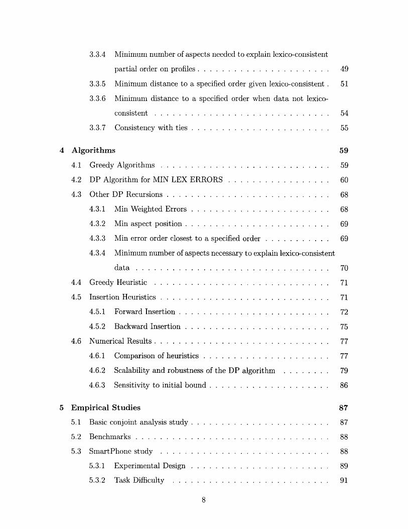
Monte Carlo Simulation. The q-compensatory constraints can be incorporated
into most existing compensatory partworth estimation techniques. For example, LIN-
MAP (Srinivasan and Shocker [63] and Srinivasan [62]) uses a linear program to find
partworths that optimize an objective function related to the set of paired conm-
parisons. Analytic center methods (Toubia et al [66]) find the analytic center of a
particular polyhedron (which is defined by linear constraints). Hierarchical Bayes
(HB) techniques (e.g., Rossi and Allenby [56]) uses a hierarchy of probability distri-
33

butions so that population data can inform and improve individual level estimation.
The sampling (random draws) over partworth distributions can be restricted to the
q-compensatory constrained region.
For simplicity of exposition, we report Monte Carlo results for LINMAP and for
rank-order data only. We obtain qualitatively similar results for consider-then-rank
synthetic data. For these tests, we use the 32 x 16 SmartPhone experimental design
that will be described in Chapter 5.
For our generating model, we modify a functional form proposed by Einhorn [14].
We first define a set of generating weights, w, = 2 1-n for n = 1 to N. We then select
each synthetic respondent c's true partworths as follows: Wnc = (n)m = 2 (1-n)
for the nth smallest partworth. Following Einhorn, m = 0 implies Dawes' model
and m = 1 implies a minimally lexicographic model. (By minimally lexicographic,
we mean that the model may not be lexicographic in the presence of measurement
error.) Setting 0 < m < 1 generates a q-compensatory model. By setting m = 0, 1/15,
2/15, 4/15, 8/15, and 16/15 we generate a range of models that are successively less
compensatory. (For 16 aspects, the smallest partworth is 2-15. Setting the largest m
to 16/15 makes the last model less sensitive to measurement error.) We then generate
1, 000 synthetic respondents for each m as follows where ujc is respondent c's true
utility for profile j.
1. For each m, generate W, normalize so wnc's sum to 1.0.
2. For each c, add error to each true profile utility: uijc = ujc + ej, where j
N(0, e) and e = 0.2, 0.4.
3. Given {Ukc}, generate a rank order of 32 cards for respondent c. Repeat for all
m.
For each respondent, we use estimate an LBA aspect order (using algorithms
developed in Chapter 4) and use LINMAP(q) to estimate q-compensatory partworths.
Both aspect orders and estimated partworths imply a rank order of the 32 profiles.
The comparison statistic is the percent of ordered pairs of profiles predicted from
34
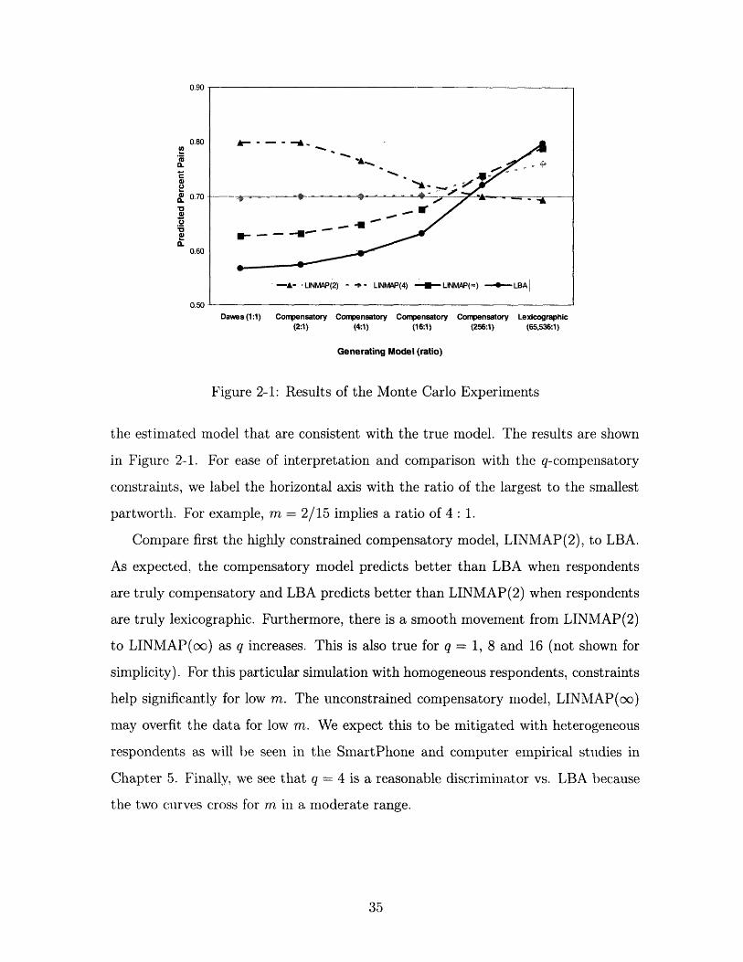
0.90
0.80
.a
0.60
0.50
Dawes(1:1) Compensatory Compensatory Compensatory Compensatory Lexicographic(2:1) (4:1) (16:1) (256:1) (65,536:1)
Generating Model (ratio)
Figure 2-1: Results of the Monte Carlo Experiments
the estimated model that are consistent with the true model. The results are shown
in Figure 2-1. For ease of interpretation and comparison with the q-compensatory
constraints, we label the horizontal axis with the ratio of the largest to the smallest
partworth. For example, m = 2/15 implies a ratio of 4: 1.
Compare first the highly constrained compensatory model, LINMAP(2), to LBA.
As expected, the compensatory model predicts better than LBA when respondents
are truly compensatory and LBA predicts better than LINMAP(2) when respondents
are truly lexicographic. Furthermore, there is a smooth movement from LINMAP(2)
to LINMAP(co) as q increases. This is also true for q = 1, 8 and 16 (not shown for
simplicity). For this particular simulation with homogeneous respondents, constraints
help significantly for low m. The unconstrained compensatory model, LINMAP(oo)
may overfit the data for low m. We expect this to be mitigated with heterogeneous
respondents as will be seen in the SmartPhone and computer empirical studies in
Chapter 5. Finally, we see that q = 4 is a reasonable discriminator vs. LBA because
the two curves cross for m in a moderate range.
35

36

Chapter 3
Complexity Analysis
In this chapter, we introduce several problems related to noncompensatory inference.
We analyze the computational complexity of each problem, showing whether they
belong to the class of problems that can be solved with polynomial-time algorithms
or belong to more difficult classes. Several problems are shown to be easy by proving
that they have a greedoid language structure. Other problems are shown to be hard
and, furthermore, hard to approximate.
3.1 NP-Completeness and Approximation
Computational Complexity. For proving properties about the hardness of var-
ious problems, we rely on the theory of computational complexity. In the 1970s,
researchers began developing the theory of NP-completeness and studying other prop-
erties of complexity classes, i.e., classes of problems with the same level of difficulty.
Garey and Johnson [17] is the standard text on NP-completeness.
Problems in class P can be solved with polynomial-time algorithms. Problems in
class NP have the property that a solution can be verified in polynomial time (e.g.,
checking whether a given traveling salesman tour has length less than k). Finally,
a problem is in the class NP-complete if it is in NP and also has the property that
any other problem in NP can be transformed to it with a polynomial-time trans-
formation. Examples of problems that are NP-complete include VERTEX COVER,
37
SATISFIABILITY, and the TRAVELING SALESMAN PROBLEM. The class NP-
complete contains essentially the "hardest" problems in NP (since any algorithm for a
NP-complete problem can be applied (after transformation) to any other problem in
NP). Specifically, if a polynomial-time algorithm were discovered for an NP-complete
problem, it would imply that P = NP and all problems in NP would be polynomially
(efficiently) solvable.
The initial framework for studying computational complexity was based in logic,
and the problems were all cast as decision problems (i.e., problems that asked a yes/no
question). Thus, instead of asking what the smallest (minimum size) vertex cover is,
it is asked if there exists a vertex cover of size less than or equal to k.
Subsequent work has extended and applied complexity analysis more directly to
optimization problems (see Ausiello et al [1]). Additionally, even though the class
NP-complete contains many hundreds of equally hard problems in the decision sense,
not all problems are equally hard when it comes to approximability. For example,
certain problems admit approximation schemes that guarantee a solution within a
factor r of optimality, while others do not. The problems that do have constant-factor
approximation algorithms belong to the class APX. Thus, even after showing that an
optimization problem is NP-hard (i.e., that all problems in NP can be transformed to
it in polynomial time, though the problem itself is not necessarily in NP), it is often
useful to determine how difficult it is to approximate it.
3.2 Easy Problems
3.2.1 Greedoid languages
Greedoids are mathematical objects initially developed by Korte and Lovasz [40] to
study conditions under which a greedy algorithm can solve optimization problems.
They have proven useful in sequencing and allocation problems (e.g., Niiio-Mora
[50]). Bjorner and Ziegler [5] and Korte et al [41] are excellent references that provide
numerous examples of greedoids. We believe that this is the first application of
38
greedoids to marketing science.
Greedoids are a class of set systems that possess certain properties. (Any matroid,
a perhaps more widely known object, is also a greedoid.) It can be shown that
greedoids have an equivalent language representation. The language form given in
Definition 3 is more appropriate for our application.
Definition 3 A greedoid language (E, L) is an alphabet E and a language L such
that
(G1) If a E L and a = y, then E L.
(G2) If ac,,3 E L and lol > IPI, then there exists an x E a such that ox E L.
Property (GI) means that if a word is in the language, then any left subword must
also be in the language. Property (G2) states that if two words are in the language,
then there exists some letter from the larger word that can be right appended to the
shorter word to make a new word in the language.
Greedoids (and greedoid languages) are important since for a certain class of
compatible objective functions (see Definition 4), the greedy algorithm is guaranteed
to return optimal solutions.
Definition 4 (from Boyd [7]) An objective function W is compatible with a language
L if the following conditions hold: If oax E L and W(ax) > W(ay) for all y such that
ay E L (i.e., x is the best choice at a) then
(a) a3x-y L, a3zy E L ==z W(a3xy) > W(aPz.y)
(x is best at every later stage)
(b) ax/3zy E L, azi3xy E L > W(ax,dz'y) > W(azoxy)
(x before z is always better than z before x)
For several problems in this chapter, we will be interested in finding the longest
word in the greedoid language. Lemma 1 shows that this objective function is com-
patible.
39
Lemma 1 The objective function W(a) = lor is compatible with any language L.
Proof. Property (a). Suppose a/3zy E L, acozy E L. Then
W(&zy) = adxzl = lazyl = W(aozy).
Property(b). Suppose ax/pz"y E L, az/3xy E L. Then
W(axzxy) = laxz-yl = az/xyl = W(azpxy).
Thus W is a compatible objective function. ]
3.2.2 Is there an aspect order that is lexico-consistent with
the data?
Here we define the problem LEX CONSISTENCY in the style of Garey and Johnson
[17] by giving the objects that make up an instance along with the decision question.
For the optimization problems that appear later in this section, we follow the style
of Ausiello et al [1] by giving the form of the instance, the form of a feasible solution,
and the measure (over feasible solutions) to be optimized.
The first problem we consider is one of the two core noncompensatory inference
problems. Given data, e.g., a set of pairs of profiles Q or a partial order on the
profiles X, we are interested in determining if there exists an aspect order that is
lexico-consistent with the data, i.e., that induces no errors with respect to the data.
We first show that this problem has a special greedoid language structure, and then
show that the problem is in complexity class P.
40
LEX CONSISTENCY
INSTANCE : Set of aspects A, set of profiles P, partial order
on profiles X
QUESTION: Is there an aspect order a such that Ex(a) = O?
-
Theorem 1 Let X be a partial order on the profiles P, and let G be the collection
of all aspect orders that are consistent with X. Then G is a greedoid language.
Proof. Property (G1). Suppose a = /3Y E G. Consider any (Pi, Pj) E X and let
X = f,(Pi, I') be the first aspect in a (if any) that differentiates Pi and Pj. If x E /,
then f(Pi, Pj) = x and Pi >-3 Pj. If x /3, then f(Pi, Pj) = 0 (by definition of x)
and is consistent with P -x Pj.
Property (G2). Suppose a, ,3 E G with Ia > /131. Let x E a be the first aspect
from a that is not also in , i.e.,
x = arg min I,(a),
and consider the new word Ox. For any (Pi, Pj) C X, there are two cases to consider.
(1) If either Pi >-p Pj or both Pi tp Pj and x A-(Pi, Pj), then Ox is consistent
with Pi >-x Pj. (2) Suppose that Pi ad Pj, and, for the sake of contradiction, that
:r e A-(Pi, Pj). This implies that f(Pi, Pj) -~ x (since ac E G), and there exists an
aspect x' c a such that f,(Pi, Pj) = x' and I,(x') < I,(x). By the definition of x,
x E /3, which contradicts fx(Pi, Pj) = x. Thus x V A-(Pi, Pj) and x is consistent
with Pi >-x Pj. El
Corollary 1 LEX CONSISTENCY is in P.
Proof. Since G is a greedoid language and W(a) = Ja( is compatible, the greedy
algorithm (which has polynomial running time) can be used to find the longest word
in G. The partial order X is lexico-consistent if and only if the maximum word length
returned by the greedy algorithm is n. Thus, we can determine if X is lexico-consistent
in polynomial time. El
3.2.3 Is there an aspect order such that each aspect intro-
duces at most k new errors?
The previous section considered whether there existed an aspect order that was per-
fectly lexico-consistent with the data. Here we relax the objective. Instead of desiring
41

an aspect order where each aspect introduces zero new errors, we consider aspect or-
ders where each aspect is permitted to cause up to k errors.
We first show that the problem has a greedoid language structure, and then show
that the problem is in class P.
Theorem 2 Let X be a partial order on the profiles, and let G be the collection of
all aspect orders such that each aspect introduces at most k (new) errors with respect
to X. Then G is a greedoid language.
Proof. Property (G1). Suppose a = /3y E
Mx (a(i)) < k, for i = 1,..., n. Since p = a(i)
Mx(a(i)), for i = 1,... ,j, showing that P E G.
Property (G2). Suppose a,3 E G and Icle
from a that is not also in f3, i.e.,
G. By the definition of G, we have
for some j < n, we have Mx(P(i) =
> 131. Let x E a be the first aspect
x = arg min I (a),aEa\/3
and consider the new word 3x. We will show that Mx(fx) < k. Let a' = a (I (x) ),
i.e., the left subword of a up to and including x. For all (Pi, P) E X such that
either Pi >-: Pj or both Pi ad Pj and x ¢ A-(Pi, Pj), the relation Pi >-x Pj is not
violated and so does not contribute to Allx(/3x). Suppose instead that Pi >-x Pj while
P : Pj and x E A-(P, Pj). By the definition of x, we have
fox(Pi, Pj) = f, (Pi, Pj) = x.
42
BOUNDED ERRORS PER ASPECT
INSTANCE: Set of aspects A, set of profiles P, partial order
on profiles X, scalar k
QUESTION: Is there an aspect order a such that MIx(a(i)) < k
for all i?
(If there was an x' \ f3 with smaller index than x that also differentiated Pi
and Pj, it would have been chosen instead of x.) This means that Pj -, Pj since
x C A-(Pi, Pj). VWe have shown that if 3x violates Pi -x Pj, then a' also violates
Pi -x Pj. Thus, Mix(x) < MAx(a') < k. o
Corollary 2 BOUNDED ERRORS PER ASPECT is in P.
Proof. Since G is a greedoid language and W(a) = lal is compatible, the greedy
algorithm (which has polynomial running time) can be used to find the longest word
in G. There exists an aspect order such that each aspect introduces at most k new
errors if and only if the maximum word length returned by the greedy algorithm is
n, which can be determined in polynomial time. ]
3.2.4 Adding unions and intersections of aspects
In regression and other methods that involve modeling with independent (or pre-
dictor) variables, it is often necessary and/or advantageous to include interactions
between variables or other nonlinear derived terms. Here we consider adding derived
aspects that are formed from unions and intersections over all pairs of aspects.
For example, if the original set of aspects included { small, medium, large }
and { red, blue, green }, then possible derived aspects would include small-and-red,
medium-or-green, and blue-or-green. We show that exanding the set of aspects in
this way does not affect the greedoid structure with respect to lexico-consistency.
Theorem 3 Let A be a set of aspects, P be a set of profiles, and X be a partial
order on the profiles P. Let A' = A U {aiuj} U {ainj}, i.e., the original aspects plus
all possible unions and intersections of two aspects, and let G be the collection of all
aspect orders over A' that are consistent with X. Then G is a greedoid language.
Proof. This follows immediately from Theorem 1. Replacing aspect set A with A'
does not change the structure of the problem. O
43
3.3 Hard Problems
In this section, we consider problems that are not in class P (unless P = NP). In
many of the proofs, we will reduce the problems to MIN SET COVER, a canonical
problem in approximation.
MIN SET COVER
INSTANCE: Collection C of subsets of a finite set S.
SOLUTION: A set cover for S, i.e., a subset C' C C such that
every element in S belongs to at least on member
of C'
MEASURE: Cardinality of the set cover, i.e., C'I.
3.3.1 Minimum number of errors
Suppose we know that there is no aspect order lexico-consistent with the data. In that
case, we might still be interested in the aspect order that induces the least number
of errors with respect to the data, i.e., that fits it best. We refer to this problem as
MIN LEX ERRORS.
Unlike LEX CONSISTENCY, MIN LEX ERRORS is not in P (unless P = NP).
Schmitt and Martignon [57] show that the decision version of this problem is NP-
complete with a reduction from VERTEX COVER. Here we strengthen their result
by showing that not only is MIN LEX ERRORS NP-hard, but it is AP-reducible to
MIN SET COVER. The following result is known for MIN SET COVER.
44
MIN LEX ERRORS
INSTANCE : Set of aspects A, a set of profiles P, and a set of
pairs X C P x P.
SOLUTION : Aspect order a such that lJol = IAI.
MEASURE: Ex(a)
Theorem 4 (Feige [16]) MIN SET COVER is not approximable within (1 -6) nn
for any > 0 unless NP C DTIME(n°(l°gl°gn))), where DTIAIE(t) is the class of
problems for which there is a deterministic algorithm running in time O(t).
By reducing a problem from MIN SET COVER, with an approximation preserv-
ing (AP) reduction, the problem is shown to be at least as hard to approximate as
MIN SET COVER. From Feige's result, that means there can be no constant factor
approximation algorithm unless NP C DTIME(nO(l ° gl° gn)) (which is unlikely).
Theorem 5 MIN SET COVER is AP-reducible to MIN LEX ERRORS.
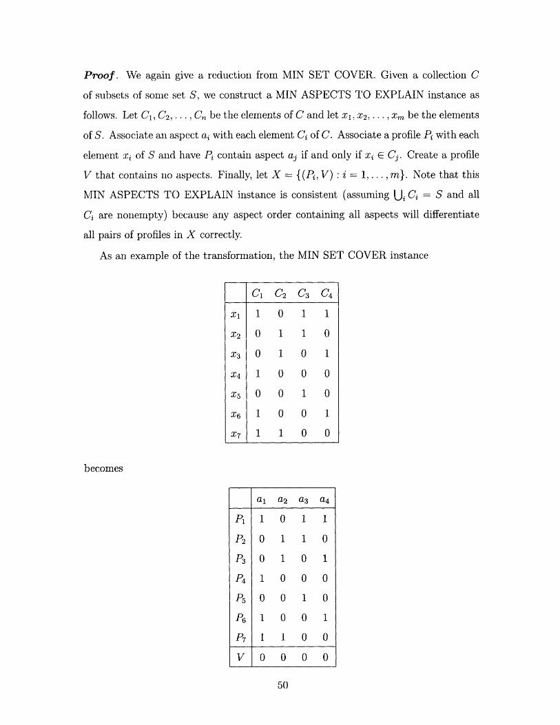
Proof. Given a collection C of subsets of set S in a MIN SET COVER instance,
we construct a MIN LEX ERRORS instance as follows. Let C1, C2,..., Cn be the
elements of C and let x1, x 2, . ., xm be the elements of S. Associate an aspect ai with
each element Ci of C. Introduce an additional aspect q. Associate a profile Pi with
each element xi of S such that
Pi = {aj : i E Cj)
Introduce new profiles V and W1, W2, ... , Wn such that
V= {q}
Wi = {ai}.
Finally, let
X = {(Pi,V): i = 1,...,m} U {(V,W): i = 1,...,n}.
Note that the (Pi, V) pairs in X will all be correctly differentiated by a if xi is
contained in somle Cj such that aj comes before q in a (i.e., if a corresponds to an
actual set cover). The (V, Wi) pairs in X encourage q to appear as left as possible
in a'. Figure 3.3.1 shows an example transformation. Notice that the transformation
can be accomplished in polynomial time.
45
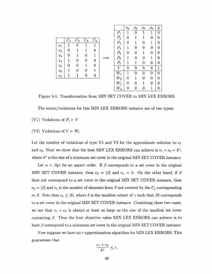
al a 2 a 3 a 4 q
P , 1 0 1 1 0
P 2 0 1 1 0 0
P3 0 1 0 1 0
P4 1 0 0 0 0P5 0 0 1 0 0
P6 1 0 0 1 0P7 1 1 0 0 0V 0 0 0 0 1
W1 1 o0 0 0
W 2 0 1 0 0 0W3 0 0 1 0 0
W 4 0 0 0 1 0
Figure 3-1: Transformation from MIN SET COVER to MIN LEX ERRORS
The errors/violations for this MIN LEX ERRORS instance are of two types:
(V1) Violations of Pi >- V
(V2) Violations of V >- WE
Let the number of violations of type V1 and V2 for the approximate solution be el
and e2. Next we show that the best MIN LEX ERRORS can achieve is el + e2 = k*,
where k* is the size of a minimum set cover in the original MIN SET COVER instance.
Let a = /3q-y be an aspect order. If corresponds to a set cover in the original
MIN SET COVER instance, then e2 = (,/ and el = 0. On the other hand, if
does not correspond to a set cover in the original MIN SET COVER instance, then
e2 = Ii1 and el is the number of elements from S not covered by the Cj corresponding
to p. Note that el > 161, where is the smallest subset of -y such that /36 corresponds
to a set cover in the original MIN SET COVER instance. Combining these two cases,
we see that el + e2 is always at least as large as the size of the smallest set cover
containing p. Thus the best objective value MIN LEX ERRORS can achieve is to
have 3 correspond to a ninimum set cover in the original MIN SET COVER instance.
Now suppose we have an r-approximation algorithm for MIN LEX ERRORS. This
guarantees thatel + e2
k* < - r,k*
46
C C2 C 3 C4
X1 1 0 1 1
x 2 0 1 1 0
X3 0 1 0 1
X4 1 0 0 0
X5 0 0 1 0
X6 1 0 0 1
X7 1 1 0 0
where k* is the size of the minimum set cover of the original problem. To transform
an r-approximate solution to MIN LEX ERRORS into a set cover for the original
MIN SET COVER instance, consider the following. If the Cj corresponding to the aj
in do not already form a set cover for the original MIN SET COVER instance, then
at most el additional elements from C need to be added to the existing group of e2
elements to form a set cover (since el corresponds to the number of elements of S not
yet covered). The size of the constructed set cover is at most e2 + el, guaranteeing a
performance ratioe2 + el
k* -< r.
Therefore, MIIN SET COVER is AP-reducible to MIN LEX ERRORS. Ol
3.3.2 Minimum weighted number of errors
It might be the case that for a given set of pairs of profiles Q, some comparisons
are more important than others. For example, perhaps the comparisons from the
earlier part of a conjoint survey are deemed more likely to be accurate than later
comparisons when a subject might be more tired.
Theorem 6 MIN WEIGHTED ERRORS is NP-hard.
Proof. This result follows directly from Theorem 5 since by setting all weights wij
equal to 1, MIN WEIGHTED ERRORS is equivalent to MIN LEX ERRORS. O
47
MIN WEIGHTED ERRORS
INSTANCE : Set of aspects A, set of profiles P, set of pairs X C
P x P along with weights wij for all (Pi, Pj) E X.
SOLUTION : Aspect order o such that Iac = AI.
MEASURE : Ex,w(a)
3.3.3 Minimum position of an aspect given lexico-consistent
Given that a set of data is lexico-consistent, we might be interested in the leftmost
position that a particular aspect can occur in among all lexico-consistent aspect or-
ders. Note that how far left an aspect occurs relates to the aspect's importance. We
call this problem MIN ASPECT POSITION.
Theorem 7 MIN SET COVER is AP-reducible to MIN ASPECT POSITION.
Proof. The reduction from MIN SET COVER is nearly the same as in the proof
for MIN LEX ERRORS, except there is no need for profiles Wi. Suppose we have an
r-approximate algorithm for MIN ASPECT POSITION, i.e.,
Ia(q) < rk* 1< r,
where k* is the size of the minimum set cover of the original problem. Note that all
feasible solutions to MIN ASPECT POSITION must be of the form a = -q-y where
corresponds to a set cover in the original MIN SET COVER instance (otherwise some
Pi >- V would be violated). Thus, the best objective value MIN ASPECT POSITION
can achieve is k* + 1, by letting /3 be a minimum set cover in the original MIN SET
COVER instance.
The Cj corresponding to the aj in /3 (from the r-approximate solution to MIN
ASPECT POSITION) form a set cover C' for the original MIN SET COVER since
all pairs (Pi, V) are correctly differentiated by a. With respect to MIN SET COVER,
48
MIN ASPECT POSITION
INSTANCE: Set of aspects A, aspect q E A, a set of profiles
P, and a set of pairs X C P x P that is lexico-
consistent.
SOLUTION: Aspect order a with Ex(a) = 0.
MEASURE : I,(q)

the performance ratio isIa(q)- 1
k*
Calculating the difference between the performance ratios of MIN SET COVER and
MIN ASPECT POSITION,
1.(q) - 1 Is(q)
k* k* + 1I,(q)-(k*+ 1)
k*(k* + 1)Ia (q) I _ 1 I.(q) 1)
k*(k* + 1) k * k* + 1
we see that
I.(q)-1 I (q) I +_ _ ),k* k*+l 1 k* k* + r
since k* > 1 and a(q) < r. Therefore, MIN SET COVER is AP-reducible to MIN
ASPECT POSITION. O
3.3.4 Minimum number of aspects needed to explain lexico-
consistent partial order on profiles
Suppose we have a set of data that is lexico-consistent. For concreteness, suppose
our data consists of a set of pairs Q. Even though a full aspect order differentiates
all possible pairs of profiles, it might be the case that a partial aspect order, i.e.,
with lal < Al, can differentiate all pairs in Q correctly. We call the problem of
finding the shortest such aspect order (that is still lexico-consistent with the data)
MIN ASPECTS TO EXPLAIN.
Theorem 8 MIN SET COVER is AP-reducible to MIN ASPECTS TO EXPLAIN.
49
MIN ASPECTS TO EXPLAIN
INSTANCE : Set of aspects A, a set of profiles P, and a set of pairs
X C P x P that is lexico-consistent.
SOLUTION: Aspect order rs such that Ex(a) = 0.
MEASURE: al
_ _
Proof. We again give a reduction from MIN SET COVER. Given a collection C
of subsets of some set S, we construct a MIN ASPECTS TO EXPLAIN instance as
follows. Let C1, C2,. . , C,, be the elements of C and let xl, x2 ,.. ., xm be the elements
of S. Associate an aspect ai with each element Ci of C. Associate a profile Pi with each
element xi of S and have Pi contain aspect aj if and only if xi E Cj. Create a profile
V that contains no aspects. Finally, let X = {(Pi, V): i = 1,. . ., m}. Note that this
MIN ASPECTS TO EXPLAIN instance is consistent (assuming Ui Ci = S and all
Ci are nonempty) because any aspect order containing all aspects will differentiate
all pairs of profiles in X correctly.
As an example of the transformation, the MIN SET COVER instance
C1 C2 C 3 C4
X1 1 0 1 1
x 2 0 1 1 0
x 3 0 1 0 1
X4 1 0 0 0
X5 0 0 1 0
x 6 1 0 0 1
x7 1 1 0 0
al a2 a3 a4
P 1 1 0 1 1
P 2 0 1 1 0
P3 0 1 0 1
P4 1 0 0 0
P5 0 0 1 0
P6 1 0 0 1
P7 1 1 0 0
V 0 O O 0
50
becomes
Now suppose we have an r-approximate algorithm for MIN ASPECTS, i.e., the
performnance ratio is guaranteed to satisfy
lal <k* -,
where k* is the size of the minimum set cover of the original problem. The best MIN
ASPECTS can do is k* by letting ac be a minimum set cover in the original MIN SET
COVER instance, because lal < k* would mean that at least one element j C S
would be uncovered and (Pj, V) would not be differentiated.
Note that the approximate solution oa correctly differentiates all pairs in X since a
is a feasible solution for MIN ASPECTS TO EXPLAIN. Thus the Cj corresponding
to the aj in a form a set cover C' for the original problem. The performance ratio
with respect to MIN SET COVER is
IC' aI <k* k* -
Therefore MIN SET COVER is AP-reducible to MIN ASPECTS. O
3.3.5 Minimum distance to a specified order given lexico-
consistent
Suppose a set of data is lexico-consistent, i.e., there exists some aspect order that
induces no errors with respect to the data. Furthermore, suppose that the research
has an idea of what the aspect should have looked like ahead of time, e.g., from self-
explicated questions at the beginning of a conjoint analysis survey. Then it might be
desirable to find the lexico-consistent aspect order that is closest in some sense to the
specified order. We call this problem MIN CONSISTENT DISTANCE, where the
distance between two aspect orders is defined as the sum of the absolute differences
in aspect position over all aspects.
51
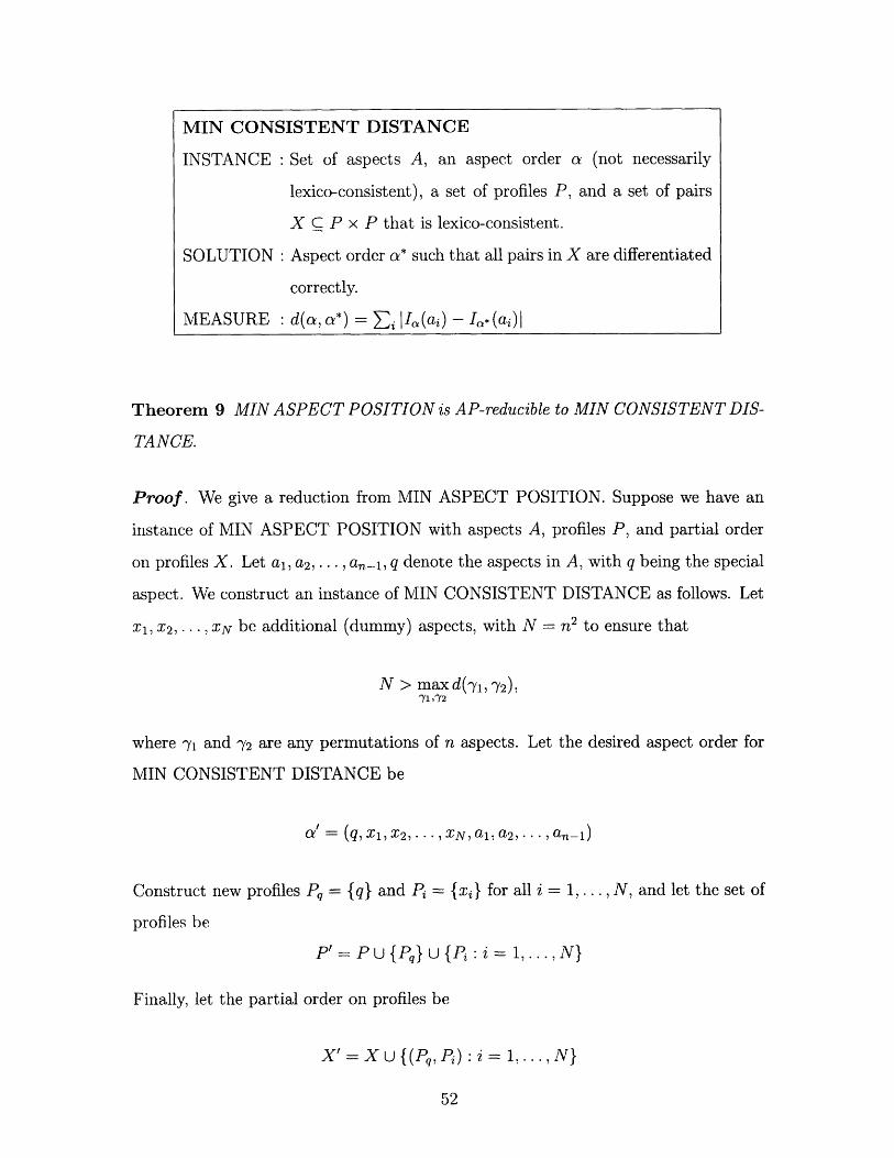
Theorem 9 MIN ASPECT POSITION is AP-reducible to MIN CONSISTENT DIS-
TANCE.
Proof. We give a reduction from MIN ASPECT POSITION. Suppose we have an
instance of MIN ASPECT POSITION with aspects A, profiles P, and partial order
on profiles X. Let al, a2,.. ., a,, q denote the aspects in A, with q being the special
aspect. We construct an instance of MIN CONSISTENT DISTANCE as follows. Let
X 1, x2, . . , XN be additional (dummy) aspects, with N = n2 to ensure that
N > max d(yl,Y 2),Y1 ,Y2
where 'y1 and y2 are any permutations of n aspects. Let the desired aspect order for
MIN CONSISTENT DISTANCE be
al = (q, Xi x2, .· · , XN, al,a2, · · · an-1)
Construct new profiles Pq= {q} and Pi = {xi} for all i = 1,..., N, and let the set of
profiles be
P' = P U Pq U {P: i= 1,..., N}
Finally, let the partial order on profiles be
X'= XU{(Pq, Pi): i = ,...,N}
52
MIN CONSISTENT DISTANCE
INSTANCE: Set of aspects A, an aspect order c (not necessarily
lexico-consistent), a set of profiles P, and a set of pairs
X C P x P that is lexico-consistent.
SOLUTION: Aspect order cr* such that all pairs in X are differentiated
correctly.
MEASURE : d(a, a*) = i IQ(ai) - I, (ai)
Note that the new pairs in X' force aspect q to come before aspects xi in any consistent
aspect order for the MIN CONSISTENT DISTANCE instance.
In order to analyze the optimal cost for MIN CONSISTENT DISTANCE, consider
a consistent aspect order oa* (of the aspects in A) that minimizes the position of aspect
q and also minimizes the distance from a* to (q, a l,a 2,. . .,an-l) as a secondary
objective. We argue that an optimal aspect order for MIN DISTANCE is 3*, where
xl, x2,..., xN immediately follow q, while all other aspects are in the same relative
order as in a*. The total cost is given by
cost(*) = dl + d2,
whered = d(a, a*), and
d2 = (N+ 1)(I, (q)- 1)
The second component of the cost, d2, is caused by q and xi shifting to the right due
to (I, (q)- 1) aspects that must appear before q in o*.
Now suppose another aspect were shifted before q. This change would increase
d2 by (N + 1) while it could only decrease d by at most n2. So this change would
worsen the cost. Furthermore, suppose that the permutation of the aspects (other
than q and xi) were changed. The value of d2 stays the same, while d1 becomes worse.
Thus 0* achieves the optimal cost for MIN CONSISTENT DISTANCE.
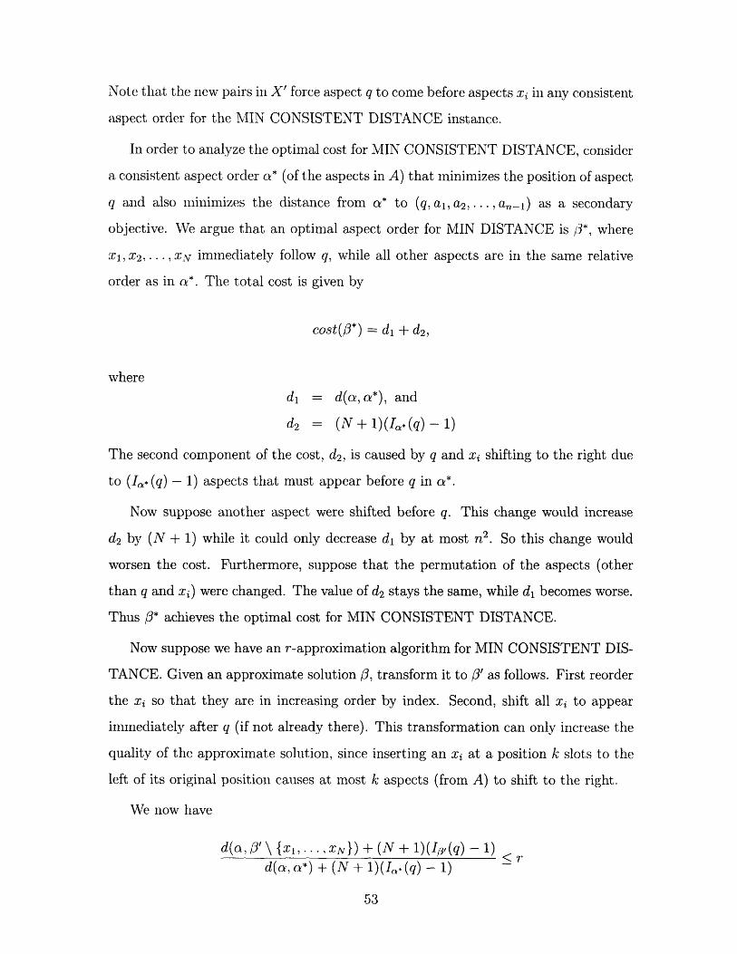
Now suppose we have an r-approximation algorithm for MIN CONSISTENT DIS-
TANCE. Given an approximate solution 3, transform it to 3' as follows. First reorder
the xi so that they are in increasing order by index. Second, shift all xi to appear
immediately after q (if not already there). This transformation can only increase the
quality of the approximate solution, since inserting an xi at a position k slots to the
left of its original position causes at most k aspects (from A) to shift to the right.
We now have
d(a, 3' \ {Z1, ... XN}) + (N + 1)(,113(q)-1)<rd(, a*) + (N + 1)(I,. (q) - 1)
53
It follows thatd(a, a-) + (N + 1)(I/3,(q) - 1)<d(a, a*) + (N + 1)(I,*(q)- 1) -
since d(ac, a*) < dist(a, 3' \ Xl,.. . , XN}) by the definition of a*. Finally,
d(ca, a*)/(N + 1) - 1 + I, (q) -d((v, a*)I(N + 1) - 1 + I* (q)
I/, (q) r1,,* (q) <r,
since d(c, a*)/(N + 1) - 1 < 0 by definition of N.
The last ratio is precisely the performance ratio of using /'\{x 1 , XN} as an ap-
proximate solution for MIN ASPECT POSITION. Thus, MIN ASPECT POSITION
is AP-reducible to MIN CONSISTENT DISTANCE, and it follows from Theorem 7
and the transitivity of AP-reducibility that MIN SET COVER is also AP-reducible
to MIN CONSISTENT DISTANCE. O
3.3.6 Minimum distance to a specified order when data not
lexico-consistent
Suppose a set of data is not lexico-consistent, i.e., there are no aspect orders that
induce zero errors with respect to the data. Furthermore, suppose that the researcher
has an idea of what the aspect order should look like ahead of time, e.g., from self-
explicated questions at the beginning of a conjoint analysis survey. Then it might be
desirable to find the minimum error aspect order (i.e., that has induces that same
number of errors as the optimal solution of MIN LEX ERRORS) that is also closest
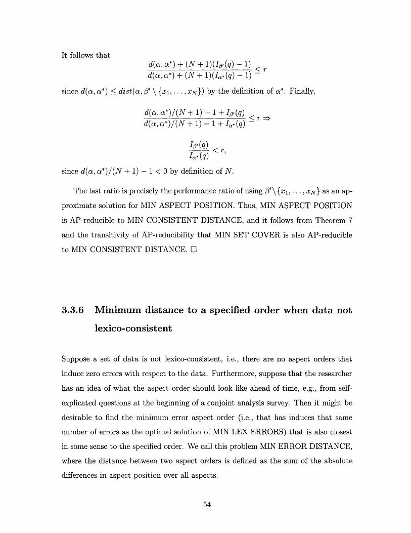
in some sense to the specified order. We call this problem MIN ERROR DISTANCE,
where the distance between two aspect orders is defined as the sum of the absolute
differences in aspect position over all aspects.
54
Theorem 10 MIN ERROR DISTANCE is not in APX (unless P = NP).
Proof. This result follows immediately from Theorem 5. If it were possible to
approximate MIN ERROR DISTANCE with some constant factor approximation
scheme, then we could use it to solve MIN LEX ERRORS exactly. O
3.3.7 Consistency with ties
Suppose that we allowed the possibility of ties between profiles. Then no aspect
order corresponding to the lexicographic decision-making process described earlier can
possibly be consistent with data that contains ties (since the lexicographic strategy
differentiates every pair of profiles given an aspect order).
Here we introduce a more general lexicographic strategy that allows for ties in the
aspect ordering. Specifically, instead of depending on an ordered subset of aspects, a
lex with ties strategy will depend on an ordered collection of subsets of aspects:
S1 - S2 - ... - > Sp,
where the sets Si form a partition of A. When the cardinality of each set is 1, the lex
with ties strategy is equivalent to the lex strategy. If ISil > 1, then the aspects in Si
are valued equally. If two profiles are considered equal before applying Si, then the
profile with more aspects from Si is preferred.
For example, suppose A = {al, a2, a3}, S1 = {al, a2}, S2 = {a3}, and we have
profiles Pi = al), P2 = a2}, P3 = {al,a 2}, and P4 = {a3 }. Then we have the
55
MIN ERROR DISTANCE
INSTANCE : Set of aspects A, aspect order c, set of profiles P, set of
pairs X C P x P that is not lexico-consistent.
SOLUTION : Aspect order a' such that Ex(a') equals minimum num-
ber of errors according to MIN LEX ERRORS
MEASURE : d(a, a') = Ei II(ai) - I,(ai)l
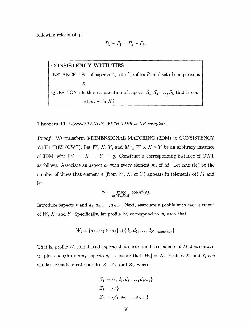
following relationships:
Theorem 11 CONSISTENCY WITH TIES is NP-complete.
Proof. We transform 3-DIMENSIONAL MATCHING (3DM) to CONSISTENCY
WITH TIES (CWT). Let W, X, Y, and M C W x X x Y be an arbitrary instance
of 3DM, with IWI = IXI = IYI = q. Construct a corresponding instance of CWT
as follows. Associate an aspect ai with every element mi of M. Let count(e) be the
number of times that element e (from W, X, or Y) appears in (elements of) M and
let
N= max count(e).eEWUXUY
Introduce aspects r and dl, d2,... , dN-1. Next, associate a profile with each element
of W, X, and Y. Specifically, let profile Wi correspond to wi such that
Wi = {aj : wi E mj} U {dl, d2,.. , dN-cont(wi)).
That is, profile Wi contains all aspects that correspond to elements of M that contain
wi plus enough dummy aspects di to ensure that [Wi4 = N. Profiles Xi and Yi are
similar. Finally, create profiles Z1, Z2, and Z3 , where
Z1 = {r, d, d2, ... , dN-l}
z 2 = {r}
Z3= {dld2, ..,dN-l}
56
CONSISTENCY WITH TIES
INSTANCE : Set of aspects A, set of profiles P, and set of comparisons
X
QUESTION : Is there a partition of aspects S1, S2 ,. .. , Sk that is con-
sistent with X?
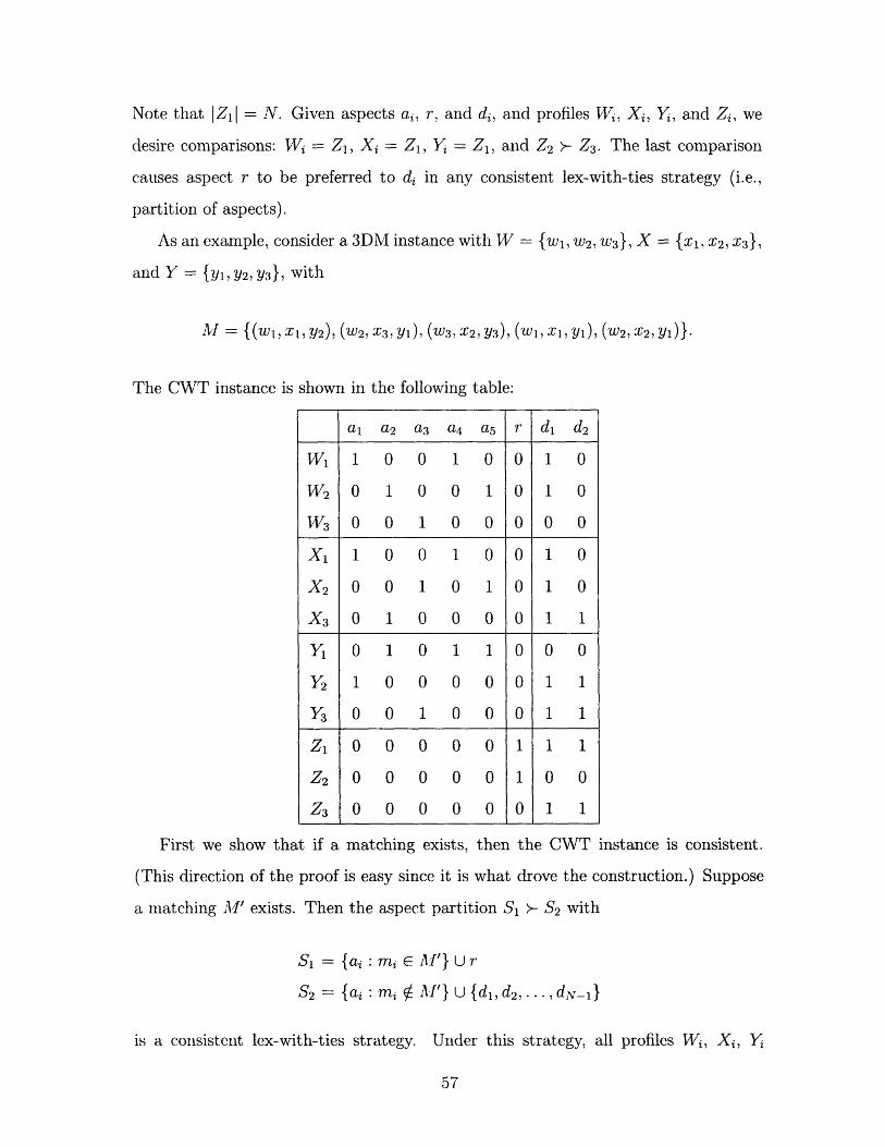
Note that IZ11 = N. Given aspects ai, r, and di, and profiles 14i, Xi, Y, and Zi, we
desire comparisons: Vi = Z 1, Xi = Z1, Y/ = Z1, and Z 2 >- Z3 . The last comparison
causes aspect r to be preferred to di in any consistent lex-with-ties strategy (i.e.,
partition of aspects).
As an example, consider a 3DM instance with W = {wl, w2, w3}, X = { 1 , X2, x 3 },
and Y = {Y1, Y2, Y3}, with
Al = {(Wl, , Y2), ( 2, X3, Y1), ( 3. X2, Y3), (l, xl, Y1), (w2, x2 , Y1)}.
The CWT instance is shown in the following table:
al a 2 a 3 a 4 a r d1 d2
W1 1 0 0 1 0 0 1 0
W 2 0 1 0 0 1 0 1 0
W 3 0 0 1 0 0 0 0 0
X 1 1 0 0 1 0 0 1 0
X 2 0 0 1 0 1 0 1 0
X 3 0 1 0 0 0 0 1 1
Y 1 1 0 1 0 O 0
Y2 1 0 0 0 0 0 1 1Y3 0 0 1 0 0 0 1 1
Z1 0 0 0 0 0 1 1 1
Z 2 0 0 0 0 0 1 0 0
Z 3 0 0 0 0 0 0 1 1
First we show that if a matching exists,
(This direction of the proof is easy since it is
then the CWT instance is consistent.
what drove the construction.) Suppose
a matching A1l' exists. Then the aspect partition S1 >- S2 with
S1 = {ai : mi E I'} U r
S 2 = {ai : mi 1lI'} U {dl, d2 ,. , dNl}
is a consistent lex-with-ties strategy. Under this strategy, all profiles Wi, Xi, Y
57
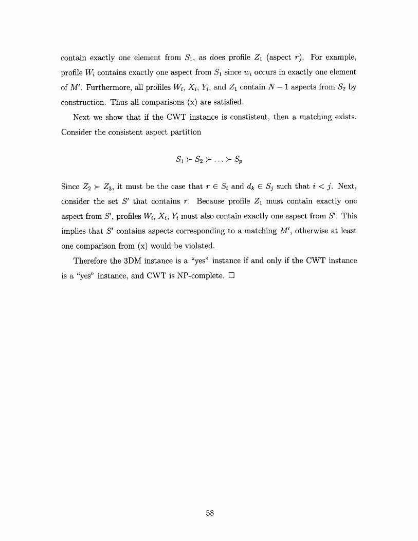
contain exactly one element from S, as does profile Z1 (aspect r). For example,
profile Wi contains exactly one aspect from S1 since wi occurs in exactly one element
of M'. Furthermore, all profiles Wi, Xi, IY, and Z1 contain N- 1 aspects from S2 by
construction. Thus all comparisons (x) are satisfied.
Next we show that if the CWT instance is constistent, then a matching exists.
Consider the consistent aspect partition
S1 S2 ... Sp
Since Z2 >- Z3, it must be the case that r E Si and dk e Sj such that i < j. Next,
consider the set S' that contains r. Because profile Z1 must contain exactly one
aspect from S', profiles Wi, Xi, Yi must also contain exactly one aspect from S'. This
implies that S' contains aspects corresponding to a matching M', otherwise at least
one comparison from (x) would be violated.
Therefore the 3DM instance is a "yes" instance if and only if the CWT instance
is a "yes" instance, and CWT is NP-complete. ]
58
Chapter 4
Algorithms
In this chapter, we present solution methods for the problems described in Chapter 3.
The problems exhibiting a greedoid language structure (e.g., LEX CONSISTENCY)
can be solved with a greedy algorithm over an appropriate objective function. We
make use of some additional structure to show that each NP-hard problem (e.g.,
MIN LEX ERRORS) can be solved with dynamic programming. Since the dynamic
programming based algorithms have exponential worst case time complexity, we an-
alyze several heuristics including a greedy heuristic and insertion based local search.
We also present several implementation enhancements to the dynamic programming
algorithm that provide significant speedup in practice.
4.1 Greedy Algorithms
In each of the decision problems shown to have a greedoid language structure, the
decision question can be rephrased as: "Is there a word of length n that is contained
in the language?" (where n is the size of the alphabet). The corresponding objective
function we are trying to maximize over words in the language is the length of the
word. Equivalently, we are maximizing a linear function over the letters where the
coefficient corresponding to (the inclusion of) each letter is equal to 1. Recall that
this objective function, W(a), was shown to be compatible in Chapter 3.
Let c(a, x.) denote the new errors directly caused by aspect x occuring after aspect
59
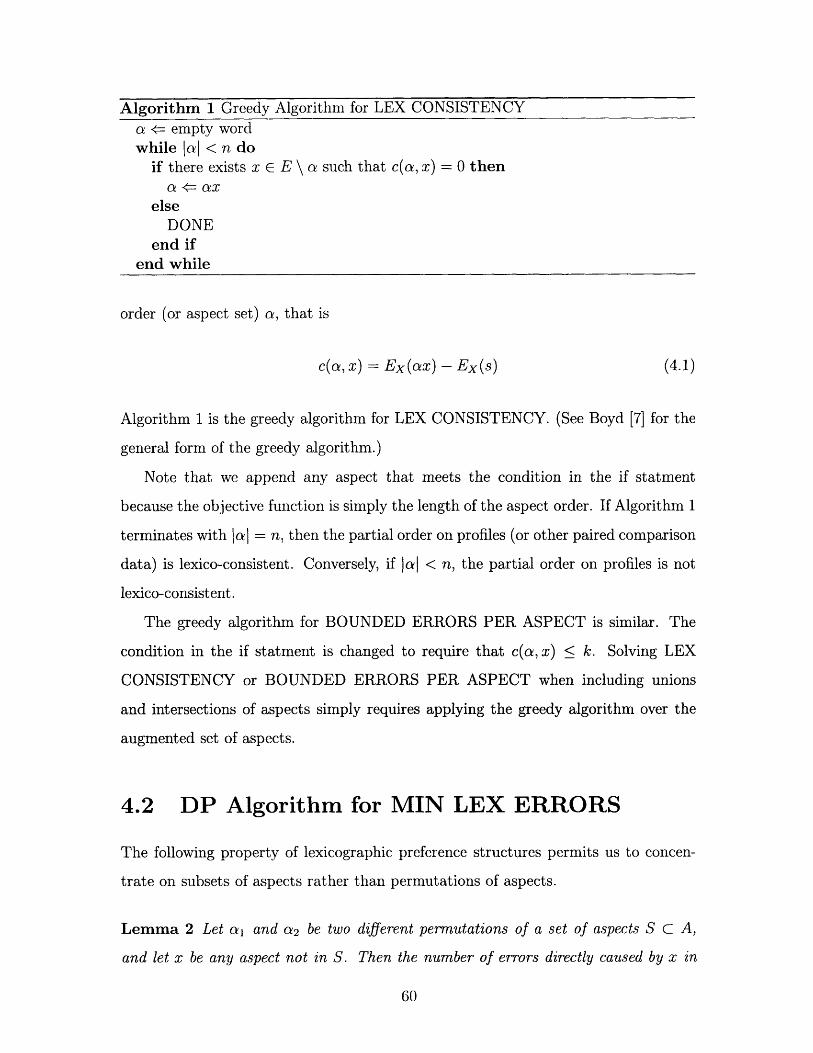
Algorithm Greedy Algorithm for LEX CONSISTENCYa = empty wordwhile a[ < n do
if there exists x C E \ a such that c(a, x) = 0 thena ax
elseDONE
end ifend while
order (or aspect set) a, that is
c(a, x) = Ex(ax) - Ex(s) (4.1)
Algorithm 1 is the greedy algorithm for LEX CONSISTENCY. (See Boyd [7] for the
general form of the greedy algorithm.)
Note that we append any aspect that meets the condition in the if statment
because the objective function is simply the length of the aspect order. If Algorithm 1
terminates with al = n, then the partial order on profiles (or other paired comparison
data) is lexico-consistent. Conversely, if al < n, the partial order on profiles is not
lexico-consistent.
The greedy algorithm for BOUNDED ERRORS PER ASPECT is similar. The
condition in the if statment is changed to require that c(a, x) < k. Solving LEX
CONSISTENCY or BOUNDED ERRORS PER ASPECT when including unions
and intersections of aspects simply requires applying the greedy algorithm over the
augmented set of aspects.
4.2 DP Algorithm for MIN LEX ERRORS
The following property of lexicographic preference structures permits us to concen-
trate on subsets of aspects rather than permutations of aspects.
Lemma 2 Let al and a 2 be two different permutations of a set of aspects S C A,
and let x be any aspect not in S. Then the number of errors directly caused by x in
60
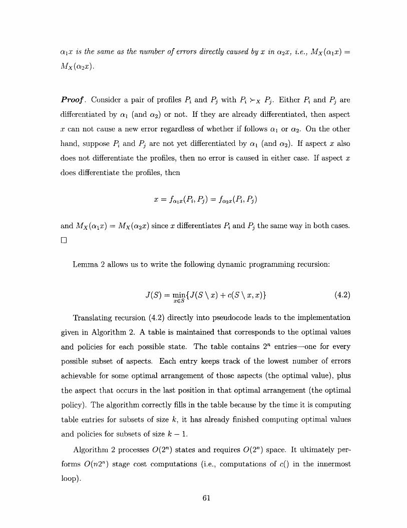
a1x is the same as the number of errors directly caused by x in a 2x, i.e., lIx(alx) =
A'x (2xz).
Proof. Consider a pair of profiles Pi and Pj with Pi >-x Pj. Either Pi and Pj are
differentiated by oal (and a 2) or not. If they are already differentiated, then aspect
x can not cause a new error regardless of whether if follows al or a 2. On the other
hand, suppose Pi and Pj are not yet differentiated by ca (and a 2). If aspect x also
does not differentiate the profiles, then no error is caused in either case. If aspect x
does differentiate the profiles, then
x = flX(Pi, Pj) = fa2(Pi, Pj)
and Aix (alx) = Mx(a 2x) since x differentiates Pi and Pj the same way in both cases.
Lemma 2 allows us to write the following dynamic programming recursion:
J(S) = min{J(S \ x) + c(S \ x, x)} (4.2)XES
Translating recursion (4.2) directly into pseudocode leads to the implementation
given in Algorithm 2. A table is maintained that corresponds to the optimal values
and policies for each possible state. The table contains 2 entries-one for every
possible subset of aspects. Each entry keeps track of the lowest number of errors
achievable for some optimal arrangement of those aspects (the optimal value), plus
the aspect that occurs in the last position in that optimal arrangement (the optimal
policy). The algorithm correctly fills in the table because by the time it is computing
table entries for subsets of size k, it has already finished computing optimal values
and policies for subsets of size k - 1.
Algorithm 2 processes 0(2 n) states and requires 0(2") space. It ultimately per-
forms O(n2") stage cost computations (i.e., computations of c() in the innermost
loop).
61
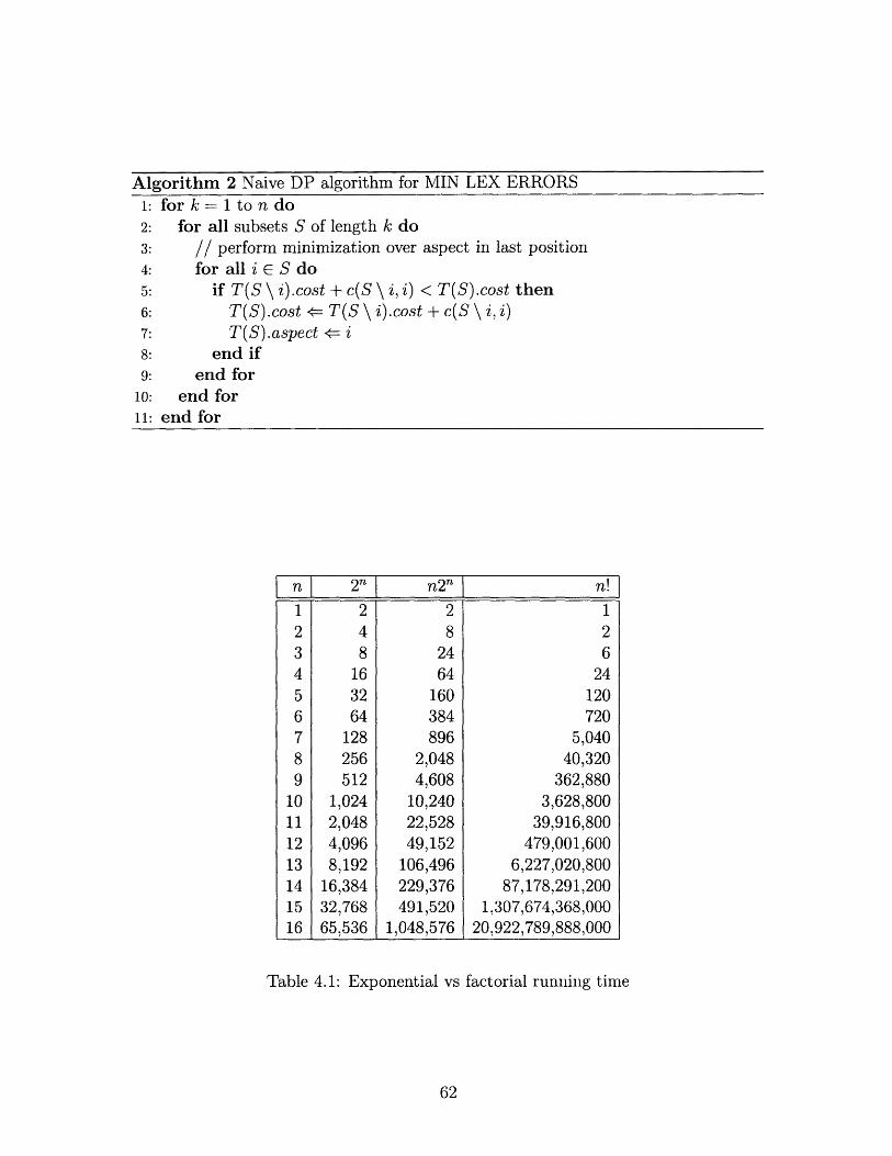
Algorithm 2 Naive DP algorithm for MIN LEX ERRORS1: for k = 1 to n do2: for all subsets S of length k do3: // perform minimization over aspect in last position4: for all i S do5: if T(S \ i).cost + c(S \ i, i) < T(S).cost then6: T(S).cost = T(S \ i).cost + c(S \ i, i)7: T(S).aspect = i8: end if9: end for
10: end for11: end for
Table 4.1: Exponential vs factorial running time
62
n 2n n2 n n!
1 2 2 1
2 4 8 2
3 8 24 64 16 64 245 32 160 1206 64 384 7207 128 896 5,0408 256 2,048 40,3209 512 4,608 362,880
10 1,024 10,240 3,628,80011 2,048 22,528 39,916,80012 4,096 49,152 479,001,60013 8,192 106,496 6,227,020,80014 16,384 229,376 87,178,291,20015 32,768 491,520 1,307,674,368,00016 65,536 1,048,576 20,922,789,888,000
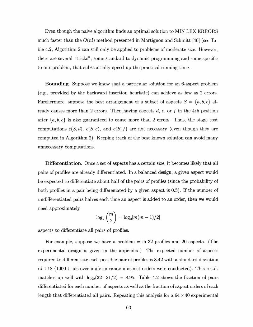
Even though the naive algorithm finds an optimal solution to MIN LEX ERRORS
much faster than the O(n!) method presented in Martignon and Schmitt [46] (see Ta-
ble 4.2, Algorithm 2 can still only be applied to problems of moderate size. However,
there are several "tricks", some standard to dynamic programming and some specific
to our problem, that substantially speed up the practical running time.
Bounding. Suppose we know that a particular solution for an 6-aspect problem
(e.g., provided by the backward insertion heuristic) can achieve as few as 2 errors.
Furthermore, suppose the best arrangement of a subset of aspects S = {a, b, c} al-
ready causes more than 2 errors. Then having aspects d, e, or f in the 4th position
after {a, b, c} is also guaranteed to cause more than 2 errors. Thus, the stage cost
computations c(S, d), c(S,e), and c(S, f) are not necessary (even though they are
computed in Algorithm 2). Keeping track of the best known solution can avoid many
unnecessary computations.
Differentiation. Once a set of aspects has a certain size, it becomes likely that all
pairs of profiles are already differentiated. In a balanced design, a given aspect would
be expected to differentiate about half of the pairs of profiles (since the probability of
both profiles in a pair being differeniated by a given aspect is 0.5). If the number of
undifferentiated pairs halves each time an aspect is added to an order, then we would
need approximately
log2 () = log2[m(m - 1)/2]
aspects to differentiate all pairs of profiles.
For example, suppose we have a problem with 32 profiles and 20 aspects. (The
experimental design is given in the appendix.) The expected number of aspects
required to differentiate each possible pair of profiles is 8.42 with a standard deviation
of 1.18 (1000 trials over uniform random aspect orders were conducted). This result
matches up well with log2 (32 · 31/2) = 8.95. Table 4.2 shows the fraction of pairs
differentiated for each number of aspects as well as the fraction of aspect orders of each
length that differentiated all pairs. Repeating this analysis for a 64 x 40 experimental
63
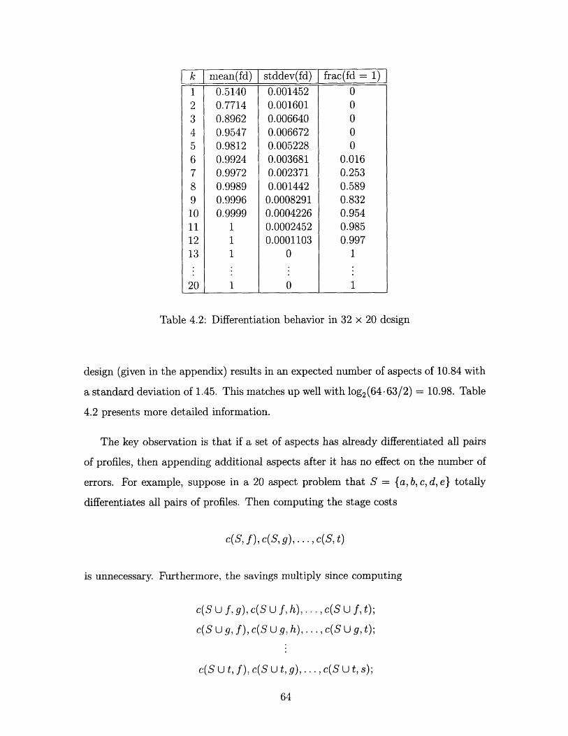
Table 4.2: Differentiation behavior in 32 x 20 design
design (given in the appendix) results in an expected number of aspects of 10.84 with
a standard deviation of 1.45. This matches up well with log2(64 63/2) = 10.98. Table
4.2 presents more detailed information.
The key observation is that if a set of aspects has already differentiated all pairs
of profiles, then appending additional aspects after it has no effect on the number of
errors. For example, suppose in a 20 aspect problem that S = {a, b, c, d, e} totally
differentiates all pairs of profiles. Then computing the stage costs
c(S, f), c(S, g), ... , c(S, t)
is unnecessary. Furthermore, the savings multiply since computing
c(SU f,g),c(SU f,h),.. .,c(SU f,t);c(S U gy,f), c(S U g,h),... ,c(SU g,t);
c(S U t,f), c(S U t, g),..., c(S U t, s);
64
| k mean(fd) stddev(fd) frac(fd = 1)1 0.5140 0.001452 02 0.7714 0.001601 03 0.8962 0.006640 04 0.9547 0.006672 05 0.9812 0.005228 06 0.9924 0.003681 0.0167 0.9972 0.002371 0.2538 0.9989 0.001442 0.5899 0.9996 0.0008291 0.83210 0.9999 0.0004226 0.95411 1 0.0002452 0.98512 1 0.0001103 0.99713 1 0 1
20 1 0 1
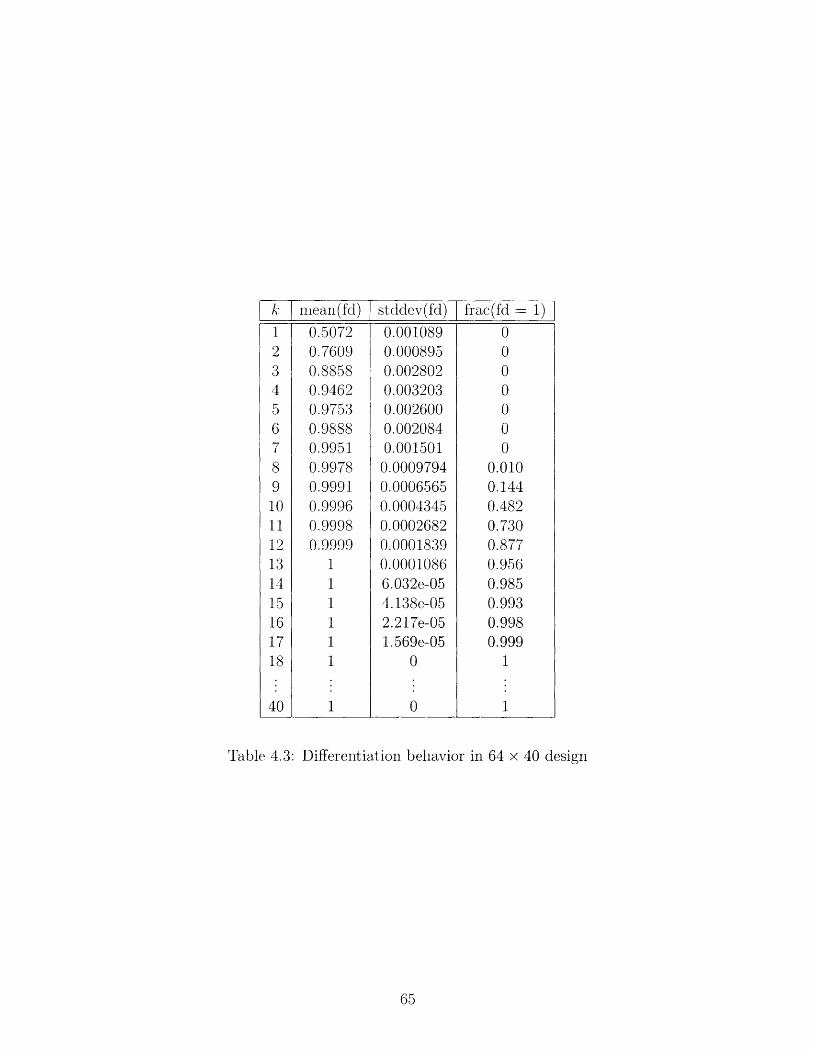
frac(fd = 1)
Table 4.3: Differentiation behavior in 64 x 40 design
65
0.0010890.0008950.0028020.0032030.0026000.0020840.001501
0.00097940.00065650.00043450.00026820.00018390.00010866.032e-054.138e-052.217e-051.569e-05
0
0
/i: mean(fd) stddev(fd)1
2
3
4Z
5
6
7
8
9
1011
12
13
1415
16
1718
40
0.50720.76090.88580.94620.97530.98880.99510.99780.99910.99960.99980.9999
1
1
1
1
1
1
I
0
0
0
0
0.0100.1441
0.4820.7300.8770.9560.9850.9930.9980.999
1I
and so on also becomes unnecessary. For this example, the total number of avoided
stage cost computations is 15 x 14 x ... x 2 = 15!.
Dynamic memory allocation. Suppose that the following stage cost computa-
tions are unnecessary due to the above considerations:
c({a, b}, c), c({a, c}, b), c({b, c}, a).
For example, it could be the case that J({a, b}), J({a, c}), and J({b, c}) are all worse
than the cost of a known solution. Then J({a, b, c}) never has to be computed at
all. In the event that many subsets of aspects can be completely ignored, it becomes
attractive to only store table entries for those subsets that actually matter.
Combining the preceding observations leads to Algorithm 3. It maintains a FIFO
queue of all sets of aspects that have costs (so far) that are less than or equal to
the cost of the best known solution. The queue also contains only sets that do not
completely differentiate the profiles. These two properties ensures that no unnecessary
stage cost computations are performed with respect to bounding and differentation.
Another property of the queue is that the sizes of the sets it contains are nonde-
creasing. This guarantees that the optimal value for a set of size k is already known
before that set is used for stage cost computations on sets of size k + 1.
Additionally, the table is designed to contain only those sets that are necessary.
The table can be implemented efficiently as a hash table.
Greedoid Initialization. One further tweak is possible, capitalizing on the
greedoid structure of the problem. First we prove the following lemma.
Lemma 3 Suppose that /3 is an ordered subset of aspects that is lexico-consistent with
the preferences in X. Then there is an optimal (full) ordering of aspects that begins
with the order 3.
66

Algorithm 3 Enhanced DP algorithm for MIN LEX ERRORS1: initialize T2: initialize Q3: bestSoFar = cost of heuristic solution4:
5: // add singleton sets to Q6: for all aspects i do7: if Ex(i) < bestSoFar then8: add {i} to T9: add {i} to Q
10: end if11: end for12:
13: while Q not empty do14: remove first set S from Q15: for all i E S do16: if T(S).cost + c(S, i) < bestSoFar then17: if (S U i) E T then18: // update existing table entry if necessary19: if T(S).cost + c(S, i) < T(S U i) then20: T(S U i).cost <= T(S).cost + c(S, i)21: T(S U i).aspect = i22: end if23: else
24: // create new table entry for this set of aspects25: add (S U i) to T26:
27: // only add to Q if this set will need further processing/expansion28: if (S U i) does not totally differentiate P then29: add (S U i) to Q30: end if31: end if32:
33: // update bestSoFar if necessary34: if (S U i) totally differentiates P and T(S U i).cost < bestSoFar then35: bestSoFar = T(S U i).cost36: end if37: end if38: end for39: end while
67
Proof. Let a be a solution to MIN LEX ERRORS (with Jcal = IAl) and suppose
there exists a subset of aspects 3 such that Ex (3) = 0. Consider the aspect order
y = (, (a \ ))
and any aspect x E a \ 3. The number of errors caused directly by x in y must be
less than or equal to the number of errors causes directly by x in a because the set of
profiles differentiated by y(,(x)) is a superset of the profiles differentiated by a(I(x)).
(This is because the set of aspects preceding x in -y is a superset of the set of aspects
preceding x in a.) Since all x E a \ 3 cause at most the same number of errors as x
in a, Ex(y) < Ex(a) which implies that Ex(y) = Ex(a). l
The significance of Lemma 3 is that the greedy algorithm can be run first to
find the longest (partial) aspect order that induces no errors (if one exists). Then
the problem size can be reduced by removing those aspects and the profiles already
differentiated by them.
4.3 Other DP Recursions
The basic property in Lemma 2 extends for most/all of the other hard problems from
the previous chapter. What follows are the appropriate modifications to the property
(stated without proof) and the resulting DP recursions.
4.3.1 Min Weighted Errors
Lemma 4 Let a and be two different permutations of a subset S of aspects, and
let x be any aspect not in S. Then the number of weighted errors directly caused by x
in ax is the same as the number of errors directly caused by x in 3x.
This property permits the following DP recursion:
J(S) = lnin{J(S \ i) + c(S \ i, i)},iES
68

where
c(T, x) = wij(ij)cxnx-T )
4.3.2 Min aspect position
Lemma 5 The position of aspect x in a does not change if the permutation of the
aspects preceding x is modified.
Consider the following DP recursion:
J(S) = min {J(S \ x) + c(S \ x, x)} xES
whereTI+1 ifx=q
c(T, x) = (n + 1) AIMx(T, x) + 1 if0 otherwise
The first term of the stage cost c(., ) is incrementally computing the number of
errors multiplied by a constant. The second term simply records the position of q.
The constant in the first term is chosen to be n + 1 so that having aspect q earlier in
the order can never compensate for having even one more error. (The constant n + 1
is an upperbound on the position of q.)
Thus, for lexico-consistent data, the DP recursion will favor all lexico-consistent
solutions over non lexico-consistent ones, and then select the lexico-consistent solution
that allows q to appear earliest in the order. Similarly, for data that is not lexico-
consistent, the DP recursion will favor all subsets that achieve the minimum error
(i.e., the optimal objective function value of MIN LEX ERRORS), and then select
the minimum error solution that allows q to appear earliest in the order.
4.3.3 Min error order closest to a specified order
Lemma 6 Let a = yx6, with -y = k, let y' be a different permutation of y, and
let /3 be some other aspect order. Then the contribution to d(/3, a) caused by x is the
same as the contribution to d(f3, y'x6) caused by x.
69
Note that in each case, the contribution to total distance caused by x is I(x) -
(k + 1)1. Now consider the following DP recursion:
J(S) = inin{J(S \ x) + c(S \ x, x)}, (4.3)xES
where
c(T, x) = n 2 Mx(T, x) + [IP(x) - (ITI + 1)].
The first term of the stage cost c(-, ) is incrementally computing the number of
errors multiplied by a constant. The second term is incrementally computing the
distance between the solution and O. The constant in the first term is chosen to be
n2 so that having an aspect order closer to P can never compensate for having more
errors. (The constant n2 is an upper bound on total distance.)
Thus, for lexico-consistent data, the DP recursion will favor all lexico-consistent
solutions over non lexico-consistent ones, and then select the lexico-consistent solution
that is closest to 3. Similarly, for data that is not lexico-consistent, the DP recursion
will favor all subsets that achieve the minimum error (i.e., the optimal objective
function value of MIN LEX ERRORS), and then select the minimum error solution
that is closest to .
4.3.4 Minimum number of aspects necessary to explain lexico-
consistent data
Lemma 7 The number of new (correct) differentiations directly caused by x in aspect
order a does not depend on the permutation of the aspects preceding x in a.
Consider the following DP recursion:
J(S) = 1min {J(S \ x) + c(S \ x, x)),
70
where
0 if iMx (Tx) = 0 and M+ (T) = 0
c(T x) = 1 if MAIx(Tx) = 0 and M1lX(Tx) > 0
oo if Mlfx(Tx) > 0
The third condition of the stage cost function guarantees that any solution with
no errors is favored over any solution with errors. The first and second conditions
serve to count the number of aspects that actually (correctly) differentiate at least one
pair of profiles. Since any aspect that differentiates no profiles at its current position
in an aspect order can be moved to a later position in the order without affecting the
total number of errors, the DP recursion computes the minimum number of aspects
required to differentiate the data.
4.4 Greedy Heuristic
Kohli and Jedidi [39] present a greedy heuristic for minimizing the number of errors
with respect to a set of paired comparisons of profiles. Algorithm 4 provides essentially
the same algorithm adapted to our formulation and notation.
Algorithm 4 Greedy heuristic for MIN LEX ERRORSa (= empty wordwhile al < n do
x* t= arg minxeE\a c(a, x)
end while
Note that if X is lexico-consistent, then applying Algorithm 4 will find an aspect
order a that is consistent with X, i.e., with Ex(a) = 0.
4.5 Insertion Heuristics
In the field of combinatorial/discrete optimization, numerous local improvement or
neighborhood search heuristics have been developed for solving hard optimization
71
problems. Here we consider two heuristics based on insertion due to the efficiency of
searching over the neighborhood of possible moves.
4.5.1 Forward Insertion
For forward insertion, a move m = (i j), with i < j, consists of moving the aspect
currently in position i to position j and shifting all aspects currently in positions
i + 1, i + 2, ..., j one position to the left. We will use the notation am to denote the
resulting aspect order after applying move m to a. For example, if a = (a, b, c, d, e)
and m = (2 --* 4), then oam = (a, c, d, b, e). Algorithm 5 gives the basic outline of the
forward insertion heuristic.
Algorithm 5 Forward insertion heuristic for MIN LEX ERRORSa <= random permutation of 1,..., nrepeat
(i - j*) = argmini<j{d = Ex ((ij))- Ex(a)}if d* < 0 then
end (i.fj*)
end ifuntil d* > 0
A naive implementation would simply compute the total number of errors from
scratch for each possible forward insertion. This would have an O(n3Q1l) running
time if O(n2) moves were scored, scoring each move required checking each pair in Q,
and checking each pair required iterating over O(n) aspects.
Due to the special nature of forward insertions, however, the change in the number
of errors resulting from applying move m, i.e.,
Ex (m) - Ex (a)
can be computed more efficiently in an incremental manner. Suppose we have an
existing aspect order a. Consider a pair (Pi, Pj) and let xl be the leftmost aspect
in a that differentiates Pi and Pj and let x2 be the second leftmost aspect in a that
differentiates them.
72

Causing a new error. First, suppose that (Pi, Pj) is currently differentiated
correctly, i.e., x C A>(Pi, Pj). Then the only way for a new error to be caused by a
move is if
(a) ax2 E A (Pi, Pj), and
(b) x1 is inserted behind x 2.
In other words, the only moves that will cause a new error are
(a(X1) ---+ j), j > I ( 2).
We will refer to this as a move family, and refer to it as (I,(xl) -> I(x 2)).
Fixing an existing error. On the other hand, suppose that (Pi, Pj) is currently
differentiated incorrectly, i.e., xl E A<(Pi, Pj). Then the only way for this error to
ble fixed by a move is if
(a) X2 C A(Pi, Pj), and
(b) xl is inserted behind x2.
In other words, the only moves that will fix the existing error are
(X (x) j), Vj > Ia(X2).
To exploit these properties, we can maintain a min binary heap for each (Pi, Pj )
in Q containing all aspects in A>-(Pi, Pj) UA-(Pi, Pj) sorted by their current positions
in a. This allows querying for the first and second minimal elements (corresponding
to the leftmost and second leftmost differentiating aspects in a) in constant time (see
Cormen et al [11].
For example, suppose
P1 = (100101)
P 2 = (001110)
and P1 >- P2, then the heap would include aspects a, c, e, and f. The pair is currently
differentiated correctly since xl = a E A>-(P1 , P2 ). However, applying any move from
73

the move family
(I0(x1) -> I,(x2)) = (1 > 3)
would cause a new error.
There are at most II2 move families that result from examining all heaps. Each
move family mf has a value associated with it (mf.delta) that corresponds to the
total change in the number of errors that (any move in) the move family would cause.
For example, if a total of three pairs in Q are affected by the same move family,
and two existing errors would be fixed while one new error would be introduced, the
combined effect of that move family over all pairs would be -1 (i.e., the total number
of errors would decrease by one).
Determining the best move over all move families. Given a list of all
relevant move families, it is necessary to compute the best overall move. Suppose all
move families that involved moving a(1) to another location were
(1 --> 3).delta = +2
(1 -*> 5).delta = -3
(1 -- > 9).delta= +1
Remember that moving a(1) to position 3 or later causes two new errors. Thus,
moving a(1) to position 5 results in a net effect of removing one error. And moving
a(l) to position 9 results in a net effect of not changing the total number of errors.
If we restricted ourselves to finding the best insertion point for a(1), it would be 5
(or 6, ... , 8).
The important thing to note is that finding the optimal insertion point for a(1)
did not necessarily require considering all O(n) insertion points. Likewise, finding
the best move over all origins (that occur in at least one move family) only requires
considering at most II move families rather than O(n2 ) possible moves. The only
requirement is that the move families be sorted first by origin, then by destination.
A radix sort can accomplish this in 0(I2Il) time.
Updating after a move. Once a best move (i* j*) has been found, the aspect
74
order and heaps must be updated. Because the relative positions of all aspects other
than a(i*) stay the same, the relative positions of those aspects in each heap remain
the same. Only the relative position of aspect a(i*) to the other aspects changes.
Specifically, its position increases and the heap property can become violated. In order
to restore the heap property, a(i*) can be swapped (downward) with its smallest child
as needed. Because the depth of each heap is O(log n), updating all heaps requires
O(log njQl) time.
Overall algorithm and complexity. The forward insertion heuristic with a
heap-based implementation first initializes all heaps which takes O(nlognlQl) time
(O(n) time for finding the elements that need to go in each heap and O(nlogn)
time for constructing each heap). Each iteration involves finding the best move and
updating the heaps after applying that move (if the move is an improvement). Find-
ing the best; move (see Algorithm 6) takes 0(1I2) time since detecting all relevant
move families takes 0(I j) time, the radix sort over origins and destinations takes
0(I2I) time, and finding the best move over all move families takes (jQj) time.
As mentioned above, updating the heaps takes O(lognQl) time. Thus, each itera-
tion requires O(lognQl) time rather than the O(n3 lQl) time complexity of the naive
implementation.
4.5.2 Backward Insertion
For backward insertion, a move m = (j - i), with j < i, consists of moving the aspect
currently in position i to position j and shifting all aspects currently in positions
i, i + 1,...,j - 1 one position to the right. For example, if a = (a, b, c, d, e) and
m = (2 +- 5), then cm = (a, e, b, c, d). Algorithm 7 provides a high level view of the
method (which strongly resembles the forward version). The analysis for finding the
best backward move is similar to the forward move case, but differs in a critical way.
Causing a new error. Suppose that (Pi, Pj) is currently differentiated correctly,
i.e., xl E A (Pi, Pj). Then the only way for a new error to be caused by a backward
move is if some aspect x E A (Pi, Pj) is moved before xl. Thus, instead of a single
relevant move family (as in the forward case), O(n) move families can be relevant for
75

Algorithm 6 Finding best forward insertion move1: // find all move families that affect number of errors2: for all (Pi,Pj) C Q do3: X1 < heap(Pi, j).f irst4: x2 ' heap(Pi, Pj).second5:
6: // see what move family would cause new error7: if x Ce A> (Pi, Pj) and x2 e A (Pi, Pj) then8: // update delta for move family9: T[I.(x) - I(x 2 )] T[I( 1) I(2)] + 1
10: end if11:
12: // see what move family would fix existing error13: if x CE A-(Pi, Pj) and x2 C A>(Pi, Pj) then14: // update delta for move family15: [IIj - X I 2()1 T[I,(xi) -I '(X2)-116: end if
17: end for
18:
19: // create sorted list of destinations for each origin (a list of lists)20: moveList radixSort(T)21:
22: // find best move23: bestAMove.delta < oc
24: for all orig in moveList do25: currentDelta z= 026: for all dest in moveList(orig) do27: currentDelta = currentDelta + T[orig -- dest]28: if currentDelta < bestMove.delta then29: bestAMove.move z (orig -- dest)30: bestMove.delta ~ currentDelta31: end if32: end for33: end for
Algorithm 7 Backward insertion heuristic for MIN LEX ERRORSa -= random l)ermutation of 1, ... , nrepeat
(j* -- *) = argmnij<,{d = Ex(ac(ji)) - Ex(o)}if d* < 0 then
a (t(j*-is)end if
until d* > 0
76
a given pair of profiles.
Fixing an existing error. On the other hand, suppose that (Pi, Pj) is currently
differentiated incorrectly, i.e., x1 E A- (Pi, Pj). Then the only way for this error to
be fixed by a move is if some aspect x E A>-(Pi, Pj) is moved before xl. Here again,
instead of a single relevant move family (as in the forward case), O(n) move families
can be relevant for a given pair of profiles.
Determining the best move over all move families. Once all relevant move
families have been computed, the best overall move can be determined in a similar way
to the forward insertion case. The only difference is that the result of the radix sort
must have the move families sorted by origin, and then by destination in decreasing
order.
Updating after a move. Once a best move (j* i*) has been found, all heaps
need to be updated. As in the forward insertion case, we only need to be concerned
with the relative positioning of ac(i*). Since the position of a(i*) has decreased, the
heap property may now be violated. However, it can be restored by swapping (i*)
(upward) with its parent as needed. This is an O(logn) operation per heap.
Overall algorithm and complexity. The form of the overall algorithm and the
complexity analysis is very similar to the forward insertion case. The only difference
is that there are O(nliQl) relevant move families. Thus, each iteration takes O(nlQl)
time.
4.6 Numerical Results
4.6.1 Comparison of heuristics
In order to compare the performance of the greedy and insertion heuristics, we con-
ducted a series of experiments. We consider two methods for generating partial orders
over profiles, each intended to allow varying the degree of lexicography (or degree of
"lexico-consistency"'). For one set of experiments, partial orders over profiles were
generated in the following way:
77

1. Given k > 0.
2. Construct a partworth vector w such that each element wi is uniformly dis-
tributed in [0, 1].
3. Raise each element of w to the kth power.
4. Then Pi preferred to Pj if aEPi Wa > aePj Wa.
Note that this is the same Einhorn generating model discussed in Section 2.3. When
k = 0, we have the Dawes equal weights model. When k = 1, we have uniform
random weights. When k is large, the operation of raising each element to the kth
power behaves similarly to the Loo norm in that it "selects" and exaggerates the
largest element. It also exaggerates the second largest element with respect to the
remaining elements, and so on. So as k grows, the degree of lexicography grows.
A second method for generating partial orders over profiles is as follows:
1. Given a random lexico-consistent profile order (i.e., a linear ordering of the
profiles that is induced by some random aspect order).
2. Given a number of iterations, flips.
3. Swap a random profile with its successor (in the linear ordering of the profiles).
4. Perform Step (3) flips times.
Here we start with a perfectly lexico-consistent profile order and introduce possible
errors by repeatedly swapping neighboring profiles in the order. When flips grows
large, the profile order approaches a uniform random profile order.
The results of varying k from 1/8 to 64 on designs of size 32 x 20 and 64 x 40 (see
Appendix A for details) are shown in Tables 4.4 and 4.5. The results of varying flips
from 2560 down to 0 are given in Tables 4.6 and 4.7. Each heuristic was run 20 times
for each parameter setting (i.e., each row of each table), and the results averaged.
The columns have the following meanings: cost = number of errors, diff = number
of errors - optimal number of errors, time = running time in seconds, and moves =
78
number of insertions. All the experiments in this chapter were carried out on a laptop
with an Intel Centrino 1.6 GHz CPU, 1 GB of memory, and the Fedora Core 4 linux
operating system. The algorithms were coded with the Java programming language.
Discussion. Both the greedy heuristic and backward insertion heuristic perform
very well over all designs and generation method parameters. The performance of
both greedy and backward improves as the degree of lexicography increases (i.e., as
k increases and f lips decreases). It is also interesting to note that the hardest case
to fit was k = 1/8 for the 64 x 40 design. This suggests that a very compensatory
profile order is harder to fit than a random one (e.g., flips = 2560 for the 64 x 40
design).
Interestingly, even though the forward insertion heuristic has a slightly better
asymptotic running time per iteration, it performs poorly compared to the backward
insertion heuristic and greedy heuristic. Furthermore, the performance appears to
degrade as the degree of lexicography increases. Wolpert and Macready [70] emphasize
that incorporating problem-specific knowledge into an optimization algorithm is very
important. For any given problem, some algorithm is best, and which is the best
depends heavily on the "landscape" of the objective function.
In the case of finding aspect orders that minimize errors (wrong comparisons), it
appears that moving aspects to earlier positions in the order is much more effective
than moving aspects forward (later in the order). This makes sense intuitively since
moving good/important aspects to the front of the order seems to have the potential
for larger gains than simply moving unimportant aspects out of the way. Practically
speaking, the backward insertion heuristic appears less susceptible to getting stuck
in (poor) local optima and often performs as well or better than the greedy heuristic
(which also focuses on the most important aspects first).
4.6.2 Scalability and robustness of the DP algorithm
In order to test the effectiveness of Algorithm 3, we applied the algorithm (seeding
it with bounds from the greedy heuristic) over all parameter settings discussed in
the previous experiment. The results are given in Tables 4.8, 4.9, 4.10, and 4.11.
79
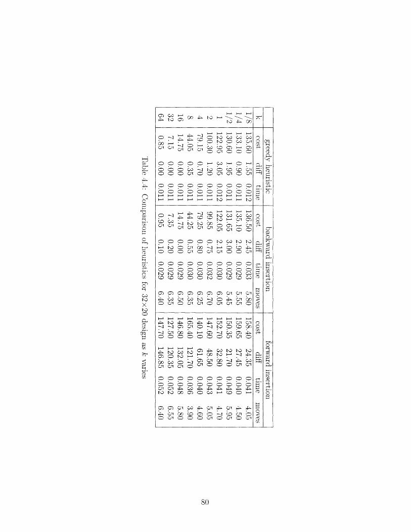
4 LID cz o4 o\
°z° CC C Ccx CD * . to CD c3 CncP t~~~~~~~C Cl CZ)CCyl C Ccn Ch C9) C CD
G~~~r C~~~~il -q -b Z
CD C) C CO O O C~r O O Cn C O 0n
0 6 z c 2Q 1Z@o o o o C 1 J Z . 166 666tz
O O O O O O t C. t tIDO O O C O cn C O O
(=)(= = CC)(= = =tl) t' t C4C-o Co co =
~= ~7- k= D =Q =,clA cl CIQ l~ Lll CC t ) r~ Q0 Cl
C) C C C C -3 C) 0 1 C 07
CD CPC -1 C (= C C C
4P to 4P a c<3 <J a Cn o
1cnoo -4
J1 Cl ocn
CD Cn C CD 4t-- t\3 00 C O
00 N) n
C) C W1 C n
=) =) C)O
C C Cn CZ .0 Cn - Cn q 01
O C1 0 0 0 cn O C1 0 Cq
80
0on
CD;t-
CD
0I-t
CD
O
CDon
0gn
H
on
c
onD
nCZ
UD
cD
C
CD
oC'D
'-'
,-onIt
O
S.
CD
-)
IJ
0OD
on-- --
Ctl :;I 9 ) C) (-;C.77cCl D C
:I
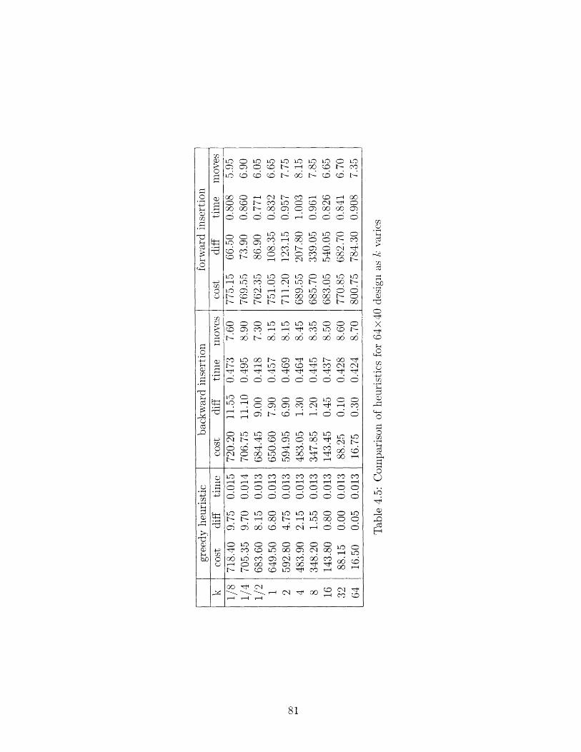
on O Ln n n n n O Ln7 G) = O O - -4 00 CD - 3n- scD 0 Q oO cc tC C
O -4 C t- 0` C 10 00°° °O S 0 0 O C X 00 OoO oO O- O O O ~ O oO O
Ln LO O Ln LO O O° m° a° c' 00 0
*- 0 C* 0 O
O L n n Ln O O =oQ c -- It cl n C- t-
,- o t o (D od oO o o o
cl Ln OE LC I L Cn 00 tS : C') Cni CO C=S C CD' Cil
u3 oLC CDLO ---
I--i -
O n D O Ln L LnC"l tI Q0 C) o oo t
= Q0 4 = 4 6 t- c -3CT O 00 D C) 00 tt- tl- cQ CLO t c3 C
LDC00
LCt'Do O
LO 0 Ln I Ln Ln LO L f onE~ ~-- ~ cO ~- ~-r--I U O O
LO = = ~LO CDo -o n o- o O
Ln ~~ Lo Ln 03 o c o c od cru: O oDO SD O oO O O czoo cs oq t o- c C oo Q cs 17tGO n C\ I C C 0C
O oO e Q Z C S S s cs LcD t c :S oo
81
7)
O0-4
00-4-.'
B
;--4
.2-40
;z7dt
C-ct
-C
C-0-4
00v,a)bC
(1).:
0
O0
0O-4
-4
oUD
)o-40
DO._
t
173OX
k-O._
c0C)x'tO
0cO-4eDI).
00C)o-4
0;400Lo
-0H-
E
Lf- L-) LO = LO L L)LrD C,-)= I CIA L O oO r- tC) C~q C~ CS VD C)' = cap Q0 L O 00 C - C=L- V- U -- o -o Q0 - 00
Ln
Ir-
(= = = = L = == C) C) n CIA It, - C")C~ -- Q 1- _q Z~ ')C'
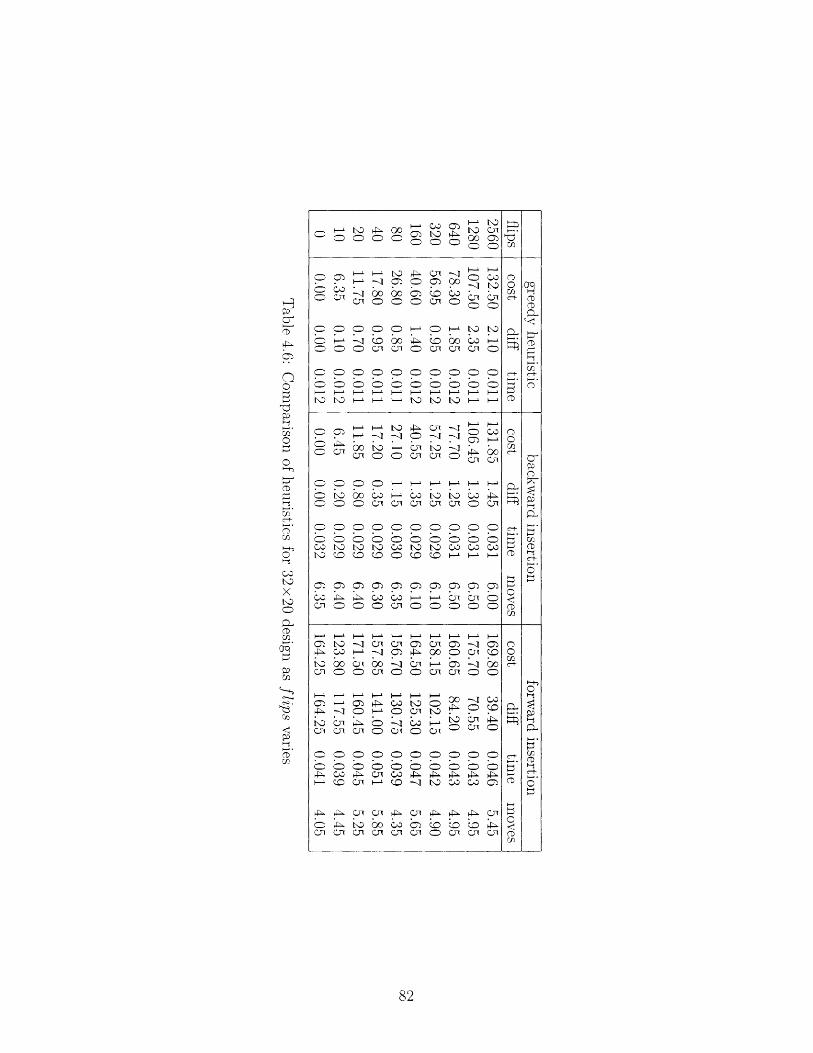
° O~3 OP Go C CC
O C z tZ 4 O X O C 40 0 -00 0 0 C00 0
O0O O O O 1 0O
O CD 00 C C C C0 O O O CC C CD JO O OOO O O3O OO OO OO O
tuD0r~ tuD totu tD
tD 4- C-l-IC cuto3 c n O 4o-A =) --l -- CM
(: C-1 C C 4-6Crl C
O GB _
g 4 o -.-o n o t
C tD 0o co
=) D C C
cl~ tl t3~to C( co 1-o
cP C~-1 1
tcD X cn OoCn 0 cn
Ci CC0 c10
C0c1
C0 C 0 C C 01
Cl O 0 O cn C:C) 01 CD 00
O) Qn °0O
OCnlCn O CJl °C-o0000J0* . . . . .
CD C C CC=
~,- )- cl l 71 CW1l 1 9c1 4. _;
C-1 CUl C CP C Cl O Cl Cnl C;
82
=bb-Fcf:
ct(CD
CcnO
r.cD
D
CDcn
nOg
CD
cP
Cf,©GoPO
0C
CDrctD
CD
0-0
CDCD
CDr·
ctiCDr_
CD
n(D
1-t
r
CD
r©CD
. _ _ _
( C C) = (Z
CC ) 7s C C C C'3 C C( Cw; P;P 'I sc '~-c '- (,;I .;l('C." CD(=) C C O= = (= C
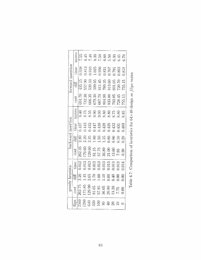
Ln LO = O O
C0 cj ot S
O O O DL Oc. b c'O -t b--s- LO Q0 Q0 Q
l) o= Lon Co S t- -- j 03 _-(cs3 -I ~ C 0 0'3 ) O LnC 30 ) O = 0 00 - t 0 00
' C C CD l CD666. .. 666666 =~::
Ln3 O O LO LO n 0 Q0 O boo o o bo bCD CD LO L
ce3 Cn C) C GD
O O LbD O O O O Ln Ln LO" -o "O O - 0 o oo -7 c-' .o -- ~ c ) C' o C l oC ¢, C C, C oO o00 - .
)O LO O O O O LD O Lt f LC 0 0 0 0 L 00 00
- C C - oo00 C )oO --J. cO O,, cO C~104 C7xl ,O r OClL ~0~ O O C~ Clr-~
O O O O O O ODO0 C Lc O (X C CO 00 0 Clc C C O O -- 6 6 6
") O O ° (= O.. oO q °U b- O
Lfc C~ Cj
n O OL- CD C
?1 -( 1---C0
c'q 'o 'o ~"o o o o o o ,t
0. . .(Z ) . . . .
,O LO .n O O . .
-- oCl o O C
83
0C
-4
(2C0. -
m;dkctL0
C4-4
Cz
-z(t
0C)0
-4
0L.
0rL-4-
O0-
CLr,
r(0C0
0-4._
r©
CL
ti
0
0
CL
,iZ
DO-t._
0
-4
C
OO0
4HCL
- - -
-
7.
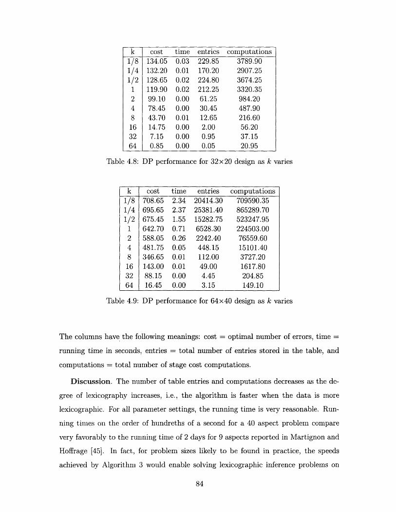
Table 4.8: DP performance for 32x20 design as k varies
Table 4.9: DP performance for 64x40 design as k varies
The columns have the following meanings: cost = optimal number of errors, time =
running time in seconds, entries = total number of entries stored in the table, and
computations = total number of stage cost computations.
Discussion. The number of table entries and computations decreases as the de-
gree of lexicography increases, i.e., the algorithm is faster when the data is more
lexicographic. For all parameter settings, the running time is very reasonable. Run-
ning times on the order of hundreths of a second for a 40 aspect problem compare
very favorably to the running time of 2 days for 9 aspects reported in Martignon and
Hoffrage [45]. In fact, for problem sizes likely to be found in practice, the speeds
achieved by Algorithm 3 would enable solving lexicographic inference problems on
84
k cost time entries computations1/8 134.05 0.03 229.85 3789.901/4 132.20 0.01 170.20 2907.251/2 128.65 0.02 224.80 3674.25
1 119.90 0.02 212.25 3320.352 99.10 0.00 61.25 984.204 78.45 0.00 30.45 487.908 43.70 0.01 12.65 216.60
16 14.75 0.00 2.00 56.2032 7.15 0.00 0.95 37.1564 0.85 0.00 0.05 20.95
k cost time entries computations1/8 708.65 2.34 20414.30 709590.351/4 695.65 2.37 25381.40 865289.701/2 675.45 1.55 15282.75 523247.95
1 642.70 0.71 6528.30 224503.002 588.05 0.26 2242.40 76559.604 481.75 0.05 448.15 15101.408 346.65 0.01 112.00 3727.2016 143.00 0.01 49.00 1617.8032 88.15 0.00 4.45 204.8564 16.45 0.00 3.15 149.10

Table 4.10: DP performance for 32x20 design as flips varies
Table 4.11: DP performance for 64x40 design as flips varies
85
flips cost time entries computations2560 130.40 0.02 205.95 3190.051280 105.15 0.01 135.15 2038.50640 76.45 0.01 126.85 1879.80320 56.00 0.01 51.45 780.25160 39.20 0.01 68.30 1009.7080 25.95 0.00 27.75 416.2040 16.85 0.00 29.80 441.8020 11.05 0.00 17.05 259.0010 6.25 0.00 5.75 113.300 0.00 0.00 0.00 20.00
flips cost time entries computations2560 259.55 0.07 803.35 26547.901280 174.40 0.02 224.65 7467.15640 127.25 0.04 510.50 16674.35320 79.35 0.02 192.85 6266.35160 56.25 0.02 181.30 5902.0580 35.55 0.01 72.90 2353.0040 20.20 0.01 33.65 1109.8520 12.80 0.00 24.60 832.8010 7.75 0.00 5.70 248.750 0.00 0.00 0.00 40.00
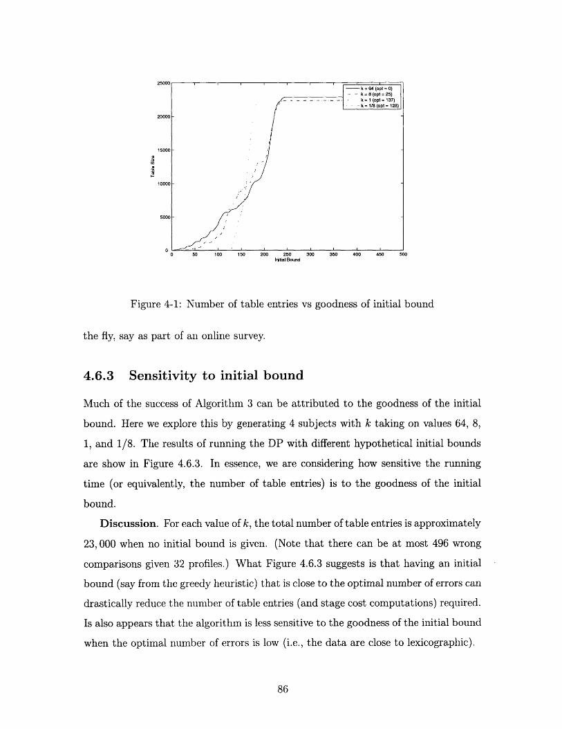
25000k = 64 (opt = 0)
- k = 8 (opt=25)k = 1 (opt = 137)
. k= 1/8 (opt=128)
20000
15000 .
10000
5000
0 50 100 150 200 250 300 350 400 450 500Initial Bound
Figure 4-1: Number of table entries vs goodness of initial bound
the fly, say as part of an online survey.
4.6.3 Sensitivity to initial bound
Much of the success of Algorithm 3 can be attributed to the goodness of the initial
bound. Here we explore this by generating 4 subjects with k taking on values 64, 8,
1, and 1/8. The results of running the DP with different hypothetical initial bounds
are show in Figure 4.6.3. In essence, we are considering how sensitive the running
time (or equivalently, the number of table entries) is to the goodness of the initial
bound.
Discussion. For each value of k, the total number of table entries is approximately
23, 000 when no initial bound is given. (Note that there can be at most 496 wrong
comparisons given 32 profiles.) What Figure 4.6.3 suggests is that having an initial
bound (say from the greedy heuristic) that is close to the optimal number of errors can
drastically reduce the number of table entries (and stage cost computations) required.
Is also appears that the algorithm is less sensitive to the goodness of the initial bound
when the optimal number of errors is low (i.e., the data are close to lexicographic).
86
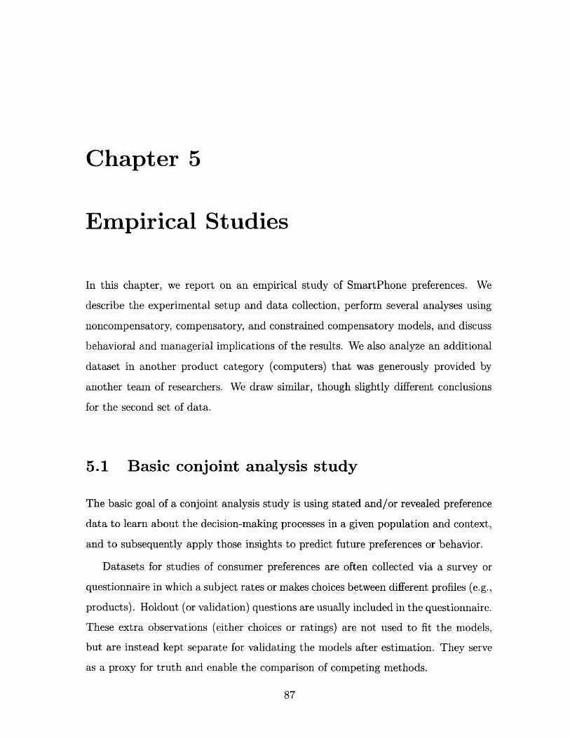
Chapter 5
Empirical Studies
In this chapter, we report on an empirical study of SmartPhone preferences. We
describe the experimental setup and data collection, perform several analyses using
noncompensatory, compensatory, and constrained compensatory models, and discuss
behavioral and managerial implications of the results. We also analyze an additional
dataset in another product category (computers) that was generously provided by
another team of researchers. We draw similar, though slightly different conclusions
for the second set of data.
5.1 Basic conjoint analysis study
The basic goal of a conjoint analysis study is using stated and/or revealed preference
data to learn about the decision-making processes in a given population and context,
and to subsequently apply those insights to predict future preferences or behavior.
Datasets for studies of consumer preferences are often collected via a survey or
questionnaire in which a subject rates or makes choices between different profiles (e.g.,
products). Holdout (or validation) questions are usually included in the questionnaire.
These extra observations (either choices or ratings) are not used to fit the models,
but are instead kept separate for validating the models after estimation. They serve
as a proxy for truth and enable the comparison of competing methods.
87
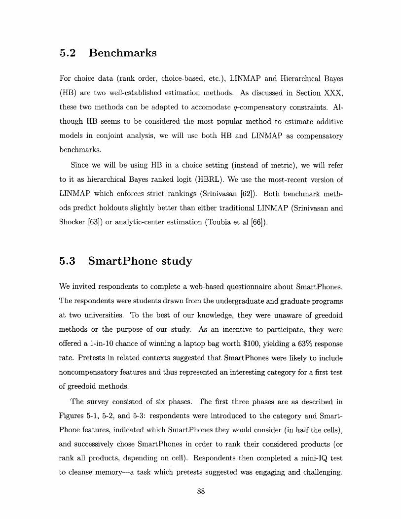
5.2 Benchmarks
For choice data (rank order, choice-based, etc.), LINMAP and Hierarchical Bayes
(HB) are two well-established estimation methods. As discussed in Section XXX,
these two methods can be adapted to accomodate q-compensatory constraints. Al-
though HB seems to be considered the most popular method to estimate additive
models in conjoint analysis, we will use both HB and LINMAP as compensatory
benchmarks.
Since we will be using HB in a choice setting (instead of metric), we will refer
to it as hierarchical Bayes ranked logit (HBRL). We use the most-recent version of
LINMAP which enforces strict rankings (Srinivasan [62]). Both benchmark meth-
ods predict holdouts slightly better than either traditional LINMAP (Srinivasan and
Shocker [63]) or analytic-center estimation (Toubia et al [66]).
5.3 SmartPhone study
We invited respondents to complete a web-based questionnaire about SmartPhones.
The respondents were students drawn from the undergraduate and graduate programs
at two universities. To the best of our knowledge, they were unaware of greedoid
methods or the purpose of our study. As an incentive to participate, they were
offered a 1-in-10 chance of winning a laptop bag worth $100, yielding a 63% response
rate. Pretests in related contexts suggested that SmartPhones were likely to include
noncompensatory features and thus represented an interesting category for a first test
of greedoid methods.
The survey consisted of six phases. The first three phases are as described in
Figures 5-1, 5-2, and 5-3: respondents were introduced to the category and Smart-
Phone features, indicated which SmartPhones they would consider (in half the cells),
and successively chose SmartPhones in order to rank their considered products (or
rank all products, depending on cell). Respondents then completed a mini-IQ test
to cleanse memory--a task which pretests suggested was engaging and challenging.
88
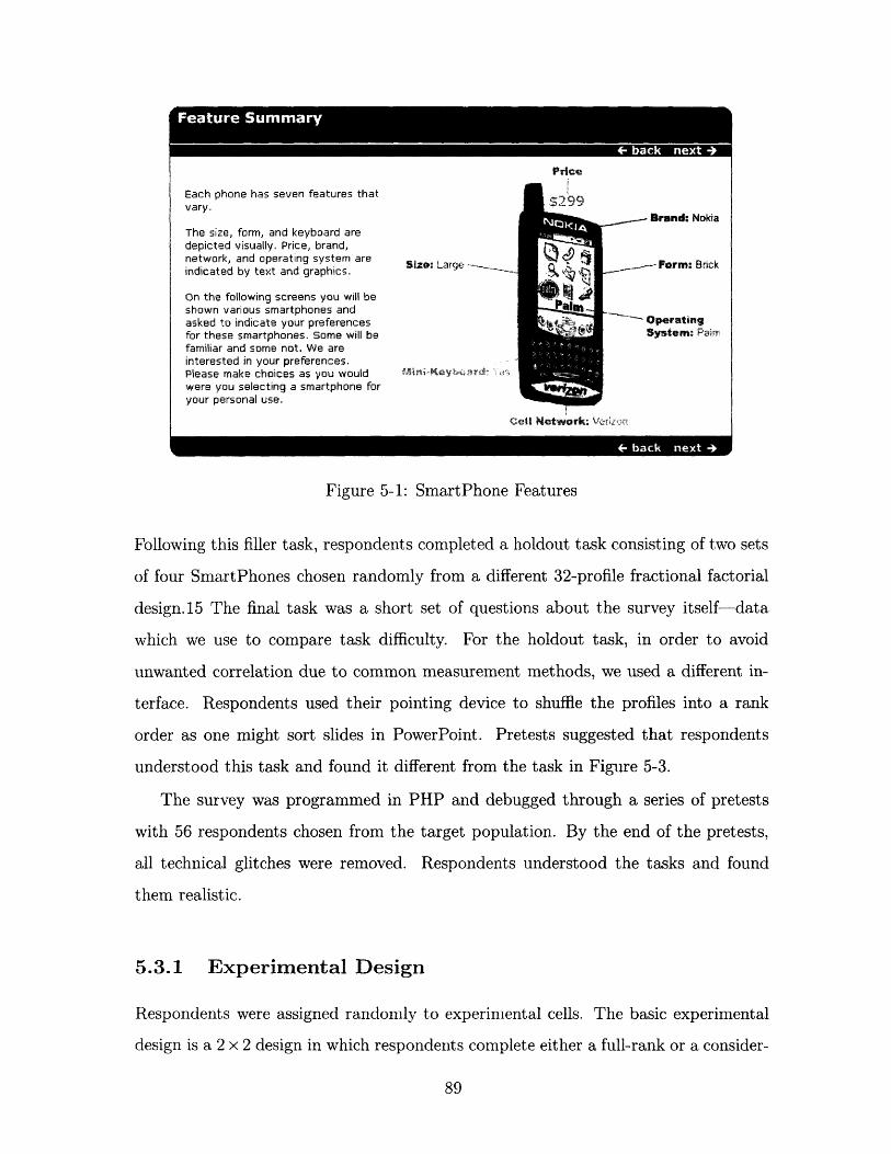
Each phone has seven features thatvary.
The size, form, and keyboard aredepicted visually. Price, brand,network, and operating system are Size: argeindicated by text and graphics.
On the following screens you will beshown various smartphones andasked to indicate your preferencesfor these smartphones. Some will befamiliar and some not. We areinterested in your preferences.Please make choices as you would M-NilKeyti,-r) & v ?,were you selecting a smartphone foryour personal use.
/__ Brand: Nokia
_ Form: Brick
* OperatingSystem: Pairn
Cell Network: Va½yz r.
Figure 5-1: SmartPhone Features
Following this filler task, respondents completed a holdout task consisting of two sets
of four SmartPhones chosen randomly from a different 32-profile fractional factorial
design.15 The final task was a short set of questions about the survey itself-data
which we use to compare task difficulty. For the holdout task, in order to avoid
unwanted correlation due to common measurement methods, we used a different in-
terface. Respondents used their pointing device to shuffle the profiles into a rank
order as one might sort slides in PowerPoint. Pretests suggested that respondents
understood this task and found it different from the task in Figure 5-3.
The survey was programmed in PHP and debugged through a series of pretests
with 56 respondents chosen from the target population. By the end of the pretests,
all technical glitches were removed. Respondents understood the tasks and found
them realistic.
5.3.1 Experimental Design
Respondents were assigned randomly to experimental cells. The basic experimental
design is a 2 x 2 design in which respondents complete either a full-rank or a consider-
89
Alan
____ ____ I~Ft~r~Si~
There are 32 smartphones shown below Please select those smatphones that you would consider purchasing for your own use.
As you click on a smartphone, a blue box wil appear Click on as many or as few as you would consider. When you are done, click NEXT, which is locatedat the bottom of the page
If you would like, you may sort the smartphones on up to three features Yo may also simply scroll through the smartphones to indicate those that youwould consider
.(miute 1). 3 hettibut~e.2). A| | (ettbute 3). 3 j
I EE1t99
S
i I ^~~Ii ~~~
$2%
Figure 5-2: SmartPhone Consideration Stage
A group of smatphones is shown below.
Please click on the smartphone that you are most likely to buy for your own use.
That smartphone wril disappear and you wil be asked for your next preference.
If you would like, you may sort the smartphones by up to three features
I(Wttibute 1) ,j ("tibute 2) - I (ribute 3) ,i2
$499 S99 499*~~~~1 God :_ : ,5f !!1 i 1; ; e!
3Cn
Figure 5-3: SmartPhone Ranking Stage
90
l
$99
4
I
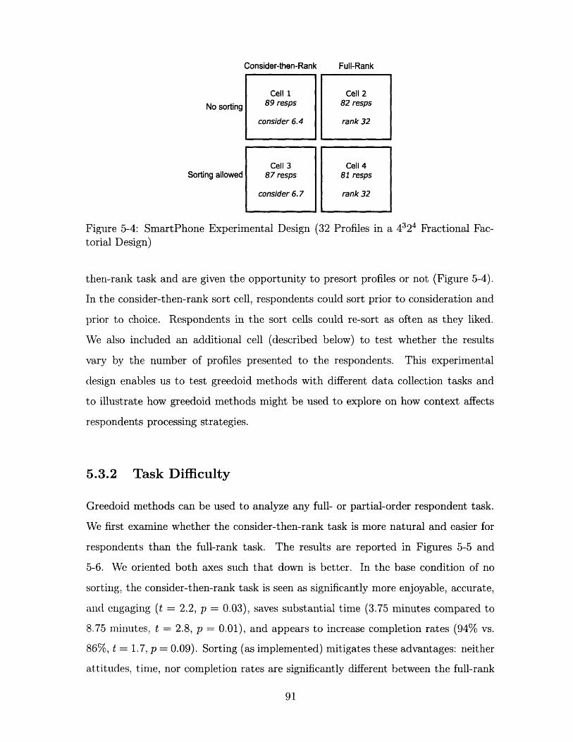
Consider-then-Rank Full-Rank
No sorting
Sorting allowed
Cell 1 Cell 289 resps 82 resps
consider 6.4 rank 32
Cell 3 Cell 487 resps 81 resps
consider 6.7 rank 32
Figure 5-4: SmartPhone Experimental Design (32 Profiles in a 4324 Fractional Fac-torial Design)
then-rank task and are given the opportunity to presort profiles or not (Figure 5-4).
In the consider-then-rank sort cell, respondents could sort prior to consideration and
prior to choice. Respondents in the sort cells could re-sort as often as they liked.
We also included an additional cell (described below) to test whether the results
vary by the number of profiles presented to the respondents. This experimental
design enables us to test greedoid methods with different data collection tasks and
to illustrate how greedoid methods might be used to explore on how context affects
respondents processing strategies.
5.3.2 Task Difficulty
Greedoid methods can be used to analyze any full- or partial-order respondent task.
We first examine whether the consider-then-rank task is more natural and easier for
respondents than the full-rank task. The results are reported in Figures 5-5 and
5-6. We oriented both axes such that down is better. In the base condition of no
sorting, the consider-then-rank task is seen as significantly more enjoyable, accurate,
an(l engaging (t = 2.2, p = 0.03), saves substantial time (3.75 minutes compared to
8.75 minutes, t = 2.8, p = 0.01), and appears to increase completion rates (94% vs.
86%, t = 1.7, p = 0.09). Sorting (as implemented) mitigates these advantages: neither
attitudes, time, nor completion rates are significantly different between the full-rank
91
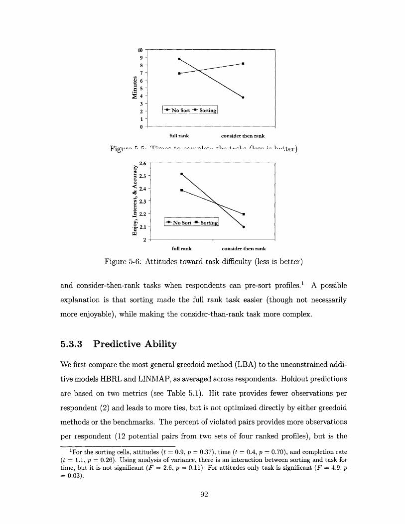
10 j9
7 -I
2 - N Sort _'No Sorti Soi1
full rank consider then rank
Fig - " " T: I i - a- - cter)
t2.6- I
: 2.5
U 2.4
2.3
a 2.2
. .21
2
full rank consider then rank
Figure 5-6: Attitudes toward task difficulty (less is better)
and consider-then-rank tasks when respondents can pre-sort profiles.1 A possible
explanation is that sorting made the full rank task easier (though not necessarily
more enjoyable), while making the consider-than-rank task more complex.
5.3.3 Predictive Ability
We first compare the most general greedoid method (LBA) to the unconstrained addi-
tive models HBRL and LINMAP, as averaged across respondents. Holdout predictions
are based on two metrics (see Table 5.1). Hit rate provides fewer observations per
respondent (2) and leads to more ties, but is not optimized directly by either greedoid
methods or the benchmarks. The percent of violated pairs provides more observations
per respondent (12 potential pairs from two sets of four ranked profiles), but is the
1For the sorting cells, attitudes (t = 0.9, p = 0.37), time (t = 0.4, p = 0.70), and completion rate(t = 1.1, p = 0.26). Using analysis of variance, there is an interaction between sorting and task fortime, but it is not significant (F = 2.6, p = 0.11). For attitudes only task is significant (F = 4.9, p= 0.03).
92
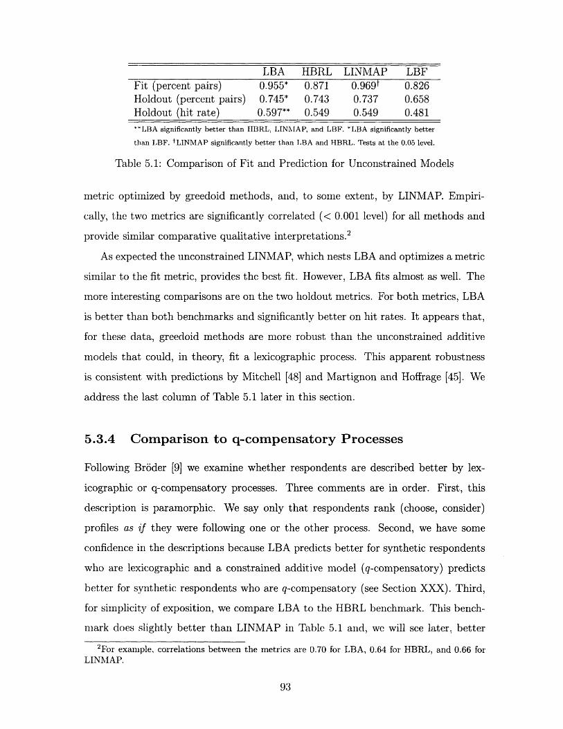
LBA HBRL LINMAP LBFFit (percent pairs) 0.955* 0.871 0.9 6 9 t 0.826Holdout (percent pairs) 0.745* 0.743 0.737 0.658Holdout (hit rate) 0.597** 0.549 0.549 0.481
**LBA significantly better than HBRL, LINMIAP, and LBF. *LBA significantly better
than LBF. tLINMAP significantly better than LBA and HBRL. Tests at the 0.05 level.
Table 5.1: Comparison of Fit and Prediction for Unconstrained Models
metric optimized by greedoid methods, and, to some extent, by LINMAP. Empiri-
cally, the two metrics are significantly correlated (< 0.001 level) for all methods and
provide similar comparative qualitative interpretations. 2
As expected the unconstrained LINMAP, which nests LBA and optimizes a metric
similar to the fit metric, provides the best fit. However, LBA fits almost as well. The
more interesting comparisons are on the two holdout metrics. For both metrics, LBA
is better than both benchmarks and significantly better on hit rates. It appears that,
for these data, greedoid methods are more robust than the unconstrained additive
models that could, in theory, fit a lexicographic process. This apparent robustness
is consistent with predictions by Mitchell [48] and Martignon and Hoffrage [45]. We
address the last column of Table 5.1 later in this section.
5.3.4 Comparison to q-compensatory Processes
Following Brdder [9] we examine whether respondents are described better by lex-
icographic or q-compensatory processes. Three comments are in order. First, this
description is paramorphic. We say only that respondents rank (choose, consider)
profiles as if they were following one or the other process. Second, we have some
confidence in the descriptions because LBA predicts better for synthetic respondents
who are lexicographic and a constrained additive model (q-compensatory) predicts
better for synthetic respondents who are q-compensatory (see Section XXX). Third,
for simplicity of exposition, we compare LBA to the HBRL benchmark. This bench-
mark does slightly better than LINMAP in Table 5.1 and, we will see later, better
2For example, correlations between the metrics are 0.70 for LBA, 0.64 for HBRL, and 0.66 forLINIAP.
93
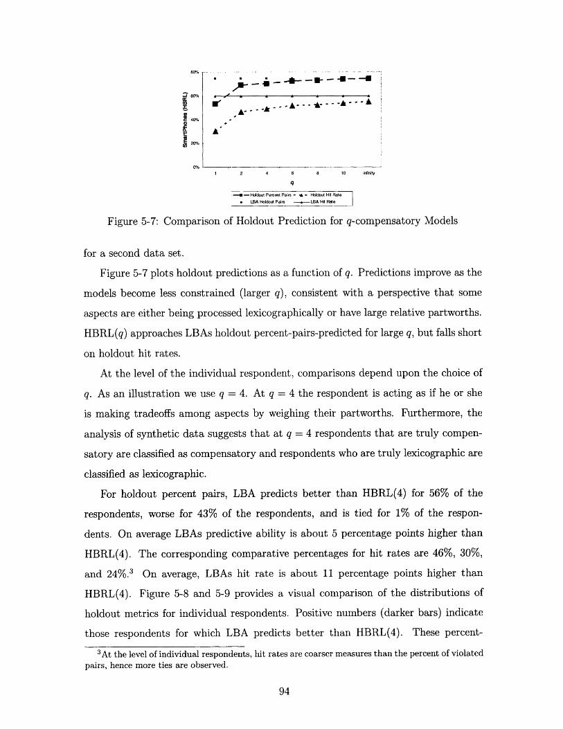
j 60%
m
r 401/0
E 20%
0T/
.,_ _ ; /.i_. ,,"-"",-' .. ..... ...
r- * - - -
A
1 2 4 6 8 10 infinity
q
- Holdout Percent Pairs - - Holdout Hit RateJ LBA Holdout Pairs LBA Hit Rate
Figure 5-7: Comparison of Holdout Prediction for q-compensatory Models
for a second data set.
Figure 5-7 plots holdout predictions as a function of q. Predictions improve as the
models become less constrained (larger q), consistent with a perspective that some
aspects are either being processed lexicographically or have large relative partworths.
HBRL(q) approaches LBAs holdout percent-pairs-predicted for large q, but falls short
on holdout hit rates.
At the level of the individual respondent, comparisons depend upon the choice of
q. As an illustration we use q = 4. At q = 4 the respondent is acting as if he or she
is making tradeoffs among aspects by weighing their partworths. Furthermore, the
analysis of synthetic data suggests that at q = 4 respondents that are truly compen-
satory are classified as compensatory and respondents who are truly lexicographic are
classified as lexicographic.
For holdout percent pairs, LBA predicts better than HBRL(4) for 56% of the
respondents, worse for 43% of the respondents, and is tied for 1% of the respon-
dents. On average LBAs predictive ability is about 5 percentage points higher than
HBRL(4). The corresponding comparative percentages for hit rates are 46%, 30%,
and 24%.3 On average, LBAs hit rate is about 11 percentage points higher than
HBRL(4). Figure 5-8 and 5-9 provides a visual comparison of the distributions of
holdout metrics for individual respondents. Positive numbers (darker bars) indicate
those respondents for which LBA predicts better than HBRL(4). These percent-
3 At the level of individual respondents, hit rates are coarser measures than the percent of violatedpairs, hence more ties are observed.
94
O^DE. .... .. ....... .......... .......
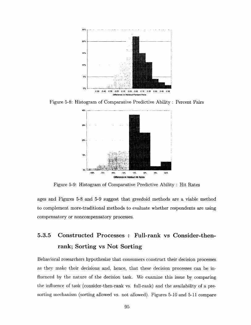
20%
15%
10%
5% -
0%
-055 -0.45 -0.35 -0.25 -0.15 -005 0.05 015 025 035 045 055
Difference In Holdout Percent Pairs
Figure 5-8: Histogram of Comparative Predictive Ability._..
: Percent Pairs
305
201
1l%
-100% -75%
Figure 5-9: Histogram of
-45% -155% 15% 450%z 75%0
Difference in Holdout Hit Rates
Comparative Predictive Ability : Hit Rates
ages and Figures 5-8 and 5-9 suggest that greedoid methods are a viable method
to complement more-traditional methods to evaluate whether respondents are using
compensatory or noncompensatory processes.
5.3.5 Constructed Processes : Full-rank vs Consider-then-
rank; Sorting vs Not Sorting
Behavioral researchers hypothesize that consumers construct their decision processes
as they make their decisions and, hence, that these decision processes can be in-
fluenced by the nature of the decision task. We examine this issue by comparing
the influence of task (consider-then-rank vs. fuill-rank) and the availability of a pre-
sorting mechanism (sorting allowed vs. not allowed). Figures 5-10 and 5-11 compare
95
j
r.
" i-.·,·l.: :·*-- "�..�·
:I:�· :�r:�-·
,...Z01 o .. ... I.. ... .. .. .' ... .. ....I .. .. ... .. .. .. .. .. . . ... .. . ... .. ...
_ . _ . .
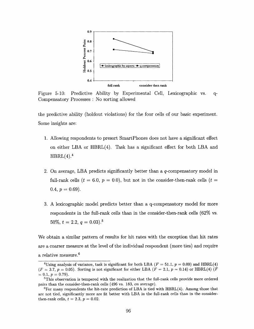
U.
.i 0.8
a 0.7 -
5 0.6 -
0oo 0.5 -
0.4
full rank consider then rank
Figure 5-10: Predictive Ability by Experimental Cell, Lexicographic vs. q-Compensatory Processes : No sorting allowed
the predictive ability (holdout violations) for the four cells of our basic experiment.
Some insights are:
1. Allowing respondents to presort SmartPhones does not have a significant effect
on either LBA or HBRL(4). Task has a significant effect for both LBA and
HBRL(4). 4
2. On average, LBA predicts significantly better than a q-compensatory model in
full-rank cells (t = 6.0, p = 0.0), but not in the consider-then-rank cells (t =
0.4, p = 0.69).
3. A lexicographic model predicts better than a q-compensatory model for more
respondents in the full-rank cells than in the consider-then-rank cells (62% vs.
50%, t = 2.2, q = 0.03). 5
We obtain a similar pattern of results for hit rates with the exception that hit rates
are a coarser measure at the level of the individual respondent (more ties) and require
a relative measure. 6
4Using analysis of variance, task is significant for both LBA (F = 51.1, p = 0.00) and HBRL(4)(F = 3.7, p = 0.05). Sorting is not significant for either LBA (F = 2.1, p = 0.14) or HBRL(4) (F= 0.1, p = 0.79).
5This observation is tempered with the realization that the full-rank cells provide more orderedpairs than the consider-then-rank cells (496 vs. 183, on average).
6 For many respondents the hit-rate prediction of LBA is tied with HBRL(4). Among those thatare not tied, significantly more are fit better with LBA in the full-rank cells than in the consider-then-rank cells, t = 2.3, p = 0.02.
96
|- -lexicographic by aspects -q-compensatory
. .~~~~~~~~~~~~~~~~~~~~~~
nn
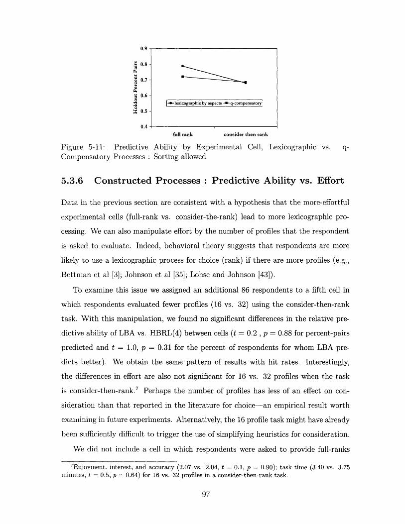
0.9
.. 0.8
P 0.7
U 0.61o0
o.sZ 0.5
0.4
full rank consider then rank
Figure 5-11: Predictive Ability by Experimental Cell, Lexicographic vs. q-Compensatory Processes: Sorting allowed
5.3.6 Constructed Processes: Predictive Ability vs. Effort
Data in the previous section are consistent with a hypothesis that the more-effortful
experimental cells (full-rank vs. consider-the-rank) lead to more lexicographic pro-
cessing. We can also manipulate effort by the number of profiles that the respondent
is asked to evaluate. Indeed, behavioral theory suggests that respondents are more
likely to use a lexicographic process for choice (rank) if there are more profiles (e.g.,
Bettmnan et al [3]; Johnson et al [35]; Lohse and Johnson [43]).
To examine this issue we assigned an additional 86 respondents to a fifth cell in
which respondents evaluated fewer profiles (16 vs. 32) using the consider-then-rank
task. With this manipulation, we found no significant differences in the relative pre-
dictive ability of LBA vs. HBRL(4) between cells (t = 0.2 , p = 0.88 for percent-pairs
predicted and t = 1.0, p = 0.31 for the percent of respondents for whom LBA pre-
dicts better). We obtain the same pattern of results with hit rates. Interestingly,
the differences in effort are also not significant for 16 vs. 32 profiles when the task
is consider-then-rank. 7 Perhaps the number of profiles has less of an effect on con-
sideration than that reported in the literature for choice--an empirical result worth
examining in future experiments. Alternatively, the 16 profile task might have already
been sufficiently difficult to trigger the use of simplifying heuristics for consideration.
We did not include a cell in which respondents were asked to provide full-ranks
7Enjoyment;. interest, and accuracy (2.07 vs. 2.04, t = 0.1, p = 0.90); task time (3.40 vs. 3.75minutes, t = 0.5, p = 0.64) for 16 vs. 32 profiles in a consider-then-rank task.
97
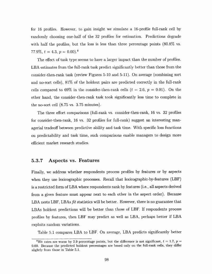
for 16 profiles. However, to gain insight we simulate a 16-profile full-rank cell by
randomly choosing one-half of the 32 profiles for estimation. Predictions degrade
with half the profiles, but the loss is less than three percentage points (80.8% vs.
77.9%, t = 4.3, p = 0.00).8
The effect of task type seems to have a larger impact than the number of profiles.
LBA estimates from the full-rank task predict significantly better than those from the
consider-then-rank task (review Figures 5-10 and 5-11). On average (combining sort
and no-sort cells), 81% of the holdout pairs are predicted correctly in the full-rank
cells compared to 69% in the consider-then-rank cells (t = 2.6, p = 0.01). On the
other hand, the consider-then-rank task took significantly less time to complete in
the no-sort cell (8.75 vs. 3.75 minutes).
The three effort comparisons (full-rank vs. consider-then-rank, 16 vs. 32 profiles
for consider-then-rank, 16 vs. 32 profiles for full-rank) suggest an interesting man-
agerial tradeoff between predictive ability and task time. With specific loss functions
on predictability and task time, such comparisons enable managers to design more
efficient market research studies.
5.3.7 Aspects vs. Features
Finally, we address whether respondents process profiles by features or by aspects
when they use lexicographic processes. Recall that lexicographic-by-features (LBF)
is a restricted form of LBA where respondents rank by features (i.e., all aspects derived
from a given feature must appear next to each other in the aspect order). Because
LBA nests LBF, LBAs fit statistics will be better. However, there is no guarantee that
LBAs holdout predictions will be better than those of LBF. If respondents process
profiles by features, then LBF may predict as well as LBA, perhaps better if LBA
exploits random variations.
Table 5.1 compares LBA to LBF. On average, LBA predicts significantly better
8Hit rates are worse by 2.9 percentage points, but the difference is not significant, t = 1.7, p =0.00. Because the predicted holdout percentages are based only on the full-rank cells, they differslightly from those in Table 5.1.
98
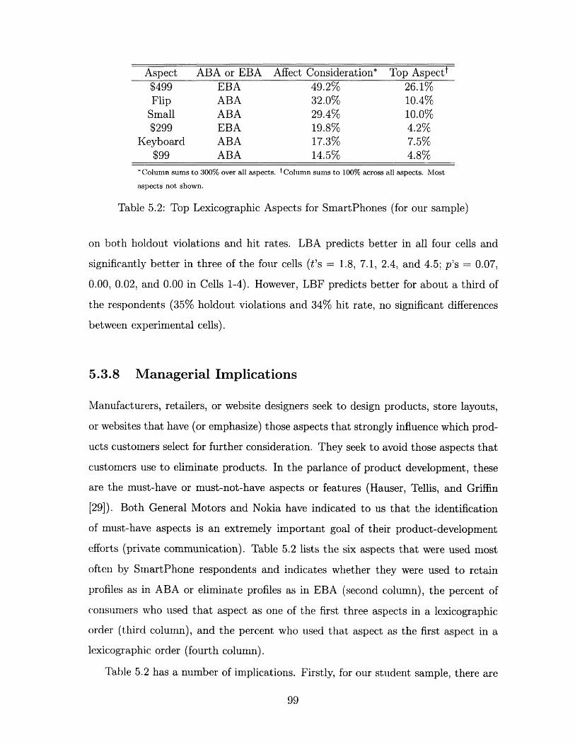
Aspect ABA or EBA Affect Consideration* Top Aspectt$499 EBA 49.2% 26.1%Flip ABA 32.0% 10.4%
Small ABA 29.4% 10.0%$299 EBA 19.8% 4.2%
Keyboard ABA 17.3% 7.5%$99 ABA 14.5% 4.8%
Column sums to 300% over all aspects. tColumn sums to 100% across all aspects. Most
aspects not shown.
Table 5.2: Top Lexicographic Aspects for SmartPhones (for our sample)
on both holdout violations and hit rates. LBA predicts better in all four cells and
significantly better in three of the four cells (t's = 1.8, 7.1, 2.4, and 4.5; p's = 0.07,
0.00, 0.02, and 0.00 in Cells 1-4). However, LBF predicts better for about a third of
the respondents (35% holdout violations and 34% hit rate, no significant differences
between experimental cells).
5.3.8 Managerial Implications
Manufacturers, retailers, or website designers seek to design products, store layouts,
or websites that have (or emphasize) those aspects that strongly influence which prod-
ucts customers select for further consideration. They seek to avoid those aspects that
customers use to eliminate products. In the parlance of product development, these
are the must-have or must-not-have aspects or features (Hauser, Tellis, and Griffin
[29]). Both General Motors and Nokia have indicated to us that the identification
of must-have aspects is an extremely important goal of their product-development
efforts (private communication). Table 5.2 lists the six aspects that were used most
often by SmartPhone respondents and indicates whether they were used to retain
profiles as in ABA or eliminate profiles as in EBA (second column), the percent of
consumers who used that aspect as one of the first three aspects in a lexicographic
order (third column), and the percent who used that aspect as the first aspect in a
lexicographic order (fourth column).
Table 5.2 has a number of implications. Firstly, for our student sample, there are
99
clear price segments for almost half the sample high-price is an elimination aspect.
Secondly, flip and small are each acceptance aspects for about 30% of the respondents.
For this sample, any manufacturer would lose considerable market share if it did not
include SmartPhones that were small and flip. The keyboard aspect is interesting.
Keyboard is an acceptance aspect for 17.3% of the respondents and an elimination
aspect for 7.5% of the respondents (not shown). On this aspect, a manufacturer
would be best advised to offer both SmartPhones with keyboards and SmartPhones
without keyboards. Finally, brand, service provider, and operating system are not
high in the lexicographic ordering.
It is interesting that, in our data, price aspects were often, but not always, elimina-
tion aspects, while all other aspects were acceptance aspects. (This is true for aspects
not shown in Table 5.2.) We do not know if this generalizes to other categories. Fur-
thermore, although high-price was the top lexicographic aspect in our study, this may
be a consequence of the category or our student sample. We do not expect price to
be the top lexicographic aspect in all categories nor do we feel that this result af-
fected the basic scientific and methodological findings about lexicographic processing
or predictive ability.
5.4 Computers from study by Lenk et al [42]
We were fortunate to obtain a classic conjoint-analysis data set in which respondents
evaluated full profiles of computers that varied on thirteen binary features: telephone
service hot line, amount of memory, screen size, CPU speed, hard disk size, CD
ROM, cache, color, availability, warranty, bundled software, guarantee, and price.
Respondents were presented with 16 full profiles and asked to provide a rating on a
10-point likelihood-of-purchase scale. They were then given a holdout task in which
they evaluated four additional profiles on the same scale. These data were collected
and analyzed by Lenk et al [42], who suggest excellent fit and predictive ability with
hierarchical Bayes compensatory models. Based on their analysis and our intuition,
we felt that the features in this study were more likely to be compensatory than those
100
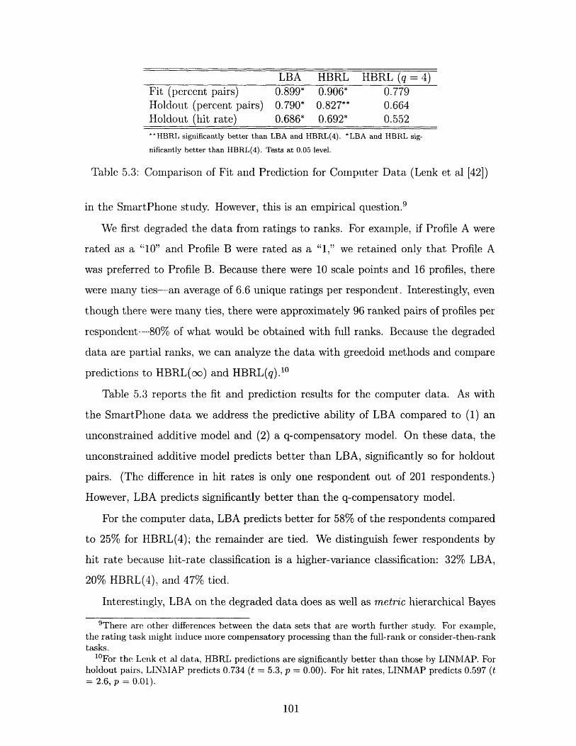
LBA HBRL HBRL (q = 4)Fit (percent pairs) 0.899* 0.906* 0.779Holdout (percent pairs) 0.790* 0.827** 0.664Holdout (hit rate) 0.686* 0.692* 0.552
**HBRI, significantly better than LBA and HBRL(4). *LBA and HBRL sig-
nificantly better than HBRL(4). Tests at 0.05 level.
Table 5.3: Comparison of Fit and Prediction for Computer Data (Lenk et al [42])
in the SmartPhone study. However, this is an empirical question. 9
We first degraded the data from ratings to ranks. For example, if Profile A were
rated as a "10" and Profile B were rated as a "1," we retained only that Profile A
was preferred to Profile B. Because there were 10 scale points and 16 profiles, there
were many ties-an average of 6.6 unique ratings per respondent. Interestingly, even
though there were many ties, there were approximately 96 ranked pairs of profiles per
respondent ---80% of what would be obtained with full ranks. Because the degraded
data are partial ranks, we can analyze the data with greedoid methods and compare
predictions to HBRL(oo) and HBRL(q). l °
Table 5.3 reports the fit and prediction results for the computer data. As with
the SmartPhone data we address the predictive ability of LBA compared to (1) an
unconstrained additive model and (2) a q-compensatory model. On these data, the
unconstrained additive model predicts better than LBA, significantly so for holdout
pairs. (The difference in hit rates is only one respondent out of 201 respondents.)
However, LBA predicts significantly better than the q-compensatory model.
For the computer data, LBA predicts better for 58% of the respondents compared
to 25% for HIBRL(4); the remainder are tied. We distinguish fewer respondents by
hit rate because hit-rate classification is a higher-variance classification: 32% LBA,
20% HBRL(4), and 47% tied.
Interestingly, LBA on the degraded data does as well as metric hierarchical Bayes
9 There are other differences between the data sets that are worth further study. For example,the rating task might induce more compensatory processing than the full-rank or consider-then-ranktasks.
10For the Leuk et al data, HBRL predictions are significantly better than those by LINMAP. Forholdout pairs, LINMAP predicts 0.734 (t = 5.3, p = 0.00). For hit rates, LINMAP predicts 0.597 (t= 2.6, p = 0.01).
101
on the ratings data (0.687, Lenk et al [42, p. 181]) and better than either OLS
(0.637, ibid.) and latent class analysis (0.408, ibid.).ll In this case, a reduction in
effort (ranking vs. rating) may have had little effect on predictive ability. For a
further discussion of ranking vs. rating data, see Huber et al [31].
Table 5.3 is consistent with the analysis of metric data by Kohli and Jedidi [39]
who found that a different lexicographic model (binary satisficing, LBS) fit almost as
well as an unconstrained additive model (0.93 fit pairs for LBS vs. 0.95 for classic
LINMAP; no data available on holdouts). The Kohli-Jedidi context is remarkably
similar to that of Lenk et al: metric ratings of 16 laptop computers described by
memory, brand, CPU speed, hard drive size, and price (in a 3322 fractional design).
Comparing the SmartPhone and computer data, we get surprisingly similar respondent-
level comparisons. LBA predicts at least as well as HBRL(4) for 57% of the Smart-
Phone respondents and 75% of the computer respondents. 12 Kohli and Jedidi [39] did
not test a q-compensatory model, but they did find that an unconstrained additive
model was not significantly different from LBS for 67% of their respondents. Thus, on
all data sets, for more than half of the respondents, noncompensatory models predict
holdout data at least as well as q-compensatory models.
We can also compare the predictive ability of LBA to an unconstrained additive
model. LBA predicts at least as well as HBRL for 49% of the SmartPhone respondents
and 62% of the computer respondents. Thus, even compared to an unconstrained
additive model, LBA is promising as a predictive tool.
1"We compare to the highest hit rate they report that for HB estimated with 12 profiles. For16 profiles they report a hit rate of 0.670. For other statistics, HB with 16 profiles performs betterthan with 12 profiles (ibid, p. 181).
12The corresponding percentages for hit rates are 71% and 80%.
102
Chapter 6
Rule-based consideration
In this chapter, we approach consideration set formation from a rule-based perspec-
tive, which can be viewed as a nonlinear generalization of lexicography. Given a
subject's consideration set, we are interested in finding the best set of rules (consist-
ing of logical expressions) that explain the data while meeting a complexity measure
budget constraint. Applying the technique to real data shows that it performs well
compared to a compensatory model of consideration set formation, while being the
simpler both in terms of complexity and explanation.
6.0.1 Related Work
Roberts and Lattin [55] give an overview of research in consideration. Mehta et al
[47] analyze consideration set formation in the context of the cost of information
search. They apply the method of simulated moments to estimate the parameters in
a random-utility model. Gensch and Soofi [19] use an information-theoretic approach
(involving maximizing entropy). Gilbride and Allenby [24] estimate screening rules
in Bayesian framework using MCMC methods. Other have also tried to estimate
elimination rules as part of the overall choice process (DeSarbo et al. [13], Jedidi and
Kohli [32], Jedidi et al. [33], Kim [37], Roberts and Lattin [54], and Swait [65]).
Because consideration set formation can be formulated as a binary classification
problem (with considered and not considered classes), existing classification algo-
103
rithims from the pattern recognition / machine learning fields can be applied. Stan-
dard techniques include logistic regression, decision trees, neural networks (NNs), and
support vector machines (SVMs). Certain techniques are more discrete in nature and
hence more relevant to the current discussion.
Consideration set formation problem bears a strong resemblance to the concept
learning task found in machine learning (see Mitchell [48]). In concept learning, which
can be viewed as a special case of classification in general, a boolean-valued function
is inferred from training examples. Early concept learning algorithms were extremely
sensitive to errors in the training data, while later enhancements improved robustness.
Decision trees (e.g., the classification and regression trees (CART) of Breiman et
al [8]) can also be viewed as rule-based. In each node of a decision tree, a question is
asked and the next decision (e.g., branch left or right) depends on the answer. Once
the path through the tree reaches a leaf node, the classification decision corresponding
to that leaf is applied. Each path from the root to a leaf corresponding to class k
can be expressed as a conjunction of conditions, e.g., "If condition A and condition
B and condition C, then assign class k". Furthermore, the collection of all paths
from the root to leaf nodes associated with class k can be viewed as a disjunction of
conjunctions (of conditions). In this chapter, we will be focusing on this natural form
of decision rule.
The main inspiration for our approach comes from a machine learning technique
called the Logical Analysis of Data (LAD) developed by Peter Hammer and others
(see Boros et al [6]). In LAD, logical rules (boolean expressions) are inferred from
training data in order to approximate a boolean function. The main steps are:
1. Generate short positive and negative patterns from the training data.
2. Prune the patterns to form a minimal cover of the training data.
3. Determine weights for the patterns to form an overall/final decision rule.
The overall goal is to discover short logical patterns in the training set that hopefully
generalize well to previously unseen observations. When applied to several standard
104
datasets froml the UCI repository, Boros et al [6] report strong performance compared
to other top methods. In particular, their single method applied well across many
different problems.
Our formulation and algorithms bear a strong resemblance to those in LAD, al-
though adapted and extended for the context of individual choice. Specific differences
include:
* Individual level estimation
* Different handling of errors
* Sparseness of data
* Asymmetric accept/reject
These differences require special treatment in our consideration set context.
6.1 Rule-based Model
6.1.1 Notation
As a convention, we will generally use lower case letters for aspects and upper case
letters for profiles (which are sets of aspects). We will let C+ denote the consideration
set and C- represent the set of profiles not considered.
6.1.2 Rule Format
Drawing on decision tree theory, we consider rules that are unions of intersections of
variables (aspects), e.g.,
(a A b) V (c A-d A e) V () (6.1)
We call each intersection expression a pattern (after LAD), and refer to the whole
expression (disjuction of conjunctions) as a rule (or consideration rule). We call
105

patterns derived from (or associated with) profiles in C+ positive patterns and those
from profiles in C- negative patterns.
For the rule above, a profile would be said to match it if the profile contained
aspects a and b, and/or contained aspects c and e but not d, and/or did not contain
aspect f. In other words, a rule matches a profile if at least one of its constituent
patterns matches that profile.
6.1.3 Decision Rules
There are several possible ways a decision rule can be constructed and used. An
acceptance rule consists of a set of positive patterns and is applied in the following
way: if a profile matches one or more positive patterns, consider it; else do not
consider it (the default decision). Conversely, a rejection rule consists of a set of
negative patterns and has the following interpretation: if a profile matches one or
more negative patterns, do not consider it; else consider it (the default decision).
It is an open question as to whether consumers are more likely to use rejection
or acceptance rules. Elimination-by-aspects (EBA), one of the early choice heuristic
formulations, focused on rejection in the context of choice. The SmartPhone study
described in Chapter 5 found that the behavior of respondents in the sample were
more consistent with a mixed LBA model than with strict ABA or EBA.
It should be noted that in LAD, both positive and negative patterns are combined
(along with weights) into a final decision rule or discriminant function. In essence,
each pattern participates in a weighted vote. While this approach is also possible
here, it makes the interpretation of the overall rule more difficult and (in our view)
less likely to represent how consumers form consideration sets in practice.
6.1.4 Rule Complexity
Note that any training set (consideration set) can be modeled exactly using this rule-
based formulation. Specifically, we can construct one pattern per profile where the
pattern's positive and negative variables are determined exactly by the presence or
106
absence of the corresponding aspects in the profile. Such a decision rule is essentially
saying. "If the profile is one of the considered profiles already seen, consider it." While
this rule achieves perfect performance on the training set, it will likely do poorly on
a previously unseen test set. Thus we would like to enforce some regularization on
the form or size of the rules in order to improve the chances of good generalization to
unseen observations. (See Hastie et al [27] for a discussion of complexity/smoothing
parameters and their effect on the bias-variance tradeoff (and test/generalization
error) .)
As a first pass, we use the total number of aspects across all patterns in a rule
as a measure of rule complexity. For example, the rule (6.1) above would have a
complexity of 6. An important variation on this theme is counting the total number
of symbols as opposed to simply aspects, and possibly assigning weights to symbols
based on the amount of mental processing power required to carry out the various
operations. This variation ties in nicely with the effort-accuracy tradeoff perspective
developed in Payne et al [52].
6.1.5 Measure of Goodness
Given a cap on the allowed complexity, how do we decide which of a given number
of rules is the best? Standard approaches include symmetric and asymmetric loss
functions. In the following section, we use a symmetric loss function such that both
types of errors (i.e., incorrectly including a profile and incorrecting excluding a profile)
are tallied and counted equally.
6.2 Computational Complexity
Before discussing a method for find the best rule given a complexity budget (i.e.,
the rule that induces the least number of errors), we show that the problem is NP-
hard. First. we show that determining whether or not a perfect rule explaining the
consideration data exists is NP-complete.
107

Theorem 12 CONSIDERATION-CONSISTENCY is NP-complete.
Proof. We reduce CONSIDERATION CONSISTENCY to SET COVER. Suppose
we are given SET COVER instance with ground set S containing elements x, 2 ,
... , x, a collection D of subsets of S, D, D2, ... , Din, and ksc, the upper bound on
set cover size. We will construct an instance of CONSIDERATION CONSISTENCY
that can be used to solve the SET COVER problem.
Let aspect set A be {al, a2,... , an}, where aspect ai corresponds to subset Di. Let
profile set P be {P1, P2,..., Pm, Y1, Y2 ,... , Ym}, where profile Pi is associated with
Pi = {aj: xi C Dj},
and Yi are dummy profiles:
yi = {}
Finally, let C+ = {Pi}, C- = {Y/}, and kcc = ksc.
For example, the SET COVER instance
would become
First, suppose there exists a set cover D' with jD'j = k < ksc. Then a consistent
rule exists consisting of k patterns each with a single positive variable corresponding
108
CONSIDERATION CONSISTENCY
INSTANCE : Set of aspects A, set of profiles P. sets C+, C- C
P, set of (positive) patterns, scalar k
QUESTION : Is there a rule of complexity < k that induces no
errors with respect to C+ and C-?
D1 D2 D3 D4
X 1 1 0 1 0
x 2 0 1 0 0
X3 1 0 0 0
X4 0 0 1 1
I

to the subsets in D'. Because D' is a set cover, all xi are covered, which implies
that all Pi are "matched" and thus cause no errors with respect to C+. Therefore, if
CONSIDERATION CONSISTENCY returns "no", it means that no set cover of size
less than or equal to ksc exists.
Conversely, suppose CONSIDERATION CONSISTENCY returns "yes". First
note that each pattern must contain only positive variables. (If a pattern contained
a negative variable, then all Y would be "matched", causing m errors with respect to
C+ and C-.) Second, note that we can trim each multi-variable pattern down to a
single variable (say the first variable). The resulting rule will still be a consistent rule
because each shortened pattern is guaranteed to match at least as many profiles Pi as
it originally did (and still does not match any profiles Y). Finally, because all profiles
in C+ are matched by single-variable rules, it must be the case that the subsets Di
corresponding to the variables in the rules form a set cover in the original problem.
Since CONSIDERATION CONSISTENCY returns a "yes" if and only if the SET
COVER instance was a "yes" instance, CONSIDERATION CONSISTENCY is NP-
complete. W
We now show that the problem of finding the best consideration rule, i.e., the rule
that induces the least number of errors with respect to the data is NP-hard and not
in APX.
109
al a 2 a3 a 4
P. 1 0 1 0
P2 0 1 0 0P3 1 0 0 0P4 0 0 1 1Y1 o o o o
Y2 0 0 0 0y3 0 0 0 oY 4 O 0 0 O
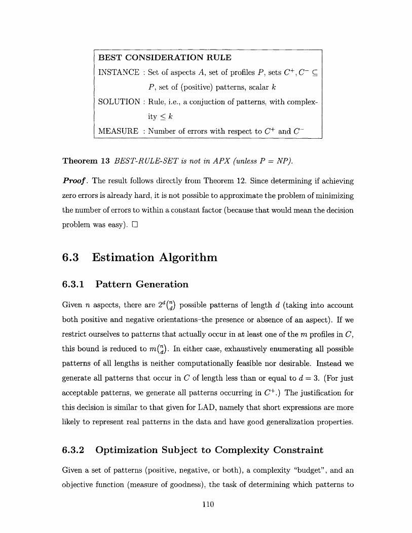
Theorem 13 BEST-RULE-SET is not in APX (unless P = NP).
Proof. The result follows directly from Theorem 12. Since determining if achieving
zero errors is already hard, it is not possible to approximate the problem of minimizing
the number of errors to within a constant factor (because that would mean the decision
problem was easy). O
6.3 Estimation Algorithm
6.3.1 Pattern Generation
Given n aspects, there are 2 d(n) possible patterns of length d (taking into account
both positive and negative orientations-the presence or absence of an aspect). If we
restrict ourselves to patterns that actually occur in at least one of the m profiles in C,
this bound is reduced to m (). In either case, exhaustively enumerating all possible
patterns of all lengths is neither computationally feasible nor desirable. Instead we
generate all patterns that occur in C of length less than or equal to d = 3. (For just
acceptable patterns, we generate all patterns occurring in C+.) The justification for
this decision is similar to that given for LAD, namely that short expressions are more
likely to represent real patterns in the data and have good generalization properties.
6.3.2 Optimization Subject to Complexity Constraint
Given a set of patterns (positive, negative, or both), a complexity "budget", and an
objective function (measure of goodness), the task of determining which patterns to
110
BEST CONSIDERATION RULE
INSTANCE : Set of aspects A, set of profiles P, sets C+, C- C
P, set of (positive) patterns, scalar k
SOLUTION : Rule, i.e., a conjuction of patterns, with complex-
ity < k
MEASURE : Number of errors with respect to C+ and C-
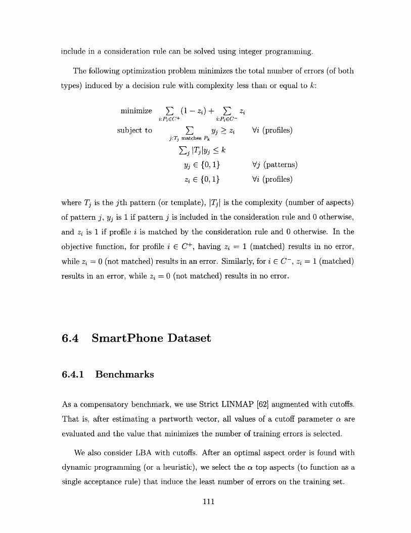
include in a consideration rule can be solved using integer programming.
The following optimization problem minimizes the total number of errors (of both
types) induced by a decision rule with complexity less than or equal to k:
minimize E (1 - zi) + i:PiCC'+ i:PiEC-
subject to E j > zij:Tj matches Pk
Ej ITjyj k
Yj C {, 1}
zi {O, 1}
Zi
Vi (profiles)
Vj (patterns)
Vi (profiles)
where Tj is the jth pattern (or template), ITjl is the complexity (number of aspects)
of pattern j, yj is 1 if pattern j is included in the consideration rule and 0 otherwise,
and zi is 1 if profile i is matched by the consideration rule and 0 otherwise. In the
objective function, for profile i E C+, having zi = 1 (matched) results in no error,
while zi = 0 (not matched) results in an error. Similarly, for i E C-, zi = I (matched)
results in an error, while zi = 0 (not matched) results in no error.
6.4 SmartPhone Dataset
6.4.1 Benchmarks
As a compensatory benchmark, we use Strict LINMAP [62] augmented with cutoffs.
That is, after estimating a partworth vector, all values of a cutoff parameter a are
evaluated and the value that minimizes the number of training errors is selected.
We also consider LBA with cutoffs. After an optimal aspect order is found with
dynamic programming (or a heuristic), we select the a top aspects (to function as a
single acceptance rule) that induce the least number of errors on the training set.
111
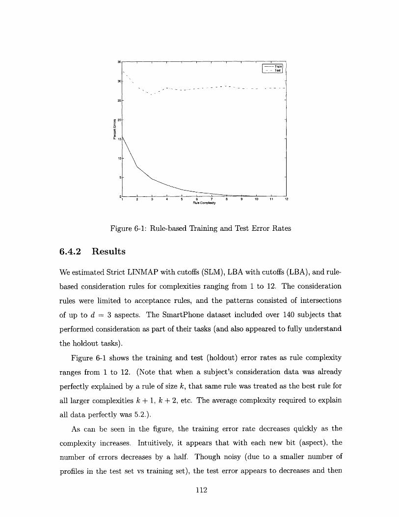
30
25
20
E
L 15
10
5
1 2 3 4 5 6 7 8 9 10 11 12Rule Complexity
Figure 6-1: Rule-based Training and Test Error Rates
6.4.2 Results
We estimated Strict LINMAP with cutoffs (SLM), LBA with cutoffs (LBA), and rule-
based consideration rules for complexities ranging from 1 to 12. The consideration
rules were limited to acceptance rules, and the patterns consisted of intersections
of up to d = 3 aspects. The SmartPhone dataset included over 140 subjects that
performed consideration as part of their tasks (and also appeared to fully understand
the holdout tasks).
Figure 6-1 shows the training and test (holdout) error rates as rule complexity
ranges from 1 to 12. (Note that when a subject's consideration data was already
perfectly explained by a rule of size k, that same rule was treated as the best rule for
all larger complexities k + 1, k + 2, etc. The average complexity required to explain
all data perfectly was 5.2.).
As can be seen in the figure, the training error rate decreases quickly as the
complexity increases. Intuitively, it appears that with each new bit (aspect), the
number of errors decreases by a half. Though noisy (due to a smaller number of
profiles in the test set vs training set), the test error appears to decreases and then
112
�CZ)J I I I I I I I I . -
I T..t
`` ~ ~ II _
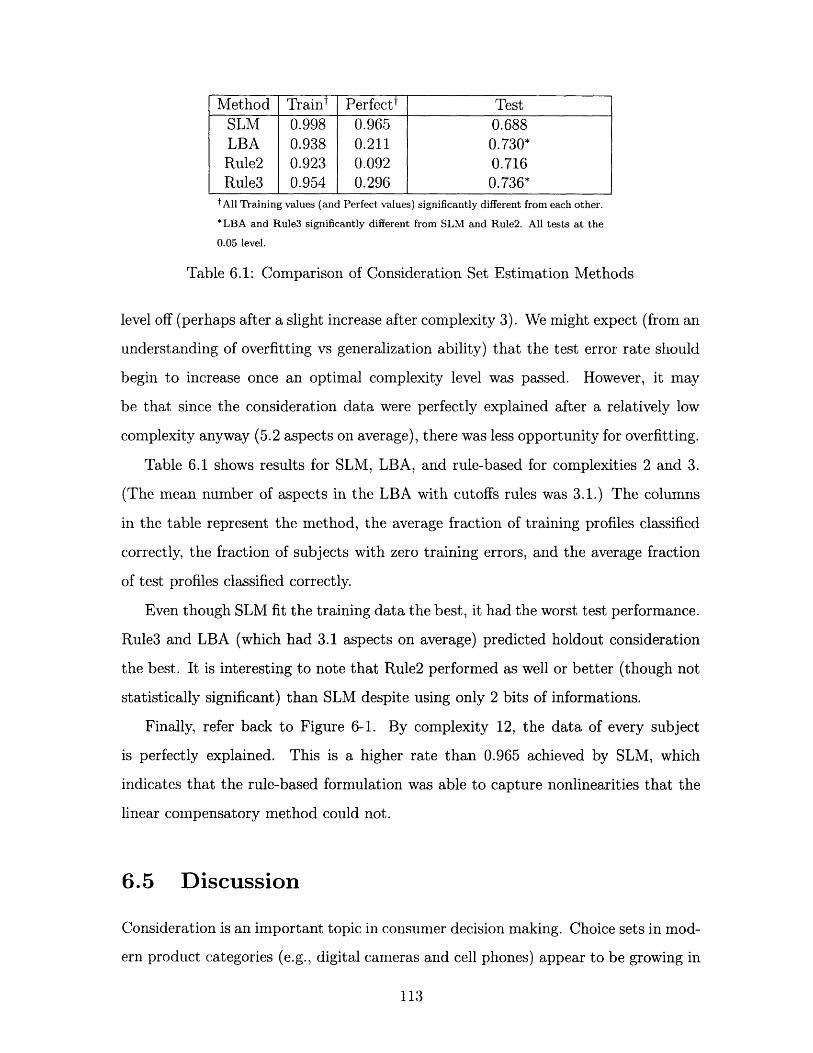
Method Train t Perfect t TestSLM 0.998 0.965 0.688LBA 0.938 0.211 0.730*Rule2 0.923 0.092 0.716Rule3 0.954 0.296 0.736*
tAll Training values (and Perfect values) significantly different from each other.
*LBA and Rule3 significantly different from SLM and Rule2. All tests at the
0.05 level.
Table 6.1: Comparison of Consideration Set Estimation Methods
level off (perhaps after a slight increase after complexity 3). We might expect (from an
understanding of overfitting vs generalization ability) that the test error rate should
begin to increase once an optimal complexity level was passed. However, it may
be that since the consideration data were perfectly explained after a relatively low
complexity anyway (5.2 aspects on average), there was less opportunity for overfitting.
Table 6.1 shows results for SLM, LBA, and rule-based for complexities 2 and 3.
(The mean number of aspects in the LBA with cutoffs rules was 3.1.) The columns
in the table represent the method, the average fraction of training profiles classified
correctly, the fraction of subjects with zero training errors, and the average fraction
of test profiles classified correctly.
Even though SLM fit the training data the best, it had the worst test performance.
Rule3 and LBA (which had 3.1 aspects on average) predicted holdout consideration
the best. It is interesting to note that Rule2 performed as well or better (though not
statistically significant) than SLM despite using only 2 bits of informations.
Finally, refer back to Figure 6-1. By complexity 12, the data of every subject
is perfectly explained. This is a higher rate than 0.965 achieved by SLM, which
indicates that the rule-based formulation was able to capture nonlinearities that the
linear compensatory method could not.
6.5 Discussion
Consideration is an important topic in consumer decision making. Choice sets in mod-
ern product categories (e.g., digital cameras and cell phones) appear to be growing in
113
both size and complexity, and most consumers need to use some sort of simplification
to wade through them. Thus, analyzing consideration-then-choice is important for
understanding decision behavior.
We have proposed a technique for estimating consideration rules built up from
short logical expressions. Using integer programming, we were able to choose the
best patterns to include in a rule given a complexity constraint (budget). When
applied to the SmartPhone dataset, the rule-based approach outperformed a more
complex compensatory approach.
There are several possible reasons for the success of the simpler model. Using
concepts from machine learning, it could be that the simpler model was more robust
in the face of error. Even though the linear compensatory approach could model most
consideration behavior perfectly, having so much freedom in choosing the continuous
weights might have allowed it to fit the noise or error in the training data. Another
possible explanation is that the rule-based approach allows for nonlinear relationships
(e.g., interactions between aspects) to be modeled. However, the benefit from this
might have been slight for this dataset considering LBA performed on par with rules
of complexity 3.
114
Chapter 7
Conclusion
7.1 Contributions
In this thesis, we have added to both the theory and practice of noncompensatory
decision processes. We introduced several new lexicographic models for consideration
and choice and a rule-based decision process for consideration. We also proposed a
constrained compensatory model that can help classify individuals as truly compen-
satory or not.
We formulated several noncompensatory inference problems and analyzed their
computational complexity. The polynomial nature of some of the problems was shown
by applying the theory of greedoid languages (for the first time in the field of mar-
keting science). The harder problems were shown to be not likely approximable to
within a constant factor.
Exact greedy algorithms were developed for the easy problems with greedoid struc-
ture, while exact dynamic programming algorithms were constructed for the hard
problems. In addition, several local search heuristics were analyzed in terms of effi-
ciency and the goodness of the bounds they could supply the dynamic programming
algorithm. Ultimately, it was shown that the exact DP method (with enhancements)
is robust and scalable. The very fast running times mean that researchers utilizing
the method will not be bogged down with computation. Furthermore, future appli-
cations where noncompensatory inference must be done on the fly (e.g., web-based
115
dynamic surveys) seem feasible.
Finally, the methods were tested on several datasets. Not only were the algorithms
found to be effective, but several interesting behavioral questions were explored.
7.2 Future Work
Further investigation into noncompensatory inference can proceed along several di-
mensions. Some of these topics have already begun to be taken up by other re-
searchers.
Clustering Similar to latent class methods in traditional conjoint analysis, it may
be beneficial to cluster respondents into several clusters and estimate a single
lexicographic strategy for each cluster. One possible way to perform the per-
cluster estimation would be to weight each possible pair of profiles according to
the observed preferences in the cluster and then solve the MIN WEIGHTED
ERRORS problem.
Nearest Neighbor Shrinkage In Hierarchical Bayes style approaches, population-
level information is used to improve individual-level estimation. A possible
extension to noncompensatory inference (similar to the previous point on clus-
tering) would be to adjust weights for profile pairs perferences to be a combina-
tion of the individual's observed preferences and those of other individuals that
are "close" by according to some metric.
Hybrid Decision Processes Perhaps the most interesting extension would be to
consider individuals with mixed or hybrid decision strategies, i.e., sometimes
noncompensatory and sometimes compensatory. It seems possible to estimate
a hybrid model that allows only a certain number of aspects to be lexicographic
with integer programming.
116

Appendix A
Experimental Designs
A 32 x 20 design was generated in MATLAB with the following commands:
nr = 32;
nc = 20;
X = cordexch(nc, nr);
The design (with 1 and -1 recoded to 1 and 0) is given in Table A. The D-
efficiency and A-efficiency of the design (when coded in were measured with the
following commands:
deff = 1 / (nr * det(inv(X'*X))^(1/nc))
aeff = 1 / (nr * trace(inv(X'*X)) / nc)
yielding
deff = 0.97690
aeff = 0.95347
Inl a similar way, the 64 x 40 design shown in Tables A and A was generated. This
design had
deff = 0.97414
aeff = 0.94849
117

00011000010010001 1 0 1 1 1 1 0100101000 1 0 1 0 1 1 01 1 1 1000100010010110000101 1 1 0 0 1 1
01001110110100000 1 1 1 1 0 0 10 1 1 1 1 1 1 0011000111 1 0 0 1 0 01 0 1 1 1 1 1
000011010 1 1 0 0 0 0 01 0 1 1 1 0 0 1100010110 1 1 1 1 1 1 1000001010 1 1 0 1 1 1
1 0 1 1 1 1 1 00000001111010101101011001010101011000101100110010011010010100110
10000100 (01101010101101 ( 0 0 0 0 1
0011111011101011110011110100111001101010010100101101 100111011011001100110101101000101110111000011001011000001111100000001110000010111001 100011000001011100111010000100010000001100111101001101001010
0100000101100010 0 1 0 0
01010101001011100010010001100011101010110010001101100110111111100100100000000111101100001010001110011100111110010111111000001110100111101100
Table A.1: 32 x 20 experimental design
118
0110101011011010101110111000
0 1 0 111 0 0 1 0 1 1 0
1 0 0 00 1 1 0 0 111 0 0111 0 0 1 0 0 0 0 0 0 1
01110011 1010010 1 0 00 1 0 0 0 1 0 111
0111010110100010110011010100
0 1 111 0 1 0 1 11 1
111110101001010 0 0 11 0 0 1 0 111 0 0
1011 1101000010000110011100101101111111000011011110000111000011111011011100101101101100111011010111010101101011001001 100000111101001001110100
0 1 0 1 0 1 1 1 1 1 0 0 1
111000011011100011000000111111101000001100000000001100011 0 0 0 00 11 0 11 0 11
111011000011101 0 11 1 0 0 1 0 1 0 1 0
01 0 0 1 0 1 0 1 0 11 0 0
0 1111100011001
1111010110100011010111100000101001100 1 000010100011011011001111011000011100110000010011011001111010010010000101011000000001001110 1 1 1
001001101111111111010111101011100111100110111000000011011010101101110001010001010110001111001000101100010000101000100000110000110 1 1
101101101110011110110101010100001010011001100111100000100101100010001010011011010000000011101111100010010100111101110111110111000101010100000110111011010011110100000100000011001010111100111100100101111010110000101000001001011010110001110101111 (0 111 0 111111 00011101001110000001101000001011001010110000001110111100001110000010000001100111011111000011 0 1 0 1 0 0 0 0 0 0 11 0 1
101100101010100010110011010011011110001101111110011001011000001111010101010000001000110001011100000111100001001011011101
011000011101110000010111111101011001110101111011001101100110111100111011101101011110110001010110
Table A.2: First half of 64 x 40 experimental design
119

001000011101101000111000111000011001101001 10001011100001110110010010011110010101000000011000100010000000010011011111100010100001110000000001100100110100111011011 0001111110000110100010000110010010001011111101111010010110011000010100011100111000101010000100001111010011011100101010110101111
00111100110011000111111 1 1 0 1 0 1 0 1
01000010011100001101110 1 0 1 0 1 0 0 0 0 11 0 11 0 0 0 0 1 0
001101 1 0 0 1 0100100001 100001 1 1 0 1 0 110 1 0 1 1 0 0 1 1111 0 1 1 1 1 1 1 0 0 01 0 1 0 1 1 0 1 0 0 110101110100000001111000100101011000110111001010111 100011110100010101101000100011001101111001101001001001000000000001100111011011100111011111001000001111011
11101000111111011010110010011100
0011100000111101011110
0001001111010100110100100001011010111101111110110110000010101001010001110001111101100010111101110011011000001010001011101110010111011101010001001000000100111101110000111000101100011011111011110011000101101110010100111000010001101011001001011010001001011001
00110110110101111100100111001011011110101011001000001101100011100001000100010100001110110111001010000011001110001111010000010010101111000111000001001000100000110000100011001111011101101110101001101101110100000101011011100001110101011110100001111100111101011000100001000111010000001110110110111011000001001000110111001010
Table A.3: Second half of 64 x 40 experimental design
120
10011 1
00100110001 1
110010100110010000101101001 1
011010001010111 1
01
Bibliography
[1] G. Ausiello, P. Crescenzi, G. Gambosi, V. Kann, A. Marchetti-Spaccamela, and
M. Protasi. Complexity and Approximation: combinatorial optimization problems
and their approximability properties. Springer, New York, 1999.
[2] Moshe Ben-Akiva and Steven R. Lerman. Discrete Choice Analysis. MIT Press,
Cambridge, MA, 1985.
[3] James R. Bettman, Mary Frances Luce, and John W. Payne. Constructive con-
sumer choice processes. Journal of Consumer Research, 25(3):187-217, December
1998.
[4] James R. Bettman and L. W. Park. Effects of prior knowledge and experience and
phase of the choice process on consumer decision processes: a protocol analysis.
Journal of Consumer Research, 7:234-248, 1980.
[5] Anders Bjorner and Gunter M. Ziegler. Introduction to greedoids. In N. White,
editor, Matroid applications, pages 284-357. Cambridge University Press, Lon-
don, 1992.
[6] Endre Boros, Peter L. Hammer, Toshihide Ibaraki, Alexander Kogan, Eddy May-
oraz, and Ilya Muchnik. An implementation of logical analysis of data. IEEE
Transactions on Knowledge and Data Engineering, 12(2):292-306, March/April
2000.
[7] Ernest Andrew Boyd. Optimization problems on greedoids. PhD thesis, Mas-
sachusetts Institute of Technology, Cambridge, MA, 1988.
121
[8] L. Breiman, J. H. Friedman, R. A. Olshen, and P. J. Stone. Classification and
Regression Trees. Wadsworth International Group, Belmont, CA, 1984.
[9] Arndt Br6der. Assessing the empirical validity of the "take the best" heuristic as
a model of human probabilistic inference. Journal of Experimental Psychology:
Learning, Memory, and Cognition, 26(5):1332-1346, 2000.
[10] Valerie M. Chase, Ralph Hertwig, and Gerd Gigerenzer. Visions of rationality.
Trends in Cognitive Sciences, 2(6):206-214, June 1998.
[11] Thomas H. Cormen, Charles E. Leiserson, Ronald L. Rivest, and Clifford Stein.
Introduction to Algorithms. MIT Press, 2nd edition, 2001.
[12] Jean Czerlinski, Gerd Gigerenzer, and Daniel G. Goldstein. How good are simple
heuristics? In Gerd Gigerenzer, Peter M. Todd, and the ABC Research Group,
Simple Heuristics That Make Us Smart, pages 97-118. Oxford University Press,
New York, 1999.
[13] Wayne S. DeSarbo, Donald R. Lehmann, Greg Carpenter, and I. Sinha. A
stochastic multidimensional unfolding approach for representing phased decision
outcomes. Psychometrika, 61:485-508, September 1996.
[14] Hillel J. Einhorn. The use of nonlinear, noncompensatory models in decision
making. Psychological Bulletin, 73(3):221-230, 1970.
[15] Hillel J. Einhorn and Robin M. Hogarth. Behavioral decision theory: processes
of judgment and choice. Annual Review of Psychology, 32:52-88, 1981.
[16] U. Feige. A threshold of in n for approximating set cover. Journal of the ACM,
45:634-652, 1998.
[17] Michael R. Garey and David S. Johnson. Computers and Intractability: a guide
to the theory of NP-completeness. W. H. Freeman, San Francisco, 1979.
[18] Dennis H. Gensch. A two-stage disaggregate attribute choice model. Marketing
Science, 6:223-231, Summer 1987.
122

[19] Dennis H. Gensch and Ehsan S. Soofi. Information-theoretic estimation of in-
dividual consideration sets. International Journal of Research in Marketing,
12:25--38, May 1995.
[20] Gerd Gigerenzer and Daniel G. Goldstein. Reasoning the fast and frugal way:
Models of bounded rationality. Psychological Review, 1003(4):650-669, 1996.
[21] Gerd Gigerenzer and Reinhard Selten. Rethinking rationality. In Gerd Gigerenzer
and Reinhard Selten, editors, Bounded rationality: the adaptive toolbox, pages
1-12. The MIT Press, Cambridge, MA, 2001.
[22] Gerd Gigerenzer and Peter M. Todd. Fast and frugal heuristics: the adaptive
toolbox. In Gerd Gigerenzer, Peter M. Todd, and the ABC Research Group,
Simple Heuristics That Make Us Smart, pages 1-12. Oxford University Press,
New York, 1999.
[23] Gerd Gigerenzer, Peter M. Todd, and ABC Research Group. Simple heuristics
that make us smart. Oxford University Press, New York, 1999.
[24] Timothy Gilbride and Greg M. Allenby. A choice model with conjunctive, dis-
junctive, and compensatory screening rules. Marketing Science, 23(3):391-406,
Summer 2004.
[25] Paul E. Green, Abba M. Krieger, and Pradeep Bansal. Completely unacceptable
levels in conjoint analysis: a cautionary note. Journal of Marketing Research,
25:293-300, August 1988.
[26] Paul E. Green, Abba M. Krieger, and Yoram (Jerry) Wind. Thirty years of
conjoint analysis: Reflections and prospects. Interfaces, 31(3 - Supplement):56-
73, May-June 2001.
[27] Trevor Hastie, Robert Tibshirani, and Jerome Friedman. The elements of sta-
tistical learning. Springer-Verlag, New York, 2001.
123

[28] John R. Hauser. Testing the accuracy, usefulness and significance of probabilistic
models: an information theoretic approach. Operations Research, 26(3):406-421,
May-June 1978.
[29] John R. Hauser, Gerald Tellis, and Abbie Griffin. Research on innovation: a
review and agenda for marketing science. forthcoming, Marketing Science, 2005.
[30] John R. Hauser and Birger Wernerfelt. An evaluation cost model of consideration
sets. Journal of Consumer Research, 16:393-408, March 1990.
[31] Joel Huber, Dan Ariely, and Greg Fischer. Expressing preferences in a principal-
agent task: a comparison of choice, rating and matching. Organizational Behav-
ior and Human Decision Processes, 87(1):66-90, January 2002.
[32] Kamel Jedidi and Rajeev Kohli. Probabilistic subset-conjunctive models for
heterogeneous consumers, November 2004. Working Paper, Graduate School of
Business, Columbia University.
[33] Kamel Jedidi, Rajeev Kohli, and Wayne S. DeSarbo. Consideration sets in
conjoint analysis. Journal of Marketing Research, 33:364-372, August 1996.
[34] Eric J. Johnson and Robert J. Meyer. Compensatory choice models of non-
compensatory processes: The effect of varying context. Journal of Consumer
Research, 11(1):528-541, June 1984.
[35] Eric J. Johnson, Robert J. Meyer, and Sanjoy Ghose. When choice models
fail: compensatory models in negatively correlated environments. Journal of
Marketing Research, 26:255-290, August 1989.
[36] Richard Johnson. Comment on 'adaptive conjoint analysis: some caveats and
suggestions'. Journal of Marketing Research, 28:223-225, May 1991.
[37] Jin Gyo Kim. Dynamic heterogeneous choice heuristics: A bayesian hidden
markov mixture model approach. Working Paper, MIT Sloan School of Manage-
ment, Cambridge, MA, 2004.
124
[38] Noreen M. Klein. Assessing unacceptable attribute levels in conjoint analysis.
Advances in Consumer Research, XIV:154-158, 1988.
[39] Rajeev Kohli and Kamel Jedidi. Representation and inference of lexicographic
preference models and their variants. Working Paper, Columbia University, New
York, NY, December 2004.
[40] Bernhard Korte and Laszlo Lovasz. Basis graphs of greedoid and two-
connectivity. Mathematical Programming Study, 24:158--165, 1985.
[41] Bernhard Korte, Laszlo Lovasz, and Rainer Schrader. Greedoids, volume 4 of
Algorithms and Combinatorics. Springer-Verlag, Berlin, 1991.
[42] Peter J. Lenk, Wayne S. DeSarbo, Paul E. Green, and Martin R. Young. Hierar-
chical bayes conjoint analysis: recovery of partworth heterogeneity from reduce
experimental designs. Marketing Science, 15(2):173-191, 1996.
[43] Gerald J. Lohse and Eric J. Johnson. A comparison of two process tracing meth-
ods for choice tasks. Organizational Behavior and Human Decision Processes,
68(1):28-43, October 1996.
[44] Mary Frances Luce, John W. Payne, and James R. Bettman. Emotional trade-off
difficulty and choice. Journal of Marketing Research, 36:143-159, 1999.
[45] Laura Martignon and Ulrich Hoffrage. Fast, frugal, and fit: Simple heuristics for
paired comparisons. Theory and Decision, 52:29-71, 2002.
[46] Laura Martignon and Michael Schmitt. Simplicity and robustness of fast and
frugal heuristics. Minds and Machines, 9:565-593, 1999.
[47] Nitin Mehta, Surendra Rajiv, and Kannan Srinivasan. Price uncertainty and
consumer search: a structural model of consideration set formation. Marketing
Science. 22(1):58--84, Winter 2003.
[48] Tom Mitchell. Machine Learning. McGraw-Hill, New York, 1997.
125
[49] H. Montgomery and 0. Svenson. On decision rules and information processing
strategies for choices among multiattribute alternatives. Scandinavian Journal
of Psychology, 17:283-291, 1976.
[50] Jose Nino-Mora. On certain greedoid polyhedra, partially indexable scheduling
problems, and extended restless bandit allocation indices. Economics Working
Paper 456, Department of Economics and Buisness, Universitat Pompeu Fabra,
2000.
[51] John W. Payne. Task complexity and contingent processing in decision mak-
ing: an information search. Organizational Behavior and Human Performance,
16:366-387, 1976.
[52] John W. Payne, James R. Bettman, and Eric J. Johnson. The Adaptive Decision
Maker. Cambridge University Press, Cambridge, UK, 1993.
[53] Robert S. Pindyck and Daniel L. Rubinfeld. Microeconomics. Pearson Prentice
Hall, Upper Saddle River, NJ, 6 edition, 2005.
[54] John H. Roberts and James M. Lattin. Development and testing of a model
of consideration set composition. Journal of Marketing Research, 28:429-440,
November 1991.
[55] John H. Roberts and James M. Lattin. Consideration: review of research and
prospects for future insights. Journal of Marketing Research, 34(3):406-410,
August 1997.
[56] Peter E. Rossi and Greg M. Allenby. Bayesian statistics and marketing. Mar-
keting Science, 22(3):304-328, Summer 2003.
[57] Michael Schmitt and Laura Martignon. Complexity of lexicographic strategies
on binary cues. unpublished, 1999.
[58] Steven M. Shugan. The cost of thinking. Journal of Consumer Research, 7(2):99-
111, September 1980.
126
[59] Herbert A. Simon. Rational choice and the structure of environments. Psychology
Review, 63:129-138, 1956.
[60] Herbert A. Simon. Models of man. Wiley, New York, 1957.
[61] Herbert A. Simon. Invariants of human behavior. Annual Review of Psychology,
41:1-19, 1990.
[62] V. Srinivasan. A strict paired comparison linear programming approach to non-
metric conjoint analysis. In Jay E. Aronson and Stanley Zionts, editors, Oper-
ations Research: Methods, Models, and Applications. Quorum Books, Westport,
CT, 1998.
[63] V. Srinivasan and Allan Shocker. Linear programming techniques for multi-
dimensional analysis of preferences. Psychometrika, 38(3):337-369, September
1973.
[64] V. Srinivasan and Gordon A. Wyner. Casemap: computer-assisted self-
explication of multiattributed preferences. In W. Henry, M. Menasco, and
K. Takada, editors, Handbook on new product development and testing, pages
91-112. D. C. Heath, Lexington, MA, 1988.
[65] Joffre Swait. A noncompensatory choice model incorporating cutoffs. Trans-
portation Research B, 35:903-928, 2001.
[66] Olivier Toubia, Duncan I. Simester, John R. Hauser, and Ely Dahan. Fast poly-
hedral adaptive conjoint estimation. Marketing Science, 22(3):272-303, Summer
2003.
[67] Amos Tversky. Elimination by aspects: A theory of choice. Psychological Review,
79:281--299, 1972.
[68] Glen L. Urban and John R. Hauser. 'listening-in' to find and explore new com-
binations of customer needs. Journal of Marketing, 68:72-87, April 2004.
127
[69] Jerry Wind, Paul E. Green, Douglas Shifflet, and Marsha Scarbrough. Courtyard
by marriott: designing a hotel facility with consumer-based marketing models.
Interfaces, 19(1):25-47, 1989.
[70] David Wolpert and William G. Macready. No free lunch theorems for optimiza-
tion. IEEE Transactions on Evolutionary Computation, 1(1):67-82, April 1997.
128