Embed Size (px)
Citation preview
Contents
Foreword vii
Chapter 1. Excursus into the History of Calculus 1
§ 1.1. G. W. Leibniz and I. Newton . . . . . . . . . . . . . . . . . . . . . . . . . . . . . . . . 2
§ 1.2. L. Euler . . . . . . . . . . . . . . . . . . . . . . . . . . . . . . . . . . . . . . . . . . . . . . . . . . . . . 5
§ 1.3. G. Berkeley . . . . . . . . . . . . . . . . . . . . . . . . . . . . . . . . . . . . . . . . . . . . . . . . . . 5
§ 1.4. J. D’Alembert and L. Carnot . . . . . . . . . . . . . . . . . . . . . . . . . . . . . . . . 6
§ 1.5. B. Bolzano, A. Cauchy, and K. Weierstrass . . . . . . . . . . . . . . . . . . . 7
§ 1.6. N. N. Luzin . . . . . . . . . . . . . . . . . . . . . . . . . . . . . . . . . . . . . . . . . . . . . . . . . . 7
§ 1.7. A. Robinson . . . . . . . . . . . . . . . . . . . . . . . . . . . . . . . . . . . . . . . . . . . . . . . . . 9
Chapter 2. Naive Foundations of Infinitesimal Analysis 10
§ 2.1. The Concept of Set in Infinitesimal Analysis . . . . . . . . . . . . . . . . . 10
§ 2.2. Preliminaries on Standard and Nonstandard Reals . . . . . . . . . . . 16
§ 2.3. Basics of Calculus on the Real Axis . . . . . . . . . . . . . . . . . . . . . . . . . . 23
Chapter 3. Set-Theoretic Formalisms of Infinitesimal Analysis 35
§ 3.1. The Language of Set Theory . . . . . . . . . . . . . . . . . . . . . . . . . . . . . . . . . 37
§ 3.2. Zermelo–Fraenkel Set Theory . . . . . . . . . . . . . . . . . . . . . . . . . . . . . . . . 47
§ 3.3. Nelson Internal Set Theory . . . . . . . . . . . . . . . . . . . . . . . . . . . . . . . . . . 64
§ 3.4. External Set Theories . . . . . . . . . . . . . . . . . . . . . . . . . . . . . . . . . . . . . . . . 72
iv Contents
§ 3.5. Credenda of Infinitesimal Analysis . . . . . . . . . . . . . . . . . . . . . . . . . . . 80
§ 3.6. Von Neumann–Godel–Bernays Theory . . . . . . . . . . . . . . . . . . . . . . . 85
§ 3.7. Nonstandard Class Theory . . . . . . . . . . . . . . . . . . . . . . . . . . . . . . . . . . . 94
§ 3.8. Consistency of NCT . . . . . . . . . . . . . . . . . . . . . . . . . . . . . . . . . . . . . . . . . 101
§ 3.9. Relative Internal Set Theory . . . . . . . . . . . . . . . . . . . . . . . . . . . . . . . . . 106
Chapter 4. Monads in General Topology 116
§ 4.1. Monads and Filters . . . . . . . . . . . . . . . . . . . . . . . . . . . . . . . . . . . . . . . . . . 116
§ 4.2. Monads and Topological Spaces . . . . . . . . . . . . . . . . . . . . . . . . . . . . . . 123
§ 4.3. Nearstandardness and Compactness . . . . . . . . . . . . . . . . . . . . . . . . . . 126
§ 4.4. Infinite Proximity in Uniform Space . . . . . . . . . . . . . . . . . . . . . . . . . . 129
§ 4.5. Prenearstandardness, Compactness, and Total Boundedness . . 133
§ 4.6. Relative Monads . . . . . . . . . . . . . . . . . . . . . . . . . . . . . . . . . . . . . . . . . . . . . 140
§ 4.7. Compactness and Subcontinuity . . . . . . . . . . . . . . . . . . . . . . . . . . . . . 148
§ 4.8. Cyclic and Extensional Filters . . . . . . . . . . . . . . . . . . . . . . . . . . . . . . . 151
§ 4.9. Essential and Proideal Points of Cyclic Monads . . . . . . . . . . . . . . 156
§ 4.10. Descending Compact and Precompact Spaces . . . . . . . . . . . . . . . 159
§ 4.11. Proultrafilters and Extensional Filters . . . . . . . . . . . . . . . . . . . . . . . 160
Chapter 5. Infinitesimals and Subdifferentials 166
§ 5.1. Vector Topology . . . . . . . . . . . . . . . . . . . . . . . . . . . . . . . . . . . . . . . . . . . . . 166
§ 5.2. Classical Approximating and Regularizing Cones . . . . . . . . . . . . . 170
§ 5.3. Kuratowski and Rockafellar Limits . . . . . . . . . . . . . . . . . . . . . . . . . . . 180
§ 5.4. Approximation Given a Set of Infinitesimals . . . . . . . . . . . . . . . . . . 189
§ 5.5. Approximation to Composites . . . . . . . . . . . . . . . . . . . . . . . . . . . . . . . . 199
§ 5.6. Infinitesimal Subdifferentials . . . . . . . . . . . . . . . . . . . . . . . . . . . . . . . . . 204
§ 5.7. Infinitesimal Optimality . . . . . . . . . . . . . . . . . . . . . . . . . . . . . . . . . . . . . 219
Contents v
Chapter 6. Technique of Hyperapproximation 223
§ 6.1. Nonstandard Hulls . . . . . . . . . . . . . . . . . . . . . . . . . . . . . . . . . . . . . . . . . . . 224
§ 6.2. Discrete Approximation in Banach Space . . . . . . . . . . . . . . . . . . . . . 233
§ 6.3. Loeb Measure . . . . . . . . . . . . . . . . . . . . . . . . . . . . . . . . . . . . . . . . . . . . . . . 242
§ 6.4. Hyperapproximation of Measure Space . . . . . . . . . . . . . . . . . . . . . . . 252
§ 6.5. Hyperapproximation of Integral Operators . . . . . . . . . . . . . . . . . . . 262
§ 6.6. Pseudointegral Operators and Random Loeb Measures . . . . . . . 272
Chapter 7. Infinitesimals in Harmonic Analysis 281
§ 7.1. Hyperapproximation of the Fourier Transform on the Reals . . . 281
§ 7.2. A Nonstandard Hull of a Hyperfinite Group . . . . . . . . . . . . . . . . . . 294
§ 7.3. The Case of a Compact Nonstandard Hull . . . . . . . . . . . . . . . . . . . 307
§ 7.4. Hyperapproximation of Locally Compact Abelian Groups . . . . 316
§ 7.5. Examples of Hyperapproximation . . . . . . . . . . . . . . . . . . . . . . . . . . . . 327
§ 7.6. Discrete Approximation of Function Spaceson a Locally Compact Abelian Group . . . . . . . . . . . . . . . . . . . . . . . . . 340
§ 7.7. Hyperapproximation of Pseudodifferential Operators . . . . . . . . . 355
Chapter 8. Exercises and Unsolved Problems 367
§ 8.1. Nonstandard Hulls and Loeb Measures . . . . . . . . . . . . . . . . . . . . . . . 367
§ 8.2. Hyperapproximation and Spectral Theory . . . . . . . . . . . . . . . . . . . . 369
§ 8.3. Combining Nonstandard Methods . . . . . . . . . . . . . . . . . . . . . . . . . . . . 371
§ 8.4. Convex Analysis and Extremal Problems . . . . . . . . . . . . . . . . . . . . . 374
§ 8.5. Miscellany . . . . . . . . . . . . . . . . . . . . . . . . . . . . . . . . . . . . . . . . . . . . . . . . . . . 376
Appendix 380
References 385
Notation Index 414
Subject Index 417

Foreword
Nonstandard methods of analysis consist generally in comparative study of twointerpretations of a mathematical claim or construction given as a formal symbolicexpression by means of two different set-theoretic models: one, a “standard” modeland the other, a “nonstandard” model.
The second half of the 20th century is a period of significant progress in thesemethods and their rapid development in a few directions.
The first of the latter appears often under the name minted by its inventor,A. Robinson. This memorable term nonstandard analysis often swaps places with itssynonymous versions like robinsonian or classical nonstandard analysis, remainingslightly presumptuous and defiant.
The characteristic feature of robinsonian analysis is a frequent usage of manycontroversial concepts appealing to the actual infinitely small and infinitely largequantities that have resided happily in natural sciences from ancient times butwere strictly forbidden in mathematics for many decades of the 20th century. Thepresent-day achievements revive the forgotten term infinitesimal analysis whichreminds us expressively of the heroic bygones of the Calculus.
Infinitesimal analysis expands rapidly, bringing about radical reconsiderationof the general conceptual system of mathematics. The principal reasons for thisprogress are twofold. Firstly, infinitesimal analysis provides us with a novel un-derstanding for the method of indivisibles rooted deeply in the mathematical clas-sics. Secondly, it synthesizes both classical approaches to differential and integralcalculus which belong to the noble inventors of the latter. Infinitesimal analysisfinds newer and newest applications and merges into every section of contemporarymathematics. Sweeping changes are on the march in nonsmooth analysis, measuretheory, probability, the qualitative theory of differential equations, and mathemat-ical economics.
The second direction, Boolean valued analysis, distinguishes itself by ampleusage of such terms as the technique of ascending and descending, cyclic envelopesand mixings, B-sets and representation of objects in V(B). Boolean valued analysisoriginated with the famous works by P. J. Cohen on the continuum hypothesis.
viii Foreword
Progress in this direction has evoked radically new ideas and results in many sectionsof functional analysis. Among them we list Kantorovich space theory, the theoryof von Neumann algebras, convex analysis, and the theory of vector measures.
The book [1], printed by the Siberian Division of the Nauka Publishers in 1990and translated into English by Kluwer Academic Publishers in 1994 (see [2]), gavea first unified treatment of the two disciplines forming the core of the present-daynonstandard methods of analysis.
The reader’s interest as well as successful research into the field assigns us thetask of updating the book and surveying the state of the art. Implementation ofthe task has shown soon that it is impossible to compile new topics and resultsin a single book. Therefore, the Sobolev Institute Press decided to launch theseries Nonstandard Methods of Analysis which will consist of monographs on variousaspects of this direction in mathematical research.
The series started with the book [3] whose English edition [4] appeared quitesimultaneously. The second in the series was the collection [5] and its Englishcounterpart [6]. This book continues the series and addresses infinitesimal analysis.
The antique treasure-trove contains the idea of an infinitesimal or an infinitelysmall quantity. Infinitesimals have proliferated for two millennia, enchanting scien-tists and philosophers but always raising controversy and sometimes despise. Afterabout half a century of willful neglect, contemporary mathematics starts payingrapt attention to infinitesimals and related topics.
Infinitely large and infinitely small numbers, alongside the atoms of mathemat-ics, “indivisibles” or “monads,” resurrect in various publications, becoming part andparcel of everyday mathematical practice. A turning point in the evolution of in-finitesimal concepts is associated with an outstanding achievement of A. Robinson,the creation of nonstandard analysis now called robinsonian and infinitesimal.
Robinsonian analysis was ranked long enough as a rather sophisticated, if notexotic, logical technique for corroborating the possibility of use of actual infinitesand infinitesimals. This technique has also been evaluated as hardly applicable andnever involving any significant reconsideration of the state-of-the-art.
By the end of the 1970s, the views of the place and role of infinitesimal analysishad been drastically changed and enriched after publication of the so-called internalset theory IST by E. Nelson and the external set theories propounded soon afterIST by K. Hrbacek and T. Kawai.
In the light of the new discoveries it became possible to consider nonstandardelements as indispensable members of all routine mathematical objects rather thansome “imaginary, ideal, or surd entities” we attach to conventional sets by ad hocreasons of formal convenience.
This has given rise to a new doctrine claiming that every set is either standardor nonstandard. Moreover, the standard sets constitute some frame of reference
Foreword ix
“dense” everywhere in the universe of all objects of set-theoretic mathematics,which guarantees healthy translation of mathematical facts from the collection ofstandard sets to the whole universe.
At the same time many familiar objects of infinitesimal analysis turn out to be“cantorian” sets falling beyond any of the canonical universes in ample supply byformal set theories. Among these “external” sets we list the monads of filters, thestandard part operations on numbers and vectors, the limited parts of spaces, etc.
The von Neumann universe fails to exhaust the world of classical mathematics:this motto is one of the most obvious consequences of the new stances of mathe-matics. Therefore, the traditional views of robinsonian analysis begin to undergorevision, requiring reconsideration of its backgrounds.
The crucial advantage of new ways to infinitesimals is the opportunity to pursuean axiomatic approach which makes it possible to master the apparatus of themodern infinitesimal analysis without learning prerequisites such as the techniqueand toolbox of ultraproducts, Boolean valued models, etc.
The suggested axioms are very simple to apply, while admitting comprehensiblemotivation at the semantic level within the framework of the “naive” set-theoreticstance current in analysis. At the same time, they essentially broaden the range ofmathematical objects, open up possibilities of developing a new formal apparatus,and enable us to diminish significantly the existent dangerous gaps between theideas, methodological credenda, and levels of rigor that are in common parlance inmathematics and its applications to the natural and social sciences.
In other words, the axiomatic set-theoretic foundation of infinitesimal analysishas a tremendous significance for science in general.
In 1947 K. Godel wrote: “There might exist axioms so abundant in their verifi-able consequences, shedding so much light upon the whole discipline and furnishingsuch powerful methods for solving given problems (and even solving them, as far asthat is possible, in a constructivistic way), that quite irrespective of their intrinsicnecessity they would have to be assumed at least in the same sense as any wellestablished physical theory” [129, p. 521]. This prediction of K. Godel turns out tobe a prophecy.
The purpose of this book is to make new roads to infinitesimal analysis moreaccessible. To this end, we start with presenting the semantic qualitative views ofstandard and nonstandard objects as well as the relevant apparatus at the “naive”level of rigor which is absolutely sufficient for effective applications without appeal-ing to any logical formalism.
We then give a concise reference material pertaining to the modern axiomaticexpositions of infinitesimal analysis within the classical cantorian doctrine. We havefound it appropriate to allot plenty of room to the ideological and historical facetsof our topic, which has determined the plan and style of exposition.
x Foreword
Chapters 1 and 2 contain the historical signposts alongside the qualitative mo-tivation of the principles of infinitesimal analysis and discussion of their simplestimplications for differential and integral calculus. This lays the “naive” foundationof infinitesimal analysis. Formal details of the corresponding apparatus of nonstan-dard set theory are given in Chapter 3.
The following remarkable words by N. N. Luzin contains a weighty argumentin favor of some concentricity of exposition:
“Mathematical analysis is a science far from the state of ultimate completionwith unbending and immutable principles we are only left to apply, despite com-mon inclination to view it so. Mathematical analysis differs in no way from anyother science, having its own flux of ideas which is not only translational but alsorotational, returning every now and then to various groups of former ideas andshedding new light on them” [335, p. 389].
Chapters 4 and 5 set forth the infinitesimal methods of general topology andsubdifferential calculus.
Chapter 6 addresses the problem of approximating infinite-dimensional Banachspaces and operators between them by finite-dimensional spaces and finite-rankoperators. Naturally, some infinitely large number plays the role of the dimensionor such an approximate space.
The next of kin is Chapter 7 which provides the details of the nonstandardtechnique for “hyperapproximation” of locally compact abelian groups and Fouriertransforms over them.
The choice of these topics from the variety of recent applications of infinitesimalanalysis is basically due to the personal preferences of the authors.
Chapter 8 closes exposition, collecting some exercises for drill and better un-derstanding as well as a few open questions whose complexity varies from nil toinfinity.
We cannot bear residing in the two-element Boolean algebra and indulge oc-casionally in playing with general Boolean valued models of set theory. For thereader’s convenience we give preliminaries to these models in the Appendix.
This book is in part intended to submit the authors’ report about the prob-lems we were deeply engrossed in during the last quarter of the 20th century. Wehappily recall the ups and downs of our joint venture full of inspiration and friend-liness. It seems appropriate to list the latter among the pleasant manifestationsand consequences of the nonstandard methods of analysis.
E. GordonA. Kusraev
S. Kutateladze
Foreword xi
References
1. Kusraev A. G. and Kutateladze S. S., Nonstandard Methods of Analysis [inRussian], Nauka, Novosibirsk (1990).
2. Kusraev A. G. and Kutateladze S. S., Nonstandard Methods of Analysis, Kluw-er Academic Publishers, Dordrecht etc. (1994).
3. Kusraev A. G. and Kutateladze S. S., Boolean Valued Analysis [in Russian],Sobolev Institute Press, Novosibirsk (1999).
4. Kusraev A. G. and Kutateladze S. S., Boolean Valued Analysis, Kluwer Aca-demic Publishers, Dordrecht etc. (1999).
5. Gutman A. E. et al., Nonstandard Analysis and Vector Lattices [in Russian],Sobolev Institute Press, Novosibirsk (1999).
6. Kutateladze S. S. (ed.), Nonstandard Analysis and Vector Lattices, KluwerAcademic Publishers, Dordrecht etc. (2000).
Chapter 1
Excursus into the History of Calculus
The ideas of differential and integral calculus are traceable from the remoteages, intertwining tightly with the most fundamental mathematical concepts.
We admit readily that to present the evolution of views of mathematical objectsand the history of the processes of calculation and measurement which gave animpetus to the modern theory of infinitesimals requires the Herculean efforts farbeyond the authors’ abilities and intentions.
The matter is significantly aggravated by the fact that the history of mathe-matics has always fallen victim to the notorious incessant attempts at providing anapologia for all stylish brand-new conceptions and misconceptions. In particular,many available expositions of the evolution of calculus could hardly be praised ascomplete, fair, and unbiased. One-sided views of the nature of the differential andthe integral, hypertrophy of the role of the limit and neglect of the infinitesimal havebeen spread so widely in the recent decades that we cannot ignore their existence.
It has become a truism to say that “the genuine foundations of analysis havefor a long time been surrounded with mystery as a result of unwillingness to admitthat the notion of limit enjoys an exclusive right to be the source of new meth-ods”(cf. [65]). However, Pontryagin was right to remark: “In a historical sense,integral and differential calculus had already been among the established areasof mathematics long before the theory of limits. The latter originated as super-structure over an existent theory. Many physicists opine that the so-called rigorousdefinitions of derivative and integral are in no way necessary for satisfactory compre-hension of differential and integral calculus. I share this viewpoint” [401, pp. 64–65].
Considering the above, we find it worthwhile to brief the reader about someturning points and crucial ideas in the evolution of analysis as expressed in the wordsof classics. The choice of the corresponding fragments is doomed to be subjective.We nevertheless hope that our selection will be sufficient for the reader to acquirea critical attitude to incomplete and misleading delineations of the evolution ofinfinitesimal methods.
2 Chapter 1
1.1. G. W. Leibniz and I. Newton
The ancient name for differential and integral calculus is “infinitesimal analy-sis.” †
The first textbook on this subject was published as far back as 1696 underthe title Analyse des infiniment petits pour l’intelligence des lignes courbe. Thetextbook was compiled by de l’Hopital as a result of his contacts with J. Bernoulli(senior), one of the most famous disciples of Leibniz.
The history of creation of mathematical analysis, the scientific legacy of itsfounders and their personal relations have been studied in full detail and evenscrutinized. Each fair attempt is welcome at reconstructing the train of thought ofthe men of genius and elucidating the ways to new knowledge and keen vision. Wemust however bear in mind the principal differences between draft papers and notes,personal letters to colleagues, and the articles written especially for publication. It istherefore reasonable to look at the “official” presentation of Leibniz’s and Newton’sviews of infinitesimals.
The first publication on differential calculus was Leibniz’s article “Nova metho-dus pro maximis et minimis, itemque tangentibus, quae nec fractals nec irrationalesquantitates moratur, et singulare pro illis calculi genus” (see [311]). This articlewas published in the Leipzig journal “Acta Eruditorum” more than three centuriesago in 1684.
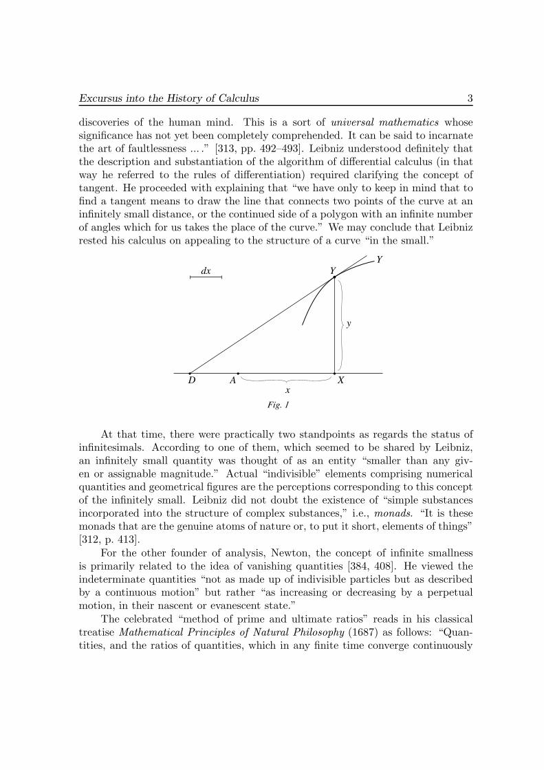
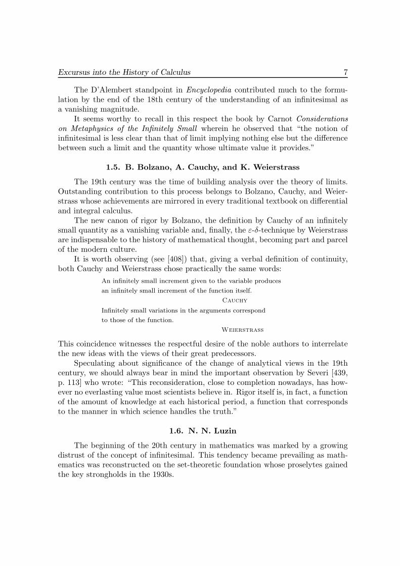
Leibniz gave the following definition of differential. Considering a curve Y Yand a tangent at a fixed point Y on the curve which corresponds to a coordinateX on the axis AX and denoting by D the intersection point of the tangent andaxis, Leibniz wrote: “Now some straight line selected arbitrarily is called dx andanother line whose ratio to dx is the same as of . . . y . . . to XD is called . . . dy ordifference (differentia) . . . of y . . . .”
The essential details of the picture accompanying this text are reproducedin Fig. 1.
By Leibniz, given an arbitrary dx and considering the function x �→ y(x) ata point x, we obtain
dy :=Y X
XDdx.
In other words, the differential of a function is defined as the appropriate linearmapping in the manner fully acceptable to the majority of the today’s teachers ofanalysis.
Leibniz was a deep thinker and polymath who believed that “the invention ofthe syllogistic form ranks among the most beautiful and even the most important
† This term was used in 1748 by Leonhard Euler in Introductio in Analysin Infinitorum [109](cf. [239, p. 324]).
Excursus into the History of Calculus 3
discoveries of the human mind. This is a sort of universal mathematics whosesignificance has not yet been completely comprehended. It can be said to incarnatethe art of faultlessness ... .” [313, pp. 492–493]. Leibniz understood definitely thatthe description and substantiation of the algorithm of differential calculus (in thatway he referred to the rules of differentiation) required clarifying the concept oftangent. He proceeded with explaining that “we have only to keep in mind that tofind a tangent means to draw the line that connects two points of the curve at aninfinitely small distance, or the continued side of a polygon with an infinite numberof angles which for us takes the place of the curve.” We may conclude that Leibnizrested his calculus on appealing to the structure of a curve “in the small.”
D A Xx
y
YY
dx
Fig. 1
At that time, there were practically two standpoints as regards the status ofinfinitesimals. According to one of them, which seemed to be shared by Leibniz,an infinitely small quantity was thought of as an entity “smaller than any giv-en or assignable magnitude.” Actual “indivisible” elements comprising numericalquantities and geometrical figures are the perceptions corresponding to this conceptof the infinitely small. Leibniz did not doubt the existence of “simple substancesincorporated into the structure of complex substances,” i.e., monads. “It is thesemonads that are the genuine atoms of nature or, to put it short, elements of things”[312, p. 413].
For the other founder of analysis, Newton, the concept of infinite smallnessis primarily related to the idea of vanishing quantities [384, 408]. He viewed theindeterminate quantities “not as made up of indivisible particles but as describedby a continuous motion” but rather “as increasing or decreasing by a perpetualmotion, in their nascent or evanescent state.”
The celebrated “method of prime and ultimate ratios” reads in his classicaltreatise Mathematical Principles of Natural Philosophy (1687) as follows: “Quan-tities, and the ratios of quantities, which in any finite time converge continuously
4 Chapter 1
to equality, and before the end of that time approach nearer to each other than byany given difference, become ultimately equal” [408, p. 101].
Propounding the ideas which are nowadays attributed to the theory of limits,Newton exhibited the insight, prudence, caution, and wisdom characteristic of anygreat scientist pondering over the concurrent views and opinions.
He wrote: “To institute an analysis after this manner in finite quantities andinvestigate the prime or ultimate ratios of these finite quantities when in theirnascent state is consonant to the geometry of the ancients, and I was willing toshow that in the method of fluxions there is no necessity of introducing infinitelysmall figures into geometry.
Yet the analysis may be performed in any kind of figure, whether finite orinfinitely small, which are imagined similar to the evanescent figures, as likewise inthe figures, which, by the method of indivisibles, used to be reckoned as infinitelysmall provided you proceed with due caution” [384, p. 169].
Leibniz’s views were as much pliable and in-depth dialectic. In his famous letterto Varignion of February 2, 1702 [408], stressing the idea that “it is unnecessaryto make mathematical analysis depend on metaphysical controversies,” he pointedout the unity of the concurrent views of the objects of the new calculus:
“If any opponent tries to contradict this proposition, it follows from our calculusthat the error will be less than any possible assignable error, since it is in our powerto make this incomparably small magnitude small enough for this purpose, inasmuchas we can always take a magnitude as small as we wish. Perhaps this is what youmean, Sir, when you speak on the inexhaustible, and the rigorous demonstration ofthe infinitesimal calculus which we use undoubtedly is to be found here. ...
So it can also be said that infinites and infinitesimals are grounded in sucha way that everything in geometry, and even in nature, takes place as if they wereperfect realities. Witness not only our geometrical analysis of transcendental curvesbut also my law of continuity, in virtue of which it is permitted to consider rest asinfinitely small motion (that is, as equivalent to a species of its own contradictory),and coincidence as infinitely small distance, equality as the last inequality, etc.”
Similar views were expressed by Leibniz in the following quotation whose endin italics is often cited in works on infinitesimal analysis in the wake of Robinson[421, pp. 260–261]:
“There is no need to take the infinite here rigorously, but only as when we sayin optics that the rays of the sun come from a point infinitely distant, and thusare regarded as parallel. And when there are more degrees of infinity, or infinitelysmall, it is as the sphere of the earth is regarded as a point in respect to the distanceof the sphere of the fixed stars, and a ball which we hold in the hand is also a pointin comparison with the semidiameter of the sphere of the earth. And then thedistance to the fixed stars is infinitely infinite or an infinity of infinities in relation
Excursus into the History of Calculus 5
to the diameter of the ball. For in place of the infinite or the infinitely small we cantake quantities as great or as small as is necessary in order that the error will beless than any given error. In this way we only differ from the style of Archimedesin the expressions, which are more direct in our method and better adapted to theart of discovery.” [311, p. 190].
1.2. L. Euler
The 18th century is rightfully called the age of Euler in the history of math-ematical analysis (cf. [45]). Everyone looking through his textbooks [112] will bestaggered by subtle technique and in-depth penetration into the essence of the sub-ject. It is worth recalling that an outstanding Russian engineer and scientist Krylovwent into raptures at the famous Euler formula eiπ = −1 viewing it as the quintes-sential symbol of integrity of all branches of mathematics. He noted in particularthat “here 1 presents arithmetic; i, algebra; π, geometry; and e, analysis.”
Euler demonstrated an open-minded approach, which might deserve the epi-thet “systemic” today, to studying mathematical problems: he applied the mostsophisticated tools of his time. We must observe that part and parcel of his re-search was the effective and productive use of various infinitesimal concepts, firstof all, infinitely large and infinitely small numbers. Euler thoroughly explained themethodological background of his technique in the form of the “calculus of zeros.”It is a popular fixation to claim that nothing is perfect and to enjoy the imaginaryfailures and follies of the men of genius (“to look for sun-spots” in the words ofa Russian saying). For many years Euler had been incriminated in the “incorrect”treatment of divergent series until his ideas were fully accepted at the turn of the20th century. You may encounter such a phrase in the literature: “As to the prob-lem of divergent series, Euler was sharing quite an up-to-date point of view.” Itwould be more fair to topsy-turvy this phrase and say that the mathematicians oftoday have finally caught up with some of Euler’s ideas. As will be shown in thesections to follow (see 2.2 and 2.3), the opinion that “we cannot admire the wayEuler corroborates his analysis by introducing zeros of various orders” is as self-assured as the statement that “the giants of science, mainly Euler and Lagrange,have laid false foundations of analysis.” It stands to reason to admit once and forever that Euler was in full possession of analysis and completely aware what he hadcreated.
1.3. G. Berkeley
The general ideas of analysis greatly affected the lineaments of the ideologicaloutlook in the 18th century. The most vivid examples of the depth of penetrationof the notions of infinitely large and infinitely small quantities into the culturalmedia of that time are in particular Gulliver’s Travels by Jonathan Swift published
6 Chapter 1
in 1726 (Lilliput and Brobdingnag) and the celebrated Micromegas 1752 writtenby bright and venomous F. M. Arouer, i.e., Voltaire. Of interest is the fact thatas an epigraph for his classical treatise [421], Robinson chose the beginning of thefollowing speech of Micromegas:
“Now I see clearer than ever that nothing can be judged by its visible magni-tude. Oh, my God, who granted reason to creatures of such tiny sizes! An infinitelysmall thing is equal to an infinitely large one when facing you; if living beings stillsmaller than those were possible, they could have reason exceeding the intellect ofthose magnificent creatures of yours which I can see in the sky, and one foot ofwhich could cover the earth” [507, p. 154].
A serious and dramatic impact on the development of infinitesimal analysiswas made in 1734 by Bishop Berkeley, a great cleric and theologian, who publishedthe pamphlet The Analyst, or a Discourse Addressed to an Infidel Mathematician,wherein it is examined whether the object, principles and inferences of the modernanalysis are more deduced than religious mysteries and points of faith [34]. By theway, this Infidel Mathematician was E. Halley, a brilliant astronomer and a youngfriend of Newton. The clerical spirit of this article by Berkeley is combined withaphoristic observations and killing precision of expression. The leitmotif of hiscriticism of analysis reads: “Error may bring forth truth, though it cannot bringforth science.”
Berkeley’s challenge was addressed to all natural sciences: “I have no contro-versy about your conclusions, but only about your logic and method. How do youdemonstrate? What objects are you conversant with, and whether you conceivethem clearly? What principles you proceed upon; how sound they may be; andhow you apply them?” Berkeley’s invectives could not be left unanswered by themost progressive representatives of the scientific thought of the 18th century, theencyclopedists.
1.4. J. D’Alembert and L. Carnot
A turning point in the history of the basic notions of analysis is associated withthe ideas and activities of D’Alembert, one of the initiators and leading authors ofthe immortal masterpiece of the thought of the Age of Enlightenment, the FrenchEncyclopedia or Explanatory Dictionary of Sciences, Arts, and Crafts.
In the article “Differential” he wrote: “Newton never considered differentialcalculus to be some calculus of the infinitely small, but he rather viewed it asthe method of prime and ultimate ratios” [408, p. 157]. D’Alembert was the firstmathematician who declared that he had found the proof that the infinitely small“do exist neither in Nature nor in the assumptions of geometricians” (a quotationfrom his article “Infinitesimal” of 1759).
Excursus into the History of Calculus 7
The D’Alembert standpoint in Encyclopedia contributed much to the formu-lation by the end of the 18th century of the understanding of an infinitesimal asa vanishing magnitude.
It seems worthy to recall in this respect the book by Carnot Considerationson Metaphysics of the Infinitely Small wherein he observed that “the notion ofinfinitesimal is less clear than that of limit implying nothing else but the differencebetween such a limit and the quantity whose ultimate value it provides.”
1.5. B. Bolzano, A. Cauchy, and K. Weierstrass
The 19th century was the time of building analysis over the theory of limits.Outstanding contribution to this process belongs to Bolzano, Cauchy, and Weier-strass whose achievements are mirrored in every traditional textbook on differentialand integral calculus.
The new canon of rigor by Bolzano, the definition by Cauchy of an infinitelysmall quantity as a vanishing variable and, finally, the ε-δ-technique by Weierstrassare indispensable to the history of mathematical thought, becoming part and parcelof the modern culture.
It is worth observing (see [408]) that, giving a verbal definition of continuity,both Cauchy and Weierstrass chose practically the same words:
An infinitely small increment given to the variable produces
an infinitely small increment of the function itself.
Cauchy
Infinitely small variations in the arguments correspond
to those of the function.
Weierstrass
This coincidence witnesses the respectful desire of the noble authors to interrelatethe new ideas with the views of their great predecessors.
Speculating about significance of the change of analytical views in the 19thcentury, we should always bear in mind the important observation by Severi [439,p. 113] who wrote: “This reconsideration, close to completion nowadays, has how-ever no everlasting value most scientists believe in. Rigor itself is, in fact, a functionof the amount of knowledge at each historical period, a function that correspondsto the manner in which science handles the truth.”
1.6. N. N. Luzin
The beginning of the 20th century in mathematics was marked by a growingdistrust of the concept of infinitesimal. This tendency became prevailing as math-ematics was reconstructed on the set-theoretic foundation whose proselytes gainedthe key strongholds in the 1930s.
8 Chapter 1
In the first edition of the Great Soviet Encyclopedia in 1934, Luzin wrote: “Asto a constant infinitely small quantity other than zero, the modern mathematicalanalysis, without discarding the formal possibility of defining the idea of a constantinfinitesimal (for instance, as a corresponding segment in some non-Archimedeangeometry), views this idea as absolutely fruitless since it turns out impossible tointroduce such an infinitesimal into calculus” [335, pp. 293–294].
The publication of the textbook Fundamentals of Infinitesimal Calculus byVygodskiı became a noticeable event in Russia at that time and gave rise to a seriousand sharp criticism. Vygodskiı tried to preserve the concept of infinitesimal byappealing to history and paedeutics.
He wrote in particular: “If it were only the problem of creating some logicalapparatus that could work by itself then, having eliminated infinitesimals from con-siderations and having driven differentials out of mathematics, one could celebratea victory over the difficulties that have been impeded the way of mathematiciansand philosophers during the last two centuries. Infinitesimal analysis originatedhowever from practical needs, its relations with the natural sciences and technology(and, later, with social sciences) becoming increasingly strong and fruitful in thecourse of time. Complete elimination of infinitesimals would hinder these relationsor even make them impossible” [515, p. 160].
Discussing this textbook by Vygodskiı, Luzin wrote in the 1940s: “This course,marked by internal integrity and lit by the great idea the author remains faithful to,falls beyond the framework of the style in which the modern mathematical analysishas been developed for 150 years and which is nearing its termination” [335, p. 398].
Luzin’s attitude to infinitesimals deserves special attention as apparent mani-festation and convincing evidence of the background drama typical of the history ofevery profound idea that enchants and inspires the mankind. Luzin had a uniquecapability of penetration into the essence of the most intricate mathematical prob-lems, and he might be said to possess a remarkable gift of foresight [308, 309, 337].
The concept of actual infinitesimals seemed to be extremely appealing to himpsychologically, as he emphasized: “The idea about them has never been success-fully driven out of my mind. There are obviously some deeply hidden reasons stillunrevealed completely that make our minds inclined to looking at infinitesimalsfavorably” [335, p. 396].
In one of his letters to Vygodskiı which was written in 1934 he predicted that“infinitesimals will be fully rehabilitated from a perfectly scientific point of view askind of ‘mathematical quanta.’ ”
In another of his publications, Luzin sorrowfully remarked: “When the mindstarts acquaintance with analysis, i.e., during the mind’s spring season, it is theinfinitesimals, which deserve to be called the ‘elements’ of quantity, that the mindbegins with. However, surfeiting itself gradually with knowledge, theory, abstrac-
Excursus into the History of Calculus 9
tion and fatigue, the mind gradually forgets its primary intentions, smiling at their‘childishness.’ In short, when the mind is in its autumn season, it allows itself tobecome convinced of the unique sound foundation by means of limits” [504].
This limit conviction was energetically corroborated by Luzin in his textbookDifferential Calculus wherein he particularly emphasized the idea that “to graspthe very essence of the matter correctly, the student should first of all made itclear that each infinitesimal is always a variable quantity by its very definition;therefore, no constant number, however tiny, is ever infinitely small. The studentshould beware of using comparisons or similes of such a kind for instance as ‘Onecentimeter is a magnitude infinitely small as compared with the diameter of thesun.’ This phrase is pretty incorrect. Both magnitudes, i.e., one centimeter andthe diameter of the sun, are constant quantities and so they are finite, one muchsmaller than the other, though. Incidentally, one centimeter is not a small length atall as compared for instance with the ‘thickness of a hair,’ becoming a long distancefor a moving microbe. In order to eliminate any risky comparisons and haphazardsubjective similes, the student must remember that neither constant magnitude isinfinitesimal nor any number, however small these might be. Therefore, it wouldbe quite appropriate to abandon the term ‘infinitesimal magnitude’ in favor of theterm ‘infinitely vanishing variable,’ as the latter expresses the idea of variabilitymost vividly” [504, p. 61].
1.7. A. Robinson
The seventh (posthumous) edition of this textbook by Luzin was published in1961 simultaneously with Robinson’s Nonstandard Analysis which laid a modernfoundation for the calculus of infinitesimals. Robinson based his research on thelocal theorem by Mal′tsev, stressing its “fundamental importance for our theory”[421, p. 13] and giving explicit references to Mal′tsev’s article dated as far back as1936. Robinson’s discovery elucidates the ideas of the founders of differential andintegral calculus, witnessing the spiral evolution of mathematics.
Chapter 2
Naive Foundations ofInfinitesimal Analysis
The most widely spread prejudice against infinitesimals resides in the opin-ion that the technique of infinitesimal analysis is extremely difficult to master.Moreover, it is usually emphasized that the nonstandard methods of analysis reston rather sophisticated sections of set theory and mathematical logic. This cir-cumstance is irrefutable but overrated, hampering in no way comprehension ofinfinitesimals.
The purpose of this chapter is to corroborate the above statement by presentingthe methodology of infinitesimal analysis at the routine level of rigor which is offeredby the modern system of mathematical education invoking the naive set-theoreticstance that stems from Cantor. Alongside with elucidating the basic concepts ofnonstandard set theory and its principles of transfer, idealization, and standard-ization, we pay attention also to comparing the new views of the basic concepts ofanalysis with those of the reverent inventors of the past. We hope so to witness thecontinual evolution and immortality of the ideas of differential and integral calculuswhich infinitesimal analysis in a today’s disguise shed new light upon.
2.1. The Concept of Set in Infinitesimal Analysis
In this section we will set forth a fragment of the foundations of infinitesimalanalysis at the level of rigor close to the current practice of teaching calculus.
2.1.1. Contemporary courses in mathematical analysis rest usually on the con-cept of set.
2.1.2. Examples.
(1) L. Schwartz, Analysis:“A set is a collection of objects.Examples: the set of all alumni of a school;
Naive Foundations of Infinitesimal Analysis 11
the set of points on a plane;the set of nondegenerate surfaces
of second-order in three-dimensional space;the set N of positive integers;the set Z of integers;the set Q of rational numbers;the set R of real numbers;the set C of complex numbers” [436].
(2) V. A. Il ′in, V. A. Sadovnichiı, and Bl. Kh. Sendov, MathematicalAnalysis:
“The concept of set was of importance when we have studied reals. We em-phasize that we view a set as a basic concept indeterminate from the others.
In this section we will study sets of an arbitrary nature which are also calledabstract sets. This implies that the objects comprising such a set which we callthe elements of this set are not necessarily some real numbers. For instance, thearbitrary functions, letters of an alphabet, planar figures, etc. may serve as elementsof an abstract set [189, p. 69].
(3) Yu. G. Reshetnyak, A Course in Mathematical Analysis:“A set for us will be one of the basic mathematical concepts inexpressible in the
other mathematical concepts. Uttering the word ‘set,’ we usually imply a collectionof objects of an arbitrary nature which we will treat as a whole. Alongside this term,set, we will use its synonyms like totality, system, assembly, and so on. We mayspeak for instance about the set of solutions to an equation, about the collection ofpictures in a museum, the totality of points of a circle and so on.
The objects, comprising a set, are the elements of this set.We assume a set given if, granted whatever object, we can determine whether
or not it is an element of the set in question” [413, p. 12].(4) V. A. Zorich, Mathematical Analysis:
“The basic hypotheses of cantorian set theory (called ‘naive’ in common par-lance) are as follows:
1◦ each set may consists of arbitrary distinct objects;2◦ each set is uniquely determined by the collection of objects comprising it;3◦ each property determines a set of objects enjoying this property.If x is an object, P is a property, with P (x) signifying that x enjoys P , then
we let {x | P (x)} stand for the class of objects possessing P .The objects comprising a class or a set are the elements of the class or the set.The words ‘class,’ ‘family,’ ‘totality,’ and ‘collection’ are viewed as synonyms
of the noun ‘set’ within the naive set theory.The following examples demonstrate the application of this terminology:
the set of letters ‘a’ in the word ‘I’;
12 Chapter 2
the set of Adam’s wives;the collection of ten digits;the family of Leguminosae;the set of grains of sand on the Earth;the totality of the points on a plane equidistant from two given points;a family of sets;the set of all sets.
The degree of certainty of definition varies greatly from set to set. This promptsus the conclusion that the concept of set is not as simple and harmless as it mightseem. For example, the definition of the set of all sets leads in fact to an outrightcontradiction” [541, pp. 17–18].
2.1.3. Infinitesimal or nonstandard analysis belongs in mathematical analysis.Therefore, this discipline fully shares the above views of sets. Consequently, infini-tesimal analysis considers as sets those and only those collections that are admittedinto the classical “standard” theory.
It is worth observing that the last statement may be reformulated as follows:Infinitesimal analysis refuses to view as sets those and only those collections that arerejected by the present-day mathematics. At the same time, infinitesimal analysisrests on refining views of sets. To put it otherwise, infinitesimal analysis resideswithin the realm of nonstandard set theory.
2.1.4. The naive set theory starts with the celebrated definitions by Cantor:“A set is any many which can be thought of as one, that is every totality of definiteelements which can be united to a whole through a law,” and a set is “everycollection into a whole M of definite and distinct objects m of our perceptionor our thought” [52, p. 173].
Such concepts are well known to be rather broad, this drawback bypassed byelaborating distinction between sets and nonsets. For instance, the term “class” isin common parlance for nominating “exceedingly huge” inappropriate collections,implying that a class is not necessarily a set. In other words, formalization of theconcepts of the naive set theory rests on clarifying and elaborating the proceduresthat introduce sets into the practice of mathematics. All sets we admit into math-ematics enjoy the same rights. This in no way implies that all sets are equal orbear no distinctions but means simply that all sets are akin, maintaining the samestatus of an ordinary member of the “universe of sets.”
2.1.5. The cornerstone of nonstandard set theory is the following perfectlytransparent underlying principle: The sets differ from each other: every set iseither standard or nonstandard. In a way, it would be more correct to speak of thetheory of sets, standard and nonstandard, rather than nonstandard set theory.
The phrase “A is a standard set” conveys the intuitive idea that A admits
Naive Foundations of Infinitesimal Analysis 13
description in accurate and unambiguous terms. We may even say that such an Abecomes an “artifact” of the cognition activities of human beings. The concept ofstandardness draws a borderline between the objects resulting from explicit math-ematical constructions, primarily, by the theorems of unique existence, which arestandard sets, and the objects originating in research in implicit, indirect manner,which are nonstandard sets.
Such objects as the numbers π, e, and sin 81 are determined uniquely in muchthe same way as the set of natural numbers N and the set R of real numbers alsocalled the reals. These are standard objects. On the other hand, an arbitrary“abstract” real number arises implicitly on assuming the set-theoretic stance ofmathematics. Such an “abstract” real number is by definition just a member ofthe standard set R, the reals. This is a routine method of introducing objects intomathematical practice: a vector is an element of a vector space; a filter is a set ofsome subsets of a given set which enjoy a few specific properties; etc.
Therefore, there are standard reals and nonstandard reals; there are standardvectors and nonstandard vectors; there are standard filters and nonstandard filters;etc. In general, there are standard sets and nonstandard sets.
By way of example, let us consider the set of grains of sand on the Earth.Archimedes wrote in his classical treatise Psammiths, the Sand-Reckoner, that:
“. . . of the numbers named by me and given in the work which I sent to Zeuxippessome exceed not only the number of the grains of sand equal in magnitude to theEarth filled up in the way described but also that of a mass equal in magnitude tothe universe ” [2, p. 358].
Therefore, the number of the grains of sand on the Earth presents a particularnatural number. However, nobody can either determine or nominate this numberprecisely, since it is absolutely impossible to implement any sequential count of allgrains of sand. Hence, the number of the grains of sand on the Earth is expressedby an “inassignable,” “indeterminate”—nonstandard—natural number and so theset of the grains of sand is nonstandard.
It goes without saying that the above views of distinction between standardand nonstandard sets are auxiliaries for mastering the rules of handling these setsin practice. We encounter a complete analogy with the situation in geometry wherethe intuitive visualizations of spatial forms help in elaborating the skills of usingthe axioms of geometry which, in the long run, are the only source of the rigorousdefinitions of points, straight lines, planes, and other geometrical objects. FollowingAlexandrov, we must observe that “axioms themselves need substantiation sincethey only summarize the available data, while starting the logical construction ofa theory” [7, p. 51]. Therefore, we are impelled to precede the formal introductionof the axioms of nonstandard set theory by discussing them qualitatively.
As we already know, any nonstandard set theory begins with the primary obser-
14 Chapter 2
vation that we distinguish two types of sets: standard and nonstandard. Moreover,we accept another three postulates or, to be more exact, versions of the principlesof infinitesimal analysis.
2.1.6. Transfer Principle. Each mathematical proposition claiming the ex-istence of some set simultaneously determines a standard set.
In other words, the unique existence theorems of mathematics provide thedirect and explicit definitions of new mathematical entities. An equivalent refor-mulation of this principle, elucidating the reasons behind its official title, reads:In order to validate some claim about all sets, it suffices to demonstrate the claimin the case of standard sets. Intuitive substantiation of the transfer principle lieswith the evident fact that, making every judgement about arbitrary sets, we actu-ally deal only with the already available sets we have defined uniquely, i.e., withstandard sets.
Pondering over the meaning of the transfer principle, we see that it containstwo aspects of the views of standard entities. The first proclaims that new standardobjects result from those already available by descriptions similar to the theoremsof unique existence, which postulates the possibility of defining standard objectsby recursion. This circumstance may be rephrased as the conclusion that eachnonempty standard set contains a standard element and each entity is standardthat results from standard elements by some unique construction or definition.
The second aspect of views of standardness, as expressed by the transfer prin-ciple is interwoven with the first, and means representativeness of the standarduniverse, i.e. the class of standard sets is sufficiently large for reflecting all featuresof the universe of sets. In other words, this postulates the possibility of studyingarbitrary sets by induction starting from actually available standard entities, i.e.,cognizability of ideal constructions of set theory.
2.1.7. Idealization Principle. Each infinite set contains a nonstandard ele-ment.
This postulate conforms perfectly with the most general views of infinity. Theidealization principle will appear often in stronger forms reflecting the inexhaustiblevariety of ideal objects. For instance, one of the popular nonstandard axiomsreads: All standard sets are members of some finite set. The number of elementsof such a “universal” set is huge and, which is most important, “inassignable,”“inexpressible,” and “unrealizable.” In other words, the size of a universal set isnonstandard and so it is no surprise that every universal set is nonstandard either.
It is worth observing that care must be exercised in handling the above postu-lates as on the other occasions by the way. Indeed, every standard set is uniquelydetermined from its standard elements in the standard environment—in the com-munity of its next of kin, other standard sets. However, an infinite standard set

Naive Foundations of Infinitesimal Analysis 15
never reduces to its standard elements since it always contains some nonstandardelement. There are many nonstandard sets containing each standard element of theoriginal set and having no other standard elements.
Another circumstance is very important to mention: the term “proposition”in the transfer principle deserves extreme caution in much the same way as in theconventional set theory although. Transfer is fully legitimate inasmuch as we applyit to the common mathematical proposition not involving the property of a setto be or not to be standard which we have introduced at a semantic level in thecapacity of another indeterminate basic concept of nonstandard set theory. Indeed,were it otherwise, we would apply transfer to the claim that every set is standard,arguing as follows: Since every standard set is standard, every set is standard bytransfer. This would yield a contradiction with idealization. Therefore, transferis not applicable to the claim that every set is standard and so the standardnesspredicate is a property inexpressible in the naive set theory.
2.1.8. Standardization Principle. To each standard set and each propertythere corresponds a new standard set comprising precisely those standard elementsof the original set that possess the property under study.
In symbols, let A be a standard set, and let P be an arbitrary property whichmay involve the standardness predicate in its formulation. The standardizationprinciple claims that there is a standard set which is usually denoted by ∗{x ∈ A :P (x)} and maintains the relation
y ∈ ∗{x ∈ A : P (x)} ↔ y ∈ {x ∈ A : P (x)}
for all standard y. The set ∗{x ∈ A : P (x)} is often referred to as the standardiza-tion of A or even briefer. We write ∗A, omitting the parameters that participate inthe definition of the standardization of A. The intuitive idea behind the standard-ization principle reflects the experience showing that if some explicit descriptions ofmathematical objects are available then we may use any definite rules for assigningnew entities of further mathematical research. Standardization extends the conven-tional comprehension principle of set formation which allows us to deal with a newsubset of a given set by collecting the elements with some prescribed property.
Thinking over the standardization principle, it is worth noting that nothingis claimed about the nonstandard elements of the result of standardization. Thisis not by chance. The point is that the two possibilities are open: a nonstandardelement can enjoy the property we use in standardization or it may fail to possessthis property.
The standardization principle must be used with the same care as elsewhere:Attempts at standardizing some “universal” set that contains all standard setswould result in a blatant contradiction.
16 Chapter 2
2.1.9. The above postulates give grounds for axiomatic presentations of non-standard set theory. We will discussed these in more detail in Chapter 3. Mean-while, we may proceed along the lines of the Zorich textbook and remark: “Asa whole, each of the available axiomatics is such that, on the one hand, it elimi-nates the known contradictions of the naive theory and, on the other hand, it ensuresfreedom of operation with concrete sets residing in various sections of mathematicsand, before all, in mathematical analysis understood in a broad sense of the word”[541, pp. 18–19].
2.2. Preliminaries on Standard and Nonstandard Reals
We now start an acquaintanceship with the surprising features of the classicalreal axis which are disclosed by the principles of infinitesimal analysis.
2.2.1. Given a set A, we will write a ∈ ◦A to abbreviate the expression “a isa standard member of A.”
2.2.2. The following hold:(1) If A is a set satisfying 1 ∈ A and such that n ∈ ◦N implies n ∈ A →
n + 1 ∈ A then A contains all standard natural numbers: ◦N ⊂ A(= the induction principle on standard naturals);
(2) Every finite set (i.e., a set admitting no injective mappings onto anyof its proper subsets), consisting of standard elements, is standarditself;
(3) Every finite standard set has only standard elements;(4) If a set contains only standard members then it is finite;(5) The totality ◦A is not a set for every infinite (= not finite) set A.
� (1): By standardization, it is possible to consider the following standardsubset of N, the set of natural numbers:
B := ∗{n ∈ N : n /∈ A}.
Assuming that B �= ∅, observe that B has the least element m which is standardby transfer. By hypothesis, m �= 1 since 1 ∈ A. Moreover, m /∈ A and so m−1 /∈ A.By transfer, m − 1 ∈ ◦
N, i.e., m − 1 ∈ B. It follows that m − 1 ≥ m, which isa contradiction. Hence, B = ∅, i.e., (∀n ∈ ◦
N)(n ∈ A), implying the inclusion◦N ⊂ A.
(2): This is immediate by transfer.(3): Each standard singleton contains a unique and, hence, standard element.
The size, i.e. the number of elements, of a finite standard set A is also standard bytransfer. Moreover, A = (A− {a}) ∪ {a} for all a ∈ A. The number of elements ofA− {a} is also standard, and we are done by the induction principle (1).
Naive Foundations of Infinitesimal Analysis 17
(4): This is straightforward by idealization.(5): Assume that ◦A is a set. The set ◦A is finite by (4) and standard by (2).
By transfer, A = A◦ and so A is finite, which is a contradiction. �
2.2.3. A natural number N is nonstandard (i.e., inassignable) if and only if Nis greater than every standard natural number. In symbols,
N ∈ N − ◦N ↔ (∀n ∈ ◦N)(N > n).
� It suffices to note that if n ∈ N is standard and N ∈ N is less than or equalto n then N is standard for instance by 2.2.2, i.e., N ∈ ◦N. �
2.2.4. In view of 2.2.3, a nonstandard natural number is called unlimited,illimited, actually infinite, or even infinite, which abuses the language.
It is a widely-spread opinion that “Euler claimed rather light-mindedly that1/0 is infinite, although he never found it worthwhile to define what infinity is; hejust invented the notation ∞.” This opinion is clearly false since Euler pointed outexplicitly in [110, p. 89] that “an infinite number and a number greater than anyassignable number are synonyms.”
The fact that N is an unlimited number is expressed symbolically as N ≈ ∞or, in more detail, N ≈ +∞.
We must mention that the epithet “infinite” for an unlimited number N leadsto confusion. Indeed, if we strictly pursue the set-theoretic stance then we view Nprimarily as a set and this set N is clearly finite in the rigorous set-theoretic sense(cf. 2.2.2(2)). The phrase “N is an infinite number” suggests misleadingly that Nis an infinite set. In actuality, N is a finite set whose size is nonstandard. Only thismeaning is implied in the concept of an infinitely large natural number N withinthe set-theoretic credo of contemporary mathematics.
2.2.5. The following hold:(1) (N ≈ +∞ and M ≈ +∞) → (N +M ≈ +∞ and NM ≈ +∞);(2) (N ≈ +∞ and n ∈ ◦
N) → (N + n ≈ +∞, N − n ≈ +∞, andnN ≈ +∞);
(3) N ≈ +∞ ↔ Nn ≈ +∞ for all n ∈ ◦N;(4) Each composite unlimited number has unlimited divisors;(5) (N ≈ +∞ and M ≥ N) → M ≈ +∞;(6) “If 1
0denotes some infinitely large number then, since 2
0is undoubt-
edly the doubled 10 , it is clear that every number, even infinitely
large, can be made still two or several times greater” (Euler, [109,p. 620]);
(7) Let t be a positive real. The integral part of t is unlimited if andonly if so is t, i.e., t is greater than every standard real;
18 Chapter 2
(8) Let ψ : N → N be a strictly increasing standard function. Then
N ≈ +∞ ↔ ψ(N) ≈ +∞
for N ∈ N.
� We will demonstrate only (7) and (8), since the other claims are easier tocheck.
(7): If the integral part s of a real t is unlimited and, nevertheless, (∃ r ∈ ◦R)(t ≤ r) then t ≤ n for some n ∈ ◦
N. Hence, n + 2 ≤ s ≤ t ≤ n, which isa contradiction. Therefore, t ≈ +∞.
Conversely, if t ≈ +∞ then s+ 1 ≥ t, where s is the integral part of t. Hence,s+ 1 ≈ +∞, which yields s ≈ +∞ by 2.2.5(2).
(8): ←: Assume first that ψ(N) ≈ +∞ and n ∈ ◦N. Then ψ(n) is standardby transfer, i.e., ψ(n) ∈ ◦N. Therefore, ψ(N) > ψ(n). Since ψ increases strictly, itfollows that N > n, i.e., N ≈ +∞.
→: Assume now that N ≈ +∞. Then N > n for all n ∈ ◦N. Hence, ψ(N) >ψ(n) ≥ n. Thus, ψ(N) ≈ +∞. �
2.2.6. Let R stand for the extended reals, i.e., R := R ∪ {−∞,+∞} with +∞and −∞ the greatest and least elements appended to R formally. It is convenientto call ∞ := {+∞,−∞} the (symbolic) potential infinity and to speak of +∞ or−∞ as about the positive or negative (symbolic) infinity.
A real t ∈ R is limited provided that there is a standard number n ∈ ◦N
satisfying |t| ≤ n. We write t ∈ ltd(R) or t ∈ ≈R whenever t is a limited elementof R. A member of R that fails to be limited is unlimited or actually large. We alsowrite t ≈ +∞ for t /∈ ≈R and t > 0. The records t ≈ −∞ and t ≈ ∞ are understoodby analogy. It is a common practice to agree that t ≈ +∞ ↔ t ∈ μ(+∞), usingthe expressions like “t lies in the monad of the point at infinity or the monad of theplus-infinity.”
An element t in R is infinitesimal or, amply, infinitely small provided that|t| ≤ 1/n for all n ∈ ◦N. In this event we write t ≈ 0 or t ∈ μ(R) and say that tbelongs to the monad of zero. (The symbol μ(R) is common alongside the notationμ(0) which signifies a close relationship with the unique separated vector topologyon R.) Infinitesimals are also referred to as actual infinitely small quantities; theunsuccessful term “differentials” have little room.
If x ≤ y and the difference between x and y fails to be infinitesimal then wewrite x � y. Since t ∈ ≈R ↔ (∀N ≈ +∞)(|t| � N); therefore, we let the record|t| � +∞ symbolize the fact that t ∈ R is a limited real.
2.2.7. The term monad (Moναζ) dates from antiquity. It is traditionallytranslated as one or unit with no sufficient ground for that. By Definition 1 of
Naive Foundations of Infinitesimal Analysis 19
Book VII of Euclid’s Elements, a monad “is 〈that〉 by virtue of which each of thethings that exist is called one” [108, p. 9].
We now exhibit some qualitative observations about the structure of a monadas expressed by Sextus Empiricus:
“Pythagoras said that the origin of the things that exist is a monad by virtueof which each of the things that exist is called one” [440, p. 361];
“A point is structured as a monad; indeed, a monad is a certain origin ofnumbers and likewise a point is a certain origin of lines” [440, p. 364];
“A whole as such is indivisible and a monad, since it is a monad, is not divisible.Or, if it splits into many pieces it becomes a union of many monads rather thana [simple] monad” [440, p. 367].
We will study the status and structure of monads in great detail later. Wenow start with considering the basic properties of the collection of infinitesimals or,which is the same, the monad comprising all infinitely small reals.
2.2.8. The following are valid:(1) (s ≈ 0 and t ≈ 0) → s+ t ≈ 0;(2) (t ≈ 0 and s ∈ ≈R) → st ≈ 0;(3) z ≈ 0 ↔ 1/z ≈ ∞ (for z �= 0):
“If z becomes a magnitude less than every assignable magnitudewhatever, i.e., infinitely small, then the value of the fraction 1
zmust
become greater than every assignable magnitude, i.e., an infinitelylarge magnitude” (Euler [110, p. 93]).
(4) If t ≈ 0 and t is standard then t = 0.
� (1): Take n ∈ ◦N. Clearly, |s| ≤ (2n)−1 and |t| ≤ (2n)−1. Hence, |s + t| ≤|s| + |t| ≤ (2n)−1 + (2n)−1 = n−1, and so s+ t is infinitesimal.
(2): Assume that s ∈ ≈R and s �= 0 (otherwise there is nothing left to prove).Take n ∈ ◦N. By hypothesis, |s| ≤ m for some m ∈ ◦N. Therefore, |t| ≤ (nm)−1.It follows that |st| ≤ |s| |t| ≤ m(nm)−1 = n−1, i.e., st ≈ 0.
(3): Let z be a limited nonzero real; i.e., 0 < |z| ≤ |n|, where n ∈ ◦N. Obviously,|1/z| ≥ 1/n, i.e., 1/z is not infinitesimal. Conversely, if z ≈ ∞ then |z| ≥ n forevery limited n, which implies z−1 ≈ 0.
(4): Note that |t| ≤ 2−1|t| provided that t is standard, which is impossible for|t| > 0. Hence, t = 0. �
2.2.9. The monad μ(R) is not a set.
� Assume the contrary. Then μ(R) is a subset of R. Moreover, t ≥ μ(R)for all t > 0, t ∈ ◦
R. Hence, t ≥ s := supμ(R). Obviously, s is a nonzeroinfinitesimal. However, 2s ≥ s → s = 0, which contradicts the existence of nonzeroinfinitesimals. �
20 Chapter 2
2.2.10. When we deal with reals, it is convenient to distinguish various casesof their interlocation.
Given s, t, r ∈ R, we write s = rt or s ≈ t(mod r) provided that (s − t)/r ≈ 0(here r �= 0). In this event we say that s and t are r-close or infinitely closemodulo r. In case r = 1, we simply write s ≈ t and call s and t infinitely close.
The founders of infinitesimal analysis often made no distinction between the re-als infinitely close to a given real and this real itself. Euler expressed this as follows:“An infinitely small quantity is exactly equal to zero” (or, in another translation,“an infinitely small quantity actually will be = 0”) [110, p. 92]. This explains therecord x = y for x ∈ R and y ∈ ◦R satisfying x ≈ y. In this respect Leibniz re-marked: “I think that those things are equal not only whose difference is absolutelynothing but also whose difference is incomparably small” [311, p. 188], empha-sizing that “the error is inassignable and cannot be found by means of whateverconstruction” [534, p. 195].
Given s, t ∈ R, we write s = O(t) for s/t ∈ ≈R. In case s = O(t) and t = O(s)we then say that s and t have the same order. If s/t ≈ 0 then we write s = o(t)and say that s is of higher order than t. Finally, if s − t = o(t) and s − t = o(s)then we call s and t equivalent and write s ∼ t.
Presenting his views on higher order infinitesimals, Leibniz wrote: “I wouldlike to add one more remark in order to prevent all arguments against the realityof differences of any orders, and, namely, that they can always be expressed inproportional finite straight lines... . I have already explained how to express first-order differences with conventional finite straight lines when first presenting theelements of this calculus in ‘Acta’ in October 1684” (see [534, pp. 188–190], cf. 1.1).
2.2.11. Given s, t ∈ R, put
s ∈ O := O(t) ↔ s = O(t); s ∈ o := o(t) ↔ s = o(t).
The Landau rules hold:
O +O ⊂ O; O + o ⊂ O; o+ o ⊂ o;Oo ⊂ o; OO ⊂ O; oo ⊂ o.
� For definiteness, demonstrate the relation O + o ⊂ O. To this end, assumethat s := O(t) and r := o(t). Then s/t ∈ ≈R and r/t ≈ 0. Hence, (s+ r)/t ∈ ≈R,i.e., s+ r = O(t). �
2.2.12. Given s, t ∈ R, the following are equivalent:(1) s ∼ t;(2) s− t = o(t) or t− s = o(s);(3) s/t ≈ 1 or t/s ≈ 1;(4) s/t ≈ 1 and t/s ≈ 1.

Naive Foundations of Infinitesimal Analysis 21
� It is clear that (1) → (2). If, for instance, t − s = o(s) then (t − s)/s ≈ 0;i.e., t/s − 1 ≈ 0. Hence, 1 − ε ≤ t/s ≤ 1 + ε for ε > 0 and ε ∈ ◦
R. Therefore,(1 − ε)−1 ≥ s/t ≥ (1 + ε)−1 and ε/(1 − ε) ≥ s/t− 1 ≥ ε/(1 + ε), i.e., s/t ≈ 1. Wehave thus demonstrated that (2) → (3) → (4), while the implication (4) → (1) isobvious. �
2.2.13. Given N ∈ N, assume that αk, βk ∈ o(1) are infinitesimals satisfyingαk ∼ βk for k := 1, . . . , N . Then
(1)∑N
k=1 αk ∼ ∑Nk=1 βk for αk, βk ≥ 0;
(2) If∑Nk=1 |αk| = O(1) then
N∑
k=1
αk ≈N∑
k=1
βk.
� To prove, note that 2.2.12 yields −εαk + αk ≤ βk ≤ αk + εαk for everystandard ε > 0, which implies (1). Moreover, if t :=
∑Nk=1 |αk| ∈ ≈R then
∣∣∣∣
N∑
k=1
(αk − βk)∣∣∣∣ ≤
N∑
k=1
|αk − βk| ≤ ε
n
N∑
k=1
|αk| ≤ ε
provided that n ∈ ◦N satisfies |t| ≤ n. �2.2.14. There is a natural number N such that for each standard real t in R
the product Nt is infinitely close to some natural number.
� Consider some finite subset {x1, . . . , xn} of R that contains all standard reals,and take some positive infinitesimal ε > 0, ε ≈ 0. The Dirichlet principle of numbertheory reads: To all ε > 0 and x1, . . . , xn ∈ R there is an integer N ∈ N such thateach of the products Nx1, . . . , Nxn differs from some integers by at most ε. We aredone on to apply this theorem with the chosen parameters. �
2.2.15. It is worth observing that the infinite proximity (as well as equivalence)of reals is not a subset of the cartesian square R × R. Were it otherwise, the imageof zero under this relation, which is the monad μ(R), would be a set which isimpossible by 2.2.9. Note also that the monad μ(R) is indivisible in the followingimplicit sense: n−1μ(R) = μ(R) for every standard n.
Pondering over the role of the monad μ(R) in the construction of the systemof integers, it stands to reason to reconsider Definition 2 of Book VII of Euclid’sElements which ends as follows: “... and a number is a magnitude composed ofmonads” [108, p. 9].
Inspecting the “nonstandard” extended reals R, we see this set and, which ismost nontrivial, its limited part ≈R to be the collection of monads about stan-dard points. A more rigorous formulation of this statement rests on the followingfundamental fact whose proof leans essentially on the standardization principle.
22 Chapter 2
2.2.16. To each limited real t there corresponds a unique standard real infin-itely close to t.
� Given t ∈ ≈R, use standardization and find the standard set A := ∗{a ∈R : a ≤ t}. Obviously, A �= ∅ and A ≤ n whenever n ∈ ◦N satisfies −n ≤ t ≤ n.Indeed, a ≤ t ≤ n for every standard a ∈ A and so A ≤ n by transfer. Since R iscomplete; therefore, A has a unique least upper bound, s := supA ∈ R. Obviously,s is standard by transfer. We will demonstrate that s ≈ t. If not, we would have|s− t| > ε for some standard ε > 0. If s > t then s > t+ε and so s ≥ a+ε for everystandard a in A. Hence s ≥ s + ε, which is impossible. The remaining possibilitys < t also leads to a contradiction since then we would find that t > s + ε and,again, s ≥ s+ ε. �
2.2.17. The standard real infinitely close to a limited real t ∈ ≈R is the stan-dard part or shadow of t. The standard part of t is denoted by st(t) or ◦t.
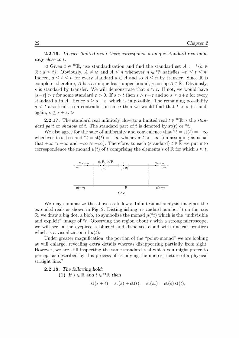
We also agree for the sake of uniformity and convenience that ◦t = st(t) = +∞whenever t ≈ +∞ and ◦t = st(t) = −∞ whenever t ≈ −∞ (on assuming as usualthat +∞ ≈ +∞ and −∞ ≈ −∞). Therefore, to each (standard) t ∈ R we put intocorrespondence the monad μ(t) of t comprising the elements s of R for which s ≈ t.
− ∞M≈ − ∞ t∈≈IR °t∈°IR 0 N≈ + ∞
+ ∞μ(t) μ(IR)
μ(− ∞) ≈IR μ(+ ∞)Fig. 2
We may summarize the above as follows: Infinitesimal analysis imagines theextended reals as shown in Fig. 2. Distinguishing a standard number ◦t on the axisR, we draw a big dot, a blob, to symbolize the monad μ(◦t) which is the “indivisibleand explicit” image of ◦t. Observing the region about t with a strong microscope,we will see in the eyepiece a blurred and dispersed cloud with unclear frontierswhich is a visualization of μ(t).
Under greater magnification, the portion of the “point-monad” we are lookingat will enlarge, revealing extra details whereas disappearing partially from sight.However, we are still inspecting the same standard real which you might prefer topercept as described by this process of “studying the microstructure of a physicalstraight line.”
2.2.18. The following hold:(1) If s ∈ R and t ∈ ≈R then
st(s+ t) = st(s) + st(t); st(st) = st(s) st(t);
Naive Foundations of Infinitesimal Analysis 23
(2) If s, t ∈ R and s ≤ t then ◦s ≤ ◦t;(3) If s, t ∈ R then
(∃ t′ ≈ t)(t′ ≥ s) ↔ ◦s ≤ ◦t ↔ (∀ ε > 0, ε ∈ ◦R)(s ≤ ◦t+ ε);
(∀ t′ ≈ t)(t′ ≥ s) ↔ ◦s < t (◦t ∈ ◦R);
(4) The standard part operation over the reals is not a set (hence, nora function).
� (1): Prove by way of illustration that the standard part operation is mul-tiplicative. Clearly, s ≈ st(s) → ts ≈ t st(s). Moreover, t ≈ st(t) → st(s)t ≈st(t) st(s) which yields, st ≈ st(s) st(t). We are done on recalling that the productof standard reals is standard too.
(2): Assume that s < t (otherwise everything is obvious). If s ≈ t then st(s) =st(t). Were this otherwise, the monads μ(s) and μ(t) would be disjoint. Hence,◦s < ◦t.
(3): In the initial equivalence, the implication to the right is obvious, while thereverse ensues from the fact that s ≤ ◦t+ s− ◦s for s ≤ ◦t. Moreover, s < t+ ε →st(s) ≤ st(t) + st(ε) = ◦t+ ε for every ε > 0, ε ∈ ◦R. This implies by transfer that◦s ≤ ◦t+ ε for all positive ε. Hence, ◦s ≤ ◦t.
Assume conversely that ◦s < ◦t. Since the monads μ◦(s) and μ(◦t) are disjoint;therefore, s < ◦t+ ε for all ε > 0, ε ∈ ◦R.
To check the arrow to the right in the lower equivalence, note that s does notbelong to the monad μ(t) of t. Hence, the whole of the monad of s lies to the leftfrom the monad of t; in symbols, μ(s) < μ(t). Therefore, ◦s < ◦t. To prove theremaining implication, observe finally that μ(t) > ◦s or t ∈ ≈R whenever ◦s = −∞.If ◦s ∈ ◦R then μ(◦s) < ◦t. Hence, t′ ≥ s whenever t′ ≈ t.
(4): If the law t �→ st(t) were a set then the monad μ(R) would also be a set(since t ∈ μ(R) ↔ ◦t = 0). It suffices to appeal to 2.2.9. �
2.3. Basics of Calculus on the Real Axis
We now discuss the fundamental notions of differential and integral calculusfor functions in a single real variable.
2.3.1. Theorem. If (an) is a standard sequence and a ∈ R is a standard realthen
(1) a is a partial limit of (an) if and only if a = ◦aN for some unlimitednatural N ;
(2) a is the limit of (an) if and only if aN is infinitely close to a for allunlimited naturals N ; in symbols,
a = lim an ↔ (∀N ≈ +∞)(aN ≈ a).
24 Chapter 2
� These claims are demonstrated similarly. Therefore, we prove one of them,for instance, (2).
Assume for the sake of definiteness that an → a and a ∈ R (the cases a = +∞and a = −∞ are settled by the same scheme). To each ε > 0 there is some n ∈ N
such that |aN − a| ≤ ε whenever N ∈ N and n ≤ N . By transfer, to each standardε > 0 there is some standard n with the same property. Every unlimited N isgreater than n and so |aN − a| ≤ ε. Since ε is arbitrary, it follows that aN ≈ a.
Assume conversely that ◦aN = a for all N ≈ +∞ and, for the sake of defi-niteness and diversity, a := −∞. Take an arbitrary standard number n ∈ ◦N. IfN ≥ M with M unlimited then aN ≤ −n. Given an arbitrary standard n, we havethus proved “something” (namely, “something” = (∃M)(∀N ≥ M)(aN ≤ −n)).By transfer, this “something” holds for all n ∈ N, which means clearly thatan → −∞. �
2.3.2. We proudly note the merits of the above tests. We have demonstratedthat the partial limits of a standard sequence are exactly those “assignable” realsthat correspond to unlimited indices. In other words, each partial limit of (an) is the“observable” value of some remote entry of (an). The tests of Theorem 2.3.1 in thestandard environment have a clear intuitive meaning in contract to the conventionaldefinitions of partial limit as the limit of some subsequence of (an) or as such a pointof the real axis whose every neighborhood intersects with every “tail” of (an).
It is illuminative to look at the explanation of the concept of a partial limitof a [generalized] sequence with which Luzin furnished the formulation of the usualdefinition (see [334, pp. 98–99]): “The reader will undoubtedly find this definitioncumbersome and abstract at the first glance. However, the feeling of obscurity willvanish if the reader invokes the concepts of ‘variable’ and ‘time’ which he or she isgrown accustomed to.
Indeed, what does this definition intend to convey if translated into the lan-guage of ‘variable’ and ‘time’? To grasp this, let us consider a variable x thatranges over a given numerical sequence M , shifting from the preceding indices tothe succeeding ones ... in the language of a variable and time this definition meansthat a ([partial]) limit of a numerical sequence M is such a real number a that thevariable x cannot leave for ever, since the values of x become however ‘close to a’from time to time.”
Using the same language in infinitesimal analysis, we may express this defini-tion in the most lucid and comprehensible manner: “If the variable x is infinitelyclose to a at some remote moment of time then a is a [partial] limit of M .”
Continuing the discussion of the tests of Theorem 2.3.1, we recall the followingdirections by Courant:
“Motivation of the rigorous definition of limit. It is no wonder thatanyone who first hears the abstract definition of the limit of a sequence will fail to
Naive Foundations of Infinitesimal Analysis 25
comprehend it completely from the very beginning. This definition of limit arrangesa game between two persons, A and B: A demands that a constant quantity abe approximately presented by some entry an so that the deviation be less thanan arbitrary bound ε = ε1 imposed exclusively by A. B meets this demand byproving the existence of such an integer N = N1 that all an satisfy the demandof ε1 from some aN on.
Then A wants to demand a new smaller bound, ε = ε2, while B, in turn, meetsthis demand by finding a new integer N = N2 (possibly, much greater), and so on.If B manages always to meet the demand by A of a however small bound then wehave the situation that is symbolically expressed as an → a.
Undoubtedly, there is a psychological difficulty in mastering this rigorous def-inition of passage to the limit. Our mental apprehension imposes upon us the ‘dy-namical’ idea of passage to the limit as a result of motion: we ‘run’ through thesequence of numbers 1, 2, 3, . . . , n, . . . and observe the behavior of the sequence an.We harbor the feeling that approximation must be visible during our ‘run.’ This‘natural’ formulation, however, does not allow a rigorous mathematical rephrasal.
To arrive at the rigorous definition, the order of consideration should be re-versed: Instead of starting with the argument n and proceeding further with thedependent variable an corresponding to n, we base our definition on the steps thatenable us to validate the statement an → a successively.
Pursuing this inspection, we must start with choosing arbitrarily small intervalabout a, and then to check whether the condition of hitting the interval is fulfilledby assuming the variable n sufficiently large. It is in this way that we come to therigorous definition of limit, assigning to the expressions ‘arbitrarily small bound’and ‘sufficiently large’ n the symbolic denotations ε and N” [64, pp. 66–67].
Compare this with the infinitesimal limit test 2.3.1(2) which reads: “If thegeneral entry aN is indistinguishable from a standard number a for all infinitelylarge N then a is declared (and, in fact, is) the limit of (an).” It is beyond a doubtthat the above chant successfully expresses the dynamical idea of passage to thelimit.
Using the tests of Theorem 2.3.1 in the standard environment, we should alwaysbear in mind that they apply only to standard sequences, failing in general fornonstandard “inassignable” sequences. For instance if we define the general entryas an := N/n, with N ≈ +∞, then an → 0 whereas aN = 1.
In other words, the tests of Theorem 2.3.1 supplement the contemporary viewsof limits rather than refuting or neglecting them. We may elaborate this claim asfollows: Defining the concept of a convergent standard sequence, by standardizationwe give birth to the standard set of all convergent sequences. All in all, the con-ventional ε-N -definition and the nonstandard definition with actual infinites andinfinitesimals coexist in a rock-solid unity.
26 Chapter 2
It is also worth emphasizing that the particular applications in practice (forinstance in physics) often supply us with some “actual,” “assignable”—standard—sequences. Moreover, these particular applications provide a definite “rigorous”meaning for an infinitely large quantity by overtly invoking or even specifying somehorizon, i.e., an upper bound beyond which the numbers are proclaimed indis-cernible. The problems of existence are also solved in practice on some semanticbasis: were a physically meaningful speed absent, we would have no reasons toseek for it. Therefore, we encounter the problem of recognizing the limit of some“assignable”—standard—sequence.
Infinitesimal analysis gives an easy receipt: “Take a general entry of your se-quence with whatever (no matter which) infinitely large index; recognize the valueof this entry up to infinitesimal and, surprise, here goes the limit.” This let uscomprehend better the reasons behind the infinitesimal methods of the foundersof differential and integral calculus who were seeking the answers to the problemsabout the exact values of particular “standard” objects: areas of figures, equationsof tangents to “named” curves, integrals of explicitly written analytical expres-sions, etc.
2.3.3. Among the most important new contribution of infinitesimal analysiswe should indicate the definition of limit for a finite sequence a[N ] := (a1, . . . , aN),with N an infinitely large natural number. The intuitive idea behind the definitionto follow happily reflects the practical tools for finding various numerical character-istics of the huge totalities of distinct entities such as thermodynamic parametersof fluid media, estimates for societal demand, etc.
2.3.4. The real a is a microlimit or nearlimit value of a finite sequence a[N ]provided that aM ≈ a for all infinitely large M less than N . In this event we alsosay that a[N ] is nearly convergent to a.
If a is a limited real then the standard part ◦a of a is the limit or S-limit ofa[N ]. In this event we write either ◦a = ≈ lim a[N ] or ◦a = S-limn≤N an. So,
◦a = ≈ lim a[N ] ↔ a ∈ ≈R ∧ (∀M ≈ +∞,M ≤ N)(aM ≈ a).
2.3.5. Assume that (an) is a standard sequence, N ≈ +∞, and a ∈ ≈R. Thenthe following are equivalent:
(1) a is a microlimit of a[N ];(2) (an) converges to ◦a.
� The implication (2) → (1) follows from 2.3.1(2). To prove (1) → (2), takean arbitrary standard ε > 0 and put
A := {m ∈ N : (∀n)((m ≤ n ≤ N) → |an − ◦a| ≤ ε)}.
Naive Foundations of Infinitesimal Analysis 27
The set A is nonempty since N ∈ A. Hence, A contains the least element m. Ifm ≈ +∞ then m − 1 ≈ +∞ and m − 1 ∈ A by hypothesis. It follows that m isstandard. Moreover, if n ≥ m and n is standard, then n ≤ N and |an − ◦a| ≤ ε.Hence, (∀ ε ∈ ◦R, ε > 0)(∃m ∈ ◦N)(∀n ∈ ◦N)(n ≥ m → |an−◦a| ≤ ε). By transfer,we conclude that (an) converges to ◦a. �
2.3.6. The above proposition rigorously corroborates the heuristic “grantedhorizon principle” which prompts us to select some “physically” or “economically”actual infinite as a measure of presentability as well as a natural bound for thesamples under study.
2.3.7. Examples.
(1) limn→∞ n−1n
= 1.� Take an infinitely large ı and note that ◦
(ı−1ı
)= ◦ (1 − 1
ı
)= 1. In more
detail, Euler wrote: “Since ı is an infinitely large number; therefore, ı−1i = 1.
Indeed, it is clear that the greater number substitute for ı, the closer the magnitudeof ı−1
ıwill become to one; if ı is greater than any assignable number then the fraction
ı−1ı will become equal to one” [109, p. 116]. �
(2) limn→∞ n2n = 0.
� If N is infinitely large then 2N = (1 + 1)N ≥ N(N − 1)/2, i.e., 0 ≤ N/2N ≤2/(N − 1) ≈ 0. Hence, N/2N ≈ 0. �
(3) limn→∞ sin(2πn!e) = 0.� Given a natural n, note that
0 < e−n∑
k=1
1k!<
3(k + 1)!
.
Hence,
0 ≤ N !(
e−N∑
k=1
1k!
)
≤ 3N !(N + 1)!
=3
N + 1≈ 0
for all unlimited N . Put x := 2πN !e and y := 2πN !∑Nk=1 1/k!. It follows that
x ≈ y and so sin y = 0. Obviously,
| sinx− sin y| = 2∣∣∣∣cos
x+ y
2sin
x− y
2
∣∣∣∣ ≤ |x− y|,
which implies that sinx ≈ y. �(4) Let (an) be a sequence such that the sequences (a2n), (a2n+1),
and (a3n) are convergent. Then (an) is convergent too.
28 Chapter 2
� By transfer, we may assume (an) standard. Given an infinitely large N ,observe that 2N ≈ +∞, 2N + 1 ≈ +∞, and 3N ≈ +∞. Consequently, a2N ≈ a,a2N+1 ≈ b, and a3N ≈ c for some standard numbers a, b, and c. In particular,a6N ≈ a ≈ c and a6N+1 ≈ b ≈ c. Hence, a = b = c, which completes the proof. �
(5) If (an) is a vanishing sequence then
limn→∞
a1 + · · · + ann
= 0.
� By transfer, we may assume (an) standard. Take N ≈ +∞ and let Mstand for the integral part of
√N . Clearly, M is infinitely large. By hypothesis,
|aN | ≤ n−1 for all n ∈ ◦N and so
sN :=∣∣∣∣a1 + · · · + aN
N
∣∣∣∣ ≤
∣∣∣∣a1 + · · · + aM
N
∣∣∣∣+∣∣∣∣aM+1 + · · · + aN
N
∣∣∣∣
≤ M
Nsupn∈N
|an| +1n
N −M − 1N
.
Since 1/N ≈ 0 and supn∈N |an| ∈ ◦R; therefore, sN is infinitely small. �(6) The space l∞ := l∞(N,R) of bounded sequences admits a Banach
limit; i.e., there is a continuous linear functional l on l∞ such that
(∃ lim an) → l(a) = lim an;lim inf an ≤ l(a) ≤ lim sup an;(′a)(n) := an+1 → l(a) = l(′a)
for all members a := (an) of l∞.� To prove, take some infinitely large natural number N . Given a standard
member a = (ak) of l∞, observe that
f(a) :=1N
2N−1∑
k=N
ak
is limited. Indeed, since a is standard; therefore, so is the real ‖a‖∞ := supn∈N |an|.Moreover,
|f(a)| ≤ 1N
2N−1∑
k=N
|ak| ≤ 1N
2N−1∑
k=N
‖a‖∞ ≤ ‖a‖∞.
Considering that l∞ × R is a standard set, apply the standardization principle toobtain the set
l := ∗{(a, t) ∈ l∞ × R : t = ◦f(a)}.
Naive Foundations of Infinitesimal Analysis 29
Demonstrate that l is a sought Banach limit. To this end, check first that l isa function. In particular, we have to show that
(∀ a ∈ l∞)(∀ t1, t2 ∈ R)((a, t1) ∈ l ∧ (a, t2) ∈ l → t1 = t2).
By transfer, we may assume a, t1, and t2 standard. In this event t1 = ◦f(a) andt2 = ◦f(a) by the definition of standardization. We are done on recalling that thestandard part of a real is defined uniquely by 2.2.16.
The linearity of l may be proven in much the same way. It is also obvious thata ≥ 0 → l(a) ≥ 0; in other words, l is a positive linear functional.
Let a be a standard sequence converging to a. Given a standard ε > 0, wethen infer from 2.3.1(2) that |aN − a| ≤ ε, . . . , |a2N−1 − a| ≤ ε since aM is infinitelyclose to a for all M ≥ N . Hence,
|f(a) − a| =∣∣∣∣
1N
2N−1∑
k=N
(ak − a)∣∣∣∣ ≤ ε,
i.e., a = ◦f(a). This, together with the positivity of l, provides the sought estimates.We are left with establishing that l is shift-invariant, i.e., l(′a) = l(a) for all
a ∈ l∞. To this end, we again assume a standard, which implies that so is ′a and,consequently,
l(′a) =◦( 1
N
2N−1∑
k=N
ak+1
)
st(N−1(aN+1 + aN+2 + · · · + a2N)
)
= st(
1N
2N−1∑
k=N
ak +1Na2N − 1
NaN
)
= ◦(f(a) +N−1a2N −N−1aN
)
= ◦f(a) + (N−1a2N ) − ◦(N−1aN ) = ◦f(a) = l(a).
The above derivation uses the fact that a2N/N and aN/N are limited as well asthe properties of the standard part operation (cf. 2.2.18). �
2.3.8. Theorem. Let f be a standard real function and let x be a standardpoint of dom(f), the domain of f . Then the following are equivalent:
(1) f is continuous at x;(2) f sends each point infinitely close to x to some point infinitely close
to f(x); in symbols,
x′ ≈ x, x′ ∈ dom(f) → f(x′) ≈ f(x).
30 Chapter 2
� (1) → (2): Let ε > 0 be a standard real. There is some δ > 0 such that|f(x′) − f(x)| ≤ ε whenever |x′ − x| ≤ δ and x′ ∈ dom(f). By transfer, there isa standard δ enjoying the same property. If x′ ≈ x and x′ ∈ dom(f) then, obviously,|x′ − x| ≤ δ (since δ ∈ ◦R). Hence, |f(x) − f(x′)| ≤ ε. Since ε ∈ ◦R is arbitrary;therefore, f(x′) ≈ f(x).
(2) → (1): Take an arbitrary ε > 0. We have to find some δ fitting the “ε-δ-definition.” By transfer, it suffices to do this on assuming ε standard. However, incase ε is standard we may take as δ whatever strictly positive infinitesimal. �
2.3.9. In view of 2.3.8(2), we call a function f : dom(f) → R microcontinuousat x provided that x ∈ dom(f) and f(x′) ≈ f(x) whenever x′ ∈ dom(f) and x′ ≈ x.
2.3.10. Commenting on Theorem 2.3.8, we note that microcontinuity and ε-δ-continuity at a point mean the same for a standard function at a standard point. Wemay also repeat the discussion of 2.3.2 and emphasize, following Courant, that “asin the case of the limit of a sequence, the Cauchy definition that rests, so to say, onthe reversal of the intuitively acceptable order in which we would prefer to considervariables. Instead of starting from the independent variable and passing then to thedependent variable, we first direct our attention to the ‘accuracy estimate’ ε, andthen we try to restrict the corresponding ‘arena’ of δ for the independent variable”[64, p. 73].
Theorem 2.3.8 eliminates the unpleasant reversal of quantifiers for all standardfunctions and points. It is curious as well as luminous to observe also that Courantreferred to the ε-δ-definition of continuity as the Cauchy definition whereas it is thedefinition of microcontinuity that mimics the words “an infinitely small incrementgiven to the variable produces an infinitely small increment of the function itself”(cf. 1.5).
At the same time, the ε-δ-definition of continuity, applicable to all functionswith no exception, is only implicitly reconstructible from microcontinuity at a pointby standardization. As always, the standard and nonstandard treatments revealtheir intricate but genuine unity in regard to continuity. This demonstrates thatthe new concept of microcontinuity of a function at a point is a valuable piece ofmathematical acquisition. The following propositions will widen the scope of ourunderstanding of microcontinuity.
2.3.11. Examples.
(1) The function x �→ x2 is microcontinuous at no unlimited point t ∈ R.
� Indeed, t+ t−1 ≈ t and, at the same time, (t+ t−1)2 − t2 ≈ 2. �(2) Let δ be a strictly positive infinitesimal. Consider the function x �→
δ sinx−1 defined as zero at the origin. This function is discontinuous at zero butmicrocontinuous.
Naive Foundations of Infinitesimal Analysis 31
� It suffices to note that sinx ∈ ≈R for x ∈ R and refer to the properties ofinfinitesimals in 2.2.8. �
2.3.12. Uniform Continuity Test. If f is a standard real function f then(1) f is microcontinuous, i.e., f is microcontinuous at every point of
dom(f) or, in symbols,
(∀x, x′ ∈ dom(f))(x′ ≈ x → f(x′) ≈ f(x));
(2) f is uniformly continuous.
� (1) → (2): Let ε > 0 be standard, and let δ > 0 be infinitesimal. Obviously,x ≈ x′ whenever |x− x′| ≤ δ. Therefore,
(∀ ε ∈ ◦R, ε > 0)(∃ δ > 0)(∀x, x′ ∈ dom(f))(|x− x′| ≤ δ → |f(x) − f(x′)| ≤ ε).
By transfer we conclude that f is uniformly continuous.(2) → (1): By transfer, to each standard ε > 0 there is some standard δ > 0
satisfying |x− x′| ≤ δ → |f(x) − f(x′)| ≤ ε for all x, x′ ∈ dom(f). Observing thatx ≈ x′ → |x− x′| ≤ δ, we complete the proof. �
2.3.13. Let f be a standard function given in a standard neighborhood ofa standard point x of ◦R. The following are equivalent:
(1) f is differentiable at x and f ′(x) = t;(2) If h is a nonzero infinitesimal then
t = st((f(x+ h) − f(x))/h).
� This is straightforward from 2.3.8. �2.3.14. Assume that y is a standard function given in a neighborhood of a stan-
dard point x and differentiable at x. Let dx be an arbitrary nonzero infinitesimal.Denote (in the wake of Leibniz) by dy the differential of y at x calculated at dx.Then
dy ≈ y(x+ dx) − y(x),dy
dx= y′(x).
� By the definition of Leibniz (cf. 1.1), from 2.3.9 we infer that
dy = y′(x)dx, y′(x) = st(y(x+ dx) − y(x)
dx
)
.
Hence,
dy ≈ y(x+ dx) − y(x)dx
dx = y(x+ dx) − y(x),
which proves the first claim. The second follows from 2.3.10. �
32 Chapter 2
2.3.15. The “nonstandard” treatments of the role of infinitesimals in the def-initions of derivatives, differentials, and increments as given in 2.3.13 and 2.3.14,supplement the following directions by Euler:
“I have already remarked that in differential calculus the problem of findingdifferentials should be understood in a relative rather than absolute sense. Thismeans that if y is a function of x then it is not its differential but rather the ratioof this differential to the differential dx that should be determined. Indeed, sinceall differentials are exactly equal to zero; therefore, whatever the function y of thequantity x might be, dy is always equal to zero; therefore, in the absolute sensethere is nothing more to be sought for.
The sound statement of the problem is as follows: x takes an infinitely small,i.e., vanishing increment dx [= evanescens, an actual number that ‘is exactly equalto zero’]; the problem is to determine the ratio of the resulting increment of thefunction y to dxs. In fact, both increments = 0; however, there is some finite ratiobetween them that is perfectly revealed in differential calculus.
For instance, if y = x2 then, as demonstrated in differential calculus, dydx = 2x
and this ratio of the increments is valid only if the increment dx which generatesdy is considered to be exactly equal to zero. Nevertheless, after this warning onthe true notion of differential has been made, it is allowed to use the conventionalexpressions that treat the differentials as in the absolute sense provided thoughthat the truth be constantly borne in mind. For instance, we have the right tosay: if y = x2 then dy = 2xdx. In actuality, if somebody said that dy = 3xdx orthat dy = 4xdx then this would be not false either, since even these equalities arevalid as dx = 0 and dy = 0. Only the first equality, however, agrees with the truerelation dy
dx= 2x” [111, p. 9].
The reader will note that Euler used the sign “=” at the places where we write“≈” (see 2.2.10). Moreover, we may emphasize that he was seeking for the dif-ferentials that he presumed existent, while working with particular (differentiable)functions. In these circumstances, it would be quite legitimate to use for findingthe differential any infinitely small dx chosen in any way.
Therefore, Euler had full grounds to say that the differential dy (calculated atan infinitely small dx) “is exactly equal to zero”; the differential dy is exactly theincrement, i.e., the “absolute differential”; and at the same time the differential dyis the “fourth proportional” for infinitely small increments, i.e., in our notation:
◦dy = 0, ◦(dy − (y(x+ dx) − y(x)) = 0;◦(dy
dx− y(x+ dx) − y(x)
dx
)
= 0.
The above analysis demonstrates the soundness of the ideas and views of Euler
Naive Foundations of Infinitesimal Analysis 33
in handling “assignable”—standard—objects, the function y and the point x, onassuming the crucial hypothesis that dx is infinitely small.
In the limelight of the above arguments we must exercise due criticism atpondering over the following words by Courant:
“If we want to understand the essence of differential calculus then we shouldbeware of viewing a derivative as a ratio of two actually existing ‘infinitely smallquantities.’ The point is that we must always start with arranging the ratio ofthe increments Δy/Δx, where the difference Δx is not equal to zero. Then weshould imagine that, either by way of transforming this ratio or by some other way,passage to the limit has been accomplished. But in no case you can imagine thatat first there is some transition from Δx to an infinitely small quantity dx which isstill other than zero and from Δy to dy after which we divide these ‘infinitely smallquantities’ one by the other. Such a view of the derivative is absolutely incompatiblewith the requirement of the mathematical clarity of notions, and it makes hardlyany sense at all” [64, pp. 126–128].
The excessive stiffness of the last phrase is but partially smoothed down bythe further clarification:
“A physicist, a biologist, a technician, or any other specialist who has to dealwith these notations in practice has therefore the right to identify, within the ac-curacy required, the derivative with the ratio of the increments... .‘Physically infinitesimal’ quantities have an exact sense. They are undoubtedlyfinite nonzero quantities, chosen though to be sufficiently small in the problemunder discussion, less for instance than some fraction of a wavelength or smallerthan the distance between two electrons in an atom; etc., generally speaking, lessthan some desirable degree of accuracy” [64, p. 135].
2.3.16. We proceed with discussion of the basics of integral calculus and startwith the “infinitesimal” definition of the Riemann integral.
2.3.17. Let f : [a, b]→ R be a standard continuous function, and let a = x1 <x2 < · · · < xN < xN+1 = b be a partition of [a, b] satisfying ξk ∈ [xk, xk+1] andxk ≈ xk+1 for k := 1, . . . , N . Then
b∫
a
f(x)dx =◦( N∑
k=1
f(ξk)(xk+1 − xk))
.
� Observe first that N is infinitely large, and appeal to the conventional defi-nition of the integral, as well as Theorems 2.3.1 and 2.3.12 for f . �
2.3.18. Theorem (the basic principle of integral calculus). “In calculation ofthe sum of an infinitely large number of infinitely small addends (of the same sign)it is possible to subtract from each addend a higher-order infinitesimal.”
34 Chapter 2
� Consider the sum ◦∑Nk=1 αk = t, with αk ≈ 0. By hypothesis, βk :=
αk − o(αk). By 2.2.13 (2) βk ∼ αk, and so
t =◦( N∑
k=1
αk
)
=◦( N∑
k=1
βk
)
,
which completes the proof. �2.3.19. The above propositions give formal grounds to consider the integral as
a finite sum of infinitely small terms, i.e., they justify the antique view of integrationas a particular instance of summation.
In this respect we find it illuminating to quote the following definition of inte-gral (“with a variable upper limit”) by Euler:
“Integration is usually defined as follows: It is said to be summation of all valuesof the differential expression Xdx which the variable x assumes consecutively at allvalues that differ by the difference dx starting from some given value up to x, withthis difference taken to be infinitely small. ... From the method presented it is in anycase clear that integration results from summation to within any accuracy, whereasintegration cannot be accomplished exactly in any other way than by assumingthese differences to be infinitesimals, i.e., zeros” [111, p. 163].
We are happy to note once again that in order to find the integral of a stan-dard continuous function it suffices, as follows from the facts presented above, tocalculate the “exact value” or standard part of only one finite sum of an infinitelylarge number of infinitely small addends in which me may neglect all higher-orderinfinitesimals. This technique does not work in general for arbitrary nonstandardfunctions. In other words, we again discover, as has been repeatedly the case before,that the nonstandard views of the objects of mathematical analysis supplement, re-fine, and elaborate but never refute their conventional counterparts.
2.3.20. All these facts manifest that the nonstandard methods of today aredirect descendants of the calculus of infinitesimals. That is why the term “infini-tesimal analysis” regains popularity as better reflecting the essence of the matterthan a somewhat extravagant term “nonstandard analysis” often causing irritation,which is quite understandable in the long run.
It deserves special emphasis that the idea of actual infinites and infinitesimalshas never abandoned the toolkit of natural sciences but rather took a short leavefrom mathematics for about thirty years. This saves us from expatiating eloquentlyon the versatility and importance of infinitesimal analysis.
Chapter 3
Set-Theoretic Formalisms ofInfinitesimal Analysis
The naive discussion of Chapter 2 of the qualitative differences between thestandard (explicit) and nonstandard (implicit) methods of introducing mathemati-cal objects has enriched our views of the infinitely large and infinitely small, makingthem more rigorous but still agreeable with intuition. Our most valuable acquisitionwas a better understanding of the methods of reasoning which are deeply rooted inthe bygones of differential and integral calculus.
At the same time, we face serious complications even in simple examples. Firstof all, the criteria remain obscure for distinguishing between standard and nonstan-dard entities, which stirs up a premonition that the principles of infinitesimal anal-ysis might be mistreated. Discontent is aggravated with appearance of the objectsthat, on the one hand, seem quite legitimate as constructed with the routine math-ematical tools but, on the other hand, cannot achieve the status of conventionalsets without contradiction.
These are galore: various monads, proximities, the collections of standard partsof infinite subsets of the reals, O’s and o’s, etc. Still more annoying is the fact thatthe “mathematical law” x �→ ◦x, the standard part operation acting from R to R,is not a function. The point is that the concept of function had been established inmathematics long before the formulation of the set-theoretic stance.
It was as far back as in 1755 that Euler wrote: “If some quantities depend onthe others in such a way that when the latter are varied the former are also subjectto varying, then the former are called the functions of the latter. This denominationhas an extremely wide range of application; it embraces all manners in which onequantity may be determined from the others. Thus, ... all quantities that dependon x in whatever manner, i.e., that are determined by x, are called the functionsof x” [110, p. 38].
This dynamical idea of how one object may depend on the other is not conveyed
36 Chapter 3
completely by the “stationary” set-theoretic view of a function as a set which pre-vails nowadays. “It is a formal set-theoretic model of the intuitive idea of a function,a model that captures an aspect of the idea, but not its full significance” [133, p. 20].
We recall in this regard that if s, t ∈ [0, 1] then
◦(s+ t) = ◦s+ ◦t, ◦0 = 0, ◦1 = 1,
and, moreover, ◦t = 0 for all t in some interval [0, h], where h is a strictly positivereal (every nonzero positive infinitesimal will do). The presence of such a “nu-merical” function is an outright contradiction or, to put it mildly, a harbinger ofantinomy.
These circumstances call for clarifying, immediately and explicitly, the conceptsand means we use as well as specifying the foundations we rest them on.
As we have already mentioned, infinitesimal analysis acquires justification with-in the set-theoretic stance. More exactly, it appears that the ideas of the naivenonstandard set theory we have presented above can be placed on the same (andso, equally solid) foundations as cantorian set theory or, strictly speaking, the ax-iomatic set theories “approximating the latter from below.”
In order to bring into focus the relations between mathematical analysis andset theory, the following statements are worth comparing:
Analysis ... is the science of the infinite itself.
Leibniz
Mathematical analysis is just the science of the infinite.
This old definition lives through ages.
Luzin
SET THEORY, an area of mathematics which studies the
general properties of sets, primarily, of infinite sets.
The Great Encyclopedic Dictionary
Consequently, the very notion of the infinite intertwines analysis and set theoryquite tightly. At the same time we should never forget that the classical articles byCantor appeared two centuries after the invention of calculus.
The attempt at grounding mathematics on set theory could be compared witha modern method of building erection, rack mounting, when a house is assembledstarting with upper stores, “from attic to cellar.” By the way, this technologyrequires that the footing of the building to be erected has been laid before the rackmounting begins. Likewise, the initial footing of mathematical analysis is a productof the material and mental activities of mankind.
The present-day mathematics leans its basic parts on set theory. In otherwords, the set-theoretic foundation has been floated under the “living quarters”of mathematics. Only the future will reveal what is going to happen next. By
Set-Theoretic Formalisms of Infinitesimal Analysis 37
now we may just state that the process continues of erecting the edifice of futuremathematics and that this process is fraught with drastic changes.
Aggravation of the state of the art, collision of opinions, and a fierce struggleof ideas are faithful witnesses of rapid development.
A collection of quotations to follow (far from claiming for completeness) willillustrate the process of polarization of views now in progress.
Pro Contra
After an initial period of distrust the newlycreated set theory made a triumphal inroadin all fields of mathematics. Its influence onmathematics of the present century is clearlyvisible in the choice of modern problems andin the way these problems are solved. Ap-plications of set theory are thus immense.
Kuratowski and
Mostowski [254, p. v]
It is claimed that the theory of sets is impor-tant for the progress of science and technol-ogy, while presenting one of the most recentachievements in mathematics. In actuality,the theory of sets has nothing to do withthe progress of science and technology norit is one of the most recent achievements ofmathematics.
Pontryagin [400, p. 6]
Part of the creation of Georg Cantor is, ofcourse, set theory, and some of this is nowtaught in high school and earlier. This isanother of the domains of mathematics thatmany persons thought could never be of theremotest practical use, and how wrong theywere. Elementary sets even find their appli-cation in little collections of murder myster-ies. Set theory has well-known connectionswith computer programs and these affect anuntold number of practical projects.
Young [533, p. 102]
Mathematics, based on Cantor set theory,changed to mathematics of Cantor set theo-ry. ... Contemporary mathematics thus stu-dies a construction whose relation to the realworld is at least problematic. ... This makesthe role of mathematics as a scientific anduseful method rather questionable. Math-ematics can be degraded to a mere gameplayed in some specific artificial world. Thisis not a danger for mathematics in the fu-ture but an immediate crisis of contempo-rary mathematics.
Vopenka [513]
Concluding the preliminary discussion we emphasize that only now, after dis-pelling the illusion that it is possible to provide some final “absolute” foundation forinfinitesimal analysis (as well as for the whole of mathematics) by the set-theoreticor whatever stance, we may proceed with exposing some available implementationsof this project.
3.1. The Language of Set Theory
Axiomatic set theories are bylaws of sound set formation. In evocative words,every axiomatics of set theory describes a world or universe that consists of all setswe need for adequate expression of our intuitive conception of the treasure-trove ofthe “cantorian paradise,” the all-embracing universe of the naive set theory.

38 Chapter 3
The present-day mathematics customarily expounds and studies any attractiveaxiomatics as a formal theory. We acknowledge readily that a formal approach hasproven itself to be exceptionally productive and successful in spite of its obviouslimitations stemming from the fact that mathematics reduces only in part to thesyntax of mathematical texts. This success is in many respects due to the paucityof formal means since the semiotic aspects, if properly distinguished, invoke theinsurmountable problem of meaning. The list of achievements of the formal ap-proach contains the celebrated Godel completeness and incompleteness theorems,independence of the continuum hypothesis and of the axiom of choice, Booleanvalued analysis, etc.
The cornerstone of a formal theory is its language. Intending to give the lattersome exact description and to study the properties of the theory, we are impelledto use another language that differs in general from the original language. It isin common parlance to call this extra language the metalanguage of the theory inquestion. The metalanguage mostly presents a collection of fragments of naturallanguages trimmed and formalized slightly but enriched lavishly with numeroustechnical terms. The tools of the metalanguage of a theory are of utmost im-portance for metamathematics. Since we are interested in applicable rather thanmetamathematical aspects of an axiomatic set theory, we never impose extremelystringent constraints on the metalanguage of the theory. In particular, we use theexpressive means and level of rigor that are common to the mathematical routine.
3.1.1. Each axiomatic set theory is a formal system. The ingredients of sucha theory are its alphabet, formulas, axioms, and rules of inference. The alphabetof a formal theory is a distinguished set A of symbols of an arbitrary nature, i.e.,a cantorian set of letters. Finite sequences of letters of A, possibly with blanks, arecalled expressions, or records, or texts. If we distinguish some set Φ(A) of expressionsby giving detailed prescriptions, algorithms, etc.; then we declare given a languagewith alphabet A and call the chosen expressions well-formed formulas. The nextstep consists in selecting some finite (or infinite) families of formulas called axiomsin company with explicit description of the admissible rules of inference whichmight be viewed as abstract relations on Φ(A). A theorem is a formula resultingfrom the axioms by successive application of finitely many rules of inference. Usingcommon parlance, we express this in a freer and cozier fashion as follows: Thetheorems of a formal theory comprise the least set of formulas which contains allaxioms and is closed under the rules of inference of the theory.
3.1.2. Of primary interest for us is some special formal language, the so-calledfirst-order language of predicate calculus.
Recall that the signature σ of a language is a triple (F, P, a) where F and Pare some sets called the set of function or operation symbols and the set of predicatesymbols, respectively, while a is a mapping of F ∪P into the set of natural numbers.

Set-Theoretic Formalisms of Infinitesimal Analysis 39
Say that u ∈ F ∪ P is an n-ary symbol or n-place symbol whenever a(u) = n. Re-garding the alphabet of a first-order language of signature σ, we usually distinguish:
(1) the set of symbols of signature σ, i.e., the set F ∪ P ;(2) the set of variables composed of lower case or upper case Latin
letters possibly with indices;(3) the set of propositional connectives: ∧, conjunction; ∨, disjunction;
→, implication; and ¬, negation;(4) the set of the symbols of quantifiers: ∀, the symbol of a universal
quantifier, and ∃, the symbol of an existential quantifier;(5) the sign of equality =;(6) the set of auxiliary symbols: the opening parenthesis (; the closing
parenthesis ); and the comma , .
3.1.3. In the language of set theory we distinguish terms and formulas.(1) A term of signature σ is an element of the least set of expressions
of the language (of the same signature σ) obeying the following conditions:(a) Each variable is a term;(b) Each nullary function symbol is a term;(c) If f ∈ F , a(f) = n, and t1, . . . , tn are terms then f(t1, . . . , tn)
is a term.(2) An atomic formula of signature σ is an expression of the kind
t1 = t2, p(y1, . . . , yn), q,
where t1, t2, y1, . . . , yn are terms of signature σ, the letter p stands for some n-arypredicate symbol, and q is a nullary predicate symbol.
(3) The formulas of signature σ constitute the least set of records obey-ing the following conditions:
(a) Each atomic formula of signature σ is a formula of signature σ;(b) If ϕ and ψ are formulas of signature σ then (ϕ ∧ ψ), (ϕ ∨ ψ),
(ϕ → ψ), and ¬ϕ are formulas of signature σ, too;(c) If ϕ is a formula of signature σ and x is a variable then (∀x)ϕ
and (∃x)ϕ are formulas of signature σ too.A variable x is bound in some formula ϕ or belongs to the domain of a quantifier
provided that x appears in a subformula of ϕ of the kind (∀x)ψ or (∃x)ψ. Inthe opposite case, x is unbound or free in ϕ. We also speak about free or boundoccurrence of a variable in a formula. Intending to stress that only the variablesx1, . . . , xn are unbound in the formula ϕ, we write ϕ = ϕ(x1, . . . , xn), or simplyϕ(x1, . . . , xn). The words “proposition” and “statement” are informally treated
40 Chapter 3
as synonyms of “formula.” A formula with no unbound variables is a sentence.Speaking about verity or falsity of ϕ, we imply the universal closure of ϕ whichresults from generalization of ϕ by every bound variable of ϕ. It is also worthobserving that quantification is admissible only by variables. In fact, the words“first-order” distinguish this syntactic feature of the formal languages we discuss.
3.1.4. The language of set theory is a first-order language whose signaturecontains only one binary predicate symbol ∈ and so it has no predicates but ∈nor any function symbols. So, set theory is a simple instance of the abstract first-order theories. We agree to write x ∈ y instead of ∈(x, y) and say that x isan element or a member of y. It is also in common parlance to speak of membershipor containment. As usual, a formula of set theory is a formal text resulting fromthe atomic formulas like x ∈ y and x = y by appropriate usage of propositionalconnectives and quantifiers.
Set theory (or strictly speaking, the set theory we profess in this book) basesupon the laws of classical logic. In other words, set theory uses the common logicalaxioms and rules of inference of predicate calculus which are listed in nearly everymanual on mathematical logic (see, for instance, [105, 238, 444]). Note also thatthe instance of predicate calculus we use in this book appears often with some ofthe epithets classical, or lower, or narrow, or first-order and is formally addressedas the first-order classical predicate calculus with equality. In addition, a particularset theory contains some special nonlogical axioms that legitimize the conceptionsof sets and classes we want to explicate. By reasonably varying the special axioms,we may come to axiomatic set theories that differ in the power of expression. Thissection describes one of the most popular axiomatic set theories, Zermelo–Fraenkelset theory symbolized as ZF or ZFC if the axiom of choice is available or stressed.
3.1.5. Among the best conveniences of any metalanguage we must mention ab-breviations. The point is that formalization of the simplest fragments of workablemathematics leads to bulky texts whose recording and playing back is problematicfor both physical and psychological reasons. For that reason we must introducemany abbreviations, building a more convenient abridged dialect of the initial sym-bolic language. Naturally, this is reasonable only if we ensure a principal possibilityof unambiguous translation from the dialect to the original and vise versa. In accordwith our intentions, we will not expatiate on the exact technique of abbreviationand translation and adhere to the every-day practice of doing Math. For instance,we use the assignment operator or definor := throughout the book, with no fussabout accompanying formal subtleties.
3.1.6. We now give some examples of abbreviated texts in the language of settheory. These examples rely on the intuition of the naive set theory. We start with
Set-Theoretic Formalisms of Infinitesimal Analysis 41
the most customary instances. Here they are:
(∃! x)ϕ(x) := (∃x)ϕ(x) ∧ (∀x)(∀ y)(ϕ(x) ∧ ϕ(y) → x = y);(∃x ∈ y)ϕ := (∃x)(x ∈ y ∧ ϕ);(∀x ∈ y)ϕ := (∀x)(x ∈ y → ϕ),
with ϕ a formula. As usual, we put x �= y := ¬(x = y) and x /∈ y := ¬(x ∈ y).Also, we use the routine conventions about the traditional operations on sets:
x ⊂ y := (∀ z)(z ∈ x → z ∈ y);
u =⋃x := (∀ z)(z ∈ u ↔ (∃ y ∈ x)z ∈ y);
u =⋂x := (∀ z)(z ∈ u ↔ (∀ y ∈ x)z ∈ y);
u = y − x := y \ x := (∀ z)(z ∈ u ↔ (z ∈ y ∧ z /∈ x)).
Given a formula ϕ, we introduce the collection Pϕ(x) of all subsets of x whichsatisfies ϕ as follows
u = Pϕ(x) := (∀ z)(z ∈ u ↔ (z ⊂ x) ∧ ϕ(z)).
In particular, if fin(y) means that y is a finite set then Pfin(x) comprises all finitesubsets of x. We call a set u empty and denote it by ∅ if u contains no elements.In other words,
u = ∅ := (∀x)(x ∈ u ↔ x �= x).
An empty set is unique practically in every set theory and so we refer to ∅ as theempty set.
These examples use one of the commonest methods of abbreviation, namely,omission of some parentheses.
3.1.7. The statement that x is the unordered pair of elements y and z isformalized as follows:
(∀u)(u ∈ x ↔ u = y ∨ u = z).
In this event we put {y, z} := x and speak about the unordered pair {y, z}. Notethat braces do not belong to the original alphabet and so they are metasymbols, i.e.symbols of the metalanguage.
An ordered pair or ordered couple and an ordered n-tuple result from the Ku-ratowski trick:
(x, y) := 〈x, y〉 := {{x}, {x, y}};(x1, . . . , xn) := 〈x1, . . . , xn〉 := 〈〈x1, . . . , xn−1〉, xn〉,
42 Chapter 3
where {x} := {x, x}. Observe the overuse of parentheses. This is inevitable andmust never be regarded as pretext for introducing new symbols. Also note that itis in common parlance to omit the attribute “ordered” while speaking about pairs,couples, and tuples.
The agreements we made enable us to ascribe a formal meaning to the expres-sion “X is the cartesian product Y ×Z of Y and Z.” Namely, we put X := {(y, z) :y ∈ Y, z ∈ Z}. Note also that the nickname “product” is in common parlance for“cartesian product.”
3.1.8. Consider the following propositions:(1) Rel (X);(2) Y = dom(X);(3) Z = im(X).
Formally these read as follows:(1′) (∀u)(u ∈ X → (∃ v)(∃w) u = (v, w));(2′) (∀u)(u ∈ Y ↔ (∃ v)(∃w)w = (u, v) ∧ w ∈ X);(3′) (∀u)(u ∈ Z ↔ (∃ v)(∃w)w = (v, u) ∧ w ∈ X).
In other words, we state in (1)–(3) that the members of X are couples, Y isthe collection of the first coordinates of the members of X , and Z comprises thesecond coordinates of the members of X . It is in common parlance to say that Yis the domain of X , and Z is the range or image of X . In this event we refer to Xas an abstract relation.
We express the fact that X is single-valued or, in symbols, Un (X) by theformula
Un (X) := (∀u)(∀ v1)(∀ v2)((u, v1) ∈ X ∧ (u, v2) ∈ X → v1 = v2).
We put Fnc (X) := Func (X) := Un (X)∧Rel (X). In case Fnc (X) is valid, we havemany obvious reasons to call X a function or even a function-class. Naturally, thisimplies that we will sometimes use the term “function-set” emphasizing the casesin which X is a function and set simultaneously. Paraphrasing the membership(u, v) ∈ X , we write v = X(u), X : u �→ v, etc. We say that F is a mapping orfunction from X to Y , implying that every member of F belongs to X × Y , whileF is single-valued, and the domain of F coincides with X ; that is,
F : X → Y := F ⊂ X × Y ∧ Fnc (F ) ∧ dom(F ) = X.
The term function-class is also applied to F if we want to stress that F is a class.The restriction of X to U is by definition X ∩ (U × im(X)). We denote it by
X � U , or X |U , or X |U . If there is a unique z satisfying (y, z) ∈ X then we put
Set-Theoretic Formalisms of Infinitesimal Analysis 43
X ‘y := z. We finally let X“y := im(X � y). Instead of X“{y} we write X(y) oreven Xy when this does not lead to misunderstanding. It is worth emphasizing thatwe always exercise a liberal view on placing and removing parentheses. In otherwords, we insert or eliminate parentheses, influenced as a rule by what is convenientor needed for formal presentation of a record we discuss.
Abstract relations deserve special attention. Relevant details follow.A correspondence Φ from X to Y is a triple Φ := (F,X, Y ) where F is some
subset of the product X × Y . Clearly, Rel (F ) holds. It is in common parlance tosay that F is the graph of Φ, in symbols, Gr(Φ) = F ; while X is the domain ofdeparture and Y is the domain of arrival or target of Φ. Recall that a relation ora binary relation on X is a correspondence whose domain of departure and targetare the same set X .
The image of A ⊂ X under Φ is the projection of (A × Y ) ∩ F to Y . Theimage of A under F is denoted by Φ(A) or simply F (A). Thus,
Φ(A) := F (A) := {y ∈ Y : (∃x ∈ A)((x, y) ∈ F )}.
To define a correspondence Φ amounts to describing the mapping
Φ : x �→ Φ({x}) ∈ P(Y ) (x ∈ X),
where P(Y ) stands for the powerset or boolean of Y which is the collection ofall subsets of Y . Abusing the language, we often identify the mapping Φ, thecorrespondence Φ, and the graph of Φ, denoting these three objects by the sameletter. We also write Φ(x) instead of Φ({x}).
The domain of definition or simply domain of Φ is the domain of the graphof Φ. In other words,
dom(Φ) := {x ∈ X : Φ(x) �= ∅}.
By analogy, the image of a correspondence is the image of its graph.
3.1.9. Assume that X and Y are abstract relations; i.e., Rel (X) and Rel (Y ).We may arrange the composite of X and Y , denoted by the symbol Y ◦X , collectingall couples (x, z) such that (x, y) ∈ X and (y, z) ∈ Y for some y:
(∀u)(u ∈ Y ◦X ↔ (∃x)(∃ y)(∃ z)(x, y) ∈ X ∧ (y, z) ∈ Y ∧ u = (x, z)).
The inverse of X , in symbols X−1, is defined as
(∀u)(u ∈ X−1 ↔ (∃x)(∃ y)(x, y) ∈ X ∧ u = (y, x)).
44 Chapter 3
The symbol IX denotes the identity relation or identity mapping on X , i.e.,
(∀u)(u ∈ IX ↔ (∃x)(x ∈ X ∧ u = (x, x))).
We will elaborate the above for correspondences. To this end, assume thatΦ := (F,X, Y ) is a correspondence from X to Y . Assign F−1 := {(y, x) ∈ Y ×X :(x, y) ∈ F}. The correspondence Φ−1 := (F−1, Y,X) is the inverse of Φ. Consideranother correspondence Ψ := (G, Y, Z). Denote by H the image of (F×Z)∩(X×G)under the mapping (x, y, z) �→ (x, z). Clearly,
H = {(x, z) ∈ X × Z : (∃ y ∈ Y )((x, y) ∈ F ∧ (y, z) ∈ G)}.
Hence, H coincides with the composite G ◦ F of the graphs G and F . The corre-spondence Ψ ◦ Φ := (G ◦F,X, Z) is the composite, or composition, or superpositionof Φ and Ψ. We have the following obvious equalities:
(Ψ ◦ Φ)−1 = Φ−1 ◦ Ψ−1, Θ ◦ (Ψ ◦ Φ) = (Θ ◦ Ψ) ◦ Φ.
A few words about another abbreviation related to correspondences: ConsiderΦ := (F,X, Y ). The polar πΦ(A) of A ⊂ X under Φ is the collection of all y ∈ Ysatisfying A× {y} ⊂ F . In other words,
πΦ(A) := πF (A) := {y ∈ Y : (∀x ∈ A)((x, y) ∈ F )}.
If Φ is fixed then we abbreviate πΦ(A) to π(A) and πΦ−1(A) to π−1(A).The simplest properties of polars are as follows:
(1) If A ⊂ B ⊂ X then π(A) ⊃ π(B);
(2) For every A ⊂ X the inclusions hold:
A ⊂ π−1(π(A)); A× π(A) ⊂ F ;
(3) If A×B ⊂ F then B ⊂ π(A) and A ⊂ π−1(B);(4) If (Aξ)ξ∈Ξ is a nonempty family of subsets of X then π(
⋃ξ∈ΞAξ) =⋂
ξ∈Ξ π(Aξ);(5) If A ⊂ X and B ⊂ Y then π(A) = π(π−1(π(A))) and π−1(B) =
π−1(π(π−1(B))).
Set-Theoretic Formalisms of Infinitesimal Analysis 45
3.1.10. Provided that Rel (X) ∧ ((X ∩Y 2) ◦ (X ∩Y 2) ⊂ X), we call X a tran-sitive relation on Y . A relation X is reflexive (over Y ) if Rel (X) ∧ (IY ⊂ X).A relation X is symmetric if X = X−1. Finally, we say that “X is an antisym-metric relation on Y ” if Rel (X) ∧ ((X ∩ X−1) ∩ Y 2 ⊂ IY ). As usual, we use theconventional abbreviation Y 2 := Y × Y .
A reflexive and transitive relation on Y is a preorder on Y . An antisymmetricpreorder on Y is an order or ordering on Y . A symmetric preorder is an equivalence.
Other terms are also applied that are now in common parlance. Recall inparticular that an order X on Y is total or linear, while Y itself is called a chain(relative to X), whenever Y 2 ⊂ X ∪ X−1. If each nonempty subset of the set Yhas a least element (relative to the order of X) then we say that X well orders Y .The terms well-ordered and well-orderable are understood correspondingly.
3.1.11. Quantifiers are bounded if they appear in the text as (∀x ∈ y) or(∃x ∈ y). The formulas of set theory (and, generally speaking, of every first-ordertheory) are classified according to how they use bounded and unbounded quantifiers.
Of especial importance to our exposition are the class of bounded formulas orΣ0-formulas and the class of the so-called Σ1-formulas. Recall that a formula ϕ isbounded provided that each quantifier in ϕ is bounded. Say that ϕ is of class Σ1 ora Σ1-formula if ϕ results from atomic formulas and their negations by using onlythe logical operations ∧, ∨, (∀x ∈ y), and (∃x).
Clearly, every bounded formula is of class Σ1. However, it is false that everyΣ1-formula is bounded. Moreover, there are formulas not belonging to the class Σ1.The corresponding examples follow. We start with bounded formulas.
3.1.12. The proposition z = {x, y} amounts to the bounded formula
x ∈ z ∧ y ∈ z ∧ (∀u ∈ z)(u = x ∨ u = y).
So, the definition of ordered pair is a bounded formula. The same holds for thedefinition of product since we may rewrite Z = X × Y as
(∀ z ∈ Z)(∃x ∈ X)(∃ y ∈ Y )(z = (x, y)) ∧ (∀x ∈ X)(∀ y ∈ Y ))(∃ z ∈ Z)(z = (x, y)).
Another bounded formula reads “a mapping F from X to Y ” (see 3.1.8). Indeed,the above shows that F ⊂ X × Y is a bounded formula. Moreover, bounded arethe expressions dom(F ) = X and Un (F ), equivalent to the respective formulas
(∀x ∈ X)(∃ y ∈ Y )(∃ z ∈ F )(z = (x, y));(∀ z1 ∈ F )(∀ z2 ∈ F )(∀x ∈ X)(∀ y1 ∈ Y )(∀ y2 ∈ Y )
(z1 = (x, y1) ∧ z2 = (x, y2) → y1 = y2).
46 Chapter 3
3.1.13. The statements, that x and y are equipollent, or equipotent, or x andy have the same cardinality , symbolically,
x � y,
each implying that there is a bijection between x and y, are all equivalent to thefollowing Σ1-formula:
(∃ f)(f : x → y ∧ im(f) = y ∧ Un (f−1)).
However, this fact is not expressible by a bounded formula. The notion of abstractrelation gives another Σ1-formula:
Rel (X) := (∀u ∈ X)(∃ v)(∃w)(u = (v, w)).
Beyond the class Σ1 lies the following formula stating that a set y is equipollent tonone of its members:
(∀x ∈ y) ¬(x � y).
3.1.14. Comments.
(1) It goes without saying that we may vary not only the special axiomsof a first-order theory (see 3.1.4) but also its logical part, i.e., the logical axiomsand rules of inference. The collections of the so-resulting theorems may essentiallydiffer from each other. For instance, eliminating the law of the excluded middlefrom the axioms of propositional calculus, we arrive at intuitionistic propositionalcalculus. Intuitionistic predicate calculus (see [133, 201]) appears in a similar way.
(2) The modern formal logic was grown in the course of the evolutionof philosophical and mathematical thought with immense difficulties. The classicalpredicate calculus originates with the Aristotle syllogistic whereas the origin ofintuitionistic logic belongs elsewhere. Other logical systems, different essentiallyfrom the two systems, were invented in various times for various purposes. Forinstance, an ancient Indian logic had three types of negation, expressing the ideas:something has never exist and cannot happen now, something was available for thetime being but is absent now, and something happens now but will disappear soon.
(3) As is seen from 3.1.6 and 3.1.7, abbreviations may appear in for-mulas, in other abbreviations, in abbreviations of abbreviations, etc. Invention ofabbreviating symbols is an art in its own right, and as such it can never be formal-ized completely. Nevertheless, systemizing and codifying the rules for abbreviationis at the request of both theory and practice. Some advice (on exact descriptions,introduction of function letters, etc.) is available in the literature [58, 175, 238].
Set-Theoretic Formalisms of Infinitesimal Analysis 47
3.2. Zermelo–Fraenkel Set Theory
As has been noted in 3.1.4, the axioms of set theory include the general logicalaxioms of predicate calculus which postulate the classical rules for logical inference.Below we list the special axioms of set theory, ZF1–ZF6 and AC. The theoryproclaiming ZF1–ZF6 as special axioms is called Zermelo–Fraenkel set theory anddenoted by ZF. Enriching ZF with the axiom of choice AC, we come to a widertheory denoted by ZFC and still called Zermelo–Fraenkel set theory (the words“with choice” are added rarely). Note that we supply the formal axioms belowwith their verbal statements in the wake of the cantorian views of sets.
3.2.1. We often encounter the terms “property” and “class” dealing with ZFC.We now elucidate their formal statuses. Consider a formula ϕ = ϕ(x) of ZFC (insymbols, ϕ ∈ (ZFC)). Instead of the text ϕ(y) we write y ∈ {x : ϕ(x)}. In otherwords, we use the so-called Church schema for classification:
y ∈ {x : ϕ(x)} := ϕ(y).
The expression y ∈ {x : ϕ(x)} means in the language of ZFC that y has theproperty ϕ or, in other words, y belongs to the class {x : ϕ(x)}. Bearing this inmind, we say that a property, a formula, and a class mean the same in ZFC. Wehas already applied the Church schema in 3.1.6 and 3.1.7. Working within ZFC,we conveniently use many current abbreviations:
U := {x : x = x} is the universe of discourse or the class of all sets;{x : ϕ(x)} ∈ U := (∃ z)(∀ y)ϕ(y) ↔ y ∈ z;
{x : ϕ(x), ψ(x)} := {x : ϕ(x)} ∩ {x : ψ(x)};
x ∪ y :=⋃
{x, y}, x ∩ y ∩ z :=⋂
{x, y, z} . . . .
We are now ready to formulate the special axioms of ZFC.
3.2.2. Axiom of Extensionality ZF1. Two sets are equal if and only ifthey contain the same elements:
(∀x)(∀ y)(∀ z)((z ∈ x ↔ z ∈ y) ↔ x = y).
Note that we may replace the last equivalence by → without loss of scope, sincethe reverse implication is a theorem of predicate calculus.
3.2.3. Axiom of Union ZF2. The union of a set of sets is also a set:
(∀x)(∃ y)(∀ z)(∃u)((u ∈ z ∧ z ∈ x) ↔ z ∈ y).
48 Chapter 3
With the abbreviations of 3.1.6 and 3.2.1, ZF2 takes the form
(∀x)⋃x ∈ U.
3.2.4. Axiom of Powerset ZF3. All subsets of each set comprise a new set:
(∀x)(∃ y)(∀ z)(z ∈ y ↔ (∀u)(u ∈ z → u ∈ x)).
In short,(∀x)P(x) ∈ U.
This axiom is also referred to as the axiom of powers.
3.2.5. Axiom of Replacement ZFϕ4 . The image of a set under each bijective
mapping is a set again:
(∀x)(∀ y)(∀ z)(ϕ(x, y)) ∧ ϕ(x, z) → y = z)→ (∀ a)(∃ b)((∃ s ∈ a)(∃ t)ϕ(s, t) ↔ t ∈ b).
In short,
(∀x)(∀ y)(∀ z)(ϕ(x, y) ∧ ϕ(x, z) → y = z)→ (∀ a)({v : (∃u ∈ a)ϕ(u, v)} ∈ U).
Here ϕ is a formula of ZFC containing no free occurrences of a. Note that ZFϕ4is a schema for infinitely many axioms since a separate axiom appears with anarbitrary choice of ϕ ∈ (ZFC). Bearing in mind this peculiarity, we often abstainfrom using a more precise term “axiom-schema” and continue speaking about theaxiom of replacement for the sake of brevity and uniformity.
Note a few useful corollaries of ZFϕ4 .
3.2.6. Let ψ = ψ(z) be a formula of ZFC. Given a set x, we may arrangea subset of x by collecting the members of x with the property ψ, namely,
(∀x){z ∈ x : ψ(x)} ∈ U.
Our claim is ZFϕ4 , with ψ(u)∧(u = v) playing the role of ϕ. This particular form ofthe axiom of replacement is often called the axiom of separation or comprehension.
3.2.7. Applying ZFϕ4 to the formula
ϕ(u, v) := (u = ∅ → v = x) ∧ (u �= ∅ → v = y)
and the set z := P(P(∅)), we deduce that the unordered pair {x, y} of two sets(cf. 3.1.7) is also a set. This assertion is often referred to as the axiom of pairing.
Set-Theoretic Formalisms of Infinitesimal Analysis 49
3.2.8. Axiom of Infinity ZF5. There is at least one infinite set:
(∃x)(∅ ∈ x ∧ (∀ y)(y ∈ x → y ∪ {y} ∈ x)).
In other words, there is a set x such that ∅ ∈ x, {∅} ∈ x, {∅, {∅}} ∈ x,{∅, {∅}, {∅, {∅}}} ∈ x, etc. The cute reader will observe a tiny gap betweenformal and informal statements of the axiom of infinity. The vigilant reader mightsuspect the abuse of the term “infinity.” In fact, the axiom of infinity belongs tothe basic cantorian doctrines and so some mystery is inevitable and welcome in thisrespect.
3.2.9. Axiom of Regularity ZF6. Each nonempty set is disjoint from atleast one of its members:
(∀x)(x �= ∅ → (∃ y)(y ∈ x ∧ y ∩ x = ∅)).
Another name for the axiom of regularity is the axiom of foundation.Applying ZF6 to a singleton, i.e., a one-point set x := {y}, we see that y /∈ y.
Speaking a bit prematurely, we may note, on taking x := {x1, . . . , xn}, that thereare no infinitely decreasing ∈-sequences x1 � x2 � · · · � xn � . . . .
3.2.10. Axiom of Choice AC. To each set x there is a choice function on x;i.e., a single-valued correspondence assigning an element of X to each nonemptymember of X ; i.e.,
(∀x)(∃ f)(Fnc (f) ∧ x ⊂ dom(f)) ∧ (∀ y ∈ x) y �= ∅ → f(y) ∈ y.
Set theory has many propositions equivalent to AC (cf. [196]). We recall thetwo most popular among them.
Zermelo Theorem (the well-ordering principle). Every set is well-orderable.
Kuratowski–Zorn Lemma (the maximality principle). LetM be a (partial-ly) ordered set whose every chain has an upper bound. Then to each x ∈ M thereis a maximal element m ∈ M satisfying m ≥ x.
3.2.11. The axiomatics of ZFC enables us to find a concrete presentation forthe class of all sets in the shape of the “von Neumann universe.” We start with theempty set. Each step of the construction consists in uniting the powersets of allavailable sets, thus making the stage for the next step. The transfinite repetitionof these steps yields the von Neumann universe. Classes (in a “Platonic” sense)are viewed as external objects lying beyond the universe of discourse. Pursuingthis approach, we consider a class as a family of sets obeying some set-theoreticproperty that is expressed by a formula of Zermelo–Fraenkel set theory. Therefore,the class consisting of some members of a certain set is a set itself (by the axiom ofreplacement). A formally sound definition of the von Neumann universe requirespreliminary acquaintance with the notions of ordinal and cumulative hierarchy. Wenow turn to a minimum of prerequisites to these objects.
50 Chapter 3
3.2.12. A set x is transitive if each member of x is a subset of x. A set xis an ordinal if x is transitive and totally ordered by the membership relation ∈.These definitions look in symbolic form as follows:
Tr (x) := (∀ y ∈ x)(y ⊂ x) := “x is a transitive set”;Ord (x) := Tr (x) ∧ (∀ y ∈ x)(∀ z ∈ x)
(y ∈ z ∨ z ∈ y ∨ z = y) := “x is an ordinal.”
We commonly denote ordinals by lower case Greek letters. Every ordinal is endowedwith the natural order by membership: given β, γ ∈ α, we put
γ ≤ β ↔ γ ∈ β ∨ γ = β.
The class of all ordinals is denoted by On. So, On := {α : Ord (α)}.An ordinal is a well-ordered set ; i.e., it is totally ordered and its every subset
has the least element (which is ensured by the axiom of regularity). We can easilysee that
α ∈ On ∧β ∈ On → α ∈ β ∨ α = β ∨ β ∈ α;α ∈ On ∧β ∈ α → β ∈ On;α ∈ On → α ∪ {α} ∈ On;
Ord (∅).
The ordinal α+1 := α∪{α} is called the successor of α or the son of α. A nonzeroordinal other than a successor is a limit ordinal. The following notation is common:
KI := {α ∈ On : (∃β) Ord (β) ∧ α = β + 1 ∨ α = ∅};KII := {α ∈ On : α is a limit ordinal};0 := ∅, 1 := 0 + 1, 2 := 1 + 1, . . . ,
ω := {0, 1, 2, . . .} = 0 ∪ N.
This is a right place to recall that the continuum we talk about in this book fromtime to time is simply the powerset of ω.
3.2.13. It is worth observing that ZFC enables us to prove the propertiesof ordinals well known at a naive level. In particular, ZFC legitimizes transfiniteinduction and recursion. We now define the von Neumann universe, purposefullyomitting formalities.
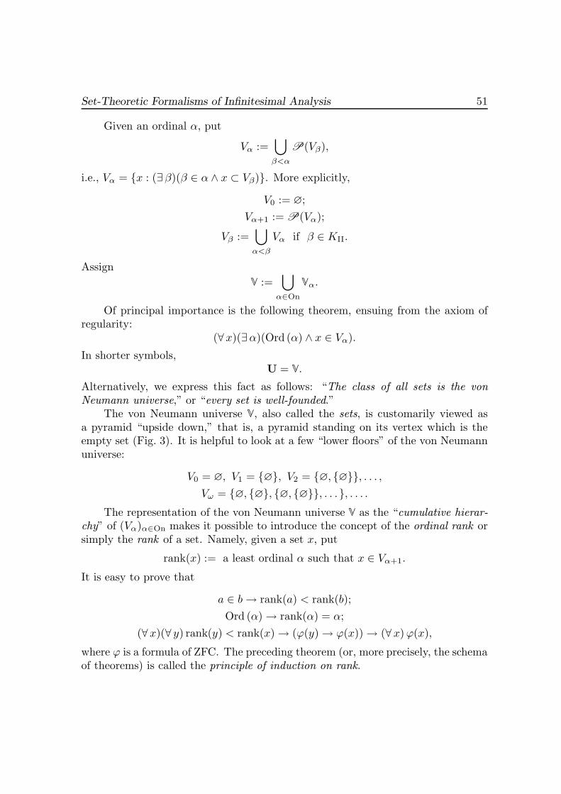
Set-Theoretic Formalisms of Infinitesimal Analysis 51
Given an ordinal α, put
Vα :=⋃
β<α
P(Vβ),
i.e., Vα = {x : (∃β)(β ∈ α ∧ x ⊂ Vβ)}. More explicitly,
V0 := ∅;Vα+1 := P(Vα);
Vβ :=⋃
α<β
Vα if β ∈ KII.
AssignV :=
⋃
α∈On
Vα.
Of principal importance is the following theorem, ensuing from the axiom ofregularity:
(∀x)(∃α)(Ord (α) ∧ x ∈ Vα).
In shorter symbols,U = V.
Alternatively, we express this fact as follows: “The class of all sets is the vonNeumann universe,” or “every set is well-founded.”
The von Neumann universe V, also called the sets, is customarily viewed asa pyramid “upside down,” that is, a pyramid standing on its vertex which is theempty set (Fig. 3). It is helpful to look at a few “lower floors” of the von Neumannuniverse:
V0 = ∅, V1 = {∅}, V2 = {∅, {∅}}, . . . ,Vω = {∅, {∅}, {∅, {∅}}, . . .}, . . . .
The representation of the von Neumann universe V as the “cumulative hierar-chy” of (Vα)α∈On makes it possible to introduce the concept of the ordinal rank orsimply the rank of a set. Namely, given a set x, put
rank(x) := a least ordinal α such that x ∈ Vα+1.
It is easy to prove that
a ∈ b → rank(a) < rank(b);Ord (α) → rank(α) = α;
(∀x)(∀ y) rank(y) < rank(x) → (ϕ(y) → ϕ(x)) → (∀x)ϕ(x),
where ϕ is a formula of ZFC. The preceding theorem (or, more precisely, the schemaof theorems) is called the principle of induction on rank.
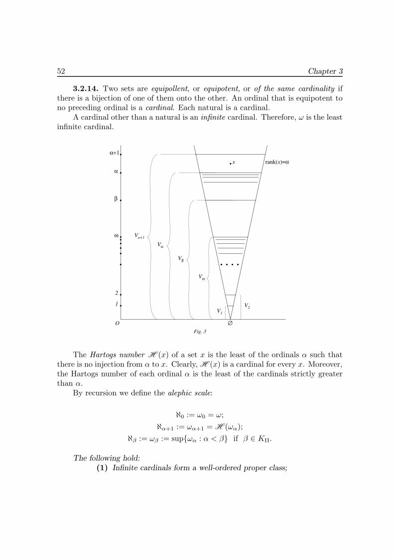
52 Chapter 3
3.2.14. Two sets are equipollent, or equipotent, or of the same cardinality ifthere is a bijection of one of them onto the other. An ordinal that is equipotent tono preceding ordinal is a cardinal. Each natural is a cardinal.
A cardinal other than a natural is an infinite cardinal. Therefore, ω is the leastinfinite cardinal.
V1
V2
Vω
Vβ
Vα
Va+1
x
O
1
2
rank(x)=α
ω
β
α
α+1
∅Fig. 3
The Hartogs number H (x) of a set x is the least of the ordinals α such thatthere is no injection from α to x. Clearly, H (x) is a cardinal for every x. Moreover,the Hartogs number of each ordinal α is the least of the cardinals strictly greaterthan α.
By recursion we define the alephic scale:
ℵ0 := ω0 = ω;ℵα+1 := ωα+1 = H (ωα);
ℵβ := ωβ := sup{ωα : α < β} if β ∈ KII.
The following hold:(1) Infinite cardinals form a well-ordered proper class;
Set-Theoretic Formalisms of Infinitesimal Analysis 53
(2) The mapping α �→ωα is an order isomorphism between the class ofordinals and the class of infinite cardinals;
(3) There is a mapping | · | from the universal class U onto the classof all cardinals such that the sets x and |x| are equipollent for allx ∈ U.
The cardinal |x| is called the cardinality or the cardinal number of a set x.Hence, each set is equipollent to a unique cardinal which is its cardinality.
A set x is countable provided that |x| = ω0 := ω, and x is at most countableprovided that |x| ≤ ω0.
Given an ordinal α, we denote by 2ωα the cardinality of P(ωα); i.e., 2ωα :=|P(ωα)|. This denotation is justified by the fact that 2x and P(x) are equipollentfor all x, with 2x standing for the class of all mappings from x to 2.
A theorem, proven by Cantor, states that |x| < |2x| for whatever set x. Inparticular, ωα < 2ωα for each ordinal α. Moreover, ωα+1 ≤ 2ωα .
The generalized problem of the continuum asks whether or not there areintermediate cardinals between ωα+1 and 2ωα ; i.e., whether or not the equalityωα+1 = 2ωα holds. For α = 0 this is the classical continuum problem.
The continuum hypothesis or CH is the equality ω1 = 2ω. Similarly, thegeneralized continuum hypothesis or GCH is the equality ωα+1 = 2ωα for all α ∈ On.
3.2.15. In the sequel we will make use of the following technical result ofprofound importance which is often called the reflection principle. In a sense, thisresult shows that all “particular” set-theoretic events happen to sets of boundedrank.
Montague–Levy Theorem. Let ϕ := ϕ(x1, . . . , xn) be a formula of ZFC.Take an ordinal α. Then there is an ordinal β such that β > α and
(∀x1, . . . , xn ∈ V β)ϕ(x1, . . . , xn) ↔ ϕVβ
(x1, . . . , xn),
where ϕVβ
is the relativization of ϕ to V β.
� Assume that the prenex normal form of ϕ looks as follows
ϕ = (Q1y1) . . . (Qmym)ψ(x1, . . . , xn, y1, . . . , ym).
In other words, ψ is quantifier-free and Qk ∈ {∃, ∀}.Put
ψk := (Qk+1yk+1) . . . (Qmym)ψ
for k := 0, . . . , m. With due precaution, it is possible to conclude that
ψk = ψk(x1, . . . , xn, y1, . . . , yk−1).
54 Chapter 3
Assigning a collection of unbound variables in ψk, find the least ordinal γ satisfying
(∃ yk)ψk → (∃ yk ∈ V γ)ψk
provided that Qk = ∃ and
(∃ yk)¬ψk → (∃ yk ∈ V γ)¬ψkprovided that Qk = ∀. Put
gk(x1, . . . , xn, y1, . . . , yk−1) := γ.
Given an ordinal α and using the axiom of replacement 3.2.5, find the set Ak(α) sothat
{gk(x1, . . . , xn, y1, . . . , yk−1) : x1, . . . , xn ∈ V α; y1, . . . , yk−1 ∈ V α} .Put
fk(α) := sup{α+ 1, (supAk(α)) + 1}.Using the so-constructed ordinal-valued functions, we successively put
f (0)(α) := α;
f (1)(α) := sup{f1(α), . . . , fm(α)};
f (s+1)(α) := f (1)(f (s)(α)) (s ∈ N).
And, finally,f(α) := sup
s∈N
f (s)(α).
Clearly, f(α) is a limit ordinal greater than α for all α. Moreover,
gk(x1, . . . , xn, y1, . . . , yk−1) < f(α)
for all x1, . . . , xn, y1, . . . , ym ∈ V f(α) and 1 ≤ k ≤ m.Putting β := f(α), considering that ψk−1 = (Qkyk)ψk, and using the definition
of gk, proceed successively as follows:
ψm = ψVβ
m
→ (ψm−1 ↔ (Qmym ∈ V β)ψm
)
→(ψm−1 ↔ ψV
β
m−1
)
→ · · · → ψ1 ↔ ψVβ
1
→ (Q1y1)ψ1 ↔ (Q1y1 ∈ V β)ψ1
→ ψ0 ↔ ψVβ
0
→ ϕ(x1, . . . , xn) ↔ ϕVβ
(x1, . . . , xn).
This ends the proof. �

Set-Theoretic Formalisms of Infinitesimal Analysis 55
Corollary. Let ϕ1, . . . , ϕm be formulas of ZFC whose unbound variables arelisted among x1, . . . , xn. Take α ∈ On. Then
(∃β > α)(∀x1, . . . , xn ∈ V β)(ϕ1 ↔ ϕVβ
1 ) ∧ · · · ∧ (ϕm ↔ ϕVβ
m ).
� Putting
ϕ(t, x1, . . . , xn) = (t = 1 ∧ ϕ1) ∨ (t = 2 ∧ ϕ2) ∨ · · · ∨ (t = m ∧ ϕm),
apply the above theorem. �
3.2.16. Study of various models of set theory often involves the ultrapowerconstruction. We now provide some details that will be needed to the reader whointends to elaborate formalities of the status of nonstandard set theories.
Assume that U is some set and ε is some relation on U . In the context of settheory, such a couple (U, ε) is often referred to as a universet or universoid. In thisevent, we will sometimes write xεy instead of (x, y) ∈ ε.
Let ϕ = ϕ(x1, . . . , xn) be a formula of ZFC. Interpret ε as membership andrestrict all quantifiers of ϕ to U . Assuming that ϕ(x1, . . . , xn) for x1, . . . , xn ∈ U ,we will write (U, ε) � ϕ(x1, . . . , xn) or ϕ(U,ε)(x1, . . . , xn) or even ϕU and speak ofthe relativization of ϕ to U . Other abbreviations are also popular.
Consider the power X := XE of some set X , where E is some index set (forthe sake of convenience, we assume X and E nonempty). Given x1, . . . , xn ∈ X andϕ = ϕ(x1, . . . , xn) ∈ (ZFC), put
[[ϕ(x1, . . . , xn)]] = {e ∈ E : ϕX(x1(e), . . . , xn(e))},
where ϕX is the relativization of ϕ to X .Assume further that F is a filter on E and
f ∼F g := [[f = g]] ∈ F (f, g ∈ X).
Denote the quotient set X/ ∼F by FX and let Ff stand for the coset of f .Clearly,
[[f ′εg′]] = [[f = f ′]] ∩ [[g = g′]] ∩ [[f ′εg′]]
for f ∼F f ′ and g ∼F g′.Therefore, [[fεg]] ∈ F ↔ [[f ′εg′]] ∈ F . In other words, we have soundly defined
on FX the following relation
Fε :={
(Ff, Fg) ∈ (FX)2 : [[fεg]] ∈ F}.
56 Chapter 3
It is easy to see thatFε =∼F ◦εX◦ ∼F
for some appropriate interpretation εX on X of the membership relation. We callFX the filtered power of X by F . If F is an ultrafilter then FX is the ultrapowerof X by F .
Given f, g ∈ X, from these definitions we infer that
Ff Fε Fg ↔ [[fεg]] ∈ F ;Ff = Fg ↔ [[f = g]] ∈ F .
In other words,(FX, Fε) � ϕFX(Ff, Fg) ↔ [[ϕ(f, g)]] ∈ F
for every atomic formula ϕ = ϕ(x, y) of ZFC.Given x ∈ X , put x(e) := x for all e ∈ E and ∗x := Fx. Note that ∗x = ∗y ↔
x = y and ∗x F∈ ∗y ↔ x ∈ y. It turns out that such effects are routine. To describethem, the following definition is in order.
Let ϕ = ϕ(x1, . . . , xn) be an arbitrary formula of ZFC. We say that ϕ is filtered(with respect to X, E , and F ) provided that
(FX, Fε) � ϕFX(Ff1, . . . ,Ffn) ↔ [[ϕ(f1, . . . , fn)]] ∈ F
for all f1, . . . , fn ∈ X.
�Los Theorem. Every formula of ZFC is filtered with respect to an arbitraryultrafilter.
� Since all atomic formulas are filtered, it suffices to check that the applicationof propositional connectives and quantification preserve filteredness. If ϕ is a filteredformula then ¬ϕ is filtered by the “golden” property of every ultrafilter: F ∈ F ↔F ′ := E − F �∈ F . We will thus establish the following (absolutely unavoidable)fact: If ψ(y) := (∀x)ϕ(x, y) and ϕ is filtered then so is ψ.
To this end, assume that [[ψ(y)]] ∈ F for y ∈ F and x ⊂ FX . Clearly,[[ψ(y)]] ⊂ [[ϕ(x, y)]] and so, (FX, Fε) � Fϕ(x, y). Since x is arbitrary, therefore,(FX, F∈) � (∀x)ϕF (x, y).
Assume finally that x, y ∈ FX implies ϕFX(x, y), i.e. [[ϕ(x, y)]] ∈ F . Check
that B := [[(∀x)ϕ(x, y)]] belongs to F as well. Indeed, to e ∈ E −B := B′ there issome x(e) satisfying ¬ϕ(x(e), y(e)). Take an arbitrary x0 in X. Put x(e) := x(e)whenever e ∈ B′ and x(e) := x0(e) otherwise. Obviously, [[ϕ(x, y)]] ⊂ E −B′ = B.Since [[ϕ(x, y)]] ∈ F , it follows that B ∈ F . The proof is complete. �
Set-Theoretic Formalisms of Infinitesimal Analysis 57
Corollary 1. Let X be a nonempty set and let ∗X be some ultrapower of X .Then
ϕX(x1, . . . , xn) ↔ ϕ∗X(∗x1, . . . , ∗xn)
for x1, . . . , xn ∈ X and ϕ ∈ (ZFC).
� By the Los Theorem ϕ∗X(∗x1, . . . , ∗xn) ↔ [[ϕ(x1, . . . , xn)]] ∈ F , where Fis the ultrafilter in question and xk(e) = (xk) for all e ∈ E . From the definitionof [[ · ]] it follows that [[ϕ(x1, . . . , xn)]] ∈ F ↔ ϕX(x1, . . . , xn), which completes theproof. �
Let X be an infinite set and let E stand for the cofinite filter on X whichconsists of the complements to X of finite subsets of X . Assume further that F issome ultrafilter finer than E . The ultrapower FX is a canonical enlargement of X ,denoted still by ∗X .
Corollary 2 (the weak idealization principle). Let ϕ = ϕ(x, y, x1, . . . , xn)be a formula of ZFC. Assume given elements x1, . . . , xn ∈ X and a canonicalenlargement ∗X of X . Then
(∀finA ⊂ X)(∃ b ∈ X)(∀ a ∈ A)ϕX(a, b, x1, . . . , xn)→ (∃ b ∈ ∗X)(∀ a ∈ A)ϕ∗X(∗a, b, ∗x1, . . . , ∗xn).
� To e ∈ E there is some b(e) in X satisfying (∀ a ∈ e)ϕX(a, b(e), x1, . . . ,xn). In other words, using b ∈ XE , we see that
[[ϕ(x, b, x1, . . . , xn)]] ⊂ {e ∈ E : a ∈ e}
where, as usual, y(e) := y for y ∈ X and e ∈ E .By the Los Theorem, ϕ∗X(∗a, Fb, ∗x1, . . . , ∗xn). This ends the proof. �Let Z be a nonempty subset of Z. This Z is a Zermelo subset of Z provided
that(a) Z is transitive in Z (i.e., a ∈ Z ∧ b ∈ Z ∧ a ∈ b → a ∈ Z);(b) Z is closed under unordered pairing;(c) a ∈ Z → ⋃
a ∈ Z ∧ P(a) ∈ Z.Let (Z, ε) be a universet. Assume given another universet (Z, ε) such that Z isa nonempty subset of Z and ε is the restriction of ε to E2. In this event (Z, ε) isa subuniverset of (Z, ε).
Assume that Z models a Zermelo subset of Z if ε is interpreted as membership.It this event Z is a Zermelo universet (in (Z, ε)). The indication of Z is oftenomitted when this leads to no confusion.
58 Chapter 3
Corollary 3. Let (X, ε) be a Zermelo universet and let ∗X be some ultrapower
of X . Assume further that X ∈ X, Y ∈ ∗X, and f : X → Y (i.e., f is an external
function), with Y := {y : y ∗X∈ Y }. Then there is some f in ∗X such that f is
a function from ∗X to Y inside (∗X) and, moreover, f(x) = f(∗x) for all x ∈ X .
� In case f = ∅, put f := ∅. If f �= ∅ then Y �= ∅. Assume that Y = FY0,where F is the ultrafilter in question on an appropriate direction E . In this event[[Y0 �= ∅]] = {e ∈ E : Y0 �= ∅} ∈ F . Redefining Y0(e), if need be, for e /∈ [[Y0 �= ∅]],we may assume that Y = FY and Y (e) �= ∅ for all e ∈ E .
Suppose that y ∈ Y and y = Fy. Clearly, [[y ∈ Y ]] ∈ F . Put h(y)(e) := y(e)for e ∈ [[y ∈ Y ]] and define h(y) at other values of e as, for instance, some memberof Y (e) ∈ X . What matters is the equality Fh(y) = y holding irrespectivelyof this choice. Given e ∈ E , define the function g(e) : X → Y (e) by the ruleg(e)(x) := h(f(x))(e) where x ∈ X . The set g(e) := {(x, g(e)(x)) : x ∈ X} is amember of X (since X is a Zermelo universet). We thus arrive at the element g ofXE satisfying g : e ∈ E �→ g(e) ∈ X. It is evident also that [[g : X → Y ]] = E . Thus,f := Fg is a function from ∗X to Y by the Los Theorem. To prove, we inspect theabove arguments and note that
f(x) = f(∗x) ↔ f(∗x) = Fh(f(x))
↔ [[g(x) = h(f(x))]] ∈ F
for x ∈ X .Moreover, by definition
g(x)(e) = g(e)(x) = h(f(x))(e)
for all e ∈ E , which finishes the proof. �3.2.17. To study deeper properties we need a more abstract procedure which
is known as the ultralimit construction. We give only a necessary minimum ofinformation on ultralimits.
Assume that (U, ε) is a universet and V := P(U). Proceed by putting
fU (u) := f(u) = {v ∈ U : (v, u) ∈ ε} (u ∈ U);E := {(A,B) ∈ V × V : (∃ a ∈ U)(A = f(a) ∧ a ∈ B)}.
Note that, given v ⊂ U , we infer by definition that
A ∈ f(v) ↔ (∃u ∈ v)(A = f(a)) ↔ (A, v) ∈ E.
In other words,f(v) = {A ∈ V : (A, v) ∈ E}.
The universet (V,E) is the protoextension of (U, ε).
Set-Theoretic Formalisms of Infinitesimal Analysis 59
3.2.18. Let (U, ε) be a universet satisfying the axiom of extensionality andlet (V,E) be the protoextension of (U, ε). Then
(1) (V,E) enjoys the axiom of extensionality;(2) f := fU : U → U is an injective mapping and
(f(u), f(v)) ∈ E ↔ (u, v) ∈ ε.
(3) (∀u ∈ U)(A, f(u)) ∈ E ↔ (∃ a)((a, u) ∈ ε ∧ A = f(a)) for allA ∈ V .
� (1): To check the axiom of extensionality in (V,E), take x, y ∈ V so that(∀ z ∈ V )(z, x) ∈ E → (z, y) ∈ E. We have to validate that x ⊂ y. Take w ∈ x, w ∈U . Then (f(w), x) ∈ E and so f(w) = f(w) and w ∈ y for some w ∈ U . However,we already know that w = w. Hence, (∀w ∈ U)w ∈ x → w ∈ y. We are done onrecalling that x, y ∈ P(U).
(2): Note that (u, v) ∈ ε amounts to u ∈ f(v). Hence, on using the validity ofthe axiom of extensionality for ε in U , we infer that
f(u) = f(v) → ((∀ z ∈ U) z ∈ f(u) ↔ z ∈ f(v))→ ((∀ z ∈ U)(z, u) ∈ ε ↔ (z, v) ∈ ε) → u = v.
Assuming now that (f(u), f(v)) ∈ E, by definition we see that f(a) = f(a) anda ∈ f(v) for some a ∈ U . Since a = u as proven; therefore, (u, v) ∈ ε. In turn, theimplication (u, v) ∈ ε → (f(u), f(v)) ∈ E is clear (and does not imply extensionalityin U) for we may take U as the element n that is requested by the definition of E.
(3): If (a, u) ∈ ε and A = f(a) then a ∈ f(u). Hence, (A, f(u)) ∈ E bydefinition. Conversely, from (2) we infer that
(A, f(u)) ∈ E → (∃ a ∈ U)A = f(a) ∧ a ∈ f(u)→ A = f(a) ∧ (f(a), f(u)) ∈ E → (a, u) ∈ ε ∧A = f(a),
which ends the proof. �Let (U, ε) be a universet satisfying the axiom of extensionality. Put U0 := U
and ε0 := ε. Using the above consecutively and granted (Uk, εk), assign
Uk+1 := P(Uk);fk(u) := {u ∈ Uk : (u, U) ∈ εk} (u ∈ Uk);
εk+1 := {(u, v) ∈ Uk+1 × Uk+1 : (∃ a ∈ Uk)(u = fk(a) ∧ a ∈ v)}.We thus acquire the sequence of injections
U0f1−→ U1
f2−→ U2 → · · · → Unfn+1−→ Un+1 → . . .
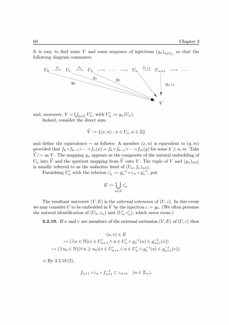
60 Chapter 3
It is easy to find some V and some sequence of injections (gn)n∈Z+so that the
following diagram commutes:
U0f1−→ U1
g0
f2−→ U2
g1
−→ · · ·g2
−→ Unfn+1−→ Un+1
gn+1
−→ · · ·
V
and, moreover, V =⋃n∈Z
U ′n, with U ′n := gn(Un).Indeed, consider the direct sum
V := {(x, n) : x ∈ Un, n ∈ Z}
and define the equivalence ∼ as follows: A member (x, n) is equivalent to (y,m)provided that fk ◦fk−1 ◦ · · ·◦fn(x) = fk ◦fk−1 ◦ · · ·◦fm(y) for some k ≥ n,m. TakeV /∼ as V . The mapping gn appears as the composite of the natural embedding ofUn into V and the quotient mapping from V onto V . The tuple of V and (gn)n∈Z
is usually referred to as the inductive limit of (Un, fn)n∈Z.Furnishing U ′n with the relation ε′n := g−1
n ◦ εn ◦ g−1n , put
E :=⋃
n∈Z
ε′n.
The resultant universet (V,E) is the external extension of (U, ε). In this eventwe may consider U to be embedded in V by the injection ι := g0. (We often presumethe natural identification of (Un, εn) and (U ′n, ε′n), which saves room.)
3.2.19. If u and v are members of the external extension (V,E) of (U, ε) then
(u, v) ∈ E
↔ (∃n ∈ N)(v ∈ U ′n+1 ∧ u ∈ U ′n ∧ g−1n (u) ∈ g−1
n+1(v))
↔ (∃n0 ∈ N)(∀n ≥ n0)(v ∈ U ′n+1 ∧ u ∈ U ′n ∧ g−1n (u) ∈ g−1
n+1(v)).
� By 3.2.18 (2),
fn+1 ◦ εn ◦ f−1n+1 ⊂ εn+1 (n ∈ Z+).

Set-Theoretic Formalisms of Infinitesimal Analysis 61
Hence,
gn ◦ εn ◦ g−1n = (gn+1 ◦ fn+1) ◦ εn ◦ (f−1
n+1 ◦ g−1n+1)
= gn+1 ◦ (fn+1 ◦ εn ◦ f−1n+1) ◦ g−1
n+1 ∈ gn+1 ◦ εn+1 ◦ g−1n+1.
We may thus assume that
(u, v) ∈ E ↔ (∃n ∈ N)(u, v) ∈ gn+1 ◦ εn+1 ◦ g−1n+1.
In this event, we also have
(u, v) ∈ gn+1 ◦ εn+1 ◦ g−1n+1
for all n ≥ n0.Clearly, v = gn+1(v) where v := g−1
n+1(v) ∈ Un+1; and u = gn+1(u) whereu := g−1
n+1(v). Moreover, uεn+1v and v ∈ Un+1, i.e. v = fn+1(a) for some a ∈ vn.Therefore, (u, fn+1(a)) ∈ εn+1. Consequently, from 3.2.18 (3) it follows that u =fn+1(u) for some u ∈ Un. Hence, u = gn+1(u) = gn+1(fn+1)(u) = gn(u) ∈ U ′n.Since (fn+1(u), v) ∈ εn+1; therefore, u ∈ v by the definition of εn+1. We are doneon observing that g−1
n (u) = u and g−1n+1(v) = v. �
3.2.20. Let (V,E) be an external extension of a universet (U, ε) enjoying theaxiom of extensionality. Then
(1) (V,E) � the axiom of extensionality;(2) (V,E) � the axiom of pairing;(3) (V,E) � the axiom of union;(4) (V,E) � the axiom of powerset;(5) (V,E) � the axiom-schema of comprehension;(6) (V,E) � the axiom of choice;(7) (V,E) � the axiom of the empty set;(8) (V,E) � the axiom of infinity;(9) (∀ a, b ∈ U)((a, b) ∈ ε) ↔ (ι(a), ι(b)) ∈ E;
(10) (∀x, y ∈ V )((x, y) ∈ E ∧ y ∈ ι(U) → x ∈ ι(U));(11) (∀U ⊂ U)(∃U ∈ V )(∀ v ∈ V )((v, U) ∈ E ↔ v ∈ ι(U)).
� (1): From 3.2.18 (1) and the induction principle in (Un, εn) we see the validityof the axiom of extensionality. It suffices to note the restriction of E to U ′n × U ′ncoincides with ε′n for all n ∈ Z+.
(2): Assume that u, v ∈ U ′n with u = gn(x) and v = gn(y). The unorderedz := {x, y} is a member of Un+1. Hence, w := gn+1(z) is a member of U ′n+1.Clearly, (z, w) ∈ E ↔ z = u ∨ z = v.
62 Chapter 3
(3): Take u ∈ V . We may assume that u = gn+2(x) and x ∈ Un+2. Put
y :=⋃
{fn+1(z) : z ∈ fn+2(x), z ∈ Un+1}.
Clearly, y ∈ Un+1. Assigning v := gn+1(y), note that
(w, v) ∈ E ↔ (∃ κ)(κ, v) ∈ E ∧ (w,κ) ∈ E
for w ∈ V .Indeed, if a ∈ Un+1 then
a ∈ y ↔ ((∃ z ∈ Un+1)z ∈ fn+2(x)) ∧ a ∈ fn+1(z)↔ (z, x) ∈ εn+2 ∧ (a, z) ∈ εn+1.
We are done on appealing to 3.2.19.(4): Take u ∈ V and let u = gn(x), with x ∈ Un. Put A := {y ∈ Un : fn+1(y) ⊂
fn+1(x)}. Check that the set v := gn+2(A) plays the role of the powerset of u inside(V,E). To this end, observe first of all that
fn+1(y) ⊂ fn+1(x) ↔ (∀ z ∈ V )(z, gn+1(fn+1(y)) ∈ E → (z, u) ∈ E
↔ (V,E) � gn(y) is a subset of x.
Given a ∈ V , we thus infer that
(a, v) ∈ E ↔ (a, gn+1(A)) ∈ E
↔ ((∃ a ∈ A)(a = gn(a)) ↔ (∃ y ∈ Un) a = gn(y) ∧ fn+1(y) ⊂ fn+1(x)↔ (∃ z ∈ V ) a = Z ∧ (V,E) � z is a subset of v
↔ (V,E) � a is a subset of v.
(5): Assume that ϕ = ϕ(x, y) ∈ (ZFC) and u, y ∈ V . Assume also thatu = gn+1(x) and put A := {z ∈ fn+1(x) : ϕ(gn(z), y)}. Clearly, A ∈ Un+1. Assignv := gn+1(A). In this event
(a, v) ∈ E ↔ (∃ z ∈ Un)a = gn(z) ∧ z ∈ A
↔ (∃ z ∈ Un)z ∈ fn+1(x) ∧ a = gn(z) ∧ ϕ(gn(z), y)↔ (a, u) ∈ E ∧ ϕ(a, y)
for a ∈ U .
Set-Theoretic Formalisms of Infinitesimal Analysis 63
(6): Assume that u = gn+1(x) and put
A := {z ∈ Un : z ∈ fn+1(x) ∧ fn+1(z) �= ∅}.There is a choice function ψ : A → Un+1 such that ψ(z) ∈ fn+1(z) for all z ∈ A.The set ψ is a member of Un+3. Put f := gn+3(ψ). It is easy to see that f playsthe role of a function inside (V,E), satisfying
(∀ v ∈ V )(v, y) ∈ E ∧ v �= 0) → (f(v), y) ∈ E.
It is such an element f that we have to demonstrate.(7)–(10): These are beyond a doubt.(11): Take g1(U) as U (which is sound since U ∈ U1). By (4) (v, U) ∈ ι ↔
(∃u ∈ U0)v = ι(u) ∧ u ∈ U . In other words, (v, U) ∈ E ↔ v ∈ ι(v). �3.2.21. Comments.
(1) Zermelo suggested in 1908 an axiomatics that coincides practicallywith ZF1–ZF3, ZF5, 3.2.5, and 3.2.6. This system, together with the Russell theoryof types, is listed among the first formal axiomatics for set theory.
The axioms of extensionality ZF1 and union ZF2 were proposed earlier byFrege (1883) and Cantor (1899). The idea of the axiom of infinity ZF5 belongs toDedekind.
(2) The axiom of choice AC seems to be in use implicitly for a longtime before it was distinguished by Peano in 1890 and Levy in 1902. This axiomwas formally introduced by Zermelo in 1904 and remained most disputable formany years. The axiom of choice is part and parcel of the most vital fragmentsof contemporary mathematics. So, it is no wonder that AC is accepted by theoverwhelming majority of working mathematicians. Discussions of the place androle of the axiom of choice may be found elsewhere [62, 123, 130, 196, 316].
(3) The axiomatics of ZFC was completely elaborated at the beginningof the 1920s. By that time the formalization of the set-theoretic language hadbeen completed, which made it possible to clarify the vague description of the typeof properties admissible in the axiom of comprehension. On the other hand, theZermelo axioms do not yield the claim of Cantor that each bijective image of a setis a set. This drawback was obviated by Fraenkel in 1922 and Scolem in 1923 whosuggested variations of the axiom of replacement. This moment seems to pinpointthe birth of ZFC.
(4) The axiom of regularity ZF6 was in fact suggested by von Neumannin 1925. This axiom is independent of the other axioms of ZFC.
(5) The system of axioms of ZFC is infinite as noted in 3.2.4. Absenceof finite axiomatizability for ZFC was proven by Montague in 1960 (see [123, 155,316, 516]).
64 Chapter 3
3.3. Nelson Internal Set Theory
The preliminary analysis of the properties of standard and nonstandard setshas shown that the von Neumann universe, if furnished with the predicate “to beor nor to be standard,” has ample room for infinitesimals but fails to accommo-date their monad, them all “viewed as one.” In other words, infinitesimal analysisdemonstrates that Zermelo–Fraenkel set theory, describing the classical world of“standard” mathematics, distinguishes only some internal part of the cantorianparadise, the universe of naive sets.
To emphasize this peculiarity, the nonstandard theory of sets we start present-ing refers to the elements of the von Neumann universe as internal sets. Therefore,a set in the sense of Zermelo–Fraenkel set theory and an internal set are synonyms.
A convenient foundation for infinitesimal analysis is given by the so-calledinternal set theory suggested by Nelson and abbreviated to IST.
3.3.1. The alphabet of IST results from the alphabet of ZFC by adjoining theonly one new symbol of the unary predicate St expressing the property of a set tobe or not to be standard.
In other words, the texts of IST may contain fragments of the type St(x) whichreads as “x is standard” or “x is a standard set.” Therefore, the semantic domainof definition for variables of IST is the world of Zermelo–Fraenkel set theory; i.e.,the von Neumann universe in which we can now discriminate between standard andnonstandard sets.
3.3.2. The formulas of IST are defined routinely on enriching the collectionof atomic formulas with the texts like St(x) where x is a variable. Each formula ofZFC is a formula of IST, whereas the converse is obviously false. To discriminatebetween the formulas of IST, we call the formulas of ZFC internal. By an externalformula, we mean a formula IST not expressible in ZFC. For instance, the text “xis standard” is an external formula of IST.
For ecological reasons, we use the following convenient abbreviations: To sig-nify that ϕ is a formula of IST, we write ϕ ∈ (IST); similarly, ϕ ∈ (ZFC) meansthat ϕ is an internal formula of IST.
3.3.3. The distinction between the formulas of IST leads naturally to thenotions of external and internal classes. If ϕ is an external formula of IST thenwe read the text ϕ(y) as follows: “y is an element of the external class {x : ϕ(x)}.”The term internal class implies the same as the term class in ZFC. We usuallyspeak simply of classes when this leads to no confusion.
3.3.4. An external class consisting of elements of some internal set x is anexternal set or, in more detail, an external subset of x. It is worth noting thateach internal class consisting of elements of some internal set is an internal set too.
Set-Theoretic Formalisms of Infinitesimal Analysis 65
Alongside the abbreviations of ZFC, the theory IST maintains some additionalagreements. We list a few of them are concluded. A list of them follows:
Vst := {x : St(x)} is the external class of standard sets;x ∈ Vst := x is standard := (∃ y)(St(y) ∧ y = x);
(∀ stx)ϕ := (∀x)(x is standard → ϕ);(∃ stx)ϕ := (∃x)(x is standard ∧ ϕ);(∀ st finx)ϕ := (∀ stx)(x is finite → ϕ);(∃ st finx)ϕ := (∃ stx)(x is finite ∧ ϕ);
◦x := {y ∈ x : y is standard}.
The external set ◦x is often called the standard part or standard core of x. Observeconspicuous collision of notations and outright abuse of the language since ◦x, withx ∈ ≈
R, denotes the value of the standard part operation at x as well as thestandard part of x as a set. Fortunately, these convenient collision and abuse areharmless, leading to confusion rarely if ever.
3.3.5. The list of axioms of IST includes all those of ZFC and three new axiom-schemata which are known collectively as the principles of nonstandard set theoryor, which slightly abuses the language, the principles of infinitesimal analysis.
(1) Transfer Principle:
(∀ stx1)(∀ stx2) . . . (∀ stxn)((∀ stx)ϕ(x, x1, . . . , xn)→ (∀x)ϕ(x, x1, . . . , xn))
for every internal formula ϕ;(2) Idealization Principle:
(∀x1)(∀x2) . . . (∀xn)((∀ st finz)(∃x)(∀ y ∈ z)ϕ(x, y, x1, . . . , xn)↔ (∃x)(∀ sty)ϕ(x, y, x1, . . . , xn)),
where ϕ ∈ (ZFC) is an arbitrary internal formula;(3) Standardization Principle:
(∀x1) . . . (∀xn)((∀ stx)(∃ sty)(∀ stz)(z ∈ y) ↔ (z ∈ x ∧ ϕ(z, x1, . . . , xn)))
for every (possibly external) formula ϕ.

66 Chapter 3
3.3.6. Powell Theorem. IST is conservative over ZFC.� Assume that ϕ is a formula of ZFC, ϕ = ϕ(x1, . . . , xn), and ϕ is proven
in IST. Assume further that the proof of ϕ uses the axioms ψ1, . . . , ψm of ZFC. Bythe Montague–Levy Theorem there is an ordinal α such that
ϕ(x1, . . . , xn) ↔ ϕVα
(x1, . . . , xn) ∧ ψVα
1 ∧ · · · ∧ ψVα
m
for all x1, . . . , xn ∈ V α.Put U0 := V α and ε0 :=∈ |V α×V α . Take Pfin(U0) as E and let F be some
ultrafilter finer than the tail filter of Pfin(U0). Denote the resulting ultrapower (=enlargement) of U0 by U1 and let ι1 : U0 → U1 stand for the canonical embeddingof U0 into U1. Repeating this construction successively, put Un+1 := Un
Pfin(U0)/Fand let ιn+1 : Un → Un+1 be the canonical embedding of Un into the ultrapow-er Un+1. Identifying Un and ιn+1(Un), consider Un as a subset of Un+1. PutU :=
⋃n∈Z
Un and ε :=⋃n∈Z
εn, where εn+1 := ιn ◦ εn ◦ ιn+1 is the appropriateinterpretation of membership. Assume further that ∗ : U0 → U stands for thecanonical embedding of U0 into U . Treat the predicate St(·) as membership in{∗u : u ∈ U0}. Since x ∈ V α → (∃β ∈ α) x ∈ V β → P(x) ∈ V β , conclude that thestandardization principle holds in U . Validity of the principles of transfer and ide-alization follows from the Los Theorem. Therefore, ψs1, . . . , ψ
sm and the principles
of IST are satisfied in (U, ε), implying that ϕU (∗x1, . . . , ∗xn) and ϕVα
(x1, . . . , xn).Consequently, ϕ holds in the von Neumann universe. �
3.3.7. The above theorem implies that the internal theorems of IST are the-orems of ZFC. In other words, proving “standard” theorems on sets we may usethe formalism of IST with the same feeling of reliability as we enjoy in ZFC. Atthe same time, we should always bear in mind that the ultimate foundation ZFCresides in the long run in its practical infallibility and semantic justification.
3.3.8. Pondering over the meaning of the formal records of the axioms ofIST, we cannot help but notice that the idealization principle looks somewhatcumbersome. While the principles of transfer and standardization in their formaldisguise adequately reflect the naive conception, put forward earlier, the formalexpression of the idealization principle may drive the reader in a quandary. Toclear the coast, we start with proving that idealization principle as stated in 3.3.5 (2)guarantees the presence of nonstandard elements.
3.3.9. There is a finite internal set containing every standard set.� Consider the following formula: ϕ := (x is finite ∧ (y ∈ x)). Note that
ϕ ∈ (ZFC). Given a standard finite z, we may find an element x such that ϕ(x, y)for all y ∈ z. Indeed, z may serve as such an x. We then complete the proof byidealization. �
Set-Theoretic Formalisms of Infinitesimal Analysis 67
3.3.10. When applying the idealization principle, we should bear in mindclearly that those finite sets are standard whose every element is standard. Thisfact was proved earlier, cf. 2.2.2. It is instructive to inspect the available formalinference which proceeds also by idealization.
3.3.11. If A is an internal set then
A = ◦A ↔ (A is standard) ∧ (A is finite).
� Look at the formula ϕ := x ∈ A ∧ x �= y. Clearly, ϕ ∈ (ZFC). Proceed byidealization as follows:
(∀ st finz)(∃x)(∀ y ∈ z)ϕ(x, y, A) ↔ (∃x)(∀ sty)(x ∈ A ∧ x �= y)↔ (∃x ∈ A)(x is nonstandard) ↔ A− ◦A �= ∅.
In other words,
A = ◦A ↔ (∃ st finz)(∀x)(∃ y ∈ z) x /∈ A ∨ x = y
↔ (∃ st finz)(∀x ∈ A)(∃ y ∈ z) x = y ↔ (∃ st finz)A ⊂ z,
which completes the proof. �3.3.12. Construction Principle. Assume that X and Y are standard sets,
while ϕ=ϕ(x, y, z) is a formula of IST. Then
(∀ stx)(∃ sty)(x ∈ X → y ∈ Y ∧ ϕ(x, y, z))↔ (∃ sty( · ))(∀ stx)(y( · ) is a function from X in Y
∧(x ∈ X → ϕ(x, y(x), z))).
� Consider the standardization F (x) := ∗{y ∈ Y : ϕ(x, y, z)}. Applying3.3.5 (3) again, arrange the standard set
F := ∗{(x,A) ∈ X × P(Y ) : F (x) = A},which is sound since P(Y ) is standard whenever so is Y . By hypothesis, (∀ stx ∈X)F �= ∅ and so. In this case, F (x) = F (x) by the definition of F . Consequently,
((∀ stx ∈ X)(F (x) �= ∅)) → ((∀x ∈ X)(F (x) �= ∅))
by transfer. Appealing now to the axiom of choice, conclude that
(∃ y( · ))(y( · ) is a function from X to Y ) ∧ (∀x ∈ X)(y(x) ∈ F (x)).
By transfer, there is a standard function y( · ) from X to Y satisfying y(x) ∈ F (x)for all x ∈ X . Recalling the definition of F once again, observe that y( · ) is a soughfunction. �
68 Chapter 3
3.3.13. In what follows (as well as precedes) we find it convenient to use somesymbolic records of the rules collected in the above propositions, deliberately butslightly abusing the language. For instance, the construction principle 3.3.12 maybe rewritten as
(1) (∀ stx)(∃ sty)ϕ(x, y) ↔ (∃ sty( · ))(∀ stx)ϕ(x, y(x)),(2) (∃ stx)(∀ sty)ϕ(x, y) ↔ (∀ sty( · ))(∃ stx)ϕ(x, y(x)),
where ϕ ∈ (IST). In other words, we will neglect the possible presence of unboundvariables in ϕ and the assumption that all quantifiers must be bounded whichimplies that x and y are assumed to range over some standard sets that are specifiedin advance. Similarly, if ϕ = ϕ(x1, . . . , xn) and ψ = ψ(y1, . . . , yn) then we will writeϕ ↔ ψ whenever
(∀ stx1) . . . (∀ stxn)(∀ sty1) . . . (∀ styn)ϕ(x1, . . . , xn) ↔ ψ(y1, . . . , yn),
and say that ϕ and ψ are equivalent (although if one of the formulas ϕ and ψ isexternal then the formulas ϕ(x1, . . . , xn) and ψ(y1, . . . , yn) are not equivalent forsome assignment of variables). Using these agreements, we will express the transferprinciple in reduced form
(3) (∀ stx)ϕ(x) ↔ (∀x)ϕ(x),(4) (∃ stx)ϕ(x) ↔ (∃x)ϕ(x),
always keeping in mind that ϕ must be an internal formula: ϕ ∈ (ZFC).It is reasonable also to write down a few elementary rules valid for every ϕ:(5) (∀x)(∀ sty)ϕ(x, y) ↔ (∀ sty)(∀x)ϕ(x, y),(6) (∃x)(∃ sty)ϕ(x, y) ↔ (∃ sty)(∃x)ϕ(x, y),
as well as some new records of the idealization principle:(7) (∀ st finz)(∃x)(∀ y ∈ z)ϕ(x, y) ↔ (∃x)(∀ sty)ϕ(x, y),(8) (∃ st finz)(∀x)(∃ y ∈ z)ϕ(x, y) ↔ (∀x)(∃ sty)ϕ(x, y),
which apply, obviously, only ϕ ∈ (ZFC).
3.3.14. These rules allow us to translate many (but definitely not all) conceptsand statements of infinitesimal analysis into equivalent definitions and theorems freefrom the notion of “standardness.” In other words, the formulas of IST express-ing “something unusual” about standard objects can be translated into equivalentformulas of ZFC which are in mathematical parlance. The procedure yielding thisresult is the Nelson algorithm or reduction algorithm which rests essentially on3.3.13 (1)–(8). The essence of this “decoding” algorithm is in using standard func-tions, idealization and transposition of quantifiers for reducing the expression understudy to a form more suitable for transfer. This translation amounts ultimately toelimination of the external notion of standardness. It is worth observing that eachcase of application of the formulas of 3.3.13 requires ensuring the hypotheses oftheir validity.
Set-Theoretic Formalisms of Infinitesimal Analysis 69
3.3.15. The Nelson algorithm consists of the following steps:(1) Rewrite a proposition of infinitesimal analysis as a formula ψ of
IST; i.e., decode all abbreviations;(2) Reduce the formula ψ of step (1) to the prenex normal form
(Q1x1) . . . (Qnxn)ϕ(x1, . . . , xn),
where Qk ∈ {∀, ∃, ∀ st, ∃ st} for k := 1, . . . , n and the matrix ϕ of ψis a formula of ZFC;
(3) In case Qn is an “internal” quantifier, i.e., ∀ or ∃; proceed byputting ϕ := (Qnxn)ϕ(x1, . . . , xn) and return to step (2);
(4) If Qn is an “external” quantifier, i.e., ∀ st or ∃ st; search the prefix(Q1x1) . . . (Qnxn) from right to left until the first internal quantifieris found;
(5) In case there is no internal quantifiers in step (4); replace the quan-tifier Qn with the corresponding internal quantifier (by 3.3.13 (3)and 3.3.13 (4)), and return to step (2), i.e., delete all superscriptsst in right-to-left order;
(6) Let Qm be the first internal quantifier encountered. Suppose thatQm+1 is an external quantifier of the same type as Qm (i.e., Qm = ∀and Qm+1 = ∀ st, or Qm = ∃ and Qm+1 = ∃ st). Transpose thequantifies by 3.3.13 (5) and 3.3.13 (6) and return to step (2);
(7) In case all the quantifiers Qm+1, . . . , Qn are of the same type, applythe idealization principle in the form 3.3.13 (7) or 3.3.13 (8), andreturn to step (2);
(8) In case the quantifiers alternate; i.e., Qp+1 is of the same type asQm while all quantifiers Qm+1, . . . , Qp are of the opposite type,apply 3.3.13 (1) or 3.3.13 (2), on assuming x := (xm+1, . . . , xp) andy := xp+1. After that return to step (2).
3.3.16. Note that an arbitrary assertion is expressible in various forms someof which can be absolutely incomprehensible. Hence, implementing the Nelsonalgorithm in practice, we must seize all possibilities of accelerating the procedure of“dragging out the external quantifiers.” In particular, it is wise sometimes to skipor leave unfinished step 3.3.15 (2). We will demonstrate this by example.
3.3.17. Examples.
(1) Infinitesimal analysis enjoys the external induction principle:
(ϕ(1) ∧ ((∀n ∈ ◦N)(ϕ(n) → ϕ(n+ 1)))) → (∀n ∈ ◦N)ϕ(n)
for every ϕ ∈ (IST).
70 Chapter 3
� The formula ϕ may be external, which prevents us from applying the Nelsonalgorithm directly to the formal record of the external induction principle.
So, consider the standardization A := ∗{n ∈ N : ϕ(n)}. Obviously, 1 ∈ A, andn+ 1 ∈ A for every standard n ∈ A.
We must prove that ◦N ⊂ A. For this purpose, write down the formula inquestion and apply the Nelson algorithm to it:
(1 ∈ A ∧ (∀ stn ∈ N)(n ∈ A → (n+ 1) ∈ A)) → ◦N ⊂ A
↔ (∀ stm)(∀ stn)(m ∈ N ∧ n ∈ N ∧ 1 ∈ A ∧ n ∈ A → (n+ 1) ∈ A)
→ m ∈ A ↔ (1 ∈ A ∧ (∀n ∈ N)(n ∈ A → (n+ 1) ∈ A)) → N ⊂ A,
which completes the proof. �
(2) The sum of infinitesimals is an infinitesimal too.
� (∀ s ∈ R)(∀ t ∈ R)(s ≈ 0 ∧ t ≈ 0 → s+ t ≈ 0)
↔ (∀ s ∈ R)(∀ t ∈ R)(s ≈ 0 ∧ t ≈ 0 → (∀ stε > 0)(|s+ t| < ε))
↔ (∀ stε > 0)(∀ s ∈ R)(∀ t ∈ R)(∀ stδ1 > 0)
(∀ stδ2 > 0)(|s| < δ1 ∧ |t| < δ2 → |s+ t| < ε)
↔ (∀ stε > 0)(∀ s ∈ R)(∀t ∈ R)(∃ stδ1 > 0)(∃ stδ2 > 0)(|s| < δ1
∧|t| < δ2 → |s+ t| < ε) ↔ (∀ stε)(∀ s) (∀ t)(∃ stδ1)(∃ stδ2)(ε > 0
∧ · · · ∧ δ2 > 0 ∧ |s| < δ1 ∧ |t| < δ2 → |s+ t| < ε)
↔ (∀ stε)(∀ s)(∀ t)(∃ stδ1)(∃ stδ2)(|s| < δ1 ∧ |t| < δ2 → |s+ t| < ε)
↔ (∀ stε)(∃ st finΔ1)(∃ st finΔ2)(∀ s) (∀ t)(∃ δ1 ∈ Δ1)(∃ δ2 ∈ Δ2)
(|s| < δ1 ∧ |t| < δ2 → |s+ t| < ε)
↔ (∀ stε)(∃ stδ1)(∃ stδ2)(∀ |s| < δ1)(∀ |t| < δ2)(|s+ t| ≤ ε)
↔ (∀ ε > 0)(∃ δ > 0)(∀ |s| < δ)(∀ |t| < δ)(|s+ t| ≤ ε). �
(3)Robinson Lemma. Let (an) be an internal numerical sequence, and an ≈0 for all n ∈ ◦N. Then there is an index N ≈ +∞ such that an ≈ 0 for all n ≤ N .
Set-Theoretic Formalisms of Infinitesimal Analysis 71
� Apply the Nelson algorithm to the conclusion:
(∃N ≈ +∞)(∀n ≤ N)(an ≈ 0)↔ (∃N ∈ N)((∀ stm ∈ N)((N ≥ m) ∧ (∀n ∈ N)(n ≤ N))
→ (∀ stε > 0)|an| < ε) ↔ (∃N)(∀ stm)(∀ stε)(∀n)(N ≥ m ∧ (n ≤ N → |an| < ε))
↔ (∀ st{m1, . . . , mp})(∀ st{ε1, . . . , εp})(∃N)(∀ k := 1, . . . , p)(N ≥ mk ∧ n ≤ N → |an| < εk)
↔ (∀ stm)(∀ stε)(∃N)(N ≥ m ∧ (n ≤ N → |an| < ε))↔ (∀ stm)(∀ stε)(m ∈ N ∧ ε > 0 → |am| < ε).
Proceed with applying the Nelson algorithm to the premise of the claim:
(∀n ∈ ◦N)(an ≈ 0) ↔ (∀ stn)(n ∈ N → (∀ stε > 0)(|an| < ε))↔ (∀ stn)(∀ stε)(n ∈ N ∧ ε > 0 → |an| < ε).
Clearly, the premise and conclusion are equivalent. �(4) Unique Determination Principle. Unique determination implies stan-
dardness in the standard environment.In symbols, if y, V ∈ VSt and ϕ = ϕ(x, y) is an arbitrary (possibly external)
formula of IST then((∃! x ∈ V )ϕ(x, y)) → St(x).
� Using the Nelson algorithm, rewrite ϕ as
ϕ(x, y) := (∀Stu)(∃Stv)ψ(x, u, v, y),
with ψ ∈ (ZFC).In particular, by the construction principle,
(∃Stv (·))(∀Stu)ψ(x, u, v(u), y). (1)
Moreover,(∀ z)(∀Stu ∃Stvψ(z, u, v, y) → z = x).
Using the Nelson algorithm, infer
(∀stv (·))(∃st finU)(∀ z)(((∀u ∈ U)ψ(z, u, v(u), y)) → z = x). (2)
Denote by U the standard finite set that corresponds by (2) to the function v(·)of (1).
Clearly, (∀u ∈ U)ψ(x, u, v(u), y) and so (∃ z)(∀u ∈ U)ψ(z, u, v(u), y). Bytransfer,
(∃Stz)(∀u ∈ U)ψ(z, u, v(u), y).
Using (2), conclude that z = x, i.e., St(x). �
72 Chapter 3
3.3.18. Alongside the theory IST by Nelson we will use some variation of thistheory, the so-called bounded (or limited) set theory BST, that was suggested byKanoveı and Reeken in [213].
The theory BST preserves the alphabet and related attributes of IST. Distinc-tions appear only in the formulation of the principles of nonstandard set theory.Moreover, the principles of transfer and standardization of IST are still valid inBST. However, the theory BST considers each internal set as included in somestandard set, implying due restrictions on the process of idealization:
(1) Boundedness Principle:
(∀x)(∃ stX)(x ∈ X);
(2) Bounded Idealization Principle:
(∀x1)(∀x2) . . . (∀xn)((∀ st finz)(∃x ∈ z0)(∀ y ∈ z)ϕ(x, y, x1, . . . , xn) ↔ (∃x ∈ z0)(∀ sty)ϕ(x, y, x1, . . . , xn)),
where ϕ ∈ (ZFC) is an internal formula and z0 is some standard set.Kanoveı and Reeken proved that the bounded idealization principle may be
replaced with the following(3) Internal Saturation Principle:
(∀x1)(∀x2) . . . (∀xn)((∀ st finz ⊂ z0) (∃x)(∀ y ∈ z)ϕ(x, y, x1, . . . , xn)↔ (∃x)(∀ sty ∈ z0)ϕ(x, y, x1, . . . , xn)),
where ϕ ∈ (ZFC) is an internal formula and z0 is some standard set.The most important property of BST is the fact that the bounded or limited
universe, comprising the members of all standard set in IST, serves as a model forBST. This implies that BST is conservative over ZFC.
3.4. External Set Theories
The basic principles of infinitesimal analysis are adequately reflected in theformal apparatus of Nelson internal set theory. The Powell Theorem enables usto view IST as a technique of studying the von Neumann universe. At the sametime, the presence of external objects completely undermines the popular belief thatthe formalism of Zermelo–Fraenkel set theory brings about a sufficient freedom ofoperation from the viewpoint of the naive set theory.
Residing in the realm of IST, we are not is a position even to raise such aninnocent question as: “Is it possible to distinguish some set of reals such that eachelement of R will admit a unique expansion in a linear combination of them with
Set-Theoretic Formalisms of Infinitesimal Analysis 73
standard coefficients, since R may be naturally viewed as a vector space over ◦R?”The amount of these inadmissible questions, undoubtedly mathematical from thesemantic point of view, is great to the extent that makes the necessity of trespassingthe frontiers of IST vital.
A priori prohibition against formulating problems is nothing but blindfoldingthe mind. The introduction of an ad hoc dogma, an “explicitly expressed prohibi-tion against thinking” (as was aphoristically remarked by Feuerbach) is absolutelyunacceptable in searching truth. A practical solution of the problem of returningto the cantorian paradise lies, in particular, in designing a formalism that wouldallow us to use the conventional means for working with sets that are external tothe von Neumann universe. We now start reviewing some axiomatic approaches toexternal sets.
The first version of an appropriate formalism was suggested by Hrbacek in hisexternal set theory abbreviated as EXT. A close version, nonstandard set theoryNST, was propounded later by Kawai. Semantically speaking, these set theoriesdemonstrate that the external universe is constructed in much the same way as theuniverse of naive sets as viewed from the standpoint of a pragmatic philistine whichthe working mathematician often occupies and mostly indulges in. Clearly, theexternal universe is at least as good as the naive cantorian paradise since the formeradmits all classical set-theoretic operations including the generation of subsets byabstract predicates (the axioms of comprehension) as well as the possibility of well-ordering arbitrary sets (the axiom of choice). At the same time the external universeincludes the full collection of all internal sets, standard and nonstandard, satisfyingthe principles of transfer, idealization, and standardization in the forms close totheir intuitive content. Strictly speaking, all internal sets belong to the externalworld by definition.
As regards the every-day needs of the conventional (standard and nonstandard)mathematical analysis, the two theories EXT and NST supply the tools of practi-cally the same power in the quantities more than enough for meeting the demandsof whatever version of analysis.
Of course, to peruse the details of the formal axiomatics of both theories isnecessary for avoiding the illusions that accompany the euphoria of universal per-missiveness. It is worth noting that the external world does not coincide with the vonNeumann universe (the axiom of regularity is omitted, which is essential). More-over, the exact formulations of the principles of infinitesimal analysis of EXT differin technical details from their analogs in IST. Therefore, EXT is not an extensionof IST whereas EXT is a conservative extension of ZFC. This gap was filled byKawai whose theory NST enriches the formal apparatus of IST and, alongside withIST and EXT, provides a reliable technique for studying ZFC.
3.4.1. The alphabet of EXT comprises the alphabet IST and a sole new symbol
74 Chapter 3
of the unary predicate, Int, expressing the property of a set to be or not to beinternal. In other words, we accept for consideration the texts that contain Int(x),or in a more verbose form “x is internal,” or amply “x is an internal set.” Intuitively,the range of variables of EXT is the external universe VExt := {x : x = x} whichincludes the internal universe VInt := {x ∈ VExt : Int(x)} whose part is thestandard universe VSt := {x ∈ VExt : St(x)}.
3.4.2. The conventions of EXT are analogous to those of ZFC and IST. Inparticular, we will continue using the “classifiers,” i.e., braces (see 3.3.3) and thetraditional symbols for the simplest operations on classes of external sets. Givena formula ϕ of EXT (in symbols, ϕ ∈ (EXT)) we proceed as before and put
(∀ stx)ϕ := (∀x)(St(x) → ϕ) := (∀x ∈ VSt)ϕ,(∃Int x)ϕ := (∃x)(Int(x) ∧ ϕ) := (∃x ∈ VInt)ϕ.
Similar rules, easily understood from context, will be hereupon used withoutfurther specification. We also need a new concept and a corresponding notation.We will say that an external set A has standard size (in writing, A ∈ V size) providedthat there are a standard set a and an external function f satisfying (∀X)(X ∈A ↔ (∃ stx ∈ a)X = f(x)).
3.4.3. Let ϕ ∈ (ZFC) be a formula of EXT that is also a formula of ZFC (i.e.,ϕ contains no symbols St and Int). Replacing each occurrence of a quantifier Q,where Q ∈ {∀, ∃}, in the record of ϕ by Qst, denote the result by ϕSt and call ϕSt
the standardization of ϕ or relativization of ϕ to VSt. By analogy, replacing eachoccurrence of a quantifier Q with QInt, we come to the formula ϕInt which is calledthe internalization ϕ or relativization of ϕ to VInt. Note that nothing happens tothe unbound variables of ϕ.
We tacitly proceed likewise with abbreviations. For instance, given externalsets A and B, we write
A ⊂ StB := (∀ stx)(x ∈ A → x ∈ B):= ((∀x)(x ∈ A → x ∈ B))St := (A ⊂ B)St;
A ∈ IntB := (A ∈ B)Int := A ∈ B := A ∈ StB := (A ∈ B)St.
3.4.4. The special axioms of EXT fall into three groups: (a) the axioms of ex-ternal set formation, (b) the axioms of interplay between the universes VSt, VInt,and VExt, and, finally, (3) the principles of transfer, idealization, and standardiza-tion.

Set-Theoretic Formalisms of Infinitesimal Analysis 75
3.4.5. The universe EXT obeys the laws of Zermelo set theory (in symbols, Z).The following axioms for external set formation accepted:
(1) Axiom of Extensionality:
(∀A), (∀B)((A ⊂ B ∧B ⊂ A) ↔ A = B);
(2) Axiom of Pairing:
(∀A)(∀B) {A,B} ∈ VExt;
(3) Axiom of Union:
(∀A)⋃A ∈ VExt;
(4) Axiom of Powersets:
(∀A) P(A) ∈ VExt;
(5) Axiom-Schema of Comprehension:
(∀A)(∀X1) . . . (∀Xn){X ∈ A : ϕ(X,X1, . . . , Xn)} ∈ VExt
for an arbitrary formula ϕ ∈ (EXT);(6) Axiom of Well-Ordering: Every external set is well-orderable.The last property, known also as the Zermelo Theorem, ensures (cf. (3.2.10))
the axiom of choice either in the conventional multiplicative form or in the formof the Kuratowski–Zorn Lemma. It is worth observing here that the routine list ofthe axioms of Z usually includes the axiom of infinity, which will appear somewhatlater in EXT.
3.4.6. The second group of the axioms of EXT comprises the following:(1) Modeling Principle. The internal universe VInt is the von Neumann
universe; i.e., if ϕ is an axiom of Zermelo–Fraenkel set theory then the internaliza-tion ϕInt is an axiom of EXT;
(2) Axiom of Transitivity:
(∀x ∈ VInt) x ⊂ VInt,
i.e., internal sets are composed of only internal elements;(3) Axiom of Embedding:
VSt ⊂ VInt,
i.e., standard sets are internal.

76 Chapter 3
3.4.7. The third group of the axioms of EXT includes the following:(1) Transfer Principle:
(∀ stx1) . . . (∀ stxn)ϕSt(x1, . . . , xn) ↔ ϕInt(x1, . . . , xn)
for every formula ϕ ∈ (ZFC);(2) Idealization Principle:
(∀Int x1) . . . (∀Intxn)(∀A ∈ V size)(((∀finz) z ⊂ A
→ (∃Int x)(∀ y ∈ z)ϕInt(x, y, x1, . . . , xn))→ (∃Int x)(∀Int y ∈ A)ϕInt(x, y, x1, . . . , xn))
for an arbitrary ϕ ∈ (ZFC);(3) Standardization Principle:
(∀A)(∃ sta)(∀ stx)(x ∈ A ↔ x ∈ a),
to each external set A there corresponds the standardization ∗A of A.
3.4.8. As a simplest useful corollary to the above axioms we mention that thebounded formulas of ZFC are absolute. To be more precise, if ϕ ∈ (Σ0) then
(∀Int x1) . . . (∀Int xn)ϕ(x1, . . . , xn) ↔ ϕInt(x1, . . . , xn),(∀ stx1) . . . (∀ stxn)ϕSt(x1, . . . , xn)
↔ ϕInt(x1, . . . , xn) ↔ ϕ(x1, . . . , xn).
In other words, we may safely express every “bounded” property of standardsets both in terms of external and internal or standard elements. For instance,x ⊂ y ↔ x ⊂ Sty ↔ x ⊂ Inty for standard sets x and y.
3.4.9. Hrbacek Theorem. EXT is conservative over ZFC. In symbols,
(ϕ is a theorem of ZFC) ↔ (ϕInt is a theorem of EXT)↔ (ϕSt is a theorem of EXT)
for all ϕ ∈ (ZFC).
� The bulky proof of this theorem can be found in [185]. �
Set-Theoretic Formalisms of Infinitesimal Analysis 77
3.4.10. Pondering over the above axiomatics, we must realize first of all thatEXT is not an extension of IST.
In other words, the internal universe VInt is not a model for Nelson’s IST sincethe idealization and standardization principles are formulated differently in EXTand IST.
The conditions for standardization in VInt are considerably less restrictive thanthose in IST. Indeed, given ϕ ∈ (IST) and A ∈ VInt, we may arrange ∗{x ∈ A :ϕ(x)} since {x ∈ A : ϕ(x)} is an external subset of A. In IST this is possibleprovided that A is standard (do not forget that to standardize the collection ofall standard elements is impossible in IST). Residing in EXT, we can find neitherexternal nor internal set containing all standard sets. Indeed:
3.4.11. There is no external set, a member of VExt, containing every standardset.
� Assume by contradiction that VSt ⊂ X for some X ∈ VExt. Applying theaxiom of comprehension 3.4.5 (5), to the formula ϕ(x) = St(x) conclude that VSt
is an external set, i.e., (∃Y )(∀Z)(Z ∈ Y ↔ St(Z)). Look at the standardization∗VSt. Observe that ∗VSt is a standard finite set containing every standard set,which is impossible. �
3.4.12. Proposition 3.4.11 shows that the idealization principle in EXT (ifrelativized to VInt) differs from its counterpart in IST not only in form but also inessence. However, the importance of these differences should not be exaggerated.
3.4.13. The following hold:(1) External naturals are the same as standard naturals;(2) A finite external set A is standard if and only if A comprises only
standard elements;
(3) The standard part ◦A := {a ∈ A : St(a)} of each external set A isof standard size;
(4) Each infinite internal set contains a nonstandard element.
� (1): By induction on standard naturals (which is, obviously, legitimate inEXT (cf. 2.2.2 (1))), N
Ext ⊃ ◦N with NExt standing for the external set of external
naturals. It is also clear that ∗∅ = ∅ and ∗1 = ∗{∅} = {∅} = 1. Hence, byinduction on external naturals (which is a routine theorem of Z), N
Ext ⊂ ◦N and so◦N = N
Ext.(2): Every standard set is internal. We may thus proceed along the lines of the
proof of 2.2.2 (3) on appealing to 3.4.6 (2). Also, by 2.2.2 (2), a finite set composedof standard elements is standard.
(3): Let ∗A stand for the standardization of A. Put f(a) := a for a ∈ ◦A.Obviously, (∀X)(X ∈ ◦A ↔ (∃stx ∈ ∗A) f(x) = X).
78 Chapter 3
(4): Let A stand for the internal set under discussion. By (3), the set ◦A is ofstandard size. Hence, we may apply the idealization principle for ϕ(x, y) := y �=x ∧ x ∈ A. Since A is infinite; therefore, (∃x ∈ A)(∀ y ∈ z) x �= y for every finitez ⊂ ◦A. Finally, (∃x ∈ A)(∀ y ∈ ◦A) x �= y. �
3.4.14. As prompted by 3.4.13 and 3.4.9, it is convenient to consider somevariation INT of IST which is a conservative extension of ZFC with EXT servingin turn as an extension of INT. The difference between INT and IST lies in theidealization and standardization principles which are stated in INT as follows:
(1) (∀A)(∀x1) . . . (∀xn)((∀ st finz)(z ⊂ A)(∃x)(∀ y ∈ z)ϕ(x, y, x1, . . . , xn) ↔ (∃x)(∀ sty ∈ A)ϕ(x, y, x1, . . . , xn)for all ϕ ∈ (ZFC);
(2) (∀A)(∃ st ∗A)(∀ stx)(x ∈ A ↔ x ∈ ∗A ∧ ϕ(x))for all ϕ ∈ (INT).
It is worth observing that the Nelson algorithm is mostly operative in INT.
3.4.15. We now describe the theory NST in a version most similar to EXTand IST (in fact Kawai has propounded a somewhat different axiomatics, enablingus to consider the classes of von Neumann–Godel–Bernays theory as external sets).
3.4.16. The alphabet and conventions of NST are exactly the same as thoseof EXT. Furthermore, NST accepts all axioms of external set formation, all axiomsof interplay between the universes of sets, and the transfer principle of EXT. Thedifferences between NST and EXT lie in the ways of stating the idealization andstandardization principles as well in the following supplementary postulate.
3.4.17. Axiom of Acceptance: Vst ∈ VExt, i.e., the standard universe ofNST is an external set.
In view of this axiom, an external set A in NST is of appropriate size, insymbols A ∈ Va−size, provided there is an external function f from VSt onto A.Note that VSt is of appropriate size. We also agree that the record a-fin(A) willimply in the sequel that there is a injective external mapping from A onto somestandard finite set.
3.4.18. Standardization Principle in NST reads:
(∀A)((∃ stX)A ⊂ X → (∃ st ∗A)(∀ stx)(x ∈ A ↔ x ∈ ∗A)).
In other words, NST allows only the standardization of the external subsets ofstandard sets rather than arbitrary external sets as is the case of EXT.
Set-Theoretic Formalisms of Infinitesimal Analysis 79
3.4.19. Idealization Principle in NST reads:
(∀Int x1) . . . (∀Int xn)(∀A ∈ Va−size)(((∀z) z ⊂ A ∧ a = fin(z)→ (∃Int x)(∀ y ∈ z)ϕInt(x, y, x1, . . . , xn))
→ (∃Int x)(∀Int y ∈ A)ϕInt(x, y, x1, . . . , xn))
for ϕ ∈ (ZFC).
3.4.20. Kawai Theorem. NST is conservative over ZFC.� The proof proceeds along the lines of the proof of the Powell Theorem on
using 3.2.20 (see [232]). �3.4.21. It is worth noting again that the internal universe V Int in NST, fur-
nished with the relativized standardization, idealization, and transfer principles,serves as a model for IST. In other words, we may safely use all technical meansof NST for handling the external sets of IST in order to discover the truths of“standard” mathematics.
3.4.22. Taking liberties with notations, we denote the external universe by VE
(irrespective of whether we imply NST or EXT). Analogously, we let VI and VS
stand for the internal and standard universes. Repeating the scheme of constructingthe von Neumann universe, i.e., consecutively taking the unions and powersets ofexternal subsets of already available sets, we start from the empty set and come tothe classical universe VC , the world of “classical sets.” In more detail,
V Cβ := {x : (∃ stα ∈ β)(x ∈ PExt(V Cα ))},VC :=
⋃
β∈OnSt
V Cβ ,
where OnSt is the class of standard ordinals. Therefore, the empty set is “classical,”and every “classical” set is composed only of “classical elements.”
3.4.23. Using recursion, i.e., walking about the stores of the classical universe,we may define the robinsonian standardization or ∗-map.
A standard set ∗A is the robinsonian standardization or the ∗-image of a “clas-sical” set A provided that every standard element of ∗A is the ∗-image of someelement of A. In symbols,
∗∅ := ∅, ∗A := ∗{∗a : a ∈ A}.It is worth observing that the soundness of standardization raises no doubts inEXT. The definition of VC shows the legitimacy of using this operation in NST todefine the robinsonian standardization.
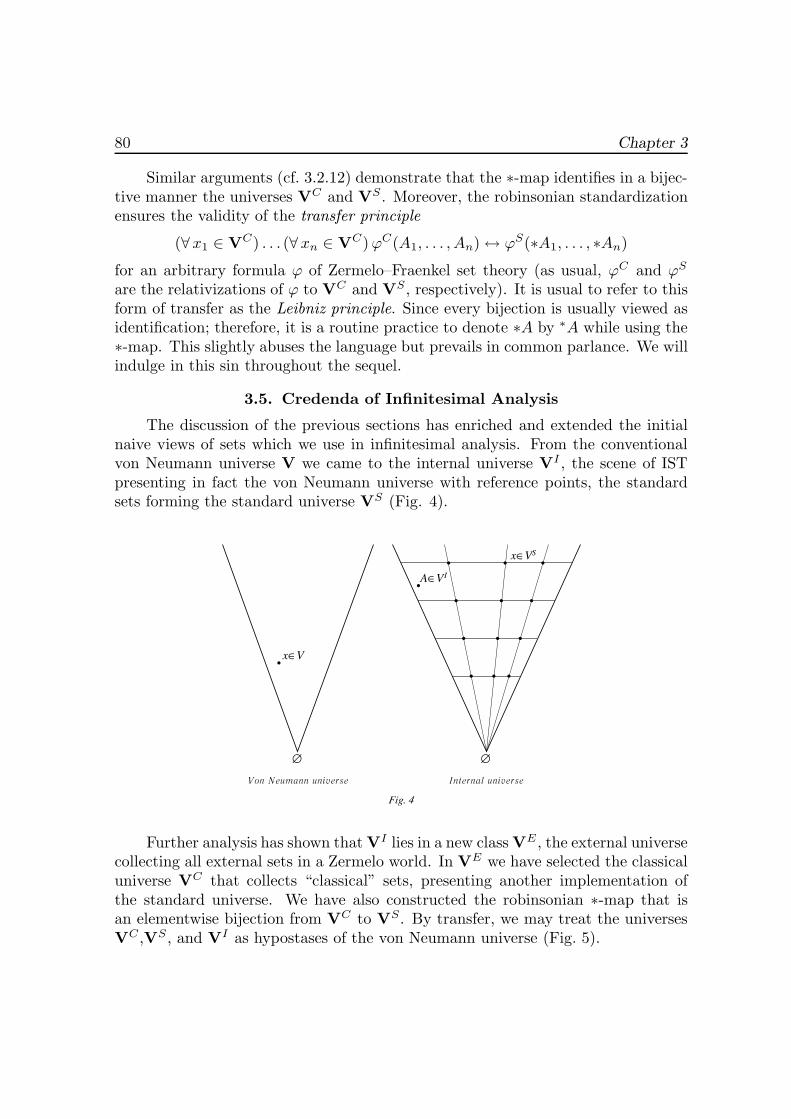
80 Chapter 3
Similar arguments (cf. 3.2.12) demonstrate that the ∗-map identifies in a bijec-tive manner the universes VC and VS. Moreover, the robinsonian standardizationensures the validity of the transfer principle
(∀x1 ∈ VC) . . . (∀xn ∈ VC)ϕC(A1, . . . , An) ↔ ϕS(∗A1, . . . , ∗An)
for an arbitrary formula ϕ of Zermelo–Fraenkel set theory (as usual, ϕC and ϕS
are the relativizations of ϕ to VC and VS, respectively). It is usual to refer to thisform of transfer as the Leibniz principle. Since every bijection is usually viewed asidentification; therefore, it is a routine practice to denote ∗A by ∗A while using the∗-map. This slightly abuses the language but prevails in common parlance. We willindulge in this sin throughout the sequel.
3.5. Credenda of Infinitesimal Analysis
The discussion of the previous sections has enriched and extended the initialnaive views of sets which we use in infinitesimal analysis. From the conventionalvon Neumann universe V we came to the internal universe VI , the scene of ISTpresenting in fact the von Neumann universe with reference points, the standardsets forming the standard universe VS (Fig. 4).
x∈V
A∈VI
x∈VS
∅ ∅
Von Neumann universe Internal universe
Fig. 4
Further analysis has shown that VI lies in a new class VE , the external universecollecting all external sets in a Zermelo world. In VE we have selected the classicaluniverse VC that collects “classical” sets, presenting another implementation ofthe standard universe. We have also constructed the robinsonian ∗-map that isan elementwise bijection from VC to VS. By transfer, we may treat the universesVC ,VS, and VI as hypostases of the von Neumann universe (Fig. 5).
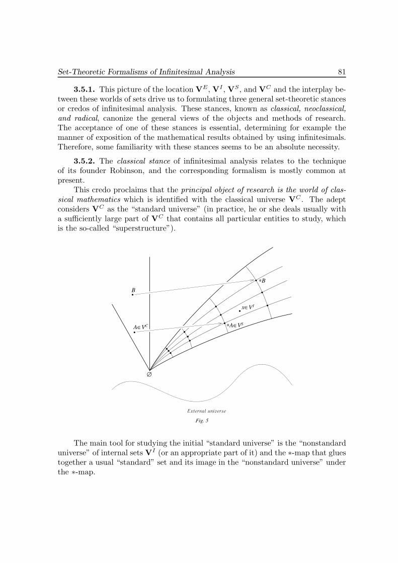
Set-Theoretic Formalisms of Infinitesimal Analysis 81
3.5.1. This picture of the location VE, VI , VS, and VC and the interplay be-tween these worlds of sets drive us to formulating three general set-theoretic stancesor credos of infinitesimal analysis. These stances, known as classical, neoclassical,and radical, canonize the general views of the objects and methods of research.The acceptance of one of these stances is essential, determining for example themanner of exposition of the mathematical results obtained by using infinitesimals.Therefore, some familiarity with these stances seems to be an absolute necessity.
3.5.2. The classical stance of infinitesimal analysis relates to the techniqueof its founder Robinson, and the corresponding formalism is mostly common atpresent.
This credo proclaims that the principal object of research is the world of clas-sical mathematics which is identified with the classical universe VC . The adeptconsiders VC as the “standard universe” (in practice, he or she deals usually witha sufficiently large part of VC that contains all particular entities to study, whichis the so-called “superstructure”).
A∈VC
B
∗B
∗A∈VS
x∈VI
∅
External universe
Fig. 5
The main tool for studying the initial “standard universe” is the “nonstandarduniverse” of internal sets VI (or an appropriate part of it) and the ∗-map that gluestogether a usual “standard” set and its image in the “nonstandard universe” underthe ∗-map.
82 Chapter 3
It is worth noting that this stance involves a specific usage of the words “stan-dard” and “nonstandard.” The robinsonian standardizations, which are the mem-bers of VS, are viewed as “nonstandard” objects. A “standard” set is by credo anarbitrary representative of the classical universe VC, a member of the “standard”universe. The adept points out that the ∗-map usually adds new “ideal” elementsto sets. He or she implies that ∗A = {∗a : a ∈ A} if and only if the “classical” or“standard” set A is finite.
For example, if the adept places R in VC and studies the ∗-image ∗R of R thenhe or she will see that ∗R plays the role of the reals in the sense of the internaluniverse VI . At the same time ∗R is not equal to the set of its standard elements:◦(∗R) = {∗t : t ∈ R}. Considering that ∗R is the “internal set of the reals R,”and ◦(∗R) is its standard part, the adept sometimes takes the liberty of writing◦R := {∗t : t ∈ R} and even R := {∗t : t ∈ R}. To visualize, the presence of new
elements in ∗R is expressed as ∗R − R �= ∅, and the adept talks of the “hyperreals”∗R extending the “standard” reals R.
A similar policy is pursued when considering an arbitrary classical set X .Namely, the adept assumes that X := {∗x : x ∈ X} and, therefore, X ⊂ ∗X .If X is infinite then ∗X −X �= ∅. In other words, the robinsonian standardizationadds new elements to all infinite sets. Furthermore, these additional “ideal” enti-ties are galore by idealization in VI which is also referred to in this stance as thetechnique of concurrence or saturation.
3.5.3. Assume that F is a correspondence and A lies in dom(F ). Call Fconcurrent or finitely satisfiable or directed on A provided that to each nonemptyfinite subset A0 of A there is some b satisfying (a0, b) ∈ F for all a0 ∈ A0.
If the above definition is abstracted by requiring that A0 has cardinality atmost given cardinal κ then we arrive to the definition of κ-concurrence.
3.5.4.Weak Concurrence Principle. To each correspondence F concurrenton A, there is some b in im(∗F ) satisfying (∗a, b) ∈ ∗F for all a ∈ A.
3.5.5. It is easy to see conversely that the validity of 3.5.4 guarantees a nat-ural analog of idealization in a somewhat weaker form than in IST as “relativizedto standard sets.” In this regard, applications often involve various conservativeenlargements of the classical set theory which allow for concurrence in the form of3.5.4 and also in stronger forms insuring the additional possibilities of introducingnonstandard entities in a manner that reflects idealization to a full extend.
3.5.6. Strong Concurrence Principle. Let F be such that ∗F is concurrenton A. Then there is b ∈ im(∗F ) satisfying (∗a, b) ∈ ∗F for all a ∈ A.
Recall that (Aγ)γ∈Γ is a centered family or has the finite intersection propertywhenever
⋂γ∈Γ0
Aγ �= ∅ for every nonempty finite subset Γ0 of Γ.
Set-Theoretic Formalisms of Infinitesimal Analysis 83
3.5.7. Saturation Principle. The following hold:(1) Let (An)n∈N be a sequence of internal sets enjoying the finite inter-
section property. Then⋂n∈∗N
An �= ∅.(1) Let (An)n∈N be an increasing sequence of internal sets and A :=⋃
n∈NAn. Then A = AN for some N ∈ ∗N.
The definition of ultralimit (cf. 3.2.17) involves arbitrariness which enables usto show that there exist enlargements satisfying the analogs of 3.5.7 and similarprinciples for each family whose index set has cardinality at most κ. In thesecircumstances, it is in common parlance to speak of κ-saturation. Rephrased inthis terminology, 3.5.7 guarantees ω0-saturation. Applications often require ω1-saturation as well.
3.5.8. The “enlarged,” “nonstandard” world, i.e., the internal universe VI
satisfies the transfer principle. Using the properties of the robinsonian standard-ization, we may rephrase it as follows:
(∀x1 ∈ VC) . . . (∀xn ∈ VC)(ϕC(x1, . . . , xn) ↔ ϕI(∗x1, . . . ,∗xn))
where ϕ is an arbitrary formula of Zermelo–Fraenkel set theory. Recall that thisform of transfer is the Leibniz principle.
3.5.9. Research in the “nonstandard universe” sometimes involves the “in-ternal set technique,” i.e., the way of arguing which rests on the fact that everyexternal set given in the “set-theoretic manner” is internal. We now specify one ofthe versions of this technique.
3.5.10. Let A be an infinite set. For any set-theoretic formula ϕ ∈ (ZFC) itis then false that
{x : ϕI(x)} = ∗A−A.
� Assume the contrary. Then the class {x : ϕI(x)} would be an internal subsetof ∗A. Consequently, A would be internal too. However, the external set ∗A−A isnot internal since A is infinite by hypothesis. �
Applications also use other easy versions of the principles of infinitesimal anal-ysis.
3.5.11. The following hold:(1) Extension Principle. Each sequence (An)n∈N of internal sets An
is extendible to some internal sequence (An)n∈∗N;(2) Overflow Principle. If A is an internal set and N ⊂ A then A
contains some infinitely large hypernatural, i.e. a member of ∗N−N;(3) Underflow Principle. If A is an internal set and every infinitely
large hypernatural N ∈ ∗N belongs to A then A contains some
standard n ∈ N;
84 Chapter 3
(4) Limitedness Principle. If B is an internal set of R consistingonly of limited reals then there is a standard real t ∈ R satisfyingB ⊂ [−t, t];
(5) Permanence Principle. If B is an internal set containing allpositive limited reals then B includes the interval [0, Ω] for someinfinitely large Ω;
(5) Cauchy Principle. If B is an internal set containing all infinitesi-mals then B includes the interval [−a, a] for some standard a ∈ R;
(6) Robinson Principle. If B is an internal set consisting only ofinfinitesimals then B is included in the interval [−ε, ε] where ε issome infinitesimal.
It is worth noting that the words “overspill” and “underspill” are in commonparlance for “overflow” and underflow.”
3.5.12. Concluding the discussion, we can say that the adept confessing theclassical credo works with the two universes, standard and nonstandard. There isa formal possibility of linking the properties of standard and nonstandard objectswith the help of the ∗-map. At the same time the adept may freely translatestatements about objects of one universe into those about their images in the otheruniverse, which is the Leibniz principle. The nonstandard universe is abundantin “ideal” elements; various transfinite constructs are realizable in it because ofthe concurrence principle. The sets falling beyond the nonstandard universe areviewed as external (this is a peculiarity of the terminology: the internal sets arenot considered external in this stance). The technique of internal sets proves to bea very effective tool.
The basic advantage of the classical stance is the availability of the ∗-mapenabling us to apply the machinery of infinitesimal analysis to the arbitrary setsof “standard” mathematics. For example, the adept may assert that a functionf : [a, b] → R is uniformly continuous if and only if ∗f : ∗[a, b] → ∗
R is microcon-tinuous; i.e., if ∗f preserves the infinite proximity between the “hyperreals.” Theprincipal complication in absorbing these notions lies in the necessity of imaginingthe enormous number of the new “ideal” entities inserted forcibly into the ordinarysets. The considerable problems are caused by a natural desire to work (at leastin the beginning) with two sets of variables that correspond to the two universes.(When we have constructed the internalization ϕI of a formula ϕ, we implicitlyassume the possibility of this procedure.)
Thus, the part and parcel of the classical stance, bilingualism and the robinso-nian standardization, determine all its peculiarities, advantages and disadvantagesof the corresponding formal machinery.
3.5.13. The neoclassical stance of infinitesimal analysis corresponds to themethodology propounded by Nelson. This credo proclaims that the principal object
Set-Theoretic Formalisms of Infinitesimal Analysis 85
of research is the world of classical mathematics which is identified with the internaluniverse VI included in the external environment VE . The “classical” sets do notenter into analysis. The standard and nonstandard elements are revealed within theordinary objects, the internal sets inhabiting VI . For instance, the field of reals isthe member R of VI which is of course the same as ∗R, the hyperreals, serving asan “ideal” object of the classical stance.
The views we have professed in Chapter 2 correspond mainly to the neoclas-sical stance. Their advantages are determined by the possibility of studying the“auld lang syne” sets with the goal of discovering new elements in their construc-tion by using additional linguistic means and opportunities. Nelson observed that“really new in nonstandard analysis are not theorems but the notions, i.e., externalpredicates” [380, p. 134].
The shortcomings of the neoclassical stance stems from the necessity of trans-ferring all definitions and properties from standard objects to their internal relativesby a highly implicit technique of standardization. We have encountered this obsta-cle before.
3.5.14. The radical stance of infinitesimal analysis proclaims that the prin-cipal object of research is the external universe in full completeness and complexityof its own structure. The adept declares “parochial” or “shy” and discards theclassical and neoclassical views of infinitesimal analysis as a technique for study ofmathematics basing on Zermelo–Fraenkel set theory.
At a first glance this credo cannot be accepted earnestly and must be dismissedas overextremist. Upon due reflection these accusations of the radical stance shouldbe rejected. This is an illusory, superficial “extremism.” A widely-accepted view ofmathematics as the science of forms and relations taken irrespective of their content,as well as the considerably less restrictive classical set-theoretic stance stemmingfrom Cantor, undoubtedly embraces the “extremist” thoughts of the objects ofinfinitesimal analysis.
Therefore, the most “intrepid” views of sets which we arrive at merge ultimatelyinto the original premises, extending and enriching it. Observe that we startedwith a “modest” claim that infinitesimal analysis considers as sets exactly the sameentities as the rest of mathematics (cf. 2.1.3). We have so come full circle.
3.6. Von Neumann–Godel–Bernays Theory
As we have already mentioned in 3.2.5, the axiom of replacement ZFϕ4 ofZermelo–Fraenkel set theory ZFC is in fact an axiom-schema embracing infinite-ly many axioms because of arbitrariness in the choice of a formula ϕ. It stands toreason to introduce some primitive object that is determined from each formula ϕparticipating in ZFϕ4 . With these objects available, we may paraphrase the contentof the axiom-schema ZFϕ4 as a single axiom about new objects. To this end, we need
86 Chapter 3
the axioms that guarantee existence for the objects determined from a set-theoreticformula.
Since all formulas are constructed by a unique procedure in finitely many steps,we find highly plausible the possibility of achieving our goal with finitely manyaxioms. It is this basic idea stemming from von Neumann that became a cornerstoneof the axiomatics of set theory which was elaborated by Godel and Bernays and iscommonly designated by NGB.
The initial undefinable object of NGB is a class. A set is a class that is a mem-ber of some class. A class other than any set is a proper class. Objectivization ofclasses constitutes the basic difference between NGB and ZFC, with the metalan-guage of the latter treating “class” and “property” as synonyms.
Axiomatic presentation of NGB uses as a rule one of the two available modifi-cations of the language of ZFC. The first consists in adding a new unary predicatesymbol M to the language of ZFC, with M(X) implying semantically that X isa set. The second modification uses two different types of variables for sets andclasses. It worth observing that these tricks are not obligatory for describing NGBand reside in exposition routinely for the sake of convenience.
3.6.1. The system NGB is a first-order theory with equality. Strictly speak-ing, the language of NGB does not differ at all from that of ZFC. However, theupper case Latin letters X, Y, Z, . . . , possible with indices, are commonly used forvariables, while the lower case Latin letters are left for the argo resulting fromintroducing the abbreviations that are absent in the language of NGB.
Let M(X) stand for the formula (∃Y )(X ∈ Y ). We read M(X) as “X isa set.”
Introduce the lower case Latin letters x, y, z, . . . (with indices) for the boundvariables ranging over sets. Speaking more exactly, the formulas (∀x)ϕ(x) and(∃x)ϕ(x), called generalization and instantiation of ϕ by x, are abbreviations ofthe formulas (∀X)(M(X) → ϕ(X)) and (∃X)(M(X) ∧ ϕ(X)), respectively. Se-mantically these formulas imply: “ϕ holds for every set” and “there is a set forwhich ϕ is true.” In this event the variable X must not occur in ϕ nor in theformulas comprising the above abbreviations.
The rules for using upper case and lower case letters will however be observedonly within the present section. On convincing ourselves that the theory of classesmay be formalized in principle, we will gradually return to the cozy and liberalrealm of common mathematical parlance. For instance, abstracting the set-theoreticconcept of function to the new universe of discourse, we customarily speak abouta function-class F implying that F might be other than a set but still obeys theconventional properties of a function. This is a sacrosanct privilege of the workingmathematician.
We now proceed with stating the special axioms of NGB.
Set-Theoretic Formalisms of Infinitesimal Analysis 87
3.6.2. Axiom of Extensionality NGB1. Two classes coincide if and onlyif they consist of the same elements:
(∀X)(∀Y )(X = Y ↔ (∀Z)(Z ∈ X ↔ Z ∈ Y )).
3.6.3. We now list the axioms for sets:
(1) Axiom of Pairing NGB2:
(∀x)(∀ y)(∃ z)(∀u)(u ∈ z ↔ u = x ∨ u = y);
(2) Axiom of Union NGB3:
(∀x)(∃ y)(z ∈ y ↔ (∃u)(u ∈ x ∧ z ∈ u));
(3) Axiom of Powerset NGB4:
(∀x)(∃ y)(∀ z)(z ∈ y ↔ z ⊂ x);
(4) Axiom of Infinity NGB5:
(∃x)(∅ ∈ x ∧ (∀ y)(y ∈ x ↔ y ∪ {y} ∈ x)).
These axioms coincide obviously with their counterparts in ZFC, cf. A.2.3, A.2.4,A.2.7, and A.2.8. However, we should always bear in mind that the verbal formu-lations of NGB1–NGB5 presume a “set” to be merely a member of another class.Recall also that the lower case Latin letters symbolize abbreviations (cf. 3.6.1).By way of illustration, we remark that, in partially expanded form, the axiom ofpowerset NGB4 looks like
(∀X)(M(X) → (∃Y )(M(Y ) ∧ (∀Z)(M(Z) → (Z ∈ Y ↔ Z ⊂ X)))).
The record of the axiom of infinity uses the following abbreviation
∅ ∈ x := (∃ y)(y ∈ x ∧ (∀u)(u /∈ y)).
Existence of the empty set is a theorem rather than a postulate in NGB in muchthe same way as in ZFC. Nevertheless, it is common to enlist the existence of theempty set in NGB as a special axiom:

88 Chapter 3
(5) Axiom of the Empty Set:
(∃ y)(∀u)(u /∈ y).
3.6.4. Axiom of Replacement NGB6. If X is a single-valued class then,for each set y, the class of the second components of those couples of X whose firstcomponents belong to y, is a set:
(∀X)(Un (X) → (∀ y)(∃ z)(∀u)(u ∈ z ↔ (∃ v)((v, u) ∈ X ∧ v ∈ y))),
where Un(X) := (∀u)(∀ v)(∀w)((u, v) ∈ X ∧ (u, w) ∈ X → v = w).As was intended, the axiom-schema of replacement ZFϕ4 turns into a single
axiom. Note that the axiom-schema of comprehension in ZF (see 3.2.5) also trans-forms into a single axiom, the axiom of comprehension. The latter reads that, toeach set x and each class Y , there is a set consisting of the common members of xand Y :
(∀x)(∀Y )(∃ z)(∀u)(u ∈ z ↔ u ∈ x ∧ u ∈ Y ).
The axiom of comprehension is weaker than the axiom of replacement since theformer ensues from NGB6 and Theorem 3.6.14 below. However, comprehension isoften convenient for practical purposes.
The collection of axioms to follow, NGB7–NGB13, relates to the formation ofclasses. These axioms state that, given some properties expressible by formulas, wemay deal with the classes of the sets possessing the requested properties. As usual,uniqueness in these cases results from the axiom of extensionality for classes NGB1.
3.6.5. Axiom of Membership NGB7. There is a class comprising everycouple of sets whose first component is a member of the second:
(∃X)(∀ y)(∀ z)((y, z) ∈ X ↔ y ∈ z).
3.6.6. Axiom of Intersection NGB8. There is a class comprising the com-mon members of every two classes:
(∀X)(∀Y )(∃Z)(∀u)(u ∈ Z ↔ u ∈ X ∧ u ∈ Y ).
3.6.7. Axiom of Complement NGB9. To each class X there is a classcomprising the nonmembers of X :
(∀X)(∃Y )(∀u)(u ∈ Y ↔ u /∈ X).
This implies the existence of the universal class U := ∅ which is the comple-ment of the empty class ∅.
Set-Theoretic Formalisms of Infinitesimal Analysis 89
3.6.8. Axiom of Domain NGB10. To each class X of couples there is a classY := dom(X) comprising the first components of the members of X :
(∀X)(∃Y )(∀u)(u ∈ Y ↔ (∃ v)((u, v) ∈ X)).
3.6.9. Axiom of Product NGB11. To each class X there is a class Y :=X × U comprising the couples whose first components are members of X :
(∀X)(∃Y )(∀u)(∀ v)((u, v) ∈ Y ↔ u ∈ X).
3.6.10. Axioms of Permutation NGB12 and NGB13. Assume that σ :=(ı1, ı2, ı3) is a permutation of {1, 2, 3}. A class Y is a σ-permutation of a class Xprovided that (x1, x2, x3) ∈ Y whenever (xı1 , xı2, xı3) ∈ X .
To each class X , there are (2, 3, 1)- and (1, 3, 2)-permutations of X :
(∀X)(∃Y )(∀u)(∀ v)(∀w)((u, v, w) ∈ Y ↔ (v, w, u) ∈ X);(∀X)(∃Y )(∀u)(∀ v)(∀w)((u, v, w) ∈ Y ↔ (u, w, v) ∈ X).
The above axioms of class formation proclaim existence of unique classes, aswas already observed. It is so in common parlance to speak about the complementof a class, the intersection of classes, etc.
3.6.11. Axiom of Regularity NGB14. Each nonempty class X has a mem-ber having no common elements with X :
(∀X)(X �= ∅ → (∃ y)(y ∈ X ∧ y ∩X = ∅)).
3.6.12.Axiom of ChoiceNGB15. To each classX there is a choice function-class on X ; i.e., a single-valued class assigning an element of X to each nonemptymember of X :
(∀X)(∃Y )(∀u)(u �= ∅ ∧ u ∈ X → (∃!v)(v ∈ u ∧ (u, v) ∈ Y )).
This is a very strong form of the axiom of choice which amounts to a possibility ofa simultaneous choice of an element from each nonempty set.
The above axiom makes the list of the special axioms of NGB complete. Amoment’s inspection shows that NGB, unlike ZFC, has finitely many axioms. An-other convenient feature of NGB is the opportunity to treat sets and propertiesof sets as formal objects, thus implementing the objectivization that is absolutelyinaccessible to the expressive means of ZFC.
90 Chapter 3
3.6.13. We now derive a few consequences of the axioms of class formationwhich are needed in the sequel.
(1) To each class X there corresponds the (2, 1)-permutation of X :
(∀X)(∃Z)(∀u)(∀ v)((u, v) ∈ Z ↔ (v, u) ∈ X).
� The axiom of product guarantees existence for the class X × U. Consecu-tively applying the axioms of the (2, 3, 1)-permutation and (1, 3, 2)-permutation tothe X × U, arrive at the class Y of 3-tuples (alternatively, triples) (v, u, w) suchthat (v, u) ∈ X . Appealing to the axiom of domain, conclude that Z := dom(Y ) isthe sought class. �
(2) To each couple of classes there corresponds their product:
(∀X)(∀Y )(∃Z)(∀w)(w ∈ Z ↔ (∃u ∈ X)(∃v ∈ Y )(w = (u, v))).
� To prove the claim, apply consecutively the axiom of product, (1), and theaxiom of intersection to arrange Z := (U × Y ) ∩ (X × U). �
Given n ≥ 2, we may define the class Un of all ordered n-tuples by virtue of3.6.13 (2).
(3) To each class X there corresponds the class Z := (Un × Um) ∩(X × Um):
(∀X)(∃Z)(∀x1) . . . (∀xn)(∀ y1) . . . (∀ ym)((x1, . . . , xn, y1, . . . , ym) ∈ Z ↔ (x1, . . . , xn) ∈ X).
(4) To each class X there corresponds the class Z := (Um × Un) ∩(Um ×X):
(∀X)(∃Z)(∀x1) . . . (∀xn)(∀ y1) . . . (∀ ym)((y1, . . . ym, x1, . . . , xn) ∈ Z ↔ (x1, . . . , xn) ∈ X).
� To demonstrate (3) and (4), apply the axiom of product and the axiom ofintersection. �
(5) To each class X there corresponds the class Z satisfying
(∀x1) . . . (∀xn)(∀ y1) . . . (∀ ym)((x1, . . . , xn−1, y1, . . . , ym, xn) ∈ Z ↔ (x1, . . . , xn) ∈ X).
� Appeal to the axioms of permutation and the axiom of product. �
Set-Theoretic Formalisms of Infinitesimal Analysis 91
3.6.14. Theorem. Let ϕ be a formula whose variables are among X1, . . . , Xn,Y1, . . . , Ym and which is predicative; i.e., all bound variables of ϕ range over sets.Then the following is provable in NGB:
(∀Y1) . . . (∀Ym)(∃Z)(∀x1) . . . (∀xn)((x1, . . . , xn) ∈ Z ↔ ϕ(x1, . . . , xn, Y1, . . . , Ym)).
� Assume that ϕ is written so that the only bound variables of ϕ are thosefor sets. It suffices to consider only ϕ containing no subformulas of the shapeY ∈ W and X ∈ X , since these subformulas might be rewritten in equivalentform as (∃x)(x = Y ∧ x ∈ W ) and (∃u)(u = X ∧ u ∈ X). Moreover, the symbolof equality may be eliminated from ϕ on substituting for X = Y the expression(∀u)(u ∈ X ↔ u ∈ Y ), which is sound by the axiom of extensionality. The proofproceeds by induction on the complexity or length k of ϕ; i.e., by the number k ofpropositional connectives and quantifiers occurring in ϕ.
In case k = 0 the formula ϕ is atomic and has the form xı ∈ xj, or xj ∈ xı, orxı ∈ Yl (ı < j ≤ n, l ≤ m). If ϕ := xı ∈ xj then, by the axiom of membership, thereis a class W1 satisfying
(∀xı)(∀xj)((xı, xj) ∈ W1 ↔ xı ∈ xj).
If ϕ := xj ∈ xı then, using the axiom of membership again, we find a class W2 withthe property
(∀xı)(∀xj)((xj, xı) ∈ W2 ↔ xj ∈ xı),
and apply 3.6.13 (1). In result, we obtain a class W3 such that
(∀xı)(∀xj)((xı, xj) ∈ W3 ↔ xj ∈ xı).
Hence, in each of these two cases there is a class W satisfying the following formula:
Φ := (∀xı)(∀xj)((xı, xj) ∈ W ↔ ϕ(x1, . . . , xn, Y1, . . . , Ym)).
By 3.6.13 (4), we may replace the subformula (xı, xj) ∈ W of Φ with the mem-bership (x1, . . . , xı−1, xı) ∈ Z1 for some other class Z1 and insert the quantifiers(∀x1) . . . (∀xı−1) in the prefix of Φ.
Let Ψ be the so-obtained formula. By 3.6.13 (5), there is some class Z2 for Ψso that it is possible to write (x1, . . . , xı−1, xı, xj) ∈ Z1 instead of the subformula(x1, . . . , xı, xı+1, . . . , xj) ∈ Z2 and to insert the quantifiers (∀xı+1) . . . (∀xj−1) inthe prefix of Ψ. Finally, on applying 3.6.13 (3) to Z2, find a class Z satisfying thefollowing formula:
(∀x1) . . . (∀xn)((x1, . . . , xn) ∈ Z ↔ ϕ(x1, . . . , xn, Y1, . . . , Ym)).
92 Chapter 3
In the remaining case of xı ∈ Yl, the claim follows from existence of the productsW := Uı−1 × Yl and Z := W × Un−ı. This completes the proof of the theorem fork = 0.
Assume now that the claim of the theorem is demonstrated for all k < p andthe formula ϕ has p propositional connectives and quantifiers. It suffices to considerthe cases in which ϕ results from some other formulas by negation, implication, andgeneralization.
Suppose that ϕ := ¬ψ. By the induction hypothesis, there is a class V suchthat
(∀x1) . . . (∀xn)((x1, . . . , xn) ∈ V ↔ ψ(x1, . . . , xn, Y1, . . . , Ym)).
By the axiom of complement, the class Z := U − V := U\V meets the requiredconditions.
Suppose that ϕ := ψ → θ. Again, by the induction hypothesis, there areclasses V and W making the claim holding for V and ψ and such that
(∀x1) . . . (∀xn)((x1, . . . , xn) ∈ W ↔ θ(x1, . . . , xn, Y1, . . . , Ym)).
The sought class Z := U − (V ∩ (U −W )) exists by the axioms of intersection andcomplement.
Suppose that ϕ := (∀x)ψ, and let V and ψ be the same as above. Applyingthe axiom of domain to the class X := U − V , obtain the class Z1 such that
(∀x1) . . . (∀xn)((x1, . . . , xn) ∈ Z1 ↔ (∃x)¬ψ(x1, . . . , xn, Y1, . . . , Ym)).
The class Z := U − Z1 exists by the axiom of complement and is the one we seeksince the formula (∀x)ψ amounts to ¬(∃x)(¬ψ). �
3.6.15. Each of the axioms of class formation NGB7–NGB13 is a corollary toTheorem 3.6.14 provided that the formula ϕ is duly chosen. On the other hand, thetheorem itself, as shown by inspection of its proof, ensues from the axioms of classformation. Remarkably, we are done on using finitely many axioms NGB7–NGB13
rather than infinitely many assertions of Theorem 3.6.14.Theorem 3.6.14 allows us to prove the existence of various classes. For instance,
to each class Y there corresponds the class P(Y ) of all subsets of Y , as well as theunion
⋃Y of all elements of Y . These two classes are defined by the conventional
formulas:
(∀u)(u ∈ P(Y ) ↔ u ⊂ Y ),
(∀u)(u ∈⋃Y ↔ (∃ v)(v ∈ Y ∧ u ∈ v)).
The above claims of existence are easy on putting ϕ(X, Y ) := X ⊂ Y and ϕ(X, Y ):= (∃V )(X ∈ V ∧ V ∈ Y ). Analogous arguments corroborate the definitions ofZ−1, im(Z), Z � Y , Z“Y , X ∪ Y , etc., with X , Y , and Z arbitrary classes.
Set-Theoretic Formalisms of Infinitesimal Analysis 93
3.6.16. Theorem. Each theorem of ZFC is a theorem of NGB.
� Each axiom of ZFC is a theorem of NGB. The only nonobvious part of theclaim concerns the axiom of replacement ZFϕ4 which we will proof.
Assume that y is not unbound in ϕ , and let {x, t, z1, . . . , zm} stand for thecomplete list of variables in the construction of ϕ. Assume further that, for all x,u, v, z1, . . . , zm, the following formula holds:
ϕ(x, u, z1, . . . , zm) ∧ ϕ(x, v, z1, . . . , zm) → u = v.
The formula is predicative since each bound variable of ϕ ranges over sets. ByTheorem 3.6.14, there is a class Z such that
(∀x)(∀u)((x, u) ∈ Z ↔ ϕ(x, u, z1, . . . , zm)).
This property of ϕ shows that the class Z is single-valued; i.e., Un (Z) is provablein NGB. By the axiom of replacement NGB6, there is a set y satisfying
(∀ v)(v ∈ y ↔ (∃u)((u, v) ∈ Z ∧ u ∈ x)).
Obviously, y satisfies the desired formula
(∀ z1) . . . (∀ zm)(∀ v)(v ∈ y ↔ (∃u ∈ x)ϕ(u, v, z1, . . . , zm)). �
3.6.17. Theorem. Each formula of ZFC expressing a theorem of NGB isa theorem of ZFC.
� The proof may be found, for instance, in [62]. It uses some general facts ofmodel theory which lie beyond the framework of the present book. �
Theorems 3.6.16 and 3.6.17 are often paraphrased as follows.
3.6.18. Theorem. Von Neumann–Godel–Bernays set theory is conservativeover Zermelo–Fraenkel set theory.
3.6.19. Among the other axiomatic set theories, we mention the so-calledBernays–Morse theory that extends NGB. Bernays–Morse set theory assumes thespecial axioms NGB1–NGB5, NGB14 and the following axiom-schema of compre-hension:
(∃X)(∀Y )(Y ∈ X ↔ M(Y ) ∧ ϕ(Y,X1, . . . , Xn)),
with ϕ an arbitrary formula without free occurrences of X .
94 Chapter 3
3.7. Nonstandard Class Theory
In this section we introduce NCT, another axiomatics analogous to IST butdiffering from IST since NCT is an extension of von Neumann–Godel–Bernays classtheory. Each of the principles of transfer, idealization, and standardization is statedin NCT as an axiom rather than an axiom-schema in IST, and so NCT, as well asNGB, is finitely axiomatizable.
3.7.1. The language of NCT results from the language of NGB by supplement-ing the alphabet of NGB with a new symbol St for the unary predicate expressingthe property of a class to be or not to be standard (the record St(X) reads: “Xis a standard class”). In much the same way as in 3.6, the variables ranging overclasses are denoted by capital Latin letters while the variable ranging over sets aredenoted by lowercase Latin letters.
We will user other abbreviations and conventions of 3.6. In particular, a classX is a set in symbols M(X), provided that X is a member of some class: M(X) :=(∃Y )(X ∈ Y ) (cf. 3.6.1). As before, the record S(X1, . . . , Xn) := ϕ(X1, . . . , Xn)means that S(X1, . . . , Xn) is an abbreviation of ϕ(X1, . . . , Xn).
All in all, the language of NCT is the language of a first order predicate calculuswith equality which contains one unary predicate symbol ∈ and one unary predicatesymbol St. We now list the special axioms of NCT.
(1) In NCT we accept the same axioms of extensionality, pairing, union,powersets, infinity, and choice as in NGB, namely, NBG1–NBG5, NBG14, NBG15
(see 3.6.2, 3.6.3, 3.6.11, and 3.6.12).(2) Axiom of Replacement in NCT reads:
(∀V )(∀x)(∃y)(∀u ∈ x)(∃v((u, v) ∈ V ) → (∃v ∈ y)((u, v) ∈ V )).
In the sequel we will use the following abbreviations:
(∃ stx)ϕ := (∃x)(St(x) ∧ ϕ),(∀ stx)ϕ := (∀x)(St(x) → ϕ).
(3) Axiom of Boundedness:
(∀x)(∃ stz)(x ∈ z).
(4) Axiom of Transfer:
(∀ stX)((∃x)x ∈ X → (∃ stx)x ∈ X).
(5) Axiom of Standardization:
(∀X)(∃ stY )(∀ stx)(x ∈ Y ↔ x ∈ X).
Starting with the empty set and appealing to the axiom of standardization, wearrive at the standard class L without any standard elements. By transfer L = ∅;i.e., the empty set is standard.
Set-Theoretic Formalisms of Infinitesimal Analysis 95
3.7.2. A formula of NCT is predicative, provided that each bound variableranges over members of some set and the standardness predicate enters only in ex-ternal quantifiers, i.e., all occurrences of quantifiers and the standardness predicatelook like ∃x, ∃ stx, ∀x, and ∀ stx. Observe that we may replace the subformula St(x)with (∃ sty)(y = x).
Let p be an arbitrary set. A class X is p-standard (in symbols, stpX) providedthat X is the p-section of some standard class Y ; i.e., (∃ stY )(X = Y ”p) withY ”p = {v : (p, v) ∈ Y }. A class X is internal, (in symbols, intX) provided that Xis p-standard for some p.
Axiom-Schema of Class Formation: If ϕ(x1, . . . , xn, Y1, . . . , Ym) is a pred-icative formula then
(1) To all classes Y1, . . . , Ym there corresponds the classT = {(x1, . . . , xn) : ϕ(x1, . . . , xn, Y1, . . . , Ym)};
(2) If ϕ is an internal formula and Y1, . . . , Yn are standard classes thenso is T .
In much the same way as in NGB, we may accept not the above axiom-schemaof class formation but rather finitely many of its particular cases (cf. NGB7–NGB13) implying the validity of the full version of the axiom-schema (see 3.6.14).Consequently, NCT is a finitely axiomatizable theory.
The following proposition is immediate from the axiom-schema of class forma-tion.
3.7.3. If ϕ and Y1, . . . , Yn are internal in the axiom-schema of class formationthen T is an internal class. Moreover, if all Yi are p-standard for the same p thenT is a p-standard class.
� Everything follows from the axiom-schema of class formation. �We now agree to use the notations:
U := {x : x = x} = {x : x /∈ ∅},E := {x : (∃u)(∃v) (x = (u, v) ∧ u ∈ v)},S := {x : St(x)},
−X := {x : x /∈ X}.
By the axiom-schema of class formation, U and E are standard classes, S is aclass. Moreover, if X and Y are some classes then −X , X ∩Y , dom(X), and X×U
are classes which are standard whenever so are X and Y .Every set x is x-standard and so x is internal since x = E
−1”x. Every standardclass X is internal since X = ({∅} ×X)”∅.
96 Chapter 3
3.7.4. The following two axioms deal with some properties of internal classes.(1) Axiom of Comprehension:
(∀ intX)(∀x)(∃y)(∀u)(u ∈ y ↔ u ∈ x ∧ u ∈ X).
(2) Axiom of Idealization:
(∀ intX)(∀ sta0)((∀ stfinc ⊆ a0)(∃x)(∀a ∈ c)((x, a) ∈ X)↔ (∃x)(∀ sta ∈ a0)((x, a) ∈ X)).
3.7.5. The following propositions are straightforward from the axiom-schemaof class formation and 3.7.3.
(1) Let ϕ be an internal predicative formula. Then
(∀ intX1) . . . (∀ intXn)(∀x)(∃y)(∀u)(u ∈ y
↔ y ∈ x ∧ ϕ(x,X1, . . . , Xn)).
In particular, the axiom-schema of comprehension of BST is valid.(2) The standardization and bounded idealization principles of BST
hold in NST.(3) Transfer Principle. If ϕ is an internal predicative formula then
(∀ stX1) . . . (∀ stXn)((∀ stx)ϕ(x,X1, . . . , Xn)→ (∀x)ϕ(x,X1, . . . , Xn)).
In particular, the transfer principle of BST is valid.(4) Each sentence provable in BST is provable in NCT.
We emphasize that the axiom-schemata of transfer, idealization, standardiza-tion, and comprehension of BST are particular instances of the analogous axiomsof NCT in which classes are determined by predicative formulas with free set vari-ables (these formula are internal for the axioms of comprehension, transfer, andidealization).
3.7.6. We note the following propositions:
(1) If x and p are sets then
stp x ↔ (∃ stz)(x = z”p) ↔ (∃ stf)(Fnc f ∧ x = f(p)).
� Assume first that x is a p-standard set. Then x = z”p for some standard zby the axioms of boundedness and transfer. Therefore, f = {(q, z”q) : q ∈ dom(z)}is a standard function and f(p) = x.
Conversely, if f is a standard function then, by the axiom of transfer, f(p) isthe p-section of the standard set {(q, u) : u ∈ f(q)}. �
Set-Theoretic Formalisms of Infinitesimal Analysis 97
(2) Let ϕ be an internal predicative formula, and let p be a set. Then
(∀ stp X1) . . . (∀ st
p Xn)((∀ stp x)ϕ(x,X1, . . . , Xn)
→ (∀x)ϕ(x,X1, . . . , Xn)).
� By 3.7.3 it suffices to prove that each nonempty p-standard class X containsa p-standard element. Assume that X = Y ”p, with stY and p ∈ r for some stan-dard r. By the axioms of comprehension, choice, and transfer there is a standardfunction f satisfying
(∀q ∈ r)((∃y)(q, y) ∈ Y → (∃y)(q, y) ∈ Y ∩ f).
Since X is nonempty; therefore, p ∈ dom(f) and f(p) is a p-standard memberof X . �
3.7.7. Given an arbitrary class C, put ◦C := C ∩ S. The axiom of standard-ization postulates that to each class X there corresponds a standard class Y suchthat ◦Y = ◦X . By transfer, such a standard class is unique. We denote it by sX .
(1) Theorem. A class X is standard if and only the intersection of Xwith each standard set is a standard set.
� Necessity follows from the axiom-schema of class formation. To prove suf-ficiency, assume that (∀ stz)(∃ stt)(t = X ∩ z). Put Y := s{x : x ∈ X} anddemonstrate that Y = X . By the axiom of boundedness it suffices to check thatz ∩X = z ∩ Y for every standard set z. From the choice of Y it follows that
◦(X ∩ z) = ◦X ∩ ◦z = ◦Y ∩ ◦z = ◦(Y ∩ z).
Since X ∩ z and Y ∩ z are standard sets, the last chain of equalities implies theclaim by transfer. �
(2) A set is standard and finite if and only if its every element is stan-dard.
� By idealization
St(x) ∧ fin(x) ↔ (∃st finy ⊆ x)(∀a ∈ x)(∃b ∈ y)(a = b)↔ (∀a ∈ x)(∃ stb ∈ x)(a = b),
which completes the proof. �We call a set standardly finite whenever its cardinality is a standard natural.
98 Chapter 3
3.7.8. Theorem. A set is standardly finite if and only if its every subclass isa set.
� Assume that x is a set, |x| = α, and f : α → x is an bijection.If x is not a standardly finite set then (∀ stn ∈ N)(α > n) by transfer. Consid-
ering the class I := {f(n) : n ∈ ◦N}, we may write
(∀st fins ⊆ N)(∃k ∈ N)(∀n ∈ s)(f(k) ∈ I ∧ n < k).
Were I set, there would exist some k ∈ N such that f(k) ∈ I and (∀ stn ∈ N)(n < k), which is impossible. Indeed, f(k) ∈ I implies that k is standard since f isa bijection.
Conversely, let x be standardly finite and X ⊆ x. Consider the class T :={n ∈ α : f(n) ∈ X}. By standardization and transfer, there is some set t suchthat t = sT and t ⊆ α. Since α ⊆ S by 3.7.7 (2); therefore, t = ◦t = ◦T = T .Consequently, X = {f(n) : n ∈ t} is a set. �
3.7.9. The p-monad of a set x (in symbols μp(x)) is the intersection of all p-standard classes including x. Since the complement of a standard class is a standardclass too, the p-monads of two sets are coincident or disjoint. From 3.7.6 (1) itfollows that
μp(x) = {y : (∀stp z)(y ∈ z ↔ x ∈ z)}.
If x is p-standard then we call the class μp(x) the monad of x and denote it byμ(x). Clearly, μ(x) =
⋂{a ∈ S : x ∈ a}.Look at an arbitrary set x. By the axiom of boundedness, x ∈ x0 for some
standard x0. By transfer, it is easy to prove that u := s{a ⊆ x0 : x ∈ a} isa standard ultrafilter and
⋂ ◦u = μ(x). Conversely, if u is an arbitrary standardultrafilter then, by transfer and idealization,
⋂ ◦u �= ∅ and μ(x) =⋂ ◦u for every
x ∈ ⋂ ◦u.The class
⋂ ◦u is the nest of an ultrafilter u; in symbols, ν(u). The class ofall ultrafilters will be denoted by Ult, while letting Ult(x) stand for the set of allultrafilters on a set x.
If x and p are sets then μp(x) = μ((p, x))”p.
� From 3.7.6 (1) it follows that
y ∈ μ((p, x))”p ↔ (p, y) ∈ μ((p, x))↔ (∀ stz)((p, x) ∈ z ↔ (p, y) ∈ z) ↔ y ∈ μp(x),
which completes the proof. �
Set-Theoretic Formalisms of Infinitesimal Analysis 99
3.7.10. A class X is p-saturated provided that X contains the p-monad of itsevery element.
(1) A set x is p-standard if and only if x is p-saturated.
� Suppose that x is p-saturated. Take an arbitrary u ∈ x and show that ubelongs to the p-section of some standard set lying in x. Indeed, assuming thecontrary, note that
(∀ stz)(u ∈ z”p → (∃v ∈ z”p)(v /∈ x)).
We may restrict the range of z in this formula to the standard set {t : t ⊆ ⋃x0},
where x0 is standard and x ∈ x0. By idealization,
(∃v /∈ x)(∀ stz)(u ∈ z”p → v ∈ z”p),
which contradicts the inclusion μp(u) ⊆ x.Therefore, (∀u ∈ x)(∃ stz)(u ∈ z”p ⊆ x). Again by idealization, find a standard
finite set z0 satisfying (∀u ∈ x)(∃z ∈ z0)(u ∈ z”p ⊆ x). It is easy that x serves asthe p-section of the standard set
⋃z0. �
(2) μp(x) = {x} ↔ stp x for arbitrary sets x and p.� The implication to the left is obvious. If, conversely, μp(x) = {x} then {x}
is p-saturated and, hence, p-standard. By transfer, x is p-standard too. �3.7.11. Axiom of Saturation:
(∀X)(∃p)(∀x ∈ X)(μp(x) ⊆ X),
i.e. each class is p-saturated for some set p.Given a class D ⊆ Ult and a set p, put
Psls(D, p) :=⋃
u∈◦D
ν(u)”p.
A semiset is a subclass of a set:
SmsX := (∃ stz)(X ⊆ z).
3.7.12. Theorem. Let X be an arbitrary class. Then there are some standardclass D ⊆ Ult and a set p such that
X = Psls(D, p).
Moreover, if X is a semiset then D may be chosen to be a set.
100 Chapter 3
� Let X be a p-saturated class. Put D = s{u ∈ Ult : ν(u)”p ⊆ X}. Then theequality in question follows from the proposition in 3.7.9. The same equality holdsin case X ∈ z, with z standard, provided that as D we take d := D ∩ Ult(r × z),where r is some standard set containing p. Observe that d is standard by transfer. �
Thus, each semiset in NCT turns out to be definable by some predicativeΣst
2 -formula. It is possible to prove also that if all quantifiers of a formula ϕ arerestricted to semisets then ϕ is equivalent to some predicative formula. Indeed, weare done on replacing all subformulas like stX with (∀ sts)(∃ stt)(t = X ∩s) and theformulas like (∃X)(SmsX → ϕ(X, . . . )) with (∃ std)(∃p)ϕ(Psls(d, p), . . . ).
The following theorem is the saturation principle in its traditional statement.Observe that, in contrast to NCT, this theorem cannot be proven or even formulatedin IST or BST.
3.7.13. Theorem. Let a class X and a standard set z0 be such that
(∀ stx ∈ z0)(∃y)((x, y) ∈ X).
Then there is a function-set f satisfying
(∀ stx ∈ z0)((x, f(x)) ∈ X).
� By the axioms of comprehension and boundedness there is a standard set tsuch that (∀x ∈ z0)((∃y)(x, y) ∈ X → (∃y ∈ t)(x, y) ∈ X). Assume that X is a p-saturated class. If (x, y) ∈ X and x is standard, then (∀y′ ∈ μ(y))(x, y′) ∈ X sinceμp((x, y)) = {x}×μp(y). Put d := s{(x, u) ∈ z×Ult(t) : {x}×(ν(u)”p) ⊆ X}. Theaxioms of choice and transfer enable us to find a standard function h : z0 → Ult(t)satisfying (∀x ∈ z0)((x, h(x)) ∈ d). Hence,
(∀ stfinz ∈ z0)(∃f)(∀x ∈ z)(∀ sta ∈ h(x))(Fnc (f) ∧ f(x) ∈ a).
By idealization, there is a function f such that (∀ stx ∈ z)(f(x) ∈ ν(h(x))). Obvi-ously, this f completes the proof. �
3.7.14. Comments.
(1) The nonstandard class theory NCT, we set forth in this section,was suggested by Andreev and Gordon in [14]. NCT is remarkable for clarity andsimplicity. In particular, NCT contains only finitely many axioms and the principlesof infinitesimal analysis become axioms rather than axiom-schemata in IST.
(2) The presence of classes enables us to implement various construc-tions with external sets, which is impossible in IST. In particular, the list of axiomsof NCT contains the axiom of saturation (cf. 3.7.11) which plays a key role in ap-plications of infinitesimal analysis.
Set-Theoretic Formalisms of Infinitesimal Analysis 101
(3) All sets in NCT are internal. The external objects of NCT areproper classes. Furthermore, in much the same way as alternative set theory ASTby Vopenka [513], NCT allows for subclasses of sets which might fail to be sets(the axiom of comprehension holds only for internal sets). We call these semisetsas minted by Vopenka. The theory NCT enjoys some other properties of AST. Inparticular, it is a theorem of NCT that x is a standardly finite set if and only if xincludes no semisets.
(4) If some internal class (in particular, internal set) X is the section ofa standard class by a set p then X is standard relative to p or p-standard, see 3.7.2.This concept of relative standardness in IST was first suggested in the article [141]which showed for instance that the transfer principle and the implication to theright in the idealization principle remain valid on replacing all occurrences of thestandardness predicate in them with the predicate of standardness relative to anarbitrary set p. This holds true in NCT (see 3.7.7 (1)).
3.8. Consistency of NCT
In this section we prove that NCT is conservative over BST.
3.8.1. Theorem. Every predicative proposition provable in NCT is provablein BST.
� We will demonstrate below that each model of BST embeds isomorphicallyinto some model of NCT as the universe of all sets, which implies the claim by thecelebrated Godel Completeness Theorem. �
3.8.2. Consider an arbitrary model M = (M,∈M , stM ) of BST. Let L standfor the enrichment of the language of BST with the elements of M viewed as newsymbols. Assume that M is a model of the language L on defining the interpretationof a symbol a inM to be a itself. The sets inM , entering a formula ϕ of the languageL, are referred to as the parameters of ϕ.
Given a formula ϕ of L with a single unbound variable, put !ϕ" := {x : M |=ϕ(x)}. Furthermore,
N := {!ϕ" : ϕ is a formula of L with a single unbound variable};
Std := {!ϕ" ∈ N : ϕ is an internal formula with unbound parameters};
Set(a) := !x ∈ a" for all a ∈ M.
Given p, q ∈ N , define
p ∈N q := (∃ a ∈ M)(p = Set(a) ∧ a ∈ q),stN p := p ∈ Std .
102 Chapter 3
3.8.3. Assume that a, b ∈ M and p, q ∈ N . Then(1) p ∈N q → (∃ a ∈ M)(p = Set(a));(2) Set(a) = Set(b) ↔ a = b;(3) If p = Set(a) and q = Set(b) then p ∈N q ↔ a ∈M b;(4) If p = Set(a) then stN p ↔ stM a.
� (1): Immediate from the definition of ∈N .(2): This follows from the validity of the axiom of extensionality in M.(3): This ensures from (1) by the definition of ∈N .(4): Note that from the definition of stN it follows that
p = {b : M |= b ∈ a} = {b : M |= ϕ(b)},
where ϕ is an internal formula with standard parameters. Consequently, M |=(∀x)(x ∈ a ↔ ϕ(x)). The axiom-schema of transfer is satisfied in M, implying thatM |= st a, i.e., stM a.
Conversely, if stM a then p = !x ∈ a" ∈ Std. �
(5) The mapping Set embeds isomorphically M as a model of L intothe model N = (N,∈N , stN ); moreover, N |= (∃X)(p ∈ X) →(∃ a ∈ M)(p = Set(a)) for all p ∈ N .
� Everything follows from (1)–(4). �Proposition 3.8.3 (5) shows that a class p is a set in N if and only if p = Set(a)
for some a ∈ M ; i.e., M does embed into N as the universe of all sets.
3.8.4. We are left with checking the validity of the axioms of NCT in themodel M.
From 3.8.3 (5) it follows that the axioms of NCT, written as predicative for-mulas, hold in N whenever they are valid in BST. This concerns the axioms ofpairing, union, powersets, infinity, choice, regularity, and boundedness. The axiomof extensionality holds in N by the construction of ∈N .
If ϕ is a formula of the language L then we let the symbol Cϕ stand forthe collection {x : ϕ(x, x1, . . . , xn)}. Assume that Φ(X1, . . . , Xn) is a predicativeformula, and ϕ1(x, x1, . . . , xm), . . . , ϕn(x, x1, . . . , xm) are some formulas of L whoseunbound variables do not enter the construction of Φ. Denote by Φ(Cϕ1 , . . . ,Cϕn
)the formula that results from Φ(X1, . . . , Xn) by replacing
(1) all occurrences of the atomic formulas like y ∈ Xj with the formulaϕj(y, x1, . . . , xm);
(2) all occurrences of the atomic formulas like Xi ∈ Xj with
(∃x)((∀y)(y ∈ x↔ ϕi(y, x1, . . . , xm)) ∧ ϕj(x, x1, . . . , xm));
Set-Theoretic Formalisms of Infinitesimal Analysis 103
(3) all occurrences of the atomic formulas like Xi = Xj with
(∀x)(ϕi(x, x1, . . . , xm) ↔ ϕj(x, x1, . . . , xm));
(4) all occurrences of the atomic formulas like Xi = x with
(∀y)(y ∈ x ↔ ϕi(y, x1, . . . , xm)).
The unbound variables of Φ(Cϕ1 , . . . ,Cϕn) are those of ϕ1, . . . , ϕn.
3.8.5. If Φ is a predicative formula and Cϕ1 , . . . ,Cϕnare collections without
unbound variables then
N |= Φ(!ϕ1", . . . , !ϕn") ↔ M |= Φ(Cϕ1 , . . . ,Cϕn).
� The proof proceeds by induction on the length of Φ on using the propositionsof 3.8.3. �
3.8.6. The axioms of NCT other than predicative formulas have the shape
(Q1X)(Q2Y )(QZ)Ψ(X, Y, Z),
where Q1, Q2 ∈ {∀, ∀ st}, Q ∈ {∃, ∃ st}, and Ψ is a predicative formula. We say thatsome formula of the above shape holds in BST for classes whenever to arbitraryformulas ϕ1(x, u1, . . . , ul) and ϕ2(x, v1, . . . , vm) of BST, assumed internal if thecorresponding quantifiers are external, there is a formula ϕ(x, w1, . . . , wn) of BST,internal if Q is an external quantifier, such that the formula
(Q1u1) . . . (Q1ul)(Q2v1) . . . (Q2vm)(Qw1) . . . (Qwn)Ψ(Cϕ1,Cϕ2,Cϕ)
holds in BST. We also assume that the variables ui, vi, and wi are absent in theconstruction of Ψ.
3.8.7. Assume that Φ has the shape
(Q1X)(Q2Y )(Q3Z)Ψ(X, Y, Z)
as in 3.8.6. If Φ holds in BST for classes then Φ is valid in N.
� Consider the case in which all quantifiers over classes in Φ are external. Takearbitrary N-standard elements !ϕ1", !ϕ2" ∈ N . Since Φ holds in BST for classes,it follows that there is an internal formula ϕ of the language L with M-standardparameters and a single unbound variable such that M |= Ψ(Cϕ1,Cϕ2,Cϕ). Hence,stN!ϕ" and N |= Ψ(!ϕ1", !ϕ2", !ϕ") by 3.8.5, which completes the proof. �
It is an easy matter to prove that the axioms of transfer, class formation,regularity, replacement, and idealization hold for classes in BST. The axioms ofstandardization, comprehension, and saturation deserve a special discussion.
We will use the definitions, notation, and above-proven facts about monadsand ultrafilters which are preserved in BST. We also need the following theoremof [13].

104 Chapter 3
3.8.8. Theorem. To each formula Φ with two unbound variables there is aninternal formula ϕ satisfying
(∀p)(∀ stx)(Φ(x, p) ↔ (∀ stU ∈ Ult)(p ∈ ν(U) → ϕ(x, U))↔ (∃ stU ∈ Ult)(p ∈ ν(U) ∧ ϕ(x, U))).
3.8.9. Theorem. The axiom of standardization of NCT holds in BST forclasses.
� Let Φ be an arbitrary formula. Without loss of generality, we may assumethat Φ has at most two unbound variables. Take some internal formula ϕ as sug-gested by Theorem 3.8.8. If p is a set and U is an ultrafilter such that p ∈ ν(U)then
(∀ stx)(Φ(x, p) ↔ ϕ(x, U)).
This proves the validity of the axiom of standardization in BST for classes sinceeach set belongs to the nest of some ultrafilter. �
Let U be an ultrafilter. Assign
dom(U) := {dom(u) : u ∈ U};im(U) := {im(u) : u ∈ U}.
It is easy to prove by transfer and idealization that dom(U) and im(U) areultrafilters for every ultrafilter U . Moreover,
(a, b) ∈ ν(U) → a ∈ ν(dom(U)) ∧ b ∈ ν(im(U));a ∈ ν(dom(U)) → (∃ b ∈ im(U))((a, b) ∈ ν(U))
for all sets a and b.
3.8.10. Theorem. The axiom of comprehension holds in BST for classes.� Let Φ be some formula with two unbound variables. By Theorem 3.8.8 there
is an internal formula ϕ satisfying
Φ(a, b) ↔ (∃ stU ∈ Ult)((a, b) ∈ ν(U) ∧ ϕ(U)).
Putψ(V,W ) := (∃U ∈ Ult)(dom(U) = V ∧ im(U) = W ∧ ϕ(U)).
Using the transfer principle of BST and Theorem 3.8.10, to each standard set Athere is a standard set R such that
(∀V ∈ Ult(A))((∃W )ψ(V,W ) → (∃W ∈ R)ψ(V,W )).
Set-Theoretic Formalisms of Infinitesimal Analysis 105
Put Y :=⋃⋃
R. By transfer and the properties of the nests of ultrafilters,
(∃ b)Φ(a, b) → (∃ stV ∈ Ult(A))(∃ stW ∈ Ult)(a ∈ ν(V ) ∧ ψ(V,W ))→ (∃ stV ∈ Ult(A))(∃ stW ∈ R)(a ∈ ν(U) ∧ ψ(V,W ))→ (∃ b ∈ Y )(∃ stU)((a, b) ∈ ν(U) ∧ ϕ(U))→ (∃ b ∈ Y )Φ(a, b)
for all a ∈ A.Assume now that Ψ(x, y, p) is an arbitrary formula. To complete the proof of
the theorem it suffices to show that to each p and each standard X there is a setY such that
(∀x ∈ X)((∃ y)Ψ(x, y, p) → (∃ y ∈ Y )Ψ(x, y, p)).
Distinguishing some standard sets X and p, put
Φ(a, b) := (∃x)(∃ p)(a = (x, p) ∧ Ψ(x, b, p)).
As we have proven already, there is a standard set Y such that the sought formulaholds for all p ∈ P . We are done on applying the axiom of boundedness. �
3.8.11. Theorem. The axiom of saturation holds in BST for classes.� By Theorem 3.8.8 to each formula Φ with two unbound variables there is an
internal formula ϕ satisfying
Φ(x, p) ↔ (∃ stU)((p, x) ∈ ν(U) ∧ ϕ(U)).
Hence, given an arbitrary set p and using 3.7.9, we infer that
(∀x)(Φ(x, p) → (∀y ∈ μp(x)) Φ(y, p)),
so completing the proof. �We have checked that all axioms of NCT hold in N, which ends the proof of
Theorem 3.8.1.
3.8.12. Comments.
(1) The fact that proper classes are not members of other classes clearlyrestricts the expressive means of NCT. In particular, it is impossible in NCT toformalize the construction of the nonstandard hull E# of an internal normed spaceE to a full extend (cf. Chapter 6). Indeed, the members of E# are the equivalenceclasses of the quotient of the class of limited members of E by the external relationof infinite proximity on E. Since these classes are both external, there is no class
106 Chapter 3
that contains them as members. However, to view the nonstandard hull of E asthe class comprising these equivalence classes we need furnish NCT with a strongerform of the axiom of choice which asserts for instance the possibility of orderingeach semiset so that each subclass of this semiset has a least element. Such an orderis a strong well-ordering. However, this cannot be implemented in NCT without acontradiction as shown in [14].
(2) We can prove that a class admits a strong well-ordering only if thereis a bijection of this class to the semiset of standard elements of some standard set(the semiset of limited members of an internal normed space fails to possess thisproperty).
(3) A class X has standard size provided that there are a function Fand a class D satisfying X = F”◦D. In this event, we may assume F internal andD standard. The article [14] contains the following
Theorem. A semiset X admits a strong well-ordering if and only if X hasstandard size.
(4) The theory NCT has tools allowing us to prove some propositionthat is equivalent to the theorem of completeness of the nonstandard hull of aninternal normed space. We mean the claim that each external S-fundamental se-quence (en) of elements of E (i.e., a sequence indexed with standard naturals andsuch that (∀ stε > 0)(∃ stn0)(∀ stm,n > n0)(‖en − em‖ < ε)) has S-limit in E (i.e.,(∃ e ∈ E)(∀ stε > 0)(∃ stn0)(∀ stn > n0)‖en − e‖ < ε)).
Analogously, NCT will allow us to formalize all considerations of Chapter 7which deal with construction some topological groups as quotient groups of hyper-finite group by external normal subgroups.
3.9. Relative Internal Set Theory
In this section we consider the theory of relative internal sets within Nelson’sinternal set theory.
3.9.1. The presence of infinitesimals in analysis opens a way of constructingnew concepts (and in fact of legitimizing the concepts that were refuted long ago)in order to study the classical objects of mathematical analysis. In particular, ournew attractive acquisition is new mathematical concepts such as a microlimit ofa finite sequence (cf. 2.3.4) or microcontinuity of a function at a point (cf. 4.4.5).These and similar concepts enable us to formulate the “infinitesimal” tests for limits(cf. 2.3.5), continuity (cf. 2.3.8 and 4.2.7), compactness (cf. 4.3.6), etc. which lie inthe backgrounds of most applications.
However, all new tests presume the standard environment which is a limitationon their applicability. Moreover, even in case we use infinitesimal tests to studying
Set-Theoretic Formalisms of Infinitesimal Analysis 107
a standard object, we often face serious obstacles that stem from this limitation.We will proceed with two typical examples.
(1) Consider the infinitesimal test for the fact that
limn→∞ lim
m→∞xnm = a
for some standard double sequence (xnm)n,m∈N and a standard real a. Apply thetest of 2.3.5 to reformulate:
A standard number a ∈ R is the limit of a standard sequence (an) if and onlyif a is a microlimit of a[N ], with N an arbitrary unlimited natural number. Insymbols,
limn→∞ lim
m→∞ xnm = a ↔ (∀N ≈ +∞)( limm→+∞xN,m ≈ a).
However, the infinitesimal limit test is not applicable since the internal sequenceym := ∗xN,m fails to be standard in general. A similar obstacle appears in testingthe double limit limx→0 limy→0 f(x, y) of a function f : R
2 → R as well as in tryingto find an infinitesimal presentation of the improper integral (cf. 2.3.6).
(2) Let us try now to supply an infinitesimal proof for the followingfamiliar proposition:
The uniform limit of a sequence of bounded uniformly continuous function ona uniform space is a uniformly continuous function.
We thus consider a standard sequence (fn)n∈N of such functions converginguniformly to a standard function f on a set X . By the same reasons as in (1), if Nis an unlimited natural and x ∈ X then fN (x) ≈ f(x), since sup{|fN (x)−f(x)| : x ∈X} ≈ 0. By 2.3.12 (cf. 4.4.6 (1)) it suffices to prove that x′ ≈ x′′ → f(x′) ≈ f(x′′)for all x′, x′′ ∈ X . Of course, f(x′) ≈ fN (x′) and f(x′′) ≈ fN (x′′). However, itis impossible to infer that fN (x′) ≈ fN (x′′) despite the fact that f is uniformlycontinuous since the infinitesimal uniform continuity test is not applicable to the(generally) nonstandard function fN .
To obviate these obstacles we will introduce relatively standard elements. In-formally speaking, a set relatively standard with respect to x is “more nonstandard”as compared with x. This reminds us of higher order infinitesimals.
3.9.2. We will consider the notion of relative standardness within IST.Denote by Ffin(f) the following: “f is a function and each member of the
image im(f) of f is a finite set.” In symbols,
Ffin(f) := Func (f) ∧ (∀x ∈ im(f)) fin(f(x)).
An element x is feasible (in symbols, (Su(x))) provided that (∃stX)(x ∈ X).We introduced the predicate “x is standard relative to y” by the formula
x st y := (∃stϕ)(Ffin(ϕ) ∧ y ∈ dom(ϕ) ∧ x ∈ ϕ(y)).
108 Chapter 3
It is worth recalling that fin(x) means only that x is a finite set or, in other words,the cardinality or size of x is a member of ω; i.e. x is a natural, possibly unlimitedwhenever x is a nonstandard set.
3.9.3. In the sequel we will use the following auxiliary proposition.
Let ϕ(x, y) be a formula of ZFC. Assume that (∀x)(∃! y)ϕ(x, y) is provable inZFC. Then the formula (∀stx)(∀y)(ϕ(x, y) → St(y)) is provable in IST.
� This is immediate by transfer. �In analogy with 3.3.4 we abbreviate some predicates as follows:
(∀ st yx)ϕ := (∀x) ((x is standard relative to y) → ϕ);(∃ st yx)ϕ := (∃x) ((x is standard relative to y) ∧ ϕ);
(∀ st fin yx)ϕ := (∀ st yx) (x is finite → ϕ);(∃ st fin yx)ϕ := (∃ st yx) (x is finite ∧ ϕ).
3.9.4. The two-place predicate x st y possesses the following properties:(1) x st y → Su(x) ∧ Su(y).(2) x st y ∧ y st z → x st z.(3) x st y ∧ fin(x) → (∀z ∈ x) z st y.(4) Su(y) ∧ St(x) → x st y.
In the last claim St is the familiar one-place predicate expressing “standard-ness” in IST; cf. 3.3.1.
� (1): Obvious.(2): Assume that x ∈ ϕ1(y) and y ∈ ϕ2(z) where ϕ1 and ϕ2 are standard
functions such that ϕ1(t) and ϕ2(t) are finite sets for all t ∈ dom(ϕi). Let h standfor the function defined as
dom(h) := dom(ϕ2), h(t) := {ϕ1(u) : u ∈ ϕ2(t) ∩ dom(ϕ1)} (t ∈ dom(ϕ2)).
Clearly, h(t) is a finite set for all t ∈ dom(ϕ2) since so is ϕ1(t) and x ∈ h(z). By3.9.3, h is a standard function, which finishes the proof of (2).
(3): Assume that ψ is a standard function such that ψ(t) is finite for all t ∈dom(ψ). Take x ∈ ψ(y). Appealing to 3.9.3 again, let g stand for the standardfunction defined by the rule
g(t) := {v : v ∈ ψ(t) ∧ v is finite} (t ∈ dom(g) := dom(ψ)).
It is clear that z ∈ g(y), and we are done on observing that g(t) is a finite set forall t ∈ dom(ψ) as a union of finite sets.
(4): Let X be a standard set. This X exists since Su(y). Define the functionϕ as ϕ(t) := {x} (t ∈ X). This is a standard function since x is standard andx ∈ ϕ(y). �
Set-Theoretic Formalisms of Infinitesimal Analysis 109
3.9.5. Relative Transfer Principle. If A is an internal formula with theonly unbound variables x, t1, . . . , tk (k ≥ 1) then
(∀st τ t1) . . . (∀st τ tk)((∀st τx)A(x, t1, . . . , tk) → (∀x)A(x, t1, . . . , tk))
for an arbitrary feasible τ .
� For brevity, put k := 1. We have to prove validity of the following propositionin IST:
(∀τ)(Su(τ) → (∀stτ t)((∀stτx)A(x, t) → (∀x)A(x, t))).
Since ¬ Su(t) → ¬(t st τ), by 3.9.4 the formula in question amounts to the following
(∀τ)(∀stτ t)((∀stτx)A(x, t) → (∀x)A(x, t)).
Translating this formula to the language of IST, infer
(∀τ)(∀stϕ)(∀t) (τ ∈ dom(ϕ) ∧ t ∈ ϕ(τ)→ ((∀stψ)(∀x)(τ ∈ dom(ψ) ∧ x ∈ ψ(τ) → A(x, t))→ (∀y)A(y, t))).
Here and in what follows, we let ϕ and ψ stand for some functions whose values arefinite sets while Φ is some set of these functions. Proceed by applying the Nelsonalgorithm 3.3.15 so arriving at the new equivalent record (in predicate calculus):
(∀stϕ) (∀τ, t) (∃stψ)(τ ∈ dom(ϕ) ∧ t ∈ ϕ(τ)∧(∀x)(τ ∈ dom(ψ) ∧ x ∈ ψ(τ) → A(x, t)) → (∀y)A(y, t)).
By idealization, the last formula amounts to the following
(∀stϕ)(∃st finΦ)(∀τ) (∀t)(τ ∈ dom(ϕ) ∧ t ∈ ϕ(τ)∧(∀ψ ∈ Φ)(∀x)(τ ∈ dom(ψ) ∧ x ∈ ψ(τ) → A(x, t)) → (∀y)A(y, t)).
By transfer, we omit the superscript st of the first two quantifiers and reduce thetask to validating the following formula in ZFC:
(∀ϕ)(∃finΦ)(∀τ, t)(τ ∈ dom(ϕ) ∧ t ∈ ϕ(τ)∧(∀ψ ∈ Φ)(∀x)(τ ∈ dom(ψ) ∧ x ∈ ψ(τ) → A(x, t))
→ (∀y)A(y, t)).
Take some function ϕ, and arrange the singleton Φ := {ψ} where ψ is defined asfollows: Put M :=
⋃im(ϕ) and M1 := {t ∈ M : (∃y) ¬A(y, t)}. The axioms of
110 Chapter 3
ZFC implies that there is a function h such that dom(h) = M1 and ¬A(h(t), t) forall t ∈ dom(h). Assign dom(ψ) := dom(ϕ) and ψ(α) := {h(ν) : ν ∈ ϕ(α) ∩ M1}(α ∈ dom(ϕ)). If ϕ(α) ∩ M1 = ∅ then ψ(α) := ∅. Note that ψ(α) is finite sinceso is ϕ(α). Distinguish τ ∈ dom(ϕ) and t ∈ ϕ(τ). To validate the formula of ZFCunder study, it suffices now to prove the following implication:
(∀x ∈ ψ(τ))A(x, t) → (∀y)A(y, t).
If t ∈ M −M1 then this implication is valid, whereas if t ∈ M1, the premise of thisimplication is false. Indeed, if x = h(t) then x ∈ ψ(τ) since t ∈ ϕ(τ) ∩M1, whereasA(h(t), t) is false. �
3.9.6. Relative Idealization Principle. Let B(x, y) be an internal formulapossibly possessing unbound variables other than x and y. Then
(∀st τ fin z)(∃x)(∀y ∈ z)B(x, y) ↔ (∃x)(∀st τy)B(x, y)
for every feasible τ .
� As in 3.9.5, we let ϕ and ψ denote some functions whose values are finitesets, while Φ and Ψ are some sets of these functions. Note first that to proof theclaim it suffices to demonstrate the implication → since the reverse implicationfollows from 3.9.4 (3).
Assume for definiteness that B contains one more unbound variable t. Thenthe task consists in validating the formula
(∀τ)(Su(τ) → (∀t)(∀st τ finx)(∃y)(∀z ∈ x)B(z, y, t)→ (∃u)(∀st τv)B(v, u, t))).
Appealing to 3.9.4 again, observe that the above formula amounts to the following
(∀τ)(∀t)((∀st τ finx)(∃y)(∀z ∈ x)B(z, y, t) → (∃u)(∀st τv)B(v, u, t)).
Rephrasing this in the language of IST, replace the predicate x st τ with the equiv-alent fragment in the language of IST to obtain
(∀τ)(∀t)((∀stϕ)(∀finx)(τ ∈ dom(ϕ) ∧ x ∈ ϕ(τ)→ (∃y)(∀z ∈ x)B(z, y, t))→ (∃u)(∀stΨ)(∀v)(τ ∈ dom(ψ) ∧ v ∈ ψ(τ) → B(v, u, t)))↔
(∀τ)(∀t)((∀stϕ)(∀finx)(τ ∈ dom(ϕ) ∧ x ∈ ϕ(τ)
Set-Theoretic Formalisms of Infinitesimal Analysis 111
→ (∃y)(∀z ∈ x)B(z, y, t))→ (∀st finΨ)(∃u)(∀ψ ∈ Ψ)(∀v)(τ ∈ dom(ψ) ∧ v ∈ ψ(τ)→ B(v, u, t)))↔
(∀st finΨ)(∃st finΦ)(∀τ)(∀t)((∀ϕ ∈ Φ)(∀finx)(τ ∈ dom(ϕ) ∧ x ∈ ϕ(τ)→ (∃y)(∀z ∈ x)B(z, y, t)) → (∃u)(∀ψ ∈ Ψ)(∀v)
(τ ∈ dom(ψ) ∧ v ∈ ψ(τ) → B(v, u, t))).
In much the same way as in the proof of 3.9.5, we may omit the superscript st inthe first two quantifiers by transfer, reducing the matter again to validating theso-obtained formula of ZFC. Take an arbitrary finite set of functions Ψ and defineΦ by the rule Φ := {ϕ} where
dom(ϕ) :=⋃
ψ∈Ψ
dom(ψ), ϕ(α) :={⋃
ψ(α) : ψ ∈ Ψ, α ∈ dom(ψ)}.
Note that ϕ(α) is a finite set. Distinguish some arbitrary τ and t. If τ /∈ dom(ϕ)then τ /∈ dom(ψ) for all ψ ∈ Ψ, implying that the formula in question is valid. Incase τ ∈ dom(ϕ), we are left with validating the implication
(∃y)(
∀z ∈⋃
{ψ(τ) : ψ ∈ Ψ, τ ∈ dom(ψ)})B(z, y, t)
→ (∃u)(∀ψ ∈ Ψ)(∀v)(τ ∈ dom(ψ) ∧ v ∈ ψ(τ) → B(v, u, t)).
Rephrase the premise of this implication as
(∃y)(∀z ∈
⋃{ψ(τ) : ψ ∈ Ψ, τ ∈ dom(ψ)})B(z, y, t)
↔(∃y)(∀z)(∃ψ ∈ Ψ)(τ ∈ dom(ψ) ∧ z ∈ ψ(τ) → B(z, y, t))
↔(∃y)(∀z)(∀ψ ∈ Ψ)(τ ∈ dom(ψ) ∧ z ∈ ψ(τ) → B(z, y, t)).
It is now clear that the premise of this implication is equivalent to its conclusion. �3.9.7. We now list a few simple corollaries to 3.9.5 and 3.9.6.
(1) In the context of 3.9.3, let x be some τ -standard element, and lety satisfy A(x, y). Then y is a τ -standard element too.
112 Chapter 3
� Immediate by relative transfer. �
(2) For a τ -standard set x to be finite it is necessary and sufficient thatx consist of τ -standard elements.
� The implication → coincides with 3.9.4 (3). To prove the reverse implication,rewrite the claim as (∀u ∈ x)(∃st τv)(u = v). By relative idealization, the lastformula may be rephrased as (∃st τ finV )(∀u ∈ x)(∃v ∈ V )(u = v) which meansthat x ⊂ V and x is finite since so is V . �
(3) fin(x) → |x| st τ .
� Immediate from (1). �
3.9.8. We now show that it is impossible to prove any analog of 3.9.5 and 3.9.6for standardization. To this end, we rewrite the alias “relative standardizationprinciple” as follows:
(1) (∀stτx)(∃stτy)(∀stτz)(z ∈ y ↔ z ∈ x ∧ C(z)),where C(z) is a formula of IST which may possess unbound variable other than z.We will demonstrate that 3.9.8 (1) leads to a contradiction even if C(z) satisfies thefollowing extra requirement: Each occurrence of the predicate st in C(z) has theshape · st τ , whereas the unary predicate st(x) is absent from C(z).
Indeed, the existence of the standard part ◦t of an arbitrary limited real t ∈ R
follows in IST by standardization, cf. 2.2.16. The same arguments may be repeatedfor the τ -standard part operation on assuming that 3.9.8 (1) holds. We now fill indetails.
Let τ be an arbitrary feasible internal set. A real x ∈ R is τ -infinitesimal (insymbols, x
τ≈ 0) provided that |x| ≤ ε for every τ -standard strictly positive ε ∈ R.From 3.9.8 (1) with the appropriate C(z) satisfying the above condition it ensuesthat
(∀τ)(∀t ∈ R)((∃st τu ∈ R)(|t| < u) → (∃st τv ∈ R)(|t− v| τ≈ 0)).
To see the falsity of 3.9.8 (1) it suffices to appeal to the following proposition.
3.9.9. There are an infinitely large natural N and x ∈ [0, 1] such that y failsto be N -standard whenever y is N -infinitely close to x.
� The proof is given below in 4.6.15. �
3.9.10. Closing the current section, we briefly present the axiomatic theoryRIST of relative internal sets. The language of this theory results from the languageof Zermelo–Fraenkel set theory by supplementing it with a sole two-place predicatest. As before, we read the expression x st y as “x is standard relative to y.” Aformula of RIST is internal if it contains no occurrences of the predicate st. Inmuch the same way as in 3.9.3 we define the external quantifiers ∀ stα, ∃ stα, ∀ st finα,
Set-Theoretic Formalisms of Infinitesimal Analysis 113
∃ st finα. The axioms of RIST contain all axioms of ZFC. Moreover, the predicatest obeys the following three axioms:
(1) (∀x) x stx;(2) (∀x)(∀y) x st y ∨ y st x;(3) (∀x)(∀y)(∀z)(x st y ∧ y st z → x st z).
Moreover, RIST, in analogy with IST, includes three new axiom-schemata.The axiom-schemata of transfer and idealization are the same as in 3.9.4 and 3.9.5,whereas we must restrict the class of formulas in the axiom-schema of standardiza-tion in accord with 3.9.6.
3.9.11.Axiom-Schema of Transfer. If ϕ(x, t1, . . . , tk) is an internal formulawith free variables x, t1, . . . , tk and τ a fixed set then
(∀st τ t1) . . . (∀st τ tk)((∀st τx)ϕ(x, t1, . . . , tk) → (∀x)ϕ(x, t1, . . . , tk)
).
3.9.12. Axiom-Schemata of Idealization. Let ϕ(x1, . . . , xk, y) be an inter-nal formula with unbound variables x1, . . . , xk, y and possibly other unbound vari-ables. Assume that τ1, . . . , τk are given and β is not standard relative to (τ1, . . . , τk).Then
(1) Restricted Idealization Principle:(∀st τ1 finz1) . . . (∀st τk finzk)(∃st βy)(∀x1 ∈ z1) . . . (∀xk ∈ zk)ϕ(x1, . . . , xk, y)↔ (∃stβy)(∀st τ1x1) . . . (∀st τkxk)ϕ(x1, . . . , xk, y).
(2) Unrestricted Idealization Principle:(∀st τ finz1) . . . (∀st τ finzk)(∃y)(∀x1 ∈ z1) . . . (∀xk ∈ zk)ϕ(x1, . . . , xk, y)↔ (∃y)(∀st τ1x1) . . . (∀st τkxk)ϕ(x1, . . . , xk, y).
3.9.13. To formulate the axiom-schema of standardization, we introduce theclass Fτ of τ -external formulas, with τ a distinguished set. If F is a class of formu-las of RIST then Fτ is defined as the least subclass of F meeting the conditions:
(1) Each atomic formula x ∈ y, with x and y variables or constants,belongs to Fτ ;
(2) If some formulas ϕ and ψ belong to Fτ then the formulas ¬ϕ andϕ → ψ belong to Fτ too;
(3) If a formula ϕ(x, y) belongs to Fτ then the formula (∃y)ϕ(x, y)belongs to Fτ as well;
(4) If a formula ϕ(x, y) belongs to Fτ and β is a set such that the set τis standard relative to β, then the formula (∃stβy)ϕ(x, y) belongsto Fτ .
114 Chapter 3
3.9.14. Axiom-Schema of Standardization. If τ is a given set and ϕ issome τ -external formula then
(∀st τy)(∃st τz)(∀st τ t)(t ∈ z ↔ (t ∈ y ∧ ϕ(t))).
3.9.15. Theorem. RIST is conservative over ZFC.
3.9.16. Comments.
(1) The content of 3.9.2–3.9.9 is taken from Gordon’s article [504]; alsosee [146]. Since the relative standardization principle is not valid, we may concludethat the standardization principle of IST is not a consequence of the other axiomsof this theory (for details, see [504, 146]).
(2) The definitions and basic properties of relative standard elementsare presented within IST. However, all these results are naturally valid in an arbi-trary nonstandard universe maintaining the idealization principle of IST. Applyingthese tools, we must surely bear in mind the particularity of the classical stance ofinfinitesimal analysis, cf. 3.5.2–3.5.12.
(3) The axiomatic theory RIST, as presented in 3.9.10–3.9.14, was pro-pounded by Peraire [395]. The last article contains Theorem 3.9.15. Prior to this,Peraire carried out an extension of IST (consistent with ZFC) by appending a se-quence of the undefinable predicates Stp(x) (read: x is “standard to the power of”1/p); cf. [393]. The articles [394] and [396] contain other results in this direction.
(4) The articles [141, 146] also consider simpler version of the conceptof relative standardness. Namely, we introduce the relation x is strongly standardrelative to τ or x is τ -strongly-standard by the formula
x sst τ := (∃stϕ) (Fnc (ϕ) ∧ τ ∈ dom(ϕ) ∧ x = ϕ(τ)).
Clearly, x sst y → x st y. However, the converse fails in general, see. [146].
(5) The relative transfer principle, as well as 3.9.4 (1, 2, 4), remains validprovided that we replace all occurrences of the predicate · st · with · sst ·. Therelative idealization principle reduces to the implication →.
(6) The following hold: (cf. [146]):
(∃N ∈ ω) (∃n < N) (¬n sstN).
� It suffices to check the falsity in IST of the following
(∀N ∈ ω) (∀n < N)(∃stϕ ∈ ωω)(n = ϕ(N)).
Set-Theoretic Formalisms of Infinitesimal Analysis 115
Rephrasing this formula by idealization and transfer, we obtain
(∃Φ ∈ Pfin(ω))(∀n,N ∈ ω)(n < N → (∃ϕ ∈ Φ)(n = ϕ(N))).
We now prove that the negation of the last formula is true in ZFC.To this end, let Φ = {ϕ1, . . . , ϕk} be some finite set of functions ϕl : ω →
ω. Take N > k. Clearly, there is some n satisfying n ∈ {0, 1, . . . , N − 1} −{ϕ1(N), . . . , ϕk(N)}. These n and N satisfy the formula n < N ∧ (∀ϕ ∈ Φ) (n �=ϕ(N)), which ends the proof. �
Chapter 4
Monads in General Topology
The set-theoretic stance of mathematics has provided us with the environmentknown today as general topology for studying continuity and proximity since thebeginning of the 20th century.
Considering the microstructure of the real axis, we have already seen that thecollection of infinitesimals arises within infinitesimal analysis as a monad, i.e., theexternal intersection of all standard elements of the neighborhood filter of zero inthe only separated topology agreeable with the algebraic structure of the field ofreals.
We may say that the notion of the monad of a filter synthesizes to some ex-tend the topological idea of proximity and the analytical idea of infinitesimality.Interplay between these ideas is the main topic of the current chapter.
We focus attention on the most elaborate ways of studying classical topologicalconcepts and constructions that surround compactness and rest on the idealizationprinciple we accept in nonstandard set theory.
The contribution of the new approach to the topic we discuss resides basicallyin evoking the crucial notion of a nearstandard point. The corresponding testfor a standard space to be compact, consisting in nearstandardness of every point,demonstrates the meaning and significance of the concept of nearstandardness whichtranslates the conventional notion of compactness from whole spaces to individualpoints. This technique of individualization is a powerful and serviceable weapon inthe toolbox of infinitesimal analysis.
It is worth observing that we conform mainly to the neoclassical credo of in-finitesimal analysis in this chapter, and so exposition proceeds in the standardenvironment unless otherwise stated.
4.1. Monads and Filters
The simplest example of a filter is well-known to be the collection of supersets of
Monads in General Topology 117
a nonempty set. Infinitesimal analysis enables us to approach an arbitrary standardfilter in much the same manner viewing this filter as standardization of the collectionof supersets of an appropriate external set, the monad of the filter. The methodfor introducing these monads and studying their simplest properties constitutes thetopic of this section.
4.1.1. Let X be a standard set and let B be a standard filterbase on X . Inparticular, B �= ∅, B ⊂ P(X), ∅ /∈ B, and B1, B2 ∈ B → (∃B ∈ B)(B ⊂B1 ∩B2). The symbol μ(B) denotes the monad of B, i.e., the external set definedas follows:
μ(B) :=⋂
{B : B ∈ ◦B}.4.1.2. An internal set A is a superset of some standard element of a standard
filterbase B if and only if A includes the monad μ(B) of B.� If A ⊃ B and B ∈ ◦B then A ⊃ μ(B) by definition. Conversely, if A ⊃ μ(B)
then by idealization there is an internal set B ∈ B such that B ⊂ μ(B), and soA ⊃ B. �
4.1.3. Each standard filter F is the standardization of the principal externalfilter of supersets of the monad μ(F ).
� In symbols, the claim reads:
(∀ stA)((A ∈ F ) ↔ (A ⊃ μ(F ))).
The last equivalence is obviously a consequence of 4.1.2. �4.1.4. The monad μ(F ) of a standard filter F is an internal set if and only if
μ(F ) is a standard set. In this event F is the standard filter of supersets of μ(F ).� If μ(F ) is an internal set then, using 4.1.3 and the idealization principle, we
find
(∃A)(∀ stF )(F ∈ F )↔ (F ⊃ A) ↔ (∀ st finU )(∃A)(∀F ∈ U )(F ∈ F ↔ F ⊃ A)
↔ (∀ stU)(∃A)(U ∈ F ↔ U ⊃ A).
By transfer, we conclude that F is the filter of supersets of some set A. Since sucha set A is unique; therefore, A = μ(F ) and, moreover, A is a standard set. �
4.1.5. Given a standard filterbase B, we call the members of μ(B) infinitesi-mal or distant, or remote, or astray (relative to B). Analogously, an element B inB such that B ⊂ μ(B) is also called an infinitesimal or distant, or remote, or astraymember of B. The collection of infinitesimal members of B is denoted by aB.
118 Chapter 4
4.1.6. Examples.
(1) The monad μ(R) is the monad of the neighborhood filter of zero inthe natural topology on R.
(2) Let B be a filterbase and let fil B be the filter with filterbase B,i.e., B is the collection of supersets of members of B. In symbols,
fil B := {F ⊂ X : (∃B ∈ B)(B ⊂ F )}.
By transfer, if B is a standard filterbase (on a standard set X) then fil B is alsoa standard filter. In this case μ(B) = μ(fil B).
Observe that in the sequel we will conveniently deal with the monad of an ar-bitrary internal filter F which is determined in a perfect analogy with the above:μ(F ) :=
⋂ ◦F . Observe also that the monad of a filter F on a standard set isalways an external superset of some internal element of F .
(3) Let Ξ be a standard direction, i.e., a nonempty directed set. Byidealization, Ξ contains an internal element that dominates all standard points of Ξ.Such a member of Ξ is called distant, or remote, infinitely large, or unlimited, orastray in Ξ.
Consider a standard base for the tail filter B := {[ξ,→) := {η ∈ Ξ : η ≥ ξ} :ξ ∈ Ξ} of Ξ. By definition, η ∈ μ(B) ↔ (∀ stξ ∈ Ξ) η ≥ ξ, i.e., the monad of thetail filter of Ξ naturally comprises remote elements of Ξ. We will use the notationaΞ := μ(B).
(4) Let E be a standard cover of a standard set X , i.e., X ⊂ ⋃E .
Consider the family Ξ(E ) of standard finite unions of elements of E . Clearly,Ξ(E ) := ∗{⋃ E0 : E0 ∈ Pst fin(E )}, where Pst fin(E ) is the set of standard fi-nite subsets of E . The external collection of remote elements of Ξ(E ) is called themonad of E and is denoted by μ(E ). Hence,
μ(E ) =⋃
{E : E ∈ ◦E }.
By analogy, we define the monad of each upward-filtered family.
(5) Assume given a correspondence f ⊂ X×Y and a filterbase F on Xsuch that f meets F , i.e., (∀F ∈ F ) dom(f) ∩ F �= ∅. As usual, we put
f(F ) := {B ⊂ Y : (∃F ∈ F )(B ⊃ f(F ))}.
Therefore, f(F ) is a filter on Y , called the image of F under the correspondence f .Assuming the standard environment, i.e., on supposing that X , Y , f , and F are
Monads in General Topology 119
standard objects, we recall the idealization principle to obtain
y ∈ μ(f(F )) ↔ (∀ stB ∈ f(F ))(y ∈ B) ↔ (∀ stF ∈ F )(y ∈ f(F ))↔ (∀ stF ∈ F )(∃x)(x ∈ F ∧ y ∈ f(x))
↔ (∀ st finF0 ⊂ F )(∃x)(∀F ∈ F0)(x ∈ F ∧ y ∈ f(x))↔ (∃x)(∀ stF ∈ F )(x ∈ F ∧ y ∈ f(x))
↔ (∃x ∈ μ(F ))(y ∈ f(x) ↔ y ∈ f(μ(F ))).
Therefore, the image of the monad of a filter is the monad of the image of thisfilter:
μ(f(F )) = f(μ(F )).
We now assume that G is a filterbase on Y such that f−1 meets G . Considerthe preimage or inverse image f−1(G ) of G under f (i.e., the image of this filterunder the correspondence f−1). Obviously, μ(f−1(G )) = f−1(μ(G )).
It is worth noting that the last relation may be proved without “saturation.”Indeed, recalling definitions, we simply deduce
μ(f−1(G )) =⋂
G∈◦G
f−1(G) = f−1( ⋂
G∈◦G
G)
= f−1(μ(G )),
i.e., the monad of the inverse image of a filter is the inverse image of the monad ofthe initial filter. Observe that, proving this, we use the possibility of dealing withthe inverse image under f of an arbitrary external subset of Y .
4.1.7. Let B1 and B2 be two standard filterbases on some standard set. Then
fil B1 ⊃ fil B2 ↔ μ(B1) ⊂ μ(B2).
� →: If B2 is standard and B2 ⊃ μ(B2) then, by 4.1.2, B2 ∈ fil B2 and soB2 ∈ fil B1. Therefore, B2 ⊃ μ(B1), yielding μ(B1) ⊂ μ(B2).
←: Let F2 be a standard element of fil B2, i.e., a superset of some standardB2 ∈ B2. By hypothesis, B2 includes the monad μ(B1). By 4.1.2, B2 ∈ fil B1 andso F2 ∈ fil B1. It suffices to appeal to the transfer principle. �
4.1.8. Consider a mapping f : X → Y . Suppose that A is a filterbase on Xand B is a filterbase on Y . Assuming the standard environment, the following arevalid:
(1) f(A ) ⊃ fil B;(2) f−1(B) ⊂ fil A ;(3) μ(f(A )) ⊂ μ(B);(4) f(μ(A )) ⊂ μ(B).
120 Chapter 4
� To prove the equivalence (1) ↔ (2), proceed as follows:
f(A ) ⊃ fil B ↔ (∀B ∈ B)(∃A ∈ A )(f(A) ⊂ B)↔ (∀B ∈ B)(∃A ∈ A )A ⊂ f−1(B) ↔ f−1(B) ⊂ fil A .
Equivalence of (1) and (3) ensues from 4.1.7. We now recall 4.1.6 (5) to infer
f(μ(A )) ⊂ μ(B) ↔ μ(A ) ⊂ f−1(μ(B))↔ μ(A ) ⊂ μ(f−1(B)) ↔ f−1(B) ⊂ fil A ,
which completes the proof. �4.1.9. Using the classical stance, we may simplify the statement of 4.1.8. This
is done by omitting the words “assuming the standard environment” while restating4.1.8 (4) as ∗f(μ(A )) ⊂ μ(B), with ∗ denoting the robinsonian standardization. Itis in common parlance to presume f := ∗f , which leads to the most comprehensibleand easily-memorized formulation. The same formulation is also often within theneoclassical and radical stances. In other words, if infinitesimal analysis is usedas a technique for exploring the von Neumann universe, we assume the explicitparameters standard unless otherwise stated, abbreviating the term “internal set”to “set.” This convenient agreement correlates obviously with the qualitative viewsof standard objects.
In the sequel, we will continue to pursue a freelance attitude, omitting anyindication to the type of sets under study whenever this entails no confusion.
4.1.10. The following hold:(1) The filters F1 and F2 have the least upper bound if and only if
μ(F1) ∩ μ(F2) �= ∅;(2) Given an upper bounded set of filters E , we have
μ(sup E ) =⋂
{μ(F ) : F ∈ ◦E },i.e., the monad of the intersection of filters is the intersection oftheir monads.
� (1): This is immediate from 4.1.7.(2): Note first that for F ∈ ◦E we have F ≤ sup E and so μ(sup E ) ⊂ μ(F ).
This implies the inclusion μ(sup E ) ⊂ ⋂{μ(F ) : F ∈ ◦E }. Assume now that F ∈◦ sup E . By the definition of filter, there is a standard finite set E0 ⊂ E such thatF ∈ sup E0. Using 4.1.3 and (1), we deduce F ⊃ μ(sup E0) =
⋂{μ(F ) : F ∈ E0}.Finally,
μ(sup E ) ⊃⋂
{μ(F ) : F ∈ E0, E0 ∈ Pst fin(E )} =⋂
{μ(F ) : F ∈ ◦E },which completes the proof. �
Monads in General Topology 121
4.1.11. Assume that A is an ultrafilter on X , i.e., an inclusion maximal mem-ber of the set F (X) of filters on X . Assume further that F is another filter on X ,i.e., F ∈ F (X). Then either μ(A ) ∩ μ(F ) = ∅ or μ(A ) ⊂ μ(F ).
� If μ(A ) ∩μ(F ) �= ∅, then, by 4.1.10 (1), we may find the least upper boundA ∨ F = A . Hence, F ⊂ A , and, by 4.1.7, μ(A ) ⊂ μ(F ). �
4.1.12. A standard filter F on X is an ultrafilter if and only if the monad ofF is easy to catch, i.e., for all standard subsets A and B in X such that A∪B = Xeither μ(F ) ⊂ A or μ(F ) ⊂ B.
� →: Since μ(F ) ⊂ A ∪ B, we may assume that μ(F ) ∩ A �= ∅. SinceA = μ({filA}); therefore, μ(F ) ⊂ A by 4.1.11.
←: Let G ⊃ F . Then, according to 4.1.7, μ(G ) ⊂ μ(F ). If A is standard andA ⊃ μ(G ), then either A ⊃ μ(F ) or A′ := X −A ⊃ μ(F ) by hypothesis. The caseA′ ⊃ μ(F ) is impossible, since we would get μ(F )∩μ(G ) ⊂ A∩A′ = ∅. Therefore,A ⊃ μ(F ) i.e., A ∈ F by 4.1.2. Consequently, A ∈ F for every standard A ∈ G .By transfer, G ⊂ F , i.e., F is an ultrafilter. �
4.1.13. A filterF is an ultrafilter if and only if A∪B ∈ F → A ∈ F ∨B ∈ F .
� →: If A ∪ B ∈ F then the monad of F is caught: μ(F ) ⊂ A ∪ B. Ifμ(F ) ∩ A �= ∅ then μ(F ) ⊂ A and A ∈ F . If μ(F ) ∩B �= ∅ then μ(F ) ⊂ B andB ∈ F .
←: Let A∪B = X . If A ∈ F then A ⊃ μ(F ). If B ∈ F then B ⊃ μ(F ); i.e.,the monad is easily caught. �
4.1.14. Each limit of a filter is one of its adherent points. An adherent pointof an ultrafilter is one of its limits.
� It suffices to assume the standard environment. Obviously, F → x ↔μ(F ) ⊂ μ(x) := μ(τ(x)). Moreover, x ∈ cl(F ) :=
⋂{cl(F ) : F ∈ F} ↔ (∀F ∈F )(∀U ∈ τ(x))(U ∩ F �= ∅) ↔ (μ(F ) ∩ μ(x) �= ∅) by 4.1.10 (1). We have thusproved the first claim.
Assume now that F is an ultrafilter. Take x ∈ cl(F ). Then μ(F ) ∩μ(x) �= ∅.Using the alternative of 4.1.11, deduce μ(F ) ⊂ μ(x); i.e., F → x. �
4.1.15. Let E be a cover of X . The following are equivalent:(1) There is a standard finite subcover E0 of E , i.e., E0 ∈ Pst fin(E )
and X ⊂ ⋃ E0;(2) The monad μ(E ) of E coincides with X ;(3) The monad μ(E ) of E is a standard set;(4) The monad μ(E ) of E is an internal set;(5) To each standard ultrafilter F on X there is a member of E be-
longing to F .
122 Chapter 4
� The implications (1) → (2) → (3) → (4) are all clear.If μ(E ) is an internal set then by 4.1.6 (4) and 4.1.4 we conclude that μ(E )
is standard; i.e., there is a standard finite E0 ⊂ E satisfying μ(E ) =⋃
E0 ⊃ X .Hence, (4) → (1).
The implication (1) → (5) is obvious. To prove (5) → (1), assume by way ofcontradiction that (∀ st finE0) ∪ E0 /∈ X . Put E ′ := {E′ := X − E : E ∈ E }. Thefamily E ′ obviously generates a filterbase on X . Let F be some ultrafilter finerthan this filterbase. In this case we may find E ∈ E such that E ∈ F . Moreover,by construction, E′ ∈ F . Thus, we come to a contradiction. �
4.1.16. In closing, we list some useful propositions that rest on the “techniqueof internal sets.”
4.1.17. Cauchy Principle. Let F be a standard filter on a standard set.Assume further that ϕ := ϕ(x) is an internal property (i.e., ϕ = ϕI for a set-theoretic formula ϕ). If ϕ(x) holds for every remote element x relative to F thenthere is a standard set F ∈ F such that (∀x ∈ F )ϕ(x).
� There is an internal set F satisfying the property in question (for instance,a remote element of the filter F ). By transfer, we conclude that there is a standardset F enjoying the same property. �
4.1.18. Granted Horizon Principle. Let X and Y be standard sets. As-sume further that F and G are standard filters on X and Y respectively satisfyingμ(F ) ∩ ◦X �= ∅. Distinguish a remote set, a “horizon,” F in aF . Given a standardcorrespondence f ⊂ X × Y meeting F , the following are equivalent:
(1) f(μ(F ) − F ) ⊂ μ(G );(2) (∀F ′ ∈ aF ) f(F ′ − F ) ⊂ μ(G );(3) f(μ(F )) ⊂ μ(G ).
� Obviously, (3) → (1) → (2). Hence, we have only to establish the implication(2) → (3).
To this end, choose a member G in ◦G . Suppose that for every standard F ′′
of ◦F there is an element x of F ′′−F for which f(x) /∈ G. By idealization, there isan element x′ in μ(F ) such that x′ /∈ F and at the same time f(x′) /∈ G. We nowput F ′ := F ∪ {x′}. Clearly, F ′ ∈ aF , which leads to a contradiction implying thatf(F ′′−F ) ⊂ G for some standard F ′′ ∈ F . Since F contains no standard elementsof X , deduce
(∀ stG ∈ G )(∃ stF ∈ F )(∀ stx ∈ F )(f(x) ∈ G).
It suffices to appeal to the transfer principle. �
Monads in General Topology 123
4.2. Monads and Topological Spaces
In this section we study the properties of the monads of neighborhood filtersin topological spaces.
4.2.1. Let (X, τ) be a standard pretopological space. Namely, to each standardpoint x of X there is a standard filter τ(x) on X of sets containing x. Put μ(x) :=μτ (x) := μ(τ(x)). We say that the elements of μ(x) are infinitely close to x.Obviously, μ(x) is the monad of the neighborhood filter τ(x) of x. A pretopologicalspace (X, τ) is a topological space provided that each neighborhood of a point in Xcontains an open neighborhood of this point. In other words, each point x in ◦X hasan infinitely small or infinitesimal neighborhood U ∈ τ(x) satisfying μ(x′) ⊂ μ(x)for all x′ ∈ U .
4.2.2. Let G be an external set in a topological space (X, τ). Put h(G) :=⋃ {μ(x) : x ∈ ◦G}. The set h(G) is the halo of G in X . The set G ∩ h(G) is theautohalo or nearstandard part of G. The nearstandard part of G is denoted bynst (G). If G ⊃ h(G) then G is called saturated or, in more detail, τ -saturated. Iffor all x ∈ G we have μ(x) ⊂ G then G is called well-saturated (well-τ -saturated).
4.2.3. A standard set is open if and only if it is saturated.
� If G is open and x ∈ ◦G then G ⊃ μ(x). Hence, G includes its halo.Conversely if G ⊃ h(G) then choose a remote element Ux of the filter τ(x) for
x ∈ ◦G. Clearly, G ⊃ Ux. Consequently, G is open by transfer. �
4.2.4. A standard element x of X is a microlimit point of U provided thatμ(x) ∩ U �= ∅. We call the standardization of all microlimit points of U , themicroclosure of U and denoted it by cl≈(U).
4.2.5. The microclosure cl≈(U) of an arbitrary internal set U is closed. If U isa standard set then the microclosure cl≈(U) coincides with the closure cl(U) of U .
� Put A := cl≈(U) = ∗{x ∈ X : μ(x) ∩ U �= ∅} and take y ∈ cl(A). Thetask is to establish that y ∈ A. By transfer, it suffices to settle the case in whichy is a standard point. Choose a standard open neighborhood V of y. By hypoth-esis, there is a standard point x ∈ V such that x ∈ A. Using the definitions ofstandardization and monad, deduce that V ⊃ μ(x) and μ(x) ∩ U �= ∅. Hence,(∀ stV ∈ τ(y))V ∩ U �= ∅. By idealization, conclude that μ(y) ∩ U �= ∅, i.e.,y ∈ cl≈(U).
Assume U standard. Obviously, ◦U ⊂ cl≈(U). By what was proved above,U ⊂ cl≈(U) and cl(U) ⊂ cl≈(U). Considering y ∈ cl(U), observe that (∀ stV ∈τ(y))V ∩ U �= ∅. By idealization, μ(y) ∩ U �= ∅, i.e., y ∈ cl≈(U). �
124 Chapter 4
4.2.6. For a point x and a nonempty set U the following are equivalent:(1) x is an adherent point of U ;(2) x is a microlimit point of U ;(3) There is a standard filter F whose monad μ(F ) lies in the monad
μ(x);(4) There is a standard net (xξ)ξ∈Ξ of points of U whose entries with
remote indices are infinitely close to x, i.e., xξ ∈ μ(x) for all ξ ∈ aΞ.� (1) → (2): If x ∈ cl(U) then the least upper bound τ(x)∨fil {U} is available.
Using 4.1.10 (1), obtain
∅ �= μ(τ(x) ∨ fil {U}) = μ(τ(x)) ∩ μ(fil {U}) = μ(x) ∩ U,
which implies that x ∈ cl≈(U).(2) → (3): If x ∈ cl≈(U) then U ∩ μ(x) �= ∅. Using 4.1.10 (1), we may now
construct a filter F such that A ∈ F ↔ A ⊃ U ∩ μ(x). Obviously, such a filter Fgives what we seek.
(3) → (4): Put Ξ := τ(x) and order Ξ as follows: ξ1 ≤ ξ2 ↔ ξ1 ⊃ ξ2. Take asxξ an arbitrary point of F ∈ F such that F ⊂ ξ. Obviously, (xξ)ξ∈Ξ is a soughtnet. Indeed, xξ ∈ μ(x) for ξ ∈ aΞ by construction.
(4) → (1): Let V be a standard neighborhood of x, and let η be an arbitraryremote index of Ξ. Obviously, xξ ∈ V for ξ ≥ η, since μ(x) ⊂ V and ξ ∈ aΞ. Itfollows that V ∩ U �= ∅ since xξ ∈ U by hypothesis. �
4.2.7. Assume that (X, τ) and (Y, σ) are standard topological spaces, f : X →Y is a standard mapping, and x is a standard point in X . The following areequivalent:
(1) f is continuous at x;(2) f sends each point infinitely close to x to a point infinitely close to
f(x), i.e.,(∀x′)(x′ ∈ μτ (x) → f(x′) ∈ μσ(f(x))).
� It suffices to refer to 4.1.8. �4.2.8. Given a set A in X , we denote by μ(A) the intersection of standard
open sets including A. The set μ(A) is the monad of A.Note that μ(∅) = ∅. If A �= ∅ then μ(A) is the monad of the neighborhood
filter of A.
4.2.9. Let (X, τ) be a standard topological space. Then(1) (X, τ) is a separated (= T1) space if and only if ◦μ(x) = {x} for
every point x ∈ ◦X ;(2) (X, τ) is a Hausdorff (= T2) space if and only if μ(x1) ∩μ(x2) = ∅
for distinct x1, x2 ∈ ◦X ;
Monads in General Topology 125
(3) (X, τ) is regular if X is a T1-space enjoying the property T3: μ(x)∩μ(A) = ∅ for every closed standard A ⊂ X and every standardpoint x /∈ A;
(4) (X, τ) is normal if X is separated and satisfies the property T4:μ(A) ∩ μ(B) = ∅ for every two disjoint closed sets A and B in X .
4.2.10. The following are true:(1) A standard set is well-saturated if and only if it is open;(2) The monad of an arbitrary set is well-saturated;(3) The monad of a standard filter F is well-saturated if and only if
F has a filterbase composed of open sets;
(4) The monad μ(A) of an arbitrary internal A is the least well-satura-ted set including A; moreover, μ(A) =
⋃ {μ(a) : a ∈ A}.� (1): If A is standard and well-saturated then A is saturated and so A is open
(see 4.2.3).On assuming conversely that A is standard and open we apply the definition
of monad to find μ(a) ⊂ A for a ∈ A, i.e., A is well-saturated.(2): The monad of a set is by definition the intersection of standard open sets.
Hence, this monad is well-saturated by (1).(3): If F has a base consisting of open standard sets then everything fol-
lows from (1). If μ(F ) is well-saturated and V is a standard member of F thenV ⊃ μ(F ) ⊃ ⋃ {Ua : a ∈ F}, where F is some remote element of F , and Ua isan infinitesimal neighborhood of a. Since
⋃ {Ua : a ∈ F} ∈ F , the claim followsby transfer.
(4): By (2), μ(A) is well-saturated. Moreover, so is the set B :=⋃ {μ(a) : a ∈
A} by (3). We are left with checking that B = μ(A). The inclusion B ⊂ μ(A) isobvious. Assume by way of contradiction that B �= μ(A). Hence, there is some x inμ(A) satisfying x /∈ B. Therefore, to each a ∈ A there is a standard neighborhoodUa of a satisfying x /∈ Ua. In other words, (∀ a ∈ A)(∃ stUa)Ua ∈ τ(a). Byidealization, note that there is a standard finite set {a1, . . . , an} ⊂ A satisfyingA ⊂ Ua1 ∪· · ·∪Uan
. Hence, x ∈ μ(A) ⊂ Ua1 ∪· · ·∪Uan, which is a contradiction. �
4.2.11. Let (X, τ) be a separated topological space. A mapping f : (X, τ) →(Y, τ) is continuous at a point x if and only if f(μτ (x) − U) ⊂ μσ(f(x)) for some(and hence every) infinitesimal neighborhood U of x.
� By separatedness μτ (x)−U = μ(x)−U , where μ(x) is the monad of the filterτ(x) of deleted neighborhoods of x, i.e., V ∈ τ(x) ↔ V ∪ {x} ∈ τ(x). Obviously,μ(x) = μτ (x)−{x}, in which case U−{x} is an infinitesimal member of τ(x). Usingthe granted horizon principle 4.1.18, conclude that f(μ(x) − U) ⊂ μσ(f(x)) ↔f(μ(x)) ⊂ μσ(f(x)) ↔ f(μτ (x)) ⊂ μσ(f(x)). �
126 Chapter 4
4.2.12. Let (Yξ, σξ)ξ∈Ξ be a family of topological spaces. Assume further that(fξ : X → Yξ)ξ∈Ξ is a family of mappings, and τ := supξ∈Ξ f
−1ξ (σξ) is the initial
topology in X with respect to (fξ : X → Yξ)ξ∈Ξ, i.e., τ is the weakest topology inX such that the mapping fξ is continuous for all ξ ∈ Ξ. In this event,
μτ (x) =⋂
ξ∈◦Ξ
f−1ξ
(μ(σξ(fξ(x)))
)
for every standard point x ∈ X .
� The claim is immediate from 4.1.8. �4.2.13. A point x′ of a Tychonoff product is infinitely close to a given point x
provided that each standard coordinate of x′ is close to the corresponding standardcoordinate of x.
� Formally speaking, let (Xξ, τξ)ξ∈Ξ be a standard family of standard topo-logical spaces. Assume further that (X , τ) is the Tychonoff product of (Xξ, τξ)ξ∈Ξ,i.e.,
X :=∏
ξ∈Ξ
Xξ; τ := supξ∈Ξ
Pr−1ξ (τξ),
where Prξ is the projection from X onto Xξ. Given x ∈ ◦X , we use 4.2.11and 4.1.6 (5) to infer
μ(x) =⋂
ξ∈◦Ξ
μ(Pr−1ξ (τξ(xξ))) =
⋂
ξ∈◦Ξ
Pr−1ξ (μ(τξ(xξ))).
Given ξ ∈ ◦Ξ, observe x′ ∈ Pr−1ξ (μ(τξ(xξ))) ↔ Prξ x′ ∈ μ(τξ(xξ)), i.e.,
Pr−1ξ (μ(τξ(xξ))) = μτξ
(xξ) ×∏
η =ξXη.
Therefore,Prξ(μ(x)) = μ(τξ(xξ))
for every standard ξ ∈ Ξ (cf. 4.1.6 (5)), which completes the proof. �
4.3. Nearstandardness and Compactness
Proximity to a standard point, existent in topological spaces, makes it possibleto give convenient tests for a set to be compact. These tests are the topic of thepresent section.
Monads in General Topology 127
4.3.1. A point x of a topological standard space (X, τ) is nearstandard or, am-ply, τ -nearstandard provided that x ∈ nst (X), i.e., if x ∈ μ(x′) for some standardx′ ∈ ◦X .
4.3.2. A point x ∈ X is nearstandard if and only if x ∈ μ(E ) for each standardopen cover E of X . In symbols,
nst (X) =⋂
{μ(E ) : E is an open cover ofX}.
� Assume first that x ∈ μ(x′) with x ∈ nst (X) and x′ ∈ ◦X . Given an opencover E , find a standard element E ∈ E satisfying x′ ∈ E, i.e., μ(x′) ⊂ E (see 4.2.3).Note that x ∈ μ(x′) ⊂ E ⊂ μ(E ).
We now take x /∈ nst (X). We then have x /∈ μ(x′) for all x′ ∈ ◦X . Hence, thereis a standard open neighborhood Ux′ of x′ satisfying x /∈ Ux′ . The standardizationE := ∗{Ux′ : x′ ∈ ◦X} is an open cover of X such that x /∈ μ(E ). �
4.3.3. Each nearstandard point of X is infinitely close to a unique standardpoint if and only if X is Hausdorff.
� If τ is a Hausdorff topology and x′, x′′ ∈ ◦X , then μ(x′) ∩ μ(x′′) �= ∅ →x′ = x′′. Conversely, assume that x ∈ μ(x′) ∩ μ(x′′) for x′, x′′ ∈ ◦X . Since xis nearstandard; therefore, x′ = x′′ by hypothesis and so x′ �= x′′ → μ(x′) ∩μ(x′′) = ∅. �
4.3.4. Define the external correspondence st(x) := {x′ ∈ ◦X : x ∈ μ(x′)}. Inthe Hausdorff case st is an external mapping from nst (X) onto ◦X .
4.3.5. If U is an internal set then cl≈(U) = ∗ st(U). In particular, a standardset U is closed if and only if U = ∗ st(U).
� Everything ensues from 4.2.5. �
4.3.6. Theorem. For a standard space X the following are equivalent:(1) X is compact;
(2) Every point of X is nearstandard;(3) The autohalo of X is an internal set.
� (1) → (2): Let E be an open cover of X . The monad μ(E ) coincides with Xby 4.1.15 (since X is compact). By 4.3.2, nst (X) =
⋂Eμ(E ) = X .
(2) → (3): Obvious.(3) → (1): Let E be a standard open cover of X . Since (∀x ∈ nst (X))
(∃ stE ∈ E ) x ∈ E; therefore, by idealization, (∃ st finE0 ⊂ E ) ∪ E0 ⊃ nst (X) ⊃ ◦X .By transfer, E0 is a cover of X . �
128 Chapter 4
4.3.7. Let C be a set in a topological space X . The following are equivalent:(1) C is compact in the induced topology;(2) C lies in the halo h(C);(3) The monad μ(C) coincides with the halo h(C).
� (1) → (2): Since C is compact in the induced topology; therefore, C ⊂nst (C) ⊂ h(C) (see 4.3.6).
(2) → (3): Clearly, h(G) =⋃{μ(x) : x ∈ ◦G} ⊂ μ(G). By hypothesis, to each
x ∈ C there is a member y in ◦C satisfying x ∈ μ(y). By 4.2.8 (2), μ(x) ⊂ μ(y).By 4.2.8 (4), μ(C) =
⋃{μ(x) : x ∈ C} ⊂ ⋃{μ(y) : y ∈ ◦C} = h(C).(3) → (1): Let E be a standard open cover of C. By definition, C ⊂ μ(C) ⊂
h(C). Therefore (cf. 4.3.2), C ⊂ μ(E ). By 4.1.15, there is a finite subcover of Cin E . �
4.3.8. For a regular space X and a set C in X the following are equivalent:(1) C is relatively compact (i.e., cl(C) is compact);(2) C lies in the nearstandard part of X .
� (1) → (2): With no extra hypotheses, Proposition 4.3.7 obviously yields:
C ⊂ cl(C) ⊂ h(cl(C)) ⊂ h(X) = h(X) ∩X = nst (X).
(2) → (1): Consider the closure cl(C), and let E be an open cover of cl(C).Hence, to each c ∈ C there is an E ∈ E containing c. Let Ec be a closed neighbor-hood of c included in E. Obviously, the family E ′ := {Ec : c ∈ C} is a standardcover of cl(C). The family E ′ ∪ {X − cl(C)} covers X and so, on using 4.3.1, weinfer C ⊂ nst (X) ⊂ μ(E ′ ∪ {X − cl(C)}). By 4.1.15, there is a finite set E0 ⊂ E ′
covering C. Obviously,⋃
E0 is closed, i.e., E0 is a cover of cl(C). Each element ofE0 is, by construction, a subset of a member of E . Therefore, we may refine a finitesubcover of cl(C) from the initial cover E . �
4.3.9. The test for relative compactness 4.3.8 allows strengthening. Namely,the microclosure is compact of an arbitrary internal subset of the nearstandard partof an arbitrary Hausdorff space.
4.3.10. Let X :=∏ξ∈ΞXξ be the standard product of some standard family
of topological spaces. A point x ∈ X is nearstandard if and only if so is its everystandard coordinate xξ ∈ nst (Xξ) for ξ ∈ ◦Ξ.
� If x ∈ nst (X ) then xξ ∈ μ(yξ) for some y ∈ ◦X and all ξ ∈ ◦Ξ by 4.1.12.It suffices to note that yξ ∈ ◦Xξ by transfer.
Assume now that xξ ∈ nst (Xξ) for ξ ∈ ◦Ξ. Consider the external functiony : ξ �→ st(xξ) from ◦Ξ to
⋃ξ∈Ξ
◦Xξ. Considering the standardization ∗y andusing 4.1.12, conclude easily that ∗y ∈ ◦X and x ∈ μ(∗y). �
Monads in General Topology 129
4.3.11. Tychonoff Theorem. The Tychonoff product of compact sets iscompact.
� By transfer, it suffices to settle the case of a standard family of standardspaces. In this event, appealing to 4.3.10, conclude that every point of the productis nearstandard. �
4.3.12. In sequel we usually consider Hausdorff compact spaces. It is in com-mon parlance to refer to such a space briefly as a compactum.
4.4. Infinite Proximity in Uniform Space
Each uniform space generates a symmetric, reflexive, and transitive externalrelation between internal points, called infinite proximity. We will now address themost important relevant constructions.
4.4.1. Let (X,U ) be a uniform space. This implies that U := {∅} in caseX = ∅. If X �= ∅ then U is a filter on X2 called the uniformity of X and enjoyingthe following properties:
(1) U ⊂ fil {IX};(2) (∀U ∈ U )(U−1 ∈ U );(3) (∀V ∈ U )(∃U ∈ U )(U ◦ U ⊂ V ).
4.4.2. Luxemburg Test. For a filter U on X2 to be a uniformity on a non-empty set X it is necessary and sufficient that the monad μ(U ) of U is an externalequivalence.
� →: Observe that
μ(U ) =⋂ ◦U =
⋂
U∈◦U
U =⋂
U∈◦U
U−1 = μ(U )−1;
μ(U ) ⊃ IX ;
μ(U ) =⋂
{U ◦ U : U ∈ ◦U } ⊃ μ(U ) ◦ μ(U ) ⊃ μ(U ) ◦ IX ⊃ μ(U ).
The above derivation rests on the fact that U−1 and U ◦ U are standard wheneverso is U . Moreover, by the definition of monad, U ⊃ μ(U ) for U ∈ ◦U .
←: By 4.1.4, the filter U is the standardization of all supersets of the monadof U , i.e.,
U ∈ ◦U ↔ U ⊃ μ(U ).
This implies that U ⊂ fil {IX} and U ∈ U → U−1 ∈ U . Consider an infinitesimalmember W of the filter U . By above, U := W−1 ∩ W ∈ U . Moreover, U ◦ U ⊂μ(U ) ◦ μ(U ) = μ(U ). Hence, to each standard V ∈ U , there is some U in Usatisfying U ◦ U ⊂ V . By transfer, conclude that U is a uniformity. �

130 Chapter 4
4.4.3. Using the Luxemburg test it is worthwhile to bear in mind that anarbitrary external equivalence on X2 may fail to be the monad of any filter (gener-ating no uniformity on X in this event). For instance, assuming that x, y ∈ R areequivalent whenever x − y ∈ ◦R, we see the external coset of zero is the standardpart ◦R of the reals R which is the monad of no filter. We conclude in particularthat this external equivalence produces no standard uniformity.
4.4.4. Consider a couple of points x and y in a space X with uniformity U .The points x and y are infinitely close (relative to U ), in symbols x ≈ U y orx ≈ y, provided that (x, y) ∈ μ(U ). If A is an arbitrary (possibly, external) set inX then we call the external set μU (A) the microhalo of A in X and denoted it by≈A. If A is a standard set then, slightly abusing consistency, we let the symbol ≈Adenote the halo h(A) of A, implying the equality h(A) = ≈◦A. Clearly, in this eventwe calculate the halo relative to the uniform topology τU on X generated by U .Observe that in this topology the monad of a standard point x consists, as it mightbe expected, of all points infinitely close to x, i.e., the monad of x coincides withthe microhalo ≈x := ≈{x} of x. A less adequate terminology is used sometimes inwhich the microhalo ≈x of an internal point x is still called the monad of x. Thisis misleading since the microhalo of a point may fail to be the monad of any filter.
4.4.5. A function f from a uniform space X to a uniform space Y is microcon-tinuous on X provided that f sends infinitely close points of X to infinitely closepoints of Y .
4.4.6. Theorem. The following hold:(1) A standard function is microcontinuous if and only if it is uniformly
continuous;(2) A standard set consists of microcontinuous functions if and only if
it is a (uniformly) equicontinuous set.
� (1): The uniform continuity of f : X → Y implies that f×(UX) ⊃ UY , withUX and UY standing for the uniformities of X and Y respectively and f×(x, x′) :=(f(x), f(x′)) for x, x′ ∈ X . Considering 4.1.8, deduce
f×(UX) ⊃ UY ↔ μ(f×(UX)) ⊂ μ(UY ).
(2): Recall that E ⊂ Y X is a (uniformly) equicontinuous set whenever
(∀V ∈ UY )(∃U ∈ UX)(∀ f ∈ E )(f−1 ◦ V ◦ f ∈ UX).
Given such a set E , by transfer we have
(∀ stV ∈ UY )(∃ stU ∈ UX)(∀ f ∈ E )(∀x, x′ ∈ U)((f(x), f(x′)) ∈ V ).
Monads in General Topology 131
In particular, if x ≈ x′ then (f(x), f(x′)) ∈ V for all f ∈ E and V ∈ ◦UY , i.e.,f(x) ≈ f(x′). Thus, an equicontinuous standard set contains only microcontinuouselements.
To prove the reverse implication, we will use the Cauchy principle 4.1.17 forthe sake of diversity.
Indeed, given V ∈ ◦UY and an arbitrary remote element U ∈ ◦UX , note that(∀ f ∈ E ) f×(U) ⊂ V . Hence, there is some standard U ∈ UX enjoying the sameinternal property. We are left with appealing to the transfer principle. �
4.4.7. Let (X,UX) and (Y,UY ) be standard uniform spaces, and let f bean internal function; f : X → Y . Let EUX and
EUY stand for the filters ofexternal supersets of ◦UX and
◦UY , respectively. In this case the following areequivalent:
(1) f is microcontinuous;(2) f : (X,EUX) → (Y,EUY ) is uniformly continuous;(3) (∀ stV ∈ UY )(∃ stU ∈ UX)(f×(U) ⊂ V ).
� (1) → (3): Take V ∈ ◦UY . Considering a remote element U ∈ ◦UX , notethat (x, x′) ∈ U → x ≈ x′ → f(x) ≈ f(x′), i.e., f×(U) ⊂ V . By the Cauchyprinciple 4.1.17, there is a standard set U enjoying the same property.
(3) → (1): Take x ≈ x′ and a standard element V ∈ UY . By hypothesis, thereis some standard U ∈ UX satisfying f×(U) ⊂ V . In particular, (f(x), f(x′)) ∈ Vand so f(x) ≈ f(x′).
(3) ↔ (2): Obvious. �4.4.8. Examples.
(1) Let X be a set, and let d be a semimetric (= deviation) on X . Inother words, assume given the (standard) objects X and d : X2 → R such that
d(x, x) = 0 (x ∈ X);d(x, y) = d(y, x) (x, y ∈ X);
d(x, y) ≤ d(x, z) + d(z, y) (x, y, z ∈ X).
Consider the cylinders {d ≤ ε} := {(x, y) ∈ X2 : d(x, y) ≤ ε} and the familyUd := fil {{d ≤ ε} : ε ∈ R, ε > 0}. Obviously, Ud furnishes X with the structure ofa uniform space, namely, the semimetric uniformity of the semimetric space (X, d).It is worth observing that the monad of the semimetric uniformity amounts to thefollowing external equivalence:
x ≈ dy ↔ d(x, y) ≈ 0 ↔ d(x, y) ∈ μ(R).
(2) Let (X,M) be a multimetric space, i.e., M is a multimetric (=a nonempty set of semimetrics on X). The monad μ(M) of M is defined as the
132 Chapter 4
intersection of the monads of the (standard) uniform spaces (X, d), with d ∈ ◦M.Namely,
x ≈ My ↔ (∀ d ∈ ◦M) d(x, y) ≈ 0.
The monad μ(M) is undoubtedly the monad of the uniformity UM := sup{Ud :d ∈ M} of the multimetric space (X,M). It stands to reason to recall that everyuniform space (X,U ) is multimetrizable, i.e., U = UM for some multimetric M.
(3) Let (X,U ) be a uniform space. Furnish the powerset P(X) withthe Vietoris uniformity whose neighborhood filterbase comprises the sets
{(A,B) ∈ P(X)2 : B ⊂ U(A), A ⊂ U(B)},where U ∈ U . Obviously, the monad μv := μv(U ) of the Vietoris uniformity is asfollows:
μv = {(A,B) : A ⊂ ≈B, B ⊂ ≈A}.(4) Let (X, τ) be a compactum, i.e., a Hausdorff compact space. The
space X is uniquely uniformizable, i.e., there is a unique uniformity U on X2
such that the uniform topology τU coincides with the original topology τ . Thisuniformity U is simply the neighborhood filter of the diagonal of X2. Therefore,μ(U ) = μτ×τ (IX). In other words, x ≈ x′ ↔ st(x) = st(x′), since μτ×τ (x, x) =μτ (x) × μτ (x) for a standard point x (see 4.2.13) and every point of X2 is near-standard (see 4.3.6).
(5) Let X and Y be nonempty sets, let UY be a uniformity on Y , andlet B be a family of subsets of X which is upward-filtered by inclusion. Considerthe uniformity U on Y X , called the “uniformity of uniform convergence on themembers of B.” The family U is the union of supersets of the following elements:
VB,U := {(f, g) ∈ Y X × Y X : g ◦ IB ◦ f−1 ⊂ U},where B ∈ B and U ∈ UY . It is immediate that
(f, g) ∈ μ(U ) ↔ (∀ stB ∈ B)(∀ stU ∈ UY )(∀x ∈ B)(f(x), g(x) ∈ U)↔ (∀ stB ∈ B)(∀x ∈ B)(f(x) ≈ g(x)) ↔ (∀x ∈ μ(B))(f(x) ≈ g(x)),
where, as usual, μ(B) :=⋃ ◦B is the monad of B. If B = {X} then we speak
about the strong uniformity Us on X . The following relation is obvious:
(f, g) ∈ μ(Us) ↔ (∀x ∈ X)(f(x) ≈ g(x)).
If B = Pfin(X) then μ(B) = ◦X and so
(f, g) ∈ μ(Uw) ↔ (∀ stx ∈ X)(f(x) ≈ g(x))
for the corresponding weak convergence Uw (or, which is the same by definition,for the uniformity of pointwise convergence).
Monads in General Topology 133
4.4.9. A set A is infinitely small or infinitesimal (relative to the uniformity U )provided that A2 ⊂ μ(U ), i.e., if any two points of A are infinitely close.
4.4.10. For a standard filter F on (X,U ) the following hold:(1) The monad μ(F ) is infinitesimal;(2) F is a Cauchy filter;(3) For every U ∈ ◦U there is some member x of ◦X such that μ(F ) ⊂
U(x).� (1) → (2): Suppose that μ(F )2 ⊂ μ(U ). Obviously μ(F )2 = μ(F×),
where F× := {F 2 : F ∈ F}, since
(x, y) ∈ μ(F×) ↔ (∀ stF ∈ F )(x ∈ F ∧ y ∈ F ) ↔ (x ∈ μ(F ) ∧ y ∈ μ(F )).
Therefore, μ(F×) ⊂ μ(U ), i.e., F× ⊃ U . This implies that F is a Cauchy filter.(2) → (3): For U ∈ ◦U there is a standard element F ∈ F satisfying F ×
F ⊂ U . If x ∈ ◦F then (∀ sty ∈ F )(y ∈ U(x)). Hence, F ⊂ U(x) and, moreover,μ(F ) ⊂ U(x).
(3) → (1): By standardization, (∃x ∈ X)μ(F ) ⊂ ≈x. Hence, μ(F ) is aninfinitesimal external set. �
4.4.11. A Cauchy filter converges if and only if its monad contains a nearstan-dard point.
� →: If F is a convergent Cauchy filter then μ(F ) ⊂ μ(x) since F → x.Hence, every point of μ(F ) is nearstandard.
←: Let μ(F ) ∩ ≈x �= ∅. Given y ∈ μ(F ) and z ∈ μ(F ) ∩ ≈x, observey ≈ z ≈ x, i.e., y ≈ x. Hence, μ(F ) ⊂ μ(x). It suffices to appeal to 4.1.7. �
4.5. Prenearstandardness, Compactness, and TotalBoundedness
The uniform spaces are well-known to enjoy a convenient test for compactness,the classical Hausdorff test. In this section we give its nonstandard analogs in thestandard environment as well as a relevant test for a point to be prenearstandardin the space of continuous functions on a compact space.
4.5.1. For an internal point x of a standard uniform space X the following areequivalent:
(1) The microhalo of x is the monad of some standard filter on X ;(2) The microhalo of x is the monad of some Cauchy filter on X ;(3) The microhalo of x coincides with the monad of an inclusion-mini-
mal Cauchy filter;(4) The microhalo of x contains some infinitesimal monad;(5) There is a standard net (xξ)ξ∈Ξ in X elements microconvergent
to x, i.e., such that xξ ≈ x for all ξ ∈ aΞ.
134 Chapter 4
� (1) → (2): If ≈x = μ(F ) for some standard filter F then μ(F ) is infinites-imal (since so is the microhalo ≈x).
(2) → (3): Suppose that ≈x = μ(F ) while F ′ is a Cauchy filter and F ′ ⊂ F .Then μ(F ′) ⊃ μ(F ) = ≈x by 4.1.17. If y ∈ μ(F ′) then y ≈ x since μ(F ′) isinfinitesimal, and so μ(F ′) = μ(x) = μ(F ). Hence, F ′ = F (see 4.1.4).
(3) → (4): Obvious.(4) → (1): Assume that ≈x ⊃ μ(F ) and F is a Cauchy filter. Put F ′ :=
fil{U(F ) : U ∈ UX , F ∈ F}. Considering U := UX , find
≈μ(F ) = μ(U ) (μ(F )) = μ(U )( ⋂
F∈◦F
F)
=⋂
F∈◦F
μ(U )(F )
=⋂
F∈◦F
⋂
U∈◦U
U(F ) =⋂
{F ′ : F ′ ∈ ◦F ′} = μ(F ′).
Clearly, ≈μ(F ) ⊃ ≈x, and so μ(F ) = ≈x = μ(F ′).(4) → (5): If F is a filter and μ(F ) ⊂ ≈x then, choosing a point from each
standard F ∈ ◦F in a routine manner and applying standardization, constructa sought net. Conversely, if (xξ)ξ∈Ξ microconverges to x then the monad of the tailfilter of this sequence lies in the microhalo ≈x. �
4.5.2. A point x, obeying one (and hence all) of the equivalent conditions4.5.1 (1)–(4), is prenearstandard in X . The external set of prenearstandard pointsin X is denoted by pst (X).
4.5.3. Every nearstandard point relative to a uniform topology is prenearstan-dard.
� Take x∈nst (X), with (X,U ) the space under study. Therefore, x ∈ ≈y forsome y ∈ ◦X . Hence, ≈x ⊃ ≈y = μ(τU (y)). By 4.5.1 conclude that x ∈ pst (X). �
4.5.4. The image of a prenearstandard point under a uniformly continuousmapping is prenearstandard.
� Let F be a Cauchy filter and μ(F ) ⊂ ≈x. Obviously, f(F ) is a Cauchyfilter on the image of X under the mapping f . Hence, μ(f(F )) ⊂ ≈f(x); i.e., f(x)is a prenearstandard point (see 4.5.2). �
4.5.5. A point of the Tychonoff product of a standard family of uniform spacesis prenearstandard if and only if so are its standard coordinates.
� →: Let (X ,UX ) be the Tychonoff product of standard spaces (Xξ,Uξ)ξ∈Ξ;i.e., X =
∏ξ∈ΞXξ and UX = supξ∈Ξ Prx−1
ξ (Uξ). Take x ∈ pst (X ). By 4.5.1,there is a Cauchy filter F on (X ,UX ) satisfying ≈x = μ(F ).
Monads in General Topology 135
Since Prξ is continuous; therefore, by 4.4.6, given a standard ξ ∈ Ξ, observethat Prξ(≈x) ⊂ ≈xξ, i.e., ≈xξ ⊃ Prξ(μ(F )) = μ(Prξ(F )). Consequently, xξ isa prenearstandard point in Xξ for all ξ ∈ ◦Ξ.
←: Assume that to each ξ ∈ ◦Ξ there is some Cauchy filter Fξ such that≈xξ = μ(Fξ). Consider the filter
F := supξ∈Ξ
Pr−1ξ (Fξ).
Obviously, F is a standard filter on X and
μ(F ) =⋂
ξ∈◦Ξ
μ(Pr−1ξ (Fξ)) =
⋂
ξ∈◦Ξ
Pr−1ξ (μ(Fξ))
=⋂
ξ∈◦Ξ
Pr−1ξ (≈xξ) = {y ∈ X : (∀ ξ ∈ ◦Ξ) yξ ≈ xξ} = ≈x.
The proof is complete. �4.5.6. A standard space is complete if and only if its every prenearstandard
point is nearstandard.
� →: Since X is complete, every Cauchy filter on X converges. Take x ∈pst (X). By 4.5.2, μ(F ) = ≈x for some Cauchy filter F . By compactness, thereis a point y in ◦X such that μ(y) ⊃ μ(F ). Hence, ≈y = μ(y) ⊃ μ(F ) ⊃ ≈x.Therefore, ≈y = ≈x, i.e., x ∈ nst (X).
←: Assume that nst (X) = pst (X) and let F be a Cauchy filter on X . Takea point x in μ(F ). Then ≈x ⊃ μ(F ) (since μ(F ) is an infinitesimal set). By 4.5.2,x ∈ pst (X). Hence, x ∈ nst (X). We are done on appealing to 4.4.11. �
4.5.7. The Tychonoff product of complete uniform spaces is complete.� By transfer, assume the standard environment. Every prenearstandard point
of a complete standard factor is nearstandard by 4.5.5. Recall now that a nearstan-dard point is a point with nearstandard standard coordinates by 4.3.10, while a pre-nearstandard point is a point with prenearstandard standard coordinates by 4.5.5.The proof is complete on chanting: “The uniform topology of a product is theproduct of the uniform topologies of factors.” �
4.5.8. The space of functions acting into a complete space is complete underthe strong uniformity.
� Let (Y,U ) be a complete standard uniform space, and let X be a standardset. Choose a prenearstandard point f ∈ Y X . By 4.5.2 and 4.4.8, there is a standardnet (fξ)ξ∈Ξ of elements of Y X such that
(∀ ξ ∈ aΞ)(∀x ∈ X)(fξ(x) ≈ f(x)).
136 Chapter 4
By 4.5.7, f is nearstandard in the weak uniformity, i.e., there is a standardelement g ∈ Y X satisfying
(∀ ξ ∈ aΞ)(∀ stx ∈ X)(fξ(x) ≈ g(x)).
Hence, for every standard x ∈ X the sequence (fξ(x))ξ∈Ξ converges to g(x).By transfer, (∀x ∈ X) fξ(x) → g(x). Consequently,
(∀U ∈ ◦U )(∀x ∈ X)(f(x), g(x)) ∈ U,
which implies that f is infinitely close to g in the strong uniformity. The proof iscomplete by referring to 4.5.6 and the transfer principle. �
4.5.9. Let E be a set in a uniform space (X,U ). The following are equivalent:(1) E is a totally bounded set; i.e., to each U ∈ U there is a finite set
E0 ⊂ E such that E ⊂ U(E0) (in other words, E has a finite U -netfor all U ∈ U );
(2) there is an internal finite cover of E by infinitesimal internal sets;(3) E has a finite skeleton; i.e., there is an internal finite set E0 in X
such that E lies in the microhalo ≈E0;(4) E lies in the microhalo of an internal totally bounded set.
� (1) ↔ (2): By definition and idealization, infer successively that
(∀ stU ∈ U )(∃E0)(E0 ⊂ E ∧E0 ∈ Pfin(X) ∧ E ⊂ U(F0))↔ (∀st finU0 ⊂ U )(∃E0)(∀U ∈ U0)(E0 ⊂ E ∧E0 ∈ Pfin(X) ∧ E ⊂ U(E0))
↔ (∃E0)(∀ stU ∈U )(E0 ⊂ E ∧E0 ∈ Pfin(X) ∧ E ⊂ U(E0))↔ (∃E0 ⊂ E)(E0 ∈ Pfin(X) ∧E ⊂ ≈E0).
(1) ↔ (3): Obviously, E is totally bounded if and only if to each standardU ∈ U there is a finite cover {E1, . . . , En} of E such that Ek × Ek ⊂ U (i.e., Ekis small of order U) for k := 1, . . . , n. We are done on appealing to the idealizationprinciple.
(3) → (4): Obvious.(4) → (1): Let U be a standard entourage of the diagonal. There is a symmetric
element V ∈ ◦U satisfying V ◦ V ⊂ U . Given a finite set E′ in X , we easily seethat V (E′) ⊃ E0, where E0 is a given totally bounded set enjoying the property≈E0 ⊃ E. Hence, U(E′) ⊃ V ◦ V (E′) ⊃ V (E0) ⊃ E. �
4.5.10. Each standard uniform space X has a universal finite skeleton, i.e.a common internal finite skeleton for all totally bounded standard sets of X .
� Recall that the union of finitely many totally bounded sets is totally bounded.Given a finite standard family E of totally bounded sets in X and a standard finitefamily U0 ⊂ UX , by 4.5.9, find a common finite set in X serving as a U -net for allE ∈ E and U ∈ U0. Proceed by idealization. �
Monads in General Topology 137
4.5.11. For a uniform space X the following are equivalent:(1) X is totally bounded;
(2) Every point of X is prenearstandard;(3) pst (X) is an internal set;(4) X has a finite skeleton.
� (1) → (2): Take x ∈ X . To each standard U ∈ U there is a standard pointx′ ∈ ◦X such that x ∈ U(x′) is an element of a finite standard U -net for X . PutF := fil ∗{U(x′) : U ∈ ◦U }. Obviously, F is a Cauchy filter (see 4.4.10). In thisevent, x ∈ μ(F ) by construction, i.e., x ∈ pst (X).
(2) → (3): Obvious.(3) → (1): Assume that the inclusion pst (X) ⊂ U(E) is false for some standard
U ∈ U and all finite standard subsets E of X . By idealization, there is an internalpoint x ∈ pst (X) satisfying x /∈ U(y) for all y ∈ ◦X . By 4.5.2, ≈x = μ(F ) forsome Cauchy filter F . Choose F ∈ ◦F so that F × F ⊂ U . For all y ∈ ◦F wethen see that x ∈ μ(F ) ⊂ U(y), which is a contradiction. Therefore, (∀ stU ∈ U )(∃ st finE ⊂ X)U(E) ⊃ pst (X). It suffices to recall that pst (X) ⊃ ◦X .
(1) ↔ (4): Follows from 4.5.9. �
4.5.12. Hausdorff Test. A uniform space is compact if and only if it is com-plete and totally bounded.
� →: If X is a compact and standard space then every point of X is nearstan-dard and, hence, prenearstandard (by 4.5.3). By 4.5.11, X is totally bounded andX is complete by 4.5.6.
←: Since X is totally bounded; therefore, X = pst (X) by 4.5.11. Since X iscomplete, pst (X) = nst (X) by 4.5.6. All in all, X = nst (X); i.e., X is compactby 4.3.6. �
4.5.13. Assume that X is an arbitrary set, Y is a uniform space, and f : X →Y is a function. The following are equivalent:
(1) f is a totally bounded mapping, i.e., im(f) is totally bounded in Y ;(2) There is an internal finite cover E of X such that f(E) is infinites-
imal for all E ∈ E , i.e., f is a nearstep function relative to E ;
(3) There are an internal n ∈ N and a set {X1, . . . , Xn} of disjointexternal sets such that X1 ∪ · · · ∪ Xn = X and f(x) ≈ (x′) for allx, x′ = Xk and k := 1, . . . , n.
� (1) → (2): By 4.5.9, there is an internal finite cover E of im(f) such thatE ∈ E → E2 ⊂ μ(UY ). Put E ′ := {f−1(E) : E ∈ E }. Obviously, E ′ is a soughtcover of X .
(2) → (3): Obvious.
138 Chapter 4
(3) → (1): Choose yk ∈ f(Xk) and put E := {yk : k = 1, . . . , n}. Clearly, E isa finite internal set. By hypothesis, E is a skeleton of f(X). Hence, im(f) is totallybounded by 4.5.9. �
4.5.14. The space CB(X, Y ) of totally bounded mappings from X to Y iscomplete in the strong uniformity.
� By 4.5.8, it suffices to demonstrate that CB(X, Y ) is closed. To this end,let a standard f : X → Y be such that (∀x ∈ X) f(x) ≈ g(x) for some totallybounded function g. Clearly, f ⊂ ≈im(g). Since im(g) is totally bounded, from4.2.5 and 4.5.9 infer that f ∈ cl(CB(X, Y )) → f ∈ CB(X, Y ). �
4.5.15. A finite cover E of a standard set X is tiny provided that E coarsensevery standard finite cover E0 of X , i.e., if every member of E is included in somemember of E0. A mapping f from X into a uniform space is microstep on Xprovided that f is nearstep relative to every tiny cover of X .
4.5.16. A function f : X → Y , with Y a complete uniform space, is prenear-standard in CB(X, Y ) relative to the strong uniformity if and only if f is microstepon X and the image of f consists of nearstandard points of Y .
� →: Using 4.5.14 and 4.5.6, conclude that f is nearstandard in the stronguniformity. Therefore, there is some g ∈ ◦CB(X, Y ) such that f(x) ≈ g(x) forall x ∈ X . Obviously, im f ⊂ ≈im(g). Moreover, im(g) ⊂ pst (Y ) (see 4.5.13).If E is a tiny cover then, by the definition of total boundedness, to each standardV ∈ UY there is a standard finite cover E ′ of X satisfying g(E)2 ⊂ V for all E ∈ E ′.Therefore, (∀E ∈ E ) g(E)2 ⊂ V , i.e., g is nearstep on E . Hence, g(x) ≈ f(x) ≈f(x′) ≈ g(x′) for all E ∈ E and x, x′ ∈ E, i.e., f is also nearstep relative to E .Since E is arbitrary, f is a microstep mapping.
←: Since im(f) ⊂ nst (Y ); therefore,
(∀x ∈ X)(∃ sty ∈ Y )(∀ stW ∈ τ(y))(f(x) ∈ W ).
By the construction principle 3.3.12,
(∀ stW ( · ))(∀x ∈ X)(∃ sty ∈ Y )(f(x) ∈ W (y)).
By idealization,
(∀ stW ( · ))(∃ st{y1, . . . , yn})(∀x ∈ X)(∃ k)(f(x) ∈ W (yk)).
We now take V ∈ UY . By hypothesis, for every tiny cover E of X and for allE ∈ E we have f(E)2 ⊂ V . Using the Cauchy principle 4.1.17 and recalling thatthe tiny covers are exactly the remote elements of the directed set of finite covers,we see that there is a standard finite cover EV satisfying f(E)2 ⊂ V for E ∈ EV .
Monads in General Topology 139
Choose a corresponding standard cover EV and a standard finite set Y0 of Yelements, for which im(f)⊂V (Y0).
Using EV and Y0, it is easy to construct a standard step function fV suchthat (∀x ∈ X)((fV (x), f(x)) ∈ V ). Obviously, if U ∈ ◦UY obeys the conditionsU = U−1 and U ◦ U ⊂ V then (fV ′(x), fV ′′(x)) ∈ V ′ ◦ V ′′−1 ⊂ U ◦ U ⊂ V forall V ′, V ′′ ⊂ U . Considering ∗{fV : V ∈ ◦UY }, note that (fV )V ∈UY
is a Cauchynet. Denote by g the standard limit of (fV )V ∈UY
in CB(X, Y ). We still see that(∀ stV ∈ UY )(∀x ∈ X)((g(x), f(x)) ∈ V ). Consequently, g ≈ f in the stronguniformity. Therefore, f is nearstandard; hence, prenearstandard by completenessof CB(X, Y ) (cf. 4.5.14). �
4.5.17. Theorem. If E is a subset of a complete separated space X then thefollowing are equivalent:
(1) E is relatively compact;(2) E is precompact (i.e., the completion of E is compact);(3) E is totally bounded;(4) E ⊂ pst (X);(5) E ⊂ nst (X);(6) E lies in the microhalo of a finite set;(7) cl(U) has a finite skeleton.
� Since X is complete; by 4.5.6, pst (X) = nst (X). Therefore, (5) → (1) → (4)(see 4.3.8). Obviously, (7) → (6) → (3) → (1) → (2). If (2) holds then cl(E) iscomplete and totally bounded by the Hausdorff test. From 4.5.11 we infer theimplication (2) → (7). �
4.5.18. Theorem. Assume that X is a compact space, Y is a complete uni-form space, and C(X, Y ) is the space of continuous functions from X to Y endowedwith the strong uniformity. For an internal member f of C(X, Y ) the following areequivalent:
(1) f is prenearstandard;(2) f is nearstandard;(3) f is microcontinuous and sends each standard point to a nearstan-
dard point.
� (1) → (2): Obviously, f is prenearstandard in Y X in the strong uniformityby 4.5.4, while f is nearstandard in Y X by 4.5.8 and 4.5.6, i.e., there is a standardg ∈ Y X such that f(x) ≈ g(x) for all x ∈ X . Let (fξ)ξ∈Ξ be a standard net inC(X, Y ) microconvergent to f . Take x′ ≈ x and note that fξ(x′) ≈ fξ(x) for allstandard ξ ∈ Ξ (since fξ is continuous and X is compact). Then (cf. 3.3.17(3))fη(x′) ≈ fη(x) for some η ∈ aΞ. Hence, g(x′) ≈ f(x′) ≈ fη(x′) ≈ fη(x) ≈ f(x) ≈g(x). Therefore, the standard function g is microcontinuous and so g ∈ CB(X, Y )by 4.4.6.
140 Chapter 4
(2) → (3): By hypothesis, there is a standard continuous function g such thatg(x) ≈ f(x) for all x ∈ X . Therefore, f(◦X) ⊂ ≈g(◦X) ⊂ ≈◦g(X) ⊂ nst (Y ).Moreover, by 4.5.6, g is microcontinuous and so f(x) ≈ g(x) ≈ g(x′) ≈ f(x′) for allx′ ≈ x.
(3) → (1): By 4.5.3, we are to demonstrate only that (3) → (2). Choosea microcontinuous f such that f(◦X) ⊂ nst (X). By the construction princi-ple 3.3.12, there is a standard function g such that g(x) ∈ ◦f(x) for all x ∈ ◦X .Check that g is uniformly continuous. To this end, choose a standard entourageV ∈ UY and a standard set W ∈ UY from the condition W ◦ W ◦ W ⊂ V . Us-ing 4.5.7, find a standard U of the unique uniformity UX (see 4.4.8 (4)) so thatf×(U) ⊂ W . Considering standard points x, x′ ∈ ◦X satisfying (x, x′) ∈ U , notethat (f(x), f(x′)) ∈ W , (f(x′), g(x′)) ∈ W , and (g(x), f(x)) ∈ W . Therefore,(g(x), g(x′)) ∈ W ◦W ◦W ⊂ V . Finally,
(∀ stV ∈ UY )(∃ stU ∈ UX)(∀ stx, x′ ∈ U)((g(x), g(x′)) ∈ V ).
By transfer, we infer g ∈ C(X, Y ).Given an arbitrary x ∈ X , observe now that f(x) = f(x′) ≈ g(x′) ≈ g(x),
where x′ is the only standard point infinitely close to x. Hence, f is infinitely closeto g in the strong uniformity. �
4.5.19. Ascoli–Arzela Theorem. Assume that X is a compact space, Y isa complete separated uniform space, and E ⊂ C(X, Y ). The set E is relativelycompact in the strong uniformity if and only if E is equicontinuous and uniformly(totally) bounded (i.e., there is some totally bounded C in Y such that f(X) ⊂ Cfor all f ∈ E).
� The claim follows from 4.5.18, 4.5.17, and 4.4.6 (2). �
4.6. Relative Monads
The notion of relatively standard element we have introduced in 3.9 is conve-nient for characterizing various topological properties.
4.6.1. Assume that τ is an arbitrary admissible element (see 3.9.2) and Xis a τ -standard topological space. Given a τ -standard point a ∈ X , define theτ -monad of a as the intersection of τ -standard neighborhoods of a:
μτ (a) :=⋂
{u ⊂ X : u is open; a ∈ u; u st τ}.
If x ∈ μτ (a) then x is τ -infinitely close to a; in symbols, xτ≈ a.
If X is a uniform space with τ -standard uniformity U then x and y are τ -infinitely close points in X , in symbols, x
τ≈ y provided that (x, y) ∈ ⋂{U ∈ U :U st τ}.
Monads in General Topology 141
If a is not an isolated point then μτ (a) − {a} �= ∅ by idealization.4.6.2. Assume that τ and λ are admissible elements; moreover, τ is λ-standard.
If a topological space X and a point a ∈ X are τ -standard and τ stλ, then(1) μλ(a) ⊂ μτ (a);
(2) If xλ≈ y then x
τ≈ y for all x, y ∈ X ;(3) If X and a are standard then μλ(a) ⊂ μ(a);
(4) If X and a are standard then xλ≈ y implies x ≈ y for all x, y ∈ X .
� The claim follows from 3.9.4 (2) also implying that X stλ, i.e., the definitionof μλ(a) is sound.
In case X and a are standard it suffices to put τ = ∅ (or another standardset) instead of ∅ since st(X) and X st ∅ are equivalent. �
4.6.3. Theorem. Assume given a topological space X , a subset A of X , anda point a ∈ X . Then
(1) A is open if and only if μτ (x) ⊂ A for all τ -standard x ∈ A;(2) A is closed if and only if each τ -standard point x ∈ X τ -infinitely
close to some point in A belongs to A: in symbols,
(∀stτx ∈ X)(∀η ∈ A)(η ∈ μτ (x) → x ∈ A).
� Everything is proven in much the same way as in the case of the standardenvironment. For completeness, we will demonstrate (1).
Let σ be the topology on X , and let σ(a) be the collection of open neighbor-hoods of a. It follows from the τ -standardness of X that σ is τ -standard as well asσ(a) is τ -standard for every τ -standard a ∈ X by 3.9.7 (1).
Assume now that A is open, and take τ -standard element x ∈ A. By definition,μτ (x) =
⋂{u : u st τ, u ∈ σ(x)}. Hence, μτ (x) ⊂ A since A ∈ σ(x).To prove the converse, assume by way of contradiction that μτ (x) ⊂ A for all
τ -standard x ∈ A, but A is not open. Since X and A are τ -standard, by relativetransfer principle we have
(∃st τx ∈ A)(∀st τU ∈ σ(x))(∃st τy)(y ∈ U ∧ y /∈ A).
Consider the binary relation R ⊂ σ(x) ×X with
(u, z) ∈ R ↔ z ∈ U ∧ z /∈ A.
Since⋂I ∈ σ(x) and
⋂I st τ for every τ -standard finite set I ⊂ σ(x), the relation R
satisfies the condition of the idealization principle. Hence, (∃y)(∀st τU ∈ σ(x))(y ∈U ∧ y /∈ A) implying that y ∈ μτ (x) − A, which is a contradiction. �
142 Chapter 4
4.6.4. Theorem. Assume that topological spaces X and Y , a mapping f :X → Y between them, and points a ∈ X and b ∈ Y are all τ -standard. If τ isa λ-standard element for some admissible λ then
(1) limx→a f(x) = b if and only if ξλ≈ a implies f(ξ)
τ≈ b for all ξ ∈ X ;(2) In case X and Y are uniform spaces, f is uniformly continuous if
and only if ξλ≈ η implies f(ξ)
τ≈ f(η) for all ξ, η ∈ X .
� We will prove (1). Using the τ -standardness of f , a, and b, infer on appealingto the relative transfer principle that
limx→a f(x) = b ↔ (∀st τW ∈ σY (b))(∃st τu ∈ σX(a))(f(u) ⊂ W ),
with σY and σX the topologies of Y and X respectively. Agree that limx→a f(x)= b and demonstrate that f(μλ(a)) ⊂ μτ (b). By 4.6.2 (1) μλ(a) ⊂ μτ (a), and so itsuffices to show that f(μτ (a)) ⊂ μτ (b) which amounts to
(∀st τW ∈ σY (b))(f(μτ(a)) ⊂ W ).
Suppose that u st τ , u ∈ σX(a), and f(u) ⊂ W . Then μτ (a) ⊂ u and so f(μτ (a)) ⊂W , which completes the proof.
To demonstrate the converse, assume that f(μλ(a)) ⊂ μτ (b). Fix an arbitraryτ -standard neighborhood W ∈ σY (b) and note that W stλ and f(μλ(a)) ⊂ Wby 3.9.4 (2).
Show first that (∃st λU ∈ σX(a))(f(U) ⊂ W ). Were this false, the relationR1 ⊂ σX(a) × Y with R1 := {(U, y) : y ∈ U ∧ f(y) /∈ W} would satisfy thehypotheses of the relative idealization principle, implying
(∃y)(∀st λU ∈ σX(a))(y ∈ U ∧ f(y) /∈ W ).
This would contradict the inclusion f(μλ(a)) ⊂ W .Thus, (∃u ∈ σX(a))(f(U) ⊂ W ). Since all parameters here are τ -standard, the
relative transfer principle implies that (∃st τU ∈ σX(a))(f(U) ⊂ W ), which is whatwas required.
Item (2) is proved along the similar lines. �4.6.5. Theorems 4.6.3 and 4.6.4 are applicable in the case of arbitrary admissi-
ble objects because we have x stx for every admissible x. For example, if τ := (X,A)(or if τ := (X, Y, f, a, b)) then X and A in Theorem 4.6.3 (and X, Y, f, a, and b inTheorem 4.6.4) are τ -standard. In particular, this implies the following proposi-tions.
(1) Assume that X is an admissible topological space and A ⊂ X .If τ := (X,A) then A is open if and only if μτ (x) ⊂ A for allτ -standard x in A.
Monads in General Topology 143
(2) Assume that X and Y are admissible topological spaces, f :X → Y ,a ∈ X , and b ∈ Y . If τ := (X, Y, f, a, b) then
limx→a f(x) = b ↔ (∀x ∈ μτ (a)) f(x) ∈ μτ (b).
4.6.6. We now consider the case of X := R in more detail. Fix an internaladmissible set τ . Let x ∈ R be an arbitrary (possibly nonstandard) real. We saythat x is τ -infinitesimal or τ -infinitely small , in symbols: x
τ≈ 0, provided that(∀st τy ∈ R+) |x| < y. As usual, the word “infinitesimal” serves as an adjective aswell as a noun.
By analogy, we introduce the following natural definitions: x is a τ -unlimitedor τ -infinitely large real, in symbols: x
τ≈ ∞ or x τ∼ ∞, provided that 1/x is τ -infinitesimal; x is a τ -limited or τ -finite real provided that x is not τ -infinitely large,in symbols: x
τ� ∞.These definitions readily imply the following:
xτ≈ 0 ↔ (∀st τy ∈ R+)(|x| ≤ y),
xτ≈ ∞ ↔ (∀st τy ∈ R+)(|x| > y),
xτ� ∞ ↔ (∃st τy ∈ R+)(|x| ≤ y).
4.6.7. A real x ∈ R+ is τ -infinitesimal if and only if |x| < ϕ(τ) for eachR+-valued standard function ϕ satisfying τ ∈ dom(ϕ).
� Necessity is obvious. To prove sufficiency suppose that y ∈ R+ and y st τ .Show that |x| < y. Since y st τ ; therefore, there exists a standard function ψsatisfying y ∈ ψ(τ), τ ∈ dom(ψ), and rngψ ⊂ Pfin(R+) (as usual, Pfin(A) standsfor the set of finite subsets of A).
By 3.9.3 we may define the standard function ϕ : dom(ψ) → R+ by puttingϕ(α) := minψ(α). By hypotheses, |x| < ϕ(τ) while y ≥ ϕ(τ) by the constructionof ϕ. �
4.6.8. If n is a natural then n stx for all x ∈ R+ such that n ≤ x.
� Denote by m the integral part [x] of x. Note that m st x and n ≤ m. Considerthe set m = {0, 1, . . . , m}. Clearly, m stm (Proposition 3.9.7 (1)). Moreover, m isa finite set, in symbols: fin(m). By 3.9.7 (2), n stm whenever n ∈ m. �
4.6.9. If λ st τ and xτ≈ 0 (x
τ≈ ∞) then xλ≈ 0 (x
λ≈ ∞). If x is λ-limited thenx is τ -limited.
� Immediate from 4.6.6. �
144 Chapter 4
4.6.10. Theorem. The following hold:(1) Limitedness Principle. If an internal set B ⊂ R consists only
of τ -limited members then there is a τ -standard t ∈ R satisfyingB ⊂ [−t, t].
(2) Permanence Principle. If an internal set B contains all positiveτ -limited reals then B includes the interval [0, Ω] with Ω some τ -unlimited real Ω.
(3) Cauchy Principle. If an internal setB contains all τ -infinitesimalsthen B includes the interval [−a, a] with a some τ -standard positivereal.
(4) Robinson Principle. If an internal set B consists only of τ -infinitesimals then B is included in the interval [−ε, ε] with ε somepositive τ -infinitesimal.
� We confine demonstration to items (1) and (4) since (2) and (3) are provedsimilarly.
(1): If λτ≈ ∞ then |ξ| < λ for all ξ ∈ B by hypothesis (cf. 4.6.6). In other
words, B is a bounded set. The set B′ := {|b| : b ∈ B} is bounded above as so B′
has the positive least upper bound μ := sup(B′). If μτ≈ ∞ then μ − 1
τ≈ ∞, andμ− 1 < |ξ| ≤ μ for some ξ ∈ B by definition. We arrive at a contradiction implyingthat ξ is limited. Consequently, μ is a τ -limited real, and so there is a τ -standardreal t ∈ R such that t > μ (cf. 4.6.6). Obviously, B ⊂ [−t, t].
(4): Take an arbitrary τ -standard real y ∈ R. By hypothesis, ξ ≤ y for allξ ∈ B′. Hence, B′ is a bounded set. Put ε := sup(B′). Note that B ⊂ [−ε, ε] andε ≤ y for all τ -standard y ∈ R. �
4.6.11. To each unlimited (infinitesimal) real x ∈ R there is a nonstandard
real η such that xη≈ ∞ (x
η≈ 0, respectively). This η may be chosen to be limited,or infinitesimal, or unlimited.
� Consider the internal relation σ ⊂ RR+ × R × R with
(f, ξ, η) ∈ σ ↔ f(η) < |x| ∧ η �= ξ.
If x is unlimited then it is easy to see that σ satisfies the hypotheses of the ideal-ization principle:
(∀st finM ⊂ RR
+ × R)(∃η)(∀(f, ξ) ∈ M)((f, ξ, η) ∈ σ).By idealization, we thus conclude that
(∃η)(∀stf ∈ RR
+)(∀stξ ∈ R)(f(η) < |x| ∧ η �= ξ).Such an η will suffice. If the so-obtained η is limited then η′ = η − ◦η ≈ 0 stillmeets the claims by 4.6.9. �
We now exhibit some examples that show how to obviate obstacles we havediscussed in the beginning of 3.9.
Monads in General Topology 145
4.6.12. Theorem. Suppose that f : R2 → R and a ∈ R are standard, and
limy→0 f(x, y) exists for each x in some neighborhood of zero. Then
limx→0
limy→0
f(x, y) = a ↔ (∀α ≈ 0)(∀β α≈ 0)(f(α, β) − a ≈ 0).
� Put a := limx→0 limy→0 f(x, y), and let
g(x) := limy→0
f(x, y).
Then g(α) ≈ a for all α ≈ 0. Observe that g is a standard function by 3.9.3, andso g(α) stα. By 4.6.2 and 3.9.4 (2), the equality g(α) = limy→0 f(α, y) amounts to
(∀β α≈ 0) f(α, β)α≈ g(α).
By 4.6.2, the approximate equalityf(α, β) ≈ g(α) follows from f(α, β)α≈ ϕ(α).
Since g(α) ≈ a; therefore, f(α, β) ≈ a.To prove the converse it suffices obviously to demonstrate that
(∀ε > 0)(∃δ)(∀x)(|x| < δ → (∃γ)(∀y)(|y| < γ → |f(x, y) − a| < ε)).
To this end, take an arbitrary standard ε and consider the internal set
M := {δ > 0 : (∀x)(|x| < δ → (∃γ)(∀y)(|y| < γ → |f(x, y) − a| < ε))}.
It is easy that M contains all infinitesimals. Indeed, if δ ≈ 0 and |x| < δ thenx ≈ 0. If γ
x≈ 0 then (∀y)(|y| < γ → yx≈ 0), so that |f(x, y) − a| < ε. By the
Cauchy principle M obviously contains some standard element. �This theorem holds also in the case when x → b and y → c for arbitrary
standard b and c. It translates routinely to infinite limits and limits at infinity aswell as to arbitrary topological spaces.
4.6.13. If f : R → R is Riemann-integrable on each bounded interval and theintegral
∫∞−∞ f(x) dx exists at least in the principal value sense, then
∞∫
−∞f(x) dx =
◦(Δ
[aΔ]∑
−[aΔ
]
∗f(kΔ))
for all a ≈ ∞ and Δa≈ 0.
� Immediate from 4.6.12. �
146 Chapter 4
4.6.14. It stands to reason now to exhibit three simple examples.(1) We first attempt at proving the “difficult” part of l’Hopital’s rule.
Suppose that f and g are standard functions differentiable in a neighborhoodof a standard point a. Suppose further that limx→a f(x) = limx→a g(x) = ∞, whileg′(x) �= 0 in a neighborhood of a and
limx→a
f ′(x)g′(x)
= d.
The task is to show that limx→a f(x)/g(x) = d. Take arbitrary points y andz ≈ a. For definiteness, assume that a < z < y. By Cauchy’s Theorem, there isa point η in [z, y] satisfying
∗f(y) − ∗f(z)∗g(y) − ∗g(z)
=∗f ′(η)∗g′(η)
≈ d
because η ≈ a.We now consider the equality
∗f(y) − ∗f(z)∗g(y) − ∗g(z)
=∗f(z)∗g(z)
(
1 −∗f(y)∗f(z)
)(
1 −∗g(y)∗g(z)
)−1
.
This formula shows that if zy≈ a then ∗f(y)/∗f(z) ≈ 0 and ∗g(y)/∗g(z) ≈ 0
by Theorem 4.6.4 (1) (more precisely, by its obvious translation to infinite limits).Hence, ∗f(z)/∗g(z) ≈ d. Thus, ∗f(z)/∗g(z) ≈ d for all z
y≈ a. By 4.6.4 (1), thismeans that limx→a f(x)/g(x) = d.
(2) We now complete the proof of the claim of 4.6.4 (2). To this end,
take x′ and x′′ so that x′N≈ x′′. By 4.6.4 (2), ∗fN (x′) ≈ ∗fN (x′′) and we readily
find that ∗f(x′) ≈ ∗f(x′′). Therefore, for all x′ and x′′ from x′N≈ x′′ it follows that
∗f(x′) ≈ ∗f(x′′). This amounts to the uniform continuity of f by 4.6.4 (2).(3) As an example of application of 4.6.11 we consider the following
proposition (cf. [3, 1.3.2]).Let (am,n)m∈N,n∈N be a standard double sequence having the limits
limn→∞ lim
m→∞ am,n = a; limm→∞ lim
n→∞ am,n = b.
Then
(∀m ≈ ∞)(∃n1, n2 ≈ ∞)((∀n < n1)(n ≈ ∞ → am,n ≈ a) ∧ (∀n > n2)(am,n ≈ b)
).
To prove, take n1 ≈ ∞ so that mn1≈ ∞ (this is possible by 4.6.11) and n2
m≈ ∞.
Monads in General Topology 147
4.6.15. Theorem. There are an unlimited natural N and a real x in [0, 1]such that if y is N -infinitely close to x then y fails to be N -standard.
� Proceed by contradiction and suppose that the claim is false. By 4.6.6, wethen obtain the following theorem of IST
(∀N ∈ N)(∀x ∈ [0, 1])(∃stϕ ∈ (Pfin(R)+)N)(∃z ∈ R+)(∀stψ ∈ R
N
+)(z ∈ ϕ(N) ∧ |x− z| < ψ(N)).
Nelson’s algorithm applies to the last formula. We agree to assume that thevariables N, x, ϕ, z, and ψ range over the sets indicated in the formula by implica-tion. Using the idealization principle, we arrive at the formula
(∀N)(∀x)(∃stϕ) (∀stΞ)(∃z)(∀ψ ∈ Ξ)(z ∈ ϕ(N) ∧ |x− z| < ψ(N)),
with Ξ ∈ Pfin(RN+).
Applying the standardization principle, proceed to the equivalent formula
(∀N)(∀x)(∀stΞ)(∃stϕ)(∃z)(∀ψ ∈ Ξ(ϕ))(z ∈ ϕ(N) ∧ |x− z| < ψ(N)),
where Ξ : Pfin(R+)N → Pfin(RN+). Drag out the universal quantifiers and apply the
idealization and transfer principles successively to come to the equivalent formula
(∀Ξ)(∃Φ)(∀N)(∀x)(∃ϕ ∈ Φ)(∀ψ ∈ Ξ(ϕ))(∃z)(z ∈ ϕ(N) ∧ |x− z| < ψ(N)),
with Φ ∈ Pfin(Pfin(R+)N). We are left with refuting the last formula in ZFC.Define the function Ξ and the set Mϕ,n as follows:
Ξ(ϕ) := {ψ}, ψ(n) := an := 1/2n|ϕ(n)|ϕ ∈ Pfin(R+)N);
Mϕ,n :=⋃
z∈ϕ(n)
(z − an, z + an),
with |ϕ(n)| the size of ϕ(n). Note that ν(Mϕ,n) ≤ 1/n, with ν standing for Lebesguemeasure. In case Φ ∈ Pfin(Pfin(R+)N) we then put
MΦ,n :=⋃
ϕ∈Φ
Mϕ,n.
Clearly, ν(MΦ,n) ≤ |Φ|/n.If the formula in question were true in ZFC then we would apply it to the
above-constructed function to obtain
(∃Φ ∈ Pfin(Pfin(R+)N)(∀n ∈ N)([0, 1] ⊂ MΦ,n).
This is a contradiction since we would have ν(MΦ,n) < 1 for n > |Φ|. �
148 Chapter 4
4.6.16. Comments.
(1) This section is an excerpt from [141] (cf. [146]).(2) From 4.6.14 it follows also that the “infinitesimal” tests 4.3.6 do not
admit abstraction to the case of τ -standard objects in contrast to the test 4.4.6 (1)(see 4.6.4).
(3) Consider the relation of strict standardness sst we have discussed in3.9.16 (4). Replacing · st · with · sst · in 4.6.6, we define τ -infinitesimal (τ -unlimitedor τ -limited) relative to the predicate · sst ·. In this event, we see from 4.6.7 that theconcept of τ -infinitesimal (τ -unlimited or τ -limited) real relative to · st τ · coincideswith the respective concept relative to · sst τ ·.
(4) Slight modification of the proof of 4.6.7 shows that the conceptsof τ -infinite proximity relative to · st · and · sst · coincide in arbitrary topologicaland uniform spaces. Therefore, Theorems 4.6.3, 4.6.4, 4.6.10, and 4.6.12 as well asPropositions 4.6.9 and 4.6.11 remain valid on substituting · sst τ · for · st τ ·.
(5) In contrast to (4), Proposition 4.6.8 fails for the predicate · sst τ ·.This entails that neither 3.9.4 (3) nor the implication ← in the relative idealizationprinciple hold on replacing · st τ · with · sst τ ·. See [141, 146] for more details.
4.7. Compactness and Subcontinuity
This section collects standard and nonstandard tests for a filter to be compactand addresses related matters. These tests supplement the similar topological factsfor sets as presented in 4.3 and 4.5. We give a few applications to the theory ofsubcontinuous correspondences which was suggested in [125, 450].
4.7.1. A filter F (on a topological space X) is compact (cf. [392]) providedthat each filter on X finer than F has an adherent point in X . Similarly, a net iscompact provided that its every subnet has a convergent subnet.
4.7.2. A standard filter F on X is compact if and only if every member ofthe monad of F is nearstandard: μ(F ) ⊂ nst (X).
� →: Take x ∈ μ(F ). Consider the ultrafilter (x) := ∗{U ⊂ X : x ∈ U} on theoriginal space X . Clearly, (x) ⊃ F and so there is a standard point x′ satisfyingx ≈ x′. In other words, x is a nearstandard point.
←: If G ⊃ F then μ(G ) ⊂ μ(F ). Take x ∈ μ(G ). Then x ∈ nst (X), i.e.x ≈ x′ for some x′ ∈ ◦X , which means that x′ is an adherent point of F . �
4.7.3. A filter F on X is compact if and only if to each open cover E of Xthere is a finite subset of E covering some member of F .
� →: It suffices to work on assuming the standard environment. In this eventif F is compact then μ(F ) ⊂ nst (X). Since nst (X) lies in the monad of every
Monads in General Topology 149
standard cover E of X ; therefore, (∃F ∈ F )(∀x ∈ F )(∃E ∈ ◦E )(x ∈ E). Take asa sought F an arbitrary infinitesimal member of F . Using the principles of transferand idealization successively, complete the proof.
←: Assume that E is an open cover of X and μ(E ) stands for the monad of E ;i.e., by transfer there are a standard member F of ∈ F and standard finite subsetE0 of E satisfying
⋃E0 ⊃ F ⊃ μ(F ). Consequently, μ(F ) ⊂ μ(E ). We are done
on recalling that nst (X) is exactly the intersection of the monads of standard opencovers of X . �
4.7.4. Proposition 4.7.3 makes it natural to seek for an analog for filters ofthe celebrated Hausdorff test for a set to be compact. To this end, we will work ina uniform space (X,U ).
4.7.5. A filter F on X is totally bounded provided that to each entourageU ∈ U there is a finite U -net for some member of F .
4.7.6. A filter F on X is complete provided that every Cauchy filter finer thanF converges in X .
4.7.7. A standard filter F is complete if and only if every prenearstandardpoint of the monad of F is nearstandard.
� →: Let x ∈ pst (X)∩μ(F ) be a prenearstandard point of F . This means thatx belongs to the monad of some Cauchy filter G . In this event μ(F ) ∩ μ(G ) �= ∅.The least upper bound of G and F is clearly a Cauchy filter. Hence, there is a pointx′ in ◦X satisfying x′ ∈ μ(G ) ∩ μ(F ). Consequently, x′ ≈ x and x ∈ nst (X).
←: Assume that G ⊃ F and G is a Cauchy filter. If x ∈ μ(G ) then x ∈μ(F ) ⊂ nst (X). This means that G has an adherent point. �
4.7.8. A standard filter F is totally bounded if and only if every point of themonad of F is prenearstandard.
� →: By transfer, to each standard member U of the uniformity U of thespace X under study, there are a standard member F of F and standard finiteset E satisfying U(E) ⊃ F . Thus, μ(F ) ⊂ U(E) and so to each x ∈ μ(F ) andeach U ∈ ◦U there is some standard x′ such that x ∈ U(x′). Put G := ∗{U(x′) :U ∈ U , x ∈ U(x′)}. Clearly, G is a base for a Cauchy filter and x ∈ μ(G ) byconstruction. Consequently, μ(F ) ⊂ pst (X).
←: Assume by way of contradiction that μ(F ) ⊂ pst (X), but F is not totallybounded. By transfer, there is a standard member U of ◦U such that to eachF ∈ ◦F and each standard finite E there is some x in F in the complement of U(E).By idealization, there is a point x in μ(F ) such that x /∈ U(y) for all standardy ∈ X . By hypothesis x ∈ μ(G ), with G a Cauchy filter. Take G ∈ ◦G so thatG×G ⊂ U . Note that x ∈ μ(G ) ⊂ U(y) for all y ∈ G, which is a contradiction. �
150 Chapter 4
4.7.9. Theorem. A filter is compact if and only if it is complete and totallybounded.
� →: It suffices to assume the standard environment. If F is a compactfilter then μ(F ) ⊂ nst (X) by 4.7.2. Since nst (X) ⊂ pst (X), conclude that F iscomplete and totally bounded.
←: Since F is a totally bounded filter; therefore, μ(F ) ⊂ pst (X) by 4.7.8.Since F is a complete filter, μ(F ) ∩ pst (X) ⊂ nst (X). Consequently, μ(F ) =μ(F ) ∩ pst (X) ⊂ nst (X). The proof in complete on recalling 4.7.2. �
4.7.10. The above is helpful in studying various topological concepts that areclose to continuity. We will address one of these concepts (cf. [125, 392, 450]).
4.7.11. A correspondence Γ from X to Y is subcontinuous at a point x ofdom(Γ) provided that the image of the neighborhood filter of x under Γ is a compactfilter on Y . A correspondence Γ is subcontinuous provided that Γ is subcontinuousat every point of dom(Γ).
4.7.12. A standard correspondence Γ from X to Y is subcontinuous if andonly if Γ(nst (X)) ⊂ nst (Y ).
� The claim follows from 4.7.2, since nst (X) is the union of monads of pointsin the standard part ◦X of X . �
4.7.13. A correspondence is subcontinuous if and only if it sends each compactfilter to a compact filter.
� Since the neighborhood filter of every point is always compact, the necessitypart is beyond a doubt. Assume now that we deal with a subcontinuous correspon-dence. Without loss of generality, we will proceed in the standard environment.Using 4.7.12 and 4.7.2, note that the image of a standard compact filter is compacttoo. It suffices to appeal to the transfer principle. �
4.7.14. In view of 4.7.13 a subcontinuous correspondence is sometimes referredto as a compact correspondence (cf. [392]).
4.7.15. Every subcontinuous correspondence with range a Hausdorff spacepreserves relative compactness.
� If U is a standard relatively compact set in X then U ⊂ nst (X). Hence,Γ(U) ⊂ nst (Y ). By 4.3.8 Γ(U) is relatively compact. �
4.7.16. Let Γ be a closed subcontinuous mapping. Then Γ is upper semicon-tinuous.
� By transfer, assume the standard environment. Let A be a standard closedset and x ∈ cl(Γ−1(A)). There is a point x′ infinitely close to x such that (x′, a′) ∈ Γfor some a′ ∈ A.
Monads in General Topology 151
Since a′ ∈ Γ(nst (X)), there is a standard point a in the target of Γ such thata ≈ a′. Since A is closed; therefore, a ∈ A. Since Γ is closed; therefore, (x, a) ∈ Γ.All in all, x ∈ Γ−1(A). �
4.7.17. Proposition 4.7.16 is established in [450] and generalizes an earlier factabout functions in [125]. In closing, we give an easy proof for a slight modificationof the test 5.1 of [125].
4.7.18. Let f : X → Y be a function with range a Hausdorff space. Then f iscontinuous if and only if to each point x in X there is an element y in Y such thatthe condition xξ → x implies existence of a subnet (xη)η∈H satisfying f(xη) → y.
� Only the sufficiency part needs proving. Assume the standard environment.By hypothesis
(∀xξ → x)(∃yη → y)(xη, yη) ∈ f,
which may easily be rewritten as
(∀x′ ≈ x)(∃y′ ≈ y)(x′, y′) ∈ f.
In particular, y′ = f(x) for some y′ ≈ y. Since Y is Hausdorff, y = f(x).Moreover, x′ ≈ x → f(x′) ≈ f(x), i.e. f is a continuous function. �
4.8. Cyclic and Extensional Filters
This section contains (mostly easy) prerequisites for descending and ascendingfilters.
4.8.1. If (Aξ)ξ∈Ξ is a family of nonempty members of V(B) and (bξ)ξ∈Ξ isa partition of unity then
(∑
ξ∈Ξ
bξAξ
)
↓ =∑
ξ∈Ξ
bξAξ↓.
� Put A :=∑ξ∈Ξ bξAξ. Given ξ ∈ Ξ, observe immediately that [[a ∈ Aξ]] ≥
[[a ∈ A]] ∧ [[A = Aξ]] = [[A = Aξ]] ≥ bξ, whenever a ∈ A↓. Using the transferprinciple for V(B), derive [[a ∈ Aξ]] = [[(∃aξ ∈ Aξ)(a = aξ)]]. Appealing to themaximum principle, infer (∃aξ ∈ Aξ↓)[[a ∈ Aξ]] = [[a = aξ]] ≥ bξ. Therefore,a =
∑ξ∈Ξ bξaξ.
Assume now that bξa = bξaξ for some aξ ∈ Aξ↓ and all ξ ∈ Ξ. Since [[A =Aξ]] ≥ bξ (ξ ∈ Ξ) by the definition of mixing, we then derive that [[a ∈ A]] ≥ [[a =aξ]]∧[[aξ ∈ Aξ]]∧[[Aξ = A]] ≥ bξ for ξ ∈ Ξ, i.e., [[a ∈ A]] ≥ ∨ξ∈Ξ bξ = 1 and a ∈ A↓. �
152 Chapter 4
4.8.2. If Aξ ∈ P(V(B)) is a cyclic set for every ξ ∈ Ξ then
∑
ξ∈Ξ
bξAξ↑ =(∑
ξ∈Ξ
bξAξ
)
↑.
� Since Aξ↑↓ = Aξ for ξ ∈ Ξ by hypothesis, from 4.8.1 we infer(∑
ξ∈Ξ
bξAξ↑)
↓ =∑
ξ∈Ξ
bξAξ↑↓ =∑
ξ∈Ξ
bξAξ.
Recall that if A is a nonempty set inside V(B) then A = A↓↑. Consequently,
∑
ξ∈Ξ
bξAξ↑ =(∑
ξ∈Ξ
bξAξ↑)
↓↑ =(∑
ξ∈Ξ
bξAξ
)
↑,
which completes the proof. �4.8.3. Let (bξ)ξ∈Ξ be a partition of unity. Assume further that (Xξ)ξ∈Ξ and
(Yξ)ξ∈Ξ are some families satisfying [[Xξ ⊃ Yξ]] = 1 for all ξ ∈ Ξ. Then[[∑
ξ∈Ξ
bξXξ ⊃∑
ξ∈Ξ
bξYξ
]]
= 1.
� Put X :=∑ξ∈Ξ bξXξ and Y :=
∑ξ∈Ξ bξYξ. Clearly, [[Y ⊂ X ]] ≥ [[X =
Xξ]] ∧ [[Xξ ⊃ Y ]] ≥ [[X = Xξ]] ∧ [[Xξ ⊃ Yξ]] ∧ [[Y = Yξ]] ≥ bξ ∧ 1 ∧ bξ = bξ for allξ ∈ Ξ. �
4.8.4. Let X be a nonempty member of V(B). Then
[[Pfin(X) = Pfin(X↓)�]] = 1,
wherePfin(A) stands as usual for the collection of finite subsets of A andPfin(X↓)�
:= {Y ↑ : Y ∈ Pfin(X↓)}↑.� The inclusion Pfin(X↓)� ⊂ Pfin(X) raises no doubt inside V(B) (since the
descent of a finite set is finite too). We are thus left with checking the relation
[[(∀t)t ∈ Pfin(X) → t ∈ Pfin(X↓)�]] = 1.
This amounts to the equality
∧{[[t ∈ Pfin(X↓)�]] : [[t ∈ Pfin(X)]] = 1
}= 1.
Monads in General Topology 153
If [[t ∈ Pfin(X)]] = 1 then the transfer principle yields
1 = [[(∃n ∈ N∧)(∃f : n → X)(t = im(f))]] =
∨
n∈N
[[f : n∧ → X]] ∧ [[t = im(f)]].
Using the mixing and maximum principles, find a countable partition of unity (bn)in B and a sequence (fn) in V(B) so that bn ≤ [[fn : n∧ → X ]]∧[[t = im(f)]]. Withoutloss of generality, we may assume that [[fn : n∧ → X ]] = 1. Put gn := f↓ : n → X↓.Then im(g) ∈ Pfin(X↓) and bn ≤ [[t = (im(g))↑]]. Therefore,
1 =∨
n∈N
[[t = (im(g))↑]] ≤∨
{[[t = u]] : u ∈ Pfin(X↓)↑}
= [[t ∈ Pfin(X↓)�]],
which completes the proof. �4.8.5. Let G be a filterbase on X , with X a subset of V(B), i.e., X ∈ P(V(B)).
Put
G ′ := {F ∈ P(X↑)↓ : (∃G ∈ G )[[F ⊃ G↑ ]] = 1};G ′′ := {G↑ : G ∈ G }.
Then G ′↑ and G ′′↑ are bases for the same filter G ↑ on X↑ inside V(B).
� Check that G ′↑ is a filterbase on X↑ inside V(B). To this end note that
[[(∀F1, F2 ∈ G ′↑)(∃F ∈ G ′↑)(F ⊂ F1 ∩ F2)]]
=∧
F1,F2∈G ′[[(∃F ∈ G ′↑)(F ⊂ F1 ⊂ F2)]].
If F1, F2 ∈ G ′ then there are G1, G2 ∈ G such that [[F1 ⊃ G1↑]] = 1 and[[F2 ⊃ G2↑]] = 1. Take G ∈ G such that G ⊂ G1 ∩G2 to find (G1 ∩G2)↑ ∈ G ′↑ and
[[F1 ∩ F2 ⊃ (G1 ∩G2)↑]] ≥ [[F1 ⊃ G1↑]] ∧ [[F2 ⊃ G2↑]] = 1.
Moreover, it is beyond a doubt that G ′′↑ is a filterbase on X↑ inside V(B). Byconstruction, G ′ ⊃ G ′′ and so G ′↑↓ ⊃ G ′′↑↓. Therefore, [[G ′↑ ⊃ G ′′↑]] = 1, implyingthat [[fil{G ′↑} ⊃ fil{G ′′↑}]] = 1, with fil{B} standing as usual for the collection ofsupersets of the members of B. Moreover,
[[(∀F1 ∈ G ′↑)(∃F2 ∈ G ′′↑)(F1 ⊃ F2)]]
=∧
F1∈G ′[[(∃F2 ∈ G ′′↑)(F1 ⊃ F2)]] = 1
since G1↑ ∈ G ′↑ for all G1 ∈ G such that [[F1 ⊃ G1↑]] = 1.This yields [[fil{G ′↑} ⊂ fil{G ′′↑}]] = 1 by the transfer principle for V(B). �

154 Chapter 4
4.8.6. The filter G ↑ inside V(B), we have constructed in 4.8.5, is the ascentof G .
4.8.7. Let G be a filterbase on the descent X↓ of a nonempty X inside V(B).Let further mix(G ) stand for the collection of mixings of nonempty families ofmembers of G . If G consists of cyclic sets then mix(G ) is a filterbase on X↓ andmix(G ) ⊃ G . Moreover, G ↑ = mix(G )↑.
� Take U, V ∈ mix(G ). This means that there exist sets Ξ and H, partitionsof unity (bξ)ξ∈Ξ and (cη)η∈H, and families (Uξ)ξ∈Ξ and (Vξ)η∈H of members of Gsuch that bξU = bξUξ for all ξ ∈ Ξ and cηV = cηVη for all η ∈ H.
Let W(ξ,η) ⊂ Uξ ∩ Vη be some element of G . Put d(ξ,η) := bξ ∧ cη. Clearly,(d(ξ,η))(ξ,η)∈Ξ×H is a partition of unity.
Consider the set W :=∑
(ξ,η)∈Ξ×H d(ξ,η)W(ξ,η), i.e. the collection of the cor-responding mixings of members of W(ξ,η). Obviously, d(ξ,η)U = bξcηU = cηbξUξ ⊃d(ξ,η)W(ξ,η) and, by the same reasons, d(ξ,η)V ⊃ d(ξ,η)W(ξ,η). Consequently, W ⊂U ∩ V and W ∈ mix(G ).
Since G consists of cyclic sets; therefore, considering 4.8.2 and 4.8.3, we inferthat mix(G )′ = mix(G ′), so completing the proof. �
4.8.8. Given a filter F on X inside V(B), put F ↓ := fil{F↓ : F ∈ F↓}. Thefilter F ↓ on X↓ is called the descent of F . A filterbase G on X↓ is extensionalprovided that there is a filter F on X such that fil{G } = F ↓. A filterbase G onX↓ is cyclic provided that fil{G } has a base consisting of cyclic sets. (Note that theepithet “cyclic” sometimes replaces “extensional” in this context in the literature.)
4.8.9. A filter F is extensional if and only if F is a cyclic filter and F =fil{mix(F )}.
� Everything follows from 4.8.2, 4.8.3, and 4.8.7. �
4.8.10. If F and G are extensional filters on the same set then F ⊃ G ↔[[F ↑ ⊃ G ↑]] = 1.
� If F ⊃ G then F ′ ⊃ G ′ and so [[F ↑ ⊃ G ↑]] = 1. Therefore, F ↑↓ ⊃ G ↑↓, i.e.F ↑↓ ⊃ G ↑↓. It suffices to recall 4.8.8. �
4.8.11. A proultrafilter is a maximal element of the set of extensional filters.4.8.12. Each proultrafilter is a maximal element of the set of cyclic filters.
� If A is proultrafilter and F is a cyclic filter finer than A then A ⊂ F ⊂mix(F ). Hence, A = F . Conversely, assume that A is a maximal cyclic filter.Then A = mix(A ) and so A is a proultrafilter. �
4.8.13. Each proultrafilter on X↓ is the descent of an ultrafilter on X .� This is immediate from 4.8.8. �
Monads in General Topology 155
4.8.14. The following hold:(1) If f : X → Y inside V(B) and [[F is a filter on X ]] = 1 then
f(F )↓ = f↓(F ↓);
(2) If f : X↓ → Y ↓ is an extensional mapping and F is a filter on X↓then
f(F )↑ = f↑ (F ↑);
(3) The image of an extensional filter under an extensional mapping isextensional;
(4) The image of a proultrafilter under an extensional mapping is a pro-ultrafilter.
� (1): Using the definitions and properties of the descent f↓ of f , observe that
G ∈ f(F )↓ ↔ (∃U ∈ f(F )↓)(G ⊃ U↓) ↔ (∃F ∈ F↓)(G ⊃ f(F )↓)↔ (∃F ∈ F↓)(G ⊃ f↓(F↓) ↔ (∃F ∈ F ↓)(G ⊃ f↓(F ) ↔ G ∈ f↓(F ↓).
(2): Using the properties of the ascent f ↑ of f , estimate the truth values asfollows:
[[G ∈ f↑(F ↑)]] = [[(∃U ∈ f↑(F ↑))(G ⊃ U)]]
= [[(∃F ∈ F ↑)(G ⊃ f↑(F ))]] =∨
F∈F
[[G ⊃ f↑(F↑)]]
=∨
F∈F
[[G ⊃ f(F )↑]] =∨
U∈f(F)′[[G ⊃ U ]] = [[(∃U ∈ f(F )′↑)(G ⊃ U)]]
= [[(∃U ∈ f(F )↑)(G ⊃ U)]] = [[G ∈ f(F )↑]].
(3): Using (2) and (1) successively, obtain
f(F )↑↓ = f↑(F ↑)↓ = f↑↓(F ↑↓) = f(F ↑↓).
The last equality ensures the claim.(4): If f : X↓ → Y ↓ is an extensional mapping and F is a proultrafilter
then F ↑ is an ultrafilter on X inside V(B). Consequently, f↑(F ↑) is an ultrafilteron Y inside V(B). Therefore, f ↑(F ↑)↓ is a proultrafilter. It suffices to note thatf ↑(F ↑)↓ = f(F ↑↓) = f(F ) by (3). �
156 Chapter 4
4.9. Essential and Proideal Points of Cyclic Monads
In this section we give a test for a filter to be cyclic and introduce some relevantconcepts we need in the sequel.
We start with a standard complete Boolean algebra B and the correspondingBoolean-valued universe V(B) which is thought of as composed of internal sets.
4.9.1. If A is an external set then the cyclic hull mix(A) of A is introduced asfollows:
An element x ∈ V(B) belongs to mix(A) if there are an internal family (aξ)ξ∈Ξ
of elements of A and an internal partition (bξ)ξ∈Ξ of unity in B such that x isthe mixing of (aξ)ξ∈Ξ by (bξ)ξ∈Ξ, i.e. bξx = bξaξ for ξ ∈ Ξ or, equivalently,x = mixξ∈Ξ(bξaξ).
The monad μ(F ) of a filter F is cyclic if μ(F ) coincides with its cyclic hullmix(μ(F )).
4.9.2. Theorem. A standard filter is cyclic if and only if so is its monad.
� →: Let F be a standard cyclic filter. Take an internal set Ξ, an internalpartition of unity (bξ)ξ∈Ξ, and a family (xξ)ξ∈Ξ of points of μ(F ). By hypothesis,F has some base G consisting of cyclic sets. Hence, μ(F ) =
⋂{G : G ∈ ◦G }. If xis a mixing of (xξ)ξ∈Ξ by (bξ)ξ∈Ξ then x belongs to every standard G in G (sincexξ ∈ G for ξ ∈ Ξ). Consequently, μ(F ) ⊃ mix(μ(F )) ⊃ μ(F ).
←: The monad μ(F ) is now a cyclic external set. Taking an infinitesimalmember F in F (i.e. F ⊂ μ(F )), note that F0 := mix(F ) ⊂ mix(μ(F )) ⊂ μ(F ).Therefore, the internal set F0 is infinitesimal and lies in F . So, (∀stF ∈ F )(∃F0 ∈F )(F0 = mix(F0) ∧ F ⊃ F0). By transfer, F has a cyclic base. �
4.9.3. Theorem. Let F be a standard filter on X↓. Put
F↑↓ := fil{F↑↓ : F ∈ F}.
Then mix(μ(F )) = μ(F↑↓), and F↑↓ is the finest cyclic filter coarser than F .
� Clearly, F↑↓ ⊂ F . By Theorem 4.9.2 μ(F↑↓) ⊃ μ(F ) and μ(F↑↓) ⊃mix(μ(F )). Take x ∈ μ(F↑↓). Using the definition of monad and the propertiesof mixing, obtain
(∀stF ∈ F )(∃(bξ)ξ∈Ξ)(∃(xξ)ξ∈Ξ)(∀ξ ∈ Ξ)(xξ ∈ F ∧ bξx = bξxξ).
Therefore,
(∀st finF0 ⊂ F )(∃(bξ)ξ∈Ξ)(∃(xξ)ξ∈Ξ)(∀F0 ∈ F0)(∀ξ ∈ Ξ)(xξ ∈ F ∧ bξxξ = bξx).
Monads in General Topology 157
By idealization
(∃(bξ)ξ∈Ξ)(∃(xξ)ξ∈Ξ)(∀stF ∈ F )(∀ξ ∈ Ξ)(xξF ∧ bξxξ = bξx).
This means that there are some elements (xξ)ξ∈Ξ in μ(F ) such that x =∑
ξ∈Ξ bξxξ,i.e. x ∈ mix(μ(F )). Conclude that μ(F↑↓) = mix(μ(F )).
Now, let G be a cyclic filter satisfying G ⊂ F . Therefore, mix(μ(G )) = μ(G ) ⊃mix(μ(F )) = μ(F↑↓). Consequently, G ⊂ F↑↓. �
4.9.4. Let x be an internal point of X↓. Define the standard filter (x) on X↓ as
(x) := ∗{U ⊂ X↓ : x ∈ U}.
In other words, (x) comprises exactly those standard subsets of X↓ that contain x.A member x of X↓ is an essential point of X↓ (in symbols, x ∈ e(X)) provided that(x)↑↓ is a proultrafilter on X↓.
4.9.5. Every point x of the monad of a standard proultrafilter F is essential.Moreover,
F = (x)↑↓ = (x)↑↓ = fil{∗{U↑↓ : x ∈ U ∧ U ⊂ X↓}}.� Since μ(F ) and (x) is an ultramonad, i.e., the monad of an ultrafilter;
therefore, (x) ⊃ F . Consequently, (x)↑↓ ⊃ F↑↓ = F . By 4.8.12 F = (x)↑↓.From 4.8.5 it follows that (x)↑↓↑ = (x)↑. By 4.8.13 x is an essential point. Finally,(x)↑↓ = F ↑↓ = F = (x)↑↓. �
4.9.6. The image of an essential point under an extensional mapping is anessential point of the target space.
� Assume that x is an essential point of X↓ and f : X↓ → Y ↓ is an ex-tensional mapping. There is a proultrafilter F satisfying x ∈ μ(F ). Clearly,f(x) ∈ f(μ(F )) = μ(f(F )). Indeed, by idealization we have
y ∈ μ(f(F )) ↔ (∀stF ∈ F )(y ∈ f(F ))↔ (∀st finF0 ⊂ F )(∃x)(∀F ∈ F0)(x ∈ F ∧ y = f(x))
↔ (∃x)(∀stF ∈ Fx ∈ F ∧ y = f(x)) ↔ (∃x ∈ μ(F ))(y = f(x))↔ y ∈ f(μ(F )).
We are done on recalling 4.8.14. �4.9.7. Assume that E is a standard set and X is a standard member of V(B).
Consider the product XE∧inside V(B), with E∧ the standard name of E in V(B).
If x is an essential point of XE∧↓ then x↓(e) is an essential point of X↓ for allstandard e ∈ E.
158 Chapter 4
� Since x ∈ XE∧↓; therefore, [[x : E∧ → X ]] = 1, i.e. x↓ : E → X↓ and[[x↓(e) = x(e∧)]] = 1 for all e ∈ E by the definition of the descent x↓.
Given a standard e ∈ E, consider the mapping sending x ∈ XE∧↓ to the pointx(e∧) in X↓. For x1, x2 ∈ XE∧↓ it is clear that
[[x1 = x2]] = [[(∀e ∈ E∧)(x1(e) = x2(e))]] =∧
e∈E[[x1(e∧) = x2(e∧)]]
≤ [[x1(e∧) = x2(e∧)]],
i.e. the above mapping is extensional. By 4.9.6 x(e∧) is an essential point of X↓.We are done on recalling that x↓(e) = x(e∧) by the definition of descent. �
4.9.8. Let F be a cyclic filter on X↓, and let eμ(F ) := μ(F ) ∩ e(X) standfor the set of essential points of the monad of F . Then eμ(F ) = eμ(F ↑↓).
� Take x ∈ eμ(F ). By definition, x belongs to the monad of some proultra-filter G . Hence, μ(G ) ∩ μ(F ) �= ∅ and so G ⊃ F . By 4.8.10 G ↑↓ ⊃ F ↑↓ andx ∈ μ(G ) ⊂ μ(F ↑↓).
If we now assume that x ∈ eμ(F↑↓) then there is an ultrafilter G on X insideV(B) such that x ∈ μ(G ↓) and G ⊃ F ↑. Since F = F↑↓ ⊂ F ↑↓ ⊂ G ↓ by 4.9.7;therefore, μ(F ) ⊃ μ(G ↓). Consequently, x ∈ eμ(F ). �
4.9.9. Let A be a subset of the descent X↓ in question. The set (X − A↑)↓,denoted by Ac, is the procomplement or cyclic complement of A.
A point x in X↓ is proideal provided that x belongs to the procomplement ofeach standard finite subset of X↓. The symbol p(X) stands for the set of proidealpoints of X↓.
4.9.10. If X↓ lacks proideal points then X is a finite set inside V(B).
� By idealization, there is a standard finite set Y in X↓ satisfying Y e = ∅.Hence, [[X − Y ↑ = ∅↑]] = 1, i.e. X = Y ↑. �
4.9.11. If X is an infinite set inside V(B) then the proideal points of X↓ com-prise a cyclic monad. The descent of the cyclic filter with monad p(X) is the cofinitefilter on X inside V(B).
� The procomplements of finite subsets of X↓ comprise a filterbase. In-deed, from (Y ∪ Z)↑↓ ⊃ Y ↑↓ ∪ Z↑↓ it follows that (Y ∪ Z)↑ ⊃ Y ↑ ∪ Z↑ and[[X − (Y ∪ Z)↑ ⊂ X−(Y ↑∪Z↑)]] = 1. Hence, (Y ∪Z)c ⊂ (X − Y ↑)↓∩(X − Z↑)↓ =Y c ∩ Zc. By Theorem 4.9.2 p(X) is a cyclic monad. Let pF stand for the filterwith monad p(X), i.e. the filter of procomplements of finite subsets of X↓. Assumefurther that cfF (X) is the filter of cofinite subsets of X inside V(B) which is the
Monads in General Topology 159
cofinite filter on X by definition. By 4.9.4
[[Y ∈ cfF (X)]] = [[(∃Z ∈ Pfin(X))(Y ⊃ X − Z)]]
=∨
A∈Pfin(X↓)[[Y ⊃ X − A↑]] =
∨
A∈Pfin(X↓)[[Y ⊃ Ac↑]]
=∨
Z∈pF
[[Y ⊃ Z↑]] = [[Y ∈ pF↑]].
Consequently, cfF (X) = pF ↑. �
4.10. Descending Compact and Precompact Spaces
In this section we apply cyclic monads to describing the descents of topologicalspaces inside Boolean valued models of set theory. The results below follow theideas of the classical articles by Robinson [421] and Luxemburg [328].
For the sake of simplicity, we always consider a nonempty uniform space (X,U )inside V(B). We also assume the standard environment: using nonstandard tools,we consider B, X , U , etc. standard sets. As usual, we write x ≈ y whenever(x, y) ∈ μ(U ↓).
4.10.1. The uniform space (X↓,U ↓) is procompact or cyclically compact pro-vided that (X,U ) is compact inside V(B). A similar sense resides in the notionof pro-total-boundedness and so on. The terms like “cyclic compactness” may beencountered in several publications.
4.10.2. Theorem. For a standard space X the following are equivalent:(1) X↓ is procompact;(2) Every essential point of X↓ is nearstandard;(3) Every essential ideal point of X↓ is nearstandard.
� (1) → (2): Let x be an essential point of X↓. Then x belongs to the monadof the proultrafilter (x)↑↓. It is thus true inside V(B) that (x)↑ converges to somemember y of X . By the maximum and transfer principles, there is a standard pointy in X↓ satisfying (x)↑↓ ⊃ U ↑(y). Hence, μ((x)↑↓) ⊂ U ↓(y) and so x ≈ y. In otherwords, x is a nearstandard point.
(2) → (3): Obvious.(3) → (1): We have to demonstrate inside V(B) that each ultrafilter on X is an
adherent point.Without loss of generality, assume that F is not a principal ultrafilter. In other
words, F is finer than the cofinite filter on X inside V(B). From 4.9.6 it follows thatμ(F ↓) ⊂ p(X). If x ∈ μ(F ↓) then F = (x)↑ by 4.9.8. Moreover, x is an essentialpoint. By hypothesis such a point is nearstandard, i.e. there is a standard point yin X↓ satisfying U ↓(y) ∩ μ(F ↓) �= ∅. This implies that y is an adherent point ofF inside V(B). �
160 Chapter 4
4.10.3. It is easy from 4.10.2 that the Boolean valued test for procompactnessdiffers from its classical analog: “A compact space is a space consisting of nearstan-dard points.” Procompact but not compact spaces are galore, providing a plentyof inessential points.
We note also that the joint application of 4.10.2 and 4.9.7 allows us easilyto produce a nonstandard proof for a natural analog of Tychonoff’s Theorem fora product of procompact spaces, the “descent of Tychonoff’s Theorem in V(B).”
4.10.4. A standard space is the descent of a totally bounded uniform space ifand only if its every essential point is prenearstandard.
� →: Let x be an essential point of X↓. Then (x)↑ is an ultrafilter insideV(B) and so (x)↑ is a Cauchy filter on X for X is totally bounded inside V(B). Thedescent of a Cauchy filter on X is a Cauchy filter on the descent of X . Therefore,x belongs to the monad of a Cauchy filter and so x is prenearstandard.
←: Take an ultrafilter F on X inside V(B). The task is to show that F isthe Cauchy filter inside V(B). Take a point x from the monad of the descent F ↓ ofF . Then x is essential and so x is prenearstandard. Consequently, the microhaloU ↓(x) of x is the monad of a Cauchy filter. It follows that F ↓ is a Cauchy filter. �
4.11. Proultrafilters and Extensional Filters
In 4.8 we have applied the monadology of infinitesimal analysis to study thecyclic filters characteristic of Boolean valued topology. In this section we give sometests for the monads of proultrafilters and extensional filters and discuss a fewrelevant properties. Throughout this section we fix a complete Boolean algebra Band the corresponding separated Boolean valued universe V(B).
4.11.1. Let X be a cyclic set which is the descent of some member of V(B). Byμd we denote the taking of the (discrete) monadic hull . In other words, μd(∅) := ∅
and, in case U is a nonempty subset of X , we assume that μd(U) is the standard-ization of the external filter of supersets of U :
x ∈ μd(U) ↔ ((∀stV ⊂ X)U ⊂ V → x ∈ U).
By analogy we define the cyclic monadic hull μc as follows:
x ∈ μc(U) ↔ (∀stV )(V = V ↑↓ ∧ V ⊂ X ∧ U ⊂ V → x ∈ V ).
In other words, if U is nonempty then the cyclic monadic hull μc(U) of U is themonad of the cyclic hull of the standardization of the filter of supersets of U .
Monads in General Topology 161
4.11.2. The cyclic monadic hull of a set U is the cyclic hull of the monadichull of U ; in symbols,
μc(U) = mix(μd(U)).
� Assume that U �= ∅ and U is a standard set satisfying V ⊃ mix(μd(U)).Using 4.9.3, note that V ⊃ W↑↓ for some member W of ∗{Y ⊂ X : Y ⊃ U}.Consequently, V ⊃ μc(U). It follows that μc(U) ⊂ mix(μd(U)) since the rightmostset is a monad.
Conversely, if V ⊃ μc(U) and V is standard then V includes the cyclic hull ofa superset of U and so V ⊃ U . Hence V ⊃ μ((∗{W : W ⊃ U})↑↓) and we are doneon recalling 4.9.3. �
4.11.3. Since X is cyclic, X is the descent of the ascent of X . Consequently,each proultrafilter on X is the descent of some ultrafilter on the ascent X↑ of X .
4.11.4. Theorem. A filter F is a proultrafilter on X if and only if the monadμ(F ) of F is cyclic and μ(F ) is easy to catch by each cyclic subset of X : eitherμ(F ) ⊂ U or μ(F ) ⊂ X − U for every cyclic set U in X .
� →: We are to prove the following:
(F is a proultrafilter )↔ μ(F ) = mix(μ(F )) ∧ (∀stV )(V = V ↑↓ → μ(F ) ⊂ V ∨ μ(F ) ⊂ V ′).
Given a standard subset V of X , note that μ(F ) ∩ V = ∅, or μ(F ) ∩ V �= ∅. Inthe first case V ′ := X − V ∈ F . In the second case we observe the filter G whosemonad is μ(F ) ∩ V . Clearly, if F is a proultrafilter and V is a cyclic set thenG = F by Theorem 4.9.2. Hence, V ∈ F .
←: Take some cyclic filter G finer than F . Obviously, G ∈ G → G′ /∈ F(otherwise we would have G′ ⊃ μ(F ) ⊃ μ(G )). Hence, G ∈ F , implying thatG = F . �
4.11.5. Theorem. LetF be a cyclic filter onX . The following are equivalent:(1) F is a proultrafilter;(2) If E is a finite set of subsets of X then either (
⋃E )′ ∈ F or
E↑↓ ∈ F for some E ∈ E ;(3) If E is a finite family of cyclic subsets of X then F contains either
a member of E or the complement of each member of E ;(4) If U is an arbitrary set then either U↑↓ ∈ F or U ′ ∈ F ;(5) If V is an arbitrary cyclic set then either V ∈ F or V ′ ∈ F .
� To prove the implication (1) → (2), use the transfer principle and the testof Theorem 4.11.4.
162 Chapter 4
Assume that F is a standard filter and E is a standard finite set of standardsubsets of X . The two cases are possible: μ(F )
⋂⋃E = ∅ or μ(F )
⋂⋃E �= ∅.
In the first case it is obvious that (⋃
E )′ belongs to F . In the second case there issome E in E satisfying E ∩ μ(F ) �= ∅. Therefore, E↑↓ ∩ μ(F ) �= ∅. Since E↑↓ isstandard, by Theorem 4.11.4 conclude that E↑↓ ⊃ μ(F ) and so E↑↓ ∈ F .
The implications (2) → (3) → (4) → (5) raise no doubts. The implication(5) → (1) ensues from Theorem 4.11.4 by transfer. �
4.11.6. Let F be a filter on X . The filter F↑↓ is a proultrafilter if and only iffor each subset U ofX either U↑↓ ∈ F or there is some F inF satisfying F↑↓ ⊂ U ′.
4.11.7. Let F be a filter on X . For F to be a proultrafilter on X it isnecessary and sufficient that F = (F )↑↓, where F is the grill of F , i.e.
U ∈ F ↔ (∀F ∈ F )(U ∩ F �= ∅).
� Assume that F is a proultrafilter. Clearly, F ⊂ F and so F = F↑↓ ⊂(F )↑↓. If V ∈ (F )↑↓ then V ⊃ U↑↓ for some U in F . Moreover, U↑↓ belongs toF by (4). Consequently, V ∈ F .
Assume now that F = (F )↑↓. Since each member of the right side is a supersetof a cyclic set by definition; therefore, F is a cyclic filter.
Let U be an arbitrary cyclic set. If U ∩ F = ∅ for some F ∈ F then U ′ ∈ F .If U ∩ F �= ∅ for all F ∈ F then U belongs to (F )↑↓ and so U ∈ F . From (5) itfollows that F is a proultrafilter. �
4.11.8. The family (F )↑↓ in 4.11.7 is the cyclic grill or (rarely) progrill of F .The meaning of this concept as well as the way of its application becomes clear
in regard to the ascending and descending technique of Boolean valued analysis.Recall that if E is a family of nonempty subsets of X↑ inside V(B) then the descentE ↓ of E is defined by the formula
U ∈ E ↓ ↔ U ⊂ X ∧ (∃E ∈ E↓)(U ⊃ E↓).
4.11.9. Let F be a filter with grill F inside V(B). Then
(F )↓ = (F ↓)↑↓.
� Using the rules for calculating truth values inside V(B), note that
[[U↑ ∈ F ]] =∧
F∈F↓[[A↑ ∩ F↑ �= ∅ ]],
where A is a subset of X . �
Monads in General Topology 163
4.11.10. An extensional filter F is a proultrafilter if and only if the cyclic grillof F is a filter.
� Clearly, F is a proultrafilter if and only if the descent F ↑ coincides withits grill inside V(B). The last happens if and only if the grill of F ↑ is a filter insideV(B). We are done on appealing to 4.11.9. �
4.11.11. A point x is essential if and only if x can be separated by a standardset from every standard cyclic set not containing x.
� In symbols, the claim reads:
x ∈ eX ↔ (∀U = U↑↓)(x /∈ U → (∃V = V ↑↓) x ∈ V ∧ U ∩ V = ∅).
Assume first that x is an essential point and U is a standard cyclic set satisfyingx /∈ U . By 4.11.3 the complement U ′ of U belongs to the filter (x)↑↓ generated bycyclic supersets of x (since (x)↑↓ is a proultrafilter by hypothesis). Hence, there issome V such that x ∈ V and V ↑↓ ∩ U �= ∅.
Assume now that the separatedness condition is fulfilled. Then (x)↑↓ meetsthe conditions of Theorem 4.11.4. Indeed, let U = U↑↓ be an arbitrary cyclic set.We are to check that either U or U ′ belongs to (x)↑↓. If x ∈ U then U ∈ (x)↑↓by definition. If x ∈ U ′ then V ∩ U = ∅ for some V ∈ (x)↑↓ by hypothesis; i.e.,V ⊂ U ′ and U ′ ∈ (x)↑↓. �
4.11.12. If the monad of an ultrafilter F has an essential point then μ(F ) ⊂eX and, moreover, F↑↓ is a proultrafilter.
� Assume that V is an arbitrary cyclic set and x ∈ μ(F ) ∩ eX . If x ∈ Vthen V ∩ μ(F ) �= ∅. Hence, V ∈ F and so V ∈ F↑↓. If x /∈ V then x ∈ U andU ∩ V = ∅ for some cyclic set U by 4.11.11. Clearly, U ∈ F↑↓. Therefore, V ′ ∈F↑↓. Recalling 4.11.5, conclude that F↑↓ is a proultrafilter. As was mentioned,this implies μ(F )↑↓ ⊂ eX . Since μ(F↑↓) = mix(μ(F )), we are done by 4.9.3. �
4.11.13. Theorem. A filter F is extensional if and only if the monad of Fis the cyclic monadic hull of its essential points.
� In symbols, the claim reads:
(F is extensional) ↔ μ(F ) = mix(μd(eμ(F ))).
The fact that F is extensional may be rewritten as follows: [[ F ↑ is a filteron X↑ ]] = 1. By the Boolean valued transfer principle, there is some set A ofproultrafilters on X such that
[[F ∈ F ↑ ]] =∧
A∈A
[[F ∈ A ↑ ]].
164 Chapter 4
Given a cyclic set F in X , we thus have
F ∈ F ↑↓ ↔ F ∈⋂
A∈A
A ↑↓.
If now F is cyclic then
F ⊃ μ(F ↑↓) ↔ F ⊃ μd
( ⋃
A∈◦A
μ(A ↑↓))
,
with ◦A the standard part of A, i.e. the external set of standard members of A.Using 4.11.2, note that
μ(F ↑↓) = mix(
μ
( ⋃
A∈◦A
μ(A ↑↓)))
.
It suffices to recall that the monad of every proultrafilter consists of essential pointsby 4.9.5 and we may take as A the set of ultrafilters finer than F . �
4.11.14. A standard set U is cyclic if and only if U coincides with the cyclicmonadic hull of the set of essential points of U .
4.11.15. Let F be a filter on X , and let b be a member of the Booleanalgebra B. Assume further that bF stands for the image of F under multiplicationby b. Then
b(bF )↑ = bF ↑.
� Proceed by calculating the truth values
[[ (bF )↑ = F ↑ ]] ≥∧
F∈F
[[ (bF )↑ ∈ F ↑ ]] ≥∧
F∈F
[[ (bF )↑ = F↑ ]]
≥∧
F∈F
∧
x∈X[[ bx ∈ F↑ ]] ≥
∧
F∈F
∧
x∈X[[ bx = x ]] ≥ b,
which completes the proof. �4.11.16. Assume that F and G are filters on the same set inside V(B) and
b ∈ B. ThenbF = bG ↔ bF ↓ = bG ↓.
� If [[ F ⊂ G ]] ≥ b then to each F ∈ F ↓ there is some G in G ↓ satisfying
[[F↑ ⊃ G↑ ]] = [[ F ⊃ G ]] ≥ b
Monads in General Topology 165
by the maximum principle. In other words, bF↑ ⊃ bG↑. Hence, bF ⊃ bG for allcyclic F and G. Consequently, bF ↓ ⊂ bG ↓.
Assume now that bF ↓ ⊂ bG ↓. Using 4.11.15, proceed successively as follows:
bF ↓ ⊂ bG ↓ → (bF ↓)↑ ⊂ (bG ↓)↑
→ b(bF ↓)↑ ⊂ b(bG ↓)↑ → b(bF ↓↑) ⊂ b(bG ↓↑) → bF ⊂ bG .
Finally, [[ F ⊂ G ]] ≥ b ↔ bF ↓ ⊂ bG ↓, which completes the proof. �4.11.17. Theorem. Let (Fξ)ξ∈Ξ be a standard family of extensional filters
and let (bξ)ξ∈Ξ be a standard partition of unity. A filterF is the mixing of (Fξ)ξ∈Ξ
by (bξ)ξ∈Ξ if and only if
(∀stξ ∈ Ξ) bξμ(F ) = bξμ(Fξ).
� By definition, F belongs to the mixing∑
ξ∈Ξ bξFξ provided that there isa family (Fξ)ξ∈Ξ such that Fξ ∈ Fξ (ξ ∈ Ξ) and, moreover, F ⊃ ∑ξ∈Ξ bξFξ. Sincethe members of the family (Fξ)ξ∈Ξ are extensional, by 4.8.1 and 4.8.2 concludethat F is extensional too and the descent F ↑ is the mixing of (F ↑ξ )ξ∈Ξ by thesame weights. Since V(B) is a separated universe, we use 4.11.16 and 4.1.6 (5) toderive
F ↑ =∑
ξ∈Ξ
bξF↑ξ
↔ (∀stξ ∈ Ξ) bξF ↑ = bξF↑ξ
↔ (∀stξ ∈ Ξ) bξF ↑↓ = bξF↑↓ξ
↔ (∀stξ ∈ Ξ) bξF = bξFξ ↔ (∀stξ ∈ Ξ)μ(bξF ) = μ(bξFξ)↔ (∀stξ ∈ Ξ) bξμ(F ) = bξμ(Fξ).
The proof is complete. �
Chapter 5
Infinitesimals and Subdifferentials
Infinitesimal analysis finds various applications in many areas of mathematics.In this chapter we discuss infinitesimals in subdifferential calculus, a branch offunctional analysis which stems from the theory of extremal problems.
Convexifying plays a key role in optimization theory. The point is that wehave the versatile and handy tools of convex analysis which have demonstratedtheir power and efficiency in the theoretical analysis and numerical solution ofconvex programs.
Local approximations to arbitrary sets and functions are the topic of non-smooth analysis which brings about a plenty of useful but complicated and oftencumbersome formulas. The meaning of the new notions such as hypertangents,Rockafellar limits, and Clarke derivatives is difficult to comprehend from their for-mal definitions.
Infinitesimal analysis offers profound and effective simplifications by “killingquantifiers ” which makes the perception of standard constructions easy and pleas-ant. We try to demonstrate this with providing an infinitesimal classification forone-sided tangents to arbitrary sets and functions. It is worth emphasizing thatmany constructions of this chapter have a wider range of applicability than subd-ifferential calculus and nonsmooth analysis.
5.1. Vector Topology
Studying local approximations involves vector topologies whose monads are thetopic of this section. Unless otherwise stated, we assume the standard environmentin the sequel.
5.1.1. Let U be a standard star-like set in a vector space, i.e., [0, 1] U ⊂ U .The set U absorbs a standard set V if and only if αV ⊂ U for some (and hence all)positive infinitesimal α.
Infinitesimals and Subdifferentials 167
� Since U absorbs V , there is some β > 0 satisfying βV ⊂ U by definition.Since U and V are both standard, by transfer we conclude that (∃ stβ > 0) βV ⊂ U .If α > 0 and α ≈ 0 then αV = α/β(βV ) ⊂ α/βU ⊂ U . The remaining claim isobvious. �
5.1.2. Let x be a standard element of a standard vector space X . The externalset {αx : α > 0, α ≈ 0} is the conatus or direction of x in X . The term “conatus”was minted by Hobbes [178, p. 173] who wrote that conatus “is motion througha space and a time less than any given, that is, less than any determined whetherby exposition or assigned by number, that is, through a point.” The collection ofall conatus of standard vectors of X is the conatus of X ; in symbols, cnt(X).
5.1.3. A standard star-like set U is absorbing in X if and only if U includesthe conatus cnt(X) of X .
5.1.4. Let X be a standard vector space over the basic field F, and let N bea standard filter on X . There is a vector topology τ on X satisfying N = τ(0)if and only if the monad μ(N ) of N includes the conatus cnt(X) and, moreover,μ(N ) is an external ≈F-submodule of X .
Here, as usual, ≈F := {t ∈ F : (∃ stn ∈ N)|t| ≤ n} is the limited part of thebasic field F endowed with the natural structure of an external ring. Recall that F
is, as usual, either C, the complex field or R, the reals.� →: Since addition is continuous at zero, μ(N )+μ(N ) = μ(N ); i.e., μ(N )
is an external subgroup of X . Take α ∈ ≈F and let G be a base for N consisting ofbalanced sets. If n ∈ ◦N satisfies |α| ≤ n then α/n x ∈ G for G ∈ ◦G and x ∈ μ(N ).Therefore, α/nx ∈ ⋂{G : G ∈ ◦G } = μ(G ) = μ(N ); hence, αx ∈ nμ(N ) = μ(N );and, finally, αμ(N ) = μ(N ) for α ∈ ≈F. Since N has a base of absorbing sets;therefore, μ(N ) ⊃ cnt(X) by 5.1.3.
←: Take U ∈ ◦N . By 4.1.4, this means that U ⊃ μ(N ). If W is an infin-itesimal member of N then the balanced hull V of W is infinitesimal too (sinceV ⊂ μ(N )). Moreover, V + V ⊂ μ(N ) + μ(N ) ⊂ μ(N ) ⊂ U . Hence,
(∀ stU ∈ N )(∃V ∈ N )(V is balanced ∧ V + V ⊂ U).
By transfer, conclude that N +N = N and, moreover, N has a base of balancedsets. By 5.1.3, observe also that N consists of standard balanced sets. Therefore,N determines a vector topology on X . �
5.1.5. To each point x of the monad μ(X) := μ(τ(0)) of a topological vectorspace X there is an unlimited natural number N satisfying Nx ∈ μ(X).
� If V is a standard neighborhood of zero and n ∈ ◦N, then (see 5.1.4) theset A(n, V ) := {m ∈ N : m ≥ n ∧ mx ∈ V } is nonempty (since μ(X) ⊂ V ). Bytransfer, there is an element N satisfying (∀ stn ∈ N)(∀ stU ∈ τ(0))(N ∈ A(n, V )).This N is obviously a sought element. �
168 Chapter 5
5.1.6. It is sometimes convenient considering nearvector topologies in applica-tions. Such a topology τ on X is characterized by the following properties: first,multiplication of the vectors of X by every scalar of the basic field is continuousand, second, addition is also jointly continuous. If τ is a nearvector topology on Xthen the couple (X, τ), as well as X itself, is a neartopological vector space. Thisnotion is natural as is clear from the following easy proposition.
5.1.7. Let X be a vector space over F and let N be a filter on X . There isa nearvector topology τ on X such that τ(0) coincides with N if and only if themonad μ(N ) of N is an external vector space over the external field of standardscalars ◦F.
5.1.8. In view of 5.1.7 we note that the monad of the neighborhood filter ofthe origin of a nearvector space is an external convex set. Every internal convexset U obviously contains arbitrary convex combinations of its elements: Givenarbitrary finitely positive scalars α1, . . . , αN with sum unity and a set {u1, . . . , uN}of elements of U we have
∑Nk=1 αkuk ∈ U . Here N is an arbitrary internal element
of N. This property is referred to as hyperconvexity. Observe that an externalconvex set may fail to be hyperconvex since it is impossible to use induction oninternal naturals in the external universe. The corroborating examples are easyfrom the following useful proposition.
5.1.9. A vector topology is locally convex if and only if the monad of its filterof zero neighborhoods is hyperconvex.
� →: Each standard neighborhood of a locally convex topology contains a stan-dard convex and, hence, hyperconvex neighborhood. The intersection of hypercon-vex external sets is hyperconvex too.
←: Every standard neighborhood of zero contains the convex hull of every in-finitesimal neighborhood of zero (since this hull is included in the monad of theneighborhood filter of zero and this monad is hyperconvex by hypothesis). Con-clude by transfer that each neighborhood of zero contains a convex neighborhoodof zero. �
5.1.10. Closing this section, we deviate slightly from the mainstream of exposi-tion to observe that infinitesimal analysis of topological vector spaces and operatorsbetween them rests on studying the interlocation of various types of point. Thisrelates to nearstandard and prenearstandard points as well as to new notions ofa “bornological nature.” We list a few relevant facts.
5.1.11. Let (X, τ) be a locally convex space, and let x be an internal pointof X . The following are equivalent:
(1) αx ≈ τ0 for every infinitesimal α ∈ F;
Infinitesimals and Subdifferentials 169
(2) x ∈ ⋂
V ∈τ(0)
⋃
n∈◦N
nV ;
(3) p(x) ∈ ≈F for every standard continuous seminorm p (a member ofthe spectrum of τ).
� (1) ↔ (2): Proceed by the Nelson algorithm:
(∀α ∈ F)(α ≈ 0 → αx ≈ 0)↔ (∀ stV ∈ τ(0))(∀α)(∀ stn ∈ N)(|α| ≤ n−1 → αx ∈ V )↔ (∀ stV ∈ τ(0))(∀α)(∃ stn ∈ N)(|α| ≤ n−1 → αx ∈ V )
↔ (∀ stV ∈ τ(0))(∃ stn ∈ N)(x ∈ nV ).
(1) → (3): If p is a continuous seminorm then |t|p(x) = p(|t|x) ≈ 0 for allt ∈ ≈R by 4.2.7. Hence, p(x) ∈ ≈R.
(3) → (1): Given a standard continuous seminorm p we have p(αx) = |α|p(x)≈ 0 whenever |α| ≈ 0. This means that αx is infinitesimal in the topology τ , whichcompletes the proof. �
5.1.12. A point x satisfying one and hence all of the equivalent conditions5.1.11 (1)–(3) is limited or finite in (X, τ). In this event we write x ∈ ltd(X, τ)or simply x ∈ ltd(X) whenever omitting the topology would entail no confusion.The external set ltd(X) is the limited or finite part of X . More exact terms like“τ -limited point” are also in common parlance.
5.1.13. Let X be a standard locally convex space. A standard set U in X isbounded if and only if U consists of limited points of X ; i.e., U ⊂ ltd(X).
� →: If U is bounded and p is a continuous seminorm on X then there isa standard t ∈ ◦
R satisfying p(U) ≤ t. Given α ≈ 0 and x ∈ U , we thus havep(αx) ≤ tα, i.e., αx ≈ 0.
←: We now use the sequential test for a set to be bounded for the sake ofdiversity.
Let (αn) be a standard vanishing sequence of scalars, and let (un) be a standardsequence of points of U . Check that αnun → 0. To this end, let N be an unlimitednatural. Then αN ≈ 0 and so αNuN ≈ 0 by hypothesis and 5.1.11 (1). �
5.1.14. A point x of a space X is bounded , in symbols x ∈ bd (X), providedthat there is a standard bounded set containing x.
5.1.15. Let X be a separated locally convex space. The following are equiva-lent:
(1) X is normable;(2) bd (X) = ltd(X);(3) μ(X) ⊂ bd (X).
170 Chapter 5
� (1) → (2): Obviously, bd (X) ⊂ ltd(X) with no hypothesis on X . If X isnormable then ltd(X) = {x ∈ X : ‖x‖ ∈ ≈
R}, where ‖ · ‖ is a suitable norm.Therefore, ltd(X) lies for instance in the unit ball BX := {x ∈ X : ‖x‖ ≤ 1}.
(2) → (3): Since μ(X) is always a subset of ltd(X), the claim is obvious.(3) → (1): Let U be an infinitesimal neighborhood of zero in X . By hypothesis,
to each x ∈ U there is a standard set V such that V is bounded and x ∈ V . Byidealization U lies in some bounded set. We are done on appealing to the celebratedKolmogorov normability test. �
5.1.16. The above proposition shows in particular that if X is a general notnecessarily normable space then X has more limited points than those boundedwhereas ltd(X) = bd (X) in a normable space X as follows from 5.1.15.
5.2. Classical Approximating and Regularizing Cones
Nonsmooth analysis intensively seeks convenient methods of local one-sidedapproximation to arbitrary functions and sets. The starting point of this search isClarke’s [263] definition of a subdifferential for a Lipschitz function.
The tangent cones and corresponding derivatives under study in nonsmoothanalysis are often defined by cumbersome and bulky formulas. In this section weapply infinitesimal analysis as a method of “killing quantifiers,” i.e. diminishingthe complexity of formulas. Routinely assuming the standard environment (see4.1.9–4.6.5), we show that the Bouligand, Clarke, and Hadamard cones as well asrelevant regularizing cones result in fact from explicit infinitesimal constructionsappealing straightforward to infinitely close points and directions.
5.2.1. Let X be a real vector space. Specifying some fixed nearvector topologyσ := σX in X with Nσ := σ(0) the neighborhood filter of zero, we also distinguisha nearvector topology τ with Nτ := τ(0). As usual, we introduce the infiniteproximity on X that stems from the uniformity on X associated with σ by puttingx1 ≈ σx2 ↔ x1 − x2 ∈ μ(Nσ). We do the same with τ . Moreover, we will assumethat σ is a vector topology. For the monad of the neighborhood filter σ(x) we usethe symbol μ(σ(x)) while denoting the monad μ(σ(0)) simpler by μ(σ).
5.2.2. Given a subset F of X and a point x′ in X , subdifferential calculusdeals with the following Hadamard, Clarke, and Bouligand cones:
Ha(F, x′) :=⋃
U∈σ(x′)α′
intτ
( ⋂
x∈F∩U0<α≤α′
F − x
α
)
;
Cl(F, x′) :=⋂
V ∈Nτ
⋃
U∈σ(x′)α′
⋂
x∈F∩U0<α≤α′
(F − x
α+ V
)
;
Infinitesimals and Subdifferentials 171
Bo(F, x′) :=⋂
U∈σ(x′)α′
clτ
( ⋃
x∈F∩U0<α≤α′
F − x
α
)
,
where, as usual, σ(x′) := x′ + Nσ. If h ∈ Ha(F, x′) then we sometimes say that Fis epi-Lipschitz at x′ in the direction of h.
Obviously,Ha(F, x′) ⊂ Cl(F, x′) ⊂ Bo(F, x′).
5.2.3. We also distinguish the hypertangent cone, the cone of feasible directionsand the contingency of F at x′ by the following relations:
H(F, x′) :=⋃
U∈σ(x′)α′
⋂
x∈F∩U0<α≤α′
F − x
α;
Fd(F, x′) :=⋂
α′>0
F − x′
α′;
K(F, x′) :=⋂
α′clτ
( ⋃
0<α≤α′
F − x′
α
)
.
It stands to reason to assume x′ ∈ F for the sake of brevity. We then may saythat H(F, x′) and K(F, x′) are the Hadamard and Bouligand cones when τ or σ isthe discrete topology respectively. In the sequel we thus assume that x′ ∈ F anduse the following abbreviations to save space:
(∀•x)ϕ := (∀x ≈ σx′)ϕ := (∀x)(x ∈ F ∧ x ≈ σx
′) → ϕ,
(∀•h)ϕ := (∀h ≈ τh′)ϕ := (∀h)(h ∈ X ∧ h ≈ τh
′) → ϕ,
(∀•α)ϕ := (∀α ≈ 0)ϕ := (∀α)((α > 0 ∧ α ≈ 0) → ϕ).
The quantifiers ∃•x, ∃•h, and ∃•α are defined by natural duality as follows
(∃•x)ϕ := (∃x ≈ σx′)ϕ := (∃x)(x ∈ F ∧ x ≈ σx
′) ∧ ϕ,
(∃•h)ϕ := (∃h ≈ τh′)ϕ := (∃h)(h ∈ X ∧ h ≈ τh
′) ∧ ϕ,
(∃•α)ϕ := (∃α ≈ 0)ϕ := (∃α)(α > 0 ∧ α ≈ 0) ∧ ϕ.
We now establish that the above cones admit simple descriptions on usinginfinitesimals.
172 Chapter 5
5.2.4. The Bouligand cone is the standardization of the ∃∃∃-cone; i.e.,h′ ∈ Bo(F, x′) ↔ (∃•x)(∃•α)(∃•h)(x+ αh ∈ F )
for a standard point h′.� From the definition of the Bouligand cone it follows that
h′ ∈ Bo(F, x′)↔ (∀U ∈ σ(x′))(∀α′ ∈ R)(∀V ∈ Nτ )(∃x ∈ F ∩ U)
(∃ 0 < α ≤ α′)(∃h ∈ h′ + V )(x+ αh ∈ F )↔ (∀U)(∀α′)(∀V )(∃x)(∃α)(∃h)
(x ∈ F ∩ U ∧ h ∈ h′ + V ∧ 0 < α ≤ α′ ∧ x+ αh ∈ F ).
By transfer,
h′ ∈ Bo(F, x′) ↔ (∀ stU)(∀ stα′)(∀ stV )(∃ stx)(∃ stα)(∃ sth)(x ∈ F ∩ U ∧ h ∈ h′ + V ∧ 0 < α ≤ α′ ∧ x+ αh ∈ F ).
By idealization,
h′ ∈ Bo(F, x′) → (∃x)(∃α)(∃h)(∀ stU)(∀ stα′)(∀ stV )(x ∈ F ∩ U ∧ h ∈ h′ + V ∧ 0 < α ≤ α′ ∧ x+ αh ∈ F
→ (∃x ≈ σx′)(∃α ≈ 0)(∃h ≈ τh
′)(x+ αh ∈ F )→ (∃•x)(∃•α)(∃•h)(x+ αh ∈ F ).
Assume conversely that a standard element h′ belongs to the standardizationof the “∃∃∃-cone.” Since every standard element of a standard filter contains themonad of this filter; therefore,
(∀ stU ∈ σ(x′))(∀ stα′ ∈ R)(∀ stV ∈ Nτ )(∃x ∈ F ∩ U)(∃ 0 < α < α′)(∃h ∈ h′ + V )(x+ αh ∈ F ).
By transfer, h′ ∈ Bo(F, x′), which completes the proof. �5.2.5. Proposition 5.2.4 may be rewritten as
Bo(F, x′) = ∗{h′ ∈ X : (∃•x)(∃•α)(∃•h)(x+ αh ∈ F )}with ∗ standing for standardization. This leads to a more impressive notation:
∃∃∃(F, x′) := Bo(F, x′).
We will proceed likewise in the sequel without circumlocution.
Infinitesimals and Subdifferentials 173
5.2.6. The Hadamard cone is the standardization of the ∀∀∀-cone:
Ha(F, x′) = ∀∀∀(F, x′).
In other words,
h′ ∈ Ha(F, x′) ↔ (x′ + μ(σ)) ∩ F + μ(R+)(h′ + μ(τ)) ⊂ F,
whenever h′, F , and x′ are standard, with μ(R+) the monad comprising positiveinfinitesimals in R.
� The claim ensues from 5.2.4 by duality on forgetting the presence of F in∃•x, which is by all means legitimate. �
5.2.7. The above implies also that
h′ ∈ Ha(F, x′) ↔ (∀•x)(∀•α)(x+ αh′ ∈ F ),h′ ∈ K(F, x′) ↔ (∃•α)(∃• h)(x′ + αh ∈ F ).
5.2.8. If h′, F , and x′ are standard then, assuming weak idealization, thefollowing are equivalent:
(1) h′ ∈ Cl(F, x′);(2) there are infinitely small U ∈ σ(x′), V ∈ Nτ , and α
′ > 0 satisfying
h′ ∈⋂
0<α≤α′x∈F∩U
(F − x
α+ V
)
;
(3) (∃U ∈ σ(x′))(∃α′)(∀x ∈ F ∩ U)(∀ 0 < α ≤ α′)(∃h ≈ τh′)
(x+ αh ∈ F ).� Deciphering the definition and using obvious abbreviations, note that
h′ ∈ Cl(F, x′)↔ (∃V )(∃U)(∃α′)(∀x ∈ F ∩ U)(∀ 0 < α ≤ α′)(∃h ∈ h′ + V )
(x+ αh ∈ F ).
By transfer and weak idealization, infer
h ∈ Cl(F, x′) → (∀ stV )(∃ stU)(∃ stα′)(∀x ∈ F ∩ V )(∀ 0 < α ≤ α′)(∃h ∈ h′ + V )(x+ αh ∈ F )
→ (∀ st{V1, . . . , Vn})(∃ stU)(∃ stα′)(∃ stV )(∀ k := 1, . . . , n)
174 Chapter 5
Vk ⊃ V ∧ (∀x ∈ F ∩ U)(∀ 0 < α ≤ α′)(∃h ∈ h′ + V )(x+ αh ∈ F )→ (∃U)(∃α′)(∃V )(∀ stV ′)V ′ ⊃ V ∧ (∀x ∈ F ∩ U)
(∀ 0 < α ≤ α′)(∃h ∈ h′ + V )(x+ αh ∈ F ).
From (1) it is now easy that there are an infinitesimal α and some V ∈ Nτ ,V ⊂ μ(τ) U ∈ σ(x′), U ⊂ μ(σ) + x′ meeting (2) and hence (3).
Conversely, if (3) holds then from the definition of ≈τ obtain
(∀ stV )(∃U)(∃α′)(∀x ∈ F ∩ U)(∀ 0 < α ≤ α′)(∃h ∈ h′ + V )(x+ αh ∈ F ).
By transfer, h′ ∈ Cl(F, x′), which ends the proof. �5.2.9. The Clarke cone is the ∀∀∃-cone
Cl(F, x′) = ∀∀∃(F, x′)
under the assumption of strong idealization. In other words,
h′ ∈ Cl(F, x′) ↔ (∀•x)(∀•α)(∃•h)(x+ αh ∈ F ).
� Take h′ ∈ Cl(F, x′). Choose x ≈σ x′ and α > 0, α ≈ 0 arbitrarily. Toeach standard member V of the neighborhood filter Nτ , by transfer there is someh satisfying h ∈ h′ + V and x+ αh ∈ F . By idealization,
(∀stV )(∃h)(h ∈ h′ + V ∧ x+ αh ∈ F )→ (∃h)(∀stV )(h ∈ h′ + V ∧ x+ αh ∈ F ) → (∃•h)(x+ αh ∈ F ),
i.e., h′ ∈ ∀∀∃(F, x′).Given h′ ∈ ∀∀∃(F, x′), take an arbitrary standard member V of the neighbor-
hood filter Nτ , some infinitesimal neighborhood U of x′, and a positive infinitesi-mal α′. By hypothesis,
(∃x ∈ F ∩ U)(∀0 < α ≤ α′)(x+ αh ∈ F )
for some h ≈τ h′. In other words,
(∀stV )(∃U)(∃α′)(∀x ∈ F ∩ U)(∀ 0 < α ≤ α′)(∃h ∈ h′ + V )(x+ αh ∈ F ).
By transfer, conclude that h′ ∈ Cl(F, x′). �
Infinitesimals and Subdifferentials 175
5.2.10. We now apply the above “infinitesimal” test for the members of theClarke cone to deducing its basic (and well-known) property. A more general state-ment will appear below.
5.2.11. The Clarke cone at each point of an arbitrary set in a topologicalvector space is convex and closed.
� By transfer, we may assume the standard environment in which all param-eters (space, topology, set, etc.) are standard.
To prove closure, take h0 ∈ clτ Cl(F, x′). Given a standard member V of theneighborhood filter Nτ and standard elements V1, V2 ∈ Nτ satisfying V1 + V2 ⊂ V ,find a standard element h′ ∈ Cl(F, x′) such that h′ − h0 ∈ V ′. Moreover, for allx ≈τ x
′ and α > 0, α ≈ 0 there is some h such that h ∈ h′ + V2 and x + αh ∈ F .Obviously, h ∈ h′ + V2 ⊂ h0 + V1 + V2 ⊂ h0 + V and so h0 ∈ Cl(F, x′).
To prove convexity it suffices to note that μ(τ) + μ(R+)μ(τ) ⊂ μ(τ), since(x, α, h) �→ x+ αh is a continuous mapping. �
5.2.12. Assume that θ is a vector topology and θ ≥ τ . Then
∀∀∃(clθF, x′) ⊂ ∀∀∃(F, x′).
Moreover, if θ ≥ σ then
∀∀∃(clθF, x′) = ∀∀∃(F, x′).
� Let h′ ∈ ∀∀∃(clθF, x′) be a standard element of the cone in question. Chooseelements x ∈ F and α > 0 such that x ≈σ x′ and α ≈ 0. Clearly, x ∈ clθF .Hence, x+ αh ∈ clθF for some h ≈τ h
′. Consider an infinitely small neighborhoodW included in μ(θ). The neighborhood αW is also an element of θ(0). Thus,x′′−(x+αh) ∈ αW for some x′′ ∈ F . Put h′′ := (x′′−x)/α. Obviously, x+αh′′ ∈ Fand αh′′ ∈ αh+ αW . Therefore,
h′′ ∈ h+W ⊂ h′ + μ(τ) +W ⊂ h′ + μ(τ) + μ(θ) ⊂ h′ + μ(τ) + μ(τ) ⊂ h′ + μ(τ);
i.e., h′′ ≈τ h′. Hence, h′ ∈ ∀∀∃(F, x′).
Assume now that θ ≥ σ and h′ ∈ ∀∀∃(F, x′). Choose an arbitrary infini-tesimal α and an element x ∈ clθF such that x ≈σ x′. Find x′′ ∈ F satisfyingx − x′′ ∈ αW , with W ⊂ μ(θ) an infinitesimal symmetric neighborhood of theorigin in θ. Since θ ≥ σ; therefore, μ(θ) ⊂ μ(σ), i.e. x − x′′ ∈ μ(θ) ⊂ μ(σ) or, inother words, x ≈σ x
′ ≈σ x′′. Considering h′ standard, note that x′′ + αh ∈ F for
some h ≈σ h′ by definition. Putting h′′ := (x′′ − x)/α+ h, infer
h′′ ∈ h+W ⊂ h+ μ(θ) ⊂ h′ + μ(θ) + μ(τ) ⊂ h′ + μ(τ) + μ(τ) ⊂ h′ + μ(τ),
i.e., h′′ ≈τ h′. Moreover,
x+ αh′′ = x+ (x′′ − x) + αh = x′′ + αh ∈ clθF.
Finally, h′ ∈ ∀∀∃(clθF, x′). �
176 Chapter 5
5.2.13. The above representation implies in particular that
Ha(F, x′) ⊂ H(F, x′) ⊂ Cl(F, x′) ⊂ K(F, x′) ⊂ clτ Fd(F, x′).
If σ = τ and F is a convex set then
Fd(F, x′) ⊂ Cl(F, x′) ⊂ cl Fd(F, x′);
whenceCl(F, x′) = K(F, x′) = cl Fd(F, x′).
5.2.14. The nonstandard definitions for the Bouligand, Hadamard, and Clarkecones show that these cones belong to the list of eight possible cones with theinfinitesimal prefix (Q•x)(Q•α)(Q•h), with Q• standing for ∀ or ∃. To describe allthese cones completely it suffices to characterize ∀∃∃-cones and ∀∃∀-cones.
5.2.15. The following holds:
∀∃∃(F, x′) =⋂
α′∀∈Nτ
⋃
U∈σ(x′)
⋂
x∈F∩U
(
V +⋃
0<α≤α′
F − x
α
)
.
� To prove, observe first that the sought equality abbreviates the following: ifh′, F , and x′ are standard then
(∀•x)(∃•α)(∃•h)(x+ αh ∈ F )↔ (∀V ∈ Nτ )(∀α′)(∃U ∈ σ(x′))(∀x ∈ F ∩ U)
(∃0 < α ≤ α′)(∃h ∈ h′ + V )(x+ αh ∈ F ).
Therefore, given h′ ∈ ∀∃∃(F, x′), a standard V in Nτ , and a standard α > 0, wemay take an internal subset of the monad μ(σ(x′)) as the sought neighborhood U .By transfer and idealization,
(∀ stV )(∀ stα′)(∀x ≈ σx′)(∃0 < α ≤ α′)(∃h ∈ h′ + V )(x+ αh ∈ F )
→ (∀x ≈ σx′)(∀ st{V1, . . . , Vn})(∀ st{α′1, . . . , α′n})
(∃h)(∃α)(∀ k := 1, . . . , n)(0 < α ≤ α′k ∧ h ∈ h′ + Vk ∧ x+ αh ∈ F )→ (∀x ≈ σx
′)(∃h)(∃α)(∀ stV )(h ∈ h′ + V ) ∧ (∀ stα′)(0 < α ≤ α′ ∧ x+ αh ∈ F ) → (∀• x)(∃•h)(∃α ≈ 0)(x+ αh ∈ F )→ h′ ∈ ∗{h′ : (∀•x)(∃•α)(∃•h)(x+ αh ∈ F )} → h′ ∈ ∀∃∃(F, x′),
which completes the proof. �
Infinitesimals and Subdifferentials 177
5.2.16. Alongside with the eight infinitesimal cones of the above classical seriesdiscussed above, there are nine more couples of cones containing the Hadamard coneand lying in the Bouligand cone. These cones result evidently from changing theorder of quantifiers. Five of these couples are constructed in a somewhat bizarremanner by analogy with the ∀∃∀-cone, the remaining couples are generated bypermutations and dualizations of the Clarke cone and the ∀∃∃-cone.
Using natural notation, we for instance infer
∀α∀h∃x(F, x′) =⋂
U∈σ(x′)
⋃
α′intτ
( ⋂
0<α≤α′
⋃
x∈F∩U
F − x
α
)
,
∃h∃x∀α(F, x′) =⋃
α′
⋂
U∈σ(x′)
clτ
( ⋃
x∈F∩U
⋂
0<α≤α′
F − x
α
)
,
∃h∀x∀α(F, x′) =⋂
U∈σ(x′)α′
clτ
( ⋂
0<α≤α′x∈F∩U
F − x
α
)
.
The last cone, narrower than the Clarke cone, is convex provided that μ(σ) +μ(R+)μ(τ) ⊂ μ(σ). We denote this cone by Ha+(F, x′). Observe that
Ha(F, x′) ⊂ Ha+(F, x′) ⊂ Cl(F, x′).
Also convex is the ∀α∃h∀x-cone, denoted by In(F, x′). Obviously,
Ha+(F, x) ⊂ In(F, x′) ⊂ Cl(F, x′).
5.2.17. Calculation of tangents to the composite of correspondences rests onspecial regularizing cones.
Assume that F ⊂ X × Y , where X and Y are vector spaces furnished withtopologies σX , τX and σY , τY . Take a′ := (x′, y′) ∈ F . Assigning σ := σX × σY ,put
R1(F, a′) :=⋂
V ∈NτY
⋃
W∈σ(a′)α′
⋂
a∈W∩F0<a≤α′
(F − a
α+ 0 × V
)
,
Q1(F, a′) :=⋂
V ∈NτY
⋃
W∈σ(a′)α′
U∈Nσ
⋂
a∈W∩F0<α≤α′x∈U
(F − a
α+ {x} × V
)
,
178 Chapter 5
QR2(F, a′) :=⋃
W∈σ(a′)α′
U∈Nσ
⋂
a∈W∩F0<α≤α′x∈U
(F − a
α+ (x, 0)
)
.
We must confess here in one of our major sins: We tacitly identify 0 andthe singleton {0}, whereas still discriminating between x and {x}. This popularabusage is very convenient and we exercise it throughout the book with no remorse.
The cones R2(F, a′), Q2(F, a′), and QR1(F, a′) are defined by duality. More-over, we use analogous notation for the case of the product of more than two spaces:The superindex of the symbol of an approximating set signifies the coordinate onwhich we impose the corresponding condition. Note also that applications usuallyinvolve pairwise coincident topologies: σX = τX and σY = τY .
We proceed with nonstandard definitions of regularizing cones.
5.2.18. If s′ ∈ X and t′ ∈ Y are standard then
(s′, t′) ∈ R1(F, a′)↔ (∀ a ≈ σa
′, a ∈ F )(∀α ∈ μ(R+))(∃ t ≈ τYt′)(a+ α(s′, t) ∈ F );
(s′, t′) ∈ Q1(F, a′)↔ (∀a ≈ σa
′, a ∈ F )(∀α∈μ(R+))(∀s ≈ τXs′)(∃t ≈ τY
t′)(a+ α(s, t) ∈ F );(s′, t′) ∈ QR2(F, a′)
↔ (∀ a ≈ σa′, a ∈ F )(∀α ∈ μ(R+))(∀ s ≈ τX
s′)(a+ α(s, t′) ∈ F ).
5.2.19. As seen from 5.2.18, the cones of the type QRj are variations of theHadamard cone, while the cones Rj are particular cases of the Clarke cone. Thecones Rj are also specializations of the cones of the type Qj if we appropriatelychoose discrete topologies. These cones are convex under the routine assumptions.We demonstrate this claim only for the cone Qj , which is clearly enough.
5.2.20. If (a, α, b) �→ a+αb is a continuous mapping from (X×Y, σ)×(R, τR)×(X × Y, τX × τY ) to (X × Y, σ) then Qj(F, a′) is a convex cone for j := 1, 2.
� By transfer, we may proceed in the standard environment, and so the testsof 5.2.18 are readily available.
Take (s′, t′) and (s′′, t′′) in Q1(F, x′). Put a ≈σ a′, a ∈ F . Let α ≈ 0 bepositive and s ≈τX
(s′ + s′′). By 5.2.18, a1 := a + α(s − s′′, t1) ∈ F for somet1 ≈τY
t′. By hypothesis, μ(σ) + α(μ(τX) × μ(τY )) ⊂ μ(σ). Therefore, a1 ≈σ aand a1 ∈ F . Applying 5.2.18 again, find t2 ≈τY
t′′ satisfying a1 + α(s′′, t2) ∈ F .Putting t := t1 + t2, observe that t ≈τY
(t′ + t′′) and
a+ α(s, t) = a+ α(s− s′′, t1) + α(s′′, t2) = a1 + α(s′′, t2) ∈ F,
Infinitesimals and Subdifferentials 179
which completes the proof since the homogeneity of Q1(F, a′) ensues from closureof the monad of a nearvector topology under multiplication by standard scalars (cf.5.1.4). �
5.2.21. The above analysis corroborates the introduction of the cones Pj andSj by standardization as follows:
(s′, t′) ∈ P2(F, a′)↔(∃ s ≈ τX
s′)(∀ t ≈ τYt′)(∀ a ≈ σa
′, a∈F )(∀α ∈ μ(R+))(a+ α(s, t) ∈ F ),(s′, t′) ∈ S2(F, a) ↔ (∀ t ≈ τY
t′)(∃ s ≈ τXs′)(∀ a ≈ σa
′, a ∈ F )(∀α ∈ μ(R+))(a+ α(s, t) ∈ F ).
The explicit definitions of Pj and Sj are available in principle (we will discussthis in the subsection to follow). However, the arising formulas (especially that forSj) are enormously cumbersome and bulky, and so, of little avail. Moreover, aswe have seen already, these explicit formulas often obscure analysis by hiding thetransparent “infinitesimal” ideas behind the formal constructions.
5.2.22. The inclusions hold
Ha(F, a′) ⊂ Pj(F, a′) ⊂ Sj(F, a′) ⊂ Qj(F, a′) ⊂ Rj(F, a′) ⊂ Cl(F, a′)
for j := 1, 2. These cones are convex provided that μ(σ)+α(μ(τX)×μ(τY )) ⊂ μ(σ)for all α > 0, α ≈ 0.
� The inclusions are immediate from the nonstandard definitions of thesecones.
As regards convexity, we have already demonstrated it for most of these cones.For the sake of perfection, we now show that S2(F, a′) is a convex cone.
The set S2(F, a′) is closed under multiplication by every positive standard realsince the monad of real infinitesimals is indivisible. We are left with checking thatS2(F, a′) is a semigroup. To this end, given standard members (s′, t′) and (s′′, t′′)of S2(F, a′), choose t ≈τY
(t′ + t′′). Then t − t′′ ≈τYt′ and there is an s1 ≈τX
s′
serving to t − t′′ by the definition of S2(F, a′). Choose a point s2 ≈τXs′′ that
“serves” to t′′ by the same definition. Clearly, (s1 + s2) ≈τX(s′+ s′′). In this event
a1 := a + α(s1, t− t′′) ∈ F for all a ∈ F and α > 0 such that a ≈σ a′ and α ≈ 0.
Since a1 is infinitely close to a′ with respect to σ, from the choice of s2 we concludethat a1+α(s2, t′′) ∈ F . Hence, a+α(s1+s2, t) ∈ F , i.e., (s′+s′′, t′+t′′) ∈ S2(F, a′).
An analogous straightforward argument proves that Pj(F, a′) is a convex conetoo. �

180 Chapter 5
5.2.23. Inspection of the proof of 5.2.22 prompts us to consider convex “en-largements” of Pj and Sj , i.e. the cones P+j and S+j that result from transferringthe quantifier ∀α. For instance, the cone P+2(F, a′) is defined as
(s′, t′) ∈ P+2(F, a′) ↔ (∀α ∈ μ(R+))(∃ s ≈ τXs′)(∀ t ≈ τY
t′)(∀ a ≈ σa
′, a ∈ F )(a+ α(s, t) ∈ F ).
In view of 5.2.19 it is reasonable to use the regularizations that result fromspecifying the cone Ha+ by choosing discrete topologies. We skip the correspondingexplicit formulas. The importance of regularizing cones stems from their role insubdifferentiation of composite mappings we address in 5.5.
5.3. Kuratowski and Rockafellar Limits
The preceding section shows that many vital constructions result from alter-nating quantifiers over infinitesimals. Similar effects arise in various problems andpertain to principal facts. We will now address those which are most often in subd-ifferential calculus. We start with some general observations concerning the Nelsonalgorithm.
5.3.1. Assume that ϕ = ϕ(x, y) ∈ (ZFC); i.e., ϕ is some formula of ZFC withno bound variables but x, y. Then
(∀x ∈ μ(F ))ϕ(x, y) ↔ (∃ stF ∈ F )(∀x ∈ F )ϕ(x, y),(∃x ∈ μ(F ))ϕ(x, y) ↔ (∀ st ∈ F )(∃x ∈ F )ϕ(x, y),
with μ(F ) standing as usual for the monad of a standard filter F .
� It suffices to demonstrate the implication → in the first of the equivalences.By hypothesis, the internal property ψ := (∀x ∈ F )ϕ(x, y) is fulfilled for every
remote element F of F . Hence, ψ is valid for some standard F by the Cauchyprinciple. �
5.3.2. Assume that ϕ = ϕ(x, y, z) ∈ ZFC. Assume further that F and G arestandard filters on some standard sets. In this case
(∀x ∈ μ(F ))(∃ y ∈ μ(G ))ϕ(x, y, z)↔ (∀ stG ∈ G )(∃ stF ∈ F )(∀x ∈ F )(∃ y ∈ G)ϕ(x, y, z)
↔ (∃ stF ( · ))(∀ stG ∈ G )(∀x ∈ F (G))(∃ y ∈ G)ϕ(x, y, z),(∃x ∈ μ(F ))(∀ y ∈ μ(G ))ϕ(x, y, z)
↔ (∃ stG ∈ G )(∀ stF ∈ F )(∃x ∈ F )(∀ y ∈ G)ϕ(x, y, z)↔ (∀ stF ( · ))(∃ stG ∈ G )(∃x ∈ F (G))(∀ y ∈ G)ϕ(x, y, z),
with F ( · ) symbolizing a function from G to F .
Infinitesimals and Subdifferentials 181
� The proof consists in appealing to the idealization and construction princi-ples together with 5.3.1. �
5.3.3. Take ϕ = ϕ(x, y, z, u) ∈ (ZFC) and let F ,G , and H be three standardfilters. Assuming the standard environment, the following hold:
(∀x ∈ μ(F ))(∃ y ∈ μ(G ))(∀ z ∈ μ(H ))ϕ(x, y, z, u)↔ (∀G( · ))(∃F ∈ F )(∃finH0 ⊂ H )(∀x ∈ F )(∃H ∈ H0)(∃ y ∈ G(H))(∀ z ∈ H)ϕ(x, y, z, u),
(∃x ∈ μ(F ))(∀ y ∈ μ(G ))(∃ z ∈ μ(H ))ϕ(x, y, z, u)↔ (∃G( · ))(∀F ∈ F )(∀ finH0 ⊂ H )(∃x ∈ F )(∀H ∈ H0)(∀ y ∈ G(H))(∃ z ∈ H)ϕ(x, y, z, u),
with G( · ) standing for a function from H to G .
� The Nelson algorithm yields
(∀x ∈ μ(F ))(∃ y ∈ μ(G ))(∀ z ∈ μ(H ))ϕ↔ (∀x ∈ μ(F ))(∀ stG( · ))(∃ stH ∈ H )(∃ y ∈ G(H))(∀ z ∈ H)ϕ
↔ (∀ stG( · ))(∀x) (∃ stF ∈ F )(∃ stH ∈ H )(x ∈ F → (∃ y ∈ G(H))(∀ z ∈ H)ϕ)
↔ (∀ stG( · ))(∃ stfinF0)(∃ st finH0)(∀x) (∃F ∈ F0)(∃H ∈ H0)(F ∈ F ∧H ∈ H ∧ (x ∈ F → (∃ y ∈ G(H))(∀ z ∈ H)ϕ))
↔ (∀ stG( · ))(∃ stfinF0 ⊂ F )(∃ st finH0 ⊂ H )(∀x) (∃F ∈ F0)(x ∈ F → (∃H ∈ H0)(∃ y ∈ G(H))(∀ z ∈ H)ϕ)
↔ (∀G( · ))(∃finF0 ⊂ F )(∃finH0 ⊂ H )(∀x)↔ ((∀F ∈ F0) x ∈ F → (∃H ∈ H0) (∃ y ∈ G(H))(∀ z ∈ H)ϕ)
↔ (∀G( · ))(∃finF0 ⊂ F )(∃finH0 ⊂ H )(∀x ∈ ∩F0)(∃H ∈ H0)(∃ y ∈ G(H))(∀ z ∈ H)ϕ.
We are done on observing that⋂
F0 ∈ F for nonempty finite subset F0 of F . �
5.3.4. Proposition 5.3.3 enables us to describe the ∀∃∀-cones and similar ag-gregates explicitly. The so-obtained descriptions are obviously bulky.
We now address the practically important constructions whose prefixes are ofthe types ∀∃, ∀∀, ∃∀, and ∃∃. We start with some linguistic tools for handlinginfinitesimals in this situation.
182 Chapter 5
5.3.5. Let Ξ be a direction, i.e. a nonempty directed set. By idealization, thereare internal elements serving as upper bounds for ◦Ξ in Ξ. Recall (see 4.1.6 (3)) thatthese bounds are remote, or infinitely large members of Ξ. Consider the standardfilterbase B := {σ(ξ) : ξ ∈ Ξ} for the so-called tail filter of Ξ, where σ is the orderon Ξ. The monad of the tail filter of Ξ obviously comprises the remote elementsof Ξ. The following notations are current: aΞ = μ(B) and ξ ≈ +∞ ↔ ξ ∈ aΞ.
5.3.6. Let Ξ and H be two directed sets, and let ξ := ξ(·) : H ↔ Ξ bea mapping. Then the following are equivalent:
(1) ξ(aH) ⊂ aΞ;(2) (∀ ξ ∈ Ξ)(∃ η ∈ H)(∀ η′ ≥ η)(ξ(η′) ≥ ξ).
� Indeed, (1) implies that the tail filter of Ξ is coarser than the image of thetail filter of H. This implies that each tail of Ξ includes the image of some tail of H,which is the claim of (2). �
5.3.7. Whenever equivalent conditions 5.3.6 (1) and 5.3.6 (2) are fulfilled, H isa subdirection of Ξ relative to ξ(·).
5.3.8. Let X be a set, and let x := x(·) : Ξ → X be a net in X (in briefnotations, (xξ)ξ∈Ξ or (xξ)). Assume further that (yη)η∈H is another net in X . Saythat (yη) is a Moore subnet of (xξ), or a strict subnet of (xξ) provided that H isa subdirection of Ξ relative to some ξ(·) satisfying yη = xξ(η) for all η ∈ H, i.e.,y = x ◦ ξ. It is worth observing that y(aH) ⊂ x(aΞ) by 4.1.6 (5).
5.3.9. The above-mentioned property of Moore subnets is a cornerstone ofa more liberal definition of subnet whose attractive feature is a close connectionwith filters. Namely, a net (yη)η∈H in X is a subnet (or a subnet in a broader sense)of (xξ)ξ∈Ξ, provided that
(∀ξ ∈ Ξ)(∃η ∈ H)(∀η′ ≥ η)(∃ξ′ ≥ ξ)(x(ξ′) = y(η′)),
i.e. in the case when every tail of x contains some tail of y. In terms of monads,this reads y(aH) ⊂ x(aΞ) or, which is more lucid,
(∀η ≈ +∞)(∃ξ ≈ +∞)(yη = xξ).
Speaking expressively, we say that (xη)η∈H is a subset of (xξ)ξ∈Ξ (this ambiguitymay lead to confusion).
It is worth observing that an arbitrary subnet is not necessarily a Moore subnet.Note also that two nets in a single set are equivalent provided that each one of themis a subnet of the other; i.e., if their monads coincide.
Infinitesimals and Subdifferentials 183
5.3.10. If F is a filter on X and (xξ) is a net in X then we say that (xξ)is subordinate to F whenever ξ ≈ ∞ ↔ xξ ∈ μ(F ). In other words, (xξ) issubordinate to F provided that the tail filter of (xξ) is finer than F . In this eventwe write xξ ↓ F by analogy with the topological notation of convergence whichslightly abuses the language. Note also that if F is an ultrafilter then F coincideswith the tail filter of every net (xξ) subordinate to F , i.e., such a net (xξ) is anultranet.
5.3.11. Theorem. Let ϕ = ϕ(x, y, z) be a formula of Zermelo–Fraenkel settheory with no bound variables but x, y, z and z a standard set. Let F be a filteron X , and let G be a filter on Y . Then the following are equivalent:
(1) (∀G ∈ G )(∃F ∈ F )(∀x ∈ F )(∃ y ∈ G)ϕ(x, y, z);(2) (∀x ∈ μ(F ))(∃ y ∈ μ(G ))ϕ(x, y, z);(3) To each net (xξ)ξ∈Ξ in X subordinate toF , there are a net (yη)η∈H
in Y subordinate to G and a strict subnet (xξ(η))η∈H of (xξ)ξ∈Ξ suchthat ϕ(xξ(η), yη, z) for all η ∈ H; in symbols,
(∀xξ ↓ F )(∃ yη ↓ G )ϕ(xξ(η), yη, z);
(4) To each set (xξ)ξ∈Ξ in X subordinate toF , there are a net (yη)η∈H
in Y subordinate to G and a subnet (xη)η∈H of (xξ)ξ∈Ξ such thatϕ(xη, yη, z) for all η ∈ H; in symbols,
(∀xξ ↓ F )(∃ yη ↓ G )ϕ(xη, yη, z);
(5) To each ultranet (xξ)ξ∈Ξ in X subordinate to F , there are anultranet (yη)η∈H subordinate to G and ultranet (xη)η∈H equivalentto (xξ)ξ∈Ξ such that ϕ(xη, yη, z) for all η ∈ H.
� (1) → (2): Take x ∈ μ(F ). By transfer, to each standard G there isa standard F satisfying (∀x ∈ F )(∃y ∈ G)ϕ(x, y, z). Therefore, (∀G ∈ ◦G )(∃y ∈ G)ϕ(x, y, z). By idealization, (∃y)(∀G ∈ ◦G )(y ∈ G)ϕ(x, y, z). Hence, y ∈ μ(G ) andϕ(x, y, z).
(2) → (3): Let (xξ)ξ∈Ξ be a standard net in X subordinate to F . Givena standard G in G and ξ ∈ ◦Ξ, put
A(G,ξ) := {ξ′ ≥ ξ : (∀ξ′′ ≥ ξ′)(∃y ∈ G)ϕ(xξ′′ , y, z)}.
By 4.1.8, aΞ ⊂ A(G,ξ). Since A(G,ξ) is an internal set, from the Cauchy principleit follows that ◦A(G,ξ) �= ∅. Therefore, there are standard mappings ξ : H → Ξand y : H → Y on the direction H := G × Ξ (under the natural order) such thatξ(η) ∈ A(G,ξ) and yη ∈ G for G ∈ G and ξ ∈ Ξ with η = (G, ξ). Obviously,ξ(η) ≈ +∞ and yη ∈ μ(G ) for η ≈ +∞.
184 Chapter 5
(3) → (4): Obvious.(4) → (1): If (1) fails then, by hypothesis,
(∃G ∈ G )(∀F ∈ F )(∃x ∈ F )(∀y ∈ G)¬ϕ(x, y, z).
Given F ∈ F , choose xF ∈ F so that ¬ϕ(x, y, z) for all y ∈ G. The so-obtainednet (xF )F∈F in X , as well as the set G, can be considered standard by transfer.Clearly, xF ↓ F . Hence, by (3) there are a direction H and a subnet (xη)η∈H
of (xF )F∈F such that we may find a subnet (yη)η∈H satisfying ϕ(xη, yη, z) for allη ∈ H.
By 5.3.9, if η is remote then xη coincides with xF for some remote F ; i.e.,xη ∈ μ(F ). By hypothesis, yη ∈ μ(G ) and, moreover, yη ∈ G. In this eventϕ(xη, yη, x) and ¬ϕ(xη, yη, x), which is a contradiction.
(1) ↔ (5): To demonstrate, note that the claim is evident in the case whenF and G are ultrafilters. We are done on recalling that each monad is a union ofultramonads. �
5.3.12. Applications often involve specifications of 5.3.11 in which the monadof one of the filters is a singleton; i.e. the filter is discrete. In this event,
(∃x ∈ μ(F ))ϕ(x, y) ↔ (∃xξ ↓ F )ϕ(xξ, y);(∀x ∈ μ(F ))ϕ(x, y) ↔ (∀xξ ↓ F )(∃xη ↓ F )ϕ(xη, y).
5.3.13. Let F ⊂ X × Y be an internal correspondence from a standard set Xto a standard set Y . Assume given a standard filter N on X and a topology τon Y . Put
∀∀(F ) := ∗{y′ : (∀x ∈ μ(N ) ∩ dom(F ))(∀ y ≈ y′)(x, y) ∈ F},∃∀(F ) := ∗{y′ : (∃x ∈ μ(N ) ∩ dom(F ))(∀ y ≈ y′)(x, y) ∈ F},∀∃(F ) := ∗{y′ : (∀x ∈ μ(N ) ∩ dom(F ))(∃ y ≈ y′)(x, y) ∈ F},∃∃(F ) := ∗{y′ : (∃x ∈ μ(N ) ∩ dom(F ))(∃ y ≈ y′)(x, y) ∈ F},
with ∗ symbolizing standardization and y ≈ y′ standing for y ∈ μ(τ(y′)). We callQ1Q2(F ) the Q1Q2-limit of F (here Qk (k := 1, 2) is one of the quantifiers ∀ or ∃).
5.3.14. It suffices in applications to restrict consideration to the case in whichF is a standard correspondence on some element of N and to study the ∃∃-limitand the ∀∃-limit. The former is the limit superior or upper limit; the latter is thelimit inferior or lower limit of F along N .
If (xξ)ξ∈Ξ is a net in the domain of F then, implying the tail filter of (xξ)ξ∈Ξ,we put
Infinitesimals and Subdifferentials 185
Liξ∈Ξ F := lim infξ∈Ξ
:= ∀∃(F ),
Lsξ∈Ξ F := lim supξ∈Ξ
F (xξ) := ∃∃(F )
and speak about Kuratowski limits.
5.3.15. If F is a standard correspondence then
∃∃(F ) =⋂
U∈N
cl( ⋃
x∈UF (x)
)
;
∀∃(F ) =⋂
U∈N
cl( ⋃
x∈UF (x)
)
,
where ¨N is the grill of a filter N on X , i.e., the family comprising all subsets ofX meeting the monad μ(N ).
In other words,
N = ∗{U ′ ⊂ X : U ′ ∩ μ(N ) �= ∅}= {U ′ ⊂ X : (∀U ∈ N )(U ∩ U ′ �= ∅)}.
We also note the relations:
∀∃(F ) =⋂
U∈N
int( ⋃
x∈UF (x)
)
,
∀∀(F ) =⋃
U∈N
int( ⋂
x∈UF (x)
)
.
5.3.16. Theorem 5.3.11 immediately describes the limits in the language ofnets.
5.3.17. An element y lies in the ∀∃-limit of F if and only if to each net (xξ)ξ∈Ξ
in dom(F ) subordinate to N there are a subnet (xη)η∈H of the net (xξ)ξ∈Ξ anda net (yη)η∈H convergent to y such that (xη, yη) ∈ F for all η ∈ H.
5.3.18. An element y lies in the ∃∃-limit of F if and only if there are a net(xξ)ξ∈Ξ in dom(F ) subordinate to N and a net (yξ)xi∈Ξ convergent to y, such that(xξ, yξ) ∈ F for any ξ ∈ Ξ.
186 Chapter 5
5.3.19. If F is an internal correspondence then
∀∀(F ) ⊂ ∃∀(F ) ⊂ ∀∃(F ) ⊂ ∃∃(F ).
Moreover, ∃∃(F ) and ∀∃(F ) are closed sets whereas ∀∀(F ) and ∃∀(F ) are open sets.� The claim about inclusions is obvious. By duality, it suffices to establish for
definiteness only the fact that the ∀∃-limit is closed.If V is a standard open neighborhood of a point y′ of cl(∀∃(F )), then there is
some y in ∀∃(F ) belonging to V . Given x ∈ μ(N ), find some element y′′ satisfyingy′′ ∈ μ(τ(y)) and (x, y′′) ∈ F . Obviously, y′′ ∈ V since V is a neighborhood of y.Therefore,
(∀x ∈ μ(N ))(∀V ∈ ◦τ(y′))(∃y′′ ∈ V )(x, y′′) ∈ F.
By idealization, conclude that y′ ∈ ∀∃(F ). �5.3.20. The above propositions make it possible to characterize the elements
of many approximating or regularizing cones in the common terms of nets (see [263,279]). Observe in particular that the Clarke cone Cl(F, x′) of a set F in X appearsas the Kuratowski limit:
Cl(F, x′) = Liτ(x′)×τR+ (0) ΓF ,
where ΓF is the homothety associated with F , i.e.
(x, α, h) ∈ ΓF ↔ h ∈ F − x
α(x, h ∈ X, α > 0).
5.3.21. Convex analysis often operates with some special variations of Kura-towski limits that involve the epigraphs of functions acting to the extended reals R.We start with recall important properties of the classical upper and lower limits.
5.3.22. Let f : X → R be a standard function on X , and let F be a standardfilter on X . If t ∈ R then
supF∈F
inf f(F ) ≤ t ↔ (∃x ∈ μ(F )) ◦f(x) ≤ t,
infF∈F
sup f(F ) ≤ t ↔ (∀x ∈ μ(F )) ◦f(x) ≤ t.
� To check the first equivalence, infer by transfer and idealization that
supF∈F
inf f(F ) ≤ t → (∀F ∈ F ) inf f(F ) ≤ t
→ (∀F ∈ F )(∀ε > 0) inf f(F ) < t+ ε → (∀ε)(∀F )(∃x ∈ F )
Infinitesimals and Subdifferentials 187
f(x) < t+ ε → (∀ stε)(∀ stF ) (∃x)(x ∈ F ∧ f(x) < t+ ε)(∃x)(∀ stε)(∀ stF )(x ∈ F ∧ f(x) < t+ ε)
→ (∃x ∈ μ(F ))(∀ stε > 0) f(x) < t+ ε → (∃x ∈ μ(F ))◦f(x) ≤ t
(this rests on 2.2.18 (3)). Observe now that x ∈ μ(F ) ⊂ F for a standard elementF of F . Hence, inf f(F ) ≤ t since inf f(F ) ≤ f(x) < t+ε for all ε > 0. By transfer,inf f(F ) ≤ t for all internal F of F , which was required.
Since −f and t are standard, from the above we deduce
infF∈F
sup f(F ) ≥ t ↔ − infF∈F
sup f(F ) ≤ −t ↔ supF∈F
inf(−f)(F ) ≤ t
↔ (∃x ∈ μ(F )) ◦(−f(x)) ≤ −t ↔ (∃x ∈ μ(F )) ◦f(x) ≥ t.
Therefore,
infF∈F
sup f(F ) < t ↔ ¬(
infF∈F
sup f(F ) ≥ t)
↔ ¬((∃x ∈ μ(F )) ◦f(x) ≥ t) ↔ (∀x ∈ μF )) ◦f(x) ≤ t.
Finally,
infF∈F
sup f(F ) ≤ t ↔ (∀ ε > 0) infF∈F
sup f(F ) < t+ ε
↔ (∀ stε > 0)(∀x ∈ μ(F )) ◦f(x) < t+ ε
↔ (∀x ∈ μ(F ))(∀ stε > 0) ◦f(x) < t+ ε ↔ (∀x ∈ μ(F )) ◦f(x) ≤ t,
since ◦f(x) is standard. �5.3.23. Let X and Y be standard sets and let f : X × Y → R be a stan-
dard function. Assume further that F and G are standard filters on X and Y ,respectively.
If t is a standard real t then
supG∈G
infF ∈F
supx∈F
infy∈G
f(x, y) ≤ t
↔ (∀x ∈ μ(F ))(∃ y ∈ μ(G )) ◦f(x, y) ≤ t.
� Put fG(x) := inf{f(x, y) : y ∈ G}. Observe that fG is a standard functionwhenever G is a standard set. Using successively the transfer principle, 5.3.22 and(strong) idealization, we infer that

188 Chapter 5
supG∈G
infF∈F
supx∈F
infy∈G
f(x, y) ≤ t ↔ (∀G ∈ G ) infF∈F
supx∈F
fG(x) ≤ t
↔ (∀ stG ∈ G ) infF∈F
supx∈F
fG(x) ≤ t ↔ (∀ stG ∈ G )(∀x ∈ μ(F )) ◦fG(x) ≤ t
↔ (∀x ∈ μ(F ))(∀ stG ∈ G )(∀ stε > 0) infy∈G
f(x, y) < t+ ε
→ (∀x ∈ μ(F ))(∀ stε > 0)(∀ stG ∈ G )(∃ y ∈ G)(f(x, y) < t+ ε)→ (∀x ∈ μ(F ))(∃ y ∈ μ(G ))(∀ stε > 0)(f(x, y) < t+ ε)
→ (∀x ∈ μ(F ))(∃ y ∈ μ(G )) ◦f(x, y) ≤ t.
Given an internal element F ⊂ μ(F ) of F and a standard element G of G , the lastrelation yields
supx∈F
infy∈G
f(x, y) ≤ t → infF∈F
supx∈F
infy∈G
f(x, y) ≤ t
→ (∀ stG ∈ G ) infF∈F
supx∈F
infy∈G
f(x, y) ≤ t
→ (∀G ∈ G ) infF∈F
supx∈F
infy∈G
f(x, y) ≤ t,
which completes the proof by transfer. �5.3.24. In view of 5.3.23 it is in common parlance to call
lim supF
infGf := sup
G∈GinfF∈F
supx∈F
infy∈G
f(x, y)
the Rockafellar limit of f .If f := (fξ)ξ∈Ξ is a family of functions from a topological space (X, σ) to R,
and if N is a filter on Ξ, then we define the limit inferior or lower limit of fat x′ ∈ X and the limit superior, or upper limit, or the Rockafellar limit of f atx ∈ X as
liN f(x′) := supV ∈σ(x′)
supU∈N
infξ∈U
infx∈V
fξ(x),
lsN (x′) := supV ∈σ(x′)
infU∈N
supξ∈U
infx∈V
fξ(x).
These last limits are often referred to as epilimits. The idea behind this is clearfrom the following easy proposition.
5.3.25. The upper and lower limits of a family of epigraphs are the epigraphsof the respective limits of the family of functions under consideration.
Infinitesimals and Subdifferentials 189
5.4. Approximation Given a Set of Infinitesimals
In this section we analyze the classical approximating cones of Clarke typeby elaborating the contribution of infinitesimals to their definition. This analysisenables us to single out new analogs of tangent cones as well as new descriptionsfor the Clarke cone.
5.4.1. We again consider a real vector space X furnished with a linear topologyσ and a nearvector topology τ . Assume that F is a set in X and x′ is a point in F .In line with 5.2, these objects are considered standard.
We start with fixing a positive infinitesimal real number α and putting
Haα(F, x′) := ∗{h′ ∈ X : (∀x ≈ τx′, x ∈ F )(∀h ≈ τh
′)(x+ αh ∈ F )},Inα(F, x′) := ∗{h′ ∈ X : (∃h ≈ τh
′)(∀x ≈ σx′, x ∈ F )(x+ αh ∈ F )},
Clα(F, x′) := ∗{h′ ∈ X : (∀x ≈ σx′, x ∈ F )(∃h ≈ τh
′)(x+ αh ∈ F )},
where ∗ stands as usual for standardization.We now consider a nonempty and, generally speaking, external set of positive
infinitesimals Λ and put
HaΛ(F, x′) := ∗⋂
α∈Λ
Haα(F, x′),
InΛ(F, x′) := ∗⋂
α∈Λ
Inα(F, x′),
ClΛ(F, x′) := ∗⋂
α∈Λ
Clα(F, x′).
We will pursue the same policy as regards notation for other types of the approxima-tions we introduce. By way of example, it is worth emphasizing that by definition
h′ ∈ InΛ(F, x′)↔ (∀α ∈ Λ)(∃h ≈ τh
′)(∀x ≈ σx′, x ∈ F )(x+ αh ∈ F )
for every standard point h′ of X .If Λ is the monad of the corresponding standard filter FΛ, where FΛ := ∗{A ⊂
R : A ⊃ Λ} then, say, for ClΛ(F, x′) we have
ClΛ(F, x′) =⋂
V ∈N
⋃
U∈σ(x′)A∈FΛ
⋂
x∈F∩Uα∈A,α>0
(F − x
α+ V
)
.
190 Chapter 5
If Λ is not a monad (for instance, a singleton) then the implicit form ofClΛ(F, x′) is determined by the particular choice of the model of analysis we dealwith. It is worth emphasizing that the monad of the ultrafilter U (α) := ∗{A ⊂R : α ∈ A} reduces in no way to the initial infinitesimal α; i.e., the set Clα(F, x′)is, generally speaking, larger than Clμ(U (α))(F, x′). At the same time, the aboveapproximations happily enjoy many advantageous properties inherent to Clarkecones. Elaborating the last claim, we will suppose as before in 5.2 that the map-ping (x, β, h) �→ x + βh from (X × R × X, σ × τR × τ) to (X, σ) is continuous atzero, which amounts to the inclusion μ(σ) + μ(R+) · μ(τ) ⊂ μ(σ)) on assuming thestandard environment.
5.4.2. Theorem. If Λ is a set of positive infinitesimals then(1) HaΛ(F, x′), InΛ(F, x′), and ClΛ(F, x′) are semigroups and
Ha(F, x′) ⊂ HaΛ(F, x′) ⊂ InΛ(F, x′) ⊂ ClΛ(F, x′) ⊂ K(F, x′),Cl(F, x′) ⊂ ClΛ(F, x′);
(2) If Λ is internal then HaΛ(F, x′) is τ -open;(3) ClΛ(F, x′) is τ -closed; moreover, if F is convex then we have
K(F, x′) = ClΛ(F, x′)
whenever σ = τ ;(4) If σ = τ then
ClΛ(F, x′) = ClΛ(cl(F ), x′);
(5) The Rockafellar formula holds
HaΛ(F, x′) + ClΛ(F, x′) = HaΛ(F, x′);
(6) If x′ is a τ -boundary point of F then
HaΛ(F, x′) = − HaΛ(F ′, x′),
with F ′ := (X − F ) ∪ {x′}.� (1): We must only check that Inα(F, x′) is a semigroup. If h′ and h′′ are
standard and belong to Inλ(F, x′) then there is some h1 ≈σ h′ such that x′′ :=x + αh1 ∈ F for all x ∈ F , x ≈σ x
′. By hypothesis, there is also some h2 ≈τ h′′
such that x′′ + αh2 ∈ F whenever x′′ ≈σ x. Finally, h1 + h2 ≈τ h′ + h′′ and,moreover, this h1 + h2 “serves” to the membership h′ + h′′ ∈ Inλ(F, x′).
If h′ ∈ Clα(F, x′) and h′ is standard then x′ + αh ∈ F and h ≈τ h′, which
implies h′ ∈ K(F, x′). The rest of the inclusions in (1) are obvious.
Infinitesimals and Subdifferentials 191
(2): If h′ is a standard element of HaΛ(F, x′) then
(∀x ≈σ x′, x ∈ F )(∀h ≈τ h
′)(∀α ∈ Λ)(x+ αh ∈ F ).
Taking 5.3.2 into account and using the fact that Λ is an internal set, we deduce:
(∃stV ∈ Nτ )(∃stU ∈ σ(x′))(∀x ∈ U ∩ F )(∀h ∈ h′ + V )(∀α ∈ Λ)(x+ αh ∈ F ).
Choose standard neighborhoods V1, V2 ∈ Nτ so that V1 + V2 ⊂ V . Then
(∀x ∈ U ∩ F )(∀h ∈ h′′ + V2)(∀α ∈ Λ)(x+ αh ∈ F )
for all standard h′′ ∈ h′ + V1; i.e. h′′ ∈ HaΛ(F, x′) for all h′′ ∈ h′ + V1.(3): Assume now that h′ is a standard element of clτ (ClΛ(F, x′)). Take an
arbitrary standard neighborhood V of h′ and again choose some standard V1, V2 ∈Nτ that satisfy the condition V1 + V2 ⊂ V . By definition, there is some h′′ inClΛ(F, x′) such that h′′ ∈ h′ + V1. By 5.4.1 and 5.3.2,
(∀α ∈ Λ)(∃stU ∈ σ(x′))(∀x ∈ F ∩ U)(∃h ∈ h′′ + V2)(x+ αh ∈ F ).
Moreover, h ∈ h′′ + V2 ⊂ h′ + V1 + V2 ⊂ h′ + V . In other words,
(∀stV ∈ Nτ )(∀α ∈ Λ)(∃stU ∈ σ(x′))(∀x ∈ F ∩ U)(∃h ∈ h′ + V )(x+ αh ∈ F ).
Therefore, h′ ∈ Clα(F, x′) for all α ∈ Λ, i.e., h′ ∈ ClΛ(F, x′).Assume now that h′ ∈ FdΛ(F, x′) and h′ is standard. Then x′ + α′h′ ∈ F for
some standard α′ > 0 by transfer. If x ≈σ x′ and x ∈ F then (x − x′)/α′ ≈σ 0.
Putting h := h′ + (x− x′)/α′ obtain h ≈τ h′ and, moreover, x+ α′h ∈ F . Since F
is convex, conclude that x+ (0, α′]h ⊂ F . In particular, x+ Λh ⊂ F . Hence,
(∀x ≈σ x′, x ∈ F )(∀α ∈ Λ)(∃h ≈τ h
′)(x+ αh ∈ F );
i.e., h′ ∈ ClΛ(F, x′). Hence,
Fd(F, x′) ⊂ ClΛ(F, x′) ⊂ K(F, x′) ⊂ cl(Fd(F, x′)).
Since ClΛ(F, x′) is τ -closed; therefore, K(F, x′) = ClΛ(F, x′).(4): The proof proceeds along the same lines as in 5.2.11.(5): Given standard k′ ∈ HaΛ(F, x′) and h′ ∈ ClΛ(F, x′), for all α ∈ Λ and all
x ∈ F satisfying x ≈ σx′, choose h from the conditions h ≈ τh
′ and x + αh ∈ F .We then obtain
192 Chapter 5
x+ α(h′ + k′ + μ(τ)) = x+ αh+ α(k′ + (h− h′) + μ(τ))⊂ (x+ μ(σ)) ∩ F + α(k′ + μ(τ) + μ(τ))⊂ (x+ μ(σ)) ∩ F + α(k′ + μ(τ)) ⊂ F,
which means that h′ + k′ belongs to HaΛ(F, x′).(6): Let −h �∈ HaΛ(F ′, x′). Then to some α in Λ there is an element h ≈τ h
′
satisfying x − αh ∈ F for an appropriate x ≈σ x′, x ∈ F . If, nevertheless, h ∈HaΛ(F, x′) then, in particular, h ∈ Haα(F, x′) and x = (x − αh) + αh ∈ F , sincex−αh ≈σ x. Hence, x ∈ F ∩F ′, i.e. x = x′. Moreover, (x′−αh)+α(h+μ(τ)) ⊂ F ,since h+μ(τ) ⊂ μ(τ(h′)). Therefore, x′ is a τ -interior point of F , which contradictsthe assumption. Hence, h �∈ HaΛ(F, x′), which ensures the inclusion − HaΛ(F, x′) ⊂HaΛ(F ′, x′). Substituting F = (F ′)′ for F ′ in the above considerations, we completethe proof of (6). �
5.4.3. It is important to note that the above analogs of the Hadamard andClarke cones are convex in many situations, as shown by the following propositions.
5.4.4. Let τ be a vector topology, and tΛ ⊂ Λ for some standard t ∈ (0, 1).Then ClΛ(F, x′) is a convex cone. If, in addition, Λ is an internal set then HaΛ(F, x′)is a convex cone too.
� Consider only the case of HaΛ(F, x′) and take a standard h in HaΛ(F ,x′).By 5.4.2 (2) HaΛ(F, x′) is open in the topology τ . Moreover, th ∈ HaΛ(F, x′), wheret is the standard positive real of the hypothesis. �
5.4.5. Let tΛ ⊂ Λ for all standard t ∈ (0, 1). Then ClΛ(F, x′), InΛ(F, x′), andHaΛ(F, x′) are convex cones.
� For definiteness, we settle the case of ClΛ(F, x′). Let h′ be a standard vectorof ClΛ(F, x′), and let 0 < t < 1 be a standard real. Take x ≈σ x′, x ∈ F andα ∈ Λ. Considering x and tα ∈ Λ, choose an element h, such that h ≈τ h
′ andx+ αth ∈ F . Since th ≈τ th
′ by 5.1.7; therefore, th′ ∈ Clα(F, x′). In other words,(0, 1) ClΛ(F, x′) ⊂ ClΛ(F, x′) by transfer. We are done on recalling 5.4.2 (1). �
5.4.6. A set Λ is representative provided that HaΛ(F, x′) and ClΛ(F, x′) areconvex cones. Propositions 5.4.4 and 5.4.5 exhibit examples of representative Λ’s.
5.4.7. Let f : X → R be a function acting to the extended reals. Givena positive infinitesimal α, a point x′ in dom(f), and a vector h′ ∈ X , put
f(Haα)(x′)(h′) := inf{t ∈ R : (h′, t) ∈ Haα(epi(f), (x′, f(x′)))},f(Inα)(x′)(h′) := inf{t ∈ R : (h′, t) ∈ Inα(epi(f), (x′, f(x′)))},f(Clα)(x′)(h′) := inf{t ∈ R : (h′, t) ∈ Clα(epi(f), (x′, f(x′)))}.
Infinitesimals and Subdifferentials 193
The derivatives f(Haα), f(Inα), and f(Clα) are introduced in a natural manner.The function f(Cl) := f(Clμ(R+)) is called the Rockafellar derivative and
denoted by f↑. Thus,
f↑α(x′) := f(Clα)(x′), f↑Λ(x′) := f(ClΛ)(x′).
If τ is discrete then HaΛ(F, x′) = InΛ(F, x′) = ClΛ(F, x′). In this case the Rockafel-lar derivative is called the Clarke derivative. The following notation is common:
f◦α(x′) := f↑α(x′), f◦Λ(x′) := f↑Λ(x′).
If Λ = μ(R+) then we omit any indications of Λ.Considering epiderivatives, we assume that the space X × R is endowed with
the conventional product topologies σ× τR and τ × τR, where τR is the conventionaltopology on R. It is sometimes convenient to furnish X × R with the couple of thetopologies σ × τ0 and τ × τR, where τ0 is the trivial topology in R. Using thesetopologies, we speak about the Clarke and Rockafellar derivatives along effectivedomain dom(f) and add the index d to the notation: f◦d , f↑Λ, d, etc.
5.4.8. The following hold:
f↑α(x′)(h′) ≤ t′
↔ (∀x ≈ σx′, t ≈ f(x′), t ≥ f(x))(∃h ≈ τh
′)◦((f(x+ αh) − t)/α) ≤ t′;f◦α(x′)(h′) < t′
↔ (∀x ≈ σx′, t ≈ f(x′), t ≥ f(x))(∀h ≈ τh
′)◦((f(x+ αh) − t)/α) < t′;
f↑α,d(x′)(h′) ≤ t′
↔ (∀x ≈ σx′, x ∈ dom(f))(∃h ≈ τh
′)◦((f(x+ αh) − t)/α) ≤ t′;f◦α,d(x
′)(h′) < t′
↔ (∀x ≈ σx′, x ∈ dom(f))(∀h ≈ τh
′)◦((f(x+ αh) − t)/α) < t′.
� To prove, appeal to 2.2.18 (3). �
5.4.9. If f is a lower semicontinuous function then
f↑α(x′)(h′) ≤ t′
↔ (∀x ≈ σx′, f(x) ≈ f(x′))(∃h ≈ τh
′)◦(f(x+ αh) − f(x)
α
)
≤ t′;
f◦α(x′)(h′) < t′
194 Chapter 5
↔ (∀x ≈ σx′, f(x) ≈ f(x′))(∀h ≈ τh
′)◦(f(x+ αh) − f(x)
α
)
< t′.
� Only the implications from left to right need checking. We settle the firstcase since both proofs are identical. Since f is lower semicontinuous; therefore,x′ ≈σ x → ◦f(x) ≥ f(x′). Consequently, if x and t satisfy t ≈ f(x′) and t ≥ f(x)then ◦t ≥ ◦f(x) ≥ f(x′) = ◦t. In other words, ◦f(x) = f(x′) and f(x) ≈ f(x′).Choosing h by hypothesis, come to the conclusion
◦(α−1(f(x+ αh) − t)) ≤ ◦(α−1(f(x+ αh) − f(x))) ≤ t′,
which completes the proof (see 4.2.7). �5.4.10. If f is a continuous function then
f↑Λ,d(x′) = f↑Λ(x′), f◦Λ,d(x
′) = f◦Λ(x′).
� It suffices to note that the continuity of f at a standard point means insymbols that (x ≈σ x
′, x ∈ dom(f)) → f(x) ≈ f(x′). �5.4.11. Theorem. Let Λ be a monad. Then
(1) If f is a lower semicontinuous function then
f↑Λ(x′)(h′) = lim supx→fx
′
α∈FΛ
infh→h′
f(x+ αh) − f(x)α
,
f◦Λ(x′)(h′) = lim supx→fx
′
α∈FΛ
f(x+ αh′) − f(x)α
,
where x → fx′ means that x → σx
′ and f(x) → f(x′);(2) If f is a continuous function then
f↑Λ,d(x′)(h′) = lim sup
x→x′α∈FΛ
infh→h′
f(x+ αh) − f(x)α
,
f◦Λ,d(x′)(h′) = lim sup
x→x′α∈FΛ
f(x+ αh′) − f(x)α
.
� To prove, recall 5.3.23 together with 5.4.9 and 5.4.10. �
Infinitesimals and Subdifferentials 195
5.4.12. Theorem. Let Λ be a representative set of infinitesimals. Then(1) If f is a directionally Lipschitz mapping at a point x′, i.e.
Ha(epi(f), (x′, f(x′))) �= ∅;
thenf↑Λ(x′) = f◦Λ(x′).
If, moreover, f is continuous at x′ then
f↑Λ(x′) = f↑Λ,d(x′) = f◦Λ,d(x
′) = f◦Λ(x′);
(2) If f is an arbitrary function and the Hadamard cone of dom(f)at x′ is nonempty, i.e. Ha(dom(f), x′) �= ∅; then
f↑Λ,d(x′) = f◦Λ,d(x
′).
� The proof of both statements sought proceeds along the same lines as inTheorem 5.4.2. We will elaborate only the case of a directionally Lipschitz f .
Put A := epi(f) and a′ := (x′, f(x′)). By hypothesis, the sets ClΛ(A , a′) andHaΛ(A , a′) are convex cones. Moreover, HaΛ(A , a′) ⊃ Ha(A , a′) and so
intτ×τRHaΛ(A , a′) �= ∅.
By the Rockafellar formula,
clτ×τR(HaΛ(A , a′)) = ClΛ(A , a′),
which completes the proof. �5.4.13. Theorem. Let f1, f2 : X → R be arbitrary functions. Take x′ ∈
dom(f1) ∩ dom(f2). Then
(f1 + f2)↑Λ,d(x′) ≤ (f1)↑Λ,d(x
′) + (f2)◦Λ,d(x′).
If, moreover, f1 and f2 are continuous at x′ then
(f1 + f2)↑Λ(x′) ≤ (f1)↑Λ(x′) + (f2)◦Λ(x′).
� Choose a standard element h′ so that
h′ ∈ dom((f2)◦Λ,d) ∩ dom((f1)↑Λ,d).
If there is no such an h′ the sought estimates are obvious.Take t′ ≥ (f1)↑Λ,d(x
′)(h′) and s′ > (f2)◦Λ,d(x′)(h′). By 5.4.8, to all x ≈σ x′,
x ∈ dom(f1) ∩ dom(f2), and α ∈ Λ there is an element h such that h ≈τ h′ and,
moreover,
δ1 := ◦((f1(x+ αh) − f1(x))/α) ≤ t′;δ2 := ◦((f2(x+ αh) − f2(x))/α) < s′.
Hence, δ1 + δ2 < t′ + s′, which gives (1).If f1 and f2 are continuous at x, then we are done on recalling 5.4.10. �
196 Chapter 5
5.4.14. In closing this section, we address some special presentations of theClarke cone in finite-dimensional space that rest on the following remarkable result.
5.4.15. Cornet Theorem. If the ambient space is finite-dimensional then theClarke cone is the Kuratowski limit of contingencies:
Cl(F, x′) = Lix→x′x∈F
K(F, x).
5.4.16. Let Λ be an external set of strictly positive infinitesimals, containingan internal vanishing sequence. Then
ClΛ(F, x′) = Cl(F, x′).
� By transfer, we may assume the standard environment.Since the inclusion ClΛ(F, x′) ⊃ Cl(F, x′) is obvious, take a standard point h′
in ClΛ(F, x′) and establish that h′ lies in the Clarke cone Cl(F, x′). By 5.3.13,
Lix→x′x∈F
K(F, x) = ∗{h′ : (∀x ≈ x′, x ∈ F )(∃h ≈ h′) h ∈ K(F, x)}.
Consequently, if x ≈ x′ and x ∈ F then there is an element h in K(F, x) infinitelyclose to h′. If (αn) is a vanishing sequence in Λ then, by hypothesis,
(∀n ∈ N)(∃hn)(x+ αnhn ∈ F ∧ hn ≈ h′).
For every standard ε > 0 and the conventional norm ‖·‖ in Rn we have ‖hn−h′‖ ≤ ε.
Since bounded sets are precompact in finite dimensions, there are sequences (αn)and (hn) such that
αn → 0, hn → h, ‖h− h′‖ ≤ ε, x+ αnhn ∈ F (n ∈ N).
By idealization, infer that there are some sequences (αn) and (hn) serving simulta-neously to every standard positive real ε. Obviously, the corresponding limit vectorh is infinitely close to h′, and, at the same time, h ∈ K(F, x) by the definition ofcontingency. �
5.4.17. We may take as Λ in 5.4.16 the monad of an arbitrary vanishing filter,for instance, the tail filter of a vanishing standard sequence (αn) of strictly positivereals. We will list the characteristics of the Clarke cone pertaining to this case andsupplementing those above. In formulation we let the symbol dF (x) stand for thedistance from a point x to a set F .
Infinitesimals and Subdifferentials 197
5.4.18. Theorem. Given a vanishing sequence (αn) of strictly positive reals,the following are equivalent:
(1) h′ ∈ Cl(F, x′);(2) lim sup
x→x′n→∞
dF (x+αnh′)−dF (x)
αn≤ 0;
(3) lim supx→x′
lim supn→∞
α−1n (dF (x+ αnh
′) − dF (x) ≤ 0;
(4) lim supx→x′x∈F
lim supn→∞
α−1n dF (x+ αnh
′) = 0;
(5) lim supx→x′
lim infn→∞ α−1
n (dF (x+ αnh′) − dF (x)) ≤ 0;
(6) limx→x′x∈F
lim infn→∞
dF (x+αnh′)
αn= 0.
� Observe first of all that if α > 0 then
◦(α−1dF (x+ αh′)) = 0 ↔ (∃h ≈ h′)(x+ αh ∈ F ),
with ◦t standing as usual for the standard part of a real t.Indeed, to demonstrate the implication ←, put y := x+ αh′ and find
dF (x+ αh′)/α = ‖x+ αh′ − y‖/α ≤ ‖h− h′‖.
Checking the reverse implication, invoke the idealization principle and succes-sively deduce:
◦(α−1dF (x+ αh′)) = 0 → (∀ stε > 0) dF (x+ αh′)/α < ε
→ (∀ stε > 0)(∃ y ∈ F )‖x+ αh′ − y‖/α < ε
→ (∃ y ∈ F )(∀ stε > 0)‖h′ − (y − x)/α‖ < ε
→ (∃ y ∈ F )‖h− (y − x)/α‖ ≈ 0.
Putting h := (y − x)/α, note that h ≈ h′, and x+ αh ∈ F .We now proceed to proving the claims. Since the implications (3) → (4) → (6)
and (3) → (5) → (6) are obvious, we will establish only that (1) → (2) → (3) and(6) → (1).
(1) → (2): Assuming the standard environment, take x ≈ x′ and N ≈ +∞.Choose x′′ ∈ F so that ‖x− x′′‖ ≤ dF (x′) + α2
N . Since
dF (x+ αNh′) − dF (x′′ + αNh
′) ≤ ‖x− x′′‖;
198 Chapter 5
therefore,
(dF (x+ αNh′) − dF (x))/αN
≤ (dF (x′′ + αNh′) + ‖x− x′′‖ − dF (x))/αN
≤ dF (x′′ + αNh′)/αN + αN .
Considering that h′ ∈ Cl(F, x′), as well as the choice of x′′ and N , we havex′′ + αNh ∈ F for some h ≈ h′. Therefore, ◦(dF (x′′ + αNh
′)/αN ) = 0. Hence,
(∀x ≈ x′)(∀N ≈ +∞) ◦(α−1N (dF (x+ αNh
′) − dF (x))) ≤ 0.
By 5.3.22, this is a nonstandard reformulation of (2).(2) → (3): It suffices to observe that if f : U ×V → R is an extended function,
F is a filter on U , and G is a filter on V then
lim supF
lim supG
f(x, y) ≤ t
↔ (∀x ∈ μ(F )) ◦lim supG
f(x, y) ≤ t
↔ (∀x ∈ μ(F ))(∀ stε > 0) infG∈G
supy∈G
f(x, y) < t+ ε
↔ (∀x ∈ μ(F ))(∀ stε > 0)(∃G ∈ G ) supy∈G
f(x, y) < t+ ε
↔ (∀x ∈ μ(F ))(∃G ∈ G )(∀ stε > 0) supy∈G
f(x, y)t+ ε
↔ (∀x ∈ μ(F ))(∃G ∈ G )(∀ stε > 0) supy∈G
f(x, y) ≤ t+ ε
↔ (∀x ∈ μ(F ))(∃G ∈ G )(∀ y ∈ G) ◦f(x, y) ≤ t.
As usual, μ(F ) stands for the monad of F .(6) → (1): Using the previous notation, observe first that
lim supF
lim infG
f(x, y) ≤ t
↔ (∀x ∈ μ(F )) supG∈G
infy∈G
[(x, y) ≤ t
↔ (∀x ∈ μ(F ))(∀ stε > 0)(∀G ∈ G ) infy∈G
f(x, y) ≤ t+ ε
↔ (∀x ∈ μ(F ))(∀G ∈ G )(∀ stε > 0) infy∈G
f(x, y) < t+ ε
↔ (∀x ∈ μ(F ))(∀G ∈ G )(∀ stε > 0)(∃ y ∈ G) f(x, y) < t+ ε
Infinitesimals and Subdifferentials 199
↔ (∀x ∈ μ(F ))(∀G ∈ G )(∃ y ∈ G) ◦f(x, y) ≤ t.
By hypothesis, the above implies
(∀x ≈ x′, x ∈ F )(∀n)(∃N ≥ n) ◦(α−1N dF (x+ αNh
′)) = 0.
In other words, x+ αNhN ∈ F for some hN satisfying hN ≈ h′.Proceeding along the same lines as in 5.4.16, conclude that h′ lies in the lower
Kuratowski limit of the contingencies of F at the points close to x′, i.e. in theClarke cone Cl(F, x′). �
5.5. Approximation to Composites
We now proceed to studying the tangents of Clarke type to composites ofcorrespondences. To this end we have to start with some topological preliminariesto open and nearly open operators.
5.5.1. As before, we consider a vector space X furnished with two topologiesσY and τX as well as another vector space Y with topologies σY and τY . Let Tbe a linear operator from X to Y . We will first address the interplay between theapproximating sets to F at a point x′, with F ⊂ X , and to the image T (F ) of Funder T at Tx′.
5.5.2. The following hold:(1) The inclusion
T (μ(σX(x′)) ∩ F ) ⊃ μ(σY (Tx′)) ∩ T (F )
amounts to the relative preopenness (ρ−) condition (with parame-ters T , F , and x′);
(∀U ∈ σX(x′))(∃V ∈ σY (Tx′))T (U ∩ F ) ⊃ V ∩ T (F );
(2) Condition (ρ−) combined with the requirement that T is a con-tinuous mapping from (X, σX) to (Y, σY ) amounts to the relativeopenness or (ρ) condition:
T (μ(σX(x′)) ∩ F ) = μ(σY (Tx′)) ∩ T (F );
(3) The operator T satisfies the relative quasiopenness or (ρ) condition
(∀U ∈ σX(x′))(∃V ∈ σY (Tx′))(clτY
(T (U ∩ F )) ⊃ V ∩ T (F ))
200 Chapter 5
if and only if
(∀W ∈ NτY)(T (μ(σX(x′)) ∩ F ) +W ) ⊃ μ(σY (Tx′)) ∩ T (F )).
� Claims (1) and (2) ensue from specialization of 5.3.2. To prove (3), we firstput
A := T (σX(x′) ∩ F ), B := σY (Tx′) ∩ T (F ),N := {N ⊂ Y 2 : (∃W ∈ NτY
)N ⊃ {(y1, y2) : y1 − y2 ∈ W}},
i.e. N is the uniformity on Y generating τY . Using these notations, apply 5.3.2and the principles of idealization and transfer to infer
(∀N ∈ N )N(μ(A )) ⊃ μ(B)↔ (∀N ∈ N )(∀ b ∈ μ(B))(∃ a ∈ μ(A ))(b ∈ N(a))
↔ (∀N ∈ N )(∀ stA ∈ A )(∃ stB ∈ B)(∀ b ∈ B)(∃ a ∈ A)(b ∈ N(a))↔ (∀ stA ∈ A )(∀N ∈ N )(∃ stB ∈ B)(B ⊂ N(A))↔ (∀ stA ∈ A )(∃ stB ∈ B)(∀N ∈ N )(B ⊂ N(A))
↔ (∀ stA ∈ A )(∃ stB ∈ B)(B ⊂ cl(A))↔ (∀A ∈ A )(∃B ∈ B)(B ⊂ cl(A)),
which completes the proof. �
5.5.3. Theorem. The following hold:(1) If T , F and x′ satisfy condition (ρ) and T is a continuous mapping
from (X, τX) to (Y, τY ) then
T (ClΛ(F, x′)) ⊂ ClΛ(T (F ), Tx′),T (InΛ(F, x′)) ⊂ InΛ(T (F ), Tx′);
if, moreover, T is an open mapping from (X, τX) to (Y, τY ) then
T (HaΛ(F, x′)) ⊂ HaΛ(T (F ), T (x′));
(2) If τY is a vector topology, T , F , and x′ satisfy condition (ρ), whileT : (X, τX) → (Y, τY ) is continuous then
T (ClΛ(F, x′)) ⊂ ClΛ(T (F ), Tx′).
Infinitesimals and Subdifferentials 201
� (1): By way of example, we will demonstrate the second inclusion. To thisend, take h′ ∈ InΛ(F, x′). Given α ∈ Λ, choose h ≈τX
h′ so that x + αh ∈ F forall x ≈σX
x′, x ∈ F . Obviously, Th ≈σXTh′ and Tx + αTh ∈ T (F ). Applying
condition (ρ), conclude that Th′ ∈ InΛ(T (F ), Tx′).Assume now that T is open, i.e.
T (μ(τX)) ⊃ μ(τY )
by 5.5.2 (1). Together with the continuity of T , this implies that the above monadscoincide. If now y ∈ T (F ), y ≈σY
Tx′, then by condition (ρ) we have y = Tx,where x ∈ F and x ≈σY
x′. Moreover, given z ≈τYTh′, we may find h ≈τX
h′ withz = Th. Therefore, for all α ∈ Λ we have x+αh ∈ F , i.e. y+αz = Tx+αTh ∈ T (F )as soon as a standard h′ is such that h′ ∈ HaΛ(F, x′).
(2): Take an infinitesimal α ∈ Λ and a standard element h′ ∈ Clα(F, x′). LetW be some infinitesimal neighborhood of the origin in τY . Then, by hypothesis,αW is also a neighborhood of the origin. By condition (ρ), given y ≈σY
Tx′,y ∈ T (F ), we find x ∈ μ(σX(x′)) ∩ F satisfying y = Tx + αω and ω ≈τY
0.Since h′ belongs to the Clarke cone, there is some h′′ such that h′′ ≈τY
h′ andx + αh′′ ∈ F . Hence, y + α(Th′′ − w) = y − αw + αTh′′ = T (x + αh′′) ∈ T (F ).Thus, Th′′ − w ∈ Th′ + μ(τY ) − w ∈ Th′ + μ(τY ) + μ(τY ) = Th′ + μ(τY ). Thisyields Th′ ∈ Clα(T (F ), Tx′). �
5.5.4. We now consider vector spaces X , Y , and Z furnished with topologiesσX , τX , σY , τY , and σZ , τZ , respectively. Let F ⊂ X × Y and G ⊂ X × Z be twocorrespondences, and let a point d′ := (x′, y′, z′) ∈ X × Y × Z meet the conditionsa′ := (x′, y′) ∈ F and b′ := (y′, z′) ∈ G. Put H := X ×G ∩ F × Z, c′ := (x′, z′). Itis worth recalling that G ◦ F = PrX×Z H, where PrX×Z is the natural projectionto X × Z along Y . We also introduce the following abbreviations:σ1 := σX × σY ; σ2 := σY × σZ ; σ := σX × σZ ; σ := σX × σY × σZ ;τ1 := τX × τY ; τ2 := τY × τZ ; τ := τX × τZ ; τ := τX × τY × τZ .
It is worth recalling that PrX×Z is a continuous and open operator (on assum-ing “lettersame” topologies). We still distinguish some set Λ of infinitesimals. Wealso need the next property of monads:
5.5.5. The monad of a composite is the composite of monads.� Let A be a filter on X × Y , and let B be a filter on Y × Z. Put
B ◦ A := fil{B ◦A : A ∈ A , B ∈ B},
where we may assume all B ◦A nonempty. Clearly,
B ◦A = PrX×Z(A× Z ∩X ×B).
202 Chapter 5
Therefore, B ◦ A is the image PrX×Z(C ), where C := C1 ∨ C2, C1 := A × {Z},and C2 := {X} × B. Since the monad of a product is the product of monads, themonad of the least upper bound of filters is the intersection of their monads, andthe monad of the image of a filter coincides with the image of its monad, we cometo the relation
μ(B ◦ A ) = PrX×Z(μ(A ) × Z ∩X × μ(B)) = μ(B) ◦ μ(A ),
which was required. �5.5.6. The following are equivalent:
(1) Condition (ρ) is fulfilled for PrX×Z , H, and c′;(2) G ◦ F ∩ μ(σ(c′)) = G ∩ μ(σ2(b′)) ◦ F ∩ μ(σ1(a′));(3) (∀V ∈ σY (y′))(∃U ∈ σX(x′))(∃W ∈ σZ(z′))
G ◦ F ∩ U ×W ⊂ G ◦ IV ◦ F,with IV standing as usual for the identity relation on V .
� Using 5.3.2, rewrite (3) as
(∀V ∈ σY (y′))(∃O ∈ σ(c′))(∀ (x, z) ∈ O, (x, z) ∈ G ◦ F )(∃ y ∈ V )(x, y) ∈ F ∧ (y, z) ∈ G ↔ (∀ (x, z) ≈ σc
′, (x, z) ∈ G ◦ F )(∃ y ≈ σY
y′)(x, y) ∈ F ∧ (y, z) ∈ G ↔ μ(σ(c′)) ∩G ◦ F⊂ μ(σ2(b′)) ∩G ◦ μ(σ1(a′)) ∩ F.
It remains to observe that
PrX×Z(μ(σ(d′)) ∩H
)
= {(x, z) ∈ G ◦ F : x ≈ σXx′ ∧ z ≈ σZ
z′ ∧ (∃ y ≈ σYy′)(x, y) ∈ F ∧ (y, z) ∈ G}
= μ(σ2(b′)
) ∩G ◦ μ(σ1(a′)) ∩ F,
which completes the proof. �5.5.7. The following are equivalent:
(1) Condition (ρ) is fulfilled for PrX×Z , H, and c′;(2) (∀W ∈ Nτ )μ(σ2(b′)) ∩G ◦ μ(σ1(a′)) ∩ F +W
⊃ μ(σ(c′)) ∩G ◦ F ;(3) (∀V ∈ σ2(b′))(∀U ∈ σ1(a′))(∃W ∈ σ(c′))
W ∩G ◦ F ⊂ clτ (V ∩G ◦ U ∩ F );(4) (∀U ∈ σX(x′))(∀V ∈ σY (y′))(∀W ∈ σZ(z′))(∃V ∈ σ(c′))
O ∩G ◦ F ⊂ clτ (G ◦ IV ◦ F ∩ U ×W );(5) If τ ≥ σ then (∀V ∈ σY (y′))(∃U ∈ σX(x′))(∃W ∈ σZ(z′))
G ◦ F ∩ U ×W ⊂ clτ (G ◦ IV ◦ F )(in this event we say that condition (ρc) is fulfilled for the point d′ := (x′, y′, z′)).
Infinitesimals and Subdifferentials 203
� From 5.5.2 (3) and the proof of 5.5.2 (3) we directly infer that (1)↔(2)↔(3).To prove the equivalence (3) ↔ (4), it suffices to observe that
(V ×W ) ∩G ◦ (U × V ) ∩ F
={(x, z)∈X × Z : x∈U ∧ z ∈ W ∧ (∃ y ∈ V )(x, y) ∈ F ∧ (y, z) ∈ G}= G ◦ IV ◦ F ∩ U ×W
for all U ⊂ X , V ⊂ Y , and W ⊂ Z. We are left with establishing (4) ↔ (5).To this end, note that (4) → (5) is obvious since (5) is a specialization of (4)
with U := X and W := Z. To validate (5) → (4), take V ∈ σY (y′) and select anopen neighborhood C ∈ σ(c′) such that G ◦F ∩C ⊂ clτ (A), where A := G ◦ IV ◦F .Given open sets U ∈ σX(x′) and W ∈ σZ(z′), put B := U × W and O := B ∩ C.Obviously, G ◦ F ∩ O ⊂ (clτ (A)) ∩ B. Assuming the standard environment andgranted a ∈ (clτ (A)) ∩ B, find a point a′ ∈ A satisfying a′ ≈τ a. Clearly, a′ ≈σ a,since μ(τ) ⊂ μ(σ) by hypothesis. The set B is σ-open and so a′ ∈ B, i.e. a′ ∈ A∩Band a ∈ clτ (A ∩B). Finally, G ◦ F ∩O ⊂ clτ (A ∩B), as required. �
5.5.8. The following hold:(1) HaΛ(H, d′) ⊃ X × HaΛ(G, b′) ∩ HaΛ(F, a′) × Z;(2) R2
Λ(H, d′) ⊃ X × R1Λ(G, b′) ∩ R2
Λ(F, a′) × Z;(3) ClΛ(H, d′) ⊃ X × Q1
Λ(G, b′) ∩ ClΛ(F, a′) × Z;(4) ClΛ(H, d′) ⊃ X × Cl(G, b′) ∩ Q2
Λ(F, a′) × Z;(5) Cl2(H, d′) ⊃ X × P 2(G, b′) ∩ S2(F, a′) × Z,
where Cl2(H, d′) is defined as
Cl2(H, d′):= ∗{(s′, t′, r′) ∈ X × Y × Z : (∀ d ≈ σd
′, d ∈ H)(∀α ∈ μ(R+))(∃ s ≈ τX
s′)(∀ t ≈ τYt′)(∃ r ≈ τZ
z′)(d+ α(s, t, r) ∈ H)}.
� We will check only (1) and (5), since the remaining claims are provable byanalogy.
(1): Assume that (s′, t′, r′) is a standard element belonging to the right side.Take d ≈σ d′ and α ∈ Λ, with d := (x, y, z) ∈ H. Clearly, a := (x, y) ∈ F anda ≈σ1 a′, while b := (y, z) ∈ G and b ≈σ2 b′. Therefore, a + α(s, t) ∈ F andb+ α(t, r) ∈ G for all α ∈ Λ and (s, t, r) ≈τ (s′, t′, r′). Hence,
d+ α(s, t, r) = (a+ α(s, t), z + αr) ∈ F × Z,
d+ α(s, t, r) = (x+ αs, b+ α(t, r)) ∈ X ×G,
204 Chapter 5
i.e. (s′, t′, r′) ∈ HaΛ(H, d′).(5): Take a standard element (s′, t′, r′) from the right of (4). By definition, we
may find s such that s ≈τXs′ and to each t ≈τY
t′ there is some r ≈τZr′ satisfying
a + α(s, t) ∈ F and b + α(t, r) ∈ G for all a ≈σ1 a′ and b ≈σ2 b′. Obviously,d+ α(s, t, r) ∈ H whenever b ≈σ d
′ and d ∈ H. �5.5.9. It should be emphasized that the mechanism of “leapfrogging” in 5.5.8
can be modified so as to meet the aims of research. These aims usually includeconvenient approximation to composites. We note in passing that the scheme isfruitful resting on the method of general position [263, 279]. By way of illustration,we state the following typical result.
5.5.10. Theorem. Let τ be a vector topology with τ ≥ σ. Let F ⊂ X × Yand G ⊂ Y × Z be correspondences such that Ha(F, a′) �= ∅. Assume further thatthe cones Q2(F, a′) × Z and X × Cl(G, b′) are in general position (relative to thetopology τ). Then
Cl(G ◦ F, c′) ⊃ Cl(G, b′) ◦ Cl(F, a′),
whenever condition (ρc) is fulfilled at d′.� The proof proceeds along the lines of [263] (compare 5.3.13) and consists in
verifying the conditions that guarantee the validity for the following estimating
Cl(G ◦ F, c′) = Cl(PrX×Z H,PrX×Z d′) ⊃ clτ (PrX×Z Cl(H, d′))⊃ PrX×Z clτ (X × Cl(G, b′) ∩Q2(F, a′) × Z)
= PrX×Z (clτ (X × Cl(G, b′)) ∩ clτ (Q2(F, a′) × Z))= PrX×Z(X × Cl(G, b′) ∩ Cl(F, a′) × Z) = Cl(G, b′) ◦ Cl(F, a′).
The proof is complete. �
5.6. Infinitesimal Subdifferentials
Optimization theory pays attention to the problem of how the accuracy ofconstraints and optimality criteria influences solutions and values in numerical cal-culation. One of the qualitative approach to this problem is reflected in the so-calledconvex ε-programming which provides tools for estimating approximations to an op-timum “by functional,” i.e. by the values of the objective function. The techniqueof ε-programming is rather specific and artificially complicated in a sense in regardto its recommendations for recalculating accuracy as ε varies. These recommenda-tions in a form of ε-subdifferential calculus are in an outright contradiction withthe common practice. The latter rests on belief that we are close to a “practicaloptimum” whenever we satisfy the complementary slackness conditions or their ver-sions corresponding to the classical case of ε = 0 with “practical accuracy.” This
Infinitesimals and Subdifferentials 205
results in a glaring discrepancy if not an abyss between the theory and practice ofoptimization.
In this section we outline an approach to bridging the gap within the radi-cal stance of infinitesimal analysis. The basic tool is the concept of infinitesimaloptimal solution which is a feasible point at which the objective function is infin-itely close to the ideal, not necessarily attained value of the program under study.The infinitesimal optimum appears so an acceptable candidate for the role of a“practical” optimum, since no “assignable” procedures can differ such an optimumfrom the conventional, “theoretical” optimum. We derive the main formulas forcalculating the so-called infinitesimal subdifferentials that reflect the new conceptof infinitesimal optimality. It is worth emphasizing that the resulting formulas forexternal sets coincide in form with their classical analogs in standard convex anal-ysis. Moreover, the new criteria for infinitesimal optimality actually involve theapproximate complementary slackness.
5.6.1. Considering a vector space X , we let E• be an ordered vector spaceextended with a greatest element +∞. Assume given a convex operator f : X → F •
and a point x in the effective domain dom(f) := {x ∈ X : f(x) < +∞} of F . Givenε ≥ 0 in the positive cone E+ of E, by the ε-subdifferential of f at x we mean theset
∂ εf(x) :={T ∈ L(X,E) : (∀x ∈ X)(Tx− Fx ≤ Tx− fx+ ε)
},
with L(X,E) standing as usual for the space of linear operators from X to E.
5.6.2. Distinguish some downward-filtered subset E of E composed of positiveelements. Assuming E and E standard, define the monad μ(E ) of E as μ(E ) :=⋂{[0, ε] : ε ∈ ◦E }. The members of μ(E ) are positive infinitesimals with respectto E ). As usual, ◦E denotes the external set of standard members of E, the standardpart of E . Observe that, adopting the canons of this field of research, we follow theradical stance of nonstandard set theory.
Without further specification we assume in the sequel that E is Kantorovichspace or a K-space also knows as a Dedekind complete vector lattice. We will assumethat the monad μ(E ) is an external cone over ◦R and, moreover, μ(E ) ∩ ◦E = 0.(In application, E is usually the filter of order-units of E.) The relation of infiniteproximity or infinite closeness between the members of E is introduced as follows:
e1 ≈ e2 ↔ e1 − e2 ∈ μ(E ) ∧ e2 − e1 ∈ μ(E ).
5.6.3. The equality holds:
⋂
ε∈◦E
∂εf(x) =⋃
ε∈μ(E )
∂εf(x).
206 Chapter 5
� Given T ∈ L(X,E), proceed successively as follows
T ∈⋂
ε∈◦E
∂εf(x) ↔ (∀ stε ∈ E )(∀x ∈ X)(Tx− Tx ≤ f(x) − f(x) + ε)
↔ (∀ stε ∈ E ) f∗(T ) := supx∈dom(f)
(Tx− f(x)) ≤ Tx− f(x) + ε
↔ (∀ stε ∈ E )0 ≤ f∗(T ) − (Tx− f(x)) ≤ −ε↔ f∗(T ) − (Tx− f(x)) ≈ 0
↔ (∃ ε ∈ E+) ε ≈ 0 ∧ f∗(T ) = Tx− f(x) + ε
↔ T ∈⋃
ε∈μ(E )
∂εf(x),
The proof is complete. �5.6.4. The external set on both sides of 5.6.3 is the infinitesimal subdifferential
of f at x. We denote this set by Df(x). The elements of Df(x) are infinitesimalsubgradients of f at x. We abstain from explicitly indicating the set E since thisleads to no confusion.
5.6.5. Assume the standard environment; i.e., let the parameters X , f , x, etc.be standard. Then the standardization of the infinitesimal subdifferential of f at xcoincides with the (zero) subdifferential of f at x, i.e.
∗Df(x) = ∂f(x).
� Given a standard T ∈ L(X,E), infer by transfer that
T ∈ ∗Df(x) ↔ T ∈ Df(x)↔ (∀ stε ∈ E )(∀x ∈ X)(Tx− Tx ≤ f(x) − f(x) + ε)↔ (∀ ε ∈ E )(∀x ∈ X)(Tx− Tx ≤ f(x) − f(x) + ε)
↔ T ∈ ∂f(x).
The above uses the equality inf E = 0 which ensues from the assumption thatμ(E ) ∩ ◦E = 0. �
5.6.6. Let F be a standard Kantorovich space and let g : E → F • be an in-creasing convex operator. If E × epi(g) and epi(f) × G are in general positionthen
D(g ◦ f)(x) =⋃
T∈Dg(f(x))
D(T ◦ f)(x).
Infinitesimals and Subdifferentials 207
If, moreover, the parameters are standard (with possible exception of x) then
◦D(g ◦ f)(x) =⋃
T∈◦Dg(f(x))
◦D(T ◦ f)(x).
� Observe that by assumption the monad μ(E ) is an external normal subgroupin F , i.e.,
ε ∈ μ(E ) → [0, ε] ⊂ μ(E ),μ(E ) + μ(E ) ⊂ μ(E ).
Using 4.6.3 and the rules for calculating ε-subdifferentials (see 4.2.11 (2)), proceedsuccessively as follows
D(g ◦ f) (x) =⋃
ε∈μ(E )
∂ε(g ◦ f) (x)
=⋃
ε∈μ(E )
⋃
ε1+ε2=εε1≥0,ε2≥0
⋃
T∈∂ε1g(f(x))
∂ε2(T ◦ f) (x)
=⋃
ε1≥0,ε2≥0ε1≈0,ε2≈0
⋃
T∈∂ε1g(f(x))
∂ε2(T ◦ f) (x)
=⋃
ε1≥0,ε1≈0
⋃
T∈∂ε1g(f(x))
⋃
ε2≥0,ε2≈0
∂ε2(T ◦ f) (x)
=⋃
ε1≥0,ε1≈0
⋃
T∈∂ε1g(f(x))
D(T ◦ f) (x).
Assume the standard environment and take S ∈ ◦D(g ◦ f)(x). Then
(g ◦ f)∗(S) = supx∈dom(g◦f)
(Sx− g ◦ f(x)) ≤ Sx− g(f(x)) + ε
for some infinitesimal ε. By transfer and the change-of-variable formula for theYoung–Fenchel transform, there is a standard operator T ∈ ◦L(E, F ) such that Tis positive, i.e. T ∈ L+(E, F ), and moreover
(g ◦ f)∗(S) = (T ◦ f)∗(S) + g∗(T ).
This implies
208 Chapter 5
ε ≥ supx∈dom(f)
(Sx− T ◦ f(x)) + supe∈dom(g)
(Te− g(e)) − Sx+ g(f(x))
= supx∈dom(f)
(Sx− Sx− (T ◦ f(x) − T ◦ f(x)))
+ supe∈dom(g)
(Te− T ◦ f(x) − (g(e) − g(f(x)))).
Put
ε1 := supe∈dom(g)
(Te− T ◦ f(x) − (g(e) − g(f(x)))),
ε2 := supx∈dom(f)
(Sx− Sx− (T ◦ f(x) − T ◦ f(x))).
Clearly, S ∈ ∂ε2(T ◦ f)(x), i.e., S ∈ ◦D(T ◦ f)(x); and T ∈ ∂ε1(g(f(x)), i.e.,T ∈ ◦Dg(f(x)) since ε1 ≈ 0 and ε2 ≈ 0. �
5.6.7. Let f1, . . . , fn : X → E• be convex operators and let n be a standardnumber. If f1, . . . , fn are in general position then
D(f1 + · · · + fn)(x) = Df1(x) + · · · +Dfn(x)
for x ∈ dom(f1) ∩ · · · ∩ dom(fn).� The proof consists in applying 5.6.3 and the rules for ε-subdifferentiation
of a sum on observing that the sum of standardly many infinitesimal summands isinfinitesimal too. �
5.6.8. Let f1, . . . , fn : X → E• be convex operators and let n be a standardnumber. Assume that f1, . . . , fn are in general position, E is a vector lattice, andx ∈ dom(f1 ∨ · · · ∨ fn). If F is a standard Kantorovich space and T ∈ L+(E, F ) isa positive linear operator then S ∈ L(X,F ) is an infinitesimal subgradient of theoperator T ◦ (f1 ∨ · · · ∨ fn) at x if and only if the following system of conditions iscompatible:
T =n∑
k=1
Tk; Tk ∈ L+(E, F ) (k := 1, . . . , n);
n∑
k=1
Tkx ≈ T (f1(x) ∨ · · · ∨ fn(x)); S ∈n∑
k=1
D(Tk ◦ fk)(x).
� Define the operators

Infinitesimals and Subdifferentials 209
(f1, . . . , fn) : X → (En)•, (f1, . . . , fn)(x) := (f1(x), . . . , fn(x));κ : En → E, κ(e1, . . . , en) := e1 ∨ · · · ∨ en.
ThenT ◦ f1 ∨ · · · ∨ fn = T ◦ κ ◦ (f1, . . . , fn).
Since T ◦ κ is a sublinear operator, we are done on appealing to 5.6.5. �5.6.9. Let X be a vector space, let E be some Kantorovich space, and let A
be a weakly order bounded set in L(X,E). Look at the regular convex operator
f = εA ◦ 〈A 〉e;
where, as usual, εA is the canonical sublinear operator
εA : l∞(A , E) → E, εA (f) := sup f(A )
and, for e ∈ l∞(A , E), the affine operator 〈A 〉e acts by the rule
〈A 〉ex := 〈A 〉x+ e, 〈A 〉x : T ∈ A → Tx.
5.6.10. Let g : E → F • be an increasing convex operator acting to a stan-dard Kantorovich space F . Assume that the image f(X) contains an algebraicallyinternal point of dom(g); and let x be an element in X such that f(x) ∈ dom(g).Then
D(g ◦ f)(x)
= {T ◦ 〈A 〉 : T ◦ ΔA ∈ Dg(f(x)), T ≥ 0, T ◦ ΔA f(x) ≈ T ◦ 〈A 〉ex}.
� If S ∈ D(g ◦f)(x) then, by 5.6.3, S ∈ ∂ε(g ◦f)(x) for some ε ≈ 0. It remainsto appeal to the respective rule of ε-differentiation. If T ≥ 0, T ◦ ΔA ∈ Dg(f(x)),and T ◦ ΔA f(x) ≈ T ◦ 〈A 〉ex then, for some ε ≈ 0, T ◦ ΔA ∈ ∂εg(f(x)). Putδ := T ◦ ΔA f(x) − T ◦ 〈A 〉ex. Then δ ≥ 0 and δ ≈ 0 by hypothesis. Hence,T ◦ 〈A 〉 ∈ ∂ε+δ(g ◦ f)(x). It remains to observe that ε+ δ ≈ 0. �
5.6.11. Under the assumptions of 5.6.10, let g be a sublinear Maharam oper-ator [268]. Then
D(g ◦ f)(x) =⋃
T∈Dg(f(x))
⋃
δ≥0,T δ≈0
T (∂δf(x)).
210 Chapter 5
� By 5.6.5, we may assume that g := T . If Tδ ≈ 0 and
Cx− Cx ≤ f(x) − f(x) + δ
for all x ∈ X then it is clear that
TC ∈ ∂Tδ(T ◦ f)(x) ⊂ D(T ◦ f)(x).
To complete the proof, take S ∈ D(T ◦ f)(x). By 4.6.3, there is an infinitesimal εsuch that S ∈ ∂ε(T◦f)(x). Appealing to the appropriate rule of ε-subdifferentiation,find some δ ≥ 0 and C ∈ ∂δf(x) so that Tδ ≤ ε and S = TC. This completes theproof. �
5.6.12. Let A be some set and let (fα)α∈A be a uniformly regular family ofconvex operators. Then
D
(∑
ξ∈Ξ
fξ
)
(x) =⋃
δ∈l1(Ξ,E)δ≥0,δ≈0
∑
ξ∈Ξ
∂δ(ξ)fξ(x);
D(supξ∈Ξ
fξ)(x)
=⋃{∑
ξ∈Ξ
αξ∂δ(ξ)fξ(x) : 0 ≤ αξ ≤ 1E ,∑
ξ∈Ξ
αξ = 1E ,
∑
ξ∈Ξ
αξfξ(x) ≈ supξ∈Ξ
fξ(x),∑
ξ∈Ξ
αξδ(ξ) ≈ 0}
.
� The claim is immediate from 5.6.11 on recalling the rules for disintegration(see [279]). �
5.6.13. It is worth observing that the formulas of 5.6.7–5.6.12 admit refine-ments in analogy with 5.6.6 on assuming the standard environment (with the pos-sible exception of x). We also emphasize that, proceeding along the above lines, wemay derive the whole spectrum of all formulas of subdifferential calculus (rules forinfimal convolutions, level sets, etc.).
5.6.14. Assume as before that f : X → E• is a convex operator acting toa standard Kantorovich space E, and let X := X (·) be a generalized point indom(f), i.e. a net of elements in dom(f). An operator T in L(X,E) is an infini-tesimal gradient of f at X provided that
f∗(T ) ≤ lim inf(TX − f(X )) + ε
Infinitesimals and Subdifferentials 211
for some positive infinitesimal ε. (Of course, we presume the rule TX := T ◦ Xhere.) Assuming the standard environment, we see that an infinitesimal subgradientis merely a support operator at a generalized point.
We agree to denote by the symbol Df(X ) the set of infinitesimal subgradientsof f at X . This set is naturally called the infinitesimal subdifferential of f at X .
We will now derive two main rules for subdifferentiation at a generalized pointwhich are of profound interest since no exact formulas are available for the respectiveε-subdifferentials.
5.6.15. Let f1, . . . , fn be a collection of standard convex operators in generalposition and let a generalized point X belong to dom(f1) ∩ · · · ∩ dom(fn). Then
D(f1 + · · · + fn)(X ) = Df1(X ) + · · · +Dfn(X ).
� Take Tk ∈ Dfk(X ) for k := 1, . . . , n, i.e.,
f∗k (Tk) ≤ lim inf(TkX − fk(X )) + εk
for some infinitesimal ε1, . . . , εn. In this case,
(f1 + · · · + fn)∗(T1 + · · · + Tn) ≤n∑
k=1
f∗k (Tk)
≤n∑
k=1
(lim inf(TkX − fk(X )) + εk)
≤ lim infn∑
k=1
(TkX − fk(X )) +n∑
k=1
εk
by the usual properties of the Young–Fenchel transform and lower limit. It remainsto observe that ε1 + · · · + εn ≈ 0 and so the inclusion ⊃ holds in the formula underproof.
To verify the reverse inclusion, reduce everything to the case n = 2 and takeT ∈ D(f1 + f2)(X ). Then
(f1 + f2)∗(T ) = f∗1 (T1) + f∗2 (T2),f∗1 (T1) + f∗2 (T2) − lim inf(TX − (f1 + f2)(X )) ≤ ε
for some ε ≈ 0, T1, and T2 such that T1 + T2 = T . Put
δ1 := f∗1 (T1) − lim inf(T1X − f1(X )),
212 Chapter 5
δ2 := f∗2 (T2) − lim inf(T2X − f2(X )).
For k := 1, 2, it is clear that
0 ≤ supx∈dom(fk)
(Tkx− fk(x)) − lim sup (TkX − fk(X )) ≤ δk.
Hence, we are left with verifying that δ1 and δ2 are both infinitesimal. To this end,note that
δ1 + δ2
≤ ε+ lim inf(TX − (f1 + f2)(X )) −2∑
k=1
lim inf(TkX − fk(X ))
≤ (ε+ lim sup(T1X − f1(X )) − lim inf(T1X − f1(X )))∧(ε+ lim sup(T2X − f2(X )) − lim inf(T2X − f2(X ))
≤ (ε+ f∗1 (T1) − lim inf(T1X − f1(X )))
∧(ε+ f∗2 (T2) − lim inf(T2X − f2(X ))) ≤ ε+ δ1 ∧ δ2.
Hence, 0 ≤ δ1 ∨ δ2 ≤ ε, which completes the proof. �5.6.16. Let F be a standard Kantorovich space and let g : E → F • be an in-
creasing convex operator. If X × epi(g) and epi(f) × F are in general positionthen
D(g ◦ f)(X ) =⋃
T∈Dg(f(X ))
D(T ◦ f)(X )
for a generalized point X in dom(g ◦ f).� Assume that
(T ◦ f)∗(S) ≤ lim inf(SX − T ◦ f(X )) + ε1,
g∗(T ) ≤ lim inf(T ◦ f(X ) − g ◦ f(X )) + ε2
for some infinitesimals ε1 and ε2. Then
(g ◦ f)∗(S) ≤ (T ◦ f)∗(S) + g∗(T )≤ lim inf(SX − T ◦ f(X ))+ε1 + lim inf(T ◦ f(X ) − g ◦ f(X )) + ε2
≤ lim inf(SX − g ◦ f(X )) + ε1 + ε2.
Consequently, S ∈ D(g ◦ f)(X ) and the right side of the formula under studysymbolizes the set included into the left side.
Infinitesimals and Subdifferentials 213
To complete the proof, take S ∈ D(g ◦ f)(X ). Then there are an infinitesimalε and an operator T satisfying
(g ◦ f)∗(S) = (T ◦ f)∗(S) + g∗(T ) ≤ lim inf(SX − g ◦ f(X )) + ε.
Put
δ1 := (T ◦ f)∗(S) − lim inf(SX − T ◦ f(X )),δ2 := g∗(T ) − lim inf(T ◦ f(X ) − g ◦ f(X )).
Using the properties of upper and lower limits, deduce, first, that
δ1 ≥ (T ◦ f)∗(S) − lim sup(SX − T ◦ f(X )) ≥ 0,δ2 ≥ g∗(T ) − lim sup(T ◦ f(X ) − g ◦ f(X )) ≥ 0
and, second, that
δ1 + δ2
≤ lim inf(SX − g ◦ f(X )) + ε− lim inf(SX − T ◦ f(X ))− lim inf(T ◦ f(X ) − g ◦ f(X )) ≤ (lim sup(SX − T ◦ f(X ))
− lim inf(SX − T ◦ f(X )) + ε) ∧ (lim sup(T ◦ f(X ) − g ◦ f(X ))− lim inf(T ◦ f(X ) − gf(X )) + ε) ≤ δ1 ∧ δ2 + ε,
since we obviously have
lim sup(T ◦ f(X ) − g ◦ f(X )) ≤ g∗(T ),lim sup(SX − T ◦ f(X )) ≤ (T ◦ f)∗(S).
Thus, 0 ≤ δ1 ∨ δ2 ≤ ε, δ1 ≈ 0, and δ2 ≈ 0. This means that T ∈ Dg(f(X )) andS ∈ D(T ◦ f)(X ). �
5.6.17. We now give an abstraction of the concept of infinitesimal subdiffer-ential which involves the widest spectrum of external possibilities.
Assume as before that F is a convex operator and B is a possibly externalsubset of dom(F ). Put
DF (B) =⋂
x∈BDF (x).
The external set DF (B) is the infinitesimal subdifferential of F along B.
214 Chapter 5
We now take some (generally, external) filterbase B in the effective domaindom(F ) of a convex operator F . Such a filterbase is sometimes referred to asgeneralized point. Define the infinitesimal subdifferential of F along B (at thegeneralized point B) by the rule
DF (B) :=⋃
B∈B
DF (B).
5.6.18. For an operator T in L(X,E), the following are equivalent:(1) T ∈ DF (B);(2) (∃B ∈ B)(∀x ∈ B)(∃ε ∈ μ(E ))T ∈ ∂ εF (x);(3) (∃B ∈ B)(∀ε ∈ ◦E )(∀x ∈ B)T ∈ ∂ εF (x);(4) (∃B ∈ B)(∀x ∈ B)(∃ε ∈ μ(E ))(F ∗(T ) ≤ Tx− Fx+ ε),
with F ∗ the Young–Fenchel transform of F ;(5) (∃B ∈ B) (∀x ∈ B) sup
x∈dom(F )
((Tx− Tx) − (Fx− Fx)) ≈ 0.
� Using the definitions, infer
DF (B) =⋃
B∈B
⋂
x∈BDF (x) =
⋃
B∈B
⋂
x∈B
⋂
ε∈◦E
∂ εF (x)
=⋃
B∈B
⋂
ε∈◦E
⋂
x∈B∂ εF (x),
which amounts to (1) ↔ (3). Citing the Cauchy principle ensures (2) ↔ (3). Theremaining equivalences follow from the definition of the Young–Fenchel transform. �
5.6.19. Let C := {C ⊂ X : (∃B ∈ B)C ⊃ B} be the external filter withbase B. Then DF (C ) = DF (B).
� It is clear that C ⊃ B and so
DF (C ) =⋃
C∈C
DF (C) ⊃⋃
B∈B
DF (B) = DF (B).
Now, if T ∈ DF (C ) then
(∀x ∈ C) supx∈dom(F )
((Tx− Tx) − (Fx− Fx)) ≈ 0
for some C in C by 5.6.18. The set C includes some member B of the filterbase Bby hypothesis. Appealing to 5.6.18, deduce T ∈ DF (B) ⊂ DF (B). �
Infinitesimals and Subdifferentials 215
5.6.20. Let B be an internal filter on X . Assume further that f : X → R isan (everywhere defined) convex function. Given x# ∈ X#, we then have
x# ∈ Df(B) ↔ (∃ε ∈ μ(R+)) f∗(x#) ≤ lim inf (x#(B) − f(B)) + ε
with μ(R+) the set of positive infinitesimals in R.
� To demonstrate the implication to the right, observe that by 5.6.18
f∗(x#) ≤ inf{〈x | x#〉 − f(x) : x ∈ B
}+ ε
for some internal B in B and every standard ε > 0.This implies that
(∀ε ∈ ◦R+) f∗(x#) ≤ lim infx∈B
(〈x | x#〉 − f(x))
+ ε.
Citing the Cauchy principle, we are done.Proceed with demonstrating the implication to the left. For this purpose, it
suffices to take some infinitesimal δ > 0 and choose B ∈ B so as to have
lim infx∈B
(〈x | x#〉 − f(x)) ≤ inf(x∗(B) − f(B)) + δ.
We may now refer to 5.6.18. �5.6.21. Let Z be a standard Kantorovich space. Assume further that C : E →
Z• is an increasing convex operator. If the sets X × epi (G) and epi (F ) × Z are ingeneral position then, given a filterbase B on dom(F ), we have
D(G ◦ F )(B) =⋃
S∈DG(F (B))
D(S ◦ F )(B).
� The proof consists in demonstrating two inclusions. To show one of them,take S ∈ DG(F (B)) and T ∈ D(S ◦ F )(B). By 5.6.18, we then have
(∃B′ ∈ B)(∀x ∈ B′)(∃ε ∈ μ(E ))T ∈ ∂ε(S ◦ F )(x);(∃B′′ ∈ B)(∀x ∈ B′′)(∃δ ∈ μ(E ))S ∈ ∂δG((S ◦ F )(x)).
Since B is a filterbase, B ⊂ B′ ∩B′′ with some B ∈ B. Moreover, for x ∈ B,the inequalities hold:
(G ◦ F )∗(T ) ≤ G∗(S) + (S ◦ F )∗(T ) ≤ Tx−G(F (x)) + ε+ δ.
216 Chapter 5
We here take account of a suitable rule for calculating the Young–Fenchel transform.Infinitesimals comprise a cone. Hence ε+ δ ≈ 0 and an appeal to 5.6.18 guaranteesthe membership T ∈ D(G ◦ F )(B). Consequently, the set on the right side of theinclusion we prove lies in the set on the left side.
To show the other inclusion which is unproven yet, take T ∈ D(G ◦ F )(B).By 5.6.18,
(∀x ∈ B) (∃ε ∈ μ(E )) (G ◦ F )∗(T ) ≤ Tx−G(F (x)) + ε
for some B in B. Applying an appropriate exact formula for the Young–Fencheltransform, find a positive operator S ∈ L+(Y, Z) satisfying
(G ◦ F )∗(T ) = G∗(S) + (S ◦ F )∗(T ).
Given x ∈ B, put
ε1 := G∗(S) − (SF (x) −G ◦ F (x)); ε2 := (S ◦ F )∗(T ) − (Tx− SFx).
It is clear that 0 ≤ ε1 + ε2 ≤ ε. Therefore, ε1 and ε2 are infinitesimals. Finally,S ∈ DG(F (B)) ⊂ DG(F (B)) and T ∈ D(S ◦ F )(B) ⊂ D(S ◦ F )(B). �
5.6.22. Let F1, . . . , Fn : X → Y • be convex operators, with n a standardinteger. If F1, . . . , Fn are in general position and B a filterbase on dom(F1) ∩ · · · ∩dom(Fn) then
D(F1 + · · · + Fn)(B) = D(F1)(B) + · · · +D(Fn)(B).
� If Tk ∈ D(Fk(B)) then there are B1, . . . , Bn ∈ B such that Tk ∈ ∂εk(Fk)(x)for each x in Bk and some infinitesimal εk. Now, if x ∈ B1 ∩ · · · ∩Bn then
T1 + · · · + Tn ∈ ∂ε1+···+εn(F1 + · · · + Fn)(x).
The sum of standardly many infinitesimals is again an infinitesimal. An appealto 5.6.18 corroborates the fact that the set on the right side of the equality underproof lies in the set on the left side.
Now, take T ∈ D(F1 + · · · + Fn)(B). Involving 5.6.18, observe that
(∀x ∈ B)(∃ε ∈ μ(E ))T ∈ ∂ε(F1 + · · · + Fn)(x)
for some B ∈ B. Given x ∈ B, we may thus choose an infinitesimal ε so as to have
(F1 + · · · + Fn)∗(T ) ≤ Tx− (F1 + · · · + Fn)(x) + ε.

Infinitesimals and Subdifferentials 217
Using an exact formula for the Young–Fenchel transform, find T1, . . . , Tn inL(X, Y ) satisfying
T =n∑
k=1
Tk;( n∑
k=1
Fk
)∗(T ) =
n∑
k=1
F ∗k (Tk).
We now putεk := F ∗k (Tk) − (Tkx− Fkx) (k := 1, . . . , n).
It is clear that εk ≥ 0 and ε1 + · · · + εn ≤ ε. Consequently, εk ≈ 0 andTk ∈ DFk(x) for all k := 1, . . . , n. This completes the proof. �
5.6.23. Let F1, . . . , Fn : X → Y • be convex operators, with n a standardinteger. Assume further that F1, . . . , Fn are in general position, Y is a vectorlattice, and B a filterbase on dom(F1 ∨ · · · ∨ Fn). If Z is a standard Kantorovichspace and T , a member of L(Y, Z), is a positive linear operator then S ∈ L(X,Z)is an infinitesimal subgradient of T ◦ (F1 ∨ · · ·∨Fn) along B if and only if, for someB ∈ B, the following system of conditions is compatible:
T =n∑
k=1
Tk; T ∈ L+(Y, Z), k := 1, . . . , n;
n∑
k=1
Tk(Fk(x)) ≈ T (F1(x) ∨ · · · ∨ Fn(x)) (x ∈ B);
S ∈n∑
k=1
D(Tk ◦ Fk)(B).
� Define the operators
(F1, . . . , Fn) : X → (Y n)•; (F1, . . . , Fn)(x) := (F1(x), . . . , Fn(x));κ : Y n → Y ; κ(y1, . . . , yn) := y1 ∨ · · · ∨ yn.
We then haveT ◦ F1 ∨ · · · ∨ Fn = T ◦ κ ◦ (F1, . . . , Fn).
Considering 5.6.22, we finish the proof. �5.6.24. Let X be a vector space. Assume further that Y is some Kantorovich
space and A is a weakly order bounded subset of L(X, Y ). Consider a regularconvex operator F = εA ◦ 〈A 〉y, where εA is as usual the canonical sublinearoperator
εA : l∞(A , E) → E, εA f := sup f(A ) (f ∈ l∞(A , E))
218 Chapter 5
and the affine operator 〈A 〉y with y ∈ l∞(A , y) acts by the rule
〈A 〉yx := 〈A 〉x+ y; 〈A〉x := A ∈ A �→ Ax.
� Subdifferential calculus implies that the compatibility of the above systemamounts to the membership S ∈ D(G ◦ F )(x) for all x ∈ B. We are thus left withdemonstrating the reverse implication.
Clearly,
D(G ◦ F )(B) = D(G ◦ EA ◦ 〈A 〉y) = ∂(G ◦ EA )(B) ◦ 〈A 〉,where B := 〈A 〉y(B). It suffices so to represent T ∈ D(G ◦ EA )(B). To this end,assume that
(∃B ∈ B) (∀x ∈ B) (∃ε ∈ μ(E ))(G ◦ EA )∗T ≤ T ◦ 〈A 〉yx−G ◦ EA ◦ 〈A 〉yx+ ε.
By the general change-of-variable formulas for the Young–Fenchel transform (The-orem 3.7.10 in [279]), we have
(G ◦ EA )∗T = G∗(T ◦ ΔA ).
Given x ∈ B, put y := 〈A 〉yx and obtain
ε ≥ (G ◦ EA )∗T + T ◦ EA y − Ty
= G∗(T ◦ ΔA ) +G ◦ EA y − Ty
= supy∈dom(G)
(T ◦ ΔA y − T ◦ ΔA ◦ EA ◦ EA y)
−(Gy −G ◦ EA y) + T ◦ ΔA ◦ EA y − Ty ≥ 0.
Hence, T ◦ΔA ∈ DG(F (B)) and T ◦ΔAFx ≈ T ◦〈A 〉yx. The proof is complete. �5.6.25. The crux of the above scheme is as follows: We find the sought pre-
sentation of a subgradient independently, in a sense, of the choice of a point, usingexactness of the rules for calculating the Young–Fenchel transform. In other words,the behavior of infinitesimal subgradients analogous to conventional “exact” sub-gradients strongly resembles that of the ε-subdifferentials reflecting the structureof the operator under study “in the large,” i.e. globally, on the whole domain ofdefinition. In consequence, although the rules for calculating infinitesimal subdif-ferentials mimic the routine formulas of local subdifferentiation, the conditions forthem to hold are noticeably more stringent, coinciding with those “in the large” forthe Young–Fenchel transform or for ε-subdifferentials.
Our scheme also opens an opportunity to abstract the entire spectrum ofthe rules for subdifferential calculus (disintegration, Rockafellar’s convolution, levelsets, etc.).
Infinitesimals and Subdifferentials 219
5.7. Infinitesimal Optimality
In this section we study a new concept of solution to an extremal problemwhich rests on infinitesimals. To simplify exposition, we address only the case of“pointwise.”
5.7.1. A point x ∈ dom(f) is an infinitesimal solution of an unconstrainedprogram f(x) → inf, with f : X → E•, provided that 0 ∈ Df(x), i.e. x is a feasiblesolution and f(x) ≈ inf{f(x) : x ∈ X}. An infinitesimal solution to an arbitraryprogram is defined by analogy.
5.7.2. A standard unconstrained program f(x) → inf has an infinitesimal solu-tion if and only if, first, f(X) is bounded below and, second, there exists a standardgeneralized solution (xε)ε∈E of the program under consideration, i.e., xε ∈ dom(f)and f(xε) ≤ e+ ε for all ε ∈ E , where e := inf f(X) is the value of the program.
� By transfer, idealization, and 5.6.3, infer that
(∃x ∈ X) 0 ∈ Df(x) ↔ (∃x ∈ X)(∀ stε ∈ E )(0 ∈ ∂εf(x))↔ (∀ st finE0 ⊂ E )(∃x ∈ X)(∀ ε ∈ E0)(0 ∈ ∂εf(x))
↔ (∀ stε ∈ E )(∃xε ∈ X)(0 ∈ ∂εf(xε))↔ (∀ ε ∈ E )(∃xε ∈ X)(∀x ∈ X)(f(x) ≥ f(xε) − ε),
which completes the proof. �5.7.3. Consider a regular convex program
g(x) ≤ 0, f(x) → inf .
Thus, g, f : X → E• (for simplicity dom (f) = dom (g) = X), for every x ∈ Xeither g(x) ≤ 0 or g(x) ≥ 0, and the element g(x) with some x ∈ X is an order unitin E.
5.7.4. Assuming the standard environment, a feasible internal point x0 is aninfinitesimal solution to the regular program 5.7.3 if and only if the following systemof conditions is compatible:
α, β ∈ ◦[0, 1E ], α+ β = 1E , ker(α) = 0;β ◦ g(x) ≈ 0, 0 ∈ D(α ◦ f)(x) +D(β ◦ g)(x).
� ←: In case of compatibility of the system, for a feasible x and some infinites-imals ε1 and ε2 we have
αf(x) ≤ αf(x) + βg(x) − βg(x) + ε1 + ε2 ≤ αf(x) + ε
220 Chapter 5
for every standard ε ∈ ◦E . In particular, α(f(x) − f(x)) ≤ αε for ε ∈ ◦E , since αis a standard mapping. Using the condition ker (α) = 0 and general properties ofmultiplicators, we see that x is an infinitesimal solution.
→: Lete := inf {f(x) : x ∈ X, g(x) ≤ 0}
be the value of the program under consideration. By hypothesis and transfer, eis a standard element. Using the transfer principle again, by the vector minimaxtheorem [279, Theorem 4.1.10 (2)], we find standard multiplicators α, β ∈◦ [0, 1E]such that
α+ β = 1E ,
0 = infx∈X
{α(f(x) − e) + β ◦ g(x)}.
Arguing in a standard way, we check that ker (α) = 0. Moreover, since x is aninfinitesimal solution; therefore, f(x)−e = ε for some infinitesimal ε. Consequently,
−αε ≤ αf(x) − αf(x) + βg(x)
for all x ∈ X . In particular, 0 ≥ βg(x) ≥ −αε ≥ −ε, i.e., βg(x) ≈ 0 and
0 ∈ ∂αε+βg(x)(α ◦ f + β ◦ g) (x) ⊂ D(α ◦ f + β ◦ g) (x),
since αε+ βg(x) ≈ 0. �
5.7.5. Consider a Slater regular program
Ax = Ax, g(x) ≤ 0, f(x) → inf;
i.e., first, A ∈ L(X,X ) is a linear operator with values in some vector space X ,the mappings f : X → E• and g : X → F • are convex operators (for the sakeof convenience we assume dom(f) = dom(g) = X); second, F is an Archimedeanordered vector space, E is a standard Kantorovich space of bounded elements; and,at last, the element g(x) with some feasible point x is a strong order unit in F .
5.7.6. Infinitesimal Optimality Criterion. A feasible point x is an infini-tesimal solution of a Slater regular program if and only if the following system ofconditions is compatible
γ ∈ L+(F,E), μ ∈ L(X , E), γg(x) ≈ 0,0 ∈ Df(x) +D(γ ◦ g)(x) + μ ◦A.

Infinitesimals and Subdifferentials 221
� ←: In case of compatibility of the system, for every feasible point x andsome infinitesimals ε1 and ε2, we have
f(x) ≤ f(x) + ε1 + γg(x) − γg(x) + ε2 − μ(Ax) + μ(Ax)≤ f(x) + ε1 + ε2 − γg(x) ≤ f(x) + ε
for every standard ε ∈ ◦E .→: If x is an infinitesimal solution, then x is also an ε-solution for an ap-
propriate infinitesimal ε. It remains to appeal to the corresponding ε-optimalitycriterion. �
5.7.7. A feasible point x is an infinitesimal Pareto solution to 5.7.5 providedthat x is a Pareto ε-solution for some infinitesimal ε (with respect to the strongorder unit 1E of the space E), i.e., if f(x) − f(x) ≤ −ε1E for a feasible x thenf(x) − f(x) = ε1E for ε ∈ μ(R+).
5.7.8. Suppose that x is an infinitesimal Pareto solution to a Slater regularprogram. Then the following system of conditions is compatible for some linearfunctionals α, β, and γ on the spaces E, F , and X respectively:
α > 0, β ≥ 0, βg(x) ≈ 0,0 ∈ D(α ◦ f)(x) +D(β ◦ g)(x) + γ ◦A.
If, in turn, the above relations are valid for some feasible point x, α(1E) = 1 andker (α) ∩E+ = 0, then x is an infinitesimal Pareto solution.
� The first part of the claim ensues from the usual Pareto ε-optimality criterionon considering the basic properties of infinitesimals.
Now, if the hypothesis of the second part of the claim is valid then, appealingto the definitions, for every feasible x ∈ X we derive
0 ≤ α(f(x) − f(x)) + βg(x) − βg(x) + ε1 + ε2
≤ α(f(x) − f(x)) + ε1 + ε2 − βg(x)
for appropriate infinitesimals ε1 and ε2. Put ε := ε1 + ε2 − βg(x). It is clear thatε ≈ 0 and ε ≥ 0. Now if f(x) − f(x) ≤ −ε1E for a feasible x, then we obtainthe equality α(f(x) − f(x)) = ε. In other words, α(f(x) − f(x) − ε1E) = 0 andf(x) − f(x) = ε1E. This means that x is a Pareto ε-optimal solution. �
5.7.9. Following the above pattern, we may find some tests for infinitesimalsolutions to other basic types of convex programs. We leave these as exercise forthe curious reader.
222 Chapter 5
5.7.10. Comments.
(1) A complete guide to the problems of nonsmooth analysis we dealwith in this chapter is impossible to submit since this theme is very topical andeven grandiose. We thus supply the reader with a few standard references, whileindicating [279] as a source of details. The following brilliant articles have deter-mined many principal directions of research in this huge area: [23, 24, 61, 80, 325,423, 424].
(2) The Renaissance of the theory of local approximation is connectedwith Clarke’s discovery of the convex tangent cone which is now named after him(see [60, 61]).
Clarke analyzed only the finite-dimensional case. The invention of a generaldefinition in an abstract topological vector space turned out a delicate problemwhich was solved by Rockafellar. The radical changes in nonsmooth analysis thatwere initiated by the Clarke cone are mirrored in dozens of surveys and monographs.We list a few of them [23, 61, 79, 80, 325].
(3) Diversity of tangent cones raised the problem of their classification.Among the pilot studies in this area we must mention the articles of Dolecki[91, 92] and Ward [517–519]. The classification of tangents of this chapter belongsto Kutateladze [283, 285, 291].
(4) The regularizing cones of the types R1 and Q1 were suggested byKusraev [256, 257, 260] and Thibault [485, 486].
(5) Epiconvergence theory for correspondences is due to optimization.The book [22] by Attouch played a significant role in propounding this theory. Ourexposition mostly follows [291].
(6) The idea to choose special collections of infinitesimals for construct-ing tangents was suggested in [290]. Discussing the problems of the Cornet Theoremwe mainly proceed in the wake of Hiriart-Urruty [177].
A general approach to approximation of sums and composites was suggestedin [260, 262]. Our exposition follows Kutateladze [291].
(7) Infinitesimal subdifferentials appeared in a series of articles by Ku-tateladze. We mention only the first complete exposition of the basics of this theoryin [286].
Chapter 6
Technique of Hyperapproximation
The most important applications of infinitesimal analysis to studying continu-ous and other infinite objects result from “discretizing” them. This implies a searchfor finite or at least finite-dimensional approximants that are infinitely close in somesense to the original objects. The analogy with the ubiquitous sequential schemessuggests that the “finiteness” in these approaches should involve actual infinites.
Among new entities we must first of all mention the nonstandard hulls ofnormed spaces which were discovered by Luxemburg and the class of measures whichwere introduced by Loeb and are known now as Loeb measures in common parlance.The concept of nonstandard hull enables us to model infinite-dimensional Banachspaces with hyperfinite-dimensional spaces. The construction of Loeb measure en-ables us to model the conventional measure spaces with measures on hyperfinitesets. We combine these ideas in the term “hyperapproximation.”
In this chapter we consider these constructions and their applications to dis-crete approximation of Banach spaces and hyperapproximation of integral and pseu-dointegral operators.
Throughout the chapter we work in the framework of the classical and evenradical stances of infinitesimal analysis since the constructions we use often manip-ulate all types of cantorian sets available in infinitesimal analysis. This in particularinvolves the necessity of cluttering the language of exposition with the prefix “hy-per” for distinguishing between standard and nonstandard finite sets, standard andnonstandard finite-dimensional vector spaces, etc.
The reader should bear in mind that some type of bilingualism is absolutelyunavoidable in confessing whatever stance of infinitesimal analysis.
Without further specification, we always choose some nonstandard universethat is sufficiently representative for our needs or work in an appropriate fragmentof such a universe (a superstructure in nonstandard parlance). We always presumethat the necessary form of saturation or κ-saturation is satisfied in the ambientuniverse of discourse. We freely use the strong concurrence principle or Nelson’s
224 Chapter 6
idealization, answering the challenges of the context (cf. 3.5.2–3.5.11). It is worthobserving that this freedom of action is absolutely lawful, revealing the inestimableadvantages of the “nonstandard” practice of doing mathematics.
6.1. Nonstandard Hulls
In this section we describe an important construction of infinitesimal analysiswhich serves as one of the most useful tools of further exposition.
6.1.1. Suppose that E is an internal vector space over ∗F where F is a basicfield of scalars, i.e. R or C. In other words, given are the two internal operations+ : E × E → E and · : ∗F × E → E satisfying the usual axioms of vector spaces.Since F ⊂ ∗
F; therefore, each internal vector space E is simultaneously an externalvector space over F but neither a normed nor a Hilbert space even if E is such inthe internal universe. Nevertheless, it is possible to associate with each internalnormed or pre-Hilbert some external Banach or Hilbert space.
Let (E, ‖ · ‖) be an internal normed space over ∗F. As usual, an element x inE is limited or infinitesimal provided that so is ‖x‖. Denote by ltd(E) and μ(E)the external sets of limited and infinitesimal elements of a normed space E. Thenotation μ(E) conforms with the agreements of Chapter 4 because μ(E) coincideswith the monad of the neighborhood filter of the zero of E.
Clearly, ltd(E) is an external vector space over F, and μ(E) is a subspace ofltd(E). Denote the quotient space ltd(E)/μ(E) by E# and make E# a normedspace by putting
‖πx‖ := ‖x#‖ := st(‖x‖) ∈ F (x ∈ ltd(E)),
where π := (·)# : ltd(E) → E# is the quotient mapping. The external normedspace (E#, ‖ · ‖) is the nonstandard hull of E. If (E, ‖ · ‖) is a standard normedspace then the nonstandard hull of E is by definition the space (∗E)#.
If x ∈ E then π(∗x) = (∗x)# is a member of (∗E)# and, moreover, ‖x‖ =‖(∗x)#‖. Thus, x �→ (∗x)# is an isometric embedding of E into (∗E)#. The imageof E under this embedding is always identified with E, providing the inclusionE ⊂ (∗E)#.
Suppose now that E and F are internal normed spaces and T : E → F is aninternal bounded linear operator. Note that
c(T ) := {C ∈ ∗R : (∀x ∈ E)‖Tx‖ ≤ C‖x‖}
is an internal bounded set of reals. Recall that ‖T‖ := inf c(T ) by the definition ofoperator norm.
Technique of Hyperapproximation 225
If ‖T‖ is a limited real, then it follows from the classical normative inequality‖Tx‖ ≤ ‖T‖ ‖x‖, valid for all x ∈ E, that T (ltd(E)) ⊂ ltd(F ) and T (μ(E)) ⊂ μ(F ).Therefore, the rule
T#πx := πTx (x ∈ E)
soundly defines the external operator T# : E# → F# that is the quotient of T bythe infinite proximity on E. The operator T# is F-linear and bounded; moreover,‖T#‖ = st(‖T‖). It is in common parlance to call T# the nonstandard hull of T .
6.1.2. Theorem. The nonstandard hull E# is a Banach space for each internal(not necessarily complete) normed space E.
� Recall the definitions and notation for the open and closed balls with centera and radius ε: If X is a normed space, x ∈ X , and ε > 0 then
◦BX(a, ε) :=
◦Bε(a) := {x ∈ X : ‖x− a‖ < 1},
BX(a, ε) := Bε(a) := {x ∈ X : ‖x− a‖ ≤ 1}.
As suggested by the nested ball test for completeness (see, for instance, [300,4.5.7]), take some sequence of balls BE#(x#
n , rn), with xn ∈ E, rn ∈ R for alln ∈ N, and limn→∞ rn = 0. We may assume that (rn) decreases. Consider thenested sequence of internal closed balls BE(xn, rn + rn/2n+1) in E. By saturation,there is some x ∈ E belonging to each of these balls. The element x# is a commonpoint of the balls BE#(x#
n , rn) for n ∈ N. �6.1.3. Let E be an internal vector space whose dimension is limited. In this
event E is referred to as hyperfinite-dimensional. Internal hyperfinite-dimensionalspaces will play a key role in what follows and so it is worthwhile to elaborate a fewrelevant details.
We first clarify the concept of the sum of hyperfinitely many elements of a vec-tor space. To this end, rephrase the definition of the sum of finitely many vectorsas a set-theoretic formula and proceed by transfer.
In more detail, if f is a sequence in E (i.e., f : N → E) then the partial sumsg(n) of the series
∑∞k=0 f(k) are defined by recursion as follows:
Seq(f) ∧ Seq(g) ∧ f(0) = g(0) ∧ (∀k ∈ N)(g(k + 1) = g(k) + f(k + 1)),
with Seq(g) standing for the formal record of the formula: “g is a sequence.”Abbreviate the above formula to Σ(f, g) and denote the cardinality of a set
M by |M |. We also identify a natural k with the set {0, 1, . . . , k − 1}. Take as Ean internal vector space (or an internal abelian group) and let Y be a hyperfinite
226 Chapter 6
subset of E. Distinguish some bijection f : {0, . . . , |Y | − 1} → Y and extend f tothe internal sequence f : ∗N → Y by letting f be zero for n > |Y | − 1. Proceedwith defining the sequence g : ∗N → E by using Σ(f, g).
By transfer, g(|Y |−1) is independent of the choice of f , and so we may soundlyput
∑x∈Y x := g(|Y | − 1). Appealing to the transfer principle again, note that the
so-defined sum of a hyperfinite set enjoys all properties of the sum of finitely manyaddends. For example, if {Ym : m < ν} is a hyperfinite internal family of subsetsof Y presenting a partition of Y then
∑
x∈Yx =
ν−1∑
k=0
∑
x∈Yk
x.
It is now easy to define an internal vector space of hyperfinite dimension asfollows:
Let E be an internal linear space. A hyperfinite internal set {e1, . . . , eΩ}, withΩ ∈ ∗N, is a basis for E provided that to each x ∈ X there is a unique hyperfiniteinternal set {x1, . . . , xΩ} in ∗F satisfying x =
∑Ωk=1 xkek. If E has a hyperfinite
basis then E is called hyperfinite-dimensional, and the internal cardinality Ω of thisbasis is the internal dimension of E; in symbols, dim(E) := Ω.
By transfer, all properties of finite-dimensional vector spaces and their finitebases carry over to hyperfinite-dimensional vector spaces and their hyperfinite bases.For example, dim(E) = Ω if and only if there exists an internally linearly indepen-dent hyperfinite subset Y in E of internal cardinality Ω, and every hyperfinite setof internal cardinality Ω + 1 is internally linearly dependent.
Clearly, we say that some hyperfinite internal set {y1, . . . , yν} is internallylinearly independent provided that
∑νj=0 λjyj �= 0 for every internal finite sequence
{λ1, . . . , λν} with at least one nonzero element.Note that if a set {y1, . . . , yν} is internally linearly independent, then it is lin-
early independent also in the external universe. Indeed, the external linear depen-dence property of E means the linear dependence property over F for all standardlyfinite subsets of E, and the latter is still linear dependence in the internal universesince every standardly finite set is internal and F ⊂ ∗
F.On the other hand, a linearly independent set in the internal universe may fail
to be so externally. For instance, if x ∈ E, x �= 0, and α ∈ ∗F − F then {x, αx}is a linearly independent set internally but it is linearly dependent in the externaluniverse since α /∈ F.
Speaking about internal vector spaces, we will imply the interval versions oflinear dependence and independence, dimension, and so on. Therefore, the adjective“internal” itself will be omitted as a rule.
Technique of Hyperapproximation 227
6.1.4. The most typical example of a hyperfinite-dimensional vector space isthe space consisting of all internal mappings x : T → ∗
C from some hyperfinite set Tto the field of hypercomplex numbers ∗C. The resulting vector space is furnishedwith the internal norm
‖x‖p :=
(∑
t∈T|x(t)|p
)1/p
(x ∈ (∗C)T ),
with p ∈ ∗R, 1 ≤ p, and denoted by lp(T ) or lp(n), with n standing for the sizeof T .
It is in common parlance to consider the internal inner product
〈x, y〉 :=∑
t∈Tx(t)y(t)
giving rise to Hilbert norm of x coincident with ‖x‖2; moreover, the index p = 2 isomitted in the notation for the norm.
In the internal universe all norms on (∗C)T are equivalent by transfer, i.e.,(∃C1, C2 > 0)(∀x)(C1‖x‖p1 ≤ ‖x‖p2 ≤ C2‖x‖p1). It is worth observing that theconstants C1 and C2 belong to ∗R and so they might be infinitesimal or unlimitedsometimes.
Recall that if E is a normed space (over C for definiteness) then E is usuallytreated as a topological space in which the neighborhood filter of an arbitrarypoint x has the shape
τE(x) := fil{Bε(x) : ε ∈ R+}.In this event, ∗E is an internal normed space over ∗C and the neighborhood filterof an arbitrary point y of ∗E has the shape
τ∗E(y) := fil{Bε(y) : ε ∈ ∗R+}.
We usually drop ∗ while indicating the addition and scalar multiplication as wellas norm and inner product of ∗E.
The space lp(n) is an internal Banach lattice. We note for the sake of complete-ness that if E is an internal normed vector lattice then E# is naturally equippedwith some order induced by the quotient mapping x �→ x#. Namely, the positivecone of E# is defined as E# := {x# : 0 ≤ x ∈ ltd(E)}. Moreover:
The nonstandard hull E# of an internal normed vector lattice E is a Banachlattice with sequentially order continuous norm. Moreover, every increasing andnorm bounded sequence in E# is order bounded.
228 Chapter 6
If p and n are limited numbers then lp(n)# is a Banach lattice order isomorphicand isometric to lq(n), where q := st(p) (see 6.1.5). Assume further that p isunlimited whereas n remains limited. Then the space lp(n)# is isomorphic to l∞(n).It is possible to show also that, in the case of n unlimited and p ≥ 1 limited, lp(n)is isomorphic to Lq(μ) for some measure μ. In case both numbers n and p ≥ 1 areunlimited, lp(n) is isomorphic to L∞(μ).
6.1.5. Theorem. If E is an internal finite-dimensional normed space and n :=dim(E) is standard then dim(E#) = n. Otherwise, E# is nonseparable.
� Check first that if E# is separable then E# is finite-dimensional. To thisend, put A# := {e# : e ∈ A} ⊂ E# for A ⊂ E. This notation applies both toexternal and internal subsets of E. If X is a normed space then we let BX standfor the unit ball of X , i.e. BX := {x ∈ X : ‖x‖ ≤ 1}. Clearly, BE# = (BE)#.
Indeed, the inclusion (BE)# ⊂ BE# follows from the fact that (∀λ ∈ ∗R)
(λ ≤ 1 → ◦λ ≤ 1). Take ξ ∈ BE# , i.e., ‖ξ‖ ≤ 1. If ‖ξ‖ < 1 then (∃e ∈ E)(ξ =e# ∧ ‖e‖ < 1), i.e., e ∈ BE , and so ξ ∈ (BE)#. If ‖ξ‖ = 1 then ξ = e#, where‖e‖ ≈ 1, and it may happen so that ‖e‖ > 1. However, in this case e′ := e
‖e‖ ≈ e,implying that e′# = e#. Consequently, ‖e′‖ = 1, and again ξ ∈ (BE)#. Similarly, if
e ∈ ltd(E) then◦BE(e, ε)# ⊂ BE#(e#, ε).
To prove that E# is finite-dimensional it suffices to show that the ball BE# iscompact. Since E# is separable by hypothesis, there is a countable dense subset{e#k : k ∈ N} of BE# . By above, we may assume that ek ∈ BE for all k ∈ N.
Take an arbitrary ε > 0 and consider the increasing sequence of internal sets
Mn :=⋃nk=0
◦BE(ek, ε) ∩ BE . Show that
⋃n∈N
Mn = BE. Indeed, if e ∈ BE then‖e# −e#
n‖ < ε for some n ∈ N, implying that ‖e−en‖ < ε, i.e., e ∈ BE(en, ε) ⊂ Mn.By saturation, Mn0 = BE for some n0 ∈ ∗N. Therefore,
BE# =( n0⋃
k=0
◦BE(ek, ε) ∩BE
)#
=n0⋃
k=0
( ◦BE(ek, ε) ∩BE
)#
⊂n0⋃
k=0
◦BE#(e#
k , ε) ∩BE# .
This inclusion allows us to conclude that {e#0 , . . . , e
#n0
} is an ε-net for BE# .Show now that if e1, . . . , en ∈ ltd(E), where n ∈ N and e#
1 , . . . , e#n are linearly
independent, then e1, . . . , en are linearly independent in E (over ∗F). Indeed, sup-pose that λ1, . . . , λn ∈ ∗F are not all zero and
∑nk=1 λkek = 0. If λ := maxk |λk|
Technique of Hyperapproximation 229
then λ �= 0 and∑nk=1 μkek = 0, where μk := λk/λ and |μk| ≤ 1. Since |μk|
is limited; therefore, ◦μk lies in ∗R. It is easy in this case that (∑nk=1 μkek)# =∑n
k=1◦μke#
k = 0. However, ‖μj‖ = 1 for some j, i.e., ◦μj �= 0, which contradicts thelinear independence of e#
1 , . . . , e#n .
The above arguments show, in particular, that if the internal dimension of Eis a standard number n, i.e., dim(E) = n; then dim(E#) ≤ n. To prove the reverseinequality we use an Auerbach basis (see [170]).
A basis {e1, . . . , en} in a normed space X is an Auerbach basis provided that‖e1‖ = · · · = ‖en‖ = 1 and
∥∥∥∥∥
n∑
k=1
αkek
∥∥∥∥∥
≥ |αj| (α1, . . . , αn ∈ F)
for all j := 1, . . . , n. This amounts to the fact that the linear span of the set (ek)k =jis orthogonal to the vector ej on the understanding that the orthogonality of M ⊂ Lto x ∈ L means that ‖x+ αy‖ ≥ ‖x‖ for all α ∈ F and x ∈ M , cf. [128].
It is well known (see, for example, [128]) that each finite-dimensional normedspace has an Auerbach basis. Consequently, such an internal basis exists also inthe internal n-dimensional space E by transfer.
Suppose that {e1, . . . , en} is an Auerbach basis for E. Check that e#1 , . . . , e
#n
are linearly independent.If∑nk=1 λke
#k = 0 then ‖∑n
k=1 λkek‖ ≈ 0, but ‖∑nk=1 λkek‖ ≥ |λj| for all
j := 1, . . . , n, contradicting the fact that all λk are standard, and at least one ofthem is nonzero. This proves that the internal dimension of E equals n; in symbols,dim(E#) = n. We have so completed the proof of the first claim of the theorem.
Suppose now that the internal dimension of E is greater than each stan-dard n. Then to such a natural n there is an internal subspace E1 ⊂ E satis-fying dim(E1) = n. Obviously, E#
1 is embedded in E# isometrically, and so E#
contains some n-dimensional subspace for all n ∈ N. In this event E# is neitherfinite-dimensional nor separable. �
6.1.6. Let F(E) stand for the set of all finite-dimensional subspaces of a normedspace E. Given F ∈ F(E), denote the dimension of F by dim(F ). By transfer∗F(E) consists of some (not necessarily all) hyperfinite-dimensional subspaces ofthe internal space ∗E. Moreover, ∗ dim is a mapping from ∗F(E) to ∗N satisfying∗ dim(F ) = dim(F ) for all F ∈ F(E).
To each vector space E there is some F in ∗F(E) satisfying E ⊂ F ⊂ ∗E. Inother words, there is some hyperfinite-dimensional subspace F ⊂ ∗E that containsall standard elements of the internal space ∗E.

230 Chapter 6
� The proof is straightforward by saturation. Indeed, put Ax := {F ∈ ∗F(E) :x ∈ F} for all x ∈ E. The family (Ax)x∈E of internal sets is nested and so itpossesses the finite intersection property. By saturation, there is some F in ∗F(E)such that x ∈ F for all x ∈ X . �
Despite simplicity of formulation and proof, the above proposition lays groundsfor numerous applications of infinitesimal analysis in Banach space theory. Thescheme of actions is here as follows:.
Embed E into a hyperfinite-dimensional vector space F . By transfer, we mayestablish various facts about the space F and operators in F by proving them forfinite-dimensional subspaces of E and operators in them. Since E lies in F , it fol-lows that we may use the standard part operation to obtain results about E andthe endomorphisms of E. This scheme is not automatic and sometimes, requiresa rather sophisticate technique for implementation. In particular, the object un-der consideration may lack the nearstandardness property which is necessary forusing the standard parts and so we are to introduce nearstandardness in an ad hocmanner, cf. [342].
6.1.7. We now shortly consider what happens with the property of an operatorin passing to nonstandard hulls.
Let E, F , and G be internal normed spaces over the field ∗F (which is thestandardization of the basic field F and coincides with ∗R or ∗C). Assume thatS, T : E → F and R : F → G are limited internal operators. Then
(1) ‖T#‖ = ◦‖T‖;(2) (S + T )# = S# + T#;(3) (λT )# = (◦λ)T# for every λ ∈ ltd(∗F);(4) (R ◦ T )# = R# ◦ T#.
� These are all obvious. �6.1.8. Suppose that E is an internal vector space with the inner product 〈·, ·〉.
As mentioned above, E# is the nonseparable Hilbert space whose inner product(·, ·) looks as follows
(x#, y#) := 〈x, y〉 (x, y ∈ E).
If T is an operator between Hilbert spaces then we let T ∗ stand the adjointof T (also known as the hermitian conjugate of T ). Let σ(T ) be the spectrum of Tand σp(T ), the point spectrum of T (i.e., the set of eigenvalues of T ).
Assume that E is an internal pre-Hilbert space and T : E → E is an internallinear operator with limited norm. Then
(1) (T ∗)# = (T#)∗;(2) If T is hermitian, or normal, or unitary operators then so is T#;(3) If E is hyperfinite-dimensional then σ(T#) = σp(T#).
Technique of Hyperapproximation 231
6.1.9. If E is an internal pre-Hilbert space and F is an internal subspace of Ethen (F⊥)# = (F#)⊥.
� Let PF be the orthoprojection in E to F , and let PF# be the orthoprojectionof E# to F#. Show that P#
F = PF# .By 6.1.7 and 6.1.8, P#
F is an orthoprojection. We are left with proving thatP#F ξ = ξ if and only if ξ ∈ F#.
If ξ = x# and x ∈ F then P#T x
# = (PFx)# = x# = ξ. Conversely, supposethat P#
F ξ = ξ. If ξ = y# then (PF y)# = y#, and so PF y−y ≈ 0. Putting x := PF y,observe that ξ = x#. Since x = PF y ∈ F ; therefore, ξ ∈ F#.
To complete the proof, note that H = F⊥ if and only if PH + PF = I andPHPF = PFPH = 0. Appealing again to 6.1.7, infer that PH# + PF# = I# andPH#PF# = PF#PH# = 0#. Hence, H# = (T#)⊥. �
We now provide three auxiliary facts helpful in the sequel. Note that in 6.1.10–6.1.12 E stands for a hyperfinite-dimensional Hilbert space.
6.1.10. If T is an internal limited normal operator then σ(T#) = {◦λ : λ ∈σ(T )}.
� Put B := {◦λ : λ ∈ σ(T )}. Clearly, B is a closed subset of C, since σ(T ) isinternal set by 4.2.5. Obviously, B ⊂ σ(T#). Suppose that μ /∈ B. Then there isa standard real δ > 0 satisfying |μ− ξ| ≥ δ for all ξ ∈ B. Consequently, |μ− ξ| ≥ δfor all ξ ∈ σ(T ).
Since μ /∈ σ(T ); therefore, (μ− T )−1 is a bounded linear operator. It is clearthat
σ((μ− T )−1) ={
1μ− λ
: λ ∈ σ(T )}
.
Since T is normal, the last equality implies that ‖(μ− T )−1‖ ≤ δ−1, i.e., the normof (μ−T )−1 is limited. By 6.1.7 (4), (μ−T )−1# = (μ(IE)# −T#)−1 = (μ−T#)−1,since (IE)# = IE# is the identity operator on E#. Hence, μ /∈ σ(T#). �
6.1.11. Assume that dim(E) = N ∈ ∗N and let A : E → E be an internal
hermitian endomorphism whose matrix (akl)Nk,l=1 in some orthonormal basis enjoys
the condition∑Nk,l=1 |akl|2 < +∞. Then all eigenvalues of A are limited and the
multiplicity of each noninfinitesimal eigenvalue is a standard natural.
� This is immediate from the equality
s∑
k=1
nk|λk|2 =N∑
k,l=1
|akl|2,
where λ1, . . . , λs is the complete list of distinct eigenvalues of A with respectivemultiplicities n1, . . . , ns. �
232 Chapter 6
6.1.12. Let A : E → E be a bounded hermitian operator and λ ∈ R, a stan-dard number. Let M stand for the set of eigenvalues of A, infinitely close to λ.Assume that M is internal and standardly finite; i.e., M = {λ1, . . . , λn} for somen ∈ N. Assume further that the multiplicity of each λk ∈ M is standard, anddenote by {ϕ1, . . . , ϕm} a complete orthonormal system of eigenvectors with eigen-values inM . In this case if f ∈ E# is an eigenvector of A# with eigenvalue λ thenf is expressible as a linear combination of the elements ϕ#
1 , . . . , ϕ#m.
� Let H be the internal linear span of {ϕ1, . . . , ϕm}. Since m is standard, itis easy to see that H# ⊂ E# is the linear span of {ϕ#
1 , . . . , ϕ#m}. Denote by E#
λ
the eigenspace of A# with eigenvalue λ. Obviously, H# ⊂ E#λ . If H# �= E#
λ then(H#)⊥ ∩E#
λ �= 0.By 6.1.9, H#⊥ = (H⊥)#. By definition, H is an invariant subspace of A, and
so H⊥ is an invariant subspace of A too. Hence, (H⊥)# is an invariant subspace ofA#. Suppose that 0 �= f ∈ (H⊥)# ∩ E#
λ . Then λ is an eigenvalue of the restrictionA|H⊥ of A# to (H⊥)#. Consequently, there is an eigenvalue γ of A|H⊥ . Eacheigenvector with eigenvalue γ is orthogonal to H and, hence, to all ϕi, which isa contradiction. �
6.1.13. Comments.
(1) It is Luxemburg who discovered the nonstandard hull of a Banachspace [328]. The ultraproducts of Banach spaces, introduced by Dacunha-Castelleand Krivine [72], are analogs of nonstandard hulls. Consult [160, 167, 170] aboutthe role of these notions in Banach space theory and further references.
(2) The question of analytical description for nonstandard hulls, wementioned in the end of 6.1.4, is studied in detail for the classical Banach spaces;see [64]. An arbitrary axiomatic external set theory enables us to obtain only resultssimilar to 6.1.4. Nevertheless, it is possible to elaborated description for nonstan-dard hulls in a restricted fragment of the von Neumann universe. For instance,if we assume that the nonstandard universe is ω0-saturated (which is a constraintfrom below) and possesses the ω0-isomorphism property (which is a constraint fromabove) then the nonstandard hull of the Banach lattice Lp([0, 1]) is isometricallyisomorphic with the lp-sum of k copies of Lp([0, 1]k), with k := 2ω0 . See [165, 170]for a detailed exposition of this fact and further references.
(3) Recall that some properties of a normed space E are “local” inthe sense that they are defined by the structure and location of finite-dimensionalsubspaces of E.
Nonstandard hulls have interesting local properties. For instance, it often hap-pens so that if some property holds “approximately” on finite-dimensional subspacesthen it holds “exactly” in the nonstandard hull of the ambient space. An exampleis the notion of finite representability, see [66, 170]. Dvoretsky had introduced the
Technique of Hyperapproximation 233
notion of finite representability (the term was minted by James) into Banach spacetheory long before the model-theoretic technique has entered the latter.
(4) The problem of conditions for Banach spaces to have isomorphicnonstandard hulls was addressed by Henson [164]. Using a special first-order lan-guage, he considered the property of approximate equivalence of Banach spaceswhich amounts to isometric isomorphism of their nonstandard hulls [164]; also see[460, 461].
(5) Propositions 6.1.7 and 6.1.8 are established in [371]. Propositions6.1.9–6.1.12 are taken from [146]. Proposition 6.1.10, valid for every normal op-erator in a hyperfinite-dimensional Hilbert space, fails in more general situations(some counterexamples are given in [528]).
6.2. Discrete Approximation in Banach Space
Study of linear operator equations in Banach space constantly and successfullyuse the method of discretization or “discrete approximation” which consists in re-placing the original equation with some approximate equation in finite dimensions.This technique involves an important problem of the limit behavior of the spectraof approximants. The present section suggests an infinitesimal approach to thisarea of research.
6.2.1. We start with the definitions of discrete approximation of a Banachspace and a linear operator.
Let X and Xn, with n ∈ N, be some Banach spaces whose norms are denotedby ‖ · ‖ and ‖ · ‖n. Assume given a dense subspace Y ⊂ X and a sequence ofsurjective linear operators (Tn) : Y → Xn satisfying
(1) limn→∞ ‖Tn(f)‖n = ‖f‖ (f ∈ Y ).
In this event ((Xn, Tn))n∈N is a discrete approximant to X . The term “strongdiscrete approximation” signifies the case in which Y = X .
A sequence (xn)n∈N, with xn ∈ Xn, converges discretely to f in Y providedthat ‖Tnf − xn‖n → 0 as n → ∞.
Let ((Xn, Tn))n∈N be a discrete approximant to X . Assume given a (possibly,unbounded) linear operator A : X → X and a sequence (An), with An an endo-morphism of Xn. Denote by DAp(A) the subspace of Y that comprises all f ∈ Ysuch that Af ∈ Y and
(2) limn→∞ ‖TnAf −AnTnf‖n = 0.
(In other words, (AnTnf) converges discretely to Af .)We call DAp(A) the approximation domain of A by (An). If DAp(A) is dense
in Y then we say that the sequence of operators (An) converges discretely to A. Incase ((Xn, Tn))n∈N is a strong discrete approximant and ‖TnA − AnTn‖n → 0 asn → ∞, we speak about uniform discrete convergence.
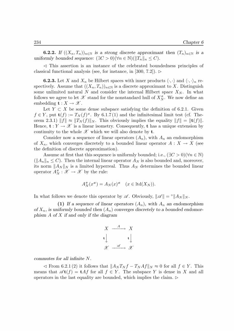
234 Chapter 6
6.2.2. If ((Xn, Tn))n∈N is a strong discrete approximant then (Tn)n∈N is auniformly bounded sequence: (∃C > 0)(∀n ∈ N)(‖Tn‖n ≤ C).
� This assertion is an instance of the celebrated boundedness principles ofclassical functional analysis (see, for instance, in [300, 7.2]). �
6.2.3. Let X and Xn be Hilbert spaces with inner products 〈·, ·〉 and 〈·, ·〉n re-spectively. Assume that ((Xn, Tn))n∈N is a discrete approximant to X . Distinguishsome unlimited natural N and consider the internal Hilbert space XN . In whatfollows we agree to let X stand for the nonstandard hull of X#
N . We now define anembedding t : X → X .
Let Y ⊂ X be some dense subspace satisfying the definition of 6.2.1. Givenf ∈ Y , put t(f) := TN (f)#. By 6.1.7 (1) and the infinitesimal limit test (cf. The-orem 2.3.1) ‖f‖ ≈ ‖TN (f)‖N . This obviously implies the equality ‖f‖ = ‖t(f)‖.Hence, t : Y → X is a linear isometry. Consequently, t has a unique extension bycontinuity to the whole X which we will also denote by t.
Consider now a sequence of linear operators (An), with An an endomorphismof Xn, which converges discretely to a bounded linear operator A : X → X (seethe definition of discrete approximation).
Assume at first that this sequence is uniformly bounded; i.e., (∃C > 0)(∀n ∈ N)(‖An‖n ≤ C). Then the internal linear operator AN is also bounded and, moreover,its norm ‖AN‖N is a limited hyperreal. Thus AN determines the bounded linearoperator A#
N : X → X by the rule:
A#N (x#) = AN (x)# (x ∈ ltd(XN)).
In what follows we denote this operator by A . Obviously, ‖A ‖ = ◦‖AN‖N .
(1) If a sequence of linear operators (An), with An an endomorphismof Xn, is uniformly bounded then (An) converges discretely to a bounded endomor-phism A of X if and only if the diagram
XA−−−−→ X
t
⏐⏐# t
⏐⏐#
XA−−−−→ X
commutes for all infinite N .
� From 6.2.1 (2) it follows that ‖ANTNf − TNAf‖N ≈ 0 for all f ∈ Y . Thismeans that A t(f) = tAf for all f ∈ Y . The subspace Y is dense in X and alloperators in the last equality are bounded, which implies the claim. �
Technique of Hyperapproximation 235
(2) Assume that a sequence of linear operators (An), with An an en-domorphism of Xn, is uniformly bounded and converges discretely to a boundedendomorphism A of X . Then DAp(A) = {f ∈ Y : Af ∈ Y }. In particular, ifY = X and the equality 6.2.1 (2) holds on some dense subset of X then it holds onthe whole X .
� Immediate from (1). �
6.2.4. From now we assume that, for all n, the spaces Xn are finite-dimensionaland all operators An and A are normal or hermitian. Then A is also normal orhermitian. In this case in view of 6.1.10 σ(A ) = {◦λ : λ ∈ σ(AN )} and the spectrumσ(A ) of A is discrete; i.e., σ(A )=σp(A ) or, in other words, σ(A ) consists only ofeigenvalues of A .
We also assume that the sequence (An) converges discretely to A. Obviouslyfor normal operators the commutativity of the diagram of 6.2.3 (1) implies theinclusion: σ(A) ⊂ σ(A ). So, the eigenvectors of A that correspond to the pointsof σ(A), may be considered as generalized eigenvectors of A. We use below thefollowing notation: T (λ) := ker(λ− T ) for an arbitrary operator T .
If A is compact operator and A (X ) ⊂ t(X) then(1) σ(A) = σ(A );(2) if λ ∈ σ(A) and λ �= 0 then A (λ) = t(A(λ)), and so dim(A (λ)) =
dim(A(λ)).
� We have to show that σ(A ) ⊃ σ(A) and each eigenvector f of A notbelonging to ker(A ) has the shape f = t(x) where x is an eigenvector of A withthe same eigenvalue as f .
Indeed, take λ ∈ σ(A ). It is possible to assume that λ �= 0. Otherwiseλ ∈ σ(A) since A is compact and normal. Since σ(A )=σp(A ), there is some fin X satisfying A f = λf . By hypothesis A f ∈ t(X), and since λ �= 0 we havef ∈ t(X).
Hence, there is a unique x ∈ X satisfying f = t(x). Since the diagramof 6.2.3 (1) commutes, t(Ax) = A (t(x)) = A f = λf . This implies that t(λx) = λf .Furthermore, since t is injective, we infer that x is an eigenvector of A with eigen-value λ. �
6.2.5. Under the hypotheses of 6.2.3 if A and AN are hermitian then(1) σλ := {ν ∈ σ(AN) : ν ≈ λ} is a finite set for each nonzero λ ∈
σ(A ); i.e., σλ = {ν1, . . . , νk} where k ∈ N;
(2) The dimension mj := dim(A(νj)N ) is finite for all j ≤ m and
∑kj=1mj = dim(A (λ));
(3) (A(ν1)N ⊕ · · · ⊕ A
(νm)N )# = A (λ);

236 Chapter 6
(4) If the family (xj1, . . . , xjmı
) is a Hilbert basis for A(νj)N for all j :=
1, . . . , k then ((x11)#, . . . , (x1
m1)#, . . . , (xk1)#, . . . , (xkmk
)#) is a Hil-bert basis for A (λ);
(5) If A(λ) ⊂ DAp(A) then there is a Hilbert basis (y11, . . . , y
1m1, . . . , yk1 ,
. . . , ykmk) for A(λ) such that TNy
jl ≈ xjl for j := 1, . . . , k; l :=
1, . . . , mj.
� It is easy to see that x# ∈ A (λ) whenever ν ≈ λ and x ∈ A(ν)N . In case
ν1, . . . , νk ∈ σλ are pairwise distinct, all x1 ∈ A(ν1)N , . . . , xk ∈ A
(νk)N are pairwise
orthogonal and so x#1 , . . . , x
#k are pairwise orthogonal too. This proves that k ≤
dim(A (λ)). The reverse inequality was proven in 6.1.6 (3).The implications (2) → (3) and (3) → (4) are obvious, while (5) follows from
the definition of t. �
6.2.6. A sequence of operators (An) is quasicompact provided that A (X ) ⊂t(X) for all unlimited N (note that (An) is not assumed convergent discretely to A).
The reason behind this definition is as follows: Assume for a moment that((Xn, Tn))n∈N is a strong discrete approximant (see 6.2.1). Then the condition6.2.1 (2) means that, for all unlimited N , the image ANx of each limited x isinfinitely close to TNy for some standard y ∈ X . Observe now that the infinitesimaltest for an operator to be compact reads (cf. 4.3.6): T is a compact operator if andonly if the image of every limited element under T is nearstandard.
We now give one simple sufficient condition of quasicompactness of a sequenceof operators (An) which holds for all Banach spaces X and Xn with n ∈ N (cf. [405]).This rests on requiring the following property of discrete approximation which wewill often use in the sequel:
(1) supn∈N
sup‖z‖=1
(inf{‖x‖n : Tnx = z}) < +∞.
(2) Assume that a sequence (An) converges discretely to a compactoperator A and, moreover, this convergence is uniform. Assume further that thediscrete approximation ((Xn, Tn))n∈N enjoys the property (1). Then (An) is aquasicompact sequence.
� Take ξ ∈ X . There is a limited element x in XN satisfying ξ = x#. Sinceevery Tn is surjective, by transfer, x = TNf for some f ∈ ∗X .
From the hypothesis about ((Xn, Tn))n∈N it follows that f may be chosenlimited. By uniform convergence ‖ANTN − TN
∗A‖N ≈ 0 and so ANx = ANTNf ≈TN∗Af .
Since A is compact and f is limited, there is a standard element h ∈ X satis-fying ∗Af ≈ h. By 6.2.2, ‖TN‖N is limited and so TN ∗Af ≈ TNh, i.e., ANx ≈ TNhand A (ξ) = t(h). �
Technique of Hyperapproximation 237
Below in 7.6 and 7.7 we will use strong discrete convergence in the situation[86] in which there are isometric embeddings ın : Xn → X and Tn := ı−1
n ◦ pn,where pn : X → ın(Xn) is the corresponding orthoprojection. It is easy to see thatthe discrete approximation in this case enjoys the above extra requirement.
Unfortunately, uniform convergence is a rare phenomenon. Therefore, to provequasicompactness for (An) is not an easy matter in many interesting cases. Wemust first of all find the conditions for x ∈ XN to be infinitesimally close to someelement of the shape TNy with some standard y ∈ X . In 7.6.15 we give one testuseful for the approach we pursue to approximating Schrodinger type operators.
6.2.7. The definition of quasicompactness acquires a rather natural standardversion since condition of the definition of 6.2.6 holds for every unlimited integer N .Then the routine infinitesimal arguments will allow us to prove the following propo-sition which holds for arbitrary parameters.
We denote the unit ball of XN with center the origin by BN , keeping thesymbol BN (ε, x) for the ball in XN with center x and radius ε.
If ((Xn, Tn))n∈N is a strong discrete approximant then (An) is a quasicompactsequence of operators if and only if
(∀ε > 0)(∃finB ⊂ X)(∃n0)(∀N > n0)(
(AN (BN )) ⊂⋃
y∈BBN (ε, TNy)
).
� ←: Take an arbitrary standard ε > 0. By transfer, we have the followinginclusion:
AN (BN) ⊂⋃
y∈BBN (ε, TNy)
for every unlimited natural N . This implies for x ∈ BN that to each standardn ∈ N there is a standard yn ∈ X satisfying ‖ANx − TNyn‖N < n−1. Since‖TNyn − TNym‖N ≈ ‖yn − ym‖ for all standard n and m; therefore, (yn)n∈N isa Cauchy sequence in X and so (yn)n∈N converges to some standard element y ∈ X .Now it is obvious that ‖ANx− TNy‖ ≈ 0.
→: Suppose the contrary. By negation,
(∃ε > 0)(∀finB ⊂ X)(∀n0)(∃N > n0)(
(AN (BN )) �⊂⋃
y∈BBN (ε, TNy)
).
Take a standard ε0 > 0 satisfying the last formula. Consider a hyperfinite setB ⊂ ∗X such that X ⊂ B.
238 Chapter 6
By transfer, from the above formula it follows that there is an unlimited Nsatisfying
AN (BN ) �⊂⋃
y∈BBN (ε, TNy).
Thus, there is some x in BN such that the distance from x to each element of theshape TNy with a standard y is greater than or equal to the standard ε0. Thisshows that the condition of the definition of quasicompactness in 6.2.6 fails for thisnumber N . �
6.2.8. Theorem. Let A be a compact hermitian endomorphism of a Hilbertspace X . Assume that ((Xn, Tn))n∈N is a discrete approximant to X , and (An)n∈N
is a quasicompact sequence convergent discretely to A, with An a hermitian endo-morphism of Xn for all n. Then
(1) The spectrum σ(A) of A coincides with the set of nonisolated limitpoints of
⋃n σ(An);
(2) If 0 �= λ ∈ σ(A) and J is a neighborhood of λ with no points ofσ(A) distinct from λ then λ is the sole nonisolated limit point ofJ ∩⋃n σ(An);
(3) If in the context of (2)
Mλn :=
∑
ν∈σ(An)∩J A(ν)n ,
then dim(Mλn ) = dim(A(λ)) = s for all sufficiently large n and there
is a sequence of orthonormal bases (fn1 , . . . , fns ) forMλ
n , convergentdiscretely to an orthonormal basis (f1, . . . , fs) for A(λ).
� This is a standard rephrasing of 6.2.4 and 6.2.5. �Certainly, our arguments fail in the case of unbounded selfadjoint operator A.
Indeed, if (An) converges discretely to A then the norm of AN is unlimited andwe face problems even in defining A#
N (see [250]). However, we may obviate theobstacles by slightly modifying the results on strong resolvent convergence (cf., forexample, [409, Theorem VIII.19] and also [117, Theorem 5.7.6]). It is worth notingalso that all facts of the theory of unbounded linear operators we use in the sequelmay be found in [409, Chapter VIII].
If λ /∈ σ(A) then we let Rλ(A) := (λ−A)−1 := (λ1−A)−1 denote the resolventof A at λ, with 1 standing as usual for the identity operator I on X , the unity ofthe endomorphism algebra of X .
6.2.9. If A is selfadjoint and the approximation domain DAp(A) of A by (An)is an essential domain of A then (Rλ(An)) converges discretely to Rλ(A) for all λsuch that λ /∈ cl(σ(A) ∪⋃n σ(An)).
Technique of Hyperapproximation 239
� Start with proving the claim for λ := ±i which obviously meets the as-sumptions. Consider only the case of λ := −i since the case of λ := i is settledsimilarly. By definition, it suffices to prove 6.2.1 (2) with R−i(A) and R−i(An) andsome dense subset Y ⊂ X .
Put Y := {(A + i)ϕ : ϕ ∈ DAp(A)}. Then Y is dense in X because DAp(A)is an essential domain of A. Take an unlimited natural N and note
((A+ i)−1 − (AN + i)−1)(A+ i)ϕ = (AN + i)−1(AN − A)ϕ.
Since ϕ ∈ DAp(A); therefore, (AN −A)ϕ ≈ 0.Given a subset B of the reals R and λ ∈ C, denote the distance from λ to B
on the plane C by ρ(λ,B). Assign S := cl(σ(A) ∪ ⋃n σ(An)). If λ satisfies thehypotheses then ρ(λ, S) > 0. By transfer,
‖(AN + i)−1‖ = ρ(λ, σ(AN))−1 ≤ ρ(λ, S)−1 � +∞.
Thus, R−i(AN )(A + i)ϕ ≈ R−i(A)(A + i)ϕ. This proves that R−i(An) convergesdiscretely to R−i(A).
We prove now that if the claim is valid for some λ0 such that λ /∈ S and if|λ − λ0| < ρ(λ0, S) then the claim holds for this λ. This will clear do since eachλ /∈ S can be connected either with i or with −i by a smooth curve lying entirelyin C − S. So we may reach λ from i or −i through finitely many circles of radiusless than ρ(λ, S).
The functions Rλ(An) (n ∈ N) and Rλ(A) are analytic in the open disk {λ ∈C : |λ− λ0| < ρ(λ0, S)}, and expand in the following uniformly convergent series:
(1) Rλ(A) =∞∑
m=0(λ− λ0)mRm+1
λ0(A),
(2) Rλ(An) =∞∑
m=0(λ− λ0)mRm+1
λ0(An).
Demonstrate that TNRλ(A)f ≈ Rλ(AN )TNf for all unlimited N and standardf ∈ Y . Since this holds for λ0; therefore,
(3)k∑
m=0(λ− λ0)mTNRm+1
λ0(A)f ≈
k∑
m=0(λ− λ0)mRm+1
λ0(AN )TNf
for all k ∈ N.Take an arbitrary standard ε > 0. Then by (1) and (2) there is some n0
satisfying∥∥∥∥Rλ(A)f −
k∑
m=0
(λ− λ0)mRm+1λ0
(A)f∥∥∥∥ < ε
for k > n0. Denote the function on the left part of the last inequality by h. Sinceh is standard, ‖TNh‖ ≈ ‖h‖. This implies that
240 Chapter 6
(4)∥∥∥TNRλ(A)f −
k∑
m=0(λ− λ0)mTNRm+1
λ0(A)f
∥∥∥N
≤ ε.
Show now that the convergence of the series in (2) is uniform in n. To thisend, note that
‖Rλ0(An)‖ = maxν
{ν : ν ∈ σ(An)} = ρ(λ0, σ(An))−1 ≤ ρ(λ0, S)−1.
Thus, q := |λ− λ0|‖Rλ0(An)‖ < 1, implying that
∥∥∥∥
∞∑
m=k+1
(λ− λ0)mRm+1λ0
(An)∥∥∥∥ ≤ ρ(λ0, S)−1qk+1
1 − q→ 0
for k → ∞. Now, since ‖TNf‖N is limited (TNf ≈ f); there is some n1 satisfying
(5)∥∥∥Rλ(An)TNf −
k∑
m=0(λ− λ0)mRm+1
λ0(AN )TNf
∥∥∥N< ε
for k > n1.Taking a standard k > max{n0, n1}, infer by (3), (4), and (5) that
‖TNRλ(A)f −Rλ(AN )TNf‖N ≤ 2ε.
Since ε > 0 is arbitrary, the proof is complete. �
6.2.10. The following proposition is a simple corollary of the above fact.
If in the conditions of 6.2.9 the resolvents of selfadjoint operators An are com-pact and (Rλ(A)) is a quasicompact sequence for some real λ /∈ cl(σ(A)∪⋃n σ(An))then 6.2.8 (1)– (3) are valid.
6.2.11. If ((Xn, Tn))n∈N is a strong discrete approximant satisfying 6.2.6 (1)then by 6.2.6 (2) the uniform convergence of the sequence of resolvents implies thatthis is a quasicompact sequence. The following proposition (cf. [409, Theorem 8.25])provides a sufficient condition for uniform convergence of resolvents.
Suppose that in the conditions of 6.2.9 the discrete approximant ((Xn, Tn))n∈N
is strong and satisfies 6.2.6 (1) and for some essential domain D ⊂ DAp(A) of Athe following condition holds
limn→∞ sup
ϕ∈D,‖ϕ‖A=1
‖(TnA−AnTn)ϕ‖n = 0,
where ‖ϕ‖A := ‖Aϕ‖+‖ϕ‖. Then the convergence of (Rλ(An)) to Rλ(A) is uniform.
Technique of Hyperapproximation 241
6.2.12. Comments.
(1) The origin of this section is the article [5] by Albeverio, Gordon,and Khrennikov. The definitions of 6.2.1 specify the concept of discrete convergencewhich stems from the works of Stummel [468, 469]. Some aspects of this notion arediscussed in the book [410]. We use the notion of discrete compactness which forour particular case amounts to discrete compactness as introduced in [410, 7.3].
(2) Discrete approximation in the case of Y = X is also used in [86]wherein Xn are some spaces of grid functions embedded into L2(Rn) as the spacesof step functions and the orthoprojections onto the latter serve as Tn. Note that inthis case Tnf differs from the table of f at the knots of the grid even for a continuousfunction f .
However, if f is smooth then it is easy to see that the difference vanishes be-tween Tnf and the table of f as n tends to infinity. The possibility of considering Anas an endomorphism of X (in this case X = L2(Rn)) simplifies the study of thelimit behavior of the spectra of approximants. The key tool for this is the conceptof uniform compactness which means that
⋃n∈N
An(U), with U the unit ball ofL2(Rn), is relatively compact (see [86]). This concept was suggested in [15].
(3) We consider here only selfadjoint operators with discrete spectraand compact resolvents but it seems that our approach may be useful in othercases. Some general results on the limit behavior of the spectra of approximants Anconverging discretely to some operator A in the general Banach spaces but in thecase of Y = X (see the definitions of 6.2.1) were obtained by Rabiger and Wolff[405, 528] also by infinitesimal methods. Gordon in [146] pursues the same approachin the special case of selfadjoint integral operators on compact groups.
(4) The proof of 6.2.7 involves Card(X)+-saturation, i.e., the properly-stated concurrence principle. Clearly, in case X is separable, it suffices to useω1-saturation of the nonstandard universe.
(5) It is interesting to compare the quasicompactness property of 6.2.6with the compactness property of the sequence (An) as in [86].
As was mentioned, the environment of [86] assumes some isometric embeddingsın : Xn → X and Tn := ı−1
n ◦ pn, with pn : X → ın(Xn) the orthoprojectionfrom X onto ın(Xn). In this event we may identify An with the endomorphismAn := ınAnTn of X .
By [86] (An) is a compact sequence, provided that⋃n An(B), with B the unit
ball of X , is relatively compact. It is easy to see that if (An) is a compact sequencein the sense of [86] then (An) is quasicompact. Indeed, if x ∈ BN for all infiniteN ∈ ∗N then ıN (x) ∈ B and AN ıNx = ıNANx ≈ y for some standard y ∈ X bythe compactness property in the sense of [86] and Theorem 4.3.6.
242 Chapter 6
6.3. Loeb Measure
The construction of Loeb measure is one of the most noticeable achievements ofinfinitesimal analysis which gave rise to applications in many sections of functionalanalysis, probability, and stochastic modeling; see [3, 69]. We now present a fewresults about the structure of Loeb measure.
6.3.1. Let (X,A , ν) be an internal measure space with ν a finitely additivemeasure; more exactly, assume that A is an internal algebra of subsets of an internalset X and ν : A → ∗
R is an internal finitely additive function on A .This implies in particular that A ⊂ ∗P(X). Moreover, if {A1, . . . , AΩ} is
a hyperfinite set of members of A , with Ω ∈ ∗N, then
⋃Ωk=1Ak ∈ A ; if Ak are
pairwise disjoint then
ν
(Ω⋃
k=1
Ak
)
=Ω∑
k=1
ν(Ak).
The union of a hyperfinite family of sets is defined in much the same way as thesum of a hyperfinite set in 6.1.3. If f : N → P(X) is a sequence in P(X) then wedefine the new sequence g : N → P(X) by recursion:
Seq(f) ∧ Seq(g) ∧ f(0) = g(0) ∧ (∀k ∈ N)(g(k+ 1) = g(k) ∪ f(k + 1)).
Abbreviate this formula to⋃
(f, g), take a hyperfinite set A0 ⊂ A , and put Ω :=|A0|. Proceed as follows: Distinguish some bijection f : {0, . . . ,Ω − 1} → A0 andextend it to the internal sequence f : ∗N → A by letting f be zero for n > Ω − 1.We now define the sequence g : ∗N → A by the rule
⋃(f, g). By transfer, g(Ω − 1)
is independent of the choice of f . Therefore, we may soundly assign⋃A∈A0
A :=g(Ω − 1). Again by transfer, the so-defined union of a hyperfinite family enjoys allproperties of the conventional finite union.
Consider the external function
◦ν : A �→ ◦(ν(A)) ∈ R• (A ∈ A ),
where ◦(ν(A)) is as usual the standard part of ν(A) whenever ν(A) is limited and◦(ν(A)) = +∞ otherwise. It is easy to see that ◦ν is a finitely additive function.
6.3.2. The Loeb measure for ν appears as a unique countably additive exten-sion of ◦ν to the external σ-algebra σ(A ) generated by A . The existence of thisextension, as will be shown in 6.3.4, ensues from the Lebesgue–Caratheodory Ex-tension Theorem, whereas the uniqueness of this extension requires a few auxiliaryfacts of a technical nature.

Technique of Hyperapproximation 243
(1) Let A0 be a countable subalgebra of A and letB0 be a complete al-gebra of subsets of X (i.e., a complete subalgebra of P(X)) generated by A0. IfS ⊂ X and for every A ∈ A0 either S ⊂ A or S ∩ A = ∅ then for every B ∈ B0
either S ⊂ B or S ∩B = ∅.
� Call a subset P of X marked provided that P :=⋂∞k=1Bk where (Bn) ⊂ A0
and for every member A of A0 either A or the complement of A to X coincides withone of the sets Bk. Let P stand for the set of all marked subsets of X . Clearly, themembers of P are pairwise disjoint and
⋃P = X ; i.e., P is a partition of X . By
the definition of marked set, if P ∈ P and A ∈ A0 then either P ⊂ A or P ∩A = ∅.Hence, A =
⋃{P ∈ P : P ⊂ A} for all A ∈ A0. Note also that B0 consists exactlyof the sets B ⊂ X of the shape B :=
⋃P ′, with P ′ ⊂ P.
We now take a set S ⊂ X such that for every A ∈ A0 either S ⊂ A orS ∩ A = ∅. Then the sequence (Bk) of all elements of A0 including S is such thatP :=
⋂Bk belongs to P. Since S ⊂ P ; therefore, if B ∈ B0 then the above shows
that only two cases are possible: either P ⊂ B implying S ⊂ B or P ∩ B = ∅
implying S ∩B = ∅. �Let c(A ) stand for the collection of all sets S ⊂ X satisfying the following
condition: There is a countable subalgebra A0 of A such that S belongs to acomplete subalgebra of subsets of X generated A0 (i.e., in a complete subalgebraof the powerset P(X)). In this event, we say that S is generated by A0. Thefollowing is immediate from the above definitions.
(2) The set c(A ) is a σ-algebra and σ(A ) ⊂ c(A ).
6.3.3. If S ∈ c(A ) then the following dilemma is open:(1) There is some A ∈ A such that A ⊂ S and ν(A) is an unlimited
real;
(2) There is a sequence (Ak)k∈N ⊂ A such that S ⊂ ⋃k Ak and ν(Ak)is a limited real for all k ∈ N.
� Let S ∈ c(A0) be a set generated by the countable subalgebra A0 of A . PutA ′0 := {A ∈ A0 : |ν(A)| � +∞}. If S ⊂ ⋃
A ′0 then (2) holds. In the oppositecase, take p ∈ S −⋃A ′0 and consider the countable set A ′′0 := {A ∈ A0 : p ∈ A}.Note that A ′′0 has the finite intersection property and consists of sets of unlimitedmeasure. Put A(n,B) := {A ∈ A : p ∈ A ⊂ B, ν(A) ≥ n}. By the properties ofA ′′0 , the set {A(n,B) : n ∈ N, B ∈ A ′′0 } has the finite intersection property. Bysaturation, there is some A in A satisfying A ∈ A(n,B) for all n ∈ N and B ∈ A ′′0 .Hence, ν(A) is unlimited, p ∈ A, and A ⊂ B for all B ∈ A ′′0 .
Assume that some C in A0 does not included A. Then either p /∈ C or p ∈X − C, implying that X − C ∈ A ′′0 and so A ⊂ X − C. Thus, if C ∈ A0 theneither A ⊂ C or A∩C = ∅. Since S is generated by A0; therefore, either A ⊂ S orA ∩ S = ∅ by 6.3.2 (1). Since p ∈ A ∩ S, it follows that A ⊂ S, implying (1).
244 Chapter 6
Assume that (1) and (2) hold simultaneously. In this event A ⊂ ⋃k Ak and
ν(A) is unlimited whereas ν(Ak) are all limited. By saturation, A ⊂ A1 ∪ · · · ∪ Anfor some n ∈ N. This is however impossible implying ν(A) ≤ ν(A1) + · · · + ν(An)which is a contradiction. �
6.3.4. Theorem. A finitely additive measure ◦ν : A → R• admits a unique
countably additive extension λ to the external σ-algebra σ(A ) generated by A .Moreover:
(1) λ(B) = inf{◦ν(A) : B ⊂ A,A ∈ A } (B ∈ σ(A ));(2) If λ(B) < +∞ for some B ∈ σ(A ) then λ(B) = sup{◦ν(A) : A ⊂ B,
A ∈ A };(3) If λ(B) < +∞ for some B ∈ σ(A ) then there is A ∈ A satisfying
λ(A&B) = 0;(4) To an arbitrary B ∈ σ(A ) either there is A ∈ A such that A ⊂ B
and ◦ν(A) = +∞, or there is a sequence (An)n∈N of sets in A suchthat B ⊂ ⋃n∈N
An and◦ν(An) < +∞ for all n ∈ N.
� The existence of λ follows from the Lebesgue–Caratheodory Extension The-orem. The validation of the hypotheses of this theorem is trivial. Indeed, take anincreasing sequence of sets (Ak)k∈N in A and suppose that A :=
⋃k Ak belongs
to A . By saturation, A = Am for some m ∈ ∗N and so ◦ν(Ak) → ◦ν(A).We now prove (1)–(3) and the claim of uniqueness. Take B ∈ σ(A ). The
Lebesgue–Caratheodory Extension Theorem guarantees in particular that
λ(B) = inf{ ∞∑
k=1
◦ν(Ak) : Ak ∈ A (k ∈ N), B ⊂∞⋃
k=1
Ak
}
for all B ∈ σ(A ). Consequently, to each 0 < ε ∈ R there is a sequence of internalsets (Ak)k∈N, satisfying B ⊂ ⋃∞
k=1Ak and∑∞
k=1◦ν(Ak) < λ(B) + ε/2. Since
ν(Ak) < ◦ν(Ak) + ε/2k+1 for all k ∈ N; therefore, given n ∈ N, we may write
ν
( n⋃
k=1
Ak
)
≤n∑
k=1
ν(Ak) ≤∞∑
k=1
◦ν(Ak) +∞∑
k=1
ε/2k+1 < λ(B) + ε.
Extend (Ak)k∈N to some internal sequence (Ak)k∈∗N by 3.5.11 (1). Consider theinternal set {n ∈ ∗N : ν (
⋃nk=1Ak) < λ(B) + ε}. Since this set contains all stan-
dard naturals, it also contains some unlimited natural Ω by overflow. Put AΩ :=⋃Ωk=1Ak. By definition, B ⊂ AΩ and ν(AΩ) < λ(B) + ε and so ◦ν(AΩ) ≤ λ(B) + ε.
This proves (1).Assume that λ(B) < +∞. By what was proven there is an internal set C ∈ A
such that B ⊂ C and ν(C) is finite. Applying (1) to C − B, infer (2). Fur-thermore, let (Ak)k∈N be an increasing sequence in A satisfying Ak ⊂ B and
Technique of Hyperapproximation 245
|ν(Ak) −λ(B)| < 1/k. By extension, consider this sequence as a part of an internalincreasing sequence (Ak)k∈∗N with the same property. By overflow, there is an un-limited hypernatural Ω ∈ ∗N satisfying |ν(AΩ)−λ(B)| < 1/Ω. Then λ(B) = ◦ν(AΩ)and it is easy to see that λ(AΩ&B) = 0. Infer (4) now from 6.3.3.
We are left with proving uniqueness. Suppose that λ1 and λ2 are two σ-additiveextensions of the measure ◦ν to σ(A ). Since σ(A ) ⊂ c(A), it is possible to apply6.3.3 to S ∈ σ(A ). In the case of 6.3.3 (1), there is some A ∈ A satisfying A ⊂ Sand ◦ν(A) = ∞, implying that λj(S) = ∞ (j := 1, 2). In the case of 6.3.3 (2),there is a sequence (Ak)k∈N in A such that S ⊂ ⋃
k Ak and ν(Ak) is limited forall k ∈ N. Without loss of generality, we may assume that this sequence increases.By 6.3.4 (1)
λj(S ∩Ak) = inf{◦ν(A) : A ∈ A , S ∩ Ak ⊂ A ⊂ Ak} (j := 1, 2).
Hence we infer in particular that λ1(S ∩ Ak) = λ(S ∩ Ak) for k ∈ N. Since S =⋃k(S ∩ Ak) and (S ∩ Ak)k∈N is an increasing sequence; therefore, λ1(S) = λ2(S).
Thus, λ1 and λ2 coincide on σ(A ). �6.3.5. Let S(A ) stand for a completion of σ(A ) with respect to λ, and let νL
stand for the extension of λ to S(A ). We may show that, in case νL(X) < +∞,the membership B ∈ S(A ) holds if and only if
sup{◦ν(A) : A ⊂ B,A ∈ A } = inf{◦ν(A) : B ⊂ A,A ∈ A } = νL(B).
The triple (X,S(A ), νL), presenting a measure space with the σ-additive measureνL, is the Loeb measure space (for (X,A , ν)); and νL, the Loeb measure (for ν).
A function f : X → ∗R is Loeb-measurable provided that f is measurable with
respect to the σ-algebra S(A ). An internal function F : X → ∗R is A -measurable
if {x ∈ X : F (x) ≤ t} ∈ A for all t ∈ ∗R. An internal A -measurable function
F : X → ∗R is a lifting of a function f : X → ∗
R whenever f(x) = ◦F (x) forνL-almost all x ∈ X .
6.3.6. Theorem. A function f : X → ∗R is Loeb-measurable if and only if f
has a lifting.
� ←: Take an A -measurable internal function F : X → ∗R. Given arbitrary
standard r ∈ R, note that
{x ∈ X : ◦F (x) ≤ r} =⋂
k∈N
{x ∈ X : F (x) ≤ r + 1/k} ∈ σ(A ),
and so the function ◦F is Loeb-measurable. If f(x) = ◦F (x) νL-almost everywherethen f is Loeb-measurable too.
246 Chapter 6
→: Assume that f is Loeb-measurable. Consider an arbitrary numbering(qk)k∈N of the rationals Q; in symbols, Q = {qk : k ∈ N}. Put Bk := {x ∈X : f(x) ≤ qk}. Choose internal sets Ak ∈ A so that νL(Ak&Bk) = 0 andAk ⊂ Al for qk ≤ ql. By extension and overflow, there is an unlimited natural Ωsuch that Ak ∈ A and if qk ≤ ql then Ak ⊂ Al for all k, l ≤ Ω. Define some internalA -measurable function F : X → ∗
R with range {q1, . . . , qΩ} by the condition thatF (x) ≤ qk is equivalent to x ∈ Ak. In more detail, if {q1, . . . , qΩ} is renumbered inincreasing order qk1 < qk2 < · · · < qkΩ then put
F (x) :=
⎧⎪⎨
⎪⎩
qk1 , if x ∈ Ak1 ,
qkl, if x ∈ Akl
− Akl−1 (1 < l ≤ Ω),qkΩ+1, if x /∈ AkΩ .
Clearly, if k ∈ N then F (x) ≤ qk amounts to f(x) ≤ qk for all x /∈ D :=⋃k∈N
Ak&Bk. Since νL(D) = 0; therefore, ◦F (x) = f(x) for νL-almost all x ∈ X . �6.3.7. An internal function F is simple if the range im(F ) of F is a hyperfinite
set. Inspection of the proof of Theorem 6.3.6 shows that each Loeb-measurablefunction has a lifting that is a simple function. Obviously, a simple internal functionF is A -measurable if and only if F−1({t}) ∈ A for all t ∈ ∗R. In this event to Fthere corresponds the internal integral
∫
X
F dν =∑
t∈im(F )
F (t)ν(F−1({t})).
If A ∈ A then, as usual,∫AF dν =
∫XFχA dν, where χA is the characteristic
function of a set A.Put AN := {x ∈ X : |F (x)| ≥ N}. An internal simple A -measurable function
F : X → ∗R is called S -integrable provided
∫AN
F dν ≈ 0 for all unlimited N .It is possible to prove that the S -integrability of F is equivalent to each of the
following conditions:(1)
∫XF dν is a limited hyperreal number and
∫AF dν ≈ 0 whenever
A ∈ A and ν(A) ≈ 0;(2)
∫X◦|F | dνL = ◦(
∫X
|F | dν) < +∞.The next two theorems deal with a finite Loeb measure space: νL(X) < +∞.
6.3.8. Theorem. Let (X,A , ν) be an internal measure space with finitelyadditive measure ν and let (X,S(A ), νL) be the Loeb measure space for (X,A , ν).A function f : X → ∗
R is νL-integrable if and only if f has an S -integrable liftingF : X → ∗
R. In this case∫
X
f dνL =◦(∫
X
F dν
)
.
Technique of Hyperapproximation 247
� Prove first that if f is bounded, Loeb-measurable and possesses a boundedlifting F then
∫Xf dνL = ◦∫
XF dν. To this end, take a simple Loeb measurable
function g with range a finite set {r1, . . . , rn}; moreover, assume that g ≤ f . Bythe theorem of 6.3.4, to the set Bk := g−1(rk) there is some Ak ∈ A satisfyingνL(Ak&Bk) = 0. The function G, equal to rk on Ak, is a lifting of g. Moreover,∫Xg dνL = ◦
∫XGdν since both integrals are finite sums equal to each other.
If a bounded lifting F1 of f satisfies the inequality then, on the one hand,∫XGdνL ≤ ∫
XF1 dν and, on the other hand, |F (x) − F1(x)| ≤ 1/n for νL-almost
all x ∈ X and for all standard n ∈ N. Hence,∫XF dν ≈ ∫
XF1 dν, implying that
∫
X
g dνL =◦(∫
X
Gdν
)
≤◦(∫
X
F1 dν))
=◦(∫
X
F dν
)
.
Hence,∫Xf dνL ≤ ◦(
∫XF dν). The reverse inequality results on replacing f with
−f and F with −F .Assume now that f is νL-integrable. Without loss of generality, assume further
that f ≥ 0. (The general case will ensue on using the standard representation of Fas the difference of its positive and negative parts: f = f+ − f−.)
Let F ′ be a lifting of f whose existence follows from Theorem 6.3.6. If Fn :=F ′ ∧ n then the above implies
◦(∫
X
Fn dν
)
=∫
X
(f ∧ n) dνL →∫
X
f dνL.
Applying to (Fn)n∈N the extension and overflow principles, find an unlimited nat-ural Ω satisfying ◦(
∫XFN dν) ≈ ∫
Xf dνL → ∫
Xf dνL for all unlimited naturals
N ≤ Ω. The function F := FΩ is an S -integrable lifting of f .Conversely, assume given an S -integrable lifting F of f . By underflow, to an
arbitrary 0 < ε ∈ R there is a standard natural n ∈ N such that∫F≥m F dν ≤ ε for
each standard m ≥ n. Applying again the above-indicated assertion for a boundedfunction, infer that
∫
X
(f ∧ n) dνL ≈∫
X
(F ∧ n) dν ≤∫
X
F dν
≤∫
X
(F ∧ n) dν + ε ≈∫
X
(f ∧ n) dνL + ε.
Hence, ◦(∫XF dν) is a limited real serving as the limit of the sequence
∫X
(f∧n) dνLas n → ∞. This ends the proof. �
248 Chapter 6
6.3.9. Theorem. Let (X,A , ν) be an internal space with ν a finitely addi-tive measure. For each simple internal A -measurable function the following areequivalent:
(1) F is S -measurable;(2) ◦
∫X
|F | dν < +∞ and ν(A) ≈ 0 implies∫A
|F | dν ≈ 0 for all A ∈ A ;
(3)∫X◦|F | dνL = ◦∫
X|F | dν.
� The proof proceeds by analogy with no complications. �6.3.10. We suppose now that X is a hyperfinite set, A := P(X), and ν is
a counting measure multiplied by Δ, i.e., ν(A) := Δ|A| for all A ∈ A , where |A|stands for the size of A and Δ ∈ ∗R+.
The corresponding Loeb measure space is denoted by (X,SΔ, νΔ), while νΔ iscalled the uniform Loeb measure with weight Δ. In the case of uniform Loeb mea-sures, every internal function F : X → ∗
R is simple and A -measurable; moreover,∫AF dν = Δ
∑x∈A F (x) for all A ∈ A .
The Loeb measure νΔ is finite provided that Δ|X | is a limited real. If Δ :=|X |−1 then the Loeb measure space (X,SΔ, νΔ) is called canonical and denoted by(X,S, νL) or (X,SX , νXL ). In the case of a finite Loeb measure, if F : X → ∗
R isan S -integrable lifting of a function f : X → R then
∫
X
f dνΔ =◦(
Δ∑
x∈XF (x)
)
by Theorem 6.3.8.
6.3.11. We now abstract Theorem 6.3.8 to the case of an infinite Loeb mea-sure νΔ.
Suppose that (X,SΔ, νΔ) is a Loeb measure space, and M ∈ SΔ enjoys theproperty: there is an increasing sequence (Mn)n∈N of internal sets satisfying thetwo conditions: M =
⋃n∈N
Mn and Δ|Mn| � +∞ for all n ∈ N.In this case we let SMΔ stand for the σ-algebra {A ∩ M : A ∈ SΔ} of subsets
of M and denote the restriction of νΔ to SMΔ by νMΔ . The space Ξ := (M,SMΔ , νMΔ ) isa σ-finite subspace of the Loeb measure space (X,SΔ, νΔ). We also let A := ∗P(X)stand for the set of all internal subsets of X .
An internal function F : X → ∗R is SM -integrable, provided that the following
hold:(1) Δ
∑ξ∈X |F (ξ)| � ∞;
(2) (∀A ∈ A)(Δ|A| ≈ 0 → Δ∑ξ∈A |F (ξ)| ≈ 0);
(3) (B ∈ A ∧B ⊂ X −M) → Δ∑ξ∈B |F (ξ)| ≈ 0.
If X = M and M is an internal set then X = Mn for some n ∈ N by ω1-saturation. In particular, νΔ(X) < +∞ and so, by 6.3.7, SM -integrability coincidesin this case with S -integrability.
Technique of Hyperapproximation 249
An internal function F : X → ∗R is a lifting of a function f : X → ∗
R providedthat f(ξ) = ◦F (ξ) for νMΔ -almost all ξ ∈ M .
6.3.12. We introduce some notation. Let L be the hyperfinite-dimensionalinternal vector space of functions F : X → ∗
R furnished with the norm ‖F‖ :=Δ∑ξ∈X |F (ξ)|. If A ∈ A then ‖F‖A := ‖FχA‖ := Δ
∑ξ∈A |F (ξ)|, where χA is the
characteristic function of A.Recall that ltd(L ) is the external subspace of L comprising the elements of
limited norm, and μ(L ) ⊂ ltd(L ) is the monad of L comprising the elementsof infinitesimal norm (see 6.1.1). The nonstandard hull L # := ltd(L )/μ(L ) isa nonseparable Banach space (in the case when the internal cardinality |X | of Xis an unlimited number). Denote by S (M) the subspace of ltd(L ) comprising theSM -integrable functions.
In the course of this subsection the set M is fixed, so we will write S insteadof S (M) and SM and abbreviate νMΔ to νΔ. Finally, we let F ∼ G symbolize therelation ‖F −G‖ ≈ 0.
(1) If F ∈ L is an arbitrary function F ∈ L then from ‖F‖ ≈ 0 itfollows that F (ξ) ≈ 0 for νΔ-almost all ξ.
� Assume that there is some A in SΔ such that νΔ(A) > 0 and ◦F (ξ) �= 0 forall ξ ∈ A. Show that in this case there is some internal B ∈ A satisfying the sameconditions.
Indeed, if νΔ(A) ≤ +∞ then νΔ(A) = sup{νΔ(B) : B ∈ A, B ⊂ A} byTheorem 6.3.4. If νΔ(A) = +∞ then, appealing again to Theorem 6.3.4, notethat either there is an internal subset B of A satisfying νΔ(B) = +∞ or there isa sequence (An) of internal sets such that A ⊂ ⋃∞
n=0An and νΔ(An) < +∞ forall n ∈ N. In the last case νΔ(A ∩ An) → +∞, and so there is some n satisfyingνΔ(A ∩ An) > 0, and again we may apply Theorem 6.3.4.
Indeed, νΔ(B) > 0 for some B ∈ A. Since T := {|F (ξ)| : ξ ∈ B} is an internalset, it follows that α := ◦(inf T ) > 0 and ◦‖F‖ ≥ ◦(αΔ|B|) = ◦ανΔ(B) > 0. �
(2) If F ∈ S and G ∼ F then G ∈ S .
� If A satisfies one of the conditions (2) or (3) in the definition of 6.3.11 then‖F‖A ≈ 0, and since ‖F − G‖ ≈ 0, it follows that ‖F − G‖A ≈ 0. Consequently,‖G‖A ≈ 0. �
The next result follows from similar arguments.
(3) The nonstandard hull S # is a closed subspace of the Banach spaceL #.
250 Chapter 6
6.3.13. Theorem. A function f : X → ∗R is νMΔ -integrable if and only if f
has an SM -integrable lifting F . In this event
∫
M
f dνMΔ =◦(
Δ∑
ξ∈XF (ξ)
)
.
� It suffices clearly to prove the theorem for f a positive function. Accordingly,suppose that f ∈ L1(νΔ) and f ≥ 0. Put fn := fχMn
. The sequence (fn) increasesand converges pointwise to the integrable function f , so
(1)∫
M
fn dνΔ → ∫
M
f dνΔ.
This implies in the limit that
(2)∫
M
|fn − fm| dνΔ → 0, n,m → +∞.
Since the support of fn lies in the internal set Mn of finite measure, by Theo-rem 6.3.8 we may find an S -integrable lifting Fn of fn vanishing beyond Mn (sinceFn(ξ) = 0 for ξ ∈ X −Mn by 6.3.11 (3)). Moreover, we have (cf. 6.3.11)
(3)∫
M
fn dνMΔ =
◦(Δ∑
ξ∈XFn(ξ)
).
It now follows from (2) that ◦‖Fn − Fm‖ → 0 as m,n → +∞. By 6.3.12 (3),there is an internal function F ∈ S satisfying ◦‖Fn − F‖ → 0. Clearly, ◦‖Fn‖ →◦‖F‖. Passage to the limit in (3) together with (1) implies that (3) holds also for Fand f .
It remains to show that f(ξ) = ◦F (ξ) for νΔ-almost all ξ. To this end, take anarbitrary natural k > 0. Clearly, ◦‖FnχMk
− FχMk‖ → 0 as n → ∞. If n > k then
Mn ⊃ Mk, implying that fnχMk= fkχMk
. Consequently, the relation FnχMk≈
FkχMkholds νΔ-almost everywhere. Hence, the relation FnχMk
−FχMk≈ FkχMk
−FχMk
also holds νΔ-almost everywhere.Since the functions in the last relation are S -integrable and supported in the
set Mk of finite measure, it follows that ◦‖FnχMk− FχMk
‖ = ◦‖FkχMk− FχMk
‖.Passing here to the limit as n → ∞, infer that ◦‖FkχMk
− FχMk‖ = 0 for any k.
By 6.3.12 (1), conclude now that the relation FkχMk≈ FχMk
holds νΔ-almosteverywhere.
Consequently, the relation fχMk≈ FχMk
holds νΔ-almost everywhere, im-plying that the relation f ≈ F |M also holds νΔ-almost everywhere because M =⋃∞k=0Mk.
Suppose now that F ∈ S and f : M → R is such that f(ξ) = ◦F (ξ) for almostall ξ ∈ M . Show that f ∈ L1(νΔ) and (3) holds for F and f . Put Fn := FχMk
.Then the relation fn := fχMk
≈ Fn holds νΔ-almost everywhere. Hence, we may
Technique of Hyperapproximation 251
apply Theorem 6.3.8 since νΔ(Mn) is finite. This yields∫
M
|fn| dνΔ = ◦‖Fn‖ ≤ ◦‖F‖.
Since (|fn|) increases and converges to |f |, it follows from the Monotone Conver-gence Theorem that f ∈ L1(νΔ). By the above, there is an S -integrable internalfunction G : X → ∗
R satisfying∫M
|fn| dνΔ = ◦‖G‖.To prove (3) for F and f , it remains to show that ‖F − G‖ ≈ 0. Note first
that if A ∈ A and A ⊂ M then A ⊂ Mn for some number n by ω1-saturation.Take such a set A and such a number n. Put FM := FχM . Then the relationsf ≈ GM and f ≈ FM hold νΔ-almost everywhere and so the relation FMn
≈ GMn
holds νΔ-almost everywhere too. But then ‖F − G‖A ≈ 0 because F and G areS -integrable.
Consider the family of formulas Γm,n(A) := {A ∈ A ∧Mn ⊂ A ∧ ‖F −G‖A ≤m−1}. To each natural N ∈ N, there is some A ∈ A such that Γm,n(A) holds forall n,m ≤ N . Hence, there is some A ∈ A satisfying all formulas Γm,n(A). Butthen M ⊂ A and ‖F − G‖A ≈ 0. Since F,G ∈ S ; therefore, ‖F − G‖X−A ≈ 0.Consequently, ‖F −G‖ ≈ 0. �
6.3.14. Take p ∈ [1,+∞), and let Lp stand for the internal vector space offunctions F : X → ∗
R under the norm
‖F‖p =◦(
Δ∑
ξ∈X|F (ξ)|p
)1/p
.
Sometimes this space and its norm are denoted lavishly by LXp,Δ, and ‖·‖p,Δ. Given
F,G ∈ Lp, we write F ∼pG whenever ‖F −G‖p ≈ 0. The nonstandard hull L #
p is
defined in exactly the same way as in Section 6.1.If A ∈ A then ‖F‖p,A = ‖FχA‖p. Denote by Sp(M) the subspace of Lp
consisting of the functions F ∈ Lp such that the power |F |p is SM -integrable.We will write simply Sp, omitting M when this leads to no confusion. Since
‖F‖p,A = ‖|F |p‖A for every internal function F and every A ∈ A; therefore, Propo-sitions 6.3.12 (1)–(3) remain valid on replacing L , S , and ‖ · ‖ with Lp, Sp, and‖ · ‖p respectively.
We also define the complex spaces Lp and Sp in a completely analogous man-ner. Furthermore, if F : X → C is an internal function then F = ReF + i ImFand
‖ ReF‖p,A, ‖ ImF‖p,A ≤ ‖F‖p,A ≤ ‖ ReF‖p,A + ‖ ImF‖p,Afor every A ∈ A.

252 Chapter 6
From the last inequalities it follows that F ∈ Lp (Sp) if and only if ReF ∈Lp (Sp) and ImF ∈ Lp (Sp).
If f : M → F, with F a basic field of scalars (i.e., R or C) then f ∈ Lp(Ξ) ifand only if there is a lifting F : X → ∗
F of f such that F ∈ Sp(M). Furthermore,‖f‖p = ◦‖F‖p.
6.3.15. Comments.
(1) The construction of Loeb measure was implemented in [322]. Thecontent of 6.3.1–6.3.10 is well known; see [3, 69]. Theorem 6.3.4 in the case of finitemeasure belongs to Loeb [322]. Henson [166] established uniqueness in the case ofinfinite measure as well as the property 6.3.4 (4); the results of 6.3.2 and 6.3.3 areextracted from [166].
(2) Theorem 6.3.6 belongs to Loeb [322, 323]. A similar characteri-zation is available for measurable mappings with values in a complete separablemetric space (see [12, 322]). The definition of S -integrable function (6.3.7) wasintroduced by Loeb [323]; somewhat earlier Anderson considered the equivalentcondition 6.3.7 (1) in [11].
(3) The concept of a σ-finite subspace of a Loeb measure space wasintroduced by Gordon in [145]. The same article reveals Theorem 6.3.13. In 6.3.11–6.3.14, we proceed along the lines of [146].
6.4. Hyperapproximation of Measure Space
The aim of this section is to show that each standard σ-finite measure spaceembeds in the Loeb measure space of an appropriate hyperfinite uniform measurespace. Some arguments below imply that the nonstandard universe enjoys Nelson’sidealization principle.
6.4.1. We now prove that, given a σ-finite measure space (X,Ω, μ), we mayconstruct a Loeb measure space (X,SΔ, νΔ) and a σ-finite subspace (M,SMΔ , νMΔ )of (X,Ω, μ) so that X ⊂ ∗X and to each p ∈ [1,∞) there corresponds an isometricembedding jp : Lp(μ) → Lp(νMΔ ). Furthermore, if f ∈ Lp(μ) then the internalfunction F := ∗f |X belongs to Sp(M) and serves as a lifting of jp(f). This impliesin particular that
∫
X
f dμ =◦(
Δ∑
ξ∈X
∗f(ξ))
for f ∈ Lp(μ) (more precisely, for each member of the coset f).Let (Y,Σ, μ) be a standard measure space. An element ξ in ∗Y is random
provided that ξ belongs to no μ-negligible set. In other words, an element ξ ∈ ∗Yis random whenever ξ /∈ ∗A for each standard A ∈ Σ satisfying μ(A) = 0.
Technique of Hyperapproximation 253
(1) Almost all elements of ∗Y are random. More precisely, there is aninternal set B ∈ Σ such that μ(∗Y −B) = 0 and every member of B is random.
� Let J be the ideal of μ-negligible sets. By idealization, there is a hyperfiniteset M ⊂ ∗J such that ∗A ∈ M for all standard A ∈ J . Put X :=
⋃M . Then
X ∈ ∗Y ∗μ(X) = 0. Obviously, if ξ ∈ ∗Y −X then ξ is a random element and Y −Xis a set of full measure. �
(2) Assume that the available nonstandard universe enjoys the concur-rence principle. Let (X,Y , μ) be a standard measure space. Then there is someξ ∈ ∗X satisfying
(∀Y ∈ Y )(μ(Y ) = 0 → ξ ∈ ∗Y ).
� Consider the internal class N := {Y ∈ Y : ∗μ(Y ) = 0}. It is possible to showby concurrence that there is a hyperfinite family G := {Gn : n < λ}, with λ ∈ ∗N,such that G ⊂ N and ∗A ∈ N ↔ ∗A ∈ G. By transfer, Y0 :=
⋃{Gn : n < λ} ∈ ∗Y .Hence, ∗μ(Y0) = 0, implying that ∗μ(∗X − Y0) = ∗μ(∗X) = μ(X). Therefore,∗X−Y0 �= ∅ (we presume of course that μ(X) > 0). Clearly, each member ∗X−Y0
satisfies the claim. �The concept of random element extends to τ -standard measure spaces. Sup-
pose to this end that τ is an admissible element and (Y,Σ, λ) is a τ -standard σ-finiteprobability space (i.e., λ(Y ) = 1). An element y ∈ Y is τ -random provided thaty /∈ A for every τ -standard λ-negligible set A ∈ Σ.
In particular, if τ is a standard real implying that (Y,Σ, λ) is a standard prob-ability space then every τ -random element y ∈ ∗Y is random. Of course, τ -randomelements are defined also in each standard space (Y,Σ, λ) given a nonstandard τ .Claim (1) remains true in the case of τ -standard space.
(3) There is an internal set B ∈ Σ such that μ(∗Y − B) = 0 and theelements of B are all τ -random.
� The proof repeats the arguments of (1); however, instead of the idealizationprinciple for τ -standard sets we appeal to the relative idealization principle. �
6.4.2. Suppose now that (Y,Σ, λ) is the product of the τ -standard probabilityspaces (Y1,Σ1, λ1) and (Y2,Σ2, λ2). If y = (y1, y2) is a τ -random element of Ythen it is easy to see that yl is a τ -standard element of Yl. The converse fails. Forexample, if y1 = y2 and the measure of the diagonal in IY := {(y, y) : y ∈ Y } iszero then (y1, y2) is not τ -random even if y1 is τ -random, since (y1, y2) belongs toIY , a τ -standard negligible set.
(1) If y1 is a τ -random element of Y1 and y2 is a (τ, y1)-random elementof Y2 then (y1, y2) is a τ -random element of Y = Y1 × Y2.
� Let A ⊂ Y1 ×Y2 be a τ -standard set with λ(A) = 0. Then Az1 := {z2 ∈ Y2 :(z1, z2) ∈ A} is (τ, z1)-standard for all z1 ∈ Y1. Put C := {z1 ∈ Y : λ2(Az1) = 0}.
254 Chapter 6
Then C is τ -standard and λ1(C) = 1 by the Fubini theorem. By hypothesis y1 is aτ -random element and so y1 ∈ C. Hence, λ2(Ay1) = 0 and y2 /∈ Ay1 because Ay1is a (τ, y1)-standard set. Thus, (y1, y2) /∈ A, implying that (y1, y2) is a τ -randomelement. �
(2) Let (Y,Σ, λ) be a τ -standard probability space. A countable family(yn)n∈∗Z is an independent sequence of τ -random elements of Y if (yn) is a τ -randomelement of the τ -standard space (Y
∗Z, λ∞), with λ∞ the countable power of λ.
6.4.3. Take an independent sequence (yn)n∈∗Z of τ -random elements of Y . Weare interested as to whether to following representation holds:
(1)∫
Y
f dλ = limn→∞
1n
n−1∑
k=0
f(yk)
with f an arbitrary τ -standard function.(2) Let (Y,Σ, λ) be a probability space, and let λ∞ stand for the count-
able power of λ on Y Z. Given an integrable function f : Y → R, denote by Af theset of sequences (yn)n∈Z ∈ Y Z satisfying (1). Then λ∞(Af ) = 1.
� Let T : Y Z → Y Z be the shift operator or, Bernoulli automorphism:
T ((yn)n∈Z) := (y′n)n∈Z, y′n := yn+1.
It is well known that T is an ergodic operator (cf. [245, Chapter 8, § 1, Theorem 1]),i.e.,
∫
Y Z
ϕdλ∞ = limn→∞
1n
n−1∑
k=0
ϕ(T ky)
for each function ϕ ∈ L1(λ∞) and almost all y ∈ Y Z.Let the mapping Π0 : Y Z → Y be defined by the formula Π0((yn)n∈Z) := y0.
By the definition of λ∞, the mapping Π0 is measure-preserving. Hence, if ϕ = f ◦Π0
then∫Y Z ϕdλ
∞ =∫Yf dλ. Moreover, ϕ(T ky) = (f ◦ Π0)(T ky) = f(yk), yielding
the claim. �(3) Theorem. If (yn)n∈∗Z is an independent sequence of τ -random
elements of Y then (1) holds for every τ -standard function f : Y → ∗R belonging
to L1(λ).� By relative transfer, from (2) we infer that Af is a τ -standard set of full
measure. Hence, every independent sequence (yn)n∈Z of τ -standard elements liesin Af . This implies the validity of (1). �
6.4.4. Theorem. If (Y,Σ, δ) is a τ -standard finite measure space then thereis an internal hyperfinite set Y0 ⊂ Y such that
∫
Y
f dδτ≈ δ(Y )
|Y0|∑
y∈Y0
f(y)
Technique of Hyperapproximation 255
for every τ -standard integrable function f : Y → ∗R.
� Note first that δ(Y ) is a τ -standard, in general, unlimited hyperreal, sincethe condition that δ is finite means exactly that δ(Y ) �= ∞. Pass from the measurespace (Y,Σ, δ) to the probability space (Y,Σ, λ) by setting λ := 1
δ(Y )δ. Obviously,
the integrals with respect to δ and λ are related as follows:∫
Y
f dδ = δ(Y )∫
Y
f dλ.
Let y := (yn)n∈∗Z be an independent sequence of τ -random elements of (Y,Σ, λ)and let N be some (τ, y)-infinite hypernatural. Since the sequence on the right sideof 6.4.3 (1) is (τ, y)-standard; therefore, from 4.6.4 (1) it follows that
∫
Y
f dλ(τ,y)≈ 1
N
N−1∑
k=0
f(yk).
Put Y0 := {y0, . . . , yN−1}. It remains to use the above-mentioned relation between
the integrals with respect to δ and λ together with the fact that α(τ,y)≈ β yields
ατ≈ β (see 4.6.2). �
6.4.5. We return to considering a standard σ-finite measure space (X,Ω, μ).Thus, there is an increasing sequence of sets Xn ∈ Ω such that μ(Xn) < +∞ for alln ∈ N and X =
⋃n∈N
Xn. If Ωn stands for the σ-algebra {A ∩ Xn : A ∈ Ω} and μnis the restriction of μ to Ωn then
∫
X
f dμ = limn→∞
∫
Xn
fn dμn
for every integrable function f : X → R, with fn := f |Xn.
Theorem. There exist an internal hyperfinite set X ⊂ ∗X and a hyperrealΔ ∈ ∗R such that ∫
X
f dμ =◦(
Δ∑
ξ∈X
∗f(ξ))
for every standard function f ∈ L1(μ).� Let τ be an unlimited hypernatural. Put (Y,Σ, δ) := (∗Xτ , ∗Ωτ , ∗μτ ). Then
(Y,Σ, δ) satisfies the hypotheses of Theorem 6.4.4. Clearly, ∗fτ is a τ -standardintegrable function on ∗Xτ . Since Y0 ⊂ ∗Xτ (see the definition of Y0 in 6.4.4), it
256 Chapter 6
follows that ∗fτ |Y0 = ∗f |Y0. Note also that from the above limit relation it followsthat ∫
X
f dμ =◦∫
∗Xτ
∗fτ dμτ .
This together with Theorem 6.4.4 yields the claim on putting Δ := δ(Y )|Y0|−1
and X := Y0 and using the fact that∫
Xf dμ is a standard real. �
6.4.6. In the sequel we will need some facts from the theory of normed Booleanalgebras. All these facts can be found in [505]. Let B be a Boolean algebra,and let m be a strictly positive finitely additive measure on B. Then B satisfiesthe countable chain condition or, in the literature of Russian provenance, B hascountable type; i.e., every disjoint subset E of B is at most countable. If B satisfiesthe countable chain condition then B is complete. A complete Boolean algebrawith a strictly positive measure is said to be normed. Recall that a measure is bydefinition a positive countably additive function on B.
Let (B1, m1) and (B2, m2) be normed Boolean algebras. Every measure-preserving homomorphism ϕ : B1 → B2 is completely additive; i.e., ϕ(supE) =supϕ(E) for all E ⊂ B1. This implies that ϕ(B1) is a regular subalgebra of B2,i.e., for every set A in ϕ(B1) the greatest lower bound of A and the least upperbound of A, if exist in B2, belong to ϕ(B1).
Suppose now that (Y,Σ, δ) is a finite measure space, and put n(Σ) := {c ∈ Σ :δ(c) = 0}. Then Σ := Σ/n(Σ) is a normed Boolean algebra with strictly positivemeasure δ such that δ([c]) = δ(c), with [c] the coset of an element c ∈ Σ in Σ. Thenormed algebra Σ is the Lebesgue algebra of (Y,Σ, δ) in common parlance.
With each measurable function f : Y → R we associate an increasing right-continuous family (etf )t∈R of elements in Σ which is called the characteristic orresolution of the identity for f and which is defined as eft := [{y : f(y) ≤ t}]. Notethat sup(eft ) = 1B and inf(eft ) = 0B.
(1) A measurable function f is integrable if and only if the integral∫∞−∞ t dδ(etf ) converges and
∫
Y
f dδ =
∞∫
−∞t dδ(etf ).
� This simple fact is well known; cf. [505, Chapter VI, § 3]. �(2) Assume that (Y,Σ, δ) is a standard finite measure space, Y0 ⊂ ∗Y
satisfies the hypotheses of Theorem 6.4.4 (with τ standard), λ := δ(Y )|Y0|−1
and (Y0, Sλ, νλ) is the corresponding Loeb measure space. Then the mapping
Technique of Hyperapproximation 257
ψ : Σ → Sλ, acting by the rule ψ([c]) := [∗c ∩ Yn] (c ∈ Σ), is a measure-preservingmonomorphism.
� This is immediate from Theorem 6.4.4 on applying the formula of this the-orem to the characteristic functions of members of Σ. �
(3) In the context of (2) suppose additionally that h ∈ L1(δ) and H :=∗h|Y0 . Suppose also that the function h : Y0 → R satisfies the equality h(y) = ◦∗h(y)for all y ∈ Y0. Then h ∈ L1(νλ),
∫Yh dδ =
∫Y0h dνλ, and H is an S -integrable
function.
� Given a standard t ∈ R, put Ct := {y ∈ Y : h(y) ≤ t}, ct := [Ct] ∈ Σ,Et := {y ∈ Y0 : h(y) ≤ t}, and et := [Et] ∈ Sλ. Then (ct)t∈R is the resolution ofthe identity for h in Σ and (et)t∈R is the resolution of the identity for h.
Note that the mapping ψ : Σ → Sλ, defined in (2), is a full monomorphism(that is, its preserves suprema and infima of arbitrary sets). So, if et := ψ(ct) then(et)t∈R is a resolution of the identity.
By transfer, et = {y ∈ Y0 : ∗h(y) ≤ t}. Using the definition of h, infer thatet1 < et2 and et1 < et2 for all standard t1 < t2. This, together with the right-continuity of the families (et)t∈R and (et)t∈R, implies that et = et for all t. We nowobtain the first two claims from (1) and the fact that ψ is measure-preserving. Thethird claim follows from 6.3.7 (1). �
6.4.7. From 6.4.1 it is clear that
μ(A) = ◦(Δ|X ∩ ∗A|)for all standard A ∈ Ω (here, as usual, ◦t := +∞ whenever t ∈ ∗R and t ≈ +∞.)This, together with the inequality μ(∗Xn) < +∞, implies that the triple Ξ =(M,SMΔ , νMΔ ), with Mn := X ∩ ∗Xn for n ∈ N and M :=
⋃n∈N
Mn, is a σ-finitesubspace of the Loeb measure space (X,SΔ, νΔ).
Theorem. Let (X,Ω, μ) be a standard σ-finite measure space. Assume alsothat X =
⋃n∈N
Xn and μ(Xn) < +∞ for all n ∈ N. Assume further that X ⊂ ∗Xand Δ ∈ ∗R satisfy the conditions of Theorem 6.4.5. PutMn := X∩∗Xn andM :=⋃n∈N
Mn. If for all p ∈ [1,+∞) and f ∈ Lp(μ) the internal function F (f) := ∗f |Xbelongs to Sp(M) and jp(f) = ◦F (f), then jp : Lp(μ) → Lp(νMΔ ) is an isometricembedding. In particular, if f ∈ L1(μ) then
∫
X
f dμ =∫
M
j1(f) dνMΔ .
� It suffices to prove the theorem for p = 1 and f ≥ 0.
258 Chapter 6
We consider the finite Loeb measure space (Mn, SΔn, νΔn
), on assuming Δn =μ(Xn)|Mn|−1 ≈ Δ|Mn||Mn|−1 = Δ. In this event the conditions of 6.4.6 (3) holdon replacing (Y,Σ, δ) with (Xn,Ωn, μn) and Y0 with Mn.
Put fn := fχXn: X → R and fn := f |Xn
. By 6.4.6 (3), ∗f |Mnis an S -
integrable lifting of ◦(∗f |Mn) and
∫
Xn
fn dμn =∫
Mn
◦(∗f |Mn) dνΔn
=◦(
Δn
∑
ξ∈Mn
∗fn(ξ))
=◦(
Δn
∑
ξ∈X
∗fn(ξ))
.
The last equality holds because ΔΔn
≈ 1 and ∗fn(ξ) = 0 for ξ ∈ X−Mn. This impliesalso that ∗fn|X is an SM -integrable lifting of j1(fn), and
∫Xfn dμ =
∫Mj1(fn) dνMΔ .
Since (j1(fn)) increases and converges pointwise to j1(f), passage to the limit inthe last equality enables us to conclude that this equality remains valid for f andj1(f) ∈ L1(νΔ). By Theorem 6.4.5,
◦(Δ∑
ξ∈X|∗fn(ξ) − ∗f(ξ)|
)
=∫
X
|fn − f | dμ → 0.
Since S (M)# is closed in L # (see 6.3.12 (3)), we now conclude that ∗f |Xbelongs to S (M), swerving an SM -integrable lifting of the function j1(f). �
6.4.8. For many concrete σ-finite measure spaces (X,Ω, μ) there are embed-dings Lp(μ) and Lp(νMΔ ) other than we have described in the preceding subsec-tion on using a σ-finite subspace (M,SMΔ , νMΔ ) of a suitable Loeb measure space(X,SΔ, νΔ). Most of these embeddings rest on constructing a measure-preservingmapping ϕ : M → X. Such a mapping ϕ induces the embedding jϕp : Lp(μ) →Lp(νMΔ ), given p ∈ [1,∞), by the rule jϕp (f) := f ◦ ϕ for all f ∈ Lp(μ). By 6.3.13and 6.3.14, jϕp (f) has a lifting F ∈ Sp(M) which we call the lifting of f . Inparticular, the following is valid.
(1) If f ∈ L1(μ) and F is an SM -integrable lifting of f then
∫
X
f dμ =◦(
Δ∑
ξ∈XF (ξ)
)
.
The interesting problem is worth noting of constructing F from f . This prob-lem was solved in an especially simple way in the preceding subsections: there isa suitable hyperfinite set X ⊂ ∗X satisfying
Technique of Hyperapproximation 259
(2) F = ∗f |X for all f ∈ L1(μ).In the general case, (2) fails even on assuming that X ⊂ ∗X. We now consider
a type of embedding for which (2) holds for a sufficiently broad class of integrablefunctions. However, we start with exhibiting a well-known example.
(3) Put X := [0, 1], and let μ be Lebesgue measure on X. Distinguishingan arbitrary hyperreal Δ ≈ 0, put N := [Δ−1] and X := {kΔ : k = 1, . . . , N}.In this event, the Loeb measure space (X,SΔ, νΔ) is in fact a probability space:νΔ(X) = 1, yielding M = X . As a mapping ϕ : X → X we take st (recall thatst(kΔ) = ◦(kΔ)).
It is possible to show that a subset A of [0, 1] is Lebesgue-measurable if andonly if st−1(A ) is Loeb-measurable and μ(A ) = νΔ(st−1(A )). The equality (2)fails to hold for each Lebesgue-integrable function f . It is easy to see on assumingthat Δ ∈ ∗Q and considering the Dirichlet function.
However, if f is Riemann-integrable on [0, 1] and F satisfies (2), then (1) holdsby 2.3.16. We will show that in this case F := ∗f |X really is an S -integrable liftingof f . Since f is bounded and the internal uniform measure νΔ is finite, it follows thatF satisfies 6.3.7 (1). Hence, F is S -integrable. If A is the set of discontinuity pointsof f then μ(A ) = 0 because f is Riemann-integrable. If kΔ ∈ X−st−1(A ) then f iscontinuous at the point ◦(kΔ), so that ∗f(kΔ) ≈ f(◦(kΔ)). Thus, ◦F (ξ) = f(st(ξ))for almost all ξ ∈ X . Consequently, F is a lifting of f ◦ st, implying that F isa lifting of f .
6.4.9. Suppose now that X is a separable locally compact Hausdorff topologicalspace, μ is a Borel measure on X finite at compact sets (μ is regular because X isseparable), and Ω is the completion of the σ-algebra of Borel sets with respect to μ.Suppose further that X =
⋃n∈N
Xn, where Xn is a compact and μ(Xn) < +∞ forall n ∈ N. Then nst (∗X) =
⋃ ∗Xn. Recall that the mapping st : nst (∗X) → X isdetermined by the condition st(x) ≈ x for all x ∈ nst (∗X) (see 4.3.4 and 4.3.6).
(1) Suppose that X is a hyperfinite set, j : X → ∗X is an internalmapping, Δ ∈ ∗R, and M := j−1(nst (∗X)).
The triple (X, j,Δ) is a hyperapproximant or hyperfinite realization of (X,Ω, μ)provided that the mapping ϕ : (M,SMΔ , νMΔ ) → (X,Ω, μ) acting by the rule ϕ :=st ◦j|M is measurable and measure-preserving.
Note that M =⋃n∈N
j−1(∗Xn), so that in this event (M,SMΔ , νMΔ ) is a σ-finitesubspace of the Loeb measure space (X,SΔ, νΔ).
We will formulate below one sufficient condition for the function F := ∗f ◦ jbe an SM -integrable lifting of f . To this end, we give the following conditionexpressing that f has a rather rapid decay at infinity:
(2) (∀B ∈ ∗P(X))(B ⊂ X −M → Δ
∑
x∈B|∗f(j(x))| ≈ 0
).
6.4.10. Let (X, j,Δ) be a hyperapproximant to (X,Ω, μ). Assume that f :
260 Chapter 6
X → R is a μ-integrable bounded function continuous μ-almost everywhere andsatisfying the condition 6.4.9 (2). Then the function F := ∗f ◦j is an SM -integrablelifting of f and so
∫
X
f dμ =◦(
Δ∑
x∈X
∗f(j(x)))
.
� Show first that F is SM -integrable. Note that 6.3.11 (2) holds because fis bounded, and 6.3.11 (3) follows from 6.4.9 (2). To verify 6.3.11 (1) put Mn :=j−1(∗Xn) and observe that ∗f ◦ j|Mn
is an S -integrable function. This is so since fis bounded and νΔ(Mn) is finite (see 6.3.7 (1)). Arguing as at the end of 6.4.8 (3),conclude that ∗f ◦ j|Mn
is a lifting of the function f |Xn. By 6.4.6 (2) this yields
∫
Xn
|f | dμ =◦(
Δ∑
x∈Mn
|∗f ◦ j|(x))
≤∫
X
|f | dμ.
Hence, there is a standard constant C such that
Δ∑
x∈D
|F |(x) < C
for every internal D ⊂ ⋃n∈NMn. By countable saturation, we may find an internal
subset D of M satisfying the last inequality. Now 6.3.11 (1) follows on apply-ing 6.4.9 (2) to B := X − D . Since ∗f ◦ j|Mn
is a lifting of f |Xnfor every n ∈ N;
therefore, ∗f ◦ j is a lifting of f . �The analogous assertion is, of course, valid for a bounded μ-almost everywhere
continuous function f ∈ Lp(μ), with p ∈ [1,∞).
6.4.11. We now consider an example.Let Ω be the σ-algebra of Lebesgue-measurable sets on X := R, and let μ
stand for Lebesgue measure on R. Choose an infinite hypernatural N ∈ ∗N − N
and an unlimited hyperreal Δ ∈ ∗R − R such that Δ ≈ 0 and NΔ ≈ +∞. For
convenience of notation we assume that N = 2L + 1 and consider the hyperfiniteset X := {kΔ : k = −L, . . . , L}. Put Xn := [−n, n] and consider the identityembedding j : X → ∗
R. Then Mn = X ∩ ∗[−n, n] and M = X ∩⋃n∈N
∗[−n, n].
(1) It is easy to see that we may rewrite 6.4.9 (2) as
(∀k, l)(
|k| < |l| < L ∧ |k|Δ ≈ +∞ → Δl∑
n=k
|∗f(nΔ)| ≈ 0)
.
Technique of Hyperapproximation 261
(2) Since the last relation holds for L satisfying LΔ ≈ +∞, it amountsto the equality
limΔ→0A→∞
Δ∑
|k|>AΔ
|f(kΔ)| = 0.
(3) For absolutely Riemann-integrable functions the last equality isequivalent to the limit relation
∞∫
−∞f(x) dx = lim
h→0h
∞∑
k=−∞f(kh).
It is known that the case of these functions is rather wide.
6.4.12. Comments.
(1) The main results of this section, including the concepts of a σ-finitesubspace of a Loeb measure space and SM -integrability, are due to Gordon [145,146]. Many substantial applications of Loeb measure belong to probability, and inthis connection most attention has been focused on studying finite Loeb measures.
Finite Radon measures that are induced by Loeb measures as well as the map-ping st were studied in [12] and other publications (see the survey [69] and the book[3]). However, the question of conditions for j ◦ ∗f |X to be a lifting of f was notaddressed.
Another construction of a lifting of the interval [0, 1] may be found in [69]. Thetreatment of σ-finite Loeb measures is essential for our further aims because theyare applied in the next chapter to the study of Haar measures on locally compactabelian groups, and the latter are mostly infinite.
(2) Condition 6.4.9 (2) holds automatically for compactly-supportedfunctions and is superfluous for finite measure spaces. The presence of a hyper-approximant in 6.4.9 (2) is a shortcoming. However, 6.4.9 (2) can be reformulatedsometimes (see 6.4.11) in standard terms. Moreover, it often happens that a hy-perapproximant can be chosen so that 6.4.9 (2) becomes superfluous.
(3) Returning again to the example 6.4.11, choose L and Δ as thefollows: Distinguishing an unlimited hyperreal τ ∈ ∗R, take Δ
τ≈ 0 and L =[τΔ
].
As above, the triple (X, j,Δ) is a hyperapproximant to the measure space (X,Ω, μ),where X := R, Ω is the σ-algebra of Lebesgue-measurable sets, and μ is Lebesguemeasure. From 4.6.13 it follows that 6.4.10 holds for each absolutely Riemann-integrable almost everywhere continuous function on R. If f is such a functionthen it is easy to see that ∗f ◦ j is SM -integrable on using the S -integrability of∗f |∗[−n,n] ◦ j for all n ∈ N, the equality of 6.4.10, and the closure of S #
M in L # (seethe proof of Theorem 6.4.7).
262 Chapter 6
(4) Solovay [452] (also see [195]) introduced the concept of a randomreal as a real belonging to no negligible Godel-constructible set in the Godel sense.He successfully used this concept for proving that various propositions in measuretheory are independent of the axioms of ZFC.
Kolmogorov’s complexity theory has the analogous concept (due to Martin-Lof [354]) of a random 0–1 sequence as a sequence lying in no negligible Markov-constructible set. Similar concepts of a random element for [0, 1] with Lebesguemeasure and an independent sequence of random elements in this case are intro-duced in [520] where Theorem 6.4.4 was established in this environment. The proofrested on the law of large numbers. For a standard finite measure space Theo-rem 6.4.4 was proved in [163] by rather different arguments.
6.5. Hyperapproximation of Integral Operators
In this section we consider the possibility of approximating an integral operatorby a hyperfinite-rank operator.
6.5.1. Recall that, given a hyperfinite set X , a standard real p ∈ [1,∞], and apositive hyperreal Δ ∈ ∗R+, we let LX
p,Δ stand for the internal space of functionsF : X → ∗
F (with F either of the fields R and C) under the norm
‖F‖p,Δ :=◦(
Δ∑
ξ∈X|F (ξ)|p
)1/p (F ∈ L X
p,Δ
).
This space is hyperfinite-dimensional since dim(LXp,Δ) = |X |. The nonstandard
hull (LXp,Δ)# of LX
p,Δ is an external Banach space which is nonseparable if |X | is anunlimited hypernatural. If p = 2 then the norm ‖F‖2,Δ is generated by the innerproduct (F,G) := Δ
∑ξ∈X F (ξ)G(ξ), and so (LX
2,Δ)# is a nonseparable Hilbertspace. As above, we abbreviate LX
p,Δ to Lp, since this leads to no confusion.If (M,SMΔ , νMΔ ) is a σ-finite subspace of the Loeb measure space (X,SΔ, νΔ)
then Sp(M)# is a closed subspace of L #p (see 6.3.12 (3)). By 6.3.14 this subspace is
isomorphic to Lp(νMΔ ). Such an isomorphism is established by sending each functionf ∈ Lp(νMΔ ) to the coset F# of a lifting F ∈ Sp(M) of f . Bearing this in mind, wewill assumed below that Lp(νMΔ ) ⊂ L #
p .Suppose now that (Xk,Ωk, μk) for k := 1, 2 are standard σ-finite measure
spaces. Furthermore, assume given two Loeb measure spaces (Xk, SΔk, νΔk
), σ-finite subspaces (Mk, S
Mk
Δk, νMk
Δk) of these spaces, and jMk
pk: Lpk
(μk) → Lpk(νMk
Δk) ⊂
L #pk
for some p1, p2 ∈ [1,+∞].Let A : Lp1(μ1) → Lp2(μ2) be a bounded linear operator. A limited in-
ternal operator A : Lp1 → Lp2 is a hyperfinite-rank approximant or, briefly, hy-perapproximant to A provided that, given an arbitrary f ∈ Lp1(μ1), we have
Technique of Hyperapproximation 263
‖G − A(F )‖p2,Δ2 ≈ 0 whenever F ∈ Lp1 is a lifting of f and G ∈ Lp2 is a lift-ing of A (f). The expressions like “A hyperapproximates A ” are also in commonparlance.
If, as in 6.4.8, the embedding jMp is induced by some internal mapping j : X →∗X, and ∗f ◦ j serves as a lifting of f then we may view ∗f ◦ j as the table of fat the knots of the hyperfinite grid j(X) (the equality of 6.4.10 shows that this isa rather natural standpoint). In this event the operator A hyperapproximates Aif A carries the table of f to some vector infinitely close to the table of the imageA (f) of f under A .
(1) An internal operator A : Lp1 → Lp2 is a hyperapproximant to A :Lp1(μ1) → Lp2(μ2) if and only if the following diagram commutes:
Lp1(μ1) A−−−−→ Lp2(μ2)
jM1p1
⏐⏐#
⏐⏐#jM2
p2
L #p1
A#−−−−→ L #p2.
(2) Assume that the linear span of M ⊂ Lp1(μ1) is dense in Lp1(μ1).If A hyperapproximates A for all f ∈ M then A is a hyperapproximant to A .
� If L (M) stands for the linear span of M then by hypothesis the diagramof (1) commutes on substituting L (M) for Lp1(μ1). By continuity, the originaldiagram commutes since L (M) is dense in Lp1(μ1). �
6.5.2. Recall that Ak : Lp1(μ1) → Lp2(μ2) is an integral operator with kernelk provided that k : X1 × X2 → F is a measurable function such that for everyf ∈ Lp1(μ1) the value g := Ak(f) of Ak at f is determined from the equality
g(s) =∫
X1
k(s, t)f(t) dμ1(t).
The fact that Ak is an integral operator with kernel k may be rewritten as
Ak(f)(s) =∫
X1
k(s, t)f(t) dμ1(t) (f ∈ Lp1(μ1)).
Let Ak : Lp1(μ1) → Lp2(μ2) be an integral operator with kernel k. Then thequestion naturally arises of whether we may construct a hyperapproximant to Aby using a lifting of the kernel k, if such a lifting exists. We should keep in mindhere that, generally speaking,
(M1 ×M2, S
M1Δ1
⊗ SM2Δ2, νM1
Δ1⊗ νM2
Δ2
)�=(M1 ×M2, S
M1×M2Δ1Δ2
, νM1×M2Δ1Δ2
).
264 Chapter 6
(The right side of the above is a σ-finite subspace of the Loeb measure space (X1 ×X2, S
X1×X2Δ1Δ2
, νX1×X2Δ1Δ2
).)However (see [12]), if M1 and M2 are finite Loeb measure spaces (in which case
M1 and M2 may be assumed internal) then SM1Δ1
⊗SM2Δ2
⊂ SM1×M2Δ1Δ2
and the identityembedding is measure-preserving.
It is easy to see that this result remains true also in the case of σ-finite subspacesof Loeb measure spaces, because each σ-finite subspace is the disjoint union ofa countable family of finite Loeb measure spaces.
Thus Lr(νM1Δ1
⊗ νM2Δ2
) is isometrically embedded in Lr(νM1×M2Δ1Δ2
) for all r ∈[1,∞). Since the embedding jMı
r : Lr(μ) → Lr(νMı
Δı), ı := 1, 2, induces the embed-
ding jM1×M2r : Lr(μ1 ⊗ μ2) → Lr(νM1
Δ1⊗ νM2
Δ2) ⊂ Lr(νM1×M2
Δ1Δ2), we may conclude
that every function k ∈ Lr(μ1 ⊗ μ2) has a lifting K ∈ Sr(M1 ×M2).It stands to reason to find the conditions for a matrix K to determine a hyper-
approximant A to A . We will address this problem for Hilbert–Schmidt operators.Up to the end of this section we agree that (X,Ω, μ) is a σ-finite measure
space, (M,SMΔ , νMΔ ) is a σ-finite subspace of the Loeb measure space (X , SΔ, νΔ).Moreover, we specify the embedding j2 : Lr(μ) → Lr(νMΔ ).
An integral operator Ak : L2(μ) → L2(μ) with kernel k is a Hilbert–Schmidtoperator provided that k ∈ L2(μ⊗ μ).
The following estimate is well known for every Hilbert–Schmidt operator:
‖Ak‖ ≤( ∫
X×X
|k|2 dμ⊗ dμ
)1/2
.
Given an internal function K ∈ S2(M × M), define the internal operator AK :L2 → L2 by the formula
AK(F )(ξ) = Δ∑
η∈XK(ξ, η)F (η) (F ∈ L2, ξ ∈ X).
Clearly, the norm of AK satisfies the following inequality:
‖AK‖ ≤(
Δ2∑
ξ,η∈X|K(ξ, η)|2
)1/2
.
6.5.3. Theorem. If Ak : L2(μ) → L2(μ) is the Hilbert–Schmidt operator withkernel k ∈ L2(μ⊗ μ), and K ∈ S2(M ×M) is a lifting of k (that is, K is a liftingof jM×M2 (k) ∈ L2(νM×MΔ2 )), then AK : L2 → L2 is a hyperapproximant to Ak.
Technique of Hyperapproximation 265
� Start with showing the closure in L2(μ ⊗ μ) of the set of k’s meeting theclaim of the theorem.
To this end, suppose that the theorem holds with kn ∈ L2(μ⊗μ) for all n ∈ N.Suppose also that ‖k − kn‖L2(μ⊗μ) → 0 as n → ∞. Since Ak − Akn
= Ak−knby
the definition of Ak, it follows from the estimate for the norm of Ak in 6.5.2 that‖Ak − Akn
‖ → 0 as n → ∞.Let Kn ∈ S2(M ×M) be a lifting of kn and let K ∈ S2(M ×M) be a lifting
of k. Then
‖A#K − A#
Kn‖ = ◦‖AK − AKn
‖ = ◦‖AK−Kn‖
≤◦(
Δ2∑
ξ,η∈X|K(ξ, η) −Kn(ξ, η)|2
)1/2
= ‖k − kn‖L2(μ⊗μ) −→n→∞ 0.
We now use the fact that the diagram of 6.5.1 (2) commutes for Aknand AKn
.Take f ∈ L2(μ). Then
j2(Ak(f)) = limn→∞ j2(Akn
(f)) = limn→∞A
#Kn
(j2(f)) = A#K(j2(f)).
To complete the proof of the theorem we have to show that the claim holdsfor the functions k of the shape ϕ ⊗ ψ, i.e., ϕ ⊗ ψ(s, t) := ϕ(s)ψ(t). Since linearcombinations of these functions are dense in L2(μ⊗μ), this will complete the proofin view of 6.5.1 (1).
To this end, put k := ϕ ⊗ ψ, where ϕ, ψ ∈ L2(μ). Denote some liftings of ϕand ψ by Φ,Ψ ∈ S2(M), respectively. Assume also that F ∈ ϕ2(M) is a lifting ofa function f ∈ L2(μ) and G ∈ S2(M), a lifting of Ak(f). Obviously, η �→ Ψ(η)F (η)is a lifting of t �→ ψ(t)f(t).
By using the Cauchy–Bunyakovskiı–Schwarz inequality and the membershipΨ, F ∈ S2(M) it is easy to show that ΨF ∈ S (M), yielding
α :=∫
X
ψ(t)f(t) dμ(t) ≈∑
η∈XΨ(η)F (η) =:β.
Since Ak(f) = αϕ, the lifting G of Ak(f) is equal to αΦ. Also, it follows fromthe definition of AK that AK(F ) = βΦ. So, ‖G − AK(F )‖2 = |α − β|‖Φ‖2 ≈ 0,which completes the proof. �
6.5.4. From 6.5.3 and 6.4.7 we infer the following corollary:(1) There is a hyperapproximant to each Hilbert–Schmidt operator in
the L2(μ) space with μ a σ-finite measure.

266 Chapter 6
Suppose now that X is a separable locally compact space, μ is a Borel measureon X, and Ω is the completion of the Borel σ-algebra with respect to μ.
Suppose that (X, j,Δ) is a hyperapproximant of the measure space (X,Ω, μ)(see 6.4.9 (1)). We consider the space X × X with the product topology. Obviously,nst (∗X × ∗X) = nst (∗X) × nst (∗X) and st((ξ, η)) = (st(ξ), st(η)) (ξ, η ∈ nst (∗X)).This implies that (X × X, j ⊗ j,Δ2) is a hyperapproximant to the measure space(X × X,Ω ⊗ Ω, μ⊗ μ).
It is an easy matter to check that(2) If f : X × X → R is a bounded μ⊗μ-almost everywhere continuous
function then the condition 6.4.9 (2) that f has a rather rapid decay at infinityamounts to the following
(∀B ∈ ∗P(X))(B ⊂ X −M)
→ Δ2
(∑
x∈B
∑
y∈X|∗f(j(x), j(y))| +
∑
x∈X
∑
y∈B|∗f(j(x), j(y))|
)
≈ 0.
(3) Assume that X is a separable locally compact topological spacewith a Borel measure μ and (X, j,Δ) is a hyperapproximant to the measure space(X,Ω, μ). If k is each bounded μ ⊗ μ-almost everywhere continuous function suchthat k ∈ L2(μ⊗μ) and |k|2 satisfies (2), then the integral operator AK with kernelK := ∗k|j(X)×j(X) is a hyperapproximant to Ak.
6.5.5. We now give a simple sufficient condition for f : X × X → R to satis-fy 6.5.4 (2).
(1) Assume that f : X2 → R satisfies the inequality
|f(x, y)| ≤ ϕ1(x)ϕ2(y) (x, y ∈ X),
with ϕ1 and ϕ2 some bounded integrable μ-almost everywhere continuous functionsof a rather rapid decay at infinity (cf. 6.4.9 (2)). Then f satisfies 6.5.4 (2).
� By hypothesis, ϕ1 and ϕ2 satisfy 6.4.9 (2) and 6.4.10. Thus, if B ⊂ X −Mthen
Δ2∑
x∈B
∑
y∈X|∗f(j(x), j(y))|
≤ Δ∑
x∈B
∗ϕ1(j(x))Δ∑
y∈X
∗ϕ2(j(y)) ≈∫
X
ϕ2 dμΔ∑
x∈B
∗ϕ1(j(x)) ≈ 0,
which completes the proof. �This proposition amounts to the following:
Technique of Hyperapproximation 267
(2) Assume that k ∈ L2(μ⊗μ) is a bounded almost everywhere continu-ous function such that |k|2 satisfies 6.5.4 (2) (or the inequality of (1)). If f ∈ L2(μ)is a bounded almost everywhere continuous function of a rather rapid decay atinfinity (cf. 6.4.9 (2)) then
Δ∑
x∈X
∣∣∣∣
∫
∗X
∗k(j(x), η)∗f(η) d ∗μ(η) − Δ∑
y∈X
∗k(j(x), j(y))∗f(j(y))∣∣∣∣
2
≈ 0.
6.5.6. In the particular case of X := R (see 6.4.11), we come to the followingcorollary.
(1) Let k ∈ L2(R2) be a bounded almost everywhere continuous func-tion such that |k|2 satisfies the inequality of 6.5.5 (1) for some absolutely integrablefunctions ϕ1 and ϕ2 on R satisfying 6.4.11 (3) (which rephrases a rather rapid de-cay). Assume that Δ ≈ 0 and L ∈ ∗N are such that LΔ ≈ +∞. Then
ΔM∑
α=−M
∣∣∣∣
∞∫
−∞
∗k(αΔ, y)∗f(y) dy − ΔL∑
β=−L
∗k(αΔ, βΔ)∗f(βΔ)∣∣∣∣
2
≈ 0
for every bounded almost everywhere continuous function f ∈ L2(R) satisfying6.4.11 (3).
We proceed by putting X := {k ∈ ∗N : |k| ≤ L}, define j : X → ∗
R byj(k) := kΔ, and consider K : X2 → ∗
R such that K := ∗k|j(X)×j(X). From (1) itfollows now that AK is a hyperapproximant to Ak (see 6.5.5 (2)).
(2) If τ ≈ +∞, Δ τ≈ 0, and L :=[τΔ
], then the relation of (1) holds for
all bounded almost everywhere continuous functions k ∈ L2(R2) and f ∈ L2(R).
� Arguing by analogy with 4.6.13, infer that
∞∫
−∞
∞∫
−∞|k(x, y)|2 dx dy =
◦(Δ2
L∑
α,β=−L|∗k(αΔ, βΔ)|2
)
.
It is easy to show along the lines of (1) that K belongs to S2(M × M) and isa lifting of k, even if |k|2 does not satisfy 6.5.4 (2). �
It is worth noting that (1) and (2) remain true on abstracting R to Rn with
an arbitrary n ≥ 1 (in this case k ∈ L2(R2n)).
6.5.7. We now pass to the standard versions of some of the above results.Clearly, the Nelson algorithm is a natural tool for this matter.
268 Chapter 6
By way of example we translate 6.5.4 (1). By Theorem 6.4.7, it is possible toassume that X ⊂ ∗X, and ∗f |X in S2(M) is a lifting of f ∈ L2(μ). We remarkthat no similar equality holds in general for lifting K : X2 → ∗
R in S2(M) fora function k ∈ L2(μ⊗μ), since (X2,Δ) can fail to meet the claim of Theorem 6.4.5in regard to (X2,Ω ⊗ Ω, μ⊗ μ). Nevertheless, such a lifting K exists in view of theremarks on 6.5.2.
Let (X,Ω, μ) be a σ-finite measure space, and let k ∈ L2(μ⊗μ). Then, to eachfinite set Φ ⊂ L2(μ) and each ε > 0, there are X ⊂ X, Δ ∈ R, and K : X2 → R
such that ∣∣∣∣
∫∫
X2
|k|2 dμ− Δ2∑
x,y
|K(x, y)|2∣∣∣∣ < ε,
and
Δ∑
x∈X
∣∣∣∣
∫
X
k(x, η)f(η) dμ(η) − Δ∑
y∈XK(x, y)f(y)
∣∣∣∣
2
< ε
for all f ∈ Φ.
� Note that 6.5.4 (1) may be rewritten as follows:Let (X,Ω, μ) be a standard σ-finite measure space, and let k ∈ L2(μ ⊗ μ) be
standard. Then
(∃finX ⊂ X)(∃Δ ∈ R+)(∃K : X2 → R)(∀stf ∈ L2(μ))(∀st0 < ε ∈ R)(∣∣∣∣
∫∫
X2
|k|2 dμ⊗ μ− Δ2∑
x,y∈X|K(x, y)|2
∣∣∣∣ < ε
∧ Δ∑
x∈X
∣∣∣∣
∫
X
k(x, η)f(η) dμ(η) − Δ∑
y∈XK(x, y)f(y)
∣∣∣∣
2
< ε
)
.
Denote the matrix of this formula by W and proceed by idealization to obtainthe equivalent proposition
(∀stΦ ∈ Pfin(L2(μ)))(∀stΞ ∈ Pfin(R+))(∃finX ⊂ X)(∃Δ ∈ R+)(∃K : X2 → R)(∀f ∈ Φ)(∀ε ∈ Ξ) W .
Since (X,Ω, μ) and k are standard, we may remove the superscript st fromthe first two quantifiers by transfer. Passing from Ξ to ε := min(Ξ) enables usto replace the second quantifier by (∀ε ∈ R+). Thus, we may eliminated the lastquantifier. �
Technique of Hyperapproximation 269
A more careful inspection of the above translation shows that while the non-standard entities X , Δ, and K in 6.5.4 (1) depend only on the elements of L2(μ)and L2(μ ⊗ μ), which are cosets, rather than on their constituents, and while thek ∈ L2(μ⊗μ) is regarded as a coset (i.e., X , Δ, and K do not depend on the choiceof a constituent in the coset k). Observe also that Φ in this formula is a finite setof square-integrable functions.
In fact, Proposition 6.5.7 is not an exact analog of 6.5.4 (1), since the firstinequality of this proposition is only one of the consequences of the fact that K inS (M) is a lifting of k. Since the phrase “K in S (M) is a lifting of k” manipulateswith strictly external entities, it cannot be translated into the language of IST, butit might give rise to various internal consequences strengthening 6.5.7.
6.5.8. We now consider a standard version of 6.5.6 (2). Denote by Hm thespace of almost everywhere continuous bounded functions in L2(Rm) (we implyLebesgue measure on R
m).
If Φ ⊂ H1 and K ⊂ H2 are finite sets of functions then to each n ∈ N thereare L ∈ N and Δ ∈ R+ satisfying LΔ > n, Δ < n−1, and
ΔL∑
α=−L
∣∣∣∣
∞∫
−∞k(αΔ, η)f(η) dη− Δ
L∑
β=−Lk(αΔ, βΔ)f(βΔ)
∣∣∣∣
2
<1n
for all f ∈ Φ and k ∈ K .
� Rewrite 6.5.6 (2) as follows:
(∃L ∈ N)(∃Δ ∈ R+)(
LΔ ≈ +∞ ∧ Δ ≈ 0 ∧ (∀stf ∈ H1)(∀stk ∈ H2)
(
ΔM∑
α=−M
∣∣∣∣
∞∫
−∞
∗k(αΔ, y)∗f(y) dy − ΔL∑
β=−L
∗k(αΔ, βΔ)∗f(βΔ)∣∣∣∣
2
≈ 0))
.
Deciphering the symbol ≈, obtain
(∃L ∈ N)(∃Δ ∈ R+)(∀stn ∈ N)(∀stf ∈ H1)(∀stk ∈ H2)(
LΔ > n ∧ Δ < n−1
∧(
ΔL∑
α=−L
∣∣∣∣
∞∫
−∞k(αΔ, η)f(η) dη − Δ
L∑
β=−Lk(αΔ, βΔ)f(βΔ)
∣∣∣∣
2
<1n
))
.
In much the same way as before, it is easy to eliminate the predicate st. �
270 Chapter 6
6.5.9. To formulate a standard version of 6.5.6 (1) is even simpler. To this end,denote by H1 the set of functions f ∈ H1 with |f |2 satisfying 6.4.11 (2), and let H2
stand for the set comprising k ∈ H2 such that |k|2 enjoys the inequality of 6.5.5 (1)for some ϕ1 and ϕ2 satisfying 6.4.11 (2). (The set Hm is defined similarly.)
If f ∈ H1 and k ∈ H2 then
limΔ→0LΔ→∞
ΔL∑
α=−L
∣∣∣∣
∞∫
−∞k(αΔ, η)f(η) dη − Δ
L∑
β=−Lk(αΔ, βΔ)f(βΔ)
∣∣∣∣
2
= 0.
� The relevant formula of 6.5.6 (1) may be rewritten in IST as
(∀L ∈ N)(∀Δ ∈ R+)(
LΔ ≈ +∞ ∧ Δ ≈ 0 → (∀stf ∈ H1)(∀stk ∈ H2)
(
ΔL∑
α=−L
∣∣∣∣
∞∫
−∞k(αΔ, η)f(η) dη − Δ
L∑
β=−Lk(αΔ, βΔ)f(βΔ)
∣∣∣∣
2
≈ 0))
.
Since a ≈ 0 ↔ (∀stn ∈ N)(|a| < 1/n), by predicate logic arrive at the followingequivalent formula
(∀stf ∈ H1)(∀stk ∈ H2)(∀stn ∈ N)(∀L ∈ N)(∀Δ ∈ R+)(LΔ ≈ +∞ ∧ Δ ≈ 0 → W ),
with W denoting the inequality of 6.5.5 (1).Writing the predicates LΔ ≈ +∞ and Δ ≈ 0 in IST, by idealization and
transfer arrive at the proposition
(∀f ∈ H1)(∀k ∈ H2)(∀n ∈ N)(∃finN ⊂ N)(∀L ∈ N)(∀Δ ∈ R+)(∀m ∈ N )((Δ < 1/m ∧ LΔ > m) → W ),
which completes the proof. �6.5.10. We consider a standard version of the definition of a hyperapproximant
to an arbitrary bounded linear operator A : Lp(R) → Lq(R), where p, q ≥ 1.Denote by H (r) the space of bounded almost everywhere continuous functions
f ∈ Lr(R) such that |f |2 satisfies 6.4.11 (2). Note that H (r) is dense in Lr(R)(r ≥ 1). We also assume that A satisfies the condition:
Technique of Hyperapproximation 271
(1) {f ∈ H (p) : A (f) ∈ H (q)} is dense in Lp(R).Let T := {TL,Δ : L ∈ N,Δ ∈ R+}, with TL,Δ := (tα,β)Lα,β=−L, be a matrix
pencil depending on two parameters and uniformly bounded in norm. Each of thematrices TL,Δ has size N ×N , with N := 2L+ 1.
(2) A matrix pencil T approximates a bounded linear operator A :Lp(R) → Lq(R) satisfying (1) provided that
limΔ→0LΔ→∞
ΔL∑
α=−L
∣∣∣∣A (f)(αΔ) −
L∑
β=−Ltαβf(βΔ)
∣∣∣∣
q
= 0
for all f ∈ H (p) ∩ A −1(H (q)).(3) Assume that T is a matrix pencil satisfying the above-stated con-
ditions. Then T approximates a bounded operator A : Lp(R) → Lq(R) if andonly if for all L ∈ ∗
N and Δ ∈ ∗R+ with Δ ≈ 0 and LΔ ≈ +∞ the operator
∗TL,Δ : LXΔ,p → LX
Δ,q, with X := {−L, . . . , L}, is a hyperapproximant to A .
� This is immediate from 6.5.10 (1) and the infinitesimal limit test (cf. 2.3.1). �(4) Assume that the equality of (2) holds for all functions f belonging
to some set M ⊂ H (p) ∩ A −1(H (q)), whose linear span is dense in Lp(R). Thenthis equality holds for all f ∈ H (p) ∩ A −1(H (q)).
� This follows from 6.5.1 (1). �6.5.11. Comments.
(1) The results of this section are due to Gordon and published in [140,146]. Our presentation follows [146].
(2) The proposition “A has a hyperapproximant” is expressible in thelanguage of IST. Therefore, we may rephrase this proposition in the standard math-ematical terms by the Nelson algorithm. In full generality, such a reformulation israther bulky. However, it means essentially that there are a sequence of finite-dimensional spaces and a sequence of finite-rank operators such that the relevantsequences of finite grids (comprising the knots of tables of the consecutive spaces),the sequence of meshsizes Δ such that the table of a function at the knots of eachgrid is a vector in the respective space, the integral of a function f is approximatedwith the sum of the values of f at the knots with meshsize Δ, and the values of thefinite-rank operator at the table of f converge to the table of A (f); cf. 6.5.10 (2).
(3) The results, analogous to Theorem 6.5.3 and its corollaries, can beabstracted to some other classes of integral operators on imposing the conditionson k under which the integral operator with kernel k is bounded from Lp to Lq (forexample, see [227]).
272 Chapter 6
(4) The infinitesimal definition of hyperapproximation in 6.5.1 is essen-tially more general than 6.5.10 (2) even in the case of the Lp(R) spaces, since theformer abstains in general from presuming the existence of a standard matrix pencilT satisfying the conditions prior to 6.5.10 (2). The distinction between these defini-tions transpires on comparison between 6.5.8 and 6.5.9. The latter may be refinedby a complete translation of 6.5.6 (2) into the standard language on consideringthat Δ
τ≈ 0. However, this refinement involves bulky and bizarre formulas.
(5) In the sequel we will need the case in which the table of f in theapproximation of A is taken on a uniform grid with meshsize Δ, whereas the tableof A (f) is taken with meshsize Δ1. Of course, Δ1 → 0 and LΔ1 → ∞ (for instance,put Δ1 := ((2L+ 1)Δ)−1). The general definition of 6.5.10 obviously encompassesthis case. Therefore, 6.4.9 (2) and 6.5.10 (3, 4) remain valid after slight changes.
(6) It is possible to abstract 6.4.9 (2) and 6.5.10 (3, 4) to the case inwhich we hyperapproximate an operator A : Lp(μ) → Lq(μ), with μ a σ-finitemeasure on a separable locally compact topological space X, by using hyperapprox-imation the corresponding measure space on X (see 6.5.4 (3)).
Here it is necessary to give a standard version of the definition of hyperapprox-imant to a measure space as some collection of a family X of finite sets, mappingsj : X → X, and reals Δ satisfying appropriate conditions. As was noted, the maindifficulties on this way are encountered in translating 6.4.9 (2) and 6.5.4 (2) to thestandard language.
We will return to similar questions in the next chapter when addressing hyper-approximation of locally compact abelian groups.
6.6. Pseudointegral Operators and Random LoebMeasures
We need a somewhat stronger version of the theorem of 6.4.6. Namely, it isdesirable now that the integral of each integrable function be approximated by thesum over a hyperfinite set to within a given infinitesimal ε.
6.6.1. Theorem. Let (X ,Ω, μ) be a standard σ-finite measure space andlet ε be a strictly positive infinitesimal. Then there are an internal hyperfinite setX ⊆ ∗X and a hyperreal Δ ∈ ∗R such that
∣∣∣∣
∫
X
f dμ− Δ∑
ξ∈X
∗f(ξ)∣∣∣∣ < ε
for all f ∈ L1(μ).
Technique of Hyperapproximation 273
� Let k be some ε-infinite integer. Then (∗Xk,∗Ωk, ∗μk) satisfies the conditions
of Theorem 6.4.4, and so there is an internal hyperfinite set X ⊆ ∗Xk such that
∫
∗Xk
h dμk − μk(∗Xk)|X |
∑
ξ∈Xh(ξ)
is k-infinite for every k-standard integrable function h : ∗Xk → ∗R. In particular,
if f ∈ L1(μ) then ∗fk is a k-standard integrable function on ∗Xk; therefore, thehyperreal ∫
∗Xk
∗fk dμk − μk(∗Xk)|X |
∑
ξ∈X
∗fk(ξ)
is k-infinitesimal and, consequently, it is ε-infinitesimal.Furthermore, from the equality
∫
X
f dμ = limn→∞
∫
Xn
fn dμn
it follows that∫
Xf dμ−∫∗Xk
∗fk dμk is ε-infinitesimal. Since ∗fk|X = ∗f |X ; there-fore, the difference ∫
X
f dμ− μk(∗Xk)|X |
∑
ξ∈X
∗fk(ξ)
is ε-infinitesimal too and so its modulus is at most ε. �
6.6.2. In the context of Theorem 6.6.1 we say that the couple (X,Δ) approxi-mates μ to within ε.
The proof of Theorem 6.6.1 proceeds exclusively by transfer and saturation,we may replace standardness by relative standardness.
More precisely, if τ is a distinguished internal set, (X ,Ω, μ) is a τ -standard σ-finite measure space μ, and ε is a positive τ -infinitesimal; then there are an internalhyperfinite set X ⊆ ∗X and a hyperreal Δ ∈ ∗R such that
∣∣∣∣
∫
∗X
F d∗μ− Δ∑
ξ∈XF (ξ)
∣∣∣∣ < ε
for every τ -standard integrable function F . In particular, this remains valid forevery infinitesimal ε.
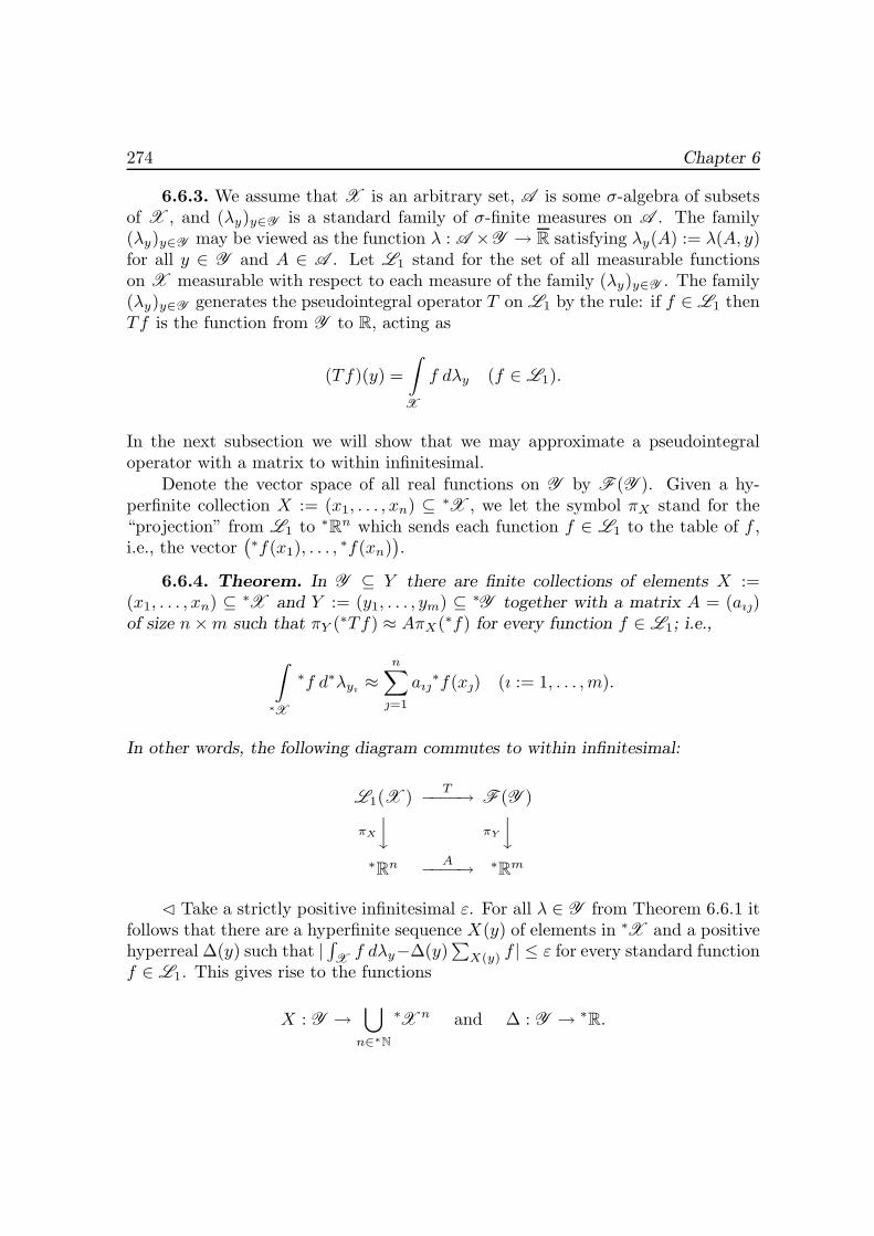
274 Chapter 6
6.6.3. We assume that X is an arbitrary set, A is some σ-algebra of subsetsof X , and (λy)y∈Y is a standard family of σ-finite measures on A . The family(λy)y∈Y may be viewed as the function λ : A ×Y → R satisfying λy(A) := λ(A, y)for all y ∈ Y and A ∈ A . Let L1 stand for the set of all measurable functionson X measurable with respect to each measure of the family (λy)y∈Y . The family(λy)y∈Y generates the pseudointegral operator T on L1 by the rule: if f ∈ L1 thenTf is the function from Y to R, acting as
(Tf)(y) =∫
X
f dλy (f ∈ L1).
In the next subsection we will show that we may approximate a pseudointegraloperator with a matrix to within infinitesimal.
Denote the vector space of all real functions on Y by F (Y ). Given a hy-perfinite collection X := (x1, . . . , xn) ⊆ ∗X , we let the symbol πX stand for the“projection” from L1 to ∗Rn which sends each function f ∈ L1 to the table of f ,i.e., the vector
(∗f(x1), . . . , ∗f(xn)).
6.6.4. Theorem. In Y ⊆ Y there are finite collections of elements X :=(x1, . . . , xn) ⊆ ∗X and Y := (y1, . . . , ym) ⊆ ∗Y together with a matrix A = (aıj)of size n×m such that πY (∗Tf) ≈ AπX(∗f) for every function f ∈ L1; i.e.,
∫
∗X
∗f d∗λyı≈
n∑
j=1
aıj∗f(xj) (ı := 1, . . . , m).
In other words, the following diagram commutes to within infinitesimal:
L1(X ) T−−−−→ F (Y )
πX
⏐⏐# πY
⏐⏐#
∗Rn A−−−−→ ∗
Rm
� Take a strictly positive infinitesimal ε. For all λ ∈ Y from Theorem 6.6.1 itfollows that there are a hyperfinite sequence X(y) of elements in ∗X and a positivehyperreal Δ(y) such that | ∫
Xf dλy−Δ(y)
∑X(y) f | ≤ ε for every standard function
f ∈ L1. This gives rise to the functions
X : Y →⋃
n∈∗N
∗X n and Δ : Y → ∗R.

Technique of Hyperapproximation 275
By extension we may assume that these functions are given on ∗Y . If y ∈ ∗Y andF ∈ ∗L1 then agree to say that Φ(y, F ) holds whenever
∣∣∣∣
∫
∗X
F d∗λy − Δ(y)∑
X(y)
F
∣∣∣∣ ≤ ε.
Given y ∈ Y , consider the internal set By := {F ∈ ∗L1 : Φ(y, F )}. Note that∗f ∈ By for all f ∈ L1 and y ∈ Y . Furthermore, to each finite collection(y1, f1), . . . , (yk, fk) ∈ Y × L1 there is an internal set ∗L1 containing all fm andlying in each Bym
, m := 1, . . . , k. As such a set we may take By1 ∩ · · · ∩ Byk. By
saturation it follows now that there is an internal set B satisfying f ∈ B ⊆ Fy forall (y, f) ∈ Y × L1. In particular, Φ(y, F ) holds for all y ∈ Y and F ∈ Φ.
Let Y0 stand for the set of y ∈ ∗Y such that Φ(y, F ) holds for all F ∈ B.Clearly, Y0 is an internal set including Y . On the other hand, there is a hyperfiniteset Y1 ⊆ ∗Y including Y . Put Y := Y0 ∩Y1. Then Y is a hyperfinite internal subsetof ∗Y including Y . Moreover, Φ(y, F ) holds for all y ∈ Y and F ∈ B. In particular,Φ(y, ∗f) holds for all y ∈ Y and f ∈ L1. Order Y somehow to obtain the tuple(y1, . . . , ym). As X we take the concatenation of the tuples Xy1 , . . . , Xym
, i.e., thetuple consisting of the tuples Xy1 , . . . , Xym
located consecutively. For definiteness,assume that X := (x1, . . . , xn) and the elements of the tuple Xyl
take the placesfrom sl+1 to sl+m in X . Define the “step” matrix A of size m× n as follows:
aıj ={
Δyı, in case sı < j ≤ sı+1,
0 otherwise.Given f ∈ L1, for all ı := 1, . . . , m we then see that
∣∣∣∣
∫
∗X
∗f d∗λyı−
n∑
j=1
aıj∗f(xj)
∣∣∣∣ =
∣∣∣∣
∫
∗X
∗f d∗λy − Δ(yı)∑
X(yı)
∗f∣∣∣∣ ≤ ε,
i.e.,∫∗X∗f d∗λyı
≈ ∑nj=1 aıj
∗f(xj). The proof is complete. �6.6.5. We now consider a particular instance of a pseudointegral operator:
an integral operator with kernel K(x, y). Suppose that, in the context of Theo-rem 6.6.4 we have some σ-finite measure on the σ-algebra A such that, for ally ∈ Y , the measure λy is absolutely continuous with respect to μ with the densityKy := K(·, y) ∈ L∞(μ). Then
(Tf)(y) =∫
X
f dλy =∫
X
fKy dμ.
In this event we may slightly strengthen Theorem 6.6.4. Namely, we may applyTheorem 6.6.1 to obtain a hyperfinite set X and a hyperreal Δ so as to approximateμ up to ε. As the matrix we may now take the table of the kernel at the knots ofthe grid X × Y with weight Δ.
276 Chapter 6
6.6.6. Theorem. Suppose that the couple (X,Δ) approximates μ. Then thereis a finite tuple Y = (y1, . . . , ym) ⊆ ∗Y such that Y ⊆ Y and πY (∗Tf) ≈ AπX(∗f),with aıj := ΔK(xı, yj).
� The proof proceeds along the lines of that of Theorem 6.6.4.Let Ψ(y, F ) stand for the internal formula
∣∣∣∣
∫
F d∗λy − Δ∑
X
∗f∗Ky
∣∣∣∣ ≤ ε.
Given f ∈ L1 and y ∈ Y , note that
∣∣∣∣
∫
X
f dλy − Δ∑
X
∗f∗Ky
∣∣∣∣ =
∣∣∣∣
∫
X
fKy dμ− Δ∑
X
∗f∗Ky
∣∣∣∣ ≤ ε,
i.e., Ψ(y, ∗f) for all y ∈ Y and f ∈ L1.Put Cy := {F ∈ L1 : Ψ(y, F )}. Then there is an internal set C ⊆ ∗L1 such
that Ψ(y, F ) holds for all y ∈ Y and F ∈ C and, moreover, L1 ⊆ C. Also, there isa hyperfinite internal tuple Y := (y1, . . . , ym) such that Y ⊆ Y and Ψ(y, ∗f) holdsfor all y ∈ Y and f ∈ L1. Then
∫
∗X
∗f dλyi≈ Δ
∑
X
fKyı=
n∑
j=1
aıjf(xj)
for all ı := 1, . . . , m. �
6.6.7. It is worth observing that the proofs of Theorems 6.6.4 and 6.6.6 givea somewhat stronger result: The matrix A of these theorems approximates T towithin a given infinitesimal ε. Moreover, since the hyperfinite Y includes Y ; there-fore, the table of a standard function g on Y is completely determined from thetable of ∗g on Y . This implies in particular that the projection πY preserves thesupremum of a bounded standard function on Y , i.e., supy∈Y g(y) = ◦maxπY (g).On the other hand, the projection πX in Theorem 6.6.6 preserves the L1-normof f in L1, i.e.,
∫X f dμ = ◦(Δ
∑X∗f). Consequently, if we furnish ∗Rm with
the sup-norm then Theorem 6.6.6 implies that to each couple (X,Δ) approxi-mating μ to within ε, there is a hyperfinite Y such that Y ⊆ Y ⊆ ∗Y and‖πY (∗Tf) −AπX(∗f)‖ ≤ ε for all f ∈ L1.
The next theorem clarifies Theorem 6.6.6. As in the latter, T stands for anintegral operator from L1 to F (Y ) with kernel K, and ε > 0 is a given infinitesimal.
Technique of Hyperapproximation 277
6.6.8. Theorem. To each hyperfinite Y ⊆ ∗Y there is a couple (X,Δ) approx-imating μ and satisfying ‖πY (∗Tf) − AπX(∗f)‖ ≤ ε for all f ∈ L1 (the matrix Ais the same as in Theorem 6.6.4).
� Put Y := {y1, . . . , ym}. If ı := 1, . . . , m then Kyıbelongs to the set
{Ky1 , . . . , Kym} and so this set is Y -standard. The space (X ,A , μ) is standard
and so Y -standard. By 6.6.2 there are a hyperfinite family X ⊆ ∗X and a positivehyperreal Δ satisfying ∣
∣∣∣
∫
∗X
F d∗μ− Δ∑
X
F
∣∣∣∣ ≤ ε
for every Y -standard integrable function F .If f ∈ L1 then ∗fKy is a Y -standard integrable function; consequently,
∣∣∣∣
∫
∗X
∗f d∗λy − Δ∑
X
fKy
∣∣∣∣ =
∣∣∣∣
∫
∗X
∗fKy d∗μ− Δ
∑
X
fKy
∣∣∣∣ ≤ ε,
which completes the proof. �6.6.9. We now abstract the Loeb construction to a random measure which is
defined in the following environment: Assume that X is an arbitrary set, A is analgebra of subsets of X , and (Y,B, ν) is a measure space with ν finitely additive.A random measure (random finitely additive measure) is a function λ : A ×Y → R
satisfying the two conditions:
(1) λA := λ(A, ·) : Y → R is B-measurable for all A ∈ A ;(2) λy := λ(·, y) is a measure (finitely additive measure) on A for
almost all y ∈ Y .In the sequel, (X,A ) and (Y,B, ν) are internal sets, with λ an internal finitely
additive random measure on A × Y .By definition, Y contains some subset Y0 of full measure such that λy is a
finitely additive measure for all y ∈ Y0. Assume further that (Y,BL, νL) stands forthe Loeb measure space for (Y,B, ν). Given λy (y ∈ Y0), consider the correspondingLoeb measure (λy)L. Observe that the domain of (λy)L includes σ(A ) by thedefinition of Loeb measure. Define the function λL : σ(A ) × Y → R as follows:Put λL(A, y) := (λy)L(A) for A ∈ σ(A ) and y ∈ Y0, while defining λL on Y − Y0
arbitrarily.
6.6.10. Theorem. The function λL constructed above is a random measurewith respect to the spaces (X, σ(A )) and (Y,BL, νL).
� By definition λLy := (λy)L is a countable additive measure for νL-almost ally ∈ Y .
278 Chapter 6
It suffices to show that λLA is BL-measurable for all A ∈ σ(A ). To this end,denote by M the set of A ∈ σ(A ) such that λLA is a BL-measurable function.
Clearly, A ⊆ M . Indeed, given A ∈ A , note that λLA(y) = λLy (A) = ◦λy(A) =◦λA(y) for all y ∈ Y0. Thus, λA is a lifting of λLA, it follows that the function λLA isBL-measurable by Theorem 6.3.6.
We now let (An)n∈N be a monotone sequence of sets in M , and put A :=limn→∞ An. Then A ∈ σ(A ). Since λLy (A) = limn→∞ λLy (An) for all y ∈ Y0, thefunction λLA is BL-measurable as the almost everywhere limit of the sequence ofBL-measurable functions (λLAn
).Thus, M is a monotone class. Since every class containing some algebra con-
tains the σ-algebra generated by this algebra; therefore, M = σ(A ). �6.6.11. We have constructed a random Loeb measure on the σ-algebra σ(A ).
Recall that by construction a Loeb measure is defined on the σ-algebra generatedby the original algebra after that it is extended to the completion of this σ-algebra.The next example demonstrates that such an extension is impossible in general inthe case of a random Loeb measure. Even if the completion of σ(A) with respect toeach measure λLy is the same for all y ∈ Y , the extension of λL on this completioncan fail to be a random measure.
Let Y be a hyperfinite set, and let ν be the uniform probability measure on thealgebra B of all internal subsets of Y . It is known in this case that BL differs fromthe powerset P(Y ). Let N be a BL-nonmeasurable subset Y . Assign X := Y ,A := B, and
λ(A, y) :={
1, if y ∈ A,
0 otherwise
for all y ∈ Y .Obviously, λ is a random measure with respect to (X,A ) and (Y,B, ν); fur-
thermore, for each y ∈ Y the corresponding Loeb measure (λy)L is defined on thewhole P(X). Therefore, we may naturally to extend λL onto P(X)×Y by puttingλL(A, y) := (λy)L(A). However, the function λL on P(X) × Y is not a randommeasure since λLN = χN is not BL-measurable.
6.6.12. We further show that each random measure may be treated as a vectormeasure and the above constructed Loeb extension of a random measure is in a sensethe Loeb extension of a vector measure.
(1) Recall that the nonstandard hull of V # of an internal normed vectorspace V is the quotient space V1/V2 where V1 := ltd(V ) and V2 := μ(V ); cf. 6.1.1.We will proceed by analogy.
Assume that F is an internal finitely additive V -valued measure on an internalmeasurable space (X,A ). Assume also that the image of F lies in some subspace V1.Then the function F# : A → V #, acting by the rule F#(A) := F (V )#, is countably

Technique of Hyperapproximation 279
additive, i.e., a measure on A . It would be natural to call a vector Loeb measurean extension of F# to the completion of σ(A ). In contrast with the scalar case,we cannot however guarantee that F# extends to σ(A ). Nevertheless, we happento show that if F is the vector measure corresponding to a random measure, thisextension is always possible.
(2) Let (Y,B, ν) be an internal measure space and let (Y,BL, νL) standfor the corresponding Loeb measure space. Denote by L0(ν) the space of B-measurable functions from Y to ∗R. As usual, we identify functions that equalν-almost everywhere.
We consider the external subspaces V1 and V2 of L0(ν) consisting of νL-almosteverywhere limited functions and νL-almost everywhere infinitesimal functions, re-spectively; i.e., f ∈ V1 (f ∈ V2) whenever there is U ∈ BL such that νL(Y −U) = 0and f(y) is limited (infinitesimal) for all y ∈ U . This definition is sound since iff ∈ V1 (f ∈ V2) and g(y) = f(y) for ν-almost all y then g(y) = f(y), implying thatg also belongs to V1 (respectively, to V2).
The quotient space V1/V2 is the nonstandard hull of L0(ν)#.We may identify the nonstandard hull L0(ν)# with the space L0(νL) of BL-
measurable functions from Y to R. Namely, we map a coset f + V2 ∈ V1/V2 to ◦f ,Theorem 6.3.6 implies that this is a linear isomorphism. Consequently,
L0(ν)# = L0(νL).
(3) Assume as before that λ is an internal random measure with respectto (X,A ) and (Y,B, ν). Assume further that λ(A, y) is limited for all A ∈ A andalmost all y ∈ Y . Let λL be an extension of λ as prompt by Theorem 6.6.10.Note that these two random measures can be considered as the vector measuresΛ : A → L0(ν) and ΛL : σ(A ) → L0(νL) acting by the rules Λ(A) := λA andΛL(A) := λLA.
6.6.13. Theorem. The measure Λ# (see 6.6.12 (1)) is defined soundly and ad-mits an extension to σ(A ); i.e., there is a vector Loeb measure for Λ. Furthermore,such an extension of Λ# agrees with ΛL on σ(A ).
� Since λ(A, y) is limited for almost all y ∈ Y , it follows that the functionΛ(A) := λA belongs to V1 for all A ∈ A . Hence, Λ# is defined on A . Keeping inmind the identification of 6.6.12 (2), for all A ∈ A we infer that
Λ#(A) = Λ(A)# = (λA)# = ◦λA = λLA = ΛL(A),
with equality holding almost everywhere. Therefore, Λ# coincides with ΛL on A .Since the measure ΛL is defined on σ(A), we conclude that ΛL is an extension ofΛ# to σ(A ). �
280 Chapter 6
6.6.14. Comments.
(1) The pseudointegral operators were introduced by Arveson [20] forstudying operator algebras on L2. They were further studied by Fakhoury [115](in L1) and Kalton [208] (in Lp for 0 < p ≤ 1). Various aspects of pseudointegraloperators are reflected in [208–211, 441–443, 455–459, 522–524]. Preliminaries topseudointegral operators are collected in [268].
(2) The main results of this section belong to Troitskiı [490].
Chapter 7
Infinitesimals in Harmonic Analysis
In this chapter we elaborate on the technique of hyperapproximation of theFourier transform on a locally compact abelian group.
We start with the Fourier transform on the reals
F : L2(R) → L2(R).
In this case the matrix of the discrete Fourier transform is applied to the table ofa function f on a grid with knots −LΔ1, . . . , LΔ1. This vector is compared withthe table of the Fourier transform F (f) of F on a grid with knots −LΔ, . . . , LΔ.We seek the conditions under which the norm of the difference of these two vectorsvanishes as Δ and Δ1 tend to zero and LΔ and LΔ1 tend to infinity (or, in otherwords, this difference is infinitesimal whenever Δ and Δ1 are infinitesimals and LΔand LΔ1 are infinites). The answer depends essentially on interplay between L, Δ,and Δ1.
In fact, the results of 7.1 for the Fourier transform on the reals have a group-theoretic nature, enabling us to abstract them to separable locally compact abeliangroups. Hyperapproximation of a locally compact abelian group G is then appliedto discrete approximation of the Hilbert space of square-integrable functions on G.
Finally, we apply all these constructions to hyperapproximation of an operatorby hyperapproximation of its symbol. We also state results about the limit behaviorof Hilbert–Schmidt operators and Schrodinger-type operators.
7.1. Hyperapproximation of the Fourier Transform onthe Reals
In this section we consider the possibility of approximating the Fourier trans-form F : L2(R) → L2(R) by a discrete Fourier transform.
282 Chapter 7
7.1.1. As regards this section, we agree that X := {k ∈ ∗Z : −L ≤ k ≤ L}and N := 2L + 1, with L an infinite hypernatural (i.e., L ≈ +∞); Δ and Δ′ arestrictly positive infinitesimals such that NΔ ≈ +∞ and NΔ′ ≈ +∞; the functionsj : X → ∗
R and j′ : X → ∗R are defined by the rules j(k) := kΔ and j′(k) := kΔ′.
Thus, (X, j,Δ) and (X, j′,Δ′) are hyperapproximants to the measure space(R,Ω, dx), where Ω is the σ-algebra of Lebesgue-measurable sets, and dx is Lebesguemeasure on R (cf. 6.4.9 (1)).
Consider the internal hyperfinite-dimensional space CX and put Ek(m) :=
δkm for all k,m ∈ X , so distinguishing the basis {Ek : k ∈ X} for CX . Each
endomorphism A of CX will be given by the matrix of A relative to this basis.
We equip CX with the two inner products (·, ·)Δ and (·, ·)Δ′ that are determined
from the conditions (Ek, Em)Δ := Δδkm and (Ek, Em)Δ′ := Δ′δkm. We also letL2Δ stand for C
X equipped with the inner product (·, ·)Δ while denoting CX with
the inner product (·, ·)Δ′ by L2Δ′ .The operator Φ : C
X → CX with matrix (exp(−2πiαβ/N))Lα,β=−L is a discrete
Fourier transform. In the sequel we will consider the discrete Fourier transformΦΔ := ΔΦ : L2Δ → L2Δ′ . It is easy to check that
(ΦΔ(F ),ΦΔ(G))Δ′ = NΔΔ′(F,G)Δ.
Thus, ‖ΦΔ‖ = NΔΔ′, and so Φ#Δ : L #
2Δ → L #2Δ′ is a nonzero operator on condition
that 0 < NΔΔ′ < +∞.Unless otherwise stated, it is assumed in this section that NΔΔ′ ≈ 1. The case
of equality holding is especially distinguished by using the notation Δ := (NΔ)−1
for Δ′. The triple (X, j, Δ) is a hyperapproximant to the measure space (R,Ω, dx)in this case.
Put M := j−1(nst (∗R)) and ϕ := st ◦j|M : M → R. Then ϕ induces a mappingj2 : L2(R) → L2(νMΔ ) ⊂ L #
2,Δ. Recall that if f ∈ L2(R) then j2(f) = F#, whereF ∈ S2(M) is a lifting of f ◦ϕ also called a lifting of f for brevity. Furthermore, iff is bounded and almost everywhere continuous with |f |2 satisfying 6.4.11 (2) thenwe may take as F the vector XΔ(f) ∈ C
X , with entries XΔ(f)k := ∗f(kΔ) fork ∈ X (cf. 6.4.11).
The entities M ′, ϕ′, j′2, and XΔ′(f) (as well as M , ϕ, j2, and XΔ
(f)) appearlikewise on substituting Δ′ (respectively, Δ) for Δ.
Finally, we let F : L2(R) → L2(R) stand for the Fourier transform on thereals:
F (f)(y) :=
∞∫
−∞f(x) exp(−2πixy) dx.
7.1.2. Theorem. If NΔΔ′ ≈ 1 then the discrete Fourier transform ΦΔ :L2,Δ → L2,Δ′ is a hyperapproximant to F : L2(R) → L2(R).
Infinitesimals in Harmonic Analysis 283
� Let M stand for the set of the characteristic functions of all intervals [0, a]and [−a, 0], with a > 0. Then the linear span of M is dense in L2(R) and so wemay appeal to 6.5.1 (2).
Put f := χ[0,a] and let T be an infinite hypernatural satisfying
(T − 1)Δ ≤ a < TΔ.
In view of the definition of hyperapproximant, we are left with proving that
Δ′L∑
k=−L
∣∣∣∣Δ
T−1∑
n=0
exp(−2πink/N) −a∫
0
exp(−2πixkΔ′) dx∣∣∣∣
2
≈ 0.
It suffices clearly to consider only the terms under the sign∑Lk=1. Moreover, we
may replace∫ a0
with∫ TΔ
0since NΔΔ′ ≈ 1 by hypothesis. Therefore,
Δ′L∑
k=−L
∣∣∣∣
TΔ∫
a
exp(−2πixkΔ′) dx∣∣∣∣
2
≤ NΔ2Δ′ ≈ Δ ≈ 0.
Simple calculation shows that we are left with proving that
Δ′L∑
k=−L|Δ(1 − exp(−2πikT/N))(1 − exp(−2πik/N))−1
−(2πikΔ′)−1(1 − exp(−2πikTΔΔ′))|2 ≈ 0.
Replacing Δ′ with Δ := (NΔ)−1, we obtain
ΔN
L∑
k=1
|1 − exp(−2πikT/N)|2|(1 − exp(−2πik/N))−1 −N/(2πik)|2 ≈ 0.
The last formula is obviously valid. Indeed, 0 < 2πk/N < π for all k ∈ [1, L].Hence, the function (1 − exp(−iϕ))−1 − (iϕ)−1 has a finite limit as ϕ → 0, andso f is bounded on [0, π]. This implies that the validity of the formula we discussfollows from the approximate equality
Δ′L∑
k=1
|(2πikΔ′)−1(1 − exp(−2πikTΔΔ′))
−NΔ(2πik)−1(1 − exp(−2πikT/N))|2 ≈ 0,
284 Chapter 7
which in turn is a consequence of the following two formulas:
1Δ′
L∑
k=1
k−2|(NΔΔ′ − 1)(1 − exp(2πikT/N))|2 ≈ 0
and1
Δ′
L∑
k=1
k−2| exp(−2πikTΔΔ′) − exp(−2πikT/N)|2 ≈ 0.
We will prove the first of them, since the second is proved similarly.Put α := NΔΔ′ − 1 ≈ 0 and a := TΔ ≈ a. Then the formula under test
amounts to the following
α2
Δ′
L∑
k=1
1k2
sin2 πka
NΔ≈ 0.
If α2MΔ′ ≈ 0 then the last formula holds since a is limited and sin2 x ≤ x2.If α2MΔ′ �≈ 0 then we put S :=
[1αΔ′]. In this case SΔ′ is limited and α2SΔ′ ≈ 0.
Hence, S < M .We now infer that
α2
Δ′
L∑
k=1
1k2
sin2 πka
NΔ=α2
Δ′
S∑
k=1
1k2
sin2 πka
NΔ+α2
Δ′
L∑
k=S+1
1k2
sin2 πka
NΔ.
The first term on the right side is infinitesimal because α2SΔ′ ≈ 0, and the secondterm is infinitesimal too since
α2
Δ′
L∑
k=S+1
1k2
≤ α2
Δ′(S−1 −M−1)
while SΔ′ and MΔ′ are unlimited. �7.1.3. We now consider two corollaries of Theorem 7.1.2.
(1) If NΔΔ′ ≈ 2πh, where h > 0 is a standard real then the discreteFourier transform ΦΔ : L2,Δ → L2,Δ′ is a hyperapproximant to the Fourier trans-form Fh : L2(R) → L2(R) acting by the rule
Fh(f)(y) :=
∞∫
−∞f(x) exp(−ixy/h) dx.
� This is immediate by passing from f ∈ L2(R) to the function ϕ defined asϕ(t) := f(2πht) and replacing Δ with Δ/2πh. �
Infinitesimals in Harmonic Analysis 285
(2) Suppose that f and F (f) are bounded almost everywhere contin-uous functions, with |f |2 and |F (f)|2 satisfying the condition
limΔ→0A→∞
Δ∑
|k|>AΔ
∣∣f(kΔ)
∣∣ = 0.
Then
limn→∞Δ′n
n∑
k=−n
∣∣∣∣
∞∫
−∞f(x) exp(−2πixkΔ′n) dx
−Δn
n∑
m=−nf(mΔn) exp(−2πikm/n)
∣∣∣∣
2
= 0
for all sequences (Δn) and (Δ′n) such that Δn → 0, Δ′n → 0, and nΔnΔ′n → 1/2as n → ∞.
� This is a standard version of Theorem 7.1.2 immediate from 6.5.10 (3) (alsosee 6.5.11 (5)). �
(3) We now compare the results on hyperapproximation of the Fouriertransform with the results on hyperapproximation of Hilbert–Schmidt operators(cf. 6.5).
The Fourier transform F is an integral operator with kernel kF (x, y) :=exp(−2πixy) a bounded analytic function.
If we consider a Hilbert–Schmidt operator A whose kernel k ∈ L2(R2) isa bounded almost everywhere continuous function with |k|2 satisfying the con-dition of 6.5.5 (1) (i.e., k ∈ H2) then the operator Ak : L2,Δ → L2,Δ with matrix(Δ∗k(αΔ, βΔ))Lα,β=−L is a hyperapproximant to A with kernel k.
The discrete Fourier transform ΦΔ, regarded as an operator from L2,Δ toL2,Δ, becomes a hyperapproximant to F provided that NΔ2 = 1 (or NΔ2 ≈ 1);cf. Theorem 7.1.2. In this event the matrix of ΦΔ takes the shape
Ak :=(ΔkF (αΔ, βΔ)
)Lα,β=−L.
The next proposition shows that if we refuse to maintain the above relations betweenN and Δ then the matrix Ak may cease determining a hyperapproximant to F .
7.1.4. If NΔ2 = 2 then the operator B : L2,Δ → L2,Δ with matrix Ak is nota hyperapproximant to the Fourier transform F .
286 Chapter 7
� Rewrite the matrix of B as
(Δ exp(−4πinm/N)
)Ln,m=−L.
Put f := χ[0;
√3/2] and show that
◦(‖B(XΔ(f)) −XΔ(F (f))‖Δ) > 0.
Choose an infinite hypernatural T so that (T − 1)Δ ≤ √3/2 < TΔ. Easy calcula-
tions show that the claim will follow from the inequality
◦(Δ3
L∑
m=L−T|1 − exp(−4πimT/N)|2|(1 − exp(−4πim/N))−1 −N/(4πim)|2
)
> 0.
Since T/N ≈ 0, it is easy that the sum under the standard part operation is atleast
(
Δ3L∑
m=L−Tsin2 2πmT
N
)(
sin2 2πmN
)−1
.
Check now that the standard part of the last hyperreal is strictly positive.To this end, note that sin2(2πm/N) decreases in m for L − T ≤ m ≤ L. PutS := [2T/3]. Then there are some infinitesimals γ and δ such that πT−3π/4π−γ ≤2πmT/N ≤ πT −π/2−δ for all M−T ≤ m ≤ M−S implying that sin2(2πmT/N)increases in this interval. Therefore, all terms increase with the so-distinguishedindices. Further, the term with index m := L − T is at least DΔ−2 for somestandard real D > 0. It is now obvious that the whole sum is at least D(T − S)Δwhich is not infinitesimal. �
7.1.5. Theorem 7.1.2 will be now abstracted to some class of tempered distri-butions. In this subsection we put N := 2L + 1 and let Δ satisfy the additionalcondition 0 < ◦(NΔ2) < +∞. If 0 < ◦(NΔΔ′) < +∞ then this condition alsosatisfies for N and Δ′.
We start with studying how to assign some element of ∗CX with a given dis-tribution. To this end, consider the operator Dd : L2,Δ → L2,Δ with matrix((2Δ)−1dnk)Ln,k=−L having the entries
dnk :=
⎧⎪⎨
⎪⎩
1, if k = n� 1,−1, if k = n −· 1,
0 otherwise,
Infinitesimals in Harmonic Analysis 287
where the symbols � and −· stand for addition and subtraction in the additivegroup of the ring ∗Z/N∗Z with the underlying set {−L, . . . , L}. In other words, ifG := DdF then G(k) = (F (k + 1) − F (k − 1))(2Δ)−1. Clearly, ‖Dd‖ ≈ +∞, andso it is impossible to speak of D#
d . To proceed further, we prove a few auxiliarypropositions.
(1) If G(n) = Dnd F then
G(n)(k) =1
(2Δ)n
n∑
r=0
(−1)r(n
r
)
F (k � n −· 2r).
Furthermore, if |k| ≤ L − n, then symbols � and −· may be replaced with + and−, respectively.
(2) IfΔ−2F (±(L− t)) ≈ 0
for all standard s and t then G(n)(±(L−m)) ≈ 0 for all standard n and m.(3) If f ∈ S(R) then Δ−s∗f(±(L− t)Δ) ≈ 0 for all standard s and t.
� Since LΔ ≈ +∞ and t is standard; therefore, (L− t)Δ ≈ +∞. Consideringthat f ∈ S(R), obtain [(L − t)Δ]−s ∗f(±(L − t)Δ) ≈ 0. Thus, 0 ≈ Δ−s[(L − t)Δ2]s ∗f(±(L− t)Δ). We are done on using the condition 0 < ◦(NΔ2) < +∞. �
(4) If f belongs to the Schwartz space S(R) and n is a standard naturalthen
‖DndXΔ(f) −XΔ(f (n))‖2,Δ ≈ 0.
� By (2) and (3),
Δ∑
|k|>L−n|(Dn
dXΔ(f))(k) −XΔ(f (n))(k)|2 ≈ 0.
In view of (1) it suffices to show that
0 ≈ S = ΔL−n∑
k=−L+n
∣∣∣∣
1(2Δ)n
n∑
r=0
(−1)r(n
r
)∗f((k + n− 2r)Δ) − ∗f (n)(kΔ)
∣∣∣∣
2
.
By the Taylor Theorem,
f(kΔ + (n− 2r)Δ) =n∑
s=0
f (s)(kΔ)s!
(n− 2r)sΔs
+f (n+1)(ξr)
(n+ 1)!(n− 2r)n+1Δn+1.
288 Chapter 7
Hence,
1(2Δ)n
n∑
r=0
(−1)r(n
r
)
f((k + n− 2r)Δ)
=1
(2Δ)n
n∑
s=0
f (s)(kΔ)s!
Δsn∑
r=0
(−1)r(n
r
)
(n− 2r)s
+Δ2n
n∑
r=0
f (n+1)(ξr)(n+ 1)!
(n− 2r)n+1.
Using the easy formula
n∑
r=0
(−1)rrs(n
r
)
={
0, if s < n,
(−1)nn!, if s = n,
infer that the first term on the right side of the penultimate formula is equal tof (n)(kΔ). Since f (n+1) is bounded on R, the modulus of the second term on theright side is bounded above by BΔ with B a standard real. Consequently, S ≤Δ · 2(L− n)B2Δ2 and we are done on appealing to (1). �
7.1.6. We now define the sequence (L (n))n∈N of external subspaces of L2,Δ
as follows:
L (0) :={
F ∈ L2,Δ : (∀ sta)(∃ stC)(
Δ[a/Δ]∑
k=−[a/Δ]
|F (k)|2 < C
)}
;
L (n+1) := Dd(L (n));
L (σ) :=∞⊕
n=0
L (n).
Assume that F ∈ ∗CX is such that
◦(Δ
L∑
k=−LF (k)∗f(kΔ)
)
= ◦(F,XΔ(f)) < +∞
for every standard f ∈ C∞0 (R).The formula
ψΔF (f) := ◦(F,XΔ(f))Δ
defines a (possibly discontinuous) linear functional ψΔF : C∞0 (R) → C.
Infinitesimals in Harmonic Analysis 289
Theorem. The following hold:(1) ψΔ
F ∈ (C∞0 (R))′ for all F ∈ L (σ);(2) If f ∈ (C∞0 (R))′ and f = ϕ(k) for some regular distribution ϕ
(k ≥ 0) then there is some F in L (σ) satisfying ψΔF = f ;
(3) ψΔDdF
= (ψΔF )′ for all F ∈ L (σ).
� Given A ≤ L, put (F,G)AΔ := Δ∑Ak=−A F (k)G(k). Suppose that f, fn ∈
C∞0 (R) and fn → f in C∞0 (R) as n → ∞. Then there is a standard real a > 0 suchthat the supports supp(fn) and supp(f) lie in [−a, a] and (fn) converges uniformlyto f . Since the supports of fn and f are compact; therefore, ‖fn‖L2 and ‖f‖L2 arelimited and ‖f − fn‖L2 → 0 as n → ∞.
Put A := [a/2]. Then
‖f‖L2 = ◦‖XΔ(f)‖A2,Δ, ‖fn‖L2 = ◦‖XΔ(fn)‖A2,Δ,◦‖XΔ(f − fn)‖A2,Δ −→
n→∞ 0.
Now, if F ∈ L (0), then
|ψΔF (f)| = |◦(F,XΔ(f))Δ| = |◦(F,XΔ(f))AΔ| ≤ ◦‖F‖A2,Δ◦‖XΔ(f)‖A2,Δ.
From the definition of L (0) it follows that ◦‖F‖A2,Δ is limited as well ◦‖XΔ(f)‖A2,Δ(we have seen this earlier). Hence, ψΔ
F (f) is limited for all f ∈ C∞0 (R). By analogy,ψΔF (fn − f) → 0 as n → ∞, and so ψΔ
F ∈ (C∞0 (R))′.Note further that (Dn
d F,XΔ(f)) = (−1)n(F,DndXΔ(f)). From 7.1.5 (4) it
follows that DndXΔ(f) = XΔ(f (n)) + T , where ‖T‖2,Δ ≈ 0. Moreover, since
supp f (n) ⊂ [−a, a]; therefore, XΔ(f (n))(k) = 0 for |k| > A.As follows from 7.1.5 (1), Dn
dXΔ(f)(k) = 0 for |k| > A+n. Since n is standard,infer that T (k) = 0 for |k| > [b/Δ] and each standard b > a. Thus, if B = [b/Δ]then (F, T )Δ = (F, T )BΔ ≈ 0, because ‖F‖B2,Δ is limited and ‖T‖B2,Δ = ‖T‖2,Δ ≈ 0.
Hence, (Dnd F,XΔ(f)) ≈ (−1)n(F,XΔ(f (n))), implying that ψΔ
DndF (f) = ψ
Δ(n)F (f).
This yields (1) and (3).To prove (2) it suffices to observe that there is no loss of generality in assuming
ϕ continuous, implying that XΔ(ϕ) ∈ L (0). �7.1.7. Put C(0) := ltd(L2,Δ); C(n+1) := DdC
(n), and
C(σ) :=∞⊕
n=0
C(n).
Obviously, C(0) ⊂ L (0), and so C(n) ⊂ L (n) for all n. Therefore, C(σ) ⊂ L (σ).The next two propositions may be proven along the lines of the proof of the abovetheorem.
290 Chapter 7
(1) If F ∈ C(σ) then ψΔF is a tempered distribution.
(2) If f = ϕ(k) and ϕ ∈ L2(R) then there is an element F in C(σ)
satisfying f = ψΔF .
Supposing that Δ′ enjoys the condition NΔΔ′ ≈ 1, we again consider thediscrete Fourier transform ΦΔ : L2,Δ → L2,Δ′ . Since ΦΔ has a limited norm;therefore, ΦΔ(C(0)) = ltd(L2,Δ′) = C(0) and Φ−1
Δ (C(0)) = C(0).Put Md := ΦΔDdΦ−1
Δ : L2,Δ′ → L2,Δ′ and define the sequence (C(n))n∈N ofexternal subspaces of L2,Δ′ by letting C(n+1) := Md
(C(n)
). It is now obvious that
ΦΔ(C(n)) = C(n) and C(σ) =⊕∞
n=0 C(n) = ΦΔC(σ). Straightforward calculationshows that the operator Md may be given by the matrix
(i
Δsin
2πβN
δαβ
)L
α,β=−L.
Given G ∈ CX and f ∈ C∞0 (R), we define ψΔ′
G (f) as in 7.1.6 on replacing Δwith Δ′ and F with G.
7.1.8. If f ∈ S(R) then
◦‖M nd (XΔ′(f)) −XΔ′(M n(f))‖ = 0.
� Considering the formulas of 7.1.7 for the matrix of Md, we are left withdemonstrating only that
Δ′L∑
β=−L
∣∣∣∣
(1Δ
sin2πβN
)nf(βΔ′) − (2πβΔ′)nf(βΔ′)
∣∣∣∣
2
≈ 0.
Show first that if T < L but TΔ′ ≈ +∞ then
W := Δ′∑
|β|>T|f(βΔ′)|2 1
Δ2n
∣∣∣∣
(
sin2πβN
)n− (2πβΔΔ′)n
∣∣∣∣
2
≈ 0.
Indeed, since NΔΔ′ ≈ 1, there is some standard C satisfying
∣∣∣∣
(
sin2πβN
)n− (2πβΔΔ′)n
∣∣∣∣
2
=∣∣∣∣β
N
∣∣∣∣
2n∣∣∣∣
(β
N
)−n(sin
2πβN
)n− (2πNΔΔ′)n
∣∣∣∣
2
≤ C
∣∣∣∣β
N
∣∣∣∣
2n
.
Infinitesimals in Harmonic Analysis 291
This enables us to estimate W as follows:
W ≤ C1Δ′∑
|β|>T|f(βΔ′)|2|βΔ′|2n.
Put ϕ(x) := x2nf(x). Since f(x) ∈ S(R); therefore, ϕ(x) ∈ L2(R). Moreover, ϕ isa bounded continuous function satisfying the equality under proof. Consequently,the internal function G : X → C, given by G(β) := ∗f(βΔ′)(βΔ′)n, is a lifting ofϕ, and G ∈ S2(M). This implies that the right side of the above upper estimatefor W is in fact an infinitesimal, yielding W ≈ 0.
By 4.6.11 there is some a ≈ +∞ such that NΔ′a≈ +∞ and NΔΔ′ − 1
a≈ 0.Put T := [a/Δ′]. Then T satisfies the preceding conditions, and so to complete theproof it suffices in view of the boundedness of f to show that
W1 := Δ′T∑
β=1
∣∣∣∣
(1Δ
sin2πβN
)n− (2πβΔ′)n
∣∣∣∣
2
≈ 0.
If 1 ≤ β ≤ T then 0 < β/N < a/(NΔ′)a≈ 0, implying that is
(
sin2πβN
)(2πβN
)−1
= 1 − αβ ,
where αβa≈ 0. Hence, Δ−n
(sin 2πβ
N
)n = (1 − αβ)(2πβΔ′)n(NΔΔ′)−n. By the
choice of a there is some δa≈ 0 satisfying (NΔΔ′)−n = 1 + δ. Finally,
Δ−n(
sin2πβN
)n= (1 + γβ)(2πβΔ′)n,
where γβa≈ 0. If γ = max{|γβ| : 1 ≤ β ≤ T} then γ
a≈ 0, yielding
W1 ≤ Δ′γ2T∑
β=1
(2πβΔ′)2n ≤ Δ′γ2(2π)n(TΔ′)2n ≤ (2π)nγ2a2nΔ′ ≈ 0,
which completes the proof. �7.1.9. Theorem. The following hold:
(1) ψΔ′G ∈ (S(R))′ for all G ∈ C(σ);
(2) F (ψΔF ) = ψΔ′
ΦΔ(F ) for all F ∈ C(σ).
292 Chapter 7
� (1): This is proved in much the same way as the theorem of 7.1.6.(2): Denote the differentiation operator in S(R) by D and let M := FDF−1.
Then M (f)(x) := 2πixf(x). It obviously suffices to check (2) for F := DndG,
where G ∈ C(σ). In this event, everything results however from the next chain ofequalities:
ψΔ′ΦΔ(F )(f) = ◦(ΦΔ(Dn
dG), XΔ′(f)) = ◦(DndG,Φ
−1Δ (XΔ′(f)))
= (−1)n◦(G,Dnd Φ−1
Δ XΔ′(f))= (−1)n◦(G,Φ−1
Δ MdXΔ′(f))= (−1)n◦(G,Φ−1
Δ XΔ′(M n(f)))= (−1)n◦(G,XΔ′(F−1M n(f)))= (−1)n◦(G,XΔ(DnF−1(f)))= (−1)n◦(G,Dn
dXΔ(F−1(f)))= ◦(Dn
dG,XΔ(F−1(f))) = ◦(F,XΔ(F−1(f)))= ψΔ
F (F−1(f))(FψΔF )(f).
The proof is complete. �7.1.10. Comments.
(1) The condition NΔΔ′ ≈ 1 of Theorem 7.1.2 arises also in the cele-brated Kotel′nikov Theorem asserting that if the spectrum of a bounded function fbelongs to the interval [−a, a] then f is completely determined from its values onthe set {nλ : −∞ < n < +∞}, with λ ≤ (2a)−1, by the formula
f(t) =∞∑
k=−∞f(kλ)
sin 2πa(t− kλ)2πa(t− kλ)
.
In our case, the values of f are calculated at the points kΔ, with Δ ≈ 1/(NΔ′),and it is easy to see that NΔ′ is exactly the length of the interval where we con-sider F (f).
(2) The condition NΔΔ′ ≈ 2πh of 7.1.3 (1) is closely tied with theuncertainty principle of quantum mechanics.
Consider the one-parameter groups of unitary operators U(u) := exp(−iuP )and V (v) := exp(−ivQ), where Q and P are the coordinate and momentum opera-tors; i.e., Q is the multiplication by the independent variable, and P := h
iddx
, whereh > 0 is a distinguished standard real, the Planck constant. We recall in this eventthat U(u)ϕ(x) = ϕ(x − uh), V (v)ϕ(x) = exp(−ivx)ϕ(x) and the commutationrelations
U(u)V (v) = exp(ihuv)V (v)U(u)
Infinitesimals in Harmonic Analysis 293
hold which may be regarded as one of the form of the uncertainty principle.Define the hyperfinite-rank operators Ud, Vd : C
X → CX with (UdF )(k) :=
F (k −· 1) and Vd the diagonal matrix
(exp(−2πink/N)δnk)Ln,k=−L.
It is easy to check that the operators Urd and V md satisfy the following commutationrelations:
UrdVmd = exp(2πirm/N)Vmd Urd (r,m ∈ ∗Z/N∗Z).
If exp(2πirm/N) ≈ exp(πihuv) then the last relation transforms into the abovecommutation relation for U and V . However, for the condition exp(2πirm/N) ≈exp(πihuv) to hold we need relate the quantities r, m, u, and v; the details arecollected in the following proposition.
(3) If r,m ∈ ∗Z/N∗Z are such that rΔ ≈ uh and 2πmΔ ≈ v, with uand v standard reals; then U rd and V
md : L2,Δ → L2,Δ are hyperapproximants to
U(u) and V (v), respectively.� As M in 6.5.1 (2) we take the set of the characteristic functions of the closed
intervals. By definition it is clear that U(u)(χ[a,b]) = χ[a+uh,b+uh]. Note that if kΔand mΔ are nearstandard then |k|, |m|, and |k − m| are all less than L. Hence,k −· m = k −m and Urd (F )(k) = F (k − r). If f = χ[a,b] then
XΔ(f)(n) ={
0, if nΔ /∈ ∗[a, b],1, if nΔ ∈ ∗[a, b],
implying that
Urd (XΔ(f))(n) ={
0, if nΔ /∈ ∗[a+ rΔ, b+ rΔ],1, if nΔ ∈ ∗[a+ rΔ, b+ rΔ].
Similarly,
XΔ(U(u)(f))(n) ={
0, if nΔ /∈ ∗[a+ uh, b+ uh],1, if nΔ ∈ ∗[a+ uh, b+ uh].
It is now obvious that
ΔL∑
k=−L|Urd (XΔ(f))(n) −XΔ(U(u)(f))(n)|2 = 2Δ
[|(uh− rΔ)/Δ|] ≈ 0,
since uh ≈ rΔ.Clearly, V (v) = F−1
h U−1(v)Fh (cf. 7.1.3 (1)) and Vd = Φ−1Δ U−1
d ΦΔ. PutΔ1 := 2πpΔ and regard U−1
d as an operator from L2,Δ1 to L2,Δ1 . By hypothe-ses, mΔ1 ≈ vh and, as was proven, U−md is a hyperapproximant to U−1(v). By7.1.3 (1), the operator ΦΔ : L2,Δ → L2,Δ1 is a hyperapproximant to Fh; i.e.,V md := Φ−1
Δ U−md ΦΔ is a hyperapproximant to F−1h U−1(v)Fh = V (v). �
294 Chapter 7
(4) Theorem 7.1.9 suggests an approach to approximating the Fouriertransform of tempered distributions by the discrete Fourier transform. Unfortu-nately, this approach is successful only the primitives of the functions in L2(R).Fortunately, this class may be enriched as shown by the following example.
Assume that ϕ = 1. Hence, ϕ is a regular distribution and by 7.1.8, ϕ = ψΔF ,
where F := XΔ(f), i.e., F (k) = 1 for all k ∈ X . Since F (1) = δ; therefore,ΦΔ(F )(k) = NΔδk0. Consequently, if G := ΦΔ(F ) then ψΔ′
G (f) = ◦(G,XΔ(f))Δ′
= ◦(NΔΔ′∗f(0)) = f(0) = δ(f), implying that F (ψF ) = ψΔ′ΦΔ(F ).
7.2. A Nonstandard Hull of a Hyperfinite Group
In this section we study a construction that assign to a hyperfinite group somelocally compact group.
7.2.1. We consider the additive group G of the ring ∗Z/N∗Z with the under-lying set {−L, . . . , L}; cf. 7.1.1. Clearly, G is an internal hyperfinite abelian group.Distinguish the two natural external subgroups G0 := {k ∈ G : kΔ ≈ 0} andGf := {k ∈ G : ◦|kΔ| < +∞} of G. It is easy to see that G0 is the intersectionof a countable family of internal sets and Gf , the union of a countable family ofinternal sets:
G0 =⋂
n∈N
j−1(∗(−n−1, n−1)), Gf =⋃
n∈N
j−1(∗[−n, n]).
Further, the mapping st : Gf → R is an epimorphism, and ker(st) = G0, i.e., isR � Gf/G0.
Suppose that A is an internal set coincident with j−1(∗(a, b)) for some a, b ∈ R.In this event st(A) = [a, b]. We now define the external set A◦ := {c ∈ A : c+G0 ⊂A}. It is easy to check that st(A◦) = (a, b). A similar definition of A◦ applies to anarbitrary internal set A. In this event it is an easy matter to that st(A) is closedand st(A◦) is open. Thus,
{st(A◦) : A is an internal subset of Gf}is a base for the topology of R. We also see that ◦(Δ|j−1(∗[a, b])|) = b − a. Thisimplies straightforwardly that (Gf , S
Gf
Δ , νGf
Δ ) is a σ-finite subspace of the Loebmeasure space (G, SΔ, νΔ) (cf. 6.3.11).
In this case νGf
Δ is an invariant measure on Gf . Moreover, the precedingequality shows that st : Gf → R is measure-preserving provided that we viewLebesgue measure as the Haar measure on R.
Let G stand for the character group of G. Then the internal mapping n �→ χn,with χn(m) := exp(2πimn/N) for n,m ∈ G, is an isomorphism from G to G. Thisclaim follows by transfer since it holds for every standard N .
Infinitesimals in Harmonic Analysis 295
In order for a character χn : G → ∗C to induce a character κ : R → C by
composition with the homomorphism st it is necessary and sufficient that χn|G0 ≈ 1.With this in mind, we naturally distinguish the external subgroup Hf := {χ ∈ G :χ|G0 ≈ 1} of G and define the monomorphism st : Hf → R by the rule st(χ)(n) :=◦χ(◦(nΔ)) for n ∈ N and χ ∈ G. Thereby, ker(st) = H0 := {χ ∈ Hf : χ|Gf
≈ 1}and so Hf/H0 ⊂ R.
(1) If n ∈ G then
χn ∈ Hf ↔ ◦(|nΔ|) < +∞;
χn ∈ H0 ↔ nΔ ≈ 0,
with Δ := (NΔ)−1.
� Indeed, if nΔ is a limited hyperreal then χn(m) = exp(2πimn/N) =exp(2πimΔnΔ) ≈ 1, because mΔ ≈ 0.
Conversely, suppose that nΔ is unlimited. Put m := [N/(2π)]. Clearly,mΔ ≈ 0. In this case χn(m) = exp 2π
(N2π
)Δ nNΔ
≈ −1, because 0 ≤ α < 1, whichis a contradiction. The proof of the other equivalence proceeds by analogy. �
Thus, the groups Gf and G0 are constructed just like the groups Gf and G0,and so Gf/G0
∼= R ∼= R.The Fourier transform F : L2(G) → L2(G) for an arbitrary locally compact
abelian group G is defined as F (f)(χ) := (f, χ). Therefore, Theorem 7.1.2 clearlyadmits a group-theoretic interpretation. We so proceed to the general situation.
Let G be an internal hyperfinite abelian group, and let G0 and Gf be subgroupsof G such that G0 ⊂ Gf and the following hold:
(A) There is a sequence (An)n∈N of internal sets such that An ⊂ Gf forall n ∈ N and G0 =
⋂{An : n ∈ N};(B) There is a sequence (Bn)n∈N of internal sets such that Bn ⊃ G0 for
all n ∈ N and Gf =⋃{Bn : n ∈ N}.
Observe that these subgroups G0 and Gf may be internal as well as external.
(2) If G0 and Gf are subgroups of G, with G0 ⊂ Gf , satisfying (A) and (B)then there is a countable sequence (Cn)n∈Z of symmetric internal subsets of G suchthat:
(a)⋂n∈Z
Cn = G0;(b)
⋃n∈Z
Cn = Gf ;(c) Cn + Cn ⊂ Cn+1 (n ∈ Z).
Further, if F is an internal subset of G then(d) F ⊂ Gf ↔ (∃n ∈ Z)(F ⊂ Cn);(e) F ⊇ G0 ↔ (∃n ∈ Z)(F ⊇ Cn).
296 Chapter 7
� These auxiliary facts are easy by saturation. �In the sequel we will work with some sequence (Cn)n∈Z satisfying the conditions
of (2). If F ⊂ Gf , then we put◦F := {g ∈ Gf : g + G0 ⊂ F}. The following is
immediate from (2).
(3) If F is an internal subset of Gf then (∀g ∈ G)(g ∈◦F ↔ (∃m ∈ Z)
(g + Cm ⊂ F )).
We denote the family of all internal subsets ofGf by In(Gf ) and put In0(Gf ) :={F ∈ In(Gf ) : G0 ⊂ F}. Put G# := Gf/G0 and let j : Gf → G# denote thequotient homomorphism. If g ∈ Gf and A ⊂ Gf then instead of j(g) and j(A) wewill write g# and A#, respectively.
7.2.2. Theorem. The following hold:
(1) The family U := {◦F# : F ∈ In(Gf )} is a neighborhood base of zero
for some uniform topology compatible with the group structureon G#. This topology is called canonical below;
(2) If F ∈ In(Gf ) then F# is closed;(3) The topological group G# is complete.
� (1): From the general theory of topological groups (see, for instance, [402])it follows that some system U of subsets of an abelian group is a neighborhood baseof zero whenever the following hold:
(a)⋂{U : U ∈ U} = {e};
(b) (∀U, V ∈ U))(∃W ∈ U)(W ⊂ U ∩ V );
(c) (∀U ∈ U)(∃V ∈ U)(V − V ⊂ U);
(d) (∀U ∈ U)(∀ξ ∈ U)(∃V ∈ U)(V + ξ ⊂ U).We now check this in our environment.(a): If g# ∈ ⋂{
◦F# : F ∈ In0(Gf )} then
((g+G0)∩
◦F �= ∅
)for all F ∈ In0(Gf )
as follows from the fact that j−1(g#) = g+G0 and j−1(◦F#) =
◦F +G0 =
◦F (see the
definition of◦F ). Consequently, there is some g1 ∈ G0 satisfying (g+ g1 +G0 ⊂ F ),
and so g ∈ F . Thus, g ∈ ⋂ In0(Gf ) = G0.
(b): This ensues from the inclusion (F1 ∩ F2)◦# ⊂◦F#
1 ∩◦F#
2 , which is checkedas above.
(c): If F ∈ In0(Gf ) then there is some n ∈ Z satisfying Cn + Cn + Cn ⊂ F
by 7.2.1 (2). Therefore, Cn+Cn+G0 ⊂ F , and hence◦Cn+
◦Cn ⊂
◦F . Consequently,
(◦Cn +
◦Cn)# =
◦C#n +
◦C#n ⊂
◦F#. Since Cn is symmetric; therefore,
◦C#n = −
◦C#n .
(d): This is checked by analogy.(2): Let F ∈ In(Gf ). We will show that F# is closed.
Infinitesimals in Harmonic Analysis 297
If g# /∈ F# then (g + G0) ∩ F = ∅, and so (g + Cn) ∩ F = ∅ for some n ∈ Z
(by ω+-saturation). Thus, (g + Cn−1 + G0) ∩ F = ∅ by 7.2.1 (2), implying that
(g# +C#n−1) ∩F# = ∅. Hence, (g# +
◦C#n−1) ∩F# = ∅ because
◦Cn−1 ⊂ Cn−1. This
proves that F# is closed since◦C#n−1 ∈ U.
(3): It follows from 7.2.1 (2), that the canonical topology on G# satisfies thefirst axiom of countability. It suffices so to show that every Cauchy sequence in G#
converges.Let (g#
n )n∈N be a Cauchy sequence in G#. By definition, to each m ∈ Z there
is ν(m) ∈ N such that g#n1
− g#n2
∈◦C#m for all n1, n2 > ν(m).
Consider the countable family
Γ := {Am,n : n > ν(m), n,m ∈ N},
whereAm,n = {g : gn − g ∈ Cm+1},
and show that Γ has the finite intersection property. To this end, take
S := {Am1,n1 , . . . , Amk,nk}
and choose n > max{ν(m1), . . . , ν(mk)}. Then g#nı
− g#n ∈
◦C#mı
. Therefore, gnı−
gn + g ∈◦Cmı
for some g ∈ G0.Thus, gnı
−gn+g+G0 ⊂ Cmı. Since g+G0 = G0, it follows that gnı
−gn ∈ Cmı
(ı := 1, . . . , k), and so gn ∈ ⋂S. By ω+-saturation,⋂
Γ is nonempty and there is
some g ∈ ⋂Γ. Considering that Cm+1 ⊂◦Cm+2 which is immediately from 7.2.1 (2),
conclude that g#n → g# as n → ∞. �
Recall that an internal finite set A is standardly finite whenever the size |A| ofA is a standard natural; cf. 3.7.7. We also let (∗) stand for the condition holds
(∀F1, F2 ∈ In0(Gf ))(F1 ⊂ F2 → (∃B ⊂ F2)(|B| ∈ N ∧ F1 +B ⊇ F2)
).
7.2.3. Theorem. The following hold:(1) The canonical topology on G# is locally compact and separable if
and only if (∗) is valid;(2) On assuming (∗), G# is compact (discrete) if and only if Gf (re-
spectively G0) is an internal subgroup of G.
� (1): Assuming (∗), show that G# is locally compact. It suffices to prove thatF# is compact for every F ∈ In0(Gf ). The closure of F# was shown in 7.2.2. Prove
298 Chapter 7
that to each neighborhood U of zero in G# there is a finite set {v1, . . . , vk} ⊂ F#
satisfying⋃kı=1(vı + U) ⊃ F#.
By 7.2.1 (2) we may choose n ∈ Z so that Cn ⊂ F and◦C#n ⊂ U . Then
Cn−1 ⊂◦Cn, since Cn−1 + Cn−1 ⊂ Cn and G0 ⊂ Cn−1. The condition (∗) implies
that there is a finite set B ⊂ F satisfying Cn−1 + B ⊃ F . Then◦Cn + B ⊃ F and
◦C#n+B# ⊃ F#. Of course, B# is finite since B is standardly finite. The separability
of G# follows from its metrizability and the fact that G# =⋃{C#
n : n ∈ Z}, witheach C#
n compact.Suppose conversely that G# is locally compact and separable. It is easy to see
that there is some n0 ∈ Z such that C#n is compact for all n ≤ n0. Show that F# is
compact for every F ∈ In(Gf ). Put V :=◦C#n0−1. Then
⋃{g# + V : g ∈ Gf} = G#.By separability, there is a sequence {gn} satisfying G# =
⋃n(g#
n + V ), and so
Gf =⋃
n
(gn +◦Cn0−1 +G0) ⊂
⋃
n
(gn + Cn0) ⊂ Gf .
Consequently, F ⊂ ⋃n(gn + Cn0) and, by ω1-saturation, there is a finite set
{n1, . . . , nk} satisfying F ⊂ ⋃kı=1 gnı
+ Cn0 . Thus, F# ⊂ ⋃kı=1 gnı
+ Cn0 , whichalso implies that F# is compact. Suppose now that G0 ⊂ F1 ⊂ F2 and let n ≤ n0
be such that Cn ⊂ F1. There are g1, . . . , gk such that g#1 , . . . , g
#k ∈ F#
2 and⋃kı=1 gı +
◦Cn−1 ⊃ F2. If h1, . . . , hk ∈ F2 and hı − gı ∈ G0 then hı +G0 = gı +G0.
Hence,
F2 +G0 ⊂k⋃
ı=1
(gı +◦Cn−1 +G0) ⊂
k⋃
ı=1
(hı + Cn) ⊂ {h1, . . . , hk} + F1.
Putting B := {h1, . . . , hk}, we arrive at (∗).(2): Suppose now that G# is compact. Given F ∈ In0(Gf ), find g1, . . . , gk ∈ Gf
satisfying
G# =k⋃
ı=1
(g#ı +
◦F#) =
( k⋃
ı=1
(gı +◦F ))#
=( k⋃
ı=1
(F + gı))#
(◦F ⊂ F ⊂ Gf ).
Obviously, K :=⋃kı=1(F + gı) ⊂ Gf is internal and K# = G#. Hence, Gf =
K +G0 ⊂ K + F ⊂ Gf . Thus, Gf = K + F is an internal set too.Suppose conversely that Gf is an internal subgroup of G. Show that G# is
compact on assuming (∗), of course. It suffices to demonstrate that
(∀n ∈ Z)(∃B ⊂ Gf )(
|B| ∈ N ∧ G# =⋃
g∈B(g# +
◦C#n))
.
Infinitesimals in Harmonic Analysis 299
By 7.2.1 (2), Cn−1 ⊂◦Cn and by (∗) there is a standardly finite B such that
Gf = B + Cn−1 = B +◦Cn =
⋃
g∈Bg +
◦Cn.
Now G# =⋃g∈B(g# +
◦C#n). We are done on omitting the simple proof of the last
claim of (2). �It is worth noting that, in the context of Theorem 7.2.3, F# is compact for all
F ∈ In(Gf ).
7.2.4. We now list a few auxiliary facts about the entities under study whichwe will use in the sequel.
(1) If F ⊂ Gf then g +◦F = (g + F )◦, j−1(j(
◦F )) =
◦F , (g +
◦F )# =
g# +◦F#, and
◦F# = c(Gf −F )#, where c(A) stands for the complement of a set A.
(2) If F ∈ In(Gf ) then◦F# is open and {
◦F# : F ∈ In(Gf )} is a base
for the canonical topology of G#.
It is worth noting that we will proceed in the context of Theorem 7.2.3 byimplication.
(3) If F1, F2 ∈ In0(Gf ) then 0 < ◦(|F1|/|F2|) < +∞.� By Theorem 7.2.3 there is a standardly finite B (i.e., |B| ∈ N) such that
F1 +B ⊃ F1 ∪F2 ⊃ F2. Then |F2| ≤ |F1 +B| ≤ |F1||B|, and so ◦(|F2|/|F1|) < +∞.Similarly, ◦(|F1|/|F2|) < +∞, which completes the proof. �
(4) A hyperreal Δ ∈ ∗R+ is a normalizing factor for a triple (G,G0, Gf )provided that 0 < ◦(Δ|F |) < +∞ for all F ∈ In0(Gf ).
It is immediately from (3) that if F ∈ In0(Gf ) then Δ := |F |−1 ∈ ∗R+ is
a normalizing factor. Consequently, there is a normalizing factor for each triple(G,G0, Gf ) satisfying the conditions of Theorem 7.2.3. It is also clear that, in caseΔ is a normalizing factor, for Δ′ to be a normalizing factor it is necessary andsufficient that 0 < ◦( Δ
Δ′)< +∞. Moreover, (3) shows that if Δ is a normalizing
factor for (G,G0, Gf ) then (Gf , SGf
Δ , νGf
Δ ) is a σ-finite subspace of the Loeb measurespace (G, SΔ, νΔ).
For the sake of simplicity, we agree to write S instead of SGf
Δ and νΔ insteadof νGf
Δ .(5) If A ∈ S and g ∈ Gf then g +A ∈ S and νΔ(g + A) = νΔ(A).
� Obvious. �(6) Let B stand for the Borel σ-algebra of G#. Then j−1(B) ∈ S for
all B ∈ B.
300 Chapter 7
� By (1) it suffices to show that j−1((Gf −F )#) ∈ S for F ∈ In(Gf ). We thuscomplete the proof by the chain of equalities
j−1((Gf − F )#) = Gf − F +G0 =⋃
n∈Z
(Cn − F ) +⋂
m∈Z
Cm,
⋃
n∈Z
(Cn − F ) +⋂
m∈Z
Cm =⋃
n∈Z
(Cn − F +⋂
m∈Z
Cm),
Cn − F +⋂
m∈Z
Cm =⋂
m∈Z
(Cn − F + Cm).
Observe that this final equality rests on ω+-saturation. �We now define the measure μΔ on B by putting
μΔ(B) := νΔ(j−1(B)).
From (5) it is immediate that μΔ is an invariant measure, while μΔ is regularbecause G# is separable. Thus, μΔ is a Haar measure on G#. We denote by L thecompletion of the σ-algebra B with respect to μΔ. The extension of μΔ to L isagain denoted by μΔ.
7.2.5. Theorem. The following hold:(1) A subset A of G# belongs to L if and only if j−1(A) ∈ S.
(2) μΔ(B) = νΔ(j−1(B)) for all B ∈ L.
� The fact that j−1(A) ∈ S (A ∈ L) and μΔ(A) = νΔ(j−1(A)) hold followsimmediately from the completeness of the Loeb measure νΔ.
It obviously suffices to prove the converse for A ⊂ G# such that j−1(A) ⊂ F ∈In0(Gf ). To show that A ∈ L and μΔ(A) = νΔ(j−1(A)) holds, it suffices to checkthat μin(A) = μout(A) = νΔ(j−1(A)), where μin(A) and μout(A) are the inner andouter Haar measures of A.
Since νΔ(F ) is limited and, hence, so is νΔ(j−1(A)); to each standard ε > 0there is an internal set D ⊂ j−1(A) satisfying νΔ(D) ≥ νΔ(j−1(A)) − ε. SinceD# ⊂ A and D# is closed; therefore, μin(A) ≥ νΔ(j−1(A)).
Suppose now that H ∈ In0(Gf ) is such that A ⊂◦H# (for example, we may
take F + F as H) and put B :=◦H# − A. Then j−1(B) =
◦H − j−1(A) and
νΔ(j−1(A)) + νΔ(j−1(B)) = νΔ(◦H) = μΔ(
◦H#), since j−1(
◦H#) =
◦H by 7.2.4 (1).
This implies that μin(A) + μin(B) ≥ μΔ(◦H#). On the other hand, it follows from
Infinitesimals in Harmonic Analysis 301
the regularity of μΔ that
μΔ(◦H#) = sup{μΔ(E) : E ⊂
◦H#, E is closed}
≥ sup{μΔ(C) + μΔ(D) : C ⊂ A, D ⊂ B, C and D are closed}= sup{μΔ(C) : C ⊂ A, C is closed}+ sup{μΔ(D) : D ⊂ B, D is closed}=μin(A) + μin(B).
Thus, μin(A) + μin(B) = μΔ(◦H#). Now, if ε > 0 then there is a closed subset C
of B satisfying μΔ(C) ≥ μin(B) −ε. Since A lies in the open set◦H# −C; therefore,
μout(A) ≤ μΔ(◦H# − C) = μΔ(
◦H#) − μΔ(C)
≤ μΔ(◦H#) − μin(B) + ε = μin(A) + ε.
Thus, μout(A) = μin(A), implying easily that μΔ(A) = νΔ(j−1(A)). �
7.2.6. Theorem 7.2.5 shows that j : Gf → G# is a measure-preserving map-ping. If f : G# → R is a μΔ-measurable function then f ◦ j : Gf → R is a νΔ-measurable function. A lifting ϕ of the latter is called a lifting of f . Thus, aninternal function ϕ : G → ∗
R is a lifting of f whenever f(g#) = ◦ϕ(g) for νΔ-almost all g ∈ Gf .
If ϕ ∈ Sp(Gf ) then ϕ is an Sp-integrable lifting of f . A somewhat more preciseexpression “ϕ is an Sp,Δ-lifting of f” is also in common parlance.
A function f belongs to Lp(μΔ), with p ∈ [1,∞], if and only if f has anSp,Δ-integrable lifting ϕ : G → ∗
R.
Furthermore,∫
G#
f dμΔ =◦(
Δ∑
g∈Gϕ(g)
)
and∫
G#
|f |p dμΔ =◦(
Δ∑
g∈G|ϕ(g)|p
)
for all p ∈ [1,∞]
302 Chapter 7
7.2.7. Let G∧ := G be the internal character group of G. Since G is hyperfinite;by transfer we infer that G∧ is isomorphic to G and so G∧ is an internal hyperfiniteabelian group.
Following [402], we represent the group S1 (more exactly, the underlying setof S1 which is the unit circle) as the interval [−1
2, 1
2] with addition modulo 1. We
take in S1 the countable family {Λk : k := 1, 2, . . .} of neighborhoods about zero,with Λk := (− 1
3k, 1
3k). In the sequel we need a few auxiliary facts.
(1) If γ ∈ Λ1, 2γ ∈ Λ1, . . . , kγ ∈ Λ1 then γ ∈ Λk.� Obvious; cf. [402]. �We now define the two external subgroups H0 ⊂ Hf of G∧ by the formulas
α ∈ H0 ↔ (∀g ∈ Gf )(α(g) ≈ 0),α ∈ Hf ↔ (∀g ∈ G0)(α(g) ≈ 0).
We will also use the countable family {W (Cn,Λk) : n ∈ Z, k ∈ N} of internalsubsets of W (Cn,Λk) ⊂ G∧ such that
α ∈ W (Cn,Λk) ↔ (∀g ∈ Cn)(α(g) ∈ Λk).
Given F ∈ In(Gf ), we define W (F,Λk) similarly.(2) H0 =
⋂n,kW (Cn,Λk) and Hf =
⋃nW (Cn,Λ1).
� The first equality is rather obvious and so we prove the second.Suppose that α ∈ W (Cn,Λ1), and m ∈ Z is such that kCm ⊂ Cn. In this event
if g ∈ Cm then α(g), 2α(g), . . . , kα(g) ∈ Λ1, and so α(g) ∈ Λk by (1). Consequently,α(g) ∈ Λk for all k and g ∈ G0, implying that α(g) ≈ 0 and α ∈ Hf .
Conversely, let α ∈ Hf , and assume that α /∈ W (Cn,Λ1) for all n. Then toeach n there is g in Cn satisfying (|α(g)| ≥ 1
3 ). By ω1-saturation, there is some gin G0 such that (|α(g)| ≥ 1
3), which contradicts the membership α ∈ Hf . �
Thus, the triple (G∧, H0, Hf ) satisfies the same conditions as (G,G0, Gf ), andso we may define the canonical topology on G∧# = Hf/H0. It follows from Theo-rem 7.2.3 that G∧# is complete (with respect to the corresponding uniformity). Ifα ∈ Hf then we let α# stand for the image of α in G∧#.
(3) Let the internal function f : G → ∗C be such that f(g1) ≈ f(g2)
whenever g1, g2 and g1−g2 ∈ G0 while◦|f(g)| < +∞ for g ∈ Gf . Then the function
f : G# → C, with f(g#) := ◦f(g) for all g ∈ Gf , is uniformly continuous on G#.
� Obvious. �We now define the mapping ψ : G∧# → G#∧ by putting
ψ(α#)(g#) := ◦(α(g))
for all α ∈ Hf and g ∈ Gf . The membership ψ(α#) ∈ G#∧ follows from (3). Also,it is an easy matter to show that ψ is soundly defined monomorphism.
Infinitesimals in Harmonic Analysis 303
7.2.8. Theorem. The mapping ψ : G∧# → ψ(G∧#) ⊂ G#∧ is a topologicalisomorphism.
� Recall (see, for instance, [402]), that the topology on the dual group G#∧ ofG# is determined by the neighborhood base of zero comprising all sets of the shapeW (F ,Λk), where
W (F ,Λk) := {h ∈ G#∧ : (∀ξ ∈ F )(h(ξ) ∈ Λk)},
with F a compact set in G# and k ∈ N.It is now easy to see that {W (C#
n ,Λk) : n ∈ Z, k ∈ N} is also a neighborhoodbase of zero in G#∧.
The easy inclusions
◦ψ(◦W (Cn,Λk+1)) ⊂ W (C#
n ,Λk),ψ−1(W (C#
n ,Λk+1)) ⊂ W (Cn,Λk)#
imply that ψ and ψ−1 are continuous. �7.2.9. Two corollaries of Theorem 7.2.8 are now in order.
(1) The image ψ(G∧#) of ψ is a closed subgroup of G#∧.
� This is immediate since G∧# is complete and ψ is uniformly continuous. �(2) G#∧ is a separable locally compact group.
Conjecture. If (G,G0, Gf ) satisfies the conditions of Theorem 7.2.3 then ψ :G∧# → G#∧ is a topological isomorphism, i.e.,
ψ(G∧#) = G#∧.
7.2.10. For brevity we let H := G∧ and identify H# with ψ(H#) by puttingh#(g#) := ◦(h(g)) for all h ∈ Hf and g ∈ Gf . Thus, G∧# = H# and H# is a closedsubgroup of G#∧. Assign
G′0 := {g ∈ G : (∀α ∈ Hf )(α(g) ≈ 0)},G′f := {g ∈ G : (∀α ∈ H0)(α(g) ≈ 0)}.
Obviously, G′0 ⊃ G0 and G′f ⊃ Gf . Put G#′ := G′f/G′0.
(1) Theorem. In the above context,
H# = G#∧ ↔ G′0 ∩Gf = G0.
304 Chapter 7
� Since G = H∧, we may apply Theorem 7.2.8 and 7.2.9 (1) to the couple(G′0, G
′f ) and infer that G#′ is a closed subgroup of H#∧. Since H# is a closed
subgroup of G#∧, the Pontryagin Duality Theorem (see [402]) yields
H#∧ = G#/Ann(H#),
where Ann(H#) := {ξ ∈ G# : (∀h ∈ H#)(h(ξ) = 0)}.Let g#′ stand for the canonical image of g ∈ G′f in G#′. Since g#′ is a character
of H#, there is an element g1 ∈ Gf satisfying g#′(h#) = g#1 (h#) for all h ∈ Hf .
Hence, h(g − g1) ≈ 0 for all h ∈ Hf , implying that g − g1 ∈ G′0. Therefore,(∀g ∈ G′f )(∃g1 ∈ Gf )(g − g1 ∈ G′0), and so G#′ = Gf/Gf ∩G′0.
Suppose now that Gf ∩G′0 = G0. Then G#′ = G#, and so Ann(H#) = 0 sinceH#∧ = G#/Ann(H#). Hence, H# = G#∧.
Suppose conversely that H# = G#∧, i.e., H#∧ = G#∧∧ and so H#∧ = G#.Then Ann(H#) = 0. If, nevertheless, g ∈ G′0 ∩ Gf − G0 then g# ∈ Ann(H#) andg# �= 0, which would be a contradiction. �
(2) G#′ = H#∧.
� Since Gf ⊂ G′f , the group H ′0 = {h ∈ H : (∀g ∈ G′f )(h(g) ≈ 0)} lies in H0.We are done on applying (1). �
7.2.11. Let S1 stand as usual for the unit circle. If χ : G → ∗S1 is an internalcharacter of G satisfying χ|G0 ≈ 0, then there is some character χ : G# → S1 suchthat χ(g#) = ◦χ(g) for all g ∈ Gf . We note that the equality G#∧ = G∧# meansthat every character h : G# → S1 has the shape of χ. We will derive some sufficientconditions for this equality to hold. We start with an auxiliary proposition.
(1) If K is an internal hyperfinite abelian group, and X : K → S1 isan internal character of K satisfying X(g) ≈ 1 for all g ∈ K then X ≡ 1.
� Let |K| = N . Then X(g)N = 1, i.e., X(g) = exp(2πimX(g)/N). Obviously,mX : G → Z/NZ is a group homomorphism. Therefore, mX(G) is a cyclic subgroupof Z/NZ, and so there is d divisible by N such thatNmX(G) = {kd : 0 ≤ k < N/d}.
If N/d is even then, putting k := N/2d, we find that
exp(2πikd/N) = exp(πi) = −1,
which contradicts the hypothesis. If N/d is odd then we put k := (N/d− 1)/2. Inthis event exp(2πikd/N) = − exp(−πid/N) ≈ −1 whenever d/N ≈ 0. If d/N �≈ 0then N/d is some standard number, say, m and exp(2πikd/N) = − exp(−πi/m) �≈ 1for m �= 1. Thus, N = d, and we may conclude that mX(G) = 0, i.e., X ≡ 1. �
(2) If G# is a discrete or compact group then G#∧ = G∧#.
Infinitesimals in Harmonic Analysis 305
� Let G# be a discrete group. Then by the second part of Theorem 7.2.3 G0
is an internal subgroup of G. By (1), Hf = {h ∈ G∧ : (∀g ∈ G0)(h(g) = 0)}.Hence, Hf is an internal subgroup of H := G∧. Moreover, G′0 := {g ∈ G : (∀h ∈Hf )(h(g) = 0)} is an internal subgroup of G. Further, Hf = Ann(G0) and G′0 =Ann(Hf ). By transfer and the theorem on duality of annihilators, G0 = G′0. Thecase of a compact group G# (that is, of an internal group Gf ) is settled in the nextsection. �
(3) If there is a subgroup K ∈ In0(Gf ) then G#∧ = G∧#.
� Note first that the triples (G0, K,G) and (K,Gf , G) satisfy all conditions ofTheorem 7.2.3. Hence, K# = K/G0 is a compact subgroup of G#, and Gf/K is adiscrete group. Therefore, we may apply (2) to these groups. We show now thatG′0 ∩Gf = G0. If not, then g0 ∈ G′0 ∩Gf −G0, and two cases are possible.
(a): g0 ∈ K: By (2) there is an internal character X : K → ∗S1 such thatX |G0 ≈ 0 and X(g0) �≈ 0. By transfer X may be extended to some internalcharacter κ ∈ Hf . Further, κ(g0) � 0, contradicting the fact that g0 ∈ G′0.
(b): g0 /∈ K: Again by (2) there is an internal character h : G → ∗S1 such thath|K ≈ 1 and h(g0) � 1. Thus, h ∈ Hf contradicting the membership g0 ∈ G′0.
Note that both cases use the fact that the characters of a locally compactabelian group separate its points. �
In the sequel we let (G,G0, Gf ) stand for a triple of groups of the environmentof Theorem 7.2.3.
7.2.12. Theorem. The group G# has an open compact subgroup if and onlyif there is an internal subgroup K ∈ In0(Gf ). Furthermore, K# is an open compactsubgroup of G#.
� If K ∈ In0(Gf ), then K + G0 = K, which implies that K# is an open set.The compactness of K# is established in 7.2.3. Obviously, if K is a subgroup of Gthen K# is a subgroup of G#.
Conversely, suppose that U ⊂ G# is an open compact subgroup. We show thatj−1(U) is an internal set. Let F ∈ In0(Gf ) be such that F# ⊂ U . For example, we
may take Cn−1 to be F if◦C#n ⊂ U (see 7.2.1 (2)). Such a Cn exists because U is
open.
Since U is compact, there is g#1 , . . . , g
#n ∈ U satisfying U =
⋃nı=1(g#
ı +◦F#).
Since U is a subgroup and F# ⊂ U ; therefore, U =⋃nı=1(g#
ı + F#). Hence,
j−1(U) = (⋃nı=1 gı +
◦F ) ⊂ ⋃nı=1 gı + F ⊂ j−1(U), which completes the proof. �
7.2.13. Let Δ be a normalizing factor of (G,G0, Gf ) (cf. 7.2.4 (4)). As abovein 7.1.1, put Δ := (Δ|G|)−1. Recall that L2,Δ(G) is an internal hyperfinite-
306 Chapter 7
dimensional space in the space ∗CG with the inner product
(ϕ, ψ)Δ := Δ∑
g∈Gϕ(g)ψ(g)
for all internal ϕ, ψ ∈ ∗CG. The L2,Δ
(G) space is defined similarly.
The discrete Fourier transform ΦGΔ : L2,Δ(G) → L2,Δ
(G) is defined as
ΦGΔ(ϕ)(χ) := (ϕ, χ)Δ(ϕ ∈ L2,Δ(G), χ ∈ G
).
Clearly, the discrete Fourier transform ΦGΔ preserves the inner product.A triple of groups (G,G0, Gf ) is admissible provided that the following hold:
(1) G#∧ = G∧#;(2) Δ is a normalizing factor for the triple (G,H0, Hf ) in 7.2.7;(3) ΦGΔ is a hyperapproximant to the Fourier transform FG#
Δ : L2(μΔ)→ L2(μ
Δ), defined as
FG#
Δ (f)(κ) :=∫
f(g)κ(g)dμ(g) (κ ∈ G#∧).
Theorem 7.1.2 shows that the triple (G,G0, Gf ) of 7.1.1 is admissible.
7.2.14. Theorem. If there is a subgroup K belonging to In0(Gf ) then thegroup (G,G0, Gf ) is admissible.
� Show first that Δ is a normalizing factor for G. To this end, consider thesubgroup K⊥ := {χ ∈ G : χ|K = 1}. It follows from 7.2.11 (1) that H0 ⊂ K⊥ ⊂ Hf .We are thus left with demonstrating that 0 < ◦(Δ|K⊥|) < +∞. To this end,note that K = G/K⊥ (see 7.2.4 (3)). Hence, |K⊥| = |G|/|K| = |G|/|K| and soΔ|K⊥| = (Δ|K|)−1, whereas 0 < ◦(Δ|K|) < +∞ because Δ is a normalizing factorfor (G,G0, Gf ) and K ∈ In0(Gf ).
We know that K# is an open compact subgroup of G# by Theorem 7.2.12.Therefore, it is discrete; and G#/K# is countable since G# is separable. Assumethat {ξk : k ∈ N} is complete system of representatives of the cosets of G#/K# andκ ∈ K#∧. Define the function fkκ : G# → C as follows: Given η ∈ G#, put
fkκ(η) :={
0, if η /∈ ξk +K#,
κ(η − ξk), if η ∈ ξk +K#.
Let M := {fkκ : k ∈ N ,κ ∈ K#∧}. Since linear combinations of characters aredense in L2(K#) and L2(G#) =
⊕∞k=0 L2(ξk +K#), the linear span of M is dense
in L2(G#), and we may apply 6.5.1 (2).
Infinitesimals in Harmonic Analysis 307
Let {xk : k ∈ N} ⊂ Gf be such that x#k = ξk for all k ∈ N. Choose κ0 ∈ K#∧
and some χ0 ∈ K so that χ0|G0 ≈ 1 and χ0 = κ0 (cf. Theorem 7.2.11 (2)). Definethe internal function ϕkχ0 : G → ∗
C by putting
ϕkχ0(y) :={
0, if y /∈ xk +K,
χ0(y − xk), if y ∈ xk +K,
for all y ∈ G.Since K + G0 = K, it follows easily that ◦ϕkχ0(y) = fkκ0(y#) for all y ∈ Gf ;
in other words, ϕkχ0 is a lifting of the function fkκ0 . Since ϕkχ0 is bounded andsupported in the internal set xk+K ⊂ Gf ; therefore, ϕkχ0 ∈ S2,Δ(G). By 6.5.1 (2)it suffices to show that ΦGΔ(ϕkχ0) is an S
2,Δ-integrable lifting FG#
Δ (fkκ0). Givenκ ∈ G#∧ and χ ∈ G∧, straightforward calculation yields
FG#
Δ (fkκ0)(κ) ={
κ(ξk)μΔ(K#), if κ|K# = κ0,0, if κ|K# �= κ0;
ΦGΔ(ϕkχ0)(χ) ={χ(xk)Δ|K|, if χ|K = χ0,
0, if χ|K �= χ0.
Since j−1(K#) = K; therefore, μΔ(K#) = ◦(Δ|K|). If κ := χ then it obviouslyfollows that κ|K# = κ0 ↔ χ|K = χ0 (cf. 7.2.11 (1)).
It is now clear that ◦ΦGΔ(ϕkχ0) = FG#
Δ (fkκ0)(κ) and ΦGΔ(ϕkχ) is a lifting ofFG#
Δ (fkκ), because χ coincides with χ#.The internal function ΦGΔ(ϕkχ0) is bounded and supported in the internal set
{χ ∈ G∧ : χ|K = χ0} ⊂ Hf , and so ΦGΔ(ϕkχ0) ∈ S2,Δ
(Hf ). �
7.3. The Case of a Compact Nonstandard Hull
This section deals with a group G such that G# is a compact group.
7.3.1. Assume that G is an internal hyperfinite group, and G0 is a subgroupof G presented as the intersection of a countable family of internal sets and suchthat to each F satisfying G0 ⊂ F ⊂ G, there is a standardly finite subset B of Genjoying the property F +B = G. In this event G# is a compact group accordingto Theorem 7.2.3.
An internal function ϕ : G → ∗C is S-continuous provided that ϕ(g1) ≈ ϕ(g2)
for all g1, g2 ∈ G satisfying g1 − g2 ∈ G0.By 7.2.7 (3), if ϕ : G → ∗
C is a pointwise limited S-continuous function, theformer attribute meaning that ◦|ϕ(g)| < +∞ for all g ∈ G; then the functionϕ : G# → C, acting by the rule ϕ(g#) = ◦ϕ(g) for all g ∈ G, is continuous.
308 Chapter 7
We will show in 7.3.4 that each continuous function from G# to C admits theabove representation. To this end, two auxiliary facts are in order.
Denote by CS(G) the set of all pointwise limited S-continuous internal func-tions ϕ : G → ∗
C. Clearly, CS(G) is an external subalgebra of the internal algebra∗CG. Put G := {ϕ : ϕ ∈ CS(G)}. Note that G is a subalgebra of C(G#). The
following result is a “discrete” version of the Urysohn Theorem.
7.3.2. If x, y ∈ G and x − y /∈ G0 then there is some ϕ in CS(G) such thatϕ(x) = 0 and ϕ(y) = 1.
� By ω+-saturation, y /∈ x+Ck for some k ∈ Z (cf. 7.2.1 (2)). Given n ∈ Z, putV0 := Ck and Vn := Ck−n. Then (Vn)n∈N is a sequence of symmetric internal setssatisfying Vn+1 + Vn+1 ⊂ Vn. By extension, there is an internal sequence (Bn)n∈∗N
of symmetric subsets of G such that Bn+1 +Bn+1 ⊂ Bn for all n ∈ ∗N and Bk = Vkfor all standard k ∈ N.
Distinguish an infinite N ∈ ∗N. Suppose that 0 ≤ m < n ≤ N , and let
Vm,n := Bm+1 + · · · + Bn. By induction on n it is immediately from the inclusionBn+1 +Bn+1 ⊂ Bn that Vm,n +Bn ⊂ Bm. Consider the rationals of the shape
r =a1
2+a2
22+ · · · +
an2n, aı ∈ {0, 1}.
Given a ∈ {0, 1}, put
Ba :={B, if a = 1,0, if a = 0.
Assign Wr := Ba11 + Ba2
2 + · · · + Bann . Then Wr ⊂ B1 + B2 + · · · + Bn = V0N ⊂
B0 = V0 = Ck. Hence, y /∈ x+B0 and so y /∈ x+Wr. Clearly, Wr ⊂ Wr′ for r < r′.Define the internal function ϕ : G → ∗
R by the rule ϕ(g) := min{r : g ∈ x+ Wr}.If g /∈ Wr+x for all rationals r of the above shape then ϕ(g) = 1 and, in particular,ϕ(y) = 1. Since x ∈ x+ 0, it follows that ϕ(x) = 0.
Show now that |ϕ(u) − ϕ(v)| ≤ 12k−1 for u − v ∈ Bk and k ∈ [0, N ]. This
will imply that ϕ is S-continuous for if u − v ∈ G0 then u − v ∈ Bk for everystandard k. Since Bk is symmetric, we may assume that ϕ(u) < ϕ(v) and observethat ϕ(v)−ϕ(u) ≤ 1
2k−1 . Note also that ϕ(u) < 1 because maxϕ = 1. Assume thatq ∈ {1, 2, . . . , 2k}, with k ≤ N , satisfies q−1
2k ≤ ϕ(u) < q2k . If q = 2k or q = 2k − 1
then 1 − ϕ(u) ≤ 12k−1 and ϕ(v) − ϕ(u) ≤ 1
2k−1 because ϕ(v) ≤ 1.Suppose now that q < 2k−1 − 1 and r = q
2k . Then ϕ(u) < r which amounts tou ∈ Wr + x by the definition of ϕ. Since v − u ∈ Bk; therefore, v ∈ Wr + Bk + x.In this event r = a1
2 + · · · + ak
2k , with am ∈ {0, 1}, and, moreover, there is some msatisfying am = 0 because q < 2k − 1. Choose the greatest m with this property.Considering the inclusion Bs +Bs ⊂ Bs−1, infer
Wr +Bk = Ba11 + · · · +B
aı+1ı+1 + · · · +Bak
k +Bk ⊂ Ba11 + · · · +B
aı−1ı−1 +Bı.
Infinitesimals in Harmonic Analysis 309
At the same time, r′ := r + 12k = a1
2 + · · · + aı−12ı−1 + 1
2k . Thus, Wr +Bk = Wr′ , andso v ∈ Wr′ +x and ϕ(v) ≤ r+ 1
2k . Finally, r− 12k ≤ ϕ(u) < ϕ(v) ≤ r+ 1
2k , implyingthat ϕ(v) − ϕ(u) ≤ 1
2k−1 . �7.3.3. The subalgebra G is uniformly closed in C(G#).� Note first that, given ψ ∈ CS(G), we obviously have
sup{ψ(ξ) : ξ ∈ G#} = ◦max{ψ(g) : g ∈ G}.
Thus, if {ϕn} is a sequence of functions converging in C(G#) to some functionf then ◦max{|ϕn(g) − ϕm(g)| : g ∈ G} → 0 as n,m → ∞. Therefore, there isa standard function N satisfying
max{|ϕn1(g) − ϕn2(g)| : g ∈ G
}<
1m
for all n1, n2 > N(m). We now consider the family of internal sets
{{ϕ : max{|ϕn(g) − ϕ(g)| : g ∈ G} < 1/m} : n > N(m)}.
which possesses the finite intersection property by the choice of N .By ω+-saturation, there is an internal function ϕ : G → ∗
C satisfying
◦max{|ϕn(g) − ϕ(g)| : g ∈ G} −→n→∞ 0.
It is clear that ϕ is pointwise limited and S-continuous. Hence, ϕn → ϕ as n → ∞.Finally, ϕ = f . �
7.3.4. Theorem. Each continuous function f : G# → C has the shape f = ϕwith ϕ : G → ∗
C some S-continuous and pointwise limited function.
� To prove, it suffices to show that G is a uniformly closed subalgebra sepa-rating the points of G#. The closure is contained in 7.3.3, while the separatednessis immediate from 7.3.2.
Indeed, assume that ξ, η ∈ G# and ξ �= η. If ξ = x# and η = y# then x−y /∈ G0
and by 7.3.2 there is some ϕ in CS(G) satisfying ϕ(x) = 0 and ϕ(y) = 1. But thenϕ(ξ) = 0, whereas ϕ(η) = 1. �
7.3.5. We continue presenting auxiliary propositions.(1) If Theorem 7.3.4 applies to each of the triples (G′, G′0, G′f ) and
(G′′, G′′0 , G′′f ) then so is (G′ ×G′′, G′0 ×G′′0 , G
′f ×G′′f ). In this event, (G′ ×G′′)# is
topologically isomorphic to G′# ×G′′#.
310 Chapter 7
� The proof is easy and thus omitted. �From 7.3.5 (1) it follows then in the case of Gf = G under consideration that
(G×G)# := (G×G)/(G0×G0) is topologically isomorphic to G# ×G# := (G/G0)×(G/G0).
(2) Assume that K : G#2 → C is a continuous function and K := k,with k : G × G → ∗
C an S-continuous internal function. Given g ∈ G, define thefunction Kg# : G# → C by the rule Kg#(·) := K(g#, ·), and also define the internalfunction kg : G → ∗
C by the rule kg(·) := k(g, ·). Then kg is S-continuous, andKg# = kg.
� Obvious. �(3) If f : G# → C is an even continuous function then there is an
internal even S-continuous function ϕ satisfying f = ϕ. Moreover, if K : G#2 → C
and k : G2 → ∗C are defined by the rules K(ξ, η) := f(ξ − η) and k(g1, g2) :=
ϕ(g1 − g2) then K = k.
� Given f = ψ, with ψ : G → ∗C an internal S-continuous function, put
ϕ(g) := 12 (ψ(g) + ψ(−g)). �
7.3.6. We now turn to interplay between integral equations on G# and simul-taneous linear algebraic equations on G.
First of all we recall that since G# is a compact group; every Haar measure μis finite and we may treat μ as a probability measure on assuming that μ(G#) = 1.This measure is in correspondence to the uniform Loeb measure on G with weightΔ := |G|−1. It follows from the definition of a lifting of a measurable functionf : G# → C (see 7.2.5 and 7.2.6) that if f = ϕ for some pointwise limited S-continuous function ϕ then ϕ is a lifting of f . Further, ϕ ∈ Sp(G) for everyp ∈ [1,∞).
In case Δ = |G|−1 we simply write L2(G) instead of L2,Δ(G). Distinguishingthe canonical orthonormal basis (eh)h∈G for L2(G), with eh(g) := |G|1/2δhg, wenow turn to the equations of the form
(1) ϕ(g) = λ|G|−1∑
h∈Gk(g, h)ϕ(h),
where k is a pointwise limited internal symmetric function.If this equation has a nonzero solution then λ is an eigenvalue. Each solution is
referred to as an eigenfunction with eigenvalue λ. Thus, the eigenvalues of (1) arethe reciprocals of the nonzero eigenvalues of the operator A given in the canonicalorthonormal basis by the matrix (agh)g,h∈G with agh := |G|−1k(g, h).
We also consider the corresponding integral equation on the group G#:

Infinitesimals in Harmonic Analysis 311
(2) f(ξ) = γ∫
G#
k(ξ, η)f(η) dμ(η),
with γ a standard real.
7.3.7. Assume that k : G2 → ∗C is a pointwise limited S-continuous internal
function and ϕ : G → ∗C is a pointwise limited internal function. Define the
internal function ψ : G → ∗C by the formula
ψ(g) := |G|−1∑
h∈Gk(g, h)ϕ(h) (g ∈ G).
Then ψ is pointwise limited and S-continuous. Moreover, if ϕ is an S-continuousfunction then
ψ(ξ) =∫
G#
ϕ(η)k(ξ, η) dμ(η) (ξ ∈ G#).
� The function ψ is pointwise limited since so are k and ϕ. By 7.3.5 (3) andthe S-continuity of k we see that k(g1, h) − k(g2, h) ≈ 0 for all h ∈ G wheneverg1 −g2 ∈ G0. In other words, there is some infinitesimal α ≈ 0 satisfying |k(g1, h)−k(g2, h)| ≤ α for all h ∈ G. Let C > 0 be a standard real, for which |ϕ(h)| ≤ C forall h ∈ G. Then |ψ(g1) − ψ(g2)| ≤ Cα ≈ 0, implying that ψ is S-continuous. Thesecond assertion follows from Theorem 6.5.3. �
7.3.8. We now list a few useful properties of the eigenvalues of the equa-tion 7.3.6 (1).
(1) The equation 7.3.6 (1) has no infinitesimal eigenvalues. If λ is a lim-ited eigenvalue and Rλ is the eigenspace with eigenvalue λ then dim(Rλ) ∈ N, i.e.,dim(Rλ) is a standard natural.
� Since k is pointwise limited, ◦∑g,h∈G |agh|2 < +∞. Hence, A meets the
hypotheses of 6.1.11 and so the claim follows. �Below we assume that the pointwise limited symmetric internal function k
in 7.3.6 (1) is S-continuous.
(2) If λ is a limited eigenvalue then to each eigenfunction ϕ ∈ Rλ thereis an S-continuous pointwise limited function proportional to ϕ.
� If ϕ ∈ Rλ and ϕ �= 0 then ϕ1 := ϕ/max{|ϕ(g)| : g ∈ G} is bounded andϕ1 ∈ Rλ. We are done on applying 7.3.7. �
If ϕ ∈ L2(G) then ‖ϕ‖2 = |G|−1∑g∈G |ϕ(g)|2 and ‖ϕ‖∞ = max{|ϕ(g)| :
g ∈ G}. Thus, ‖ϕ‖ ≤ ‖ϕ‖∞. Note nevertheless the following:
(3) If ϕ is an eigenfunction of the equation 7.3.6 (1) with a limitedeigenvalue λ and ‖ϕ‖ = 1 then ϕ is S-continuous.
312 Chapter 7
� Suppose that ϕ1 := Cϕ is an S-continuous eigenfunction of 7.3.6 (1) satisfy-ing ‖ϕ1‖∞ = 1 (which is available by (2)). Then ‖ϕ‖∞ = 1, yielding
∫G# |ϕ1|2 dμ
> 0. However, ϕ1 is a lifting of ϕ1 and ◦‖ϕ1‖2 =∫G# |ϕ1|2 dμ by the pointwise
limitedness of these functions and 7.2.6. Thus, 0 < ◦‖ϕ1‖ < +∞. Note now thatϕ2 = ϕ1/‖ϕ1‖ is an S-continuous and pointwise limited function, with ‖ϕ2‖ = 1.Since ϕ2 = C1ϕ, ‖ϕ‖ = 1, and C1 > 0; therefore, it follows that C1 = 1 implyingthat ϕ2 = ϕ. �
The claim of 7.3.8 (3) holds clearly for every eigenfunction ϕ satisfying 0 <◦‖ϕ‖ < +∞.
7.3.9. Let f : G# → C be a continuous solution of the integral equation7.3.6 (2), with γ a standard number, γ �= 0.Then there are a standard natural n, some eigenvalues λ1, . . . , λn of 7.3.5 (1)
and pointwise limited S-continuous eigenfunctions ϕ1, . . . , ϕn such that λı ≈ γ andϕı ∈ Rλı
for all ı := 1, . . . , n and f is a linear combination of ϕ1, . . . , ϕn.
� By Theorem 6.5.3 (cf. 7.3.7) the above operator A with matrix agh :=|G|−1/2k(g, h) in the canonical orthonormal basis of L2(G) is a hyperapproximantto the integral operator A with kernel k : G#2 → C. This means that the followingdiagram commutes:
L2(G#) A−−−−→ L2(G#)
j2
⏐⏐#
⏐⏐#j2
L2(G)# A−−−−→ L2(G)#
Recall that the mapping j2 assigns to each function f ∈ L2(G#) the coset ofan S2(G)-lifting of it; i.e., the S2(G)-lifting of f ◦ j, where j : G → G# is thequotient homomorphism. The diagram makes it clear that j2(f) is an eigenvectorof A# with the eigenvalue γ−1. By 6.1.10, there is some eigenvalue λ−1 ≈ γ−1
of A. By 7.3.8 (3), every normalized eigenfunction ϕ of A with eigenvalue λ−1 isS-continuous (0 < ◦|λ−1| < +∞). Moreover, ϕ is an eigenfunction of A , witheigenvalue γ−1 by 7.3.7.
Since A is a compact operator; therefore, the eigenvalue γ−1 of A has finitemultiplicity. Hence, there is only a standardly finite number of eigenvalues of Ainfinitely close to γ−1, each of standardly finite multiplicity. This means that theconditions of 6.1.12 are fulfilled.
Hence, to some standard n there are λ1, . . . , λn ≈ γ−1 and pairwise orthonor-mal ϕ1, . . . , ϕn ∈ L2(G) such that ϕk ∈ Rλ−1
kfor all k ≤ n and j2(f) =
∑nk=1 Ckϕ
#k .
Since ϕk is S-continuous, ϕk is an S2(G)-lifting of ϕk. Hence ϕ#k = j2(ϕk), and so
f =n∑
k=1
Ckϕk. �
Infinitesimals in Harmonic Analysis 313
Closing this section, we address the problem of the general form of irreducibleunitary representations of G#.
Let V be an internal Hilbert space. A unitary representation T of a groupG in V (i.e., T is a homomorphism from G to the bounded endomorphism spaceB(V ), with T (g) a unitary operator for every g ∈ G) is S-continuous provided that‖T (g)−IV ‖ ≈ 0 for all g ∈ G0, with IV standing as usual with the identity mappingin V . Such a mapping T : G → B(V ) is a hyperrepresentation provided that if V isan internal hyperfinite-dimensional Hilbert space: in symbols, dim(V ) = n ∈ ∗N.
In the sequel we deal only with hyperrepresentations. If dim(V ) is a standardhypernatural then each S-continuous irreducible unitary representation T : G →∗B(V ) determines the continuous representation T of G# by the rule T (g#) :=◦T (g). This T is a unitary representation too. Moreover, the character κ of T maybe written as χ, with χ a character of T . Therefore, ‖κ‖ = ◦‖χ‖ = 1, since T isirreducible. This implies that T is irreducible too.
It is worth noting that the converse is also true. Precisely, we have the followingabstraction of Theorem 7.2.11 (2) for commutative groups.
7.3.10. Theorem. Each S-continuous irreducible unitary representation Tof G generates an irreducible unitary representation T of G# by the formula T (g#):= ◦T (g) for all g ∈ G. Conversely, each irreducible unitary representation of G#
has the shape T for some S-continuous irreducible unitary representation T of G.
� To prove the first claim it suffices to show that each S-continuous irreducibleunitary representation has finite rank. This will be done in 7.3.11.
The second claim follows from 7.3.12 by the well-known properties of irreducibleunitary representations of a compact group (for example, see [377; Chapter 6, Sec-tion 32]). �
7.3.11. Every S-continuous irreducible unitary representation of G has stan-dardly finite rank.
� Given ξ ∈ V , consider the sesquilinear form
ϕξ(η, ζ) := |G|−1∑
g∈G(T (g)ξ, η)(T (g)ξ, ζ).
Let Bξ : V → V be the linear operator acting by the rule ϕξ(η, ζ) := (Bξη, ζ).Simple calculation shows that Bξ commutes with every operator T (g), and so
by the Schur Lemma Bξ = α(ξ)I, with α(ξ) ∈ ∗C.Therefore, ϕξ(η, ζ) = α(ξ)(η, ζ). Putting η := ζ, find ϕξ(ζ, ζ) = α(ξ)‖ζ‖2 =
α(ζ)‖ξ‖2. The last equality implies that there is some hyperreal D in ∗R such thatα(ξ) = D‖ξ‖2 for all ξ ∈ V . Assume that the vector ξ is a norm-one vector. Then
314 Chapter 7
ϕξ(ξ, ξ) = α(ξ) = D. Hence,
D = |G|−1∑
g∈G|(T (g)ξ, ξ)|2
for every norm-one vector ξ ∈ V .Show now that ◦D > 0. To this end, consider the internal function ψ : G → ∗
R
given by ψ(g) := |(T (g)ξ, ξ)|2. It is easy that ψ is S-continuous. Consequently,‖ψ‖2 = ◦‖ψ‖2 = D, where the left side implies the L2(G#) norm. The definition ofψ yields ψ(e) = 1, where e is the identity of G. Consequently, ψ(e#) = 1. Since ψis a continuous function; therefore, ‖ψ‖ > 0 as required.
Now, let θ1, . . . , θn ∈ V form some orthonormal basis for V . Then
|G|−1∑
g∈G|(T (g)θk, θ1)|2 = ϕθk
(θ1, θ1) = α(θk)‖θ1‖2 = D.
Since T (g) is a unitary operator, the family {T (g)θk : k := 1, . . . , n} is an orthonor-mal basis; i.e.,
n∑
k=1
|(T (g)θk, θ1)|2 = ‖θ1‖2 = 1.
Summing the last equality over g and multiplying by |G|−1, from the previousequality we infer that nD = 1. The standardness of n is now clear since ◦D > 1. �
7.3.12. The linear span of all functions ψ, with ψ(g) a matrix entry of someS-continuous irreducible unitary representation of G, is dense in C(G#).
� Inspection of the proof of Theorem 32 of [402] shows that the linear span ofeigenfunctions of all integral equations with kernels like f(x−y), with f : G# → C acontinuous even function, is dense in C(G#). By 7.3.5 (3) and 7.3.9, the linear spaceof linear combinations of functions like ϕ, with ϕ an S-continuous eigenfunction ofsome equation of the form 7.3.6 (1) with 0 < ◦|λ| < +∞ and k(g, h) := f(g−h) foran appropriate S-continuous even function f : G → ∗
C, is dense in C(G#).The rest of the proof proceeds in fact along the lines of the proof of Theorem 32
in [402] and is presented here only for the sake of completeness.We so assume that k(g, h) := f(g − h) in 7.3.5 (1) for an even continuous
function f : G# → C. By 7.3.8 (1), the dimension of Rλ is standardly finite. Letϕ1, . . . , ϕn form a complete orthonormal system of eigenfunctions of 7.3.6 (1). More-over, we may and will presume the latter S-continuous. Obviously, if ϕ(g) ∈ Rλ,then ϕ(a+g) ∈ Rλ for all a ∈ G. Thus, ϕ1(a+g), . . . , ϕn(a+g) also comprise a com-plete orthonormal system of eigenfunctions of 7.3.6 (1), and so there is a unitary

Infinitesimals in Harmonic Analysis 315
matrix U(a) := (uıj(a))nı,j=1 satisfying
ϕı(a+ g) =n∑
j=1
uıj(a)ϕj(g).
Show now that {U(a) : a ∈ G} is a representation of G. Indeed, uıj(a + b) =∑nk=1 uık(a)ukj(b). Since {ϕı : ı := 1, . . . , n} is orthonormal,
uıj(a) = |G|−1∑
g∈Gϕı(a+ g)ϕj(g).
Since ϕı are pointwise limited and S-continuous, the last equality implies thatuıj(a) is S-continuous. Since U(·) is a unitary representation of G, there is a unitarymatrix V such that U(a) = V X(a)V −1 for all a ∈ G, with
X(a) :=
⎛
⎜⎝
T1(a) 0. . .
0 Tn(a)
⎞
⎟⎠ ,
and Tı is an irreducible unitary representation of G for all ı := 1, . . . , n.Since X(a) = V −1U(a)V , all matrix entries of each representation Tı are stan-
dardly finite linear combinations of S-continuous functions, that is, the representa-tions Tı are themselves S-continuous. Similarly, the entries uıj are standardly finitelinear combinations of matrix entries of Tı’s with limited coefficients.
Putting g := 0 in the above expression for ϕı(a + g) infer that each ϕı is astandardly finite linear combination of uıj’s with limited coefficients, and hence alsoof some matrix entries ψk of the representations Tı’s. Clearly, if ϕı =
∑nj=1Cjψj
then ϕı =∑nj=1◦(Cj)ψj. �
7.3.13. Comments.
(1) By Theorem 7.2.3, G# is a compact group if and only if Gf isan internal subgroup of G. We may thus assume without loss of generality thatGf = G. By 7.2.11 it suffices to show that each character κ ∈ G#∧ has the shape χwith some χ ∈ G∧ satisfying the condition χ|G0 ≈ 1 (cf. 7.2.7 (3)). The last is easysince the system of all character like χ is complete. This completeness ensues in turnfrom a slight modification of the Peter–Weyl Theorem asserting the completenessof the character set of irreducible representations of a compact group (cf. [402]).
(2) It is worth noting that all considerations of this section but theresults on the character group remain valid on assuming that G is internal hyper-finite nonabelian group, while the external subgroups G0 and Gf , with G0 ⊂ Gf ,satisfying the conditions (A) and (B) of 7.2.1, are normal subgroups of G.

316 Chapter 7
(3) The proof of 7.3.11 is analogous to that of Theorem 22.13 in [174]asserting that each irreducible representation of a compact group has finite rank.However the context of 7.3.11 is easier since we deal her with hyperfinite groupswhich may be treated as finite groups in many aspects.
7.4. Hyperapproximation of Locally Compact AbelianGroups
In this section we turn to hyperapproximation of a topological group whichis in fact the main topic of Chapter 7. Most results concern the case of locallycompact abelian group.
7.4.1. Recall that if G is a topological abelian group, then the monad μG(0)of G (i.e. the monad of the neighborhood filter of zero) and the nearstandard partnst (∗G) of G are determined by the formulas
μG(0) :=⋂
{∗U : 0 ∈ U, U ⊂ G, U is open},
nst (∗G) := {ξ ∈ ∗G : (∃η ∈ G)(ξ ≈ η)},
with ξ1G≈ ξ2 := ξ1 ≈ ξ2 meaning that ξ1 − ξ2 ∈ μG(0).
The mapping st : nst (∗G) → G, acting by the rule st(ξ) ≈ ξ for all ξ ∈ nst (∗G),is an epimorphism with kernel μG(0), and so, G ∼= nst (∗G)/μG(0). We simply write
μ(0) and ξ1 ≈ ξ2 instead of μG(0) and ξ1G≈ ξ2 when this leads to no confusion.
Now the main definition is in order.Assume that G is a standard topological group, G is an internal hyperfinite
group, and j : G → ∗G is an internal mapping. The couple (G, j) is a hyperapprox-imant of G provided that the following hold:
(1) To each ξ ∈ nst (∗G) there is some g in G satisfying j(g) ≈ ξ;(2) If g1, g2 ∈ j−1(nst (∗G)) then j(g1 + g2) ≈ j(g1) + j(g2);(3) If g ∈ j−1(nst (∗G)) then j(−g) ≈ −j(g);(4) j(0) = 0.
We could have postulated that j(0) ≈ 0 in (4) of course, but we may the exactequality by an obvious change while keeping (1)–(3) intact.
It is worth noting that the above definition does not presume that the groupG under study nor any hyperapproximant to it are abelian, whereas we still use thesymbols + and 0 for denoting the group operation and the neutral element of G.However, if G is abelian then a hyperapproximant of G is also presumed abelian.
Put Gf := j−1(nst (∗G)), G0 := j−1(μ(0)), and j := st ◦j|Gf. Then the condi-
tions (1)–(4) amount to requiring that j : Gf → G be an epimorphism with kernelker(j) = G0. We let j stand for the induced isomorphism j between G# := Gf/G0
and G. The quotient homomorphism of Gf onto G# is denoted simply by #.
Infinitesimals in Harmonic Analysis 317
7.4.2. Say that (G, j) is a nice hyperapproximant to a separable locally com-pact abelian group G provided that the corresponding triple (G,G0, Gf ) is admis-sible (cf. 7.2.13).
As a helpful example of nice hyperapproximation, we consider the additivegroup G := {−L, . . . , L} of the ring ∗Z/N∗Z, where N := 2L + 1 is an infinitehypernatural and Δ ≈ 0 is a strictly positive infinitesimal satisfying NΔ ≈ +∞.Define the mapping j : G → ∗
R by putting j(k) := kΔ for all k ∈ G. Obviously,(G, j) is a hyperapproximant to the additive group of the reals R. Theorem 7.1.2,together with 7.2.1 (1), shows that this (G, j) is also a nice hyperfinite approximant.
7.4.3. If G is a separable locally compact group and (G, j) is its hyperap-proximant then the triple (G,G0, Gf ) satisfies the conditions of Theorem 7.2.3.Moreover, j : G# → G is a topological isomorphism.
� Since G is locally compact and separable, assume that G =⋃∞n=1 Un where
each Un is a relatively compact open set. It is then easy that Gf =⋃∞n=1 j
−1(∗Un).By exact analogy, if {Vn : n ∈ N} is a countable neighborhood base of zero ofG consisting of relatively compact sets then G0 =
⋂n∈N
j−1(∗Vn). Therefore, Gfis a countable union and G0 is a countable intersection of internal sets, whichimplies that G# admits the canonical topology by Theorem 7.2.2. The hypothesesof Theorem 7.2.3 follow on observing that G# is a locally compact group. We areleft with proving that j and j−1 are continuous at zero.
Given a neighborhood V about the zero of G, find a relatively compact neigh-borhood about the zero of V 1 so that V 1 ⊂ V . Consider the internal set F :=j−1(∗V 1). Clearly, G0 ⊂ F and so
◦F# is a neighborhood about the zero of G#. The
continuity of j at zero follows from the easy relation j(◦F#) ⊂ V 1 ⊂ V .
Take a neighborhood about the zero of G# of the shape◦F#, with F an in-
ternal subset of Gf including G0. Since G0 =⋂{j−1(∗U) : U is a neighborhood
about the zero of G}, by ω+-saturation we infer that there is a relatively standardneighborhood U about the zero of G satisfying j−1(∗U) ⊂ F . Let V be a neighbor-hood about the zero of G such that V + V + V ⊂ U . From the obvious inclusionV ⊂ V + V , it follows that j−1(∗V ) + j−1(∗V ) ⊂ j−1(∗U). Therefore, if ξ ∈ V and
j−1(ξ) = g# or, which is the same, j(g) ≈ ξ) then g ∈◦F . Hence, j−1(V ) ⊂
◦F#. �
7.4.4. Theorem. Each separable locally compact abelian group with a com-pact and open subgroup possesses a nice hyperapproximant.
� Theorems 7.2.12 and 7.2.14 show that in this case every hyperapproximantis nice, and so it suffices to prove the existence of some hyperapproximant.
(1) Assume that G is a separable locally compact abelian group witha compact and open subgroup U . Denote the quotient group G/U by D and consider
318 Chapter 7
the short exact sequence U ⊂ Gπ→ D , with π the quotient homomorphism. By
ω+-saturation and the countability of D there is a hyperfinite set T ⊂ ∗D satisfyingD ⊂ T . Let ∗D(T ) stand for the internal subgroup of ∗D generated by T and putH := ∗π−1(∗D(T )). Thus, the following diagram commutes
U⊂−−−−→ G
π−−−−→ D
id
⏐⏐# id
⏐⏐# id
⏐⏐#
U⊂−−−−→ H
ε−−−−→ ∗D(T ) ,
with the bottom row a short exact sequence and ε := ∗π|∗H an internal mapping.Recall that a finitely generated abelian group splits in the direct sum of a free
subgroup and a finite subgroup (see [305; § 10, Theorem 8]). By transfer, inferthat ∗D(T ) = D1 ⊕ D2, where D1 is a hyperfinite abelian group and D2 is a (non-standardly) free abelian hyperfinitely generated group. Putting Hı := ε−1(Dı) forı := 1, 2, note that H = H1 +H2 and H1 ∩H2 = ∗U while the following are exactsequences:
∗U ⊂ H1ε1→ D1; ∗U ⊂ H2
ε2→ D2,
with εı := ε|Hıfor ı := 1, 2.
Look at these sequences thoroughly. Start with the first of them, applyingtransfer to the van Kampen Theorem (see [174, Chapter 2, Theorem 9.5]). Givenan infinitesimal neighborhood V of zero (which means V ⊂ μ(0))) with V ⊂ ∗U ,find a hypernatural k, a hyperfinite group R, and a continuous epimorphism ϕ :∗U → ∗Sk ⊕R satisfying ker(ϕ) ⊂ V . Here S is the unit circle.
(2) Let R be a normal subgroup of a group L with the quotient groupL/R isomorphic H. In this event L is an extension of R by H; in symbols,Ext(H,R) := L.
In these terms, the above means that H1 is an extension of ∗U by D1. Sinceϕ is an epimorphism, there is an extension L of ∗Sk ⊕ R by D1, so that for someinternal group L and an internal homomorphism γ : H1 → L the following diagramcommutes:
∗U ⊂−−−−→ H1ε1−−−−→ D1
ϕ
⏐⏐#
⏐⏐#γ
⏐⏐#id
∗Sk ⊕Rκ−−−−→ L
δ−−−−→ D1 ,
with the bottom row a short exact sequence. This commutative diagram impliesthat γ is an epimorphism.
Infinitesimals in Harmonic Analysis 319
The easy equality Ext(D1, Sk ⊕ R) = Ext(D1, S
k) ⊕ Ext(D1, R) implies theexistence of the two short exact sequences
∗Sk κ1→L1δ1→ D1,
Rκ2→L2
δ2→ D1,
yielding the bottom row of the above diagram to within isomorphism as follows:L := {(l1, l2) ∈ L1 ⊕ L2 : δ1(l1) = δ2(l2)}, κ := (κ1,κ2), δ(l1, l2) := δ1(l1) =δ2(l2). Since ∗Sk is a divisible group, the first of these sequences splits; i.e., thereis a monomorphism χ : D1 → L1 serving as a right inverse of δ1. The group L2 ishyperfinite since so is each of the groups R and D1.
Note that ϕ is open as a continuous epimorphism of compact groups, and soϕ(V ) is a neighborhood about the zero of ∗Sk ⊕R, implying that ϕ(V ) ∩ ∗Sk is aneighborhood about the zero of ∗Sk. Given an arbitrarily small ε > 0, we may findin the unit circle S a finite subgroup that is an ε-net for S. Consequently, thereis a hyperfinite subgroup F ⊂ ∗Sk satisfying F + (ϕ(V ) ∩ ∗Sk) = ∗Sk. We nowconsider the hyperfinite subgroup M ⊂ L given by
M := {(κ1(f) + χ(d), l) : f ∈ F, d ∈ D1, l ∈ L2, δ2(l) = d}.Since γ is an epimorphism; therefore, γ−1(m) �= ∅ for all m ∈ M . Choose a membergm from each set γ−1(m) by internal choice, and put G1 := {gm : m ∈ M}. Definethe operation +1 in G1 by the rule gm1 +1 gm2 := gm1+m2 . Thus, γ(gm1 +1 gm2) =γ(gm1) + γ(gm2) = m1 + m2. Obviously, (G1,+1) is a hyperfinite abelian group.We will need a few properties of (G1,+1).
(3) If m,m1, m2 ∈ M then gm1 +1 gm2 ≈ gm1 + gm2 and −1gm ≈ −gm.� Since γ(gm1 +1 gm2) = γ(gm1)+γ(gm2), the commutative diagram (2) yields
ε1(gm1 +1 gm2 − gm1 − gm2) = 0, i.e., gm1 +1 gm2 − gm1 − gm2 ∈ ∗U . Using theleft square of this diagram and the fact that κ is a monomorphism, infer thatϕ(gm1 +1 gm2 − gm1 − gm2) = 0. The last formula may be rewritten as gm1 +1
gm2 − gm1 − gm2 ∈ V ⊂ μ(0), which proves the first claim. The proof of the claimassertion proceeds along the same lines. �
(4) To each h ∈ H1 there is some g in G1 satisfying g ≈ h.
� Take an arbitrary element h ∈ H1. Using the structure of the group L andthe splitting of (2) ∗Sk κ1→ L1
δ1→ D1, find that γ(h) = (κ1(s) + χ(d), l), wherel ∈ L2 and δ2(l) = d. Since F + (ϕ(V ) ∩ ∗Sk) = ∗Sk, there is some f in Fsatisfying s − f ∈ ϕ(V ) ∩ ∗Sk. But then m = (κ1(f) + χ(d), l) ∈ M . Show nowthat gm ≈ h. To this end note that ε1(h) = ε1(gm) = d, and so l − gm ∈ ∗U .Moreover, γ(l) − γ(gm) = (κ1(f − s), 0) = κ((f − s, 0)) = κϕ(l − gm). Thus,ϕ(l − gm) = (f − s, 0) ∈ ϕ(V ) ∩ ∗Sk ⊂ ϕ(V ), implying that l − gm ∈ ϕ−1(ϕ(V )) =V + ker(ϕ) ⊂ V + V ⊂ μ(0). �
320 Chapter 7
(5) The group GU := ∗U∩G1 is a subgroup of G1. The couple (GU , ↪→),with ↪→ the identity embedding of GU into
∗U , is a hyperapproximant to U .� This is immediate from (3) and (4) since U is a compact and open subgroup
of G. �(6) We turn now to inspecting the exact sequence ∗U ↪→ H2
ε2→ D2;cf. (1).
Let νı : ∗D(T ) → Dı be the quotient mapping. Choose a hypernatural m suchthat (ν2(T ) − ν2(T )) ∩mD2 = 0. The existence of m is easy by transfer since if Pis a finite subset of a free finitely generated abelian group H then there is a naturalm satisfying P ∩mH ⊂ 0.
Put Q := D2/mD2. Then Q is a hyperfinite abelian group. Denote the quotienthomomorphism from D2 onto Q by λ. By construction, ν2(T ) is injective. Byinternal choice, take an element dq in each λ−1(q), with q ∈ Q, so that if λ−1(q) ∩ν2(T ) �= ∅ then dq ∈ ν2(T ) (this dq is unique because λ is a monomorphism onν2(T )). Put G3 := {dq : q ∈ Q}. Define some operation +3 over G3 by the ruledq1 +3 dq2 := dq1+q2 . Thus, λ(dq1 +3 dq2) = λ(dq1) + λ(dq2).
(7) To each d ∈ D there is some q in Q satisfying ν2(d) = dq. Ifdq1 , dq2 ∈ ν2(D) then dq1 +3 dq2 = dq1 + dq2 .
Note that + on the right side of the last equality stands for addition in D2
while ν2(D) is an external subgroup of D2 in general.� The first claim follows from the definition of dq since ν2(D) ⊂ ν2(T ). If
dq1 , dq2 ∈ ν2(D) then dq1 + dq2 ∈ ν2(D). Put dq1 + dq2 := dq3 . Since λ is ahomomorphism; therefore, q3 = λ(dq1 + dq2) = λ(dq1) + λ(dq2) = q1 + q2. On theother hand, λ(dq1 +3 dq2) = λ(dq1)+λ(dq2) = q1 +q2 = q3. Thus, λ−1(q3)∩ν2(T ) ={dq1 + dq2}, and so dq3 = dq1 + dq2 = dq1 +3 dq2 . �
(8) Denote the restriction of the group operation +1 to GU by +U .Since D2 is a free abelian group, the sequence ∗U ⊂ H2
ε2→ D2 splits; i.e. there isa monomorphism μ2 : D2 → H2 which is a right inverse of ε2. Consider the setG2 := {g + μ(dq) : g ∈ GU , q ∈ Q} and define the operation +2 on G2 by putting(g1 +μ(dq1)) +2 (g2 +μ(dq2)) := g1 +U g2 +m(dq1 +3 dq2). Since H2 = ∗U ⊕μ2(D2)and GU ⊂ ∗U , it is easy to see that (G2,+2) is a hyperfinite abelian group andG2 ∩ ∗U = GU .
(9) Suppose now that G = G1 × G2. Define j : G → ∗G by the rulej((g1, g2)) := g1 + g2. Then (G, j) is a hyperapproximant to G.
� Take ξ ∈ G. Since G ⊂ H = H1 + H2 (cf. (1)); therefore, ξ = h1 + h2,with h1 ∈ H1 and h2 ∈ H2. By the diagram of (1), d := π(ξ) = ε1(h1) + ε2(h2).Thus, ε2(h2) = ν2(d) ∈ ν2(D) because d ∈ D . By (7), ν2(d) = dq. Hence, there issome g in ∗U satisfying h2 = g + μ(dq). By (5), GU approximates ∗U , and sinceU is compact, there is some g0 in GU such that g0 ≈ g. Hence, g2 = g0 + μ(dq) ≈
Infinitesimals in Harmonic Analysis 321
g + μ(dq) = h2 and g2 ∈ G2. By (3) there is some g1 in G1 satisfying g1 ≈ h1.Consequently, g1+g2 ≈ h1+h2 = ξ. This ensures the first condition of the definitionof hyperapproximant (cf. 7.4.1 (1)). Since the fourth condition is obvious, it remainsto verify 7.4.1 (2) and 7.4.1 (3).
Suppose that g1 + g2 ≈ ξ ∈ G and g′1 + g′2 ≈ ξ′ ∈ G, with g1, g′1 ∈ G1 and
g2, g′2 ∈ G2. The claim is that g1 +1 g
′1 +g2 +2 g
′2 ≈ ξ+ξ′. By (3), g1 +1 g
′1 ≈ g1 +g′1.
Consequently, it suffices to show that g2 +2 g′2 ≈ g2 +g′2. To this end, put d := π(ξ).
Since g1 + g2 ≈ ξ; therefore, g1 + g2 − ξ ∈ ∗U and so ε(g1 + g2) = d (see thediagram of (1)). From gı ∈ Hı it follows that ε2(g2) = ν2(d) ∈ ν2(D). Similarly,ε2(g′2) = ν2(d′2) ∈ ν2(D), with d′ := π(ξ′). This implies easily that g2 = g+μ(ν2(d))and g′2 = g′+μ(ν2(d′)). By (7) note now that g2+2g
′2 = g+U g
′+μ(ν2(d)+ν2(d′)) =g+U g
′+ μ(ν2(d)) + μ(ν2(d′)). Also, by (5) g+U g′ ≈ g+ g′, which yields 7.4.1 (2).
Check 7.4.1 (3) by analogy. �We have thus completed the proof of Theorem 7.4.4. �
7.4.5. Theorem. Each separable locally compact abelian group possessesa nice hyperapproximant.
� Each locally compact abelian group is presented as the product of Rm for
some m ≥ 0 and a group with a compact and open subgroup (for example, see [151;Chapter 2, § 10.3, Theorem 1]). It is also clear that if G1 and G2 are separablelocally compact abelian groups with nice hyperapproximants then G1 × G2 alsopossesses a nice hyperapproximant. We are done on appealing to Theorem 7.4.4and recalling 7.4.2. �
7.4.6. Let (G, j) be a hyperapproximant to a group G. If U ⊂ G is a relativelycompact neighborhood about zero then G0 ⊂ j−1(∗U) ⊂ Gf , implying that Δ :=|j−1(∗U)|−1 is a normalizing factor of the triple (G,G0, Gf ) (cf. 7.2.4 (4)). Theexternal subgroups G0 and Gf , determined by the hyperapproximant (G, j) of G,lead in turn to the external subgroups H0, Hf ⊂ G (cf. 7.2.7).
If (G, j) is a hyperapproximant to G then it is natural to approximate thedual G of G by G. If (G, ı) is a hyperapproximant to G then Gf = ı−1(nst (∗G))and G0 = ı−1μ
G(1). Here 1 is the neutral element of G, i.e., the identically one
character on G.Let (G, j) and (G, ı) be hyperapproximants to the separable locally compact
abelian groups G and G, respectively. The couple (G, ı) is a dual of (G, j) providedthat the following hold:
(1) H0 ⊂ G0;(2) ı(h)(j(g)) ≈ h(g) for all h ∈ Gf and g ∈ Gf .
Note that if G is a compact group then Gf = G and (1) holds automaticallyby 7.2.11 (1).
322 Chapter 7
The Loeb measure νΔ on G induces the Haar measure μΔ on G#. The topo-logical isomorphism j transforms μΔ into the Haar measure μΔ on G. Obviously,every Haar measure on G is obtainable in this manner.
If f : G → R is a measurable function then each lifting of f ◦ j is shortly calleda lifting of f (cf. 7.2.6).
7.4.7. Let (G, j) be a hyperapproximant to a separable locally compact abeliangroup G and Δ a normalizing factor of the triple (G,G0, Gf ). Assume that p ∈[1,∞) is standard and f : G → C. Then f ∈ Lp(G) if and only if f has an Sp,Δ-integrable lifting. Further, if p = 1 and ϕ : G → ∗
C is an S1,Δ-integrable liftingof f then
∫
f dμΔ =◦(
Δ∑
g∈Gϕ(g)
)
.
� This is an easy rephrasing of 7.2.6. �It now follows directly from 6.4.9.(1) that the triple (G, j,Δ) is a hyperapprox-
imant to the measure space (G, μΔ) and Proposition 6.4.10 reads:
7.4.8. If in the context of 7.4.7 f ∈ L1(G) is a bounded Haar almost every-where continuous function satisfying the condition
(∀B ∈ ∗P(G))(
B ⊂ G−Gf → Δ∑
g∈G|∗f(j(g))| ≈ 0
)
,
then ϕ := ∗f ◦ j is an S1,Δ-integrable lifting of f and
∫
f dμΔ =◦(
Δ∑
g∈G
∗f(j(g)))
.
7.4.9. Assume that χ ∈ ∗G and κ ∈ G. Then χG≈ κ if and only if χ(ξ) ≈ κ(ξ)
for all ξ ∈ nst (∗G).
� Suppose that χ ≈ ∗κ. If ξ ∈ nst (∗G) then ξ ≈ η ∈ G. If u is a relatively
compact neighborhood of η in G then ξ ∈ u. By hypothesis, (χ− ∗κ ∈ ∗W (u,Λk))for every standard k (see the proof of Theorem 7.2.8), which means that χ(ξ) ≈∗κ(ξ).
Conversely, suppose that χ(ξ) ≈ ∗κ(ξ) for all ξ ∈ nst (∗G). In this event if F isa compact subset of G, then ∗F ⊂ nst (∗G). Hence, (χ(ξ) ≈ ∗
κ(ξ)) for all ξ ∈ ∗F ,and so χ− ∗κ ∈ ∗W (F,Λk) for every standard k. �
Infinitesimals in Harmonic Analysis 323
7.4.10. Theorem. Assume that (G, j) is a nice hyperapproximant to a separa-ble locally compact abelian G and (G, ı) is a dual hyperapproximant to G. Assumefurther that Δ is a normalizing factor of the triple (G,G0, Gf ) constructed from(G, j). Then the following hold:
(1) (|G| · Δ)−1 is a normalizing factor of the triple (G, G0, Gf ) con-structed from (G, ı);
(2) If F : L2(G, μΔ) → L2(G, μΔ
) is the Fourier transform then Fpreserves the inner product;
(3) The discrete Fourier transform ΦGΔ : L2,Δ(G) → L2,Δ
(G) is a hy-perapproximant to F .
� (1): Show first that H0 = G0 and Hf = Gf . If h ∈ G0 then ı(h) ≈ 1, andso ı(h)(ξ) ≈ 1 for all ξ ∈ nst (∗G) by 7.4.9. Consequently, ı(h)(j(g)) ≈ 1 for allg ∈ Gf , implying that h(g) ≈ 1 by 7.4.6 (2). Hence, h ∈ H0. Thus, G0 ⊂ H0 whilethe reverse inclusion is the claim of 7.4.6 (1).
The inclusion Gf ⊂ Hf is an easy consequence of 7.2.6 (2) and 7.4.9. Thereverse inclusion has a somewhat more complicated proof.
Take h ∈ Hf . Then h ∈ G#∧ (recall that h(g#) = ◦h(g)). Given ı, determineı in exactly the same manner as j is determined from j. Now, ı : G# → G is atopological isomorphism by 7.4.3. Put κ := h ◦ j−1 ∈ G. Since G# = Gf/G0,there is some h1 in Gf satisfying ı(h#
1 ) = h ◦ j−1. If g ∈ Gf then ı(h#1 )(j(g#)) =
st ı(h1)(st j(g)) ≈ ı(h1)j(g) ≈ h1(g) by 7.4.6 (2). On the other hand,
ı(h#1 )(j(g#)) = hj−1(j(g#)) = h(g#) ≈ h(g).
Thus, h(g) ≈ h1(g) for all g ∈ Gf . This means that h · h1 ∈ H0 = G0 ⊂ Gf .Since h1 ∈ Gf , it follows that h ∈ Gf , which proves the second of the equalities inquestion. Item (1) is now clear since (G, j) is a nice hyperapproximant.
(2): This is immediate from (3).(3): Let γ : L2(G#, μ) → L2,Δ(G)# stand for the embedding induced by the
natural homomorphism # : Gf → G#. In more detail, γ sends each functionf ∈ L2(G#, μΔ) to the coset of an L2,Δ(Gf )-lifting of f , i.e., of f ◦ # in L2,Δ(G)#.
Similarly, let γ : L2(G#∧, μΔ
) → L2,Δ
(G)# stand for the embedding induced
by the natural homomorphism # : Gf → G#. Since (G, j) is a nice hyperap-proximant; therefore, the equalities we have just established (1) show that G# iscanonically isomorphic to G#∧, with the isomorphism associating the character hwith an element h# ∈ G#∧ for h ∈ Gf = Hf . Moreover, recalling the definition of
324 Chapter 7
admissible triple in 7.2.13, we easily infer that the following diagram commutes:
L2(G#, μΔ)FG#
Δ−−−−→ L2(G#∧, μ#Δ)
γ
⏐⏐#
⏐⏐#γ
L2,Δ(G)#(ΦG
Δ)#−−−−→ L2,Δ
(G)#
Since the topological isomorphisms j and ı carry the measures μΔ onG# and μΔ
on G#∧ to the measures μΔ on G and μΔ
on G, respectively. Therefore, we arrive atthe isomorphisms j∗ : L2(G, μΔ) → L2(G#, μΔ) and ı∗ : L2(G, μ
Δ) → L2(G#, μ
Δ)
such that j∗(f) := f ◦ j and ı∗(ϕ) := ϕ ◦ ı.Furthermore, the diagram commutes:
L2(G, μΔ) F−−−−→ L2(G, μΔ
)
j∗⏐⏐#
⏐⏐#ı∗
L2(G#, μΔ)FG#
Δ−−−−→ L2(G#∧, μΔ
)
It follows immediately from the definitions that γ ◦ j∗(f) is the coset of anS2,Δ-lifting of f , i.e., γ ◦ j∗(f) = j2,Δ(f). Similarly, γ ◦ ı∗ = j
2,Δ, and j2,Δ and
j2,Δ
are induced by j and ı, respectively. Comparing the preceding diagrams, wesee that the following diagram commutes
L2(G, μΔ) F−−−−→ L2(G, μΔ
)
j2,Δ
⏐⏐#
⏐⏐#j2,Δ
L2,Δ(G#, μΔ)(ΦG
Δ)#−−−−→ L2,Δ
(G#∧)
yielding (3). �7.4.11. We note first that since the couple (G, j) in 7.4.1 is a nonstandard
object, Nelson’s algorithm is not applicable to the proposition “(G, j) is a hyperap-proximant to G,” because this algorithm deals only with the formulas containingonly standard parameters. To obviate this obstacle, we will proceed with the fol-lowing definition.
A standard sequence ((Gn, jn))n∈N, with Gn a finite abelian group and jna mapping of Gn into G for n ∈ N, is a sequential approximant or approximating
Infinitesimals in Harmonic Analysis 325
sequence to a separable locally compact abelian group G provided that (GN , jN ) isa hyperapproximant to G for all N ≈ +∞.
Let ((Gn, jn))n∈N be a sequential approximant to G. We call it a dual for((Gn, jn))n∈N provided that (GN , jN ) is a dual hyperapproximant to (GN , jN ) forall N ≈ +∞.
A function f : G → C is rapidly decreasing or has rapid decay with respectto a sequential approximant ((Gn, jn))n∈N to G provided that for each relativelycompact neighborhood U about the zero of G and each infinite N ∈ ∗N the conditionholds (cf. 7.4.8)
(∀B ∈ ∗P(G))(
B ⊂ G−Gf → Δ∑
g∈G|∗f(j(g))| ≈ 0
)
,
with Δ := |j−1N (∗U)| · |Gn|−1.
The Nelson algorithm fully applies to these definitions. However, it is impos-sible to obtain each hyperapproximant from some sequential approximant partic-ularly in case the nonstandard universe ∗V (R) is not an ultrapower of V (R) withrespect to some ultrafilter on N. However, a thorough inspection of the proof ofTheorem 7.4.4 shows that there is some sequential approximant to each separablelocally compact abelian group.
In the propositions to follow K and K stand for the families of all compactsubsets of G and G, while T0 and T0 are some bases for the neighborhood filtersabout the zeros of G and G, respectively.
7.4.12. Assume that to each n ∈ N there are a sequence of finite abelian groupsGn and a mapping jn : Gn → G, with G a separable locally compact abelian groupand T0 a base of relatively compact neighborhood filter about the zero of G. Then((Gn, jn))n∈N is a sequential approximant to G if and only if the following hold:
(1) (∀ξ ∈ G)(∀U ∈ T0)(∃f ∈ ∏n∈NGn)(∃n0 ∈ N)(∀n > n0)
((ξ − jn(fn) ∈ U);(2) (∀K ⊂ K )(∀U ∈ T0)(∃m ∈ N)(∀n > m)(∀g, h ∈ Gn)
((jn(g), jn(h) ∈ K → (jn(g + h) − jn(g) − jn(h) ∈ U)∧ (jn(g) + jn(−g) ∈ U)).
� This is immediate by the Nelson algorithm on considering that nst (∗G) =⋃{∗K : K ⊂ G is compact}. �
7.4.13. Let ((Gn, jn))n∈N be a sequential approximant to the separable locallycompact abelian group G. Then the following hold:
(1) f : G → C is a rapidly decreasing function with respect to thissequence if and only if
326 Chapter 7
(∀U ∈ T0)(∀ε > 0)(∃n0 ∈ N)(∃K ∈ K )(∀n > n0)(∀B ⊂ j−1
n (G −K)) 1|j−1
n (U)|∑g∈B |f(jn(g))| < ε;
(2) To each Haar measure μ on G there is some U in T0 satisfying
∫
f dμ = limn→∞
1|j−1n (U)|
∑
g∈Gn
|f(jn(g))|
for all bounded μ-almost everywhere continuous function f : G → C
of rapid decay with respect to ((Gn, jn))n∈N.
� To prove (1) apply the Nelson algorithm to the definition of rapidly increasingfunction. To prove (2), do the same with 7.4.8. �
7.4.14. Let ((Gn, jn))n∈N and ((Gn, jn))n∈N be the same as in 7.4.11. Then
((Gn, jn))n∈N is dual to ((Gn, jn))n∈N if and only if the following hold:
(1) (∀V ∈ T0)(∃n0 ∈ N)(∃K ∈ K )(∃ε > 0)(∀n > n0)(∀χ ∈ Gn)(∀g ∈ j−1
n (K)(|χ(g) − 1| < ε → jn(χ) ∈ V );(2) (∀K ∈ K )(∀L ∈ K )(∀ε > 0)(∃n0 ∈ N)(∀n > n0)
(∀g ∈ j−1n (K))(∀χ ∈ j−1
n (L)(|jn(χ)(jn(g)) − χ(g)| < ε).
� To prove, apply the Nelson algorithm to definition of dual hyperapproximantin 7.4.6. �
7.4.15. Let ((Gn, jn))n∈N be a sequential approximant to a separable locally
compact abelian group G and let ((Gn, jn))n∈N be a dual sequential approximant
to G. Suppose that μ is a Haar measure on G and F : L2(G) → L2(G) is theFourier transform on G. Suppose further that U ∈ T0 corresponds to μ in accordto 7.4.13 (2).
In this event if f and |F (f)| are bounded and Haar almost everywhere con-tinuous functions with |f |2 and |F (f)|2 of rapid decay with respect to the abovesequential approximants then
limn→∞
|j−1n (U)||Gn|
∑
χ∈Gn
∣∣∣∣
∫
G
f(ξ)jn(χ)(ξ) dμ(ξ)
− 1|j−1n (U)|
∑
g∈Gn
f(jn(g))χ(g)∣∣∣∣
2
= 0.
� To prove, apply the Nelson algorithm to Theorem 7.4.10. �

Infinitesimals in Harmonic Analysis 327
7.4.16. Comments.
(1) The results of this section belong to Gordon [140, 142, 144, 146].
(2) If G is a compact group then Gf = G and each standard finite-rankS-continuous unitary representation of G determines (as explained in the previoussection) a unitary representation T of G# of the same rank. This representationgives rise to an equivalent representation T ◦j of G. Theorem 7.3.10 shows that if Gpossesses a hyperapproximant (G, j) then each irreducible unitary representationof G takes the same shape with some S-continuous irreducible unitary representa-tion T of G.
(3) The main results of this section are stated for separable locallycompact abelian groups. However, we may omit the separability assumption inmost cases on assuming that the λ+-saturation rather than ω+-saturation of thenonstandard universe, with λ the weight of G (which is by definition the least ofthe cardinals of bases for the topology of G).
(4) We may construct a dual approximant to the character group inthe cases of the unit circle and a discrete group. This, together with a thoroughinspection of the proof of Theorem 7.4.4, shows that each separable locally compactabelian group with a compact and open subgroup possesses a couple of dual hy-perapproximants. Therefore, the same holds for all locally compact abelian groupssince we may construct dual hyperapproximants to R straightforwardly (cf. 7.1).
(5) If |f |2 obeys the conditions of 7.4.8, while |F (f)|2 meets the sameconditions on replacing G, G,Δ, Gf with G, G, Δ, Gf , respectively; then 7.4.10 (3)amounts to the following:
(Δ|G|)−1∑
h∈G|F (f)(ı(h)) − ΦΔ(∗f ◦ j)(h)|2 ≈ 0,
which reads in more detail as:
(Δ|G|)−1∑
h∈G
∣∣∣∣
∫
∗G
∗f(ξ) · ı(h)(ξ)dμΔ(ξ) − Δ∑
g∈G
∗f(j(g)) · h(g)∣∣∣∣
2
≈ 0.
7.5. Examples of Hyperapproximation
We now consider hyperapproximation of particular groups: the additive groupof the reals R, the unit circle, the τ -adic solenoid, the additive group of τ -adicintegers, and profinite abelian groups.
328 Chapter 7
7.5.1. We start with returning the nice hyperapproximant to the additive groupof R as given in 7.4.2. We let G := {−L, . . . , L} stand for the additive group ofthe ring ∗Z/N∗Z, where N := 2L+ 1, NΔ ≈ +∞, Δ ≈ 0, and j : G → ∗
R acts asj(k) := kΔ. In this case the dual group G is isomorphic to G as shown by assigningto each n ∈ G the character χn with χn(m) := exp(2πinm/N). The group R
is isomorphic to R as shown by assigning to each t ∈ R the character κt withκt(x) := exp(2πitx). A dual hyperapproximant (G, ι) is defined by ı(n) := n
NΔ , or,more precisely, ı(χn)(x) := exp( 2πin
NΔx).
From 7.2.1 (1) we infer 7.4.1 (1). It is easy to verify 7.4.1 (2). Indeed, j(m) =mΔ ≈ x and ı(m) = m
NΔ ≈ t, so that
exp(2πitx) = exp 2πiı(m)(j(n)) ≈ exp(2πimn/N).
The corresponding hyperapproximant to the Fourier transform was thoroughly in-spected in 7.1.
7.5.2. We now construct a hyperapproximant to the unit circle S, also denotedby S1. It is convenient to represent S1 in the form of the interval [−1/2, 1/2) aswas done before. We consider addition modulo 1 as the group operation +S on S.
The dual group S is isomorphic to the additive group Z by assigning to n ∈ Z
the character κn(x) := exp(2πinx).We take asG the same group {−L, . . . , L} as in 7.5.1, whereN := 2L+1 ≈ +∞,
and we define the mapping j : G → ∗S by j(m) := m/N for m ∈ G. The mappingı : G → ∗
Z is defined on the dual hyperapproximant (G, ı) by ı(n) := n; moreprecisely, ı(χn) := κn, where χn is the character defined in 7.5.1. Since Z isa discrete group, G0 = 0 and Gf = Z. Since S is compact, it suffices to verify only7.4.1 (2) which is just as trivial as before. Applying Theorem 7.4.10 to this case,we come to the following:
(1) Let f : [−1/2, 1/2) → C be a Riemann-integrable function. Then
L∑
n=−L
∣∣∣∣
1/2∫
−1/2
f(x) exp(−2πinx) dx− 1N
L∑
m=−Lf(m/N) exp(−2πimn/N)
∣∣∣∣
2
≈ 0
whenever N := 2L+ 1 is an infinite hypernatural.By a suitable change of variables we come to the following:
(2) Assume that f is a Riemann-integrable function on [−l, l], while Nand Δ satisfy N := 2L+ 1 ≈ +∞ and ◦(NΔ) = 2l. Then
L∑
n=−L
∣∣∣∣
l∫
−lf(x) exp(πinx/l) dx− Δ
L∑
m=−Lf(mΔ) exp(−2πimn/N)
∣∣∣∣
2
≈ 0.
Infinitesimals in Harmonic Analysis 329
7.5.3. In the following two subsections we construct hyperapproximants toprofinite abelian groups.
So, we consider a standard sequence ((Kn, ϕn))n∈N, where Kn is a finite abeliangroup and ϕn : Kn+1 → Kn is an epimorphism for all n ∈ N.
Let (K,ψ) := lim←−(Kn, ϕn) be the projective limit of ((Kn, ϕn))n∈N. This meansthat K is a group and there is a sequence of surjective homomorphisms ψ :=(ψn)n∈N, with ψn : K → Kn such that ϕn ◦ ψn+1 = ψn for all n ∈ N. Thetopology of (K,ψ) is induced from
∏nKn. Given N ≈ +∞, put G := ∗KN . Then
∗ψN : K → ∗KN = G is an epimorphism.
(1) Let j : G → ∗K be an internal mapping (not a homomorphism ingeneral) that is a right inverse of ∗ψN with j(0) = 0. Then (G, j) is a hyperapprox-imant to K.
� By the definition of the topology of K, we have the following description forinfinite proximity on ∗K:
(∀α, β ∈ ∗K)(αK≈ β ↔ (∀ stn)(∗ψn(α) = ∗ψn(β))).
The group K is compact, so 7.4.1 (1) is satisfied and we are left with showingthat 7.4.1 (2) and 7.4.1 (3), because 7.4.1 (4) holds by definition. Given n > m, weintroduce the homomorphism ϕnm : Kn → Km by the rule ϕnm := ϕn−1 ◦ · · · ◦ϕm.Then ϕn,n−1 = ϕn−1 and ϕnm ◦ ψn = ψm. Hence, given a standard n in N, wesuccessively infer
∗ψn(j(a+ b)) = ∗ϕNn ◦ ∗ψN (j(a+ b))
= ∗ϕNn(a+ b) = ∗ϕNn(a) + ∗ϕNn(b).
Similarly,
∗ψn(j(a) + j(b)) = ∗ψn(j(a)) + ∗ψn(j(b)) = ∗ϕNn(a) + ∗ϕNn(b),
which yields 7.4.1 (2) on considering the above description of infinite proximityon ∗K. By analogy we derive 7.4.1 (3) so completing the proof. �
(2) In the context of (1)
G0 = {a ∈ G : (∀ stn)(∗ϕNn(a) = 0)},
with ϕnm : Kn → Km, and K � G/G0 = G#.
330 Chapter 7
7.5.4. If (K,ψ) := lim←−(Kn, ϕn) then the dual K takes the shape lim←−(Kn, ϕn),
with ϕn : Kn → Kn+1 acting by the rule ϕn(χ) := χ ◦ ϕn (χ ∈ Kn).The embeddings ψn : Kn → K are defined similarly. Given n > m, we define
the embeddings ϕnm : Km → Kn as ϕnm(χ) := χ ◦ ϕnm for all χ ∈ Kn, whichyields ϕnm = ϕm ◦ · · · ◦ ϕn−1 and ψm = ψn ◦ ϕnm.
(1) Assume that (G, j) is the hyperapproximant of K defined as in7.5.3 (1); i.e., G := KN and j : G → ∗K is the right inverse of ∗ψN . Then (K, ψN )is a hyperapproximant of K dual to (G, j).
� Note first that 7.4.1 (2–4) hold automatically because ψN is a homomor-phism. Since K is the inductive limit of (Kn); therefore, K =
⋃n∈N
An, withAn := {χ ◦ ψn : χ ∈ Kn}. By transfer, ∗K =
⋃n∈∗N
An. Since Kn is a stan-dard finite set, it follows that ∗An = {χ ◦ ∗ψn : χ ∈ Kn}. Thus, each stan-dard element κ ∈ ∗K has the shape κ = χ ◦ ∗ψn for some standard n andχ ∈ KN . Consequently, ∗ϕnM (χ) ∈ Kn and ψN (∗ϕnN (χ)) = κ, which yields7.4.1 (1). We have 7.4.6 (1) automatically because K is compact. If χ ∈ Kn, then∗ψN (χ)(j(a)) = χ(∗ψN (j(a))) = χ(a), yielding 7.4.6 (2). �
(2) In the context of 7.5.3 (1) and (1), assume that f : K → C isa bounded and Haar almost everywhere continuous function. Then
∑
χ∈KN
∣∣∣∣
∫
∗K
f(α)χ(ψN (α)) d∗μK(α) − |KN |−1∑
a∈KN
f(j(a))χ(a)∣∣∣∣
2
≈ 0,
with μK standing for the Haar measure on K satisfying μK(K) = 1.
� Straightforward from 7.4.10 and 7.4.16 (5). �
7.5.5. We now apply the results of the preceding subsection to the constructinga hyperapproximant to the ring Δτ of τ -adic integers (see [151, 174]).
We let the symbol a | b denote the fact that b divides a, while rem(a, b) willstand for the remainder from dividing a by b.
Let τ := (an)n∈N be a standard sequence of naturals such that an > 1 andan |an+1. Denote by An the ring Z/anZ which in our case is conveniently regardedas the ring of smallest positive residues modulo an, i.e., An = {0, 1, . . . , an − 1}.
Let ϕn : An+1 → An be the epimorphism, sending a ∈ An+1 to the remain-der from dividing a by an; in symbols, ϕn(a) := rem(a, an). The ring Δτ :=lim←−(An+1, ϕn) is the ring of τ -adic integers.
We define the embedding ν : Z → Δτ by putting ν(a)n := rem(a, an) for alla ∈ N and n ∈ Z.
Infinitesimals in Harmonic Analysis 331
Then the sequence ν(a) belongs to∏n∈N
An and ϕn(ν(a)n+1) = ν(a)n, and soν(a) ∈ Δτ . It is easy that ν(Z) is dense in Δτ . Put jn := ν|An
: An → Δτ . Thenjn is a right inverse of ψn : Δτ → An. Indeed, if ξ := (ξn)n∈N ∈ Δτ then ψn(ξ) = ξ.Since rem(a, an) = a for a ∈ An, infer that ψn(ν(a)) = a.
If N ≈ +∞ then the couple (∗AN , ∗jN ) is a hyperapproximant to Δτ . More-over, Δτ is topologically isomorphic to
∗AN/G0, with
G0 := {a ∈ ∗AN : (∀ stn)(an |a)}.
� Immediate from 7.5.3 (1, 2). �
7.5.6. We now describe the dual Δτ (see [174]). Assign Q(τ) := { man
: m ∈Z, n ∈ N}. Since an |am for n ≤ m, it follows that Q
(τ) is a subgroup of the additivegroup Q. Obviously, Z ⊂ Q
(τ). Put Z(τ) := Q
(τ)/Z.It is well known that Δτ
∼= Z(τ). To describe an isomorphism we introduce the
following notation. If ξ := (ξn)n∈N ∈ Δτ then we write ξn = rem(ξ, an). This agreeswith the case in which ξ = ν(a) for some a ∈ Z; i.e., rem(a, an) = rem(ν(a), an).
In what follows, we identify ν(a) with a, implying that Z ⊂ Δτ . Then theequality ξ = ηan + rem(ξ, an) holds for some η ∈ Δτ .
Put {ξ/an} := (rem(ξ, an))/an ∈ Q(τ). It is then easy that {Cξ/an} ≡
C{ξ/an} (mod Z) and {ξ/an + η} = {ξ/an}, with C ∈ Z and η ∈ Δτ .Assume now that (C/an) is the coset of C/an ∈ Q
(τ) in Z(τ). Then the
character χ(C/an) ∈ Δτ is given by the formula
χ(C/an)(ξ) = exp(2πi{ξ/an}) (ξ ∈ Δτ ).
We now describe the embedding ψn : An → Δτ .In the case under consideration An is isomorphic to An by sending each m to
the character χm ∈ An given by χm(a) := exp(2πima/an) for a ∈ An.Hence,
ψn(χm)(ξ) = χm(ψn(ξ)) = χn(rem(ξ, an))= exp(2πim rem(ξ, an)/an) = exp(2πi{mξ/an}).
Carrying out appropriate identifications, we may assume that ψn : An → Z(τ) is
given by the formula ψn(m) = (m/an).
For an arbitraryN ≈ +∞, the couple (∗AN , ∗ψN ) is a hyperapproximant of Δτ
dual to (∗AN , ∗jN ).� Follows from 7.4.10. �
332 Chapter 7
(1) If N ≈ +∞ and f : Δτ → C is a standard bounded functionthat is continuous almost everywhere with respect to the Haar measure μτ , withμτ (Δτ ) = 1, then
∗aN−1∑
k=0
∣∣∣∣
∫
∗Δτ
∗f(ξ) exp(−2πi{kξ/∗aN}) dμτ(ξ)
−a−1N
∗aN−1∑
n=0
∗f(n) exp(−2πikn/∗aN )∣∣∣∣
2
≈ 0.
� Follows from 7.4.4 (5). �
7.5.7. In the forthcoming two subsections we hyperapproximate the τ -adicsolenoid. Recall (see [151, 174]) that the τ -adic solenoid Στ is represented as [0, 1)×Δτ , with the group operation +τ defined as
(x, ξ) +τ (y, η) := ({x+ y}, ξ + η + [x+ y]),
with [a] and {a} standing for the integral and fractional parts of a real a. Thetopology on Στ is given by the system (Vn)n∈N of neighborhoods about zero, with
Vn := {(x, ξ) : 0 ≤ x < 1/an, (∀k ≤ n)(rem(x, ak) = 0)}⋃
{(x, ξ) : 1 − 1/an < x < 1, (∀k ≤ n)(rem(x+ 1, ak) = 0)}
(recall that τ := {an : n ∈ N}).The above readily yields the following description for the infinitesimals in Στ .
(1) If (x, ξ) ∈ ∗Στ then
(x, ξ)Στ≈ 0 ↔ x ≈ 0 ∧ ξ
Δτ≈ 0 ∨ x ≈ 1 ∧ ξ + 1Δτ≈ 0.
Distinguishing some N ≈ +∞, put G := ∗Z/∗a2N∗Z = {0, 1, . . . , ∗a2
N − 1} andintroduce the mapping j : G → Στ by the rule
j(a) := ({a/aN}, [a/aN ]) (a ∈ G).
As in the preceding subsection, we assume that Z ⊂ Δτ . In this event, [a/aN ] < aN .
(2) The couple (G, j) is a hyperapproximant to the τ -adic solenoid Στ .
Infinitesimals in Harmonic Analysis 333
� Since a+G b ≡ a+ b (mod a2N ); therefore, a+G b ≡ a+ b (mod aN ), and so
{(a+G b)/aN} = (rem(a+G b, aN))/aN= (rem(a+ b, aN ))/aN = {{a/aN} + {b/aN}}.
We will show that [(a +G b)/aN ]Δτ≈ [(a + b)/aN ] = [a/aN ] + [b/aN ] + [{a/aN} +
{b/aN}]. By (1) this implies that j(a+G b)Στ≈ j(a) + j(b).
Put a := q(a)aN + r(a) and b := q(b)aN + r(b), i.e., q(a) = [a/aN ] and q(b) =[b/aN ]. Let a + b := q(a + b)aN + r(a + b). If q(a + b) = saN + r then a + b =sa2N + raN + r(a+ b) and raN + r(a+ b) ≤ (aN − 1)aN + aN − 1 = a2
N − 1. Thus,a +G b = rem((a + b), a2
N) = raN + r(a + b), and so q(a +G b) = r. Therefore,q(a + b) ≡ q(a +G b) (mod aN ). Since an | aN for all standard n, it follows thatq(a+ b) ≈ q(a+G b).
To prove the relation j(−G a) ≈ j(a) it suffices to represent a as a = qaN + r,use the fact that −G a = a2
N − a, and settle the two cases r = 0 and r �= 0.To show that (G, j) is a hyperapproximant to Στ it remains to prove (cf. 7.4.1)
that to each couple (x, ξ) ∈ Στ there is some a in G satisfying j(a) ≈ (x, ξ).To this end, choose some r < aN such that r/aN ≤ x < (r + 1)/aN and putq := rem(∗x, aN). Then q < aN , and we are done on letting a := qaN + r. �
By 7.5.5 and (1), Στ � G/G0, with
G0 ={a ∈ G : {a/aN} ≈ 0 ∧ [a/aN ]
Δτ≈ 0 ∨ {a/aN} ≈ 1 ∧ [a/aN ] + 1Δτ≈ 0
}.
We may also provide a more concise description for G0.(3) G0 = {a ∈ G : (∀ stn)(exp(2πia/(aNan))) ≈ 1)}.
� Given a standard n, assume that exp(2πia/(aNan)) ≈ 1. Then there issome k ∈ Z satisfying (a/(aNan) ≈ k). If a := qaN + r then a/(aNan) = (q +r/aN )/an ≈ k ∈ ∗Z. Since an is standard, it follows that q + r/aN ≈ kan ∈ ∗Z,where q ∈ ∗Z and 0 ≤ r/aN < 1, so that the two cases r/aN ≈ 0 and r/aN ≈ 1are possible. In the first case q ≈ kan and q = kan, because both numbers are
integers. Therefore, r/aN ≈ 0 and qΔτ≈ 0, and so a ∈ G0. In the second case of
r/aN ≈ 1 if q �≡ −1 (mod an) then q + 1 = tan + s, where 0 < s < an. Therefore,q + r/aN = s − 1 + tan + r/aN ≈ s + tan ≈ kan. Then s/an + t ≈ k, which isimpossible if s �= 0. Thus, q ≡ −1 (mod an), and again a ∈ G0.
Suppose conversely that a ∈ G0 and a := qaN + r. The two cases are in order:
(a) r/aN ≈ 0, qΔτ≈ 0; (b) r/aN ≈ 1, q
Δτ≈ 0. In the first case exp(2πia/(aNan)) =exp(2πi(a/an + r/(aNan))) = exp(2πia/(aNan)) ≈ 1, since q/an ∈ ∗Z. The secondcase is settled similarly. �
334 Chapter 7
(4) If τ is a standard sequence (an)n∈N of naturals with an > 1 andan |an+1, G := {0, 1, . . . , a2
N − 1} is the additive group of ∗Z/a2N∗Z, and G0 = {a ∈
G : (∀ stn)(exp(2πia/(aNan))) ≈ 1}; then the τ -adic solenoid Στ is topologicallyisomorphic to G# := G/G0.
7.5.8. We now construct a dual hyperapproximant of Στ . It is well knownthat Στ � Q
(τ) := {m/an : m ∈ Z, n ∈ N}. We may exhibit an isomorphism byassociating with each α := m/an ∈ Q
(τ) the character κα ∈ Στ such that
κα(x, ξ) := exp(2πiα(x+ rem(ξ, an))) (x ∈ [0, 1], ξ ∈ Δτ )
(see [151, 174]).As in the case of an arbitrary finite group, G is isomorphic to G by sending
each b ∈ G to the character χb with χb(a) := exp(2πiab/a2N) for all a ∈ G. As a
dual hyperapproximant to the hyperapproximant of Στ constructed above, considerthe couple (G, ı) with ı : G → ∗
Q(τ) acting by the rule ı(b) := b/aN . More
precisely, ı : G → Στ carries each χb ∈ G to the character κb/an∈ ∗Στ , on
assuming that G is presented as the group of absolutely smallest residues, i.e.,G = {−1
2a2N , . . . ,
12a2N − 1}.
To check 7.4.1 (1–4) is an easy matter in this case. As regards 7.4.6 (1, 2) itsuffices again to validate the second condition, which holds now as equality. Indeed,if a ∈ G and a := qaN+r then [a/aN ] = q < aN , i.e., rem([a/aN ], aN) = [a/aN ] = q.Now κı(b)(j(a)) = exp(2πi(b/aN)(r/aN + q)) = exp(2πiab/a2
N) = χb(a).
Let f : Στ → C be a bounded almost everywhere continuous function withrespect to the Haar measure μΣτ
, with μΣτ(Στ ) = 1. If N ≈ +∞ then
(1)∫
Στ
f dμτ =◦(
1a2
N
a2N−1∑
k=0
f({k/aN}, [k/aN ]))
;
(2)a2
N/2−1∑
m=−a2N/2
∣∣∫
Στ
f(x, ξ) exp(−2πi(m/aN )(x+ rem(ξ, aN))dμΣτ
− 1a2
N
a2N−1∑
k=0
f({k/aN}, [k/aN ]) exp(−2πikm/a2N )∣∣2 ≈ 0.
� The claim follows from 7.4.10 and 7.4.16 (5). �7.5.9. We now construct a hyperapproximant to the additive group of the field
Qp of p-adic numbers, with p a standard prime integer.Assume given M and N with M,N,N − M ≈ +∞. As a hyperfinite abelian
group G we consider the additive group of the ring ∗Z/pN ∗Z, which is convenientlyrepresented here as the group of smallest positive residues G := {0, 1, . . . , pN − 1}.We also define the mapping j : G → ∗
Qp, by putting j(n) := n/pM ∈ ∗Q ⊂ Qp forn ∈ G.
Infinitesimals in Harmonic Analysis 335
(1) If n ∈ G then
j(n) ∈ nst (∗Qp) ↔ (∃ stk ∈ N)(pM−k |n).
Moreover, if
n = a−kpM−k + a−k+1pM−k+1 + · · · + aN−M−1p
N−1,
with 0 ≤ aı < p, then
j(n) = st(j(n)) =∞∑
ı=−kaıp
ı.
(Recall that j := st ◦j|Gf, cf. 7.4.1.)
� If pM−k | n then n has the shape of the statement and the claim followsfrom the fact that N −M − 1 is an infinite hypernatural. Conversely, suppose thatnp−M ≈ ξ ∈ Qp and |ξ|p = pk, with k ∈ Z. Since |np−M−ξ|p ≈ 0, there is an infiniteb ∈ ∗N such that np−M − ξ = pbε1 where ε1 is the unit of ∗Zp. By assumption,ξ = p−kε2, where ε2 is the unit of Zp. This implies that n = pM−kε2 + pM+bε1.Since k is standard; therefore, M − k < M + b, implying that pM−k |n in ∗Zp and,hence, also in Z. �
(2) The couple (G, j) is a hyperapproximant to the additive group Q+p
of Qp. Moreover,
Gf = {n ∈ G : (∃ stk)(pM−k |n)},G0 = {n ∈ G : (∀ stk)(pM+k |n)}.
� The sought equalities follow from (1). To verify 7.4.1 (1–4) it suffices to showthat j : Gf → Qp is an epimorphism.
Denote the addition of G by ⊕. Let n = n1 ⊕ n2, i.e., n1 + n2 = n + tpM .Then |n1p
−M +n2p−M −np−M |p ≤ pN−M , and so j(n1 +n2) = j(n1 ⊕n2) because
N −M is infinite.Since st : nst (∗Qp) → Qp is a homomorphism, obtain j(n1+n2) = j(n1)+j(n2).
This proves that j is a homomorphism. To verify that j is surjective, note that ifξ =
∑∞ı=−k aıp
ı then, defining n as in (1), we find that j(n) ≈ ξ. �(3) Q
+p � Gf/G0 = G#.
Let G(0) := {n ∈ G : pM |n}. Then G(0) is an internal subgroup of G satisfyingG0 ⊂ G(0) ⊂ Gf . Since |G(0)| = pN−M , we may take Δ := pM−N as a normalizingfactor of the triple (G,G0, Gf ).
(4) The equality j(G(0)) = Zp holds. Moreover, the normalizing factorΔ := pM−N induces on Qp the Haar measure μΔ with μΔ(Zp) = 1 (this measure isdenoted by μp in the sequel).
336 Chapter 7
7.5.10. We now derive a standard version of the condition for an S1,Δ-integr-able lifting to exist as stated in 7.4.8.
(1) For f : Qp → C to satisfy the condition (cf. 7.4.8)
(∀B ∈ ∗P(G))(
B ⊂ G−Gf → Δ∑
g∈G|∗f(j(g))| ≈ 0
)
,
it is necessary and sufficient that the relation
limm,n→∞
1pn
∑
0≤k<pm+n+l
pl�k
|f(k/pm+l)| = 0
holds uniformly in l.
� If B ⊂ G−Gf then pM−k � L for all n ∈ B and every standard k. The latteramounts to the condition that pM−L � n for some infinite L. Thus, B ⊂ G−Bf ifand only if B ⊂ BL := {n : pM−L � n}. However, BL is an internal set for everyinfinite L. Hence, the hypothesis may be reformulated as follows: If L is an infinitehypernatural such that L < M < N and N −M is also infinite then
1pN−M
∑
0≤k<pN
pM−L�k
|∗f(k/pM)| ≈ 0.
Putting n := N −M , m := L, and l := M − L, infer that
1pn
∑
0≤k<pm+n+l
pl�k
|∗f(k/pm+l)| ≈ 0
for all infinite m and n and for every l. The last relation yields the claim. �(2) If f : Qp → C is a bounded and Haar almost everywhere continuous
function satisfying (1), then f is integrable and
∫
Qp
f dμp =◦( 1pN−M
∑
0≤k<pN
∗f(k/pM ))
,
or, standardly, ∫
Qp
f dμp = limm,n→∞
1pn
∑
0≤k<pm+n
∗f(k/pm).
Infinitesimals in Harmonic Analysis 337
7.5.11. We now construct a dual hyperapproximant to Q+p . Recall that Q
+p
is isomorphic with Q+p by sending with each ξ ∈ Q
+p to the character κξ(η) :=
exp(2πi{ξη}), with {ζ} the fractional part of a p-adic number ζ. Identifying Q+p
and Q+p in this manner, we construct a hyperapproximant (G, j) to Qp by letting
j(n) := n/pN−M for n ∈ G.
(1) The couple (G, j) is a hyperapproximant to the dual Q+p of (G, j).
� The claim about hyperapproximation for (G, j) was established in 7.5.9 (2).We are left with checking that (G, j) is dual to (G, j) (see 7.4.6). To verify 7.4.6 (2)is an easy matter:
κj(m)(j(n)) = exp(2πi{j(n)j(m)}) = exp(2πi{nm/pN})
= exp(2πinm/pN ) = χm(n).
To verify 7.4.6 (1), it suffices to show that
(∀m)(((∃ stk)(pM−k | m) → exp(2πimn/pN ) ≈ 1)→ (∀ stk)(pN−M+k | n)).
Were this false, we would find some k satisfying n = qpN−M+k + r and 0 < r <pN−M+k . The two cases are possible.
(1): ◦(r/pN−M+k) = 0. Put a := [pN−M+k/(2r)] and m := apM−k (obviously,m < pN ). Then
exp(2πimn/pN )= exp(2πi[pN−M+k/(2r)](r/pN−M+k)) ≈ exp(πi) = −1,
which is a contradiction.(2): ◦(r/pN−M+k) = α and 0 < α ≤ 1. Putting m := pM−k−1, infer that
exp(2πimn/pN ) ≈ exp(2πiα/p) �= 1, and we again arrive at a contradiction. �(2) Consider the Fourier transform F : L2(Qp) → L2(Qp) with
F (f)(ξ) :=∫
Qp
f(η) exp(−2πi{ξη}) dμp(η).
Let f ∈ L2(Qp) be such that |f |2 and |F (f)|2 are bounded almost everywherecontinuous functions satisfying 7.5.10 (1). Then
1pM
pN−1∑
k=0
∣∣∣∣
∫
Qp
f(η) exp(−2πi{ηk/pN−M}) dμp(η)
− 1pN−M
pN−1∑
n=0
f(n/pM) exp(−2πikn/pN )∣∣∣∣
2
≈ 0,
338 Chapter 7
whenever N,M,N −M ≈ +∞.� The claim follows from Theorem 7.4.10 and 7.4.16 (5). �7.5.12. The field of p-adic numbers is abstracted to the ring Qα of α-adic
numbers, where α = {an : n ∈ Z} is a doubly infinite sequence of naturals suchthat an |an+1 for n ≥ 0 and an+1 |an for n < 0. This ring is described in detail in[151; Chapter 2, § 3.7]. It is shown in [174] that the group Q
+α is isomorphic to Q
+
α,
with α(n) := α(−n).
Let M,N ≈ +∞, and let G := {0, 1, . . . , ∗aM∗aN − 1} be the additive groupof ∗Z/∗(aMaN )∗Z. Suppose that j : G → Q
+α and j : G → Q
+
αare defined by the
rules j(a) := aa−1−M and j(a) := aa−1
N for a ∈ G.
Then the couple (G, j) is a hyperapproximant to Q+α , and the couple (G, j) is
a dual hyperapproximant to Q+
α. Moreover,
Gf := {a ∈ G : (∃ stk ∈ Z)(a−Masgn kk |a)},
G0 := {a ∈ G : (∀ stk ∈ Z)(a−Masgn kk |a)},
and Δ := a−1N is a normalizing factor for the triple (G,G0, Gf ). Similar definitions
apply to Gf , G0, and Δ := a−1−M , a normalizing factor for the triple (G, G0, Gf ).
� The proof of this proposition is analogous to 7.5.9–7.5.11. �7.5.13. Comments.
(1) Hyperapproximation of the unit circle (cf. 7.5.2) was studied indetail by Luxemburg in [329]; however, the concept of hyperapproximant was notsuggested. The article [329] in particular contains 7.5.2 (2) for continuous functionsas well as many interesting applications of infinitesimal analysis to Fourier series.However, the approach of [329] was limited since the theory of Loeb measure andthe technique of saturation were not available at that time.
(2) Propositions 7.5.3 (1, 2) remain valid in case Kn is a ring. In thisevent K and G are rings too, and the mapping j from G to ∗K is an “almosthomomorphism,” i.e., in addition to the already-mentioned properties, j maintainsthe relation j(ab) ≈ j(a)j(b) for all a and b. Moreover, the set G0, as defined in7.5.3 (2), will be a two-sided ideal.
(3) Proposition 7.4.8 shows that, given f satisfying 7.5.6 (1), we have
∫
Δτ
f(ξ) dμτ(ξ) =◦( 1aN
∗aN−1∑
n=0
∗f(n))
,
Infinitesimals in Harmonic Analysis 339
which amounts to the standard equality∫
Δτ
f(ξ) dμτ(ξ) = limN→∞
1aN
aN−1∑
n=0
f(n).
(4) If f is continuous then we obtain a stronger equality:∫
Δτ
f(ξ) dμτ(ξ) = limN→∞
1N
N−1∑
n=0
f(n).
This follows from the strict ergodicity of the shift by 1 in Δτ which ensues in turnfrom the inequality χ(1) �= 1 holding for every nontrivial character χ ∈ Δτ (see [245;Chapter 4, § 1, Theorem 1]). In regard to the sequence τ := {(n+ 1)! : n ∈ N}, thisequality was derived within analytic number theory for a slightly broader functionclass containing all functions in 7.5.6 (1) (for instance, see [403]). This result showsthat for f to be bounded and almost everywhere continuous the condition is notnecessary that ∗f ◦ j be a lifting of f (here f is defined on a compact abelian groupG, and (G, j) is a hyperapproximant to G).
(5) If we take as τ the sequence (pn+1)n∈N then Δτ is the ring Zp ofp-adic integers. Consequently (cf. 7.5.5), Zp � Kp/Kp0, where Kp = ∗
Z/pN ∗Z,Kp0 := {a ∈ Kp : (∀ stn)(pn |a)}, and N ≈ +∞.
(6) The ring Δ := Δ{(n+1)!:n∈N}, referred sometimes to as the ring ofpolyadic integers, plays a rather important role in number theory. From 7.5.5 itfollows that Δ � K/K0, with
K := ∗Z/N !∗Z,K0 := {a ∈ K : (∀ stn)(n |a)}
and N ≈ +∞.Hyperapproximation enables us to give a simple proof to the fact that Δ �∏
p∈P Zp, with P the set of all prime numbers (cf. [146]).(7) Clearly, the mapping of 7.5.11 fails to approximate the multiplica-
tion of Qp in contrast to the case of Zp.Indeed, let m and n in G be presented as m := pM−1 and n := pM+1. Then
j(m) = p−1 and j(n) = p, and so j(m)j(n) = 1. The two cases are possible: If2M ≤ N then j(mn) = pM ≈ 0. On the other hand, if 2M > N then, since wediscuss the addition of Z/pNZ, we obtain mn = pM−(N−M). Here mn /∈ Gf forN −M is infinite.
By analogy we may prove that the hyperapproximant of 7.5.1 to the additivegroup of the field R fails to hyperapproximate the multiplication of R for whatev-er Δ.
340 Chapter 7
(8) Vershik and Gordon [503] proved the approximability of a nilpotentLie group whose Lie algebra has a basis with rational structure constants andstudied the class of discrete groups approximable by finite groups in detail.
The article [503] raised the question of approximability of classical simple Liegroups, in particular, SO(3). The article [6] by Alekseev, Glebskiı, and Gordongives a negative answer to this question by proving that for a compact Lie group Gto be approximable by finite groups it is necessary and sufficient that to each ε > 0there is a finite subgroup H of G serving as a ε-net for G with respect to somemetric that defines the topology of G. This article [6] also contains the definitionof approximability of normed commutative Hopf algebras [6] by finite-dimensionalbialgebras as well as a proof that a compact group is approximable if and only ifits commutative Hopf algebra is approximable by finite-dimensional commutativeHopf algebras.
7.6. Discrete Approximation of Function Spaces ona Locally Compact Abelian Group
Using the results of 7.4, we proceed with discrete approximation of the Hilbertfunction space over a locally compact abelian group.
In the sequel we let G stand for the primal locally compact group, while de-noting the dual of G by G.
7.6.1. We distinguish some (left)invariant metric ρ on G, which enables us torephrase the definition of sequential approximant 7.4.11 as follows:
A sequence ((Gn, jn))n∈N of couples of finite groups Gn and maps jn : Gn → Gis a sequential approximant or approximating sequence to G provided that to allε > 0 and all compact K ⊂ G there is N > 0 such that for all n > N the followinghold:
(1) jn(Gn) is an ε-net for K;(2) If ◦n is the multiplication on Gn then
ρ(jn(g1 ◦n g±12 ), jn(g1)jn(g2)±1) < ε for all g1, g2 ∈ j−1
n (K);(3) jn(en) = e, with en and e the units of Gn and G, respectively.
A locally compact group G is approximable provided that G possesses a se-quential approximant.
Recall that if μ is the (distinguished) Haar measure on G and ((Gn, jn))n∈N isa sequential approximant to G then every bounded μ-almost everywhere continuousfunction f : G → C of rapid decay is integrable and
∫
G
f dμ = limn→∞Δn
∑
g∈Gn
f(jn(g)),
Infinitesimals in Harmonic Analysis 341
with Δn := μ(U)
|j−1n (U)| (see 7.4.13 (1) which distinguishes some compact neighborhood
U about the zero of U such that μ(U) = 1). The numerical sequence (Δn) isa sequential normalizing factor for ((Gn, jn))n∈N. As a sequential normalizing factorwe may take each sequence (Δ′n) equivalent to (Δn).
Given a compact group G, we put Δn := |Gn|−1, while we let Δn := 1 if G isa discrete group.
We now consider a dual couple of sequential approximants ((Gn, jn))n∈N and((Gn, jn))n∈N for G, cf. 7.4.14. If (Δn) is a sequential normalizing factor for((Gn, jn))n∈N (with respect to μ) then (Δn), with Δn := (|Gn|Δn)−1, is a se-quential normalizing factor for ((Gn, jn))n∈N (with respect to the Haar measure μ).Note that if Gn is a finite abelian group then the dual Gn of Gn is isomorphic toGn and so |Gn| = |Gn|.
The Fourier transform Fn : L2(Gn) → L2(Gn) acts by the rule
Fn(ϕ)(χ) := Δn
∑
g∈Gn
ϕ(g)χ(g),
while the inverse Fourier transform F−1n takes the shape
F−1n (ψ)(g) = Δn
∑
χ∈Gn
ψ(χ)χ(g).
We will also denote the Fourier transform of f by f .Given p ≥ 1, we let Sp(G) stand for the space comprising f : G → C such
that |f |p is a bounded μ-almost everywhere continuous function of rapid decay. Iff ∈ S2(G) then we put Tnf := f ◦ jn : Gn → C and Tnf := f ◦ jn : Gn → C .(Thus, Tnf is the table of f at the knots of jn(Gn), while Tnf is the table of f atthe knots of jn(Gn).) By 7.4.15
limn→∞ Δn
∑
χ∈Gn
|Tnf(χ) − Fn(Tnf)(χ)|2 = 0.
7.6.2. In the sequel we let Lp(Gn) and Lp(Gn) stand for the spaces CGn and
CGn furnished with the respective norms
‖ϕ‖(p)n :=
⎛
⎝Δn
∑
g∈Gn
|ϕ(g)|p⎞
⎠
1/p
, ‖ψ‖(p)n :=
⎛
⎝ Δn
∑
χ∈Gn
|ψ(χ)|p⎞
⎠
1/p
.
342 Chapter 7
In case p = 2 we denote them by Xn and Xn, omitting the subscript p = 2 in thesymbols of their norms. By analogy, we put X := L2(G) and X := L2(G). Finally,we let Y (Y ) stand for S2(G), a dense subspace of X (for S2(G), a dense subspaceof X, respectively). We imply a distinguished couple of sequential approximants((Gn, jn))n∈N and ((Gn, jn))n∈N.
The sequences ((Lp(Gn), Tn))n∈N and ((Lp(Gn), Tn))n∈N are discrete approxi-mants to Lp(μ) and Lp(μ) respectively.
� Immediate from 7.4.10 and 7.4.13 (2). �
7.6.3. In the sequel we confine exposition to the case of a group with a compactand open subgroup. We start with a discrete group G. In this event X = l2(G)and the definition of sequential approximant simplifies significantly.
If G is a discrete group and ((Gn, jn))n∈N is a sequential approximant to G(cf. 7.4.11 and 7.4.12) then
(1) lim−→ jn(Gn) = G;
(2) (∀a, b ∈ G)(∃n0 ∈ N )(∀n > n0)(∀g, h ∈ Gn)(jn(g) = a, jn(h) = b → jn(g ◦n h±1) = ab±1);
(3) jn(en) = e.
Since the Haar integral of a function f on a discrete group produces the sumof the values of f , we may write the integrability condition as
(4) (∀f ∈ l1(G))(∀ε > 0)(∃finK ⊂ G)( ∑
ξ∈G−K|f(ξ)| < ε
).
From (1) it is straightforward that
(5) (∀finK ⊂ G)(∃n0 ∈ N )(∀n > n0)(jn(Gn) ⊃ K).
A subset of a discrete group is compact whenever it is finite. Consequently,Δn = 1 with Δn a normalizing factor. From (4) and (5) we readily infer that everyintegrable function has rapid decay. Hence, Y = X , and ((Xn, Tn))n∈N is a strongdiscrete approximant.
It is an easy matter to construct an isometric embedding ın : Xn → X servingas a right inverse of Tn and satisfying the condition
supn
sup‖z‖=1
(inf{‖x‖n : Tnx = z}) < +∞.
Indeed, we may put
ın(ϕ)(ξ) :={ϕ(g), ξ = jn(g),0, ξ /∈ jn(Gn).
Infinitesimals in Harmonic Analysis 343
7.6.4. We now address the general case of a locally compact abelian group Gwith a compact and open subgroup K.
Put L := G/K. Then L is a discrete group and L ⊂ G, since L = {p ∈ G :p|K = 1}. Let μ stand as before for the Haar measure on G satisfying μ(K) = 1.Then the dual Haar measure μ on G enjoys the property μ(L) = 1. The discretegroup K is isomorphic to G/L. Let {al : l ∈ L} be a selection of pairwise distinctrepresentatives of the cosets of G/K and let {ph : h ∈ K} be a selection of pairwisedistinct representatives of the cosets comprising G/L. Note that ph(k) = h(k) forall k ∈ K.
(1) If a ∈ G and p ∈ G then there is a unique quadruple of l ∈ L,k ∈ K, h ∈ K, and s ∈ L such that
a = al + k, p = ph + s, p(a) = ph(al)s(l)h(k).
Take ϕ ∈ L2(G) and l ∈ L. Denote by ϕl a function in L2(K) such thatϕl(k) = ϕ(al + k). Obviously, ‖ϕ‖2 =
∑l∈L ‖ϕl‖2. Using the Fourier transform
on the compact group K, we arrive at the formula ϕl(k) =∑h∈K clhh(k). The
correspondence ϕ ↔ (clh)l∈L,h∈K, which is denoted in the sequel by ι, is a unitary
isomorphism between the Hilbert spaces L2(G) and l2(L× K), where
l2(L× K) :={
(clh)l∈L,h∈K :
∑
l∈L,h∈K|clh|2 < +∞
}
.
Clearly, ι depends on the particular choice of {al : l ∈ L} for G/K.By analogy, given ψ ∈ L2(G) and h ∈ K, we define ψh ∈ L2(L) by the
rule ψh(s) := ψ(ph + s). Then ψh(s) =∑l∈L dlhs(l) and the correspondence
ψ ↔ (dlh)l∈L,h∈K, which is denoted in the sequel by ι, is again a unitary isomor-
phism between the Hilbert spaces L2(L) and l2(L×K). This isomorphism dependsagain on the particular choice of a selection {ph : h ∈ K} of pairwise distinctrepresentatives of the cosets comprising G/L. Thus,
ψ(ph + s) =∑
l∈Ldhls(l)
for ψ ∈ L2(G).Take ϕ ∈ L2(G) and insert the expression for p(a) from 7.6.4 (1) in the Fourier
transformϕ(p) =
∫
G
ϕ(g)p(g)dμ(g).
344 Chapter 7
Thenϕ(ph + s) =
∑
l∈L
∫
K
ϕl(k)ph(al)s(l)h(k)dμ(k).
Since∫Kϕl(k)h(k) dμ(k) = clh and s(l) = s(−l), infer that
ϕ(ph + s) =∑
l∈Lph(a−l)c−lhs(l).
Comparing the last formula with the above representation for ψ(ph + s), we arriveat the following conclusion:.
(2) The Fourier transform F : L2(G) → L2(G) amounts to the unitaryoperator in l2(L× K) with matrix
f(h, l, h′, l′) = ph′(l′)δh,h′δ−l,l′ .
Denote by Dtest the subspace of L2(G) comprising ϕ such that ϕ and ϕ areboth compactly supported. Assume also that Dtest stands for the subspace of L2(G)which is defined by exactly the same property. Clearly, F (Dtest) = Dtest.
7.6.5. Suppose that ϕ ∈ L2(G), ι(f) = (clh)l∈L,h∈K , and
ι(f) = (dlh)l∈L,h∈K .
Then ϕ ∈ Dtest if and only if there are finite sets A ⊂ L and B ⊂ K such thatclh = 0 for (l, h) /∈ A×B. In this event there also exist finite sets R ⊂ L and S ⊂ Ksuch that dlh = 0 for (l, h) /∈ R× S.
� The claim follows on observing that the matrix f(h, l, h′, l′) has a sole nonzeroentry in each row and each column. �
Let ((Gn, jn))n∈N and (Gn, jn))n∈N be a dual couple of sequential approximantsto G.
7.6.6. There is an index n0 ∈ N such that, for all n > n0, the sets Kn :=j−1n (K) and Ln := j−1
n (L) are subgroups of Gn and Gn; ((Kn, jn|Kn))n∈N and
((Ln, jn|Ln
))n∈N are sequential approximants to K and L; and Ln is the dual of
Ln := Gn/Kn.
� Take N ≈ +∞. We must check that KN := j−1N (∗K) is a subgroup of GN .
Assume that jN (a) ∈ ∗K and jN (b) ∈ ∗K. Then jN (a± b) ≈ jN (a) ± jN (b) ∈ ∗K,implying that jN (a±b) ∈ ∗K, since K is a compact and open subgroup. Therefore,KN is a subgroup.
Infinitesimals in Harmonic Analysis 345
Further, (KN , jN |KN) obviously meets the conditions 7.4.1 (1, 2), which proves
that ((Kn, jn|Kn))n∈N is a sequential approximant to K; cf. 7.4.11. The claim about
the dual sequential approximant is established by analogy.We are left with demonstrating that LN is the dual of LN := GN/KN , which
amounts to the equivalence
jN (κ) ∈ ∗L ↔ κ|KN≡ 1
holding for all κ ∈ GN .If jN (κ) ∈ ∗L then jN (κ)|∗K ≡ 1. Hence, 1 = jN (κ)(jN (g)) ≈ κ(g) for g ∈ KN .
Note that κ and g are nearstandard since L and K are compact. Consequently,κ|KN
≈ 1 and κ|KN≡ 1 by 7.2.11 (1).
Assume conversely that κ|KN≡ 1. Then κ(g) = 1 for all g ∈ GN satisfying
jN (g) ≈ 0. This, along the lines of the proof of 7.4.10, implies that jN (κ) ∈nst (∗G). Let k ∈ ∗K. Then there is some g in KN satisfying jN (g) ≈ k. Therefore,jN (κ)(k) ≈ jN (κ)(jN (g)) ≈ κ(g) = 1, and so jN (κ)|∗K ≈ 1. Since K is a discretegroup, conclude that jN (κ)|∗K ≡ 1. �
7.6.7. In what follows, Kn and Ln are subgroups of Gn and Gn for all n ∈ N.A sequential approximant ((Ln, j′n))n∈N of a discrete group L is compatible
with a sequential approximant ((Gn, jn))n∈N provided that to each finite set B ⊂ Lthere is an index n0 ∈ N satisfying the condition: j′n(λ) = l ∈ B implies j−1
n (l) = λfor all n > n0 and λ ∈ Ln.
We may rephrase this as follows:A sequential approximant ((Ln, j′n))n∈N to a discrete group L is compatible
with a sequential approximant ((Gn, jn))n∈N if and only if, given N ≈ +∞ anda standard l ∈ L, we have j′N (λ) = l ↔ j−1
N (l) = λ for all λ ∈ LN .
A sequential approximant ((Gn, jn))n∈N to G is a dual to a sequential approx-imant ((Gn, jn))n∈N to G if and only if the following hold for all N ≈ +∞:
(1) If χ ∈ GN is such that χ(g) ≈ 1 for all g ∈ j−1n (nst (∗G)) then
jN (χ) ≈ 0;(2) If jN (g) ∈ nst (∗G) and jN (χ) ∈ nst (∗G) then jN (χ)(jN (g)) ≈
χ(g).
� This is immediate from 7.4.6 and 7.4.11. �
7.6.8. A dual sequential approximant ((Ln, j′n))n∈N to some sequential ap-
proximant ((Ln, jn|Ln
))n∈N to L is compatible with ((Gn, jn))n∈N.
A dual sequential approximant ((Kn, j′n))n∈N, with Kn := Gn/Ln, to a sequen-
tial approximant ((Kn, jn|Kn))n∈N is compatible with ((Gn, jn))n∈N.
346 Chapter 7
� Take λ ∈ LN and j′N (λ) = l ∈ L. Note that jN (κ)(l) ≈ κ(λ) for κ ∈ LNby the definition of dual sequential approximant in 7.6.7. We have to prove thatj−1N (l) = λ. To this end, observe that there is a sole element λ′ ∈ GN satisfyingjN (λ′) = l. Indeed, if jN (λ′) = jN (λ′′) = l then jN (a − b) ≈ jN (a) − jN (b) ∈ ∗Kfor a ∈ λ′ and b ∈ λ′′. Since K is compact and open; therefore, jN (a− b) ∈ K, andso a − b ∈ KN and λ′ = λ′′. Clearly, κ(λ) ≈ κ(λ′) for all κ ∈ LN and, arguing asin the proof of Theorem 7.4.10, we arrive at the equality λ′ = λ. �
7.6.9. Let {al : l ∈ L} be a selection of pairwise distinct representatives ofthe cosets comprising G/K. Assume given ε > 0 and a finite set B ⊂ L. Then forall sufficiently large n ∈ N there is a selection {αλ : λ ∈ Ln} of pairwise distinctrepresentatives of the cosets comprising Gn/Kn such that ρ(aj′n(λ), αλ) < ε for all
λ ∈ j′n−1(B). Here ((Ln, j′n))n∈N is a sequential approximant to L compatible with
((Gn, jn))n∈N.
� Clearly, the claim may be rephrased nonstandardly as follows:Let {al : l ∈ L} be a selection of pairwise distinct representatives of the cosets
comprising G/K. Then to each N ≈ +∞ there is a selection {αλ : λ ∈ LN}of pairwise distinct representatives of the cosets comprising GN/KN such thatjN (αλ) ≈ al for all λ ∈ j′−1
N (L), with j′N (λ) = l.Put R := j−1
N (∗{al : l ∈ L}) ⊂ GN . Define the internal equivalence ∼ on R bythe rule g ∼ h ↔ g − h ∈ KN and assign R′ := R/ ∼. Also, define the internal setS ⊂ R′ by putting S := {r ∈ R′ : |r| = 1}, and assign S′ :=
⋃S. Then j−1
N (al) ∈ S′
for every standard l ∈ L.Put S′′ := {λ ∈ LN : (∃g ∈ S′)(g ∈ λ)} and let T stand for a selection of
pairwise distinct representatives of the cosets belonging to L− S′′. It is then clearthat S′ ∩ T = ∅ and S′ ∪ T is a selection of pairwise distinct representatives of thecosets belonging to LN . �
7.6.10. Example. Let G be the additive group of Qp, the field of p-adicnumbers.
Choose two sequences of integers r, s → ∞ and put n := r+s. Assume furtherthat Gn is the additive group of the ring Z/pnZ := {0, 1, . . . , pn−1} (this particularpresentation of this ring is material for what follows). Define jn : Gn → Qp by therule jn(k) := k
pr . Then ((Gn, jn))n∈N is a sequential approximant to G; cf. 7.5.9.
The dual group G := Qp is isomorphic with Qp. An arbitrary character ofQp takes the shape χξ(η) := exp(2πi{ξη}) for ξ ∈ Qp, with ξ → χξ a topologicalisomorphism. We may thus identify Qp with Qp and consider a dual sequentialapproximant as another sequential approximant to Qp. We also identify Gn withGn. Then the dual sequential approximant ((Gn, jn))n∈N is given by the formulajn(m) := m
ps ; cf. 7.5.10.

Infinitesimals in Harmonic Analysis 347
As a compact and open subgroup K of G we take the additive group of Zp, thering of p-adic integers. Then Kn := j−1
n (K) = prGn := {kpr : k := 0, 1, . . . , ps− 1}.To define the quotient group L := G/K, we denote by Q
(p) the additive groupof the rationals of the shape m
pl , with l > 0. Clearly, L is isomorphic to Q(p)/Z. The
quotient group Ln := Gn/Kn is isomorphic to Z/prZ := {0, 1, . . . , pr − 1}. Definethe embedding j′n : Ln → L by the rule j′n(t) := t
pr . It is an easy matter to checkthat ((Ln, j′n))n∈N is a sequential approximant to L compatible with the sequentialapproximant ((Gn, jn))n∈N.
The sets { kpl : k < pl, k|p} and {0, 1, . . . , pr − 1} are complete families of
pairwise distinct representatives of the cosets comprising G/K and Ln := Gn/Kn
respectively, which meet the hypothesis of 7.6.9. We omit the simple proof of thisfact.
In accord with the above identifications, we have L = Zp = K and K = L.Therefore, Ln = {0, 1, . . . , pr−1} � {kps : k = 0, 1, . . . , pr−1}, Kn = {0, 1, . . . , ps−1}; and if j′n : Kn → L is given by the rule j′n(u) := u
ps then ((Kn, j′n))n∈N is a
sequential approximant to G/L := K = L compatible with the sequential approxi-mant ((Gn, jn))n∈N.
The set {0, 1, . . . , ps−1} is a selection of pairwise distinct representative of thecosets comprising Kn := Gn/Ln, which meets the hypothesis of 7.6.9 with respectto this sequential approximant.
(1) The matrix of the Fourier transform (in the context of 7.6.4 (2)) isas follows:
f((m, l), (u, v), (m′, l′), (u′, v′))
= exp(
−2πim′u′
pl′+v′
)
δ(m,l),(m′,l′)δ(pv−u,v),(u′,v′).
� Put Γp := {(m, l) : m|p, 0 ≤ m < pl}. On easy grounds, we may identifyl2(L × K) with l2(Γ2
p). Since the equality upv = pv−u
pv holds in Q(p), we complete
the proof. �Analogous considerations apply to the finite Fourier transform Fn : L2(Gn) →
L2(Gn). More precisely,
(2) The matrix of the finite Fourier transform Fn (in the context of7.6.4 (2)) is as follows:
f(l, v, l′, v′) = exp(
−2πil′v′
pn
)
δpr−l,l′δvv′ .
348 Chapter 7
� Identify L2(Gn) with l2(Ln × Kn) by the rule
ϕ(l + kpr) :=ps−1∑
h=0
clh exp2πikhps
(ϕ ∈ L2(Gn), 0 ≤ l < pr − 1, 0 ≤ k < ps − 1).
Also, identify L2(Gn) with l2(Ln × Kn) by the rule
ψ(v + tps) :=pr−1∑
l=0
dlv exp2πitlpr
(ψ ∈ L2(Gn), 0 ≤ v < ps − 1, 0 ≤ t < pr − 1).
We thus come to the chain of equalities:
Fn(ϕ) = ϕ(v + tps) =1ps
pn−1∑
u=0
ϕ(u) exp(
−2πiu(v + tps)pn
)
=1ps
pr−1∑
l=0
ps−1∑
k=0
ps−1∑
h=0
clh exp(
2πikhps
)
exp(
−2πi(l + kpr)(v + tps)pn
)
=pr−1∑
l=0
clv exp(
−2πilvpn
)
exp(
−2πiltpr
)
,
completing the proof. �
7.6.11. If ((Xn, Tn))n∈N is a discrete approximant then it usually fails to bestrong. However, we may slightly change ((Xn, Tn))n∈N to make it strong. In thissubsection we construct a strong discrete approximant ((Xn, Sn))n∈N to a spaceX which enjoys 6.2.6 (1) as well as the property ‖Tnf − Snf‖n → 0 holding forall f belonging to some dense subset of Y . Clearly, in this event the strong discreteapproximant with Sn determines the same embedding t : X → X as the discreteapproximant with Tn.
Some strong discrete approximant in the case of Rn was constructed in [86].
Here we consider only the case of a group with a compact and open subgroup. Aswas mentioned in 7.6.3, if G is a discrete group then every discrete approximant((Xn, Tn))n∈N is strong, with 6.2.6 (1) holding.
Infinitesimals in Harmonic Analysis 349
(1) Let G be a compact group. Then the normalizing factor takes theshape Δn := |Gn|−1. In this event the discrete approximant ((Xn, Tn))n∈N may failto be strong. The dense subspace Y ⊆ X consists of bounded almost everywherecontinuous functions and it is easy to check that Tn is not extendible to the wholeof X in general. We define Sn : X → Xn by the rule:
Sn(f)(g) :=∑
χ∈Gn
f(jn(χ))χ(g).
(2) Assume now that G is a locally compact abelian group with a com-pact and open subgroup K. Assume further that L := G/K, while ((Gn, jn))n∈N
and ((Gn, jn))n∈N is a dual couple of sequential approximants to G. Suppose thatKn meets the hypothesis of 7.6.6, Ln := Gn/Kn, and ((Ln, j′n))n∈N is a sequentialapproximant to L compatible with ((Gn, jn))n∈N.
Distinguish a selection {al : l ∈ L} of pairwise distinct representatives of thecosets comprising L. Dropping to a subsequence, if need be, we may assume by7.6.9 that to each n ∈ N there is a selection {αλ : λ ∈ Ln} of pairwise distinctrepresentatives of the cosets comprising Ln such that
limn→∞ jn(αj′n−1(l)) = al (l ∈ L).
Denote by S′n the same operator from L2(K) to L2(Kn) as in (1). We also defineSn : X → Xn as
Snϕ(αλ + ξ) := S′nϕj′n(λ)(ξ) (ξ ∈ Kn, λ ∈ Ln).
Here, as well as above, ϕl(k) := ϕ(al + k).
7.6.12. In case the group under study is compact, ((Xn, Sn))n∈N is a strongdiscrete approximant to X such that ‖Tnf −Snf‖n → 0 for all f ∈ Y and 6.2.6 (1)holds.
� Since {χ(g) : χ ∈ Gn} is an orthonormal basis for Xn; therefore, ‖Sn(f)‖2 =∑χ∈Gn
|f(jn(χ))|2. The group Gn is discrete and so the discrete approximant
((Xn, Tn))n∈N to X will be strong. Hence,
limn→∞
∑
χ∈Gn
|f(jn(χ))|2 = ‖f‖2 = ‖f‖2,
and so, ‖Sn(f)‖ → ‖f‖.
350 Chapter 7
If f ∈ Y then, on applying Theorem 7.4.15 to the inverse Fourier transform,infer that ‖Tn(f) − F−1
n Tnf‖ → 0 as n → ∞. Now, by the definition of the inverseFourier transform F−1
n Tnf = Sn(f).To demonstrate that 6.2.6 (1) holds for the discrete approximant ((Xn, Sn))n∈N,
define the embedding ın : Xn → X by the rule
ın(ϕ)(ξ) :=∑
χ∈Gn
Fn(ϕ)(χ)jn(χ)(ξ).
Then ın(Xn) = {∑χ∈Gn
cχjn(χ)}. Moreover, it is easy that ın(Sn(f)) = f for allf ∈ ın(Xn). Therefore, if pn : X → ın(Xn) is an orthoprojection then Sn = ı−1
n ◦pn,yielding 6.2.6 (1). �
7.6.13. In case we study a locally compact group with a compact and opensubgroup, ((Xn, Sn))n∈N is a strong discrete approximant to X satisfying 6.2.6.(1).Moreover, ‖Tnϕ− Snϕ‖n → 0 as n → ∞ for all ϕ ∈ S2(G).
� As shown above, the correspondence ϕ ↔ {ϕl : l ∈ L} implements a uni-tary isomorphism between the Hilbert spaces X and
∏l∈LX
(l), where each X(l)
coincides with L2(K). By analogy, the correspondence ψ ↔ {ψλ : λ ∈ Ln}, withψλ(ξ) := ψ(αλ + ξ), implements a unitary isomorphism between the Hilbert spacesXn and
∏l∈LX
(λ)n , where each X
(λ)n coincides with L2(Kn). Identifying unitarily
isomorphic Hilbert spaces, obtain
Sn ({ϕl : l ∈ L)} ={S′nϕjn(λ) : λ ∈ Ln
}.
This yields the first part of the claim since S′n satisfies 7.6.12.To prove the second part, we first assume that ϕ is a compactly supported con-
tinuous function. Then there is a standard finite set A ⊂ L such that ϕ(al + k) = 0for all k ∈ K whenever l /∈ A. Take N ≈ +∞. It suffices to show only that‖TNϕ − SNϕ‖ ≈ 0. Let {αλ : λ ∈ LN} be a selection of pairwise distinct repre-sentatives of the cosets comprising LN such that the nonstandard version of 7.6.9holds. Given g ∈ KN , we then see that TNϕ(αλ + g) = ϕ ◦ jN (αλ + g) �= 0if and only if j′N (λ) ∈ A. If j′N (λ) = l ∈ A then, considering the definitionof hyperapproximant in 7.4.1 (2) and the relation jN (αλ) ≈ al, we may writeTNϕ(αλ + g) = ϕ(jN (αλ + g)) ≈ ϕ(jN (αλ) + jN (g)) ≈ ϕ(al + jM (g)) = TNϕl(g).We also use here the fact that a compactly supported continuous function ϕ isuniformly continuous, and so from α ≈ β it follows that ϕ(α) ≈ ϕ(β) even fornonstandard α and β; cf. 2.3.12. Now, the definition of Sn in 7.6.11 (2) yieldsSNϕ(αλ + g) = S′Nϕl(g). If j′N (λ) = l ∈ A then TNϕl ≈ S′nϕl by 7.6.12, and ifj′N (λ) = l /∈ A then ϕl = 0 and so S′Nϕl = 0. Since the size of A is standardlyfinite; therefore, ‖TNϕ− SNϕ‖N ≈ 0.
Infinitesimals in Harmonic Analysis 351
Let ϕ be an arbitrary member of S2(G). Distinguish an arbitrary standardreal ε > 0. Then there is a compactly supported continuous function ψ satisfying‖ϕ − ψ‖ < ε. By the definition of discrete approximation, ‖TN (ϕ) − TN (ψ)‖N =‖TN (ϕ − ψ)‖N ≈ ‖ϕ − ψ‖. By the same reason, ‖SN (ϕ) − SN (ψ)‖N ≈ ‖ϕ − ψ‖,implying that ‖TN (ϕ) − TN (ψ)‖N + ‖SN (ϕ) − SN (ψ)‖N < 2ε. Moreover, ‖TNϕ−SNϕ‖N ≤ ‖TN (ϕ) − TN (ψ)‖N + ‖TN (ψ) − SN (ψ)‖N + ‖SN (ϕ) − SN (ψ)‖N < 5εbecause ‖TN (ψ)−SN(ψ)‖N ≈ 0. Since ε > 0 is an arbitrary standard real; therefore,‖TNϕ− SNϕ‖N ≈ 0. �
By analogy we may define Sn : L2(G) → L2(Gn) satisfying 7.6.13. Assume that{πν : ν ∈ Kn} is a selection of pairwise distinct representatives of the cosets com-prising Gn/Ln such that 7.6.9 holds for the sequential approximant ((Gn, jn))n∈N,and S′n : L2(L) → L2(Ln) is an operator satisfying 7.6.11 for the sequential approx-imant ((Ln, jn|
Ln))n∈N to L. Then Snψ(πν + η) = S′nψj′n(ν)
(η) for all ν ∈ Kn and
η ∈ Ln.
7.6.14. We now return to 7.6.10. If ϕ ∈ L2(Qp) is an almost everywherecontinuous function then we have the chain of equalities
(Tnϕ)(j+ kpr) = ϕ(jn(j+ kpr)) = ϕ(j
pr+ k)
= ϕ(l,m)(k) =∑
(u,v)∈Γp
c(l,m)(u,v) exp(
2πikupv
)
,
with (l,m) ∈ Γp and l/pm = j/pr.To calculate Snϕ, note that L = Zp and so j′n : Kn → L is a dual approximant
of jn|Kn. Using 7.6.11 (1), obtain
Snϕ(j+ kpr) = S′nϕj′n(j)(jn(kpr)) = S′nϕ(l,m)(k)
=∑
w∈Kn
c(l,m)j′n(w)
exp2πiwkps
=∑
v≤s
∑
(u,v)∈Γp
c(l,m)(u,v) exp(
2πikupv
)
.
If ϕ ∈ Dtest (cf. 7.6.5) while r and s satisfy the relationsm > r, v > s, c(l,m)(u,v) = 0,and n = r + s, then the above expressions for Sn and Tn yield Snϕ = Tnϕ.
Comparing 7.6.10 (1) and 7.6.10 (2) with the expression for Sn, infer thatSn(f) = Fn(Snf) for all f ∈ L2(Qp). Moreover, if f ∈ Dtest then Tn(f) = Fn(Tnf).Since Dtest is dense in X , we have established Theorem 7.4.15 in the case underconsideration.
352 Chapter 7
7.6.15. Given N ≈ +∞, we define the space X := X#N and the operator
t : X → X as in 6.2.3. Here XN := L2(GN ) and X := L2(G) (cf. 7.6.2). Proposi-tion 6.2.4 shows that it is important to know the condition for ϕ ∈ X
(b)N to satisfy
the containment ϕ# ∈ tX .We say that ϕ ∈ X
(b)N is proxy-standard; in symbols, ϕ ∈ proxy(X(b)
N ) providedthat there is some f ∈ X satisfying ϕ# = t(f). We will use the notations:
H(GN ) := GN − j−1N (proxy(∗G)), H(GN ) := GN − j−1
N (proxy(∗G)),
H(LN ) := LN − j′−1N (L), H(KN ) := KN − j′
−1
N (K).
Theorem. An element ϕ ∈ X(b)N is proxy-standard if and only if the following
hold:(1) ΔN
∑g∈B |ϕ(g)|2 ≈ 0 for every internal subset B of H(GN );
(2) ΔN
∑χ∈C |FN (ϕ)(χ)|2 ≈ 0 for every internal subset C of H(GN ).
� →: Assume that ϕ := t(f). Since Dtest is dense in X , we may suppose thatto each standard ε > 0 there is some ψ in Dtest satisfying
ΔN
∑
g∈GN
|ϕ(g) − ψ(jN (g))|2 < ε.
The Fourier transform is an isometry, and ψ ◦ jN ≈ FN (ψ ◦ jN ) by Theorem 7.4.10.Hence,
ΔN
∑
χ∈GN
|FN (ϕ)(χ) − ψ(jN (χ))|2 < ε.
Clearly, the same estimates hold in the case when summation ranges over someinternal subsets of GN and GN . The functions ψ and ψ are compactly supported,and so ∗ suppψ ⊂ proxy(∗G) and ∗ supp ψ ⊂ proxy(∗G). Consequently, givenarbitrary internal sets B ⊂ H(GN ) and C ⊂ H(GN ), we have ψ ◦ jN |B = 0 andψ ◦ jN |C = 0. The above estimates now yield
ΔN
∑
g∈B|ϕ(g)|2 < ε, ΔN
∑
χ∈C|FN (ϕ)(χ)|2 < ε.
Since ε > 0 is an arbitrary standard real, the proof of necessity is complete.←: Assume now that ϕ enjoys the conditions (1) and (2). Distinguish some
complete families {αλ : λ ∈ LN} and {πν : ν ∈ KN} of pairwise distinct repre-sentatives of the cosets comprising LN and GN/LN respectively, which satisfy the
Infinitesimals in Harmonic Analysis 353
nonstandard version of 7.6.9 (cf. the proofs of 7.6.8 and 7.6.9). If λ ∈ LN andk ∈ KN then
ϕ(αλ + k) =∑
ν∈KN
σλ,νν(k).
To complete the prove, we need two auxiliary facts.(A) If P ⊂ H(LN ) and Q ⊂ H(KN ) are internal then
∑
λ∈P
∑
ν∈KN
|σλν |2 ≈ 0,∑
ν∈Q
∑
λ∈LN
|σλ,ν |2 ≈ 0.
� Note in this case that the normalizing factors take the shape ΔN := |KN |−1
and ΔN := |LN |−1; cf. 7.6.1 (as K we take some relatively compact open neigh-borhood about the zero of G). Let P ⊂ H(LN ) be an internal set. Then B =P + KN ⊂ H(GN ). Since {ν(k) : ν ∈ KN} is an orthonormal basis for L2(KN ),infer from (A) that:
0 ≈ |KN |−1∑
g∈B|ϕ(g)|2 = |KN |−1
∑
λ∈P
∑
k∈KN
|ϕ(αλ + k)|2
= |KN |−1∑
λ∈P
∑
k∈KN
∣∣∑
ν∈KN
σλνν(k)∣∣2 =
∑
λ∈P
∑
ν∈KN
|σλν |2.
Similarly, given ν ∈ KN and γ ∈ LN , note that
FN (ϕ)(πν + γ) =∑
λ∈LN
σλ,νγ(λ).
Hence, ∑
ν∈Q
∑
λ∈LN
|σλ,ν |2 ≈ 0
for each internal subset Q of H(KN ).Repeating the calculations that led to the formula of 7.6.4 (2) for the Fourier
transform FN , obtain σλ,ν = πν(αλ)σ−λν . Hence, |σλ,ν | = |σ−λν |, yielding thesecond of the equalities in question. �
The groups L and K are countable since G is separable. Therefore, there areincreasing sequences of finite subsets A′m ⊂ L and B′m ⊂ K such that L =
⋃m∈N
A′mand K =
⋃m∈N
B′m. Put Am := j′−1N (A′m) and Bm := j′
−1
N (B′m). Define thesequence (ϕm)m∈N ⊂ XN by the rule
ϕm(αλ + k) :=
{ ∑
ν∈Bm
σλνν(k), if λ ∈ Am,
0, if λ /∈ Am.
354 Chapter 7
(B) The following holds in X :
ϕ# = limm→∞ϕ
#m.
� It suffices to check that to each standard ε > 0 there is a standard naturalm0 satisfying ‖ϕ − ϕm‖ < ε for all m > m0. In much the same way as this isdone for L2(G), we may easily demonstrate that the correspondence ϕ ↔ {σλ,ν :λ ∈ LN , ν ∈ KN} implements a unitary isomorphism between the Hilbert spacesL2(GN ) and l2(LN × KN ). Therefore,
‖ϕ− ϕm‖2 =∑
(λ,ν)∈LN×KN−Am×Bm
|σλν |2.
It is clear that L ⊂ A′M ⊂ ∗L and K ⊂ B′M ⊂ ∗K for every M ≈ +∞. Also, P :=LN −AM ⊂ H(LN ) and Q := KN −BM ⊂ H(KN ). If S ⊂ LN × KN −AM ×BMthen ∑
(λ,ν)∈S|σλν |2 ≤
∑
(λ,ν)∈P×KN
|σλν |2 +∑
(λ,ν)∈LN×Q|σλν |2.
The two sums on the right side of the above equality are infinitesimal by (A), andso ‖ϕ−ϕM‖2 ≈ 0. Consider the internal set C := {m ∈ ∗N : ‖ϕ−ϕm‖ < ε}. As wehave just established, C contains all infinite hypernaturals M . By underflow, thereis some natural m0 such that C contains all m > m0, which ends the proof. �
Since ‖ϕ‖ is limited,∑
λ∈LN|σλν |2 is limited too, implying that so is each of
the hyperreals σλν . Given l ∈ L and h ∈ K, put clh := ◦σj′−1
N(l)j′
−1N (k)
and define
fm ∈ Dtest for m ∈ N by the rule
fm(al + ξ) :=
⎧⎨
⎩
∑
h∈B′m
clhh(ξ), if l ∈ A′m,
0, if l /∈ A′m.
Using 7.6.9 and 7.6.12, infer that
SN (fm)(αλ + k) =
{ ∑
ν∈Bm
cjN (λ)j′N (ν)
ν(k), if λ ∈ Am,
0, if λ /∈ Am,
and SN (fm) ≈ TN (fm). Therefore, SN (fm)# = t(fm). At the same time,
‖SN (fm) − ϕm‖2 =∑
λ∈Am
∑
ν∈Bm
|σλν − cjN (λ)j′N (ν)
|2.
This is an infinitesimal since σλν ≈ cjN (λ)j′N (ν)
and the size of Am×Bm is standardly
finite. From (B) it follows now that ϕ# = limm→∞ t(fm), yielding ϕ# ∈ t(X). �
Infinitesimals in Harmonic Analysis 355
7.6.16. Comments.
(1) The results of this section are taken from the article [5] by Albev-erio, Gordon, and Khrennikov.
(2) As regards 7.6.10 (2), it is worth noting that the celebrated Cooley–Tukey algorithm for the fast Fourier transform rests on exactly the same calcula-tions; cf. [25].
(3) Inspecting 7.6.10, we observe that the analogous considerations ap-ply to each of the groups Qa, where a := (an)n∈Z is an arbitrary sequence ofnaturals (see the definitions in [174] wherein these groups are denoted by Ωa). Acouple of dual sequential approximants to Qa is described in the Introduction to thebook [146]. It is well known (for instance, see [151]) that each totally disconnectedlocally compact abelian group is isomorphic to Qa with a suitable a.
(4) Theorem 7.4.15, together with the construction of a strong discreteapproximant and Proposition 7.6.12, yields Theorem 6.1 in [85] of approximationof locally compact abelian groups by finite groups in the sense of Weyl systems inthe case of a group with a compact and open subgroup. To derive Theorem 6.1of [85] from Theorem 7.4.15 in the case of R
n, it is necessary to use the strongapproximant of L2(Rn) that is given in [86].
7.7. Hyperapproximation of PseudodifferentialOperators
In this section we hyperapproximate pseudodifferential operators on a locallycompact abelian group with a compact open subgroup.
7.7.1. Let G be a locally compact abelian group and let G be the dual of G.(1) Given a sufficiently good function f : G× G → C, we may define a
(possible unbounded) linear operator Af : L2(G) → L2(G) by the rule
Afψ(x) :=∫
G
f(x, χ)ψ(χ)χ(x)dμ(χ) (ψ ∈ L2(G)).
We say that Af is a pseudodifferential operator with symbol f .
(2) An nth approximant A(n)f : C
(Gn) → C(Gn) to Af is defined as
A(n)f ϕ(x) := Δn
∑
χ∈Gn
f(jn(x), jn(χ))Fn(ϕ)(χ)χ(x) (ϕ ∈ Xn, x ∈ Gn).
We confine exposition to the case of G a group with a compact and open sub-group K. As before, L := G/K, and we distinguish some selections {al : l ∈ L}and {ph : h ∈ K} of pairwise distinct representatives of the cosets comprising L
and K := G/L.

356 Chapter 7
(3) Clearly, the mappings (jn, jn) : Gn×Gn → G×G define a sequentialapproximant toG×G. Denote by S(2)
n : L2(Gn×Gn) → L2(G×G) the mapping thatis defined in 7.6.13 for this approximant. Therefore, ((L2(Gn × Gn), S(2)
n ))n∈N is astrong discrete approximant to L2(G× G) and we may define another approximantfor Af by the rule:
B(n)f ϕ(x) := Δn
∑
χ∈Gn
(S(2)n f)(x, χ)Fn(ϕ)(χ)χ(x).
7.7.2. For Af to be a Hilbert–Schmidt operator it is necessary and sufficientthat f ∈ L2(G× G). In this event,
‖Af‖ ≤∫∫
G×G
|f(x, χ)|2 dμ⊗ μ(x, χ).
� The claim, almost evident as stated, is well known in the classical theory ofpseudodifferential operators (for instance, see [33]).
Indeed, the proof is immediate on observing that the kernel of Af has the shapeK(x, y) := (F
Gf)(x, x− y), with F
Gthe Fourier transform in the second variable.
Hence, ‖K(x, y)‖L2(G2) = ‖f(x, χ)‖L2(G×G)
. �
7.7.3. Theorem. If Af is a Hilbert–Schmidt operator then(1) The sequence (B(n)
f ) in 7.7.1 (3) is uniformly bounded, i.e.,
(∃n0)(∀n > n0)(
|Bn‖ ≤ ‖f(x, χ)‖L2(G×G)
);
(2) The sequence (B(n)f ) converges discretely to Af with respect to the
strong discrete approximant ((Xn, Sn))n∈N in 7.6.13; moreover, thisconvergence is uniform;
(3) If f ∈ S2(G× G) (with the notation of 7.6.1) then ‖An−Bn‖ → 0.Moreover, (1) and (2) hold for (A(n)
f ).
� The proof proceeds in a few steps.(a): Take N ≈ +∞. Clearly, ‖Bn‖ ≤ ‖S(2)
n f‖n for all n ∈ ∗N. We recall here inparticular that ‖Fn‖ = 1 and |χ(x)| = 1. By the definition of discrete approximant,‖S(2)
N f‖N ≈ ‖f‖. If f ∈ S2(G× G) then ‖S(2)N f − TNf‖N ≈ 0. This yields (1) and
(3), and so we are left with (2).
Infinitesimals in Harmonic Analysis 357
(b): Let ı and ı stand for the unitary isomorphisms of 7.6.4 (1) between L2(G)and l2(L× K) and between L2(G) and l2(L× K). Then Af , as an endomorphismof l2(L× K), takes the shape
(ıAfϕ)(l, h) =∑
h′,l′(ıf)(l, h′, l + l′, h− h′)ph′(al)(ıϕ)(l′, h′).
� Indeed, given ϕ ∈ L2(G), find
ϕ(phs) =∑
l∈L(ıϕ)(l, h)s(l),
Afϕ(al + k) =∑
h∈K(ıAfϕ)(l, h)h(k).
Similarly,f(al + k, ph + s) =
∑
h′∈K
∑
l′∈L(ıf)(l, h, l′, h′) ¯s(l′)h′(k),
with ıf := (ı⊗ ı)f . Simple calculations, resting on 7.6.4 (1) and 7.7.1 (1), yield theclaim. �
(c): Distinguish some selections of pairwise distinct representatives {αλ : λ ∈LN} and {πν : ν ∈ KN} of the cosets comprising LN and KN so as to satisfy thenonstandard version of 7.6.9 (cf. the proof of 7.6.9). Then
(ıB(N)f ϕ)(λ, ν) =
∑
ν′,λ′(ıf)(j′N (λ), j′N (ν′), j′N (λ+ λ′), j′N (ν − ν′))
×pıν′(αλ)(ıNFN (ϕ))(λ′, ν′).
� Indeed, it is obvious that if K× L is a compact and open subgroup of G×G.Moreover, L × K = G × G/K × L and {(al, ph) : l ∈ L, h ∈ K} is a selection ofpairwise distinct representatives of the cosets comprising L and K. Furthermore,{(αλ, πν) : λ ∈ LN , ν ∈ KN} is a selection of pairwise distinct representatives of thecosets comprising LN × KN = GN × GN/KN × LN which satisfies the nonstandardversion of 7.6.9. It is easy to see then that
S(2)N f(αλ + ξ, πν + η)
=∑
λ′∈LN
∑
ν′∈KN
(ıf)(j′N (λ), j′N(ν), j′N (λ′)j′N (ν′))η(λ′)ν′(ξ),
358 Chapter 7
where ((LN , j′N ))n∈N is some sequential approximant to L compatible with thesequential approximant ((GN , jN ))n∈N (see the definition in 7.6.7). Moreover,((KN , j′N ))n∈N is a sequential approximant to K dual to the sequential approx-imant ((KN , jN |KN
))n∈N to K.As above, the unitary isomorphisms ıN : L2(GN ) → l2(LN × KN ) and ıN :
L2(GN ) → l2(LN × KN ) are defined by the rules
ϕ(αλ + ξ) :=∑
ν∈KN
(ıNϕ)(λ, ν)ν(ξ),
ψ(πν + η) :=∑
λ∈LN
(ıNψ)(λ, ν)η(λ).
Arguing as in (b), complete the proof. �(d): If ψ ∈ L2(G) then ‖ıNB(N)
f SNψ − ıNSNAfψ‖ ≈ 0.
� We start with auxiliary calculations. It is immediate by definition that(d1) (ıNSNψ)(λ, ν) = (ıψ)(j′N (λ), j′N (ν)).
By 7.6.4 (2),(d2) ıψ(j′N (λ), j′N(ν)) = ıψ(−j′N (la), j′N(ν))p
j′N
(ν)(a−j′
N(λ)).
Analogous calculations, together with (d1), yield(d3) (ıNFN (SNψ))(λ, ν) = (ıψ)(j′N (−λ), j′N (ν))πν(α−λ).
From (b), (d1), (c), and (d3) we infer the two formulas:
(d4) ıNSNAfψ)(λ, ν) =∑l′,h′ (ıf)(j′N (λ), h′, j′N (λ)
+l′, j′N (ν) − h′)ph′(aj′N (λ))ıψ(l′, h′);
(d5) (ıB(N)f SNψ)(λ, ν)
=∑ν′,λ′ (ıf)(j′N (λ), j′N (ν′), j′N (λ+ λ′), j′N (ν − ν′))πν′(αλ)
(ıψ)(j′N (−λ′), j′N (ν′))πν′(α−λ′).Assume now that f ∈ D
(2)test. This implies that there are some finite sets A ⊂ L
and B ⊂ K such that (ıf)(l, h, l′, h′) = 0 whenever (l, h, l′, h′) /∈ (A×B)2.The space D(2)
test is dense in L2(G× G). Choose standard finite sets A1 and B1
so that (A−A) ∪A ⊂ A1 ⊂ L and (B−B) ∪B ⊂ B1 ⊂ K. Put C := j′−1N (A1) and
D := j′−1
N (B1).From (d4) it is then clear that (ıNSNAfψ)(λ, ν) = 0 for (λ, ν) /∈ C×D. Hence
we must confine the domains of l and h′ to A1 and B1 respectively. Since the finitesets A1 and B1 are standard, from 7.6.3 it follows that j′N (α±α′) = j′N (α)±j′N (α′)and j′N (β ± β′) = j′N (β) ± j′N (β′) for α, α′ ∈ C and β, β′ ∈ D.
These observations, together with (b), show that we may rewrite (d4) as follows:
Infinitesimals in Harmonic Analysis 359
(d6) (ıNSNAfψ)(λ, ν)=∑λ′∈C
∑ν′∈D (ıf)(j′N (λ), j′N (ν′), j′N (λ+ λ′), j′N (ν − ν′))
×(ıψ)(−j′N (λ), j′N (ν))pj′N (ν′)(aj′N (λ))pj′N (ν′)(a−j′N (λ′)).
By the same reason, we may assume that the variables λ′ and ν′ in the sum onthe right side of (d5) range over C and D respectively, while (ıB(N)
f SNψ)(λ, ν) = 0for (λ, ν) /∈ C ×D.
Comparing (d4) and (d6), note that the terms under the summation sign differin the coefficients πν′(αλ)πν′(α−λ′) in (d5) and
pj′N (ν′)(aj′N (λ))pj′N (ν′)(a−j′N (λ′))
in (d6). However, these coefficients are infinitely close to one another by the non-standard version of 7.6.9. Consequently, the left sides of (d5) and (d6) are infinitelyclose to one another since the sums on the right sides have standardly many nonzeroterms. This implies (d), and 7.7.3 (2) for f ∈ D
(2)test. �
The general case results from the following auxiliary proposition.(e): If 7.7.3 (2) holds for Af , with f ranging over some dense subset Y of
L2(G× G), then 7.7.3 (2) holds for all f ∈ L2(G× G).
� It suffices to prove that ‖SNAf −B(N)f SN‖ ≈ 0. Take an arbitrary standard
ε > 0 and choose ψ ∈ Y so that ‖f − ψ‖ < ε. Then
‖SNAf −B(N)f SN‖ ≤ ‖SNAf − SNAψ‖
+‖SNAψ −B(N)ψ SN‖ + ‖B(N)
ψ SN −B(N)f SN‖.
Note further that ‖SNAψ −B(N)ψ SN‖ ≈ 0 by hypothesis. By 6.2.2, ‖SN‖ is limited,
and so
‖SNAf − SNAψ‖ ≤ ◦‖SN‖‖Af−ψ‖ ≤ ◦‖SN‖‖f − ψ‖ ≤ ◦‖SN‖ε,‖B(N)
ψ SN −B(N)f SN‖ ≤ ‖B(N)
ψ−f‖◦‖SN‖ ≤ ◦‖SN‖‖f − ψ‖ ≤ ◦‖SN‖ε.The arbitrary choice of ε > 0 completes the proof of (e). �
We have happily completed the proof of Theorem 7.7.3 �7.7.4. If Af is a Hilbert–Schmidt hermitian operator then the following hold:
(1) The spectrum σ(Af) coincides with the set of nonisolated limitpoints of
⋃n σ(B(n)
f );(2) If 0 �= λ ∈ σ(Af ) and J is a neighborhood about λ containing no
points of σ(Af) but λ then λ is the only nonisolated limit point ofJ ∩⋃n σ(B(n)
f ).� Immediate from 7.7.3 and 6.2.8, on recalling 6.2.3 (1) and 7.6.13. �
360 Chapter 7
7.7.5. The operators A(n)f and B
(n)f may fail to be hermitian even in the case
when Af is selfadjoint. This compels us in this context to formulate the rest ofTheorem 6.2.8 as follows:
In the context of 7.7.4, assume additionally that Af is selfadjoint and the se-quence (C(n)), with C(n) a hermitian endomorphism of Xn, possesses the property:
‖B(n)f − C(n)‖n → 0 as n → ∞. Then the following hold:
(1) If
Mλn :=
∑
ν∈σ(C(n))∩JC(n)(ν)
(cf. 7.7.4 (2)) then
dim(Mλn ) = dim(Af (λ)) = s
for all sufficiently large n, and there is a sequence of orthonor-mal bases (fn1 , . . . , f
ns )n∈N for M
λn converging discretely to some
orthonormal basis (f1, . . . , fs) for Af (λ) with respect to the dis-crete approximant ((Xn, Tn))n∈N;
(2) In the context of (1), if f1, . . . , fs ∈ S2(G) then the sequence oforthonormal bases ((fn1 , . . . , f
ns ))n∈N converges discretely to the or-
thogonal basis (f1, . . . , fs) with respect to the discrete approximant((Xn, Tn))n∈N.
7.7.6. We now address the so-called Schrodinger-type operators.Let f : G× G → C take the shape
f(x, χ) := a(x) + b(χ) (x ∈ G, χ ∈ G).
If a(x) ≥ 0 and a(x) → ∞ as x → ∞ then Af is a Schrodinger-type operator.Up to the end of this section, we assume that a(·) and b(·) are almost ev-
erywhere continuous locally bounded real functions on G and G respectively, witha(x) → ∞ as x → ∞ and b(χ) → ∞ as χ → ∞. We also suppose that G and thesequential approximant to G under study satisfy all hypotheses of 7.7.5.
It is easy to see that the definition of Af in 7.7.1 (1) leads in this context to
Afψ(x) = a(x)ψ(x) +∨b ∗ ψ(x),
where ∗ is the convolution on L1(G) and∨b is the inverse Fourier transform of the
function b treated as a distribution on G.
Infinitesimals in Harmonic Analysis 361
Similarly, the discrete approximant of 7.7.1 (2) now satisfies the formula
A(n)f ϕ(x) = a(jn(x))ϕ(x) + F (−1)
n (b ◦ jn) ∗ ϕ(x).
Under the assumptions we made, each Schrodinger-type operator on a locally com-pact abelian group with compact and open subgroup has discrete spectrum con-sisting of real eigenvalues of finite multiplicity:
α1 ≤ λ2 ≤ · · · ≤ λk · · · → ∞; k → ∞.
The proof may be supplied along the lines of [506], wherein this was proven for Qp.It is also easy to see that the operators A(n)
f are selfadjoint in this environment.
7.7.7. Theorem. Assume that Af is a Schrodinger-type operator such that aand b satisfy the conditions of 7.7.6 and the approximation domain of Af by the
sequence (A(n)f ) of 7.7.1 (2) is an essential domain of Af . Then the following hold:(1) The spectrum σ(Af ) comprises the nonisolated limit points of the
set⋃n σ(A(n)
f );(2) If J is a neighborhood of λ containing no points σ(Af) but λ then
λ is the only nonisolated limit point of J ∩⋃n σ(A(n)f );
(3) In the context of (2), if
Mλn :=
∑
ν∈σ(A(n)f
)∩JA
(n)f
(ν)
then dim(Mλn ) = dim(Af (λ)) = s for all sufficiently large n and
there is a sequence of orthonormal bases ((fn1 , . . . , fns ))n∈N for M
λn
converging discretely to an orthonormal basis (f1, . . . , fs) for Af (λ)
with respect to the discrete approximant ((Xn, Sn))n∈N (and alsowith respect to the discrete approximant ((Xn, Tn))n∈N providedthat the eigenfunctions of Af belong to S (G)).
� Without loss of generality, we may assume a and b positive functions. ThenAf and A
(n)f are positive operators satisfying −1 /∈ cl(σ(Af) ∪ ⋃n σ(A(n)
f ). By
6.2.10 it suffices to prove that (R−1(A(n)f )) is a quasicompact sequence.
So, given N ≈ +∞ and ψ ∈ Xn, we will prove that if ‖(A(N)f + I)ψ‖N is
limited then ψ satisfies the conditions of Theorem 7.6.15. Since ‖R−1(A(N)f )‖ ≤ 1;
therefore, ‖ψ‖N is limited, implying that ((A(N)f + I)ψ, ψ) is limited too. However,
((A(N)f + I)ψ, ψ) = (a · ψ, ψ) + (F (−1)
N (b) ∗ ψ, ψ) + (ψ, ψ),
(F (−1)N (b) ∗ ψ, ψ) = (b · FN (ψ),FN(ψ)),
362 Chapter 7
and so (aψ, ψ) and (bFN (ψ), FN(ψ)) are limited hyperreals. Assume now by wayof contradiction that the first condition of Theorem 7.6.15 fails. Then there are aninternal set B ⊂ H(GN ) and a standard hyperreal c > 0 satisfying the inequalityΔN
∑x∈B |ψ(x)|2 > c. Since a(x) → ∞ as x → ∞, we may find L ≈ ∞ satisfying
a(x) > L for all x ∈ B. The above implies that
(aψ, ψ) ≥ ΔN
∑
x∈Ba(x)|ψ(x)|2 ≥ Lc,
which contradicts the limitedness of (aψ, ψ).The second condition of Theorem 7.6.15 is checked by analogy. �We now describe a class of Schrodinger-type operators satisfying the conditions
of Theorem 7.7.7.We will use the unitary isomorphisms ı and ı defined in the proof of Theo-
rem 7.7.3. Despite the fact that a /∈ L2(G) and b /∈ L2(G), we denote by ıa and ı bthe functions in l2(L× K) such that
a(al + k) =∑
h∈K(ıa)(l, h)h(k);
b(ph + s) =∑
l∈L(ı b)(l, h)s(l).
7.7.8. Let Af be a Schrodinger-type operator. Assume also that a and bmeet the above requirements and, moreover, S(l) := {h ∈ K : (ıa)(l, h) �= 0} andT (h) := {l ∈ L : (ı b)(l, h) �= 0} are finite sets for all l ∈ L and h ∈ K. Then Dtest
is an essential domain of Af serving as the approximation domain of Af by (A(n)f ).
� Recall that the space Dtest comprises the functions ϕ ∈ L2(G) such that ϕand ϕ are compactly supported. This implies that there are finite sets A[ϕ] ⊂ L
and B[ϕ] ⊂ K satisfying (ıϕ)(l, h) = 0 for (l, h) /∈ A[ϕ] ×B[ϕ].We proceed by simple calculation resting on 7.6.4 (2), which yields(1) (ıAfϕ)(l, h) =
∑
h′∈B[ϕ]
(ıa)(l, h′ − h)(ıϕ)(l, h′)
+∑
l′∈A[ϕ]
(ı b)(l − l′, h)(ıϕ)(l′, h)ph(a−l)ph(al′).
This formula shows that Afϕ ∈ Dtest and, moreover,
A[Afϕ] ⊂ A[ϕ] ∪(A[ϕ] +
⋃
h∈B[ϕ]
T (h))
= A′[ϕ];
B[Afϕ] ⊂ B[ϕ] ∪(B[ϕ] −
⋃
l∈A[ϕ]
S(l))
= B′[ϕ].
Infinitesimals in Harmonic Analysis 363
If ϕ ∈ D(Af ) then ıAfϕ satisfies (1) with A[ϕ] = L and B[ϕ] = K.Given finite sets A ⊂ L and B ⊂ K, denote by P (A,B) the orthoprojection
from L2(G) to the subspace of functions ϕ satisfying A[ϕ] ⊂ A and B[ϕ] ⊂ B.Then, it is easy from (1) that P (A,B)Afϕ = AfP (A′, B′)ϕ, with
A′ := A ∪(A−
⋃
h∈BT (h)
), B′ := B ∪
(B +
⋃
l∈AS(l)
).
Given ε > 0, we may find finite sets A ⊂ L and B ⊂ K such that ‖P (A,B)ϕ −ϕ‖ < ε and ‖P (A,B)Afϕ − Afϕ‖ < ε. Since A ⊂ A′ and B ⊂ B′; therefore,‖P (A′, B′)ϕ − ϕ‖ < ε. Hence, if ψ := P (A′, B′)ϕ then ψ ∈ Dtest and, moreover,‖ϕ− ψ‖ < ε and ‖Afϕ−Afψ‖ < ε. Thus, Dtest is an essential domain of Af .
We are left with proving that SN (Afψ) ≈ A(N)f SNψ for all N ≈ +∞ and each
standard ψ ∈ Dtest. To this end, we conveniently rewrite the definitions of Af andA
(n)f in 7.7.6 as follows:
Afψ(x) = a(x)ψ(x) + F−1(bψ)(x),
A(N)f ϕ(x) = a(jN (x))ϕ(x) + F−1
N (bFNϕ)(x).
The supports of ψ and ψ enjoy the obvious relations:
suppψ ⊂⋃
l∈A[ψ]
al +K = C, supp ψ ⊂⋃
h∈B[ψ]
ph + L = D.
From 7.7.3 (d1), (d2) it follows that
(2) suppSNψ ⊂ ⋃{αλ +KN : λ ∈ j′−1N (A[ψ])} = CN ,
suppFNSNψ ⊂ ⋃{πν + LN : ν ∈ j′−1
N (B[ψ])} = DN .However, SNAfψ = SN (aψ) + SNF−1(bψ) and
A(N)f SNψ = a ◦ jN · SNψ + F−1
N (b ◦ jN · FNSNψ).
Since ψ is compactly supported; therefore, a ·ψ belongs to the subspace Y of 7.6.12,and so SN (a ·ψ) ≈ TN (a ·ψ) = a ◦ jN ·ψ ◦ jN . Since a is bounded on C, we furtherinfer that
‖a ◦ jN · SNψ − a ◦ jN · ψ ◦ jN‖2N
= ΔN
∑
x∈CN
|a(jN (x))(SNψ(x) − ψ(jN (x))|2 ≈ 0.
364 Chapter 7
Consequently, SN (a · ψ) ≈ a ◦ jN · SNψ, and we are left with proving only thatSNF−1(b · ψ) ≈ F−1
N (b ◦ jN · FNSNψ).Since Afψ ∈ Dtest ⊂ Y and, as we have just established, a · ψ ∈ Y ; therefore,
F−1(b · ψ) ∈ Y , implying that SNF−1(b · ψ) ≈ TNF−1(b · ψ) = F−1(b · ψ) ◦ jN .It is also clear that FNSNψ ≈ FNTNψ ≈ ψ ◦ jN since SNψ ≈ TNψ and FN isbounded.
Note that supp ψ ◦ jN ⊂ DN . Using (2) and the boundedness of b on D, wefinally obtain b ◦ jN · FNSNψ ≈ b ◦ jN · ψ ◦ jN , which implies that F−1
N (b ◦ jN ·FNSNψ) ≈ F−1
N (b ◦ jN · ψ ◦ jN ) ≈ F−1(b · ψ) ◦ jN . �
7.7.9. We now return to the example of 7.6.10, where G := Qp and G := Qp
to within isomorphism. The article [506] treats the Schrodinder-type operator withsymbol
f(x, χ) := a(|x|p) + b(|χ|p).If a(|x|p) → ∞ as x → ∞ and b(|χ|p) → ∞ as χ → ∞ then such an operatorsatisfies the conditions of 7.7.8 since a and b are constant functions on the cosetsof Qp/Zp, implying that the sets S(l) and T (h) in 7.7.8 are singletons.
Using the dual couple of sequential approximants to Qp which is described in7.6.10, we may easily write out the nth approximant A(n)
f defined in 7.7.6. Namely,given n := r + s, we have
A(n)f ϕ(k) = a(pr|k|p) +
1pn
n−1∑
j,m=0
b(ps|m|p)ϕ(k − j) exp2πijmn
.
7.7.10. The concept of Weyl symbol may be abstracted to the case of a locallycompact abelian group G if G admits division by 2. This means that to each x ∈ Gthere is some y ∈ G satisfying y + y = x and from y + y = 0 it follows that y = 0for all y ∈ G. In this event we denote y by 1
2y := y/2 and assume that the mappingx �→ 1
2x is continuous on G. Note that if G admits division by 2 then so does G;i.e., 1
2χ(x) := χ( 12x).
The operator Wf with Weyl symbol f : G× G → C is defined by the rule
Wf :=∫∫
G×G
f(y, γ)UyVγγy/2dμ⊗ μ(y, γ),
withf(y, γ) :=
∫∫
G×G
f(x, χ)χ(γ)γ(x) dμ⊗ μ(x, χ).
Infinitesimals in Harmonic Analysis 365
Clearly, Wf is a symmetric operator if and only if f is a real function. If f has theshape a(x) + b(χ) then Af = Wf .
It is an easy matter to calculate the kernel Kf (x, y) of Wf . To this end, denoteby f (2)(x, y) the inverse Fourier transform of f(·, ·) with respect to the secondvariable; i.e., f (2)(x, y) :=
∫Gf(x, χ)χ(y)dμ(χ). Then Kf (x, y) = f (2)(x+y
2, y − x).
If the entries Gn of the sequential approximant ((Gn, jn))n∈N also admit divi-sion by 2 then we will say that the sequential approximant ((Gn, jn))n∈N approxi-mates the division by 2 on G whenever
(∀ε > 0)(∀K ∈ K )(∃N > 0)(∀n > N)(∀g ∈ j(−1)N (K))
ρ(jn(g/2), jn(x)/2) < ε.
It is easy to see that if p is an odd prime then the sequential approximant of 7.6.10approximates the division by 2 on Qp.
If the division by 2 is approximable then we may define some sequential ap-proximant (W (n)
f ) as follows: Define fn : Gn × Gn → C as
fn(g, κ) := f(jn(g), jn(κ)),
and let fn stand for the finite Fourier transform of fn:
fn(h, χ) :=1
|Gn|∑
g,κ
fn(g, κ)χ(g)κ(h).
ThenW
(n)f :=
1|Gn|
∑
h,χ
fn(h, χ)UhVχχ(h/2),
with (Uhϕ)(g) := ϕ(g + h) and (Vχϕ)(g) := χ(g)ϕ(g).Let f (2)
n stand for the inverse Fourier transform of fn with respect to the secondvariable; i.e.,
f (2)n (g, s) := Δn
∑
κ
fn(g, κ)κ(s).
Then
(W (n)f ϕ)(s) = Δn
∑
g
f (2)n
(s+ g
2, g − s
)
ϕ(g).
7.7.11. If f ∈ S2(G × G) then the sequence (W (n)f ) converges discretely to
Wf with respect to the strong discrete approximant ((Xn, Sn))n∈N in 7.6.13 andthis convergence is uniform.
366 Chapter 7
� The proof proceeds along the lines of 7.7.3. �Propositions 7.7.4 and 7.7.5 are also applicable in this environment. Moreover,
the proposition of 7.7.5 holds for the sequence (W (n)f ), since each W (n)
f is hermitianas follows from the fact that fn is a real function.
7.7.12. Comments.
(1) The pseudodifferential operator Af with symbol f is usually definedas
Af :=∫ ∫
G×G
f(h, ξ)VhUξdμ(h)dμ(ξ),
with f := FG⊗FG
(f). It is easy to show by routine calculations with the formula∫Gχ(ξ)dμ(χ) = δ(ξ), where
∫Gϕ(ξ)δ(ξ)dμ(ξ) = ϕ(0), well-known in the distribu-
tion theory on locally compact abelian groups that if ψ ∈ L2(G) then the value Afψmay be found by the formula in 7.7.1. It is also easy to justify these calculationsrigorously, but this is immaterial for the aims of this section and so we use thedefinition of 7.7.1.
(2) Similar calculations lead to an analogous formula for the nth appro-ximant:
A(n)f =
1|Gn|
∑
g∈Gn,χ∈Gn
fn(γχ, g)X(g, χ),
with fn := FGn⊗ F
Gn(fn) and fn(g, χ) := f(jn(g), jn(χ)).
(3) Note that in case G := R the symbol of (1) is not the Weyl symbol(symmetric symbol) of an operator but rather the so-called qp-symbol. See [506]about the qp-symbols of operators in L2(Qn
p ) spaces.The interrelation between the qp-symbols of A and A∗ is not simple. Also,
the conditions for the symbol f to make Af selfadjoint are rather complicated,Moreover, these conditions do not guarantee that A(n)
f or B(n)f will be selfadjoint
for a selfadjoint Af . The theory of pseudodifferential operators in L2(Rn) alsoconsiders symmetric or Weyl symbols. The operator Wf with Weyl symbol f isselfadjoint if and only if f is a real function [33].
(4) The content of this section is taken from the article [5] by Albeverio,Gordon, and Khrennikov.
Chapter 8
Exercises and Unsolved Problems
This chapter collects not only simple questions for drill but also topics forserious research intended mostly at the graduate and postgraduate levels. Someproblems need a creative thought to clarify and specify them. In short, this selectionis rather haphazard, appearing in statu nascendi.
The problems in [271, 273–276, 278, 280] are the core of this chapter.
8.1. Nonstandard Hulls and Loeb Measures
8.1.1. The concept of nonstandard hull, stemming from the seminal works byLuxemburg, is a topical object of intensive study.
Many interesting facts are now in stock on the structure of the nonstandardhulls of Banach spaces and topological vector spaces (cf. [71, 187, 188, 466]). Howev-er, much is still unravelled in the interaction of the main constructions and conceptsof Banach space theory and the various instances of nonstandard hulls. There isno detailed description for the nonstandard hulls of many function and operatorspaces we deal with in functional analysis. We will give a few relevant statements.
By X# we denote the nonstandard hull of a normed space X ; i.e. the quotientspace of the external subspace of limited elements ltd(X) by the monad μ(X) of theneighborhood filter about the origin of X , cf. 6.1.1. The prerequisites to functionalanalysis may be found in [83, 84, 227, 397].
Problem 1. Find conditions for X# to possess the Kreın–Milman property interms of X .
Look at [274] for a close bunch of problems related to the Kreın–Milman The-orem and its abstraction to Kantorovich spaces.
Problem 2. Find conditions for X# to possess the Radon–Nikodym propertyin terms of X .
368 Chapter 8
Problem 3. Study other geometric properties of the nonstandard hull of a Ba-nach space such as smoothness, rotundity, the Asplund property, etc.
Problem 4. What is the stalkwise nonstandard hull of a continuous (measur-able) Banach bundle? The same problem for the corresponding space of continuous(measurable) sections.
Problem 5. Describe the nonstandard hulls of various classes of boundedlinear operators such as Radon–Nikodym operators, radonifying operators, ordersumming, p-absolutely summing and similar operators, etc.
8.1.2. The vector space M(ν) of cosets of measurable functions on a finitemeasure space (Ω,B, ν) possesses the metric
ρ(f, g) :=∫
Ω
|f − g|1 + |f − g| dν.
Furnished with the metric topology, M(ν) becomes a topological vector space.Consider the nonstandard hull M(ν)# := ltd(M(ν))/μρ(0), with μρ(0) := {f ∈
M(ν) : ρ(f, 0) ≈ 0} and ltd(M(ν)) := {f ∈ M(ν) : εf ∈ μρ(0) for ε ≈ 0}. Let(Ω,BL, νL) stand for the corresponding Loeb measure space. Then M(ν)# andM(νL) are isometric spaces.
Problem 6. What is the matter with the space of Bochner measurable vector-functions M(ν,X)? The same problem for Gelfand measurable and Pettis measur-able functions.
Assume that E is an order ideal in M(ν); i.e., E is a subspace of M(ν) and,given f ∈ M(ν) and g ∈ E, the inequality |f | ≤ |g| implies that f ∈ E. Denote byE(X) the space of f ∈ M(ν,X) such that the function v(f) : t �→ ‖f(t)‖ (t ∈ Q)belongs to E, implying identification of equivalent functions. If E is a Banachlattice then E(X) is a Banach space under the mixed norm |‖f‖| = ‖v(f)‖E.
Problem 7. Describe the nonstandard hull of E(X).
8.1.3. Assume that (X,Σ, μ) is a finite measure space. Consider a hyperfi-nite set M ⊂ ∗X , satisfying μ(A) = |A ∩M |/|M |. Let (M,SL, νL) stand for thecorresponding Loeb measure space.
Problem 8. Is it true that under a suitable embedding ϕ : Σ/μ → SL/νLthe regular subalgebra ϕ(Σ/μ) is splittable? If this is so, describe the internal setsthat correspond to the complementary factor (presenting, so to say, the “purelynonstandard” members of SL/νL).
Problem 9. The same problem for embedding an interval with Lebesgue mea-sure in some Loeb measure space.
Exercises and Unsolved Problems 369
Problem 10. The same problem for the spaces implied in Problems 70 and 71.
8.1.4. Let (X,A , λ) and (Y,B, ν) be standard finite measure spaces. A func-tion μ : A × Y → R is a random measure if
(1) the function μ(A, ·) is B-measurable for all A ∈ A ;(2) the function μ(·, y) is a finite positive measure on A for ν-almost
all y ∈ Y .Problem 11. Suggest a definition of random Loeb measure μL so that it
serves as a random measure for (X,AL, λL) and (Y,BL, νL).
Problem 12. Describe interplay between the integral operators∫f(x) dμ(x, ·)
and∫f(x) dμL(x, ·)? What is the analog of S-integrability here?
Some solution to Problems 11 and 12, belonging to Troitskiı [490], is presentedin Section 6.6.
Problem 13. Suggest a definition of vector-lattice-valued Loeb measure (inthe absence of any topology). Do it so that the random Loeb measure of Problem 11correlates with the concept of Loeb measure for the vector measure A �→ μ(A, ·).
8.1.5. The next three problems are invoked by the article [18], belonging tothe theory of spaces of differentiable functions (cf. [78, 131, 132, 356, 357]).
Problem 14. Suggest a nonlinear potential theory by using the concept ofLoeb measure.
Problem 15. Suggest a version of nonstandard capacity theory.
Problem 16. Define and study the spaces of differential forms by using Loebmeasure (cf. [131, 132]).
8.2. Hyperapproximation and Spectral Theory
8.2.1. In Chapter 7 we saw that each locally compact abelian group admitshyperapproximation; moreover, this approximation agrees with the Pontryagin–vanKampen duality and the Fourier transform for the original group is approximatedthe discrete Fourier transform on an approximant. This explains interest in studyingthe case of noncommutative groups. We come to a new class of “approximable”locally compact groups. This class seemingly includes amenable groups; however,no precise description is known for this class of groups.
Problem 17. Given a locally compact (not necessarily abelian) group G, con-struct hyperapproximants to bounded endomorphisms of the L2(G) space.
370 Chapter 8
8.2.2. Approximations for locally compact abelian groups allow us to con-struct hyperapproximants to pseudodifferential operators in the Hilbert space ofsquare integrable functions on a locally compact abelian group. This was done forthe Schrodinger-type operators and Hilbert–Schmidt operators in the case of a spe-cial class of groups with compact and open subgroups in [503]. Another approachwas pursued in [405, 406, 527].
The latter is more general since it is confined to the spaces of functions on a lo-cally compact group. However, the former leads to more refined results. Therefore,interplay between these two approaches seems promising. The intriguing prob-lem arises of abstracting available results to other pseudodifferential operators ona locally compact group and constructing analogous approximants to operators infunction spaces over other approximable groups.
Another bunch of problems consists in studying the limit behavior of spectraand eigenvalues of hyperapproximants to a pseudodifferential operator on a locallycompact abelian group.
Problem 18. Study the limit behavior of the spectrum and eigenvalues ofa hyperapproximant to a Schrodinger-type operator with positive potential growingat infinity. The same problem for a Hilbert–Schmidt operator.
Problem 19. The same problem as in Problem 18 for a Schrodinger operatorwith periodic potential.
Problem 20. Study interplay between hyperapproximants to a locally com-pact abelian group and its Bohr compactification.
Problem 21. Construct approximants to a Schrodinger-type operator withalmost periodic potential on using Problem 20 and study their convergence.
Problem 22. Study the limit behavior of the spectra of approximants ina boundary value problem for the Schrodinger operator in a rectangular domainof a finite-dimensional space.
8.2.3. We now list a bunch of problems relating to approximants to operatorsin function spaces over a noncommutative locally compact group and convergenceof these approximants.
Problem 23. Approximate various irreducible representations of the Heisen-berg group by using representations of approximating finite groups.
Problem 24. Given a Hilbert function space on the Heisenberg group, findapproximants to the operators in the algebra spanned over multiplications by thematrix elements of irreducible representations and shifts.
Problem 25. The same as in Problem 24 for other approximable nilpotentgroups and suitable matrix groups over local fields.
Exercises and Unsolved Problems 371
Problem 26. Study the approximation problem for simple Lie groups.
Problem 27. Study methods for summation of divergent series over an ap-proximable discrete group, basing on hyperapproximation of this group.
Problem 28. Study interplay between nonstandard summation methods ofdivergent series with nonstandard extensions of a densely defined operator.
8.2.4. Hyperapproximation of operators is not always determined from hyper-approximation of a locally compact group. Moreover, if the domain of the operatorunder study is a function space over a domain other than a group the above-presented scheme of hyperapproximation is not applicable in general. However, wemay try to construct hyperapproximants on using the specifics of the domain of anoperator. We list a few relevant problems. Observe that Problems 30 and 31 areformulated jointly with Pliev.
Problem 29. Suggest a theory of Fredholm determinants that rests on ap-propriate hyperapproximation.
Problem 30. Prove the Lidskiı Theorem of coincidence of the matrix andspectral traces of a trace-class operators by hyperapproximation.
Problem 31. Use nonstandard discretization methods for studying the spec-tral properties of operator pencils. In particular, find an analog of the KeldyshTheorem on completeness of the derived chains of operator pencils (cf. [236]).
Problem 32. Construct a hyperfinite-rank analog of the Radon transform[161] in the spirit of [140, 142, 144, 146] (see Chapter 7).
Problem 33. Apply hyperapproximation of the Radon transform to analyzingthe discrete scanning schemes of computer tomography [375].
8.3. Combining Nonstandard Methods
8.3.1. We have mentioned elsewhere that there are various ways of combin-ing nonstandard methods: we may proceed with infinitesimal construction insidea Boolean valued universe or we may seek for Boolean valued interpretation in theframework of some theory of internal or external sets; cf. [271] and 4.8–4.11. How-ever, serious difficulties arise and it is not always clear how to obviate them. At thesame time, successive application of nonstandard methods leads often to a successas in [277, 280, 282, 294].
Problem 34. Develop a combined “scalarization-discretization” technique ofunifying various combinations of nonstandard methods.

372 Chapter 8
Problem 35. Suggest a Boolean valued version of the concept of Loeb mea-sure and the relevant integration theory. Study the respective classes of operators.In particular, invent some Kantorovich-space-valued Loeb measure.
Problem 36. Give Boolean valued interpretations of available nonstandardhulls. Study the corresponding “descended” nonstandard hulls.
Problem 37. Using various nonstandard methods, derive a combined transferprinciple from finite-dimensional normed algebras to relevant classes of Banachalgebras.
Problem 38. Using a combined technique of “scalarization-discretization,”construct some hyperapproximants to representations of locally compact groups.
8.3.2. Substituting the laws of intuitionistic logic for the logical part of ZF(cf. [121, 150, 479]), we come to intuitionistic set theory ZFI. We may constructmodels for ZFI by using a similar scheme. Namely, considering a complete Heytinglattice, study numeric systems inside Heyting valued models and the correspondingalgebraic structures; cf. [120, 133, 201].
Problem 40. Study classical Banach spaces inside Heyting valued models;cf. [50].
Problem 41. Does some interpretation of Hilbert space theory inside Heytingvalued models lead to a meaningful theory of Hilbert modules?
8.3.3. Consider the following claim.
Let X and Y be normed spaces. Assume given X0 a subspace of X and T0
a bounded linear operator from X0 to Y . Then, to each 0 < ε ∈ R, there is abounded linear extension T of T0 to the whole of X such that ‖T‖ ≤ (1 + ε)‖T0‖.
The Hahn–Banach Theorem fails in constructive mathematics. However (cf.[37]), it is well known that the above claim holds for functionals; i.e., in the caseof Y = R. Consequently, this claim is valid for functionals inside every Heytingvalued model.
The same claim holds in the classical sense, i.e., in the von Neumann uni-verse for compact operators ranging in the space C(Q) of continuous functions ona compact space Q (see [318]).
Problem 42. Does the affinity of the two extension theorems for a functionaland a compact operator ensue from some transfer principle for Heyting valuedmodels?
Problem 43. For which objects and problems of functional analysis and oper-ator theory is there an effective transfer principle resting on the technique of Heytingvalued models? Topoi? Sheaves? (Cf. [122] and the entire collection [180].)
Exercises and Unsolved Problems 373
8.3.4. Let B be a quantum logic (cf. [281]). If we define the functions [[ · ∈ · ]]and [[ · = · ]] by the formulas of [154, 2.1.4] and introduce the same truth values as in[154, 2.1.7] then all Axioms ZF2–ZF6 and AC become valid inside the universe V(B).Therefore, we may practice set theory inside V(B). In particular, the reals insideV(B) correspond to observables in a mathematical model of a quantum mechanicalsystem (cf. [476]).
In [476] there is shown that if B is a quantum logic [281] then V(B) servesfor a certain quantum set theory. Studying quantum theories as logical systems isa challenging topic as well as constructing quantum set theory and developing thecorresponding quantum mathematics. However, this area of research still leavesmuch to be discovered. Adequate mathematical tools and signposts reveal them-selves most likely in the theory of von Neumann algebras and various “noncom-mutative” branches stemming from it such as noncommutative probability theory,noncommutative integration, etc.
Problem 44. Is there any reasonable version of the transfer principle frommeasure (integral) theory to noncommutative measure (integral) theory resting onthe model V(B) of quantum set theory?
Problem 45. Suggest a noncommutative theory for Loeb measure; i.e., applythe construction of Loeb measure to a measure on a quantum logic.
Problem 46. Suggest a theory of noncommutative vector (center-valued) in-tegration on a von Neumann algebra (AW ∗-algebra) and study the relevant spacesof measurable and integrable elements by Boolean valued realization.
Problem 47. What properties of the quantum complex numbers (i.e., thecomplex numbers inside V(B) for a quantum logic B) correspond to meaningfulproperties of a von Neumann algebra (AW ∗-algebra)?
8.3.5. Let E be a vector lattice.An operator T fromE to an arbitrary vector space F is called disjointly additive
if T (x1+x2) = T (x1)+T (x2) for all x1, x2 ∈ E such that x1 ⊥ x2 (i. e., x1∧x2 = 0).We denote by U (E, F ) the set of all disjointly additive order bounded operatorsfrom E to F . The members of U (E, F ) are abstract Urysohn operators (cf. [355]).
Assume that F is a Kantorovich space. As demonstrated in [355], we makeU (E, F ) into a Kantorovich space by furnishing U (E, F ) with the following order:S ≥ 0 if and only if S(x) ≥ 0 for all x ∈ E, with S1 ≥ S2 implying that S1 −S2 ≥ 0.
A disjointly additive operator in a Kantorovich space which commutes witheach band projection we call an abstract Nemytskiı operator.
Problem 48. Apply the “scalarization-discretization” method to nonlinearintegral Urysohn operators as well as to their abstract analogs, i.e., bounded dis-jointly additive operators.
374 Chapter 8
Problem 49. Give a Boolean valued interpretation of disjointly additive func-tional and study the corresponding class of nonlinear operators.
Problem 50. Leaning on Problem 49, describe the band that is generated bya positive disjointly additive operator.
Problem 51. Suggest some Boolean valued realization for an abstract Ne-mytskiı operator and find its functional representation.
8.3.6. The next problem resembles a species of convex analysis. However, itreflects the principal difficulty that stems from nonuniqueness of the standard partoperation and related infinitesimal constructions inside a Boolean valued universe.
Problem 52. Considering a standard Kantorovich space, describe the subd-ifferential ∂p of the operator p(e) := inf ∗{f ∈ E : f ≥ e}.
8.4. Convex Analysis and Extremal Problems
8.4.1. We start with problems on extreme points.
Problem 53. Study the points infinitely close to extreme points of a subdif-ferential.
Problem 54. Find the Boolean valued status of the o-extreme points of a sub-differential [279].
Problem 55. Describe the external equivalences that are kept invariant underthe Young–Fenchel transform (cf. [279]).
8.4.2. Assume that (Q,Σ, μ) is a measure space, X is a Banach space, andE is a Banach lattice. Let Y stand for some space of measurable vector functionsu : Q → X , with identification of equivalent functions. Suppose that f : Q ×X →E• is a convex mapping in the second variable x ∈ X for almost all t ∈ Q, withthe composite t �→ f
(t, u(t)
)measurable for all u ∈ Y . We may then define some
integral operator If over Y by the formula
If (u) :=∫
Q
f(t, u(t)
)dμ(t) (u ∈ Y ).
We agree that If (u) := +∞ if the vector function f(·, u(·)) fails to be integrable.
Clearly, If : Y → E• is a convex operator. Convex analysis pays much attentionto operators of this sort.
In particular, the problems are topical of describing the subdifferential ∂If(u0)and the Young–Fenchel transform (If )∗ also called the conjugate of (If )∗. As
Exercises and Unsolved Problems 375
regards the general properties of convex operators, see [279, 315]; see [55, 100, 315]about integral convex functionals (in the case of E = R).
Using the results of 6.3 and 6.4, we present the integral functional If as follows
If (u) =◦(
ΔN∑
k=1
f(tk, u(tk)
))
(u ∈ Y ).
Problem 56. Study the convex integral functional If by means of the aboverepresentation. In particular, derive some formulas for calculating the subdifferen-tial ∂If (u0).
Problem 57. Study convex and nonconvex integrands and corresponding in-tegral functionals by infinitesimal discretization,
8.4.3. Various selection theorems are listed among powerful tools for studyingfunctionals like If . We now state two available results precisely (cf. [55, 100, 315]).
Assume that Q is a topological (measurable) space, and X is a Banach space.A correspondence Γ ⊂ Q×X is called lower semicontinuous (measurable) providedthat Γ−1(G) is open (measurable) for all open G ⊂ X . A mapping γ : dom(f) → Xis a selection from Γ provided that γ(q) ∈ Γ(q) for all q ∈ dom(Γ).
Michael Continuous Selection Theorem. Suppose that Q is a paracom-pact space, Γ is lower semicontinuous correspondence, and Γ(q) is a nonemptyclosed convex set for all q ∈ Q. Then there is a continuous selection from Γ.
Rokhlin–Kuratowski–Ryll-Nardzewski Theorem. Suppose that Q is ameasurable space, X is a Polish space, i.e. a complete separable metric space, andΓ ⊂ Q × X is a measurable correspondence, with Γ(q) closed for all q ∈ Q. Thenthere is a measurable selection from Γ.
Problem 58. Carry out hyperapproximation of a paracompact space and sug-gest a nonstandard proof of the Michael Continuous Selection Theorem.
Problem 59. Find a nonstandard approach to the measurable selection prob-lem and, in particular, suggest a nonstandard proof for the Rokhlin–Kuratowski–Ryll-Nardzewski Theorem.
8.4.4. The following problems rest on the concept of infinitesimal optimum.As regards the prerequisites to convex analysis, see [100, 279, 422, 487].
Problem 60. Suggest a concept of infinitesimal solution to problems of opti-mal control and variational calculus.
Problem 61. Find an infinitesimal extension of an abstract nonlinear ex-tremal problem with operator constraints and study the behavior of infinitesimaloptima.
376 Chapter 8
Problem 62. Pursue an infinitesimal approach to relaxation of nonconvexvariational problems.
Problem 63. Suggest some subdifferential calculus for functions over Booleanalgebras and study the extremal problems of optimal choice of some member ofa Boolean algebra.
8.5. Miscellany
In the subsection we collect a few groups of problems related to various areasof mathematics.
8.5.1. Relative Standardness.
Problem 64. Using the Euler broken lines with higher infinitesimal meshsizeas compared with an infinitesimal ε in the van der Pol equation, find a direct proof ofexistence of “canards”—duck-shaped solutions—avoiding change-of-variable (pas-sage to the Lenard plane) (cf. [542]).
Consider another definition of relative standardness:
x : st : y ⇐⇒ (∃stf)(x = f(y)).
This definition implies that there is a natural n : st : y succeeding some naturalsnonstandard relative to y. This leads to a model of infinitesimal analysis with the“perforated” set of naturals which satisfies the transfer principle and the implicationto the right in the idealization principle.
Problem 65. Suggest a reasonable axiomatics for such a version of infinitesi-mal analysis.
Assume that y is an admissible set and (X,Σ, μ) is a y-standard space withσ-additive measure μ. An element x in X is called y-random provided that x /∈ Afor every y-standard set A ∈ Σ satisfying μ(A) = 0.
From 6.4.2 (1) we infer the following
Theorem. If (X1,Σ1, μ1) and (X2,Σ2, μ2) are standard finite measure spaces,ξ1 is a random element in X1, and ξ2 is a ξ1-random element in X2; then (ξ1, ξ2) isa random element in the product X1 ×X2.
Problem 66. Is the converse of the above theorem true?
Problem 67. Study properties of “dimensional” (“inhomogeneous”) real axis.
Problem 68. Is it possible to justify the physicists’ manipulations with frac-tional dimensions?
Exercises and Unsolved Problems 377
8.5.2. Topology and Radon Measures. Assume that X is an internalhyperfinite set and R ⊂ X2 is an equivalence on X which is the intersection of somefamily of k internal sets, with k a cardinal. Assume further that the nonstandarduniverse is k+-saturated (as usual, κ+ is the least cardinal greater than κ). FurnishX# := X/R with the topology possessing {F# : F ⊂ X ; F is internal} a base forthe collection of closed sets. Then X# is compact if and only if to each internalA ⊃ R there is a standardly-finite subset K of X of standardly finite size such thatX = A(K) where A(K) := {y ∈ X : (x, y) ∈ A for some x ∈ K}. Moreover, everycompact set may be presented is this manner.
Problem 69. Using these terms, describe connected, simply connected, dis-connected, and extremally disconnected compact spaces.
Problem 70. Is each Radon measure on X# induced by some Loeb measureon X? In other words, is it true that to each Radon measure μ on X# there isa Loeb measure νL on X such that A ⊂ X# is μ-measurable if and only if π−1(A) isνL-measurable, with μ(A) = νL(π−1(A)) (here π : X → X# stands for the quotientmapping).
It is well known that to each compact space X there are an internal hyperfiniteset X and an internal mapping Φ : X → ∗X satisfying
(∀stξ ∈ ∗X )(∃x ∈ X )(Φ(x) ≈ ξ);
moreover, if R := {(x, y) : Φ(x) ≈ Φ(y)} then X/R is homeomorphic with ∗X .
Problem 71. Is it true that to each Radon measure μ onX there are some Φsatisfying the above conditions (or for all these Φ) and some Loeb measure νL on X(induced by an internal function ν : X → ∗
R “measuring the atoms”) such that
∫
X
f dμ =◦(∑
x∈X
∗f(Φ(x)
)ν(x)
)
for all bounded almost continuous functions f?
Problem 72. Describe other topological properties of X# (regularity, localcompactness, etc.) in terms of the properties of R. What other types of space maybe obtained in the same manner?
Problem 73. Study the monads that serve as external preorders (i.e., quasi-uniform spaces).
8.5.3. Theory of Entire Functions. The next bunch of problems wassuggested by Gordon.
378 Chapter 8
Problem 74. Describe the class of nonstandard polynomials whose shadowsare entire functions or entire functions of finite degree σ.
Recall that if f is an internal function from ∗X to ∗C such that |f(∗x)| islimited for all x ∈ X then the shadow or standard part of f is the function ◦f fromX to C such that (◦f)(x) = ◦f(x).
Problem 75. Interpret the Paley–Wiener Theorem [428] in terms of Prob-lem 74.
Problem 76. Find infinitesimal proofs for the Kotel ′nikov Theorem and otherinterpolation theorems for entire functions [237, 314].
Problem 77. Using expansion of polynomials, derive the theorems on productexpansion of entire functions (similar to the Eulerian expansion of sinx) [217, 328].
8.5.4. Ergodic Theory. The bunch of Problems 78–83 is suggested by Ka-churovskiı [275].
Let N be an unlimited natural. A numeric sequence {xn}Nn=0 is called mi-croconvergent if there is some real x∗ such that xn ≈ x∗ for all unlimited n ≤ N .Assume that a sequence {xn}∞n=0 converges in the conventional sense. The followingthree cases determine three types of convergence:
(1) White convergence: the sequence {xn}Nn=0 microconverges for allunlimited N ;
(2) Color convergence: there are two unlimited naturals N and M suchthat the sequence {xn}Nn=0 is microconvergent whereas the sequence{xn}Mn=0 is not;
(3) Black convergence: the sequence {xn}Nn=0 is not microconvergentfor every unlimited N .
Von Neumann Ergodic Theorem. Let U be an isometry of a complexHilbert space H and let HU be the fixed point subspace of U , i.e., HU = {f ∈ H :Uf = f}. Denote the orthoprojection to HU by PU . Then
limn→∞
∥∥∥∥
1n+ 1
n∑
k=0
Ukf − PUf
∥∥∥∥H
= 0
for all f ∈ H.
Corollary. Assume that (Ω, λ) is a finite measure space, T is an automorphismof this space, and f ∈ L2(Ω). Then the sequence
{1
n+1
∑nk=0 f(T kx)
}∞n=0converges
in the norm of L2(Ω).Let L1(Ω) stand for the external set of the elements f ∈ L1(Ω) such that
‖f‖1 � ∞ and λ(E) ≈ 0 implies∫Ef dλ ≈ 0 for all E ⊂ Ω. We also put L2(Ω) =
{f ∈ L2(Ω) : f2 ∈ L1(Ω)}. The next result is established in [205]; see [191, 192] forrelated topics.
Exercises and Unsolved Problems 379
Theorem of Bounded Fluctuation. If fbelongs to L2(Ω) then the sequenceof averages of f has bounded fluctuation (and consequently, its convergence is whiteor color, that is, nonblack).
Problem 78. Find other (possibly weaker) sufficient conditions that implybounded fluctuation and nonblack convergence for the sequence of averages in theabove corollary.
Problem 79. Find necessary conditions implying bounded fluctuation andnonblack convergence for the sequence in the above corollary which are as close aspossible to the sufficient conditions of Problem 78.
Problem 80. The same as Problem 78 for the von Neumann Statistical Er-godic Theorem.
Problem 81. The same as Problem 79 for the von Neumann Statistical Er-godic Theorem and Problem 80.
Problem 82. The same as Problem 79 for the Birkhoff–Khinchin ErgodicTheorem.
Problem 83. The same as Problem 79 for the Birkhoff–Khinchin ErgodicTheorem and Problem 82.
8.5.5. We now list a few problems belonging to none of the above bunches.
Problem 84. Find criteria for nearstandardness and prenearstandardness forthe elements of concrete classical normed spaces.
Problem 85. Develop the theory of bornological spaces resting on the monadof a bornology [182].
Problem 86. Find comparison tests for finite sums with infinitely many terms.
Problem 87. Construct approximation schemata for general algebraic (Bool-ean valued) systems.
Let X be a Banach space and let B be a complete Boolean algebra. Denote byB[X ] a completion inside V(B) of the metric space X∧, the standard name of X .
Problem 88. Find Banach spaces X and Boolean algebras B satisfying theequality B[X ′] = B[X ]′ inside V(B).
Appendix
Here we sketch the theory of Boolean valued models of set theory in brief.More complete introductions are available in [29, 263, 276, 281].
A.1. Let B stand for a distinguished complete Boolean algebra. By a Booleanvalued interpretation of an n-ary predicate P on a class X we mean any mappingR : Xn → B.
Suppose that L is a first-order language with some predicates P0, P1, . . . , Pn,and let R0, R1, . . . , Rn stand for some Boolean valued interpretations of these pred-icates on a class X .
Given a formula ϕ(u1, . . . , um) of the language L and elements x1, . . . , xm ∈X , we define the truth value [[ϕ(x1, . . . , xm) ]] ∈ B by usual induction on the lengthof ϕ.
Dealing with atomic formulas, we put
[[Pk(x1, . . . , xm) ]] := Rk(x1, . . . , xm).
The steps of induction use the following rules:
[[ϕ ∨ ψ ]] := [[ϕ ]] ∨ [[ψ ]],
[[ϕ ∧ ψ ]] := [[ϕ ]] ∧ [[ψ ]],
[[ϕ → ψ ]] := [[ϕ ]] ⇒ [[ψ ]],
[[ ¬ϕ ]] := [[ϕ ]]∗,
[[ (∀x)ϕ ]] :=∧
x∈X[[ϕ(x) ]],
[[ (∃x)ϕ ]] :=∨
x∈X[[ϕ(x) ]],
with the symbols ∨, ∧, ⇒, ( · )∗,∧
,∨
on the right sides of the equalities designatingthe conventional Boolean operations on B and a ⇒ b := a∗ ∨ b.
Appendix 381
A.2. A proposition ϕ(x1, . . . , xm), with x1, . . . , xm ∈ X and ϕ(u1, . . . , um)a formula, is valid (true, veritable, etc.) in an algebraic system X := (X,R0, . . . , Rn)if [[ϕ(x1, . . . , xm) ]] = 1, where 1 is the greatest element of B. In this event we writeX |= ϕ(x1, . . . , xm).
All logically true statements are valid in X. If the predicate P0 symbolizesequality then we require that the B-system X := (X,=, R1, . . . , Rn) satisfies theaxioms of equality. If this requirement is fulfilled then all logically true statements ofthe first-order logic with equality, expressible in the language L := {=, P1, . . . , Pn},are valid in the B-system X.
A.3. We now consider a Boolean valued interpretation on a class X of thelanguage L := {=,∈} of ZFC, i.e., the first-order language L with the two binarypredicates: = and ∈. We denote the interpretations of these predicates by [[ · = · ]]and [[ · ∈ · ]], respectively. Thus, [[ · = · ]], [[ · ∈ · ]] : X ×X → B, and
[[ = (x, y) ]] = [[ x = y ]], [[ ∈ (x, y) ]] = [[ x ∈ y ]] (x, y ∈ X).
Our nearest aim is to characterize the B-systems X := (X, [[ · = · ]], [[ · ∈ · ]])that model ZFC so that X |= ZFC. The last condition amounts to the fact that allaxioms of ZFC are valid in X. So, for instance, by the rules of 1.2.1 , the validityof the axiom of extensionality 1.1.4 (1) means that, for all x, y ∈ X ,
[[ x = y ]] =∧
z∈X([[ z ∈ x ]] ⇔ [[ z ∈ y ]]),
where a ⇔ b := (a ⇒ b) ∧ (b ⇒ a) for all a, b ∈ B.
A.4. A B-system X is called separated whenever for all x, y ∈ X the statement[[ x = y ]] = 1 implies x = y. An arbitrary B-system X becomes separated after tak-ing the quotient modulo the equivalence relation ∼ := {(x, y) ∈ X2 : [[ x = y ]] = 1}.(This is done with the help of the well-known Frege–Russell–Scott trick; see [276].)
A B-system X is said to be isomorphic to a B-system X′ := (X ′, [[ · = · ]]′,
[[ · ∈ · ]]′), if there is a bijection β : X → X ′ such that [[x = y ]] = [[ βx = βy ]]′ and[[ x ∈ y ]] = [[ βx ∈ βy ]]′ for all x, y ∈ X .
A.5. Theorem. There is a unique B-system X up to isomorphism such that
(1) X is separated;(2) The axioms of equality are valid in X;(3) The axiom of extensionality and the axiom of regularity hold in X;(4) If a function f : dom(f) → B satisfies dom(f)∈V and dom(f) ⊂ X,
then[[ y ∈ x ]] =
∨
z∈dom(f)
(z) ∧ [[ z = y ]] (y ∈ X)
382 Appendix
for some x ∈ X;(5) For each x ∈ X, there is a function f : dom(f) → B with dom(f) ∈
V, dom(f) ⊂ X, such that equality holds in (4) for all y ∈ X.
A.6. A B-system enjoying A.5 (1–5) is called a Boolean valued model of settheory and is denoted by the symbol V(B) := (V(B), [[ · = · ]], [[ · ∈ · ]]). The class V(B)
is also called the Boolean valued universe over B. The basic properties of V(B) areformulated as follows:
(1) Transfer Principle. Every axiom, and hence every theorem, ofZFC is valid in V(B); in symbols, V(B) |= ZFC.
(2) Mixing Principle. If (bξ)ξ∈Ξ is a partition of unity in B, and(xξ)ξ∈Ξ is a family of elements of V(B), then there is a uniqueelement x ∈ V(B) satisfying bξ ≤ [[ x = xξ ]] for all ξ ∈ Ξ.
The element x is called the mixing of (xξ)ξ∈Ξ by (bξ)ξ∈Ξ and is denoted bymixξ∈Ξ bξxξ.
(3) Maximum Principle. For every formula ϕ(u) of ZFC, possiblywith constants from V(B), there is an element x0 ∈ V(B) satisfying
[[ (∃u)ϕ(u) ]] = [[ϕ(x0) ]].
It follows in particular that if [[ (∃!x)ϕ(x) ]] = 1, then there is a unique x0 inV(B) satisfying [[ϕ(x0)]] = 1.
A.7. There is a unique mapping x �→ x∧ from V to V(B) obeying the followingconditions:
(1) x = y ↔ [[ x∧ = y∧]] = 1; x ∈ y ↔ [[ x∧ ∈ y∧]] = 1 (x, y ∈ V),(2) [[ z ∈ y∧]] =
∨x∈y[[ x∧ = z ]] (z ∈ V(B), y ∈ V).
This mapping is called the canonical embedding of V into V(B) and x∧ is referredto as the standard name of x.
(3) Restricted Transfer Principle. Let ϕ(u1, . . . , un) be some re-stricted formula, i.e., the quantifiers of ϕ(u1, . . . , un) have the form(∀u)(u ∈ v → . . . ) or (∃u)(u ∈ v∧ . . . ) abbreviated to (∀u ∈ v) and(∃u ∈ v). Then
ϕ(x1, . . . , xn) ↔ V(B) |= ϕ(x∧1 , . . . , x
∧n)
for all x1, . . . , xn ∈ V.
A.8. Given an element X ∈ V(B), we define its descent X↓ as X↓ := {x ∈V(B) : [[ x ∈ X ]] = 1}. The descent of X is a cyclic set; i.e., X↓ is closed undermixing. More precisely, if (bξ)ξ∈Ξ is a partition of unity in B and (xξ)ξ∈Ξ is a familyof elements of X↓, then the mixing mixξ∈Ξ bξxξ lies in X↓.

Appendix 383
A.9. Let F be a correspondence from X to Y inside V(B), i.e., X, Y, F ∈ V(B)
and [[F ⊂ X × Y ]] = [[F �= ∅ ]] = 1. There is a unique correspondence F↓ from X↓to Y ↓ satisfying F (A)↓ = F↓(A↓) for every set A ⊂ X↓ inside V(B). Furthermore,[[F is a mapping from X to Y ]] = 1 if and only if F↓ is a mapping from X↓ to Y ↓.
In particular, a function f : Z∧ → Y inside V(B), where Z ∈ V, defines itsdescent f↓ : Z → Y ↓ by f↓(z) = f(z∧) for all z ∈ Z.
A.10. We suppose that X ∈ P(V(B)) and define a function f : dom(f) → Bby putting dom(f) = X and im(f) = {1}. By A.5 (4) there is an element X↑ ∈ V(B)
satisfying[[ y ∈ X↑ ]] =
∨
x∈X[[ x = y ]] (y ∈ V(B)).
The element X↑, unique by the axiom of extensionality, is called the ascentof X . Moreover, the following are true:
(1) Y ↓↑ = Y (Y ∈ V(B)),(2) X↑↓ = mix(X) (X ∈ P(V(B))),
where mix(X) consists of all mixings of the form mix bξxξ, with (xξ) ⊂ X and (bξ)a partition of unity in B.
A.11. Assume that X, Y ∈ P(V(B)) and let F be a correspondence from Xto Y . The following are equivalent:
(1) There is a unique correspondence F↑ from X↑ to Y ↑ inside V(B)
such that dom(F↑) = dom(F )↑ and
F↑(A↑) = F (A)↑
for every subset A of dom(F );(2) The correspondence F is extensional, i.e.,
y1 ∈ F (x1) → [[ x1 = x2 ]] ≤∨
y2∈F (x2)
[[ y1 = y2 ]].
A correspondence F is a mapping from X to Y if and only if [[F↑ : X↑ →Y ↑ ]] = 1. In particular, a mapping f : Z → Y ↓ generates a function f↑ : Z∧ → Ysuch that [[ f↑(x∧) = f(x) ]] = 1 for all x ∈ Z.
A.12. We assume that a nonempty set X carries some B-structure; i.e., weassume given a mapping d : X ×X → B satisfying the “metric axioms”:
(1) d(x, y) = 0 ↔ x = y;(2) d(x, y) = d(y, x);(3) d(x, y) ≤ d(x, z) ∨ d(z, y).
384 Appendix
Then there are an element X ∈ V(B) and an injection ι : X → X ′ := X ↓such that d(x, y) = [[ ι(x) �= ι(y) ]] and every element x′ ∈ X ′ may be representedas x′ = mix bξιxξ, with (xξ) ⊂ X and (bξ) a partition of unity in B. This factenables us to consider sets with B-structure as subsets of V(B) and to handle themaccording to the rules described above.
A.13. Comments.
Boolean valued analysis (the term was coined by Takeuti) is a branch of func-tional analysis which uses Boolean valued models of set theory [473, 475]. Sincerecently this term has been treated in a broader sense implying the tools that reston simultaneous use of two distinct Boolean valued models.
It was the Cohen method of forcing whose comprehension led to the inventionof Boolean valued models of set theory which is attributed to the efforts by Scott,Solovay, and Vopenka (see [29, 195, 276, 426, 511]).
A more detailed information on the topic of this Appendix can be found in [29,148, 276, 281]. The machinery of Boolean valued models is framed as the techniqueof ascending and descending which suits the problems of analysis [263, 276, 281].The embedding of the sets with Boolean structure into a Boolean valued universeleans on the Solovay–Tennenbaum method for complete Boolean algebras [453]
References
1. Akilov G. P. and Kutateladze S. S., Ordered Vector Spaces [in Russian],Nauka, Novosibirsk (1978).
2. Aksoy A. G. and Khamsi M. A., Nonstandard Methods in Fixed Point Theory,Springer-Verlag, Berlin etc. (1990).
3. Albeverio S., Fenstad J. E., et al., Nonstandard Methods in Stochastic Anal-ysis and Mathematical Physics, Academic Press, Orlando etc. (1990).
4. Albeverio S., Luxemburg W. A. J., and Wolff M. P. H. (eds.), Advances inAnalysis, Probability and Mathematical Physics: Contributions of Nonstan-dard Analysis, Kluwer Academic Publishers, Dordrecht (1995).
5. Albeverio S., Gordon E. I., and Khrennikov A. Yu., “Finite dimensional ap-proximations of operators in the Hilbert spaces of functions on locally com-pact abelian groups,” Acta Appl. Math., 64, No. 1, 33–73 (2000).
6. Alekseev M. A., Glebskiı L. Yu., and Gordon E. I., On Approximations ofGroups, Group Actions, and Hopf Algebras [Preprint, No. 491], Inst. AppliedFiz. Ros. Akad. Nauk, Nizhniı Novgorod (1999).
7. Alexandrov A. D., Problems of Science and the Researcher’s Standpoint [inRussian], Nauka (Leningrad Branch), Leningrad (1988).
8. Alexandrov A. D., “A general view of mathematics,” in: Mathematics: ItsContent, Methods and Meaning. Ed. by A. D. Alexandrov, A. N. Kol-mogorov, and M. A. Lavrent′ev. Dover Publications, Mineola and New York(1999). (Reprint of the 2nd 1969 ed.)
9. Aliprantis C. D. and Burkinshaw O., Locally Solid Riesz Spaces, AcademicPress, New York etc. (1978).
10. Aliprantis C. D. and Burkinshaw O., Positive Operators, Academic Press,New York (1985).
11. Anderson R. M., “A nonstandard representation of Brownian motion and Itointegration,” Israel J. Math. Soc., 25, 15–46 (1976).
12. Anderson R. M., “Star-finite representations of measure spaces,” Trans. Amer.Math. Soc., 271, 667–687 (1982).
386 References
13. Andreev P. V., “On the standardization principle in the theory of boundedsets,” Vestnik Moskov. Univ. Ser. I Mat. Mekh., No. 1, 68–70 (1997).
14. Andreev P. V. and Gordon E. I., “The nonstandard theory of classes,” Vladi-kavkaz. Mat. Zh., 1, No. 4, 2–16 (1999). (http://alanianet.ru/omj/jour-nal.htm)
15. Anselone P. M., Collectively Compact Operator Approximation. Theory andApplications to Integral Equations, Englewood Cliffs, Prentice Hall (1971).
16. Archimedes, Opera Omnia, Teubner, Stuttgart (1972).17. Arens R. F. and Kaplansky I., “Topological representation of algebras,”
Trans. Amer. Math. Soc., 63, No. 3, 457–481 (1948).18. Arkeryd L. and Bergh J., “Some properties of Loeb–Sobolev spaces,” J. Lon-
don Math. Soc., 34, No. 2, 317–334 (1986).19. Arkeryd L. O., Cutland N. J., and Henson W. (eds.), Nonstandard Analysis.
Theory and Applications (Proc. NATO Advanced Study Institute on Non-standard Anal. and Its Appl., International Centre for Mathematical Studies,Edinburgh, Scotland, 30 June–13 July), Kluwer Academic Publishers, Dor-drecht etc. (1997).
20. Arveson W., “Operator algebras and invariant subspaces,” Ann. of Math.,100, No. 2, 433–532 (1974).
21. Arveson W., An Invitation to C∗-Algebras, Springer-Verlag, Berlin etc.(1976).
22. Attouch H., Variational Convergence for Functions and Operators, Pitman,Boston etc. (1984).
23. Aubin J.-P. and Ekeland I., Applied Nonlinear Analysis, Wiley-Interscience,New York (1979).
24. Aubin J.-P. and Frankowska H., Set-Valued Analysis, Birkhauser-Verlag, Bos-ton (1990).
25. Auslander L. and Tolimieri R., “Is computing with finite Fourier transformpure or applied mathematics?” Bull. Amer. Math. Soc., 1, No. 6, 847–897(1979).
26. Bagarello F., “Nonstandard variational calculus with applications to classicalmechanics. I: An existence criterion,” Internat. J. Theoret. Phys., 38, No. 5,1569–1592 (1999).
27. Bagarello F., “Nonstandard variational calculus with applications to classicalmechanics. II: The inverse problem and more,” Internat. J. Theoret. Phys.,38, No. 5, 1593–1615 (1999).
28. Ballard D., Foundational Aspects of “Non”-Standard Mathematics, Amer.Math. Soc., Providence, RI (1994).
29. Bell J. L., Boolean-Valued Models and Independence Proofs in Set Theory,Clarendon Press, New York etc. (1985).
References 387
30. Bell J. L., A Primer of Infinitesimal Analysis, Cambridge University Press,Cambridge (1998).
31. Bell J. L. and Slomson A. B., Models and Ultraproducts: an Introduction,North-Holland, Amsterdam etc. (1969).
32. Berberian S. K., Baer ∗-Rings, Springer-Verlag, Berlin (1972).33. Berezin F. A. and Shubin M. A., The Schrodinger Equation, Kluwer Academic
Publishers, Dordrecht (1991).34. Berkeley G., The Works. Vol. 1–4, Thoemmes Press, Bristol (1994).35. Bigard A., Keimel K., and Wolfenstein S., Groupes et Anneaux Reticules,
Springer-Verlag, Berlin etc. (1977). (Lecture Notes in Math., 608.)36. Birkhoff G., Lattice Theory, Amer. Math. Soc., Providence (1967).37. Bishop E. and Bridges D., Constructive Analysis, Springer-Verlag, Berlin etc.
(1985).38. Blekhman I. I., Myshkis A. D., and Panovko A. G., Mechanics and Applied
Mathematics. Logics and Peculiarities of Mathematical Applications [in Rus-sian], Nauka, Moscow (1983).
39. Blumenthal L. M., Theory and Applications of Distance Geometry, ClarendonPress, Oxford (1953).
40. Bogolyubov A. N., “Read on Euler: he is a teacher for all of us,” Nauka vSSSR, No. 6, 98–104 (1984).
41. Boole G., An Investigation of the Laws of Thought on Which Are Foundedthe Mathematical Theories of Logic and Probabilities, Dover Publications,New York (1957).
42. Boole G., Selected Manuscripts on Logic and Its Philosophy, Birkhauser-Verlag, Basel (1997). (Science Networks. Historical Studies, 20.)
43. Borel E., Probability et Certitude, Presses Univ. de France, Paris (1956).44. Bourbaki N., Set Theory [in French], Hermann, Paris (1958).45. Boyer C. B., A History of Mathematics, John Wiley & Sons Inc., New York
etc. (1968).46. Bratteli O. and Robinson D., Operator Algebras and Quantum Statistical
Mechanics, Springer-Verlag, New York etc. (1982).47. Bukhvalov A. V., “Order bounded operators in vector lattices and in spaces
of measurable functions,” J. Soviet Math., 54, No. 5, 1131–1176 (1991).48. Bukhvalov A. V., Veksler A. I., and Geıler V. A., “Normed lattices,” J. Soviet
Math., 18, 516–551 (1982).49. Bukhvalov A. V., Veksler A. I., and Lozanovskiı G. Ya., “Banach lattices:
some Banach aspects of their theory,” Russian Math. Surveys, 34, No.2,159–212 (1979).
50. Burden C. W. and Mulvey C. J., “Banach spaces in categories of sheaves,”in: Applications of Sheaves (Proc. Res. Sympos. Appl. Sheaf Theory to
388 References
Logic, Algebra and Anal., Durham, 1977), Springer-Verlag, Berlin etc., 1979,pp. 169–196.
51. Canjar R. M., “Complete Boolean ultraproducts,” J. Symbolic Logic, 52,No. 2, 530–542 (1987).
52. Cantor G., Works on Set Theory [in Russian], Nauka, Moscow (1985).53. Capinski M. and Cutland N. J., Nonstandard Methods for Stochastic Fluid
Mechanics, World Scientific Publishers, Singapore etc. (1995). (Series onAdvances in Mathematics for Applied Sciences, Vol. 27.)
54. Carnot L., Reflections on Metaphysics of Infinitesimal Calculus [Russiantranslation], ONTI, Moscow (1933).
55. Castaing C. and Valadier M., Convex Analysis and Measurable Multifunc-tions, Springer-Verlag, Berlin etc. (1977). (Lecture Notes in Math., 580.)
56. Chang C. C. and Keisler H. J., Model Theory, North-Holland, Amsterdam(1990).
57. Chilin V. I., “Partially ordered involutive Baer algebras,” in: ContemporaryProblems of Mathematics. Newest Advances [in Russian], VINITI, Moscow,27, 1985, pp. 99–128.
58. Church A., Introduction to Mathematical Logic, Princeton University Press,Princeton (1956).
59. Ciesielski K., Set Theory for the Working Mathematician, Cambridge Uni-versity Press, Cambridge (1997).
60. Clarke F. H., “Generalized gradients and applications,” Trans. Amer. Math.Soc., 205, No. 2, 247–262 (1975).
61. Clarke F. H., Optimization and Nonsmooth Analysis, New York, Wiley (1983).62. Cohen P. J., Set Theory and the Continuum Hypothesis, Benjamin, New York
etc. (1966).63. Cohen P. J., “On foundations of set theory,” Uspekhi Mat. Nauk, 29, No. 5,
169–176 (1974).64. Courant R., A Course of Differential and Integral Calculus. Vol. 1 [Russian
translation], Nauka, Moscow (1967).65. Courant R. and Robbins H., What Is Mathematics? An Elementary Approach
to Ideas and Methods. Oxford University Press, Oxford etc. (1978).66. Cozart D. and Moore L. C. Jr., “The nonstandard hull of a normed Riesz
space,” Duke Math. J., 41, 263–275 (1974).67. Cristiant C., “Der Beitrag Godels fur die Rechfertigung der Leibnizschen
Idee von der Infinitesimalen,” Osterreich. Akad. Wiss. Math.-Natur. Kl.Sitzungsber. II, Bd 192, No. 1–3, 25–43 (1983).
68. Curtis T., Nonstandard Methods in the Calculus of Variations, Pitman, Lon-don (1993). (Pitman Research Notes in Mathematics, 297.)
69. Cutland N. J., “Nonstandard measure theory and its applications,” Bull.London Math. Soc., 15, No. 6, 530–589 (1983).
References 389
70. Cutland N. J., “Infinitesimal methods in control theory, deterministic andstochastic,” Acta Appl. Math., 5, No. 2, 105–137 (1986).
71. Cutland N. J. (ed.), Nonstandard Analysis and Its Applications, CambridgeUniversity Press, Cambridge (1988).
72. Dacunha-Castelle D. and Krivine J.-L., “Applications des ultraproduits al’etude des espaces et des algebres de Banach,” Studia Math., 41, 315–334(1972).
73. Dales H. and Woodin W., An Introduction to Independence for Analysts,Cambridge University Press, Cambridge (1987).
74. Dauben J. W., Abraham Robinson. The Creation of Nonstandard Analysis,a Personal and Mathematical Odyssey, Princeton University Press, Princeton(1995).
75. Davis M., Applied Nonstandard Analysis, John Wiley & Sons, New York etc.(1977).
76. Day M., Normed Linear Spaces, Springer-Verlag, New York and Heidelberg(1973).
77. de Jonge E. and van Rooij A. C. M., Introduction to Riesz Spaces, Mathe-matisch Centrum, Amsterdam (1977).
78. Dellacherie C., Capacities and Stochastic Processes [in French], Springer-Verlag, Berlin etc. (1972).
79. Dem′yanov V. F. and Vasil′ev L. V., Nondifferentiable Optimization [in Rus-sian], Nauka, Moscow (1981).
80. Dem′yanov V. F. and Rubinov A. M., Constructive Nonsmooth Analysis,Verlag Peter Lang, Frankfurt/Main (1995).
81. Diener F. and Diener M., “Les applications de l’analyse non standard,”Recherche, 20, No. 1, 68–83 (1989).
82. Diener F. and Diener M. (eds.), Nonstandard Analysis in Practice, Springer-Verlag, Berlin etc. (1995).
83. Diestel J., Geometry of Banach Spaces: Selected Topics, Springer-Verlag,Berlin etc. (1975).
84. Diestel J. and Uhl J. J., Vector Measures, Amer. Math. Soc., Providence, RI(1977). (Math. Surveys; 15.)
85. Digernes T., Husstad E., and Varadarajan V., “Finite approximations of Weylsystems,” Math. Scand., 84, 261–283 (1999).
86. Digernes T., Varadarajan V., and Varadhan S., “Finite approximations toquantum systems,” Rev. Math. Phys., 6, No. 4, 621–648 (1994).
87. Dinculeanu N., Vector Measures, VEB Deutscher Verlag der Wissenschaften,Berlin (1966).
88. Dixmier J., C∗-Algebras and Their Representations [in French], Gauthier-Villars, Paris (1964).
390 References
89. Dixmier J., C∗-Algebras, North-Holland, Amsterdam, New York, and Oxford(1977).
90. Dixmier J., Les Algebres d’Operateurs dans l’Espace Hilbertien (Algebres devon Neumann), Gauthier-Villars, Paris (1996).
91. Dolecki S., “A general theory of necessary optimality conditions,” J. Math.Anal. Appl., 78, No. 12, 267–308 (1980).
92. Dolecki S., “Tangency and differentiation: marginal functions,” Adv. in Appl.Math., 11, 388–411 (1990).
93. Dragalin A. G., “An explicit Boolean-valued model for nonstandard arith-metic,” Publ. Math. Debrecen, 42, No. 3–4, 369–389 (1993).
94. Dunford N. and Schwartz J. T., Linear Operators. Vol. 1: General Theory,John Wiley & Sons Inc., New York (1988).
95. Dunford N. and Schwartz J. T., Linear Operators. Vol. 2: Spectral Theory.Selfadjoint Operators in Hilbert Space, John Wiley & Sons Inc., New York(1988).
96. Dunford N. and Schwartz J. T., Linear Operators. Vol. 3: Spectral Operators,John Wiley & Sons Inc., New York (1988).
97. Dunham W., Euler: The Master of Us All, The Mathematical Association ofAmerica, Washington (1999). (The Dolciani Mathematical Expositions, 22.)
98. Eda K., “A Boolean power and a direct product of abelian groups,” TsukubaJ. Math., 6, No. 2, 187–194 (1982).
99. Eda K., “On a Boolean power of a torsion free abelian group,” J. Algebra,82, No. 1, 84–93 (1983).
100. Ekeland I. and Temam R., Convex Analysis and Variational Problems, North-Holland, Amsterdam (1976).
101. Eklof P., “Theory of ultraproducts for algebraists,” in: Handbook of Mathe-matical Logic, North-Holland, Amsterdam, 1977.
102. Ellis D., “Geometry in abstract distance spaces,” Publ. Math. Debrecen, 2,1–25 (1951).
103. Emel′yanov E. Yu., “Invariant homomorphisms of nonstandard enlargementsof Boolean algebras and vector lattices,” Siberian Math. J., 38, No. 2, 244–252 (1997).
104. Engeler E., Metamathematics of Elementary Mathematics [in German], Sprin-ger-Verlag, Berlin etc. (1983).
105. Ershov Yu. L. and Palyutin E. A., Mathematical Logic [in Russian], Nauka,Moscow (1987).
106. Esenin-Vol′pin A. S., “Analysis of potential implementability,” in: LogicStudies [in Russian], Izdat. Akad. Nauk SSSR, Moscow, 1959, pp. 218–262.
107. Espanol L., “Dimension of Boolean valued lattices and rings,” J. Pure Appl.Algebra, No. 42, 223–236 (1986).
References 391
108. Euclid’s “Elements.” Books 7–10 [Russian translation], Gostekhizdat, Mos-cow and Leningrad (1949).
109. Euler L., Introduction to Analysis of the Infinite. Book I [Russian trans-lation], ONTI, Moscow (1936); [English translation], Springer-Verlag, NewYork etc. (1988).
110. Euler L., Differential Calculus [Russian translation], Gostekhizdat, Leningrad(1949).
111. Euler L., Integral Calculus. Vol. 1 [Russian translation], Gostekhizdat, Mo-scow (1950).
112. Euler L., Opera Omnia. Series Prima: Opera Mathematica. Vol. 1–29,Birkhauser-Verlag, Basel etc.
113. Euler L., Foundations of Differential Calculus, Springer-Verlag, New York(2000).
114. Faith C., Algebra: Rings, Modules, and Categories. Vol. 1, Springer-Verlag,Berlin etc. (1981).
115. Fakhoury H., “Representations d’operateurs a valeurs dans L1(X,Σ, μ),”Math. Ann., 240, No. 3, 203–212 (1979).
116. Farkas E. and Szabo M., “On the plausibility of nonstandard proofs in anal-ysis,” Dialectica, 38, No. 4, 297–310 (1974).
117. Fattorini H. O., The Cauchy Problem, Addison-Wesley (1983).118. Foster A. L., “Generalized ‘Boolean’ theory of universal algebras. I. Subdirect
sums and normal representation theorems,” Math. Z., 58, No. 3, 306–336(1953).
119. Foster A. L., “Generalized ‘Boolean’ theory of universal algebras. II. Identitiesand subdirect sums of functionally complete algebras,” Math. Z., 59, No. 2,191–199 (1953).
120. Fourman M. P., “The logic of toposes,” in: Handbook of Mathematical Logic,North-Holland, Amsterdam, 1977.
121. Fourman M. P. and Scott D. S., “Sheaves and logic,” in: Applications ofSheaves (Proc. Res. Sympos. Appl. Sheaf Theory to Logic, Algebra andAnal., Durham, 1977), Springer-Verlag, Berlin etc., 1979, pp. 302–401.
122. Fourman M. P., Mulvey C. J., and Scott D. S. (eds.), Applications of Sheaves(Proc. Res. Sympos. Appl. Sheaf Theory to Logic, Algebra and Anal.,Durham, 1977), Springer-Verlag, Berlin etc., 1979.
123. Fraenkel A. and Bar-Hillel I., Foundations of Set Theory, North-Holland,Amsterdam (1958).
124. Fuchs L., Partially Ordered Algebraic Systems, Pergamon Press, Oxford(1963).
125. Fuller R. V., “Relations among continuous and various noncontinuous func-tions,” Pacific J. Math., 25, No. 3, 495–509 (1968).
392 References
126. Gandy R. O., “Limitations to mathematical knowledge,” in: Logic Colloqui-um-80, North-Holland, New York and London, 1982, pp. 129–146.
127. Georgescu G. and Voiculescu I., “Eastern model theory for Boolean-valuedtheories,” Z. Math. Logik Grundlag. Math., No. 31, 79–88 (1985).
128. Glazman I. M. and Lyubich Yu. I., Finite-Dimensional Linear Analysis, M.I.T.Press, Cambridge (1974).
129. Godel K., “What is Cantor’s continuum problem?” Amer. Math. Monthly,54, No. 9, 515–525 (1947).
130. Godel K., “Compatibility of the axiom of choice and the generalized continu-um hypothesis with the axioms of set theory,” Uspekhi Mat. Nauk, 8, No. 1,96–149 (1948).
131. Gol′dshteın V. M., Kuz′minov V. I., and Shvedov I. A., “The Kunneth for-mula for Lp-cohomologies of warped products,” Sibirsk. Mat. Zh., 32, No. 5,29–42 (1991).
132. Gol′dshteın V. M., Kuz′minov V. I., and Shvedov I. A., “On approximation ofexact and closed differential forms by compactly-supported forms,” Sibirsk.Mat. Zh., 33, No. 2, 49–65 (1992).
133. Goldblatt R., Topoi: Categorical Analysis of Logic, North-Holland, Amster-dam etc. (1979).
134. Goldblatt R., Lectures on the Hyperreals: An Introduction to NonstandardAnalysis, Springer-Verlag, New York etc. (1998).
135. Goodearl K. R., Von Neumann Regular Rings, Pitman, London (1979).136. Gordon E. I., “Real numbers in Boolean-valued models of set theory and
K-spaces,” Dokl. Akad. Nauk SSSR, 237, No. 4, 773–775 (1977).137. Gordon E. I., “K-spaces in Boolean-valued models of set theory,” Dokl. Akad.
Nauk SSSR, 258, No. 4, 777–780 (1981).138. Gordon E. I., “To the theorems of identity preservation in K-spaces,” Sibirsk.
Mat. Zh., 23, No. 3, 55–65 (1982).139. Gordon E. I., Rationally Complete Semiprime Commutative Rings in Boolean
Valued Models of Set Theory, Gor′kiı, VINITI, No. 3286-83 Dep (1983).140. Gordon E. I., “Nonstandard finite-dimensional analogs of operators in
L2(Rn),” Sibirsk. Mat. Zh., 29, No. 2, 45–59 (1988).141. Gordon E. I., “Relatively standard elements in E. Nelson’s internal set theo-
ry,” Sibirsk. Mat. Zh., 30, No. 1, 89–95 (1989).142. Gordon E. I., “Hyperfinite approximations of locally compact Abelian gro-
ups,” Dokl. Akad. Nauk SSSR, 314, No. 5, 1044–1047 (1990).143. Gordon E. I., Elements of Boolean Valued Analysis [in Russian], Gor′kiı State
University Press, Gor′kiı (1991).144. Gordon E. I., “Nonstandard analysis and compact Abelian groups,” Sibirsk.
Mat. Zh., 32, No. 2, 26–40 (1991).
References 393
145. Gordon E. I., “On Loeb measures,” Izv. Vyssh. Uchebn. Zaved. Mat., No. 2,25–33 (1991).
146. Gordon E. I., Nonstandard Methods in Commutative Harmonic Analysis,Amer. Math. Soc., Providence, RI (1997).
147. Gordon E. I. and Lyubetskiı V. A., “Some applications of nonstandard analy-sis in the theory of Boolean valued measures,” Dokl. Akad. Nauk SSSR, 256,No. 5, 1037–1041 (1981).
148. Gordon E. I. and Morozov S. F., Boolean Valued Models of Set Theory [inRussian], Gor′kiı State University, Gor′kiı (1982).
149. Gratzer G., General Lattice Theory, Birkhauser-Verlag, Basel (1978).150. Grayson R. J., “Heyting-valued models for intuitionistic set theory,” Applica-
tions of Sheaves (Proc. Res. Sympos. Appl. Sheaf Theory to Logic, Algebraand Anal., Durham, 1977), Springer-Verlag, Berlin etc., 1979, pp. 402–414.
151. Gurariı V. P., Group Methods in Commutative Harmonic Analysis [in Rus-sian], VINITI, Moscow (1988).
152. Gutman A. E., “Banach fibering in lattice normed space theory,” in: Lin-ear Operators Compatible with Order [in Russian], Sobolev Institute Press,Novosibirsk, 1995, pp. 63–211.
153. Gutman A. E., “Locally one-dimensionalK-spaces and σ-distributive Booleanalgebras,” Siberian Adv. Math., 5, No. 2, 99–121 (1995).
154. Gutman A. E., Emel′yanov E. Yu., Kusraev A. G., and Kutateladze S. S.,Nonstandard Analysis and Vector Lattices, Kluwer Academic Publishers,Dordrecht (2000).
155. Hallet M., Cantorian Set Theory and Limitation of Size, Clarendon Press,Oxford (1984).
156. Halmos P. R., Lectures on Boolean Algebras, Van Nostrand, Toronto, NewYork, and London (1963).
157. Hanshe-Olsen H. and Stormer E., Jordan Operator Algebras, Pitman Pub-lishers Inc., Boston etc. (1984).
158. Harnik V., “Infinitesimals from Leibniz to Robinson time—to bring themback to school,” Math. Intelligencer, 8, No. 2, 41–47 (1986).
159. Hatcher W., “Calculus is algebra,” Amer. Math. Monthly, 89, No. 6, 362–370(1989).
160. Heinrich S., “Ultraproducts of L1-predual spaces,” Fund. Math., 113, No. 3,221–234 (1981).
161. Helgason S., The Radon Transform, Birkhauser-Verlag, Boston (1999).162. Henle J. M. and Kleinberg E. M., Infinitesimal Calculus, Alpine Press, Cam-
bridge and London (1979).163. Henson C. W., “On the nonstandard representation of measures,” Trans.
Amer. Math. Soc., 172, No. 2, 437–446 (1972).
394 References
164. Henson C. W., “When do two Banach spaces have isometrically isomorphicnonstandard hulls?” Israel J. Math., 22, 57–67 (1975).
165. Henson C. W., “Nonstandard hulls of Banach spaces,” Israel J. Math., 25,108–114 (1976).
166. Henson C. W., “Unbounded Loeb measures,” Proc. Amer. Math. Soc., 74,No. 1, 143–150 (1979).
167. Henson C. W., “Infinitesimals in functional analysis,” in: Nonstandard Anal-ysis and Its Applications, Cambridge University Press, Cambridge etc., 1988,pp. 140–181.
168. Henson C. W. and Keisler H. J., “On the strength of nonstandard analysis,”J. Symbolic Logic, 51, No. 2, 377–386 (1986).
169. Henson C. W. and Moore L. C. Jr. “Nonstandard hulls of the classical Banachspaces,” Duke Math. J., 41, No. 2, 277–284 (1974).
170. Henson C. W. and Moore L. C. Jr., “Nonstandard analysis and the theory ofBanach spaces,” in: Nonstandard Analysis. Recent Developments, Springer-Verlag, Berlin etc., 1983, pp. 27–112. (Lecture Notes in Math., 983.)
171. Henson C. W., Kaufmann M., and Keisler H. J., “The strength of nonstandardmethods in arithmetic,” J. Symbolic Logic, 49, No. 34, 1039–1057 (1984).
172. Hermann R., “Supernear functions,” Math. Japon., 31, No. 2, 320 (1986).173. Hernandez E. G., “Boolean-valued models of set theory with automorphisms,”
Z. Math. Logik Grundlag. Math., 32, No. 2, 117–130 (1986).174. Hewitt E. and Ross K., Abstract Harmonic Analysis. Vol. 1 and 2, Springer
-Verlag, Berlin etc. (1994).175. Hilbert D. and Bernays P., Foundations of Mathematics. Logical Calculi and
the Formalization of Arithmetic [in Russian], Nauka, Moscow (1979).176. Hilbert’s Problems [in Russian], Nauka, Moscow (1969).177. Hiriart-Urruty J.-B., “Tangent cones, generalized gradients and mathematical
programming in Banach spaces,” Math. Oper. Res., 4, No. 1, 79–97 (1979).178. Hobbes T., Selected Works. Vol. 1 [Russian translation], Mysl′, Moscow
(1965).179. Hoehle U., “Almost everywhere convergence and Boolean-valued topologies,”
in: Topology, Proc. 5th Int. Meet., Lecce/Italy 1990, Suppl. Rend. Circ.Mat. Palermo, II. Ser. 29, 1992, pp. 215–227.
180. Hofmann K. H. and Keimel K., “Sheaf theoretical concepts in analysis: Bun-dles and sheaves of Banach spaces, Banach C(X)-modules,” in: Applicationsof Sheaves, Proc. Res. Sympos., Durham, 1977, Springer-Verlag, Berlin etc.,1979, pp. 415–441.
181. Hofstedter D. R., Godel, Escher, Bach: an Eternal Golden Braid, VintageBooks, New York (1980).
182. Hogbe-Nlend H., Theorie des Bornologie et Applications, Springer-Verlag,Berlin etc. (1971).
References 395
183. Horiguchi H., “A definition of the category of Boolean-valued models,” Com-ment. Math. Univ. St. Paul., 30, No. 2, 135–147 (1981).
184. Horiguchi H., “The category of Boolean-valued models and its applications,”Comment. Math. Univ. St. Paul., 34, No. 1, 71–89 (1985).
185. Hrbacek K., “Axiomatic foundations for nonstandard analysis,” Fund. Math.,98, No. 1, 1–24 (1978).
186. Hrbacek K., “Nonstandard set theory,” Amer. Math. Monthly, 86, No. 8,659–677 (1979).
187. Hurd A. E. (ed.), Nonstandard Analysis. Recent Developments, Springer-Verlag, Berlin (1983).
188. Hurd A. E. and Loeb H., An Introduction to Nonstandard Analysis, AcademicPress, Orlando etc. (1985).
189. Il′in V. A., Sadovnichiı V. A., and Sendov Bl. Kh., Mathematical Analysis[in Russian], Nauka, Moscow (1979).
190. Ionescu Tulcea A. and Ionescu Tulcea C., Topics in the Theory of Lifting,Springer-Verlag, Berlin etc. (1969).
191. Ivanov V. V., “Geometric properties of monotone functions and probabilitiesof random fluctuations,” Siberian Math. J., 37, No. 1, 102–129 (1996).
192. Ivanov V. V., “Oscillations of means in the ergodic theorem,” Dokl. Akad.Nauk, 347, No. 6, 736–738 (1996).
193. Jaffe A., “Ordering the universe: the role of mathematics,” SIAM Rev., 26,No. 4, 473–500 (1984).
194. Jarnik V., Bolzano and the Foundations of Mathematical Analysis, Societyof Czechosl. Math. Phys., Prague (1981).
195. Jech T. J., Lectures in Set Theory with Particular Emphasis on the Methodof Forcing, Springer-Verlag, Berlin (1971).
196. Jech T. J., The Axiom of Choice, North-Holland, Amsterdam etc. (1973).197. Jech T. J., “Abstract theory of abelian operator algebras: an application of
forcing,” Trans. Amer. Math. Soc., 289, No. 1, 133–162 (1985).198. Jech T. J., “First order theory of complete Stonean algebras (Boolean-valued
real and complex numbers),” Canad. Math. Bull., 30, No. 4, 385–392 (1987).199. Jech T. J., “Boolean-linear spaces,” Adv. in Math., 81, No. 2, 117–197
(1990).200. Jech T. J., Set Theory, Springer-Verlag, Berlin (1997).201. Johnstone P. T., Topos Theory, Academic Press, London etc. (1977).202. Johnstone P. T., Stone Spaces, Cambridge University Press, Cambridge and
New York (1982).203. Jordan P., von Neumann J., and Wigner E., “On an algebraic generalization
of the quantum mechanic formalism,” Ann. Math., 35, 29–64 (1944).204. Kachurovskiı A. G., “Boundedness of mean fluctuations in the statistic er-
godic theorem,” Optimization, No. 48(65), 71–77 (1990).
396 References
205. Kachurovskiı A. G., “The rate of convergence in ergodic theorems,” UspekhiMat. Nauk, 51, No. 4, 73–124 (1996).
206. Kadison R. V. and Ringrose J. R., Fundamentals of the Theory of OperatorAlgebras, Vol. 1 and 2, Amer. Math. Soc., Providence, RI (1997). Vol. 3and 4, Birkhauser-Verlag, Boston (1991–1992).
207. Kalina M., “On the ergodic theorem within nonstandard models,” Tatra Mt.Math. Publ., 10, 87–93 (1997).
208. Kalton N. J., “The endomorphisms of Lp (0 ≤ p ≤ 1),” Indiana Univ.Math. J., 27, No. 3, 353–381 (1978).
209. Kalton N. J., “Linear operators on Lp for 0 < p < 1,” Trans. Amer. Math.Soc., 259, No. 2, 319–355 (1980).
210. Kalton N. J., “Representation of operators between function spaces,” IndianaUniv. Math. J., 33, No. 5, 639–665 (1984).
211. Kalton N. J., “Endomorphisms of symmetric function spaces,” Indiana Univ.Math. J., 34, No. 2, 225–247 (1985).
212. Kamo S., “Nonstandard natural number systems and nonstandard models,”J. Symbolic Logic, 46, No. 2, 365–376 (1987).
213. Kanovei V. and Reeken M., “Internal approach to external sets and univers-es,” Studia Logica, part 1: 55, 227–235 (1995); part II: 55, 347–376 (1995);part III: 56, 293–322 (1996).
214. Kanovei V. and Reeken M., “Mathematics in a nonstandard world. I,” Math.Japon., 45, No. 2, 369–408 (1997).
215. Kanovei V. and Reeken M., “A nonstandard proof of the Jordan curve theo-rem,” Real Anal. Exchange, 24, No. 1, 161–169 (1998).
216. Kanovei V. and Reeken M., “Extending standard models of ZFC to modelsof nonstandard set theories,” Studia Logica, 64, No. 1, 37–59 (2000).
217. Kanoveı V. G., “On well-posedness of the Euler method of decomposition ofsinus to infinite product,” Uspekhi Mat. Nauk, 43, No. 4, 57–81 (1988).
218. Kanoveı V. G., “Nonsoluble hypothesis in the theory of Nelson’s internalsets,” Uspekhi Mat. Nauk, 46, No. 6, 3–50 (1991).
219. Kanoveı V. G., “A nonstandard set theory in the ε-language,” Mat. Zametki,70, No. 1, 46–50 (2001).
220. Kant I., Selected Works. Vol. 3 [Russian translation], Mysl′, Moscow (1964).221. Kantorovich L. V., “On semi-ordered linear spaces and their applications to
the theory of linear operations,” Dokl. Akad. Nauk SSSR, 4, No. 1–2, 11–14(1935).
222. Kantorovich L. V., “General forms of some classes of linear operations,” Dokl.Akad. Nauk SSSR, 3, No. 9, 101–106 (1936).
223. Kantorovich L. V., “On one class of functional equations,” Dokl. Akad. NaukSSSR, 4, No. 5, 211–216 (1936).

References 397
224. Kantorovich L. V., “On some classes of linear operations,” Dokl. Akad. NaukSSSR, 3, No. 1, 9–13 (1936).
225. Kantorovich L. V., “To the general theory of operations in semi-ordered spa-ces,” Dokl. Akad. Nauk SSSR, 1, No. 7, 271–274 (1936).
226. Kantorovich L. V., “On functional equations,” Transactions of LeningradState University, 3, No. 7, 17–33 (1937).
227. Kantorovich L. V. and Akilov G. P., Functional Analysis, Pergamon Press,Oxford and New York (1982).
228. Kantorovich L. V., Vulikh B. Z., and Pinsker A. G., Functional Analysisin Semiordered Spaces [in Russian], Gostekhizdat, Moscow and Leningrad(1950).
229. Kaplansky I., “Projections in Banach algebras,” Ann. of Math. (2), 53,235–249 (1951).
230. Kaplansky I., “Algebras of type I,” Ann. of Math. (2), 56, 460–472 (1952).231. Kaplansky I., “Modules over operator algebras,” Amer. J. Math., 75, No. 4,
839–858 (1953).232. Kawai T., “Axiom systems of nonstandard set theory,” Logic Symposia, Proc.
Conf. Hakone 1979/1980, Springer-Verlag, Berlin etc., 1981, pp. 57–65.233. Kawebuta Sh., “A ‘non-standard’ approach to the field equations in the func-
tional form,” Osaka J. Math., 23, No. 1, 55–67 (1986).234. Keisler H. J., Elementary Calculus: An Approach Using Infinitesimals, Prin-
dle, Weber, and Schmidt, Boston, Mass. (1976).235. Keisler H. J., “An infinitesimal approach to stochastic analysis,” Mem. Amer.
Math. Soc., 48, 184 p. (1984).236. Keldysh M. V., “On completeness of eigenfunctions of some classes of non-
self-adjoint operators,” Uspekhi Mat. Nauk, 26, No. 4, 15–41 (1971).237. Khurgin Ya. I. and Yakovlev V. P., Compactly Supported Functions in Phys-
ics and Technology [in Russian], Nauka, Moscow (1971).238. Kleene S., Mathematical Logic, John Wiley & Sons, New York etc. (1967).239. Kline M., Mathematical Thought From Ancient to Modern Times, Oxford
University Press, Oxford (1972).240. Kolesnikov E. V., Kusraev A. G., and Malyugin S. A., On Dominated Opera-
tors [Preprint, No. 26], Sobolev Institute of Mathematics, Novosibirsk (1988).241. Kollatz L., Functional Analysis and Numerical Mathematics [in German],
Springer-Verlag, Berlin etc. (1964).242. Kolmogorov A. N. and Dragalin A. G., Mathematical Logic. Supplementary
Chapters [in Russian], Moscow University Press, Moscow (1984).243. Kopperman R., Model Theory and Its Applications, Allyn and Bacon, Boston
(1972).244. Kopytov V. M., Lattice-Ordered Groups [in Russian], Nauka, Moscow (1984).
398 References
245. Kornfeld I. P., Sinai Ya. G., and Fomin S. V., Ergodic Theory, Springer-Verlag, Berlin (1982).
246. Korol′ A. I. and Chilin V. I., “Measurable operators in a Boolean valuedmodel of set theory,” Dokl. Akad. Nauk UzSSR, No. 3, 7–9 (1989).
247. Kramosil I., “Comparing alternative definitions of Boolean-valued fuzzy sets,”Kybernetika, 28, No. 6, 425–443 (1992).
248. Krasnosel′skiı M. A., Positive Solutions of Operator Equations, P. NoordhoffLtd., Groningen (1964).
249. Kreisel G., “Observations of popular discussions on foundations,” in: Ax-iomatic Set Theory. Proc. Symposia in Pure Math., Amer. Math. Soc.,Providence, RI, 1971, 1, pp. 183–190.
250. Krupa A., “On various generalizations of the notion of an F -power to thecase of unbounded operators,” Bull. Polish Acad. Sci. Math., 38, 159–166(1990).
251. Kudryk T. S. and Lyantse V. E., “Operator-valued charges on finite sets,”Mat. Stud., 7, No. 2, 145–156 (1997).
252. Kudryk T. S., Lyantse V. E., and Chujko G. I., “Nearstandardness of finitesets,” Mat. Stud., 2, 25–34 (1993).
253. Kudryk T. S., Lyantse V. E., and Chujko G. I., “Nearstandard operators,”Mat. Stud., 3, 29–40 (1994).
254. Kuratowski K. and Mostowski A., Set Theory, North-Holland, Amsterdametc. (1967).
255. Kuribayashi Y., “Fourier transform using nonstandard analysis,” RIMS Ko-kyuroku, 975, 132–144 (1996).
256. Kusraev A. G., “Subdifferentials of nonsmooth operators and necessary con-ditions for an extremum,” Optimization (Novosibirsk), No. 24, 75–117 (1980).
257. Kusraev A. G., “On a general method of subdifferentiation,” Dokl. Akad.Nauk SSSR, 257, No. 4, 822–826 (1981).
258. Kusraev A. G., “Boolean valued analysis of duality between universally com-plete modules,” Dokl. Akad. Nauk SSSR, 267, No. 5, 1049–1052 (1982).
259. Kusraev A. G., “General disintegration formulas,” Dokl. Akad. Nauk SSSR,265, No. 6, 1312–1316 (1982).
260. Kusraev A. G., “On the subdifferentials of composites of sets and functions,”Sibirsk. Mat. Zh., 23, No. 2, 116–127 (1982).
261. Kusraev A. G., “On Boolean valued convex analysis,” Mathematische Opti-miering. Theorie und Anwendungen. Wartburg/Eisenach, 1983, pp. 106–109.
262. Kusraev A. G., “On the subdifferential of a sum,” Sibirsk. Mat. Zh., 25,No. 4, 107–110 (1984).
263. Kusraev A. G., Vector Duality and Its Applications [in Russian], Nauka,Novosibirsk (1985).

References 399
264. Kusraev A. G., “Linear operators in lattice-normed spaces,” in: Studieson Geometry in the Large and Mathematical Analysis. Vol. 9 [in Russian],Trudy Inst. Mat. (Novosibirsk), Novosibirsk, 1987, pp. 84–123.
265. Kusraev A. G., “Boolean valued analysis and JB-algebras,” Siberian Math. J.,35, No. 1, 114–122 (1994).
266. Kusraev A. G., “Dominated operators,” in: Linear Operators Compatiblewith Order [in Russian], Sobolev Institute Press, Novosibirsk, 1995, pp. 212–292.
267. Kusraev A. G., Boolean Valued Analysis of Duality Between Involutive Ba-nach Algebras [in Russian], North Ossetian University Press, Vladikavkaz(1996).
268. Kusraev A. G., Dominated Operators, Kluwer Academic Publishers, Dor-drecht (2000).
269. Kusraev A. G. and Kutateladze S. S.,“Analysis of subdifferentials by meansof Boolean valued models,” Dokl. Akad. Nauk SSSR, 265, No. 5, 1061–1064(1982).
270. Kusraev A. G. and Kutateladze S. S., Notes on Boolean Valued Analysis [inRussian], Novosibirsk University Press, Novosibirsk (1984).
271. Kusraev A. G. and Kutateladze S. S., “On combination of nonstandard meth-ods. I,” Sibirsk. Mat. Zh., 31, No. 5, 111–119 (1990).
272. Kusraev A. G. and Kutateladze S. S., “Nonstandard methods for Kantorovichspaces,” Siberian Adv. Math., 2, No. 2, 114–152 (1992).
273. Kusraev A. G. and Kutateladze S. S., “Nonstandard methods in geometricfunctional analysis,” Amer. Math. Soc. Transl. Ser. 2, 151, 91–105 (1992).
274. Kusraev A. G. and Kutateladze S. S., “The Kreın–Milman theorem and Kan-torovich spaces,” Optimization (Novosibirsk), No. 51 (68), 5–18 (1992).
275. Kusraev A. G. and Kutateladze S. S., 55 Unsolved Problems of NonstandardAnalysis [in Russian], Novosibirsk University Press, Novosibirsk (1993).
276. Kusraev A. G. and Kutateladze S. S., Nonstandard Methods of Analysis,Kluwer Academic Publishers, Dordrecht etc. (1994).
277. Kusraev A. G. and Kutateladze S. S., “Boolean-valued introduction to thetheory of vector lattices,” Amer. Math. Soc. Transl. Ser. 2, 163, 103–126(1995).
278. Kusraev A. G. and Kutateladze S. S., “Nonstandard methods in functionalanalysis,” in: Interaction Between Functional Analysis, Harmonic Analysis,and Probability Theory, Marcel Dekker Inc., New York, 1995, pp. 301–306.
279. Kusraev A. G. and Kutateladze S. S., Subdifferentials: Theory and Applica-tions, Kluwer Academic Publishers, Dordrecht etc. (1995).
280. Kusraev A. G. and Kutateladze S. S., “On combined nonstandard methodsin the theory of positive operators,” Mat. Stud., 7, No. 1, 33–40 (1997).

400 References
281. Kusraev A. G. and Kutateladze S. S., Boolean Valued Analysis, Kluwer Aca-demic Publishers, Dordrecht etc. (1999).
282. Kusraev A. G. and Kutateladze S. S., “On combined nonstandard methods infunctional analysis,” Vladikavkaz. Mat. Zh., 2, No. 1 (2000). (http://alania-net.ru/omj/journal.htm)
283. Kutateladze S. S., “Infinitesimal tangent cones,” Sibirsk. Mat. Zh., 27, No. 6,67–76 (1985).
284. Kutateladze S. S., “Microlimits, microsums, and Toeplitz matrices,” Opti-mization (Novosibirsk), No. 35, 16–23 (1985).
285. Kutateladze S. S., “Nonstandard analysis of tangential cones,” Dokl. Akad.Nauk SSSR, 284, No. 3, 525–527 (1985).
286. Kutateladze S. S., “A variant of nonstandard convex programming,” Sibirsk.Mat. Zh., 27, No. 4, 84–92 (1986).
287. Kutateladze S. S., “Cyclic monads and their applications,” Sibirsk. Mat. Zh.,27, No. 1, 100–110 (1986).
288. Kutateladze S. S., Fundamentals of Nonstandard Mathematical Analysis.Vol. 1: Naive Foudations of Infinitesimal Methods; Vol. 2: Set-TheoreticFoundations of Nonstandard Analysis; Vol. 3: Monads in General Topology[in Russian] (1986).
289. Kutateladze S. S., “On nonstandard methods in subdifferential calculus,”in: Partial Differential Equations [in Russian], Nauka, Novosibirsk, 1986,pp. 116–120.
290. Kutateladze S. S., “Epiderivatives determined by a set of infinitesimals,”Sibirsk. Mat. Zh., 28, No. 4, 140–144 (1987).
291. Kutateladze S. S., “Infinitesimals and a calculus of tangents,” in: Studiesin Geometry in the Large and Mathematical Analysis [in Russian], Nauka,Novosibirsk, 1987, pp. 123–135.
292. Kutateladze S. S., “On topological notions pertaining to continuity,” Sibirsk.Mat. Zh., 28, No. 1, 143–147 (1987).
293. Kutateladze S. S., “Monads of proultrafilters and extensional filters,” Sibirsk.Mat. Zh., 30, No. 1, 129–133 (1989).
294. Kutateladze S. S., “On fragments of positive operators,” Sibirsk. Mat. Zh.,30, No. 5, 111–119 (1989).
295. Kutateladze S. S., “The stances of nonstandard analysis,” in: ContemporaryProblems of Analysis and Geometry [in Russian], Nauka, Novosibirsk, 1989,pp. 153–182. (Trudy Inst. Mat., 14.)
296. Kutateladze S. S., “Credenda of nonstandard analysis,” Siberian Adv. Math.,1, No. 1, 109–137 (1991).
297. Kutateladze S. S., “Nonstandard tools for convex analysis,” Math. Japon.,43, No. 2, 391–410 (1996).

References 401
298. Kutateladze S. S. (ed.), Vector Lattices and Integral Operators, Kluwer Aca-demic Publishers, Dordrecht (1996).
299. Kutateladze S. S., Formalisms of Nonstandard Analysis [in Russian], Novosi-birsk University Press, Novosibirsk (1999).
300. Kutateladze S. S., Fundamentals of Functional Analysis, Kluwer AcademicPublishers, Dordrecht (1996).
301. Kuz′mina I. S., “Lusitania and its creator,” in: Nauka v SSSR, No. 1, 107–110(1985).
302. Lacey H. E., The Isometric Theory of Classical Banach Spaces, Springer-Verlag, Berlin etc. (1974).
303. Lambek J., Lectures on Rings and Modules, Blaisdell, Waltham (1966).304. Landers D. and Rogge L., Nonstandard Analysis [in German], Springer-
Verlag, Berlin etc. (1994).305. Lang S., Algebra, Addison-Wesley, Reading (1965).306. Langwitz D., “Nicht-standard-mathematik, begrundel durch eine Verallge-
meinerung der Korpererweiterung,” Exposit. Math., 1, 307–333 (1983).307. Larsen R., Banach Algebras, an Introduction, Dekker, New York (1973).308. Lavrent′ev M. A., “Nikolaı Nikolaevich Luzin,” Uspekhi Mat. Nauk, 29,
No. 5, 177–182 (1979).309. Lavrent′ev M. A., Science. Technical Progress. Personnel [in Russian], Nau-
ka, Novosibirsk (1980).310. League J.-M., “Science, technology, and the world,” Nauka i Zhizn′, No. 11,
3–11 (1986).311. Leibniz G. W., “Nova Methodus pro Maximis et Minimis, Itemque Tangen-
tibus, quae nec Fractals nec Irrationales Quattitates, et Singulare pro IllusCalculi Genns,” Uspekhi Mat. Nauk, 3, No. 1, 166–173 (1948).
312. Leibniz G. W., Selected Works. Vol. 1 [Russian translation], Mysl′, Moscow(1983).
313. Leibniz G. W., Selected Works. Vol. 2 [Russian translation], Mysl′, Moscow(1984).
314. Levin B. Ya., Distribution of Roots of Entire Functions [in Russian], Gostekh-izdat, Moscow (1956).
315. Levin V. L., Convex Analysis in Spaces of Measurable Functions and ItsApplication in Mathematics and Economics [in Russian], Nauka, Moscow(1985).
316. Levy A., Basic Set Theory, Springer-Verlag, Berlin etc. (1979).317. Li N., “The Boolean-valued model of the axiom system of GB,” Chinese Sci.
Bull., 36, No. 2, 99–102 (1991).318. Lindenstrauss J., “Extension of compact operators,” Mem. Amer. Math.
Soc., 48, 112 p. (1964).
402 References
319. Lindenstrauss J. and Tzafriri L., Classical Banach Spaces. Vol. 1: SequenceSpaces, Springer-Verlag, Berlin etc. (1977).
320. Lindenstrauss J. and Tzafriri L., Classical Banach Spaces. Vol. 2: FunctionSpaces, Springer-Verlag, Berlin etc. (1979).
321. Locher J. L. (ed.), The World of M. C. Escher, Abradale Press, New York(1988).
322. Loeb P. A., “Conversion from nonstandard to standard measure spaces andapplications to probability theory,” Trans. Amer. Math. Soc., 211, 113–122(1975).
323. Loeb P. A., “An introduction to nonstandard analysis and hyperfinite prob-ability theory,” in: Probabilistic Analysis and Related Topics. Vol. 2 (Ed.A. T. Bharucha-Reid), Academic Press, New York, 1979, pp. 105–142.
324. Loeb P. and Wolff M. P. H. (eds.), Nonstandard Analysis for the WorkingMathematician, Kluwer Academic Publishers, Dordrecht etc. (2000).
325. Loewen P. D., Optimal Control via Nonsmooth Analysis, Amer. Math. Soc.,Providence, RI (1993).
326. Lowen R., “Mathematics and fuzziness,” in: Fuzzy Sets Theory and Applica-tions (Louvain-la-Neuve, 1985), NATO Adv. Sci. Inst. Ser. C: Math. Phys.Sci., 177, Reidel, Dordrecht, and Boston, 1986, pp. 3–38.
327. Lutz R. and Gose M., Nonstandard Analysis. A Practical Guide with Appli-cations, Springer-Verlag, Berlin etc. (1981). (Lecture Notes in Math., 881.)
328. Luxemburg W. A. J., “A general theory of monads,” in: Applications ofModel Theory to Algebra, Analysis and Probability, Holt, Rinehart, andWinston, New York, 1969, pp. 18–86.
329. Luxemburg W. A. J., “A nonstandard approach to Fourier analysis,” in:Contributions to Nonstandard Analysis, North-Holland, Amsterdam, 1972,pp. 16–39.
330. Luxemburg W. A. J. (ed.), Applications of Model Theory to Algebra, Analysisand Probability, Holt, Rinehart, and Winston, New York (1969).
331. Luxemburg W. A. J. and Robinson A. (eds.), Contribution to Non-StandardAnalysis, North-Holland, Amsterdam (1972).
332. Luxemburg W. A. J. and Zaanen A. C., Riesz Spaces. Vol. 1, North-Holland,Amsterdam and London (1971).
333. Luzin N. N., “Real function theory: State of the art,” in: Proceedings ofthe All-Russia Congress of Mathematicians (Moscow, April 27–May 4, 1927),Glavnauka, Moscow and Leningrad, 1928, pp. 11–32.
334. Luzin N. N., The Theory of Real Functions [in Russian], Uchpedgiz, Moscow(1940).
335. Luzin N. N., Collected Works. Vol. 3 [in Russian], Izdat. Akad. Nauk SSSR,Moscow (1959).
References 403
336. Luzin N. N., Differential Calculus [in Russian], Vysshaya Shkola, Moscow(1961).
337. “Luzin N. N. is an outstanding mathematician and teacher,” Vestnik Akad.Nauk SSSR, No. 11, 95–102 (1984).
338. Lyantse V. E., “Is it possible to ignore nonstandard analysis?” in: GeneralTheory of Boundary Problems [in Russian], Naukova Dumka, Kiev, 1983,pp. 108–112.
339. Lyantse V. E., “On nonstandard analysis,” in: Mathematics of Today [inRussian], Vishcha Shkola, Kiev, 1986, pp. 26–44.
340. Lyantse V. E., “Nearstandardness on a finite set,” Dissertationes Math., 369,63 p. (1997).
341. Lyantse V. E. and Kudrik T. S., “On functions of discrete variable,” in:Mathematics of Today [in Russian], Vishcha Shkola, Kiev, 1987.
342. Lyantse W. and Kudryk T., Introduction to Nonstandard Analysis, VNTLPublishers, Lviv (1997).
343. Lyantse V. E. and Yavorskyj Yu. M., “Nonstandard Sturm–Liouville differ-ence operator,” Mat. Stud., 10, No. 1, 54–68 (1998).
344. Lyantse V. E. and Yavorskyj Yu. M., “Nonstandard Sturm–Liouville differ-ence operator. II,” Mat. Stud., 11, No. 1, 71–82 (1999).
345. Lyubetskiı V. A., “On some algebraic problems of nonstandard analysis,”Dokl. Akad. Nauk SSSR, 280, No. 1, 38–41 (1985).
346. Lyubetskiı V. A. and Gordon E. I., “Boolean completion of uniformities,”in: Studies on Nonclassical Logics and Formal Systems [in Russian], Nauka,Moscow, 1983, pp. 82–153.
347. Lyubetskiı V. A. and Gordon E. I., “Immersing bundles into a Heyting valueduniverse,” Dokl. Akad. Nauk SSSR, 268, No. 4, 794–798 (1983).
348. MacLane S., Categories for the Working Mathematician, Springer-Verlag,New York (1971).
349. Mal′tsev A. I., Algebraic Systems. Posthumous Edition, Springer-Verlag,New York and Heidelberg (1973).
350. Malykhin V. I., “New aspects of general topology pertaining to forcing,”Uspekhi Mat. Nauk, 43, No. 4, 83–94 (1988).
351. Malykhin V. I. and Ponomarev V. I., “General topology (set-theoretic di-rection),” in: Algebra. Topology. Geometry [in Russian], VINITI, Moscow,1975, 13, pp. 149–229.
352. Manin Yu. I., A Course in Mathematical Logic, Springer-Verlag, Berlin etc.(1977).
353. Marinakis K., “The infinitely small in space and in time,” Trans. HellenicInst. Appl. Sci., No. 8, 62 p. (1970).
354. Martin-Lof P., “The definition of random sequences,” Inform. and Control.,9, 602–619 (1966).

404 References
355. Mazon J. M. and Segura de Leon S., “Order bounded orthogonally additiveoperators,” Rev. Roumaine Math. Pures Appl., 35, No. 4, 329–354 (1990).
356. Maz′ya V. G., The Spaces of S. L. Sobolev [in Russian], Leningrad UniversityPubl. House, Leningrad (1985).
357. Maz′ya V. G. and Khavin V. P., “A nonlinear potential theory,” UspekhiMat. Nauk, 27, No. 6, 67–138 (1972).
358. Mckee T., “Monadic characterizable in nonstandard topology,” Z. Math. Lo-gik Grundlag. Math., 26, No. 5, 395–397 (1940).
359. Medvedev F. A., “Cantor’s set theory and theology,” in: Historio-Mathemati-cal Studies [in Russian], Nauka, Moscow, 1985, 29, pp. 209–240.
360. Medvedev F. A., “Nonstandard analysis and the history of classical analysis,”in: Laws of the Development of Modern Mathematics [in Russian], Nauka,Moscow, 1987, pp. 75–84.
361. Melter R., “Boolean valued rings and Boolean metric spaces,” Arch. Math.,No. 15, 354–363 (1964).
362. Mendelson E., Introduction to Mathematical Logic, Van Nostrand, Princetonetc. (1963).
363. Milvay C. J., “Banach sheaves,” J. Pure Appl. Algebra, 17, No. 1, 69–84(1980).
364. Mochover M. and Hirschfeld J., Lectures on Non-Standard Analysis, Springer-Verlag, Berlin etc. (1969). (Lecture Notes in Math., 94.)
365. Molchanov I. S., “Set-valued estimators for mean bodies related to Booleanmodels,” Statistics, 28, No. 1, pp. 43–56 (1996).
366. Molchanov V. A., The One-Dimensional Mathematical Analysis in Nonstan-dard Presentation [in Russian], K. A. Fedin Saratov Ped. Inst., Saratov(1989).
367. Molchanov V. A., “The use of double nonstandard enlargements in topology,”Sibirsk. Mat. Zh., 30, No. 3, 64–71 (1989).
368. Molchanov V. A., Introduction into the Calculus of Infinitesimals [in Russian],K. A. Fedin Saratov Ped. Inst., Saratov (1990).
369. Molchanov V. A., Nonstandard Convergences in the Spaces of Mappings [inRussian], K. A. Fedin Saratov Ped. Inst., Saratov (1991).
370. Monk J. D. and Bonnet R. (eds.), Handbook of Boolean Algebras. Vol. 1–3,North-Holland, Amsterdam etc. (1989).
371. Moore L. C. Jr., “Hyperfinite extensions of bounded operators on a separableHilbert space,” Trans. Amer. Math. Soc., 218, 285–295 (1976).
372. Mostowski A., Constructible Sets with Applications, North-Holland, Amster-dam (1969).
373. Murphy G., C∗-Algebras and Operator Theory, Academic Press, Boston,(1990).

References 405
374. Namba K., “Formal systems and Boolean valued combinatorics,” in: South-east Asian Conference on Logic (Singapore, 1981), Stud. Logic Found. Math.,111, North-Holland, Amsterdam and New York, 1983, pp. 115–132.
375. Natterer F., The Mathematics of Computerized Tomography, Teubner andJohn Wiley & Sons, Stuttgart and Chichester, etc. (1986).
376. Naımark M. A., Normed Rings, Noordhoff, Groningen (1959).377. Naımark M. A., Representation Theory of Groups [in Russian], Nauka, Mos-
cow (1976).378. Nelson E., “Internal set theory. A new approach to nonstandard analysis,”
Bull. Amer. Math. Soc., 83, No. 6, 1165–1198 (1977).379. Nelson E., Radically Elementary Probability Theory, Princeton University
Press, Princeton (1987).380. Nelson E., “The syntax of nonstandard analysis,” Ann. Pure Appl. Logic,
38, No. 2, 123–134 (1988).381. Nepeıvoda N. N., Applied Logic [in Russian], Novosibirsk University Press,
Novosibirsk (2000).382. Neubrunn I., Riecan B., and Riecanou Z., “An elementary approach to some
applications of nonstandard analysis,” Rend. Circl. Math. Palermo, No. 3,197–200 (1984).
383. Neumann J., von, Collected Works. Vol. 1 and 2, Pergamon Press, New York,Oxford, London, and Paris (1961).
384. Newton I., The Mathematical Papers of Isaac Newton [in Russian], ONTI,Moscow and Leningrad (1937).
385. Ng Siu-Ah, Hypermodels in Mathematical Finance. Modelling via Infinitesi-mal Analysis, World Scientific, Singapore etc. (2001).
386. Nishimura H., “Boolean valued and Stone algebra valued measure theories,”Math. Logic Quart., 40, No. 1, 69–75 (1994).
387. Novikov P. S., Constructive Mathematical Logic from the Point of View ofClassical Logic [in Russian], Nauka, Moscow (1977).
388. Ozawa M., “Boolean valued analysis approach to the trace problem of AW ∗-algebras,” J. London Math. Soc. (2), 33, No. 2, 347–354 (1986).
389. Ozawa M., “Embeddable AW ∗-algebras and regular completions,” J. LondonMath. Soc., 34, No. 3, 511–523 (1986).
390. Ozawa M., “Boolean-valued interpretation of Banach space theory and mod-ule structures of von Neumann algebras,” Nagoya Math. J., 117, 1–36 (1990).
391. Pedersen G. K., Analysis Now, Springer-Verlag, Berlin etc. (1995).392. Penot J.-P., “Compact nets, filters and relations,” J. Math. Anal. Appl., 93,
No. 2, 400–417 (1983).393. Peraire Y., “Une nouvelle theorie des infinitesimaux,” C. R. Acad. Sci. Paris
Ser. I., 301, No. 5, 157–159 (1985).
406 References
394. Peraire Y., “A general theory of infinitesimals,” Sibirsk. Mat. Zh., 31, No. 3,107–124 (1990).
395. Peraire Y., “Theorie relative des ensembles internes,” Osaka J. Math., 29,No. 2, 267–297 (1992).
396. Peraire Y., “Some extensions of the principles of idealization transfer andchoice in the relative internal set theory,” Arch. Math. Logic., 34, 269–277(1995).
397. Pietsch A., Operator Ideals, VEB Deutschen Verlag der Wissenschaften, Ber-lin (1978).
398. Pinus A. G., Boolean Constructions in Universal Algebras, Kluwer AcademicPublishers, Dordrecht etc. (1993).
399. Pirce R. S., “Modules over commutative regular rings,” Mem. Amer. Math.Soc., No. 70 (1967).
400. Pontryagin L. S., Analysis of Infinitesimals [in Russian], Nauka, Moscow(1980).
401. Pontryagin L. S., Mathematical Analysis for Schoolchildren [in Russian], Nau-ka, Moscow (1980).
402. Pontryagin L. S., Continuous Groups [in Russian], Nauka, Moscow (1984).403. Postnikov A. G., Introduction to Analytic Number Theory [in Russian], Nau-
ka, Moscow (1971).404. Prokhorova M. F., “On relative nearstandardness in IST,” Siberian Math. J.,
39, No. 3, 518–521 (1998).405. Raebiger F. and Wolff M. P. H., “On the approximation of positive operators
and the behavior of the spectra of the approximants,” in: Integral EquationsOperator Theory, 1997, 28, pp. 72–86.
406. Raebiger F. and Wolff M. P. H., “Spectral and asymptotic properties of dom-inated operators,” J. Austral. Math. Soc. Ser. A, 63, 16–31 (1997).
407. Rasiowa E. and Sikorski R., The Mathematics of Metamathematics, PWN,Warsaw (1962).
408. Reader on the History of Mathematics [in Russian], Prosveshchenie, Moscow(1977).
409. Reed M. and Simon B., Methods of Modern Mathematical Physics, AcademicPress, New York and London (1972).
410. Reinhardt H.-J., Analysis of Approximation Methods for Differential and In-tegral Equations, Springer-Verlag, New York, Berlin, Heidelberg, and Tokyo(1985).
411. Rema P. S., “Boolean metrization and topological spaces,” Math. Japon., 9,No. 9, 19–30 (1964).
412. Repicky M., “Cardinal characteristics of the real line and Boolean-valuedmodels,” Comment. Math. Univ. Carolin., 33, No. 1, 184 (1992).
References 407
413. Reshetnyak Yu. G., A Course of Mathematical Analysis. Vol. 1, Part 1 [inRussian], Sobolev Institute Press, Novosibirsk (1999).
414. Revuzhenko A. F., Mechanics of Elastico-Plastic Media and NonstandardAnalysis [in Russian], Novosibirsk University Press, Novosibirsk (2000).
415. Rickart Ch., General Theory of Banach Algebras, Van Nostrand, Princeton(1960).
416. Riesz F. and Szokefalvi-Nagy B., Lectures on Functional Analysis [in French],Academi Kiado, Budapest (1972).
417. Robert A., Analyse Non-Standard, Queen’s University Press, Kingston (1984).418. Robert A., “One approache naive de l’analyse non-standard,” Dialectica, 38,
287–290 (1984).419. Robinson A., Introduction to the Theory of Models and to the Metamathe-
matics of Algebra, North-Holland, Amsterdam (1963).420. Robinson A., “The metaphysics of the calculus,” Problems in the Philosophy
of Mathematics, North-Holland, Amsterdam, 1967, 1, pp. 28–46.421. Robinson A., Non-Standard Analysis, Princeton Univ. Press, Princeton
(1996).422. Rockafellar R. T., Convex Analysis, Princeton University Press, Princeton
(1970).423. Rockafellar R. T., The Theory of Subgradients and Its Applications to Prob-
lems of Optimization: Convex and Nonconvex Functions, Springer-Verlag,Berlin etc. (1981).
424. Rockafellar R. T. and Wets R. J.-B., Variational Analysis, Springer-Verlag,Birkhauser-Verlag (1998).
425. Rosser J. B., Logic for Mathematicians, McGraw-Hill voon Company Inc.,New York etc. (1953).
426. Rosser J. B., Simplified Independence Proofs. Boolean Valued Models of SetTheory, Academic Press, New York and London (1969).
427. Rubio J. E., Optimization and Nonstandard Analysis, Marcel Dekker, NewYork and London (1994). (Pure and Applied Mathematics, 184.)
428. Rudin W., Functional Analysis, McGraw-Hill Inc., New York (1991).429. Ruzavin G. I., Philosophical Problems of the Foundations of Mathematics [in
Russian], Nauka, Moscow (1983).430. Sakai S. C∗-Algebras and W ∗-Algebras, Springer-Verlag, Berlin etc. (1971).431. Salbany S. and Todorov T., “Nonstandard analysis in topology: nonstandard
and standard compactifications,” J. Symbolic Logic, 65, No. 4, 1836–1840(2000).
432. Saracino D. and Weispfenning V., “On algebraic curves over commutativeregular rings,” in: Model Theory and Algebra (a Memorial Tribute to Abra-ham Robinson), Springer-Verlag, New York etc., 1969. (Lecture Notes inMath., 498.)
408 References
433. Sarymsakov T. A. et al., Ordered Algebras [in Russian], Fan, Tashkent (1983).434. Schaefer H. H., Banach Lattices and Positive Operators, Springer-Verlag,
Berlin etc. (1974).435. Schroder J., “Das Iterationsverfahren bei allgemeinierem Abshtandsbegriff,”
Math. Z., Bd 66, 111–116 (1956).436. Schwartz L., Analysis. Vol. 1 [in French], Hermann, Paris (1967).437. Schwarz H.-U., Banach Lattices and Operators, Teubner, Leipzig (1984).438. Schwinger J., “Unitary operator bases. The special canonical group,” Proc.
Natl. Acad. Sci. USA, 46, 570–579, 1401–1405 (1960).439. Severi F., “Italian algebraic geometry, its rigor, methods, and problems,”
Mathematics, 3, No. 1, 111–141 (1959).440. Sextus Empiricus, Selected Works. Vol. 1 [Russian translation], Mysl′, Mos-
cow (1976).441. Shamaev I. I., “On decomposition and representation of regular operators,”
Sibirsk. Mat. Zh., 30, No. 2, 192–202 (1989).442. Shamaev I. I., “An operator disjoint from lattice homomorphisms, Maharam
operators, and integral operators,” Optimization (Novosibirsk), No. 46, 154–159 (1990).
443. Shamaev I. I., Topological Methods for the Theory of Regular Operators inKantorovich Spaces: ScD Thesis [in Russian], Yakutsk (1994).
444. Shoenfield J. R., Mathematical Logic, Addison-Wesley, Reading (1967).445. Shoenfield J. R., “Axioms of set theory,” in: Handbook of Mathematical
Logic, North-Holland, Amsterdam, 1977.446. Shotaev G. N., “On bilinear operators in lattice-normed spaces,” Optimiza-
tion (Novosibirsk), No. 37, 38–50 (1986).447. Sikorski R., Boolean Algebras, Springer-Verlag, Berlin etc. (1964).448. Sikorskiı M. R., “Some applications of Boolean-valued models to study oper-
ators on polynormed spaces,” Sov. Math., 33, No. 2, 106–110 (1989).449. Smith K., “Commutative regular rings and Boolean-valued fields,” J. Sym-
bolic Logic, 49, No. 1, 281–297 (1984).450. Smithson R., “Subcontinuity for multifunctions,” Pacific J. Math., 61, No. 4,
283–288 (1975).451. Sobolev V. I., “On a poset valued measure of a set, measurable functions and
some abstract integrals,” Dokl. Akad. Nauk SSSR, 91, No. 1, 23–26 (1953).452. Solovay R. M., “A model of set theory in which every set of reals is Lebesgue
measurable,” Ann. of Math. (2), 92, No. 2, 1–56 (1970).453. Solovay R. and Tennenbaum S., “Iterated Cohen extensions and Souslin’s
problem,” Ann. Math., 94, No. 2, 201–245 (1972).454. Solov′ev Yu. P. and Troitskiı E. V., C∗-Algebras and Elliptic Operators in
Differential Topology [in Russian], Factorial, Moscow (1996).
References 409
455. Sourour A. R., “Operators with absolutely bounded matrices,” Math. Z.,162, No. 2, 183–187 (1978).
456. Sourour A. R., “The isometries of Lp(Ω, X),” J. Funct. Anal., 30, No. 2,276–285 (1978).
457. Sourour A. R., “A note on integral operators,” Acta Sci. Math., 41, No. 43,375–379 (1979).
458. Sourour A. R., “Pseudo-integral operators,” Trans. Amer. Math. Soc., 253,339–363 (1979).
459. Sourour A. R., “Characterization and order properties of pseudo-integral op-erators,” Pacific J. Math., 99, No. 1, 145–158 (1982).
460. Stern J., “Some applications of model theory in Banach space theory,” Ann.Math. Logic, 9, No. 1, 49–121 (1976).
461. Stern J., “The problem of envelopes for Banach spaces,” Israel J. Math., 24,No. 1, 1–15 (1976).
462. Stewart I., “Frog and Mouse revisited,” Math. Intelligencer, 8, No. 4, 78–82(1986).
463. Stroyan K. D., “Infinitesimal analysis of curves and surfaces,” in: Handbookof Mathematical Logic, North-Holland, Amsterdam, 1977.
464. Stroyan K. D., “Infinitesimal calculus in locally convex spaces. I,” Trans.Amer. Math. Soc., 240, 363–384 (1978); “Locally convex infinitesimal cal-culus. II,” J. Funct. Anal., 53, No. 1, 1–15 (1983).
465. Stroyan K. D. and Bayod J. M., Foundations of Infinitesimal Stochastic Anal-ysis, North-Holland, Amsterdam etc. (1986).
466. Stroyan K. D. and Luxemburg W. A. J., Introduction to the Theory of In-finitesimals, Academic Press, New York etc. (1976).
467. Struik D. J., A Concise History of Mathematics, Dover Publications, NewYork (1987).
468. Stummel F., “Diskrete Konvergenz Linearer Operatoren. I,” Math. Ann.,190, 45–92 (1970).
469. Stummel F., “Diskrete Konvergenz Linearer Operatoren. II,” Math. Z., 120,231–264 (1971).
470. Sunder V. S., An Invitation to Von Neumann Algebras, Springer-Verlag, NewYork etc. (1987).
471. Szekely G. J., Paradoxes in Probability Theory and Mathematical Statistics[in Russian], Mir, Moscow (1990).
472. Tacon D. G., “Nonstandard extensions of transformations between Banachspaces,” Trans. Amer. Math. Soc., 260, No. 1, 147–158 (1980).
473. Takeuti G., Two Applications of Logic to Mathematics, Iwanami and Prince-ton University Press, Tokyo and Princeton (1978).
474. Takeuti G., “A transfer principle in harmonic analysis,” J. Symbolic Logic,44, No. 3, 417–440 (1979).
410 References
475. Takeuti G., “Boolean valued analysis,” in: Applications of Sheaves (Proc.Res. Sympos. Appl. Sheaf Theory to Logic, Algebra and Anal., Durham,1977), Springer-Verlag, Berlin etc., 1979, pp. 714–731.
476. Takeuti G., “Quantum set theory,” in: Current Issues in Quantum Logic(Erice, 1979), Plenum Press, New York and London, 1981, pp. 303–322.
477. Takeuti G., “C∗-algebras and Boolean valued analysis,” Japan J. Math., 9,No. 2, 207–246 (1983).
478. Takeuti G., “Von Neumann algebras and Boolean valued analysis,” J. Math.Soc. Japan, 35, No. 1, 1–21 (1983).
479. Takeuti G. and Titani S., “Heyting-valued universes of intuitionistic set theo-ry,” Logic Symposia, Proc. Conf. Hakone 1979/1980, Springer-Verlag, Berlinand New York, 1981, pp. 189–306. (Lecture Notes in Math., 89.)
480. Takeuti G. and Titani S., “Globalization of intuitionistic set theory,” Ann.Pure Appl. Logic, 33, No. 2, 195–211 (1987).
481. Takeuti G. and Zaring W. M., Introduction to Axiomatic Set Theory, Sprin-ger-Verlag, New York etc. (1971).
482. Takeuti G. and Zaring W. M., Axiomatic Set Theory, Springer-Verlag, NewYork (1973).
483. Tall D., “The calculus of Leibniz—an alternative modern approach,” Math.Intelligencer, 2, No. 1, 54–60 (1979/1980).
484. Tanaka K. and Yamazaki T., “A nonstandard construction of Haar measureand weak Koenig’s lemma,” J. Symbolic Logic, 65, No. 1, 173–186 (2000).
485. Thibault L., “Epidifferentielles de fonctions vectorielles,” C. R. Acad. Sci.Paris Ser. I Math., 290, No. 2, A87–A90 (1980).
486. Thibault L., “Subdifferentials of nonconvex vector-valued mappings,” J. Math.Anal. Appl., 86, No. 2 (1982).
487. Tikhomorov V. M., “Convex analysis,” in: Analysis. II. Convex Analysis andApproximation Theory, Encycl. Math. Sci. 14, 1-92 (1990).
488. Topping D. M., “Jordan algebras of self-adjoint operators,” Mem. Amer.Math. Soc., 53, 48 p. (1965).
489. Trenogin V. A., Functional Analysis [in Russian], Nauka, Moscow (1980).490. Troitskiı V. G., “Nonstandard discretization and the Loeb extension of a fam-
ily of measures,” Siberian Math. J., 34, No. 3, 566–573 (1993).491. Tsalenko M. Sh. and Shul′geıfer E. F., Fundamentals of Category Theory [in
Russian], Nauka, Moscow (1974).492. Uspenskiı V. A., “Seven considerations on the philosophical topics of mathe-
matics,” in: Laws of the Development of Modern Mathematics [in Russian],Nauka, Moscow, 1987, pp. 106–155.
493. Uspenskiı V. A., What Is Nonstandard Analysis? [in Russian], Nauka, Mos-cow (1987).
References 411
494. Van de Berg I., Nonstandard Asymptotic Analysis, Springer-Verlag, Berlinetc. (1987).
495. van der Hoeven J., “On the computation of limsups,” J. Pure Appl. Algebra,117–118, 381–394 (1997).
496. Varadarajan V., Quantization of Semisimple Groups and Some Applications[Preprint] (1996).
497. Veksler A. I., “On a new construction of the Dedekind completion of somelattices and l-groups with division,” Siberian Math. J., 10, No. 6, 1206–1213(1969).
498. Veksler A. I., “Banach cyclic spaces and Banach lattices,” Dokl. Akad. NaukSSSR, 213, No. 4, 770–773 (1973).
499. Veksler A. I. and Geıler V. A., “On the order and disjoint completeness ofsemiordered linear spaces,” Sibirsk. Mat. Zh., 13, No. 1, 43–51 (1972).
500. Veksler A. I. and Gordon E. I., “Nonstandard extension of not-everywhere-defined positive operators,” Sibirsk. Mat. Zh., 35, No. 4, 640–647 (1994).
501. Venkataraman K., “Boolean valued almost periodic functions: existence ofthe mean,” J. Indian Math. Soc., 43, No. 1–4, 275–283 (1979).
502. Venkataraman K., “Boolean valued almost periodic functions on topologicalgroups,” J. Indian Math. Soc., 48, No. 1–4, 153–164 (1984).
503. Vershik A. M. and Gordon E. I., “The groups locally embedded into the classof finite groups,” Algebra and Analysis, 9, No. 1, 72–86 (1997).
504. Vilenkin N., “The commander of ‘Lusitania’,” Znanie—Sila, No. 1, 27–29(1984).
505. Vladimirov D. A., Boolean Algebras in Analysis, Kluwer Academic Publish-ers, Dordrecht (2001).
506. Vladimirov V. S., Volovich I. V., and Zelenov E. I., p-Adic Analysis andMathematical Physics [in Russian], Nauka, Moscow (1994).
507. Voltaire, Verses and Proses [Russian translation], Moskovskiı Rabochiı, Mos-cow (1997).
508. von Neumann J., Collected Works. Vol. 1: Logic, Theory of Sets and Quan-tum Mechanics, Pergamon Press, Oxford etc. (1961).
509. von Neumann J., Collected Works. Vol. 3: Rings of Operators, PergamonPress, New York, Oxford, London, and Paris (1961).
510. von Neumann J., Collected Works. Vol. 4: Continuous Geometry and OtherTopics, Pergamon Press, Oxford, London, New York, and Paris (1962).
511. Vopenka P., “General theory of .-models,” Comment. Math. Univ. Carolin.,7, No. 1, 147–170 (1967).
512. Vopenka P., “The limits of sheaves over extremally disconnected compactHausdorff spaces,” Bull. Acad. Polon. Sci. Ser. Sci. Math. Astronom.Phys., 15, No. 1, 1–4 (1967).
412 References
513. Vopenka P., Mathematics in the Alternative Set Theory, Teubner, Leipzig(1979).
514. Vulikh B. Z., Introduction to the Theory of Partially Ordered Spaces, Noord-hoff, Groningen (1967).
515. Vygodskiı M. Ya., Fundamentals of the Calculus of Infinitesimals [in Russian],GTTI, Moscow and Leningrad (1933).
516. Wang Hao and McNaughton R., Axiomatic Systems of Set Theory [in French],Gauthier-Villars, Paris; E. Nauwelaerts, Louvain (1953).
517. Ward D. E., “Convex subcones of the contingent cone in nonsmooth calculusand optimization,” Trans. Amer. Math. Soc., 302, No. 2, 661–682 (1987).
518. Ward D. E., “The quantification tangent cones,” Canad. J. Math., 40, No. 3,666–694 (1988).
519. Ward D. E., “Corrigendum to ‘Convex subcones of the contingent cone innonsmooth calculus and optimization,’ ” Trans. Amer. Math. Soc., 311,No. 1, 429–431 (1989).
520. Wattenberg F., “Nonstandard measure theory: Avoiding pathological sets,”Trans. Amer. Math. Soc., 250, 357–368 (1979).
521. Weil A., “Euler,” Amer. Math. Monthly, 91, No. 9, 537–542 (1984).522. Weis L., “Decompositions of positive operators and some of their applica-
tions,” in: Functional Analysis: Survey and Recent Results. Vol. 3: Proc.3rd Conf., Paderborn, 24–29 May, 1983, Amsterdam, 1984.
523. Weis L., “On the representation of order continuous operators by randommeasures,” Trans. Amer. Math. Soc., 285, No. 2, 535–563 (1984).
524. Weis L., “The range of an operator in C(X) and its representing stochastickernel,” Arch. Math., 46, 171–178 (1986).
525. Weispfenning V., “Model-completeness and elimination of quantifiers for sub-direct products of structures,” J. Algebra, 36, No. 2, 252–277 (1975).
526. Westfall R., Never at Rest. A Bibliography of Isaak Newton, CambridgeUniversity Press, Cambridge (1982).
527. Wolff M. P. H., “An introduction to nonstandard functional analysis,” in:L. O. Arkeryd, N. J. Cutland, and C. Ward Henson (eds): NonstandardAnalysis, Theory and Applications, Kluwer Academic Publishers, Dordrecht,1997, pp. 121–151.
528. Wolff M. P. H., “On the approximation of operators and the convergence ofthe spectra of approximants,” in: Operator Theory: Advances and Applica-tions, 1998, 103, pp. 279–283.
529. Wright J. D. M., “Vector lattice measures on locally compact spaces,” Math.Z., 120, No. 3, 193–203 (1971).
530. Yamaguchi J., “Boolean [0, 1]-valued continuous operators,” Internat. J. Com-put. Math., 68, No. 1–2, 71–79 (1998).
References 413
531. Yessenin-Volpin A. S., “The ultra intuitionistic criticism and the traditionalprogram for foundations of mathematics,” in: Intuitionism and Proof Theory,North-Holland, Amsterdam and London, 1970, pp. 3–45.
532. Yood B., Banach Algebras. An Introduction, Carleton University Press, Ot-tawa (1988).
533. Young L., Lectures on the Calculus of Variations and Optimal Control Theory,Chelsea Publishing Co., New York (1980).
534. Yushkevich A. P., “Leibniz and the foundation of infinitesimal calculus,” Us-pekhi Mat. Nauk, 3, No. 1, 150–164 (1948).
535. Zaanen A. C., Riesz Spaces. Vol. 2, North-Holland, Amsterdam etc. (1983).536. Zaanen A. C., Introduction to Operator Theory in Riesz Spaces, Springer-
Verlag, Berlin etc. (1997).537. Zadeh L., The Concept of a Linguistic Variable and Its Application to Ap-
proximate Reasoning, Elsevier, New York etc. (1973).538. Zel′dovich Ya. B. and Sokolov D. D., “Fractals, similarity, and intermediate
asymptotics,” Uspekhi Fiz. Nauk, 146, No. 3, 493–506 (1985).539. Zhang Jin-wen, “A unified treatment of fuzzy set theory and Boolean valued
set theory fuzzy set structures and normal fuzzy set structures,” J. Math.Anal. Appl., 76, No. 1, 297–301 (1980).
540. Zivaljevic R., “Infinitesimals, microsimplexes and elementary homology the-ory,” Amer. Math. Monthly, 93, No. 7, 540–544 (1986).
541. Zorich V. A., Mathematical Analysis. Part 1 [in Russian], Nauka, Moscow(1981).
542. Zvonkin A. K. and Shubin M. A., “Nonstandard analysis and singular per-turbations of ordinary differential equations,” Uspekhi Mat. Nauk, 39, No. 2,77–127 (1984).
Notation Index
ltd(·), 18≈
R, 18�, 18Fnc (·), 42Func (·), 42IST, 64St, 64ϕ ∈ (IST), 64ϕ ∈ (ZFC), 64Vst, 65(∀ stx)ϕ, 65(∃ stx)ϕ, 65(∀ st finx)ϕ, 65(∃ st finx)ϕ, 65◦x, 65EXT, 73NST, 73Int(·), 74VExt, 74VInt, 74VSt, 74ϕ ∈ (EXT), 74V size, 74ϕSt, 74ϕInt, 74NCT, 94Psls(D, p), 99!ϕ", 101Su(·), 107
x st y, 108RIST, 112μ(·), 117, 123, 124aB, 117(X, τ), 123h(G), 123nst (G), 123cl≈(U), 123x ≈ y, 130≈A, 130pst (X), 134xτ≈ a, 140
Pfin, 143G ↑, 154F ↓, 154(x), 157e(X), 157Ac, 158p(X), 158μd, 160(F )↑↓, 162E ↓, 162cnt(X), 167ltd(X), 169BX , 170, 228Ha(F, x′), 171Bo(f, x′), 171Cl(F, x′), 171H(F, x′), 171
Notation Index 415
Fd(F, x′), 171K(F, x′), 171∃∃∃(F, x′), 172∀∀∀(F, x′), 173∀∃∃(F, x′), 176∀α∀h∃x(F, x′), 177∃h∃x∀α(F, x′), 177∃h∀x∀α(F, x′), 177Ha+(F, x′), 177R1(F, a′), 178Q1(F, a′), 178QR2(F, a′), 1780 = {0}, 178R2(F, a′), 178Q2(F, a′), 178QR1(F, a′), 178∀∀(F ), 184∃∀(F ), 184∃∃(F ), 184Li, 185Ls, 185f(Haα)(x′)(h′), 193f(Inα)(x′)(h′), 193f(Clα)(x′)(h′), 193Df , 206εA , 209〈A 〉e, 209ltd(E), 224μ(E), 224E#, 224(·)#, 224T#, 225B0L(a, ε), 225
BL(a, ε), 225Seq(f), 225dim(E), 226lp(n), 227σ(T ), 230σp(T ), 230DAp(A), 233
t(f) = TN (f)#, 234A#N , 234
B(λ), 235Rλ(A), 238S(A ), 245νL, 245(X,SΔ, νΔ), 248(X,SX , νXL ), 248SMΔ , 248νMΔ , 248(M,SMΔ , νMΔ ), 248L , 249S , 249νΔ, 249Lp, 251LXp,Δ, 251, 262
‖ · ‖p,Δ, 251‖F‖p,A, 251Sp(M), 251‖F‖p,Δ, 262Ak, 263AK , 264ϕ⊗ ψ, 265L2Δ, 282ΦΔ, 282Δ, 282XΔ(f), 282XΔ(f)k, 282F , 282, 295Dd, 286�, 287−· , 287L (n), 288L (σ), 288ψΔF , 288
C(σ), 289C(n), 289Md, 290G0, 294, 316Gf , 294, 316
416 Notation Index
G, 294◦F , 296In(Gf ), 296In0(Gf ), 296G#, 296, 316SGf
Δ , 299G∧ := G, 302S1, 302, 328G∧#, 302G′0, 303G′f , 303G#′ := G′f/G
′0, 303
L2,Δ
(G), 306
ΦGΔ, 306FG#
Δ , 306ϕ, 307CS(G), 308j, 316Ext, 318Δτ , 330a | b, 330rem(a, b), 330Q
(τ), 331Z
(τ), 331Στ , 332Q
+p , 335
Qα, 338
Fn, 341F−1n , 341
Sp(G), 341Tn, 341Tn, 341Lp(Gn), 341Lp(Gn), 341ι, 343ι, 343Dtest, 344Dtest, 344Sn, 349X , 352t, 352XN , 352proxy(X(b)
N ), 352Af , 355A
(n)f , 355
S(2)n , 356B
(n)f , 356
ı, 357Wf , 364[[ · ]], 3801, 381|=, 381V(B), 382X↓, 382X↑, 383
Subject Index
∗-image, 79
A-measurable internal function, 245
B-structure, 383
n-ary symbol, 39n-place symbol, 39
p-monad, 98p-saturated class, 99p-section, 95p-standard class, 95
Q1Q2-limit, 184
S-continuous function, 307S-continuous representation, 313S-integrable internal function, 246SM -integrable function, 248Sp-integrable lifting, 301Sp,Δ-lifting, 301
U-net, 136
κ-concurrence, 82κ-saturation, 83
σ-finite subspace, 248σ-permutation, 89Σ0-formula, 45Σ1-formula, 45
τ -adic solenoid, 332τ -infinitesimal, 112, 143τ -monad, 140τ -random element, 253τ -strongly-standard element, 114
ε-subdifferential, 205ε-δ-technique, 7
abstract Nemytskiı operator, 373abstract relation, 42abstract Urysohn operator, 373adjoint, 230admissible triple, 306alephic scale, 52Alexandrov, 13alphabet, 39antisymmetric relation, 45appropriate size, 78approximable group, 340approximating sequence, 325approximation domain, 233Archimedes, 5ascending and descending, viiascent, 383ascent of a filter, 154assignment operator, 40astray element, 118at most countable set, 53atomic formula, 39Attouch, 222Auerbach basis, 229autohalo, 123auxiliary symbols, 39axiom of acceptance, 78axiom of choice, 49, 89axiom of complement, 88axiom of comprehension, 48, 88axiom of domain, 89axiom of embedding, 75axiom of extensionality, 47, 87axiom of foundation, 49axiom of infinity, 49, 87axiom of intersection, 88axiom of membership, 88axiom of pairing, 48, 87axiom of powers, 48
418 Subject Index
axiom of powerset, 48, 87axiom of product, 89axiom of regularity, 49, 89axiom of replacement, 48, 88axiom of separation, 48axiom of the empty set, 88axiom of transitivity, 75axiom of union, 47, 87axioms of interplay, 74axioms of permutation, 89
basic field, 224Berkeley, 5, 6Bernays–Morse theory, 93Bernoulli, 2Bernoulli automorphism, 254binary relation, 43Bolzano, 7boolean, 43Boolean algebra of countable type, 256Boolean valued analysis, viiBoolean valued model, 382Boolean valued universe, 382Bouligand, 170, 171, 176Bouligand cone, 170bound occurrence, 40bound variable, 39, 86bounded formula, 45bounded formulas are absolute, 76Bounded Idealization Principle, 72bounded point, 169bounded quantifier, 45bounded set, 72Boundedness Principle, 72
canonical embedding, 382canonical enlargement, 57canonical Loeb measure space, 248Cantor, 10, 12, 36, 37cantorian set, 12cardinal, 52cardinal number of a set, 53cardinality, 46, 52, 53Carnot, 7cartesian product, 42Cauchy, 7, 180, 183Cauchy principle, 84, 144centered family, 82chain, 45characteristic, 256Church schema, 47Clarke, 170, 176, 222Clarke cone, 170Clarke derivative, 193
class, 47, 64, 86class of all sets, 47class-function, 42classical universe, 79classification, 47cofinite filter, 159compact correspondence, 150compact filter, 148compact net, 148compact sequence of operators, 241compactum, 129compatible sequential approximant, 345complete filter, 149complexity of a formula, 91composite, 44composition, 44conatus of a space, 167conatus of a vector, 167concurrent correspondence, 82condition (∗), 297cone of feasible directions, 171conservative theory, 93containment, 40contingency, 171continuum, 50continuum hypothesis, 53continuum problem, 53Cornet Theorem, 196correspondence, 43countable chain condition, 256countable set, 53counting measure with weight, 248Courant, 24cumulative hierarchy, 51cyclic complement, 158cyclic filterbase, 154cyclic grill, 162cyclic monad, 156cyclic monadic hull, 160cyclic set, 382cyclically compact space, 159
D’Alembert, 6Dacunha-Castelle, 232de l’Hopital, 2definor, 40derivatives along effective domain, 193descent, 382descent of a family, 162descent of a filter, 154deviation, 131differential, 2direction, 167, 182directionally Lipschitz mapping, 195
Subject Index 419
discrete approximation, 233discrete compactness, 241discrete convergence, 233discrete filter, 184discrete Fourier transform, 282, 306discrete spectrum, 235disjointly additive operator, 373distant element, 117, 118Dolecki, 222domain, 42, 43domain of arrival, 43domain of definition, 43domain of departure, 43dual hyperapproximant, 321dual sequential approximant, 325
eigenfunction, 310eigenvalue, 310element, 40element of quantity, 8empty class, 88empty set, 41epi-Lipschitz mapping, 171epilimits, 188equality sign, 39equipollent sets, 46, 52equipotent sets, 46, 52equivalent nets, 182ergodic operator, 254essential point, 157Euler, 5, 17, 19, 20, 27, 32, 34, 35, 376Euler formula, 5expression, 38extended reals, 186extension of a group, 318extension principle, 83extensional correspondence, 383extensional filterbase, 154external extension, 60external formula, 64external quantifier, 69external set, 64external set formation, 74external universe, 74
falsity, 40Fenchel, 207, 211Feuerbach, 73filtered formula, 56filtered power, 56finite Loeb measure space, 246first-order language, 38first-order theory, 40formal system, 38
formula of signature σ, 39free occurrence, 39free variable, 39function, 43function symbol, 39function-class, 86, 89function-set, 42
generalization, 86generalized continuum hypothesis, 53generalized point, 210generalized problem of the continuum, 53Godel, ixGordon, 377granted horizon principle, 122graph, 43
Hadamard, 170, 171, 176Hadamard cone, 170halo, 123Hartogs number, 52hermitian conjugate, 230Hilbert–Schmidt operator, 264Hiriart-Urruty, 222Hrbacek, viii, 73Hrbacek Theorem, 76hyperapproximant to a group, 316hyperapproximant to a measure space, 259hyperapproximant to an operator, 262hyperapproximation of an operator, 262hyperconvexity, 168hyperfinite realization of a measure
space, 259hyperfinite-dimensional vector space,
225, 226hyperrepresentation, 313hypertangent cone, 171
idea of variability, 9idealization principle, 65, 76identity mapping, 44identity relation, 44Il′in, 11image, 42image of a set, 43independent sequence, 254indivisible element, 3inductive limit, 60infinite cardinal, 52infinite closeness, 205infinite proximity, 129, 205infinitely close points, 130infinitely large element, 118, 182infinitely small entity, 4infinitely small neighborhood, 123
420 Subject Index
infinitely small quantity, 9infinitely small set, 133infinitesimal element, 117infinitesimal gradient at a generalized
point, 210infinitesimal in a normed space, 224infinitesimal limit test, 23infinitesimal neighborhood, 123infinitesimal Pareto solution, 221infinitesimal set, 133infinitesimal solution, 219infinitesimal subdifferential, 206, 211infinitesimal subgradient, 206instantiation, 86internal class, 64, 95internal dimension, 226integral operator, 263internal quantifier, 69internal saturation principle, 72internal set, 64internal set technique, 83internal universe, 74internalization, 74internally linearly independent set, 226inverse of a correspondence, 44inverse relation, 44
Kachurovskiı, 378Kawai, viii, 73Kawai Theorem, 79Keldysh Theorem, 371killing of quantifiers, 166Kolmogorov, 170Krivine, 232Kuratowski, 37, 180, 185, 186, 196, 199Kuratowski limit, 185Kuratowski lower limit, 184Kuratowski upper limit, 184Kuratowski–Zorn lemma, 49
Landau, 20language of set theory, 40Leibniz, 2, 4, 5, 20, 31, 36Leibniz principle, 80, 83length of a formula, 91lifting, 245, 249limit inferior, 184, 188limit ordinal, 50limit superior, 184, 188limited element in a normed space, 224limited part of a space, 169limited point, 169limited set, 72limitedness principle, 44, 184
linear order, 45Lipschitz, 170, 171, 195Loeb measure, 245Loeb measure space, 245Loeb-measurability, 245�Los Theorem, 56lower limit, 188Luxemburg, 159, 232, 367Luzin, x, 8, 9, 24, 36
Maharam, 209Mal′tsev, 9mapping, 42mathematical analysis, 4maximality principle, 49measure, 256member, 40membership, 40metalanguage, 38metasymbol, 41method of indivisibles, 4method of prime and ultimate ratios, 3Michael Theorem, 375microclosure, 123microcontinuous function, 130microcontinuous function at a point, 30microhalo, 130microlimit point, 123Micromegas, 6microstep mapping, 138mixing, 382modeling principle, 75monad, 3, 18, 117, 124monad of a set, 98monad of a topological vector space, 167monadic hull, 160Montague–Levy Theorem, 53Moore subnet, 182Mostowski, 37multimetric, 131multimetric space, 131
naive set, 12naive standard set, 12nearstandard part, 123nearstandard point, 127nearstep function, 137neartopological vector space, 168nearvector topology, 168negligible set, 252Nelson, viii, 180, 181Nelson algorithm, 169neoclassical stance, 84nest, 98
Subject Index 421
Newton, 3, 4, 6nice hyperapproximant, 317nonstandard analysis, viinonstandard element, 14nonstandard hull, 224, 279nonstandard hull of an operator, 225normalizing factor, 299normed Boolean algebra, 256
operation symbol, 39operator norm, 224order, 45ordered n-tuple, 42ordered pair, 42ordinal, 50ordinal rank, 51orthogonality in a normed space, 229overflow principle, 83
Pareto, 221partition, 243permanence principle, 84, 144Planck constant, 292Pliev, 371point spectrum, 230polar, 44polyadic integers, 339Pontryagin, 1, 37Powell Theorem, 66powerset, 43predicate calculus, 40predicate symbol, 39predicative formula, 91predicative formula of NCT, 95prenearstandard point, 134preorder, 45pretopological space, 123principle of induction on rank, 51principles of infinitesimal analysis, 65principles of nonstandard set theory, 65pro-total-boundedness, 159procompact space, 159procomplement, 158progrill, 162proideal point, 158projective limit, 329proper class, 86property, 47proposition, 40propositional connectives, 39protoextension, 58proultrafilter, 154proxy-standard element, 352pseudodifferential operator, 355
quantifiers, 39quasicompact sequence of operators, 236
radical stance, 85random element, 252random finitely additive measure, 277random measure, 277, 369range, 42rank, 51rapid decay, 325rapidly decreasing function, 325record, 38reflection principle, 53reflexive relation, 45regularizing cones, 177relation, 43relatively standard set, 376relativization, 55, 74remote element, 117, 118, 182representative set, 192Reshetnyak, 11resolution of the identity, 256restriction, 43ring of τ -adic integers, 330Robinson, 4, 6, 9, 70, 159Robinson Lemma, 70Robinson principle, 84, 144robinsonian standardization, 79Rockafellar, 180, 188, 190, 193, 195, 222Rockafellar derivative, 193Rockafellar formula, 190Rockafellar limit, 188Rokhlin–Kuratowski–Ryll-Nardzewski
Theorem, 375
Sadovnichiı, 11saturated set, 123saturation principle, 83Schrodinger-type operator, 360Schwartz, 10Scott, 384semimetric, 131semimetric space, 131semiset, 99Sendov, 11sentence, 40sequential approximant, 324, 340sequential normalizing factor, 341set, 51, 86, 94set of standard size, 74Severi, 7shadow, 378signature, 39signature of a language, 39
422 Subject Index
simple internal function, 246single-valued correspondence, 42singleton, 49size, 16Solovay, 384son, 50spectrum, 230standard core, 65standard environment, 14, 71standard part, 65, 77standard part operation, 23standard size, 106standard universe, 74standardization of a formula, 74standardization principle, 65, 76standardly finite set, 97, 297standardness, 64statement, 40strict subnet, 182strong concurrence principle, 82strong discrete approximation, 233strong uniformity, 132subcontinuous correspondence, 150subdifferential calculus, 166subdirection, 182subnet, 182subnet in a broader sense, 182subordinate net, 183subuniverset, 57successor, 50superposition, 44Swift, 6symbol of an operator, 355symmetric relation, 45
table, 263Takeuti, 384target, 43term, 39text, 38theorem, 38Thibault, 222tiny finite cover, 138topological space, 123total order, 45totally bounded filter, 149transfer principle, 65, 76transitive relation, 45, 50triple, 90
ultralimit construction, 58ultranet, 183ultrapower, 56ultrapower construction, 55
unbound variable, 39uncertainty principle, 292underflow principle, 83uniform compactness, 241uniform discrete convergence, 233uniform Loeb measure, 248uniformity, 129uniformity of pointwise convergence, 132unique determination principle, 71unit ball, 228universal class, 88universal closure, 40universal mathematics, 3universe, 47universe of sets, 12universet, 55universoid, 55unlimited real, 17unordered pair, 41upper limit, 188
vanishing quantity, 3variables, 39Varignion, 4verity, 40Vietoris uniformity, 132Voltaire, 6von Neumann universe, 49von Neumann–Godel–Bernays theory, 86Vopenka, 37, 384Vygodskiı, 8
Ward, 222weak convergence, 132weak concurrence principle, 82weak idealization principle, 57Weierstrass, 7weight of a group topology, 327well-τ -saturated set, 123well-formed formula, 38well-orderable set, 45well-ordered set, 45, 50well-ordering principle, 49well-saturated set, 123Weyl symbol, 364
Young, 37, 207, 211
Zermelo set theory, 75Zermelo subset, 57Zermelo Theorem, 49, 75Zermelo universet, 57Zermelo–Fraenkel set theory, 40, 47Zorich, 11, 16