University of South CarolinaScholar Commons

Theses and Dissertations

Spring 2019

Inflated Standard Errors of MCMC Estimates inIRTDongho Shin

Follow this and additional works at: https://scholarcommons.sc.edu/etdPart of the Statistics and Probability Commons

This Open Access Thesis is brought to you by Scholar Commons. It has been accepted for inclusion in Theses and Dissertations by an authorizedadministrator of Scholar Commons. For more information, please contact dillarda@mailbox.sc.edu.

Recommended CitationShin, D.(2019). Inflated Standard Errors of MCMC Estimates in IRT. (Master's thesis). Retrieved fromhttps://scholarcommons.sc.edu/etd/5272

INFLATED STANDARD ERRORS OF MCMC ESTIMATES IN IRT

by

Dongho Shin

Bachelor of Science

Hanyang University, 2012

Submitted in Partial Fulfillment of the Requirements

For the Degree of Master of Science in

Statistics

College of Arts and Sciences

University of South Carolina

2019

Accepted by:

Brian Habing, Director of Thesis

John Grego, Reader

David Hitchcock, Reader

Cheryl L. Addy, Vice Provost and Dean of the Graduate School

ii

© Copyright by Dongho Shin, 2019

All Rights Reserved.

iii

ACKNOWLEDGEMENT

First of all, I would like to thank God for his guidance throughout this journey. I

have no doubt that he will continue to lead me through this path in the future.

Next, I would like to extend my thanks to the University of South Carolina and

the Statistics Department for giving me the opportunity to pursue my dream and develop

my love for mathematics and statistics. Specifically, thank you Dr. Brian Habing for your

guidance and mentorship in completing this Thesis. Throughout the year I have worked

with you, I have developed the mindset of a statistician as a researcher – I have learned to

stay curious and strive to find answers. I pray that all goes well with you and your family.

Also, I would like to thank Dr. Vladimir Temlyakov, Dr. Paramita Chakraborty,

Dr. Joshua Tebbs for fueling my passion in mathematics and statistics. Throughout the

three years I have learned from you all, I was able to reassure myself that mathematics

and statistics are the subjects that I wish to pursue in life.

Next, many thanks to my parents and family in South Korea. Both of you have

always had faith in me and supported me with prayers and love. Your prayers have

pushed me through the hardest times. In addition, special thanks to my closest friends in

Korea for supporting me throughout this journey: JaeJoon Lee(JJ), Chanwoo Park(URK),

Youngmin Lim (Tazo), Hanho Jung, Joonsuk Oh, Okjin Sim, Sooryun Yoon (Ryan),

iv

Chaesun Lim (James), Saegyu Oh, Byungmu Min(Neil). I dearly hope each one of you

could find your passion that can fill your life with abundance and happiness. I would not

be here today if it were not for you all.

Finally, special thanks to my dear friends I have met in this foreign country. My

roommate Dohson Kim, good friends Tyler, Duncan, Ryan, Nick, Akashi, and many

more that have helped come this far. I wish to meet again in the near future, with all of us

a step closer to the dreams we have shared and what we pursue in life.

“You should never view your challenges as a disadvantage. Instead, it's important

for you to understand that your experience facing and overcoming adversity is actually

one of your biggest advantages.” I will always keep this quote in my heart, and

continuously strive to pursue my dreams.

v

ABSTRACT

Two widely used algorithms for estimating item response theory (IRT) parameters

are Markov chain Monte Carlo (MCMC) and the EM algorithm. In general, the MCMC

algorithm has advantages over the EM algorithm - for example, the MCMC algorithm

allows one to estimate the desired posterior distribution and also works more

straightforwardly with complex IRT models. This ease of use, allows one to implement

the MCMC algorithm without carefully consideration. Previous studies, Hendrix (2011)

and Lee (2016), noted that the estimated standard errors from the MCMC algorithm are

larger than those from the EM algorithm. Therefore, this study investigate the reason

behind the larger standard error problem more in depth. In addition, it explores IRT

parameter estimation in R including, including coding the MCMC method and using the

mirt package for implementing the EM algorithm.

vi

TABLE OF CONTENTS

Acknowledgements ............................................................................................................ iii

Abstract ................................................................................................................................v

List of Tables ................................................................................................................... viii

List of Figures .................................................................................................................... ix

Chapter 1: Introduction .......................................................................................................1

1.1 Item Response Theory ...........................................................................................1

1.2 Common Unidimensional Dichotomous IRT Models ............................................3

1.3 Parameter Estimation ..............................................................................................6

1.4 Outline of Work .....................................................................................................7

Chapter 2: Estimating Algorithms ......................................................................................8

2.1 MCMC Algorithms ................................................................................................8

2.2 EM Algorithm .......................................................................................................12

Chapter 3: Comparison of MH/Gibbs and EM Algorithm ...............................................16

3.1 Motivation ............................................................................................................16

3.2 Simulation Design .................................................................................................17

3.3 Equating and Scaling ............................................................................................20

3.4 Simulation Results ...............................................................................................21

Chapter 4: Reasoning and Possible Solution ....................................................................36

4.1 Supporting Evidence and Reasoning ...................................................................36

4.2 Possible Solution ...................................................................................................38

vii

Chapter 5: Conclusion and Future Study ..........................................................................43

References ..........................................................................................................................46

Appendix A: R Code ..........................................................................................................47

viii

LIST OF TABLES

Table 3.1 Simulation Design..............................................................................................18

Table 3.2 Acceptance rate for each MH/Gibbs Chain .......................................................24

Table 3.3 Number of Examinees answered correctly for each item ..................................26

Table 3.4 Item difficulty parameter estimates from the MH/Gibbs Algorithm .................27

Table 3.5 Item discrimination parameter estimates from the MH/Gibbs Algorithm .........28

Table 3.6 Comparison of 2PL model in mirt package and in classical IRT ......................29

Table 3.7 Item difficulty parameter estimates from the EM Algorithm ............................31

Table 3.8 Item discrimination parameter estimates from the EM Algorithm ....................32

Table 3.9 Comparison of item difficulty parameter estimates ...........................................33

Table 3.10 Comparison of item discrimination parameter estimates ................................34

Table 4.1 Item difficulty estimates after re-centering ability distribution .........................40

Table 4.2 Item discrimination estimates after re-centering ability distribution .................41

ix

LIST OF FIGURES

Figure 1.1 Example of an Item Characteristic Curve ..........................................................2

Figure 1.2 ICC for different item parameters (1PL) ............................................................3

Figure 1.3 ICCs with different item parameters (2PL) ........................................................5

Figure 3.1 Trace plots for item difficulty parameter estimates for item 1-4 ......................22

Figure 3.2 ACF plot for the item difficulty parameter estimates before thinning .............23

Figure 3.3 ACF plot for the item difficulty parameter estimates after thinning by 50 ......24

Figure 3.4 Scatter plots for comparing true item parameter and MH/Gibbs estimates .....25

Figure 3.5 Scatter plots for comparing true item parameter and EM estimates ................30

Figure 3.6 Histogram of the item difficulty parameter from MH/Gibbs (item 1, 17) .......35

Figure 4.1 Trace plots for mean ability and mean item difficulty distribution ..................38

1

CHAPTER 1

INTRODUCTION

1.1 Item Response Theory

Item response theory (IRT) is a class of tools for modeling the relationship

between examinees’ performances on test items and the examinees’ levels on an overall

measure of the latent traits (e.g. ability, attitude, etc.) that the test was designed to

measure. The main purpose of IRT is to provide a framework for evaluating latent traits

of examinees and also assessing properties (e.g. difficulty) of individual items on the test.

Roughly speaking, IRT models can be classified into two categories:

unidimensional and multidimensional. The difference between the two categories

depends on dimensionality of latent traits. Unidimensional IRT models assume that only

one ability is measured by a set of items in a test whereas multidimensional IRT model

assume that more than one ability is measured by the examinees performance on a test. In

addition, IRT models also can be categorized based on the type of scoring used.

Dichotomous IRT models are those where there are only two possible scores (correct=1,

incorrect=0) for each items whereas polytomous IRT models are for items that have more

than two possible scores.

Each IRT model has a unique mathematical expression that relates the probability

of answering an item correctly to the abilities of the examinees and the properties of the

items. This mathematical model is called the item characteristic curve (ICC). Figure 1.1

2

is an example ICC for an item. It illustrates the examinees’ ability level (X-axis) and the

probability of answering them item correctly (Y-axis).

Figure 1.1: Example of an item characteristic curve

The IRT models include a set of assumptions about the item characteristics which

are closely related to an examinee’s performance on an item. The three most common

assumptions for unidimensional dichotomous IRT models are called the Monotone

Homogeneity Model (MHM; Mokken, 1971) which has three criteria:

1. Unidimensional latent trait : For each examinee, only one latent trait, ability,

is related with the probability to answer item correctly.

2. Local independence : The item responses are independent, given examinee

ability.

3. Monotonicity : The probability of answering items correctly is higher for

examinees with greater ability.

3

1.2 Common Unidimensional Dichotomous IRT Models

In this section, the three most popular IRT models that are appropriate for

unidimensional dichotomous item response data are introduced. These models are called

the1PL (Rasch), 2PL and 3PL. The major distinction among these models is in the

number of parameters used to describe the items.

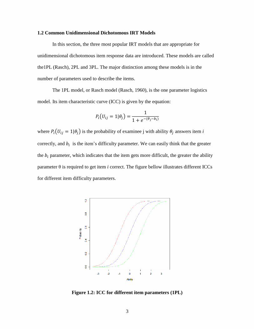
The 1PL model, or Rasch model (Rasch, 1960), is the one parameter logistics

model. Its item characteristic curve (ICC) is given by the equation:

( )

where ( ) is the probability of examinee j with ability answers item i

correctly, and is the item’s difficulty parameter. We can easily think that the greater

the parameter, which indicates that the item gets more difficult, the greater the ability

parameter θ is required to get item i correct. The figure bellow illustrates different ICCs

for different item difficulty parameters.

Figure 1.2: ICC for different item parameters (1PL)

4

The item difficulty parameter is the point on the ability scale where the

probability of answering correctly is 0.5. This item difficulty parameter is sometimes

called the location parameter because it indicates the position of the ICC. Since it is

assumed that item difficulty is the only parameter that influences examinee’s

performance (besides the ability of the examinee) in the 1PL model, ICCs with different

item difficulty parameters cannot cross each other (they are parallel). One advantage of

the 1PL model is that there is only one item parameter, which is item difficulty, and the

1PL model has sufficient statistics for the estimation of the item difficulty parameter.

This sufficient statistics is simply the count or sum of correct answers for an item over all

examinees, which makes estimation simple.

The 2PL, two parameter logistic model, is very similar to 1PL model except for

one more additional element which is the item discrimination parameter, . The ICC for

the 2PL model is as follows:

( )

Note, that since the 2PL model was developed by Lord (1952) to be similar to the

cumulative normal distribution, a scaling factor D=1.7 is required to make the logistic

function as close as possible to the normal ogive function. The Item discrimination

parameter, , indicates how well the item separates examinees into different ability

levels. In terms of the ICC, the discrimination parameter is proportional to the slope of

the ICC at the point on the ability scale. For example, a large value of the

discrimination parameter results in a very steep ICC which makes it useful for separating

examinees with abilities less than from examinees with abilities greater than . Figure

1.3 below shows ICCs with different difficulty parameters and discrimination parameters.

5

The ICCs for the 2PL model are not parallel as they were for 1PL model. Thus, ICCs

with different discrimination parameters can cross each other since they have different

slope and also has different location. Note that 2PL model is mainly used in this

simulation study.

Figure 1.3: ICC with different item parameters (2PL)

Lastly, by adding one more item parameter called the guessing parameter, the 2PL

model can be extended to the 3PL model. Since this simulation study doesn’t contain the

3PL model, it is only briefly introduced by the following equation.

( )

The guessing parameter represents the probability of answering the item correctly for

examinees with low ability. For example, suppose that there is a multiple choice question

with 4 choices. Even though examinees have no knowledge about the question, the

probability of getting that item correctly is 0.25. In this case, the guessing parameter is

6

0.25. Therefore, in this perspective, the guessing parameter provides a non-zero lower

asymptote for the item characteristic curve.

1.3 Parameter Estimation

Within the context of item response theory, one of the major goals is to achieve a

quality measure of the ability of examinees on an educational test. There are several

methods to estimate the latent trait of examinees. In this section, two common methods

are briefly introduced; maximum likelihood estimation (MLE) and Bayesian estimation,

both assuming the item parameters were known.

MLE ability estimation is based on the examinee’s vector of binary responses on

a test and the known values of the item parameters. Under the local independence

assumption, the probability of the vector of item responses ( ) for a given examinee is

given by the likelihood function below.

( | ) ∏ ( )

( ( ))

MLE obtains the ability estimates by maximizing this likelihood function. MLE is

one of the most popular traditional method, but when it comes to estimating IRT model

parameters, the MLE has a problem with estimating ability for examinees who answer all

item correctly or answer all item incorrectly. This is due to the fact that MLE for these

type of examinees gives positive infinity or negative infinity ability estimates.

On the other hand, the Bayesian estimation method considers the latent trait as a

random variable that follows some prior distribution. Then the Bayesian method provides

a way to combine the likelihood function and the prior information about the distribution

of the unknown parameters by using Bayes’ theorem as

7

∫

In this way, the Bayesian estimation method generates the posterior distribution

that is proportional to the product of the likelihood and prior distribution. Then the

posterior distribution is used to make inferences about the unknown parameters. Note that

since prior distributions regulates the maximum and minimum estimates of ability, there

is no such problem like the MLE estimating infinite value for ability of examinees who

answer all item correctly (or incorrectly).

1.4 Outline of work

Both the MLE and Bayesian methods can easily estimate latent traits of

examinees with known item parameters. However, the item parameters are not known a

priori. Therefore, many different estimation methods have been developed such as JMLE

(Birnbaum, 1968) and MML/EM (e.g. Baker and Kim, 2004). In chapter 2, two more

recent estimation methods, the Bayesian EM algorithm and the Monte Carlo Markov

chain (MCMC) method will be discussed. Comparison of the parameter estimates from

the two algorithms will be given in Chapter 3. The motivation for this simulation study,

details about the simulation and results including larger standard error problem are also

presented in Chapter 3. Chapter 4 discusses the possible solution to the larger standard

error in detail. Finally, a conclusion and possible future studies are discussed in Chapter 5.

8

CHAPTER 2

ESTIMATING ALGORITHMS

2.1 MCMC Algorithms

Markov chain Monte Carlo (MCMC) algorithms are structured to give a sequence

of observations from the joint posterior distribution of the parameters. The main idea of

MCMC is to define a stationary Markov chain and then simulate observations from that

chain. Observations simulated by MCMC are used to make inferences about the ability

and item parameters in the IRT model. There are various MCMC algorithms to generate

Markov chains (e.g. Metropolis, Metropolis-Hastings, Gibbs sampling and Metropolis-

Hastings within Gibbs). These algorithms each work somewhat differently but in general,

MCMC algorithms starts with simulating a “candidate” sample from a proposal

distribution. The candidate sample is not automatically accepted as a draw from the

posterior but are accepted probabilistically based on an acceptance probability. The

acceptance probability can be calculated via an acceptance function in the algorithm from

the proposal distribution and the full joint density to ensure that the algorithm achieves

the stationary distribution, the target posterior distribution that we are interested in.

Therefore, by repeating the steps above, generating candidates from proposal distribution

and accepting/rejecting candidates, the Markov chain converges to a stationary

distribution (the posterior distribution).

9

2.1.1 Metropolis Hastings Algorithm

The Metropolis Hastings algorithm (Metropolis, Rosenbluth, Rosenbluth & Teller,

1953; Hastings, 1970) generates Markov chains that are able to approximate a target (the

posterior) probability distribution by using a certain probability called the acceptance

probability, briefly introduced in previous section. Simply, the acceptance probability

represents the probability of accepting the new candidate from the proposal distribution.

The way the Metropolis Hastings (M-H) algorithm works is as following:

1. Choose an initial starting value

2. Generate a candidate value from the proposal density .

3. Accept with acceptance probability

where is the stationary distribution and is the proposal distribution.

Then, . Otherwise

4. Repeat Step 2 and Step 3 as many time you desire.

Note that when M-H algorithm calculate acceptance probability ,

appears in both the numerator and the denominator. Therefore, we only need to know

up to some constant of proportionality. This is very convenient when is the

complete conditional distribution or the posterior distribution.

In addition, if one chooses the proposal distribution to be a symmetric distribution

(symmetry around the previous value), then calculating acceptance probability

becomes simple. This is due to the fact that when proposal distribution is symmetric,

10

then . Therefore, the acceptance probability is

(

) (

).

Even though one of the strengths of the M-H algorithm lies in the flexibility of the

proposal distribution, one should be careful to choose proposal distribution since it

greatly affects the rate at which the Markov chain achieves stationarity as Chib and

Greenberg (1995) observed.

2.1.2 Gibbs Sampler Algorithm

The Gibbs Sampler (Geman and Geman, 1984) algorithm is another interative

algorithm designed to construct a dependent sequence of parameter values whose

distribution converges to the target stationary distribution (the posterior distribution in

Bayesian estimation). The important thing in the Gibbs sampler is that the algorithm

simulates (draws) the observations from the complete conditional distribution. For

example, in IRT, when the desired target distribution is where is

ability parameter, is item parameter and U is the response matrix, two complete

conditional distributions are required.

∫

and

∫

Then, the Gibbs sampler algorithm follows these steps.

1. Sample from and update

11

2. Sample from and update

3. Repeat Step 1 and Step 2 as many time you desire

Note that the Gibbs sampler algorithm is a special case of the M-H algorithm. The

Gibbs sampler algorithm sets the complete conditional distribution as the proposal

distribution with acceptance probability . One advantage of the Gibbs sampler is

that by using a complete conditional distribution, it simplifies the sampling (drawing)

step. However, when it is not possible to get the complete conditional distribution, then

Gibbs sampler algorithm cannot be implemented.

2.1.3 Metropolis Hastings within Gibbs

In this simulation study, the Metropolis-Hastings within Gibbs methods is used.

Even though the Metropolis-Hasting algorithm (M-H) is very flexible when it comes to

choosing proposal distributions, any distribution can be chosen to generate the next

candidate value for each iteration, some proposal distributions may generate improbable

candidates which can largely affect the rate at which the Markov chain becomes

stationary. Therefore, as Gelman, Rberts and Gilks (1996) mentioned, the pure M-H

method doesn’t work for most IRT models because maintaining reasonable acceptance

probabilities with a large number of parameters becomes extremely difficult. Moreover,

since the Gibbs algorithm requires the posterior distribution to be the complete

conditional distribution, which it is not in this simulation setting, implementing a pure

Gibbs algorithm is inadequate for this setting. Therefore, in this simulation study, the

combination of the two methods, which is called the Metropolis Hasting within Gibbs

algorithm (MH/Gibbs), is used. In this algorithm, we iteratively sample from the

12

complete conditionals according to the Gibbs algorithm, but for complete conditionals we

use a single iteration of the M-H algorithm as Chib and Greenberg (1995) explained. It

follows the steps below:

1. Attempt to draw from :

(a) Draw a candidate value for from proposal distribution

(b) Accept with acceptance probability

{

}

Otherwise, set

2. Attempt to draw from :

(a) Draw a candidate value for from proposal distribution

(b) Accept with acceptance probability

{

}

Otherwise, set

3. Repeat step 1 and 2 until k reaches desired number of iterations.

The resulting Markov chain has stationary distribution

as we desired.

2.2 EM Algorithm

In general, the EM algorithm is an iterative procedure for finding maximum

likelihood estimates of the parameters of probability models in the presence of

unobserved random variables. It can also be used for Bayes modal estimation. In IRT,

13

here the latent random variable is unobserved, we want to find estimates of item

parameters. Note that the latent traits (abilities) of examinees are treated as the missing

value (Bock and Aitkin, 1981) and item response matrix (U) is considered the observed

data. Therefore, (U, ) is considered to be the unobserved complete data and

represents the joint probability density function of the complete data where represents

the ability and represents the item parameters to be estimated.

The way the EM algorithm works is that given the matrix of provisional item

parameters at the p-th cycle, is computed by maximizing the [

with respect to item parameters . This process is repeated until a convergence criteria is

met. So the E-step (Estimation) and M-step (Maximization) in EM algorithm for p-th

iteration are:

E-Step : Compute [

M- Step : Choose such that maximize the posterior expectation.

To apply the EM algorithm more practically with IRT, Bock and Aitkin (1981)

reformulated the initial maximum likelihood estimation of item parameters in the

marginal distribution. By characterizing the population distribution, as if the population

distribution is known, this reformulation allows the EM algorithm to be computationally

feasible and to produce consistent item parameter estimates. To be specific, Bock and

Aitkin (1981) discretize the ability distribution empirically using two new notation

(Baker and Kim, 2004)

∑ ( | )

14

∑∏

∑ ∏

∑ ( | )

∑∏

∑ ∏

The are the number of examinees expected to have ability . The

represents the number of examinees at ability who are expected to answer correctly to

the item. Note that and are the artificial data which are created by above equation.

In addition, ∏

represents the quadrature form of the conditional

probability of with and item paramters. With and , below equations are

the quadrature form of marginal likelihood.

∑ [

∑ [

∑

Therefore, the EM algorithm now becomes the following :

E-Step : Compute and

M- Step : solve equations above using and

15

Then continue to iterate the E-Step and M-step until suitable convergence criteria is met.

Note that the EM algorithm permits the imposition of the Bayesian structure on the

estimation process. The two methods are compared in the next chapter.

16

CHAPTER 3

COMPARSION OF MH/GIBBS AND EM ALGORITHMS

3.1 Motivation

MH/Gibbs and the EM algorithm are two widely used methods to estimate IRT

parameters. One of the major distinctions is that the EM algorithm allows one to compute

point estimates for IRT model parameters, but the MH/Gibbs method allows one to

estimate the whole posterior distribution. In general, the MH/Gibbs method has some

advantages over the EM algorithm. For example, since the MH/Gibbs method is highly

flexible, it works easier with complex IRT model and also works with a larger

dimensional situations whereas the EM algorithm is somewhat limited to less

complicated testing situations because it does not work well with high dimensions. In

addition, the MH/Gibbs methods is easy to implement since many program packages

have been developed such as OpenBugs (Lunn, Spiegelhalter, Thomas, & Best, 2009),

JAGS (Plummer, 2013) and Stan (Stan Development Team, 2016).

However, Hendrix (2011) and Han Kil Lee (2016) mentioned that the estimated

standard errors for IRT parameter estimates from the MH/Gibbs method are larger than

the estimated standard error from the EM algorithm. Both Hendrix and Lee speculated on

a possible reason for larger standard error problem in MH/Gibbs, which was a high

correlation between item difficulty and the ability of the examinees within the Gibbs

steps. For example, if the ability estimates at p-th iteration was large on average due to

17

random error, then the item difficulty parameter estimates will tend to be larger in the

next run and vice versa.

Hendrix suggested that shifting and rescaling the ability estimate’s distribution at

every update of MCMC, basically keeping the ability distribution centered at mean 0 and

scaled to 1 at every iteration step of MCMC, would resolve the larger standard error

problem. In her study, with 3PL model using OpenBugs, she use a post-hoc centering

which is re-centering the ability estimates distribution at each iteration after the entire

MCMC procedure has finished. On the other hand, Lee followed up in a more

complicated manner to correct the issue. Instead of shifting and rescaling ability

estimator at the end of the iteration, he presented the way to implement the linking

procedure between each iteration, which he called In-chain Centered MCMC. This

method, which is programed in Fortran, allows the standard errors from MCMC to better

approximate the standard errors from the EM algorithm based Bayes model estimation

asymptotically.

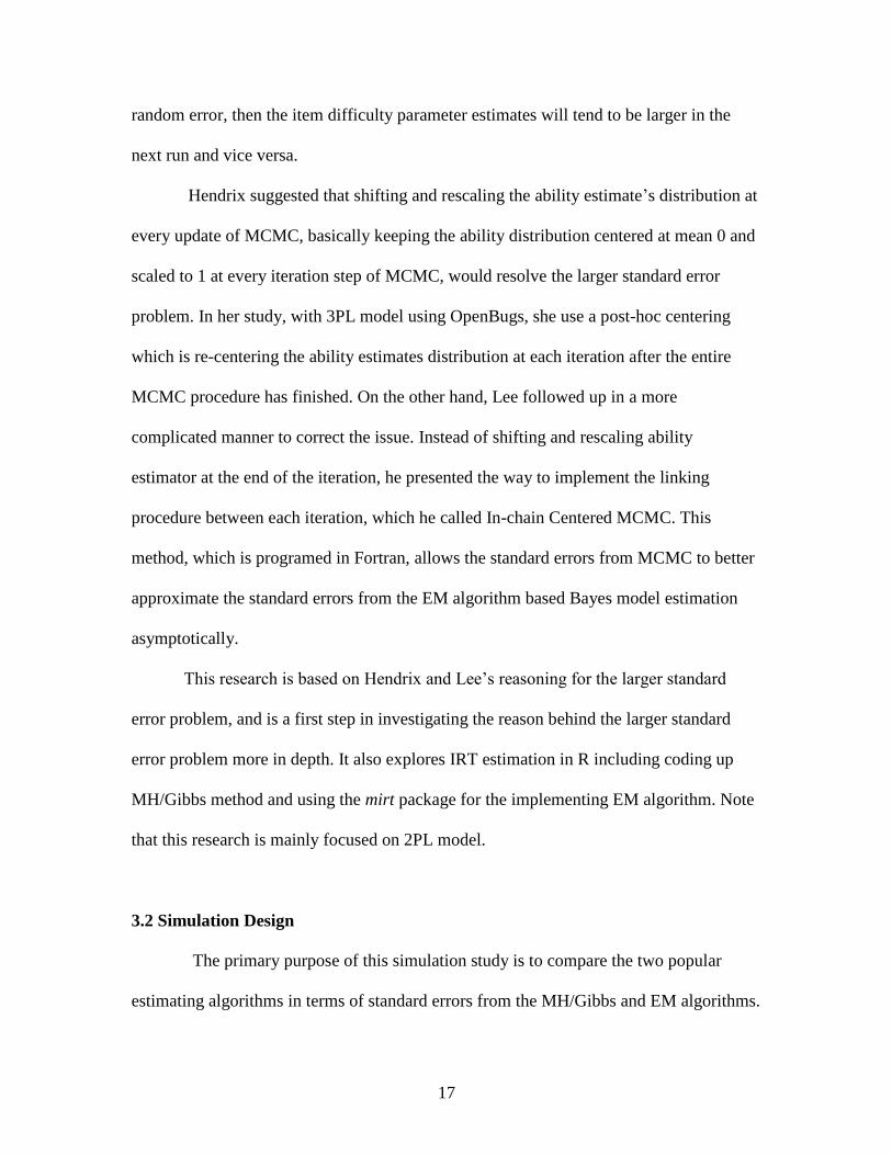
This research is based on Hendrix and Lee’s reasoning for the larger standard

error problem, and is a first step in investigating the reason behind the larger standard

error problem more in depth. It also explores IRT estimation in R including coding up

MH/Gibbs method and using the mirt package for the implementing EM algorithm. Note

that this research is mainly focused on 2PL model.

3.2 Simulation Design

The primary purpose of this simulation study is to compare the two popular

estimating algorithms in terms of standard errors from the MH/Gibbs and EM algorithms.

18

The simulation study begins with generating the item response matrix U. For this study,

one of the most popular IRT model, the 2PL, is considered. In particular, the true item

parameters are fixed when generating the response matrix U instead of randomly

generating true item parameters from a given distribution. Further, the two algorithms are

applied to the same response matrix U. Therefore, it is much easier to compare the

difference in two algorithms in terms of estimating item parameters. The table below

presents the simulation design in detail. Note that I used the most common prior and

proposal distributions that are found in the literature (Patz and Junker, 1999). For

proposal distributions, I choose the variance of the distribution to give the recommended

acceptance rate.

Table 3.1 Simulation Design

Contents MH/Gibbs EM Algorithm

IRT Model 2PL

Number of items 20

Number of Examinees 500

Prior Distribution

Proposal Distribution

-

Iteration 30,000 -

Programming R mirt (R-package)

One of the challenging thing for this simulation is keeping track of how the

lognormal is parameterized. Note for discrimination parameter, α, we can think of

drawing new values as .

19

In addition, the other problem occurs when MH/Gibbs algorithm is coded with the

log-likelihood for numerical stability. When MH/Gibbs calculates the acceptance

probability for an item parameter, the formula is:

(

)

(

|

)

( |

) (

) ( |

)

If we want to get the log-likelihood, the equation above becomes

(

) [

(

|

)

( |

) (

) ( |

)

Note that

is the likelihood,

are the priors, and

( |

) is evaluating the probability of generating the new candidate

value from the current candidate value. This can be easily coded with R. For example,

( |

) can be coded as (

) . However, R can

give a negative infinite value for (

|

)

( |

)

when this ratio is very close to 0 due

to limitations in floating point math. This is because, since the algorithm is coded with

the log-likelihood, gives a negative infinite value which makes chain stop.

Therefore, I found different way to code it. The acceptance rate equation can be modified

as in the following equations.

(

)

( |

)

[ (

) [

(

)

( ( ))

( |

)

( )

( ( ))

20

Instead of using directly, I replaced it with

based on the derivation above. By doing so, I could avoid the numerical

stability problem. Detailed R code is attached in the appendix. In addition, it takes some

time to run MH/Gibbs especially with a large number of iteration and also with a larger

response matrix U. It takes approximately 20 minutes with 500 examinees and 20 items.

3.3 Equating and Scaling

Before the simulation results are presented, there is one more concept that should

be introduced. In order to compare item parameter estimates from MH/Gibbs and EM

algorithm, the process of equating estimates must be carried out. This process deals with

the fact that the ability scale is arbitrary. Therefore, we cannot compare results from two

different algorithms directly without equating. Simply, estimates from both algorithm

should be on the same metric of the true item parameters. Thus, item parameters which

are estimated by MH/Gibbs algorithm have to be converted to the true item parameter

scale. In the same manner, the item parameters which are estimated by the EM algorithm

also have to be converted to the true item parameter scale.

In this study, for equating, the mean and sigma method (e.g. Hambleton,

Swaminathan and Rogers, 1991) is used for determining the scaling constant. Following

is the detail of mean and sigma methods.

21

Note that true stands for the true parameter values and method stands for estimates from

the algorithm. Also, s stands for standard deviation of the corresponding .

Once the coefficients A and B are determined, the item parameter estimates from

MH/Gibbs method or EM algorithm are placed on the same scale as true item parameters

using relationships below:

3.4 Simulation Results

3.4.1 MH/Gibbs Results

In this simulation, the item response matrix, U, is generated based on 20 items

and 500 examinees. Then, the MH/Gibbs algorithm is used to estimate the item

parameters and ability parameters with 30,000 iterations. Before presenting the results

from the MH/Gibbs method, since we are estimating the posterior distributions based on

a Markov chain, there are two main things to diagnosis. It is very important to check if

the chain has reached a stationary distribution and if there is autocorrelations between

successive parameter draws. Note that, in this simulation, the initial 15,000 iterations are

discarded (burn-in) to get stationary posterior distribution, and only every 50 draws is

kept from the posterior distribution to deal with the autocorrelation (thinning).

First, figures below are the trace plots for some item parameters to check if the

Markov chain converges. Trace plots illustrates how MH/Gibbs chains behave. Trace

plots from the simulation study show that the Markov chain for different item parameter

reasonably converges after discard initial 15,000 value. Also, from the trace plots, it

seems like all the chains converges fairly quickly, which indicates that these are efficient

22

chains which was expected since well-known prior distributions for item parameter have

been used. I decided to discard first 15,000 iteration because there were some unstable

chain for some items (For example, some item has some unstable point around 13,000

iteration). Note that all the chains become stationary after 15,000 iteration. Therefore,

convergence criteria is satisfied after burn-in.

Figure 3.1: Trace plots for item difficulty parameter estimates for item 1-4

23

Second, the figures below are the auto correlation function (ACF) plots. These

plots graphically summarize the strength of the relationship between an observation in a

time series and observation at the prior time step. Before thinning, the plot indicates that

the item parameter estimates for each item have strong correlation across iterations. This

is not surprising because when MH/Gibbs algorithm generates a candidate value based on

the previous candidate value. However, as we can see, after thinning by 50, the ACF

plots provide reasonable evidence that there is no severe autocorrelation (smaller values

that were tried still showed significant autocorrelation).

Figure 3.2: ACF plot for the item difficulty parameter estimates before thinning

24

Figure 3.3: ACF plot for the item difficulty parameter estimates after thinning by 50

Finally, when it comes to estimating parameters by using the MH/Gibbs method,

it is important to check the acceptance rate since it is related to efficiency of the chain.

Gelman et al. (1996) suggests that the variance of proposal distribution be selected to

achieve acceptance rate of about 25% to 50% for univariate draws which indicates that

chains maybe reasonably efficient. The table below shows the acceptance rate for the

item and ability parameters from the simulation study.

Table 3.2 Acceptance rate for each MH/Gibbs Chain

Acceptance Rate (500 examinees and 20 items)

Ability Parameter Item Parameter

Chain 1 0.4759679 0.2214483

Chain2 0.4661011 0.2205367

Chain 3 0.4538831 0.2186667

25

As we can see from the above table, the acceptance rates for the item parameters

from the simulation are about 20% which is similar to the recommended rate. One

finding is that having more examinees to get better estimates results in a decreased

acceptance rate (With 250 examinee, the acceptance rate for the item parameters was

25%). In addition, to achieve about 20% acceptance rate, the variance of the proposal

distributions for item parameters was set to be 0.05.

After accounting for burn-in, thinning and checking the acceptance rate, we can

now present the results from the MH/Gibbs method. It seems that the MH/Gibbs

estimates are reasonably close to true item and ability parameters judging by scatterplots

below.

Figure 3.4: Scatter plots for comparing true item parameter and MH/Gibbs estimates

The Scatterplot for item discrimination parameter, α, looks like it has a bit of a

megaphone shape, which indicates that MH/Gibbs method might have some problems

with higher value of α, item discrimination parameters. This phenomenon can be

explained by table 3.3.

26

Table 3.3 Number of Examinees answered correctly for each item

Item True Parameters

MH/Gibbs Estimates

For discrimination

parameter

# of Examinee

who answered Correct

4 452

8 398

12 265

16 136

20 48

The table 3.3 shows that the true item parameters which were used in simulation

study and also the estimates from MH/Gibbs method. From the table, we can see that the

MH/Gibbs’s item discrimination estimate for item 4 (+1.32) is quite different from true

item discrimination parameter (+1.8). This is due to the fact that almost every (more than

90%) examinees answered item 4 correctly. As mentioned in Chapter 1, the item

discrimination parameter α indicates how well an item is able to distinguish between who

are knowledgeable and who are not. Therefore, if almost every examinees get the item 4

correctly, it is hard for the MH/Gibbs algorithm to estimate the item discrimination

parameter close to the true parameter (in the response matrix U, it is just an item that

most of examinees answered correctly!) Note that it isn’t clear why item 20 didn’t

experience the same difficulty.

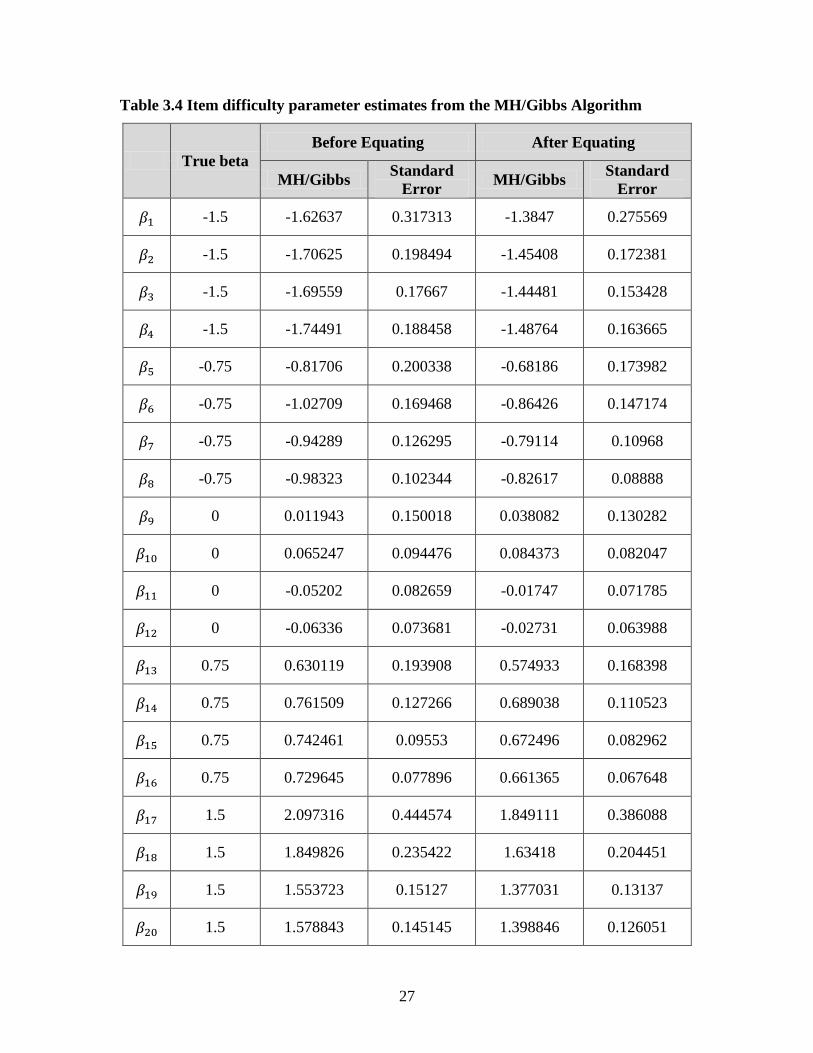
Table 3.4 illustrates the item parameter estimates from the MH/Gibbs algorithm.

Note that all the estimates are equated to the true parameter so we can compare these

estimates to the true item parameters since the scale is on the same metric as discussed in

chapter 3.3. In addition, for the same reason, these estimates can be compared with the

estimates from the EM algorithm.

27

Table 3.4 Item difficulty parameter estimates from the MH/Gibbs Algorithm

True beta

Before Equating After Equating

MH/Gibbs Standard

Error MH/Gibbs

Standard

Error

-1.5 -1.62637 0.317313 -1.3847 0.275569

-1.5 -1.70625 0.198494 -1.45408 0.172381

-1.5 -1.69559 0.17667 -1.44481 0.153428

-1.5 -1.74491 0.188458 -1.48764 0.163665

-0.75 -0.81706 0.200338 -0.68186 0.173982

-0.75 -1.02709 0.169468 -0.86426 0.147174

-0.75 -0.94289 0.126295 -0.79114 0.10968

-0.75 -0.98323 0.102344 -0.82617 0.08888

0 0.011943 0.150018 0.038082 0.130282

0 0.065247 0.094476 0.084373 0.082047

0 -0.05202 0.082659 -0.01747 0.071785

0 -0.06336 0.073681 -0.02731 0.063988

0.75 0.630119 0.193908 0.574933 0.168398

0.75 0.761509 0.127266 0.689038 0.110523

0.75 0.742461 0.09553 0.672496 0.082962

0.75 0.729645 0.077896 0.661365 0.067648

1.5 2.097316 0.444574 1.849111 0.386088

1.5 1.849826 0.235422 1.63418 0.204451

1.5 1.553723 0.15127 1.377031 0.13137

1.5 1.578843 0.145145 1.398846 0.126051

28

Table 3.5 Item discrimination parameter estimates from the MH/Gibbs Algorithm

True alpha

Before Equating After Equating

MH/Gibbs Standard

Error MH/Gibbs

Standard

Error

0.6 0.543856 0.102558 0.693118 0.098576

1 0.888103 0.133673 1.023999 0.128483

1.4 1.152511 0.189272 1.278141 0.181923

1.8 1.328806 0.26443 1.447591 0.254163

0.6 0.515594 0.093155 0.665953 0.089538

1 0.774396 0.119402 0.914708 0.114766

1.4 1.101033 0.159481 1.228662 0.153289

1.8 1.764723 0.29222 1.866584 0.280874

0.6 0.492948 0.090945 0.644187 0.087414

1 0.895434 0.11652 1.031046 0.111996

1.4 1.27932 0.171757 1.400027 0.165088

1.8 1.693482 0.251721 1.798108 0.241948

0.6 0.486881 0.089765 0.638355 0.08628

1 0.847934 0.120399 0.98539 0.115724

1.4 1.314458 0.175127 1.433801 0.168327

1.8 1.917273 0.340122 2.013211 0.326916

0.6 0.411142 0.087032 0.565556 0.083653

1 0.825845 0.152358 0.964159 0.146443

1.4 1.423255 0.249652 1.538373 0.239959

1.8 1.767269 0.395577 1.869031 0.380219

29

3.4.2 EM Results

For evaluating the EM algorithm, the same response matrix U is used from the

previous section (based on 20 items and 500 examinees). It was implemented in the R

package mirt (Chalmers, 2019) which is designed to analyze dichotomous or polytomous

response data using unidimensional or multidimensional latent trait models under the

item response theory paradigm.

Since the mirt package doesn’t parameterize the 2PL model in the classical way,

the 2PL model had to be re-parameterized from the standard mirt parameter

implementation. Luckily, the mirt package gives a way to define one’s item response

function. The difference between the 2PL model in mirt package and classical 2PL model

is explained in the table below. (Detailed R code to make this adjustment is in the

appendix)

Table 3.6 Comparison of 2PL model in mirt package and in classical IRT

Mirt package Classical IRT

2PL ( )

( )

Parameter estimates from the EM algorithm are reasonably close to the true item

and ability parameters judging by scatterplots below (Figure 3.5). Note that the pattern of

the scatterplots are very similar to those for the MH/Gibbs estimates. As mentioned in

chapter 3.4.1, since almost every examinees answered item 4 correctly, it is hard for EM

algorithm to estimate close to true item parameter for item 4. As a consequence, there is

one highly biased estimates on item discrimination parameter.

30

Figure 3.5: Scatter plots for true item parameter and EM estimates

One advantage of using the EM algorithm is that it takes significantly less time

compared to the MH/Gibbs method for the 2PL model. The EM algorithm takes less than

1 minute to estimate the parameters whereas MH/Gibbs takes about 15 to 20 minute for

the same response matrix U. Table 3.7 and 3.8 below show how well the EM algorithm

estimates the true item parameters. As we can see, EM algorithm estimates are

reasonably close to true item parameters. Also the standard errors are smaller than the

standard errors from the MH/Gibbs algorithm. Note that, even though standard errors

from EM algorithm is based on Fisher information, the estimated standard errors are not

the exact standard error since we don’t have the true parameter values when we estimates

using the EM algorithm. Table 3.7 and table 3.8 show the item difficulty and

discrimination parameter estimates from the EM algorithm. In addition, table 3.9 and

table 3.10 represent the comparison of item parameter estimates from the MH/Gibbs

algorithm and the EM algorithm.

31

Table 3.7 Item difficulty parameter estimates from the EM Algorithm

True beta

Before Equating After Equating

EM Standard

Error EM

Standard

Error

-1.5 -1.45125 0.195 -1.35289 0.186466

-1.5 -1.56539 0.156 -1.46203 0.149173

-1.5 -1.56297 0.138 -1.45972 0.13196

-1.5 -1.6116 0.132 -1.50622 0.126223

-0.75 -0.71995 0.136 -0.6536 0.130048

-0.75 -0.94956 0.118 -0.87316 0.112836

-0.75 -0.8749 0.094 -0.80177 0.089886

-0.75 -0.92204 0.082 -0.84684 0.078411

0 0.006944 0.112 0.041486 0.107098

0 0.048306 0.080 0.081037 0.076499

0 -0.04509 0.069 -0.00827 0.06598

0 -0.06603 0.063 -0.0283 0.060243

0.75 0.555376 0.130 0.565915 0.12431

0.75 0.687414 0.096 0.692175 0.091798

0.75 0.683781 0.078 0.6887 0.074586

0.75 0.676838 0.069 0.682061 0.06598

1.5 1.818814 0.300 1.774058 0.28687

1.5 1.6803 0.179 1.641606 0.171166

1.5 1.425043 0.117 1.397521 0.111879

1.5 1.457163 0.112 1.428234 0.107098

32

Table 3.8 Item discrimination parameter estimates from the EM Algorithm

True beta

Before Equating After Equating

EM Standard

Error EM

Standard

Error

0.6 0.603544 0.087 0.69321 0.077415

1 0.972257 0.132 1.0213 0.117457

1.4 1.261191 0.183 1.2784 0.162838

1.8 1.46412 0.222 1.458971 0.197541

0.6 0.573535 0.079 0.666507 0.070296

1 0.840472 0.103 0.904034 0.091652

1.4 1.203802 0.143 1.227334 0.127245

1.8 1.902378 0.267 1.848943 0.237583

0.6 0.559242 0.076 0.653789 0.067627

1 0.975071 0.110 1.023803 0.097881

1.4 1.374137 0.156 1.378902 0.138812

1.8 1.829946 0.225 1.784491 0.20021

0.6 0.542887 0.077 0.639236 0.068516

1 0.938413 0.112 0.991184 0.09966

1.4 1.421868 0.171 1.421374 0.15216

1.8 2.107792 0.297 2.031725 0.264278

0.6 0.464991 0.083 0.569922 0.073855

1 0.912467 0.134 0.968097 0.119236

1.4 1.575983 0.246 1.558509 0.218897

1.8 1.937583 0.344 1.880269 0.306099

33

3.4.3 Comparison

The table 3.8 and 3.9 compares the MH/Gibbs and EM algorithm estimates. The

major finding is that after the estimated item parameters from MH/Gibbs and EM

algorithm are converted to the metric of the true item parameters (equating), the standard

errors from MH/Gibbs method are larger than standard errors from EM algorithm. The

results from all 3 different MH/Gibbs chains showed the larger standard error problem. In

addition, there is no significant difference in the estimated item parameters.

Table 3.9 Comparison of item difficulty parameter estimates

True beta

MH/Gibbs EM

Estimates Standard

Error Estimates

Standard

Error

-1.5 -1.3847 0.275569 -1.35289 0.186466

-1.5 -1.45408 0.172381 -1.46203 0.149173

-1.5 -1.44481 0.153428 -1.45972 0.13196

-1.5 -1.48764 0.163665 -1.50622 0.126223

-0.75 -0.68186 0.173982 -0.6536 0.130048

-0.75 -0.86426 0.147174 -0.87316 0.112836

-0.75 -0.79114 0.10968 -0.80177 0.089886

-0.75 -0.82617 0.08888 -0.84684 0.078411

0 0.038082 0.130282 0.041486 0.107098

0 0.084373 0.082047 0.081037 0.076499

0 -0.01747 0.071785 -0.00827 0.06598

0 -0.02731 0.063988 -0.0283 0.060243

0.75 0.574933 0.168398 0.565915 0.12431

0.75 0.689038 0.110523 0.692175 0.091798

0.75 0.672496 0.082962 0.6887 0.074586

0.75 0.661365 0.067648 0.682061 0.06598

1.5 1.849111 0.386088 1.774058 0.28687

1.5 1.63418 0.204451 1.641606 0.171166

1.5 1.377031 0.13137 1.397521 0.111879

1.5 1.398846 0.126051 1.428234 0.107098

34

Table 3.10 Comparison of item discrimination parameter estimates

True alpha

MH/Gibbs After Equating

EM Standard

Error EM

Standard

Error

0.6 0.693118 0.098576 0.69321 0.077415

1 1.023999 0.128483 1.0213 0.117457

1.4 1.278141 0.181923 1.2784 0.162838

1.8 1.447591 0.254163 1.458971 0.197541

0.6 0.665953 0.089538 0.666507 0.070296

1 0.914708 0.114766 0.904034 0.091652

1.4 1.228662 0.153289 1.227334 0.127245

1.8 1.866584 0.280874 1.848943 0.237583

0.6 0.644187 0.087414 0.653789 0.067627

1 1.031046 0.111996 1.023803 0.097881

1.4 1.400027 0.165088 1.378902 0.138812

1.8 1.798108 0.241948 1.784491 0.20021

0.6 0.638355 0.08628 0.639236 0.068516

1 0.98539 0.115724 0.991184 0.09966

1.4 1.433801 0.168327 1.421374 0.15216

1.8 2.013211 0.326916 2.031725 0.264278

0.6 0.565556 0.083653 0.569922 0.073855

1 0.964159 0.146443 0.968097 0.119236

1.4 1.538373 0.239959 1.558509 0.218897

1.8 1.869031 0.380219 1.880269 0.306099

In addition, the item difficulty parameters for some items (for example, item

1,2,17,18) have the much higher standard errors compared to the other items both for

MH/Gibbs and EM. Most of the standard errors for the item difficulty parameter

estimates are around 0.10 but item 1 and 17 have standard errors of 0.27 and 0.39 for

MH/Gibbs method and 0.18 and 0.28 for EM algorithm. Note that this problem gets

severe when running the simulation with 250 examinees or less. Two histograms below

35

indicate the possible reason behind this. As we can see, the difficulty estimates for item 1

and item 17 have skewed distribution whereas the other difficulty estimates have

approximately normally distributed. This might cause higher standard errors for these

items.

Figure 3.6: Histogram of the item difficulty parameter from MH/Gibbs (item 1, 17)

Also Note that the MH/Gibbs estimates have random differences in estimating

item parameters with an identical response matrix U. This is due to the fact that the

MH/Gibbs algorithm randomly generates candidates from the proposal distribution.

36

CHAPTER 4

REASONING AND POSSIBLE SOLUTION

4.1 Supporting evidence and reasoning

In general, the MH/Gibbs algorithm is a simulation method that is structured to

generate sequences of observations to achieve unknown quantities of a given target

distribution whereas the EM algorithm is a method for finding maximum likelihood or

Bayes modal estimate of a model in the presence of missing data. Therefore, intuitively,

the MH/Gibbs method may have a larger standard error because the standard error of

item parameter estimates from MH/Gibbs contains the error coming from the simulation

generated sequence, whereas standard error from EM algorithm is simply calculated by

using Fishers information.

As noted by Hendrix (2011), the reasoning for larger standard error problem

becomes clear when we compare how two algorithms work. When the EM algorithm

proceeds to find the conditional expectation, [ from chapter 2, the

EM algorithm includes the following:

∑[∫ {∑ ( )

} ( |

)

]

Note that ( | ) part is the posterior distribution so using Bayes theorem to get the

following.

37

( | )

( | )

∫ ( | )

Therefore, the equation above becomes,

∑[∫ {∑ ( )

}

( | )

∫ ( | )

]

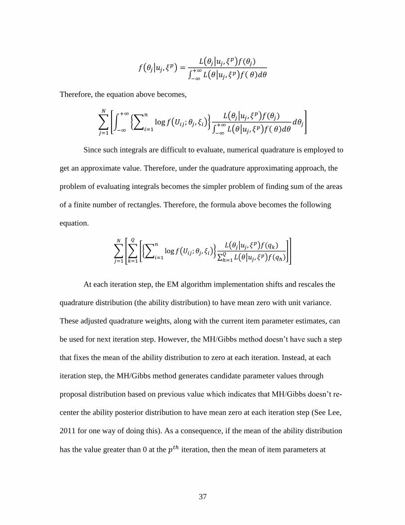
Since such integrals are difficult to evaluate, numerical quadrature is employed to

get an approximate value. Therefore, under the quadrature approximating approach, the

problem of evaluating integrals becomes the simpler problem of finding sum of the areas

of a finite number of rectangles. Therefore, the formula above becomes the following

equation.

∑[∑ [{∑ ( )

}

( | )

∑ ( | )

]

]

At each iteration step, the EM algorithm implementation shifts and rescales the

quadrature distribution (the ability distribution) to have mean zero with unit variance.

These adjusted quadrature weights, along with the current item parameter estimates, can

be used for next iteration step. However, the MH/Gibbs method doesn’t have such a step

that fixes the mean of the ability distribution to zero at each iteration. Instead, at each

iteration step, the MH/Gibbs method generates candidate parameter values through

proposal distribution based on previous value which indicates that MH/Gibbs doesn’t re-

center the ability posterior distribution to have mean zero at each iteration step (See Lee,

2011 for one way of doing this). As a consequence, if the mean of the ability distribution

has the value greater than 0 at the iteration, then the mean of item parameters at

38

iteration is likely to get large and vice versa. This pattern could cause inflated

standard errors.

Figure 4.1: Trace plots for mean ability and mean item difficulty distribution

The figure 4.1 shows the mean of ability parameter posterior at each iteration and

mean of item difficulty parameter posterior distribution at each iteration. We can easily

check that mean of ability distributions at each iteration deviates from zero. In addition,

two trace plots have same pattern which indicates that mean of item difficulty parameter

gets bigger when the mean of ability parameter from previous iteration is large as

explained above. This is very clear when calculating the correlation between the mean of

the ability estimates and the mean of the item parameter estimates at iteration. The

correlation is 0.87 in this case which indicates that these two estimates are highly

correlated.

4.2 Possible solution

As mentioned on in section 4.1, the larger standard error problem for MH/Gibbs

method mainly comes from the fact that MH/Gibbs method doesn’t re-center the mean of

39

ability parameter distribution (posterior distributions at each iteration) to zero. Therefore,

we attempted an adjustment to the MH/Gibbs method address this. To make this

adjustment, one of the possible ways is to manually set the mean of the ability parameter

distribution at each iteration to zero after entire MCMC process has finished (as in

Hendrix, 2011). As mentioned above, if the MH/Gibbs method generates mean of ability

parameter distribution greater than zero, the mean of the difficulty parameter estimates

would be increased and the larger standard error problem occurs. Therefore, by adjusting

the mean of the ability parameter distribution at each iteration, as in the EM algorithms

re-center the ability distribution at each iteration, we might avoid the larger standard error

problem.

To be specific, the mean of the ability parameter is calculated at each iteration and

see how much each mean deviates from zero. Then, that deviation is added to the

estimated item parameter values in the same iteration step (The MH/Gibbs in this

simulation study starts its chain with estimating the ability parameter first). It follows the

equation below. Note that the new parameter estimates from this adjusted method are also

required to be equated to true item parameters so it can be compared with the EM

algorithm.

then

then

Table 4.1 and 4.2 below represent the comparison of the MH/Gibbs and EM

algorithm in term of item parameter estimates and standard error after re-centering the

ability distribution to have mean zero. Note that this is done by manually re-centering

after the entire MH/Gibbs procedure has finished.

40

Table 4.1 Item difficulty estimates after re-centering the ability distribution

MCMC

Standard

Error EM

Standard

Error

-1.5 -1.3847 0.269828 -1.35289 0.186466

-1.5 -1.45408 0.164761 -1.46203 0.149173

-1.5 -1.44481 0.148034 -1.45972 0.13196

-1.5 -1.48764 0.155851 -1.50622 0.126223

-0.75 -0.68186 0.169316 -0.6536 0.130048

-0.75 -0.86426 0.135671 -0.87316 0.112836

-0.75 -0.79114 0.096932 -0.80177 0.089886

-0.75 -0.82617 0.076121 -0.84684 0.078411

0 0.038082 0.121923 0.041486 0.107098

0 0.084373 0.071818 0.081037 0.076499

0 -0.01747 0.058902 -0.00827 0.06598

0 -0.02731 0.050475 -0.0283 0.060243

0.75 0.574933 0.162522 0.565915 0.12431

0.75 0.689038 0.098491 0.692175 0.091798

0.75 0.672496 0.071588 0.6887 0.074586

0.75 0.661365 0.056593 0.682061 0.06598

1.5 1.849111 0.3843 1.774058 0.28687

1.5 1.63418 0.198699 1.641606 0.171166

1.5 1.377031 0.122007 1.397521 0.111879

1.5 1.398846 0.113939 1.428234 0.107098

41

Table 4.2 Item discrimination estimates after re-centering the ability distribution

MCMC

Standard

Error EM

Standard

Error

0.6 0.693118 0.107947 0.69321 0.077415

1 1.023999 0.135924 1.0213 0.117457

1.4 1.278141 0.189764 1.2784 0.162838

1.8 1.447591 0.254868 1.458971 0.197541

0.6 0.665953 0.099655 0.666507 0.070296

1 0.914708 0.11703 0.904034 0.091652

1.4 1.228662 0.157424 1.227334 0.127245

1.8 1.866584 0.283516 1.848943 0.237583

0.6 0.644187 0.097642 0.653789 0.067627

1 1.031046 0.119876 1.023803 0.097881

1.4 1.400027 0.169183 1.378902 0.138812

1.8 1.798108 0.247677 1.784491 0.20021

0.6 0.638355 0.096605 0.639236 0.068516

1 0.98539 0.13 0.991184 0.09966

1.4 1.433801 0.1723 1.421374 0.15216

1.8 2.013211 0.327967 2.031725 0.264278

0.6 0.565556 0.096906 0.569922 0.073855

1 0.964159 0.155635 0.968097 0.119236

1.4 1.538373 0.245211 1.558509 0.218897

1.8 1.869031 0.389328 1.880269 0.306099

42

As we can see, the standard errors from the MH/Gibbs algorithm get close to the

standard errors from the EM algorithm after re-centering the ability distribution, the

standard errors from the MH/Gibbs for some item difficulty parameters even get smaller

than the EM algorithm’s.

Note that even after re-centering the ability distribution, standard errors for the

item discrimination parameter from the MH/Gibbs algorithm don’t really get smaller or

similar to standard errors from the EM algorithm. This is due to the fact that, in this study,

the ability distribution was centered to have mean zero, but it was not rescaled to have a

unit standard deviation. It is obvious if we take a look at the 2PL model again.

( )

From , re-centering the mean ability distribution only have effect on item

difficulty parameter estimates, but has nothing to do with item discrimination parameter

estimates. Hendrix’s study (2011) includes shifting and also scaling the ability

distribution and the result shows that it also alleviates the larger standard error problem

for the item discrimination estimates.

43

CHAPTER 5

CONCLUSION AND FUTURE STUDY

It is often said that the MH/Gibbs method has some advantages over the EM

algorithm when it comes to estimating IRT model parameters since the MH/Gibbs

method can estimate the desired posterior distribution and also works more

straightforwardly with complex IRT Model. However, one often applies the MH/Gibbs

methods without paying enough attention to the standard error. Assessing standard error

is very important since it is a measure of the accuracy of the resulting parameter

estimates.

In this simulation study, the results show that there is almost no difference

between MH/Gibbs method and EM algorithm in terms of parameter estimates for 2PL

model. The EM algorithm gives identical parameter estimates every time run it and the 3

chains (replications) from MH/Gibbs give very similar results. Both algorithms provide

very close estimates to the true ability and item parameters. However, for the 2PL model,

the MH/Gibbs method has larger standard errors for all parameters than the EM

algorithm, which indicates that EM algorithm maybe a more accurate method to estimate

the 2PL model. (Also 10 times faster!) Therefore, it is not wise to apply MH/Gibbs

method without carefully assessing the standard error.

This work presented one possible remedy to the larger standard error problem that

the MH/Gibbs method has. As mentioned in detail in chapter 4.2, after regulating the

44

highly correlated pattern, by rescaling the mean of the ability parameters to be 0 at every

iteration, the standard error gets very close to or sometimes less than standard error from

EM algorithm. The shortcoming of this study is that it manually sets the mean of ability

parameters to 0 instead of making an adjustment to inside of MH/Gibbs algorithm

(Between the each iteration in algorithm). In addition, the attempt to correct the issue

doesn’t include rescaling the ability distribution at each iteration, and this was the reason

that larger standard error problem for the item discrimination estimates wasn’t resolved.

Therefore, in future study, we need to further examine the proposals of Hendrix (2011)

and Lee (2016).

45

REFERENCE

Baker, F.A & Kim, S. 2004. Item Response Theory: parameter estimation techniques;

second edition revised and expanded. New York: Marcel Dekker, Inc

Bock, R.D & Aitkin, M. 1981. Marginal maximum likelihood estimation of item

parameter: Application of an EM algorithm. Psychometrika, 46(4): 443-459

Chang. M. 2017. A comparison of Two MCMC Algorithm for Estimating 2PL IRT Models.

PhD thesis, Southern Illinois University

Chib, S & Greenberg, E. 1995. Understanding the Metropolis-Hastings Algorithm. The

American Statistician, 49(4): 327-335

Chalmers, R.P. 2012. Mirt: A multidimensional Item Response Theory Package for the R

environment. Journal of Statistical Software, 48(6).

Hambleton, R.K & Swaminathan, H & Rogers, H.J. 1991. Fundamentals of Item Response

Theory. SAGE Publications

Han Kil, Lee. 2016. Some Issues in Markov Chain Monte Carlo Estimation for Item

Response Theory. PhD thesis, UNIVERSITY OF SOUTH CAROLINA

Hoff, P.D. 2009. A first course in Bayesian Statistical Methods. Springer

Kim, J.S & Daniel M.B. 2007. Estimating Item Response Theory Models Using Markov

Chain Monte Carlo Methods. Educational Measurement Issues and Practice,

26(4): 38-51.

L. Hendrix. 2011. Fast EM Based Posterior Approximation for IRT Item Parameters.

PhD thesis, UNIVERSITY OF SOUTH CAROLINA

R. J Patz and B.W. Junker. 1999. A Straightforward Approach to Markov Chain Monte

Carol Methods for Item Response Model. Journal of Educational and Behavioral

Statistics, 24(2):146-178

Sheng, Y. & Headrick.T.C. 2007. JMASM27: An Algorithm for Implementing Gibbs

Sampling for 2PNO IRT MODEL(Fortran). Journal of Modern Applied Statistical

Methods, 6(1): Article 33.

46

Wim J. van der Linden. 2015. Handbook of Item Response Theory; Volume two:

Statistical Tools. CRC Press

47

APPENDIX A

R CODE

# Set up #

source("http://www.stat.sc.edu/~habing/courses/irtS14.txt")

B=c(-1.5,-1.5,-1.5,-1.5,-0.75,-0.75,-0.75,-0.75,0,0,0,0,0.75,0.75,0.75,0.75,1.5,1.5,1.5,1.5)

A=c(0.6,1.0,1.4,1.8,0.6,1.0,1.4,1.8,0.6,1.0,1.4,1.8,0.6,1.0,1.4,1.8,0.6,1.0,1.4,1.8)

C= rep(0, 20)

theta_U=rnorm(500)

U= irtgen(theta_U, A,B,C, type="logistic")

U=as.matrix(U)

N=nrow(U)

K=ncol(U)

theta0=rep(0,N)

beta0=rep(0,K)

alpha0=rep(1,K)

pro.t.var=0.55 #proposal variance#

pro.a.var=0.05 #proposal variance#

pro.b.var=0.05 #proposal variance #

# MH-Gibbs Algorithm #

cpf=function(thetas, alphas, betas, N, K){

theta = matrix(thetas, ncol=1)%*%matrix(alphas, nrow=1)

ab=t(matrix(diag(matrix(alphas, ncol=1)%*%matrix(betas, nrow=1)),K,N))

logit = (theta-ab)

probs = 1/(1+exp(1.7*(-logit)))

return(probs)

48

}

MHGtheta=function(theta0, alpha0, beta0, U, N, K, pro.t.var){

theta.star = theta0 + matrix(rnorm(N, sd=sqrt(pro.t.var)))

lk = cpf(theta0, alpha0, beta0, N, K)

lk = ifelse(U==1, lk, 1-lk)

lkhood.0 = apply(log(lk), 1, sum)+ log(dnorm(theta0,0,1)) #prior theta~N(0.1)#

lk.star=cpf(theta.star, alpha0, beta0, N, K)

lk.star=ifelse(U==1, lk.star, 1-lk.star)

lkhood.star=apply(log(lk.star), 1, sum)+ log(dnorm(theta.star,0,1))

log.r = lkhood.star - lkhood.0

accept = ifelse(log(runif(N))<log.r, 1, 0)

acc.rate.theta = sum(accept)/N

theta.star=ifelse(accept==1, theta.star, theta0)

return(list(acc.rate.theta, theta.star))

}

MHGbeta=function(theta0, alpha0, beta0, U, N, K, pro.a.var, pro.b.var){

lalpha0=log(alpha0)

lalpha.star=lalpha0+rnorm(K, sd=sqrt(pro.a.var))

alpha.star=exp(lalpha.star)

beta.star=beta0+rnorm(K, sd=sqrt(pro.b.var))

lk = cpf(theta0, alpha0, beta0, N, K)

lk = ifelse(U==1, lk, 1-lk)

lkhood.0=apply(log(lk), 2, sum)+apply(matrix(log(dnorm(lalpha0,0,1)), ncol=K)-

2*lalpha0, 1, sum)+ log(dnorm(beta0,0,sqrt(2)))

lk.star=cpf(theta0, alpha.star, beta.star, N, K)

lk.star=ifelse(U==1, lk.star, 1-lk.star)

lkhood.star=apply(log(lk.star), 2, sum)+apply(matrix(log(dnorm(lalpha.star,0,1)),

ncol=K)-2*lalpha.star, 1, sum)+ log(dnorm(beta.star,0,sqrt(2)))

log.r= lkhood.star - lkhood.0

49

accept = ifelse(log(runif(K))<log.r, 1, 0)

acc.rate.itempar=sum(accept)/K

beta.star = ifelse(accept==1, beta.star, beta0)

alpha.star = ifelse(accept==1, alpha.star, alpha0)

return(list(acc.rate.itempar, alpha.star, beta.star))

}

#Iteration Part#

iteration=function(pro.t.var, pro.a.var, pro.b.var){

theta.result = MHGtheta(theta0, alpha0, beta0, U, N, K, pro.t.var)

rate.theta = theta.result[[1]]

theta.star = theta.result[[2]]

item.result = MHGbeta(theta.star,alpha0, beta0, U, N, K, pro.a.var, pro.b.var)

rate.itempars = item.result[[1]]

alpha.star = item.result[[2]]

beta.star = item.result[[3]]

return(list(theta.star, alpha.star, beta.star, rate.theta, rate.itempars))

}

## Run it ##

S=30000

save.alpha = NULL

save.beta = NULL

save.theta = NULL

save.rate.theta=NULL

save.rate.itempars=NULL

for(s in 1:S){

out = iteration(pro.t.var, pro.a.var, pro.b.var)

50

save.theta = cbind(save.theta, out[[1]])

save.alpha = cbind(save.alpha, out[[2]])

save.beta = cbind(save.beta, out[[3]])

save.rate.theta = cbind(save.rate.theta, out[[4]])

save.rate.itempars = cbind(save.rate.itempars, out[[5]])

theta0=out[[1]]

alpha0=out[[2]]

beta0=out[[3]]

}

# EM Algorithm #

library("mirt")

colnames(U)=paste('Q', 1:20)

name='B2PL'

par=c(a=1,b=0)

est=c(TRUE, TRUE)

low<-c(0.2,-2.5);up<-c(2.5,2.5)

P.B2PL<-function(par,Theta,ncat){

a<-par[1]; b<-par[2]

P1<-1/(1+exp(-1.7*a*(Theta-b)))

cbind(1-P1,P1)

}

B2PL<-createItem(name,par=par,est=est,P=P.B2PL,lbound=low,ubound=up)

EM<-

mirt(U,1,rep('B2PL',20),customItems=list(B2PL=B2PL),method='EM',parpriors=list(c((1

:20)*2-1,'lnorm',0,1),c((1:20)*2,'norm',0,2)), SE=TRUE)

emresult=coef(EM, simplify=T)