Embed Size (px)
Citation preview

INFLATION AND ECONOMIC GROWTH NEXUS IN THE
SOUTHERN AFRICAN DEVELOPMENT COMMUNITY:
A PANEL DATA INVESTIGATION
by
Monaheng Seleteng
Submitted in partial fulfilment of the
requirements for the degree
PhD (Economics)
in the
Faculty of Economic and Management Sciences
at the
University of Pretoria
2012
©© UUnniivveerrssiittyy ooff PPrreettoorriiaa

ii
Declaration
“ I declare that the thesis, which I hereby submit for the degree PhD (Economics) at the University of Pretoria, is my own work and has not previously been submitted by
me for a degree at another university.”

iii
ACKNOWLEDGEMENTS
First and foremost, I would like to thank the All Mighty God for seeing me through
this journey. I would also like to convey my sincere gratitude to a number of people
and some institutions without whose contributions this thesis would not have been
successfully completed. I wish to thank my supervisor and co-supervisor, Dr. Manoel
Bittencourt and Prof. Reneé van Eyden, respectively, for having provided guidance,
support and patience ensuring a successful completion of the thesis. I highly
appreciate their contributions and comments.
I would also like to thank my employer, the Central Bank of Lesotho, for allowing me
to pursue my studies and also for their financial support throughout the four years of
my study leave. I would also like to thank my colleagues at the Research
Department of the Central Bank of Lesotho due to their sacrifices of taking over my
duties and responsibilities during the entire period of my study leave, I am humbly
thankful to them. I am also thankful to the academic staff and my fellow classmates
at the Department of Economics for their valuable comments throughout the years. I
would also like to thank the Economics Society of South Africa (ESSA) for giving me
an opportunity to present one of the papers in their conference. Furthermore, I would
like to thank Economic Modelling for accepting and publishing one of the chapters of
the thesis.
Furthermore, I am grateful to my wife and son, ‘Matlotliso and Tlotliso, respectively
for unwavering encouragement, unconditional support, and for believing in me at all
times and also for their sacrifices despite the little attention they received during this
work. I also wish to extend my thanks to my mother, sister, brother and mother-in-
law for their moral support at all times.

iv
ABSTRACT
Inflation and Economic Growth Nexus In The
Southern African Development Community:
A Panel Data Investigation
by
Monaheng Seleteng
Supervisor : Dr. Manoel Bittencourt
Co-Supervisor: Prof. Reneé van Eyden
Department : Economics
Degree : PhD (Economics)
The aim of the thesis is to examine the relationship between inflation and economic
growth using the Southern African Development Community (SADC) as a case
study. The motivation emanates not only because of the lack of studies analysing
this relationship in the SADC region, but also due to the fact that this relationship
may differ from the one that exists in developed countries due to the level of
economic development and prudent macroeconomic policies being practised in the
latter (Sarel, 1996). The relationship may differ because the vast majority of
developed countries have established independent central banks with a clear
mandate to keep inflation levels within a specific range (adopted an inflation
targeting framework). However, in most developing countries, central banks do not
have a clear inflation targeting monetary policy framework, for instance, in the SADC
region, only South Africa has adopted an inflation targeting monetary policy
framework. High inflation episodes are known to contribute to macroeconomic
instability, therefore policy makers find it important to understand the kind of the

v
relationship that exists between inflation and economic growth in order to develop
and implement sound macroeconomic policies. Therefore, inflation is viewed to be
one of the basic indicators of macroeconomic stability; hence it is an indicator of the
ability of the government to manage the economy. High levels of inflation may be
indicative of a lack of sound governance by the monetary authority of a country. In
addition, it is a sign of government that has lost control of its finances (Fischer,1993).
The thesis addresses issues of nonlinearities in the inflation-growth nexus by
endogenously estimating the threshold level of inflation below which inflation may
have no, or positive, impact on economic growth, or above which inflation may be
detrimental to economic growth. It also assesses the effects of a shock to inflation in
South Africa, being the largest economy in the region, on inflation and economic
growth of the rest of the region.
First, different panel data methodologies; Fixed Effects (FE), Difference Generalised
Method of Moments (DIF-GMM), System Generalised Method of Moments (SYS-
GMM), and Seemingly Unrelated Regression (SUR) estimators are used in order to
examine the relationship between inflation and economic growth in the region.
Second, Panel Smooth Transition Regression (PSTR) methodology is utilised to
examine the nonlinearities in the inflation-growth nexus. In particular, the threshold
level of inflation is endogenously estimated and the smoothness of the transition
from a low to a high inflation regime in the region is also estimated1. Thirdly, the
effects of South African inflation on the inflation and economic growth in the rest of
the region are assessed using impulse-response functions derived from estimating a
Panel Vector Autoregression (PVAR) model. Overall, the study deals with problems
which are normally encountered when using cross-country data such as
endogeneity, heterogeneity and cross-sectional dependence.
The main findings of the study are that inflation and economic growth in the region
are negatively related, as is also the case in other regions of the world as depicted
by the empirical literature (Fischer, 1993 and De Gregorio, 1993). Therefore, in
terms of the inflation-growth link, the SADC region is not different from all the other
1 Published in Economic Modelling

vi
regions around the globe. Secondly, the threshold level of inflation in the region is
estimated at 18.9 per cent, which is in line with the findings of authors like Drukker et
al. (2005), Mignon and Villavicencio (2011), and Ibarra and Trupkin (2011), who
found a threshold level of 19.2 per cent, 19.6 per cent, and 19.1 per cent for
developing countries. However, this threshold level marginally exceeds that of Khan
and Senhadji (2001), Schiavo and Vaona (2007), Moshiri and Sepehri (2009) and
Espinoza et al. (2010), which studies report threshold values between 10 and 12 per
cent for developing countries. The empirical results also reveal that shocks to South
African inflation have significant economic impact on inflation, openness, investment
and economic growth in the rest of the SADC region. In particular, more interestingly,
South African inflation is found to have a negative and statistically significant impact
on economic growth in the region for up to about 12 years after the shock, after
which, it becomes insignificant.
The contribution of the thesis to the literature is that, firstly, this looks into the
inflation-growth relationship in the context of Africa, in particular the SADC region; as
such an investigation or research has not been conducted before. Secondly, the
research takes advantage of panel data methodologies so as to provide more robust
estimates and confront the potential bias emanating from problems such as
endogeneity, heterogeneity and cross-country dependence that may have affected
previous empirical work on inflation-growth nexus. This is believed to provide more
informative estimates on the inflation-growth link, and therefore deepens our
knowledge of the region.

vii
TABLE OF CONTENTS
CHAPTER ONE ......................................................................................................... 1
BACKGROUND AND INTRODUCTION ..................................................................... 1
1.1 INTRODUCTION .................................................................................................. 1
1.2 HISTORY AND OBJECTIVES OF SADC ............................................................. 2
1.3 SADC ECONOMIC PERFORMANCE .................................................................. 4
1.4 PROBLEM STATEMENT ..................................................................................... 8
1.5 OBJECTIVE OF THE STUDY ............................................................................ 10
1.6 CONTRIBUTIONS OF THE STUDY .................................................................. 11
1.7 OUTLINE OF THE STUDY ................................................................................ 12
CHAPTER TWO ....................................................................................................... 14
INFLATION AND ECONOMIC GROWTH NEXUS IN THE SADC
A PANEL DATA INVESTIGATION ........................................................................... 14
2.1 INTRODUCTION AND MOTIVATION ................................................................ 14
2.2 LITERATURE REVIEW ...................................................................................... 16
2.3 DATA DESCRIPTION ........................................................................................ 18
2.4 METHODOLOGY ............................................................................................... 22
2.4.1 Unit Root Testing .................................................................................. 23
2.4.2 Fixed Effects Estimator ......................................................................... 24
2.4.3 Difference and System GMM Estimators .............................................. 25
2.4.4 Seeminlgy Unrelated Regression (SUR) Estimator .............................. 26
2.5 EMPIRICAL RESULTS ...................................................................................... 27
2.5.1 Regression Results from Annual Data .................................................. 27
2.5.2 Diagnostic Tests Results ...................................................................... 32
2.6 CONCLUSION ................................................................................................... 33
CHAPTER THREE ................................................................................................... 35
NON-LINEARITIES IN INFLATION-GROWTH NEXUS IN THE SADC REGION: A PANEL SMOOTH TRANSITION REGRESSION APPROACH ................................ 35
3.1 INTRODUCTION ................................................................................................ 35
viii
3.2 LITERATURE REVIEW ...................................................................................... 36
3.3 METHODOLOGY AND DATA ............................................................................ 41
3.3.1 Panel Smooth Transition Regression Model ......................................... 41
3.3.1.1 Testing for Linearity .............................................................................. 43
3.3.1.2 Testing for the Number of Transition Functions .................................... 45
3.3.2 The Data ............................................................................................... 45
3.4 EMPIRICAL RESULTS ...................................................................................... 49
3.4.1 Linearity and No Remaining Non-Linearity Results .............................. 49
3.4.2 Model Estimation Results ..................................................................... 50
3.5 CONCLUSION ................................................................................................... 53
CHAPTER FOUR ..................................................................................................... 55
EFFECTS OF SOUTH AFRICAN INFLATION ON THE SADC REGION:
A PANEL VECTOR AUTOREGRESSION APPROACH .......................................... 55
4.1 INTRODUCTION ................................................................................................ 55
4.2 LITERATURE REVIEW AND STYLIZED FACTS............................................... 57
4.2.1 Inflation and Economic Growth Trends in the SADC Region ................ 57
4.2.2 Trade Flows Within the Region ............................................................. 59
4.2.3 Literature Review .................................................................................. 62
4.3 METHODOLOGY AND DATA ............................................................................ 64
4.3.1 The Data ............................................................................................... 64
4.3.2 Unit Root Testing .................................................................................. 64
4.3.3 Panel Vector Autoregression Model ..................................................... 65
4.4 EMPIRICAL RESULTS ...................................................................................... 68
4.5 CONCLUSION ................................................................................................... 72
CHAPTER FIVE ....................................................................................................... 73
CONCLUSION ......................................................................................................... 73
REFERENCES ......................................................................................................... 77

ix
LIST OF FIGURES
Figure 1: Southern African Development Community (SADC) Map ........................... 3
Figure 2: Estimated Transition Function for SADC Region ...................................... 53
Figure 3: Intraregional Trade Linkages ..................................................................... 61
Figure 4: Impulse Responses to South African Inflation Rate Shock ....................... 70

x
LIST OF TABLES
Table 1: Sub-Saharan Africa’s and SADC’s Contribution to World GDP and
Population: 2009 ........................................................................................................ 4
Table 2: Percentage Distribution of GDP at Market Prices ......................................... 5
Table 3: SADC Real Growth Rates ............................................................................ 6
Table 4: Consumer Price Inflation for SADC Countries .............................................. 8
Table 5: Variable Description ................................................................................... 20
Table 6: Correlation Matrix for 11 SADC Countries .................................................. 21
Table 7: Descriptive Statistics .................................................................................. 22
Table 8: Panel Unit Root Tests ................................................................................ 24
Table 9: Dynamic Fixed Effects (FE) Estimates ....................................................... 28
Table 10: Dynamic Difference-Generalised Method of Moments Estimates ............ 28
Table 11: Dynamic System- Generalised Method of Moments Estimates ................ 29
Table 12: Dynamic Seemingly Unrelated Regression (SUR) Estimates................... 29
Table 13: Seemingly Unrelated Regressions ........................................................... 31
Table 14: Variable Description ................................................................................. 46
Table 15: Correlation Matrix for 11 SADC Countries ................................................ 47
Table 16: Descriptive Statistics ................................................................................ 48
Table 17: Panel Unit Root Tests .............................................................................. 49
Table 18: Linearity Tests .......................................................................................... 49
Table 19: Tests of No Remaining Non-Linearity ....................................................... 50
Table 20: PSTR Model Estimation ........................................................................... 51
Table 21: Summary Statistics of Economic Growth and Inflation ............................. 58
Table 22: Direction of Merchandise Trade, 2008 ..................................................... 60
Table 23: Panel Unit Root Tests .............................................................................. 65
Table 24: Dynamic Results ...................................................................................... 68
Table 25: Shocks and Variance Decomposition ....................................................... 71
1
CHAPTER ONE
BACKGROUND AND INTRODUCTION
1.1. INTRODUCTION
Central banks across the world are concerned with high levels of prices and strive for
achievement and maintenance of price stability. Therefore, the common objective of
macroeconomic policy is a low inflation rate which usually creates an environment
conducive to rapid economic growth (Fischer, 1993). Hence policy makers find it
important to understand this relationship so that sound policies can be developed.
For instance, adoption of an inflation targeting monetary policy framework by
countries such as New Zealand and United Kingdom, has been proven to work quiet
well in curbing inflation. If inflation is detrimetal to economic growth, it follows that
policy-makers should aim for low rates of inflation. This can be achieved by
increasing the interest rates which will inturn reduce investment and consumption
spending and this could cool down an overheating economy. However,
macroeconomic stability, defined as a low inflation rate is a necessary although not a
sufficient condition for sustained economic growth. This is evidenced by the fact that
most countries have grown slowly despite low inflation, for instance, this transpired in
the Franc zone during the 1980s (Fischer, 1983). Many cross-country studies
suggest the existence of a negative relationship between these two variables and the
magnitude of this relationship is envisaged to vary from region to region depending
on the level of development and other factors. This is because many developed
countries have well-established and independent central banks with a clear mandate
to keep inflation level within a particular target range.
As highlighted by (Hineline, 2003) the effects that inflation has on growth has been
questioned since the early 1990s. From the various time-series and panel data
studies, a stylized fact emerged, namely that there are substantial differences across
countries. On the one hand, some studies used linear techniques and just
investigated the nature of the inflation-growth nexus. The literature on inflation-
growth relationships is quite extensive, starting with the work of De Gregorio (1993)
and Fischer (1993) who, respectively found the existence of a negative relationship

2
between inflation and economic growth. On the other hand, other studies used non-
linear techniques and argued that there exists a threshold or optimal level of inflation
below which inflation may have no or even a positive effect on growth, and above
which inflation may be detrimental to economic growth. Therefore, this body of
research investigated the nonlinearities in the inflation-growth relationship. Such
studies include, among others; Sarel, 1996; Bruno and Easterly, 1998; Ghosh and
Phillips, 1998; Khan and Senhadji, 2001; Moshiri and Sepehri, 2004; Mubarik, 2005;
Lee and Wong, 2005; Drukker et al., 2005; Pollin and Zhu, 2006; Li, 2006; Hineline,
2007; Schiavo and Vaona, 2007; Espinoza et al., 2010; Kan and Omay, 2010; Ibarra
and Trupkin, 2011; and Mignon and Villavicencio, 2011, who all used cross-country
data for both developing and developed countries to find that the negative
relationship between inflation and economic growth exists after certain threshold
level(s). Detailed methodological issues, data sets and findings are discussed in
Chapter three of the thesis. Therefore, this leads to the question; how low should the
inflation rate be? That is, at what level of inflation does the relationship between
inflation and economic growth become negative (Furuoka et al., 2009).
1.2 HISTORY AND OBJECTIVES OF SADC
In 1980, nine Southern African countries, namely; Angola, Botswana, Lesotho,
Malawi, Mozambique, Swaziland, Tanzania, Zambia and Zimbabwe formed the
Southern African Development Coordination Conference (SADCC) in an attempt to
decrease member countries’ external economic dependence on South Africa and to
promote regional co-operation in development projects (Ligthelm, 2006). Namibia
joined shortly after its independence in 1990 and these ten countries established the
Southern African Development Community (SADC) in August 1992 when these
countries signed the SADC Treaty. According to Oosthuizen (2006), technically the
organisation came into being on the 30 September 1993 when the Treaty entered
into force. The Republic of South Africa joined later in August 1994 after all-race
elections and Mauritius became the twelveth member in August 1995. The
Democratic Republic of Congo and Sychelles joined in 1997 and Madagascar also
became a member in 2005. Therefore, SADC currently consists of fifteen member
states, namely; Angola, Botswana, Democratic Republic of Congo (DRC), Lesotho,
Madagascar, Malawi, Mauritius, Mozambique, Namibia, Seychelles, South Africa

3
(SA), Swaziland, Tanzania, Zambia and Zimbabwe, and its headquarters are in
Gaborone, Botswana. The member countries have differing levels of education,
health provisions and other socio-economic development. However, they have
similar trade patterns and trade between themselves (Nel, 2004). Figure 1 depicts
the map of the SADC region.
The Article 5 of the SADC Treaty highlights the overall objectives of the Treaty, as
the promotion of economic growth and socio-economic development that will
eventually eradicate poverty, and promote and maintain peace, security and
democracy, through regional cooperation and integration (SADC, 2011).
Figure 1: Southern African Development Community (SADC) Map
Source: http://www.sadc-reep.org.za/

4
1.3 SADC ECONOMIC PERFORMANCE
Table 1: Sub-Saharan Africa’s and SADC’s Contribution to World GDP and Population: 2009
World Sub-Saharan
Africa
SADC
GDP in current prices (Billion US$) 57 722.09 8 93.73 468.83
% of World - 1.55 0.81
Population (Millions) 6 726.06 778.19 268.56
% of World - 11.57 3.99
Source: International Monetary Fund, September 2011
Table 1 depicts that both Sub-Saharan Africa (SSA) and SADC have an insignificant
contribution to the world’s GDP. Furthermore, as a share of world’s population, these
two regions constitute 11.6 per cent and 4 per cent for SSA and SADC, respectively.
In general, Table 1 shows that although this thesis uses the SADC region as a case
study, the contribution of this region towards the world GDP at large is very marginal,
hence the findings derived from this region may not necessarily be a true reflection
of the world at large. Nevertheless, it is important to understand what is happening in
the SADC region in terms of inflation and economic growth.

5
Table 2: Percentage Distribution of GDP at Market Prices (Constant: 2000=100)
Countries 2004 2005 2006 2007
Angola 5.54 6.31 7.23 8.39
Botswana 3.46 3.43 3.42 3.34
DRC 2.20 2.21 2.25 2.25
Lesotho 0.43 0.42 0.43 0.42
Madagascar 1.86 1.83 1.86 1.86
Malawi 0.80 0.77 0.80 0.81
Mauritius 2.34 2.31 2.32 2.28
Mozambique 2.65 2.71 2.83 2.85
Namibia 1.84 1.82 1.81 1.80
Seychelles 0.25 0.24 0.24 0.24
South Africa 68.42 67.95 68.96 67.91
Swaziland 0.63 0.61 0.60 0.58
Tanzania 5.22 5.29 5.46 5.50
Zambia 1.74 1.73 1.77 1.77
Zimbabwe 2.65 2.37 - -
Total SADC 100 100 100 100
Source: International Monetary Fund, September 2011
As depicted in Table 2, South Africa is the largest contributor to GDP in the SADC
region at 67.9 per cent in 2007, followed by Angola and Tanzania at 8.4 per cent and
5.5 per cent in 2007, respectively. Botswana is the fourth largest contributor to GDP
in the region throughout the entire period. Therefore, South Africa is a giant in Africa
and dominates the SADC region. The smallest contributors are Lesotho, Seychelles,
Swaziland and Malawi at 0.42 per cent, 0.24 per cent, 0.58 per cent and 0.81 per
cent in 2007, respectively. The marginal contributions of these individual countries’
GDP towards SADC GDP may be due to the fact that these countries got their
national independence from colonial rule, from such countries as United Kingdom,
among others. Hence they may still be exploring their resources in order to
experience high and sustainable economic growth rates that may lead to higher
contributions in the future.

6
Table 3: SADC Real Growth Rates (Annual Percentage Changes)
Countries 2004 2005 2006 2007
Angola 11.2 20.6 20.7 22.6
Botswana 6.0 1.6 5.1 4.8
DRC 6.6 7.8 5.6 6.3
Lesotho 2.4 3.0 4.7 4.5
Madagascar 5.3 4.6 5.0 6.2
Malawi 5.5 2.6 2.1 9.5
Mauritius 5.5 1.5 4.9 5.8
Mozambique 7.9 8.4 8.7 7.3
Namibia 12.3 2.5 7.1 5.4
Seychelles -2.9 6.7 6.4 9.6
South Africa 4.6 5.3 5.6 5.6
Swaziland 2.3 2.2 2.9 2.8
Tanzania 7.8 7.4 7.0 6.9
Zambia 5.4 5.3 6.2 6.2
Zimbabwe -6.9 -2.2 -3.5 -3.7
Average SADC (Excl. Zimbabwe) 5.7 5.7 6.6 7.4
Source: International Monetary Fund, September 2011
In recent years, on average, the real economic growth rate in the region hovered
between 5.7 per cent and 7.4 per cent, from 2004 to 2007. Highest growth rates in
the region were recorded in Angola and the lowest were recorded in Zimbabwe
throughout the entire period, with Zimbabwe being the only country in the region that
registered negative growth rates in recent years. This can be attributed to the
persistent economic and humanitarian situation which led to high unemployment and
poverty in that country in recent years (IMF, 2011). Hyperinflation episodes were
also experienced in recent years in Zimbabwe as depicted in Table 4. These
episodes of hyperinflation led to the demise of the local currency (Zimbabwean
Dollar) and also led to complete dollarization during this period under consideration.
The local currency virtually disappeared from circulation, and goods and services
were priced in foreign currencies such as the US Dollar and the South African Rand.
Therefore, Zimbabwe can be thought of as a country that lost control of its own
finances due to hyperinflation episodes that were experienced in recent years, which

7
ultimately led to the collapse of the economy. Therefore, Zimbabwe is regarded as
an outlier since it may distort the true picture of the inflation and growth trends in the
region.
As it is well established by theoretical and empirical literature, high inflation episodes
are detrimental to economic growth. The negative growth rates in Zimbabwe were
further attributable to the deterioration in investors’ perception which ultimately leads
to worsening of the business climate in that country. However, for the entire region,
on average, inflation remains relatively low at below 10 per cent throughout the
entire period as depicted in Table 4. This low inflation rates are indicative of the fact
that the countries have over the years been striving towards the SADC inflation
convergence criteria that stipulate inflation rate of 5 per cent and 3 per cent by 2012
and 2018, respectively (SADC, 2011). The highest real economic growth rates in the
region during the period under consideration were recorded in Angola. The faster
economic growth in this country can be attributed to oil production as new deepwater
oilfields became operational. Furthermore, this higher growth rates are also
attributed to diamond mine output as production at kimberlite mines increased.
Manufacturing production also improved due to a better economic environment and
construction from rehabilitation of infrastructure. In addition; good weather, increase
in the cultivated area and timely availability of inputs are also highlighted as key
factors that led to higher agricultural production in Angola (IMF, 2011). In general,
higher growth rate in Angola seems to reflect a typical convergence growth pattern
from a lower base.

8
Table 4: Consumer Price Inflation for SADC Countries (Annual Percentage Changes)
Countries 2004 2005 2006 2007
Angola 43.54 24.76 11.67 12.25
Botswana 6.95 8.61 11.56 7.08
DRC 3.99 21.32 13.20 16.7
Lesotho 5.02 3.44 6.05 8.03
Madagascar 13.81 18.51 10.77 10.30
Malawi 11.43 15.41 13.97 7.95
Mauritius 4.77 4.91 8.91 9.35
Mozambique 12.66 7.17 13.24 8.16
Namibia 4.15 2.26 5.05 6.73
Seychelles 3.84 0.88 -0.33 5.32
South Africa 1.39 3.40 4.64 7.10
Swaziland 3.45 4.77 5.30 8.1
Tanzania 0.03 8.63 6.42 7.03
Zambia 17.97 18.32 9.02 10.66
Zimbabwe 282.38 302.12 1096.68 24411.03
Average SADC (Excl. Zimbabwe) 9.50 10.17 8.53 8.91
Source: International Monetary Fund, September 2011
Several observations can be made from the stylized facts in the SADC region.
Firstly, the contribution of the region to the world’s GDP is small at 0.81 per cent. In
terms of distribution of GDP within the region, SA remains the largest contributor
throughout the years. Hence it is important to assess the effects of South Africa on
the rest of the region, focussing on inflation and economic growth in particular.
Thirdly, the member countries of the SADC seems to be converging in terms of
inflation and economic growth rates, with an exception of Zimbabwe, which has been
registering consistently high inflation rates over recent years.
1.4 PROBLEM STATEMENT
Although a significant body of research investigating the inflation-growth relationship
exists for developed as well as developing countries, none has been conducted for

9
African economies in particular. For instance, Ghosh and Phillips (1998) investigated
this relationship among all IMF member countries and found a negative and
statistically significant relationship between inflation and economic growth. Similarly,
Khan and Senhadji (2001) used a dataset for 140 countries comprising both
industrial and developing countries and they also found a negative relationship
between inflation and economic growth. Furthermore, Sepehri and Moshiri (2004)
compared the dataset for 24 OECD countries, 14 middle-income countries, 26 lower-
middle income countries and 28 low-income countries and also found a negative
relationship between the two variables2.
The particular focus of this study is the SADC region. As stipulated by the SADC
mission statement, the main mission of SADC is to promote sustainable and
equitable economic growth and socio-economic development through efficient
productive systems, deeper co-operation and integration, good governance and
durable peace and security, so that the region emerges as a competitive and
effective player in international relations and the world economy (SADC, 2011). The
importance of investigating the inflation-growth nexus in this region stems from the
notion that the member states are striving towards common goals and therefore are
likely to pursue similar macroeconomic policies. The motivation for the analysis
emanates not only due to the lack of any studies analysing inflation and economic
growth in the SADC region, but more generally, because of the fact that this
relationship may differ from the one that exists in developed countries due to the
level of economic development and prudent macroeconomic policies that are being
practiced in those regions (Sarel, 1996). The relationship may differ between
developed and developing countries because a vast majority of developed countries
have established independent central banks with a clear mandate to keep inflation
levels within a specific range through adoption of an inflation targeting framework.
However, in most developing countries, the central banks do not have a clear
inflation targeting monetary policy framework. Brazil is an exception since it has a
fairly independent central bank but has adopted an inflation targeting monetary
policy framework.
2 SADC member countries included in the sample of Low-income countries: Democratic Republic of Congo, Madagascar, Malawi, Tanzania, Zambia and Zimbabwe; Lower-middle income: Swaziland; Upper-middle income: Botswana, Mauritius and South Africa.

10
Furthermore, as discussed earlier, inflation is viewed to be one of the basic
indicators of macroeconomic stability. It is an indicator of the ability of governments
to manage the economy. Hence high levels of inflation may be indicative of a lack of
sound governance by the monetary authority of a country. It may even be a sign of
government that has lost control of its finances (Fischer,1993).
1.5 OBJECTIVE OF THE STUDY
The general objective of this study is to investigate the nature of the inflation-growth
relationship in the SADC context. Therefore, the study seeks to better understand
the effect of inflation on growth and whether SADC countries in particular are striving
towards common goals of achievement and maintainence of price stability. This has
important implications since theoretical models are considered to be relevant for the
role of policy on inflation. In order to achieve this main objective, the research is
decomposed into three specific objectives. Firstly, to investigate the general
relationship between inflation and economic growth using different panel data
econometric techniques which allows for several estimation problems such as
endogeneity, heterogeneity, and cross-sectional dependence. Secondly, to
investigate the nonlinearity of the inflation-growth nexus. In particular, the study
estimates the threshold (optimal) level of inflation which is conducive for economic
growth in the region. Thirdly, to investigate the response of a shock to inflation in
South Africa on inflation and economic growth in the rest of the SADC region. This
impulse-response analysis is in this context interesting because South Africa is the
largest economy in the region and trades extensively with the rest of the region.
On the one hand, it may be the case that most countries in the region import goods
and services from South Africa. This is likely to happen because South Africa is
better equipped in producing certain products given the state of technology, skills,
infrastructure, well-developed financial systems and good physical infrastructure.
Furthermore, South Africa is within reasonable proximity of many SADC countries;
hence these countries benefit from lower transportation costs amongst other things
when trading with South Africa, rather than countries further away. Therefore, it may
be expected that movements in South African inflation are likely to have economic
implications on inflation and economic growth in the rest of the region.
11
On the other hand, there may be no or limited economic spill-overs into the rest of
the SADC region due to the fact that if goods and services produced in South Africa
are relatively more expensive. These countries may opt to trade with the countries
other than South Africa (substutution effect) where they can get these good and
services at lower costs.
1.6 CONTRIBUTIONS OF THE STUDY
The study contributes to the body of knowledge in the field of economics by
enhancing the understanding of the inflation-growth relationship in the SADC region
in ways that have not been done before. Firstly, to the best of my knowledge, this is
the only study that looks into the inflation-growth relationship in the context of SADC.
The sample is restricted to only include countries in the SADC region since these
countries exhibit similar characteristics. Furthermore, this research takes advantage
of panel data methodologies so as to provide more robust estimates and confront the
potential bias emanating from problems such as endogeneity, cross-country
dependence and unobserved country-specific effects that may have affected
previous empirical work on inflation-growth nexus.
Additional contributions of this study include the use of a non-linear model to
investigate the inflation-growth nexus. Some previous research determined the
threshold levels exogenously and did not take into account, the unobserved
heterogeneity at both country and time levels, for instance, Fischer (1993) and Bruno
and Easterly (1998). This study contributes to the body of knowledge by estimating
the threshold level endogenously. The smoothness of the transition from a low to a
high inflation regime is also estimated. Since non-linearities in the inflation-growth
relationship has never been researched in the SADC context before, this warrants
further investigation so as to ascertain if the same interrelationship exists as in
developed countries. The study concludes by investigating the impulse-responses
between inflation of the largest economy in the region, South Africa, and inflation and
economic growth of the other economies in the region.

12
1.7 OUTLINE OF THE STUDY
The rest of the study is structured into three papers. Chapter two contains the first
paper and sets the stage for investigating the inflation-growth nexus in the SADC
region. This analysis employs panel data econometric techniques to examine the
inflation-growth relationship in the region based on data ranging from 1980 to 2008.
The chapter uses Fixed Effects (FE), Difference and System Generalised Method of
Moments (DIF-GMM and SYS-GMM) and Seemingly Unrelated Regression (SUR)
estimators in examining the inflation-growth nexus. Overall, the results depict a
significant inverse relationship between inflation and economic growth in the SADC
region.
The second paper is presented in chapter three. This chapter examines the
nonlinearities in the inflation-growth nexus in the SADC region and estimates the
threshold level of inflation below which inflation may not have any impact, or a
positive impact on growth, or above which inflation may have a detrimental impact on
economic growth. In order to deal with the problems of endogeneity and
heterogeneity, the paper uses the Panel Smooth Transition Regression (PSTR)
method developed by González et al. (2005). The results depict the threshold level
of inflation to be 18.9 per cent, below which inflation has no impact on economic
growth and above which inflation is detrimental to economic growth in the SADC
region.
Chapter four investigates the effects of South African inflation on the rest of the
SADC region, looking specifically at the response of a shock to South African
inflation on the inflation and economic growth in the rest of the SADC countries. The
analysis is conducted using impulse-response functions derived from a Panel Vector
Autoregression (PVAR) as developed by Holtz-Eakin et al. (1988). The PVAR
methodology is known to have the capacity to deal with the simultaneity problem,
thus avoiding a task of determining which variables are exogenous. In addition, this
methodology allows for different economic and institutional arrangements in each
country, thus; it allows for heterogeneity of cross-sectional units. The findings reveal
that South African inflation has a significant impact on inflation, openness,
investment and economic growth in the SADC region mainly due to the high trade
13
linkages in the region. In particular, most interestingly, South African inflation is
found to have a negative and statistically significant impact on economic growth in
the region for up to about 12 years after the shock, after which, the response
becomes insignificant. Chapter five discusses the conclusion of the research and
identifies areas for future research.
Although the thesis combines three different papers, they all fall under the same
theme of inflation and economic growth nexus in the SADC region. The results show
that a negative relationship exists between these two variables as is the case in
developed countries. Secondly, this research shows that the threshold level of
inflation in the SADC region is about 18.9 per cent and this is in line with the results
derived by some researchers such as Drukker et al., (2005), Mignon and
Villavicencio (2011), and Ibarra and Trupkin (2011), who found threshold levels of
19.2 per cent, 19.6 per cent and 19.1 per cent, respectively, for developing countries.
These findings are higher than the 2.5 per cent, 1 – 3 per cent, and 5 per cent found
by Ghosh and Phillips (1998), Khan and Senhadji (2001) and Moshiri and Sepehri
(2004), respectively, for developed countries. Therefore, this shows that central
banks need to put measures in place to improve economic growth by reducing
inflation when it is above or near this threshold level. As discussed earlier, these
measures may entail an adoption of a clear inflation targeting monetary policy
framework mechanism. Thirdly, the findings reveal that since South Africa is the
largest economy in the region, with extensive trade relations with the rest of the
SADC countries, its inflation has significant implications on inflation, openness,
investment and economic growth in the region.

14
CHAPTER TWO
INFLATION AND ECONOMIC GROWTH NEXUS IN THE SADC:
A PANEL DATA INVESTIGATION
2.1 INTRODUCTION AND MOTIVATION
The common objective of macroeconomic policy is a low inflation rate which usually
creates an environment conducive to rapid economic growth. Low inflation may
facilitate economic growth by encouraging capital accumulation and increasing price
flexibility. Given the fact that prices are sticky downwards, a moderate rise in the
level of prices will provide greater relative price flexibility required for an efficient
allocation of resources (Tobin, 1972). However, macroeconomic stability, defined as
a low inflation rate is a necessary, but not sufficient condition for sustained economic
growth. This is evidenced by the fact that most countries have grown slowly despite
low inflation, for instance, this transpired in the Franc zone during the 1980s
(Fischer, 1983). Many cross-country studies suggest the existence of a negative
relationship between these two variables. Furthermore, the magnitude of this
relationship is envisaged to vary from region to region depending on the level of
development and other factors.
Although a significant body of research investigating the inflation-growth relationship
exists for developed as well as developing countries, none has been conducted for
African economies in particular. For instance, Ghosh and Phillips (1998) employed a
large dataset covering all IMF member countries and found a negative and
statistically significant relationship between inflation and economic growth. Khan and
Senhadji (2001) used a large data set of 140 countries comprising both industrial
and developing countries. Due to the short time span of data from developing
countries, their analysis was conducted using an unbalanced panel. They found a
negative relationship between inflation and economic growth. Sepehri and Moshiri
(2004) compared the datasets for 24 OECD countries, 14 middle-income countries,
26 lower-middle income countries and 28 low-income countries and also found a
negative relationship between the two variables to exist for all four datasets.

15
This paper analyses the inflation-growth relationship in the SADC. The importance of
investigating the inflation-growth nexus in this region stems from the notion that the
member states are striving towards common goals and therefore are likely to pursue
similar macroeconomic policies.
The motivation for the analysis emanates not only due to the lack of studies
analysing inflation and economic growth in the SADC region, but more generally,
because of the fact that this relationship may differ from the one that exists in
developed countries due to the level of economic development and prudent
macroeconomic policies that are being practised in those regions (Sarel, 1996).
Furthermore, inflation is viewed to be one of the basic indicators of macroeconomic
stability, and can therefore be regarded as an indicator of the ability of the
government to manage the economy. High levels of inflation may be indicative of a
lack of sound governance by the monetary authority of a country, or even a sign that
government has lost control of its finances (Fischer,1993).
The contribution of this paper to the literature is twofold: Firstly, to the best of my
knowledge, this is the only study that looks into the inflation-growth relationship in
the context of SADC. The sample is restricted to only include countries in the SADC
region since these countries exhibit similar characteristics. Secondly, and more
importantly, the study takes advantage of panel data methodologies so as to provide
more robust estimates and confront the potential bias emanating from problems such
as endogeneity, cross-country dependence and unobserved country-specific effects
that may have affected the outcome of previous empirical work on inflation-growth
nexus. In addition, these new panel data methods are able to accomodate
unbalanced panels.
The remainder of the paper is organised as follows: Section 2.2 focuses on the
relevant literature, while Section 2.3 contains the data description and section 2.4
discusses the methodology. The empirical results are presented in Section 2.5 and
Section 2.6 concludes.

16
2.2 LITERATURE REVIEW
The literature on inflation-growth relationships is extensive, starting with the work of
De Gregorio (1993), using an endogenous growth model and dealing with a panel of
twelve Latin American countries during the 1950 - 1985 period, the author found that
these two variables are negatively related. Fischer (1993) used a spline technique
regression in a panel of ninety-three countries during the 1961 - 1988 period,
consisting of both developed and developing countries to analyse the inflation-
growth relationship. He also found that high inflation retards the growth of output by
reducing investment and the rate of productivity growth.
Research at the International Monetary Fund (IMF) conducted by Sarel (1996),
Ghosh and Phillips (1998), Khan and Senhadji (2001), and Espinoza et al. (2010)
also detected the existence of a negative relationship between inflation and growth
after inflation reaches particular threshold levels. In particular, Sarel (1996) used
ordinary least squares (OLS) to test for structural breaks in the inflation-growth
relationship using panel data for eighty-seven countries for the period 1970 – 1990.
The findings revealed a threshold level of 8 per cent, above which inflation negatively
affects growth. Furthermore, Ghosh and Phillips (1998) used panel regressions with
a combination of nonlinear treatment of inflation and growth relationship, among a
panel of 145 countries for the period 1960 – 1998. The results depict a threshold
level of 2.5 per cent above which inflation is detrimental to growth. Moreover, Khan
and Senhadji (2001) make use of non-linear least squares (NLLS) technique to
estimate the threshold levels separetely for industrial and developing countries using
a panel of 140 countries for the period 1960 – 1998, and find the threshold levels to
be 1 – 3 per cent and 11 – 12 per cent for industrial and developing countries,
respectively. Espinoza et al. (2010) used a smooth transition model for a panel of
165 countries during the 1960 – 2007 period to investigate the inflation-growth nexus
and found an inflation threshold of 10 per cent above which inflation quickly becomes
harmful to growth.
Furthermore, Kalirajan and Singh (2003) looked at the inflation-growth relationship in
the context of India in order to examine whether developing countries’ perspective is
different. They made use of the ordinary least squares (OLS) regression technique

17
utilising annual data from 1971-1998 and found that an increase in inflation from any
level has a negative effect on economic growth. Moshiri and Sepehri (2004) used a
non-linear specification and a data set from four groups of countries at various
stages of development and also found that a negative inflation-growth relationship
exists above certain optimal levels. In particular, the findings revealed a threshold
level of 15 per cent, 11 per cent, and 5 per cent for lower-middle-income countries,
low-income countries and middle-income countries, respectively. However, the
findings showed no evidence of an inflation-growth relationship in the OECD
countries.
Mubarik (2005) examined the inflation-growth relationship for Pakistan using an
annual data set from 1973 to 2000 and conclude that inflation is detrimental to
economic growth above a threshold level of 9 per cent. Furthermore, Pollin and Zhu
(2006) used a non-linear regression framework and looked at the inflation-growth
relationship for 80 countries over the 1961 and 2000 period using middle-income and
low-income countries and found that inflation is detrimental to economic growth after
a threshold level of 15 – 18 per cent.
Using threshold autoregressive (TAR) methodology, Furuoka et al. (2009) examined
the issue of the existence of threshold effects in the relationship between the inflation
rate and growth rate of GDP in the context of Malaysia employing annual data from
1970 to 2005. The authors found that inflation significantly retards growth after
reaching a threshold value 3.89 per cent. Kan and Omay (2010) looked at the
inflation-growth relationship using panel data from 6 industrialised countries and also
found the existence of a statistically significant negative relationship between
inflation and economic growth for inflation rates above the endogenously determined
critical threshold level of 2.52 per cent.
The above brief review of studies on the inflation-growth nexus demostrates that
inflation is detrimetal to economic growth after reaching a particular inflexion point. A
vast majority of previous research on inflation-growth nexus focused on cross-
sectional data covering a large number of countries and also looked at averages
over long periods of time (Hineline, 2007). Some researchers such as Barro (1998)
used panel data in order to increase the sample size and to consider the time-

18
dimension of inflation and economic growth because these variables have varied
over time within countries. The findings revealed the existence of a negative
inflation-growth relationship.
In order to avoid business cycle influence, a conventional approach is to use five or
ten-year averages. However, as highlighted by Bruno and Easterly (1998), using
higher frequency data usually strengthens the findings. Furthermore, Alexander
(1997) points out that averaging over several years may obscure useful information
in the data, so that studies using annual data are preferable. Bittencourt (2012) used
an annual data set for four Latin American countries ranging from 1970 to 2007, and
based on panel time-series data analysis, found that inflation is detrimental to
economic activity in that region. According to Bond et al. (2010) the use of annual
data provides enough time series observations and this allows for heterogeneity
across countries. Their research controlled for time-invariant country-specific
characteristics that may affect investment and growth. They used annual data for
seventy-five countries for the period 1960 – 2000 and found evidence of a positive
relationship between investment as a share of GDP and the long-run growth rate of
GDP per capita.
In this paper the focus is on the inflation-growth nexus in the SADC region, using
panel data techniques, so as to account for heterogeneity, endogeneity and cross-
sectional dependence.
2.3 DATA DESCRIPTION
We use annual data obtained from the World Bank Development Indicators (WDI),
IMF International Financial Statistics (IFS), Penn World Tables (PWT), Freedom
House and Polity IV database, for the period 1980 to 2008. The growth and inflation
variables used in the analysis include growth in real GDP (growth) and inflation tax
(infltx). Throughout the study, we prefer to use inflation tax (infltx) instead of inflation
because it adequately captures the loss of purchasing power or financial loss of
value incurred by holders of cash, fixed-return assets and fixed-income (not indexed
to inflation) due to the effects of inflation (Roubini and Sala-i-Martin, 1992).
According to these authors, through inflation tax, governments are able to repress

19
the financial sector as their easy source of revenue for the public budget. The other
control variables are standard in the growth literature as discussed in Durlauf et al.
(2005) and Levine and Renelt (1992) who used Leamer’s extreme bounds analysis
to analyse growth accounting regressions. Levine and Renelt (1992) found that only
investment’s share of GDP, initial level of GDP, secondary-school enrolment rate,
average annual rate of population growth and trade are robust in the growth
regressions. We follow their work and use a set of variables that control for factors
associated with economic growth. These control variables include the ratio of gross
fixed capital formation to GDP (gfcf) - a Solow determinant; ratio of imports and
exports to GDP (open) – it is expected that more open economies display faster
growth rates, mainly because higher exports imply an increased inflow of foreign
exchange into the country and also imports of intermediate materials may be growth
enhancing; a measure of financial development, namely the ratio of private sector
credit extension to GDP (pvtcrd) – it is expected that more access to finance
increases economic activity; as well as a number of institutional variables
representing a measure of the level of freedom status (fs) in the country and level of
democracy (inst); and a measure of the size of the government (gov), measured as
government consumption expenditure as a share of GDP. Moreover, we interact
openness with gross fixed capital formation in order to capture the notion that more
open economies tend to encourage higher levels of fixed investment within the
country, which is expected to induce higher economic growth. Private sector credit
extension is also interacted with the level of institutional freedom to reflect that
financial deepening is also induced by free and independent institutions in the
economy. Detailed variable description is presented in Table 5.

20
Table 5: Variable Description
Data on variables such as black market exchange rate premium, corruption
perception index, fiscal balance as a share of GDP, government spending on
education, real GDP per capita, school enrolment ratios (for both primary and
secondary school enrolments), urbanisation (share of urban population to total
population), civil liberties, population size and population growth were also
considered as part of the explanatory variable set. However, most of these were
dropped from regressions due to statistical insignificance and/or lack of data for
some countries in the sample. Four SADC member countries, in particular Angola,
Democratic Republic of Congo, Seychelles and Zimbabwe were dropped from the
analysis due to data unavailability. Therefore, the number of countries included in the
sample amounts to eleven.
3Freedom status (measured on a one-to-seven scale, with one representing the highest degree of freedom and seven the lowest).
Variable Description Source cpi Consumer price index IFS fs3 Freedom status Freedom House gfcf Gross fixed capital formation as a share of GDP WDI gov Government consumption expenditure as a share
of GDP [government consumption expenditure/nominal GDP – calculated from WDI data]
Own calculations
growth Growth of real GDP Own calculations infl Annual inflation rate (annual growth rate of CPI) IFS infltx Inflation tax, calculated as [infl/(1+infl)] Own calculations inst Institutional variable (as measured by polity2 in
polity IV dataset) Polity2
open Exports + imports as share of GDP WDI pvtcrd Private sector credit extension as share of GDP IFS rgdp pvtcrd_inst open_gfcf
Real GDP (national currency; millions) Pvtcrd×inst Open×gfcf
WDI Own calculations Own calculations

21
Table 6: Correlation Matrix for 11 SADC Countries (1980 – 2008)
growth infltx fs gov open_gfcf pvtcrd_inst
growth 1
infltx -0.12** 1
fs 0.14** -0.55*** 1
gov -0.02 -0.29*** 0.54*** 1
open_gfcf
pvtcrd_inst
0.23***
0.05
-0.01
-0.31***
0.26***
0.47***
0.06
0.19***
1
0.06
1
***/**/* denotes significance at 1%, 5% and 10%, respectively All the variables are expressed in logarithmic form except for institutional variable (inst) since it ranges from -10 to +10. The variable (fs) is measured on a one-to-seven scale, with one representing the highest degree of freedom and seven the lowest.
Table 6 depicts correlation among the variables. As expected, inflation and economic
growth presents a negative and statistically significant relationship at the 5 per cent
significance level. Therefore this preliminary inspection of data, shows that there is
indeed an existence of a negative relationship between inflation and economic
growth in the SADC region as expected. Freedom status is significant and has an
expected sign implying that if the country is free from political influences, then the
market system is expected to operate efficiently and this is beneficial for economic
growth. Since open economies tend to grow faster (Wacziarg and Welch, 2008) and
investment is a Solow growth determinant, then it can be expected that an
interaction variable of openness and gross fixed capital formation will as well be
positively related to growth. Not all the control variables are statistically significant
but have the correct or expected signs. In particular, the measure of size of the
government also has an expected sign indicating that if government spending is
channelled towards unproductive sectors or when expenditures just covers salaries
and other current spending items, it will do little to enhance economic growth in a
country. This is confirmed by the finding of Bittencourt (2012), that bigger
governments tend to be detrimental to economic growth. An interaction variable
between a measure of financial development and freedom of institutions in the
country, also have positive correlation with growh as expected, implying that if
financial institutions are free from political influences, then they may operate

22
optimally and this may be growth enhancing. Descriptive statistics are presented in
Table 7.
Table 7: Descriptive Statistics
growth infltx gov fs open_gfcf pvtcrd_inst
Mean 0.04 0.14 0.31 1.17 7.47 1.88 Median 0.04 0.10 0.19 1.00 10.25 0.07 Maximum 0.19 0.98 3.03 2.00 17.79 29.19 Minimum -0.15 -0.01 0.07 0.00 -1.22 -2.64 Std. Dev. 0.05 0.13 0.38 0.71 6.20 5.39 Skewness -0.17 3.06 3.81 -0.25 -0.23 3.42 Kurtosis 5.03 14.71 20.78 2.02 1.38 14.89
Jarque-Bera 57.30 2359.01 5051.65 16.26 38.19 2538.14 Probability 0.00 0.02 0.00 0.00 0.00 0.00
Observations 324 324 324 324 324 324 # countries 11 11 11 11 11 11
Table 7 shows that on average, inflation tax in the SADC region is around 14 per
cent and the economic growth rate is around 4 per cent from 1980 – 2008. The
highest economic growth rate was recorded at 19 per cent and this may be
attributable to the faster growth rate that was experienced in Lesotho in the late
1990s due to the construction of dams, roads and other infrastructure pertaining to
the Lesotho Highlands Water Project.
2.4 METHODOLOGY
Four panel data methodologies are used and then compared in the analysis. In
particular, the Fixed Effects (FE) model specification acknowledges cross-section
heterogeneity and assumes a different intercept for each country included in the
sample. It can be argued that there is reverse causality or economic endogeneity,
implying that higher growth actually generates higher inflation and not the inverse
(Bittencourt, 2012). Therefore, Generalised Method of Moments (GMM)4 deals with
the endogeneity problem in the dataset. As discussed in chapter one, countries in
4 SYS-GMM augments the DIF-GMM by making an assumption that first differences of instrument variables are uncorrelated with FE. This allows for the introduction of more instruments and hence improves efficiency.

23
the SADC region are striving towards common goals and therefore are likely to
pursue similar macroeconomic policies, implying that there is between-country
dependence. The Seemingly Unrelated Regressions (SUR) estimator deals with
cross-country dependence. Before the regressions are run, unit root tests are
performed in order to determine the order of integration of the variables.
2.4.1 Unit Root Testing
Consider the following data generating process:
��� = � + ����� + �� (1)
We use the Im, Pesaran and Shin (2003) (IPS) unit root test as well as the Levin, Lin
and Chu (2002) (LLS) specification to test for the presence of a unit root in the panel.
The Levin, Lin and Chu (2002) (LLC) specification assumes a common unit root
process, i.e. common � for all cross-sections (assumes parameter homogeneity) as
apposed to the IPS test which assumes individual unit root processes, i.e. individual
�� ’s for every cross-section (allows for heterogenous parameters). Since LLC does
not consider a possible heterogeneity bias present in the data, IPS generally would
be the preferred test. However, LLC unit root test results confirm IPS test results, i.e.
all variables are stationary, with the exception of gov and fs, which are stationary in
first differences. Therefore, the first differences of gov variable is used in the model,
whereas the rest of the variables are used in levels. The IPS unit root test shows that
pvtcrd_inst is integrated of order one I(1), but LLC unit root test shows that this
variable is stationary in levels. Results for unit root tests are reported in Table 8.

24
Table 8: Panel Unit Root Tests
growth infltx gov fs open_gfcf pvtcrd_inst
IPS W-stat Levels [P-value]
-4.91*** [0.00]
-3.28*** [0.00]
0.27 [0.61]
-0.02 [0.49]
-1.62** [0.05]
-0.92 [0.18]
Differences [P-value]
-8.77*** [0.00]
-10.00*** [0.00]
-6.83*** [0.00]
-4.50*** [0.00]
-10.13*** [0.00]
-7.19*** [0.00]
LLC t*-stat Levels [P-value]
-2.89*** [0.00]
-1.98** [0.02]
-0.60 [0.27]
-0.39 [0.35]
-1.39* [0.08]
-1.66** [0.05]
Differences [P-value]
8.64*** [0.00]
-9.94*** [0.00]
-6.66*** [0.00]
-3.51*** [0.00]
-10.08*** [0.00]
-6.07*** [0.00]
***/**/* denotes significance at 1%, 5% and 10%, respectively. [P-values] are in square brackets. All the variables are expressed in logarithmic form except for an interaction variable between pvtcrd and inst since inst ranges from -10 to +10. 2.4.2 Fixed Effects Estimator
Consider the following two-way error component regression model:
��� = � + ���′ + ��� (2)
��� = �� + �� + ���
where �� = unobserved individual effect
�� = unobserved time effect
��� = stochastic disturbance term
� = 1, 2, …, N
� = 1, 2, …, T
If �� and �� are assumed to be fixed parameters to be estimated and ��� ∼ ���(0, ���)
then (2) represents a two-way fixed effects (FE) error component model. Note
further that the ��� are assumed independent of the stochastic disturbance term (���)
for all � and �. Since � > �, FE is the appropriate estimator to use in this case.
Furthermore, as already discussed, the FE estimator reduces statistical endogeneity
and when � → ∞, FE reduces the Nickell Bias. The choice of a two-way fixed effects
estimator is informed by the fact that countries are different and hence this caters for
cross-sectional heterogeneity. In addition, there were periods of high inflation
episodes observed in the SADC region during our sample period, hence the time-
effects takes this into account through the use of time dummy variables.

25
2.4.3 Difference and System GMM Estimators
Difference and system generalised method of moments (DIF-GMM and SYS-GMM)
for dynamic panels have gained much popularity in recent years. This is due to the
fact that these estimators are able to circumvent several modelling concerns such as
endogeneity of regressors. Research papers that propose the use of generalised
method of moment estimators include Holtz-Eakin, Newey and Rosen (1988),
Arellano and Bond (1991), Arellano and Bover (1995); and Blundell and Bond
(1998).
A recurring debate in the literature is that, in examining the relationship between
inflation and growth, we are considering two endogenous variables (Temple, 2000).
Therefore, to investigate this, the Hausman (1978) test for endogeneity is conducted
and it confirms endogeneity in the model, as we reject the null of exogeneity of the
regressors with a Hausman test statistic of 18.57. The test is "� distributed with
degrees of freedom equal to the number of X regressors (See Table 9). The DIF-
GMM and SYS-GMM are designed to deal with the endogeneity problem, and also to
fit linear models with a dynamic dependent variable, additional control variables and
fixed effects (Roodman, 2009). Other studies such as Cukierman et al. (1993) uses
several indicators as instruments, including central bank independence and turnover
of central bank governors. However, due to data unavailability of such indicators in
the SADC region, our DIF-GMM and SYS-GMM methods uses lagged values of
growth, infltx and gfcf as instruments. In particular, since growth, inflation and
investment are assumed to be endogenous, they are instrumented with their first
lags. It should be noted that in this instance we are not using the full instrumental
variables (IV) set at our disposal, hence we are just controlling for endogenous
variables.
Consider the following data generating process:
��� = ���,�� + ���′ + �� (3)
where �� = �� + #��
$%��& = $%���& = $%�����& = 0

26
Cross-sectional units are indexed by � and time is indexed by �. A vector of control
variables is represented by � and this may include lagged values for both dependent
variable and controls. The fixed effects and idiosyncratic shocks are represented by
�� and ���, respectively. The panel has (� × �) dimension and may be unbalanced.
When ��,�� is subtracted from both sides of (3), we get an equivalent equation of
growth presented as:
∆��� = (�−1)��,�� + ���′ + �� (4)
In DIF-GMM, estimation occurs after the data is differenced once in order to
eliminate the fixed effects, while the SYS-GMM augments the DIF-GMM by
estimating both in differences and in levels (Roodman, 2009). Therefore, SYS-GMM
augments the DIF-GMM by making an assumption that first differences of instrument
variables are uncorrelated with FE and thus allows for the introduction of more
instruments, thereby improving efficiency. Therefore, the extra moment conditions
embedded within the SYS-GMM estimators render it to be a better estimator. When
using these two estimators, caution needs to be exercised with respect to the
number of instruments used. In particular, numerous instruments can overfit the
endogenous variables and therefore the results will not be robust. This paper uses
the Sargan (1958) test (an equivalent of Hansen (1982) test) to test for
overidentification of restrictions.
2.4.4 Seeminlgy Unrelated Regression (SUR) Estimator
This estimator was proposed by Zellner (1962) and this allows for cross-sectional
dependence and therefore captures efficiency due to the correlation of the
disturbances across country-specific equations. As discussed earlier, countries in the
SADC region are striving towards common goals and therefore are likely to pursue
similar macroeconomic policies, implying that there might be cross-country
dependence in the sample. The reason for the interdependece emanates from the
fact that over the years countries experience increasing economic and financial
integration, which implies strong interdependence among countries (Baltagi, 2008).
The presense of cross-sectional dependence implies that FE estimators are still
consistent although inefficient, hence the standard errors are biased. Therefore,
Seemingly Unrelated Regressions (SUR) estimator deals with cross-country

27
dependence. The SUR estimator is based on large-sample properties of large T and
small N datasets in which � → ∞. Hoyos and Sarafidis (2009) points out that panel
data sets usually exhibit cross-sectional dependence, which usually arise due to the
presence of common shocks and unobserved components that become part of the
error term.
Therefore, testing for cross-sectional dependence is important in estimating panel
data models. For this paper, the sample is, T = 29 and N = 11 (T > N) and the
approapriate test is the Breusch-Pagan (1980) Lagrange Multiplier (LM) test. In this
case the null of no cross-sectional dependence was rejected at the 1 per cent level
of significance, with a Breusch-Pagan LM statistic equal to 48.67, indicating that
there is indeed cross-sectional dependence in the SADC region and this warrants
the use of a SUR model. As highlighted by Bittencourt (2012) the SUR estimates
different country time series, which are then weighted by the covariance matrix of
disturbances. Therefore, this methodology disaggregates the analysis further, in
order to allow for a more in-depth view of the effects of the inflationary processes on
growth in the region. (See Table 13).
2.5 EMPIRICAL RESULTS
2.5.1 Regression Results from Annual Data
This section discusses the results from the FE, DIF-GMM, SYS-GMM and SUR
panel data methodologies. Results are summarised from Table 9 to Table 12 and
detailed SUR results are presented in Table 13.

28
Table 9: Dynamic Fixed Effects (FE) Estimates
Dependent Variable: growth
Model 1 Model 2 Model 3 Model 4 Model 5 constant -3.08
(-8.34)*** -3.22*** (-8.63)
-3.62*** (-8.62)
-5.56*** (-6.25)
-5.72*** (-6.26)
growth (-1) 0.23*** (3.61)
0.24*** (3.75)
0.18*** (2.45)
0.13 (1.69)
0.12 (1.58)
infltx -0.27*** (-2.32)
-0.34*** (-2.78)
-0.46*** (-3.60)
-0.54*** (-4.11)
-0.57*** (-4.01)
d(gov) -0.66 (-1.66)
-0.82*** (-2.03)
-0.99*** (-2.38)
-1.32*** (-2.75)
fs -0.27 (-0.95)
0.01 (0.02)
0.02 (0.06)
open_gfcf 0.37*** (2.49)
0.39*** (2.59)
pvtcrd_inst -0.01 (-0.65)
R2 0.361 0.375 0.424 0.447 0.448 F-test [p-value] [0.11] # of obs. 216 215 185 185 180 # of countries 11 11 11 11 11
Table 10: Dynamic Difference-Generalised Method of Moments Estimates
Dependent Variable: growth
Model 1 Model 2 Model 3 Model 4 Model 5 constant - - - - - growth (-1) 0.15***
(2.57) 0.23*** (3.96)
0.18*** (2.89)
0.13*** (1.94)
0.13** (1.84)
infltx -0.22*** (-2.35)
-0.19*** (-2.92)
-0.27*** (-2.89)
-0.30*** (-3.25)
-0.25*** (-2.31)
d(gov) -0.14 (-0.80)
-0.09 (-0.43)
-0.15 (-0.75)
-0.22 (-0.90)
fs -0.16 (-0.59)
0.06 (0.20)
0.12 (0.35)
open_gfcf 0.11*** (2.56)
0.12*** (2.73)
pvtcrd_inst -0.02 (-1.00)
Arellano & Bond Test for AR(2)
[0.97] [0.37] [0.54] [0.469] [0.466]
Sargan Test [0.448] [0.426] [0.399] [0.378] [0.350] # of obs. 207 195 167 167 153 # of countries 11 11 11 11 11

29
Table 11: Dynamic System- Generalised Method of Moments Estimates
Dependent Variable: growth
Model 1 Model 2 Model 3 Model 4 Model 5 constant -2.78***
(-6.95) -2.57*** (-6.11)
-2.74*** (-6.58)
-3.03*** (-6.57)
-2.98*** (-5.40)
growth (-1) 0.25*** (2.65)
0.32*** (4.24)
0.29*** (3.87)
0.25*** (3.00)
0.24*** (2.81)
infltx -0.16*** (-2.15)
-0.15** (-1.85)
-0.17*** (-2.10)
-0.21*** (-2.89)
-0.19*** (-2.02)
d(gov) -0.04 (-0.45)
-0.06 (-0.68)
-0.02 (-0.21)
-0.04 (-0.42)
fs 0.02 (0.15)
-0.08 (-0.60)
0.06 (0.40)
open_gfcf 0.02*** (2.48)
0.03*** (2.66)
pvtcrd_inst -0.02 (-1.67)
Arellano & Bond Test for AR(2)
[0.83] [0.48] [0.57] [0.55] [0.58]
Sargan Test [0.17] [0.04] [0.02 [0.02] [0.12] # of obs. 243 228 198 198 180 # of countries 11 11 11 11 11 Table 12: Dynamic Seemingly Unrelated Regression (SUR) Estimates
Dependent Variable: growth
Model 1 Model 2 Model 3 Model 4 Model 5 constant -2.77***
(-11.08) -2.53*** (-10.49)
-2.70*** (-10.44)
-3.09*** (-11.14)
-3.22*** (-9.85)
growth (-1) 0.25*** (4.75)
0.32*** (6.40)
0.30*** (5.66)
0.26*** (4.77)
0.24*** (4.27)
infltx -0.16*** (-2.32)
-0.16*** (-2.45)
-0.22*** (-2.73)
-0.25*** (-3.16)
-0.26*** (-2.79)
d(gov) -0.68*** (-2.08)
-0.81*** (-2.37)
-0.83*** (-2.50)
-1.14*** (-2.77)
fs -0.07 (-0.63)
-0.14 (-1.21)
0.03 (0.18)
open_gfcf 0.02*** (3.34)
0.03*** (3.66)
pvtcrd_inst -0.02 (-1.47)
R2 0.114 0.190 0.195 0.238 0.239 # of obs. 243 228 198 198 180 # of countries 11 11 11 11 11 For Table 9 to Table 12, ***/**/* denotes significance at 1%, 5% and 10%, respectively Note: t-statistics in parenthesis and p-values in square brackets. All the

30
variables are expressed in logarithmic form except for the interaction variable between pvtcrd and inst since inst ranges from -10 to +10. The variable fs is measured on a one-to-seven scale, with one representing the highest degree of freedom and seven the lowest. All four panel data methods reveal that the measure of inflation which is our variable
of interest, infltx, is negatively related to growth and statistically significant for all the
models. For instance, using SYS-GMM estimate reported in Table 11, a 10 per cent
increase in inflation tax will reduce the economic growth rate by about 1.9 per cent
and this is a detrimental effect. This is because inflation in the economy will cause
production to slow down since products are produced at higher prices. Inflation also
increases the welfare cost to society, reduces international competitiveness of a
country because of more expensive exports, and thereby reduces economic growth
in the long-run (Khan and Senhadji, 2001).
A measure of the size of the government, gov has a negative sign for all the models,
but statistically significant for FE and SUR models. The negative sign for the gov
coefficient demonstrates that high government consumption spending may not
necessarily fuel economic growth in fact, it may retard economic growth, if such
spending is made on non-productive sectors of the economy. Barro (1996) also
found that the ratio of government consumption expenditure to GDP had a negative
association with growth, because government consumption had no direct effect on
private productivity.
The results for freedom status (fs) are mixed. There are instances whereby the
coefficient is positive and other instances whereby it is negative, but statistically
insignificant for all the models. The positive sign may be viewed to indicate that a
higher level of political freedom in the region tends to encourage higher economic
growth. The high degree of political freedom bodes well for investment climate and
this may lead to faster economic growth.
The interaction variable of domestic investment (gfcf) and openness (open) has a
positive sign as expected and is statistically significant in all models, indicating that
more open economies tend to encourage higher domestic investment and therefore
leads to faster economic growth. In particular, firstly, if economies are more open,

31
this encourages inflow of funds into the country and this is growth enhancing.
Secondly, domestic firms may become more efficient because of competition from
foreign firms and this is also growth enhancing. Thirdly, if the country is able to
export more products, this leads to an inflow of foreign exchange into the country
and, in addition, imports of raw materials from the rest of the world would imply more
production in the domestic economy.
On the other hand, an interaction variable between a measure of financial
development (pvtcrd) and a measure of freedom of institutions (inst) is negative and
statistically insignificant for all the models. The results depicts that financial
deepness coupled with freedom of institutions in the SADC region have no effect on
economic growth, and this is contrary to our expectations. This unexpected finding
may be attributable to data quality problems for the region under consideration.
When we disaggregate the analysis further and make use of the SUR estimator that
takes into account any between-country dependence present in the data, the
findings are mixed.
Table 13: Seemingly Unrelated Regressions (Dependent Variable: growth)
gov infltx open_gfcf pvtcrd_inst
Botswana -1.97* -0.94*** -0.35*** -2.87*** Lesotho -0.35 1.46*** 3.82*** 0.30*** Madagascar 2.10*** 0.06 0.26*** -838.10*** Mozambique 0.04 -0.12 -0.97 -2.28*** Mauritius -0.73 1.20*** -0.03 0.05*** Malawi 1.37*** 0.19 -0.04 0.18 Namibia 0.05 0.97*** -1.31*** -0.33 South Africa 1.79*** -0.88** -0.86** -0.35*** Swaziland 2.07*** 0.29 -0.05 -0.54 Tanzania 0.26 -0.29 3.02*** 623.24 Breusch-Pagan LM test statistic = +,. ./, [P=value = 0.33] Zambia excluded due to SUR model limitation (only 10 countries can be included) fs excluded due to insufficient observations across countries. ***/**/* denotes significance at 1%, 5% and 10% significance level, respectively
Table 13 shows that the negative and statistically significant impact of our main
variable of interest, infltx to economic growth in the region emanates from Botswana
and South Africa. This is in line with our a priori expectations given the fact that the

32
combined contribution of these two countries towards SADC’s GDP accounts for
about 70 per cent as depicted in Table 2 in Chapter One. Mozambique and Tanzania
also depicted negative coefficients although statistically insignificant. On the
contrary, in Lesotho, Mauritius and Namibia, we observe a positive association
between inflation growth. This positive significant association can potentially be
interpreted that despite increases in inflation tax, these countries still managed to
register positive growth rates, although these growth rates may still be below their
potential growth rates. In a nutshell, the estimates reported in Table 13 depict that
inflation is detrimental to economic growth in more developed countries and
beneficial to economic growth in less developed countries in the SADC region. In
particular, Botswana and South Africa are the most developed countries in the region
whereas Lesotho is one of the least developed countries in the region. This is an
interesting finding and deserves more attention for future research.
2.5.2 Diagnostic Tests Results
The Chow (1960) F-test was used to test for fixed effects. We tested the null of no
individual effects (H0: µ1=µ2=…=µN-1= 0) against the alternative that individual effects
are not all equal to zero. In this case, F=1.59 leading to a rejection of the null at all
levels of significance. Therefore, the conclusion is that countries in the SADC region
are not homogenous and hence these differences have to be controlled for. The
second-order serial correlation test developed by Arellano and Bond (1991) depicts
that there is no second-order serial correlation present, both in DIF-GMM and SYS-
GMM models. In addition, the Sargan (1958) test for over-identification of
restrictions was used and the results indicate that the restrictions are not over-
indentified and therefore the results are robust and not weakened by many
instruments. Furthermore, the Breusch-Pagan (1980) LM test for cross-sectional
dependence was used and the null hypothesis of no cross-sectional dependence
was rejected at 1 per cent level of significance, indicating that there is indeed cross-
sectional dependence in the SADC region. Results for testing for cross-sectional
dependence are reported in Table 13.
Following Barro (1998), although not reported, a similar analysis is conducted using
three-year and five-year averages. The results show that our variable of interest,

33
infltx, is negative but statistically insignificant for all the models. The F-test reported
for the FE methodology tests whether the country-specific effects are all equal to
zero and in this case the test lead to a rejection of the null of no individual effects.
The second-order serial correlation test depicts that there is no second-order serial
correlation both in DIF-GMM and SYS-GMM models. The test for over-identification
of restrictions, the Sargan test, shows that the DIF-GMM results are not robust and
they are weakened by many instruments and therefore these results cannot be relied
upon. In general, the results derived by using three-year and five-year averages are
not as robust and meaningful as the results derived using annual data.5. Hence we
base our emphasis and conclusions on the results reported from Table 9 to Table
13.
2.6 CONCLUSION
This paper investigates the inflation-growth relationship in the SADC region using
panel data methodologies. The vast majority of previous research in this field has
found that a negative relationship between these two variables exists, although the
magnitude of the correlation varies from one region to another depending on the
level of economic development. Based on available annual data covering the period
of 1980 to 2008, we found an inverse relationship between the two variables of
interest. The size of the government was found to have a negative and statistically
significant impact on economic growth using FE and SUR models. The interaction
variable between openness and domestic investment depicts a strong positive
impact on economic growth. However, there is no evidence that financial deepness
coupled with free and independent institutions encourages economic growth, and
this finding may be attributable to the quality of data for the SADC region.
The paper makes use of the FE, DIF-GMM, SYS-GMM and SUR estimators, and all
four methodologies confirmed that there is indeed a negative relationship between
inflation and economic growth in the SADC context as discovered by other studies in
other regions of the world. Many researches in this field have found that at low levels
5 Furthermore, as a robustness check of our results, we used Random Coefficients (RC) and Fixed
Effects with Instrumental Variables (FE-IV) estimators. The coefficients had correct signs but were statistically insignificant and not robust.

34
of inflation, there is a positive relationship between inflation and economic growth,
but at higher levels of inflation, the sign switches and becomes negative, meaning
that at higher levels of inflation, there is a negative relationship between inflation and
economic growth (Fischer, 1993; Khan and Senhadji, 2001). In addition, Drukker et
al., (2005), Mignon and Villavicencio (2011), and Ibarra and Trupkin (2011), found
threshold levels of 19.2 per cent, 19.6 per cent and 19.1 per cent, respectively, for
developing countries. These findings are higher than 2.5 per cent, 1 – 3 per cent,
and 5 per cent found by Ghosh and Phillips (1998), Khan and Senhadji (2001) and
Moshiri and Sepehri (2004), respectively, for developed countries. This implies that
there is a possibility that the inflation-growth relationship is non-linear. It is therefore
in this conjecture that subsequent research on this topic would be to investigate the
optimal level/threshold level of inflation in the SADC region, above which inflation
may be detrimental to economic growth, below which inflation may not have an effect
on economic growth or even be beneficial to economic growth. Therefore, it is
necessary to examine the inflation-growth non-linearities in the SADC context. This
is the topic of the next chapter.

35
CHAPTER THREE
NON-LINEARITIES IN INFLATION-GROWTH NEXUS IN THE SADC
REGION: A PANEL SMOOTH TRANSITION REGRESSION APPROACH6
3.1 INTRODUCTION
The primary objective of macroeconomic policies is to attain high and sustainable
output growth rates coupled with low and stable inflation rates (Kan and Omay,
2010), implying that a certain magnitude of inflation is necessary to “grease the
wheels” of the economy (Temple, 2000). Therefore, policy makers find it important to
understand this relationship in order to ensure sound policy making. If inflation is
detrimental to economic growth, it follows that policy-makers should aim for low rates
of inflation. Therefore, this leads to the question; how low should the inflation rate
be? That is, at what level of inflation does the relationship between inflation and
economic growth become negative (Furuoka et al., 2009). Previous empirical
research in this field has shown a positive relationship between these two variables
to exist when the inflation rate is low and a negative relationship when the inflation
rate is high, hence implying that there is an optimal level, or a threshold level of
inflation, at which the sign switches from positive to negative. Such studies include,
amongst others; Sarel, 1996; and Ghosh and Phillips, 1998; who advocate that
inflation has a detrimental effect on economic growth, after reaching a threshold level
of 8 per cent and 2.5 per cent, respectively and therefore monetary policy should aim
at achieving a low level of inflation.
The above-mentioned studies include both linear and non-linear approaches to
modelling. In some instances, the threshold levels are exogenously determined, for
instance, Fischer (1993) and; Bruno and Easterly (1998). Also, in certain cases, the
unobserved heterogeneity at both country and time dimensions are not accounted
for. The contribution of this paper is therefore to estimate the threshold level
endogeneously and also to estimate the smoothness of the transition from a low to a
high inflation regime. We adopt a relatively new econometric technique, Panel
Smooth Transition Regression (PSTR), for threshold estimation and inference
6 Published in Economic Modelling.

36
developed by González et al. (2005) which addressess the problems of endogeneity
and heterogeneity in a non-linear framework. To the best of my knowledge, non-
linearities in the inflation-growth relationship has never been investigated in the
Southern African Development Community (SADC) context, hence this warrants
further investigation so as to ascertain if a similar relationship as in developed
countries exists.
The purpose of the paper is to precisely estimate the threshold level of inflation
below which inflation may not have any impact, or a positive impact, on economic
growth or above which inflation may be detrimental to economic growth, using panel
data for the period 1980 – 2008.
The organisation of the paper is as follows: section 3.2 provides a review of the
literature. Section 3.3 focusses on the research methodology and data description.
Empirical results are contained in section 3.4, while concluding remarks are
presented in section 3.5.
3.2 LITERATURE REVIEW
Non-linearities in the inflation-growth nexus have attracted interest among economic
researchers in recent years. Research in this field has however provided mixed
results, largely depending on the methodology used. Furthermore, thresholds also
vary substantially when analysing developed and developing countries respectively,
implying that the level of development in countries under consideration may be an
important factor.
One of the first papers to examine the possibility of non-linearities in the inflation-
growth nexus is that of Fischer (1993). Using a panel of ninety-three countries
consisting of both developed and developing countries, Fischer uses spline
regression techniques and arbitrarily divides the sample into three threshold levels or
breaks, namely inflation rates less than 15 per cent, inflation rates between 15 per
cent and 40 per cent, and inflation rates above 40 per cent. The results depict the
presence of non-linearities in the relationship between inflation and growth.
However, the fact that the thresholds are determined exogenously by dividing the
sample arbitrarily by using breaks to represent the thresholds presents a limitation in

37
this case. Similarly, Bruno (1995) investigates the inflation-growth relationship
among 127 countries (consisting of both developed and developing countries) and
finds that growth rates only decline when inflation rates move beyond 20-25 per cent
and that growth increases as inflation rises up to the 15-20 per cent range.
Furthermore, Sarel (1996) tests for structural breaks in the inflation-growth
relationship using panel data for eighty-seven countries for the period 1970 - 1990.
The results reveal a significant structural break at an annual inflation rate of 8 per
cent, implying that below this rate, inflation does not have a significant effect on
growth, while above 8 per cent inflation has a negative and statistically significant
impact on growth. Bruno and Easterly (1998) also examine the determinants of
economic growth using data from twenty-six countries during the period 1961 - 1992.
They exogenously determine the threshold level of inflation as 40 per cent and find
the interrelationship between inflation and growth to be inconclusive. Furthermore,
Ghosh and Phillips (1998) consider data for 145 countries for the period 1960 - 1996
and combine a non-linear treatment of the inflation growth-relationship with an
extensive examination of robustness. Their findings reveal the existence of a
statistically significant threshold level of 2.5 per cent above which inflation negatively
affects growth. The study also find that the inflation-growth relation is convex, so that
the decline in growth associated with an increase from 10 to 20 per cent in the
inflation rate is much larger than that associated with moving from 40 to 50 per cent.
In addition, Khan and Senhadji (2001) estimate the threshold levels separately for
industrial and developing countries using a panel of 140 countries for the period
1960 - 1998. They make use of non-linear least squares (NLLS) estimation and find
the threshold levels to be 1-3 per cent and 11-12 per cent for industrial and
developing countries, respectively. Their results suggest that the inflation level below
these threshold levels have no effect on growth, while inflation rates above these
levels have a significant negative impact on growth. Similarly, Moshiri and Sepehri
(2004) use a non-linear specification and the data from four groups of countries at
various stages of development and examine the possibility of various thresholds
(rather than a single threshold) across countries at various stages of development.
They found the thresholds levels varying widely from as high as 15 per cent per year
for lower middle-income countries to 11 per cent for low-income countries, and 5 per
cent for upper-middle income countries. Their results also depict no statistically

38
significant relationship between inflation and economic growth in the Organisation for
Economic Coorperation and Development (OECD) countries.
A similar study is also carried out by Lee and Wong (2005), who uses a threshold
regression model to investigate the existence of inflation thresholds for Taiwan and
Japan using data for the period 1962 - 2002 for Taiwan and 1970 - 2001 for Japan,
respectively. The results suggest threshold levels of 7.25 per cent for Taiwan and
9.66 per cent for Japan. Drukker et al. (2005) investigate the non-linearities in the
inflation-growth relationship using data of 138 countries over the period 1950 - 2000.
The results reveal one threshold value of 19.16 per cent, below which inflation do not
have a statistically significant effect on growth and above which inflation has a
negative and statistically significant impact on long-run growth.
In addition, a study by Pollin and Zhu (2006) report the existense of a non-linear
relationship between inflation and economic growth for 80 countries over the 1961 -
2000 period, using middle-income and low-income countries. The paper finds an
inflation threshold of between 15 and 18 per cent, above which inflation is
detrimental to economic growth and below which inflation is beneficial to economic
growth. Similarly, Li (2006) estimates a non-linear relationship between inflation and
economic growth for 27 developing and 90 developed countries over the 1961 –
2004 period. The results reveal two threshold levels of 14 per cent and 38 per cent
for developing countries. When the inflation rate is below 14 per cent, the effects of
inflation on growth are positive and insignificant. Between 14 and 38 per cent, the
effects are strongly negative and significant and above 38 per cent the effects
diminish but remain significantly negative. Furthermore, the study reveal a threshold
level of 24 per cent for developed countries, above which the effects of inflation on
growth remain significantly negative, but the marginal effect of inflation on growth
diminishes.
Furthermore, Schiavo and Vaona (2007) use a nonparametric estimator and
semiparametric instrumental variable (IV) estimator to assess the non-linearities
between inflation and economic growth, and also the existence of a threshold level of
inflation. They use a dataset for 167 countries (comprising of developed and
developing countreis) covering the period 1960 - 1999. The results reveal the
existence of a threshold level of 12 per cent for developed countries, where below
39
this level, inflation seems not to be harmful to growth, while it is harmful above the 12
per cent level. Due to high variability of growth performances in developing
countries, the study did not find a precise threshold level of inflation for the group of
countries included in the analysis. Similarly, Furuoka et al. (2009) tests for the
existence of threshold effects in the inflation-growth relationship in the context of
Malaysia, using endogenous threshold autoregressive (TAR) models proposed by
Hansen (1999). The study uses annual data covering the period 1970 - 2005 and
finds a threshold level of 3.89 per cent above which inflation significantly retards
growth of GDP and below which inflation is positive and significantly related to
growth. On the other hand, Espinoza et al. (2010) use a smooth transition regression
(STR) model to investigate the speed at which inflation beyond a threshold becomes
harmful to growth. The study employs a panel of 165 countries covering the period
1960 - 2007. The results show that inflation above a threshold of 10 per cent and 1
per cent quickly becomes harmful to growth; for emerging economies and advanced
economies, respectively.
In a recent paper, Kan and Omay (2010), re-examine the threshold effects in the
inflation-growth nexus with a panel of six industrialised economies (Cananda,
France, Italy, Japan, UK and US) covering the period 1972 - 2005. They use panel
smooth transition regression (PSTR) which takes into account the non-linearities in
the data. They also control for unobserved heterogeneity in both cross-section and
time dimensions. The results reveal a threshold level of 2.52 per cent, above which
inflation negatively and significantly affects economic growth. Similarly, Ibarra and
Trupkin (2011) also use a PSTR model with fixed effects to investigate the non-
linearities in the inflation-growth nexus among 120 countries for the period 1950 -
2007. Their results depict a threshold level of 19.1 per cent for non-industrialised
countries and a high speed of transition from low to high inflation regimes. By the
same token, Mignon and Villavicencio (2011) also rely on a PSTR model to
investigate the non-linearities in the inflation-growth relationship among 44 countries
covering the period 1961 - 2007 and find a threshold level of 19.6 per cent for lower-
middle and low-income countries.
On a different note, Eggoh (2010) investigate the linkage between financial
development and economic growth using PSTR for 71 countries, comprising both
40
developed and developing countries, from 1960 to 2004. The findings reveal that the
relationship between financial development and economic growth is nonlinear. The
results specifically show that inflation, the ratio of government expenditures to GDP,
degree of openness to trade and financial development affects the nonlinearity
between financial development and growth. Furthermore, Eggoh (2011) examine the
inflation effects on finance and growth using a similar data set and PSTR
methodology. The findings reveal an inflation threshold of 20 per cent, above which
economic growth is not affected, or negatively affected by financial development.
The study also finds that the impact of financial development on growth is positive
and significant for inflation below the 10 per cent level.
In the SADC context, research in inflation-growth nonlinearities is limited to a few
country level studies. For instance, Hodge (2006) uses a South African data to test
whether the data supports the findings of other cross-section studies that inflation
has a negative effect on growth over the longer term. He further investigates whether
higher economic growth can be gained at the cost of higher inflation in the short run.
The study makes use of annual data from 1950 to 2002. The findings of the study
reveal that inflation retards economic growth in the long run in South Africa.
Similarly, Phiri (2010) investigates the inflation threshold level that is detrimental to
finance-growth activity for the South African economy. He uses quarterly data for the
period 2000 to 2010 and the results reveal an inflation threshold level of 8 per cent.
Furthermore, Leshoro (2012) re-examined the inflation-growth relationship in South
Africa using quarterly data for the period 1980 to 2010. He adopts the threshold
regression model developed by Khan and Senhadji (2001) and estimates an inflation
threshold level of 4 per cent, below which there is a positive but statistically
insignificant relationship between inflation and growth, and above which the
relationship becomes negative and significant.
Several observations can be highlighted from the literature discussed above. Firstly;
there seems to be consensus that the inflation-growth relationship is non-linear,
implying the existence of a threshold level of inflation below which inflation has either
no significant impact, or a positive impact on growth, and above which inflation has a
negative impact on economic growth. The threshold level(s) vary from country to
country depending on the stage of economic development, institutional

41
arrangements and structural realities. Secondly, developing countries seem to have
higher threshold levels as compared to developed countries and this is largely
attributable to the sound macroeconomic policies being implemented by the latter.
Therefore, since the SADC region comprises of developing countries, it is expected
that the threshold level would be around the same range as that found by previous
research in this field such as Ibarra and Trupkin (2011), and Mignon and
Villavicencio (2011), who found a threshold level of 19.1 per cent and 19.6 per cent
for developing countries, respectively. Therefore, there seems to be a consensus
that high inflation rates will have a negative impact on growth, and this turning point
(threshold level) will most likely be reached once inflation exceeds 15 to 20 per cent
(Heintz and Ndikumana, 2011). Thirdly, the choice of estimation model and
robustness check also play an important role in examining the non-linearities in the
inflation-growth nexus.
Attractive models in the panel data context are those that in addition to accounting
for non-linearities between the variables, also account for problems such as
endogeneity and heterogeneity, hence this paper adopts the PSTR model developed
by González et al. (2005) in investigating the non-linearities in the inflation-growth
nexus. An important limitation of previous studies investigating the non-linearities of
the inflation-growth nexus is that, the samples were arbitrarily divided using breaks
that represent the thresholds, meaning that threshold levels were exogenously
determined, for instance, Fischer (1993). Therefore, the main contribution of this
paper is to determine the threshold levels endogenously. Furthermore, the study also
investigates the speed of the transition from one inflation regime to another.
3.3 METHODOLOGY AND DATA
3.3.1 Panel Smooth Transition Regression Model
This section describes the model specification and the data being used to assess the
non-linearity of the relationship between inflation and economic growth. The paper
adopts the PSTR approach developed by González et al. (2005) which caters for the
heterogeneity problem in a non-linear framework. A PSTR model is a fixed effects
model with exogenous regressors. The model is therefore a panel model with
coefficients that vary across individuals and over time.

42
The PSTR model is the extension of a smooth transition regression (STR) modelling
to panel data with heterogeneity across the panel members and over time (Chang
and Chiang, 2011). It allows for heterogeneity in the regression coefficients by
assuming that coefficients are continuous functions of an observable variable
through a bounded function of such variable, referred to as transition function and,
fluctuates between extreme regimes (González et al., 2005). The fact that the
transition variable is cross section-specific and time-varying implies that the
regression coefficients for each of the cross-sections in the panel are changing over
time. A simple PSTR model with two extreme regimes and a single transition
function can be defined as:
��� = �� + 0′ 1�� +
′ 1��g(3��; 5, 6) + �� (5)
where � = 1, … , �, � = 1, … , �, and N and T denote the cross-section and time-
dimension of the panel, respectively. The dependent variable ��� (growth) is a scalar,
�� represents the fixed country effects, 1�� is k-dimensional vector of time-varying
exogenous variables (y1, gov, open_gfcf and pvtcrd_inst), 3�� is the threshold
variable (infltx), 6 is the threshold parameter (inflation threshold) and, �� is the
residual term. The slope parameter 5 denotes the smoothness of the transition from
one regime to the other. As 5 → ∞, the transition function approaches an indicator
function �(3�� > 68) that takes the value of 1 if 3�� > 68. As 5 → 0, the transition
function becomes a homogenous or linear panel regression model with fixed effects.
Ibarra and Trupkin (2011) point out that if 5 is sufficiently high, then the PSTR model
reduces to a threshold model with two regimes as in Khan and Senhadji (2001).
Therefore, in such a case, the direct effect of inflation on economic growth will be
given by 0′ for those countries with inflation less than or equal to 68, and by 0
′ + ′
for those countries where inflation exceeds 68.
The transition function 9(3��; 5, 6) is a continuous function of the observable variable
3�� and is normalised to be bounded between 0 and 1; and these extreme values are
associated with regression coefficients 0 and 0
′ + ′ . In general, the value of 3��
determines the value of 9(3��; 5, 6) and thus the effects of inflation on growth:

43
:�� = △<=>
△?=>= 0
′ + ′ 9(3��; 5, 6) for country � at period �. (6)
We follow Granger and Teräsvirta (1993), Teräsvirta (1994), Jansen and Teräsvirta
(1996), and González et al. (2005) and consider the following logistic transition
function:
g(3��; 5, 6) = @1 + expD−5 ∏ (3��F8G − 68HI
� (7)
where 6 = (6, … , 6F)′ is an m-dimensional vector of location parameters, and 5 > 0
and 6 ≤ 6� ≤, … , 6F are identification restrictions. The PSTR model can be
generalised to allow for more than r different regimes as follows:
��� = �� + 0′ 1�� + ∑ 8
′L8G 1��gMD3��
8 ; 58 , 68H + �� (8)
where the transition functions gMD3��8 ; 58 , 68H, N = 1, … O depend on the slope
parameters 58and on location parameters 68. If O = 1, 3��8 = 3�� , and 58 → ∞ for all
N = 1, … O , the transition function becomes an indicator function, with I[A]=1 if event
A occurs, and I[A]=0 otherwise; then the model in (8) becomes a PTR model with r+1
regimes. Therefore this multi-level PSTR can be viewed as generalisation of the
multiple regime PTR in Hansen (1999).
3.3.1.1 Testing for Linearity
González et al. (2005) outlined a procedure for tesing linearity against a PSTR
model. This is deemed important since the PSTR is not identified if the data-
generating process (DGP) is linear, therefore a linearity test is viewed to be
necessary to avoid the estimation of unidentified models. The null hypothesis is;
P0: = 0. However, the test is non-standard because under this null hypothesis, the
PSTR model contains unidentified nuisance parameters (Hansen, 1996). Therefore,
we adopt a possible solution developed by Luukkonen et al. (1988) and replace the
transition function 9(3��; 5, 6) by its first-order Taylor expansion around 5 = 0 and test

44
the linearity hypothesis as P0: 5 = 0. After reparameterization, this leads to the
following auxiliary regression:
��� = �� + 0′∗1�� +
′∗1��3�� + ⋯ + F′∗ 1��3��
F + ��∗ (9)
where the parameter vectors ′∗, … F
′∗ are multiples of 5 and ��∗ = �� + TF
∗1��,
where TF is the remainder of the Taylor expansion. Therefore testing P0: 5 = 0 in (5)
is equivalent to testing the P0∗:
′∗ = ⋯ = F′∗ = 0 in (9). Then standard tests can be
applied. We follow Colletaz and Hurlin (2006) and use Wald, Fischer and Likelihood
ratio tests;
The Wald LM test can be written as:
UVW = XY(ZZ[\�ZZ[])
ZZ[\ (10)
where K is the number of explanatory variables, ^^T0 is the panel sum of squared
residuals under P0 (linear panel model with individual effects) and ^^T is the panel
of sum of squared residuals under P (PSTR model with m regimes).
The Fischer LM test can be written as:
UV_ = XY(ZZ[\�ZZ[])/Fa
ZZ[\/(YX�X�Fa) (11)
with an approximate distribution of F(mk,TN-N-mk).
The likelihood ratio test can be written as:
UT = −2%log (^^T − log (^^T0) (12)
All these linearity tests are distributed "�(e) under the null hypothesis.

45
3.3.1.2 Testing for the Number of Transition Functions
According to Teräsvirta (1994) linearity tests also serve to determine the appropriate
order of m of the logistic transition function in (7) or equivalently the order of extreme
regimes. We therefore test the null of no remaining non-linearity in the transition
function. Consider an auxiliary regression (9) with r=2 or three regimes:
��� = �� + 0′∗1�� +
′∗1��g(3�� ; 5, 6) + �
′∗1��g�(3��� ; 5�, 6�) + ��
∗ (13)
The null hypothesis of no remaining heterogeneity in an estimated three-regime
PSTR model can be formulated as P0: 5� = 0 in (13). However, as already indicated,
this test is non-standard because under this null hypothesis, the PSTR model
contains unidentified nuisance parameters. Therefore, this identification problem is
circumvented by replacing transition function, g�(3��� ; 5�, 6�) by the Taylor expansion
around 5� = 0, resulting in the following auxiliary regression:
��� = �� + 0′∗1�� +
′∗1��g(3�� ; 5, 6) + f1��3�� + ��
∗ (14)
Using the auxiliary regression (10) with r=2, testing the null hypothesis of no
remaining non-linearity is defined as P0: f = 0. Denote ^^T0 as the panel sum of
squared resuduals under P0 (i.e. in a PSTR model with one transition function), and
^^T as the sum of squared residuals of the transformed model (14). Given a PSTR
with r* transition functions, the procedure is as follows; test H0: r=r* against
H1:r=r*+1. If H0 is not rejected, then the procedure ends. Otherwise, the null
hypothesis H0:r=r*+1 is tested against H1:r=r*+2. The testing procedure continues
until the first acceptance of the null hypothesis of no remaining heterogeneity. It
should be kept in mind that at each step of the sequential procedure, the significance
level must be reduced by a constant factor g, such as 0 < g < 1 in order to avoid
excessively large models. As suggested by González et al. (2005), we assume
g = 0.5.
3.3.2 The Data
The study makes use of the same data used in chapter two. The growth and inflation
variables used in the analysis are growth in real GDP (growth) and inflation tax

46
(infltx), respectively. We follow, amongst others, the work of Levine and Renelt
(1992) and also Durlauf et al. (2005) in choosing a set of variables that controls for
other factors associated with economic growth. However, in addition to the variables
used in chapter two, a measure of conditional convergence namely, lagged real GDP
(y1) is included as part of the explanatory variables. The other control variables
include the ratio of gross fixed capital formation to GDP (gfcf), ratio of imports and
exports to GDP (open), a measures of financial development − the ratio of private
sector credit extension to GDP (pvtcrd), an institutional variable, representing a
measure of the level of political rights in the country/level of democracy (inst), and a
measure of the size of the government (gov). Moreover, we interact openness with
gross fixed capital formation in order to capture the notion that more open
economies tend to encourage higher domestic investment within the country
(open_gfcf), which is expected to induce higher economic growth. Private sector
credit extension is also interacted with the level of institutional freedom to reflect that
deepness of financial development is also induced by more free and independent
institutions in the economy (pvtcrd_inst). Variable descriptions are presented in
Table 14.
Table 14: Variable Description
Variable Description Source cpi Consumer price index IFS gfcf Gross fixed capital formation as a share of GDP WDI gov gdp rgdp
Government consumption expenditure as a share of GDP [government consumption expenditures/nominal GDP – calculated from WDI data] Nominal GDP (national currency; millions) Real GDP (national currency; millions)
Own calculation WDI WDI
growth Growth of real GDP Own calculation infl Annual inflation rate (annual growth rate of CPI) IFS infltx Inflation tax [infl/(1+infl)] Own calculation inst Institutional variable (as measured by polity2 in
polity IV dataset) PolityIV Database
y1 Lagged value of real GDP [y1=rgdp(-1)] Own calculation open crd
Exports + imports as share of GDP Private sector credit extension (national currency; millions)
WDI IFS
pvtcrd open_gfcf pvtcrd_inst
Private sector credit extension as share of GDP [pvtcrd=crd/gdp] open×gfcf pvtcrd×inst
Own calculation Own calculation Own calculation

47
As already discussed in chapter two, a number of variables such as black market
exchange rate premium, corruption perception index, and others were also
considered as potential explanatory variables. However, these were dropped from
the analysis, due to statistical insignificance and/or lack of data for some countries in
the sample. Similarly, as mentioned earlier, four SADC member countries, in
particular Angola, Democratic Republic of Congo, Seychelles and Zimbabwe were
dropped from the analysis due to data unavailability. Therefore, the number of
countries included in the sample remains at eleven.
Table 15 depicts the correlation among the variables. As expected, inflation and
economic growth presents a negative and statistically significant relationship at the 5
per cent significance level. In terms of the control variables the measure of the size
of the government (gov) had an unexpected positive sign although not statistically
significant. The interaction variable of private sector credit extension as a share of
GDP and institutions (pvtcrd_inst) has an expected positive sign but is also not
statistically significant. Lagged value of real GDP (y1) and an interation variable
between openness as a share of GDP and gross fixed capital formation as a share
of GDP (open_gfcf), both have expected signs and are statistically significant.
Therefore, this preliminary inspection of data shows that a negative relationship
between inflation and economic growth in the SADC region indeed exists as
expected. Descriptive statistics are presented in Table 16.
Table 15: Correlation Matrix for 11 SADC Countries (1980 – 2008)
growth infltx y1 gov open_gfcf pvtcrd_inst
growth 1
infltx -0.12** 1
y1 -0.13* 0.09 1
gov 0.02 -0.29*** -0.47*** 1
open_gfcf
pvtcrd_inst
0.23***
0.05
-0.01
-0.31***
0.16
-0.13*
0.06
0.19***
1
0.06
1
***/**/* denotes significance at 1%, 5% and 10%, respectively. All the variables are expressed in logarithmic form except for the institutional variable (inst) since it ranges from -10 to +10.
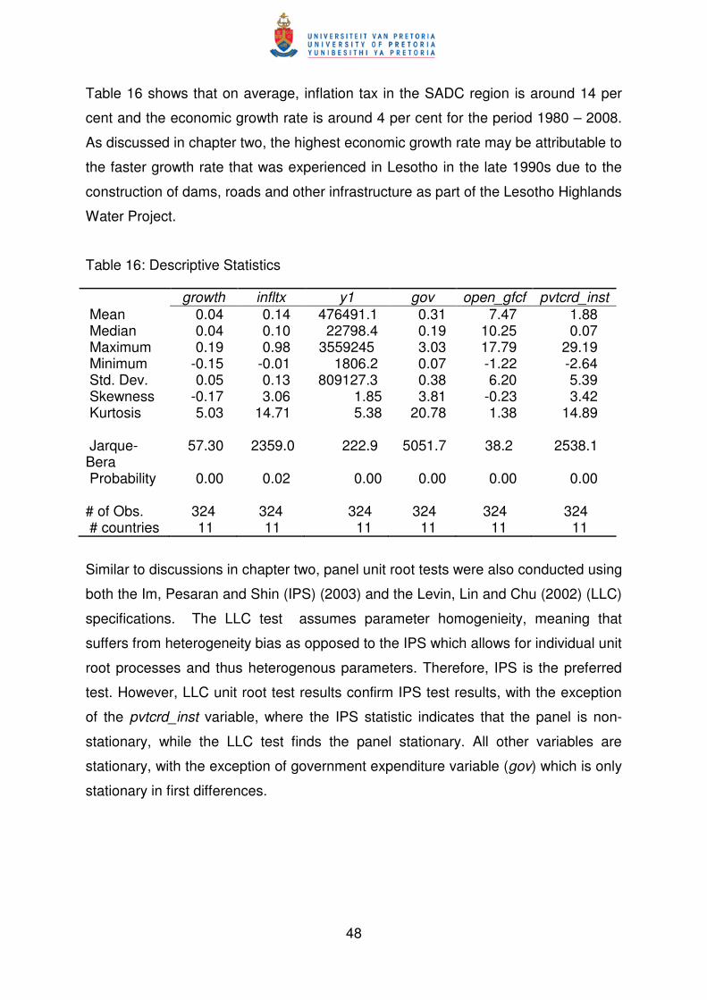
48
Table 16 shows that on average, inflation tax in the SADC region is around 14 per
cent and the economic growth rate is around 4 per cent for the period 1980 – 2008.
As discussed in chapter two, the highest economic growth rate may be attributable to
the faster growth rate that was experienced in Lesotho in the late 1990s due to the
construction of dams, roads and other infrastructure as part of the Lesotho Highlands
Water Project.
Table 16: Descriptive Statistics
Similar to discussions in chapter two, panel unit root tests were also conducted using
both the Im, Pesaran and Shin (IPS) (2003) and the Levin, Lin and Chu (2002) (LLC)
specifications. The LLC test assumes parameter homogenieity, meaning that
suffers from heterogeneity bias as opposed to the IPS which allows for individual unit
root processes and thus heterogenous parameters. Therefore, IPS is the preferred
test. However, LLC unit root test results confirm IPS test results, with the exception
of the pvtcrd_inst variable, where the IPS statistic indicates that the panel is non-
stationary, while the LLC test finds the panel stationary. All other variables are
stationary, with the exception of government expenditure variable (gov) which is only
stationary in first differences.
growth infltx y1 gov open_gfcf pvtcrd_inst
Mean 0.04 0.14 476491.1 0.31 7.47 1.88 Median 0.04 0.10 22798.4 0.19 10.25 0.07 Maximum 0.19 0.98 3559245 3.03 17.79 29.19 Minimum -0.15 -0.01 1806.2 0.07 -1.22 -2.64 Std. Dev. 0.05 0.13 809127.3 0.38 6.20 5.39 Skewness -0.17 3.06 1.85 3.81 -0.23 3.42 Kurtosis 5.03 14.71 5.38 20.78 1.38 14.89
Jarque-Bera
57.30 2359.0 222.9 5051.7 38.2 2538.1
Probability 0.00 0.02 0.00 0.00 0.00 0.00
# of Obs. 324 324 324 324 324 324 # countries 11 11 11 11 11 11

49
Table 17: Panel Unit Root Tests
growth infltx y1 gov open_gfcf pvtcrd_inst
IPS W-stat Levels [P-value]
-4.91*** [0.00]
-3.28*** [0.00]
-93.7*** [0.00]
0.27 [0.61]
-1.62** [0.05]
-0.92 [0.18]
Differences [P-value]
-8.77*** [0.00]
-10.00*** [0.00]
-140.0*** [0.00]
-6.83*** [0.00]
-10.13*** [0.00]
-7.19*** [0.00]
LLC t*-stat Levels [P-value]
-2.89*** [0.00]
-1.98** [0.02]
-64.2*** [0.00]
-0.60 [0.27]
-1.39* [0.08]
-1.66** [0.05]
Differences [P-value]
-8.64*** [0.00]
-9.94*** [0.00]
-201.9*** [0.00]
-6.66*** [0.00]
-10.08*** [0.00]
-6.07*** [0.00]
***/**/* denotes significance at 1%, 5% and 10%, respectively. [p-values] are in brackets. 3.4 EMPIRICAL RESULTS7
3.4.1 Linearity and No Remaining Non-Linearity Results
The linearity tests results are presented in Table 18 and show that the null
hypothesis that the model is linear is rejected for all three tests, implying that the
relationship between inflation and growth in the SADC region is indeed nonlinear.
Table 18: Linearity Tests
Test Statistic P-value
Lagrange Multiplier – Wald (LMW) 26.969 0.003
Lagrange Multiplier – Fischer (LMF) 2.771 0.003
Likelihood Ratio (LR) 28.586 0.000
H0: Linear Model; H1: PSTR Model with at least one threshold.
Table 19 presents the test for no remaining non-linearity after assuming a two-
regime model. The results indicate that the null hypothesis cannot be rejected,
implying that the model has only one threshold or two regimes. Thus implies that in
the SADC region, there is only one threshold level of inflation which separates the
low inflation regime and high inflation regime.
7 Thanks to C.Hurlin for providing the Matlab codes for PSTR estimation.
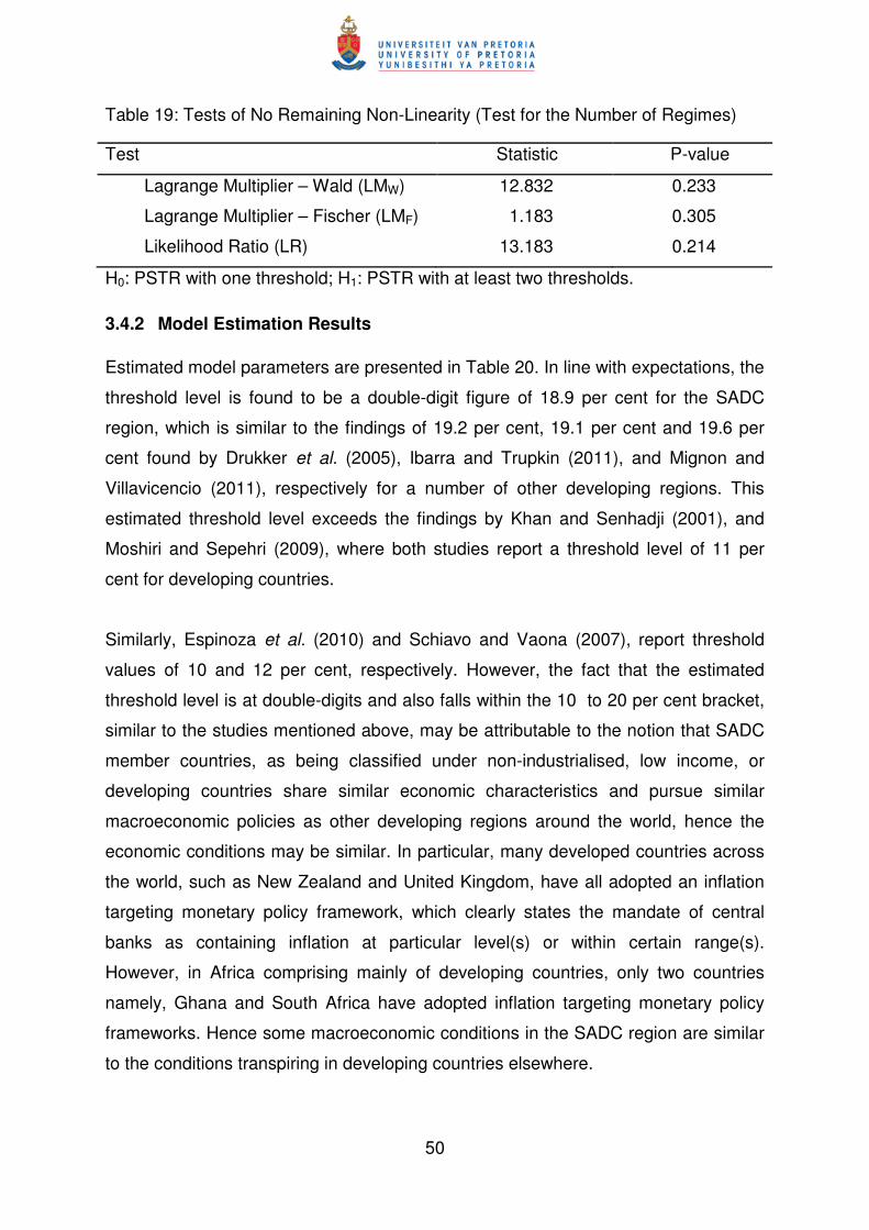
50
Table 19: Tests of No Remaining Non-Linearity (Test for the Number of Regimes)
Test Statistic P-value
Lagrange Multiplier – Wald (LMW) 12.832 0.233
Lagrange Multiplier – Fischer (LMF) 1.183 0.305
Likelihood Ratio (LR) 13.183 0.214
H0: PSTR with one threshold; H1: PSTR with at least two thresholds.
3.4.2 Model Estimation Results
Estimated model parameters are presented in Table 20. In line with expectations, the
threshold level is found to be a double-digit figure of 18.9 per cent for the SADC
region, which is similar to the findings of 19.2 per cent, 19.1 per cent and 19.6 per
cent found by Drukker et al. (2005), Ibarra and Trupkin (2011), and Mignon and
Villavicencio (2011), respectively for a number of other developing regions. This
estimated threshold level exceeds the findings by Khan and Senhadji (2001), and
Moshiri and Sepehri (2009), where both studies report a threshold level of 11 per
cent for developing countries.
Similarly, Espinoza et al. (2010) and Schiavo and Vaona (2007), report threshold
values of 10 and 12 per cent, respectively. However, the fact that the estimated
threshold level is at double-digits and also falls within the 10 to 20 per cent bracket,
similar to the studies mentioned above, may be attributable to the notion that SADC
member countries, as being classified under non-industrialised, low income, or
developing countries share similar economic characteristics and pursue similar
macroeconomic policies as other developing regions around the world, hence the
economic conditions may be similar. In particular, many developed countries across
the world, such as New Zealand and United Kingdom, have all adopted an inflation
targeting monetary policy framework, which clearly states the mandate of central
banks as containing inflation at particular level(s) or within certain range(s).
However, in Africa comprising mainly of developing countries, only two countries
namely, Ghana and South Africa have adopted inflation targeting monetary policy
frameworks. Hence some macroeconomic conditions in the SADC region are similar
to the conditions transpiring in developing countries elsewhere.

51
In the SADC context, the estimated threshold level is also significantly higher than
the 4 per cent level estimated by Leshoro (2012) for South Africa. This is also higher
than the 8 per cent inflation threshold level that is found to be detrimental towards
finance-growth activity for South African economy as estimated by Phiri (2010). This
may be due to the fact that South Africa is the most developed country in the region
and to a certain extent pursues different macroeconomic policies than the other
SADC member countries. In particular, South Africa is the only country in the SADC
region that has formally adopted an inflation targeting monetary policy framework,
meaning that the South African Reserve Bank has a clear mandate of keeping the
inflation rate within the 3 – 6 per cent band. However, the other SADC countries do
not have this clear mandate of keeping inflation rate within a particular target range;
hence these countries may not be able to adequately control the rate of inflation
when it is high. Therefore, given the above reasons, the estimated threshold level of
inflation in the SADC region is at reasonable levels at 18.9 per cent.
Table 20: PSTR Model Estimation
Dependent variable: growth
Variable jk jl
infltx -0.0971 (-0.3935)
-2.2903*** (-2.4380)
y1 -0.0033*** (-1.9928)
-0.0179 (-0.2343)
gov -0.0878 (-0.5110)
-0.8255*** (-2.6839)
open_gfcf 4.4143*** (3.3919)
-0.7444*** (-2.2193)
pvtcrd_inst -0.0079*** (-2.1351)
0.0183*** (1.9891)
Transition Parameters Threshold (c) 18.96 Slope (γ) 77.37 ***/**/* denotes significance at the 1%, 5% and 10% levels, respectively. Values in parentheses are t-statistics based on standard errors corrected for heteroscedasticity.
All the coefficients, with the exception of the coefficient for lagged real GDP (y1) are
statistically significant in the high inflation regime. The signs of coefficients are all
consistent with empirical growth literature. The coefficient for the threshold variable

52
(infltx) is negative for both regimes, but statistically insignificant for the low inflation
rate regime ( 0) and statistically significant for the high inflation rate regime ( ).
This means that the effect of inflation on economic growth is not strong when
inflation rate is below the threshold level of 18.9 per cent but very strong when it is
above the threshold level. These results are similar as those of Ibarra and Trupkin
(2011). The coefficient associated with the lagged real GDP (y1) is negative in both
regimes but statistically significant in the low inflation regime. This may be an
indication of conditional convergence in the SADC region when inflation rates are
below the threshold level. These results are in line with those found by Chen and
Gupta (2006) that there is convergence in the SADC region implying that poorer
countries are able to catch up with the richer countries. Government spending is
found to have a negative and significant impact on economic growth in high inflation
regimes, indicating that higher levels of government spending do not necessarily
lead to higher economic growth. Some level of government spending is necessary to
maintain service levels and thus economic growth in a country. However, when
channelled towards unproductive sectors or when expenditure mainly covers salaries
and other current spending items, it will do little to enhance economic growth in a
country. This is confirmed by the finding of Bittencourt (2012) that bigger
governments tend to be detrimental to economic growth in four Latin American
countries.
An interaction variable between private sector credit and an institutional variable
(pvtcrd_inst) has a negative sign in the low inflation regime and a positive sign in the
high inflation regime. This is unexpected since economic theory postulates that at
low levels of inflation, and when institutions are free and independent from political
pressure, more credit may be extended to the private sector and this may be growth
enhancing (Levine and Renelt, 1992; Temple, 2000). Furthermore, at high inflation
episodes, it is also expected that less credit may be extended to the private sector
and this may hamper investment projects and this actually retards economic growth.
The unexpected signs of the coefficients of this interaction variable in both low and
high inflation rate regimes may be attributable to data quality problems in the region.
The coefficient associated with an interaction of openness and domestic investment
(open_gfcf) is positive and statistically significant in the low inflation regime indicating
that more open economies tend to encourage domestic investment when inflation
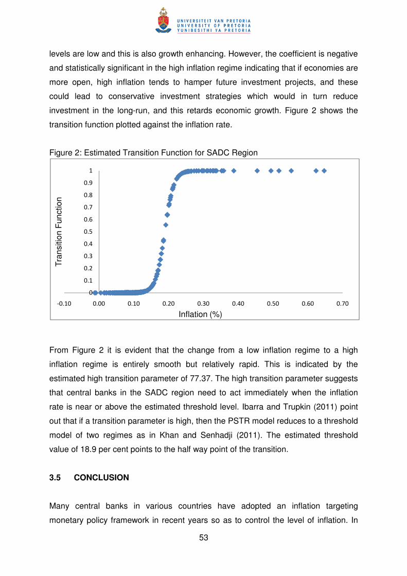
53
levels are low and this is also growth enhancing. However, the coefficient is negative
and statistically significant in the high inflation regime indicating that if economies are
more open, high inflation tends to hamper future investment projects, and these
could lead to conservative investment strategies which would in turn reduce
investment in the long-run, and this retards economic growth. Figure 2 shows the
transition function plotted against the inflation rate.
Figure 2: Estimated Transition Function for SADC Region
From Figure 2 it is evident that the change from a low inflation regime to a high
inflation regime is entirely smooth but relatively rapid. This is indicated by the
estimated high transition parameter of 77.37. The high transition parameter suggests
that central banks in the SADC region need to act immediately when the inflation
rate is near or above the estimated threshold level. Ibarra and Trupkin (2011) point
out that if a transition parameter is high, then the PSTR model reduces to a threshold
model of two regimes as in Khan and Senhadji (2011). The estimated threshold
value of 18.9 per cent points to the half way point of the transition.
3.5 CONCLUSION
Many central banks in various countries have adopted an inflation targeting
monetary policy framework in recent years so as to control the level of inflation. In
0
0.1
0.2
0.3
0.4
0.5
0.6
0.7
0.8
0.9
1
-0.10 0.00 0.10 0.20 0.30 0.40 0.50 0.60 0.70
Tra
nsiti
on F
unct
ion
Inflation (%)

54
doing so, these countries determined the threshold level of inflation exogenously.
This paper, however, revisits the inflation-growth nexus by applying a smooth
transition regression model for panel data (PSTR) which precisely determines the
threshold level of inflation endogenously, hence an important advantage of the PSTR
over the alternative models that have been used to estimate such a relationship. In
particular, the threshold level of inflation in the SADC region is estimated at 18.9 per
cent, above which inflation is detrimental to economic growth. This relatively new
panel data econometric technique also estimates the smoothness of the function that
links one regime (low) to another regime (high). The estimated speed of the
transition is indicative of the fact that central banks in the SADC region need to act
immediately when inflation rate is near or above the estimated threshold level.
In a nutshell, the findings reveal that although the SADC countries are striving
towards common goals and also due to the fact that most of these countries have
managed to reduce their inflation rates to single digits in recent years, these
countries are still divergent in terms of their inflation rates and economic growth
rates. As already indicated, South Africa is the only country within the region which
has formally adopted the inflation targeting monetary policy framework of 3 – 6 per
cent and this is way below the estimated threshold level of 18.9 per cent for the
entire SADC region.
55
CHAPTER FOUR
EFFECTS OF SOUTH AFRICAN INFLATION ON THE SADC REGION:
A PANEL VECTOR AUTOREGRESSION APPROACH
4.1 INTRODUCTION
Macroeconomic stability is viewed as a precondition for increased economic growth.
Therefore, central banks’ main objective throughout the world is the achievement
and maintenance of price stability. Central banks in the SADC region are no
exception, they also formulate policy in an attempt to achieve and maintain low
levels of inflation which is conducive to higher economic growth. Within the SADC
region, South Africa is the largest economy with an abundant supply of natural
resources; well-developed financial, legal, communications, energy, and transport
sectors; a well-developed stock exchange; and modern infrastructure supporting an
efficient distribution of goods to major urban areas throughout the region. South
Africa’s exports of goods and services destined to the SADC region amount to about
9.1 per cent of its total exports, whereas its imports from the region is about 2.8 per
cent of the total (Trade and Industry Policy Secretariat (TIPS), 2012). The
dependence of SADC members on South Africa through trade is further illustrated in
section 4.2.2.
On the one hand, as discussed in chapter one, it may be the case that most
countries in the region import goods and services from South Africa. As discussed in
chapter one, this is likely to happen because South Africa is better equipped in
producing certain products given the state of technology, skills, infrastructure, well-
developed financial systems and good physical infrastructure. Furthermore, South
Africa is within reasonable proximity of many SADC countries; hence these countries
benefit from lower transportation costs amongst other things when trading with South
Africa, rather than countries further away. Therefore, it may be expected that
movements in South African inflation are likely to have economic implications on
inflation and economic growth in the rest of the region.

56
On the contrary, there may be no economic spill-overs into the rest of the SADC
region due to the fact that if goods and services produced in South Africa are
relatively more expensive, through substition these countries may opt to trade with
the other countries rather than South Africa, where they can buy good and services
at lower costs.
Similar to our intentions, Beetsma et al. (2006) investigated the trade spill-overs of
fiscal policy in the European Union (EU) using a Panel Vector Autoregression
(PVAR) technique. They argued that policy changes in one country may have
potentially important effects on other countries specifically in the EU, in their case.
According to their research, the importance of such spill-overs helps to determine the
interdependence of national macroeconomic policies and the interest that
governments might have in each others’ policy stances.
In this paper we follow the work of Beetsma et al. (2006) and use a Panel Vector
Autoregression (PVAR) developed by Holtz-Eakin et al. (1988) to generate impulse-
response functions that we then use to analyse the impact of shocks to the South
African inflation rate on inflation and economic growth rates of the other SADC
countries. The PVAR technique allows for country-specific heterogeneity. Zuniga
(2011) points out that the PVAR model offers advantages over other methods
because it accounts for dynamics in the system and endogeneity problems.
Therefore, the impulse-response functions derived from this technique show the
response of (inflation, openness, investment and economic growth in other SADC
countries) to an orthogonal shock from another variable of interest in the analysis
(South African inflation), hence identifying the response of the impact of one shock at
a time.
Given limited empirical evidence on the impact of inflation shocks in one country on
other countries in the SADC region, we hope to contribute to the literature by
investigating the matter, using an annual dataset for the period 1980-2008.
The rest of the paper is organised as follows: section 4.2 discusses the literature
review and stylized facts of inflation and economic growth in the SADC region.
57
Section 4.3 contains the data description and research methodology. Empirical
results are discussed in section 4.4 while section 4.5 concludes.
4.2 LITERATURE REVIEW AND STYLIZED FACTS
4.2.1 Inflation and Economic Growth Trends in the SADC Region
Table 21 presents summary statistics of the two key variables under investigation.
Comparisons across countries in the region reveal that the average annual real
economic growth rate is 5.2 per cent, while the average annual inflation rate over the
period 2004-2008 is 10.0 per cent. During that period, on average, the highest
inflation rate in the region was recorded in Angola at 20.9 per cent and the lowest in
South Africa at 5.6 per cent. However, when considering the entire 1980-2008
period, real economic growth rate averaged 3.5 per cent and inflation averaged 30.1
per cent, excluding Democratic Republic of Congo (DRC) and Zimbabwe, which are
considered to be outliers during the entire period because of hyperinflation episodes
experienced during the 1980 – 2008 period as evident from Table 21.
The highest growth rate was experienced in Angola and the lowest growth rate in
Zimbabwe, with Zimbabwe being the only country in the region that registered
negative growth rates throughout 2004-2008. This can be attributed to the persistent
economic and humanitarian situation which led to high unemployment and poverty in
that country in recent years (IMF, 2009). The lowest growth rate in Zimbabwe is also
attributable to hyperinflation episodes in recent years. The highest real economic
growth rate in Angola can be attributed to oil production, as new deepwater oilfields
became operational, as well as an increase in output of the kimberlite diamond
mining industry. Manufacturing production also improved due to a better economic
environment and the construction sector benefited from rehabilitation of
infrastructure during 2004-2008. In addition, good weather, increase in the cultivated
area and timely availability of inputs are also highlighted as key factors that led to
higher agricultural production (IMF, 2011). In general, a faster growth rate from a
relative low income level in Angola seems to reflect a typical convergence growth
pattern.

58
Hyperinflation episodes were experienced in Zimbabwe in recent years, hence this
country is regarded as an outlier, and as such may distort the true picture of the
inflationary trends in the region. These episodes of hyperinflation led to the demise
of the local currency (Zimbabwean Dollar) and to complete towards the end of the
investigative period. The local currency virtually disappeared from circulation, and
goods and services are priced in foreign currencies such as the US Dollar and the
South African Rand. As it is well established in theoretical and empirical literature,
high inflation episodes are detrimental to economic growth (Bittencourt, 2012). The
negative growth rates in the country were further attributable to the deterioration in
investors’ perception which ultimately led to the worsening of the business climate in
the country. For the entire region, on average, inflation is considered high at 30.1 per
cent for the entire period of 1980-2008. However, looking at the averages from 2004
to 2008, inflation averaged 10.0 per cent, a lowering in inflation by a considerable
margin.
Table 21: Summary Statistics of Economic Growth and Inflation
% change in real GDP % change in CPI 1980-2008 2004-2008 1980-2008 2004-2008 Angola 5.3 17.8 189.9 20.9 Botswana 7.1 4.1 10.2 9.4 DRC - 4.3 1214.9 14.7 Lesotho 3.4 3.8 10.9 6.9 Madagascar 1.7 5.6 15.7 12.6 Mauritius 2.9 4.6 8.4 7.3 Malawi 2.9 5.6 20.5 11.5 Mozambique 4.1 7.8 18.6 10.1 Namibia8 6.3 5.7 Seychelles 2.9 3.8 4.3 8.9 South Africa 2.5 4.9 10.0 5.6 Swaziland 5.1 2.7 10.9 6.9 Tanzania 4.6 7.3 20.3 5.8 Zambia 2.1 5.8 41.3 13.7 Zimbabwe 1.4 -6.8 971.8 - SADC 3.5 5.2 30.19 10.0 Source: International Monetary Fund (IMF), September 2011
Compared to developed countries, at this double digit rate, inflation in the SADC
region is considered to be relatively high (IMF, 2011). It is widely established that
8 Data not available in earlier years because Namibia gained independence from South Africa in 1990.
9 Excluding Democratic Republic of Congo (DRC) and Zimbabwe.
59
inflation causes many distortions in any economy because it will lead to prices of
consumables to rise, real income of households to decrease and therefore
households’ purchasing power to decline (Ahortor and Adenutsi, 2011). Therefore, in
the long run, inflation reduces economic growth because the economy needs a
certain level of saving to finance investment projects which will in turn stimulate
economic growth. In high inflation episodes, effective functioning of financial
institutions is compromised and this creates a level of uncertainty with regard to
future prices and interest rates, ultimately increasing risk among trading partners and
hence discourage domestic and foreign trade. In addition, inflation makes it difficult
for entrepreneurs to plan their activities since it makes it difficult to effectively predict
demand and average costs of production.
4.2.2 Trade Flows Within the Region
Table 22 depicts the direction of merchandise trade of SADC member states with the
African region and the world at large. The table shows that exports of goods from
countries such as Angola, Mozambique and Zimbabwe as percentage of total
exports destined to Africa, were significantly high, with 98.7 per cent of Angola’s
exports destined to South Africa. However, as percentage of the total exports
destined to the rest of the world, Zimbabwe’s exports to South Africa are the largest
at 32.3 per cent. Shares of exports to South Africa as percentages of exports
destined to the world from other SADC member countries such as Democratic
Republic of Congo, Madagascar, Mauritius, Mozambique, Tanzania and Zambia
were small at single-digits for the year 2008.

60
Table 22: Direction of Merchandise Trade, 2008
Country Exports to SA10 as percentage of Imports from SA as percentage of World Africa World Africa Angola 4.54 98.70 4.64 83.11
DRC 0.17 2.21 28.44 50.88
Madagascar 1.90 33.61 5.68 61.62
Malawi 14.18 48.00 40.79 70.59
Mauritius 3.30 30.70 9.62 73.32
Mozambique 9.23 66.99 27.36 91.25
Seychelles11 - - - -
Tanzania 3.60 17.72 7.34 41.65
Zambia 8.23 30.61 52.46 81.94
Zimbabwe 32.34 55.93 59.64 81.30
Source: International Monetary Fund, 2009
Table 22 further shows that imports from South Africa as percentage of imports from
the entire African region (with the exception of Tanzania) were significantly high at
above 50 percent. This therefore demonstrates that most countries in the SADC
region rely heavily on South Africa, being the largest economy in the region. This
therefore may potentially have some inflationary implications for other countries in
the region since some of the inflation may be imported from South Africa while the
remaining portion of inflation may be domestically generated or imported from other
regions. For instance, merchandise imports of Mozambique from South Africa as
percentage of merchandise imports from the entire African region is 91 per cent,
demonstrating that in the entire African region, this country relies heavily on South
Africa. However, due to data limitations in the region, inflation in these respective
countries is not decomposed into imported and domestically generated categories,
therefore we will assume that given economic theory and the trade flows within the
region, that the possibility of importing inflation through trade linkages do exist,
bearing in mind that South Africa has abundant supply of natural resources; well-
developed financial, legal and communications, energy and transport sectors; and
10
Trade data for South Africa include data from all the Southern African Customs Union (SACU) countries (Botswana, Lesotho, Namibia, South Africa and Swaziland). 11
Data for Seychelles not available.

61
modern infrastructure supporting an efficient distribution of goods and services to
major urban areas throughout the region.
Closer economic linkages among countries imply increased exposure to shocks,
both positive and negative, in partner countries. Hence, developments in one
economy can spillover to other countries through several channels, depending on
the depth of the underlying economic linkages (IMF, 2012). The IMF highlights these
channels as: (i) trade in goods and services; (ii) financial sector interconnections; (iii)
flow of capital; (iv) labour movements and remittance flows. Furthermore, institutional
factors can also play a role: examples may include the Common Monetary Area
(CMA) exchange rate arrangement in Southern Africa, where the three smaller
member countries (Lesotho, Namibia and Swaziland) have an exchange rate peg to
the South African rand. Given the data limitations problem in the SADC region, it is
challenging to quantify the significance of these channels.
Figure 3: Intraregional Trade Linkages
Source: IMF Direction of Trade Statistics (2012) 12
12
The network analysis conducted using a specialized software called NodeXL.

62
Figure 3 depicts intraregional exports larger than 1 per cent of the exporter’s GDP
and these are identified by the arrows connecting the exporter to the importer. The
size of each country’s bubble indicates the number of countries for which it is a
significant export destination and the thickness of each line indicates the size of its
bilateral exports relative to GDP (IMF, 2012). The figure confirms that exports to
South Africa exceed 1 per cent of GDP for 11 SADC countries and the trade linkages
of this magnitude depict the potential for a non-negligible macroeconomic impact on
these 11 SADC countries if economic conditions in South Africa deteriorate.
4.2.3 Literature Review
In the literature, many cross-country studies on inflation and economic growth exist
and results seem consistent. However, there is limited empirical evidence or studies
investigating any impact of a shock in one variable in one country on other variables
in another country or region. Hence to the best of our knowledge, empirical literature
has hardly given any attention to inflation spill-overs from one particular country to
other countries; therefore it is not clear as to what extent the policymakers in the
other SADC countries should be concerned with inflation in South Africa.
Evidence from some of the cross-country studies on inflation-growth relationship are
discussed thoroughly in chapters two and three. These studies include, among
others, De Gregorio (1993) who used a panel of twelve Latin American countries and
found that these two variables are negatively related. Similarly, Fischer (1993) used
a spline technique to analyse the inflation-growth relationship and also found that
high inflation retards growth of output.
Relevant to our research, Beetsma et al. (2006) investigated the trade spill-overs of
fiscal policy among 14 European Union (EU) countries for the period 1965 – 2004
using a Panel Vector Autoregression (PVAR) technique. In particular, the study
estimates the overall effect of domestic fiscal impulses on exports by trading
partners in Europe in two steps. Firstly, they estimated the link between domestic
fiscal impulse and domestic output (referred to as fiscal block), and secondly they
estimated the link between foreign exports and domestic output (referred to as trade
block). By combining these two links, they were able to quantify the overall effect of a

63
domestic fiscal impulse on foreign exports. Therefore, firstly for the fiscal block, their
study used a PVAR model in which responses of output to the fiscal shocks were
traced out. Secondly, for the trade block, they used a panel trade model based on
the gravity approach and then estimated the dynamic responses of bilateral exports
by the EU trading partners to domestic output.
Similar to Beetsma et al. (2006) our focus is to investigate the inflation spill-overs
from South Africa to the rest of the SADC region for the period 1980 – 2008 using a
PVAR model. In particular, our study focuses on the response of a shock to South
African inflation on the inflation and economic growth in the rest of the SADC region.
As discussed in chapter one, an advantage of focusing on SADC countries is that
this helps to limit the potential heterogeneity as these economies share many
similarities and they are striving towards common goals.
Several observations can be highlighted from the information presented above.
Firstly; empirical literature on inflation and economic growth depicts that a negative
and statistically significant relationship between these variables exists. Secondly, the
five-year average inflation rate in the region reported earlier is at double-digits which
is considered to be high relative to developed countries. Thirdly, many countries
within the SADC region rely on imports from South Africa, being considered to be the
largest economy in the region and therefore better equipped to produce certain
products given the state of technology, skills, infrastructure, well-developed financial
systems and good physical infrastructure. Furthermore, South Africa is within
reasonable proximity of many SADC countries; hence these countries benefit from
lower transportation costs, amongst other things, when trading with South Africa,
rather than countries further away. Therefore, based on the literature review and
stylized facts in the region, it may be expected that a positive shock to inflation in
South Africa may potentially lead to a positive response in inflation in the rest of the
SADC region and this may also negatively affect economic growth in the region.

64
4.3 METHODOLOGY AND DATA
4.3.1 The Data
The study uses similar data as discussed in chapters two and three. However, in
addition to the variables used, South African inflation tax rate (SA_infltx) is included
in the estimation of a Panel Vector Autoregression (PVAR) model. We closely follow
the work of Levine and Renelt (1992) and use a set of variables that controls for
other factors associated with economic growth. The growth and inflation variables
used in the analysis are growth in real GDP (growth) and inflation tax (infltx),
respectively. The ratio of gross fixed capital formation to real GDP (gfcf) and the ratio
of imports and exports to GDP (open) are included as control variables.
Contrary to the analysis in the previous two chapters, two SADC member countries,
in particular Angola and Seychelles are now included in the analysis because they
have data available for all variables of interest. Thus, the number of countries
included in the sample now increased from eleven to thirteen13.
4.3.2 Unit Root Testing
Similar to chapter two and three, panel unit root tests were also conducted using
both the Im, Pesaran and Shin (2003) (IPS) and the Levin, Lin and Chu (2002) (LLC)
specifications. As discussed in the previous two chapters, the LLC test assumes a
common � for all cross-sections as apposed to the IPS which assumes individual �� ’s
for cross-sections. Im, Pesaran and Shin (2003) used Monte-Carlo simulation and
compared IPS and LLC, under the assumption of no cross-sectional correlation in
panels and their findings revealed that the IPS test is more powerful than the LLC
test. Therefore, IPS generally would be the preferred test. Furthermore, as
highlighted by Hoang and Mcnown (2006), even though the IPS test requires a
balanced panel, it is the most often unit root test used in practice. Table 23 shows
that all the variables are stationary in levels. According to the LLC test gfcf is only
stationary in first differences, however, we will accept the IPS result of stationarity in
levels in this case, for reasons provided above.
13 Dataset includes: Angola, Botswana, Lesotho, Madagascar, Malawi, Mauritius, Mozambique, Namibia, Seychelles, South Africa, Swaziland, Tanzania and Zambia.

65
Table 23: Panel Unit Root Tests
SA_infltx infltx gfcf open growth
IPS W-stat Levels [P-value]
-7.38*** [0.00]
-5.06*** [0.00]
-2.36*** [0.01]
-4.02*** [0.00]
-7.76*** [0.00]
Differences [P-value]
-7.91*** [0.00]
-6.63*** [0.00]
-10.07*** [0.00]
-9.16*** [0.00]
-9.97*** [0.00]
LLC t*-stat Levels [P-value]
-11.42*** [0.00]
-1.44** [0.07]
-1.01 [0.16]
-1.92*** [0.03]
-7.62*** [0.00]
Differences [P-value]
-11.45*** [0.00]
-3.15*** [0.00]
-9.61*** [0.00]
-4.12*** [0.00]
-12.28*** [0.00]
***/**/* denotes significance at 1%, 5% and 10%, respectively. All variables are in logarithm form. [p-values] are in square brackets. 4.3.3 Panel Vector Autoregression Model
This section describes the model specification being used to assess the response of
inflation and economic growth in other SADC countries due to a shock to South
African inflation The paper adopts the PVAR approach which controls for
heterogeneity and endogeneity in a panel framework. A PVAR combines the VAR
approach, which treats all variables in the system as endogenous, with a panel data
approach, which allows for unobserved heterogeneity14 (Love and Zicchino, 2006).
Suitable models in the panel data context are those that deal with problems such as
endogeneity and heterogeneity. In this paper we adopt the PVAR model developed
by Holtz-Eakin et al. (1988) in investigating the response of inflation and economic
growth among SADC countries following shocks to South African inflation. The main
contribution of this paper is to use impulse-response functions to assess the impact
of a shock to one variable in one country and the response of two specific variables
(inflation and economic growth) in the other countries as a region.
Due to the limited time-span of data for countries in the SADC region, using a single
VAR model will not be appropriate since this compromises the degree of freedom.
A PVAR allows us to overcome this problem. Following the work of Levine and
Renelt (1992), the key variables used in this analysis include; SA_infltx, infltx, open,
14
Thanks to Inessa Love for providing her STATA program for statistical calculations.
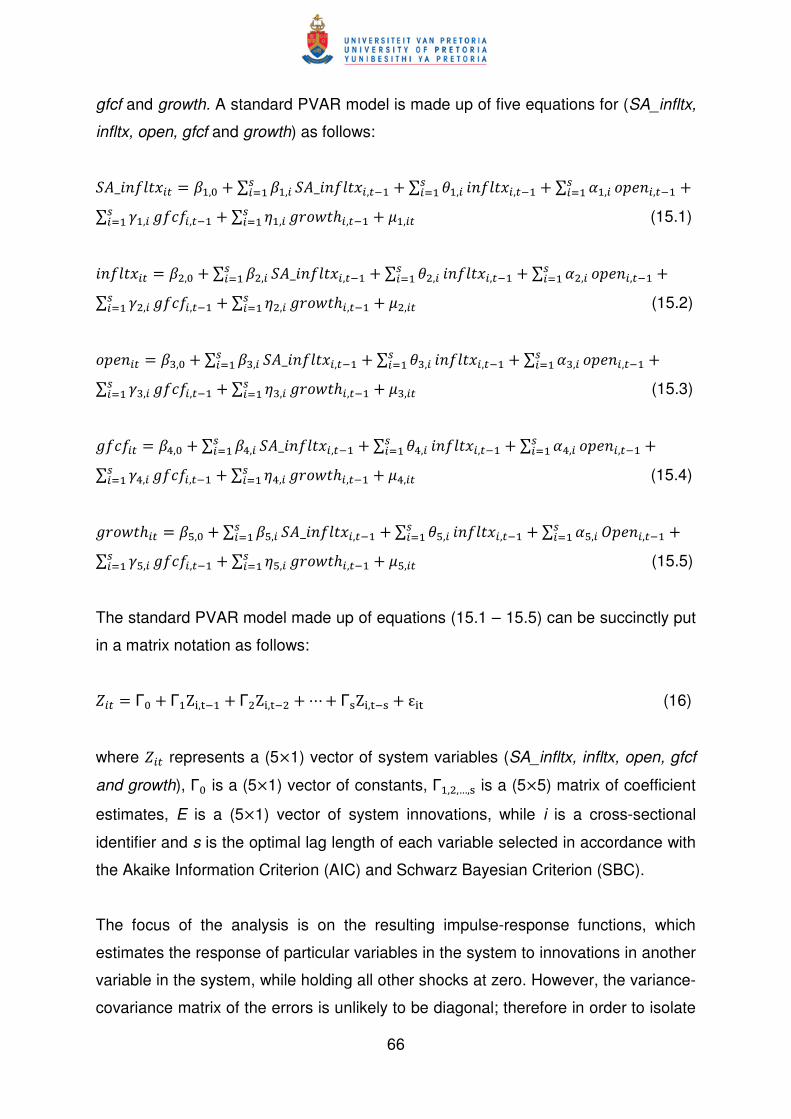
66
gfcf and growth. A standard PVAR model is made up of five equations for (SA_infltx,
infltx, open, gfcf and growth) as follows:
^m_�opq�1�� = ,0 + ∑ ,�r�G ^m_�opq�1�,�� + ∑ f,�
r�G �opq�1�,�� + ∑ �,�
r�G st:o�,�� +
∑ 5,�r�G 9p6p�,�� + ∑ u,�
r�G 9Osv�ℎ�,�� + �,�� (15.1)
�opq�1�� = �,0 + ∑ �,�r�G ^m_�opq�1�,�� + ∑ f�,�
r�G �opq�1�,�� + ∑ ��,�
r�G st:o�,�� +
∑ 5�,�r�G 9p6p�,�� + ∑ u�,�
r�G 9Osv�ℎ�,�� + ��,�� (15.2)
st:o�� = x,0 + ∑ x,�r�G ^m_�opq�1�,�� + ∑ fx,�
r�G �opq�1�,�� + ∑ �x,�
r�G st:o�,�� +
∑ 5x,�r�G 9p6p�,�� + ∑ ux,�
r�G 9Osv�ℎ�,�� + �x,�� (15.3)
9p6p�� = y,0 + ∑ y,�r�G ^m_�opq�1�,�� + ∑ fy,�
r�G �opq�1�,�� + ∑ �y,�
r�G st:o�,�� +
∑ 5y,�r�G 9p6p�,�� + ∑ uy,�
r�G 9Osv�ℎ�,�� + �y,�� (15.4)
9Osv�ℎ�� = z,0 + ∑ z,�r�G ^m_�opq�1�,�� + ∑ fz,�
r�G �opq�1�,�� + ∑ �z,�
r�G {t:o�,�� +
∑ 5z,�r�G 9p6p�,�� + ∑ uz,�
r�G 9Osv�ℎ�,�� + �z,�� (15.5)
The standard PVAR model made up of equations (15.1 – 15.5) can be succinctly put
in a matrix notation as follows:
|�� = Γ0 + ΓZ~,�� + Γ�Z~,��� + ⋯ + Γ�Z~,��� + ε~� (16)
where |�� represents a (5×1) vector of system variables (SA_infltx, infltx, open, gfcf
and growth), Γ0 is a (5×1) vector of constants, Γ,�,…,� is a (5×5) matrix of coefficient
estimates, E is a (5×1) vector of system innovations, while i is a cross-sectional
identifier and s is the optimal lag length of each variable selected in accordance with
the Akaike Information Criterion (AIC) and Schwarz Bayesian Criterion (SBC).
The focus of the analysis is on the resulting impulse-response functions, which
estimates the response of particular variables in the system to innovations in another
variable in the system, while holding all other shocks at zero. However, the variance-
covariance matrix of the errors is unlikely to be diagonal; therefore in order to isolate

67
the shocks to one of the VAR errors it is necessary to decompose the residuals in
such a way that they become orthogonal. In order to do this, PVAR uses a Cholesky
decomposition of the variance-covariance matrix of residuals (Love and Zicchino
2006; Zuniga 2011). The convention is to adopt a particular ordering and allocate
any correlation between the residuals of any two elements to the variable that comes
first in the ordering. Therefore the assumption is that the variables at the beginning
of the ordering contemporaneously affect variables that follow them, as well as with a
lag, while the latter variables affect the former only with a lag.
Our analysis assumes that the contemporaneous causal order runs from South
African inflation (SA_infltx) to inflation in the rest of SADC (infltx) to openness (open)
to investment (gfcf) and to economic growth (growth). The fact that South African
inflation is placed first assumes that South African inflation contemporaneously affect
all variables in rest of the SADC region while the other variables affect South African
inflation only with a lag15.
The PVAR methodology imposes a restriction that there are common dynamics
across cross-sectional units. However, this is likely to be violated in practice;
therefore in order to overcome this, we have to allow for individual heterogeneity by
means of fixed effects, denoted by ℱ~ in the model. Therefore the model in (16)
becomes:
|�� = Γ0 + ΓZ~,�� + ⋯ + Γ�Z~,��� + ℱ~+ε~� (17)
The correlation between fixed effects and lagged regressors is avoided using a
mean-differencing transformation referred to as Helmert transformation (Arellano and
Bover, 1995). This Helmert tranformation removes the forward means and preserves
the orthogonality, and therefore allows for the use of lagged regressors as
instruments. The data series are time-demeaned before the Helmert transformation
is carried out, since the model uses untransformed variables as instruments of the
Helmert transformed variables. As a consequence, these allows for estimation of
coefficients using System Generalized Method of Moments (SYS-GMM). Lagged 15
As a robustness check, different orderings were used but the results remained more or less the same.

68
values of SA_infltx, infltx, open, gfcf and growth are used as instruments. Following
Love and Zicchino (2006), the analysis uses the coefficient bands for the impulse-
response functions as estimated by Monte Carlo simulation, with 1 000 being the
number of repetitions used.
4.4 EMPIRICAL RESULTS
The coefficients of the PVAR estimation, which are used to construct the impulse
response functions (IRFs) are depicted in Table 24 and the impulse-response graphs
are presented in Figure 4. The continuous line represents the point estimate
(response to a shock) of the impulse response and the broken lines represent the 90
per cent confidence bands.
Table 24: Dynamic Results
GMM Estimates Response of: SA_infltx infltx open gfcf Growth
Response to: SA_infltx(t-1) 0.712***
(11.702) -0.028
(-0.343) -0.019
(-0.142) 0.056
(1.217) -0.142*** (-2.081)
Infltx(t-1) -0.006 (-0.294)
0.879*** (12.892)
0.002 (0.030)
-0.004 (-0.183)
-0.051 (-1.621)
open(t-1) -0.019 (-0.976)
0.051 (1.847)
0.863*** (13.976)
-0.012 (-0.616)
0.009 (0.462)
gfcf(t-1) -0.026 (0.473)
-0.041 (-0.464)
-0.021 (-0.125)
0.695*** (10.031)
0.083 (1.198)
growth(t-1) 0.062 (1.189)
-0.048 (-0.455)
0.046 (0.258)
0.181*** (3.680)
0.067 (0.849)
Note: Five-variable VAR model is estimated by GMM, country and time fixed effects are removed prior to estimation. Reported numbers show the coefficients of regressing the column variables on lags of the row variables. Heteroscedasticity adjusted t-statistics are in parentheses. ***/**/* denotes significance at 1%, 5% and 10%, respectively.
Dynamic results and impulse-responses are reported in Table 24 and Figure 4,
respectively. The result of particular interest is the response of economic growth in
the SADC region to a positive shock on South African inflation. Table 24 shows that
a response of economic growth in the rest of the SADC region to a shock on the
South African inflation rate is negative and statistically significant. In particular, a 10

69
per cent increase in South African inflation tax leads to a 1.4 per cent reduction in
the economic growth rate in the rest of the SADC region. Furthermore, the response
of economic growth in the SADC region to a shock in SA inflation tax, is positive but
statistically insignificant for up to about one period as depicted in Figure 4. This
positive response of economic growth in the short-run may be attributable to inflation
expectations, implying that if inflation is expected to be high in the future, then
current consumption may rise and this may have positive implications for economic
growth. However, Figure 4 depicts that in the long-run, economic growth in the
region responds negatively and significantly to a shock in SA inflation tax. The
response remains negative and statistically significant for up to about 12 periods
after the shock, after which it becomes insignificant. This finding is in line with our
expectations since it has been established in Table 22 of section 4.2.2 that
merchandise imports (as a share of merchandise imports from South Africa) of most
countries in the SADC region are mainly from South Africa. Furthermore, response
of inflation in the SADC region to a positive shock on South African inflation is
positive and statistically significant for up to three periods after the shock, after
which the impact becomes statistically insignificant. Although not of particular
interest, responses of openness to trade and investment in the SADC region to a
shock on South African inflation are positive and statistically significant for a short
period of time; implying that South African inflation affect openness and investment
in the rest of the SADC region significantly for a short period of time.
Figure 4 further shows that a one standard deviation shock to the South African
inflation rate results in an immediate and statistically significant increase in itself for
up to about 15 periods after the shock, after which the impact becomes statistically
insignificant.

70
Figure 4: Impulse Responses to South African Inflation Rate Shock (Response to Cholesky One S.D. Innovations ± 1 S.E.)
In order to determine the ability of South African inflation shocks to explain
fluctuations in the inflation and economic growth in the rest of the SADC region, a
standard variance decomposition exercise is conducted and the results are
presented in Table 25.
-0.02
-0.01
0
0.01
0.02
1 3 5 7 9 11 13 15 17 19 21 23 25
Response of open to SA_infltx
-0.01
0
0.01
0.02
0.03
0.04
1 3 5 7 9 11 13 15 17 19 21 23 25
Response of SA_infltx to SA_infltx
-0.006
-0.004
-0.002
0
0.002
0.004
1 3 5 7 9 11 13 15 17 19 21 23 25
Response of growth to SA_infltx
-0.005
0
0.005
0.01
0.015
1 3 5 7 9 11 13 15 17 19 21 23 25
Response of infltx to SA_infltx
-0.002
0
0.002
0.004
0.006
1 3 5 7 9 11 13 15 17 19 21 23 25
Response of gfcf toSA_infltx

71
Table 25: Shocks and Variance Decomposition
Forecast Horizon
(Years)
Fraction of Variance That Can Be Attributed to Shocks to:
SA_infltx infltx open gfcf growth
A. SA infltx 10 20
0.9413 0.9219
0.0095 0.0132
0.0369 0.0524
0.0047 0.0051
0.0075 0.0074
B. Infltx 10 20
0.0004 0.0004
0.9023 0.8386
0.0915 0.1542
0.0039 0.0049
0.0019 0.0019
C. open 10 20
0.0015 0.0015
0.0151 0.0152
0.9829 0.9828
0.0002 0.0003
0.0003 0.0003
D. gfcf 10 20
0.0144 0.0143
0.1795 0.0242
0.0826 0.0920
0.8242 0.8096
0.0608 0.0599
E. growth 10 20
0.0263 0.0266
0.0132 0.0356
0.0206 0.0213
0.0072 0.0073
0.9127 0.9096
Table 25 reports the results of variance decomposition and the estimates represent
the percentage of variation in the row variable explained by the column variable. The
first column shows the fraction of the 10 and 20 period-ahead forecast error that can
be explained by South African inflation shocks. South African inflation has less
impact on inflation in the entire SADC region, accounting for about 0.04 per cent of
its short-run and long-run variance. The table further illustrates that South African
inflation also has a marginal impact on openness and investment in the rest of the
region, accounting for about 0.15 per cent and 1.44 per cent, respectively of its
short-run and long-run variance. Similarly, the impact on economic growth in the rest
of the region is also small at 2.6 per cent. However, the decomposition of variance of
South African inflation indicates that this variable is most likely explained by its own
variations at 94 per cent and 92 per cent of its short-run and long-run variance,
respectively.

72
4.5 CONCLUSION
Within the SADC region, South Africa is the largest economy. It has an abundant
supply of natural resources; well-developed financial, legal, communications, energy,
and transport sectors; a well-developed stock exchange; and modern infrastructure
supporting an efficient distribution of goods to major urban areas throughout the
region. Therefore, it can be expected that any shocks in the South African economy
may have potential spill-over effects onto the rest of the SADC region.
The impulse response results derived from estimating a five-variable PVAR
demonstrates that shocks to South Africa inflation rate have statistically significant
impact on inflation in the rest of the SADC region. South African inflation may be
transmitted through into the rest of the SADC region because these countries trade
significantly with South Africa. The results also show that South African Inflation has
a negative and statistically significant impact on economic growth in the SADC
region for up to 12 years, after which, the impact becomes statistically insignificant.

73
CHAPTER FIVE
CONCLUSION
The aim of the thesis is to examine the relationship between inflation and economic
growth focusing on the Southern African Development Community (SADC) as a case
study. Motivation for the analysis emanates not only due to the lack of studies
analysing inflation and economic growth in the SADC region, but more generally,
because of the fact that this relationship may differ from the one that exists in
developed countries due to the level of economic development and prudent
macroeconomic policies that are being practised in developed regions (Sarel, 1996).
Furthermore, inflation is viewed to be one of the basic indicators of macroeconomic
stability, hence it is an indicator of the ability of the government to manage the
economy. High levels of inflation may be indicative of a lack of sound governance by
the monetary authority of a country. An extensive body of literature suggests that
inflation and economic growth are negatively related (De Gregorio, 1993 and
Fischer, 1993).
The thesis also addresses the issue of the existence of a threshold level of inflation
below which inflation may not have an impact, or a positive impact, on economic
growth or above which inflation may be detrimental to economic growth. Therefore,
the threshold level(s) vary substantially when analysing developed and developing
countries respectively, implying that the level of development in countries under
consideration may be an important factor. On the one hand, Ibarra and Trupkin
(2011), and Mignon and Villavicencion (2011) found a threshold level of 19.1 per
cent and 19.6 per cent for developing countries, respectively. On the other hand,
Khan and Senhadji (2001) estimated a threshold level to be between 1-3 per cent
and 11-12 per cent for industrial countries and developing countries, respectively.
The thesis further assesses the effects of a shock to inflation in South Africa, being
the largest economy in the region, on inflation and economic growth in the rest of the
SADC region.
First, different conventional panel data methodologies; Fixed Effects (FE), Difference
Generalised Method of Moments (DIF-GMM), System Generalised Method of
Moments (SYS-GMM), and Seemingly Unrelated Regression (SUR) estimators are

74
used in order to examine the relationship between inflation and economic growth in
the region. The main finding is that all four models show that there is an inverse
relationship between the two variables of interest. This is because inflation in the
economy will cause production to slow down since products are produced at higher
prices. Inflation also increases the welfare cost to society, reduces international
competitiveness of a country because of more expensive exports, thereby reducing
economic growth in the long-run (Khan and Senhadji, 2001). These findings are
similar to those of Fischer (1993) and De Gregorio (1993). A measure of the size of
the government was found to have a negative and statistically significant impact on
economic growth. The negative sign is indicative of a notion that high government
spending may not necessarily fuel economic growth, in fact it may retard economic
growth, if such spending is made on non-productive sectors of the economy
(Bittencourt, 2012). The interaction variable between openness and domestic
investment depicts a strong positive impact on economic growth. This demonstrates
that more open economies tend to encourage higher domestic investment and
therefore leads to faster economic growth. However, the findings do not depict any
evidence that financial deepness coupled with free and independent institutions
encourages economic growth.
Second, Panel Smooth Transition Regression (PSTR) methodology is applied to
endogenously estimate the threshold level of inflation in the SADC region. The
smoothness of the transition from a low to high inflation regime is also estimated.
The findings reveal that the threshold level of inflation in the region is 18.9 per cent
for the SADC region, which is to some extent similar to the findings of 19.2 per cent,
19.1 per cent and 19.6 per cent found by Drukker et al. (2005), Ibarra and Trupkin
(2011) and, Mignon and Villavincencio (2011), respectively for a number of other
developing countries. The results also show that the impact of inflation on economic
growth is not statistically significant for the low inflation regime, but only statistically
significant for the high inflation regime; meaning that inflation only affects growth
negatively if it is above 18.9 per cent. Evidence of convergence is also found in the
region when inflation is below the threshold level. Government consumption
spending is found to have a negative impact on economic growth in high inflation
regimes, indicating that high government spending does not necessarily lead to
higher economic growth, since the spending may be channelled towards

75
unproductive sectors. The findings reveal that although the SADC countries are
striving towards a common goal and although most of these countries have
managed to reduce their inflation rates to single digits in recent years, these
countries are still divergent in terms of their inflation and economic growth rates.
Third, impulse-response functions derived from the Panel Vector Autoregression
(PVAR) model are used to assess the effects of South African inflation on inflation
and economic growth in the rest of the region. The findings reveal that since South
Africa is the largest economy in the region, and hence trades significantly with the
other SADC countries, it has significant implications for inflation, openness,
investment and growth in the rest of the SADC region. However, it should be noted
that there may be other factors emanating from elsewhere, not just from South
Africa, that may have an impact or effect on inflation, openness, investment and
economic growth in the rest of the SADC region. Furthermore, some inflationary
pressures may also be domestically generated in respective countries and not
necessarily imported from South Africa.
The thesis contributes to the body of knowledge in the field of economics by
enhancing the understanding of the inflation-growth nexus in the SADC region in
ways that have not been done before. To the best of our knowledge, this is the only
study that looks into the inflation-growth relationship in the context of SADC. In
addition, the thesis uses different panel data econometric techniques to deal with
problems which are normally encountered when using cross-country data such as
endogeneity, heterogeneity and cross-sectional dependence. Hence problems
encountered by previous research in this field are adequately addressed. High
inflation episodes are known to contribute to macroeconomic instability (defined as
high inflation rates) therefore policy makers find it important to understand the kind of
the relationship that exists between inflation and economic growth in order to ensure
the development and implementation of sound macroeconomic policies. Therefore,
the issue of inflation and economic growth has become the issue of considerable
interest among many economists in recent years. Discussions on inflation and
economic growth are usually included in the Agendas of many economic forums
around the world including International Monetary Fund (IMF) and World Bank
Annual meetings.

76
For future research, the inflation-growth nexus can be investigated in the context of
smaller regional blocs in Southern Africa, such as Common Monetary Area (CMA)
and Southern African Customs Union (SACU). The CMA is a monetary and
exchange rate arrangement between Lesotho, Namibia, South Africa and Swaziland.
This arrangement resembles an asymmetric monetary union, with the bigger country
– South Africa – being responsible for monetary policy formulation and
implementation (Alweendo, 2000). Therefore, the inflation-targeting monetary policy
framework adopted by South Africa is in practice a de facto monetary policy
framework for the CMA as a whole. Hence, South Africa may also be expected to
have economic spill-over effects into the rest of the CMA. It may also be interesting
to investigate this relationship in the SACU context. The SACU agreement involves
Lesotho, Botswana, Namibia, South Africa and Swaziland. The goods grown,
produced or manufactured in the SACU and imports from one member state to
another are free of customs duties and quantitative restrictions. However, these
countries have common restrictions towards imports from the rest of the world.
SACU also has free trade arrangements (FTA) with many trading blocs and
countries around the world. Member countries are also allowed to have bi-lateral
trade arrangements with other blocs around the world. Therefore, since these
countries have common external restrictions, it would be interesting to investigate
how this would affect the inflationary pressures and hence economic growth in such
a region. Furthermore, for future research, the study can also be expanded to
incorporate the entire Sub-Saharan Africa (SSA) region and this would allow for
cross-regional comparison.

77
REFERENCES
AHORTOR, C,. and ADENUTSI, D. (2011). Inflation, Capital Accumulation and Economic Growth in Import-Dependent Developing Countries. Munich Personal RePEc Archieve. Working Paper No. 29353. ALEXANDER, W. (1997). Inflation and Economic Growth: Evidence from a Growth Equation. Applied Economics , 29, 233-238. ALWEENDO, T. (2000). The Challenges of Monetary Policy for Namibia within the Common Monetary Arrangement. Welcome Address by the Governor, Mr. T.K. Alweendo of Bank of Namibia, 2nd Annual Bankers Conference, October, Windhoek, Namibia ARELLANO, M., and BOND, S. (1991). Some Tests of Specification for Panel Data: Monte Carlo Evidence and an Application to Employment Equations. Review of Economic Studies , 58, 277-297. ARELLANO, M., and BOVER, O. (1995). Another Look at Instrumental Variables Estimation of Error Components Models. Journal of Econometrics , 68, 29-51. BALTAGI, B. (2008). Econometric Analysis of Panel Data (4 ed.). John Wiley and Sons, Ltd. BARRO, R. (1996). Inflation and Economic Growth. Federal Reserve Bank of St.Louis Review , 78, 153-69. BARRO, R. (1998). Determinants of Economic Growth: A Cross-Country Empirical Study. Cambridge, Massachusetts. The MIT Press.
BEETSMA, R., GIULIODORI, M., and KLAASSEN, F. (2006). Spill-overs in the European Union. Economic Policy, October, 639 - 687.
BITTENCOURT, M. (2012). Inflation and Economic Growth in Latin America: Some Panel Time-Series Evidence. Economic Modelling, 29, 333 - 340.
_______________. (2012). Financial Development and Economic Growth in Latin America: Is Schumpeter Right? Journal of Policy Modeling, 34(22), 341 - 355.
BLUNDELL, R., and BOND, S. (1998). Initial Conditions and Moment Restrictions in Dynamic Panel Data Models. Journal of Econometrics , 87, 115-143. BOND, S., LEBLEBICIOĞLU, A., and SCHIANTARELLI, F. (2010). Capital Accumulation and Growth: A New Look At The Empirical Evidence. Journal of
Applied Econometrics, 25, 1073 - 1099.
BREUSCH, T., and PAGAN, A. (1980). The Lagrange Multiplier Test and its Application to Model Specification in Econometrcs. Review of Economic Studies , 47, 239 - 253.

78
BRUNO, M. (1995). Does Inflation Really Lower Growth? Finance and Development. September, 35-38. BRUNO, M., and EASTERLY, W. (1998). Inflation Crises and Long-run Growth. Journal of Monetary Economics , 41, 3-26.
BURDEKIN, R., DENZAU, A., KEIL M., SITTHIYOT, T., and WILLETT, T. (2004). When Does Inflation Hurt Economic Growth? Different Non-linearities for Different Economies. Journal of Macroeconomics , 26, 519-532. CHANG, T.,and CHIANG, G. (2011). Regime-Switching Effects of Debt on Real GDP Per Capita: The Case of Latin America and Caribbean Countries. Economic Modelling , 28, 2404-2408. CHEN, P.-P., and GUPTA, R. (2006). An Investigation of Openness and Economic Growth in Using Panel Estimation. Department of Economics Working Paper Series .
CHOW, G. (1960). Test of Equality Between Sets of Coefficients in Two Linear Regressions. Econometrica, 28, 591-605. COLLETAZ, G., and HURLIN, C. (2006). Threshold Effect in the Public Capital Productivity: An International Panel Smooth Transition Approach. University of Orleans Working Paper .Growth, Investment and Real Rates. carneige-Rochester Conference Series on Public Policy , 39, 95-140. CUKIERMAN, A., KALAITZIDAKIS, P., SUMMERS, L., and WEBB, S. (1993). Central Bank Independece, Growth, Investment and Real Rates. Carneige-Rochester Conference Series on Public Policy , 39, 95-140. DE GREGORIO, J. (1993). Inflation, Taxation and Long-run Growth. Journal of Monetary Economics , 31, 271-298. DIRECTIONS OF TRADE STATISTICS YEARBOOK (December, 2009). International Monetary Fund. Washington D.C. DRUKKER D., GOMIS-PORQUERAS, P., and HERNANDEZ-VERME, P. (2005). Threshold Effects in the Relationship Between Inflation and Growth: A New Panel-Data Approach. 11th International Conference on Panel Data. DURLAUF, S., JOHNSON, P., TEMPLE, J. (2005). Handbook of Economic Growth- Growth Econometrics Chapter 8, 1, Part A, 555 - 677. EGGOH, J. (2010). Financial Development and Growth: A Panel Smooth Regression Approach. Journal of Economic Development, 35 (1), 15-33. _______. (2011). Inflation Effects on Finance-Growth Link: A Panel Smooth Threshold Approach. International Economic Journal. D01:10.1080/10168737.2011.631025

79
ERBAYKAL, E., & OKUYAN, A. (2008). Does Inflation Depress Economic Growth? Evidence from Turkey. International Research Journal of Finance and Economics (17). ESPINOZA, R., LEON, H., and PRASAD, A. (2010). Estimating the Inflation-Growth Nexus - A Smooth Transition Model. IMF Working Paper WP/10/76 . FISCHER, S. (1993). The Role of Macroeconomic Factors in Growth. Journal of Monetary Economics , 32, 485-512. FURUOKA, F., MANSUR, K., & MUNIR, Q. (2009). Inflation and Economic Growth in Malaysia: A Threshold Regression Approach. ASEAN Economic Bulletin , 26 (2), 180-93. GHOSH, A., and PHILLIPS, S. (1998). Warning: Inflation may be harmful to your Growth. IMF Staff Papers , 45 (4), 672-710. GONZÁLEZ, A., TERÄSVIRTA, T., and VAN DIJK, D. (2005). Panel Smooth Transition Regression Models. Working Paper Series in Economics and Finance. Stockholm Sschool of Economics , 604. GRANGER, C., and TERÄSVIRTA, T. (1993). Modelling Non-linear Economic Relationships. Oxford. Oxford University Press . HANSEN, B. (1982). Large Sample Properties of Generalized Method of Moments Estimators. Econometrica , 50, 1029-1054. _________. (1996). Inference When a Nuisance Parameter is not Identified Under the Null Hypothesis. Journal of Econometrics , 64, 413-430. _________. (1999). Threshold Effects in Non-Dynamic Panels: Estimating, Testing and Inference. Journal of Econometrics , 93, 345-368. HAUSMAN, J. (1978). SpecificationTests in Econometrics. Econometrica , 46, 1251 - 1271. HEINTZ, J., and NDIKUMANA, L. (2011). Is there a Case for Formal Inflation Targeting in Sub-Saharan Africa? Journal of African Economies. 20(2), 67-103. HINELINE, D. (2007). Examining the robustness of inflation and growth relationship. Southern Eeconomic Journal , 73 (4), 1020-1037. HOANG, N., and MCNOWN, R. (2006). Panel Data Unit Roots Tests Using Various Estimation Methods. Working Paper. Department of Economics. University of Colorado at Boulder. HOLTZ-EAKIN, D., NEWEY, W., and ROSEN, H. (1988). Estimating Vector Autoregression with Panel Data. Econometrica , 56 (6), 1371-1395.

80
HOYOS, R., and SARAFIDIS, V. (2009). Testing for Cross-sectional Dependence in Panel Data Models. The Stata Journal , 6 (4), 482-496. IBARRA, R., and TRUPKIN, D. (2011). The Relationship Between Inflation and Growth: A Panel Smooth Transition Regression Approach. Research Network and Research Centers Program of Banco Central del Uruguay (Working Paper). IM, K., PESARAN, M., and SHIN, Y. (2003). Testing for Unit Roots in Heterogeneous Panels, Journal of Econometrics., 115, 53 - 74. JANSEN, E., and TERÄSVIRTA, T. (1996). Testing Parameter Constancy and Super Exogeneity in Econometric Equations. Oxford Bulletin of Economics and Statistics , 58, 735-763. KAN, E., and OMAY, T. (2010). Re-examining the threshold effects in the inflation-growth nexus with cross-sectionally dependent non-linear panel: evidence from six industrialised economies. Economic Modelling , 27, 996-1005. KHAN, M., and SENHADJI, S. (2001). Threshold Effects in the relationship between inflation and growth. IMF Staff Papers , 48 (1). LEE, C., and WONG, Y. (2005). Inflationary Threshold Effects in the Relationship between Financial Devopment and Economic Growth: Evidence from Taiwan and Japan. Journal of Economic Development , 30 (1), 49-69. LESHORO, T. 2012. Estimating the Inflation Threshold for South Africa. University of South Africa Working Paper 285. LEVIN, A., LIN, C.-F., and CHU, C.-S. (2002). Unit Root Tests in Panel Data: Asymptotic and Finite-Sample Properties. Journal of Econometrics , 108 (1), 1-24. LEVINE, R., RENELT, D., 1992. A Sensitivity Analysis of Cross-Country Growth Regressions. The American Economic Review 82 (4), 942-963. LI, M. (2006). Inflation and Economic Growth: Threshold Effects and Transmission Mechanisms. University of Alberta Working Papers , 2006. LIGTHELM, A. (2006). Structure and Growth of Intra-SADC Trade. Bureau of Market
Research. University of South Africa. No. 358. LOVE, I., and ZICCHINO, L. (2006). Financial Development and Dynamic Investment Behaviour: Evidence From Panel Vector Autoregression. Quarterly Review of Economics and Finance , 46, 190-210. LUUKKONEN, R., SAIKKONEN, P., and TERÄSVIRTA, T. (1988). Testing Linearity Against Smooth Transition Autoregressive Models. Biometrika , 75, 491-499. MALLICK, H. (2008). Inflation and Growth Dynamics: The Indian Experience. Journal of Economic Policy Reform , 11 (3), 163-172.

81
MIGNON, V., and VILLAVICENCIO, A. (2011). On the Impact of Inflation on Output Growth: Does The Level of Inflation Matter? Journal of Macroeconomics , 33, 455-464. MOSHIRI, S., and SEPEHRI. (2004). Inflation-Growth Profiles Across Countries: Evidence from Developing and Developed Countries. International Review of Applied Economics , 18 (2), 191-207. MUBARIK, A. (2005). Inflation and Growth: An Estimate of the Threshold Level of Inflation in Pakistan. State Bank of Pakistan-Research Bulletin , 1 (1), 35-44. NEL, L. (2004). The Prospect of a Monetary Union between SADC and SACU: A Critical Analysis. Masters of Commerce Dissertation. University of Pretoria. OOSTHUIZEN, G. (2006). The Southern African Development Community: The Organisation, Its Policies and Prospects. Institute of Global Dialogue. South Africa. PHIRI, A. (2010). At What Level is Inflation Least Detrimental Towards Finance-Growth Activity in South Africa? Journal of Sustainable Development in Africa, 12, 6.
POLLIN, R., and ZHU, A. (2006). Inflation and Economic Growth: A Cross-Country Non-linear Analysis. Journal of Post Keynesian Economics , 28 (4), 593. RAPHAEL, E., HYGINUS, L., and ANANTHAKRISHNAN, P. (2010). Estimating the Inflation-Growth Nexus - A Smooth Transition Model. IMF Working paper. WP/10/76. International Monetary Fund .
REGIONAL ECONOMIC OUTLOOK - SUB SAHARAN AFRICA (OCTOBER, 2012). International Monetary Fund. Washington D.C. ROODMAN, D. (2009). How to Do xtabond2: An Introduction to Difference and System GMM in Stata. Stata Journal , 9 (1). ____________. (2009). Practioners' Corner: A Note on the Theme of Too Many Instruments. Oxford Bulletin of Economics and Statistics , 71 (1).
ROUBINI, N., and SALA-I-MARTIN, X. (1995), A Growth Model of Inflation, Tax Evasion and Financial Repression. Journal of Monetary Economics, 35, 275 - 301. SADC. (2011). Retrieved from SADC Website: www.sadc.int. SAREL, M. (1996). Non-Linear Effects of Inflation on Economic Growth. IMF Staff Papers , 43 (1), 199-215. SARGAN, J. (1958). The Estimation of Economic Relationship using Instrumental Variables. Econometrica , 26, 393-415. SCHIAVO, S., and VAONA, A. (2007). Nonparametric and Semiparametric Evidence on the Long-run Effects of Inflation on Growth. Economics Letters , 94, 452-458.

82
SEPEHRI, A., and MOSHIRI, S. (2004). Inflation-Growth Profiles Across Countries: Evidence from Developing and Developed Countries. International Review of Applied Economics , 18, 191-207.
SWAMY, P. (1970). Efficient Inference in a Random Coefficient Regression Model. Econometrica , 38 (2), 311-323. TEMPLE, J. (2000). Inflation and Growth: Short Stories and Tall. Journal of Economic Surveys , 14 (4). TERÄSVIRTA, T. (1994). Specification Estimation and Evaluation of Smooth Transition Autoregressive Models. Journal of American Statistical Association , 89, 208-218.
TOBIN, J. (1972). Inflation and Unemployment. American Economic Review, 62, 1-18. TRADE AND INDUSTRY POLICY SECRETARIAT (TIPS). Database. February 2012. Johannesburg. South Africa. WACZIARG, R., and WELCH, K. (2008). Trade Liberalization and Growth: New Evidence. World Bank Economic Review, 22, 2. WORLD ECONOMIC OUTLOOK (October, 2011). International Monetary Fund. Washington D.C. ZELLNER, A. (1962). An Efficient Method of Estimating Seemingly Unrelated Regressions and Tests of Aggregation Bias. Journal of American Statistical Association , 500-509. ZUNIGA, M. (2011). On the Path to Economic Growth, Do Remittances Help? Evidence from Panel VARs. The Developing Economies. 49 (2), 171-202.