Influence of Macroeconomic Variables on Exchange Rates - …joebm.com/papers/194-W10044.pdf · · 2014-01-03Exchange rates play a significant role in ... We used bootstrapping technique

Abstract—Exchange rates play a significant role in

international trade not only in fixing the prices but also in

determining the nature of hedging to be arranged to avoid

exchange rate risks. In this article we used three countries

yearly exchange rates with their macroeconomic variables such

as relative interest rates etc to study the impact they exert on

exchange rates. We used bootstrapping technique to increase

the sample size to run regression to study the effect. The

previous researchers used general regression models to

establish relationships but we have applied multi models by

linking complementary variables to identify the best model.

Our results showed that model B was robust which indicated all

macroeconomic variables significantly influenced the exchange

rates except employment and budget deficit. Most of the

macroeconomic variables showed opposite sign contrary to the

expectations and we concluded that the psychological factors

like investor confidence dominate over economic variables in

deciding exchange rate fluctuation.

Index Terms—Bootstrapping, exchange rate, hedging,

inflation rate, interest rate.

I. INTRODUCTION

Exchange rate fluctuation or stability is the major concern

which determines the quantum and direction of foreign trade

and commerce [1].

Exchange rate (XR) fluctuation and its effect on the

volume of international trade is an important subject for

empirical investigation, after the adoption of floating

exchange rate 1973. Exchange rate fluctuation is defined as

the risk associated with unpredicted movements in exchange

rate. Macroeconomic variables such as interest rate, inflation

rate, the balance of payments, tax rate etc influence the XR

randomly. These macroeconomic variables are unstable and

volatile depending on the state of the economy prevailing in

their countries [2]. In addition increased cross border

currency flows due to foreign direct investment and service

like banking, insurance, education, tourism cause the

exchange rate fluctuate randomly. Advent of on line trading,

currency speculation is rampant and cause exchange rates to

fluctuate.

The role of XR in imports and exports is crucial. In

addition a country’s overall economic performance is

reflected by XR [3]. Macroeconomic variables prevail in

home and host countries determine the exchange rate

equilibrium in long-run. Short-run fluctuations are temporary

caused by arrival of economic information from time to time

from home and host countries. Increasingly the incoming and

outgoing foreign direct investments create massive capital

Manuscript received September 16, 2013; revised November 20, 2013.

The authors are with the Graduate School of Business University Tun

Abdul Razak, Malysia (e-mail: [email protected],

[email protected]).

flows and directly influence XR. Even counties which follow

floating rate and non intervention policy sometimes feel

uncomfortable when the XR become volatile. Fluctuations of

XR have significant impact on countries’ import and export

behavior [4] and ultimately culminate in current account

balance and foreign currency reserves held by the central

banks.

Recent global economic turmoil affected significantly

different systems of economy. Exchange rate is not an

exception as it is closely aligned to macroeconomic variables.

Country with an appreciating home currency will experience

its goods become more expensive in international market

which may affect the exports and at the same time imports

become inexpensive [5]. This is a double blow to the home

country which will rapidly affect the BOP. In contrast if

domestic currency depreciates, imports will be expensive in

the domestic market and local companies would find their

goods more attractive due to lower prices in international

markets.

XR not only influences imports, exports and direct

investments but also several service sectors like banking,

insurance, education, tourism. In addition consolidation of

financial statements of foreign subsidiaries with domestic

parent also becomes cumbersome. While translating foreign

subsidiary financial statements in home currency the

exchange rates paly the spoil shot. XRs extensively deflate or

inflate profit and asset values of the foreign subsidiary as the

opening and closing XRs substantially differ, thereby

creating a situation where mandatory manipulation is

permissible which ultimately results in wrong reporting. The

pertinent example is Enron.

The Asian economic crisis caused by currency

depreciation in the late 90s and the recent sub-prime loan

crisis of 2008 eroded not only market capitalization of

companies but also severely strained the national economies

[6]. To bailout the distressed companies the governments

used tax payers’ money in the hope of recovering the amount

spent in future once these organizations stabilize. To bridge

the gap, the governments increase the tax rates and also bring

in new taxes such as service tax and surcharges. These

measures bring in some disparity and imbalance in economic

alignment which affect the exchange rates ultimately. This

prompted to investigate the role of relative interest rates (IR),

inflation rates (IFR) and a host of economic variables of

home and host countries in determining the XRs.

This paper is organized as follows: section one introduces

the topic and discuses the importance of XRs, section two

explains the relationship between exchange rate and

important macroeconomic variables. Section three explains

the methodology and data while section four discusses the

results obtained by analysis. Section five concludes the

paper.

Influence of Macroeconomic Variables on Exchange Rates

Ravindran Ramasamy and Soroush Karimi Abar

DOI: 10.7763/JOEBM.2015.V3.194 276

Journal of Economics, Business and Management, Vol. 3, No. 2, February 2015

II. XR AND MACROECONOMIC VARIABLES

Home and host countries’ interest rates play a significant

role in exchange rate determination. The interest rates are

adjusted quarterly by the central bank as part economic

management. If inflationary pressure prevails in the country,

the central bank will increase base lending rate to curtail the

money supply among the people and companies to make

borrowings expensive. Assuming the host country does not

adjust the interest rate, this increase in one country creates

inequilibrium in demand and supply for money and in turn it

causes the exchange rate to move to equilibrium. If not

arbitrage profits are possible in borrowing and investing

between countries. If both home and host countries

simultaneously increase or decrease the interest rates

matching, then there will be no effect on exchange rate due to

interest rate. The relative interest rate is an important factor

which influences XRs.

This increase in the general price level of goods and

services in an economy is inflation, measured by

the Consumer Price Index. In other words price raise is

inflation and the same is depreciation of home currency in

international parlance. When the home inflation rate is high

the home currency will lose value and vice versa. Inflation

and exchange rate are negatively correlated. A country with

lower inflation exhibits a rising currency value and vice versa.

Exchange rate hike indicates the loss of home currency value.

The balance of payments (BOP) is a net indicator of

outflow and inflow of foreign currencies. Outflows and

inflows are caused by international trade and services [7].

The BOP comprises current account and financial account.

The current account includes merchandise, services, interest,

dividends, unilateral transfers and errors and omissions. The

inflows are credited and outflows are debited to this current

account and finally the resulting net balance indicates the

surplus or deficit generated in a year. The financial account

records the FDIs and the portfolio investments’ inflows and

outflows. Both these accounts jointly determine the foreign

exchange reserves available in a country [8]. The floating rate

regime countries will not use these reserves at the times of

crisis in exchange rate while countries which follow managed

float will use this to regulate the exchange rate by suitably

releasing foreign currencies required from this reserve [9].

Relationship between the employment rate and exchange

rate is unclear because the employment rate can be quantified

in several ways. Underemployment issue is a challenge that

could not be quantified with accuracy. The service sector is

another problem area which uses manpower. The services

cannot be stored and idle time quantification is problematic.

If the home currency depreciates there will be an increased

demand for home country’s goods in foreign countries which

leads to more production in home country and thus leads to

more employment and vice versa [10].

The national governments should spend within the national

income by collecting tax. If expenditure exceeds the revenue

the governments will finance the gap by borrowing or by

printing currency notes. These actions erode the confidence

of the external parties who have financial dealings with the

home country. If the governments fail to raise finance by

taxes they go in for foreign debt. Foreign debts and budget

deficit create financial imbalance which leads to exchange

rate fluctuation [11].

Corruption surfaces at lower rungs of society due to

poverty, poor standard of living prevailing in a country. In

contrast the rich indulge in corrupt practices to accumulate

wealth as it satisfies their ego and increases the political and

muscle power in a society. The ineffective legal system, and

lenient or lack of punishment for corrupt practices also

increases corruption. Due to corruption the economic system

of a country is severely impaired and cost of doing business

in that country increases. The first blow is received by the

infrastructure of that country. Substandard materials, lengthy

operating procedures, bureaucratic delay by government

officials, lengthy legal battles are the consequences of

corruption. There is a positive relationship between

corruption and exchange rate which leads to depreciation of

home currency. Corruption also results in insecurity and

fixed costs for the international trade in the form of extortion

and bribes which ultimately affects the exchange rates.

Multinational companies establish subsidiary companies

in other countries to reduce their cost of production as the

input costs are cheaper in the host countries. These produce

goods in large volume and export. This results in massive

cash flows which affect XRs [12].

III. METHODOLOGY

This study investigates nine important macroeconomic

variables’ relationship and their influence on exchange rates.

Regression modeling technique is widely applied to estimate

coefficients for independent variables, to test hypotheses and

to evaluate the importance of each independent variable in

the model. Following the same path this article also uses the

following theoretical model to assess the importance

macroeconomic variables.

𝑦 = 𝑎 + 𝛽𝑖𝑥𝑖 + … + 𝛽𝑛𝑥𝑛 + 𝜀 , 𝑖 = 1,… ,𝑛.

where

y = Exchange rate

a = Intercept

β = Regression coefficient to be estimated

x = Independent variable

i = List of independent variables

x1=Relative interest rates

x2=Relative inflation rate

x3=Relative balance of payments

x4=Relative employment rate

x5=Relative corruption index

x6=Relative gross domestic product

x7=Relative deficit/surplus rate

x8=Relative tax rate

x9=Relative borrowing rate

When a country’s GDP is less the government will face a

deficit in its budget which will lead for higher tax rates to

collect more revenue. If public resents the governments will

borrow locally by issuing bonds or from foreign financial

institutions to bridge the gap. These actions will inflation.

These variables are closely linked and complementary and

therefore a multi modeling technique is adopted to clearly see

the effect of these variables by linking them as follows.

Model A will be the traditional model which will include

all the nine variables together

277


Model B will link the GDP and budget deficit as they are

complementary

Model C will link the GDP, budget deficit and tax rate

Model D will link the GDP, budget deficit, tax rate and

borrowing

Model E will link the GDP, budget deficit, tax rate and

inflation

The above five models are tested in AMOS software and

their fit indices are assessed by Chi-Square and Root mean

squared error approximation (RMSEA).

IV. DATA

To test the above models exchange rates AUD/USD,

Euro/USD, AUD/Euro are considered. These XRs are

considered because United States, Australia and Germany

(representative for Euro) are strong economies with

minimum unemployment, less corrupt and lesser deficit in

their budgets. These counties faced the recent global

economic crisis more or less on the same level. Data

regarding the macroeconomic variables were collected from

the central banks of respective countries. To model the

independent and dependent variables the sample size is to be

larger. Time series annual data was collected for ten years

which yielded only 30 data samples. Hence to augment the

sample size the data is bootstrapped to 200. This is acceptable

because for most of the economic variables the data is

published annually. Even after collecting 10 years of data

only ten samples are available for each country.

V. RESULTS AND DISCUSSION

Inflation rate shows minus mean for AUD and Euro. The

Australian inflation rate has declined steeply from 5.039

percent and Euro inflation also has declined but marginally.

When AUD and Euro are compared the inflation has not

declined instead it has increased by 2.35 percent. The other

variable with the minus sign is the deficit/surplus. The

Australian deficit financing has declined marginally. The

BOP for Euro and for AUD also show negative balances

which indicate that these countries imports are more than the

exports by 1.203 and 1.067 percentages respectively. The

standard deviation for inflation is also high when compared

to the other variables for AUD/USD. It is 19.314 percent and

for Euro/USD and AUD/Euro are 2.335 and 2.413 percent

respectively.

TABLE I: DESCRIPTIVE STATISTICS OF XRS AND RELATIVE ECONOMIC VARIABLES

AUD/USD Euro/USD AUD/EURO

Mean Std. Dev Mean Std. Dev Mean Std. Dev

Exchange rate 1.224 0.180 0.768 0.058 1.591 0.183

Interest rate 1.471 0.227 0.909 0.105 1.633 0.305

Inflation rate -5.039 19.314 -0.036 2.335 2.358 2.413

BOP 1.074 0.207 -1.203 0.478 -1.067 0.630

GDP 0.167 0.025 1.010 0.141 0.168 0.036

Tax Rate 1.390 0.083 0.899 0.091 1.559 0.161

Borrowings 0.232 0.023 0.900 0.068 0.260 0.038

Deficit/surplus -0.061 0.446 0.345 0.304 2.349 3.587

Employment rate 1.035 0.036 0.989 0.062 1.048 0.029

Corruption Index 1.183 0.035 1.069 0.050 1.108 0.030

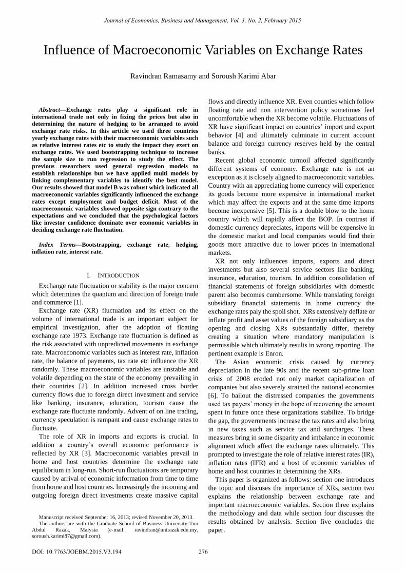
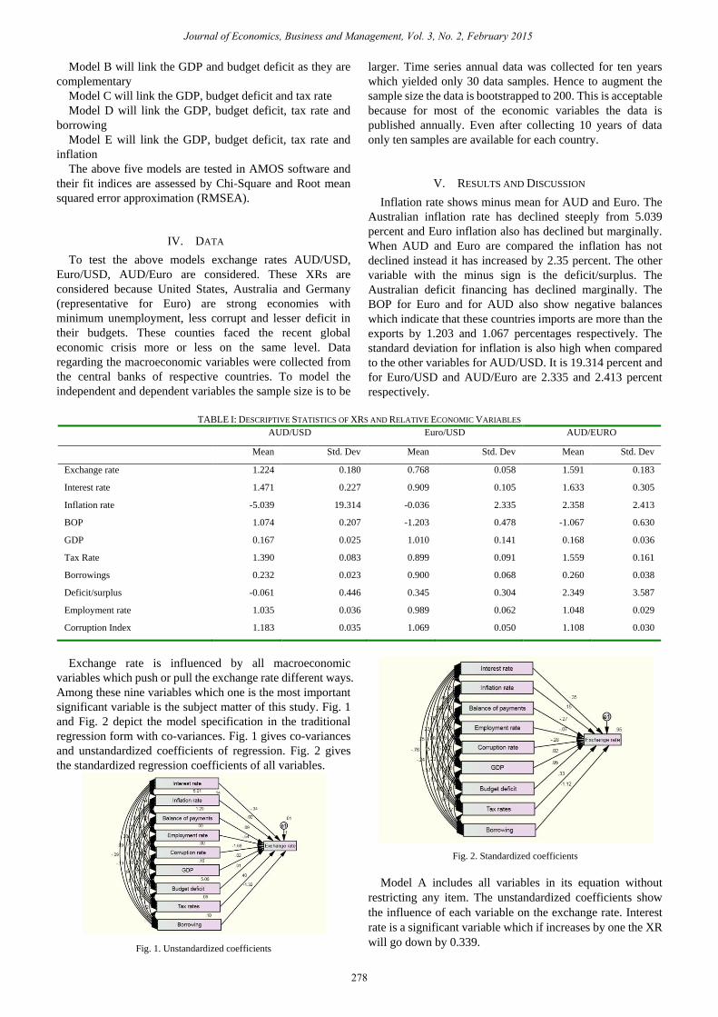
Exchange rate is influenced by all macroeconomic

variables which push or pull the exchange rate different ways.

Among these nine variables which one is the most important

significant variable is the subject matter of this study. Fig. 1

and Fig. 2 depict the model specification in the traditional

regression form with co-variances. Fig. 1 gives co-variances

and unstandardized coefficients of regression. Fig. 2 gives

the standardized regression coefficients of all variables.

Fig. 1. Unstandardized coefficients

Fig. 2. Standardized coefficients

Model A includes all variables in its equation without

restricting any item. The unstandardized coefficients show

the influence of each variable on the exchange rate. Interest

rate is a significant variable which if increases by one the XR

will go down by 0.339.

278


TABLE II: REGRESSION ESTIMATES OF MODEL A

Unstandardized S.E. C.R. Sig Label Standardized R2

Interest -0.339 0.070 -4.825 *** a -0.349 0.946

Inflation 0.022 0.008 2.851 0.004 b 0.150

BOP -0.088 0.026 -3.388 *** c -0.273

Employment rate -0.535 0.466 -1.148 0.251 d -0.072

Corruption -1.684 0.424 -3.976 *** e -0.278

GDP 0.020 0.277 0.071 0.943 f 0.022

Deficit/Surplus 0.008 0.008 0.940 0.347 g 0.048

Tax 0.399 0.180 2.213 0.027 h 0.328

Borrowing -1.315 0.350 -3.756 *** i -1.118

The corruption variable is another significant variable

which also shows a negative relationship with XR. If

corruption increases by 100% the exchange rate drops by

168.4%. Similarly the BOP influences the exchange rate

significantly. The other variables are contributing to XR in a

meager way as they are insignificant. The standardized

coefficients indicate the relative importance of independent

variables in the model. Borrowings, interest rate and tax rate

are the highly influential variables.

TABLE III: REGRESSION ESTIMATES OF MODEL B


Interest -0.340 0.068 -4.972 *** a -0.350 0.946

Inflation 0.022 0.008 2.870 0.004 b 0.150

BOP -0.088 0.026 -3.442 *** c -0.273


Corruption -1.692 0.388 -4.363 *** e -0.279

GDP 0.008 0.008 0.941 0.346 f 0.009

Deficit/Surplus 0.008 0.008 0.941 0.346 f 0.048

Tax 0.397 0.176 2.26 0.024 h 0.326

Borrowing -1.303 0.206 -6.310 *** i -1.108

In model B, GDP and deficit financing are linked together

as they are very closely related. When GDP is more the

deficit will be less and vice versa. Instead of having two

complementary independent variables they are linked

together and the model is run as model B. GDP and deficit

financing show the same values for regression coefficients

(0.008), standard error (0.008), critical ratio (0.941),

significance (0.346) but slightly differ in standardized

coefficients (0.009 and 0.048). The standardized coefficient

GDP is reduced from 2.2% to less than 1% (0.9%). All

variables are significant except employment rate which may

be unconnected to exchange rate.

When the GDP is low to fulfill the expenditure gap the

deficit financing is applied and the tax rates are increased to

collect more revenue. Hence these three variables are closely

linked together. As such they are linked to take the same

values in model C. The R2 slightly goes down from the

original model (94.6% to 93.7%). This proves these variables

could be linked to be parsimonious. In addition in the

previous models these variables were insignificant and in this

model also they are insignificant after linking them as one

variable.

TABLE IV: REGRESSION ESTIMATES OF MODEL C


Interest -0.311 0.073 -4.273 *** a -0.320 0.937

Inflation 0.016 0.008 1.998 0.046 b 0.104

BOP -0.123 0.022 -5.566 *** c -0.380


Corruption -1.906 0.407 -4.681 *** e -0.315

GDP 0.002 0.009 0.242 0.809 f 0.002

Borrowing -1.700 0.116 -14.668 *** i -1.446

If deficit and tax collections are low the government will

go in for borrowings to sustain. On this assumption all four

variables are linked in model D to assess the impact of other

variables on exchange rate. The R2 drops drastically to 45.6%

and most of the variables become insignificant except

inflation.

279


TABLE V: REGRESSION ESTIMATES OF MODEL D


Interest 0.311 0.175 1.776 0.076 a 0.321 0.456

Inflation 0.054 0.022 2.494 0.013 b 0.361

BOP 0.019 0.058 0.331 0.740 c 0.060

Employment rate 2.082 1.314 1.584 0.113 d 0.280

Corruption -0.261 1.153 -0.226 0.821 e -0.043

GDP 0.021 0.025 0.845 0.398 f 0.023

Model E is under the assumption that the budget deficit

and borrowings are closely connected to inflation and as such

inflation is linked to model D variables. This model produces

poor results. The R2 further drops to 43.6% and all variables

become insignificant except inflation. This model fit is poor.

TABLE VI: REGRESSION ESTIMATES OF MODEL E


Interest 0.311 0.178 1.746 0.081 a 0.321 0.436

Inflation 0.040 0.017 2.350 0.019 b 0.267

BOP 0.019 0.060 0.327 0.744 c 0.060

Employment rate 1.958 1.332 1.470 0.142 d 0.263

Corruption 0.008 1.142 0.007 0.995 e 0.001

GDP 0.040 0.017 2.350 0.019 b 0.044

The fit indices of various models are given below. The

AIC and BCC suggest that the model B fit is ideal. In

addition the RMSEA is 0.000 for this model while others

show poor fit with higher RMSEA. To substantiate this, the

R2 is very high at 94.6% for this model.

TABLE VII: FIT INDICES OF DIFFERENT MODELS

Model CMIN DF P CMIN/DF RMSEA AIC BCC

Model A - - - - - 110.000 177.222

Model B 0.002 1 0.966 0.002 0.000 108.002 174.002

Model C 4.670 2 0.097 2.335 0.215 110.670 175.448

Model D 67.221 3 - 22.407 0.859 171.221 234.777

Model E 68.244 4 - 17.061 0.744 170.244 232.577

VI. CONCLUSION

In this research three economically sound relatively less

unemployment and less corrupt countries XRs are chosen to

investigate. Interestingly many variables show the opposite

relationships. For instance, interest rate, BOP and inflation

rates should influence the exchange rate positively as per

theory but the results show the opposite. We interpret this as

true for these reasons; firstly the currency values of these

countries are fairly stronger, the strength comes from

confidence of public and investors and not from economic

variable prevailing in these countries. Secondly the

independent variables have complex interrelationships and

interactions among themselves which may not be captured by

a weak traditional regression model. Thirdly these countries’

economies are fairly corrupt free, stable in interest rates and

least unemployment rates prevail, hence the model gives

diametrically opposite results. This may be due to the

inclusion of macroeconomic variables ignoring the

psychological factor which is the confidence of investors and

traders on the performance or stability of these economies.

REFERENCES

[1] F. Allen and D. Gale, “Competition and financial stability,” Journal of

Money, Credit, and Banking, pp. 433-480, 2004

[2] E. Kocenda and J. Valachy, “Exchange rate volatility and regime

change: A visegrad comparison,” Journal of Comparative Economics,

pp. 727-753, 2006

[3] A. C. Arize, T. Osang, and D. J. Slottje, “Exchange rate volatility and

foreign trade: Evidence from thirteen LDCs,” Journal of Business and

Economics Statistics, pp. 10-17, 2000

[4] K. L. Wang and C. B. Barrett, “Estimating the Effects of Exchange

Rate Volatility on Export Volumes,” Journal of Agricultural and

Resource Economics, pp. 225-255, 2007

[5] C. Sauer and A. K. Bohara, “Exchange rate volatility and exports:

Regional differences between developing and industrialized countries,”

Review of International Economics, 2001

[6] G. Corsetti, P. Pesenti, and N. Roubini, “What caused the asian

currency and financial crisis?” Japan and the World Economy, pp.

305-373, 1999

[7] A. J. Makin, “International economics, finance and trade,” The

Balance of Payments and the Exchange Rate, vol. I, 2004

[8] S. Tenreyro, “On the trade impact of nominal exchange rate volatility,”

Journal of Development Economics, pp. 485-508, 2007

[9] A. R. Ghosh, A. M. Gulde, and H. C. Wolf, Exchange Rate Regimes:

Choices and Consequences, The MIT Press, 2003

[10] H. Duncan, “The effect of exchange rate volatility on trade and

employment: A brief review of the literature economics,”

Macroeconomy, Economic Bias and Employment, vol. 28, no. 3, pp.

133-152, 2001

280


[11] G. Schnabl, “The Russian currency basket: Recent developments in

Russia’s exchange rate policies and the role of the Euro,”

Intereconomics, pp. 135-141, 2006

[12] A. C. Arize, J. Malindretos, and K. M. Kasibhatla, “Does exchange rate

volatility depress flows: The case of LDCs,” International Advances in

Economic Research, pp. 7-19, 2003

Ravindran was born at Tiruvannamalai, Tamil Nadu,

India, on 14-05-1956. He completed his M.Com

(accountancy and taxation specializations) at

University of Madras. Later he obtained M.Phil., and

Ph.D at the same university. He completed his MBA

under IGNOU, a famous Indian open university. He passed CIMA

professional exam with a third rank in world in one of the accounting papers.

He is an associate member of CIMA. He published many articles on

quantitative finance and won a best paper award for presenting a paper on

valuation of collateralized debt obligations (CDOs) at a Sydney conference

in 2009. Presently he is working at University Tun Abdul Razak as professor

of accounting and finance.

His research interests are in the area of derivatives, their pricing

mechanisms, assessing their risk in combination with the underlying and

hedge the risk they possess in both individual and portfolio construct.

Soroush the second author has completed his MBA at University Tun Abdul

Razak, and pursuing his PhD in the finance area.

281


Documents

Influence of Macroeconomic Variables on Exchange Rates - …joebm.com/papers/194-W10044.pdf · · 2014-01-03Exchange rates play a significant role in ... We used bootstrapping technique