Influence of polymer type, composition, and interfaceon the structural and mechanical properties of core/sheathtype bicomponent nonwoven fibers

Mehmet Dasdemir • Benoit Maze •

Nagendra Anantharamaiah •

Behnam Pourdeyhimi

Received: 11 January 2012 / Accepted: 12 April 2012 / Published online: 27 April 2012

� Springer Science+Business Media, LLC 2012

Abstract In this study, we investigated the effect of

polymer type, composition, and interface on the structural

and mechanical properties of core–sheath type bicompo-

nent nonwoven fibers. These fibers were produced using

poly(ethylene terephthalate)/polyethylene (PET/PE), poly-

amide 6/polyethylene (PA6/PE), polyamide 6/polypropylene

(PA6/PP), polypropylene/polyethylene (PP/PE) polymer

configurations at varying compositions. The crystallinity,

crystalline structure, and thermal behavior of each com-

ponent in bicomponent fibers were studied and compared

with their homocomponent counterparts. We found that the

fiber structure of the core component was enhanced in

PET/PE, PA6/PE, and PA6/PP whereas that of the sheath

component was degraded in all polymer combinations

compared to corresponding single component fibers. The

degrees of these changes were also shown to be composi-

tion dependent. These results were attributed to the mutual

interaction between two components and its effect on the

thermal and stress histories experienced by polymers dur-

ing bicomponent fiber spinning. For the interface study, the

polymer–polymer compatibility and the interfacial adhe-

sion for the laminates of corresponding polymeric films

were determined. It was shown that PP/PE was the most

compatible polymer pairing with the highest interfacial

adhesion value. On the other hand, PET/PE was found to

be the most incompatible polymer pairings followed by

PA6/PP and PA6/PE. Accordingly, the tensile strength

values of the bicomponent fibers deviated from the theo-

retically estimated values depending on core–sheath com-

patibility. Thus, while PP/PE yielded a higher tensile

strength value than estimated, other polymer combinations

showed lower values in accordance with their degree of

incompatibility and interfacial adhesion. These results

unveiled the direct relation between interface and tensile

response of the bicomponent fiber.

Introduction

Bicomponent fibers are designed to meet requirements of

two materials into one single fiber by hosting two com-

ponents along the fiber length. Therefore, they are also

known as ‘‘composite’’, ‘‘conjugate’’, and ‘‘hetero’’ fibers.

Natural counterpart of a bicomponent fiber is wool which

consists of hydrophobic outer layer (scales) and strong,

oriented fibrous structures inside. Formation of typical melt

spun bicomponent fibers or filaments involve coextruding

two polymers from a single spinneret with a desired cross-

sectional arrangement. As it is possible to produce spe-

cialty fibers by selecting cross-sectional designs depending

on the end-use application, bicomponent fibers have gained

great commercial interest.

Bicomponent fibers can be classified according to the

distribution of each component within cross-sectional area.

Typical cross-section configurations include side-by-side,

core/sheath (c/s), islands-in-the-sea, alternating segments

or segmented-pie, citrus and tipped (see Fig. 1). Most of

the bicomponent fibers commercially produced today have

c/s structures. In the c/s bicomponent fiber structure, one of

M. Dasdemir (&)

Textile Engineering Department, University of Gaziantep,

27310 Gaziantep, Turkey

e-mail: dasdemir@gantep.edu.tr

B. Maze � B. Pourdeyhimi

The Nonwovens Institute, North Carolina State University,

Raleigh, NC 27695, USA

N. Anantharamaiah

Hollingsworth & Vose Company, Floyd, VA 24091, USA

123

J Mater Sci (2012) 47:5955–5969

DOI 10.1007/s10853-012-6499-7

the components (sheath) functions as a shell and surrounds

the second component (core). Depending on the location of

the core component these fibers can be either concentric

where the core is at the center (see Fig. 1b) or eccentric

(see Fig. 1c). The eccentric configuration is used for pro-

viding self-crimping properties. On the other hand, if the

fiber and fabric strength are mostly desired, concentric

configuration can be chosen. Major application areas of

these fibers are nonwovens. There are several purposes of

using these materials in a nonwoven product. These include

but are not limited to the following: bonding (self-bonding)

improvement in thermally bonded nonwovens, strength and

flexibility increase, cost reduction, and surface property

enhancement [1–4]. In addition, bicomponent fibers [5] and

nonwovens [6] were recently shown to be a good candidate

for the formation of thermoplastic composite structures.

Polymer viscosities, rates of cooling, and surface ten-

sions of the two components are critical for the formation

and properties of bicomponent fibers [3, 4]. Polymer vis-

cosities of each component should be comparable at the

spin pack along with the temperature to obtain desired

cross-section [1, 3]. Rates of cooling determine the orien-

tation of each component while the surface tensions

determine the adhesion between two components and the

final cross-sectional shape in the resultant bicomponent

fiber.

Previous studies on bicomponent fibers have mainly

focused on the structure and physical properties of bicom-

ponent fibers at high-speed melt spinning [7–13]. In these

studies, several polymer combinations (listed in Table 1)

have been investigated to observe the effect of interaction of

two components on the structure of each component in the

fiber. The differences in the characteristics of the two poly-

mers in bicomponent fiber including melt (elongational)

viscosities and solidification temperatures were some of the

major factors affecting the interaction of two components

[8]. These factors can influence the spinline stresses acting

on each component and change their thermal histories. As a

result, the fiber structure for each component in bicomponent

fiber develops under different conditions compared to cor-

responding single component fiber. For instance, in PET/PP

(c/s) bicomponent fiber, PET yields higher orientation and

orientation-induced crystallization, whereas PP shows lower

structure formation than corresponding single component

PET and PP fibers [7, 8]. Similar results were also obtained

for other polymer combinations listed in Table 1 at high-

speed melt spinning. Even though major application areas of

c/s type bicomponent fibers are nonwovens, all of the above-

mentioned studies were conducted for high-speed melt spun

fibers and very limited literature [14] is available for

bicomponent nonwoven fibers.

One of the other major factors affecting the interaction is

the compatibility of two polymers used in bicomponent fiber.

Cho et al. [11, 12] studied PET/LLDPE and PET/HDPE

bicomponent melt spun fibers in both c/s and s/c configura-

tions. It was found that using PE in the sheath component

yielded interfacial stability which was formed at lower take-

up velocities compared to when it was used in the core

component. It was attributed to the difference in the thermal

expansion of each component and their thermal behavior in

either combination. The interfacial instability, in other words

phase separation, at the interface was also observed for PET/

poly(phenylene sulfide) (PPS) c/s type bicomponent melt-

spun fibers [15]. The observation of the phase separation at

the interface was attributed to the incompatibility of these

polymers used in bicomponent fibers. On the other hand,

when two compatible polymers were used, strong interfacial

adhesion between these two components could be obtained.

For instance using PET with biodegradable aliphatic poly-

esters such as poly(butylene succinate-lactate) (PBSL) or

poly(L-lactic acid) (PLLA) in c/s configuration resulted in

physical adhesion of the core and sheath components which

(a) (b) (c) (d)

(e) (f) (g) (h)

Fig. 1 Types of bicomponent

fiber cross-sections: side-by-

side (a), sheath–core with

concentric (b) and eccentric

(c) configurations, islands-in-

the-sea (d), alternating segments

with stripes (e) and pies (f),citrus (g), and tipped trilobal (h)

5956 J Mater Sci (2012) 47:5955–5969

123

was induced by the interfacial interaction during melt spin-

ning [16]. For these bicomponent fibers, enhanced mechan-

ical properties compared to a single PET fiber was reported.

However, the influence of the interface on mechanical

properties of bicomponent fibers has not been fully

elucidated.

In this study, we investigated the effects of polymer type,

composition, and interface on the structure and mechanical

properties of bicomponent nonwoven fibers. In this regard,

typical c/s type bicomponent nonwoven fibers were pro-

duced using PET, polyamide 6 (PA6), PP, and PE polymers

in poly(ethylene terephthalate)/polyethylene (PET/PE),

polyamide 6/polyethylene (PA6/PE), polyamide 6/polypro-

pylene (PA6/PP), and polypropylene/polyethylene (PP/PE)

(c/s) polymer configurations at varying compositions. The

structure of each component in bicomponent fibers were

studied and compared with their homocomponent counter-

parts. Also, tensile properties of bicomponent fibers and

interface between two polymers used in these fibers were

characterized to get a deeper insight into the relation

between the mechanical responses of bicomponent fibers and

interface.

Materials

Commercial fiber grades of PET, PA6, PP, and linear low

density PE were used for producing fibers and making

films. Some of the basic properties and suppliers of these

polymers are listed in Table 2.

Methods

Production of nonwoven fibers

Homocomponent and bicomponent nonwoven fibers were

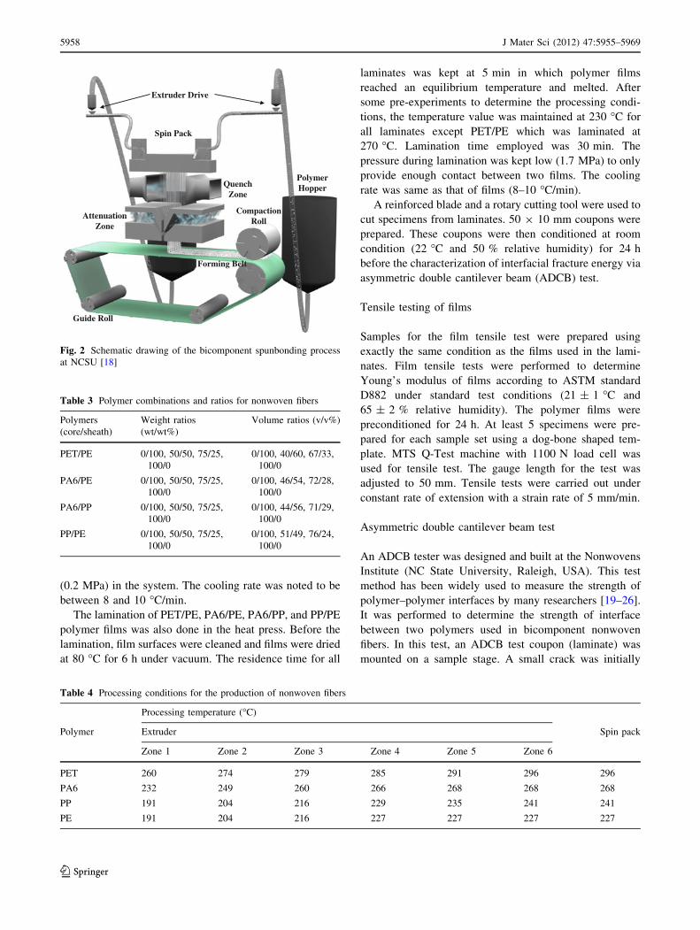
produced using the spunbonding process (see Fig. 2) at the

Nonwovens Institute’s pilot facility (NC State University,

Raleigh, NC, USA). The bicomponent fiber cross-section

chosen was a c/s structure with different polymer ratios

listed in Table 3. Overall throughput was adjusted to

0.6 g/min for each hole for an 1162 holes spinneret. Fibers

were quenched with quenchers on either side and the

quench air temperature was 11 �C. Screw pressures for

both extruders were adjusted to 5 MPa. Processing tem-

peratures for each polymer are listed in Table 4. Drawn

fibers with an expected fiber denier value of 1.6 were

collected during the process for investigation.

Preparation of films, laminates, and test coupons

A heat press was used for the preparation of films. Before

making films, PA6 and PET polymer pellets were dried at

80 �C for 24 h under vacuum while other polymers were

used as-received. Processing temperatures were 180 �C for

PE, 200 �C for PP, 240 �C for PA6, and 270 �C for PET.

The residence time in which polymer pellets melt in a

defined geometry without any pressure was set to 5 min.

The pressure was then applied with 3.5 MPa increment at

every 30 s until pressure level reached to 35 MPa. Cooling

was done under pressure by circulating high pressure air

Table 1 Previous studies on the structure and physical properties of bicomponent fibers at high-speed melt spinning

Acronym Polymer Configurations References

PET/PP Poly(ethylene terephthalate)/polypropylene c/s [7, 8]

PET/PS PET/polystyrene c/s [7]

PET/HDPE PET/high density polyethylene c/s and s/c [11, 12]

PET/LLDPE PET/linear low density polyethylene c/s and s/c [11, 12]

HMPET/LMPET High molecular weight PET/low molecular weight PET c/s and s/c [9, 10]

PBAT/PBT Poly(butylene adipate-co-terephthalate)/poly(butylene terephthalate) c/s [13]

Table 2 Properties and suppliers of polymers

Polymer Trade name Supplier Densitya, q (g/cm3) Melting temperatureb, Tm (�C)

PET F-61HC Eastman Chemical Co. 1.41 250

PA6 Ultramid BS-2702 BASF 1.13 220

PP CP-360H Sunoco 0.905 166

PE Aspun 6850A Dow Chemical Co. 0.955 129

a The density values of PA6, PP, and PE were obtained from corresponding polymer data sheet supplied by the producer. PET density value was

taken from the Ref. [17]b The melting temperatures of all polymers were peak melting temperatures and measured by means of a differential scanning calorimeter at a

heating rate of 10 �C/min

J Mater Sci (2012) 47:5955–5969 5957

123

(0.2 MPa) in the system. The cooling rate was noted to be

between 8 and 10 �C/min.

The lamination of PET/PE, PA6/PE, PA6/PP, and PP/PE

polymer films was also done in the heat press. Before the

lamination, film surfaces were cleaned and films were dried

at 80 �C for 6 h under vacuum. The residence time for all

laminates was kept at 5 min in which polymer films

reached an equilibrium temperature and melted. After

some pre-experiments to determine the processing condi-

tions, the temperature value was maintained at 230 �C for

all laminates except PET/PE which was laminated at

270 �C. Lamination time employed was 30 min. The

pressure during lamination was kept low (1.7 MPa) to only

provide enough contact between two films. The cooling

rate was same as that of films (8–10 �C/min).

A reinforced blade and a rotary cutting tool were used to

cut specimens from laminates. 50 9 10 mm coupons were

prepared. These coupons were then conditioned at room

condition (22 �C and 50 % relative humidity) for 24 h

before the characterization of interfacial fracture energy via

asymmetric double cantilever beam (ADCB) test.

Tensile testing of films

Samples for the film tensile test were prepared using

exactly the same condition as the films used in the lami-

nates. Film tensile tests were performed to determine

Young’s modulus of films according to ASTM standard

D882 under standard test conditions (21 ± 1 �C and

65 ± 2 % relative humidity). The polymer films were

preconditioned for 24 h. At least 5 specimens were pre-

pared for each sample set using a dog-bone shaped tem-

plate. MTS Q-Test machine with 1100 N load cell was

used for tensile test. The gauge length for the test was

adjusted to 50 mm. Tensile tests were carried out under

constant rate of extension with a strain rate of 5 mm/min.

Asymmetric double cantilever beam test

An ADCB tester was designed and built at the Nonwovens

Institute (NC State University, Raleigh, USA). This test

method has been widely used to measure the strength of

polymer–polymer interfaces by many researchers [19–26].

It was performed to determine the strength of interface

between two polymers used in bicomponent nonwoven

fibers. In this test, an ADCB test coupon (laminate) was

mounted on a sample stage. A small crack was initially

Extruder Drive

Spin Pack

Quench Zone

Attenuation Zone

Forming Belt

Compaction Roll

Polymer Hopper

Guide Roll

Fig. 2 Schematic drawing of the bicomponent spunbonding process

at NCSU [18]

Table 3 Polymer combinations and ratios for nonwoven fibers

Polymers

(core/sheath)

Weight ratios

(wt/wt%)

Volume ratios (v/v%)

PET/PE 0/100, 50/50, 75/25,

100/0

0/100, 40/60, 67/33,

100/0

PA6/PE 0/100, 50/50, 75/25,

100/0

0/100, 46/54, 72/28,

100/0

PA6/PP 0/100, 50/50, 75/25,

100/0

0/100, 44/56, 71/29,

100/0

PP/PE 0/100, 50/50, 75/25,

100/0

0/100, 51/49, 76/24,

100/0

Table 4 Processing conditions for the production of nonwoven fibers

Processing temperature (�C)

Polymer Extruder Spin pack

Zone 1 Zone 2 Zone 3 Zone 4 Zone 5 Zone 6

PET 260 274 279 285 291 296 296

PA6 232 249 260 266 268 268 268

PP 191 204 216 229 235 241 241

PE 191 204 216 227 227 227 227

5958 J Mater Sci (2012) 47:5955–5969

123

created between two polymer sheets in the laminate with a

razor blade. A moving blade was then inserted into the

opening and pushed forward at a constant speed of 3 lm/s.

After the crack was stabilized, the length of the opening

crack which is an inverse function of the strength of

interface between two films was obtained and recorded

from several locations along the specimen during the test.

This was done by taking the picture of the crack at an

interval of 5 min. A total of 34 pictures of the crack were

taken for each specimen. The first 10 and last 4 images

were omitted and the remaining 20 images were analyzed.

From each image, 5 measurements along the crack were

done using an image analysis program. Three specimens

for each sample were tested in the ADCB tester and a total

of around 300 measurements were analyzed for each

sample set. Except PET/PE where PET component was too

fragile during crack opening, all polymer interfaces were

characterized.

Tensile testing of single fibers

Fiber tensile tests were performed according to ASTM

standard D3822-07 under standard test conditions (21 ±

1 �C and 65 ± 2 % relative humidity). The fibers were

preconditioned for 2 days. Linear density of the single fibers

was measured using the vibroscope method (ASTM D

1577-07) in a Vibromat ME Textechno� test equipment and

fiber deniers were noted. Each individual fiber was then

pasted on paper cardboards. Great care was taken not to

deform the fibers. At least 10 specimens were prepared for

each sample set. MTS Q-Test machine with 50 g load cell

was used for tensile test. The gauge length for the test was

adjusted to 25.4 mm (1 inch). Tensile tests were carried out

under constant rate of extension with an extension rate of

15 mm/min.

Wide angle X-ray diffraction

An Omni instrumental wide angle X-ray diffractometer

(WAXD) was used to determine the crystallite dimensions

of homocomponent nonwoven fibers and each component

in the bicomponent nonwoven fibers. The instrument was

operated at 30 kV and 20 mA with a Be-filtered Cu-Karadiation source (k = 1.54 A). The fibers were manually

wound around a sample holder which was then perpen-

dicularly positioned to the X-ray beam. They were scanned

at a rate of 0.1 s-1 from 5� to 40� (2h).

Differential scanning calorimetry (DSC)

Thermal analysis was carried out for homocomponent and

bicomponent nonwoven fibers by means of DSC. Perkin

Elmer Diamond DSC calorimeter and Pyriss Series

Diamond DSC software were used for thermal analysis of

all samples. The sample weights were in the range

of 3–5 mg. Samples were scanned at the heating rate of

10 �C/min with temperature ranging from 25 to 270 �C.

Scanning electron microscopy (SEM)

SEM images were taken for bicomponent nonwoven fibers.

To take a clear cross-section image, fibers were dipped into

liquid nitrogen in which they freeze, and then fractured

using a razor blade. Images of the samples were taken after

they were coated with a layer of AuPd at a 5 kV acceler-

ating voltage and 40 nA beam current in a Hitachi S-3200

SEM.

Results and discussions

Effect of polymer type and composition on structural

properties

Crystallinity and crystalline structure

The percent crystallinity of polymers in the homocompo-

nent and bicomponent fibers was calculated using Eq. 1

[27]:

X ¼ DHf � DHc

w� DH0f

� 100 ð1Þ

where X is the percent crystallinity of a polymer, DHf is the

heat of fusion of the polymer (measured from the area

under the melting peak of the DSC curve), DHc heat of cold

crystallization of the polymer, DHf0 is the theoretical heat

of fusion for perfectly crystalline polymer (obtained from

literature), and w is the weight fraction of the polymer in

bicomponent fiber (for homocomponent fibers w = 1). The

theoretical heats of fusion for homopolymers were assumed

to be 230 J/g [28], 293 J/g [28], 140 J/g [29], 209 J/g [30]

for PA6, PE, PET and PP, respectively. Cold crystallization

peak was not observed for polymers in both homocompo-

nent and bicomponent fibers so DHc was assumed to be

zero.

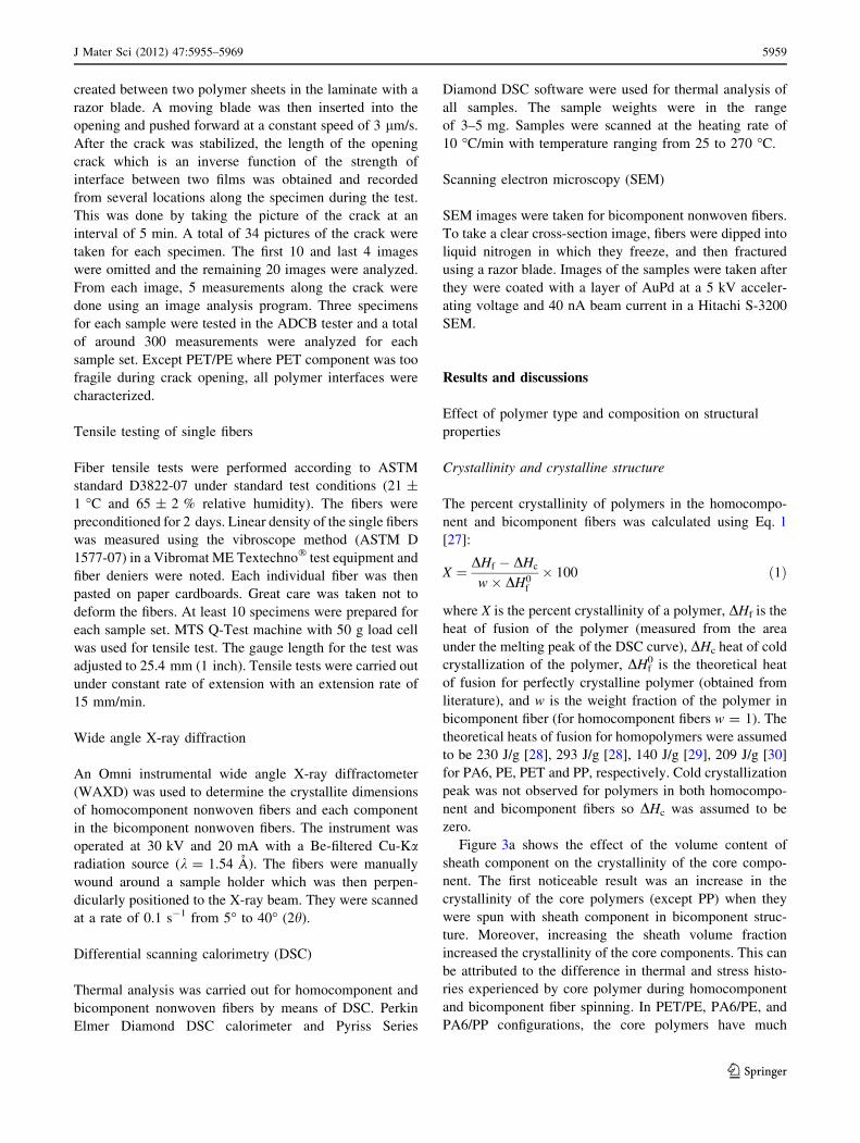
Figure 3a shows the effect of the volume content of

sheath component on the crystallinity of the core compo-

nent. The first noticeable result was an increase in the

crystallinity of the core polymers (except PP) when they

were spun with sheath component in bicomponent struc-

ture. Moreover, increasing the sheath volume fraction

increased the crystallinity of the core components. This can

be attributed to the difference in thermal and stress histo-

ries experienced by core polymer during homocomponent

and bicomponent fiber spinning. In PET/PE, PA6/PE, and

PA6/PP configurations, the core polymers have much

J Mater Sci (2012) 47:5955–5969 5959

123

higher solidification temperatures than the sheath polymers

[8, 11, 12, 14]. Therefore, during bicomponent fiber spin-

ning, the core components solidify earlier than the sheath

polymers. Before the solidification of these core compo-

nents takes place, they experience spinline stress which

induces orientation in this component. In a bicomponent

system, a larger portion of this spinline stress at or near the

solidification temperature of the polymer typically acts on

the component having higher elongational viscosity [7, 8].

It was also previously shown that the spinline stress

experienced by the same polymer was higher in bicom-

ponent spinning than the corresponding single fiber spin-

ning [7, 8]. In our case PET and PA6 have much higher

elongational viscosities than PP and PE and experienced a

great portion of the total spinline stress at solidification

temperature of the former polymers [8, 14]. Therefore, the

solidification stress experienced by the core polymer in

bicomponent system can be expected to be higher than the

stress experienced by the same polymer in homocomponent

system and increase with increasing the volume content of

the sheath polymer. Therefore, it can be postulated that as a

result of higher level of solidification stresses, the degrees of

orientation-induced crystallization were improved for PA6

and PET in bicomponent system as compared to same

polymers in homocomponent system. In the PP/PE config-

uration, the solidification temperatures of two polymers are

very close to each other [14]. Therefore, it was not expected

from PP to experience a high degree of improved solidifi-

cation stresses that can increase the crystallinity. Also, due to

their similar chemical structure and compatibility, PP and PE

may undergo molecular interaction such as inter-diffusion of

the chains at their interfacial vicinity. Such molecular

interactions may prevent chains from forming crystallites

near the interface. Depending on the composition of two

polymers these interactions may also vary. This may be the

possible reason for observing a decrease in crystallinity of PP

fiber.

For the sheath polymers, we observed a decrease in the

crystallinity in comparison to their homocomponent

counterparts (see Fig. 3b). Also, the percent crystallinity of

these polymers gradually decreased with increasing the

volume content of the core polymer. This is also closely

related to the difference in spinline stresses acting on these

polymers during homocomponent and bicomponent fiber

spinning. After the solidification of the core polymer takes

place, the spinline stress on the sheath polymer suddenly

vanishes [8]. This causes a stress relaxation on the sheath

polymer. The degree of this stress relaxation increases with

increasing the volume content of core component. As a

result orientation-induced crystalline formation reduces in

the sheath polymers.

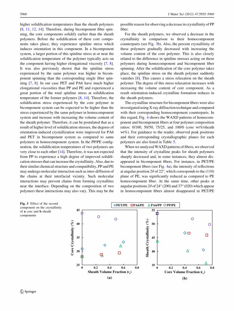
The crystalline structure for bicomponent fibers were also

investigated using X-ray diffraction technique and compared

with their corresponding homocomponent counterparts. In

this regard, Fig. 4 shows the WAXD patterns of homocom-

ponent and bicomponent fibers at four polymer composition

ratios: 0/100, 50/50, 75/25, and 100/0 (core wt%/sheath

wt%). For guidance to the reader, observed peak positions

and their corresponding crystallographic planes for each

polymers are also listed in Table 5.

When we analyzed WAXD patterns of fibers, we observed

that the intensity of crystalline peaks for sheath polymers

sharply decreased and, in some instances, they almost dis-

appeared in bicomponent fibers. For instance, in PET/PE

bicomponent fibers (see Fig. 4a), the intensity of reflections

at angular position 2h of 22�, which corresponds to the (110)

plane of PE, was significantly reduced as compared to PE

homocomponent fiber. At the same time, other peaks at

angular positions 2h of 24� (200) and 37� (020) which appear

in homocomponent fibers almost disappeared in PET/PE

(a) (b)

PET/PE PA6/PE PA6/PP PP/PE

25

30

35

40

45

0 0.2 0.4 0.6 0.8

Cor

e C

ryst

allin

ity

(%)

Sheath Volume Fraction (vs)

35

40

45

50

55

0 0.2 0.4 0.6 0.8

Shea

th C

ryst

allin

ity

(%)

Core Volume Fraction (vc)

Fig. 3 Effect of the second

component on the crystallinity

of a core and b sheath

components

5960 J Mater Sci (2012) 47:5955–5969

123

(a) (b)

5 10 15 20 25 30 35 40

Cou

nt R

ate

(cps

)

2 (degree)

(0/100)

(50/50)

(75/25)

(100/0)

PET/PE

5 10 15 20 25 30 35 40

Cou

nt R

ate

(cps

)

2 (degree)

(0/100)

(50/50)

(75/25)

(100/0)

PA6/PE

(c) (d)

5 10 15 20 25 30 35 40

Cou

nt R

ate

(cps

)

2 (degree)

(0/100)

(50/50)

(75/25)

(100/0)

PP/PE

5 10 15 20 25 30 35 40

Cou

nt R

ate

(cps

)

2 (degree)

(0/100)

(50/50)

(75/25)

(100/0)

PA6/PP

Fig. 4 WAXD patterns of

homocomponent and

bicomponent nonwoven fibers:

a PET/PE, b PA6/PE, c PA6/PP,

and d PP/PE

Table 5 Observed peak positions for each polymer in homocomponent and bicomponent nonwoven fibers

Polymer 1st Peak position 2nd Peak position 3rd Peak position

2h (�) Crystallographic

plane (hkl)2h (�) Crystallographic

plane (hkl)2h (�) Crystallographic

plane (hkl)

PET 18.1–18.4 (010) 26.3–26.5 (100) – –

PA6 21.7–22.1 (200) – – – –

PP 14.4–14.9 (110) 17.2–17.5 (040) 18.8–19.6 (130)

PE 21.9–22.3 (110) 24.2–24.4 (200) 36.8–36.9 (020)

J Mater Sci (2012) 47:5955–5969 5961

123

bicomponent fibers. This means that they went through stress

relaxation and therefore, have no orientation. Moreover, the

degree of intensity reduction became more pronounced with

increasing the core volume fraction in bicomponent fiber.

Similar results were also obtained for other bicomponent

fibers (see Fig. 4b–d). These results suggest that size and/or

perfection of crystallites decreased for sheath polymers

when they were spun in bicomponent structure. They also

support our previous statement on crystallinity decrease for

sheath polymers as a result of stress relaxation occurring in

bicomponent fiber spinning.

The X-ray diffraction patterns for core polymers also

showed some difference from their homocomponent

counterparts. For instance, in PET/PE bicomponent fibers

(see Fig. 4a), the crystalline peaks for PET at angular

positions 2h of 18� (010) and 26� (100) became more

noticeable compared to those for homocomponent PET

fiber. Also, increasing the sheath volume content from 25

to 50 % in the bicomponent fiber yielded slightly better

resolved peak for the core polymer. These results also

suggest that the orientation-induced crystallization of PET

has improved. For other polymer combinations, we

observed a slight decrease in peak width which can also be

related to change in crystallization behavior.

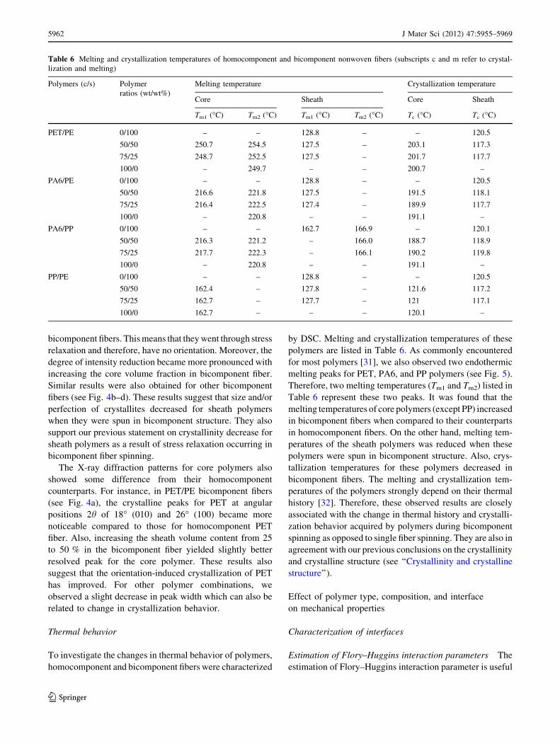
Thermal behavior

To investigate the changes in thermal behavior of polymers,

homocomponent and bicomponent fibers were characterized

by DSC. Melting and crystallization temperatures of these

polymers are listed in Table 6. As commonly encountered

for most polymers [31], we also observed two endothermic

melting peaks for PET, PA6, and PP polymers (see Fig. 5).

Therefore, two melting temperatures (Tm1 and Tm2) listed in

Table 6 represent these two peaks. It was found that the

melting temperatures of core polymers (except PP) increased

in bicomponent fibers when compared to their counterparts

in homocomponent fibers. On the other hand, melting tem-

peratures of the sheath polymers was reduced when these

polymers were spun in bicomponent structure. Also, crys-

tallization temperatures for these polymers decreased in

bicomponent fibers. The melting and crystallization tem-

peratures of the polymers strongly depend on their thermal

history [32]. Therefore, these observed results are closely

associated with the change in thermal history and crystalli-

zation behavior acquired by polymers during bicomponent

spinning as opposed to single fiber spinning. They are also in

agreement with our previous conclusions on the crystallinity

and crystalline structure (see ‘‘Crystallinity and crystalline

structure’’).

Effect of polymer type, composition, and interface

on mechanical properties

Characterization of interfaces

Estimation of Flory–Huggins interaction parameters The

estimation of Flory–Huggins interaction parameter is useful

Table 6 Melting and crystallization temperatures of homocomponent and bicomponent nonwoven fibers (subscripts c and m refer to crystal-

lization and melting)

Polymers (c/s) Polymer

ratios (wt/wt%)

Melting temperature Crystallization temperature

Core Sheath Core Sheath

Tm1 (�C) Tm2 (�C) Tm1 (�C) Tm2 (�C) Tc (�C) Tc (�C)

PET/PE 0/100 – – 128.8 – – 120.5

50/50 250.7 254.5 127.5 – 203.1 117.3

75/25 248.7 252.5 127.5 – 201.7 117.7

100/0 – 249.7 – – 200.7 –

PA6/PE 0/100 – – 128.8 – – 120.5

50/50 216.6 221.8 127.5 – 191.5 118.1

75/25 216.4 222.5 127.4 – 189.9 117.7

100/0 – 220.8 – – 191.1 –

PA6/PP 0/100 – – 162.7 166.9 – 120.1

50/50 216.3 221.2 – 166.0 188.7 118.9

75/25 217.7 222.3 – 166.1 190.2 119.8

100/0 – 220.8 – – 191.1 –

PP/PE 0/100 – – 128.8 – – 120.5

50/50 162.4 – 127.8 – 121.6 117.2

75/25 162.7 – 127.7 – 121 117.1

100/0 162.7 – – – 120.1 –

5962 J Mater Sci (2012) 47:5955–5969

123

to predict the degree of miscibility of polymer pairs used in

bicomponent fibers. It can be estimated using Eqs. 2 and 3:

v12 ¼hVi d1 � d2ð Þ2

RTð2Þ

where v12 is the Flory–Huggins parameter describing the

interaction between polymer segments 1 and 2, di is the

solubility parameter for polymer i, R is the gas constant,

T is the temperature, and hVi is the mean molar volume of

two polymers

hVi ¼ffiffiffiffiffiffiffiffiffiffi

V1V2

pð3Þ

The solubility parameters for polymers were estimated

via the use of group contribution methods (GCMs), which

account for the contribution of each group present in the

repeat unit of the polymer. The calculations of solubility

parameter for each polymer via the use of GCMs are given

by Eqs. 4, 5.

d ¼

P

i

Fi

Vð4Þ

V ¼ M

q; ð5Þ

where Fi is the molar attraction constant of group i, V is the

total molar volume, M is the molecular weight of the repeat

unit, and q is the density of the polymer.

Values of F were determined by regression analysis for

various common structural groups and reported by several

100 140 180 220 260

Hea

t F

low

(E

ndo

up)

Temperature (°C)

PET/PE

0/100

50/50

75/25

100/0

(a)

100 140 180 220

Hea

t F

low

(E

ndo

up)

Temperature (°C)

PA6/PE

0/100

50/50

75/25

100/0

(b)

140 160 180 200 220

Hea

t F

low

(E

ndo

up)

Temperature (°C)

PA6/PP

0/100

50/50

75/25

100/0

(c)

100 120 140 160 180

Hea

t F

low

(E

ndo

up)

Temperature (°C)

PP/PE

0/100

50/50

75/25

100/0

(d)

Fig. 5 DSC thermograms of

homocomponent and

bicomponent nonwoven fibers:

a PET/PE, b PA6/PE, c PA6/PP,

and d PP/PE

J Mater Sci (2012) 47:5955–5969 5963

123

researchers [33–37]. In our calculations, we used the most

recent F values reported by Coleman and Painter [37]. The

solubility parameters for PET, PA6, PP, and PE were then

calculated and found to be 12.4, 10.1, 8, and 7.4

(cal/cm3)0.5, respectively. It is important to point out that in

our calculations, we did not count any inter- and intra-

molecular interactions such as hydrogen bonding. After the

calculation of solubility parameters, the Flory–Huggins

interaction parameters were calculated at spinneret

temperatures employed in bicomponent spinning process

(296 �C for PET/PE, 268 �C for PA6/PE and PA6/PP,

241 �C for PP/PE). Calculated Flory–Huggins interaction

parameters were 1.11, 0.256, 0.523, and 0.014 for PET/PE,

PA6/PE, PA6/PP, and PP/PE, respectively. Note that lower

the number, the better the polymer–polymer interaction as

miscibility increases when the Flory–Huggins interaction

parameter approaches zero. Therefore, we can conclude

that the most compatible polymer pair studied is PP/PE

(0.014). On the other hand, we obtained a large interaction

parameter (1.11) for PET/PE suggesting that this polymer

pair is highly incompatible in nature.

Interfacial adhesion The interfacial adhesion in PA6/PE,

PA6/PP, and PP/PE were measured using ADCB test

method. Due to the challenges encountered in testing of

PET/PE substrate, we could not characterize this polymer

pair (see ‘‘Asymmetric double cantilever beam test’’). The

ADCB test has been shown to be a reliable test for studying

fracture toughness at the polymer–polymer interfaces [19–

26]. In this test, the interfacial fracture energy between two

rectangular polymer beams is measured by equating the

energy needed to generate two new surfaces with the

elastic energy stored in these beams [38]. This test also

assumes that the released energy only comes from the

bending energy of the beam [19] and the critical energy

release rate at zero velocity is equal to the measured energy

release rate at very low speed [39]. After these two

assumptions are made, the interfacial fracture energy can

be calculated using the following formula by obtaining the

crack length with ADCB method.

Gc ¼3D2E1h3

1E2h32

8a4� E1h3

1C22 þ E2h3

2C21

E1h31C3

2 þ E2h32C3

1

� �2; ð6Þ

where Gc is the interfacial fracture energy, D is the

thickness of the wedge, Ei is the stiffness (Young’s

Modulus) of the beam i, hi is the thicknesses of the beam

i, a is the crack length, and Ci is the correction factor:

Ci ¼ 1þ 0:64hi

að7Þ

The first part of Eq. 6 was derived from simple beam

theory and can only be applied when a/hi is C10 [40]. For

small crack lengths, a correction factor (second part of

Eq. 6) is required to calculate the interfacial fracture

energy in the proper limit. PA6/PE and PA6/PP had con-

siderably large cracks (a/h [ 10) in which simple beam

theory yields more reliable results.

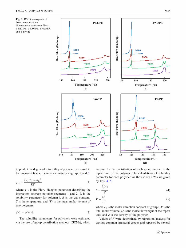
The interfacial fracture energies of three polymer pairings

were compared (see Fig. 6). Our results show that the

interfacial fracture energy of the PA6/PP is the lowest

(2.15 ± 0.1 J/m2) and that of PP/PE is the highest

(50.6 ± 3.1 J/m2). PA6/PE (4.03 ± 0.43 J/m2) yields

higher result than PA6/PP but still much lower than PP/PE.

These results are in accordance with our calculations for the

Flory–Huggins interaction parameters for these polymer

pairs.

Tensile properties

The tensile properties of homocomponent and bicomponent

nonwoven fibers were measured using single fiber tensile

test. Results are listed in Table 7. Maximum stress values

and secant modulus at 10 % strain for bicomponent fibers

ranged between the values obtained for corresponding ho-

mocomponent core and sheath fibers. However, strains at

break and fiber toughness results for bicomponent fibers

(except PP/PE) were much lower than those for corre-

sponding homocomponent core and sheath fibers. This can

be ascribed to the weak interfacial adhesion between two

components in bicomponent fibers which can lead to sliding

and debonding of the components. Due to this weak inter-

facial adhesion, load transfer between components may be

inefficient and therefore early fracture may occur in one of

the component. Thus, early failure may be expected and

deterioration on some tensile properties can be observed.

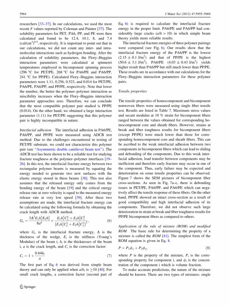
Figure 7 shows the SEM pictures of bicomponent fiber

cross-sections. As seen in Fig. 7a–c, there is debonding

issues in PET/PE, PA6/PP, and PA6/PE which can nega-

tively affect the tensile response of these fibers. On the other

hand, PP/PE showed an intact cross-section as a result of

good compatibility and high interfacial adhesion of its

components. Therefore, we did not observe such large

deterioration in strain at break and fiber toughness results for

PP/PE bicomponent fibers as compared to others.

Application of the rule of mixture (ROM) and modified

ROM The basic rule for determining the property of a

mixture is called the ROM [41]. The simplest form of the

ROM equation is given in Eq. 8.

P ¼ P1/1 þ P2/2; ð8Þ

where P is the property of the mixture, Pi is the corre-

sponding property for component i, and /i is the concen-

tration of the component i which is volume fraction.

To make accurate predictions, the nature of the mixture

should be known. There are two types of mixtures: single

5964 J Mater Sci (2012) 47:5955–5969

123

phase and two phase. In the single-phase systems, com-

ponents are miscible or soluble in each other such as

miscible copolymers. Properties of this type of mixture can

be predicted by using Eq. 9. On the other hand, in the two-

phase systems, components are immiscible or partially

miscible in each other such as composites. The mixture

rule for this type of system is given in Eq. 10 which is a

modified version of the ROM (MROM) and may be

applicable to a mixture with two continuous phases, e.g.,

laminates and block copolymers.

P ¼ P1/1 þ P2/2 þ I/1/2; ð9Þ

where I is the interaction term which is related to

intermolecular interactions and packing. It must be

determined empirically from experiment data and can be

either positive or negative. If there is no interaction, I = 0.

Pn ¼ Pn1/1 þ Pn

2/2; ð10Þ

where n is a constant and determined by the type of the

system and kind of the property.

The ROM is also a simple and useful tool to predict

some properties of composite materials. For instance,

micromechanical behavior of unidirectionally aligned

long-fiber composite can be predicted this way [42].

Bicomponent fibers having a core–sheath structure can also

be treated as a unidirectional composite where the core

polymer replaces reinforcement fiber and sheath polymer is

considered as a matrix. Hence, bicomponent fibers were

treated as a composite material and the applicability of the

ROM to the bicomponent fibers was investigated in this

study.

The ROM (Eq. 9) was applied to predict the maximum

stress values of bicomponent nonwoven fibers. In our

treatment, the ROM does not account any positive or

negative interaction between two components (I = O), so

Eq. 9 becomes the simple form of the ROM given in Eq. 8.

Hence, it predicts the maximum stress values of bicom-

ponent fiber without having any intermolecular interactions

and packing between sheath and core component.

We also applied the MROM (Eq. 10) to account for any

positive and negative interaction between the components

and predicted the maximum stress values of bicomponent

nonwoven fibers. Typically, upper bound value for n in

Eq. 10 is considered to be 1. However, our treatment

includes n values that are [1. By doing so, we aimed to

predict the properties of polymer pairs that can also show

intermolecular interactions and packing. To determine

n values, we performed a regression analysis.

0

15

30

45

60

PP/PE PA6/PE PA6/PP

Inte

rfac

ial F

ract

ure

Ene

rgy,

Gc

(J/m

2 )

Fig. 6 Interfacial fracture energies for polymer pairs used in

bicomponent nonwoven fibers (error bars the standard error)

Table 7 Tensile properties of homocomponent and bicomponent nonwoven fibers (standard errors are given in parentheses)

Polymers (c/s) Polymer ratios

(wt/wt%)

Fiber denier Maximum

stress (MPa)

Strain at

break (%)

Fiber toughness

(MPa)

Secant modulus

at 10 % (MPa)

PET/PE 0/100 1.66 (±0.05) 96 (±2) 371 (±11) 367 (±7) 504 (±12)

50/50 1.65 (±0.05) 169 (±4) 79 (±3) 84 (±3) 546 (±48)

75/25 1.64 (±0.07) 234 (±9) 85 (±6) 115 (±9) 602 (±66)

100/0 1.78 (±0.14) 360 (±10) 106 (±6) 200 (±13) 691 (±96)

PA6/PE 0/100 1.66 (±0.05) 96 (±2) 371 (±11) 367 (±7) 504 (±12)

50/50 1.63 (±0.05) 262 (±3) 106 (±3) 166 (±6) 573 (±25)

75/25 1.54 (±0.04) 390 (±4) 115 (±4) 266 (±11) 708 (±43)

100/0 1.63 (±0.06) 501 (±4) 148 (±6) 414 (±18) 718 (±20)

PA6/PP 0/100 1.44 (±0.05) 157 (±4) 333 (±15) 362 (±27) 492 (±18)

50/50 1.72 (±0.03) 274 (±4) 104 (±2) 172 (±3) 566 (±19)

75/25 1.71 (±0.06) 380 (±7) 119 (±5) 267 (±12) 690 (±11)

100/0 1.63 (±0.06) 501 (±4) 148 (±6) 414 (±18) 718 (±20)

PP/PE 0/100 1.66 (±0.05) 96 (±2) 371 (±11) 367 (±7) 504 (±12)

50/50 1.62 (±0.07) 130 (±3) 294 (±20) 289 (±21) 514 (±25)

75/25 1.62 (±0.05) 153 (±2) 355 (±15) 394 (±19) 507 (±25)

100/0 1.44 (±0.05) 157 (±4) 333 (±15) 362 (±27) 492 (±18)

J Mater Sci (2012) 47:5955–5969 5965

123

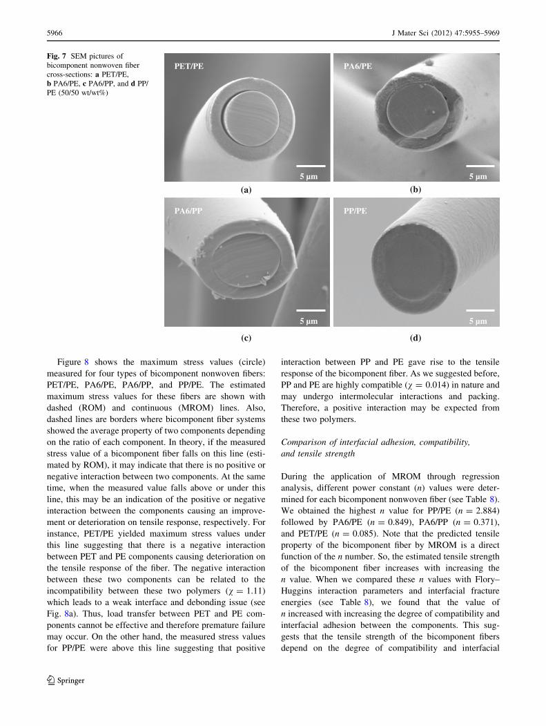
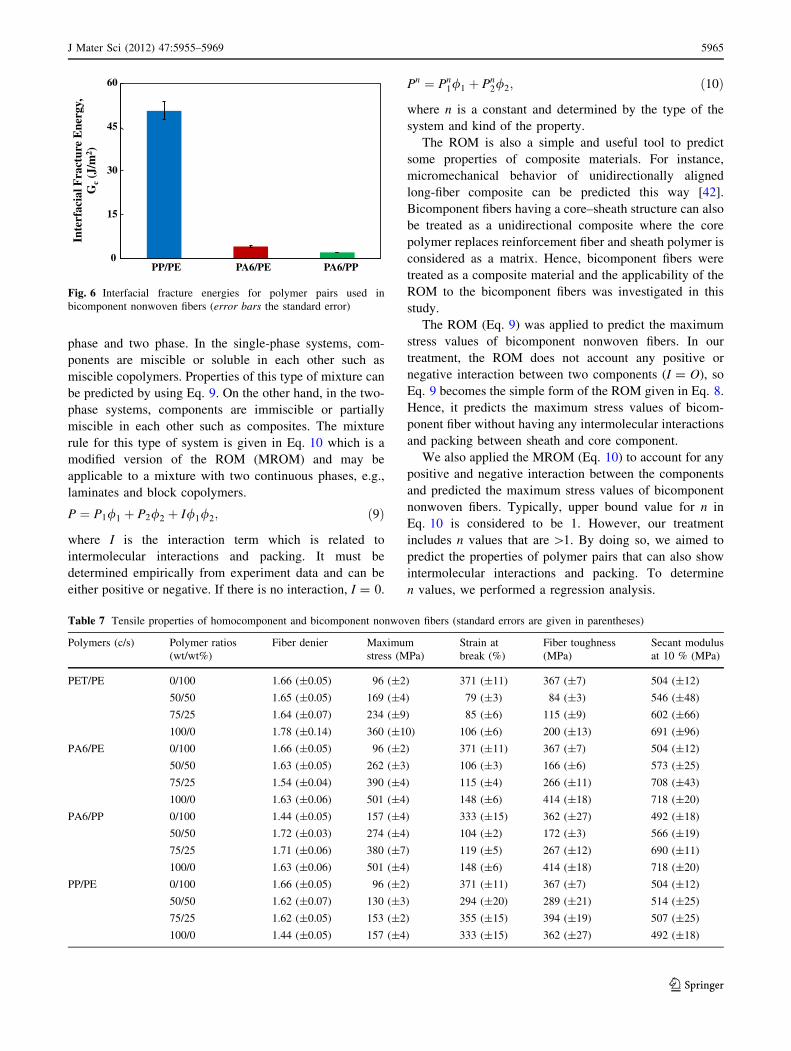
Figure 8 shows the maximum stress values (circle)

measured for four types of bicomponent nonwoven fibers:

PET/PE, PA6/PE, PA6/PP, and PP/PE. The estimated

maximum stress values for these fibers are shown with

dashed (ROM) and continuous (MROM) lines. Also,

dashed lines are borders where bicomponent fiber systems

showed the average property of two components depending

on the ratio of each component. In theory, if the measured

stress value of a bicomponent fiber falls on this line (esti-

mated by ROM), it may indicate that there is no positive or

negative interaction between two components. At the same

time, when the measured value falls above or under this

line, this may be an indication of the positive or negative

interaction between the components causing an improve-

ment or deterioration on tensile response, respectively. For

instance, PET/PE yielded maximum stress values under

this line suggesting that there is a negative interaction

between PET and PE components causing deterioration on

the tensile response of the fiber. The negative interaction

between these two components can be related to the

incompatibility between these two polymers (v = 1.11)

which leads to a weak interface and debonding issue (see

Fig. 8a). Thus, load transfer between PET and PE com-

ponents cannot be effective and therefore premature failure

may occur. On the other hand, the measured stress values

for PP/PE were above this line suggesting that positive

interaction between PP and PE gave rise to the tensile

response of the bicomponent fiber. As we suggested before,

PP and PE are highly compatible (v = 0.014) in nature and

may undergo intermolecular interactions and packing.

Therefore, a positive interaction may be expected from

these two polymers.

Comparison of interfacial adhesion, compatibility,

and tensile strength

During the application of MROM through regression

analysis, different power constant (n) values were deter-

mined for each bicomponent nonwoven fiber (see Table 8).

We obtained the highest n value for PP/PE (n = 2.884)

followed by PA6/PE (n = 0.849), PA6/PP (n = 0.371),

and PET/PE (n = 0.085). Note that the predicted tensile

property of the bicomponent fiber by MROM is a direct

function of the n number. So, the estimated tensile strength

of the bicomponent fiber increases with increasing the

n value. When we compared these n values with Flory–

Huggins interaction parameters and interfacial fracture

energies (see Table 8), we found that the value of

n increased with increasing the degree of compatibility and

interfacial adhesion between the components. This sug-

gests that the tensile strength of the bicomponent fibers

depend on the degree of compatibility and interfacial

5 µm

PET/PE

5 µm

PA6/PE

5 µm

PA6/PP

5 µm

PP/PE

(a) (b)

(c) (d)

Fig. 7 SEM pictures of

bicomponent nonwoven fiber

cross-sections: a PET/PE,

b PA6/PE, c PA6/PP, and d PP/

PE (50/50 wt/wt%)

5966 J Mater Sci (2012) 47:5955–5969

123

adhesion between the components. For example, PP/PE

bicomponent nonwoven fiber had the highest n value of

2.884 and showed the highest degree of compatibility

(v = 0.014) and interfacial adhesion (50.6 J/m2).

The relation between compatibility and tensile strength

of the bicomponent fibers can also allow us to establish

a physical meaning to the n value in terms of polymer

compatibility. It can be said that for incompatible poly-

mer pairings n values\1 can be expected. When a polymer

pairing passes through the incompatible region, the n then

becomes 1 and if there is any positive interaction (e.g.,

intermolecular reaction or entanglement) between compo-

nents, the n will further go up. Therefore, the n can be a

useful tool to screen and evaluate polymer compatibilities

and possible interaction which is either already existing or

introduced afterward. However, it is important to point out

that n cannot be a global constant for all type of systems

because processing conditions may affect mechanical

properties. But we may observe similar trends for similar

polymer systems.

From a practical point of view, the results listed in

Tables 7 and 8 provide a reference guide for those who

want to estimate the degree of the compatibility of poly-

mers and its effect on the tensile strength of the bicom-

ponent nonwoven fibers. In light of this study, after

obtaining the Flory–Huggins interaction parameter for a

spinnable polymer pairings, the interfacial behavior of the

bicomponent fiber may be practically estimated by com-

paring with polymer combinations studied here.

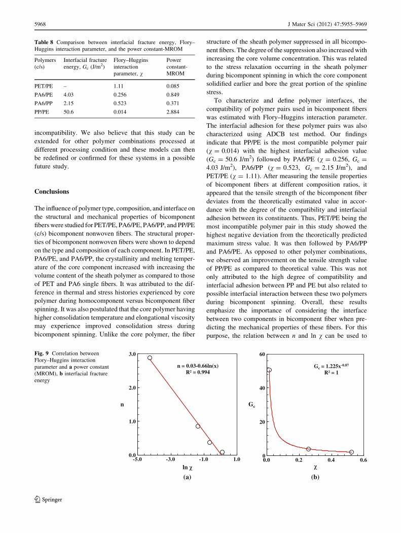
It is also possible to establish a mathematical relation

among v, n, and Gc values (see Fig. 9). After correlating

these values, we obtained linear relations between n and ln

v (see Fig. 9a). Also, a power law relation between Gc and

v was determined (see Fig. 9b). These mathematical

models strengthen our conclusion based on the dependence

of interfacial adhesion and tensile response on polymer

(a) (b)

(c) (d)

50

150

250

350

0.0 0.2 0.4 0.6 0.8 1.0

Max

imum

Str

ess

(MP

a)

PET Volume Fraction

PET/PE

ROM

MROM (n=0.09)

50

200

350

500

0.0 0.2 0.4 0.6 0.8 1.0

Max

imum

Str

ess

(MP

a)

PA6 Volume Fraction

PA6/PE

ROM

MROM (n=0.85)

100

250

400

550

0.0 0.2 0.4 0.6 0.8 1.0

Max

imum

Str

ess

(MP

a)

PA6 Volume Fraction

PA6/PP

ROM

MROM (n=0.37)

80

110

140

170

0.0 0.2 0.4 0.6 0.8 1.0

Max

imum

Str

ess

(MP

a)

PP Volume Fraction

PP/PE

ROM

MROM (n=2.88)

Fig. 8 Measured and estimated

tensile strength values for

bicomponent nonwoven fibers:

a PET/PE, b PA6/PE, c PA6/PP,

and d PP/PE

J Mater Sci (2012) 47:5955–5969 5967

123

incompatibility. We also believe that this study can be

extended for other polymer combinations processed at

different processing condition and these models can then

be redefined or confirmed for these systems in a possible

future study.

Conclusions

The influence of polymer type, composition, and interface on

the structural and mechanical properties of bicomponent

fibers were studied for PET/PE, PA6/PE, PA6/PP, and PP/PE

(c/s) bicomponent nonwoven fibers. The structural proper-

ties of bicomponent nonwoven fibers were shown to depend

on the type and composition of each component. In PET/PE,

PA6/PE, and PA6/PP, the crystallinity and melting temper-

ature of the core component increased with increasing the

volume content of the sheath polymer as compared to those

of PET and PA6 single fibers. It was attributed to the dif-

ference in thermal and stress histories experienced by core

polymer during homocomponent versus bicomponent fiber

spinning. It was also postulated that the core polymer having

higher consolidation temperature and elongational viscosity

may experience improved consolidation stress during

bicomponent spinning. Unlike the core polymer, the fiber

structure of the sheath polymer suppressed in all bicompo-

nent fibers. The degree of the suppression also increased with

increasing the core volume concentration. This was related

to the stress relaxation occurring in the sheath polymer

during bicomponent spinning in which the core component

solidified earlier and bore the great portion of the spinline

stress.

To characterize and define polymer interfaces, the

compatibility of polymer pairs used in bicomponent fibers

was estimated with Flory–Huggins interaction parameter.

The interfacial adhesion for these polymer pairs was also

characterized using ADCB test method. Our findings

indicate that PP/PE is the most compatible polymer pair

(v = 0.014) with the highest interfacial adhesion value

(Gc = 50.6 J/m2) followed by PA6/PE (v = 0.256, Gc =

4.03 J/m2), PA6/PP (v = 0.523, Gc = 2.15 J/m2), and

PET/PE (v = 1.11). After measuring the tensile properties

of bicomponent fibers at different composition ratios, it

appeared that the tensile strength of the bicomponent fiber

deviates from the theoretically estimated value in accor-

dance with the degree of the compatibility and interfacial

adhesion between its constituents. Thus, PET/PE being the

most incompatible polymer pair in this study showed the

highest negative deviation from the theoretically predicted

maximum stress value. It was then followed by PA6/PP

and PA6/PE. As opposed to other polymer combinations,

we observed an improvement on the tensile strength value

of PP/PE as compared to theoretical value. This was not

only attributed to the high degree of compatibility and

interfacial adhesion between PP and PE but also related to

possible interfacial interaction between these two polymers

during bicomponent spinning. Overall, these results

emphasize the importance of considering the interface

between two components in bicomponent fiber when pre-

dicting the mechanical properties of these fibers. For this

purpose, the relation between n and ln v can be used to

Table 8 Comparison between interfacial fracture energy, Flory–

Huggins interaction parameter, and the power constant-MROM

Polymers

(c/s)

Interfacial fracture

energy, Gc (J/m2)

Flory–Huggins

interaction

parameter, v

Power

constant-

MROM

PET/PE – 1.11 0.085

PA6/PE 4.03 0.256 0.849

PA6/PP 2.15 0.523 0.371

PP/PE 50.6 0.014 2.884

Gc = 1.225x-0.87

R² = 1

0

20

40

60

0.0 0.2 0.4 0.6

Gc

n = 0.03-0.66ln(x)R² = 0.994

0.0

1.0

2.0

3.0

-5.0 -3.0 -1.0 1.0

n

ln

(a) (b)

Fig. 9 Correlation between

Flory–Huggins interaction

parameter and a power constant

(MROM), b interfacial fracture

energy

5968 J Mater Sci (2012) 47:5955–5969

123

determine the deviation in actual tensile response of a

bicomponent fiber system from the theoretically estimated

value. One of the other important outputs of this study is

that it provides a reference guide and path for those who

want to predict the interfacial behavior of a spinnable

polymer pairings in bicomponent fiber structure. This can

be achieved practically by calculating the Flory–Huggins

interaction parameter for the polymer pairings and using

the relation between Gc and v or comparing with results

presented in this study.

References

1. Cooke TF (1996) In: Lewin M, Preston J (eds) High technology

fibers, part D. Marcel Dekker Inc, New York

2. Wilkie AE (1999) Int Nonwovens J 8:146

3. Khatwani PA, Yardi SS (2003) Man Made Text India 46:19

4. Jeffries R (1971) Bicomponent fibres. Merrow Publishing Co.

Ltd, Watford

5. Zhang JM, Peijs T (2010) Composites Part A 41:964. doi:

10.1016/j.compositesa.2010.03.012

6. Dasdemir M, Maze B, Anantharamaiah N et al (2011) J Mater Sci

46:3269. doi:10.1007/s10853-010-5214-9

7. Kikutani T, Arikawa S, Takaku A et al (1995) Sen-i Gakkaishi

51:408

8. Kikutani T, Radhakrishnan J, Arikawa S et al (1996) J Appl

Polym Sci 62:1913. doi:10.1002/(SICI)1097-4628(19961212)62:

11\1913:AID-APP16[3.0.CO;2-Z

9. Radhakrishnan J, Kikutani T, Okui N (1996) Sen-i Gakkaishi

52:618

10. Radhakrishnan J, Kikutani T, Okui N (1997) Text Res J 67:684

11. Cho HH, Kim KH, Kang YA et al (2000) J Appl Polym

Sci 77:2254. doi:10.1002/1097-4628(20000906)77:10\2254:AID-

APP19[3.0.CO;2-M

12. Cho HH, Kim KH, Kang YA et al (2000) J Appl Polym

Sci 77:2267. doi:10.1002/1097-4628(20000906)77:10\2267:AID-

APP20[3.0.CO;2-5

13. Shi XQ, Ito H, Kikutani T (2006) Polymer 47:611. doi:10.1016/

j.polymer.2005.11.051

14. Fedorova N (2006) Ph.D. Dissertation. North Carolina State

University, Raleigh, NC

15. Houis S, Schmid M, Lubben J (2007) J Appl Polym Sci 106:1757.

doi:10.1002/app.26846

16. El-Salmawy A, Kimura Y (2001) Text Res J 71:145. doi:10.1177/

004051750107100209

17. Iroh JO (1999) In: Mark JE (ed) Polymer data handbook. Oxford

University Press, New York

18. Durany A, Anantharamaiah N, Pourdeyhimi B (2008) Interna-

tional nonwovens technical conference, Houston, TX

19. Boucher E, Folkers JP, Hervet H et al (1996) Macromolecules

29:774. doi:10.1021/ma9509422

20. Brown HR (2001) Macromolecules 34:3720. doi:10.1021/ma9

91821v

21. Creton C, Kramer EJ, Hui CY et al (1992) Macromolecules

25:3075. doi:10.1021/ma00038a010

22. Eastwood EA, Dadmun MD (2002) Macromolecules 35:5069.

doi:10.1021/ma011701z

23. Laurens C, Creton C, Loger L (2004) Macromolecules 37:6814.

doi:10.1021/ma0400259

24. Seo Y, Kim H (2008) Int J Mater Form 1:795

25. Washiyama J, Kramer EJ, Hui CY (1993) Macromolecules

26:2928. doi:10.1021/ma00063a043

26. Washiyama J, Kramer EJ, Creton CF et al (1994) Macromole-

cules 27:2019. doi:10.1021/ma00086a007

27. Choi YB, Kim SY (1999) J Appl Polym Sci 74:2083. doi:

10.1002/(SICI)1097-4628(19991121)74:8\2083:AID-APP25[3.

0.CO;2-G

28. Wunderlich B (1973) Macromolecular physics. Academic Press,

New York

29. Mehta A, Gaur U, Wunderlich B (1978) J Polym Sci Polym Phys

Ed 16:289. doi:10.1002/pol.1978.180160209

30. Clark EJ, Hoffman JD (1984) Macromolecules 17:878. doi:

10.1021/ma00134a058

31. Runt J, Harrison IR (1980) In: Marton L, Marton C, Fava RA

(eds) Methods of experimental physics: polymers, crystal struc-

ture and morphology. Academic Press, New York

32. Bershteæin VA, Egorov VM (1994) Differential scanning calo-

rimetry of polymers: physics, chemistry, analysis, technology.

Ellis Horwood, New York

33. Small PA (1953) J Appl Chem 3:71

34. Hoy KL (1970) J Paint Technol 42:76

35. van Krevelen PW (1972) Properties of polymers. Elsevier,

Amsterdam

36. Coleman MM, Graf JF, Painter PC (1991) Specific interactions

and the miscibility of polymer blends: practical guides for pre-

dicting & designing miscible polymer mixtures. Technomic

Publishing Co, Lancaster, PA

37. Coleman MM, Painter PC (2006) Miscible polymer blends

background and guide for calculations and design. DEStech

Publications, Inc, Lancaster, PA

38. Benkoski JJ, Flores P, Kramer EJ (2003) Macromolecules 36:

3289. doi:10.1021/ma034013j

39. Kim H, Rafailovich M, Sokolov J (2004) Polym Int 53:287. doi:

10.1002/pi.1367

40. Kanninen MF (1973) Int J Fract 9:83

41. Nielsen LE (1978) Predicting the properties of mixtures. Marcel

Dekker, Inc., New York

42. Mallick PK (2008) Fiber-reinforced composites: materials,

manufacturing, and design. CRC Press, Boca Raton, FL

J Mater Sci (2012) 47:5955–5969 5969

123