1 3

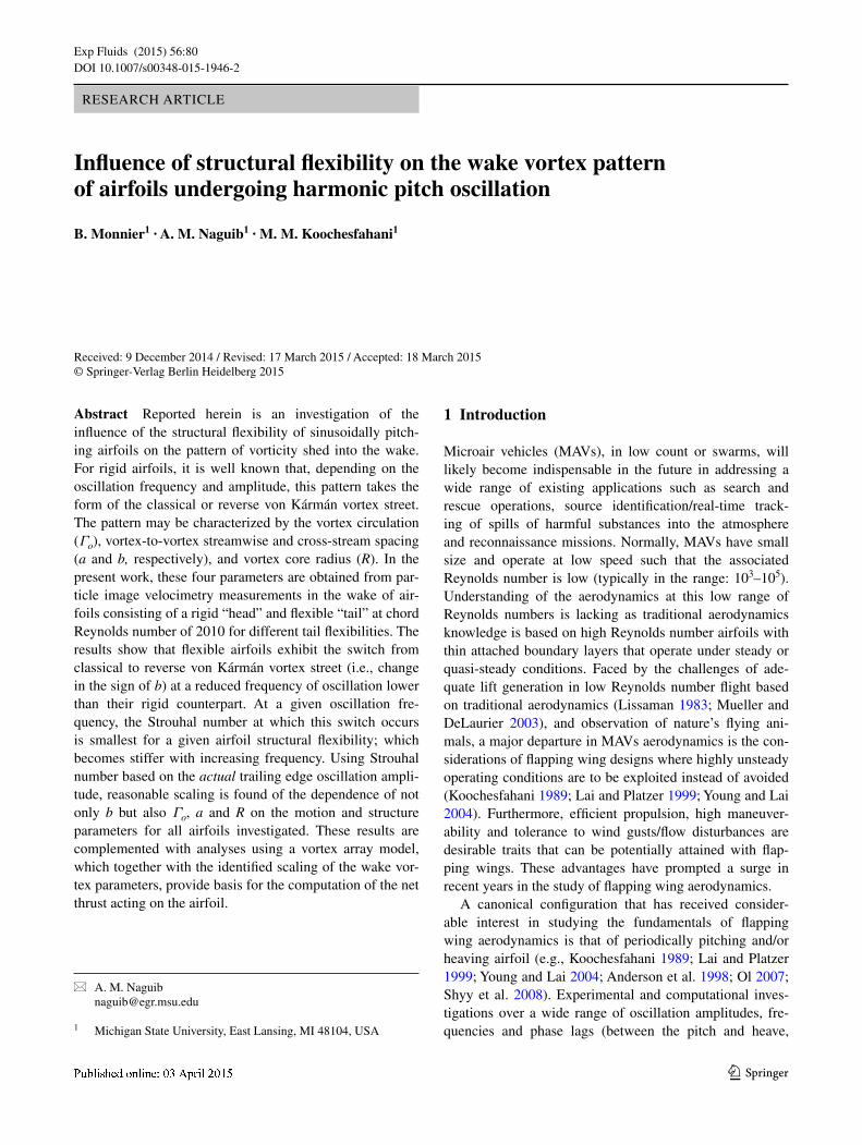
Exp Fluids (2015) 56:80 DOI 10.1007/s00348-015-1946-2

RESEARCH ARTICLE

Influence of structural flexibility on the wake vortex pattern of airfoils undergoing harmonic pitch oscillation

B. Monnier1 · A. M. Naguib1 · M. M. Koochesfahani1

Received: 9 December 2014 / Revised: 17 March 2015 / Accepted: 18 March 2015 © Springer-Verlag Berlin Heidelberg 2015

1 Introduction

Microair vehicles (MAVs), in low count or swarms, will likely become indispensable in the future in addressing a wide range of existing applications such as search and rescue operations, source identification/real-time track-ing of spills of harmful substances into the atmosphere and reconnaissance missions. Normally, MAVs have small size and operate at low speed such that the associated Reynolds number is low (typically in the range: 103–105). Understanding of the aerodynamics at this low range of Reynolds numbers is lacking as traditional aerodynamics knowledge is based on high Reynolds number airfoils with thin attached boundary layers that operate under steady or quasi-steady conditions. Faced by the challenges of ade-quate lift generation in low Reynolds number flight based on traditional aerodynamics (Lissaman 1983; Mueller and DeLaurier 2003), and observation of nature’s flying ani-mals, a major departure in MAVs aerodynamics is the con-siderations of flapping wing designs where highly unsteady operating conditions are to be exploited instead of avoided (Koochesfahani 1989; Lai and Platzer 1999; Young and Lai 2004). Furthermore, efficient propulsion, high maneuver-ability and tolerance to wind gusts/flow disturbances are desirable traits that can be potentially attained with flap-ping wings. These advantages have prompted a surge in recent years in the study of flapping wing aerodynamics.

A canonical configuration that has received consider-able interest in studying the fundamentals of flapping wing aerodynamics is that of periodically pitching and/or heaving airfoil (e.g., Koochesfahani 1989; Lai and Platzer 1999; Young and Lai 2004; Anderson et al. 1998; Ol 2007; Shyy et al. 2008). Experimental and computational inves-tigations over a wide range of oscillation amplitudes, fre-quencies and phase lags (between the pitch and heave,

Abstract Reported herein is an investigation of the influence of the structural flexibility of sinusoidally pitch-ing airfoils on the pattern of vorticity shed into the wake. For rigid airfoils, it is well known that, depending on the oscillation frequency and amplitude, this pattern takes the form of the classical or reverse von Kármán vortex street. The pattern may be characterized by the vortex circulation (Γo), vortex-to-vortex streamwise and cross-stream spacing (a and b, respectively), and vortex core radius (R). In the present work, these four parameters are obtained from par-ticle image velocimetry measurements in the wake of air-foils consisting of a rigid “head” and flexible “tail” at chord Reynolds number of 2010 for different tail flexibilities. The results show that flexible airfoils exhibit the switch from classical to reverse von Kármán vortex street (i.e., change in the sign of b) at a reduced frequency of oscillation lower than their rigid counterpart. At a given oscillation fre-quency, the Strouhal number at which this switch occurs is smallest for a given airfoil structural flexibility; which becomes stiffer with increasing frequency. Using Strouhal number based on the actual trailing edge oscillation ampli-tude, reasonable scaling is found of the dependence of not only b but also Γo, a and R on the motion and structure parameters for all airfoils investigated. These results are complemented with analyses using a vortex array model, which together with the identified scaling of the wake vor-tex parameters, provide basis for the computation of the net thrust acting on the airfoil.

* A. M. Naguib naguib@egr.msu.edu

1 Michigan State University, East Lansing, MI 48104, USA

Exp Fluids (2015) 56:80

1 3

80 Page 2 of 17

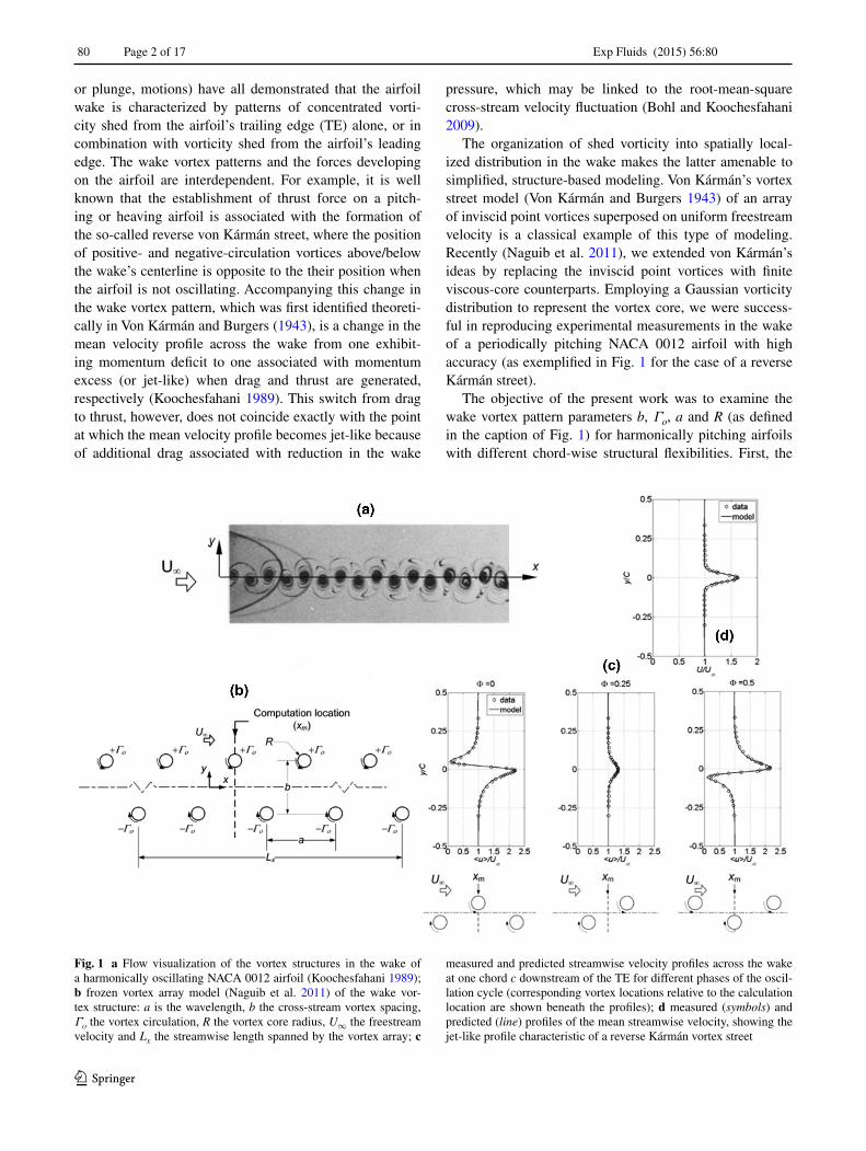
or plunge, motions) have all demonstrated that the airfoil wake is characterized by patterns of concentrated vorti-city shed from the airfoil’s trailing edge (TE) alone, or in combination with vorticity shed from the airfoil’s leading edge. The wake vortex patterns and the forces developing on the airfoil are interdependent. For example, it is well known that the establishment of thrust force on a pitch-ing or heaving airfoil is associated with the formation of the so-called reverse von Kármán street, where the position of positive- and negative-circulation vortices above/below the wake’s centerline is opposite to the their position when the airfoil is not oscillating. Accompanying this change in the wake vortex pattern, which was first identified theoreti-cally in Von Kármán and Burgers (1943), is a change in the mean velocity profile across the wake from one exhibit-ing momentum deficit to one associated with momentum excess (or jet-like) when drag and thrust are generated, respectively (Koochesfahani 1989). This switch from drag to thrust, however, does not coincide exactly with the point at which the mean velocity profile becomes jet-like because of additional drag associated with reduction in the wake

pressure, which may be linked to the root-mean-square cross-stream velocity fluctuation (Bohl and Koochesfahani 2009).

The organization of shed vorticity into spatially local-ized distribution in the wake makes the latter amenable to simplified, structure-based modeling. Von Kármán’s vortex street model (Von Kármán and Burgers 1943) of an array of inviscid point vortices superposed on uniform freestream velocity is a classical example of this type of modeling. Recently (Naguib et al. 2011), we extended von Kármán’s ideas by replacing the inviscid point vortices with finite viscous-core counterparts. Employing a Gaussian vorticity distribution to represent the vortex core, we were success-ful in reproducing experimental measurements in the wake of a periodically pitching NACA 0012 airfoil with high accuracy (as exemplified in Fig. 1 for the case of a reverse Kármán street).

The objective of the present work was to examine the wake vortex pattern parameters b, Γo, a and R (as defined in the caption of Fig. 1) for harmonically pitching airfoils with different chord-wise structural flexibilities. First, the

Fig. 1 a Flow visualization of the vortex structures in the wake of a harmonically oscillating NACA 0012 airfoil (Koochesfahani 1989); b frozen vortex array model (Naguib et al. 2011) of the wake vor-tex structure: a is the wavelength, b the cross-stream vortex spacing, Γο the vortex circulation, R the vortex core radius, U∞ the freestream velocity and Lx the streamwise length spanned by the vortex array; c

measured and predicted streamwise velocity profiles across the wake at one chord c downstream of the TE for different phases of the oscil-lation cycle (corresponding vortex locations relative to the calculation location are shown beneath the profiles); d measured (symbols) and predicted (line) profiles of the mean streamwise velocity, showing the jet-like profile characteristic of a reverse Kármán vortex street

Exp Fluids (2015) 56:80

1 3

Page 3 of 17 80

general relationship between variation in these param-eters and the mean thrust force acting on the airfoil will be investigated using the vortex array model of Naguib et al. (2011). Subsequently, the influence of airfoil flexibility and oscillation frequency and amplitude on the wake vortex parameters will be examined employing an experimental study. The combination of the model and the experimen-tal results will help identify airfoil flexure characteristics and motion parameters that are favorable to thrust gen-eration. This information may then be capitalized upon in future wake control schemes aiming to manipulate the thrust acting on the airfoil via alteration of the wake vortex configuration.

It should be noted that though several studies exist of airfoils having chord-wise structural flexibility [e.g., (Heathcote and Gursul 2007; Liu 2009; Thiria and Godoy-Diana 2010; Kang et al. 2011)], none of these is focused on quantifying the wake vortex pattern and their dependence on motion and structural parameters. Instead, these studies, and others not cited here for brevity, are concerned with the effect of structural flexibility on the forces and thrust efficiency. In addition to enabling new ideas for wake con-trol, as stated above, the present focus on the wake vortex pattern is motivated by the possibility of coupling knowl-edge of the wake pattern parameters with the vortex array model in a semiempirical tool for engineering calculations of the net thrust acting on oscillating airfoils. Specifically, we seek to identify appropriate scaling of the vortex pattern parameters with variation in the airfoil’s motion and struc-tural parameters. Such empirically identified scaling can then be used to specify the vortex configuration for a given application, which in turn can be used with the vortex array model to calculate the thrust force.

2 Experimental setup

The present measurements take place in a free-surface closed-return water tunnel with test section dimensions of 19 cm × 15.3 cm × 43.4 cm in height, width and length,

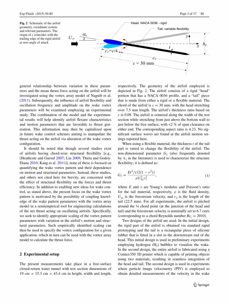
respectively. The geometry of the airfoil employed is depicted in Fig. 2. The airfoil consists of a rigid “head” portion that has a NACA 0036 profile, and a “tail” piece that is made from either a rigid or a flexible material. The chord of the airfoil is c = 30 mm, with the head stretching over 7.5 mm length. The airfoil’s thickness ratio based on c is 0.09. The airfoil is centered along the width of the test section while stretching from just above the bottom wall to just below the free surface, with <2 % of span clearance on either end. The corresponding aspect ratio is 4.23. No sig-nificant surface waves are found at the airfoil motion set-tings reported here.

When using a flexible material, the thickness t of the tail part is varied to change the flexibility of the airfoil. The non-dimensional parameter G1 (also frequently denoted by π1 in the literature) is used to characterize the structure flexibility; it is defined as:

where E and ν are Young’s modulus and Poisson’s ratio for the tail material, respectively, ρ is the fluid density, U∞ is the freestream velocity, and c2 is the length of the tail (22.5 mm). For all experiments, the airfoil is pitched around the ¼ chord point (at the junction of the head and tail) and the freestream velocity is nominally set to 6.7 cm/s (corresponding to a chord Reynolds number Rec = 2010).

Two designs of the airfoil are used. In the initial design, the rigid part of the airfoil is obtained via standard rapid prototyping and the tail is a rectangular piece of silicone rubber that is fitted in a slot in the downstream end of the head. This initial design is used in preliminary experiments employing hydrogen (H2) bubbles to visualize the wake. In the second design, the entire airfoil is fabricated using a Connex350 3D printer which is capable of printing objects using two materials, resulting in seamless integration of the head and tail. The second design is used in experiments where particle image velocimetry (PIV) is employed to obtain detailed measurements of the velocity in the wake

(1)G1 =Et3/(12(1 − ν2))

ρU2∞

c32

,

Fig. 2 Schematic of the airfoil geometry, coordinate system and relevant parameters. The origin of x coincides with the trailing edge of the rigid airfoil at zero angle of attack

Exp Fluids (2015) 56:80

1 3

80 Page 4 of 17

of the airfoil. The characteristics (t and G1) of both designs are shown in Table 1 for all the experiments presented here.

In both the flow visualization and PIV studies, the airfoil is pitched symmetrically around a mean angle of attack of zero with an amplitude αo and frequency f. Table 1 summa-rizes the range of frequencies and amplitudes investigated in this work. The corresponding reduced frequencies and Strouhal numbers are also listed; note that hp is the peak-to-peak trailing edge displacement amplitude of the rigid airfoil; see Fig. 2. The airfoil pitching motion is imposed using a servo motor controlled by a Galil DMC-1030 con-troller. The motor is installed on top of the test section, and the airfoil is held vertically. The angular motion of the motor is captured using an optical encoder.

The H2 bubble flow visualization is performed using a 50-μm (0.002-in.)-diameter stainless steel wire that is placed just downstream of the trailing edge of the airfoil. A function generator delivering a square wave signal, ampli-fied by a dedicated amplifier, provides the voltage neces-sary to activate the H2 electrolysis. The frequency of the square wave is set to 15 Hz, and the resulting hydrogen-bubble images are recorded at a rate of 30 frames/s using a Pulnix 1040 camera (1024 pixel × 1024 pixel).

For PIV measurements, silver-coated hollow glass spheres (Potter Industries Inc.-SH400S20) with a mean diameter of about 20 μm are used to seed the flow. A 500 mW Lasiris Magnum SP Laser operating at a wave-length of 680 nm is employed to illuminate the glass spheres in the wake of the airfoil at about mid-span. A 12-bit 1392 pixel × 1024 pixel PCO Pixelfly QE camera is used to record the PIV snapshots. The camera and laser pulses are synchronized using a Stanford Research Sys-tems DG535 digital delay generator. One thousand pairs of images are acquired and processed for each case at the maximal frequency allowed by our setup (5 Hz). The PIV region of interest is limited to the wake region and is about 1.5 chord long in the streamwise (x) direction and 2 chord wide in the cross-stream (y) direction. Interrogation of PIV images is done using the code by Thielicke and Stamhuis (http://pivlab.blogspot.com), yielding a velocity vector for every 16 pixel × 16 pixel interrogation region (cor-responding to 0.028c × 0.028c). A three-point estimator with Gaussian fit is used to determine the cross-correlation

peak, which yields a 0.1 pixel rms uncertainty in particle displacement (Raffel et al. 2007) or 0.11 cm/s uncertainty in the velocity. Vector validation is implemented using a standard deviation and a local median check. The percent-age of bad vectors is typically 2–5 %. These are replaced via interpolation.

The actual trailing edge peak-to-peak displacement (hp,actual) is determined from images of the trailing edge, which is captured in the field of view of the flow visualiza-tion and PIV pictures. The trailing edge position is found as function of time, and the resulting time series is phase-sorted based on the imposed frequency of oscillation. The phase-sorted signal is checked for symmetry and harmonic fidelity, and only cases exhibiting asymmetry of <5 % of the peak-to-peak of the signal and harmonic fidelity of better than 99 % are presented in the current paper. Only a handful cases, particularly at the highest frequency and thinnest airfoil tail, did not meet these criteria. For all other cases, hp,actual is determined as the difference between the maximum and minimum of the phase-sorted signal. The uncertainty in measuring the trailing edge displacement is estimated as the root-mean-square of the difference between the measured and expected displacement of the rigid airfoil for all amplitudes and frequencies.

3 Model description and implications

In the following, the relationship between the wake vortex parameters, b, Γo and a and the mean thrust acting on the airfoil is explored using the vortex array model demon-strated in Fig. 1. The focus of the analysis is on “simple” wakes that are characterized by shedding of one positive and one negative vortex per airfoil oscillation cycle. Also, only the reverse Kármán vortex street configuration is con-sidered, where the vortex with positive (ccw) circulation is above the wake’s centerline (in the present choice of coor-dinate system), and vice versa, and the mean velocity pro-file is jet-like. This is done to focus the analysis on wake vortex characteristics that are favorable for thrust genera-tion. The analysis does include the “neutral wake,” where the centers of the opposite-signed vortices are colocated on the wake centerline, as a limiting case that separates

Table 1 Experimental conditions

Flow visualization/initial airfoil design PIV/new design

Frequency f 1–5 Hz in increments of 1 Hz 3.29, 4.27 and 5.23 Hz

Amplitude αo 1°–10° in increments of 1° 2°–7° in increments of 1°

Reduced frequency k = πfc/U∞ 1.41–7.03 4.63, 6.19 and 7.35

Strouhal number St = fhp/U∞ 0.01–0.58 0.08–0.43

t (mm) 0.8 and 1.6 0.8, 1.0 and 1.6

G1 0.6, 4.5 and 97 (rigid) 0.7, 1.3, 5.3 and 97 (rigid)

Exp Fluids (2015) 56:80

1 3

Page 5 of 17 80

conditions leading to mean velocity deficit from those lead-ing to mean velocity excess in the wake and the possibility of producing net mean thrust on the airfoil. Furthermore, to get insight into the influence of each of the three wake vor-tex parameters on the mean thrust, each parameter is varied independently from the other two. Inevitably, this approach results in a combination of parameters that may not coexist in physical observations since in reality all three parame-ters cannot be varied independently by changing the oscil-lation parameters of the airfoil. Nevertheless, the explored parameter space does include parameter combinations that are physically observable. Moreover, from flow control perspective, information from the explored parameter space can be useful for devising a wake control scheme that pro-duces a combination of wake vortex parameters desirable for thrust generation yet inaccessible through the oscilla-tion of the airfoil alone.

In Naguib et al. (2011), we showed that the mean streamwise force coefficient (Cf) acting on a harmonically pitching airfoil computed using the vortex array model is in good agreement with published results. For reference, the specific equations of the model are given by:

with

where subscript i represents the ith vortex in an array of N vortices (half of which have positive (ccw) circulation and the other half have negative (cw) circulation), xc and yc indicate the coordinates of the vortex core center, r is the distance from the core center to point (x, y) where the streamwise and cross-stream velocity components, u and v, respectively, are computed, and the remainder of the sym-bols are defined in the caption of Fig. 1.

To calculate the mean streamwise force coefficient Cf, the computed mean and root-mean-square (rms) veloc-ity profiles at a given streamwise location in the wake are substituted in the streamwise integral momentum equation, which simplifies to the following form for the flow con-sidered [see (Bohl and Koochesfahani 2009; Naguib et al. 2011)]:

where U is the mean streamwise velocity, urms and vrms are the streamwise and cross-stream rms velocities,

(2)u(x, y) = U∞ −

∑N

i=1

Γi(ri)

2π

(y − yci)

r2i

(3)v(x, y) =

∑N

i=1

Γi(ri)

2π

(x − xci)

r2i

(4)Γi(ri) = Γo

[

1 − e−(ri/Ri)2]

,

(5)Cf =2

c

∞∫

−∞

[

U

U∞

(

U

U∞

− 1

)

+u2

rms

U2∞

−v2

rms

U2∞

]

dy,

respectively. Equation (5) yields a positive value for Cf when a net thrust is acting on the airfoil and a negative value in the case of net drag. At sufficiently high oscillation frequency and/or amplitude, the wake structure switches to the reverse von Kármán configuration and the term on the right-hand side involving the mean streamwise velocity becomes positive, and hence, together with the term involv-ing the rms of the same velocity component, contributes to thrust. On the other hand, the term involving vrms is nega-tive definite and hence accounts for the presence of a drag component in Cf. In fact, this term is a substitution for the mean pressure term at the x location of the analysis, using the cross-stream integral momentum equation. For conveni-ence, upon establishment of the reverse von Kármán wake, Cf may be decomposed into thrust and drag components (Cf,t and Cf,d, respectively), where:

In the following discussion of each vortex parameter, the dependence of the model-computed profiles of U, urms and vrms on each of the wake vortex parameters will be exam-ined first. The outcome of this examination will be subse-quently used to interpret the trend seen in Cf variation with the wake vortex parameter under consideration. The range of parameter values employed in the analysis encompasses the values observed in the experimental component of the present investigation while spanning a somewhat wider parameter space to reveal some interesting limits of the wake configuration.

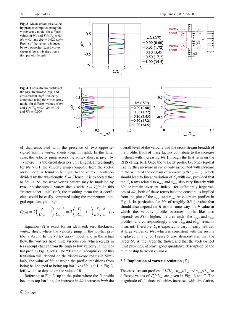
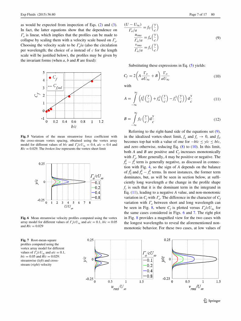
3.1 Implication of cross‑flow vortex spacing (b)

The cross-flow vortex spacing b is defined as the y-coor-dinate of the positive-signed vortex minus that of the neg-ative-signed vortex. As mentioned above, the analysis is conducted for the neutral and reverse von Kármán wakes, corresponding to b/c ≥ 0. Figure 3 (left) shows the pre-dicted mean streamwise velocity profiles for different val-ues of b/c. As expected, for the neutral wake (b/c = 0), the velocity profile is uniform and has a magnitude equal to the freestream velocity. As b/c increases, the profile becomes jet-like with the peak velocity exceeding the freestream velocity and becoming progressively larger. Beyond b/c = 0.1, the peak velocity magnitude does not increase anymore and additional increase of b/c merely results in the profile becoming wider in the y direction. Moreover, the shape of the profile becomes top-hat-like, reminiscent

(6)Cf ,t =2

c

∞∫

−∞

[

U

U∞

(

U

U∞

− 1

)

+u2

rms

U2∞

]

dy

(7)Cf ,d = −2

c

∞∫

−∞

[

v2rms

U2∞

]

dy

Exp Fluids (2015) 56:80

1 3

80 Page 6 of 17

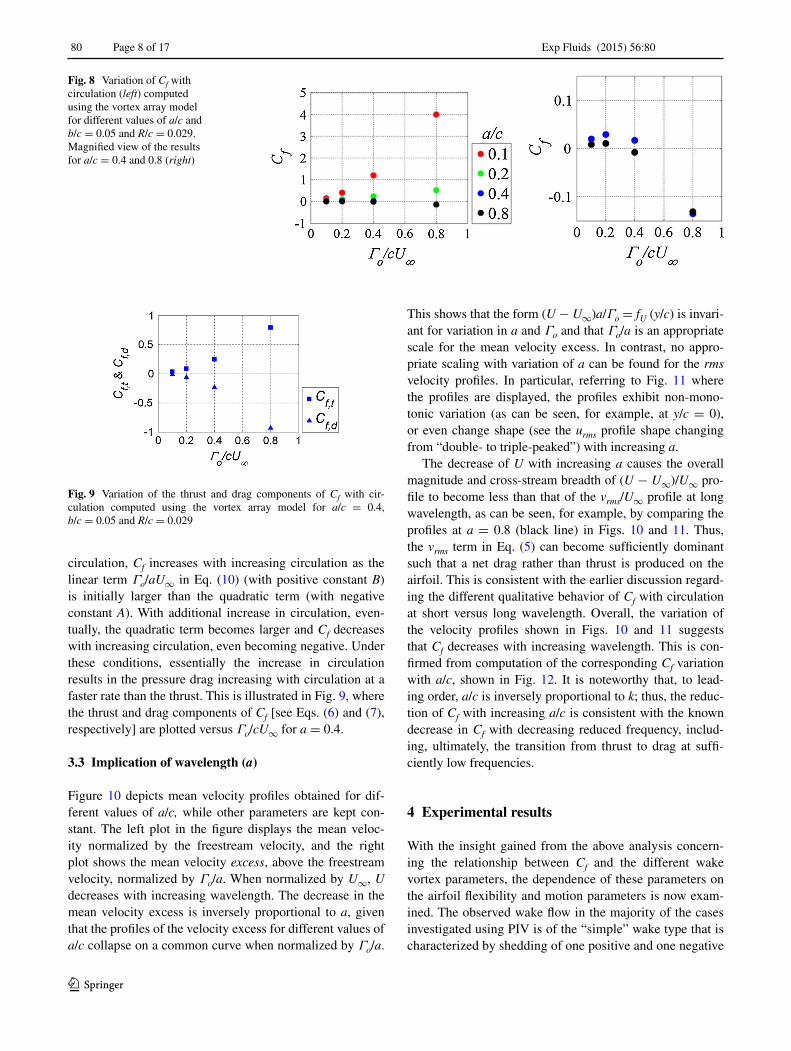
of that associated with the presence of two opposite-signed infinite vortex sheets (Fig. 3, right). In the latter case, the velocity jump across the vortex sheet is given by γ (where γ is the circulation per unit length). Interestingly, for b/c > 0.1, the velocity jump computed from the vortex array model is found to be equal to the vortex circulation divided by the wavelength: Γo/a. Hence, it is expected that as b/c → ∞, the wake vortex pattern may be modeled by two opposite-signed vortex sheets with γ = Γo/a. In this “vortex-sheet limit” (vsl), the resulting mean thrust coeffi-cient could be easily computed using the momentum inte-gral equation, yielding:

Equation (8) is exact for an idealized, zero thickness, vortex sheet, where the velocity jump in the top-hat pro-file is abrupt. In the vortex array model, and in the actual flow, the vortices have finite viscous core which results in less abrupt change from the high to low velocity in the top-hat profile (Fig. 3, left). The “degree of abruptness” of this transition will depend on the viscous-core radius R. Simi-larly, the value of b/c at which the profile transitions from being bell-shaped to being top-hat-like (b/c ≈ 0.1 in Fig. 3, left) will also depend on the value of R.

Referring to Fig. 3, up to the point where the U profile becomes top-hat-like, the increase in b/c increases both the

(8)Cf ,vsl = 2

(

γ

U∞

+ 1

)

γ

U∞

b

c= 2

(

Γo

aU∞

+ 1

)

Γo

aU∞

b

c

overall level of the velocity and the cross-stream breadth of the profile. Both of these factors contribute to the increase in thrust with increasing b/c [through the first term on the RHS of Eq. (6)]. Once the velocity profile becomes top-hat like, further increase in b/c is only associated with increase in the width of the domain of nonzero (U/U∞ − 1), which should lead to linear variation of Cf with b/c, provided that the Cf terms related to urms and vrms also vary linearly with b/c, or remain invariant. Indeed, for sufficiently large val-ues of b/c, both of these terms become constant as implied from the plot of the urms and vrms cross-stream profiles in Fig. 4. In particular, for b/c of roughly 0.5 (a value that should also depend on R in the same way the b value at which the velocity profile becomes top-hat-like also depends on R) or higher, the area under the urms and vrms profiles (and correspondingly under u2

rms and v2rms) remains

invariant. Therefore, Cf is expected to vary linearly with b/c at large values of b/c, which is consistent with the results displayed in Fig. 5. Figure 5 also demonstrates that the larger b/c is, the larger the thrust, and that the vortex-sheet limit provides, at least, good qualitative description of the relationship between Cf and b.

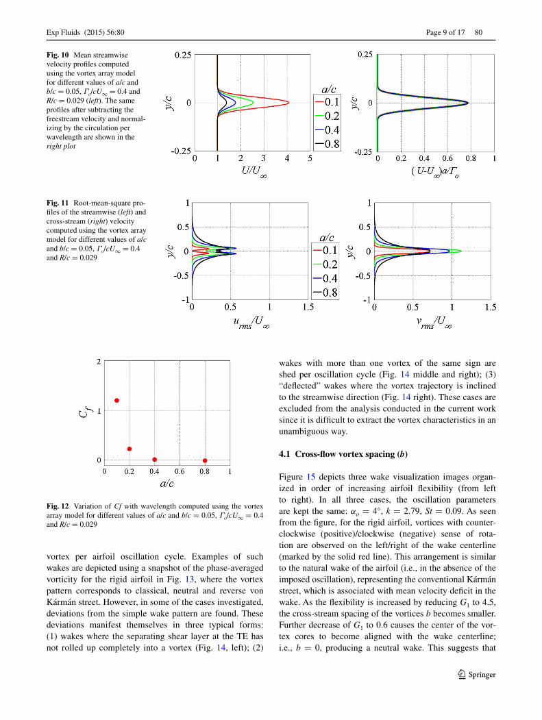
3.2 Implication of vortex circulation (Γο)

The cross-stream profiles of U/U∞, urms/U∞ and vrms/U∞ for different values of Γo/cU∞ are given in Figs. 6 and 7. The magnitude of all three velocities increases with circulation,

Fig. 3 Mean streamwise veloc-ity profiles computed using the vortex array model for different values of b/c and Γο/cU∞ = 0.4, a/c = 0.4 and R/c = 0.029 (left). Profile of the velocity induced by two opposite-signed vortex sheets (right). γ is the circula-tion per unit length

Fig. 4 Cross-stream profiles of the rms streamwise (left) and cross-stream (right) velocity computed using the vortex array model for different values of b/c and Γο/cU∞ = 0.4, a/c = 0.4 and R/c = 0.029

Exp Fluids (2015) 56:80

1 3

Page 7 of 17 80

as would be expected from inspection of Eqs. (2) and (3). In fact, the latter equations show that the dependence on Γo is linear, which implies that the profiles can be made to collapse by scaling them with a velocity scale based on Γo. Choosing the velocity scale to be Γo/a (also the circulation per wavelength; the choice of a instead of c for the length scale will be justified below), the profiles may be given by the invariant forms (when a, b and R are fixed):

Substituting these expressions in Eq. (5) yields:

with

Referring to the right-hand side of the equations set (9), in the idealized vortex-sheet limit, fu and fv → 0, and fU becomes top-hat with a value of one for −b/c ≤ y/c ≤ b/c, and zero otherwise, reducing Eq. (8) to (10). In this limit, both A and B are positive and Cf increases monotonically with Γo. More generally, A may be positive or negative. The fu2 − fv

2 term is generally negative, as discussed in connec-tion with Fig. 4, so the sign of A depends on the balance of fU

2 and fu2 − fv

2 terms. In most instances, the former term dominates, but, as will be seen in section below, at suffi-ciently long wavelength a the change in the profile shape fv is such that it is the dominant term in the integrand in Eq. (11), leading to a negative A value, and non-monotonic variation in Cf with Γo. The difference in the character of Cf variation with Γo between short and long wavelength can be seen in Fig. 8, where Cf is plotted versus Γo/cU∞ for the same cases considered in Figs. 6 and 7. The right plot in Fig. 8 provides a magnified view for the two cases with the longest wavelengths to reveal the aforementioned non-monotonic behavior. For these two cases, at low values of

(9)

(U − U∞)

Γo/a= fU

(y

c

)

urms

Γo/a= fu

(y

c

)

vrms

Γo/a= fv

(y

c

)

(10)Cf = 2

(

AŴo

aU∞

+ B

)

Ŵo

aU∞

(11)A =

∞∫

−∞

(

f 2U

(y

c

)

+ f 2u

(y

c

)

− f 2v

(y

c

))

dy

c

(12)B =

∞∫

−∞

fU

(y

c

)

dy

c

Fig. 5 Variation of the mean streamwise force coefficient with the cross-stream vortex spacing, obtained using the vortex array model for different values of b/c and Γο/cU∞ = 0.4, a/c = 0.4 and R/c = 0.029. The broken line represents the vortex-sheet limit

Fig. 6 Mean streamwise velocity profiles computed using the vortex array model for different values of Γο/cU∞ and a/c = 0.1, b/c = 0.05 and R/c = 0.029

Fig. 7 Root-mean-square profiles computed using the vortex array model for different values of Γο/cU∞ and a/c = 0.1, b/c = 0.05 and R/c = 0.029: streamwise (left) and cross-stream (right) velocity

Exp Fluids (2015) 56:80

1 3

80 Page 8 of 17

circulation, Cf increases with increasing circulation as the linear term Γo/aU∞ in Eq. (10) (with positive constant B) is initially larger than the quadratic term (with negative constant A). With additional increase in circulation, even-tually, the quadratic term becomes larger and Cf decreases with increasing circulation, even becoming negative. Under these conditions, essentially the increase in circulation results in the pressure drag increasing with circulation at a faster rate than the thrust. This is illustrated in Fig. 9, where the thrust and drag components of Cf [see Eqs. (6) and (7), respectively] are plotted versus Γo/cU∞ for a = 0.4.

3.3 Implication of wavelength (a)

Figure 10 depicts mean velocity profiles obtained for dif-ferent values of a/c, while other parameters are kept con-stant. The left plot in the figure displays the mean veloc-ity normalized by the freestream velocity, and the right plot shows the mean velocity excess, above the freestream velocity, normalized by Γo/a. When normalized by U∞, U decreases with increasing wavelength. The decrease in the mean velocity excess is inversely proportional to a, given that the profiles of the velocity excess for different values of a/c collapse on a common curve when normalized by Γo/a.

This shows that the form (U − U∞)a/Γo = fU (y/c) is invari-ant for variation in a and Γo and that Γo/a is an appropriate scale for the mean velocity excess. In contrast, no appro-priate scaling with variation of a can be found for the rms velocity profiles. In particular, referring to Fig. 11 where the profiles are displayed, the profiles exhibit non-mono-tonic variation (as can be seen, for example, at y/c = 0), or even change shape (see the urms profile shape changing from “double- to triple-peaked”) with increasing a.

The decrease of U with increasing a causes the overall magnitude and cross-stream breadth of (U − U∞)/U∞ pro-file to become less than that of the vrms/U∞ profile at long wavelength, as can be seen, for example, by comparing the profiles at a = 0.8 (black line) in Figs. 10 and 11. Thus, the vrms term in Eq. (5) can become sufficiently dominant such that a net drag rather than thrust is produced on the airfoil. This is consistent with the earlier discussion regard-ing the different qualitative behavior of Cf with circulation at short versus long wavelength. Overall, the variation of the velocity profiles shown in Figs. 10 and 11 suggests that Cf decreases with increasing wavelength. This is con-firmed from computation of the corresponding Cf variation with a/c, shown in Fig. 12. It is noteworthy that, to lead-ing order, a/c is inversely proportional to k; thus, the reduc-tion of Cf with increasing a/c is consistent with the known decrease in Cf with decreasing reduced frequency, includ-ing, ultimately, the transition from thrust to drag at suffi-ciently low frequencies.

4 Experimental results

With the insight gained from the above analysis concern-ing the relationship between Cf and the different wake vortex parameters, the dependence of these parameters on the airfoil flexibility and motion parameters is now exam-ined. The observed wake flow in the majority of the cases investigated using PIV is of the “simple” wake type that is characterized by shedding of one positive and one negative

Fig. 8 Variation of Cf with circulation (left) computed using the vortex array model for different values of a/c and b/c = 0.05 and R/c = 0.029. Magnified view of the results for a/c = 0.4 and 0.8 (right)

Fig. 9 Variation of the thrust and drag components of Cf with cir-culation computed using the vortex array model for a/c = 0.4, b/c = 0.05 and R/c = 0.029

Exp Fluids (2015) 56:80

1 3

Page 9 of 17 80

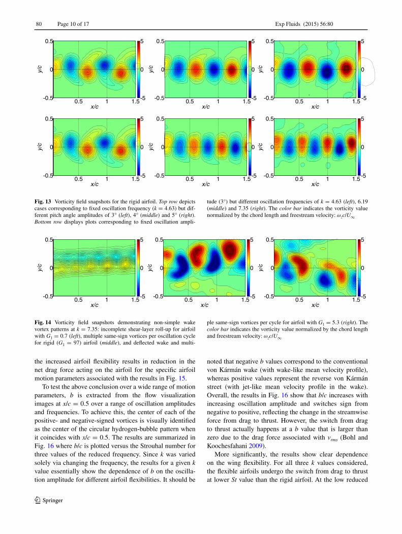
vortex per airfoil oscillation cycle. Examples of such wakes are depicted using a snapshot of the phase-averaged vorticity for the rigid airfoil in Fig. 13, where the vortex pattern corresponds to classical, neutral and reverse von Kármán street. However, in some of the cases investigated, deviations from the simple wake pattern are found. These deviations manifest themselves in three typical forms: (1) wakes where the separating shear layer at the TE has not rolled up completely into a vortex (Fig. 14, left); (2)

wakes with more than one vortex of the same sign are shed per oscillation cycle (Fig. 14 middle and right); (3) “deflected” wakes where the vortex trajectory is inclined to the streamwise direction (Fig. 14 right). These cases are excluded from the analysis conducted in the current work since it is difficult to extract the vortex characteristics in an unambiguous way.

4.1 Cross‑flow vortex spacing (b)

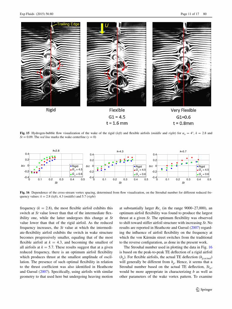
Figure 15 depicts three wake visualization images organ-ized in order of increasing airfoil flexibility (from left to right). In all three cases, the oscillation parameters are kept the same: αo = 4°, k = 2.79, St = 0.09. As seen from the figure, for the rigid airfoil, vortices with counter-clockwise (positive)/clockwise (negative) sense of rota-tion are observed on the left/right of the wake centerline (marked by the solid red line). This arrangement is similar to the natural wake of the airfoil (i.e., in the absence of the imposed oscillation), representing the conventional Kármán street, which is associated with mean velocity deficit in the wake. As the flexibility is increased by reducing G1 to 4.5, the cross-stream spacing of the vortices b becomes smaller. Further decrease of G1 to 0.6 causes the center of the vor-tex cores to become aligned with the wake centerline; i.e., b = 0, producing a neutral wake. This suggests that

Fig. 10 Mean streamwise velocity profiles computed using the vortex array model for different values of a/c and b/c = 0.05, Γο/cU∞ = 0.4 and R/c = 0.029 (left). The same profiles after subtracting the freestream velocity and normal-izing by the circulation per wavelength are shown in the right plot

Fig. 11 Root-mean-square pro-files of the streamwise (left) and cross-stream (right) velocity computed using the vortex array model for different values of a/c and b/c = 0.05, Γο/cU∞ = 0.4 and R/c = 0.029

Fig. 12 Variation of Cf with wavelength computed using the vortex array model for different values of a/c and b/c = 0.05, Γο/cU∞ = 0.4 and R/c = 0.029

Exp Fluids (2015) 56:80

1 3

80 Page 10 of 17

the increased airfoil flexibility results in reduction in the net drag force acting on the airfoil for the specific airfoil motion parameters associated with the results in Fig. 15.

To test the above conclusion over a wide range of motion parameters, b is extracted from the flow visualization images at x/c = 0.5 over a range of oscillation amplitudes and frequencies. To achieve this, the center of each of the positive- and negative-signed vortices is visually identified as the center of the circular hydrogen-bubble pattern when it coincides with x/c = 0.5. The results are summarized in Fig. 16 where b/c is plotted versus the Strouhal number for three values of the reduced frequency. Since k was varied solely via changing the frequency, the results for a given k value essentially show the dependence of b on the oscilla-tion amplitude for different airfoil flexibilities. It should be

noted that negative b values correspond to the conventional von Kármán wake (with wake-like mean velocity profile), whereas positive values represent the reverse von Kármán street (with jet-like mean velocity profile in the wake). Overall, the results in Fig. 16 show that b/c increases with increasing oscillation amplitude and switches sign from negative to positive, reflecting the change in the streamwise force from drag to thrust. However, the switch from drag to thrust actually happens at a b value that is larger than zero due to the drag force associated with vrms (Bohl and Koochesfahani 2009).

More significantly, the results show clear dependence on the wing flexibility. For all three k values considered, the flexible airfoils undergo the switch from drag to thrust at lower St value than the rigid airfoil. At the low reduced

x/c

y/c

0.5 1 1.5-0.5

0

0.5

-5

0

5

x/c

y/c

0.5 1 1.5-0.5

0

0.5

-5 -5

0

5

x/c

y/c

0.5 1 1.5-0.5

0

0.5

0

5

x/c

y/c

0.5 1 1.5-0.5

0

0.5

-5

0

5

x/c

y/c

0.5 1 1.5-0.5

0

0.5

-5

0

5

x/c

y/c

0.5 1 1.5-0.5

0

0.5

-5

0

5

Fig. 13 Vorticity field snapshots for the rigid airfoil. Top row depicts cases corresponding to fixed oscillation frequency (k = 4.63) but dif-ferent pitch angle amplitudes of 3° (left), 4° (middle) and 5° (right). Bottom row displays plots corresponding to fixed oscillation ampli-

tude (3°) but different oscillation frequencies of k = 4.63 (left), 6.19 (middle) and 7.35 (right). The color bar indicates the vorticity value normalized by the chord length and freestream velocity: ωzc/U∞

x/c

y/c

0.5 1 1.5-0.5

0

0.5

-5

0

5

x/c

y/c

0.5 1 1.5-0.5

0

0.5

-5

0

5

x/c

y/c

0.5 1 1.5-0.5

0

0.5

-5

0

5

Fig. 14 Vorticity field snapshots demonstrating non-simple wake vortex patterns at k = 7.35: incomplete shear-layer roll-up for airfoil with G1 = 0.7 (left), multiple same-sign vortices per oscillation cycle for rigid (G1 = 97) airfoil (middle), and deflected wake and multi-

ple same-sign vortices per cycle for airfoil with G1 = 5.3 (right). The color bar indicates the vorticity value normalized by the chord length and freestream velocity: ωzc/U∞

Exp Fluids (2015) 56:80

1 3

Page 11 of 17 80

frequency (k = 2.8), the most flexible airfoil exhibits this switch at St value lower than that of the intermediate flex-ibility one, while the latter undergoes this change at St value lower than that of the rigid airfoil. As the reduced frequency increases, the St value at which the intermedi-ate-flexibility airfoil exhibits the switch in wake structure becomes progressively smaller, equaling that of the most flexible airfoil at k = 4.3, and becoming the smallest of all airfoils at k = 5.7. These results suggest that at a given reduced frequency, there is an optimum airfoil flexibility which produces thrust at the smallest amplitude of oscil-lation. The presence of such optimal flexibility in relation to the thrust coefficient was also identified in Heathcote and Gursul (2007). Specifically, using airfoils with similar geometry to that used here but undergoing heaving motion

at substantially larger Rec (in the range 9000–27,000), an optimum airfoil flexibility was found to produce the largest thrust at a given St. The optimum flexibility was observed to shift toward stiffer airfoil structure with increasing St. No results are reported in Heathcote and Gursul (2007) regard-ing the influence of airfoil flexibility on the frequency at which the von Kármán street switches from the traditional to the reverse configuration, as done in the present work.

The Strouhal number used in plotting the data in Fig. 16 is based on the peak-to-peak TE deflection of a rigid airfoil (hp). For flexible airfoils, the actual TE deflection (hp,actual) will generally be different from hp. Hence, it seems that a Strouhal number based on the actual TE deflection, Stte, would be more appropriate in characterizing b as well as other parameters of the wake vortex pattern. To examine

Fig. 15 Hydrogen-bubble flow visualization of the wake of the rigid (left) and flexible airfoils (middle and right) for αo = 4°, k = 2.8 and St = 0.09. The red line marks the wake centerline (y = 0)

0 0.1 0.2 0.3 0.4 0.5-0.4

-0.2

0

0.2

0.4

St

b/c

k=2.8

RigidG

1 = 4.5

G1

= 0.6

0 0.1 0.2 0.3 0.4 0.5-0.4

-0.2

0

0.2

0.4

St

b/c

k=4.3

RigidG

1= 4.5

G1

= 0.6

0 0.1 0.2 0.3 0.4 0.5-0.4

-0.2

0

0.2

0.4

St

b/c

k=5.7

RigidG

1= 4.5

G1

= 0.6

Fig. 16 Dependence of the cross-stream vortex spacing, determined from flow visualization, on the Strouhal number for different reduced fre-quency values: k = 2.8 (left), 4.3 (middle) and 5.7 (right)

Exp Fluids (2015) 56:80

1 3

80 Page 12 of 17

this idea, the PIV data are employed to determine b in a more systematic way than from the flow visualization. For this analysis, the sequence of vorticity fields is first phase ordered based on the measured frequency of oscillation of the airfoil. Focusing on x/c = 0.5, two phases of the oscil-lation cycle are identified where the negative and positive vortex core centers are located at this streamwise loca-tion (where the vortex centers are taken to correspond to the minimum and maximum vorticity, respectively, within the oscillation cycle). At these phases, the y locations of the vortex cores are determined and b is computed as y for the positive vortex core center minus the corresponding y for the negative vortex. The uncertainty in determining b is estimated to be equal to the PIV grid spacing of ±0.028c, or 10 % of the largest b/c value observed. The uncertainty in the determination of Stte predominantly comes from the error in the measurement of the trailing edge displacement (see Sect. 2). Figure 17 shows b/c plotted versus St (left plot) and Stte (right plot). Inspection of Fig. 18 shows that in fact by plotting b/c versus Stte, the results exhibit col-lapse that is not seen when plotting against St.

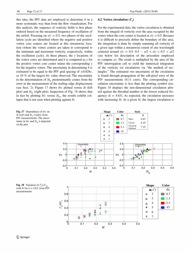
4.2 Vortex circulation (Γο)

For the experimental data, the vortex circulation is obtained from the integral of vorticity over the area occupied by the vortex when the core center is located at x/c = 0.5. Because it is difficult to precisely define the boundary of this area, the integration is done by simply summing all vorticity of a given sign within a streamwise extent of one wavelength centered around x/c = 0.5: 0.5 − a/2 < x/c < 0.5 + a/2 (see below for description of the procedure employed to compute a). The result is multiplied by the area of the PIV interrogation cell to yield the numerical integration of the vorticity (or circulation) via “the method of rec-tangles.” The estimated rms uncertainty of the circulation is found through propagation of the sub-pixel error of the PIV measurements (0.11 cm/s). The corresponding cir-culation uncertainty is less than the plotting symbol size. Figure 18 displays the non-dimensional circulation plot-ted against the Strouhal number at the lowest reduced fre-quency (k = 4.63). As expected, the circulation increases with increasing St. At a given St, the largest circulation is

Fig. 17 Dependence of b/c on St (left) and Stte (right); from PIV measurements. The uncer-tainty in b/c and Stte is depicted on the plot

Shape Color Style ααααo (°) G1 k

2 0.7 Open 4.63

3 1.3 Closed 6.19

4 5.3 Closed &Outlined 7.35

5 97

6

7

0 0.1 0.2 0.3 0.4 0.5-0.4

-0.2

0

0.2

0.4

St

b/c

Uncertainty

0 0.1 0.2 0.3 0.4 0.5-0.4

-0.2

0

0.2

0.4

Stte

b/c

Uncertainty

Fig. 18 Variation of Γo/cU∞ with St for k = 4.63; from PIV measurements

Shape Color ααααo (°) G1

2 0.7

3 1.3

4 5.3

5 97

6

7

0 0.1 0.2 0.3 0.4 0.50

0.2

0.4

0.6

0.8

1

St

Γ o/cU

∞

Exp Fluids (2015) 56:80

1 3

Page 13 of 17 80

attained when using the flexible airfoil with the least flex-ibility (G1 = 5.3; shown using red symbols). The two most flexible airfoils produce the smallest circulation with the difference between the circulations produced by the differ-ent airfoils becoming more pronounced as St increases. The qualitative trends seen in Fig. 18 are also found to be simi-lar to those found at the two highest reduced frequencies.

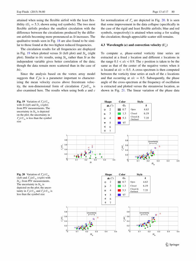
The circulation results for all frequencies are displayed in Fig. 19 when plotted versus St (left plot) and Stte (right plot). Similar to b/c results, using Stte rather than St as the independent variable gives better correlation of the data; though the data remain more scattered than in the case of b/c.

Since the analysis based on the vortex array model suggests that Γo/a is a parameter important to character-izing the mean velocity excess above freestream veloc-ity, the non-dimensional form of circulation Γo/aU∞ is also examined here. The results when using both a and c

for normalization of Γo are depicted in Fig. 20. It is seen that some improvement in the data collapse (specifically in the case of the rigid and least flexible airfoils; blue and red symbols, respectively) is attained when using a for scaling the circulation; though appreciable scatter still remains.

4.3 Wavelength (a) and convection velocity (Uc)

To compute a, phase-sorted vorticity time series are extracted at a fixed y location and different x locations in the range 0.1 < x/c < 0.9. The y position is taken to be the same as that of the center of the negative vortex when it is located at x/c = 0.5. A cross-spectrum is then computed between the vorticity time series at each of the x locations and that occurring at x/c = 0.5. Subsequently, the phase angle of the cross-spectrum at the frequency of oscillation is extracted and plotted versus the streamwise location, as shown in Fig. 21. The linear variation of the phase data

Fig. 19 Variation of Γo/cU∞ with St (left) and Stte (right); from PIV measurements. The uncertainty in Stte is depicted on the plot; the uncertainty in Γo/cU∞ is less than the symbol size

Shape Color Style αααα o (°) G1 k

2 0.7 Open 4.63

3 1.3 Closed 6.19

4 5.3 Closed &Outlined 7.35

5 97

6

7

0 0.1 0.2 0.3 0.4 0.50

0.2

0.4

0.6

0.8

1

St

Γ o/cU

∞

0 0.1 0.2 0.3 0.4 0.50

0.2

0.4

0.6

0.8

1

Stte

Γ o/c

U∞

Uncertainty

Fig. 20 Variation of Γo/cU∞ (left) and Γo/aU∞ (right) with Stte; from PIV measurements. The uncertainty in Stte is depicted on the plot; the uncer-tainty in Γo/cU∞ and Γo/cU∞ is less than the symbol size

Shape Color Style ααααo (°) G1 k

2 0.7 Open 4.63

3 1.3 Closed 6.19

4 5.3 Closed &Outlined 7.35

5 97

6

7

0 0.1 0.2 0.3 0.4 0.50

0.2

0.4

0.6

0.8

1

Stte

Γ o/c

U∞

Uncertainty

0 0.1 0.2 0.3 0.4 0.50

0.2

0.4

0.6

0.8

1

Stte

Γ o/aU

∞

Uncertainty

Exp Fluids (2015) 56:80

1 3

80 Page 14 of 17

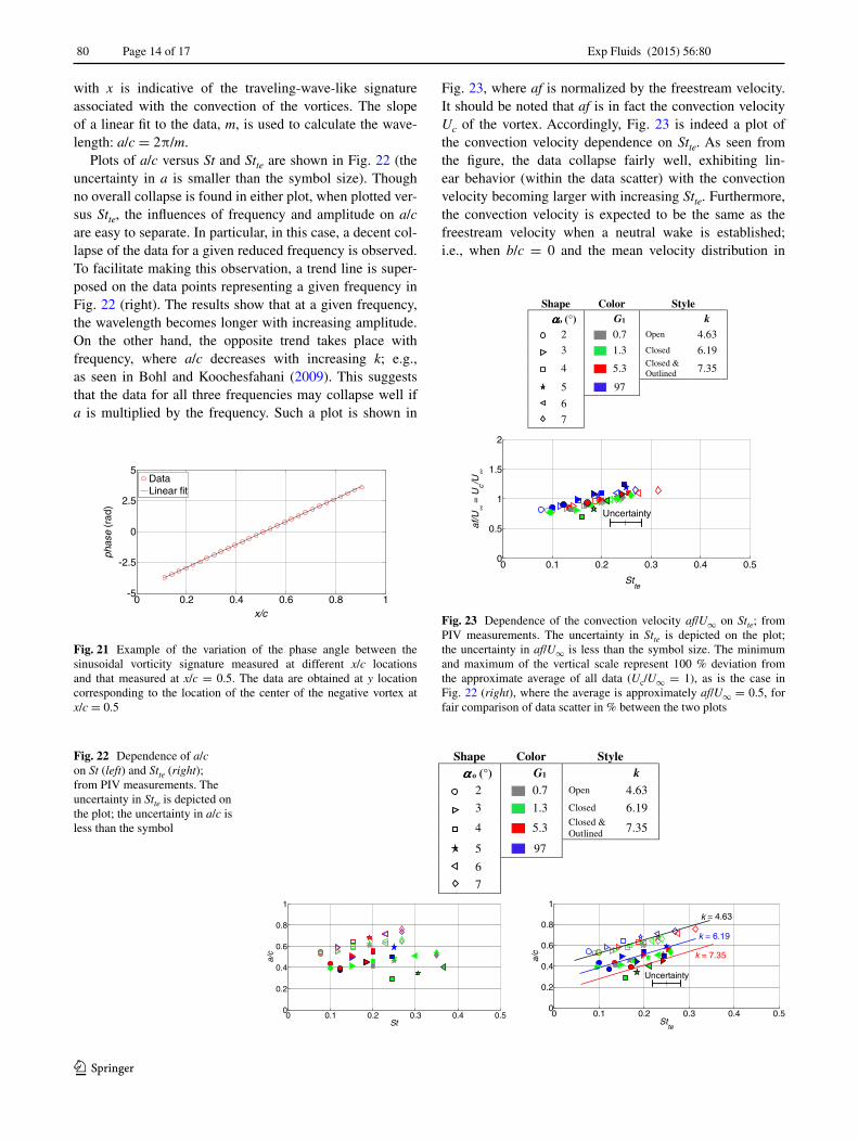
with x is indicative of the traveling-wave-like signature associated with the convection of the vortices. The slope of a linear fit to the data, m, is used to calculate the wave-length: a/c = 2π/m.

Plots of a/c versus St and Stte are shown in Fig. 22 (the uncertainty in a is smaller than the symbol size). Though no overall collapse is found in either plot, when plotted ver-sus Stte, the influences of frequency and amplitude on a/c are easy to separate. In particular, in this case, a decent col-lapse of the data for a given reduced frequency is observed. To facilitate making this observation, a trend line is super-posed on the data points representing a given frequency in Fig. 22 (right). The results show that at a given frequency, the wavelength becomes longer with increasing amplitude. On the other hand, the opposite trend takes place with frequency, where a/c decreases with increasing k; e.g., as seen in Bohl and Koochesfahani (2009). This suggests that the data for all three frequencies may collapse well if a is multiplied by the frequency. Such a plot is shown in

Fig. 23, where af is normalized by the freestream velocity. It should be noted that af is in fact the convection velocity Uc of the vortex. Accordingly, Fig. 23 is indeed a plot of the convection velocity dependence on Stte. As seen from the figure, the data collapse fairly well, exhibiting lin-ear behavior (within the data scatter) with the convection velocity becoming larger with increasing Stte. Furthermore, the convection velocity is expected to be the same as the freestream velocity when a neutral wake is established; i.e., when b/c = 0 and the mean velocity distribution in

0 0.2 0.4 0.6 0.8 1-5

-2.5

0

2.5

5

x/c

phas

e (r

ad)

DataLinear fit

Fig. 21 Example of the variation of the phase angle between the sinusoidal vorticity signature measured at different x/c locations and that measured at x/c = 0.5. The data are obtained at y location corresponding to the location of the center of the negative vortex at x/c = 0.5

Fig. 22 Dependence of a/c on St (left) and Stte (right); from PIV measurements. The uncertainty in Stte is depicted on the plot; the uncertainty in a/c is less than the symbol

Shape Color Style αααα o (°) G1 k

2 0.7 Open 4.63

3 1.3 Closed 6.19

4 5.3 Closed &Outlined 7.35

5 97

6

7

0 0.1 0.2 0.3 0.4 0.50

0.2

0.4

0.6

0.8

1

St

a/c

0 0.1 0.2 0.3 0.4 0.50

0.2

0.4

0.6

0.8

1

Stte

a/c

Uncertainty

k = 6.19

k = 7.35

k = 4.63

Shape Color Style ααααo (°) G1 k

2 0.7 Open 4.63

3 1.3 Closed 6.19

4 5.3 Closed &Outlined 7.35

5 97

6

7

0 0.1 0.2 0.3 0.4 0.50

0.5

1

1.5

2

Stte

af/U

∞=

Uc/U

∞

Uncertainty

Fig. 23 Dependence of the convection velocity af/U∞ on Stte; from PIV measurements. The uncertainty in Stte is depicted on the plot; the uncertainty in af/U∞ is less than the symbol size. The minimum and maximum of the vertical scale represent 100 % deviation from the approximate average of all data (Uc/U∞ = 1), as is the case in Fig. 22 (right), where the average is approximately af/U∞ = 0.5, for fair comparison of data scatter in % between the two plots

Exp Fluids (2015) 56:80

1 3

Page 15 of 17 80

the wake is uniform and equal to U∞. Though it is difficult to pinpoint because of data scatter, it appears that Uc/U∞ assumes a value of 1 in the Stte range of approximately 0.15–0.2, which overlaps with the Stte range at which b/c ≈ 0 in Fig. 17.

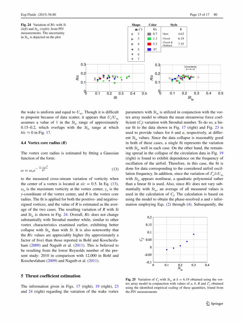
4.4 Vortex core radius (R)

The vortex core radius is estimated by fitting a Gaussian function of the form:

to the measured cross-stream variation of vorticity when the center of a vortex is located at x/c = 0.5. In Eq. (13), ωo is the maximum vorticity at the vortex center, yo is the y-coordinate of the vortex center, and R is the vortex core radius. The fit is applied for both the positive- and negative-signed vortices, and the value of R is estimated as the aver-age of the two cases. The resulting variation of R with St and Stte is shown in Fig. 24. Overall, R/c does not change substantially with Strouhal number while, similar to other vortex characteristics examined earlier, exhibiting better collapse with Stte than with St. It is also noteworthy that the R/c values are appreciably higher (by approximately a factor of five) than those reported in Bohl and Koochesfa-hani (2009) and Naguib et al. (2011). This is believed to be resulting from the lower Reynolds number of the pre-sent study: 2010 in comparison with 12,000 in Bohl and Koochesfahani (2009) and Naguib et al. (2011).

5 Thrust coefficient estimation

The information given in Figs. 17 (right), 19 (right), 23 and 24 (right) regarding the variation of the wake vortex

(13)ω = ωoe−

(y−yo)2

R2

parameters with Stte is utilized in conjunction with the vor-tex array model to obtain the mean streamwise force coef-ficient (Cf) variation with Strouhal number. To do so, a lin-ear fit to the data shown in Fig. 17 (right) and Fig. 23 is used to provide values for b and a, respectively, at differ-ent Stte values. Since the data collapse is reasonably good in both of these cases, a single fit represents the variation with Stte well in each case. On the other hand, the remain-ing spread in the collapse of the circulation data in Fig. 19 (right) is found to exhibit dependence on the frequency of oscillation of the airfoil. Therefore, in this case, the fit is done for data corresponding to the considered airfoil oscil-lation frequency. In addition, since the variation of Γo /cU∞ with Stte appears nonlinear, a quadratic polynomial rather than a linear fit is used. Also, since R/c does not vary sub-stantially with Stte, an average of all measured values is used in the calculation of Cf. The calculation is based on using the model to obtain the phase-resolved u and v infor-mation employing Eqs. (2) through (4). Subsequently, the

Fig. 24 Variation of R/c with St (left) and Stte (right); from PIV measurements. The uncertainty in Stte is depicted on the plot

Shape Color Style ααααo (°) G1 k

2 0.7 Open 4.63

3 1.3 Closed 6.19

4 5.3 Closed &Outlined 7.35

5 97

6

7

0 0.1 0.2 0.3 0.4 0.50

0.1

0.2

0.3

St

R/c

0 0.1 0.2 0.3 0.4 0.50

0.1

0.2

0.3

Stte

R/c

Uncertainty

Fig. 25 Variation of Cf with Stte at k = 6.19 obtained using the vor-tex array model in conjunction with values of a, b, R and Γo obtained using the identified empirical scaling of these quantities, found from the PIV measurements

Exp Fluids (2015) 56:80

1 3

80 Page 16 of 17

mean and rms velocity profiles are computed and integrated from y/c = −2 to 2 according to Eq. (5) to calculate Cf. The selected integration limits are sufficiently far to ensure that U is the same as the freestream velocity and that the rms terms have decayed to zero. The accuracy of using the vortex array model to compute Cf has already been demon-strated in Naguib et al. (2011).

Using the procedure explained above and knowing the freestream velocity, frequency of oscillation and chord length, values of a, b, R and Γο are obtained at different Stte values in the range 0.1–0.3 and used in connection with the vortex array model to compute Cf for k = 6.19. The results are shown in Fig. 25. The data exhibit the expected trend of switching from drag (Cf < 0) to thrust with increasing Stte. It is noted, however, that the accuracy of the Cf results is dependent on the accuracy of the wake vortex param-eters, which exhibit a fair amount of scatter, particularly for Γο and R (Figs. 19 (right) and 24, respectively). Over-all, Fig. 25 highlights the usefulness of coupling empirical scaling of the wake vortex parameters with the vortex array model to estimate the mean streamwise force acting on the airfoil.

6 Conclusions

Particle image velocimetry measurements are taken in the wake of harmonically pitching airfoils possessing a flexible “tail,” the structural flexibility of which is varied over three orders of magnitude. Data are obtained at Rec = 2010 for different oscillation amplitudes and frequencies. The focus of the data analysis is on extracting the circulation (Γο), the streamwise and cross-stream spacing (a and b, respec-tively) of the vortices shed into the wake, and the vortex core radius (R). The influence of the airfoil flexibility on how these parameters vary with change in the amplitude and frequency of oscillation is investigated.

The results show that, for a given oscillation amplitude, flexible airfoils require lower reduced frequency of oscil-lation than their rigid counterpart to exhibit a switch in the wake vortex pattern from classical to reverse von Kármán street (i.e., b switching sign from negative to positive). At a given reduced frequency, an optimum airfoil flexibility exists which results in the earliest switch in the vortex pat-tern with increasing oscillation amplitude. This optimum flexibility shifts toward stiffer tails with increasing reduced frequency. More interestingly, reasonable correlation for all airfoils examined is found for the variation of b/c with Strouhal number (St) if the latter is defined using the actual oscillation amplitude of the trailing edge (Stte). Similar correlations are also found for the dependence of the cir-culation, streamwise spacing, convection velocity and vor-tex core radius. Additional investigations are required to

examine how the identified scaling depends on Reynolds number and airfoil shape.

Using a vortex array model of the wake, insight is gained into the ramification of the observed variation of the wake parameters with Stte on the mean thrust acting on the airfoil for the reverse von Kármán wake. The results show that the mean thrust is directly proportional to b but inversely proportional to a. At sufficiently large values of b (which depend on the vortex core radius), the wake vortex pattern may be approximated by two vortex sheets, leading to linear dependence of the thrust coefficient on b. On the other hand, though typically the mean thrust increases with increasing Γο, at sufficiently large values of a, the behavior could be non-monotonic, leading to the possibility of pro-ducing a net drag force at high values of circulation.

Overall, the combination of the scaling of the wake vor-tex parameters with Stte and the vortex array model pro-vides a useful tool for computation of the net thrust acting on harmonically pitching airfoils. This utility is demon-strated here by using the empirically identified scaling of the wake vortex parameters in conjunction with the vortex array model to estimate the mean streamwise force coef-ficient variation with Strouhal number. In addition, the understanding of the implications of the wake vortex con-figuration on the net thrust acting on the airfoil provides basis for an interesting approach for thrust manipulation by attempting to alter the wake vortex pattern to one with desired thrust characteristics.

Acknowledgments This work was supported by AFOSR Grant Number FA9550-10-1-0342; program manager Dr. Douglas Smith.

References

Anderson JM, Streitlien K, Barrett DS, Triantafyllou MS (1998) Oscil-lating foils of high propulsive efficiency. J Fluid Mech 360:41–72

Bohl DG, Koochesfahani MM (2009) MTV measurement of the vor-tical field in the wake of an airfoil oscillating at high reduced frequency. J Fluid Mech 620:63–88

Heathcote S, Gursul I (2007) Flexible flapping airfoil propulsion at low Reynolds numbers. AIAA J 45(5):1066–1079

Kang C-K, Aono H, Cesnik CES, Shyy W (2011) Effects of flexibil-ity on the aerodynamic performance of flapping wings. J Fluid Mech 689:31, 32–74

Koochesfahani MM (1989) Vortical patterns in the wake of an oscil-lating airfoil. AIAA J 27(9):1200–1205

Lai JCS, Platzer MF (1999) Jet characteristics of a plunging airfoil. AIAA J 37(12):1529–1537

Lissaman PBS (1983) Low-Reynolds-number airfoils. Annu Rev Fluid Mech 15:223–239

Lai A, Liu, F (2009) Computation of a rigid airfoil in plunging motion with a flexible trailing beam. AIAA paper 2009-726-685

Mueller TJ, DeLaurier JD (2003) Aerodynamics of small vehicles. Annu Rev Fluid Mech 35:89–111

Naguib AM, Vitek J, Koochesfahani MM (2011) Finite-core vortex array model of the wake of a periodically pitching airfoil. AIAA J 49(7):1542–1550

Exp Fluids (2015) 56:80

1 3

Page 17 of 17 80

Ol MV (2007) Vortical structures in high frequency pitch and plunge at low Reynolds number. AIAA paper 2007-4233

Raffel M, Willert CE, Wereley ST, Kompenhaus J (2007) Particle image velocimetry—a practical guide, 2nd edn. Springer, New York

Shyy W, Lian Y, Tang J, Liu H, Trizila P, Stanford B, Bernal L, Cesnik C, Friedmann P, Ifju P (2008) Computational aerodynamics of low Reynolds number plunging, pitching and flexible wings for MAV applications. AIAA paper 2008-523

Thiria B, Godoy-Diana R (2010) How wing compliance drives the effi-ciency of self-propelled flapping flyers. Phys Rev E 82:015303(R)

Von Kármán T, Burgers JM (1943) General aerodynamic theory—perfect fluids. In: Durand WF (ed) Aerodynamic theory, Division E, vol 2. Springer, Berlin, p 308

Young J, Lai JCS (2004) Oscillation frequency and amplitude effects on the wake of a plunging airfoil. AIAA J 42(10):2042–2052