Information Asymmetry and Corporate Cash Holdings

Kee H. Chunga,*, Jang-Chul Kimb, Young Sang Kimb, and Hao Zhangc

aSchool of Management, State University of New York (SUNY) at Buffalo Buffalo, NY 14260, USA

bHaile/US Bank College of Business, Northern Kentucky University Highland Heights, KY 41099, USA

cE. Philip Saunders College of Business, Rochester Institute of Technology Rochester, NY 14623, USA

____________

*Corresponding Author: Kee H. Chung, Department of Finance and Managerial Economics, School of Management, State University of New York (SUNY) at Buffalo, Buffalo, NY 14260. Tel.: 716-645-3262; fax: 716-645-3823; E-mail address: keechung@buffalo.edu. The authors thank Soku Byoun, Jaehoon Hahn, Nikolay Halov, Kyojik “Roy” Song, and session participants at the 2011 FMA conference for valuable comments and discussion.    

Information Asymmetry and Corporate Cash Holdings

Abstract

In this study we analyze the effect of information asymmetry on corporate cash holdings and whether the effect of cash holdings on firm value varies across firms with different levels of information asymmetry. We show that companies that operate in higher information asymmetry environments hold smaller cash using various measures of information asymmetry. We also show that cash adds less value to shareholders in companies with high levels of information asymmetry after controlling for other determinants of firm value. On the whole, our results support the shareholder interest hypothesis of cash holdings over the managerial entrenchment hypothesis and the managerial flexibility hypothesis. JEL Classification: G30, G32, G34 Keywords: Cash holdings, Information asymmetry, Corporate governance, Firm value

1

I. Introduction

U.S. corporations hold large amounts of liquid assets. For instance, cash and marketable

securities account for, on average, 22.5% of total assets of publicly traded companies during the

ten-year period from 2000 through 2009.1 In this study we analyze the effect of information

asymmetry on corporate cash holdings and whether the effect of cash holdings on firm value

varies with the firm’s information environment. Although prior research sheds significant light

on both the determinants and value implication of corporate cash holdings, there is only limited

evidence regarding how information asymmetry affects cash holdings and their value

implications. Given the critical role of information asymmetry in both financial decision-making

processes and financial theories, analysis of corporate cash (i.e., one of the most discretionary

and liquid corporate assets) through the lens of information asymmetry seems overdue. We

provide such evidence using various measures of information asymmetry developed in the

market microstructure literature.2 To our best knowledge, the present study is the first to analyze

corporate cash holdings using these metrics.3

Corporate cash holdings allow firms to exploit profitable investment opportunities and

make obligatory debt payments in case of cash flow shortfalls without having to access external

capital markets, avoiding both transaction costs and information asymmetry costs. However,

corporate cash holdings may come at a cost if managers use them for their own benefits at the

expense of shareholders. Information asymmetry is likely to influence corporate cash holdings

because it affects both managerial behavior and the ability of outsiders to understand managerial

1 Nonfinancial U.S. companies hold $1.93 trillion in cash and other liquid assets at the end of September 2010. (Source: Wall Street Journal, December 10, 2010). 2 The empirical validity of these metrics is well established and they are likely to capture information asymmetry better than other measures (e.g., R&D expenditure and the market-to-book ratio) used in prior research. 3 In addition to these metrics, we also use additional information asymmetry measures used in corporate finance study such as analysts following, and dispersion of analysts forecasting for robustness tests.

2

actions in the presence of the principal-agent problem. For example, the free cash flow problem

(Jensen, 1986) may be more severe in firms with higher information asymmetry since it would

be difficult for outsiders to monitor and interpret managerial actions. Alternatively, both

managers and shareholders may be more concerned about future capital needs in firms with

higher information asymmetry as they worry about possible underpricing of their future equity

issuance (Myers and Mujluf, 1984).

Numerous studies analyze the determinants of corporate cash holdings and suggest that

companies hold cash for the transaction cost, precautionary, tax, and agency motives. Baumol

(1952), Miller and Orr (1966), Meltzer (1993), and Mulligan (1997) analyze the transaction cost

motive for holding cash. Opler, Pinkowitz, Stulz, and Williamson (1999) find evidence that

supports the static tradeoff model of cash holdings.4 In particular, they find larger cash holdings

in companies with greater growth opportunities, riskier cash flows, lower credit ratings, and

smaller market capitalizations. Pinkowitz and Williamson (2001) examine the effect of bank

power on cash holdings and show that strong Japanese banks influence firms to hold large cash

balances. Foley, Hartzell, Titman, and Twite (2007) show that U.S. multinational firms hold

large cash in their foreign subsidiaries because of the tax costs associated with repatriating

foreign income. Bates, Kahle, and Stulz (2009) dispute the tax motive for cash holdings based on

the finding that even companies without foreign operation or income hold large cash. Duchin

(2010) and Subramaniam, Tang, Yue, and Zhou (2011) show that diversified firms hold less cash

than single-division firms. Song and Lee (2012) find that firms in East Asian countries maintain

large precautionary cash holdings even after the economy recovers from the 1997 financial crisis.

4 The static tradeoff model of cash holdings assumes that the firm equates the marginal cost of holding liquid assets to the marginal benefit of holding those assets.

3

Dittmar, Mahrt-Smith, and Servaes (2003) show that companies in countries with lower

investor protection hold more cash than do companies in other countries. Kalcheva and Lins

(2007) find that firms hold more liquid assets when there is a greater discrepancy between the

controlling shareholder’s cash flow rights and voting rights. Harford, Mansi, and Maxwell

(2008) show, however, that firms with poorer corporate governance structure have smaller cash

reserves. Bates, Kahle, and Stulz (2009) find a significant increase in the average cash-to-assets

ratio for U.S. industrial firms during 1980-2006 and attribute it to an increase in the overall

riskiness of cash flows.

A number of studies examine the effect of corporate cash holdings on firm performance

and market valuation. Mikkelson and Partch (2003) analyze whether conservative financial

policies benefit managers at the expense of shareholders by examining the operating

performance of firms that hold large cash. They show that firms that maintain large cash

holdings exhibit greater research and development (R&D) investments and greater growth in

assets, and conclude that holding large cash reserves does not hinder corporate performance.

Pinkowitz and Williamson (2004) find that the value of cash is higher in firms with better growth

options and more volatile investment opportunities.

Faulkender and Wang (2006) show that the marginal value of cash (measure by abnormal

stock returns) declines with larger cash holdings, higher leverage, better access to capital

markets, and greater cash distribution via dividends. Pinkowitz, Stulz, and Williamson (2006)

find that the value of corporate cash holdings is smaller in countries with poorer investor

protection because controlling shareholders have greater ability to extract private benefits from

cash holdings in such countries. Dittmar and Mahrt-Smith (2007) show that cash holdings are

more valuable for companies with better governance structures and companies with poor

4

governance structures dissipate cash quickly in ways that reduce operating performance.

Harford, Mansi, and Maxwell (2008) find that firms with poor shareholder rights and excess cash

have low profitability and small market valuations.

More recently, Liu and Mauer (2011) find a positive relation between the sensitivity of

CEO compensation to stock price volatility and cash holdings and a negative relation between

CEO risk-taking incentive (vega) and the value of cash to shareholders. Tong (2011) shows that

the value of cash is lower in diversified firms than in single-division firms, and firm

diversification has a negative impact on the value of cash among firms with poor corporate

governance. Fresard and Salva (2010) find that the value of excess cash is greater for firms

cross-listed on the U.S. market than their domestic peers. Fresard (2010) finds that larger cash

reserves lead to future market share gains at the expense of industry rivals and interprets the

result as evidence that corporate cash holdings strategically influence product market outcomes.

Denis and Sibilkov (2010) show cash holdings are more valuable for financially constrained

firms because higher cash holdings allow them to undertake value-increasing projects that might

otherwise be bypassed.

While prior research provides significant insights on corporate cash holdings and their

ramifications, there is only limited evidence regarding the effect of information asymmetry on

cash holdings. Opler, Pinkowitz, Stulz, and Williamson (1999) show that firms with larger R&D

expenses hold more liquid assets. Although firms with larger R&D expenses may have greater

information asymmetry, larger R&D expenses may also reflect greater growth opportunities. It is

also possible that firms with larger cash reserves spend more on R&D activities. Dittmar, Mahrt-

Smith, and Servaes (2003) use the market-to-book ratio as a proxy for information asymmetry,

5

which is subject to the same criticism as R&D expenses. Furthermore, it is unclear how the

market valuation of cash holdings varies with the firm’s information environment.

In this study, we consider three competing hypotheses of the effect of information

asymmetry on cash holdings. The shareholder interest hypothesis of cash holdings posits that the

size of cash that a firm holds is negatively related to the degree of information asymmetry

between the firm’s managers and outside shareholders. In contrast, both the managerial

entrenchment hypothesis and the managerial flexibility hypothesis predict a positive relation

between cash holdings and information asymmetry. [Section II provides a detailed description of

these hypotheses.]

Our empirical results show that corporate cash holdings are negatively and significantly

related to various measures of information asymmetry. The results are robust to different

estimation methods, including the fixed effects and Fama-MacBeth regressions as well as the

regressions using changes in the variables. Consistent with the findings of prior research, we

show that the firm’s size-adjusted market value is positively and significantly related to the level

of excess cash it holds. More important, we find that cash adds less value to shareholders in

companies with high levels of information asymmetry, and this result is quite robust across

different measures of information asymmetry. We interpret these results as evidence that

managers are more likely to misuse cash (and thus cash adds less value to the company) when it

is difficult for outside shareholders to monitor managerial actions because of high information

asymmetry. On the whole, our results support the shareholder interest hypothesis of cash

holdings that corporate cash holdings are determined by shareholder interests rather than by

managerial entrenchment or managerial flexibility.

6

Although the principal-agent conflict and information asymmetry are central to many

financial theories, prior research provides limited empirical evidence on the role of information

asymmetry in the principal-agent problem. Our study underscores the importance of information

asymmetry in corporate decisions by analyzing its effect on a corporate asset that is highly

vulnerable to managerial waste. U.S. companies hold increasingly large amounts of cash during

the last two decades. Management has an easy access to cash reserves and much of their use is

discretionary. While the conflict of interests associated with corporate excess cash has been

recognized since at least Jensen (1986), how information asymmetry can exacerbate the conflict

of interests has not been well understood. Our study makes an important contribution to the

literature by providing evidence on how information asymmetry may affect both the level and

value implication of corporate cash holdings.

The remainder of the paper is organized as follows. Section II describes our three

hypotheses of corporate cash holdings. Section III presents the detailed description of data

sources, variable measurement methods, and summary statistics. Section IV analyzes the relation

between cash holdings and various measures of information asymmetry using different

estimation methods, study samples, and variable measurements. This section also examines the

effect of information asymmetry on corporate payout and share repurchase decisions. Section V

analyzes whether the effect of cash holdings on firm value varies with information asymmetry.

Section VI ends the paper with a brief summary and concluding remarks.

II. Statement of Hypotheses

Jensen (1986) suggests that corporate managers may undertake value-decreasing projects

when they are endowed with more cash than they can invest in profitable projects (i.e., projects

7

with positive net present values). Jensen argues that this agency problem could be minimized by

reducing the amount of free cash flow available to managers.5 Jensen (1986) and Stulz (1990)

predict that shareholders will restrict managers’ access to free cash flow to mitigate the agency

problem. To the extent that mangers’ incentives and abilities to engage in value-destroying

activities vary with a firm’s information environment, the amount of cash that mangers could

hold (or, more precisely, the amount of cash that shareholders allow managers to hold) is likely

to depend on the firm’s information environment.

For instance, shareholders of companies operating in opaque information environments

may not want managers to hold large cash because it is difficult and costly for them to monitor

managerial actions in such environments. In contrast, if the firm’s information environment is

transparent and thus there is little information asymmetry between mangers and outside

shareholders, shareholders may allow mangers to hold large cash because they could effectively

monitor managerial actions and punish those mangers who waste cash. These considerations

suggest that, all things being equal, the size of cash that a firm holds is likely to be negatively

related to the degree of information asymmetry between the firm’s managers and outside

shareholders. We call this the shareholder interest hypothesis of cash holdings.

There are two important implicit assumptions behind the shareholder interest hypothesis

of cash holdings. The first assumption is that shareholders have the power and means to control

corporate cash holdings. Prior research provides some supports for this assumption. For example,

Faleye (2004) shows that proxy contests increase with excess cash reserves, and following such

contests, executive turnover and cash distributions to shareholders increase while cash holdings

5 Jensen (1986) holds that firms could minimize the agency cost of free cash flow by increasing future debt service requirements (i.e., interest payments) without the retention of the proceeds from the new debt issuance (e.g., by issuing debt in exchange for stock).

8

decrease. La Porta, Lopez-de-Silanes, Shleifer, and Vishny (2000) show that greater shareholder

rights are associated with higher dividend payouts, suggesting that shareholders can force

managers to return excess cash to them in countries with good legal protection for shareholders.

We provide additional evidence regarding the first assumption later in the paper (in Section

IV.D) by analyzing the effect of information asymmetry on corporate dividend payout and share

purchase decisions. The second assumption is that managers are more likely to misuse cash and

thus cash adds less value to the company when it is difficult for outsiders to monitor and

interpret managerial actions due to high information asymmetry. We provide empirical evidence

regarding this assumption in Section V.

If these two assumptions do not hold, cash holdings may not be inversely related to

information asymmetry. For instance, suppose managers can hoard excess cash because

shareholders are not able to force them to disgorge the cash. In that case, entrenched managers

may want to maintain large cash reserves to pursue their own objectives at the expense of

shareholders. For instance, risk-averse managers may maintain large cash balances to reduce

liquidity risk because their human capital is tied up in the company. Entrenched managers may

also hold large cash to pursue self-serving investment projects without the discipline of the

capital markets–they may want to undertake poor projects that the capital market would not

finance simply because they could obtain large personal benefits (perquisites) from those

projects. If managerial entrenchment were more prominent in companies with greater

information asymmetry, we would observe a positive relation between cash holdings and

information asymmetry. We call this the managerial entrenchment hypothesis of cash holdings.

Cash flow shortfalls might prevent a firm from undertaking profitable projects if the firm

does not have liquid assets. Hence, it is valuable for firms to maintain a certain level of cash

9

reserves for future investment opportunities. Myers and Majluf (1984) underscore the fact that

corporate liquidity enables firms to undertake new projects without having to rely on external

capital markets, thereby avoiding both flotation costs and information asymmetry costs (e.g.,

underpricing) that often accompany equity issuances. Corporate liquidity is likely to be most

valuable to a firm that operates in opaque informational environments because the firm could

avoid large flotation and information asymmetry costs when profitable investment opportunities

show up. All things being equal, therefore, it is in the interest of both managers and shareholders

to maintain larger cash reserves when the level of information asymmetry is higher. In contrast to

the shareholder interest hypothesis of cash holdings discussed above, these considerations

suggest a positive relation between the level of cash holdings and the extent of information

asymmetry. We call this the managerial flexibility hypothesis of corporate cash holdings.

Both the managerial entrenchment hypothesis and the managerial flexibility hypothesis of

cash holdings predict a positive relation between cash holdings and information asymmetry, but

for different reasons. The managerial flexibility hypothesis is based on a benign behavior of

managers who hoard cash to exploit uncertain future investment opportunities for the benefit of

shareholders. The managerial entrenchment hypothesis is based on a self-interested behavior of

managers who hoard cash to use it more for their own benefits than for the benefit of

shareholders. In what follows, we provide empirical evidence regarding these hypotheses based

on a large sample of publicly traded U.S. companies.

III. Data Sources, Variable Measurement, and Descriptive Statistics

In this section we explain our data sources and variable measurement procedures, and

present descriptive statistics.

10

A. Data Sources

We obtain data required for our analysis from the following sources: the NYSE’s Trade

and Quote (TAQ), the Center for Research in Security Prices (CRSP), the Institutional Brokers'

Estimate System (I/B/E/S), the CDA/Spectrum Institutional (13F) Holdings, the RiskMetrics

Governance Database (formerly called the Investor Responsibility Research Center), and

Standard & Poor's Compustat for the 17-year period from 1993 through 2009. Our initial sample

includes all stocks listed on the NYSE, AMEX, and NASDAQ. We exclude from the study

sample financial companies (SIC Codes 6000-6999), utility companies (SIC Codes 4900-4999),

companies with an average annual share price less than $5, and non-U.S. companies.6

We apply the following data filters to trades and quotes to clean errors and outliers in the

TAQ database (see Huang and Stoll, 1996): a) delete a quote if either the bid or ask price is

negative; b) delete a quote if either the bid or ask size is negative; c) delete a quote if the bid-ask

spread is greater than $4 or negative; d) delete trades and quotes if they are out of time sequence

or involve an error; e) delete before-the-open and after-the-close trades and quotes; f) delete a

trade if the price or volume is negative; and g) delete trades and quotes if they changed by more

than 10% compared to the last transaction price and quote.

B. Measures of Information Asymmetry

The theory of agency (e.g., Myers and Majluf, 1984) concerns the conflict of interests

and information asymmetry between corporate insides (e.g., managers) and outsiders (e.g.,

existing and potential shareholders), while the theory of market microstructure concerns the 6 Following prior research (see Bates, Kahle, and Stulz, 2009), we exclude financial firms because they may hold cash to meet capital requirements and utilities because their cash holdings may be subject to regulatory supervision.

11

information asymmetry between informed and uninformed traders. Diamond (1985) shows that

lower information asymmetry between corporate insiders and outsiders results in lower

information asymmetry between traders because the public release of inside information to

outsiders makes traders' beliefs more homogeneous and reduces the information asymmetry

between informed and uninformed traders. Chung, Elder, and Kim (2010) provide empirical

evidence that higher information asymmetry between corporate insider and outsiders results in

higher information asymmetry among traders in the secondary securities markets.

Following prior research (e.g., Bharath, Pasquariello, and Wu, 2009), we employ various

measures of information asymmetry that are commonly used in the market microstructure

literature, including the price impact of a trade, the adverse selection component of the spread,

and the probability of information-based trading, to examine the effect of information asymmetry

on corporate cash holdings.7 Although these measures are not without drawbacks, we use them in

our analysis because they are more likely to accurately measure information asymmetry than

other alternative measures (e.g., R&D expenditure and the market-to-book ratio) that are

employed in previous studies. To assess the sensitivity of our results with respect to different

measures of information asymmetry, we also use the dispersion of financial analysts’ earnings

forecasts and an aggregate (composite) metric as additional measures of information asymmetry.

We measure the price impact of a trade for firm i by

Price Impacti,τ = Qi,τ[(Mi,τ+5 – Mi,τ) / Mi,τ]; (1)

7 A number of studies employ these measures to analyze various issues in corporate finance, investments, and asset pricing. See Lee, Mucklow, and Ready (1993), Brennan and Subrahmanyam (1995), Heflin and Shaw (2000), Easley, Hvidkjaer, and O’Hara (2002), Fuller (2003), Flannery, Kwan, and Nimalendran (2004), Graham, Koski, and Loewenstein (2006), Odders-White and Ready (2006), Chen, Goldstein, and Jiang (2007), Kang and Liu (2008), Fang, Noe, and Tice (2009), and Lipson and Mortal (2009). Madhavan (2000) and Lipson (2003) suggest that more interesting research can be generated by linking corporate finance and market microstructure.

12

where Mi,τ and Mi,τ+5 are quote midpoints at time τ and τ + 5 minutes, respectively, and Qi,τ is

equal to 1 for buyer-initiated trades and –1 for seller-initiated trades. We calculate the mean

value of Price Impacti,τ in each year from 1993 through 2009 by weighting each trade equally.

The price impact of a trade measures the extent to which a trade alters share price and thus it

captures the value of private information held by informed traders.

The adverse selection component of the bid-ask spread also captures the value of private

information held by informed traders. We estimate the adverse selection component of the spread

using the models developed by Lin, Sanger, and Booth (1995), Glosten and Harris(1988), and

George, Kaul and Nimalendran(1991).8 Lin, Sanger, and Booth (LSB) (1995) use the following

regression model to estimate the adverse-selection component of the spread:

∆Quotet = λSt-1 + εt;   (2)

In equation (2), ∆Quotet = Quotet – Quotet-1 and St-1 = Pt-1 – Quotet-1, where Quotet is the quote

midpoint at time t, Pt-1 and Quotet-1 are the transaction price and the quote midpoint at time t-1,

respectively, and λ is the proportion of the adverse-selection component in the spread. We take

the logarithm transformation of Quote, P, and S when we estimate λ.

In the Glosten and Harris (GH) (1988) model, the adverse-selection component and other

components, such as inventory holding and order processing components, are expressed as a

linear function of transaction volume. The GH model uses the following regression model to

estimate the adverse-selection component of the spread:

Pt – Pt-1 = c0(Qt – Qt-1) + c1(QtVt – Qt-1Vt-1) + z0Qt + z1QtVt + εt; (3)

8 Van Ness, Van Ness, and Warr (2001) show that the models of Glosten and Harris (1988), George, Kaul and Nimalendran (1991), and Lin, Sanger and Booth (1995) yield more accurate estimates of the adverse selection cost than other models. We omit firm subscript i for simplicity. We estimate the adverse selection cost for a stock only if the stock traded at least three times per day on average in each year.

13

where Pt is the transaction price at time t, Vt is the number of shares traded at time t, εt is the

error term that captures both the rounding error and the arrival of public information, and Qt is

equal to 1 for buyer-initiated trades and –1 for seller-initiated trades. We estimate the adverse-

selection component by Z0 = 2(z0 + z1Vt) and the transitory component by C0 = 2(c0 + c1Vt). The

bid-ask spread in the GH model is the sum of Z0 and C0. We use the average share volume for

stocki, to estimate Z0 and C0. We measure the adverse-selection component (as a proportion of

the spread) by Z0/(Z0 + C0).

George, Kaul, and Nimalendran (GKN) (1991)usethe following regression model to

estimate the adverse-selection component:

; (4)

where TRt is the transaction return at time t, MRt is the quote midpoint return calculated from the

quote midpoint immediately following the transaction at time t, sq is the percentage bid-ask

spread, Qt equals 1 for buyer-initiated trades and –1 for seller-initiated trades, ρ1 measures the

order-processing component, and (1 – ρ1) measures the adverse-selection component.

We estimate the probability of information-based trading (PIN) for each firm in each year

using the sequential trade model of Easley, Kiefer, O’Hara, and Paperman (EKOP) (1996).The

EKOP model of the trade process for firm i over trading day j is represented by the following

likelihood function:

(5)

V

t1ttq10tt ε)Q(Qsρρ)MR2(TR +−+=− −

;!S)T(ε

e!B])Tε[(µ

)eδ(1α

!S])Tε[(µ

e!B)T(ε

eδα

!S)T(ε

e!B)T(ε

)eα(1)θ|S,(BL

ji,

Sji,iTε

ji,

Bji,ii)Tε(µ

ii

ji,

Sji,ii)Tε(µ

ji,

Bji,iTε

ii

ji,

Sji,iTε

ji,

Bji,iTε

iiji,ji,i

ji,

ji,i

ji,

ji,ii

ji,

ji,ii

ji,

ji,i

ji,

ji,i

ji,

ji,i

−+−

+−−

−−

+−+

++

−=

14

where Bi,j is the number of buyer-initiated trades for the day, Si,j is the number of seller-initiated

trades for the day, αi is the probability that an information event has occurred, δj is the

probability of a low signal given an event has occurred, µi is the probability that a trade comes

from an informed trader given an event has occurred, is the probability that the uninformed

traders will actually trade, Ti,j is total trading time for the day, and θi = (αi, δi, εi, µi) represents

the vector of parameters to be estimated. We estimate these parameters θi for firm i for each year

by maximizing the joint likelihood over the J observed trading days in a calendar year:

(6)

We then estimate the probability of information-based trading (PIN) for firm i for each year as

; (7)

We use the dispersion of analysts’ earnings forecasts (DISP) as an additional measure of

information asymmetry.9 Following prior studies,10 we obtain DISP by dividing the standard

deviation of analysts’ one-year earnings forecasts by the previous year-end share price.

Finally, we also construct a composite score of information asymmetry (SCORE). In each

year, we sort firms according to each information asymmetry (IA) measure and group them into

deciles, where Decile 1 includes firms with the lowest information asymmetry and Decile 10

includes firms with the highest information asymmetry. Nest, we assign IA score of 1 to all

firms in Decile 1 and IA score of 10 to all firms in Decile 10. We then obtain the composite

information asymmetry score of each firm in each year by averaging the IA score across our six 9 Drobetz, Gruninger, and Hirschvogl (2010) show that the market valuation of corporate cash holdings decreases with the dispersion of analysts’ earnings forecasts. However, they do not examine how corporate cash holdings are related to the dispersion of earnings forecasts. 10 See Lang and Lundholm (1996), Kinney, et al. (2002), Bailey, et al. (2003), Gu and Wu (2003), Heflin, et al. (2003), Hope (2003), Zhang (2006), Guntay and Hackbarth (2010), and Chordia, Roll, and Subrahmanyam (2011).

iε

∏=

=J

1jiji,ji,iiii ).θ|S,(BL)θ|(ML

iii

iii ε̂2µ̂α̂

µ̂α̂PIN+

=

15

information asymmetry measures (i.e., Price Impact, LSB, GH, GKN, PIN and DISP). By

definition, the value of SCORE ranges from 1 (the lowest information asymmetry) to 10 (the

highest information asymmetry).

C. Cash Holdings and Control Variables

Following Opler, Pinkowitz, Stulz, and Williamson (1999) and Harford, Mansi, and

Maxwell (2008), we measure corporate cash holdings by the ratio of cash and marketable

securities to non-cash assets (NCA) (NCA = total assets – cash and marketable securities). We

also employ an alternative measure of cash holdings, the ratio of cash and marketable securities

to total assets, to assess the robustness of our results with respect to different definitions of cash

holdings. Prior studies [see Harford, Mansi, and Maxwell (2008) and references therein] show

that a significant portion of cross-sectional variation in corporate cash holdings can be explained

by various firm characteristics. Following these studies, we include a number of firm

characteristics in our regression analysis as control variables. These variables include analyst

following, stock market liquidity, institutional ownership, corporate governance quality, NCA,

cash flow ratio, net working capital ratio, market-to-book value ratio, R&D expenditure ratio,

debt ratio, a dummy variable for dividend payout, acquisition expenditure ratio, capital

expenditure ratio, and a measure of industry risk.

We measure analyst following by the number of financial analysts covering the firm,

stock liquidity by the time-weighted quoted bid-ask spread,11 institutional ownership by the

percentage of shares held by institutions, and governance quality by the governance index

11We measure the quoted bid-ask spread of stock i at time τ by Quoted Spreadi,τ = (Aski,τ – Bidi,τ)/Mi,τ; where Aski,τ is the ask price of stock i at time τ, Bidi,τ is the bid price of stock i at time τ, and Mi,τ is the mean of Aski,τ and Bidi,τ. For each stock, we then calculate the time-weighted average quoted spread in each year from 1993 through 2009.

16

developed by Gompers, Ishii, and Metrick (GIM) (2003). We obtain cash flow ratio by dividing

earnings after interest, dividend, and taxes, but before depreciation by NCA, net working capital

ratioby dividing current assets net of cash minus current liabilities by NCA, market-to-book ratio

by dividing the book value of assets minus book value of equity plus the market value of equity

by NCA, R&D expenditure ratio by dividing R&D expenditures by NCA, debt ratio by dividing

total debt (short- and long-term debt) by NCA, acquisition expenditure ratio by dividing

acquisition expenditures by NCA, capital expenditure ratio by dividing capital expenditure by

NCA, and industry risk is the ratio of the industry average of the standard deviation of cash flow

for the past ten years to NCA.12 Our model also includes a dummy variable for dividend policy

which equals one for firms that paid a common dividend and zero otherwise. To control for

industry and time effect, we also include two-digit SIC industry dummies and year dummies.

D. Descriptive Statistics

Table 1 shows descriptive statistics on cash holdings, seven information asymmetry

measures, and other stock attributes for our study sample of firms.13 The results show that the

mean and median values of cash holdings as measured by the ratio of cash and marketable

securities to non-cash assets (NCA) are 0.6625 and 0.1134, respectively.14 When we measure

cash holdings by the ratio of cash and marketable securities to total assets, the mean and median

values are 0.2029 and 0.1018.These results suggest that both measures of cash holdings are

12 We use the Fama and French 48-industry classification method when we calculate industry risk. 13 All variables are winsorized at the 0.5% and 99.5% to reduce the effect of outliers. 14 The mean value (0.6625) of the ratio of cash and marketable securities to NCA is much larger than the median value. We check our data for accuracy and confirm that the large mean value is due to some firms with large cash ratios that remain in the study sample even after winsorization.

17

highly skewed.15 The mean and median values of price impact are 0.0019 and 0.0012. The mean

(median) values of the adverse selection component of the bid-ask spread according to models of

Lin, Sanger, and Booth (LSB) (1995), Glosten and Harris (GH) (1988), and George, Kaul, and

Nimalendran (GKN) (1991) are 0.2700 (0.2099), 0.2515 (0.2123), and 0.3251 (0.3359),

respectively. The mean and median values of the probability of information-based trading (PIN)

are 0.1853 and 0.1829, respectively. The mean and median values of DISP are 0.0073 and

0.0012, respectively, and the mean value of the composite information asymmetry measure

(SCORE) is 5.3365. Our sample stocks are followed by eight analysts on average and 75% of

them are covered by at least three analysts. Less than one third of companies in our study

sample paid a common dividend.

Panel A in Table 2 shows time-series variations in the mean and median values of cash

holdings and non-cash assets (NCA) for our study sample of firms. Consistent with the result in

Bates, Kahle, and Stulz (2009), the mean and median cash to total assets ratios during 2000-2009

are around 20-24% and 8-15%, respectively, which are larger than the corresponding figures

during the 1990s. The median values of cash holdings as measured by the ratio of cash to non-

cash assets are about 6.7-9.5% during 1993-2000 and 12.4-18% during 2001-2009.16 The

corresponding mean values are much higher because some firms have high cash to non-cash

assets ratios. Panel B in Table 2 shows that there are significant variations in cash holdings and

non-cash assets across industries. For example, firms in medical equipment, pharmaceutical

products, business services, computers, and electronic equipment industries hold larger cash than

firms in other industries. We include both year and industry dummy variables in our regression

15 In our regressions, we use the logarithm of the variables with a skewed distribution (e.g., the ratio of cash and marketable securities to non-cash assets) to reduce the influence of extreme observations. 16 The results indicate that although the subprime crisis significantly reduced corporate cash holdings in 2008, the level of cash holdings quickly rebounded to the pre-crisis level in 2009.

18

analysis in the next section to account for the variation in cash holdings over time and across

industries.

IV. Empirical Results

In this section we conduct regression analysis to examine the relation between corporate

cash holdings and information asymmetry and perform a number of robustness tests using

different variable measurements, sample selections, and estimation methods.

A. Information Asymmetry and Corporate Cash Holdings

To examine how the level of corporate cash holdings is related to our information

asymmetry measures after controlling for the effects of other variables, we estimate the

following regression model:

Log(1 + Cashi,t/NCAi,t)= β0 + β1 (Price Impacti,t, LSBi,t, GHi,t, GKNi,t, PINi,t, DISPi,t, or SCOREi,t)

+ β2Analyst Followingi,t + β3 Quoted Spreadi,t + β4 Institutional Ownershipi,t

+ β5Log(GIM-Indexi,t) + β6 Log(NCAi,t) + β7 Cash Flow Ratioi,t

+ β8 Net Working Capital Ratioi,t + β9 Market to Book Ratioi,t

+ β10R&D Expenditure Ratioi,t + β11 Debt Ratioi,t + β12 Dividend Dummyi,t

+ β13Acquisition Expenditure Ratioi,t + β14 Capital Expenditure Ratioi,t

+ β15Industry Riski,t+ Year Dummy Variables

+ Industry Dummy Variables using Two-Digit SIC Industry Code + εi,t,; (8)

where Cashi,t/NCAi,t is the ratio of cash and marketable securities to non-cash assets (NCA) for

firm i in year t, Price Impacti,t is the mean price impact of trades, LSBi,t/GHi,t/GKNi,t are the Lin,

19

Sanger, and Booth (LSB), Glosten and Harris (GH), and George, Kaul and Nimalendran (GKN)

adverse selection components of the spread, PINi,t is the probability of information-based

trading, DISPi,t is the dispersion of analysts’ earnings forecasts, SCOREi,t is the composite

information asymmetry score, Analyst Followingi,t is the number of financial analysts following

the firm, Quoted Spreadi,t is the time weighted proportional quoted bid-ask spread, Institutional

Ownershipi,t is the percentage of shares held by institutions, GIM-Indexi,t is the GIM governance

index, Cash Flow Ratioi,t is the ratio of earnings to NCA, Net Working Capital Ratioi,t is the ratio

of current assets net of cash minus current liabilities to NCA, Market-to-Book Ratioi,t is the ratio

of the book value of assets minus book value of equity plus the market value of equity to NCA,

R&D Expenditure Ratioi,t is the ratio of R&D expenditures to NCA,17 Debt Ratioi,t is the ratio of

total debt to NCA, Dividend Dummy is equal to one for firms that paid a common dividend and

zero otherwise, Acquisition Expenditure Ratioi,t is the ratio of acquisition expenditures to NCA,

Capital Expenditure Ratio i,t is the ratio of capital expenditure to NCA, Industry Riski,t is the ratio

of the industry average of the standard deviation of cash flow for the past ten years to NCA, and

εi,t is the error term.

Table 3 shows the results of the ordinary least squares (OLS) regressions with clustered

standard errors at the firm level using the pooled data of cross-sectional and time-series

observations.18 Because the number of observations for the GIM governance index is much

smaller than the number of observations for all other variables, we estimate the regression model

with and without the GIM governance index to fully utilize our data as well as to assess the

sensitivity of our results with respect to different study samples. Panel A show the results when

17 When R&D is missing, we set it equal to zero. 18 We obtain qualitatively similar results when we estimate the model using standard errors that are robust to simultaneous correlation along two dimensions, firms and time, suggested in Thompson (2011).

20

we exclude Log(GIM-Index) from the regression model and Panel B show the results when we

include Log(GIM-Index) in the regression model.

The results show that Log(Cash/NCA) is negatively and significantly related to all seven

measures of information asymmetry (i.e., Price Impact, LSB, GH, GKN, PIN, DISP, and

SCORE), regardless of whether or not we include Log(GIM-Index) in the regression model,

indicating that firms with higher information asymmetry tend to hold smaller cash.19 These

results support the shareholder interest hypothesis of corporate cash holdings (over the

managerial flexibility hypothesis and the managerial entrenchment hypothesis) that shareholders

of companies operating in opaque information environments may not want managers to hold

large cash because it is difficult and costly for them to monitor managerial actions in such

environments.20

19 The results are also economically significant. For example, an increase in Price Impact from the 25th percentile to 75th percentile value results in a 21% decrease in cash holding (i.e., Cash/NCA). To see this point, note that (-11.9562) * (0.0024 – 0.0006) = -0.0215, where -11.9562 is the regression coefficient on Price Impact in Table 3, 0.0024 is the 75th percentile value of Price Impact, and 0.0006 is the 25th percentile value of Price Impact. The percentage change in Cash/NCA would be equal to [(exp(Log(1 + 0.1134) – 1 – 0.0215 ) - 0.1134)]/0.1134 = -0.2090, where 0.1134 is the mean value of Cash/NCA. Likewise, an increase in LSB from the 25th percentile to the 75th percentile results in a 22% decrease in cash holding (i.e., Cash/NCA). Note that (-0.0860) * (0.3916 – 0.1288) = -0.0226, where -0.0860 is the regression coefficient on LSB in Table 3, 0.3916 is the 75th percentile value of LSB, and 0.1288 is the 25th percentile value of LSB. The percentage change in Cash/NCA would be equal to [(exp(Log(1 + 0.1134) – 0.0226) - 1 - 0.1134)]/0.1134 = -0.2195, where 0.1134 is the mean value of Cash/NCA. 20 One may argue that the lower level of cash holdings for firms with greater information asymmetry results from the fact that it is easier for managers of these firms to spend cash away, leaving only small cash in their firms. However, La Porta, Lopez-de-Silanes, Shleifer, and Vishny (2000) and Dittmar, Mahrt-Smith, and Servaes (2003) suggest shareholder interests rather than managerial self-interests determine corporate cash holdings in countries with good legal protections for shareholders. We address this issue in Section IV.D. It is important to note that the negative relation between cash holdings and information asymmetry is not necessarily inconsistent with the precautionary demand theory of cash holdings, which posits that firms hold cash for unforeseen contingencies. The precautionary cash holdings would increase with information asymmetry only if outside financing costs increase with information asymmetry. If, empirically, outside financing costs do not increase with information asymmetry, the precautionary cash holdings would not be related to information asymmetry. Indeed, Helwege and Liang (1996) and Graham and Harvey (2001) find evidence that corporate managers do not consider information asymmetry a significant factor in their financing decisions. Specifically, Helwege and Liang (1996, p. 457) hold that “asymmetric information variables have no power to predict the relative use of public bonds over equity.” Graham and Harvey (2001, p. 219) write “In general, these findings are not consistent with the pecking-order idea that informationally induced equity undervaluation causes firms to avoid equity financing.”

21

These results, together with the result that firms with more antitakeover provisions (i.e.,

greater potential managerial entrenchment) hold less cash (discussed below), suggest that

corporate cash holdings are more likely determined by shareholder interests rather than by

managerial self-interests. These results are somewhat at odds with the finding of Dittmar,

Mahrt-Smith, and Servaes (2003) that firms in countries with low levels of shareholder

protection hold more cash than firms in countries with high levels of shareholder protection.

They interpret this result as evidence for the managerial entrenchment theory of corporate cash

holdings.

Our results are in line with the finding of Opler, Pinkowitz, Stulz, and Williamson (1999)

that mangers who are more likely to be entrenched do not hold more cash, Mikkelson and Partch

(2003) that there is no significant difference in ownership structure between firms that hold large

cash and those do not, and La Porta, Lopez-de-Silanes, Shleifer, and Vishny (2000) that

shareholders can force managers to return excess cash to them in countries with better legal

protections for shareholders. As Dittmar, Mahrt-Smith, and Servaes (2003) suggest, one possible

reason why shareholder interests rather than managerial self-interests determine corporate cash

holdings in the U.S. may be the superior shareholder protection rights that exist in the U.S. On

the whole, our results suggest that shareholders of U.S. corporations enjoy good legal protections

and thus they can force their companies to disgorge the cash if information asymmetry is high.

Consistent with the findings of Opler, Pinkowitz, Stulz, and Williamson (1999), Harford,

Mansi, and Maxwell (2008), and Bates, Kahle, and Stulz (2009), we find larger cash holdings in

firms with greater growth opportunities (e.g., higher market-to-book value ratio and R&D

expenditure ratio), smaller NCA, lower GIM governance index, larger institutional ownership,

lower debt ratio, lower net working capital ratio, no dividend payout, and lower acquisition

22

expenditure ratio. 21 We find no significant relation between cash holdings and industry

risks.22The positive relation between cash holdings and growth opportunities may be driven by

the transaction cost and precautionary motives for holding cash–firms with a larger number of

profitable investment opportunities would find it optimal to hold greater cash reserves to

minimize the transaction cost.23 The negative relation between cash holdings and firm size

(NCA) suggests that there are economies of scale in the transaction motive for holding cash.

Larger firms may hold smaller cash also because they have a better access to the capital

markets.24

Larger cash holdings for less levered firms suggest that variables that make debt costly

make cash holdings advantageous. The negative relation between cash holdings and the net

working capital ratio suggests that cash and working capital are substitutes. Companies that pay

dividends have smaller cash perhaps because they could raise funds at low cost by cutting their

dividends (whereas companies that do not pay dividends have to rely on more costly capital

markets to raise funds). In addition, dividend-paying companies may afford to maintain smaller

21 Lins, Servaes, and Tufano (2010) find that firms use lines of credit instead of non-operational (excess) cash to exploit future business opportunities. 22 Bates, Kahle, and Stulz (2009) find that cash holdings are significantly related to industry risks. The difference between their and our results may be attributable to the fact that our regression model includes industry dummy variables whereas theirs does not. 23 If a firm is short of cash required for undertaking profitable projects, it has to raise funds in the capital markets, liquidate existing assets, reduce dividends, or pass up the projects. Because it is costly to raise funds, regardless of whether the firm does so by selling assets or using the capital markets, firms with greater investment opportunities have an incentive to maintain larger cash balances. John (1993) also finds that firms with high market-to-book ratios tend to hold more cash and interprets the result as evidence that firms hold greater amounts of cash when they are subject to greater financial distress costs. To the extent that agency costs of managerial discretion are greater for firms with smaller growth opportunities (Stulz, 1990), the managerial entrenchment hypothesis predicts that firms with smaller growth opportunities (Opler, Pinkowitz, Stulz, and Williamson, 1999) hold larger cash. The positive relation between cash holdings and growth opportunities is inconsistent with the managerial entrenchment hypothesis. 24 Harford, Mansi, and Maxwell (2008) consider firm size a proxy for takeover deterrent. The negative relation between cash holdings and firm size is not consistent with the prediction of the managerial entrenchment hypothesis that large firms hold more cash because they are less likely to be a takeover target (and thus their managers are more likely to be entrenched).

23

cash reserves because they have a better access to the capital markets due to lower agency costs

(Easterbrook, 1984).

We find that firms with greater analyst following hold more cash than firms with fewer

analysts. The relation between cash holdings and institutional ownerships becomes weaker (and

switch signs) when we include Log(GIM-Index) in the regression model. One possible

interpretation of this result is that internal corporate governance and institutional monitoring may

substitute for each other. To the extent that financial analysts provide external monitoring of

managers and fewer antitakeover provisions (i.e., lower GIM governance index) lead to better

managerial performance, managers’ incentives and abilities to engage in value-destroying

activities would be smaller for firms with greater analyst following and/or lower GIM-Index.25

Viewed in this light, larger cash holdings for firms that are followed by more analysts and/or

with fewer antitakeover provisions are also consistent with the shareholder interest hypothesis of

cash holdings. Alternatively, the negative relation between cash holdings and the GIM

governance index may reflect that managers of companies with more antitakeover provisions

spend cash more quickly than managers of companies with fewer antitakeover provisions.26

The results show that firms with lower stock market liquidity (larger quoted bid-ask

spreads) hold smaller cash. To the extent that the bid-ask spread reflects the level of information

asymmetry (because the quoted bid-ask spread includes the adverse selection component of the

spread), the negative relation between cash holdings and spreads is more consistent with the

shareholder interest hypothesis rather than the managerial flexibility hypothesis or the

managerial entrenchment hypothesis of corporate cash holdings.

25 Antitakeover provisions shelter management from the scrutiny and discipline of the market for corporate control. 26 Harford, Mansi, and Maxwell (2008) favor this interpretation.

24

B. Regression Results using Different Measures of Analyst Following and Cash Holdings

The study sample used in the previous sections comprises only those firms that are

included in the TAQ, CRSP, Institutional Brokers' Estimate System (I/B/E/S), CDA/Spectrum

Institutional (13F) Holdings, and Compustat databases. Because the number of firms included in

the I/B/E/S database is much smaller than the number of firms in other databases,27 our sample

size is smaller than it could have been had we not included analyst following in our regression

models. To assess the sensitivity of our results with respect to how we select our study sample

and measure analyst coverage, we re-estimate regression model (8) using the expanded study

sample that also includes firms that are not in the I/B/E/S database (we assume that these firms

have no analyst following). As we did earlier, we obtain the regression results with and without

the GIM governance index in the model and find qualitatively similar results. Hence we only

report the results with the GIM index in the model. The results (see Panel A in Table 4) show

that the estimated regression coefficients on all five measures of information asymmetry (i.e.,

Price Impact, LSB, GH, GKN, and PIN) are negative and significant, indicating that firms with

higher information asymmetry hold smaller cash. The results for other variables are also

qualitatively similar to those presented in Table 3.

Some prior studies scale both the dependent and relevant independent variables by total

assets instead of non-cash assets (NCA). To determine whether our results are sensitive to how

we scale variables, we reproduce Table 3 using Log(Cash/Total Assets) instead of Log(Cash/

NCA) as the dependent variable, Log(Total Assets) instead of Log(NCA), and all other relevant

independent variables (Cash Flow Ratioi,t, Net Working Capital Ratioi,t, Market-to-Book Ratioi,t,

27 Chung (2000) shows that only 1,947 (62.9%) of the 3,097 NYSE/AMEX companies included in the Compustat database are covered by the I/B/E/S database and only 1,782 (44.1%) of the 4,042 NASDAQ companies include in the Compustat database are covered by the I/B/E/S database in 1996.

25

R&D Expenditure Ratioi,t, Debt Ratioi,t, and Acquisition Expenditure Ratioi,t) scaled by total

assets. The results (see Panel B in Table 4) show that the estimated regression coefficients on

LSB, GH, GKN, and SCORE are all negative and significant at the 1% level. The coefficients on

Price Impact, PIN, and DISP are also negative, but insignificant. As in Panel A of Table 4, the

results for other variables are also qualitatively similar to those presented in Table 3. Overall,

these results suggest that our main results are robust to different measures of analyst following

and cash holdings.

C. Further Robustness Checks

To further assess the robustness of our results, we examine whether our results are

sensitive to different estimation methods. Specifically, we employ the following three estimation

methods: (1) the fixed-effects regression; (2) the Fama-MacBeth regression; and (3) the

regression using changes in the variables. In general, a causal relation between variables can be

better tested using their time-series co-variation. We use the fixed-effects regression method to

assess whether we could establish the negative relation between information asymmetry and

corporate cash holdings from the time-series variation in these and other control variables. We

estimate the regression model using changes in both the dependent and independent variables as

an additional robustness check.

We report the results of the fixed effects regression in Panel A of Table 5 and the results

of the Fama-MacBeth regression in Panel B of Table 5. The fixed effects regression results show

that corporate cash holdings are negatively and significantly related to information asymmetry

variables. As in Table 3, we also find that cash holdings are positively and significantly related

to the number of analysts, institutional ownership, market-to-book ratio, and R&D expenditure

26

ratio, and negatively and significantly related to the GIM governance index, quoted spreads,

NCA, cash flow ratio, the net working capital ratio, dividend dummy, acquisition expenditure

ratio, and capital expenditure ratio. The Fama-MacBeth regression results show also that

corporate cash holdings are negatively and significantly related to all seven measures of

information asymmetry and the GIM governance index. The results for other variables are

generally similar to those in Table 3.

In Table 6, Panel A and Panel B present the regressions results only using changes in the

information asymmetry measures (i.e., Δ Information Asymmetry) as the key independent

variables. Panel A shows the results when we exclude Δ Log(GIM-Index) from the regression

model and Panel B shows the results when we include Δ Log(GIM-Index) in the regression

model. The regression results using changes in the variables show that changes in cash holdings

are significantly and negatively related to changes in the five measures of information

asymmetry (Price Impact, LSB, PIN, DISP, and SCORE) when we do not include the change in

GIM-Index in the regression model. When we include the change in GIM-Index in the model,

we find that regression coefficients on all seven information asymmetry variables are negative

and statistically significant. The results for other variables are qualitatively similar to those from

the level variables in Table 3. In particular, the results show that changes in cash holdings are

positively related to changes in analyst following.

Panel C and Panel D in Table 6 show the results when lagged changes in the information

asymmetry measures (i.e., Lag(Δ Information Asymmetry)) are added to the regression model.

The results show that the coefficients on Δ Information Asymmetry are qualitatively similar to

those in Panel A. The estimated coefficients on Lag(Δ Information Asymmetry) are negative and

significant (except when we measure information asymmetry by GKN) when we do not include

27

the change in GIM-Index in the regression model (see Panel C). When we include the change in

GIM-Index in the regression model (see Panel D), the estimated coefficients on Lag(Δ GKN), Δ

DISP, Lag(Δ DISP), and Lag(Δ SCORE) are negative but insignificant while the coefficients on

other changes in the information asymmetry measures are all negative and significant. These

results provide further support for our conjecture that information asymmetry exerts an influence

on corporate cash holdings.

On the whole, our regression results in Table 3 through Table 6 indicate that firms hold

less cash when they operate in high information asymmetry environments, and more cash when

they have fewer antitakeover provisions and/or they are followed by a larger number of analysts.

We find mixed results on how cash holdings are related to institutional ownership, depending on

different estimation methods and study samples.

D. Additional Evidence on the Shareholder Interest Hypothesis from Dividend Payout and Share Repurchase Decisions Although we show that firms with higher information asymmetry have smaller cash

balances and interpret the result as evidence in support of the shareholder interest hypothesis

(i.e., shareholders of companies operating in opaque information environments leave managers

with smaller cash because it is difficult for them to monitor managerial actions in such

environments), we cannot rule out the possibility that the negative relation between information

asymmetry and cash holdings may be driven by some other reasons. For instance, the lower level

of cash holdings for firms with greater information asymmetry may result from the fact that it is

easier for them to spend cash away on pet projects, leaving only small cash balances.28

28 We call this the managerial spending hypothesis. Harford, Mansi, and Maxwell (2008) provide evidence that is supportive of this hypothesis.

28

To shed some light on these issues, we consider two likely channels through which the

shareholder interest hypothesis might actually work–the firm’s dividend payout and share

repurchase decisions. If the shareholder interest hypothesis of cash holdings were true, we would

expect that firms with higher information asymmetry are more likely to payout their residual

cash as dividends and/or repurchase their shares, resulting in lower cash holdings. On the other

hand, if the negative relation between cash holdings and information asymmetry were driven by

managerial waste of cash, we would not observe a higher propensity to payout or repurchase in

firms with higher information asymmetry.

To examine how information asymmetry affects the firm’s dividend payout and share

repurchase decisions, we estimate the following regression model:

Dividend Increasei,t or Repurchase Changei,t = β0 + β1 Residual Cashi,t-1

+ β2 (Price Impacti,t, LSBi,t, GHi,t, GKNi,t, PINi,t, DISPi,t, or SCOREi,t)

+ β3Residual Cashi,t-1 * (Price Impacti,t, LSBi,t, GHi,t, GKNi,t, PINi,t, DISPi,t, or SCOREi,t)

+ β4Institutional Ownershipi,t + β5 Idiosyncratic Risk i,t + β6 Firm Agei,t

+ β7Sale Growthi,t + β8 Market-to-Book Ratioi,t + β9Price-Earning Ratioi,t

+ β10 Annual Return i,t-1 + β11 Log(MVE i,t-1)

+ Industry Dummy Variables using Two-Digit SIC Industry Code + εi,t;(9)

where Dividend Increasei,t is the percentage increase in the annual cash dividend payment;29

Repurchase Changei,t is the change in the annual repurchase amount from year t-1 to year t

29We obtain the annual cash dividend payment by adding all regular cash dividends (i.e., CRSP Distribution Code between 1222 and 1252) within each year. We assume that Dividend Increasei,t= 0 if there is no increase in dividends.

29

scaled by the market value of equity at the beginning of year t;30 Residual Cashi,t-1 is the residual

from a modified version of regression model (8);31 Idiosyncratic Risk is log[(1- R2)/ R2], where

R2 is the coefficient of determination estimated from an expanded market model (see Morck,

Yeung, and Yu, 2000);32 Firm Age is the number of years since the firm first appears in the

CRSP database; Sale Growth is the percentage change in annual sales; Price-Earnings Ratio is

the ratio of stock price to net income per share; Annual Return is the logarithm of the

continuously compounded annual stock return; MVE is the market value of equity, and all other

variables are the same as defined in regression model (8).

Because Dividend Increasei,t is a left-censored variable, we use the Tobit regression

model and report the results in Panel A of Table 7. Column 1 shows that the estimated

coefficient on Residual Cash is positive and significant, suggesting that firms with greater

residual cash payout larger dividends. Columns 2 through 8 show the results when we add both

Information Asymmetry and the interaction term between Residual Cash and Information

Asymmetry to the regression model. The results show that all of the seven regression coefficients

on the interaction term are positive and significant, indicating that firms with higher information

asymmetry are more likely to payout their residual cash to shareholders as dividends. The

estimated coefficients on Residual Cash are positive and significant only in two regressions

(when we measure information asymmetry by Price Impact and GH). These results suggest that

30 We measure the annual repurchase amount by the sum of quarterly repurchase amounts, where quarterly repurchase amount is obtained by multiplying the quarterly number of repurchased shares (Compustat data item CSHOPQ) by the average repurchase price (Compustat data item PRCRAQ). Data on CSHOPQ and PRCRAQ are available only after 2004. Hence our analysis of share repurchase is based on the 2004-2009 data. 31 We drop the information asymmetry variables, Analyst Following, Quotes Spread, Institutional Investors, and Log(GIM-Index) from regression model (8). Residual Cash is the residual from this modified version of the regression model (8). Harford, Mansi, and Maxwell (2008) use the same model to estimate residual cash. 32 We follow Morck, Yeung, and Yu (2000) and use the following expanded market model: rj,t= αj + β1,j rm,t-1 + β2,j ri,t-1 + β3,j rm,t + β4,j ri,t + β5,j rm,t+1 + β6,j ri,t+1 + εj,t, where rj,t is stock j’s return in week t, rm,t is the CRSP value-weighted market index, and ri,tis the Fama and French value-weighted 48-industry index.

30

the positive relation between Residual Cash and Dividend Increase is likely to exist mainly in

firms with high information asymmetry.

Panel B in Table 7 shows the OLS regression results for Repurchase Change. Similar to

the result in Panel A, Column 1 shows that the estimated coefficient on Residual Cash is positive

and significant, suggesting that firms with greater residual cash repurchase more shares. The

coefficients on the interaction variables between Residual Cash and Information Asymmetry are

all positive and significant except for the regression using Price Impact as information

asymmetry measure (i.e., Column 2). These results indicate that firms with high information

asymmetry also increase share repurchase to payout residual cash. Overall, we interpret the

results in Table 7 as evidence that shareholders of firms with high information asymmetry want

managers to increase cash dividends or share repurchase to payout residual cash.

V. Does the Effect of Cash Holdings on Firm Value Vary with Information Asymmetry?

A number of studies analyze the relation between cash holdings and firm value. These

studies show that the effect of cash holdings on firm value varies across countries with different

investor protection laws (Pinkowitz, Stulz, and Williamson, 2006), across firms with different

financial policies (Faulkender and Wang, 2006), across firms with different investment

opportunity sets (Pinkowitz and Williamson, 2004), and across firms with different internal

governance structures (Dittmar and Mahrt-Smith, 2007 and Harford, Mansi, and Maxwell, 2008).

In this section we shed further light on the issue by analyzing the effect of information

asymmetry on the relation between cash holdings and firm value.

In the previous section we find evidence that supports the shareholder interest hypothesis

of cash holdings–companies that operate in opaque informational environments hold smaller

31

cash because shareholders of these companies do not want managers to hold large cash due to the

difficulty and high cost of monitoring managerial actions in such environments. An implicit

assumption behind the shareholder interest hypothesis is that managers are more likely to misuse

cash (and thus cash adds less value to the company) when it is difficult for outsiders to monitor

and interpret their actions.

We test the empirical validity of this assumption by examining whether cash adds less

value to companies that operate in more opaque information environments after controlling for

other known determinants of firm value. Specifically, we estimate the following regression

model, which is a modified version of the models used in prior studies that analyze the effect of

cash holdings on the firm’s market value [see Pinkowitz, Stulz, and Williamson (2006), Dittmar

and Mahrt-Smith (2007), and Bates, Kahle, and Stulz (2009)]:33

; (10)

where Xt is the level of variable X in year t, dXt+2is the change in the level of X from year t to

year t + 2 (i.e., Xt+2 – Xt), dXt-2 is the change in the level of X from year t – 2 to year t (i.e., Xt –

Xt-2), MV is the market value of the firm calculated at fiscal year end as the sum of the market

value of equity, the book value of short-term debt, and the book value of long-term debt, NCA is

non-cash assets defined as total assets minus liquid assets, E is earnings before extraordinary

items plus interest, deferred tax credits, and investment tax credits, RD is research and

33These models are based on the valuation model used in Fama and French (1998).

ti,

2ti,8

ti,

ti,7

ti,

2-ti,6

ti,

2ti,5

ti,

ti,4

ti,

2-ti,3

ti,

2ti,2

ti,

ti,10

ti,

ti,

NCAdD

βNCAD

βNCAdRD

βNCAdRD

βNCARD

βNCAdE

βNCAdE

βNCAE

ββNCAMV +++ ++++++++=

ti,

2ti,15

ti,

2-ti,14

ti,

2ti,13

ti,

2-ti,12

ti,

2ti,11

ti,

ti,10

ti,

2-ti,9 NCA

dMVβ

NCAdNCA

βNCAdNCA

βNCAdI

βNCAdI

βNCAI

βNCAdD

β +++ +++++++

( ) ti,ti,ti,18ti,17ti,16 ε DummyHIA *Cash ExcessβDummyHIA βCash Excessβ ++++

32

development expenditure,34D is common dividends paid, and I is interest expense. We estimate

Excess Cashi,t for each firm in each year using the 2SLS method of Dittmar and Mahrt-Smith

(2007) provided in the Appendix of their paper. The dummy variable for high information

asymmetry, HIA Dummyi,t, is equal to one for firms that belong to the top tercile of each

information asymmetry measure (i.e., Price Impact, LSB, GH, GKN, PIN, DISP, and SCORE),

and zero for firms in the bottom tercile. We use the dummy variable approach for more intuitive

interpretation of the coefficients and also to mitigate the measurement problem associated with

information asymmetry metrics. Following Dittmar and Mahrt-Smith (2007), we use the fixed-

effects regression method to estimate regression model (9) using all firm-year observations with

positive excess cash.35 We report the regression results in Panel A of Table 8.

Consistent with the finding of Dittmar and Mahrt-Smith (2007), we find that firm value is

positively associated with the magnitude of excess cash, regardless of how we measure

information asymmetry. The estimated regression coefficients on Excess Cash range from

12.1288 to 14.5336 across different measures of information asymmetry and are all statistically

significant at the 1% level. The regression coefficients on HIA Dummy are negative and

significant at the 1% level when we measure information asymmetry by price impact, adverse

selection components of the spread (LSB, GH, and GKN), the dispersion of analysts’ earnings

forecasts (DISP), and the composite information asymmetry score (SCORE). The regression

coefficient on PIN is also negative, but not significant. These results are generally consistent

34 When R&D is missing, we set it equal to zero. 35 Following Dittmar and Mahrt-Smith (2007), we estimate the model using only those firms with positive excess cash. To accurately measure the effect of information asymmetry on firm value, we first regress Excess Cash on HIA Dummy and obtain residuals and then estimate regression model (9) using the residuals instead of Excess Cash. Because HIA Dummy is orthogonal to the residual variable, the regression coefficient on HIA Dummy captures the effect of information asymmetry on firm value that is independent of the correlation between HIA and Excess Cash. The regression coefficient (and its t-statistic) on excess cash itself is invariant to the orthogonalization.

33

with our prior that firm value decreases with information asymmetry because investors are likely

to require higher returns from firms with greater information asymmetry.

More important, the estimated regression coefficients on the interaction term between

Excess Cash and all seven information asymmetry variables are negative and significant at the

1% level, suggesting that excess cash is less valuable to shareholders in companies that operate

in higher information asymmetry environments. Hence, combination of excess cash and high

information asymmetry is detrimental to shareholders. The impact of information asymmetry on

the market valuation of excess cash is economically significant. For example, the value of excess

cash for firms in the top tercile of Price Impact is only 12.9022 (= 14.5336 – 1.6314), which is

11% smaller than the corresponding figure (14.5336) for firms in the bottom tercile. For another

example, the value of excess cash for firms in the top tercile of LSB is only 7.5202 (= 13.1254 –

5.6052), which is 42% smaller than the corresponding figure (13.1254) for firms in the bottom

tercile. We find qualitatively similar results from other measures of information asymmetry.

To check the robustness of our results, we also estimate regression model (10) with all

firm-year observations with positive excess cash using the Fama-MacBeth method. For brevity,

Panel B in Table 8 reports the regression results for the key independent variables. We find that

the results are qualitatively identical to those reported in Panel A.

On the whole, these results in Table 8 are consistent with the conjecture that managers

are more likely to waste corporate cash and thus corporate cash adds less value to the company

when it is difficult for outsiders to monitor and interpret managerial actions because of higher

information asymmetry. The relations between firm value and other explanatory variables are

qualitatively similar to those reported in prior studies.

34

Dittmar and Mahrt-Smith (2007) find that corporate governance structure has an

important bearing on how excess cash affects firm valuation. They show that the value of excess

cash in increasing a firm’s market value is much greater if the firm has a better governance

structure. To determine whether the relation between firm value and information asymmetry

remains intact even after controlling for the effect of corporate governance structure on firm

value, we add both LGIM and the interaction between LGIM and Excess Cash to the above

regression model, where LGIM equals one for firms that have below-median GIM governance

indices and zero otherwise as previously defined. The number of observations (3,600+) in the

regressions with governance variables (i.e., LGIM and the interaction between LGIM and Excess

Cash) is much smaller than the number of observations (6,300+) in the regressions without these

variables because many companies in the TAQ/CRSP/Compustat databases are not included in

the IRRC database. Hence the regression results with governance variables shed some light on

whether our results regarding the effect of information asymmetry on firm value are sensitive to

study samples.

The seven columns in Table 9 (see Panel A) show the fixed effects regression results

when we include each of the seven high information asymmetry dummy variables, LGIM, and

their respective interaction with Excess Cash in the regression model, where the dummy variable

for high information asymmetry, HIA Dummyi,t, is equal to one for firms that belong to the top

tercile of each information asymmetry measure, and zero for firms in the bottom tercile.36 As in

Table 8, we find that the estimated regression coefficients (8.9150, 8.9967, 10.3254, 7.5970,

7.0062, 9.4725, and 8.0927) on Excess Cash are all positive and significant, whereas the

estimated regression coefficients (−6.7826, −6.7618, −7.6060, −4.6326, −4.6555, −7.4667,

36 As in Table 8, we use the orthogonalized excess cash variable in the regression.

35

−6.9615) on the seven interaction variables between HIA and Excess Cash are all negative and

significant at the 1% level. Consistent with Dittmar and Mahrt-Smith (2007), we find that firm

value is positively and significantly related to the interaction variable between LGIM and Excess

Cash, indicating that cash adds more value to shareholders in companies with better corporate

governance. We obtain qualitatively similar results (see Panel B in Table 9) from the Fama-

MacBeth regressions. Overall, these results indicate that how information asymmetry affects the

relation between cash holdings and firm value does not materially depend on corporate

governance structure.

VII. Summary and Concluding Remarks

U.S. corporations hold large amounts of cash and marketable securities and a number of

researchers analyze available data to shed some light on the causes and consequences of

corporate cash holdings. Prior research shows that the level of cash holdings is determined by a

number of variables, including the transaction cost, precautionary, and speculative motives,

taxes, regulatory and legal environments for investor protection, uncertainty in cash flows,

ownership structure, and internal corporate governance mechanisms. Other studies show that the

market valuation of cash holdings depends on a number of factors, such as corporate governance

structure, financial leverage, regulatory and legal environments for investor protection, corporate

diversification, and CEO’s risk-taking incentives.

Although prior research sheds significant light on corporate cash holdings, there is scanty

evidence regarding how information asymmetry affects cash holdings and their value

implications. Information asymmetry is at the heart of many financial theories and it is also

likely to play a pivotal role in corporate cash holdings especially because cash is one of the most

36

discretionary and liquid corporate assets that could be wasted easily by manages when they have

too much of it without proper monitoring. In the present study, we shed further light on the

determinants and value implications of corporate cash holdings by analyzing the effect of

information asymmetry on both cash holdings and the market valuation of cash holdings.

We propose that information asymmetry has an important bearing on cash holdings

because it affects both managerial behavior and the ability of outsiders to understand managerial

actions. Using a battery of regression analyses and different measures of information asymmetry,

we show that firms hold less cash when the level of information asymmetry is higher. We also

show that cash adds less value to shareholders in companies with high levels of information

asymmetry. We interpret these results as evidence that managers are more likely to waste

corporate cash when it is difficult for outside shareholders to monitor and interpret managerial

actions. On the whole, our study underscores the importance of the firm’s information

environments in corporate cash-holding decisions and provides discriminating evidence that

supports the shareholder interest hypothesis of cash holdings over the managerial entrenchment

hypothesis and the managerial flexibility hypothesis.

37

References

Bailey, W., Li, H., Mao, C. X., Zhong, R., 2003. Regulation fair disclosure and earnings information: Market, analyst, and corporate responses. Journal of Finance 58, 2487–2514. Bates, T. W., Kahle, K. M., Stulz, R. M., 2009. Why do U.S. firms hold so much more cash than they used to? Journal of Finance 64, 1985–2021. Baumol, W. J., 1952. The transactions demand for cash: An inventory theoretic approach. Quarterly Journal of Economics 66, 545–556. Bharath, S. T., Pasquariello, P., Wu, G., 2009. Does asymmetric information drive capital structure decisions? Review of Financial Studies 22, 3211–3243.

Brennan, M., Subrahmanyam, A., 1995. Investment analysis and price formation in securities markets. Journal of Financial Economics 38, 361–381.

Chen, Q., Goldstein, I., Jiang, W., 2007. Price informativeness and investment sensitivity to stock price. Review of Financial Studies 20, 619–650.

Chordia, T., Roll, R., Subrahmanyam, A., 2011. Recent trends in trading activity and market quality, Journal of Financial Economics 101, 243–263.

Chung, K. H., 2000. Marketing of stocks by brokerage firms: The role of financial analysts. Financial Management 29, 35–54. Chung, K. H., Elder, J., Kim, J. C., 2010. Corporate governance and liquidity. Journal of Financial and Quantitative Analysis 45, 265-291. Denis, D., Sibilkov, V., 2010. Financial constraints, investment, and the value of cash holdings. Review of Financial Studies 23, 247–269. Diamond, D. W., 1985. Optimal release of information by firms. Journal of Finance 40, 1071–1094. Dittmar, A., Mahrt-Smith, J., 2007. Corporate governance and the value of cash holdings. Journal of Financial Economics 83, 599–634. Dittmar, A., Mahrt-Smith, J., Servaes, H., 2003. International corporate governance and corporate cash holdings. Journal of Financial and Quantitative Analysis 38, 111–133. Drobetz, W., Gruninger, M. C., Hirschvogl, S., 2010. Information asymmetry and the value of cash. Journal of Banking and Finance 34, 2168–2184. Duchin, R., 2010. Cash holdings and corporate diversification. Journal of Finance 65, 955–992.

38

Easley, D., Hvidkjaer, S., O’Hara, M., 2002. Is information risk a determinant of asset returns? Journal of Finance 57, 2185–2221. Easley, D., Kiefer, N., O’Hara, M., Paperman, J., 1996. Liquidity, information, and infrequently traded stocks. Journal of Finance 5, 1405–1436. Easterbrook, F., 1984. Two agency-cost explanations of dividends. American Economic Review 74, 650–659. Faleye, O., 2004. Cash and corporate control. Journal of Finance 59, 2041–2060. Fama, E. F., French, K. R., 1998.Taxes, financing decisions, and firm value. Journal of Finance 53, 819–843. Fama, E. F., MacBeth, J. D., 1973. Risk, return, and equilibrium: Empirical tests. Journal of Political Economy 81, 607–636. Fang, V., Noe, T., Tice, S., 2009. Stock market liquidity and firm value. Journal of Financial Economics 94, 150–169. Faulkender, M., Wang, R., 2006. Corporate financial policy and the value of cash. Journal of Finance 61, 1957–1990.

Flannery, M., Kwan, S., Nimalendran, M., 2004. Market evidence on the opaqueness of banking firms' assets. Journal of Financial Economics 71, 419–460.

Foley, C. F., Hartzell, J., Titman, S., Twite, G. J., 2007. Why do firms hold so much cash? A tax-based explanation. Journal of Financial Economics 86, 579–607. Fresard, L., 2010. Financial strength and product market behavior: The real effects of corporate cash holdings. Journal of Finance 65, 1097–1122. Fresard, L., Salva, C., 2010. The value of excess cash and corporate governance: Evidence from U.S. cross-listings. Journal of Financial Economics 98, 359–384. Fuller, K. P., 2003. The impact of informed trading on dividend signaling: a theoretical and empirical examination. Journal of Corporate Finance 9, 385–407. George, T. J., Kaul, G., Nimalendran, M., 1991. Estimation of the bid-ask spread and its components: A new approach. Review of Financial Studies 4, 623–656. Glosten, L. R., Harris, L. E., 1988. Estimating the components of the bid-ask spread. Journal of Financial Economics 21, 123–142. Gompers, P. A., Ishii, J. L., Metrick, A., 2003.Corporate governance and equity prices. Quarterly Journal of Economics 118, 107–155.

39

Graham, J., Harvey, C., 2001. The theory and practice of corporate finance: Evidence from the field. Journal of Financial Economics 60, 187-243.

Graham, J., Koski J., Loewenstein, U., 2006. Information flow and liquidity around anticipated and unanticipated dividend announcements. Journal of Business 79, 2301–2336.

Gu, Z., Wu, J. S., 2003. Earnings skewness and analyst forecast bias. Journal of Accounting and Economics 35, 5–29.

Guntay, L., Hackbarth, D., 2010. Corporate bond credit spreads and forecast dispersion. Journal of Banking and Finance 34, 2328–2345.

Harford, M., Mansi, S., Maxwell, W. F., 2008. Corporate governance and a firm’s cash holdings. Journal of Financial Economics 87, 535–555. Heflin, F., Subramanyam, K.R., Zhang, Y., 2003. Regulation FD and the financial information environment: Early evidence. The Accounting Review 78, 1–37.

Heflin, F., Shaw, K., 2000. Blockholder ownership and market liquidity. Journal of Financial and Quantitative Analysis 35, 621–633.

Helwege, J., Liang, N., 1996, Is there a pecking order? Evidence from a panel of IPO firms. Journal of Financial Economics 40, 429-458.

Hope, O., 2003. Accounting policy disclosures and analysts’ forecasts, Contemporary Accounting Research 20, 295–321.

Huang, R. D., Stoll, H. R., 1996. Dealer versus auction markets: A paired comparison of execution costs on NASDAQ and the NYSE. Journal of Financial Economics 41, 313–357. Jensen, M., 1986. Agency costs of free cash flow, corporate finance and takeovers. American Economic Review 76, 323–329. John, T. A., 1993. Accounting measures of corporate liquidity, leverage, and costs of financial distress. Financial Management 22, 91–100. Kalcheva, I., Lins, K. V., 2007.International evidence on cash holdings and expected managerial agency problems. Review of Financial Studies 20, 1087–1112. Kang, Q., Liu, Q., 2008. Stock trading, information production, and executive incentives. Journal of Corporate Finance 14, 484–498. Kinney, W., Burgstahler, D., Martin, R., 2002. Earning surprise “materiality” as measured by stock returns. Journal of Accounting Research 40, 1297-1329.

40

La Porta, R., Lopez-De-Silanes, F., Shleifer, A., Vishny, R., 2000. Investor protection and corporate governance. Journal of Financial Economics 58, 3–27. Lang, M. H., Lundholm, R. J., 1996. Corporate disclosure policy and analyst behavior. The Accounting Review 71, 467–492.

Lee, C., B. Mucklow, and M. Ready, 1993. Spreads, depths, and the impact of earnings information: An intraday analysis. Review of Financial Studies 6, 345–374.

Lin, J-C., Sanger., G. C., Booth, G. G., 1995. Trade size and components of the bid-ask spread. Review of Financial Studies 8, 1153–1183. Lins, K., Servaes, H., Tufano, P., 2010. What drives corporate liquidity? An international survey of cash holdings and lines of credit. Journal of Financial Economics 98, 160-176. Lipson, M. L., 2003. Market microstructure and corporate finance. Journal of Corporate Finance 9, 377–384. Lipson, M. L., and S. Mortal, 2009. Liquidity and capital structure. Journal of Financial Markets 12, 611–644. Liu, Y., Mauer, D., 2011. Corporate cash holdings and CEO compensation incentives. Journal of Financial Economics 102, 183–198. Madhavan, A., 2000. Market microstructure: A survey. Journal of Financial Markets 3, 205–258. Meltzer, A. H., 1993. The demand for money: A cross-section study of business firms. Quarterly Journal of Economics 77, 405–422. Mikkelson, W., Partch, M., 2003. Do persistent large cash reserves hinder performance. Journal of Financial and Quantitative Analysis 38, 275–294. Miller, M. H., Orr, D., 1966.A model of the demand for money by firms. Quarterly Journal of Economics 80, 413–435. Mulligan, C. B., 1997. Scale economies, the value of time, and the demand for money: Longitudinal evidence from firms. Journal of Political Economy 105, 1061–1079. Myers, S., Majluf, N., 1984. Corporate financing and investment decisions when firms have information that investors do not have. Journal of Financial Economics 13, 187–221.

Odders-White, E., Ready, M., 2006. Credit ratings and stock liquidity. Review of Financial Studies 19, 119–157.

Opler, T., Pinkowitz, L., Stulz, R. M., Williamson, R., 1999. The determinants and implications of corporate cash holdings. Journal of Financial Economics 52, 3–46.

41

Pinkowitz, L., Stulz, R. M., Williamson, R., 2006. Does the contribution of corporate cash holdings and dividends to firm value depend on governance? A cross-country analysis. Journal of Finance 61, 2725–2751. Pinkowitz, L., Williamson, R., 2001. Bank power and cash holdings: Evidence from Japan. Review of Financial Studies 14, 1059–1082. Pinkowitz, L., Williamson, R., 2004. What is a dollar worth? The market value of cash holdings. Working paper, Georgetown University. Song, K., Lee. Y., 2012. Long-term effects of a financial crisis: Evidence from cash holdings of East Asian firms. Journal of Financial and Quantitative Analysis, forthcoming. Stulz, R., 1990. Managerial discretion and optimal financing policies. Journal of Financial Economics 26, 3–27. Subramaniam, V., Tang, T., Yue, H., Zhou, X., 2011. Firm structure and corporate cash holdings. Journal of Corporate Finance17, 759–773. Thompson, S. B., 2011. Simple formulas for standard errors that cluster by both firm and time. Journal of Financial Economics99, 1–10. Tong, Z., 2011. Firm diversification and the value of cash holdings. Journal of Corporate Finance17, 741–758. Van Ness, B. F, Van Ness, R. A., Warr, R. S., 2001. How well do adverse selection components measure adverse selection? Financial Management 30, 77–98. Zhang, X. F., 2006. Information uncertainty and stock returns. Journal of Finance 61, 105–136.

42

Table 1 Descriptive Statistics Cash/NCA is the ratio of cash and marketable securities to non-cash assets (NCA = total assets – cash and marketable securities), Cash/Total Assets is the ratio of cash and marketable securities to total assets, Price Impactis the mean price impact of trades, LSB/GH/GKN are the Lin, Sanger, and Booth (LSB), Glosten and Harris (GH), and George, Kaul and Nimalendran (GKN) adverse selection components of the spread, PIN is the probability of information-based trading, DISPi,t is the dispersion of analysts’ earnings forecasts, SCOREi,t is the composite information asymmetry score, Analyst Following is the number of financial analysts following the firm, Quoted Spread is the time weighted proportional quoted bid-ask spread, Institutional Ownership is the percentage of shares held by institutions, GIM-Index is the GIM governance index, Cash Flow Ratio is the ratio of earnings to NCA, Net Working Capital Ratio is the ratio of current assets net of cash minus current liabilities to NCA, Market-to-Book Ratio is the ratio of the book value of assets minus book value of equity plus the market value of equity to NCA, R&D Expenditure Ratio is the ratio of R&D expenditures to NCA, Debt Ratio is the ratio of total debt to NCA, Dividend Dummy is equal to one for firms that paid a common dividend and zero otherwise, Acquisition Expenditure Ratio is the ratio of acquisition expenditures to NCA, Capital Expenditure Ratio is the ratio of capital expenditure to NCA, and Industry Risk is the ratio of the industry average of the standard deviation of cash flow for the past ten years to NCA. Percentile

Variable N Mean Standard Deviation 25th 50th 75th

Cash/NCA 48,216 0.6625 2.0763 0.0258 0.1134 0.4481 Cash/Total Assets 48,216 0.2029 0.2337 0.0252 0.1018 0.3094 Price Impact 48,216 0.0019 0.0022 0.0006 0.0012 0.0024 LSB 46,924 0.2700 0.1763 0.1288 0.2099 0.3916 GH 46,073 0.2515 0.1480 0.1564 0.2123 0.3054 GKN 46,043 0.3251 0.1351 0.2370 0.3359 0.4299 PIN 47,914 0.1853 0.0733 0.1313 0.1829 0.2365 DISP 35,971 0.0073 0.0312 0.0004 0.0012 0.0034 SCORE 35,971 5.3365 1.3566 4.3333 5.3333 6.3333 Analyst Following 48,216 7.9709 7.6613 3.0000 5.0000 11.0000 Quoted Spread 48,216 0.0169 0.0211 0.0032 0.0088 0.0227 Institutional Ownership 48,216 0.5135 0.2815 0.2752 0.5235 0.7481 GIM-Index 18,332 9.1022 2.6646 7.0000 9.0000 11.0000 NCA 48,216 1,914.78 5,740.57 60.45 248.02 1028.43 Cash Flow Ratio 48,216 -0.4110 1.3785 -0.0023 0.0841 0.1420 Net Working Capital Ratio 48,216 0.0283 0.3766 -0.0508 0.0779 0.2265 Market-to-Book Ratio 48,216 4.2534 7.8461 1.3013 1.9129 3.5288 R&D Expenditure Ratio 48,216 0.1662 0.4717 0.0000 0.0046 0.1127 Debt Ratio 48,216 0.2316 0.2196 0.0220 0.1942 0.3662 Dividend Dummy 48,216 0.2991 0.4579 0.0000 0.0000 1.0000 Acquisition Expenditure Ratio 48,216 0.0332 0.0810 0.0000 0.0000 0.0203 Capital Expenditure Ratio 48,216 0.0876 0.0940 0.0296 0.0571 0.1069 Industry Risk 48,216 2.2471 3.2057 0.4462 1.1264 2.3062

43

Table 2 Time-Series and Industry Variations in Cash Holdings and Non-Cash Assets Panel A show time-series variations in cash holdings and non-cash assets and Panel B shows variations in cash holdings and non-cash assets across industries during our 17-year study period from 1993 through 2009. As in Dittmar and Mahrt-Smith (2007), we use the Fama and French 48-industryclassification. Panel A: Time-Series Variations in Cash Holdings and Non-Cash Assets Cash/NCA Cash/Total Assets NCA ($ in millions) Year Mean Median Mean Median Mean Median 1993 0.4231 0.0837 0.1635 0.0773 1,214 140 1994 0.3610 0.0705 0.1506 0.0659 1,189 142 1995 0.4446 0.0674 0.1610 0.0632 1,190 147 1996 0.6447 0.0883 0.1932 0.0811 1,154 132 1997 0.6199 0.0922 0.1915 0.0844 1,200 143 1998 0.4910 0.0729 0.1762 0.0680 1,351 173 1999 0.6297 0.0753 0.1911 0.0700 1,565 211 2000 0.7340 0.0949 0.2121 0.0867 1,705 233 2001 0.7541 0.1404 0.2298 0.1231 1,933 268 2002 0.6771 0.1478 0.2237 0.1287 2,052 298 2003 0.6921 0.1590 0.2245 0.1372 2,258 363 2004 0.8524 0.1752 0.2390 0.1491 2,255 359 2005 0.8774 0.1796 0.2361 0.1522 2,223 378 2006 0.8443 0.1501 0.2269 0.1304 2,442 443 2007 0.9091 0.1454 0.2276 0.1270 2,630 441 2008 0.7127 0.1237 0.2065 0.1101 3,551 543 2009 0.6914 0.1655 0.2200 0.1420 3,495 545  

44

Panel B: Variations in Cash Holdings and Non-Cash Assets across Industries

Cash/NCA Cash/Total Assets NCA ($ in millions) Mean Median Mean Median Mean Median Agriculture 0.1481 0.0759 0.1095 0.0706 1,828 607 Food Products 0.1224 0.0278 0.0719 0.0270 3,329 590 Candy and Soda 0.1528 0.0299 0.0888 0.0291 5,895 2,187 Alcoholic Beverages 0.1537 0.0639 0.0998 0.0601 8,098 933 Tobacco Products 0.1732 0.0797 0.1218 0.0738 15,130 2,742 Recreational Products 0.2125 0.0698 0.1307 0.0652 738 103 Entertainment 0.2381 0.0689 0.1231 0.0644 1,626 495 Printing and Publishing 0.2042 0.0186 0.0710 0.0183 2,268 1,089 Consumer Goods 0.1462 0.0514 0.0980 0.0489 1,978 337 Apparel 0.1988 0.0710 0.1287 0.0663 724 263 Healthcare 0.2329 0.0632 0.1222 0.0594 1,106 216 Medical Equipment 1.0332 0.3008 0.3021 0.2312 557 57 Pharmaceutical Products 3,8228 1.3035 0.5302 0.5659 1,434 27 Chemicals 0.2273 0.0401 0.1031 0.0385 2,934 1,070 Rubber and PlasticProduct 0.0863 0.0390 0.0703 0.0375 631 280 Textiles 0.0489 0.0114 0.0389 0.0112 743 384 Construction Materials 0.1550 0.0521 0.0903 0.0495 1,581 385 Construction 0.1271 0.0612 0.0877 0.0577 1,472 587 Steel Works 0.0786 0.0331 0.0643 0.0321 2,131 647 Fabricated Products 0.0920 0.0161 0.0645 0.0159 359 205 Machinery 0.2554 0.0809 0.1477 0.0749 1,437 289 Electrical Equipment 0.3290 0.0828 0.1523 0.0765 1,182 189 Automobiles and Trucks 0.1153 0.0517 0.0873 0.0492 4,058 527 Aircraft 0.0753 0.0388 0.0581 0.0374 8,792 1,778 Shipbuilding, Railroad 0.1520 0.0692 0.1051 0.0647 939 469 Defense 0.2632 0.0942 0.1454 0.0861 4,755 763 Precious Metals 0.2106 0.1103 0.1422 0.0993 2,016 553 Nonmetallic Mining 0.3001 0.0555 0.1067 0.0526 4,223 788 Coal 0.0876 0.0406 0.0638 0.0390 2,276 1,292 Petroleum and Natural Gas 0.0951 0.0302 0.0658 0.0293 4,071 694 Telecommunications 0.2941 0.0567 0.1377 0.0536 6,379 851 Personal Services 0.3087 0.0865 0.1656 0.0796 717 211 Business Services 0.8928 0.3718 0.3162 0.2710 844 102 Computers 0.7176 0.4040 0.3146 0.2878 1,312 94 Electronic Equipment 0.6935 0.3501 0.2985 0.2593 1,159 133 Measuring and Control Equipment 0.5405 0.2912 0.2549 0.2255 584 99

Business Supplies 0.1062 0.0246 0.0540 0.0240 3,952 940 Shipping Containers 0.0508 0.0204 0.0373 0.0200 2,558 1,510 Transportation 0.1814 0.0541 0.1006 0.0513 3,095 607 Wholesale 0.0982 0.0291 0.0667 0.0282 1,293 422 Retail 0.1951 0.0562 0.1119 0.0532 2,263 430 Restaurants, Hotels, Motels 0.0967 0.0412 0.0745 0.0396 1,272 302 Miscellaneous 0.7832 0.1337 0.2141 0.1179 2,337 172

   

45

Table 3 Regression Results on the Relation between Information Asymmetry and Cash Holdings  This table shows the results of the Ordinary Least Squares (OLS) regressions with clustered standard errors at the firm level using the pooled data of cross-sectional and time-series observations. We estimate the following regression model:

Log(1+ Cashi,t /NCAi,t) = β0 + β1 (Price Impacti,t, LSBi,t, GHi,t, GKNi,t, PINi,t, DISPi,t, or SCOREi,t)

+ β2 Analyst Followingi,t + β3 Quoted Spreadi,t + β4 Institutional Ownershipi,t + β5Log(GIM-Indexi,t) + β6 Log(NCAi,t) + β7 Cash Flow Ratioi,t+ β8Net Working Capital Ratioi,t

+ β9 Market-to-Book Ratioi,t+ β10 R&D Expenditure Ratioi,t + β11Debt Ratioi,t + β12Dividend Dummyi,t + β13Acquisition Expenditure Ratioi,t+ β13Capital Expenditure Ratioi,t + β14 Industry Riski,t

+ Year Dummy Variables + Industry Dummy Variables using Two-Digit SIC Industry Code + εi,t,; where Cashi,t/NCAi,t is the ratio of cash and marketable securities to non-cash assets (NCA) for firm i in year t, Price Impacti,t is the mean price impact of trades, LSBi,t/GHi,t/GKNi,t are the Lin, Sanger, and Booth (LSB), Glosten and Harris (GH), and George, Kaul and Nimalendran (GKN) adverse selection components of the spread, PINi,t is the probability of information-based trading, DISPi,t is the dispersion of analysts’ earnings forecasts, SCOREi,t is the composite information asymmetry score, Analyst Followingi,t is the number of financial analysts following the firm, Quoted Spreadi,t is the time weighted proportional quoted bid-ask spread, Institutional Ownershipi,t is the percentage of shares held by institutions, GIM-Indexi,t is the GIM governance index, Cash Flow Ratioi,t is the ratio of earnings to NCA, Net Working Capital Ratioi,t is the ratio of current assets net of cash minus current liabilities to NCA, Market-to-Book Ratioi,t is the ratio of the book value of assets minus book value of equity plus the market value of equity to NCA, R&D Expenditure Ratioi,t is the ratio of R&D expenditures to NCA, Debt Ratioi,t is the ratio of total debt to NCA, Dividend Dummy is equal to one for firms that paid a common dividend and zero otherwise, Acquisition Expenditure Ratioi,t is the ratio of acquisition expenditures to NCA, Capital Expenditure Ratio i,t is the ratio of capital expenditure to NCA, Industry Riski,t is the ratio of the industry average of the standard deviation of cash flow for the past ten years to NCA, and εi,t is the error term. Numbers in parenthesis are t-statistics.

46

Panel A: Results When Log(GIM-Index) is Not Included in the Model Dependent Variable: Log(1+ Cash/NCA) 1 2 3 4 5 6 7 Intercept 0.6380***

(31.71) 0.6013*** (30.25)

0.6065*** (29.98)

0.6016*** (29.94)

0.6581*** (31.60)

0.6157*** (30.11)

0.6949*** (31.55)

Price Impact -11.9562*** (-11.18)

LSB -0.0860*** (-7.86)

GH -0.0873*** (-7.27)

GKN -0.0604*** (-4.98)

PIN -0.2266*** (-8.65)

DISP

-0.1712*** (-2.96)

SCORE

-0.0122*** (-9.37)

Analyst Following 0.0062*** (19.74)

0.0059*** (18.58)

0.0061*** (18.92)

0.0060*** (19.19)

0.0059*** (18.63)

0.0063*** (19.80)

0.0055*** (17.52)

Quoted Spread -1.1948*** (-10.34)

-1.7194*** (-14.13)

-1.7268*** (-13.18)

-1.4538*** (-11.75)

-1.4812*** (-12.86)

-1.5068*** (-8.76)

-1.5477*** (-9.11)

Institutional Ownership

0.0252*** (2.98)

0.0437*** (5.07)

0.0460*** (5.24)

0.0453*** (5.25)

0.0367*** (4.32)

0.0006 (0.06)

0.0007 (0.08)

Log(NCA) -0.0763*** (-34.40)

-0.0707*** (-32.53)

-0.0723*** (-32.79)

-0.0698*** (-31.61)

-0.0759*** (-34.25)

-0.0741*** (-32.00)

-0.0757*** (-32.57)

Cash Flow Ratio -0.0136*** (-7.55)

-0.0131*** (-7.21)

-0.0131*** (-7.14)

-0.0134*** (-7.34)

-0.0130*** (-7.18)

-0.0128*** (-6.85)

-0.0125*** (-6.67)

Net Working Capital Ratio

-0.1147*** (-11.01)

-0.1113*** (-10.68)

-0.1124*** (-10.69)

-0.1080*** (-10.53)

-0.1098*** (-10.72)

-0.1084*** (-9.21)

-0.1085*** (-9.22)

Market-to-Book Ratio

0.0216*** (40.72)

0.0216*** (36.47)

0.0216*** (36.23)

0.0221*** (35.98)

0.0217*** (40.30)

0.0227*** (33.35)

0.0224*** (32.96)

R&D Expenditure Ratio

0.3235*** (28.64)

0.3280*** (28.01)

0.3260*** (27.58)

0.3252*** (27.65)

0.3253*** (28.61)

0.3293*** (25.02)

0.3322*** (25.21)

Debt Ratio -0.1325*** (-12.99)

-0.1380*** (-13.35)

-0.1407*** (-13.55)

-0.1457*** (-14.20)

-0.1389*** (-13.69)

-0.1094*** (-10.15)

-0.1010*** (-9.34)

Dividend Dummy -0.0061 (-1.45)

-0.0024 (-0.57)

-0.0048 (-1.13)

-0.0059 (-1.41)

-0.0079* (-1.88)

-0.0086** (-1.98)

-0.0056 (-1.29)

Acquisition Expenditure Ratio

-0.1073*** (-7.78)

-0.0995*** (-7.19)

-0.0965*** (-6.85)

-0.0972*** (-6.96)

-0.0948*** (-6.86)

-0.1290*** (-8.53)

-0.1314*** (-8.73)

Capital Expenditure Ratio

0.2041*** (8.65)

0.1991*** (8.29)

0.2073*** (8.56)

0.1978*** (8.18)

0.2169*** (9.17)

0.1552*** (6.09)

0.1430*** (5.61)

Industry Risk 0.0012** (2.11)

0.0012** (2.18)

0.0014** (2.41)

0.0012** (2.08)

0.0012** (2.07)

0.0005 (1.04)

0.0006 (1.15)

Year Dummies Yes Yes Yes Yes Yes Yes Yes Industry Dummies Yes Yes Yes Yes Yes Yes Yes N 48,216 46,924 46,073 46,043 47,914 35,971 35,971 R2 0.78 0.78 0.78 0.78 0.78 0.79 0.79

*Significant at the 10% level. **Significant at the 5% level. ***Significant at the 1% level.

47

Panel B: Results When Log(GIM-Index) is Included in the Model Dependent Variable: Log(1+ Cash/NCA) 1 2 3 4 5 6 7 Intercept 0.6146***

(17.76) 0.6106*** (18.05)

0.6165*** (17.97)

0.6217*** (17.82)

0.6350*** (17.71)

0.5257*** (15.58)

0.5770*** (15.24)

Price Impact -6.6799** (-2.21)

LSB -0.0941*** (-6.43)

GH -0.0821*** (-4.48)

GKN -0.1332*** (-6.97)

PIN -0.1569*** (-4.17)

DISP

-0.3268** (-2.40)

SCORE

-0.0082*** (-4.34)

Analyst Following 0.0042*** (10.33)

0.0037*** (9.18)

0.0038*** (9.38)

0.0035*** (8.64)

0.0041*** (9.91)

0.0036*** (8.92)

0.0032*** (8.24)

Quoted Spread -1.3261*** (-2.94)

-2.1573*** (-5.10)

-2.2566*** (-5.21)

-1.7722*** (-4.12)

-1.5103*** (-3.69)

-1.3709*** (-3.09)

-1.5647*** (-3.63)

Institutional Ownership

-0.0275** (-2.03)

-0.0221* (-1.66)

-0.0226* (-1.68)

-0.0174 (-1.33)

-0.0263** (-1.97)

-0.0277** (-2.22)

-0.0232* (-1.84)

Log(GIM-Index) -0.0218*** (-3.02)

-0.0199*** (-2.80)

-0.0211*** (-2.95)

-0.0206*** (-2.98)

-0.0227*** (-3.19)

-0.0175*** (-2.57)

-0.0168** (-2.48)

Log(NCA) -0.0589*** (-18.14)

-0.0571*** (-18.15)

-0.0582*** (-18.11)

-0.0539*** (-16.94)

-0.0593*** (-18.09)

-0.0513*** (-16.00)

-0.0531*** (-16.12)

Cash Flow Ratio -0.0084*** (-3.32)

-0.0079*** (-3.18)

-0.0082*** (-3.28)

-0.0073*** (-2.99)

-0.0083*** (-3.30)

-0.0085*** (-3.53)

-0.0081*** (-3.37)

Net Working Capital Ratio

-0.0928*** (-6.41)

-0.0913*** (-6.36)

-0.0924*** (-6.43)

-0.0860*** (-6.48)

-0.0919*** (-6.37)

-0.0765*** (-5.73)

-0.0757*** (-5.63)

Market-to-Book Ratio

0.0290*** (13.23)

0.0290*** (13.09)

0.0293*** (13.12)

0.0305*** (12.64)

0.0289*** (13.04)

0.0328*** (13.68)

0.0321*** (13.21)

R&D Expenditure Ratio

0.4007*** (9.88)

0.4053*** (10.22)

0.4103*** (10.12)

0.3994*** (10.27)

0.4079*** (9.85)

0.4476*** (9.88)

0.4422*** (9.42)

Debt Ratio -0.0543*** (-3.51)

-0.0510*** (-3.30)

-0.0539*** (-3.49)

-0.0619*** (-4.09)

-0.0534*** (-3.49)

-0.0362** (-2.49)

-0.0336** (-2.30)

Dividend Dummy -0.0246*** (-4.57)

-0.0192*** (-3.59)

-0.0216*** (-4.09)

-0.0202*** (-3.94)

-0.0247*** (-4.62)

-0.0236*** (-4.63)

-0.0208*** (-4.11)

Acquisition Expenditure Ratio

-0.1057*** (-4.75)

-0.1049*** (-4.69)

-0.1019*** (-4.50)

-0.1051*** (-4.77)

-0.1033*** (-4.66)

-0.1180*** (-5.45)

-0.1203*** (-5.64)

Capital Expenditure Ratio

-0.1937*** (-4.47)

-0.2005*** (-4.71)

-0.1858*** (-4.45)

-0.1977*** (-4.60)

-0.1813*** (-4.30)

-0.1624*** (-4.05)

-0.1650*** (-4.13)

Industry Risk 0.0003 (0.59)

0.0004 (0.80)

0.0002 (0.54)

0.0003 (0.75)

0.0004 (0.77)

-0.0002 (-0.49)

-0.0001 (-0.25)

Year Dummies Yes Yes Yes Yes Yes Yes Yes Industry Dummies Yes Yes Yes Yes Yes Yes Yes N 18,332 18,233 17,940 17,856 18,273 16,153 16,153 R2 0.69 0.69 0.69 0.69 0.69 0.70 0.70

*Significant at the 10% level. **Significant at the 5% level. ***Significant at the 1% level.  

48

Table 4 Regression Results on the Relation between Information Asymmetry and Cash Holdings using Different Measures of Analyst Following and Cash Holdings  

This table shows the results of the Ordinary Least Squares (OLS) regressions with clustered standard errors at the firm level using the pooled data of cross-sectional and time-series observations. Panel A shows the results of the following regression model:

Log(1+ Cashi,t /NCAi,t) = β0 + β1 (Price Impacti,t, LSBi,t, GHi,t, GKNi,t, PINi,t, DISPi,t, or SCOREi,t)

+ β2 Analyst Followingi,t + β3 Quoted Spreadi,t + β4 Institutional Ownershipi,t + β5Log(GIM-Indexi,t) + β6 Log(NCAi,t) + β7 Cash Flow Ratioi,t+ β8Net Working Capital Ratioi,t

+ β9 Market-to-Book Ratioi,t+ β10 R&D Expenditure Ratioi,t + β11Debt Ratioi,t + β12Dividend Dummyi,t + β13Acquisition Expenditure Ratioi,t+ β13Capital Expenditure Ratioi,t + β14 Industry Riski,t

+ Year Dummy Variables + Industry Dummy Variables using Two-Digit SIC Industry Code + εi,t,; where Cashi,t/NCAi,t is the ratio of cash and marketable securities to non-cash assets (NCA) for firm i in year t, Price Impacti,t is the mean price impact of trades, LSBi,t/GHi,t/GKNi,t are the Lin, Sanger, and Booth (LSB), Glosten and Harris (GH), and George, Kaul and Nimalendran (GKN) adverse selection components of the spread, PINi,t is the probability of information-based trading, DISPi,t is the dispersion of analysts’ earnings forecasts, SCOREi,t is the composite information asymmetry score, Analyst Followingi,t is the number of financial analysts following the firm (we assume zero analyst following for firms not included in the I/B/E/S database), Quoted Spreadi,t is the time weighted proportional quoted bid-ask spread, Institutional Ownershipi,t is the percentage of shares held by institutions, GIM-Indexi,t is the GIM governance index, Cash Flow Ratioi,t is the ratio of earnings to NCA, Net Working Capital Ratioi,t is the ratio of current assets net of cash minus current liabilities to NCA, Market-to-Book Ratioi,t is the ratio of the book value of assets minus book value of equity plus the market value of equity to NCA, R&D Expenditure Ratioi,t is the ratio of R&D expenditures to NCA, Debt Ratioi,t is the ratio of total debt to NCA, Dividend Dummy is equal to one for firms that paid a common dividend and zero otherwise, Acquisition Expenditure Ratioi,t is the ratio of acquisition expenditures to NCA, Capital Expenditure Ratio i,t is the ratio of capital expenditure to NCA, Industry Riski,t is the ratio of the industry average of the standard deviation of cash flow for the past ten years to NCA, and εi,t is the error term. Panel B shows the results when variables are scaled by Total Assetsi,t instead of NCA. We use Log(Cash/Total Assets) instead of Log(Cash/ NCA) as the dependent variable, Log(Total Assets) instead of Log(NCA), and all other relevant independent variables (Cash Flow Ratioi,t, Net Working Capital Ratioi,t, Market-to-Book Ratioi,t, R&D Expenditure Ratioi,t, Debt Ratioi,t, and Acquisition Expenditure Ratioi,t) scaled by total assets. Numbers in parenthesis are t-statistics.

 

49

Panel A: Results When Firms not Included in the I/B/E/S Database are Assumed to Have No Analyst Following Dependent Variable: Log(1+ Cash/NCA)

1 2 3 4 5 6 7 Intercept 0.6679***

(16.24) 0.6605*** (16.14)

0.6609*** (16.08)

0.6586*** (16.21)

0.6774*** (15.91)

0.5257*** (15.58)

0.5770*** (15.24)

Price Impact -9.2751*** (-4.60)

LSB -0.1011*** (-7.19)

GH -0.0754*** (-4.15)

GKN -0.1325*** (-6.83)

PIN -0.1302*** (-3.48)

DISP

-0.3268** (-2.40)

SCORE

-0.0082*** (-4.34)

Analyst Following 0.0040*** (10.12)

0.0034*** (8.77)

0.0037*** (9.10)

0.0034*** (8.36)

0.0039*** (9.74)

0.0036*** (8.92)

0.0032*** (8.24)

Quoted Spread -1.1915*** (-3.09)

-2.2936*** (-6.32)

-2.3783*** (-6.30)

-1.8643*** (-5.36)

-1.9268*** (-5.41)

-1.3709*** (-3.09)

-1.5647*** (-3.63)

Institutional Ownership

-0.0279** (-2.02)

-0.0234* (-1.70)

-0.0235* (-1.69)

-0.0159 (-1.19)

-0.0248* (-1.82)

-0.0277** (-2.22)

-0.0232* (-1.84)

Log(GIM-Index) -0.0264*** (-3.56)

-0.0250*** (-3.41)

-0.0269*** (-3.64)

-0.0253*** (-3.53)

-0.0281*** (-3.80)

-0.0175*** (-2.57)

-0.0168** (-2.48)

Log(NCA) or Log(Total Assets)

-0.0605*** (-17.25)

-0.0584*** (-16.89)

-0.0593*** (-16.91)

-0.0549*** (-15.94)

-0.0602*** (-16.90)

-0.0513*** (-16.00)

-0.0531*** (-16.12)

Cash Flow Ratio -0.0082*** (-3.13)

-0.0076*** (-2.94)

-0.0077*** (-2.99)

-0.0068*** (-2.70)

-0.0077*** (-2.95)

-0.0085*** (-3.53)

-0.0081*** (-3.37)

Net Working Capital Ratio

-0.0921*** (-6.49)

-0.0899*** (-6.37)

-0.0904*** (-6.34)

-0.0851*** (-6.42)

-0.0896*** (-6.28)

-0.0765*** (-5.73)

-0.0757*** (-5.63)

Market-to-Book Ratio

0.0297*** (15.29)

0.0296*** (14.48)

0.0295*** (14.02)

0.0311*** (13.65)

0.0290*** (14.06)

0.0328*** (13.68)

0.0321*** (13.21)

R&D Expenditure Ratio

0.3880*** (9.89)

0.3976*** (10.10)

0.4076*** (10.04)

0.3928*** (10.09)

0.4040*** (9.98)

0.4476*** (9.88)

0.4422*** (9.42)

Debt Ratio -0.0687*** (-4.42)

-0.0662*** (-4.22)

-0.0701*** (-4.48)

-0.0776*** (-5.06)

-0.0707*** (-4.56)

-0.0362** (-2.49)

-0.0336** (-2.30)

Dividend Dummy -0.0227*** (-4.09)

-0.0163*** (-2.92)

-0.0194*** (-3.55)

-0.0179*** (-3.35)

-0.0227*** (-4.08)

-0.0236*** (-4.63)

-0.0208*** (-4.11)

Acquisition Expenditure Ratio

-0.1022*** (-4.64)

-0.1003*** (-4.51)

-0.0977*** (-4.32)

-0.0990*** (-4.49)

-0.0987*** (-4.48)

-0.1180*** (-5.45)

-0.1203*** (-5.64)

Capital Expenditure Ratio

-0.2147*** (-4.88)

-0.2126*** (-4.90)

-0.1974*** (-4.59)

-0.2104*** (-4.78)

-0.1986*** (-4.62)

-0.1624*** (-4.05)

-0.1650*** (-4.13)

Industry Risk 0.0012* (1.93)

0.0012* (1.85)

0.0010 (1.55)

0.0010 (1.63)

0.0011* (1.80)

-0.0002 (-0.49)

-0.0001 (-0.25)

Year Dummies Yes Yes Yes Yes Yes Yes Yes Industry Dummies Yes Yes Yes Yes Yes Yes Yes N 19,285 19,125 18,799 18,693 19,210 16,153 16,153 R2 0.68 0.67 0.67 0.67 0.67 0.70 0.70

*Significant at the 10% level. **Significant at the 5% level. ***Significant at the 1% level.

50

Panel B: Results When Variables are Scaled by Total Assets Dependent Variable: Log(1+ Cash/Total Assets)

1 2 3 4 5 6 7 Intercept 0.3845***

(20.00) 0.3938*** (21.05)

0.3992*** (21.10)

0.4062*** (21.53)

0.3872*** (19.69)

0.3619*** (18.74)

0.4111*** (19.42)

Price Impact -0.8025 (-0.51)

LSB -0.0753*** (-8.46)

GH -0.0582*** (-5.56)

GKN -0.1070*** (-9.62)

PIN -0.0204 (-1.04)

DISP

-0.0654 (-1.22)

SCORE

-0.0072*** (-6.24)

Analyst Following 0.0021*** (9.30)

0.0017*** (7.84)

0.0019*** (8.55)

0.0016*** (7.22)

0.0021*** (9.18)

0.0019*** (8.76)

0.0017*** (7.51)

Quoted Spread -0.4800** (-1.97)

-0.8410*** (-3.82)

-0.8693*** (-3.84)

-0.5662** (-2.59)

-0.5084** (-2.36)

-0.5816** (-2.35)

-0.6247** (-2.52)

Institutional Ownership

-0.0169** (-2.13)

-0.0143* (-1.83)

-0.0139* (-1.75)

-0.0079 (-1.03)

-0.0158** (-2.01)

-0.0112 (-1.42)

-0.0101 (-1.29)

Log(GIM-Index) -0.0199*** (-4.39)

-0.0183*** (-4.09)

-0.0197*** (-4.33)

-0.0187*** (-4.30)

-0.0203*** (-4.47)

-0.0190*** (-4.17)

-0.0180*** (-4.02)

Log(NCA) or Log(Total Assets)

-0.0232*** (-14.14)

-0.0230*** (-14.40)

-0.0240*** (-14.73)

-0.0214*** (-13.73)

-0.0232*** (-14.23)

-0.0226*** (-14.04)

-0.0244*** (-14.79)

Cash Flow Ratio -0.0037** (-2.34)

-0.0033** (-2.12)

-0.0035** (-2.27)

-0.0033** (-2.12)

-0.0037** (-2.35)

-0.0051*** (-3.15)

-0.0047*** (-2.92)

Net Working Capital Ratio

-0.0681*** (-7.17)

-0.0659*** (-6.97)

-0.0679*** (-7.17)

-0.0644*** (-7.01)

-0.0678*** (-7.16)

-0.0598*** (-6.55)

-0.0587*** (-6.39)

Market-to-Book Ratio

0.0133*** (9.29)

0.0127*** (9.00)

0.0129*** (9.03)

0.0129*** (9.86)

0.0132*** (9.27)

0.0131*** (9.57)

0.0116*** (8.69)

R&D Expenditure Ratio

0.4692*** (12.21)

0.4500*** (11.81)

0.4573*** (11.92)

0.4742*** (12.89)

0.4755*** (12.80)

0.5596*** (15.16)

0.5426*** (14.58)

Debt Ratio -0.1669*** (-17.06)

-0.1612*** (-16.39)

-0.1657*** (-16.73)

-0.1652*** (-17.33)

-0.1659*** (-17.04)

-0.1463*** (-15.46)

-0.1407*** (-15.00)

Dividend Dummy -0.0295*** (-8.37)

-0.0257*** (-7.31)

-0.0279*** (-7.92)

-0.0243*** (-7.29)

-0.0294*** (-8.39)

-0.0260*** (-7.65)

-0.0243*** (-7.15)

Acquisition Expenditure Ratio

-0.1878*** (-15.80)

-0.1867*** (-15.73)

-0.1883*** (-15.67)

-0.1816*** (-15.57)

-0.1873*** (-15.74)

-0.1920*** (-15.54)

-0.1952*** (-15.81)

Capital Expenditure Ratio

-0.3999*** (-13.50)

-0.4012*** (-13.62)

-0.3993*** (-13.45)

-0.3846*** (-13.50)

-0.3982*** (-13.47)

-0.3686*** (-12.84)

-0.3710*** (-12.93)

Industry Risk 0.0001 (0.47)

0.0002 (0.77)

0.0001 (0.44)

0.0002 (0.74)

0.0001 (0.47)

-0.0000 (-0.13)

0.0000 (0.13)

Year Dummies Yes Yes Yes Yes Yes Yes Yes Industry Dummies Yes Yes Yes Yes Yes Yes Yes N 18,332 18,233 17,940 17,856 18,273 16,153 16,153 R2 0.55 0.56 0.56 0.55 0.55 0.70 0.70

*Significant at the 10% level. **Significant at the 5% level. ***Significant at the 1% level.      

51

Table 5 Results of the Fixed-effects Regression and the Fama-MacBeth Regression

This table shows the results of the following regression model:

Log(1+ Cashi,t /NCAi,t) = β0 + β1 (Price Impacti,t, LSBi,t, GHi,t, GKNi,t, PINi,t, DISPi,t, or SCOREi,t) + β2 Analyst Followingi,t + β3 Quoted Spreadi,t + β4 Institutional Ownershipi,t

+ β5Log(GIM-Indexi,t) + β6 Log(NCAi,t) + β7 Cash Flow Ratioi,t+ β8Net Working Capital Ratioi,t + β9 Market-to-Book Ratioi,t+ β10 R&D Expenditure Ratioi,t + β11Debt Ratioi,t + β12Dividend Dummyi,t

+ β13Acquisition Expenditure Ratioi,t+ β13Capital Expenditure Ratioi,t + β14 Industry Riski,t + Year Dummy Variables or Industry Dummy Variables using Two-Digit SIC Industry Code + εi,t,;

where Cashi,t/NCAi,t is the ratio of cash and marketable securities to non-cash assets (NCA) for firm i in year t, Price Impacti,t is the mean price impact of trades, LSBi,t/GHi,t/GKNi,t are the Lin, Sanger, and Booth (LSB), Glosten and Harris (GH), and George, Kaul and Nimalendran (GKN) adverse selection components of the spread, PINi,t is the probability of information-based trading, DISPi,t is the dispersion of analysts’ earnings forecasts, SCOREi,t is the composite information asymmetry score, Analyst Followingi,t is the number of financial analysts following the firm, Quoted Spreadi,t is the time weighted proportional quoted bid-ask spread, Institutional Ownershipi,t is the percentage of shares held by institutions, GIM-Indexi,t is the GIM governance index, Cash Flow Ratioi,t is the ratio of earnings to NCA, Net Working Capital Ratioi,t is the ratio of current assets net of cash minus current liabilities to NCA, Market-to-Book Ratioi,t is the ratio of the book value of assets minus book value of equity plus the market value of equity to NCA, R&D Expenditure Ratioi,t is the ratio of R&D expenditures to NCA, Debt Ratioi,t is the ratio of total debt to NCA, Dividend Dummy is equal to one for firms that paid a common dividend and zero otherwise, Acquisition Expenditure Ratioi,t is the ratio of acquisition expenditures to NCA, Capital Expenditure Ratio i,t is the ratio of capital expenditure to NCA, Industry Riski,t is the ratio of the industry average of the standard deviation of cash flow for the past ten years to NCA, and εi,t is the error term. Numbers in parenthesis are t-statistics. Panel A shows the fixed-effects regression results and Panel B shows the Fama-MacBeth regression results.

 

52

Panel A: Fixed-effects Regression Results Dependent Variable: Log(1+ Cash/NCA)

1 2 3 4 5 6 7 Intercept Price Impact -10.170***

(-6.91)

LSB

-0.0192*** (-2.65)

GH

-0.0162* (-1.90)

GKN

-0.0273*** (-3.16)

PIN

-0.1224*** (-6.77)

DISP

-0.1377** (-2.53)

SCORE

-0.0044*** (-4.90)

Analyst Following 0.0025*** (12.15)

0.0025*** (12.20)

0.0026*** (12.21)

0.0023*** (11.18)

0.0025*** (11.86)

0.0022*** (10.74)

0.0021*** (10.17)

Quoted Spread -0.1765 (-0.73)

-0.9101*** (-4.11)

-0.9788*** (-4.28)

-0.7036*** (-3.26)

-0.7441*** (-3.36)

-0.7464*** (-2.86)

-0.8011*** (-3.10)

Institutional Ownership

0.0289*** (3.83)

0.0322*** (4.26)

0.0316*** (4.12)

0.0279*** (3.74)

0.0308*** (4.09)

0.0083 (1.09)

0.0106 (1.41)

Log(GIM-Index) -0.0676*** (-8.72)

-0.0692*** (-8.86)

-0.0700*** (-8.87)

-0.0622*** (-8.05)

-0.0674*** (-8.68)

-0.0531*** (-6.81)

-0.0538*** (-6.90)

Log(NCA) -0.0919*** (-39.55)

-0.0901*** (-38.84)

-0.0899*** (-38.49)

-0.0847*** (-36.66)

-0.0914*** (-39.42)

-0.0815*** (-34.40)

-0.0827*** (-34.70)

Cash Flow Ratio -0.0064*** (-5.94)

-0.0065*** (-6.02)

-0.0071*** (-6.54)

-0.0059*** (-5.45)

-0.0062*** (-5.68)

-0.0059*** (-5.38)

-0.0058*** (-5.33)

Net Working Capital Ratio

-0.1235*** (-20.74)

-0.1249*** (-20.81)

-0.1241*** (-20.59)

-0.1154*** (-19.76)

-0.1227*** (-20.52)

-0.1168*** (-19.29)

-0.1169*** (-19.33)

Market-to-Book Ratio 0.0225*** (53.58)

0.0229*** (52.92)

0.0227*** (52.34)

0.0258*** (54.20)

0.0225*** (53.44)

0.0258*** (52.91)

0.0256*** (52.37)

R&D Expenditure Ratio

0.3051*** (27.24)

0.3175*** (27.72)

0.3171*** (27.59)

0.2928*** (25.40)

0.3053*** (27.26)

0.3268*** (25.48)

0.3274*** (25.54)

Debt Ratio 0.0655*** (9.58)

0.0641*** (9.39)

0.0631*** (9.17)

0.0544*** (8.01)

0.0641*** (9.38)

0.0665*** (9.69)

0.0673*** (9.81)

Dividend Dummy 0.0140*** (4.03)

0.0150*** (4.30)

0.0150*** (4.28)

0.0139*** (4.06)

0.0144*** (4.15)

0.0113*** (3.26)

0.0116*** (3.35)

Acquisition Expenditure Ratio

-0.1175*** (-9.97)

-0.1169*** (-9.91)

-0.1182*** (-9.88)

-0.1154*** (-9.89)

-0.1178*** (-9.99)

-0.1236*** (-10.60)

-0.1240*** (-10.65)

Capital Expenditure Ratio

-0.1107*** (-5.20)

-0.1083*** (-5.08)

-0.1056*** (-4.90)

-0.1238*** (-5.84)

-0.1142*** (-5.35)

-0.1153*** (-5.42)

-0.1179*** (-5.55)

Industry Risk -0.0008** (-2.23)

-0.0008** (-2.22)

-0.0008** (-2.13)

-0.0007** (-2.18)

-0.0008** (-2.12)

-0.0008** (-2.22)

-0.0007** (-2.09)

Year Dummies Yes Yes Yes Yes Yes Yes Yes Industry Dummies No No No No No Yes Yes N 18,332 18,233 17,940 17,856 18,273 16,153 16,153 R2 0.60 0. 60 0. 60 0.61 0. 60 0.61 0.61

*Significant at the 10% level. **Significant at the 5% level. ***Significant at the 1% level.      

53

Panel B: Fama-MacBeth Regression Results Dependent Variable: Log(1+ Cash/NCA)

1 2 3 4 5 6 7 Intercept 0.4812***

(12.78) 0.4793*** (11.62)

0.5024*** (10.85)

0.4708*** (11.67)

0.4914*** (11.83)

0.4080*** (9.35)

0.4472*** (9.85)

Price Impact -12.0295** (-2.39)

LSB -0.0756*** (-4.98)

GH -0.1211*** (-3.81)

GKN -0.1207*** (-4.69)

PIN -0.1321*** (-4.81)

DISP

-0.2110** (-2.45)

SCORE

-0.0065** (-2.71)

Analyst Following 0.0029*** (5.42)

0.0025*** (4.87)

0.0024*** (4.79)

0.0023*** (4.67)

0.0028*** (5.56)

0.0024*** (4.46)

0.0021*** (3.83)

Quoted Spread -2.2660* (-1.94)

-2.9448*** (-3.47)

-3.7728*** (-3.89)

-2.6387** (-3.47)

-2.6729*** (-3.17)

-1.3709*** (-3.09)

-4.2547** (-2.50)

Institutional Ownership

-0.0252** (-2.83)

-0.0185** (-2.47)

-0.0193** (-2.34)

-0.0146** (-2.22)

-0.0228** (-2.78)

-0.0218*** (-3.41)

-0.0184** (-2.86)

Log(GIM-Index) -0.0209*** (-6.54)

-0.0195*** (-6.35)

-0.0195*** (-6.27)

-0.0190*** (-5.77)

-0.0220*** (-6.90)

-0.0177*** (-6.37)

-0.0172*** (-6.13)

Log(NCA) -0.0490*** (-10.72)

-0.0466*** (-10.15)

-0.0480*** (-9.74)

-0.0435*** (-9.96)

-0.0489*** (-10.02)

-0.0425*** (-8.37)

-0.0431*** (-8.49)

Cash Flow Ratio 0.0088 (0.74)

0.0056 (0.60)

0.0056 (0.61)

0.0040 (0.49)

0.0077 (0.68)

0.0054 (0.53)

0.0052 (0.54)

Net Working Capital Ratio

-0.0784*** (-7.70)

-0.0771*** (-7.79)

-0.0778*** (-7.69)

-0.0715*** (-7.31)

-0.0776*** (-7.58)

-0.0678*** (-6.61)

-0.0669*** (-6.59)

Market-to-Book Ratio

0.0351*** (16.83)

0.0357*** (16.46)

0.0356*** (16.84)

0.0354*** (16.74)

0.0350*** (16.54)

0.0369*** (23.53)

0.0364*** (22.73)

R&D Expenditure Ratio

0.4147*** (11.59)

0.4094*** (11.23)

0.4092*** (11.20)

0.4145*** (12.08)

0.4197*** (12.01)

0.4994*** (14.61)

0.4856*** (14.02)

Debt Ratio -0.0533*** (-7.41)

-0.0527*** (-7.02)

-0.0546*** (-7.24)

-0.0630*** (-9.51)

-0.0550*** (-7.00)

-0.0363*** (-6.07)

-0.0341*** (-5.45)

Dividend Dummy -0.0271*** (-10.43)

-0.0221*** (-8.64)

-0.0218*** (-8.45)

-0.0205*** (-7.67)

-0.0266*** (-10.76)

-0.0227*** (-7.81)

-0.0201*** (-7.07)

Acquisition Expenditure Ratio

-0.1047*** (-5.84)

-0.1003*** (-5.02)

-0.1011*** (-5.10)

-0.0958*** (-4.74)

-0.1007*** (-5.50)

-0.1105*** (-5.51)

-0.1119*** (-5.75)

Capital Expenditure Ratio

-0.1895*** (-6.04)

-0.1785*** (-5.83)

-0.1732*** (-6.01)

-0.1709*** (-5.71)

-0.1761*** (-6.01)

-0.1485*** (-5.29)

-0.1465*** (-5.30)

Industry Risk 0.0024 (0.90)

0.0018 (0.70)

0.0019 (0.72)

0.0017 (0.70)

0.0025 (0.88)

-0.0008 (-0.75)

-0.0016* (-1.94)

Year Dummies No No No No No Yes Yes Industry Dummies Yes Yes Yes Yes Yes Yes Yes N 18,332 18,233 17,940 17,856 18,273 16,153 16,153 R2 0.70 0.70 0.70 0.69 0.70 0.69 0.69

*Significant at the 10% level. **Significant at the 5% level. ***Significant at the 1% level.    

54

Table 6 Regression Results using Changes in the Variables

Panel A and Panel B show the results of the following regression model:

Δ Log(1+ Cashi,t/NCAi,t) = β0 + β1 Δ (Price Impacti,t, LSBi,t, GHi,t, GKNi,t, PINi,t, DISPi,t, or SCOREi,t) + β2 Δ Analyst Followingi,t + β3 Δ Quoted Spreadi,t + β4 Δ Institutional Ownershipi,t

+ β5Δ Log(GIM-Indexi,t) + β6 Δ Log(NCAi,t) + β7 Δ Cash Flow Ratioi,t+ β8 Δ Net Working Capital Ratioi,t + β9 Δ Market-to-Book Ratioi,t+ β10 Δ R&D Expenditure Ratioi,t + β11 Δ Debt Ratioi,t + β12Δ Dividend Dummyi,t

+ β13Δ Acquisition Expenditure Ratioi,t+ β14Δ Capital Expenditure Ratioi,t+ β15 Δ Industry Riski,t + Year Dummy Variables + Industry Dummy Variables using Two-Digit SIC Industry Code + εi,t,;

where ∆ denotes change in the variable, Cashi,t/NCAi,t is the ratio of cash and marketable securities to non-cash assets (NCA) for firm i in year t, Price Impacti,t is the mean price impact of trades, LSBi,t/GHi,t/GKNi,t are the Lin, Sanger, and Booth (LSB), Glosten and Harris (GH), and George, Kaul and Nimalendran (GKN) adverse selection components of the spread, PINi,t is the probability of information-based trading, DISPi,t is the dispersion of analysts’ earnings forecasts, SCOREi,t is the composite information asymmetry score, Analyst Followingi,t is the number of financial analysts following the firm, Quoted Spreadi,t is the time weighted proportional quoted bid-ask spread, Institutional Ownershipi,t is the percentage of shares held by institutions, GIM-Indexi,t is the GIM governance index, Cash Flow Ratioi,t is the ratio of earnings to NCA, Net Working Capital Ratioi,t is the ratio of current assets net of cash minus current liabilities to NCA, Market-to-Book Ratioi,t is the ratio of the book value of assets minus book value of equity plus the market value of equity to NCA, R&D Expenditure Ratioi,t is the ratio of R&D expenditures to NCA, Debt Ratioi,t is the ratio of total debt to NCA, Dividend Dummy is equal to one for firms that paid a common dividend and zero otherwise, Acquisition Expenditure Ratioi,t is the ratio of acquisition expenditures to NCA, Capital Expenditure Ratio i,t is the ratio of capital expenditure to NCA, Industry Riski,t is the ratio of the industry average of the standard deviation of cash flow for the past ten years to NCA, and εi,t is the error term. Panel C and Panel D show the results when Lag(ΔInformation Asymmetry) is added to the regression model. Numbers in parenthesis are t-statistics.  

55

Panel A: Results When Δ Information Asymmetry is Included in the Model and Log(GIM-Index) is Not Included in the Model

Dependent Variable: ΔLog(1+ Cash/NCA) Δ Price

Impact Δ LSB Δ GH Δ GKN Δ PIN Δ DISP ΔSCORE

1 2 3 4 5 6 7 Intercept 0.0098

(1.24) 0.0049 (0.61)

0.0075 (0.89)

0.0055 (0.74)

0.0109 (1.41)

0.0086 (1.06)

0.0075 (0.93)

Δ Information Asymmetry

-13.232*** (-9.59)

-0.0333*** (-4.58)

-0.0077 (-1.08)

-0.0112 (-1.44)

-0.0984*** (-5.35)

-0.3986*** (-4.17)

-0.0068*** (-7.48)

Δ Analyst Following 0.0040*** (9.23)

0.0050*** (13.61)

0.0049*** (13.66)

0.0044*** (13.20)

0.0042*** (9.75)

0.0040*** (11.52)

0.0039*** (11.36)

Δ Quoted Spread -1.7847*** (-6.71)

-2.4441*** (-8.19)

-2.5832*** (-8.17)

-1.9078*** (-13.80)

-2.4097*** (-7.97)

-1.9726*** (-7.96)

-2.0015*** (-7.97)

Δ Institutional Ownership

0.1197*** (7.36)

0.1232*** (6.45)

0.1225*** (6.43)

0.0946*** (10.72)

0.1213*** (7.09)

0.0671*** (6.93)

0.0688*** (7.08)

Δ Log(NCA) -0.3027*** (-12.97)

-0.2900*** (-12.66)

-0.2888*** (-12.65)

-0.2440*** (-34.95)

-0.2973*** (-12.21)

-0.2496*** (-29.93)

-0.2508*** (-30.07)

Δ Cash Flow Ratio 0.0042* (1.80)

0.0046** (2.01)

0.0042* (1.87)

0.0009 (0.50)

0.0044* (1.82)

-0.0006 (-0.31)

-0.0006 (-0.33)

Δ Net Working Capital Ratio

-0.0687*** (-3.47)

-0.0633*** (-3.21)

-0.0586*** (-3.13)

-0.0688*** (-3.57)

-0.0643*** (-3.25)

-0.0732** (-2.34)

-0.0730** (-2.33)

Δ Market-to-Book Ratio

0.0106*** (3.66)

0.0098*** (2.97)

0.0097*** (2.95)

0.0156*** (22.81)

0.0108*** (3.54)

0.0161*** (20.36)

0.0161*** (20.37)

Δ R&D Expenditure Ratio

-0.0304* (-1.67)

-0.0243 (-1.39)

-0.0250 (-1.46)

0.0117 (1.07)

-0.0276 (-1.41)

0.0099 (0.60)

0.0095 (0.58)

Δ Debt Ratio 0.0305 (1.14)

0.0290 (1.18)

0.0349 (1.44)

0.0349** (2.20)

0.0320 (1.17)

0.0551** (2.37)

0.0559** (2.36)

Dividend Dummy -0.0060 (-1.31)

-0.0010 (-0.26)

-0.0021 (-0.52)

-0.0026 (-0.67)

-0.0046 (-1.00)

-0.0013 (-0.30)

-0.0018 (-0.41)

Δ Acquisition Expenditure Ratio

-0.0350** (-2.51)

-0.0366*** (-2.57)

-0.0429*** (-3.06)

-0.0495*** (-3.98)

-0.0368*** (-2.57)

-0.0703*** (-4.71)

-0.0695*** (-4.66)

Δ Capital Expenditure Ratio

0.1146*** (5.10)

0.1282*** (5.64)

0.1343*** (5.77)

0.1116*** (5.07)

0.1229*** (5.45)

0.0677*** (2.70)

0.0658*** (2.62)

Δ Industry Risk -0.0019*** (-2.96)

-0.0017*** (-2.59)

-0.0014** (-2.00)

-0.0012** (-2.02)

-0.0018*** (-2.68)

-0.0007 (-1.11)

-0.0006 (-0.99)

Year Dummies Yes Yes Yes Yes Yes Yes Yes Industry Dummies Yes Yes Yes Yes Yes Yes Yes N 41,280 38,931 37,509 37.464 40,870 26,318 26,318 R2 0.42 0.38 0.38 0.42 0.42 0.45 0.45

*Significant at the 10% level. **Significant at the 5% level. ***Significant at the 1% level.        

56

Panel B: Results When Δ Information Asymmetry is Included in the Model and Log(GIM-Index) is Included in the Model

Dependent Variable: ΔLog(1+ Cash/NCA) Δ Price

Impact Δ LSB Δ GH Δ GKN Δ PIN Δ DISP ΔSCORE

1 2 3 4 5 6 7 Intercept 0.0068

(1.44) 0.0051 (1.09)

0.0050 (1.04)

0.0065 (1.37)

0.0087* (1.87)

0.0077* (1.72)

0.0076* (1.69)

Δ Information Asymmetry

-8.7343*** (-3.57)

-0.0150*** (-2.78)

-0.0141* (-1.77)

-0.0219** (-2.40)

-0.0431*** (-2.63)

-0.2426** (-2.41)

-0.0031*** (-3.51)

Δ Analyst Following 0.0014*** (5.09)

0.0015*** (5.42)

0.0016*** (5.58)

0.0013*** (4.71)

0.0014*** (5.18)

0.0011*** (3.72)

0.0010*** (3.66)

Δ Quoted Spread -1.6344*** (-3.86)

-2.4322*** (-6.11)

-2.5523*** (-6.21)

-2.0998*** (-5.39)

-2.3887*** (-6.00)

-2.3846*** (-4.75)

-2.4392*** (-4.92)

Δ Institutional Ownership

0.0312*** (3.68)

0.0313*** (3.71)

0.0287*** (3.37)

0.0253*** (3.00)

0.0320*** (3.75)

0.0117 (1.42)

0.0128 (1.55)

Δ Log(GIM-Index) 0.0118 (0.87)

0.0138 (0.98)

0.0166 (1.20)

0.0013 (0.10)

0.0117 (0.85)

0.0075 (0.57)

0.0069 (0.52)

Δ Log(NCA) -0.1736*** (-21.31)

-0.1709*** (-21.26)

-0.1726*** (-21.17)

-0.1635*** (-19.48)

-0.1727*** (-21.19)

-0.1534*** (-18.06)

-0.1541*** (-18.03)

Δ Cash Flow Ratio 0.0002 (0.12)

-0.0001 (-0.03)

-0.0004 (-0.23)

-0.0003 (-0.20)

0.0003 (0.20)

0.0010 (0.56)

0.0009 (0.55)

Δ Net Working Capital Ratio

-0.1181*** (-4.32)

-0.1179*** (-4.22)

-0.1163*** (-4.18)

-0.1092*** (-4.11)

-0.1169*** (-4.29)

-0.0856*** (-3.22)

-0.0858*** (-3.23)

Δ Market-to-Book Ratio

0.0183*** (10.51)

0.0185*** (9.88)

0.0188*** (10.36)

0.0221*** (11.14)

0.0182*** (10.31)

0.0244*** (13.16)

0.0244*** (13.16)

Δ R&D Expenditure Ratio

0.2304*** (5.32)

0.2496*** (5.65)

0.2459*** (5.61)

0.2340*** (5.32)

0.2324*** (5.35)

0.2337*** (3.97)

0.2320*** (3.95)

Δ Debt Ratio 0.0646 (1.54)

0.0650 (1.55)

0.0639 (1.52)

0.0590 (1.40)

0.0645 (1.55)

0.0576 (1.39)

0.0576 (1.39)

Dividend Dummy 0.0047 (1.09)

0.0046 (1.08)

0.0048 (1.08)

0.0032 (0.79)

0.0042 (0.98)

0.0027 (0.63)

0.0028 (0.65)

Δ Acquisition Expenditure Ratio

-0.0983*** (-5.86)

-0.0995*** (-5.88)

-0.1037*** (-6.03)

-0.0900*** (-5.42)

-0.0998*** (-5.95)

-0.1002*** (-6.00)

-0.1001*** (-6.00)

Δ Capital Expenditure Ratio

-0.0497* (-1.77)

-0.0532* (-1.91)

-0.0540* (-1.90)

-0.0581** (-2.12)

-0.0516* (-1.83)

-0.0489* (-1.91)

-0.0491* (-1.92)

Δ Industry Risk -0.0003 (-0.78)

-0.0003 (-0.77)

-0.0005 (-1.00)

-0.0004 (-0.90)

-0.0002 (-0.46)

-0.0000 (-0.10)

-0.0000 (-0.03)

Year Dummies Yes Yes Yes Yes Yes Yes Yes Industry Dummies Yes Yes Yes Yes Yes Yes Yes N 15,290 15,198 14,717 14,685 15,204 12,798 12,798 R2 0.46 0.45 0.45 0.45 0.46 0.45 0.45

*Significant at the 10% level. **Significant at the 5% level. ***Significant at the 1% level.                

57

Panel C: Results When both Δ Information Asymmetry and Lag (Δ Information Asymmetry) are Included in the Model and Log(GIM-Index) is Not Included in the Model

Dependent Variable: Δ Log(1+ Cash/NCA) Δ Price

Impact Δ LSB Δ GH Δ GKN Δ PIN Δ DISP ΔSCORE

1 2 3 4 5 6 7 Intercept 0.0084

(0.99) -0.0011 (-0.13)

0.0038 (0.42)

0.0017 (0.22)

0.0111 (1.35)

0.0053 (0.78)

0.0030 (0.45)

Δ Information Asymmetry

-13.050*** (-9.39)

-0.0414*** (-5.34)

-0.0105 (-1.29)

-0.0071 (-0.82)

-0.1065*** (-5.41)

-0.5161*** (-3.96)

-0.0078*** (-7.28)

Lag (Δ Information Asymmetry)

-1.3342** (-2.20)

-0.0311*** (-4.06)

0.0181** (-2.12)

-0.0118 (-1.48)

-0.0329* (-1.81)

-0.3230** (-2.36)

-0.0039*** (-3.78)

Δ Analyst Following 0.0045*** (11.47)

0.0048*** (12.78)

0.0048*** (12.92)

0.0041*** (12.16)

0.0046*** (11.75)

0.0030*** (9.10)

0.0029*** (8.88)

Δ Quoted Spread -1.5142*** (-5.64)

-2.3606*** (-7.50)

-2.4688*** (-7.47)

-1.7204*** (-11.46)

-2.1272*** (-7.38)

-2.2979*** (-8.08)

-2.3540*** (-8.36)

Δ Institutional Ownership

0.1233*** (6.08)

0.1310*** (6.47)

0.1363*** (6.69)

0.0986*** (10.26)

0.1271*** (6.38)

0.0617*** (5.57)

0.0646*** (5.82)

Δ Log(NCA) -0.2890*** (-12.88)

-0.2865*** (-12.87)

-0.2867*** (-13.03)

-0.2316*** (-29.58)

-0.2816*** (-13.39)

-0.2331*** (-23.25)

-0.2350*** (-23.36)

Δ Cash Flow Ratio 0.0029 (1.26)

0.0042* (1.80)

0.0036 (1.60)

-0.0003 (-0.15)

0.0035 (1.49)

-0.0005 (-0.23)

-0.0004 (-0.17)

Δ Net Working Capital Ratio

-0.0797*** (-3.24)

-0.0774*** (-3.17)

-0.0616*** (-2.89)

-0.0771*** (-4.26)

-0.0736*** (-3.30)

-0.0951*** (-4.05)

-0.0946*** (-4.05)

Δ Market-to-Book Ratio

0.0090** (2.45)

0.0083** (2.33)

0.0081** (2.31)

0.0155*** (17.78)

0.0087** (2.44)

0.0158*** (15.58)

0.0158*** (15.57)

Δ R&D Expenditure Ratio

-0.0310* (-1.94)

-0.0326* (-1.92)

-0.0317* (-1.90)

0.0019 (0.18)

-0.0312** (-2.02)

0.0198 (0.87)

0.0184 (0.80)

Δ Debt Ratio 0.0346 (1.18)

0.0389 (1.30)

0.0548* (1.86)

0.0615*** (2.61)

0.0409 (1.51)

0.0869** (2.00)

0.0874** (1.99)

Dividend Dummy 0.0041 (0.99)

0.0059 (1.39)

0.0057 (1.27)

0.0015 (0.36)

0.0054 (1.28)

-0.0023 (-0.46)

-0.0022 (-0.44)

Δ Acquisition Expenditure Ratio

-0.0290** (-1.97)

-0.0336** (-2.16)

-0.0400*** (-2.66)

-0.0512*** (-3.71)

-0.0344** (-2.48)

-0.0797** (-4.58)

-0.0791*** (-4.54)

Δ Capital Expenditure Ratio

0.1138*** (4.48)

0.0999*** (3.70)

0.1023*** (3.71)

0.0963*** (3.61)

0.1176*** (4.85)

0.0741** (2.40)

0.0712** (2.32)

Δ Industry Risk -0.0017*** (-2.84)

-0.0017*** (-2.67)

-0.0015*** (-2.20)

-0.0011* (-1.94)

-0.0014** (-2.41)

-0.0008 (-1.46)

-0.0007 (-1.29)

Year Dummies Yes Yes Yes Yes Yes Yes Yes Industry Dummies Yes Yes Yes Yes Yes Yes Yes N 34,948 32,388 30,600 30,558 34,513 19,785 19,785 R2 0.36 0.34 0.35 0.38 0.35 0.43 0.43

*Significant at the 10% level. **Significant at the 5% level. ***Significant at the 1% level.        

58

Panel D: Results When both Δ Information Asymmetry and Lag (Δ Information Asymmetry) are Included in the Model and Log(GIM-Index) is Included in the Model

Dependent Variable: Δ Log(1+ Cash/NCA) Δ Price

Impact Δ LSB Δ GH Δ GKN Δ PIN Δ DISP ΔSCORE

1 2 3 4 5 6 7 Intercept 0.0067

(1.34) 0.0065 (1.33)

0.0067 (1.30)

0.0077 (1.54)

0.0084* (1.68)

0.0093* (1.93)

0.0092* (1.92)

Δ Information Asymmetry

-8.7022*** (-3.52)

-0.0216*** (-3.42)

-0.0196** (-2.27)

-0.0165* (-1.69)

-0.0592*** (-3.04)

-0.1721 (-1.54)

-0.0033*** (-3.28)

Lag (Δ Information Asymmetry)

-0.5239** (-2.37)

-0.0183*** (-2.98)

0.0142* (-1.80)

0.0002 (0.02)

-0.0309* (-1.76)

-0.1146 (-1.06)

-0.0014 (-1.46)

Δ Analyst Following 0.0014*** (4.98)

0.0015*** (5.06)

0.0015*** (5.21)

0.0011*** (3.98)

0.0015*** (4.93)

0.0008*** (2.76)

0.0008*** (2.66)

Δ Quoted Spread -1.5968*** (-3.40)

-2.4752*** (-5.76)

-2.5607*** (-5.74)

-2.1011*** (-5.04)

-2.3700*** (-5.40)

-1.6713*** (-3.90)

-1.7012*** (-4.03)

Δ Institutional Ownership

0.0316*** (3.59)

0.0313*** (3.58)

0.0281*** (3.17)

0.0259** (2.95)

0.0325*** (3.66)

0.0137 (1.59)

0.0150* (1.73)

Δ Log(GIM-Index) 0.0122 (0.89)

0.0168 (1.19)

0.0188 (1.35)

0.0033 (0.25)

0.0118 (0.86)

0.0128 (0.95)

0.0122 (0.90)

Δ Log(NCA) -0.1724*** (-20.54)

-0.1708*** (-20.42)

-0.1721*** (-20.04)

-0.1592*** (-18.57)

-0.1714*** (-20.41)

-0.1416*** (-15.91)

-0.1424*** (-15.87)

Δ Cash Flow Ratio 0.0002 (0.09)

-0.0000 (-0.02)

-0.0001 (-0.06)

0.0005 (0.29)

0.0003 (0.19)

0.0013 (0.68)

0.0013 (0.67)

Δ Net Working Capital Ratio

-0.1239*** (-4.22)

-0.1175*** (-4.05)

-0.1170*** (-4.03)

-0.1061*** (-3.89)

-0.1238*** (-4.20)

-0.0869*** (-2.98)

-0.0871*** (-2.99)

Δ Market-to-Book Ratio

0.0183*** (9.28)

0.0180*** (9.19)

0.0189*** (9.95)

0.0215*** (10.32)

0.0184*** (9.16)

0.0247*** (12.41)

0.0247*** (12.38)

Δ R&D Expenditure Ratio

0.2372*** (5.26)

0.2564*** (5.73)

0.2450*** (5.44)

0.2343*** (5.33)

0.2350*** (5.15)

0.2191*** (3.86)

0.2184*** (3.85)

Δ Debt Ratio 0.0623 (1.42)

0.0657 (1.50)

0.0635 (1.43)

0.0593 (1.36)

0.0615 (1.41)

0.0545 (1.29)

0.0543 (1.28)

Dividend Dummy 0.0050 (1.13)

0.0066 (1.46)

0.0064 (1.38)

0.0042 (0.97)

0.0051 (1.15)

0.0022 (0.49)

0.0022 (0.50)

Δ Acquisition Expenditure Ratio

-0.0939*** (-5.32)

-0.0979*** (-5.50)

-0.1020*** (-5.57)

-0.0865*** (-5.01)

-0.0950*** (-5.37)

-0.0951*** (-5.30)

-0.0953*** (-5.32)

Δ Capital Expenditure Ratio

-0.0596** (-2.08)

-0.0578** (-2.01)

-0.0581** (-1.97)

-0.0658** (-2.35)

-0.0552* (-1.89)

-0.0408 (-1.52)

-0.0413 (-1.54)

Δ Industry Risk -0.0004 (-0.90)

-0.0003 (-0.75)

-0.0005 (-1.14)

-0.0003 (-0.60)

-0.0002 (-0.54)

0.0002 (0.39)

0.0002 (0.48)

Year Dummies Yes Yes Yes Yes Yes Yes Yes Industry Dummies Yes Yes Yes Yes Yes Yes Yes N 14,265 14,110 13,428 13,402 14,154 14,154 11,147 R2 0.45 0.45 0.45 0.45 0.45 0.45 0.45

*Significant at the 10% level. **Significant at the 5% level. ***Significant at the 1% level.    

59

Table 7 Testing Whether Information Asymmetry Affects Corporate Decisions to Payout Cash To examine how information asymmetry affects the firm’s dividend payout and share repurchase decisions, we estimate the following regression model:

Dividend Increasei,t or Repurchase Changei,t = β0 + β1 Residual Cashi,t-1 + β2 (Price Impacti,t, LSBi,t, GHi,t, GKNi,t, PINi,t, DISPi,t, or SCOREi,t) + β3 Residual Cashi,t-1

* (Price Impacti,t, LSBi,t, GHi,t, GKNi,t, or PINi,t) + β4 Institutional Ownershipi,t + β5 Idiosyncratic Risk i,t + β6 Firm Agei,t + β7Sale Growthi,t + β8 Market-to-Book Ratioi,t + β9Price-Earning Ratioi,t+ β10 Annual Return i,t-1 + β11 Log(MVE i,t-1) + Industry Dummy Variables using Two-Digit SIC Industry Code + εi,t;

where Dividend Increasei,t is the percentage increase in the annual cash dividend payment; Repurchase Changei,t is the change in the annual repurchase amount from year t-1 to year t scaled by the market value of equity at the beginning of year t; Residual Cashi,t-1 is the residual from a modified version of regression model (8); Idiosyncratic Risk is log[(1- R2)/ R2], where R2 is the coefficient of determination estimated from an expanded market model; Firm Ageis the number of years since the firm first appears in the CRSP database; Sale Growth is the percentage change in annual sales; Price-Earnings Ratio is the ratio of stock price to net income; Annual Return is the logarithm of the continuously compounded annual stock return; MVE is the market value of equity, and all other variables are the same as defined in regression model (8). Panel A shows the Tobit-regression results for Dividend Increase and Panel B shows the OLS results for Repurchase Change.  Panel A: Tobit-Regression Results for Dividend Increase Dependent Variable: Dividend Increase Price Impact LSB GH GKN PIN DISP SCORE 1 2 3 4 5 6 7 8 Intercept -0.3156***

(-2.78) -0.3575*** (-3.07)

-0.3568*** (-3.20)

-0.3741*** (-3.32)

-0.3438*** (-3.11)

-0.3773*** (-3.15)

-0.3470*** (-3.06)

-0.2794** (-2.27)

Residual Cash t-1 0.3218*** (5.95)

0.1587** (2.10)

0.0807 (0.81)

0.1673* (1.76)

0.0263 (0.19)

-0.2222* (-1.73)

0.2366*** (4.18)

-0.3721** (-2.01)

Information Asymmetry t-1 9.2579 (0.93)

-0.0701* (-1.85)

0.0139 (0.30)

0.0044 (0.07)

0.2154 (1.63)

-10.5656*** (-5.39)

-0.0133** (-2.29)

Residual Cash t-1 * Information Asymmetry t-1

164.4145*** (3.11)

0.7074*** (2.70)

0.5051* (1.77)

0.9432** (2.51)

3.5293*** (4.70)

31.0919*** (4.52)

0.1282*** (3.61)

Institutional Ownership t -0.1865*** (-5.53)

-0.1736*** (-5.09)

-0.1554*** (-4.83)

-0.1607*** (-4.92)

-0.1810*** (-5.76)

-0.1791*** (-5.22)

-0.1344*** (-3.89)

-0.1354*** (-3.92)

Idiosyncratic Risk t

0.0103 (1.27)

0.0108 (1.34)

0.0062 (0.80)

0.0049 (0.63)

0.0050 (0.67)

0.0095 (1.18)

0.0058 (0.73)

0.0046 (0.59)

Firm Age t -0.0037*** (-10.28)

-0.0037*** (-10.44)

-0.0031*** (-9.22)

-0.0032*** (-9.33)

-0.0030*** (-9.12)

-0.0036*** (-9.89)

-0.0032*** (-8.99)

-0.0032*** (-9.16)

Sale Growth t 0.0272 (0.89)

0.0291 (0.96)

0.0306 (1.05)

0.0315 (1.07)

0.0366 (1.29)

0.0267 (0.88)

0.0254 (0.84)

0.0298 (0.99)

Market-to-Book Ratio t 0.0211*** (3.38)

0.0212*** (3.43)

0.0218*** (3.70)

0.0227*** (3.83)

0.0208*** (3.56)

0.0207*** (3.34)

0.0184*** (3.02)

0.0196*** (3.21)

Price-Earnings Ratio t 0.0002 0.0002 0.0002 0.0002 0.0002 0.0001 0.0003 0.0003

60

(0.51) (0.59) (0.60) (0.59) (0.57) (0.31) (0.86) (0.87) Annual Return t-1 0.1484***

(6.93) 0.1388*** (6.51)

0.1447*** (7.14)

0.1485*** (7.22)

0.1356*** (6.85)

0.1468*** (6.81)

0.1218*** (5.63)

0.1360** (6.30)

Log(MVE t-1) 0.0466*** (8.72)

0.0505*** (8.49)

0.0439*** (8.68)

0.0433*** (8.36)

0.0427*** (8.65)

0.0507*** (8.63)

0.0404*** (7.41)

0.0393*** (6.62)

Year Dummies Yes Yes Yes Yes Yes Yes Yes Yes Industry Dummies Yes Yes Yes Yes Yes Yes Yes Yes N 10,874 10,874 10,781 10,543 10,525 10,852 9,558 9,558 Pseudo R2 0.06 0.06 0.06 0.06 0.06 0. 06 0. 07 0. 07

61

Panel B: OLS Regression Results for Repurchase Change Dependent Variable: Repurchase Change Price Impact LSB GH GKN PIN DISP SCORE 1 2 3 4 5 6 7 8 Intercept -0.0228***

(-3.21) -0.0224*** (3.16)

-0.0237*** (-3.24)

-0.0211*** (-2.62)

-0.0183** (-2.26)

-0.0228*** (-3.21)

-0.0198** (-2.41)

-0.0219** (-2.42)

Residual Cash t-1 0.0049*** (3.84)

0.0050*** (3.44)

-0.0006 (-0.21)

-0.0019 (-0.63)

-0.0044 (-0.64)

-0.0020 (-0.42)

0.0056*** (3.48)

-0.0279* (-1.94)

Information Asymmetry t-1 -0.1422 (-0.11)

0.0019 (0.91)

0.0025 (0.63)

-0.0034 (-0.97)

0.0127* (1.80)

0.0001*** (3.61)

0.0002 (0.56)

Residual Cash t-1 * Information Asymmetry t-1

0.1874 (0.83)

0.0242*** (2.70)

0.0410*** (2.65)

0.0320* (1.82)

0.0492** (2.02)

0.0002*** (3.13)

0.0062** (2.40)

Institutional Ownership t -0.0063*** (-5.89)

-0.0065*** (-5.91)

-0.0068*** (-6.07)

-0.0069*** (-5.86)

-0.0064*** (-5.44)

-0.0055*** (-4.66)

-0.0074*** (-5.22)

-0.0072*** (-4.90)

Idiosyncratic Risk t

0.0006 (1.54)

0.0006 (1.56)

0.0007* (1.71)

0.0008* (1.83)

0.0007 (1.61)

0.0006 (1.55)

0.0006 (1.31)

0.0007 (1.38)

Firm Age t -0.0001*** (-4.49)

-0.0001*** (-4.44)

-0.0001*** (-4.80)

-0.0001*** (-3.91)

-0.0001*** (-3.93)

-0.0001*** (-3.70)

-0.0001*** (-2.97)

-0.0001*** (-2.83)

Sale Growth t -0.0000** (-2.12)

-0.0000** (-2.08)

-0.0000** (-2.17)

-0.0000** (-1.97)

-0.0000** (-2.05)

-0.0000* (-1.90)

-0.0000*** (-3.39)

-0.0000*** (-3.53)

Market-to-Book Ratio t 0.0002 (1.27)

0.0002 (1.28)

0.0003* (1.85)

0.0003* (1.70)

0.0002 (1.13)

0.0002 (1.42)

0.0002 (0.91)

0.0003 (1.25)

Price-Earnings Ratio t 0.0001 (1.04)

0.0001 (1.02)

0.0001 (0.95)

0.0001 (1.02)

0.0001 (1.03)

0.0001 (0.87)

0.0000 (0.91)

0.0000 (0.87)

Annual Return t-1 0.0062*** (7.79)

0.0062*** (7.74)

0.0062*** (7.72)

0.0061*** (7.56)

0.0065*** (7.89)

0.0060*** (7.09)

0.0074*** (7.40)

0.0073*** (7.22)

Log(MVE t-1) 0.0007*** (3.53)

0.0007*** (3.35)

0.0008*** (3.76)

0.0008*** (3.46)

0.0007*** (3.22)

0.0010*** (3.76)

0.0005** (1.98)

0.0007** (1.99)

Year Dummies Yes Yes Yes Yes Yes Yes Yes Yes Industry Dummies Yes Yes Yes Yes Yes Yes Yes Yes N 11,057 11,057 10,786 10,353 10,237 10,877 8,691 8,691 Pseudo R2 0.07 0.07 0.07 0.08 0.08 0.07 0.08 0.08

*Significant at the 10% level. **Significant at the 5% level. ***Significant at the 1% level.

62

Table 8 Testing Whether the Effects of Cash Holdings on Firm Value Vary with Information Asymmetry

This table shows the results of the following regression model:

;

where Xtis the level of variable X in year t, dXt+2is the change in the level of X from year t to year t + 2 (i.e., Xt+2 – Xt), dXt-2is the change in the level of X from year t – 2 to year t (i.e., Xt – Xt-2), MV is the market value of the firm calculated at fiscal yearend as the sum of the market value of equity, the book value of short-term debt, and the book value of long-term debt, NCA is non-cash assets defined as total assets minus liquid assets, E is earnings before extraordinary items plus interest, deferred tax credits, and investment tax credits, RD is research and development (R&D) expenditure, D is common dividends paid, and I is interest expense. When R&D is missing, we set it equal to zero. We calculate Excess Cashi,tusing the 2SLS method of Dittmar and Mahrt-Smith (2007) for each firm in each year. The dummy variable for high information asymmetry, HIA Dummyi,t, is equal to one for firms that belong to the top tercile according to each information asymmetry measure (i.e., Price Impact, LSB, GH, GKN, and PIN), and zero for firms in the bottom tercile. Panel A shows the fixed-effects regression results using all firm-year observations with positive excess cash. Panel B show the Fama-MacBeth regression results. Numbers in parenthesis are t-statistics. Panel A: Fixed-Effects Regression Results

Dependent Variable: MVi,t/NCAi,t Price Impact LSB GH GKN PIN DISP SCORE 1 2 3 4 5 6 7 Ei,t/NCAi,t -0.1787***

(-2.86) 0.0963 (1.38)

0.1932*** (2.63)

0.3831*** (5.02)

-0.3312*** (-4.40)

2.0501*** (18.13)

2.1760*** (18.76)

dEi,t+2/NCAi,t -0.0434*** (-3.77)

-0.0387*** (-3.23)

-0.2450*** (-6.45)

-0.0860*** (-4.79)

-0.0477*** (-4.11)

-0.0129 (-1.20)

-0.0070 (-0.67)

dEi,t-2/NCAi,t -0.0392*** (-3.34)

0.0170 (1.45)

0.0435*** (3.51)

0.0025 (0.20)

-0.0301** (-2.37)

-0.0419*** (-2.93)

0.0095 (0.59)

RDi,t/NCAi,t 3.3018*** (31.96)

4.7769*** (46.08)

4.2708*** (36.28)

4.1108*** (36.28)

4.7799*** (39.10)

6.3279*** (41.20)

6.2807*** (39.86)

dRDi,t+2/NCAi,t -0.0213 (-0.96)

0.0725*** (3.46)

-0.0251 (-1.23)

-0.0393 (-0.85)

-0.0051 (-0.23)

0.0691*** (3.49)

0.0691*** (3.59)

dRDi,t-2/NCAi,t -0.0469** (-2.12)

-0.0368 (-1.55)

-0.0670** (-2.28)

-0.0861** (-2.17)

-0.0577** (-2.30)

-0.0610 (-1.58)

-0.0569 (-1.51)

ti,

2-ti,9

ti,

2ti,8

ti,

ti,7

ti,

2-ti,6

ti,

2ti,5

ti,

ti,4

ti,

2-ti,3

ti,

2ti,2

ti,

ti,10

ti,

ti,

NCAdD

βNCAdD

βNCAD

βNCAdRD

βNCAdRD

βNCARD

βNCAdE

βNCAdE

βNCAE

ββNCAMV

+++++++++= +++

ti,

2ti,15

ti,

2-ti,14

ti,

2ti,13

ti,

2-ti,12

ti,

2ti,11

ti,

ti,10 NCA

dMVβ

NCAdNCA

βNCAdNCA

βNCAdI

βNCAdI

βNCAI

β +++ ++++++

( ) ti,ti,ti,18ti,17ti,16 ε DummyHIA *Cash ExcessβDummyHIA βCash Excessβ ++++

63

Di,t/NCAi,t -0.1584 (-0.64)

-0.1911 (-1.25)

-0.2179 (-0.97)

-0.1613 (-0.32)

-0.5860*** (-2.97)

0.2277 (0.24)

1.2036 (1.07)

dDi,t+2/NCAi,t 0.0213 (0.10)

-0.0269 (-0.37)

0.2606 (1.61)

-0.1577* (-1.91)

-0.0502 (-0.37)

1.0854* (1.73)

0.9182 (1.36)

dDi,t-2/NCAi,t 0.1319** (2.04)

-0.0437 (-0.53)

0.2279** (2.16)

-0.2686** (-2.37)

0.4190*** (4.95)

0.3529** (2.12)

0.0029 (0.02)

Ii,t/NCAi,t 4.4741*** (5.29)

5.1830*** (8.04)

4.9440*** (8.08)

-0.4618 (-0.31)

-0.6899 (-0.62)

-16.2002*** (-6.03)

-17.0008*** (-6.22)

dIi,t+2/NCAi,t -0.2137*** (-3.29)

-0.0206 (-0.12)

-0.2616*** (-3.93)

-0.2950*** (-4.25)

-0.0000 (-0.00)

-0.1606 (-0.87)

-0.2012 (-1.11)

dIi,t-2/NCAi,t -0.0186 (-0.56)

-0.0255* (-1.85)

0.0812* (1.84)

-0.0099 (-0.66)

0.1174*** (5.91)

0.0399** (2.43)

-0.0162 (-0.89)

dNCAi,t+2/NCAi,t 0.0080*** (4.90)

0.0013 (0.74)

0.0084*** (4.91)

0.0230*** (2.83)

0.0089*** (3.18)

0.0033** (2.06)

0.0036** (2.33)

dNCAi,t-2/NCAi,t 0.0003 (1.31)

0.0001 (0.65)

-0.0146*** (-5.98)

0.0005** (2.19)

-0.0071*** (-4.41)

0.0002 (0.69)

0.0003 (1.27)

dMVi,t+2/NCAi,t -0.0074*** (-3.18)

-0.0345*** (-12.68)

-0.0088** (-2.01)

-0.0285*** (-7.04)

-0.0497*** (-13.44)

-0.0087* (-1.77)

-0.0060 (-1.17)

Excess Cashi,t 14.5336*** (31.32)

13.1254*** (46.55)

14.0729*** (46.88)

13.8129*** (43.38)

12.1288*** (30.57)

13.7128*** (32.27)

12.9014*** (33.70)

HIA Dummyi,t -0.3444*** (-2.75)

-1.2007*** (-10.30)

-0.6357*** (-5.74)

-0.8907*** (-7.40)

0.0211 (0.19)

-0.9690*** (-7.62)

-0.6118*** (-5.11)

Excess Cashi,t* HIA Dummyi,t

-1.6314*** (-2.97)

-5.6052*** (-10.05)

-5.4441*** (-10.72)

-3.1125*** (-5.76)

-2.2509*** (-4.64)

-1.9587*** (-3.30)

-1.5699*** (-2.70)

Year Dummies Yes Yes Yes Yes Yes Yes Yes N 9,759 9,468 9,218 9,158 9,665 6,423 6,395 R2 0.46 0.50 0.49 0.49 0.47 0.53 0.53

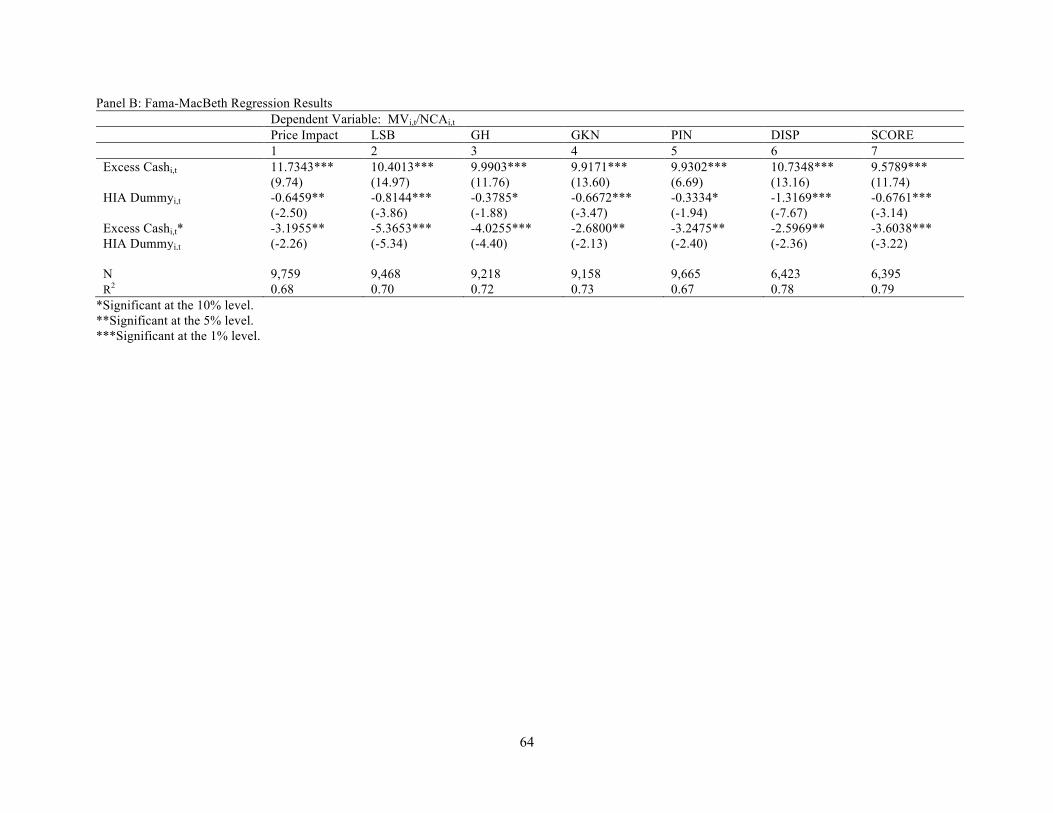
64

Panel B: Fama-MacBeth Regression Results Dependent Variable: MVi,t/NCAi,t Price Impact LSB GH GKN PIN DISP SCORE 1 2 3 4 5 6 7 Excess Cashi,t 11.7343***

(9.74) 10.4013*** (14.97)

9.9903*** (11.76)

9.9171*** (13.60)

9.9302*** (6.69)

10.7348*** (13.16)

9.5789*** (11.74)

HIA Dummyi,t -0.6459** (-2.50)

-0.8144*** (-3.86)

-0.3785* (-1.88)

-0.6672*** (-3.47)

-0.3334* (-1.94)

-1.3169*** (-7.67)

-0.6761*** (-3.14)

Excess Cashi,t* HIA Dummyi,t

-3.1955** (-2.26)

-5.3653*** (-5.34)

-4.0255*** (-4.40)

-2.6800** (-2.13)

-3.2475** (-2.40)

-2.5969** (-2.36)

-3.6038*** (-3.22)

N 9,759 9,468 9,218 9,158 9,665 6,423 6,395 R2 0.68 0.70 0.72 0.73 0.67 0.78 0.79

*Significant at the 10% level. **Significant at the 5% level. ***Significant at the 1% level.

65

Table 9 Testing Whether the Effect of Cash Holdings on Firm Value Vary with Information Asymmetry Regardless of Corporate Governance Structure

This table shows the results of the following regression model:

; where Xtis the level of variable X in year t, dXt+2is the change in the level of X from year t to year t + 2 (i.e., Xt+2 – Xt), dXt-2is the change in the level of X from year t – 2 to year t (i.e., Xt – Xt-2), MV is the market value of the firm calculated at fiscal yearend as the sum of the market value of equity, the book value of short-term debt, and the book value of long-term debt, NCA is non-cash assets defined as total assets minus liquid assets, E is earnings before extraordinary items plus interest, deferred tax credits, and investment tax credits, RD is research and development (R&D) expenditure, D is common dividends paid, and I is interest expense. When R&D is missing, we set it equal to zero. We calculate Excess Cashi,tusing the 2SLS method of Dittmar and Mahrt-Smith (2007) for each firm in each year. The dummy variable for high information asymmetry, HIA Dummyi,t, is equal to one for firms that belong to the top tercile according to each information asymmetry measure (i.e., Price Impact, LSB, GH, GKN, and PIN), and zero for firms in the bottom tercile. LGIM equals one for firms that have below-median GIM governance indices and zero otherwise. Panel A shows the fixed-effects regression results using all firm-year observations with positive excess cash. Panel B show the Fama-MacBeth regression results. Numbers in parenthesis are t-statistics. Panel A: Fixed-Effects Regression Results

Dependent Variable: MVi,t/NCAi,t Price Impact LSB GH GKN PIN DISP SCORE 1 2 3 4 5 6 7 Ei,t/NCAi,t 3.8838***

(16.27) 4.7756*** (21.29)

3.6165*** (15.77)

3.9985*** (18.53)

3.6117*** (15.79)

3.5613*** (12.45)

3.8015*** (13.74)

dEi,t+2/NCAi,t 1.4222*** (7.50)

1.5052*** (8.35)

1.4713*** (8.33)

0.2897** (1.97)

1.5935*** (8.90)

0.3321** (2.09)

0.2805* (1.73)

dEi,t-2/NCAi,t 0.1057* (1.88)

0.0462 (0.88)

0.0167 (0.33)

0.1017* (1.86)

0.0867 (1.63)

0.0121 (0.09)

-0.3349** (-2.36)

RDi,t/NCAi,t 11.2151*** (25.92)

9.4602*** (24.15)

9.6062*** (27.52)

9.3882*** (27.97)

12.8364*** (29.92)

10.0739*** (28.35)

10.8789*** (27.49)

ti,

2-ti,9

ti,

2ti,8

ti,

ti,7

ti,

2-ti,6

ti,

2ti,5

ti,

ti,4

ti,

2-ti,3

ti,

2ti,2

ti,

ti,10

ti,

ti,

NCAdD

βNCAdD

βNCAD

βNCAdRD

βNCAdRD

βNCARD

βNCAdE

βNCAdE

βNCAE

ββNCAMV

+++++++++= +++

ti,

2ti,15

ti,

2-ti,14

ti,

2ti,13

ti,

2-ti,12

ti,

2ti,11

ti,

ti,10 NCA

dMVβ

NCAdNCA

βNCAdNCA

βNCAdI

βNCAdI

βNCAI

β +++ ++++++

( )ti,ti,18ti,17ti,16 DummyHIA *Cash ExcessβDummyHIA βCash Excessβ +++

( ) ti,ti,ti,20ti,19 εLGIM *Cash ExcessβLGIMβ +++

66

dRDi,t+2/NCAi,t 4.6342*** (14.49)

5.7449*** (17.27)

5.6474*** (14.67)

2.9804*** (12.18)

3.3744*** (11.20)

4.2455*** (14.46)

4.3042*** (13.41)

dRDi,t-2/NCAi,t -0.1244 (-0.25)

1.4976*** (3.49)

0.7380* (1.77)

5.6540*** (8.40)

2.9092*** (5.14)

-0.7724* (-1.71)

1.2217** (-2.55)

Di,t/NCAi,t 6.5904*** (5.71)

4.4318*** (4.12)

4.8461*** (4.77)

12.5978*** (11.69)

8.4519*** (6.15)

10.9093*** (9.02)

19.7467*** (13.26)

dDi,t+2/NCAi,t 0.0467 (0.07)

-0.4388 (-0.71)

-0.5373 (-0.99)

9.3551*** (9.24)

0.6509*** (0.84)

5.0493*** (6.52)

5.1610*** (5.76)

dDi,t-2/NCAi,t -0.3996 (-0.51)

-1.6211** (-2.11)

-1.4103** (-2.01)

-1.2738** (-2.02)

-6.3644*** (-4.24)

-3.6245*** (-3.15)

-0.8127 (-0.53)

Ii,t/NCAi,t -16.9196 (-7.68)

-18.5796*** (-8.26)

-23.8584** (-10.86)

-9.8398*** (-5.28)

-17.6011*** (-8.01)

-13.1452*** (-5.56)

-10.4985*** (-4.43)

dIi,t+2/NCAi,t -21.4150*** (-11.51)

-12.0262*** (-8.28)

-11.1988*** (-7.75)

-12.7326*** (-10.52)

-23.2229*** (-11.97)

-9.6445*** (-6.96)

-8.6642*** (-6.30)

dIi,t-2/NCAi,t -8.7046*** (-9.20)

-9.4169*** (-10.55)

-18.7537*** (-8.69)

3.7015* (1.83)

-10.0887*** (-10.65)

-5.3022* (-1.75)

-13.5626*** (-4.50)

dNCAi,t+2/NCAi,t 0.7782*** (17.41)

0.4966*** (12.24)

0.4963*** (12.18)

0.5357*** (15.50)

0.7438*** (17.37)

0.4957*** (13.16)

0.6201*** (16.01)

dNCAi,t-2/NCAi,t 0.1290*** (3.41)

0.1192*** (3.38)

0.4172*** (6.72)

-0.0284 (-0.45)

0.1927*** (5.15)

0.2705*** (3.71)

0.5825*** (7.17)

dMVi,t+2/NCAi,t -0.0958*** (-7.88)

-0.0629*** (-7.23)

-0.0822*** (-6.01)

-0.0022 (-0.29)

-0.0261*** (-2.70)

0.0064 (0.85)

-0.0133* (-1.71)

Excess Cashi,t 8.9150***

(28.07) 8.9967*** (28.77)

10.3254*** (29.85)

7.5970*** (25.97)

7.0062*** (24.01)

9.4725*** (28.12)

8.0927*** (26.95)

HIA Dummyi,t -0.5189*** (-4.37)

-0.5160*** (-5.69)

-0.4432*** (-5.50)

-0.3334*** (-4.49)

-0.3941*** (-3.69)

-0.8725*** (-10.07)

-0.5553*** (-7.08)

Excess Cashi,t* HIA Dummyi,t

-6.7826*** (-9.53)

-6.7618*** (-14.41)

-7.6060*** (-15.80)

-4.6326*** (-11.19)

-4.6555*** (-7.96)

-7.4667*** (-14.30)

-6.9615*** (-14.38)

LGIMi,t 0.1850** (2.34)

0.0437 (0.55)

0.1034 (1.34)

0.1072 (1.60)

0.1202 (1.54)

0.1512** (2.03)

0.1846** (2.49)

Excess Cashi,t* LGIMi,t

3.5597*** (6.69)

1.6004*** (3.33)

1.4833*** (3.03)

1.1362*** (2.74)

2.9113*** (6.08)

1.8066*** (3.63)

2.5819*** (5.53)

Year Dummies Yes Yes Yes Yes Yes Yes Yes N 4,517 4,346 4,328 4,299 4,472 3,665 3,625 R2 0.53 0.55 0.53 0.59 0.53 0.61 0.63

67

Panel B: Fama-MacBeth Regression Results Dependent Variable: MVi,t/NCAi,t Price Impact LSB GH GKN PIN DISP SCORE 1 2 3 4 5 6 7 Excess Cashi,t 6.2847***

(7.53) 7.2728*** (6.56)

6.9730*** (4.87)

5.6909*** (4.64)

5.6775*** (5.81)

7.1798*** (7.02)

6.2859*** (6.15)

HIA Dummyi,t 0.0638 (0.49)

-0.3541*** (-4.34)

-0.1568 (-1.27)

-0.3069*** (-4.47)

-0.1210 (-1.22)

-0.5285*** (-5.29)

-0.3905*** (-5.34)

Excess Cashi,t* HIA Dummyi,t

-4.9147*** (-4.25)

-4.9970*** (-3.68)

-4.2066*** (-3.19)

-2.8547** (-2.34)

-3.6259*** (-3.35)

-4.4853*** (-5.15)

-4.3008*** (-4.17)

LGIMi,t -0.0009 (-0.02)

-0.0725 (-1.31)

-0.0419 (-0.66)

0.0445 (0.81)

0.0255 (0.35)

0.1360** (2.01)

0.1181* (1.88)

Excess Cashi,t* LGIMi,t

0.0463 (0.05)

-1.1667 (-1.75)

-1.7697* (-1.76)

0.0788 (0.19)

1.0111 (1.04)

1.7568* (1.80)

1.2917 (1.33)

N 4,517 4,346 4,328 4,299 4,472 3,665 3,625 R2 0.74 0.72 0.72 0.72 0.73 0.76 0.78

*Significant at the 10% level. **Significant at the 5% level. ***Significant at the 1% level.