Information Guidelines Explanatory Note Uncertainty ...€¦ · Web viewFurther discussion of stochastic modelling with Bayesian probability quantification is in the appendix (section

Information Guidelines Explanatory Note Uncertainty analysis—Guidance for groundwater modelling within a risk management framework

© Commonwealth of Australia, 2018.Uncertainty analysis—Guidance for groundwater modelling within a risk management framework is licensed by the Commonwealth of Australia for use under a Creative Commons By Attribution 4.0 International licence with the exception of the Coat of Arms of the Commonwealth of Australia, the logo of the agency responsible for publishing the report, content supplied by third parties, and any images depicting people. For licence conditions see: http://creativecommons.org/licenses/by/4.0/

This report should be attributed as Middlemis H and Peeters LJM (2018) Uncertainty analysis—Guidance for groundwater modelling within a risk management framework. A report prepared for the Independent Expert Scientific Committee on Coal Seam Gas and Large Coal Mining Development through the Department of the Environment and Energy, Commonwealth of Australia 2018. The Commonwealth of Australia has made all reasonable efforts to identify content supplied by third parties using the following format ‘© Copyright, [name of third party]’.

This publication is funded by the Australian Government Department of the Environment and Energy. The views and opinions expressed in this publication are those of the authors and do not necessarily reflect those of the Australian Government or the Minister for the Environment and Energy.

While reasonable efforts have been made to ensure that the contents of this publication are factually correct, the Commonwealth does not accept responsibility for the accuracy or completeness of the contents, and shall not be liable for any loss or damage that may be occasioned directly or indirectly through the use of, or reliance on, the contents of this publication.

Citation Middlemis H and Peeters LJM (2018) Uncertainty analysis—Guidance for groundwater modelling within a risk management framework. A report prepared for the Independent Expert Scientific Committee on Coal Seam Gas and Large Coal Mining Development through the Department of the Environment and Energy, Commonwealth of Australia 2018.

Acknowledgements This report was finalised by the Independent Expert Scientific Committee on Coal Seam Gas and Large Coal Mining Development (IESC) based on consideration of work commissioned by the Office of Water Science (OWS) on behalf of the IESC in January 2018 through the Department of the Environment and Energy.

Contributors to this work were Glen Walker (IESC), Sarah Taylor (OWS), Peter Baker (OWS) and Natasha Amerasinghe (OWS).

The Department acknowledges the traditional owners of country throughout Australia and their continuing connection to land, sea and community. We pay our respects to them and their cultures and to their elders both past and present.

Contact details

1This initiative is funded by the Australian Government.

www.iesc.environment.gov.au

For information about this report or about the work of the IESC please contact: IESC Secretariat Office of Water Science Department of the Environment and Energy GPO Box 787 CANBERRA ACT 2601This report can be accessed at http://www.iesc.environment.gov.au/

Table of Contents

Overview.......................................................................................................................................................4

The role of the IESC..................................................................................................................................................4

The purpose of the Explanatory Notes......................................................................................................................4

Legislative context....................................................................................................................................................5

Preamble.......................................................................................................................................................6

Executive summary........................................................................................................................................7

Risk management framework...................................................................................................................................7

Early and ongoing engagement and consultation to select the best methods............................................................8

Uncertainty methods................................................................................................................................................8

Choosing a method...................................................................................................................................................9

1. Introduction.........................................................................................................................................10

2. Sources of uncertainty..........................................................................................................................12

3. Risk context, causal pathways and adaptive management...................................................................14

3.1 Uncertainty is integral to risk management................................................................................................14

3.2 Causal pathways........................................................................................................................................14

3.3 Adaptive management...............................................................................................................................15

4. Guiding principles for uncertainty analysis...........................................................................................16

5. Importance of acknowledging bias.......................................................................................................17

6. Modelling workflow for uncertainty analysis........................................................................................18

7. Modelling workflow, confidence level, conditional calibration.............................................................22

7.1 Modelling workflow (conceptual viewpoints).............................................................................................22

7.2 AGMG model confidence level classification...............................................................................................23

7.3 Conditional calibration in uncertainty analysis...........................................................................................25

8. Model complexity/simplicity................................................................................................................27

8.1 Geological complexity................................................................................................................................27



8.2 Model complexity overheads.....................................................................................................................27

9. Uncertainty quantification techniques..................................................................................................29

10. Engagement and communication.....................................................................................................31

10.1 Engagement...............................................................................................................................................31

10.2 Calibrated language...................................................................................................................................31

11. Case Study—Mining Area C, Southern Flank Valley...........................................................................33

12. Fatal flaws checklist.........................................................................................................................35

13. Abbreviations...................................................................................................................................37

14. Glossary...........................................................................................................................................38

15. References........................................................................................................................................46

Appendix: Uncertainty quantification approaches.......................................................................................52

A.1 Model prerequisites for uncertainty quantification....................................................................................52

A.2 Uncertainty quantification approaches.......................................................................................................56

A.3 Qualitative uncertainty analysis (assumption hunting)...............................................................................59

A.4 Sensitivity analysis.....................................................................................................................................61



OverviewThe role of the IESC

The Independent Expert Scientific Committee on Coal Seam Gas and Large Coal Mining Development (the IESC) is a statutory body under the Environment Protection and Biodiversity Conservation Act 1999 (Cth) (EPBC Act). The IESC’s key legislative functions are to:

• provide scientific advice to the Commonwealth Environment Minister and relevant state ministers on coal seam gas (CSG) and large coal mining development proposals that are likely to have a significant impact on water resources;

• provide scientific advice to the Commonwealth Environment Minister on bioregional assessments (CoA 2015a) of areas of CSG and large coal mining development;

• provide scientific advice to the Commonwealth Environment Minister on research priorities and projects;

• collect, analyse, interpret and publish scientific information about the impacts of CSG and large coal mining activities on water resources;

• publish information relating to the development of standards for protecting water resources from the impacts of CSG and large coal mining development and;

• provide scientific advice on other matters in response to a request from the Commonwealth or relevant state ministers.

Further information on the IESC’s role is on the IESC website (CoA 2015b).

The purpose of the Explanatory Notes

One of the IESC’s key legislative functions is to provide scientific advice to the Commonwealth Environment Minister and relevant state ministers in relation to coal seam gas and large coal mining development proposals that are likely to have a significant impact on water resources.

The IESC outlines its specific information requirements in the IESC Information Guidelines (IESC 2018). This information and data is requested to enable the Committee to formulate robust scientific advice for regulators on the potential water-related impacts from coal seam gas and large coal mining developments.

For some topics, Explanatory Notes have been written to supplement the IESC Information Guidelines, giving more detailed guidance to help the coal seam gas and large coal mining industry prepare environmental impact assessments. These topics are chosen based on the IESC’s experience of providing advice on over 100 development proposals.

Explanatory Notes are intended to assist proponents in preparing environmental impact assessments. They provide tailored guidance and describe up-to-date robust scientific methodologies and tools for specific components of Environmental Impact Assessments on coal seam gas and large coal mining developments. Case studies and practical examples of how to present certain information are also discussed.

Explanatory Notes provide guidance rather than mandatory requirements and proponents are encouraged to refer to issues of relevance to their particular project.

The tools and methods identified in this document are reviewed to help proponents understand the range of available approaches to uncertainty analysis in groundwater modelling and are designed to be utilised across a range of regulatory regimes. This Explanatory Note cannot address all aspects of uncertainty analysis in groundwater modelling undertaken for environmental impact assessment and proponents are encouraged to refer to specialised literature and engage with their relevant state regulators.

The IESC recognises that approaches, methods, tools and software will continue to develop. The Information Guidelines and Explanatory Notes will be reviewed and updated as necessary to reflect these advances.





Legislative context

The Environment Protection and Biodiversity Conservation Act 1999 (Cth) (EPBC Act) states that water resources in relation to coal seam gas and large coal mining developments are a matter of national environmental significance.

A water resource is defined by the Water Act 2007 (Cth) (CoA 2007) as: ‘(i) surface water or groundwater; or (ii) a water course, lake, wetland or aquifer (whether or not it currently has water in it); and includes all aspects of the water resource (including water, organisms and other components and ecosystems that contribute to the physical state and environmental value of the resource)’.

Australian and state regulators who are signatories to the National Partnership Agreement seek the IESC’s advice under the EPBC Act 1999 (Cth) at appropriate stages of the approvals process for a coal seam gas or large coal mining development that is likely to have a significant impact on water resources. The regulator determines what is considered to be a significant impact based on the Significant Impact Guidelines 1.3.



PreambleGroundwater modelling is a core aspect of assessing the potential environmental impacts of coal seam gas and large coal mines on groundwater, surface water, and other natural ecosystems. To better understand model reliability, robustness and accuracy, an uncertainty analysis is often required. This analysis quantifies and qualifies the uncertainty in groundwater model predictions. Sources of uncertainty include model parameters, the underlying conceptual model, and observation data. Uncertainty analysis is not routinely used in groundwater modelling for environmental impact assessment. However, there is growing and widespread national and international recognition—across government, industry, research and academia—of the importance of uncertainty analysis in groundwater modelling and decision-making.

Decision-making should be guided by an understanding of risk within a robust risk assessment framework. Simply put, risk—involving both the likelihood and consequence of a particular hazard or impact—cannot be assessed without an understanding of uncertainty. Therefore it is necessary to understand, quantify, predict, manage, mitigate, reduce and communicate uncertainty to enable wise decision-making and inform management, policy and technical matters.

The aim of this Explanatory Note is simple: to provide proponents and their consultants with a high-level introduction and strategic overview of uncertainty analysis relating to groundwater modelling for environmental impact assessment. This document is not a textbook, instruction manual or formal guideline. It is intended to provide initial guidance on the value of and need for uncertainty analysis in groundwater modelling. The reference list contains sources of detailed guidance on techniques.

The IESC recognises that making uncertainty analysis a routine component of environmental impact assessment represents a major reform for groundwater modelling in Australia, if not internationally, and that this change will take time. The IESC also recognises the large and growing number of approaches, methods, software and tools available for uncertainty analysis, and the rapid rate at which this field is developing. Consequently this Explanatory Note is not a static document. The IESC anticipates regular updates to it—and to the overarching IESC Information guidelines for proponents preparing coal seam gas and large coal mining development proposals (IESC 2018)—to reflect theoretical advances and practical improvements in the field of uncertainty analysis in groundwater modelling. These updates will capture important new ideas, developments, methods, approaches, software and tools as they emerge.



Executive summaryPredictive uncertainty analysis is an important part of the groundwater modelling process. Current practice in environmental impact assessments typically involves developing a single numerical groundwater model with limited uncertainty analysis. Considered in a risk management context, this approach is often insufficient to predict the range of potential impacts and their likelihood. A quantitative uncertainty analysis, however, delivers a range of model prediction scenarios with associated likelihoods, each plausible in that it is consistent with all available information and data. Uncertainty analysis also indicates the main sources of uncertainty and by how much the uncertainty in outcomes can be reduced by incorporating further data into the model.

This Explanatory Note supports the IESC Information guidelines for proponents preparing coal seam gas and large coal mining development proposals (IESC 2018) (the Information Guidelines) and complements the Australian groundwater modelling guidelines (Barnett et al. 2012) (AGMG). It provides proponents, consultants and regulators with information on the value of and need for undertaking an uncertainty analysis within a risk management framework. It gives an overview of three examples of uncertainty analysis approaches and some theoretical and practical considerations when undertaking uncertainty analysis in a groundwater modelling project.

It does not provide a step-by-step guide to undertaking an uncertainty analysis. This would not be feasible, given the many approaches and methodologies that are available and continue to be developed. The appropriate approach will depend on the characteristics of the proposed coal seam gas (CSG) or coal mining development and its risk profile, and should be selected in consultation with relevant regulators.

A robust uncertainty analysis will ensure that management options and approaches are commensurate with the level of risk and the likelihood of any particular impact. However, even the most comprehensive modelling and uncertainty analysis cannot completely rule out the potential for unwanted outcomes.

The context for this Explanatory Note is the IESC Information Guidelines, which require:

• modelling results to be presented to show the range of possible outcomes based on uncertainty analysis

• assessment of potential impacts to outline the quality of, and the risks and uncertainty inherent in, the background data and the modelling, particularly with respect to predicted potential scenarios

• the assessment to acknowledge uncertainties in the modelling, identify the sources of errors (e.g. conceptual model and parameter uncertainty) and quantify the level of uncertainty.

This Explanatory Note provides three examples of methods of quantifying uncertainty, and establishes three key guiding principles for any uncertainty analysis:

• the model used must be fit for the purpose of providing information about uncertainty in a way that allows decision-makers to understand the effects of uncertainty on project objectives, and the effects of potential bias

• uncertainty must be considered and addressed at the problem definition stage (when deciding on the approach to groundwater modelling and what questions that modelling will address) and at each subsequent stage of the workflow

• engagement with regulatory agencies (noting the IESC is not a regulator) is required, to discuss and agree on the methodologies and understand the implications of the results.

Risk management framework

A well-executed groundwater model uncertainty analysis provides estimates of the predicted water-related impacts of proposed developments and their likelihoods. These estimates contribute to environmental assessments and management planning when they are embedded within a risk management framework (i.e. consequence and likelihood are quantified). Uncertainty analysis also gives information on the effect of uncertainty in the data, knowledge or modelling on the predicted outcomes, providing a robust foundation for decision-making.



The risk management standard AS/NZS ISO 31000:2009 defines risk as the effect of uncertainty on project objectives, and characterises risk as a function of the likelihood and consequence of an outcome. An uncertainty analysis should therefore be carried out within a risk management context, where the model predictions of the consequences (impacts) of the development or management options should be quantified or characterised with related uncertainties (likelihoods).

This means that a hydrogeological risk assessment is needed at an early stage in the project. This should include a qualitative uncertainty analysis, which should be reviewed throughout the project. Where large coal mines and CSG projects are classified as posing high environmental risk, a quantitative uncertainty assessment is warranted. The level of resources, effort and detail applied to this assessment should be commensurate with the potential risks and/or consequences of the project. During the risk and uncertainty assessment process socially and economically acceptable, and effective risk treatments may be identified that can reduce the requirements for quantitative uncertainty analysis.

As an integral part of a risk management framework, groundwater models should be designed to systematically investigate the causal pathways for potential impacts on water resources and water-dependent assets. This allows characterisation of the uncertainty/likelihood of the impact, enabling the investigation of risk treatment options.

Early and ongoing engagement and consultation to select the best methods

As there are many complex issues involved in uncertainty analysis, the proponent and the regulator need to have early and ongoing dialogue. They need to agree about what model outcomes are required given the risk context, what approaches to groundwater modelling and uncertainty analysis are appropriate and to what extent the analysis needs to be conservative (i.e. deliberately overestimate impacts).

Within the resources available for the impact assessment, there is a trade-off between the complexity of the uncertainty analysis and the complexity of the groundwater model. More complex groundwater models tend to take longer to run, while more comprehensive uncertainty analysis approaches require more model runs. This requires a balance between the simplicity and complexity of the model that is used for uncertainty evaluation, such that it is commensurate with the complexity of the uncertainty analysis methodology applied, and the risk/consequence profile of the project. In selecting the appropriate level of complexity, in either the model or the uncertainty analysis, it is important to fully and transparently document the choices made and the consultations and risk assessments involved.

As well as constraints on the available data and resources, and the technical challenges, a major factor in justifying choices in groundwater modelling and uncertainty analysis is the effect on the model outcomes. From a precautionary viewpoint, it is often justified when undertaking an impact assessment to make conservative choices—that is, choices that will overestimate hydrological changes. For example, an uncertainty analysis with conservative assumptions may require less complex modelling approaches and yet may provide acceptable outcomes. The level of conservatism applied to the impact assessment modelling must be communicated to decision-makers and resource managers so that an appropriate level of conservatism can be applied to decisions and management plans. This will avoid compounding over-conservatism. Demonstrating the degree of conservatism will add confidence to the model output.

Uncertainty methods

This Explanatory Note outlines three general approaches to analysing uncertainties of the models applied. In increasing order of complexity and of the level of resources required, they are:

1. deterministic scenario analysis with subjective probability assessment

2. deterministic modelling with linear probability quantification

3. stochastic modelling with Bayesian probability quantification.

The Explanatory Note outlines how the technical and practical challenges are surmountable, even when considering the resource limitations of practical impact assessment studies. The three general approaches do not address conceptual/structural uncertainty as such, unless those issues can be parameterised appropriately in the groundwater model. Even then, justifications would be required to give confidence that the modelling packages used and the methods applied are suitable to investigate the conceptual or structural uncertainties.





Deterministic scenario analysis with subjective probability assessmentThe first approach can be described as a sensitivity style of uncertainty analysis. It consists of running the model a limited number of times for different scenarios of parameter or input values (usually previously identified from sensitivity testing).

The main advantage of this kind of ‘what-if’ analysis is that it is straightforward to implement and communicate and is not computationally demanding. The main drawbacks are that the selection of scenarios is commonly subjective, and that the likelihood of a scenario is not quantified. The likelihood of different scenarios can only be expressed in qualitative, subjective terms.

Deterministic modelling with linear probability quantificationThe second approach assumes that the model behaves linearly for parameter values in the vicinity of the adopted history-match (conditional) calibration, and that the uncertainty in parameters and observations can be approximated by normal or log-normal distributions.

The main advantage is that this method provides an objective and repeatable estimate of the likelihood of the model outcomes through confidence intervals. The drawbacks are that it is computationally more demanding, the interpretation and communication is more complex than the first approach and, most importantly, that the assumptions about normality and linearity need to be justified.

Stochastic modelling with Bayesian probability quantificationIn the third approach the model is evaluated repeatedly to create an ensemble of model outcomes, where the performance of each individual model is quantified by fitting the history-match observations within specified criteria. Based on such an ensemble of model outcomes, the likelihood of any particular model outcome can be computed.

The main advantage is that it does not require assumptions about linear model behaviour or normally distributed parameters. The drawbacks are that it is even more computationally demanding than the second approach and that, while the assumptions about normality and linearity are relaxed, there are other assumptions involved in the analysis, such as those relating to the method of generating the ensemble of model runs or the way the fit with observations is calculated.

Choosing a method

Whichever method is used, a crucial practical requirement is a stable groundwater model that converges over a wide range of parameter values. This requires careful design, testing and review of the model(s).

There is no single preferred method of uncertainty analysis. There may be alternative methods not discussed here that could be more suitable for a particular development. Regardless of the approach selected, the proponent should present all information in their assessment, with a discussion of which parameters are included in the uncertainty analysis and why. They should also include a formal examination of the uncertainty in these parameters and in the observations, data, and boundary conditions, plus a description of what is an acceptable level of model-to-measurement misfit, to objectively evaluate the performance of the model.

This Explanatory Note includes a fatal flaws checklist highlighting key elements of an uncertainty analysis that reviewers should look for. Without these elements or adequate justification of the applied methodology (with consideration of the risk context), the uncertainty analysis presented may not be suitable. The key elements include:

• clear definition of the required model outcomes

• justification of the methods and assumptions

• open, transparent and logical documentation of methods and results in a way that is amenable to scrutiny

• evidence of consultation and communication between proponent and regulator.





1. Introduction This Explanatory Note supports the Information Guidelines by providing guidance on the need for incorporating uncertainty analysis in groundwater modelling undertaken for environmental impact assessment. It highlights some common methods for quantifying uncertainty in groundwater modelling that could be useful for proponents of CSG and large coal mining developments. It also provides some guidance on engagement with regulators and communication of uncertainty.

Key considerations outlined in the Information Guidelines must include (where applicable):

• the importance of identifying water-dependent environmental assets and potential impact pathways

• the need for environmental impact assessments to be based on conceptual, analytical and numerical modelling and related water and salt balances

• the need to base adaptive management on monitoring and evaluation of mitigation measures.

With regard to model uncertainty, the Information Guidelines suggest:

• modelling results be presented to show a range of possible outcomes based on uncertainty analysis

• assessments of potential impacts outline the quality of, and the risks and uncertainty inherent in, the background data and the modelling, particularly with respect to predicted potential scenarios

• assessments acknowledge uncertainties in modelling, identify the sources of errors (e.g. conceptual model and parameter uncertainty) and quantify the level of uncertainty.

The Explanatory Note focuses on practical uncertainty methods. It is designed to provide guidance that applies to CSG and large coal mine proposals, with reference to other documents on methodologies for groundwater modelling and uncertainty assessments. It is not a comprehensive treatise on uncertainty methods. Interested readers should refer to the specialised literature (e.g. Vrugt 2016, Doherty 2015, Caers 2011) indicated in the reference list.

This Explanatory Note draws from and should be read in conjunction with:

• IESC Information Guidelines (IESC 2018)

• Australian groundwater modelling guidelines (AGMG) (Barnett et al. 2012)

• Modelling water-related ecological responses to coal seam gas extraction and coal mining (CoA 2015)

• Coal seam gas extraction: Modelling groundwater impacts (CoA 2014a)

• Subsidence from coal seam gas extraction in Australia (CoA 2014b)

• Subsidence from coal mining activities: Background review (CoA 2014c)

• Significant impact guidelines 1.3: Coal seam gas and large coal mining developments—Impacts on water resources (CoA 2013)

• NCGRT national groundwater modelling uncertainty workshop 2017 (Middlemis et al. [in press])

• Methodology for bioregional assessments of the impacts of coal seam gas and coal mining development on water resources (Barrett et al. 2013)

The uptake of state-of-the-art uncertainty quantification methods in groundwater modelling has been slow. One reason why uncertainty analysis is not yet a standard modelling practice is that practical guidance on methods and applications does not exist. Another reason for reluctance to embrace uncertainty analysis in modelling is the misconception that it is too difficult to perform, cannot be incorporated into the decision-making process and it cannot be understood by policymakers and the public (Pappenberger and Beven 2006).



This Explanatory Note aims to address some of these issues, although it cannot address all aspects of uncertainty analysis. It complements existing guidelines such as the AGMG. There are few published examples of detailed uncertainty analysis in practice, other than the bioregional assessments (Barrett et al. 2013, Peeters et al. 2016), Office of Groundwater Impact Assessment (Queensland) (OGIA 2016a, 2016b) and IESC knowledge project (Turnadge et al. 2018) studies. Although these studies are not typical in a practical or commercial project sense, they demonstrate the practicability of methods.



2. Sources of uncertaintyThe subsurface environment is complex, heterogeneous and difficult to directly observe, characterise or measure. Groundwater systems are influenced by geology, topography, vegetation, climate, hydrology and human activities; thus uncertainty affects our ability to accurately measure or describe the existing or predicted states of these systems.

Simulation modelling is used to investigate current and future system states and thus support decisions on groundwater resource assessment, management and policy. The AGMG provides information on simulation modelling (Barnett et al. 2012).

Groundwater models are simplified representations of ‘real world’ systems that are continuously refined with new evidence, conceptualisations and uncertainties, to investigate the effects of management options on future eventualities. While models cannot predict the future with total confidence, decision-makers and stakeholders use model results to inform decisions on the acceptable level of risk in a specific context (e.g. potential impact). Model results should therefore be accompanied by uncertainty analyses that qualify or quantify the confidence we have in the modelled outcomes for specified courses of action.

There are different ways to categorise uncertainty, but it is often categorised into two main types (Barnett et al. 2012):

• deficiency in our knowledge of the natural world (including the effects of error in measurements)

• failure to capture the complexity of the natural world (or what we know about it).

For the purpose of this Explanatory Note, it is helpful to consider four sources of scientific uncertainty affecting groundwater model simulations:

• structural/conceptual—geological structure and hydrogeological conceptualisation assumptions applied to derive a simplified view of a complex hydrogeological reality (any system aspect that cannot be changed in an automated way in a model)

• parameterisation—hydrogeological property values and assumptions applied to represent complex reality in space and time (any system aspect that can be changed in an automated way in a model via parameterisation)

• measurement error—combination of uncertainties associated with the measurement of complex system states (heads, discharges), parameters and variability (3D spatial and temporal) with those induced by upscaling or downscaling (site-specific data, climate data)

• scenario uncertainties—guessing future stresses, dynamics and boundary condition changes (e.g. mining, climate variability, land and water use change).

These four sources of scientific uncertainty result in predictive uncertainty—the bias and error associated with model simulations (Figure 1). Bias is systematic error that displaces the model outputs away from the accepted ‘true’ value. Error is the difference (spread) between the average value of model simulations and the ‘true’ value. Bias and error affect the precision of model results, even when that model is consistent with the conceptual understanding of the system and the related observations and measurements.



Figure 1—Processes that contribute to uncertainty

Note: Plot A illustrates how errors and biases in model predictions (clusters of small green dots) can shift predictions away from the ‘true’ values (large central red dots). Plot B illustrates how bias and variance in modelled data can affect the model calibration.

Source: Adapted from Richardson et al. [in press], Doherty and Moore [in press].

Being overcommitted to one conceptualisation over others (bias)—perhaps the wrong one—could lead to simulations that overestimate or underestimate impacts. If the uncertainty analysis focuses only on errors and neglects to account for or discuss biases, incomplete and distorted evidence of the accuracy of model predictions will be provided.

For detailed background information and discussion of uncertainty issues and methodologies, see the National Centre for Groundwater Research and Training (NCGRT) report on the groundwater modelling uncertainty workshop (Middlemis et al. [in press]).



3. Risk context, causal pathways and adaptive management3.1 Uncertainty is integral to risk management

Risk is defined as the effect of uncertainty on project objectives (AS/NZS ISO 31000:2009). It is characterised or quantified as a function of the likelihood and consequences of an outcome. Freeze et al. (1990) characterise the role of models in decision support as quantifying the level of risk associated with management options. It follows that if a model is applied to support environmental decision-making, its simulations of the consequences of management options must quantify the related uncertainties (Doherty and Moore [in press]).

Uncertainty analysis is therefore an integral part of a robust risk management framework, as it informs and complements other aspects such as risk assessment and management, communicating outcomes and prioritising efforts to reduce uncertainty (e.g. by acquiring data on key processes) (Walker [in press]). An example of high-priority (but relatively low-cost) data that reduces uncertainty in groundwater models is accurate LiDAR topographical data. Accurate definition of the interface between the surface and the sub-surface is critical for implementing boundary conditions in a model to represent surface water features (e.g. creeks and rivers), evapotranspiration and spring features (Doble and Crosbie 2017).

In environmental management, risk has negative connotations generally associated with the hazards or impacts of a development. Uncertainty is also commonly seen as a negative factor. Understanding uncertainty can have positive consequences (Begg 2013) including opportunities to achieve desired benefits (e.g. to justify expenditure on a mining project where sound environmental management can manage other project risks). However, value judgements are involved in all risk assessments. These value judgements depend on the economic, social and environmental values established in public policies, business cultures and community viewpoints.

The precautionary principle is incorporated in the principles of ecologically sustainable development (ESD), which are promoted by the objectives of the EPBC Act 1999 (Cth) (CoA 1999). The ESD principles establish that social considerations are a key factor in decision-making processes, along with economic and environmental factors. These principles are very important, and have been tested in Australian law, notably in the Queensland Land Court case in 2015 in relation to the proposed Adani Carmichael coal mine (QLC 48 2015). For more information on the precautionary principle and ESD, see the independent review of the EPBC Act (CoA 2009).

In the context of this Explanatory Note, the precautionary principle means that if a development raises the risk of harm to the environment (i.e. in non-trivial likelihood and consequence terms), then proportionate precautionary measures should be taken even if some cause-and-effect relationships are not completely scientifically established.

The two main preconditions for applying the precautionary principle are:

• the threat of serious or irreversible environmental damage

• scientific uncertainty as to the nature and scope of the threat of environmental damage.

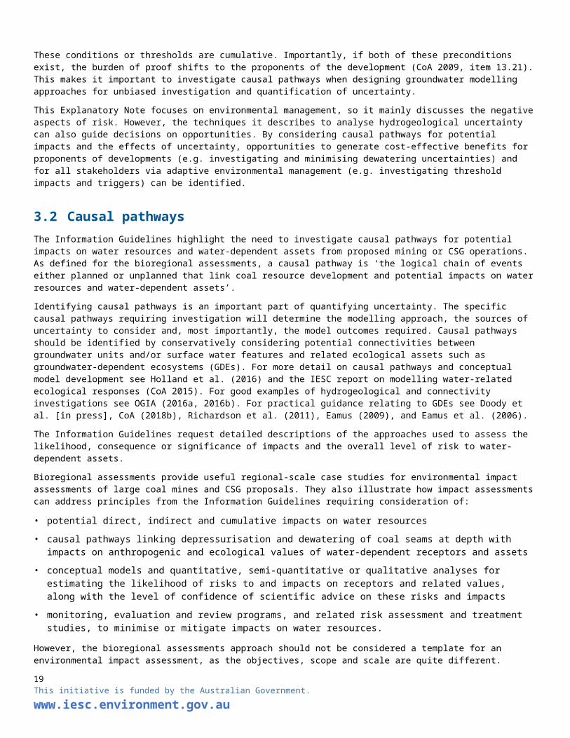
These conditions or thresholds are cumulative. Importantly, if both of these preconditions exist, the burden of proof shifts to the proponents of the development (CoA 2009, item 13.21). This makes it important to investigate causal pathways when designing groundwater modelling approaches for unbiased investigation and quantification of uncertainty.

This Explanatory Note focuses on environmental management, so it mainly discusses the negative aspects of risk. However, the techniques it describes to analyse hydrogeological uncertainty can also guide decisions on opportunities. By considering causal pathways for potential impacts and the effects of uncertainty, opportunities to generate cost-effective benefits for proponents of developments (e.g. investigating and minimising dewatering uncertainties) and for all stakeholders via adaptive environmental management (e.g. investigating threshold impacts and triggers) can be identified.

3.2 Causal pathways

The Information Guidelines highlight the need to investigate causal pathways for potential impacts on water resources and water-dependent assets from proposed mining or CSG operations. As defined for the bioregional assessments, a causal pathway is ‘the logical



chain of events either planned or unplanned that link coal resource development and potential impacts on water resources and water-dependent assets’.

Identifying causal pathways is an important part of quantifying uncertainty. The specific causal pathways requiring investigation will determine the modelling approach, the sources of uncertainty to consider and, most importantly, the model outcomes required. Causal pathways should be identified by conservatively considering potential connectivities between groundwater units and/or surface water features and related ecological assets such as groundwater-dependent ecosystems (GDEs). For more detail on causal pathways and conceptual model development see Holland et al. (2016) and the IESC report on modelling water-related ecological responses (CoA 2015). For good examples of hydrogeological and connectivity investigations see OGIA (2016a, 2016b). For practical guidance relating to GDEs see Doody et al. [in press], CoA (2018b), Richardson et al. (2011), Eamus (2009), and Eamus et al. (2006).

The Information Guidelines request detailed descriptions of the approaches used to assess the likelihood, consequence or significance of impacts and the overall level of risk to water-dependent assets.

Bioregional assessments provide useful regional-scale case studies for environmental impact assessments of large coal mines and CSG proposals. They also illustrate how impact assessments can address principles from the Information Guidelines requiring consideration of:

• potential direct, indirect and cumulative impacts on water resources

• causal pathways linking depressurisation and dewatering of coal seams at depth with impacts on anthropogenic and ecological values of water-dependent receptors and assets

• conceptual models and quantitative, semi-quantitative or qualitative analyses for estimating the likelihood of risks to and impacts on receptors and related values, along with the level of confidence of scientific advice on these risks and impacts

• monitoring, evaluation and review programs, and related risk assessment and treatment studies, to minimise or mitigate impacts on water resources.

However, the bioregional assessments approach should not be considered a template for an environmental impact assessment, as the objectives, scope and scale are quite different. Bioregional assessments provide advice on development stressors, causal pathways, receptors and assets but they are not development specific. Bioregional assessments do, however, inform environmental impact assessment studies by providing regional context information and, importantly, independent cumulative impacts assessment.

The Cooper subregion bioregional assessment (CoA 2017) considered causal pathways and the coal development horizon, concluding that detailed modelling for impact assessment was not warranted and that conceptual modelling was adequate at that time. This example demonstrates how establishing a low-risk context, via consideration of causal pathways and undertaking a risk assessment at an early stage, can be used to justify a qualitative approach to impact and uncertainty assessments, especially under an adaptive management framework (e.g. subject to future changes to the Cooper Basin coal development pathway).

3.3 Adaptive management

Adaptive management is often justifiably used to address environmental issues in the face of uncertainty. However, the long time lags affecting groundwater processes can mean that it may be difficult to reverse the impacts of an action (Walker [in press]). By the time monitoring shows that a significant ecological asset will be affected, it may be too late to prevent impacts occurring. For example, groundwater drawdown could continue to increase due to the hydrogeological time lag effects despite groundwater extraction ceasing.

Tolerance of an unwanted outcome (or failure) is related to the cost of failure. If the cost is relatively low, then a moderate likelihood of failure may be tolerated, provided there are economically and socially acceptable risk-reduction options that can be implemented in a timely fashion. On the other hand, if the cost of failure is high (e.g. unwanted impacts on high-value ecosystems), the likelihood of failure must be low for a management option or adaptive management plan to be deemed socially and economically acceptable, and effective.

This drives the need for a conservative approach to impact assessment. Such an approach includes careful analysis of uncertainties and investigation of options for risk treatments and mitigation. It is also important to communicate the residual risk and be able to adaptively manage it. However, even the most comprehensive modelling and uncertainty analysis study cannot completely rule out the potential for unwanted outcomes.





4. Guiding principles for uncertainty analysisHill et al. (2004) summarise some fundamental principles that are shared by all groundwater modelling guidelines. These are based on ideas set out in the 2001 modelling guidelines (Middlemis et al. 2001), which remain valid for this Explanatory Note:

The aim of most guidelines is to reduce and reveal model uncertainty for the users of modeling studies, including resource management decision makers and the community. This is achieved by promoting transparency in modeling methodologies and encouraging innovation, consistency, and best practice. Guidance is provided to non-specialist modelers and auditors or reviewers of models by outlining the steps involved in scoping, managing, and evaluating the results of groundwater modeling studies. The guidelines serve modeling specialists by providing a baseline set of ideas and procedures from which they can innovate. The guidelines are intended for use in raising the minimum standard of modeling practice and allowing appropriate flexibility, without limiting necessary creativity or rigidly specifying standard methods. The guidelines also should not limit the ability of modelers to use simple or advanced techniques, appropriate for the study purpose. Techniques recommended in the guidelines may be omitted, altered, or enhanced, subject to the modeler providing a satisfactory explanation for the change and negotiation with the client and/or regulator as required. Not all aspects of the guidelines would necessarily be applicable to every study. It also is acknowledged that standardization of modeling methods will not preclude the need for subjective judgment during the model development process. The guidelines are to be applied to new groundwater flow modeling studies and reviews of existing models. The guidelines should be seen as a best practice reference point for framing modeling projects, assessing model performance, and providing clients with the ability to manage contracts and understand the strengths and limitations of models across a wide range of studies (scopes, objectives, budgets) at various scales in various hydrogeological settings. The intention is not to provide a prescriptive step-by-step guidance, as the site-specific nature of each modeling study renders this impossible, but to provide overall guidance and to help make the reader aware of the complexities of models, and how they may be managed.

While these general guiding principles allow for flexibility, this Explanatory Note insists on some minimum standards:

• clear definition of the specific model outcomes sought

• justification of the methods and assumptions applied

• open, transparent and logical documentation of methods and results in a manner that is open to scrutiny.

This Explanatory Note provides further information on the key elements of how model uncertainty can be analysed in the context of supporting a practical environmental impact assessment for large coal mining and CSG proposals. It should not be interpreted as a step-by-step guide to comprehensively analysing uncertainty.



5. Importance of acknowledging bias Richardson et al. [in press] discuss, in relation to groundwater modelling, some of the cognitive biases that everyone is prone to, such as availability, confirmation, confidence and framing bias (see glossary). Although a groundwater model is designed to be an objective representation of physical reality, the multitude of choices and assumptions that need to be made during modelling and uncertainty analysis make bias in predictions unavoidable.

A prime example of bias is adopting a conservative methodology in which impacts are overestimated. Underschultz et al. (2018) show that such an approach, especially when conservatism in geological representation is combined with conservatism in groundwater modelling, can lead to very biased results. For example, they show that current water and salt production from CSG in Queensland is about 25 per cent of the estimates made by government and academia before the 2011 expansion of CSG to liquefied natural gas export, and about 70 per cent of the industry estimates made in 2010–11. They attribute the discrepancy to various factors including:

• the level of conservatism applied by the gas industry, government and academia in the earlier estimates

• systemic underestimation of the cumulative effects of depressurisation of the coal resource by multiple operators

• not accounting for near-well multi-phase flow effects.

Biased analysis may be acceptable in some cases, provided a conservative methodology is applied logically, justified transparently and documented comprehensively (e.g. Ferré 2016).

While bias in modelling can never be completely eliminated, known biases need to be honestly and transparently communicated as part of the uncertainty analysis. An uncertainty analysis that only focuses on errors will provide incomplete and distorted evidence of modelling accuracy. From a management perspective, modelling is considered to have failed if there is sufficient bias for a poor decision to be made (e.g. through lack of transparency or inadequate uncertainty analysis), especially if the consequence is large (Walker [in press]).

As a result, conceptual models for large coal mines and CSG developments should consider and minimise potential biases when analysing how causal pathways can transmit direct, indirect and cumulative impacts from coal seams to water resources or water-related assets. More than one model conceptualisation or realisation may need to be tested to understand the effect of conceptual or other sources of uncertainty and bias on model outputs. This may lead to more than one mathematical model, as outlined in the AGMG (Barnett et al. 2012). The multiple models may be of different types—e.g. conceptual, analytical or numerical—depending on the objective to be investigated.

Minimising and acknowledging bias in investigations of causal pathways is a key element of the ecological values analysis at the problem definition stage, along with data analysis, conceptualisation, and the initial risk analysis and treatment options assessment.



6. Modelling workflow for uncertainty analysisUncertainty analysis should be considered at the problem definition stage and at each subsequent stage of the workflow. It should be integrated within a risk management framework (i.e. initial qualitative risk assessment, subsequent review/revision and, where warranted, quantitative risk assessment) and involve meaningful (‘without prejudice’) consultation between proponents and regulators on methodologies and assumptions. Note that the IESC is not a regulator.

In the case of an extension or expansion of an existing approved development where there is an existing groundwater model, it is even more important that the proponent and regulators engage early. Agreement is needed on the approach to uncertainty analysis and on the capability of the existing model to be used for this analysis. There is also an expectation that data from the existing operation will be applied to improve the groundwater conceptualisation and associated mathematical modelling.

A conceptual example of an iterative approach to groundwater modelling is illustrated in Figure 2. Initially a preliminary risk assessment is done, possible risk mitigations are considered, and the model is conceptualised to meet the objectives. As the modelling and assessment workflow proceeds through its iterations, the objectives should be reviewed according to risk, and complexity may be added or refined as necessary. In the preliminary stages, there may not be any need for numerical modelling. If risks are not high at any stage, nothing more may be required and the investigation may be cut short. Most large coal mines and CSG projects are likely to pose high environmental risks. This means the proponent should conduct a quantitative uncertainty assessment to a level of detail commensurate with the potential risks and consequences of the project. Risk assessments may be able to identify socially and economically acceptable, and effective risk treatments that may reduce the requirements for quantitative uncertainty analysis.

Figure 2—Conceptual example of an iterative approach to groundwater modelling



Note: The approach is based on current best practices and involves setting and refining objectives (management target cycle), identifying and assessing risk mitigation options (intervention cycle) and analysing assumptions and conceptualisations (assumption cycle).

Source: Guillaume et al. 2016.

The AGMG states that objective consideration of uncertainty is warranted for every groundwater project (Barnett et al. 2012). For high-risk projects, the lack of an objective uncertainty assessment is a metric for model failure. For low-risk projects, it may be acceptable to describe the effect of uncertainty on the project objectives in more qualitative terms. For some large coal mines and CSG projects it may be possible to justify a low-risk categorisation and simpler methods.

The following key principles, consistent with the AGMG, should drive a modelling workflow (Figure 3) which aims to objectively assess uncertainty.

• While all projects require at least a qualitative uncertainty analysis discussing how model assumptions can potentially affect simulations, high-risk projects also require a quantitative uncertainty assessment. The level of detail included should be commensurate with the potential risks and consequences of the project. This means that a preliminary hydrogeological risk assessment and qualitative uncertainty analysis are needed at an early stage in every project.

• Modelling methods must consider the coal mining or CSG development stressors (dewatering and depressurisation) and causal pathways for potential impacts on water resources and water-related assets.

• Project objectives and what the model needs to predict in specific and measurable terms require explicit definition. For example, threshold or trigger impact terms provide information on which decisions may be based objectively.

• The methodology should be designed to provide information about the uncertainty in conceptualisations and model simulation outputs in a way that allows decision-makers to understand the effects of uncertainty on project objectives and the effects of potential bias. In other words, the model should be specifically fit for this purpose.

• A balance between simplicity and complexity is required when developing a model for uncertainty evaluation, commensurate with the risk/consequence profile of the project. This may require development of more than one model.

• Model simulations should be constrained with available observations and information.

• The range of model outcomes that are consistent with all observations and information should be presented (e.g. calibration-constrained model outcomes).

Modelling and methodology assumptions and choices, the logic behind these, and how they may affect simulations, uncertainties and potential bias, must be reported. The results should be presented clearly such that they are not prone to misinterpretation.

The workflow requires multiple iterations during the project. This means revisiting objectives, assumptions, conceptualisations and simulations, as well as the risk assessment and consideration of any risk treatments applied to mitigate impacts, in a process of engagement with regulators.

The proponent should engage with regulatory agencies at the outset and at subsequent key stages, to discuss and agree on methodologies and ongoing refinements (iterations) and to understand the implications of the results. This is particularly important for projects that need to assess the potential impacts from subsidence. Currently there are multiple conceptualisations of the height of fracture zones with no consensus on which is better. Additionally there is no general agreement on how to best represent the changes to and variability in aquifer properties following subsidence in a groundwater model. As a result it is not possible to identify a particular approach to groundwater modelling and uncertainty analysis that is globally applicable when assessing subsidence-related impacts. The modeller and the regulator will need to consider a range of approaches and agree on a suitable one.

Figure 3 includes suggestions as to when engagement should happen. Engagement can be conducted on a ‘without prejudice’ basis. Effectively communicating the results of uncertainty analyses will require engagement throughout the investigation, not simply at the end to present the results (Richardson et al. [in press], Barnett et al. 2012).

The high profile of global issues such as climate variability, energy security and controversial developments has raised awareness of uncertainty and risk among environmentalists, industry, regulators and the community. This has raised expectations that scientific results



will be presented honestly, precisely and transparently. There are instances of both understatement and overstatement of uncertainties, reflecting distortion of the assessments. In some cases this is deliberately aimed at undermining the science (Walker [in press]). Transparent documentation provides objective evidence of the uncertainty methods and assumptions applied. Formal engagement gives the regulator and the community confidence that all potential impacts have been considered and that the proposed monitoring and adaptive management measures are appropriate.

Decision-makers need to know:

• the ‘most likely’ outcome

• whether there are circumstances that may result in unacceptable outcomes

• what risk or mitigation treatments or adaptive management initiatives may be applied.

Careful choice of language that aligns with decision-making (e.g. positive or negative framing and using thresholds) makes it easier for all stakeholders to understand the ideas presented without further analysis (Richardson et al. [in press]). For example, a 5 per cent chance that drawdown will be greater than 1 m (negative framing) is the same as a 95 per cent chance that it will be less than 1 m (positive framing). The framing used should be consistent within the documentation.





Figure 3—Suggested modelling uncertainty analysis workflow

7. Modelling workflow, confidence level, conditional calibration7.1 Modelling workflow (conceptual viewpoints)

The traditional model workflow (Figure 4, left column) outlined in the AGMG consists of data collation, model design (usually a complex model), calibration, prediction and sensitivity analysis before application of the results to support decisions. This is quite different to an uncertainty-driven workflow (Figure 4, right column). An uncertainty-driven workflow can be conceptually viewed as working in the opposite direction. It starts with careful consideration of the decisions required, then builds a model specifically to support decision-making (Ferré 2016). The model must achieve a suitable balance between simplicity and complexity for use in computationally intensive uncertainty analysis. Uncertainty analysis is used to support decision-making and also to identify the data needed to reduce uncertainty.

Figure 4—Conceptualisations of the traditional (left) and uncertainty-driven (right) modelling workflows

Source: Adapted from Ferré 2016.

Although the uncertainty workflow differs conceptually from the traditional workflow, the AGMG encourages innovation and adaption of modelling methods (Barnett et al. 2012). A different view of the workflow is warranted in this Explanatory Note because an uncertainty-driven approach is designed and applied specifically to support decisions by exploring uncertainties within a risk and adaptive management framework. The traditional workflow tends to result in complex models despite the AGMG encouraging finding the right balance between complexity and simplicity for the project objectives. Successful uncertainty analysis is founded on achieving optimal model complexity.

The uncertainty-driven approach usually requires carefully designed models with short run times for the often large numbers of runs involved. Careful design can take many forms. It includes ensuring that model simulations are stable and that complexity is included where it is relevant to the project objective (‘effective simplicity’), while not using long run times as an excuse to avoid necessary complexity. The computational burden often associated with running models multiple times should not be overstated: the requirement is only to run as



many realisations as necessary to generate robust statistics from multiple model outputs. In other words, thousands of runs may not always be required. This is discussed further in section A.2.3, with reference to Figure 10.

7.2 AGMG model confidence level classification

While this Explanatory Note is philosophically integrated and consistent with the AGMG (Barnett et al. 2012), it recommends a slightly different approach to classifying model confidence levels. While the AGMG model confidence level classification table (Barnett et al. 2012, Section 2, Table 2-1) is reasonable, the related commentary and guidance are not always clear.

Alternative methods of assessing confidence level have been tested. One is a method of indicating which attributes in the table are satisfied for a given model and assessing the confidence level by considering the score counts in each class (see Figure 5). This avoids the tendency where one guideline comment may be ‘cherry-picked’ to undermine the model confidence classification, rather than considering the balance of model performance against the entire table of attributes.

In the example presented in Figure 5, the model achieves a Class 2 result overall. Using the AGMG model confidence level classification table, it would be in Class 1. This is because the AGMG commentary indicates that a single Class 1 attribute is sufficient to classify a model as Class 1 overall, even if the weight of evidence indicates otherwise.

However, the approach shown in Figure 5 may also be prone to manipulation. A better method would require the modeller or reviewer to indicate in the table which conditions are satisfied and explain why others are not satisfied and why this is relevant to the model objectives, outcomes and uncertainties. This approach is consistent with other recommendations in this Explanatory Note for modellers to justify assumptions and choices in technical reports in a manner that is transparent and open to scrutiny.



CLASS DATA CALIBRATION PREDICTION QUANTITATIVE INDICATORS

1 (simple)

Not much / Sparse coverage Not possible. Timeframe >> Calibration Timeframe >10x

√ No metered usage. ~ Large error statistic. Long stress periods. Stresses >5x

Low resolution topo DEM. Inadequate data spread. Poor / no validation. Mass balance > 1% (or one-off 5%)

Poor aquifer geometry. Targets incompatible with model purpose.

Targets incompatible with model purpose.

Properties <> field values.

Basic / Initial conceptualisation.



No review by Hydro / Modeller.

2 (impact

assessment)

√ Some data / OK coverage. Weak seasonal match. √ Timeframe > Calibration √ Timeframe = 3-10x

~ Some usage data/low volumes.

~ Some long term trends wrong. Long stress periods. √ Stresses = 2-5x

√ Baseflow estimates. Some K & S measurements.

√~ Partial performance (e.g. some stats / part record / model-measure offsets).

√ OK validation. ~ Mass balance < 1%

√ Some high res. topo DEM &/or some aquifer geometry.

√ Head & Flux targets used to constrain calibration.

√ Calib. & prediction consistent (transient or steady-state)

~ Some properties <> field values. Review by Hydrogeologist.

√ Sound conceptualisation,reviewed & stress-tested.

Non-uniqueness and qualitativeuncertainty partially addressed.

√ Significant new stresses not in calibration.

Some coarse discretisation inkey areas of grid or at key times

3 (complex simulator

Plenty data, good coverage. Good performance stats. Timeframe ~ Calibration Timeframe < 3x

Good metered usage info. √~ Most long term trends matched. √ Similar stress periods. Stresses < 2x

√ Local climate data. ~ Most seasonal matches OK. Good validation. ~ Mass balance < 0.5%

~ Kh, Kv & Sy measurementsfrom range of tests.

Present day head / flux targets,with good model validation.

Transient calibration andprediction.

√~ Properties ~ field measurements.

√ High res. topo DEM all areas &good aquifer geometry.

√~ Non-uniqueness minimised,qualitative uncertainty justified.

√~ Similar stresses to thosein calibration.

√ No coarse discretisation inkey areas (grid or time).

Mature conceptualisation. √ Review by experienced Modeller.

Figure 5—AGMG model confidence level case study example (after Table 2-1 of Barnett et al (2012) Australian Groundwater Modelling Guideline) Note: Achieved attributes are shown with a tick and partially achieved attributes with a tilde. Source: After N Merrick, personal comment.



7.3 Conditional calibration in uncertainty analysis

The traditional workflow of model development has been characterised as a means of reducing parameter bias and uncertainty through calibrating the model against measured observations of historical hydrologic system behaviour. This process is known as parameter identification or estimation, inverse solution or history-matching (Barnett et al. 2012, Neuman and Wierenga 2003). A model that is demonstrably consistent with monitoring data (especially if head and flux calibration targets are matched) is traditionally considered a reliable deterministic simulator of future behaviour.

However, neither the structure nor the parameter values of a deterministic model are unique. This ‘equifinality’ problem has long been recognised as generic and not simply a matter of identifying a system’s ‘true’ model structure or parameter values (Beven 1993). In fact a ‘true’ model for a hydrologic system does not exist, due to the sources of uncertainty outlined previously. Even the most complex model can, by definition, only be approximate in its attempted simulation of environmental processes.

Doherty and Moore [in press] show that the calibration process does not reduce the uncertainty of a simulation where it is sensitive to parameters or combinations of parameters that lie within the ‘calibration null space’. The calibration null space comprises model parameters and combinations that are not informed by the available historical measurements and therefore cannot be inferred through a calibration process. In other words, any calibration process attempting to estimate many parameters will likely be non-unique, because it contains parameters of the null space (Doherty and Christensen 2011). Another characteristic of parameters that lie within the null space is that they can be added to any solution of an inverse problem with no or minimal effect on model outputs.

The so-called null space Monte Carlo (NSMC) method, implemented in the PEST parameter estimation software, allows users to generate multiple calibrated models with different sets of parameters. It is a flexible and efficient technique for nonlinear predictive uncertainty analysis (Doherty 2010). NSMC methods involve defining stochastic parameter sets that maintain or precondition calibration, rather than post-conditioning Monte Carlo results by removing runs that do not meet a set calibration criterion.

However, Doherty and Moore [in press] also show that calibration is a valid first step in a two-step uncertainty analysis process using linear methods (see section A.2.2):

1. Finding a history-match (inverse) solution of minimum error variance1 by fitting model outputs to the calibration dataset of heads and fluxes, preferably during a period of wide-ranging hydrological stress. This reduces non-uniqueness. It can be achieved using the uncertainty analysis technique of pilot point parameter estimation with regularisation, a means of ensuring that parameter estimates do not move far from initial estimates that are considered to be reasonable (Barnett et al. 2012).

2. Quantifying the error in simulations made by the history-matched model.

A model that is carefully calibrated (and/or subsequently validated) in this way should be qualified as a conditionally calibrated (validated) model, in that it has not yet been falsified by tests against observational data (Beven and Young 2013). It is conditional on the history-matching data used and on the numerical intricacies of the inversion method (including the optimisation algorithm).

Any changes to the calibration data and method may result in a different optimal model. There is a need to continue testing and updating models as new data becomes available. This may lead to model rejection due to changes in the system. Rejection or falsification of models is an important part of model building, as it leads to better understanding of the system and ultimately a better performing model.

Conditionally calibrated models are useful for running simulations within the range of the calibration and evaluation data (Barnett et al. 2012) and for enabling updates in the light of future research and development or changes in catchment characteristics.

A conditionally calibrated model can be considered a ‘receptacle for expert knowledge’ (Doherty and Moore [in press]) or a ‘good representation of the system of interest’ (Barnett et al. 2012) in terms of:

• the conceptualisation and parameterisation used to represent real-world hydraulic properties with effective simplicity (or appropriate complexity)

1 Minimum error variance means minimum spread of the error; it does not mean that the bias of a simulation is minimised—see Figure 1.



• the historical behaviour of the system, as the history-match (conditional calibration) constrains parameters to a narrow stochastic range.

Deterministic scenario analysis using a conditionally calibrated model and subjective probability assessment should only be considered as an uncertainty quantification approach when the probability of the scenarios can be established independently. An example would be evaluating a future climate change scenario where the probability of the scenario is established by climate modelling. If an independent probability estimate of the scenario is not available but it can be established that the conceptualisation and parameterisation is conservative (i.e. that it overestimates the impact), then a deterministic scenario analysis can be used as a screening tool for further investigation and detailed modelling or in qualitative uncertainty analysis in a low-risk context (e.g. see section A.2.1).

A conditional calibration approach can be used to provide the prior probability foundation for a tractable but not strictly Bayesian investigation of stochastic uncertainty (see section A.2.3). However, it does not necessarily reduce sources of predictive bias that may be introduced via simplification assumptions or via a conditional calibration process that compensates for model defects through biased parameter values of the history-match model (Doherty and Moore [in press]).



8. Model complexity/simplicity8.1 Geological complexity

The level of hydrogeological complexity in any model should be suitable for its purpose (Neuman and Wierenga 2003). An important purpose of a modelling study is to provide information about the uncertainty in conceptualisations and model simulation outputs in a way that allows decision-makers to understand the effects of uncertainty on project objectives and the effects of potential bias.

Refsgaard et al. (2012) concluded that geological models influence model predictions less for flow modelling simulations compared to prediction of chemical concentrations, provided that (history-match) conditional calibration against head and discharge data is performed and that model simulations are confined to:

• the same types of variables used for conditional calibration (e.g. head and flux data)

• similar hydrological stress regimes (pumping, climate and timeframes).

Harrar et al. (2003, cited in Refsgaard et al. 2012) reached similar conclusions: while simple models of geological heterogeneity produced capture zones similar to those produced by more complex models, these models of different heterogeneity/complexity produced very different predictions of travel time and solute breakthrough. Put simply, the model predictive error will generally increase the larger the difference between the nature of model predictions and the calibration history-match.

These principles are consistent with the AGMG (Barnett et al. 2012). In these cases, the inevitable (unknown) errors in the geological interpretations can to some extent be compensated for by the biased parameter values of the history-match model. However, geological model uncertainties become crucial where groundwater models that are history-matched to head and discharge data for the historical pumping or climate record are then used for extrapolation beyond that conditional calibration base. In such ‘out of range’ simulations the geological structure is often the dominant source of uncertainty, so alternative hydrogeological conceptualisations should form part of the uncertainty assessment.

Some structural uncertainties can be investigated by testing alternative conceptualisations, either by parameterising the conceptualisation issue (e.g. faults) or applying Bayes’ theorem to combine/evaluate the known and unknown conceptual models. As some modelling packages may not be suitable for investigating some conceptual or structural uncertainty issues (e.g. subsidence), the modeller must justify the methods and software applied.

8.2 Model complexity overheads

Highly complex models are expensive to develop and usually run slowly or are not numerically stable. This hinders the methods used for uncertainty analysis to quantify the extent to which the complexity and parameterisation of the model allow for the available observations to be matched within specified criteria to reduce predictive uncertainty. It is also difficult to scrutinise and communicate all aspects of highly complex models. This renders them less transparent, which can lead to a loss in confidence in the model results (Saltelli and Funtowicz 2014).

There are also concerns that the AGMG (Barnett et al. 2012) is being used inappropriately in some cases to justify ‘indiscriminate complexification’ of models, rather than ‘effective simplification’ (Voss 2011a), where that would be more appropriate for the investigation context, objectives and resources (Doherty 2010). There are also cases where opponents of coal mining or CSG developments have suggested that environmental impact assessments may be fatally flawed because of claims that models do not capture adequate complexity.

Although greater complexity does not necessarily translate directly to a stronger technical basis for regulatory decisions, the use of overly simplified models may result in erroneous decisions. This Explanatory Note advocates an approach that goes beyond platitudes about subjectively making a model ‘as simple or complex as required, but not too simple or complex’. Rather:



• the model must be designed to be fit for the specific purpose of providing information about uncertainty in a way that allows decision-makers to understand the effects of uncertainty on project objectives, and the effects of potential bias

• engagement with regulatory agencies is required from the outset and at throughout the modelling study, to discuss and agree on the uncertainty analysis methodologies and understand the implications of the results.



9. Uncertainty quantification techniques Practical implementation of the concepts described above can be a daunting task, especially when seeking an approach that respects the theoretical nuances of uncertainty quantification in a transparent way while being pragmatic in the face of finite modelling resources.

A wide variety of uncertainty quantification techniques have been developed for water resources in the last four decades (Maier et al. 2014). Uncertainty quantification techniques can be classified in three groups.

1. Deterministic scenario analysis with subjective probability assessment

The model is run with a limited number of different plausible parameter combinations. In hydrogeological model reports, this is often referred to as sensitivity analysis (see section A.4). For these results to be used in risk analysis a subjective, often informal probability needs to be specified (e.g. a description such as ‘worst case’). The groundwater impact assessment for the Santos Narrabri Gas Project (CDM Smith 2016) is an example of the application of this uncertainty quantification technique. Further discussion of deterministic scenario analysis with subjective probability assessment is in the appendix (section A.2.1).

2. Deterministic modelling with linear probability quantification

The model is calibrated (either automated or by trial and error) to obtain a single-parameter combination that is considered to be realistic and minimises the mismatch between observed and simulated values. The model is assumed to behave linearly in the vicinity of this optimal parameter combination. It is also assumed that the uncertainty in parameters and observations can be described through multivariate normal distributions. This may require transforming parameters and observations through, for instance, a log transform. Using linear error propagation equations, the predictive uncertainty can be expressed as a confidence interval based on the standard deviation. Rassam et al. (2013) presents an example of the application of this uncertainty quantification technique in the alluvial groundwater system of the Upper Namoi River. Further discussion of deterministic modelling with linear probability quantification is in the appendix (section A.2.2).

3. Stochastic modelling with Bayesian probability quantification

An ensemble of model predictions is generated, based on a large number of model evaluations with different parameter values that are all consistent with prior knowledge of the system and, if available, with observations. Random or Monte Carlo sampling of prior parameter distributions to find acceptable parameter combinations can be very inefficient. Vrugt (2016) provides an overview of the more efficient Markov Chain Monte Carlo methods to generate ensembles of model predictions. The underground water impact report (Queensland Water Commission 2012) on the Surat Cumulative Management Area used this uncertainty quantification technique. Further discussion of stochastic modelling with Bayesian probability quantification is in the appendix (section A.2.3).

While the AGMG recommends linear uncertainty methods due to their computational efficiency, this Explanatory Note endorses their use for a groundwater impact assessment only where the underlying assumptions can be shown to be justified.

There is no single preferred method that must be applied to any project. There may be other methods, not outlined here, that are more suitable for a particular project. However, it is important to acknowledge that each uncertainty analysis method has different underpinning assumptions. It is the modeller’s responsibility to discuss and justify each assumption in the technical reporting in an environmental impact assessment in a manner that is transparent and open to scrutiny, and to present the results clearly to reduce the risk of misinterpretation. The main assumptions, advantages and drawbacks of each group of uncertainty quantification techniques are summarised in Table 1 and discussed in detail in the appendix (section A.2).

Even the most comprehensive modelling and uncertainty analysis study cannot completely rule out the potential for unwanted outcomes. It is therefore important to be transparent about how the different sources of uncertainty are treated in the study. Middlemis et al. [in press], for instance, report that a 2017 multidisciplinary workshop on uncertainty analysis concluded that ‘faults may be included as specific model features only where explicit evidence exists’. Where some minor or inconclusive evidence exists, faults could be considered as part of a sensitivity and uncertainty analysis involving parameterisation of fault features and consideration of probabilities. The important point



here is that ‘absence of evidence is not evidence of absence’. Causal pathways for potential impacts must be adequately investigated to support an unbiased investigation and quantification of uncertainty, as outlined in section 3.

The assumption-hunting approach (Peeters 2017) provides a framework to systematically discuss assumptions in terms of the rationale behind the assumption chosen and its potential effects on the simulations required of the model to address the project objectives (see appendix section A.3 for more on this approach). This can be complemented by a sensitivity analysis to gain insights about the modelled system by identifying which parameters can be constrained by data and which parameters have the greatest influence on the model outcomes. This is a first step in an analysis of data worth or of the value of information to guide further data collection, model development and monitoring design. Appendix section A.4 describes the role of sensitivity analysis in an uncertainty quantification workflow.

Table 1—Overview of uncertainty analysis methods with main advantages and drawbacks

METHOD ADVANTAGES DRAWBACKS

Deterministic scenario analysis with subjective probability assessment

Straightforward to implement and communicate.

• need to justify chosen parameter values

• does not quantify probability of outcomes

• parameter interaction effects

• may not account for conceptualisation and scenario uncertainty.*

Deterministic modelling with linear probability quantification

Quantifies probability of model outcomes.

Computationally efficient (number of model evaluations needed is less than 10 times the number of parameters).

• assumes parameters and observation errors can be described with a normal distribution

• assumes model behaves linearly (including parameter interactions/combinations)


Stochastic modelling with Bayesian probability quantification

Quantifies probability of model outcomes.

Flexible in describing parameter distributions.

Allows for non-linear model behaviour and parameter interactions.

Wide variety of methods to sample parameter space.

• computationally demanding (number of model evaluations needed is more than 10 times the number of parameters)

• requires formal description of parameter distributions and observation uncertainty

• need to demonstrate adequate sampling of parameter space


* Each method can only assess the uncertainty arising from the parameters included in the uncertainty analysis. All of these methods can investigate the effects of conceptual or scenario uncertainty, either by evaluating the method for alternative conceptualisations and scenarios or by including scenario or conceptualisation in the parameterisation. For instance, scenario uncertainty can be analysed by making the specified future pumping rate a parameter in the model. An example of conceptual model uncertainty analysis is simulating a potential laterally impermeable fault as a zone of grid cells with hydraulic properties ranging from default values (no fault present) to several orders of magnitude less than or more than the surrounding material (fault present).





10. Engagement and communicationEffective communication requires engagement throughout the investigation, not simply at the end to present the results (Richardson et al. [in press], Barnett et al. 2012).

The key to successful engagement and communication is to design and undertake the investigation and present the results and related information about uncertainty in a way that will allow decision-makers to understand the effects of uncertainty on project objectives (Richardson et al. [in press]). The analysis presented should be:

1. based on agreed and transparent model objectives

2. tailored to decision-makers’ needs

3. focused on the messages that are relevant to their decisions

4. presented in plain and clear (precise, jargon-free) language, made fully transparent for independent scrutiny, and not open to misinterpretation.

10.1 Engagement

Engagement with regulatory agencies is required at the outset of the workflow and at subsequent key stages (Figure 3) to discuss and agree on the methodologies and understand the implications of the results. This requires meaningful two-way dialogue between modellers and decision-makers. The discussions should be on a ‘without prejudice’ basis. Communicating final results to decision-makers is the last step in what should be a series of communication steps beforehand.

Transparency about the modelling objectives is critical. These objectives need to be discussed early in the project workflow. This may require agreement to develop more than one model to address different objectives, such as mine dewatering options (where data is often adequate) or impact assessment at sensitive receptors (where data may be sparse). Using one model to address all issues has often delivered sub-optimal results in the past. However, recent advances in software (unstructured grids) and hardware (networked processors) mean that a well-designed one-model approach may be adequate provided that it considers causal pathways and evaluates the effects of uncertainties.

Effective communication of uncertainty requires an understanding of the role of decision-makers, their needs, and how they interact with other parties informing and responding to the decision-making process. Richardson et al. [in press] identify five main actors in the water resource management process: the water manager (regulator), the modeller (technician), the reviewer (independent), the stakeholders/public, and the project proponent. The water manager, as the primary decision-maker for coal resource projects, should interact with all parties, including the public (e.g. landholders). This means they will require the modeller to generate outputs that all stakeholder groups can understand.

Together, the model impact assessment results and uncertainty analysis should be used by decision-makers as a guide to the likelihood of consequences (beneficial or adverse) and by all parties to assess management options. Two-dimensional and three-dimensional visualisation of conceptual models and other data can be helpful in explaining complex scientific processes and communicating concepts and simulation results. The AGMG (Barnett et al. 2012) provides comprehensive guidance on reporting and visualisation. Pilot studies show the promise of model platforms that allow stakeholders to interactively interrogate groundwater model results (Castilla-Rho et al. 2015).

10.2 Calibrated language

Using consistent and precise language to communicate the analysis will help to prevent the subjective biases of the water manager or the project proponent affecting their decision-making. It is critical for all parties not to distort the implications of the findings presented in the assessment. To reduce the scope for distortion, the modeller should present the methods and results in a way that is not open to misinterpretation.



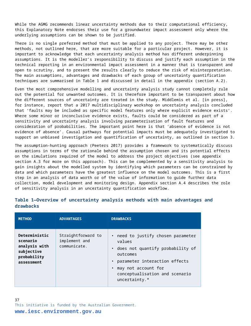
For any decision-maker, it is important to have a clear description of the level of confidence in the model’s ability to provide accurate simulations, along with a quantified level of uncertainty. Confidence in this sense is an estimate of the quality of evidence and agreement among information sources about a given simulation or assessment (CoA 2015). This should be discussed at the problem definition stage and throughout the workflow, to reduce the potential for the final results to be questioned and to help prioritise data acquisition to decrease measurement and conceptual uncertainties.

The IPCC (2013) devised a set of narrative descriptors of the likelihood of future climate outcomes that relate directly to probability classes (reflecting uncertainty). Those principles have been combined with risk-based visualisation methods to develop an approach (Table 2) to effective communication (after Richardson et al. [in press]). This comprises:

• narrative descriptors of the likelihood of a given outcome, with careful consideration of which description best fits the impact being assessed

• quantitative ranges of probabilities from an uncertainty analysis

• qualitative visual methods (risk assessment style colour-coding).

Richardson et al. [in press] provide other examples of the use of calibrated language to rank confidence in uncertainty analysis. For example, combinations of agreement and evidence are given, with ‘agreement’ being a qualitative term that should be developed by a technical reference group for a project.

In Table 2 the colour coding relates to the likelihood of exceedance, and is designed to support the narrative descriptions. The 10 th (dark green) and 90th (red) percentiles each have about a 10 per cent probability of occurring. For the 10th percentile there is approximately a 10 per cent probability that the outcome will be less than the prediction, while for the 90th percentile there is approximately a 10 per cent probability that the outcome will be greater than the prediction. Approximately 80 per cent of outcomes will lie within the light green to orange categories. It is important to note though that an 80 per cent probability based on a set of 1000 simulations means that 200 simulations predicted outcomes outside the criteria range selected.

Table 2—Example of a combined numeric, narrative and visual approach to describing likelihood

PERCENTILE (outcomes ranked from small to large)

COLOUR CODE

DESCRIPTION (in terms of likelihood of exceedance)

ALTERNATIVE DESCRIPTION OR FRAMING

<10% It is very likely that the outcome is larger than this value

It is very unlikely that the outcome is smaller than this value

10–33% It is likely that the outcome is larger than this value

It is unlikely that the outcome is smaller than this value

33–67% It is as likely as not that the outcome is larger than this value

It is as likely as not that the outcome is smaller than this value

67–90% It is unlikely that the outcome is larger than this value

It is likely that the outcome is smaller than this value

>90% It is very unlikely that the outcome is larger than this value

It is very likely that the outcome is smaller than this value

Note: Some projects may justifiably use other values for the ‘very likely’ or ‘unlikely’ descriptors, such as 95 per cent or 5 per cent.



11. Case Study—Mining Area C, Southern Flank ValleyBHP Billiton is developing the set of iron ore deposits in Mining Area C (North and South Flank) in the Pilbara region of Western Australia. The methodology applied to the 2017 Mining Area C assessment involved developing multiple conceptual and numerical groundwater models representing different hydrogeological and eco-hydrological conceptualisations. A comprehensive uncertainty analysis was applied to predict the range of impacts and to mitigate and manage potential impacts on water-related receptors (BHP Billiton 2017a, 2017b).

The BHP Billiton Water Resource Management Strategy is designed to mitigate and/or minimise operational impacts on surface water and groundwater as part of ‘business as usual’ activities. The strategy is consistent with the Western Australian Water in Mining Guideline (Government of Western Australia 2013), which encourages a consultative and cooperative relationship between regulators and proponents, and early identification of water management issues to clearly outline information requirements for assessment (as does this Explanatory Note).

The BHP Billiton strategy applies a risk-based approach that considers scientific uncertainty along with early warning triggers and thresholds of hydrological change and ecosystem response. In the early stages of the process, these triggers and thresholds are typically conservative and precautionary, reflecting incomplete scientific knowledge. As scientific understanding improves, the level of uncertainty reduces and management triggers and thresholds are iteratively refined.

Two alternative groundwater models were developed, each based on materially different hydrogeological conceptualisations: one conservative with respect to the ease of drawdown propagation towards key ecological assets and the other less so. The models used different parameter combinations but were calibrated to the same observations of groundwater levels, spring flows and the catchment water balance.

To address uncertainty, multiple model scenarios were devised and analysed using the two alternative groundwater models. These scenarios represented parameter variability and the (uncertain) potential hydraulic connections within and between the regional and ore body aquifers. The initial model set comprised 2000 variants. Of these, 192 were calibrated with justified confidence to be used in the assessment. The resulting outputs were presented as a range of drawdown responses to a range of dewatering volumes from proposed operations at South Flank, as well as the cumulative response from other operations.

The assessment recognised the temporal and spatial variance in water balances (Figure 6) and cumulative effects from other mining activities in the area, with consideration of mid-case and high-case mine production schedules. Dewatering volumes in excess of demand are managed via licensed discharge. Water supply augmentation during deficit periods is managed via licensed sources other than dewatering. The mine closure strategy proposed backfilling of pit voids to above the recovered standing water level (nominally 5 m above the groundwater level), so there are no post-mining inflow volumes to be considered.

The predicted drawdown resulting from dewatering activities in the catchment was presented in terms of a range between the 20 th and 80th

percentiles (P20 to P80) (see BHP Billiton 2017a and 2017b for details). In this case, low percentiles represent a smaller drawdown footprint and dewatering requirement, and high percentiles represent a larger drawdown footprint and dewatering requirement. The range was not intended to represent confidence intervals; it was intended to indicate that the most likely prediction lies somewhere within the P20 to P80 range at most locations in the catchment. The results have been used by the regulator for licensing decisions and to evaluate the BHP Billiton monitoring and adaptive management program.



Figure 6—Combined Mining Area C water balance showing annual dewatering estimates for two mine areas (South Flank and Mining Area C), compared with water demand (labelled as ‘Water use’), and the uncertainty range

Source: BHP Billiton 2017a.39This initiative is funded by the Australian Government.


12. Fatal flaws checklistThe fatal flaws checklist (Table 3) comprises eight sets of questions on key elements of an uncertainty analysis that reviewers should look for. Without these elements or adequate justification of the applied methodology (with consideration of the risk context), the uncertainty analysis presented may not be suitable. The first two sets are generic compliance questions about whether uncertainty has been considered adequately (in the given risk context), so they do not require specific technical skills to consider. The last six sets of questions deal with more technical issues that require specialist hydrogeology and modelling skills to consider.

The checklist should be considered alongside the general guidance provided in:

• this Explanatory Note

• the IESC Information Guidelines, including its checklist (IESC 2018)

• leading practice requirements (notably Table 9-1 of Barnett et al. 2012)

• the IESC recommendations on modelling methods (CoA 2014a, 2015b).

Although the criteria are presented in checklist format, the answers should include cross-references to where the objective evidence is provided to address the issue, identifying a specific subsection of the environmental impact assessment, not simply a chapter or section.

Table 3—Fatal flaws review checklist for uncertainty assessment

Is there evidence of engagement (‘without prejudice’) between the project proponent and regulatory agencies, from the project outset and at subsequent key stages (Figure 3):

to discuss and agree on the project objectives and the modelling objectives?

to discuss and agree on the uncertainty analysis methodologies, including the nature and scope of

the (minimum requirement) qualitative uncertainty analysis, and the quantitative uncertainty analysis for high-risk projects?

to review the reporting on the modelling and uncertainty analyses?

to agree on justifications of assumptions/criteria applied to implement the methodology?

to understand the implications of the results in terms of environmental decision-making?

to identify whether an independent technical review of the modelling and/or the uncertainty

analysis is warranted?

Is the modelling and uncertainty analysis methodology designed to provide information for decision

makers on the effects of uncertainty on the project objectives (echoing the definition of risk in AS/NZS ISO31000:2009) and on the effects of potential bias?

Are the adopted conceptual model, complexity–simplicity balance and applied modelling package

capabilities commensurate with the overall risk context and the models purpose of investigating the uncertainty/risk issues (i.e. based on the evidence available of engagement identified in item 1)?



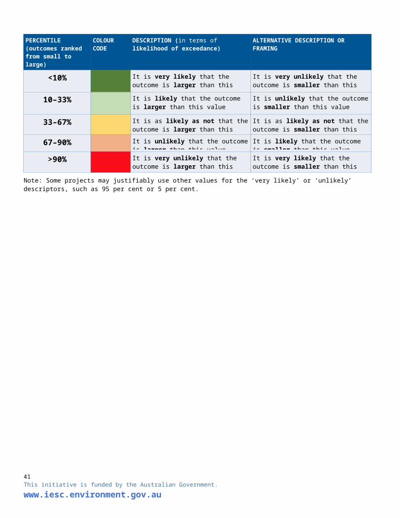
Has the uncertainty assessment and modelling methodology been designed and implemented using all

the available data? Detailed consideration of the hydrological stressors arising from the development and of natural stressors, including climate variability, and unbiased consideration of water-related asset values and causal pathways for potential impacts (direct, indirect and cumulative) should be provided.

Where history-match conditional calibration is undertaken, has it minimised non-uniqueness and error

variance (using approaches recommended in the AGMG)? If not, is a reasoned justification provided? Is an acceptable level of model-to-measurement mismatch defined for the conditional calibration?

Are all simulations consistent with all relevant information/data (using approaches recommended in

the AGMG)? If not, is a reasoned justification provided?

Has the model been submitted to stress testing in which a number of extreme parameter combinations

(representing a computationally intensive automated conditional calibration or stochastic model evaluation) are tested for model convergence?

Has a parameter sensitivity analysis and/or a parameter identifiability analysis been completed to

identify which parameters can be constrained by the available observations and which parameters affect the simulations the most? Are the implications discussed?

Have all reports been prepared in an open, honest and transparent way that is:

open to independent scrutiny and not prone to misinterpretation

based on agreed and transparent model objectives

tailored to decision-makers’ needs (focusing on messages relevant to their decisions)

presented in plain and clear language (precise, jargon-free, calibrated), with useful graphics.



13. AbbreviationsSHORT FORM MEANING

AGMG Australian Groundwater Modelling Guidelines (Barnett et al. 2012)

CoA Commonwealth of Australia

CSG Coal seam gas

EPBC Act Environment Protection and Biodiversity Conservation Act 1999 (Cth)

ESD Ecologically sustainable development

GDE Groundwater-dependent ecosystem

IESC Independent Expert Scientific Committee on Coal Seam Gas and Large Coal Mining Development

Kh Horizontal hydraulic conductivity

Kv Vertical hydraulic conductivity

LiDAR Light detection and ranging

m Metre

ML Megalitres

ML/d Megalitres per day

NCGRT National Centre for Groundwater Research and Training

NSMC Null space Monte Carlo

NSW New South Wales

OGIA Office of Groundwater Impact Assessment (Queensland)

PEST Parameter estimation software (open-source) for application to any model and often used in uncertainty analysis methods. http://pesthomepage.org/

R Recharge (groundwater)

RCS Relative composite sensitivity

S Storativity (of an aquifer)

Sy Specific yield (of an unconfined aquifer)

T Transmissivity (of an aquifer)—a product of hydraulic conductivity and saturated aquifer thickness



14. Glossary

TERM DESCRIPTION

Bias Bias is systematic error which displaces the model outputs in a predictable way. This influences the trueness in the model output, where trueness is the difference between the average value obtained from model predictions and an accepted true value (Richardson et al. [in press]). Four of the most relevant and common biases that can affect communication of uncertainty are listed below (New Zealand Government 2016).

Bias—availability People tend to judge events that are easily recalled as more risky or more likely to occur than events that are not readily available to memory. An event may have more availability if it occurred recently, if it was a high-profile event, or if it has some other significance for an individual or group.

Bias—confidence People typically have too much confidence in their own judgements. This appears to affect almost all professions, as well as the lay public. The few exceptions are people who receive constant feedback on the accuracy of their predictions, such as weather forecasters. The psychological basis for this unwarranted certainty seems to be insensitivity to the weaknesses in assumptions on which judgements are based.

Bias—confirmation Confirmation bias is the filtering of new information to fit previously formed views. In particular, it is the tendency to accept as reliable new information that supports existing views, but to see as unreliable or erroneous and filter out new information that is contrary to current views. People may ignore or dismiss uncertainty information if it contradicts their current beliefs.

Bias—framing How probabilistic information is framed can influence how that information is understood as well as the confidence that people have in the information. ‘Priming’ the brain with a particular stimulus can affect how it responds to a later stimulus. Using expressions that take advantage of this priming (i.e. the direction and expression are consistent) can reduce cognitive strain, which makes it easier for stakeholders to understand the idea presented without requiring further analysis. For example, the phrase ‘there is a 5 per cent chance the drawdown in the groundwater level will be greater than 0.2 m’ may leave a different impression than the phrase ‘there is a 95 per cent chance the water drawdown level will be less than 0.2 m’; even though the two phrases contain the same information. The latter requires less mental workload because your brain is already ‘primed’ to think about being ‘down’ when it hears ‘less than’. This is particularly effective when paired with explicit advice about whether precautionary action is advised.

Bioregional assessments A series of scientific analyses of the ecology, hydrology, geology and hydrogeology of a bioregion, with explicit assessment of the potential direct, indirect and cumulative impacts of CSG and coal mining development on water resources. The central purpose of bioregional assessments is to inform the understanding of impacts on and risks to water-dependent assets that arise in response to current and future pathways of CSG and large coal mining development. See www.bioregionalassessments.gov.au

Calibration—conditional Conditional calibration is a process by which parameters are adjusted until model simulations fit historical measurements or observations, indicating that the model has not yet been falsified by tests against observational data, and that the model is accepted as a good representation of (or receptacle of knowledge about) the physical system of interest.



TERM DESCRIPTION

Calibration null space Model parameters/combinations not informed by historical measurements. To the extent that a prediction is sensitive to individual parameters, and/or to combinations of parameters that lie within the ‘calibration null space’, the uncertainty of that prediction is not reduced via the calibration process at all (Doherty and Moore [in press]).

Causal pathway (from bioregional assessments glossary)

The logical chain of events either planned or unplanned that link coal resource development and potential impacts on water resources and water-dependent assets.

Communication/engagement

The key to successful communication is to present the information about uncertainty in a way that is most likely to aid decision-making. To achieve this, analysis of uncertainty information in model output needs to be: (i) adequately tailored to decision makers’ needs; (ii) focused on the messages that are most likely to be relevant to their decisions; and (iii) presented in plain and clear (precise, non-technical) language (Richardson et al. [in press]).

Cumulative impact— coal seam gas or large coal mine

The total impact of a CSG and/or large coal mining development on water resources when all past, present and reasonably foreseeable actions that are likely to impact on water resources are considered.

Equifinality Explicit recognition that there may be multiple model representations that provide acceptable simulations for any environmental systems. The concept of equifinality is distinguished from non-identifiability or non-uniqueness: non-identifiability can be described as a poorly defined optimum of the calibration objective function, while non-uniqueness can be described as multiple local optima (Beven 2006).

FEFLOW Commercial software for simulation of saturated and unsaturated flow, mass transport (multiple solutes) and heat, using the finite element method. Can be coupled to MIKE 11 to simulate flow in river and stream networks. https://www.mikepoweredbydhi.com/products/feflow

Fit for purpose In the context of uncertainty analysis, a groundwater model must be designed to be fit for the purpose of providing information about uncertainties in the conceptualisations and model simulation outputs in a way that allows decision makers to understand the effects of uncertainty on project objectives (echoing the AS/NZS ISO 31000:2009 risk definition) and the effects of potential bias.

Groundwater-dependent ecosystems (GDE)

Ecosystems that require access to groundwater on a permanent or intermittent basis to meet all or some of their water requirements so as to maintain their communities of plants and animals, ecological processes and ecosystem services. GDEs include terrestrial vegetation, wetlands (swamps, lakes and rivers) and ecosystems in aquifers and caves. The types and characteristics of GDEs are discussed further in the Explanatory Note for GDEs (Doody et al. [in press]).

High-risk systems Systems where environmental or economic risks are high, that lack socially and economically ancceptable, and effective risk treatments and where long time lags apply. Such systems require detailed uncertainty analysis.

HydroGeoSphere Commercial software for simulation of saturated and unsaturated flow, transport of mass and heat.



TERM DESCRIPTION

Includes solution of 2D overland flow and 1D flow in river and stream networks. Also includes discrete fracture networks. https://www.aquanty.com/hydrogeosphere/

Hypothesis In the environmental risk management context where groundwater modelling is applied, the hypothesis to be tested typically comprises the conjecture of an unwanted outcome or consequence associated with a particular development and/or management strategy. In practice, the hypothesis should be clearly stated in terms of threshold impacts (preferably regulatory-based) and/or resource condition indicators, and should be closely linked with the specified modelling objectives. The hypothesis of an unwanted outcome can never be completely rejected.

Low-risk systems Systems with low environmental or economic risks and/or with socially and economically acceptable, and effective risk treatments available. These systems may not need detailed uncertainty analysis.

Mike-SHE Commercial software for integrated modelling of surface water flow (2D overland flow and 1D stream flow networks) and groundwater flow (3D, unsaturated-saturated). https://www.mikepoweredbydhi.com/products/mike-she

Minimum error variance The error variance is the statistical variance of the error variable (i.e. the variance of the modelled to measured misfit (or difference) error term). Minimum error variance means minimum spread of the error; it does not mean that the bias of a simulation is minimised. (See section 2, Figure 1—right).

Model—analytical A model that provides an exact mathematical solution of a given problem by making simplifying assumptions (for example, that properties of the aquifer are considered to be constant in space and time).

Model—conceptual A descriptive and/or schematic hydrological, hydrogeological and ecological representation of a site, environment or process showing the stores, flows and uses of water, which illustrates the geological formations, water resources and water-dependent assets. It provides a basis for developing water and salt balances and inferring water-related ecological responses to changes in hydrology, hydrogeology and water quality.

Model—coupled—externally

A model where the surface flow and subsurface flow are solved for separately but without iteration within a time step (i.e. solve surface flow first, then groundwater, then advance to next time step—usually short time steps for dynamic surface water systems and longer time steps for groundwater systems). Example: Mike-SHE.

Model—coupled—fully A model where the surface flow and subsurface flow and dynamic exchanges are solved simultaneously within a time step (i.e. iteration proceeds at the same time step for all processes, usually constrained by surface water, as that is most dynamic; this can cause significant computational overhead). Examples: HydroGeoSphere, MODHMS.

Model—coupled—iteratively

A model where the surface flow and subsurface flow are solved for separately, but iteratively within a time step (i.e. solve surface flow first, then groundwater, then iterate within time step to convergence before advancing to next time step—short time steps for surface water and longer time steps for



TERM DESCRIPTION

groundwater). Example: MODFLOW.

Model—deterministic A model which results in the same output for the same input. Most regional models developed for impact assessment are deterministic.

Model—distributed A model in which there is spatial variability of parameter distributions across domain, and local-scale processes also represented, such as recharge/discharge zones, rivers, wells.

Model—empirical A model that uses algorithms or mathematical relationships that are based on observations/evidence (empiricism) but do not necessarily have a physical basis (e.g. regressions that do not necessarily establish a causal relationship).

Model—integrated A model that provides an integrated solution of surface and groundwater flow and dynamic exchanges via coupling techniques (see previous definitions).

Model—lumped A model where hydrological processes are lumped to the catchment scale (no spatial variability within the catchment/domain).

Model—numerical A model where space and/or time are divided into discrete pieces. Similar to analytical models as they make simplifying assumptions; however, features of the governing equations and boundary conditions in numerical models (e.g. aquifer geometry, hydrogeological properties, pumping rates or sources of solute) can be specified as varying over space and time. This enables more complex representations of groundwater or surface water systems than could be achieved with an analytical model.

Model—physically based A model with algorithms designed to realistically represent physical processes (e.g. depth-dependent ET).

Model—stochastic A model which produces different outputs for the same inputs (element of randomness). Can invoke stochastic via PEST on deterministic model.

Model complexity (Middlemis et al. 2001)

The degree to which a model application resembles, or is designed to resemble, the physical hydrogeological system (adapted from the model fidelity definition given in Ritchey and Rumbaugh 1996, cited in Middlemis et al. 2001). There are three main complexities (in order of increasing complexity): basic, impact assessment and aquifer simulator. Higher complexity models have a capability to provide for more complex simulations of hydrogeological processes and/or address resource management issues more comprehensively.

Model failure A model has failed if the predictive uncertainty margins underestimate the probability of an unwanted outcome or if there is sufficient bias for a poor decision to be made on the basis of the bias, especially if the consequence of this is large.

Model purpose (AGMG definition, based on

AGMG definition for defining a modelling study purpose in terms of the objectives, complexity and resources:



TERM DESCRIPTION

Middlemis et al. 2001, Table 2.1.1)

(a) The modelling study objective and purpose must be clearly stated in specific and measurable terms, along with the resource management objectives that the model will be required to address

(b) The overall management constraints should be outlined in terms of budget, schedule, staged development and long-term maintenance, and eventual ownership and use of the model.

(c) The model complexity must be assessed and defined to suit the study purpose, objectives and resources available for each model study.

(d) The model complexity assessment must involve negotiation between a client/end-user and the modelling team, including the model reviewer, and relevant government agency representatives.

Model simplicity (effective) (Middlemis et al. 2001)

The simplicity (or parsimony) principle implies that a conceptual model has been simplified yet retains enough complexity to adequately represent the physical system and its behaviour for the specified purpose of the model. The term ‘effective model simplicity’ was discussed by Voss (2011a, 2011b). Model simplification involves testing and removing all redundant elements of the model to which prediction is insensitive.

Model simplicity (optimal) Optimal model simplicity is achieved by testing and removing all elements of the model that the prediction is not sensitive to (optimal means no redundant elements). However, where the prediction is sensitive to parameters that are not informed by the calibration dataset, uncertainty reduction via calibration can be minimal, even if a model is perfectly calibrated. Furthermore, the parameters that cannot be estimated uniquely are just as important as those that can be estimated uniquely when exploring predictive uncertainty (Doherty and Moore [in press]).

MODFLOW Modular groundwater flow modelling software (open source) developed by the US Geological Survey, regarded as industry standard (https://water.usgs.gov/ogw/modflow/). Refer to AGMG for more information on this and other groundwater modelling software packages.

MODHMS Commercial software that is coupled with MODFLOW for integrated surface water and groundwater flow and solute transport simulations. Refer to AGMG for more information.

Non-identifiable (Barnett et al. 2012, s.5.4.1)

Model parameters can be non-identifiable or non-unique if the mathematical equations that describe a situation of interest depend on parameters in combination (e.g. R/T, R/Sy or T/S), rather than individually, in such a way that the product or ratio of parameters may be identifiable, but not the individual parameters themselves (Barnett et al. 2012).

Non-uniqueness The principle that many different possible sets of model inputs can produce nearly identical computed outputs for any given model.

Precautionary principle (ESD context)

Where there are threats of serious or irreversible environmental damage, lack of full scientific certainty should not be used as a reason for postponing measures to prevent environmental degradation (see www.environment.gov.au/about-us/esd/publications/national-esd-strategy-part1#GoalsEtc).

The precautionary principle has four central components:



TERM DESCRIPTION

1. taking preventive action in the face of uncertainty

2. shifting the burden of proof to the proponents of an activity

3. exploring a wide range of alternatives to possibly harmful actions

4. increasing public participation in decision-making (Kriebel et al. 2001).

It has been suggested that ecologically sustainable development (ESD) is not a factor to be balanced against other considerations; rather, ESD is the balance between development and environment/social imperatives.

Probability density function / probability distribution function

The probability distribution of a random variable specifies the chance that the variable takes a value in any subset of the real numbers. For example: ‘there is a probability of p that the variable is between x and y’.

Proponent (actor in engagement process)

The person or organisation that owns the project or development (e.g. a mine). The project proponent is asking the water manager to make a decision related to impacts on a water resource. The project proponent commissions studies by outside professionals such as consulting hydrogeologists.

Reviewer (actor in engagement process)

A person conducting an external review of a modelling study. The review may be more or less comprehensive depending on the requirements of the particular case. The reviewer is typically appointed by the water manager to support her/him to match the modelling capability of the modeller.

Risk (calculation) Combination of consequence and likelihood (AS/NZS ISO 31000:2009).

Risk (definition) Effect of uncertainty on management objectives (AS/NZS ISO 31000:2009). Effect can be positive or negative deviation from the expected.

Risk (descriptive) Can be roughly equated to the probability of an unwanted outcome as a consequence of a particular decision, multiplied by the cost associated with its occurrence (Doherty and Moore [in press]).

Sensitivity analysis The study of how uncertainty in the output of a model (numerical or otherwise) can be apportioned to different sources of uncertainty in the model input.

Significant impact Defined by the Significant impact guidelines (CoA 2013) as an impact which is important, notable or of consequence, having regard to its context or intensity. Whether an action is likely to have a significant impact depends on the sensitivity, value and quality of the water resource affected, and on the intensity, duration, magnitude and geographic extent of the impacts.

Type I error (statistical) ‘False positive’ meaning the failure to correctly reject, or the incorrect or false acceptance of the hypothesis (e.g. accepting (or not rejecting) the hypothesis of an unwanted outcome when it is indeed unlikely).

Type II error (statistical) ‘False negative’ meaning falsely rejecting the hypothesis (e.g. wrongly rejecting the hypothesis of an



TERM DESCRIPTION

unwanted outcome when it can indeed eventuate).

Type III error (statistical) Put simply: the right answer to the wrong question (not a definitive definition).

Uncertainty—measurement error

Combination of uncertainties associated with the measurement of complex aquifer system states (heads, discharges), parameters and variability (3D spatial and temporal) with those induced by upscaling or downscaling (site-specific data, climate data).

Uncertainty—parameterisation

Uncertainties associated with hydrogeological property values and assumptions applied to represent complex reality in space and time (any system aspect that can be changed in an automated way in a model via parameterisation).

Uncertainty— predictive The quantification of uncertainty in predictions. The bias and spread associated with model predictions that are made via a model that is consistent with the conceptual understanding of the system and associated measurements.

Uncertainty— scenario Uncertainties associated with guessing future stresses, dynamics and boundary condition changes (e.g. mining, climate variability, land and water use change).

Uncertainty— structural/conceptual

Uncertainties associated with geological structure and hydrogeological conceptualisation assumptions applied to derive a simplified view of a complex hydrogeological reality (any aspect of a system that cannot be changed in an automated way in a model). See also Barnett et al. (2012, section 3.4).

Some structural uncertainties can be investigated by testing alternative conceptualisations, either by parameterising the conceptualisation issue (e.g. faults) or applying Bayes’ theorem to combine/evaluate the known and unknown conceptual models. For example, faults may be included as specific model features only where explicit evidence exists. Where some minor/inconclusive evidence exists, faults could be considered as part of a sensitivity/uncertainty analysis involving parameterisation of the fault features, and consideration of probabilities. The key point to note is that ‘absence of evidence is not evidence of absence’ and that causal pathways for potential impacts must be adequately investigated to support an unbiased investigation and quantification of uncertainty.

Uncertainty (definition) Uncertainty is the state, even partial, of deficiency of information related to the understanding or knowledge of an event, its consequence, or its likelihood (AS/NZS ISO 31000:2009).

Uncertainty (source/type) Any deficiency in information relating to understanding or knowledge in four main classes/sources of uncertainty:

1. structural/conceptual uncertainty

2. parameter/input uncertainty

3. measurement error

4. scenario uncertainties.

Uncertainty analysis The quantification of uncertainty in predictions.



TERM DESCRIPTION

(predictive uncertainty)

Uncertainty analysis (qualitative)

A formal and structured discussion of all model choices and assumptions and their effect on predictions. The discussion is organised by answering following four questions with ‘low’, ‘medium’ or ‘high’ (Peeters 2017): What is the likelihood that:

1. I would have made the same choice if I had more or different data?

2. I would have made the same choice if I had more time and money?

3. I would have made the same choice if I had a better model/software?

4. the model predictions are very different if I change the assumption?

Uncertainty analysis (quantitative)

Quantitative uncertainty analysis seeks to find all model predictions that are consistent with (or constrained by) the observations.

Water balance A mathematical expression of water flows and exchanges, described as inputs, outputs and changes in storage. Surface water, groundwater and atmospheric components should be included.

Water manager (actor in engagement process)

The person or organisation responsible for the management or protection of the water resources, and thus of the modelling study and the outcome (the problem owner).

Water resource Defined by the Water Act 2007 (Cth) (CoA 2007) as ‘surface water or groundwater or a watercourse, lake, wetland or aquifer (whether or not it currently has water in it); and includes all aspects of the water resource, including water, organisms and other components and ecosystems that contribute to the physical state and environmental value of the water resource.’ Broadly, a water resource encompasses the water body itself and all aspects that contribute to its physical state and environmental value, such as the associated water quality and any associated organisms, ecological processes and ecosystems.



15. ReferencesAcworth RI, Rau GC, Halloran LJS and Timms WA 2017. Vertical groundwater storage properties and changes in confinement determined

using hydraulic head response to atmospheric tides. Water Resources Research, 53: 2983–2997.

AS/NZS ISO 31000:2009. Risk management—Principles and guidelines. Standards Australia, Sydney.

Barnett B, Townley LR, Post V, Evans RE, Hunt RJ, Peeters L, Richardson S, Werner AD, Knapton A and Boronkay A 2012. Australian groundwater modelling guidelines. Waterlines report. National Water Commission, Canberra. Available [online]: http://webarchive.nla.gov.au/gov/20160615064846/http://archive.nwc.gov.au/library/waterlines/82 accessed August 2018.

Barrett DJ, Couch CA, Metcalfe DJ, Lytton L, Adhikary DP and Schmidt RK 2013. Methodology for bioregional assessments of the impacts of coal seam gas and coal mining development on water resources. Report prepared for the Independent Expert Scientific Committee on Coal Seam Gas and Large Coal Mining Development through the Department of Sustainability, Environment, Water, Population and Communities, Commonwealth of Australia. Available [online]: http://www.bioregionalassessments.gov.au/methods/bioregional-assessment-methodology accessed August 2018.

Begg S 2013. Uncertainty, decisions, models and people. 2nd AusIMM international geometallurgy conference (GeoMet 2013). Available [online]: http://www.ausimm.com.au/geomet2013/presentations/uncertainty_decisions_models_and_people-Begg.pdf accessed August 2018.

Beven K 2018. On hypothesis testing in hydrology: Why falsification of models is still a really good idea. Wiley Interdisciplinary Reviews: Water.

Beven K 2006. A manifesto for the equifinality thesis. Journal of Hydrology, 320: 18–36.

Beven K 1993. Prophecy, reality and uncertainty in distributed hydrological modelling. Advances in Water Resources, 16: 41–51.

Beven K and Young P 2013. A guide to good practice in modelling semantics for authors and referees. Water Resources Research, 49: 5092–5098.

BHP Billiton 2017a. Mining Area C Southern Flank proposal: Hydrological impact assessment and water management summary. Available [online]: www.epa.wa.gov.au/sites/default/files/PER_documentation/Appendix%207%20-%20Hydrological%20Impact%20Assessment.pdf accessed August 2018.

BHP Billiton 2017b. Mining Area C: Hydrological impact assessment and water management summary. Available [online]: www.epa.wa.gov.au/sites/default/files/PER_documentation/Appendix%207%20-%20Rev%206%20EMP%20Hydrological%20Impact%20and%20Management%20Summary.pdf accessed August 2018.

Brunner P, Simmons C, Cook P and Therrien R 2010. Modelling surface water-groundwater interaction with MODFLOW: Some considerations. Ground Water, 48: 174–180.

Caers J 2011. Modelling uncertainty in the earth sciences. John Wiley & Sons, New Jersey.

Castilla-Rho JC, Mariethoz G, Rojas R, Andersen MS and Kelly BFJ 2015. An agent-based platform for simulating complex human-aquifer interactions in managed groundwater systems. Environmental Modelling and Software, 73: 305–323.

CDM Smith 2016. Santos Limited Narrabri gas project groundwater impact assessment – Appendix F. Report prepared by CDM Smith for Santos. Available [online]: http://majorprojects.planning.nsw.gov.au/page/development-categories/mining--petroleum---extractive-industries/petroleum/?action=view_job&job_id=6456 accessed August 2018.

Commonwealth of Australia (CoA) 2018a. Independent Expert Scientific Committee on Coal Seam Gas and Large Coal Mining Development - website. Available [online]: http://iesc.environment.gov.au/ accessed August 2018.

Commonwealth of Australia (CoA) 2018b. Groundwater dependent ecosystems atlas - website. Bureau of Meteorology. Available [online]: www.bom.gov.au/water/groundwater/gde/index.shtml accessed August 2018.



Commonwealth of Australia (CoA) 2017. Bioregional Assessments: Cooper subregion - website. Available [online]: http://www.bioregionalassessments.gov.au/assessments/cooper-subregion accessed August 2018.

Commonwealth of Australia (CoA) 2015. Modelling water-related ecological responses to coal seam gas extraction and coal mining. Report prepared by Auricht Projects and the Commonwealth Scientific and Industrial Research Organisation for the Department of the Environment, Commonwealth of Australia. Available [online]: http://environment.gov.au/water/publications/modelling-water-related-ecological-responses-csg-extraction accessed August 2018.

Commonwealth of Australia (CoA) 2014a. Coal seam gas extraction: Modelling groundwater impacts. Knowledge report, prepared by Coffey Geotechnics for the Department of the Environment, Commonwealth of Australia. Available [online]: http://environment.gov.au/water/publications/csg-extraction-modelling-groundwater-impacts accessed August 2018.

Commonwealth of Australia (CoA) 2014b. Subsidence from coal seam gas extraction in Australia, Background review. Report prepared by Sinclair Knight Merz Pty Ltd for the Department of the Environment, Commonwealth of Australia. Available [online]: http://environment.gov.au/water/publications/background-review-subsidence-coal-seam-gas-extraction-australia accessed August 2018.

Commonwealth of Australia (CoA) 2014c. Subsidence from coal mining activities: Background review. Report prepared by Sinclair Knight Merz Pty Ltd for the Department of the Environment, Commonwealth of Australia. Available [online]: http://environment.gov.au/water/publications/background-review-subsidence-from-coal-mining-activities accessed August 2018.

Commonwealth of Australia (CoA) 2013. Significant impact guidelines 1.3: Coal seam gas and large coal mining developments—Impacts on water resources. Available [online]: http://environment.gov.au/resource/significant-impact-guidelines-13-coal-seam-gas-and-large-coal-mining-developments-impacts accessed August 2018.

Commonwealth of Australia (CoA) 2009. The Australian Environment Act—Report of the independent review of the Environment Protection and Biodiversity Conservation Act 1999. Department of the Environment, Water, Heritage and the Arts, Canberra. Available [online]: www.environment.gov.au/system/files/resources/5f3fdad6-30ba-48f7-ab17-c99e8bcc8d78/files/final-report.pdf accessed August 2018.

Commonwealth of Australia (CoA) 2007. Water Act 2007 (Cth). Available [online]: https://www.legislation.gov.au/Details/C2018C00247 accessed August 2018.

Commonwealth of Australia (CoA) 1999. Environment Protection and Biodiversity Conservation Act 1999 (Cth). Available [online]: https://www.legislation.gov.au/Details/C2016C00777 accessed August 2018.

Cook P, Miller A, Shanafield M and Simmons C 2016. Predicting water resource impacts of unconventional gas using simple analytical equations. Ground Water, 55(3): 387–398.

Crosbie R, Peeters L and Carey H 2016. Groundwater modelling. Submethodology M07 from the Bioregional Assessment Technical Programme. Department of the Environment and Energy, Bureau of Meteorology, Commonwealth Scientific and Industrial Research Organisation and Geoscience Australia, Commonwealth of Australia. Available [online]: http://www.bioregionalassessments.gov.au/methods/groundwater-modelling accessed August 2018.

Dausman AM, Doherty J, Langevin CD and Dixon J 2010. Hypothesis testing of buoyant plume migration using a highly parameterized variable-density groundwater model at a site in Florida, USA. Hydrogeology Journal, 18(1): 147–160.

David K, Timms WA, Barbour SL and Mitra R 2017. Tracking changes in the specific storage of overburden rock during longwall coal mining. Journal of Hydrology, 553: 304–320.

Department of Primary Industries Office of Water 2012. NSW Aquifer Interference Policy: NSW Government policy for the licencing and assessment of aquifer interference activities. NSW Department of Primary Industries, a division of NSW Department of Trade and Investment, Regional Infrastructure and Services. Available [online]: https://www.resourcesandgeoscience.nsw.gov.au/landholders-and-community/coal-seam-gas/codes-and-policies/aquifer-interference-policy accessed August 2018.

Doble R and Crosbie R 2017. Review: Current and emerging methods for catchment-scale modelling of recharge and evapotranspiration from shallow groundwater. Journal of Hydrology, 25: 3–23.



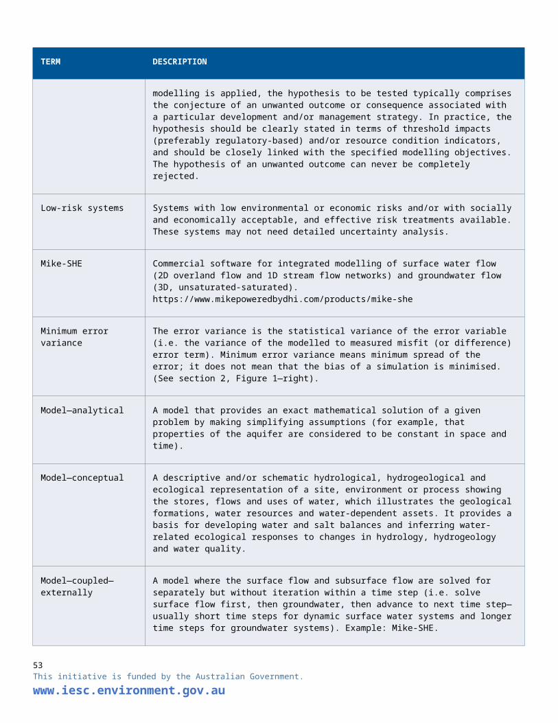
Doble R, McCallum J, Turnadge C, Peeters L, Wu B and Mallants D 2017. Modelling inter-aquifer leakage associated with well integrity failure. Report prepared by the Commonwealth Scientific and Industrial Research Organisation for the Department of the Environment and Energy, Commonwealth of Australia, Canberra. Available [online]: https://www.environment.gov.au/system/files/resources/98aa5634-f402-40c1-bcc0-2c7bbc71378e/files/modelling-inter-aquifer-leakage-associated-with-well-integrity-failure.pdf accessed August 2018.

Doherty J 2016. PEST model-independent parameter estimation user manual Part I: PEST software. 6th edition. Watermark Numerical Computing, Brisbane. Available [online]: www.pesthomepage.org accessed August 2018.

Doherty J 2015. Calibration and uncertainty analysis for complex environmental models. Watermark Numerical Computing, Brisbane. Available [online]: www.pesthomepage.org accessed August 2018.

Doherty J 2010. Model-based environmental decision-making. Watermark Numerical Computing, Brisbane. Available [online]: www.pesthomepage.org accessed August 2018.

Doherty J and Christensen S 2011. Use of paired simple and complex models in reducing predictive bias and quantifying uncertainty. Water Resources Research, 47:12.

Doherty J and Hunt RJ 2009. Two statistics for evaluating parameter identifiability and error reduction. Journal of Hydrology, 366: 119–127.

Doherty J and Moore C [in press]. Simple is beautiful. Background paper No. 3. In Middlemis H, Walker G, Peeters L, Moore C, Hayes P and Richardson S (eds) NCGRT national groundwater modelling uncertainty workshop, Sydney, 10 July 2017. National Centre for Groundwater Research and Training, Adelaide.

Doody TM, Hancock PJ and Pritchard JL [in press]. Assessing groundwater-dependent ecosystems: IESC Information Guidelines Explanatory Note. Report prepared for the Independent Expert Scientific Committee on Coal Seam Gas and Large Coal Mining through the Department of the Environment and Energy, Commonwealth of Australia.

Eamus D 2009. Identifying groundwater dependent ecosystems. A guide for land and water managers. Report prepared by University of Technology, Sydney for Land and Water Australia, Canberra. Available [online]: https://www.uts.edu.au/sites/default/files/aglw-groundwater.pdf accessed August 2018.

Eamus D, Froend R, Loomes R, Hose G and Murray B 2006. A functional methodology for determining the groundwater regime needed to maintain the health of groundwater-dependent vegetation. Australian Journal of Botany, 54: 97–114.

Ferré T 2016. Seeing things differently: Rethinking the relationship between data, models, and decision-making. 2016 Darcy Lecture Series in Groundwater Science. Available [online]: https://www.youtube.com/watch?v=6YnYGwYSmQk accessed August 2018.

Freeze RA, Massmann J, Smith L, Sperling T and James B 1990. Hydrogeological decision analysis:1. A framework. Ground Water, 28(5): 738–766.

Government of Western Australia 2013. Western Australian water in mining guideline. Water Licensing Delivery Series Report No. 12. Department of Water, Perth. Available [online]: https://www.water.wa.gov.au/__data/assets/pdf_file/0019/1819/105195.pdf accessed August 2018.

Guillaume JHA, Hunt RJ, Comunian A, Blakers RS and Fu B 2016. Chapter 28: Methods for exploring uncertainty in groundwater management predictions. In Jakeman AJ, Barreteau O, Hunt RJ, Rinaudo J and Ross A (eds) Integrated groundwater management. Springer International Publishing, New York.

Hayes P and Nicol C [in press]. Uncertainty by design: Sufficient model simplification to make predictive uncertainty analysis tractable. Background paper No.4. In Middlemis H, Walker G, Peeters L, Moore C, Hayes P and Richardson S (eds) NCGRT national groundwater modelling uncertainty workshop, Sydney, 10 July 2017. National Centre for Groundwater Research and Training, Adelaide.

Herckenrath D, Doherty J and Panday S 2015. Incorporating the effect of gas in modelling the impact of CBM extraction on regional groundwater systems. Journal of Hydrology, 523: 587–601.

Hill MC and Tiedeman CR 2007. Effective groundwater model calibration. John Wiley & Sons, New Jersey.



Hill MC, Middlemis H, Hulme P, Poeter E, Riegger J, Neumann S, Williams H and Anderson M 2004. Brief overview of selected groundwater modelling guidelines. Proceedings of FEM-Modflow: International conference on finite element models, modflow and more. Karlovy Vary, Czech Republic, 13–16 September 2004.

Holland KL, Aryal SK, Bruce J, Carey H, Davies P, Ford J, Henderson B, Herr A, Janardhanan S, Merrin LE, Mitchell PJ, Mount RE, O’Grady AP, Ransley T, Sander R and Schmidt RK 2016. Conceptual modelling for the Maranoa-Balonne-Condamine subregion. Product 2.3 for the Maranoa-Balonne-Condamine subregion from the Northern Inland Catchments Bioregional Assessment. Department of the Environment and Energy, Bureau of Meteorology, Commonwealth Scientific and Industrial Research Organisation and Geoscience Australia, Commonwealth of Australia. Available [online]: http://data.bioregionalassessments.gov.au/product/NIC/MBC/2.3 accessed August 2018.

IESC 2018. Information Guidelines for proponents preparing coal seam gas and large coal mining development proposals. Available [online]: http://iesc.environment.gov.au/publications/information-guidelines-independent-expert-scientific-committee-advice-coal-seam-gas accessed August 2018.

IPCC 2013. Climate change: The physical science basis. Contribution of Working Group I to the Fifth Assessment Report of the Intergovernmental Panel on Climate Change. Cambridge University Press, Cambridge.

Kriebel D, Tickner J, Epstein P, Lemons J, Levins R, Loechler E, Quinn M, Rudel R, Schettler T and Stoto M 2001. The precautionary principle in environmental science. Environmental Health Perspectives, 109/9: 871–876. Available [online]: https://www.ncbi.nlm.nih.gov/pmc/articles/PMC1240435/ accessed August 2018.

Mackie Environmental Research 2013. Wallarah 2 coal project - Environmental impact statement. Appendix I Groundwater impact assessment. Report prepared by Mackie Environmental Research for Wyong Areas Coal Joint Venture. Available [online]: http://majorprojects.planning.nsw.gov.au/page/development-categories/mining--petroleum---extractive-industries/mining/?action=view_job&job_id=4974 accessed August 2018.

Maier H, Kapelan Z, Kasprzyk J, Kollat J, Matott L, Cunha M, Dandy G, Gibbs M, Keedwell E, Marchi A, Ostfeld A, Savic D, Solomatine D, Vrugt J, Zecchin A, Minsker B, Barbour E, Kuczera G, Pasha F, Castelletti A, Giuliani M and Reed P 2014. Evolutionary algorithms and other metaheuristics in water resources: Current status, research challenges and future directions. Environmental Modelling and Software, 62: 271–299.

Meerschaert MM, Dogan M, van Dam RL, Hyndman DW and Benson DA 2013. Hydraulic conductivity fields: Gaussian or not? Water Resources Research, 49: 4730–4737.

Middlemis H, Merrick N, Ross J, and Rozlapa K 2001. Groundwater flow modelling guideline. Report prepared for Murray–Darling Basin Commission by Aquaterra Consulting Pty Ltd. Available [online]: www.mdba.gov.au/sites/default/files/archived/mdbc-GW-reports/2175_GW_flow_modelling_guideline.pdf accessed August 2018.

Middlemis H, Walker G, Peeters L, Moore C, Hayes P and Richardson S [in press]. NCGRT national groundwater modelling uncertainty workshop, Sydney, 10 July 2017. National Centre for Groundwater Research and Training, Adelaide.

Moore C and Doherty J 2005. The role of the calibration process in reducing model predictive error. Water Resources Research, 41(5): W0520.

Neuman SP and Wierenga PJ 2003. A comprehensive strategy of hydrogeologic modeling and uncertainty analysis for nuclear facilities and sites. Report prepared by University of Arizona for the US Nuclear Regulatory Commission. Report NUREG/CR-6805.

New Zealand Government 2016. A draft guide to communicating and managing uncertainty when implementing the National Policy Statement for freshwater management 2014. Ministry for the Environment, Wellington. Available [online]: http://www.mfe.govt.nz/publications/fresh-water/draft-guide-communicating-and-managing-uncertainty-when-implementing accessed August 2018.

Office of Groundwater Impact Assessment (OGIA) 2016a. Groundwater connectivity between the Condamine Alluvium and the Walloon Coal Measures. A hydrogeological investigation report. Compiled by the Office of Groundwater Impact Assessment, Department of Natural Resources and Mines, Queensland Government.



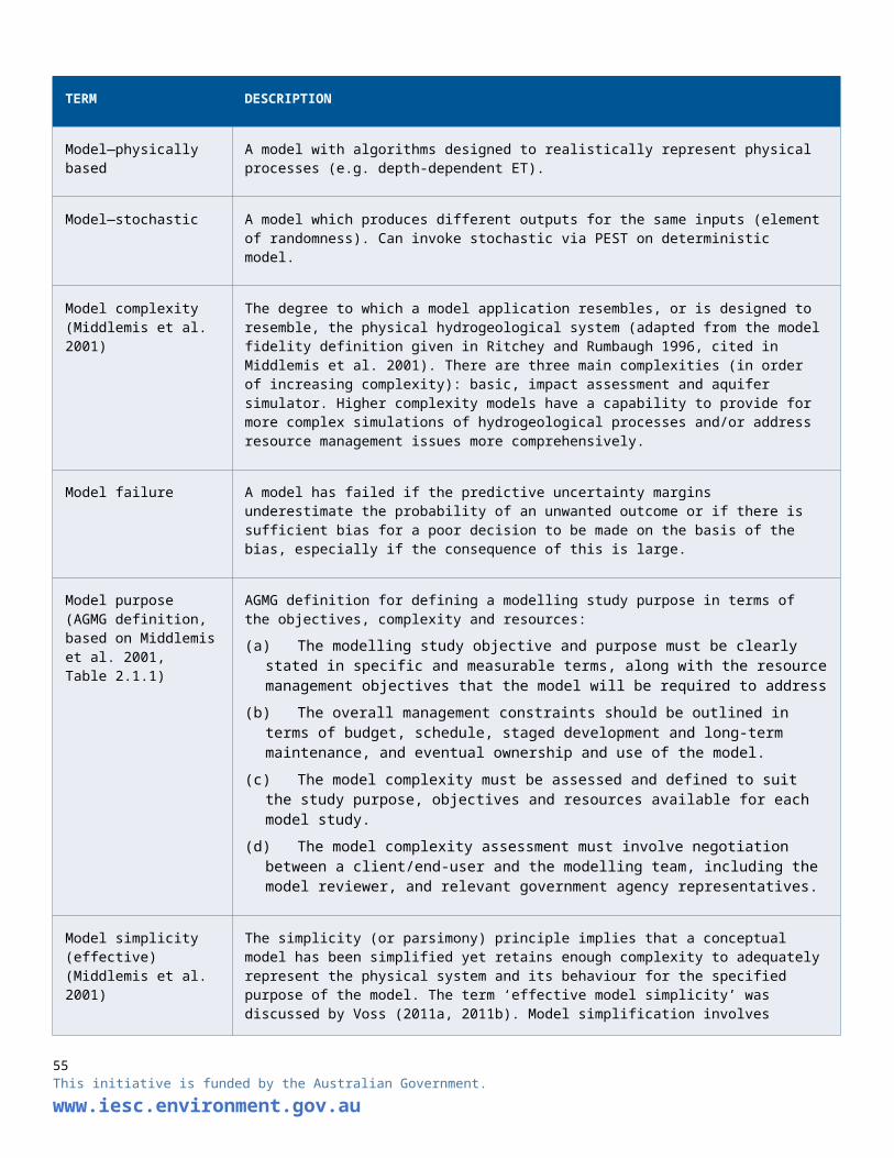
Office of Groundwater Impact Assessment (OGIA) 2016b. Groundwater modelling report for the Surat Cumulative Management Area. Compiled by the Office of Groundwater Impact Assessment, Department of Natural Resources and Mines, Queensland Government.

Pappenberger F and Beven KJ 2006. Ignorance is bliss: Or seven reasons not to use uncertainty analysis. Water Resources Research, 42: W05302.

Peeters L [in press]. Uncertainty analysis in groundwater modelling: Where to start? Background paper No. 2. In Middlemis H, Walker G, Peeters L, Moore C, Hayes P and Richardson S (eds) NCGRT national groundwater modelling uncertainty workshop, Sydney, 10 July 2017. National Centre for Groundwater Research and Training, Adelaide.

Peeters L 2017. Assumption hunting in groundwater modeling: Find assumptions before they find you. Ground Water, 55: 665–669.

Peeters L, Pagendam D, Gao L, Hosack G, Jiang W and Henderson B 2016. Propagating uncertainty through models. Submethodology M09 from the Bioregional Assessment Technical Programme. Department of the Environment and Energy, Bureau of Meteorology, Commonwealth Scientific and Industrial Research Organisation and Geoscience Australia, Commonwealth of Australia. Available [online]: http://www.bioregionalassessments.gov.au/methods/propagating-uncertainty-through-models accessed August 2018.

Pianosi F, Beven K, Freer J, Hall JW, Rougier J, Stephenson DB and Wagener T 2016. Sensitivity analysis of environmental models: A systematic review with practical workflow. Environmental Modelling and Software, 79: 214–232.

Plischke E, Borgonovo E and Smith CL 2013. Global sensitivity measures from given data. European Journal of Operational Research, 226: 536–550.

Queensland Government 2000. Water Act 2000 (Queensland). Available [online]: https://www.legislation.qld.gov.au/view/html/inforce/current/act-2000-034 accessed August 2018.

Queensland Land Court (QLC) 48 2015. Adani Mining Pty Ltd v Land Services of Coast and Country Inc. & Ors [2015]. Land Court of Queensland. Available [online]: http://archive.sclqld.org.au/qjudgment/2015/QLC15-048.pdf accessed August 2018.

Queensland Water Commission 2012. Underground water impact report for the Surat Cumulative Management Area. Report prepared by Coal Seam Gas Water, Queensland Water Commission, for the State of Queensland. Available [online]: https://www.dnrm.qld.gov.au/__data/assets/pdf_file/0016/31327/underground-water-impact-report.pdf accessed August 2018.

Rassam DW, Peeters L, Pickett T, Jolly I and Holz L 2013. Accounting for surface-groundwater interactions and their uncertainty in river and groundwater models: A case study in the Namoi River, Australia. Environmental Modelling and Software, 50: 108–119.

Refsgaard JC, Christensen S, Sonnenborg TO, Seifert D, Højberg AL and Troldborg L 2012. Review of strategies for handling geological uncertainty in groundwater flow and transport modeling. Advances in Water Resources, 36: 36–50.

Richardson S, Irvine E, Froend R, Boon P, Barber S and Bonneville B 2011. Australian groundwater-dependent ecosystem toolbox part 1: Assessment framework. Waterlines report. National Water Commission, Canberra. Available [online]: http://webarchive.nla.gov.au/gov/20160615084626/http://archive.nwc.gov.au/library/waterlines/69-70 accessed August 2018.

Richardson S, McMillan M and Currie D [in press]. Communicating uncertainty to decision-makers and stakeholders. Background paper No. 5. In Middlemis H, Walker G, Peeters L, Moore C, Hayes P and Richardson S (eds) NCGRT national groundwater modelling uncertainty workshop, Sydney, 10 July 2017. National Centre for Groundwater Research and Training, Adelaide.

Saltelli A 2002. Sensitivity analysis for importance assessment. Risk Analysis, 22: 579–590.

Saltelli A and Annoni P 2010. How to avoid a perfunctory sensitivity analysis. Environmental Modelling and Software, 25: 1508–1517.

Saltelli A and Funtowicz S 2014. When all models are wrong. Issues in Science and Technology, 30: 79–85.

Tonkin M and Doherty J 2009. Calibration-constrained Monte Carlo analysis of highly parameterized models using subspace techniques. Water Resources Research, 45: W00B10.

Turnadge C, Mallants D and Peeters L 2018. Sensitivity and uncertainty analysis of a regional-scale groundwater flow model featuring coal seam gas extraction. Report prepared by the Commonwealth Scientific and Industrial Research Organisation for the Department of the Environment and Energy, Commonwealth of Australia. Available [online]:



https://www.environment.gov.au/system/files/resources/c77d54f5-4ece-4904-a2d5-03ce8427a341/files/sensitivity-and-uncertainty-analysis-regional-scale-groundwater-flow.pdf accessed August 2018.

Underschultz JR, Vink S and Garnett A 2018. Coal seam gas associated water production in Queensland: Actual vs predicted. Journal of Natural Gas Science and Engineering, 52: 410–422.

Voss C 2011a. Editor’s message: Groundwater modeling fantasies—part 2, down to earth. Hydrogeology Journal, 19: 1455–1458.

Voss C 2011b. Editor’s message: Groundwater modeling fantasies—part 1, adrift in the details. Hydrogeology Journal, 19: 1281–1284.

Vrugt JA 2016. Markov Chain Monte Carlo simulation using the DREAM software package: Theory, concepts, and MATLAB implementation. Environmental Modelling and Software, 75: 273–316.

Walker G [in press]. Predictive uncertainty in groundwater modelling: How is it best used? Background paper No. 1. In Middlemis H, Walker G, Peeters L, Moore C, Hayes P and Richardson S (eds) NCGRT national groundwater modelling uncertainty workshop, Sydney, 10 July 2017. National Centre for Groundwater Research and Training, Adelaide.

White JT, Doherty JE and Hughes JD 2014. Quantifying the predictive consequences of model error with linear subspace analysis. Water Resources Research, 50(2): 1152–1173.



Appendix: Uncertainty quantification approachesAs indicated in section 9, this appendix discusses in greater detail:

1. model prerequisites for uncertainty quantification

2. uncertainty quantification approaches

3. qualitative uncertainty analysis

4. sensitivity analysis.

This Explanatory Note does not recommend any particular software or approach, and is not intended to give a step-by-step description of how to carry out an uncertainty analysis. This is covered in other publications such as Peeters [in press], Doherty (2015), Caers (2011) and Hill and Tiedeman (2007). The focus of this appendix is to highlight the main assumptions that underpin uncertainty quantification.

A.1 Model prerequisites for uncertainty quantification

The prerequisites for uncertainty quantification of groundwater model outcomes are listed below. If any one of these prerequisites is not satisfied, adequate quantification of uncertainty is not possible. Qualitative or semi-quantitative uncertainty analysis may be possible.

A1.1 Clearly defined model outcomes in space and timeIt is not possible to quantify the uncertainty of a groundwater model as a whole (e.g. as an overall index of uncertainty based on quantifying the uncertainty of each element: structural/conceptual, parameterisation, measurement and scenario). It is only feasible in a practical way to quantify the uncertainty of model simulations. It is therefore essential that the model outcomes that will be used to inform the decision-making process are explicitly defined in space and time. Examples are the maximum drawdown at a key bore or spring, the change in surface water – groundwater exchange flux along a river reach for a specific period, and the drawdown contours during or after cessation of coal or CSG development activities.

Some policy documents explicitly list trigger levels or impact thresholds. Notably:

• the NSW Aquifer Interference Policy (Department of Primary Industries Office of Water 2012) specifies a 2 m drawdown trigger/threshold for invoking ‘make good’ arrangements

• the Water Act 2000 (Queensland Government 2000) specifies bore trigger thresholds at 2 m for unconsolidated aquifers and 5 m for consolidated aquifers.

For assets where these are applicable, model outcomes can be specified directly as a function of these thresholds and trigger levels. If these are not available, the relevant model outcomes and threshold levels need to be discussed and agreed on with the various stakeholders before modelling starts. Such discussions may need to include an evaluation of existing regulatory thresholds and how they should be interpreted in a stochastic context for uncertainty analysis. There also needs to be clear recognition that, in an uncertainty analysis framework, trigger levels are not simply fixed values but may change depending on an acceptable level of exceedance probability or failure tolerance (section 3).

This is illustrated in Figure 7. The black line shows the exceedance curve of a consequence value. If, for example, the consequence value in Figure 7 is drawdown in centimetres, then the location shown by the black arrow on the graph indicates that there is a 28 per cent probability of exceeding 8.3 cm drawdown. The red boxes and lines indicate acceptable levels of risk. The ‘single requirement’ box is defined by a 10 per cent probability of exceeding 30 cm drawdown. The black line showing the model results is to the left of the red box, which means that the condition ‘less than 10 per cent probability of exceeding 30 cm drawdown’ is satisfied. This concept can be expanded by using more than one requirement. The ‘dual requirement’ box, for instance, represents the condition ‘8 per cent probability of exceeding 20 cm drawdown AND 60 per cent probability of exceeding 10 cm drawdown’. The bold red line shows a complete exceedance



curve as a boundary line. This figure highlights the need to not only define a threshold of acceptable change but also define a threshold of acceptable probability of exceedance.

Figure 7—Relationship between impact thresholds or consequence value and acceptable probability of exceeding a given threshold

Note: Discrete or continuous boundary lines to specification of acceptable risk. Source: Modified from Helton and Breeding 1993, cited in Turnadge et al. 2018.

A.1.2 Parameters or model features that are included in the uncertainty analysisThere is a practical upper limit to the number of model features that can be included in the uncertainty quantification. Before starting the analysis, a decision is needed on which parameters to include and which parameters to fix (exclude from the analysis). This selection needs to be done during the conceptualisation phase of the groundwater model, as it affects the design and construction of the numerical model.

A more far-reaching consequence of this selection is that the uncertainty analysis will result not in a full probabilistic simulation but in a probabilistic simulation that is conditional on the source of uncertainty included in the analysis. It is important that these assumptions and their justifications are communicated clearly so that reviewers, regulators and other stakeholders can easily identify which sources of uncertainty are included and which are not.



The parameterisation of models traditionally has a focus on (conditional) calibration (see section 7.3), in which parameters are included to achieve the smallest residuals to historical measurements in a least-squares error term sense. These are not necessarily the same parameters that have the greatest influence on simulations. A trivial example is that effective porosity in a confined aquifer will have very limited influence on groundwater head simulations but will dominate any solute transport simulations. It is also worth noting that parameterisation is only one of several key sources of uncertainty, and that conceptual or structural uncertainty can have a greater influence on uncertainty than parameterisation (Barnett et al. 2012, section 3.4).

Due to the many non-linearities inherent in groundwater modelling, identifying which parameters can be constrained by data and which are important is often non-trivial. This requires a comprehensive sensitivity analysis, which is discussed in detail in section A.4. Pianosi et al. (2016) list several sensitivity analysis methods for parameter screening where, especially for highly parameterised models, the highly influential parameters are identified. This subset of highly influential parameters can then be subjected to a comprehensive uncertainty analysis. Such screening fits well within the workflow as outlined in Figure 3.

A.1.3 Probability distributions for each of the parameters included in the uncertainty analysis and a description of the covariance between parameters

For each of the three types of practical uncertainty quantification methods listed above in section 9, it is important to define the plausible range over which a parameter can vary. This can be formalised through a probability distribution function. A probability distribution of a parameter is the set of probabilities assigned to each possible value of the parameter. A uniform probability distribution, for instance, gives all values between the minimum and maximum an equal probability (left column in Figure 8). Such a probability distribution is recommended when it is possible to identify the plausible range, but not which values in this range are more likely than others. Even without a large database of parameter measurements, it is often possible to judge that some parameters are more likely than others. In such a situation, a triangular distribution (middle column in Figure 8) is recommended. In a triangular probability distribution, the probability of a parameter value increases linearly from the minimum to the most likely value. For values larger than the most likely value, the probability decreases linearly to the maximum value of that parameter.



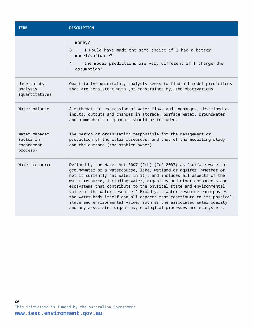
Figure 8—Examples of probability distributions for uniform, triangular and normal parameter distributions with their logarithmic counterparts

If a large database of parameter measurements is available, a normal or Gaussian distribution can be specified (Figure 8, right column). The probability is bell-shaped, centred on the mean and with a width proportional to the standard deviation. Parameters are often assumed to be normally distributed, even when there are not sufficient measurements to reliably estimate the mean and standard deviation. In such cases, the mean and standard deviation are estimated through expert judgement. It is important to note that a normal distribution is not bounded by a minimum and maximum value. Sampling randomly from such a distribution may inadvertently lead to unrealistic parameter values, such as negative recharge values.

Many hydraulic properties, such as hydraulic conductivity or storage, can vary over orders of magnitude. For those parameters, it is often advisable to specify probability distributions on log-transformed values. It is good practice to explicitly state the base of the log transform (natural logarithm, e or base 10). There is still ongoing debate about whether the log of hydraulic conductivities can be described with normal distributions (Meerschaert et al. 2013).

When a database of hydraulic property measurements is available, it is advisable to fit a probability distribution empirically. When there is no database of available measurements or the database is too small to reliably fit a probability distribution, a probability distribution needs to be estimated based on literature values and expert information. In cases where the estimated range spans more than an order of magnitude (e.g. 0.01 m/d to 1.0 m/d), it is advisable to carry out a log transform. In a coal mining and CSG context, information on aquifer storage properties and changes with time can be difficult to obtain, but some recent useful information is available in David et al. (2017) and Acworth et al. (2017).

Some parameters may be correlated, such as hydraulic conductivity (K) and storativity (S) which are both influenced by the lithology. Many parameters are also spatially correlated. This correlation needs to be expressed as a covariance between parameters. While correlation between parameters can be specified directly as covariance, spatial correlation is usually expressed with geostatistical techniques through a



variogram. When using pilot point parameterisation, for instance, the spatial correlation between pilot point parameters is expressed by a covariance matrix, informed by a variogram that the user specifies (Doherty 2015, 2016).

In some models, the parameterisation can be quite complex, such as a depth-dependent hydraulic conductivity or a multiplier on a spatially variable recharge field. For such complex parameterisation it is advisable to verify that the specified range of parameter values results in plausible model input values. Some parameters are designed to compensate for structural limitations of the model, such as high hydraulic conductivity values to represent small-scale fractures. If this is the case, it needs to be included in the justification of the chosen parameter prior distributions.

A1.4 Converging groundwater model over the entire plausible range of model parameters It is essential that the groundwater model can be evaluated over the entire range of parameter combinations defined above. It is recommended to submit the model to a stress test in which a number of extreme parameter combinations are tested for convergence before committing to a computationally intensive automated conditional calibration or stochastic model evaluation.

With a strategic choice of parameter combinations, this type of stress test can yield very useful insights on parameter sensitivity and model behaviour (for more details see Crosbie et al. 2016).

A1.5 Measurement uncertainty of each observation and/or a project-specific assessment of acceptable model-to-measurement misfit

The reference model used in the uncertainty scenario analysis needs to have an acceptable misfit between simulated and observed data before it can be used in simulations. In uncertainty quantification, this misfit is used to obtain the probability distribution of any parameter value. The goal is to find parameter combinations that result in model residuals that are equal to or smaller than the measurement uncertainty.

Observations such as groundwater heads or groundwater – surface water fluxes can be affected by small-scale local processes not captured in the model. It is therefore recommended to include these upscaling issues in the measurement uncertainty. Alternatively, one can think of the measurement uncertainty as the maximum acceptable misfit of modelled-to-measured values. Defining this acceptable misfit is very much project-specific and model-specific. It is up to the modeller, in discussion with the client, the regulator and other stakeholders, to define and justify the acceptable misfit and how to integrate this in the uncertainty quantification workflow.

A.2 Uncertainty quantification approaches

A2.1 Deterministic scenario analysis with subjective probability assessmentIn deterministic scenario analysis, a single realisation of a numerical model (e.g. the model that best fits the historical observations) is used for simulations. For these results to be useful in a risk framework, it is necessary to express the probability of this single realisation. This is a subjective assessment, based on knowledge of the system, the design of the model and the modeller’s experience.

The model with parameter values that best match the observations is often described at the ‘most likely’. Many modellers aim to be conservative in selecting parameters, especially when parameters are not easily constrained by observations. In such situations, where some aspects of the model will be ‘most likely’ and others ‘conservative’, it becomes difficult to assess whether the simulations are ‘most likely’ or ‘conservative’ overall.

To further complicate this issue, parameters are not necessarily conservative for all model outcomes. For example, for a given pumping rate, high hydraulic conductivity values can be conservative when calculating the time lags that affect streamflow depletion. The higher the hydraulic conductivity is, however, the smaller the drawdown. In this case, high conductivity values are not conservative for drawdown simulation effects.

Perturbing parameter values in an ad hoc sensitivity analysis (e.g. one parameter at a time) by an arbitrary amount does provide some insight to model behaviour. But this is not sufficient for uncertainty quantification unless the following questions can be answered:



• What is the probability of the perturbed value and corresponding simulations?

• How is the amount of perturbation determined and how does this relate to the probability distribution of the parameters (see section A.1.3)?

• Are parameter interaction effects accounted for?

The subjective probability quantification in deterministic scenario analysis can readily be questioned. A comprehensive, formal sensitivity analysis is encouraged, such as through analysis of the Jacobian matrix of a model or an ensemble of model runs. This can be used to objectively assess the importance of particular parameter values and will also allow a more robust uncertainty quantification (see section A.4).

This does not mean that the deterministic scenario analysis approach is without merit, whether or not a formal comprehensive sensitivity analysis is conducted. If it can be established that the conceptualisation and parameterisation is conservative, a deterministic scenario analysis can be used as a screening tool to delineate areas for further research and detailed modelling or as part of a qualitative uncertainty analysis (for more details see Peeters [in press]), especially if there is a formal sensitivity analysis.

A2.2 Deterministic modelling with linear probability quantificationLinear error propagation techniques can be used to compute simulation confidence intervals for any given model with a single set of parameter values (the conditionally calibrated model). Such a model is referred to below as the reference model (e.g. the model that best fits the historical observations).

These linear error propagation techniques form the basis of the PREDVAR and PREDUNC tools provided in the PEST package (Doherty 2016). The main assumptions are:

1. the model behaves linearly in the immediate vicinity of the selected parameter values

2. the parameter values, or their transformed values, are normally distributed. Interactions between parameters are described through multivariate normal distributions

3. the parameter values used in the reference model represent the mean of the normal distribution

4. the measurement uncertainty is normally distributed. Correlation in measurement uncertainty is captured through a multivariate normal distribution

5. the model outcomes are normally distributed.

The model is evaluated at least twice for each parameter. The change in model outcome corresponding to perturbing each parameter in isolation is captured in a Jacobian matrix. As shown in Moore and Doherty (2005), this matrix can be combined with the covariance matrix describing the uncertainty in parameters and the covariance matrix describing the measurement uncertainty to calculate the prediction uncertainty. The model outcomes of the reference model are considered to be the mean of a normal distribution. The result of the error propagation provides the standard deviation.

An automated conditional calibration seeks a parameter combination that provides a best fit in a least-squares sense, for instance by using the Levenberg-Marquardt algorithm as implemented in PEST. In subsequent linear error propagation, this parameter combination is then considered as the mean of the multivariate normal distribution. An automated conditional calibration, even when using regularisation, can result in parameter combinations that are only a local rather than a global minimum of the response surface. This can lead to false confidence in the calibrated parameter values and associated model predictions.

Another pitfall is that, due to parameter correlation, parameters compensate for conceptual issues or for other parameters (e.g. the response of an aquifer often depends on ratios of model parameters such as aquifer diffusivity (T/S), or recharge and transmissivity (R/T)) (Barnett et al. 2012). The classic example is provided in Doherty (2010), where incorrectly specified head boundary conditions lead to a small residual in head values but biased hydraulic conductivity estimates. Using such biased values in a simulation obviously compromises the simulation and its confidence intervals. Relatively low-cost data-gathering techniques, such as a LiDAR survey of river bed and spring elevations, can greatly reduce the uncertainty in boundary conditions and thereby the uncertainty in inferred hydraulic property values.



Doherty (2015) and White et al. (2014) provide some strategies to minimise bias in parameter values by pre-processing observations and using multi-component objective functions.

As indicated in section A.1.5, it is essential that the measurement uncertainty for each observation is assessed independently from the model. Moore and Doherty (2005) show that the predictive uncertainty depends greatly on the measurement uncertainty and what is considered an acceptable model-to-measurement misfit. In formal linear error propagation, the weights of observations in the objective function are inversely proportional to the measurement uncertainty (i.e. measurements with small uncertainty will have greater weight). Adjusting weights of observations is a straightforward way to combine different types of observations, to emphasise observations that align with the model outcomes of interest, to reflect the reliability of observations and to compensate for scale and structural issues.

To avoid criticism that the weighting of observations is a deliberate attempt to pervert the model outcome, the weighting must be justified in a transparent way. One way of expressing this is by presenting the confidence interval that a weight corresponds to, assuming measurement error is normally distributed. A groundwater level measurement that is assigned a weight of one corresponds to a normal distribution with a mean equal to the observed value and a standard deviation of 1 m. If one considers model outcomes within two standard deviations as acceptable (containing approximately 90 per cent of the probability mass), any model outcome within 2 m of the observed value is deemed acceptable.

Giving all observations equal weight is not recommended, as that implicitly assumes that the measurement and structural uncertainty is equal throughout the model domain, which is seldom an appropriate assumption.

Many outcomes from groundwater models are non-linear functions of the model parameters. A naïve application of linear error propagation methods can therefore lead to nonsensical results. Consider, for instance, an analysis that results in a drawdown prediction of 0.5 m with a standard deviation of 0.3 m. The 90th percentile prediction interval for a normal distribution, defined as [-1.96, +1.96s], then becomes [-0.088, 1.088]. This would imply that in this model the development can cause a rise in groundwater levels.

The modeller needs to verify and show that the model outcomes are sufficiently close to a linear function of the parameters for the linear error propagation to produce sensible results.

When using the deterministic approach with linear error propagation, it is not straightforward to consider multiple conceptualisations, as the method is based on a single, deterministic reference model.

A.2.3 Stochastic modelling with Bayesian probability quantification Stochastic modelling relaxes many of the assumptions on linearity and normality of parameters by evaluating a large number of parameter combinations and presenting the model outcomes as an ensemble.

In Bayesian inference (Figure 9), a prior distribution is specified for each parameter (and eventual joint distribution between parameters), encapsulating the current state of information and knowledge. A sampling algorithm evaluates a large number of parameter combinations and preferentially retains parameter combinations with a high likelihood—i.e. a close fit to observations. The updated range of parameter values is called the posterior (or post-calibration) parameter distribution. This posterior parameter distribution is randomly sampled, and the corresponding model outcomes form the posterior predictive distribution.



Figure 9—Schematic representation of stochastic modelling with Bayesian probability

Note: The prior parameter distributions (blue) are sampled and evaluated based on a likelihood function (inference). The ensemble of acceptable parameter combinations and corresponding predictions is called the posterior (yellow).

The number of model evaluations required is problem specific. The number of samples from a posterior parameter or predictive distribution is considered sufficient if the moments of interest converge. If one is interested in the 95th percentile of a distribution, one has to verify that this summary statistic does not change with an increasing number of model runs. Measures of central tendency, such as the mean and the median, tend to converge more quickly than the extremes of a distribution (e.g. the 95th or 99th percentile). The number of model runs required therefore depends on the shape of the posterior distribution as well as on the summary statistics of interest.

This is illustrated in Figure 10, in which a regional-scale groundwater model is evaluated 300 times and four different model outcomes are computed. The boxplots showing the distribution of these four metrics are very similar, even if on the left-hand side the boxplot only represents 200 model runs and on the right-hand side it represents 300 model runs. This indicates that for this particular case, 300 model runs are sufficient to characterise the distribution of these four metrics.



Figure 10—Statistical distributions of four predictions relating to the Pilliga Sandstone aquifer, simulated using the revised Gunnedah Basin groundwater flow model

Note: (a) = maximum drawdown (MXD); (b) = time elapsed at which maximum drawdown occurred (tMXD); (c) = number of model cells at which drawdown exceeded 2 m (NDD); (d) = maximum vertical flux (MXQ).

Source: Turnadge et al. 2018.

The stochastic approach allows specification of prior parameter distributions other than Gaussian, with, as an extreme, a fully empirical parameter distribution. Specification of these prior parameter distributions is the most appropriate way to incorporate existing knowledge into the uncertainty quantification. If the observation data is very informative (i.e. it can constrain many of the parameters), specifying a too-narrow prior parameter distribution may result in not fully sampling parameter space and not including parameter combinations that provide equal or better fits to the data. Conversely, specifying too wide a prior distribution will make the sampling algorithm very inefficient and will greatly increase the number of model evaluations required to find parameter combinations that fit the data.

If the data is not very informative (i.e. it cannot constrain the parameters relevant to the model outcomes of interest), the posterior parameter distributions will be nearly identical to the prior distributions. As with deterministic modelling with linear error propagation, it is essential to identify which parameters can be constrained by the available observations.

Observations are introduced in the stochastic approach through the likelihood function. It can be shown that if measurement errors are assumed to be normally distributed, this is identical to linear error propagation. The discussion of weighting observations in previous sections is at least as applicable to the stochastic approach. The modeller needs to specify the error model for the observations independently of the model and to define an acceptable level of model-to-measurement misfit.

Null space Monte Carlo is a special case of a stochastic approach in which the posterior parameter distribution is not generated through sampling from prior parameter distributions but in which the posterior parameter space is defined by the null-space (Tonkin and Doherty 2009). The null-space is formed by linear combinations of parameters that have no impact on the model objective function. Random sampling of the null-space ensures that all the model runs in the ensemble of model runs have a similar model-to-measurement misfit. This is a very efficient sampling algorithm but it still relies on parameter values that can be described through multivariate normal distributions, and the definition of the null-space hinges on a linearisation of a single model run through singular value decomposition.

Approximate Bayesian computation relaxes the need to have a closed-form, analytic expression of the likelihood function. This method, like the generalised likelihood uncertainty estimation (GLUE) technique, allows the modeller to specify how the likelihood is calculated. For instance, there can be a set of constraints that need to be satisfied simultaneously (e.g. head residuals less than 2 m, flux residuals less than 1 ML/d and aquitard Kh less than aquifer Kh). This method allows much more flexibility in specifying the likelihood, and is transparent and straightforward to communicate.

The stochastic approach is more amenable to accommodating multiple conceptualisations. In Bayesian model averaging, each conceptualisation is assigned a prior probability and included in the sampling.



A.3 Qualitative uncertainty analysis (assumption hunting)

As indicated in section 0, each model, regardless of complexity or severity of potential impacts, needs to be subjected to a qualitative uncertainty analysis in terms of a systematic and rigorous assessment of the model assumptions and choices. The justification of model choices is standard practice in groundwater model reporting. The AGMG (Barnett et al. 2012) recommends a ‘limitations and opportunities’ section to highlight the main limitations that can influence results. From the previous section it is clear that each uncertainty quantification approach is based on a number of assumptions that need to be justified and checked.

In the bioregional assessments, qualitative uncertainty analysis is presented together with the results of the uncertainty quantification (Peeters et al. 2016). Each assumption is scored on whether the assumption or model choice is driven by data availability, time and budget available for the project, or technical challenges. The most important score, however, is the perceived effect of the assumption on the model outcomes. Summarising these scores in a table allows reviewers and stakeholders to quickly assess the importance of the various model assumptions which is particularly valuable in an environmental impact assessment.

The qualitative uncertainty analysis has great potential as a communication tool to engage stakeholders. It gives modellers and proponents an opportunity to transparently record the effects of various assumptions that have been logically considered in the modelling process. It also establishes common ground between modellers and independent reviewers, requiring reviewers to precisely articulate why they disagree with the scoring and reasoning presented.

Table 4 illustrates the concept of a qualitative uncertainty analysis with an assumption that is often made in groundwater modelling studies: representing aquifer properties as spatially uniform. The table shows both the scoring and its justification. This example highlights that it is possible to score ‘medium’ on the prediction attribute despite scoring ‘high’ on the data and resources attributes.

Table 4—Illustrative example of qualitative uncertainty analysis undertaken in the bioregional assessments, based on the assumption of applying spatially uniform aquifer properties

DATA RESOURCES TECHNICAL PREDICTION

Spatially uniform aquifer properties

High High Medium Medium

Large dataset of property observations needed to characterise a priori spatial variability.Large dataset of head or flux observations needed to infer posterior spatial variability.

Spatially heterogeneous parameterisation increases dimensionality of parameter inference and uncertainty quantification. As this increases the number of model evaluations, a larger budget and longer time frame is needed for modelling.

Most groundwater model codes allow spatially variable hydraulic properties.Efficiently implementing a spatial field generator that adheres to prior knowledge remains challenging.

If the equivalent properties in the uniform parameterisation capture natural variability, the range of drawdown predictions will be comparable to those of a spatially variable parameterisation.Drawdown predictions will be locally different if spatial heterogeneity is high or localised (such as through faults).

Source: Peeters et al. 2016.

There are various ways to justify assumptions. For many issues in simulating coal resource development, there is academic and technical literature that explores effects on simulation. Examples are Brunner et al. (2010) on representing surface water – groundwater connectivity in MODFLOW; Herckenrath et al. (2015) and CoA (2014a) on simulating dual-phase flow for CSG production; Cook et al. (2016) on propagation of depressurisation through aquitards; and Doble et al. (2017) on the effect of leaky bores. The latter two also explore the effects of assumptions from first principles, starting from the fundamental groundwater flow equations.



Another approach to test assumptions, especially those very specific to the model study, is to carry out numerical experiments with a small-scale model. Crosbie et al. (2016) analyse the effect of aquifer heterogeneity on regional drawdown simulations. Hayes and Nicol [in press] report building a simplified large-scale model to justify selection of boundary conditions. Mackie Environmental Research (2013) explores the effect of aquitard heterogeneity through detailed small-scale stochastic analysis. This kind of hypothesis testing can be extended to quantify the likelihood that a hypothesis regarding conceptualisation or even potential impact is correct (e.g. Beven 2018, Dausman et al. 2010).

The most objective approach to assess the effect of an assumption is to incorporate the assumption in the parameterisation so that it can be tested through a formal, comprehensive sensitivity analysis (see section A.4).

A.4 Sensitivity analysis

Saltelli (2002) defines sensitivity analysis as:

The study of how uncertainty in the output of a model (numerical or otherwise) can be apportioned to different sources of uncertainty in the model input.

In this definition, sensitivity analysis augments uncertainty quantification as it identifies which sources of uncertainty contribute most to predictive uncertainty. This is the first step in designing strategies to reduce predictive uncertainty by gathering new data or undertaking additional modelling.

There is, however, an important role for sensitivity analysis as a first step in an uncertainty quantification. The computational load of uncertainty quantification increases dramatically with an increasing number of parameters. Factor screening or prioritisation aims to identify which parameters have the largest effect on model outcomes so that parameters with no or negligible effect can be excluded from the uncertainty quantification.

Closely related to this goal is parameter identifiability. Only parameters to which the objective function is sensitive can be constrained by the observations. Hill and Tiedeman (2007) and Doherty and Hunt (2009) provide metrics for parameter identifiability from analysis of a Jacobian matrix, created through systematic, one-at-a-time perturbation of a single parameter set.

For example, a high value for the relative composite sensitivity (RCS) factor calculated via PEST from the Jacobian matrix for a parameter indicates that the model calibration is sensitive to that parameter, but that the measurements have provided enough information to adequately constrain the uncertainty. A low RCS value indicates that the model calibration is not sensitive to the parameter because the measurements do not inform/constrain the calibration, and thus the effect on predictive uncertainty should be evaluated. Note that a numerical criterion is not applicable to this guidance, as the RCS is a relative factor—‘high’ and ‘low’ are relative to the RCS factors calculated for a model.

While this is a good starting point for a comprehensive sensitivity analysis, Saltelli and Annoni (2010) show that this can lead to misleading results, especially when the model is non-linear and highly parameterised. Pianosi et al. (2016) provide a comprehensive overview of global sensitivity analysis methods and their application in environmental modelling. In the bioregional assessments (Peeters et al. 2016), the density-based approach by Plischke et al. (2013) is applied to all groundwater and surface water models. The advantages of this approach are that it makes no assumption about the shape of the correlation between parameters and simulations and that it can be applied to any given ensemble of model runs—i.e. there is no specified sampling algorithm required.

These complex issues should be considered in any sensitivity analysis that supports uncertainty analysis. The implications of the various assumptions and methods applied should be logically and transparently reported.



Documents

Information Guidelines Explanatory Note Uncertainty ...€¦ · Web viewFurther discussion of stochastic modelling with Bayesian probability quantification is in the appendix (section