Embed Size (px)
Citation preview
WORKING PAPER SER IES
ISSN 1561081-0
9 7 7 1 5 6 1 0 8 1 0 0 5
NO. 572 / JANUARY 2006
INFORMATION, HABITS,AND CONSUMPTION BEHAVIOR
EVIDENCE FROM MICRO DATA
by Mika Kuismanen and Luigi Pistaferri

In 2006 all ECB publications will feature
a motif taken from the
€5 banknote.
WORK ING PAPER SER IE SNO. 572 / JANUARY 2006
INFORMATION, HABITS, AND CONSUMPTION
BEHAVIOR
EVIDENCE FROM MICRO DATA 1
by Mika Kuismanen 2 and Luigi Pistaferri 3
1 We thank the anonymous referee for helpful comments and suggestions. The opinions expressed in the paper are those of the authors and do not necessarily reflect those of the ECB.
2 Research Department, European Central Bank, Kaiserstrasse 29, 60311 Frankfurt, Germany; e-mail: [email protected] Stanford University, Department of Economics, 579 Serra Mall, Stanford, CA 94305-6072, U.S.A.; e-mail: [email protected]
This paper can be downloaded without charge from http://www.ecb.int or from the Social Science Research Network
electronic library at http://ssrn.com/abstract_id=872542.

© European Central Bank, 2006
AddressKaiserstrasse 2960311 Frankfurt am Main, Germany
Postal addressPostfach 16 03 1960066 Frankfurt am Main, Germany
Telephone+49 69 1344 0
Internethttp://www.ecb.int
Fax+49 69 1344 6000
Telex411 144 ecb d
All rights reserved.
Any reproduction, publication andreprint in the form of a differentpublication, whether printed orproduced electronically, in whole or inpart, is permitted only with the explicitwritten authorisation of the ECB or theauthor(s).
The views expressed in this paper do notnecessarily reflect those of the EuropeanCentral Bank.
The statement of purpose for the ECBWorking Paper Series is available fromthe ECB website, http://www.ecb.int.
ISSN 1561-0810 (print)ISSN 1725-2806 (online)
3ECB
Working Paper Series No. 572January 2006
CONTENTS
Abstract 4
Non-technical summary 5
1 Introduction 7
2 The model 8
2.1 Approximating the Euler equation 9
2.2 Superior information 11
2.3 The consumption function 13
3 Empirical approach 14
3.1 Identification of ψ 15
4 The data 16
5 Results 18
6 Conclusions 20
Tables 21
Appendices 23
Appendix A: Second order approximationof the Euler equation 23
Appendix B: Proof of the constancy of κ 23
References 25
28European Central Bank WWorking Paper Series

Abstract
Most of the empirical literature on consumption behaviour over the last decades has focused onestimating Euler equations. However, there is now consensus that data-related problems make thisapproach unfruitful, especially for answering policy relevant issues. Alternatively, many papers haveproposed using the consumption function to forecast behaviour. This paper follows in this tradition, byderiving an analytical consumption function in the presence of intertemporal non-separabilities, �superiorinformation�, and income shocks of di¤erent nature, both transitory and permanent. The results provideevidence for durability, and show that people are relatively better at forecasting short-term rather thanlong-term shocks.
JEL classi�cation: D11,D12,D82,E21Keywords: Consumption, Superior Information, Durability, Habit Persistence, Panel Data
4ECBWorking Paper Series No. 572January 2006

Non-technical summary
Up to recent years many researchers have studied consumer choice under the assumption that preferences
are time separable. Also, most of the empirical literature on consumption behaviour over the last decades has
focused on estimating the �rst order condition of the intertemporal maximization problem under uncertainty.
However, recent literature has shown that given the lack of cross-sectional variability in interest rates, lack
of information on individual discount rates, and reliable measures of uncertainty, the results using this
approach are mixed at best. The problem of delivering credible estimates of structural parameters, such as
the elasticity of intertemporal substitution or the coe¢ cient of prudence, as well as its inadequacy to answer
policy-relevant questions, has made the search for alternative approaches a priority in macroeconomics.
Our approach is to study the consumption function. We show that it is possible to approximate the �rst
order condition of the intertemporal maximization problem under uncertainty and the constant relative risk
aversion preferences without resorting to log-linearization. In addition we show how such approximation can
be implemented even in the presence of a general form of intertemporal non-separability, covering both habit
persistence and durability. We relax the assumption that the individual knows no more than the ecometrician
regarding future income prospects. In particular, we assume that people may be able to forecast the actual
realizations of income shocks (transitory and permanent) with a certain degree of con�dence, and that their
expectations become increasingly less precise as the forecast horizon widens.
Most of the consumption function literature uses aggregate data while our empirical analysis is conducted
on individual data. This means that we avoid a number of di¢ cult aggregation issues. The main di¢ culty
of implementing our approach is to �nd a data set that satis�es two principal requirements: it features a
longitudinal component, and it contains information on household consumption, income, and assets. The
PSID (Panel Study of Income Dynamics) satis�es the �rst requirement fully and the second partly. In par-
ticular, data on assets are available only at �ve-year intervals (starting in 1984), and the only consumption
data available is for food. As it is not clear how well food consumption behavior generalizes to non-durable
consumption behavior, we use imputed non-durable consumption data. The idea is to impute consump-
tion to all PSID households combining PSID data with consumption data from repeated CEX (Consumer
Expenditure Survey) cross-sections. The �nal sample used in our analysis is composed of 1,125 households.
We estimate a dynamic consumption function using microeconomic data. We show that the dynamics
hinge upon a number of structural parameters: the degree of intertemporal separability in preferences (which
may indicate habit persistence or durability), the slope of the intertemporal consumption path (which cap-
tures the importance of the precautionary motive for savings), the impact of advance information about
future income prospects (which signals a discrepancy of information between the individual and the econo-
5ECB
Working Paper Series No. 572January 2006
metrician), and the forecastability of permanent shocks relative to transitory shocks.

Our �ndings point to the existence of durability rather than habit persistence. This means that the
conventional de�nition of non-durable consumption most likely includes goods that provide services for
longer than one year, thus obscuring (or o¤setting) any habit persistence that may exist in the data. We
�nd evidence for a positively sloped consumption path, meaning that consumers delay spending in response to
the risks they face. As for the superior information issue we �nd that consumers have substantial information
regarding near future income changes, especially short-lived ones.
6ECBWorking Paper Series No. 572January 2006
1 Introduction
Most of the empirical literature on consumption behaviour over the last decades has focused on estimating the
Euler equation, i.e., the �rst order condition of the intertemporal maximization problem under uncertainty
(Hall (1978)). However, given the lack of cross-sectional variability in interest rates, lack of information on
individual discount rates, and reliable measures of uncertainty, the results using this approach are mixed at
best (Attanasio and Low (2004), Browning and Lusardi (1995), Attanasio (2000) and Carroll (2001)). The
inability of the Euler equation approach to deliver credible estimates of structural parameters, such as the
elasticity of intertemporal substitution or the coe¢ cient of prudence, as well as its inadequacy to answer
policy-relevant questions, has made the search for alternative approaches a priority in macroeconomics.
A popular alternative to the Euler equation is to study the consumption function. This approach is
complicated by the fact that realistic assumptions about preferences and uncertainty prevent �nding a closed
form solution, and hence the model can only be simulated (Zeldes (1989)). To overcome such di¢ culty, many
approximations have been proposed (Campbell and Mankiw (1987), Fuhrer (2001)). Our paper follows in
this tradition, although it departs from it on a number of important ways. First, we show that, as long as the
higher moments of the conditional distribution of consumption are constant over time, we can approximate
the Euler equation under CRRA preferences without resorting to log-linearization. Secondly, we are able to
derive such approximation even in the presence of a general form of intertemporal non-separability, covering
both habit persistence and durability (Constantinides and Ferson (1991)). Thirdly, we relax the assumption
that the individual knows no more than the ecometrician regarding future income prospects. In particular,
we assume that people may be able to forecast the actual realizations of income shocks (transitory and
permanent) with a certain degree of con�dence, and that their expectations become increasingly less precise
as the forecast horizon widens. Fourthly, most of the consumption function literature uses aggregate data,
while our empirical analysis is conducted on individual data drawn from the US PSID, thus avoiding a
number of aggregation issues.
Using our assumptions, we derive an expressions that relates current consumption to once and twice
lagged consumption, lagged assets, and lagged income. We deal with the issue of endogeneity using a
conventional instrumental variable procedure, whereby lags of income and consumption act as excluded
variables. The reduced form coe¢ cients of this relationship are complicated, non-linear functions of all
the parameters of the model. A minimum distance procedure maps these reduced form coe¢ cients into
the structural parameters, while the covariance between unexplained consumption and unexplained income
changes permits identi�cation of one remaining crucial parameter, the forecastability of permanent shocks
7ECB
Working Paper Series No. 572January 2006
relative to transitory shocks.
The rest of the paper is organized as follows. In Section 2 we present the model, discuss the approximation
of the Euler equation and derive an analytical expression for the consumption function under the assumption
of �superior information�. In Section 3 we discuss the empirical approach and the identi�cation issues.
Section 4 deals with the data, while Section 5 presents the results. Section 6 concludes.
2 The Model
Households are assumed to maximize the expected discounted utility of current and future consumption. We
assume that the utility function is of the constant-relative-risk-aversion (CRRA) form, and so the problem
is to:
maxEt
" 1Xi=0
�1
1 + �
�i c�t+i1� 1'
1� 1'
#(1)
where Et indicates that the expectation is conditional to the information set available to the individual
at time t, � is the rate of subjective time preference, and ' is the elasticity of intertemporal substitution.
Preferences are de�ned over the composite term c�t+i = ct+i � hct+i�1. This allows for non-separability
in utility over time. The parameter h measures habit persistence (if h > 0) or durability (h < 0). Habit
persistence implies that higher is the previous consumption (bigger is the habit), higher also must be the
current consumption to deliver the same e¤ect. Also note that habits wear o¤ over time. On the other hand,
not all nondurables or services are perishable so that consumption and expenditure can be equated. Some
goods and services are durables in their nature thus adding to utility over time, see Costantinides and Ferson
(1991).
The maximization problem is subject to the per-period budget constraint:
at+1 = (1 + r) (at + yt � ct) (2)
where at is �nancial wealth at the beginning of period t. The real interest rate is assumed to be constant
over time,1 yt is income, and ct consumption. This translates into a lifetime budget constraint of the form:
1Xi=0
Et (ct+i)
(1 + r)i= at +
1Xi=0
Et (yt+i)
(1 + r)i(3)
whereP1i=0
Et(yt+i)(1+r)i = Ht represents the expected discounted value of human wealth.
The Euler equation of this problem for a generic period i is:
1Time-varying interest rate can be easily added to the analysis.
8ECBWorking Paper Series No. 572January 2006
Et+i
"�c�t+i+1c�t+i
�� 1'
#=1 + �
1 + r
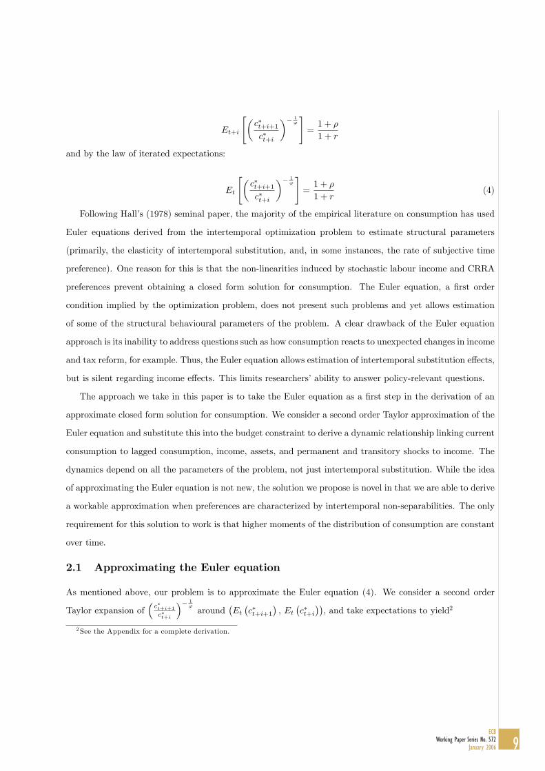
and by the law of iterated expectations:
Et
"�c�t+i+1c�t+i
�� 1'
#=1 + �
1 + r(4)
Following Hall�s (1978) seminal paper, the majority of the empirical literature on consumption has used
Euler equations derived from the intertemporal optimization problem to estimate structural parameters
(primarily, the elasticity of intertemporal substitution, and, in some instances, the rate of subjective time
preference). One reason for this is that the non-linearities induced by stochastic labour income and CRRA
preferences prevent obtaining a closed form solution for consumption. The Euler equation, a �rst order
condition implied by the optimization problem, does not present such problems and yet allows estimation
of some of the structural behavioural parameters of the problem. A clear drawback of the Euler equation
approach is its inability to address questions such as how consumption reacts to unexpected changes in income
and tax reform, for example. Thus, the Euler equation allows estimation of intertemporal substitution e¤ects,
but is silent regarding income e¤ects. This limits researchers�ability to answer policy-relevant questions.
The approach we take in this paper is to take the Euler equation as a �rst step in the derivation of an
approximate closed form solution for consumption. We consider a second order Taylor approximation of the
Euler equation and substitute this into the budget constraint to derive a dynamic relationship linking current
consumption to lagged consumption, income, assets, and permanent and transitory shocks to income. The
dynamics depend on all the parameters of the problem, not just intertemporal substitution. While the idea
of approximating the Euler equation is not new, the solution we propose is novel in that we are able to derive
a workable approximation when preferences are characterized by intertemporal non-separabilities. The only
requirement for this solution to work is that higher moments of the distribution of consumption are constant
over time.
2.1 Approximating the Euler equation
As mentioned above, our problem is to approximate the Euler equation (4). We consider a second order
Taylor expansion of�c�t+i+1c�t+i
�� 1'
around�Et�c�t+i+1
�, Et
�c�t+i
��, and take expectations to yield2
2See the Appendix for a complete derivation.
9ECB
Working Paper Series No. 572January 2006
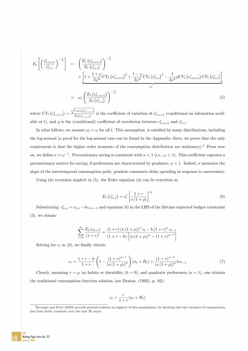
Et
"�c�t+i+1c�t+i
�� 1'
#=
Et�c�t+i+1
�Et�c�t+i
� !� 1'
��1 +
1 + '
2'2CVt
�c�t+i+1
�2+1� '2'2
CVt�c�t+i
�2 � 1
2'2%CVt
�c�t+i+1
�CVt
�c�t+i
��| {z }
!t
= !t
Et�c�t+i+1
�Et�c�t+i
� !� 1'
(5)
where CVt�c�t+i+1
�=
qV art(c�t+i+1)Et(c�t+i+1)
is the coe¢ cient of variation of c�t+i+1 (conditional on infomation avail-
able at t), and % is the (conditional) coe¢ cient of correlation between c�t+i+1 and c�t+i.
In what follows, we assume !t = ! for all t. This assumption is satis�ed by many distributions, including
the log-normal (a proof for the log-normal case can be found in the Appendix; there, we prove that the only
requirement is that the higher order moments of the consumption distribution are stationary).3 From now
on, we de�ne � = !�1. Precautionary saving is consistent with � < 1 (i.e., ! > 1). This coe¢ cient captures a
precautionary motive for saving; if preferences are characterized by prudence, � < 1. Indeed, � measures the
slope of the intertemporal consumption path: prudent consumers delay spending in response to uncertainty.
Using the recursion implicit in (5), the Euler equation (4) can be rewritten as
Et�c�t+i
�= c�t
�1 + r
� (1 + �)
�i'(6)
Substituting c�t+i = ct+i�hct+i�1 and equation( 6) in the LHS of the lifetime expected budget constraint
(3), we obtain:
1Xi=0
Et (ct+i)
(1 + r)i=(1 + r) (� (1 + �))
'ct � h (1 + r)' ct�1
(1 + r � h)h(� (1 + �))
' � (1 + r)'�1i
Solving for ct in (3), we �nally obtain:
ct =1 + r � h1 + r
1� (1 + r)
'�1
(� (1 + �))'
!(at +Ht) +
(1 + r)'�1
(� (1 + �))'hct�1 (7)
Clearly, assuming r = �, no habits or durability (h = 0), and quadratic preferences (� = 1), one obtains
the traditional consumption function solution (see Deaton, (1992), p. 82):
ct =r
1 + r(at +Ht)
3Krueger and Perri (2003) provide partial evidence in support of this assumption, by showing that the variance of consumptionhas been fairly constant over the last 20 years.
10ECBWorking Paper Series No. 572January 2006
2.2 Superior Information
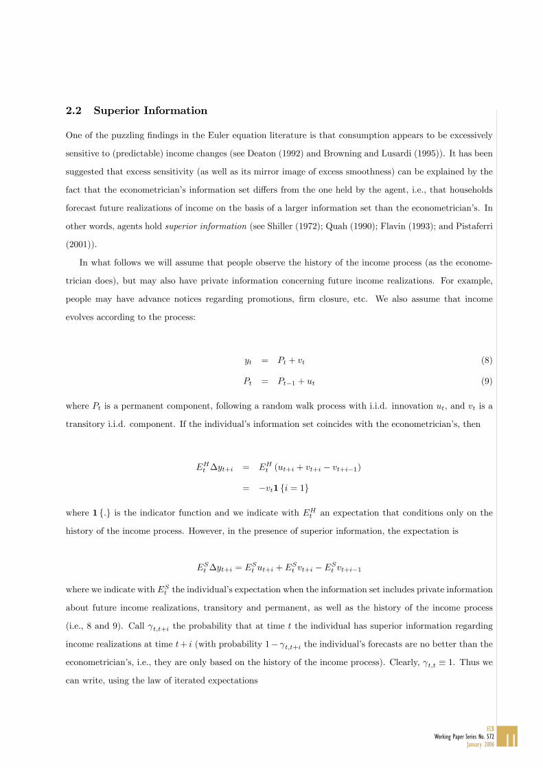
One of the puzzling �ndings in the Euler equation literature is that consumption appears to be excessively
sensitive to (predictable) income changes (see Deaton (1992) and Browning and Lusardi (1995)). It has been
suggested that excess sensitivity (as well as its mirror image of excess smoothness) can be explained by the
fact that the econometrician�s information set di¤ers from the one held by the agent, i.e., that households
forecast future realizations of income on the basis of a larger information set than the econometrician�s. In
other words, agents hold superior information (see Shiller (1972); Quah (1990); Flavin (1993); and Pistaferri
(2001)).
In what follows we will assume that people observe the history of the income process (as the econome-
trician does), but may also have private information concerning future income realizations. For example,
people may have advance notices regarding promotions, �rm closure, etc. We also assume that income
evolves according to the process:
yt = Pt + vt (8)
Pt = Pt�1 + ut (9)
where Pt is a permanent component, following a random walk process with i.i.d. innovation ut, and vt is a
transitory i.i.d. component. If the individual�s information set coincides with the econometrician�s, then
EHt �yt+i = EHt (ut+i + vt+i � vt+i�1)
= �vt1 fi = 1g
where 1 f:g is the indicator function and we indicate with EHt an expectation that conditions only on the
history of the income process. However, in the presence of superior information, the expectation is
ESt �yt+i = ESt ut+i + ESt vt+i � ESt vt+i�1
where we indicate with ESt the individual�s expectation when the information set includes private information
about future income realizations, transitory and permanent, as well as the history of the income process
(i.e., 8 and 9). Call t;t+i the probability that at time t the individual has superior information regarding
income realizations at time t+ i (with probability 1� t;t+i the individual�s forecasts are no better than the
econometrician�s, i.e., they are only based on the history of the income process). Clearly, t;t � 1. Thus we
can write, using the law of iterated expectations
11ECB
Working Paper Series No. 572January 2006
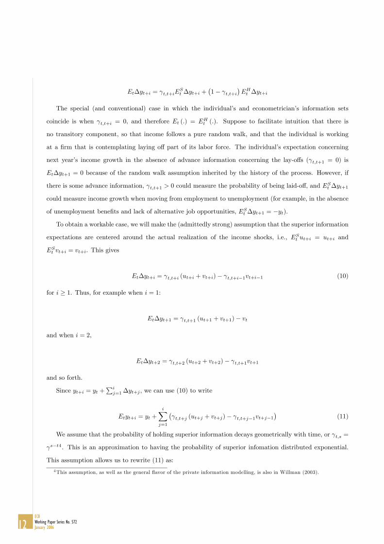
Et�yt+i = t;t+iESt �yt+i +
�1� t;t+i
�EHt �yt+i
The special (and conventional) case in which the individual�s and econometrician�s information sets
coincide is when t;t+i = 0, and therefore Et (:) = EHt (:). Suppose to facilitate intuition that there is
no transitory component, so that income follows a pure random walk, and that the individual is working
at a �rm that is contemplating laying o¤ part of its labor force. The individual�s expectation concerning
next year�s income growth in the absence of advance information concerning the lay-o¤s ( t;t+1 = 0) is
Et�yt+1 = 0 because of the random walk assumption inherited by the history of the process. However, if
there is some advance information, t;t+1 > 0 could measure the probability of being laid-o¤, and ESt �yt+1
could measure income growth when moving from employment to unemployment (for example, in the absence
of unemployment bene�ts and lack of alternative job opportunities, ESt �yt+1 = �yt).
To obtain a workable case, we will make the (admittedly strong) assumption that the superior information
expectations are centered around the actual realization of the income shocks, i.e., ESt ut+i = ut+i and
ESt vt+i = vt+i. This gives
Et�yt+i = t;t+i (ut+i + vt+i)� t;t+i�1vt+i�1 (10)
for i � 1. Thus, for example when i = 1:
Et�yt+1 = t;t+1 (ut+1 + vt+1)� vt
and when i = 2,
Et�yt+2 = t;t+2 (ut+2 + vt+2)� t;t+1vt+1
and so forth.
Since yt+i = yt +Pij=1�yt+j , we can use (10) to write
Etyt+i = yt +iX
j=1
� t;t+j (ut+j + vt+j)� t;t+j�1vt+j�1
�(11)
We assume that the probability of holding superior information decays geometrically with time, or t;s =
s�t4 . This is an approximation to having the probability of superior infomation distributed exponential.
This assumption allows us to rewrite (11) as:
4This assumption, as well as the general �avor of the private information modelling, is also in Willman (2003).
12ECBWorking Paper Series No. 572January 2006
Etyt+i = yt +iX
j=1
� j (ut+j + vt+j)� j�1vt+j�1
�(12)
Substitution of (12) intoP1i=0
Et(yt+i)(1+r)i = Ht gives:
Ht = yt1 + r
r� 1rvt +
1 + r
r
1Xi=1
�
1 + r
�iut+i +
1Xi=1
�
1 + r
�ivt+i (13)
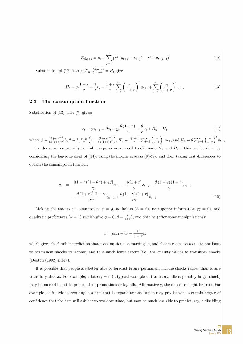
2.3 The consumption function
Substitution of (13) into (7) gives:
ct � �ct�1 = �at + yt� (1 + r)
r� �
rvt +Hu +Hv (14)
where � = (1+r)'�1
(�(1+�))'h, � =1+r�h1+r
�1� (1+r)'�1
(�(1+�))'
�,Hu =
�(1+r)r
P1i=1
� 1+r
�iut+i andHv = �
P1i=1
� 1+r
�ivt+i.
To derive an empirically tractable expression we need to eliminate Hu and Hv. This can be done by
considering the lag-equivalent of (14), using the income process (8)-(9), and then taking �rst di¤erences to
obtain the consumption function:
ct =[(1 + r) (1� � ) + �]
ct�1 �
� (1 + r)
ct�2 �
� (1� ) (1 + r)
at�1
�� (1 + r)2(1� )
r yt�1 +
� (1� ) (1 + r)r
vt�1 (15)
Making the traditional assumptions r = �, no habits (h = 0), no superior information ( = 0), and
quadratic preferences (� = 1) (which give � = 0, � = r1+r ), one obtains (after some manipulations):
ct = ct�1 + ut +r
1 + rvt
which gives the familiar prediction that consumption is a martingale, and that it reacts on a one-to-one basis
to permanent shocks to income, and to a much lower extent (i.e., the annuity value) to transitory shocks
(Deaton (1992) p.147).
It is possible that people are better able to forecast future permanent income shocks rather than future
transitory shocks. For example, a lottery win (a typical example of transitory, albeit possibly large, shock)
may be more di¢ cult to predict than promotions or lay-o¤s. Alternatively, the opposite might be true. For
example, an individual working in a �rm that is expanding production may predict with a certain degree of
con�dence that the �rm will ask her to work overtime, but may be much less able to predict, say, a disabling
13ECB
Working Paper Series No. 572January 2006
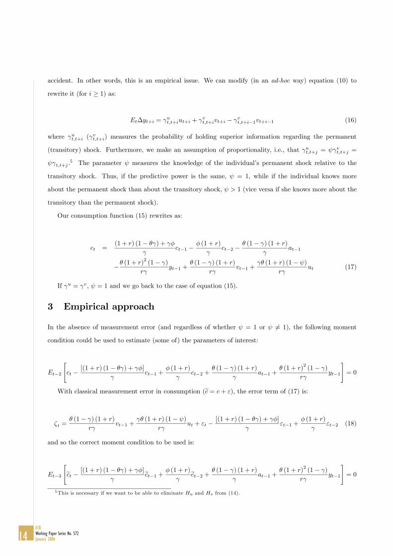
accident. In other words, this is an empirical issue. We can modify (in an ad-hoc way) equation (10) to
rewrite it (for i � 1) as:
Et�yt+i = ut;t+iut+i + vt;t+ivt+i � vt;t+i�1vt+i�1 (16)
where ut;t+i ( vt;t+i) measures the probability of holding superior information regarding the permanent
(transitory) shock. Furthermore, we make an assumption of proportionality, i.e., that ut;t+j = vt;t+j =
t;t+j .5 The parameter measures the knowledge of the individual�s permanent shock relative to the
transitory shock. Thus, if the predictive power is the same, = 1, while if the individual knows more
about the permanent shock than about the transitory shock, > 1 (vice versa if she knows more about the
transitory than the permanent shock).
Our consumption function (15) rewrites as:
ct =(1 + r) (1� � ) + �
ct�1 �
� (1 + r)
ct�2 �
� (1� ) (1 + r)
at�1
�� (1 + r)2(1� )
r yt�1 +
� (1� ) (1 + r)r
vt�1 + � (1 + r) (1� )
r ut (17)
If u = v, = 1 and we go back to the case of equation (15).
3 Empirical approach
In the absence of measurement error (and regardless of whether = 1 or 6= 1), the following moment
condition could be used to estimate (some of) the parameters of interest:
Et�2
"ct �
[(1 + r) (1� � ) + �]
ct�1 +� (1 + r)
ct�2 +
� (1� ) (1 + r)
at�1 +� (1 + r)
2(1� )
r yt�1
#= 0
With classical measurement error in consumption (ec = c+ "), the error term of (17) is:
�t =� (1� ) (1 + r)
r vt�1 +
� (1 + r) (1� )r
ut + "t �[(1 + r) (1� � ) + �]
"t�1 +
� (1 + r)
"t�2 (18)
and so the correct moment condition to be used is:
Et�3
"ect � [(1 + r) (1� � ) + �]
ect�1 + � (1 + r)
ect�2 + � (1� ) (1 + r)
at�1 +
� (1 + r)2(1� )
r yt�1
#= 0
5This is necessary if we want to be able to eliminate Hu and Hv from (14).
14ECBWorking Paper Series No. 572January 2006
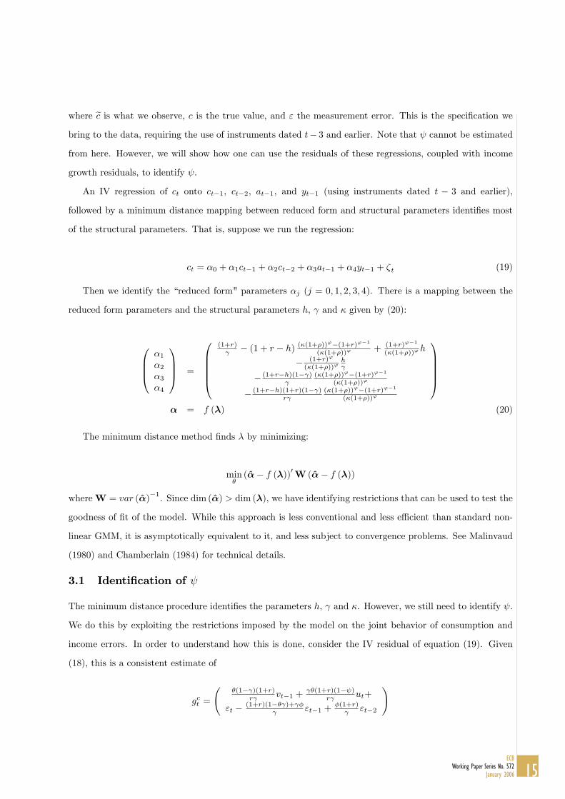
where ec is what we observe, c is the true value, and " the measurement error. This is the speci�cation webring to the data, requiring the use of instruments dated t� 3 and earlier. Note that cannot be estimated
from here. However, we will show how one can use the residuals of these regressions, coupled with income
growth residuals, to identify .
An IV regression of ct onto ct�1, ct�2, at�1, and yt�1 (using instruments dated t � 3 and earlier),
followed by a minimum distance mapping between reduced form and structural parameters identi�es most
of the structural parameters. That is, suppose we run the regression:
ct = �0 + �1ct�1 + �2ct�2 + �3at�1 + �4yt�1 + �t (19)
Then we identify the �reduced form" parameters �j (j = 0; 1; 2; 3; 4). There is a mapping between the
reduced form parameters and the structural parameters h, and � given by (20):
0BB@�1�2�3�4
1CCA =
0BBBB@(1+r) � (1 + r � h) (�(1+�))
'�(1+r)'�1(�(1+�))' + (1+r)'�1
(�(1+�))'h
� (1+r)'
(�(1+�))'h
� (1+r�h)(1� )
(�(1+�))'�(1+r)'�1(�(1+�))'
� (1+r�h)(1+r)(1� )r
(�(1+�))'�(1+r)'�1(�(1+�))'
1CCCCA� = f (�) (20)
The minimum distance method �nds � by minimizing:
min�(�̂� f (�))0W (�̂� f (�))
whereW = var (�̂)�1. Since dim (�̂) > dim (�), we have identifying restrictions that can be used to test the
goodness of �t of the model. While this approach is less conventional and less e¢ cient than standard non-
linear GMM, it is asymptotically equivalent to it, and less subject to convergence problems. See Malinvaud
(1980) and Chamberlain (1984) for technical details.
3.1 Identi�cation of
The minimum distance procedure identi�es the parameters h, and �. However, we still need to identify .
We do this by exploiting the restrictions imposed by the model on the joint behavior of consumption and
income errors. In order to understand how this is done, consider the IV residual of equation (19). Given
(18), this is a consistent estimate of
gct =
�(1� )(1+r)
r vt�1 + �(1+r)(1� )
r ut+
"t � (1+r)(1�� )+ � "t�1 +
�(1+r) "t�2
!
15ECB
Working Paper Series No. 572January 2006
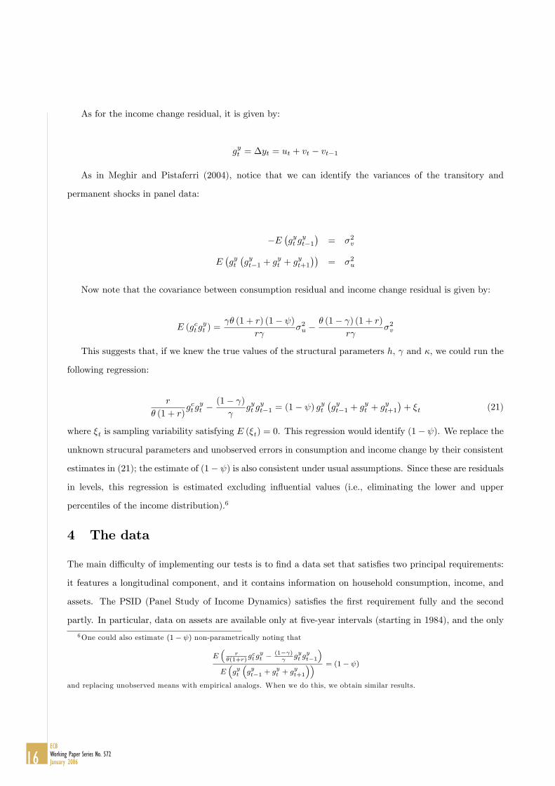
As for the income change residual, it is given by:
gyt = �yt = ut + vt � vt�1
As in Meghir and Pistaferri (2004), notice that we can identify the variances of the transitory and
permanent shocks in panel data:
�E�gyt g
yt�1�= �2v
E�gyt�gyt�1 + g
yt + g
yt+1
��= �2u
Now note that the covariance between consumption residual and income change residual is given by:
E (gctgyt ) =
� (1 + r) (1� )r
�2u �� (1� ) (1 + r)
r �2v
This suggests that, if we knew the true values of the structural parameters h, and �, we could run the
following regression:
r
� (1 + r)gctg
yt �
(1� )
gyt gyt�1 = (1� ) g
yt
�gyt�1 + g
yt + g
yt+1
�+ �t (21)
where �t is sampling variability satisfying E (�t) = 0. This regression would identify (1� ). We replace the
unknown strucural parameters and unobserved errors in consumption and income change by their consistent
estimates in (21); the estimate of (1� ) is also consistent under usual assumptions. Since these are residuals
in levels, this regression is estimated excluding in�uential values (i.e., eliminating the lower and upper
percentiles of the income distribution).6
4 The data
The main di¢ culty of implementing our tests is to �nd a data set that satis�es two principal requirements:
it features a longitudinal component, and it contains information on household consumption, income, and
assets. The PSID (Panel Study of Income Dynamics) satis�es the �rst requirement fully and the second
partly. In particular, data on assets are available only at �ve-year intervals (starting in 1984), and the only
6One could also estimate (1� ) non-parametrically noting that
E�
r�(1+r)
gct gyt �
(1� )
gyt gyt�1
�E�gyt
�gyt�1 + gyt + gyt+1
�� = (1� )
and replacing unobserved means with empirical analogs. When we do this, we obtain similar results.
16ECBWorking Paper Series No. 572January 2006

consumption data available is for food. It is not clear how well food consumption behavior generalizes to non-
durable consumption behavior. For this reason, we use imputed non-durable consumption data following the
method proposed in Blundell, Pistaferri and Preston (2004). The idea is to impute consumption to all PSID
households combining PSID data with consumption data from repeated CEX cross-sections.7 The approach
consists of writing the demand for food (a consumption item available in both surveys) as a function of
prices, total non-durable expenditure, and a host of demographic and socio-economic characteristics of the
household. Food expenditure and total expenditure are modeled as jointly endogenous. Under monotonicity
(normality) of food demands, these functions can be inverted to obtain a measure of non-durable consumption
in the PSID. Blundell, Pistaferri and Preston (2004) review the conditions that make this procedure reliable
and show that it is able to reproduce remarkably well the trends in the consumption distribution. We refer
the interested reader to that paper for more technical details.8
Since the PSID has been widely used for microeconometric research, we shall only sketch the description
of its structure in this section.9 The PSID started in 1968 collecting information on a sample of roughly 5,000
households. Of these, about 3,000 were representative of the US population as a whole (the core sample),
and about 2,000 were low-income families (the Census Bureau�s Survey of Economic Opportunities, or SEO
sample). Thereafter, both the original families and their split-o¤s (children of the original family forming a
family of their own) have been followed.
The PSID includes a variety of socio-economic characteristics of the household, including age, education,
labor supply, and income of household members. Questions referring to income and wages are retrospective;
thus, those asked in 1993, say, refer to the 1992 calendar year. In contrast, many researchers have argued
that the timing of the survey questions on food expenditure is much less clear (see Hall and Mishkin (1982)
and Altonji and Siow (1987), for two alternative views). Typically, the PSID asks how much is spent on food
in an average week. Since interviews are usually conducted around March, it has been argued that people
report their food expenditure for an average week around that period, rather than for the previous calendar
year as is the case for family income. We assume that food expenditure reported in survey year t refers to
the previous calendar year.
All monetary variables are de�ated using the CPI (1982-84). Education level is computed using the PSID
7Previous studies (Skinner (1987)) have imputed non-durable consumption data in the PSID using CEX regressions of nondurable consumption on consumption items (food, housing, utilities) and demographics available in both the PSID and theCEX.
8The de�nition of total non-durable consumption we use is similar to Attanasio and Weber (1995). It includes food (at homeand away from home), alcoholic beverages and tobacco, services, heating fuel, transports (including gasoline), personal care,clothing and footwear, and rents. It excludes expenditure on various durables, housing (furniture, appliances, etc.), health, andeducation. Unlike Attanasio and Weber, we also includes services from housing and vehicles (data kindly provided by DavidJohnson at BLS).
9See Hill (1992) for more details about the PSID.
17ECB
Working Paper Series No. 572January 2006
variable �grades of school �nished�. Individuals who changed their education level during the sample period
are allocated to the highest grade achieved. We construct a PSID panel data set using data on households
continuously present from 1980 to 1985.10 To avoid dealing with a number of complicated issues having to
do with family formation, family dissolution, human capital accumulation and retirement choices, we select a
sample of demographically stable households. Thus, ours is a sample of continuously married couples headed
by a male (with or without children). We eliminate households facing some dramatic family composition
change over the sample period. In particular, we keep only those with no change, and those experiencing
changes in members other than the head or the wife (children leaving parental home, say). We next eliminate
households headed by a female. We also eliminate households with missing report on education,11 and those
with topcoded income. We drop some income outliers.12 We then drop those born before 1920 or after 1959.
As noted above, the initial 1967 PSID contains two groups of households. The �rst is representative of the
US population (61 percent of the original sample); the second is a supplementary low income subsample
(also known as SEO subsample, representing 39 percent of the original 1967 sample). To account for the
changing demographic structure of the US population, starting in 1990 a representative national sample of
2,000 Latino households has been added to the PSID database. We exclude both Latino and SEO households
and their split-o¤s. Finally, we drop those aged less than 25 or more than 65. This is to avoid problems
related to changes in family composition and education, in the �rst case, and retirement, in the second. The
�nal sample used in the exercise below is composed of 1,125 households.
Our measure of income includes earnings of all household members and income from assets; it is net of
federal taxes (available in the survey); it excludes transfers. Our measure of assets is the sum of assets from
own farm or business, checking/savings accounts, other real estate assets, stocks and IRAs, home equity, and
other savings, net of household liabilities. We also experimented with a de�nition of assets that excludes
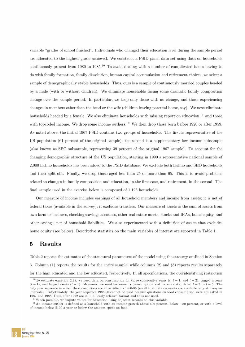
home equity (see below). Descriptive statistics on the main variables of interest are reported in Table 1.
5 Results
Table 2 reports the estimates of the structural parameters of the model using the strategy outlined in Section
3. Column (1) reports the results for the entire sample, while columns (2) and (3) reports results separately
for the high educated and the low educated, respectively. In all speci�cations, the overidentifying restriction10To estimate equation (19), we need data on consumption for three consecutive years (t, t � 1, and t � 2), lagged income
(t � 1), and lagged assets (t � 1). Moreover, we need instruments (consumption and income data) dated t � 3 to t � 5. Theonly year sequence in which these conditions are all satis�ed is 1980-85 (recall that data on assets are available only at �ve-yearintervals). Unfortunately, the year sequence 1985-90 cannot be used because questions on food consumption were not asked in1987 and 1988. Data after 1992 are still in �early release� format and thus not used.11When possible, we impute values for education using adjacent records on this variable.12An income outlier is de�ned as a household with an income growth above 500 percent, below �80 percent, or with a level
of income below $100 a year or below the amount spent on food.
18ECBWorking Paper Series No. 572January 2006

is not rejected by the data. All the reduced form regressions also include a variety of demographic controls
(age, family size, number of children, grades of schooling and race).
Starting from �, we �nd that its estimate is quite similar across groups and displays very low standard
errors. Recall that � is an indicator of the slope of the intertemporal consumption path. A �nding � < 1
supports the precautionary motive for saving. This is indeed what we �nd.
Next, we turn to h, the parameter that measures the extent of habit persistence/durability in preferences
for consumption. Given that h < 0, we �nd evidence that durability dominates habit persistence. The e¤ect
is stronger among the low educated. The standard errors are high, however, and so inference must be taken
with caution.
We now turn to . According to the interpretation given above, it should measure the probability
that individuals draw their expectation about future realizations of the income shocks from some �superior
information�distribution rather than from historical realizations. The estimate in the whole sample is close
to 1 (statistically, the hypothesis that = 1 cannot be rejected). We �nd somewhat higher estimates among
the high educated, and lower estimates among the low educated. A few things must be remarked. First, we
strongly rejects the hypothesis of no superior information ( = 0). Second, we �nd that is very high. This
could, however, also be interpreted as an indication that people�s superior information are not necessarily
centered around the actual realization of the shock. That is, people may tend to exaggerate (in one sense
or another) their expectation of the shock, behaving over-optimistically in the case of a positive shock and
over-pessimistically in the case of a negative shock. With a longer panel this e¤ect would probably be
averaged out.
The �nal parameter we estimate is . Recall that measures the di¤erence in (relative) prediction power
for the permanent and the transitory shock. Our results show that people have better predictive power about
the transitory shock than the permanent shock. The e¤ect is magni�ed when we estimate the parameters
separately by education.
In Table 3 we perform some sensitivity analysis to check the robustness of our results. One common
feature is the remarkable similarity among experiments. In column (1) we replicate our baseline estimates
of Table 2. In columns (2)-(4) we adopt di¤erent de�nitions of wealth, consumption, and income (excluding
home equity; excluding services from housing and vehicles; and including transfers, respectively). Interest-
ingly, excluding durable services from our de�nition of consumption gives a lower estimate of h, the extent of
�durability�in preferences for consumption. Including transfers in our de�nition of consumption reduces the
probability of predicting permanent shocks relative to transitory shocks. In columns (5) and (6) we check
the sensitivity of our results with respect to assumptions made about the parameters r; �, and '. In column
19ECB
Working Paper Series No. 572January 2006

(5) we assume r = � = 0:02. In column (6) we assume ' = 0:5, which corresponds to a coe¢ cient of relative
risk aversion of 2, a standard benchmark outside the log-utility case (' = 1). This last case predictably
increases the estimate of �, as consumers are now assumed to be more prudent, hence engaging more in
precautionary savings behavior.
6 Conclusions
In this paper we estimate a dynamic consumption function using microeconomic data drawn from the PSID.
We show that the dynamics hinge upon a number of structural parameters: the degree of intertemporal
separability in preferences (which may indicate habit persistence or durability), the slope of the intertemporal
consumption path (which captures the importance of the precautionary motive for savings), the impact of
advance information about future income prospects (which signals a discrepancy of information between
the individual and the econometrician), and the forecastability of permanent shocks relative to transitory
shocks.
Our �ndings point to the existence of durability rather than habit persistence. This agrees with �ndings
by Hayashi (1985) and Mankiw (1982), and in general with the lack of evidence for habit persistence found
in Dynan (2001) and others. This means that the conventional de�nition of non-durable consumption most
likely includes goods that provide services for longer than one year, thus obscuring (or o¤setting) any habit
persistence that may exist in the data. See Hayashi (1985).
As predicted by models with prudent consumers facing uncertain income, we �nd evidence for a positively
sloped consumption path, meaning that consumers delay spending in response to the risks they face. As for
the superior information issue, our results, taken at face value, would suggest that consumers have substantial
information regarding near future income changes, especially short-lived ones. These results are consistent
with two di¤erent explanations. The �rst is that most of the uncertainty is concentrated in the far distant
future, and so it still generates precautionary savings. Alternatively, it may represent a violation of the
assumption that consumers�expectations are centered around the actual realizations of the shocks. More
likely, consumers are exaggerating (in one sense or another) their expectations, and therefore what should
be interpreted as exaggeration is interpreted as excess information. This is an identi�cation problem that
cannot be solved in the context of our model. Nevertheless, the forecastability of transitory shocks relative
to permanent shocks does not su¤er from this identi�cation problem (as long as �exaggeration�in predicting
transitory shocks and permanent shocks is similar), and the results reveal that consumers are more able to
predict the arrival of temporary shocks that persistent ones.
Future work should be directed towards trying to solve these identi�cation problems, perhaps through
the use of subjective expectations data (Dominitz and Manski (1997)), or through alternative speci�cations
of the information set of the individuals.
20ECBWorking Paper Series No. 572January 2006
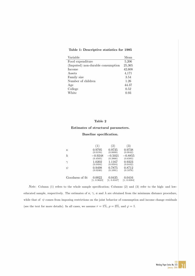
Table 1: Descriptive statistics for 1985
Variable MeanFood expenditure 5,206(Imputed) non-durable consumption 25,365Income 42,608Assets 4,171Family size 3.54Number of children 1.26Age 44.37College 0.52White 0.93
Table 2
Estimates of structural parameters.
Baseline speci�cation.
(1) (2) (3)� 0:9795
(0:0194)0:9735(0:0008)
0:9738(0:0042)
h �0:9248(0:4505)
�0:5021(0:3866)
�0:8855(0:6383)
1:0202(0:0494)
1:1167(0:0504)
0:9323(0:0442)
0:9498(0:0240)
0:7875(0:1091)
0:8712(0:1078)
Goodness of �t 0:0022[1; 0:9623]
0:0435[1; 0:8347]
0:0416[1; 0:8384]
Note : Column (1) refers to the whole sample speci�cation; Columns (2) and (3) refer to the high- and low-
educated sample, respectively. The estimates of �, , a and � are obtained from the minimum distance procedure,
while that of comes from imposing restrictions on the joint behavior of consumption and income change residuals
(see the text for more details). In all cases, we assume r = 1%, � = 3%, and ' = 1.
21ECB
Working Paper Series No. 572January 2006
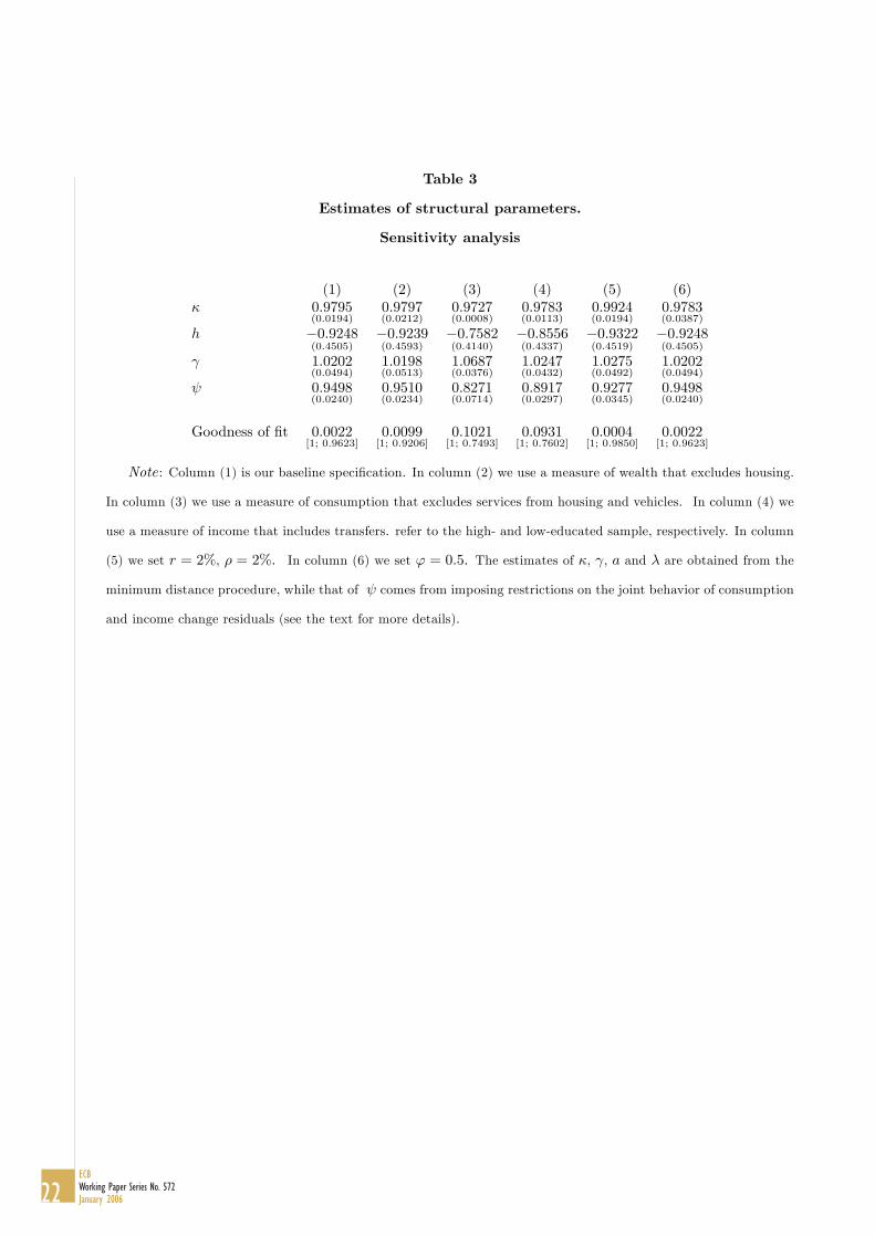
Table 3
Estimates of structural parameters.
Sensitivity analysis
(1) (2) (3) (4) (5) (6)� 0:9795
(0:0194)0:9797(0:0212)
0:9727(0:0008)
0:9783(0:0113)
0:9924(0:0194)
0:9783(0:0387)
h �0:9248(0:4505)
�0:9239(0:4593)
�0:7582(0:4140)
�0:8556(0:4337)
�0:9322(0:4519)
�0:9248(0:4505)
1:0202(0:0494)
1:0198(0:0513)
1:0687(0:0376)
1:0247(0:0432)
1:0275(0:0492)
1:0202(0:0494)
0:9498(0:0240)
0:9510(0:0234)
0:8271(0:0714)
0:8917(0:0297)
0:9277(0:0345)
0:9498(0:0240)
Goodness of �t 0:0022[1; 0:9623]
0:0099[1; 0:9206]
0:1021[1; 0:7493]
0:0931[1; 0:7602]
0:0004[1; 0:9850]
0:0022[1; 0:9623]
Note : Column (1) is our baseline speci�cation. In column (2) we use a measure of wealth that excludes housing.
In column (3) we use a measure of consumption that excludes services from housing and vehicles. In column (4) we
use a measure of income that includes transfers. refer to the high- and low-educated sample, respectively. In column
(5) we set r = 2%, � = 2%. In column (6) we set ' = 0:5. The estimates of �, , a and � are obtained from the
minimum distance procedure, while that of comes from imposing restrictions on the joint behavior of consumption
and income change residuals (see the text for more details).
22ECBWorking Paper Series No. 572January 2006

A Appendix: Second order approximation of the Euler equation
As explained in section 2 we consider a second order Taylor expansion of�c�t+i+1c�t+i
�� 1'
around�Et�c�t+i+1
�, Et
�c�t+i
��:
This gives:
�c�t+i+1c�t+i
�� 1'
=
E�c�t+i+1
�E�c�t+i
� !� 1'
� 1
'
E�c�t+i+1
�E�c�t+i
� !� 1'�c�t+i+1 � E
�c�t+i+1
��E�c�t+i+1
�+1
'
E�c�t+i+1
�E�c�t+i
� !� 1'�c�t+i � E
�c�t+i
��E�c�t+i
�+1 + '
2'21
E�c�t+i+1
�2 E�c�t+i+1
�E�c�t+i
� !� 1' �c�t+i+1 � E
�c�t+i+1
��2+1� '2'2
1
E�c�t+i
�2 E�c�t+i+1
�E�c�t+i
� !� 1' �c�t+i � E
�c�t+i
��2� 1
2'2E�c�t+i+1
�E�c�t+i
� E �c�t+i+1�E�c�t+i
� !� 1' �c�t+i+1 � E
�c�t+i+1
�� �c�t+i � E
�c�t+i
��Taking expectations give equation (5) in the text.
B Appendix: Proof of the constancy of �
We rewrite our expression for !t (omitting the time condition for simplicity):
!t =
�1 +
1 + '
2'2CV
�c�t+i+1
�2+1� '2'2
CV�c�t+i
�2 � 1
2'2%c�t+i+1;c�t+iCV
�c�t+i+1
�CV
�c�t+i
��Our problem is to show that the term ! is time independent. Note that in what follows we de�ne c�t+i+1
as x and c�t+i as y:
Let us start by assuming joint log-normality for both x and y (i.e., joint normality for x and y):
�xy
�~ logN
e�x+
12�
2x
e�y+12�
2y
! e2�x+2�
2x � e2�x+�2x cov (x; y)
e2�y+2�2y � e2�y+�
2y
!where �a = E (log a) and �2a = var (log a).
It follows that the squared coe¢ cient of variation of x can be expressed as:
CV (x)2=var (x)
E (x)2 =
e2�x+2�2x � e2�x+�2x
e2�x+�2x
= e�2x � 1
which is not a function of the mean �x. This is symmetrically also true for CV (y)2. Thus, assuming �2x and
�2y are constant over time is enough to prove time-invariance of CV (x)2 and CV (y)2.
23ECB
Working Paper Series No. 572January 2006

The next step is to show that the term %c�t+i+1;c�t+iCV�c�t+i+1
�CV
�c�t+i
�also does not vary over time.
Note that using our notation:
%xyCV (x)CV (y) =cov (x; y)
E (x)E (y)=
E (xy)
e(�x+�y)+12 (�2x+�2y)
� 1
Utilising the results above we can show that
E (xy) = E�eln xeln y
�= E
�eln x+ln y
�= eE(ln x+ln y)+
12var(ln x+ln y)
= e(�x+�y)+12 (�
2x+�
2y+2e%xy�x�y)
where e%xy = cov (lnx; ln y), and thus
%xyCV (x)CV (y) =e(�x+�y)+
12 (�
2x+�
2y+2e%xy�x�y)
e(�x+�y)+12 (�2x+�2y)
� 1
= e12 2e%xy�x�y � 1
again, not a function of the means. If the covariance between lnx and ln y is also constant over time, then
� is constant over time.
24ECBWorking Paper Series No. 572January 2006
References
[1] Altonji, Joseph and Siow, Aloysius.(1987), �Testing the Response of Consumption to Income Changes
with (Noisy) Panel Data�, Quarterly Journal of Economics. 102(2): 293-328.
[2] Attanasio, Orazio. (1999), � Consumption�, in Handbook of Macroeconomics, by J. Taylor and M.
Woodford (eds.), North-Holland: Amsterdam
[3] Attanasio, Orazio and Low, Hamish. (2004), � Estimating Euler Equations�, Rewiev of Economic
Dynamics, 7, 406-435.
[4] Attanasio, Orazio and Weber, Guglielmo. (1995), �Is Consumption Growth Consistent with Intertem-
poral Optimization? Evidence from the Consumer Expenditure Survey�, Journal of Political Economy,
103(6): 1121-57.
[5] Blundell, Richard, Pistaferri, Luigi and Preston, Ian. (2004), �Imputing Consumption in the PSID Using
Food Demand Estimates from the CEX�, The Institute for Fiscal Studies, WP04/27.
[6] Browning, Martin and Lusardi, Annamaria.(1996), �Household Saving: Micro Theories and Micro
Facts�, Journal of Economic Literature�, 34(4): 1797-1855.
[7] Campbell, John and Mankiw, Gregory. (1989), �Consumption, Income and Interest Rates: Reinterpret-
ing the Time series Evidence�, Blanchard,Olivier and Fischer, Stanley (eds), NBER Macroeconomic
Annual, Cambridge, Mass. and London: MIT Press, 185-216.
[8] Carroll, Christopher. (2001), � Death to the Log-Linearized Consumption euler Equation! (And Very
Poor Health to the Second-Order Approximation)�, Advances in Macroeconomics, 1(1):6.
[9] Chamberlain, Gary.(1984), �Panel Data�, Griliches, Zvi and Intriligator, Michael (Eds.), Handbook of
Econometrics, Volume II. North-Holland, Amsterdam; 1248-1318.
[10] Constantinides, George and Ferson,Wayne. (1991), �Habit Persistence and Durability in Aggregate
Consumption: Empirical Tests�, Journal of Financial Economics.29(2): 199-240.
[11] Deaton, Angus. (1992), � Understanding Consumption�, Oxford University Press.
[12] Dominitz, Je¤ and Manski, Charles. (1997), �Using Expectations Data to Study Subjective Income
Expectations�, Journal of the American Statistical Association. 92(439): 855-67.
25ECB
Working Paper Series No. 572January 2006
[13] Dynan, Karen. (2000); �Habit Formation in Consumer Preferences: Evidence from Panel Data�, Amer-
ican Economic Review. 90(3): 391-406.
[14] Flavin, Marjorie.(1993), �The Excess Smoothness of Consumption: Identi�cation and Interpretation�,
Review of Economic Studies. 60(3): 651-66.
[15] Fuhrer, Je¤rey. (2000), �Habit Formation in Consumption and Its Implications for Monetary-Policy
Models�, American Economic Review. 90(3): 367-90.
[16] Hall, Robert E. (1978), � Stochastic Implications of the Life Cycle-Permanent Income Hypothesis:
Theory and Evidence�Journal of Political Economy, 86(6): 971-987
[17] Hall, Robert and Mishkin, Frederic. (1982), �The Sensitivity of Consumption to Transitory Income:
Estimates from Panel Data on Households�, Econometrica. 50(2): 461-81
[18] Hill, M. (1992), �The Panel Study of Income Dynamics: A User�s Guide�, Newbury Park, California:
Sage Publications
[19] Hayashi, Fumio. (1985), �The Permanent Income Hypothesis and Consumption Durability: Analysis
Based on Japanese Panel Data�, Quarterly Journal of Economics; 100(4): 1083-1113.
[20] Krueger, Dirk and Perri, Fabrizio. (2003), �On the Welfare Consequences of the Increase in Inequality
in the United States�, Macroeconomic Annual 2003: 82-120 NBER, Cambridge, MA.
[21] Malinvaud, Edmond. (1980), Statistical Methods of Econometrics, 3rd rev. ed. Amsterdam: North-
Holland.
[22] Mankiw, Gregory. (1982), �Hall�s Consumption Hypothesis and Durable Goods�, Journal-of-Monetary-
Economics. 10(3): 417-25.
[23] Meghir, Costas and Pistaferri, Luigi. (2004); �Income Variance Dynamics and Heterogeneity�, Econo-
metrica. 72(1): 1-32.
[24] Pistaferri, Luigi. (2001), �Superior Information, Income Shocks, and the Permanent Income Hypothe-
sis�, Review of Economics and Statistics. 83(3): 465-76.
[25] Quah, Danny. (1990), �Permanent and Transitory Movements in Labor Income: An Explanation for
�Excess Smoothness�in Consumption�, Journal of Political Economy. 98(3): 449-75.
26ECBWorking Paper Series No. 572January 2006
[26] Shiller, Robert. (1972), �Rational Expectations and the Structure of Interest Rates�Ph.D Thesis, MIT,
Cambrodge, MA.
[27] Skinner, Jonathan. (1987), �A Superior Measure of Consumption From the Panel Study of Income
Dynamics�Economics Letters 23, 213-216.
[28] Willman, Alpo (2003), �Consumption, Habit Persistence, Imperfect Information and the Life-Time
Budget Constraint�European Central Bank. WP, August 2003, N. 251.
[29] Zeldes, Stephen. (1989), �Optimal Consumption with Stochastic Income: Deviations from Certainty
Equivalence�Quarterly-Journal-of-Economics. 104(2): 275-98.
27ECB
Working Paper Series No. 572January 2006
28ECBWorking Paper Series No. 572January 2006
European Central Bank Working Paper Series
For a complete list of Working Papers published by the ECB, please visit the ECB’s website(http://www.ecb.int)
531 “Market power, innovative activity and exchange rate pass-through in the euro area”by S. N. Brissimis and T. S. Kosma, October 2005.
532 “Intra- and extra-euro area import demand for manufactures” by R. Anderton, B. H. Baltagi,F. Skudelny and N. Sousa, October 2005.
533 “Discretionary policy, multiple equilibria, and monetary instruments” by A. Schabert, October 2005.
534 “Time-dependent or state-dependent price setting? Micro-evidence from German metal-workingindustries” by H. Stahl, October 2005.
535 “The pricing behaviour of firms in the euro area: new survey evidence” by S. Fabiani, M. Druant,I. Hernando, C. Kwapil, B. Landau, C. Loupias, F. Martins, T. Y. Mathä, R. Sabbatini, H. Stahl andA. C. J. Stokman, October 2005.
536 “Heterogeneity in consumer price stickiness: a microeconometric investigation” by D. Fougère,H. Le Bihan and P. Sevestre, October 2005.
537 “Global inflation” by M. Ciccarelli and B. Mojon, October 2005.
538 “The price setting behaviour of Spanish firms: evidence from survey data” by L. J. Álvarez andI. Hernando, October 2005.
539 “Inflation persistence and monetary policy design: an overview” by A. T. Levin and R. Moessner,November 2005.
540 “Optimal discretionary policy and uncertainty about inflation persistence” by R. Moessner,November 2005.
541 “Consumer price behaviour in Luxembourg: evidence from micro CPI data” by P. Lünnemannand T. Y. Mathä, November 2005.
542 “Liquidity and real equilibrium interest rates: a framework of analysis” by L. Stracca,November 2005.
543 “Lending booms in the new EU Member States: will euro adoption matter?”by M. Brzoza-Brzezina, November 2005.
544 “Forecasting the yield curve in a data-rich environment: a no-arbitrage factor-augmentedVAR approach” by E. Mönch, November 2005.
545 “Trade integration of Central and Eastern European countries: lessons from a gravity model”by M. Bussière, J. Fidrmuc and B. Schnatz, November 2005.
546 “The natural real interest rate and the output gap in the euro area: a joint estimation”by J. Garnier and B.-R. Wilhelmsen, November 2005.

29ECB
Working Paper Series No. 572January 2006
547 “Bank finance versus bond finance: what explains the differences between US and Europe?”by F. de Fiore and H. Uhlig, November 2005.
548 “The link between interest rates and exchange rates: do contractionary depreciations make adifference?” by M. Sánchez, November 2005.
549 “Eigenvalue filtering in VAR models with application to the Czech business cycle”by J. Beneš and D. Vávra, November 2005.
550 “Underwriter competition and gross spreads in the eurobond market” by M. G. Kollo,November 2005.
551 “Technological diversification” by M. Koren and S. Tenreyro, November 2005.
552 “European Union enlargement and equity markets in accession countries”by T. Dvorak and R. Podpiera, November 2005.
553 “Global bond portfolios and EMU” by P. R. Lane, November 2005.
554 “Equilibrium and inefficiency in fixed rate tenders” by C. Ewerhart, N. Cassola and N. Valla,November 2005.
555 “Near-rational exuberance” by J. Bullard, G. W. Evans and S. Honkapohja, November 2005.
556 “The role of real wage rigidity and labor market frictions for unemployment and inflationdynamics” by K. Christoffel and T. Linzert, November 2005.
557 “How should central banks communicate?” by M. Ehrmann and M. Fratzscher, November 2005.
558 “Ricardian fiscal regimes in the European Union” by A. Afonso, November 2005.
559 “When did unsystematic monetary policy have an effect on inflation?” by B. Mojon, December 2005.
560 “The determinants of ‘domestic’ original sin in emerging market economies”by A. Mehl and J. Reynaud, December 2005.
561 “Price setting in German manufacturing: new evidence from new survey data” by H. Stahl,December 2005
562 “The price setting behaviour of Portuguese firms: evidence from survey data” by F. Martins,December 2005
563 “Sticky prices in the euro area: a summary of new micro evidence” by L. J. Álvarez, E. Dhyne,M. M. Hoeberichts, C. Kwapil, H. Le Bihan, P. Lünnemann, F. Martins, R. Sabbatini, H. Stahl,P. Vermeulen and J. Vilmunen, December 2005
564 “Forecasting the central bank’s inflation objective is a good rule of thumb” by M. Diron andB. Mojon, December 2005
565 “The timing of central bank communication” by M. Ehrmann and M. Fratzscher, December 2005
566 “Real versus financial frictions to capital investment” by N. Bayraktar, P. Sakellaris andP. Vermeulen, December 2005

30ECBWorking Paper Series No. 572January 2006
567 “Is time ripe for a currency union in emerging East Asia? The role of monetary stabilisation”by M. Sánchez, December 2005
568 “Exploring the international linkages of the euro area: a global VAR analysis” by S. Dées,F. di Mauro, M. H. Pesaran and L. V. Smith, December 2005
569 “Towards European monetary integration: the evolution of currency risk premium as a measurefor monetary convergence prior to the implementation of currency unions” by F. González andS. Launonen, December 2005
570 “Household debt sustainability: what explains household non-performing loans? An empiricalanalysis” by L. Rinaldi and A. Sanchis-Arellano, January 2006
571 “Are emerging market currency crises predictable? A test” by T. A. Peltonen, January 2006
572 “Information, habits, and consumption behavior: evidence from micro data” by M. Kuismanenand L. Pistaferri, January 2006

ISSN 1561081-0
9 7 7 1 5 6 1 0 8 1 0 0 5