GEODESIC DOME ANALYSIS.

Item Type text; Thesis-Reproduction (electronic)

Authors Shirley, William Floyd.

Publisher The University of Arizona.

Rights Copyright © is held by the author. Digital access to this materialis made possible by the University Libraries, University of Arizona.Further transmission, reproduction or presentation (such aspublic display or performance) of protected items is prohibitedexcept with permission of the author.

Download date 03/06/2018 15:26:05

Link to Item http://hdl.handle.net/10150/275145

INFORMATION TO USERS

This reproduction was made from a copy of a document sent to us for microfilming. While the most advanced technology has been used to photograph and reproduce this document, the quality of the reproduction is heavily dependent upon the quality of the material submitted.

The following explanation of techniques is provided to help clarify markings or notations which may appear on this reproduction.

1.The sign or "target" for pages apparently lacking from the document photographed is "Missing Page(s)". If it was possible to obtain the missing page(s) or section, they are spliced into the film along with adjacent pages. This may have necessitated cutting through an image and duplicating adjacent pages to assure complete continuity.

2. When an image on the film is obliterated with a round black mark, it is an indication of either blurred copy because of movement during exposure, duplicate copy, or copyrighted materials that should not have been filmed. For blurred pages, a good image of the page can be found in the adjacent frame. If copyrighted materials were deleted, a target note will appear listing the pages in the adjacent frame.

3. When a map, drawing or chart, etc., is part of the material being photographed, a definite method of "sectioning" the material has been followed. It is customary to begin filming at the upper left hand corner of a large sheet and to continue from left to right in equal sections with small overlaps. If necessary, sectioning is continued again—beginning below the first row and continuing on until complete.

4. For illustrations that cannot be satisfactorily reproduced by xerographic means, photographic prints can be purchased at additional cost and inserted into your xerographic copy. These prints are available upon request from the Dissertations Customer Services Department.

5. Some pages in any document may have indistinct print. In all cases the best available copy has been filmed.

University MicnSilms

International 300 N. Zeeb Road Ann Arbor, Ml 48106

1324112

SHIRLEY, WILLIAM FLOYD

GEODESIC DOME ANALYSIS

THE UNIVERSITY OF ARIZONA M.S. 1984

University Microfilms

International 300 N. Zeeb Road, Ann Arbor, MI 48106

PLEASE NOTE:

In all cases this material has been filmed in the best possible way from the available copy. Problems encountered with this document have been identified here with a check mark V .

1. Glossy photographs or pages if

2. Colored illustrations, paper or print

3. Photographs with dark background

4. Illustrations are poor copy

5. Pages with black marks, not original copy

6. Print shows through as there is text on both sides of page

7. Indistinct, broken or small print on several pages )/

8. Print exceeds margin requirements

9. Tightly bound copy with print lost in spine

10. Computer printout pages with indistinct print

11. Page(s) lacking when material received, and not available from school or author.

12. Page(s) seem to be missing in numbering only as text follows.

13. Two pages numbered . Text follows.

14. Curling and wrinkled pages

15. Other

University Microfilms

International

GEODESIC DOME ANALYSIS

by

William Floyd Shirley

A Thesis Submitted to the Faculty of the

DEPARTMENT OF CIVIL ENGINEERING AND ENGINEERING MECHANICS

In Partial Fulfillment of the Requirements For the Degree of

MASTER OF SCIENCE WITH A MAJOR IN CIVIL ENGINEERING

In the Graduate College

THE UNIVERSITY OF ARIZONA

19 8 4

STATEMENT BY AUTHOR

This thesis has been submitted in partial fulfillment of requirements for an advanced degree at The University of Arizona and is deposited in the University Library to be made available to borrowers under rules of the Library.

Brief quotations from this thesis are allowable without special permission, provided that accurate acknowledgment of source is made. Requests for permission for extended quotation from or reproduction of this manuscript in whole or in part may be granted by the head of the major department or the Dean of the Graduate College when in his or her judgment the proposed use of the material is in the interests of scholarship. In all other instances, however, permission must be obtained from the author.

SIGNED:

APPROVAL BY THESIS DIRECTOR

This thesis has been approved on the date shown below:

REIDAR pdORHOVDE Professor of Civil Engineering

and Engineering Mechanics

Date

ACKNOWLEDGMENTS

The author wishes to thank the faculty and staff of the

Department of Civil Engineering for the help received during his

education at the University of Arizona. In particular, Dr. Erdal Atrek

and Dr. Mohammad Ehsani are thanked for the fine instruction received

in their classes and for serving on the author's M.S. Committee.

Special thanks go to Dr. Ralph M. Richard for his personal encour­

agement to enter graduate school; and the author would also like to

express his sincere gratitude to Dr. Reidar Bjorhovde for his advice,

encouragement, and guidance in completing this thesis.

Thanks are extended to the author's father, mother, and

brother for their patience. Special thanks also go to the author's

grandparents for their financial support — without them, none of

this would be possible.

The author acknowledges the assistance of Mun Foo Leong in

conducting the dome test. Rarely does a man such as "Eddie" come along

and give so much while asking so little in return. The efforts of

Charlotte McDole in typing the manuscript are also gratefully

acknowledged.

Lastly, the author thanks his two closest companions:

John Joseph Aube, and Carla Rae Wohlers. To balance the often cold and

sterile environment of academia, these two offered humor, excitement,

and love. Thank you both.

iii

TABLE OF CONTENTS

Page

LIST OF ILLUSTRATIONS v

LIST OF TABLES viii

ABSTRACT ix

1. INTRODUCTION 1

2. SCOPE 9

3. DEVELOPMENT OF GEODESIC DOMES 11

4. FULL SCALE TESTING OF DOMES 29

4.1 Dome Test by H.C. Nutting Company 31 4.2 Dome Test at University of Arizona 33

5. THEORETICAL ANALYSIS 52

6. COMPARISON OF THEORETICAL AND EXPERIMENTAL RESULTS .... 72

7. SUMMARY AND CONCLUSIONS 88

APPENDIX A 90

APPENDIX B 105

REFERENCES 115

iv

LIST OF ILLUSTRATIONS

Figure Page

1 Plan and Profile of a Typical Geodesic Dome 2

2 Joining Methods for Hub and Panel Domes 5

3 Common Joint Types for Hub Domes 6

4 Steel Strap Usage in Panel Domes .... 6

5 The Platonic Polyhedra 14

6 Frequency Division With Class I Method 15

7 Generation of a Three-Frequency Icosahedral Geosphere ... 18

8 Faces of a Three-Frequency Icosahedral Geodesic Sphere . . 19

9 Cross Section of an Icosahedron 20

10 A Regular Pentagon Formed From the Edges of an Icosahedron 21

11 Positions of the Intersphere and Innersphere of an Icosahedron 22

12 Projection of Face Divisions Onto Sphere 24

13 Projection of an Internal Edge Onto a Sphere 25

14 Three-Frequency Icosahedron Net 27

15 Plan and Profile of Pease Domes 30

16 Panels for 39' diameter Dome 32

17 Loaded Area and Gauge Locations for 39' Diameter Dome (Plan View) 34

18 Loaded Area and Gauge Locations for 39' Diameter Dome (Profile View) 35

19 Panels for 45' Dome 37

20 Cross S-ection of Framing Members for 45' Dome 40

v

vi

LIST OF ILLUSTRATIONS — Continued

Figure Page

21 Loaded Area for 45' Dome 40

22 Sandbags Used for Loading 41

23 Plastic Sheets Sealing Dome 41

24 Measurement Reference Tables 43

25 Data Recording Procedures 45

26 Set-up to Record Footing Movement 46

27 First Load Ramp in Place on Dome 46

28 Two-by-Two Nailing Cleats 48

29 Two-by-Four Perimeter Forms 48

30 Loading the Dome 49

31 Principal Axes of Wood 57

32 Dome Nodal Positions 59

33 Deflection Results Using Bar Elements and Bar With Trim Elements for Model 45' Dome 60

34 Deflection Results Using Beam Elements and Beam With Trim Elements to Model 45' Dome 61

35 Deflection Results Using Trim Elements to Model 45' Dome 62

36 Deflection Results Using Bar Elements and Bar With Trim Elements to Model 39' Dome 63

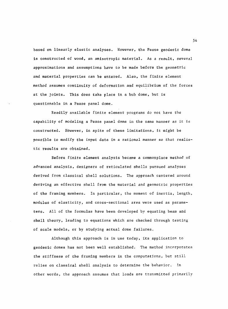
37 Deflection Results Using Beam Elements and Beam With Trim Elements to Model 39' Dome 64

38 Deflection Results Using Trim Elements to Model 45' Dome 65

39 Deflection Results of 45' Diameter Dome Modeled Using Trim Elements of Various Thickness (Asymmetric Loading, Side A) 68

vii

LIST OF ILLUSTRATIONS -- Continued

Figure Page

40 Deflection Results of 45' Diameter Dome Modeled Using Trim Elements of Various Thickness (Asymmetric Loading, Side 8) 69

41 Deflection Results of 45' Diameter Dome Modeled Using Trim Elements of Various Thickness (Symmetric Loading, Sides A and 8) 70

42 Deflection Results of 39' Diameter Dome Modeled Using Trim Elements of Various Thickness (Symmetric Loading) 71

43 Plumb Bob Deflections, Rebound, and Surveyed Deflections for the 45' Dome 73

44 Deflection Data for the 45' Dome Plotted With the Five Finite Element Models 76

45 Deflection Data for the 39' Dome Plotted With the Five Finite Element Models 79

46 Deflection Data for 39' Dome Plotted With the Three Modified Shell Models 85

LIST OF TABLES

Table Page

1 Tabulated Deflection Results for Thirty-Nine Foot Diameter Dome 36

T 2 Deflection Results for Forty-Five Foot Diameter

Dome 50

T 3 Deflection Results for Forty-Five Foot Diameter

Dome 51

viii

ABSTRACT

Results of physical testing and analytical studies are presented

for two geodesic domes. The domes are of the Pease panel dome variety

with different diameters. Deflection distributions are reported for

domes having symmetrically and asymmetrically applied uniform loads.

The development of geodesic domes is discussed with particular

attention paid to the calculation of chord factors. Information

regarding the development of domes from various polyhedra is also

included.

Analytical studies concentrate on the evaluation of conventional

finite element models. Beam, bar, and trim elements are used in various

combinations to model the structure. Application of various modified

shell analyses are also included.

It is concluded that Pease panel domes, if adequately preloaded,

can be modeled using pinned-end beam elements or trim elements. The

load distribution behavior of the domes, in regard to truss or membrane

action, is also discussed.

ix

CHAPTER 1

INTRODUCTION

Figure 1 shows the plan and profile views of a typical geo­

desic dome. Developed in the 1940s by R. Buckminster Fuller, the

geodesic dome is now part of a family of structures known as reticu­

lated shells [1,2]. These are structures that approximate simple

solid shells through frameworks of linear structural members [2]. In

particular, the geodesic dome is a multi-faceted polyhedron in which

all the vertices lie on the surface of a sphere [3]. When the ver­

tices are connected with struts, a series of complete, and incomplete,

intersecting great circles are formed [4].

Many domes have been built since Fuller first invented the

structure. Although the dome is best suited to enclosing large areas

where interior divisions or interior supporting members are undesir­

able, domes have a variety of applications including: industrial

structures, portable military shelters, commercial buildings, homes,

greenhouses and children's playground structures. The geodesic dome

has been the architectural and engineering solution for a variety of

structural problems.

In spite of the number of domes in use today, after more than

thirty years, the geodesic dome remains a novelty. The reasons for

this may lie in the methods of design and analysis of the structures.

Geodesic domes are mathematically derived systems and the mathematics

1

Ca) PLAN

(b) PROFILE

FIGURE 1. PLAN AND PROFILE OF A TYPICAL GEODESIC DOME

3

involved is both tedious and complicated. In addition, any structure

that is built should be evaluated by testing or a thorough engineering

analysis to insure that it meets the required building codes. Al­

though a variety of approaches have been used, methods for design and

analysis of geodesic domes are still not well established.

Although few full scale tests on domes have been completed,

some domes have been subjected to such adverse conditions that they

are often pointed to as examples of the dome's structural integrity.

In 1955, Fuller produced a series of domes for the United States Air

Force's D. E. W. (Distant Early Warning) line that extends across 3000

miles of frozen tundra in Alaska and Canada. These fifty-five foot

diameter, forty-foot high domes withstood static load testing for wind

velocities in excess of 220 miles per hour [1],

A test with tabulated deflection data was performed using a

North American AT-6 Army Trainer equipped with a 650 horsepower Pratt-

Whitney engine to produce wind speeds in excess of seventy miles per

hour. The test was accomplished by backing the aircraft up to the

dome at different angles, and no structural damage was reported [3].

In 1959, a number of load deflection tests were performed by the H. C.

Nutting Company on two different Pease plywood domes. The domes were

able to withstand a uniform load of 100-110 pounds per square foot on

their apex and surrounding triangles [5].

In the absence of a full scale test, adequate structural

analysis must be provided to support the dome's structural integrity.

Some of the approaches that have been used to analyze geodesic domes

include: the equations of equilibrium applied to the three

4

dimensional truss [6], finite element analysis applied to the frame

and its panels [7], a modified shell analysis using member properties

to calculate an effective shell thickness [2,9,18], and classical

shell analysis [8]. All of these methods have a strong basis in

theory, and some have been developed after studying actual dome

failures or the behavior of scale models. Each method attempts to

provide an analysis procedure for any or all of the following causes

of dome failure: the overstressing of individual members either

axially or flexurally, buckling of individual members, local or

"dimple" buckling of the overall shell, and overall shell instability.

Each of the above approaches was chosen after making assump­

tions based on the characteristics of the particular dome being looked

at. However, the general application of any one of these methods to

geodesic domes can be questionable, due to the uncertainties inherent

in the structure and its details, as well as the loading conditions.

To understand why the results of these methods may be unreli­

able in regard to some geodesic domes, a closer look at dome construc­

tion is required. Figures 2(a) and 2(b) represent the two joining

techniques commonly used in dome construction today. In Figure 2(a)

the five triangular panels that form the apex of a hub dome are shown.

Note that at each joint, all the framing members are securely pinned.

The hub shown is typical, but other forms have been used as shown in

Figure 3. The structurally important feature of the hub dome is that

the compressive and tensile axial forces in the joining members are

transmitted through the joint.

(a) HUB DOME APEX

(b) PANEL DOME APEX

FIGURE 2. JOINING METHODS FOR HUB AND PANEL DOMES

Cb) GUSSET PLATE (a) TRIODETICS

FIGURE 3. COMMON JOINT TYPES FOR HUB DOMES

STEEL STRAPS

FIGURE 4. STEEL STRAP USAGE IN PANEL DOMES

7

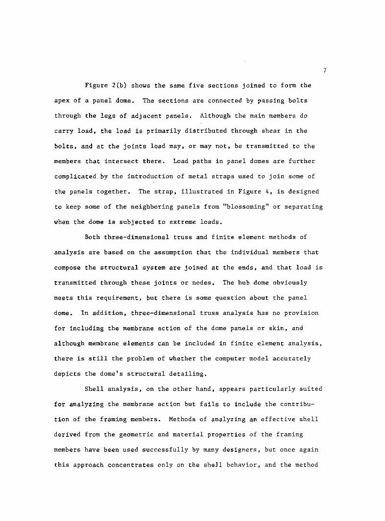
Figure 2(b) shows the same five sections joined to form the

apex of a panel dome. The sections are connected by passing bolts

through the legs of adjacent panels. Although the main members do

carry load, the load is primarily distributed through shear in the

bolts, and at the joints load may, or may not, be transmitted to the

members that intersect there. Load paths in panel domes are further

complicated by the introduction of metal straps used to join some of

the panels together. The strap, illustrated in Figure 4, is designed

to keep some of the neighboring panels from "blossoming" or separating

when the dome is subjected to extreme loads.

Both three-dimensional truss and finite element methods of

analysis are based on the assumption that the individual members that

compose the structural system are joined at the ends, and that load is

transmitted through these joints or nodes. The hub dome obviously

meets this requirement, but there is some question about the panel

dome. In addition, three-dimensional truss analysis has no provision

for including the membrane action of the dome panels or skin, and

although membrane elements can be included in finite element analysis,

there is still the problem of whether the computer model accurately

depicts the dome's structural detailing.

Shell analysis, on the other hand, appears particularly suited

for analyzing the membrane action but fails to include the contribu­

tion of the framing members. Methods of analyzing an effective shell

derived from the geometric and material properties of the framing

members have been used successfully by many designers, but once again

this approach concentrates only on the shell behavior, and the method

8

has only been applied to hub domes where the joints are either pinned

or fixed [2,10]. The domes analyzed by this procedure have also been

quite large, where the grid element and membrane element have been

essentially in the same plane; for example, the framing members are

curved or the grid modulus is small compared to the radius of curva­

ture [9].

Recognizing the extensive use of domes today, it is essential

that the reliability of the methods of analysis be determined. To

date, domes have been analyzed in what appears to be a random choice

of any of the methods described above. In view of the Pease panel

dome's differences in construction detailing, this is a practice that

should not be made lightly and certainly warrants further investiga­

tion. The need for cohesive and rational methods that agree with test

results is obvious.

CHAPTER 2

SCOPE

Although some full scale tests of geodesic domes have been

performed, it has not been possible to find any where the results have

been compared with those of analytical studies. A modified shell

analysis method was developed on the basis of a study of dome failures

[Wright, 1965] and the behavior of scale models [Lederer, 1963].

However, all of these structures exhibited properties that differ

substantially from the Pease panel dome [2,6].

This study will examine the available methods of analysis as

they apply to Pease panel domes. Utilizing the available data from

tests conducted by the H. C. Nutting Company [5] and the data from a

full scale test conducted by the author, the analysis procedure that

is best suited for these structures will be determined. The theoret­

ical evaluation will concentrate particularly on refining some of the

present techniques and assessing the possibility of combining the

different approaches.

To accomplish this task, the geodesic dome will be modeled for

computer analysis in a number of different ways. Each of the models

will emulate the geometric, material, and joining assumptions used in

the analyses described above. In addition, this procedure will also

allow some of the different analysis techniques to be combined into

one model. To check the validity of the results, each model will be

9

loaded in the same manner as the full scale tests, and computer-

predicted deformations will be checked against test deflections.

The comparison of the theoretical and the experimental data

will be used to evaluate the suitability of each model as a design

tool for Pease panel domes. It is anticipated that this will produce

a reliable method of structural evaluation of these domes.

CHAPTER 3

DEVELOPMENT OF GEODESIC DOMES

The first domes appear to have been built in the Near East,

India, and the Mediterranean region [11]. Generally they were used

only for the smallest of buildings.

Domes became technically significant during the Roman era with

the development of better building materials, and the recognition of

arch action [12]. The domes of this period were constructed as a

series of arches having the same center, which allowed for much larger

structures, but the overall size was still limited due to the thrust

developed at the base [11,12]. Rammed earth was the common method of

buttressing, used to resist the thrust, until the development of

concentric chains and iron girdles during the Renaissance [11,12].

These buttressing techniques reduced the base thrust and domes became

even larger, culminating in diameters of around 150 feet [11,12],

Fuller combined the arch principal and new materials into a

dome design that would distribute stresses entirely within the struc-

ure itself. The geodesic dome distributes load compressively through

chord members that lie longitudinally along the great circles. The

base thrust, or horizontal component of force, transmitted from these

compressive members is then resisted by meridian chord members that

lie along small circles of the sphere forming a series of tension

rings.

11

12

Fuller's design thus eliminated the need for large buttress type

footings. Geodesic domes can be supported by light walls or set

directly on the ground. The design employs circles which enclose the

most area with the least perimeter to define the space and triangles

which enclose the least area with the most perimeter to distribute the

forces, thus producing a design that is strong but lightweight [13].

To gain an appreciation for the geodesic dome, as it is commonly

thought of today, requires a closer look at the geometry that led to its

development. Geodesic mathematics includes the study of polyhedra,

spherical trigonometry, plane trigonometry, and plane geometry. In

researching this topic, several references were reviewed [1,3,4,14,-

15,16]. The two that proved to be the most helpful in understanding

geodesic mathematics were: Polyhedra, University of California Press,

1976, and Domebook 2, Pacific Domes, 1971 [3,14],

The term "geodesic," which comes from the Greek word for "earth

dividing," was originally used in connection with large land surveys

that included the earth's curvature in the calculations [12]. In

mathematics, the term is used to describe a line between two points on

any mathematically derived surface. If that surface is curved, then any

geodesic line on that surface is also curved. When the surface is a

sphere, the geodesic lines will be segments of great circles, with a

great circle being any circle with a center that coincides with the

sphere's, and thus divides the sphere into two equal parts.

Fuller's geodesic domes were developed from the realization

that a sphere can be generated from a network of intersecting geodesic

lines, forming triangles with their legs either following those lines,

or joining along them. By replacing the curved geodesic lines with

chords joining the intersections, the spheres can be fashioned from

planar triangular elements, producing a sphere-shaped polyhedron.

Since the polyhedron is produced using chords instead of curved geo­

desic lines, the terms "geodesic dome" and "geodesic polyhedra" are

actually misnomers; however, due to their common use by dome designers

and manufacturers, the terminology will also be used in this study.

Although a variety of polyhedra can be used to form domes, the

most common are the platonic polyhedra, illustrated in Figure 5. The

tetrahedron, hexahedron, octahedron, icosahedron, and dodecahedron are

the only five polyhedra that are composed of identical sides, angles,

and faces. The inherent symmetry of this class of polyhedra allows for

further subdivision of the faces into elements of equal size. It is

this quality that makes these polyhedra the most desirable for domes.

There are two principal methods of subdividing the faces of

the platonic polyhedra: Class I, also called the Alternate Method,

and Class II, also known as the Triacon Method. Both of these methods

begin with dividing the nontriangular faces of the polyhedra into

triangles by connecting the center of the face to each of its ver­

tices. Further subdivision of each triangle is unique to each method.

Since the Class I method appears to be the most common, it will be

presented here. The reader is referred to the references mentioned

above for treatises on the Class II approach.

Figure 6 illustrates how each of the triangular faces can be

subdivided, by dividing the legs into equal segments, then connecting

the divisions with lines running parallel to the legs, forming rows of

14

TETRAHEDRON

HEXAHEDRON

OCTAHEDRON

ICOSAHEDRON

DODECAHEDRON

FIGURE 5. THE PLATONIC POLYHEDRA

1 FREQUENCY

3 FREQUENCY

5 FREQUENCY

FIGURE 6. FREQUENCY DIVISION WITH CLASS I METHOD

smaller triangles. The number of equal divisions made along any leg

of the face triangle is defined as the frequency of the structure.

Thus, everything from one frequency tetrahedrons to infinite frequency

dodecahedrons is possible.

Geodesic domes are usually formed from icosahedrons and dodeca­

hedrons. Compared to the other forms of platonic polyhedra, these two

forms produce the least number of different sized faces and edges,

compared to the number of faces and edges generated when the frequency

is increased and the polyhedron is expanded to form a sphere. In

addition, the difference between the longest and the shortest elements

is smaller than for the other polyhedra. The domes that are fashioned

from these two types will therefore have a more uniform appearance

than those produced from the others.

The task of designing a geodesic dome with a number of fre­

quencies and polyhedra to choose from can be difficult. However,

mathematical relationships have been developed between the overall

dimensions of a polyhedron and the length of the edges. The chord

factor is a number, that when multiplied by the radius of the geodesic

dome, will give the lengths of the individual struts. When the fre­

quency of a polyhedron increases, so does the number of faces, edges,

and vertices, and if that polyhedron is being expanded to form a

sphere, then the number of different sized faces and edges will also

increase. An individual chord factor is defined for each different

edge length produced. Generally, the number of chord factors asso­

ciated with any particular dome will equal its trequency, although the

17

number is dependent on the polyhedron chosen, and the method used to

subdivide the polyhedron faces.

Within the Class I and Class II methods of subdivision, there

are several approaches that can be used to calculate the chord fac­

tors. The development presented here is called Class 1, Method 1. To

illustrate the approach, the chord factors for a geodesic dome gen­

erated by a three-frequency icosahedron will be determined. Chord

factors for other polyhedra and frequencies are contained in Appendix

A.

Figure 7(a) shows a typical triangular icosahedron face that

has been subdivided using the Class I approach. At this point, the

reassembled polyhedron is an icosahedron whose plane faces as shown in

Figure 7(b). The polyhedron will rest inside a circumscribing sphere

with each of its vertices touching the surface of the sphere. The

geodesic sphere can now be generated by projecting from the center of

the polyhedron, each edge and vertex of the subdivided faces, to the

surface of the circumscribing sphere, as in Figure 7(c). The final

product, a geodesic sphere generated from a three-frequency icosa­

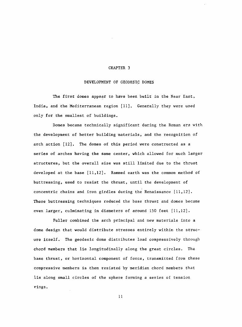
hedron, is shown in Figure 8(a).

As the subdivided face is projected onto the sphere, each of

the edges must elongate. Noting the symmetry, a careful examination

of Figure 7(c) reveals that three unique edges and two unique faces

have been produced. Figure 8(b) illustrates these for one of the

principal icosahedron faces. Chord factors for each of the edges can

be calculated by analyzing the icosahedral geometry.

SSDiVlDED FACP n *" IC°WS op

f^AsSEMBlED ICosahedROu

( c ) PR°JECTI0n

Ge^ration

ONTO SpHERE

OF a TmEE-mQl!ES,

CY ICOSAHEDRAL

ge°sphere

a) THREE-FREQUENCY ICOSAHEDRAL GEOSPHERE

b) THE DIFFERENT PANELS AND EDGES

FIGURE 8. FACES OF A THREE-FREQUENCY ICOSAHEDRON GEODESIC SPHERE

20

Figure 9 shows the cross section of an icosahedron that has

been split in two by passing a cutting plane through two opposing

edges. The circle surrounding the cross-section has the same radius

as the sphere circumscribing the geodesic icosahedron. This is the

radius that the chord factors are related to. Inspecting the geometry

of the figure reveals that ABCD is a golden rectangle, and that

lengths AB and DC are equal to the diagonals of a regular pentagram of

edge length AD. By relating sides AD and BC to sides AB and CD, the

Pythagorean theorem can be used to relate the circumscribing radius,

Rj, to the edges of the principal icosahederal faces.

diagonals equal to AB. Application of the law of cosines yields

CUTTING PLANE SECTION

FIGURE 9. CROSS SECTION OF AN ICOSAHEDRON

Figure 10 shows a regular pentagon of sides equal to AD and

(AB)2 = 2(AD)2(1 - cos 108°) (1)

21

FIGURE 10. A REGULAR PENTAGON FORMED FROM THE EDGES OF AN ICOSAHEDRON

substituting for cos 72° = - cos 108° gives

(AB)2 = 2(AD)2(1 + cos 1 2 ° ) . (2)

Applying the Pythagorean theorem to Figure 9,

(2RP2 = .AB2 + AD2 (3)

and substituting for AB gives:

_ _ AD J 3 + 2 cos 72° •I ~ 2 (4)

For a geodesic sphere of radius equal to unity, edges AD = 1.051462.

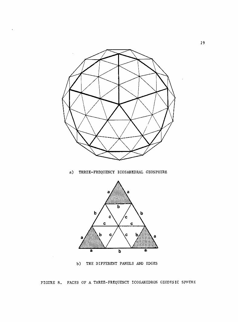
Further derivation of the individual chord factors requires

the definition of the intersphere and innersphere, denoted R^ and R^,

respectively. Shown in Figure 11, the intersphere is tangent to the

midpoint of each of the icosahedron edges, and the innersphere is

tangent to the center of the faces.

From Figure 11, the radius of the intersphere, R£, is

_ M -v 2(AD)2(1 + cos 72°) 2 2 2 (5)

The innersphere is tangent to the center of each face, and the

radius R^ therefore will be perpendicular and its arc tangent at a

point one-third from the triangle's base along the altitude AE. Since

22

B

FIGURE 11. POSITIONS OF THE INTERSPHERE AND INNERSPHERE OF AN ICOSAHEDRON

the faces of the icosahedron are equilateral triangles, AE can be

found in terms of its edge length, AD, as:

AE JTad

2

Applying the Pythagorean theorem to Figure 11,

(R3)2 - <V2 - (2AE)2

and substituting for AE and R^ yields,

( 6 )

(7)

D A D I 5 + 6 c o s 7 2 ' 3 " 2 (8)

23

For a three frequency icosahedron, the edges AD are divided

into three equal segments, which are then projected onto the circum­

scribing sphere, as shown in Figure 12. From the right triangle

with sides AD/6 and R^, a new radius, R^, can be computed as:

(R )2 = (R )2 + |AD\2 4 16/ (9)

substituting for R^ yields:

(R )2 = AD2 (1 + cos 72°) AD2 4 2 36

= AD2 (19 + 18 cos 72°) 36

,

Hence, R, = VAD2 (19 + 18 cos 72°) 4 6 . (10)

Further inspection of Figure 12 shows that the triangles OGH

and OG'H' are similar, so the chord length GH can be found as,

GH -

\ • < H >

From above, the computed length of edge AD is 1.051462, when Rj equals

unity. Substituting these values into the equation for chord GH, GH =

0.4035482. This is the chord factor for the subdivided edge of length

b. CF b = 0.4035482 . (12)

Referring again to Figure 12, the angle 0 can be found by

applying the law of cosines to triangle OAG'. Thus,

, (R.)2 + (R,)2 - (AD/3)2 cos 0 = 1 4

2(RL)(R4) • (13)

FIGURE 12. PROJECTION OF FACE DIVISIONS ONTO SPHERE

Reapplying the law of cosines to triangle OAG, the chord length AG is

found to be

(AG)2 = (Rx)2 + (Rx)2 - 2(R1)(R1) cos 0

OR AG

= 2(Rl) (1 - cos 0),

= Rj J2(1 - cos 0)' . (14)

Making the proper substitutions with R^ = 1.0 yields AG = 0.348615.

Since the chord AG is identical to the subdivided edge of length a,

CFa = 0.348615 (15)

The remaining chord factor can be calculated by applying the

same techniques as described above. Figure 13(b) illustrates the

internal edge of the subdivided icosahedron face being projected onto

25

\R1

' J R5 erV

^̂ 4

K

K'

(a)SUBDIVICED FACE (b) PROJECTION

FIGURE 13. PROJECTION OF AN INTERNAL EDGE ONTO A SPHERE

the circumscribing sphere. Since the subdivision of the icosahedron

face produced nine equilateral triangles of edge length AD/3, as shown

in Figure 13(a), the length of IK = 2(AD)/3. Inspection of Figures 12

and 7(b) show that the distance from the center to I or K will equal

R^. Application of Pythagoras' theorem to Figure 13(b) gives

(R5)2 = (R4)2 - (AD/3)2.

From the right triangle OJI,

a cos p = _5

R4

and the application of the law of cosines to OJ'I' yields:

(I'J')2 = (Rx)2 + (Rl)2 - 2(R1)(R1) cos 6

( 1 6 )

= 2(Rj) (1 - cos 8) (17)

Since the chord length I'J' is equal to the projected edge of length

C, substitution of = 1.0 into the above equations results in

CFc = 0.412411 ( 1 8 )

The development of chord factors facilitates the task of

determining the geometry of geodesic domes, but another topic that

also requires attention is the truncation of the dome. The full

geodesic sphere is seldom used for a geodesic dome. More often the

sphere is truncated along some convenient path providing a usable

enclosure without excessive height. Designations of truncation vary

among authors, although the method presented by Pugh in Polyhedra [14]

appears to be the most descriptive.

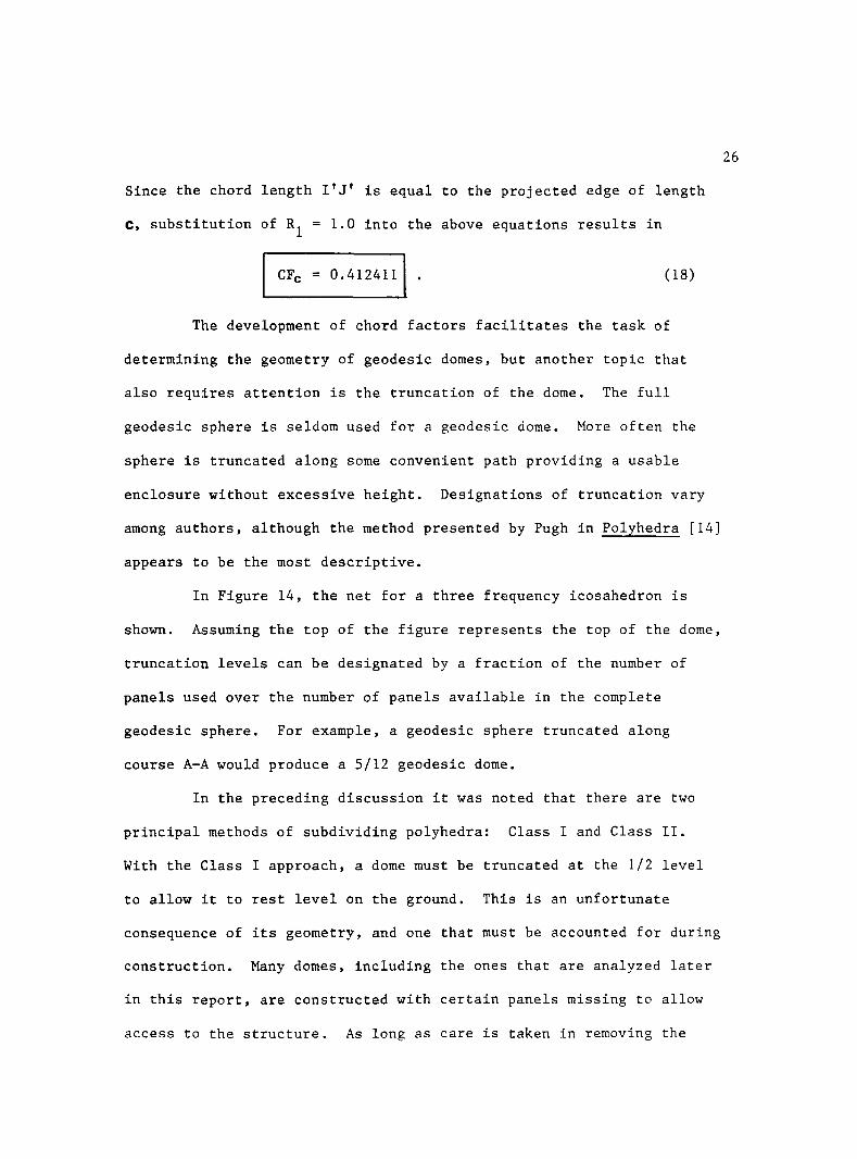
In Figure 14, the net for a three frequency icosahedron is

shown. Assuming the top of the figure represents the top of the dome,

truncation levels can be designated by a fraction of the number of

panels used over the number of panels available in the complete

geodesic sphere. For example, a geodesic sphere truncated along

course A-A would produce a 5/12 geodesic dome.

In the preceding discussion it was noted that there are two

principal methods of subdividing polyhedra: Class I and Class II.

With the Class I approach, a dome must be truncated at the 1/2 level

to allow it to rest level on the ground. This is an unfortunate

consequence of its geometry, and one that must be accounted for during

construction. Many domes, including the ones that are analyzed later

in this report, are constructed with certain panels missing to allow

access to the structure. As long as care is taken in removing the

27

75/180 — * y \ A A ^ 5/12

175/180 ^r/ \Z\/__— 3^36 180/180 V V V V V y1

FIGURE 14. THREE-FREQUENCY ICOSAHEDRON NET

appropriate panels, a dome developed using the Class I approach can be

constructed to rest evenly at any truncation level.

Domes developed using the Class II approach will sit evenly at

any level of truncation. This results from the spherical geometry

that is utilized in their generation. It should be noted that Ful­

ler's domes were developed using the Class II approach, and for very

large structures, it is preferred instead of Class I.

The introduction of multiple frequency polyhedrons and various

levels of truncation adds complexity to the structural design and

analysis of geodesic domes. If a large dome of relatively low

frequency is built, then the design of the framing members becomes the

principal concern. On the other hand, if a dome of equal size is

28

built using a very high frequency, the structure will more closely

resemble a shell, and the shell behavior becomes the dominant concern.

Various levels of truncation can also alter the stress dis­

tribution within the structure. The general geodesic dome design

philosophy suggests that the dome may be truncated anywhere without

losing any structural integrity. However, it is intuitively obvious

that a dome built of sufficiently high frequency may develop excessive

stresses near the base if it is truncated too deeply. The accurate

determination of these stresses would be dependent on the method of

analysis chosen.

If a reliable method of analysis is available, a geodesic dome

of any desired diameter and height can be designed by determining the

appropriate length of members that will generate a dome capable of

resisting the applied loads.

CHAPTER 4

FULL SCALE TESTING OF DOMES

The accuracy of a method of analysis can be evaluated through

full scale tests. By measuring the behavior of the structure under

load and comparing the results with those predicted by various meth­

od (s) of analysis, the reliability of each method can be determined.

Ideally the data collected to represent the structure's behavior would

include nodal deflections and member strains at as many points as

possible. However, due to the size of some structures, and the

materials used to construct them, the ideal is not always the prac­

ticable .

The two geodesic dome tests discussed in the following in­

volved structures with over one hundred framing members and forty-two

joints. With this many degrees of freedom, it was deemed impractical

to record data for all of the joints and members. Therefore nodal

deflections were collected only at significant points. Also, since

both structures were made of wood, the use of strain gauges was diffi­

cult if not impossible, preventing any measurement of the individual

member stresses.

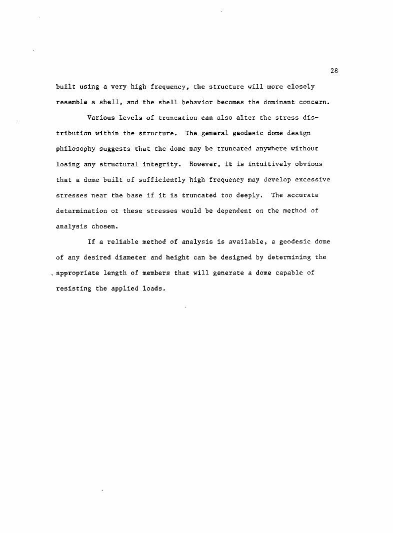
Both domes were Pease panel domes generated from a three-fre-

quency icosahedron truncated at the 5/12 level. A total of fifteen

panels were removed from five different locations around the base to

provide access to the dome. Figure 15 shows the plan and profile of

29

ca) PLAN

(to PROFILE

FIGURE 15. PLAN AND PROFILE OF PEASE DOMES

31

the resulting structure. The remaining dome characteristics were

unique to each structure and will be described separately.

4.1 Dome Test by H.C. Nutting Company

Detail data from tests conducted by the H. C. Nutting Company

are given in reference [5]. In addition to deflections, the report

includes a description of the dome, the testing procedure, and photo­

graphs .

Figure 16 shows the assembly drawings for the two basic trian­

gle panels used to construct the dome. The framing members were 2" by

2" S4S, kiln dried, construction grade, costal region Douglas Fir.

The frame sheathing was Douglas Fir Plywood Association (DFPA) exte­

rior grade overlaid fir plywood, as made by U.S. Plywood Corporation

under the trade name Duraply. The sheathing was 5/16" thick, includ­

ing a permanently bonded phenol resin, cellulose fiber sheet attached

to the face. The sheathing material was bonded to the framing members

using a urea-type (URAC 185) glue and HD10DC 1 1/4" staples.

The thirty-nine foot diameter, sixteen foot, three-inch high

structure was assembled in panel dome fashion by bolting the appro­

priate panels together in the correct sequence. The frame fasteners

used were 3/8" NC bolts with corresponding nuts and washers. No data

were provided regarding the number of bolts used to fasten the panels

together, or their positioning along the legs of the panels.

As the panels were being bolted together, the steel straps

binding the panels at the vertices were also installed. Shown in Fig­

ure 4, the straps are held to the framing members with threaded nails.

14.00

47.906" 95.813

(a) HEXAGON PANEL

12.00'

47.906" »j

95.813"

(b) PENTAGON PANEL

FIGURE 16. PANELS FOR 39' DIAMETER DOME

33

Once the dome had been assembled, the 2" by 4", S4S, Douglas

Fir base plates were secured to the foundation by 3/8" anchor hook

bolts.

After a visual inspection of the structure, during which the

structure's appearance prior to loading was noted, a total of twelve

gauges (0.001 inch accuracy) were placed at the apex and critical

vertices of the dome, to measure vertical and horizontal deflections.

Figure 17 indicates the gauge positions and numbers.

To prevent any slippage of the loading materials, two-by-fours

were nailed around the loaded area perimeter. The uniform load was

applied using standard concrete blocks of known weight that were

distributed over the loaded area as uniformly as possible. The loaded

area, shown in Figures 17 and 18, consisted of the apex of the dome,

bounded by straight lines that connected every other vertex of the

second level, producing a projected horizontal area of 350 square

feet. Uniform loads of thrity, sixty, and seventy-five pounds per

square foot were applied.

After sustaining the full load for approximately twenty-six

hours, the loading material was removed and recovery at the different

load intervals recorded. Tabulated deflections for this test are

given in Table 1.

4.2 Dome Test at University of Arizona

The dome tested by the author was a forty-five foot diameter,

eighteen foot, eight-inch high, Pease panel dome, manufactured by

Domes and Homes of Texas. Figure 19 shows the assembly drawings for

FIGURE 17. LOADED AREA AND FOR 39' DIAMETER DOME

GAUGE LOCATIONS (PLAN VIEW)

FIGURE 18. LOADED AREA AND GAUGE LOCATIONS FOR 39' DIAMETER DOME (PROFILE VIEWS)

TABLE 1.

Time

TABULATED

Load (psf)

DEFLECTION RESULTS

6H

FOR THIRTY-NINE

6V 15H

T FOOT DIAMETER DOME

15V 29H 27bv 27bv 27V 27H 14V 1AH

11/10/59

12:10 PM — -- — -- Dials Set to Zero and Loading Began -- -- -- -- —

1:50 30 -.042 + .010 -.067 -.000 -.047 + .040 -.047 + .008 -.031 + .029 -.048 -.055

4:00 60 -.153 + .012 -.200 -.004 -.122 + .089 -.095 + .020 -.058 + .100 -.101 -.088

11/11/59

8:00 AM 60 -.180 -.008 -.220 + .016 -.130 + .104 -.096 + .051 -.103 +.255* -.102 -.055

10:00 60 -.182 -.005 -.222 + .020 -.132 + .100 -.095 + .055 -.105 + .258 -.103 -.059

12:00 75 -.173 -.010 -.280 + .039 -.150 + .123 -.105 + .080 -.119 + .270 -.130 -.058

1:00 PM 75 -.175 -.011 -.283 + .039 -.150 + .122 -.108 + .080 -.120 + .261 -.131 -.058

2:00 75 -.178 -.012 -.288 + .042 -.150 + .122 -.108 + .086 -.120 + .249 -.133 -.154

3:00 75 -.180 -.015 -.291 + .045 -.153 + .121 -.109 + .094 -.120 + .240 -.131 -.149

4:00 75 -.182 -.016 -.293 + .047 -.154 + .121 -.108 + .099 -.119 + .234 -.133 -.146

11/12/59

12:20 PM 75 -.196 -.029 -.310 + .057 -.165 + .122 -.100 + .149 -.104 + .130 -.149 -.097

2:00 75 -.197 -.028 -.313 + .054 -.170 + .122 -.104 + .143 -.110 + .181 -.152 -.121

R E C 0 V E R Y

3:00 60 -.167 -.018 -.261 + .046 -.158 + .116 -.091 + .136 -.103 + .194 -.135 -.131

4:30 30 -.154 -.012 -.203 + .030 -.135 + .093 -.070 + .124 -.085 + .217 -.113 -.153

6:00 -- -.111 -.006 -.119 + .007 -.092 + .056 -.032 + .101 -.054 + .215 -.064 -.166

11/13/59

4:45 PM - - -.096 -.012 -.078 -.035 -.079 + .036 -.011 + .054 -.010 + .289 -.043 -.200

Percentage Recovery 51.3 58.6 75.1 53.5 70.7 89.9 63.8 91.7 71.7

* Dial gauge support possibly disturbed. V -- Denotes Vertical displacement. H -- Denotes Horizontal displacement. Minus (-) sign prefix denotes dovmward movement for vertical dials and movement toward center of dome for horizontal dials. Plus (+) sign prefix denotes upward movement for vertical dials and outward movement for horizontal dials. T -- Reprinted from the report made to the Pease Woodwork Company by the H. C. Nutting Company [5].

19.00 22.25

15.00 18.25

15.00 *

4~ 18.25" j

15.00"__Jf_

15.00 j r i

20.00

(SUBOIVIOEO DIMENSIONS AS BELOW)

(a) HEXAGON PANEL

8.75"

31.50" ig 75„

. -t-

14.50

19.75"

8.75"

11 13.00" 41.50" 13.00'-! 41.50

34.25- 40.50" ~ 34.25" -

(b) PENTAGON PANEL

FIGURE 19. PANELS FOR 49' DIAMETER DOME

38

the two basic panels used in the construction. The framing members,

shown in cross-section in Figure 20, were bevelled 2" by 6", kiln

dried, construction grade, Southern Yellow Pine. The interior sup­

porting members were 2" by 6" lumber of the same grade and species and

were joined to the main framing members with coated sixteen-penny

nails.

The framing sheathing material was the American Plywood Asso­

ciation's 5/16" five-ply, C-D grade, interior-exterior, Exposure 1,

plywood. The sheathing material was bonded to the framing members

using a urea-type (URAC 185) glue and 1 1/2" staples spaced every six

inches or less.

Assembly of the dome was achieved by bolting together the

sides of adjacent panels with 3/8" ASTM A307 bolts and corresponding

nuts and washers. A total of four bolts were used to join each side

of one panel to the adjacent one. The locations of the fasteners for

each of the basic panels are shown in Figure 19.

To expedite construction, five or six triangular panels were

assembled to form each vertex, and then these sections were bolted

together to form the completed dome. At each vertex, galvanized steel

straps, as shown in Figure 4, were nailed to the framing members.

Assembly of the dome was completed by anchoring the 2" by 6"

bevelled base plates to bevelled shim plates, placed on the founda­

tion, with 3/8" anchor hook bolts. A photograph of a typical footing

is shown in Figure 26.

The final step in construction was to tighten each of the

bolts firmly. After each bolt was tightened, the surrounding wood was

lightly marked with spray paint to insure that none were missed.

Preparations for testing began with the making of sand bags.

Since the loading was to take place in the early summer before the

annual rains, it was felt that heavy-duty paper bags would suffice.

The use of sand bags also made the actual load placement a little

easier due to convenient handling and bag size.

It was decided that a load of thirty pounds per square foot on

a projected horizontal area of 700 square feet would cause enough

measurable deflection to check the results against the different

methods of analysis. In addition, it was the same load that had been

used in the Nutting test [5], and also was a load that could be placed

within the required constraints on manpower and time.

Each sand bag was filled with thirty pounds of sand, and

placed so that it rested on a surface area of approximately one square

foot. The weight of each bag was controlled by first filling the bag

with shovelfuls of sand, and then moving it to a scale where the exact

weight was adjusted manually. For the projected load area, shown in

Figure 21, the total load of the sand bags was determined as:

in# 1 ? Side A : 399 Bags ' — " =• = 34.4#/ft

bag 348.2 ft.

Side B : 403 Bags * — * =• = 34.7/!/ft2. bag 348.2 ft.

Before the sand bags were put in place, preparations for

recording the data were made. To seal the interior of the dome from

the wind, heavy-duty plastic sheets were stapled over each of the

40

4.75"

FIGURE 20. CROSS SECTION OF FRAMING MEMBERS FOR 45' DOME

FIGURE 21. LOADED AREA FOR 45' DOME

41

FIGURE 22. SANDBAGS USED FOR LOADING

FIGURE 23. PLASTIC SHEETS SEALING DOME

42

openings. Shown in Figure 23, the plastic sheets were weighted at the

bottom with sand bags and two-by-fours. Across one of the openings,

two overlapping sheets were used, providing access to the dome in­

terior.

From the sixteen nodes indicated on Figure 21, ten-ounce plumb

bobs were suspended using twenty-two gauge, nonbraided steel wire.

Approximately ten -inches beneath each plumb bob, a one-square-foot

table was constructed and leveled. Shown in Figure 24, these tables

provided the reference datum for the vertical and horizontal

deflections.

A reference grid was drawn on the table surface by first

locating the point directly beneath the plumb bob tip. This was

accomplished by first swinging the bob in a gentle arc and tracking

its motion in the reflection of a mirror with a line scribed across

its surface. When the mirror was positioned so that the path of the

tip followed the line, the two end points of the line were marked.

The process was then repeated with an arc normal to the first arc.

The intersection of the two arcs gave the point directly beneath the

plumb bob tip. Since the dome was constructed with a convenient

north-south axis, a northern y-axis and eastern x-axis were estab­

lished using the previously defined point as the origin. All data

regarding horizontal movement of the structure were obtained using

this procedure.

Vertical deflections were obtained by placing the same scribed

mirror against a carpenter's square and reading the distance between

43

FIGURE 24. MEASUREMENT REFERENCE TABLES

44

the plumb bob tip and the table surface. The photographs in Figure 25

illustrate the procedures used in the two methods of data collection.

In addition to the plumb bobs, an independent method of measur­

ing nodal deflections was provided by using differential leveling from

an outside reference point, and a surveying rod calibrated to 0.005

feet (0.06 inches). After each stage of loading, the plumb bob data,

as well as the surveying data, were recorded.

To check for movement at the footings, a two-foot length of

ten gauge music wire was attached to the panel base plates. In this

way, motion would be detected due to either movement of the footing or

slippage of the base plates on the footing. To gauge any movement, a

one-square-foot table was constructed normal to the music wire. The

set-up, shown in Figure 26, was completed by drawing a horizontal and

vertical grid with the origin coinciding with the projection of the

music wire tip. During testing, no measurable motion of the footings

or base plates was detected.

Prior to loading, two ramps were built to transport the sand

bags to the loaded area. The first ramp weighed 210 pounds and was

positioned over node ten, making an angle with the x-axis of 18° and

an angle with the horizontal of 36°. The second ramp weighed 180

pounds, was position over node 15, and made angles of 18° with the

x-axis and 42° with the horizontal. The ramps and their relative

positions are shown in Figures 21 and 27.

To confine the sand bags within the loaded area, a perimeter

of two-by-fours was constructed around the apex. The two-by-fours

were set on edge and nailed to two-by-two cleats which were nailed to

45

FIGURE 25. DATA RECORDING PROCEDURES

46

FIGURE 26. SET-UP TO RECORD FOOTING MOVEMENT

FIGURE 27. FIRST LOAD RAMP IN PLACE ON DOME

47

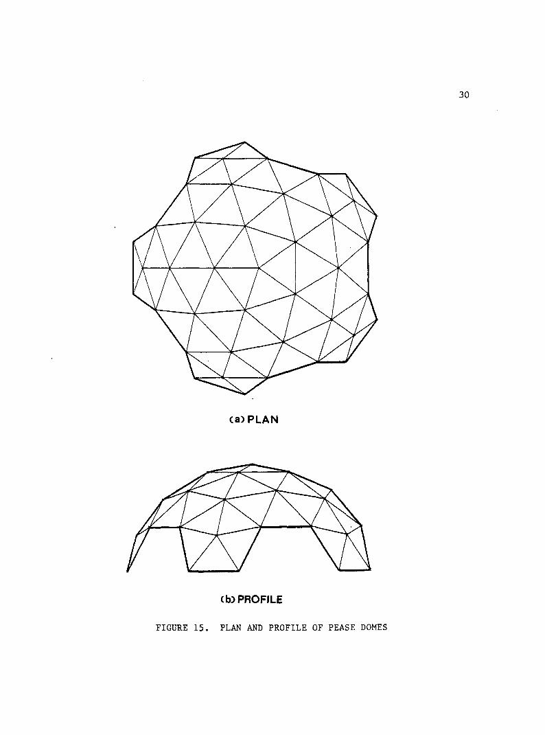
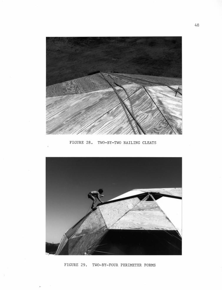
the dome. All the cleats and two-by-fours were nailed only to the

triangular section upon which they rested and were not secured or

allowed to protrude onto any adjacent section. In this fashion, each

section was allowed to behave independently of the adjacent one, and

the structure could respond normally. The perimeter forms are shown

in Figures 28 and 29.

To prevent any disturbance to the plumb bobs during the pre­

loading construction and during loading, each plumb bob was set into a

cardboard support, placed on the individual table grids, producing at

least six inches of slack in the suspending wires. After each stage

of loading was completed, the supports were removed and the plumb bobs

allowed to come to rest before the measurements were recorded.

Deflections were recorded five times during the test: (1) no

load (initial readings), (2) load on side A, (3) load on sides A and B

(full load), (4) load on side B, and (5) no load (recovery). A period

of approximately twenty-four hours passed between each set of read­

ings, allowing the dome to fully settle under each load.

The sand bags were lifted to the loading area by placing five

bags in a cart and then hauling the cart up with a rope passed over a

pulley at the apex, using a truck at the opposite end. Using this

set-up, shown in Figure 30, three men were able to place approximately

seventy-five bags per hour. Working with a two-man crew for all but

two days, the entire test was completed in seventeen days.

During the last stages of loading, some of the plumb bobs were

dislodged at the nodes. Deflection results are presented in Tables

2-3, and where data was lost it has been so noted.

48

FIGURE 28. TWO-BY-TWO NAILING CLEATS

FIGURE 29. TWO-BY-FOUR PERIMETER FORMS

49

FIGURE 30. LOADING THE DOME

TABLE 2. DEFLECTION1 RESULTS FOR FORTY-FIVE FOOT DIAMETER DOME

NODE LOAD ON SIDE A FULL LOAD (SIDES A&B)

NODE PLUMB BOBS SURVEYING PLUMB BOBS SURVEYING

l -0.7813 -1.02 -1.4688 -1.62 2 -0.7188 -0.96 -0.8750 -1.62 3 +0.0625 +0.06 -1.1562 -0.96 4 +0.0312 +0.0G -0.9688 -1.08 5 -1.3437 -1.32 -1.6875 -1.74 6 -0.0625 -0.44 -1.3750 -1.68 7 +0.0312 -0.30 -0.6875 -0.80 8 -1.3437 -1.2C -0.9375 -1.02 9 -0.9375 -0.82 -0.2812 -0.30 10 -0.2500 +0.56 -0.7813 +0.40 11 -0.0625 -0.72 -0.4375 -0.42 12 -0.0313 -0.54 -0.5937 -0.90 13 -0.2187 -0.72 -0.6250 -0.72 14 -0.4687 -0.44 -1.2812 -1.08 15 -0.0625 -0.12 -0.1875 -0.78 16 -0.4687 -0.66 -0.8125 -1.20

T Deflections taken from initial datum. Rebound deflections measured from new datum set after dome was under full load.

* From plumb bob data unless otherwise noted. ** From survey data. + Upward movement. - Downward movement.

Lost plumb bob. Plumb bob disturbed and rehung at full load. Deflection data lost, but rebound still calculable.

TABLE 3. DEFLECTION7 RESULTS FOR FORTY-FIVE FOOT DIAMETER DOME

LOAD ON SIDE B UNLOADED NODE

UNLOADED NODE

PLUMB BOBS SURVEYING PLUMB BOBS SURVEYING REBOUND

l -1.42 -1.02 +0.600** l -1.42 -1.02 +0.600**

2 -1.2813 -1.62 -1.7032 -1.68 +0.2031

3 -0.98 -1.08 +0.5937

4 -1.9063 -1.20 -0.90 +0.1800**

5 -1.1250 -1.20 -0.9375 -0.54 +0.7500

6 -0.98 -0.78 +1.1250

7 -0.7188 -0.72 -0.5838 -0.60 +0.0937

8 -1.0937 -0.90 -0.8125 -0.72 +0.1250

9 -0.5000 -0.54 . -0.4062 -0.60 -0.1250 10 -0.9688 -0.54 -0.7500 -0.90 +0.0313

11 -0.5000 -0.40 -0.3750 -0.42 +0.0625

12 -0.5937 -0.72 -0.4687 -0.66 +0.1250

13 -0.5000 -0.68 -0.4375 -0.60 +0.1875

14 -1.0625 -0.90 -0.9219 -0.78 +0.3593

15 -0.1875 -0.66 -0.0938 -0.42 +0.0937

16 -0.90 -0.72 +0.7500

T Deflections taken from initial datum. Rebound deflections measured from new datum set after dome was under full load.

* From plumb bob data unless otherwise noted. ** From survey data. + Upward movement. - Downward movement.

Lost plumb bob. Plumb bob disturbed and rehung at full load. Deflection data lost, but rebound still calculable.

CHAPTER 5

THEORETICAL ANALYSIS

The four most commonly used methods of analyzing geodesic

domes are:

(1) equilibrium equations applied to analysis of the

three-dimensional truss

(2) classical shell analysis

(3) finite element analysis of the three-dimensional truss/

frame and its panels

(4) shell analysis, using an effective thickness derived from

the geometric and material properties of the framing members,

Depending on the characteristics of the particular dome chosen, some

of the methods are more suitable than others.

Analyzing a geodesic dome as a three-dimensional truss assumes

that the structure distributes load axially through pinned end mem­

bers. The stiffness contribution of the panels is therefore ignored.

For hub domes of intermediate frequency, with light flexible panels

that offer no structural contribution, it is intuitively obvious that

this model is adequate. The details of the model fit the structure,

and the analysis can be performed with a small computer program.

If the contribution of the framing members is ignored, then

classical shell analysis can be used to analyze the geodesic dome. If

the dome were built with a very high frequency and had panels that

52

53

were joined continuously across the dome's surface, then this method

of analysis might be chosen. However, it has already been established

(Chapter 3) that geodesic dome behavior can differ substantially from

shell behavior.

Finite element analysis (FEM) is perhaps the most commonly

used method of advanced structural analysis today. The basic concept

of FEM involves discretizing large systems into individual components

or subsystems ("superelements"), mathematically modeling them, and

then reassembling the structure within the bounds of physical equil­

ibrium and continuity [17]. In this fashion, very large systems can

be analyzed without overlooking or having to make excessive approxima­

tions of the contributions of any of the individual components.

Since the geodesic dome is composed of individual elements, it

is easily modeled using finite elements. The sheathing material can

be represented with constant strain triangles (trim elements) or plate

bending elements, and the framing members modeled using either bar or

beam elements. In addition, the elements can-be mixed in any combina­

tion, depending on the characteristics of the particular dome. By

modeling with pinned end bar elements, a three-dimensional truss

analysis is performed, and a classical shell analysis can be approxi­

mated by using trim elements or plate bending elements. If the dome

has rigid joints, then beam elements can be used to model the framing,

and end moments will be included in the combinations.

Although the advantages of a finite element analysis are

numerous, the method has some limitations in its application to geo­

desic domes. The computer programs that are readily available are

54

based on linearly elastic analyses. However, the Pease geodesic dome

is constructed of wood, an anisotropic material. As a result, several

approximations and assumptions have to be made before the geometric

and material properties can be entered. Also, the finite element

method assumes continuity of deformation and equilibrium of the forces

at the joints. This does take place in a hub dome, but is

questionable in a Pease panel dome.

Readily available finite element programs do not have the

capability of modeling a Pease panel dome in the same manner as it is

constructed. However, in spite of these limitations, it might be

possible to modify the input data in a rational manner so that realis­

tic results are obtained.

Before finite element analysis became a commonplace method of

advanced analysis, designers of reticulated shells pursued analyses

derived from classical shell solutions. The approach centered around

deriving an effective shell from the material and geometric properties

of the framing members. In particular, the moment of inertia, length,

modulus of elasticity, and cross-sectional area were used as parame­

ters. All of the formulas have been developed by equating beam and

shell theory, leading to equations which are checked through testing

of scale models, or by studying actual dome failures.

Although this approach is in use today, its application to

geodesic domes has not been well established. The method incorporates

the stiffness of the framing members in the computations, but still

relies on classical shell analysis to determine the behavior. In

other words, the approach assumes that loads are transmitted primarily

by membrane action. In the case of hub domes with nonstructural

panels, the load is carried by the framing members, and this method of

analysis would be in error. Some of the research work [2] has includ­

ed bending to compensate for asymmetric loading. The application of

these approaches to Pease panel domes may have some merit since the

transmission of loads in these domes is unclear.

Before applying this method of analysis to geodesic domes, it

is necessary to discuss its development. The method has been derived

to estimate the ultimate loads on reticulated shells. However, the

subject of dome frequency appears to have been ignored in these

studies. It has been pointed out in the previous chapter that a

geodesic dome will come closer to resembling a shell as its frequency

increases. Thus, applying the developed formulas to any one specific

dome is speculative without first checking the formulas through full-

scale tests.

In this study, Pease panel domes have been analyzed with

finite element models that incorporate all of the readily available

elements, as well as elements that have properties derived from modi­

fied shell analysis. Specifically, the conventional element models

include: (1) bar elements, (2) bar elements with trims, (3) beam

elements, (4) beam elements with trims, and (5) trim elements.

The modified shell analysis was performed with constant strain

triangles having thicknesses derived from the equations provided by

Wright [2], McCutcheon and Dickie [9], and Kloppel and Schardt [18].

The decision to use trim elements over plate bending elements was

arrived at after reviewing the test data in tables 2-3. The wood

56

structures did not appear stiff enough to warrant the use of plate

bending elements.

Modeling a wood structure as a linearly elastic, isotropic

material required some assumptions and approximations of the input

material properties. The computations for each model were performed

using the SAPIV Structural Analysis Program, developed at the Univer­

sity of California, Berkeley [19], and the data were tailored to meet

the input requirements. The material parameters required by the

program include a modulus of elasticity for the bar elements, a modu­

lus of elasticity and a Poisson's ratio for the beam elements, and

three elastic moduli, three Poisson's ratios and a shear modulus for

the trim elements.

Wood is an orthotropic material which has independent mechan­

ical properties for each of its three mutually orthogonal axes [20].

Figure 31 shows the three principal axes in relation to the grain

direction and the growth rings of the wood [20]. To describe the

elastic properties of wood completely, twelve constants are required:

three moduli of elasticity, three shear moduli, and six Poisson's

ratios [20],

The three moduli of elasticity are designated E , E^, and E^,

where the subscripts indicate the axis of loading. For the bar and

beam elements, it was assumed that the primary load effects were

directed along the longitudinal axis, and the corresponding modulus of

elasticity was entered.

The moduli of elasticity for plywood are dependent on the

direction of the plies [21]. Direct calculation of the three moduli

57

RADIAL (R)

TANGENTIAL (T)

LONGITUDINAL CL)

FIGURE 31. PRINCIPAL AXES OF WOOD

for plywood was impossible with the data provided, and an alternative

approach was therefore used. To be conservative, it was assumed that

only one half of the plies would carry the stresses in any one direc­

tion, and whatever contribution the remaining plies provided was

ignored. Thus, all three required moduli of elasticity for the con­

stant strain triangle were made equal to the longitudinal modulus of

elasticity, and the panel thickness was cut in half.

The three shear moduli are designated G , G , and G , where LK LI KX

the subscripts indicate the plane of strain. From Figure 31, the

plane of interest for the constant strain triangles is the LT plane,

and this value of the shear modulus was entered.

The six Poisson's ratios are designated ^LR' ̂ LT'

M^, and where the first subscript indicates the axis of the

applied stress and the second indicates the axis of deformation. For

the beam elements, the loads are assumed to be longitudinal, and the

Poisson's ratio therefore was computed as the average of and Mo­

using the assumption that only one half of the plywood's plies provide

the stiffness in any particular direction, the values of Poisson's

ratio for the constant strain triangle were also entered as the

average of and

The deflection results for the five different finite element

modeling schemes of the Pease panel dome are presented in Figures 33

through 38. Figures 33 and 36 illustrate the two domes that were

modeled using pinned end bar elements (three-dimensional truss case),

and bar elements with constant strain triangles. Figures 34 and 37

give the results for the beam and the beam with constant strain tri­

angle models for the forty-five foot and thirty-nine foot diameter

domes respectively. The results of the constant strain triangle

models (Shell Analysis) are presented in Figures 35 and 38.

Input data for the models representing the modified shell

analysis were the same as for the constant strain triangles, above,

with the exception that the thickness of the panels was determined by

the formulas given in the following. These are taken from several

studies [2,9,18].

In Wright's development [2], the equations of bending for a

curved member are related to the bending of a shell, culminating in

(a) PLAN

(b} PROFILE

FIGURE 32. DOME NODAL POSITIONS

1 x10-1

9

8

7

6

5

BAR 0---0 BAR. and TRIM 0----0

.. --·---- ~--- - -----. _l

1----------1--------- --------- -

- ----+--------------- - -

I I

\ \ \ - J ___ -

I - -- -- - --------, --

• I I I

-- --- -~ - ~ .. J--l\ I \ I I \ I \ I

I \ I \ I

i \l \~

\ \ \ \

~ q )!) \ I \ I \ I \ I (6 \ I

\ I

t!J

7 8 9 10 11 2 3 4 1 6 5 16 15 14 13 12

NODAL POINTS

FIGURE 33. DEFLECTION RESULTS USING BAR ELEMENTS AND BAR WITH TRIM ELEMENTS TO MODEL 45' DOME

60

61

BEAM © © BEAM and TRIM © -©

1x10

UJ

LL

r2 1x10

NODAL POINTS

FIGURE 34. DEFLECTION RESULTS USING BEAM ELEMENTS AND BEAM WITH TRIM ELEMENTS TO MODEL 45' DOME

62

TRIM 0—0

1x10

UJ

UJ

1x10 9 10 11 2 3 4 1 6 5 16 15 14 13 12 7

NODAL POINTS FIGURE 35. DEFLECTION RESULTS USING TRIM ELEMENTS TO MODEL 45' DOME

2 1---- ----· - - · · ·· ·

---·------

8 -- --~ --··-- ·- -------- - - --

6 1------· ---- - - - · · · ·-- · · .

4 1---------- ------- • ··

BAR 0--0 BARandTRIM 0----0

'L - \-

\

0 " 1-------------- - · ---- - ---- - ·- ---- - -

2

-3 1x10

_..,

1 6 15

NODAL POINTS

14

FIGURE 36. DEFLECTION RESULTS VSING BAR ELEMEKTS AND BAR WITH TRIM ELEMENTS TO MODEL 39' DOXE

27

63

z 0 -.... (.)

1 8

6

4

2

BEAM' 0--0 BEAMandTRIM 0----0

-------- -- - - -- ····- -----·- · ··--·· . ·· - . ---- --·-- - - .

------ ---·--- ... -------- · ------------ . . . - -- - . ·-· -

----- ----- ·---· --- - - ·· · · ·- -- - --- -

1.x10-1 0------q 8

- - --------------\-- - - · ------ -- - -- - -- \ " --

~----------

6 -------------·-·· _ __ _ \ --- -- - ------ - -- - \

\ ·-- ----------,-4

w ; 2 _J ~---------- -- ---u.; w c

1 x102 ....,._ ___________________ ___.:~-----

8 6 1---------·-- ... --- ---- - ------- -

4 - ------

1------- -- -- - -

2 .,__ ____ _

-3 1x10

1 6 15

NODAL POINTS

14

FIGURE 3 7. DEFLECTION RESULTS USING B L-'0-f AND BEAM WI7H TRIM ELEHINTS TO MODEL 39 ' DOME

\ \

\

b

27

64

TRIM 0----0 1

.. - . ~ - - - - - ·- . · ------ ---- ---·------·----~--- ----- - -

8 +----- ---· ·----------- ------ -J------ ------ ---- ·---- . ------------ -----· - - .

6

4

2 1--------~.-------------- - - · ···- - - .

- - - - - - ~ i I -- - - ---- - - - -- - ~

I !

1x10-1 r------------~----~--------------~---------~ .-. (/'J w z (.)

8

6 -_,

I I z

.:. z 4 -- -- ----- - ----- - -·· -·- . - - - -- ! 0 1----------------------- -- - i ~ ; u I

~ ' 2 ~---------------------------~-----i LL w 0

1 X 10-2

8

6

4

2

r---------------------------------------~~-----

1x103~-r--------~--------~--------~--------~~~ 1 6 15

NODAL POl NTS

14 27

FIGURE 38. DEFLECTION RESULTS USING TRIH ELEMENTS TO HODEL 39' DO~!E

65

the effective thickness equation:

t' = 2/T./T7T d9)

where I is the moment of inertia, and A is the cross-sectional area of

the framing members. Substituting for the representative parameters

from the two test domes, t1 = 4.75 inches for the forty-five foot

diameter dome, and t' = 1.63 inches for the thirty-nine foot diameter

dome.

McCutcheon and Dickie [9] have derived an effective shell

thickness formula after examining model studies of 225 foot diameter

domes designed in western Canada. They concluded that domes are much

stiffer under symmetric loading than that predicted by Wright. Work­

ing from a basic shell buckling equation, the effective shell thick­

ness is given as:

t' = 2.4 3JI/L' (20)

where I is the moment of inertia, and L is the length of the framing

members. For the forty-five foot diameter dome, this yields t' = 1.52

inches, and for the thirty-nine foot diameter dome, t' =0.56 inches.

This represents reductions of t' of 68% (forty-five foot dome) and 66f-

(thirty-nine foot dome) when compared with the results using equation

(19).

Prior to the work of Wright and McCutcheon and Dickey, Kloppei

and Schardt [18] developed an effective thickness equation on the

basis of their studies of framed domes. Their equations is:

, _ ifT . A 3 L ( 2 1 )

where A is the cross-sectional area and L is the length of the rrar.ir.e

67

members. This gives values of t1 = 0.16 inches and t' = 0.07 inches

for the forty-five and thirty-nine foot diameter domes, respectively.

In other words, equation (21) predicts a significantly higher stiff­

ness than that obtained by equations (19) and (20).

The thickness of the constant strain triangles used in the

conventional finite element models was 0.250 inches for the forty-five

foot diameter dome and 0.156 inches for the thirty-nine foot diameter

dome. This is in semi-rational agreement only with the results of

equation (21).

Figures 39 through 42 illustrate the deflection results that

were obtained using the three effective shell thicknesses. Figures 39

and 40 show the results for an asymetric loading of the forty-five

foot diameter dome (see Figure 21), and Figures 41 and 42 depict

symmetric loading on both the forty-five foot and the thirty-nine foot

diameter domes.

The finite element meshes, numbering schemes, and nodal coor­

dinate data for the two domes are shown in detail in Appendix B of

this report. A complete discussion of the results and how they corre­

late with the experimental data will be provided in the next chapter.

I

68

* Node 4 had upward movement t= 0.157 inches © —0 and has not been plotted. t= 1.523 inches © ©

t= 4.750 inches ©

1x10

iu

u_ LU 0-

1x10

.-4 1x10

NODAL POINTS

FIGURE 39. DEFLECTION RESULTS OF 45' DIAMETER DOME MODELED US TNG TRIM ELEMENTS OF VARIOUS THICKNESS (ASYMMETRIC LOADING, SIDE A)'

69

* Node 5 had upward movement tss 0.157 inches 0- Q and has not been plotted. ts 1.523 inches 0 0

t= 4.750 inches 0

1x10

UJ

2 1x10

UJ -j u. UJ

1x10

,-4 1x10

1x10

NODAL POINTS

FIGURE 40. DEFLECTION RESULTS OF 45' DIAMETER DOME MODELED USING TRIM ELEMENTS OF VARIOUS THICKNESS (ASYMMETRIC LOADING, SIDE E)

70

t= 0.157 inches O O t= 1.523 inches ©< t= 4.750 inches ©-

O-AYO-CY-O-Q

1x10

UJ

u_ LU

1x10

1x10 9 10 11 2 3 4 1 6 5 16 15 14 13 12 7

NODAL POINTS

FIGURE 41. DEFLECTION RESULTS OF 45' DIAMETER DOME MODELED L'SINT

TRIM ELEMENTS OF VARIOUS THICKNESS (SYMMETRIC LOADING, SIDES A AND

ts0.066 inches O O t = 0.559 inches O* O t= 1.625 inches Q.

O-

1x10

—

x 1*10

2 ' W z o h o UJ -j UL UJ D

1x10

1x10 14 27 15 1 6

NODAL POINTS

FIGURE 42. DEFLECTION RESULTS OF 39' DIAMETER DOME MODELED I 'STN

TRIM ELEMENTS OF VARIOUS THICKNESS (SYMMETRIC LOADING)

CHAPTER 6

COMPARISON OF THEORETICAL AND EXPERIMENTAL RESULTS

Figure 43 shows the results from the forty-five foot diameter

dome test. Presented in the graph are the deflections under full

load, as indicated by the plumb bobs and the surveying. The rebound

or "recovery" deflections have also been included.

There is a reasonable correlation between the survey measure­

ments and the plumb bob data. At node 5 the two curves come closest

to matching, with the two values differing by only 3.0%. At node 15,

however, the data differ by 76.0%. Overall, the mean difference

between the two curves is 20.7%. This is derived from the absolute

difference of each of the points, since at some of the nodes the

surveying data curve lies above that of the plumb bob data, while at

other nodes it lies below.

The variation in the two curves comes from error inherent in

the two methods of data collection. As was noted in Chapter Four,

once the structure was under load, some of the joints underwent enough

movement to dislodge the evebolts holding the plumb bobs. Although it

is theoretically possible that some of the plumb bobs could have

slipped a little without coming completely free, it is felt that this

did not take place for two reasons. First, the plumb bobs only

weighed ten ounces. This is not enough for the plumb bobs to pull

free under their own weight. Second, the evebolts used had capered

73

* Survey data used for rebound curve. MAX. DEFLECTION © O ** Not plotted, Node 9 had upward REBOUND 0~~~0

aenection, and negative rebound. SURVEYING 10

1x10

UL

1x10

1x10

NODAL POINTS

FIGURE 43. PLUMB BOB DEFLECTION'S, REBOUND, AND SURVEYED DEFLECTIONS FOR THE ,5 ' DOME

74

screw ends. If the joints underwent movement that allowed for slip­

page, the joint would be widening while the eyebolt diameter would be

decreasing. Thus, during the settling of the structure under load,

the plumb bobs would either have dropped out completely or not at all.

A more reasonable source of the variation comes from the

surveying. In particular, the rod placement is probably responsible.

The mean variation of 20.7% applied to the maximum deflection of 1.7

inches is only 0.35 inches. This could easily come from a slight

misplacement of the rod at the joint, particularly since some of the

members at a joint may be moving independently of the other members

intersecting at the joint. This is undoubtedly taking place or other­

wise the space created allowing the plumb bobs to dislodge could not

have been formed.

Conclusions drawn from the comparison of theoretical and

experimental data will be based on plumb bob readings wherever pos­

sible. At the points where data from the plumb bobs were lost, sur­

veying data has been substituted and is so indicated on the plots.

Also, as mentioned in the previous chapter, only vertical deflections

will be evaluated as an indicator of the dome behavior. They are

significantly greater than the horizontal deflections, and as such,

will be affected less by any experimental error.

The rebound curve shown in Figure 43 contains the most useful

information. Due to constraints on manpower and time, it was impos­

sible to preload the structure before testing. For this reason, the

maximum deflection readings presented in Figure 43 cannot be taken as

the actual deflections the structure would undergo if leaded again.

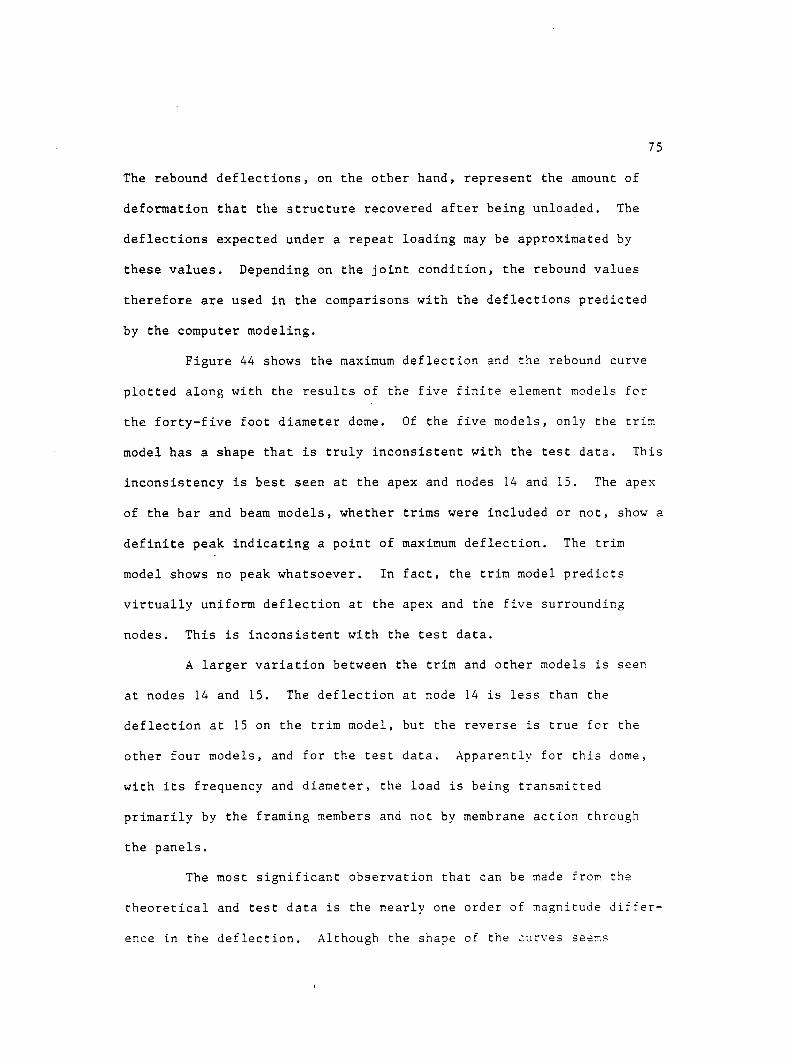
75

The rebound deflections, on the other hand, represent the amount of

deformation that the structure recovered after being unloaded. The

deflections expected under a repeat loading may be approximated by

these values. Depending on the joint condition, the rebound values

therefore are used in the comparisons with the deflections predicted

by the computer modeling.

Figure 44 shows the maximum deflection and the rebound curve

plotted along with the results of the five finite element models for

the forty-five foot diameter dome. Of the five models, only the trim

model has a shape that is truly inconsistent with the test data. This

inconsistency is best seen at the apex and nodes 14 and 15. The apex

of the bar and beam models, whether trims were included or not, show a

definite peak indicating a point of maximum deflection. The trim

model shows no peak whatsoever. In fact, the trim model predicts

virtually uniform deflection at the apex and the five surrounding

nodes. This is inconsistent with the test data.

A larger variation between the trim and other models is seen

at nodes 14 and 15. The deflection at node 14 is less than the

deflection at 15 on the trim model, but the reverse is true for the

other four models, and for the test data. Apparently for this dome,

with its frequency and diameter, the load is being transmitted

primarily by the framing members and not by membrane action through

the panels.

The most significant observation that can be made from the

theoretical and test data is the nearly one order of magnitude differ­

ence in the deflection. Although the shape of the curves seer.s

76

MAX. DEFLECTION G— —0 REBOUND 0— —0 TRIMS O—• —O BARS WITH TRIMS CD-- - -• BEAMS WITH TRIMS £r- — - -A BARS CD • BEAMS A— A

8

4

1x10 W 8 LU

o UJ -J u_ UJ Q

-1 1x10

8

6

4

-2 1x10

-q, 1m.

/Ax /-̂ sx /' S.S • '̂ 2̂ \ /

V I

I I -1 I • 1 I I 7 8 9**10 11 2 3 4* 1 * 6 5 16 15 14 13 12

NODAL POINTS

FIGURE 44. DEFLECTION DATA FOR THE 45' DOME PLOTTED WITH THE FIVE FINITE ELEMENT MODELS

reasonable, there is a large discrepancy in the values. The rebound

curve is closer to the predicted values with a mean difference of

69.4% from the bar and beam models around the loading ramps, but

having a mean separation of 82.3% around the apex.

Of particular interest is the nodal points where the loading

ramps were placed. . These two points, nodes 10 and 15, show the least

rebound deflection of all the nodes monitored, and they come closest

to falling within the range of the theoretical results. During load­

ing, these nodes were subjected to repeated applications of 160 pounds

(the weight of 5 sand bags and the loading cart) as well as any load

contributed by the man unloading the cart (approximately 150 pounds).

A superficial examination of the test data would suggest that

the dome is a much softer structure than the computer analysis indi­

cates. With the deflections being far in excess of those predicted by

the theoretical analysis, this appears to make sense. However, obser­

vations of the rebound curve suggest that this is not so. The rebound

curve lies closer to the theoretical curve than the maximum deflection

curve but, in particular, the two nodes that received the most load in

the structure have rebound deflections small enough that they lie

closest to the theoretical data. In other words, it appears that due

to this dome's structural details there exists enough free space in

the panel corners to allow either individual pieces of the structure

or complete sections to undergo rigid body translations of an inch or

more before the pieces or sections redistribute their load.

Further confirmation for these rigid body translations can be

found by examining the apex portion of either the maximum deflection

curve or the rebound curve. Theoretically, the apex should undergo

the most deflection, and the five adjacent nodes deflecting a uniform

but slightly smaller amount. The curves indicate movement approximat­

ing this, but in a far more haphazzard pattern.

If the members or the panel section corners that intersect at

a node are allowed to undergo independent rigid body translations,

then it can no longer be expected that there will be a continuity of

deflection for all members at a joint, or for all the joints that

occur at the same level. Thus, the occurrence of gaps that allowed

some of the plumb bobs to fall, and the discrepancies between the

surveying and plumb bob data. It is important to note that once the

structure is placed under enough load to eliminate the rigid body

translations, it appears to match the behavior of the appropriate

computer model.

In Figure 45 the maximum deflection and rebound curves are

plotted, along with the results of the five finite element models for

the thirty-nine foot diameter dome. For this dome, all five finite

element models are in close correlation with the test results. Once

again, the apex and nodes 14 and 15 reveal the most useful observa­

tions .

Theoretically, the apex node should undergo the most deflec­

tion. However, in this case, neither the maximum deflection curve nor

the rebound curve indicate this. There are two possible reasons for

this. One, that there was an error in the data collection, or two,

that the method of loading allowed for neighboring nodes to undergo

translation first. The latter appears to be the most reasonable, and

i I 8 :

s ;

4 .

2 .

•1

8 :

6 !

4 .

2 .

•2

8 :

6 !

4 .

2 .

•3

79

MAX. DEFLECTION 0 O REBOUND O O TRIMS O— BARS WITH TRIMS EL • BEAMS WITH TRIMS <£> & BARS • • BEAMS A A

"~t 1 H-15 14 27

NODAL POINTS

FIGURE 45. DEFLECTION DATA FOR THF 39' DOME

PLOTTED WITH THE FIVE FINITE ELEMENT MODELS

80

it is confirmed by the observations made of the forty-five foot

diameter dome.

If loading proceeds from the lower nodes up to the apex (as in

the forty-five foot dome), it is realistic to conclude that any rigid

body translations taking place in the structure will follow the same

pattern. Therefore, the apex node will be the last node to stiffen,

and thus have less translation, resulting in a smaller deflection.

The data provided for the thirty-nine foot diameter dome did not

include enough data points or a more detailed description of the

loading procedure to permit a detailed examination of this relation­

ship. The data in Figure 45 show that the results of the framing

member models and the membrane action model exhibit the same shape as

the test data. In the forty-five foot dome, nodes 14 and 15 showed a

sharp contrast with the two load distribution models, but none exists

for this dome. The inclusion of more test points may have resolved

this, but it may be an indication that for this dome's diameter and

frequency, a balance has been reached between the load carrying action

of the framing members and the panels. It is unwarranted at this

stage to form any firm conclusions about this, given the number of

other uncertainties that are inherent in the panel dome's construction

details.

At node 27 there is a large deviation from the predicted

behavior. Referring to Figures 17 and 18 that show the node posi­

tions, it can be seen that this node lies at one of the corners of an

opening. The relatively small difference between the maximum

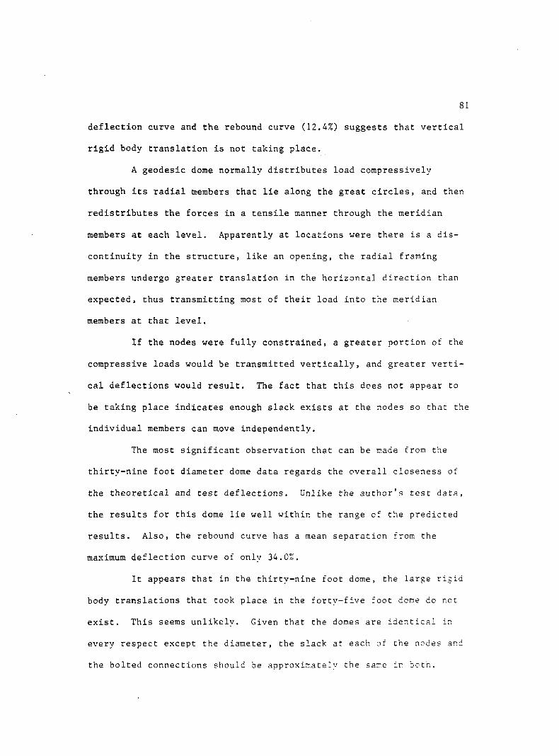
81

deflection curve and the rebound curve (12.4%) suggests that vertical

rigid body translation is not taking place.

A geodesic dome normally distributes load compressivelv

through its radial members that lie along the great circles, and then

redistributes the forces in a tensile manner through the meridian

members at each level. Apparently at locations were there is a dis­

continuity in the structure, like an opening, the radial framing

members undergo greater translation in the horizontal direction than

expected, thus transmitting most of their load into the meridian

members at that level.

If the nodes were fully constrained, a greater portion of the

compressive loads would be transmitted vertically, and greater verti­

cal deflections would result. The fact that this does not appear to

be taking place indicates enough slack exists at the nodes so that the

individual members can move independently.

The most significant observation that can be made from the

thirty-nine foot diameter dome data regards the overall closeness of

the theoretical and test deflections. Unlike the author's test data,

the results for this dome lie well within the range cf the predicted

results. Also, the rebound curve has a mean separation from the

maximum deflection curve of only 34.0%.

It appears that in the thirty-nine foot dome, the large rigid

body translations that took place in the forty-five foot dome do not

exist. This seems unlikely. Given that the domes are identical in

every respect except the diameter, the slack at each of the nodes and

the bolted connections should be approximately the same ir both.

Since the thirty-nine foot dome was loaded with significantly more

weight than the forty-five foot dome (75 PSF versus 34 PSF), it would

be expected that the maximum deflection curve would lie even further

above the rebound curve than for the forty-five foot dome. At the

same time, the rebound curve would be pushed lower, toward the theo­

retical curves. Only the latter actually takes place.

The most reasonable explanation for this is that the thirty-

nine foot dome was preloaded in some fashion before testing. In the

report made to the Pease Woodwork Company [5], from which this test

data are taken, no mention is made as to whether this took place or

not. The alternative solution is to assume that the dome was erected

in such a fashion that the slack was removed at all the connections,

producing a structure that was much stiffer than the author's. How­

ever, the description given in the report regarding erection and

materials appears close enough to the author's to make this unlikely.

After examining the data for both domes, it has been concluded

that with sufficient preload applied, all joint settlements will be

removed. The dome's subsequent structural behavior will generally

follow that of the computer models. The question that still remains

to be answered is which model provides the best results.

Examination of Figures 44 and 45 reveals that modeling with

bars, bars and trims, beams, and beams with trims, produce deflection

results that vary in degree only. In other words, all four of these

models produce curves that are identical in shape, but each represent

a structure of different stiffness. Of the four models, bar elements

appear to give the most accurate representation. It can therefore be

83

concluded that the necessity of including fixed ends, or the addi­

tional stiffness of the panel elements, into the model is not

required. This may have significant practical implication.

Apparently, a panel dome that distributes load primarily with

its framing members does so in a manner much like a three-dimensional

truss. . Once the slack has been removed from the structure, the com­

pression members that meet at a node butt against each other, trans­

mitting load, and the tensile members that meet, effectively transmit

load through the steel straps provided at each joint.

It should be noted that while the bar element model provides

the best representation of vertical deflections for a Pease panel dome

that distributes load with its framing members, it disregards the

flexural stresses induced in the framing members by load applied along

their length. The most satisfactory solution can be achieved by using

pinned end beam elements. With this model the relative stiffness of

the bar element model can be kept, while the flexural action of the

applied end moments can also be included.

The trim model that represents load distribution through

membrane action was deemed unacceptable for the forty-five foot dome.

However, the thirty-nine foot diameter dome's deflection curves

correspond to the trim model's. The modified shell analysis relied on

the development of an effective shell thickness to represent the

dome's behavior and was modeled using trim elements. The deflection

results for the modified shell analysis, the original crirc model, and

the test results for the thirty-nine foot dome have been plotted in

Figure 46.

84

Of the three modified shell thicknesses, only the value cal­

culated using Kloppel and Schardt's [18] formula gives a curve that

falls within the test data range. The results of the remaining two

thicknesses give deflections that are too small to be realistic. It

was assumed in Chapter Five that the use of plate bending elements

would give an even stiffer representation for the modified shell

analysis than the trim elements. It was therefore decided that this

model would be ignored, even though plate bending theory was used in

the development of the formulas. This assumption now appears valid.

In much the same way that the beam element model gave results similar

to the bar element model, only stiffer, it is assumed that the same

things would take place with the shell elements.

Examination of the curves in Figure 46 also reveals that the

use of the actual panel thickness, instead of Kloppel and Schardt's

derived thickness, yields acceptable results when compared to the test

data. This is due to the closeness of the effective and actual panel

thicknesses.

An evaluation of the performance given by each of the effec­

tive shell formulas in response to asymmetric loading cannot be

obtained with the available data. Although measurements were mace

while the forty-five foot dome was subjected to asymmetric loading, no

rebound data was collected until the structure had been completely

unloaded. Given the requirement that the structure must be adequately

preloaded before the deflection values prove to be reliable, the best

that can be hoped for would be a match in the shape of the theoretical

and test curves. In this case, however, all three theoretical curves

85

MAX. DEFLECTION El • t=0.066n O O

REBOUND El "G t= 0.559" O O ORIGINAL TRIM £> A t= 1.625" G>

1x10

V—

-2

O z

z o H-o UJ -j u_ LLI Q

-3 1x10

27 15 14 1

NODAL POINTS

FIGURE 46. DEFLECTION DATA FOR 39' DOME PLOTTED WITH THE THREE MODIFIED SHELL MODELS

have the same shape (Figures 40 and 41). What must be determined is

whether the stiffness of the dome changes enough to warrant recommend­

ing a curve different from Klbppel and Schardt's to predict the struc­

tural behavior. The forty-five foot dome's behavior does not seem to

follow the membrane action model. This is the one that the effective

shell models are related to. In order to form a reliable evaluation

of this concept, deflection data from an asymmetric loading of a dome

that distributes load primarily through membrane action is required.

A careful examination of the theoretical and experimental data

for the thirty-nine foot dome (Figure 46) reveals that although the

shape of the trim element curves match the test data, some of the

points deviate a fair amount. Point 27, in particular, does not seem

to match, and a possible explanation for this has been given above.

Further examination of Figure 46 reveals that the test results for

nodes 1 and 6 fall equally within the range of the predicted results

for the other models. As mentioned briefly above, this could be an

indication that this dome is distributing load through both the panels

and the framing members instead of primarily through only one of the

systems.

If this is the case, then it would be valuable to relate this

dome's frequency and size to a convenient number so that an estimate

of what constitutes the dividing line between shell and truss action

can be identified. The chord factors developed in Chapter Three are

not sufficient, since the two domes tested were of identical fre­

quencies, but still behave differently. It might be suitable to

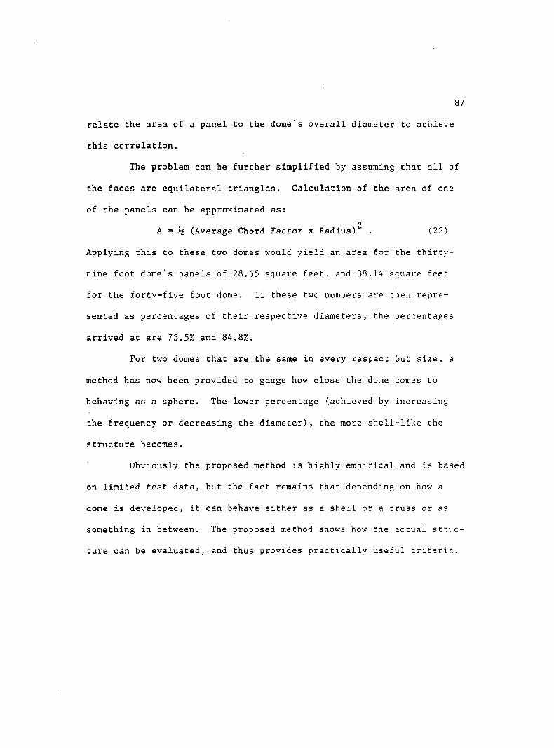
87

relate the area of a panel to the dome's overall diameter to achieve

this correlation.

The problem can be further simplified by assuming that all of

the faces are equilateral triangles. Calculation of the area of one

of the panels can be approximated as:

2 A = % (Average Chord Factor x Radius) . (22)

Applying this to these two domes would yield an area for the thirty-

nine foot dome's panels of 28.65 square feet, and 38.14 square feet

for the forty-five foot dome. If these two numbers are then repre­

sented as percentages of their respective diameters, the percentages

arrived at are 73.5% and 84.8%.

For two domes that are the same in every respect but size, a

method has now been provided to gauge how close the dome comes to

behaving as a sphere. The lower percentage (achieved by increasing

the frequency or decreasing the diameter), the more shell-like the

structure becomes.

Obviously the proposed method is highly empirical and is based

on limited test data, but the fact remains that depending on how a

dome is developed, it can behave either as a shell or a truss or as

something in between. The proposed method shows how the actual struc­

ture can be evaluated, and thus provides practically useful criteria.

CHAPTER 7

SUMMARY AND CONCLUSIONS

The purpose of this study has been to gather load and deforma­

tion data for the Pease panel dome, and to develop a reliable method

of structural evaluation. From the two full-scale tests analyzed in

this report and the results of the various computer models, the fol­

lowing conclusions can be given:

1. The structural detailing of the Pease panel dome contains

enough slack in the joints for either individual pieces

of the structure or complete sections to undergo rigid

body translations of an inch or more before redistribut­

ing load.

2. Once the structure has been given an adequate preload,

compression members intersecting at the joints will

transfer load through direct contact, and tensile members

will distribute load through the steel straps provided at

the joints.

3. From the computer models investigated, a pinned-end beam

finite element model is recommended for analyzing the

Pease panel dome that distributes load primarily though

its framing members. The model provides the flexural

data required for designing the framing members, and also

emulates the structure's three-dimensional truss action.

88

4. For Pease panel domes that distribute load primarily

through membrane action, a constant strain triangle

(trim) model is recommended. The thickness of the trim

element used should be as calculated with the formula

provided by Kloppel and Schardt [18].

5. In determining the dividing line between load distribu­

tion through framing members or membrane action through

the panels, it is recommended that the area of a single

panel be looked at in relation to the overall size of the

dome. The method proposed in this report (equation 22,

etc.) develops a ratio between the average panel area and

the dome diameter.

Two points have been bought out in this study that should be

further investigated. The first deals with asymmetric loading. Three

methods of modified shell analysis have been discussed, and it was

noted that the loading pattern played a role in their development.

The only dome that was subjected to asymmetric loading, however, did

not distribute load through membrane action and was therefore not

suitable for use in evaluation of the different formulas.

The second point concerns the identification of the geometric

characteristics that make a dome perform as either a three-dimensional

truss or a shell. The method proposed here is based on limited test

data. The development of a more refined and tested technique would be

of value to dome designers.

89

APPENDIX A

CHORD FACTORS AND RELATED INFORMATION FOR VARIOUS POLYHEDRONS

AND FREQUENCIES DEVELOPED USING THE CLASS I METHOD

90

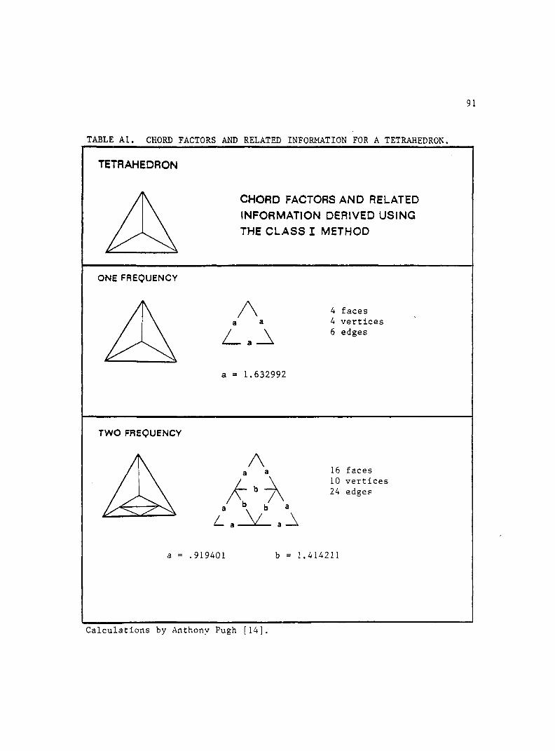
91

TABLE Al. CHORD FACTORS AND RELATED INFORMATION FOR A TETRAHEDRON.

TETRAHEDRON

CHORD FACTORS AND RELATED INFORMATION DERIVED USING THE CLASS I METHOD

ONE FREQUENCY

A a a

Z_, A a = 1.632992

4 faces 4 vertices 6 edges

TWO FREQUENCY

A a a

b a

16 faces 10 vertices 24 edges

a = .919401 b = 1.414211

Calculations by Anthony Pugh [14],

TABLE A2. CHORD FACTORS AND RELATED INFORMATION FOR A TETRAHEDRON.

TETRAHEDRON

CHORD FACTORS AND RELATED INFORMATION DERIVED USING THE CLASS I METHOD

THREE FREQUENCY

A b c c b

a b c c b a L. a-̂ b a

36 faces 20 vertices 54 edges

a = .509138 b = .853001 .977847

FOUR FREQUENCY

A a a

d e e d

Are e"^v d e f f e d

£ C - X - F -x-cjx a b c e e c b 3

d d -X- a ±

64 faces 34 vertices 96 edges

a = .337424 b = .577350 c = .517045

d = .605812 e = .765367 f = .999998

Calculations by Anthony Pugh [14].

TABLE A3. CHORD FACTORS AND RELATED INFORMATION FOR A TETRAHEDRON.

TETRAHEDRON

CHORD FACTORS AND RELATED INFORMATION DERIVED USING THE CLASS I METHOD

SIX FREQUENCY A a a

d e e d

ar* "x"e "x e g f f g 8

e f h j j h f e

a9 # i.^fl \ a e f h j J h f e d

aT c-)ff C"X a b c e g f f g e c b a I— a d e e d a

144 faces 74 vertices 216 edges

a = .194934 b = .342998 c = .248791

d = .314152 e = .436954 f = .459500

g = .335397 h = .632457 j = .671424

Calculations by Anthony Pugh [14].

TABLE A4. CHORD FACTORS AND RELATED INFORMATION FOR A HEXAHEDRON.

HEXAHEDRON

CHORD FACTORS AND RELATED INFORMATION DERIVED USING THE CLASS I METHOD

ONE FREQUENCY

a = 1.157362

A b b

Z_ a A 24 faces 14 vertices 36 edges

b = ,919402

TWO FREQUENCY

A c c

b e

96 faces 50 vertices 144 edges

a = .605811 b = .533266

c = .473130 d = .650115

Calculations by Anthony Pugh [14].

TABLE A5. CHORD FACTORS AND RELATED INFORMATION FOR A HEXAHEDRON.

HEXAHEDRON

CHORD FACTORS AND RELATED INFORMATION DERIVED USING THE CLASS I METHOD

THREE FREQUENCY

a = .381642 b = .458831 c = .369777

A e e

/r '"X h 9 g h

kj f-\ e d c c d e

l a^z baz. all

d = .345108 e = .305593 f = .437710

2 1 6 faces 110 vertices 324 edges

g = .342890 h = .340067 j = .427099

FOUR FREQUENCY

a = b = c = d = e =

.274774

.338201

.279081

.268070

.250832

A f f

A t I n n I

• k j j k I

/<r9-*-hX"9jX f e d c c d e f

L- a V b b a A

f = g = h = j = k =

.223925

.313678

.351406

.275377

.259338

384 faces 194 vertices 576 edges

1 = m = n = P =

.252585

.329564

.245520

.314678

Calculations by Anthony Pugh [14].

96

TABLE A6. CHORD FACTORS AND RELATED INFORMATION FOR AN OCTAHEDRON.

OCTAHEDRON

CHORD FACTORS AND RELATED INFORMATION DERIVED USING THE CLASS I METHOD

ONE FREQUENCY

8 faces 6 vertices 12 edges

1.1414213

TWO FREQUENCY

32 faces 18 vertices 48 edges

.765367 1.000000

Calculations by D. Andrews and A. Steinbrecher [22].

97

TABLE A7. CHORD FACTORS AND RELATED INFORMATION FOR AN OCTAHEDRON.

OCTAHEDRON

CHORD FACTORS AND RELATED INFORMATION DERIVED USING THE CLASS I METHOD

THREE FREQUENCY

a = .459507

aAa

X-b-X b c c b

ar°^-c-\ a b c c b a

L a-̂ Z. a A

b = .632456

72 faces 38 vertices 108 edges

c = .671421

FOUR FREQUENCY

a = .320365 b = .447214 c = .438871

aAa 1 2 8

Arb-X 66 d e e d 1 9 2

ar ® e"x d e f f e d

a f C"X a b c e e c b a Z_a _V. d -V. d a A

d = .459506 e = .517638 f = .577350

faces vertices edges

Calculations by D. Andrews and A. Steinbrecher [22].

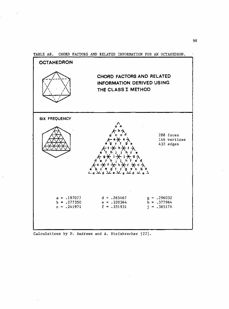
TABLE A8. CHORD FACTORS AND RELATED INFORMATION FOR AN OCTAHEDRON.

OCTAHEDRON

CHORD FACTORS AND RELATED INFORMATION DERIVED USING THE CLASS I METHOD

SIX FREQUENCY A

a a

/f b\ d c c «

e\ e g f f a e

/t"f y~.h^" f "X e f h j j h f e

A 9~S d e f h i j h f e d

X-c h f ^ c "X a b c e g f f g e c b a

i— a d -̂ •4- 0 e d -̂ 4- a

288 faces 146 vertices 432 edges

a = .197077 b - .277350 c = .241971

d = .265467 e = .320364 f = .331931

g = .296032 h = .377964 j = .385176

Calculations by D. Andrews and A. Steinbrecher [22].

TABLE A9. CHORD FACTORS AND RELATED INFORMATION FOR AN OCTAHEDRON.

OCTAHEDRON

CHORD FACTORS AND RELATED INFORMATION DERIVED USING THE CLASS I METHOD

NINE FREQUENCY a a \

d e e d A-®#8 "X

h g f f a h /r k -fr ) k-X

k n m I I m n k

J I P r q 1 r T | J k l-)fq>s^q-y I*

k m p q s t t s q p m k /t*n "X"'- -)(-1 ̂ -t h k m P I ' t t s q p m k h

/ r f l - * i i ^ g - x d e f j l p r q q r p | j f e d

/ f c - X - f - y - m - J e p ^ - p - ^ - m ^ f f c - \ a b c e g k n m l | m n k 9 e c b a La JwLd ̂ £-h-^ k j^k-^h-^d-^-aA

684 faces 326 vertices 972 edges

a = .124277 g = .162497 n = .185970 b = .175412 h = .185086 P = .240797 c = . 141457 j = .220863 q = .245917 d = .153795 k = .210702 r = .232229 e = .195190 1 = .206355 s = .262613 f = .1-78374 m = .215719 t = .264949

Calculations by D. Andrews and A. Steinbrecher [22].

100

TABLE A10. CHORD FACTORS AND RELATED INFORMATION FOR AN ICOSAHEDRON.

ICOSAHEDRON

CHORD FACTORS AND RELATED INFORMATION DERIVED USING THE CLASS I METHOD

ONE FREQUENCY

faces vertices edges

a -= 1.051462

TWO FREQUENCY

80 faces 42 vertices 120 edges

.546533 .618034

Calculations by Joseph D. Clinton [23].

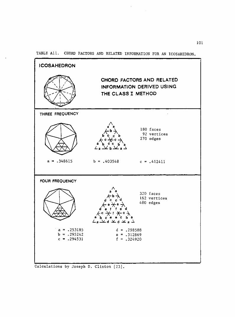
101

TABLE All. CHORD FACTORS AND RELATED INFORMATION FOR AN ICOSAHEDRON.

ICOSAHEDRON

CHORD FACTORS AND RELATED INFORMATION DERIVED USING THE CLASS I METHOD

THREE FREQUENCY

a = .348615

A a a

a~b\ b c c b

a b c c b a I— a b a

b = .403548

180 faces 92 vertices 270 edges

c = .412411

FOUR FREQUENCY

a = .253185 b = .295242 c = .294531

A a a

d c c d

Ar e^-e"X d e f f e d

x-c -*-f * R C \ a b c e e c b a Z_a

d = .298588 e = .312869 f = .324920

320 faces 162 vertices 480 edges

Calculations by Joseph D. Clinton [23].

TABLE A12. CHORD FACTORS AND RELATED INFORMATION FOR AN ICOSAHEDRON.

ICOSAHEDRON

CHORD FACTORS AND RELATED INFORMATION DERIVED USING THE CLASS I METHOD

FIVE FREQUENCY

a = .198147 b = .231790 c = .225686

aAa

>9^

a b ce 99 e c ba

d = .231598 e = .247243 f = .255167

500 faces 252 vertices 750 edges

g = h = j =

.245086

.245346

.261598

SIX FREQUENCY

aAa

d e e d

e g f .f g e A-f *J*. f-X e f J k k j. f e

4-9-fc k;}fck & 9 -fc. d e f I k K I f e d

a b e e g f f g e c b a la -^-d ̂ e-^-e^d-^a

720 362

faces vertices

1080 edges

a = .162567 b = .190477 c = .181908

d = .187383 e = .202820 f = .205908

g = .198013 j = .215354 k « .216628

Calculations by Joseph D. Clinton [23].

TABLE A13. CHORD FACTORS AND RELATED INFORMATION FOR A DODECAHEDRON.

DODECAHEDRON

CHORD FACTORS AND RELATED INFORMATION DERIVED USING THE CLASS I METHOD

ONE FREQUENCY

A b b

A a A 60 faces 32 vertices 90 edges

a = .713640 b = .640850

TWO FREQUENCY

A c c

/ t d .^ b c

Z . A z _ a A

240 faces 122 vertices 360 edges

a = .362841 b = .340339

c = .324734 d = .376681

Calculations by Anthony Pugh [14].

104

TABLE A14. CHORD FACTORS AND RELATED INFORMATION FOR A DODECAHEDRON.

DODECAHEDRON

o CHORD FACTORS AND RELATED INFORMATION DERIVED USING THE CLASS I METHOD

THREE FREQUENCY

a = .237657 b = .252597 c = .228242

A e e

Ar »-X h g a h

A\f f \ e d c c d e

/. a b a

d = .225128 e = .213490 f = .252116

540 faces 272 vertices 810 edges

g = .225438 h = .224087 j = .249539

FOUR FREQUENCY

A f f

Jr I n n I

I k j i k I

f e d c c d e f l. a-V. b-V. b -V- aA

960 faces 482 vertices 1440 edges

a = .175924 b = .188429 c = .171879 d = .169507

e = .166955 f = .158465 g = .185219 h = .191986

j = .172304 k = .169639 1 = .167350 m = .189191

n - .165468 p = .185279

Calculations by Anthony Pugh [14].

APPENDIX B

FINITE ELEMENT MESHES, NUMBERING SCHEMES,

AND NODAL COORDINATE DATA USED IN ANALYSIS

105

106

35

20

33 36

32, 22

23 1&2

42

30, 24

38 29. 25

28 26

27.

40 39

FIGURE Bl. NODAL NUMBERING SCHEME

107

96 86 76 77,

36 ,66 46

.52 56 87

100 92

22 20

70 .62 ,45 42

27

65 67, 30. 32

60, 10 40 25 47 23

,83 55

53. 34 28 80 78 49,

.38 58 29 85 88 33 69 24

99 93 68 64

44 43 59

39 94 98 89 84,

FIGURE B2. BEAM AND BAR ELEMENT NUMBERING SCHEME

108

,46 37 26 36

40 27 20

35 32

30 37

55 58 25 42

14 44

39 28 60 53

33 34 29 38

24 43

54 59 49

FIGURE B3. TRIM ELEMENT NUMBERING SCHEME

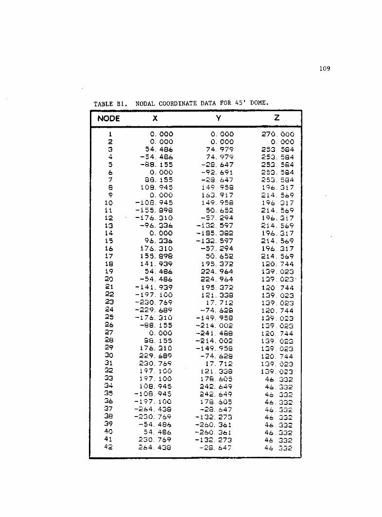
109

TABLE Bl. NODAL COORDINATE DATA FOR 45' DOME.

NODE X Y Z

1 0. 000 0 000 270 000 2 0. 000 0. 000 0 000 3 54. 486 74. 979 253 584 *+ -54. 486 74. 979 253 584 5 -88. i 55 -28. 647 2 33 584 6 0. 000 -92. 691 253 3cs4 7 88. i 55 -28. 647 ef D J 584 8 iOS. 945 149. vsy 1 317 9 0. 000 i63. 9 i 7 214 569

10 -108. 945 149. 958 196 317 ii -155. 398 50. 6d2 214 569 12 • -176. 3i0 -57. 294 196 3 i 7 13 -96. 336 — 132. 597 214 JO9 14 0. 000 -135. 3S2 1 TO 317 15 96. 336 -132. 597 214. 569 16 176. 310 -57. 294 196 317 17 i 55. 398 50. 652 214 569 18 141. 939 195. 372 120 744 19 54. 486 224. 964 139. 023 20 -54. 486 224. 964 139. 023 21 -141. 939 i 95. 372 120 744 22 -197. iOO i2i. 338 139 023 23 -230. 769 17. 712 139. 023 24 -229. 689 -74. 628 120. 744 25 — i / 6. 310 -i 49. 958 1 LiV. 023 26 -88. 155 -214. 002 139. 023 27 0. 000 -241. 488 120. 744 28 38. i 55 -214. 002 139. 023 29 176. 310 -i 49. 958 1 LiV . 023 30 229. 689 -74. 628 120. 744 31 c: U 0. 769 17. 7X2 139. 023 32 i 97. iOO 121. 338 139. 023 33 197. 100 178. 605 46 jot 34 108. 945 242. 649 46. 332 35 -iOS. 945 242. 649 46. 332 36 -197. 100 i 7o. 605 46. o J2 37 -264. 438 — c!ci. 647 46. JJ'2 38 — el L? 0 . 769 -132. 273 46. JJe: 39 -54. 486 -260. 361 46. *-\ O Jel 40 54. 486 -260. 36 i 46. 332 41 230. 769 -132. 273 46. 332 ^2 264. 43a -28. 647 46 332

TABLE B2. NODAL COORDINATE DATA FOR 39' DOME.

NODE X Y z

1 0. 000 0. 000 234. 000 2 0. 000 0. 000 0. 000 3 47. 908 65. 939 219. 346 4 -47. 908 65. 939 219. 346 5 -77. 517 -25. 186 219. 346 6 0. 000 -81. 505 219. 346 7 77. 517 -25. 186 219. 346 8 96. 478 132. 790 166. 777 9 0. 000 143. 931 184. 499

10 -96. 478 132. 790 166. 777 11 -136. 886 44. 477 184. 499 12 -156. 105 -50. 722 166. 777 13 -84. 600 -116. 442 184. 499 14 0. 000 -164. 139 166. 777 15 84. 600 -116. 442 184. 499 16 156. 105 -50. 722 166. 777 17 136. 886 44. 477 184. 499 IS 124. 582 171. 472 99. 161 19 47. 908 197. 037 117. 360 20 -47. 908 197. 037 117. 360 21 -124. 582 171. 472 99. 161 2P -172. 215 106. 328 117. 360 23 -201.823 15. 205 117. 360 24 -201. 577 -65. 496 99. 161 25 -156. 105 -128. 395 117. 360 26 -76. 827 -187. 246 117. 360 27 0. 000 -211. 951 99. 161 29 76. 827 -187. 246 117. 3&0 29 156. 105 -128. 895 117. 360 30 201. 577 -65. 496 99. 161 31 201. S23 15. 205 117. 360 32 172. 215 106. 32S 117. 360 33 172. 215 1 54. 902 33. 217 34 94. 431 211. 477 33. 217 35 -94. 431 211. 477 33. 217 36 -i72. 215 i 54. 905 33. 517 37 -230. 257 -25. 186 33. 217 38 -201.823 -113. 667 33. 217 39 -47. 908 -226. 625 33. 217

. 40 47. 908 -226. 622 33. 217 41 201.823 -113. 667 33. 217 42 230. 257 -25. 1S6 33. 217

Ill

TABLE B3. BAR ELEMENT CONNECTIVITY

ELEMENT NODE NODE ELEMENT NODE NODE ELEMENT NODE NODE NUMBER I J NUMBER I J NUMBER I J

1 3 4 44 28 29 87 21 36 2 4 5 45 31 32 88 • 24 38 3 5 6 46 20 21 89 27 40 4 6 7 47 23 24 90 30 42 5 7 3 48 26 27 91 34 19 6 1 3 49 29 30 92 36 22 7 1 4 50 32 18 93 38 25 a 1 5 51 18 8 94 40 28 9 1 6 52 21 10 95 42 31

10 1 7 53 24 12 96 20 35 n 8 9 54 27 14 97 23 37 12 10 11 55 30 16 98 26 39 13 12 13 56 8 19 99 29 41 14 14 15 57 10 22 100 32 •33 15 16 17 58 12 25 16 9 10 5V 14 28 17 11 12 60 16 31 18 13 14 61 19 9 19 15 16 62 22 11 20 17 8 63 25 13 21 8 3 64 28 15 2? 10 4 65 31 17 23 12 5 66 9 20 24 14 6 67 11 23 25 16 7 69 13 26 26 3 9 69 15 29 27 4 11 70 17 - 32 23 5 13 71 20 10 29 6 15 72 23 12 30 7 17 73 26 14 31 9 4 74 29 16 32 11 5 75 32 8 33 13 6 76 33 34 34 15 7 77 35 36 35 17 3 79 37 38 36 18 19 79 39 40 37 21 22 80 41 42 39 24 25 81 33 18 39 27 28 82 35 21 40 30 31 S3 37 24 41 19 20 84 39 27 42 22 23 85 41 30 43 25 26 86 18 34

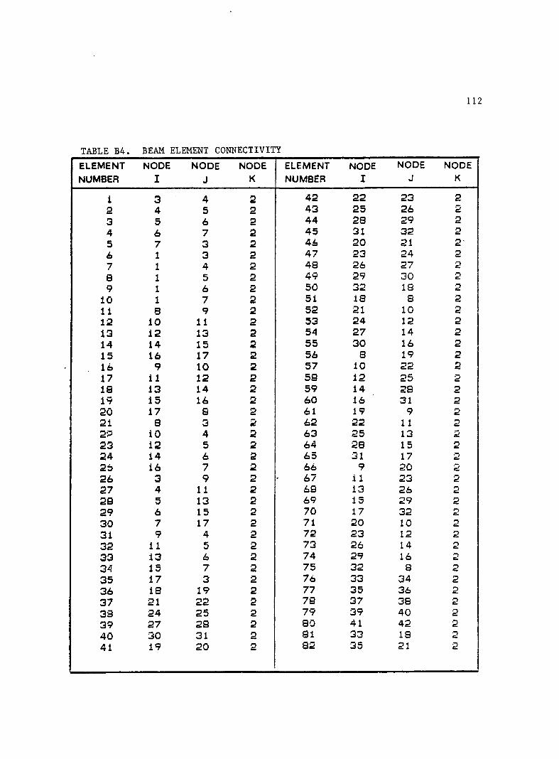
112

TABLE B4. BEAM ELEMENT CONNECTIVITY

ELEMENT NODE NODE NODE ELEMENT NODE NODE NODE

NUMBER I J K NUMBER I J K

i 3 4 2 42 22 23 2 2 4 5 2 43 25 26 2 3 5 6 2 44 28 29 2 4 6 7 2 45 31 32 2 5 7 3 2 46 20 21 2* 6 1 3 2 47 23 24 2 7 1 4 2 48 26 27 2 8 1 5 2 49 29 30 2 9 1 6 2 50 32 18 2

10 1 7 2 51 IS 8 2 11 8 9 2 52 21 10 2 12 10 11 2 53 24 12 2 13 12 13 2 54 27 14 2 14 14 15 2 55 30 16 2 15 16 17 2 56 8 19 2 1 6 9 10 2 57 10 22 2 17 11 12 2 58 12 25 2 18 13 14 2 59 14 28 2 19 i 5 16 2 60 16 31 2 20 17 S 2 61 19 9 2 21 S 3 2 62 22 11 2 2? iO 4 2 63 25 13 2 23 i2 5 2 64 28 15 2 24 14 6 2 65 31 17 2 2b i6 7 2 66 9 20 2 26 3 9 2 67 i 1 23 2 27 4 11 2 68 13 26 2 28 5 13 2 69 15 29 2 29 6 15 2 70 17 32 2 30 7 17 2 71 20 10 2 31 9 4 2 72 23 12 2 32 11 5 2 73 26 14 2 33 13 6 2 74 29 16 2 34 15 7 2 75 32 8 2 35 17 3 2 76 33 34 2 36 18 19 2 77 35 36 2 37 21 22 2 78 37 38 2 33 24 25 2 79 39 40 2 39 27 28 2 80 41 42 2 40 30 31 2 81 33 18 2 41 19 20 2 82 35 21 2

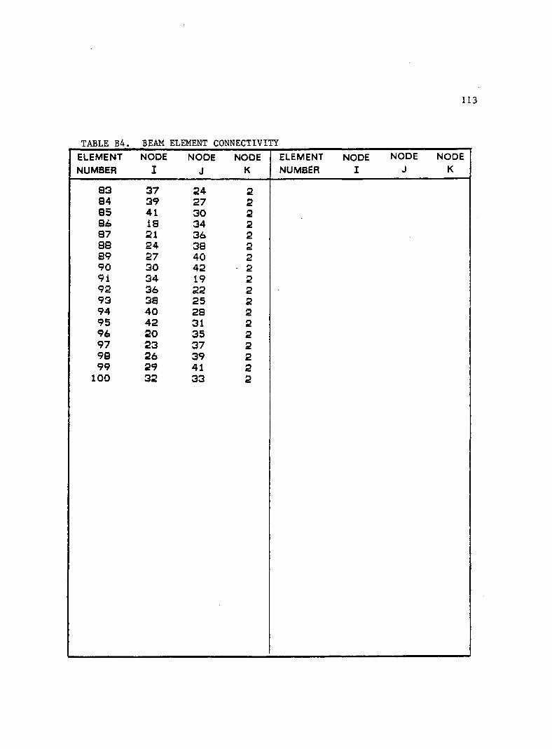
113

TABLE B4. BEAM ELEMENT CONNECTIVITY

ELEMENT NODE NODE NODE NUMBER I J K

83 37 24 2 84 39 27 2 85 41 30 2 86 18 34 2 87 21 36 2 88 24 38 2 89 27 40 2 90 30 42 2 9i 34 19 2 92 36 22 2 93 38 25 2 94 40 28 2 95 42 31 2 96 20 35 2 97 23 37 2 98 26 39 2 99 29 41 2

100 32 33 2

ELEMENT NODE NODE NODE NUMBER I J K

114

TABLE B5. TRIM ELEMENT CONNECTIVITY

ELEMENT NODE NODE NODE ELEMENT NODE NODE NODE NUMBER I J K NUMBER I J K

1 3 4 1 42 12 23 24 2 4 5 1 43 14 26 27 3 5 6 1 44 16 29 30 4 6 7 1 45 8 32 18 5 7 3 1 46 33 34 18 6 3 8 9 47 35 36 21 7 4 iO i 1 48 37 38 24 8 5 12 13 49 39 40 27 9 6 14 15 50 41 42 30

10 7 16 17 51 34 19 18 11 4 3 9 52 36 22 21 12 5 4 11 53 38 25 24 13 6 5 13 54 40 28 27 14 7 6 15 55 42 31 30 15 3 7 17 56 32 33 18 16 10 4 9 57 20 35 21 17 12 5 11 58 23 37 24 18 14 6 13 59 26 39 27 19 16 7 15 60 29 41 30 20 8 3 17 21 19 8 18 22 22 10 21 23 25 12 24 24 28 14 27 25 31 16 30 26 8 19 9 27 10 22 11 28 12 25 13 29 14 28 15 30 16 31 17 31 19 20 9 32 22 23 11 33 25 26 13 34 28 29 15 35 31 32 17 36 20 10 9 37 23 12 11 38 26 14 13 39 29 16 15 40 32 8 17 41 10 20 21

REFERENCES

1. Marks, Robert, and Fuller, R.B., The Dymaxion World of Buckminster Fuller, Anchor Press, New York, 1973.

2. Wright, D.T., "Membrane Forces and Buckling in Reticulated Shells," Journal of the Structural Division, ASCE, February, 1965.

3. Pacific Domes, Domebook Two, Random-House, New York, 1971.

4. Kenner, Hugh, Geodesic Math and How to Use It, University of California Press, Berkeley, CA, 1976.

5. Nutting Co., H.C., engineering report made to the Pease Woodwork Company, Cincinnati, Ohio, December, 1959.

6. Lederer, Ferdinand, "Membrane Forces and Buckling in Reticulated Shells," Discussion, Journal of the Structural Division, ASCE, October, 1965.

7. Rawlings, J.P., "Stress Analysis of a 45 ft. Diameter, 3 Frequency, Timber and Plywood Dome," engineering report prepared for Domes and Homes, Whitehouse, Texas, October, 1982.

8. Guinn, Robert, "Cathedralite Church Design, Daly City," engineering report, June, 1969.

9. McCutcheon, J.O., and Dickie, J.F., "Membrane Forces and Buckling in Reticulated Shells," Discussion, Journal of the Structural Division, ASCE, October, 1965.

10. McCutcheon, J.O., Eremin, A.A., Moses, G., Bradshaw, R.R., del Pozo, F., Beles, A.A., Dean, D.L., Lederer, F., Pagano, M., "Membrane Forces and Buckling in Reticulated Shells," Discussion, Journal of the Structural Division, ASCE, October, 1965.

11. C., Pe, Architecture, Art of," Ency. Brit., 1979.

12. Yarnall, William, Dome Builders Handbook Number Two, Running Press, Philadelphia, PA, 1978.

13. Jacobs, David, "An Expo Named Buckminster Fuller," New York Times, April 23, 1967.

115

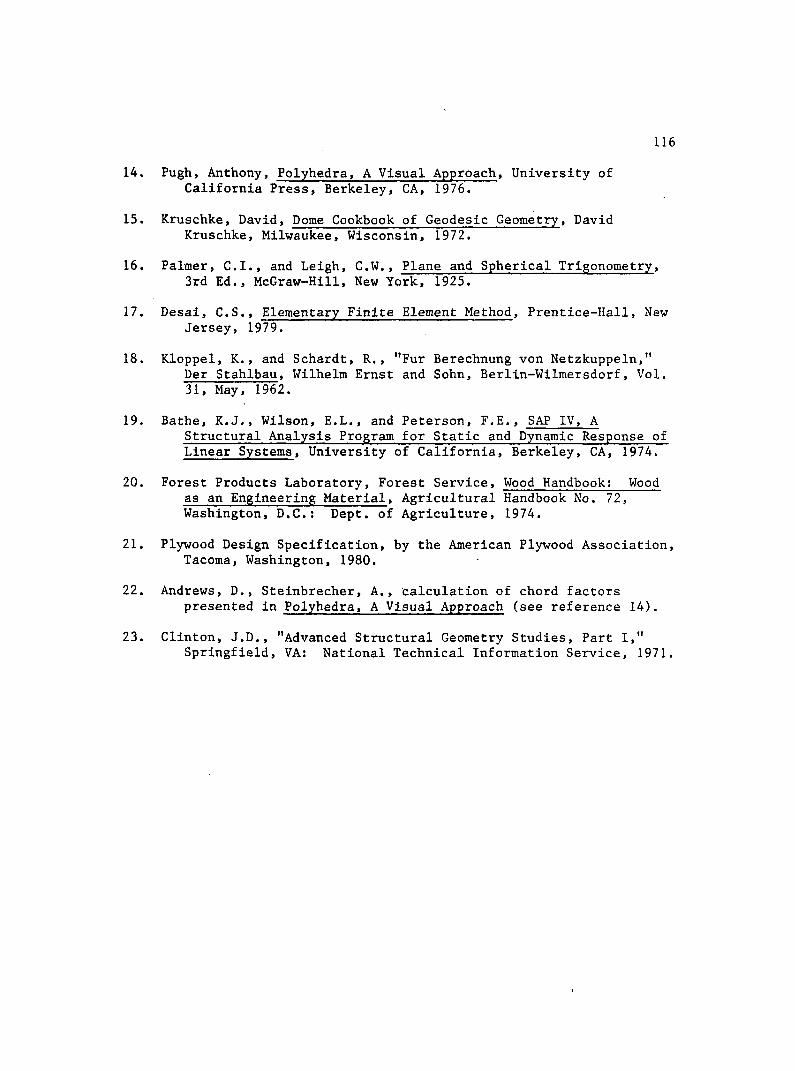
116

14. Pugh, Anthony, Polyhedra, A Visual Approach, University of California Press, Berkeley, CA, 1976.

15. Kruschke, David, Dome Cookbook of Geodesic Geometry, David Kruschke, Milwaukee, Wisconsin, 1972.

16. Palmer, C.I., and Leigh, C.W., Plane and Spherical Trigonometry, 3rd Ed., McGraw-Hill, New York, 1925.

17. Desai, C.S., Elementary Finite Element Method, Prentice-Hall, New Jersey, 1979.

18. Kloppel, K., and Schardt, R., "Fur Berechnung von Netzkuppeln," Per Stahlbau, Wilhelm Ernst and Sohn, Berlin-Wilmersdorf, Vol. 31, May, 1962.

19. Bathe, K.J., Wilson, E.L., and Peterson, F.E., SAP IV, A Structural Analysis Program for Static and Dynamic Response of Linear Systems, University of California, Berkeley, CA, 1974.

20. Forest Products Laboratory, Forest Service, Wood Handbook: Wood as an Engineering Material, Agricultural Handbook No. 72, Washington, D.C.: Dept. of Agriculture, 1974.

21. Plywood Design Specification, by the American Plywood Association, Tacoma, Washington, 1980.

22. Andrews, D., Steinbrecher, A., calculation of chord factors presented in Polyhedra, A Visual Approach (see reference 14).

23. Clinton, J.D., "Advanced Structural Geometry Studies, Part I," Springfield, VA: National Technical Information Service, 1971.