SPECIFICATION ERRORS IN ESTIMATINGCOST FUNCTIONS: THE CASE OF THE

NUCLEAR ELECTRIC GENERATING INDUSTRY.

Item Type text; Dissertation-Reproduction (electronic)

Authors JORGENSEN, EDWARD JOHN.

Publisher The University of Arizona.

Rights Copyright © is held by the author. Digital access to this materialis made possible by the University Libraries, University of Arizona.Further transmission, reproduction or presentation (such aspublic display or performance) of protected items is prohibitedexcept with permission of the author.

Download date 10/06/2018 07:04:46

Link to Item http://hdl.handle.net/10150/184149

INFORMATION TO USERS

While the most advanced technology has been used to photograph and reproduce this manuscript, the quality of the reproduction is heavily dependent upon the quality of the material submitted. For example:

o Manuscript pages may have indistinct print. In such cases, the best available copy has been filmed.

® Manuscripts may not aiways be complete. In such cases, a note will indicate that it is not possible to obtain missing pages.

o Copyrighted material may have been removed from the manuscript. In such cases, a note will indicate the deletion.

Oversize materials (e.g., maps, drawings, and charts) are photographed by sectioning the original, beginning at the upper left-hand corner and continuing from left to right in equal sections with small overlaps. Each oversize page is also filmed as one exposure and is available, for an additional charge, as a standard 35mm slide or as a 17"x 23" black and white photographic print.

Most photographs reproduce acceptably on positive microfilm or microfiche but lack the clarity on xerographic copies made from the microfilm. For an additional charge, 35mm slides of 6"x 9" black and white photographic prints are available for any photographs or illustrations that cannot be reproduced satisfactorily by xerography.

Order Number 8726809

Specification errors in estimating cost functions: The case of the nuclear electric generating industry

Jorgensen, Edward John, Ph.D.

The University of Arizona, 1987

D·MaI 300 N. Zeeb Rd. Ann Arbor, MI 48106

SPECIFICATION ERRORS IN ESTIMATING COST FUNCTIONS:

THE CASE OF THE NUCLEAR ELECTRIC GENERATING INDUSTRY

by

Edward John Jorgensen

A Dissertation Submitted to the Faculty of the

DEPARTMENT OF ECONOMICS

In Partial Fulfillment of the Requirements For the Degree of

DOCTOR OF PHILOSOPHY

In the Graduate College

THE UNIVERSITY OF ARIZONA

1987

THE UNIVERSITY OF ARIZONA GRADUATE COLLEGE

As members of the Final Examination Committee, we certify that we have read

the dissertation prepared by Edward John Jorgensen

entitled _.Specification Errors in Estimating Cost Functions: The Case

of the Nuclear Electric Generating Industry.

and recommend that it be accepted as fulfilling the dissertation requirement

for the Degree of Doctor of Philosophy

.r .... ~~ 0 , ... -.~('~ 7---/Z-E) Date

7 !~ 7 /?) Date

Date

7-2-4- ~7 Date

Date

Final approval and acceptance of this dissertation is contingent upon the candidate's submission of the final copy of the dissertation to the Graduate College.

I hereby certify that I have read this dissertation prepared under my direction and recommend that it be accepted as fulfilling the dissertation requirement.

Dissertation Director Date

STATEMENT BY AUTHOR

This dissertation has been submitted in partial fulfillment of requirements for an advanced degree at The University of Arizona and is deposited in the University Library to be made available to borrowers under rules of the Library.

Brief quotations from this disse~tation are allowable without special permission, provided that accurate acknowledgement of source is made. Requests for permission for extended quotation from or reproduction of this manuscript in whole or in part may be granted by the head of the major department or the Dean of the Graduate College when in his or her judgment the proposed use of the material is in the interests of scholarship. In all other instances, however, permission must be obtained from the author.

SIGNED:

ACKNOWLEDGMENTS

I would like to extend thanks and appreciation to the

following people: Dr. Ronald Oaxaca for directing this

research, Dr. Michael Ransom for providing valuable guidance

regarding computer programming and to Drs. Lester Taylor and

David Conn for their critical comments. Further thanks are

extended to Mrs. Evelyn Jorgensen for the typing of the many

drafts. Last of all to my wife, Julie, for her loving

support.

iii

1 ..

2.

TABLE OF CONTENTS

LIST OF TABLES ••••• • • • • • · . . . · . . . LIST OF ILLUSTRATIONS • . . .. · . . · . . · . . . ABSTRACT. • • . . . . . . • • • . . . · . . . IN 'I'RODUCT I ON. • • . . . . . . .. . · . · . . . . . DUALITY OF COST AND PRODUCTIONS • · .. · . . . . .

Duality .• 0 • ~ • "'" •• 0 0 •• I: •••••

Profit Functions ••••••• 0 ••••

Cost Minimization •••••••••••• Duality for the Regulated Firm ••••••• Approximation Theory •••••••••••• Flexible Functional Forms •••••••• Summary •••••••• · . . · . . . . . . .

Page

vi

vi i

ix

1

9

10 11 18 24 34 36 61

3. STOCHASTIC SPECIFICATION OF COST AND PRODUCTION

4.

FUNCTIONS • • • • • • • • • • · . . · . . . . . . 62

Uncertainty. • • • • • • • • • • • • • • ... 62 Stochastic Specification • • • • • • • • •• 63 Expected Profit Maximization • • • • • • 69 The Specification of a Cost Function • • •• 73 Distribution of Output and Cost Shares 0 •• 77 Summary ••••••••••• 0 • • • • .. ... 85

NUCLEAR POWER GENERATION •• · . . · . . . . .0. Nuclear Power Industry · . . . • • 0 • • Summary. • • • • • • • • · . . · . . · . . .

86

90 105

5. ESTIMATION UNDER ALTERNATIVE SPECIFICATIONS. 106

Estimation Techniques •••••••••••• The Generalized Box-Cox. • • • • • • •• The Fourier Flexible Form •••••••••• Conclusions •••••••• · . . . . . .

iv

110 111 123 14].

6.

TABLE OF CONTENTS--Continued

SUMMARY AND CONCLUSIONS • • • • • • • •

APPENDIX A: TECHNICAL CLARIFICATION •• . . . . . . . . APPENDIX B: SAMPLE DATA. • • • •

LIST OF REFERENCES •••••••• . . . . . .

v.

Page

142

146

151

153

Table

1.

2.

3.

4.

5.

6.

7.

LIST OF TABLES

Nuclear units Ordered and Cancelled, 1972, 1982 ••••••••••••• • • 0 • • •

Average Construction Costs for Nuclear Units Entering Commercial Operation for 1971 through 1984 •• 0 ••••••••• . . . . Estimated and Actual Construction Costs for Nuclear Power Units Entering Commercial Operation in 1984 •••••••••••••• . . Estimates of Generalized Box-Cox Coefficients--Non-Homothetic •• · . . . . . . . Estimates of Generalized Box-Cox Coefficients--Homothetic •••• · . . . . . . . Estimates of Generalized BoX-COX Substitute Elasticities--Non-Homothetic. . . . . Skewness and Kurtosis of Cost and Factor Share Equation Residuals for non-Homothetic Generalized BoX-COX •••••••••••• • • •

8. Skewness and Kurtosis for Entire System of Equations for the Non-Homothetic Generalized Box-Cox ••••••••••••• · . . . . . . .

9. Scaling Factors and Multi-Indices for the

Page

93

94

96

113

114

117

120

122

Fourier Cost Function: KT = 35 • eo •••• 0 • 126

10.

11.

12.

Estimates of Fourier Cost Function Parameters--Non-Homothetic • • • •

Estimates of Fourier Cost Function Parameters--Homothetic • • • • • •

. . . . . . .

. . . . . . . Estimates of Fourier Flexible Form Substitute Elasticities--Non-Homothetic.

'Vi

131

134

136

LIST OF TABLES--Continued

Table

13. Skewness and Kurtosis of Cost Function and Factor Share Equations for Residuals

vii

Page

for Non-Homothetic Fourier Flexible Form ••••• 138

14. Skewness and Kurtosis Measures for Entire System for the Non-Homothetic Fourier Flexible Form. 0 0 ••••••••••••••• 139

15. Out-of-Sample Forecast of Generalized Box-Cox and Fourier Flexible Forms Additive Normal •••• Q ••••••••••• 0 140

16. Out-of-Sample Forecast of Generalized Box-Cox and Fourier Flexible Forms Logistic Normal • • • • • • • • • • • • • • • • • 140

Figure

1.

2.

3.

4.

LIST OF ILLUSTRATIONS

Geometrical interpretation of the subgradient inequality. 0 •• . . . . . .

Geometrical representation of a subgradient set • 0 • • • • · . . . . . .

Graphical illustration of the input requirement set for two inputs ••

The generalized tangency solution •••

• • • •

. . . . 5. Cost minimization for the regulated

firm •••••••• • • • • 0 • • • • • •

6. Graphical representation of a Laurent series •••••••• . . . · . . . . . .

7. Pressurized water reactor •• . . · . . . . . . 8. Boiling water reactor •••• . . eo. • • • •

viii

Page

15

17

20

23

28

48

89

91

This study

duality theory.

ABSTRACT

is an application of production-cost

Duality theory is reviewed for the

competitive and rate-of-return regulated firm. The cost

fUnction is developed for the nuclear electric power

generating industry of the United States using capital, fuel

and labor factor inputs. A compar i son is made between the

Generalized Box-Cox (GBC) and Fourier Flexible (FF)

functional forms. The GBC functional form nests the

Generalized Leontief, Generalized Square Root Quadratic and

Translog functional forms, and is based upon a second-order

Taylor-series expansion. The FF form follows from a

Fourier-series expansion in sine and cosine terms using the

Sobolev norm as the goodness of fit measure. The Sobolev

norm takes into account first and second derivatives. The

cost function and two factor shares are estimated as a

system of equations using maximum likehood techniques

with Additive Standard Normal and Logistic Normal error

distributions. In summary, none of the special cases of the

GBC function form are accepted. Homotheticity of the

underlying production technology can be rejected for both

the GBC and FF forms, leaving only the unrestricted veriians

supported by the data. Residual analysis indicates a slight

ix

x

improvement in skewness and kurtosis for univariate and

multivariate cases when the Logistic Normal distribution is

used.

CHAPTER 1

INTRODUCTION

Neo-classical economic theory assumes optimizing

be ha v i 0 ron the par t 0 f apr od u c i ng fir m , i. e., the fir m is

assumed to choose an input bundle that minimizes the cost

of producing each possible output while facing fixed

technological

Given fixed

possibilities and competitive

input prices this behavior

input markets.

determ i nes the

minimum cost of production as a function of output.

Generalizing further by allowing input prices to vary, the

cost function can be written as a function of both input

prices and output. The cost function carries with it the

advantage that its partial derivatives with respect to input

prices yield the corresponding input demand functions and

the sum of the values of input demand equals cost. These

analytic properties follow from a fundamental duality

between the cost function and the underlying production

possibilities. The optimization behavior of the firm

establishes the cost function as the source of all

economically relevant characteristics of the production

technology.

In principle, a production function can be solved

directly for input demands. In this case the underlying

1

2

production function is estimated and then the constant

output, factor demand curves are found by inverting the

implied first order conditions yielding closed form

solutions. This is referred to as solving the primal

problem. However, this is a very tedious procedure.

In general, production functions are used to derive

implications for factor usage and costs as various

parameters change. Modeling of complex technologies require

more sophisticated economic representations le~ding to

increasingly complex solution procedures. It is possible to

specify a system of demand equations by setting the value of

the marginal product equal to the rental price as implied by

optimization. This can lead to an algebraic morass for all

but the simplest functional forms.

An alternative approach exists in the dual problem.

This approach has been used extensively during the past ten

years. The behavioral assumption of the firm is profit

maximization or cost minimization. When coupled with the

further assumption of existence of either a profit function

relating profit level to prices or a cost function relating

total costs to output and factor prices, duality theory can

be appealed to. In this case, the cost or profit functions

relate information about the underlying production

technology.

3

The dual approach offers distinct advantages over

using the primal, ever. when the functional form is unknown.

First, it is possible to derive the factor demands by

differentiation of the cost. function.. This result follows

from Shephard's Lemma (Varian (1984). A profit function

can be ~anipulated in a similar manner

yielding input demands and outpwt

Elasticities of sUbs't:ii.tution can

(Hotelling's Lemma)

supply functions.

be found after

differentiating twice. The primal approach requires matrix

inversion in order to find the substitution elasticities

(Silberberg (1978». In gl.eneral, the dual approach is more

convenient and offers greater ease in estimation.

While the empirical researcher has benefited

tremendously from duality theory, there is one remaining

problem, the selection of the "flexible functional form".

Attempts to solve this problem are made by choosing a

general specification to be used in estimation. These

flexible functional forms do not impose a priori

restr'ictions on the elasticities of substitution.

Generalized Leontief (Oiewert (197l)) and the Translog

(Christensen, Jorgenson and Lau (1973» are perhaps the best

known of the flexible forms. These forms are generally

based upon Taylor-series expansions and provide local,

second-order approximation to an unknown function. As these

forms are flexible and do not restrict substitution

elasticities, it is necessary to consider other criteria

4

when selecting a specific specification for empirical work.

In an effort to ease the problem associated with selection,

Denny (l974), Kiefer (1976) and Berndt and Khaled (1979)

have developed the generalized Box-Cox form which nests the

translog and generalized Leontief flexible forms as special

cases. Now, depending upon the value of the Box-CoX

parameter,

realized.

the translog and generalized Leontief forms are

This allows for direct statistical tests for

special cases to be constructed, using the generalized Box­

Cox form as the maintained hypothesis.

By standing back and reviewing the evolutionary

development of flexible forms, a pattern becomes apparent.

The general approach has been to generate a finite

collection of (in general, logarithmic) fixed parameter cost

functions where each function has performed "well" in some

application. Given that the true or correct cost function

exists, then any flexible form that does not generate the

true cost function as a special case will bias any

statistical inferences (see Gui1key, Lovell and Sickles

(1981». Continuation along these lines will lead to an ever

larger set of models, each leading to biased statistical

inference if some plausible alternative is in fact true. In

simplest terms, the problem seems to be that the class of

5

applicable functional forms which could be considered is

infinitely large (see Blackorby, Primont and Russell

(1980».

Gallant (1981, 1982) acknowledges the above problem

and proposes an alternative approach of selecting a flexible

functional form. First, determine which approximation

errors are important and which are not, Le., choose a norm

e which is sensitive to critical approximation errors

e = g* - g where 9* is the true cost function and g is its

aproximation. Second, find a functional form gK with a

variable number of parameters such that as the number of

parameters gets large, the average approximation error tends

to zero. As the goal in economic analysis is to approximate

derivatives or equivalently elasticities of the unknown

function, it is important to take errors of derivatives into

account. The Sobolev norm is the appropriate measure of

distance which takes into account the errors of

approximation of derivatives as well as the unknown

function; it is the Fourier flexible form that achieves

close approximation in Sobo1ev norm. It is this property

that distinguishes it from other forms such as Translog,

Generalized Leontief, etc.

Gallant (1982) labels this property "Sobolev

flexibility" and contrasts this with "Diewert flexibility"

used in local approximation. Diewert flexibility refers to

forms using second order Taylor-series approximation to an

6

arbitrary twice-differentiable cost function at a given

point (Diewert (1974». The Fourier form globally

approximates derivatives as well as the cost function to

within an average bias made arbitrarily small, given a

sufficient number of observations. Now the focus can be

removed from the selection of a single specification out of

essentially an infinite number of functional forms to the

selection of the number of parameters. The required number

of parameters is any number which is sufficient, there is no

specific number than can be given a priori. These

parameters are not structural parameters, but are designed

to give a better fit of the unknown surface. It is a

jUdgment call as to the number of parameters used in

applications. In general, the number of parameters will

depend upon sample size. However a desired IIdegrees of

freedom ll could be adopted and once the sample size is given,

the number of necessary parameters is determined. In

practice, this is usually not the case.

There has been considerable controversy as to the

properties of parameter estimates and test statistics

obtained by applying least squares estimation techniques to

flexible functional forms based upon Taylor-series

expansions. Simmons and Weiserbs (1979) find that errors in

approximating an unknown function with either a first or

second-order Taylor-series expansion causes problems in the

7

interpretation of statistical tests. White (1980) concludes

that standard regression techniques do not necessarily lead

toT a y I 0 r- s e r i esc 0 e f f i c i en t s • In g en era I, 0 r din a r y I e as t

squares estimates of Taylor-series do not necessarily

provide reliable information about local properties

(derivatives or elasticities) of an unknown function.

White's (1980) criticism of reliance on Taylor-series

approximation has been mitigated somewhat by Byron and Bera

(1983). Byron and Bera show that White's assumptions are

overly restrictive and that suitable scaling will reduce any

bias in parameter estimation. While flexible functional

forms satisfy economic flexibility in the sense that there

are no a priori restrictions on substitution elasticities"

it is possible that the parameter set has desirable

statistical properties only in special or limited cases.

The desirable properties of the Fourier flexible form

have been exploited in only limited cases. Gallant (1981),

Ewis & Fisher (1984), Kumm (1981) and t"lohlgenant (1983)

apply the Fourier approximation to consumer demand using

indirect utility function setting. Gallant (1982) and

Chalfant (1983) apply the logarithmic Fourie~ cost function

to the u.s. manufacturing sector and U.S. agriculture sector

respectively, using aggregated data. All stUdies thus far

have made the standard neoclassical assumptions of utility

maximization of the consumer or cost minimization of the

firm. This dissertation will apply the logarithmic Fourier

8

and generalized Box-Cox cost functions to the nuclear

electric generation industry using plant level data. This

research w ill compare the general i zed Box -Cox and the

Fourier forms under different error structure

specifications.

The study will proceed as follows. Chapter 2 is a

brief review of duality theory and the flexible functional

forms used to date, including the Fourier approximation.

Chapter 3 is an introduction to the treatment of the error

specification of a system of cost share equations. Chapter

4 is a description of the u.s. nuclear electric power

generating industry. Chapter 5 is a discussion of data

construction and estimation procedure to be used in the

analysis. Final results and evaluations are included in

Chapter 6. Chapter 7 concludes the study with a summary and

discussion.

Appendix A provides further clarification of

specific items contained within Chapters 2, 3 and 5. Each

item is referenced by superscripts. Appendix B lists the

sample data used in this study.

CHAPTER 2

DUALITY OF COST AND PRODUCTION FUNCTIONS

Duality theory has dramatically changed applied

econometric analysis of factor demand systems. It enables

the analyst to derive systems of demand equations which are

consistent with the assumptions underlying the optimizing

behavior of an economic agent simply by differentiating a

function, as opposed to solving explicitly a constrained

optimization problem. The cost and profit function duals to

the firm's production function offer distinct theoretical

and practical advantages. The qualitative results of

production theory follow from the properties of the dual

functions without restrictive assumptions on the

separability and divisibility of commodities and convexity

or underlying smoothness of production possibilitieso

The primary practical advantage follows from the

relatively simple relation between the dual functions and

the corresponding demand and supply functions. For example,

differentiation of the cost function yields conditional

factor demands and summation of factor price times

conditional factor demand yields the cost function. A

similar argument holds for the profit function and net

output supply functions. In this chapter a very general

9

10

exposition of duality theory for cost and production

correspondences is presented and developed under perfect

certainty.

Duality

From a purely mathematical point of view, duality

theory rests heavily on a theorem due to Minkowski (see

Rockafe11ar [1970]" pp. 95-98). It is based on the fact

that every c10sed1 convex 2 set in Rn can be characterized as

the intersection of its supporting ha1fspaces. Prior to

illustrating the importance of the above theorem in economic

duality theory some preliminary assumptions are reviewed.

A production technology is completely determined by

the production possibility set YcR n with typical element z.

This is the set of all feasible production plans, i.e., Y

gives a complete description of the technological

possibilities facing the firm. Generally, the vector z

associated with a subvector of inputs to the production

process -g and the complementary subvector y with the ouputs

as z =(-x,y), lI£R k +, y £R.(n-k)+. Hence there are k inputs

to production and (n-It) outputs. Further it is assumed

(Debreu, (1959) Chapter 3) that (1) Y is closed and convex,

(2) o £ Y, and (3) Y n RJt + = { <t> } • Assumption (1) assures

continuity of demand, (2) assumes that the firm can have

zero output, i.e., the firm can leave the market and (3)

assumes irreversibility of production. The requirement that

11

y is convex is equivalent to requiring that the production

function be concave.

Profit Functions

The firm is assumed to maximize profits. Note the

production possibility set Y defines the feasible set for

this maximization problem. The value function for this

problem is called the generalized profit function.

* * n(z ) = sup <z ,z> such that z € Y. (2.1) z

In equation (2.1) z* is the price system for inputs -x and

outputs y and <,> denotes the generalized inner product.

For the single output firm with production function f(x), z*

= (P,w) for P the output price and w a (kxl) vector of input

prices. For this'case the profit function can be written

n(p,w) = sup {PY - <w,x>} z e Y

= sup {Pf(x) - <w,x>} :it

The generalized profit function as illustrated by

(2.1) is the pointwise supremum of affine functions over the

convex set Y, i.e., the linear function n(.) is maximized

over the convex set Y. Such a set is called the convex

support function of the production possibility set. The

support function expresses the dependence of the supremum on

* z (see Rockafellar [1970] p, 112). As n(.) is the pointwise

12

supremum of affine functions, n is convex in the price

• system z (Rockafellar [1970], pp. 35-36). The support

function completely characterizes the set Y since Y is

completely determined by its support 3• In order to link

support functions and level sets, it is necessary to

introduce indicator functions and convex conjugates.

An indicator function of convex set Y is defined as

{

0 for z£Y c5(zIY) =

+00 for zttY.

15 (z I Y) i sac 0 n vex fun c t i o'n sin ce Y i sac 0 n vex set by

assumption and the indicator function of a convex set is

convex. Using indicator functions, the profit maximization

problem can be rewritten as

n(z*) = sup {<z·,z> - O{ZIY)}. z £ Rn

(2.2)

Now 0(.) penalizes solutions not in the feasible region.

The constrai ned max imi zat ion of (2.1) has been transformed

into the unconstrained maximiz~tion of (2.2).

The transfor,med profit function (2.2) defines a

cOLrepondence between the profit function • n(z ) and

production possibility set Y. The profit function is the

convex conjugate of the indicator function of the production

possibility set. Following the notation of Rockafellar

13

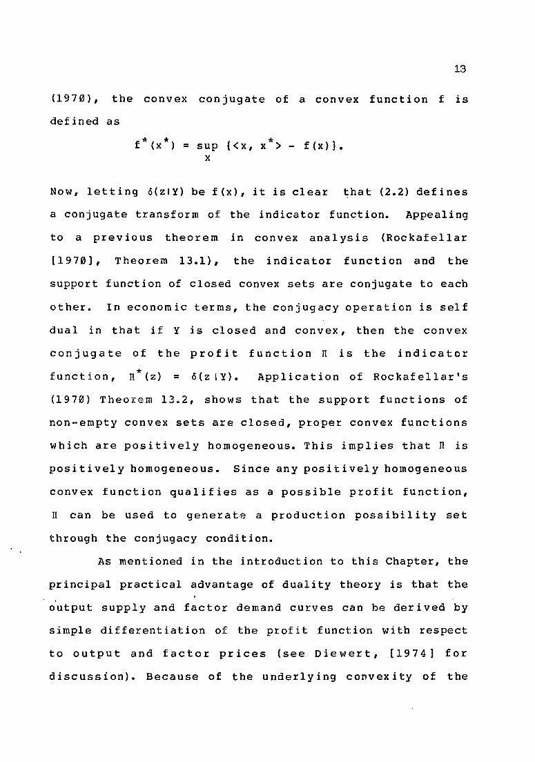
(1970), the convex conjugate of a convex function f is

defined as

* sup {<x, x > - f(x}}. x

Now, letting o(zIY) be f(x), it is clear ~hat (2.2) defines

a conjugate transform of the indicator function. Appealing

to a previous theorem in convex analysis (Rockafellar

[1970], Theorem 13.1), the indicator function and the

support function of closed convex sets are conjugate to each

other. In economic terms, the conjugacy operation is self

dual in that if Y is closed and convex, then the convex

conjugate of the profit function IT is the indicator

function, * IT (z) = o(zIY). Application of Rockafellar's

(1970) Theorem 13.2, shows that the support functions of

non-empty convex sets are closed, proper convex functions

which are positively homogeneous. This implies that IT is

positively homogeneous. Since any positively homogeneous

convex function qualifies as a possible profit function,

II can be used to generat,e a production possibility set

through the conjugacy condition.

As mentioned in the introduction to this Chapter, the

principal practical advantage of duality theory is that the .

output supply and factor demand curves can be derived by

simple differentiation of the profit function with respect

to output and factor prices (see Diewert, [1974] for

discussion). Because of the underlying convexity of the

14

profit function the subgradient sets of the profit function

are examined rather than the simple derivative.

The necessary first order conditions for optimality of

convex problems are characterized by the "subgradient"

inequality. A vector x* is said to be a subgradient of f at

* a point x if fez) > f(x) + <x ,z-x> for all z, i.e, the

graph of the affine function h(z) = f(x) + <x*,z-x> is a

non-vertical supporting hyperplane to the convex set epi(f)4

at the point (x,f(x». This relation is illustrated

geometrically in Figure 1.

Restating the subgradient inequality, the affine

approximation of function f at point x is allrlays less than

f. Therefore, the function f is at a global minimum at x if

o is an element of the subgradient set. In continuing with

the notation of Rockafellar (1970), the set of all

subgradients of f at x is denoted by af(x). If f is finite,

differentiable at x, the subgradient set consists of a

single unique element the gradient of f at x, Le., af (x) =

Vf(x) (see Rockafellar [1970], po 242).

It is necessary to consider a special case of

subgraaients, the subgradient set of an indicator function

of a convex set. * By definition, x e: atS(xIC), for C

and convex, if and only if

* 6(ZIC) > 6(xIC) + <x , z-x> for all z.

closed

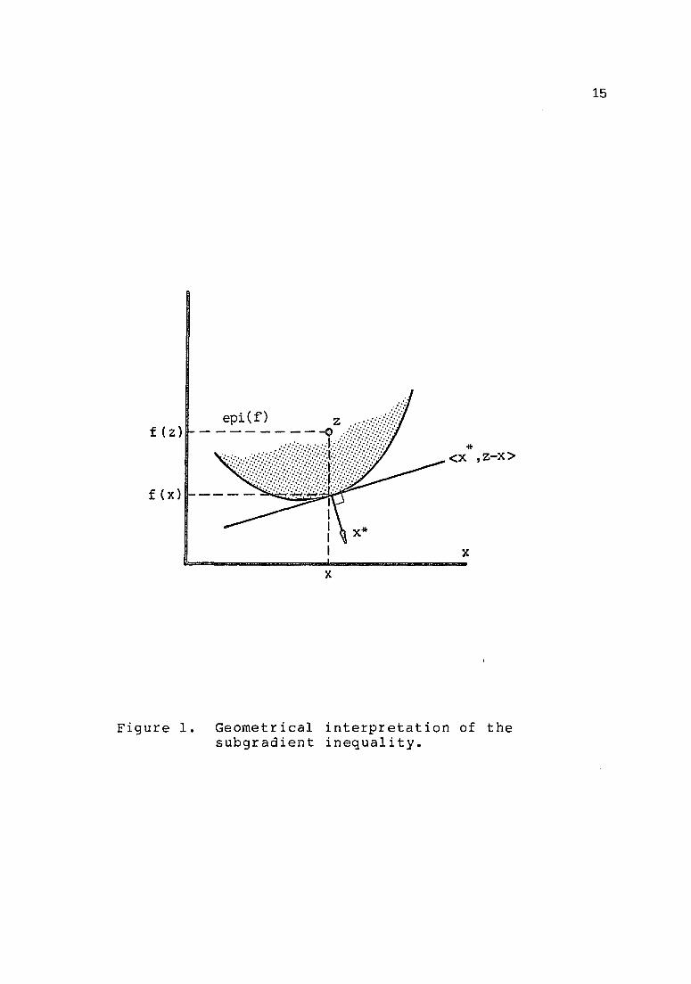
f (z)

* <x ,z-x>

f (x)

x x

Figure 1. Geometrical interpretation of the subgradient inequality.

15

16

This relation carries the following interpretation, for x E C

( '* )5 f . '* . 1 and 0 ~ x ,:r.-x or z E C, l .. e., that x 1S norma to C at

x. Therefore ao(xIC) is the normal cone at x and do(xIC) = 4>

for x (t C. Figure 2 gives simple geometrical representatives

of subgradient ~ets.

Without proof 6 , the subgradient sets of a closed

convex function are equivalent in that

x '1\: af(x) if and only if x.e: af*(x*).

Generalizing this relation to the profit function '* JI(z ) and

* its conjugate JI (z)

z*e: aJI*(z) if and only if z e: aJI(z*). (2.3)

* The multivalued mapping from z to z or equivalently the

supply and demand correspondences are given by subgradient

set of the profit function n • Further analysis of

equation (2.3) shows that since n*(z) = o(zIY), n* is the "

indicator function of the production possibility set Y. It

* * follows immediately that z e: a&(zIY) which implies that z

is in the normal cone to the production possibility set Y.

The relation * 'If Z e: an (z) is the first order optimality

condition for the profit maximization problem * n (z ) = sup z

{<z*,z> - cS(z p)}, i.e., z"" e; ~II*(Z) is equivalent to

"" z e: an(z).

7

nonr61 cone

af(x)

17

Figure 2. Geometrical representation of a subgradient set.

18

Cost Minimization

The cost function of the firm can be considered to be

a variant of the profit function. The cost function gives

the minimum cost of producing a given level of output y at

factor prices w. For the single output firm

C(w,y) = inf<w,x> such that f(x)~y. ]I

(2.4)

The economic behavior of the firm can be reduced to a two

stage process. First the firm chooses the cost minimizing

method of produc i ng output Y as descr ibed in (2.4). Second,

the profit maximizing level of output is determined

(P, w) = sup {Py - C(w,y)}. y

(2.5)

If the underlying production technology exhibits constant

returns to scale: profits may be unbounded. Suppose there

exists some (P,~) such that optimal profits are strictly

positive.

Pf (x) - <We x> = TI >0.

Now, suppose production is scaled by t, then profits are

P f (t x) - (w , t x) ~ t P f (x) - t ( w , x) = t TI > TI.

Thus profits are unbounded and no maximal profit point may

exist. Therefore, the only meaningful profit level for a

constant-returns-to-scale firm is that of zero profits, and

19

the profit function in (205) is identically zero. If the

firm is operating at zero profits, it is indifferent as to

the output level, and the firm level of output is determined

by industry demand. Once this level of output is

determined, the firm can be viewed as a cost minimizer with

respect to input selection, conditional upon output level.

The cost function defined in (2.4) is the central

focus in duality theory. The cost function completely

summarizes the production technology. Differentiation of

the cost fUnction with respect to input prices yields the

system of conditional factor demand functions (see Diewert

[1974], Shephard [1970]). These two powerful results make

the cost function especially appealing in applied

econometric analyses.

The constrained cost minimization problem of (2.4)

can be reformulated as an unconstrained minimization through

the introduction of the indicator function of the level sets

of the production technology. ~efine the input requirement

set V(y) for a single output firm as follows:

v ( y ) = {x £: R n + i f ( It ) ~y } •

V(y) is assumed to be a convex set which implies that

the function f is a quasiconcave production function.

Figure 3 illustrates the input requirement set for the two

...... ....... ....... ....... ........

Figure 3. Graphical illustration of the input requirement set for two inputs.

20

21

input cases. Further, define the indicator function of V(y)

by

{ o for x e: V(y) o(xIV(y» =

_00 for x It V(y).

Using the above indicator function, the constrained cost

minimizing function (2.4) can be rewritten in unconstrained

form as

C(w,y) = inf{(w,x) - o(xIV(y»}. x

(2.6)

Agair., 0(.) acts as a penalty on potential solutions not in

the feasible reg ions. When vie'r'led as a function of w

alone 8 , C(w,y) is the concave 9 support function, i.e., the

pointwise infimum of affine functions of the level set V(y)

of the function f. As a function is characterized up to a

monotonic transform by its level sets, knowledge of the cost

function is equivalent to knowledge of the underlying

production technology. The cost function as defined by

equation (2.6) gives the cor.respondence between the cost

function and the level sets of the production function. The

cost function is the concave conjugate of the indicator

function of the level set V(y), where the concave conjugate

of a concave function f is defined as

f*(x*)= inf{<x*,x> - f(x)}. x

22

A comparison of equation (2.6) and the above definition

shows that C(w,y) defines the concave conjugate transform of

the indicator function 6(x IV(y». In general the conjugate

operation over a closed set is self-dual, i.e., the concave

conjugate of the cost function is the indicator function.

Therefore C*(x,y) = ~(xIV(Y». In this case the conjugate

operation is performed with y fixed. By letting y vary,

and recalculating the conjugate '* c (x ,y) the indicator

functions of all level sets V(y) can be generated. Further

analysis shows that C is positively hornoge~eous and that any

positively homogeneous concave function is a viable

candidate for a cost function; C can be used to generate the

level sets of a production function.

Examination of the first order condition for the

generalized solution of (2.6) requires that optimal input

levels be selected so thatwEa6(xIV(y». A vector w is a

supergradient of V(y) at point x if and only if

o (z I V (y » ~ o( x I v (y » + (ttl, Z - x) for all z E V (y) •

The supergradient inequality reduces to (-w,z-x) ~ 0 for all

Z E V(y). This means that -w is normal to V(y) at x as

illustrated in Figure 4.

The supergradients of a closed, concave function and

its conjugate are dual as

t'J E ae'* (x I y) i fan don 1 y i f x £ a C (w I Y ) •

23

" ':':" .. :.: .... V( y) ":"

/ I ~ ":" ":'::'

/< " " ........... -w I "" <W·K>

Figure 4. The Generalized tangency solution.

24

Hence, x the factor demand correspondence condi t iona1 upon

output y is given by the supergradient set of C at x.

No assumptions regarding differentiability have been

made concerning either the profit function or the cost

function. If differentiability is assumed, the set of

subgradients is replaced by the gradient vector 'Vf and the

set of optimizers is replaced by unique values. For

example, the set of subgradients to C at w is replaced by

VC(w) and the set of cost minimizing factor demands becomes

unique. However, differentiability of the cost function

with respect to input prices is equivalent to strict

quasiconcavity10 of production functions (see Saijo (1983)

for discussion). The assumption of differentiability

determines the production structure.

Duality and the Regulated Firm

While duality theory was developed under the

assumption of an unregulated firm,

to the rate-of-return regulated

applicability (see Cowing (1983),

Waverman (1981) and Smith (1981)).

it has also been applied

firm without proof of

Diewert (1981), Fuss and

Fare and Logan (1983a)

establish a duality between cost and production functions

for a firm sUbject to rate-of-return regulation (see

Averch and Johnson (1962)).

Formalization of the rate-of-return constraint faced

by the regulated firm requires further notation. Let the

25

input vector of the production process be redefined to

indicate the single rate base input Xs

x = (x_s,x s )'

for x ~ Rk+. The corresponding input price vector is

W = (1I1_ s ' ws )

where W E Rk+ and Ws is the acquisition price for the single

rate base input. Again, P is the price of the single

output,. however it is now assumed to be a continuous

function of output, Le., P = P(y) where P is such that

total revenue is a nondecreasing function of output. The

rate-of-return constraint facing the regulated firm is

(2.7)

where ~ denotes the excess rate-of-return parameter. This

formulation constrains the cost minimization process

equivalently in both inpui and price spaces.

The corresponding set of input vectors meeting (2.7)

is given by

(2.8)

Fare and Logan (l983a) show that the rate-of-return

production function F(X,w,P,~) exists and that it can be

decomposed into two parts, namely the unregulated production

26

function, f(x) and the rate-of-return constraint, R(w,y,P,~)

f(x,w,P,~) ";: max {ye y I x £V(y) ()R(t"1,y,P,~)}

NOw, an input vector x is feasible for the rate-of-return

regulated firm producing single output y, if and only if x

belongs to input requirement set V(y) and the regulatory

constraint R(w,y,p,a) or equivalently

V(w,y,p,q) = V(y) () R(t"1,y"P,~) (2.9)

where V(lrJ,y,P,~) is the rate-of-return regulated input

requirement set.

The cost function under the rate-of-return

constraint is defined as

CR(W,y,p,ex) = min {wox I x ER{w,y,P,a)}. x

CR(W,y,P,c) represents the minimum cost for the rate-of­

return constraint to be satisfied independently of

technology. Now, the cost function of the regulated firm

can be defined as

C(t'l,y,P,a.) = min {l:I'X I Xc (V(y) () R(ltl,y,P,CX»} x

(2.10)

and represents. the miminum cost of producing output y

given w, P and ex where the technological constraint V(y) and

rate-of-return constraint R(w,y,p,a) are simultaneously

met. Equation (2.10) can be decomposed into the unregulated

27

cost function C(w,y) and the cost of satisfying the rate-

of-return constraint CR(w,y,p,a), but not necessarily as an

equality. The relationship is given (w,y,P,a)

C(w,y,p,a) > max {C(w,y), CR(w,y,p,a)}. (2.11)

Equation (2.11) is homogeneous of degree one in input and

output prices, and is not homogeneous of degree one in input

prices alone (see Cowing, (1981».

To show that equation (2.11) is not met with

equality consider the two input cases illustrated in Figure

5. I-I represents an isoquant for the unregulated firm.

The rate-of-return constraint is given by R-R, while the

shaded area represents the regulated input requirement set

V(w,y,P,a). For given prices (w,P) and excess rate-of-

return, the rate-of-return regulated cost minimum is * x •

The cost minimum for the unregulated firm is xc. The

minimum cost of satisfying only the rate-of-return

constraint is x R• Clearly, strict inequality of (2.11) can

hold and the rate-of-return technology does not have a dual

contingent, i.e., the decomposition of the F(x,l."J,P,a) into

the unregulated production f (x) and the rate-of-return

constraint R(w,y,p,a) does not have a similar counterpart

with re~pect to the rate-of-return regulated cost function

C(w,y,P,a).

Xl

R

\°::'::°::°:::::0::: V ( w ,Y , P ,ex. )

"(i:W~t:Mi-WL .. ~------------~~~------~2

Figure 5. Cost minimization for the regulated firm.

28

29

A more formal argument as to the lack 0= a dual

relationship for the rate-of-return regulated case proceeds

as follows. Define the following cost minimization:

d(y,x,P,a) = min {w x 1 C(w,y,P,a} > I} w

Define the following distance function, D(y,x,w,P,a), for

the rate-of-return regulated technology as follows:

D (y , x , l:1, P , a) = rna x { A I f (X / A, w, P , a) ~ y}.

To show duality between f(x/A ,wrp,a) and C(w,y,P,a), the

distance function d from the dual problem must equal the

distance function D from the primal. There can be no

direct duality between f(·) and C(·) as D(·) depends on w

and d does not. However, it is possible to reconstruct

f(·) from C(·) using the rate-of-return constraint. The

basic idea is to utilize the duality between C(w,y) and f(x)

and then to use the rate-of-return constraint to obtain the

rate-of-return regulated production function f(x,w,P,a) •

. Fare and Logan (1983a) prove in their propositions 3

and 4 that the rate-of-return regulated cost function,

C(lrJ,y,P r ().) has properties that allow derivation of the

unregulated cost function C(w,y) from C(w,y,P,o.}. Briefly,

proposition 3 says, by lowering the output price P, or

raising the excess rate-of-return regulator a, the rate-of-

return regulated cost function can be made to coincide with

the unregulated cost function. This is possible because

30

these changes to P or ex make the rate-of-return constraint

non-binding leaving only V{y) as the remaining constraint,

and C{w,y,~~ coincides with C{w,y). Propositiion 4 shows

that by minimizing C{w,y,P,a) over P or a yields

C(w,y) = min C(w,y,P,a) = min C{w,y,P,a). (2.12) P a

Therefore, given C{w,y,P, 'l) and the rate-of-return

constraining R{w,y,P, a), the unregulated cost function

C{w,y) is determined. Applying standard duality theory

yields the unregu1ative production f{x) from C{w,y). As the

regulated production function f{x,w,P,a) consists of the

unregulated production function f{x) and the rate-of-return

constraint f{x,w,Pva) can be reconstructed.

As a direct duality between rate-of-return,

regulated cost and production functions does not exist, it

fol1o~s that application of Shephard's Lemma is not correct

as Shephard's Lemma relies only on dual information. In

their continuing research, Fire and Logan (1983b) develop

the rate-of-return regulated version of Shephard's Lemma. In

brief, the rate-of-return constraint is formulated as in

equation (2.7). Exploiting the dual relationship between

the unregulated cost and distance function, C(w,y) and

D{y,x,), (Shephard, (1970» allows the use of 2.12 to be used

to prove a duality theorem equating the cost function

* C (w,y,P,a) obtained from dual information only, and the

31

rate-of-return constrained cost function C(w,y,P,a.). Now,

formulating a constrained optimization, the rate-of-return

constrained cost function C(w;y;P,a.) can be obtained as the

saddle point of a Lagrangean function after applying the

envelope theorem. Assuming differentiability of the cost

function allows the rate-of-re~urn regulated version of

Shephard's Lemma to be written as

x_ s = (1 - a.(C* - py)-1Ca.)-1Cw_s (2 .. 13a)

Xs = (1 - a. (1 + a. ) (C* - Py) -lCa ) -1cws (2.13b)

The Lagrangean function used in deriving the above

relationships is

D(y,x) is the distance function used in

proving duality between the unregulated cost and productions

(see Shephard (1970), Diewert (1982». Application of the

envelope theorem yields

Cw- s = (1 - AR)X_ s , (2.l4a)

Cws = (1 - (1 + a. ) AR)X S ' (2.l4b)

Cp = ARY, (2.l4c)

Ca. = - ARwsxs· (2.l4d)

32

The derivatives of L(·) with respect to AT and AR return the

constraints. Manipulation of (2.14) and the rate-of-return

constraint yields the rate-of-return version of Shephard's

Lemma as given in (2.13). Proceeding further, the A11en-

Uzawa substitution elasticity formulation must be

considered. Given the rate-of-return regulated version

(2.13) of Shephard's Lemma the partial elasticities of

substitution are derived as follows,

(2.15)

where Sj is the cost share of the jth factor upset and

£. . = a 1 nx . / a 1 nw . , 1J 1 J (2.16)

the price e~?sticity of factcr demand. Equat i on (2.15) can

be rewritten as

* a .. = (C /w·x.) (w·/x·)ax·/aw·, 1J J J J 1 1 J i = j. (2.17)

From ( 2 • 13), for i = j

From (2.17)

0·. = 1J

C*

(1 - U(C*- py)-lC~)-lCi (1 -

1(1 - a(c*- py)-lC~)-lC*i

- C*i(l - a(C* - py)-lC:)-2(C; a(C*- py)-2C*j

a(c * ) -1 * 1 - Py CCI~ J J

For i, j ;t s,

a .. = 1J

c*

C· C· 1 J

For j = s,

c* °sj = C* s C*j(l - u(C* - py)-lC~ )-1

(2.18)

[C*Sj - C*s (1 - u(l +a) (C*- py)-lc:)-l (1 +u) (C*- py)-l

33

Note that when the rate-of-return regulated cost function is

constrained to be consistent with an unregulated cost

minimizing objective function, Cu = CUi = 0 and the

expression reduces to the conventional Uzawa definition.

34

The duality theorem underlying the derivation of the

rate-of-returned version of Shephard's Lemma can use either

part of the equation (2.12) and the rate-of-return

constraint (2.8). The min properties of (2.12) are proved

by Fare and Logan (1983a). Derivation of analytic

expressions for the regulated cost function are very

difficult, even for the most simple forms of unregulated

cost and production functions (see Fare and Logan (1983a)

for example).

Approximation Theory

As mentioned previously most flexible functional

forms are intended to be second-order approximations to an

arbitrary function. Diewert (1974) defines f* to be a

second order approximation to f at Xo if

( i )

( i i ) * af /ax I = af/ax I (2.19)

(i i i) a2 f* /axax'l = a2 f/axax'(. x=xo x=xo

35

If (* possesses the above properties ll , then Diewert labels

f* a locally flexible functional form. The mathematical

definition12 of a second order local approximation is

* For f, a series expansion of f, f*-f would be the

remainder term. The above relation implies that the

numerator f* -f converges to zero faster than Ilx-x oU2•

Barnett (1983) notes that for twice continuously

differentiable functions this definition is equivalent to

Diewert's definition of a second order approximation of f at

.lI o • According to Lau (1974, p. 183),Christensen, Jorgenson

and Lau (1973; 1975) define a fUnction f*(x) to be a second-

order approximation to f(x) at xo'if

and I f * (x) - f '( x) ~ ~ K \I X' - x 0 11 3 i \I x 0 1\ 3 (2.20)

for all x in a prescribed neighborhood of Xo where K is a

constant for a given Xo and' 1'\,,11 13 denotes the Euclidean

norm operator~ The above definition says that the deviation

of the approximation f* from the true f is of third order

importance 14 • Barnett (1983) shows that while the

definition of flexibility of Diewert's is implied by Lau's,

the converse is not necessarily true. Any second-order

36

Taylor-series approximation satisfies both Diewert's and

Lau's definitions of a second order approximation.

The correct i nterpretat i on of a flex ible funct ional

form is that it is an approximation to the underlying true

function itself. Many properties of the true function are

not preserved under a Taylor series or a polynomial

expansion, therefore care must be taken in making inferences

about the true function from properties of the approximating

function. The first principle of choice is that a flexible

function form be capable of approximating an arbitrary

function to the desired degree of accuracy.

Flexible Functional Forms

It is common knowledge that optimizing behavior by

economic agents implies certain theoretical restrictions on

observed behavior. Therefore consistenc~7 is necessary

between these theoretical restrictions and the specified

functional forms used in applied work. Selection of a

functional form for production analysis requires that (i) it

be consistent with optimizing behavior, (ii) it is

sufficiently flexible to accommodate various technologies

and (iii) sufficiently simple so that existing econometric

techniques may be applied. In general, while economic

theory postulates specific behavior on the parts of agents

involved, it does not specify functional form. Considerable

37

attention has been given to the specification of flexible

functional forms for production and cost functions.

The Arrow, et al. (1961) Constant Elasticity of

substitution (CES) production function 15 generalized to k

inputs is

f(x) k

= [~Il' X .- p] -1 /p . 1 1 1 1=

One criteria of flexibility is whether a functional form is

consistent with an arbitrary set of sUbstitution

elasticities. The CES function form imposes the restriction

that the Allen-Uzawa 16 partial elasticities of sUbstitution

between any two pairs of inputs is constrained to be

constant across all possible pairs, aij = l/(l+p) for itj.

In most applied work it is unreasonable to impose a

restriction of this type, especially when the number of

inputs is greater than two.

Using the constancy of the elasticity of substitution

as a point of departure, Christens~nf Jorgenson and Lau

(1971) proposed the Translog (TL) functional form. The TL

functional form exhibits arbitrary elasticities of

substitution between pairs of inputs, and can be considered

to be a quadratic approximation in logarithms to the

production function at a particular point. The TL

production function for a single output with k inputs is

k k k 1 n( f (x» = Ilo + ~ i lnx i + (1/2):E i; i jInx ilnxj. (2.10)

i=l i=l j=l

38

The profit maximizing problem using the TL production

function can be solved yielding output share equations.

Without loss of generality let

Y=f(x)= exp[g(ln:)].

The profit maximization problem for the firm can be phrased

as k

rna x n = Poe x p [g (1 n x)] - .L. t<1 i xi. x 1=1

The necessary, first order conditions are

poexp[g(lnx)] .ag(lnx) .1 - wi = 0, i=l, ••• ,k a 1 nx i xi

rew'riting

ag(1nx) i=l, ••• ,k

a lnx i

where mi is the cost share of revenue. The TL form allows

the calculation of mi directly as

ag(1nx) = a' 1 +

k 2: a . ·1nx ., . 1 1) J J=

i=1, ••• ,k.

A translog cost function has been used extensively in

various applications (see the example Berndt and Wood

(1975), Christensen et ale (1976), Pindyck (1979), Nelson

39

and Wohar (1983) • A very general TL cost function

incorporating the possibility of technical change is

1 n C (w , y) = ex 0 + ex 0 n y + (l /2) Y yy ( 1 ny) 2 +

k k k + E ex·lnw· + (1/2) E E y. ·lnw·lnw· +

i=l 1 1 i=l j=l 1) 1 )

+ T t + Ie '" T· 1 nw· .i..J 1 1

1=1

where Inc (w, y) = logarithm of total costs,

Inw· = logarithm of factor price, 1

Iny = logarithm of output,

and t = time.

(2.22)

i=l, ••• ,k,

The TL cost function can be interpreted as a second order

approximation to an arbitrary twice-differentiable cost

function that places no a priori restrictions on the Allen

partial elasticities of sUbstitution. Note that (2.22) is

not dual to the trans log production technology as

represented by equat ion (2.21).

In order to correspond to a well-behaved production

function, the representative cost function must be

homogeneous of degree one in factor pricesl7 • This implies

40

the following relationships among the estimated parameters

of (2.11).

k

(l. 1 = 1

"y . = 0 i~t y1

k L:y .. = . 1 1) 1=

and n L T i = o. i=l

k k L L y .. = o.

i=l j=l 1J

Due to the equality of cross partial derivatives a further

symmetry condition is assumed corresponding to the

additional restriction that y .. = 1)

Y .. for all )1 i, j

combinations. A convenient feature of the TL cost function

representation is that the application of Shephard's lemma

yields the system of cost share equations.

S·= 1 k

.L 1=1

'* w·x· (w,y) 1 1 ..

for i=l, ••• ,k.

alnC(w,y) k = = (Ii + Yyilny + LYi)·lnw).

)=1

41

The Allen-Uzawa elasticities of substitution are

for i ~ j, i=l, ••• ,k

0 .. = (y .. + 8. 2-8')/8. 2 for i=J' 11 11 1 1 1

In the generalized form of the TL cost function,

incorporating technical change, the parameter T· 1

represents the technical change bias. That is, when

technical change is functionally dependent on the time trend

t, technical change is input i saving, input neutral or

input using according to Li less than, equal to or greater

than zero, respectively. Technical change is Hicks neutral

at a constant exponential rate

all i. 18

if Ti equals zero for

Homotheticity involves the restriction that Yyi

equal zero for each i, which implies independence of factor

share and the level of output producing a linear expansion

path. Constant returns to scale requires that Yyy be

restricted to equal one.

Diewert (1971) proposes an alternative to the

Translog fUnctional form for a cost function. This

functional form is a quadratic in the square roots of input

prices and is a generalization of the Leontief cost

function, and carries the property that it can attain any

set of partial elasticities of SUbstitution using a minimal

42

number of parameters. The Generalized Leontief (GL) cost

function can be written as

C(w,y} k k

= y [,L La" w ' 1/2 w J' 1/2 ] 1=1 j=1 1J 1

Application of Shephard's lemma yields the system of derived

demands

)~ = y '" 8, , w ,l/2w, -1/2

i~l 1 J J 1 i=l, ••• ,k.

The symmetry of 8ij = 13ji is used in the derivation of the

cost minimizing input bundle xi.

Berndt and Kha1ed (1979) nest the Generalized

Leontief and Generalized Square Root Quadratic (GSRQ) as

special cases and the Trans10g as a limiting case into the

Generalized Box-Cox (GBC) cost function. In the absence of

technical change, the nonhomothetic GBC cost function is

written as

where

G(w)

13(Y,W)

C(w,y} =[1+ G(W}]1/A ya(Y,w} (2.24)

k k k =a. + o L a 1'W 1' (A) + (1/2) " '\' 'YiJ,wi (;\}W J' (A),

i=l i~l ~1

k = 8 + (1/2}81ny + "ct>,1nw, ,i..J 1 1

1=1

= [w ~/ 2 - 1] / [A /2] 1

j=1, ••• ,k i

43

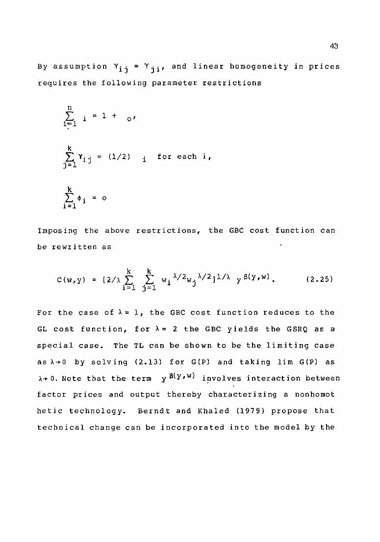
By assumption Yij = Yji , and linear homogeneity in prices

requires the following parameter restrictions

n " = 1 + .L..J i 0'

l't=l

k L y .. = (1/2) i for each i, . 1 1J J=

k L <1>. = 0 . 1 1=1

Imposing the above restrictions, the GBC cost function can

be rewritten as

(2.25)

For the case of A= 1, the GBC cost function reduces to the

GL cost function, for A= 2 the GBe yields the GSRQ as a

special case. The TL can be shown to be the limiting case

as A-+O by solving (2.13) for G(p) and taking lim G(p) as

A-+ O. Note that the term y a(y,w) i~vo1ves interaction between

factor prices and output thereby characterizing a nonhomot

hetic technology. Berndt and Khaled (1979) propose that

technical change can be incorporated into the model by the

44

addition of a multiplication term exp T(tvw) where

k T(t,ltl) = t(T+ " T·lnw·) .L- 1 1

i=l

and

C = [1 + G(w)]l/AyS(Y,w) eT(t,w).

The expressions for factor shares for the GBC cost

function are

S· = 1

w. A/ 2 [ 1

k

L j=l

y .. w. A/2] IJ J

k k A L ~ y .. w· /2 w. A/2 i=l ~l IJ 1 J

The Allen-Uzawa partial elasticities of substitution are

a .. = 1 - A + [Yo . (w·w·) A/2] C-A + FJ. (y,t) IJ IJ 1 J

SiSj Sj

Fj(y,t) 1 s· J

a .. = 1 - A + y.. w· C-A - + 11 11 1

s·2 1

+[1 - Fi(y,tll]

Si

Fi (y,t) +

S· 1

for i¢j,

~Fi(y,tl + [1 - Fi(y,tl]

S· s· 1 1

45

C where C =

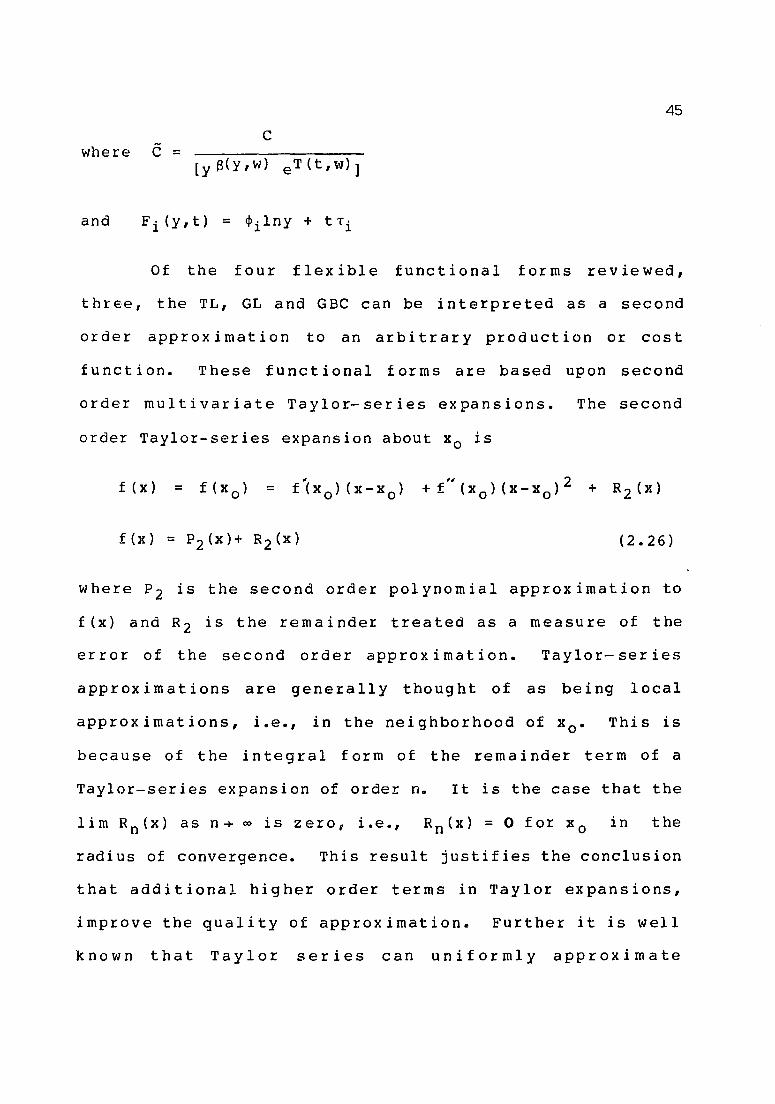
Of the four flexible functional forms reviewed,

three, the TL, GL and GBC can be interpreted as a second

order approximation to an arbitrary production or cost

function. These functional forms are based upon second

order multivariate Taylor-series expansions. The second

order Taylor-series expansion about Xo is

f (x) = =

(2.26)

where P2 is the second order polynomial approximation to

f(x) and R2 is the remainder treated as a measure of the

error of the second order approximation. Taylor- ser ies

approximations are generally thought of as being local

approx imations, Le., in the neighborhood of xo. This is

because of the integral form of the remainder term of a

Taylor-series expansion of order n. It is the case that the

lim R n (It) as n -+ 00 is z e r 0, i. e., R n (x) = 0 for x 0 in the

radius of convergence. This result justifies the conclusion

that additional higher order terms in Taylor expansions,

improve the quality of approximation. Further it is well

known that Taylor series can uniformly approximate

46

analytic l9 functions. A sequence of functions {f n (x)}

converges to f(x} if for each E. >0 there exists N(t:) such

that for n~N(E.)

I[f(x} - fn(x}11 <~

A Taylor-series expansion meets the above criteria (see

Levinson and Redheffer (l970), Theorem 3.4.), and is

therefore uniform.

It is implicit in Taylor's series that there e~ists

no singularities 20 • When singularities exist the Taylor

series approximations may be unstable in the neighborhood of

the singularity. Barnett (l983) argues that the smooth

functions postulated by economists may not be analytic.

Isolated singularities may exist and cause the Taylor series

approximation to behave poorly near the singularity.

Barnett proposes the Laurent series expansion be used as it

is applicable in situations where singularities exist. The

Laurent series

k fez) - ~ - LJ

n = ~oo An(z-a)n

conyerges uniformly to fez) in the perforated disk {z:z-zo

(see Levinson and Redhoffer (1970), Theorem

9.2, p. 164). This can be represented by an annulus bounded

by two concentric circles C I and C 2 such that fez) is

analytic in the annulus and at each point of C1 and C2 0

fez) may be singular at some points outside C1 and singular

47

at some points inside of C2• Figure 6 shows a graphical

interpretation.

Given the above situation the Laurent series can be

written in the form

where f 1 (z) has a Taylor-series expansion valid within a

circle with a as center and f2 has a series expansion in the

negat i ve powers of (z - a) val id except at z = a. The ser ies

converges and represents f (z) in the open annulus generated

by continuously increasing circle CI and decreasing C2 until

each of the two circles reaches a point where f (z) is

singular. The Laurent series expansion can be explicitly

written as

GO -1 f (z) = L bn (z -a) n +E cn(z-a)n. (2.27)

n=o n=-oo

Note that if fez) is analytic inside C2 ,the Laurent series

reduces to the Taylor series expansion of fez) with center

at a. If z = a is the only singular point of fez) in C2 ,

the Laurent expansion (2.16) converges for all z in CI ,

except at z = a 21 •

Barnett (1983) argues that a truncated Laurent series

expansion offers a more "well behaved" remainder term than

48

Figure 6. Graphical representation of a Laurent series.

49

the truncated Taylor-series. The remainder term of a

truncated Laurent series consists of two parts

R(z) = R1 (z) + R2 (Z)

where R1 (z) is the remainder of the Taylor series and R2 (Z)

is the remainder of the principal part. Barnett postulates

that R1 (Z) and R2 {z) offset each other as z varies resulting

in a remainder term with a low variability relative to R1 {Z)

alone. However, this argument for using the Laurent series

does r.ot follow from theoretical justifications but is

empirically based. While it may be the case for specific

classes of functions, it does not hold universally. The

strength of the Laurent series is its ability to approximate

functions in neighborhoods of singularities, not in the

remainder term of a truncated series.

The Laurent series expansion of the Trans10g cost

function is

k + l: a·1nw· + . 1 1 1 1=

k 1 l: B· (1 nw . ) -.11

1=1

35

k k

k .~Yyi1nY1nwi 1=1

~ ~ y. ·1 nw· 1 nw . i=l j=l 1J 1 )

(2. 28)

50

Appealing to Shephard's Lemma,the system of cost shares is

k S i = ex i + Y y i 1 ny + ,L Y i jl nw i + f\ (1/1 nw i 2 )

J=l

i=l, ••• ,k.

The Laurent system of factor shares nearly doubles the

number of parameters compared with theTL and requires further

restriction of the coefficients prior to estimation.

The functional forms based upon second-order

approximations can uniformly approximate an unknown analytic

function but not its derivatives. In general, the desired

outcome of empirical demand studies is meant to be a set of

estimated elasticities, either price or sUbstitution

elasticities. 'llhese are derived as partial derivatives of

the unknown function, a profit or cost function in the case

of input demand for a cost minimizing producer.

Elasticities are transformations of partial derivatives

which express the curvature of the unknown function in

dimensionless terms. Second-order approximation does not

provide approximation of higher order derivatives, but only

of the unknown fUnction that is twice continuously

differentiable, i.e., the notion of the remainder term

incorporates only errors of approximation of the unknown

function, not its derivatives.

51

Starting from first principles, consider the errors

in the approximation of the true cost function f(x) by a

flexible functional form f(xle). The error-sum-of-squares

If(x I.e) - f(x) I 2 from fitting n data points is driven to

zero; however, the fit is perfect only if the true

disturbance term is indentically zero for every observation.

Clearly, the nth-order approximation does not necessarily

approximate the second order derivatives with zero error.

This Euclidean measure of distance does not lead to a

r'eliable approximation of derivatives. Gallant (1981),

suggests that the Sobolev norm is the appropriate measure of

distance. The Sobolev measure of the distance of an

approximating function g(x) from the true function g*(x) is

1Ig'(X)~g(X) m,P,H

= J A * 10 9 (x) H

oft

11.1 ~m

The integer m is the number of times that * 9 is

differentiable, A the mUlti-index of differentation and H is.

the reg ion 0 f a p pro x i mat ion.o The Sobolev measure of

distance is large whenever oAg* - oAg is large, f~r any

index A. The real number p represents the Lp norm for which

approximation of the function. and its derLvatives are

achieved. The Sobolev norm is a measure of distance between

* 9 (x) and g(x) which takes derivatives into account.

Gallant (1981) shows that the expansion of an unknot<ln

52

function in a Fourier series will approximate closely in the

Sobolev measure of distance.

Given the region of approximation H and the

unknown function g(x) defined over the closure of H, H for

some E >0 the flex ible functional form gK should be able to T

achieve· approximation such that

S A * A P 10 9 (x) - 0 g(x)ldu (E for

·H

and A * A 10 9 (x) - 0 gK(x)1 (E for all x in H, T

where u(x) is a continuous probability distribution defined

on H giving the relative frequency with which data in the

sample span H are observed as sample size tends to infinity

(Gallant and Holly (1980». KT denotes the number of

parameters as a function of sample si ze T in 9 (x). In

general, this should hold up to and include second-order

derivatives, as higher order derivatives are not relevant in

most economic studies. Gallant (1981, p. 218) cites a

previous result of Edmonds and Mascatelli (1977)22 which

shows that a Fourier series expansion has the ability to

approximate an unknown function as closely as derived in

Sobolev norm. For m>2, and for

<I> k (x ) = e i k'x

a typical element of a Fourier series, there exists a

sequence of coefficients {ak} such that

1 im II f - 2: ak <Pk II = 0, ¥ P , 1 <P< 00 •

K -+ ro m-l,P,H Ik I*<K

The sequence of coefficients does not depend on P. The

above result motiva~es the use of a series expansion of the

form ,

= L a e ikx I k I * <K k

achieving close approximation of a function f in Solobev

norm. Note that the representation of f by the Fourier

series improves in quality as more terms are added to the

approximating series so that the Solobev measure of the

approximating error can be made arbitrarily small. The

Fourier form achieves closer and closer approximation in the

Sobolev sense as more parameters are added. This leads to

unbiased tests of hypothesis {Gallant (1982») and consistent

estimate of elasticities (El Badawi, Gallant and Souza

( 1 9 83 »). W h i lea d d i t ion alp a ram e t e r s can be add eat 0 0 the r

flexibly functional forms as well, there is no assurance

that additional parameters improve approximation of

derivatives as is the case with the Fourier form.

The theory of the firm implies restrictions or

plausible hypotheses upon the functional form of the cost

function, such as positive linear homogeneity of factor

prices, constant returns to scale, homotheticity,

53

54

monotonicity and concavity. Equivalent conditions can be

imposed on the logarithmic transformation of the cost

function 23 As the standard cost function C(w) is the

minimum cost of producing output level y, the use of

Shephard's Lemma allows for the determination of the

conditional factor demands

Further

Xi = aC(w,y)/awi

= Cia

differentiation of

elasticity of substitution"

C· 1

a .. 1J

C· C. 1 J

a .. (w,y) 1J

allows determination of

and the constant output price elasticity

T) . • = a.. s· = TJ· • (w, y) 1J 1) 1 1J

\

where Sj is the cost share of input j. In applied work it

is the estimation of the substitution and price elasticities

that are of interest. These elasticities have equivalent

expressions for logarithmic values of factor prices and

output. Consider the log transformation of prices and

output and define

Ii = lnwi + lnai >0, i = l, ••• ,k,

and v = lny + lna y >0.

55

The In a's are location parameters used to insure that all

logged prices are positive and carry the interpretation of

chang ing the dimensional units of quantity, Le., a change

from pounds to kilograms. Taking anti-logs and solving for

factor price and output yields

l' W. = ella. i = 1, ••• ,k

1 1

Y = e v lay.

The cost function can be written as

Application of Shephard's Lemma yields

aC(t-!, y) C(t<1.Y)W-J. \1g =

aT;]

and a 2 C(w, y) W- l [V 2g diag \1g]w- l ,

= C(w, y) + \1gVg -awaw

,

for V g = a 9 ( 1, v) I aI, V 2 9 = a 2 g ( 1, v) I a 1 a l' and

ttl = diag (t:1).

The vector of factor shares becomes

s = agel, v)/al •

The elasticities of substitution are the elements of

56

and the vector price elasticities as

11 = ~diag ('\]g) •

In application it is the share equations that are

fitted to data to recover information about the underlying

parameter structure. Approximation of the true cost

function g(l,v) is desired over a rectangle in the positive

orthant of R(k+l) whose size is at the discretion of the

researcher. Once the size is determined, the rectangle must

be rescaled so that no edge is longer than 21. as the

Fourier Form is periodic in prices 24 • The location of the

positive orthant by choice of ai is only for convenience as

any shift in location is absorbed in the magnitude of the

coefficients. It is critical that the rescaled rectangle

have no edge greater than 2rr •

Before proceeding further, it is necessary to

introduce the concept of a mUlti-index. A mUlti-index is an

n-vector with integer 00mponents.

whose norm is defined as

57

For example for k = (1, 2, 3), lit \* = 6. A multi-index can

be used in denoting partial differentiation. Let A be a

multi-index with non-negative componen~s.

diffe~entiation of a function f(x) is written as

Ihl* Cl

= ------------------ f (x) •

The part ial

For example, ~ = (1, 2, 3) yields the si xth-order partial

derivative

= 6

d ""xl 2 3 f(x). o 1 ax 2 ax 3

Multi-indices provide a convenient way to express a

multivariate Fourier series. A typical element of a

multivariate Fourier series would be

e i k'x = cos (klx) + i sin ( klx ) •

Fo r k = (1, 2, 3),

Now a mUltivariate Fourier series expansion of order K can

be written as

L ak eiklx

•

Ikl* < K

58

The conventional multivariate Fourier series can be

re-expressed as a double sum after taking into account

complex conjugates. This requires a restructuring of the

multi-indices according to a set of simple ruleso In

summary, it can be shown that the multivariate FouI'ier

series of order K can be expressed as

A J

L: a=l

.E )=-J

A J = L {lloa+ 2L [UjaCOS(jk'aX) - vjaisin(jk~X)]}

0.=1 j=l

for suitably chosen values of A, J and the multi-index. See

Gallant (1982) and Monahan (1981) for complete details.

The general form of the Fourier flexible form used as

an approximation to the true cost function g is

A J = a o + bx + (1/2) xtx + L .2:

a=l )=-J

59

and a o ' aoe. and b are real valued. Noting that ei~= cos~ +

isin~ , the above expansion can be rewritten as

, a o + bx + (1/2) xCx

The derivatives of gK (xIG) are o T

and

The scaling ~actor As is used to keep all xi within the

internal (0, 2~). The parameter vector of the logarithmic

Fourier cost function gK (x 19) is T

a = 1, ••• ,A; j = 1, ••• ,J

and has nominal length 1 + (k + 1) + A(l + 2J) prior to

60

restrictions on positive homogeneity in prices. Homogeneity

k imposes the restriction L b. = 1.

i=l 1 This nonhomogeneous

restriction reduces the number of nominal parameters by one

as b· = 1 J

k -~ b·.

. 1 1 1= Homogeneity also places restrictions upon

the coefficients Uja and Vga depending upon the mUlti-index

as follows k

if ~ki '* 0, a= 1, ••• , A. i=l

The remaining restrictions imposed by positive homogeneity

follow from compariso(l 'of the matrix C from the quadratic

portion and the Fourier expansions along k a • The symetric

matrix C is overparameterized compared to the A parameters

of the Four ier expans ion. Therefore, the effective number

of parameters is less than 1 + (k + I} + A(l + 2J).

The econometric specification of input demand

systems cannot rely solely upon approximation error as the

source of randomness. The statistical distribution of

factor demand must consider the fundamental sources of

uncertainty facing the firm. In the next chapter the

possible sources of uncertainty, as viewed by the firm, and

the consequences of these random factors on the stochastic

specification on cost and production functions are examined.

61

Summary

Exploitation of deterministic duality theory allows

explorati~n of the relationship of cost and production

functions of the firm. This dual relationship is developed

using simple geometric concepts from convex analysis.

Further, the argument for using flexible functional forms is

developed prior to leading into a review of the functional

forms generally used in empirical applications. The Fourier

flexible form is reviewed as an alternative to the Taylor

series approximation.

CHAPTER 3

STOCHASTIC SPECIFICATION OF COST AND PRODUCTION FUNCTIONS

Th i s chapter introduces stochast i c spec i f icat ion of

production and cost relationships. As most firms are unable

to fully control all aspects of the production process, the

individual firm must purchase inputs and sell output in

markets subject to random fluctuations in supply and demand.

In Chapter 1 the problem of the firm was analyzed under

perfect certainty and the corresponding output supply and

input demand are derived as deterministic functions of

pr ices. In this chapter the problem of the firm is analyzed

recognizing the impact of uncertainty in the firm's decision

process.

Uncertainty

The modeling of the firm under uncertainty is crucial

in the analysis and development of the appropriate

econometric model. The statistical model must recognize

factors beyond the firm's control which impact the production

decisions of the firm. The model must be able to distinguish

between sources of uncertainty and sources of statistical

error. The traditional interpretation of an error term

follows from the divergence between the information set of

the firm and the econometrician. The observable information

62

63

used by the econometrician is almost always a proper subset

of the firm's information set.

The sources of uncertainty for the can be

grouped into two basic categories.

i) Output price variability. The output price during

the production period may not be known with

certainty.

ii) Optimization errors. The firm may utilize sub­

optimal input-output combinations as part of the

managerial decision.

The category of uncertainty encountered by the practicing

econometrician depends in large part upon what are the areas

of focus. If attention is focused on the production function

and estimates of the underlying parameters, then output

price variability is of major importance. As soon as the

first order conditions for profit maximization are

considered, output price and factor price variability must be

reviewed carefully. Early work by Zellner, Kmenta and Dreze

(1966) recognized the impact of a stochastic price

specification upon the necessary first order conditions.

-----------B-tv.:h-u-st-i c Spe c i fica t i on

The most common, almost standard procedure is to

append a multiplicative error to a deterministic production

function as y = f(x)£. Again x is a (kxl) vector of inputs

and £ is a well behaved error. Often £ is assumed to be

64

log-normally distributed. This assumption facilitates the

common log-linear form of estimation leading to the

interpretation that E: represents factor neutral sources of

variation of the marginal products of all inputs. Just and

Pope (1978) focus on the use of multiplicative error

structures and the underlying implications on the firm.

Just and Pope argue that the multiplicative error places

implausible restrictions on the behavior of the firm towards

risk.

Just and Pope begin their analysis by setting out

eight postulates that they believe give reasonable a priori

specifications that stochastic production functions should

meet. Postulates one, two and three are essentially the

deterministic concepts of positive output, positive marginal

product and diminishing marginal product rewritten to

accommodate the concept of expected output. They hinge

their analysis on postulates four, five and six. These

postulates are germane to their argument:

Postulate 4. A change in the variance of random

components in production should not necessarily imply a

change in expected output when all production factors are

held fixed [3E(y)/3Var(E:) = 0 should be possible]. It might

be the case that error variance behaves like a factor of

production in output expectations.

65

Postulate 5. Increasing, decreasing or constant

marginal risk should all be possibilities [aVar(y)/axi ~ "] < All three possibilities should exist depending upon

input. For example, irrigation could possibly reduce the

variance of production whereas dronght would possibly

increase the variance.

Postulate 6. A change in risk should not

necessarily lead to a change in factor use for a risk­

neutral (profit maximizing) producer [axi*/avar(e:) = 0 is

possible where xi* is the optimal input level]. This can be

restated that a change in risk does not affect the behavior

of a risk-neutral producer [Arrow (1971)]. Postulates 7 and

8 concern the variability of marginal product and constant

return to scal~ respectively.

Just and Pope argue that a multiplicative error

specification violates Postulate 6. Under the assumption

that e: be distributed log normally2

2 It can be easily shown that E(y)e:= f(x)E(e U) = f(x)e(1/2) a

[see Aitchison and Brown, (1957)], i.e., mean output is a

function of 0 2 • NOw, the firm is assumed to maximize

expected profits with known output and factor prices

max E[Pof(x)e u - ~.x] It

66

where Po is output price and w is a vector of input prices.

The resulting first order conditions of the above

maximization are

\1f ( x)

where Vf(x) is the vector of first derivatives fie

Differentiation of the first-order conditions

* * P -le- (1/2) a 2

Cl Vf (x ).~ = -1 'ttl 0

ax aa 2 2

P -1 G-1e -(1/2)a 2

* 11L = -1 \'1 >0, aa 2 2

0

assuming concavity of f and complementarity of all factors,

* where x is the vector of optimal inputs and G is the

appropriate Hessian matrixc Therefore, an increase in 0 2

will increase the utilization of all factors and it appears

that the assumption of risk neutrality of Postulate 6 is

violated.

This result, ~owever, is in contrast with the earlier

work of Rothschild and Stiglitz (1970).3 Rothschild and

Stiglitz argue that the concept of increasing risk is not

equivalent to that implied by equating the risk of a random

var iable X with the var iance of X. Whi Ie Just and Pope show

that an increase in variance changes the utilization of

inputs as ax*/aa 2 >0, it can be shown that it is possible to

alter the variance of output, Var(y), without changing the

67

mean level of output. It follows directly that Var(y) =

2 o - e ) and

However, Rothschild and Stiglitz illustrate that it is

possible to shift probability weights from the center to the

tails in such a way as to leave the mean unchanged. Their

argument is as follows: consider two random variables X and

Y with cumulative distribution functions F and G. Let Sex) =

G(x) - F(x), and f and g be the density functions of F and G

res pee t i vel y. It follow s t hat for g ( x ) ~ 0 f or a 11 x, g is a

density function with the same mean as f.

For g = f + s then

1 1 1 J g(x)dx = o

J f(x)dx + J s(x)dx = 1

and 1 J xg(x)dx o

o 0

1 = f x[f(x) + s(x)]dx

o

1 = f xf(x)dx.

o

1 1 since J s(x)dx = J xs(x)dx = 0 for all xe[O,1]4

o 0

Adding a function like s to f shifts probability weight from

the center to the tails. The function s = g - f is labeled

a mean preserving spread. If a non-zero location parameter

is included in the log-normal distribution, it is possible

68

to de fin e a mea n pre s e r v in g s pre ad. Now a E (y) / aVa r (y) = 0

and Postulate 6 is satisfied, Le, the multiplicative error

specification y ::: f(x)e u does satisfy Postulate 6 \<1hen

appropriate care is taken regarding the definition of risk.

Postulate 5 allows for the possibility of increasing,

decreasing or constant marginal risk. The traditional

multiplicative log-normal error specification violates

Postulate 5 as

Var(y) = f(x)2 var (£)

and a Va r (y) / a x i = 2 f (x) f i( x) Va r (£) > o.

This says that increased use of an input increases the

variance of output. This seems counter to a priori reasoning

as certainly some inputs are thought to be variance reducing.

For example, the use of irrigation would nave a negative

effect on the variance of agricultural output attributable to

weather. So clearly, the mul t ipl icat i ve error spec if icat ion

imposes a restriction on the input-output relationship in

that risk reducing inputs cannot be properly reflected.

Additional focus has to be placed on the additive

error specification, y = f (x) + £. This ;5pecification

imposes the restriction that the variance of output is

independent of the level of input utilization. The basic

difference between the multiplicative and additive error

structure is in the coefficient of variation, CV = (standard

69

deviation of y}/E(y}. For the multiplicative case, CV = [f(x}oe/f(x)ue] = o .. /ue which is independent of the level

of input. For the additive specification, CV = ~/f(x},

i.e., the CV is inversely proportional to input levels.

Expected Profit Maximization

It will be assumed that the objective of the firm is

to maximize the expected utility of profits

max E{U(n)} = U[Poy - C(y}] (3.1)

The necessary and sufficient conditions for a maximum are

E[U'(n*) (Po ,

C(y})] = 0 (3.2)

" * C'(y} ) U'( n*} C'(y}] and E[u(n ) (Po - - < 0 (3.3)

where n* P of (x * , e ) w'x * * is the of optimal = - ,x vector

inputs and U is the Von Neumann-Morgenstern' utility function

of the firm. Under the assumption of risk neutrality5, d'= 0

and equation (2=3) reduces to * '* - u(n )C(x )<0 as u' > o.

Further analysis will focus on the risk-neutral firm facing

random production as well as output and factor price

uncertainty.

Letting y =f(x)e= exp[g(lnx}]e the profit maximization

relation consistent with risk neutrality ~ written as

max E (n) = E [ (P of (x) e- t'l'x}] x

= E [poexp (g (lnx}}e - {'I' x]

= exp(g(lnx})E(poe) ,

- E(t:J)x.

70

, = exp(g(lnx))E(l?oe:) - E(t·l)lC.

The resulting first order conditions are

exp(g(lnx))Vg(3Inx/3x)E(P Oe:) = E(w).

It is necessary to consider the relationship of Po and e:

If e: represents a firm specific exogenous shock 6 to the

production process it is reasonable to assume independence of

Po and e: and E(Poe:) = E(Po)E(e:). It is also reasonable to

assume independence of output price Po and factor prices w as

the industry is considered to be competitive. The necessary

conditions can be rewritten as

x· 1

E(PO

) exp(g(lnx)) =

3g

3lnxi E(e:) i = l, ... ,k

sin c e 3 I n x /3 xi': 1/ xi. Determining expected values and

using the relation that y = exp[g(lnx)] e: , the first

order conditions can be rewritten as?

• x· 1

exp(g(1nx)) =

Since profits are assumed

= 3g --- • E(e:)/e:Vi

alnx i

(3.4)

= y .• 1

random with mean zero, Yi is

not identical to the factor share of the ith input. Taking

logarithms of (3.4) and substituting y. for (w.x.)/(P y) yields 1. 1.1. 0

(3.5)

71

Consider the Translog production function for a

single output. k k k

g(ln(x» = a o + La.·lnx. + (l/2) LEa. ·lnx·lnx·. i=11 1 i=l j=11) 1 )

The resulting output share of the ith input Yi = og/olnxi =

k a. + Ea.· .lnx·. The

1 . 1 1) ) )=

traditional analysi~ specifies a

muitiplicative log-normal error for the production function

together with an additive error structure for the output

share equations:

k Y· = ex. + }a··lnx. + e: 1·, 1 1 j:l 1) J

i=l, ••• ,k.

Clearly, the error structure of (3.6) is not internally

consistent. If a multiplicative production errorS is

specified y = f(x)e: the output share equations are log-

linear as shown in (3.5).

It has been assumed that Po and e: are independent.

However, if this assumption is relaxed, it is equivalent to

acknowledging that there can be aggregate shocks to the

industry which affect all firms. If prices are such that the

output market clears, the equilibrium output price will

depend upon demand and production. The equilibrium will be

72

defined by a pair of equilibrium price and output

distributions. However, in a stochastic model it is not

possible to define an industry supply curve. Consider an

industry consisting of n identical firms each producing

with a single input Cobb-Douglas production technology and

facing a constant elastic inverse demand curve.

where £ = ell (3.7)

and (3.8)

Note that in the above model, equilibrium price is a function

The firm is assumed to

maximize expected profits '\

max E ( II x

The resulting first order condition is

or

Xa - 1 ell] = WI,.. I ......

2 Taking expected values and noting that E(e ll ) = e(1/2)a yields

2 1 : x * = [ ( w / cd e - (1/2 ) a (1-13) ] ( - as + a -1 )

when * x is the optimal level of input x. Correspondingly,

73

Clearly, a supply function cannot be defined for the case

because of the stochastic element,

* y ( *)0. 11 = X e

* for x as defined above.

The Specification of a Cost Function

The traditional cost function is defined as the

minimum cost of producing a given level of output given

factor prices. Under the assumption of stochastic output it

is difficult to support the traditional definition of a cost

function. It is more the case that the firm sets some level

of inputs and chooses from a set of output distibutions. The

underlying assumption of the firm is to maximize expected

profits

rna x E ( IT) = E [ Po f (x) e: - w' x] • x

In order to define a cost function that takes the stochastic

elements of output and factor prices into account, it is

necessary to understand the decision making process of the

firm. The underlying tenet is that inputs are selected on

the basis of expected output and expected factor prices.

Define the sto~hastic cost function Cs(we,ye) as the minimum

expected cost of producing dn expected output level ye.

74

The profit maximization relation is now

(3.9)

where ye = E[f(x}€].

Assuming that the stochastic cost function es(we,ye}

can be defined, the system of conditional factor demands can

be derived from the application of Shephard's Lemma.

e x· = ae s (we ,ye) / aE (w i) i=l, ••• , k (3.10) 1

for y = ye + Uo

w = E (w) + v

Uo = y - ye

= f(x}€ - f(x}E(€}

= f (x) ( € - E(€)}.

The defined relationships between observed output, inputs and

factor prices are subject to the standard errors in variable

interpretation. If the mean value of the production

technology exhibits constant returns to scale, the cost

function is linearly separable in output, es(we,ye}

y e e(w e }9. If E(t-l) = Ttl, i.e, factor prices are known when

75

input decisions are ~ade,

c*(w,ye>= yec*(w)

* = (y- uo ) c (w)

* = yC (w)

* = yC (w)

The error structure is now heteroscedastic as cov(Uo ) =

E(yC*(w) - C*)2 and the variance-covariance matrix contains

parameters of the cost function. If the model is

multiplicative, y = ye U o implies C* = yC*(\,l)UO which is

* * linear in logs as InC = lny + InC ("J) + In u o ' which

resolves the heteroscedastic problem.

The traditional procedure followed by most econometricians

is to postulate a specific cost function C(w,y) and apply

Shephard's Lemma to obtain a system of conditional factor

demand equations and append an additive error term

'. (3.11)

This additive stochastic specification is equivalent to

E (trl) +v

for linear conditional demands satisfying

* x· 1

k = a. + :Ea. ·E(w·)

1 . 1 1) ) )=

w,y

= a. 1

= CX. 1

k + L, cxi": (wJ.-v J.) · 1 .J J=

k + 2: cx .. w. -

· 1 1 J J J=

k + La.··w.

· 1 1 J J J=

k L:CL.V' . 1 1 J J J=

76

where ui = The regressors are correlated with

the error term and the ordinary least squares estimators

are inconsistent.

The specification of additive errors can be justified

by arguing that the information available to the

econometrician and the producing firm concerning the

production technology is not identical. This view is held by

MacElroy (1981}. The production function is formulated as

(3.12)

where e: =(e: 1 , e 2 , ••• , e: k ) and e:o are known to the firm, but

remain unobserved in general. In the above

specification output y and inputs Xi' i = 1, ••• ,k are

stochastic. The corresponding dual stochastic cost function

is

(3.13)

77

where C(w, y-£o) is the deterministic dual to the production

function as defined above, and lrl'£ isa linear combination of

the observational errors. The system of conditional factor

demands again follow from Shephard's Lemma

(3.14)

However, if a firm faces production or price uncertainty, a

measurement error argument as developed by MacElroy is not a

valid response to the commonly used additive error

specification.

Distribution of Output and Cost Shares

Earlier, the system of output shares consistent with

the firm's maximization of profits under uncertainty was

derived as

where y. 1 = It

, i = l, ••• ,k,

is first nece s s a-r y to

understand some basic concepts before preceeding with any

statistical analysis. First, output shares are always

positive and since output is assumed stochastic the mass of

the distribution is concentrated on the (0,1) interval.

Second, as the industry is assumed to be competitive, that

is, the firm cannot affect output or input price

distributions, free entry ensures zero expected profits in

10 the long run. However, the actual profit level may be

78

positive, negative or zero. Third, the adding up constraint k L Yi = 1 cannot be imposed as in general total revenue does i=l

not equal total cost, as profits are not in general equal to

zero.

In much applied work the investigator derives a

deterministic system of output shares and then appends an

additive multivariate normal error term. For example, for

the three input case the resulting system is

(3.15a)

(3.15b)

(3.15c)

where e:: = and i = 1, 2, 3 is a (e:: 1 ,e:: 2 ,e:: 3 ),

vector of parameters. Imposition of the deterministic

3 adding up constraint L Yi = 1 results in a system of output

i=l

shares that is singular, Le., knowing any (k-1) of the

k output shares leads to Yk = 1 -L:

j=l It is necessary to

to drop one of the share equations prior to estimation. Jf

output is stochastic, the adding up constraint is only

approximately satisfied. Further, the use of a mUltivariate

normal di str ibut i on is i nconsi stent with boundedness of an

output share, O~Yi~l. As the normal distribution is defined

79

from - 00 to +00 , there is a positive probability that

shares be outside the interval [0,1]. Also, use of the

normal distribution implies that the covariance matrix for

each observation is the same and that the distribution of

the shares is symmetric about the mean. Further, additive

errors are not consistent with a multiplicative error

specification in the production function.

The distributional problems associated with the use

of an additive multivariate normal error structure has been

explored by Woodland (1979). Woodland proposes the use of

the Dirichlet distribution defined over the (k-1)

dimensional simplex,

The Dirichlet distribution is a mUltivariate generalization

of the Beta distribution which automaticlly constrains the

shares to lie on the (k-1) dimensional unit simplex. The

Dirichlet density function for (Y l , ••• , Yk - l ) is

where Yk = k-l

1 - L Y i , (al, ••• ,a m) is a vector of parameters i=l

such that ai ~ 0, f(.) is the gamma function and (Y 1 , ••• ,Y k)

is constrained to the (k-1) dimensional unit simplex. The

marginal distributions of the Dirichlet are Beta

80

distributions, and the distribution of Yk is also Beta. A

useful property of the Dirichlet distribution is that the

expectation of the ith share is precisely the ith

deterministic share.

k E(Yil x) = Y i (x \ Bi) I 2: Y·(x\8·) i = 1, ••• , k

j=l 1 1

and that E. = y. - Yi (X\8) has zero expectation. The 1 1

variances and co var iances between the k shares are

a. . ::; - a . a . / (a 2 ( a + 1)) = - Y . Y . / M (z 1J 1 J 0 0 1 J 0

+ 1), i.t:j, i, j=l, ••• ,k

k k k where a o = 2:a. = M(2:z.) =

i=l 1 i=l 1 MZo and Zo = 2: zi for z. = a·/n.

i=l 1. 1.

M is a "variance parameter": the larger M the smaller are

the elements of the covariance matrix. Note tha t the

covariance terms are all non positive and that since the

shares sum to one the covariance for any share equation

system must satisfy

k

.2:. (1 i j = -1=J

a . . < o. 11

k

.2: 1=1

a· . 1J

= 0 for all i and therefore

Clearly this imposes restrictions on the

economic content of the variance, covariance matrix. Note

that in general, if it is assumed that if the firm maximizes

expected profits under uncertainty

The expectation of output share Yi

E(Y i ) = E(c) [ ag/alnxi]E(l/£Vi)

= ag/alnx i [E (E) E (l/E vi)]

= ag/alnxi only if E(t:)E(l/Evi) = 1,

81

i.e., with uncertainty the expectation of output share is

equal to the deterministic output share only under certain

situations.

An alternative to the Dirichlet distribution would be

to take logarithms of both sides of

i = l, ... ,k.

yielding

= k + In(ag/alnxi) + vi.

Now In Yi can take all values in the interval (-00,00 ). A

priori most of the mass of the distribution of {Yi} will be

concentrated in the (k - 1) dimensional unit simplex. As

output shares are unlikely to be greater than one, lnY i will

be skewed to the left. A possible transformation would be

to divide the output shares Yi by Yk

and then take logarithms.

Using the system of output shares as defined by (3.l5a-c),

the transformed system is

In(Y l /Y 3 ) = lnfl(lc, al)

In(Y2 /Y 3 ) - lnf 2 (x, a2 )

lnf 3 (x,a 3 ) + E1

In f 3 ( ]C., a 3) + E 2

where

In Y3 = In f 3 (x,S3) -I- £3 and Ei = In Ei - In E3

for i = 1, 2.

82

This transformed system may be more applicable to a

mUltivariate normal distribution.

As mentioned earlier, it is mathematically cumbersome

to handle the restrictions that each cost share be bounded

between zero and one, and at the same time have the cost

shares sum to one. Aitchison and Begg (1976) in a paper

concerned with statistical techniques for medical diagnosis

propose using the following logistic transformations for

t=1, ••• ,r-1,

where

and

For

r-1 ut = exp(vt)/(l + l: exp(vi»

i=l

r-l ur = 1/(1 + L exp(vi» =

i=1 1 - LU' .

j r J

distributed multivariate normal

N(U, ;E), Aitchison and Shen (1980) show that the logistic

transformation U = (ul, ••• ,ur_l) or its inverse log ratios'v

can be used to define a logistic-normal distribution defined 11

over the (r-l) dimensional unit simplex. Under the above

83

transformation u can be said to have the logistic-normal

distribution and have the following density function

r , L r -1 ( ll, l:;) = I 21T l: I -1/2 ( . n u j ) -1 ex p [ -1/2 { 1 n ( u/ u r) - II }

J=l

l: -1 { 1 n ( u/ u r) - l.I } ] •

This density function is defined over the strictly positive

simplex because of the logarithmic transformation involved.

Consider the system of cost shares dual to the output

share system (3.l5a-c),

8 1 = gl(y,w, (31' vI)

8 2 = g2(y,w, (32' v 2)

8 3 = g3(y,w, 83' v 3)

k 12 where l: 8· = 1 . When the above system is normalized by

i=l 1

dividing through by S3 = 1 - 8 1 - 8 2 and then taking

logarithms of both sides, the transformed system is

where VI and v 2 are additive errors and (3= ( (31' (32' (33) the

vector of parameters. Now In(8 l /s 3 ) and In(8 2/8 3 ) have the

correct range as required by the normal distribution since

can be less than or greater than zero.

84

If El , E2 are assumed multivariate normal, then Sl and S2

have the Logistic-Normal distribution as defined above.

The value of the Logistic-Normal distribution is that

it can closely appoximate the Dirichlet but remain more

flexible. For example, if the cost shares are Dirichlet

distributed, cov(Si'Sj)<O for i:l= j, with the negative covariances

dominating. This can be illustrated as follows: let S =

(Sl, ••• ,Sk) be the (lxk) vector of cost shares, and

1'= (1, ••• ,1) a (lxk) vector of ones. The summing up ~

constraint can be written as IS = 1.

var (f~S) = E[ (IS - E(f~;» ((S - E(f'S) )~].

~ ~

However, E(IS) = IE(S)

" ", var (IS)" = E[(fS - IE(S» ( IS -IE(S»] '."'.",,..,

, , , = E[ I(S - E(S) (S - E(S) )J]

= I'E [S - E (S) ] [S - E (S) fr ,

= 11:.1

which implies .-

1:.J = 0 as I :;e: o. Therefore, 1:. 1= ~ cr •• = 0 • 1 J 1

for all i = l, ••• ,k. The Logistic-Normal places no such

restriction on the covariance matrix and makes it more

appealing for economic analysis. However, analyt ic

expressions for moments of the Logistic-Normal distribution

are not available as with the Dirichlet distribution.

85

Summary

The behavioral assumptions of the firm are examined

under uncertainty. The stochastic specification of both

production and cost relationship most commonly used in

empirical work is investigated and found to be inconsistent

with the specified optimization problem. The Logistic­

Normal distribution is proposed for the system of output

and/or cost shares. This distribution handles the

restriction that an individual cost share be bounded to the

interval (0,1) and the requirement that the sum of cost

shares equal one.

CHAPTER 4

NUCLEAR POWER GENERATION

Prior to any economic analysis it is fir~t necessary

to have an understanding of the underlying technical

properties of the system to be analyzed. These insights are

necessary in any description of input sUbstitution

possibilities as determined by econometric modeling. This

is especially true regarding the nuclear electric generating

industry.

The difference between energy produced by the

combustion of a hydrocarbon fuel such as oil and nuclear

energy is related to differences between the chemical bond

that acts between atoms and the binding of the particles

which make up the nucleus of the atom. During combustion

the chemical bonds holding a molecule together are broken,

releasing energy. In a fission reaction the nuclei of atoms

are split. The end result of both processes is heat;

however, the binding forces are much stronger than chemical

bonds. This means that it is more difficult to fission

a~omic nuclei, but when achieved, the energy released is

much greater. The generation of heat through a controlled

fission chain reaction is the basis of the nuclear reactor.

86

· 87

Most of the nuclear generating units within the

United States are based upon the light water reactor due, in

part, to the early needs of the military nuclear submarine

program which used water-cooled reactors. Light (naturally

occurring) water contains virtually no "heavy" hydrogen

(deuterium) in its molecules; in "heavy" water the hydrogen

is replaced almost entirely by an isotope of hydrogen,

deuterium. Of the light water technology, there are two

types of reactors: pressurized water reactor (PWR) and

boiling water reactor (BWR). In the PWR the water does not

boil, but gives up its heat in a heat exchanger. In the BWR

the system is pressurized at a lower pressure than the PWR,

but the water is allowed to boil and the resulting steam is

used directly to drive the turbines. The specifics of each

design will be reviewed next.

The fuel of a PWR consists of pellets of uranium

oxide enriched to around three percent and sealed in long

metal tubes. This metal cladding must be strong enough to

hold the fuel and the smaller atoms formed during fission,

while at the same time be relatively transparent to moving

neutrons which are necessary to sustain the reaction. It is

further necessary that the cladding be able to withstand the

heat generated by the fissionary atoms. The primary system

of water coolant and moderation pressurized to approximately

140 kg/sq-cm flows up through the fuel assemblies collecting

heat. In the steam generator the hot, pressurized water

88

transfers heat to a low pressure secondary circulation

system. This secondary water turns to steam which is then

expanded through a turbine driving an electrical generator

and finally condensed and recirculated. There is not direct

contact between the primary and secondary flow systems.

Figure 7 illustrates a PWR system.

The useful life of fuel assemblies in the core of a

PWR is approximately three years. There is a slow burn-up

of the uranium 235 atoms and a build-up of the smaller

fission product atoms within the fuel. Some of these

fission products are absorbers of neutrons and act to slow

down the chain reaction. Any refueling requires the reactor

to be shut down. An important feature of a PWR is that it

is compact and robust9 The major component parts such as

the pressure vessel, steam generators, pumps etc., all

follow from well-established engineering processes and

reliability. The compactness of the fuel assemblies means

that a lot of heat is produced in a relatively small volume.

The maintenance of coolant flow is critical. Back-up

cooling systems are incorporated into the primary

circulation loop as part of the safety system.

The BWR also uses enriched uranium fuel in pellet

form but has many features apart from the PWR. The BWR

establishes stable boiling conditions where there is a large

degree of self-regulation. This is because the coolant acts

as moderator. If the fuel core becomes too hot, more steam

•• -~

Q: 6

• .. 0-

.'

. ~

'<1

~.

0: :4

Ii; --....p"J •.

CONTAINMENT

STE:-Alv'l 9e::NE:RA-rO

CONTROL RODS

j;tJI1:LL o 0 ·0'» "

" " " .. .. .

PRE:se,UJ<.\Ze::R

PUMP

:::;:::::;::~.-.

l=aeAC-rOR. VeSSE:L-

~: 4'·

:'6 ~ . .~

~"

~ . •• . ' (: :~.

9 ••

"i­,.: ~:

S'"""r E:.Al-v1

-----, I

I __ ---1 FEEt:::) WA,ER

. ........ r----o·

JIl., ,: :,;0;;.- :,.,.,' ,',; '.' ,=~ :",:",f' ,ii'-': .,:;' i:" ;;~.lg Figure 7. Pressurized water reactor.

(Xl \.0

90

is formed reducing the amount of liquid water around the

fuel, slowing down the reaction and lowering the

temperature. This is because boiling water is an effective

heat transfer medium. As water boils it is transformed from

liquid water to steam absorbing extra heat, known as latent

heat. As steam condenses, latent heat is released. These

physical properties of water allow its use as a composite

coolant-moderator. The reactor output can be controlled by

varying the speed of the circulating water through the core,

because like the self-regulation mechanism the quality,

i.e., the percentage of saturated vapor in the liquid-vapor

mixture, changes. This change in the proportion of liquid

water and steam in the space surrounding the fuel elements

controls the chain reaction.

In general the BWR is physically larger. The

operating pressure is about one-half of the PWR, running at

60-70 kg/sq-cm. There is no heat transfer unit as the steam

is used directly in the turbogenerator unitso Figure 8

shows a representative BWR unit.

Nuclear Power Industry

Previous to the 1973-1974 oil crisis, nuclear power

was perceived by many electric utilities as being the lowest

cost alternative energy source for base-load generation in

most regions of the United States. It was felt that while

the capital costs of nuclear plants were higher than

91

• 1-1 0 +J 0 CO

rl Q) 1-1

ill 1-1 (J\ Q)

1 +J

m 113 ~

0 2 0'

I:

8 • .-i

r-I

--., oc • .-i

~I-0

In~ III

lUI jlU ~ Ire

• ~I co

I I Q) 1-1 :J 0'

• .-i

1%.1

92

comparable fossil-fueled plants, the lower operating costs

of nuclear plants more than made up for the higher initial

cost. Further, it was thought that construction costs would

decline as plant size increased due to economics of scale

effects, and that future nuclear plants would operate at

high levels of reliability. Forecasts of nuclear power

supplying up to 50 percent of total electric generation by

the year 2000 were made with great ease. Clearly, this

early optimism has not met with reality.

The problems facing the nuclear electric industry can

be illustrated by examining the status of new plant orders

placed and plant cancellations in Table 1. It must first be

stated that cancellations prior to 1980 reflect units that

never reached the construction stage. In more recent years,

1980 through 1982, cancellations reflect plants well into

the construction processes that have been abandoned and

reflect 19,019 megawatts (MWe) of base-load cancelled. Most

changes reflect the downward movement in long term growth

rates of base-load electricity demand.

The estimated real average cost per net kilowatt

(kWe) of generating capacity for 51 nuclear units in

commercial operation is shown in Table 2. The data show

93

Table 1. Nuclear units Ordered and Cancelled, 1972-82

Construction Orders Placed Cancellations started

Year Number MWe Number MWe Number MWe

pre 1972 131 1139,392 13 13

1972 38 41,315 7 6,117 13

1973 41 46,791 13 13 " 1974 28 33,263 7 7,216 13

1975 4 4,148 13 14,699 13

1976 3 3,8134 1 1,1513 13

1977 4 5,0413 10 113,814 13

1978 2 2,2413 14 14,487 13

1979 13 0 8 9,552 13

19813 13 0 16 18,13131 4 3,789

1981 13 0 6 5,781 5 4,631

1982 13 0 18 21,937 9 10,597

Total 251 245,993 1130 109,754 18 19,1317

Source: Energy Information Administration, u.S. Department Energy, Nuclear Plant Cancellations: Courses, Costs and Consequences, DOE/EIA-13392 (washington, DC, April, 1983).

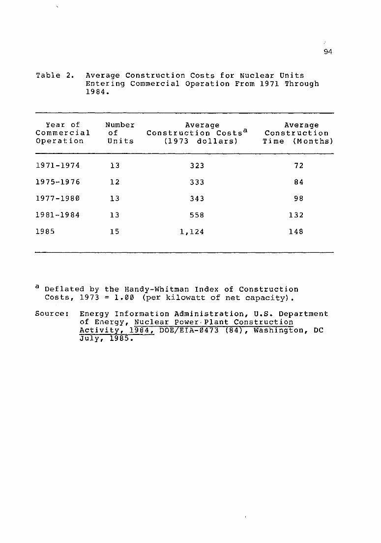
Table 2. Average Construction Costs for Nuclear Units Entering Commercial Operation From 1971 Through 1984.

Year of Number Average Average

94

Commercial of Construction Costs a Construction Operation Units (1973 dollars) Time (Months)

1971-1974 13 323 72

1975-1976 12 333 84

1977-1980 13 343 98

1981-1984 13 558 132

1985 15 1,124 148

a Deflated by the Handy-Whitman Index of Construction Costs, 1973 = 1.00 (per kilowatt of net capacity).

Source: Energy Information Administration, U.s. Department of Energy, Nuclear Power· Plant Construction Activity, 1984, DOE!EIA-0473 (84), Washington, DC July, 1985.

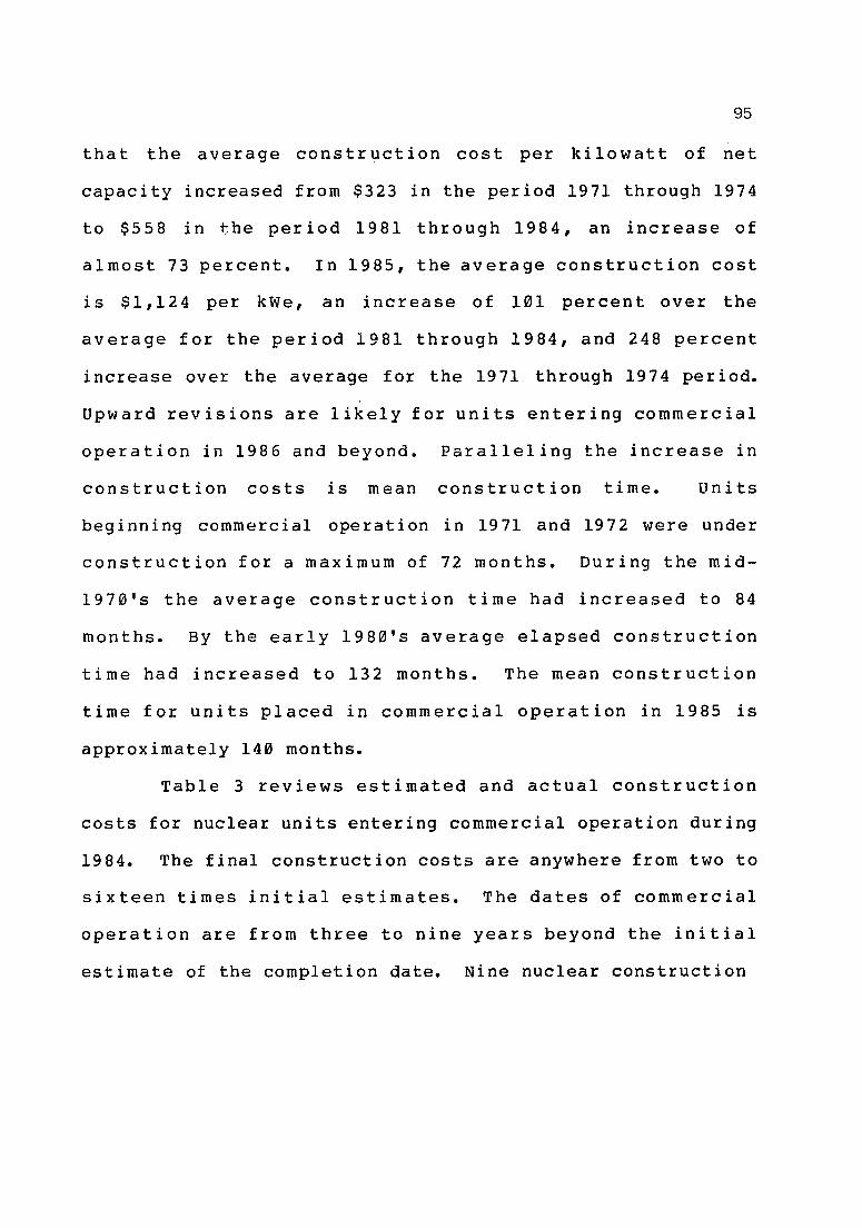
95

that the average construction cost per kilowatt of net

capacity increased from $323 in the period 1971 through 1974

to $558 in the period 1981 through 1984, an increase of

almost 73 percent. In 1985, the average construction cost

is $1,124 per kWe, an increase of 101 percent over the

average for the period 1981 through 1984, and 248 percent

increase over the average for the 1971 through 1974 period.

Upward revisions are likely for units entering commercial

operation in 1986 and beyond. Paralleling the increase in

construction costs is mean construction time. llnits

beginning commercial operation in 1971 and 1972 were under

construction for a maximum of 72 months. During the mid-

1970's the average construction time had increased to 84

months. By the early 1980's average elapsed construction

time had increased to 132 months. The mean construction

time for units placed in commercial operation in 1985 is

approximately 140 months.

Table 3 reviews estimated and actual construction

costs for nuclear units entering commercial operation during

1984. The final construction costs are anywhere from two to

sixteen times initial estimates. The dates of commercial

operation are from three to nine years beyond the initial

estimate of the completion date. Nine nuclear construction

96

Table 3. Estimated and Actual Construction Costs for Nuclear Power Units Entering Commercial Operation in 1984.

Initial Initial Estimate Estimate Final of Total of Date of Estimate Design

Cost Completion Commercial of Total Capacity Unit

($x10 6 ) Date Operation Cost

($x10 6 ) (Net MWe)

Summer 1 234.0 1/77 1/84 1,313.3 900

McGuire 2 358.4 11/75 3/84 1,083.0 1180

San Onofre 3 151.4 6/76 4/84 1,796.2 1100

La Salle 3 300.4 10/76 6/84 1,080.5 1078

WPPSS 2 187.4 9/77 12/84 3,200.9 1171

Callaway 1 839.0 10/81 12/84 3,070.0 1100

Source: Energy Information Administration, U.S. Department of Energy, Nuclear Power Plant Construction Activity, 1984, DOE!EIA-0473 (84) , Washington,DC, July, 1984

projects were cancelled during 1984.

97

A total of $6.8

billion in disbursed funds had been reported for the nine

units.

The exact details behind the increase in construction

lead time is a complex issue and will not be explored in

detail. However, the situation can be generalized as

follows. Construction delays for plants ordered before 1972

were primarily involuntary in the sense that electric

utilities were trying to complete new plants as quickly as

possible. Plants built in later years were subjected to

both voluntary and involuntary delays. For example,

uncertain demand conditions made delays sensible.

Regulatory procedures at both state and federal levels

became more complex and lengthy, reengineering of plants to

meet new safety requirements, and the complexity of plants

increased construction lead times. In any case, longer lead

times were symptomatic of factors leading to increased

construction costs and increased costs of nuclear power as

capital had to stand idle for extended periods of time. The

increased lead times required the utilities to meet

forecests of demand farther and farther into the future

increasing the uncertainty of matching future demand and the

correct level of capacity.

Regarding generation costs, capacity factor is a key

determinant of nuclear power plant costs. Capacity factor (CP)

equals net generation divided by hours in the year times

98

unit design electrical rating (OER).

CP = Net gen (kwe)/[8760 * OER].

Capacity ratings used to measure nuclear capacity factors is

the "design electrical rating" (OER) as reported by the

nuclear operator. The OER is the nominal net electrical

output of the generat i ng uni t and is determined dur i ng the

plant design. This definition suggests that OER remains

constant over the unit's life. Reductions in plant capacity

due to changes in regulation or equipment are reflected in

"maximum dependable capability" (MOC). Each measure is used

to generate capacity utilization figures. The capacity

factors calculated from MOC is greater than or equal to

those from OER, as MOC reflects capacity rating reductions

below the design level. A number of utilities have reduced

the reported DER therefore increasing capacity utilization.

This, in turn, would be reflected in the per-kw capital

cost. The altering of OER leads to an inconsistent measure

of capital cost over time (see Komanoff and Boxer, 1976 for

fUrther details). The OER is used in this research and is

the value at the first day of operation.

Nuclear electric power units are described as base

load plants and not as intermediate load or peaking plants.

Therefore differences in capacity utilization factors across

plants due to "load following" is not a problem. Komanoff

(1976) showed that the reasons for differences in capacity

factors across nuclear plants could be attributed to four

99·

factors: 1) scheduled outages, 2) equipment failures, 3)

regulatory inspection and 4) load following. Load

following represents between one to four percent of lost

capacity utilization.

Nuclear units have higher fixed cost but lower fuel

costs compared to equivalent fossil fuel plants. Based on

conventional assumptions for plant construction and fuel

costs, a nuclear electric plant needs capacity factors in

the neighborhood of 70-80 percent to have a clear-cut

advantage over coal. Conversely, nuclear capacity factors

in the 45-60 percent range, give coal a cost edge over

nuclear. On an average, capacity factors of nuclear plants

in the United States run in the neighborhood of 60-65

percent. Early calculations supporting the economic

cornpetiveness of nuclear power were based upon operating­

capar,ity factors of 80 percent. The reduction of capacity

factor from the expected 80 percent to say 65 percent makes

nuclear power more expensive as capital costs are spread

over a smaller number of kilowatt hours. This may

substantially reduce or eliminate any economic advantage of

nuclear over other base load alternatives.

Between 1965 and 1973 electricity consumption grew at

an annual rate of approximately seven percent. Between 1973

and 1978 (the post oil crisis period) electricity

consumption grew at an annual rate of three and one-half

percent.

100

This reduction in the rate of growth of

electricity consumption reflects the dramatic increase in

electricity prices, a deep recession and perhaps an

increased sense of conservation. Base-load construction

prior to 1974 was based upon expectations that demand would

continue at or even surpass the seven percent level. After

the 1974 oil crisis estimates of future demand were revised

to reflect the new economic situation and construction

programs were reduced. With substantia; capacity in the

construction pipeline, new orders were reduced sharply, and

plants on order where construction had not started or had

not progressed very far had their operating dates deferred

or cancelled. It can be said with confidence that changes

in demand expectations accounted for a large portion of the

observed reduction of new orders, deferrals and

cancellations of base-load nuclear plants, especially since

there was a parallel reduction of new orders of fossil

fueled plants over the same period.

It is generally assumed in comparative studies of

nuclear and non-nuclear electricity generation that the cost

of capital is uniform over all alternatives. There is some

opinion that investments in nuclear power are more risky

than investments in other commercial power generating

technologies. Any legitimate concern by investors as to the

economic viability of nuclear power will be reflected in the

values (prices) of the securities of nuclear relative to

101.

non-nuclear utilities. There are three basic concerns about

nuclear power as viewed from the perspective of the

investor:

1) Concern that projects currently under construction

will not be finished.

2) Concern that the efficiency of newly operating

plants will be less than expected and the shareholders will

be penal i zed.

3) Concern about the safety of the nuclear technology.

A review of the nuclear electric industry shows that

none of the three basic concerns materialized prior to 1979.

The first cancellation of a nuclear power unit that resulted

in sUbstantial abandonment losses occurred in 1980. Also

prior to 1979, stockhblders were not penalized for the poor

performance of operating power plants as increased costs

were passed on to the consumers. Any concern about safety

and any associated liability was lessened by the Price­

Anderson Act of 1974. The provision limits a utilities

liability for third party damages to $560 million in case of

an accident effectively shielding shareholders from

substantial losses. In general, the nuclear industry

reflecteo optimism prior to 1979. After the Three Mile

Island (TMI) accident of March 28, 1979, the seasons changed

for the nuclear industry as a whole. The magnitude of the

damage and the estimated cost of cleanup surpassing $1.5

102

billion forced the industry to realize that an accident

could push losses well beyond the insured limit.

The effect of TMI increased the investors perceptions

of the possibility of large, financial losses due to an

accident. Similarily, the cancellation of partially

constructed plants and low operating efficiency sensitized

the investor further. The financial markets perceived the

concerns as the relative security prices of nuclear

utilities fell and a positive relative rate of return

differential for nuclear utility securities compared to non­

nuclear securities developed. As security returns in any

time period are assumed to reflect all the information

available to investors, the return differential reflects the

additional compensation needed to induce investors to bear

additional risk. This is especially true when considering

the post TMI nuclear power industry.

Investor attitude regarding the nuclear power

industry has been analyzed by Hewlett (1984). Hewlett

analyzed relative rate-of-return differentials for the

nuclear and non-nuclear industries prior to and immediately

following TMI and found a positive rate of return

differential of one to two points on an annualized basis for

the post TMI-period. This premium represents an incremental

cost of capital to nuclear relative to non-nuclear

industries during the sample period. This result is in

contrast to the period prior to the TMI accident where no

··103

substantial differential was formed. Hewlett uses two

models to capture the reactions of investors r.egarding the

nuclear power industry. The Capital Asset Pricing Model

(CAPM) and a direct estimation procedure gave similar

mututally reinforcing results as to the rate of return

differentials for the pre and post TMI accident. A caveat

is necessary, as· the underlying risk of nuclear technology

may not be the singular reason for the return premium. In

an unregulated market economic forces distribute the risk

potential between consumers, owners and society in general.

with respect to the nuclear industry, the distribution of

risk is controlled by the regulatory agency whose behavior

is difficult to predict. Clearly, uncertainty regarding

regulatory policy contributes to the perceived returns of

investments in nuclear power.

While the relative demise of the nuclear power

industry can be explained using basic economic theory,

environmental and political constraints must also be

rev iewed. These factors make it difficult to build a

nuclear plant even when indicated by traditional economic

analyses. The decline of the nuclear power industry

precedes the Three Mile Island accident and can be at least

partially explained by economic consideration. However, the

post Three Mile Island attitude clearly represents growing

concern over nuclear safety in the united States. Until a

104

consensus can be established regarding nuclear safety,

further expansion is simply not in the cards.

Radioactive waste from spent reactor fuel must be

disposed of. Waste disposal represents both technical and

management problems that have not been fully resolved.

Public sensitivity or awareness of safe radioactive waste

disposal is a concern representing another important

constraint on the nuclear-energy industry. Public concern

is over both the disposal of uranium mine tailings as well

as spent reactor fuel containing fission products with long

half lives requiring storage periods of thousands of years.

Clearly, the waste disposal problem represents a serious

political constraint on further development of nuclear

energy.

The regulatory environment facing the nuclear

electric generating industry in the United States is

complex, multifaceted and extremely difficult to model.

Previous studies have considered the nuclear electric

generation and demand uncertainty (Braeutigram and Quirk

(1984)), utility decision analysis (Ellis and Zimmerman

(1983)), operating plant reliability (Joskow and Rozanski

(1979)) and valuation (Zimmerman (1983)). The results of

these studies ar~ contradictory and depend greatly upon the

years on which the studies were based as well as underlying

assumptions.

105

The nonminimizing behavior attributed by the Averch­

Johnson rate-of-return model as analyzed in Chapter 2 does

not give the capability of understanding the environment

facing the nuclear electric industry because it does not

provide the proper framework. Joskow (1974) poses many

questions concerning regulation in general, including

regulatory lags, regulatory procedures and instruments and

inflation. Clearly, regulation is not a homogeneous process

and has many influencing factors.

Summary

A large part of the decline of the nuclear power

industry can be explained by economic factors. Reduction of

the growth rate of electricity consumption coupled with

increased construction lead times and poor reliability have

direct economic impact on the industry as a whole. Recent

events have made nuclear investments appear to be far more

risky than was once thought. Further concerns about safety

and waste disposal have forced non-direct economic

constraints on th~ nuclear industry~

CHAPTER 5

ESTIMATION UNDER ALTERNATIVE SPECIFICATIONS

The dual, cost side of production, is modeled using

the Logistic-Normal distribution for systems of cost shares

and is compared to the traditional additive mUltivariate

normal error specification for both Generalized Box-Cox and

Fourier flexible forms. Homotheticity of production

technology is not assumed. A joint system of cost function

and cost share equations is specified and estimated.

This analysis represents a best case scenario, i.e.,

prior to large distortions such as the unanticipated changes

in the industry as the ten-month moratorium on operating

licenses or the promulgation of ne .. ·l rules adopted in

response to the Three Mile Island accident in 1979. The

sample consists of ne\!l base-load plants that started

comm erc ia1 opera t i on bet ween the years 1974-1978. Plan ts

recently entering commercial operation are used because

greater substitution between inputs is possible ex ante than

ex post. The sample used in the analysis is plant level

rather than aggregate, industry-level data. The system of

cost and cost share equations are estimated with 1978 data.

The data are comprised of 24 base-load nuclear fueled

private steam electric plants representing 35 operating

reactor units. Nuclear-electric power operation is

106

107 '

specified to be a function of t~ese inputs: capital K~ labor

L and fuel P. Estimation of the cost function-cost share

system requi res data on input level s XK , XL' Xp, input

prices wK' wL' wp as well as data on output y.

It is possible that an individual electric utility

may be simultaneously engaged in generation, transmission

and distribution. It is assumed that the production

function of the firm is additive separable in generation,

transmission and distribution. This allows attention to be

focused on the power generation segment of production at the

plant level. The use of firm level data would reflect

substitution with respect to the total operation of the

firm.

All data were taken from the Energy Information

Administration's Historical Plant Cost and Annual Produc~ion

Expenses for Selected Electric Plants r 1978 (Production Ex­

penses), and Statistics of Privately Owned Electric Utili­

ties in the U.S., Classes A & B:o (Statistics). Additional

data were taken from Moody's Public Utility Manual. The data

are constructed as follows:

Y: Output. Net nuclear electric generation in million

of kwh. (EIA'S Production Expenses).

wp: Pr ice of fuel. The annual average in cen ts per

mill i on BTU. (E lA's Product i on Expenses).

where

108

wL : Labor wage rate. The sum of total salaries and

wages charged to the production account multiplied

by the ratio of nuclear to total net generation,

plus total employee pension and benefits paid

multiplied by the ratio of nuclear to total

employees. To arrive at the yearly price of labor,

this number is divided by the number of full time

employees plus one-half the number of part-time

employees. (EIA's statisti~s).

wK: User cos t of capi tal. Following Christensen and

qt

r

<5

b

Jorgenson (1969) the rental price of capital is

calculated as

wK = [qt-l (1 + r)-(l- <5 )qt) (1 - bds)/l - bs )

= acquisition cost of a unit of capital,

= yield on latest issue of long term debt,

= depreciation rate,

= combined federal and state corporate income tax

rate,

d = present value of depreciation allowances,

s = ratio of common equity to total capitalization.

The acquisition cost of capital, q, is calculated by

the deflated value of capital investment by installed

generating capacity, where capacity is measured by the

manufacturer's maximum name plate rating. Data on

109

investment and installed capacity are found in EIA's

Statistics. The deflator used is the Handy-Whitman Index of

plant construction costs found in Moody's Public Utility

Manual. The Handy-Whi tman Index l is al so used to calculate

q. This Index gives values for six geographical regions.

The utility bond yield r is the most recent

individual utility rate reported in Moody's. The combined

federal and state corporate income tax rate is calculated as

b = 0.48 - 0.52g

where g is the state corporate income tax rate as reported

in the Commerce Clearing House (l980). This equation

follows from Ackinson and Halvorsen (l980). The equity­

capital ratio is found in Moody's.

The economic life of a nuclear electric plant is

ambiguous. This is because of the lack of experience

regarding the life a commercial plant as the number of

plants reaching decommissioning is limited. It will be

assumed that the economic life is 30 years. Straight line

depreciation is assumed, and the present value of

depreciation allowances is (see Christensen and

Jorgenson (1969})

d = 1/(30r) [1 - (l/1+r}30]

The rate of depreciation is found in Moody's for different

utilities, and ranges from 3.3 to 4.0 percent.

110

Fuel Expenditure: Total nuclear fuel expenses. (EIA's

Production Expenses).

Labor Expenditure: The sum of total salaries and wages

charged to the production account times the ratio of nuclear

to total net generation plus total employee pension and

benefits paid multiplied by the ratio of nuclear to total

employees. 2 (EIA's Statistics).

Capital Expenditure: Long-term interest payments

multiplied by the inverse of the ratio of.long term

debt to total capital plus depreciation. This, in turn, was

multiplied by th8 ratio of nuclear production plant to total

utility plant. (EIA'S Statistics and Moody's). Total cost

was defined to be the sum of fuel, labor and capital

expenditures. The respective cost shares for each input are

obtained by dividing its expenditures by total cost. The

quantities of each input are obtained by dividing its

expenditure by the appropriate price.

Estimation Techniques

Numerical optimization techniques are used to

estimate the specified cost function and (N-I) related cost

share equations. In review, once the functional form of a

cost function is selected, the cost-share equations are

found by differentiationo As the system of cost share

equation is singular, one equation is dropped and (N-I) are

estimated as a system, including the cost function.

111

The estimation procedure used is Maximum Likelihood.

The system of equations is assumed to represent ~ reduced

form system. Once the functional form of the cost function

is selected, the cost function and associated cost share

equations are fitted using the GRADX algorithm of GQOPT/PC,

Version 3.51 by R.E. Quandt and S.M. Goldfeld. The GRADX

algorithm uses quadratic hill-climbing techniques in double

precision. the numerical derivatives as generated by GQOPT

are used rather than supplying analytic derivatives.

Fortran code was used in specifying the functional form,

cost shares and any associated necessary programming. The

Generalized Box-Cox and Fourier Flexible Form are estimated

under different assumptions regarding the error structure

i.e, standard normal and logistic normal distributions are

assumed to represent the underlying error specification.

The Generalized Box-Cox

The generalized Box-Cox offers a parametric approach

to the selection of functional form.

transformation of price

A/2 = p. 1

" /2

-1

Through the Box-Cox

special uses arise. equal one and two results in the

generalized Leontief and generalized square root quadratic

respectively, as special cases. The translog is the

112

limiting case as A tends to zero. Byallo\'ling A to be a

free parameter during estimation, the special cases can be

statistically tested for. The special cases of translog,

generalized Leontief and generalized square cost quadratic

can be tested for by restricting the Box-Cox parameter A

Tables 4 and 5 summarize the estimation results of the

generalized Box-Cox parameter under standard normal and

logistic normal error distributions~ for homothetic and non­

homothetic production technologies.

Focusing on Table 4, assuming non-homotheticity and

standard normal error distribution, the estimated value fo~

>. equals 1.3114 with asymptotic standard error of 0.2374,

the translog (>. = 0) and generalized square cost quadratic

(>' = 2) are rejected while the generalized Leontief {>. = 1)

is not. A 95 percent confidence interval formed using a t­

distribution with 13 degrees of freedom and a equal to 0.05

ranges from A = 1.8242 to A = 0.7986. The special cases

of trans10g and generalized square root quadratic are not

accepted, while the generalized Leontief is not rejected

given the data.

From Table 5 the estimated value of A , assuming

homotheticity and standard normal error distributi0~, is

1.4734 with 3symptotic standard error of 0.2171. In this

instance the trans10g is again rejected while the

generalized Leontief and generalized square root quadratic

Table .4. Estimates of Generalized Box-Cox Coefficients-­Non-Homothetic.

Parametera,b Logistic Normal Standard Normal

y KK

y LL

B

e

1.4499 1. 00'Hl (0.2723)

2.0000 1.3114 (0.2374)

1.0000 2.0000'

0.3025 0.2546' 0.3589 0.2787 0.2754 0.3342 (0.1061) (0.0509) (0.0957) (0.0961) (0.0971) (0.1112)

-0.0415 -0.0316 -0.0532 -0.0336 -0.0336 -0.0453 (0.0275) (0.0214) (0.0226) (0.0318) (0.0243) (0.0290)

0.1493 0.1623 0.1055 0.1847 0.1684 0.1584 (0.0531) (0.0288) (0.0500) (0.0459) (0.0444) (0.0601)

0.0531 0.0394 0.0684 0.0318 0.0247 0.0485 (0.0324) (0.0237) (0.0249) (0.0362) (0.0269) (0.0307)

0.1625 0.0415 0.3468 0.0845 0.0259 0.2839 (0.2319) (0.0273) (0.0525) (0.0229) (0.0268) (0.0525)

0.0186 0.0116 0.0324 0.0338 0.0304 0.0499 (0.0241) (0.0163) (0.0212) (0.0269) (0.0:219) (0.0243)

0.5898 0.5971 0.5755 0.5770 0.6885 0.5696 ( 0 • 16 2 9 ) ( 0 • 1 61 7 ) ( (3 • 16 6 2 ) ( 0 • 1 4 4 8 ) ( 0 • 1°J 4 2 ) ( iii • 14 6 5 )

-0.0586 -0.0454 -0.0828 0.0382 0.0852 0.0216 (0.0297) (0.2074) (0.2125) (0.1772) (0.1971) (0.1791)

-0.0177 -0.0179 -0.0173 -0.0186 -0.0204 -0.0185 (0.0058) (0.0058) (0.111057) (0.0077) (0.0041) (0.0077)

0.0636 0.0648 0.0615 0.0840 0.111734 0.0818 (0.0131) (0.0130) (0.0130) (0.0216) (0.01~0) (0.0216)

~K -0.0459 -0.0469 -0.0442 -0.0654 -0.0530 -0.0633

Log 9.4613 9.3052 9.1807 114.4921 107.0001 101.0312 Likelihood

a A = 1 Corresponds to a Generalized Leontief functional form, while ). = 2 corresponds to a Generalized Square Root Quadratic form.

b Numbers within parenthesis are asymptotic standard errors.

113

Table 5. Estimates of Genera1~zed Box-cox Coefficients-­Homothetic.

parametera,b Logistic Normal Standard Normal

1. 5885 1. 131HHl 2.13131313 1.4734 1.13131313 2.001313 (13.41333) (13.217l)

'YKK 13.9199 13.3551 13.6391 13.4793 13.3691 13.6206 (13.2967) (0.1351313) (13.1165) (13.13593) (13.13246) .(13.11397)

\L -13.1589 -13.13419 -13.1097 -13.13684 -13.13493 -13.139313 (13.13564) (13.13282) (0.0428) (13.13327) (13.13HI6) (13.134113)

y 13.1136 13.1956 13.2582 13.2534 0.2248 13.2799 EE (13.2357) (13.1341313) (13.13798) (13.0791) (13.13126) (13.13799)

"Y 13.2228 ~.13534 13 .14 82 0.0874 0.13577 13.1391 KL (0.13755) (13.13286) (0.13439) (0.1111) (13.131138) {0.1337l)

'YKE 13.6652 -13.13368 13.1872 13.13268 -0.13597 13.21396 (13.4552) (13.0302) (13.13517) (13.13617) (13.0113) (13.13614)

'Y 13.1"98 0.0292 0.13497 0.0439 13.13301 13.0965 LE (0.0725) (0.0178) (0.0350) (0.13333) (13.13097) (0.0526)

B 0.3845 0.40131 13.3960 0.6011 13.6128 13.62136 (13.16136) (0.1705) (0.1520) (0.1921) (13.0144) (13.13149)

e -13.47138 -13.45S2 -13.4612 -13.14136 -13.1212 -13.1567 (13.21375) (13.2248) (13.1987) (13.0191) (0.0147) (0.13188)

Log -3.817 -11. 303 -4.461 106.5213 99.9580 93.9964 Likelihood

a A = 1 Corresponds to a Generalized Leo~tief functional form, while A = 2 corresponds to a Generalized Square Root Quadratic form.

b Numbers \'lithin parenthesis are ~symptotic standard errors.

114

115

are also rejected given the data. The limits of a 95

percent conf idence interval are A = 1.8362 and A = 1.0106.

Under the assumption of homotheticity the critical t­

distribution value for 15 degrees of freedom is 2.131. The

translog functional form is rejected under both assumptions

of non-homotheticity and homotheticity of the underlying

production process. The value of h is somewhere between

that for the generalized Leontip.f and generalized square

root quadratic, apparently closer to the generalized

Leontief.

A likelihood ratio test (see Theil, pg. 396) to

again consider the special cases substantiates the previous

findings. Again considering Tabla 4 the ,1alue of the log­

likelihood function for unrestricted A is 114.4921. The

value of the likelihood ratio tests for A = 1 and A = 2 are

14.9840 and 26.9218. When compared to the chi-square

critical value of 3.8415 for Ct = 0.05, it is clear that

these special cases are rejected. Table 5 provides the

unrestricted A = 1.4734 under the assumption of

homotheticity. Again both special cases of generalized

Leontief and generalized square root quadratic are rejected,

as the likelihood ratio tests for A = 1 and A =2 are

13.1266 and 25.0498. The critical chi-square value is

3.8415, rejecting the special cases at the CI, = 0005 level.

The confidence interval testing procedure is supported by

the likelihood ratio tests, with the difference being the

116

additional rejection of the generalized Leontief in the non-

homothetic case.

It is also of interest to test the hypotheses of

homotheticity of the underlying process. Again assuming the

error is distributed as an additive standard normal, a

likelihood ratio test can be used. The homothet ic

assumption imposes two restrictions on the generalized Box­

Cox functional form ( 4>K = 4>L = cll E = 0). Homogeneity of

degree one in factor prices is imposed, imposing the

restriction 4>K + cll L + cll E = 0. Therefore cll K = 4>L = 0

forces cll E to equal zero. Again from Tables 4 and 5 the

value of the likelihood ratio test is 15.9416. The critical

value of the chi-square distribution with two degrees of

freedom and CL = 0.05 is 5.99147. Clearly the null

hypothesis of homotheticity can be rejected.

Table 6 provides mean values of the generalized Box­

Cox sUbstitution elasticities for both assumed error

distributions under non-homotheticity. For the additive

standard normal error distribution, substitutability between

input pairs is found for capital and labor as well as labor

and f u e 1 • Un de r the ass u m p t ion 0 f a log i s tic nor mal e l~ r 0 r

distribution the signs of the sUbstitution elasticities are

similar to the additive normal error distribution.

Table 6. Estimates of Generalized Box-Cox Substitution Elasticjties--No~-Homothetic

Logistic Normal Standard Normal

A 1.4499 1.3114

°Kt 0.5590 0.5971

O'KE -0.0157 -0.0361

oLE 0.0943 0.0947

117 .

11S

Residual analyses allows a comparison of the

postulated additive and logistic normal error distributions.

The two measures used are skewness and kurtosis. Skewness

(5) is a measure of the degree of nonsymmetry of a

distribution. The ratio of the third moment of the

distribution to the third power of the standard deviation is

commonly used,

As 0 3 and ~3 are in general unknown, the estimated values

Sand 83 are used where

1\

~3 = liT

and

~3 = (liT ~ (Xi _ x)2)3/2, 1

wher~ ii is the estimated residual of the respective cost

function, labor and energy share equations and T is the

number of observations. For 5 greater than zero, the

distribution has a long tail in the positive direction. For

5 less than zero, the tail is in the opposite direction.

The distribution is perfectly symmetric if 5 equals zero.

Kurtosis (K) is defined by

119 '

where

" )J4 = liT

as )J4 is, in general, unknown. Kurtosis measures the

"thickness" of the tails of the distribution in question.

For K large, the distribution has long thick tails. Table 7

summarizes the characteristics of both the additive normal

and log istic normal error assumptions on the residual

analysis. In general, the Logistic Normal residuals are less

skewed and have thinner tails than the residuals of the

additive normal error distribution. The change was most

dramatic for the energy share equation. While all equations

showed some improvement towards more symmetry, the

improvement is small.

Mardia (1970) develops multivariate measures of

skewness and kurtosis. 3 Mardia's generalization to a p-

variate random vector fo~ skewness is

where R 3 = [r,· 3] and r· . = ( X . - 1I: )' ~ - 1 (X· - X). IJ 1J 1 J The

mUltivariate measure of kurtosis is

where R4 = [r· .4]. As the skewness and kurtosis measures 1 J

for the multivariate case, b l , p and b 2 , p respectively, are

used in residual analysis, the vector X is the (24 x 3)

120

Table 7. Skewness and Kurtosis of Cost and Factor Share Equation Residuals for Non-Homothetic Generalized Box-'Cox.

Equation

Cost Labor Share Energy Share

Additive Error

S -1.7843 2.3371 1.2537

K 1.3991 1.1901 2.2258

Logistic-Normal

S -1.3079 2.0001 0.9742

K 1.3374 1.2107 2.4285

121·

vectJr of residuals of the cost and cost shares of labor and

energy respectively. The similarity between univariate and

multivariate measures is obvious~ Further, Mardia shows that

for any symmetric distribution about the vector of means,

that bl,p equals zeroe

For the null hypothesis of the residuals following

a normal distribution testing proceeds as follows. For the

standard normal distribution bl,p = 0, Mardia proves the

following:

A = (1/6)T (bl,p) _ x2 [p(p + l) (p + 2}/6)

and

B = (b2 ,p - p(p + 2» / (Bp(p + 2}/T)l/2 - N(0,l).

Both bl,p and b 2 ,p are invariant under nonsingular

transformations of the data. The values of bl,p and b 2 ,p

are given in Table B. For the additive error assumption A =

9.3124, while the critical chi-square with ten degrees of

freedom and a = 0.05 is lB.3070, bl,p is not significant.

The value of B is 1~8026 which is less than 2.064 so that

b 2 ,p - p(p + 2} is not significant, and the hypothesis that

the data carne from a normal distribution is supported. For

the Logistic-Normal error distribution the same conclusion

can be made. However, there is a slight improvement, but

the hypothesis of normality cannot be rejected no matter

what the specification.

Table 8. Skewness and Kurtosis for Entire System of Equations for the Non-Homothetic Generalized BOK-COl{

Entire System

Additive Error

2.3281

18.9423

A 9.3124

B 1.7630

Logistic-Normal

2.2784

19.0370

9.3124

B 1.8026

122 . ;,. .,

1.23

The Fourier Flexible Form

It is critical when using the Fourier flexible form

that the data be scaled such that region of approximation is

over (0,21T). This is because the Fourier cost function is

periodic, while the standard cost function is not. The

procedure used in rescaling is as follows. First, for each

logged value of price and output, subtract the minimum of . ':t

that ser ies and add a small number e: >0. The result is a

set of transformed variables between e: and 00 • Now an y

covariates such as output are rescaled by the scalar.

In (maximum rescaled factor price) + e: Ac = ----------------------------------------------

In! maximum value of covariate J l minimum value of covariate

+ e:

Finally, all data are scaled by

As = 6/[ln (maximum rescaled factor price) +€].

AS ensures that all data are scaled to the (0,21T) interval.

The form of the logrithmic Fourier flexible form is

determined by selection of the appropriate multi-index k •

As defined in Chapter 2, the Fourier Cost Function is

A J = U o + bx + (1/2)xCx + ~ {uo~ + 2 ~[UjaCos(jAsk~x)

~=l j=l.

where 2

C -- - A s

124

The choice of A and J determines the number of variables in

Different values of A and J yield different

requirements as to the number of variables in the equation.

It is this variability regarding the number of parameters

entering the equation that sets the Fourier form apart from

other flexible forms.

For this research the largest norm of included multi-

indices is 3. For J = 1 and A = 10 the length of the

parameter vector is 35. As positive homogeneity of factor

prices is jmposed, the effective parameter length can be

reduced to 30. To see the reduction in parameters, consider

the model to be the sum of Translog

uo + bx + (1/2)xCx

plus the sum of A = 10 univariate Fourier series expansions

along the directions ka ,

A J l: {U Ofl + 2 :E [UjaCOS(jAslt~X) - vjexsin(jAslc;~x)]}.

ex=l j=l.

The matr ix C of the Translog portion is a (4 x 4) symmetr ic

matrix which necessarily satisfies four homogeneous

restrictions :E C ij = 0, for i, j = K,L,E,Y, j

following from

the imposition of linear homogeneity in factor prices.

125

There matrix C can have at most six free parameters. From

the parameterization

Six of the uoa are free and four must be set to zero. Thus,

the parameter vector S is subject to one nonhomogeneous

restriction corresponding to the deleted input share, and

four homogeneous restrictions which reduces the number of

parameters from 35 to 30.

If homotheticity is to be imposed there is a

reduction of A as only the main effects are considered,

i.e., output is independent of other factors. Thi sis

analogous to the hypothesis of zero interaction in an

exper imental design. The term It~x can be viewed as a

measure of the covariance of x with the specific multi-index

vector k~. Under non-homotheticity there is an interaction

with output and the other exogenous variables that ~ust be

considered. Table 9 lists the required scaling factors

and the included mUlti-indices used in the estimation.

Using the mUlti-indices listed in Table 9, A = 10 and

J = 1, the resulting cost function can be written as

gK (xiS) ~ a o + b~ + (1/2)xCx T

Table 9. Scaling Factors and Multi-Indices for the Fourier Cost Function: KT = 35.

XK = InwK - In( 0.815) + 8

XL = Inw L - In(l5.659) + 8

XE = InwE In( 0.161) + 8

Xy = Ac[lny - In(1208.8) + 8

In(0.606) - In(0.161) +8 AC = - 0.51435

In (1590.5.1) - In(1208.8) + 8

A = 6/(ln(0.606) - In(0.161) + 8) = 4.5266 s

8 = 10-5

Multi-Indices ( I k (l\ * <3)

(l= 1 2 3 4 5 6 7 8 9 10

kK 0 1 1 " 1 1 " 1 1 " kL " -1 " 1 -1 " 1 -1 0 1

kE " " -1 -1 0 -1 -1 " -1 -1

ky 1 0 0 " -1 -1 -1 1 1 1

I k(l\ * 1 2 2 2 3 3 3 3 3 3

126

+ uo 3 + 2{U3COS[AS(XK-XE)] - v3sin[AS(XK-XE)]}

+ uo4 + 2{u4cOS[AS(XL-XE)] - v4sin[AS(XL-XE)]}

+ Uog + 2{UgCOS[A S (X K-X E+X y )] - VgSin[As(XK-XE-Xy )]}

127

+ uo10 + 2{u10cos[AS(XL-XE+Xy)] - vl~sin[As(XL-XE+Xy)]}.

The resulting parameter vector has nominal length equal to

3S. If homotheticity is imposed, there is zero interaction

between output and input prices. This involves deletion of

the last six mUlti-indices kS through k10 , or equivalently

setting the coefficients {uoS' uS' vS,.··,uo10' u10' v10}

equal to zero. Homotheticity reduces the value of A from 10

to 4, reducing the nominal parameter vector length from 3S

to 17 given J = 1.

128

Differentiation of the logarithmic Fourier flexible

form yields share equations of the form

A J ( a/a Xi) g K (X I 8) = b i - L {u 0 a k a X + 2 L j [ u j a sin (j s ka x)

T a=l a=l

Again, using the multi-indices given in Table 9, A = 10 and

J = 1, the corresponding share of factor i can be rewritten

explicitly as

Si = b i - AS {uo2(XK-X~) + 2u 2sin[A s (X K-X L)]

+ 2v2cOS[AS(XK-XL)]}ki2

+ {u o 3(X K-X E ) + 2u3sin[As(XK-XE)] + 2v3cOS[AS(XK-XE)j }k i3

+ {uOS(XK-XL-XyJ + 2uSsin[ As(XK-XL-X y )]

+ 2VSCOS[AS(XK-XL-Xy)]}kiS

+ {u o 6(X K-X E-Xy ) + 2u6sin[As(XK-XE-XY)]

+ 2v6cos[AS(XK-XL-Xy)]}ki6

+ {uo7(XL-XE-Xy) + 2u7sin[A s (X L-X E-Xy )]

+ 2v7cOS[AS(XL-XE-Xy)]}ki7

+ {UOS(XK-XL+Xy) + 2uSsin[As(XK-XL+XY)]

+ 2VSCOS[AS(XK-XL+Xy)]}kiS

+ {U09(XK-XE+Xy} + 2u9sin[AS(XK-XE+Xy}]

+ 2v9cos[AS(XK-~L+Xy}]}ki9

+ {u10(X L-XE+Xy } + 2u10sin[AS(XL-XE+Xy)]

+ 2v10cos[As(XL-XE+Xy}]}k10

129

for i = K,L,E. The above equation representing the share of

input i will reduce further depending upon the specification

of the particular multi-index k icx • It is important to

recognize that the mUlti-index representing output does not 5

enter into the share equations.

An expenditure system is formed with the cost

function and (n-l) of the share equations. One share

equation may be discarded due to the restriction that the

cost shares sum to one [see Theil (1971, section 7.7)].

Using the estimated parameters, elasticities of substitution

are obtained from the second order derivatives.

As mentioned earlier, imposition of positive

homogeneity of factor prices results in over

parameterization because of the interaction of the quadratic

portion and sine-cosine terms of the Fourier expansion. A

priori, it is not possible to determine which four

parameters are to be set equal to zero. These parameters

were identified by comparing the values of the 10g-

likelihood function across all possible combinations of

parameterse The final choice was determined by the set of

130

zeroed parameters corresponding to the largest value of the

log-likelihood functions.

The estimated parameters of the Fourier Flexible

Form are listed in Table 10 for both additive and logistic-

normal error distribution under the assumption of non-

homotheticity. Table 11 summarizes the estimated parameters

when homotheticity is imposed. The likelihood ratio test 'I ~

for homotheticity ~ non-homotheticity at a =0.05 is 30.13.

The critical chi-square with thirteen degrees of freedom is

22.3621, rejecting the notion of homotheticity for the

additive normal error distribution.

Table 12 is a summary of the estimated substitution

elasticities under both error distributions •.. The values are

near identical with the exception of the elasticities of

capital and energy and labor with energy. These

elasticities are much greater under the logistic-normal

error specification compared with the additive normal.

'131

Table 10. Estimates of Fourier Cost Function Parameters-­Non-Homothetic

Additive Normal Logistic Normal

a o -0.5389 -0.5129 (0.1790) (0.1930)

b k 0.7329 0.6399

b L 0.0918 0.0999 (0.0460) UL0796)

bE 0.1843 0.2602 (0.0829) (CL1715)

by -0.2034 -0.1748 (0.1678) (0.1947)

Uo1 0.3521 -0.4381 (0.0407) (0.0378)

U02 -0.0465 0.0837 (0.0193) (0.0444)

U03 -0.0075 -0.0071 (0.0076) (0.0088)

U04 -0.0045 0.0037 (0.0051) (0,,0034)

U05 -0.0515 -0.0479 (0.0295) (0.0282)

U0 6 -0.0363 0.0418 (0.0289) (0.0210)

U07 -0.0284 -0.0025 (0.0183) (0.0023)

U0 8 -0.0413 0.0005) (0.0554) (0.0005)

U09 0.0215 0.0197 (0.0344) (0.0279)

Table 1121. Continued.

Uol 121 121.0375 121.121523 (121.121199) (121.121379)

U1 121.3521 121.3412 (121.1631) (121.1585)

VI 121.1211211121 121.1211211217 (121.0006) (121.012109)

U2 121.0055 -0.121003 (0.0029) (121.012127)

V2 -121.012125 121.12112118 (121.0026) (121.121027)

U3 0.003121 121.121031 (0.012153) (121.12112149)

V3 0.012142 121.1211214121 (121.0047) (121.0039)

U4 0.121031 121.1211211214 (0.012159) (0.0005)

V4 -0.012189 121.01211212 (0.0071) (121.12101214)

U5 0.121072 121.12112156 (0.0072) (121.012148)

V5 -121.0048 -121.1211211212 (0.0084) (121.1211211218)

U6 -121.1376 121.121799 (121.0651) (121.0795)

V6 0.0971 -121012112141 (121.5828) (121.12112148)

U7 121.03121121 0,,121478 (121.12115121) (121.121434)

V7 121.000121 121.121121121121 (0.121121121121) (121.12112112113)

Us 121.1210013 121.12100121 (0.12113121121) (121.1211211210)

133

Table 10. Continued.

V8 0.0089 0.0047 (0.0084) (0.0050)

U9 0.0143 -0.0003 (0.0092) (0.0006)

V9 0.0000 0.0000 (0.0000) (0.0000)

U10 0.0307 0.0029 (000265) (0.0004)

V10 0.0000 0.0000 (0.0000) (0.0000)

Log- 126.0401 10.0003 Likelihood

Asymptotic Standard Errors in parenthesis

Table 11. Estimates of Fourier Cost Function Parametes-­Homothetic

Additive Normal Logistic-Normal

a o -0.5021 -0.4799 (0.1642) (0.1789)

b k 0.7921 0.7912

b L 0.1011 0.0973 (0.0472) (0.0517)

bE 0.1068 0.1115 (0.091l) (0.0977)

by 0.2141 0.2157 (0.0999) (0.0100)

Uo1 -0.2374 -0.0179 (0.0501) (0.0579)

U02 -0.0461 -0.0379 (0.0371) (0.0389)

U03 -0.0081 -0.0104 (0.0582) (0.0421)

U04 -13.0031 -0.0047 (0.0391) (0.0411)

U1 0.3817 0.3916 (0.1642) (0.1599

VI 0.0008 0.0008 (0.0008) (0.0008)

U2 0.0049 0.0041 (0.0031) (0.0033)

V2 -0.0037 -0.0040 (0.0029) (0.0027)

U3 0.0030 0.0021 (0.0049) (0.0052)

134

135

Table 11. Continued.

V3 0.0041 0.0047 (0.0051) (0.0055)

U4 0.0041 0.0030 (0.0061) (0.0047)

V4 -0.0093 -0.0047 (0.0070) (0.0057)

Log 110.9742 -3.4786 Likelihood

Table 12. Estimates of Foul:ier Flexible Form Substitution Elasticities--Non-Homothetic

136

Elasticity Additive Normal Logistic-Normal

a KL 13.4311 13.4559

a KE -13.13975 -13.13579

a 13.13847 13.13895 LE

137

Univariate measures of skewness and kurtosis are

provided in Table 13. In general, the residuals of all

equations when taken individually are less skewed, i.e., t.he

value of S moves closer to zero for the logistic-normal

distribution. The K values indicate that the residual of

the logistic-normal error distribution have thinner tails

compared to the standard normal. The improvement is towar.ds

a more symmetrical distribution; however, the improvement is

slight.

Using Mardia's system the measure of skewness and

kurtosis is summariz20 in Table 14. For the assumption of an

additive standard error distribution, A equals 8.9184, the

criticcll chi-square at the five percent level and ten degrees

of freeaom is 18.3070, therefore bl,p is not significant.

The value of B is 0.9025 which is less than the value of the

normal distribution, so the hypotheses that the residuals

were from a normal distribution cannot be rejected. A

similar argument holds for the logistic normal error

distribution assumption. While there is some improvement

with the logistic normal distribution, the hypothesis of

normality cannot be rejected under either error

specification.

138

Table 13. Skewness and Kurtosis of Cost Function and Factor Share Equations for Residuals for Non-Homothetic Fourier Flexible Form.

Equat ion

Cost Labor Share Energy

Additive Error

S -1.6841 2.1331 1.0783

K 1.3917 2.5789

Logistic-Normal

s -1.0081 2.0784 1.0700

K 1.2791 1.1984 2.4913

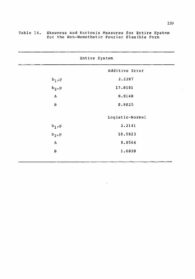
139

Table 14. Skewness and Kurtosis Measures for Entire System for the Non-Homothetic Fonrier Flexible Form

Entire System

Additive Error

2.2287

17.0181

8.9148

B 0.9025

Logistic-Normal

2.2141

18.5823

8.8564

B 1.6020

140

An out-of-sample forecast using a plant entering

commercial operation in 1979 indicates that the Generalized

Box-Cox and the Fourier Flexible Form both give reason~ble

estimates of costs and factor shares. Tables 15 and 16

summarize the results. On balance the Fourier Flexible Form

gives slightly better results usiny percent error as the

measure of comparison under both additive and logistic normal

distribution.

Table 15. Out-of-Sample Forecasts of Non-Homothetic Generalized Box-Cox and Fourier Flexible Forms-Additive Normal.

Generalized Box-Cox Fourier Estimated Actual % Error Estimated Actual

SK 10.683 10.699 -2.28 10.685 10.699

S .. 10.1091 10.1095 -4.21 'L 091 10.1095 ... SE 0.226 10.2106 9.71 10.224 10.2106

Table 16. Out-of-Sample Forecasts of Non-Homothetic Generalized Box-Cox and 'Fourier Flexible Forms-Logistic Normal

Generalized Box-Cox Fourier Estimated Actual 0- Error Estimated Actual "

SK 10.695 10.699 -10.57 10.698 10.699

SL 10.1095 10.1095 10.10 10.1091 10.1095

S'" l!o 13.2110 10.2106 1.94 10.211 0.2106

% Error

-2.1010

-4.21

8.74

% Error

-10.14

-4.21

2.43

141

Conclusions

The assumption of homotheticity can be rejected for

both Generalized Box-Cox and the Fourier Flexible Form using

likelihood ratio tests at the five percent level. Univariate

and multivariate measures of skewness and kurtosis indicate a

movement towards a more symmetrical distribution with the

logistic normal specification, however, the improvement is

slight.

".

CHAPTER 6

SUMMARY AND CONCLUSIONS

This study is an application of production-cost

duality theory focusing on the nuclear electric power

generating industry of the United States. Through duality

theor y, the ex i stence of a well-behaved technology impl ies

the existence of a cost function that captures all the

available information of the underlying technology. This

allows the specification of a cost function, offering

distinct advantages for use in empirical analysis. The

specification of a cost function is not without difficulties

however. I f the pos tula ted cost funct ion spec i f i cat ion is

not of the correct functional form of the unknown cost

function, then specification bases are biased and the

estimators do not have desirable statistical propertieso

A comparison is made between Generalized Box-Cox and

Fourier Flexible forms under alternative error distribution

specificationso The Generalized Box-Cox nests the

Generalized Leontief, Generalized Square Root Quadratic and

Translog fUnctional forms as special cases. The Fourier

Flexible form is different from other flexible cost function

in that the goodness of fit measure is the Sobolev norm. As

the desired result of an economic study is to determine

142

143

elasticities, either price or substitution, then it is

important to approximate closely the function and its first

and second derivatives. Higher order approximations are not

important. The Sobolev norm is the relevant measure of

distance in this case.

Inconsistencies become apparent when an additive­

error specification of cost function is usedo The cost

function is the minimum cost associated with a specific

level of output, given fixed factor prices. Output is

random. Using a new concept, minimum expected cost, cost

share equations follow via Shephards Lemma. As the cost

shares necessarily sum to one--one of the shares may be

dropped. Since individual cost shares lie between zero and

one, the multivariate normal distribution can only

approximate the distribution of shares. Application of a

logistic transformation to the system of (N-l) shares leads

to a new Logistic-Normal distribution.

Plant level data of 24 nuclear electric generating

facilities for 1978 are used to compare the Generalized Box­

Cox and Fourier Flexible forms for additive normal and

Logistic-Normal error distribution. None of the special.

cases of the Generalized Box-Cox form are accepted. Also

homotheticity of the underlying production technology can be

rejecte0. for both the Generalized Box-Cox and Fourier

functional forms, leaving only the unrestricted versions

supported by the data.

144

Residual analysis shows a slight improvement in

skewness and kurtosis for univariate and mUltivariate cases

when the logistic normal distribution is used. However, the

hypothesis of normality cannot be rejected for the system.

The estimated substitution elasticities are very

similar in magnitude and sign between both Box-Cox and

Fourier functional forms under additive normal and logistic

normal error distributions. These SUbstitution elasticities

show little SUbstitution between capital and fuel v and for

labor and fuel. This is perhaps expected as the underlying

technology for nuclear electric generation is restrictive.

Once a commitment to using enriched uranium as the energy

source is made, any potential substitution of fuels is not

possible. There are no nuclear units that have substitute

fuel technologies.

Further questions remain however. The data are

cross sectional in nature and represent only 1978. It would

be interesting to analyze data over a longer period using

mixed time series and cross sectional data. This study has

not recognized the regulatory environment in which this

industry operates. Regulation must be taken into account in

the post Three Mile Island time span. However, the

regulatory environment facing the nuclear electric

generating industry in the United States is not homogeneous.

Clearly, other factors such as public attitude, rate base

145

valuation etc. must be taken into account. As nuclear

electric generation represents technology once removed from

traditional Rankine or Brayton cycles of electricity

generation, it would be of interest to identify factor

productivity changes.

APPENDIX A

TECHNICAL CLARIFICATION

Chapter 2

1. Set Sin R n (E u c 1 ide ann spa c e) is c los e d if x n e: S, n = 1,2, ••• , lim xn ~ XO implies xOe: S.

2. Set S is convex if for evel:y x,x· e: S and scalar such that O~ '( ~l, TX + (1- T ) x· e: S •

... 3. McFadden (1978), p. 24, uses distance functions

to establish full, mathematical duality between cost and transformation functions.

4. ep i (f) = {( x , ~) I ~ > f (x), f (x) < IX) } . -5. For C con vex a f) d f = 0 (,x I C), 9 i v en x e: C, z c C, and

x* e: af(x) the~ o><x*, z - x>. X*fZ af(x) if and only if f(z»f(x) + <x , z-- x> by definition. If x e: C, f(x) = IX) by definition of an indicator function, and the condition is v iolated. Then x It C impl ies f (x) = <P. For x e:: C the condition is trivially satisfied for all z e: C. Therefore O><x , z - x> for all z e: C.

6. Follows from Rockafellar (1970), Theorem 23.5, pp 218-219.

7. f(tx) = tf(x) for t>o

8. Actually, the cost fundtion is conditional upon output level y.

9. A function 9 from Rn to [_00, + 00] is concave if -g is convex, Rockafellar (1970) p. 307.

10. For X a non-empty convex set of Rn c;nd f ~X -+-R. f is strictly quasiconcave function on X if and only if for Xl' x 2 e: X, xl,;t x2' f (Xl) ~ f (x2) and te: (O,l) implies f(x l ) < f(txl + ll-t)x2)·

11. McFadden (1973) uses the same definition.

146

147

12. This is som~times written as (*(x) - f(x) = O(lIx­which is read f (x) - f (x) is of smaller order than Xo112. See Theil (1971), p. 358.

13. This is *equivalent to which is read f (x) - f(x) is See Theil (1971), p. 358.

* f (x) - f(x) = O(lIx-at most of order«x -

* 14. This implies further that the deviation of f anm f is bounded by the remainder term of a second order Taylor series approximationo See Lau (1974).

15. This functional form is known in the mathematics; literature as a mean of order P.

16. Allen-Uzawa Partial Elasticities of Substitutiom is a measure of factor substitution between inputs i and j~ holding all other input prices fixed. See Mundlak (1968» for formal definition.

17. C(t1rl,y) = tC(ltl,y) for t>o.

18. Berndt and Khaled (1979)

change as exp(T(t,w», where T(t,w)

formulate technical k

= t ( L + L L i 1 nw i ) . i=l

19. A complex function f(x) is analytic at point oXID if f is differentiable throughout some E ~eighborhood 1 xo. See Levinson and Redheffer (1970).

20. A point x = Xo is a singular point of f (x), iff f(x) is not differentiable at Xo but every E neighborhood on Xo contains points where f(x) is differentiable.

21. See Levinson and Redheffer (1970), Theorem 9.4 p. 167.

22. Follows [Lorn Corollary 1 in Edmonds and Mascatell~ (1977) •

23. A cost iunction is homogeneous of degree one irn f act 0 r p ric e s i f C ( t w , y ) = t C ( w , y ) for t > 0 • The c 0 stt function can be written C(w,y) = exp[g(1ntl1,lny)]. FOlr positive homogeneity, C(tw,y) = exp[g(ln(tw) ,lny) = exp[g(lnt + lnw,lny)] = tC(w,y). Taking logarithms, g(ln(tt'1),lny) = lnt + InC(1rl,y) = lnt + g(ln~l,lny). Similar results follow for constant returns to scale, homo­thecity, etc.

148

24. A Fourier series is periodic, i.e, f(x+nT} = f(x} for integer n, where T is the primitive period (the smallest period T)O). A cost function is not periodic. A Fourier series approximation of a continuous function can be made as ~ccurate as desired as long as data are scaled within the interval (O,21T). This approximation will diverge if the periodicity is violated, the so-called Gibb's phenomenon. At points where x is continuous the Fourier series converges. However, in the neighborhood of points of discontinuity convergence does not occur and oscillations occur in the approximating function (see Kreyszig [l983]).

Chapter 3

1. It is further assumed that the industry is competitive so that the firm cannot affect the price distribution, Le., it has neither monoply or monopsony power in the output or input market respectively.

2. The two paramete:r; log normal has moments of any order; the jth moment is E(x J } = exp(ju + (1/2}j 2 a 2 ).

~ 3. The contrast in the measure of risk as used by Just and Pope (1977) and Rothschild and stiglitz, (1970) is essentially definitional. Although it is impossible to "prove ll \'lhich definition is better, Rothschild and Stiglitz provide a definition that is more consistent than the mean­variance approach.

4. The denisty function s(x} as used by Rothschild and Stiglitz (1970) is a step function over the closed interval [0,1].

5. In general, output and expected profit will vary with the level of risk aversion. Expected profit will be the greatest for firms which are closest to being risk neutral. This v iew is consistent with standard econom ic theory regarding economic profits as a reward to risk­bearing. See Sandmo, 1971, p. 71 for complete discussion.

6. If the shock is at the industry level, highly possible that Po and E w ill be correlated, therefore not independent.

it is and

7. It is assumed that the distributions of input price wi and outprice price Po are lognormally distributed a s 'ltl i = w i e x p ( e i) a n,d P 0 = Poe x p ( u 0 ). The n E ( wi) = wiE(expei}' E(P o } = PQE(expuo}, for E(\'li} = w~ and E(P o } = Po· Taking ratio yield~ ElWi~/E(PQ} = (wi/Po) i w2ere ui = exp(lJ·-).J + 1/2( a· + a }} Slnce e·~N (lJ· a· )

1 0 2'J. 0 1 l' 1 and Uo~N (lJo'Oo) 0

149

8. Mundlak (1964) comments on the problem of internal consistency of the error structure when additive and multiplicative errors are assumed.

9. See Varian (1984), p. 28.

10. Specifically, the In(1r) specification restricts profits to be strictly positive which is inconsistent under the assumption that firms behave competitively.

11. The adding up constraint is satisfied even for the stochastic specification as the cost function is conditional upon the output level. Once output level is determined L: Si = 10

i

12. In general, the transformation ui = exp(vi)/ r

(L:exp(vi»' i=l

i=l, ••• ,r. Now r-1

u r = 1/(1 + L: exp(vi»· t i=1

(1 + L exp (v i) ) •

for v t = 1n(u t /ur.)' vr = 0 and

i=1 Aitchison and She'1

d (1980) use the following notation U =

exp(v)/(l d

1 - L u ., . 1 J J=

variables.

+L: exp(vj»' v = j=l

and U and v are (d

log(U/ud+l) where ud+l = x 1) vectors of transformed

Chapter 5

1. It has been common practice to use the Handy­Whitman Index of Construction Costs to deflate the acquisition cost of capital. Smith and Cowing (1978) note that these indices do not reflect regional variation of capital costs, but are used to evaluate the capital value of existing plants at a given location. The Handy-Whitman indices are only for correcting intertemporal variation in capital costs for a given region.

150

2. This choice of formulation of labor expenditure was made because of the form of available data. Pension and benefit payments are not separated into different accounts but are given as a lump sum for all employees. Similarly, salaries and wages paid is not separated into a nuclear production account. It is possible to formulate labor expenditures as a weighted average of nuclear to total output or nuclear to total employees. All formulations are positively correlated. Given the data structure, it is felt that the formulation used more strongly reflects the data available.

3. The notation used in the derivation of skewness and Kurtosis is 1'= (1,1,1), a (lx3) matrix of ones, and t-1 the (TXT) inverse of the variance/covariance matrix of estimated residuals.

4. In this case lnai the shift parameter defined in Chapter 1 is equivalent to the log of the minimum price of a specific input i, i.e., lnai = min(lnwi}' i = l, ••• ,k. The same argument holds for the rescaling of output.

5. Using matrix notation the vector k can be partitional as k = (kl,{' k L , kE , ky) = (r ,k y ). It is the partition r that comes Into play in the share equations.

APPENDIX B

SAMPLE DATA

Observation Number Raw data Sample SK SL SE SE

1 1 .74761 .56894E-01 .19550 .23873 2 2 .762t2 .55354E-01 .18223 .14995 3 3 .87480 .40955E-01 .84240E-01 .11603 4 4 .73612 .47094E-01 .• 21679 .13134 5 5 .79804 .81317E-01 .12064 .10682 6 6 .59922 .16791 .23288 .20062 7 7 .69315 .85693E~01 .22115 .22607 8 8 .78637 .37094E-01 .17653 .27692 9 9 .74325 .96096E-01 .16065 .14524

10 10 .69986 .34052E-01 .26609 .29697 11 11 .68980 .41776E-01 .26842 .30563 12 12 .70548 g60000E-01 .23452 .18347 13 13 .76923 .60452E-01 .17032 .20837 14 14 .81702 .33730E-01 .14925 .19558 15 15 .46210 .64984E-01 .47291 .30266 17 17 .68586 .32061E-01 .28208 .29818 18 18 .59097 .61238E-01 .34779 .28798 19 19 .78594 .95924E-01 .11813 .15296 20 20 .73835 .17092E-01 .24456 .34534 21 21 .66578 .47784E-01 .28644 .15986 22 22 .84616 .28574E-01 .12526 .30559 23 23 .88784 .57442E-01 .54721E-01 .23835E-01 24 24 .77869 .. 75212E-01 .14610 .10686

151

152

Y WE WL WK QE QL QK

5.9199 .375 22.980 1.170 66.54 .316 81.557 5.2181 .250 15.659 1.193 55.88 .271 48.993 5.0002 .198 23.523 1.191 55.96 .229 96.610 8.2732 .161 23.423 1.180 95.77 .143 44.369 2.5921 .214 17.482 0.952 27.27 .225 40.549 2.5526 .410 17.550 1.081 27.25 .459 26.594 9.1336 .227 19.418 0.931 106.85 .484 81.655

13.4836 .244 19.398 0.901 146.80 .388 177.090 1.2088 .336 20.593 0.8"'5 13.32 .130 23.664 9.8960 .366 18.004 1.045 106.86 .278 98.440

10.1010 .322 18.556 0.922 110.25 .307 102.022 4.3768 .256 19.426 0.945 45.38 .153 36.981 2.6037 .344 19.079 0.891 32.19 .206 56.129 3.8563 .250 19.302 0.824 40.31 .118 66.951 7.7352 .332 19.101 0.844 86.25 .206 33.152 3.2063 .440 20.947 1.103 35.78 .115 27.703 9.9169 .430 17.556 1.214 104.89 .292 90.333

15.9051 .334 17.123 1.220 165.09 .567 76.798 2.4440 .271 17.428 0.904 26.69 .337 53.232

13.7599 .309 21.579 0.815 149.89 .150 171.571 3.9737 .310 17.556 1.224 45.49 .134 26.779 4.0222 .606 17.549 1.159 45.83 .361 161.869 1.6656 .196 21.938 1.184 18.02 .169 48.399 2.4449 .328 22.124 1.403 29.48 .225 36.734

LIST OF REFERENCES

Aitchison, J. and C.B. Begg, 1976, Statistical Diagnosis When Basic Cases Are Not Classified With Certainty, Biometreka 63, 1-12.

Aitchison, J. and J.A.C. Brown, 1957, The Lognormal Di str ibut ion-W i th Spec i al Reference to its Uses in Economics (London: Cambridge University Press).

Aitchison, J. and S.M. Shen, 1980, Logistic-Normal Distributions: Some Properties and Uses, Biometreka 67,261-272.

Arrow, K., 1971, Essays in the Theory of Risk (Chicago: Markham Publishing Co.)

Arrow, K., H. Chenery, B. Minhas and R. Solow, 1961, Capital-Labor S~bstitution and Economic Efficiency, Review of Economics and Statistics 63, 225-250.

Atkinson, S. and R. Halvorsen, 1984, Parametric Efficiency Tests, Economies of Scale, and Input Demand in U.S. Electric Power Generation, International Economic Review 25, 647-662.

Atkinson, S. and R. Halvorsen, 1980, A Test of Relative and Absolute Price Efficiency in Regulated Industries, Review of Economics and Statistics 62, 81-88.

Atkinson, S. and R. Halvorsen, 1976, Interfuel Substitution in Steam Electric Power Generation, Journal of Political Economy 84, 959-978.

Averch, H. and L. Johnson, 1962, BE!havior of the Firm Under Regulatory Constraint, American Economic Review 52, 1052-1069.

Barnett, W.A., 1983, Definitions of 'Second Order Approximation' anc of 'Flexible Functional Form', Economics Letters 12, 31-35.

Berndt, E.R. and M.S. Khaled. 1979, Parametric Productivity Measurement and Choice Among Flexible Functional Forms, Journal of Political Economy 87, 1220-1245.

153

154

Berndt, E.R. and D.O. Wood, 1975, Technology, Prices and the Derived Demand for Energy, The Revie\'l of Economics and Statistics 58, 259-268.

Blackorby, C., D. Primont and R.R. Russell, 1978, Duality, Separability and Functional Structure: Theory and Economic Applications (New York: North Holland).

Braeutigram, R. B. and J.P. Quirk, 1984, Demand Uncertainty and the Regulated Firm, International Economic Review 25, 45-60.

Byron, R.P. and A.K. Bera, 1983, Least Squares Approximations to Unknown Regression Functions: A Comment, International Economic Review 24, 255-260.

Caves, D.W. and L.R. Christensen, 1980, Global Properties of Flexible Functional Forms, The American Economic Review 70, 422-432.

Chalfant, J.A., 1983, Choosing Among Flexible Functional Forms: An Application of the Generalized Box-Cox and the Fourier Flexible Forms to U.S. Agriculture, Unpublished Ph.D. dissertation, North Carolina State University, Raleigh.

Chalfant, J.A. and R.K. Gallant, 1982, Substitution Elasticities with the Function: Some Monte Carlo Results, Statistics Mimeograph Series No. Carolina State University, Raleigh.

Estimating Fourier Cost Institute of 1614, North

Christensen, L.R. and W.H. Greene, 1976, Economies of Scale in Ug S$ Electric Power Generation l Journal of Political Economy 84, 655-676.

Christensen, L.R., D.Wu Jorgenson and L.J. Lau, 1975. Transcendental Logarithmic Utility Functions, American Economic Review 65, 367-383.

Christensen, L.R., D.W. Jorgenson and L.J. Lau, 1973, Transcendental Logarithmic Production Frontiers, The Review of Economics and Statistics 65, 28-45.

Cowing, T.G., 1981, Duality and the Estimation of a Restricted Technology. Volume 2 of Advances in Applied Microeconomics. Edited by v. Kenny Smith. (Greenwich: JAI Press).

155

Cowing, T.G. and V.K. Smith, 1978, The Estimation of a Production Technology: A Survey of Econometric Analyses of Steam-Electric Generation, Land Economics 54, 156-186.

Debreu, G., 1959, The Theory of Value (New Haven: Iale University press).

Denney, N., 1974, The Relationship Between Functional Forms for the Production System, Canadian Journal of Economics 7, 21-31.

Diewert, W.E., 1982, Duality Approaches to Microeconomic Theory. VOlUmE! 2 of Handbook of Mathematical Economics. Edited by K. Arrow and M. Intrilligata (Amsterdam: North Holland Publishing Company)

Diewert, W.E., 1981, Th€:! Theory of Total Factor Productivity Measurement in Regulated Industries. Edited by T. G. Cowing and R. E. Stevenson, (Amsterdam: North Holland Publishing Company).

Diewert, W.E., 1974, Applications of Duality Theory. Chapter 3 of Frontiers of Quantative Economics. Edited by M.O. Intriligator and D.A. Kendrick (Amsterdam: North-Holland Publishing Company).

Diewert, W.E., 1973, Functional Forms for Profit and Transformation Functions, Journal of Economic Theory 6, 284-316.

Diewert, W.E., 1971, An Application of the Shephard Duality Theorem: A Generalized Leontief Production Function, Journal of Political Economy 79, 481-507.

Edmonds, D.E. and V.B. Mascatelli, 1977, Fourier Approximation and Embeddings of Sobolev Spaces, Dissertations Mathematyczne CXLV.

Elbadawi, 1., A.R. Gallant and G. Souza, 1983, An Elasticity Can be Estimated Consistently Without A Priori Knowledge of Functional Form, Econometrica 51, 1731-1751.

Ell is, R. P. and M. B. Zimmerman, 1983, What Happened to Nuclear Power: A Discrete Choice Model of Technology Adoption, The Review of Economics and Statistics, 234-242.

Energy Information Administration, 1983, Nuclear Cancellations: Causes, Costs and Consequences Government Printing Office).

156

Plan t (U.S.

Ewes, N.A. and D. Fisher, 1982, TO\Alard a Consistent Estimate of the Substitutability Between Money and Near Monies: An Application of the Fourier Flexible Form, Faculty Working Papers No. 21. Department of Economics, North Carolina state University, Raleigh.

Fare, R. and J. Logan, 1983a, The Rate-of-Return Regulated Firm: Cost and Production Duality, Bell Journal of Economics, 405-414.

Fare, R. and J. Logan, 1983b, The Rate-of-Return Regulated Version of Shephard's Lemma, Economic Letters 13, 297-302.

Fuss, M.A. and L. Weverman, 1982, Multiproduct-Multiinput Cost Functions for a Regulated Utility: The Case of Telecommunications in Canada in Studies in Public Regulation. Edited by G. Fromm (Cambridge: MIT Press) •

Gallant, A.R., 1982, Unbiased Determination of Production Technologies, Journal of Econometrics 20, 285-323.

Gallant, A.R., 1981, On the Bias in Flexible FurJctional Forms and an Essentially Unbiased Form: The Fourier Flexible Form, Journal of Econometrics 15, 211-245.

Gallant, A.R. and A. Holly, 1980, Statistical Inference in an Implicit, Nonlinear, Simultaneous Equation Model in the Context of Maximum Likelihood Esti~ation,. Econometrica 48, 697-720.

Guilkey, D.K. and C.A.K. Lovell, 1980, On the Flexibility of the Translog Approximation, International Economic Review 21, 137-147.

Handy-Whitman Index of Electric Utility Construction Costs v as reported in Moody's Public utility Manual (1985).

Hewlett, J.G., 1984, Investor perceptions of Nuclear Power, Energy Information Administration, (U.S. Government Printing Office.

Joskow, P.L., 1979, The Effects of Learning by Doing on Nuclear Plant Operating Reliability, The Review of Economics and Statistics 61, 161-168.

15.7

Joskow, P.L., 1974, Inflation and Environmental Concern: Structural Change in the Process of Public utility Price Regulation, The Journal of Law and Economics, 2, 291-327.

Just, R.E. and R.D. Pope, 1978, Stochastic Specification of ProdUction Functions and Economic Implications, Journal of Econometrics 7, 67-86.

Kiefer, N.M., 1976, Quadratic Utility, Labor Supply, and Commodity Demand, In S.M. Goldfeld and R.E. Quandt r eds., Studies in Nonlinear Estimation (Cambridge: Ballinger Publishing Co.).

Komanoff, C. and N.A. Boxer, 1977, Nuclear Plant Performance/Update: Data Through December 31, 1976, Komanoff Energy Associates.

Komanoff, S., 1976, Power Plant Performance: Nuclear and Coal Capacity Factors and Economics (New York and SaL Francisco: Council on Economic Priorities).

Kreyszig, E., 1983, Advanced Engineering Mathematics, 5th ed., (New York: John Wiley and Sons).

Kumm, M.S., 1981, A Comparison of the Generalized Box-Cox and Fourier Functional Forms: An Application to the North Carolina Residential Time-of-Use Electricity Pricing Experiment, Unpublished Ph.D. dissertation, Duke University.

Lau, L.J., 1974, Comments on Application of Duality Theory. Chapter 3 of Frontiers of Qual-,>~+::ive Economics. Edited by M.D. Intriligator and D.A. Kendrick (Amsterdam: North Holland).

Levinson, N. and R.M. Redheffer, '1970, Complex Variables (San Francisco: Holden-Day, Inc.).

Mardia, K.V., 1970, Measures of Multivariate Skewness and Kurtosis with Applications, Biometrika 57, 519-530.

MacElroy, M., 1981, Duality and the Error Structure in Demand Systems, Discussion Paper Series, Economic Research Center (National Opinion Research Center, Chicago) •

McFadden, D., 1978, Estimation Techniques for the Elasticity of Substitution and Other Production Parameters, in Vol. II of M. Fuss and D. McFadden, eds., Production Economics (Amsterdam: North Holland).

..... 158

Moody's Investors Service, Inc., 1965, Moody's Public Utility Manual.

Mundlak, Y., 1964,Transcendenta1 Multiproduct Production Functions, 1964, International Economic Review 5, 273-284.

Nelson, R.A. and M.E. Wohar, 1983, Regulation, Scale Economies, and productivity in Steam Electric Generation, International Economic Review 24, 57-79.

Pendyck, R., 1979, Interfuel Substitution and the Industrial Demand for Energy: An International Comparison, Review of Economics and Statistics 61, 169-179.

Pope, R.D. and R.A. Kramer, 1979, Production Uncertainty and Factor Demands for the Competitive Firm, Southern Economic Journal 46, 489-501.

Quandt, R.E. and S.M. Goldfeld, 1985, GQOPT/PC Version 3.51.

Rippon, Su, 1984, Nuclear Energy (London: Heinmann).

Rockafellar, R.T., 1970, Convex Analysis, (Princeton: Princeton University Press).

Rossi, P.E., 1984, Specification and Analysis of Econometric Production Models, Unpublished Ph.D. dissertation, University of Chicago.

Rothschild, M. and J.E. Stiglitz, 1970, Increasing Risk: I. A Definition, Journal of Economic Theory 2, 225-243.

Saijo, T., 1983, Differentiability of the Cost Function is Equivalent to Strict Quasiconcavity of the Production Function, Economics Letters 12, 135-139.

Sandmo, A., 1971, On the Theory of the Competitive Firm Under Price Uncertainty, The American Economic Review 61, 65-73.

Shephard, R.W., Functions,

1970, Theory of Cost and Production (Princeton: Princeton University Press).

Silberberg, E., 1978, The Structure of Economics; A Mathematical Analysis (New York: McGraw-Hill Book Company) •

159

Simmons, P. and D. Weiserbs, 1979, Translog Flexible Forms and Associated Demand Systems, American Economic Review 69, 892-901.

Stewart, J.F., 1979, Plant Size, Plant Factor, and the Shape of the Average Cost Function in Electric Power Genera t i on: A Nonhomogeneous Capi tal Approach, The Bell Journal of Economics 10, 549-565.

Theil, H., 1971, principles of Econometrics (New York: John Wiley and Sons).

Varian, H.R., 1984, Hicroeconomic Analysis, 2nd Ed. (New York: W.W. Norton and Co.).

Wales, T.J., 1977, On the Flexibility of Flexible Functional Forms, Journal of Econometrics 5, 183-193.

Wllite, H., 1980, Using Least Squares to Approximate Unknown Regression Functions, International Economic Review 21, 149-170.

Wohlgenant, M.K., 1983, Estimating Demand ElastiC"ities for Food, Texas Agr. i cu 1 t ur al Ex per i ment Station, Staf f Paper Series, Departmental Information Report, DIR 84-1, SP-3.

Woodland, A.D., 1979, Stochastic Specification and the Estimation of Share Equations, Journal of Econometrics 10, 361-383.

Z ell n e r, A. , J. K men t a and J. 0 r e z e , 19 6 6 , Spec i f i cat ion an d Estimation of Cobb-Douglas Production Function Models, Econometrica 34, 784-795.

Zellner, A. and N.S. Revankar, 1969., Generalized Production Functions, Review of Economic Studies 36, 241-250.

Zimmerman, M.B., 1983, The Valuation of Nuclear Power in the Post Three Mile Island Era, The Eenergy Journal 4, 15-29.