Information VisibilityAnd Its Effect On

Supply Chain Dynamics

by

Yogesh V. Joshi

B. Tech., Mechanical Engineering (1998)Indian Institute of Technology, Bombay, India

Submitted to the Department of Mechanical Engineeringin partial fulfillment of the requirements for the Degree of

Master of Science

at theMASSACHUSETTS INSTITUTE OF TECHNOLOGY

June 2000

© 2000 Massachusetts Institute of TechnologyAll rights reserved

Signature of Author ………………………………………………………………………Department of Mechanical Engineering

May 18, 2000

Certified by ……………………………………………………………………………...Sanjay Sarma

The Cecil and Ida Green Career Development ChairAssociate Professor for Mechanical Engineering

Accepted by ……………………………………………………………………………….Ain A. Sonin

Chairman, Department Committee on Graduate Students

2

Information Visibility And Its Effect On Supply Chain Dynamics

by

Yogesh V. Joshi

Submitted to the Department of Mechanical Engineeringon May 8, 2000 in partial fulfillment of the

requirements for the Degree of Master of Science

Abstract

Supply chains are nonlinear dynamic systems, the control of which is complicatedby long, variable delays in product and information flows. In this thesis, we present anovel framework for improving the visibility of information in supply chains by reducingthe delays in information flow. We first analyze the growth and evolution of productionand operations management software over the past three decades, and the current trendsin their development, coupled with recent advances in radio frequency technology,wireless communications, data representation methods, and the internet. Informationvisibility is identified as one of the key elements for successful implementation of anysuch software. We analyze the dynamics of a supply chain under different scenarios ofinformation visibility and forecasting decisions with the help of simulations. Possibleimprovements in supply chain costs are identified, provided information visibility. Wepropose a framework to achieve information visibility in the supply chain using radiofrequency tags, tag readers, product identification codes, an object description language,and the internet.

Thesis Supervisor: Sanjay SarmaTitle: The Cecil and Ida Green Career Development Chair

Associate Professor for Mechanical Engineering

3

Acknowledgements

Many people have contributed to my research for completing this thesis. Its beena wonderful learning experience.

I am grateful to Sanjay for providing me the opportunity and resources to work ona project as exciting as this. Its been great working with Sanjay – he is very encouraging,and as Prasad once told me, his enthusiasm for work is highly contagious. My numerousbrainstorming sessions with him have always greatly revitalized my motivation.

I’d like to thank all at the Auto-ID Center for their support. Special thanks toNiranjan for the numerous debates and discussions I’ve had with him about everyconceivable topic under the sun.

My thanks to all at RAMLab for their help – especially Mahadevan whom Iinevitably call whenever I have a question and don’t know whom to ask; and Paula forbearing so many of those zwrites.

Thanks to David Rodriguera for making my life at MIT simple!

And a final big thanks to my parents and all my friends @ MIT and inCambridge/Boston (I dare not start listing names lest I skip one!) for their encouragementand support!

4

Table of contents

List of Figures.................................................................................................................... 5List of Tables ..................................................................................................................... 61. Introduction................................................................................................................... 72. Analysis of current SCM practices............................................................................ 10

2.1 Introduction........................................................................................................... 102.2 Materials requirement planning (MRP) ................................................................ 112.3 Manufacturing resource planning (MRP II) ......................................................... 122.4 Enterprise resource planning (ERP)...................................................................... 132.5 Supply chain management .................................................................................... 172.6 Advanced Planning and Scheduling (APS) .......................................................... 192.7 Business process optimization (BPO)................................................................... 202.8 Collaborative planning, forecasting and replenishment (CPFR) .......................... 212.9 Data acquisition techniques .................................................................................. 22

2.9.1 Barcodes......................................................................................................... 242.9.2 Radio frequency identification (RFID) tags .................................................. 242.9.3 Electronic data interchange (EDI) ................................................................... 25

3. Modeling supply chain dynamics .............................................................................. 283.1 Introduction............................................................................................................. 283.2 The beer game......................................................................................................... 283.3 A system dynamics model for the beer distribution network ................................. 303.4 Beer game model simulations................................................................................. 353.5 Explanation of simulation results............................................................................ 45

4. A framework for information visibility .................................................................... 474.1 Introduction............................................................................................................. 474.2 Information visibility in real time ........................................................................... 474.3 Basic building blocks.............................................................................................. 48

4.3.1 Electronic Product Code (ePC)........................................................................ 484.3.2 Tag readers....................................................................................................... 484.3.3 Object Naming Service (ONS) ........................................................................ 494.3.4 Object description language (ODL)................................................................. 494.3.5 Fitting them together........................................................................................ 50

4.4 A generalized framework for information visibility............................................... 514.4.1 Framework within an individual supply chain unit ......................................... 514.4.2 Framework extended to the entire supply chain .............................................. 54

4.5 Implementing the proposed framework in the beer game ...................................... 555. Conclusions.................................................................................................................. 58References........................................................................................................................ 60Appendix A...................................................................................................................... 64

5

List of Figures

Figure 1.1 Dynamic Communication and Trading ..........................................................9Figure 2.1 MRP: inputs and outputs ............................................................................. 12Figure 2.2 A simple supply chain ..................................................................................18Figure 2.3 Supply chain decisions .................................................................................19Figure 3.1 The beer distribution network ......................................................................29Figure 3.2 The traditional beer game board...................................................................30Figure 3.3 Vensim model for the traditional beer game ................................................33Figure 3.4 Effective inventory levels in the traditional supply chain ............................35Figure 3.5 Orders placed by units in the traditional supply chain .................................35Figure 3.6 Beer game simulation Case I........................................................................38Figure 3.7 Effective inventory levels for Case I ............................................................39Figure 3.8 Orders placed for Case I ...............................................................................39Figure 3.9 Beer game simulation Case II.......................................................................40Figure 3.10 Effective inventory levels for Case II...........................................................41Figure 3.11 Orders placed for Case II..............................................................................41Figure 3.12 Beer game simulation Case III .....................................................................42Figure 3.13 Effective inventory levels for Case III .........................................................43Figure 3.14 Orders placed for Case III ............................................................................43Figure 3.15 Beer game simulation Case IV.....................................................................44Figure 3.16 Effective inventory levels for Case IV .........................................................45Figure 3.17 Orders placed for Case IV ............................................................................45Figure 3.18 Comparison of costs in the four cases ..........................................................46Figure 4.1 Activities flowchart at the distributor...........................................................52Figure 4.2 Real time data acquisition at the distributor .................................................54Figure 4.3 Flow in a traditional supply chain ................................................................55Figure 4.4 Layered approach to information visibility ..................................................55Figure 4.5 Contemporary supply chains ........................................................................56Figure 4.6 Proposed framework for information visibility in the beer game ................57

6

List of Tables

Table 2.1 MRP Software........................................................................................... 12Table 2.2 ERP Software............................................................................................ 15Table 2.3 SAP R/3 Modules [8]................................................................................ 16Table 2.4 Supply chain activities. ............................................................................. 19Table 3.1 Equations simulating the traditional beer game........................................ 33Table 3.2 Comparison of the four cases.................................................................... 45Table A.1 Equations simulating the beer game for Case I. ....................................... 64Table A.2 Equations simulating the beer game for Case II. ...................................... 65Table A.3 Equations simulating the beer game for Case III...................................... 66Table A.4 Equations simulating the beer game for Case IV...................................... 67

7

Chapter 1

Introduction

Manufacturing environments today have lean machines and optimizedmanufacturing processes. While a great deal of research is underway to improveefficiencies with these strategies, manufacturing companies are also looking for betterways of getting their products to customers in a timely and cost-efficient fashion – i.e.,for managing their complex, intricate supply chains. A recent survey [1] indicates that onan average, most manufacturing companies spend about 12% to 15% of their revenues onsupply chain activities. An improved manufacturing process might fail to achieve benefitfor the company if the product manufactured is not selling in the market, or is not madeavailable in the right place at the right time. A situation wherein a customer goes to aretail store to buy a particular product, finds that product to be out of stock, and ends upbuying a competitor’s product, is commonly reported by companies such as Procter &Gamble. Such incidents lead to lost sales and revenues for the company in question. Themarginal cost of opportunity of lost sales is more for the company than for the retailer.(The retailer doesn’t lose much if he runs out of stock for detergent A, since most likelythe customer will go ahead and buy a detergent B.) At the same time, excessive stockraises inventory costs and likelihood of the product getting outdated. Shortening ofproduction cycles makes it more and more important that the product gets to the marketrapidly. If the production cycle is shorter than the time a product spends in the supplychain, the product will go out of production before the customer receives it. This makes itimpossible to detect and react to quality problems. This follows from Little’s law, whichstates, “the average number of jobs in the system, L, is given by

L = _W (1.1)

where, _ = the average arrival rate of jobs; andW = the average time a job spends in the system.”From Little’s law, its clear that other things equal, the average time that a product

spends in a supply chain is directly proportional to the average number of jobs in thesystem. Due to abovementioned reasons, companies feel a need for visibility ofappropriate information into the product distribution network, and real time informationupdates to optimize scheduling and planning costs.

Today, companies use a variety of software applications for obtaining appropriateproduct information, and for planning and optimizing performance of their supply chains.These applications include Materials Requirement Planning (MRP), ManufacturingResources Planning (MRPII), and Enterprise Resource Planning (ERP) for their day-to-day planning activities. Some companies have taken initiative to implement AdvancedPlanning and Scheduling (APS) packages for simultaneous scheduling and planning withtheir supplier/s. Most of these applications are focused internally within an enterprise.They depend on data gathered at regular intervals from purchasing, manufacturing,distribution, and sales operations. Current techniques for gathering data include manual

8

data entry by operators at various locations into logbooks or data-entry terminals, usageof barcodes, and tags. Transfer of information across units is usually effected by mail,phone, fax, email, or electronic data interchange (EDI). Data gathered by thesetechniques is typically not in real time – it is updated on a daily, weekly or monthly basis.Also, there is significant percentage of errors in manual data entry. Barcode scanningrequires operators and introduces constraints regarding orientation of the product andcleanliness of labels for fast, efficient data collection. Using EDI is expensive, andmoreover, not all suppliers and buyers have the infrastructure setup to use it. As a result,information access is usually restricted to localized zones. Communication between unitsis normally pipelined sequentially, and revising and reorganizing of plans takes aconsiderable amount of time. Differing data formats across trading partners introduceincompatibility – and a need to convert data from one format to another.

The advent of the internet has led to the emergence of new business models andincreased competitive pressures, forcing companies to operate more efficiently than everbefore. To be profitable and to thrive, companies are collaborating closely with allpartners in the supply chain – from the supplier’s supplier to the customer’s customer.These trading partners need to share forecasts, manage inventories, schedule labor,optimize deliveries, and thus improve overall productivity. Software for Business ProcessOptimization (BPO), and Collaborative Planning, Forecasting and Replenishment

RETAILER

Communications andTrading Network.

Data

Data

Deal-making

Deal-making

Deal-making

Data

Logistics, scheduling,and planning decisions.

Logistics, scheduling,and planning decisions.

SUPPLIER

MANUFACTURER

Logistics, scheduling,and planning decisions.

Figure 1.1 Dynamic Communication and Trading.

9

(CPFR), are correspondingly evolving to help companies collaboratively forecast andplan amongst partners, manage customer relations, and improve product life cycles andmaintenance. Traditional supply chains are rapidly evolving into “dynamic tradingnetworks” [2] – comprised of groups of independent business units sharing ‘planning andexecution information’ to satisfy demand with an immediate, coordinated response. Thisis shown in Figure 1.1.

Most of the software packages mentioned above fall in the realm of ‘Logistics,Scheduling and Planning’ shown in Figure 1.1. The second layer, i.e., deal-makingamongst trading partners, is dependent to a huge extent on company strategies and properalignment of business motives. Moreover, both these layers rely on the communicationsmanagement layer for their data acquisition and storage needs. Thus, to facilitateinteraction between these partners in a supply chain or independent business units in adynamic trading network, it is essential to establish a strong communications link that iscapable of gathering information in real-time and making it available to everyoneconcerned instantaneously, preferably in a standardized format. Information gathered isuseful not only for collaboration amongst units but also for planning and schedulingwithin a unit – based on data inputs from the same unit as well as other units. Forexample, to decide the production schedule in an assembly plant, a car manufacturerneeds information about inventories at the distribution centers and retailers, a unifiedforecast of demand for the cars, capability of suppliers to provide required parts forassembly, as well as current capabilities of the assembly plant under consideration, interms of inventory levels, labor, scheduled shutdowns, etc. In this thesis, we provide aframework for achieving complete information visibility in supply chains or tradingnetworks using the internet, and technology being developed at MIT’s Auto-ID Center –electronically coded tags, automatic identification systems, and standardized formats fordata representation.

The thesis is laid out as follows: In Chapter 2, we review the basics of supplychains and their changing needs with recent changes in business models, development ofthe internet, and rise of new software applications. We analyze the current practices insupply chain management (SCM) – the evolution of enterprise applications (MRP,MRPII, ERP) to inter-enterprise applications (APS, BPO, CPFR). In Chapter 3, wedemonstrate the need for visibility in supply chains, and with help of simulations, thebenefits achieved by improving visibility. In Chapter 4, we propose a framework forachieving complete visibility, and concretizing instant communication amongst all unitsin the supply chain or trading network. In Chapter 5, we conclude by illustrating thebenefits and improvements provided by implementing the proposed framework; andpropose issues to be researched further for seamlessly implementing and integrating theframework with simultaneous developments in associated fields.

10

Chapter 2

Analysis of current SCM practices

2.1 Introduction

The past three decades have seen tremendous developments in software forproduction and operations management. This has been a direct result of developments incomputers and information technology, and also of the way companies ran theirbusinesses. There has been a distinct trend of increased collaboration withinorganizations and amongst trading partners over the years. The traditional way of doingbusiness with clear-cut lines of demarcation between roles and responsibilities ofindividual units is fast giving way to shared roles and responsibilities amongst tradingpartners. The growth of software applications over the years reflects these trends.

The foremost software application developed during the early 1970s to helpwarehouses to plan inventory and shop floors to plan production was materialsrequirement planning (MRP). The widespread popularity of MRP in manufacturingdepartments prompted the development of manufacturing resource planning (MRP II) inthe 1970s. MRP II built upon MRP, by tying it to the company’s financial system. By late1980s, companies found an increasing need to integrate together information from alldifferent units within the organization in order to be able to take better decisions forimproving productivity and increasing profits. This led to the development of enterpriseresource planning (ERP) applications. ERP built upon MRP II, by adding functionality toinclude many more departments within the organization. Implementation of ERPinvolved extensive use of developments in information technology. With competitionincreasing with time, to remain in business, companies soon found it necessary tooptimize the entire product “supply chain”. This called for collaboration not only withinthe organization, but also with trading partners in the supply chain. The importance ofmanaging customer relationships, being flexible to respond to changes in organizationalstructure as well as customer demand, managing the product life cycle, etc. influenced thegrowth of next generation software applications - advanced planning and scheduling(APS). This software used optimization algorithms to compute the optimal productionplan and machine schedules to reduce operating costs and improve profits. Competition,partner collaboration and increasing demands for customer responsiveness drove furtherdevelopments in APS, and these newer software packages, generically known asBusiness Process Optimization (BPO) software are slowly replacing ERP/MRP II/MRPacross all industries [3]. Having optimized so far, companies now are looking for ways toreduce lost sales, match supply and demand with least inventory, and remain as lean aspossible. Companies are also adapting a new concept called collaborative forecasting,planning and replenishment (CPFR) to achieve the above.

In this chapter, we review the developments from MRP to CPFR. We analyze themotivation, structure, examples, benefits and drawbacks for each of these applications.

11

2.2 Materials requirement planning (MRP)

In a manufacturing operation, answering questions regarding which materials andcomponents are needed, in what quantities, and when, is extremely vital. Traditionally,majority of the manufacturing organizations controlled sub-assemblies and componentsusing order-point methods. In the early 1970s, a software application was developed toprovide companies with answers to the above questions – it was materials requirementplanning (MRP). An MRP system uses as inputs the demand information from the masterproduction schedule (MPS) with a description of what components go into a finishedproduct (the bill of materials - BOM), the order or production times for components, andthe current inventory status. The system calculates the exact quantity, need date andplanned order release date for each of the sub-assemblies, components and materials

Figure 2.1 MRP: inputs & outputs.

Master ProductionSchedule (MPS)

InventoryStatus Records

Product StructureRecords (BOM)

Purchase &Production Plans

MaterialsRequirement

Planning(MRP)

Items

Quantities

Description

Production unitfinal product orproduct group.

Planning horizon6-18 months

Time raster1 week, 1 month.

Planningfrequencyweekly, monthly.

Items

Quantity inInventory.

ProductionStage

AllocationResources

12

required to manufacture products listed on the MPS [4]. This is shown in Figure 2.1.MRP aids in controlling inventories, and managing work orders, purchase orders, andsales orders. MRP helps companies adapt easily to changes in customer requirements byrevising production and purchase plans when the MPS is changed. It improves customerservice by providing ability to the company of consistently delivering finished productsto the customer in a reliable and timely fashion. It helps maximize resource utilization,and reduce costs by pruning inventory to minimum required levels. Table 2.1 lists someexamples of commercial MRP software packages.

Implementing and operating an MRP system was a major challenge for manycompanies. The program makes assumptions like infinite capacity, certain economicbatch quantities, and fixed lead times. MRP success requires a realistic master productionschedule, methods of controlling as well as planning priority, accurate purchasing leadtimes, a balanced approach to processing change (handling unplanned events), and mostimportantly, accurate data and timely data processing.

MAS 90 MRP Module for Windows (http://www.20-20.com/MAS90_MRP.htm)

MAX ML System (http://www.cimco-th.com/micromax.htm)

TXbase Manufacturing System (www.txbase.com)

CMS Manufacturing System (http://www.cybor.co.nz/cms/cmsmanu.html)

INMASS MRP System (http://www.inmass.com/)

Concorde XAL System (http://www.idsc.co.uk/idp/xal/m&r.htm)

Table 2.1 MRP Software

At the base of all MRP computations are correct BOM and inventory statusrecords. If these are inaccurate, the MRP system will plan wrong items and wrongquantities – garbage in, garbage out. The salient problems arising from inaccurate recordsare the lack of required items, disrupted production, and late deliveries. Data used byMRP is taken from the records maintained by different units in the company. Themethods used for data acquisition and records keeping are reviewed later in this chapter.

Companies soon realized that information in an MRP system is useful tofunctional areas other than manufacturing and operations. By late 1970s, a new policyemerged from MRP. It evolved into Manufacturing Resource Planning, or MRP II.

2.3 Manufacturing resource planning (MRP II)

The manufacturing modules of MRP II include all the elements of MRP, plusadditional developments:

• Feedback – from the shop floor as to how the work has progressed, to all levels ofthe schedule, so that the next run can be updated on a regular basis.

• Resource scheduling – it takes into account the plant and equipment required toconvert raw materials into finished goods while scheduling. This means thatcapacity is taken into account (unlike MRP). The drawback is that capacity is

13

considered only after the MRP schedule has been prepared; hence time allotmentmight be insufficient.

• Batching rules can be incorporated into the scheduling of resources, either Lot forLot, economic batch quantity, or part period cover rules [5].

• Other software modules like “rough cut capacity planning” (RCCP) can beincorporated to help the scheduling process.

The focus of MRP II is to aid better management of company resources byproviding information based on the production plan to all functional areas or units. Itenables testing of “what if” scenarios by using simulation [6]. For example, a shopmanager can see the effect of changing the MPS on the purchasing requirements forcertain critical suppliers or the workload on bottleneck work centers, without actuallyauthorizing the schedule. The MRP plan can be used along with prices and product andactivity costs from the accounting system to project dollar amounts for shipments,product costs, overhead allocations, inventories, backlogs, and much more. Informationfrom MRP II is useful to many functional areas in the firm as follows:

• Purchasing – purchase orders• Production – production scheduling and control, inventory control, capacity

planning• Finance – financial resources needed for material, labor, overhead, etc• Accounting – actual cash flow projections over time, production costs, etc

Although planning information generated by an MRP II system provides insightsinto the implications of MPS and materials plan, it has its drawbacks. The system worksoff fixed lead times, and does not allow for variable lead times, a very unrealisticassumption. In MRP II too, batch-sizing rules are fixed, and batch splitting isdiscouraged, unless “expediting” a batch to speed up a late delivery.

Since a full MRP II implementation can act as an integrated database for thecompany, it means that the company must put great emphasis on data accuracy. Errors inrecording in one part of the system will result in problems for all users. Suppliers of MRPII software encourage users to aim for a data accuracy of between 95 to 98% [5].Methods used for data acquisition and records keeping are discussed later in this chapter.

MRP II focuses on internal operations in a company. The system was devised tocater for the situation where most manufacturing is carried out at a single site, with manyoutdated assumptions. Soon the need was felt for providing and exchanging informationdirectly with other functional units and manufacturing sites within the enterprise. Toincorporate these requirements, a new system called “enterprise resource planning”(ERP) has evolved from MRP II.

2.4 Enterprise resource planning (ERP)

The development of ERP systems was an inside-out process of evolution, startingfrom inventory control packages, to MRP to MRP II, further expanding to include other

14

enterprise processes such as sales and order management, marketing, purchasing,warehouse management, financial and managerial accounting, and human resourcesmanagement. While MRP II includes many of these functions, it looks inwards at theheart of individual sites whereas ERP looks out to the wider picture at the entireenterprise level.

An ERP system is a configurable information systems package that integratesinformation and information based processes within and across functional areas andmultiple sites in an organization [7]. ERP represents the application of new informationtechnology to the MRP II model. This includes the move to relational databasemanagement systems (RDBMS), the use of a graphical use interface (GUI), opensystems, and client-server architecture.

ERP systems are developed based on a reference enterprise business model,chosen by the developers of the ERP system. The developers implicitly promote thenotion that the reference model used embodies best business practices. Differentreference models reflect different preferred business practices, including underlying dataand process models as well as organizational structures. There can be considerablemismatches between the actual company-specific business practices and the referencemodels embedded in the ERP system. While at the abstract level best practices may be“universal”, at the detailed process level these mismatches create considerableimplementation and adaptation problems.

Mismatches can also occur between the actual organizational structure and theimplicitly embedded organizational structure in the reference model of the ERP software.Most of the current generation of ERP packages are based on a traditional hierarchical,functional view of the organization. Work in organizations can be distributed over manygeographic and/or organizationally dispersed regions. An organization can be global –ignoring national boundaries, structured by functional units; or it could be multinational,wherein, administrative structure is demarcated into convenient geographical units, withlocal regulations and capabilities. It can support multiple languages and currencies, orenforce use of a single language and currency, or any combination thereof.

Visibility of transactions across units can be at a detailed or aggregate level.Ownership of data can be centralized and owned by the company or localized and ownedby individual units. The organization can choose between using multiple databasearchitecture, single database architecture, and client-server systems and batch processsystems. ERP systems keep evolving continuously in terms of technology used andfunctionality offered. Migrating between new and old versions of an ERP package isproblematic when the versions are not backward compatible, or when an organization hasmade modifications to the earlier installed version.

Thus, an ERP package has many detailed options, parameters, capabilities andmodels built into it when developed by a vendor. An organization implementing an ERPpackage must clearly understand, identify, and outline its objectives in thisimplementation, and its requirements and expectations from the ERP package. It is

15

important that the organization match these expectations against the solutions providedby different ERP packages, and select the appropriate ERP vendor whose approach alignsbest with the organization’s underlying business model, business practices, andrequirements. Some software vendors providing ERP packages today are listed in Table2.2.

SAP http://www.sap.comComputer Associates International http://www.cai.comSystems Software Associates http://www.ssax.comOracle http://www.oracle.comBaan http://www.baan.comPeoplesoft http://www.peoplesoft.co.nzJD Edwards http://www.jdedwards.com

Table 2.2 ERP Software

For example, SAP R/3 is a commonly used ERP application in many industries. Itconsists of many modules that link operational steps [8]. They can be used alone orcombined with other solutions. Some of the modules that SAP R/3 has are listed in Table2.3.

By implementing ERP applications, organizations aimed to replace complex,disparate, obsolescent systems, improve competitive performance, and improve the poorquality and visibility of information. ERP applications help organizations trackcustomers, money, materials, assets, labor, utilization, etc.

ERP systems have their shortcomings. They are built for recording events thathave already occurred, rather than planning for what will be. Thus, they are good atrecord keeping but not at intelligent decision-making. They can accommodate complexworkflows, but lack the ability to adapt and restructure with changes in surroundings.They also lack the ability to scale to large volumes since their order taking capacities arelimited. While they integrate multiple business functions, they lack the ability to expandtheir scope to multiple enterprises. Lastly, tracking of enterprise information is possibleon the basis of data entered into ERP databases in different units of the enterprise. Thesolution provided by an ERP application is accurate to the extent data in the ERPdatabase is accurate. Thus, it is necessary that for optimal decision-making, data in therecords be accurate and real time. We discuss methods of data acquisition and recordskeeping later in this chapter.

Through the 1990s, most large industrial companies have installed ERP systems.ERP systems manage and share data within an enterprise – they manage the “internalsupply chain”. Companies today need to plan across a wider span of activities and maketrade-offs to optimize the “overall” profitability. This requires sophisticated systems thatanalyze the interplay of complex interactions across enterprises – between the company,its suppliers, its distributors, and other trading partners in its “supply chain”. In the nextsection, we analyze supply chains and the changing objectives of a company as a tradingpartner in today’s supply chains.

16

Table 2.3 SAP R/3 Modules [8]

Financial Accounting Collect data relevant to accounting, providing complete documentation and comprehensive information, and anup-to-the-minute basis for enterprise-wide control and planning.

Treasury Module for financial management aimed to ensure liquidity of the company worldwide, structures financialassets profitably, and minimizes risks.

Controlling An array of compatible planning and control instruments for company-wide controlling systems, with auniform reporting system for coordinating the contents and procedures of company’s internal processes.

Enterprise Controlling Continuously monitors company’s success factors and performance indicators on the basis of speciallyprepared management information.

Investment Management Offers integrated management and processing of investment measures and projects from planning tosettlement, including pre-investment analysis and depreciation simulation.

Production Planning Provides comprehensive processes for all types of manufacturing: from repetitive, make-to-order, andassemble-to-order production, through process, lot and make-to-stock manufacturing, with functions forextended MRP II and electronic kanban, plus optional interfaces to process control systems, CAD, etc.

Materials Management Optimizes all purchasing processes with workflow-driven processing functions, enables automated supplierevaluation, lowers procurement and warehousing costs with accurate inventory and warehouse management,and integrates invoice verification.

Plant Maintenance andService Management

Provides planning, control, and processing of scheduled maintenance, inspection, damage-related maintenance,and service management to ensure availability of operational systems, including plants and equipmentdelivered to customers.

Quality Management Monitors, captures, and manages all processes relevant to quality assurance in the entire enterprise, coordinatesinspection processing, initiates corrective measures, and integrates laboratory information systems.

Project System Coordinates and controls all phases of a project, in direct cooperation with Purchasing and Controlling, fromquotation to design and approval, to resource management and cost settlement.

Sales and Distribution Actively supports sales and distribution activities with outstanding functions for pricing, prompt orderprocessing, and on-time delivery, interactive multilevel variant configuration, and a direct interface toProfitability Analysis and Production.

Human ResourcesManagement

Provides solutions for planning and managing your company’s human resources, using integrated applicationsthat cover all personnel management tasks and help simplify and speed the processes.

SAP Business InformationWarehouse

This independent data warehouse solution summarizes data from R/3 applications and external sources toprovide executive information for supporting decision-making and planning. Reports covering a wide range ofinformation requirements, automated data staging, and standard R/3 business process models ensure rapidimplementation and low operating costs. This “return on information” means that the SAP BusinessInformation Warehouse soon pays for itself.

17

2.5 Supply chain management

In the early 1990s, the phrase “supply chain management (SCM)” came into use.The original motive of SCM was “elimination of barriers between trading partners” inorder to facilitate synchronization of information between them. Recent literature offersmany variations on the same theme when defining a supply chain. A working definition

by Stevens [9] defines a supply chain as “a connected series of activities that is concernedwith planning, coordinating and controlling materials, parts, and finished goods fromsupplier to customer. It is concerned with two distinct flows (material and information)through the organization.” Many authors consider strategic decision-making and systemsintegration a differentiating virtue of supply chains. Still others consider carriers, andsometimes even the government, as integral components of a supply chain. Tayur, et al..[10], provide a comprehensive review of supply chain literature, including definitions ofthe terms used in this field.

Figure 2.2 shows the structure of a typical supply chain. It consists of a number ofunits – beginning with suppliers, who provide raw materials to factories or manufacturingplants, which manufacture products and send them to distribution centers. These transportthem to regional distributors or wholesale dealers, who ship them to retailers. The end ofa traditional supply chain is usually the customer, who buys products from the retailer.Although this composition is typical, supply chains vary in length. Different industriesmight have slightly differing structures of their supply chain. A manufacturing giantmight have a highly structured distribution network – comprising of central warehouse,regional warehouses and local warehouses – through which a product goes before itreaches the retailer. Or, a small, regional company may suffice with having just onedistributor for supplying products to its retailers. An entire supply chain could existwithin one company. Or a supply chain can span multiple enterprises before it reaches thecustomer. Traditionally, planning, purchasing, manufacturing, distribution, and marketingoperated independently along the supply chain. Each activity had its own set of objectivesand often, these objectives were conflicting (for example – manufacturing operations may

Figure 2.2 A simple supply chain.

Supplier 1

Supplier 2

Supplier M

Manufacturer 1

Manufacturer 2

Manufacturer N

DistributionCenter 1

DistributionCenter 2

DistributionCenter O

Wholesaler 1

Wholesaler 2

Wholesaler P

Retailer 1

Retailer 2

Retailer Q

Customer 2

Customer 1

Customer R

18

be designed to maximize throughput and minimize costs, with little consideration forinventory levels, distribution capabilities or market demand). Supply chain managementhas evolved as a strategy to coordinate activities of these independent functions, andcreate a single, integrated plan for the entire organization.

In a supply chain, decisions taken are usually classified as strategic, tactical, oroperational. Strategic decisions are usually linked with the company’s corporate strategy,and guide the design of the supply chain. They are typically made over a long period oftime (2-5 years or more), and traditionally involve all partners in the supply chain.Tactical decisions are taken on a monthly to annual basis, whereas operational decisionsare short term, and directly affect day-to-day activities. Tactical and operational decisionsare traditionally taken independently in individual units of the supply chain – in awarehouse, on the shop floor in a factory, etc. They deal with forecasting, procurement,production and inventory management, warehousing and distribution, and logisticsissues. For example, in a soap factory, deciding which type and what quantity of soapsshould be produced during the current week, and which machines and assembly linesshould be used for this purpose, are operational decisions. MRP, MRP II and ERP helpenterprises take tactical and operational decisions.

Every company performs five basic activities in its supply chain: buy, make,move, store and sell. There are a multitude of decisions, strategic, tactical andoperational, to be taken at each of these five actions. These are listed in Table 2.4. Supplychain simulation tools are commonly used to derive the optimal answers to strategicissues proposed in Table 2.4. The most common representation of a supply chain is amulti-commodity, multiple sources, and multiple sinks network. Hicks [11] proposes afour step methodology for using simulation and optimization techniques for reachingthese strategic decisions. The network is first modeled as a set of nodes and arcs, and alinear-mixed-integer-programming problem is formulated. Powerful optimization solversare applied on this network to evaluate total costs. Step 2 consists of simulating thenetwork over a period of time in order to observe its behavior. The result is a supplychain network design, including the structure and a proposed policy scheme. In step 3,

Figure 2.3 Supply chain decisions

Strategic2-5 years

Operational1-30 days

Tactical1-12 months

19

the policy is optimized using simulation-optimization. The final step is testing the designfor robustness.

Activity Strategic Decision Tactical & Operational Decision

Buy Choosing suppliers, long term contracts vs.short term deals

Type and quantity of raw material to bepurchased, date, time and location of arrival

Make Factory locations, Product lines, Proximityto end customer

Scheduling production, allocating resources

Move Setting up transportation network,outsourcing vs. in-house function

Planning optimal routes for trucks

Store Distribution network design, warehouselocations

Loading / unloading operations, book-keeping

Sell Demand forecasting, special promotions Order fulfillment, customer service

Table 2.4 Supply chain activities.

The objective of supply chain management activities is to meet customer demandfor guaranteed delivery of high quality, low cost, customized products with minimal lead-time. The attempt is to improve responsiveness, understand consumer demand,intelligently control the manufacturing process, and align together the objectives of allpartners in the supply chain. To achieve this objective, companies need to have visibilityinto the entire supply chain of transaction and planning systems – of its own plans as wellas those of its suppliers and customers. Also, the company should be flexible enough thatit can adjust, rebuild and re-optimize plans in real time, to take care of unexpected eventstaking place in the supply chain.

These needs have propelled the development of optimization packages formanaging the entire business process, beginning with advanced planning and scheduling(APS) tools to help companies match their supply with demand, and later integration withmodules for customer relationship management and product lifecycle management. Webegin with a review of APS tools in the next section.

2.6 Advanced Planning and Scheduling (APS)

Supply chain management requires responsive, intelligent decision support toolsto determine optimal (or at least feasible) methods of satisfying customer demand andproduct supply. APS tools have been developed with the intention of meeting thisrequirement. These systems aim at optimizing the supply chain objective discussed in theprevious paragraph subject to constraints of resource availability, capacity costs, laborand materials costs, and transportation resources. They help companies forecast demandwith the help of sophisticated modeling and statistical techniques [12]. Given their

20

memory-resident and exception based nature, together with their object-oriented designand algorithmic domain expertise, they are technologically far superior to ERP and giveresults very fast compared to ERP. APS tools are designed to help companies create plansand schedules that are based on system constraints. APS tools generate a high rate ofreturn by shortening the forecast cycles, enhancing visibility of production plans andschedules, increasing accuracy of order date commitments, taking real-time decisions inthe face of supply / demand fluctuations, and planning in real-time rather than batchprocessing.

APS fails to yield the above-mentioned improvements if companies do not adoptnew procedures and modify their business processes simultaneously. Although APS toolsare “intelligent”, they are hampered due to their focus on manufacturing, distribution andtransportation functions in the supply chain. This focus is acceptable in traditional, slowmoving environments. The current fast-paced business environments warrant a broaderscope of planning efforts. Where customization and perfect delivery are the price forgetting business, customer interaction is the main driver behind the entire productdelivery process [13]. Software vendors have moved on from pure APS tools to buildinga complete set of software for business process optimization.

2.7 Business process optimization (BPO)

Companies like i2 Technologies [14], planning and optimization softwarevendors, have developed software solutions for business process optimization (BPO).BPO is a class of decision-intelligence software that features multi-enterpriseoptimization and integration. ERP, legacy and other transaction systems, are built forrecording what already happened. BPO software leverages current infrastructure, byderiving raw data from ERP systems or any other existing data source. Next, it engagesan integrated set of planning engines to produce an optimal solution based on a completeview of the enterprise and its trading partners. Last, it feeds the optimal solution databack into the transaction system for execution. Its major components typically include thefollowing [14]:• Product life cycle management: this spans the entire product development and

product lifecycle process – from early concept definition, through development andtest, launch, to product phase-out. It provides support for strategic issues and dailyoperations.

• Supply chain management, this includes:§ Demand fulfillment – to provide fast, accurate, and reliable responses to

customer orders. It is mainly an execution-level process that includes ordercapturing, customer verification, order promising, backlog management, andorder fulfillment.

§ Demand planning – to understand customers’ buying patterns and developaggregate, collaborative forecasts. It is by definition a planning process thatfeeds into the supply planning process, and subsequently the demandfulfillment process. It involves long-term, intermediate-term and short-termtime horizons.

21

§ Supply planning – to optimally allocate enterprise resources to meet demand.This is a planning-level process that spans the strategic and tactical supply-planning processes. It includes long-term planning, inventory planning,distribution planning, collaborative procurement, transportation planning andsupply allocation.

• Customer Relationship Management (CRM):§ Creating demand through identifying and acquiring customers, and

developing marketing content and offers.§ Matching demand with customized product offerings.§ Fulfilling demand by executing the sales transaction (either directly, or

through indirect channels), and providing real-time, integrated orderfulfillment.

§ Managing long-term customer relationships, by servicing customer needs andcross-selling and up-selling opportunities.

• Inter-process planning includes:§ Integrated Sales and Operations Planning – ability to review the operation

plan with the revenue objectives for the financial periods – based on thedifferent plans of the different authority domains – including promotion plans,new product introduction plans, possible long-term contracts etc.

§ Financial Planning – ability to project revenues, earnings and other financialmeasures for the next few financial periods based on the plans of the differentauthority domains with the organization on a continual basis and changes inthe market conditions. It will also be able to suggest corrective actions toalleviate the deviations from the strategic plan. This will help in monitoringmetrics for different authority domains of the organization to provide them aquick feedback on their impact on the entire financial plan.

• Strategic Planning: enables companies to plan scenarios, set goals, and monitor theperformance.

Here, it is necessary to note that BPO software gets data from traditional legacysystems or ERP software. Hence, problems of data management associated with ERP andlegacy systems apply directly to BPO software too. These data management issues arediscussed later in this chapter. In the next section, we review the concept of CPFR.

2.8 Collaborative planning, forecasting and replenishment (CPFR)

MRP, MRP II, ERP, and to some extent, APS helped companies to achieveefficient production and operations planning and scheduling. We observe an increasingtrend towards improving demand forecasting and fulfillment through the development ofAPS to BPO to CPFR. CPFR attempts to determine the right number of specific productsto put in an individual store on a particular day of the year [15]. Unpredictable factorssuch as weather, transportation delays, production problems, and administrative errorscan all wreck havoc on supply and demand. Product promotions create massive swings indemand. Suppliers are forced to carry unprecedented amounts of safety stock, or stay leanand risk being unable to fulfill demand. The first option raises costs for everyone; the

22

second results in lost sales, and frustrates customers. Also, reducing inventory costsreturns hidden savings in the supply chain, due to factors like freeing up of fixed assets,capital costs for inventory, manufacturing inefficiencies, redundant handling andtransportation, and improved customer service.

CPFR takes an integrated approach to supply chain management among anetwork of trading partners. Trading partners share forecast and results data. CPFRsoftware analyzes this data, and alerts planners at each company to exceptional situationsthat could affect delivery or sales performance. Trading partners then collaborate toresolve these exceptions by adjusting plans, expediting orders, correcting data entryerrors. Representatives from retail stores, manufacturers and consulting firms have cometogether to form a Voluntary Inter-industry Standards Committee (VICS) to take theleadership role in improving the flow of product and information through the entiresupply chain [16]. The VICS Committee volunteers detailed guidelines for companies toimplement CPFR. It also provides a CPFR roadmap for companies to supplement thevoluntary guidelines. These are described in detail in [16].

If implemented correctly, CPFR improves data communication among tradingpartners. It improves forecasting and planning by providing the ability to see plannedresults. A retailer can prevent out-of-stock situations, especially during productpromotions. A manufacturer can optimize product mix, promotion timing, and marginsacross supply chains. Better partnership with suppliers results in lower inventory levels atretailers. Manufacturers can make-to-demand rather than make-to-stock, and offersavings in inventory and production costs, and product obsolescence costs.

Implementation of CPFR begins with an understanding amongst trading partnersto develop specific plans in different product categories based on best practices. It isessential that both partners own the agreed upon plans and processes in order to achievesuccess. The jointly accepted plan determines which product should be sold when, whereand how. To do this, the plan is implemented in each company using existing planningand scheduling systems, and is required to be made accessible to either party.

Similar to all software systems discussed before, the successful implementation ofCPFR is dependent on data available to existing systems at each trading partner, and theirability to communicate with each other. This ability is dependent on data representationstandards and modes of data communication used by involved parties. Usually, eachsystem has its unique method of representing data making it difficult to be used directlyby another system. Therein stems the need for an industry standard for datarepresentation.

2.9 Data acquisition techniques

As discussed earlier, the success of all software applications in terms of deliveringwhat they promised depends on the availability of the right data at the right place at theright time, in the right format. Data inputs are usually required from the supply chain unit

23

under consideration (internal data) and sometimes from units other than the one underconsideration (external data).

Internal data inputs include transactions associated with receiving material,staging, storage, location, picking, manufacturing, product status, etc. These transactionsare processed by personnel in goods receiving, material handling, storage, accounting,inspection, shipping, and order entry [17]. Material planners, schedulers, order entry andmanpower planning personnel process conversion transactions. Identification transactionsinclude item identification, specifications, order numbers, locations, update transactions,etc. These transactions may influence the status, schedule, or location of the product.

External data transactions involve purchase, acquisition, movement and locationof items in the supply chain – including purchase order data, advance-shipping notices,etc. Buyers, suppliers, transporters and receiving personnel, all of who are responsible fordata integrity, process these transactions.

In today’s manufacturing setups, the time span between an event taking place andits registration and availability in the computer system is unacceptably long. The lag fromthe time an event occurs until the time it gets registered into the system results inproliferation of bad (un-updated) data and the creation of a blank spot in informationvisibility. Companies cover themselves by using safety stocks and safety lead times. As aresult, inventory increases. A complementary problem is the entry of faulty information,i.e., the data captured can contain faulty amounts (ex: 900 instead of 800) or wrong partnumbers (ex: B2413 instead of 82413). This gives rise to poor record accuracy. Dataaccuracy is vital for any company planning its production using enterprise systems [18].For example, an inventory record which reports inventories lower than actual can triggeran unnecessary order that drives up inventory and wastes capacity. A record higher thanactual can result in stock-outs and perhaps work stoppages. Also, for optimal utilizationof the unit’s resources, it is essential that accurate information on resource status bemaintained.

Traditionally, shop floor operators enter data into workbooks or sheets of paper,after which data-entry operators type it into a computer. Alternatively, shop-flooroperators type in data into computer terminals located on the shop floor. Studies showthat with this technique, there is likelihood of 1 error for every 300 characters entered[18]. Another venue for errors is the transcribing of data during entry. Also, real-timedata acquisition is not achieved because of the inherent delays in this method – betweenthe gathering and entry of data.

To overcome these disadvantages, automatic data capture techniques have beendeveloped, and are under development. These techniques make it possible to enter astream of data using automated operations. This can be achieved by multiple means – forexample, by expressing the data in a machine-readable code, information can be enteredin a computer with a code-reading device; or by using voice data entry system, where avoice recognition agent captures data from the words spoken by the operator; by machinevision, other optical systems, or mechanical and inductive flags. A software application

24

in the computer can then process the information further. Data is transferred from point topoint using manual methods, electronic data interchange (EDI), virtual private networks(VPN) or the internet. We discuss these briefly below.

2.9.1 Barcodes

The most common example of automating data acquisition is the use of barcodes.A barcode symbol consists of a series of parallel, adjacent bars and spaces.Predetermined width patterns are used to code actual data into the symbol. To readinformation contained in this symbol, a scanning device is moved across the symbol fromone side to the other, or triggered with a button. As it is moved or triggered, the barcodedecoder analyzes the barcode width patterns of bars and spaces, and the original data isrecovered. Typically, laser scanners can read barcodes from near contact till 12 inchesdistance (very powerful scanners go up to as much as 4 feet).

The most popular barcode format is the Universal Product Code (UPC) Format,which is found on almost all products today. Developed by the Uniform Code Council(UCC), and available since the early 1970s, this format is universally recognized [19].Barcodes offer speed, accuracy, efficiency, and consistency in data acquisition. A studyconducted by Swamidass [20] presents ample industry evidence about the use andbenefits of barcodes as an enabling technology in manufacturing environments, and itscontribution to manufacturing cost reduction, overall quality improvement, cycle-timereduction, and improved profitability.

Although the barcode offers a lot of benefits, it has its drawbacks – it storeslimited amount of data, it needs to be maintained clean so that the reader can read thebars and spaces, the object should be oriented properly such that a line of sight should beestablished between the barcode and the reader, they cannot be embedded into productsor pallets, operator intervention is required to read a barcode, barcodes can be easilycopied, allowing counterfeit use and compromise, etc. Radio frequency identificationtags, also known as RFID tags, are widely emerging as a complementary technology tohelp overcome these drawbacks.

2.9.2 Radio frequency identification (RFID) tags

RFID tags basically consist of a transponder that is electronically programmedwith unique data. Data is read/written on the tag through an antenna or a coil by atransceiver (with a decoder), which is connected to a host computer. RFID tags andantennas come in a variety of sizes and shapes. The tags are categorized as active orpassive. Active RFID tags are powered by an internal battery and are typically read/writeand have various memory sizes. The battery-operated power gives the tag a longer readrange, with a trade-off of greater size, greater cost and limited operational life. PassiveRFID tags operate without a separate external power source and obtain operating powergenerated from the reader. As a result, they are lighter, cheaper and long lasting ascompared to active tags. They usually have short read range, and require a high-powered

25

reader. They are typically read only, and are programmed with a unique set of data(usually 32 or 128 bits) [21].

The significant advantage of RFID tags is the non-contact, non-line-of-sightnature of the technology. Tags can be read through a variety of substances like snow, fog,paint, and other visually and environmentally challenging conditions, where barcodes andother technologies are useless. They can also be read in challenging circumstances atremarkable speeds (less than 100 ms). They possess read/write capability. No operatorintervention is necessary. Tags have an anti-collision feature, which allows for reading ofmultiple tags at once. They can be read from significant distances, too. Most importantly,it is not possible to copy RFID tag data through mechanical means, and by usingencryption techniques, unauthorized replication will be virtually impossible.

Today, companies like Texas Instruments (TI) and Philips Semiconductors aredeveloping and producing RFID technology. Tag costs (active tags - $5-50, passive tags -$2-3 [22]), compatibility, ease of use, and open standards, are important concerns inbringing this technology into everyday use. TI plans to get tag costs down to 50 centsusing proprietary Tag-it technology and production volumes in the order of millions.

Motorola is developing “Bistatix” technology with the objective of reducing theRFID tag prices and making them affordable [23]. Bistatix works on a capacitivecoupling principle, where-in, electric fields are capacitively coupled to and from a readerand tag. It consists primarily of an IC chip connecting antennae printed on a sheet ofpaper. As in an inductive system, a Bistatix reader/writer generates an excitation field,which serves as both the tag’s source of power and its master clock. The tag cyclicallymodulates its data contents and transmits them to the reader’s receiver circuit. The readerdemodulates and decodes the data signal and provides a formatted data packet to a hostcomputer for further data processing. Because of its simple design and construction, thesetags are simple to manufacture. This reduces production cost. The tags also offer stabilityof operation due to absence of a capacitor, and offer robustness as long as the IC remainsintact. The tag can be bent, cut, torn; as long as some remnants of the electrode areconnected to the silicon chip. In terms of tag orientation, they perform optimally atparallel planes of reader and tag, but monopole-coupled bistatix tags do not require thisorientation constraint. They can be applied to any physical configuration, are veryflexible, thin, flat, and not limited with regard to the substrate material.

Thus, Bistatix tags eliminate some of the drawbacks of inductive RFID tags –they are low-cost and easy to make and use. The issue of compatibility and standardsremains to be resolved.

2.9.3 Electronic data interchange (EDI)

EDI is a member of a larger family of technologies used for communicatingbusiness messages electronically, including facsimile, electronic mail, telex, and

26

computer bulletin boards. EDI is commonly defined as application to application transferof business transactions on a computer.

EDI implementation involves understanding EDI standards, communications linkbetween partners, and available software. EDI standards developed beginning in 1960,when proprietary standards were implemented and organizations were created to developindustry and inter-industry standards. Use of EDI increased dramatically during late1970s and early 1980s, and ANSI ASC X12 (American National Standards Institute,Accredited Standards Committee) was chartered to develop standards to facilitateelectronic interchange of business transactions. EDI implementation involves acommunication medium for electronically transferring data between organizations. Thereare many popular channels for EDI communication. At the top of the list are ValueAdded Networks (VANs), which are similar to electronic mailboxes, as they providepostbox service between EDI users (ref 2.21). VANs have the capability to exchange datawith a wide variety of computers using appropriate communication protocols. VANs arepopular with small sized companies, running low volumes of transactions. Companiesrunning high volumes of transactions prefer Direct Connections, which are usuallytelephone lines connected with modems at both ends, dedicated solely for the purpose oftransactions transfers. EDI software is the front-end for interaction with people. Thesoftware package should allow data to be entered and encoded into an EDI standardformat, and also decode incoming EDI data and convert it to in-house data formats.

Common use of EDI is in sales, order processing and purchasing, inventorymanagement, distribution, financial management, etc. Implementation aspects have moreto do with managerial support than technical implementation. Trading partneragreements, vendor agreements, VAN agreements, role of lawyers and auditors, andsecurity of communication are some of the issues of concern. Costs associated with EDIinclude hardware costs (computers, VAN, and appropriate software) depending on scaleof implementation. These costs are quite large (average hub investment of $1 million,plus spokes investment of an average of $45,000 [24]). This is coupled with adjustmenttime, and lack of human resources skilled in using EDI. Using EDI requires a company toalso educate its trading partners to use it. Company data structures sometimes do not fitstandard EDI form, which forces manual intervention in the process [25]. Integration oflegacy systems poses a big problem before companies using EDI. Also, EDI standardsare inflexible. VANs are costly too. Also, each transaction in EDI is in a separate format,causing VAN costs to rise higher. Large companies have annual EDI transactions to theorder of 100 million, VANs charge companies on a transactions basis. Hence companiesare looking for the cheapest network to conduct their transactions.

Although EDI is still better than paper based transactions, it doesn’t lend itself tochange. Today’s business models emphasize on speed of transactions, reducing productlifecycle, having multiple partners in the supply chain, and a strong collaborative focus.EDI is traditionally a hub and spoke architecture (with VANs), emphasizing growth withtrading partner, slow to change standards, has limited capabilities, and requires experts toimplement it. The internet offers a very cost-efficient replacement for VANs used forEDI. As a result, companies are gradually moving towards using EDI together with the

27

internet to cut costs, and later eliminate use of EDI totally and move on to internet basedbusiness-to-business services for conducting all their transactions. Companies are alsosteadily migrating towards using extensible Markup Language (XML) for representingtheir data. Still, issues like standardization of internet based transaction protocols,security and encryption of data transfer on the internet, representation of complex data,etc. are points of concern which we shall discuss in more detail in Chapter 4. In the nextchapter, we study the dynamics at play in a typical manufacturing supply chain, undervarying conditions of information visibility and trading partner collaboration.

28

Chapter 3

Modeling supply chain dynamics

3.1 Introduction

As seen in the previous chapter, one of the fundamental requirements foroptimizing supply chain performance is availability of the right data at the right place andthe right time in the right format, i.e., visibility of appropriate information in the supplychain. This, coupled with increased willingness for collaboration between tradingpartners has been observed to drive down costs in the supply chain. In this chapter, weinvestigate these claims by modeling a supply chain for a beer manufacturer – what ispopularly known as the beer game. The earliest description of the game dates back to thework of Forrester [26] in industrial dynamics. The System Dynamics group at MITfurther developed the game to the format it is played in today. Many researchers insupply chain management and system dynamics have studied the beer game. Logisticsexecutives at Proctor and Gamble, while examining the order patterns of their product –pampers, observed an increase in the amplitude of fluctuation in the orders placed at theretailers to the orders placed at the factory. They called this phenomenon the bullwhipeffect [34]. The bullwhip effect is a repeatable observation in many supply chains thatlack information visibility, including the beer game. I played the beer game as part of aLogistics Systems class exercise at MIT, and had a first hand experience of supply chaindynamics in action. In this chapter, we simulate the supply chain for a beer manufacturerunder different conditions of information visibility and collaboration with the help ofsystem dynamics models. We present our conclusions at the end of this chapter.

3.2 The beer game

The “Beer Game” is a realistic simplification of the supply chain for beermanufacture. The game is popularly used as an introduction to systems thinking,dynamics, computer simulation, and supply chain management. It has been played bythousands of people, all over the world from high-school students to CEOs of majorcorporations [27]. It serves as an excellent experiment for studying the effect of systemmicrostructure (individual behavior and decision-making under given circumstances) onsupply chain dynamics [28].

Factory WholesalerDistributor Retailer

CustomersSuppliers

Figure 3.1 The beer distribution network.

29

The beer distribution network under consideration consists of supplier, factory,distributor, wholesaler, retailer and end customers. It is shown in Figure 3.1. Each week,customers place demand with the retailer, who fulfils it from his inventory. He, in turn,orders beer from the wholesaler, who provides it out of his current inventory. Thewholesaler gets his supply from the distributor, who gets his supply from the factory. Thefactory brews beer. Every week, inventory in each unit keeps depleting, and theparticipants replenish the inventory to maintain required safety stock levels. There areordering, shipping, production and communication delays between each of these units inthe supply chain. Each unit incurs costs for maintaining inventory and running intobacklogs. The objective is to minimize supply chain costs by trying to maintain inventoryat safety stock levels while meeting incoming demand.

Traditionally, the beer game is played on a board representing the beerdistribution network. A sample board is shown in Figure 3.2. There are four individualunits: Factory (F), Distributor (D), Wholesaler (W), and Retailer (R).

Each box between units in Figure 3.2 represents one week of delay – thus, there isa two-week delay between an order being shipped by the distributor and the wholesalerreceiving it. Similarly, there is a two-week delay between an order placed by the retailer

and the wholesaler being notified about it. Each unit in the supply chain actsindependently, without collaboration, as is common practice in traditional businesses, andhence a given unit does not have much information about inventories held at other unitsin the supply chain at any given time. The only interaction between units is receiving

Figure 3.2 The traditional beer game board. [30a]

30

orders and shipping crates to customer, and placing orders and receiving crates from thesupplier. The supply chain simulated above is far simpler than a real life supply chain.Some of the simplifications include:

• It consists of only four independent units.• We exclude random events – for ex: machine failures, transportation issues,

strikes, etc.• We do not impose capacity constraints• We do not impose financial constraints, etc.

Detailed instructions on how the game is played can be found in [28], [29] or[30]. In the next section, we explain the dynamics in the supply chain for beer with thehelp of a Vensim model.

3.3 A system dynamics model for the beer distribution network

The beer game described above represents the supply chain in a typicalmanufacturing industry. It is a good example of a system with simple structure, lowcombinatorial complexity, and high dynamic complexity – arising due to interactionamongst agents over time [31]. Being a dynamic system, the individual variables aretightly coupled together, and interact strongly with one another and the rest of the system.They are strongly governed by feedback. Multiple factors influence their values,introducing non-linearity into the system. The future values of many variables depend ontheir historical values. In the traditional game, there are multiple points where delay isintroduced into the system. Delays create instability and oscillations in the system,causing inventory levels to significantly sway from the expected safety stock level.(Adding delays makes system eigenvalues complex conjugates, yielding oscillatorysolutions, and relevant system parameters determine whether the oscillations are dampedor exponential [31].)

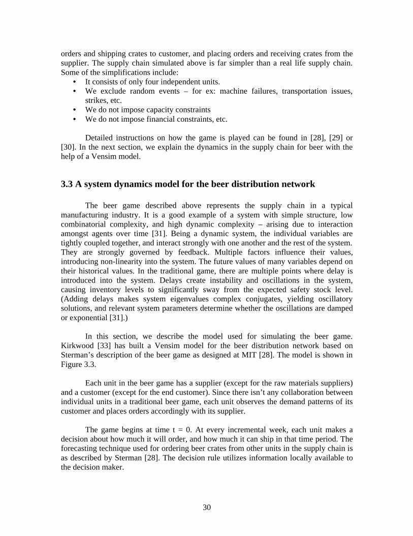
In this section, we describe the model used for simulating the beer game.Kirkwood [33] has built a Vensim model for the beer distribution network based onSterman’s description of the beer game as designed at MIT [28]. The model is shown inFigure 3.3.

Each unit in the beer game has a supplier (except for the raw materials suppliers)and a customer (except for the end customer). Since there isn’t any collaboration betweenindividual units in a traditional beer game, each unit observes the demand patterns of itscustomer and places orders accordingly with its supplier.

The game begins at time t = 0. At every incremental week, each unit makes adecision about how much it will order, and how much it can ship in that time period. Theforecasting technique used for ordering beer crates from other units in the supply chain isas described by Sterman [28]. The decision rule utilizes information locally available tothe decision maker.

31

At each unit, the Effective Inventory, EI, at time t, is given byEI(t) = I(t) - B(t) (3.1)

I(t) = Inventory, given byI(t) = 0

t ( inv(_)/ _)•d_inv(_)/ _ = i(_) – s(_)

Integrated numerically:I(t) = I(t-1) + i(t) – s(t) (3.2)

inv(_)/ (_) = change in inventory during each time intervali(t) = incoming orders

= crates sold by the supplier, received with delays(t) = crates sold by this unit

= minimum required to satisfy customer ordersnote that I(0) = 12

B(t) = cumulative backlog at the unit, is given byB(t) = 0

t ( b(_)/ _)•d_b(_)/ _ = o(_) – s(_)

Integrated numerically:B(t) = B(t-1) + o(t) – s(t) (3.3)

b(_)/ _ = backflow at each unit, i.e., the accumulation of backlog during in each timeperiod

o(t) = orders placed at this unitnote that B(0) = 0

In general, Orders placed by a unit, O, at time t, are given byO(t) = max (0, IO(t)) (3.4)

IO(t) = indicated order rate, is computed based on three factors:§ expected losses from the stock (L)§ discrepancy between desired and actual stock (AS)§ discrepancy between desired and actual supply line (ASL)

IO(t) = L(t) + AS(t) + ASL(t) (3.5)L(t) = xl • Lt-1 + (1-xl) • L0 (3.6)AS(t) = xs • (S

* - S(t)) (3.7)ASL(t) = xsl • (SL* - SL(t)) (3.8)

xl, xs, xsl = weight factors determined through regressive expectationS(t) = stock of cratesS* = desired stock [=12 in beer game]SL(t) = supply lineSL* = desired supply line

= expected lag • desired throughput

Applied to the beer game, the equation for Orders placed, O(t), is given by

32

O(t) = max (0, IO(t))

IO(t) = Demand Forecast + actual stock gap + actual supply line gapIO(t) = Demand Forecast + A•(12 – EI(t)) – B•Spl(t) (3.9)Spl(t) = 0

t ( sf(_)/ _).d_sf(_)/ _ = O(_) – i(_)

Integrated numerically:Spl(t) = Spl(t-1) + O(t) – i(t) (3.10)

Spl(t) = supply line gapsf(_)/ _ = accumulation in the supply line during every time interval

A, B = weight factors

The Demand Forecast function would typically be either the SMOOTH orFORECAST function of Vensim. The time delays for the crates to move between unitsare accounted by the FIXED DELAY function. The equations described above arerepresentative of one unit in the supply chain. The complete set of equations describingthe model drawn in Figure 3.3 is listed in Table 3.1. Solving them becomes quitecomplex due to the interdependence of many variables in the model.

We ran the simulation for a span of 36 weeks, the typical time period for whichthe beer game is played. Figure 3.4 shows the effective inventory levels at all units in thesupply chain over the simulated period. Figure 3.5 shows the orders placed by individualunits during this time. Inventory costs are assumed to be 0.50 $/unit/week and backlogcosts are assumed to be 1.00 $/unit/week [28]. The customer demand was kept constant at4 crates of beer for the first 4 weeks. A step increase to 8 crates was applied at the 5th

week, and the demand was maintained constant at 8 throughout the rest of the simulation.

nventory

SMOOTHTIME <SMOOTHTIME>

Backlog

in

placed

bFlow

ordered

SupplyL

sFlow

<A> <B>A <A>B

Inventory 0

<SMOOTHTIME> <SMOOTHTIME>

Backlog 0

<A>

sold 0 in 0

placed 0

bFlow 0

<B>

ordered 0

SupplyL 0

sFlow 0

<B>

RETAILER WHOLESALER DISTRIBUTOR FACTORY

Inventory 1

Backlog 1

sold 1 in 1

placed 1

bFlow 1

ordered 1

SupplyL 1sFlow 1

Inventory 2

Backlog 2

sold 2 in 2

placed 2

bFlow 2

ordered 2

SupplyL 2

sFlow 2

coming

Figure 3.3 Vensim model for the traditional beer game.(Developed by Prof. C. Kirkwood at ASU. Based on Sterman’s description of the beer game

developed at MIT.)

Cost

cost increase

<Backlog>

<Backlog 0>

<Backlog 1>

<Backlog 2>

<Inventory>

<Inventory 0>

<Inventory 1>

<Inventory 2>

Eff Env

og>

ory>

Eff Inv 0

<Backlog 0>

<Inventory 0>

Eff Inv 1

<Backlog 1>

<Inventory 1>

Eff Inv 2

<Backlog 2>

<Inventory 2>

33

No: Variable and defining equation Comments(01) A = 0.25 Forecasting parameter(02) B = 0.33 Forecasting parameter(03) Backlog = INTEG( bFlow , 0) Backlog at retailer(04) Backlog 0 = INTEG( bFlow 0 , 0) Backlog at wholesaler(05) Backlog 1 = INTEG( bFlow 1 , 0) Backlog at distributor(06) Backlog 2 = INTEG( bFlow 2 , 0) Backlog at factory(07) bFlow = ORDer - sold Accumulation of backlog at retailer(08) bFlow 0 = ordered - sold 0 Accumulation of backlog at wholesaler(09) bFlow 1 = ordered 0 - sold 1 Accumulation of backlog at distributor(10) bFlow 2 = ordered 1 - sold 2 Accumulation of backlog at factory(11) coming = ordered 2 Materials in transit to factory(12) Cost = INTEG( cost increase , 0) Total supply chain cost(13) cost increase = 1 * ( Backlog + Backlog 0 + Backlog 1 + Backlog 2 ) + 0.5 * (

Inventory + Inventory 0 + Inventory 1 + Inventory 2 )Weekly supply chain cost

(14) Eff Env = Inventory - Backlog Effective Inventory at retailer(15) Eff Inv 0 = Inventory 0 - Backlog 0 Effective Inventory at wholesaler(16) Eff Inv 1 = Inventory 1 - Backlog 1 Effective Inventory at distributor(17) Eff Inv 2 = Inventory 2 - Backlog 2 Effective Inventory at factory(18) FINAL TIME = 36 The final time for the simulation.(19) in = DELAY FIXED( sold 0 , 2, 4) Incoming orders at retailer(20) in 0 = DELAY FIXED( sold 1 , 2, 4) Incoming orders at wholesaler(21) in 1 = DELAY FIXED( sold 2 , 2, 4) Incoming orders at distributor(22) in 2 = DELAY FIXED( coming , 2, 4) Incoming orders at factory(23) INITIAL TIME = 0 The initial time for the simulation.(24) Inventory = INTEG( in - sold , 12) Physical inventory at retailer(25) Inventory 0 = INTEG( in 0 - sold 0 , 12) Physical inventory at wholesaler(26) Inventory 1 = INTEG( in 1 - sold 1 , 12) Physical inventory at distributor(27) Inventory 2 = INTEG( in 2 - sold 2 , 12) Physical inventory at factory(28) ORDer = 4 + STEP ( 4, 5) Weekly customer orders(29) ordered = DELAY FIXED( placed , 1, 4) In transit orders by retailer(30) ordered 0 = DELAY FIXED( placed 0 , 1, 4) In transit orders by wholesaler(31) ordered 1 = DELAY FIXED( placed 1 , 1, 4) In transit orders by distributor(32) ordered 2 = DELAY FIXED( placed 2 , 1, 4) In transit orders by factory(33) placed = MAX ( 0, SMOOTH ( ORDer , SMOOTHTIME ) + A * ( 12 - ( Inventory

- Backlog ) - B * SupplyL ) )Orders placed by retailer

(34) placed 0 = MAX ( 0, SMOOTH ( ordered , SMOOTHTIME ) + A * ( 12 - (Inventory 0 - Backlog 0 ) - B * SupplyL 0 ) )

Orders placed by wholesaler

(35) placed 1 = MAX ( 0, SMOOTH ( ordered 0 , SMOOTHTIME ) + A * ( 12 - (Inventory 1 - Backlog 1 ) - B * SupplyL 1 ) )

Orders placed by distributor

(36) placed 2 = MAX ( 0, SMOOTH ( ordered 1 , SMOOTHTIME ) + A * ( 12 - (Inventory 2 - Backlog 2 ) - B * SupplyL 2 ) )

Orders placed by factory

(37) SAVEPER = TIME STEP Frequency at which output is stored.(38) sFlow = placed - in Supply line accumulation - retailer(39) sFlow 0 = placed 0 - in 0 Supply line accumulation - wholesaler(40) sFlow 1 = placed 1 - in 1 Supply line accumulation - distributor(41) sFlow 2 = placed 2 - in 2 Supply line accumulation - factory(42) SMOOTHTIME = 1 Forecasting parameter(43) sold = MIN ( Inventory + in , ORDer + Backlog ) Crates sold by retailer(44) sold 0 = MIN ( Inventory 0 + in 0 , ordered + Backlog 0 ) Crates sold by wholesaler(45) sold 1 = MIN ( Inventory 1 + in 1 , ordered 0 + Backlog 1 ) Crates sold by distributor(46) sold 2 = MIN ( Inventory 2 + in 2 , ordered 1 + Backlog 2 ) Crates sold by factory(47) SupplyL = INTEG( sFlow , 0) Supply line for retailer(48) SupplyL 0 = INTEG( sFlow 0 , 0) Supply line for wholesaler(49) SupplyL 1 = INTEG( sFlow 1 , 0) Supply line for distributor(50) SupplyL 2 = INTEG( sFlow 2 , 0) Supply line for factory(51) TIME STEP = 1 The time step for the simulation.

Table 3.1 Equations simulating the traditional beer game

34

From Figure 3.4, we observe that effective inventory at the retailer, which is the sumof physical inventory and backlog, becomes zero first, and then negative. This pattern isrepeated at the wholesaler, distributor, and the factory with a time delay and amplification ofmagnitude. This also has an affect on the orders placed by units every week, as observed in

Orders placed by Retailer

4 8 12 16 20 24 28 32 36Time in Weeks

ced

Orders placed by Wholesaler

100

75

50

25

0

0 4 8 12 16 20 24 28 32 36Time in Weeks

Orders placed

Orders placed by Distributor

4 8 12 16 20 24 28 32 36Time in Weeks

ced

Orders placed by Factory

100

75

50

25

0

0 4 8 12 16 20 24 28 32 36Time in Weeks

Orders placed

Figure 3.5 Orders placed by units in the traditional supply chain.

8 12 16 20 24 28 32 36Time in Weeks

iler Inventory

40

0

-40

-80

0 4 8 12 16 20 24 28 32 36Time in Weeks

Effective Wholesaler Inventory

Effective Inventory Levels at Distributor

8 12 16 20 24 28 32 36Time in Weeks

ributor Inventory

Effective Inventory Levels at Factory

80

40

0

-40

-80

0 4 8 12 16 20 24 28 32 36Time in Weeks

Effective Factory Inventory

Figure 3.4 Effective inventory levels in the traditional supply chain

35

Figure 3.5. We see a surge in the orders placed as the weeks pass by, and this surge increasesfrom retailer to wholesaler to distributor to factory. This pattern of demand amplification upalong the supply line is regularly observed in the beer game trials, and also in many industrialsettings. Procter and Gamble (P&G) first observed this pattern in their Pampers business.While the consumer demand for Pampers was fairly constant, they observed that the demandas seen by wholesalers had a large variation. And by the time the demand reached P&G, thefluctuations were even higher. They named this phenomenon the “bullwhip effect” [34].Hewlett Packard has also observed demand amplification and distortion in their printer supplychain [34a]. The bullwhip effect distorts demand information as it passes up along the supplychain. It causes cycles of excessive inventory and severe backlogs, poor product forecasts,unbalanced capacities, poor customer service, uncertain production plans, and high backlogcosts, or sometimes even lost sales.

Lee, et al. [34] have given more examples of industrial supply chains suffering fromthe bullwhip effect, and analyzed its probable causes. Delay in passing information from oneunit to another is a primary cause. Another important cause is independent demandforecasting within each unit with emphasis on its customer – retailers forecast demand forcustomers, wholesalers forecast demand for retailers, etc. A third cause is the unavailability ofdownstream / upstream information to other units in the supply chain, causing them to takedecisions on limited available data. These constitute lack of information visibility, along withlack of collaboration efforts amongst units in the supply chain.

In the next section, we simulate the beer game under different conditions to study theeffect of information visibility and lack of collaboration on its dynamics. We simulate it undertwo different forecasting policies. These policies are based on forecasting functions built-in inVensim. We then simulate the beer game without and with information visibility andcollaboration. We present the supply chain dynamics observed under each of these situations,and compare supply chain costs.

3.4 Beer game model simulations

Following are the different simulation scenarios for the beer game, intended toproduce varying system dynamics:

I. Using FORECAST function for demand forecasting, without information visibilityor collaboration.

II. Using SMOOTH function for demand forecasting, without information visibility orcollaboration.

III. Using FORECAST function for demand forecasting, with information visibility andcollaboration

IV. Using SMOOTH function for demand forecasting, with information visibility andcollaboration.

The FORECAST function in Vensim provides a trend extrapolation forecast of thefuture value of a variable based on its past behavior. The SMOOTH function provides aexponential smoothing of input depending on delay time input to the function. Values for

36

forecasting parameters suggested in [28] are based on extensive observation of the data frommany beer games played in the past. We ran sample runs of the simulation to converge onoptimal values for the forecasting function parameters.

In the traditional beer game, end customer demands are only visible to the retailer.Also, there is a 2-week delay in passing order requests from one unit to another. Furthermore,inventory levels and backlogs at individual units are cut-off from each other. Each unitforecasts its demand. These constitute a lack of information visibility and collaboration.Providing information visibility and collaborating amongst units implies elimination of theabove mentioned delays in data communication, availability of end customer demand to allunits, and a sharing of unit-specific information such as inventory levels, planned purchases,supply line levels, etc. In case III and IV, we build new models of the beer game from firstprinciples to incorporate these improvements in collaboration and information sharing. Inthese simulations, the customer demand is made visible to all the four units in the supplychain directly in real time, and is not restricted only to the retailer. Although not used in thepolicy for taking forecasting or shipping decisions, also available to all units is informationabout inventory and backlog levels at each of the units.

We present below the analysis for each of the four cases described above. For eachcase, we first present the Vensim model used to simulate the beer game. As in the previoussection, the model diagram depicts all the variables used in the model, and also theinterrelations between variables. The detailed equations describing these variables are listed intables in Appendix A. The supply chain dynamics associated with each model are presented ingraphs for effective inventory at each unit during the time period of simulation, and the ordersplaced by each unit. We also calculate the total inventory costs associated with each case, andcompare them in Figure 3.18.

The forecasting technique used for ordering beer crates from other units in the supplychain with information visibility is similar to the one described earlier; except that it makesuse of global information visibility. It accounts for current customer demand, and forecastsdemand a few weeks ahead as required. Direct use of customer demand alone has yielded usgood results. As a future exercise, we can make available information about inventory levelsand backlogs at each unit for decisions being made about how many crates should be shippedor how much beer should the factory manufacture next; and study supply chain dynamicsunder changed visibility and ordering policy conditions.

37

Case I

Information Visibility and Collaboration amongst units: NO

Forecasting function: FORECAST

Behavior:The bullwhip effect is very strong in this case. Changes in orders placed are sharp and rapid.Orders vary from (4 to 35) for the retailer. This amplifies to (0 to 100) for the factory.Inventory levels show massive swings from (0 to 25) for the retailer to (–75 to 175) for thefactory. System behavior does not reach a steady state, the factory inventory is hovering highat about 150 at the end of the simulation.

Inventory

SMOOTHTIME <SMOOTHTIME>

Backlog

sold in

placed

bFlow

ORDer

ordered

SupplyL

sFlow

<A> <B>A <A>B

Inventory 0

<SMOOTHTIME> <SMOOTHTIME>

Backlog 0

<A>

sold 0 in 0

placed 0

bFlow 0

<B>

ordered 0

SupplyL 0

sFlow 0

<B>

RETAILER WHOLESALER DISTRIBUTOR FACTORY

Inventory 1

Backlog 1

sold 1 in 1

placed 1

bFlow 1

ordered 1

SupplyL 1sFlow 1

Inventory 2

Backlog 2

sold 2 in 2

placed 2

bFlow 2

ordered 2

SupplyL 2

sFlow 2

coming

S

SL<S> <S> <S>

<SL> <SL><SL>

MaxOrder<MaxOrder> <MaxOrder> <MaxOrder>

Traditional Beer Game - Using the "FORECAST" forecasting function

Figure 3.6 Beer game simulation Case I.

Cost

cost increase

<Backlog>

<Backlog 0>

<Backlog 1>

<Backlog 2>

<Inventory>

<Inventory 0>

<Inventory 1>

<Inventory 2>

Eff Env

<Backlog>

<Inventory>

Eff Inv 0

<Backlog 0>

<Inventory 0>

Eff Inv 1

<Backlog 1>

<Inventory 1>

Eff Inv 2

<Backlog 2>

<Inventory 2>

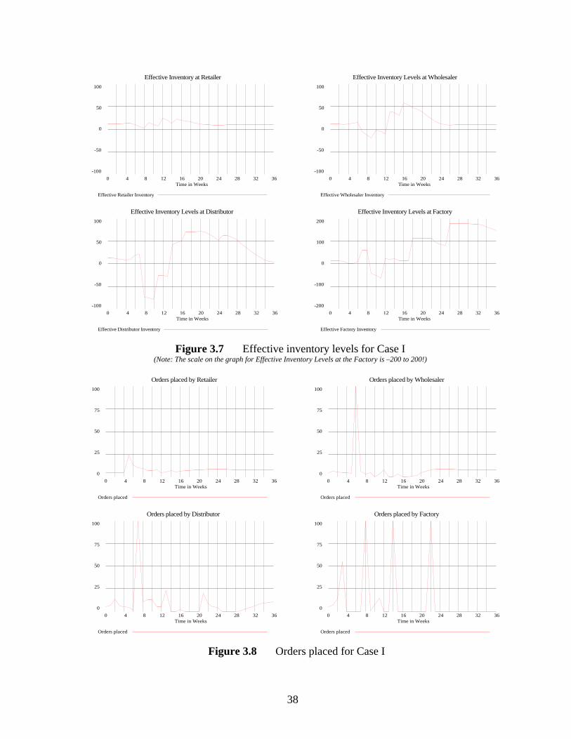
38

Effective Inventory at Retailer

100

50

0

-50

-100

0 4 8 12 16 20 24 28 32 36Time in Weeks

Effective Retailer Inventory

Effective Inventory Levels at Wholesaler

100

50

0

-50

-100

0 4 8 12 16 20 24 28 32 36Time in Weeks

Effective Wholesaler Inventory

Effective Inventory Levels at Distributor

100

50

0

-50

-100

0 4 8 12 16 20 24 28 32 36Time in Weeks

Effective Distributor Inventory

Effective Inventory Levels at Factory

200

100

0

-100

-200

0 4 8 12 16 20 24 28 32 36Time in Weeks

Effective Factory Inventory

Figure 3.7 Effective inventory levels for Case I(Note: The scale on the graph for Effective Inventory Levels at the Factory is –200 to 200!)

Orders placed by Retailer

100

75

50

25

0

0 4 8 12 16 20 24 28 32 36Time in Weeks

Orders placed

Orders placed by Wholesaler

100

75

50

25

0

0 4 8 12 16 20 24 28 32 36Time in Weeks

Orders placed

Orders placed by Distributor

100

75

50

25

0

0 4 8 12 16 20 24 28 32 36Time in Weeks

Orders placed

Orders placed by Factory

100

75

50

25

0

0 4 8 12 16 20 24 28 32 36Time in Weeks

Orders placed

Figure 3.8 Orders placed for Case I

39

Case II

Information Visibility and Collaboration amongst units: NO

Forecasting function: SMOOTH

Behavior:The bullwhip effect is strong in this case too. The forecasting function behaves bettering thiscase, and shows smooth behavior compared to the one in the previous case. Order variation atthe retailer is from (4 to12) and it amplifies to (0 to 30) at the factory. Inventory levels swingfrom (0 to 15) at the retailer and (–35 to 60) at the factory. At the end of 36 weeks, theinventory levels at distributor and factory haven’t yet achieved steady state.

Inventory

SMOOTHTIME <SMOOTHTIME>

Backlog

sold in

placed

bFlow

ordered

SupplyL

sFlow

<A> <B>A <A>B

Inventory 0

<SMOOTHTIME> <SMOOTHTIME>

Backlog 0

<A>

sold 0 in 0

placed 0

bFlow 0

<B>

ordered 0

SupplyL 0

sFlow 0

<B>

RETAILER WHOLESALER DISTRIBUTOR FACTORY

Inventory 1

Backlog 1

sold 1 in 1

placed 1

bFlow 1

ordered 1

SupplyL 1sFlow 1

Inventory 2

Backlog 2

sold 2 in 2

placed 2

bFlow 2

ordered 2

SupplyL 2

sFlow 2

coming

S

SL<S> <S> <S>

<SL> <SL><SL>

Traditional Beer Game - Using the "SMOOTH" forecasting function.

Figure 3.9 Beer game simulation Case II.

Cost

cost increase

<Backlog>

<Backlog 0>

<Backlog 1>

<Backlog 2>

<Inventory>

<Inventory 0>

<Inventory 1>

<Inventory 2>

Eff Env

>

>

Eff Inv 0

<Backlog 0>

<Inventory 0>

Eff Inv 1

<Backlog 1>

<Inventory 1>

Eff Inv 2

<Backlog 2>

<Inventory 2>

40

100

50

0

-50

-100

0 4 8 12 16 20 24 28 32 36Time in Weeks

Effective Retailer Inventory

100

50

0

-50

-100

0 4 8 12 16 20 24 28 32 36Time in Weeks

Effective Wholesaler Inventory

Effective Inventory Levels at Distributor

100

50

0

-50

-100

0 4 8 12 16 20 24 28 32 36Time in Weeks

Effective Distributor Inventory

Effective Inventory Levels at Factory

100

50

0

-50

-100

0 4 8 12 16 20 24 28 32 36Time in Weeks

Effective Factory Inventory

Figure 3.10 Effective inventory levels for Case II

Orders placed by Retailer

100

75

50

25

0

0 4 8 12 16 20 24 28 32 36Time in Weeks

Orders placed

Orders placed by Wholesaler

100

75

50

25

0

0 4 8 12 16 20 24 28 32 36Time in Weeks

Orders placed

Orders placed by Distributor

100

75

50

25

0

0 4 8 12 16 20 24 28 32 36Time in Weeks

Orders placed

Orders placed by Factory

100

75

50

25

0

0 4 8 12 16 20 24 28 32 36Time in Weeks

Orders placed

Figure 3.11 Orders placed for Case II

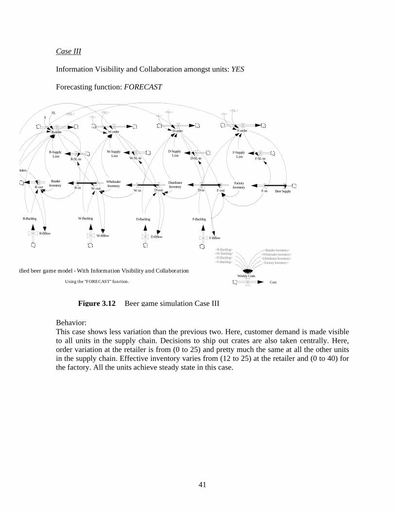
41

Case III

Information Visibility and Collaboration amongst units: YES

Forecasting function: FORECAST

Behavior:This case shows less variation than the previous two. Here, customer demand is made visibleto all units in the supply chain. Decisions to ship out crates are also taken centrally. Here,order variation at the retailer is from (0 to 25) and pretty much the same at all the other unitsin the supply chain. Effective inventory varies from (12 to 25) at the retailer and (0 to 40) forthe factory. All the units achieve steady state in this case.

RetailerInventoryR-out R-in

WholesalerInventory

W-out W-in

DistributorInventory

D-out D-in

FactoryInventory

F-out F-in Beer Supply

R-Backlog W-Backlog D-Backlog F-Backlog

R-BflowW-Bflow D-Bflow F-Bflow

R-order W-order D-order F-order

Orders

R-SupplyLine

W-SupplyLine

D-SupplyLine

F-SupplyLine

R-SL-in W-SL-in D-SL-in F-SL-in

<ISL>SLS

<SL><S> <S>

<SL> <S><SL>

<D-Backlog> <Distributor Inventory><F-Backlog> <Factory Inventory>

<R-Backlog> <Retailer Inventory><W-Backlog> <Wholesaler Inventory>

Cost

Weekly Costsified beer game model - With Information Visibility and Collaboration

Using the "FORECAST" function.

Figure 3.12 Beer game simulation Case III

42

Effective Inventory at Retailer

100

50

0

-50

-100

0 4 8 12 16 20 24 28 32 36Time in Weeks

Effective Retailer Inventory

Effective Inventory Levels at Wholesaler

100

50

0

-50

-100

0 4 8 12 16 20 24 28 32 36Time in Weeks

Effective Wholesaler Inventory

Effective Inventory Levels at Distributor

100

50

0

-50

-100

0 4 8 12 16 20 24 28 32 36Time in Weeks

Effective Distributor Inventory

Effective Inventory Levels at Factory

100

50

0

-50

-100

0 4 8 12 16 20 24 28 32 36Time in Weeks

Effective Factory Inventory

Figure 3.13 Effective inventory levels for Case III

Orders placed by Retailer

100

75

50

25

0

0 4 8 12 16 20 24 28 32 36Time in Weeks

Orders placed

Orders placed by Wholesaler

100

75

50

25

0

0 4 8 12 16 20 24 28 32 36Time in Weeks

Orders placed

Orders placed by Distributor

100

75

50

25

0

0 4 8 12 16 20 24 28 32 36Time in Weeks

Orders placed

Orders placed by Factory

100

75

50

25

0

0 4 8 12 16 20 24 28 32 36Time in Weeks

Orders placed

Figure 3.14 Orders placed for Case III

43

Case IV

Information Visibility and Collaboration amongst units: YES

Forecasting function: SMOOTH

Behavior:This case has the least variations. The variation in orders is (4 to 12) for all units in the supplychain. Effective inventory varies from (8 to 20) for the retailer and (4 to 25) for the factory.All units achieve steady state behavior in this case.

RetailerInventoryR-out R-in

WholesalerInventory

W-outW-in

DistributorInventory

D-out D-in

FactoryInventory

F-out F-in Beer Supply

R-Backlog W-Backlog D-Backlog F-Backlog

R-BflowW-Bflow D-Bflow F-Bflow

R-order W-order D-order F-order

Orders

R-SupplyLineW-Supply

LineD-Supply

LineF-Supply

LineR-SL-in W-SL-in D-SL-in F-SL-in

ISL>SL

S

<SL><S> <S>

<SL><S>

<SL>

<D-Backlog> <Distributor Inventory><F-Backlog> <Factory Inventory>

<R-Backlog> <Retailer Inventory><W-Backlog> <Wholesaler Inventory>

Cost

Weekly Costsodified Beer Game Model - With Information Visibility and Collaboration.

Using the "SMOOTH" function.

Figure 3.15 Beer game simulation Case IV

44

Effective Inventory at Retailer

100

50

0

-50

-100

0 4 8 12 16 20 24 28 32 36Time in Weeks

Effective Retailer Inventory

Effective Inventory Levels at Wholesaler

100

50

0

-50

-100

0 4 8 12 16 20 24 28 32 36Time in Weeks

Effective Wholesaler Inventory

Effective Inventory Levels at Distributor

100

50

0

-50

-100

0 4 8 12 16 20 24 28 32 36Time in Weeks

Effective Distributor Inventory

Effective Inventory Levels at Factory

100

50

0

-50

-100

0 4 8 12 16 20 24 28 32 36Time in Weeks

Effective Factory Inventory

Figure 3.16 Effective inventory levels for Case IV

Orders placed by Retailer

100

75

50

25

0

0 4 8 12 16 20 24 28 32 36Time in Weeks

Orders placed

Orders placed by Wholesaler

100

75

50

25

0

0 4 8 12 16 20 24 28 32 36Time in Weeks

Orders placed

Orders placed by Distributor

100

75

50

25

0

0 4 8 12 16 20 24 28 32 36Time in Weeks

Orders placed

Orders placed by Factory

100

75

50

25

0

0 4 8 12 16 20 24 28 32 36Time in Weeks

Orders placed

Figure 3.17 Orders placed for Case IV

45

3.5 Explanation of simulation results

Case InformationVisibility andCollaboration

ForecastingFunction

Cost$

I No FORECAST 3020II No SMOOTH 1482III Yes FORECAST 957IV Yes SMOOTH 852

Table 3.2 Comparison of the four cases.

Figure 3.8 and 3.11 clearly show the bullwhip effect in the supply chain in theabsence of information visibility. Figure 3.10 and 3.11 also show the amplification offluctuations in demand and inventory levels from retailer to factory. We observe that the

bullwhip effect is more pronounced in case I than case II. This is an outcome of theforecasting function used in the two cases. The “FORECAST” function used in case Ichanges rapidly with changes in inputs. These get amplified very easily as demandforecasting progresses upstream in the supply chain. On the other hand, the “SMOOTH”function used in case II changes smoothly despite rapid changes in inputs – creating asmooth continuous effect, resulting in well-behaved ordering patterns.

Figure 3.18 Comparison of costs in the four cases.

Total Costs in Case II

3,500

2,625

1,750

875

0

0 4 8 12 16 20 24 28 32 36Time in Weeks

Total Inventory Costs in the Supply Chain

Total Costs in Case I

3,500

2,625

1,750

875

0

0 4 8 12 16 20 24 28 32 36Time in Weeks

Total Inventory Costs in the Supply Chain

Total Costs in Case III

3,500

2,625

1,750

875

0

0 4 8 12 16 20 24 28 32 36Time in Weeks

Total Inventory Costs in the Supply Chain

Total Costs in Case III

3,500

2,625

1,750

875

0

0 4 8 12 16 20 24 28 32 36Time in Weeks

Total Inventory Costs in the Supply Chain

46

The behavior of the supply chain in cases III and IV (where we achieveinformation visibility of customer demand at each unit) is a great improvement over thosein cases I and II. We see that information visibility and collaboration has almosteliminated the bullwhip effect. In case III and IV, we provided visibility by makingavailable customer demand data to all units, and eliminating communication delaysbetween units by assuming instantaneous communication. This elimination of delays andcollaborated forecasting of demand has clearly eliminated the ripple effect in inventorylevels at or orders placed by individual units. We observe that in cases of improvedinformation visibility, the effective inventory has not fallen into backlog, and hasconsistently delivered the goods demanded by the customer. We also observe that the“SMOOTH” function is a better forecasting technique than the “FORECAST” functionfor this example of the beer game. Given the extremely complex nature of supply chains,with many inherent interdependencies, and external influencing factors, differentforecasting techniques might yield different results. Although given these complexities,an important conclusion falls out of the above simulations while comparing results ofcase I with case III; and case II with case IV. We see that for a given forecastingtechnique, information visibility and collaboration offers a huge savings (~ 40% to 70%)in inventory costs in the supply chain.

Information visibility in a supply chain aims at having the right data at the rightplace and the right time in the right format – for ex: customer demand for crates of beerper week, inventory and backlog levels in each unit, etc. An initiative to provideinformation visibility can be implemented as primarily a combination of two importantsub-initiatives: having the technology required for achieving real time data management;and willingness of supply chain units for sharing their data with trading partners andcollaborate in the supply chain. We discussed the latter initiative – of planning,forecasting and replenishing demand collaboratively – in the previous chapter. We alsotalked about current technological means for achieving information visibility and theirlimitations. In the next chapter, we describe a framework for achieving informationvisibility in supply chains that can overcome most of these limitations.

47

Chapter 4

A framework for information visibility

4.1 Introduction

In the previous chapters, we saw the pronounced need for visibility of informationin the supply chain. All software reviewed in Chapter 2 operates successfully if correctinformation is available to it. In Chapter 3, we saw the improvements in supply chaincosts offered by information visibility. In this chapter, we propose a framework by whichwe can achieve information visibility in real time.

4.2 Information visibility in real time

As explained in Chapter 2, most data that is gathered today is not real time. Datais gathered using various techniques – manual, barcodes or tags. Different people gatherit at different times of the day in individual units of the supply chain, on the shop floor orin the warehouse. This data is then entered in the computerized database at apredetermined time, at regular intervals. Thus, the database is updated in fixed quanta oftime. In between these time periods, which typically can last from a few hours to a fewdays, the database is only pseudo-real time. This introduces visibility gaps in the system.In many instances, other units in the supply chain base their decisions on data that theygather from this unit under consideration. They are provided with inaccurate data, whichresults in sub-optimal decision-making.

To achieve real time visibility of information, we need to:1. Have real time data acquisition mechanisms.2. Convert acquired data into relevant information: using standardized, secure

representation.3. Have instantaneous access to this information.

We propose the use of automated tracking systems to achieve real time dataacquisition. The purpose of an automated tracking system is to capture relevant dataabout the object under consideration and pass it on to another application. Therequirements of such a system include:

• A mechanism to locate the object.• A mechanism to gather relevant data.• Interface with other applications to exchange this data.

We propose the use of radio frequency tags, in conjunction with tag readers toachieve real time data acquisition.

48

Data acquired by tag readers will then be passed on to a software application. Thisapplication, in conjunction with a lookup table and object description language, processthe data and convert it into relevant information, and store it at the appropriate location sothat others can utilize it to take sensible decisions.

Instantaneous information access can be achieved through the internet.

4.3 Basic building blocks

The basic building blocks of the framework outlined above are radio frequencytags, electronic product codes, tag readers, object naming service, an object descriptionlanguage, the internet, and a controlling software application.

4.3.1 Electronic Product Code (ePC)

The encoded bits on the radio frequency tag will constitute an object identificationcode, called “electronic Product Code”, or in short, the ePC. Brock [35] invented the ePCat the MIT Auto-ID Center. Brock defines ePC as “a numbering scheme that can provideunique identification for physical objects, assemblies and systems.” The code acts as apointer to another location where information is stored remotely about the object beingidentified by the code.

ePC is being developed as a replacement for the fast depleting UCC (UniformCode Council) barcode, and is aimed to be the next generation object identifier. The ePCprimarily consists of bits providing a unique identification to every object. The ePC wasinitially defined in Foley, et al. [36a]. More details about the ePC can be found at [36].

4.3.2 Tag readers

Given that every object is labeled with a unique ePC, the next task is to identifythem. This is done with the help of radio frequency tag readers. Foley, et al. [36a] definetag readers as “a microcontrolled unit with an output coil wound for a particular carrierfrequency. It consists of peak detector hardware, comparators, and firmware for doingbackscatter communications.” The tag reader generates a radio frequency sine wave thattransmits energy to the tag, and receives data from it.

All points of data acquisition will be equipped with tag readers, capable ofreading the ePC on tags within their read range. Tag readers can currently read within arange of 1-3 meters. Further developments in tag reading technology will hopefullyextend the space covered by a single tag reader. Also, anti-collision technology enablesreading of more than one tag within a given readers range (up to as much as 50 persecond currently [38], and more with time). As objects come into the reading zone, thetag reader reads the object ePCs. Once the tag reader has received bits from the object,

49

the bits are arranged into a sequence of numbers, which constitutes the unique ePC forthe object being identified.

4.3.3 Object Naming Service (ONS)

ePC received from the tag reader is passed on to a protocol that will helpdetermine where to locate information corresponding to the ePC under consideration.This protocol is called “Object Naming Service” (ONS), and is being developed at theAuto-ID Center by Sarma, et al. [37]. The task of the ONS is to point to the source ofquery the destination where information relevant to the ePC being queried is stored.Information about objects will be stored at convenient locations on the internet. Forexample: information about an object, say soap X, can be stored on the website ofcompany Y, which manufactures soap X. Anyone wishing to know more about soap Xcan access that information from the ePC of soap X. The company database could containsuch information about soap X as the constituents of the soap, skin type serviced,manufacturing date and location, shipping details, etc. Different parts of this informationwould be relevant to different persons coming in contact with soap X, for differentpurposes, all along the supply chain for soap X, from the manufacturer to the consumer.The ONS would serve the purpose of connecting the source of query to this informationon the internet.

4.3.4 Object description language (ODL)

The location to which the ONS points for information about a particular object isan IP (internet protocol) address. At this IP address, information about the object isrepresented. Since no units in the supply chain communicate solely within itself, but alsowith other units in its supply chain, the language used for this representation shouldsatisfy requirements like:

• Possess a standardized, open format.• Be inter-operable.• Be scalable.• Provide required security features.• Be robust and manageable.• Be easy to implement.

The extensible Markup Language (XML) lends itself easily to satisfy many of theabove criteria. XML is a “meta-language” that defines syntax rules for “well-formed”documents, and define an unlimited number of languages for specific industries andapplications. It has rapidly become the standard for defining data interchange formats.

Many independent committees are working towards defining standard practices forthe use of XML. The Techniques and Methodologies Working Group (TMWG), apermanent working group under the United Nations Center for Facilitation of Proceduresand Practices for Administration, Commerce and Transport (CEFACT) has come out

50

with specific recommendations for converting current standard EDI syntax into XMLsyntax [39]. The World Wide Web Consortium (W3C) is involved in developing coreXML technologies and other standards related to XML [40]. The Organization for theAdvancement of Structured Information Standards (OASIS), a vendor neutralinternational consortium, focuses on making XML standards practical and easy to adopt[41]. A recent OASIS spin-off is XML.ORG, an industry web portal, and aims atestablishing an open, distributed system for enabling the use of XML in electroniccommerce and other industrial applications. XML.ORG is designed to provide a crediblesource of accurate, timely information about the application of XML in industrial andcommercial settings and to serve as a reference repository for XML specifications such asvocabularies, document type definitions (DTD), schemas, and namespaces [42].

Recently, UN/CEFACT and OASIS have joined forces to initiate a worldwide projectto standardize XML business specifications. UN/CEFACT and OASIS have establishedthe Electronic Business XML (ebXML) initiative to develop a technical framework thatwill enable XML to be utilized in a consistent manner for the exchange of all electronicbusiness data [43]. The ebXML initiative intends to develop relevant and open technicalspecifications to support domestic and international electronic business exchanges.

The Auto-ID Center at MIT is developing the Product Markup Language (PML) as a“standard language” for describing physical objects [44]. Based on XML, PML will buildlayers of increasingly specific data describing physical objects. The objective ofdeveloping PML, as defined by the Auto-ID Center, are:

• should translate or contain static data - such as dosage, shipping, expiration,advertising and recycling information.

• should provide instructions for machines that "process" or alter a product - suchas microwaves, laundry appliances, machine tools and industrial equipment.

• may need to communicate dynamic data: information that changes as a productages or as it is consumed - such as volume, temperature, moisture and pressure.

• may need to include software, or programs, which describe how an object behaves- for instance: a .pml file may contain the program which describes how fast thetires on your car will wear before they need to be replaced, or how fast an objectmay burn in case of a fire.

4.3.5 Fitting them together

The ePCs on tags, coupled with tag readers and the controlling softwareapplication form an automated tracking system for real time data acquisition. Along withONS, an appropriate object description language, and the internet, we can convertacquired data into relevant information and store it securely at appropriate locations. Weexplain this framework in detail in the next section.

51

4.4 A generalized framework for information visibility

We describe the framework with the help of an example – the distributor in thesupply chain for beer.

4.4.1 Framework within an individual supply chain unit

The distributor receives beer crates from his supplier, which is the factory, and heships out crates to his customer, which is the wholesaler. In real life, a distributor willtypically receive more than one product from more than one factory, and will ship a mixof products to multiple wholesalers, or directly to retailers. The framework proposedbelow is highly scalable and can be easily extended to include the case of multipleproducts, multiple suppliers and multiple customers.

The distributor typically operates out of a large warehouse. Crucial tasks associatedwith running this distribution center are shown in Figure 4.1.

Implementing a tracking system for real time data acquisition would require that:• All beer crates have radio frequency tags attached to them• All tags carry an ePC on them• The shipment receiving station be equipped with tag readers• The inventory shelves be equipped with tag readers

Receive shipments from factory

Record their arrival add them to local inventory

Receive orders for shipping out crates to wholesalers

Create shipments to go by combining current items in stock as per demand

Dispatch product to wholesalers (coordinate the transportation activities)

Update local inventory levels

Figure 4.1 Activities flowchart at the distributor.

52

• The dispatch location be equipped with tag readers

Data acquisition begins from the point when goods arrive at the warehouse. At thereceiving dock, crates are offloaded from the trucks and put on to the conveyor beltsreceiving them into the warehouse inventory. Tag readers at the entry point, which readthe ePCs on the tags, surround these conveyor belts. The crates then proceed to inventoryshelves, which are also equipped with tag readers. When orders from customers areprocessed, and packages are ready to be shipped, they are passed out on to the loadingdock through a set of tag readers again which note the ePCs of the crates being shipped.This is shown schematically in Figure 4.2. A software application managing dataacquisition for the distributor warehouse communicates with the tag readers installed atvarious locations in the warehouse. It receives large amounts of data from many inputs.This data has the potential to be converted into real time information. The softwareapplication gathers the ePCs of products being tracked by the tag readers, queries theONS for the web address where information about the product is stored, updates thatinformation if necessary, plus maintains localized data records relevant to operations ofthe warehouse. The updated product information can be stored either in a centralizeddatabase or distributed databases.

For example: when a beer crate comes in through the receiving docks of thewarehouse, it passes through the tag readers at the incoming station. The tag reader readsthe ePC of the tag on this beer crate and passes this information to the softwareapplication managing the data acquisition process. The software application, inconjunction with the ONS, locates the address at which detailed information about thiscrate is stored. Since the software application also knows the location of the tag readerfrom which it has received information about the beer crate, it is in a position to updatelocation information relevant to this beer crate. With requisite security features andaccess control, the data acquisition software can now access information about this beercrate, as well as update the current status of the crate, and maintain real time dataaccuracy. The beer crate is then stored in inventory at the warehouse – typically onshelves. We equip each of these shelves with a tag reader. The software applicationcontinuously receives information from these tag readers about the ePCs of the cratesstored on the inventory shelves. If the application records a new ePC, it immediatelycoordinates with the ONS to reach the information site of this crate, and learninformation about the crate from that site. It can again update the information about thiscrate – about its current location, time, and destination and waiting period if known.Provided the waiting period for a crate is known, the software application can alert thewarehouse managers at a suitable time before the end of the period about further shippingactions for that crate. The software application can also perform other routine tasks, suchas issuing warnings if the crate is reaching its expiry date, etc.

53

Receiving incoming shipments: The tag readersautomatically record ePCs of the crates being

received into the warehouse, as the crates pass intothe warehouse on a conveyor belt.

Tag readers

Tag readers

Inventory: The shelves are equipped with tag readersthat continuously monitor which crate is located wherein the warehouse. This provides real-time visibility into

the exact status of inventory in the warehouse.

Based on incoming orders,products are packaged together

to be shipped to customer.

oducts get loaded into trucks at the shippingk of the warehouse, they again pass throughg readers that note ePCs of products being

shipped out.

Tag readers

Tag readers

Outgoingshipments

Incomingshipments

Beer Crate

Tag

Figure 4.2 Real time data acquisition at the distributor.

54

4.4.2 Framework extended to the entire supply chain

There is a marked difference in the manner in which information and productsflow through traditional supply chains and those of today. In order to achieve fasterdeliveries, reductions in cost, product customizations, all in all, better customer

relationship management; companies today adopt multiple channels of productdistribution. This demands information flow in the supply chain to not be serial, but takeplace from any point to any other point.

In the generic supply chain, we visualize information visibility as shown in Figure4.4 and 4.5. In each individual supply chain unit, automated tracking systems will acquiredata in real time as described above. The data corresponding to objects will be updatedand stored at the location described by the ePC. The software application acquiring datain real time will store information pertinent to the unit under consideration in the localunit database. This can contain information about current inventory, the total quantities ofdifferent products, individual ePCs of each product, information about upcoming ordersand shipping schedules for the unit, etc.The issue of what information should be storedlocally is entirely the prerogative of the individual supply chain unit under consideration,and should be resolved with mutual understanding with other partners in the supply chain(since many of them will be involved in contributing to the generation of this

Suppliers Distributors Wholesalers Retailers CustomersManufacturers

Flow of Information, with delays (serial).

Flow of Goods (serial).

Figure 4.3 Flow in a traditional supply chain.

Instantaneous, secure communication over the internet.

Converting data into relevant information -description and representation, storage at relevant

location.

Real time data acquisition throughautomated tracking systems.

Supply ChainUnit Data

Figure 4.4 Layered approach to information visibility.

55

information). The individual supply chain unit information can be made available on theinternet to authorized users. These users can typically be trading partners in the supplychain or end customers. They can use this information for taking further decisions.Provided all trading partners in the product delivery network reach an agreement onimplementing such a collaborative framework of data acquisition, description andrepresentation, with instantaneous, secure communication over the internet, we can hopeto achieve real time information visibility in the entire product supply chain.

4.5 Implementing the proposed framework in the beer game

The beer distribution network described in the previous chapter consists of fourindividual units, plus raw materials suppliers to the factory, and end consumers of beer.The information required for determining ordering and shipping quantities and consumerdemand forecasting in this supply chain includes past behavior of consumer demand(updated till the latest possible date), inventory levels and backlog levels at each unit.

pliers Distributors Wholesalers Retailers CustomersManufacturers

ron

RetailerInformation

WholesalerInformation

ManufacturerInformation

DistributorInformation

CustomerInformation

Flow of Goods – multiple channels.

Authorized access.

Communication on the internet.

Traditional product flow channel, through each unit in the supply chain.

A new business model – direct shipping of product from factory to consumer.

A new business model – using one of the intermediate units to channel product flow to consumer.

Figure 4.5 Contemporary supply chains.

56

Internet

Beer CratesWith RF Tags.

Tag Reader onInventory

Shelf.

etailer Inventory.

Beer CratesWith RF Tags.

Tag Reader onInventory

Shelf.

WholesalerInventory.

Beer CratesWith RF Tags.

Tag Reader onInventory

Shelf.

Factory Inventory.

eer Cratesth RF Tags.

g Reader onInventory

Shelf.

Distributornventory.

RetailerDatabase

WholesalerDatabase

FactoryDatabase

DistributorDatabase

XML Server

XML ServerML Server

XML Server

CustomerDemand

Software Application

- Gets the required data fromrequired sources (customer

demand, inventory levels andbacklog at each units.)

- Forecasts beer productionschedule for factory.

- Determines quantity ofcrates to be shipped betweenunits, based on demands and

quantities already in thesupply line.

TAILER

FACTORYRIBUTOR

WHOLESALERFigure 4.2Automated data

acquisition at thedistributor.

Communication link – authorized public access.

Security check for authorizing access.

Communication link – private access.

DISTRIBUTORFigure 4.6 Proposed framework for information visibility in the beer game.

ONS

57

We propose that each unit deploy a real time data acquisition system as structuredin section 4.4. Since in this example, the most important data required for decision-making in the supply chain is inventory and backlog levels, putting tags on beer cratesand equipping inventories in each unit with tag readers is the first step towards achievinginformation visibility. Tag readers on inventory shelves will read crate ePCs. Thesoftware application interfacing with these tag readers will record the ePCs in a localdatabase, as well as lookup the ONS to access the crates description database. It will thenupdate the newly acquired data for the crates under consideration – their new location,tasks completed, next task on hand, etc. The software application can be a locally runningprogram, or a remote program interfacing with tag readers over a network. At each unit,the software application can pass on the data acquired in real time to higher-levelenterprise management software. The task of recording weekly customer demand shouldbe assigned to one of the supply chain units – the retailer is in the best position to handlethis task. In fact, weekly customer demand can also be extracted from sales per week thatget recorded at the retailer.

58

Chapter 5

Conclusions

The research presented in this thesis is part of a larger initiative to change the waydata about physical objects is acquired, understood, represented as useful information,and utilized efficiently. Here, we focus on the data related to products moving in theirsupply chains.

We began with a review of developments in production and operationsmanagement software and supply chain management software over the last three decades.A look into the requirements for successful implementation of these software andrequirements of supply chains of today points to real time information visibility as one ofthe crucial factors for efficient supply chain management. To illustrate impact on costsincurred in the supply chain, we ran computer simulations of supply chain models underdiffering conditions of information visibility. The results show that information visibilityand collaboration provide ~ 40 to 70% reduction in inventory costs alone! Otherintangible benefits include reduction in lost sales due to absence of backlogs, improvedcustomer service due to timely delivery of orders, more confidence in managing thesupply chain due to accurate, real time knowledge of location of products moving in thesupply chain.

We then presented a novel framework for improving information visibility insupply chains. This involves first developing automated object tracking and dataacquisition systems – with the help of radio frequency tags and tag readers. Thesesystems eliminate time delays associated with current industrial data acquisition methods,as well as reduce possibility of error in data entry, by minimizing human intervention.The key concept in the proposed data acquisition technique is the use of an electronicproduct code, ePC, for identifying each single object. This code is currently beingdeveloped at MIT’s Auto-ID Center. In conjunction with tags and readers, this uniqueobject code provides easy identification and tracking of individual objects. The next stepinvolves converting acquired data into sensible information. The key concepts in theproposed framework for achieving this are the use of an object naming service, ONS, forresolving the location where description about the object is stored, and an objectdescription language, ODL, to describe details about the object being tracked at the latestavailable time. An interfacing software application does the task of acquiring the ePCfrom the tag readers, querying thr ONS with the ePC, accessing the location whereinformation about the product is stored, converting recent product specific data acquiredinto relevant information in an ODL, and updating the location of information storagewith the latest available data. Real time information visibility in supply chains is achievedby accessing this data in real time over the internet, from any location in the supply chain.

Crucial to achieving real time information visibility is the widespread adoption ofthe proposed framework – within a single product supply chain as well as supply chainsfor different products. Common standards for communication, rules regarding security,

59

authorization and encryption for the use and access of product data are issues that supplychain units will find crucial during implementation of the framework. Under certainsituations, trading partners might not wish to reveal their information – safety and privacyof information then becomes crucial to earning the trust of these trading partners.

The rapid development of the internet has led to many changes in ways businessesare run. More and more companies are moving online for procuring raw materials,interacting with customers, and delivering directly to them by bypassing existingchannels for product flow. Stores are turning into showrooms; computers are becomingthe shopping store; and the shipment delivery boy is replacing the checkout counter. In aworld where the customer has a lot of options and loyalty changes with the click of abutton, achieving customer satisfaction will take much more than old-fashionedmanufacturing shop floors and supply chains. We believe that achieving visibility ofinformation is the first step towards success in this competition.

In conclusion, this thesis outlines an overarching framework. Much needs to bedone in terms converting these concepts to reality. The ePC, ONS and an ODL need to bestandardized and developed and made viable to be used worldwide as the de-factostandards for object identification and data representation. An industrial experiment, suchas implementing a real time data acquisition system in a warehouse (as illustrated in theprevious chapter) would be a first step towards providing proof of concept. Furtherexpansion of this system to other units in a supply chain would be the next step. Weenvision an eventual adoption of this framework in all supply / value chains or tradingnetworks.

60

References

[1] Quinn F. J., ‘The Payoff Potential in Supply Chain Management’, Supply ChainManagement Review.(http://quinn.ascet.com/)

[2] Cole S.J., Woodring S.D., Chun H., and Gatoff J., ‘Dynamic Trading Networks’, TheForrester Report, January 1999.

[3] McCullough S.S., ‘Time to replace your MRP?’, The Forrester Report, February1999.

[4] Fogarty D.W., Blackstone J.H., and Hoffman T.R., “Production and InventoryManagement”, South Western Publishing Company, 1991.

[5] Richards H., ‘Notes on Manufacturing Strategy and Performance MeasurementProcesses’, Institute for Manufacturing, University of Cambridge.(http://www-mmd.eng.cam.ac.uk/people/ahr/dstools/proces/mrp2.htm)

[6] Krajewski L.J., and Ritzman L.P., “Operations Management”, Addison-WesleyPublishing Company, 1999.

[7] Kumar K., and Hillegersberg J.V., ‘ERP – Experience and Evolution’,Communications of the ACM, 43(4), pp 22-26, April 2000.

[8] SAP, ‘SAP R/3 System Overview’.(http://www.sap.com/solutions/r3/index.htm)

[9] Stevens G.C., ‘Integrating the supply chain’, Intl. J of Physical Distribution andMaterials Management, Vol-19, pp 3-8, 1989.

[10] Tayur S., Ganeshan R., and Magazine M., “Quantitative Models for Supply ChainManagement”, Kluwer’s International Series, 1999.

[11] Hicks D.A., ‘A four step methodology for using simulation and optimizationtechnologies in strategic supply chain planning’, Proceedings of the 1999 WinterSimulation Conference, pp 1215-1220.

[12] Gormley J.H. III, Woodring S.D., and Lieu K.C., ‘Supply chain beyond ERP’ TheForrester Report, May 1997.

61

[13] Padmos J., Hubbard B., Duczmal T., and Saidi S., ‘How i2 integrates simulation insupply chain optimization’, Proceedings of the 1999 Winter Simulation Conference, pp1350-1355.

[14] i2 Technologies.(http://www.i2.com)

[15] Syncra Systems.(http://www.syncra.com)

[16] Voluntary Interindustry Commerce Standards.(http://www.vics.org)

[17] Yao A.C., and Carlson J.G., ‘The impact of real-time data communication oninventory management’, Intl. J. of Production Economics, Vol-59, pp 213-219, 1999.

[18] Lindau R., and Lumsden K., ‘The use of automatic data capture systems in inventorymanagement’, Intl. J. of Production Economics, Vol-59, pp 159-167, 1999.

[19] Bruce P., ‘Barcode and EDI – “the right stuff” for consumer goods manufacturers’,Automatic I.D. News, 14(4), pp 46-47, April 1998.

[20] Swamidass P.M., ‘Bar code users and their performance’, Unova Inc, July 1998.

[21] The AIM Global Network, ‘What is RFID?’(http://www.aimglobal.org)

[22] Loudin A., ‘RFID comes into its own’, Warehousing Management , 6(3), pp 30-32,April 1999.

[23] Motorola, ‘Bistatix White paper’, Version 4.1, March 1999.(http://www.motorola.com)

[24] Yating L., and Zhang J., ‘Electronic Data Interchange – EDI’.(http://www.biz.uiowa.edu/class/6k220_park/OldStudProjects/S97/group4/EDI.html)

[25] Erwin B., Callahan P.D., and Cho D., ‘Will the web kill EDI?’, The ForresterReport, February 1996.

[26] Forrester J.W., “Industrial Dynamics”, MIT Press, Cambridge, MA, 1961.

[27] Sterman J. D., ‘The Beer Distribution Game: An Annotated Bibliography Coveringits History and Use in Education and Research’, July 1992.(http://learning.mit.edu/pra/tool/bibl.html)

62

[28] Sterman J. D., ‘Modeling Managerial Behavior: Misperceptions of Feedback in aDynamic Decision Making Experiment’, Management Science, 35(3), pp 321-339, 1989.

[29] Instructions for playing the beer game.(http://learning.mit.edu/pra/tool/beer.html)

[30] Kirkwood C. W., ‘The Beer Game Production-Distribution Exercise: Running LargeSessions’.(http://www.public.asu.edu/~kirkwood/sysdyn/BGame/BGame.htm)

[30a] Masters J., ‘Lecture Notes – MIT Class on Logistics Systems’, Fall 1999.

[31] Sterman J.D., “Business Dynamics: Systems Thinking and Modeling for a ComplexWorld”, Irvin McGraw-Hill, 2000.

[33] Kirkwood C. W., ‘Business Process Analysis Workshops: System DynamicsModels’, Department of Management, Arizona State University, Tempe, AZ 85287-4006.(http://www.public.asu.edu/~kirkwood/sysdyn/SDWork/SDWork.htm)

[34] Lee H.L., Padmanabhan V., and Whang S., ‘The bullwhip effect in supply chains’,Sloan Management Review, pp 93-102, Spring 1997.

[34a] Hewlett Packard, ‘The Bullwhip Effect - Exploring Causes and Counter Strategies’.(http://www.internetsolutions.enterprise.hp.com/supplychain/library/articles/bullwhip_content.html)

[35] MIT Auto-ID Center - Fact Sheet on ePC.(http://auto-id.mit.edu/)

[36] MIT Auto-ID Center.(http://auto-id.mit.edu/)

[36a] Foley J.T., ‘An Infrastructure for Electromechanical Appliances on the Internet’,S.B. & M.Eng. Thesis, Massachusetts Institute of Technology, Cambridge, MA, May1999.

[37] MIT Auto-ID Center - Fact Sheet on ONS.(http://auto-id.mit.edu/)

[38] Intermec News Report, Logistics Management & Distribution Report, June 1999.(http://www.manufacturing.net/magazine/logistic/archives/1999/log0601.99/491.htm)

[39] TMWG, ‘TMWG Recommendations on XML’, UN/CEFACT/TMWG/NO89/Rev.5,September 1999.

[40] The World Wide Web Consortium.

63

(http://www.w3c.org)

[41] Organization for the Advancement of Structured Information Standards.(http://www.oasis-open.org)

[42] XML.ORG: The XML Industry Portal.(http://www.xml.org)

[43] ebXML: Electronic Business XML initiative.(http://www.ebxml.org)

[44] MIT Auto-ID Center - Fact Sheet on PML.(http://auto-id.mit.edu/)

64

Appendix A

No: Variable and defining equation Comments(01) A = 0.26 Forecasting parameter(02) B = 0.088 Forecasting parameter(03) Backlog = INTEG( bFlow , 0) Backlog at retailer(04) Backlog 0 = INTEG( bFlow 0 , 0) Backlog at wholesaler(05) Backlog 1 = INTEG( bFlow 1 , 0) Backlog at distributor(06) Backlog 2 = INTEG( bFlow 2 , 0) Backlog at factory(07) bFlow = ORDer - sold Accumulation of backlog at retailer(08) bFlow 0 = ordered - sold 0 Accumulation of backlog at wholesaler(09) bFlow 1 = ordered 0 - sold 1 Accumulation of backlog at distributor(10) bFlow 2 = ordered 1 - sold 2 Accumulation of backlog at factory(11) coming = ordered 2 Materials in transit to factory(12) Cost = INTEG( cost increase , 0) Total inventory cost in supply chain(13) cost increase = 1 * ( Backlog + Backlog 0 + Backlog 1 + Backlog 2 ) + 0.5 * (

Inventory + Inventory 0 + Inventory 1 + Inventory 2 )Weekly inventory cost in supply chain

(14) Eff Env = Inventory - Backlog Effective Inventory at retailer(15) Eff Inv 0 = Inventory 0 - Backlog 0 Effective Inventory at wholesaler(16) Eff Inv 1 = Inventory 1 - Backlog 1 Effective Inventory at distributor(17) Eff Inv 2 = Inventory 2 - Backlog 2 Effective Inventory at factory(18) FINAL TIME = 36 The final time for the simulation.(19) in = DELAY FIXED( sold 0 , 2, 4) Incoming orders at retailer(20) in 0 = DELAY FIXED( sold 1 , 2, 4) Incoming orders at wholesaler(21) in 1 = DELAY FIXED( sold 2 , 2, 4) Incoming orders at distributor(22) in 2 = DELAY FIXED( coming , 2, 4) Incoming orders at factory(23) INITIAL TIME = 0 The initial time for the simulation.(24) Inventory = INTEG( in - sold , 12) Physical inventory at retailer(25) Inventory 0 = INTEG( in 0 - sold 0 , 12) Physical inventory at wholesaler(26) Inventory 1 = INTEG( in 1 - sold 1 , 12) Physical inventory at distributor(27) Inventory 2 = INTEG( in 2 - sold 2 , 12) Physical inventory at factory(28) MaxOrder = 100 A limit on the maximum order placed(29) ORDer = 4 + STEP ( 4, 5) Weekly customer orders(30) ordered = DELAY FIXED( placed , 1, 4) In transit orders by retailer(31) ordered 0 = DELAY FIXED( placed 0 , 1, 4) In transit orders by wholesaler(32) ordered 1 = DELAY FIXED( placed 1 , 1, 4) In transit orders by distributor(33) ordered 2 = DELAY FIXED( placed 2 , 1, 4) In transit orders by factory(34) placed = MIN ( MAX ( 0, FORECAST ( ORDer , 2, 4) + A * ( S - ( Inventory -

Backlog ) ) + B * ( SL - SupplyL ) ) , MaxOrder )Orders placed by retailer

(35) placed 0 = MIN ( MAX ( 0, FORECAST ( ordered , 2, 4) + A * ( S - ( Inventory0 - Backlog 0 ) ) + B * ( SL - SupplyL 0 ) ) , MaxOrder )

Orders placed by wholesaler

(36) placed 1 = MIN ( MAX ( 0, FORECAST ( ordered 0 , 2, 4) + A * ( S - (Inventory 1 - Backlog 1 ) ) + B * ( SL - SupplyL 1 ) ) , MaxOrder )

Orders placed by distributor

(37) placed 2 = MIN ( MAX ( 0, FORECAST ( ordered 1 , 2, 4) + A * ( S - (Inventory 2 - Backlog 2 ) ) + B * ( SL - SupplyL 2 ) ) , MaxOrder )

Orders placed by factory

(38) S = 12 Forecasting parameter(39) SAVEPER = TIME STEP Frequency at which output is stored.(40) sFlow = placed - in Supply line accumulation - retailer(41) sFlow 0 = placed 0 - in 0 Supply line accumulation - wholesaler(42) sFlow 1 = placed 1 - in 1 Supply line accumulation - distributor(43) sFlow 2 = placed 2 - in 2 Supply line accumulation - factory(44) SL = 14.7 Forecasting parameter(45) SMOOTHTIME = 1 Forecasting parameter(46) sold = MIN ( Inventory + in , ORDer + Backlog ) Crates sold by retailer(47) sold 0 = MIN ( Inventory 0 + in 0 , ordered + Backlog 0 ) Crates sold by wholesaler(48) sold 1 = MIN ( Inventory 1 + in 1 , ordered 0 + Backlog 1 ) Crates sold by distributor(49) sold 2 = MIN ( Inventory 2 + in 2 , ordered 1 + Backlog 2 ) Crates sold by factory(50) SupplyL = INTEG( sFlow , 8) Supply line for retailer(51) SupplyL 0 = INTEG( sFlow 0 , 8) Supply line for wholesaler(52) SupplyL 1 = INTEG( sFlow 1 , 8) Supply line for distributor(53) SupplyL 2 = INTEG( sFlow 2 , 8) Supply line for factory(54) TIME STEP = 1 The time step for the simulation.

Table A.1 Equations simulating the beer game for Case I.

65

No: Variable and defining equation Comments(01) A = 0.26 Forecasting parameter(02) B = 0.088 Forecasting parameter(03) Backlog = INTEG( bFlow , 0) Backlog at retailer(04) Backlog 0 = INTEG( bFlow 0 , 0) Backlog at wholesaler(05) Backlog 1 = INTEG( bFlow 1 , 0) Backlog at distributor(06) Backlog 2 = INTEG( bFlow 2 , 0) Backlog at factory(07) bFlow = ORDer - sold Accumulation of backlog at retailer(08) bFlow 0 = ordered - sold 0 Accumulation of backlog at wholesaler(09) bFlow 1 = ordered 0 - sold 1 Accumulation of backlog at distributor(10) bFlow 2 = ordered 1 - sold 2 Accumulation of backlog at factory(11) coming = ordered 2 Materials in transit to factory(12) Cost = INTEG( cost increase , 0) Total supply chain cost(13) cost increase = 1 * ( Backlog + Backlog 0 + Backlog 1 + Backlog 2 ) + 0.5 * (

Inventory + Inventory 0 + Inventory 1 + Inventory 2 )Weekly supply chain cost

(14) Eff Env = Inventory - Backlog Effective Inventory at retailer(15) Eff Inv 0 = Inventory 0 - Backlog 0 Effective Inventory at wholesaler(16) Eff Inv 1 = Inventory 1 - Backlog 1 Effective Inventory at distributor(17) Eff Inv 2 = Inventory 2 - Backlog 2 Effective Inventory at factory(18) FINAL TIME = 36 The final time for the simulation.(19) in = DELAY FIXED( sold 0 , 2, 4) Incoming orders at retailer(20) in 0 = DELAY FIXED( sold 1 , 2, 4) Incoming orders at wholesaler(21) in 1 = DELAY FIXED( sold 2 , 2, 4) Incoming orders at distributor(22) in 2 = DELAY FIXED( coming , 2, 4) Incoming orders at factory(23) INITIAL TIME = 0 The initial time for the simulation.(24) Inventory = INTEG( in - sold , 12) Physical inventory at retailer(25) Inventory 0 = INTEG( in 0 - sold 0 , 12) Physical inventory at wholesaler(26) Inventory 1 = INTEG( in 1 - sold 1 , 12) Physical inventory at distributor(27) Inventory 2 = INTEG( in 2 - sold 2 , 12) Physical inventory at factory(28) ORDer = 4 + STEP ( 4, 5) Weekly customer orders(29) ordered = DELAY FIXED( placed , 1, 4) In transit orders by retailer(30) ordered 0 = DELAY FIXED( placed 0 , 1, 4) In transit orders by wholesaler(31) ordered 1 = DELAY FIXED( placed 1 , 1, 4) In transit orders by distributor(32) ordered 2 = DELAY FIXED( placed 2 , 1, 4) In transit orders by factory(33) placed = MAX ( 0, SMOOTH ( ORDer , SMOOTHTIME ) + A * ( S - (

Inventory – Backlog ) ) + B * ( SL - SupplyL ) )Orders placed by retailer

(34) placed 0 = MAX ( 0, SMOOTH ( ordered , SMOOTHTIME ) + A * ( S - (Inventory 0 - Backlog 0 ) ) + B * ( SL - SupplyL 0 ) )

Orders placed by wholesaler

(35) placed 1 = MAX ( 0, SMOOTH ( ordered 0 , SMOOTHTIME ) + A * ( S - (Inventory 1 - Backlog 1 ) ) + B * ( SL - SupplyL 1 ) )

Orders placed by distributor

(36) placed 2 = MAX ( 0, SMOOTH ( ordered 1 , SMOOTHTIME ) + A * ( S - (Inventory 2 - Backlog 2 ) ) + B * ( SL - SupplyL 2 ) )

Orders placed by factory

(37) S = 12 Forecasting parameter(38) SAVEPER = TIME STEP Frequency at which output is stored.(39) sFlow = placed - in Supply line accumulation - retailer(40) sFlow 0 = placed 0 - in 0 Supply line accumulation - wholesaler(41) sFlow 1 = placed 1 - in 1 Supply line accumulation - distributor(42) sFlow 2 = placed 2 - in 2 Supply line accumulation - factory(43) SL = 14.7 Forecasting parameter(44) SMOOTHTIME = 1 Forecasting parameter(45) sold = MIN ( Inventory + in , ORDer + Backlog ) Crates sold by retailer(46) sold 0 = MIN ( Inventory 0 + in 0 , ordered + Backlog 0 ) Crates sold by wholesaler(47) sold 1 = MIN ( Inventory 1 + in 1 , ordered 0 + Backlog 1 ) Crates sold by distributor(48) sold 2 = MIN ( Inventory 2 + in 2 , ordered 1 + Backlog 2 ) Crates sold by factory(49) SupplyL = INTEG( sFlow , 8) Supply line for retailer(50) SupplyL 0 = INTEG( sFlow 0 , 8) Supply line for wholesaler(51) SupplyL 1 = INTEG( sFlow 1 , 8) Supply line for distributor(52) SupplyL 2 = INTEG( sFlow 2 , 8) Supply line for factory(53) TIME STEP = 1 The time step for the simulation.

Table A.2 Equations simulating the beer game for Case II.

66

No: Variable and defining equation Comments(01) Beer Supply = "F-order" Raw materials supplied to the beer factory.(02) Cost = INTEG( Weekly Costs , 0) Total Inventory Costs in the supply chain.(03) Customer Orders = 4 + STEP ( 4, 5) Orders placed by customer.(04) "D-Backlog" = INTEG( "D-Bflow" , 0) Backlog at Distributor(05) "D-Bflow" = "W-order" - "D-out" Accumulation of backlog at Distributor.(06) "D-in" = DELAY FIXED( "F-out" , 2, 4) Incoming orders at the Distributor.(07) "D-order" = MAX ( 0, FORECAST ( Customer Orders , 3, 6) + S -

Distributor Inventory + "D-Backlog" + SL - "D-SupplyLine" )Orders placed by the Distributor.

(08) "D-out" = MIN ( Distributor Inventory + "D-in" , "W-order" + "D-Backlog" )

Orders shipped out by the Distributor.

(09) "D-SL-in" = "D-order" - "D-in" Accumulation in supply line of the Distributor.(10) "D-SupplyLine" = INTEG( "D-SL-in" , ISL ) Supply line for the Distributor.(11) Distributor Inventory = INTEG( "D-in" - "D-out" , S ) Inventory Level at the Distributor.(12) "F-Backlog" = INTEG( "F-Bflow" , 0) Backlog at Factory.(13) "F-Bflow" = "D-order" - "F-out" Accumulation of backlog at Factory.(14) "F-in" = DELAY FIXED( Beer Supply , 2, 4) Incoming orders at the Factory.(15) "F-order" = MAX ( 0, FORECAST ( Customer Orders , 4, 8) + S -

Factory Inventory + "F-Backlog" + SL - "F-SupplyLine" )Orders placed by the Factory.

(16) "F-out" = MIN ( Factory Inventory + "F-in" , "D-order" + "F-Backlog" )

Orders shipped out by the Factory.

(17) "F-SL-in" = "F-order" - "F-in" Accumulation in supply line of the Factory.(18) "F-SupplyLine" = INTEG( "F-SL-in" , ISL ) Supply line for the Factory.(19) Factory Inventory = INTEG( "F-in" - "F-out" , S ) Inventory Level at the Factory.(20) FINAL TIME = 36 The final time for the simulation.(21) INITIAL TIME = 0 The initial time for the simulation.(22) ISL = 8 Initial Supply line level.(23) "R-Backlog" = INTEG( "R-Bflow" , 0) Backlog at Retailer.(24) "R-Bflow" = Customer Orders - "R-out" Accumulation of backlog at Retailer.(25) "R-in" = DELAY FIXED( "W-out" , 2, 4) Incoming orders at the Retailer.(26) "R-order" = MAX ( 0, FORECAST ( Customer Orders , 1, 2) + S -

Retailer Inventory + "R-Backlog" + SL - "R-SupplyLine" )Orders placed by the Retailer.

(27) "R-out" = MIN ( Retailer Inventory + "R-in" , Customer Orders +"R-Backlog" )

Orders shipped out by the Retailer.

(28) "R-SL-in" = "R-order" - "R-in" Accumulation in supply line of the Retailer.(29) "R-SupplyLine" = INTEG( "R-SL-in" , ISL ) Supply line for the Retailer.(30) Retailer Inventory = INTEG( "R-in" - "R-out" , S ) Inventory Level at the Retailer.(31) S = 12 Desired inventory level.(32) SAVEPER = TIME STEP The frequency with which output is stored.(33) SL = 16 Desired supply line level.(34) TIME STEP = 1 The time step for the simulation.(35) "W-Backlog" = INTEG( "W-Bflow" , 0) Backlog at Wholesaler.(36) "W-Bflow" = "R-order" - "W-out" Accumulation of backlog at Wholesaler.(37) "W-in" = DELAY FIXED( "D-out" , 2, 4) Incoming orders at the Wholesaler.(38) "W-order" = MAX ( 0, FORECAST ( Customer Orders , 2, 4) + S -

Wholesaler Inventory + "W-Backlog" + SL - "W-SupplyLine" )Orders placed by the Wholesaler.

(39) "W-out" = MIN ( Wholesaler Inventory + "W-in" , "R-order" + "W-Backlog" )

Orders shipped out by the Wholesaler.

(40) "W-SL-in" = "W-order" - "W-in" Accumulation in supply line of the Wholesaler.(41) "W-SupplyLine" = INTEG( "W-SL-in" , ISL ) Supply line for the Wholesaler.(42) Weekly Costs = 0.5 * ( Retailer Inventory + Wholesaler Inventory +

Distributor Inventory + Factory Inventory ) + 1 * ( "R-Backlog" +"W-Backlog" + "D-Backlog" + "F-Backlog" )

Weekly Inventory Costs in the supply chain.

(43) Wholesaler Inventory = INTEG( "W-in" - "W-out" , S ) Inventory Level at the Wholesaler.

Table A.3 Equations simulating the beer game for Case III.

67

No: Variable and defining equation Comments(01) Beer Supply = "F-order" Raw materials supplied to the beer factory.(02) Cost = INTEG (Weekly Costs , 0) Total Inventory Costs in the supply chain.(03) Customer Orders = 4 + STEP ( 4, 5) Orders placed by customer.(04) "D-Backlog" = INTEG( "D-Bflow" , 0) Backlog at Distributor(05) "D-Bflow" = "W-order" - "D-out" Accumulation of backlog at Distributor.(06) "D-in" = DELAY FIXED( "F-out" , 2, 4) Incoming orders at the Distributor.(07) "D-order" = MAX ( 0, SMOOTH ( Customer Orders , 1) + S -

Distributor Inventory + "D-Backlog" + SL - "D-SupplyLine" )Orders placed by the Distributor.

(08) "D-out" = MIN ( Distributor Inventory + "D-in" , "W-order" + "D-Backlog" )

Orders shipped out by the Distributor.

(09) "D-SL-in" = "D-order" - "D-in" Accumulation in supply line of the Distributor.(10) "D-SupplyLine" = INTEG( "D-SL-in" , ISL ) Supply line for the Distributor.(11) Distributor Inventory = INTEG( "D-in" - "D-out" , S ) Inventory Level at the Distributor.(12) "F-Backlog" = INTEG( "F-Bflow" , 0) Backlog at Factory.(13) "F-Bflow" = "D-order" - "F-out" Accumulation of backlog at Factory.(14) "F-in" = DELAY FIXED( Beer Supply , 2, 4) Incoming orders at the Factory.(15) "F-order" = MAX ( 0, SMOOTH ( Customer Orders , 1) + S - Factory

Inventory + "F-Backlog" + SL - "F-SupplyLine" )Orders placed by the Factory.

(16) "F-out" = MIN ( Factory Inventory + "F-in" , "D-order" + "F-Backlog")

Orders shipped out by the Factory.

(17) "F-SL-in" = "F-order" - "F-in" Accumulation in supply line of the Factory.(18) "F-SupplyLine" = INTEG( "F-SL-in" , ISL ) Supply line for the Factory.(19) Factory Inventory = INTEG( "F-in" - "F-out" , S ) Inventory Level at the Factory.(20) FINAL TIME = 36 The final time for the simulation.(21) INITIAL TIME = 0 The initial time for the simulation.(22) ISL = 8 Initial Supply line level.(23) "R-Backlog" = INTEG( "R-Bflow" , 0) Backlog at Retailer.(24) "R-Bflow" = Customer Orders - "R-out" Accumulation of backlog at Retailer.(25) "R-in" = DELAY FIXED( "W-out" , 2, 4) Incoming orders at the Retailer.(26) "R-order" = MAX ( 0, SMOOTH ( Customer Orders , 1) + S - Retailer

Inventory + "R-Backlog" + SL - "R-SupplyLine" )Orders placed by the Retailer.

(27) "R-out" = MIN ( Retailer Inventory + "R-in" , Customer Orders + "R-Backlog" )

Orders shipped out by the Retailer.

(28) "R-SL-in" = "R-order" - "R-in" Accumulation in supply line of the Retailer.(29) "R-SupplyLine" = INTEG( "R-SL-in" , ISL ) Supply line for the Retailer.(30) Retailer Inventory = INTEG( "R-in" - "R-out" , S ) Inventory Level at the Retailer.(31) S = 12 Desired inventory level.(32) SAVEPER = TIME STEP The frequency with which output is stored.(33) SL = 16 Desired supply line level.(34) TIME STEP = 1 The time step for the simulation.(35) "W-Backlog" = INTEG( "W-Bflow" , 0) Backlog at Wholesaler.(36) "W-Bflow" = "R-order" - "W-out" Accumulation of backlog at Wholesaler.(37) "W-in" = DELAY FIXED( "D-out" , 2, 4) Incoming orders at the Wholesaler.(38) "W-order" = MAX ( 0, SMOOTH ( Customer Orders , 1) + S -

Wholesaler Inventory + "W-Backlog" + SL - "W-SupplyLine" )Orders placed by the Wholesaler.

(39) "W-out" = MIN ( Wholesaler Inventory + "W-in" , "R-order" + "W-Backlog" )

Orders shipped out by the Wholesaler.

(40) "W-SL-in" = "W-order" - "W-in" Accumulation in supply line of the Wholesaler.(41) "W-SupplyLine" = INTEG( "W-SL-in" , ISL ) Supply line for the Wholesaler.(42) Weekly Costs = 0.5 * ( Retailer Inventory + Wholesaler Inventory +

Distributor Inventory + Factory Inventory ) + 1 * ( "R-Backlog" + "W-Backlog" + "D-Backlog" + "F-Backlog" )

Weekly Inventory Costs in the supply chain.

(43) Wholesaler Inventory = INTEG( "W-in" - "W-out" , S ) Inventory Level at the Wholesaler.

Table A.4 Equations simulating the beer game for Case IV.