NASA / TP- 97-206238//_,"- .3/

Inherent Conservatism in Deterministic

Quasi-Static Structural AnalysisV. Verderaime

Marshall Space Flight Center, Marshall Space Flight Center, Alabama

November 1997

https://ntrs.nasa.gov/search.jsp?R=19980006779 2020-05-06T11:23:39+00:00Z

The NASA STI Program Office...in Profile

Since its founding, NASA has been dedicated to

the advancement of aeronautics and spacescience. The NASA Scientific and Technical

Information (STI) Program Office plays a key

part in helping NASA maintain this importantrole.

The NASA STI Program Office is operated by

Langley Research Center, the lead center forNASA's scientific and technical information. The

NASA STI Program Office provides access to the

NASA STI Database, the largest collection of

aeronautical and space science STI in the world. The

Program Office is also NASA's institutional

mechanism for disseminating the results of its

research and development activities. These results

are published by NASA in the NASA STI Report

Series, which includes the following report types:

TECHNICAL PUBLICATION. Reports of

completed research or a major significant phase

of research that present the results of NASA

programs and include extensive data or

theoretical analysis. Includes compilations of

significant scientific and technical data and

information deemed to be of continuing reference

value. NASA's counterpart of peer-reviewed

formal professional papers but has less stringent

limitations on manuscript length and extent of

graphic presentations.

TECHNICAL MEMORANDUM. Scientific and

technical findings that are preliminary or of

specialized interest, e.g., quick release reports,

working papers, and bibliographies that containminimal annotation. Does not contain extensive

analysis.

CONTRACTOR REPORT. Scientific and

technical findings by NASA-sponsored

contractors and grantees.

CONFERENCE PUBLICATION. Collected

papers from scientific and technical conferences,

symposia, seminars, or other meetings sponsored

or cosponsored by NASA.

SPECIAL PUBLICATION. Scientific, technical,

or historical information from NASA programs,

projects, and mission, often concerned with

subjects having substantial public interest.

TECHNICAL TRANSLATION.

English-language translations of foreign scientific

and technical material pertinent to NASA'smission.

Specialized services that complement the STI

Program Office's diverse offerings include creating

custom thesauri, building customized databases,

organizing and publishing research results...even

providing videos.

For more information about the NASA STI Program

Office, see the following:

• Access the NASA STI Program Home Page at

http ://www.sti.nasa.gov

• E-mail your question via the Internet to

help@sti.nasa.gov

• Fax your question to the NASA Access Help

Desk at (301) 621-0134

• Telephone the NASA Access Help Desk at (301)621-0390

Write to:

NASA Access Help Desk

NASA Center for AeroSpace Information

800 EIkridge Landing Road

Linthicum Heights, MD 21090-2934

NASA / TP-97-206238

Inherent Conservatism in Deterministic

Quasi-Static Structural AnalysisV. Verderaime

Marshall Space Flight Center, Marshall Space Flight Center, Alabama

National Aeronautics and

Space Administration

Marshall Space Flight Center

November 1997

Acknowledgments

This study is in response to updating of prevailing techniques. The author is appreciative

of Dr. W.R. Humphries' leadership, recommendations, and professional support, thanks to

Dr. B.E. Goldberg for his detailed technical review, and grateful to Mr. F. Harrington for his documentation

support.

NASA Center for AeroSpace Information

800 Elkridge Landing Road

Linthicum Heights, MD 21090-2934

(301) 621-0390

Available from:

National Technical Information Service

5285 Port Royal Road

Springfield, VA 22161

(703) 487-4650

ii

TABLE OF CONTENTS

I. INTRODUCTION ........................................................................................................... 1

II. CONVENTIONAL SAFETY FACTOR ......................................................................... 2

A. Historical Note ........................................................................................................... 2

B. Consequence of Excessive Conservatism .................................................................. 3

III. DATA CHARACTERIZATION ...................................................................................... 6

A. Central Moments and Distributions ........................................................................... 6

B. Statistical Format ....................................................................................................... 8

C. Resistive Uniaxial Stress ........................................................................................... 9

D. Combining Statistical Data ...................................................................................... 10

E. Interfering Distributions .......................................................................................... 11

IV. APPLIED UNIAXIAL STRESS ................................................................................... 12

A. Vehicle Quasi-Static Design Loads ......................................................................... 12

B. Total Combined Structural Loads ............................................................................ 15

C. Structural Stress Response ...................................................................................... 16

D. Equivalent Uniaxial Strength ................................................................................... 16

V. SAFETY CHARACTERIZATION ............................................................................... 20

A. Probabilistic Safety Factor ....................................................................................... 20

B. Failure Concept ....................................................................................................... 21

C. First Order Reliability .............................................................................................. 22

VI. CONCLUSIONS AND RECOMMENDATIONS ........................................................ 25

REFERENCES ............................................................................................................................. 26

APPENDICES .............................................................................................................................. 27

,.,

111

LIST OF FIGURES

1. Normal probability density plot ........................................................................................... 7

2. K-factors for one-sided normal distribution ........................................................................ 9

3. One-sided normal distribution withA-Basis ..................................................................... 10

4. Failure concept .................................................................................................................. 11

5. Time-dependent response .................................................................................................. 12

6. Failure concept governing zones ....................................................................................... 21

7. Density function of random variabley .............................................................................. 22

8. Reliability versus safety index ........................................................................................... 23

A I. One-sided test critical value of D ...................................................................................... 30

A2. Stress frequency distributions ............................................................................................ 31

V

NOMENCLATURE

C

K

L

M

N

n

P

S

R

SF

W

x

Z

71

/1

CY

= Constant coefficient

= Sample size tolerance factor

= Loads, kips

= Moment, kip-in

= Probabilistic range factor

= Statistical sample number

= Probability

= Stress, ksi

= Reliability

= Conventional safety factor

-- Weight, kips

= Specimen value

= Safety index

= Coefficient of variation, _/Ia

= Statistical mean

= Standard deviation

Subscripts

A

P

PL

R

s

tu

ty

x,y,z

= Applied stress

= Propellant

= Payload

= Resistive stress

= Structure

= Ultimate stress

= Yield stress

= Orthogonal axes

vii

TECHNICAL PAPER

INHERENT CONSERVATISM IN DETERMINISTIC

QUASI-STATIC STRUCTURAL ANALYSES

I. INTRODUCTION

In designing reliable and affordable next generation carriers to orbit, performance of aerospace

frame structures once more emerges as a critical limiting component requiring innovative configurations,

updated materials, and refined analyses. And because designing for structural safety is in direct contention

with performance and cost, a study was initiated to explore the prevailing deterministic structural safety

factor assumptions and standards for their often suspected conservatism.

The origin of the conventional safety factor, its simplistic application, its verification criteria, and

launch vehicle performance sensitivities to its excesses were briefly reflected upon. Though raw data

dispersions were noted to be processed through probability techniques, current practice is to reduce them

to deterministic input values for quasi-static substructural loads and stress computations; and there lies the

cradle of excessive conservatism. As deterministic values were combined and manipulated throughout the

computations, the imbedded statistical dispersions were impelled to be summed rather than root-summed-

squared, which violated error propagation laws that predicted cumulative excessively applied loads and

stresses.

Conserving the data in statistical format and complying with the error propagation laws throughout

the structural computation processes lead to designer controlled and leaner safety factors which are treated

in the conventional manner to assess the structural relative safety and to experimentally verify the structural

response. In examining the role of the safety factor in the failure concept, the safety factor only increases

the number of standard deviations of the applied stress, which decreases the applied and resistive stress

overlap.

The safety factor expressing the applied and resistive stresses in statistical format was integrated

into the first order reliability method to provide the option of designing the structural frame to a specified

uniform and absolute reliability, or to relate the arbitrarily specified design safety factor to a normalize

reliability. Unexpectedly, the safety factor as currently applied is proportionately relative only with materials

and welds having identical coefficients of variation. As the coefficient of variation increases, the relative

proportion of the safety factor and the normalized reliability decreases.

II. CONVENTIONAL SAFETY FACTOR

The conventional safety factor has served the aerostructural community very well through many

progressive changes in materials, associated disciplines, and subjective assumptions. Perhaps its success is

owed to its unchallenged safety conservatism and to its neglected performance potential. It should be

instructive to assess excessive safety factor consequences to payload performance, and subsequently to

cost, through its sensitivity to surplus weight over global structural areas. Local stress concentration regions

identified by abrupt changes of geometry, loads, metallurgy, and temperature are of less consequence to

performance.

A. Historical Note

Though there was very little statistical data on loading conditions in 1932, there was evidence that

successfully designed airplanes did not yield. Since the common structural materials were 17ST aluminum

alloy and 4130 steel, and since the aluminum had an ultimate-to-yield stress ratio of 1.5, the arbitrary 1.5

safety factor at fracture was universally accepted ! by the Commerce, Air Force, and Navy departments.

Steel structures were obviously penalized by that standard, but it was acceptable because of their limited

applications at that time. During the Apollo program, NASA field centers chose to reduce the ultimate

safety factor to 1.4, in order to capitalize on recently improved aluminum properties to increase vehicle

performance. Again its penalty to high strength steels was ignored. The 1.4 factor at fracture is now an

official NASA standard, 2 and it is expressed by:

SFtu=l.4: StuSA (1)

Though safety factors generally are specified at all levels of material fundamental property changes,

the safety factor based on polycrystalline yield is difficult to verify. Plastic deformation starts in different

locations, numbers, and intensities, and it is hard to detect and determine where and how much deformation

has progressed until large enough parts have been affected and detected. This phenomenon explains why

different gauge lengths in uniaxiaI tensile tests provide different elastic limits, why yield coefficient s of

variations are higher than strength variations, and why the elastic limit is more difficult to detect in brittle

materials. Exceeding the yield point permanently changes the structural boundary conditions and reduces

fatigue life. Similar degradation phenomena may e_xist- !ncomposites (matrix cracking) with varyingconsequence in stiffness or utility. These, among others, are reasons for which explicli_cie-id-safety factors

should be contingent on the consequence 3 of each operational case.

Nevertheless, current deterministic experimental tests consist of a static structural elastic response

verification to predicted maximum operational environments, and of an ultimate safety factor of 1.4

verification to avoid operating in the plastic region of most aerostructural polycrystalline materials. The

fracture safety factor subsequently has been rationalized to cover rare operational events in which no

statisticaldesigndataexists.Its traditionalandhistoricalusagenowexertsthegreatestinfluenceondesignandcontractuallybindingacceptancecriteria.

It shouldbecautionedthatadeterministicstatictestisapass-failexperimentof combinedphysicalphenomenaresulting in singlenumbersthat often approximateexpectedfracturevaluesfor the wrongreasons.Comprehensivepretestandposttestanalysesareessentialfor resolvingthe right reasonandforlearningthemostfrom thetestinvestment.A testnotconductedto fractureprovideslittle informationnomatterhowwell thecomplexstructureperformsthereafter.While the loadinginstant,location,andnatureof yielding maybedifficult to experimentallydetect,testingto fractureleaveslittle doubt.

B. Consequence of Excessive Conservatism

A deterministic static test should prove the article to not be marginally or excessively safe for all the

right reasons. A meaningful stress audit should present negative and positive margins and consequences

for both cases. While the cause and consequences of negative margins derived from tests are invariably

modified, sources and consequences of excessive positive margins are often ignored at the ultimate expense

of payload performance. The dilemma and magnitude of excessive conservatism may be best appreciated

through illustrations of the carrier performance sensitivities to surplus structural safety. For example, a

monocoque shell structural weight is defined by:

=Clrlt

where two of the dimensions (r and/) envelop the structural element size and shape that are usually optimized

by the system's operational environments, payload performance, and cost. The thickness, t, is controlled

by normal stress limitations and by the designer's selected safety. Applying the safety factor on the load, p,

a hypothetical tank minimum thickness is approximated from the material physics:

t = p(SF)rStu

and the shell weight is rewritten to relate to the safety factor by:

Cllr2 p( SF)

stu

The weight performance sensitivity 4 to the safety factor is given by the change in weight to change in the

safety factor:

OWs _ Cllr2pO(SF)Stu cg(SF)

--_s - Cllr2p(SF)Stu - (SF) '

resulting in a direct proportionality of 1 percent increase in weight for each percent increase in safety

factor. This sensitivity may be a useful thumb rule for assessing the safety factor penalty to structural

element performance subjected to normal stresses.

The length and width of a plate in bending is another example of the element size that is fixed by

the structural system, and the thickness parameter is approximated from:

I

FCzM(SF)]_t=L _-s2,, j '

where the ultimate tension and compression stresses are assumed symmetrical. The plate weight is:

I

C31bFM(SF)] __= L b-_-£,j

Proceeding as before, the bending plate weight sensitivity to the safety factor is the partial of the weight

divided by the weight:

OWs n _O(SF)

w =,,.-, _--s-_?,

and the bending sensitivity turns out to be half of the normal stress sensitivity. However, bending stresses

are primarily local and are not as weight prevalent as normal stresses in aerospace structures. Sensitivities

should be verified on all global, high-performance flight structures to effectively support trades and design

insight.

The ultimate ripple effect of excessive safety factors may be realized from flight performance

parameters. Using the welt-known rocket equation:

%A V- A VIoss = Ispgln Ws + Wp + WpL '

and assuming the orbital and propulsion parameters are constant, then the mass fraction remains a constant:

AV-AVIoss

exp. IsPg Wp

= Wp +Ws+WpL=C4 '

and the propellant weight to orbit is:

G% =1-_4 (N +wpL)•

4

The sensitivity of the propellant weight increase to accommodate structural weight increase is:

B

% Ws+wPL

Using the weight-to-safety factor relationship developed above, the sensitivity of increased propellant

weight consumption to accommodate the safety factor increase is:

OWp Ws O(SF)m

Wp Ws+WpL (SF)

The ripple effect continues in that, increasing the propellant weight further increases the tank size

and tank weight, which necessitates more propellant weight, etc. The increased tank size and associated

propellant loading facilities represent the initial manufacturing costs. The increased tank and propellant

weights are the recurring costs of lost performance. Recognizing the penalties of excessive safety factors

and potential rippling effects, then it seems not enough for a senior structural analyst to design a reliable

structure. His hallmark should be a lean reliable design such as to create and shift the least excessive

conservatism burden downstream onto the vehicle performance and supporting disciplines.

On the other side of conservatism is the acceptance and compensation of marginal assumptions

made in structural modeling. The above shell thickness example was a strength of materials approximation

of an elasticity theory tube in which the thickness-to-radius ratio is assumed very small, such that the radial

strain may be assumed uniform across the thickness to simplify the compatibility and boundary conditions.

The error is often less than 1 percent for common shell properties and is usually ignored. The plate is also

a strength of materials approximation which assumes the elastic cross section to remain rectangular after

bending. Most analytical and finite element method models are also approximations to simplify and expedite

solutions with negligible resulting errors. Nevertheless, it is incumbent on the analyst to assess and estimate

errors before dismissing them or lavishing approximate solutions with arbitrary gut compensating factors.

It's all part of the professional bag of creditable experience.

5

III. DATA CHARACTERIZATION

Models are idealized into the simplest mathematical expressions within the physical phenomena of

the data and its intended application. Not all data is equally important, as noted by Pareto's principal 5 and

as can be distinguished by sensitivity analyses. Data having negligible effect on performance may be

reduced to deterministic values. Data having major consequences must be characterized and processed in

statistical format throughout the computational process involving single and combined phenomena.

Data that must be expressed and processed in statistical format is developed in this section, and

those familiar with probability methods may wish to defer it. Those pragmatists interested in reviewing

basic probability expressions will find most of the statistics and probabilistic techniques required for

structures in this section. 5 While acknowledging the immense contributions of statisticians to structural

analyses, it is often more important, in an established process, that structural analysts learn a little statisticsthan a statistician know a little structures.

A. Central Moments and Distributions

Variations are intrinsic in all observed phenomena and are of little engineering information in raw

form. The best approach to summarizing a table of raw data of any distribution is to define the centroid

about which the data is scattered. This variable is the first central moment 6 of the independent variables

commonly known as the sample mean, or sample average, and is defined by:

/7

where x i is the ith specimen value, and n is the total number of specimens. The sample mean is calculated

from a limited sample size and is, therefore, an estimate of the population mean. A measure of the dispersion

of the data about the mean is the second central moment known as the sample variance, and its square root:

1

1 n 2 _ (3)

is called the sample standard deviation "c_" and is a measure of the actual variation in a set of data.

The coefficient of variation is a relative variation, or scatter, among sets and is defined as the ratio

of the standard deviation and the mean:

_ o- (4)rl-_

6

The coefficient of variation is an effective technique for supporting judgment through comparison with

other known events. Coefficients of variation are known to be small for biological phenomena, but they are

large for natural materials. Coefficients of variation are small for highly controlled manmade materials and

are larger for brittle materials. A knowledge of typical coefficients of recurring sources may serve as a

source for judging quality and acceptability of data. Estimates of some common material structural properties

characterized by coefficients of variations are metal ultimate strengths 0.05, yield 0.07, weights 0.015,

steel fracture toughness 0.07, constant amplitude fatigue 0.40, and filament composite strength 0.12.

Another technique used to evaluate raw data is the population probability density distribution,

which defines the area shape of the distribution. Distribution shapes are fixed by their natural scatter of

data about their means. Shapes are modeled by distribution functions to estimate the probability of a desired

value for an assigned range of probability. As shapes become more complex, distribution models become

more difficult, and skills and labor to apply them escalate. There are obviously many continuous distributions

that may be constructed and favored by academicians, but normal distributions are most widely used by

practitioners because they are the easiest and because the mean of"n" independent observations is believed

to approach a normal distribution as "n" approaches infinity (central limit theory). It is also a good

representation of many natural physical variables or for small samples with no dominating variance. The

equation of the normal probability density distribution is:

1 ex- l[Xi-U]2,f(x)= --_ p-_-[_ j for-_o<x<oo ,

(5)

assuming true values of a very large sample size. Normally distributed phenomena are sometimes disguised

as nonnormal when data samples are selected from casually broadened and unscreened sources. Most

metallic mechanical properties are known to be normally distributed, though fatigue properties are not, as

fatigue is presently understood.

Analytical advantages in using normal probability distributions are that they may be completely

defined by two variables (/Aand o'), and it is the most developed theory having many of their characteristics

well established. The area within a specified number of standard deviations of a probability density plot

represents the proportion of the data population captured. One standard deviation about the average of a

normal distribution is calculated to capture 68.3 percent of the data tabulated as illustrated in figure 1. Two

standard deviations include 95.5 percent of the data, and three standards include 99.7 percent.

Inflection

/_ 10 2a 3a

FIGURE 1.--Normal probability density plot.

The normaldistribution plot and the mathematical test for the normality of data distribution are

programmed in quick basic in appendices A 1 and A2 for convenience. Most engineering data distributions

are one-sided, occurring in the lower or upper sides of the data, such that either side may be developed into

a split normal, should the distribution not pass the normality test. This cognizance and the central limit

theory justify the presumption that structural probability demand and capability distributions may be

normalized by constructing a mirror image of the engaged side about its peak frequency value and calculating

the standard deviation from the constructed symmetrical distribution. This universal normalizing technique

is illustrated in appendix A3 and is applicable to normal and nonnormal observed structural data. Hence, all

structural data in this study is assumed to be generalized into normal probability distributions and, therefore,

benefits from existing first-order techniques to simplify and expedite solutions with negligible consequences.

B. Statistical Format

In structural analysis, tolerance limit is a convenient statistical format for all input and output data

which defines the distribution and specifies a statistical range of variations about the data's most probable

value. Statistical tolerance limits may be defined from a normal probability density plot for any given

proportion of data and are commonly expressed in statistical parameter format:

rli m = ]./+ NO" , (6)

or in using equation (4):

Tli m = la(l +_Nrl) , (7)

where Tis the input-output data, such as loads or stress. The range factor N is a designer controlled number

of standard deviations required to capture a specified percent of data from the high or low side (+) of a plot.

On many nonredundant critical structures, the range factor of N=3 is selected to capture a realistically high

percent or observed extreme of the data population. In current deterministic analysis, the single values of

the mean and standard deviation are substituted in equations (6) or (7) to reduce them to single value input-

output data. It must be emphasized that once the tolerance limit format is converted into a deterministic

value, it cannot be decomposed into its original statistical format from the deterministic value alone.

However, true values of the mean and the standard deviation in equation (6) are not generally

known from small sample sizes, for they may not contain a given portion of the population estimated by

equations (2) and (3). In other words, the same test conducted on the same number of specimens by different

experimenters will result in different means and standard deviations because of the inherent randomness in

the specimens and testing. The population must contain results from all of these experiments.

To insure with a certain percentage of confidence that the given portion is contained in the population,

a K-factor is determined to account for the sample size and proportion. Figure 2 provides the K-factor for

random variables with 95 percent confidence levels and three probabilities (0.90, 0.95, and 0.99) in a one-

sided normal distribution. Other confidence K-factors may be computed from the program provided in

8

appendixB fromwhichtheK-factor maximum or minimum design value may be determined for a specified

probability and confidence. That allowable design value is the upper or lower tolerance limit defined by:

Tli m = la+ Ka (8)

_k

5.595%ConfidenceLevel

5OI 1 0.99Probability

4,5 \ /j 0.95 Probability4.0 \ ,,, / j 0.90Probability3.5 i /

\ "-.._'__ /

2.5 _- ...=/_._____2.0 - _1.5

0 10 20 30 40 50 60 70 80Numberof Samples, n

9O

FIGURE 2.--K-factors for one-sided normal distribution.

C. Resistive Uniaxial Stress

The resistive stress probabilistic distribution is a direct data characterization of material strength

from a uniaxial stress test. While most of NASA material properties are specified by "A" and "B" bases,

the tolerance limit of equation (8) is specified for the lower half of the distribution:

S R =,u g - Ka R , (9)

and by the number of test samples. Test samples may range from standard uniaxial tensile specimens

through pressure bottles. It's a trade between the initial cost of extensive material sample testing and the

recurring cost of lost performance of global structures based on designing to a larger factor to compensate

for small sample property predictions.

Consistent with critical main structures and welds, the stress dispersion is often autonomously

assumed as 3 a, or K=3, requiring at least 32 test samples (figure 2) for an A-Basis material. An A-Basis

property allows that 99 percent of materials produced will exceed the specified value with 95 percent

confidence. The B-Basis allows 90 percent with the same 95 percent confidence. Figure 3 illustrates the

probability and confidence plot for an A-Basis design.

9

,u,MeanLargeSample -_ cr = 0size \ _ _ _1_ f

\ _1 _. _.1 ,, /SmallSample \ o_1,_ _1%/

Size __[b 7

95%Confidence_]

I I I N I ' I

Limits //"-

FIGURE 3.--One-sided normal distribution with A-Basis.

Most normally distributed material properties are developed in tolerance limit format as in equation

(9). However, they are more often reduced and published as deterministic single values, and cannot be

decomposed again into tolerance limit format as required for reliability analyses. These published 7

deterministic properties are a serious loss of existing but incompatible data for future applications of reliabilitymethods.

D. Combining Statistical Data

Combining data that are statistically characterized variables and are mutually exclusive may be

defined as a multivariable function by combining their dispersions through the following error propagation

laws.8, 9 When two or more independent variables are added or subtracted, their means are added or subtracted

and their standard deviations are root-sum-squared (rss) by the summation function rule:

_ !,.v2 +_2 (lO)for z=x+y, rrz-X,., x-Vy

Applying this to the sum of a string of tolerance limits gives:

I

T=i_=lTi:i_=l/di+:= • N2(7 2 (11)

When independent variables are multiplied and/or divided (+ exponent), their coefficients of variation are

root-sum-squared according to the power function rule:

for z=xay b, rlz=._/a2rl} +b2q 2 , (12)

where r/z represents the coefficient of variation of that product. Elastic modulus and Poisson's ratio are

defined by multivariables having measured dispersions and must be combined by the power function rule.

10

Though these rules apply to all statistically formatted and manipulated input-output data through loads and

stress computational processes, deviations are inaccessible for complying with these functional rules indeterministic methods.

E. Interfering Distributions

Another type of data characterization is the development of a third distribution from two opposing

distributions defined by their tolerance limit formats, such as in the failure concept. Failure occurs when

demand exceeds capability. When applied stresses and material strengths are defined by probability

distributions, probability of failure increases as their tail overlap area increases as shown in figure 4. The

overlap area suggests the probability that a weak material will encounter an excessively applied stress to

cause failure. The probability of failure decreases as the designer controlled difference of the distribution

means increases and the natural distribution shapes decrease.

q ,UR ---,UA , \Resistive

Stress

(Capability)

StressII

#R

FIGURE 4.--Failure concept.

As discussed before, just the distribution side producing the worst case design problem is of any

engineering interest, as is clearly demonstrated by the failure concept of figure 4. Only data from the right

half of the applied stress distribution (greatest demand) is engaged with data from only the left side (weakest

capability) of the resistive stress. Data from the other two disengaged distribution halves is irrelevant to the

failure concept. Having defined the resistive stress distribution in subsection 3 above, the applied stress

distribution computational process follows before the failure, or reliability, concept may be developed insection V.

ll

IV. APPLIED UNIAXIAL STRESS

This section develops the normal distribution worst half of the uniaxial equivalent applied stress on

a first-cut structural frame design, and then iterates allowable stresses to satisfy specified safety. It

characterizes probability data in statistical format and scrutinizes all data input-output throughout structural

computation processes for dispersions-and-assumptions contributing to excessive conservatism. Structura[

computational processes leading to applied uniaxial stress normal distribution include: multiaxial quasi-

static design loads; multiaxial static design loads; multiaxial stresses; state of stress; failure criteria; applied

uniaxial stresses.

A. Vehicle Quasi-Static Design Loads

Events that design vehicle substructures include on-pad assembly, liftoff, max Q, high-g, separation,

etc. Launch vehicle forcing functions used to generate ascent generalized forces include: wind speed,

shear, gust and direction; propulsion thrust rise, oscillations, and mismatch; thrust vector control angle and

rate; vehicle acceleration and angle of attack; mass distribution; other special trajectory generated

environments.

Because input environments to response analysis are time-dependent and statistically characterized,

the induced loads output is also time-dependent and of a statistical nature. The response histories at select

grid points are illustrated in figure 5, in which a specific time event may produce a maximum internal load

for a degree of freedom (DOF) at one grid point only. Other time events produce maximum loads at other

grid points as shown Where a maximum internal load response is identified at a grid point, the free-body

diagram of the included substructure experiencing that maximum response is constructed with all time-

consistent loads acting along the total system. This computational process for designing different parts

through time-consistent and statistically dispersed loads is repeated for each substructure at each unique

event time producing the maximum load response about each axis. The end product of the structural response

to environmental excitations is a set of maximum design loads, or "limit loads," and event times for all the

system substructures and critical regions.

I I I

\ ' II II I1 t

GridPoints ..._._4

I I I

F57 _ _ _ t

F 7 tl t2 t3 t

FIGURE 5.--Time-dependent response.

12

Aerospaceloadsmodelingusesestablishedcomputationalstructuraldynamicsprinciplesandsolutiontechniquesl0,11for multi degrees-of-freedom(MDOF) structures.Modelsassumethestructuralsystemtobe representedby a networkof finite elementsdesignatedalongthebodypossessingmass,damping,andstiffness.Naturalandinducedenvironmentsactasforcing functionsat discretegrid points.Themotionofthe total structureis composedof a systemof substructureswhich areexpressedby the linear matrixdifferentialequation:

[MI{S((t)}+[C]{2(t)}+[K]{X(t)I={F(t)}

Theaccelerationmatrix, {X(t)}, is thetime-dependentphysicalcoordinatesatDOE The[M], [C],and[K]

coefficientsaremass,damping,and stiffnessmatrices,respectively.Dispersionof input data to thesecoefficientsisusuallyconstantornegligibleandmaybedefinedaso'-=-0 throughout the computations. The

forcing function {F(t)} is a matrix of time-dependent environmental excitations acting along the structural

body. Its columns represent time increments. Its matrix rows represent discrete grid points of body internal

DOF at which natural or induced environments are acting at one instant of time. Data characteristics of

these forcing functions are of a statistical nature, having notable dispersions and consequences. Subsequently,

they must be defined in statistical format and must be further treated by error propagation laws of equations(10) and (12).

However, these forcing functions are currently defined by deterministic variables and are bounded

to be summed algebraically when combining through all the following major steps in the quasi-static

computations. The combined summation includes the deviations which generate a major source ofuncontrolled conservatism.

The above matrix differential equation is comprised of a set of coupled equations of motion which

may be uncoupled through the mode-superposition method to determine the response of a system to a set

of forcing functions. The system's undamped natural frequencies co and mode shapes [¢] are solved from

the undamped eigenvalue problem, ([K]-co 2[MI) [¢]=0, to obtain the coordinate transformation:

N

{XI=[(_]{qI:_lO'qr(t): " ,

where q is the generalized coordinates for r=-1, 2, 3 .... N modes. The shape matrix [q_] rows represent the

mode shape values at each DOF grid point, and columns represent different mode shapes relating to each

natural frequency. Substituting the coordinate transformation equation into the linear matrix differential

equation and premultiplying by the transpose of the mode shape, results in the equation of motion in terms

of modal matrices and generalized coordinates. Because of orthogonality, coefficient matrices are diagonal

matrices, and the uncoupIed system differential equation of motion reduces to:

r {F(t)} ,

13

where[I]=[0]T[M][0], [2_og]=[¢p]T[c][o],and[_02 ]=[O]r[ K][¢] are the generalized (unity) mass matrix,..... t .... T • •

damping matrix, and snffness mamx, respectwely, m determm_stxc format, and [¢] {F(t)} _s the generahzedforce in statistical format.

The generalized force is calculated from a given a set of forcing functions also in statistical format,

and the generalized coordinates q;q,q are then determined by integrating the uncoupled system differential

equation for events characterized by associated forcing functions. Substituting these generalized coordinates

into the coordinate transformation equation above yields the desired system physical coordinates X, _', X.

These physical coordinates are then used to compute the substructure internal loads to form a set of quasi-

static design loads calculated through a loads transformation matrix (LTM) of the inquired internal loads.

Applying the substructure's stiffness matrix into the modal displacement method, the internal loads {L(t)}

of the substructure are given by:

{L(t)}:[K]{X(,)} ,

where [K] selects rows of the substructure stiffness matrix corresponding to the desired internal DOF

grid points, and:

{X(t)}:[T]{X(t)}

is the total substructure displacements. The [T] matrix selects the substructure DOF out of the system

displacements. The loads matrix may be rewritten as:

{L(t)}:[CrM]{q(t)} , (13)

where:

[LTM]:[K] [T] [¢]

is the load transformation matrix. The resulting internal loads, {L(t)}, are the desired quasi-static response

load at grid point "g" substructure, and results are expressed with forcing functions F i in statistical format

and "ci" time consistent response gains (influence coefficients):

or:

Lg=ClF 1 +c2F 2 +c3F 3 +c4F 4 +c5F 5 +K

Lg =c I (ill + NI°'I )+c2(112 +N2cr2)+c3(]'13 +N3cr3)+c4(/d4 + N40"4 )+K

(14)

(15)

influencing respective subscript grid point. The resulting equation (15) defines a linear combination of the

elements of a random vector having a combined mean:

F/

]lg-- nl i_lCi].l i

Y_c ii=1

(16)

14

and combined standard deviation:

I

1(Tg- n 1 (ciNi(Ti)2

]_ c iN ii=l

(17)

Combining equations (16) and (17), and autonomously selecting the final probability range factor N, the

desired output probabilistic response (or limit) load at grid point g is:

Lg = lag + N(yg . (18)

However, in the deterministic method, all the terms in equation (15) are summed which reduces the

deterministic load response to:

?/ r/

Lg =iY,=lcilai +i_ciNic_ i (19)

While the first term on the right side of equation (19) may be reduced to the combined mean of equation

(16), the second term violates the summation function rule, equation (11), and reflects the worse-on-worse

input-output process which is excessively conservative.

B. Total Combined Structural Loads

Other structural loads that must be combined with the quasi-static loads are the static ground and

flight environmentally induced loads which include thermal, pressure, vibration, acoustic, etc. These loads

are statistically derived and must be statistically formatted as in equation (6) and combined consistently

with operational event and time by equation (11):

or:

=k___lpk --- Y_Nko" k , (20)Lg + n k=l

ZUkk=l

Lg =lag(l+ Ngl_g) , (21)

where Lg is the load at grid point g, and k represents all the induced loads at an event and time. Ng is

autonomously selected for that grid point. Induced loads with negligible variations and consequences may

simplify the computations by assuming o'= 0 in the summation function rule.

15

However, in the current deterministic method, all static loads are reduced to deterministic terms

and added to deterministically reduced quasi-static loads in which all means and standard deviations are

added:

n n

Lg =k_=ll.tk +ky_.21Nl_Crk , (22)

contrary to the summation function rule Of equation. (l l). Furthermor e, the statistically formatted staticload cannot be appropriately added to the deterministic quasi-static load. This step in the loads process

generates a second source of excessive conservatism, in which the correct total load derived from equation

(20) is smaller than the determinist total load from equation (22).

C. Structural Stress Response

The structural stress model is represented by the same network of finite elements designated along

the body with grid points corresponding with those on the quasi-static loads model above. Then each

substructure is analyzed for the worst combination of time constant loads acting over the grid points that

produce the greatest applied stress. Since input loads are expressed in statistical format as in equation (21),

the computed stress output should also be produced in statistical format:

S:pg(l+Ngrlg) , (23)

through the error propagation laws of equations (10) and (12) for all stress components at each grid point.

The coefficient of variation r/g is the same as that derived from loads in equation (21).

In deterministic methods, the input statistical variables, equation (21), are treated as single values,

and they again violate the error propagation laws when combined in computations of the structural response.

To create a third source of excessive conservatism the NESSUS/FEM 12 module should be considered

when using finite element methods.

D. Equivalent Uniaxial Strength

Proceeding with the search for sources of excess conservatism in the current deterministic process,

the state of stress and failure criteria were examined. In order that applied triaxial stresses acting at any grid

point, may be equated to the resistive (or ultimate) uniaxial stress in equation (1), the applied triaxial

stresses must first be reduced into one dimensional (resultant) stress and then indexed to an equivalent

uniaxial yield strength.

The complex state of stress at a point on an oblique surface of a solid may be readily derived 13 by

modeling the three normal principal stress components acting along the orthogonal principal axes of a

tetrahedron. The sum of forces along each axis provides three linear homogeneous equations to be solved

simultaneously. A nontrivial solution of stress on the oblique surface is obtained by setting the resulting

determinant of the stress coefficients to zero. The solution to the determinant is reduced to a cubic equation

having three combinations of component stresses as coefficients li of the oblique normal stress:

16

s3=6s2-ZzS-13=o ,

known as invariant. The first invariant is the sum of the determinant diagonal which relates to the

hydrostatic stress:

*I=Sl+S2+S3 ,

with a mean stress of Smean = I 1/3. The second invariant is the sum of the principal minors:

I2=I[(sI-S2 )2+($2-S3 )2+($3-S1 )2] ,

that relates to shear stress. These shear stresses should be in statistical format but are currently defined as

deterministic values. The third invariant is the determinant of the whole matrix. These invariants of the

state of stress are noted to be independent of material properties, which incites the next point.

Currently, there is no theory that directly relates multiaxial stresses with uniaxial yield or ultimate

stress. However, there are several criteria in which the elastic limit of a multiaxial stress state is empirically

related to the uniaxial tensile yielding, and results are reasonably consistent with experimental observations.

The Mises yield criterion 14 is based on the minimum strain energy distortion theory which supposes that

hydrostatic strain (change in volume) does not cause yielding, but changing shape (shear strain) does cause

permanent deformation. Hence, the yield criterion relates the experimental uniaxial tensile elastic limit, Sty,

to the principal shear stresses through the square root of only the second invariant of the stress matrix. Then

using the second invariant, the Mises initiation of yield criterion is expressed in its familiar form by:

I

S,y= 2[ s,-s2 ] (24)

which depends on a function of all three principal shear stresses. Because of squared terms, it is

independent of stress signs and, therefore, it is applicable to compression and tensile combinations of

multiaxial stresses. And because of isotropy, the second invariant implies that it is independent of

selected axes and may be expressed about any oblique plane:

I

Sty =[S 2 + S2 + S2-SxSy-SxSz-SyS z +3($2y +$2 z + $2z)] 2 (25)

17

S_

Using equation (25), the pure shear yield stress reduces to Ssy =_- and is a good approximation of test

results. Having established the yield stress by equations (24) and (25), the criterion also expresses the

equivalent applied uniaxial tensile stress over the total elastic and inelastic range about that yield stress:

i

Seqiv.=[S7 22 2 2 2+S¢ +S_ -SxSy-SxSz-SyS z +3(S._, +Sxz +Syz)]2 (26)

As noted above, these invariant stresses are in fact probabilistic stresses. But the current deterministic

application of the Mises criterion, as expressed by equation (26), again violates the error propagation laws

enforcing a larger combined stress case than the statistically complied case, thus rendering a fourth sourceof excessive conservatism. Since the four sources of excessive conservatism build on each other sequentially

in the applied stress computational process, equations (25) and (26) represent the total accumulative yield

and allowable stresses respectively. If the Mises stress of equation (25) exceeds the allowable stress of

equation (1), the structural thickness is increased and the applied stress process is iterated.

Returning to the Mises criterion of equation (26), the local multiaxial stresses should be in statistical

format:

Si = (la i + Nicr i) , (27)

and may be appropriately combined through the error propagation laws by expanding the functional

relationship in a multivariable Taylor series about a design point (mean) of the system. The mean of the

Mises combined applied stresses is determined from equations (26) and (27):

2 2 _t.txl.ty_l.tyl.tz_l.tzt.tx+3(i.txy t.ty z it.:.,:

The combined standard deviation is calculated from:

F( o'ISA _2 ¢ O_SA ._2 ( O_SA ._2

J +t<°zO1

f(O3SA ,2 +{'°3S_,_,A(y,.-_2 (c9S A .)2}}2J (aSyz(29)

18

and the controlled standard deviation is:

F('O_SA -)2 (O_SA ,]2 ( O_SA _2

t1

f (, OS A ._2 ( OlSA f12 (. OqSA "_2

The probability range factor is calculated from equations (29) and (30):

_'a

NA=_A A '

and using equation (6), the coefficient of variation is:

(30)

(31)

O" A

FIA =_A " (32)

The partials of each term under the radical of equation (26) are given by the chain rule:

dg-6 dw I dw

The normal partials are:

dS i - dw dS i -2.,/_ dSi

OSA _ 2].ly -fix -ltz o_SA _ 2tl z -11y-I1 x

-_y- 2SA ' -'_z- 2SA

OSA _ 2t.t x -I.ty -It z

-_x- 2SA '

and the shear partials are:

o3SA 3_Uxy aS A 3]-1y z aS A _

olSxy- SA ' o3Syz- SA ' OSzx- SA

, (33)

(34)

All partials are evaluated at the system mean. Applying equations (28), (29), (22), and (23) provides the

appropriate applied stress of the system in statistical format:

_A =]'IA (I+ NAF]A ) • (35)

19

V. SAFETY CHARACTERIZATION

Having defined the probabilistic resistive stress by equation (9), and having amended the probabilistic

applied stress by equation (35), a relative probabilistic safety factor may be established, and its experimental

verification limits, its relative role in the failure concept and absolute safety index may be completely

characterized.

A. Probabilistic Safety Factor

Generically, a safety factor is expressed as the ratio of the resistive to the applied stresses, where the

resistive stress is reference to the ultimate or yield strength of an A- or B-based material and the applied

stress is designed to not exceed an arbitrarily specified safety factor. A probabilistic safety factor expresses

the applied and resistive stresses in probabilistic format:

SF=_A: Ptu(1-KrIR )I.IA(I+ NAtlA )(36)

In designing to a specified safety factor, the designer controllable variables are the: material K-factor by

choosing the number of test specimens as discussed before; the applied stress range factor selected

autonomously by the loads analysts; and maximum predicted applied stress to not exceed the specified

safety factor.

To verify the design safety factor of equation (36) on a substructure, two conditions must be

experimentally confirmed, the maximum predicted operational applied stress and the structural response to

the predicted applied stress. It must be noted that the maximum predicted operational applied stress can

only be confirmed by field or flight tests, and it may be many flights before each unique event producing

the maximum load environment at each different substructure is achieved. It should be further noted that if

the design operational applied stress is exceeded well into the program operational phase flight (exceeds

yield safety factor), the contingency safety factor of equation (1) will accommodate it as nonlinearly inelastic

on the "first loading" (cycle) and subsequently linearly elastic.

The structural response of the NASA standard is experimentally verified through a static test in

which the maximum predicted operational applied stress with a safety factor of at least one will cause the

material to yield, and the operational applied stress increased by a safety factor of at least 1.4 times will

produce fracture. If yield and fracture occur prematurely, the stress math model or material properties are

in error, or a sneak phenomenon may be involved. Response dispersions of test articles vary witb materials

and manufacturing dispersions.

The probabilistic structural response of equation (36) is experimentally verified to a predicted leaner

applied stress. Structures tested to the more conservative deterministic applied stresses possess more margins

20

thanthemoreappropriateprobabilisticappliedstresses.Therefore,it isexpectedthatthoseexistingstructurestestedto deterministicstressesandfound submarginalmaybeperfectlyadequate.Thosefound adequatemaybeexcessivelyconservative.

B. Failure Concept

While the prevailing deterministic safety factor is the most commonly specified structural safety

criterion, the mechanics of how safety is achieved in the failure concept are not expansively understood. In

applying the probabilistic safety factor to the failure concept diagram of figure 6, equation (36) is noted todefine three zones:

]I R - SR = FlR - (]JR - KCYR ) = KCYR , (37)

S R-S A =(SF)S A -S A =(SF-1)S A =(SF-1)(_I A +NA(7 A ) (38)

SA --]dA =(_A +NAaA )-]IA = NAaA (39)

Applied I • ,/dR --,HA ,

Stress I /

__ n Tail u_' Overlap , ' /,t._-'-------_'_ \ I _ /-

_a I _'_u u /

I|

UA SA SR

\Resistive

.. Stress

(Capability)

Stress

PR

FIGURE 6.--Failure concept governing zones.

The mid zone is observed as an extension of the applied stress distribution by the safety factor:

(4O)

Thus, the primary role of the safety factor is to decrease the applied stress tail overlap in the failure concept

by extending the applied stress tolerance limit in figure 6 through the combined equations (38) and (39):

Neff_ A = S R -11A = NACT A +(SF- 1)(].1 A + NACT A ) ,

from which the effective applied stress range factor is:

SF-l +NAS FNeff- r]a

(41)

21

The sum of the three zones is the difference of the applied and resistive stress distribution means:

IJR-PA = (t-IR-SR )+(SR-SA )+(SA --IDA) (42)

Though equation (42) combines probability contributions of applied, resistive, and safety factor range

factors which together decrease the tails overlap, and failure as shown in figure 6, their integrated difference

suggests a relative safety assessment looking for an absolute safety reference.

C. First Order Reliability

Many advanced techniques are being investigated and are evolving 15 for providing reliable structural

designs. In the meantime, assuming split normal probability distributions and defining resistive and applied

stresses in probabilistic format as in equation (36) leads to the first order reliability method may be compatible

with prevailing practices, codes, and skills.

The concept of failure was introduced by figure 4, in which the distribution tails overlap suggests

the probability that a weak resistive material will encounter an excessively applied stress to cause failure.

This is to say that the probability of success is reliability and that the reliability is less than I00 percent.

Therefore, the probability of interference is the probability of failure and is governed by the difference of

their means, pR--pa. Increasing the difference of the means decreases the tail interference area.

Given that the applied and resistive stress probability density functions are independent, they may

be combined to form a third random variable density function 16 in y =SR-SA. If SR and SA are normally

distributed random variables, then y =S-SA are also normally distributed and:

PY = (Yy _ L L Y _1](43)

2 2where t.ty =]AR-11A and Cry =_j(YR+CrA . The y-variable distribution is plotted in figure 7.

_ System..

Reliability

*l [, I I

'yPyl -_ y>0

FIGURE 7.--Density function of random variable y.

22

The reliability of the third density function expressed in terms of y is:

oc

R= P( S R > S A )= P(y >0)= _Pydy , (44)

where Py is the y-density function of equation (43). Letting Z- Y-PY then Crydz = dy. The lower limitO'y '

of Zis:

Zl _ O-llY _ ]IR -PA2 2

Cry _J(7 R + (7 A

As y approaches infinity, Z approaches infinity, and the reliability of equation (44) is reduced to:

(45)

The integration of equation (45) is programmed in the appendix C. Given the reliability R, the

safety index "Z" value is printed, which may then be translated into statistical design parameters through

the safety index expression:

Z =_Z I = ,LIR - P A2 2

_/(7 R + (YA

(46)

Equation (46) formulates the probability concept. Increasing the safety index and the standard

deviations increases the means difference, which decreases tail interference area and the probability of

failure. The reliability relationship with the safety index is plotted in figure 8, and the reliability notation

0.9n represents n 9s after the decimal.

.=

.m

I 1. __

0'92 "'""-. _I_ Z = ]JR-- _'/A

-0.94 _ _._,- 0 .2\

0.9 6 I]]]-T[_[_<C[ t lILILI IS.... IIIIIIII _.1t I_IILI IS

0.910 ] I_1

I 2 3 4 5 6

Safety Index, Z

FIGURE &--Reliability versus safety index.

23

Recognizingthatthesafetyindexfrom equation(46)sharesthesamedifferenceandfunctionof theappliedandresistivestressdistributionmeansexpressedbyequation(42),thensubstitutingandsimplifyingreducesthesafetyindexto thedesiredexpression:

(47)

Thedesignerautonomouslyselectedvariables17arethesafetyfactorandtherangefactors.Thesafetyindexis notedto beaboutanorderof magnitudemoresensitive18to thesafetyfactor:

thanto therangefactor:

-_-=C6(I+ NArlA )o(SF)(SF)

"Z =CrNAFIA g A '

(SF)IIA . The safety index is even less sensitive to coefficients ofwhere the common coefficient is C6 -PR-PA

variation. The coefficients of variation are passive variables derived from statistical data, and they vary and

combine in the structural computational process from region to region with variations in applied stresses

and materials (including welds), which suggests that the safety factor or safety index varies from region to

region. A specified common safety factor will not provide a common reliability.

The safety index provides structural analysts the options of designing substructures to specified

uniform safety factors and then calculating the absolute reliability from region to region having different

statistical variables, or of designing substructures to specified uniform reliability by adjusting safety factors

from region to region. Equation (47) is particularly important to the structural system in that the combined

probability of range and safety factors autonomously specified by the materials, loads, and stress disciplines

may be integrated and optimized into a specified absolute reliability uniformly across the vehicle structure

regardless of region to region material or operational environmental changes.

Developing a reliability criterion is an on-going concern in the aerostructural community. Selecting

an arbitrary standard reliability is no better than the current standard safety factor. It should be expected to

be derived from some compelling physical or economic constraint, such as risk:

,-isk=Y PkCk ,k

where Pk is the probability of the outcome and Ck is the consequence of the outcome k. However, risk

requires great efforts, skills, and data. The results of risk are too sensitive to simple changes in failure

processes, assumptions, and perceptions. A component common reliability criteria development is more

compatible with the general designer culture and current practices.

24

VI. CONCLUSIONS AND RECOMMENDATIONS

The cause and nature of the long-suspected excessive conservatism in the prevailing structural

deterministic method have been identified as an inherent violation of the error propagation laws incurred

when reducing statistical data to deterministic values and combining them through several structural

computation processes. These errors are restricted to the applied loads and stress distribution computations,

and because mean and variations of the tolerance limit format are added, the errors are positive, serially

cumulative, and excessively conservative. Since the quasi-static structural deterministic conservatism varies

with design and analysis and is generally indefinable, stress audits based on deterministic pass-fail safety

factors are speculative, all of which should provide incentives for adapting probabilistic structural methods.

While most probabilistic methods in development would circumvent errors of propagation laws,

patching, and partially converting existing deterministic methods may be more expedient and would provide

the familiarity, confidence, and correlation with current experience base desired in new approaches.

25

REFERENCES

1. Shanley: "Historical Note on the 1.5 Factor of Safety for Aircraft Structures," Journal of theAerospace Sciences, June 1961.

2. Anon: "Structural Design and Test Factors of Safety for Spaceflight Hardware," NASA-STD-5001,

June 1996.

3. Blair, J.C.; and Ryan, R.S.: "The Role of Criteria in Design and Management of Space Systems,"AIAA 92-1585, SDM Conference, March 1992.

4. Meyer, S.I.; Data Analysis, 1st ed., John Wiley & Sons, Inc.: NY, 1975.

5. Miller, I.; and Freund, J.E.: Probability and Statistics for Engineers, Prentice-Hall, Inc., 1977.

6. Dieter, G.C.: Mechanical Metallurgy, 3rd ed., McGraw Hill, Inc.: NY, 1986.

7. Anon: "Metallic Materials and Elements for Aerospace Vehicle Structures," MIL-Handbook 5E.

September 1976.

8. Meyer, S.I.: Data Analysis, I st ed., John Wiley & Sons, Inc., New York, NY, 1975.

9. Hahn, G.; and Shapiro, S.: Statistical Models in Engineering, John Wiley & Sons: NY, 1967.

10. Craig, R.R.: Structural Dynamics, John Wiley & Sons, Inc., NY, 1981.

I I. Eldridge, J.: "Coupled Loads Analysis for Space Shuttle Payloads," NASA TM-103581, MSFC, AL,

May 1992.

12. Millwater, H.: "Recent Developments of the NESSUS Probability Structural Analysis Computer

Program," AIAA, SDM paper 92-284, January 1992.

13. Chung, T.J.: Applied Continuum Mechanics, The Press Syndicate of the University of Cambridge:NY, 1996.

14. Lubliner, J.: Plasticity Theory, Macmillan Publishing Company, NY, 1990.

15. Ryan, R.S.; and Townsend, J.S.: Application of Probabilistic Analysis�Design Methods in Space

Programs: The Approach, The Status, and The Need, AIAA, April 1993.

16. Kapur, K.C.; and Lamberson, L.R.: "Reliability in Engineering Design," AIAA 91-1386, 1st ed.,John Wiley & Sons, NY, 1977.

17. Verderaime, V.: "Aerostructural Safety Factor Criteria Using Deterministic Reliability," AIAA Journal

of Spacecraft and Rockets, vol. 30, No. 2, March-April 1993, pp. 244-247.

18. Neal, D.M., et al.: "Model Sensitivities in Stress-Strength Reliability Computations," MTL TR 91-3,

January 1991.

26

APPENDICES

The following programs are presented for the structural analysts' information, convenience, and

library. Recognizing that programs are computer and software specific, the following are coded in Quick-

Basic for their simplicity and application to pocket computers, and because of their easy conversion to

other languages. This appendix is broken down as follows:

A1. Normal probability density

distribution program

A2. Normality distribution test program

A3. Normalizing skewed distribution

(Split normal)

B. K-factor program

C. Safety index programs

D. Mises criterion program

A 1. Normal Probability Density Distribution

Program

' NORMAL PROBABILITY DENSITY CURVE

OPEN"CLIP:"FOR OUTPUT AS # I

INPUT "MEAN =",M

INPUT "STD DEVIATION =',SD

INPUT "START =",XS

INPUT "FINISH =",XF

INPUT "INCREMENTS =",NX

DX=(XF-XS)/(NX- I )FOR I= 1 TO NX

X=XS + (I-1)*DX

F=EXP(-.5*((X-M)/SD)^2)

F=F/((2*3. !4159" SD)^.5)WRITE #3,X,F

PRINT X,FNEXT I

CLOSE # I

STOP

A2. Normality Distribution Test Program

' NORMAL DISTRIBUTION TEST

' Kolmogorov-Smimov (normality test)' Critical values (n > 30): a=.i0, d=.805;

' a=.05, d=.886; a=.01, d=l.03OPEN"CLIP:"FOR OUTPUT AS #2

' Input data

CLEAR:INPUT "N=";N

DIM A(N),D(N),Z(N)FOR I= 1 TO N

INPUT A(I)NEXT I

' sort data

K=N- 1

LINE180:FOR X=I TO K

B=A(X)

IF B<=A(X+ 1) GOTO line250

A(X)=A(X+ 1)

A(X+ !)=BY=I

T=X- 1

line250:NEXT X

IF Y--0 GOTO line300

Y=0K=T

GOTO LINE180line300:

PRINT "SORT DONE"

'mean and std. deviation

FOR I= 1 TO N

C=C+A(I)D=D+A(I)*A(I)

27

NEXTIM=C/NSD=((D-N*M*M)/(N-1))^.5PRINT"MEAN=";MPRINT"STDDEV=";SD

'standardizednormalFOR1=1TONZ(I)=(A(I)-M)/SDNEXT I

'cumulative normalFOR I= I TO NX=Z(I):T=XG=EXP(-X *X/2)/SQR(2*3.14159)A 1=.31938:A2=-.35656:A3= 1.78147A4=- 1.82 t 25:A5=1.330427IF X<0 THEN T=-X

Y=I/(l+.2316419*T)P=((((A5*Y+A4)*Y+A3)*Y+A2)*Y+A !)*YF=I-G*PIF X<0 THEN F= I-F

DI=I/N 'empirical cumulativeD(I)=ABS (F-DI)IF DM<D(I) THEN DM=D(I):J=INEXT I

'resultsFOR 1= 1 TO NPRINT D(I)NEXT IPRINT "WORST SAMPLE #";JPRINT "ABS DIFFERENCE, D";DMCLOSE #2END

Figure A1 is a plot of the D critical values

for a one-sided distribution. The distribution is not

normal if the program test result exceeds the "D"

critical value. Most engineering data distributions

are one-sided, occurring in the lower or upper sides.

0450.40 99% Confidence1:{=:5_]_7_] 95% Confidence

0.35

=1 0.30t_

._ 0.25020

0t5

0.100 10 20 30 40 50 150

Numberof Specimen, n

FIGURE A 1.--One-sided test critical value of D.

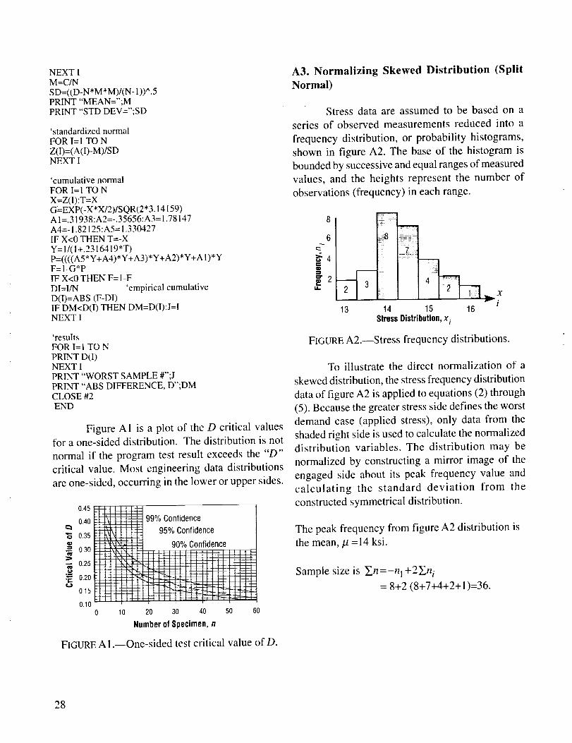
A3. Normalizing Skewed Distribution (Split

Normal)

Stress data are assumed to be based on a

series of observed measurements reduced into a

frequency distribution, or probability histograms,

shown in figure A2. The base of the histogram is

bounded by successive and equal ranges of measured

values, and the heights represent the number of

observations (frequency) in each range.

6

_4

1213 14

Stress

7.: ::

._.Xv i

15 16

Distribution,x i

FIGURE A2.--Stress frequency distributions.

To illustrate the direct normalization of a

skewed distribution, the stress frequency distribution

data of figure A2 is applied to equations (2) through

(5). Because the greater stress side defines the worst

demand case (applied stress), only data from the

shaded right side is used to calculate the normalized

distribution variables. The distribution may be

normalized by constructing a mirror image of the

engaged side about its peak frequency value and

calculating the standard deviation from the

constructed symmetrical distribution.

The peak frequency from figure A2 distribution is

the mean,/.t = 14 ksi.

Sample size is Yn=-n 1+ 2]_n i

= 8+2 (8+7+4+2+ 1)=36.

28

Sum of variations about the mean B. K-Factor Program

v=2Y_ni(xi-l,t)2

2×8 (14.0-14.0)2=0

2x7 ( 14.5-14.0)2=3.5

2x4 ( 15.0-14.0)2=8.0

2x2 (15.5-14.0)2=9.0

2xl (16.0-14.0)2=8.0v=28.5.

The variance is

or2 v 28.5 0 8-Er-_T_l---3_= . 1 ,

and the standard deviation from equation (3)is 6=-0.90 ksi.

The coefficient of variation from equation (40)

is/ a 0.90=_=--]T =0.065 .

'SPLIT NORMAL DISTRIBUTION'INPUT DATA

CLEAR: INPUT "PEAK FREQUENCY=",MUINPUT "NUMBER OF BARS=",NDIM F(N), X(N)FOR I= l TO N

INPUT F(I)NEXT I

FOR I= 1 TO N

INPUT X(I)NEXT I

'CACULATE

S=0:FOR I=2 TO N

S=S+2 *F(I)NEXT 1

SS=S+F(I)PRINT'SAMPLE SIZE=",SSVMU=0:FOR I=l TO N

VMU=VMU+2*F(I)*(X(I)-MU)^2NEXT I

PRINT"VARIATIONS FROM MEAN=",VMU

PRINT "MEAN=",MUSD=(VMU/(SS- 1))^.5

PRINT "STD DEV=",SDCOF=SD/MU

PRINT"COEF OF VAR=",COF

'K- FACTOR

MARIO:

DEFDBL A-Z

INPUT"SAMPLE SIZE=";NS

INPUT "PROPORTION";P

INPUT "CONFIDENCE=";CLIF NS>90 THEN PRINT'SAMPLE SIZE SHOULD

BE SMALLER THAN 90":WHILE INKEY$='"':WENDSTART=TIMER

PI=3.141592654#

'INVERSE NORMAL

Q=I-P:T=SQR(-2*LOG(Q))A0=2.30753:AI=.27061:B ! =.99229:B2=.0481

NU=A0+A 1*T:DE= I +B 1*T+B2*T*T

X=T-NU/DE

L0: Z= 1/SQR(2*PI)*EXP(-X*X/2):IF X>2 GOTO L3V=25-13*X*X

FOR N= I 1 TO 0 STEP- l

U=(2*N+ 1)+(- ! )^(N+ [ )*(N+ I )*X*X/VV=U:NEXT N

F=.5-Z*X/V

W=Q-F:GOTO L2L3:V=X+30

FOR N=29 TO 1 STEP - 1U=X+N/V

V=U :NEXT N

F=Z/V :W=Q-F :GOTO L2L2:L=L+ 1

R=X:X=X-WIZ

E=ABS(R-X)IF E>.00001 GOTO L0

'END OF INVERSE NORMAL

'CALCULATION OF FACTORIAL

N=NS:NU=N- I

MT=INT(NU/2) :UT=NU- 2*MTGT=I

FOR I= 1 TO MT- 1+LITKT=I

IF UT=0 GOTO L I

KT=I-.5

L! :GT=GT*KT

NEXT l

GT=GT*(1 +UT* (SQR(PI)- 1))

GF=GT* 2^(NU/2 - 1)'END OF FACTORIAL

'SECANT METHOD

KP=X:J= l :K=KP

K0=K:GOSUB INTEGRATION:SF0=SF

K=K*(I+.0001):KI=K:GOSUBINTEGRATION:SFI =SF

29

BEGIN:K=K1-SFI*(KI-K0)/(SF1-SF0)

IF ABS((K 1-K)/K I)<.000001 GOTO RESULTJ=J+ 1:K0=K 1:K 1=K :SF0=SF I

GOSUB INTEGRATION:SFI =SF:GOTO BEGIN

RESULT:FINISH=TIMER

BEEP:BEEP

PRINT "K =";USING"##.####";K

PRINT "TIME=";FINISH-START;"SECONDS"'END OF SECANT METHOD

WHILE MOUSE(0)<>( I):WENDGOTO MARIO

INTEGRATION:LI=0:L2=10

IF N>40 THEN L2=20

DL=KP*SQR(N):TP=K*SQR(N)Y=NU/2

M=2:E=0:H=(L2-L I)/2X=LI :GOSUB FUNCTION

Y0=Y:X=L2:GOSUB FUNCTIONYN=Y:X=L 1+H:GOSUB FUNCTION

U=Y: S=(Y0+YN+4*U)*H/3START:M=2*M

D=S:H=H/2:E=E+U:U=0

FOR I= 1 TO M/2

X=L 1+H*(2*I- I):GOSUB FUNCTION

U=U+YNEXT I

S=(Y0+YN+4*U+2*E)*H/3

IF AB S((S-D)/D)>.00001 # GOTO STARTSF=S/GF-CL

RETURN

'END OF SIMPSON

FUNCTION: Z=TP*X/SQR(NU)-DL

T0=Z:G0= i/SQR(2*PI)*EXP(-Z* Z/2)A 1=.3 i 93815:A2=-.3565638:A3= 1.781478:

A4=- 1.821256:A5= 1.330274

IF Z<0 THEN T0=-Z

W= 1/( 1+. 231649*T0)P l =((((A5*W+A4)*W+A3)*W+A2)*W+A 1)*W

PH=I-G0*PI

IF Z<0 THEN PH= 1-PH

Y=PH*X^(NU - I)*EXP(-X*X/2)

RETURN

C. Safety Index Programs

'SAFETY INDEX FROM RELIABILITY

'NORMIN (.5,P, 1)DEFDBL A-Z

LL: INPUT'Probability=';PPI=3.141593

30

PI=3.141593

Q= I-P:T=SQR(-2*LOG(Q))A0=2.30753 :a t =.27061

B 1=.99229:B2=.0481

NU=A0+a 1*T

DE= I+B 1*T+B2*T*T

X=T-NU/DE

'CUMULATIVE NORMAL

L0: Z= I/SQR(2*PI)*EXP(-X*X/2)IF X>2 GOTO L 1

V=25-13*X*X

FOR N= 11 TO 0 STEP- 1

U=(2*N+ 1)+(- I )^(N+ 1)*(N+ ! )*X*X/VV=U:NEXT N

F=.5-Z*X/V

W=Q-FGOTO L2

L 1 :V=X+30

FOR N=29 TO 1 STEP-1

U=X+N/V

V=U:NEXT N

F=Z/V:W=Q-F:GOTO L2

L2:L=L+ 1

R=X:X=X-W/Z

E=ABS(R-X)IF E>.001 GOTO L0

PRINT "SAFETY INDEX IS"

PRINT USING "##.####";X

GOTO LL

END

'RELIABILITY FROM SAFETY INDEX

'NORMIN (0.5,P, 1)DEFDBL A-Z

'INPUT'P=';P:PI=3.141593

PI=3.141593

'Q= 1-P:T=SQR(-2*LOG(Q))'A0=2.30753:A!=.27061

'B ! =.99229:B2=.048 l'NU=A0+a i *T

'DE= l +B I *T+B2*T*T

'X=T-NU/DE

'CUMULATIVE NORMAL

INPUT"X=";X

Z= I/SQR(2*PI)*EXP(-X*X/2)IF X>2 GOTO L I

V=25-13*X*X

FOR N= 11 TO 0 STEP- 1

U=(2*N+ 1)+(- 1)^(N+ 1)*(N+ l )*X*X/V

Form ApprovedREPORT DOCUMENTATION PAGE OMBNo.0704-0188

Public reporting burden for lhis collection of information is eslimated to average 1 hour per response, including the lime for reviewing instructions, searching existing data sources,gathering and maintaining the data needed, and completing and reviewing the correction of information. Send comments regarding this burden estimate or any other aspect of thiscollection of information, including suggestions for reducing this burden, to Washington Headquarlera Services, Directorate for Information Operalion and Reports, f 215 JeffersonDavis Highway, Suite 1204, Arlington, VA 22202-4302, and to the Office of Management and Budget, Paperwork Reduction Project (0704-0188), Washington, DC 20503

1. AGENCY USE ONLY (Leave Blank) 2. REPORT DATE 3. REPORT TYPE AND DATES COVERED

November 1997 Technical Paper

4. TITLE AND SUBTITLE 5. FUNDING NUMBERS

Inherent Conservatism in Deterministic Quasi-Static

Structural Analysis

6. AUTHORS

V. Verderaime

7. PERFORMINGORGANIZATIONNAME(S)ANDADDRESS(ES)

George C. Marshall Space Flight Center

Marshall Space Flight Center, Alabama 35812

9.SPONSORING/MONITORINGAGENCYNAME(S)ANDADDRESS(ES)

National Aeronautics and Space Administration

Washington, DC 20546-0001

8. PERFORMING ORGANIZATIONREPORT NUMBER

M-840

10. SPONSORING/MONITORING

AGENCY REPORT NUMBER

NASA/TP-97-206238

11. SUPPLEMENTARY NOTES

Prepared by Structures and Dynamics Laboratory, Science and Engineering Directorate

12a. DISTRIBUTION/AVAILABILITY STATEMENT

Unclassified-Unlimited

Subject Category 39Standard Distribution

12b. DISTRIBUTION CODE

;13. ABSTRACT (Maximum 200 words)

The cause of the long-suspected excessive conservatism in the prevailing structural

deterministic safety factor has been identified as an inherent violation of the error propagation

laws when reducing statistical data to deterministic values and then combining them

algebraically through successive structural computational processes. These errors are restricted

to the applied stress computations, and because mean and variations of the tolerance limit format

are added, the errors are positive, serially cumulative, and excessively conservative. Reliability

methods circumvent these errors and provide more efficient and uniform safe structures. The

document is a tutorial on the deficiencies and nature of the current safety factor and of its

improvement and transition to absolute reliability.

14. SUBJECT TERMS

safety factors, deterministic method, error propagation laws, safety factor conservatism,

structural reliability, first order reliability, structural failure concept, safety index,

Mises failure criterion

17. SECURITY CLASSIFICATION 18. SECURITY CLASSIFICATION 19. SECURITY CLASSIFICATIONOF REPORT OF THIS PAGE OF ABSTRACT

Unclassified Unclassified Unclassified

NSN 7540-01-280-5500

15. NUMBER OF PAGES

4O16. PRICE CODE

A0320. LIMITATION OF ABSTRACT

Unlimited

Standard Form 298 (Rev. 2-89)PrescribedbyANSI SId 239-18298-402

V=U:NEXT N

F=.5-Z*X/V:F= 1-F

GOTO L2

L 1 :V=X+30

FOR N=29 TO 1 STEP-1

U=X+N/V

V=U:NEXT N

F=Z/V:F= ! -F

L2:

PRINT F

END

D. Mises Criterion Program

'ERROR PROPAGATION METHOD;' MISES CRITERION

DEFDBL A-Z

INPUT'NUMBER OF NORMAL STRESS=",NS

DIM STATIC NSM(3),NSSD(3),NSNF(3),

NSFD(3),LNS(3)

FOR I= i TO NS

PRINT "NORMAL LOAD MEAN(";I;")="

INPUT NSM(t)

PRINT'NORMAL LOAD STD. DEVIATION(";I;")="

INPUT NSSD(I)

PRINT'NORMAL LOAD N-FACTOR(";I;')="

INPUT NSNF(I)NEXT I

INPUT "NUMBER OF SHEAR STRESSES=',MS

DIM STATIC SSM(3),SSSD(3),SSNF(3),SSFD(3),

LSS(3)FOR I= I TO MS

PRINT "SHEAR LOAD MEAN(";I;")="

INPUT SSM(I)

PRINT "SHEAR LOAD STD. DEVIATION(";I;')="

INPUT SSSD(1)

PRINT "SHEAR LOAD N-FACTOR(";I;")="

INPUT SSNF(I)NEXT I

'CALCULATION OF SYSTEM MEAN

S 1=0:FOR I= 1TO NS:S ! =S 1+NSM(I)^2:NEXT 1

S2=0:FOR I= 1TO MS:S2=S2+SSM(I)^2:NEXT I

MZ I = S 1-NSM( 1)*NSM(2)-NSM(1)*NSM(3)

MZ2=MZI-NSM(2)*NSM(3)+3*S2

MZ= SQR(MZ2)'CALCULATION OF DERIVATIVES

NSFD(1)=(2*NSM(I)-NSM(2)-NSM(3))/2/MZ

NSFD(2)=(2*NSM(2)-NSM(1)-NSM(3))I2/MZ

NSFD(3)=(2*NSM(3)-NSM(I)-NSM(2))/2/MZ

FOR I= 1 TO MS:SSFD(I)=3*SSM(I)/MZ:NEXT I

'CALCULATION OF SUM OF SQUARES OF' NORMAL STRESSES

S3=0:S4=0:FOR I= 1 TO NS

S3=S3+(NSFD(I)*NSSD(I))^2

S4=S4+(NSNF(I)*NSFD(I)*NSSD(I))^2NEXT I

'CALCULATION OF SUM OF SQUARES OF' SHEAR STRESSES

$5=0:$6=0: FOR I=1 TO MS

S5=S5+(SSFD(I)*SSSD(I))^2S6=S6+(SSNF(I)*SSFD(I)*SSSD(I))^2NEXT I

'CALCULATION OF SYSTEM STANDARD

'AND EFFECTIVE DEVIATIONS

SZ=SQR(S3+S5):SN=SQR(S4+S6)NE=SN/SZ

'CALCULATION OF SYSTEM COEFFICIENT

' OF VARIATION

ETA=SZ/MZ

'CALCULATION OF SYSTEM TOLERANCE LIMIT

TL=MZ+(NE*SZ)

'CALCULATION OF MISES FUNCTION

FOR I= 1 TO NS

LNS(I)=(NSM(I)+NSNE(I)*NSSD(I))^2NEXT I

FOR I= 1 TO MS

LSS(I)=(SSM(I)+SSNF(I)*SSSD(I))^2NEXT I

FMI=0:FOR I=! TO NS

FM 1=FM 1+LNS(I) :NEXT IFM2=0:FOR I=1 TO MS

FM2=FM2+LSS(I):NEXT 1

FM= SQR(FM 1+3*FM2)

PRINT "COMBINED APPLIED STRESSS =";FM

PRINT "MEAN =";MZPRINT "STANDARD DEVIATION ="SZ

PRINT "EFFECTIVE N =";NEPRINT "COEFFICIENT OF VARIATION =";ETA

PRINT "TOLERANCE LIMIT =";TL

31