Discussion Papers No. 655, May 2011 Statistics Norway, Research Department

Taryn Ann Galloway and Stephen Pudney

Initiation into crime: An analysis of Norwegian register data on five birth cohorts

Abstract: We construct linked register data on five Norwegian birth cohorts, covering: criminal charges after age 15; family characteristics and history up to age 15; and (for males) IQ test scores. A longitudinal analysis of the risk of initiation into crime in early adulthood suggests an increased risk for the children of young and unmarried mothers and for those experiencing disruptive family events including divorce or maternal death during childhood. There is a relationship between continuity of parental employment and reduced risk, with no evidence of harm from mothers' employment. Cognitive ability remains strongly associated with reduced risk after allowing for family history and circumstances.

Keywords: Norway, Crime, Family, Cognitive ability, Register data

JEL classification: C33, I18, K42

Acknowledgements: We are grateful to Torbjørn Skardhamar for valuable advice and assistance. Statistics Norway and the UK economic and Social Research Council through the MiSoC research center (award no. RES-518_285_001) provided financial and other support. This research was completed whilst Pudney was a Faculty Visiting Scholar at the Department of Economics at the University of Melbourne.

Address: Taryn Ann Galloway Statistics Norway, Research Department. E-mail: tag@ssb.no

Stephen Pudney, Insitute for Social and Economic Research, University of Essex. E-mail: spudney@essex.ac.uk

Discussion Papers comprise research papers intended for international journals or books. A preprint of a Discussion Paper may be longer and more elaborate than a standard journal article, as it may include intermediate calculations and background material etc.

© Statistics Norway Abstracts with downloadable Discussion Papers in PDF are available on the Internet: http://www.ssb.no http://ideas.repec.org/s/ssb/dispap.html For printed Discussion Papers contact: Statistics Norway Telephone: +47 62 88 55 00 E-mail: Salg-abonnement@ssb.no ISSN 0809-733X Print: Statistics Norway

3

Sammendrag

Denne forsløpsanalysen følger de fem kohortene født 1977-1981 i Norge for å avdekke forhold knyttet

til første siktelse for lovbrudd fra og med den kriminelle lavalderen (15 år). Det er benyttet detaljerte

registerdata som inkluderer opplysinger om siktelse for lovbrudd, familiebakgrunn og familiehistorie.

For menn er det også et mål på kognitive ferdigheter (IQ) fra sesjon. Analysen viser at hazarden for

(første) siktelse er høyere for barn av unge og ugifte mødre samt for dem som opplevde skilsmisse

eller at moren døde. At foreldre har hatt en stabil tilknytning til arbeidsmarkedet gjennom oppveksten

henger sammen med redusert risiko for kriminalitet, og det er ingen tegn til at mors sysselsetting øker

risikoen for kriminalitet. En sammenheng mellom kognitive ferdigheter og kriminalitet holder seg

etter at en rekke familiekjennetegn og andre relevant bakgrunnsvariabler er tatt hensyn til.

1 Introduction

Crime is an important social issue everywhere. It has direct effects, generating large so-

cial losses through the costs to victims of loss, damage, injury and distress; and to gov-

ernment through the costs of the criminal justice, policing, correction and health systems.

See Justisdepartementet and Norges Forsikringsforbund (1990) and Justis- og politideparte-

mentet (2005) for analyses of the costs of crime in Norway and Entorf and Spengler (2002)

for a wider European perspective. More important, crime can be seen as an indirect symp-

tom of failures in personal development, socialization and education of children - failures

which represent very large losses of human potential. Despite the large research literature

addressing various aspects of these issues, there remains limited evidence giving both a broad

picture of the range of anti-social activity and a detailed longitudinal picture of the develop-

ment processes leading to criminal outcomes. There is huge potential to fill in such gaps in

knowledge based on quantitative research from the very rich and largely unexploited register

data that exist in the Nordic countries, in Norway in particular.

This paper has three main aims. The first is to introduce a new data resource for Nor-

way, constructed by linking data registers relating to (parental) earnings and employment,

education, military conscription and criminal charges for five complete birth cohorts born

1977-81. We discuss the advantages and limitations of this dataset, demonstrate its poten-

tial value for understanding the social processes leading to criminal activity, and analyze the

data, focusing on the important process of initiation into criminality.

The second aim is to re-examine the contentious issue of the relationship between cog-

nitive ability and criminal behavior. We first demonstrate the strong negative ability-crime

gradient that exists in Norwegian register data. We develop an economic model of the the-

ory of ‘rational’ crime to show that such a gradient can have a simple economic basis (and

thus be open to influence by policy), rather than being the inherent genetic relationship

envisaged by some of the more extreme commentators. We also modify our basic model by

introducing ability-dependent detection rates and show that this model, perhaps counterin-

tuitively, is compatible with attenuation, or possibly even reversal, of a negative relationship

between ability and criminal involvement. Since our measure of crime is based on the subset

4

of crimes detected by the police (and resulting in a charge but not necessarily a court con-

viction), some bias in the empirical ability-crime gradient is likely. We consider the biases

involved and conclude that they are unlikely to be strong enough to generate a completely

spurious gradient.

Our third aim is to examine, in as much detail as possible, the influence that family

circumstances and events during childhood have on the subsequent risk of involvement in

crime. A particular issue here is the relationship between a youth’s experience of divorce or

bereavement and later criminal involvement. This aim is motivated by policy concerns which

require a detailed understanding of these childhood influences and especially the timing of

sensitive periods during which children are especially vulnerable to adverse conditions and

events and potentially amenable to suitably-designed social interventions.

We begin in the next section by explaining the Norwegian data registers and the con-

struction of our matched dataset covering five birth cohorts. Section 3 then introduces the

issue of cognitive ability as measured (for males only) by the compulsory Armed Forces Gen-

eral Ability Test, demonstrates the strong ability gradient in the hazard rate for onset of

detected crime and discusses its possible behavioral foundations, based on the development

of an human capital model of crime. Section 4 demonstrates and highlights the main find-

ings about the importance of childhood circumstances and events for the onset of crime for

males and families. Section 5 introduces IQ variables into the analysis (for male cohorts)

and shows that controlling for a rich set of family, geographical and cohort influences reduces

the empirical ability-crime gradient only slightly. Furthermore, we show that estimates of

the influence of these other factors are largely robust to the exclusion of IQ variables.

2 Norwegian social institutions and administrative reg-

isters

The individual-level statistical records maintained by the Norwegian authorities are an ex-

tremely valuable resource for long-term longitudinal research. They are the subject of an

increasing flow of economic research (Røed and Raaum 2003) and there is great scope for

progress on a wide range of social and economic research, exploiting databases that link core

demographic and economic data to records from other parts of public administration, such

5

as the criminal justice system. A major objective of the work presented in this paper is to

pioneer the construction of a dataset that brings together records from several spheres of

public administration including pension records related to employment and earnings, edu-

cation, law enforcement and the armed forces. Individual-level data can be linked across

different register data sources by means of a unique person identifier, and further identifiers

of parents, siblings and half-siblings allow us to link parental data to the individuals studied

here.

2.1 The 1977-81 birth cohorts and the administrative registers

The age of criminal responsibility varies greatly between European countries, ranging from

7 years in Ireland and Switzerland to 18 in Belgium and Luxembourg. In Norway, people

are held responsible for their criminal actions from age 15 so we focus on the first five

birth cohorts for which we have full histories of criminal charges after the age of criminal

responsibility. Since the charge data are available for the years 1992-2004, we base our

analysis on the cohorts born 1977-1981, to give an observation window of at least eight years

beyond the age of criminal responsibility. In constructing variables describing childhood

history, we use information from earlier data registers for the sequence of sixteen calendar

years covering the period from birth to the fifteenth birthday. These micro-historical data

are far more detailed than the information generally available to researchers working with

longitudinal survey data

2.2 The criminal justice system and charge register

The crime register records individual charges for specific offenses from 1992 to 2004. There

are hundreds of criminal offense codes in the data and offenses are, in addition, classified as

either crimes or misdemeanors to indicate seriousness. A start and end date is recorded for

each offense, although it is difficult to date some crimes precisely. The records are largely

complete: 98.8% of the criminal charges in the register for 1992-2004 have at least a start or

end year, but missing dates are most prevalent in crime categories (economic, environmental,

and sex crimes) which we do not study here. In general, we use the start date to date the

6

crime in question.1 If a month but not a day is recorded for a given crime, we use the 15th

of the month as the date of the crime; if both the month and day are missing, we date the

crime as having occurred on 1 July of the relevant year.

The concept of ‘charge’ used here differs somewhat from the strict legal usage. Specif-

ically, a person is recorded as having been charged with a crime in our data if the police

arrested the individual, charged him or her with the offense and the criminal investigation of

the particular case was then closed and considered solved by the police. Thus, cases where

persons are arrested and charged with an offense, but subsequently released and no longer

considered a suspect in a pending criminal investigation are not recorded in the data. Use of

the criminal charge as the basic unit of analysis implies that, to be recorded in our dataset,

a crime has to come to the attention of the police, an arrest be made and the case judged to

be sufficiently strong to warrant a criminal charge and successful closure of the investigation.

Inclusion in the dataset does not require that the person is tried and convicted.

Using criminal charge as an indicator of crime is analogous to a hypothesis test, involving

the possibility of type I error (failure to charge a guilty individual) and type II error (charge

of an innocent individual). The use of criminal charge rather than arrest or conviction is

a compromise between these types of error. It improves the coverage of crimes relative

to a measure based on court convictions and, given the high standard of proof (“beyond

reasonable doubt”) required for a court conviction, this seems a reasonable extension of

coverage. On the other hand, it does not risk the inclusion of invalid policing decisions to

the same degree as would data based on arrest rather than charge.

2.3 Crime categories and trends in onset

The charge records identify a very large number of legally-defined crime categories which

it would not be feasible to distinguish separately in the empirical analysis. Nevertheless,

there are important qualitative differences between types of crime so we need to maintain a

degree of disaggregation. As a compromise between the conflicting demands of feasibility and

detail, we adopt a six-category classification: theft (misdemeanor); theft (crime); alcohol-

related offenses; drug offenses; violent crime; and property damage. We also work with an

1In the very few cases with a missing start date, but information on end date, we use the end date instead.

7

‘all crime’ category which covers all six of these and a small residual category of extremely

heterogeneous offenses (ranging from breaking the boating speed limit to treason). The only

offenses omitted from the all crime category and this analysis are economic offenses (certain

forms of “white-collar crime”), environmental offenses (such as violations of hunting laws

or pollution laws), sexual offenses and offenses related to workplace safety. The excluded

categories of offenses are all very small and thereby not amenable to detailed analyses such

as those performed here.

Differences between birth cohorts are potentially important, because, if there exists a

formative period of socialization during childhood when long-term perceptions and behav-

ioral norms are crystalized, then variations over time in aggregate crime rates will induce

behavioral differences between cohort groups. Table 1 summarizes the proportions of people

in the 15-23 age range who were charged with each of these offense types, by gender and

birth cohort. For both men and women there is a monotonic increase across birth cohorts

in the proportion receiving a criminal charge. The increase is stronger for women, whose

cohort-specific charge rate increased by 39% over the 5-year span, compared with 14% for

men. The increases were particularly large for alcohol- and drug-related offenses (respectively

30% and 47% for men and 50% and 71% for women). Note, however, that the absolute gap

between the male and female charge rate has remained consistently high, ranging from 16.2

percentage points in the 1978 cohort to 17.3 points for the 1979-81 cohorts.

Table 1 Charge rates by offense, gender and birth cohort: all aged 15-23

Birth cohort1977 1978 1979 1980 1981

Offense F M F M F M F M F MTheft (misdemeanor) 1.9 3.1 2.5 3.3 2.4 3.8 2.7 3.8 2.8 4.0Theft (crime) 1.1 7.6 1.2 7.1 1.3 8.0 1.3 7.6 1.4 7.4Alcohol offenses 0.8 7.9 1.0 8.8 1.1 9.5 1.2 9.7 1.2 10.3Drug offenses 1.4 5.9 1.8 6.6 2.0 7.7 2.4 8.5 2.4 8.7Violence 0.4 4.8 0.7 4.9 0.7 5.4 0.8 5.4 0.9 5.8Property damage 0.2 3.7 0.3 4.2 0.3 4.5 0.4 4.4 0.4 4.3Any crime 5.6 22.0 6.7 22.9 7.0 24.3 7.5 24.8 7.8 25.1Notes: Percentages; F and M denote females and males, respectively.

The large rise in crime rates documented for youths here is also reflected in a general–and

substantial–rise in charge rates in the general population from the late 1980s up through the

8

start of the new millennium 2. There is some indication of crime rates leveling out in recent

years. This rise in Norwegian crime through the 1990s and the start of the millenium runs

counter to expectations given that both economic theory (Becker 1968) and many empirical

papers, including Carmichael and Ward (2001), Reilly and Witt (1996), Britt (1994) point to

a positive relationship between unemployment and crime. The start of the rise in crime did

coincide with a dramatic economic downturn associated with a large rise in unemployment

at the end of the 1980s in Norway, but crime rates continued to increase despite a general

trend of solid economic growth and low unemployment throughout the mid- and late-1990s

3. Cyclical economic downturns and transitory increases at the turn of the millennium and

associated with the current financial crisis have been moderate in Norway.

We are concerned with the process of initiation into crime, as reflected in the police charge

records. The important analytical concept here is the hazard rate, defined as the probability

of onset in a given time period conditional on no (detected) criminal activity prior to that

time. Given that the crimes are dated to the day, we are able to implement this concept

based on days since the individual turned 15. However, for ease of interpretation, we present

the hazard rates as functions of time measured in (fractions) of (age) years. In other words,

age 16 is use to represent the hazard rate associated with an individual’s 1-year duration

occurring at his or her sixteenth birthday.

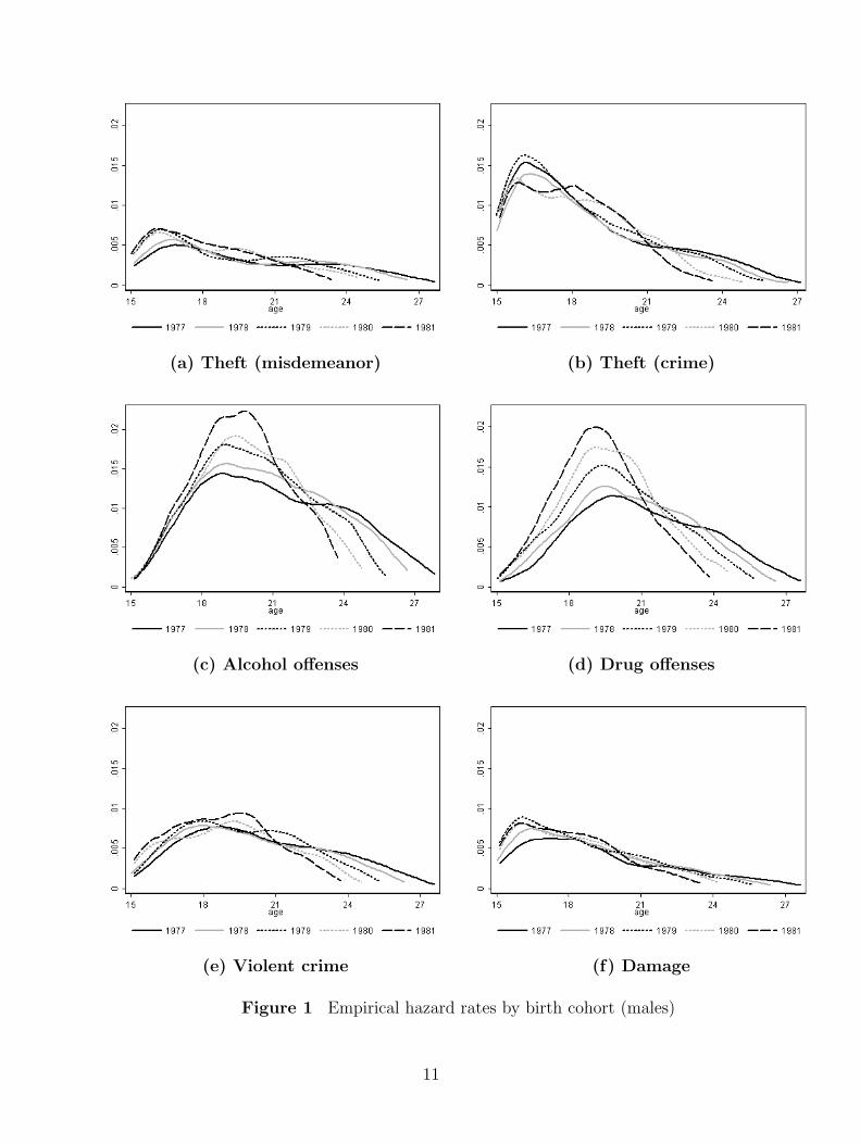
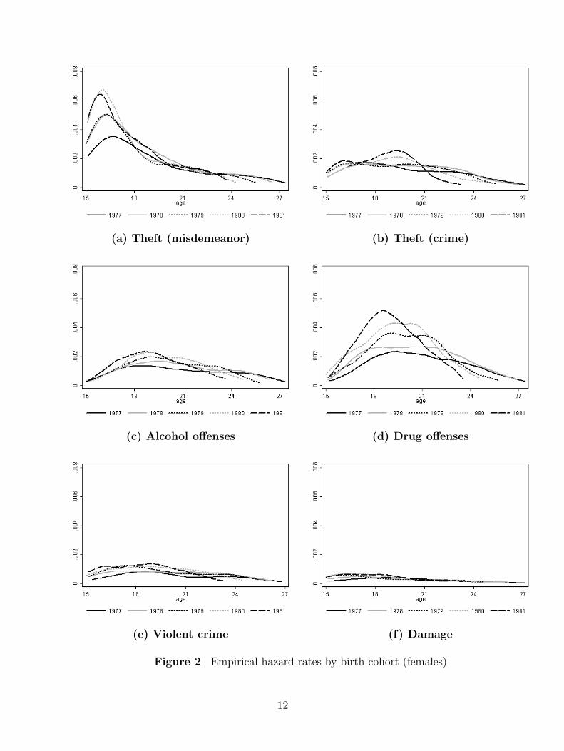
To summarize how risk of onset varies with age, we plot non-parametric estimates of the

hazard rate estimated using a weighted kernel method. Figures 1 and 2 show these empirical

hazard functions estimated separately by gender, birth cohort and crime category. In all

cases, there is a non-monotonic profile, with a rapid rise in risk of onset from age 15 to a

principal peak somewhere between age 16.5 and 20, depending on the population group and

crime category. The decline in risk past the peak age is always much slower than the initial

rise, but the shape of the hazard function is often quite complex.

The hazard functions all display in some degree a common pattern of differences between

cohorts. For the 1977 and 1978 cohorts, the hazard function is more extended to the right,

and the principal peak is generally less pronounced than for later cohorts. This implies a

noticeable tendency over the 5-year span for onset to shift from the twenties to the teenage

2See http://www.ssb.no/lovbrudde/3See Statistics Norway (2005) for a general description of the macroeconomic situation in Norway in the

relevant period.

9

years. This change is strong for drug and alcohol offenses for both sexes but (for males

particularly) much weaker for other offense types. The change in the pattern of onset risk

across cohorts is very pronounced for females in all crime categories, suggesting a definite

change in behavioral norms among a significant part of the young female population.

10

(a) Theft (misdemeanor) (b) Theft (crime)

(c) Alcohol offenses (d) Drug offenses

(e) Violent crime (f) Damage

Figure 1 Empirical hazard rates by birth cohort (males)

11

(a) Theft (misdemeanor) (b) Theft (crime)

(c) Alcohol offenses (d) Drug offenses

(e) Violent crime (f) Damage

Figure 2 Empirical hazard rates by birth cohort (females)

12

3 Cognitive ability and crime

The relationship between cognitive ability and criminal activity has also been studied with

varying degrees of detail elsewhere. Most famously, Herrnstein and Murray (1994), but also

Kandel et al (1988), White et al (1989), Moffitt (1993), Farrington (1998) and Heckman

et al (2006), have found evidence of a significant link between early cognitive ability and

criminal activity. However, it is important to be cautious about this empirical relationship,

since its interpretation is not a simple matter. We contribute to the interpretation and

further understanding of such evidence by examining the possible economic foundation for

an ability-crime gradient, based on human capital theory (Ehrlich 1973, Lochner 2004), and

by subsequently developing a human capital model of crime with differential ability.

The basic human capital model of crime is then extended to incorporate ability-dependent

detection rates. As many researchers have previously suggested, if general ability reduces

the likelihood of detection, one would expect to find low-ability criminals over-represented

among those who are brought to justice. This is a very old idea: Austin O’Malley (1760-

1854) wrote “the reason there are so many imbeciles among imprisoned criminals is that an

imbecile is so foolish even a detective can detect him”, and the more serious research literature

has acknowledged the same possibility for at least eighty years (Murchison 1926, pp. 36-7).

Contrary to this intuition, our human capital model of crime shows that differential detection

rates by ability lead to attenuation or, possibly even reversal, of a (negative) ability-crime

gradient. Following the development and discussion of the human capital model of crime,

we then describe the ability test data, which are produced as a by-product of the Norwegian

system of male military conscription. Our findings demonstrate the existence of an empirical

ability-crime gradient in Norway. Finally, we consider possible sources of measurement bias

and assess the possibility that the empirical gradient is a spurious statistical artefact.

3.1 Ability and criminal behavior

Few theories of criminality focus specifically on the relationship between cognitive ability and

crime. One simple theory is that individuals with low cognitive ability have less capacity to

understand fully the long-term consequences of certain behaviors (like crime and drug use)

13

which may be tempting in the short-term, but harmful longer-term. As a consequence, low-

ability individuals tend to make choices which give rise to unanticipated long-term harms.

There is some experimental evidence (see Burks et al 2008) backing the foundation of this

argument, but failures of decision-making are not necessary for a behavioral ability-crime

gradient, and similar relationships can be derived from the standard economic model of

‘rational’ crime.

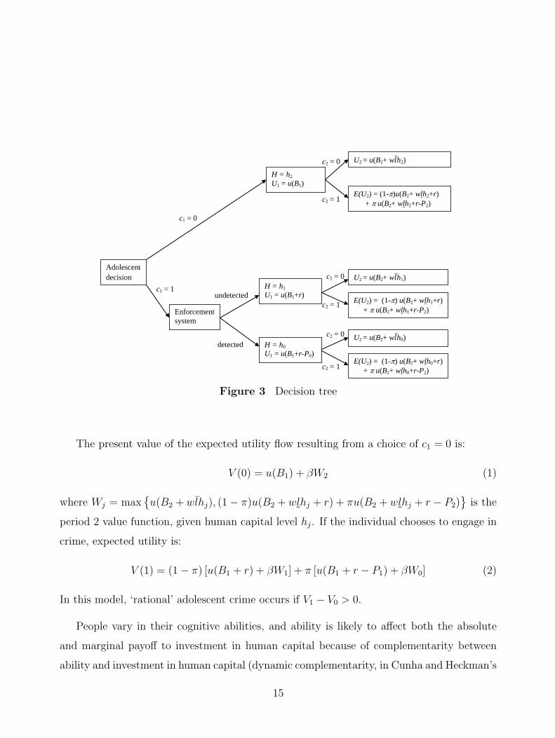
We use a stylized two-period model of acquisitive crime and human capital formation

to demonstrate this proposition. Our model differs from that of Lochner (2004) in several

ways. We simplify by using a 2-period rather than multi-period framework and we do not

distinguish different levels of crime intensity, nor general and criminal ability. Importantly,

we relax the strong assumption of risk neutrality and allow for a scarring effect of a criminal

record. The individual is assumed to have a concave utility function u(.) common to both

periods and all states of the world. In period 1 (‘adolescence’), the individual can engage in

crime (c1 = 1) or not (c1 = 0). Miscarriages of justice do not happen, so there is a positive

probability of detection, π, only if c1 = 1. During adolescence, legal income is B1, illegal

income (if crime is committed) is r and the penalty if detected is equivalent to an income

loss of P1. At the end of adolescence, human capital can take one of three levels: H = h0 if

the individual engages in crime and is detected; H = h1 if criminally active but undetected;

and H = h2 if he or she has had a blameless adolescence. The positive difference h1 − h0

represents the scarring effect of a criminal record and h2 − h1 is the loss of human capital

resulting from a diversion of effort from educational investment into illegal activity. In period

2 (‘adulthood’), the individual’s illegal activity is c2 ∈ {0, 1}. He or she receives an uncertain

income consisting of non-labor income B2 and wlH labor income where w is the return on

human capital H and l is labor supply, equal to l if effort is diverted to crime and a higher

level l otherwise. For simplicity, we assume that the levels l and l are dictated exogenously by

the jobs available in the labor market and are not ability-dependent within the three human

capital classes. The penalty for detected adult crime is P2 and the probability of detection

is again π. Adult utility is discounted by a factor β. The complex decision problem facing

a fully-informed adolescent is summarized in Figure 3.

14

Adolescent decision

H = h2 U1 = u(B1)

H = h0 U1 = u(B1+r-P0)

H = h1 U1 = u(B1+r)

Enforcement system

E(U2) = (1-π)u(B2+ wlh2+r) + π u(B2+ wlh2+r-P2)

U2 = u(B2+ w𝑙h1)

E(U2) = (1-π) u(B2+ wlh1+r) + π u(B2+ wlh1+r-P2)

U2 = u(B2+ w𝑙h0)

E(U2) = (1-π) u(B2+ wlh0+r) + π u(B2+ wlh0+r-P2)

U2 = u(B2+ w𝑙h2)

c1 = 0

c1 = 1 undetected

detected

c2 = 0

c2 = 1

c2 = 0

c2 = 0

c2 = 1

c2 = 1

Figure 3 Decision tree

The present value of the expected utility flow resulting from a choice of c1 = 0 is:

V (0) = u(B1) + βW2 (1)

where Wj = max{u(B2 + wlhj), (1− π)u(B2 + wlhj + r) + πu(B2 + wlhj + r − P2)

}is the

period 2 value function, given human capital level hj. If the individual chooses to engage in

crime, expected utility is:

V (1) = (1− π) [u(B1 + r) + βW1] + π [u(B1 + r − P1) + βW0] (2)

In this model, ‘rational’ adolescent crime occurs if V1 − V0 > 0.

People vary in their cognitive abilities, and ability is likely to affect both the absolute

and marginal payoff to investment in human capital because of complementarity between

ability and investment in human capital (dynamic complementarity, in Cunha and Heckman’s

15

(2008) terminology). To accommodate this, we allow the human capital levels h0, h1 and h2,

to depend parametrically on ability A and assume that dhj/dA > 0 for all j and that the

differences h2−h1 and h1−h0 are also increasing in A. How does V (1)−V (0) vary with A?

First consider the case where the detection probability π is ability-invariant, in which case

d[V (1)−V (0)]/dA = β {d[W1 −W2]/dA− πd[W1 −W0]/dA}. The value function derivatives

are

dWj

dA=

u′(B2 + wlhj)wldhj/dA if c2(hj) = 0

[(1− π)u′(B2 + wlhj + r) + πu′(B2 + wlhj + r − P2)]wldhj/dA if c2(hj) = 1

(3)

where c2(hj) = 0 indicates an optimal choice of adult honesty given human capital hj and

c2(hj) = 1 indicates criminality.

The structure of d[V (1)−V (0)]/dA depends on the configuration of optimal decisions in

adulthood. To see the issues involved, consider the specific case where c2(h2) = c2(h1) = 0

and c2(h0) = 1 or 0, defining the class of individuals who would choose legality if they enter

adulthood without a criminal record but may continue criminality into adulthood otherwise.

It is the main group of interest, since empirical evidence suggests very strongly that most

adolescent offending behavior is a transient phase rather than a long-term career decision

and that, where significant adult criminality does occur, it is generally preceded by youth

crime.

Under these assumptions, if the scarring effect is not too great, so that the individual

expects to be non-criminal in adulthood, even if convicted as an adolescent (c2(h0) = 0), the

ability gradient of V (1)− V (0) is:

d[V (1)− V (0)]

dA= − βwl

{[u′2dh2

dA− u′1

dh1

dA

]+ π

[u′1dh1

dA− u′0

dh0

dA

]}(4)

where u′j is marginal utility at the point B2 +wlhj. By concavity, u′2 < u′1 < u′0 and the two

terms in square brackets are ambiguous in sign. However, each is positive if the interaction

between ability and human capital is sufficiently strong to offset the decline in marginal utility

with increasing income, that is ifdhj+1/dA

dhj/dA>

u′ju′j+1

for j = 0, 1.4 Thus, for individuals disposed

4Note that, if utility is linear, there is an unambiguous negative gradient. Also, if the scarring effect h1−h0

is ability-invariant rather than increasing, the sign of the second term in square brackets is unambiguouslypositive.

16

towards legality in adulthood, we expect to see a negative ability gradient in V (1)−V (0) so

that increasing ability reduces the likelihood of adolescent criminality.

If the scarring effect is strong enough that the adolescent, if detected, expects to continue

criminality in adulthood (c2(h0) = 1), the derivative dW0/dA switches to the second form in

(3) and expression (4) changes to:

d[V (1)− V (0)]

dA= − βw

{l

[u′2dh2

dA− u′1

dh1

dA

]+ π

[lu′1

dh1

dA− lu+

0′dh0

dA

]+ π2l

[u+

0′ − u++

0′] dh0

dA

}(5)

where u+0′

= u′(B2 + wlh0 + r) and u++0′

= u′(B2 + wlh0 + r − P2). Of the three terms

in square brackets in (5), the first two are expected to be predominantly positive, since the

increase in human capital accumulation and labor market attachment produced by increased

ability is likely to outweigh any decline in the marginal utility of income. The final term

in square brackets is unambiguously negative because of diminishing marginal utility, but

likely to be small because of the term π2.

The overall conclusion from our interpretation of conditions (4) and (5) is that forward-

looking behavior by young people is highly likely (but not certain) to generate a negative

ability-crime gradient in a world where the detection probability is constant and where human

capital earns substantial rewards. This simple analysis is certainly not a full description of

criminal behavior, especially for non-acquisitive crime, but it serves to make an important

point. The existence of an ability-crime gradient does not necessarily imply the existence

of any fundamental genetic process leading automatically to criminal behavior, nor does it

necessarily imply that participants in crime are defective in terms of their decision-making

capacity. Instead, the ability-crime gradient arises here purely as a consequence of the

(relatively) poor legal economic opportunities open to low-ability individuals.

Now consider the possibility that the risk of detection is also ability-dependent. How

do conditions (4) and (5) change? In both cases, an additional term appears in the ability

gradient of V (1)− V (0). The new term is:

− dπdA

[u(B1 + r)− u(B1 + r − P1) +W1 −W0] (6)

17

The detection risk is decreasing in ability, utility is increasing in income and the value

function is increasing in human capital, so dπ/dA < 0, u(B1 + r)− u(B1 + r − P1) > 0 and

W1−W0 > 0. Thus the additional component (6) of d[V (1)−V (0)]/dA is definitely positive

and the impact of ability-related detection risk is to attenuate or conceivably even reverse

the negative ability-crime gradient. This leaves open the sign and magnitude of the gradient

as an empirical question, to which we now turn.

3.2 The military service ability test

All male members of the 1977-81 birth cohorts were in principle required to present them-

selves (normally between ages 18 and 20) for drafting into the Norwegian armed forces for

Military Service. As part of the recruitment process, all young men were required to take

the Armed Forces General Ability Test (GAT), used primarily to assess recruits’ suitability

for military service. In practice, approximately 6-9% of men from the 1977-81 cohorts did

not take the GAT, for a variety of unrecorded reasons. One of the principal circumstances

in which the test would not be taken is where the individual has a record of severe physical

or mental illness or disability which would clearly make him ineligible for military service.

Without access to medical records and more detailed records from the draft, it is not pos-

sible to look at this in greater depth. In a very small number of cases,5 individuals were

excluded from the draft due to heavy, repeated involvement in very serious violent crimes.

The IQ data from the Norwegian military draft has been used extensively for research pur-

poses (Kristensen and Bjerkedal 2007, Sundet et al 1988, Sundet et al 2004 Sundet et al

2005, Black et al 2007, 2009) and it is noted to be of particularly high quality and coverage

by Flynn (1987).

The GAT is a combination of three time-limited multiple-choice components: a test of

arithmetic ability (30 items, 25 mins.); a word similarities test (54 items, 8 mins.); and a

figures test (36 items, 20 mins.). The first two components are broadly similar to those in

the widely-used Wechsler IQ test and the third is similar to the Raven Progressive Matrices

test. Test-retest reliabilities for the three components have been reported as .84, .72 and .90

(Sundet et al 1988). The three component scores are transformed to conform to the standard

5According to information from the Norwegian Conscription Office (”Vernepliktsverket”), these casesnumbered 6 persons born in 1977, 13 persons born 1978, 17 persons born 1979, 37 persons born 1980 and58 persons born 1981.

18

normal distribution on a benchmark sample then summed and reported on a 1-9 scale (the

‘stanine’ scale), where category 5 corresponds to average IQ of 100 and one stanine unit

corresponds to a difference of 7.5 IQ points based on the common IQ scoring with mean 100

and standard deviation 15. Sundet et al (2004) give more detail on the GAT and show that

the rising trend in measured ability over the 1950s to the mid 1990s (the Flynn effect) had

essentially ended by the time the 1977-81 birth cohorts encountered the draft.

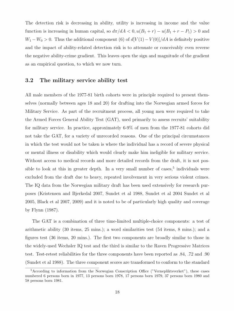
Figure 4 shows the striking empirical IQ gradient in the data for men, for whom the peak

level of onset risk is 6-17 times higher for the lowest ability group than for the highest. These

gradients are steep for all crime categories, but especially so for theft crime and violence and

least so for alcohol and drug crimes. One of our objectives in this paper is to examine the

extent to which these gradients remain after allowing for the effect of other relevant factors,

such as the child’s family history.

19

(a) Theft (misdemeanor) (b) Theft (crime)

(c) Alcohol offenses (d) Drug offenses

2(e) Violent crime (f) Damage

Figure 4 Empirical hazard rates by IQ category (males)

20

3.3 Measurement bias

There are two main sources of bias in the empirical ability-crime gradient in charge data:

a selection bias arising from the fact that charged criminals are possibly not a random

sample of all criminals; and an errors-in-variables bias caused by the measurement error in

IQ tests. Consider first the selection bias, using the notation of section 3.1. The conditional

probability D(A) of being a criminal appearing in the charge register is D(A) = P (A)π(A),

where P (A) is the probability of committing crime. Define the true ability-crime gradient

as the proportionate effect g = ∂ lnP/∂A, whose empirical counterpart is g = g+∂ lnπ/∂A.

The negative term ∂ ln π/∂A is the selection bias induced by ability-related crime detection

which can lead to some degree of exaggeration of the true gradient.

The existence of a strong IQ-crime gradient in many different sets of self-reported survey

data and in the charge-based register data we analyze here suggests that the gradient we

observe is not primarily a statistical artefact arising from over-representation of low-ability

criminals among the group of charged offenders. More detailed survey-based tests also find

little evidence for a large bias: for example, Moffitt and Silva (1988) compared mean IQs of

detected and undetected young offender subsamples from a longitudinal New Zealand survey

that were matched in terms of their self-reported delinquency. There was no significant IQ

difference between the two groups (although both groups had significantly lower mean IQs

than non-delinquent survey members), suggesting that the IQ gradient is a genuine aspect

of behavior rather than a detection-related artefact.

A second measurement difficulty is also worthy of note. Any IQ test score is an indicator,

not a direct observation, of ability. If there is (classical) random measurement error in

these test scores, then estimates will be subject to an attenuation bias and a tendency

to underestimate the importance of cognitive ability. The situation here is not quite the

classical measurement error case, because two errors are present in the use of a test score as

the ability measure: the usual attenuation bias arising from a negative correlation between

the measurement error and the measured test score; and an upward bias due to the fact that

test scores are generally standardized by dividing by the standard deviation of the test score

rather than the standard deviation of the test score minus its error.6 Thus the measurement

6The standardization used in our GAT variable is more complex than this (see section 3.1) but the samegeneral point applies.

21

error involves less attenuation than is normally the case. To illustrate this, consider a test

score T linearly related to ability A, with a measurement error ε with mean zero and variance

σ2. Thus T = a+bA+ε. If ability is defined to have zero mean and unit standard deviation,

the standardized test score is:

T s =bA+ ε√b2 + σ2

=√ρA+

√1− ρ ε

σ(7)

where ρ = b2/(b2 + σ2) is the test-retest reliability.

Now suppose that a crime variable C is related to ability through a linear regression:

C = α + βA+ u, which can be rewritten using (7) as:

C = α +β√ρT s +

[u− β

√1− ρρ

ε

σ

](8)

There are two distortions here: the composite error in square brackets is negatively correlated

with the covariate T s; and the coefficient β has been transformed to β/√ρ by the inappro-

priate normalization. It is easy to show that the probability limit of the regression estimate

of the crime-ability gradient is√ρβ, which involves less attenuation than the standard mea-

surement error result of ρβ. Thus, if the test-retest reliability is 0.81, say, the attenuation

bias in this simple model is 10% rather than the 19% in the conventional errors-in-variables

case.

With available data, it is impossible for us to evaluate the net effect on the ability-

crime gradient of distortions due to differential detection by ability and attenuation due to

measurement error, but the two sources of bias should be borne in mind when interpreting

estimates of ability effects both here and in the rest of the applied literature.

4 Modeling the onset of crime

Criminal behavior is dynamic. A majority of people never have any significant involvement

in crime; many have only a brief period of criminality; some rapidly develop a criminal

habit early in life but then grow out of it, usually more slowly; others become longer-term

criminals. Many authors including Sampson and Laub (1993), Laub and Sampson (2003)

and Nagin and Tremblay (1999, 2001) have used discrete typologies of this kind as a latent

structure underlying observed criminal careers. Criminal careers can be very complex but

22

they all share a common feature, the initiation or onset event, which is critically important.

Obviously, crime cannot happen if onset never occurs and, less obviously, early onset may

be associated with higher offending rates and longer duration of subsequent criminal careers

(Sampson and Laub 1993). Consequently, we focus our analysis on the process of initiation

or onset rather than modeling the whole criminal career, which brings with it the attendant

risk of misspecification of a more complex process.

4.1 The Cox partial likelihood approach

We treat the time (measured in days from the fifteenth birthday) until the first recorded arrest

within the relevant crime category as the completed duration δ. Note that δ may have a

defective distribution with positive probability mass at δ = +∞ for ‘persistent non-offenders’.

The Cox (1972) model of δ is based on the following proportional hazards specification:

h(t|x(t)) = exp(x(t)β)h0(t) (9)

where h(t|x(t)) is the conditional hazard rate at elapsed time t, defined as the probability

of onset within the short time interval (t, t + dt) divided by the width of the interval dt.

The probability is conditional on no criminal charge prior to age t and on a set of variables

x(t) constructed to describe the individual’s personal characteristics and history up to age t.

The function h0(t) is the baseline hazard function, interpretable as the hazard function for

a benchmark individual with characteristics x(t) = 0. We analyse onset through criminal

charges which can occur only from age 15 onwards. All our explanatory covariates relate

either to time-invariant characteristics (such as birth cohort, mother’s marital status at

birth) or to the history of events up to age 15 (such as the occurrence of parental divorce at

different stages of childhood). None of these variables change after age 15, so our covariates

are in fact invariant to t, which represents time measured from age 15 onwards.

The partial likelihood approach to estimation involves maximization of the likelihood of

onset at the observed time δi conditioned on the risk set of sampled durations which are still

in progress at time t (see Lancaster (1990) for further details). We allow for right censoring

and use Breslow’s (1974) method for dealing with tied durations in the sample of observed

23

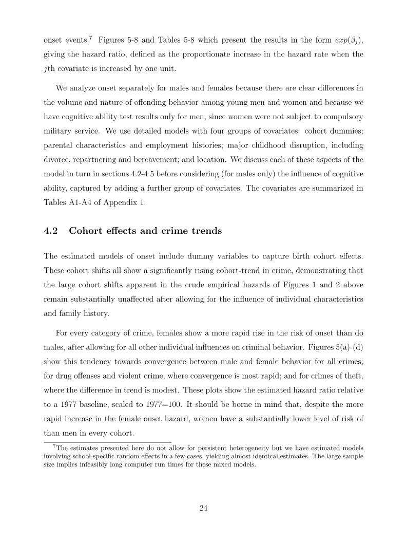
onset events.7 Figures 5-8 and Tables 5-8 which present the results in the form exp(βj),

giving the hazard ratio, defined as the proportionate increase in the hazard rate when the

jth covariate is increased by one unit.

We analyze onset separately for males and females because there are clear differences in

the volume and nature of offending behavior among young men and women and because we

have cognitive ability test results only for men, since women were not subject to compulsory

military service. We use detailed models with four groups of covariates: cohort dummies;

parental characteristics and employment histories; major childhood disruption, including

divorce, repartnering and bereavement; and location. We discuss each of these aspects of the

model in turn in sections 4.2-4.5 before considering (for males only) the influence of cognitive

ability, captured by adding a further group of covariates. The covariates are summarized in

Tables A1-A4 of Appendix 1.

4.2 Cohort effects and crime trends

The estimated models of onset include dummy variables to capture birth cohort effects.

These cohort shifts all show a significantly rising cohort-trend in crime, demonstrating that

the large cohort shifts apparent in the crude empirical hazards of Figures 1 and 2 above

remain substantially unaffected after allowing for the influence of individual characteristics

and family history.

For every category of crime, females show a more rapid rise in the risk of onset than do

males, after allowing for all other individual influences on criminal behavior. Figures 5(a)-(d)

show this tendency towards convergence between male and female behavior for all crimes;

for drug offenses and violent crime, where convergence is most rapid; and for crimes of theft,

where the difference in trend is modest. These plots show the estimated hazard ratio relative

to a 1977 baseline, scaled to 1977=100. It should be borne in mind that, despite the more

rapid increase in the female onset hazard, women have a substantially lower level of risk of

than men in every cohort.

7The estimates presented here do not allow for persistent heterogeneity but we have estimated modelsinvolving school-specific random effects in a few cases, yielding almost identical estimates. The large samplesize implies infeasibly long computer run times for these mixed models.

24

(a) All crimes (b) Drug offenses

(c) Violent crime (d) Theft crimes

Figure 5 Cohort-specific hazard ratios for males and females (Cox partial likelihood estimates)

4.3 Parental background

One of the great advantages of Norwegian register data is the availability of information which

allows us to construct an employment history for each parent during the entire childhood

of the birth cohorts studied here. Employment status rests on the concept of an income

unit (grunnbeloep) abbreviated as G, which is used in the Norwegian public pension system

to determine the accumulation of pension rights through employment. Roughly speaking, a

person is credited with one year of earned pension rights if he or she earned more than 1G

in a given year. Norwegian pension records therefore carefully record the number of years in

which a person has earned over 1G. Since the monetary amount of G has to be comparable

25

over several years, the value of 1G in Norwegian kroner is adjusted, usually once a year, by

the Norwegian parliament and closely follows average wage growth in Norway. Currently, 1G

is just under half the minimum old-age pension for a single person in Norway and can be said

to be roughly equivalent to half the subsistence annual wage. Following the practice of the

Norwegian pension system, we treat any year as one of employment if the parent in question

generated earnings of 1G or more, and summarize the employment history by the number

of years of the parent’s employment up to the child’s fifteenth birthday (a maximum of 16

years). The resulting variable is a direct measure of the parent’s labor market attachment.

While the pension data provides a measure of parental labor market earnings, data on

other income sources, in particular public benefits, are not available prior to 1993. As

a result, we are unable to construct full family income histories or discuss child poverty

as one of the risk factors for criminal involvement. In most cases, however, measures of

prolonged parental unemployment, like those we construct here, will be sufficient to capture

children living in difficult economic circumstances, since the Norwegian social security system

generally provides sufficient security in the case of short-term stints of unemployment.

Information on the parents’ highest level of education was extracted from the National

Database on Education, described in detail by Vangen (2007). We distinguish three educa-

tional levels: low education refers to the compulsory level or below (nine years’ schooling for

most of the parents studied here);8 the medium level is education beyond the compulsory

minimum within the secondary school level; while education at the tertiary level is classed

as high.

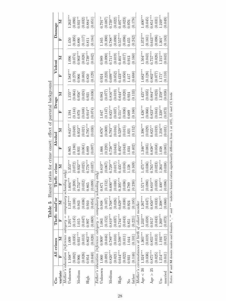
The relationship between parental characteristics and history in the onset model is sum-

marized in Tables 5-6 and in Figure 6. Parental education is an important ‘protective’ factor,

particularly paternal education, which has a strong restraining effect on the onset risk for all

categories of crime, for both sons and daughters. The average risk reduction associated with

a father who has high rather than low education is large, ranging from 25% for minor theft to

8An educational reform made in the 1960s raised compulsory schooling, so some of the older parentsof the 1977-81 cohorts had only seven years’ compulsory schooling. Following a 1997 reform, the currentminimum is ten years.

26

almost 60% for violent crime. Maternal education has a much smaller effect, mainly confined

to sons, where the greatest risk reduction is around 25% for theft and violent crime.9

Teenage motherhood raises the risk of crime onset significantly (relative to the reference

category of births to a mother age 21-25) for both sons and daughters, the effect ranging

from around 25% for minor theft to over 50% for violence. Birth to a mother in her late

twenties (or older) is associated with a slightly reduced risk. Unmarried motherhood is a

further risk factor, raising the hazard rate by up to 40% (for theft crime).

9Note, however, that the few cases of unknown maternal education are significantly associated with raisedonset risk, so estimates of the impact of maternal education should be interpreted with caution.

27

Table

5H

azar

dra

tios

for

crim

eon

set:

effec

tof

par

enta

lbac

kgr

ound

Co-

All

crim

esT

hef

t:m

isd

’or

Th

eft:

crim

eA

lcoh

olD

rugs

Vio

lent

Dam

age

vari

ate

FM

FM

FM

FM

FM

FM

FM

Mot

her’

sed

ucat

ion

(ref

eren

ceca

tego

ry=

com

pulsor

ysc

hool

ing

only

)U

nkno

wn

1.16

8∗∗

1.00

91.

291∗

∗1.

317∗

∗∗1.

604∗

∗∗1.

353∗

∗∗0.

965

0.84

5∗∗∗

1.19

41.

155∗

∗1.

583∗

∗∗1.

096

1.45

01.

263∗

∗∗

(0.0

82)

(0.0

35)

(0.1

45)

(0.1

00)

(0.2

09)

(0.0

72)

(0.1

80)

(0.0

49)

(0.1

44)

(0.0

64)

(0.2

79)

(0.0

74)

(0.3

95)

(0.0

90)

Med

ium

0.96

60.

931∗

∗∗1.

015

0.94

30.

752∗

∗∗0.

932∗

∗∗0.

931

0.95

3∗∗

0.97

00.

956∗

0.96

60.

903∗

∗∗0.

890

0.93

1∗∗

(0.0

26)

(0.0

13)

(0.0

47)

(0.0

36)

(0.0

52)

(0.0

25)

(0.0

61)

(0.0

21)

(0.0

48)

(0.0

24)

(0.0

83)

(0.0

28)

(0.1

17)

(0.0

32)

Hig

h0.

954

0.86

3∗∗∗

0.99

70.

910

0.86

50.

776∗

∗∗0.

889

0.79

5∗∗∗

0.91

4∗∗

0.92

10.

850

0.73

9∗∗∗

0.81

10.

884∗

∗

(0.0

40)

(0.0

20)

(0.0

69)

(0.0

54)

(0.0

99)

(0.0

37)

(0.0

97)

(0.0

30)

(0.0

74)

(0.0

36)

(0.1

29)

(0.0

42)

(0.1

84)

(0.0

51)

Fath

er’s

educ

atio

n(r

efer

ence

cate

gory

=co

mpu

lsor

ysc

hool

ing

only

)U

nkno

wn

1.06

00.

909∗

1.08

30.

948

0.87

10.

819∗

∗1.

066

0.87

6∗1.

047

0.98

30.

924

0.98

91.

165

0.79

1∗∗

(0.0

91)

(0.0

46)

(0.1

52)

(0.1

07)

(0.1

52)

(0.0

67)

(0.2

20)

(0.0

69)

(0.1

47)

(0.0

77)

(0.2

23)

(0.0

90)

(0.3

90)

(0.0

87)

Med

ium

0.82

0∗∗∗

0.78

9∗∗∗

0.81

9∗∗∗

0.76

8∗∗∗

0.69

0∗∗∗

0.72

9∗∗∗

0.73

8∗∗∗

0.79

3∗∗∗

0.82

5∗∗∗

0.81

6∗∗∗

0.69

9∗∗∗

0.71

1∗∗∗

0.78

8∗∗

0.73

9∗∗∗

(0.0

21)

(0.0

10)

(0.0

37)

(0.0

26)

(0.0

38)

(0.0

17)

(0.0

43)

(0.0

16)

(0.0

37)

(0.0

19)

(0.0

52)

(0.0

19)

(0.0

90)

(0.0

22)

Hig

h0.

644∗

∗∗0.

599∗

∗∗0.

744∗

∗∗0.

629∗

∗∗0.

395∗

∗∗0.

435∗

∗∗0.

492∗

∗∗0.

529∗

∗∗0.

551∗

∗∗0.

644∗

∗∗0.

423∗

∗∗0.

401∗

∗∗0.

557∗

∗∗0.

497∗

∗∗

(0.0

22)

(0.0

11)

(0.0

43)

(0.0

30)

(0.0

36)

(0.0

16)

(0.0

43)

(0.0

15)

(0.0

36)

(0.0

20)

(0.0

50)

(0.0

17)

(0.0

96)

(0.0

23)

No

0.93

11.

044

0.85

10.

924

0.78

91.

138

1.03

41.

021

0.68

90.

924

1.41

70.

913

0.45

50.

976

fath

er(0

.146

)(0

.101

)(0

.221

)(0

.185

)(0

.230

)(0

.169

)(0

.402

)(0

.152

)(0

.160

)(0

.133

)(0

.688

)(0

.160

)(0

.242

)(0

.178

)M

othe

r’s

circ

umst

ance

sat

birt

hof

coho

rtm

embe

rA

ge<

201.

324∗

∗∗1.

365∗

∗∗1.

233∗

∗∗1.

267∗

∗∗1.

571∗

∗∗1.

475∗

∗∗1.

346∗

∗∗1.

396∗

∗∗1.

426∗

∗∗1.

425∗

∗∗1.

682∗

∗∗1.

504∗

∗∗1.

373∗

∗∗1.

400∗

∗∗

(0.0

36)

(0.0

19)

(0.0

59)

(0.0

47)

(0.0

90)

(0.0

36)

(0.0

85)

(0.0

29)

(0.0

66)

(0.0

35)

(0.1

28)

(0.0

43)

(0.1

61)

(0.0

45)

Age

>25

0.87

5∗∗∗

0.85

5∗∗∗

0.91

5∗0.

850∗

∗∗0.

810∗

∗∗0.

765∗

∗∗0.

838∗

∗0.

825∗

∗0.

823∗

∗∗0.

884∗

∗∗0.

802∗

∗∗0.

757∗

∗∗0.

643∗

∗∗0.

851∗

∗∗

(0.0

25)

(0.0

13)

(0.0

43)

(0.0

33)

(0.0

59)

(0.0

23)

(0.0

58)

(0.0

19)

(0.0

44)

(0.0

23)

(0.0

77)

(0.0

26)

(0.0

96)

(0.0

31)

Un-

1.25

4∗∗∗

1.19

3∗∗∗

1.26

9∗∗∗

1.39

8∗∗∗

1.40

0∗∗∗

1.26

4∗∗∗

1.03

81.

216∗

∗∗1.

320∗

∗∗1.

259∗

∗∗1.

171∗

1.21

5∗∗∗

1.30

1∗1.

249∗

∗∗

mar

ried

(0.0

41)

(0.0

21)

(0.0

73)

(0.0

60)

(0.0

96)

(0.0

38)

(0.0

85)

(0.0

31)

(0.0

73)

(0.0

38)

(0.1

10)

(0.0

43)

(0.1

83)

(0.0

49)

Note

s:F

an

dM

den

ote

male

san

dfe

male

s;∗,∗∗

an

d∗∗∗

ind

icate

haza

rdra

tios

sign

ifica

ntl

yd

iffer

ent

from

1at

10%

,5%

an

d1%

level

s

28

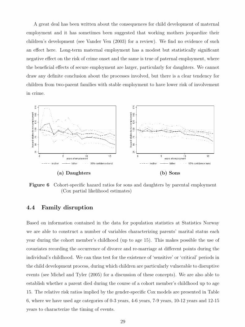
A great deal has been written about the consequences for child development of maternal

employment and it has sometimes been suggested that working mothers jeopardize their

children’s development (see Vander Ven (2003) for a review). We find no evidence of such

an effect here. Long-term maternal employment has a modest but statistically significant

negative effect on the risk of crime onset and the same is true of paternal employment, where

the beneficial effects of secure employment are larger, particularly for daughters. We cannot

draw any definite conclusion about the processes involved, but there is a clear tendency for

children from two-parent families with stable employment to have lower risk of involvement

in crime.

(a) Daughters (b) Sons

Figure 6 Cohort-specific hazard ratios for sons and daughters by parental employment(Cox partial likelihood estimates)

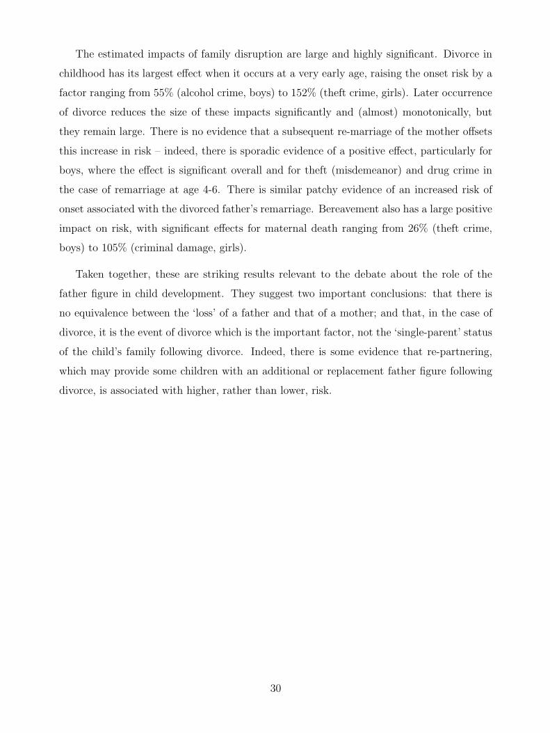
4.4 Family disruption

Based on information contained in the data for population statistics at Statistics Norway

we are able to construct a number of variables characterizing parents’ marital status each

year during the cohort member’s childhood (up to age 15). This makes possible the use of

covariates recording the occurrence of divorce and re-marriage at different points during the

individual’s childhood. We can thus test for the existence of ‘sensitive’ or ‘critical’ periods in

the child development process, during which children are particularly vulnerable to disruptive

events (see Michel and Tyler (2005) for a discussion of these concepts). We are also able to

establish whether a parent died during the course of a cohort member’s childhood up to age

15. The relative risk ratios implied by the gender-specific Cox models are presented in Table

6, where we have used age categories of 0-3 years, 4-6 years, 7-9 years, 10-12 years and 12-15

years to characterize the timing of events.

29

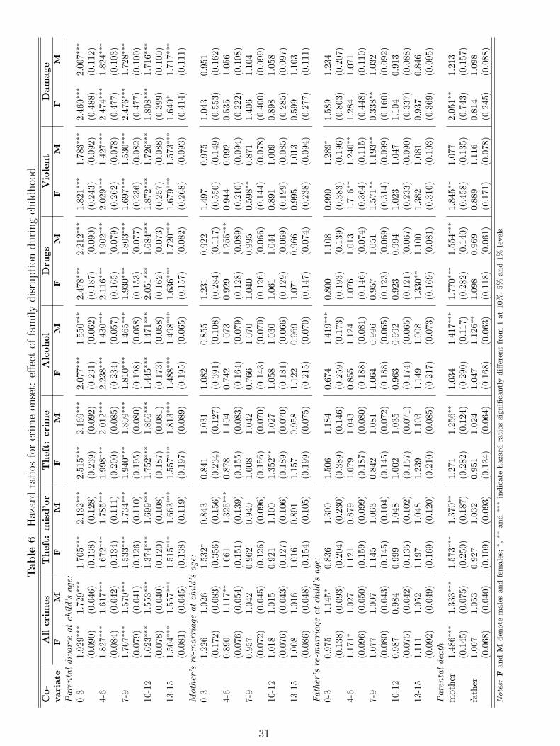
The estimated impacts of family disruption are large and highly significant. Divorce in

childhood has its largest effect when it occurs at a very early age, raising the onset risk by a

factor ranging from 55% (alcohol crime, boys) to 152% (theft crime, girls). Later occurrence

of divorce reduces the size of these impacts significantly and (almost) monotonically, but

they remain large. There is no evidence that a subsequent re-marriage of the mother offsets

this increase in risk – indeed, there is sporadic evidence of a positive effect, particularly for

boys, where the effect is significant overall and for theft (misdemeanor) and drug crime in

the case of remarriage at age 4-6. There is similar patchy evidence of an increased risk of

onset associated with the divorced father’s remarriage. Bereavement also has a large positive

impact on risk, with significant effects for maternal death ranging from 26% (theft crime,

boys) to 105% (criminal damage, girls).

Taken together, these are striking results relevant to the debate about the role of the

father figure in child development. They suggest two important conclusions: that there is

no equivalence between the ‘loss’ of a father and that of a mother; and that, in the case of

divorce, it is the event of divorce which is the important factor, not the ‘single-parent’ status

of the child’s family following divorce. Indeed, there is some evidence that re-partnering,

which may provide some children with an additional or replacement father figure following

divorce, is associated with higher, rather than lower, risk.

30

Table

6H

azar

dra

tios

for

crim

eon

set:

effec

tof

fam

ily

dis

rupti

onduri

ng

childhood

Co-

All

crim

esT

hef

t:m

isd

’or

Th

eft:

crim

eA

lcoh

olD

rugs

Vio

lent

Dam

age

vari

ate

FM

FM

FM

FM

FM

FM

FM

Par

enta

ldi

vorc

eat

child

’sag

e:0-

31.

929∗

∗∗1.

729∗

∗∗1.

705∗

∗∗2.

132∗

∗∗2.

515∗

∗∗2.

169∗

∗∗2.

077∗

∗∗1.

550∗

∗∗2.

478∗

∗∗2.

212∗

∗∗1.

821∗

∗∗1.

783∗

∗∗2.

460∗

∗∗2.

007∗

∗∗

(0.0

90)

(0.0

46)

(0.1

38)

(0.1

28)

(0.2

39)

(0.0

92)

(0.2

31)

(0.0

62)

(0.1

87)

(0.0

90)

(0.2

43)

(0.0

92)

(0.4

88)

(0.1

12)

4-6

1.82

7∗∗∗

1.61

7∗∗∗

1.67

2∗∗∗

1.78

5∗∗∗

1.99

8∗∗∗

2.01

2∗∗∗

2.23

8∗∗∗

1.43

0∗∗∗

2.11

6∗∗∗

1.90

2∗∗∗

2.02

9∗∗∗

1.42

7∗∗∗

2.47

4∗∗∗

1.82

4∗∗∗

(0.0

84)

(0.0

42)

(0.1

34)

(0.1

11)

(0.2

00)

(0.0

85)

(0.2

34)

(0.0

57)

(0.1

65)

(0.0

79)

(0.2

62)

(0.0

78)

(0.4

77)

(0.1

03)

7-9

1.70

7∗∗∗

1.57

0∗∗∗

1.53

3∗∗∗

1.73

4∗∗∗

1.94

0∗∗∗

1.80

9∗∗∗

1.81

0∗∗∗

1.46

5∗∗∗

1.93

0∗∗∗

1.80

3∗∗∗

1.69

7∗∗∗

1.53

0∗∗∗

2.47

6∗∗∗

1.72

8∗∗∗

(0.0

79)

(0.0

41)

(0.1

26)

(0.1

10)

(0.1

95)

(0.0

80)

(0.1

98)

(0.0

58)

(0.1

53)

(0.0

77)

(0.2

36)

(0.0

82)

(0.4

77)

(0.1

00)

10-1

21.

623∗

∗∗1.

553∗

∗∗1.

374∗

∗∗1.

699∗

∗∗1.

752∗

∗∗1.

866∗

∗∗1.

445∗

∗∗1.

471∗

∗∗2.

051∗

∗∗1.

684∗

∗∗1.

872∗

∗∗1.

726∗

∗∗1.

808∗

∗∗1.

716∗

∗∗

(0.0

78)

(0.0

40)

(0.1

20)

(0.1

08)

(0.1

87)

(0.0

81)

(0.1

73)

(0.0

58)

(0.1

62)

(0.0

73)

(0.2

57)

(0.0

88)

(0.3

99)

(0.1

00)

13-1

51.

504∗

∗∗1.

557∗

∗∗1.

515∗

∗∗1.

663∗

∗∗1.

557∗

∗∗1.

813∗

∗∗1.

488∗

∗∗1.

498∗

∗∗1.

636∗

∗∗1.

720∗

∗∗1.

679∗

∗∗1.

573∗

∗∗1.

640∗

1.71

7∗∗∗

(0.0

81)

(0.0

45)

(0.1

38)

(0.1

19)

(0.1

97)

(0.0

89)

(0.1

95)

(0.0

65)

(0.1

57)

(0.0

82)

(0.2

68)

(0.0

93)

(0.4

14)

(0.1

11)

Mot

her’

sre

-mar

riag

eat

child

’sag

e:0-

31.

226

1.02

61.

532∗

0.84

30.

841

1.03

11.

082

0.85

51.

231

0.92

21.

497

0.97

51.

043

0.95

1(0

.172

)(0

.083

)(0

.356

)(0

.156

)(0

.234

)(0

.127

)(0

.391

)(0

.108

)(0

.284

)(0

.117

)(0

.550

)(0

.149

)(0

.553

)(0

.162

)4-

60.

890

1.11

7∗∗

1.06

11.

325∗

∗∗0.

878

1.10

40.

742

1.07

30.

929

1.25

5∗∗∗

0.94

40.

992

0.53

51.

056

(0.0

76)

(0.0

54)

(0.1

51)

(0.1

39)

(0.1

55)

(0.0

83)

(0.1

64)

(0.0

79)

(0.1

28)

(0.0

89)

(0.2

10)

(0.0

94)

(0.2

22)

(0.1

08)

7-9

0.95

71.

042

0.96

20.

940

1.00

81.

042

0.76

61.

070

1.04

00.

995

0.59

8∗∗

0.87

11.

406

1.10

4(0

.072

)(0

.045

)(0

.126

)(0

.096

)(0

.156

)(0

.070

)(0

.143

)(0

.070

)(0

.126

)(0

.066

)(0

.144

)(0

.078

)(0

.400

)(0

.099

)10

-12

1.01

81.

015

0.92

11.

100

1.35

2∗∗

1.02

71.

058

1.03

01.

061

1.04

40.

891

1.00

90.

898

1.05

8(0

.076

)(0

.043

)(0

.127

)(0

.106

)(0

.189

)(0

.070

)(0

.181

)(0

.066

)(0

.129

)(0

.069

)(0

.199

)(0

.085

)(0

.285

)(0

.097

)13

-15

1.00

81.

016

1.01

60.

891

1.15

70.

958

1.12

20.

969

1.07

10.

966

0.99

51.

013

0.59

91.

103

(0.0

86)

(0.0

48)

(0.1

54)

(0.1

05)

(0.1

99)

(0.0

75)

(0.2

15)

(0.0

70)

(0.1

47)

(0.0

74)

(0.2

38)

(0.0

94)

(0.2

77)

(0.1

11)

Fath

er’s

re-m

arri

age

atch

ild’s

age:

0-3

0.97

51.

145∗

0.83

61.

300

1.50

61.

184

0.67

41.

419∗

∗∗0.

800

1.10

80.

990

1.28

9∗1.

589

1.23

4(0

.138

)(0

.093

)(0

.204

)(0

.230

)(0

.389

)(0

.146

)(0

.259

)(0

.173

)(0

.193

)(0

.139

)(0

.383

)(0

.196

)(0

.803

)(0

.207

)4-

61.

171∗

1.02

71.

121

0.87

91.

079

1.04

30.

855

1.12

41.

076

1.01

31.

716∗

∗1.

240∗

∗1.

284

1.07

1(0

.096

)(0

.050

)(0

.159

)(0

.099

)(0

.187

)(0

.080

)(0

.188

)(0

.081

)(0

.146

)(0

.074

)(0

.364

)(0

.115

)(0

.448

)(0

.110

)7-

91.

077

1.00

71.

145

1.06

30.

842

1.08

11.

064

0.99

60.

957

1.05

11.

571∗

∗1.

193∗

∗0.

338∗

∗1.

032

(0.0

80)

(0.0

43)

(0.1

45)

(0.1

04)

(0.1

45)

(0.0

72)

(0.1

88)

(0.0

65)

(0.1

23)

(0.0

69)

(0.3

14)

(0.0

99)

(0.1

60)

(0.0

92)

10-1

20.

987

0.98

40.

999

1.04

81.

002

1.03

50.

963

0.99

20.

923

0.99

41.

023

1.04

71.

104

0.91

3(0

.075

)(0

.042

)(0

.135

)(0

.102

)(0

.157

)(0

.071

)(0

.174

)(0

.065

)(0

.121

)(0

.067

)(0

.233

)(0

.090

)(0

.337

)(0

.088

)13

-15

1.11

11.

052

1.19

71.

048

1.23

91.

103

1.14

91.

008

1.33

0∗∗

1.10

01.

382

1.08

10.

937

0.84

6(0

.092

)(0

.049

)(0

.169

)(0

.120

)(0

.210

)(0

.085

)(0

.217

)(0

.073

)(0

.169

)(0

.081

)(0

.310

)(0

.103

)(0

.369

)(0

.095

)Par

enta

lde

ath

mot

her

1.48

6∗∗∗

1.33

3∗∗∗

1.57

3∗∗∗

1.37

0∗∗

1.27

11.

256∗

∗1.

034

1.41

7∗∗∗

1.77

0∗∗∗

1.55

4∗∗∗

1.84

5∗∗

1.07

72.

051∗

∗1.

213

(0.1

45)

(0.0

75)

(0.2

50)

(0.1

87)

(0.2

82)

(0.1

24)

(0.2

90)

(0.1

17)

(0.2

82)

(0.1

40)

(0.4

58)

(0.1

35)

(0.7

43)

(0.1

57)

fath

er1.

007

1.05

30.

927

1.03

20.

951

1.02

41.

047

1.12

6∗∗

1.09

80.

969

0.88

91.

116

0.81

41.

098

(0.0

68)

(0.0

40)

(0.1

09)

(0.0

93)

(0.1

34)

(0.0

64)

(0.1

68)

(0.0

63)

(0.1

18)

(0.0

61)

(0.1

71)

(0.0

78)

(0.2

45)

(0.0

88)

Note

s:F

an

dM

den

ote

male

san

dfe

male

s;∗,∗∗

an

d∗∗∗

ind

icate

haza

rdra

tios

sign

ifica

ntl

yd

iffer

ent

from

1at

10%

,5%

an

d1%

level

s

31

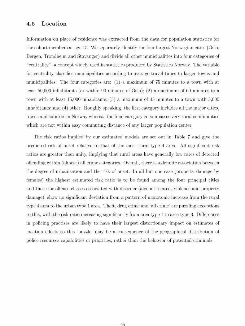
4.5 Location

Information on place of residence was extracted from the data for population statistics for

the cohort members at age 15. We separately identify the four largest Norwegian cities (Oslo,

Bergen, Trondheim and Stavanger) and divide all other municipalities into four categories of

“centrality”, a concept widely used in statistics produced by Statistics Norway. The variable

for centrality classifies municipalities according to average travel times to larger towns and

municipalities. The four categories are: (1) a maximum of 75 minutes to a town with at

least 50,000 inhabitants (or within 90 minutes of Oslo); (2) a maximum of 60 minutes to a

town with at least 15,000 inhabitants; (3) a maximum of 45 minutes to a town with 5,000

inhabitants; and (4) other. Roughly speaking, the first category includes all the major cities,

towns and suburbs in Norway whereas the final category encompasses very rural communities

which are not within easy commuting distance of any larger population center.

The risk ratios implied by our estimated models are set out in Table 7 and give the

predicted risk of onset relative to that of the most rural type 4 area. All significant risk

ratios are greater than unity, implying that rural areas have generally low rates of detected

offending within (almost) all crime categories. Overall, there is a definite association between

the degree of urbanization and the risk of onset. In all but one case (property damage by

females) the highest estimated risk ratio is to be found among the four principal cities

and those for offense classes associated with disorder (alcohol-related, violence and property

damage), show no significant deviation from a pattern of monotonic increase from the rural

type 4 area to the urban type 1 area. Theft, drug crime and ‘all crime’ are puzzling exceptions

to this, with the risk ratio increasing significantly from area type 1 to area type 3. Differences

in policing practises are likely to have their largest distortionary impact on estimates of

location effects so this ‘puzzle’ may be a consequence of the geographical distribution of

police resources capabilities or priorities, rather than the behavior of potential criminals.

32

Table

7H

azar

dra

tios

for

crim

eon

set:

effec

tof

loca

tion

Co-

All

crim

esT

hef

t:m

isd

’or

Th

eft:

crim

eA

lcoh

olD

rugs

Vio

lent

Dam

age

vari

ate

FM

FM

FM

FM

FM

FM

FM

Are

asou

tsid

eth

efo

urpr

inci

palci

ties

(ref

eren

ceca

tego

ry=

very

rura

l)A

rea

11.

217∗

∗1.

115∗

0.98

11.

221∗

∗∗1.

343∗

∗∗1.

191∗

∗∗1.

489∗

∗∗1.

154∗

∗∗1.

346∗

∗∗1.

246∗

∗∗1.

488∗

∗∗1.

214∗

∗∗1.

523∗

∗∗1.

188∗

∗∗

(0.0

60)

(0.0

26)

(0.0

99)

(0.0

87)

(0.2

150)

(0.0

51)

(0.1

62)

(0.0

40)

(0.1

22)

(0.0

58)

(0.2

03)

(0.0

58)

(0.3

12)

(0.0

63)

Are

a2

1.39

2∗∗∗

1.11

7∗∗∗

1.56

9∗∗∗

1.39

9∗∗∗

1.46

0∗∗∗

1.09

9∗∗∗

1.55

3∗∗∗

1.12

8∗∗∗

1.51

3∗∗∗

1.41

7∗∗∗

1.26

4∗∗

1.05

31.

608∗

∗∗0.

956

(0.0

51)

(0.0

20)

(0.1

09)

(0.0

75)

(0.1

25)

(0.0

37)

(0.1

31)

(0.0

30)

(0.1

04)

(0.0

50)

(0.1

38)

(0.0

40)

(0.2

58)

(0.0

40)

Are

a3

1.48

5∗∗∗

1.20

4∗∗∗

1.93

9∗∗∗

1.86

8∗∗∗

1.45

1∗∗∗

1.22

2∗∗∗

1.33

8∗∗∗

1.07

0∗∗∗

1.67

5∗∗∗

1.78

7∗∗∗

1.12

41.

066∗

1.13

71.

011

(0.0

53)

(0.0

21)

(0.1

29)

(0.0

95)

(0.1

22)

(0.0

39)

(0.1

13)

(0.0

28)

(0.1

12)

(0.0

60)

(0.1

23)

(0.0

39)

(0.1

88)

(0.0

41)

Pri

ncip

alci

ties

Osl

o1.

978∗

∗∗1.

502∗

∗∗3.

457∗

∗∗2.

946∗

∗∗1.

690∗

∗∗1.

400∗

∗∗1.

062

1.03

31.

930∗

∗∗2.

133∗

∗∗1.

976∗

∗∗1.

456∗

∗∗1.

555∗

1.70

0∗∗∗

(0.0

96)

(0.0

38)

(0.2

78)

(0.1

89)

(0.2

03)

(0.0

67)

(0.1

47)

(0.0

44)

(0.1

77)

(0.0

96)

(0.2

85)

(0.0

79)

(0.3

59)

(0.0

94)

Ber

gen

1.50

5∗∗∗

1.17

8∗∗∗

2.02

1∗∗∗

1.95

8∗∗∗

1.95

2∗∗∗

1.58

0∗∗∗

1.27

1∗1.

178∗

∗∗1.

586∗

∗∗1.

868∗

∗∗1.

613∗

∗∗1.

242∗

∗∗0.

907

0.98

9(0

.087

)(0

.036

)(0

.203

)(0

.151

)(0

.244

)(0

.079

)(0

.183

)(0

.052

)(0

.168

)(0

.096

)(0

.272

)(0

.077

)(0

.282

)(0

.072

)T

rond

heim

1.67

4∗∗∗

1.08

4∗∗

2.56

7∗∗∗

2.17

0∗∗∗

2.13

8∗∗∗

1.07

90.

900

0.69

2∗∗∗

2.05

3∗∗∗

1.66

9∗∗∗

2.13

0∗∗∗

1.02

00.

806

0.97

9(0

.107

)(0

.040

)(0

.270

)(0

.186

)(0

.294

)(0

.073

)(0

.174

)(0

.045

)(0

.229

)(0

.103

)(0

.369

)(0

.080

)(0

.306

)(0

.085

)St

avan

ger

1.87

0∗∗∗

1.15

9∗∗∗

2.45

6∗∗∗

1.74

9∗∗∗

1.60

6∗∗∗

1.17

0∗∗

1.64

6∗∗∗

0.97

02.

848∗

∗∗2.

191∗

∗∗1.

686∗

∗∗1.

038

0.58

20.

872

(0.1

33)

(0.0

47)

(0.2

99)

(0.1

83)

(0.0

83)

(0.0

88)

(0.2

87)

(0.0

62)

(0.3

25)

(0.1

39)

(0.3

71)

(0.0

93)

(0.3

02)

(0.0

91)

Note

s:F

an

dM

den

ote

male

san

dfe

male

s;∗,∗∗

an

d∗∗∗

ind

icate

haza

rdra

tios

sign

ifica

ntl

yd

iffer

ent

from

1at

10%

,5%

an

d1%

level

s

33

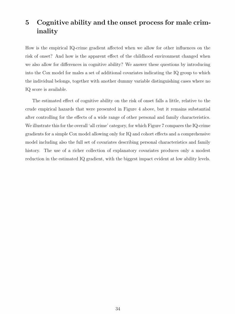
5 Cognitive ability and the onset process for male crim-

inality

How is the empirical IQ-crime gradient affected when we allow for other influences on the

risk of onset? And how is the apparent effect of the childhood environment changed when

we also allow for differences in cognitive ability? We answer these questions by introducing

into the Cox model for males a set of additional covariates indicating the IQ group to which

the individual belongs, together with another dummy variable distinguishing cases where no

IQ score is available.

The estimated effect of cognitive ability on the risk of onset falls a little, relative to the

crude empirical hazards that were presented in Figure 4 above, but it remains substantial

after controlling for the effects of a wide range of other personal and family characteristics.

We illustrate this for the overall ‘all crime’ category, for which Figure 7 compares the IQ-crime

gradients for a simple Cox model allowing only for IQ and cohort effects and a comprehensive

model including also the full set of covariates describing personal characteristics and family

history. The use of a richer collection of explanatory covariates produces only a modest

reduction in the estimated IQ gradient, with the biggest impact evident at low ability levels.

34

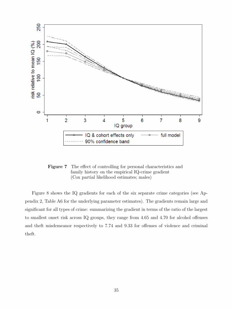
Figure 7 The effect of controlling for personal characteristics andfamily history on the empirical IQ-crime gradient(Cox partial likelihood estimates; males)

Figure 8 shows the IQ gradients for each of the six separate crime categories (see Ap-

pendix 2, Table A6 for the underlying parameter estimates). The gradients remain large and

significant for all types of crime: summarizing the gradient in terms of the ratio of the largest

to smallest onset risk across IQ groups, they range from 4.65 and 4.70 for alcohol offenses

and theft misdemeanor respectively to 7.74 and 9.33 for offenses of violence and criminal

theft.

35

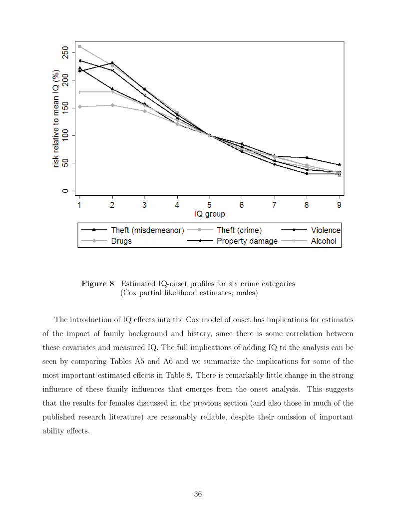
Figure 8 Estimated IQ-onset profiles for six crime categories(Cox partial likelihood estimates; males)

The introduction of IQ effects into the Cox model of onset has implications for estimates

of the impact of family background and history, since there is some correlation between

these covariates and measured IQ. The full implications of adding IQ to the analysis can be

seen by comparing Tables A5 and A6 and we summarize the implications for some of the

most important estimated effects in Table 8. There is remarkably little change in the strong

influence of these family influences that emerges from the onset analysis. This suggests

that the results for females discussed in the previous section (and also those in much of the

published research literature) are reasonably reliable, despite their omission of important

ability effects.

36

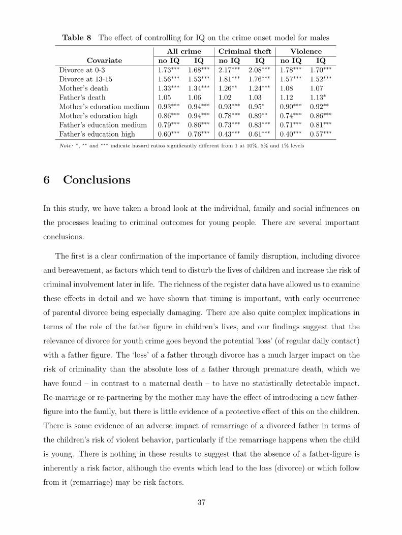
Table 8 The effect of controlling for IQ on the crime onset model for males

All crime Criminal theft ViolenceCovariate no IQ IQ no IQ IQ no IQ IQ

Divorce at 0-3 1.73∗∗∗ 1.68∗∗∗ 2.17∗∗∗ 2.08∗∗∗ 1.78∗∗∗ 1.70∗∗∗

Divorce at 13-15 1.56∗∗∗ 1.53∗∗∗ 1.81∗∗∗ 1.76∗∗∗ 1.57∗∗∗ 1.52∗∗∗

Mother’s death 1.33∗∗∗ 1.34∗∗∗ 1.26∗∗ 1.24∗∗∗ 1.08 1.07Father’s death 1.05 1.06 1.02 1.03 1.12 1.13∗

Mother’s education medium 0.93∗∗∗ 0.94∗∗∗ 0.93∗∗∗ 0.95∗ 0.90∗∗∗ 0.92∗∗

Mother’s education high 0.86∗∗∗ 0.94∗∗∗ 0.78∗∗∗ 0.89∗∗ 0.74∗∗∗ 0.86∗∗∗

Father’s education medium 0.79∗∗∗ 0.86∗∗∗ 0.73∗∗∗ 0.83∗∗∗ 0.71∗∗∗ 0.81∗∗∗

Father’s education high 0.60∗∗∗ 0.76∗∗∗ 0.43∗∗∗ 0.61∗∗∗ 0.40∗∗∗ 0.57∗∗∗

Note: ∗, ∗∗ and ∗∗∗ indicate hazard ratios significantly different from 1 at 10%, 5% and 1% levels

6 Conclusions

In this study, we have taken a broad look at the individual, family and social influences on

the processes leading to criminal outcomes for young people. There are several important

conclusions.

The first is a clear confirmation of the importance of family disruption, including divorce

and bereavement, as factors which tend to disturb the lives of children and increase the risk of

criminal involvement later in life. The richness of the register data have allowed us to examine

these effects in detail and we have shown that timing is important, with early occurrence

of parental divorce being especially damaging. There are also quite complex implications in

terms of the role of the father figure in children’s lives, and our findings suggest that the

relevance of divorce for youth crime goes beyond the potential ’loss’ (of regular daily contact)

with a father figure. The ‘loss’ of a father through divorce has a much larger impact on the

risk of criminality than the absolute loss of a father through premature death, which we

have found – in contrast to a maternal death – to have no statistically detectable impact.

Re-marriage or re-partnering by the mother may have the effect of introducing a new father-

figure into the family, but there is little evidence of a protective effect of this on the children.

There is some evidence of an adverse impact of remarriage of a divorced father in terms of

the children’s risk of violent behavior, particularly if the remarriage happens when the child

is young. There is nothing in these results to suggest that the absence of a father-figure is

inherently a risk factor, although the events which lead to the loss (divorce) or which follow

from it (remarriage) may be risk factors.

37

Second, we have confirmed the strong association between low cognitive ability and the

risk of criminality. The empirical IQ-crime gradient is very strong for all categories of crime

and is only reduced to a modest degree when we make allowance for family circumstances

and history. We have considered the possibility that this association is a biased picture of

the true behavioral association between cognitive ability and criminal behavior induced by

the fact that our outcome measure is based on criminal charges, which might be more easily

avoided by high-ability criminals. It is impossible to be sure about this, but we have argued

that there are theoretical reasons to expect an ability gradient and that ability-selection bias

is unlikely to be sufficiently strong to generate a purely spurious association. We have argued

that the ability-crime gradient observed empirically can arise purely from differences in legal

economic opportunity between low- and high-ability people and it is not necessary to resort

to explanations based on genetic processes or mental deficiency to rationalize the finding.

Policy debates can accommodate ability effects without raising the spectre of eugenics.

Third, various aspects of parental background are important as influences on child out-

comes. Unsurprisingly, there is evidence that both maternal and paternal education are

important protective factors and that the children of very young mothers are more likely to

become involved in criminality. Perhaps more interesting from the policy viewpoint is the

positive influence of parental labor market attachment on the children. This is very clear

for the father, but is also significant for mothers – so we have found no evidence to suggest

that working mothers are harming their children’s development.

Fourth, there is strong evidence of a large rise in crime across the five cohorts studied,

suggesting that macro-level changes in economic or social conditions relevant for criminal

involvement may have occurred, particularly for young women, over a relatively short period

of time. We do not speculate on the causes of this, but it seems to us to represent a potentially

important change in the nature of society.

Finally, our results demonstrate the value of matched register data for lifecourse research.

Even the most detailed survey-based longitudinal data, like the UK birth cohorts, cannot

provide the same degree of detail on family history and the timing of events. We have found

this micro-historical detail to be critical for an understanding of the way that the impact

of family events varies with the particular family context. As these matched datasets are

38

developed further in the future, they are likely to play an increasingly important part in

research on lifecourse dynamics.

References

[1] Becker, G.S (1968). Crime and punishment: an economic approach Journal of PoliticalEconomy 82, 169-217.

[2] Breslow, N. E. (1974). Covariance analysis of censored survival data, Biometrics 30,89-99.

[3] Britt, C.L. (1994) Crime and unemployment among youths in the United States, 1958-1990, American Journal of Economics and Sociology, 53, 99-109.

[4] Burks, S. V., Carpenter, J. P., Gotte, L. and Rustichini, A. (2008). Cognitive skills explaineconomic preferences, strategic behavior and job attachment, Bonn: IZA DiscussionPaper no. 3609

[5] Carmichael, F and Ward, R. (2001), Male unemployment and crime in England andWales, Economics Letters, 73, 111-115.

[6] Cox, D. R. (1972). Regression models and life tables (with discussion), Journal of theRoyal Statistical Society, series B 34, 187-220.

[7] Cunha, F. and J. Heckman (2007), The Technology of Skill Formation, Bonn: IZADiscussion Paper 2550.

[8] Ehrlich, I. (1973). Participation in illegitimate activities: a theoretical and empiricalinvestigation, Journal of Political Economy 81, 531-567.

[9] Entorf, H. and H. Spengler (2002) Crime in Europe. Causes and Consequences. Springer.

[10] Flynn, J. R. (1987). Massive IQ gains in 14 nations: what IQ tests really measure,Psychological Bulletin 101, 171-191.

[11] Farrington, D. (1998). Predictors, causes, and correlates of male youth violence. InM. Tonry and N. Morris (Eds.), Crime and justice: A review of research (Vol. 7, pp.421-475). Chicago: University of Chicago Press.

[12] Heckman, J. J., Stixrud, J., Urzua, S. (2006). The effects of cognitive and noncognitiveabilities on labor market outcomes and social behavior, Journal of Labor Economics 24,411-482.

[13] Herrnstein, R. J. and Murray, C. (1994). The Bell Curve. Intelligence and Class Struc-ture in American Life. New York: Free Press.

[14] Hopkins, K. D. and Bracht, G. H. (1975). Ten-year stability of verbal and nonverbal IQscores, American Educational Research Journal 12, 469-477.

39

[15] Justisdepartementet and Norges Forsikringsforbund (1990). Hva koster kriminalitetensamfunnet? (What Does Crime Cost Society?) Utredningsrapport.

[16] Justis- og politidepartementet (2005). Kriminalitetens samfunnsmessige kostnader.(Crime’s Societal Costs) Rapport 2005, Korrigert opptrykk mars 2006.

[17] Kandel, E., Mednick, S. A., Kirkegaard-Sorensen, L., Hutchings, B., Knop, J., Rosen-berg, R., Schulsinger, F.(1988). IQ as a Protective Factor for Subjects at High Risk forAntisocial Behavior, Journal of Consulting and Clinical Psychology 56, 224-226.

[18] Lancaster, T. (1990). The Econometric Analysis of Transition Data. Cambridge: Cam-bridge University Press.

[19] Laub, J. H. and Sampson, R. J. (2003). Shared Beginnings, Divergent Lives. DelinquentBoys to Age 70. Cambridge MA: Harvard University Press.

[20] Lochner, L. (2004). Education, Work, and Crime: A Human Capital Approach, Inter-national Economic Review 45, 811-843.

[21] Michel, G. F. and Tyler, A. N. (2005). Critical period: a history of the transition fromquestions of when, to what, to how, Developmental Psychobiology 46, 156-162.

[22] Moffitt, T. E. (1993). Adolescence-limited and life-course persistent antisocial behavior:A developmental taxonomy. Psychological Review 100, 674-701.

[23] Moffitt, T. E. and Silva, P. A. (1988). IQ and delinquency: a direct test of the differentialdetection hypothesis. Journal of Abnormal Psychology 97, 330-333.

[24] Murchison, C. (1926). Criminal Intelligence. Worcester MA: Clark University Press.

[25] Nagin, D. S. and Tremblay, R. E. (1999) Trajectories of boys’ physical aggression,opposition and hyperactivity on the path to physically violent and non-violent juveniledelinquency. Child Development 70, 1181-1196.

[26] Nagin, D. S. and Tremblay, R. E. (2001). Analyzing developmental trajectories of dis-tinct but related behaviors: A group-based method. Psychological Methods 6, 18-34.

[27] Reilly, B., Witt, R. (1996). Crime, deterrence and unemployment in England and Wales:an empirical analysis. Bulletin of Economic Research, 48, 3307-3378.

[28] Røed, K. and Raaum, O. (2003). Administrative registers - unexplored reservoirs ofscientific knowledge?, Economic Journal, 113, F258-F281.

[29] Sampson, R. J. and Laub, J. H. (1993). Crime in the Making: Pathways and TurningPoints Through Life. Cambridge MA: Harvard University Press.

[30] Sundet, J. M., Tambs, K., Magnus, P. and Berg, K. (1988). On the question of seculartrends in the heritability of IQ test scores: a study of Norwegian twins, Intelligence 12,47-59.

40

[31] Sundet, J. M., Barlaug, D. G. and Torjussen, T. M. (2004). The end of the Flynn effect.A study of secular trends in mean intelligence scores of Norwegian conscripts during halfa century. Intelligence 32, 349-362.

[32] Statistics Norway (2005). Økonomiske analyser (Economic Analyses) 6/2005.

[33] Van der Ven, T. (2003). Working Mothers and Juvenile Delinquency. El Paso TX: LFBScholarly Publishing LLC.

[34] Vangen, (2007). Nasjonal utdanningsdatabase NUDB. Dokumentasjonsrapport, Notater2007/54, Statistics Norway.

[35] White, J., Moffitt, T. and Silva, P. (1989). A Prospective Replication of the ProtectiveEffects of IQ in Subjects at High Risk for Juvenile Delinquency, Journal of Consultingand Clinical Psychology 57 71924.

41

Appendix 1: Data Summary

Table A.1 Parental Background

Birth cohort1977 1978 1979 1980 1981

Mother’s educationlow 66.6 66.5 66.9 67.3 67.3medium 22.5 22.1 21.3 20.3 20.3high 8.8 9.3 9.7 10.4 10.4unknown 2.1 2.1 2.0 2.2 2.0Father’s educationlow 22.7 21.8 22.0 22.0 21.6medium 50.6 51.2 50.1 50.8 50.6high 24.8 25.1 25.3 25.3 25.9unknown 1.9 1.9 1.9 1.9 1.9Mother’s age at birth of 1st childage < 20 50.3 49.5 49.8 48.7 48.2age 20-25 23.5 23.4 23.5 23.2 23.3age > 25 26.2 27.1 26.7 28.1 28.5Mother’s marital status at birth of cohort memberunmarried 7.7 7.7 8.4 9.0 9.9Notes: Percentages in given category.

Table A.1 Parental Employment

Birth cohort1977 1978 1979 1980 1981

Number of years mother in employment (up to age 15 of child)mean 9.07 9.36 9.62 9.88 10.21std. dev 5.07 5.09 5.10 5.09 5.08pct. non-employment 7.3 6.9 6.4 6.0 5.510th percentile 1 1 2 2 225th percentile 5 6 6 6 6median 9 10 10 11 1175th percentile 14 14 14 15 1590th percentile 16 16 16 16 16Number of years father in employment (up to age 15 of child)mean 15.0 15.0 14.9 14.9 14.9std. dev 2.7 2.8 2.8 2.9 2.9pct. non-employment) 1.2 1.2 1.3 1.3 1.210th percentile 13 13 12 12 1225th percentile 16 16 16 16 16median 16 16 16 16 1675th percentile 16 16 16 16 1690th percentile 16 16 16 16 16Notes:.

42

Table A.2 Family disruption

Birth cohort1977 1978 1979 1980 1981

Parental divorce by age of cohort member:any age 18.5 18.9 19.4 20.0 20.20-3 4.2 4.5 4.5 4.9 4.94-6 4.0 4.1 3.9 4.1 4.37-9 3.5 3.5 3.9 4.3 4.510-12 3.7 3.9 4.1 3.7 3.713-15 3.1 2.9 3.0 3.0 2.9Mother’s re-marriage by age of cohort member:any age 5.4 5.4 5.5 5.7 5.60-3 0.5 0.5 0.6 0.6 0.64-6 1.1 1.2 1.2 1.3 1.27-9 1.4 1.4 1.3 1.4 1.410-12 1.4 1.3 1.3 1.3 1.413-15 1.0 0.9 1.1 1.1 1.0Father’s re-marriage by age of cohort member:any age 5.8 5.8 5.7 5.9 6.00-3 0.5 0.6 0.5 0.6 0.74-6 1.2 1.3 1.3 1.2 1.27-9 1.5 1.4 1.4 1.5 1.410-12 1.5 1.5 1.4 1.4 1.513-15 1.1 1.1 1.1 1.2 1.2Parental deathmother 0.7 0.7 0.8 0.7 0.7father 1.8 1.9 1.8 2.0 1.9Notes: Percentages in given category.

Table A.3 Residence at age 15

Birth cohort1977 1978 1979 1980 1981

Principal cities:Oslo 6.2 6.1 6.3 6.2 6.1Bergen 4.3 4.3 4.4 4.5 4.7Trondheim 3.0 2.9 2.9 2.9 2.9Stavanger 2.1 2.3 2.1 2.2 2.1Areas outside of principal cities:Area 1 8.6 8.6 8.5 8.6 8.6Area 2 27.1 27.0 27.2 26.5 26.3Area 3 32.1 32.3 32.4 32.5 33.1Other 16.6 16.5 16.2 16.6 16.1Notes: Percentages.

43