Embed Size (px)
Citation preview

7/27/2019 Injection Mould Design
http://slidepdf.com/reader/full/injection-mould-design 1/160
DESIGN, ANALYSIS AND SIMULATION IN
INJECTION IN-MOLD LABELING
WERKZEUGAUSLEGUNG, ANALYSE UND
SIMULATION DES IN-MOLD LABELING
SPRITZGIEßENS
Von der Fakultät Energie-, Verfahrens-, und Biotechnik der Universität Stuttgartzur Erlangung der Würde eines Doktor-Ingenieurs (Dr.-Ing.)
genehmigte Abhandlung
Vorgelegt von
M.Sc. Patcharee Larpsuriyakulaus Bangkok, Thailand
Hauptberichter: Prof. Dr.-Ing. H.-G. Fritz
Mitberichter: Prof. Dr.-Ing. C. Merten
Tag der mündlichen Prüfung: 26. März 2009
Institut für Kunststofftechnik der Universität Stuttgart
2009

7/27/2019 Injection Mould Design
http://slidepdf.com/reader/full/injection-mould-design 2/160
2

7/27/2019 Injection Mould Design
http://slidepdf.com/reader/full/injection-mould-design 3/160
Acknowledgements
This Ph.D. dissertation was performed during my work as scientific coworker in thedepartment of process analysis and modeling at the Institute of Plastics Technology (IKT),University of Stuttgart.
My very first sincere thanks are given to Prof. Dr.-Ing. H.-G. Fritz, director of the instituteand my supervisor, who not only accepted and gave me chances to conduct scientific worksself-reliantly but also was abundantly helpful and offered invaluable assistance, support andguidance. It was my honor to be one of the institute members to work in an internationalenvironment on interesting projects under his supervision.
Deepest gratitude is also given to Prof. Dr.-Ing. C. Merten for his revision of the dissertation.
Special thanks go to Ligia Mateica and Lin Leyu, my diploma students at the IKT, who madea contribution to my experiments, and all the colleagues and technicians at the IKT for their
supports, cooperation and good advices.
As a scholar, I am very grateful to The Royal Thai Government and Land of Baden-Württemberg for granting me the financial support to do the Ph.D. in the field of polymer engineering in Germany.
Eventually, I personally would like to thank my parents and my family for their encouragingand assistance during my long stay in Germany.
Stuttgart, March 2009 Patcharee Larpsuriyakul

7/27/2019 Injection Mould Design
http://slidepdf.com/reader/full/injection-mould-design 4/160
4
7/27/2019 Injection Mould Design
http://slidepdf.com/reader/full/injection-mould-design 5/160
I
Content
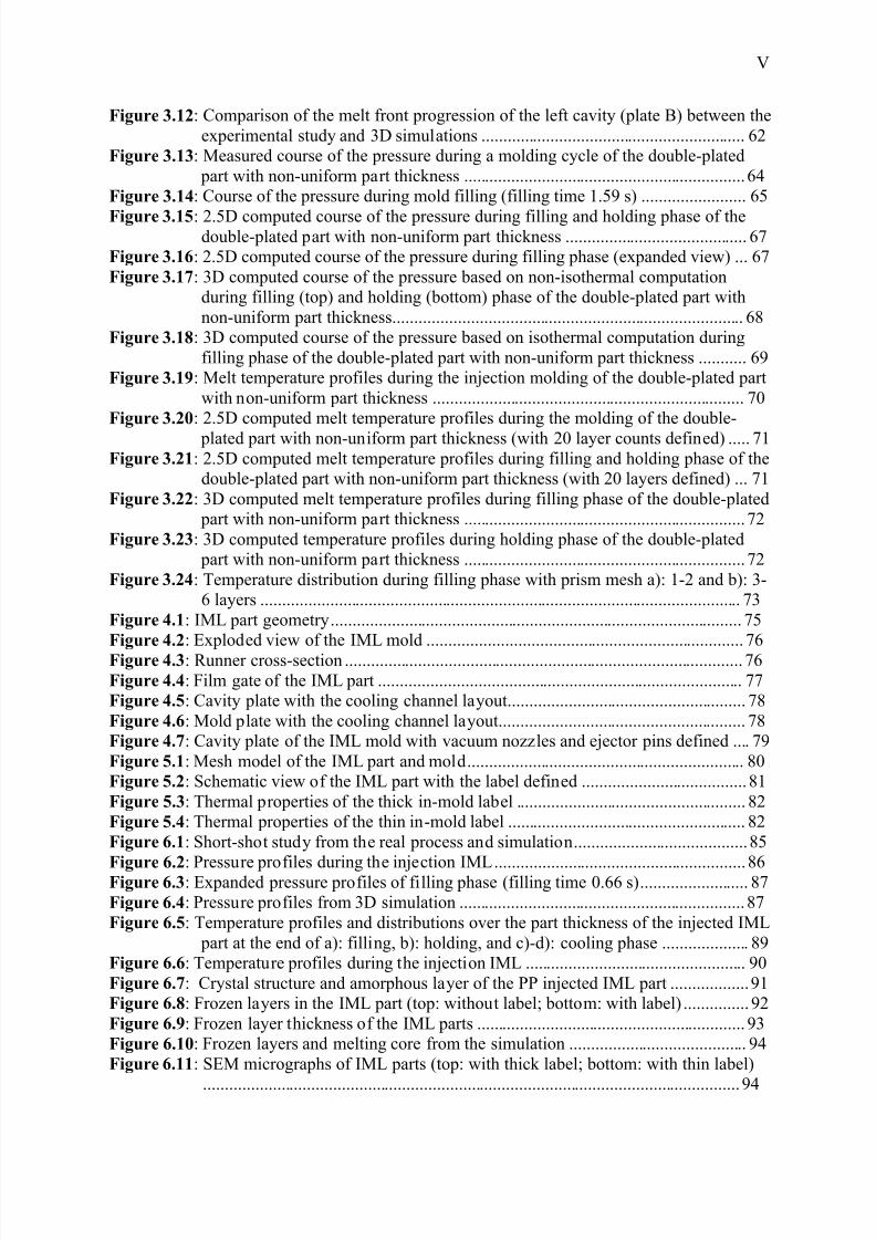
List of Figures ........................................................................................................................ IV
List of Tables........................................................................................................................ VII
List of Symbols and Abbreviations ................................................................................... VIII
Abstract ................................................................................................................................ XII
Kurzfassung ........................................................................................................................ XIII
1 Introduction and Objectives ......................................................................................... 1
2 Fundamentals ................................................................................................................ 4
2.1 Injection Mold Design ....................................................................................... 4
2.1.1 Runner System Design .......................................................................... 6
2.1.2 Gate Design ........................................................................................... 9
2.1.3 Cooling System Design ....................................................................... 12
2.1.4 Design of Ejection ............................................................................... 17
2.1.5 Design of Venting ............................................................................... 18
2.1.6 Selection of Mold Materials ................................................................ 20
2.1.7 Part Shrinkage ..................................................................................... 20
2.2 Injection In-Mold Labeling ............................................................................ 22
2.2.1 A Brief History of IML ....................................................................... 22
2.2.2 Injection IML Process ......................................................................... 22
2.2.3 Key Label Properties ........................................................................... 24
2.2.4 Automation in IML ............................................................................. 25
2.3 Injection Molding Simulation ........................................................................ 28
2.3.1 Concept of the Hele-Shaw Model (2.5D Analysis)............................. 29
2.3.2 Concept of Solid Modeling (3D Analysis) .......................................... 31
2.3.3 Viscosity Models for Thermoplastics ................................................. 33
2.3.4 Thermal Equation of State................................................................... 35
2.3.5 Numerical Discretization Methods...................................................... 36
3 Flow Analysis and Simulation in Injection Molding based on the Double-Plated
Part with Non-Uniform Part Thickness .................................................................... 41
3.1 Design of Experiments .................................................................................... 41
3.1.1 Part Geometry ..................................................................................... 41
3.1.2 Material Properties .............................................................................. 42
3.1.3 Machine Setting................................................................................... 44
3.1.4 Melt Pressure and Melt Temperature Detection by means of aCombined Pressure and Temperature Transducer .............................. 45
3.2 Simulation on a Basis of Surface Mesh (2.5D Simulation) .......................... 46
3.2.1 Discretization of the Model ................................................................. 46
3.3 Simulation on the Basis of Volume Mesh (3D Simulation) ......................... 48
7/27/2019 Injection Mould Design
http://slidepdf.com/reader/full/injection-mould-design 6/160
II
3.3.1 Discretization of the Model ................................................................. 48
3.4 Simulation Parameters ................................................................................... 50
3.5 Simulation Results and Its Comparison with the Real Injection Molding
Process .............................................................................................................. 50 3.5.1 Filling Analysis (Short-Shot Study) .................................................... 51
3.5.2 Course of the pressure ......................................................................... 63
3.5.3 Time/temperature Profiles ................................................................... 69
4 Design of an Injection Mold for Injection In-Mold Labeling ................................. 75
4.1 IML Part Geometry ........................................................................................ 75
4.2 Type of Mold .................................................................................................... 75
4.3 Runner Design ................................................................................................. 76
4.4 Gating ............................................................................................................... 77
4.5 Mold Cooling ................................................................................................... 77
4.6 Part Release/Ejection ...................................................................................... 78
4.7 Mold Venting ................................................................................................... 79
4.8 Label Insertion................................................................................................. 79
5 Simulation and Experimental Study on the Injection In-Mold Labeling Process 80
5.1 Simulation on the Injection In-Mold Labeling ............................................. 80
5.1.1 Mesh Generation ................................................................................. 80
5.1.2 Viscosity Model .................................................................................. 80
5.2 Experimental Study on the Injection In-Mold Labeling ............................. 81
5.2.1 IML Part Geometry ............................................................................. 81
5.2.2 In-mold Label Properties ..................................................................... 81
5.2.3 Design of Experiments ........................................................................ 83
6 IML-Simulation and Experimental Results .............................................................. 85
6.1 Melt Front Advancement................................................................................ 85
6.2 Course of the Pressure .................................................................................... 86
6.3 Temperature Profiles and Distributions ....................................................... 88
6.4 Structure of an Injected IML Part ................................................................ 90
6.5 Warpage of an Injected IML Part ................................................................. 95
6.6 Modulus of Elasticity .................................................................................... 106
7/27/2019 Injection Mould Design
http://slidepdf.com/reader/full/injection-mould-design 7/160
III
7 Summary .................................................................................................................... 110
References ............................................................................................................................ 113
Appendix 1 Standard Components of an Injection Mold ................................ 118
Appendix 2 Description of the Simulation program Moldex3D®
.................... 120
Appendix 3 Comparison of the melt front progression of the right cavity between the
experimental study and 2.5D simulations ............................................................... 124
Appendix 4 Comparison of the melt front progression of the right cavity between the
experimental study and 3D simulations .............................................................. 125
Appendix 5 2.5D simulation results of the double-plated part with non-
uniform part thickness based on the tetrahedral derivative mesh with 10, 20 and
30 layers defined ........................................................................................................ 127
Appendix 6 2.5D simulation results of the double-plated part with non-
uniform part thickness based on the voxel derivative mesh with 10, 20 and 30
layers defined 131
Appendix 7 Types of Labels used in Packaging ................................................ 135
Appendix 8 Temperature Measurement with IR Thermometers ................... 137
LEBENSLAUF .................................................................................................................... 142
7/27/2019 Injection Mould Design
http://slidepdf.com/reader/full/injection-mould-design 8/160
IV
List of Figures
Figure 2.1: Flow chart for methodical designing of injection molds [9] ................................. 5
Figure 2.2: Basic runner system layouts .................................................................................. 6
Figure 2.3: Filling patterns resulting from various injection rates in an unbalanced runner
system ................................................................................................................... 7
Figure 2.4: Commonly used runner cross sections................................................................... 8
Figure 2.5: Comparison of the flow efficiency of different runner shapes .............................. 8
Figure 2.6: Runner diameter and flow length determination ................................................... 9
Figure 2.7: Pin-point gate design [9] ...................................................................................... 10
Figure 2.8: Diaphragm (a) and disk (b) gate designs ............................................................. 11
Figure 2.9: Film gate design ................................................................................................... 11
Figure 2.10: Submarine gate design ....................................................................................... 12
Figure 2.11: Heat flow assessment in an injection mold [21] ................................................ 13
Figure 2.12: Analytical computation of the cooling system [21] ........................................... 14
Figure 2.13: Position of cooling channel and temperature uniformity [21] ........................... 15
Figure 2.14: Thermal reactions during a steady conduction [21, 22]..................................... 16
Figure 2.15: Suggested diameter of ejector pins depending on critical length of buckling andinjection pressure................................................................................................ 17
Figure 2.16: Cup mold with annular channel for venting [28] ............................................... 18
Figure 2.17: Evacuation of the microinjection mold [32] ...................................................... 19
Figure 2.18: Dimensional changes as a function of time [36] ................................................ 21
Figure 2.19: Injection in-mold labeling sequencing [43] ....................................................... 23
Figure 2.20: Label holding with vacuum ............................................................................... 26
Figure 2.21: Simplified electrostatic charging for round-shaped products [46] .................... 28
Figure 2.22: Definition of shell analysis ................................................................................ 29
Figure 2.23: Modeling of shell model [49] ............................................................................ 30 Figure 2.24: Thickness assignment in shell modeling ........................................................... 30
Figure 2.25: True 3D flow pattern.......................................................................................... 32
Figure 2.26: Physical and mathematical modeling [71] ......................................................... 38
Figure 2.27: Discretization of a FEM model (left) and a BEM model (right) ....................... 39
Figure 2.28: Comparison between the discretization methods............................................... 39
Figure 3.1: Geometry of the model ........................................................................................ 41
Figure 3.2: Viscosity (a) and pVT-diagram (b) of Novolen 3200 MC from Moldex3Ddatabank ............................................................................................................. 43
Figure 3.3: Combined pressure and temperature sensor for plastic injection molding [72] .. 45
Figure 3.4: Tetrahedral derivative surface mesh (global mesh size 3 mm, 1 mm at the
transition) ........................................................................................................... 47 Figure 3.5: Voxel derivative surface mesh (global mesh size 3 mm) .................................... 47
Figure 3.6: Volume mesh of the double-plated model ........................................................... 48
Figure 3.7: Close-up view of the 3D mesh models ................................................................ 49
Figure 3.8: Short-shot study from the experiment and 2.5D simulations (with 20 layersdefined)............................................................................................................... 53
Figure 3.9: Comparison of the melt front progression between the experimental study and 3Dnon-isothermal simulations ................................................................................ 56
Figure 3.10: Comparison of the melt front progression between the experimental study and3D simulation with prism mesh 3-6 layers based on the isothermal computation............................................................................................................................ 59
Figure 3.11: Comparison of the melt front progression of the left cavity (plate B) between theexperimental study and 2.5D simulations .......................................................... 60
7/27/2019 Injection Mould Design
http://slidepdf.com/reader/full/injection-mould-design 9/160
V
Figure 3.12: Comparison of the melt front progression of the left cavity (plate B) between theexperimental study and 3D simulations ............................................................. 62
Figure 3.13: Measured course of the pressure during a molding cycle of the double-plated part with non-uniform part thickness ................................................................. 64
Figure 3.14: Course of the pressure during mold filling (filling time 1.59 s) ........................ 65
Figure 3.15: 2.5D computed course of the pressure during filling and holding phase of thedouble-plated part with non-uniform part thickness .......................................... 67
Figure 3.16: 2.5D computed course of the pressure during filling phase (expanded view) ... 67
Figure 3.17: 3D computed course of the pressure based on non-isothermal computationduring filling (top) and holding (bottom) phase of the double-plated part withnon-uniform part thickness................................................................................. 68
Figure 3.18: 3D computed course of the pressure based on isothermal computation duringfilling phase of the double-plated part with non-uniform part thickness ........... 69
Figure 3.19: Melt temperature profiles during the injection molding of the double-plated partwith non-uniform part thickness ........................................................................ 70
Figure 3.20: 2.5D computed melt temperature profiles during the molding of the double-
plated part with non-uniform part thickness (with 20 layer counts defined) ..... 71
Figure 3.21: 2.5D computed melt temperature profiles during filling and holding phase of thedouble-plated part with non-uniform part thickness (with 20 layers defined) ... 71
Figure 3.22: 3D computed melt temperature profiles during filling phase of the double-plated part with non-uniform part thickness ................................................................. 72
Figure 3.23: 3D computed temperature profiles during holding phase of the double-plated part with non-uniform part thickness ................................................................. 72
Figure 3.24: Temperature distribution during filling phase with prism mesh a): 1-2 and b): 3-6 layers ............................................................................................................... 73
Figure 4.1: IML part geometry ............................................................................................... 75
Figure 4.2: Exploded view of the IML mold ......................................................................... 76
Figure 4.3: Runner cross-section ............................................................................................ 76
Figure 4.4: Film gate of the IML part .................................................................................... 77
Figure 4.5: Cavity plate with the cooling channel layout....................................................... 78
Figure 4.6: Mold plate with the cooling channel layout......................................................... 78
Figure 4.7: Cavity plate of the IML mold with vacuum nozzles and ejector pins defined .... 79
Figure 5.1: Mesh model of the IML part and mold ................................................................ 80
Figure 5.2: Schematic view of the IML part with the label defined ...................................... 81
Figure 5.3: Thermal properties of the thick in-mold label ..................................................... 82
Figure 5.4: Thermal properties of the thin in-mold label ....................................................... 82
Figure 6.1: Short-shot study from the real process and simulation ........................................ 85
Figure 6.2: Pressure profiles during the injection IML .......................................................... 86 Figure 6.3: Expanded pressure profiles of filling phase (filling time 0.66 s) ......................... 87
Figure 6.4: Pressure profiles from 3D simulation .................................................................. 87
Figure 6.5: Temperature profiles and distributions over the part thickness of the injected IML part at the end of a): filling, b): holding, and c)-d): cooling phase .................... 89
Figure 6.6: Temperature profiles during the injection IML ................................................... 90
Figure 6.7: Crystal structure and amorphous layer of the PP injected IML part .................. 91
Figure 6.8: Frozen layers in the IML part (top: without label; bottom: with label) ............... 92
Figure 6.9: Frozen layer thickness of the IML parts .............................................................. 93
Figure 6.10: Frozen layers and melting core from the simulation ......................................... 94
Figure 6.11: SEM micrographs of IML parts (top: with thick label; bottom: with thin label)
............................................................................................................................ 94

7/27/2019 Injection Mould Design
http://slidepdf.com/reader/full/injection-mould-design 10/160
VI
Figure 6.12: Asymmetrical thermal-induced residual stress caused by unbalanced coolingacross the molded part thickness introduces part warpage ................................ 95
Figure 6.13: Cooling stresses according to Knappe [88], thermal contraction and thedevelopment of inherent stresses according to Stitz [89] ................................... 96
Figure 6.14: Measurement of the part warpage ...................................................................... 97
Figure 6.15: Warpage of the IML parts .................................................................................. 98 Figure 6.16: Thermal induced warpage of the substrate due to bending stress...................... 98
Figure 6.17: Thermal induced warpage of the label owing to the bending stress .................. 98
Figure 6.18: Total warpage of the IML molded part .............................................................. 98
Figure 6.19: Part warpage from 3D simulations (IML1 setting; Tw = 40 oC) ..................... 102
Figure 6.20: Part warpage from 3D simulations .................................................................. 103
Figure 6.21: Warpage as a result of different molding effects [a): total thermal displacement, b): total in-mold constraint effect displacement, c): total moldbase thermaldeformation effect displacement] ..................................................................... 105
Figure 6.22: Comparison of the warpage between experiment and 3D simulation ............. 105
Figure 6.23: Modulus of elasticity of molded part without label compared with injected IML
parts molded with thick and thin label ............................................................. 107
Figure 6.24: Stress-strain graph of IML part (left: with thick label; right: with thin label) . 108
Figure 6.25: Effect of the mold temperature combination settings on the two mold halves onthe modulus of elasticity of parts molded with PP Novolen 3200 MC ............ 109
Flowchart for the Moldex3D software system ...................................................................... 120
Material selection from Moldex3D databank........................................................................ 121
Machine setting (CAE analysis interface) ............................................................................. 122
The analysis performed in the console mode ........................................................................ 123
Short-shot study from 2.5D simulations based on tetrahedral derivative mesh as a function of the number of layer counts defined .................................................................. 128
2.5D computed course of the temperature during filling and holding phase based ontetrahedral derivative mesh as a function of the number of mesh layer countsdefined .............................................................................................................. 129
2.5D computed average (left) and center (right) temperature distribution during filling phase based on tetrahedral derivative mesh as a function of the number of mesh layersdefined .............................................................................................................. 130
Short-shot study from 2.5D simulation based on voxel derivative mesh as a function of thenumber of layers defined .................................................................................. 132
2.5D computed course of the temperature during filling and holding phase based on voxelderivative mesh as a function of the number of mesh layers defined .............. 133
2.5D computed average (left) and center (right) temperature distribution during filling phase
based on tetrahedral derivative mesh as a function of the number of mesh layersdefined .............................................................................................................. 134
Electromagnetic spectrum ..................................................................................................... 137
Absorption, Reflection and Transmission of semi-transparent materials ............................. 139
Transmission of Infrared through Polypropylene ................................................................. 140

7/27/2019 Injection Mould Design
http://slidepdf.com/reader/full/injection-mould-design 11/160
VII
List of Tables
Table 2.1: Machine and mold requirements for injection IML .............................................. 24
Table 2.2: Comparison between inside and outside gating for injection IML ....................... 24
Table 3.1: Specification of the injection molding machine .................................................... 44
Table 3.2: Machine settings for the injection molding ........................................................... 44
Table 3.3: Number of part element of the surface mesh ........................................................ 47
Table 3.4: Number of the part element from different volume meshes ................................. 50
Table 3.5: Calculation time as a function of the surface mesh type ....................................... 50
Table 3.6: Calculation time as a function of the volume mesh type ...................................... 51
Table 5.1: List of the IML experimental studies .................................................................... 84
Standard components as per ISO .......................................................................................... 119
Minimum thickness of various plastics (Note with 3.43 µm Thermometer) ........................ 141

7/27/2019 Injection Mould Design
http://slidepdf.com/reader/full/injection-mould-design 12/160
VIII
List of Symbols and Abbreviations
Latin Alphabets
aT [-] temperature shift factor
A [mm2] cross-section area
A [mm2] surface area
AC [mm2] surface of the cooling channel
AP [mm2] surface of the molding
AS [%] after-shrinkage
b [mm] distance between channels
c p [J/mol K] specific heat capacity of the polymer melt at constant pressure
d [mm] diameter of the cooling channel
D, DA [mm] diameter
DC [kV] direct current
E [V/m] magnitude of an electric field
E [MPa] modulus of elasticity
E0 [J/mol] fluid activation energy
F [N] force
h [mm] height of the cavity
I [mm] distance between surfaces
j [%] cooling error
K [-] consistency index
L [mm] flow length
L [mm] unguided length of the ejector pin
L [-] flow efficiency of the melt through a runner
n [-] power law index
p [bar] pressure, injection pressure
p [mm] perimeter

7/27/2019 Injection Mould Design
http://slidepdf.com/reader/full/injection-mould-design 13/160
IX
PS [%] processing shrinkage
q [m] point of charge
ADQ& [W/m2] additional heat flux
C Q& [J] heat exchange with coolant
E Q& [J] heat exchange with environment
KS Q& [W/m2] heat flux from molding
R [mm] radius
R [J/mol K] universal gas constant
Rc [Rockwell] hardness unit
Re [-] Reynolds number
s [mm] part thickness
s [mm] critical length of buckling
S [-] fluidity
SD [%] shrinkage after demolding
t [s] time
T [oC] temperature
Tc [oC] crystallization temperature
TC [oC] coolant center temperature
TCW [oC] cooling channel wall temperature
TS [%] total shrinkage
TW [oC] mold wall temperature
u [m/s] average velocity of the coolant
V & [cm3/s] volume throughput
w [mm] part width
W [g] part weight
z [mm] thickness

7/27/2019 Injection Mould Design
http://slidepdf.com/reader/full/injection-mould-design 14/160
X
Greek Alphabets
α [o] tunnel gate angle
α [1/K] linear expansion coefficient
β [o] tunnel gate angle
γ & [1/s] shear rate
η [Pas] dynamic viscosity
0η [Pas] zero shear viscosity
λ [W/m K] thermal conductivity of the polymer
Aϑ [o
C] quenching temperature
E ϑ [oC] freezing temperature
ρ [g/cm3] density, density of the coolant
σ [MPa] stress
τ [Pa] shear stress
*τ [Pa] critical shear stress
xυ [m/s] velocity in x direction
yυ [m/s] velocity in y direction
z υ [m/s] velocity in z direction
xυ [m/s] average velocity in x direction
yυ [m/s] average velocity in y direction
z υ [m/s] average velocity in z direction
Abbreviations
2.5D 2.5 dimensional
3D 3 dimensional
ABS acrylonitrile butadiene styrene

7/27/2019 Injection Mould Design
http://slidepdf.com/reader/full/injection-mould-design 15/160
XI
AISI American Iron and Steel Institute
BEM boundary element method
CAD computer-aided design
DIN Deutsches Institut für Normung
EOAT end-of-arm tool
FEM finite element method
FDM finite difference method
FVM finite volume method
GF-PA glass-reinforced polyamide
GNF Generalized Newtonian Fluid
HDPE high density polyethylene
IML in-mold labeling
IR infrared
PA polyamide
PC polycarbonatePDE partial differential equation
PE polyethylene
PMMA polymethylmethacrylate
POM polyoxymethylene
PP polypropylene
PS polystyrene
S1, S2 sensor node 1 and 2
SEM scanning electron microscope
WLF William-Landel-Ferry

7/27/2019 Injection Mould Design
http://slidepdf.com/reader/full/injection-mould-design 16/160
XII
Abstract
Years ago, the production of packaging with the injection-IML has been established. This procedure concept ranks nowadays among the most modern technologies in the area of the plastic packaging. With this manufacturing technique, label and packaging, both are of the
same polymer materials, become inseparably connected during the injection molding process.Since thermal conductivity of the polymeric label material is clearly smaller than that of themetal mold wall, thermal induced warpage of injected IML part or part surface deformationcould be occurred. The objective of this work is to analyze and simulate the filling, holding,and cooling phases of the injection IML process by means of the simulation programMoldex3D® and to study the effect of inserted label on the warpage behavior and modulus of elasticity of injected parts. For this study, the injection mold for injection IML equipped withvacuum ports for holding the label was designed and constructed. For the automation of theinjection IML process, a linear pneumatic robot was employed.
As a preliminary examination, the experimental study and numerical simulation of the meltfront advancement, course of the pressure and melt temperature profile during the injectionmolding of double-plated parts with non-uniform part thickness were done in order to acquire
better understanding of the simulation program Moldex3D® prior to its application later on tothe injection IML simulation calculations. The molded part composes of two thin plates
joined together with a cold runner. One fan gate is connected to the thick side of the first plate and the other connected to the thin side of the second plate. Comparisons between theexperiment and simulation performed with the same molding parameters were carried out.From the results, 2.5D simulation was verified to be more reliable than 3D simulation
particularly in terms of predicting the melt front advancement as well as the melt pressuredevelopment during the molding. Owing to the complex flow and unbalance of the pressure
within two cavities of the part, 3D simulation based on non-isothermal computation failed to predict course of the pressure and hence the melt front advancement within both cavities.However, with the 3D isothermal computation, improvement in accuracy was achieved. This
phenomenon resulted from the instability of the 3D simulation program. By molding thedouble-plated part separately, both 2.5D and 3D simulation results agreed well with thosefrom the experiments.
After the preliminary examination has been done, analysis and 3D simulation on filling,holding, and cooling phases of the injection IML process and warpage behavior of injectedIML parts were investigated, since the presence of label can significantly affect the molding
process. From the study, good agreement of the mold filling, holding, and cooling results
between 3D simulation and experiment was acquired. Structure and warpage behavior of IML parts were also investigated. In order to cope with part warpage problem, variations inmold temperature on the stationary and moving mold halves were carried out. With thehigher mold temperature setting on the label side, part warpage was reduced. Furthermore,study of the effect of the mold temperature combination settings on the modulus of elasticityof the IML part was conducted. The results revealed that despite a slight reduction in themodulus of elasticity of the IML part owing to the different mold temperature settings on twomold halves, modulus of elasticity of the IML part was still found to be satisfactory.
7/27/2019 Injection Mould Design
http://slidepdf.com/reader/full/injection-mould-design 17/160
XIII
Kurzfassung
Seit geraumer Zeit, hat sich die Herstellung von Verpackungskomponenten nach dem In-Mold-Labeling-Spritzgießverfahren (IML) etabliert. Bei dieser Technologie werden dasEtikett und die Verpackung, die i.a. aus demselben Material bestehen, im Zuge des
Formgebungsschrittes unlösbar miteinander verbunden. Beim Einspritzvorgang desPlastifikats in die mit dem Etikett bestückte Kavität kann es dazu kommen, dass das Etikettaus seiner Ursprungslage verschoben oder gefaltet wird. Außerdem ist dieWärmeleitfähigkeit des Label-Materials deutlich niedriger als die der metallischenWerkzeugwandung, so dass es zu Strukturfehlern auf der Formteiloberfläche und/oder zueinem Verzug des Spritzgießteils kommen kann. Im Rahmen dieser Arbeit werden deshalbdie Formfüll- und Bauteil-Abkühlvorgänge beim IML-Spritzgießen analysiert, wobei dasSimulationsprogramm Moldex3D® zum Einsatz kommt. Die dabei gewonnenen Ergebnissewerden mit denen des realen Prozesses verglichen. Des Weiteren werden die generiertenProdukte im Bezug auf ihren Verzug und ihren E-Modul bewertet. Für diese Studie wurde einspezielles Spritzgießwerkzeug, welches mit Vakuumanschlüssen für die Positionierung undFixierung des In-Mold-Etiketts ausgerüstet ist, konstruiert und gebaut. Für dieAutomatisierung des IML-Spritzgießprozesses wurde ein linearer, pneumatisch betätigter Roboter eingesetzt.
Um ein besseres Verständnis für das Simulationsprogramm bezüglich seiner Funktionsweisevor der Anwendung auf das In-Mold-Labeling-Spritzgießen zu erwerben, wurden vorabsimulative und experimentelle Voruntersuchungen bezüglich der Fließfrontenverläufe, der Druckverläufe und der Temperaturprofile beim Spritzgießen von Doppelplatten mitDickensprung durchgeführt. Dieses Formteil besteht aus zwei plattenförmigen Kavitäten, die
jeweils über einen Filmanschnitt an der dicken und der dünnen Seite der Kavität angespritzt
werden. Ein Vergleich von Versuchs- und Simulationsergebnissen wurde durchgeführt.Dabei zeigte sich, dass eine 2.5D-Simulation hinsichtlich der Voraussagen der Fließfrontenverläufe in den Kavitäten sowie der Schmelzedruckverteilungen während desSpritzgießens zu einer zufrieden stellenden Übereinstimmung führte. Infolge des komplexenFüllvorgangs und der „Druckumkehr“ innerhalb der beiden Kavitäten konnte die nicht-isotherme 3D-Simulation den Druck und somit die Fließfrontenverläufe nicht richtigwiedergeben. Mit der isothermen 3D-Simulation konnte hingegen eine deutlicheVerbesserung in der Genauigkeit erzielt werden. Des Weiteren wurde die Doppelplatte inzwei Einzelplatten zerlegt, die separat gespritzt werden. Mit diesen Platten konnten sowohl2.5D- als auch 3D- Füllbildsimulationen erfolgreich durchgeführt und dieFließfrontenverläufe in der Kavität richtig beschrieben werden.
Da das Etikett auf den Formteil-Herstellungsprozess zurückwirken kann, wurden nach diesenVoruntersuchungen die Einflüsse des Etiketts unter Durchführung von 3D-Simulationen
bezüglich der Füll-, Nachdruck-, und Kühlphase sowie hinsichtlich des Verzugsverhaltens beim In-Mold-Labeling-Spritzgießen studiert. Dabei wurde eine gute Übereinstimmung vonVersuchs- und Simulationsergebnissen festgestellt. Weiterführend wurden die Struktur unddas Verzugsverhalten des IML-Formteils analysiert. Um den Verzug des IML-Formteils zureduzieren wurden die Spritzgießversuche mit verschiedenen Werkzeugtemperatur-Kombinationen durchgeführt. Dabei zeigte sich, dass mit einer höheren Werkzeugtemperatur auf der Labelseite der Verzug verringert werden kann. Zusätzlich wurde der Einfluss der Werkzeugtemperatur-Kombination auf die Steifigkeit des IML-Formteils untersucht. Es
zeigte sich, dass trotz einer geringfügigen Verringerung des Elastizitätsmoduls des IML-

7/27/2019 Injection Mould Design
http://slidepdf.com/reader/full/injection-mould-design 18/160
XIV
Formteils infolge der unterschiedlichen Werkzeugtemperaturen der beiden Werkzeughälftender Elastizitätsmodul des IML-Formteils noch in einem akzeptablen Bereich bleibt.
7/27/2019 Injection Mould Design
http://slidepdf.com/reader/full/injection-mould-design 19/160
1
1 Introduction and Objectives
Numerous new polymer grades have been developed over the last few years for specificapplications. Some of these materials may require different production methods toaccomplish the articles required, such as compression and injection molding, blow molding,
extrusion, and thermoforming. In most cases, a mold is required to give the product thedesired shape. At the present time, injection molding seems to be the most common andeconomical method to produce plastic products, especially when large quantities are required.Therefore, it is very important that a mold must be carefully designed and preciselyconstructed. This may be performed by experience or with the help of CAD/CAM andsimulation programs. By using special programs, many calculations can be performed rapidlyand accurately, and newly created mold designs can be easily checked for efficiency of meltflow, cooling, strength of materials, etc. Various programs can be used to check for physicalstrength and to check with other programs the expected efficiency of filling the mold cavities,gate location and sizes, runner sizes, the cooling layout, and so on. Note that all thesimulation results depend on the accuracy of the data provided, such as reasonableassumptions as to temperatures, pressures, and times. In this study, the injection mold whichwas used in the injection in-mold labeling of the flat part has been designed and constructed.Details of this IML mold inclusively the mold components as well as their geometries anddimensions are described in Chapter 4.
In conventional injection molding, mold filling can be successfully predicted for thin partsusing the Hele-Shaw model. It assumes that the flow profiles are the same at all gapwise
positions. Conventional algorithm extracts mid-plane surface of the part to represent the 3Dgeometry. These simulation codes are usually referred to as 2.5D. It simplifies the 3Dgeometry model into 2.5D mid-plane and proceeds to the simulation [1]. This technology has
been successfully applied to simulate the molding process of most thin shell plastic parts. Inthe past decade 3D simulation programs have become widely available. However, 2.5D
programs cannot take advantage of these models. Especially for thick parts, the 3D effects areabsolutely obvious and can no longer be precisely analyzed by the conventional 2.5Dmethods. Moreover, the effort required to generate 2.5D models from 3D models issometimes equivalent to generating 3D information from the beginning [2]. Another solutionis to avoid the use of the Hele-Shaw equations and solve the governing equations in their fullgenerality [3] that means it provides a true 3D solution.
Nowadays, numerous commercial simulation programs for injection molding are available.Usually, users are told that 3D simulation has advantages over 2.5D one. Also, there are
many studies conducted in the last years in order to compare the efficiency and accuracy of 2.5D to 3D simulation concepts. In spite of this, it is still worth performing such acomparison of one’s own simulation program, whether it would be able to deal with morecomplex problem. For this reason, flow analysis and simulation by means of the double-
plated part with non-uniform part thickness were carried out as a preliminary examinationwhich is shown in Chapter 3. By doing this, a better understanding of the simulation programregarding how it works, its strength and weakness can be obtained. In this study, Moldex3Dsimulation program which is capable of the true 3D (Solid models) CAE analysis was used.Simulations were carried out based on 2.5D mid-plane (Hele-Shaw) and 3D analyses andlater their results were evaluated and compared with each other and with those from the realmolding process.
7/27/2019 Injection Mould Design
http://slidepdf.com/reader/full/injection-mould-design 20/160
2
More than 25 years ago the production of packaging articles with the injection in-moldlabeling (IML) technology has been established. This molding concept ranks nowadaysamong the most modern technologies in the area of plastic packaging. In-mold labeling is a
pre-decorating technique used worldwide for blow molded bottles as well as for injectionmolded and thermoformed containers or other plastic objects. Injection in-mold labeling is an
injection molding technique, in which the film, label or decorating material is back injected.In the in-mold labeling process, a label is placed in the open mold and held in the desired
position by vacuum ports, electrostatic attraction or other appropriate means. The mold closesand molten plastic resin is injected into the mold where it conforms to the shape of the object.The plastic melt envelopes the label, making it an integral part of the molded part. With thismanufacturing technique, the label and packaging, both are of the same polymeric material,
become inseparably adhered during the injection molding process. Besides the injectionmolding machine, process parameters, and the quality of the labels used, the quality of injected IML parts is significantly affected by the injection mold, which must be deliberatelydesigned and carefully constructed. Main advantage of injection in-mold labeling is theintegration of a follow-up step into the injection molding process. The heat transport
reduction owing to the label and the associated slightly higher molding cycle time are someunfavorable aspects of this molding technique. By back injection of the plastic melt into thecavity preloaded with the label, it can occasionally come to the situation that the label isfolded, slipped or shifted from its starting position, whereby the injected IML part becomesuseless. In addition, the thermal conductivity of the label material is significantly smaller thanthat of the metal mold wall, so that the thermally induced warpage of the injected IML part or surface deformation could occur.
Since the label has different thermal properties relative to the polymer melt and mold, the presence of the label as an insert can significantly affect the filling, holding, cooling andwarpage behaviors of the injection molding process. To fully consider the complex insert
effects, especially warpage of the IML part, a true three-dimensional finite element solution[4, 5] is a better choice than the traditional 2.5-dimensional finite element solution [6 and 7].Warpage is caused by variations in shrinkage throughout the part. For injection molded part,the part is constrained in the mold. During the solidification of an injection molded part,shrinkage of the solidified layer is prevented by two mechanisms. Firstly, adhesion to themold walls restrains (at least the outer skin of) the solid layers from moving, and secondly,the newly formed solid surface will be kept fixed by the stretching forces of melt pressure.In-cavity residual stresses are then built up during solidifications. Due to the nature of constrained quenching, the residual stress distribution is largely determined by the varying
pressure history coupled with the frozen layer growth. Once the part is ejected from the mold,these residual stresses will be released in the form of shrinkage deformation. If the initialstrains, which are equivalent to the in-cavity residual stresses, are symmetric, the part willshrink uniformly without any warpage and post-mold residual stresses.
The objective of this work can be subdivided into two subtasks. Firstly, the experimentalstudy and numerical simulations of the melt front advancement, course of the pressure andmelt temperature profile during the injection molding of double-plated parts with non-uniform part thickness will be carried out. This will be done by means of the injectionsimulation program Moldex3D®. Furthermore, simulation results from 2.5D and 3Dsimulation calculations will be verified. Secondly, analysis and simulation on filling, holding,and cooling phases of the injection IML process and warpage behavior of injected IML parts
will be investigated, in order to study the effect of in-mold labels on the injection moldingand warpage behaviors of injected IML parts. In this stage, only 3D simulation calculation

7/27/2019 Injection Mould Design
http://slidepdf.com/reader/full/injection-mould-design 21/160
3
will be conducted and its results will then be compared with those of the experiments. Inaddition, the injected part quality particularly in terms of degree of part warpage and modulusof elasticity will be evaluated.
7/27/2019 Injection Mould Design
http://slidepdf.com/reader/full/injection-mould-design 22/160
4
2 Fundamentals
2.1 Injection Mold Design
One basic requirement must be met by every mold that is intended to run on an automatic
injection molding machine is that the molded parts must be ejected automatically without theneed for secondary finishing operations (degating, machining to final dimensions, etc.). Froma practical standpoint, the classification of injection molds should be accomplished on the
basis of the major features of the design and operation [8, 9, 10, and 11]. These include:
• the type of gating, i.e. runner system and means of separation,
• the type of ejection used for the molded parts,
• the presence or absence of external or internal undercuts on the part to be molded, and
• the manner in which the molded part is released.
The DIN ISO standard 12165 “Components for Compression, Injection, and Compression-Injection Molds” classifies molds on the basis of the following criteria:
• standard molds (two-plate molds),
• split-cavity molds (split-follower molds),
• stripper plate molds,
• three-plate molds,
• stack molds,
• hot runner molds.
Standard components of an injection mold are shown in Appendix 1. There are also coldrunner molds for runnerless processing of thermosetting resins in analogy to the hot runner molds used for processing thermoplastic compounds and elastomers.
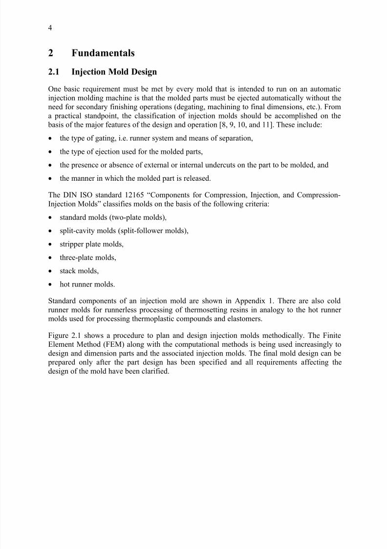
Figure 2.1 shows a procedure to plan and design injection molds methodically. The FiniteElement Method (FEM) along with the computational methods is being used increasingly todesign and dimension parts and the associated injection molds. The final mold design can be
prepared only after the part design has been specified and all requirements affecting thedesign of the mold have been clarified.
7/27/2019 Injection Mould Design
http://slidepdf.com/reader/full/injection-mould-design 23/160
5
Figure 2.1: Flow chart for methodical designing of injection molds [9]

7/27/2019 Injection Mould Design
http://slidepdf.com/reader/full/injection-mould-design 24/160
6
2.1.1 Runner System Des
A runner system directs the pressure is required to pushwithin the melt while the mat
and also facilitates the flow.low pressure requirements, tand scrap, and high clampinmaximize efficiency in bothsame time, however, runner s
pressure capability.
There are three basic runner These concepts are illustrated
Fig
The "H" (branching) and radinaturally balanced runner procavities, so that each cavity is
naturally unbalanced, it cacounterparts, with minimumsystem can be artificially balsegments.
The number of cavities in amolding process but also foartificial balancing of the stana symmetrical runner system
Inevitable, the possible numb
are 2, 4, 8, 16, 32, 64 etc. N
ign
melt flow from the sprue to the mold che melt through the runner system. Frictioerial is flowing through the runner raises th
hile large runners facilitate the flow of mey require a longer cooling time, more ma
forces. Designing the smallest adequateraw material use and energy consumptionze reduction is constrained by the molding
system layouts typically used for a multi-cin the Figure 2.2.
ure 2.2: Basic runner system layouts
al (star) systems are considered to be natur vides equal distance and runner size from tfilled under the same conditions. Although
accommodate more cavities than itsrunner volume and less tooling cost. Ananced by changing the diameter and the le
mold plays a crucial role not only for thr the quality of the injection molded partdard (herringbone or in-line) runner system,ith H- or T- branching is recommended.
er of cavities resulted from the symmetrica
te that, despite artificial balancing, molds
avities. Additionalnal heat generatede melt temperature
aterial at relativelyterial consumptionunner system willn molding. At the
achine's injection
avity system [12].
ally balanced. Thehe sprue to all thethe herringbone is
aturally balancedunbalanced runner ngth of the runner
efficiency of thes. Because of thean employment of
l runner alignment
ith 10, 14 and 20
7/27/2019 Injection Mould Design
http://slidepdf.com/reader/full/injection-mould-design 25/160
cavities, which are aligned inare not recommended for the
Balanced flow into the cavitiachieved by changing the ru
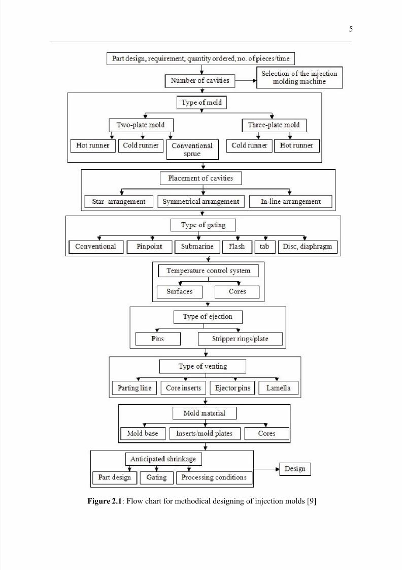
seemingly balanced filling.detrimental to part uniformity. be used to balance the flow o possible, then the runner syste
To balance a runner system,reducing the diameter of rundiameter excessively may cahand, increased frictional sheresistance to flow and fill thediameters will increase mold
runner system designed for balanced runner system requcontrol will alter filling patter
For example, if a standard (infilling patterns will occur. Geout onto the runner, while aThis is because at a slower ifirst encounters. It moves out
branches are filled, the meltresistant than the downstream
filling patterns between these
Figure 2.3: Filling patterns
one or two rolls, cannot provide the unifor roduction of precise parts [13].
es is a prerequisite for a quality part prodner size and length. Changing the gate dim
owever, it affects the gate freeze-off timWhenever possible, a naturally balanced rumaterial into the cavities. If a naturally bal
m should be artificially balanced [14, 15].
elt flow is encouraged to the cavities farthesers feeding the other cavities. Note that dese it to freeze prematurely, causing a shortar heating may actually reduce the resin'scavity even faster [16]. Keep in mind that nmanufacturing and maintenance costs. An a
ne material may not work for others. Fur res tighter process controls. A small variaof the mold, leading to consistently unbala
line) runner system with various injection raerally speaking, a slow injection rate will fiaster injection rate will first fill the parts c jection rate, the melt tends to hesitate at tto fill the remaining runner system. By theat the first, upstream gates may have alregates, due to solidification. Varied injection
wo extremes, as illustrated in Figure 2.3.
resulting from various injection rates in an usystem
7
filling and hence
ction. This can beension may give a
greatly, which isner system shouldnced runner is not
t from the sprue byreasing the runner shot. On the other iscosity, and thus,on-standard runner rtificially balanced
her, an artificiallyion in the processced filling.
tes is used, variousst fill parts further osest to the sprue.e restricted gate ittime all the runner ady become morespeed will result in
balanced runner
7/27/2019 Injection Mould Design
http://slidepdf.com/reader/full/injection-mould-design 26/160
8
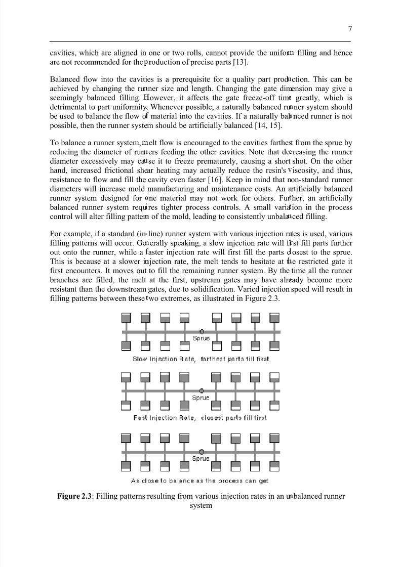
Figure 2.4 shows commonly best in terms of a maximum vloss. However, the tooling comachined so that the two semi
The trapezoidal runner also wside of the mold. It is commonot be released properly, aninterferes with mold sliding a
Figure
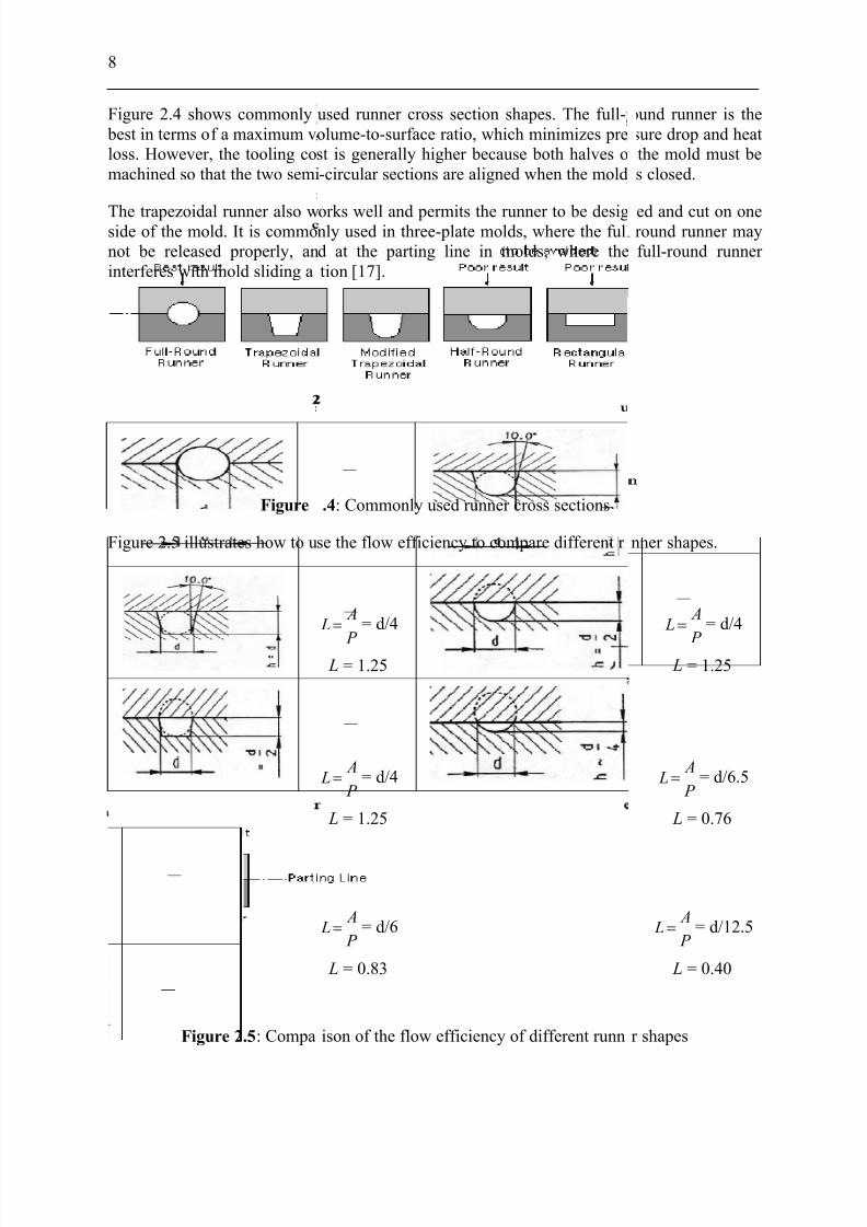
Figure 2.5 illustrates how to u
Figure 2.5: Compa
used runner cross section shapes. The full-r olume-to-surface ratio, which minimizes prest is generally higher because both halves o-circular sections are aligned when the mold
orks well and permits the runner to be designly used in three-plate molds, where the fulld at the parting line in molds, where thetion [17].
.4: Commonly used runner cross sections
se the flow efficiency to compare different r
P
A L= = d/4
L = 1.25
P
A L= = d/4
L = 1.25
P
A L= = d/6
L = 0.83
ison of the flow efficiency of different runn
ound runner is thesure drop and heatthe mold must be
is closed.
ed and cut on one-round runner mayfull-round runner
nner shapes.
P
A L= = d/4
L = 1.25
P
A L= = d/6.5
L = 0.76
P
A L= = d/12.5
L = 0.40
r shapes

7/27/2019 Injection Mould Design
http://slidepdf.com/reader/full/injection-mould-design 27/160
9
To compare runners of different shapes, the flow efficiency L of the melt through a runner,which is an index of flow resistance, is employed. The higher the flow efficiency of the meltthrough the runner, the lower the flow resistance is. Flow efficiency can be defined as [18]:
P
A L= (2-1)
where L = flow efficiency of the melt through a runner,
A = cross section area,
P = perimeter.
The diameter and length of runners influence the flow resistance [19]. The higher the flowresistance in the runner, the higher the pressure drop will be. Reducing flow resistance inrunners by increasing the diameter will use more resin material and cause longer cycle time if the runner has to cool down before ejection. One may first design the runner diameter byusing empirical data or the equation (2-2). Then fine-tune the runner diameter usingcomputational analysis to optimize the delivery system. Figure 2.6 shows the definition of theflow length L used for calculating the runner diameter. Following is the formula for runner diameter determination [18]:
Figure 2.6: Runner diameter and flow length determination
4
4 LW DA
⋅= (2-2)
where DA = runner diameter (mm),
W = part weight (g),
L = flow length (mm).
2.1.2 Gate Design
A gate is a small opening through which the polymer melt enters the cavity. Gate design for a particular application includes selection of the gate type, dimensions, and location. It isdictated by the part and mold design, the part specifications (e.g., appearance, tolerance,concentricity), the type of material being molded, the fillers, the type of mold plates, andeconomic factors (e.g., tooling cost, cycle time, allowable scrap volume). Gate design is of great importance to part quality and productivity.
The following provides an overview of the most commonly encountered types of gates:
7/27/2019 Injection Mould Design
http://slidepdf.com/reader/full/injection-mould-design 28/160
10
• Pinpoint gate (automatically trimmed),
• Diaphragm gate,
• Disk gate,
• Film gate and,
• Submarine gate (automatically trimmed).
The gate location should be at the thickest area of the part, preferably at a spot where thefunction and appearance of the part are not impaired. This leads the material to flow from thethickest areas through thinner areas to the thinnest areas, and helps maintain the flow andholding paths. Gate location should be central so that flow lengths are equal to each extremityof the part.
Symmetrical parts should be gated symmetrically, to maintain that symmetry. Asymmetricflow paths will allow some areas to be filled, packed, and frozen before other areas are filled.
This will result in differential shrinkage and probable warpage of the parts. Gate lengthshould be as short as possible to reduce an excessive pressure drop across the gate. Gatesshould always be small at the beginning of the design process so they can be enlarged, if necessary. The freeze-off time at the gate is the maximum effective cavity holding time.However, if the gate is too large, freeze off might be in the part, rather than in the gate, or if the gate freezes after the holding pressure is released, flow could reverse from the part back into the runner system. A well-designed gate freeze-off time will also prevent back flow of the injected material. Fiber-filled materials require larger gates to minimize breakage of thefibers when they pass through the gate [11].
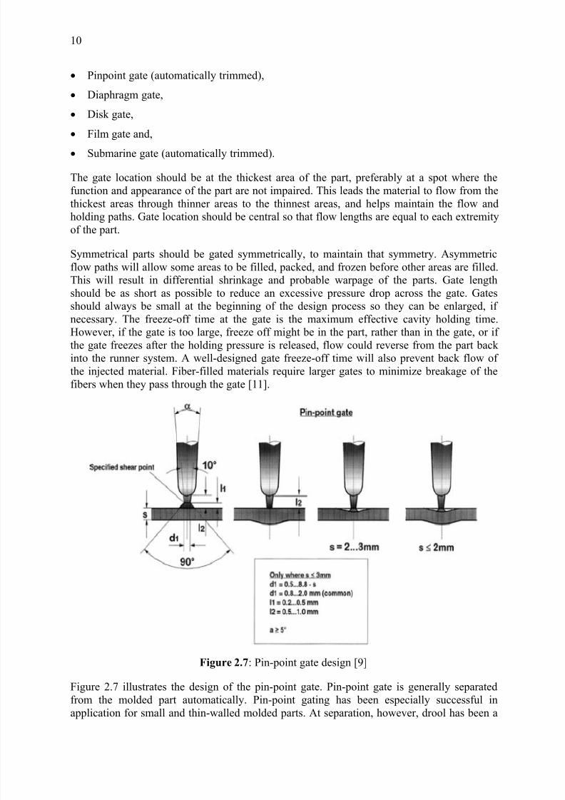
Figure 2.7: Pin-point gate design [9]
Figure 2.7 illustrates the design of the pin-point gate. Pin-point gate is generally separated
from the molded part automatically. Pin-point gating has been especially successful inapplication for small and thin-walled molded parts. At separation, however, drool has been a

7/27/2019 Injection Mould Design
http://slidepdf.com/reader/full/injection-mould-design 29/160
11
problem with certain polymers and premature solidification of the pin gate may make itdifficult to optimize holding time.
The diaphragm gate (see Fig. 2.8 (a)) is useful for producing cylindrical parts with the highest possible degree of concentricity and avoidance of weld lines. On the other hand, the
diaphragm encourages jetting which, however, can be controlled by varying the injection rateso as to create a swelling material flow. Having to remove the gate by means of subsequentmachining is a disadvantage of this gate type. Disk gate (Fig. 2.8 (b)) is used preferably for internal gating of cylindrical parts in order to eliminate disturbing weld lines. With fibrousreinforcements, for instance, the disk gate can aggravate the tendency for distortion. The disk gate must also be removed subsequent to the part ejection.
Figure 2.8: Diaphragm (a) and disk (b) gate designs
Figure 2.9: Film gate design

7/27/2019 Injection Mould Design
http://slidepdf.com/reader/full/injection-mould-design 30/160
12
Figure 2.9 illustrates the recommended dimension of a film gate. The film gate is used whena uniform flow front especially in flat molded parts is desired. This kind of flow leads to fewinternal stresses and little tendency to warp of the part. A certain tendency of the melt toadvance faster in the vicinity of the sprue can be offset by correcting the cross-section of thefilm gate. The film gate is usually trimmed off the part after ejection.
Figure 2.10 depicts the dimensional design of the submarine (tunnel) gate. As same as the pin-point gate, this type of gate is trimmed off the molded part during mold opening or directly on ejection at a specified cutting edge.
Figure 2.10: Submarine gate design
2.1.3 Cooling System Design
Generally, heat from the melt injected into the cavity has to be rapidly and uniformlyextracted until the injected part possesses a sufficient rigidity and then can be demoldedwithout a risk to warp. To calculate the heat flux and design the heat exchange-system of amold, the total amount of heat carried into the mold has to be first determined. In the range of
quasi-steady operation, heat flux applied to the mold (positive value) and heat flux to beremoved from the mold (negative value) have to be in equilibrium. Heat flux balance can bedescribed in the following form [20]:
0=+++ C AD E KS QQQQ &&&& (2-3)
where KS Q& = Heat flux from molding,
E Q& = Heat exchange with environment,
ADQ& = Additional heat flux (e.g. from hot runner),
C Q& = Heat exchange with coolant.
7/27/2019 Injection Mould Design
http://slidepdf.com/reader/full/injection-mould-design 31/160
13
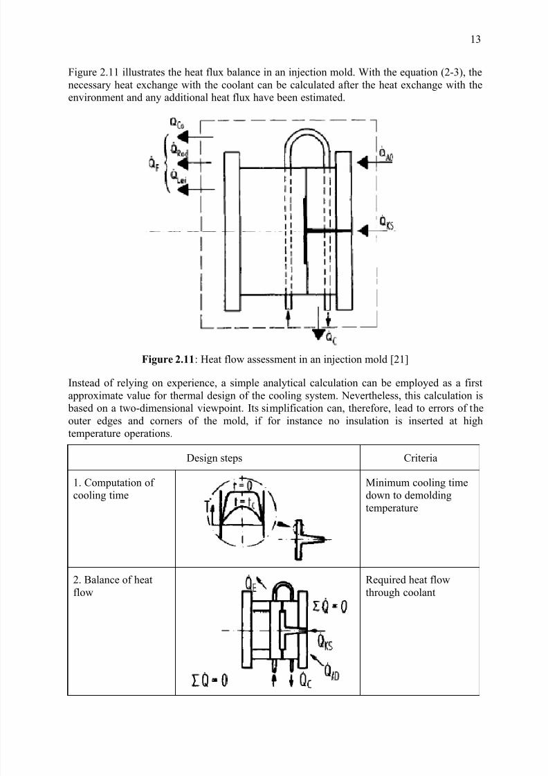
Figure 2.11 illustrates the heat flux balance in an injection mold. With the equation (2-3), thenecessary heat exchange with the coolant can be calculated after the heat exchange with theenvironment and any additional heat flux have been estimated.
Figure 2.11: Heat flow assessment in an injection mold [21]
Instead of relying on experience, a simple analytical calculation can be employed as a firstapproximate value for thermal design of the cooling system. Nevertheless, this calculation is
based on a two-dimensional viewpoint. Its simplification can, therefore, lead to errors of theouter edges and corners of the mold, if for instance no insulation is inserted at hightemperature operations.
Design steps Criteria
1. Computation of cooling time
Minimum cooling timedown to demoldingtemperature
2. Balance of heatflow
Required heat flowthrough coolant
7/27/2019 Injection Mould Design
http://slidepdf.com/reader/full/injection-mould-design 32/160
14
3. Flow rate of coolant
Uniform temperaturealong cooling line
4. Diameter of cooling line
Turbulent flow
5. Position of cooling line
Heat flow uniformity
6. Computation of pressure drop
Selection of heatexchanger modificationof diameter or flow rate
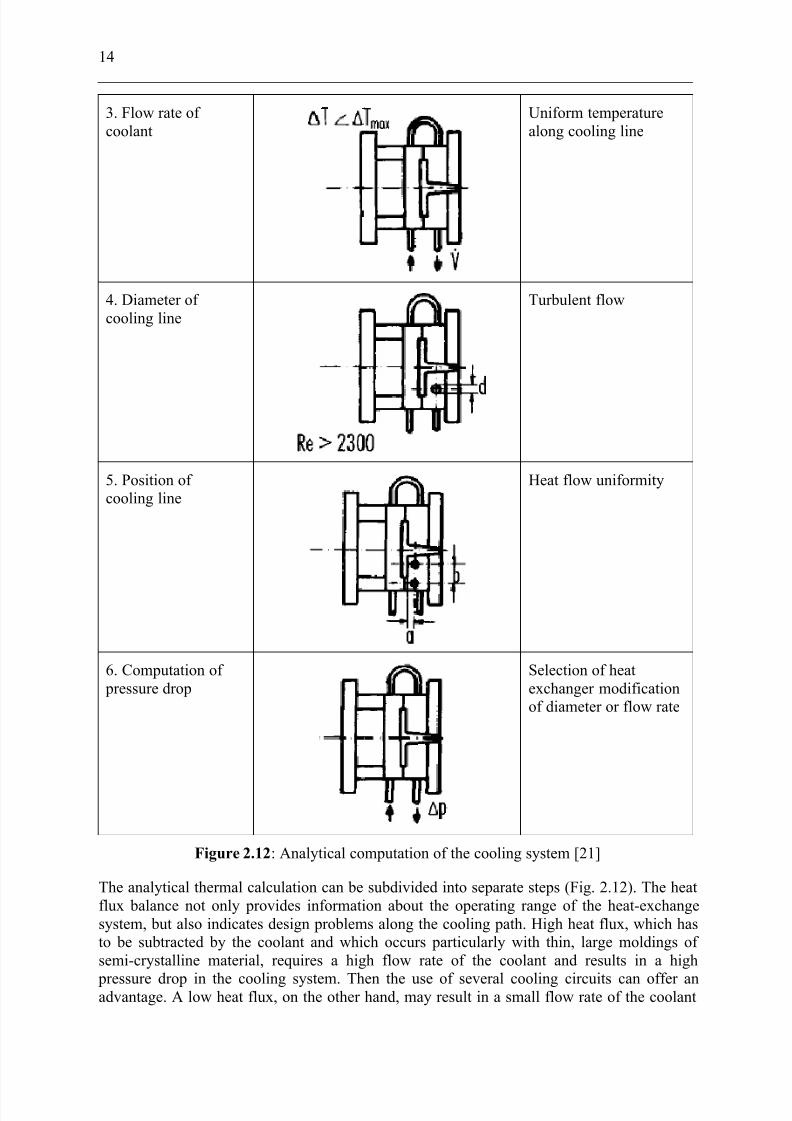
Figure 2.12: Analytical computation of the cooling system [21]
The analytical thermal calculation can be subdivided into separate steps (Fig. 2.12). The heatflux balance not only provides information about the operating range of the heat-exchangesystem, but also indicates design problems along the cooling path. High heat flux, which hasto be subtracted by the coolant and which occurs particularly with thin, large moldings of semi-crystalline material, requires a high flow rate of the coolant and results in a high
pressure drop in the cooling system. Then the use of several cooling circuits can offer anadvantage. A low heat flux, on the other hand, may result in a small flow rate of the coolant
7/27/2019 Injection Mould Design
http://slidepdf.com/reader/full/injection-mould-design 33/160
15
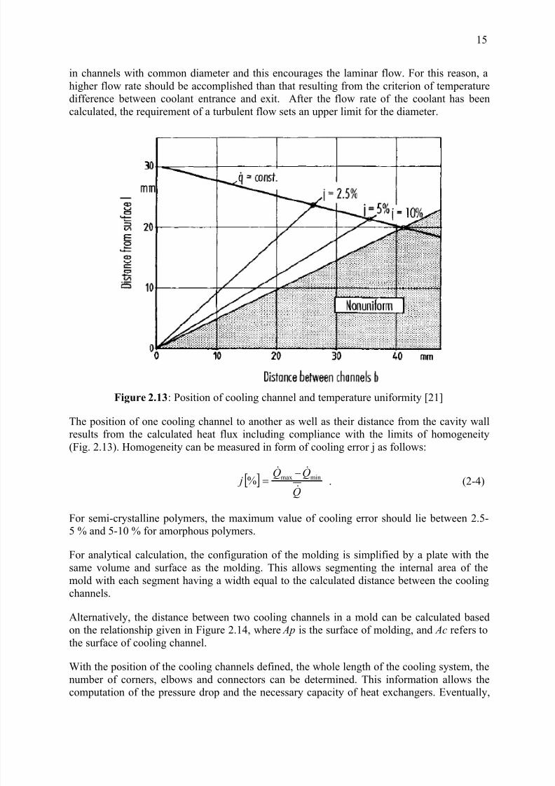
in channels with common diameter and this encourages the laminar flow. For this reason, ahigher flow rate should be accomplished than that resulting from the criterion of temperaturedifference between coolant entrance and exit. After the flow rate of the coolant has beencalculated, the requirement of a turbulent flow sets an upper limit for the diameter.
Figure 2.13: Position of cooling channel and temperature uniformity [21]
The position of one cooling channel to another as well as their distance from the cavity wallresults from the calculated heat flux including compliance with the limits of homogeneity(Fig. 2.13). Homogeneity can be measured in form of cooling error j as follows:
[ ]Q
QQ j
&
&&minmax%
−= . (2-4)
For semi-crystalline polymers, the maximum value of cooling error should lie between 2.5-5 % and 5-10 % for amorphous polymers.
For analytical calculation, the configuration of the molding is simplified by a plate with thesame volume and surface as the molding. This allows segmenting the internal area of themold with each segment having a width equal to the calculated distance between the coolingchannels.
Alternatively, the distance between two cooling channels in a mold can be calculated basedon the relationship given in Figure 2.14, where Ap is the surface of molding, and Ac refers tothe surface of cooling channel.
With the position of the cooling channels defined, the whole length of the cooling system, thenumber of corners, elbows and connectors can be determined. This information allows the
computation of the pressure drop and the necessary capacity of heat exchangers. Eventually,

7/27/2019 Injection Mould Design
http://slidepdf.com/reader/full/injection-mould-design 34/160
16
the minimum diameter of the cooling channel or the maximum flow rate of the coolant for agiven permissible pressure drop can be calculated.
Figure 2.14: Thermal reactions during a steady conduction [21, 22]
Controlled cooling channels are essential in a mold and require special attention in molddesign. The cooling medium must be in turbulent flow, rather than laminar flow, in order totransfer heat out of the molded part at an adequate rate [23]. The Reynolds number is used to
determine whether the coolant will be turbulent. It is the dimensionless number that issignificant in the design of any system in which the effect of viscosity is important incontrolling the velocity or the flow pattern of a fluid. Following is the equation for calculating the Reynolds number:
η
ρ Ud =Re (2-5)
where ρ = density of the coolant,
U = average velocity of the coolant,
d = diameter of the cooling channel,η = dynamic viscosity of the coolant.
The transition between laminar and turbulent flow is often indicated by a critical Reynoldsnumber, which depends on the exact flow configuration and must be determinedexperimentally. Within circular channels the critical Reynolds number is generally acceptedto be 2300, where the Reynolds number is based on the channel diameter and the averagevelocity U within the channel. Anyhow, to ensure the turbulent flow in the cooling channel,the Reynolds number should be at least 10,000 [24].
7/27/2019 Injection Mould Design
http://slidepdf.com/reader/full/injection-mould-design 35/160
17
2.1.4 Design of Ejection
Ejection of a molded article is normally accomplished mechanically by the opening stroke of the molding machine. If this simple ejection effected by the movement of the clamping unit isnot sufficient, ejection can be performed pneumatically or hydraulically [25].
As a consequence of the processing shrinkage, molded parts tend to be retained on moldcores. Following are various types of ejectors commonly used to release molded parts:
• Ejector pins,
• Ejector sleeves,
• Stripper plates, stripper bars, stripper rings,
• Slides and lifters,
• Air ejectors,
• Disc or valve ejectors, etc.
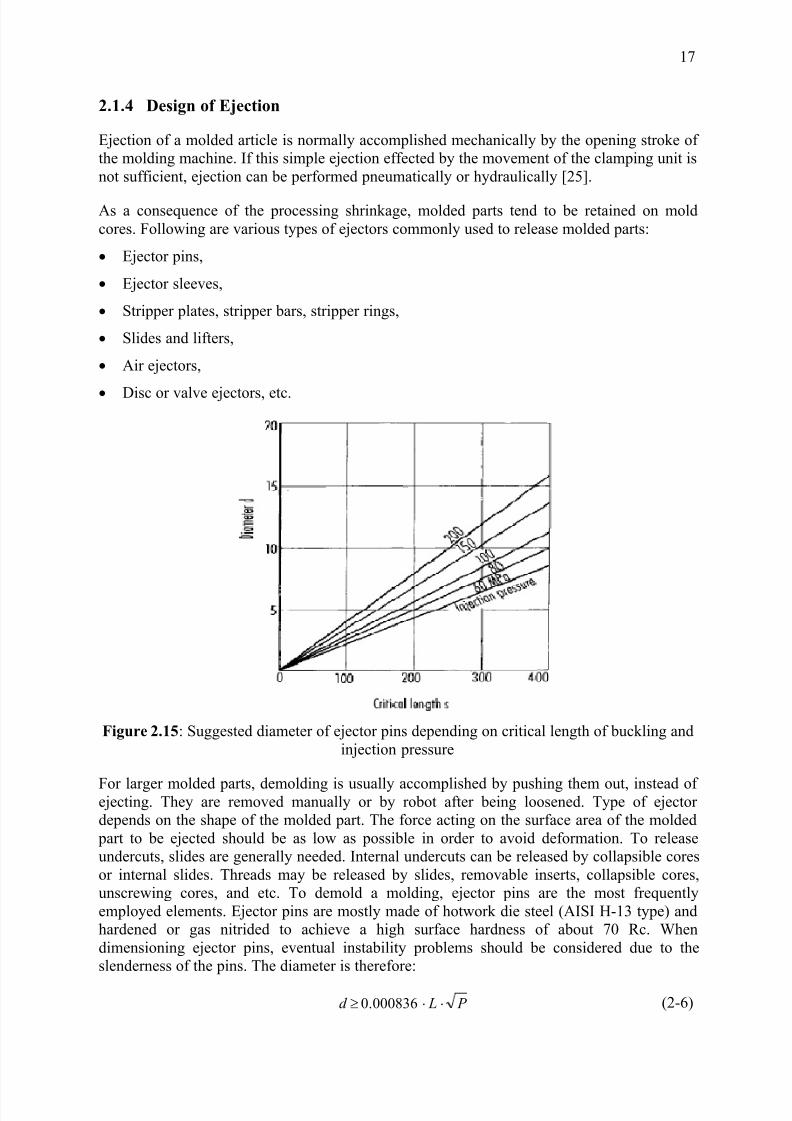
Figure 2.15: Suggested diameter of ejector pins depending on critical length of buckling andinjection pressure
For larger molded parts, demolding is usually accomplished by pushing them out, instead of ejecting. They are removed manually or by robot after being loosened. Type of ejector depends on the shape of the molded part. The force acting on the surface area of the molded
part to be ejected should be as low as possible in order to avoid deformation. To releaseundercuts, slides are generally needed. Internal undercuts can be released by collapsible coresor internal slides. Threads may be released by slides, removable inserts, collapsible cores,unscrewing cores, and etc. To demold a molding, ejector pins are the most frequentlyemployed elements. Ejector pins are mostly made of hotwork die steel (AISI H-13 type) andhardened or gas nitrided to achieve a high surface hardness of about 70 Rc. Whendimensioning ejector pins, eventual instability problems should be considered due to theslenderness of the pins. The diameter is therefore:
P Ld ⋅⋅≥ 000836.0 (2-6)

7/27/2019 Injection Mould Design
http://slidepdf.com/reader/full/injection-mould-design 36/160
18
For steel P is nearly 100 MPa, and the equation above becomes
Ld ⋅≥ 028.0 (2-7)
where L is the unguided length of the pin.
The diameter of an ejector pin dependent on critical length of buckling and injection pressurecan be taken directly from the Figure 2.15 [21, 26, 27], which is derived from the equation(2-6).
2.1.5 Design of Venting
During mold filling the melt has to displace the air which is contained in the cavity. If thiscannot be done, the air can prevent a complete filling of the cavity. Beside this the air may
become so hot from compression that it burns the surrounding material. The moldingcompounds may decompose, outgas or form a corrosive residue on cavity walls.
Most molds do not need special design features for venting because air has sufficient possibilities to escape along ejector pins or at the parting line. This is called passive venting.In case of a rib, an additional joint for venting is obtained by dividing the mold inserts intotwo pieces. With the passive venting, it was assumed that the air can escape through joiningfaces, but this is feasible only if the faces have sufficient roughness and the injection processis adequately slow to allow the air to escape. This solution fails, however, for molding thin-walled parts with relatively short injection times. Here, special venting channels becomenecessary.
An annular channel situated on the parting line around the round-shaped part is another reasonable venting method (Fig. 2.16). The annular gap is not interrupted by flanges but it iscontinuous in form. Melt penetration into the venting channel can be prevented by adjustingthe gap width so as to just prevent entrance of the melt. Usual gap widths vary from 20 µm inaccordance with the polymer employed.
Figure 2.16: Cup mold with annular channel for venting [28]
Porous sintered metals that open out into free space, have not proved suitable for venting because they tend to clog rapidly. But if the sintered metals open into a cooling channel,completely new perspectives open up for the use of sintered metal mold inserts, since anexisting cooling water circuit can provide active venting to the cavity. The water from thecircuit draws the air out of the cavity via the sintered metal insert, without water entering thecavity.

7/27/2019 Injection Mould Design
http://slidepdf.com/reader/full/injection-mould-design 37/160
19
If ejector pins are located in an area where the air may be trapped, they can also function as aventing. Frequently, the so-called venting pins are employed. They can be grooved or kept0.02 to 0.05 mm smaller in diameter than the receiving hole. To avoid flashing, a certain gapwidth, which is polymer-specific, cannot be exceeded after mold clamping. The critical gapwidth for specific polymers is as follows [29]:
• Polycrystalline thermoplastics: 0.015 mm
(PP, PA, GF-PA, POM, PE)
• Amorphous thermoplastics: 0.03 mm
(PS, ABS, PC, PMMA)
• Extremely low viscous materials: 0.003 mm
Apart from active venting by means of the cooling water circuit, which was alreadymentioned above, partial or complete evacuation of the cavity prior to the injection process is
possible. This type of venting is used in the injection molding of microstructures, sinceconventional venting gaps are too large for the extremely low-viscosity plastic melts [30]. Inthermoset and elastomer processing, there are applications that require evacuation of thecavity, primarily to improve the accuracy of reproduction and the molded part quality [31].Evacuation of the molds is only sufficient, if the whole mold structure is sealed off. Due tomany moving parts on the mold, such as slides, ejectors, etc., this is extremely complicatedand virtually impossible to achieve. The mold is instead surrounded with a closed jacket or
box that has only one parting line. This type of construction for a microinjection mold isschematically shown in Figure 2.17.
Figure 2.17: Evacuation of the microinjection mold [32]
7/27/2019 Injection Mould Design
http://slidepdf.com/reader/full/injection-mould-design 38/160
20
2.1.6 Selection of Mold Materials
The requirements to be met while selecting mold material are machinability, ability toharden, ability to take a polish, corrosion resistance, etc.
There is a long list of factors to be considered in selecting materials for plastic molds. The primary factors are:
• Type of polymer to be molded,
• Method of forming cavities,
• Mold wear and mold life,
• Physical or chemical properties,
• Quantity of parts to be made,
• Mold fabrication,
• Cost.
Mold wear is one of the most troublesome problems to handle. Primary factors influencingmold wear and mold life are the case depth (for the case hardening steels), surface hardnessof the mold, and the abrasive characteristics of the material being molded.
A mold hardened to less than Rockwell C 50 is likely to fail in compression before it wearsexcessively. Mold life increases as the hardness increases to about Rockwell C 60. Further gains from increased hardness above C 60 are unpredictable because of increased brittlenessat sharp corners. With the same surface hardness, mold life is much shorter with thinner cases. Resistance to parting-line indentation of pressure or flash lands is a function of steelsurface hardness and internal compressive strength.
The forces involved in the injection molding operation are compressive. They are exerted bythe clamping ram and internal melt pressure. Most mold platens are made of cast steel withyield strength of about 386 MPa. Allowing a safety factor of 7, a permissible load of 54 MPais defined [23]. Molds that are built for long life and high activity are heat-treated either initially or whenever the intermediate hardness of the cavities begins to affect the quality of the product unfavorably.
Mold life is a term used to define the number of acceptable piece parts produced from asingle mold. Some of the material choices made by the mold designer to increase mold lifeinclude:
• Short Run: Possible choices might be aluminum and low carbon steel.
• Medium Run: Possible choices would be P20, P21, and medium carbon steels.
• Long Run: Possible choices would be chrome plated or nitrated P20, stainless steel,inserted tool steels of H13, D2, S7 or other air and oil hardening steel choices.
2.1.7 Part Shrinkage
By shrinkage or tolerance is meant the dimensions to which a cavity and core should be
fabricated in order to produce a product of desired shape and size. Shrinkage is a function of mold temperature, part thickness, injection pressure, and melt temperature [35]. Moreover,

7/27/2019 Injection Mould Design
http://slidepdf.com/reader/full/injection-mould-design 39/160
21
shrinkage is influenced by cavity pressure to a very large degree. Depending on the pressurein the cavity alone, the shrinkage may vary as much as 100 %.
Part thickness will cause a change in shrinkage. The thicker the part, the higher shrinkagevalue resulted. The mold and melt temperature also influence shrinkage. A cooler mold will
result in less shrinkage, whereas a hotter melt will cause more shrinkage. The longer the timein the cavity, the closer the part comes to mold dimensions, which means less in shrinkage[23, 33, and 34].
In the injection molding process, shrinkage is the difference between an arbitrary dimensionin the cavity and the corresponding dimension in the injected part with reference to the cavitydimension.
Figure 2.18: Dimensional changes as a function of time [36]
Figure 2.18 shows the dimensional changes as a function of time, where 0 is the dimension incold mold, 1 is the dimension in hot mold, 2 is dimension in mold under clamping force andholding pressure, 3 is dimension of part after demolding, 4 is measurement of processingshrinkage (DIN 16901), and 5 is dimension after storage. Usually the dimensions of thecavity change from thermal expansion (01) and mechanical loading during operation(12). Anyway, the effect of time on the dimensions of the molding has to be taken intoaccount (25). The demolding shrinkage (point 3), which is measured immediately after the
part has been ejected, and the processing shrinkage (point 4) have to be differentiated. The processing shrinkage is measured after storing the injected part in a standard climate for 16hours [37]. In this context the cavity dimension has to be determined at an ambienttemperature of 23oC ± 2oC. After extended storage, another dimension change may occur
from the effect of temperature changes and especially from post-conditioning, this is called post-shrinkage (45). This change is caused by relaxation of residual stresses, re-orientation,
7/27/2019 Injection Mould Design
http://slidepdf.com/reader/full/injection-mould-design 40/160
22
and post-crystallization in semi-crystalline materials. The sum of processing shrinkage and post-shrinkage is called total shrinkage.
The simplest way to estimate shrinkage for dimensioning a mold is to consult tables. Thesedata are provided by the raw-material suppliers in the data sheets for their respective
materials. However, these data neither allow a sufficiently accurate prediction of shrinkagenor are pertinent to the process parameters known or configurations of moldings from whichthe shrinkage was obtained. Transfer to other configurations is, therefore, difficult. Another and increasingly more accurate estimate of shrinkage behavior is provided by FE simulation[38]. Exact dimensioning of parts with the aid of this method is not yet possible. However,the process and the part can be optimized in respect to shrinkage and distortion behavior.Since several physical parameters such as crystallization behavior cannot as yet bedetermined, some material data cannot be determined with sufficient accuracy and hence it isstill not possible to make an exact predictive simulation of part dimensions.
2.2 Injection In-Mold Labeling
2.2.1 A Brief History of IML
Pioneered in Europe in the late 1970’s, injection in-mold labeling (injection-IML) hasexperienced rapid adoption and high annual growth rates. IML application began with paper labels on PS substrates. IML in Europe is a mainstream process used extensively, but notexclusively, for food packaging. Until recently, low cavitation molds and relatively slowcycle times adequately served the demands of the European Market [39]. An estimated 85 %to 95 % of rigid food packaging there now uses IML, as do some durable goods such asreturnable beer crates.
IML reportedly started in the U.S. in the early 1980s. Shape Inc. in Biddeford, Me., was oneof the first to get into injection IML, taking a license in 1982 from Cerbo in Sweden, whichheld patents on a technique to inject the melt through the label. In 1983, Shape applied the
process, using Cerbo’s automation, to production of video cassette sleeves in a two-cavitymold [40]. By Procter & Gamble and Owens-Illinois Packaging (now part of GrahamPackaging), the first applications were blow molded HDPE bottles with paper labels coatedwith a heat-activated adhesive. Problems with label quality, feeding, and handling kept IMLactivity low-key in the U.S. until the mid-1990s, when it was rekindled by molders’ attemptsto eliminate secondary operations, reduce the scrap rate from post-mold labeling, and to
produce a “no-label” look similar to that of blow molded articles.
2.2.2 Injection IML Process
The use of IML (In-Mold Labeling) in the injection molding technology provides significantadvantages for the manufacturer or marketer of the product as well as the end user. Iteliminates secondary steps in the manufacturing process and the end result is permanent.
Injection in-mold labeling is an injection molding process, in which a flat, even film surface,is back injected. In-Mold-Labeling is often used in the packaging industry as an alternative to
printing when design requirements call for a high degree of flexibility or else when theimpression cannot be directly molded on the part. The labels are usually a printed
polypropylene film with a thickness of 50-100 µm. The advantages of In-Mold-Labeling are
listed below [41]:

7/27/2019 Injection Mould Design
http://slidepdf.com/reader/full/injection-mould-design 41/160
23
• One step process (integration of the downstream process directly with the injectionmolding process),
• Highly attractive print quality,
• Increased surface coverage- multi language product descriptions,
• No stopping production for changeover to new print pattern,
• Short print runs can be produced cost-effectively,
• Absolute bonding between label and container,
• Reduce in wall thickness, less material used, and hence material cost reduction,
• Ease of recycling.
The disadvantages, on the other hand, are for instance a heat transport reduction caused bythe label, the slightly increased cycle times owing to the insertion of the label into the mold
cavity and the part warpage possibly occurred from the existence of the label, which leads tothe non-uniform cooling of the part [42].
Figure 2.19 illustrates the sequence of the injection IML process. In the in-mold labeling process, a label is first placed in the open mold and held in the desired position by vacuumnozzles, electrostatic attraction, or other appropriate means. The mold closes and then molten
plastic resin is injected into the mold where it conforms to the shape of the object. The hot plastic envelopes the label and makes it an integral part of the molded object. As soon as themelt cools down to the ejection temperature, the injected IML-part is ready to be demolded,usually with the help of a robot.
The difference between glue applied labels and in-mold labels is that a glue applied label is"on" the surface of the plastic object; the in-mold label is "in" the wall of the object. In-Mold-Labeling makes no more demands on the machine than those made by thin-walled molding.Table 2.1 shows the requirements for the injection molding machine and mold for theinjection IML. To produce packaging with 5-sided label integrated, inside gating (patented)must be employed. This procedure offers an uninterrupted decoration of the injected part.
Figure 2.19: Injection in-mold labeling sequencing [43]
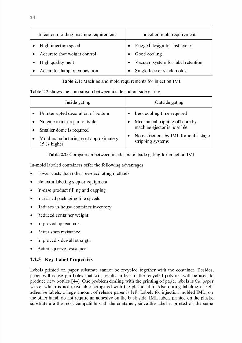
7/27/2019 Injection Mould Design
http://slidepdf.com/reader/full/injection-mould-design 42/160
24
Injection molding machine requirements Injection mold requirements
• High injection speed
• Accurate shot weight control
• High quality melt
• Accurate clamp open position
• Rugged design for fast cycles
• Good cooling
• Vacuum system for label retention
• Single face or stack molds
Table 2.1: Machine and mold requirements for injection IML
Table 2.2 shows the comparison between inside and outside gating.
Inside gating Outside gating
• Uninterrupted decoration of bottom
• No gate mark on part outside
• Smaller dome is required
• Mold manufacturing cost approximately15 % higher
• Less cooling time required
• Mechanical tripping off core bymachine ejector is possible
• No restrictions by IML for multi-stagestripping systems
Table 2.2: Comparison between inside and outside gating for injection IML
In-mold labeled containers offer the following advantages:
• Lower costs than other pre-decorating methods
• No extra labeling step or equipment
• In-case product filling and capping
• Increased packaging line speeds
• Reduces in-house container inventory
• Reduced container weight
• Improved appearance
• Better stain resistance
• Improved sidewall strength• Better squeeze resistance
2.2.3 Key Label Properties
Labels printed on paper substrate cannot be recycled together with the container. Besides, paper will cause pin holes that will results in leak if the recycled polymer will be used to produce new bottles [44]. One problem dealing with the printing of paper labels is the paper waste, which is not recyclable compared with the plastic film. Also during labeling of self adhesive labels, a huge amount of release paper is left. Labels for injection molded IML, onthe other hand, do not require an adhesive on the back side. IML labels printed on the plasticsubstrate are the most compatible with the container, since the label is printed on the same
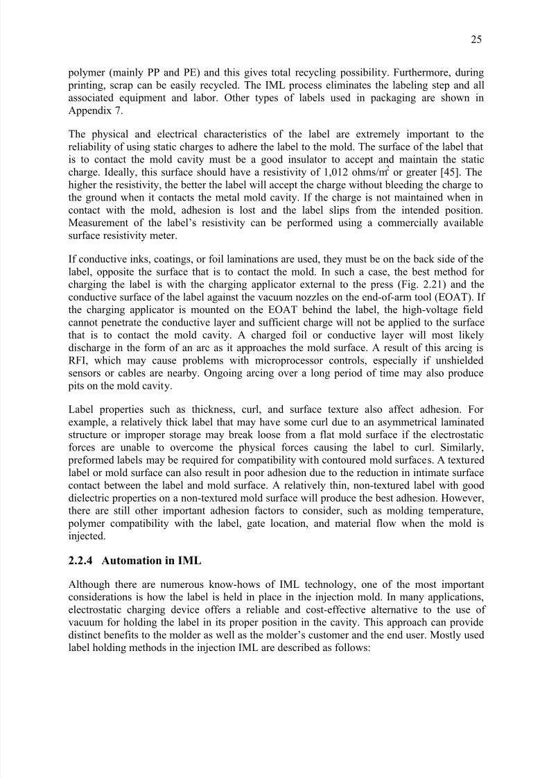
7/27/2019 Injection Mould Design
http://slidepdf.com/reader/full/injection-mould-design 43/160
25
polymer (mainly PP and PE) and this gives total recycling possibility. Furthermore, during printing, scrap can be easily recycled. The IML process eliminates the labeling step and allassociated equipment and labor. Other types of labels used in packaging are shown inAppendix 7.
The physical and electrical characteristics of the label are extremely important to thereliability of using static charges to adhere the label to the mold. The surface of the label thatis to contact the mold cavity must be a good insulator to accept and maintain the staticcharge. Ideally, this surface should have a resistivity of 1,012 ohms/m2 or greater [45]. Thehigher the resistivity, the better the label will accept the charge without bleeding the charge tothe ground when it contacts the metal mold cavity. If the charge is not maintained when incontact with the mold, adhesion is lost and the label slips from the intended position.Measurement of the label’s resistivity can be performed using a commercially availablesurface resistivity meter.
If conductive inks, coatings, or foil laminations are used, they must be on the back side of the
label, opposite the surface that is to contact the mold. In such a case, the best method for charging the label is with the charging applicator external to the press (Fig. 2.21) and theconductive surface of the label against the vacuum nozzles on the end-of-arm tool (EOAT). If the charging applicator is mounted on the EOAT behind the label, the high-voltage fieldcannot penetrate the conductive layer and sufficient charge will not be applied to the surfacethat is to contact the mold cavity. A charged foil or conductive layer will most likelydischarge in the form of an arc as it approaches the mold surface. A result of this arcing isRFI, which may cause problems with microprocessor controls, especially if unshieldedsensors or cables are nearby. Ongoing arcing over a long period of time may also produce
pits on the mold cavity.
Label properties such as thickness, curl, and surface texture also affect adhesion. For example, a relatively thick label that may have some curl due to an asymmetrical laminatedstructure or improper storage may break loose from a flat mold surface if the electrostaticforces are unable to overcome the physical forces causing the label to curl. Similarly,
preformed labels may be required for compatibility with contoured mold surfaces. A texturedlabel or mold surface can also result in poor adhesion due to the reduction in intimate surfacecontact between the label and mold surface. A relatively thin, non-textured label with gooddielectric properties on a non-textured mold surface will produce the best adhesion. However,there are still other important adhesion factors to consider, such as molding temperature,
polymer compatibility with the label, gate location, and material flow when the mold isinjected.
2.2.4 Automation in IML
Although there are numerous know-hows of IML technology, one of the most importantconsiderations is how the label is held in place in the injection mold. In many applications,electrostatic charging device offers a reliable and cost-effective alternative to the use of vacuum for holding the label in its proper position in the cavity. This approach can providedistinct benefits to the molder as well as the molder’s customer and the end user. Mostly usedlabel holding methods in the injection IML are described as follows:
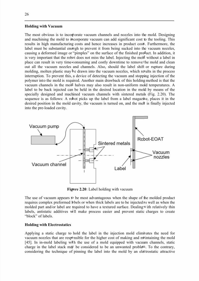
7/27/2019 Injection Mould Design
http://slidepdf.com/reader/full/injection-mould-design 44/160
26
Holding with Vacuum
The most obvious is to incor and machining the mold to iresults in high manufacturing
label must be substantial enocausing a deformed image or is very important that the rob
place can result in very time-out all the vacuum nozzlesmolding, molten plastic mayinterruption. To prevent this,
polymer into the mold is requvacuum channels in the mollabel to be back injected canspecially designed and mach
sequence is as follows: A rodesired position in the mold cinto the pre-loaded cavity.
Fig
The use of vacuum appears trequires complex preformed lmolded part and/or label are r labels, antistatic additives w“block” of labels.
Holding with Electrostatics
Applying a static charge tovacuum nozzles that are resp[45]. In in-mold labeling wi
charge in the label stack maconsidering the technique of
orate vacuum channels and nozzles into thcorporate vacuum can add significant cost tcosts and hence increases in product cost
gh to prevent it from being sucked into th“pimples” on the surface of the finished prot does not miss the label. Injecting the molonsuming and costly downtime to remove
and channels. Also, should the label shifte drawn into the vacuum nozzles, which re
a device of detecting the vacuum and stoppiired. Another main drawback of this holding
halves may also result in non-uniform mobe held in the desired location in the mol
ined vacuum channels with sintered metal
ot picks up the label from a label magaziavity, the vacuum is turned on, and the mel
re 2.20: Label holding with vacuum
be most advantageous when the shape of t bels or when thick labels are to be injectedequired to have a textured surface. Dealingll make process easier and prevent static
hold the label in the injection mold eliminsible for the higher cost of making and mh the use of a mold equipped with vacuu
be considered to be an unwanted proble pinning the label into the mold by an ele
e mold. Designingo the tooling. This. Furthermore, the
e vacuum nozzles,uct. In addition, itwithout a label in
he mold and cleanor rupture duringults in the processng injection of themethod is that the
ld temperatures. Ad by means of thes (Fig. 2.20). The
e, places it in theis finally injected
he molded products well as when theith relatively thincharges to create
ates the need for intaining the moldm channels, static
. To the contrary,trostatic attractive
7/27/2019 Injection Mould Design
http://slidepdf.com/reader/full/injection-mould-design 45/160
27
force, it is necessary to control static charges to be able to feed, pick and deliver the labelsand in the mold to make the label adhere long enough to have the melt injected and the labelremains in the intended position.
Static electricity is an imbalance in the charge of a material, which means that there are a
larger number of positive and/or negative charges than at equilibrium. A negatively chargedsurface has an excess of electrons and a positive surface is lacking electrons. A chargedsurface will produce an electrostatic field which is directed perpendicularly from any point of the surface. Static electricity does not flow across a surface or rather it moves very slowlywhich means that there will be a charge buildup with time when running a process. Thestrength of an electric field is defined in terms of the force that an imaginary test chargewould experience if it was placed in the field. The magnitude, E, of an electric field at a
particular location in an electrostatic system is the force acting upon a unit positive charge placed at that point. Thus, the force experienced by a point charge, q, in a field E is:
F =qE (2-8)
Units will be 1 Newton/C = 1 Nm/As = 1 V/m. In practical work kV/m is used rather thanV/m. A practical way of representing the electrostatic field is by the use of field lines. Atevery point on a field line the direction of the field line is determined by the tangent to thefield line at that point and the density of the field lines is a measure of the field strength.
In the electrostatic process, the robot picks up the label from the magazine with suction. Ahigh static charge is placed on the label as the end-of-arm tool (EOAT) with the labelapproaches the mold surface. Then, the robot positions the label, releases the vacuum, and thelabel is transferred to the surface of the mold cavity. Neither vacuum in the mold nor adhesive on the label is needed (Fig. 2.21). When a static charge is placed on a label of
suitable material and construction, the label will be attracted electrostatically to the groundedmetal surface of the mold and may stick with excellent adhesion for up to several minutes.One caution to be taken when charging the label is that the label must contain no ink or coating with antistatic properties. Generally, labels should have good dielectric properties andshould be a good insulator.
Using electrostatics to their full advantage requires the following components:
• A robot with a suitably designed end-of-arm tool (EOAT),
• A label magazine,
• A high-voltage DC charging power supply with adjustable output capability,
• A label of proper material and construction to accept and maintain a static charge.
Figure 2.21 illustrates the simplified electrostatic charging method used for round-shaped products. Use of a remote-mounted charging applicator is a simplified way to apply a charge.It requires little modification of the EOAT, is relatively easy to set up, and can satisfy therequirements of many different sizes and shapes of labels with the same charging applicator.
In this charging process, the robot picks up the label at the magazine, orients the label, and passes it by the charging bar. The surface is charged by a high voltage corona discharge (3-10kV) from the tips of a small conical cluster of fine wires mounted on the underside of a light
moveable plate. This plate is moved between the field meter sensing aperture and the materialsurface exposed through the instrument base plate. Corona is usually generated as a brief

7/27/2019 Injection Mould Design
http://slidepdf.com/reader/full/injection-mould-design 46/160
28
pulse (20 ms) immediately bwithin 20 ms. The moving plvoltage connections so reliabvoltages. The ground referencharging bar and the label bec
surface of the cavity, releasesthe surface of the mold.
Figure 2.21: Simplifi
The fixture on the EOATconductive surface should bedirectly behind the label [46].
to provide sufficient holdinggrounded conductive surface
All conductive components oedges and corners. There shou
2.3 Injection Molding
For 30 years, the CAE softwmodel. The calculation algdifference method for temper
development of injection moand the subsequent cooling pr part to represent the 3D geosimplifies the 3D geometryThis technology has been sucshell plastic parts. In the paHowever, 2.5D programs cagenerate 2.5D models from 3from scratch [2]. The prepar Indeed model preparation no
The widespread used simulatwhich the three-dimensional,
efore the plate is moved away. The platete and instrument construction shield the fiee measurements can be made down to evece surface behind the label attracts the elecomes charged. The robot places the label in
the vacuum to the suction cups, and the lab
d electrostatic charging for round-shaped pr
equires a grounded conductor such as aat least as large as the label and mounte
The suction cups should have the minimum
power to prevent the label from slipping af the fixture.
f the robot fixture must be grounded and shld be no sharp edges or corners within 1 in.
Simulation
are for mold filling has been developed barithms use finite element method for pature, such as introduced by Hieber and S
ding, plastic simulation tools are used to pocess. Conventional algorithm extract mid-petry. These simulation codes are usually ref odel into 2.5D mid-plane and proceeds to
cessfully applied to simulate the molding pst decade, 3D CAD systems have becomen’t take advantage of these models. The
models is sometimes equivalent to generattion of such a mesh can take a considerabrepresents the greatest share of time of a fill
ion programs today take a basis of computhin-walled geometry in two-dimensional
moves fully awayld meter from high
quite low surfacetric field from theosition against the
l stays in place on
ducts [46]
metal plate. The6.35 to 12.7 mm
diameter necessary
d attracting to the
ould have roundedf the label [47].
sed on Hele-Shawessure and finiteen [1]. During the
redict mold fillinglane surface of theerred to as 2.5D. Itthe simulation [1].ocess of most thinwidely available.
effort required tong 3D informatione amount of time.ing analysis [48].
tation model, withshell elements is
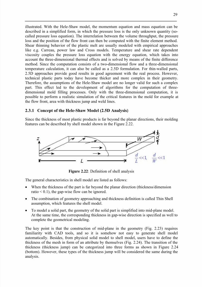
7/27/2019 Injection Mould Design
http://slidepdf.com/reader/full/injection-mould-design 47/160
29
illustrated. With the Hele-Shaw model, the momentum equation and mass equation can bedescribed in a simplified form, in which the pressure loss is the only unknown quantity (so-called pressure loss equation). The interrelation between the volume throughput, the pressureloss and the position of the flow front can then be computed with the finite element method.Shear thinning behavior of the plastic melt are usually modeled with empirical approaches
like e.g. Carreau, power law and Cross models. Temperature and shear rate dependentviscosity couples the pressure loss equation with the energy equation, which takes intoaccount the three-dimensional thermal effects and is solved by means of the finite differencemethod. Since the computation consists of a two-dimensional flow and a three-dimensionaltemperature calculation, it can also be called as a 2.5D formulation. For thin-walled parts,2.5D approaches provide good results in good agreement with the real process. However,technical plastic parts today have become thicker and more complex in their geometry.Therefore, the assumptions of the Hele-Shaw model are no longer valid for such a complex
part. This effect led to the development of algorithms for the computation of three-dimensional mold filling processes. Only with the three-dimensional computation, it is
possible to perform a realistic simulation of the critical features in the mold for example at
the flow front, area with thickness jump and weld lines.
2.3.1 Concept of the Hele-Shaw Model (2.5D Analysis)
Since the thickness of most plastic products is far beyond the planar directions, their moldingfeatures can be described by shell model shown in the Figure 2.22.
Figure 2.22: Definition of shell analysis
The general characteristics in shell model are listed as follows:
• When the thickness of the part is far beyond the planar direction (thickness/dimensionratio < 0.1), the gap-wise flow can be ignored.
• The combination of geometry approaching and thickness definition is called Thin Shellassumption, which features the shell model.
• To model a solid part, the geometry of the solid part is simplified into mid-plane model.At the same time, the corresponding thickness in gap-wise direction is specified as well tocomplete the geometrical modeling.
The key point is that the construction of mid-plane in the geometry (Fig. 2.23) requiresfamiliarity with CAD tools, and so it is somehow not easy to generate shell modelautomatically. Besides, from physical solid model to shell model, users have to define thethickness of the mesh in form of an attribute by themselves (Fig. 2.24). The transition of thethickness (thickness jump) can be categorized into three forms as shown in Figure 2.24
(bottom). However, these types of the thickness jump will be considered the same during theanalysis.
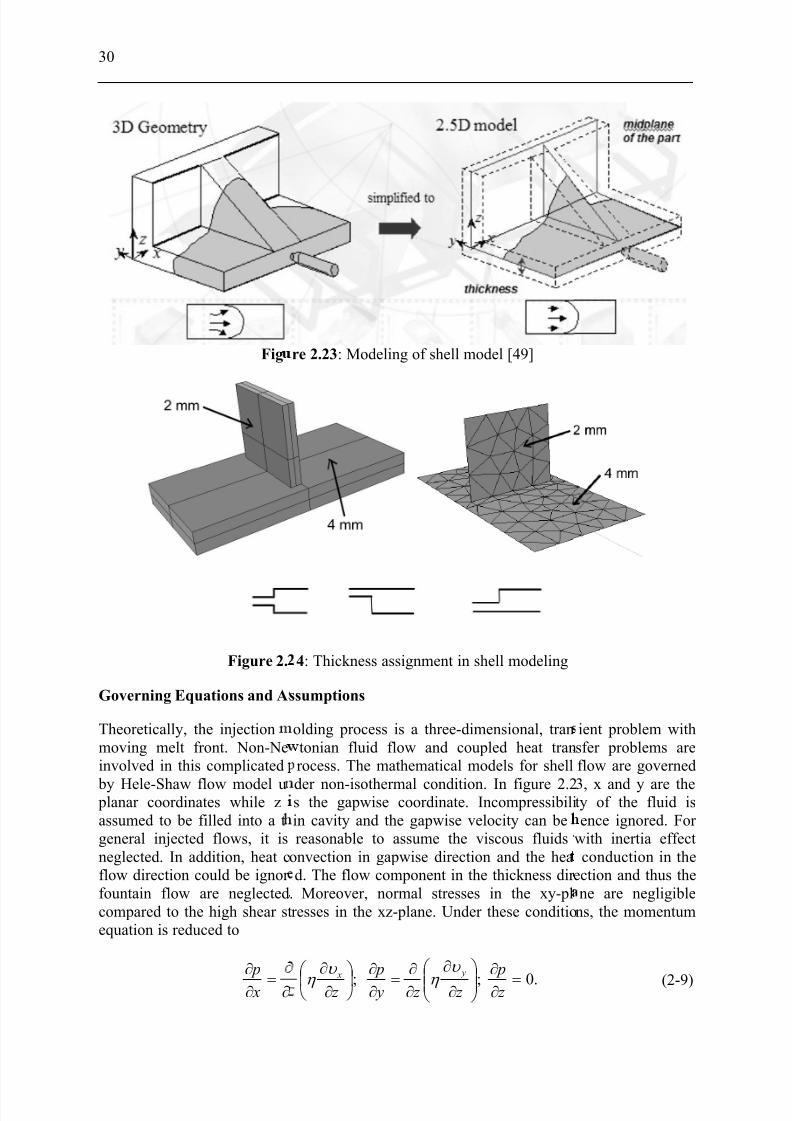
7/27/2019 Injection Mould Design
http://slidepdf.com/reader/full/injection-mould-design 48/160
30
Fig
Figure 2.
Governing Equations and A
Theoretically, the injectionmoving melt front. Non-Neinvolved in this complicated
by Hele-Shaw flow model u planar coordinates while zassumed to be filled into a tgeneral injected flows, it isneglected. In addition, heat cflow direction could be ignor fountain flow are neglected.compared to the high shear stequation is reduced to
∂=∂∂ x
p
re 2.23: Modeling of shell model [49]
4: Thickness assignment in shell modeling
ssumptions
olding process is a three-dimensional, trantonian fluid flow and coupled heat tranrocess. The mathematical models for shell
der non-isothermal condition. In figure 2.2s the gapwise coordinate. Incompressibiliin cavity and the gapwise velocity can bereasonable to assume the viscous fluids
onvection in gapwise direction and the head. The flow component in the thickness dir Moreover, normal stresses in the xy-pl
resses in the xz-plane. Under these conditio
.0;; =∂∂
∂
∂
∂∂
=∂∂
∂
∂
z
p
z z y
p
z
y xυ
η
υ
η
ient problem withsfer problems areflow are governed
3, x and y are thety of the fluid isence ignored. For
with inertia effectconduction in the
ection and thus thene are negligible
ns, the momentum
(2-9)
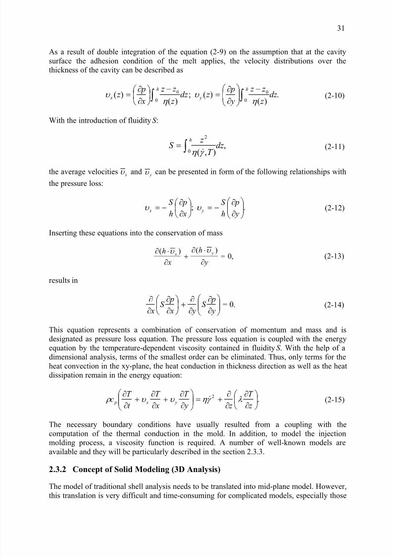
7/27/2019 Injection Mould Design
http://slidepdf.com/reader/full/injection-mould-design 49/160
31
As a result of double integration of the equation (2-9) on the assumption that at the cavitysurface the adhesion condition of the melt applies, the velocity distributions over thethickness of the cavity can be described as
.)()(;)()( 0
0
0
0
dz z
z z
y
p
z dz z
z z
x
p
z
h
y
h
x
∫∫−
∂
∂
=
−
∂
∂
= η υ η υ (2-10)
With the introduction of fluidity S :
,),(0
2
dz T
z S
h
∫=γ η &
(2-11)
the average velocities xυ and yυ can be presented in form of the following relationships with
the pressure loss:
.;
∂∂
−=
∂∂
−= y
p
h
S
x
p
h
S y x υ υ (2-12)
Inserting these equations into the conservation of mass
,0)()(=
∂
⋅∂+
∂
⋅∂
y
h
x
h y xυ υ
(2-13)
results in
.0=
∂∂
∂∂
+
∂∂
∂∂
y
pS
y x
pS
x(2-14)
This equation represents a combination of conservation of momentum and mass and isdesignated as pressure loss equation. The pressure loss equation is coupled with the energyequation by the temperature-dependent viscosity contained in fluidity S . With the help of adimensional analysis, terms of the smallest order can be eliminated. Thus, only terms for theheat convection in the xy-plane, the heat conduction in thickness direction as well as the heatdissipation remain in the energy equation:
.2
∂∂
∂∂+=
∂∂+
∂∂+
∂∂
z
T
z y
T
x
T
t
T c y x p λ γ η υ υ ρ & (2-15)
The necessary boundary conditions have usually resulted from a coupling with thecomputation of the thermal conduction in the mold. In addition, to model the injectionmolding process, a viscosity function is required. A number of well-known models areavailable and they will be particularly described in the section 2.3.3.
2.3.2 Concept of Solid Modeling (3D Analysis)
The model of traditional shell analysis needs to be translated into mid-plane model. However,this translation is very difficult and time-consuming for complicated models, especially those

7/27/2019 Injection Mould Design
http://slidepdf.com/reader/full/injection-mould-design 50/160
32
with significantly different thicknesses. Besides, the features of some parts are usuallyignored such as round corners and regions in thickness jump. In solid or 3D analysis, userscan decide whether to take them into considerations. The result of solid analysis providesinformation i.e. over fountain flow, corner effect, fiber-induced warpage etc. which cannot bederived from those of traditional shell analysis.
Figure 2.25: True 3D flow pattern
Figure 2.25 illustrates some 3D flow phenomena. These will be lost by using 2.5D model tosimulate, such as flow passes expansion and contraction area, flow passes spheres, flow
passes a small dimension-to-thickness ratio area, and flow of material containing fibers. Inthe injection molding process, filling of cavity is the first key step. Basically, it is a three-dimensional, transient problem with moving melt front. Non-Newtonian fluid flow andcoupled heat transfer problems are involved in this complicated process.
Governing Equations and Assumptions
The mathematical models for solid flow (3D flow) are also governed by conservation of mass, the conservation of momentum, and the conservation of energy. For general injectedflows, it is reasonable to assume them as the viscous fluids. At filling stage, both polymer andair are assumed incompressible. The polymer melt is assumed to behave as Generalized
Newtonian Fluid (GNF). Hence the 3D flow motion can be mathematically described by thefollowing equations:
Conservation of mass:
0=∂
∂+
∂
∂+
∂
∂
z y x
z y x υ υ υ (2-16)
Conservation of energy:
2
γ η λ λ λ υ υ υ ρ ρ &
+
∂
∂
∂
∂
+
∂
∂
∂
∂
+
∂
∂
∂
∂
+
∂
∂
+∂
∂
+∂
∂
=∂
∂ z
T
z y
T
y x
T
x z
T
y
T
x
T
ct
T
c z y x P P (2-17)
7/27/2019 Injection Mould Design
http://slidepdf.com/reader/full/injection-mould-design 51/160
33
Conservation of momentum:
02
02
02
=∂∂
−
∂∂
∂∂
+
∂∂
+∂
∂
∂∂
+
∂
∂+
∂∂
∂∂
=∂∂−
∂∂+
∂∂
∂∂+
∂∂
∂∂+
∂∂+
∂∂
∂∂
=∂∂
−
∂∂
+∂∂
∂∂
+
∂∂
+∂
∂
∂∂
+
∂∂
∂∂
z
p
z z y z y z x x
y
p
z y z y y y x x
x
p
z x z y x y x x
z z y x z
y z y x y
x z x y x
υ η
υ υ η
υ υ η
υ υ η υ η υ υ η
υ υ η
υ υ η
υ η
(2-18)
Generally, the density of the melt is assumed to be constant during filling phase (ρ=const.). Inthe holding phase, however, the compressibility of the melt must be taken into account, inwhich the reduction of the flow rate as a result of change of the pressure and temperature iscomputed.
The ignorance of the compressibility in the conservation of mass is permissible only duringfilling phase.
2.3.3 Viscosity Models for Thermoplastics
Viscosity is an index of the resistance of fluid to flow. The viscosity of simple fluids, for example water, is usually a constant value at constant temperature. These fluids are generallyreferred to as Newtonian fluids. The viscosity of thermoplastics is, however, verycomplicated and very nonlinear. Unlike simple fluids, the viscosity of thermoplastic dependson its chemical structure, composition and processing conditions. With a given chemical
structure and formulation, viscosity of thermoplastics depends primarily on the temperature,shear rate and pressure. To understand the viscosity nature of thermoplastics, shear stress,shear rate and viscosity must be first defined.
The viscosity of thermoplastics shows strong dependence on temperature. Typically,viscosity drops dramatically when temperature increases. Two temperature dependence of theviscosity that are widely accepted, namely Arrhenius (Exponential) model and William-Landel-Ferry (WLF) model will be described later. Many different mathematical models usedfor describing the steady shear viscosity behavior of thermoplastics have been proposed. Butthe most acceptable viscosity models for one dimensional flow are described below.
Power-Law Model:
( ) 1−= n K γ η & (2-19)
whereη is the viscosity, γ & is shear rate, n is the Power Law Index, and K is the consistency
index. For a Newtonian fluid, Power Law Index = 1; for a shear-thinning fluid, this value lies between 0 and 1 and for a shear-thickening fluid, it is greater than 1.
The Power-Law model has the weak point in determining the viscosity of the melt in theupper Newtonian region that is the region with low shear rate. Using this model in fillingsimulation may cause the over-estimation of the viscosity at low shear rate region.
7/27/2019 Injection Mould Design
http://slidepdf.com/reader/full/injection-mould-design 52/160
34
Carreau Model:
n−
+
=1
*0
0
1 γ τ
η
η η
&
(2-20)
where 0η is the zero shear (Newtonian) viscosity, τ∗ represents the critical shear stress
roughly characterizing transition shear stress from the Newtonian range to the pseudo plasticregion, and n represents the shear rate sensitivity, 0 < n < 1, where 1-n roughly characterizesthe slope of the line over the pseudo plastic region in the logarithmic plot.
Modified Cross Model:
n−
+
=1
*
0
0
1 γ τ
η
η η
&
(2-21)
A general form of the constitutive equation for incompressible non-Newtonian fluid can bewritten as follows:
( ) D I E p E p iη τ σ 2+−=+−= (2-22)
The apparent viscosity η in the above equation is a function of the first (I1), second (I2) and
third (I3) invariants of the rate of deformation tensor. For incompressible fluids, the firstinvariant becomes identically equal to zero. The third invariant vanishes for simple shear
flows and is normally neglected in non-viscometric flows as well. The apparent viscosity thenis a function of the second invariant alone. Hence the second invariant can be written as:
∑∑ ⋅=i j
jiij I γ γ &&2 (2-23)
Viscosity is a decreasing function of temperature. The temperature-time superposition principle of viscoelasticity describes the dependence of viscosity on temperature as follows.It states that a change in the temperature from T1 to T2 does not affect the functionaldependence of η onγ & , but merely alters the zero shear viscosity and the shear rate at which
transition from Newtonian to pseudoplastic behavior occurs. As temperature increases, the
viscosity curve at T1, in the log (η) versus log (γ & ) plot, is shifted by a “shift factor” log( Ta )given by:
1120
2210
)(
)( a
ρ η
ρ η
⋅⋅
⋅⋅=
T T
T T T (2-24)
Where 1 ρ and 2 ρ denote the densities at the temperature values T1 and T2, respectively. Thetemperature effect on the viscosity function η is described in many references [50, 51, and52] by the Arrhenius equation. This law states that for thermorheologically simple fluids the
shift factor Ta is given by
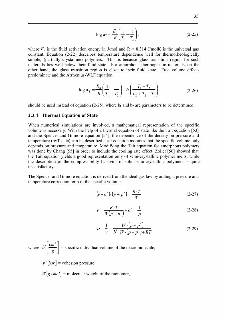
7/27/2019 Injection Mould Design
http://slidepdf.com/reader/full/injection-mould-design 53/160
35
log aT =
−
21
0 11
T T R
E , (2-25)
where E 0 is the fluid activation energy in J/mol and R = 8.314 J/molK is the universal gas
constant. Equation (2-22) describes temperature dependence well for thermorheologicallysimple, (partially crystalline) polymers. This is because glass transition region for suchmaterials lies well below their fluid state. For amorphous thermoplastic materials, on theother hand, the glass transition region is close to their fluid state. Free volume effects
predominate and the Arrhenius-WLF equation
−+
−−
−=
122
211
21
0T
11 alog
T T b
T T b
T T R
E (2-26)
should be used instead of equation (2-25), where b1 and b2 are parameters to be determined.
2.3.4 Thermal Equation of State
When numerical simulations are involved, a mathematical representation of the specificvolume is necessary. With the help of a thermal equation of state like the Tait equation [53]and the Spencer and Gilmore equation [54], the dependence of the density on pressure andtemperature (pvT-data) can be described. Tait equation assumes that the specific volume onlydepends on pressure and temperature. Modifying the Tait equation for amorphous polymerswas done by Chang [55] in order to include the cooling rate effect. Zoller [56] showed thatthe Tait equation yields a good representation only of semi-crystalline polymer melts, whilethe description of the compressibility behavior of solid semi-crystalline polymers is quite
unsatisfactory.The Spencer and Gilmore equation is derived from the ideal gas law by adding a pressure andtemperature correction term to the specific volume:
( ) ( )W
T R p pbv
⋅=+⋅− ** (2-27)
( ) ρ
1*
*=+
+⋅
= b p pW
T Rv (2-28)
( )( ) RT p pW b
p pW
v ++⋅⋅+⋅==
**
*1 ρ (2-29)
where
g
cmb
3* = specific individual volume of the macromolecule,
[ ]bar p* = cohesion pressure,
[ ]mol g W / = molecular weight of the monomer,
7/27/2019 Injection Mould Design
http://slidepdf.com/reader/full/injection-mould-design 54/160
36
⋅ K mol
energie R = universal gas constant.
However, the Spencer and Gilmore equation is not valid in the temperature range below themelting point.
For the simulations in this thesis, a modified Tait model (Eq. 3-3) is used. This model can predict the abrupt volumetric change for semi-crystalline polymers and it is also suitable for amorphous polymers.
Because the melt is assumed to be incompressible, the thermal equation of state will bedisregarded for the conservation of mass and momentum. However, for the holdingsimulation, compressibility of the melt must be regarded and the thermal equation of statemust be taken into account to both equations.
2.3.5 Numerical Discretization Methods
In the design of engineering structures, numerical simulation plays an increasingly importantrole. This can be attributed to the high costs or practical difficulties related to experiments,which have to confront rapid advances in the computational power and the resulting decreasein the costs for computer simulations. However, in order to supplement or even replaceexperiments, simulation approaches have to fulfill strong requirements. An essential demandis that the simulation calculations are efficient and lead to accurate and reliable results (Fig.2.26). This in turn will depend upon the mathematical model of the physical problem whichmust be solved with a specific simulation tool by applying assumptions about the loadingsituation, initial and boundary conditions.
The mathematical model of a physical problem is described using partial differentialequations, which comprise different physical parameters. An analytical solution of theseequations as a system is not always possible because of their complexity and non-linearity.Because of this, a numerical method is necessary for solving the problem. The numericalmethod requires a discretization of the equation system and a reformulation of the differentialequations into an algebraic form. The discretization is usually a compromise between coarseand fine meshing. With a relatively coarse discretization, the solutions of the problem will beattained with fewer resolutions. With extremely fine discretization, almost unlimitedsimulation time results. Generally for the solution of complex flow in injection molding, four numeric discretization methods are used:
• Finite difference method (FDM),• Finite element method (FEM),
• Boundary element method (BEM),
• Finite volume method (FVM).
The finite difference method is widespread since the 1930s and used to solve partial-differential equations. Because of its simplicity, this discretization method is applied to manymodels with simple geometry. A finite difference is a mathematical expression of the form
f ( x + b) − f ( x + a). If a finite difference is divided by b − a, one gets a difference quotient. Theapproximation of derivatives by finite differences plays a central role in finite differencemethods for the numerical solution of differential equations, especially boundary value
problems [57, 58, 59, and 60]. FDM shows a disadvantage when meshing a complex
7/27/2019 Injection Mould Design
http://slidepdf.com/reader/full/injection-mould-design 55/160
37
geometry. In injection molding simulation, FDM is used to calculate the melt temperaturedevelopment during molding.
The Finite element method is well known since the 1960s with the beginning of thecomputer age and used for finding approximate solutions of partial differential equations
(PDE) as well as integral equations such as the heat transport equation. The solution approachis based either on eliminating the differential equation completely (steady state problems), or rendering the PDE into an approximating system of ordinary differential equations, which arethen solved using standard techniques such as finite differences, Runge-Kutta, etc [61, 62,and 63]. In solving partial differential equations, the primary challenge is to create anequation that approximates the equation to be studied, but is numerically stable, meaning thaterrors in the input data and intermediate calculations do not accumulate and cause theresulting output to be meaningless. The Finite Element Method is a good choice for solving
partial differential equations over complex domains (like cars and oil pipelines), when thedomain changes (as during a solid state reaction with a moving boundary), when the desired
precision varies over the entire domain, or when the solution lacks smoothness.
Comparison to the finite difference method
The finite difference method (FDM) is an alternative way for solving PDEs. The differences between FEM and FDM are the following [64]:
• The finite difference method is an approximation to the differential equation; the finiteelement method is an approximation to its solution.
• The most attractive feature of the FEM is its ability to handle complex geometries (and boundaries) with relative ease. While FDM in its basic form is restricted to handlerectangular shapes and simple alterations thereof, the handling of geometries in FEM is
theoretically straightforward.• The most attractive feature of finite differences is that it can be very easy to implement.
• There are reasons to consider the mathematical foundation of the finite elementapproximation more sound, for instance, because the quality of the approximation
between grid points is poor in FDM.
• The quality of a FEM approximation is often higher than in the corresponding FDMapproach, but this is extremely problem dependent and several examples to the contrarycan be provided.
The boundary element method is a numerical computational method of solving linear partial differential equations which have been formulated as integral equations (i.e. in boundary integral form). It can be applied in many areas of engineering and science includingfluid mechanics, acoustics, electromagnetics, and fracture mechanics [65, 66, 67, 68, 69 and70]. The boundary element method attempts to use the given boundary conditions to fit
boundary values into the integral equation, rather than values throughout the space defined bya partial differential equation. Once this is done, in the post-processing stage, the integralequation can then be used again to calculate numerically the solution directly at any desired
point in the interior of the solution domain. The boundary element method is often moreefficient than other methods, including finite elements, in terms of computational resourcesfor problems where there is a small surface/volume ratio. Conceptually, it works by
constructing a "mesh" over the modeled surface. However, for many problems boundary

7/27/2019 Injection Mould Design
http://slidepdf.com/reader/full/injection-mould-design 56/160
38
element methods are significantly less efficient than volume-discretization methods (Finiteelement method, Finite difference method, Finite volume method).
Figure 2.26: Physical and mathematical modeling [71]
Physical modelPhysical theory: Electromagnetism, continuum mechanics, nuclear physics, …
Assumptions:
Static, harmonic, transient analysis2D, 3D, axisymmetric , shell, …Type of material (elastic, plastic, …)Kinematics (large deformations, …)Load case
Numerical model for FEM, BEM, FDM, FVM, …
Element type:Mesh density:Solution parameters:
Triangular, no. of nodes, integration order, …Coarse, locally refined, …Error bounds, tolerances, time integration, iteration, …
Mathematical modelChoice of coordinate system, units, independent variables Differential equation, Integral equations
Boundary and initial conditions constraints
Interpretation of results:experience, common
sense
Accuracy of solution of mathematical model
Improve phys.Model,
modify assumption
Refine num.model, adaptivity
Engineering solution
Real s stem
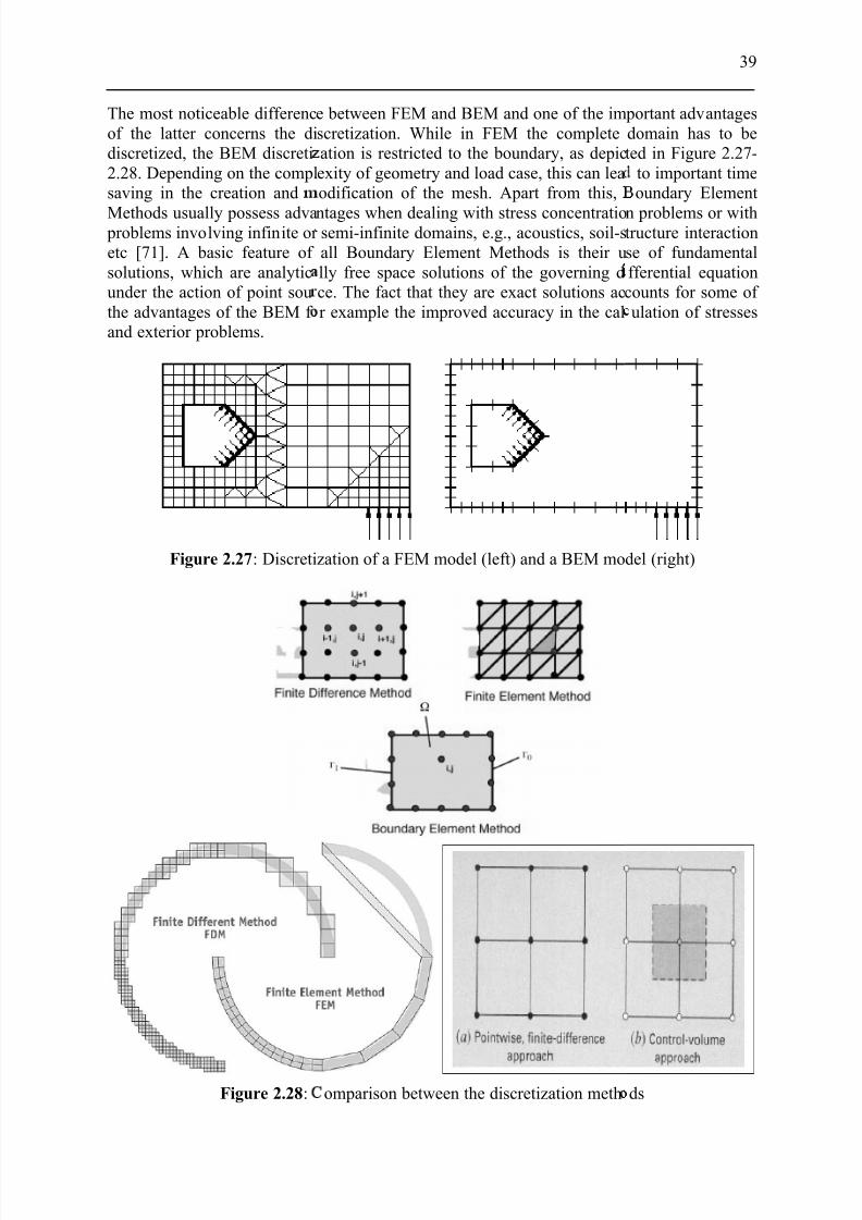
7/27/2019 Injection Mould Design
http://slidepdf.com/reader/full/injection-mould-design 57/160
The most noticeable differencof the latter concerns the didiscretized, the BEM discreti2.28. Depending on the complsaving in the creation and
Methods usually possess adva problems involving infinite or etc [71]. A basic feature of solutions, which are analyticunder the action of point southe advantages of the BEM f and exterior problems.
Figure 2.27: Discreti
Figure 2.28:
e between FEM and BEM and one of the imscretization. While in FEM the completeation is restricted to the boundary, as depicexity of geometry and load case, this can leaodification of the mesh. Apart from this,
ntages when dealing with stress concentratiosemi-infinite domains, e.g., acoustics, soil-sall Boundary Element Methods is their ully free space solutions of the governing dce. The fact that they are exact solutions acr example the improved accuracy in the cal
zation of a FEM model (left) and a BEM mo
omparison between the discretization meth
39
portant advantagesdomain has to beted in Figure 2.27-
to important timeoundary Element
n problems or withtructure interactionse of fundamentalfferential equationcounts for some of ulation of stresses
del (right)
ds

7/27/2019 Injection Mould Design
http://slidepdf.com/reader/full/injection-mould-design 58/160
40
The finite volume method is a method for representing and evaluating partial differentialequations as algebraic equations. Similar to the finite difference method, values are calculatedat discrete places on a meshed geometry. "Finite volume" refers to the small volumesurrounding each node point on a mesh. In the finite volume method, volume integrals in a
partial differential equation that contain a divergence term are converted to surface integrals,
using the divergence theorem. These terms are then evaluated as fluxes at the surfaces of eachfinite volume. Because the flux entering a given volume is identical to that leaving theadjacent volume, these methods are conservative. Another advantage of the finite volumemethod is that it is easily formulated to allow for unstructured meshes. The method is used inmany computational fluid dynamics packages. The most compelling feature of the FVM isthat the resulting solution satisfies the conservation of quantities such as mass, momentum,energy, and species. This is exactly satisfied for any control volume as well as for the wholecomputational domain and for any number of control volumes. Even a coarse grid solutionexhibits exact integral balances. FVM is the ideal method for computing discontinuoussolutions arising in compressible flows. FVM is also preferred while solving partialdifferential equations containing discontinuous coefficients [71].

7/27/2019 Injection Mould Design
http://slidepdf.com/reader/full/injection-mould-design 59/160
3 Flow Analysis a
the Double-Plat
A number of simulation pack the injection molding process,of the injection mold is to oholding, and cooling. By mecavity is filled. However, witnon-uniform part thicknesses
polymer melt within the cav between the real injectionAccording to this, experiment
part thickness were conductedacquire better understandingthe injection in-mold labelin
2.5D and 3D simulations.The investigation of the injecnon-uniform part thickness ca
1. Simulation on a basis of s
2. Simulation on a basis of v
3. Comparison of all simulati
3.1 Design of Experi
3.1.1 Part Geometry
In order to examine the effi predicting the mold filling bnon-uniform part thickness w
Figure 3.1 shows the part momolding processes. This mold
d Simulation in Injection Mol
d Part with Non-Uniform Part
ges are nowadays commercially available f one of these is Moldex3D®. The objectiveserve flow behavior of polymer melt durinns of simulation, it is possible to anticipatean increase in the complexity of the molde2.5D simulation loses its precision of pre
ty. With 3D simulation, on the other hanolding process and the simulation is gon the mold filling of the double-plated par
. As a preliminary examination, this study wf the simulation program Moldex3D prior t. The experimental results were then comp
tion molding simulation based on the doubbe subdivided into three subtasks:
rface mesh (2.5D simulation)
lume mesh (3D simulation)
on results with the real process
ents
iency and accuracy of 2.5D and 3D simhavior of the polymer melt, a special doubs modeled (Fig. 3.1).
igure 3.1: Geometry of the model
el and its dimensions used for all simulatioed part has the dimensions of 60x210 mm w
41
ing based on
Thickness
r the simulation of f the flow analysisg the mold filling,the way the mold parts or in case of icting the flow of , better agreementenerally provided.t with non-uniformas done in order too its application inared to those from
le-plated part with
lation in terms of le-plated part with
s and the injectionith the thickness of
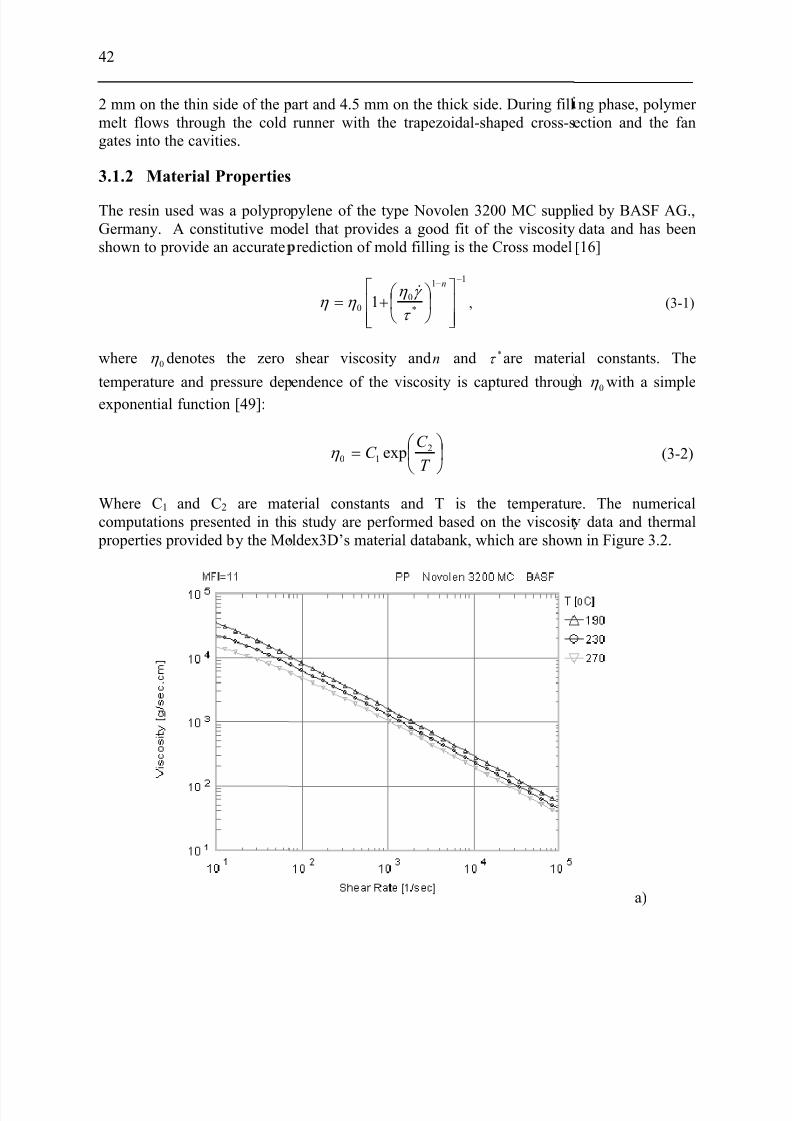
7/27/2019 Injection Mould Design
http://slidepdf.com/reader/full/injection-mould-design 60/160
42
2 mm on the thin side of the pmelt flows through the coldgates into the cavities.
3.1.2 Material Properties
The resin used was a polyproGermany. A constitutive moshown to provide an accurate
where 0η denotes the zero
temperature and pressure dep
exponential function [49]:
Where C1 and C2 are matcomputations presented in thi
properties provided by the Mo
art and 4.5 mm on the thick side. During fillrunner with the trapezoidal-shaped cross-s
pylene of the type Novolen 3200 MC suppldel that provides a good fit of the viscosityrediction of mold filling is the Cross model
11
*
00 1
−−
+=
n
τ
γ η η η
&,
shear viscosity and n and *τ are materi
endence of the viscosity is captured throug
=
T
C C 2
10 expη
erial constants and T is the temperatur s study are performed based on the viscositldex3D’s material databank, which are show
ng phase, polymer ection and the fan
ied by BASF AG.,data and has been
[16]
(3-1)
al constants. The
h0
η with a simple
(3-2)
e. The numericaldata and thermal
n in Figure 3.2.
a)
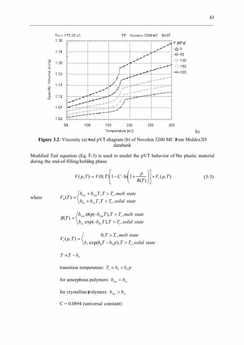
7/27/2019 Injection Mould Design
http://slidepdf.com/reader/full/injection-mould-design 61/160
Figure 3.2: Viscosity (a)
Modified Tait equation (Eq.during the end-of-filling/holdi
),( T pV
whereb
bT V
s
m)(1
10 +
+=
b
bT B
s
m
ex
e)(
3
3=
b
T pV t
),(7
=
5bT T −≡
transition temp
for amorphous
for crystalline
C = 0.0894 (un
nd pVT-diagram (b) of Novolen 3200 MC f databank
-3) is used to model the pVT behavior of ng phase.
),(
)(
1ln1),0( T pV
T B
pC T V t +
+⋅−=
state solid T T T b
statemelt T T T b
t s
t m
,,
,,
2
2
<
>
state solid T T T b
statemelt T T T b
t s
t m
,), p(
,), p(
4
4
>−
>−
state solid T T pbT b
statemelt T T
t
t
,),exp(
,,0
98 >−
>
erature: pbbT t 65 +≡
polymers: sm bb 11 =
olymers: sm bb 11 >
iversal constant)
43
b)
om Moldex3D
he plastic material
(3-3)
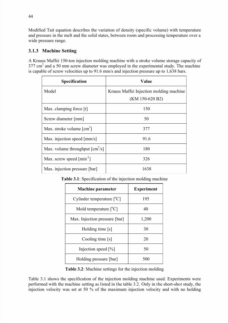
7/27/2019 Injection Mould Design
http://slidepdf.com/reader/full/injection-mould-design 62/160
44
Modified Tait equation describes the variation of density (specific volume) with temperatureand pressure in the melt and the solid states, between room and processing temperature over awide pressure range.
3.1.3 Machine Setting
A Krauss Maffei 150-ton injection molding machine with a stroke volume storage capacity of 377 cm3 and a 50 mm screw diameter was employed in the experimental study. The machineis capable of screw velocities up to 91.6 mm/s and injection pressure up to 1,638 bars.
Specification Value
Model Krauss Maffei Injection molding machine
(KM 150-620 B2)
Max. clamping force [t] 150
Screw diameter [mm] 50
Max. stroke volume [cm3] 377
Max. injection speed [mm/s] 91.6
Max. volume throughput [cm3/s] 180
Max. screw speed [min-1] 326
Max. injection pressure [bar] 1638
Table 3.1: Specification of the injection molding machine
Machine parameter Experiment
Cylinder temperature [oC] 195
Mold temperature [oC] 40
Max. Injection pressure [bar] 1,200
Holding time [s] 30
Cooling time [s] 20
Injection speed [%] 50
Holding pressure [bar] 500
Table 3.2: Machine settings for the injection molding
Table 3.1 shows the specification of the injection molding machine used. Experiments were
performed with the machine setting as listed in the table 3.2. Only in the short-shot study, theinjection velocity was set at 50 % of the maximum injection velocity and with no holding
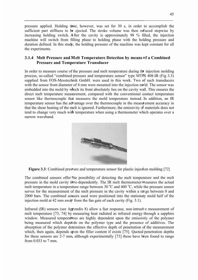
7/27/2019 Injection Mould Design
http://slidepdf.com/reader/full/injection-mould-design 63/160
pressure applied. Holding tisufficient part stiffness to bincreasing holding switch.machine will switch from fiduration defined. In this stud
the experiments.
3.1.4 Melt Pressure and
Pressure and Temp
In order to measure course of process, so-called “combinedsupplied from FOS-Messtechwith the sensor front diameter embedded into the mold by wdirect melt temperature meas
sensor like thermocouple thatemperature sensor has the adthat the shear heating of the mtend to change very much witnarrow waveband.
Figure 3.3: Combined pres
The combined sensors offer pressure in the mold cavity timelt temperature in a temperaserves for the measurement o
2000 bars. The combined seninjection mold at 42 mm awa
Infrared (IR) sensors (see Apmelt temperature [73, 74] bywindow. Measured temperat
being measured which depeabsorption of the polymer detwhich, then again, depends ufor these sensors are 2-7 mmfrom 0.033 to 7 mm.
e, however, was set for 30 s, in order ejected. The stroke volume was then re
fter the cavity is approximately 98 % filling phase to holding phase with the hol, the holding pressure of the machine was k
elt Temperature Detection by means
erature Transducer
the pressure and melt temperature during th pressure and temperature sensor” type MTPnik GmbH. were used in this work. Two oof 4 mm were mounted into the injection mich its front absolutely lies on the cavity wa
urement, compared with the conventional c
t measures the mold temperature instead.antage over the thermocouple in the measu
elt is ignored. Furthermore, the emissivity otemperature when using a thermometer wh
ure and temperature sensor for plastic inject
he possibility of detecting the melt temper e-dependently. The IR melt thermometer
ture range between 30 oC and 400 oC, whilef the melt pressure in the cavity within a ra
sors used were positioned into the stationar from the fan gate of each cavity (Fig. 3.1).
endix 8) allow a fast response, non-intrusimeasuring heat radiated as infrared energyres are highly dependent upon the emissivds on the polymer type and the presenceermines the effective depth of penetration oon the filler content if exists [75]. Quoted
, although experimentally [73] these have b
45
to accomplish theuced stepwise by
lled, the injectionding pressure andept constant for all
f a Combined
injection moldingS 408-IR (Fig 3.3)f such transducersld. The sensor wasll. This ensures theontact temperature
In addition, an IR ement accuracy inmaterials does not
ich operates over a
on molding [72]
ature and the melteasures the actual
the pressure sensor ge between 0 and
y mold half of the
e measurement of through a sapphireity of the polymer of additives. The
f the measurement penetration depthsen found to range
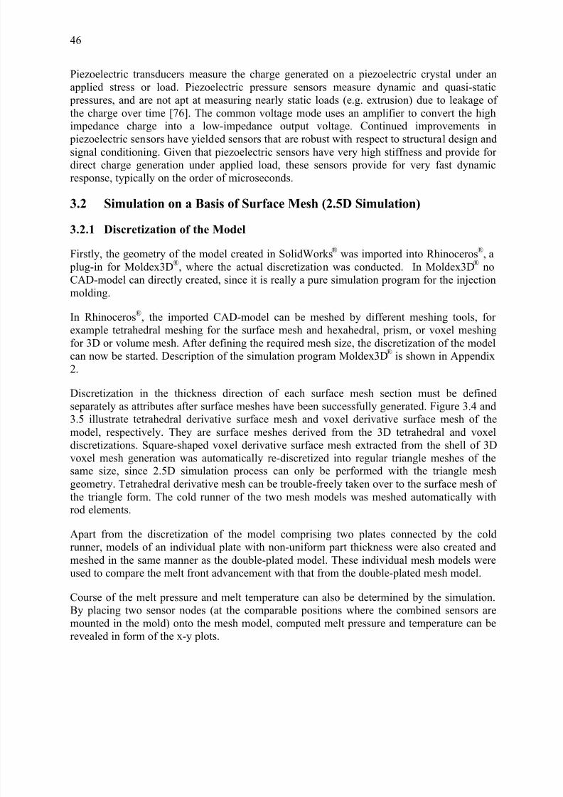
7/27/2019 Injection Mould Design
http://slidepdf.com/reader/full/injection-mould-design 64/160
46
Piezoelectric transducers measure the charge generated on a piezoelectric crystal under anapplied stress or load. Piezoelectric pressure sensors measure dynamic and quasi-static
pressures, and are not apt at measuring nearly static loads (e.g. extrusion) due to leakage of the charge over time [76]. The common voltage mode uses an amplifier to convert the highimpedance charge into a low-impedance output voltage. Continued improvements in
piezoelectric sensors have yielded sensors that are robust with respect to structural design andsignal conditioning. Given that piezoelectric sensors have very high stiffness and provide for direct charge generation under applied load, these sensors provide for very fast dynamicresponse, typically on the order of microseconds.
3.2 Simulation on a Basis of Surface Mesh (2.5D Simulation)
3.2.1 Discretization of the Model
Firstly, the geometry of the model created in SolidWorks® was imported into Rhinoceros®, a plug-in for Moldex3D®, where the actual discretization was conducted. In Moldex3D® no
CAD-model can directly created, since it is really a pure simulation program for the injectionmolding.
In Rhinoceros®, the imported CAD-model can be meshed by different meshing tools, for example tetrahedral meshing for the surface mesh and hexahedral, prism, or voxel meshingfor 3D or volume mesh. After defining the required mesh size, the discretization of the modelcan now be started. Description of the simulation program Moldex3D® is shown in Appendix2.
Discretization in the thickness direction of each surface mesh section must be definedseparately as attributes after surface meshes have been successfully generated. Figure 3.4 and
3.5 illustrate tetrahedral derivative surface mesh and voxel derivative surface mesh of themodel, respectively. They are surface meshes derived from the 3D tetrahedral and voxeldiscretizations. Square-shaped voxel derivative surface mesh extracted from the shell of 3Dvoxel mesh generation was automatically re-discretized into regular triangle meshes of thesame size, since 2.5D simulation process can only be performed with the triangle meshgeometry. Tetrahedral derivative mesh can be trouble-freely taken over to the surface mesh of the triangle form. The cold runner of the two mesh models was meshed automatically withrod elements.
Apart from the discretization of the model comprising two plates connected by the coldrunner, models of an individual plate with non-uniform part thickness were also created and
meshed in the same manner as the double-plated model. These individual mesh models wereused to compare the melt front advancement with that from the double-plated mesh model.
Course of the melt pressure and melt temperature can also be determined by the simulation.By placing two sensor nodes (at the comparable positions where the combined sensors aremounted in the mold) onto the mesh model, computed melt pressure and temperature can berevealed in form of the x-y plots.
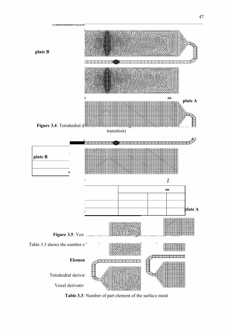
7/27/2019 Injection Mould Design
http://slidepdf.com/reader/full/injection-mould-design 65/160
Figure 3.4: Tetrahedral d
Figure 3.5: Vox
Table 3.3 shows the number o
Elemen
Tetrahedral derivat
Voxel derivativ
Table 3.3:
plate B
plate B
rivative surface mesh (global mesh size 3 mtransition)
l derivative surface mesh (global mesh size
f part elements of the two surface mesh type
t typeNumber of part ele
Double plate Plate A
ive surface mesh 10,658 5,329
surface mesh 5,896 2,951
Number of part element of the surface mesh
47
, 1 mm at the
mm)
.
ent
Plate B
5,333
2,949
plate A
plate A

7/27/2019 Injection Mould Design
http://slidepdf.com/reader/full/injection-mould-design 66/160
48
3.3 Simulation on the
3.3.1 Discretization of th
Figure 3.6 illustrates the 3D
model was discretized by me performed by three differentIn order to compare the effecthe part thickness on the acc
process, part model was meshmesh layers over the thick anfall into two main categories:section of the plates (Fig. 3.7).
Figure 3.
Like 2.5D simulation, twotemperature sensors are plac
position where the combinedmelt pressure and melt tempe
process.
In a same way as the 2.5D dthe double-plated part, whichrunner. These separated platetypes with one or three meshin the thick side of each plate,
Auto tetrahedral meshing m
creation. The advantage of thof this method are that there a
Basis of Volume Mesh (3D Simulati
Model
discretization of the double-plated model.
ans of the FEM-method. The discretizationesh types: tetrahedral, voxel and prism mof the mesh types as well as the number o
racy of the simulation results compared wited with these mesh types and each with thed the thin section of each plate. By this conmesh with one-two layers and three-six laye
: Volume mesh of the double-plated model
ensor nodes which function as the combed onto the surface of the volume mesh
ensors are mounted in the mold, in order torature and to compare them with those fro
scretization, two individual plate models whad been first connected to each other bywere then discretized with tetrahedral, pris
layer counts in the thin side and three or sixrespectively.
thod is the easiest method for three-dime
auto tetrahedral method is its convenience.re too many elements and it is hard to contr
plate A
plate B
n)
The double-plated
of the model wasshes, respectively.f mesh layers over h the real moldingifferent number of cept, mesh modelsrs in the thin-thick
ined pressure andat the comparable
etect course of thethe real molding
ere separated fromthe S-shaped cold, and voxel mesh
mesh layer counts
sional solid mesh
The disadvantagesl the mesh quality.
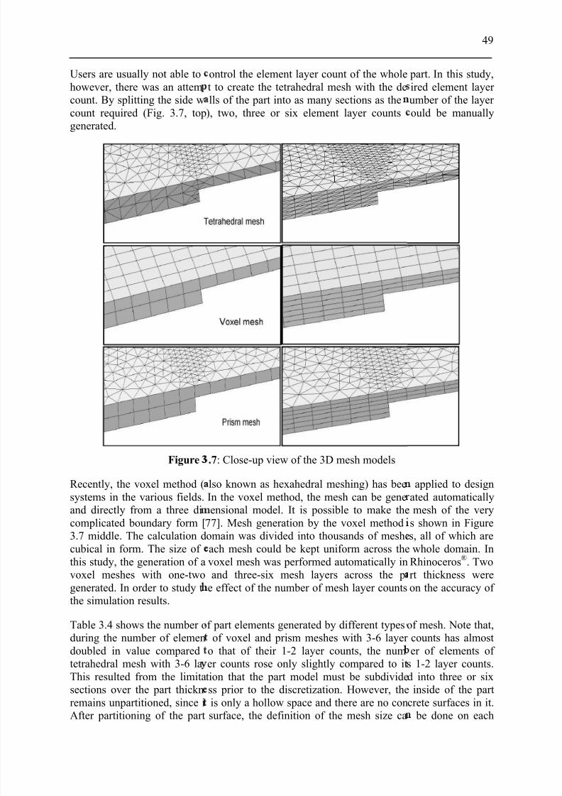
7/27/2019 Injection Mould Design
http://slidepdf.com/reader/full/injection-mould-design 67/160
Users are usually not able tohowever, there was an attemcount. By splitting the side wcount required (Fig. 3.7, topgenerated.
Figure
Recently, the voxel method (systems in the various fields.and directly from a three dicomplicated boundary form [3.7 middle. The calculation dcubical in form. The size of
this study, the generation of avoxel meshes with one-twogenerated. In order to study tthe simulation results.
Table 3.4 shows the number oduring the number of elemendoubled in value comparedtetrahedral mesh with 3-6 laThis resulted from the limitasections over the part thicknremains unpartitioned, since iAfter partitioning of the part
ontrol the element layer count of the wholet to create the tetrahedral mesh with the dells of the part into as many sections as the
), two, three or six element layer counts
.7: Close-up view of the 3D mesh models
lso known as hexahedral meshing) has beeIn the voxel method, the mesh can be geneensional model. It is possible to make the
77]. Mesh generation by the voxel methodomain was divided into thousands of mesheach mesh could be kept uniform across the
voxel mesh was performed automatically inand three-six mesh layers across the p
e effect of the number of mesh layer counts
f part elements generated by different typesof voxel and prism meshes with 3-6 layer
o that of their 1-2 layer counts, the numer counts rose only slightly compared to ittion that the part model must be subdividess prior to the discretization. However, theis only a hollow space and there are no consurface, the definition of the mesh size ca
49
part. In this study,ired element layer umber of the layer ould be manually
applied to designated automaticallymesh of the very
s shown in Figures, all of which arewhole domain. In
Rhinoceros®. Twort thickness wereon the accuracy of
of mesh. Note that,counts has almoster of elements of
s 1-2 layer counts.d into three or six
inside of the partcrete surfaces in it.
be done on each

7/27/2019 Injection Mould Design
http://slidepdf.com/reader/full/injection-mould-design 68/160
50
surface partition. It is possible to create surfaces within the hollow part in order to achieve theconcrete surfaces which can be partitioned and meshed later. Nevertheless, it was so time-consuming and arduous that creating surfaces within the hollow part was abstained.
Element type
Number of part element
1-2 layers 3-6 layers
Double Plate A Plate B Double Plate A Plate B
Tetrahedral volumemesh
65,956 34,660 34,46970,223 36,910 36,488
Voxel volume mesh 11,275 7,275 7,156 20,348 11,999 11,533
Prism volume mesh 22,211 12,739 12,631 53,071 28,356 27,903
Table 3.4: Number of the part element from different volume meshes
3.4 Simulation Parameters
All 2.5D and 3D simulations were conducted using the same machine setting parameters as inthe real molding process (Table 3.2). With Moldex3D’s 2.5D simulation, it is necessary todefine the number of mesh layers across the part thickness self-reliantly. In this study, 2.5Dsimulations were conducted with the mesh layer count of 10, 20, and 30 layers in order toevaluate the effect thereof on the accuracy of the simulation results. Mesh layer count is oneof the simulation parameters that affects the accuracy of the simulation results and can be
varied independently during the simulation. Usually, the higher the number of mesh layers,the higher the accuracy and the longer the simulation time result.
3.5 Simulation Results and Its Comparison with the Real Injection
Molding Process
In order to trace the progression of the melt in mold cavities, mold-filling simulations were performed on double-plated part with non-uniform part thickness. The validity of the fillinganalysis was confirmed by comparison of flow front predictions, pressure, and temperaturedevelopments with full-shot and short-shot experiments on the double-plated geometry asshown in Figure 3.1. Two-dimensional and three-dimensional mold filling simulations were
also compared with each other in order to acquire the best results.
Element typeCalculation time [s]
Double plate Plate A Plate B
Tetrahedral derivative surface mesh 1,516 635 581
Voxel derivative surface mesh 662 228 252
Table 3.5: Calculation time as a function of the surface mesh type
7/27/2019 Injection Mould Design
http://slidepdf.com/reader/full/injection-mould-design 69/160
51
Element type
Calculation time [s]
1-2 layers 3-6 layers
Double Plate A Plate B Double Plate A Plate B
Tetrahedral volume mesh 6,515 3,169 3,249 6,966 3,325 3,233
Voxel volume mesh 877 511 570 1,997 947 903
Prism volume mesh 2,061 1,038 1,025 5,396 2,628 2,526
Table 3.6: Calculation time as a function of the volume mesh type
Table 3.5 and 3.6 display the calculation times of filling and holding simulations as afunction of surface and volume mesh types, respectively. Concerning the time used to
compute filling and holding simulations, it is clear that owing to smaller amounts of elementsof the surface mesh of the comparable model, less calculation time is required. 2.5Dsimulation is also advantageous over 3D simulation regarding the reliability and simulationtime when molded parts are simple in form.
3.5.1 Filling Analysis (Short-Shot Study)
The advancement of the melt front at different filling times is displayed by different color bands. From the melt front advancement one can
• Examine filling/holding pattern of the molding,
• Check potential incomplete filling (short shot) process,• Check unbalanced flow/over-pack-induced flashing problems,
• Identify weld line locations,
• Identify air trap locations,
• Check flow contribution from each gate for runner balance,
• Check proper gate location to balance flow and eliminate weld lines.
Figure 3.8 shows the comparison of the melt front progression in filling phase between the
experiment and 2.5D simulations. Simulations were performed with the standard solver and based on non-isothermal computation using 20 mesh layer counts over the part thicknessdefined. Standard solver is a fast and easy solid solution of Moldex3D which requiresmoderate mesh resolution in computing. From the figure, the simulation results agree wellwith the real injection molding process. As already described, in the real injection molding
process, the right cavity of the part was completely filled prior to the left cavity at the filledvolume of around 78 %. Then holding followed and the changeover of the holding directionwithin the two cavities resulted after holding had ended. The simulation results derived fromthe tetrahedral derivative and the voxel derivative meshes are nearly identical in quality andwhen compared with the melt advancement from the real process this proves the higher accuracy of 2.5D simulation over 3D simulation (Fig. 3.9), particularly in predicting the
filling progression of this specific double-plated part. Both computed melt front times werecomparable, step by step, to those in the real molding process. At 78 % filled volume, the

7/27/2019 Injection Mould Design
http://slidepdf.com/reader/full/injection-mould-design 70/160
52
computed melt fronts of the two derivative meshes had reached the end of the right cavity,while the melt front in the left cavity was computed somewhat further than that in the realmolding process. However, this is the only deviation being found by 2.5D simulations.
Short-shot study Tetrahedral derivative mesh Voxel derivative mesh
3 2 % f i l l e d
3 8 % f i l l e d
4 9 % f i l l e d
5 6 % f i l l e d
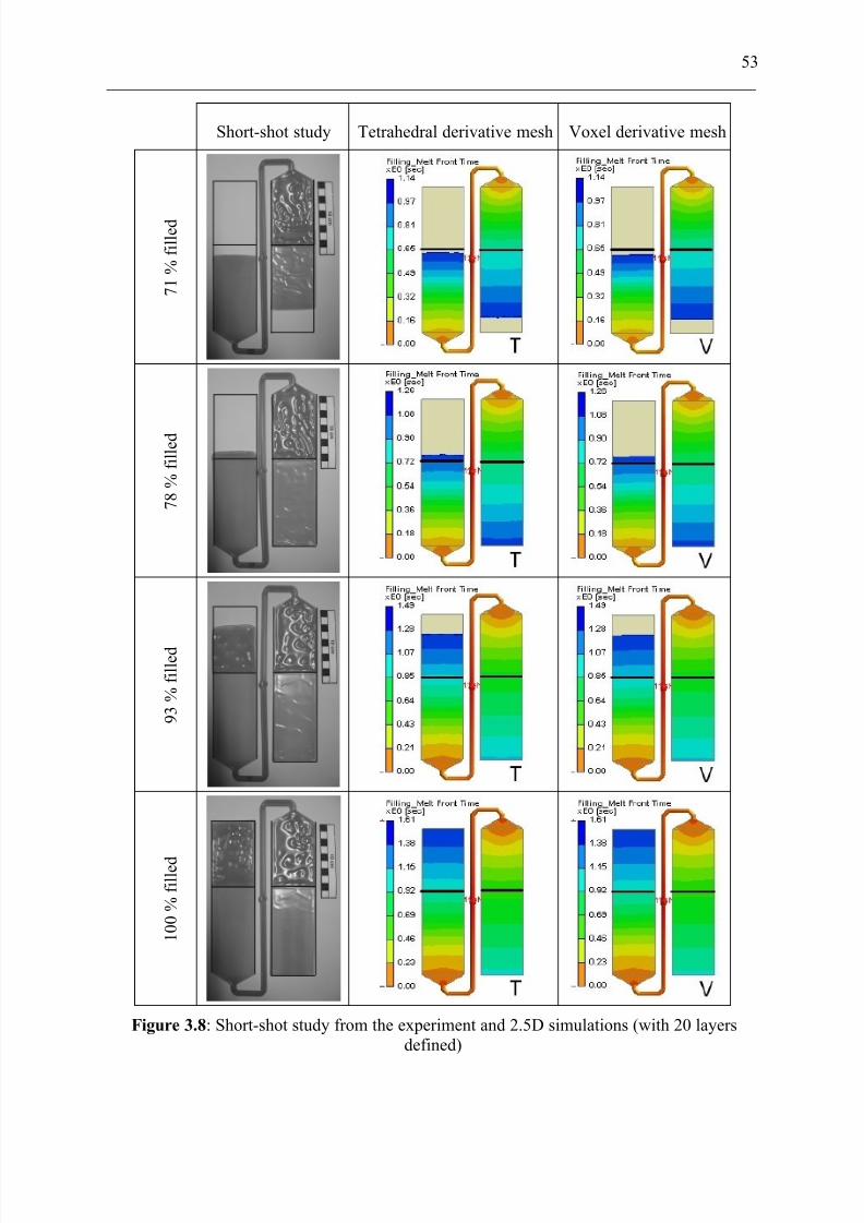
7/27/2019 Injection Mould Design
http://slidepdf.com/reader/full/injection-mould-design 71/160
53
Short-shot study Tetrahedral derivative mesh Voxel derivative mesh
7 1 % f i l l e d
7 8 %
f i l l e d
9 3 % f i l l e d
1 0 0 % f i l l e d
Figure 3.8: Short-shot study from the experiment and 2.5D simulations (with 20 layersdefined)

7/27/2019 Injection Mould Design
http://slidepdf.com/reader/full/injection-mould-design 72/160
54
32 % filled 38 % filled 49 % filled
P r i s m m e s h
3 - 6 l a y e r s
P r i s m m e s h
1 - 2 l a y e r s
V o x e l m e s h
3 - 6 l a y e r s
V o x e l m e s h
1
- 2 l a y e r s
T e t r a h e d r a l m e s h
3 - 6 l a y e r s
T e t r a h e d r a l m e s h
1 - 2 l a y e r s
S h o r t - s h o t s t u d y
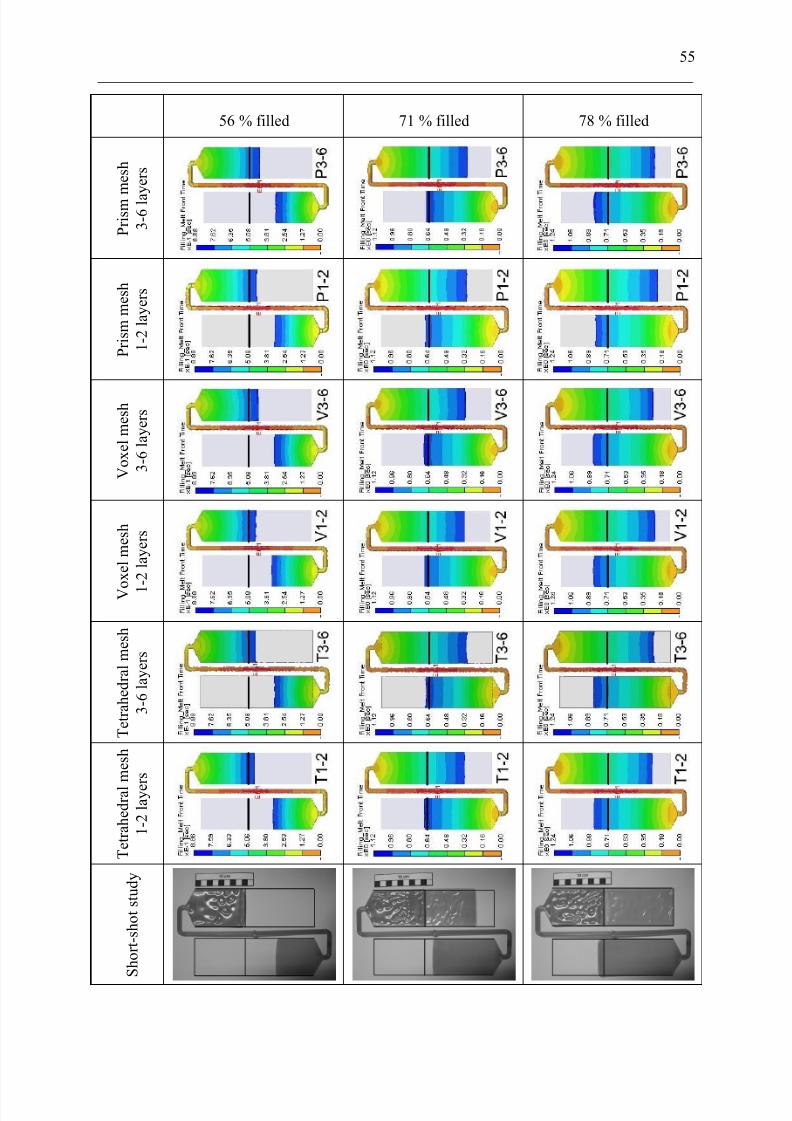
7/27/2019 Injection Mould Design
http://slidepdf.com/reader/full/injection-mould-design 73/160
55
56 % filled 71 % filled 78 % filled
P r i s m m e s h
3 - 6 l a y e r s
P r i s m m e s h
1 - 2 l a y e r s
V o x e l m e s h
3 - 6 l a y e r s
V o x e l m e s h
1
- 2 l a y e r s
T e t r a h e d r a l m e s h
3 - 6 l a y e r s
T e t r a h e d r a l
m e s h
1 - 2 l a y e r s
S h o r t - s h o t s t u d y
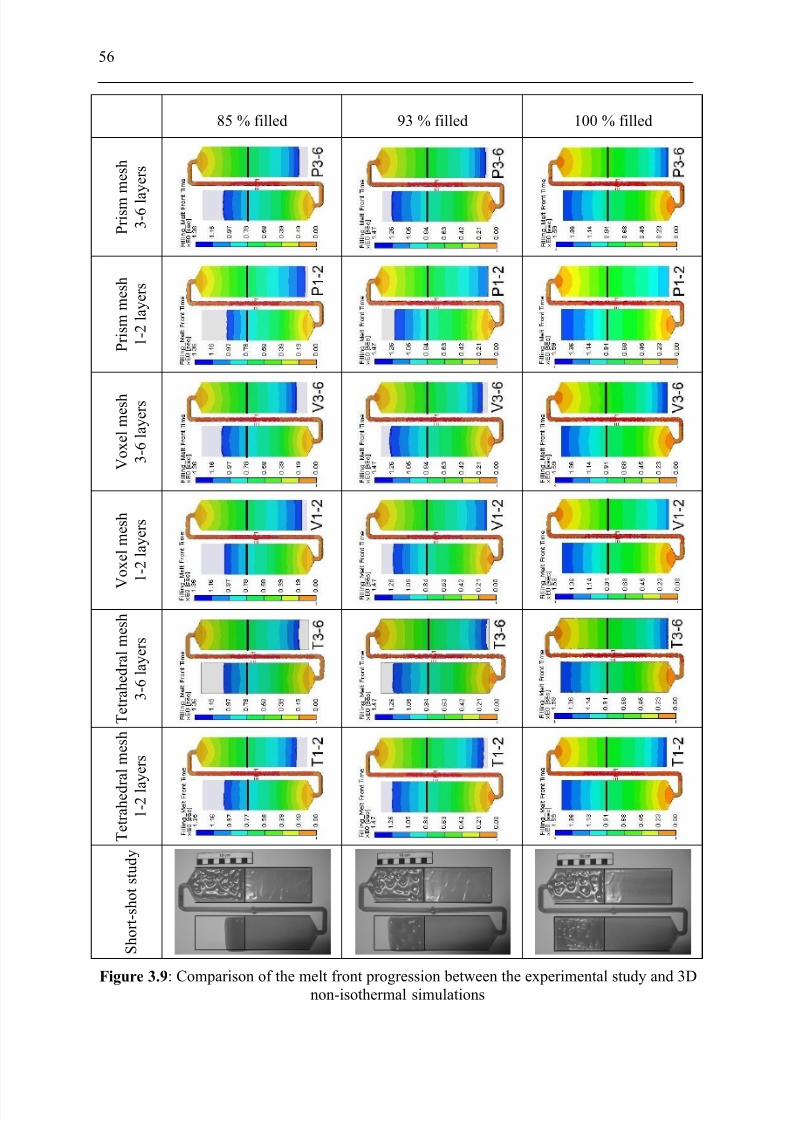
7/27/2019 Injection Mould Design
http://slidepdf.com/reader/full/injection-mould-design 74/160
56
85 % filled 93 % filled 100 % filled
P r i s m m e s h
3 - 6 l a
y e r s
P r i s m m e s h
1 - 2 l a y e r s
V o x e l m e s h
3 - 6 l a y e r s
V o x e l m e s h
1 - 2 l a y e r s
T e t r a h e d r a l m e s h
3 - 6 l a y e r s
T e t r a h e d r a l m e s h
1 - 2 l a
y e r s
S h o r t - s h o t s t u d y
Figure 3.9: Comparison of the melt front progression between the experimental study and 3Dnon-isothermal simulations
7/27/2019 Injection Mould Design
http://slidepdf.com/reader/full/injection-mould-design 75/160
57
Figure 3.9 shows the melt front advancement derived from the short-shot study (left) of thereal molding process and 3D simulation results using different mesh types. Usually in a short-shot study, the injection molding of the part is carried out without the holding pressure, whichresults in a high degree of part shrinkage. By doing this, the real melt front progression will
be obtained without any manipulation of the flow front from the holding pressure. In this
study, 3D simulations were performed with standard solver and based on non-isothermalcomputation. In the real molding process, flow deceleration phenomena have been involvedin the filling phase. The melt spread from the fan gates into the cavities until 35 % filledvolume where the melt advancement in both cavities was almost the same. At the filledvolume of about 38 %, melt front gradually expanded and changed its shape from the fan-shaped nearly to the parallel one. At the 49 % filled volume, melt front in the thick section of the right cavity advanced further than in the thin section of the left cavity. At this stage,
because of less flow resistance in the thick section of the right cavity, flow deceleration in thethin section of the left cavity developed and the melt in thick section can therefore advance alittle bit more quickly than in the other section. As time went by, the melt in the thick sectionof the right cavity that had experienced less flow resistance spread faster than in the thin
section of the left cavity. As the melt front in the thick section of the right cavity had crossedthe transition where the part thickness suddenly changes, the flow velocity increased. Despitethe increasing flow resistance as a result of the smaller cross-section area in the thin sectionof the right cavity, the melt front velocity in this section increased, since the injectionvelocity was set constant. While the right cavity was completely filled at around 78 % filledvolume, the melt front in the left cavity was just found at slightly behind its transition. Rightafter the first cavity has been completely filled, holding of this cavity took place. At the sametime, the left cavity was further filled with the holding pressure until this cavity was totallyfilled and almost no melt flow deceleration existed at this time. Although the thick section of the left cavity was merely filled with the holding pressure, melt front velocity in this sectionincreased compared to the thin section of the same cavity as it passed through the transition.This is because of the lower flow resistance as well as the fact that the holding pressure,which also drives the melt to flow, dedicates to the filling only in this section of the leftcavity.
Usually, the accuracy of the simulation results depends highly upon the mesh quality and themesh resolution. Moreover, to compute the molding properties which differentiate over the
part thickness e.g. melt temperature effectively, part in the thickness direction must bemeshed generally suggested with 3 mesh layer counts. Considering 3D simulations withdifferent mesh types and numbers of mesh layers (Fig 3.9), at the beginning of the molding
process, the results from the mold filling simulations are nearly identical in filling pattern upuntil the shape of the melt front. Some simulation results show the melt front in convex form,the others in concave form. But these are not important in predicting the flow behavior of themelt in the cavity. Much more important is the so-called melt front time (term used inMoldex3D®), which is the position of the melt front in the cavity as a function of the fillingtime. With the melt front time, occurrence of weld line and air trap, for example, can also be
predicted.
According to Figure 3.9, differences in filling can already be seen at 78 % filled volume.With the voxel mesh with 1-2 layer counts (1 mesh layer in the thin section and 2 mesh layersin the thick section of the part) and the prism mesh with 1-2 layer counts, the melt front in theright cavity advances somewhat faster and thus farther than the other meshing types.
Compared to the real molding process, however, all the computed melt front advancementsdeviate from that of the real molding process, which has already reached the end of the right

7/27/2019 Injection Mould Design
http://slidepdf.com/reader/full/injection-mould-design 76/160
58
cavity. At this point, filling phase has terminated. In the left cavity, the melt advancement of all the simulations slightly exceeds the real molding situation. At 85 % filled volume, themelt fronts in the right cavity of the voxel mesh with 1-2 layer counts and the prism meshwith 1-2 layer counts nearly approach the end of the cavity, while these of the other meshingtypes remain farther away from the end of the cavity. In the left cavity, all the computed melt
fronts advance farther than the melt front of the real process. Not until the 93 % filled volumehave the melt fronts of the voxel mesh with 1-2 layer counts and the prism mesh with 1-2layer counts reached the end of the right cavity. In the left cavity, the computed melt frontsare at the position comparable to that of the real molding process.
The effect of the number of mesh layers over the part thickness on the accuracy of thesimulation results were not clearly confirmed by this study. Usually, with more mesh layers,the accuracy and calculation time increase. Instead, no distinct improvement in the accuracyof predicting the melt front advancement was acquired.
Tetrahedral meshing compared to prism and voxel meshing was verified to be the worst
method concerning the accuracy of the simulation results and calculation time (see Table3.6), since its mesh quality is poor and the number of elements created by tetrahedralmeshing in one part is markedly high compared to the uniform elements generated by prismor voxel meshing. Surprisingly, the 3D simulation results, independent of the mesh types andthe number of mesh layers over the part thickness, deviated much from the actual moldingsituation. This resulted mainly from the numerical instability of the 3D-filling simulation of Moldex3D®. This double-plated part is a highly complex part regarding the flow and pressureimbalance between the two plates with non-uniform part thickness. Flow deceleration hasalso been involved in filling because of the different flow resistances in the cavities. Since thesource code of this simulation program is unknown, no further statement can be made bynow.
Based on simulations of the double-plated part proposed in this study, all the simulationresults has shown that 2.5D numerical computation of Moldex3D® is more stable and morereliable than its 3D numerical computation. This is evidence that 3D simulation does notalways function correctly and if a complex flow system involved as can be seen in themolding of the double-plated part, limitations of the simulation program becomeconspicuous. Since it is possible to set the simulation parameters in Moldex3D® freely,another 3D simulation process based on the isothermal computation with the standard solver was carried out in order to examine the effect of the computational mode setting on theaccuracy of the simulation results. The result of mold filling simulation based on theisothermal computation is introduced in Figure 3.10. From this figure, melt front progression
in each filling step of the isothermal based computation of 3D simulation agrees well withthat from the real molding process. Compared to the results of 3D simulation based on non-isothermal computation shown in the Figure 3.9, obvious improvement in predicting the meltfront advancement and the proximity of the results of the isothermal based computation of 3Dsimulation to the real process were astonishingly provided. At the beginning of filling,however, outrunning of the computed melt front remained unsolved. In addition, thesimulation results show that at every filling step the right cavity always has higher degree of filled volume than the other. The tendency of the right cavity to be filled prior to the other was thus given by isothermal based 3D simulation. At 78 % filled volume, the simulationshows that the right cavity was completely filled and began to be packed by the holding
pressure, while the melt front in the left cavity had already passed its transition. The rest of the cavity filling from the simulation did not substantially differentiate from the real process.

7/27/2019 Injection Mould Design
http://slidepdf.com/reader/full/injection-mould-design 77/160
59
The reason why the isothermal simulation results better agree with the real process, which isnot usual, is based on the assumption that with the complex flow balance induced from theflow resistance differentials and the pressure changeover between the two cavities, non-isothermal numerical computation of the filling pressure as a function of the flow velocitiesand temperature became instable which resulted in the wrong prediction in pressure level and
pressure balancing between the two cavities (Fig. 3.17) and thus the melt advancement wasforetold in the incorrect way.
38 % 78 %
49 % 85 %
56 % 93 %
71 % 100 %
Figure 3.10: Comparison of the melt front progression between the experimental study and3D simulation with prism mesh 3-6 layers based on the isothermal computation
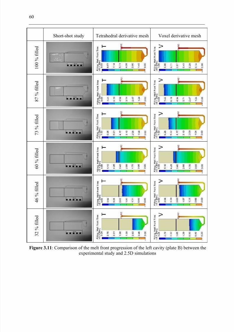
7/27/2019 Injection Mould Design
http://slidepdf.com/reader/full/injection-mould-design 78/160
60
Short-shot study Tetrahedral derivative mesh Voxel derivative mesh
1 0 0 %
f i l l e d
8 7 %
f i l l e d
7 3 %
f i l l e d
6 0 % f i l l e d
4 6 % f i l l e d
3 2
% f i l l e d
Figure 3.11: Comparison of the melt front progression of the left cavity (plate B) between theexperimental study and 2.5D simulations
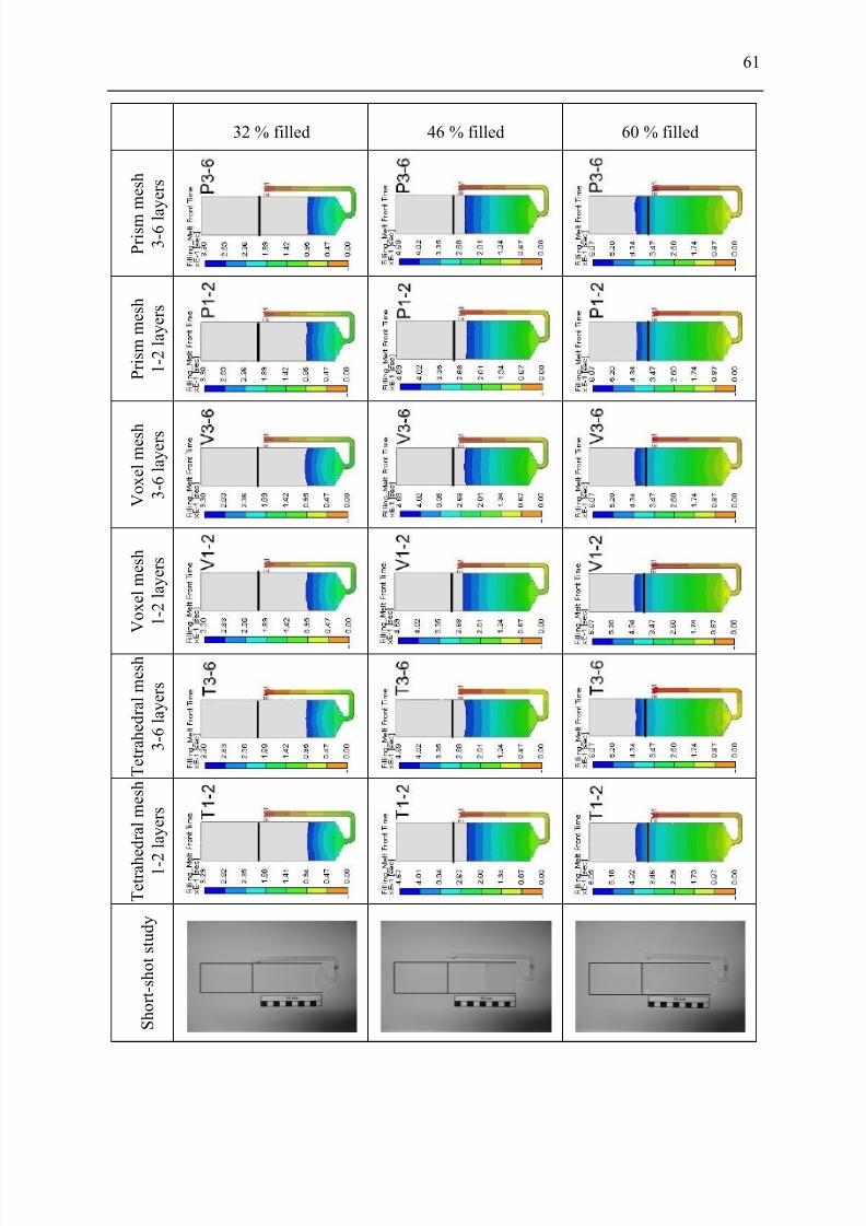
7/27/2019 Injection Mould Design
http://slidepdf.com/reader/full/injection-mould-design 79/160
61
32 % filled 46 % filled 60 % filled
P r i s m
m e s h
3 - 6 l a
y e r s
P r i s m m e s h
1 - 2 l a y e r s
V o x e l m e s h
3 - 6 l a y e r s
V o x e l m e s h
1 - 2 l a y e r s
T e t r a h e d r a l m e s h
3 - 6 l a y e r s
T e t r a h e d r a l m e s h
1 - 2
l a y e r s
S h o r t - s h o t s t u d y
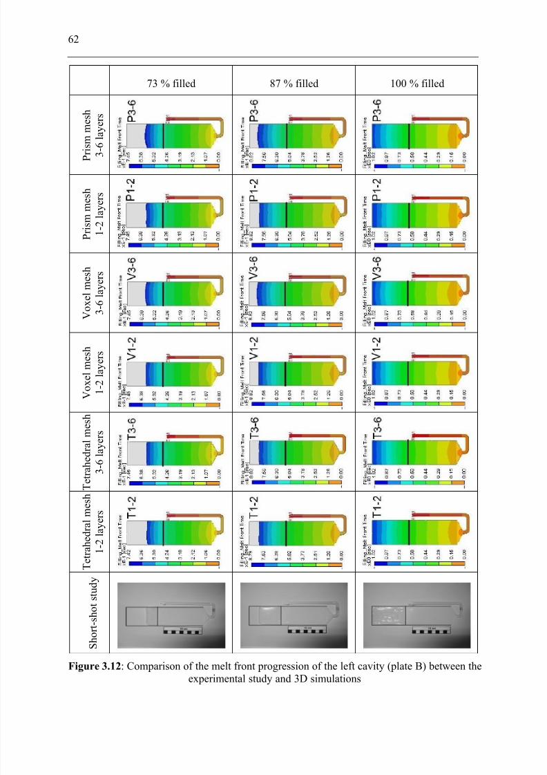
7/27/2019 Injection Mould Design
http://slidepdf.com/reader/full/injection-mould-design 80/160
62
73 % filled 87 % filled 100 % filled
P r i s m
m e s h
3 - 6 l a
y e r s
P r i s m m e s h
1 - 2 l a y e r s
V o x e l m e s h
3 - 6 l a y e r s
V o x e l m e s h
1 - 2 l a y e r s
T e t r a h e d r a l m e s h
3 - 6 l a y e r s
T e t r a h e d r a l m e s h
1 - 2
l a y e r s
S h o r t - s h o t s t u d y
Figure 3.12: Comparison of the melt front progression of the left cavity (plate B) between the
experimental study and 3D simulations
7/27/2019 Injection Mould Design
http://slidepdf.com/reader/full/injection-mould-design 81/160
63
Since 3D simulation of the double-plated part failed to predict the melt front progression,further simulations using a single cavity with the same dimensions should also be performedin order to prove the capability of the 3D-subroutine of Molex3D. By closing one side of thecold runner in the moving mold half, an individual injected part instead of double-plated partwill be acquired. During molding, the polymer melt can only flow through the opening side
of the cold runner into the cavity. By this way, molding conditions can be constantlycontrolled and the complexity of the molding is significantly reduced.
Figure 3.11 shows the comparison of the melt front advancement of the left cavity betweenthe experimental study and 2.5D simulation performed with the standard solver and based onnon-isothermal computation and with 20 mesh layer counts over the part thickness defined.2.5D simulation results show the comparable melt front advancement to that of 3Dsimulation. The outrunning of the melt front in every filling step also arose from 2.5Dsimulation. From 32 % to 73 % filled volume, both 3D and 2.5D simulations show thequalitatively comparable melt front advancements. From 73 % filled volume on, a slightoutrunning of the 3D-computed melt front advancement compared with that of the 2.5D
occurred. Particularly the slight outrunning of the melt front makes the 3D simulation resultsmore reliable, since they even approximate the real molding process.
Figure 3.12 displays the comparison of the melt front advancement of the left cavity betweenthe experimental study and 3D simulations performed with standard solver and based on non-isothermal computation. From the beginning, the 3D computed melt front advancement ineach filling step fairly outran the melt front of the real molding process. Apart from this, noobvious deviation in the melt front advancement between the mesh types and the number of mesh layers over the part thickness was noticed.
Comparison of the melt front progression of the right cavity between the experimental study,
2.5D simulations, and 3D simulations was also performed. Similar to the left cavity, theoutrunning of the melt advancement from the beginning of filling up to 74 % filled volumecomputed by 2.5D and the 3D simulation is viewable. This is shown in Appendix 3 and 4.
As a whole image, no decisive accuracy deviation in predicting the melt front advancement between 3D simulation and 2.5D simulation was manifested when molding the platesseparately, since the complexity of the flow and unbalancing of the pressure within the twocavities as a system were dismantled. In addition, no extensive disagreement among thesimulation results of the molding of these individual plates was proved. Furthermore, theadvantage of the higher regularity of the voxel derivative mesh over the tetrahedral derivativemesh cannot be observed. For 2.5D mold filling simulation, higher number of the mesh layer
count over the part thickness dedicated mainly to the computation of the temperaturedistribution within the molded part rather than to the prediction of the melt front advancement(Appendix 5 and 6).
3.5.2 Course of the pressure
The moment at which the changeover or holding switch is activated, determines when thealteration of the velocity-controlled filling phase into the pressure-controlled holding phase isrealized. The point of switching should agree, if possible, with the volumetric filling of thecavity, since the cavity is to be filled with a defined velocity. Shrinkage arising in holding
phase must be compensated by a given holding pressure. Pressure fluctuations and pressure
peaks must be avoided at the point of switching, so that a constant and harmonious transition
7/27/2019 Injection Mould Design
http://slidepdf.com/reader/full/injection-mould-design 82/160
64
between injecting phase and holding phase results and no negative influences can impair thequality of the molded part.
Figure 3.13: Measured course of the pressure during a molding cycle of the double-plated part with non-uniform part thickness
Figure 3.13 illustrates course of the pressure developed during an injection molding cycle of the double-plated part with non uniform part thickness. Courses of the pressure weremeasured by two of the combined pressure and temperature sensors built into each cavity atthe position approximately 42 mm near the gates. A peak and a spontaneous pressure dropcan be seen on the pressure-S1 and pressure-S2 curves, which represent a too early holdingswitch and a too late holding switch, respectively. The proper holding switch is suggested to
be at 98 % of filled volume for molding with a hydraulic injection molding machine, sincethis type of injection molding machine reacts relatively slowly to the changes in machinesettings. Normally, this kind of peak or spontaneous pressure drop within a pressure gradientis undesirable. If holding was implemented too early, the cavity will be completely filled byholding instead of filling and an incomplete mold filling or high shrinkage of the molded parthas to be expected. If, to the contrary, holding switch was done too late, the cavity will beoverpacked or flashes may be developed.
As can be seen from the Figure 3.13, the maximum pressure measured during holding phaseof the plate A which has the gate connected to the thick section is 350 bars, whereas themaximum pressure during holding of the second cavity with the gate connected to the thinsection is only 300 bars. This is because the melt can be rapidly transported into the thicker section of the first plate as a result of the lower flow resistance. The lower the resistance of the cavity, the lower the pressure level will be contributed. In the first cavity, this pressurelevel remained by this value almost throughout holding phase. Shortly before the end of
holding phase, the pressure measured by this point began to gradually drop and sloped downto the ambient pressure. In a comparable manner, the pressure maximum plateau during
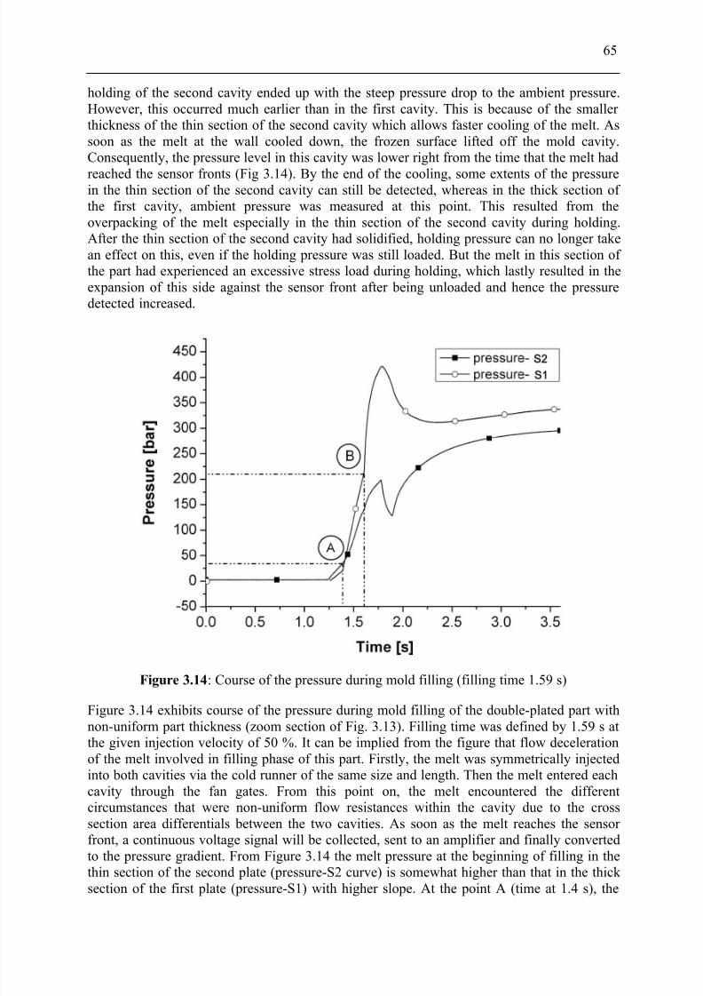
7/27/2019 Injection Mould Design
http://slidepdf.com/reader/full/injection-mould-design 83/160
65
holding of the second cavity ended up with the steep pressure drop to the ambient pressure.However, this occurred much earlier than in the first cavity. This is because of the smaller thickness of the thin section of the second cavity which allows faster cooling of the melt. Assoon as the melt at the wall cooled down, the frozen surface lifted off the mold cavity.Consequently, the pressure level in this cavity was lower right from the time that the melt had
reached the sensor fronts (Fig 3.14). By the end of the cooling, some extents of the pressurein the thin section of the second cavity can still be detected, whereas in the thick section of the first cavity, ambient pressure was measured at this point. This resulted from theoverpacking of the melt especially in the thin section of the second cavity during holding.After the thin section of the second cavity had solidified, holding pressure can no longer takean effect on this, even if the holding pressure was still loaded. But the melt in this section of the part had experienced an excessive stress load during holding, which lastly resulted in theexpansion of this side against the sensor front after being unloaded and hence the pressuredetected increased.
Figure 3.14: Course of the pressure during mold filling (filling time 1.59 s)
Figure 3.14 exhibits course of the pressure during mold filling of the double-plated part withnon-uniform part thickness (zoom section of Fig. 3.13). Filling time was defined by 1.59 s atthe given injection velocity of 50 %. It can be implied from the figure that flow decelerationof the melt involved in filling phase of this part. Firstly, the melt was symmetrically injectedinto both cavities via the cold runner of the same size and length. Then the melt entered eachcavity through the fan gates. From this point on, the melt encountered the differentcircumstances that were non-uniform flow resistances within the cavity due to the crosssection area differentials between the two cavities. As soon as the melt reaches the sensor front, a continuous voltage signal will be collected, sent to an amplifier and finally convertedto the pressure gradient. From Figure 3.14 the melt pressure at the beginning of filling in the
thin section of the second plate (pressure-S2 curve) is somewhat higher than that in the thick section of the first plate (pressure-S1) with higher slope. At the point A (time at 1.4 s), the
7/27/2019 Injection Mould Design
http://slidepdf.com/reader/full/injection-mould-design 84/160
66
first buckling of the two curves is defined. This is the point where the melt front in the thick section of the first plate reached the transition to the thin section of the same plate.
After the point A, the melt in the first plate flowed into the thin section with the higher meltfront velocity because of the constant injection velocity, despite the increasing flow
resistance as a result of the decrease in the cross section area. Whereas the melt front in thesecond plate was still being found in the thin section (Fig. 3.9). With an increase in the flowlength in the first plate as well as the higher flow resistance in the thin section of the first
plate, much higher filling pressure was necessary compared to the thin section of the second plate and hence a steep pressure gradient resulted. The increase in filling pressure in the first plate also influences filling in the second plate, since they are connected to each other by thecold runner of the same size. If higher pressure is supplied in one branch of the runner, thesame amount of the pressure must be provided to the other, except for the hot runner systemwith valve gate control. And this is the reason why the pressure in the second plate alsoincreases, but with gentler gradient.
Point B (the second buckling, filling time at 1.59 s) is the point where the plate A wascompletely filled with the melt following with the melt compression whereas the melt front inthe plate B had already crossed its transition. This results in the highly steep pressure gradientof the pressure-S1 curve. This point is counted as the actual filling time obtained from themolding machine. From the figure, the maximum melt pressure in the plate A is atapproximately 215 bars, while the maximum melt pressure in the plate B is approximately150 bars high. As already mentioned above, the pressure supplied to one cavity is also takingan effect on the other, since they are connected to each other by the cold runner. While themelt in the plate A was being packed, the plate B was being topped off, not by the effect of the filling velocity but actually by the effect of holding pressure, and the melt front in this
plate, which was found at this time in its thick section, continued to move toward the end of
the cavity. So the melt pressure in the plate B after point B kept rising but with the gentler gradient compared with the steep gradient (compression) of the plate A. Because the plate Awas filled first, the melt in this plate was excessively packed by the holding pressure. Under this molding situation, the plate A will generally suffer from overpacking, which results in adeterioration of this part under some mechanical loads. In the same way, the plate B,especially the thick section, which was filled with the holding pressure instead of the fillingvelocity, will also suffer from excessive shrinkage and warpage. Apart from the moldingsituation, gate should be positioned at the thickest section of the part in order that holding can
bring about the highest and longest efficiency, since the thick section will solidify last.Considering the plate B, the fan gate is connected to the thin section of this part. Duringholding phase, this thin section will solidify prior to the thick section. Consequently, the thick section will be insufficiently packed and non-uniform shrinkage and warpage result.
As already mentioned a peak and a spontaneous pressure drop can be seen on the pressure-S1and pressure-S2 curves, which represent a too early holding switch and a too late holdingswitch, respectively. Although this peak and spontaneous pressure drop in course of the
pressure are not optimum, they cannot be avoided, since filling of this molding system is notsymmetrical as usual. Flow deceleration, unbalance and direction changeover of holdinginvolved in the filling and holding phases and they make this molding process almostimpossible to be repeated and more difficult to be controlled. In industry, molding of such a
part is seldom performed, since the mold maker and part designer will always avoid positioning gate and arranging the cavities into the mold in the manner they know that qualityand repeatability of molded parts will hardly be guaranteed.
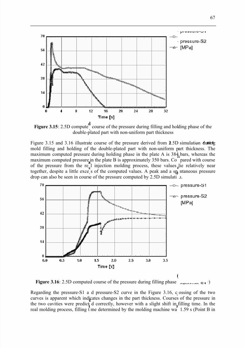
7/27/2019 Injection Mould Design
http://slidepdf.com/reader/full/injection-mould-design 85/160
Figure 3.15: 2.5D computedouble-p
Figure 3.15 and 3.16 illustratmold filling and holding of maximum computed pressuremaximum computed pressureof the pressure from the retogether, despite a little excedrop can also be seen in cours
Figure 3.16: 2.5D compute
Regarding the pressure-S1 acurves is apparent which indi
the two cavities were predictreal molding process, filling t
course of the pressure during filling and hollated part with non-uniform part thickness
e course of the pressure derived from 2.5Dthe double-plated part with non-uniform pduring holding phase in the plate A is 384
in the plate B is approximately 350 bars. Col injection molding process, these valuess of the computed values. A peak and a spe of the pressure computed by 2.5D simulati
d course of the pressure during filling phase
d pressure-S2 curve in the Figure 3.16, ccates changes in the part thickness. Courses
d correctly, however with a slight shift inme determined by the molding machine wa
67
ding phase of the
simulation duringart thickness. The bars, whereas the pared with courselie relatively near ntaneous pressuren.
expanded view)
ossing of the twoof the pressure in
filling time. In the1.59 s (Point B in
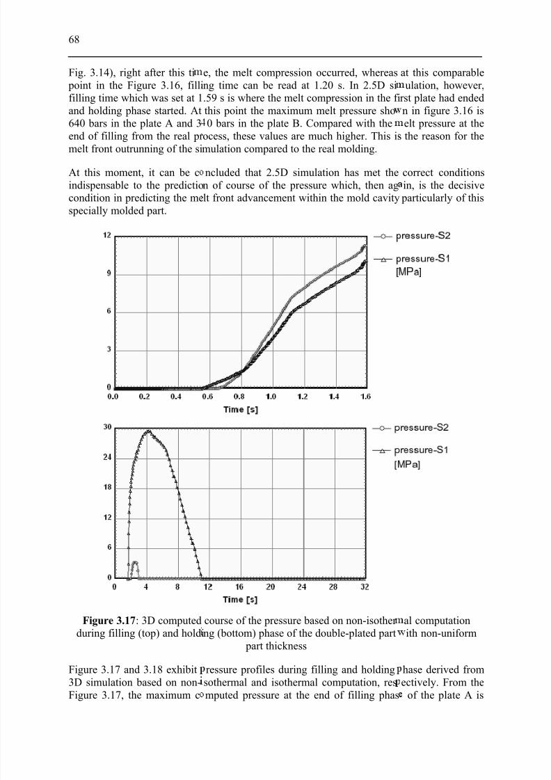
7/27/2019 Injection Mould Design
http://slidepdf.com/reader/full/injection-mould-design 86/160
68
Fig. 3.14), right after this ti point in the Figure 3.16, fillifilling time which was set at 1and holding phase started. At640 bars in the plate A and 3
end of filling from the real pr melt front outrunning of the si
At this moment, it can be cindispensable to the predictiocondition in predicting the mespecially molded part.
Figure 3.17: 3D computedduring filling (top) and holdi
Figure 3.17 and 3.18 exhibit
3D simulation based on non-Figure 3.17, the maximum c
e, the melt compression occurred, whereasng time can be read at 1.20 s. In 2.5D si.59 s is where the melt compression in the fithis point the maximum melt pressure sho0 bars in the plate B. Compared with the
ocess, these values are much higher. This ismulation compared to the real molding.
ncluded that 2.5D simulation has met then of course of the pressure which, then aglt front advancement within the mold cavity
course of the pressure based on non-isother ng (bottom) phase of the double-plated part
part thickness
ressure profiles during filling and holding
sothermal and isothermal computation, resmputed pressure at the end of filling phas
at this comparableulation, however,
rst plate had endedn in figure 3.16 iselt pressure at the
the reason for the
correct conditionsin, is the decisive
particularly of this
al computationith non-uniform
hase derived from
ectively. From theof the plate A is
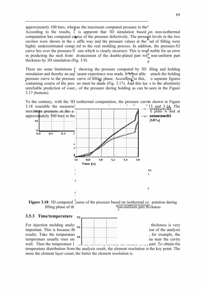
7/27/2019 Injection Mould Design
http://slidepdf.com/reader/full/injection-mould-design 87/160
approximately 100 bars, wher According to the results, icomputation has computed cocavities were shown in the shighly underestimated compa
curve lies over the pressure-Sin predicting the melt frontthickness by 3D simulation (F
There are some limitations isimulation and thereby an unp
pressure curve to the pressurecontaining course of the presunreliable prediction of cours3.17 (bottom).
To the contrary, with the 3D3.18 resemble the measuredmaximum pressure at the eapproximately 500 bars in the
Figure 3.18: 3D computedfilling phase of th
3.5.3 Time/temperature
For injection molding analysimportant. This is because thresults. Take the temperaturetemperature usually rises stewall. Then the temperature ltemperature distribution from
more the element layer count,
eas the maximum computed pressure in theis apparent that 3D simulation based
urse of the pressure defectively. The pressuuffle way and the pressure values at the
red to the real molding process. In additio
one which is clearly incorrect. This is respdvancement of the double-plated part wit
ig. 3.9).
showing the pressure computed by 3Dleasant experience was made. It is not able tcurve of filling phase. According to this, t
ure must be made (Fig. 3.17). And this leae of the pressure during holding as can be
isothermal computation, the pressure curve pressure curves shown in the Figure 3.d of filling can be read at 665 bars in t
plate B. These values were however highly
ourse of the pressure based on isothermal codouble-plated part with non-uniform part th
rofiles
is, the element layer count across the par element layer count determines the resolutdistribution across the thickness direction
ply because of the shear heating phenomewers down slowly around the middle of thethe analysis result, the element resolution is
the better the element resolution is.
69
late B is 115 bars.on non-isothermale levels in the twond of filling weren, the pressure-S2
nsible for an error non-uniform part
illing and holdingattach the holdingo separate figures
s to the absolutelyseen in the Figure
s shown in Figure13 and 3.14. Thee plate A and atverestimated.
putation duringckness
thickness is veryion of the analysis, for example, thena near the cavity part. To obtain thethe key point. The
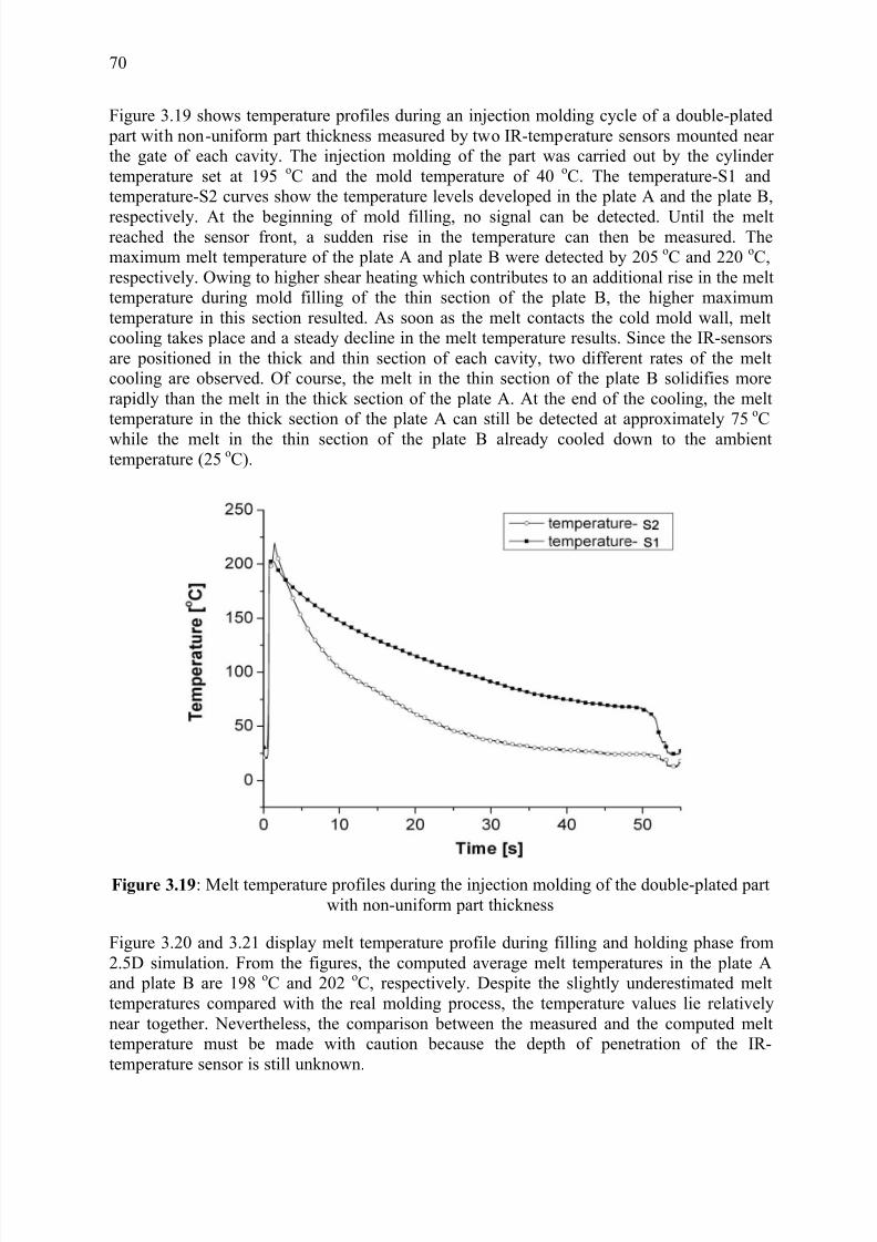
7/27/2019 Injection Mould Design
http://slidepdf.com/reader/full/injection-mould-design 88/160
70
Figure 3.19 shows temperature profiles during an injection molding cycle of a double-plated part with non-uniform part thickness measured by two IR-temperature sensors mounted near the gate of each cavity. The injection molding of the part was carried out by the cylinder temperature set at 195 oC and the mold temperature of 40 oC. The temperature-S1 andtemperature-S2 curves show the temperature levels developed in the plate A and the plate B,
respectively. At the beginning of mold filling, no signal can be detected. Until the meltreached the sensor front, a sudden rise in the temperature can then be measured. Themaximum melt temperature of the plate A and plate B were detected by 205 oC and 220 oC,respectively. Owing to higher shear heating which contributes to an additional rise in the melttemperature during mold filling of the thin section of the plate B, the higher maximumtemperature in this section resulted. As soon as the melt contacts the cold mold wall, meltcooling takes place and a steady decline in the melt temperature results. Since the IR-sensorsare positioned in the thick and thin section of each cavity, two different rates of the meltcooling are observed. Of course, the melt in the thin section of the plate B solidifies morerapidly than the melt in the thick section of the plate A. At the end of the cooling, the melttemperature in the thick section of the plate A can still be detected at approximately 75 oC
while the melt in the thin section of the plate B already cooled down to the ambienttemperature (25 oC).
Figure 3.19: Melt temperature profiles during the injection molding of the double-plated partwith non-uniform part thickness
Figure 3.20 and 3.21 display melt temperature profile during filling and holding phase from2.5D simulation. From the figures, the computed average melt temperatures in the plate Aand plate B are 198 oC and 202 oC, respectively. Despite the slightly underestimated melttemperatures compared with the real molding process, the temperature values lie relativelynear together. Nevertheless, the comparison between the measured and the computed melttemperature must be made with caution because the depth of penetration of the IR-temperature sensor is still unknown.
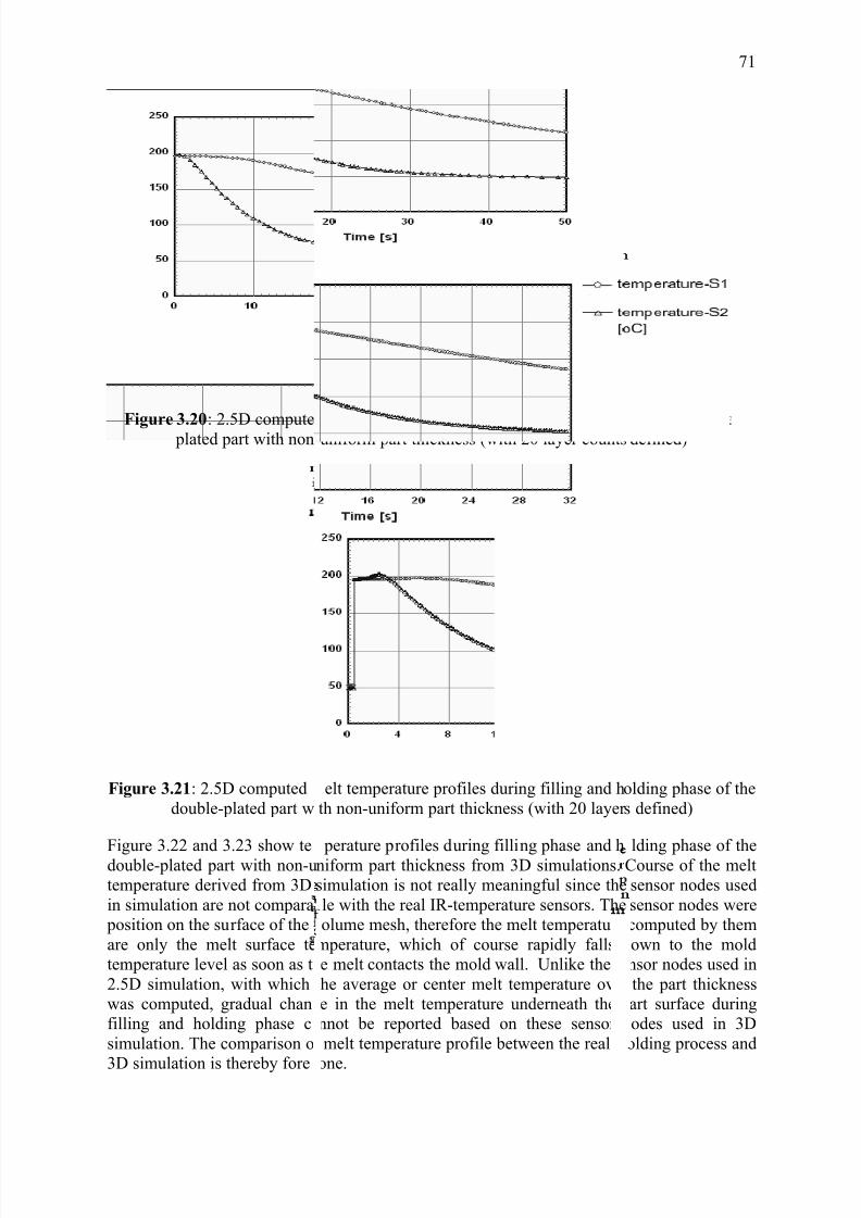
7/27/2019 Injection Mould Design
http://slidepdf.com/reader/full/injection-mould-design 89/160
Figure 3.20: 2.5D compute plated part with non
Figure 3.21: 2.5D computeddouble-plated part w
Figure 3.22 and 3.23 show tedouble-plated part with non-utemperature derived from 3Din simulation are not compara
position on the surface of theare only the melt surface tetemperature level as soon as t2.5D simulation, with whichwas computed, gradual chanfilling and holding phase csimulation. The comparison o
3D simulation is thereby fore
d melt temperature profiles during the moldi-uniform part thickness (with 20 layer counts
elt temperature profiles during filling and hth non-uniform part thickness (with 20 layer
perature profiles during filling phase and hniform part thickness from 3D simulations.simulation is not really meaningful since thele with the real IR-temperature sensors. Theolume mesh, therefore the melt temperature
mperature, which of course rapidly fallse melt contacts the mold wall. Unlike the s
the average or center melt temperature ovee in the melt temperature underneath thennot be reported based on these sensor melt temperature profile between the real
one.
71
g of the double-defined)
olding phase of thes defined)
lding phase of theCourse of the meltsensor nodes usedsensor nodes werecomputed by themown to the moldnsor nodes used inthe part thicknessart surface duringodes used in 3D
olding process and
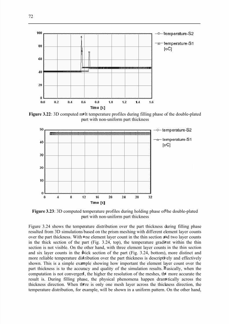
7/27/2019 Injection Mould Design
http://slidepdf.com/reader/full/injection-mould-design 90/160
72
Figure 3.22: 3D computed m p
Figure 3.23: 3D computed t p
Figure 3.24 shows the temperesulted from 3D simulationsover the part thickness. Within the thick section of the psection is not visible. On theand six layer counts in the tmore reliable temperature disshown. This is a simple exa
part thickness is to the accur computation is not convergenresult is. During filling pha
thickness direction. When thtemperature distribution, for e
lt temperature profiles during filling phase oart with non-uniform part thickness
emperature profiles during holding phase of art with non-uniform part thickness
rature distribution over the part thickness d based on the prism meshing with different elne element layer count in the thin section a
art (Fig. 3.24, top), the temperature gradiother hand, with three element layer countsick section of the part (Fig. 3.24, bottom),ribution over the part thickness is descripti ple showing how important the element laacy and quality of the simulation results., the higher the resolution of the meshes, thse, the physical phenomena happen dram
re is only one mesh layer across the thick xample, will be shown in a uniform pattern.
f the double-plated
he double-plated
uring filling phaseement layer countsd two layer countsnt within the thinin the thin sectionmore distinct and
ely and effectivelyyer count over theasically, when themore accurate thetically across the
ness direction, theOn the other hand,

7/27/2019 Injection Mould Design
http://slidepdf.com/reader/full/injection-mould-design 91/160
when the part is meshed intdistribution will be shown wimore physical phenomena wilthe suitable mesh resolution f
Figure 3.24: Temperature dis
In conclusion, it is well-knosimulation and experimental r simple in form and relatively
by 2.5D simulation, whichsimple flow. Contrary to 2.5thickness introduced in this s
failed to predict course of theflow pattern within the cavit
many layers across the thickness directioth high value portion in the middle of thel be taken into account during the process. Tr numerical simulation is one of the most cr
ribution during filling phase with prism mes6 layers
n from the former studies that better agreesult can be generally expected [78]. If theuniform in thickness, reasonable solutionsis proved in this study to be sufficient fosimulation, with the double-plated part wit
udy, 3D simulation based on non-isotherm
pressure during filling and hence malfuncties. This is probably due to some assumpti
73
n, the temperatureayers. That meanserefore, setting upcial factors.
a)
b)a): 1-2 and b): 3-
ment between 3Dart to be molded isre also achievable predicting such anon-uniform part
l computation has
ned to foretell theons required to be

7/27/2019 Injection Mould Design
http://slidepdf.com/reader/full/injection-mould-design 92/160
74
made in the governing equations as well as numerical difficulties and inaccuracies that arelikely to appear when the real molding conditions deviate much from the assumptions madeor when the molded part is highly complex. With the separated parts with non-uniform partthickness, however, non-isothermal based 3D computation of Moldex3D® has been proved to
be reliable in predicting the flow behavior of the polymer melt in injection molding process
and particularly in predicting the temperature distribution across the part thickness when thenumber of mesh layer count is chosen properly. Credible melt temperature prediction is oneof the utmost conditions especially when the back injection of a film is to be handled. Bythese reasons, non-isothermal based 3D computation of Moldex3D® will be used for thesimulation on the injection in-mold labeling which will be discussed later in Chapter 5 and 6.
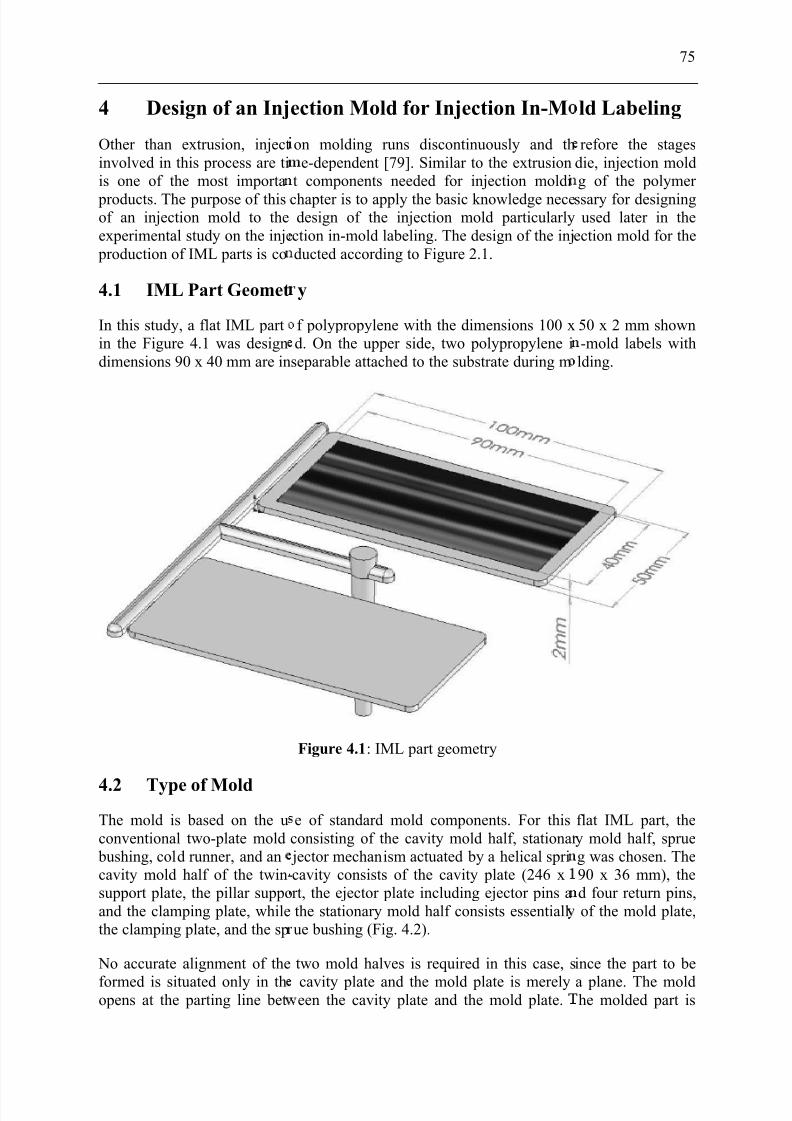
7/27/2019 Injection Mould Design
http://slidepdf.com/reader/full/injection-mould-design 93/160
4 Design of an Inj
Other than extrusion, injectinvolved in this process are tiis one of the most importa
products. The purpose of thisof an injection mold to theexperimental study on the inje
production of IML parts is co
4.1 IML Part Geomet
In this study, a flat IML partin the Figure 4.1 was designdimensions 90 x 40 mm are in
4.2 Type of Mold
The mold is based on the uconventional two-plate mold
bushing, cold runner, and ancavity mold half of the twin-support plate, the pillar suppoand the clamping plate, whilethe clamping plate, and the sp
No accurate alignment of the
formed is situated only in thopens at the parting line bet
ection Mold for Injection In-M
on molding runs discontinuously and the-dependent [79]. Similar to the extrusion
t components needed for injection moldi
chapter is to apply the basic knowledge necedesign of the injection mold particularly
ction in-mold labeling. The design of the injducted according to Figure 2.1.
y
f polypropylene with the dimensions 100 xd. On the upper side, two polypropylene iseparable attached to the substrate during m
Figure 4.1: IML part geometry
e of standard mold components. For thisconsisting of the cavity mold half, stationar jector mechanism actuated by a helical spricavity consists of the cavity plate (246 xrt, the ejector plate including ejector pins athe stationary mold half consists essentiallue bushing (Fig. 4.2).
two mold halves is required in this case, s
cavity plate and the mold plate is merelyeen the cavity plate and the mold plate.
75
ld Labeling
refore the stagesdie, injection moldg of the polymer
ssary for designingused later in the
ection mold for the
50 x 2 mm shown-mold labels withlding.
flat IML part, they mold half, sprueg was chosen. The90 x 36 mm), thed four return pins,of the mold plate,
ince the part to be
a plane. The moldhe molded part is
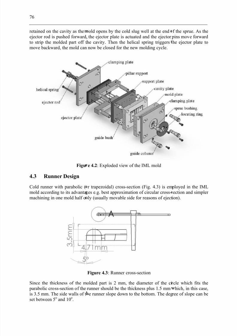
7/27/2019 Injection Mould Design
http://slidepdf.com/reader/full/injection-mould-design 94/160
76
retained on the cavity as theejector rod is pushed forward,to strip the molded part off tmove backward, the mold can
Figu
4.3 Runner Design
Cold runner with parabolic (mold according to its advantamachining in one mold half o
Since the thickness of the m parabolic cross-section of the
is 3.5 mm. The side walls of tset between 5o and 10o.
old opens by the cold slug well at the endthe ejector plate is actuated and the ejector
he cavity. Then the helical spring triggersnow be closed for the new molding cycle.
e 4.2: Exploded view of the IML mold
r trapezoidal) cross-section (Fig. 4.3) is emes e.g. best approximation of circular cross-ly (usually movable side for reasons of eject
Figure 4.3: Runner cross-section
olded part is 2 mm, the diameter of the cirunner should be the thickness plus 1.5 mm
e runner slope down to the bottom. The deg
f the sprue. As the pins move forwardhe ejector plate to
ployed in the IMLection and simpler ion).
cle which fits thehich, in this case,
ree of slope can be
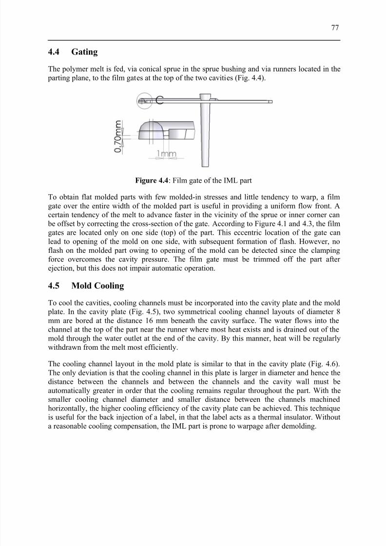
7/27/2019 Injection Mould Design
http://slidepdf.com/reader/full/injection-mould-design 95/160
77
4.4 Gating
The polymer melt is fed, via conical sprue in the sprue bushing and via runners located in the parting plane, to the film gates at the top of the two cavities (Fig. 4.4).
Figure 4.4: Film gate of the IML part
To obtain flat molded parts with few molded-in stresses and little tendency to warp, a filmgate over the entire width of the molded part is useful in providing a uniform flow front. Acertain tendency of the melt to advance faster in the vicinity of the sprue or inner corner can
be offset by correcting the cross-section of the gate. According to Figure 4.1 and 4.3, the filmgates are located only on one side (top) of the part. This eccentric location of the gate canlead to opening of the mold on one side, with subsequent formation of flash. However, noflash on the molded part owing to opening of the mold can be detected since the clampingforce overcomes the cavity pressure. The film gate must be trimmed off the part after ejection, but this does not impair automatic operation.
4.5 Mold Cooling
To cool the cavities, cooling channels must be incorporated into the cavity plate and the mold plate. In the cavity plate (Fig. 4.5), two symmetrical cooling channel layouts of diameter 8mm are bored at the distance 16 mm beneath the cavity surface. The water flows into thechannel at the top of the part near the runner where most heat exists and is drained out of themold through the water outlet at the end of the cavity. By this manner, heat will be regularlywithdrawn from the melt most efficiently.
The cooling channel layout in the mold plate is similar to that in the cavity plate (Fig. 4.6).The only deviation is that the cooling channel in this plate is larger in diameter and hence the
distance between the channels and between the channels and the cavity wall must beautomatically greater in order that the cooling remains regular throughout the part. With thesmaller cooling channel diameter and smaller distance between the channels machinedhorizontally, the higher cooling efficiency of the cavity plate can be achieved. This techniqueis useful for the back injection of a label, in that the label acts as a thermal insulator. Withouta reasonable cooling compensation, the IML part is prone to warpage after demolding.

7/27/2019 Injection Mould Design
http://slidepdf.com/reader/full/injection-mould-design 96/160
78
Figure 4.5:
Figure 4.6
4.6 Part Release/Ejec
Figure 4.7 illustrates the cavivacuum nozzles, each of whithe mold filling. In addition,required to strip the molded p
ejector system. During moldmold cavity is absolutely cle
Cavity plate with the cooling channel layou
: Mold plate with the cooling channel layout
ion
ty plate of the IML mold. Each cavity is eh is occupied by a sintered metal for holdifour ejector pins in the cavity and other sirt off the mold. The part is ejected by mea
losing, the return pins press the ejector platred and the ejector pins are not damaged b
uipped with threeg the label duringin the runner are
s of the machine’s
es back so that they the melt stream.
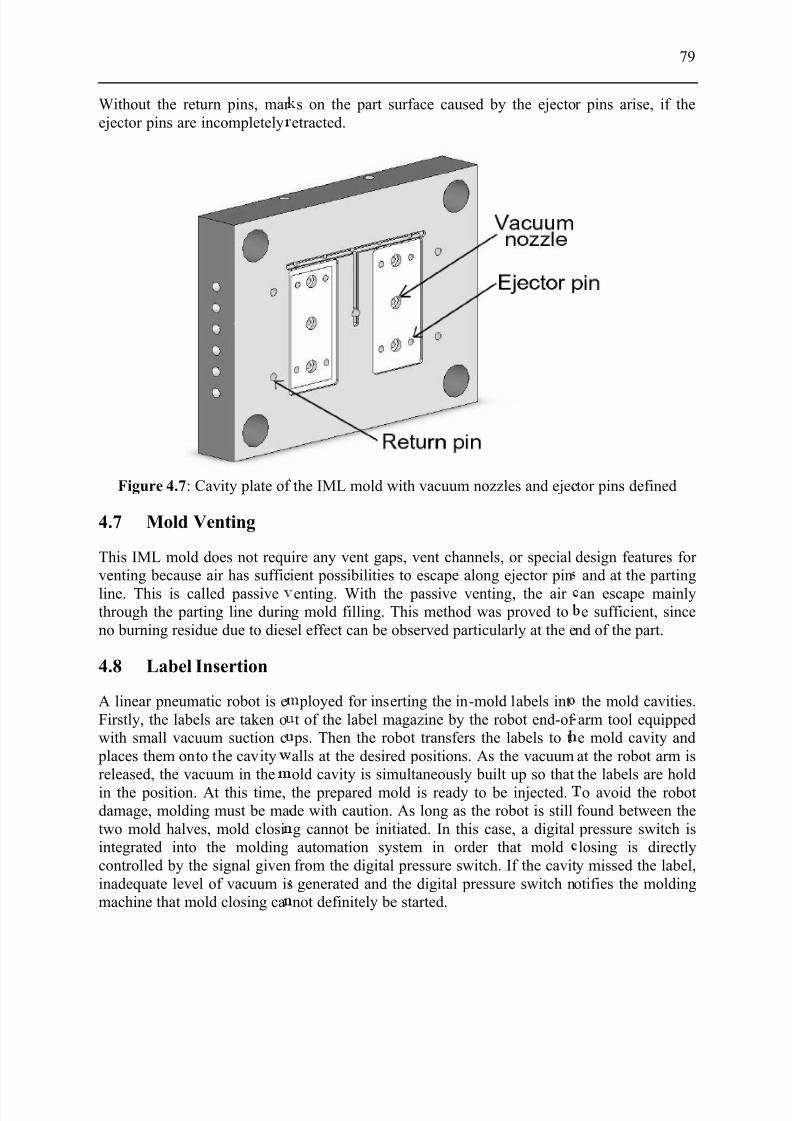
7/27/2019 Injection Mould Design
http://slidepdf.com/reader/full/injection-mould-design 97/160
Without the return pins, mar ejector pins are incompletely
Figure 4.7: Cavity plate of
4.7 Mold Venting
This IML mold does not requventing because air has suffic
line. This is called passivethrough the parting line durinno burning residue due to dies
4.8 Label Insertion
A linear pneumatic robot is eFirstly, the labels are taken owith small vacuum suction c
places them onto the cavityreleased, the vacuum in thein the position. At this time,damage, molding must be matwo mold halves, mold closiintegrated into the moldingcontrolled by the signal giveninadequate level of vacuum ismachine that mold closing ca
s on the part surface caused by the ejectoetracted.
the IML mold with vacuum nozzles and ejec
ire any vent gaps, vent channels, or specialient possibilities to escape along ejector pin
enting. With the passive venting, the air g mold filling. This method was proved toel effect can be observed particularly at the e
ployed for inserting the in-mold labels intt of the label magazine by the robot end-of ps. Then the robot transfers the labels to talls at the desired positions. As the vacuumold cavity is simultaneously built up so thatthe prepared mold is ready to be injected.de with caution. As long as the robot is stillg cannot be initiated. In this case, a digitalautomation system in order that moldfrom the digital pressure switch. If the cavitgenerated and the digital pressure switch n
not definitely be started.
79
r pins arise, if the
tor pins defined
design features for and at the parting
an escape mainlye sufficient, since
nd of the part.
the mold cavities.arm tool equippede mold cavity andat the robot arm isthe labels are holdo avoid the robot
found between the pressure switch islosing is directlyy missed the label,otifies the molding

7/27/2019 Injection Mould Design
http://slidepdf.com/reader/full/injection-mould-design 98/160
80
5 Simulation and
Mold Labeling
5.1 Simulation on the
5.1.1 Mesh Generation
One of the key steps of thgeneration. Once the part mwere successfully created, 3Dthis study, the generation of
plug-in for Moldex3D®. Firstland runners were meshed wit
Two sensor nodes are place
sensors are mounted in the incombined pressure and tempinjected mold half, the first saway from the film gate. Themeasured from the end of thewere discretized using rod elmodels can be exported toconditions e.g. melt injectiosimulation can be conducted
Figure
The number of the part elemeis 4,084 prism elements. Mol
5.1.2 Viscosity Model
As injected material, polyproThe viscosity function and thmaterial databank are shown ithe parameter listed in Table
from BASF was also used in smaterials regarding the part w
Experimental Study on the Inje
rocess
Injection In-Mold Labeling
finite element method for numerical codel (usually 3D-CAD model) and the opti-mesh can be generated based on the createhe part and mesh model was performed usy, the IML part model along with the labels prism and tetrahedral elements, respectivel
onto the mesh model at corresponding p
ection mold, namely on the side without laberature sensor used in the injection moldiensor can be found at approximately 20 %econd one was placed at approximately 20cavity. Subsequently, the cooling channelsments and tetrahedral elements, respectivel
oldex3D®, the injection point and the n point must be defined. Finally, 3D no
ith Moldex3D®.
.1: Mesh model of the IML part and mold
t is 73,594, whereas the total number of the base was meshed with 386,794 tetrahedral e
ylene type Novolen 3200 MC supplied by pVT-diagram of the used material derivedn Figure 3.2. Simulations on the IML were c5.1. In addition to polypropylene, polystyre
ome experiments in order to make the comparpage of the injected IML parts.
ction In-
putation is meshum surface mesh
d surface mesh. Inng Rhinoceros®, as well as the sprue(Fig. 5.1).
ositions where the
el. It is a so-calledg process. In theof the part lengthof the part length
and the mold base. Before the mesh
ecessary boundary-isothermal based
two label elementslements.
ASF was applied.rom Moldex3D®’sarried out based onne 158 K supplied
rison between two
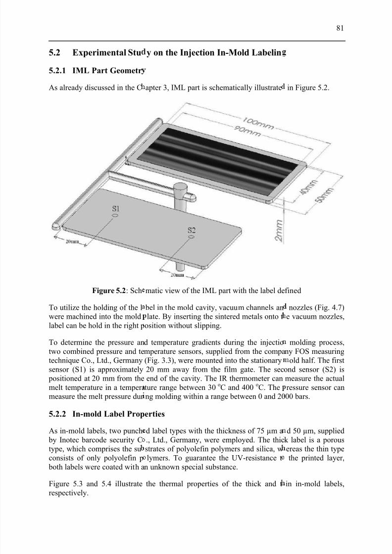
7/27/2019 Injection Mould Design
http://slidepdf.com/reader/full/injection-mould-design 99/160
5.2 Experimental Stu
5.2.1 IML Part Geometr
As already discussed in the C
Figure 5.2: Sch
To utilize the holding of the lwere machined into the moldlabel can be hold in the right p
To determine the pressure antwo combined pressure and tetechnique Co., Ltd., Germanysensor (S1) is approximately
positioned at 20 mm from the
melt temperature in a temperameasure the melt pressure dur
5.2.2 In-mold Label Prop
As in-mold labels, two punch by Inotec barcode security Ctype, which comprises the suconsists of only polyolefin p
both labels were coated with a
Figure 5.3 and 5.4 illustraterespectively.
y on the Injection In-Mold Labelin
apter 3, IML part is schematically illustrate
matic view of the IML part with the label de
bel in the mold cavity, vacuum channels anlate. By inserting the sintered metals onto t
osition without slipping.
d temperature gradients during the injectiomperature sensors, supplied from the compa(Fig. 3.3), were mounted into the stationary20 mm away from the film gate. The secend of the cavity. The IR thermometer can
ture range between 30o
C and 400o
C. Theng molding within a range between 0 and 20
erties
d label types with the thickness of 75 µm a., Ltd., Germany, were employed. The thicstrates of polyolefin polymers and silica, wlymers. To guarantee the UV-resistance t
n unknown special substance.
the thermal properties of the thick and t
81
in Figure 5.2.
fined
nozzles (Fig. 4.7)e vacuum nozzles,
molding process,ny FOS measuring
old half. The firstond sensor (S2) ismeasure the actual
ressure sensor can00 bars.
d 50 µm, suppliedk label is a porousereas the thin typethe printed layer,
in in-mold labels,
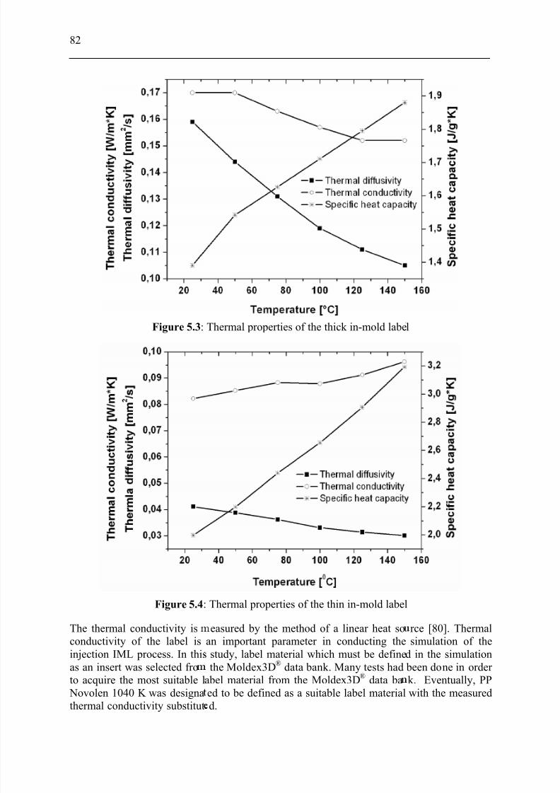
7/27/2019 Injection Mould Design
http://slidepdf.com/reader/full/injection-mould-design 100/160
82
Figure 5.3:
Figure 5.4:
The thermal conductivity isconductivity of the label isinjection IML process. In thisas an insert was selected froto acquire the most suitable l
Novolen 1040 K was designathermal conductivity substitut
Thermal properties of the thick in-mold labe
Thermal properties of the thin in-mold label
easured by the method of a linear heat soan important parameter in conducting thestudy, label material which must be definethe Moldex3D® data bank. Many tests had
abel material from the Moldex3D® data ba
ed to be defined as a suitable label materiald.
l
rce [80]. Thermalsimulation of the
d in the simulation been done in order k. Eventually, PP
with the measured
7/27/2019 Injection Mould Design
http://slidepdf.com/reader/full/injection-mould-design 101/160
83
5.2.3 Design of Experiments
Usually, in injection molding process there are many different machine and process parameters responsible for the properties of the injection molded parts. Changes in parameters such as melt temperature, mold temperature, and injection velocity affect the
orientation, mechanical properties or even the surface roughness of the molded part. Thus theinjection molding technique forms a nonlinear, complex, multi-variable process, in which theinfluences of the parameters superimpose on the quality criteria. During the optimization of the injection molding process, the task consists of analyzing the magnitude of the influence of the individual parameters on the quality criteria and determining the connection betweensingle parameters and the quality criteria. Experiences from the earlier studies have shownthat the following parameters are important: injection velocity, holding pressure, cylinder temperature, holding switch, and mold temperature.
According to this knowledge, following parameters were selected in order to carry outsystematic experiments. As the normal setting (IML1), the experiment was carried out with
the following parameters:• Holding pressure: 500 bar
• Injection velocity: 50 %
• Cylinder temperature: 195 oC
• Mold temperature: 40 oC on the two mold halves, and
• Holding switch: 98 % filled volume
In addition, holding time and cooling time were entirely set at the constant values of 8 and 9
seconds, respectively.Table 5.1 shows the list of the IML experimental studies. Compared to the normal setting(IML1) holding pressure was varied by the IML2 and IML3 experiments. In IML4 and IML5,injection velocity was changed, whereas the holding switch was differently set in IML6 andIML7. Cylinder temperature was also varied in IML8 and IML9 experiments. Moldtemperature variation was performed by IML10 to IML13 experiments.
7/27/2019 Injection Mould Design
http://slidepdf.com/reader/full/injection-mould-design 102/160
84
Experiment Parameter setting Detail Remark
IML1 Normal setting 40 oC/40 oC stationary/moving plate
IML2 Holding pressure variation 400 bar
IML3 Holding pressure variation 600 bar
IML4 Injection velocity variation 30 %
IML5 Injection velocity variation 70 %
IML6 Holding switch variation 90 %
IML7 Holding switch variation 95 %
IML8 Cylinder temperature variation 180o
C
IML9 Cylinder temperature variation 210 oC
IML10 Mold temperature variation 35 oC/60 oC stationary/moving plate
IML11 Mold temperature variation 60 oC/35 oC stationary/moving plate
IML12 Mold temperature variation 35 oC/70 oC stationary/moving plate
IML13 Mold temperature variation 70 oC/35 oC stationary/moving plate
Table 5.1: List of the IML experimental studies
7/27/2019 Injection Mould Design
http://slidepdf.com/reader/full/injection-mould-design 103/160
85
6 IML-Simulation and Experimental Results
6.1 Melt Front Advancement
Figure 6.1 shows the melt front advancement from the short-shot study conducted with IML1
molding parameters but without holding pressure compared with that from 3D simulation.
Figure 6.1: Short-shot study from the real process and simulation
30 % filled
40 % filled
80 % filled
90 % filled
100 % filled
7/27/2019 Injection Mould Design
http://slidepdf.com/reader/full/injection-mould-design 104/160
86
From the short-shot study, it is obvious that the melt front advancement at each filling step of simulation agrees well with the advancement from the real molding process. At the beginningthe melt flows symmetrically into both cavities through the film gate. Despite the film gates,
both cavities were filled first from the inner corners of the part at the beginning of the filling phase. This resulted from the failure to optimize the cross-section of the film gates and from
the shear heating of the melt occurring especially at the runner wall and at the corner of thecold runner. In course of filling, the flow fronts at the outer edges advance faster, so that thecavities were filled nearly parallel to the film gate. In addition, it can be seen that startingfrom an 80 % filled volume the melt front in the right cavity slightly outruns the left cavity.This is due to the shallow window, electrically discharged onto the right cavity which helpsfixing the label during molding, which causes the slightly reduced flow resistance in the rightcavity. Therefore the right cavity was completely filled with extremely small time difference
before the left cavity. In this case, the right cavity which was already filled had experiencedthe excessive holding pressure, which caused the unnecessary stress to the molded part. In thesimulation, however, such difference of the melt front advancement in the cavities is notnoticeable.
6.2 Course of the Pressure
Figure 6.2: Pressure profiles during the injection IML
Figure 6.2 to 6.4 show pressure profiles during filling phase from the experiment and 3Dsimulation conducted with IML1 molding parameters.
The maximum pressures at the end of filling phase, determined using two sensor nodes placed at the comparable positions where the IR temperature sensors are mounted in themold, were defined by 91 (S1) and 26 (S2) bars, respectively, while the measured pressure
peaks from the 1st
and the 2nd
sensors lied with approximately 150 and 50 bars. Comparingthe values from the 1st sensors, it can be stated that despite the underestimated pressure from
7/27/2019 Injection Mould Design
http://slidepdf.com/reader/full/injection-mould-design 105/160
3D simulation, the pressuretogether. From the experimeresults from the excessive holthe end of holding phase, thevolume constraint from the c
values increase. Concerningmolding with the hydraulic
pressure is apparently too higParts that have experienced thigh residual stresses and he
pressure with gradually reduc
Figure 6.3: Expande
Figure
alues from the experiment and simulationt, there is a small kink on the 1st sensor pding pressure and the compressibility of thecompressed melt becomes more relaxed andavity against the front of the sensor. By thi
he excessive holding pressure, holding was pressure which was entirely set at 500 b, not for holding switch itself but for the whe excessive holding pressure during moldice are prone to warpage. To cope with thid values should be set instead.
d pressure profiles of filling phase (filling ti
6.4: Pressure profiles from 3D simulation
87
lay relatively near essure curve. This polymer melt. Atexpanded with the
s way the pressure
performed duringars. This constantole holding period.ng usually contains, profiled holding
e 0.66 s)
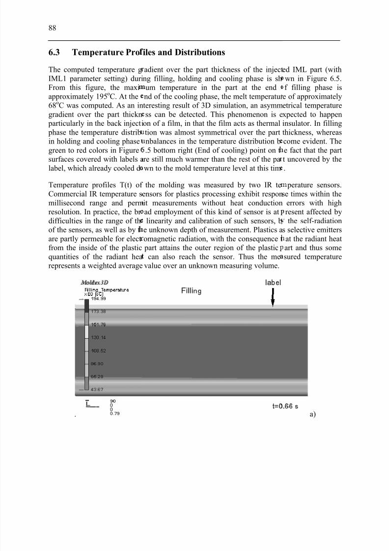
7/27/2019 Injection Mould Design
http://slidepdf.com/reader/full/injection-mould-design 106/160
88
6.3 Temperature Pro
The computed temperature gIML1 parameter setting) duriFrom this figure, the maxi
approximately 195o
C. At the68oC was computed. As an ingradient over the part thickn
particularly in the back injecti phase the temperature distribin holding and cooling phasegreen to red colors in Figuresurfaces covered with labels alabel, which already cooled d
Temperature profiles T(t) of
Commercial IR temperature smillisecond range and permresolution. In practice, the br difficulties in the range of thof the sensors, as well as by tare partly permeable for electfrom the inside of the plasticquantities of the radiant hearepresents a weighted average
iles and Distributions
adient over the part thickness of the injectng filling, holding and cooling phase is shum temperature in the part at the end
nd of the cooling phase, the melt temperatur teresting result of 3D simulation, an asymmss can be detected. This phenomenon is e
on of a film, in that the film acts as thermaltion was almost symmetrical over the partnbalances in the temperature distribution b.5 bottom right (End of cooling) point on tre still much warmer than the rest of the pawn to the mold temperature level at this tim
the molding was measured by two IR te
ensors for plastics processing exhibit responit measurements without heat conductionad employment of this kind of sensor is atlinearity and calibration of such sensors, b
e unknown depth of measurement. Plastics aomagnetic radiation, with the consequence t part attains the outer region of the plastic
can also reach the sensor. Thus the mevalue over an unknown measuring volume.
ed IML part (withwn in Figure 6.5.f filling phase is
e of approximatelyetrical temperaturexpected to happeninsulator. In fillingthickness, whereascome evident. Thee fact that the partt uncovered by the.
perature sensors.
se times within theerrors with highresent affected bythe self-radiation
s selective emittersat the radiant heatart and thus somesured temperature
a)
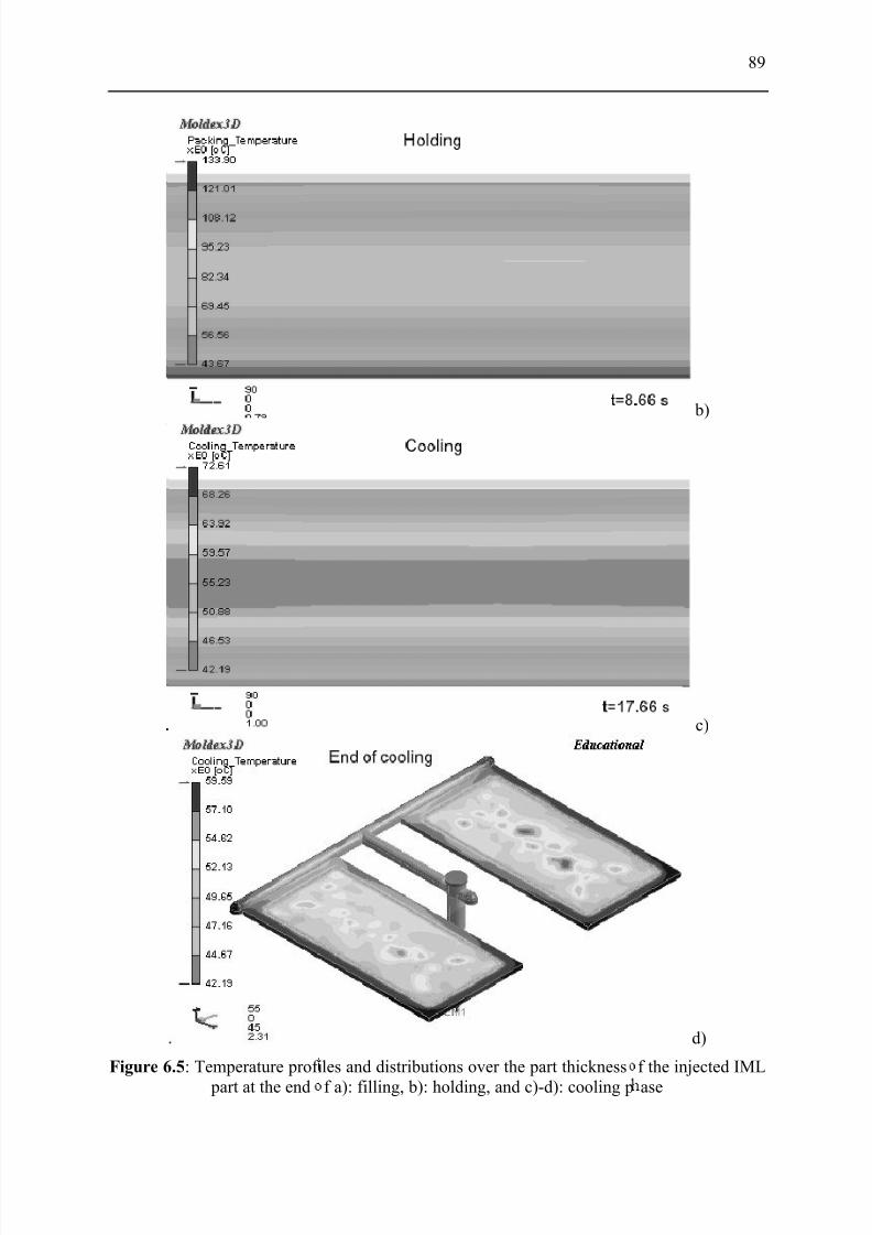
7/27/2019 Injection Mould Design
http://slidepdf.com/reader/full/injection-mould-design 107/160
Figure 6.5: Temperature profi
part at the end
les and distributions over the part thickness
f a): filling, b): holding, and c)-d): cooling p
89
b)
c)
d)
f the injected IML
ase

7/27/2019 Injection Mould Design
http://slidepdf.com/reader/full/injection-mould-design 108/160
90
Figure 6.6: Temperature profiles during the injection IML
Figure 6.6 shows temperature profiles during the injection molding of the part molded with
IML1 molding parameters. From Figure 6.6, the maximum melt temperature, detected near the gate (1st sensor) is approximately 230 oC, whereas the temperature peak measured awayfrom the gate (2nd sensor) is 220 oC. Compared with those determined from 3D simulation,the maximum temperatures lay relative near together. Because of the unknown depth of measurement of the IR sensors, a comparison of the temperature gradients from experimentand simulation is foregone at this state.
6.4 Structure of an Injected IML Part
In-mold labeling as one of the film insert molding techniques offers many benefits in terms of production time and cost savings as well as esthetics of the products. However, this molding
technique has one main drawback, in that the molded parts prone to warpage as a result of anasymmetric cooling process. And because the morphology differentiation over the partthickness of the injection molded part has a tremendous influence on the mechanical behavior of the part, it is necessary to investigate the structure of the IML part closely.
Figure 6.7 illustrates crystalline structures as well as amorphous layer of the IML part. Under the light microscope, four different zones in the IML part can be distinguished. On the labelside, porous label structure as well as fine and crystalline structures can be seen, respectively.In the middle of the IML part, crystalline structure (spherulites) can only be found, whereasthe amorphous layer in addition to the fine and course crystalline structures can be detectedon the opposite side.
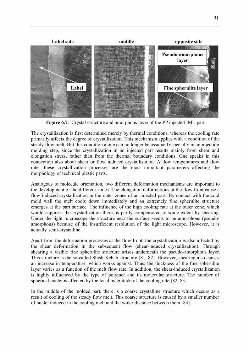
7/27/2019 Injection Mould Design
http://slidepdf.com/reader/full/injection-mould-design 109/160
91
Figure 6.7: Crystal structure and amorphous layer of the PP injected IML part
The crystallization is first determined merely by thermal conditions, whereas the cooling rate primarily affects the degree of crystallization. This mechanism applies with a condition of thesteady flow melt. But this condition alone can no longer be assumed especially in an injectionmolding step, since the crystallization in an injected part results mainly from shear andelongation stress, rather than from the thermal boundary conditions. One speaks in thisconnection also about shear or flow induced crystallization. At low temperatures and flowrates these crystallization processes are the most important parameters affecting themorphology of technical plastic parts.
Analogous to molecule orientation, two different deformation mechanisms are important tothe development of the different zones. The elongation deformations at the flow front cause aflow induced crystallization in the outer zones of an injected part. By contact with the coldmold wall the melt cools down immediately and an extremely fine spherulite structureemerges at the part surface. The influence of the high cooling rate at the outer zone, whichwould suppress the crystallization there, is partly compensated to some extent by shearing.Under the light microscope the structure near the surface seems to be amorphous (pseudo-amorphous) because of the insufficient resolution of the light microscope. However, it isactually semi-crystalline.
Apart from the deformation processes at the flow front, the crystallization is also affected by
the shear deformation in the subsequent flow (shear-induced crystallization). Throughshearing a visible fine spherulite structure arises underneath the pseudo-amorphous layer.This structure is the so-called Shish-Kebab structure [81, 82]. However, shearing also causesan increase in temperature, which works against. Thus, the thickness of the fine spherulitelayer varies as a function of the melt flow rate. In addition, the shear-induced crystallizationis highly influenced by the type of polymer and its molecular structure. The number of spherical nuclei is affected by the local magnitude of the cooling rate [82, 83].
In the middle of the molded part, there is a coarse crystalline structure which occurs as aresult of cooling of the steady flow melt. This coarse structure is caused by a smaller number of nuclei induced in the cooling melt and the wider distance between them [84].
Label side middle opposite side
Label
Pseudo-amorphous
layer
Fine spherulite layer
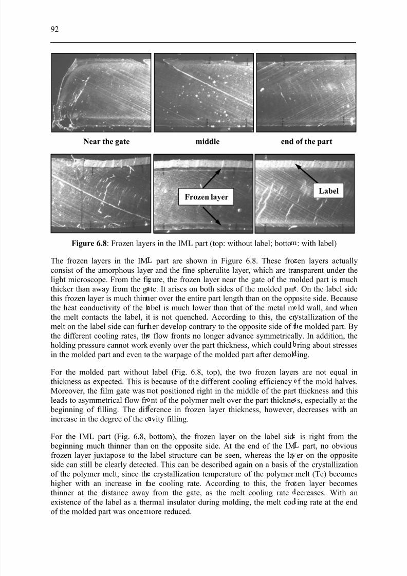
7/27/2019 Injection Mould Design
http://slidepdf.com/reader/full/injection-mould-design 110/160
92
Near the gate
Figure 6.8: Frozen laye
The frozen layers in the IMconsist of the amorphous layelight microscope. From the fithicker than away from the gthis frozen layer is much thinthe heat conductivity of the lthe melt contacts the label, itmelt on the label side can furtthe different cooling rates, thholding pressure cannot work in the molded part and even to
For the molded part withoutthickness as expected. This isMoreover, the film gate was
leads to asymmetrical flow fr beginning of filling. The dif increase in the degree of the c
For the IML part (Fig. 6.8, beginning much thinner thanfrozen layer juxtapose to theside can still be clearly detectof the polymer melt, since thhigher with an increase in tthinner at the distance away
existence of the label as a theof the molded part was once
middle end
rs in the IML part (top: without label; botto
part are shown in Figure 6.8. These fror and the fine spherulite layer, which are traure, the frozen layer near the gate of the mte. It arises on both sides of the molded par er over the entire part length than on the opp bel is much lower than that of the metal m
is not quenched. According to this, the cr er develop contrary to the opposite side of tflow fronts no longer advance symmetrical
evenly over the part thickness, which couldthe warpage of the molded part after demol
label (Fig. 6.8, top), the two frozen layer because of the different cooling efficiencyot positioned right in the middle of the part
nt of the polymer melt over the part thickneerence in frozen layer thickness, however,vity filling.
bottom), the frozen layer on the label sidon the opposite side. At the end of the IMlabel structure can be seen, whereas the laed. This can be described again on a basis o
crystallization temperature of the polymer e cooling rate. According to this, the frofrom the gate, as the melt cooling rate
rmal insulator during molding, the melt cooore reduced.
Frozen layer
of the part
: with label)
en layers actuallynsparent under theolded part is much. On the label sideosite side. Becauseld wall, and whenstallization of thee molded part. By
ly. In addition, thering about stressesing.
s are not equal inf the mold halves.thickness and this
s, especially at thedecreases with an
is right from the part, no obvious
er on the oppositethe crystallization
melt (Tc) becomesen layer becomesecreases. With an
ing rate at the end
Label
7/27/2019 Injection Mould Design
http://slidepdf.com/reader/full/injection-mould-design 111/160
Figure 6
Figure 6.9 shows the frozentemperature settings. There a
parts molded with thick and tthe two frozen layers, one onside (stationary mold half) wseen from Figure 6.9, in geexplicitly thicker than on the
between the polymer melt andmold half of the part molded
thick label, since the label actof the thick labels (Fig. 5.4 anthick label is somewhat thinnthe thickness of the label itselmelt. Rule of thumb is, the thi
With the mold wall temperatfrozen layer thickness can bewarpage of the IML part.temperature on the label sisomewhat thicker than that g
the opposite side is thinner.side (Tw35/60 and Tw35/70
F r o z e n l a y e r t h i c k n e s s [ m
m ]
*Tw stationar
.9: Frozen layer thickness of the IML partslayer thickness of the IML part injectede three types of samples namely parts injein labels, respectively. For each type of samthe label side (moving mold half) and anotre measured at comparable distance from teral, the frozen layers on the opposite silabel side. This resulted from the high temthe cold mold wall. In addition, the frozen lwithout label is much thicker than parts mo
as a thermal insulator. Despite the higher td 5.5), the frozen layer on the label side of ter than that of the IML part with thin label.f that also affects, to a large extent, the coolcker the label, the better it is to be a thermal i
re combinations (different mold half tempeconsiderably influenced with the expectatioThe experimental results show that wite (Tw60/35 and Tw70/35) the frozen laynerated by the IML1 setting. As expected,
o the contrary, with the higher mold tempe, the frozen layer is thinner on this side
mold half/moving mold half
93
ith different moldcted without label,les, thicknesses of er on the oppositee gate. As can be
e of the label areerature differenceyer on the movinglded with thin and
ermal conductivitye part molded withThis is because of ing of the polymer nsulator.
ature settings), then to cope with the
the lower molder on this side ishe frozen layer on
rature on the labelnd thicker on the
7/27/2019 Injection Mould Design
http://slidepdf.com/reader/full/injection-mould-design 112/160
94
opposite side. The effect of thwill be descriptively discusse
Figure 6.10: Fr
Figure 6.10 shows the numeduring filling phase at differe
accomplished for three differ simulated at a mold temperatmold temperature combinatioconducted. All other moldinresults shown in Figure 6.10,mold temperature of 40 oCsomewhat thinner than on tthickness near the gate on thesimulation result agrees qualitof 70 oC on the label side anexhibits a smaller thickness c
frozen layer thickness on theother side. This indicates thatthe thermal boundary conditio
Figure 6.11: SEM microgra
e mold wall temperature combination on thein Chapter 6.5.
ozen layers and melting core from the simul
rical simulated frozen layers and the meltt mold temperature combination settings. 3
ent mold temperature combinations. Firstlyre of 40 oC on both mold halves. Then thof 35 oC/70 oC and 70 oC/35 oC (label side
parameters were kept constant. Accordinifferent thicknesses of the frozen layers can
on both mold halves, the frozen layer oe other side. In the real molding situatiolabel side is much thinner than on the other atively well with the real molding situation.
35 oC on the opposite side, the frozen layompared to that at the mold temperature of
label side increases, if this mold half is k 3D simulation program is able to consider sns qualitatively correct.
hs of IML parts (top: with thick label; botto
MFrozen layer
IML part warpage
tion
ng core occurringsimulations were
filling phase wasmolding with the
opposite side) wasto the simulation
be computed. At athe label side is
, the frozen layer ide. However, thisWith temperaturesr on the label side0 oC, whereas the
pt colder than thech asymmetries in
: with thin label)
Label
Label
elting core
7/27/2019 Injection Mould Design
http://slidepdf.com/reader/full/injection-mould-design 113/160
Figure 6.11 shows the SEMThe figures on the left are tnitrogen and then breaking icutting. As can be seen, thichas experienced the sudden
detached from the substrate astill tightly cling to the part.strength of the IML part in the
6.5 Warpage of an Inj
Warpage in association with tlocally shrinkage differentialsthickness [85]. The processinvolume relaxation and orientacontraction. Many dimension
also from the three dimensio part shrinkage. It is not easydepends on many parameter temperature, pressure and pr affect the shrinkage and warp
During the part shrinkage, acontraction in relation to the pinherent stress and crystallizat
parameters interact with eacTherefore, the effect between
Figure 6.12: Asymmetricalacross the
The internal stress can be maithermally induced stress is raitemperature in cooling proce
(Fig. 6.12). The flow inducecaused by shearing between
icrographs of the IML parts molded with the IML parts prepared by immersing the sto two pieces. On the right, the IML partsIML label remains adhere to the part surfa
mechanical load (breaking) whereas the t
ound the broken area. By cutting, both the tThis realization will be discussed later in asection 6.6 Modulus of elasticity.
ected IML Part
he injection molding develops as a result of in the flow and transverse direction, to the flg and the post-shrinkage are caused by theion relaxation of the molding material as wel errors result from the part warpage. By
al deviations from the cavity, which is deto predict the degree of part warpage, since
and environment. Besides the molding p perties of the polymer resin, stiffness andge of the molded part in a great value.
ditional mechanisms which lead to a decreure thermal expansion are also involved. Thion. The interaction of these parameters is v
other and are, at the same time, dependhe molding parameters would not be elabora
thermal-induced residual stress caused by unolded part thickness introduces part warpag
nly evoked by the cooling, expansion and flsed by a difference of mold wall temperatur s, and caused by a non-uniform cooling o
stress, shear stress or wall shear stress, onelt front and mold wall during filling phase
95
ck and thin labels.amples into liquidwere prepared by
ce even if the partin label has been
ick and thin labelsssociation with the
residual stresses or ow or over the partcrystallization, byl as by the thermalarpage one speaks
eloped during thethe warpage itself arameters such as
part thickness also
ase in the thermalse are for examplery complex. Soment on each other.ted on the details.
balanced cooling
w effect [85]. Theand polymer meltthe melt polymer
the other hand, ishich brings about
7/27/2019 Injection Mould Design
http://slidepdf.com/reader/full/injection-mould-design 114/160
96
orientations of macromolecules. The thermally induced stress is a dominant inherent stresswith respect to the stress magnitude [86]. The thermally induced stress leads to thedeformation of parts, whereas the flow induced stress causes anisotropy and optical
properties, affecting surface molding state of the parts. Figure 6.12 shows how a flat part becomes deformed through different cavity temperatures existing on the left and right sides.
Shrinkage is suppressed on the mold side with lower temperature, and the side with higher temperature undergoes more pronounced shrinkage. A type of bi-metal effect occurs [87].
The development of the inherent (internal) cooling stress which is described in a highlycomprehensible manner by Stitz's solidification model [89] is shown in Figure 6.13, righthand side. The pronounced temperature profile that prevails in the solidifying melt duringcooling (a) gives rise to a dissimilar thermal contraction potential in the different layers (b).The mechanical link that exists between the individual layers prevents them from slidingfreely over each other and gives rise to a mean contraction (c). The impeded thermalexpansion leads to the development of internal strains over the cross-section of the molded
part.
Figure 6.13: Cooling stresses according to Knappe [88], thermal contraction and thedevelopment of inherent stresses according to Stitz [89]
It is possible to specify an approximation equation for the cooling strain, according to
Knappe, which shows a parabolic strain profile over the molding cross-section (Fig. 6.13, lefthand side). The tensile phase of the cooling strain is located in the core of the molded part,
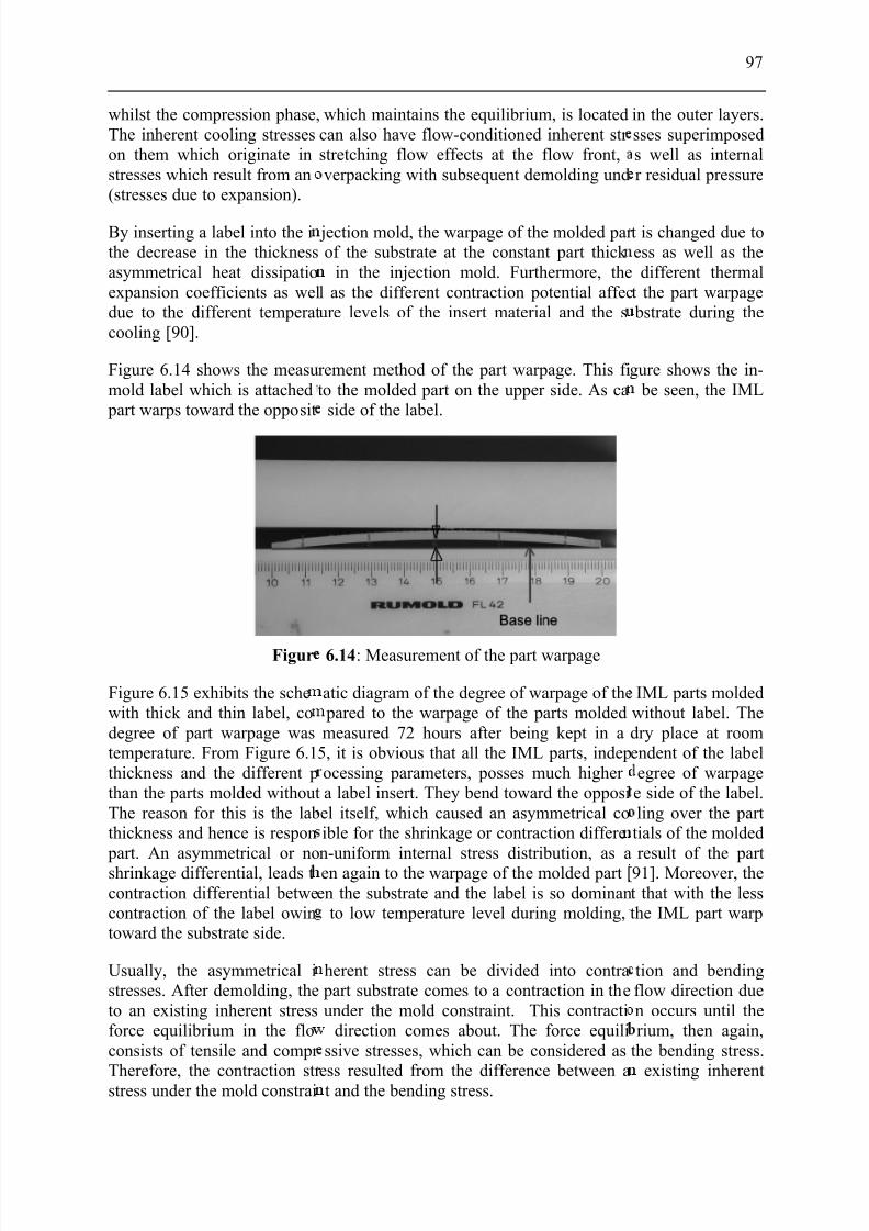
7/27/2019 Injection Mould Design
http://slidepdf.com/reader/full/injection-mould-design 115/160
whilst the compression phase,The inherent cooling stresseson them which originate instresses which result from an(stresses due to expansion).
By inserting a label into the ithe decrease in the thicknessasymmetrical heat dissipatioexpansion coefficients as weldue to the different temperatcooling [90].
Figure 6.14 shows the measumold label which is attached
part warps toward the opposit
Figur
Figure 6.15 exhibits the schewith thick and thin label, codegree of part warpage wastemperature. From Figure 6.1thickness and the different pthan the parts molded withoutThe reason for this is the labthickness and hence is respon
part. An asymmetrical or noshrinkage differential, leads tcontraction differential betwecontraction of the label owintoward the substrate side.
Usually, the asymmetrical istresses. After demolding, theto an existing inherent stressforce equilibrium in the floconsists of tensile and compr
Therefore, the contraction str stress under the mold constrai
which maintains the equilibrium, is locatedcan also have flow-conditioned inherent str stretching flow effects at the flow front,verpacking with subsequent demolding und
jection mold, the warpage of the molded par of the substrate at the constant part thick
in the injection mold. Furthermore, thel as the different contraction potential affecure levels of the insert material and the s
rement method of the part warpage. This fito the molded part on the upper side. As ca
side of the label.
6.14: Measurement of the part warpage
atic diagram of the degree of warpage of the pared to the warpage of the parts moldedmeasured 72 hours after being kept in a
5, it is obvious that all the IML parts, indepocessing parameters, posses much higher a label insert. They bend toward the opposiel itself, which caused an asymmetrical coible for the shrinkage or contraction differen-uniform internal stress distribution, as aen again to the warpage of the molded part [en the substrate and the label is so dominan
to low temperature level during molding,
herent stress can be divided into contra part substrate comes to a contraction in theunder the mold constraint. This contracti
direction comes about. The force equilissive stresses, which can be considered as
ess resulted from the difference between at and the bending stress.
97
in the outer layers.sses superimposeds well as internalr residual pressure
t is changed due toess as well as thedifferent thermal
t the part warpage bstrate during the
gure shows the in-be seen, the IML
IML parts moldedwithout label. Thedry place at roomendent of the labelegree of warpagee side of the label.ling over the parttials of the moldedresult of the part
91]. Moreover, thet that with the lessthe IML part warp
tion and bendingflow direction duen occurs until therium, then again,
the bending stress.
existing inherent
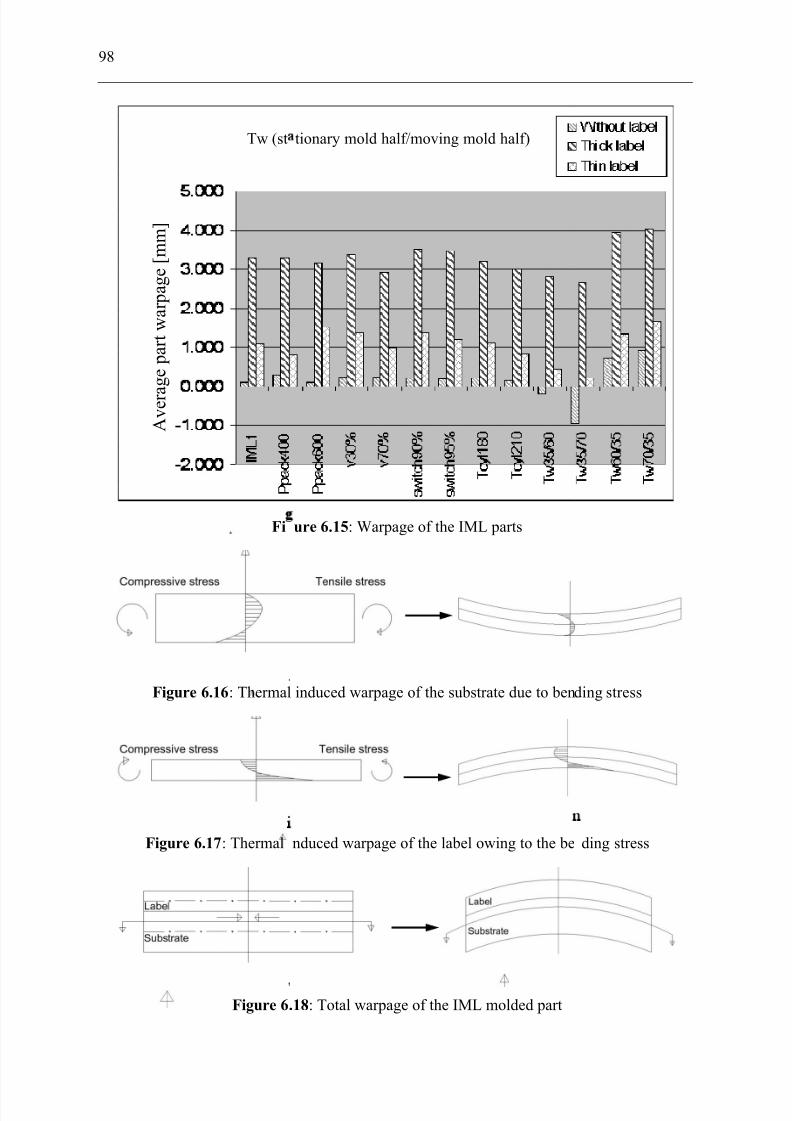
7/27/2019 Injection Mould Design
http://slidepdf.com/reader/full/injection-mould-design 116/160
98
Fi
Figure 6.16: Thermal
Figure 6.17: Thermal
Figure 6
A v e r a
g e p a r t w a r p a g e [ m m ]
Tw (st
ure 6.15: Warpage of the IML parts
induced warpage of the substrate due to ben
nduced warpage of the label owing to the be
.18: Total warpage of the IML molded part
tionary mold half/moving mold half)
ding stress
ding stress
7/27/2019 Injection Mould Design
http://slidepdf.com/reader/full/injection-mould-design 117/160
99
If only the pure contraction stress is considered, a decrease in the length of the substrate inthe flow direction after demolding will only be seen. To the contrary, if only the pure bendingstress is considered, the substrate will warp toward the warmer side after demolding (Fig.6.16) by the bending moment which equals to the multiplication of the bending stress, surfacearea, and the distance between the surface and the middle plane of the substrate.
Due to the heat transport phenomena in injection mold, the in-mold label also subjects to anasymmetrical temperature profile. Without the mold constraint, the label will commonly warptoward the warmer side, which is side to be connected to the substrate (Fig. 6.17).Considering the total deformation of the composite construction (IML part), these effects canno longer be separately taken into account and hence must be joined together due to themechanical coupling between the substrate and the label.
Because of much smaller thickness and hence less stiffness of the label compared to those of the substrate and the higher expansion coefficient of the substrate, the higher contractionduring the rest cooling of the substrate especially near the transition to the label owing to
higher temperature field during molding can be implied. Consequently, as a compositeconstruction, the label is forced to warp toward the substrate, whereas the substrate at thetransition must be stretched (Fig. 6.18). There were tensile and compressive stresses resultingfrom these individual length alterations, which take effect on the respective surfaces of thelabel and the substrate. These stresses bring about the bending moment, which finally leads tothe IML part warpage. It can be said that the degree of the part warpage is as a consequenceof the relationship between bending stress, surface area, and the distance from the surface tothe middle plane of the whole IML part. For the compact decorating materials, the rigidity aswell as the coefficient of linear expansion of the substrate and the decorating material has alarger influence on the warpage of composite part.
For the parts molded without label as an insert, despite the equal mold temperature settingson the two mold halves, they bend toward the stationary mold half (Fig. 6.19, middle), whichhas lower cooling efficiency than on the other mold half (Chapter 3). This occurrence can beeasily described by Stitz's solidification model (Fig. 6.13). An asymmetrical temperature
profile over the part thickness during cooling evoked by the different cooling efficiencies of the mold halves causes a thermal contraction differential. With the higher melt temperaturenear the stationary mold half, the higher contraction of the melt develops during cooling andhence brings the part to warp toward this side.
The experimental results also exhibit that IML parts molded with thick labels have higher degrees of warpage than parts molded with thin labels. This is because of the thermal
conductivity of the labels as well as the displacement of the middle axis of the substratecompared with the middle axis of the IML part. Thick label has a higher thermal conductivitythan thin label (Fig. 5.3-5.4). If two label types are of the same thickness, the temperaturemaximum in the substrate connected to the label with higher conductivity appears further away from the transition between label and substrate. Consequently, the IML part with higher thermal conductivity tends to warp with higher degree toward the substrate side.
Nevertheless, the effect of the volume contraction difference between label and substrate far outweighs the effect of the asymmetrical temperature distribution because much higher temperature of the substrate leads to the higher volume contraction compared to the label.The increase in the average contraction level of the substrate in relation to the averagecontraction level of the label leads to a warpage of the IML part toward the substrate sideafter the settlement of the thermal induced inherent stress. In addition, with an increase in thethickness of the same label type, the middle axis of the substrate is shifted compared with the
7/27/2019 Injection Mould Design
http://slidepdf.com/reader/full/injection-mould-design 118/160
100
middle axis of the whole IML part to the substrate side. By this effect, the degree of warpageis intensified along with the increase in label thickness.
Besides the label thickness, the degree of part warpage is affected to a considerable extent bythe mold temperature. The experimental study conducted by Wielpütz [90] has shown that the
degree of part warpage of the IMD (in-mold decoration) part with compact decoratingmaterial can be influenced by heating the decorating material prior to inserting it into themold cavity. This procedure, however, is not suitable for the injection in-mold labeling.Firstly, the temperature of the tempered IML label is hardly to be maintained uniformlythroughout the production. Secondly, the tempering of the label contributes to thedevelopment of static charges, which consequently causes an attraction of an individual labelwithin the label stack. A blocking of labels occurs. This complicates the handling of the labeland also the whole production of the IML products. All of these speaks against the temperingof the in-mold label. Therefore, in this study, the effect of the mold temperature variation on
both mold halves was concentrated instead.
An attempt to rectify the part warpage was carried out in this study. By setting the moldtemperature on the moving mold half higher than on the other (Tw35/60 and Tw35/70), thedegree of part warpage of the IML parts was reduced to some different extents. For molded
parts without label, the part warpage was, to the contrary, intensified by these settings.Thereby, the warpage direction was reversed so that the parts warp toward the moving moldside. This indicates that the excessive temperature difference in both mold halves involved inthe molding of the part without label insert.
From Figure 6.15, the last four experimental variants are interesting, with which differentmold temperature combination settings for both mold halves were given, namely thecombinations of Tw=35oC/60oC (stationary half/moving half) and vice versa and
Tw=35oC/70oC and vice versa. The experimental results show that the degree of warpage of the molded part is greatly affected by the mold temperature combination. As mentionedabove, if the mold temperature on the label side is chosen higher than on the opposite side, asmaller degree of warpage is to be realized, except for the parts molded without label. Thetemperature difference between the two mold halves is decisive to the degree of partwarpage. An increase in the mold temperature on the label side resulted in the decrease of theheat flow through the label. On the other hand, the temperature field within the label becomesmore homogeneous. The asymmetrical temperature profile turns to be more symmetrical over the thickness of the label. In addition, the temperature level in the label is increased with anincrease in the mold temperature on the label side and thereby the contraction differential
between the label and the substrate becomes smaller, less warpage occurs. To the contrary, by
decreasing the mold temperature on the label side, strong asymmetrical temperature profile isinduced, which leads to extreme temperature difference between the average label andsubstrate temperatures and ,of course, higher degree of warpage.
By tempering the IML parts molded with these conditions (Tw35/60, Tw35/70, Tw60/35, andTw70/35), it can be manifested that all these parts exhibit higher degree of part warpage after
being stored in an oven at the temperature of 80 oC for 24 hours. The reason for this is thehigher contraction of the substrate as a result of the relaxation encouraged by tempering.While the tempering of both thick and thin labels at the same condition shows no effect to thecontraction (shrinkage of label), the warpage of the tempered IML parts are then aggravatedmerely by the contraction in the flow direction of the substrate. Parts molded without labeldifferentiate themselves from the IML parts. Tempering part without label molded with themold temperature of 40 oC on both mold halves shows a little warpage alteration relative to

7/27/2019 Injection Mould Design
http://slidepdf.com/reader/full/injection-mould-design 119/160
101
the IML parts. Because its temperature distribution over that part thickness is nearlysymmetrical, the contraction arises also nearly symmetrically and the warpage has increased
by a small amount. As soon as this temperature symmetry was interfered during molding process, for example by the mold wall temperature combination, the part warpage will bestrongly influenced by the tempering.
As already mentioned, the effect of the volume contraction difference between label andsubstrate dominates the effect of the asymmetrical temperature distribution on the partwarpage. In this study, besides the injected IML part with polypropylene substrate, IML partswith polystyrene substrate were also molded in order to study the effect of the substratematerial and mold temperature combination which provoke the contraction differentials andhence warpage of the IML part. The experimental results have revealed that little to nowarpage of the IML part molded with PS as substrate can be detected. This is because thevolume contraction of PS is much lower than that of PP, the effect of the contractiondifference is hence negligible. Despite the asymmetrical temperature distribution over the PS
part thickness, the stiffness of PS substrate remains invincible so that the mold temperature
combination shows no effect on the warpage of the referred part (compare Fig. 6.19 with6.20).
The amount of the temperature difference which can be set between the mold halves dependson the composite part thickness as well as the polymer resin used. How and on which scalethis temperature difference between the mold halves affect the IML part property will bediscussed in Chapter 6.6.
Figures 6.19 and 6.20 illustrate the computed degree of part warpage from 3D simulations.As mentioned above, mold temperature combination settings have little to no effect on thedegree of the part warpage of the IML part molded with PS as the substrate.
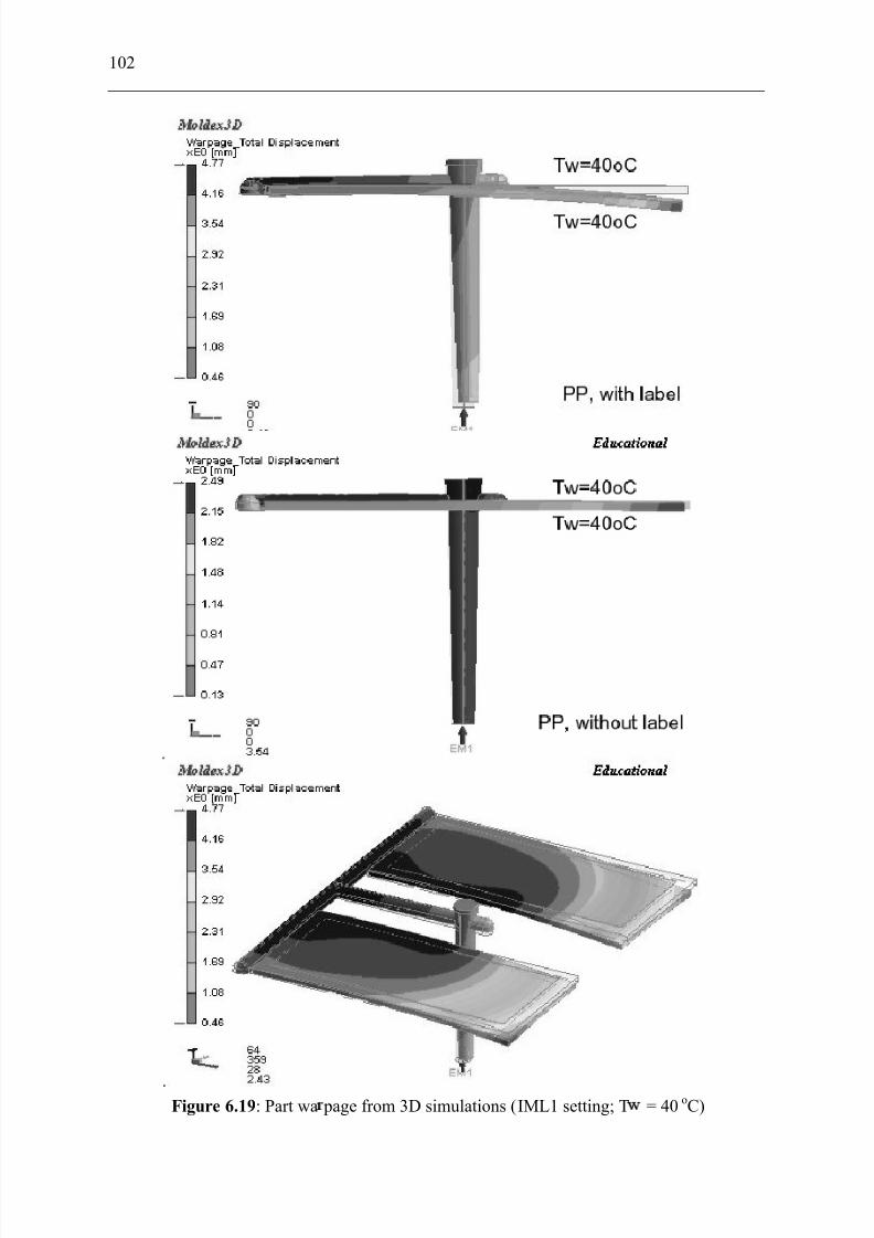
7/27/2019 Injection Mould Design
http://slidepdf.com/reader/full/injection-mould-design 120/160
102
Figure 6.19: Part wa page from 3D simulations (IML1 setting; T = 40 oC)
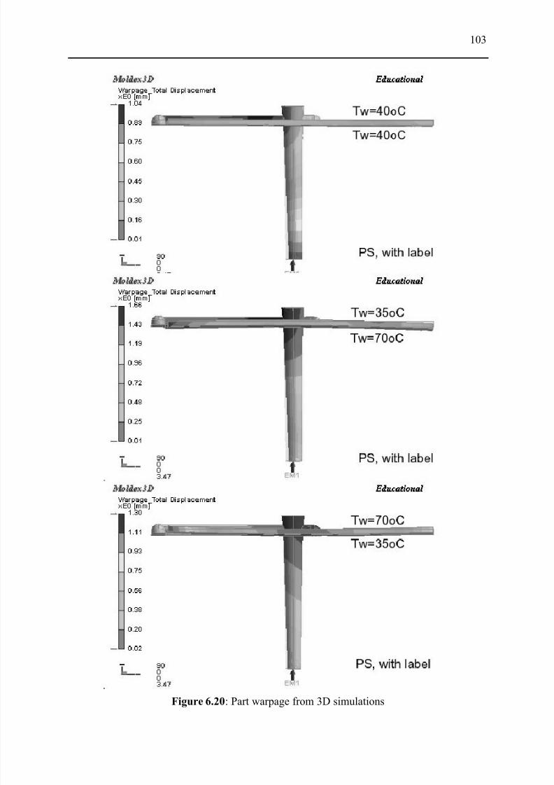
7/27/2019 Injection Mould Design
http://slidepdf.com/reader/full/injection-mould-design 121/160
Figure 6.20: Part warpage from 3D simulations
103
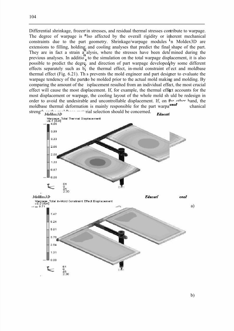
7/27/2019 Injection Mould Design
http://slidepdf.com/reader/full/injection-mould-design 122/160
104
Differential shrinkage, frozenThe degree of warpage isconstraints due to the partextensions to filling, holding,They are in fact a strain a
previous analyses. In additio possible to predict the degreeffects separately such as bthermal effect (Fig. 6.21). Thwarpage tendency of the partcomparing the amount of theeffect will cause the most dismost displacement or warpagorder to avoid the undesirablmoldbase thermal deformatiostrength or the moldbase mate
in stresses, and residual thermal stresses conlso affected by the overall rigidity or ingeometry. Shrinkage/warpage modulesand cooling analyses that predict the final
alysis, where the stresses have been dete
to the simulation on the total warpage dispand direction of part warpage developedthe thermal effect, in-mold constraint ef
s prevents the mold engineer and part desigto be molded prior to the actual mold makinisplacement resulted from an individual effe
placement. If, for example, the thermal effee, the cooling layout of the whole mold she and uncontrollable displacement. If, on tn is mainly responsible for the part warparial selection should be concerned.
tribute to warpage.herent mechanicaln Moldex3D areshape of the part.mined during the
lacement, it is also by some differentect and moldbasener to evaluate theg and molding. Byct, the most crucialct accounts for theuld be redesign inhe other hand, thee, the mechanical
a)
b)
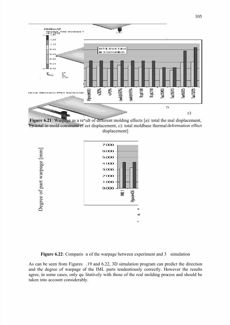
7/27/2019 Injection Mould Design
http://slidepdf.com/reader/full/injection-mould-design 123/160
Figure 6.21: Warpage as a re b): total in-mold constraint ef
Figure 6.22: Comparis
As can be seen from Figuresand the degree of warpage oagree, in some cases, only qutaken into account considerabl
D e g r e e o f p a r t w a r p
a g e [ m m ]
ult of different molding effects [a): total theect displacement, c): total moldbase thermal
displacement]
n of the warpage between experiment and 3
.19 and 6.22, 3D simulation program can pf the IML parts tendentiously correctly. Hlitatively with those of the real molding proy.
105
c)mal displacement,deformation effect
simulation
redict the directionowever the resultscess and should be
7/27/2019 Injection Mould Design
http://slidepdf.com/reader/full/injection-mould-design 124/160
106
6.6 Modulus of Elasticity
The most important mechanical property of a polymeric material is its stress-strain curve.This curve is obtained by stretching a sample in a tensile testing machine and measuring thesample’s extension and the load required to reach this extension. Since polymeric materials
show viscoelastic behavior (a combination of elastic and viscous behavior) that is highlysensitive to temperature and, in some materials, relative humidity variations, it is important touse samples of standard shapes, preconditioned at a constant and standard temperature andrelative humidity before testing. Also, they must be stretched at a constant speed if the resultsare to be comparable to other tests. The stress-strain curve provides information about themodulus of elasticity (Young’s modulus), which is related to the material’s stiffness or rigidity. This curve also provides information about the yield point, tensile strength, andelongation at break. The curve defines toughness (the area under the curve), which is theenergy per unit volume required to cause the sample to fail. Thus, the stress-strain curvereveals much about a material’s mechanical behavior. The information obtained includes thematerial’s elastic property, yield strength, and toughness based on the stress-strain data.
Modulus of elasticity is actually the slope of the curve within the elastic area of the specimen.The greater the modulus of elasticity, the stiffer the material or the smaller the elastic strainwill be. The modulus of elasticity, E, is the ratio of normal stress to corresponding strain(straight line) for stresses below the proportional limit of the material (Hooke’s law); it is theratio of stress to strain in a test specimen (tensile, compression, etc.) that is elasticallydeformed.
For the execution of the tensile testing with polymers, the DIN EN ISO 527 represents the preferential standard, which covers the examination of molding materials, films and boards aswell as glass-reinforced polymeric materials. A substantial experimental basic condition for the execution of this test is the use of suitable test sample. In this study, test specimens of type 1BA which is a proportional reduction of the type 1B on a scale of 1:2 are employed.
Figure 6.23 illustrates the modulus of elasticity of the part molded without label comparedwith the IML part molded with thick and thin label, respectively. From this figure, it can beseen that labels have strengthened the molded part to some different extent dependent on typeof the label used and the molding parameter. Furthermore, IML parts molded with thin labelmostly shows higher modulus than the parts molded with thick label. The modulus of elasticity of the IML part is mainly affected by the structure of the labels rather than by their thickness. This resulted particularly from the stretching of the label film, by which thestrength of the film increases. As already mentioned in Section 5.2.2, the thick label is a
porous type, which comprises the substrates of polyolefin polymers and silica. And thisstructure imparts the better adhesion between the label and the substrate. The thin label, onthe other hand, composed of many layers of polyolefin polymers (Fig. 6.11), which are
biaxially stretched. Despite higher thickness of the thick label compared to thin label andalthough the thick label film also underwent the stretching to some degrees, highly orientedstructure of the thin label as can be seen in the Figure 6.11 dominates and this is responsiblefor the elevated modulus of elasticity of these IML parts.
The melt temperature also affects the modulus of elasticity of the molded part. Usually, withthe relatively high melt temperature, the polymer macromolecules may be shortened or damaged, and hence the strength decreases. In this study, however, the melt temperature wasset at the range between 180 oC and 210 oC during molding which is not excessively high, so
7/27/2019 Injection Mould Design
http://slidepdf.com/reader/full/injection-mould-design 125/160
that only the slight reductionhigher settings.
Figure 6.23: Modulus of elas
pa
Holding pressure affects themolded without label, the optlabel, holding pressure can beholding pressure of 500 bars glabel. Normally parts that hamore at risk of having high inmodulus.
Injection velocity of 50 % ha
not for the part molded witho best condition for all the mold
From Figure 6.23, it can bemodulus of elasticity in an inthick label has declined withmodulus of elasticity of Itemperature in one mold halmerely to a small extent so t
part by varying the mold teelasticity of the part is only
elasticity of the part molded
M
o d u l u s o f e l a s t i c i t y [ M P a ]
in the modulus of all the molded parts is
icity of molded part without label compared
rts molded with thick and thin label
modulus of the molded part in differentimal holding pressure is 400 bars. For partsset higher in order to acquire high modulusives the highest modulus of elasticity to thee exposed the exceeding holding pressureternal stress, which contributes to the reduct
s been proved to be the most optimal for all
t label, whereas holding switch at 98 % of ed part.
een that the mold temperature combinationteresting way. The modulus of elasticity of the mold temperature combination settings.L part molded with thin label decreasedifferentiates from the other. However, thiat it can be concluded that to rectify the w perature in the two mold halves differentlnfluenced in an unharmed way, compared
ithout label using the IML1 molding parame
107
ascertained at the
with injected IML
anners. For partsmolded with thick
of elasticity. WhileML parts with thinuring molding are
ion of strength and
the IML parts but
illed volume is the
settings affect thethe IML part withIn the same way,
s when the molds reduction occursarpage of the IMLy, the modulus of to the modulus of
ters.
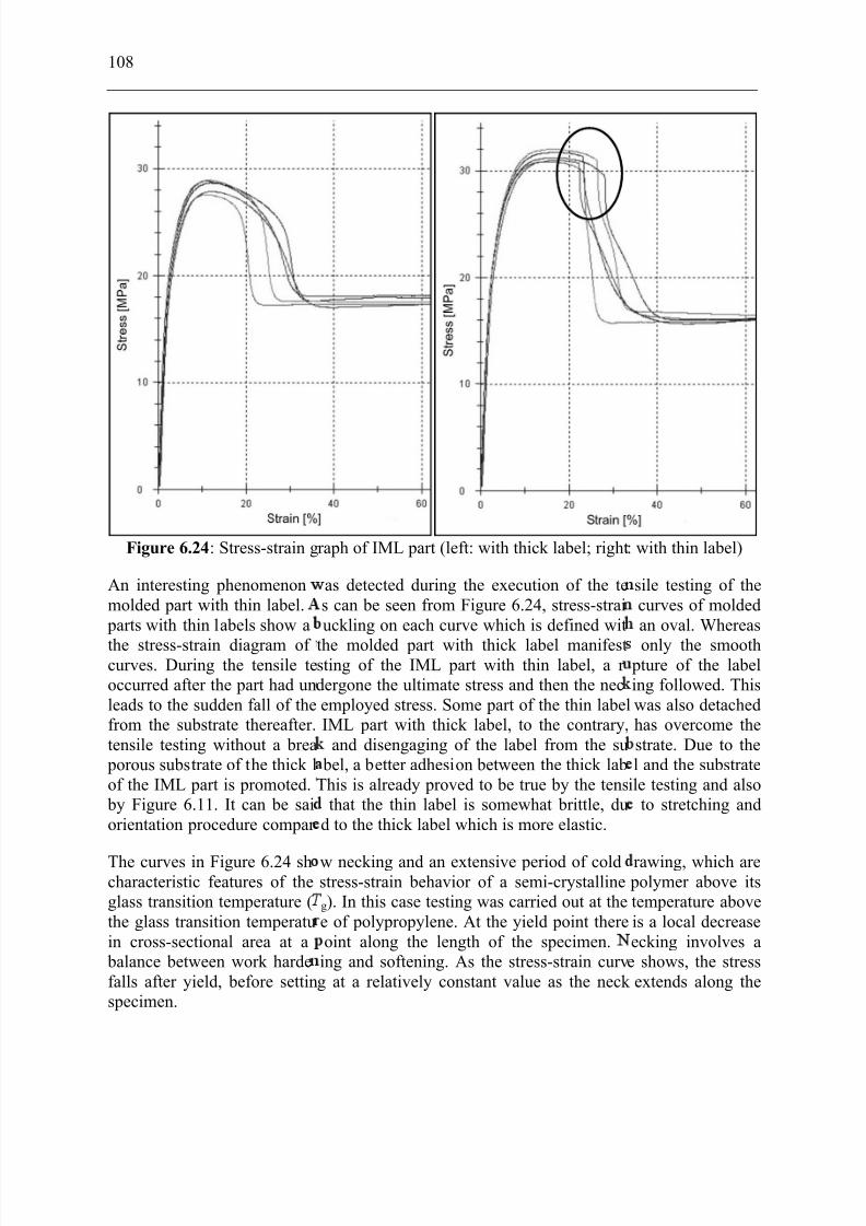
7/27/2019 Injection Mould Design
http://slidepdf.com/reader/full/injection-mould-design 126/160
108
Figure 6.24: Stress-strain g
An interesting phenomenonmolded part with thin label.
parts with thin labels show a
the stress-strain diagram of curves. During the tensile teoccurred after the part had unleads to the sudden fall of thefrom the substrate thereafter.tensile testing without a brea
porous substrate of the thick lof the IML part is promoted.
by Figure 6.11. It can be saiorientation procedure compar
The curves in Figure 6.24 shcharacteristic features of theglass transition temperature (the glass transition temperatuin cross-sectional area at a
balance between work hardefalls after yield, before settinspecimen.
raph of IML part (left: with thick label; right
as detected during the execution of the tes can be seen from Figure 6.24, stress-straiuckling on each curve which is defined wit
the molded part with thick label manifeststing of the IML part with thin label, a r dergone the ultimate stress and then the necemployed stress. Some part of the thin labelIML part with thick label, to the contrary,
and disengaging of the label from the su bel, a better adhesion between the thick labThis is already proved to be true by the tens
that the thin label is somewhat brittle, dud to the thick label which is more elastic.
w necking and an extensive period of coldstress-strain behavior of a semi-crystallineg). In this case testing was carried out at thee of polypropylene. At the yield point thereoint along the length of the specimen.
ing and softening. As the stress-strain curvg at a relatively constant value as the neck
: with thin label)
sile testing of thecurves of moldedan oval. Whereas
only the smooth pture of the labeling followed. Thiswas also detachedhas overcome thestrate. Due to thel and the substrate
ile testing and alsoto stretching and
rawing, which are polymer above itstemperature aboveis a local decreaseecking involves ae shows, the stressextends along the
7/27/2019 Injection Mould Design
http://slidepdf.com/reader/full/injection-mould-design 127/160
Figure 6.25: Effect of the mothe modulus of el
Figure 6.25 shows the effecelasticity of the polypropylenout in order to study the effecof elasticity as well as the e
performed with polypropylenmold temperature settings ar halves into consideration, sinis defined by 10 degree interv
The experimental results dispgreatly affect on the modulu
optimal mold temperature ranFor the molding of polyprosuggested. Anyway, all theelasticity.
M o d u l u s o f e l a s t i c i t y [
M P a ]
ld temperature combination settings on the tasticity of parts molded with PP Novolen 32
t of the mold temperature combinations o part molded without label. This set of expet of the mold temperature combination settilongation at yield of the molded part. Thee as the injected material and without labe
starting at 20 oC up to 60 oC without tae no label involves in the molding. The temls.
ay that not the difference between the moldof elasticity or elongation at yield of the
ge, to the contrary, influences much on theylene, the mold temperature range frommolded parts possess the satisfactory le
109
o mold halves on0 MC
n the modulus of iments was carriedgs on the modulusexperiments wereas an insert. The
ing the side mold perature difference
temperatures doesmolded parts. The
odulus of the part.5 oC to 50 oC isel of modulus of
E l o n g a t i o n a t y i e l d
[ % ]
7/27/2019 Injection Mould Design
http://slidepdf.com/reader/full/injection-mould-design 128/160
110
7 Summary
Within this thesis, 2.5D injection molding simulation based on the generalized Hele-Shawmodel and 3D simulation were introductory performed with a double-plated part with non-uniform thickness in order to evaluate the efficiency and accuracy of the simulation program
Moldex3D. The 2.5D simulations were carried out based on two different surface mesh typesand by varying the number of mesh layers that can be freely defined during the simulation
parameter setting. The 3D simulations, in the same way, were conducted with three differentvolume mesh types and by varying the number of element layer counts over the partthickness.
The results gained from 2.5D and 3D simulations have shown that the number of mesh layer over the part thickness has little to no effect on the accuracy of the simulation results in termsof predicting the melt front advancement in the cavity. On the other hand, noticeabledeviation in the temperature distribution between the mesh types and the number of meshlayers can be acquired. In case of 3D simulation, tetrahedral meshing compared to prism and
voxel meshing is proved to be the worst meshing method concerning the melt frontadvancement prediction and calculation time. Unexpectedly, 3D non-isothermal basedsimulation results deviated much from the actual molding situation, while 2.5D simulationcan better predict the filling pattern of this part. This results mainly from the numericalinstability of the 3D filling simulation of Moldex3D when a highly complex moldingsituation is involved. In addition, the computed pressure levels in the two cavities wereirregularly predicted. The pressure-S2 curve lies over the pressure-S1 one which is clearlyincorrect compared to the real pressure profiles. This is mainly responsible for an error in
predicting the melt front advancement of the double-plated part with non-uniform partthickness by 3D simulation.
For 2.5D mold filling simulation, higher number of the mesh count over the part thicknessdedicates mainly to the computation of the temperature distribution within the molded partrather than to the prediction of the melt front advancement. The advantage of the higher regularity of the voxel derivative mesh over the tetrahedral derivative mesh cannot beobserved.
If, instead of 3D simulation based on non-isothermal computation, 3D simulation based onisothermal computation was performed, obvious improvement in predicting the melt frontadvancement and the proximity of the results to the actual process were provided. This is alsodue to the instability of non-isothermal numerical computation.
When molding the plates with non-uniform thickness separately, no decisive accuracydeviation in predicting the melt front progression between 3D and 2.5D simulation wasmanifested because the complexity of the flow and unbalancing of pressure between the twocavities as a system are eliminated.
Despite slightly underestimated, course of the melt temperature during filling and holding phase from 2.5D simulation lies relatively close to that of the real molding process(experiment). To the contrary, course of the melt temperature derived from 3D simulationwas not really meaningful since the sensor nodes used in the simulation are not comparablewith the real IR-temperature sensor and thus course of the temperature cannot be reasonablyreported based on these sensor nodes used in 3D simulation. Generally, a comparison
between the measured and the computed melt temperature must be made with caution
7/27/2019 Injection Mould Design
http://slidepdf.com/reader/full/injection-mould-design 129/160
111
because the depth of penetration of the IR-temperature sensor is unknown and this can be problematic when the melt temperature in a relatively thick cavity should be measured.
Contrary to the complex double-plated part with non-uniform part thickness, with the IML part that is relatively simple in the form, Moldex3D can predict the flow pattern, course of the
pressure and temperature trouble-freely and correctly. In addition, an asymmetricaltemperature gradient over the part thickness can be distinctly detected. This phenomenon isexpected to occur particularly in the back injection of a film, because the film acts as athermal insulator. In filling phase the temperature distribution was almost symmetrical over the part thickness, whereas in holding and cooling phase unbalances in the temperaturedistribution became evident. Different frozen layer thicknesses can also be computed by 3Dsimulation. This indicates that this 3D simulation program is able to consider asymmetries inthe thermal boundary conditions qualitatively correctly when molding the IML part.
Structure of the IML part was also examined. Four different zones in the IML part can bedistinguished under the light microscope. On the label side, porous label structure as well as
fine and coarse crystalline structures can be seen whereas the coarse crystalline structure(spherulites) and the amorphous layer can be seen in the middle and the side without label of the IML part, respectively. The frozen layers can also be seen under the light microscope.They arise as a result of the quenching of the melt as it contacts the cold mold wall. On thelabel side this frozen layer is much thinner over the entire part length than on the oppositeside since the crystallization of the melt on the label side can further develop contrary to theopposite side of the molded part.
IML parts usually warp toward the opposite side of the label. This is because of much smaller thickness and less stiffness of the label compared to the substrate as well as the higher expansion coefficient of the substrate. With the existence of a label as an insert, the warpage
of a molded part is changed due to the decrease in the thickness of the substrate at theconstant part thickness as well as the asymmetrical heat dissipation in the injection mold. Thedifferent temperature fields between the insert material and the substrate during moldcooling, together with the different thermal expansion coefficient as well as the differentcontraction potential play an important role to the occurrence of this part warpage. Higher contraction of the substrate especially near the transition to the label occurs during the restcooling phase owing to higher temperature field during molding process. The effect of thevolume contraction difference between label and substrate, however, far outweighs the effectof the asymmetrical temperature distribution because much higher temperature of thesubstrate leads to the higher volume contraction compared to the label.
Besides the label thickness, the degree of part warpage is influenced by the mold temperature.By setting the mold temperature on the label side higher than on the other, the degree of partwarpage of the IML parts can be reduced, since the temperature field within the molded part
became more homogeneous and hence the contraction differential between the label and thesubstrate became smaller.
Contrary to the PP substrate, little to no warpage of the IML part molded with amorphous PSas the substrate can be detected. This is because the volume contraction of PS is muchsmaller than that of PP, the effect of the contraction difference is thus negligible. Despite theasymmetrical temperature distribution over the PS part thickness, the stiffness of PS remainsinvincible so that the mold temperature combination settings show no effect on the warpage
of the referred part. This supports the statement that the effect of the volume contraction

7/27/2019 Injection Mould Design
http://slidepdf.com/reader/full/injection-mould-design 130/160
112
difference between label and substrate dominates the effect of the asymmetrical temperaturedistribution on part warpage.
3D simulation program can predict the direction and the degree of warpage of the IML partstendentiously correctly. However the results agree, in some cases, only qualitatively with
those of the real molding process. This should be taken into account.
Tensile testing has shown that IML parts have higher modulus of elasticity than parts moldedwithout label. This is because label has strengthened the IML molded parts to some degreedependent on type of the labels used and the molding conditions. In addition, the modulus of elasticity of the IML part is mainly affected by the structure of the labels rather than by their thickness, since the IML parts molded with thin labels show higher modulus than the partsmolded with thick labels. This results particularly from the stretching of the label film. Theexperimental results have also manifested that modulus of elasticity of the IML parts moldedwith thin and thick labels decreases when the mold temperature in one mold half differentiates from the other. However, this reduction occurs merely to a small extent so that
it can be concluded that to reduce the warpage of the IML part by varying the moldtemperature in the two mold halves differently, the modulus of elasticity of the part is onlyinfluenced in an unharmed way.

7/27/2019 Injection Mould Design
http://slidepdf.com/reader/full/injection-mould-design 131/160
113
References
[1] C. A. Hieber, S. F. SHEN, A Finite-element and finite-difference simulation of the
injection molding filling process, Journal of Non-Newt Fluid Mech, Volume 7, 1980
[2] J. H. ERIK, P. L. HANS, A unified finite element model for the injection molding process, Computational Methods Appl. Mech, 178, 1999
[3] E. Pichelin, T. COUPEZ, Finite element solution of the 3D filling problem for viscous
incompressible fluid , Comput Methods Appl. Mech. 163, 1998
[4] K. Talwar, F. Costa, V. Rajupalem, L. Antanovski and C. Friedl, Three dimensional
simulation of plastic injection molding , SPE ANTEC Proceedings , 1, 563- 566, 1998
[5] Z. Fan, B. Lin, F. Costa, X. Jin, R. Zheng, P. Kennedy, Three-dimensional warpage
simulation for injection molding , SPE Annual Technical Conference, 2004
[6] P. Kennedy, Flow Analysis of Injection Molds, Hanser, New York, 1995
[7] Z. Fan, R. Zheng, P. Kennedy, H.Yu, A. Bakharev, Warpage analysis of solid
geometry, SPE Annual Technical Conference, 2000
[8] P. Unger, E. Lindner, Gastrow Injection Molds 130 Proven Designs, 3rd Edition, CarlHanser Verlag, 2002
[9] P. Unger, Gastrow Injection Molds 130 Proven Designs, 4th Edition, Carl Hanser Verlag, 2006
[10] H. Rees, Understanding injection mold design, Carl Hanser Verlag, 2001
[11] F. Beitl, 1000 Tips zum Spritzgießen Band 4: Anschnitt-Technologie- Grundlagen mitPraxisanleitungen, Hüthig Verlag Heidelberg, 2006
[12] www.scudc.scu.edu/cmdoc/dg_doc/develop/books/dg/index_sp.htm
[13] F. Beitl, Grundlagen zur Angusskanaltechnik mit Leistungsberechnung, DeutschesIndustrieforum für Technologie, 2006
[14] R.G.E. Pye, Injection Mould Design (for Thermoplastics), Ilitte Books Ltd., 1968
[15] Kunststoff-Verarbeitung im Gespräch, 1: Spritzgießen, BASF, Ludwigshafen, 1979
[16] C. A. Hieber and H. H. Chiang, Rheological Acta 28, 321-332, 1989
[17] Kegelanguß, Schirmanguß, Bandanguß. Technical Information, BASF, 1985
[18] F. Beitl, 1000 Tips zum Spritzgießen Band 3: Angusskanaltechnik- Grundlagen mit
Praxisanleitungen, Hüthig Verlag Heidelberg, 2006
[19] H.-D. Stank, Anforderungen an den Anguß, seine Aufgaben, Anordnung am
Spritzgußteil. Anguß- und Anschnittprobleme beim Spritzgießen, Ingenieurwissen,VDI-Verlag, Düsseldorf, 1975

7/27/2019 Injection Mould Design
http://slidepdf.com/reader/full/injection-mould-design 132/160
114
[20] E. Schürmann, Abschätzmethoden fur die Auslegung von Spritzgießwerkzeugen.
Dissertation, Tech. University, Aachen, 1979
[21] G. Menges, W. Michaeli, P. Mohren, How to Make Injection Molds, 3rd Edition, CarlHanser Verlag, 2001
[22] O. Kretzschmar, Rechnerunterstiitzte Auslegung von Spritzgießwerkzeugen mit
segmentbezogenen Berechnungsverfahren. Dissertation, Tech. University, Aachen,1985
[23] Dominick. V. Rosato, Donald V. Rosato, M. G. Rosato, Injection Molding Handbook ,3rd Edition, Kluwer Academic Publishers, 2000
[24] N. Rott, Note on the History of the Reynolds Number , Annual Review of FluidMechanics, Vol. 22, 1990
[25] Entformungseinrichtungen. Technical Information, 4.4, BASF, Ludwigshafen/Rh.,1969
[26] H. Bangert, Systematische Konstruktion von Spritzgießwerkzeugen und
Rechnereinsatz , Dissertation, Techn. Univ., Aachen, 1981
[27] H. Bangert, E. Doring, E, U. Lichius, W. Kemper, W, E. Schumann, Bessere
Wirtschaftlichkeit beim Spritzgießen durch optimale Werkzeugauslegung , Paper block VII at the 10th Tech. Conference on Plastics, IKV, Aachen, March 12-14, 1980
[28] S. E. Giragosian, Continous mold venting . Mod. Plast, 44 (1966), 11
[29] W. Hartmann, Entlüften des Formhohlraums, Paper at the VDI Conference, Nürnberg, December 6-7, 1978
[30] A. Rogalla, Analyse des Spritzgießens mikrostrukturierter Bauteile aus
Thermoplasten, Dissertation, RWTH, Aachen, 1997
[31] U. Meiertoberens, C. Herschbach, R. Maaß, Verbesserte Technologien für die
Elastomerverarbeitung , Gummi, Fasern, Kunststoffe, 47 (1994), 10, pp. 642-649
[32] K. Notz, Entlüftung von Spritzgießwerkzeugen, Plastverarbeiter, 45 (1994), 11
[33] N. S. Rao, G. Schumacher, Design formulas for plastics engineers, 2nd Edition, CarlHanser Verlag, 2004
[34] N. S. Rao, K. O’Brien, Design data for plastics engineers, Carl Hanser Verlag, 1998
[35] A. R. Calhoun, J. Golmanavich, Fundamental skills and polymer science, Society of plastics engineers, 2004
[36] W. B. Hoven-Nievelstein, Die Verarbeitungsschwindung thermoplastischer
Formmassen, Dissertation, Tech. University, Aachen, 1984
[37] German Standard: DIN 16901: Kunststoff-Formteile Toleranzen und Abnahmebedingungen für Längenmaße
7/27/2019 Injection Mould Design
http://slidepdf.com/reader/full/injection-mould-design 133/160
115
[38] M. G. Potsch, Prozessimulation zur Abschätzung von Schwindung und Verzug
thermoplastischer Spritzgussteile, Dissertation, RWTM, Aachen, 1991
[39] P. Gelardi, In Mold Decorating and In Mold Labeling & The Future, PlasticsTechnology Magazine’s Paint-Free Color Conference 2004
[40] Top 50 Innovations: In-Mold Decorating & Labeling , Plastics Technology’s OnlineArticle, www. Ptonline.com
[41] D. Cook, Advances in IML for Thin Wall Packaging , 13th International In-MoldLabeling Conference, 2005
[42] B. König, Verfahren zum Herstellen von mit bedruckten Etiketten versehenen
Formkörpern nach dem so genannten In-Mould-Labelling (IML)-Verfahren sowie
Etikett für ein In-Mould-Labelling (IML)- Verfahren, Deutsches Patentamt,Patentschrift DE 196 19 462 C1, 1997
[43] N. N., Exxon Mobil Chemical Films Europe
[44] D. Sinigaglia, IML Labels and the Environment , 13th International In-Mold LabelingConference, 2005
[45] S. E. Shelton, Feature Article In-Mold Labeling: Electrostatics Are the Way to Go,Plastics Technology’s Online Article, www. Ptonline.com
[46] Simco electrostatic control
[47] S. E. Shelton, Use of Electrostatics for In-mold label applications
[48] W. Cao, C. Shen, Two Solutions for Three-Dimensional Flow Simulation of Injection
Molding , Antec 2005
[49] Moldex CAE software handbook
[50] R. B. Bird, R.C. Armstrong, and O. Hassager, Dynamics of Polymeric Liquids, Vol. 1,John Wily & Sons, 1987
[51] J.D. Ferry, Viscoelastic Properties of Polymers, John Wily & Sons, 1980
[52] W. Michaeli, Extrusion Dies for Plastics and Rubbers, Oxford University Press, 1992
[53] P. Zoller. A study of the pressure-volume-temperature relationships of four relatedamorphous polymers: Polycarbonate, polyarylate, phenoxy, and polysulfone. Journal
of Polymer Science, 20:1453–1464, 1982
[54] R.S. Spencer and G.D. Gilmore. Equation of state for polystyrene. Journal of Applied
Physics, 20:502–506, 1949.
[55] R.Y. Chang, C.H. Chen, and K.S. Su. Modifying the tait equation with cooling rateeffects to predict the pressure-volume-temperature bahaviors of amorphous polymers:
Modelling and experiments. Polymer Engineering and Science, 36(13):1789–1795,1996.
7/27/2019 Injection Mould Design
http://slidepdf.com/reader/full/injection-mould-design 134/160
116
[56] P. Zoller. Pressure-volume-temperature relationship of solid and molton polypropylene and poly(butene-1). Journal of Applied Polymer Science, 23:1057– 1061, 1979.
[57] W. F. Ames, Numerical Method for Partial Differential Equations, Section 1.6.
Academic Press, New York, 1977
[58] F. B. Hildebrand, Finite-Difference Equations and Simulations, Section 2.2. Prentice-Hall, Englewood Cliffs, New Jersey, 1968
[59] G. Boole, A Treatise On The Calculus of Finite Differences, 2nd Ed., Macmillan andCompany, 1872
[60] H. Freeman, Finite Differences for Actuarial Students, 1967
[61] www.feadomain.com
[62] www.solid.ikp.liu.se
[63] www.math.nist.gov
[64] R. W. Clough, W. L. Edward L, Early Finite Element Research at Berkeley, Retrievedon 2007-10-25
[65] W. C. Gibson, The Method of Moments in Electromagnetics. Chapman & Hall, 2008
[66] P. K. Banerjee, The Boundary Element Methods in Engineering , McGraw-HillCollege, 1994
[67] L. C. Wrobel, M. H. Aliabadi, The Boundary Element Method . Wiley, 2002
[68] www.boundary-element-method.com
[69] www.conceptanalyst.com
[70] www.imtek.uni-freiburg.de/simulation
[71] www.iam.uni-stuttgart.de/bem/home_bem_introduc.html
[72] www.fos-messtechnik.de[73] F. Obendrauf, G. Langecker, W. Friesenbichler, Int. Polym. Proc. 13:1 71-77, 1998
[74] C. Maier, Polym. Eng. Sci. 36:11 1502-1512, 1996
[75] A. L. Kelly, E. C. Brown and P. D. Coates, Infrared Melt Temperature Measurement:
Effect of Filler Content on Penetration Depth, IRC in Polymer Science &Technology, School of Engineering, Design and Technology, University of Bradford,Bradford, BD7 1DP, UK
[76] D. O. Kazmer, P. Knepper, S. Johnston, A review of in-mold pressure and
temperature instrumentation, University of Massachusetts Lowell

7/27/2019 Injection Mould Design
http://slidepdf.com/reader/full/injection-mould-design 135/160
117
[77] K. Kobayashi, H. Shimizu and M. Kaiho, Numerical simulation of unsteady turbulent
flow by voxel method , JSME International journal Series B, Volume 47 No.3, 2004
[78] J. Zachert, Analyse und Simulation Dreidimensionaler Strömungsvorgänge beim
Spritzgießen, Rheinisch-Westfälische Technische Hochschule Aachen, Dissertation
1998
[79] F. Johannaber, Injection Molding Machines, Hanser Publishers, Munich, 1994
[80] T. Wiegmann, F. Oehmke, Dichte, Wärmeleitfähigkeit und Wärmekapazität
automatisiert Messen, Kunststoffe 80 (1990) 11, p. 1255-1258
[81] K. Janeschitz-Kriegl, Polymer solidification by crystallisation under heat transfer and
flow conditions, Process in Colloid & Polymer Science 87: 117-127, 1993
[82] S. Vleeshouwers, H. Meijer, A rheological study of shear induced crystallization, Rheological Acta 35, 1996
[83] S. Hoffmann, Berechnungen von Kristallisationsvorgängen in Kunststoffformteilen,PhD study at Aachen University, 2002
[84] W. Michaeli, M. Bussmann, Shear-Induced Morphology Prediction in Injection
Molded Semi-Crystalline Thermoplastics, ANTEC 2005
[85] H. G. Pötsch, Prozeßsimulation zur Abschätzung von Schwindung und Verzug
thermoplastischer Spritzgussteile. Rheinisch-Westfälische Technische HochschuleAachen, Dissertation, 1991
[86] S. Galuschka, Hinterspritztechnik-Herstellung von textil-kaschierten Spritzgießteilen,Rheinisch-Westfälische Technische Hochschule Aachen, Dissertation, 1994
[87] O. Zöllner, Optimised Mould Temperature Control , Bayer
[88] W. Knappe, Die Festigkeit thermoplastischer Kunststoffe in Abhängigkeit von den
Verarbeitungsbedingungen , Kunststoffe Bd. 51, 1961
[89] S. Stitz, Analyse der Formteilbildung beim Spritzgießen von Plastomeren als
Grundlage für die Prozeßsteuerung , Rheinisch-Westfälische Technische HochschuleAachen, Dissertation, 1973
[90] M. Wielpütz, Analyse der Hinterspritztechnik kompakter Dekormaterialien,Rheinisch-Westfälische Technische Hochschule Aachen, Dissertation, 2003
[91] P. Larpsuriyakul, Injection –IML and its effects on the injected part properties,Proceeding 20th Stuttgarter Kunststoff-kolloquium, 2007
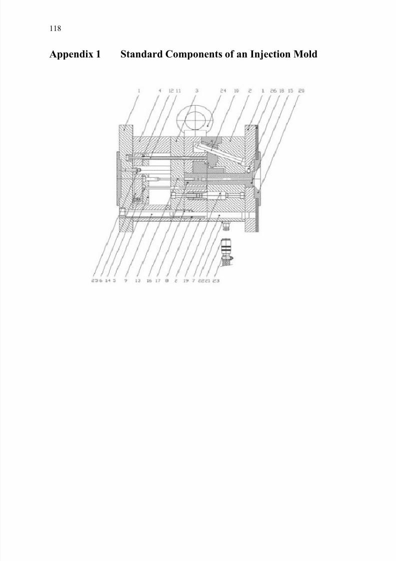
7/27/2019 Injection Mould Design
http://slidepdf.com/reader/full/injection-mould-design 136/160
118
Appendix 1 Standard Components of an Injection Mold

7/27/2019 Injection Mould Design
http://slidepdf.com/reader/full/injection-mould-design 137/160
119
Pos.* Designation standard
1 Clamping plate -
2 Cavity plate -
3 Backing plate -
4 Riser -
5 Ejector retainer plate -
6 Ejector base plate -
7 Locating guide pillar ISO 8017
8 Locating guide bush ISO 8018
9 Centering sleeve ISO9449
10 Guide pillar, angle pin ISO/CD 8404
11 Ejector pin, cylindrical head ISO 6751
12 Ejector sleeve ISO 8405
13 Shouldered ejector pin, cylindrical head ISO 8694
14 Ejector pin, conical head -
15 Sprue bushing ISO 10072
16 Sprue puller insert ISO/CD 1691517 Socket head cap screw ISO 4762
18 Dowel pin ISO 8734
19 Locating unit, round ISO 8406
20 Locating ring ISO 10907-1
21 Coupling -
22 Connecting nipple -
23 Hose clip -
24 Lifting eye bolt -
25 Support pillar ISO 10073
26 Thermal insulating sheet ISO 15600
- Plain plate ISO 6753-2
- Designation and symbols ISO 12165
- Specification sheets for injection molds ISO 16916
Standard components as per ISO
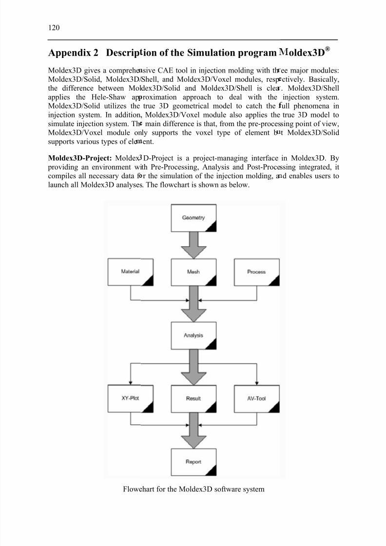
7/27/2019 Injection Mould Design
http://slidepdf.com/reader/full/injection-mould-design 138/160
120
Appendix 2 Descrip
Moldex3D gives a compreheMoldex3D/Solid, Moldex3D/the difference between Mol
applies the Hele-Shaw apMoldex3D/Solid utilizes theinjection system. In addition,simulate injection system. ThMoldex3D/Voxel module onsupports various types of ele
Moldex3D-Project: Moldex providing an environment wicompiles all necessary data f launch all Moldex3D analyses
Flowc
ion of the Simulation program
sive CAE tool in injection molding with thShell, and Moldex3D/Voxel modules, respdex3D/Solid and Moldex3D/Shell is clea
roximation approach to deal with thetrue 3D geometrical model to catch theMoldex3D/Voxel module also applies themain difference is that, from the pre-proces
ly supports the voxel type of element bent.
D-Project is a project-managing interfaceth Pre-Processing, Analysis and Post-Procer the simulation of the injection molding, a. The flowchart is shown as below.
hart for the Moldex3D software system
oldex3D®
ee major modules:ctively. Basically,. Moldex3D/Shell
injection system.ull phenomena intrue 3D model to
sing point of view,t Moldex3D/Solid
in Moldex3D. Byssing integrated, itd enables users to

7/27/2019 Injection Mould Design
http://slidepdf.com/reader/full/injection-mould-design 139/160
Pre-processing:
Generally, Pre-Processing tak quality, proper and feasiblecorresponding thermal, mec
Processing, Moldex3D offeMeshKit, and Mesh.
Mate
To get better simulation, thePolymer material behaviorsdifferentiate much from thosexacerbated by the existingmarket. As a result, an accurat
Moldex3D provides users a by selecting the material froBesides, Moldex3D also enaentering some basic informati
Process condition setting isresults. Moldex3D supportsinterface. CAE analysis inter molding machine characteris
es three categories of data: geometrical mod process conditions, and suitable materianical and rheological properties. To h
s the following tools: Material Wizard,
ial selection from Moldex3D databank
selection of suitable material is one of there very complicated during a cycle of injee of low molecular weight materials. Theersatility of the different polymer materia
e and comprehensive material database is ne
aterial database to tailor the analysis to fit ndatabase and linking it to the run of the p
les users to add a new material into this mn of material properties.
ne of the most important steps in obtainiwo types of interfaces: CAE analysis inteace is easier to use but with a weaker link ics. Machine interface is, however, much
121
el with good meshl properties with
elp users in Pre-
Process Wizard,
ost crucial issues.ction molding andsituation is further ls available in theessary.
umerous materials,roject for analysis.aterial database by
g reliable analysisface and Machinewith the injectionore linked to the
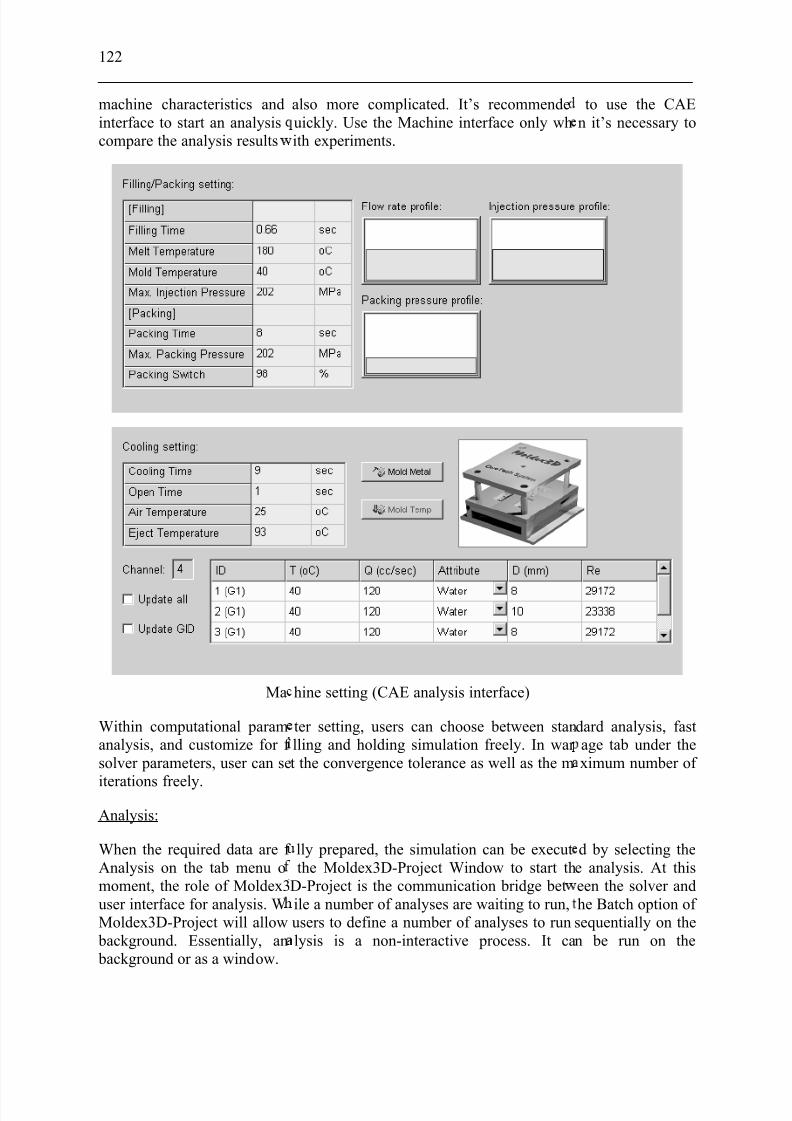
7/27/2019 Injection Mould Design
http://slidepdf.com/reader/full/injection-mould-design 140/160
122
machine characteristics andinterface to start an analysiscompare the analysis results
Ma
Within computational paramanalysis, and customize for f solver parameters, user can se
iterations freely.
Analysis:
When the required data are f Analysis on the tab menu omoment, the role of Moldex3user interface for analysis. WMoldex3D-Project will allow
background. Essentially, an background or as a window.
also more complicated. It’s recommendeuickly. Use the Machine interface only whith experiments.
hine setting (CAE analysis interface)
ter setting, users can choose between stanlling and holding simulation freely. In war t the convergence tolerance as well as the m
lly prepared, the simulation can be executthe Moldex3D-Project Window to start th
D-Project is the communication bridge betile a number of analyses are waiting to run,users to define a number of analyses to runlysis is a non-interactive process. It ca
to use the CAEn it’s necessary to
dard analysis, fastage tab under theximum number of
d by selecting thee analysis. At thiseen the solver andhe Batch option of sequentially on then be run on the
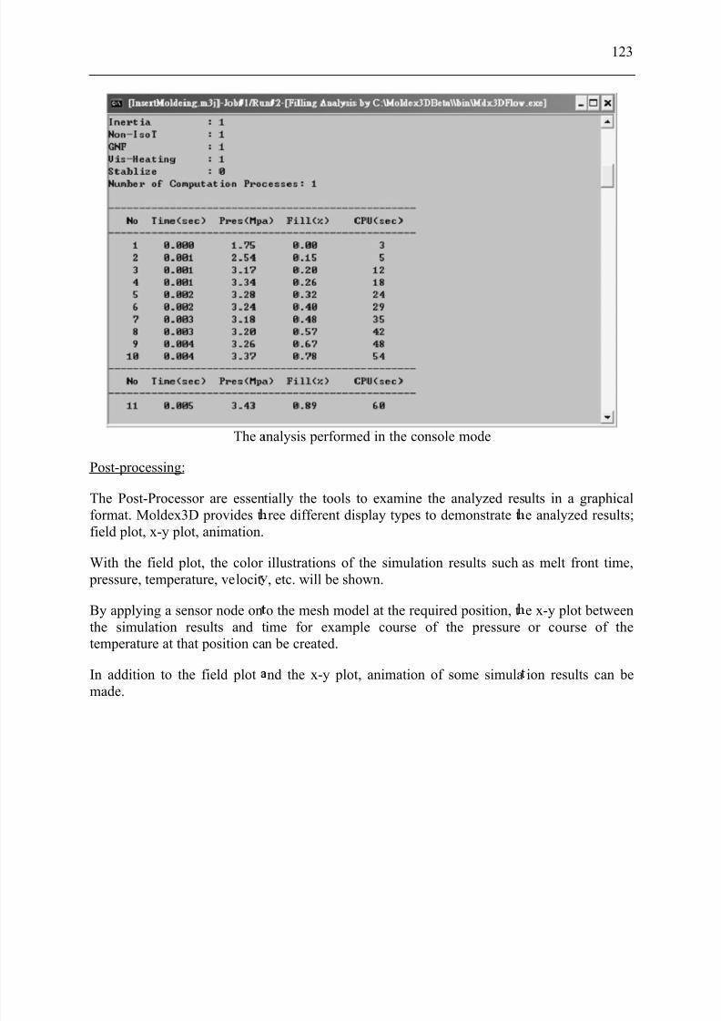
7/27/2019 Injection Mould Design
http://slidepdf.com/reader/full/injection-mould-design 141/160
The a
Post-processing:
The Post-Processor are essenformat. Moldex3D provides t
field plot, x-y plot, animation.With the field plot, the color
pressure, temperature, velocit
By applying a sensor node onthe simulation results and ttemperature at that position ca
In addition to the field plotmade.
nalysis performed in the console mode
tially the tools to examine the analyzed resree different display types to demonstrate t
illustrations of the simulation results such, etc. will be shown.
o the mesh model at the required position, time for example course of the pressuren be created.
nd the x-y plot, animation of some simula
123
ults in a graphicale analyzed results;
as melt front time,
e x-y plot betweenor course of the
ion results can be

7/27/2019 Injection Mould Design
http://slidepdf.com/reader/full/injection-mould-design 142/160
124
Appendix 3 Compa
right ca
2.5D si
Short-shot study
1 0 0 %
f i l l e d
8 7 % f i l l e d
7 4 % f i l l e d
6 2 % f i l l e d
4 6 % f i l l e d
3 6 % f i l l e d
ison of the melt front progressi
ity between the experimental s
ulations
Tetrahedral derivativemesh
Voxe
n of the
udy and
derivative mesh
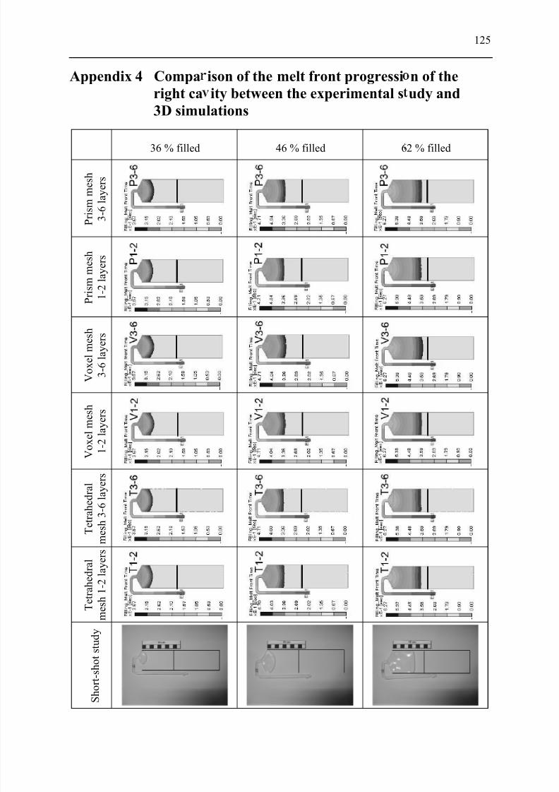
7/27/2019 Injection Mould Design
http://slidepdf.com/reader/full/injection-mould-design 143/160
Appendix 4 Compa
right ca
3D simu
36 % filled
P r i s m m e s h
3 - 6 l a y e r s
P r i s m
m e s h
1 - 2 l a
y e r s
V o x e l m e s h
3 - 6 l a y e r s
V o x e l m e s h
1 - 2 l a y e r
s
T e t r a h e d r a l
m e s h 3 - 6 l a y e r s
T e t r a h e d r a l
m e s h 1 - 2 l a y e r s
S h
o r t - s h o t s t u d y
ison of the melt front progressi
ity between the experimental s
lations
46 % filled 6
125
n of the
udy and
2 % filled

7/27/2019 Injection Mould Design
http://slidepdf.com/reader/full/injection-mould-design 144/160
126
74 % filled
P r i s m
m e s h
3 - 6 l a
y e r s
P r i s m m e s h
1 - 2 l a y e r s
V o x e l m e s h
3 - 6 l a y e r s
V o x e l m e s h
1 - 2 l a y e r s
T e t r a h e d r a l m e s h
3 - 6 l a y e r s
T e t r a h e d
r a l m e s h
1 - 2 l a y e r s
S h o r t - s h o t s t u d y
87 % filled 1
0 % filled
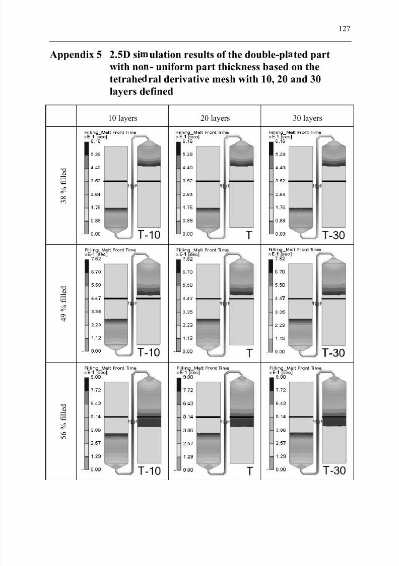
7/27/2019 Injection Mould Design
http://slidepdf.com/reader/full/injection-mould-design 145/160
Appendix 5 2.5D si
with no
tetrahe
layers d
10 layers
3 8
% f i l l e d
4 9 % f i l
l e d
5 6 %
f i l l e d
ulation results of the double-pl
- uniform part thickness based
ral derivative mesh with 10, 20
efined
20 layers
127
ted part
on the
and 30
30 layers
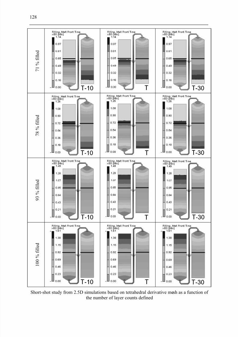
7/27/2019 Injection Mould Design
http://slidepdf.com/reader/full/injection-mould-design 146/160
128
7 1 % f i l l e d
7 8 % f i l l e d
9 3 % f i l l e d
1 0 0 % f i l l e d
Short-shot study from 2.5D sitmulations based on tetrahedral derivative mehe number of layer counts defined
sh as a function of

7/27/2019 Injection Mould Design
http://slidepdf.com/reader/full/injection-mould-design 147/160
2.5D computed course otetrahedral derivative me the temperature during filling and holding ph as a function of the number of mesh layer
129
hase based onounts defined

7/27/2019 Injection Mould Design
http://slidepdf.com/reader/full/injection-mould-design 148/160
130
2.5D computed average (left) based on tetrahedral deriva
and center (right) temperature distribution dive mesh as a function of the number of mes
ring filling phaseh layers defined
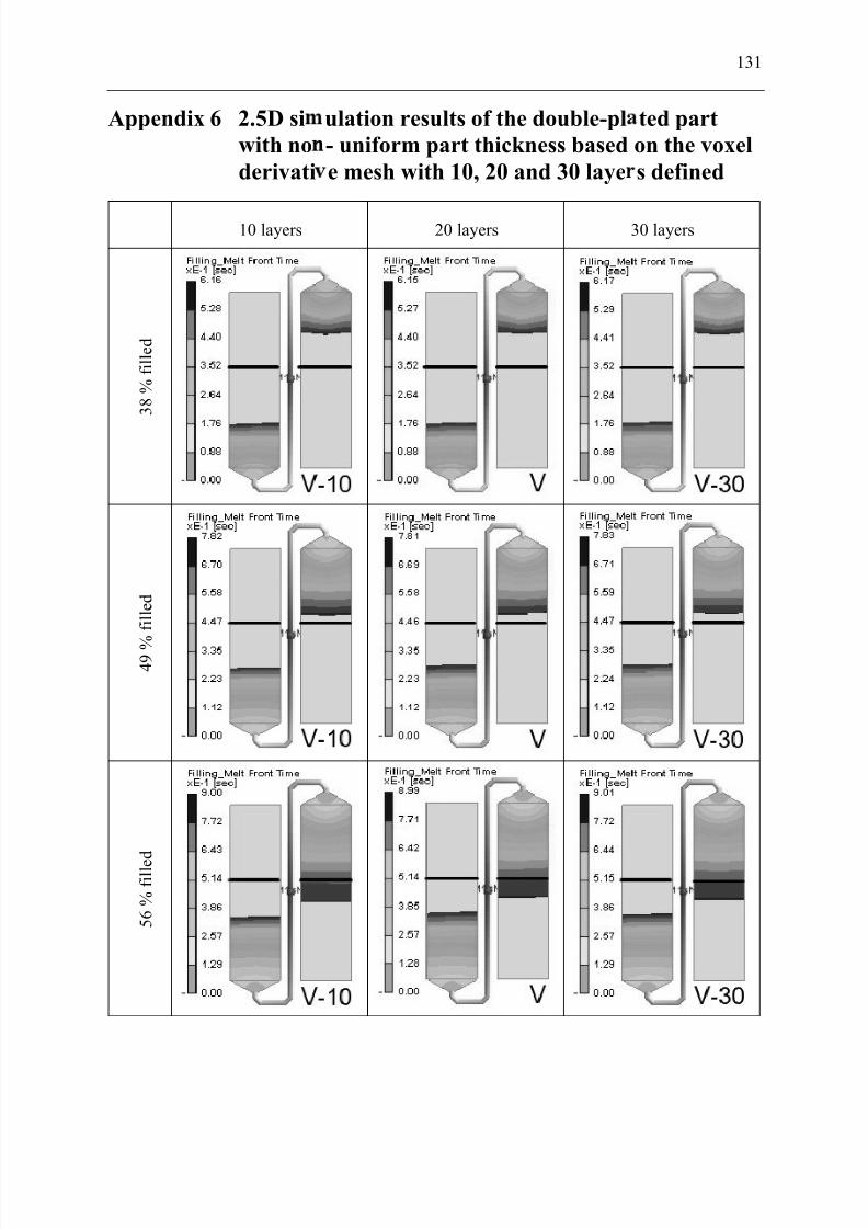
7/27/2019 Injection Mould Design
http://slidepdf.com/reader/full/injection-mould-design 149/160
Appendix 6 2.5D si
with no
derivati
10 layers
3 8 % f i l l e d
4 9 %
f i l l e d
5 6 % f i l l e d
ulation results of the double-pl
- uniform part thickness based
e mesh with 10, 20 and 30 laye
20 layers
131
ted part
on the voxel
s defined
30 layers
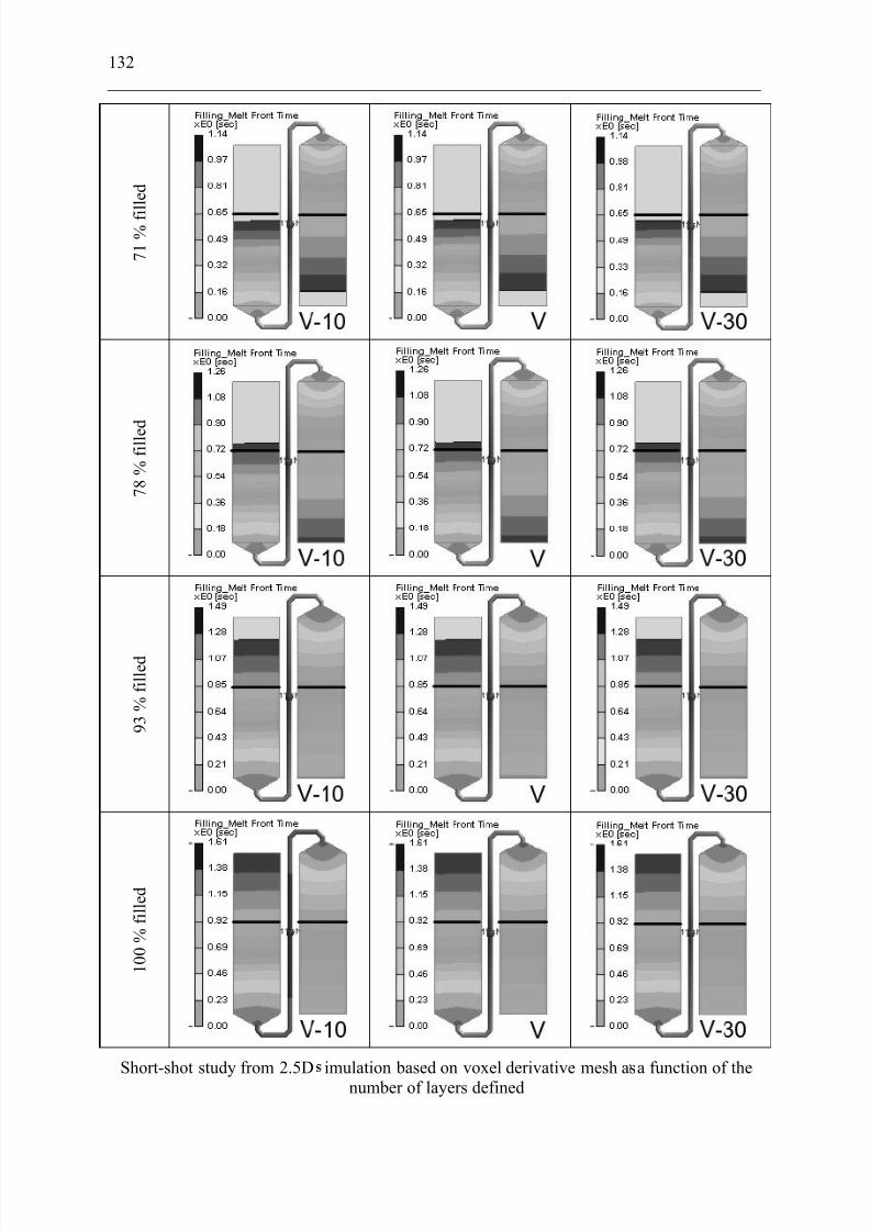
7/27/2019 Injection Mould Design
http://slidepdf.com/reader/full/injection-mould-design 150/160
132
7 1 % f i l l e d
7 8 % f i l l e d
9 3 % f i l l e d
1 0 0 % f i l l e d
Short-shot study from 2.5D imulation based on voxel derivative mesh asnumber of layers defined
a function of the
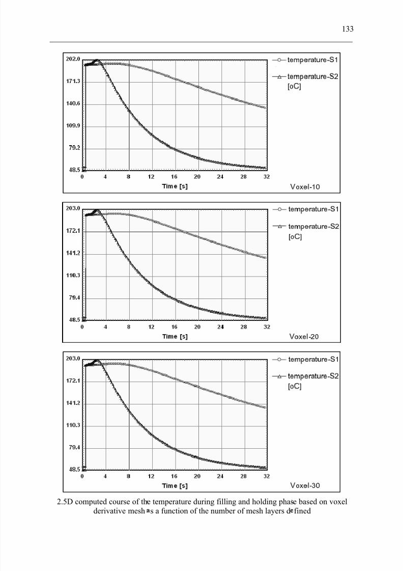
7/27/2019 Injection Mould Design
http://slidepdf.com/reader/full/injection-mould-design 151/160
2.5D computed course of thderivative mesh
e temperature during filling and holding phass a function of the number of mesh layers d
133
e based on voxelfined
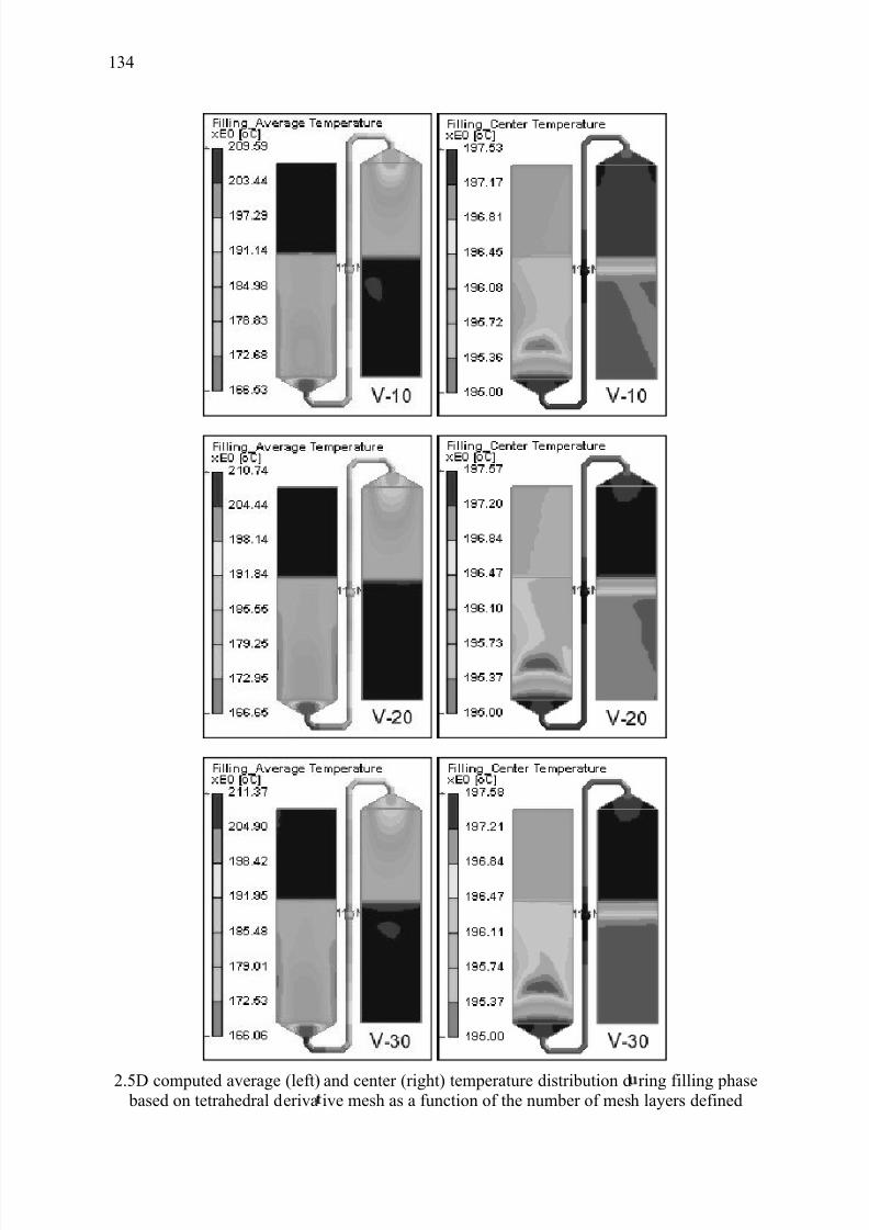
7/27/2019 Injection Mould Design
http://slidepdf.com/reader/full/injection-mould-design 152/160
134
2.5D computed average (left) based on tetrahedral deriva
and center (right) temperature distribution dive mesh as a function of the number of mes
ring filling phaseh layers defined

7/27/2019 Injection Mould Design
http://slidepdf.com/reader/full/injection-mould-design 153/160
135
Appendix 7 Types of Labels used in Packaging
There are numerous types of the label used in packaging. Each type is manufactureddifferently from each other but they have some of the same characteristics.
In-mold labels (IML): In-mold labels for blow molding have a heat activated adhesiveapplied to them that is activated during the application process. For injection molding, noadhesive is necessary because of higher temperature involved during molding. The labelmaterial can be printed using several different printing processes, such as flexography, offset,screen and hot stamping. In-mold labels are water, grease, weather, and scuff resistant. Thelabel appears as part of the container and has great shelf appeal. They are used for labelinghealth and personal care products, toys, motor oil, beverages, chemicals and cleaning
products.
Thermal labels: There are two different types of thermal labels, thermal transfer and directthermal labels. Each uses a heat process when imprinted.
• Thermal Transfer Labels
In thermal transfer printing, a ribbon runs over the top of the label material and together they pass between a metal plate and a print head. The print head, which is heated, comes down onthe ribbon, causing the coating from the ribbon to be transferred to the label material to createthe image. Thermal transfer labels are manufactured on rolls or as continuous fan foldedlabels. The label stock is not a special paper but must meet the weight, finish and sizerequirements of the thermal printer.
• Direct Thermal Labels
In direct thermal printing, no ribbon is necessary to create an image. The label material isheat sensitive. The print head is heated as in thermal transfer and when it comes in contactwith the special direct thermal label stock, it causes a chemical reaction which creates theimage. Direct thermal labels are manufactured on rolls or as continuous fan folded labels. Thelabel is printed on a thermal label printer. Special direct thermal label stock is required.
Linerless labels: Linerless labels are pressure sensitive labels that do not have a liner. Thelabels are wound on a roll that has had a release coating applied to the front of the facestock to prevent the adhesive from sticking on the label below. The available facestocks includestandard paper, film and direct thermal. Linerless labels are available with permanent,removable and repositionable adhesives. Using linerless labels eliminates the waste of the
liner material and allows more labels per roll. This increases efficiencies by reducing thenumber of roll changes, eliminating time used to separate the label from the liner andeliminates time and cost of disposing of the liner waste.
Glue applied labels: A glue applied labels does not have an adhesive layer. It is adhered tothe product by glue being applied to the label or to the container during the application
process. A cold glue or hot glue adhesive is used to apply the label. The label can be printedon most any type of paper. It can also be printed on metallized paper or film. Once the labelis printed, you have the option of adding off-line features to the label, such as foil stamping,die cutting and embossing. Glue applied labels generally cost less than other types of container labels. The material cost is generally less and the labels can be applied at high
speeds. Glue applied labels are also more environmentally friendly because there is less wasteand the waste is easier to recycle.

7/27/2019 Injection Mould Design
http://slidepdf.com/reader/full/injection-mould-design 154/160
136
Shrink labels: Shrink labels are non-adhesive sleeves constructed from film material thatshrinks when heat is applied. Film material such as PVC, PETG, OPP and PP are used in themanufacturing of these labels. Shrink labels allow 360 degrees of print area and will conformto the shape of the container when heat is applied. This allows the packaging company to usesome uniquely shape containers that have extreme contours without compromising the copy
or graphics. Using shrink labels provides an opportunity to decorate the container with somevery eye catching designs. It also provides more printing space for product information sincethe label can be printed the entire 360 degrees versus a pressure sensitive label that wouldonly allow a certain area of the container to be labeled. There are many product areas inwhich shrink labels are used, such as food and beverage products, pharmaceuticals, consumer
products, cosmetics, personal care products and pesticides.
Stretch labels: Stretch labels are used to label and decorate products such as beverages, food, personal care products, chemicals and cleaning products. They are similar to shrink labels inthat they allow 360 degrees of print area on the label around the container. The label isconstructed of a stretch film material that has elasticity to it. The label is stretched over the
container and released when it is in the proper location. Once released, it will fit snug andform to the contours of the container. The stretch sleeve label does not need any glue or heatto enable it to stay in place. The labels are available on clear or opaque film and can bereverse printed. They are supplied on rolls and a perforation can be added between labels if desired. The stretch labels can be supplied for manual, semi-automatic or automatic labelingapplications.
The application process does not cause any fumes and it does not contaminate the container with glue. The application of the label is a very clean process and very environmentalfriendly. The stretch label is moisture proof and is easy to remove from the container at thetime of recycling due to the absence of glue.
Smart labels: Smart labels contain electronic devices that have read/write memory used tostore and access information. The electronic device is a radio frequency identification (RFID)transponder or tag. The RFID technology, like bar codes, is used to automatically capturedata. It is different from a bar code in that it can hold much more data, it can bereprogrammed, and its data is accessed by a reader but it does not need optical contact withthe reader to be read. Some common applications where smart labels would be used aresupply chain management, production control, work-in-process, baggage identification andtracking, express delivery services, reusable container tracking and security systems. Theindustry acceptance of smart labels has been slow. The RFID technology can improve
performance and efficiency but is expensive to start up. As more companies commit to the
use of this new technology it will become more widely accepted and many will benefit fromits capabilities.
Security labels: There are many different options for adding security to the labels. The typeof security used on the labels will depend on the label use, the desired level of security andwhat the user is trying to protect against, such as counterfeiting or product fraud. To providethe proper level of security, many times several security features are used.
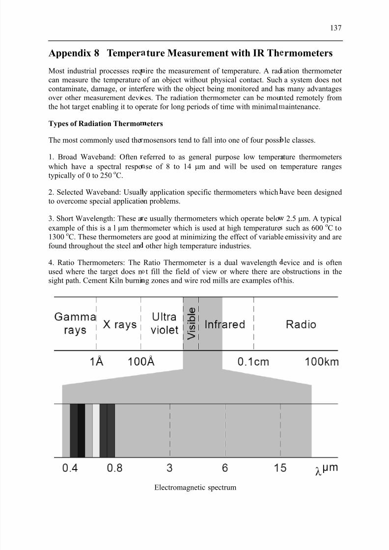
7/27/2019 Injection Mould Design
http://slidepdf.com/reader/full/injection-mould-design 155/160
Appendix 8 Temper
Most industrial processes reqcan measure the temperaturecontaminate, damage, or inter
over other measurement devithe hot target enabling it to op
Types of Radiation Thermo
The most commonly used the
1. Broad Waveband: Oftenwhich have a spectral respotypically of 0 to 250 oC.
2. Selected Waveband: Usuallto overcome special applicatio
3. Short Wavelength: These aexample of this is a l µm ther 1300 oC. These thermometersfound throughout the steel an
4. Ratio Thermometers: Theused where the target does nsight path. Cement Kiln burni
ture Measurement with IR Th
ire the measurement of temperature. A radof an object without physical contact. Suchfere with the object being monitored and ha
es. The radiation thermometer can be mouerate for long periods of time with minimal
eters
mosensors tend to fall into one of four possi
eferred to as general purpose low temperase of 8 to 14 µm and will be used on t
y application specific thermometers whichn problems.
e usually thermometers which operate belomometer which is used at high temperatureare good at minimizing the effect of variableother high temperature industries.
Ratio Thermometer is a dual wavelengtht fill the field of view or where there areg zones and wire rod mills are examples of
Electromagnetic spectrum
137
rmometers
ation thermometer a system does not
s many advantages
ted remotely fromaintenance.
le classes.
ture thermometersemperature ranges
ave been designed
2.5 µm. A typicalsuch as 600 oC toemissivity and are
evice and is oftenobstructions in thehis.
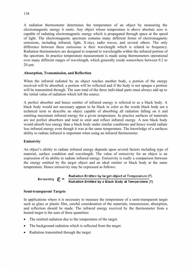
7/27/2019 Injection Mould Design
http://slidepdf.com/reader/full/injection-mould-design 156/160
138
A radiation thermometer determines the temperature of an object by measuring theelectromagnetic energy it emits. Any object whose temperature is above absolute zero iscapable of radiating electromagnetic energy which is propagated through space at the speedof light. The electromagnetic spectrum contains many different forms of electromagneticemissions, including infrared, light, X-rays, radio waves, and several others. The only
difference between these emissions is their wavelength which is related to frequency.Radiation thermometers are designed to respond to wavelengths within the infrared portion of the spectrum. In practice temperature measurement is made using thermometers operationalover many different ranges of wavelength, which generally reside somewhere between 0.2 to20 µm.
Absorption, Transmission, and Reflection
When the infrared radiated by an object reaches another body, a portion of the energyreceived will be absorbed, a portion will be reflected and if the body is not opaque a portionwill be transmitted through. The sum total of the three individual parts must always add up to
the initial value of radiation which left the source.
A perfect absorber and hence emitter of infrared energy is referred to as a black body. A black body would not necessary appear to be black in color as the words black body are atechnical term to describe an object capable of absorbing all radiation falling on it andemitting maximum infrared energy for a given temperature. In practice surfaces of materialsare not perfect absorbers and tend to emit and reflect infrared energy. A non black bodywould absorb less energy than a black body under similar conditions and hence would radiateless infrared energy even though it was at the same temperature. The knowledge of a surfacesability to radiate infrared is important when using an infrared thermometer.
Emissivity
An object’s ability to radiate infrared energy depends upon several factors including type of material, surface condition and wavelength. The value of emissivity for an object is anexpression of its ability to radiate infrared energy. Emissivity is really a comparison betweenthe energy emitted by the target object and an ideal emitter or black body at the sametemperature. Hence emissivity may be expressed as follows:
Semi-transparent Targets
In applications where it is necessary to measure the temperature of a semi-transparent targetsuch as glass or plastic film, careful consideration of the materials, transmission, absorption,and reflection should be made. The infrared energy received by the thermometer from aheated target is the sum of three quantities:
• The emitted radiation due to the temperature of the target.
• The background radiation which is reflected from the target.
• Radiation transmitted through the target.
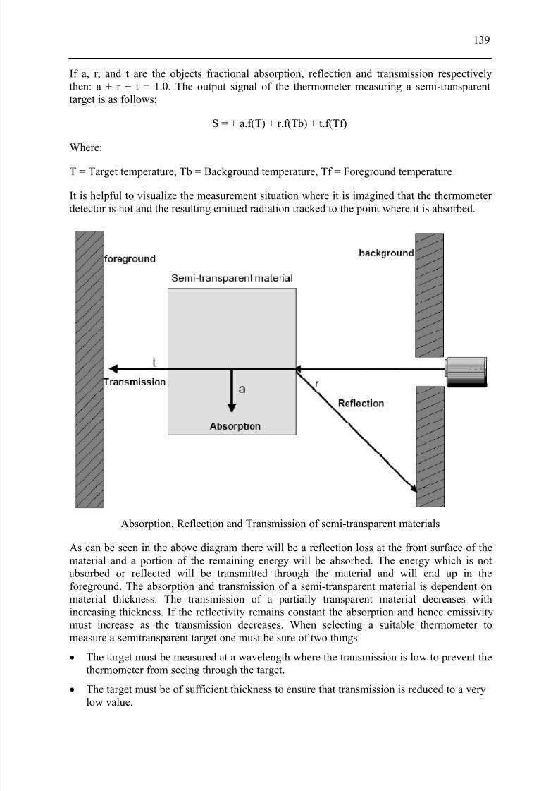
7/27/2019 Injection Mould Design
http://slidepdf.com/reader/full/injection-mould-design 157/160
139
If a, r, and t are the objects fractional absorption, reflection and transmission respectivelythen: a + r + t = 1.0. The output signal of the thermometer measuring a semi-transparenttarget is as follows:
S = + a.f(T) + r.f(Tb) + t.f(Tf)
Where:
T = Target temperature, Tb = Background temperature, Tf = Foreground temperature
It is helpful to visualize the measurement situation where it is imagined that the thermometer detector is hot and the resulting emitted radiation tracked to the point where it is absorbed.
Absorption, Reflection and Transmission of semi-transparent materials
As can be seen in the above diagram there will be a reflection loss at the front surface of thematerial and a portion of the remaining energy will be absorbed. The energy which is notabsorbed or reflected will be transmitted through the material and will end up in theforeground. The absorption and transmission of a semi-transparent material is dependent onmaterial thickness. The transmission of a partially transparent material decreases withincreasing thickness. If the reflectivity remains constant the absorption and hence emissivitymust increase as the transmission decreases. When selecting a suitable thermometer tomeasure a semitransparent target one must be sure of two things:
• The target must be measured at a wavelength where the transmission is low to prevent thethermometer from seeing through the target.
•
The target must be of sufficient thickness to ensure that transmission is reduced to a verylow value.

7/27/2019 Injection Mould Design
http://slidepdf.com/reader/full/injection-mould-design 158/160
140
Plastics
Most plastics are processed at relatively low temperatures as they rapidly decompose attemperatures above a few hundred degrees Celsius. Many types of plastic include filler materials to give color and modify mechanical properties etc. In even moderate thickness
these are often opaque over large parts of the infrared spectrum and are therefore easilymeasured using traditional low temperature wide band thermometers.
Plastic Films:
Thin plastic films have a transmission and hence emissivity which is strongly wavelengthdependent.
Transmission of Infrared through Polypropylene
The figure above clearly shows how a thin sample of plastic is highly transparent over much
of the infrared spectrum. In this case a broad band thermometer will “see” through the sampleand will tend to measure whatever is behind it. The figure also clearly shows a region around3.4 µm where the sample is suddenly quite opaque. In the infrared part of the spectrum thisopaque region is associated with particular molecular resonances within the structure of thematerial. Many common plastics contain saturated hydrogen to carbon molecular bonds (C-H
bond) and it is these bonds which are responsible for the effects seen at wavelengths close to3.4 µm. Measurement of temperature of these types of plastic film is often possible if thethermometer is operational at a wavelength where the plastic film is opaque. It should benoted however that plastic materials have many different compositions and not all include theC-H bond. Some plastic films such as polyurethane, acrylic and some fluorocarbons are notso opaque at 3.43 µm and a better result is obtained at 7.9 µm (C-O bond).

7/27/2019 Injection Mould Design
http://slidepdf.com/reader/full/injection-mould-design 159/160
141
Emissivity:
The transmission and the reflections from the surface of the target limit the emissivity of anysemi-transparent target. For most hydrocarbon plastics the reflection coefficient is 0.04 per surface, and this sets an upper limit of 0.96 for the emissivity even when it is totally opaque.
The emissivity value will fall with reducing thickness of the plastic film, leading to anincrease in transmission from the behind the target. It is useful to specify a minimumthickness for a particular plastic material to ensure reliable temperature measurement results.
Minimum Thickness:
When specifying material minimum thickness, an acceptable transmission value must first bedefined. The acceptable transmission at a very low value of 2 % is defined, resulting inemissivity values of >0.94. This definition gives minimum thickness figures which areconservative and which will prove reliable for the vast majority of applications. Minimumthickness to meet this criterion for various plastics is shown in the table below. This
Minimum thickness specification should be used with caution as the amount of transmission,which can be tolerated, may vary enormously from one application to the next.
MaterialMin Thickness
(for E ≥ 0.94)
Polypropylene 20 µm
Polyethylene 20 µm
Polyamide (Nylon) 40 µm
Acrylic 80 µm
Polystyrene 80 µm
Polyvinyl Chloride (PVC) 100 µm
Polyurethane 100 µm
Cellulose Acetate 100 µm
Polycarbonate 150 µm
Polyester (PET) 300 µm
Polyvinylidene Chloride (PVDC) 300 µm
Minimum thickness of various plastics (Note with 3.43 µm Thermometer)

7/27/2019 Injection Mould Design
http://slidepdf.com/reader/full/injection-mould-design 160/160
142
LEBENSLAUF
Vorname Patcharee Nachname LARPSURIYAKUL
Geschlecht weiblich
Geburtsdatum 12.03.1977Geburtsort Bangkok, Thailand
Studium
1995-1999 Studiengang Werkstoffwissenschaft (Polymer Science)Chulalongkorn University, Bangkok, ThailandAbschluss Akademischer Grad Bachelor of Science
1999-2001 Studiengang Werkstoffwissenschaft (Polymer Science)
Chulalongkorn University, Bangkok, ThailandAbschluss Akademischer Grad Master of Science
2001 Erhalt des Stipendiums der thailändischen Regierung,um in Deutschland auf dem Gebiet Kunststofftechnik zu
promovieren
Sprachkurse
Juli 1998-April 1999 Besuchen eines englischen Sprachkurses in Thailand,