Embed Size (px)
Citation preview
Insect Inspired Vision for Micro Aerial Vehicle Navigation Joshua Fernandes, Adam Postula
ITEE, The University of Queensland.
[email protected], [email protected]
Mandayam Srinivasan, Saul Thurrowgood
QBI, The University of Queensland.
[email protected], [email protected]
Abstract
This paper describes a generic platform for vision
based navigation which is partially inspired by the
biological principles that underlie insect vision
and navigation. The system developed uses a
CMOS sensor that is directly interfaced with a
Field Programmable Gate Array (FPGA), to
calculate an optical flow field in real time, and
control an unmanned vehicle. The imaging
system also provides useful information about the
vehicle‟s surroundings, enabling the construction
of terrain maps.
1 Introduction
The use of Micro Aerial Vehicles (MAVs) in real world
applications is increasing in scope – with sizes that range
from ten centimetres to a metre. There are several
challenges associated with fully autonomous operation in
dynamic environments; coupled with the fact that the
airframes only support a reduced payload capacity. This
enforces the need for a guidance system that can be
integrated onto the vehicle such that it does not interfere
with its aerodynamics. Hence, passive sensing methods are
preferred, i.e., the use of vision, as opposed to active
sensing methods which are often bulky, expensive and
radiation emitting. A glance at a fly evading a rapidly
descending hand, or orchestrating perfect landings on the
rim of a teacup, would convince even the most sceptical
observer that insects are excellent navigators and possess
visual systems that are fast, reliable and precise [Srinivasan
et al., 2004]. The insights gained by analysing the
principles of insect flight can be synthesized in real time
reactive systems, because they offer novel and
computationally elegant solutions for robotic guidance.
When an insect moves in its environment, the image of
the environment moves in its eyes. The pattern of image
motion, (or “optic flow”, as it is known), depends upon the
nature of the insect‟s motion (roll, yaw and pitch, and the
translations along the three axes), as well as the
three-dimensional structure of the environment, and the
distances to objects in it [Srinivasan, 2011]. Insects analyse
the resulting optic flow to avoid collisions with obstacles,
control flight speed, perform smooth landings, and
calculate distance flown (odometry). Thus, the optic flow
pattern carries valuable information that can be used for
vision-based guidance of aircraft.
This paper presents the research and development of an
integrated on-board solution for the navigation of a MAV,
consisting of a CMOS sensor directly interfaced to an
FPGA, which makes use of real time optical flow data to
control the vehicle. Ideally, in order to meet real time
requirements, video information needs to be handled at
high speeds and in a parallel fashion. This makes FPGAs
an ideal choice as they are high performance devices that
use a parallel processing approach. They comprise
numerous logic gates and have dedicated units for memory
allocation, arithmetic and logic etc., which can be
reconfigured on the fly to build any processing network.
This flexibility makes for an ideal platform for real-time
processing of high-bandwidth pixel data. In addition, an
FPGA allows for relatively quick development, is a cost
effective solution and provides a convenient path of
migration to an Application Specific Integrated Circuit
(ASIC), at a later stage, as planned for this project.
2 Background
To date, there have been several methods to develop
passive guidance systems utilizing vision. Most
approaches require complex iterative algorithms that can
only be run from a base station i.e. a dedicated platform
like a PC or similar, where control of the MAV is based on
visual information obtained from an on-board camera.
These solutions inherently have limitations and bottlenecks
in terms of the processing capability, as they are sequential
in nature. Furthermore, they limit the effective range of
operation of the vehicle, as it can only operate within the
communication zone of the base station. [Zuffrey and
Floreano, 2006] [Ruffier and Franceschini, 2005]
Other researchers have proposed a parallel processing
approach, i.e. the use of Field Programmable Gate Arrays
(FPGAs) to perform computations in order to meet real
time requirements. [Arribas and Maciá, 2001] created an
implementation using a correlation algorithm to track
motion. Their implementation achieved 22fps on images of
resolution 96x96 pixels. In 2002, the same authors [Arribas
and Maciá, 2003] developed an implementation on an
FPGA using the [Horn and Schunck, 1981] algorithm,
Proceedings of Australasian Conference on Robotics and Automation, 7-9 Dec 2011, Monash University, Melbourne Australia.
Page 1 of 8
which computes optical flow by calculating intensity
gradients in space and time. Their implementation made
use of two FPGAs working in parallel to compute flow
fields for images that were 50x50 pixels in resolution, at 19
fps. [D´ıaz et al., 2006] created a modified version of the
[Lucas and Kanade, 1984] algorithm to compute optical
flow fields at a rate of 30fps on images that were 320x240
pixels in resolution. They used a specially designed FIR
filter to decrease latency and storage requirements.
[Browne et al. 2008] also created an implementation using
a differential based algorithm, which generated flow fields
for 120x120 image locations at 2fps. This frame rate would
be less than optimal for real-time flight control. [Garratt et
al., 2009] also developed an implementation on an FPGA,
using the Image Interpolation Algorithm [Srinivasan,
1994] to calculate a two dimensional optical flow field,
comprising 36 equally spaced vectors on 1024x768 images
at 30fps. There are of course, other studies that have used
FPGAs for image processing but the above examples
pertain specifically to this arena of research.
Our research aims to create a fully integrated solution
for robotic vision and guidance. Our prototype system
improves on work done in 2001 by [Arribas et al, 2001]. As
stated earlier, the CMOS sensor is interfaced directly with
the FPGA 1 . Our implementation also uses an image
pyramid approach, which confers several important
advantages. First, this method reduces the processing time
by a significant amount. Second, it improves the search
range. Third, the CMOS sensor and the entire calculation
stage use the same clock (PixClk), which implies that the
calculations can be as fast as the camera will permit. Thus,
the calculation speed is always matched to the frame rate of
the camera, potentially saving power consumed by the
FPGA. Finally, the entire implementation uses only 8 bit
integers and basic mathematical operators; allowing for
possible implementations of a large number of
computation units on a single FPGA. This enables
performance improvements in terms of processing speed to
be achieved with an application specific architecture and
an intrinsically parallel processing approach.
3 The Image Matching Algorithm
The Image Matching algorithm segments the image
into regions and generates an optical flow vector for each
region, based on the image motion in that region. A
complete and in depth description of the Image Matching
algorithm can be found in [Buelthoff et al., 1990]. The
following section presents a simplified explanation of the
algorithm, together with the improvements implemented
here.
Our fundamental assumption is that the maximum
possible displacement of an object inside a block is limited
to „ ‟ pixels in any direction – the actual value is dependent
on the expected velocity of the vehicle with respect to other
1 Interfacing of the camera directly to the FPGA was also done by
[Garratt et al, 2009].
objects, as seen in the image plane. One of the aims of this
research is to detect objects in the path of the MAV; and it
is generally the case that a given pixel has the same
velocity as those of its neighbours (since they usually
belong to the same object) and are collectively located in a
roughly square neighbourhood, or window, of size „ ‟
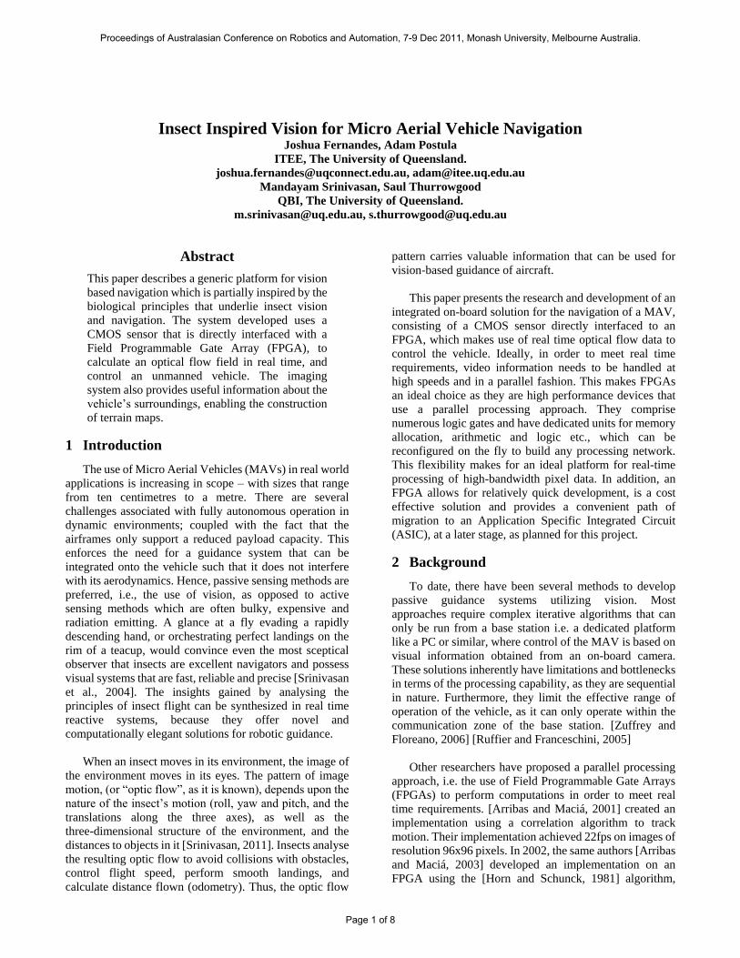
centred around that pixel. The motion of that pixel at (x, y)
is given by the motion of the window, of size ,
centred at (x, y), out of possible
combinations as illustrated in left hand panel of Figure 1.
The motion of the patch of pixels is estimated for each
possible displacement in the window by calculating the
strength of the match for each displacement, as shown in
the right-hand panel of Figure 1.
If Φ represents a matching function that gives a value
proportional to the match between two pixels of intensities
I1 and I2, the match strength C (x, y: u, v) for point (x, y) and
pixel displacements (u, v), then the match is calculated by
taking the sum of the match values between each pixel in
the displaced patch Pv in the first frame and the
corresponding pixel in the patch in the second frame, as
specified by equation (1):
where i, j Pv.
There are several methods for calculating the matching
function. Two methods were selected and analysed for
performance because of their low computational cost. The
first is the sum of absolute differences (SAD), which is
calculated between pixel values of the current frame and
the next frame of the respective region. The second method
involves calculating the sum of squared differences (SSD)
of the respective pixel intensity values. With either
method, a lower value of represents a better match. Both
methods were tested on several sets of video data as well as
still images with varying levels of artificially imposed
motion. Samples were taken with varying levels of contrast
and the results of the two methods compared. It was
observed that, for those samples with lower levels of
contrast, the SSD results were consistently slightly off in
comparison to the ground truth data; the SAD method
however appeared to produce results that resembled the
ground truth data. For higher levels of contrast both
methods performed the same. The samples were then
normalised and analysed. The results of the SSD method
Figure1: The panel on the left shows an „ ‟ of 2 and the panel on
the right shows the movement of the patch window.
Proceedings of Australasian Conference on Robotics and Automation, 7-9 Dec 2011, Monash University, Melbourne Australia.
Page 2 of 8

were then found to be comparable to that of the ground
truth data of those samples with lower contrast, and the
SAD method showed almost no difference at all. Tables 1
and 2 below illustrate the mead standard error (MSE)
differences in results of the low contrast non normalised
samples and the normalised samples. The SAD method
was selected as it was found to be less sensitive to variation
in image contrast, and it requires less processing as the
images did not require normalisation.
Statistics of the Non-Normalized Results
Method # Vectors MSE (x) MSE (y)
SSD 88 3.39 2.98
SAD 88 0.38 0.32
Table 1: Statistics of the Non-Normalised results
Statistics of the Normalized Results
Method # Vectors MSE (x) MSE (y)
SSD 88 0.47 0.41
SAD 88 0.36 0.32
Table 2: Statistics of the Normalised results
This algorithm has several advantages that make it
ideal for implementation on an FPGA. It is two
dimensional in nature, which means that it does not suffer
from the aperture problem except in severe cases, and is
not very susceptible to noise. Since patch windows
normally overlap, match strengths for neighbouring pixels
tend to be relatively the same; the exception being at
window or motion edges. Consequently the flow field that
is generated tends to be relatively smooth. Gradient based
approaches tend to contain errors that arise from the
sensitivity of numerical differentiation to noise [Camus,
1994]. The presented matching technique does not require
the calculated match strengths to have any relationship to
the theoretical values and only requires that it best fit the
motion of the objects correctly. An illustration being when
the illumination between frames changes rapidly- although
this has an adverse effect on individual match strengths, it
does not change the position of the best match. On the
other hand, a gradient based approach would break down
under these conditions because the basic assumption of
constant image illumination would no longer be valid
[Buelthoff et al., 1990]. If required, our method can
generate flow fields with 100% density (except near the
borders), since vectors can be calculated for each pixel. In
addition, as each window calculation is independent of all
of the others, the entire process can be parallelized, thus
making it ideal for implementation on an FPGA.
4 Algorithm Implementation
As an initial feasibility test the algorithm was
implemented in software in the C programming language,
without the use of any special image processing libraries.
This enabled testing and development of the algorithm in
its most basic form, allowing easy porting to an FPGA.
Tests of this implementation showed that it was possible to
achieve a frame rate of 38 fps with an „ ‟ value of 2, on
images that were 640x480 pixels in resolution.
The FPGA selected for use for this project was an
Altera Cyclone IV 4CE115. The device offers a
combination of low power consumption, high functionality
and low cost. Its architecture is extremely efficient and is
designed for use where a higher logic density is required
rather than a higher input/output pin count – making it
ideal for this project. The CMOS digital video sensor used
for this project is the Micron MT9P031. This RGB sensor
has a maximum output resolution of 5 Megapixels at 15fps
and has an on-chip Analog to Digital Converter (ADC), of
12-bit resolution. In addition the sensor has an I2C
interface bus for control, which allows real time control of
the video sensor‟s parameters such as gain (analog and
digital), exposure, etc. For our implementation we require
a high frame rate over a high precision ADC. Hence, we
have configured the sensor to run at VGA resolution
(640x480). This results in a (conservatively specified)
frame rate of 50 fps (the system has been successfully
tested with a frame rate of 110fps and is capable of a
maximum of 150fps). Another benefit of running at a
lower image resolution allows us to “bin” and “skip” pixels
to enable better low light performance. Binning and
skipping of pixels is a process of reducing resolution by
combining adjacent same-colour pixels to produce one
pixel output; effectively making all the pixels in the
sensor‟s field of view (2560x1920 pixels) contribute to the
output image. In addition, this process results in an output
image with reduced sub-sampling artefacts [Terasic
Manual, 2010].
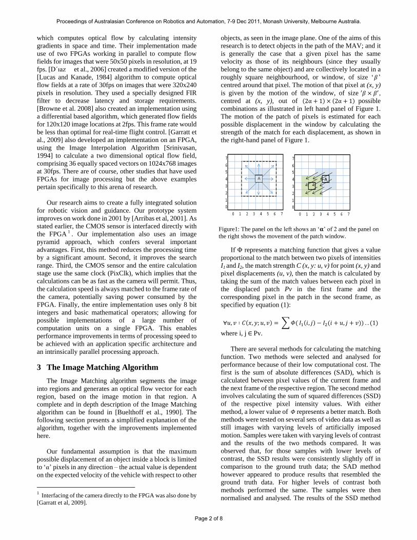
The overall architecture diagram is shown in Figure 2.
It contains multiple sub systems, each of which is briefly
discussed in this section. The configuration for the CMOS
sensor takes place in the “I2C CMOS Config” unit. This
unit consists of an I2C bus through which the camera
communicates with the sensor. The sensor has a number of
registers that control various parameters like channel gains,
sensor exposure, frame resolutions etc. At start up, this unit
initialises each of these registers with specific pre-set
values. Another benefit of this form of control is that it
allows the user or autonomous vehicle to change any of
these parameters during normal operation of the FPGA,
and does not require the device to be reprogrammed. For
example if the vehicle suddenly flew into a region of direct
sunlight, it could autonomously adjust the exposure rate to
compensate for this extra light. The CMOS sensor captures
light intensities and sends this raw pixel data to the FPGA,
where it is captured by the “CMOS Capture” Unit. The
sensor makes use of a clock signal, referred to as the
PixClk, with which pixel data is latched. In addition, the
sensor also sends out two synchronisation signals
–“Line_Valid”, that is asserted during the active region of
the frame, and a “Frame_Valid” signal that is used to
envelope frames. A combination of these two signals
allows us to differentiate between valid pixel data and
blanking pixels (horizontal and vertical) and thus only
capture valid pixel data.
Proceedings of Australasian Conference on Robotics and Automation, 7-9 Dec 2011, Monash University, Melbourne Australia.
Page 3 of 8
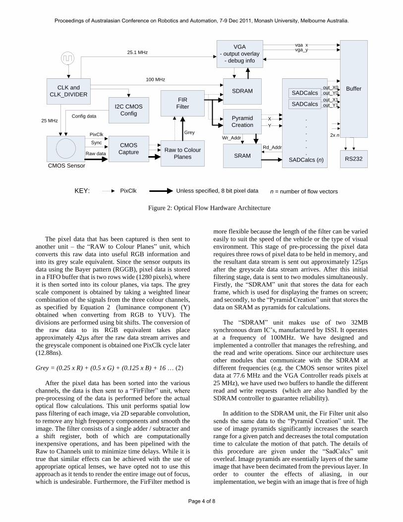
Figure 2: Optical Flow Hardware Architecture
CLK and
CLK_DIVIDER
CMOS Sensor
CMOS
Capture
I2C CMOS
Config
Raw to Colour
Planes
FIR
Filter
25 MHzConfig data
PixClk
Raw data
Sync
Grey
SDRAM
100 MHz
Pyramid
Creation
SRAM
Wr_Addr
SADCalcsout_X0
Y
X
SADCalcs out_Y1
Rd_Addr
Buffer
2x n
RS232
VGA
- output overlay
- debug info
out_Y0
out_X1
25.1 MHz
vga_xvga_y
Unless specified, 8 bit pixel dataPixClk
.
.
.
.
.
.
SADCalcs (n)
n = number of flow vectorsKEY:
The pixel data that has been captured is then sent to
another unit – the “RAW to Colour Planes” unit, which
converts this raw data into useful RGB information and
into its grey scale equivalent. Since the sensor outputs its
data using the Bayer pattern (RGGB), pixel data is stored
in a FIFO buffer that is two rows wide (1280 pixels), where
it is then sorted into its colour planes, via taps. The grey
scale component is obtained by taking a weighted linear
combination of the signals from the three colour channels,
as specified by Equation 2 (luminance component (Y)
obtained when converting from RGB to YUV). The
divisions are performed using bit shifts. The conversion of
the raw data to its RGB equivalent takes place
approximately 42µs after the raw data stream arrives and
the greyscale component is obtained one PixClk cycle later
(12.88ns).
Grey = (0.25 x R) + (0.5 x G) + (0.125 x B) + 16 … (2)
After the pixel data has been sorted into the various
channels, the data is then sent to a “FirFilter” unit, where
pre-processing of the data is performed before the actual
optical flow calculations. This unit performs spatial low
pass filtering of each image, via 2D separable convolution,
to remove any high frequency components and smooth the
image. The filter consists of a single adder / subtracter and
a shift register, both of which are computationally
inexpensive operations, and has been pipelined with the
Raw to Channels unit to minimize time delays. While it is
true that similar effects can be achieved with the use of
appropriate optical lenses, we have opted not to use this
approach as it tends to render the entire image out of focus,
which is undesirable. Furthermore, the FirFilter method is
more flexible because the length of the filter can be varied
easily to suit the speed of the vehicle or the type of visual
environment. This stage of pre-processing the pixel data
requires three rows of pixel data to be held in memory, and
the resultant data stream is sent out approximately 125µs
after the greyscale data stream arrives. After this initial
filtering stage, data is sent to two modules simultaneously.
Firstly, the “SDRAM” unit that stores the data for each
frame, which is used for displaying the frames on screen;
and secondly, to the “Pyramid Creation” unit that stores the
data on SRAM as pyramids for calculations.
The “SDRAM” unit makes use of two 32MB
synchronous dram IC‟s, manufactured by ISSI. It operates
at a frequency of 100MHz. We have designed and
implemented a controller that manages the refreshing, and
the read and write operations. Since our architecture uses
other modules that communicate with the SDRAM at
different frequencies (e.g. the CMOS sensor writes pixel
data at 77.6 MHz and the VGA Controller reads pixels at
25 MHz), we have used two buffers to handle the different
read and write requests (which are also handled by the
SDRAM controller to guarantee reliability).
In addition to the SDRAM unit, the Fir Filter unit also
sends the same data to the “Pyramid Creation” unit. The
use of image pyramids significantly increases the search
range for a given patch and decreases the total computation
time to calculate the motion of that patch. The details of
this procedure are given under the “SadCalcs” unit
overleaf. Image pyramids are essentially layers of the same
image that have been decimated from the previous layer. In
order to counter the effects of aliasing, in our
implementation, we begin with an image that is free of high
Proceedings of Australasian Conference on Robotics and Automation, 7-9 Dec 2011, Monash University, Melbourne Australia.
Page 4 of 8

frequencies (using the FirFilter unit) and then start the sub
sampling process for the next layer; where we double the
length of the filter for each layer in accordance with
Shannon‟s Sampling Theorem [Marks, 1990]. Practically,
this is done by convolving the first layer with a low pass
filter and then sub sampling. For our implementation, we
use two levels of pyramids. We start with images that are
640x480 in resolution. After the pyramidal process, the
lowest layer has images of resolution 160x120.
The “Pyramid Creation” unit also keeps track of the „x‟
and „y‟ coordinates of pixels, using the two
synchronization signals from the sensor - Line_Valid and
Frame_Valid. Pyramidal data is stored on SRAM for quick
and easy access during the calculation stage. Our
implementation makes use of 1MB Synchronous RAM,
also manufactured by ISSI. The SRAM uses the PixClk for
its read and write operations. The addresses for the
pyramids are generated based on the pixels „x‟ and „y‟
co-ordinates and are given by:
SRAM_Address = Offset + (y × row_no.) + (x) … (3)
where the „row_no.‟ refers to the current row that gets
incremented when the „x‟ coordinate reaches the end of a
line, and the offset is based on the respective level of the
pyramid. Each pyramid has a different offset, so as to make
data retrieval easy and prevent write address conflicts. The
image pyramids are created 62µs after the pre-processed
data has been sent out from the FirFilter unit.
The optical flow calculation unit, called “SAD Calcs”
(Sum of Absolute Differences), is the unit that is
responsible for calculating the optical flow vector for a
given region. Since this is a process that is repeated over
various regions of the image, this unit has specifically been
designed and developed to function as a module that can be
repeated any number of times, each for a specific region
and calculations for all regions can then be performed in
parallel. Regions are selected to allow for an overlap of the
edges so that almost all motion can be captured. Since all
these modules run in parallel, care has been taken to
prevent read errors and conflicts when communicating
with the SRAM. During the read process each module
raises a flag, and if two or more flags are raised they are
handled in the order that they were raised.
Each unit runs on the basis of a finite state machine
(FSM) to guarantee deterministic behaviour, as shown in
Figure 3. The FSM has five basic states of operation. The
first state, “Grab1” gets the pyramid pixel data for that
specific region of the first frame and stores it on registers
for quick access. This is termed the “Reference Block” and
is of size 3x3, and can be increased as needed. Once the
pixel coordinates reach the end of the first frame, a
transition is made to the next state, “Grab 2”, which
performs the exact same task as the first state but on the
second frame‟s pyramid data. This region is termed the
“Comparison Block” and is of size 7x7 pixels, giving us a
maximum search radius, or „ ‟, of 2 pixels, for each
pyramid level. Fundamentally, the Comparison block is the
search region that is used to locate the Reference block, in
the next state. When the counter reaches 60 rows past the
given region, a transition is made to the next state
“CalculateSAD”. The figure of 60 rows was selected so as
to allow all data for the second frame‟s pyramids to be
loaded from SRAM, and it includes enough time for
resolving race conditions, should there be flags raised from
other units.
The next two states are the ones that are responsible for
performing calculations and finding the region with the
best correspondence (lowest SAD score). This is where the
image pyramid approach excels. We start calculations on
the highest layer and find the closest match on that layer
and then use that location as a starting point for the next
layer, and so on. Two counters, „dx‟ and „dy‟, keep track of
the horizontal and vertical translations in the search region
for each layer. For each set of translations the Reference
block is compared to the Comparison block, by taking the
absolute differences between pixel intensities and adding
them up for each translation.
After each translation is complete, a transition is made
to the next state, “Check Minimum”, where the new sum is
compared to the minimum of the earlier translations. If the
new sum is lower, it is saved as the new minimum value,
along with its „dx‟ and „dy‟ values. At the end of this
process, these two values of „dx‟ and „dy‟ are used as the
starting location for the next layer. The process continues
until all horizontal and vertical translations are completed
within the search regions on all layers. Each layer takes
approximately 58 clock cycles to load the pixel contents to
registers and 50 clock cycles to perform calculations at
each layer; altogether a total of 266 clock cycles per patch
window. 2 We have a Reference block of 3x3 and a
Comparison block of 7x7, so we make 5x5 translations or
2 The highest layer of pyramids is also written to registers as
well as SRAM. Hence during the calculations stage, it does not
require excess time to load the contents of the highest layer.
Grab1
- Load
Reference
Block
Grab2
- Load
Comparison
Block
Finished
- Send result
to buffer
- Reset
variables
Calculate SAD
- Compute sum
- Increment dx
and dy
Check
Minimum
- Check if new
sum is lower
than minimum
y == (60 rows + start of region)
Done flag == 0
dx && dy < 5
Done flag == 1
y == 479y != 479
y == 479
Figure 3: FSM of the SAD Calculation Unit (SADCalcs)
Proceedings of Australasian Conference on Robotics and Automation, 7-9 Dec 2011, Monash University, Melbourne Australia.
Page 5 of 8

Figure 4: Architecture Timing (not to scale)
25 in total, per layer. Once this process has been
completed, a transition is made to the “Finished” state
where a flag is raised to indicate that the process is
completed. Each SADCalcs unit takes 3.4µs to complete
all its calculations and output the resultant flow vector
data. Refer to Figure 4, which details the timing of the
entire process. The idle time for the system is
approximately 2.5ms. The use of the image pyramid
scheme achieves a significantly quicker result than the
traditional method of searching for pixels at the original
resolution. In our implementation we use a maximum
displacement of 2 pixels, and two levels of pyramids. This
effectively means that we can search for a maximum radius
of 14 pixels in any direction on the image at the original
resolution. Using the pyramidal scheme this takes a total of
75 translations, (two levels of pyramids, and the actual
image). In comparison, performing the same search at the
original resolution would require 784 translations (the time
for calculations per translation is the same, regardless of
method used).
The architecture also makes use of a digital-to-analog
converter (DAC) from Analog Devices, the ADV7123.
The DAC generates VGA signals based on controls from
the “VGA Controller” Unit, thus allowing us to monitor in
real time what the CMOS sensor “sees”. To facilitate
debugging, we have used the same operating resolution as
that of the CMOS sensor i.e., 640x480 (VGA) with a
refresh rate of 25.1MHz. Our implementation uses the
pixel data, stored in SDRAM as a background. The
calculated optical flow field from the SADCalcs unit is
then superimposed over the background. Another benefit
of this arrangement is that during remote testing on aerial
vehicles, the VGA output can be converted to composite
video and the feed monitored on the ground using a
wireless downlink and receiver, if required. The
architecture also makes use of an UART interface, for
debugging purposes. This buffers the calculated optical
flow data and transmits it at a slower rate, 115200 baud
(RS232 standard). There are other interfaces that can be
developed and created for faster communication.
5 Experimental Results
The prototype platform has been tested in indoor and
outdoor environments. Indoor testing has been done using
a textured visual environment and the corresponding
optical flow fields calculated, shown in Figure 5, and
compared with the ground truth data, as shown in Figure 6.
The ground truth data for the frame was generated by
shifting the pixels in the frame 8 pixels up. Table 3 shows
the mean and standard deviation of the computed
displacement of the flow vectors, for the x and y directions
respectively (88 vectors each). From the illustration, and
the table below, we see that the calculated optical flow
field closely corresponds to the ground truth data. To
facilitate debugging, we have used small blue dots to mark
the middle of each search region and green boxes to
indicate the middle of the calculated region of best match;
to make visualisation easier in the illustration; we have
superimposed yellow lines connecting these dots.
Figure 5: Optical flow results on a textured pattern
Proceedings of Australasian Conference on Robotics and Automation, 7-9 Dec 2011, Monash University, Melbourne Australia.
Page 6 of 8
Statistics of the Computed Flow Vectors
# Vectors µ (x) σ (x) µ (y) σ (y)
88 0.01 0.41 7.96 0.49
Table 3: Statistics of the optical flow vectors computed in Fig. 5.
Figure 7 shows the optical flow results obtained from
testing in an outdoor environment, and is compared with
ground truth data shown in Figure 8. The ground truth data
for this frame was obtained by shifting the pixels in the
frame 8 pixels down and 8 pixels to the right. Table 4 gives
the mean and standard deviation of the flow vectors in the x
and y direction. The optical flow results correspond closely
to the ground truth data from the illustration and the table.
Statistics of the Computed Flow Vectors
# Vectors µ (x) σ (x) µ (y) σ (y)
88 7.95 0.52 8.04 0.47
Table 4: Statistics of the optical flow vectors computed in Fig. 7.
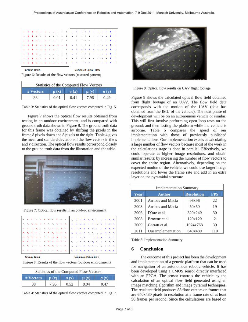
Figure 9 shows the calculated optical flow field obtained
from flight footage of an UAV. The flow field data
corresponds with the motion of the UAV (data has
obtained from the IMU of the vehicle). The next phase of
development will be on an autonomous vehicle or similar.
This will first involve performing open loop tests on the
ground, and then testing the platform while the vehicle is
airborne. Table 5 compares the speed of our
implementation with those of previously published
implementations. Our implementation excels at calculating
a large number of flow vectors because most of the work in
the calculations stage is done in parallel. Effectively, we
could operate at higher image resolutions, and obtain
similar results; by increasing the number of flow vectors to
cover the entire region. Alternatively, depending on the
expected motion of the vehicle, we could use larger image
resolutions and lower the frame rate and add in an extra
layer on the pyramidal structure.
Implementation Summary
Year Author Resolution FPS
2001 Arribas and Macia 96x96 22
2003 Arribas and Macia 50x50 19
2006 D´ıaz et al 320x240 30
2008 Browne et al 120x120 2
2009 Garratt et al 1024x768 30
2011 Our implementation 640x480 110
Table 5: Implementation Summary
6 Conclusion
The outcome of this project has been the development
and implementation of a generic platform that can be used
for navigation of an autonomous robotic vehicle. It has
been developed using a CMOS sensor directly interfaced
with an FPGA. The sensor controls the vehicle by the
calculation of an optical flow field generated using an
image matching algorithm and image pyramid techniques.
The resultant field produces 88 flow vectors on frames that
are 640x480 pixels in resolution at a frame rate of at least
50 frames per second. Since the calculations are based on
Figure 6: Results of the flow vectors (textured pattern)
Figure 7: Optical flow results in an outdoor environment
Figure 8: Results of the flow vectors (outdoor environment)
Figure 8: Results of the flow vectors (outdoor environment)
Figure 9: Optical flow results on UAV flight footage
Proceedings of Australasian Conference on Robotics and Automation, 7-9 Dec 2011, Monash University, Melbourne Australia.
Page 7 of 8
the PixClk of the CMOS camera, the system is actually
capable of generating flow at a much higher rate and has
been tested successfully at 110 fps.
Our implementation has several benefits in
comparison with other implementations. The sensor is
directly interfaced with the FPGA and the architecture is
able to compute the optical flow field at significantly faster
rates, as outlined in Table 5. The platform has been tested
in indoor as well as outdoor environments and the next
stage in development will be outdoor testing on a vehicle
that will eventually use the optic flow information for
autonomous navigation.
References
[Arribas and Macia, 2001] P. Arribas and F. Maciá. FPGA implementation of Camus correlation optical flow algorithm for Real Time Images.14th International Conference on Vision Interface, pp. 33-38, 2001.
[Arribas and Macia, 2003] P. Arribas and F. Maciá. FPGA implementation of the Santos-Victor optical flow algorithm for real time image processing: a useful attempt. Proceedings of SPIE,5117:23-32, 2003.
[Browne et al., 2008] T. Browne, J. Condell, G. Prasad and T. McGinnity. An Investigation into Optical Flow Computation on FPGA Hardware.Proceedings of the International Machine Vision and Image Processing Conference, pp 176-181, 3-5 September 2008.
[Buelthoff et al., 1990] H. Buelthoff, J. Little and T. Poggio, “A Parallel Algorithm for Real Time computation of Optical Flow,” Nature, vol. 337, no 6207, pp. 549-553, 1990.
[Camus, 1994] T. Camus, Real time Optical Flow. PhD Thesis, Brown University, USA, 1994.
[D´ıaz et al., 2006] J. D´ıaz, E. Ros, F. Pelayo, E. Ortigosa and S.Mota. FPGA-based real-time optical-flow system.IEEE Transactions on Circuits and Systems for Video Technology, vol.16, no. 2, pp. 274-279, 2006
[Garratt et al., 2009] M. Garratt, A. Lambert and T.
Guillemette, “FPGA Implementation of an Optical Flow Sensor using the Image Interpolation Algorithm.” Proceedings of theAustralasianConference on Robotics and Automation, Sydney, Australia, 2009.
[Horn and Schunck, 1981]B. Horn and B. Schunck. Determining Optical Flow.Artificial Intelligence,17:185–203, 1979.
[Lucas and Kanade, 1984] B. Lucas and T. Kanade. AnIterative image registration technique with an applicationto stereo vision Proceeding DARPA Image Understanding Workshop, pp.121–130, 1984.
[Marks, 1990] Robert J. Marks. Introduction to Shannon sampling and Interpolation Theory.pp.324-341Springer Texts in Electrical Engineering, New York: Springer, 1991
[Ruffier and Franceschini, 2005] Ruffier, F and Franceschini, N. Optic flow regulation: the key to aircraft automatic guidance. Robotics and Autonomous Systes.177-194. 2005.
[Srinivasan et al., 2004] Srinivasan, Mandyam and Zhang, Shaowu. Small brains, smart minds: Vision, perception and cognition in honeybees.The Visual Neurosciences, edited by Leo Chalupa and J. S. Werner, MIT Press, 2004, pp.1501-1513.
[Srinivasan 2011] Srinivasan M. V. Honeybees as a model for the study of Visually Guided flight Navigation and Biologically Inspired Robotics. Physiological Reviews 91, pp. 389 – 411.
[Terasic Manual, 2010] TerasicTRDB-D5M Hardware Specification Datasheet.http: www.cse.hcmut.edu.vn/dce/celab/altera/index.php?option=com_docman&task=doc_details&gid=9&Itemid=36,. Accessed 12/05/2011
[Zuffrey and Floreano, 2006] Zuffrey, J and Floreano D. Fly-inspired Visual Steering of an Ultralight Indoor Aircraft. IEEE Transactions on Robotics, vol. 22, pp. 137-146, 2006.
Proceedings of Australasian Conference on Robotics and Automation, 7-9 Dec 2011, Monash University, Melbourne Australia.
Page 8 of 8