Embed Size (px)
Citation preview
Instituto de Desarrollo Tecnológico para la Industria Química (INTEC)Universidad Nacional de Litoral (UNL) – CONICET
Güemes 3450, 3000 Santa Fe, [email protected]
The distribution function
Types of transportation modes and costs
Distribution network design and planning
Brief review of important routing and scheduling problems (TSP, VRP, PDP)
The PDP with transshipment (PDPT)
The vehicle routing problem in multi-echelon networks with and without crossdocking (VRP-SCM & VRPCD-SCM)
Conclusions
J. CERDÁ - PASI 2011 2
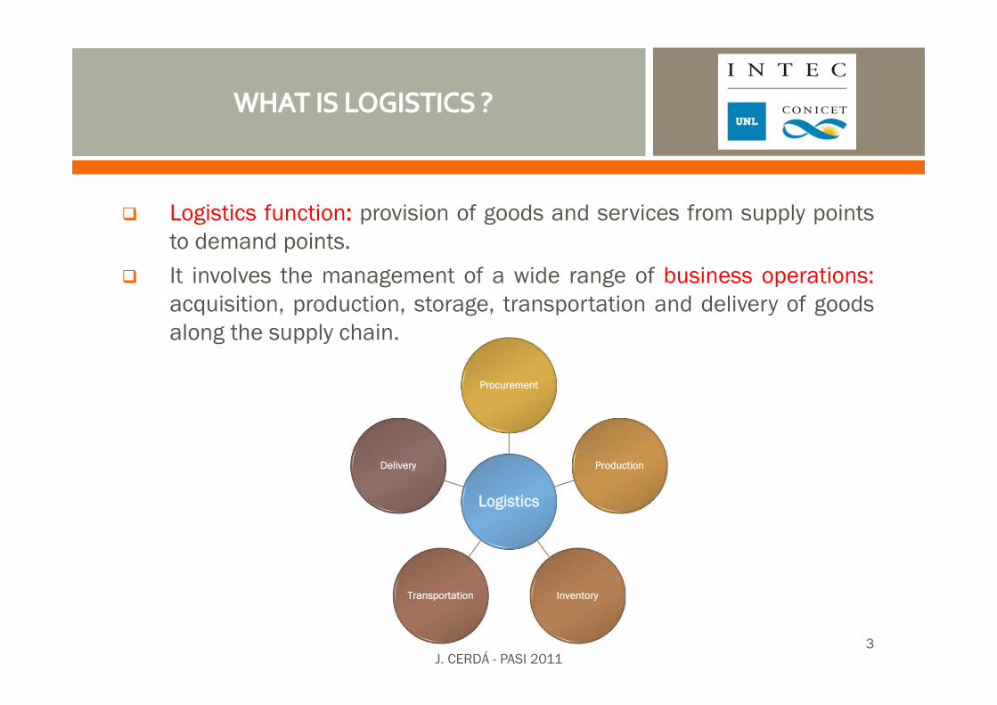
Logistics function: provision of goods and services from supply pointsto demand points.It involves the management of a wide range of business operations:acquisition, production, storage, transportation and delivery of goodsalong the supply chain.
Logistics
Procurement
Production
InventoryTransportation
Delivery
J. CERDÁ - PASI 20113
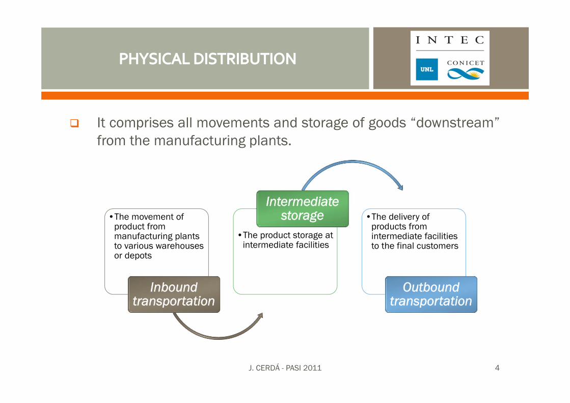
It comprises all movements and storage of goods “downstream”from the manufacturing plants.
•The movement of product from manufacturing plants to various warehouses or depots
Inbound transportation
•The product storage at intermediate facilities
Intermediate storage •The delivery of
products from intermediate facilities to the final customers
Outbound transportation
J. CERDÁ - PASI 2011 4
Transportation play a key role because products are rarelyproduced and consumed at the same location.
The last transportation step from distribution centers tocustomers (i.e. the outbound transportation), is usually themost costly link of the distribution chain.
Distribution costs accounts for about 16% of the salevalue of an item; approximately one fourth is due to theoutbound transportation.
J. CERDÁ - PASI 2011 5
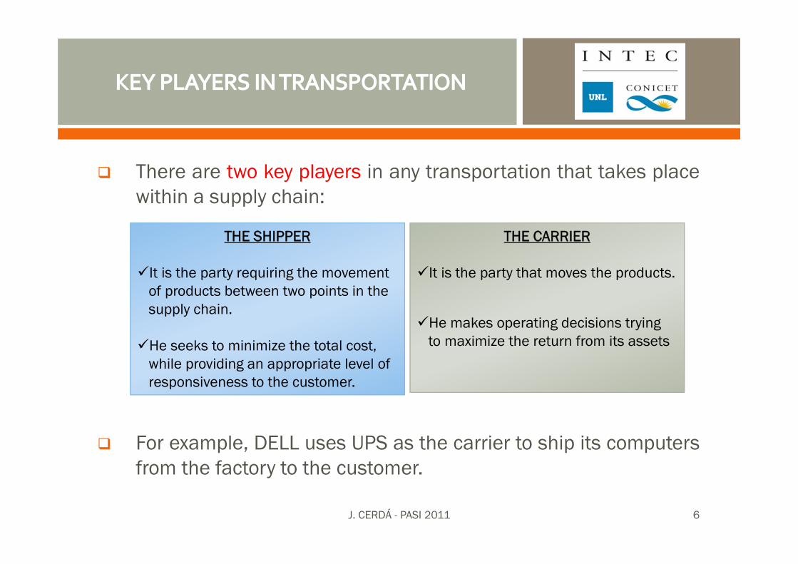
There are two key players in any transportation that takes placewithin a supply chain:
For example, DELL uses UPS as the carrier to ship its computersfrom the factory to the customer.
THE SHIPPER
It is the party requiring the movement of products between two points in the supply chain.
He seeks to minimize the total cost, while providing an appropriate level of responsiveness to the customer.
THE CARRIER
It is the party that moves the products.
He makes operating decisions trying to maximize the return from its assets
J. CERDÁ - PASI 2011 6
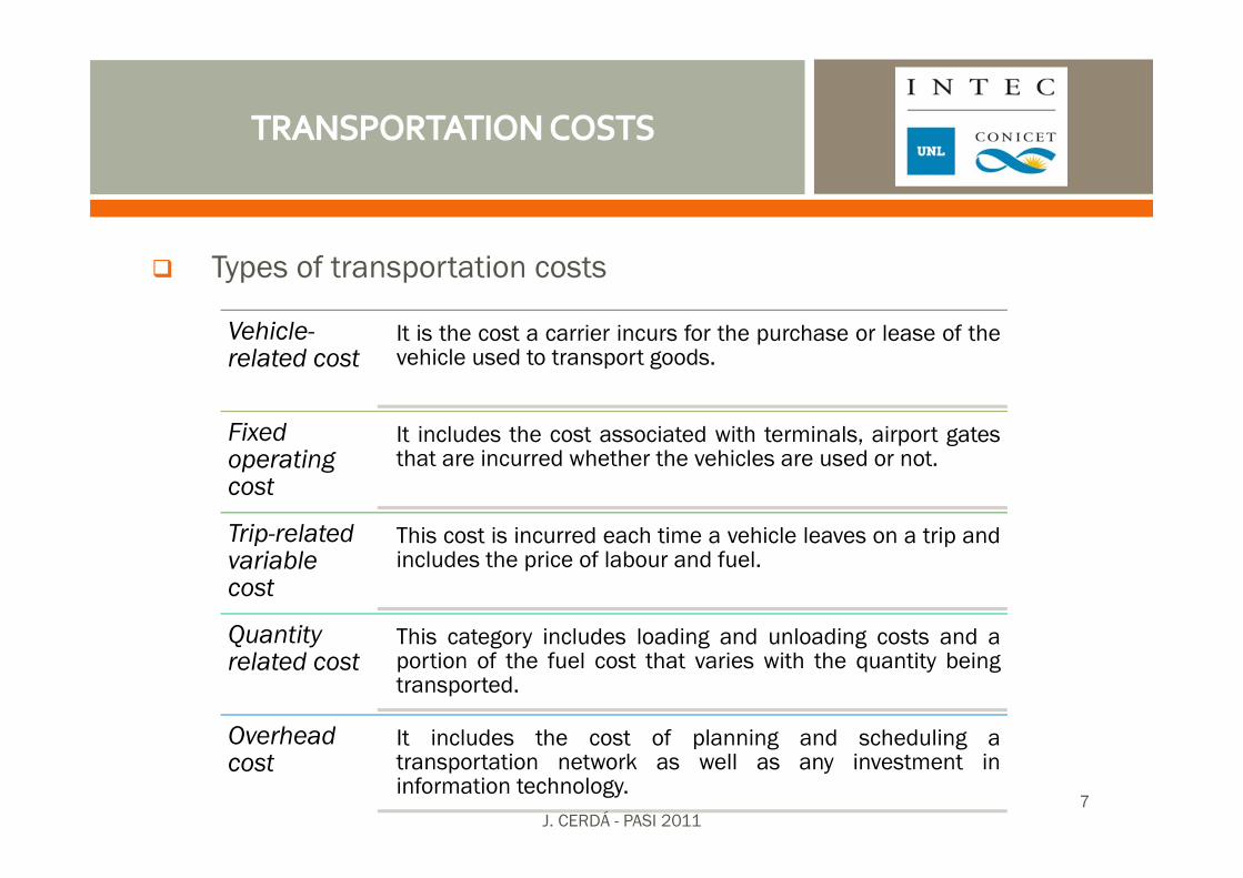
Types of transportation costs
Vehicle-related cost
It is the cost a carrier incurs for the purchase or lease of thevehicle used to transport goods.
Fixed operating cost
It includes the cost associated with terminals, airport gatesthat are incurred whether the vehicles are used or not.
Trip-related variable cost
This cost is incurred each time a vehicle leaves on a trip andincludes the price of labour and fuel.
Quantity related cost
This category includes loading and unloading costs and aportion of the fuel cost that varies with the quantity beingtransported.
Overhead cost
It includes the cost of planning and scheduling atransportation network as well as any investment ininformation technology.
J. CERDÁ - PASI 20117
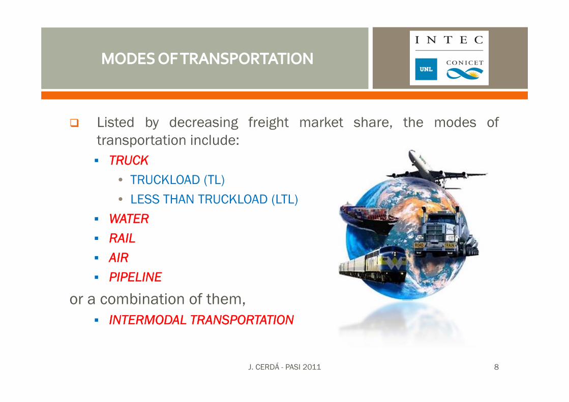
Listed by decreasing freight market share, the modes oftransportation include:
TRUCK• TRUCKLOAD (TL)• LESS THAN TRUCKLOAD (LTL)
WATERRAILAIRPIPELINE
or a combination of them,INTERMODAL TRANSPORTATION
J. CERDÁ - PASI 2011 8
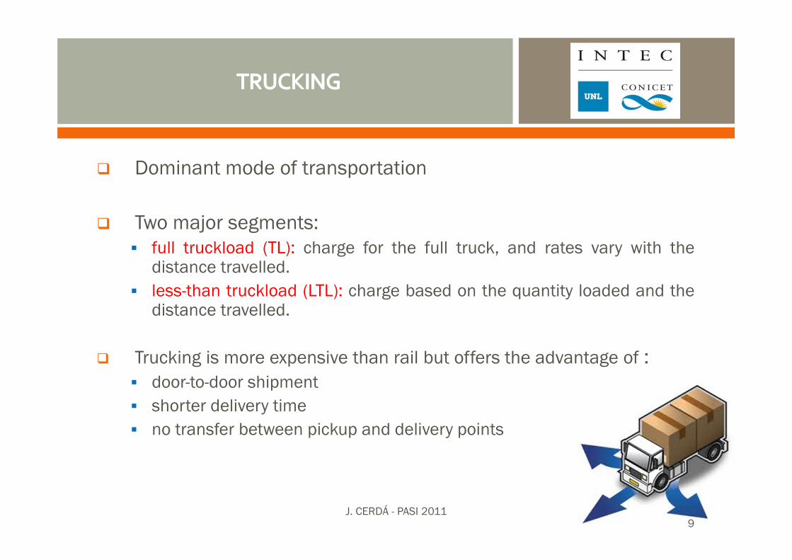
Dominant mode of transportation
Two major segments:full truckload (TL): charge for the full truck, and rates vary with thedistance travelled.less-than truckload (LTL): charge based on the quantity loaded and thedistance travelled.
Trucking is more expensive than rail but offers the advantage of :door-to-door shipmentshorter delivery timeno transfer between pickup and delivery points
J. CERDÁ - PASI 20119
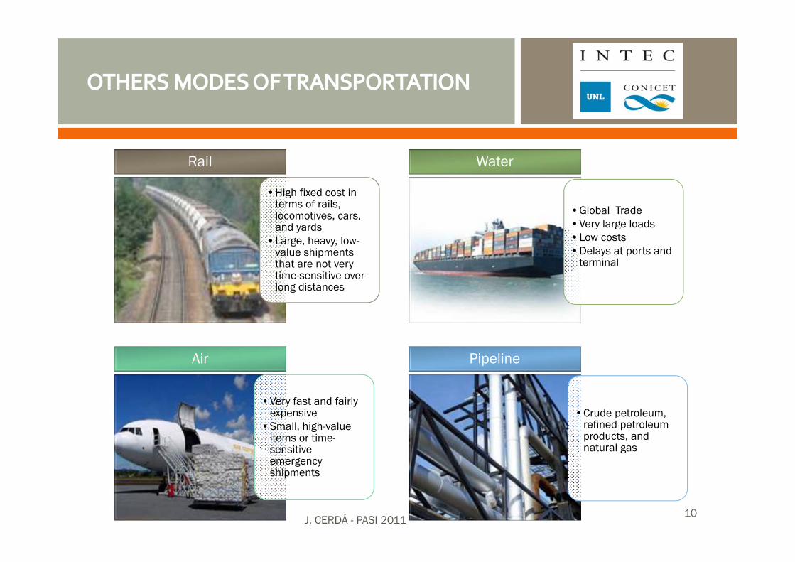
•High fixed cost in terms of rails, locomotives, cars, and yards
•Large, heavy, low-value shipments that are not very time-sensitive over long distances
Rail
•Global Trade•Very large loads•Low costs•Delays at ports and
terminal
Water
•Very fast and fairly expensive
•Small, high-value items or time-sensitive emergency shipments
Air
•Crude petroleum, refined petroleum products, and natural gas
Pipeline
J. CERDÁ - PASI 201110
Response Time (RT). The time between the placement andthe delivery of a customer order.
Location of warehouses closer to the market reduce RT.
Trade-off between response time and inventory costs. A
decrease of RT produces an increase of the number and
fixed-cost of facilities, and the inventory costs.
Major issue to solve the trade-off: Level of inventory
aggregation
J. CERDÁ - PASI 2011 11
Transportation costs
A higher number of warehouses lowers both average distanceto customers and outbound transportation costs.
Warehousing allows consolidation of shipments from multiplesuppliers in the same truck, to get lower inbound costs.
Product customization at the delivery stage is postponed untilreceiving customer orders at the warehouse.
Major issues: Consolidation of inbound shipments andtemporal order aggregation at the delivery stage (frequency ofvisits vs. full truckload) .
Trade-off between customer service level and outboundtransportation costs.
J. CERDÁ - PASI 2011 12
Product Availability (PA). It is the probability of having therequested product in stock when a customer order arrives.
Direct shipping centralizes inventories at the manufacturer site, andguarantees a high level of PA with lower amounts of inventories.
Warehousing disaggregates inventories at intermediate facilities, tolower response time and transportation costs, but decreasing theproduct availability.
For products with low/uncertain demand, or high-value products, allinventories are better aggregated at the manufacturer storage.
For low value, high-demand products, all inventories are betterdisaggregated and hold close to the customers.
J. CERDÁ - PASI 2011 13
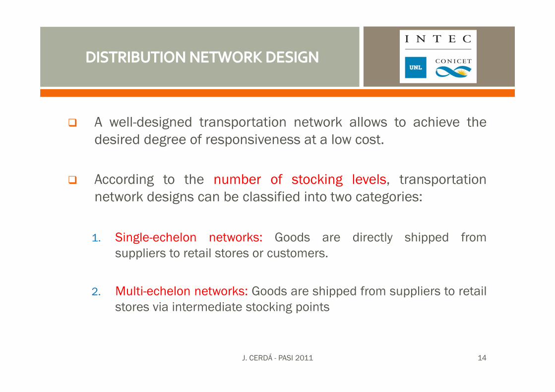
A well-designed transportation network allows to achieve thedesired degree of responsiveness at a low cost.
According to the number of stocking levels, transportationnetwork designs can be classified into two categories:
1. Single-echelon networks: Goods are directly shipped fromsuppliers to retail stores or customers.
2. Multi-echelon networks: Goods are shipped from suppliers to retailstores via intermediate stocking points
J. CERDÁ - PASI 2011 14
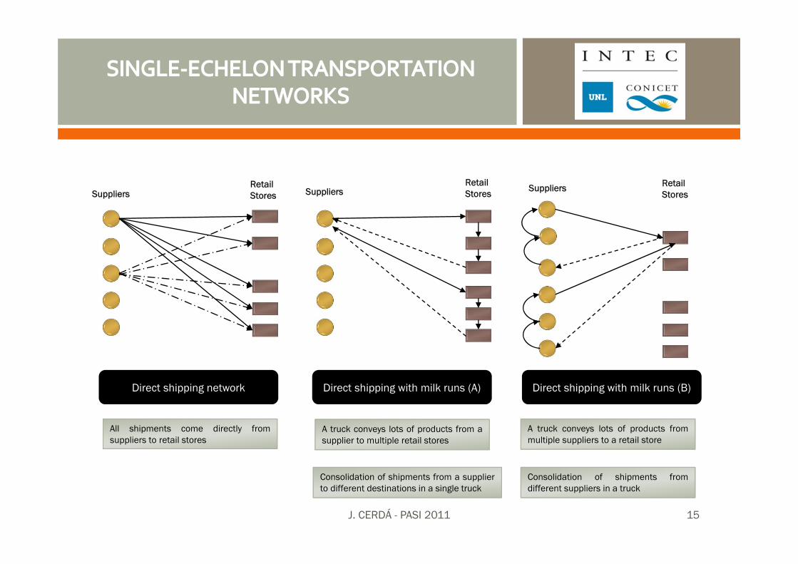
Direct shipping network Direct shipping with milk runs (A) Direct shipping with milk runs (B)
A truck conveys lots of products from asupplier to multiple retail stores
Consolidation of shipments from a supplierto different destinations in a single truck
A truck conveys lots of products frommultiple suppliers to a retail store
Consolidation of shipments fromdifferent suppliers in a truck
All shipments come directly fromsuppliers to retail stores
SuppliersRetailStores Suppliers
RetailStores
Suppliers RetailStores
J. CERDÁ - PASI 2011 15
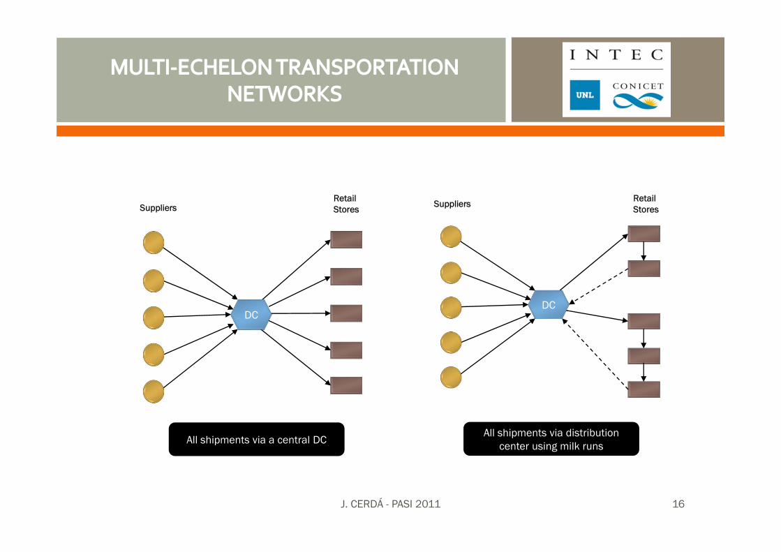
All shipments via a central DCAll shipments via distribution
center using milk runs
DCDC
SuppliersRetailStores
SuppliersRetailStores
J. CERDÁ - PASI 2011 16
Consolidation operations combine shipments from differentsuppliers and destined for multiple customers in the sametruck.
Break-bulk operations at warehouses to customize a largeshipment from various origins into multiple, smaller shipmentsto customers.
Cross-docking operations to perform break-bulk operations overingoing, consolidated shipments right after their arrival at theintermediate facility, and immediately dispatch the customizedparcels to their destinations.
J. CERDÁ - PASI 2011 17
Distribution management involves a variety of decision-making problems at three levels: strategic, tactical, and operational planning levels.
Strategic decisions deal with the distribution network design, including the number, location and size of facilities.
Tactical decisions include: a) the area served by each depot; b) the fleet size and composition; c) inventory policies at each facility; d) customer service levels.
Operational decisions are concerned with the routing and scheduling of vehicles on a day-to-day basis.
J. CERDÁ - PASI 2011 18
TSP Travelling salesman problem
MTSP M-travelling salesman problem
VRP/VRPTW Single depot, vehicle routing problem without or with time windows
m-VRPTW Multi-depot, vehicle routing problem with time windows
PDPTW Pickup and delivery problem with time windows
VRPCD Pickup and delivery problem with cross-docking at a central depot
VRP-SCM Vehicle routing and scheduling problem in a multi-echelon supply chain
VRPCD-SCM Vehicle routing and scheduling problem with cross-docking in a multi-echelon supply chain
J. CERDÁ - PASI 2011 19
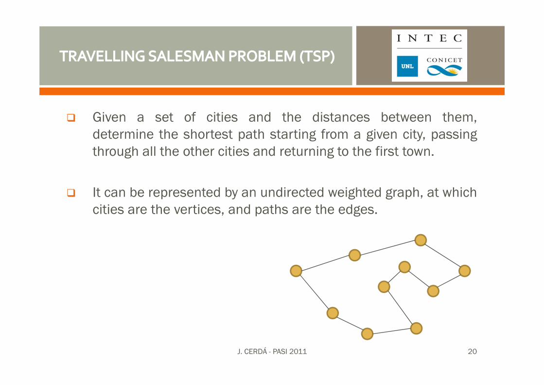
Given a set of cities and the distances between them,determine the shortest path starting from a given city, passingthrough all the other cities and returning to the first town.
It can be represented by an undirected weighted graph, at whichcities are the vertices, and paths are the edges.
J. CERDÁ - PASI 2011 20
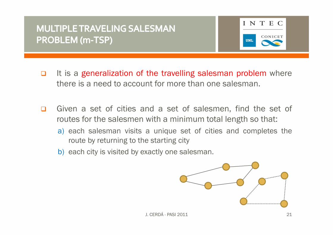
It is a generalization of the travelling salesman problem wherethere is a need to account for more than one salesman.
Given a set of cities and a set of salesmen, find the set ofroutes for the salesmen with a minimum total length so that:a) each salesman visits a unique set of cities and completes the
route by returning to the starting cityb) each city is visited by exactly one salesman.
J. CERDÁ - PASI 2011 21
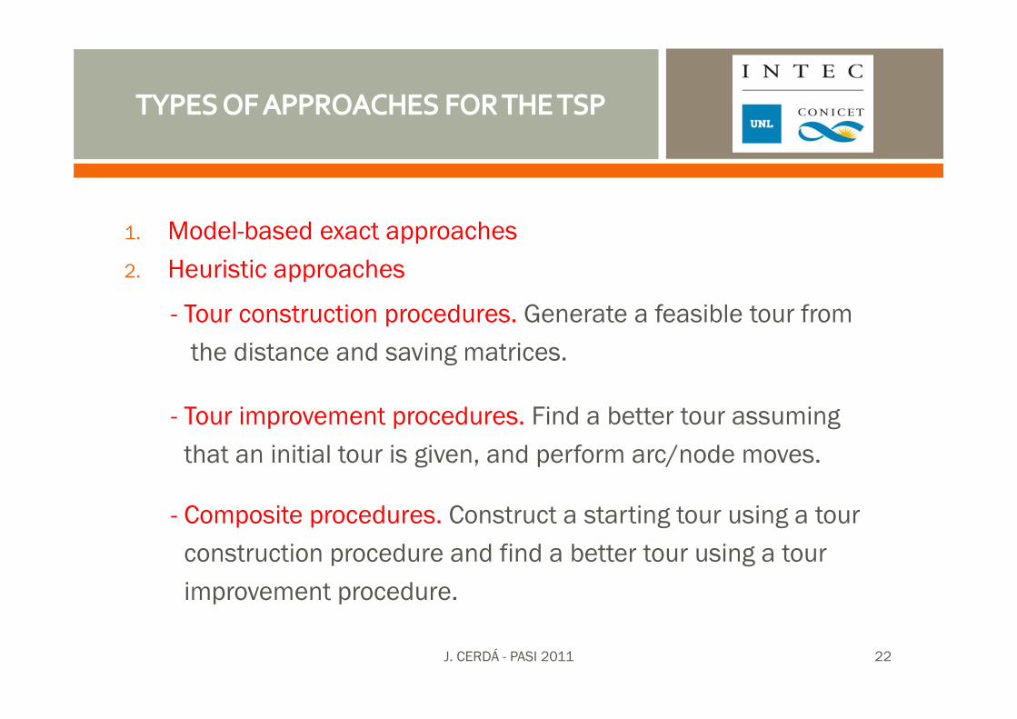
1. Model-based exact approaches2. Heuristic approaches
- Tour construction procedures. Generate a feasible tour fromthe distance and saving matrices.
- Tour improvement procedures. Find a better tour assumingthat an initial tour is given, and perform arc/node moves.
- Composite procedures. Construct a starting tour using a tourconstruction procedure and find a better tour using a tourimprovement procedure.
J. CERDÁ - PASI 2011 22
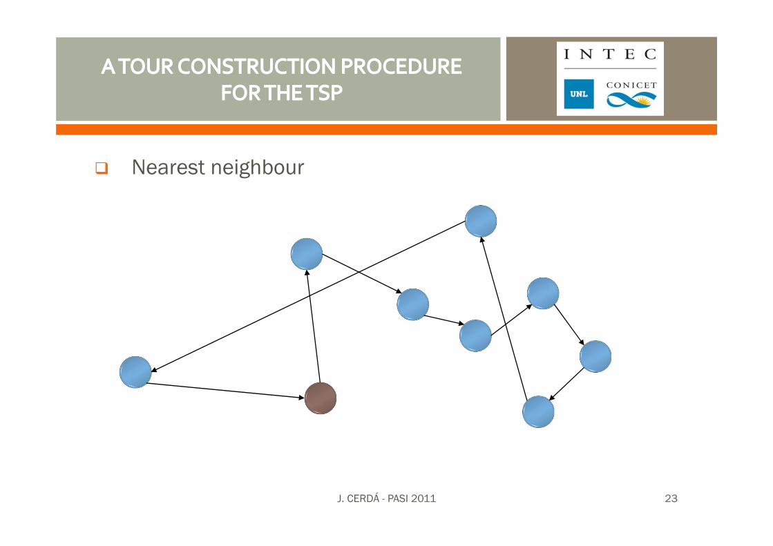
Nearest neighbour
J. CERDÁ - PASI 2011 23
Generalization of the m-TSP, where a demand is associated toeach node and every vehicle has a finite capacity.
In VRP, the sum of fixed costs (associated to the number ofused vehicles) and variable costs (associated to the totaldistance traveled) is minimized.
Generate optimal routes for the vehicle fleet based on a given roadnetwork so as to meet customers demands while satisfying capacity and
time constraints at minimum transportation cost
GOAL
J. CERDÁ - PASI 2011 24
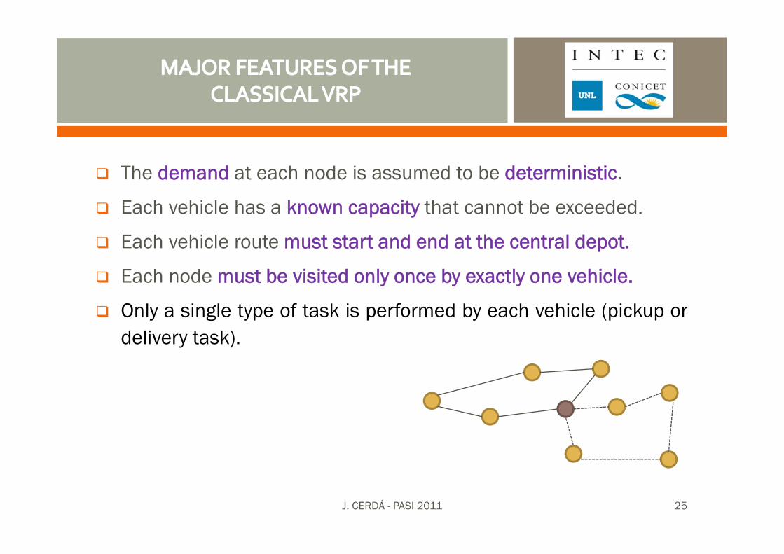
The demand at each node is assumed to be deterministic.
Each vehicle has a known capacity that cannot be exceeded.
Each vehicle route must start and end at the central depot.
Each node must be visited only once by exactly one vehicle.
Only a single type of task is performed by each vehicle (pickup ordelivery task).
J. CERDÁ - PASI 2011 25
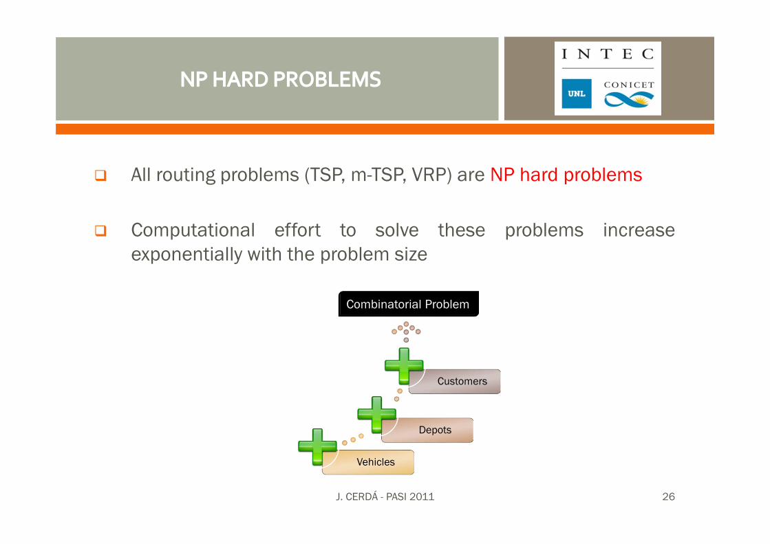
All routing problems (TSP, m-TSP, VRP) are NP hard problems
Computational effort to solve these problems increaseexponentially with the problem size
Vehicles
Depots
Customers
Combinatorial Problem
J. CERDÁ - PASI 2011 26
1. Routing ProblemA spatial problem. Temporal considerations are ignored. No apriori restrictions on delivery times (i.e. no TW constraints)and goods can be delivered within a short period of time (i.e.maximum service time constraints can be ignored).
2. Routing and Scheduling ProblemThe movement of each vehicle must be traced through bothtime and space. Visiting times to various locations are ofprimary importance. Temporal considerations may no longerbe ignored and time restrictions guide the routing andscheduling activities.
J. CERDÁ - PASI 2011 27
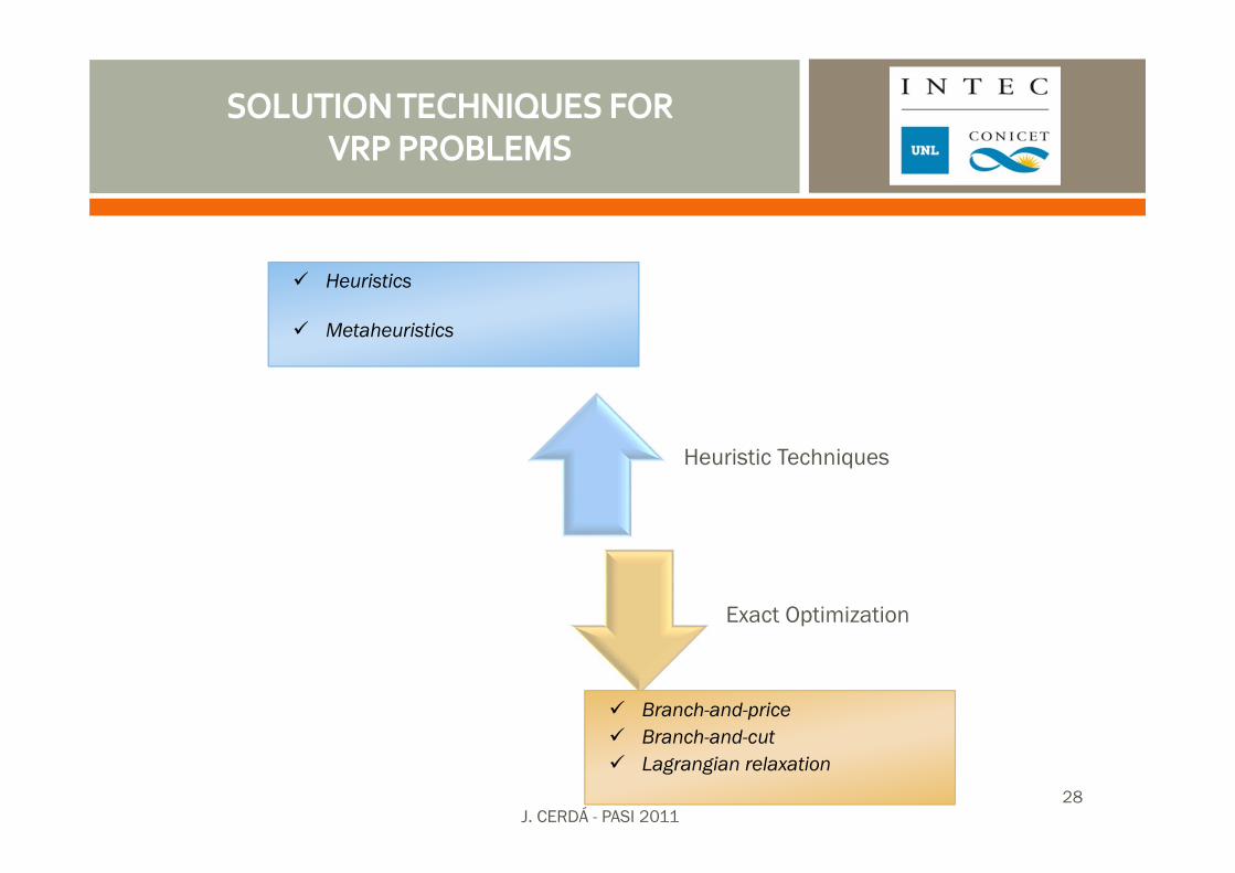
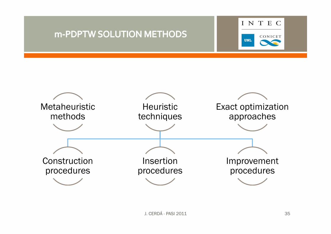
Heuristic Techniques
Exact Optimization
Heuristics
Metaheuristics
Branch-and-price Branch-and-cutLagrangian relaxation
J. CERDÁ - PASI 201128
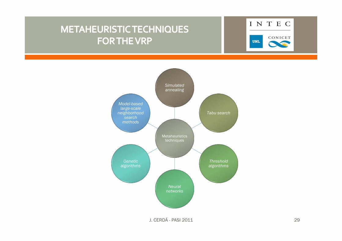
Metaheuristicstechniques
Simulated annealing
Tabu search
Threshold algorithms
Neural networks
Genetic algorithms
Model-based large-scale
neighborhood search
methods
J. CERDÁ - PASI 2011 29
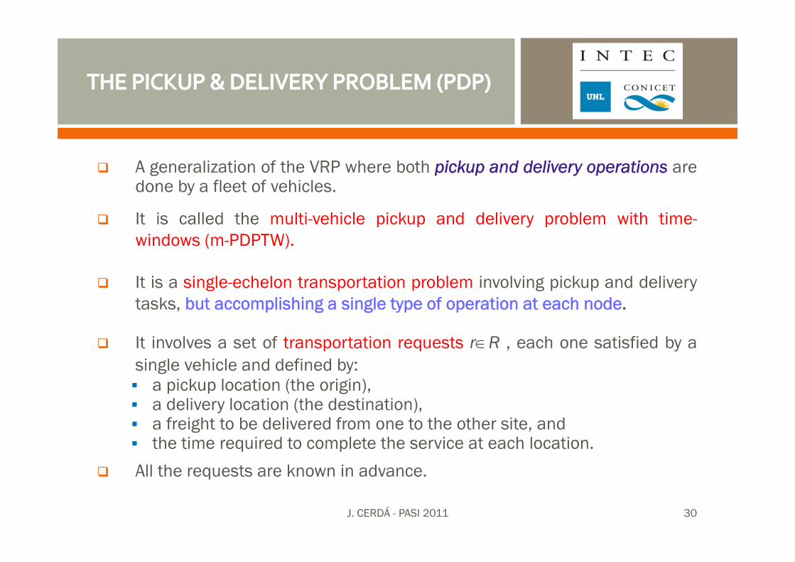
A generalization of the VRP where both pickup and delivery operations aredone by a fleet of vehicles.
It is called the multi-vehicle pickup and delivery problem with time-windows (m-PDPTW).
It is a single-echelon transportation problem involving pickup and deliverytasks, but accomplishing a single type of operation at each node.
It involves a set of transportation requests r∈R , each one satisfied by asingle vehicle and defined by:
a pickup location (the origin),a delivery location (the destination),a freight to be delivered from one to the other site, andthe time required to complete the service at each location.
All the requests are known in advance.
J. CERDÁ - PASI 2011 30
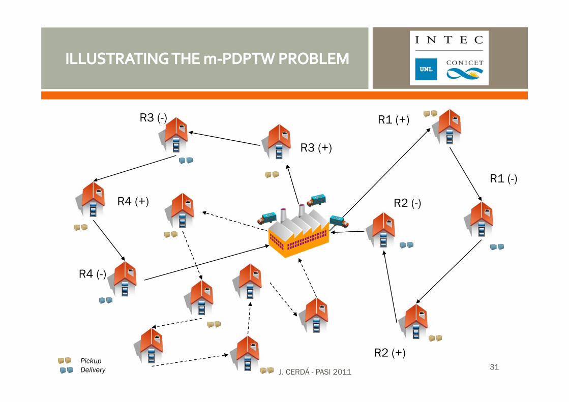
R1 (-)
R1 (+)
R2 (+)
R2 (-)
R3 (+)
R3 (-)
R4 (+)
R4 (-)
PickupDelivery J. CERDÁ - PASI 2011
31
Vehicles depart and return to the central depot (tour constraint).
Each transportation request must be serviced by a singlevehicle. Pickup and delivery locations related to the samerequest are visited by the same vehicle (pairing constraint).
Each pickup location has to be visited prior to the associateddelivery location (precedence constraint).
Each vehicle can satisfy one or more customer requests (a“composite” milk run).
J. CERDÁ - PASI 2011 32
Vehicle capacity must never be exceeded after visiting a pickup node(capacity constraint at pickup nodes).
A vehicle must transport enough load to meet customer demand whenservicing a delivery node (capacity constraint at delivery nodes). Onlyimportant for requests involving multiple pickup points.
The service at each node must be started within the specified timewindow (time window constraints).
The total time/distance travelled from the depot to a certain nodemust be greater than the one required to reach a preceding node onthe tour (compatibility between routes and schedules).
J. CERDÁ - PASI 2011 33
The alternative problem goals aim to minimize:the total distance travelledthe total travel time required to service all customer requeststhe total customers’ inconveniencea weighted combination of total service time and customers’inconvenience.
Customer inconvenience is usually a linear function of acustomer’s waiting time (because of late arrivals).
J. CERDÁ - PASI 2011 34
Metaheuristicmethods
Heuristic techniques
Constructionprocedures
Insertionprocedures
Improvementprocedures
Exact optimizationapproaches
J. CERDÁ - PASI 2011 35
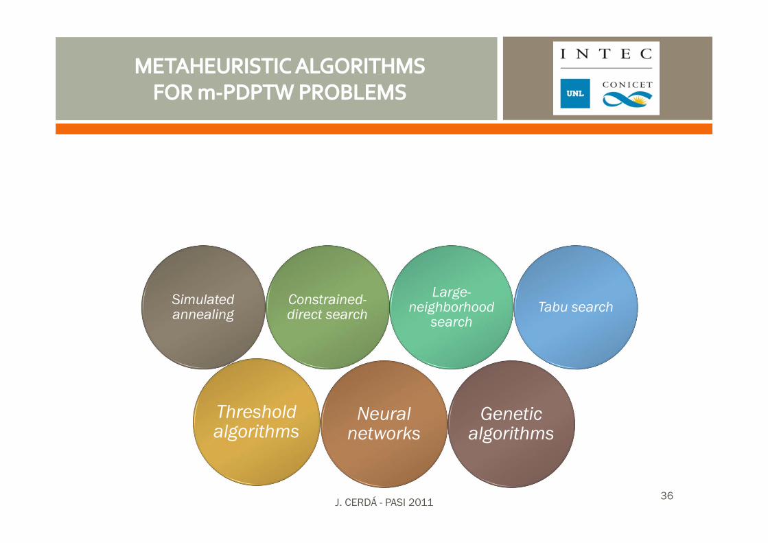
Simulatedannealing
Constrained-direct search
Large-neighborhood
searchTabu search
Thresholdalgorithms
Neural networks
Geneticalgorithms
J. CERDÁ - PASI 201136
1. Dynamic programming
2. Branch-and-price
3. Branch-and-cut
J. CERDÁ - PASI 2011 37
The PDPTW problem with transshipment
J. CERDÁ - PASI 2011
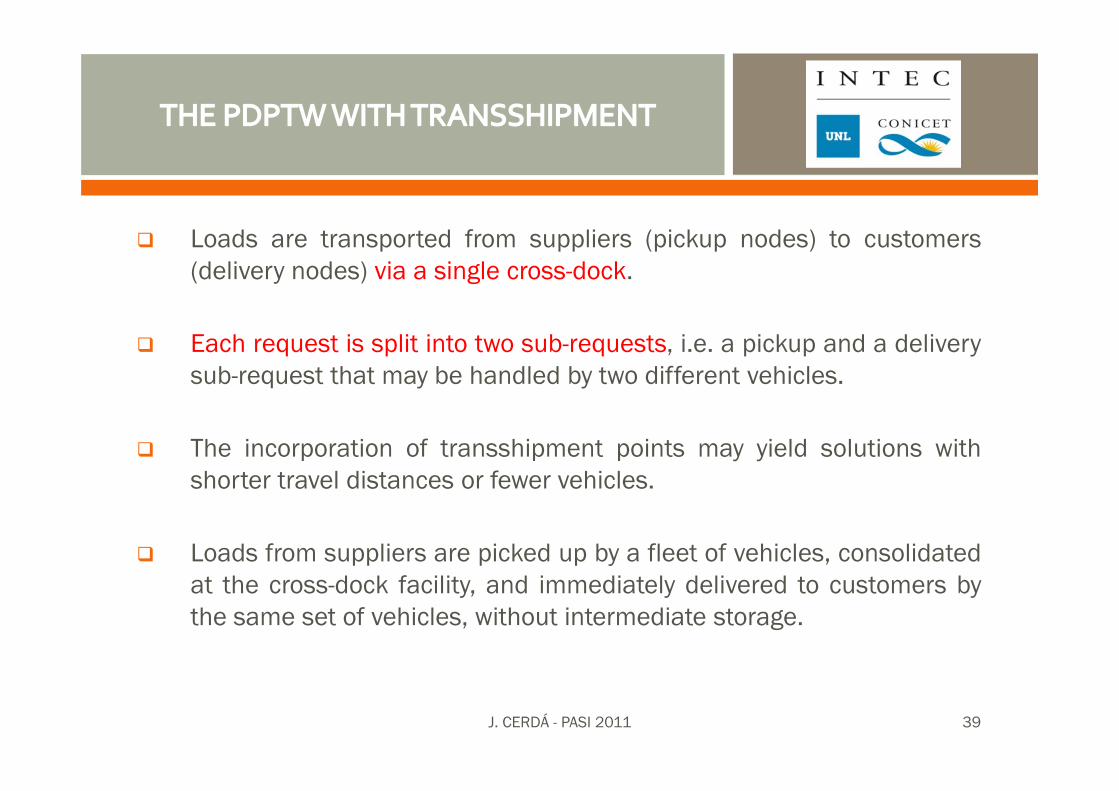
Loads are transported from suppliers (pickup nodes) to customers(delivery nodes) via a single cross-dock.
Each request is split into two sub-requests, i.e. a pickup and a deliverysub-request that may be handled by two different vehicles.
The incorporation of transshipment points may yield solutions withshorter travel distances or fewer vehicles.
Loads from suppliers are picked up by a fleet of vehicles, consolidatedat the cross-dock facility, and immediately delivered to customers bythe same set of vehicles, without intermediate storage.
J. CERDÁ - PASI 2011 39
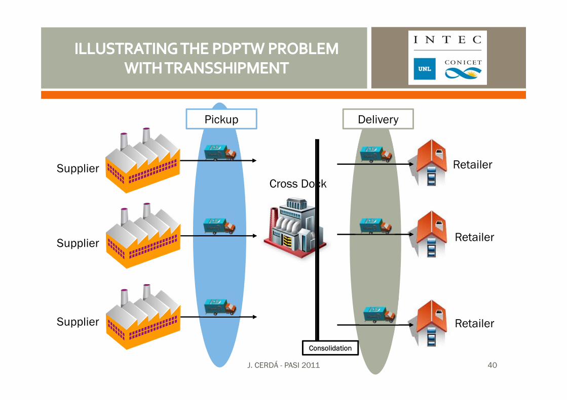
Cross Dock
Retailer
Retailer
Retailer
Supplier
Supplier
Supplier
Pickup Delivery
Consolidation
J. CERDÁ - PASI 2011 40
Each node must be visited only once by a single vehicle.
Each vehicle can pick up loads from more than one supplier anddeliver loads to more than one customer. Milk runs are allowed.
Pickup and delivery routes start and end at the cross-dockfacility.
Loads to pickup/deliver at problem nodes are known data.
The total amounts unloaded at the receiving dock and loadedinto trucks at the shipping dock should be equal. There is noend inventory at the cross-dock facility.
J. CERDÁ - PASI 2011 41
Service time windows for the nodes are usually specified.
The problem goal is to minimize the total transportation costwhile satisfying all customer requests.
J. CERDÁ - PASI 2011 42
The vehicle routing problem with time windows in the supply chain management
J. CERDÁ - PASI 2011
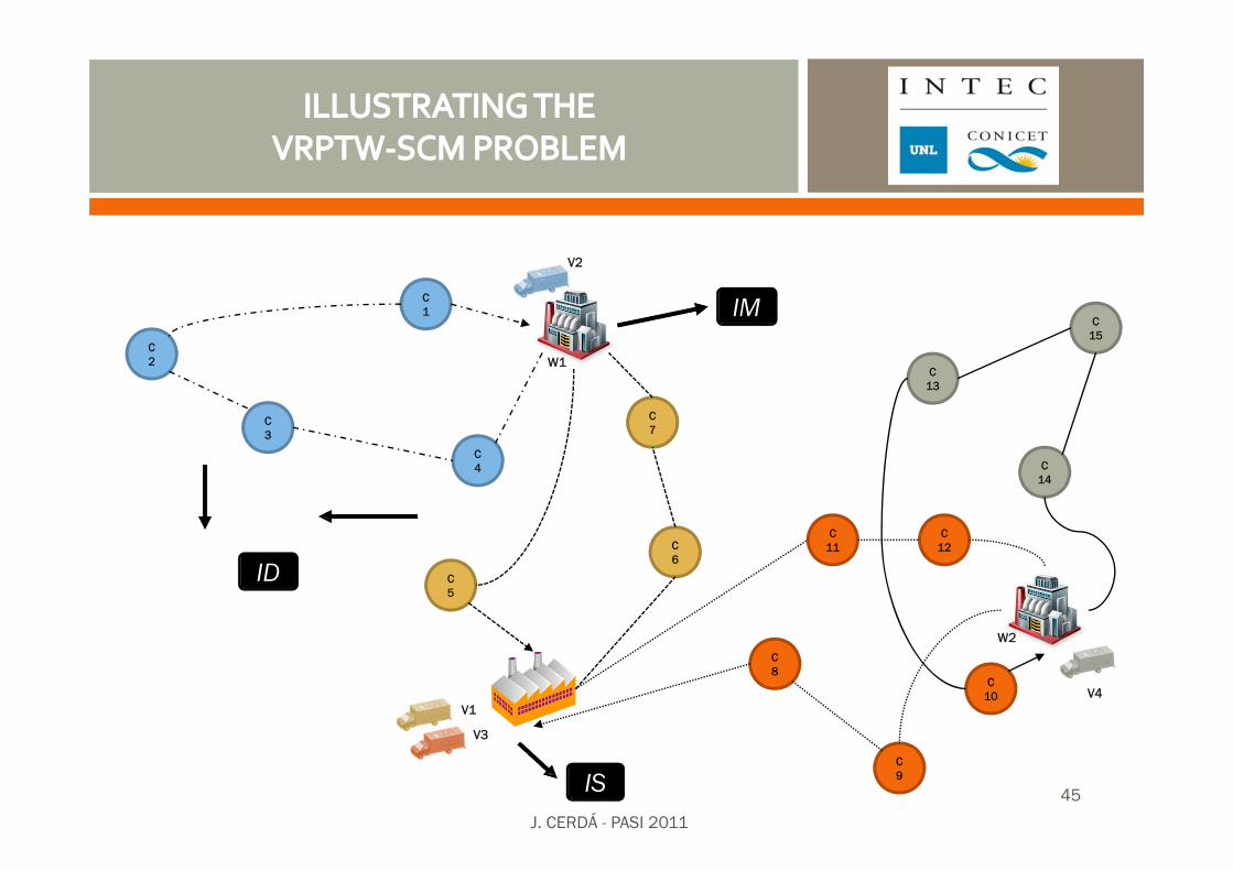
PROBLEM GOAL: Determine the best operational planning ofmulti-echelon transportation networks comprising factories,warehouses, and customers (the problem nodes).
Different types of distribution strategies like direct shipping,shipping via DC or regional warehouses, or a mix of them (hybridstrategies) can be implemented.
To resemble the logistics activities at multi-site distributionnetworks, multiple events at every node can occur.
J. CERDÁ - PASI 2011 44
C6
C7
C5
C4
C1
C2
C3
C8
C9
C10
C14
C15
C13
C11
C12
V2
V1
V3
V4
IM
ID
IS
W1
W2
J. CERDÁ - PASI 2011
45
Types of nodes“Pure” source nodes (IS), usually manufacturer storages, where vehiclescarry out only pickup operationsMixed nodes (IM), like DCs, where visiting vehicles can accomplish pickupand/or delivery operations.Destination nodes (ID), like consumer zones, where visiting trucks justperform delivery operations
Number of events. The number of events for a location must be at leastequal to the number of vehicles stops for performing pickup/deliveryoperations at the optimum.
Global precedence. For each vehicle stop, the model provides all the visitsthe vehicle has made before.
J. CERDÁ - PASI 2011 46
Multiple products are distributed from manufacturing plants andwarehouses to customers.
Customer requests may involve several products (multi-commoditydistribution) and do not generally have predefined suppliers
The amounts of products to pick up at source nodes by a vehicle are notpredefined but chosen by the model.
Multiple partial shipments to a customer location are allowed (ordersplitting)
Milk runs are performed on both sides, i.e. inbound and outbound sides.Then, several customers can be serviced by the same truck.
J. CERDÁ - PASI 2011 47
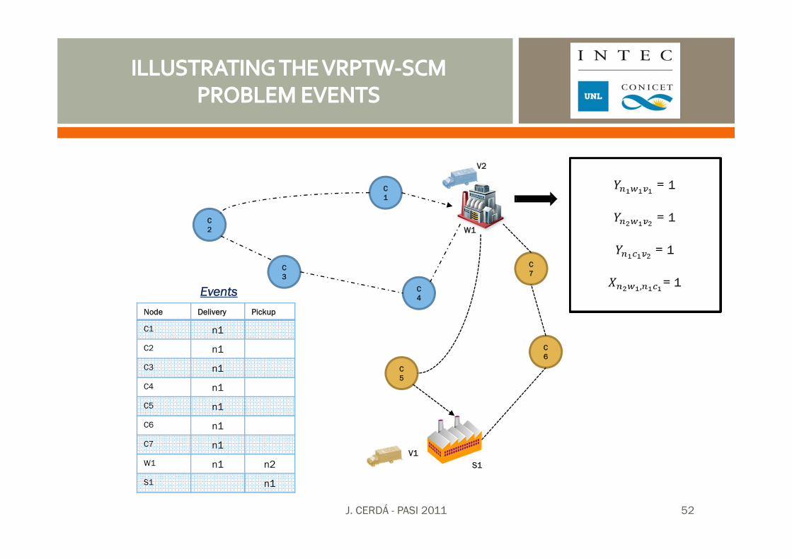
Problem events are the vehicle stops at DCs and customer locations.
A location can be visited either by multiple trucks or several times by thesame vehicle. Then, several events can sequentially occur at any site.
A set of pre-specified, timely-ordered events for each site are defined. Itsnumber is chosen by the user.
A vehicle can accomplish pickup and delivery operations during a stop atat DCs.
The magnitude and composition of the freight transported by a vehicle atany stop must be traced in order to meet:
capacity constraints at pickup locationsproduct availability constraints at delivery points
J. CERDÁ - PASI 2011 48
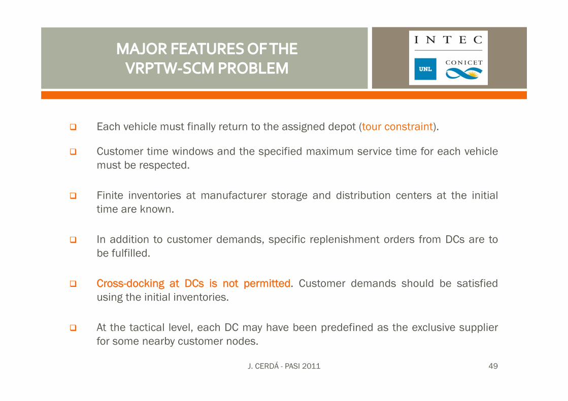
Each vehicle must finally return to the assigned depot (tour constraint).
Customer time windows and the specified maximum service time for each vehiclemust be respected.
Finite inventories at manufacturer storage and distribution centers at the initialtime are known.
In addition to customer demands, specific replenishment orders from DCs are tobe fulfilled.
Cross-docking at DCs is not permitted. Customer demands should be satisfiedusing the initial inventories.
At the tactical level, each DC may have been predefined as the exclusive supplierfor some nearby customer nodes.
J. CERDÁ - PASI 2011 49
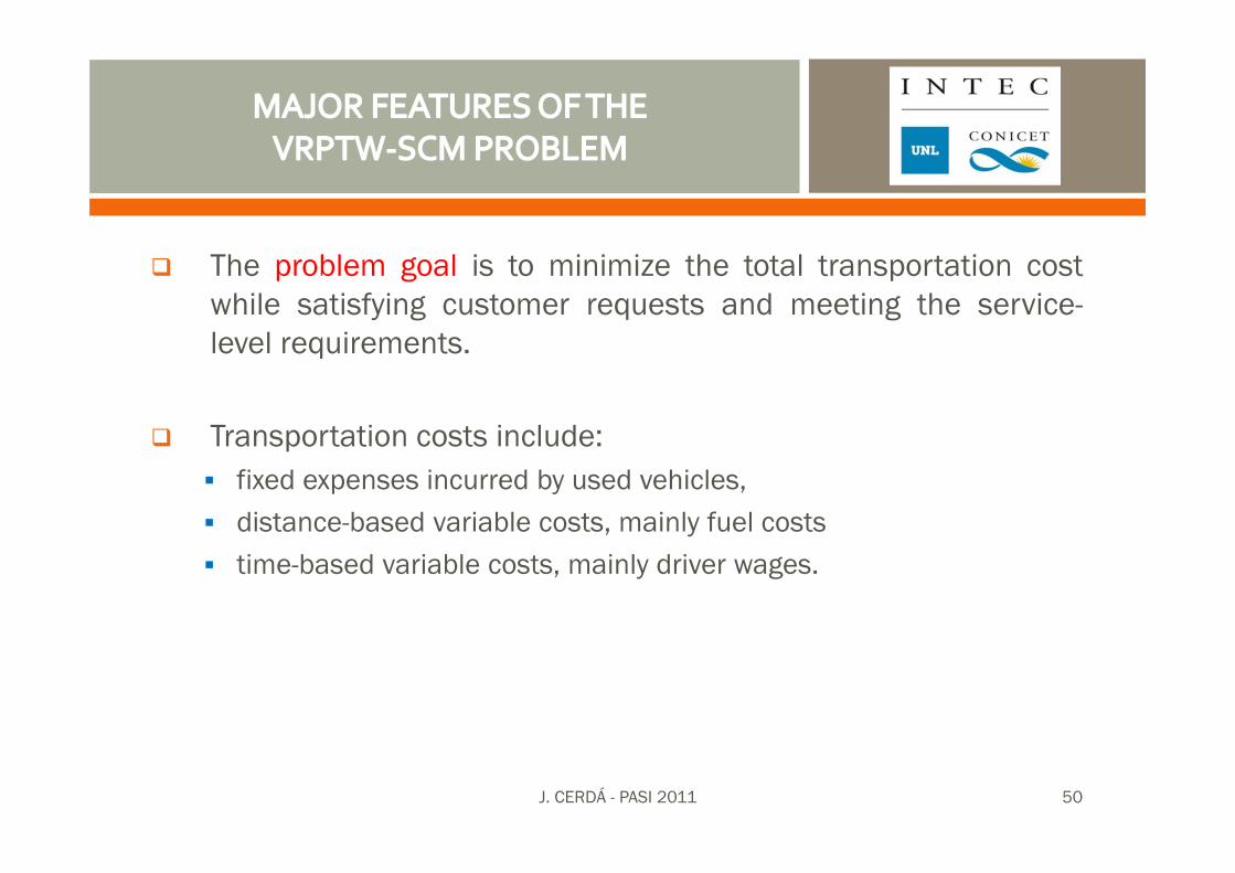
The problem goal is to minimize the total transportation costwhile satisfying customer requests and meeting the service-level requirements.
Transportation costs include:fixed expenses incurred by used vehicles,distance-based variable costs, mainly fuel coststime-based variable costs, mainly driver wages.
J. CERDÁ - PASI 2011 50
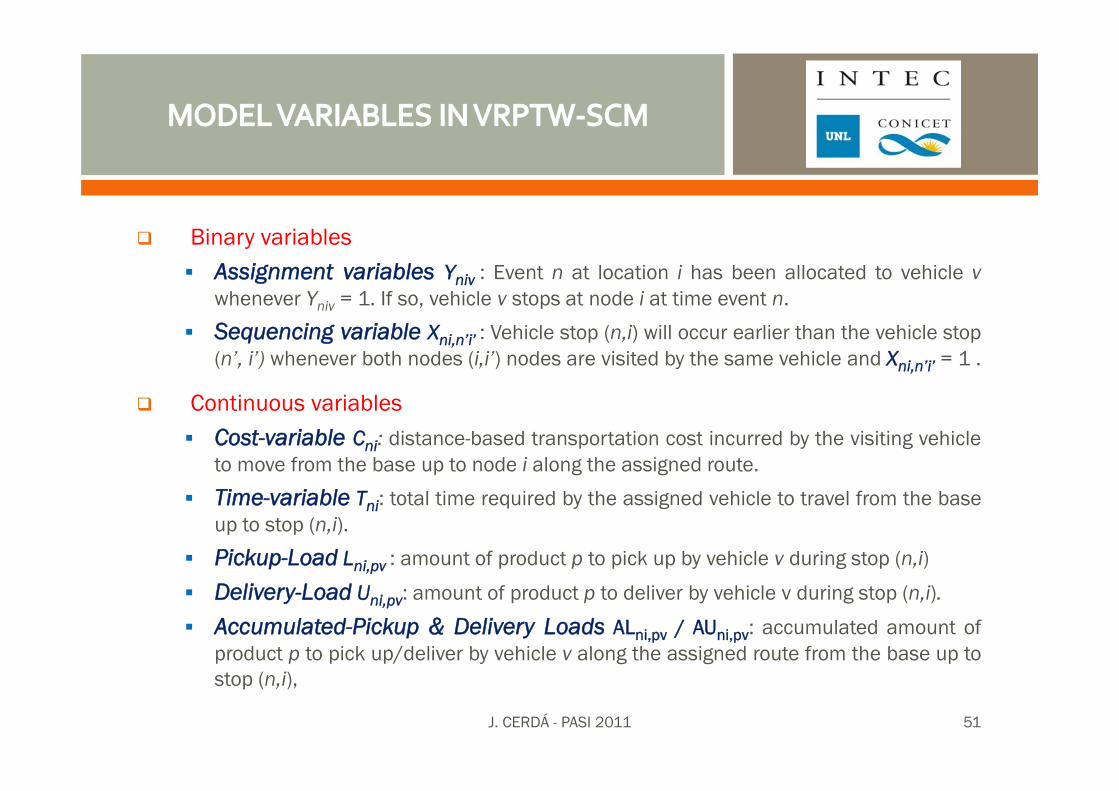
Binary variablesAssignment variables Yniv : Event n at location i has been allocated to vehicle vwhenever Yniv = 1. If so, vehicle v stops at node i at time event n.
Sequencing variable Xni,n’i’ : Vehicle stop (n,i) will occur earlier than the vehicle stop(n’, i’) whenever both nodes (i,i’) nodes are visited by the same vehicle and Xni,n’i’ = 1 .
Continuous variablesCost-variable Cni: distance-based transportation cost incurred by the visiting vehicleto move from the base up to node i along the assigned route.
Time-variable Tni: total time required by the assigned vehicle to travel from the baseup to stop (n,i).Pickup-Load Lni,pv : amount of product p to pick up by vehicle v during stop (n,i)
Delivery-Load Uni,pv: amount of product p to deliver by vehicle v during stop (n,i).
Accumulated-Pickup & Delivery Loads ALni,pv / AUni,pv: accumulated amount ofproduct p to pick up/deliver by vehicle v along the assigned route from the base up tostop (n,i),
J. CERDÁ - PASI 2011 51
C6
C7
C5
C4
C1
C2
C3
V2
V1
W1
Node Delivery Pickup
C1 n1
C2 n1
C3 n1
C4 n1
C5 n1
C6 n1
C7 n1
W1 n1 n2
S1 n1
S1
Events
J. CERDÁ - PASI 2011 52
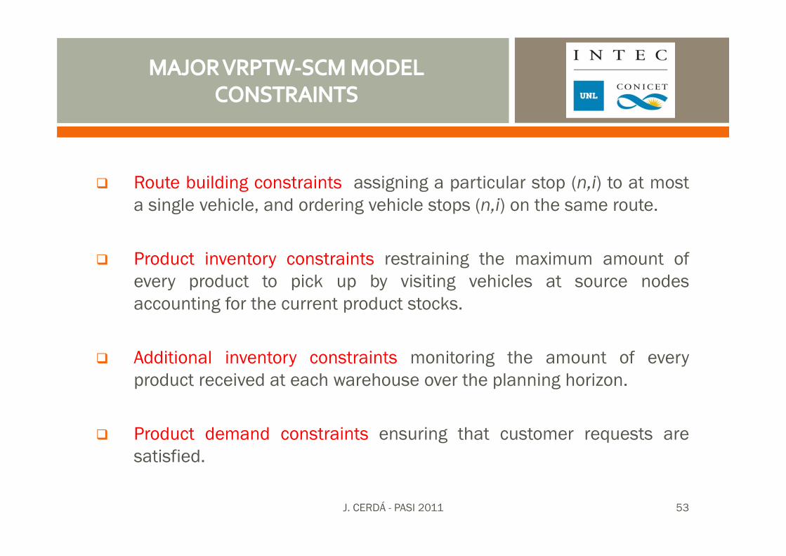
Route building constraints assigning a particular stop (n,i) to at mosta single vehicle, and ordering vehicle stops (n,i) on the same route.
Product inventory constraints restraining the maximum amount ofevery product to pick up by visiting vehicles at source nodesaccounting for the current product stocks.
Additional inventory constraints monitoring the amount of everyproduct received at each warehouse over the planning horizon.
Product demand constraints ensuring that customer requests aresatisfied.
J. CERDÁ - PASI 2011 53
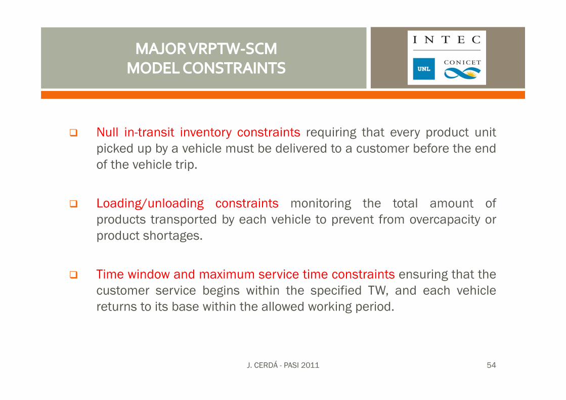
Null in-transit inventory constraints requiring that every product unitpicked up by a vehicle must be delivered to a customer before the endof the vehicle trip.
Loading/unloading constraints monitoring the total amount ofproducts transported by each vehicle to prevent from overcapacity orproduct shortages.
Time window and maximum service time constraints ensuring that thecustomer service begins within the specified TW, and each vehiclereturns to its base within the allowed working period.
J. CERDÁ - PASI 2011 54
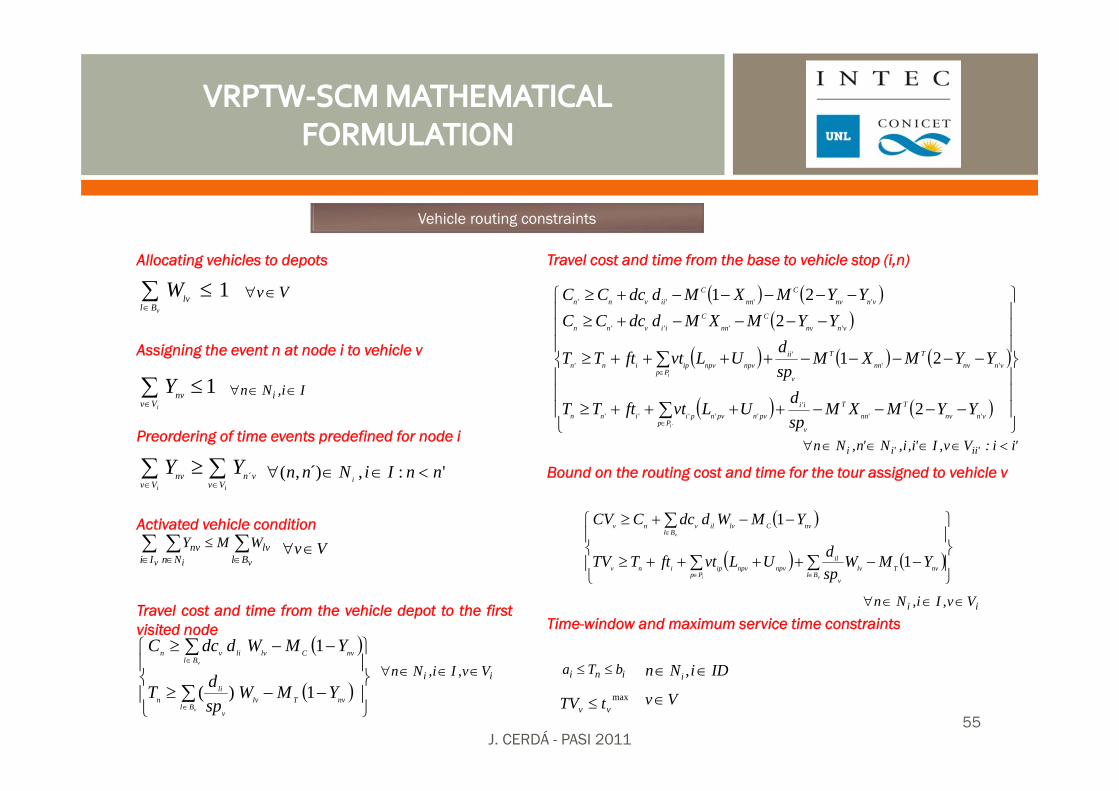
Allocating vehicles to depots
Assigning the event n at node i to vehicle v
Preordering of time events predefined for node i
Activated vehicle condition
Travel cost and time from the vehicle depot to the firstvisited node
∑∈
≤vBl
lvW 1 Vv∈∀
∑∈
≤iVv
nvY 1 Ii,Nn i ∈∈∀
∑∑∈∈
≥ii Vv
vnVv
nv YY ´ ':,´),( nnIiNnn i <∈∈∀
∑∑ ∑∈∈ ∈
≤vv i Bl
lvIi Nn
nv WMY Vv∈∀
( )
( ) ⎪⎭
⎪⎬
⎫
⎪⎩
⎪⎨
⎧
−−≥
−−≥
∑
∑
∈
∈
v
v
BlnvTlv
v
lin
BlnvClvlivn
YMWspdT
YMWddcC
1)(
1ii Vv,Ii,Nn ∈∈∈∀
Travel cost and time from the base to vehicle stop (i,n)
Bound on the routing cost and time for the tour assigned to vehicle v
Time-window and maximum service time constraints
( ) ( )( )
( ) ( ) ( )
( ) ( ) ⎪⎪⎪
⎭
⎪⎪⎪
⎬
⎫
⎪⎪⎪
⎩
⎪⎪⎪
⎨
⎧
−−−−++++≥
−−−−−++++≥
−−−−+≥
−−−−−+≥
∑
∑
∈
∈
vnnvT
nnT
v
ii
Pppvnpvnpiinn
vnnvT
nnT
v
ii
Ppnpvnpvipinn
vnnvC
nnC
iivnn
vnnvC
nnC
iivnn
YYMXMspd
ULvtftTT
YYMXMspd
ULvtftTT
YYMXMddcCCYYMXMddcCC
i
i
'''
'''''
'''
'
''''
''''
2
21
221
'
'ii:Vv,I'i,i,N'n,Nn 'ii'ii <∈∈∈∈∀
( )
( ) ( )⎪⎭
⎪⎬
⎫
⎪⎩
⎪⎨
⎧
−−++++≥
−−+≥
∑∑
∑
∈∈
∈
vi
v
BlnvTlv
v
il
Ppnpvnpvipinv
BlnvClvilvnv
YMWspdULvtftTTV
YMWddcCCV
1
1
ii Vv,Ii,Nn ∈∈∈∀
ini bTa ≤≤ IDiNn i ∈∈ ,max
vv tTV ≤ Vv∈
Vehicle routing constraints
J. CERDÁ - PASI 201155
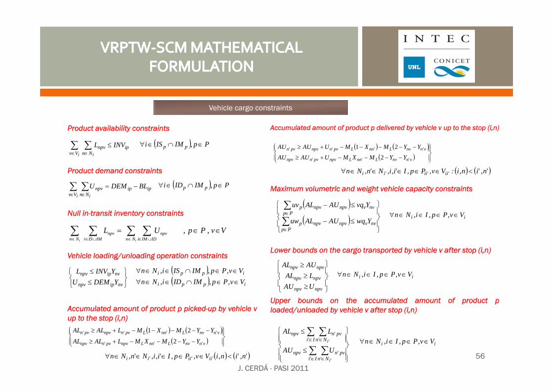
Product availability constraints
Product demand constraints
Null in-transit inventory constraints
Vehicle loading/unloading operation constraints
Accumulated amount of product p picked-up by vehicle vup to the stop (i,n)
Accumulated amount of product p delivered by vehicle v up to the stop (i,n)
Maximum volumetric and weight vehicle capacity constraints
Lower bounds on the cargo transported by vehicle v after stop (i,n)
Upper bounds on the accumulated amount of product ploaded/unloaded by vehicle v after stop (i,n)
Vehicle cargo constraints
∑ ∑∈ ∈
≤i iVv Nn
ipnpv INVL ( ) Pp,IMISi pp ∈∩∈∀
∑ ∑∈ ∈
−=i iVv Nn
ipipnpv BLDEMU ( ) Pp,IMIDi pp ∈∩∈∀
∑ ∑∑ ∑∈ ∪∈∈ ∪∈
∈∈=ii Nn IDIMi
npvNn IMISi
npv VvPpUL ,,
⎭⎬⎫
⎩⎨⎧
≤≤
nvipnpv
nvipnpv
YDEMUYINVL ( ) ippi Vv,Pp,IMISi,Nn ∈∈∩∈∈∀
( ) ippi Vv,Pp,IMIDi,Nn ∈∈∩∈∈∀
( ) ( )( ) ⎪⎭
⎪⎬⎫
⎪⎩
⎪⎨⎧
−−−−+≥
−−−−−+≥
v'nnvL'nnLnpvpv'nnpv
v'nnvL'nnLpv'nnpvpv'n
YYMXMLALAL
YYMXMLALAL
2
21
( ) ( )'n,'in,iVv,Pp,I'i,i,N'n,Nn 'ii'ii'ii <∈∈∈∈∈∀
( ) ( )( ) ⎪⎭
⎪⎬⎫
⎪⎩
⎪⎨⎧
−−−−+≥
−−−−−+≥
v'nnvL'nnLnpvpv'nnpv
v'nnvL'nnLpv'nnpvpv'n
YYMXMUAUAU
YYMXMUAUAU
2
21
( ) ( )'n,'in,i:Vv,Pp,I'i,i,N'n,Nn 'ii'ii'ii <∈∈∈∈∈∀
( )( ) ⎪
⎭
⎪⎬
⎫
⎪⎩
⎪⎨
⎧
≤−
≤−
∑
∑
∈
∈
Ppnvvnpvnpvp
Ppnvvnpvnpvp
YwqAUALuw
YvqAUALuvii Vv,Pp,Ii,Nn ∈∈∈∈∀
⎪⎭
⎪⎬
⎫
⎪⎩
⎪⎨
⎧
≥≥≥
npvnpv
npvnpv
npvnpv
UAULAL
AUALii Vv,Pp,Ii,Nn ∈∈∈∈∀
⎪⎪⎭
⎪⎪⎬
⎫
⎪⎪⎩
⎪⎪⎨
⎧
≤
≤
∑ ∑
∑ ∑
∈ ∈
∈ ∈
I'i N'npv'nnpv
I'i N'npv'nnpv
'i
'i
UAU
LALii Vv,Pp,Ii,Nn ∈∈∈∈∀
J. CERDÁ - PASI 2011
56
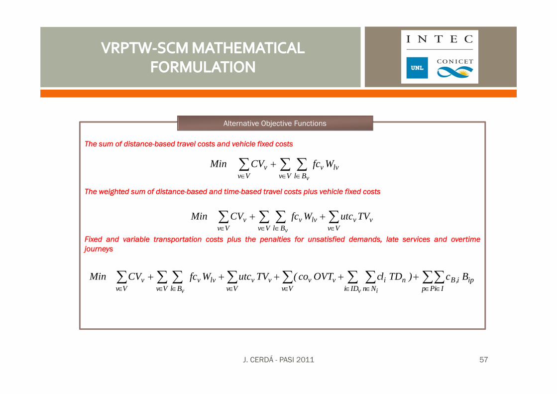
The sum of distance-based travel costs and vehicle fixed costs
The weighted sum of distance-based and time-based travel costs plus vehicle fixed costs
Fixed and variable transportation costs plus the penalties for unsatisfied demands, late services and overtimejourneys
Alternative Objective Functions
∑ ∑∑∈ ∈∈
+Vv Bl
lvvVv
vv
WfcCVMin
∑∑ ∑∑∈∈ ∈∈
++Vv
vvVv Bl
lvvVv
v TVutcWfcCVMinv
∑∑∑ ∑∑ ∑ ∑ ∑∑∈ ∈∈ ∈∈ ∈ ∈ ∈∈
+++++Pp Ii
ipi,BniIDi NnVv Bl Vv Vv
vvvvlvvVv
v Bc)TDlcOVTco(TVutcWfcCVMinv iv
J. CERDÁ - PASI 2011 57

The VRPCD‐SCM problem with cross‐docking
J. CERDÁ - PASI 2011
Generalization of the VRP-SCM problem to consider the possibility ofcross-docking.
Intermediate depots may keep finite stocks of fast-moving products(warehousing) and act as cross-dock platforms for slow-moving, high-valueitems.
Replenishment orders and cross-docking operations are triggered whenthe initial stock in a warehouse is insufficient to meet the demand of theassigned customers.
Inbound and outbound vehicles must stay at receiving/shipping docks ofDCs until they complete their delivery/pickup tasks.
Target product inventories at the end of the planning horizon may bespecified.
J. CERDÁ - PASI 2011 59
Product inventories at cross-dock facilities must be traced over theplanning horizon.
Sequencing of pickup and delivery operations by different vehicles at thesame warehouse now become important.
The problem goal aims to minimize fixed and variable transportationcosts.
J. CERDÁ - PASI 2011 60
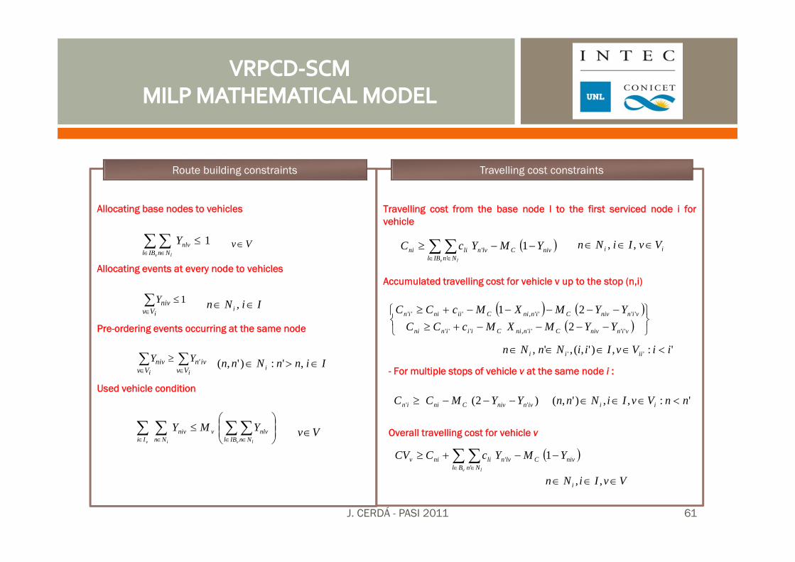
Allocating base nodes to vehicles
Allocating events at every node to vehicles
Pre-ordering events occurring at the same node
Used vehicle condition
Route building constraints
∑∑∈ ∈
≤v lIBl Nn
nlvY 1 Vv∈
1≤∑∈ iVv
nivY IiNn i ∈∈ ,
∑∑∈∈
≥ii Vv
iv'nVv
niv YY IinnNnn i ∈>∈ ,':)',(
∑ ∑∑∑∈ ∈ ∈∈
⎟⎟⎠
⎞⎜⎜⎝
⎛≤
v v liIi IBl Nnnlvv
Nnniv YMY Vv∈
Travelling cost from the base node l to the first serviced node i forvehicle
Accumulated travelling cost for vehicle v up to the stop (n,i)
- For multiple stops of vehicle v at the same node i :
Travelling cost constraints
( )nivCIBl Nn
lvnlini YMYcCv l
−−≥ ∑ ∑∈ ∈
1'
' ii VvIiNn ∈∈∈ ,,
( ) ( )( ) ⎭
⎬⎫
⎩⎨⎧
−−−−+≥−−−−−+≥
vinnivCinniCiiinni
vinnivCinniCiiniin
YYMXMcCCYYMXMcCC
'''','''
'''','''
221
':,)',(,', '' iiVvIiiNnNn iiii <∈∈∈∈
( )∑ ∑∈ ∈
−−+≥v lBl
nivCNn
lvnliniv YMYcCCV 1'
'
VvIiNn i ∈∈∈ ,,
Overall travelling cost for vehicle v
)2( '' ivnnivCniin YYMCC −−−≥ ':,,)',( nnVvIiNnn ii <∈∈∈
J. CERDÁ - PASI 2011 61
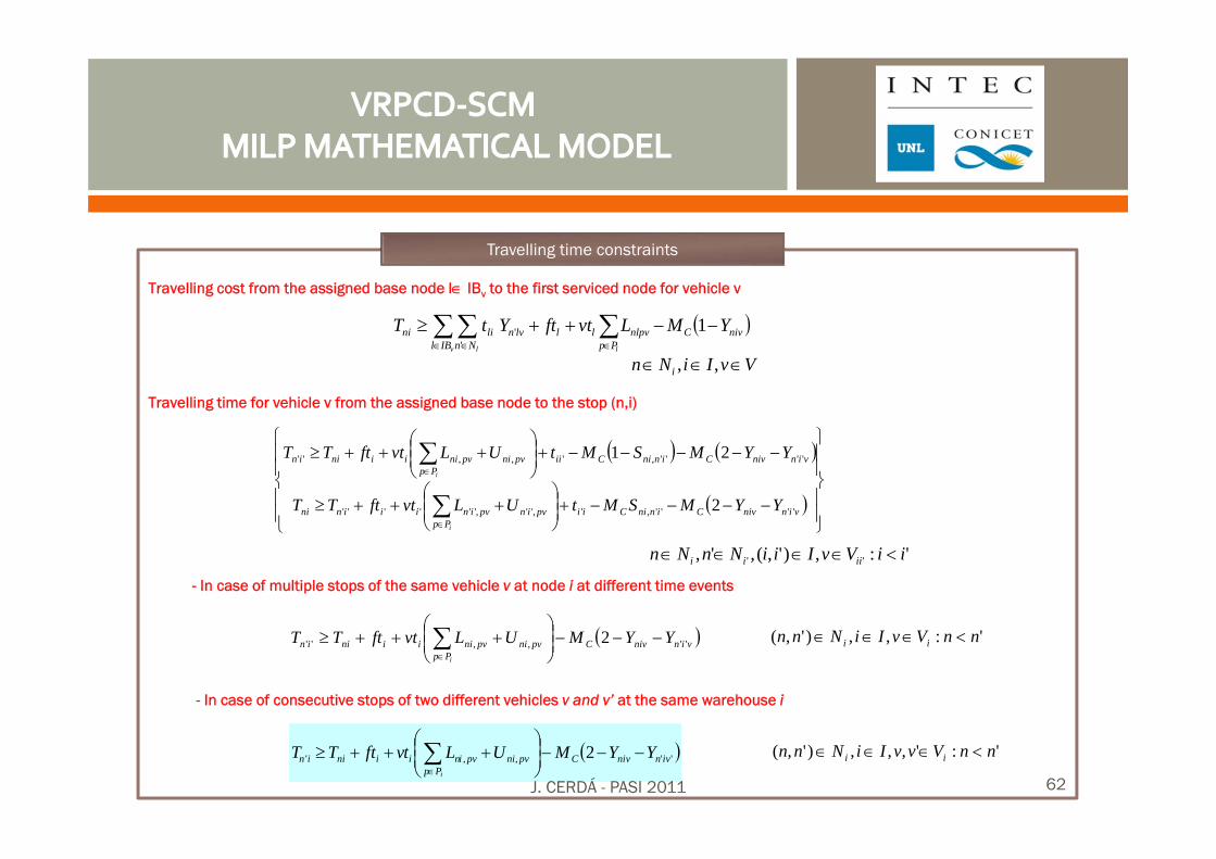
Travelling cost from the assigned base node l∈ IBv to the first serviced node for vehicle v
Travelling time for vehicle v from the assigned base node to the stop (n,i)
- In case of multiple stops of the same vehicle v at node i at different time events
- In case of consecutive stops of two different vehicles v and v’ at the same warehouse i
Travelling time constraints
( )nivCIBl Nn Pp
nlpvlllvnlini YMLvtftYtTv l l
−−++≥ ∑∑ ∑∈ ∈ ∈
1'
'
VvIiNn i ∈∈∈ ,,
':,)',(,', '' iiVvIiiNnNn iiii <∈∈∈∈
( ) ( )
( ) ⎪⎪
⎭
⎪⎪
⎬
⎫
⎪⎪
⎩
⎪⎪
⎨
⎧
−−−−+⎟⎟⎠
⎞⎜⎜⎝
⎛+++≥
−−−−−+⎟⎟⎠
⎞⎜⎜⎝
⎛+++≥
∑
∑
∈
∈
vinnivCinniCiiPp
pvinpviniiinni
vinnivCinniCiiPp
pvnipvniiiniin
YYMSMtULvtftTT
YYMSMtULvtftTT
i
i
'''',','',''''''
'''',',,''
2
21
( )vinnivC
Pppvnipvniiiniin YYMULvtftTT
i
'',,'' 2 −−−⎟⎟⎠
⎞⎜⎜⎝
⎛+++≥ ∑
∈
':,,)',( nnVvIiNnn ii <∈∈∈
':',,,)',( nnVvvIiNnn ii <∈∈∈
( )'',,' 2 ivnnivCPp
pvnipvniiiniin YYMULvtftTTi
−−−⎟⎟⎠
⎞⎜⎜⎝
⎛+++≥ ∑
∈
J. CERDÁ - PASI 2011 62
Overall travelling time for vehicle v
Time window and maximum service-time constraints
Travelling time constraints
( )nivCBl Nn
lvnilPp
pvnipvniiiniv YMYtULvtftTOTv li
−−+⎟⎟⎠
⎞⎜⎜⎝
⎛+++≥ ∑ ∑∑
∈ ∈∈
1'
',, VvIiNn i ∈∈∈ ,,
inii bTa ≤≤ IiNn i ∈∈ ,
maxvv tOT ≤ Vv∈
Product availability constraints
∑∑∈ ∈
≤i iVv
ipNn
pvni IIL ,For pure sources: iPpISi ∈∈ ,
For warehouses: ii PpIMiNn ∈∈∈ ,,
Overall product balance at each intermediate facility
IMiPp i ∈∈ ,
Product demand constraints at customer nodes
ip
Vv Nnpvni DU
i i
∑∑∈ ∈
≥, iPpIDi ∈∈ ,
nip
Vvip
nnNn
pvin AINVIILi i
+≤∑ ∑∈
≤∈''
,'
∑∑∑∑∈ ∈∈ ∈
−+≤i ii i Vv
ipNn
pvniVv
ipNn
pvni FINVUIIL ,,
J. CERDÁ - PASI 2011 63
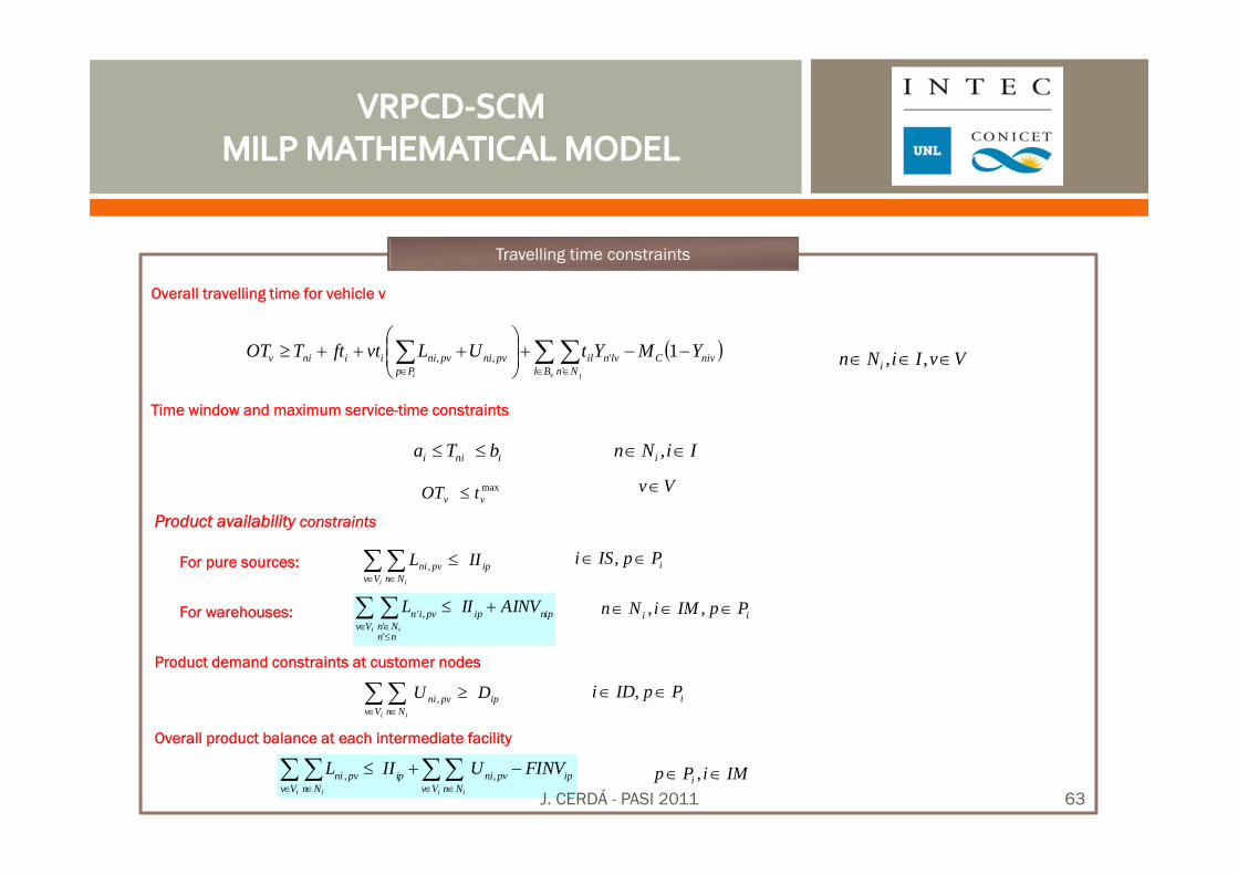
Overall product balance for every vehicle
Accumulated amount of product p picked up by vehicle v up to the stop (n,i)
Accumulated amount of product p delivered by vehicle v up to the stop (n,i)
Vehicle capacity constraints Bounds on variables AUni,pv and ALni,pv
Vehicle-related constraints
( )∑ ∑∑ ∑∪∈ ∈∪∈ ∈
=IDIMi Nn
pvniIMISi Nn
pvniii
UL ,, VvPp ∈∈ ,
( ) ( )( ) ⎭
⎬⎫
⎩⎨⎧
−−−−+≥−−−−−+≥
vinnivLinniLpvnipvinpvni
vinnivLinniLpvinpvnipvin
YYMSMLALALYYMSMLALAL
'''',,,'',
'''',,'',,''
221 ',':,,)',(,'', '' iinnVvPpIiiNnNn iiii ≠<∈∈∈∈∈
( )ivnnivLpvinpvnipvin YYMLALAL ',',,' 2 −−−+≥ ':,,)',( nnVvIiNnn ii <∈∈∈
( ) ( )( ) ⎭
⎬⎫
⎩⎨⎧
−−−−+≥−−−−−+≥
vinnivLinniLpvnipvinpvni
vinnivLinniLpvinpvnipvin
YYMSMUULULYYMSMUULUL
'''',,,'',
'''',,'',,''
221 ',':,,)',(,'', ' iinnVvPpIiiNnNn iiii ≠<∈∈∈∈∈
( )( )
⎪⎪⎭
⎪⎪⎬
⎫
⎪⎪⎩
⎪⎪⎨
⎧
≥−
≤−
≤−
∑∑
∈
∈
0,,
,,
,,
pvnipvni
vPp
pvnipvnip
vPp
pvnipvnip
AUAL
qvAUALuv
qwAUALuw
VvIiNn vi ∈∈∈ ,, ⎪⎭
⎪⎬
⎫
⎪⎩
⎪⎨
⎧
≤≤
≤≤
∑ ∑∑ ∑
∪∈ ∈
∪∈ ∈
IMISi Nnpvinpvnipvni
IMISi Nnpvinpvnipvni
i
i
UAUU
LALL
' '','',,
' '','',,
PpVvIiNn vi ∈∈∈∈ ,,,
Relationship between variables Lni,pv / Uni,pv with Yniv
nivLpvni YML ≤, iii VvPpIMISiNn ∈∈∪∈∈ ,),(,
nivLpvni YMU ≤, iii VvPpIDIMiNn ∈∈∪∈∈ ,,,
- In case of multiple stops of the same vehicle v:
- In case of multiple stops of the same vehicle v: ( )ivnnivLpvinpvnipvin YYMUULUL ',',,' 2 −−−+≥
J. CERDÁ - PASI 2011 64
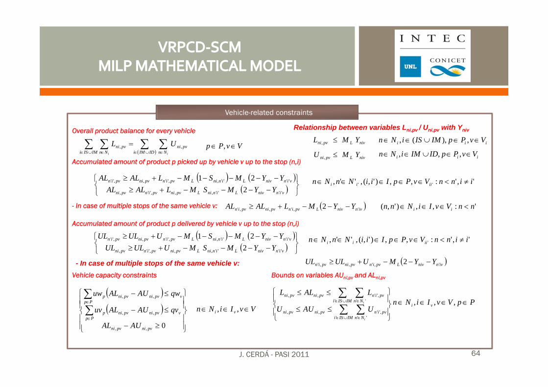
Additional inventory received at cross-docking facilities from other sources
':,,)',( nnPpIMiNnn i <∈∈∈
PpIMiNn i ∈∈∈ ,,
Alternative Objective Functions
⎥⎦
⎤⎢⎣
⎡+ ∑ ∑∑∑
∈ ∈ ∈∈ Vv IBl Nnnlvv
Vvv
v l
YfcCVMin
⎥⎦
⎤⎢⎣
⎡ ∑∈Vv
vOTMin
∑∈
+≥iVv
pvinnipipn UAIAI ,''
∑∑∑∈ ∈∈
≤≤i ii Nn Vv
pvinnipVv
pvni UAIU'
,',
J. CERDÁ - PASI 201165
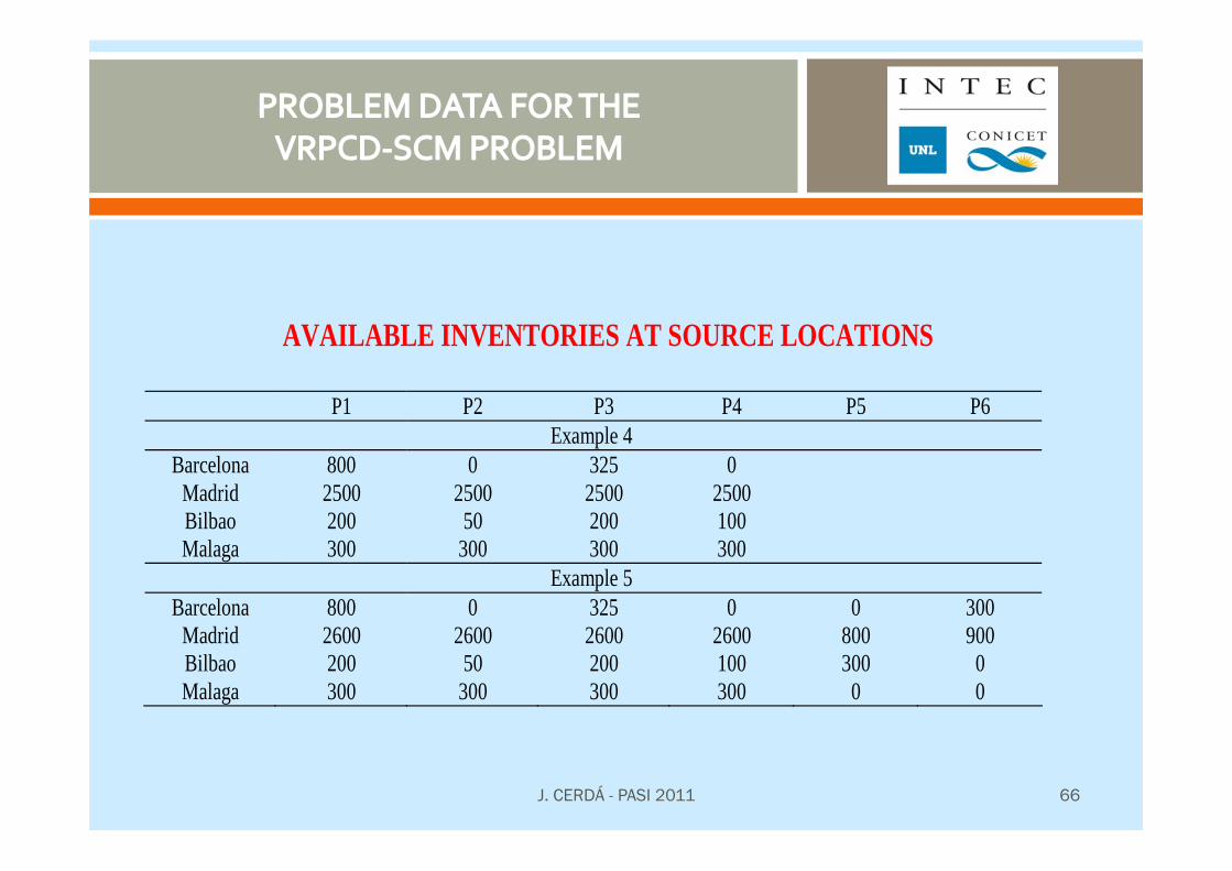
AVAILABLE INVENTORIES AT SOURCE LOCATIONS
P1 P2 P3 P4 P5 P6 Example 4
Barcelona 800 0 325 0 Madrid 2500 2500 2500 2500 Bilbao 200 50 200 100 Malaga 300 300 300 300
Example 5 Barcelona 800 0 325 0 0 300
Madrid 2600 2600 2600 2600 800 900 Bilbao 200 50 200 100 300 0 Malaga 300 300 300 300 0 0
J. CERDÁ - PASI 2011 66
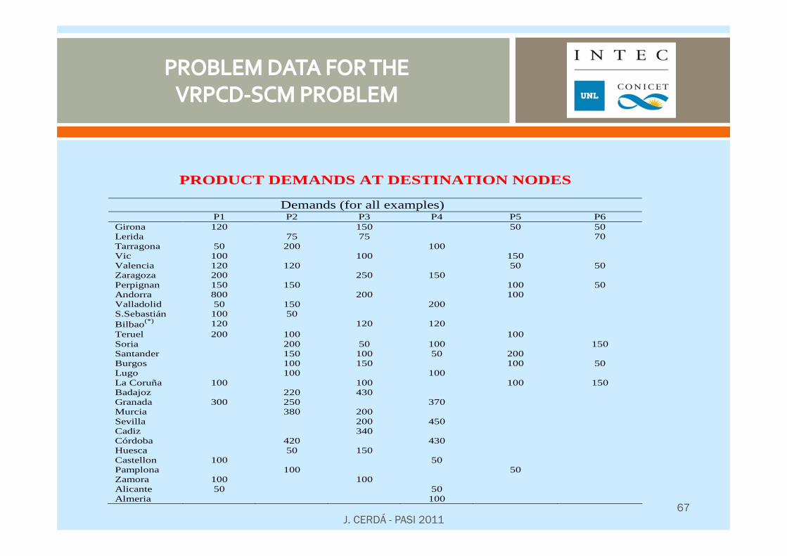
PRODUCT DEMANDS AT DESTINATION NODES
Demands (for all examples) P1 P2 P3 P4 P5 P6 Girona 120 150 50 50 Lerida 75 75 70 Tarragona 50 200 100 Vic 100 100 150 Valencia 120 120 50 50 Zaragoza 200 250 150 Perpignan 150 150 100 50 Andorra 800 200 100 Valladolid 50 150 200 S.Sebastián 100 50 Bilbao(*) 120 120 120 Teruel 200 100 100 Soria 200 50 100 150 Santander 150 100 50 200 Burgos 100 150 100 50 Lugo 100 100 La Coruña 100 100 100 150 Badajoz 220 430 Granada 300 250 370 Murcia 380 200 Sevilla 200 450 Cadiz 340 Córdoba 420 430 Huesca 50 150 Castellon 100 50 Pamplona 100 50 Zamora 100 100 Alicante 50 50 Almeria 100
J. CERDÁ - PASI 201167
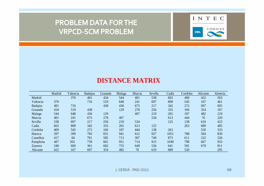
DISTANCE MATRIX
Madrid Valencia Badajoz Granada Malaga Murcia Sevilla Cadiz Cordoba Alicante Almeria Madrid 370 401 434 544 401 538 663 400 422 563 Valencia 370 716 519 648 241 697 808 545 167 461 Badajoz 401 716 438 436 675 217 342 272 697 605 Granada 434 519 438 129 278 256 335 166 354 167 Malaga 544 648 436 129 407 219 265 187 482 219 Murcia 401 241 675 278 407 534 613 444 76 220 Sevilla 538 697 217 256 219 534 125 138 610 423 Cadiz 663 808 342 335 265 613 125 263 689 485 Cordoba 400 545 272 166 187 444 138 263 520 333 Huesca 397 399 783 831 941 612 927 1051 788 564 830 Castellon 417 66 781 585 713 307 749 873 611 232 526 Pamplona 407 502 739 841 951 714 915 1049 798 667 933 Zamora 248 600 361 682 755 649 536 641 591 670 811 Alicante 422 167 697 354 482 76 610 689 520 295
J. CERDÁ - PASI 2011 68
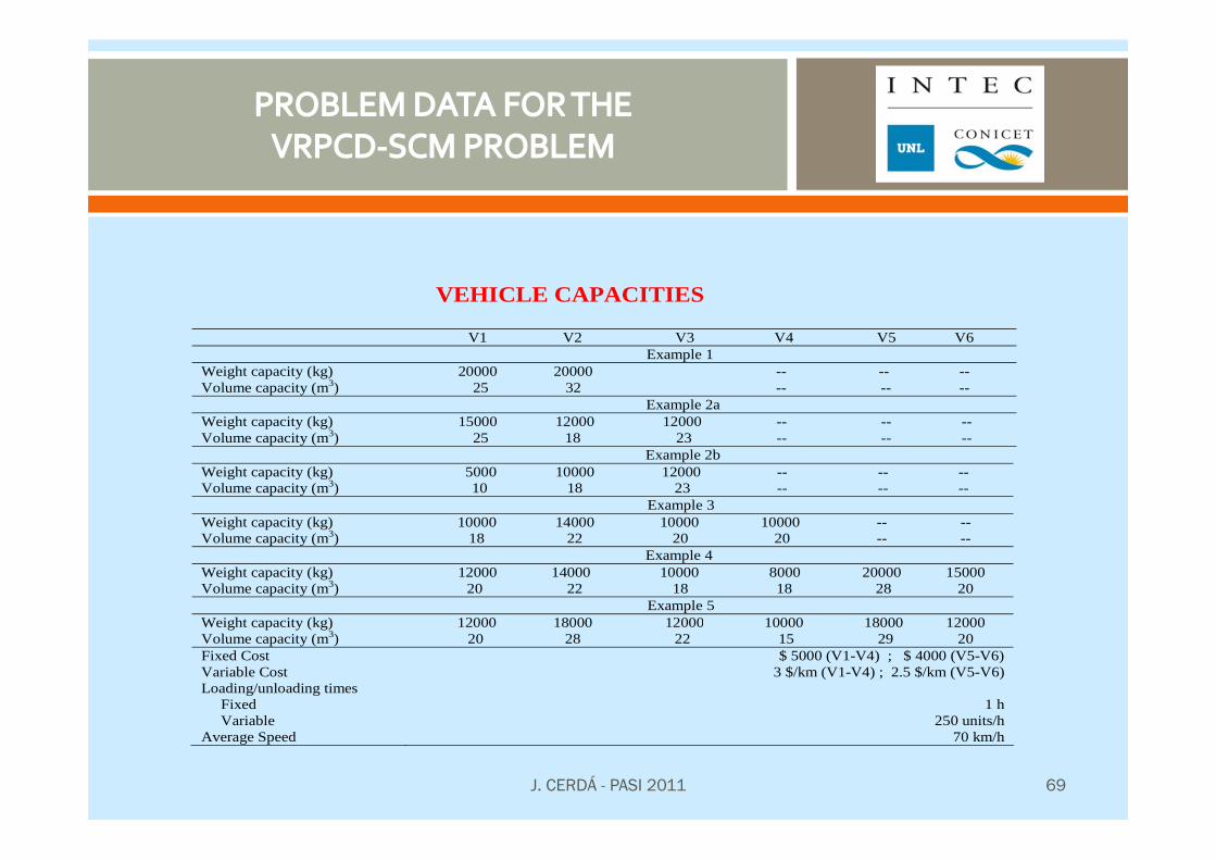
VEHICLE CAPACITIES
V1 V2 V3 V4 V5 V6 Example 1 Weight capacity (kg) 20000 20000 -- -- -- Volume capacity (m3) 25 32 -- -- --
Example 2a Weight capacity (kg) 15000 12000 12000 -- -- -- Volume capacity (m3) 25 18 23 -- -- --
Example 2b Weight capacity (kg) 5000 10000 12000 -- -- -- Volume capacity (m3) 10 18 23 -- -- --
Example 3 Weight capacity (kg) 10000 14000 10000 10000 -- -- Volume capacity (m3) 18 22 20 20 -- --
Example 4 Weight capacity (kg) 12000 14000 10000 8000 20000 15000 Volume capacity (m3) 20 22 18 18 28 20
Example 5 Weight capacity (kg) 12000 18000 12000 10000 18000 12000 Volume capacity (m3) 20 28 22 15 29 20 Fixed Cost Variable Cost
$ 5000 (V1-V4) ; $ 4000 (V5-V6) 3 $/km (V1-V4) ; 2.5 $/km (V5-V6)
Loading/unloading times Fixed Variable
1 h
250 units/h Average Speed 70 km/h
J. CERDÁ - PASI 2011 69
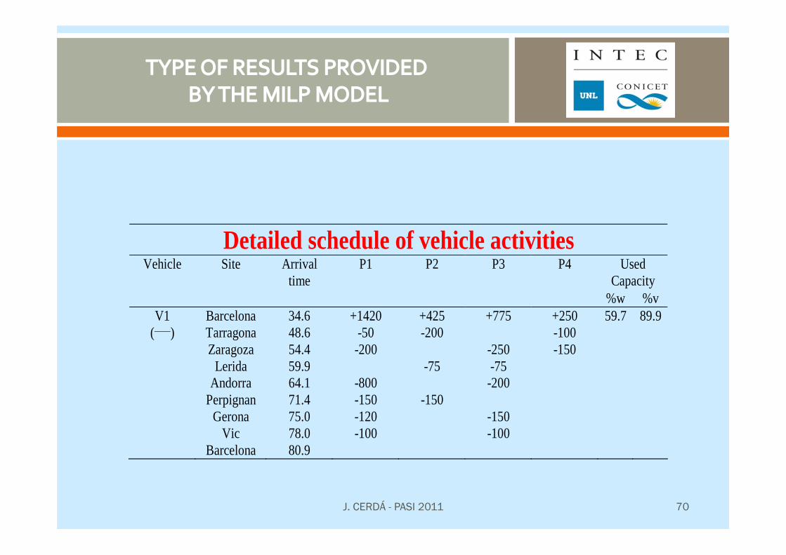
Detailed schedule of vehicle activities Used
Capacity Vehicle Site Arrival
time P1 P2 P3 P4
%w %v V1 Barcelona 34.6 +1420 +425 +775 +250 59.7 89.9
(____) Tarragona 48.6 -50 -200 -100 Zaragoza 54.4 -200 -250 -150 Lerida 59.9 -75 -75 Andorra 64.1 -800 -200 Perpignan 71.4 -150 -150 Gerona 75.0 -120 -150 Vic 78.0 -100 -100 Barcelona 80.9
J. CERDÁ - PASI 2011 70
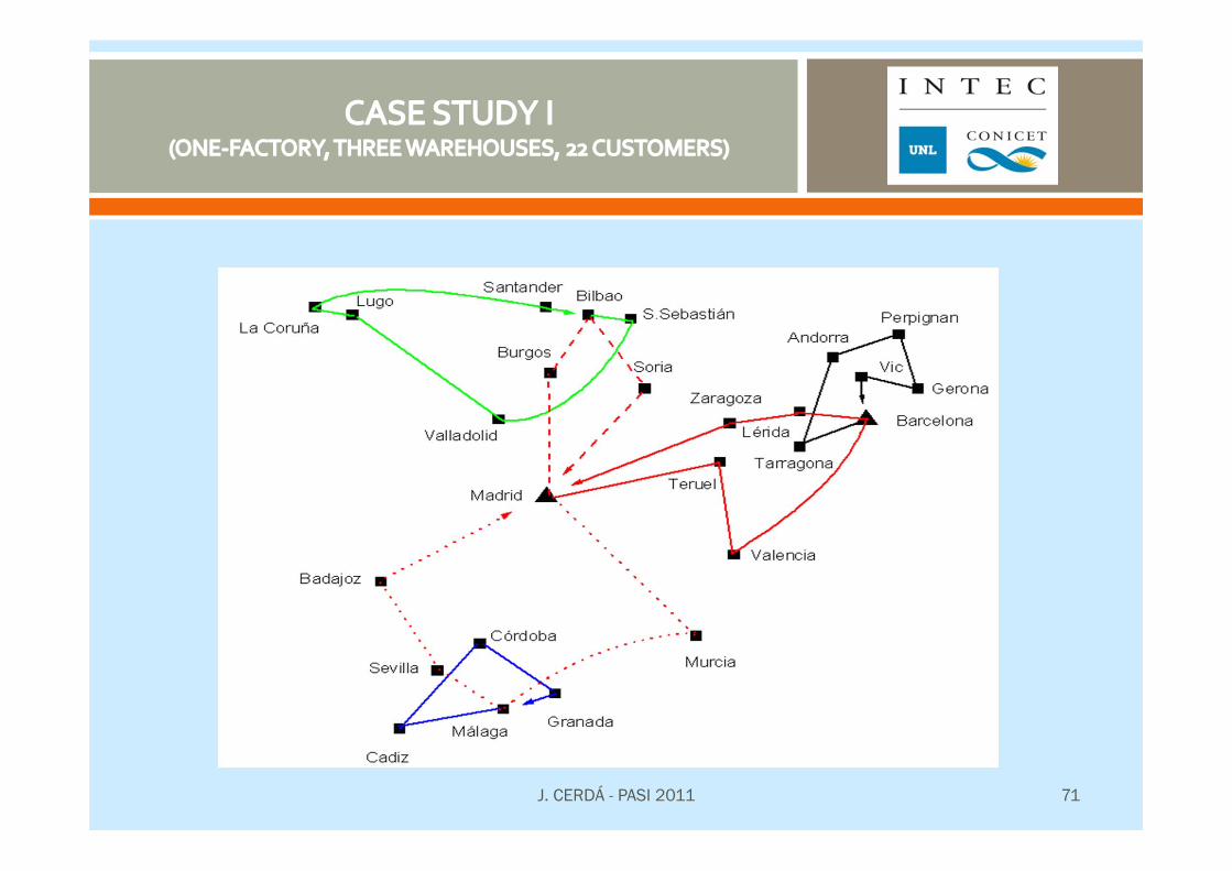
J. CERDÁ - PASI 2011 71
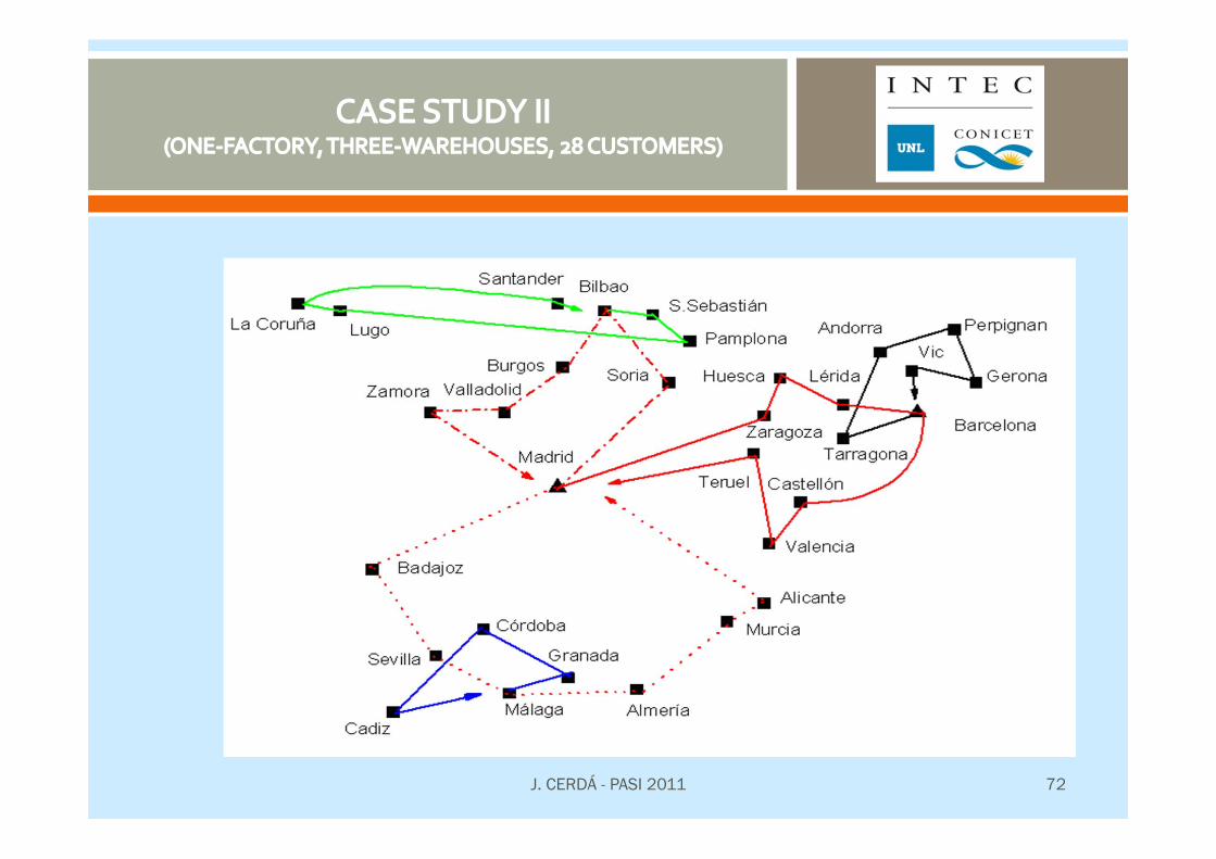
J. CERDÁ - PASI 2011 72
Transportation is a significant link between different stages in aglobal supply chain.
Small reductions in transportation expenses could result insubstantial total savings over a number of years.
The use of vehicle routing and scheduling models and techniquescan be instrumental in realizing those savings.
Different types of vehicle routing problems have studied over theyears; most of them dealing with single-echelon networks and a singletype of operation (pickup or delivery) at every location.
Since they are NP-hard, solution methods based on metaheuristictechniques are generally applied.
Recently, new model-based approaches have been developed forthe operational planning of multi-echelon distribution networks
The so-called VRPCD-SCM problem includes many features usuallyarising in the operation of real-world distribution networks.
Further work on this area is still under way.
J. CERDÁ - PASI 2011 73

J. CERDÁ - PASI 2011


![INDUSTRIA AUDIOVISUAL - ZEMOS98 · INDUSTRIA AUDIOVISUAL - Pedro Jiménez – ZEMOS98 - - EACINE - 2008/2009 PRODUCCIÓN [professional + amateur = proam] - El desarrollo tecnológico](https://img.pdfslide.net/doc/110x75/5f4a91d14e71e3673c7814b4/industria-audiovisual-industria-audiovisual-pedro-jimnez-a-zemos98-eacine.jpg)