Integer Programming ISE 418 Lecture 12

Integer ProgrammingISE 418

Lecture 12

Dr. Ted Ralphs

ISE 418 Lecture 12 1

Reading for This Lecture

• Nemhauser and Wolsey Sections II.1.1-II.1.3, II.1.6

• Wolsey Chapter 8

• CCZ Chapter 3, Section 7.5

1


Describing conv(S)

• We have seen that, in theory, conv(S) has a finite description.

• If we “simply” construct that description, we could turn our MILP intoan LP.

• So why aren’t IPs easy to solve?

– The size of the description is generally HUGE!– The number of facets of the TSP polytope for an instance with 120

nodes is more than 10100 times the number of atoms in the universe.– It is physically impossible to write down a description of this polytope.– Not only that, but it is very difficult in general to generate these facets

(this problem is not polynomially solvable in general).

2


For Example

• For a TSP of size 15

– The number of subtour elimination constraints is 16,368.– The number of comb inequalities is 1, 993, 711, 339, 620.– These are only two of the know classes of facets for the TSP.

• For a TSP of size 120

– The number of subtour elimination constraints is 0.6× 1036!– The number of comb inequalities is approximately 2× 10179!

3


Valid Inequalities Revisited

• Recall that the inequality denoted by (π, π0) is valid for a polyhedron Qif πx ≤ π0 ∀x ∈ Q.

• Note that an inequality (π, π0) is valid if and only if

π0 ≥ maxx∈Q

π>x

• Alternatively, an inequality (π, π0) is valid if

π0 ≥ F (b),

where F is a dual function with respect to the optimization problem

maxx∈Q

π>x

• In fact, many classes of valid inequalities used in solvers are generated inthis way.

• Thus, there is an inextricable link between valid inequalities andoptimization.

4


Cutting Planes

• The term cutting plane usually refers to an inequality valid for conv(S),but which is violated by the solution to the (current) LP relaxation.

• Cutting plane methods attempt to improve the bound produced by the LPrelaxation by iteratively adding cutting planes to the initial LP relaxation.

• Taken to its limit, this is an algorithm for solving MILPs that fits intothe general “dual improvement” framework.

• Adding such inequalities to the LP relaxation may improve the bound(this is not a guarantee).

5


The Separation Problem

• Formally, the problem of generating a cutting plane can be stated asfollows.

Separation Problem: Given a polyhedron Q ⊆ Rn and x∗ ∈ Rn,determine whether x∗ ∈ Q and if not, determine (π, π0), an inequalityvalid for Q such that πx∗ > π0.

• This problem is stated here independent of any solution algorithm.

• However, it is typically used as a subroutine inside an iterative methodfor improving the LP relaxation.

• In such a case, x∗ is the solution to the LP relaxation (of the currentformulation, including previously generated cuts).

• We will see that the difficulty of solving this problem exactly is stronglytied to the difficulty of the optimization problem itself.

• Any algorithm for solving the separation problem can be immediatelyleveraged to produce an algorithm for solving the optimization problem.

• This algorithm is know as the cutting plane algorithm.

6


Generic Cutting Plane Method

Let P = {x ∈ Rn | Ax ≤ b} be the initial formulation for

max{c>x | x ∈ S}, (MILP)

where S = P ∩ Zr+ × Rn−p+ , as defined previously.

Cutting Plane Method

P0 ← Pk ← 0while TRUE do

Solve the LP relaxation max{c>x | x ∈ Pk} to obtain a solution xk

Solve the problem of separating xk from conv(S)if xk ∈ conv(S) then

STOPelse

Determine an inequality (πk, πk0) valid for conv(S) but for whichπ>xk > πk0 .

end ifPk+1 ← Pk ∩ {x ∈ Rn | (πk)>x ≤ πk0}.k ← k + 1

end while

7


Questions to be Answered

• How do we solve the separation problem in practice?

• Will this algorithm terminate?

• If it does terminate, are we guaranteed to obtain an optimal solution?

8


The Separation Problem as an Optimization Problem

Separation Problem: Given a polyhedron Q ⊆ Rn and x∗ ∈ Rn, determinewhether x∗ ∈ Q and if not, determine (π, π0), a valid inequality for Q suchthat πx∗ > π0.

• Closer examination of the separation problem for a polyhedron revealsthat it is in fact an optimization problem.

• Consider a polyhedron Q ⊆ Rn and x∗ ∈ Rn.

• The separation problem can be formulated as

max{πx∗ − π0 | π>x ≤ π0 ∀x ∈ P, (π, π0) ∈ Rn+1} (SEP)

along with some normalization to prevent (SEP) being unbounded.

• When Q is a polytope, we can reformulate this problem as the LP

max{πx∗ − π0 | π>x ≤ π0 ∀x ∈ E},

where E is the set of extreme points of Q.

• When Q is not bounded, the reformulation must account for the extremerays of Q.

9


The Normalization

• There are multiple ways to normalize, e.g.,

– π0 = 1 or– ‖π‖ = 1.

• These are equivalent with respect to reducing the separation problem toan optimization problem

• Different normalizations will, however, result in different optimal solutionsand will behave differently in a computational setting.

• The issue of how to normalize will come up again in later lectures.

10


The Polar

Definition 1. The polar of a set S is S∗ = {y ∈ Rn | yx ≤ 1 ∀x ∈ S}.

Theorem 1. Given a1, . . . , am ∈ Qn and 0 ≤ k ≤ m, let

Q1 = {x ∈ Rn | aix ≤ 1, i = 1, . . . , k; aux ≤ 0, i = k + 1, . . . ,m}

Q2 = conv({0, a1, . . . , ak}) + cone({ak+1, . . . an})

Then Q∗1 = Q2 and Q∗2 = Q1

• From this definition, we can see that if Q is a polyhedron containing theorigin, then have that

1. Q∗ is also a polyhedron containing the origin;2. Q∗∗ = Q;3. Q∗ is bounded if and only if Q contains the origin in its interior;4. aff(Q∗) is the orthogonal complement of lin(Q) and dim(Q∗) +

dim(lin(Q)) = n.

11


Interpreting the Polar

• The polar can be roughly interpreted as the (normalized) set of all validinequalities.

• Without some normalization, it would contain all scalar multiples of eachinequality.

• Because of the normalization used here, the polar is sometimes calledthe 1-Polar in this context.

• There is a one-to-one correspondence between the facets of thepolyhedron and the extreme points of the 1-Polar when

– the polyhedron is full-dimensional and– the origin is in its interior,

• Hence, the separation problem can be seen as an optimization problemover the polar.

12


The Membership Problem

Membership Problem: Given a polyhedron Q ⊆ Rn and x∗ ∈ Rn, determinewhether x∗ ∈ Q.

• The membership problem is a decision problem and is closely related tothe separation problem.

• In fact, the dual of (SEP) is a formulation for the membership problem:

minλ∈RE+

{0>λ

∣∣ Eλ = x∗, 1>λ = 1}, (MEM)

where E is a matrix whose columns are the extreme points of Q.

• In other words, we try to express x∗ as a convex combination of extremepoints of Q.

• When this LP is infeasible, the certificate is a separating hyperplane.

• We can solve this LP by column generation.

• In each iteration, a new column is “generated” by optimizing over Q.

• We can picture this algorithm in the “primal space” to understand whatit’s doing.

13


Example: Separation Algorithm with Optimization Oracle

Figure 1: Polyhedron and point to be separated

14



Figure 2: Iteration 1

15




16




17




18




19


The Separation Problem for the 1-Polar

• The column generation algorithm for solving (MEM) can be interpretedas a cutting plane algorithm for solving (SEP).

• The separation problem (SEP) for Q has one inequality for each extremepoint of Q.

• We can generate these inequalities using a cutting plane algorithm.

• This is a bit circular...this requires solving the separation problem for Q∗,the 1-Polar.

• For a given π∗ ∈ Rn, the separation problem for Q∗ is to determinewhether π∗ ∈ Q∗ and if not, determine x ∈ E such that π∗x < 1.

• In other words, we are asking whether π∗ is a valid inequality for Q.

• As before, this problem can be formulated as

max{π∗x | x ∈ Q},

which is an optimization problem over Q!

20


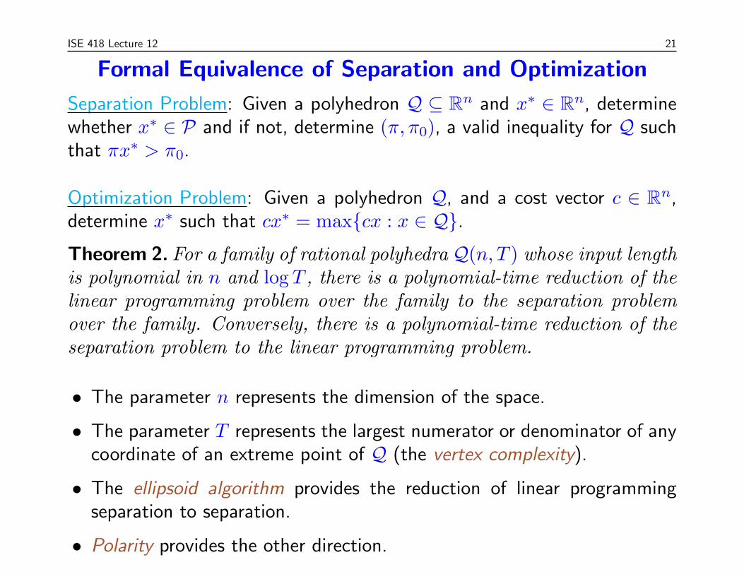
Formal Equivalence of Separation and Optimization

Separation Problem: Given a polyhedron Q ⊆ Rn and x∗ ∈ Rn, determinewhether x∗ ∈ P and if not, determine (π, π0), a valid inequality for Q suchthat πx∗ > π0.

Optimization Problem: Given a polyhedron Q, and a cost vector c ∈ Rn,determine x∗ such that cx∗ = max{cx : x ∈ Q}.Theorem 2. For a family of rational polyhedra Q(n, T ) whose input lengthis polynomial in n and log T , there is a polynomial-time reduction of thelinear programming problem over the family to the separation problemover the family. Conversely, there is a polynomial-time reduction of theseparation problem to the linear programming problem.

• The parameter n represents the dimension of the space.

• The parameter T represents the largest numerator or denominator of anycoordinate of an extreme point of Q (the vertex complexity).

• The ellipsoid algorithm provides the reduction of linear programmingseparation to separation.

• Polarity provides the other direction.

21


Proof: The Ellipsoid Algorithm

• The ellipsoid algorithm is an algorithm for solving linear programs.

• The implementation requires a subroutine for solving the separationproblem over the feasible region (see next slide).

• We will not go through the details of the ellipsoid algorithm.

• However, its existence is very important to our study of integerprogramming.

• Each step of the ellipsoid algorithm, except that of finding a violatedinequality, is polynomial in

– n, the dimension of the space,– log T , where is the largest numerator or denominator of any coordinate

of an extreme point of Q, and– log ‖c‖, where c ∈ Rn is the given cost vector.

• The entire algorithm is polynomial if and only if the separation problemis polynomial.

22


Classes of Inequalities

• As we have just shown, producing general facets of conv(S) is as hardas optimizing over S.

• Thus, the approach often taken is to solve a “relaxation” of the separationproblem.

• This “relaxation” is usually obtained in one of several ways.

– It can be obtained in the usual way by relaxing some constraints toobtain a more tractable problem.

– The “structure” of the inequalities may be somehow restricted to makethe right-hand side easy to compute.

– We may also use a dual function to compute the right-hand side ratherthan computing the “optimal” right-hand side.

• We will see examples of the second approach in later lectures.

• In either of the first two cases, the class of inequalities we want togenerate typically defines a polyhedron C.

• C is what we earlier called the closure.

• The separation problem for the class is the separation problem over theclosure.

23

Documents

Integer Programming ISE 418 Lecture 12