Integer Programming ISE 418 Lecture 8

Integer ProgrammingISE 418

Lecture 8

Dr. Ted Ralphs

ISE 418 Lecture 8 1

Reading for This Lecture

• Wolsey Chapter 2

• Nemhauser and Wolsey Sections II.3.1, II.3.6, II.4.1, II.4.2, II.5.4

• “Duality for Mixed-Integer Linear Programs,” Guzelsoy and Ralphs

1

ISE 418 Lecture 8 2

The Efficiency of Branch and Bound

• In general, our goal is to solve the problem at hand as quickly as possible.

• The overall solution time is the product of the number of nodesenumerated and the time to process each node.

• Typically, by spending more time in processing, we can achieve a reductionin tree size by computing stronger (closer to optimal) bounds.

• This highlights another of the many tradeoffs we must navigate.

• Our goal in bounding is to achieve a balance between the strength of thebound and the efficiency with which we can compute it.

• How do we compute bounds?

– Relaxation: Relax some of the constraints and solve the resultingmathematical optimization problem.

– Duality: Formulate a “dual” problem and find a feasible to it.

• In practice, we will use a combination of these two closely-relatedapproaches.

2

ISE 418 Lecture 8 3

Relaxation

As usual, we consider the MILP

zIP = maxc>x | x ∈ S, (MILP)

where

P = x ∈ Rn+ | Ax ≤ b (FEAS-LP)

S = P ∩ (Zp+ × Rn−p+ ) (FEAS-MIP)

Definition 1. A relaxation of IP is a maximization problem defined as

zR = maxzR(x) | x ∈ SR

with the following two properties:

S ⊆ SRc>x ≤ zR(x), ∀x ∈ S.

3

ISE 418 Lecture 8 4

Importance of Relaxations

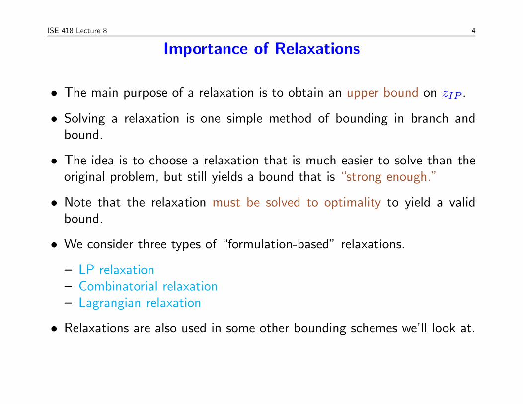
• The main purpose of a relaxation is to obtain an upper bound on zIP .

• Solving a relaxation is one simple method of bounding in branch andbound.

• The idea is to choose a relaxation that is much easier to solve than theoriginal problem, but still yields a bound that is “strong enough.”

• Note that the relaxation must be solved to optimality to yield a validbound.

• We consider three types of “formulation-based” relaxations.

– LP relaxation– Combinatorial relaxation– Lagrangian relaxation

• Relaxations are also used in some other bounding schemes we’ll look at.

4

ISE 418 Lecture 8 5

Aside: How Do You Spell “Lagrangian?”

• Some spell it “Lagrangean.”

• Some spell it “Lagrangian.”

• We ask Google.

• In 2002:

– “Lagrangean” returned 5,620 hits.

– “Lagrangian” returned 14,300 hits.

• In 2007:

– “Lagrangean” returns 208,000 hits.

– “Lagrangian” returns 5,820,000 hits.

• In 2010:

– “Lagrangean” returns 110,000 hits (and asks “Did you mean: Lagrangian?”)


• In 2014 (strange regression!):

– “Lagrangean” returns 1,140,000 hits


5

ISE 418 Lecture 8 6

The Branch and Bound Tree as a “Meta-Relaxation”

• The branch-and-bound tree itself encodes a relaxation of our originalproblem, as we mentioned in the last lecture.

• As observed previously, the set T of leaf nodes of the tree (includingthose that have been pruned) constitute a valid disjunction, as follows.

– When we branch using admissible disjunctions, we associate with eacht ∈ T a polyhedron Xt described by the imposed branching constraints.

– The collection Xtt∈T then defines a disjunction.

• The subproblem associated with node i is an integer program withfeasible region S ∩ P ∩Xt.

• The problemmaxt∈T

maxx∈P∩Xt

c>x (OPT)

is then a relaxation according to our definition.

• Branch and bound can be seen as a method of iteratively strengtheningthis relaxation.

• We will later see how we can add valid inequalities to the constraint ofP ∩Xt to strengthen further.

6

ISE 418 Lecture 8 7

Obtaining and Using Relaxations

• Properties of relaxations

– If a relaxation of (MILP) is infeasible, then so is (MILP).– If zR(x) = c>x, then for x∗ ∈ argmaxx∈SR zR(x), if x∗ ∈ S, then x∗

is optimal for (MILP).

• The easiest way to obtain relaxations of (MILP) is to relax some of theconstraints defining the feasible set S.

• It is “obvious” how to obtain an LP relaxation, but combinatorialrelaxations are not as obvious.

7

ISE 418 Lecture 8 8

Example: Traveling Salesman Problem

The TSP is a combinatorial problem (E,F) whose ground set is the edgeset of a graph G = (V,E).

• V is the set of customers.

• E is the set of travel links between the customers.

A feasible solution is a subset of E consisting of edges of the form i, σ(i)for i ∈ V , where σ is a simple permutation V specifying the order in whichthe customers are visited.

IP Formulation: ∑nj=1 xij = 2 ∀i ∈ N−∑i∈Sj 6∈S

xij ≥ 2 ∀S ⊂ V, |S| > 1.

where xij is a binary variable indicating whether σ(i) = j.

8

ISE 418 Lecture 8 9

Combinatorial Relaxations of the TSP

• The Traveling Salesman Problem has several well-known combinatorialrelaxations.

• Assignment Problem

– The problem of assigning n people to n different tasks.– Can be solved in polynomial time.– Obtained by dropping the subtour elimination constraints and the

upper bounds on the variables.

• Minimum 1-tree Problem

– A 1-tree in a graph is a spanning tree of nodes 2, . . . n plus exactlytwo edges incident to node one.

– A minimum 1-tree can be found in polynomial time.– This relaxation is obtained by dropping all subtour elimination

constraints involving node 1 and also all degree constraints notinvolving node 1.

9

ISE 418 Lecture 8 10

Exploiting Relaxations

• How can we use our ability to solve a relaxation to full advantage?

• The most obvious way is simply to straightforwardly use the relaxationto obtain a bound.

• However, by solving the relaxation repeatedly, we can get additionalinformation.

• For example, we can generate extreme points of conv(SR).

• In an indirect way (using the Farkas Lemma), we can even obtainfacet-defining inequalities for conv(SR).

• We can use this information to strengthen the original formulation.

• This is one of the basic principles of many solution methods.

10


Lagrangian Relaxation

• A Lagrangian relaxation is obtained by relaxing a set of constraints fromthe original formulation.

• However, we also try to improve the bound by modifying the objectivefunction, penalizing violation of the dropped constraints.

• Consider a pure IP defined by

max c>x

s.t. A′x ≤ b′

A′′x ≤ b′′

x ∈ Zn+,

(IP)

where SR = x ∈ Zn+ | A′x ≤ b′ bounded and optimization over SR is“easy.”

• Lagrangian Relaxation:

LR(u) : zLR(u) = maxx∈SR

(c− uA′′)x+ ub′′.

11


Properties of the Lagrangian Relaxation

• For any u ≥ 0, LR(u) is a relaxation of (IP) (why?).

• Solving LR(u) yields an upper bound on the value of the optimalsolution.

• We will show later that this bound is at least as good as the boundyielded by solving the LP relaxation.

• Generally, we try to choose a relaxation that allows LR(u) to be evaluatedrelatively easily.

• Recalling LP duality, one can think of u as a vector of “dual variables.”

12


A (Very) Brief Tour of Duality

• Suppose we could obtain an optimization problem “dual” to (MILP)similar to the standard one we can derive for an LP.

• Such a dual allows us to obtain bounds on the value of an optimalsolution.

• The advantage of a dual over a relaxation is that we need not solve it tooptimality1.

• Any feasible solution to the dual yields a valid bound.

• For (MILP), there is apparently no single standard “dual” problem.

• Nevertheless, there is a well-developed duality theory that generalizesthat of LP duality, which we summarize next.

• This duality theory will be discussed in more detail later in the course.

1Note, however, that duals and relaxations are close relatives in a sense we will discuss later

13


A Quick Overview of LP Duality

• We consider the LP relaxation of (MILP) in standard formx ∈ Rn+

∣∣ Ax = b, (LP)

where A = [A | I] and x is extended to include the slack variables.

• Recall that there always exists an optimal solution that is basic.

• We construct basic solutions by

– Choosing a basis B of m linearly independent columns of A.– Solving the system BxB = b to obtain the values of the basic variables.– Setting remaining variables to value 0.

• If xB ≥ 0, then the associated basic solution is feasible.

• With respect to any basic feasible solution, it is easy to determine theimpact of increasing a given activity.

• The reduced costcj = cj − c>BB−1Aj.

of (nonbasic) variable j tells us how the objective function value changesif we increase the level of activity j by one unit.

14


The LP Value Function

• From the resource (dual) perspective, the quantity u = cBB−1 is a

vector that tells us the marginal economic value of each resource.

• Thus, the vector u gives us a price for each resource.

• This price vector can be seen as the gradient of the value function

φLP (β) = maxx∈S(β)

c>x, (LPVF)

of an LP, where for a given β ∈ Rm, S(d) = x ∈ Rn+ | Ax = d.

• We let φLP (β) = −∞ if β ∈ Ω = β ∈ Rm | S(β) = ∅.

• These gradients can be seen as linear over-estimators of the valuefunction.

• The dual problems we’ll consider are essentially aimed at producing suchover-estimators.

• We’ll generalize to non-linear functions.

15


LP Value Function Example

φLP (β) = min 6y1 + 7y2 + 5y3

s.t. 2y1 − 7y2 + y3 = β

y1, y2, y3 ∈ R+

Note that we are minimizing here!

16


The LP Dual

• To understand the structure of the value function in more detail, firstnote that it is easy to see φLP is concave.

• Now consider an optimal basis matrix B for the instance (LP).

– The gradient of φLP at b is u = cBB−1.

– Since φLP (b) = u>b and φLP is concave, we know that φLP (β) ≤ u>βfor all β ∈ Rm.

• The traditional LP dual problem can be viewed as that of finding a linearfunction that bounds the value function from above and has minimumvalue at b.

17


The LP Dual (cont’d)

• As we have seen, for any u ∈ Rm, the following gives a upper bound onφLP (b).

g(u) = maxx≥0

[c>x+ u>(b− Ax)

]≥ c>x∗ + u>(b− Ax∗)

= c>x∗

= φLP (b)

• With some simplification, we can obtain an explicit form for this function.

g(u) = maxx≥0

[c>x+ u>(b− Ax)

]= u>b+ max

x≥0(c> − u>A)x

• Note that

maxx≥0

(c> − u>A)x =

0, if c> − u>A ≤ 0>,

∞, otherwise,

18


The LP Dual (cont’d)

• So we have

g(u) =

u>b, if c> − u>A ≤ 0>,

∞, otherwise,

which is again a linear over-estimator of the value function.

• An LP dual problem is obtained by computing the strongest linearover-estimator with respect to b.

minu∈Rm

g(u) = min b>u

s.t. u>A ≥ c> (LPD)

19


Combinatorial Representation of the LP Value Function

• From the fact that there is always an extremal optimum to (LPD), weconclude that the LP value function can be described combinatorially.

φLP (β) = minu∈E

u>β (LPVF)

for β ∈ Rm, where

E =cBA

−1E | E is the index set of a dual feasible bases of A

• Note that E is also the set of extreme points of the dual polyhedronu ∈ Rm | u>A ≥ c>.

20


The MILP Value Function

• We now generalize the notions seen so far to the MILP case.

• The value function associated with (MILP) is

φ(β) = maxx∈S(β)

c>x (VF)

for β ∈ Rm, where S(β) = x ∈ Zp+ × Rn−p+ | Ax = β.

• Again, we let φ(β) = −∞ if β ∈ Ω = β ∈ Rm | S(β) = ∅.

21


Example: MILP Value Function

φ(β) = min 12x1 + 2x3 + x4

s.t x1 − 32x2 + x3 − x4 = β and

x1, x2 ∈ Z+, x3, x4 ∈ R+.

3

0

φ(β)

β1-1-2-3 3 42-4 −32 −1

2−52−7

2

52

32

12

12

32

52

72

1

2

Note again that we are minimizing here!

22


A General Dual Problem

• A dual function F : Rm → R is one that satisfies F (β) ≥ φ(β) for allβ ∈ Rm.

• How to select such a function?

• We may choose one that is easy to construct/evaluate and/or for whichF (b) ≈ φ(b).

• This results in the following generalized dual of (MILP).

min F (b) : F (β) ≥ φ(β), β ∈ Rm, F ∈ Υm (D)

where Υm ⊆ f | f : Rm→R.• We call F ∗ strong for this instance if F ∗ is a feasible dual function andF ∗(b) = φ(b).

• This dual instance always has a solution F ∗ that is strong if the valuefunction is bounded and Υm ≡ f | f : Rm→R. Why?

23


LP Dual Function

• It is straightforward to obtain a dual function: simply take the dual ofthe LP relaxation.

• In practice, working with this dual just means using dual simplex to solvethe relaxations.

• Note again that since dual simplex maintains a dual feasible solution atall times, we can stop anytime we like.

• In particular, as soon as the upper bound goes below the current lowerbound, we can stop solving the LP.

• This can save significant effort.

• With an LP dual, we can “close the gap” by adding valid inequalities tostrengthen the LP relaxation.

• The size of the gap in this case is a measure of how well we are able toapproximate the convex hull of feasible solutions (near the optimum).

24


The Lagrangian Dual

• We can obtain a dual function from a Lagrangian relaxation by letting

L(β, u) = maxx∈SR(β)

(c− uA′′)x+ uβ′′,

where SR(d) = x ∈ Zn+ | A′x ≤ d

• Then the Lagrangian dual function, φLD, is

φLD(β) = minu≥0

L(β, u)

• We will see a number of ways of computing φLD(b) later in the course.

25


Dual Functions from Branch-and-Bound

As before, let T be set of the terminating nodes of the tree. Then,assuming we are branching on variable disjunctions, in a leaf node t ∈ T ,the relaxation we solve is:

φt(β) = max c>x

s.t. Ax = β,

lt ≤ x ≤ ut, x ≥ 0

The dual at node t:

φt(β) = min πtβ + πtlt + πtut

s.t. πtA+ πt + πt ≥ c>

π ≥ 0, π ≤ 0

We obtain the following strong dual function:

maxt∈Tπtβ + πtlt + ˆπtut,

where (πt, πt, ˆπt) is an optimal solution to the dual at node t.

26


The Duality Gap

• In most cases, the the value of an optimal solution to a given dualproblem is not equal to the value of an optimal solution to (MILP).

• The difference between these values for a particular instance is known asthe duality gap or just the gap.

• It is typically reported as a percentage of the value of the best knownsolution (this is called the relative gap).

• The size of the relative gap is a rough measure of the difficulty of aproblem.

• It can help us estimate how long it will take to solve a given problem bybranch and bound.

27


Strong Duality

• When the duality gap is guaranteed to be zero, we say we have a strongdual.

• For linear programs, the LP dual is a strong dual.

• For integer programs, the dual (D) is a strong dual, since the valuefunction itself is a solution for which the gap is zero.

• Of course, obtaining a description of the value function is more difficultthan solving theinteger program itself.

28

Documents

Integer Programming ISE 418 Lecture 8