1

Integrated Agriculture and

Productivity Project

Impact Evaluation Endline Report

DEVELOPMENT IMPACT EVALUATION (DIME)

The World Bank

Funding for this study generously provided by the Global Agriculture and Food Security Program (GAFSP), the

South Asian Food and Nutrition Security Initiative (SAFANSI), and the i2i program for impact evaluation. The views

expressed do not necessarily reflect the U.K. government’s official policies or the policies of the World Bank and its

Board of Executive Directors.

2

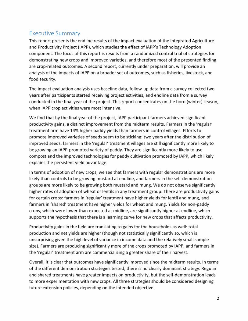
Executive Summary This report presents the endline results of the impact evaluation of the Integrated Agriculture

and Productivity Project (IAPP), which studies the effect of IAPP’s Technology Adoption

component. The focus of this report is results from a randomized control trial of strategies for

demonstrating new crops and improved varieties, and therefore most of the presented finding

are crop-related outcomes. A second report, currently under preparation, will provide an

analysis of the impacts of IAPP on a broader set of outcomes, such as fisheries, livestock, and

food security.

The impact evaluation analysis uses baseline data, follow-up data from a survey collected two

years after participants started receiving project activities, and endline data from a survey

conducted in the final year of the project. This report concentrates on the boro (winter) season,

when IAPP crop activities were most intensive.

We find that by the final year of the project, IAPP participant farmers achieved significant

productivity gains, a distinct improvement from the midterm results. Farmers in the ‘regular’

treatment arm have 14% higher paddy yields than farmers in control villages. Efforts to

promote improved varieties of seeds seem to be sticking: two years after the distribution of

improved seeds, farmers in the ‘regular’ treatment villages are still significantly more likely to

be growing an IAPP-promoted variety of paddy. They are significantly more likely to use

compost and the improved technologies for paddy cultivation promoted by IAPP, which likely

explains the persistent yield advantage.

In terms of adoption of new crops, we see that farmers with regular demonstrations are more

likely than controls to be growing mustard at endline, and farmers in the self-demonstration

groups are more likely to be growing both mustard and mung. We do not observe significantly

higher rates of adoption of wheat or lentils in any treatment group. There are productivity gains

for certain crops: farmers in ‘regular’ treatment have higher yields for lentil and mung, and

farmers in ‘shared’ treatment have higher yields for wheat and mung. Yields for non-paddy

crops, which were lower than expected at midline, are significantly higher at endline, which

supports the hypothesis that there is a learning curve for new crops that affects productivity.

Productivity gains in the field are translating to gains for the households as well: total

production and net yields are higher (though not statistically significantly so, which is

unsurprising given the high level of variance in income data and the relatively small sample

size). Farmers are producing significantly more of the crops promoted by IAPP, and farmers in

the ‘regular’ treatment arm are commercializing a greater share of their harvest.

Overall, it is clear that outcomes have significantly improved since the midterm results. In terms

of the different demonstration strategies tested, there is no clearly dominant strategy. Regular

and shared treatments have greater impacts on productivity, but the self-demonstration leads

to more experimentation with new crops. All three strategies should be considered designing

future extension policies, depending on the intended objective.

3

Table of Contents

Executive Summary ............................................................................................................... 2

Impact Evaluation Summary .................................................................................................. 5

Country Context ........................................................................................................................................ 5

Integrated Agricultural Productivity Project (IAPP) .................................................................................. 6

Evaluation Questions ................................................................................................................................ 7

Motivation................................................................................................................................................. 7

Description of Demonstration Approaches .............................................................................................. 9

Evaluation Design .................................................................................................................................... 10

Data and Sampling .................................................................................................................................. 11

Interpreting Charts .................................................................................................................................. 11

Results ................................................................................................................................ 13

Agricultural productivity ......................................................................................................................... 13

Paddy yields ........................................................................................................................................ 13

Yields for other IAPP crops .................................................................................................................. 14

Adoption of Crops and Varieties Promoted by IAPP ............................................................................... 15

Paddy................................................................................................................................................... 15

Mung ................................................................................................................................................... 17

Wheat .................................................................................................................................................. 18

Mustard ............................................................................................................................................... 18

Lentil .................................................................................................................................................... 19

Use of Improved Inputs and Technologies ............................................................................................. 20

Additional Harvest Outcomes .............................................................................................. 23

Crop Mix .................................................................................................................................................. 24

Appendix A .......................................................................................................................... 27

Sampling .................................................................................................................................................. 27

Specification Details ................................................................................................................................ 27

KG Yields.................................................................................................................................................. 28

Adoption ................................................................................................................................................. 30

Use of Improved Inputs and Technologies ............................................................................................. 33

Agricultural Outcomes ............................................................................................................................ 34

Crop’s Share of Total Cultivated Area ..................................................................................................... 35

Crop Model ............................................................................................................................................. 36

4

Appendix B .......................................................................................................................... 37

KG Yields.................................................................................................................................................. 37

Adoption ................................................................................................................................................. 38

Input Usage ............................................................................................................................................. 39

Agricultural Outcomes ............................................................................................................................ 40

Crop’s Share of Total Cultivated Area ..................................................................................................... 41

List of Tables and Figures

Table 1: Data Sample ...................................................................................................................................................................... 11

Table 2: Share of mono-cropped plots, by crop .............................................................................................................................. 13

Table 3: Harvest Values of Different Crops, Endline Survey ........................................................................................................... 26

Figure A 1: Shared Demonstration Plot – Dark green represents shared area of technology demonstration ................................. 9

Figure 1: Paddy Yields for Different Treatments, Endline Survey Year, All Farmers ....................................................................... 14

Figure 2: Paddy Adoption (of any IAPP Variety) Over Time, Regular Demonstration Treatment, Endline Survey.......................... 16

Figure 3: Adoption for Paddy at Endline, by Treatment Group ...................................................................................................... 17

Figure 4: Adoption of Wheat in Different Treatment Groups, Endline Survey Year ....................................................................... 18

Figure 5: Adoption of Mustard, Endline .......................................................................................................................................... 19

Figure 6: Fertilizer Use for Paddy, Endline Survey Year .................................................................................................................. 21

Figure 7: Technology use for Paddy, Endline Survey Year .............................................................................................................. 22

Figure 8: Outcomes for All Crops, Endline Survey Year................................................................................................................... 24

Figure 9: Diversification, Endline Survey Year ................................................................................................................................. 25

Appendix A: List of Tables and Figures, Endline

Appendix A - Table 1: Crop Specific Yield (Kg/Ha) – IAPP Crops, Endline Survey Year .................................................................... 29

Appendix A - Table 2: Adoption of Paddy and Mung ...................................................................................................................... 30

Appendix A - Table 3: Adoption – Five IAPP Crops, Endline Survey Year ........................................................................................ 32

Appendix A - Table 4: Input Usage on Paddy Plots, Endline Survey Year ........................................................................................ 33

Appendix A - Table 5: Farm Total Agriculture Outcomes, Endline Survey Year .............................................................................. 34

Appendix A - Table 6: Individual Crop’s Cultivated Areas as a Share of Total Area, Endline Survey Year ....................................... 35

Appendix A - Table 7: Diversification of Crops, Endline Survey Year .............................................................................................. 35

Appendix A - Table 8: Crop Production Model ............................................................................................................................... 36

Appendix A - Figure 1: Yield All Crops (Kg/Ha), Endline Survey Year .............................................................................................. 28

Appendix A - Figure 2: Adoption of Other Crops ............................................................................................................................ 31

Appendix B: List of Tables and Figures, Adoption Year

Appendix B - Table 1: Crop Specific Yield (Kg/Ha) – IAPP Crops, Adoption Year ............................................................................. 37

Appendix B - Table 2: Adoption of Paddy and Mung ...................................................................................................................... 38

Appendix B - Table 3: Adoption – Five IAPP Crops, Adoption Year ................................................................................................. 38

Appendix B - Table 4: Input Usage on Paddy Plots, Adoption Year................................................................................................. 39

Appendix B - Table 5: Farm Total Agriculture Outcomes, Adoption Year ....................................................................................... 40

Appendix B - Table 6: Individual Crop’s Cultivated Areas as a Share of Total Area, Adoption Year ................................................ 41

Appendix B - Table 7: Diversification of Crops, Adoption Year ....................................................................................................... 41

Appendix B - Table 8: Harvest Values of Different Crops, Adoption Year ....................................................................................... 42

5

Impact Evaluation Summary

Country Context Bangladesh has achieved impressive growth and poverty reduction over the last two decades,

but still faces many challenges. With a population of 161 million (in 2015), the country’s poverty

rate is at 31.5%.1 According to an analysis by the 2010 Household Income and Expenditure

Survey (HIES), approximately 41 percent of the population do not get the nutritional

requirement of 2,122 kilo-calories per day.2 At the country-level, 41 percent of children below

age 5 are stunted due to chronic malnutrition.3 However, according to the 2010 poverty

assessment, poverty declined 1.8 percentage points every year between 2000 and 2005, and

1.7 percentage points every year between 2005 and 2010. Poverty decline has mainly been due

to growth in labor income and change in demographics.

Nutrition, linked to agriculture, is essential for a changing demographic to perform well in the

labor market in terms of productivity. Agricultural growth has shown encouraging trends.

Starting from a low of around 2 percent in the 1980s, agricultural growth improved only

marginally (to about 2.2 percent) in the 1990s but then accelerated sharply and steadily

throughout the 2000s to peak at about 5 percent in the late 2000s. Although Bangladesh has

increased agricultural productivity over the last few decades, yields are far below potential. The

estimated yield gap for paddy corresponds to a potential production increase of 24 percent and

55 percent for the Boro and Aus seasons respectively. 4,5,6

The government is pushing for increased use of productive technologies and more intensive

agricultural practices to improve food security and sustain economic growth. To that end, the

Ministry of Agriculture developed the Integrated Agricultural Productivity Project (IAPP), which

sponsors research to develop improved crop varieties and promote adoption of improved

varieties and production practices through a farmer field school approach (FFS).

1 http://data.worldbank.org/country/bangladesh 2 Bangladesh Bureau of Statistics, Ministry of Planning, 2010, “Bangladesh – Household Income and Expenditure Survey 2010.” 3 National Institute of Population Research and Training (NIPORT), Mitra and Associates, and ICF International. 2013. Bangladesh Demographic and Health Survey 2011. Dhaka, Bangladesh and Calverton, Maryland, USA: NIPORT, Mitra and Associates, and ICF International. 4 The boro (winter) season is from roughly December to March. The aus (spring) season is from roughly march to June. 5 A.H.M.M. Haque, F.A. Elazegui, M.A. Taher Mia, M.M. Kamal and M. Manjurul Haque. “Increase in rice yield through the use of quality seeds in Bangladesh,” African Journal of Agricultural Research Vol. 7(26), pp. 3819-3827, 10 July, 2012. http://www.academicjournals.org/ajar/PDF/pdf2012/10%20Jul/Haque%20et%20al.pdf 6 Sayed Sarwer Hussain. “Bangladesh, Grain and Feed Annual 2012,” USDA Foreign Agricultural Service. http://gain.fas.usda.gov/Recent%20GAIN%20Publications/Grain%20and%20Feed%20Annual_Dhaka_Bangladesh_2-22-2012.pdf

6

Integrated Agricultural Productivity Project (IAPP)

IAPP is designed to improve the income and livelihoods of crop, fish, and livestock farmers in

Bangladesh. The project started in 2011 and closes in 2016. It consists of four separate

components:

1. Component 1: Technology Generation and Adaptation

2. Component 2: Technology Adoption

3. Component 3: Water Management

4. Component 4: Project Management

The project is located in eight districts: four in the south, and four in the north. In all, 375

unions (administrative areas) were selected to receive project activities.

The impact evaluation focuses on IAPP’s Component 2 (technology adoption) for crops and

fisheries.7 IAPP’s approach to technology adoption is adapted from the farmer field school (FFS)

methodology. IAPP works with farmer groups (of around 20 people) to promote new

technologies. For two years farmers receive training in the promoted technologies. In the first

year of operation, the “demonstration year”, IAPP promotes technologies through two main

activities. First, a “demonstration farmer” in the group cultivates a promoted variety on a

demonstration plot. This farmer is given all necessary inputs (seed, fertilizer, etc.) to grow the

crop, along with training on improved production techniques. The rest of the group is trained in

the promoted technologies. In the second year, the “adoption year”, the rest of the group is

encouraged to adopt the promoted technologies. These “adoption farmers” are given seeds,

but must purchase other inputs themselves.

The following brief provides results from the endline round of data collection for the IAPP

impact evaluation. It builds on an interim report produced in 2015, which shared midterm

results (at the conclusion of the adoption year). This brief will focus on gains since the midline,

primarily comparing Boro (winter) season 2014-15 (adoption year) and Boro season 2015-16

(endline survey year).8

7 The Technology Adoption component also covers livestock, but this was not a focus for the impact evaluation. Therefore, the conclusions of this report are only generalizable to participants in the crop and fisheries activities of IAPP. IAPP aims to achieve new technology adoption of crops for 175,000 farmers, fisheries for 60,000 farmers, and livestock for 60,000 farmers. 8 The Demonstration Plot Evaluation was implemented during Boro season, so this brief focus on project impacts in Boro season. However, impact evaluation from midterm survey rounds showed that Boro paddy yields were already quite high, with limited scope for improvement. The project subsequently turned its focus to other seasons (Aus and Amman) as they have more potential for yield increases, and promoted some shorter-duration varieties. The endline survey collected data on all seasons. A forthcoming report of the technology adoption evaluation will examine impacts in Aus and Amman seasons.

7

Evaluation Questions

The Impact Evaluation (IE) of IAPP contributes to understanding of technology adoption

through two lenses. First, the technology adoption component is evaluated using a randomized

phase-in of project villages, with a focus on crops and fisheries interventions (referred to as the

“technology adoption evaluation”). Second, innovations in technology demonstration are

tested through a randomized control trial to understand what approach to demonstration plots

delivers best results (referred to as the “demonstration plot evaluation”).

The demonstration plot evaluation is designed to test a fundamental question about

technology adoption: to what extent can “learning by doing” increase technology adoption over

“learning by observing”? It compares the relative effectiveness of single demonstration plots

(the standard approach) to more distributed demonstration strategies that allow more people

to experiment with new technologies. The demonstration plot evaluation focuses only on

crops: adoption of new varieties of existing crops and cultivation of less-common crops.

The main evaluation questions are:

1. Does participation in an IAPP crop group lead to increased technology adoption,

improved yields, and/or higher income?

2. Does sharing demonstration packages among many farmers (as opposed to a single

farmer) lead to more technology adoption and higher yields?

The first question speaks to a desire to understand whether certain activities in IAPP were

successful as planned. The second question seeks to understand whether the technology

dissemination strategy promoted by IAPP can be improved upon.

This impact evaluation is led by the World Bank’s Development Impact Evaluation Initiative

(DIME), the agriculture Global Practice, and the government of Bangladesh’s IAPP project

implementation unit, in collaboration with external research partners: Yale University and the

NGO Innovations for Poverty Action.

Motivation

Bangladesh invests in a large network of agricultural extension providers to increase the

productivity of crops, fish, and livestock farmers. Under normal circumstances, local extension

workers engage with farmers through scattered demonstration plots and irregular outreach.

IAPP provides a more intensive strategy through the farmer field school (FFS) approach, where

farmer groups receive bi-weekly courses and within-group technology demonstrations.

8

The farmer field schools are designed to increase technology adoption and therefore yields

among their members and surrounding communities. However, there is little evidence of the

effectiveness of this approach. The IAPP evaluation will rigorously evaluate the FFS approach to

measure its effectiveness compared to the status quo extension method.

Even within the FFS approach, there are questions on how to best spur technology adoption

within groups. In the (1) standard demonstration plots, demonstration farmers receive a

specified “demonstration package”, which is a complete package of seeds, fertilizer, and other

inputs needed to effectively cultivate the crop being promoted.9 The theory of change is that by

observing and interacting with the demonstration farmer, other group members will learn

about the new production process. Primarily, this is information about the availability of the

demonstrated crop and an example of yields under certain conditions. However, farmers

considering adopting a new farming process cannot tell how yields they observe on the

demonstration plot will compare to yields they would get on their own fields due to differences

in soil quality, input usage, cultivation knowledge, etc. In fact, it is well documented that yields

on farmer’s fields in Bangladesh rarely approach yields on demonstration plots.10

If demonstration plots do not provide a realistic indication of potential yields from new

technologies, this is likely to affect technology adoption. Additionally, it might result in a

situation where farmers adopt crops ill-suited to their land, resulting in welfare loss. One way to

overcome this problem may be to simply have (2) more demonstration farmers: if farmer

group members see more of their neighbors successfully growing a new crop,11 they are more

likely to gain accurate information on their chances of success. Further, this allows more

members of the farmer group to ‘learn by doing’, improving the likelihood of their adopting the

new crop. Foster and Rosenszweig, in a study on technology adoption during the green

revolution in India, found that farmers’ own experiences, and that of their neighbors, were

important drivers of technology adoption and income.12

At the opposite end of the spectrum from traditional demonstration is (3) complete

decentralization. Under this model, all members of the farmer group are encouraged to

cultivate small ‘demonstration’ plots on their own land, essentially moving from ‘learning by

observing’ to ‘learning by doing’. All group members have an opportunity to learn how to

cultivate the new crop, and get a more accurate measure of what the yields would be on their

own farms. But demonstration plots are costly to support, requiring the project to invest in

9 For example, a standard package for paddy included 16 kg of seeds, enough to cultivate approximately 0.7ha. 10 Sattar, Shiekh A. “Bridging the Rice Yield Gap in Bangladesh”. In Bridging the Rice Yield Gap in the Asia-Pacific Region. By Minas K. Papdemetriou, Frank J. Dent and Edward M. Herath. Food and Agricultural Organization of the United Nations Regional Office for Asia and the Pacific. Bangkok, Thailand. October 2000. 11 Note that this “new crop” can be thought of as a different crop or simply a new variety of a previously cultivated crop. 12 Rosenzweig, Mark R. “Learning by Doing and Learning from Others: Human Capital and Technical Change in Agriculture.” University of Chicago Press. Journal of Political Economy, Vol. 103, No. 6 (Dec., 1995), pp. 1176-1209

9

seeds, fertilizer, advice, and other inputs. Given fixed amounts of funding, increasing the

number of demonstration farmers requires having smaller plots, potentially giving up on

economies of scale. It’s not clear what the optimal number of demonstration farmers is. In

addition, farmers may need additional incentives to participate in this scheme, given that they

are not yet confident that the new crop will be an improvement over their old.

Description of Demonstration Approaches The demonstration plot evaluation determines which approach to crop demonstration will lead

to most farmers adopting improved technologies in the following season. The three different

demonstration approaches tested are:

1. Regular demonstration plots: The status quo in IAPP. One demonstration farmer is

chosen for each type of technology introduced into the group (1-4 crops). These

demonstration farmers receive a ‘package’ of free seeds, fertilizer, and training. The

selected farmers cultivate the promoted crop in the first year, and the rest of the group

is expected to learn from them. In the second year, all farmers are encouraged to grow

the crop. They are offered free seeds, but no inputs or special training.

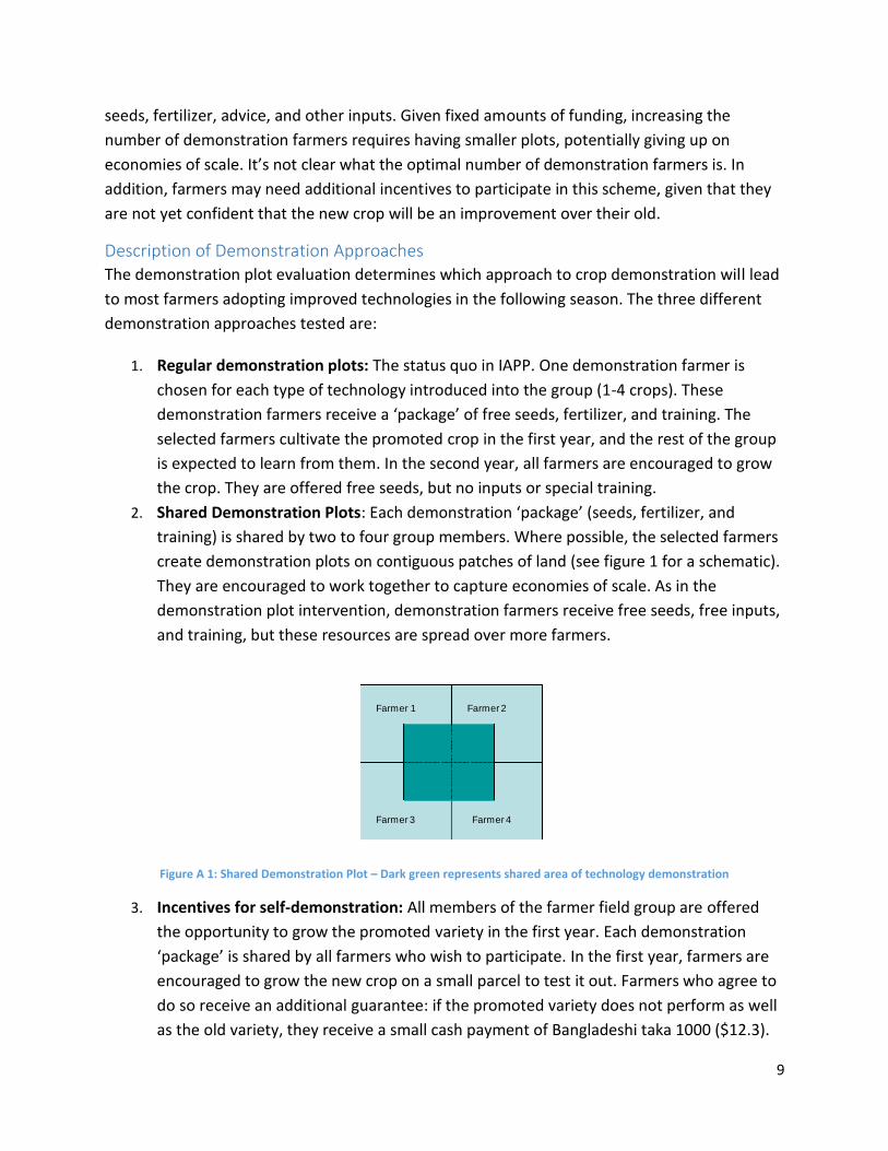
2. Shared Demonstration Plots: Each demonstration ‘package’ (seeds, fertilizer, and

training) is shared by two to four group members. Where possible, the selected farmers

create demonstration plots on contiguous patches of land (see figure 1 for a schematic).

They are encouraged to work together to capture economies of scale. As in the

demonstration plot intervention, demonstration farmers receive free seeds, free inputs,

and training, but these resources are spread over more farmers.

Figure A 1: Shared Demonstration Plot – Dark green represents shared area of technology demonstration

3. Incentives for self-demonstration: All members of the farmer field group are offered

the opportunity to grow the promoted variety in the first year. Each demonstration

‘package’ is shared by all farmers who wish to participate. In the first year, farmers are

encouraged to grow the new crop on a small parcel to test it out. Farmers who agree to

do so receive an additional guarantee: if the promoted variety does not perform as well

as the old variety, they receive a small cash payment of Bangladeshi taka 1000 ($12.3).

Farmer 1

Farmer 4Farmer 3

Farmer 2

10

The primary purpose of this payment is to signal to the farmers that the extension

providers are confident that the new seed will outperform the old. To see whether the

payment should be given out, the research team identified reference farms in each

village at the beginning of the season that grew traditional varieties of the promoted

crop. If output on the reference farm is higher than output of the promoted variety, the

farmer receives his small payment.13 These payments were made by DIME’s research

partner, the NGO Innovations for Poverty Action (IPA) using their core research funding.

Evaluation Design The demonstration plot evaluation is a randomized control trial concentrated in two districts,

Rangpur and Barisal. Within these districts, 220 villages took part in the evaluation. The

demonstration plot evaluation in Rangpur was conducted only for Paddy. In Barisal, it was

conducted for paddy, wheat, mung, lentil, mustard, and sesame.

The villages were randomly allocated into five treatment arms:

1. Long-term control (20 villages): IAPP activities begin in 2016. Until then, villages receive

standard normal services from the government.

2. Short-term control (36 villages): IAPP activities began in 2014 (all with standard

demonstration approach). Until then, villages received normal extension services from

the government.

3. Regular demonstration plots (54 villages): IAPP project activities started in 2012. All

villages have the standard demonstration approach.

4. Shared demonstration plots (56 villages): IAPP activities began in 2012. All villages have

demonstration plots shared among multiple farmers, as described above.

5. Incentives for self-demonstration (54 villages): IAPP activities began in 2012. Instead of

demonstration plots, all farmer group members were offered incentives to adopt the

new crop variety, as described above.

The short-term and medium-term impact of the various treatment arms on variables of interest

is captured by comparing outcomes for each treatment group with the control groups. Data

was collected before and after the project was rolled out in the short-term control villages in

2014; analysis was provided in the form of preliminary and interim reports. The final round of

data collection was done in 2015, comparing each treatment group to the long-term control

group to assess long-term impacts. This endline report focuses on the final IE analysis. The

midterm analysis includes both short- and long-term controls. The endline analysis includes

13 Measurement was done during the seeding phase, which gives a good prediction of the harvest, and was conducted by IPA under DIME supervision. For data analysis purposes, yields are measured post-harvest using household surveys. Since the surveys are not tied to the payouts, there should be no incentive to misreport. Additionally, farmers have to sign contracts saying they will cultivate the new crop to the best of their abilities, and this is monitored by the FFS. To the extent that it is observable, farmers will not be able to receive a payout if they purposefully try to obtain poor yields on their demo plots.

11

only long-term controls, as the short-term controls began IAPP activities shortly after the

midline was completed.

Data and Sampling The impact evaluation draws on data from four rounds of household surveys, and

administrative data on group membership and demonstration status. The household surveys

contain detailed data on household characteristics, agricultural production, livestock, fisheries,

household socioeconomic status, and nutrition outcomes.

For the analysis in this report, we use a panel dataset constructed from three rounds of

household surveys: baseline (2012), midline round 2 (2014), and endline (2015).14 The sample is

restricted to the 1,732 unique households present in each of the three survey rounds, in Barisal

and Rangpur districts. Details on the complete sampling strategy are included in the appendix.

We use the concept of “shadow” demonstration villages and farmers for much of the analysis.

A control village was considered a shadow demonstration village for a certain crop if local

agricultural officials stated that the village would demonstrate this crop when they began IAPP

activities. Similarly, we designated “shadow” demonstration farmers in each control group;

these were farmer groups most likely to demonstrate when IAPP began in their village.

Table 1 shows the allocation of the sample across treatment arms.

Table 1: Data Sample

Interpreting Charts In the charts that follow, we compare outcomes in our three treatment groups to those in the

control group. While presented as comparisons of means, the graphs are actually based on the

results of regressions. The regression specifications are explained in detail for each regression

in the appendix, but in general they are ANCOVA regressions, including all three treatment

14 A midline round 1 survey was done in 2013, however, the scope and sample were more limited, as it focused specifically on the activities of the assigned demonstration farmers.

Survey Round Total ControlRegular

Treatment

Shared Plot

Treatment

Incentives

Treatment

Households 1732 220 830 349 333

Villages 102 14 46 21 21

Households 1732 220 830 349 333

Villages 102 14 46 21 21

Households 1732 220 830 349 333

Villages 102 14 46 21 21

Baseline

Adoption Year

(midline round 2)

Endline

12

dummies and baseline value of the dependent variable as independent variables. The

regressions also include district fixed effects; standard errors are clustered at the village level.

In the charts, the leftmost column of each cluster is the measured value of the mean of the

outcome variable in the control group. Additional columns represent the treatment effect for

treatment groups, and are constructed by adding the estimated treatment effect to the control

mean. The height of the bar is near the actual mean of the outcome variable for the treatment

group, but will be slightly different due to the controls in the regression.

The bars represent the 95 percent confidence interval of the treatment effect. When control

mean is outside of the error bars, this means that the treatment effect is greater than zero with

at least 95 percent statistical confidence. Confidence of treatment effects is also represented

with stars. One, two, and three stars mean the treatment effect is statistically different from

zero with 90 percent, 95 percent, or 99 percent confidence respectively.

For each chart there is a corresponding regression table in the appendix section. The number

referencing of these tables can be found in the ‘Notes’ section of each chart. Appendix A and B

list the tables for endline and midline round 2 survey years, respectively.15 The discussion of

each chart is supplemented by a comparison of means from endline and adoption survey years

provided in relevant tables in Appendix A and B.

The demonstration plot evaluation was conducted on paddy in Rangpur and Barisal, and for the

other IAPP promoted crops (wheat, mung, lentil, mustard and sesame) in Barisal only. Any chart

analyzing the demonstration plot evaluation for paddy includes both Barisal and Rangpur; and

for other crops only include Barisal.

15 Note that results from the midline survey were shared in the 2015 brief. They are recalculated here for exactly the same sample as used in the endline analysis.

13

Impact Evaluation Findings

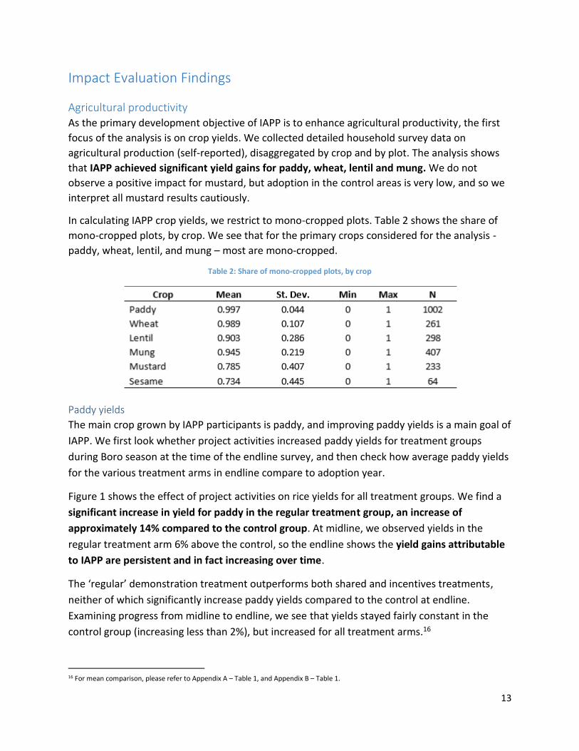
Agricultural productivity As the primary development objective of IAPP is to enhance agricultural productivity, the first

focus of the analysis is on crop yields. We collected detailed household survey data on

agricultural production (self-reported), disaggregated by crop and by plot. The analysis shows

that IAPP achieved significant yield gains for paddy, wheat, lentil and mung. We do not

observe a positive impact for mustard, but adoption in the control areas is very low, and so we

interpret all mustard results cautiously.

In calculating IAPP crop yields, we restrict to mono-cropped plots. Table 2 shows the share of

mono-cropped plots, by crop. We see that for the primary crops considered for the analysis -

paddy, wheat, lentil, and mung – most are mono-cropped.

Table 2: Share of mono-cropped plots, by crop

Paddy yields

The main crop grown by IAPP participants is paddy, and improving paddy yields is a main goal of

IAPP. We first look whether project activities increased paddy yields for treatment groups

during Boro season at the time of the endline survey, and then check how average paddy yields

for the various treatment arms in endline compare to adoption year.

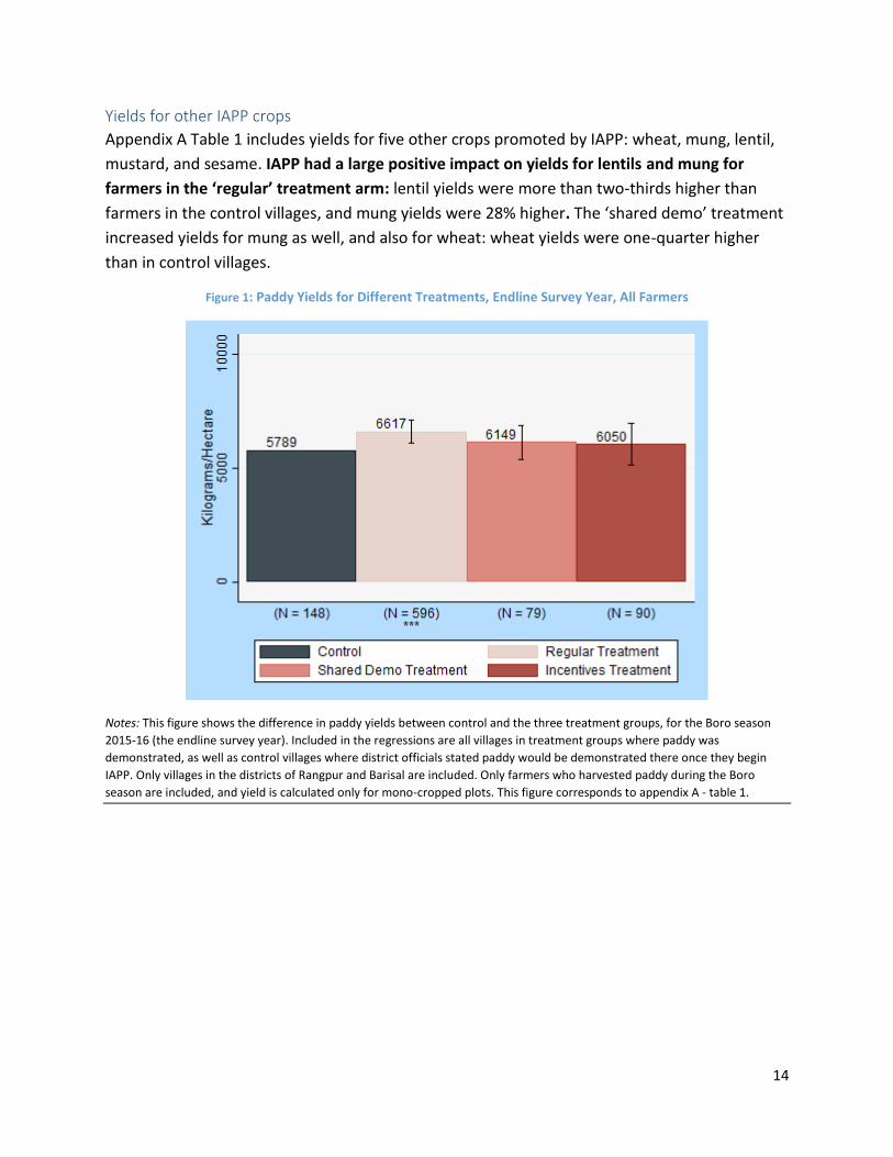
Figure 1 shows the effect of project activities on rice yields for all treatment groups. We find a

significant increase in yield for paddy in the regular treatment group, an increase of

approximately 14% compared to the control group. At midline, we observed yields in the

regular treatment arm 6% above the control, so the endline shows the yield gains attributable

to IAPP are persistent and in fact increasing over time.

The ‘regular’ demonstration treatment outperforms both shared and incentives treatments,

neither of which significantly increase paddy yields compared to the control at endline.

Examining progress from midline to endline, we see that yields stayed fairly constant in the

control group (increasing less than 2%), but increased for all treatment arms.16

16 For mean comparison, please refer to Appendix A – Table 1, and Appendix B – Table 1.

14

Yields for other IAPP crops

Appendix A Table 1 includes yields for five other crops promoted by IAPP: wheat, mung, lentil,

mustard, and sesame. IAPP had a large positive impact on yields for lentils and mung for

farmers in the ‘regular’ treatment arm: lentil yields were more than two-thirds higher than

farmers in the control villages, and mung yields were 28% higher. The ‘shared demo’ treatment

increased yields for mung as well, and also for wheat: wheat yields were one-quarter higher

than in control villages.

Figure 1: Paddy Yields for Different Treatments, Endline Survey Year, All Farmers

Notes: This figure shows the difference in paddy yields between control and the three treatment groups, for the Boro season

2015-16 (the endline survey year). Included in the regressions are all villages in treatment groups where paddy was

demonstrated, as well as control villages where district officials stated paddy would be demonstrated there once they begin

IAPP. Only villages in the districts of Rangpur and Barisal are included. Only farmers who harvested paddy during the Boro

season are included, and yield is calculated only for mono-cropped plots. This figure corresponds to appendix A - table 1.

15

Adoption of Crops and Varieties Promoted by IAPP

We next examine whether participants were more likely to adopt the crops and varieties

promoted by IAPP, focusing on paddy, wheat, mung, lentil, mustard, and sesame. Overall, we

find that IAPP caused statistically significant increases in the adoption of promoted varieties of

paddy, and cultivation of mung and mustard.

Paddy

In Figure 2 we focus on regular treatment groups, and explore adoption of IAPP-promoted

varieties over time. The outcome variables are a yes/no indicator for whether farmers adopt

any paddy variety promoted by IAPP, and a yes/no indicator for whether farmers adopt the

specific variety demonstrated in their village. 17 In all cases, we consider farmers to have

adopted a variety if they use any of that variety on any of their plots.18 At baseline, 68% of

farmers in control villages cultivated IAPP-promoted varieties, and adoption was not

significantly higher in any of the treatment villages. At the end of the adoption year, we

observed that IAPP had a significant, positive impact on adoption of the promoted paddy

varieties in the regular treatment group compared to control group; farmers who were

provided with seeds (“adoption farmers”) were 19 p.p. more likely to adopt. The endline data

shows the adoption gap was fully sustained in subsequent years, when farmers were

responsible for procuring their own inputs.

We observe significantly higher use of IAPP varieties at endline by both adoption farmers

(farmers that received seeds in year 2 of the project) and other farmers in the regular

treatment group (approximately 19 p.p. and 16 p.p. more than control group, respectively).

Overall, this provides evidence that IAPP’s approach effectively spurred adoption of paddy

varieties, those effects spilled over to other farmers over time, and adoption gains persisted

through endline.

17 While farmers were encouraged to demonstrate the exact IAPP variety demonstrated in their village, in practice this variety was sometimes not available or was no longer recommended by IAPP. 18 Differences in the variety promoted from that demonstrated are detailed in the “IAPP Adoption Distribution Monitoring Report 2014”, prepared by DIME.

16

Figure 2: Paddy Adoption (of any IAPP Variety) Over Time, Regular Demonstration Treatment, Endline Survey

Notes: This figure shows adoption of IAPP-promoted varieties of paddy at baseline, during the adoption year (midline), and

during the endline survey year. Results are for Boro season in each period. Households are considered to adopt an IAPP variety

if they cultivate any IAPP variety. We include all farmers that grew any paddy, who are either in paddy demonstration villages

or in shadow paddy demonstration villages. Adoption farmers are farmers that received inputs from the project during the

adoption year. Adoption farmers and other farmers are compared against the same controls. This figure corresponds to

appendix A - table 2. *,**,*** signify that the estimate of the treatment effect (compared to control) is greater than zero at a

confidence level of 90 percent, 95 percent, or 99 percent respectively.

In Figure 3, we consider adoption of paddy in the three treatment groups at the endline. First,

we explore whether farmers are more likely to grow paddy at all. For a commonly-grown crop

like paddy, we do not expect to see much effect for this measure, but we include it for

comparison as this is the primary indicator for the other, less commonly grown, crops. Second,

we analyze whether farmers adopt any variety of paddy promoted by IAPP. Finally, we look at

whether farmers adopt the exact variety of paddy that was demonstrated in their villages. Note

that all variety measures are self-reported, and therefore will contain error, so we interpret the

variety-specific results with caution.

Two-thirds of farmers already cultivated paddy at baseline, and, as expected, we do not find

that IAPP had a significant impact on the likelihood of cultivating paddy. However, when we

look at cultivation of the specific varieties promoted by IAPP, we see that all farmers

67.7% 73.5%

050

100

Perc

en

t

(N = 152) (N = 610)

Baseline(All Farmers)

69.9%

88.5%

(N = 153) (N = 211)**

Adoption Year(Adoption Farmers)

69.9%84%

(N = 153) (N = 362)**

Adoption Year(Other Farmers)

66.6%

86.0%

050

100

Perc

en

t

(N = 144) (N = 217)**

Endline Year(Adoption Farmers)

66.6%82.2%

(N = 144) (N = 350)**

Endline Year(Other Farmers)

Control Regular Treatment

17

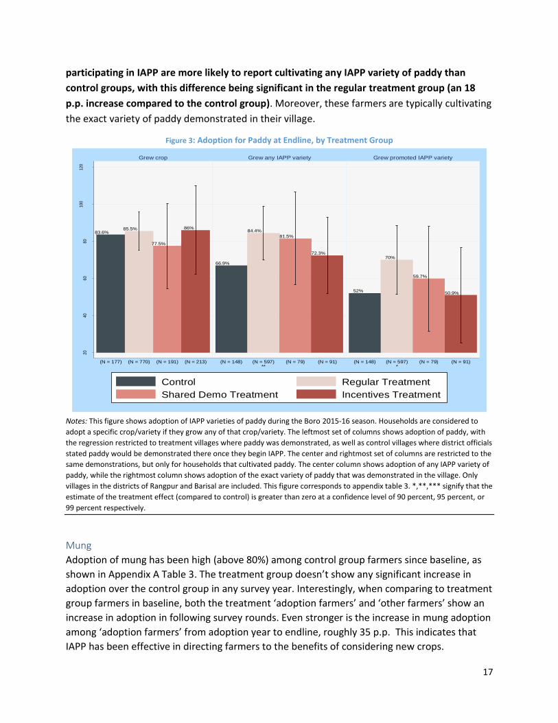
participating in IAPP are more likely to report cultivating any IAPP variety of paddy than

control groups, with this difference being significant in the regular treatment group (an 18

p.p. increase compared to the control group). Moreover, these farmers are typically cultivating

the exact variety of paddy demonstrated in their village.

Figure 3: Adoption for Paddy at Endline, by Treatment Group

Notes: This figure shows adoption of IAPP varieties of paddy during the Boro 2015-16 season. Households are considered to

adopt a specific crop/variety if they grow any of that crop/variety. The leftmost set of columns shows adoption of paddy, with

the regression restricted to treatment villages where paddy was demonstrated, as well as control villages where district officials

stated paddy would be demonstrated there once they begin IAPP. The center and rightmost set of columns are restricted to the

same demonstrations, but only for households that cultivated paddy. The center column shows adoption of any IAPP variety of

paddy, while the rightmost column shows adoption of the exact variety of paddy that was demonstrated in the village. Only

villages in the districts of Rangpur and Barisal are included. This figure corresponds to appendix table 3. *,**,*** signify that the

estimate of the treatment effect (compared to control) is greater than zero at a confidence level of 90 percent, 95 percent, or

99 percent respectively.

Mung

Adoption of mung has been high (above 80%) among control group farmers since baseline, as

shown in Appendix A Table 3. The treatment group doesn’t show any significant increase in

adoption over the control group in any survey year. Interestingly, when comparing to treatment

group farmers in baseline, both the treatment ‘adoption farmers’ and ‘other farmers’ show an

increase in adoption in following survey rounds. Even stronger is the increase in mung adoption

among ‘adoption farmers’ from adoption year to endline, roughly 35 p.p. This indicates that

IAPP has been effective in directing farmers to the benefits of considering new crops.

83.6%85.5%

77.5%

86%

20

40

60

80

100

120

Pe

rce

nt

(N = 177) (N = 770)

(N = 191)

(N = 213)

Grew crop

66.9%

84.4%

81.5%

72.3%

(N = 148) (N = 597) **

(N = 79)

(N = 91)

Grew any IAPP variety

52%

70%

59.7%

50.9%

(N = 148) (N = 597) *

(N = 79)

(N = 91)

Grew promoted IAPP variety

Control Regular Treatment

Shared Demo Treatment Incentives Treatment

18

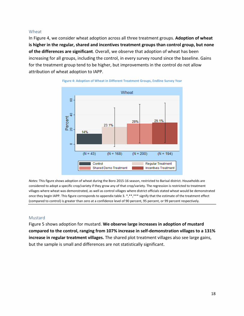
Wheat

In Figure 4, we consider wheat adoption across all three treatment groups. Adoption of wheat

is higher in the regular, shared and incentives treatment groups than control group, but none

of the differences are significant. Overall, we observe that adoption of wheat has been

increasing for all groups, including the control, in every survey round since the baseline. Gains

for the treatment group tend to be higher, but improvements in the control do not allow

attribution of wheat adoption to IAPP.

Figure 4: Adoption of Wheat in Different Treatment Groups, Endline Survey Year

Notes: This figure shows adoption of wheat during the Boro 2015-16 season, restricted to Barisal district. Households are

considered to adopt a specific crop/variety if they grow any of that crop/variety. The regression is restricted to treatment

villages where wheat was demonstrated, as well as control villages where district officials stated wheat would be demonstrated

once they begin IAPP. This figure corresponds to appendix table 3. *,**,*** signify that the estimate of the treatment effect

(compared to control) is greater than zero at a confidence level of 90 percent, 95 percent, or 99 percent respectively.

Mustard

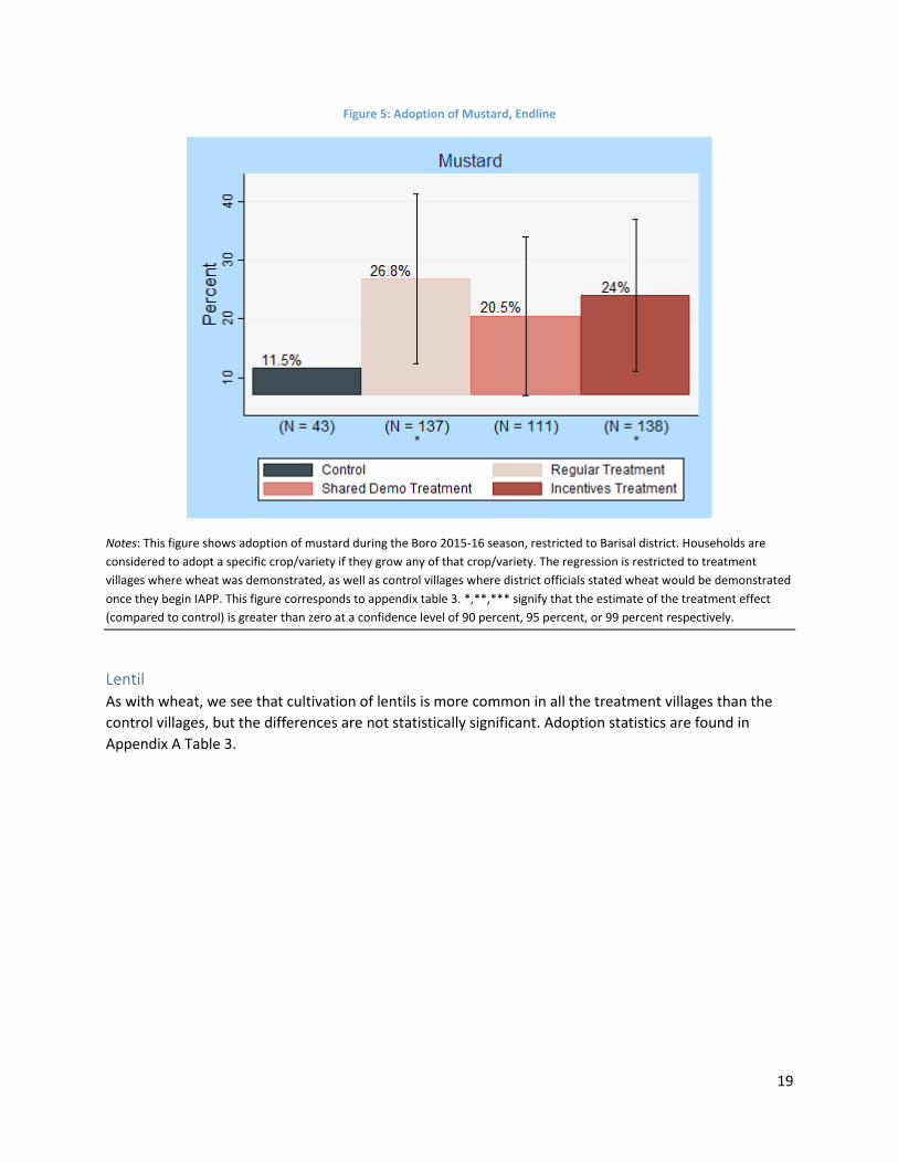
Figure 5 shows adoption for mustard. We observe large increases in adoption of mustard

compared to the control, ranging from 107% increase in self-demonstration villages to a 131%

increase in regular treatment villages. The shared plot treatment villages also see large gains,

but the sample is small and differences are not statistically significant.

19

Figure 5: Adoption of Mustard, Endline

Notes: This figure shows adoption of mustard during the Boro 2015-16 season, restricted to Barisal district. Households are

considered to adopt a specific crop/variety if they grow any of that crop/variety. The regression is restricted to treatment

villages where wheat was demonstrated, as well as control villages where district officials stated wheat would be demonstrated

once they begin IAPP. This figure corresponds to appendix table 3. *,**,*** signify that the estimate of the treatment effect

(compared to control) is greater than zero at a confidence level of 90 percent, 95 percent, or 99 percent respectively.

Lentil As with wheat, we see that cultivation of lentils is more common in all the treatment villages than the

control villages, but the differences are not statistically significant. Adoption statistics are found in

Appendix A Table 3.

20

Use of Improved Inputs and Technologies

To better understand the drivers of the agricultural productivity gains, in this section we

explore use of inputs and improved technologies. First, we look at correlations between input

use and crop yields to get a basic idea of whether increases in any input from the average

farmer are likely to impact yield.19 The details of this analysis are in Appendix A Table 8. We

separate the analysis by crop, and see that different combinations of inputs correlate with

higher yields for the various IAPP crops.

For paddy, use of urea and new seeds is correlated with higher yields, while other soil additives

had insignificant or even negative correlations. Utilizing paid labor and irrigation also correlates

with higher paddy yields. For wheat, only use of TSP is correlated with higher yields. For lentil,

usage of TSP and DAP is correlated with higher yields, as are utilizing labor and irrigation. For

mung, use of MOP and manure are associated with higher yields, as are paid labor and

irrigation. For mustard, use of vitamins and irrigation correlate with higher yields. We interpret

these correlations cautiously; it is possible some inputs are negatively correlated with yields

because they are applied on less fertile plots, but we do not have a way to control for soil

quality. We do not observe significant positive correlations between use of the technologies

introduced by IAPP (line planting, vermicomposting, and double transplantation) and yield

gains.

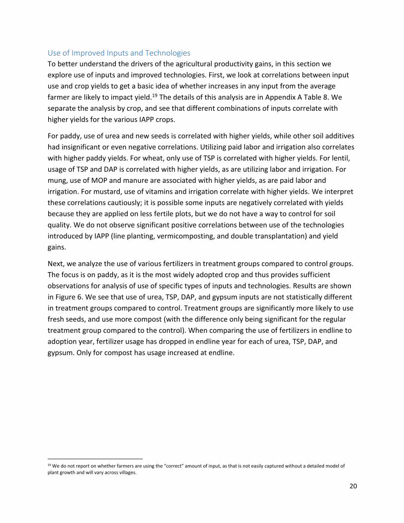
Next, we analyze the use of various fertilizers in treatment groups compared to control groups.

The focus is on paddy, as it is the most widely adopted crop and thus provides sufficient

observations for analysis of use of specific types of inputs and technologies. Results are shown

in Figure 6. We see that use of urea, TSP, DAP, and gypsum inputs are not statistically different

in treatment groups compared to control. Treatment groups are significantly more likely to use

fresh seeds, and use more compost (with the difference only being significant for the regular

treatment group compared to the control). When comparing the use of fertilizers in endline to

adoption year, fertilizer usage has dropped in endline year for each of urea, TSP, DAP, and

gypsum. Only for compost has usage increased at endline.

19 We do not report on whether farmers are using the “correct” amount of input, as that is not easily captured without a detailed model of plant growth and will vary across villages.

21

Figure 6: Fertilizer Use for Paddy, Endline Survey Year

Notes: This figure details input use for plots that cultivated paddy during the Boro 2015-16 season. The sample is all households

that cultivate paddy and are located in paddy demonstration villages (or shadow demonstration villages). Although, only

villages in the districts of Rangpur and Barisal are included. The unit is the amount of input use (in kg) per hectare. Households

that cultivate paddy but did not report use of an input are included in the analysis, with their use of the input set to zero.

Households that only reported use of input in a unit not convertible to kg are not included in the regression. This figure

corresponds to appendix table 4. *,**,*** signify that the estimate of the treatment effect (compared to control) is greater

than zero at a confidence level of 90 percent, 95 percent, or 99 percent respectively.

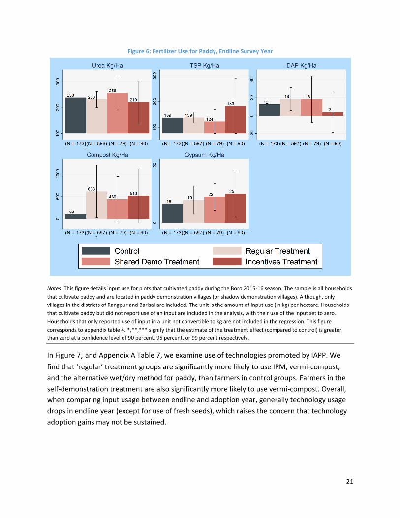
In Figure 7, and Appendix A Table 7, we examine use of technologies promoted by IAPP. We

find that ‘regular’ treatment groups are significantly more likely to use IPM, vermi-compost,

and the alternative wet/dry method for paddy, than farmers in control groups. Farmers in the

self-demonstration treatment are also significantly more likely to use vermi-compost. Overall,

when comparing input usage between endline and adoption year, generally technology usage

drops in endline year (except for use of fresh seeds), which raises the concern that technology

adoption gains may not be sustained.

22

Figure 7: Technology use for Paddy, Endline Survey Year

Notes: This figure details technology use for plots mono-cropped with paddy during the Boro 2015-16 season. The sample is all

households that cultivate paddy plots and are located in paddy demonstration villages (or shadow demonstration villages).

Although, only villages in the districts of Rangpur and Barisal are included. The plot share variables are measured as the

percentage of area cultivating paddy that uses IAPP/fresh seeds. The remaining variables are dummy variables that take the

value of 1 if the household used the technology. This figure corresponds to appendix table 4. *,**,*** signify that the estimate

of the treatment effect (compared to control) is greater than zero at a confidence level of 90 percent, 95 percent, or 99 percent

respectively.

23

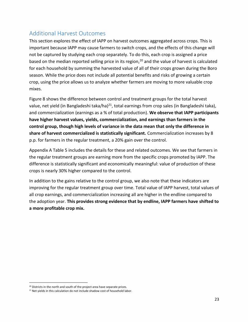
Additional Harvest Outcomes This section explores the effect of IAPP on harvest outcomes aggregated across crops. This is

important because IAPP may cause farmers to switch crops, and the effects of this change will

not be captured by studying each crop separately. To do this, each crop is assigned a price

based on the median reported selling price in its region,20 and the value of harvest is calculated

for each household by summing the harvested value of all of their crops grown during the Boro

season. While the price does not include all potential benefits and risks of growing a certain

crop, using the price allows us to analyze whether farmers are moving to more valuable crop

mixes.

Figure 8 shows the difference between control and treatment groups for the total harvest

value, net yield (in Bangladeshi taka/ha)21, total earnings from crop sales (in Bangladeshi taka),

and commercialization (earnings as a % of total production). We observe that IAPP participants

have higher harvest values, yields, commercialization, and earnings than farmers in the

control group, though high levels of variance in the data mean that only the difference in

share of harvest commercialized is statistically significant. Commercialization increases by 8

p.p. for farmers in the regular treatment, a 20% gain over the control.

Appendix A Table 5 includes the details for these and related outcomes. We see that farmers in

the regular treatment groups are earning more from the specific crops promoted by IAPP. The

difference is statistically significant and economically meaningful: value of production of these

crops is nearly 30% higher compared to the control.

In addition to the gains relative to the control group, we also note that these indicators are

improving for the regular treatment group over time. Total value of IAPP harvest, total values of

all crop earnings, and commercialization increasing all are higher in the endline compared to

the adoption year. This provides strong evidence that by endline, IAPP farmers have shifted to

a more profitable crop mix.

20 Districts in the north and south of the project area have separate prices. 21 Net yields in this calculation do not include shadow cost of household labor.

24

Figure 8: Outcomes for All Crops, Endline Survey Year

Notes: This figure shows changes in yields, harvest value, and total earnings. Total harvest value (in Bangladeshi taka; 1 Taka is

equal to about .013 USD at the time of writing the report) is calculated by multiplying the harvest amount of each crop by the

median price in the region for that crop. Net yield (in Bangladeshi taka/ha) is the total harvest value minus input costs

(including labor) per hectare. Commercialization is calculated as the total earnings divided by the total production and is a

measure on how much a household produces for its own production and for economic return. Total earnings (in Bangladeshi

taka) is the amount made from selling crops. This figure corresponds to appendix table 5. *,**,*** signify that the estimate of

the treatment effect (compared to control) is greater than zero at a confidence level of 90 percent, 95 percent, or 99 percent

respectively.

Crop Mix

As seen in the previous section, total harvest value, earnings, and commercialization increase in

the treatment groups, and this is likely due to changing the crop mix. First, we look at whether

crop diversification increases, which can have positive effects on soil health and resilience

(neither of which we measure directly as part of this study). We find that the average number

of crops grown at endline is significantly higher for both the regular and self-demonstration

treatments (see Appendix A Table 7). As shown in Figure 9, however, farmers are not changing

the share of land dedicated to their primary crops, implying that they are trialing new crops on

smaller areas of land.

25

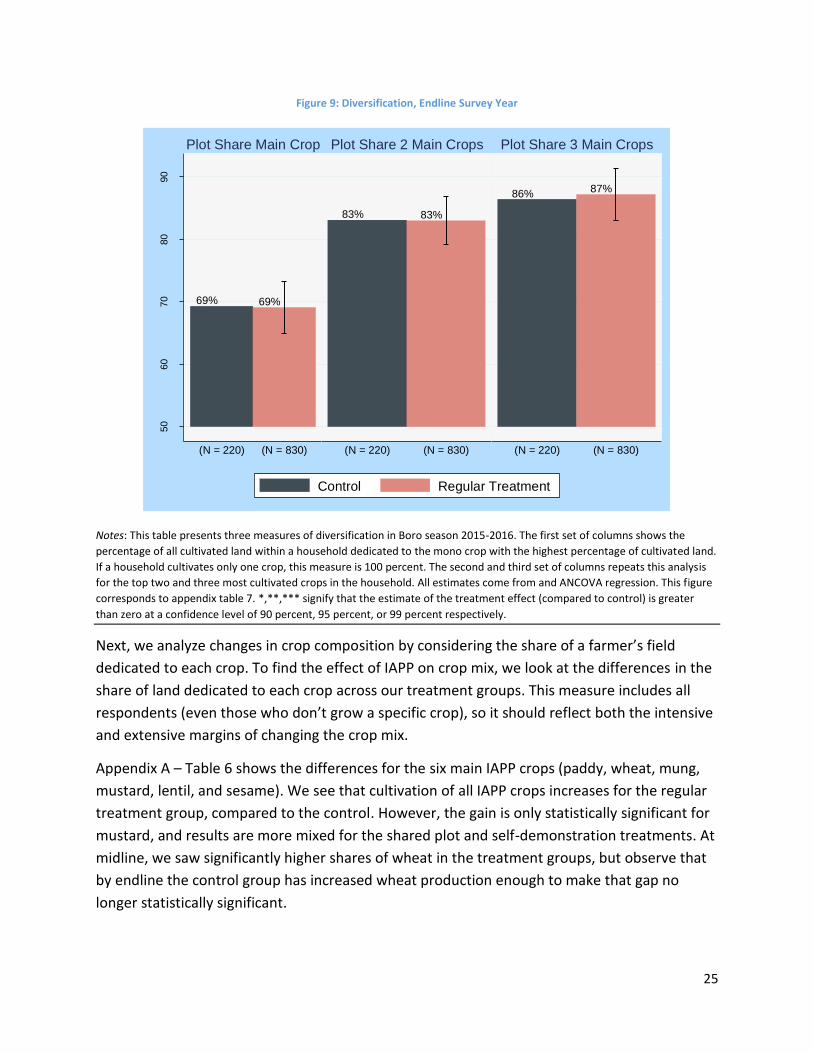
Figure 9: Diversification, Endline Survey Year

Notes: This table presents three measures of diversification in Boro season 2015-2016. The first set of columns shows the

percentage of all cultivated land within a household dedicated to the mono crop with the highest percentage of cultivated land.

If a household cultivates only one crop, this measure is 100 percent. The second and third set of columns repeats this analysis

for the top two and three most cultivated crops in the household. All estimates come from and ANCOVA regression. This figure

corresponds to appendix table 7. *,**,*** signify that the estimate of the treatment effect (compared to control) is greater

than zero at a confidence level of 90 percent, 95 percent, or 99 percent respectively.

Next, we analyze changes in crop composition by considering the share of a farmer’s field

dedicated to each crop. To find the effect of IAPP on crop mix, we look at the differences in the

share of land dedicated to each crop across our treatment groups. This measure includes all

respondents (even those who don’t grow a specific crop), so it should reflect both the intensive

and extensive margins of changing the crop mix.

Appendix A – Table 6 shows the differences for the six main IAPP crops (paddy, wheat, mung,

mustard, lentil, and sesame). We see that cultivation of all IAPP crops increases for the regular

treatment group, compared to the control. However, the gain is only statistically significant for

mustard, and results are more mixed for the shared plot and self-demonstration treatments. At

midline, we saw significantly higher shares of wheat in the treatment groups, but observe that

by endline the control group has increased wheat production enough to make that gap no

longer statistically significant.

69% 69%

50

60

70

80

90

Perc

en

t

(N = 220) (N = 830)

Plot Share Main Crop

83% 83%

(N = 220) (N = 830)

Plot Share 2 Main Crops

86% 87%

(N = 220) (N = 830)

Plot Share 3 Main Crops

Control Regular Treatment

26

The analysis implies that farmers in endline are shifting to mustard, compared to other IAPP

crops. When looking at the median prices, mustard is priced around 18 -20 BG Taka/kg higher

than wheat, and farmers spend more paid and unpaid labor days on wheat than mustard in

adoption year, so the shift towards mustard contributes to the increase in profitability observed

in the previous section.22

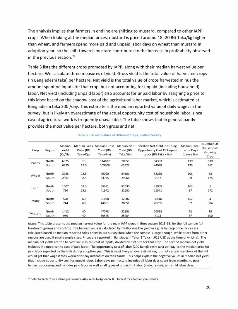
Table 3 lists the different crops promoted by IAPP, along with their median harvest value per

hectare. We calculate three measures of yield. Gross yield is the total value of harvested crops

(in Bangladeshi taka) per hectare. Net yield is the total value of crops harvested minus the

amount spent on inputs for that crop, but not accounting for unpaid (including household)

labor. Net yield (including unpaid labor) also accounts for unpaid labor by assigning a price to

this labor based on the shadow cost of the agricultural labor market, which is estimated at

Bangladeshi taka 200 /day. This estimate is the median reported value of daily wages in the

survey, but is likely an overestimate of the actual opportunity cost of household labor, since

casual agricultural work is frequently unavailable. The table shows that in general paddy

provides the most value per hectare, both gross and net.

Table 3: Harvest Values of Different Crops, Endline Survey

Notes: This table presents the median harvest value for the main IAPP crops in Boro season 2015-16, for the full sample (all

treatment groups and control). The harvest value is calculated by multiplying the yield in Kg/Ha by crop price. Prices are

calculated based on median reported sales prices in our survey data when the sample is large enough, while prices from other

regions are used if small sample sizes. Prices are reported in Bangladeshi Taka (1 Taka = .013 USD at the time of writing). The

median net yields are the harvest value minus cost of inputs, divided by plot size for that crop. The second median net yield

includes the opportunity cost of paid labor. The opportunity cost of labor (200 Bangladeshi taka per day) is the median price for

paid labor reported by the HHs during adoption year. This is most likely an overestimation; it is not certain members of the HH

would get that wage if they worked for pay instead of on their farms. This helps explain the negative values in median net yield

that include opportunity cost for unpaid labor. Labor days per hectare includes all labor days spent from planting to post-

harvest processing and includes paid labor as well as all types of unpaid HH labor (male, female, and child labor days).

22 Refer to Table 2 for endline year results. Also, refer to Appendix B – Table 8 for adoption year results.

Crop Region

Median

Yield

(Kg/Ha)

Median Sales

Price (BG

Taka/Kg)

Median Gross

Yield (BG

Taka/Ha)

Median Net

Yield (BG

Taka/Ha)

Median Net Yield Including

Opportunity Cost Of Unpaid

Labor (BG Taka / Ha)

Median Total

Labor Days

(days / Ha)

Number Of

Households

Growing

Crop

North 6525 15 114187 70555 54383 139 639

South 6920 17.5 103806 62523 44948 135 362

North 3955 22.5 79090 54101 38265 103 83

South 2397 20 53925 29066 9157 99 175

North 1607 53.3 85681 82530 49905 163 1

South 786 53.3 41942 32680 15571 87 272

North 528 60 31698 12082 -19882 157 4

South 744 60 44661 38051 20285 87 384

North 1412 40 47078 32551 20563 72 85

South 989 40 39545 25704 4123 87 100

Paddy

Wheat

Lentil

Mung

Mustard

27

Appendix A

Sampling The Baseline Household Survey was implemented in all eight project districts: Rangpur,

Kurigram, Nilfamari, and Lalmonirhat districts in the North and Barisal, Patuakhali, Barguna, and

Jhalokathi districts in the South.

Two districts (Rangpur and Barisal) are included in the demonstration plots evaluation. 110

villages were sampled in each district. The baseline survey was conducted concurrently with the

IAPP group formation (for the DPE districts, the baseline occurred just before group formation).

Of the total IAPP group members, 15 were randomly selected for the baseline survey.23 The

sample is representative of farmers who were eligible for participation in IAPP and were part of

the initial IAPP group formation.

Specification Details

The regression specification used for all results is an ANCOVA specification, described by the

following equation:

𝑂𝑢𝑡𝑐𝑜𝑚𝑒𝑖,𝑡 = 𝛼 + 𝛽1𝑇𝑟𝑒𝑎𝑡𝑖 + 𝛽2𝑂𝑢𝑡𝑐𝑜𝑚𝑒𝑖,𝑡−1 + 𝛽3𝐶𝑜𝑛𝑡𝑟𝑜𝑙𝑠 + 𝜀𝑖,𝑡

The control variables consist of dummies signifying whether baseline data was unavailable and

a set of district dummies. If the observation did not have a valid measure of outcome variable

at time t-1, the lagged outcome is set to zero (and its effect on the outcome is absorbed by a

dummy). The error term is assumed to be correlated across villages but otherwise iid, so the

specifications cluster standard errors at the village level.

23A miscommunication led to sampling the wrong farmer group (a group that had previously existed, not the new group formed by IAPP) in eight treatment villages and 12 control DPE villages. These villages were dropped for the purpose of the baseline analysis. However, the sample was redrawn during follow-up surveys.

28

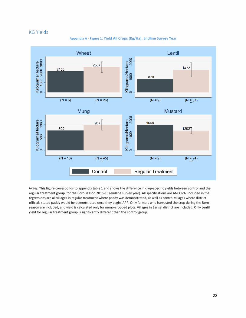
KG Yields Appendix A - Figure 1: Yield All Crops (Kg/Ha), Endline Survey Year

Notes: This figure corresponds to appendix table 1 and shows the difference in crop-specific yields between control and the

regular treatment group, for the Boro season 2015-16 (endline survey year). All specifications are ANCOVA. Included in the

regressions are all villages in regular treatment where paddy was demonstrated, as well as control villages where district

officials stated paddy would be demonstrated once they begin IAPP. Only farmers who harvested the crop during the Boro

season are included, and yield is calculated only for mono-cropped plots. Villages in Barisal district are included. Only Lentil

yield for regular treatment group is significantly different than the control group.

29

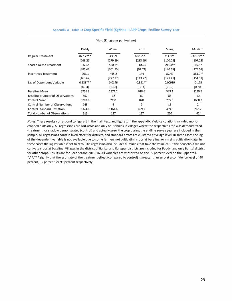
Appendix A - Table 1: Crop Specific Yield (Kg/Ha) – IAPP Crops, Endline Survey Year

Notes: These results correspond to figure 1 in the main text, and figure 1 in the appendix. Yield calculations included mono-

cropped plots only. All regressions are ANCOVAs and only households in villages where the respective crop was demonstrated

(treatment) or shadow demonstrated (control) and actually grew the crop during the endline survey year are included in the

sample. All regressions contain fixed effect for districts, and standard errors are clustered at village level. In some cases the lag

of the dependent variable is not available due to some farmers not cultivating crops at baseline, or missing cultivation data. In

these cases the lag variable is set to zero. The regression also includes dummies that take the value of 1 if the household did not

cultivate crops at baseline. Villages in the district of Barisal and Rangpur districts are included for Paddy, and only Barisal district

for other crops. Results are for Boro season 2015-16. All variables are winsorized on the 99 percent level on the upper tail.

*,**,*** signify that the estimate of the treatment effect (compared to control) is greater than zero at a confidence level of 90

percent, 95 percent, or 99 percent respectively.

Regular Treatment 827.2*** 436.9 602.5** 211.9** -375.8***

[268.21] [279.29] [233.99] [100.08] [107.23]

Shared Demo Treatment 360.2 560.2* -109.3 295.4** -66.87

[385.67] [301.35] [92.72] [140.65] [279.57]

Incentives Treatment 261.1 465.2 144 87.49 -363.0**

[463.62] [277.27] [113.77] [121.41] [154.11]

Lag of Dependent Variable 0.133*** 0.0146 0.321** 0.00939 -0.175

[0.04] [0.18] [0.14] [0.10] [0.20]

Baseline Mean 5756.8 2374.2 618.6 543.1 1239.5

Baseline Number of Observations 852 12 60 86 10

Control Mean 5789.8 2151 870 755.6 1668.3

Control Number of Observations 148 6 9 16 2

Control Standard Deviation 1324.6 1164.4 429.7 409.3 262.2

Total Number of Observations 913 127 127 220 62

Mustard

Yield (Kilograms per Hectare)

Paddy Wheat Lentil Mung

30

Adoption

Appendix A - Table 2: Adoption of Paddy and Mung

Notes: These results correspond to figures 2 and 4 in the main text. The baseline regression is an OLS regression and the other

regressions are ANCOVAs. Only households in villages where paddy or mung respectively were demonstrated (treatment) or

shadow demonstrated (control) and grew paddy during the respective year are included in the sample. Demonstration farmers

in control villages are “shadow” demonstration farmers that community facilitators claimed would have demonstrated the crop

had the demonstration taken place in this group, and who were also part of the baseline survey. Adoption farmers are farmers

that received inputs from the project during the adoption year. Adoption farmers and other farmers are compared against the

same controls. Results are for Boro season, 2015-16. Villages in districts of Rangpur and Barisal are included for paddy, and only

villages of Barisal are included for mung. All regressions contain fixed effect for districts and standard errors are clustered at

village level. All ANCOVA regressions have dummies identifying households not surveyed at baseline and those that did not

cultivate paddy at baseline. *,**,*** signify that the estimate of the treatment effect (compared to control) is greater than zero

at a confidence level of 90 percent, 95 percent, or 99 percent respectively.

Baseline

Regular Treatment 0.057 0.186** 0.141** 0.194** 0.155**

[0.09] [0.07] [0.06] [0.08] [0.07]

Lag of Dependent Variable 0.170*** 0.169*** 0.186*** 0.150***

[0.04] [0.03] [0.07] [0.03]

Control Mean 0.678 0.699 0.699 0.667 0.667

Control Number of Observations 152 153 153 144 144

Control Standard Deviation 0.469 0.46 0.46 0.473 0.473

Total Number of Observations 762 364 515 361 494

Baseline

Regular Treatment -1.216*** -0.0973 -0.324* 0.353 -0.569*

[0.29] [0.30] [0.14] [0.34] [0.25]

Lag of Dependent Variable 0.125 0.496*** 0.179 0.277

[0.28] [0.12] [0.31] [0.15]

Control Mean 0.947 0.947 0.947 0.842 0.842

Control Number of Observations 19 19 19 19 19

Control Standard Deviation 0.229 0.229 0.229 0.375 0.375

Total Number of Observations 136 41 107 41 108

Other

Farmers

Adoption Year Endline Survey Year

Adoption of Growing Mung

Adoption Year Endline Survey Year

All

Farmers

Adoption

Farmers

Other

Farmers

Adoption

Farmers

Adoption of IAPP Paddy Varieties

All

Farmers

Adoption

Farmers

Other

Farmers

Adoption

Farmers

Other

Farmers

31

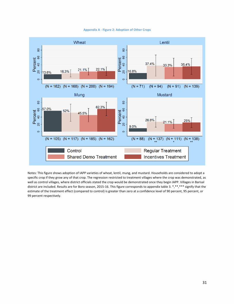
Appendix A - Figure 2: Adoption of Other Crops

Notes: This figure shows adoption of IAPP varieties of wheat, lentil, mung, and mustard. Households are considered to adopt a

specific crop if they grow any of that crop. The regression restricted to treatment villages where the crop was demonstrated, as

well as control villages, where district officials stated the crop would be demonstrated once they begin IAPP. Villages in Barisal

district are included. Results are for Boro season, 2015-16. This figure corresponds to appendix table 3. *,**,*** signify that the

estimate of the treatment effect (compared to control) is greater than zero at a confidence level of 90 percent, 95 percent, or

99 percent respectively.

32

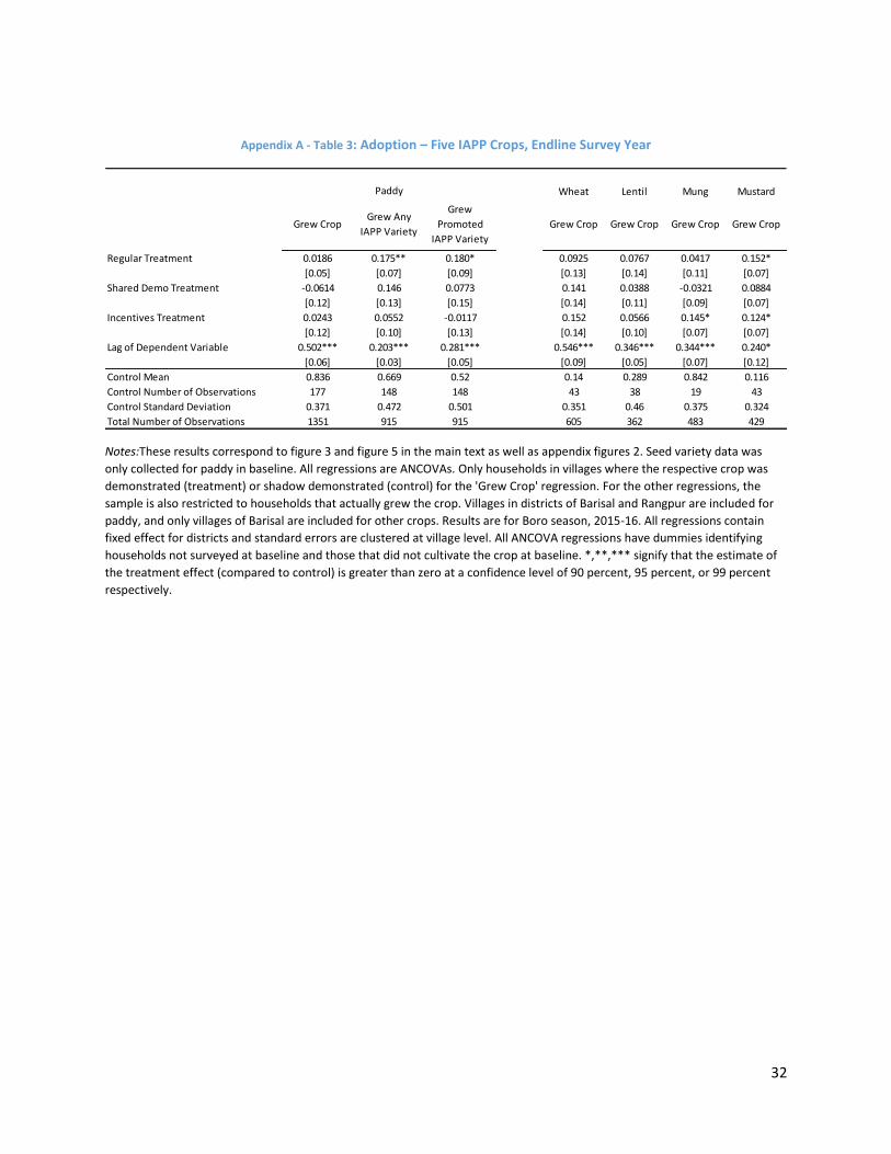
Appendix A - Table 3: Adoption – Five IAPP Crops, Endline Survey Year

Notes:These results correspond to figure 3 and figure 5 in the main text as well as appendix figures 2. Seed variety data was

only collected for paddy in baseline. All regressions are ANCOVAs. Only households in villages where the respective crop was

demonstrated (treatment) or shadow demonstrated (control) for the 'Grew Crop' regression. For the other regressions, the

sample is also restricted to households that actually grew the crop. Villages in districts of Barisal and Rangpur are included for

paddy, and only villages of Barisal are included for other crops. Results are for Boro season, 2015-16. All regressions contain

fixed effect for districts and standard errors are clustered at village level. All ANCOVA regressions have dummies identifying

households not surveyed at baseline and those that did not cultivate the crop at baseline. *,**,*** signify that the estimate of

the treatment effect (compared to control) is greater than zero at a confidence level of 90 percent, 95 percent, or 99 percent

respectively.

Wheat Lentil Mung Mustard

Regular Treatment 0.0186 0.175** 0.180* 0.0925 0.0767 0.0417 0.152*

[0.05] [0.07] [0.09] [0.13] [0.14] [0.11] [0.07]

Shared Demo Treatment -0.0614 0.146 0.0773 0.141 0.0388 -0.0321 0.0884

[0.12] [0.13] [0.15] [0.14] [0.11] [0.09] [0.07]

Incentives Treatment 0.0243 0.0552 -0.0117 0.152 0.0566 0.145* 0.124*

[0.12] [0.10] [0.13] [0.14] [0.10] [0.07] [0.07]

Lag of Dependent Variable 0.502*** 0.203*** 0.281*** 0.546*** 0.346*** 0.344*** 0.240*

[0.06] [0.03] [0.05] [0.09] [0.05] [0.07] [0.12]

Control Mean 0.836 0.669 0.52 0.14 0.289 0.842 0.116

Control Number of Observations 177 148 148 43 38 19 43

Control Standard Deviation 0.371 0.472 0.501 0.351 0.46 0.375 0.324

Total Number of Observations 1351 915 915 605 362 483 429

Grew Crop

Grew

Promoted

IAPP Variety

Grew Crop Grew CropGrew Any

IAPP VarietyGrew Crop Grew Crop

Paddy

33

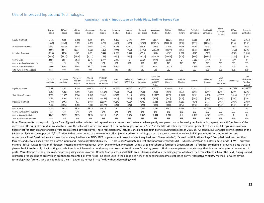
Use of Improved Inputs and Technologies Appendix A - Table 4: Input Usage on Paddy Plots, Endline Survey Year

Note: These results correspond to figure 7 and figure 8 in the main text. All regressions are only on crop instances where paddy was grown. Variables are kg per hectare for regressions with 'per hectare' the

regression title. Variables are dummy variables (take the value of 1 for yes and value of 0 for no) for regression with “used” in the title. All other regression has percent as their unit. All regressions contain

fixed effect for districts and standard errors are clustered at village level. These regression only include Barisal and Rangpur districts during Boro season 2015-16. All continuous variables are winsorized on the

99 percent level on the upper tail. *,**,*** signify that the estimate of the treatment effect (compared to control) is greater than zero at a confidence level of 90 percent, 95 percent, or 99 percent

respectively. Fresh Seed varities are those that are acquired from an NGO, IAPP or government project, and not acquired from "bazar retailer", "a seed multiplication village", "recycled seed from another

farmer", and recycled seed from own farm." Inputs and Technology Definitions: TSP - Triple SuperPhosphate (a great phosphorous fertilizer); MOP - Muriate of Potash or Potassium Chloride ; FYM - Farmyard

manure ; NPKS - Mixed fertilizer of Nitrogen, Potassium and Phosphorous; DAP - Diammonium Phosphate, widely used phosphorous fertilizer ; Green Manure - a fertilizer consisting of growing plants that are

plowed back into the soil ; Line Planting - a technique in which weeds around a crop are taken out to allow crop's healthy growth ; IPM - an ecosystem-based strategy that focuses on long-term prevention of

pests ; VermiCompost - the process of composting using various worms ; Double Transplant - a small field area is transplanted to let seedlings grow which are then transplanted all over the field ; Dapog - a bed

is prepared for seedling to grow which are then transplanted all over fields - no soil is used in the dapog bed hence the seedlings become established early ; Alternative Wet/Dry Method - a water-saving

technology that farmers can apply to reduce their irrigation water use in rice fields without decreasing yield.

Regular Treatment -7.535 0.158 -1.032 3.295 1.063 -0.165 0.102 509.4* 916.7 -1130.6 0.0515 1.013 -13.78 6.267 0.0158

[15.40] [11.40] [7.78] [6.28] [0.69] [0.43] [0.10] [297.20] [2045.25] [1222.00] [0.18] [0.93] [116.01] [6.58] [0.02]

Shared Demo Treatment 17.82 -15.23 12.83 6.074 0.331 -0.472 -0.0142 339.8 1602.3 -784.6 -0.146 -0.105 46.64 5.817 0.013

[33.64] [23.77] [16.34] [5.92] [1.10] [0.44] [0.30] [257.43] [2957.93] [881.44] [0.67] [2.15] [191.06] [13.31] [0.01]

Incentives Treatment -18.66 43.96 -16.5 8.58 0.888 -0.359 0.448 411.6 1898.4 -679.3 0.821 -0.705 -28.32 -8.705 0.0149

[42.39] [54.13] [14.86] [10.21] [1.33] [0.50] [0.32] [304.14] [3546.76] [803.59] [0.79] [2.04] [228.49] [11.51] [0.02]

Control Mean 238.4 139.4 94.32 16.46 1.377 0.846 0 99.19 2949.5 1168.8 0 3.215 356.4 0 12.44 0

Control Number of Observations 173 173 173 173 173 173 173 173 173 173 173 173 173 173 173 173

Control Standard Deviation 128.6 91.48 76.63 37.17 5.469 3.622 0 660 9313.1 12852.2 0 8.812 1079 0 51.54 0

Total Number of Observations 938 939 939 939 939 939 939 939 938 939 939 939 939 939 939 939

Regular Treatment 0.39 1.185 3.195 -0.0673 -337.1 0.0565 0.176* 0.245*** 0.201*** -0.0533 0.205* 0.219*** 0.123* 0.05 0.00289 0.0427***

[0.45] [4.21] [6.47] [4.37] [638.14] [0.05] [0.09] [0.05] [0.05] [0.04] [0.11] [0.07] [0.06] [0.05] [0.00] [0.01]

Shared Demo Treatment 0.193 -3.477 1.956 -0.967 1328.5 0.0411 0.114 0.0802 0.180** 0.0356 -0.0199 0.0301 0.104 0.00696 0.0138 0.0212

[0.60] [6.57] [8.40] [6.86] [801.88] [0.07] [0.16] [0.09] [0.08] [0.07] [0.14] [0.07] [0.06] [0.05] [0.01] [0.01]

Incentives Treatment -0.833 1.062 -0.27 1.873 1537.0* 0.0842 0.0364 0.0482 0.028 -0.0284 0.019 -0.145 0.172* 0.0736 0.0191 0.0239

[1.66] [10.24] [8.35] [7.57] [855.06] [0.14] [0.12] [0.10] [0.08] [0.06] [0.14] [0.10] [0.09] [0.07] [0.02] [0.02]

Control Mean 1.235 7.025 28.24 28.75 4043.3 0.671 0.411 0.402 0.191 0.0925 0.457 0.59 0.00578 0.15 0 0

Control Number of Observations 173 173 173 173 173 173 173 173 173 173 173 173 173 173 173 173

Control Standard Deviation 4.041 25.57 29.25 24.76 3811.2 0.471 0.425 0.462 0.334 0.291 0.5 0.493 0.076 0.358 0 0

Total Number of Observations 939 939 939 939 939 939 939 939 939 939 939 939 939 939 939 939

Ammonia

per Hectare

Used Vermi-

CompostUsed Dapog

Borax per

Hectare

Lime per

Hectare

Compost

per Hectare

Manure per

Hectare

FYM per

Hectare

NPKS per

Hectare

Urea per

Hectare

TSP per

Hectare

MOP per

Hectare

Gypsum per

Hectare

Zinc per

Hectare

Pest Solid

per Hectare

Vitamins

per Hectare

Potassium

per Hectare

Paid Labor

Days per

Hectare

Unpaid

Labor Days

per Hectare

Irrigation

Spending

per Hectare

Used

Alternative

Wet/Dry

Method

Used

Double

Transplant

% Plots with

IAPP Variety

% Plots with

FreshSeed

Interaction

FreshSeed

and IAPP

Variety

Used Green

Manure

Used Line

PlantingUsed IPM

Used

Irrigation

DAP per

Hectare

Pest l iquid

per Hectare

Phere-

mones per

Hectare

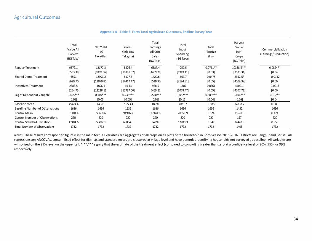
34

Agricultural Outcomes

Appendix A - Table 5: Farm Total Agriculture Outcomes, Endline Survey Year

Notes: These results correspond to figure 8 in the main text. All variables are aggregates of all crops on all plots of the household in Boro Season 2015-2016. Districts are Rangpur and Barisal. All

regressions are ANCOVAs, contain fixed effect for districts and standard errors are clustered at village level and have dummies identifying households not surveyed at baseline. All variables are

winsorized on the 99% level on the upper tail. *,**,*** signify that the estimate of the treatment effect (compared to control) is greater than zero at a confidence level of 90%, 95%, or 99%

respectively.

Total

Value All

Harvest

(BG Taka)

Net Yield

(BG

Taka/Ha)

Gross

Yield (BG

Taka/Ha)

Total

Earnings

All Crop

Sales

(BG Taka)

Total

Input

Spending

(BG Taka)

Total

Plotsize

(Ha)

Harvest

Value

IAPP

Crops

(BG Taka)

Commercialization

(Earnings/Production)

Regular Treatment 9679.1 12177.3 8876.4 6587.4 -257.5 0.0761** 10338.5*** 0.0824**

[6583.38] [9399.86] [10381.57] [4469.29] [1949.11] [0.03] [3523.34] [0.04]

Shared Demo Treatment 6591 12901.2 8127.5 1420.6 -669.7 0.0478 8352.5* -0.0112

[8629.70] [12879.85] [14417.47] [5520.90] [2194.31] [0.05] [4509.39] [0.06]

Incentives Treatment 2888.5 4896.1 44.43 968.5 -1487 0.0561 4400.1 0.0013

[8254.75] [12228.11] [13797.06] [5469.23] [2078.47] [0.05] [4307.72] [0.06]

Lag of Dependent Variable 0.495*** 0.169*** 0.233*** 0.550*** 1.052*** 0.586*** 0.696*** 0.102**

[0.05] [0.05] [0.05] [0.05] [0.11] [0.04] [0.05] [0.04]

Baseline Mean 45424.4 64301 76273.4 18992 7021.7 0.588 32838.2 0.388

Baseline Number of Observations 1636 1636 1636 1636 1636 1636 1432 1636

Control Mean 51404.4 56468.6 94916.7 27144.8 20551.9 0.524 35670.5 0.424

Control Number of Observations 220 220 220 220 220 220 197 220

Control Standard Deviation 47484.6 56492.1 63064.6 34399 17780.3 0.347 32420.3 0.353

Total Number of Observations 1732 1732 1732 1732 1732 1732 1495 1732

35

Crop’s Share of Total Cultivated Area

Appendix A - Table 6: Individual Crop’s Cultivated Areas as a Share of Total Area, Endline Survey Year

Notes: These results correspond to figure 9 in the main text. Plot share is calculated as the mono plot area dedicated to a certain crop, divided by

total cultivated area in Boro season 2015-2016. The value is set to zero if a household did not grow the crop. All regressions are ANCOVAs, contain

fixed effect for districts, standard errors are clustered at village level and have dummies identifying households not surveyed at baseline. *,**,***

signify that the estimate of the treatment effect (compared to control) is greater than zero at a confidence level of 90 percent, 95 percent, or 99

percent respectively.

Appendix A - Table 7: Diversification of Crops, Endline Survey Year

Notes: These results correspond to figure 10 in the main text. Number of crops is the number of types of crops grown by the household, two

instances of the same crop is counted once. The share of the main crop(s) area of total cultivated area includes monocropped crops. All

regressions are ANCOVAs, contain fixed effect for districts, standard errors are clustered at village level and have dummies identifying households

not surveyed at baseline. *,**,*** signify that the estimate of the treatment effect (compared to control) is greater than zero at a confidence level

of 90%, 95%, or 99% respectively.

Boro Wheat Lentil Mung Mustard Sesame

Regular Treatment 0.00248 0.0037 0.00717 0.014 0.0156* 0.000705

[0.03] [0.02] [0.01] [0.01] [0.01] [0.00]

Shared Demo Treatment -0.0258 -0.00612 -0.0108 0.0389 0.014 0.00287

[0.05] [0.02] [0.01] [0.03] [0.01] [0.00]

Incentives Treatment -0.0484 -0.00196 0.00398 0.0211 0.0112 0.00246

[0.04] [0.02] [0.01] [0.02] [0.01] [0.00]

Lag of Dependent Variable 0.476*** 0.623** 0.187*** 0.405*** 0.0788 0.106

[0.04] [0.25] [0.04] [0.04] [0.06] [0.09]

Control Mean 0.547 0.0305 0.011 0.0352 0.0112 0.000274

Control Number of Observations 220 220 220 220 220 220

Control Standard Deviation 0.353 0.117 0.0527 0.141 0.0547 0.00406

Total Number of Observations 1732 1732 1732 1732 1732 1732

Main Crop 2 Main Crops 3 Main Crops 4 Main Crops

Regular Treatment 0.874** -0.00492 -0.00238 0.00665 0.00949

[0.43] [0.02] [0.02] [0.02] [0.02]

Shared Demo Treatment 0.846 -0.00283 -0.00967 -0.00669 0.000378

[0.52] [0.03] [0.02] [0.02] [0.02]

Incentives Treatment 1.341** -0.0159 -0.00283 0.0164 0.0257

[0.59] [0.02] [0.02] [0.02] [0.02]

Lag of Dependent Variable 0.373*** 0.295*** 0.232*** 0.195*** 0.240***

[0.05] [0.03] [0.04] [0.06] [0.09]

Control Mean 5.959 0.693 0.831 0.864 0.875

Control Number of Observations 220 220 220 220 220

Control Standard Deviation 3.495 0.236 0.219 0.213 0.212

Total Number of Observations 1732 1732 1732 1732 1732

Number of Crops

Share Of Total Cultivated Area For:

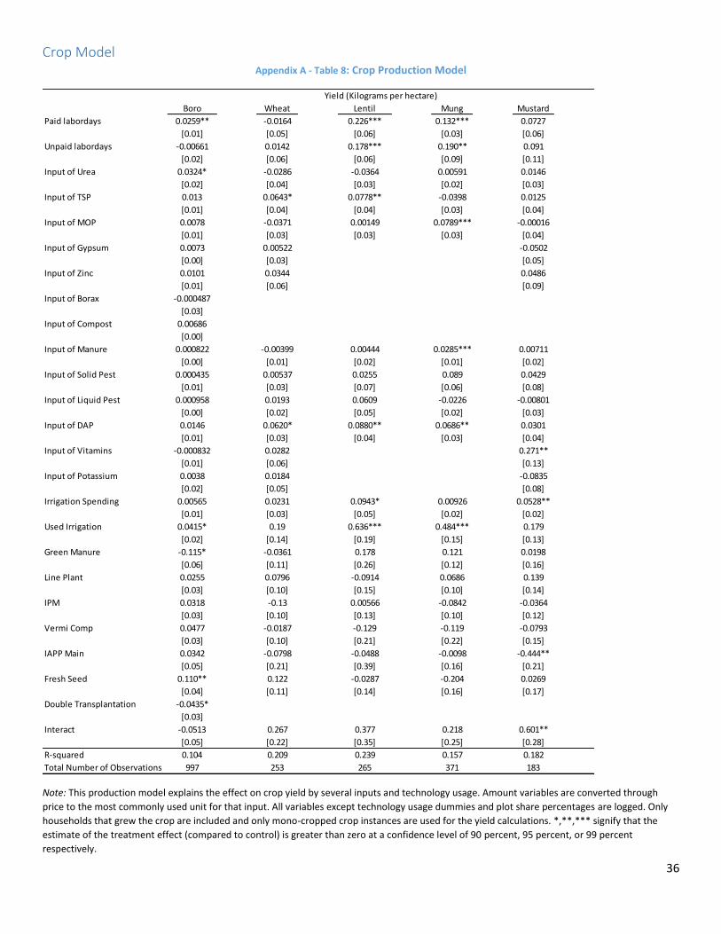
36

Crop Model Appendix A - Table 8: Crop Production Model

Note: This production model explains the effect on crop yield by several inputs and technology usage. Amount variables are converted through

price to the most commonly used unit for that input. All variables except technology usage dummies and plot share percentages are logged. Only

households that grew the crop are included and only mono-cropped crop instances are used for the yield calculations. *,**,*** signify that the

estimate of the treatment effect (compared to control) is greater than zero at a confidence level of 90 percent, 95 percent, or 99 percent

respectively.

Boro Wheat Lentil Mung Mustard

0.0259** -0.0164 0.226*** 0.132*** 0.0727

[0.01] [0.05] [0.06] [0.03] [0.06]

-0.00661 0.0142 0.178*** 0.190** 0.091

[0.02] [0.06] [0.06] [0.09] [0.11]

Input of Urea 0.0324* -0.0286 -0.0364 0.00591 0.0146

[0.02] [0.04] [0.03] [0.02] [0.03]

Input of TSP 0.013 0.0643* 0.0778** -0.0398 0.0125

[0.01] [0.04] [0.04] [0.03] [0.04]

Input of MOP 0.0078 -0.0371 0.00149 0.0789*** -0.00016

[0.01] [0.03] [0.03] [0.03] [0.04]

Input of Gypsum 0.0073 0.00522 -0.0502

[0.00] [0.03] [0.05]

Input of Zinc 0.0101 0.0344 0.0486

[0.01] [0.06] [0.09]

Input of Borax -0.000487

[0.03]

Input of Compost 0.00686

[0.00]

Input of Manure 0.000822 -0.00399 0.00444 0.0285*** 0.00711

[0.00] [0.01] [0.02] [0.01] [0.02]

Input of Solid Pest 0.000435 0.00537 0.0255 0.089 0.0429

[0.01] [0.03] [0.07] [0.06] [0.08]

Input of Liquid Pest 0.000958 0.0193 0.0609 -0.0226 -0.00801

[0.00] [0.02] [0.05] [0.02] [0.03]

Input of DAP 0.0146 0.0620* 0.0880** 0.0686** 0.0301

[0.01] [0.03] [0.04] [0.03] [0.04]

Input of Vitamins -0.000832 0.0282 0.271**

[0.01] [0.06] [0.13]

Input of Potassium 0.0038 0.0184 -0.0835

[0.02] [0.05] [0.08]

Irrigation Spending 0.00565 0.0231 0.0943* 0.00926 0.0528**

[0.01] [0.03] [0.05] [0.02] [0.02]

Used Irrigation 0.0415* 0.19 0.636*** 0.484*** 0.179

[0.02] [0.14] [0.19] [0.15] [0.13]

Green Manure -0.115* -0.0361 0.178 0.121 0.0198

[0.06] [0.11] [0.26] [0.12] [0.16]

Line Plant 0.0255 0.0796 -0.0914 0.0686 0.139

[0.03] [0.10] [0.15] [0.10] [0.14]

IPM 0.0318 -0.13 0.00566 -0.0842 -0.0364

[0.03] [0.10] [0.13] [0.10] [0.12]

Vermi Comp 0.0477 -0.0187 -0.129 -0.119 -0.0793

[0.03] [0.10] [0.21] [0.22] [0.15]

IAPP Main 0.0342 -0.0798 -0.0488 -0.0098 -0.444**

[0.05] [0.21] [0.39] [0.16] [0.21]

Fresh Seed 0.110** 0.122 -0.0287 -0.204 0.0269

[0.04] [0.11] [0.14] [0.16] [0.17]

Double Transplantation -0.0435*

[0.03]

Interact -0.0513 0.267 0.377 0.218 0.601**

[0.05] [0.22] [0.35] [0.25] [0.28]

R-squared 0.104 0.209 0.239 0.157 0.182

Total Number of Observations 997 253 265 371 183

Yield (Kilograms per hectare)

Paid labordays

Unpaid labordays

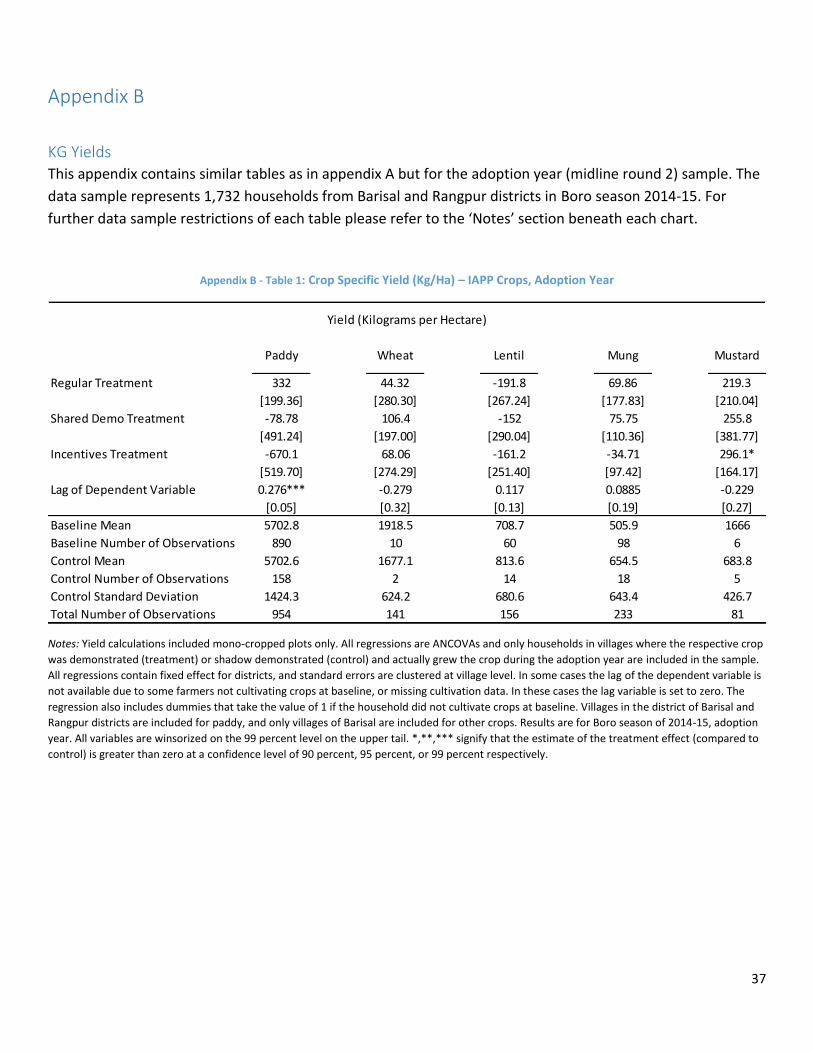
37

Appendix B

KG Yields This appendix contains similar tables as in appendix A but for the adoption year (midline round 2) sample. The

data sample represents 1,732 households from Barisal and Rangpur districts in Boro season 2014-15. For

further data sample restrictions of each table please refer to the ‘Notes’ section beneath each chart.

Appendix B - Table 1: Crop Specific Yield (Kg/Ha) – IAPP Crops, Adoption Year

Notes: Yield calculations included mono-cropped plots only. All regressions are ANCOVAs and only households in villages where the respective crop

was demonstrated (treatment) or shadow demonstrated (control) and actually grew the crop during the adoption year are included in the sample.

All regressions contain fixed effect for districts, and standard errors are clustered at village level. In some cases the lag of the dependent variable is

not available due to some farmers not cultivating crops at baseline, or missing cultivation data. In these cases the lag variable is set to zero. The

regression also includes dummies that take the value of 1 if the household did not cultivate crops at baseline. Villages in the district of Barisal and

Rangpur districts are included for paddy, and only villages of Barisal are included for other crops. Results are for Boro season of 2014-15, adoption

year. All variables are winsorized on the 99 percent level on the upper tail. *,**,*** signify that the estimate of the treatment effect (compared to

control) is greater than zero at a confidence level of 90 percent, 95 percent, or 99 percent respectively.

Regular Treatment 332 44.32 -191.8 69.86 219.3

[199.36] [280.30] [267.24] [177.83] [210.04]

Shared Demo Treatment -78.78 106.4 -152 75.75 255.8

[491.24] [197.00] [290.04] [110.36] [381.77]

Incentives Treatment -670.1 68.06 -161.2 -34.71 296.1*

[519.70] [274.29] [251.40] [97.42] [164.17]

Lag of Dependent Variable 0.276*** -0.279 0.117 0.0885 -0.229

[0.05] [0.32] [0.13] [0.19] [0.27]

Baseline Mean 5702.8 1918.5 708.7 505.9 1666

Baseline Number of Observations 890 10 60 98 6

Control Mean 5702.6 1677.1 813.6 654.5 683.8

Control Number of Observations 158 2 14 18 5

Control Standard Deviation 1424.3 624.2 680.6 643.4 426.7

Total Number of Observations 954 141 156 233 81

Yield (Kilograms per Hectare)

Paddy Wheat Lentil Mung Mustard

38

Adoption

Appendix B - Table 2: Adoption of Paddy and Mung24

Midline results included in Appendix A – Table2

Appendix B - Table 3: Adoption – Five IAPP Crops, Adoption Year

Notes: Seed variety data was only collected for paddy in baseline. All regressions are ANCOVAs. Only households in villages where the respective

crop was demonstrated (treatment) or shadow demonstrated (control) for the 'Grew Crop' regression. For the other regressions, the sample is also

restricted to households that actually grew the crop. Villages in districts of Barisal and Rangpur are included for paddy, and only villages of Barisal

are included for other crops. Results are for Boro season, 2014-15, adoption year. All regressions contain fixed effect for districts and standard

errors are clustered at village level. All ANCOVA regressions have dummies identifying households not surveyed at baseline and those that did not

cultivate the crop at baseline. *,**,*** signify that the estimate of the treatment effect (compared to control) is greater than zero at a confidence

level of 90 percent, 95 percent, or 99 percent respectively.

24 Refer to Appendix A – Table2

Wheat Lentil Mung Mustard

Regular Treatment -0.0304 0.177*** 0.281*** 0.195*** -0.0168 -0.0898 0.064

[0.04] [0.06] [0.08] [0.07] [0.14] [0.11] [0.08]

Shared Demo Treatment -0.0735 0.143 0.277** 0.209*** -0.0621 -0.173* 0.0151

[0.09] [0.12] [0.14] [0.08] [0.12] [0.09] [0.07]

Incentives Treatment -0.00349 0.113 0.236* 0.333*** 0.0746 0.0666 0.1

[0.10] [0.13] [0.14] [0.07] [0.10] [0.05] [0.06]

Lag of Dependent Variable 0.573*** 0.217*** 0.262*** 0.363*** 0.244*** 0.419*** 0.231**

[0.06] [0.03] [0.04] [0.11] [0.05] [0.05] [0.09]

Control Mean 0.893 0.696 0.506 0.0465 0.447 0.947 0.209

Control Number of Observations 177 158 158 43 38 19 43

Control Standard Deviation 0.31 0.461 0.502 0.213 0.504 0.229 0.412

Total Number of Observations 1351 954 954 605 362 483 429

Paddy

Grew CropGrew Any

IAPP Variety

Grew

Promoted

IAPP Variety

Grew Crop Grew Crop Grew Crop Grew Crop

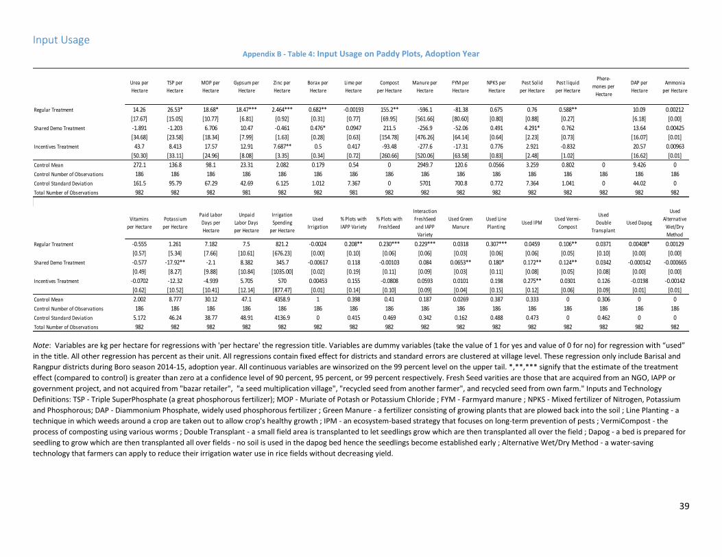
39

Input Usage Appendix B - Table 4: Input Usage on Paddy Plots, Adoption Year

Note: Variables are kg per hectare for regressions with 'per hectare' the regression title. Variables are dummy variables (take the value of 1 for yes and value of 0 for no) for regression with “used”

in the title. All other regression has percent as their unit. All regressions contain fixed effect for districts and standard errors are clustered at village level. These regression only include Barisal and

Rangpur districts during Boro season 2014-15, adoption year. All continuous variables are winsorized on the 99 percent level on the upper tail. *,**,*** signify that the estimate of the treatment

effect (compared to control) is greater than zero at a confidence level of 90 percent, 95 percent, or 99 percent respectively. Fresh Seed varities are those that are acquired from an NGO, IAPP or

government project, and not acquired from "bazar retailer", "a seed multiplication village", "recycled seed from another farmer", and recycled seed from own farm." Inputs and Technology

Definitions: TSP - Triple SuperPhosphate (a great phosphorous fertilizer); MOP - Muriate of Potash or Potassium Chloride ; FYM - Farmyard manure ; NPKS - Mixed fertilizer of Nitrogen, Potassium

and Phosphorous; DAP - Diammonium Phosphate, widely used phosphorous fertilizer ; Green Manure - a fertilizer consisting of growing plants that are plowed back into the soil ; Line Planting - a

technique in which weeds around a crop are taken out to allow crop's healthy growth ; IPM - an ecosystem-based strategy that focuses on long-term prevention of pests ; VermiCompost - the

process of composting using various worms ; Double Transplant - a small field area is transplanted to let seedlings grow which are then transplanted all over the field ; Dapog - a bed is prepared for

seedling to grow which are then transplanted all over fields - no soil is used in the dapog bed hence the seedlings become established early ; Alternative Wet/Dry Method - a water-saving

technology that farmers can apply to reduce their irrigation water use in rice fields without decreasing yield.

Regular Treatment 14.26 26.53* 18.68* 18.47*** 2.464*** 0.682** -0.00193 155.2** -596.1 -81.38 0.675 0.76 0.588** 10.09 0.00212

[17.67] [15.05] [10.77] [6.81] [0.92] [0.31] [0.77] [69.95] [561.66] [80.60] [0.80] [0.88] [0.27] [6.18] [0.00]

Shared Demo Treatment -1.891 -1.203 6.706 10.47 -0.461 0.476* 0.0947 211.5 -256.9 -52.06 0.491 4.291* 0.762 13.64 0.00425

[34.68] [23.58] [18.34] [7.99] [1.63] [0.28] [0.63] [154.78] [476.26] [64.14] [0.64] [2.23] [0.73] [16.07] [0.01]

Incentives Treatment 43.7 8.413 17.57 12.91 7.687** 0.5 0.417 -93.48 -277.6 -17.31 0.776 2.921 -0.832 20.57 0.00963

[50.30] [33.11] [24.96] [8.08] [3.35] [0.34] [0.72] [260.66] [520.06] [63.58] [0.83] [2.48] [1.02] [16.62] [0.01]

Control Mean 272.1 136.8 98.1 23.31 2.082 0.179 0.54 0 2949.7 120.6 0.0566 3.259 0.802 0 9.426 0

Control Number of Observations 186 186 186 186 186 186 186 186 186 186 186 186 186 186 186 186

Control Standard Deviation 161.5 95.79 67.29 42.69 6.125 1.012 7.367 0 5701 700.8 0.772 7.364 1.041 0 44.02 0

Total Number of Observations 982 982 982 981 982 982 981 982 982 982 982 982 982 982 982 982

Regular Treatment -0.555 1.261 7.182 7.5 821.2 -0.0024 0.208** 0.230*** 0.229*** 0.0318 0.307*** 0.0459 0.106** 0.0371 0.00408* 0.00129

[0.57] [5.34] [7.66] [10.61] [676.23] [0.00] [0.10] [0.06] [0.06] [0.03] [0.06] [0.06] [0.05] [0.10] [0.00] [0.00]

Shared Demo Treatment -0.577 -17.92** -2.1 8.382 345.7 -0.00617 0.118 -0.00103 0.084 0.0653** 0.180* 0.172** 0.124** 0.0342 -0.000142 -0.000665

[0.49] [8.27] [9.88] [10.84] [1035.00] [0.02] [0.19] [0.11] [0.09] [0.03] [0.11] [0.08] [0.05] [0.08] [0.00] [0.00]

Incentives Treatment -0.0702 -12.32 -4.939 5.705 570 0.00453 0.155 -0.0808 0.0593 0.0101 0.198 0.275** 0.0301 0.126 -0.0198 -0.00142

[0.62] [10.52] [10.41] [12.14] [877.47] [0.01] [0.14] [0.10] [0.09] [0.04] [0.15] [0.12] [0.06] [0.09] [0.01] [0.01]

Control Mean 2.002 8.777 30.12 47.1 4358.9 1 0.398 0.41 0.187 0.0269 0.387 0.333 0 0.306 0 0

Control Number of Observations 186 186 186 186 186 186 186 186 186 186 186 186 186 186 186 186

Control Standard Deviation 5.172 46.24 38.77 48.91 4136.9 0 0.415 0.469 0.342 0.162 0.488 0.473 0 0.462 0 0

Total Number of Observations 982 982 982 982 982 982 982 982 982 982 982 982 982 982 982 982

Urea per

Hectare

TSP per

Hectare

MOP per

Hectare

Gypsum per

Hectare

Zinc per

Hectare

Borax per

Hectare

Lime per

Hectare

Compost

per Hectare

Manure per

Hectare

Ammonia

per Hectare

NPKS per

Hectare

Pest Solid

per Hectare

Pest l iquid

per Hectare

Phere-

mones per

Hectare

DAP per

Hectare

FYM per

Hectare

Vitamins

per Hectare

Potassium

per Hectare

Paid Labor

Days per

Hectare

Unpaid

Labor Days

per Hectare

Irrigation

Spending

per Hectare

Used

Alternative

Wet/Dry

Method

Used Green

Manure

Used Line

PlantingUsed IPM

Used Vermi-

Compost

Used

Double

Transplant

Used DapogUsed

Irrigation

% Plots with

IAPP Variety

% Plots with

FreshSeed

Interaction

FreshSeed

and IAPP

Variety

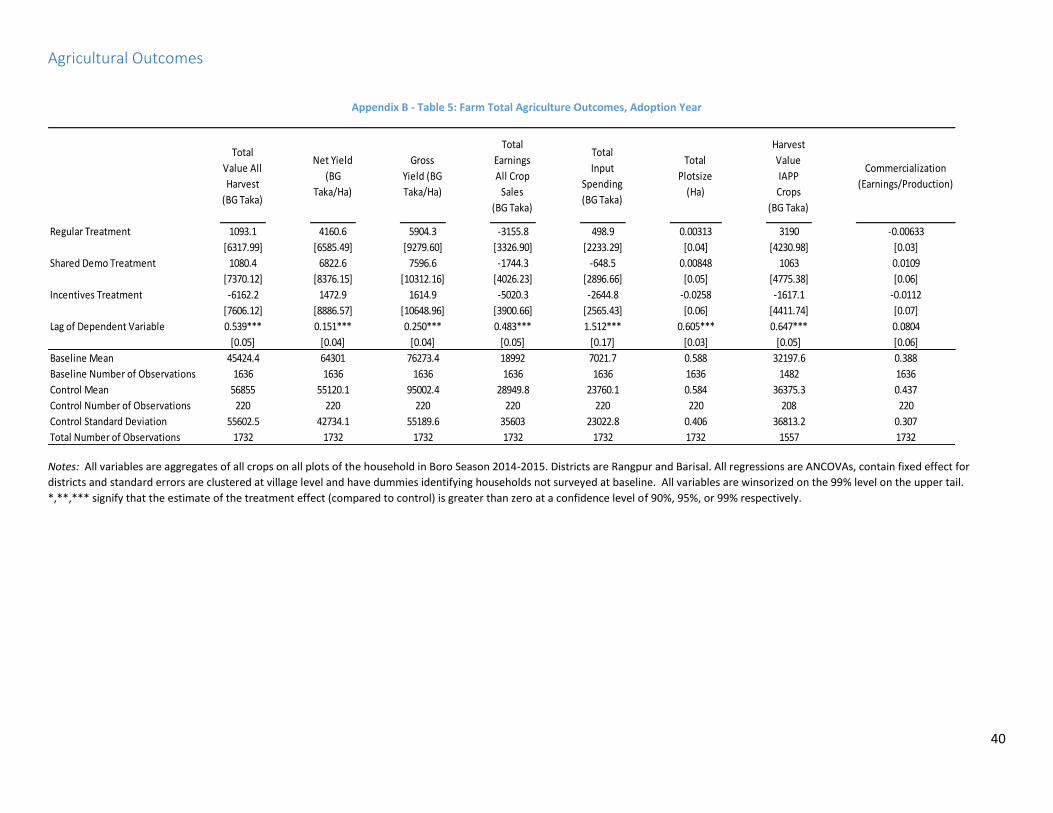
40

Agricultural Outcomes

Appendix B - Table 5: Farm Total Agriculture Outcomes, Adoption Year

Notes: All variables are aggregates of all crops on all plots of the household in Boro Season 2014-2015. Districts are Rangpur and Barisal. All regressions are ANCOVAs, contain fixed effect for

districts and standard errors are clustered at village level and have dummies identifying households not surveyed at baseline. All variables are winsorized on the 99% level on the upper tail.

*,**,*** signify that the estimate of the treatment effect (compared to control) is greater than zero at a confidence level of 90%, 95%, or 99% respectively.

Total

Value All

Harvest

(BG Taka)

Net Yield

(BG

Taka/Ha)

Gross

Yield (BG

Taka/Ha)

Total

Earnings

All Crop

Sales

(BG Taka)

Total

Input

Spending

(BG Taka)

Total

Plotsize

(Ha)

Harvest

Value

IAPP

Crops

(BG Taka)

Commercialization

(Earnings/Production)

Regular Treatment 1093.1 4160.6 5904.3 -3155.8 498.9 0.00313 3190 -0.00633

[6317.99] [6585.49] [9279.60] [3326.90] [2233.29] [0.04] [4230.98] [0.03]

Shared Demo Treatment 1080.4 6822.6 7596.6 -1744.3 -648.5 0.00848 1063 0.0109

[7370.12] [8376.15] [10312.16] [4026.23] [2896.66] [0.05] [4775.38] [0.06]

Incentives Treatment -6162.2 1472.9 1614.9 -5020.3 -2644.8 -0.0258 -1617.1 -0.0112

[7606.12] [8886.57] [10648.96] [3900.66] [2565.43] [0.06] [4411.74] [0.07]

Lag of Dependent Variable 0.539*** 0.151*** 0.250*** 0.483*** 1.512*** 0.605*** 0.647*** 0.0804

[0.05] [0.04] [0.04] [0.05] [0.17] [0.03] [0.05] [0.06]

Baseline Mean 45424.4 64301 76273.4 18992 7021.7 0.588 32197.6 0.388

Baseline Number of Observations 1636 1636 1636 1636 1636 1636 1482 1636

Control Mean 56855 55120.1 95002.4 28949.8 23760.1 0.584 36375.3 0.437

Control Number of Observations 220 220 220 220 220 220 208 220

Control Standard Deviation 55602.5 42734.1 55189.6 35603 23022.8 0.406 36813.2 0.307

Total Number of Observations 1732 1732 1732 1732 1732 1732 1557 1732

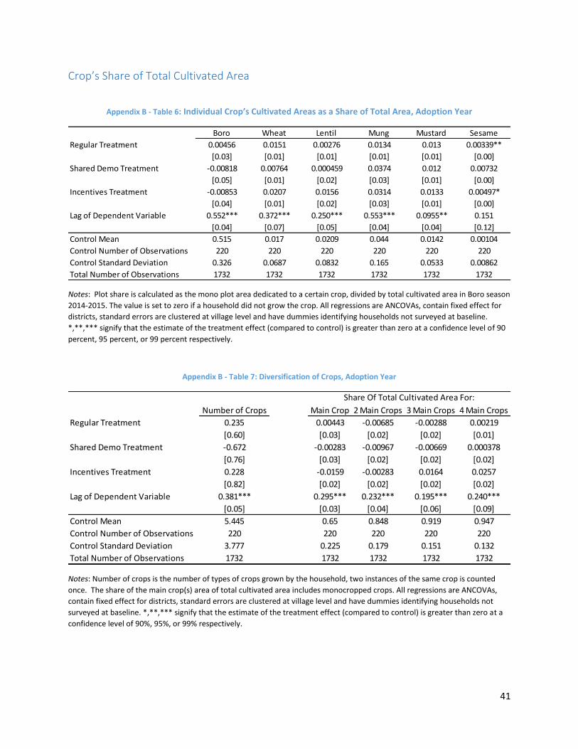
41

Crop’s Share of Total Cultivated Area

Appendix B - Table 6: Individual Crop’s Cultivated Areas as a Share of Total Area, Adoption Year

Notes: Plot share is calculated as the mono plot area dedicated to a certain crop, divided by total cultivated area in Boro season

2014-2015. The value is set to zero if a household did not grow the crop. All regressions are ANCOVAs, contain fixed effect for

districts, standard errors are clustered at village level and have dummies identifying households not surveyed at baseline.

*,**,*** signify that the estimate of the treatment effect (compared to control) is greater than zero at a confidence level of 90

percent, 95 percent, or 99 percent respectively.

Appendix B - Table 7: Diversification of Crops, Adoption Year

Notes: Number of crops is the number of types of crops grown by the household, two instances of the same crop is counted

once. The share of the main crop(s) area of total cultivated area includes monocropped crops. All regressions are ANCOVAs,

contain fixed effect for districts, standard errors are clustered at village level and have dummies identifying households not

surveyed at baseline. *,**,*** signify that the estimate of the treatment effect (compared to control) is greater than zero at a

confidence level of 90%, 95%, or 99% respectively.

Boro Wheat Lentil Mung Mustard Sesame

Regular Treatment 0.00456 0.0151 0.00276 0.0134 0.013 0.00339**

[0.03] [0.01] [0.01] [0.01] [0.01] [0.00]

Shared Demo Treatment -0.00818 0.00764 0.000459 0.0374 0.012 0.00732

[0.05] [0.01] [0.02] [0.03] [0.01] [0.00]

Incentives Treatment -0.00853 0.0207 0.0156 0.0314 0.0133 0.00497*

[0.04] [0.01] [0.02] [0.03] [0.01] [0.00]

Lag of Dependent Variable 0.552*** 0.372*** 0.250*** 0.553*** 0.0955** 0.151

[0.04] [0.07] [0.05] [0.04] [0.04] [0.12]

Control Mean 0.515 0.017 0.0209 0.044 0.0142 0.00104

Control Number of Observations 220 220 220 220 220 220

Control Standard Deviation 0.326 0.0687 0.0832 0.165 0.0533 0.00862

Total Number of Observations 1732 1732 1732 1732 1732 1732

Main Crop 2 Main Crops 3 Main Crops 4 Main Crops

Regular Treatment 0.235 0.00443 -0.00685 -0.00288 0.00219

[0.60] [0.03] [0.02] [0.02] [0.01]

Shared Demo Treatment -0.672 -0.00283 -0.00967 -0.00669 0.000378

[0.76] [0.03] [0.02] [0.02] [0.02]

Incentives Treatment 0.228 -0.0159 -0.00283 0.0164 0.0257

[0.82] [0.02] [0.02] [0.02] [0.02]

Lag of Dependent Variable 0.381*** 0.295*** 0.232*** 0.195*** 0.240***

[0.05] [0.03] [0.04] [0.06] [0.09]

Control Mean 5.445 0.65 0.848 0.919 0.947

Control Number of Observations 220 220 220 220 220

Control Standard Deviation 3.777 0.225 0.179 0.151 0.132

Total Number of Observations 1732 1732 1732 1732 1732

Number of Crops

Share Of Total Cultivated Area For:

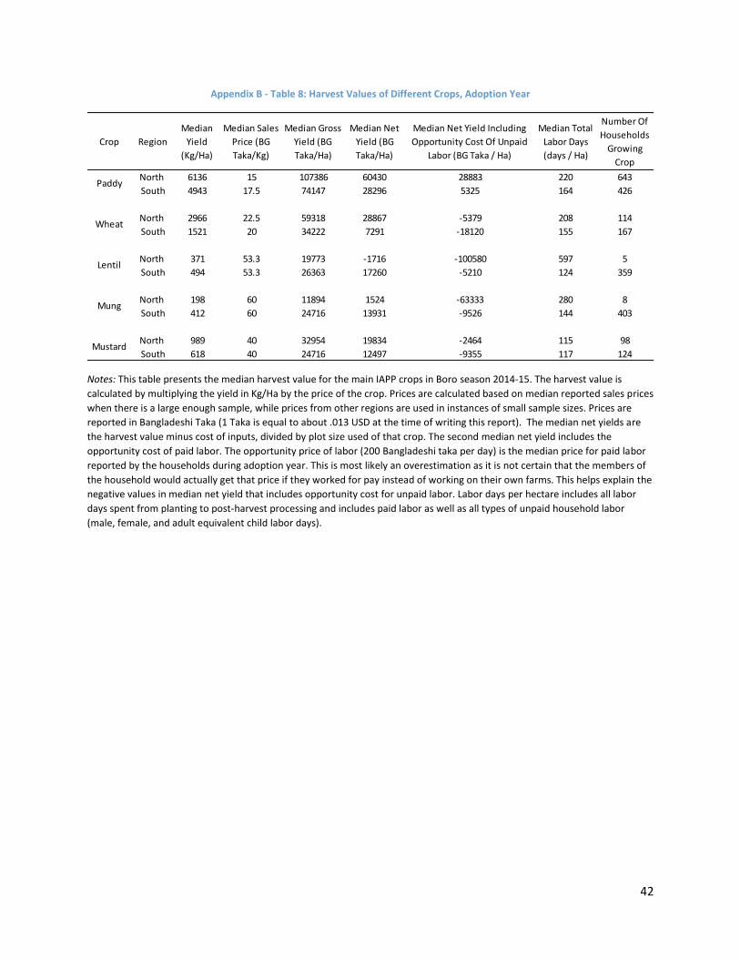
42

Appendix B - Table 8: Harvest Values of Different Crops, Adoption Year

Notes: This table presents the median harvest value for the main IAPP crops in Boro season 2014-15. The harvest value is

calculated by multiplying the yield in Kg/Ha by the price of the crop. Prices are calculated based on median reported sales prices

when there is a large enough sample, while prices from other regions are used in instances of small sample sizes. Prices are

reported in Bangladeshi Taka (1 Taka is equal to about .013 USD at the time of writing this report). The median net yields are

the harvest value minus cost of inputs, divided by plot size used of that crop. The second median net yield includes the

opportunity cost of paid labor. The opportunity price of labor (200 Bangladeshi taka per day) is the median price for paid labor

reported by the households during adoption year. This is most likely an overestimation as it is not certain that the members of

the household would actually get that price if they worked for pay instead of working on their own farms. This helps explain the

negative values in median net yield that includes opportunity cost for unpaid labor. Labor days per hectare includes all labor

days spent from planting to post-harvest processing and includes paid labor as well as all types of unpaid household labor

(male, female, and adult equivalent child labor days).

Crop Region

Median

Yield

(Kg/Ha)

Median Sales

Price (BG

Taka/Kg)

Median Gross

Yield (BG

Taka/Ha)

Median Net

Yield (BG

Taka/Ha)

Median Net Yield Including

Opportunity Cost Of Unpaid

Labor (BG Taka / Ha)

Median Total

Labor Days

(days / Ha)

Number Of

Households

Growing

Crop

North 6136 15 107386 60430 28883 220 643

South 4943 17.5 74147 28296 5325 164 426

North 2966 22.5 59318 28867 -5379 208 114

South 1521 20 34222 7291 -18120 155 167

North 371 53.3 19773 -1716 -100580 597 5

South 494 53.3 26363 17260 -5210 124 359

North 198 60 11894 1524 -63333 280 8

South 412 60 24716 13931 -9526 144 403

North 989 40 32954 19834 -2464 115 98

South 618 40 24716 12497 -9355 117 124

Paddy

Wheat

Lentil

Mung

Mustard