Integrated Quality and Quantity Modeling of a Production …web.mit.edu/manuf-sys/www/oldcell1/papers/kim-gershwin-qq04.pdf · OR Spectrum manuscript No. (will be inserted by the

OR Spectrum manuscript No.(will be inserted by the editor)

Integrated Quality and Quantity Modeling of

a Production Line

Jongyoon Kim, Stanley B. Gershwin

Department of Mechanical Engineering, Massachusetts Institute of TechnologyCambridge, Massachusetts 02139-4307

Received: December, 2003 / Revised version: May, 2004

Abstract During the past three decades, the success of the Toyota Pro-duction System has spurred much research in manufacturing systems engi-neering. Productivity and quality have been extensively studied, but thereis little research in their intersection. The goal of this paper is to analyzehow production system design, quality, and productivity are inter-relatedin small production systems. We develop a new Markov process model formachines with both quality and operational failures, and we identify impor-tant differences between types of quality failures. We also develop modelsfor two-machine systems, with infinite buffers, buffers of size zero, and fi-nite buffers. We calculate total production rate, effective production rate(ie, the production rate of good parts), and yield. Numerical studies usingthese models show that when the first machine has quality failures and theinspection occurs only at the second machine, there are cases in which theeffective production rate increases as buffer sizes increase, and there arecases in which the effective production rate decreases for larger buffers. Wepropose extensions to larger systems.

Key words Quality, Productivity, Manufacturing System Design

1 Introduction

1.1 Motivation

During the past three decades, the success of the Toyota Production Sys-tem has spurred much research in manufacturing systems design. Numerousresearch papers have tried to explore the relationship between production

Send offprint requests to: [email protected]

2 Jongyoon Kim, Stanley B. Gershwin

system design and productivity, so that they can show ways to design facto-ries to produce more products on time with less resources (such as people,material, and space). On the other hand, topics in quality research have cap-tured the attention of practitioners and researchers since the early 1980s.The recent popularity of Statistical Quality Control (SQC), Total QualityManagement (TQM), and Six Sigma have demonstrated the importance ofquality.

These two fields, productivity and quality, have been extensively stud-ied and reported separately both in the manufacturing systems researchliterature and the practitioner literature, but there is little research in theirintersection. The need for such work was recently described by authors fromthe GM Corporation based on their experience [13]. All manufacturers mustsatisfy these two requirements (high productivity and high quality) at thesame time to maintain their competitiveness.

Toyota Production System advocates admonish factory designers to com-bine inspections with operations. In the Toyota Production System, themachines are designed to detect abnormalities and to stop automaticallywhenever they occur. Also, operators are equipped with means of stoppingthe production flow whenever they note anything suspicious. (They call thispractice jidoka.) Toyota Production System advocates argue that mechani-cal and human jidoka prevent the waste that would result from producinga series of defective items. Therefore jidoka is a means to improve qualityand increase productivity at the same time [23], [24]. But this statement isarguable: quality failures are often those in which the quality of each part isindependent of the others. This is the case when the defect takes place dueto common (or chance or random) causes of variations [16]. In this case,there is no reason to stop a machine that has made a bad part becausethere is no reason to believe that stopping it will reduce the number ofbad parts in the future. In this case, therefore, stopping the operation doesnot influence quality but it does reduce productivity. On the other hand,when quality failures are those in which once a bad part is produced, allsubsequent parts will be bad until the machine is repaired (due to special orassignable or systematic causes of variations) [16], catching bad parts andstopping the machine as soon as possible is the best way to maintain highquality and productivity.

Non-stock or lean production is another popular buzzword in manufac-turing systems engineering. Some lean manufacturing professionals advo-cate reducing inventory on the factory floor since the reduction of work-in-process (WIP) reveals the problems in the production lines [3]. Thus, itcan help improve product quality. It is true in some sense: less inventoryreduces the time between making a defect and identifying the defect. But itis also true that productivity would diminish significantly without stock [5].Since there is a tradeoff, there must be optimal stock levels that are specificto each manufacturing environment. In fact, Toyota recently changed theirview on inventory and are trying to re-adjust their inventory levels [9].

Integrated Quality and Quantity Modeling of a Production Line 3

What is missing in discussions of factory design, quality, and produc-tivity is a quantitative model to show how they are inter-related. Most ofthe arguments about this are based on anecdotal evidence or qualitativereasoning that lack a sound scientific quantitative foundation. The researchdescribed here tries to establish such a foundation to investigate how pro-duction system design and operation influence productivity and productquality by developing conceptual and computational models of two-machine-one-buffer systems and performing numerical experiments.

1.2 Background

1.2.1 Quality models There are two extreme kinds of quality failures basedon the characteristics of variations that cause the failures. In the qualityliterature, these variations are called common (or chance or random) causevariations and assignable (or special or unusual) cause variations [18].

Figure 1 shows the types of quality failures and variations. Commoncause failures are those in which the quality of each part is independent ofthe others. Such failures occur often when an operation is sensitive to exter-nal perturbations like defects in raw material or when the operation uses anew technology that is difficult to control. This is inherent in the design ofthe process. Such failures can be represented by independent Bernoulli ran-dom variables, in which a binary random variable, which indicates whetheror not the part is good, is chosen each time a part is operated on. A goodpart is produced with probability π, and a bad part is produced with proba-bility 1−π. The occurrence of a bad part implies nothing about the qualityof future parts, so no permanent changes can have occurred in the machine.For the sake of clarity, we call this a Bernoulli-type quality failure. Mostof the quantitative literature on inspection allocation assumes this kind ofquality failure [21]. In this case, if bad parts are destined to be scrapped, itis useful to catch them as soon as possible because the longer before theyare scrapped, the more they consume the capacity of downstream machines.However, there is no reason to stop a machine that has produced a bad partdue to this kind of failure.

The quality failures due to assignable cause variations are those in whicha quality failure only happens after a change occurs in the machine. In thatcase, it is very likely that once a bad part is produced, all subsequent partswill be bad until the machine is repaired. Here, there is much more in-centive to catch defective parts and stop the machine quickly. In additionto minimizing the waste of downstream capacity, this strategy minimizesthe further production of defective parts. For this kind of quality failure,there is no inherent measure of yield because the fractions of parts that aregood and bad depend on how soon bad parts are detected and how quicklythe machine is stopped for repair. In this paper, we call this a persistent-type quality failure. Most quantitative studies in Statistical Quality Control(SQC) are dedicated to finding efficient inspection policies (sampling inter-


val, sample size, control limits, and others) to detect this type of qualityfailure [26].

In reality, failures are mixtures of Bernoulli-type quality failures andpersistent-type quality failures. It can be argue that the quality strategyof the Toyota Production System [17], in which machines are stopped assoon as a bad part is detected, is implicitly based on the assumption of thepersistent-type quality failure. In this paper, we focus on persistent failures.

Mean

Bernoulli- type quality failure

Random Variation

Markovian- type quality failure

Repair takes place Upper

Specification Limit

Lower Specification

Limit Assignable Variation (tool breakage) takes

place

Fig. 1 Types of Quality Failures

1.2.2 System yield System yield is defined here as the fraction of input toa system that is transformed into output of acceptable quality. This is animportant metric because customers observe the quality of products onlyafter all the manufacturing processes are done and the products are shipped.The system yield is a complex function of how the factory is designed andoperated, as well as of the characteristics of the machines. Some of influenc-ing factors include individual operation yields, inspection strategies, opera-tion policies, buffer sizes, and other factors. Comprehensive approaches areneeded to manage system yield effectively. This research aims to developmathematical models to show how the system yield is influenced by thesefactors.

1.2.3 Quality improvement policy System yield is a complex function ofvarious factors such as inspection, individual operation yields, buffer size,operation policies, and others. There are many ways to affect the systemyield. Inspection policy has received the most attention in the literature.Research on inspection policies can be divided into optimizing inspectionparameters at a single station and the inspection station allocation prob-lem. The former issue has been investigated extensively in the SQC liter-ature [26]. Here, optimal SQC parameters such as control limits, samplingsize, and frequency are sought for an optimal balance between the inspec-


tion cost and the cost of quality. The latter research looks for the optimaldistributions of inspection stations along production lines [21].

Improving individual operation yield is another important way to in-crease the system yield. Many studies in this field try to stabilize the pro-cess either by finding root causes of variation and eliminating them or bymaking the process insensitive to external noise. The former topic has nu-merous qualitative research papers in the fields of Total Quality Manage-ment (TQM) [2] and Six Sigma [19]. Quantitative research is more orientedtoward the latter topic. Robust engineering [20] is an area that has gainedsubstantial attention.

It has been argued that inventory reduction is an effective means to im-prove system yield. Many lean manufacturing specialists have asserted thatless inventory on the factory floor reveals problems in the manufacturinglines more quickly and helps quality improvement activities [1], [17].

There also have been investigations to explain the relationship betweenplant layout design and quality [7]. They argue that U-shaped lines arebetter than straight lines for producing higher quality products since thereare more points of contact between operators. There is also less materialmovement, and there are other reasons.

There are many ways to improve system yield, but using only a singlemethod will give limited gains. The effectiveness of each method is greatlydependent on the details of the factory. Thus, there is need to determinewhich method or which combination of methods is most effective in eachcase. The quantitative tools that will be developed from this research canhelp fulfill this need.

1.3 Outline

In Section 2 we introduce the structure of the modeling techniques used inthis paper. We present modeling, solution techniques, and validation of the2-machine-1-finite buffer case in Section 3. Discussions on the behavior ofa production line based on numerical experiments are provided in Section5. A future research plan is shown in Section 6. Parameters of many of thesystems studied numerically here, and details of the analytical solution ofthe two-machine line, can be found in the appendices.

2 Mathematical Models

2.1 Single machine model

There are many possible ways to characterize a machine for the purposeof simultaneously studying quality and quantity issues. Here, we model amachine as a discrete state, continuous time Markov process. Material isassumed continuous, and µi is the speed at which Machine i processes ma-terial while it is operating and not constrained by the other machine or the


buffer. It is a constant, in that µi does not depend on the repair state ofthe other machine or the buffer level.

Figure 2 shows the proposed state transitions of a single machine withpersistent-type quality failures. In the model, the machine has three states:

? State 1: The machine is operating and producing good parts.? State -1: The machine is operating and producing bad parts, but the

operator does not know this yet.? State 0: The machine is not operating.

r

p

g f

State 1 State -1 State 0

Fig. 2 States of a Machine

The machine therefore has two different failure modes (i.e. transition tofailure states from state 1):

? Operational failure: transition from state 1 to state 0. The machine stopsproducing parts due to failures like motor burnout.

? Quality failure: transition from state 1 to state -1. The machine stopsproducing good parts (and starts producing bad parts) due to a failurelike a sudden tool damage.

When a machine is in state 1, it can fail due to a non-quality relatedevent. It goes to state 0 with transition probability rate p. After that anoperator fixes it, and the machine goes back to state 1 with transition rate r.Sometimes, due to an assignable cause, the machine begins to produce badparts, so there is a transition from state 1 to state -1 with a probability rateg. Here g is the reciprocal of the Mean Time to Quality Failure (MTQF).A more stable operation leads to a larger MTQF and a smaller g.

The machine, when it is in state -1, can be stopped for two reasons: itmay experience the same kind of operational failure as it does when it isin state 1; and the operator may stop it for repair when he learns that itis producing bad parts. The transition from state -1 to state 0 occurs atprobability rate f = p + h where h is the reciprocal of the Mean Time ToDetect (MTTD). A more reliable inspection leads to a shorter MTTD and a


larger f . (The detection can take place elsewhere, for example at a remoteinspection station.) Note that this implies that f > p. Here, for simplicity,we assume that whenever a machine is repaired, it goes back to state 1. Allthe indicated transitions are assumed to follow exponential distributions.

Single Machine Analysis To determine the production rate of a single ma-chine, we first determine the steady-state probability distribution. This iscalculated based on the probability balance principle: the probability ofleaving a state is the same as the probability of entering that state. Wehave

(g + p)P (1) = rP (0) (1)

fP (−1) = gP (1) (2)

rP (0) = pP (1) + fP (−1) (3)

The probabilities must also satisfy the normalization equation:

P (0) + P (1) + P (−1) = 1 (4)

The solution of (1)–(4) is

P (1) =1

1 + (p + g)/r + g/f(5)

P (0) =(p + g)/r

1 + (p + g)/r + g/f(6)

P (−1) =g/f

1 + (p + g)/r + g/f(7)

The total production rate, including good and bad parts, is

PT = µ(P (1) + P (−1)) = µ1 + g/f

1 + (p + g)/r + g/f(8)

The effective production rate, the production rate of good parts only, is

PE = µP (1) = µ1

1 + (p + g)/r + g/f(9)

The yield is

PE

PE + PT

=P (1)

P (1) + P (−1)=

f

f + g(10)


2.2 2-Machine-1-Buffer continuous model

A flow (or transfer) line is a manufacturing system with a very specialstructure. It is a linear network of service stations or machines (M1, M2, ...,Mk) separated by buffer storages (B1, B2, ..., Bk−1). Material flows fromoutside the system to M1, then to B1, then to M2, and so forth until itreaches Mk, after which it leaves. Figure 3 depicts a flow line. The rectanglesrepresent machines and the circles represent buffers.

M B M B M B M B M1 1 2 2 3 3 4 4 5

Fig. 3 Five-Machine Flow Line

2-machine-1-buffer (2M1B) models should be studied first. Then a de-composition technique, that divides a long transfer line into multiple 2-machine-1-buffer models, could be developed. (See [14].) Among the variousmodeling techniques for the 2M1B case, including deterministic, exponen-tial, and continuous models, the continuous material line model is used forthis research because it can handle deterministic but different operationtimes at each operation. This is an extension of the continuous material se-rial line modeling of [10] by adding another machine failure state. Figure 4shows the 2M1B continuous model where the machines, buffer and discreteparts are represented as valves, a tank, and a continuous fluid.

M

M

MM

B

B

1 22

1

Fig. 4 Two-Machine-One-Buffer Continuous Model

We assume that an inexhaustible supply of workpieces is available up-stream of the first machine in the line, and an unlimited storage area ispresent downstream of the last machine. Thus, the first machine is neverstarved, and the last machine is never blocked. Also, failures are assumedto be operation dependent (ODF).

Finally, we assume that each machine works on a different feature. Forexample, the two machines may be making two different holes. We do notconsider cases where the both machines work on the same hole, in whichthe first machine does a roughing operation and the second does a finishingoperation. This allows us to assume that the failures of the two machinesare independent.


2.3 Infinite buffer case

An infinite buffer case is a special 2M1B line in which the size of the buffer(B) is infinite. This is an extreme case in which the first machine (M1)never suffers from blockage. To derive expressions for the total productionrate and the effective production rate, we observe that when there is infinitebuffer capacity between two machines (M1, M2), the total production rateof the 2M1B system is a minimum of the total production rates of M1 andM2. The total production rate of machine i is given by (8), so the totalproduction rate of the 2M1B system is

P∞T = min

[

µ1(1 + g1/f1)

1 + (p1 + g1)/r1 + g1/f1,

µ2(1 + g2/f2)

1 + (p2 + g2)/r2 + g2/f2

]

(11)

The probability that machine Mi does not add non-conformities is

Yi =Pi(1)

Pi(1) + Pi(−1)=

fi

fi + gi

(12)

Since there is no scrap and rework in the system, the system yield be-comes

f1f2

(f1 + g1)(f2 + g2)(13)

As a result, the effective production rate is

P∞E =

f1f2

(f1 + g1)(f2 + g2)P∞

T (14)

The effective production rate evaluated from (14) has been comparedwith a discrete-event, discrete-part simulation. Table 1 shows good agree-ment. The parameters for these cases are shown in Appendix B.

Table 1 Validation of Infinite Buffer Case

Case # P∞E (Analytic) P∞

E (Simulation) %Difference

1 0.762 0.761 0.172 0.708 0.708 0.003 0.657 0.657 0.004 0.577 0.580 -0.505 0.527 0.530 -0.426 0.745 0.745 0.017 0.762 0.760 0.308 1.524 1.522 0.149 0.762 0.762 0.0010 1.524 1.526 -0.13

As indicated in Section 2.1, the detection of quality failures due to ma-chine M1 need not occur at that machine. For example, the inspection of


the feature that M1 works on could take place at an inspection station atM2, and this inspection could trigger a repair of M1. (We call this qualityinformation feedback. See Section 4.) In that case, the MTTD of M1 (andtherefore f1) will be a function of the amount of material in the buffer. Wereturn to this important case in Section 4.

2.4 Zero buffer case

The zero buffer case is one in which there is no buffer space between themachines. This is the other extreme case where blockage and starvation takeplace most frequently.

In the zero-buffer case in which machines have different operation times,whenever one of the machines stops, the other one is also stopped. In ad-dition, when both of them are working, the production rate is min[µ1, µ2].Consider a long time interval of length T during which M1 fails m1 timesand M2 fails m2 times. If we assume that the average time to repair M1 is1/r1 and the average time to repair M2 is 1/r2, then the total system downtime will be close to D = m1

r1

+ m2

r2

. Consequently, the total up time will beapproximately

U = T − D = T − (m1

r1+

m2

r2) (15)

Since we assume operation-dependent failures, the rates of failure arereduced for the faster machine. Therefore,

pbi = pi

min(µ1, µ2)

µi

, gbi = gi

min(µ1, µ2)

µi

, and f bi = fi

min(µ1, µ2)

µi

(16)

The reduction of pi is explained in detail in [10]. The reductions of gi

and fi are done for the same reasons.Table 2 lists the possible working states α1 and α2 of M1 and M2. The

third column is the probability of finding the system in the indicated state.The fourth and fifth columns indicate the expected number of transitionsto down states during the time interval from each of the states in column 1.

Table 2 Zero-Buffer States, Probabilities, and Expected Numbers of Events

α1 α2 Probability π(α1, α2) Em1(α1, α2) Em2(α1, α2)

1 1fb1

fb1+gb

1

fb2

fb2+gb

2

pb1Uπ(1, 1) pb

2Uπ(1, 1)

1 -1fb1

fb1+gb

1

gb2

fb2+gb

2

pb1Uπ(1,−1) f b

2Uπ(1,−1)

-1 1gb1

fb1+gb

1

fb2

fb2+gb

2

fb1Uπ(−1, 1) pb

2Uπ(−1, 1)

-1 -1gb1

fb1+gb

1

gb2

fb2+gb

2

fb1Uπ(−1,−1) f b

2Uπ(−1,−1)


From Table 2, the expectations of m1 and m2 are

Em1 =∑1

α1=−1

∑1

α2=−1Em1(α1, α2) =

Ufb1(pb

1+gb

1)

fb1+gb

1

Em2 =∑1

α1=−1

∑1

α2=−1Em2(α1, α2) =

Ufb2(pb

2+gb

2)

fb2+gb

2

(17)

By plugging them into equation (15), we find total production rate:

P 0T =

min[µ1, µ2]

1 +fb1(pb

1+gb

1)

r1(fb1+gb

1)

+fb2(pb

2+gb

2)

r2(fb2+gb

2)

(18)

The effective production rate is

P 0E =

fb1fb

2

(fb1 + gb

1)(fb2 + gb

2)P 0

T (19)

The comparison with simulation is shown in in Table 3. The parametersof the cases are shown in Appendix B.

Table 3 Zero Buffer Case

Case # P 0E(Analytic) P 0

E(Simulation) %Difference

1 0.657 0.662 -0.732 0.620 0.627 -1.153 0.614 0.621 -1.034 0.529 0.534 -0.995 0.480 0.484 -0.776 0.647 0.651 -0.577 0.706 0.712 -0.918 1.377 1.406 -2.109 0.706 0.711 -0.7710 1.377 1.380 -0.22

3 2-Machine-1-Finite-Buffer Line

The two-machine line is the simplest non-trivial case of a production line.In the existing literature on the performance evaluation of systems in whichquality is not considered, two-machine lines are used in decomposition ap-proximations of longer lines. (See [10].)

We define the model here and show the solution technique in AppendixA.

3.1 State definition

The state of the 2M1B line is defined as (x, α1, α2) where


? x: the total amount of material in buffer B, 0 ≤ x ≤ N ,? α1: the state of M1. (α1 = −1, 0, or 1),? α2: the state of M2. (α2 = −1, 0, or 1)

The parameters of machine Mi are µi, ri, pi, fi, gi and the buffer size isN .

3.2 Model development

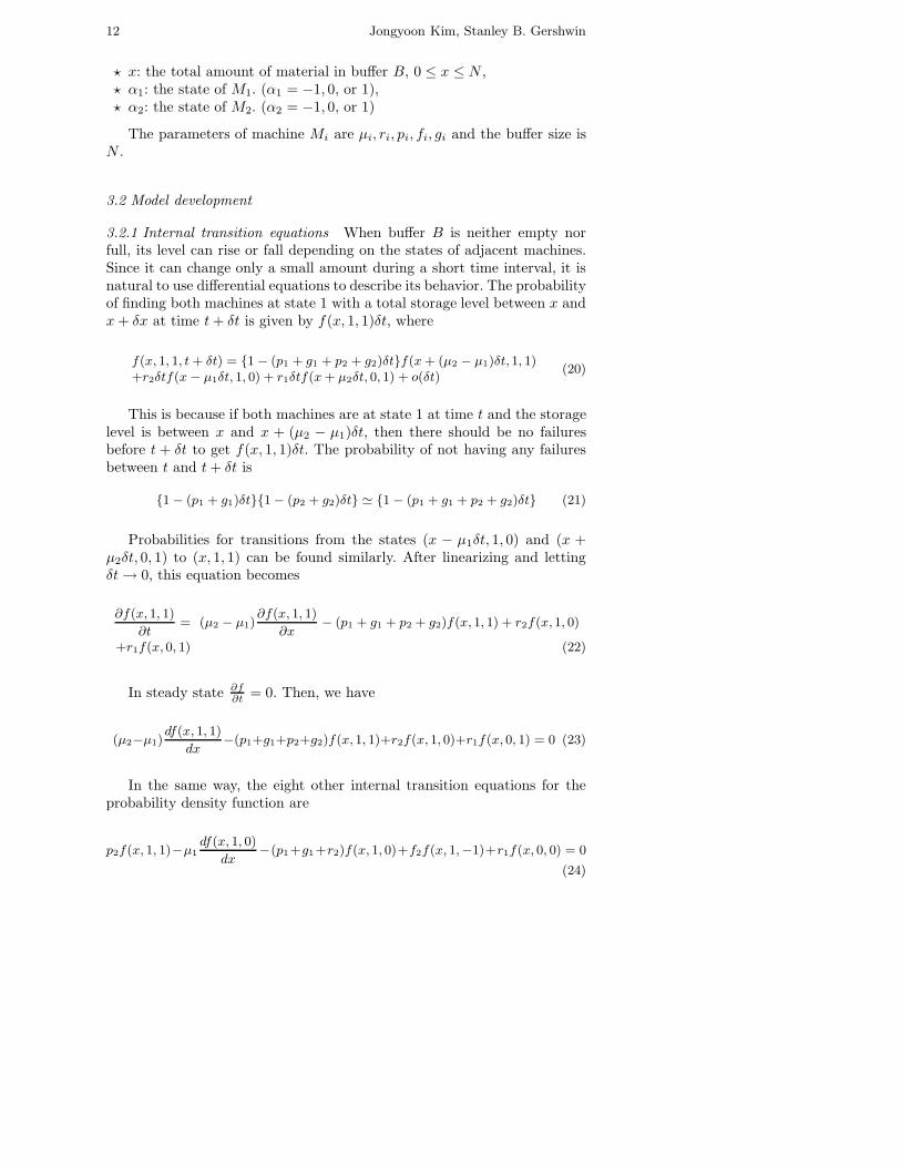
3.2.1 Internal transition equations When buffer B is neither empty norfull, its level can rise or fall depending on the states of adjacent machines.Since it can change only a small amount during a short time interval, it isnatural to use differential equations to describe its behavior. The probabilityof finding both machines at state 1 with a total storage level between x andx + δx at time t + δt is given by f(x, 1, 1)δt, where

f(x, 1, 1, t + δt) = {1 − (p1 + g1 + p2 + g2)δt}f(x + (µ2 − µ1)δt, 1, 1)+r2δtf(x − µ1δt, 1, 0) + r1δtf(x + µ2δt, 0, 1) + o(δt)

(20)

This is because if both machines are at state 1 at time t and the storagelevel is between x and x + (µ2 − µ1)δt, then there should be no failuresbefore t + δt to get f(x, 1, 1)δt. The probability of not having any failuresbetween t and t + δt is

{1 − (p1 + g1)δt}{1 − (p2 + g2)δt} ' {1 − (p1 + g1 + p2 + g2)δt} (21)

Probabilities for transitions from the states (x − µ1δt, 1, 0) and (x +µ2δt, 0, 1) to (x, 1, 1) can be found similarly. After linearizing and lettingδt → 0, this equation becomes

∂f(x, 1, 1)

∂t= (µ2 − µ1)

∂f(x, 1, 1)

∂x− (p1 + g1 + p2 + g2)f(x, 1, 1) + r2f(x, 1, 0)

+r1f(x, 0, 1) (22)

In steady state ∂f∂t

= 0. Then, we have

(µ2−µ1)df(x, 1, 1)

dx−(p1+g1+p2+g2)f(x, 1, 1)+r2f(x, 1, 0)+r1f(x, 0, 1) = 0 (23)

In the same way, the eight other internal transition equations for theprobability density function are

p2f(x, 1, 1)−µ1df(x, 1, 0)

dx−(p1+g1+r2)f(x, 1, 0)+f2f(x, 1,−1)+r1f(x, 0, 0) = 0

(24)


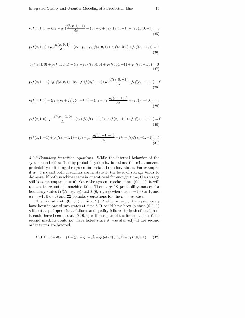
g2f(x, 1, 1) + (µ2 − µ1)df(x, 1,−1)

dx− (p1 + g + f2)f(x, 1,−1) + r1f(x, 0,−1) = 0

(25)

p1f(x, 1, 1)+µ2df(x, 0, 1)

dx−(r1+p2+g2)f(x, 0, 1)+r2f(x, 0, 0)+f1f(x,−1, 1) = 0

(26)

p1f(x, 1, 0) + p2f(x, 0, 1) − (r1 + r2)f(x, 0, 0) + f2f(x, 0,−1) + f1f(x,−1, 0) = 0(27)

p1f(x, 1,−1)+g2f(x, 0, 1)−(r1+f2)f(x, 0,−1)+µ2df(x, 0,−1)

dx+f1f(x,−1,−1) = 0

(28)

g1f(x, 1, 1)− (p2 + g2 + f1)f(x,−1, 1) + (µ2 − µ1)df(x,−1, 1)

dx+ r2f(x,−1, 0) = 0

(29)

g1f(x, 1, 0)−µ1df(x,−1, 0)

dx−(r2+f1)f(x,−1, 0)+p2f(x,−1, 1)+f2f(x,−1,−1) = 0

(30)

g1f(x, 1,−1)+ g2f(x,−1, 1) + (µ2 −µ1)df(x,−1,−1)

dx− (f1 + f2)f(x,−1,−1) = 0

(31)

3.2.2 Boundary transition equations While the internal behavior of thesystem can be described by probability density functions, there is a nonzeroprobability of finding the system in certain boundary states. For example,if µ1 < µ2 and both machines are in state 1, the level of storage tends todecrease. If both machines remain operational for enough time, the storagewill become empty (x = 0). Once the system reaches state (0, 1, 1), it willremain there until a machine fails. There are 18 probability masses forboundary states (P (N, α1, α2) and P (0, α1, α2) where α1 = −1, 0 or 1, andα2 = −1, 0 or 1) and 22 boundary equations for the µ1 = µ2 case.

To arrive at state (0, 1, 1) at time t + δt when µ1 = µ2, the system mayhave been in one of two states at time t. It could have been in state (0, 1, 1)without any of operational failures and quality failures for both of machines.It could have been in state (0, 0, 1) with a repair of the first machine. (Thesecond machine could not have failed since it was starved). If the secondorder terms are ignored,

P (0, 1, 1, t + δt) = {1 − (p1 + g1 + pb2 + gb

2)δt}P (0, 1, 1) + r1P (0, 0, 1) (32)


After the usual analysis, (32) becomes

∂P (0, 1, 1)

∂t= (p1 + g1 + pb

2 + gb2)P (0, 1, 1) + r1P (0, 0, 1) (33)

In steady state

−(p1 + g1 + pb2 + gb

2)P (0, 1, 1) + r1P (0, 0, 1) = 0 (34)

There are 21 other boundary equations derived similarly for µ1 = µ2

[14]:

P (0, 1, 0) = 0 (35)

gb2P (0, 1, 1) − (p1 + g1 + fb

2 )P (0, 1,−1) + r1P (0, 0,−1) = 0 (36)

p1P (0, 1, 1) − r1P (0, 0, 1) + µ2f(0, 0, 1) + f1P (0,−1, 1) + r2P (0, 0, 0) = 0 (37)

−(r1 + r2)P (0, 0, 0) = 0 (38)

p1P (0, 1,−1) − r1P (0, 0,−1) + µ2f(0, 0,−1) + f1P (0,−1,−1) = 0 (39)

g1P (0, 1, 1) − (f1 + pb2 + gb

2)P (0,−1, 1) = 0 (40)

P (0,−1, 0) = 0 (41)

g1P (0, 1,−1) + gb2P (0,−1, 1) − (f1 + fb

2 )P (0,−1,−1) = 0 (42)

−(pb1 + gb

1 + p2 + g2)P (N, 1, 1) + r2P (N, 1, 0) = 0 (43)

p2P (N, 1, 1)−r2P (N, 1, 0)+µ1f(N, 1, 0)+f2P (N, 1,−1)+r1P (N, 0, 0) = 0 (44)

g2P (N, 1, 1) − (pb1 + gb

1 + f2)P (N, 1,−1) = 0 (45)

P (N, 0, 1) = 0 (46)

−(r1 + r2)P (N, 0, 0) = 0 (47)

P (N, 0,−1) = 0 (48)

gb1P (N, 1, 1) − (f b

1 + g2 + p2)P (N,−1, 1) + r2P (N,−1, 0) = 0 (49)


−r2P (N,−1, 0) + µ1f(N,−1, 0) + f2P (N,−1,−1) + p2P (N,−1, 1) = 0 (50)

gb1P (N, 1,−1) + g2P (N,−1, 1) − (f b

1 + f2)P (N,−1,−1) = 0 (51)

µ1f(0, 1, 0) = r1P (0, 0, 0) + pb2P (0, 1, 1) + f b

2P (0, 1,−1) (52)

µ1f(0,−1, 0) = pb2P (0,−1, 1) + f b

2P (0,−1,−1) (53)

µ2f(N, 0, 1) = r2P (N, 0, 0) + pb1P (N, 1, 1) + f b

1P (N,−1, 1) (54)

µ2f(N, 0,−1) = pb1P (N, 1,−1) + g2P (N, 0, 1) + f b

1P (N,−1,−1) (55)

3.2.3 Normalization In addition to these, all the probability density func-tions and probability masses must satisfy the normalization equation:

∑

α1=−1,0,1

∑

α2=−1,0,1

N∫

0

f(x, α1, α2)dx + P (0, α1, α2) + P (N, α1, α2)

= 1 (56)

3.2.4 Performance measures After finding all probability density functionsand probability masses, we can calculate the average inventory in the bufferfrom

x =∑

α1=−1,0,1

∑

α2=−1,0,1

N∫

0

xf(x,α1, α2)dx + NP (N, α1, α2)

(57)

The total production rate is

PT = P 1T =

∑

α2=−1,0,1

µ1

[

N∫

0

{f(x,−1, α2) + f(x, 1, α2)}dx + P (0, 1, α2) + P (0,−1, α2)

]

+µ2{P (N, 1,−1) + P (N, 1, 1) + P (N,−1,−1) + P (N,−1, 1}(58)

The rate at which machine M1 produces good parts is

P 1E =

∑

α2=−1,0,1

µ1[

N∫

0

f(x, 1, α2)dx + P (0, 1, α2)] + µ2{P (N, 1,−1) + P (N, 1, 1)}

(59)


The probability that the first machine produces a non-defective partis then Y1 = P 1

E/PT . Similarly, the probability that the second machinefinishes its operation without adding a bad feature to a part is Y2 = P 2

E/PT ,where

P 2E =

∑

α1=−1,0,1

µ2[

N∫

0

f(x, α1, 1)dx + P (N, α1, 1)] + µ1{P (0,−1, 1) + P (0, 1, 1)}

(60)

Therefore, the effective production rate is

PE = Y1Y2PT (61)

3.3 Validation

The 2M1B systems with the same machine speed (µ1 = µ2) are solvedin Appendix A. As we have indicated, we represent discrete parts in thismodel as a continuous fluid and time as a continuous variable. We compareanalytical and simulation results in this section. In the simulation, bothmaterial and time are discrete. Details are presented in [14].

-10.00%

-8.00%

-6.00%

-4.00%

-2.00%

0.00%

2.00%

4.00%

6.00%

8.00%

10.00%

1 4 7 10

13

16

19

22

25

28

31

34

37

40

43

46

49

Case Number

% e

rror

of

P E

-10.00%

-8.00%

-6.00%

-4.00%

-2.00%

0.00%

2.00%

4.00%

6.00%

8.00%

10.00%

1 4 7 10

13

16

19

22

25

28

31

34

37

40

43

46

49

Case Number

% e

rror

of

Inv

Fig. 5 Validation of the intermediate buffer size case

Figure 5 shows the comparison of the effective production rate and theaverage inventory from the analytic model and the simulation. 50 cases aregenerated by changing machines and buffer parameters and % errors areplotted in the vertical axis. The parameters for theses cases are given inAppendix B. The % error in the effective production rate is calculated from

PE%error =PE(A) − PE(S)

PE(S)× 100(%) (62)


where PE(A) and PE(S) are the effective production rates estimated fromthe analytical model and the simulation respectively. But the % error in theaverage inventory is calculated from

InvE%error =InvE(A) − InvE(S)

0.5 × N× 100(%) (63)

where InvE(A) and InvE(S) are average inventory estimated from the an-alytical model and the simulation respectively and N is a buffer size1.

The average absolute value of the % error in the effective productionrate estimation is 0.76% and it is 1.89% for average inventory estimation.

4 Quality Information Feedback

Factory designers and managers know that it is ideal to have inspectionafter every operation. However, it is often costly to do this. As a result,factories are usually designed so that multiple inspections are performed at asmall number of stations. In this case, inspection at downstream operationscan detect bad features made by upstream machines. We call this qualityinformation feedback. A simple example of the quality information feedbackin 2M1B systems is when M1 produces defective features but does not haveinspection and M2 has inspection and it can detect bad features made byM1. In this situation, as we demonstrate below, the yield of a line is afunction of the size of buffer. This is because when buffer gets larger, morematerial can accumulate between an operation (M1) and the inspectionof that operation (M2). All such material will be defective if a persistentquality failure takes place. In other words, if buffer is larger, there tends tobe more material in the buffer and consequently more material is defective.In addition it takes longer to have inspections after finishing operations. Wecan capture this phenomenon with the adjustment of a transition probabilityrate of M1 from state -1 to state 0.

Let us define f q1 as a transition rate of M1 from state -1 to state 0 when

there is a quality information feedback and f1 as the transition rate withoutthe quality information feedback. The adjustment can be done in a way that

the yield of M1 is the same asZ

g

1

Zg

1+Zb

1

where

? Zb1: the expected number of bad parts generated by M1 while it stays in

state -1.? Zg

1 : the expected number of good parts produced by M1 from the mo-ment when M1 leaves the -1 state to the next time it arrives at state-1.

1 This is an unbiased way to calculate the error in average inventory. If it werecalculated in the same way as the error in the effective production rate, the errorwould depend on the relative speeds of the machines. This is because there willbe a lower error when the buffer is mostly full (ie, when M1 is faster than M2)and a higher error when the buffer is empty (when M1 is faster than M2).


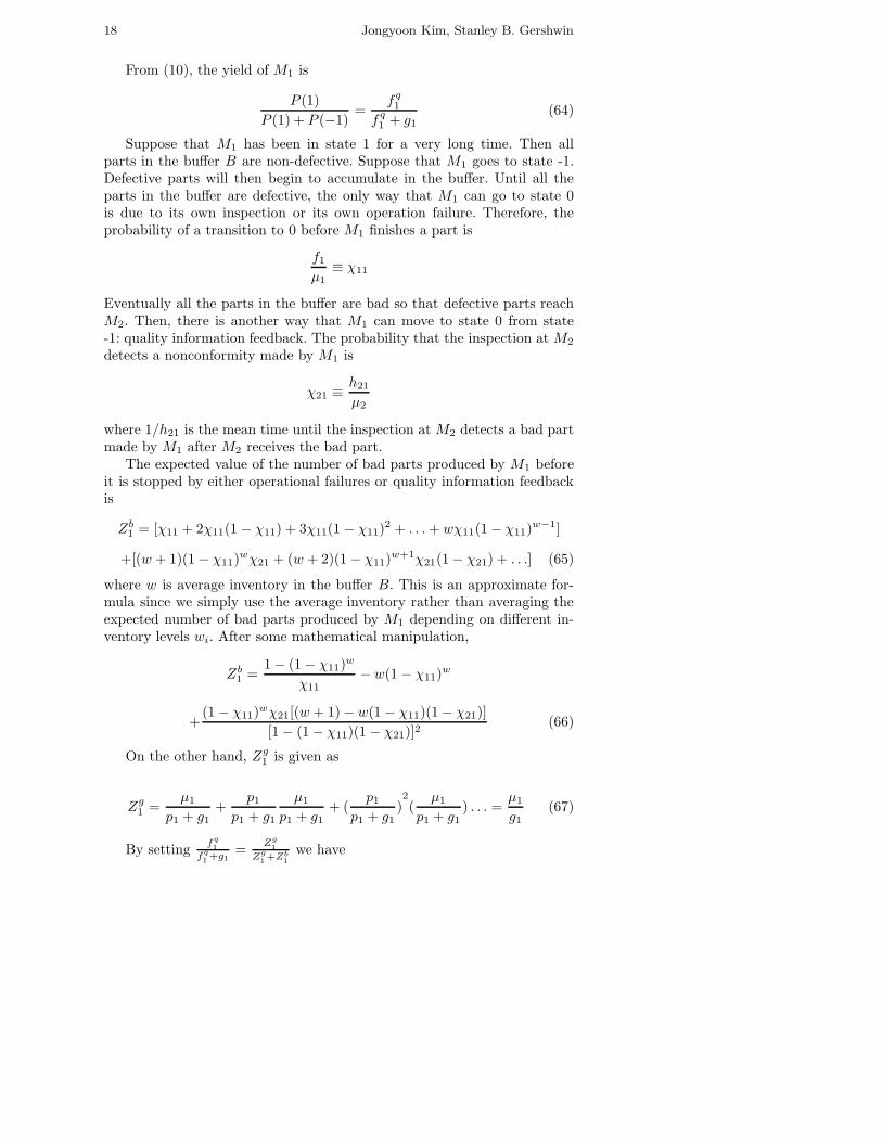
From (10), the yield of M1 is

P (1)

P (1) + P (−1)=

f q1

f q1 + g1

(64)

Suppose that M1 has been in state 1 for a very long time. Then allparts in the buffer B are non-defective. Suppose that M1 goes to state -1.Defective parts will then begin to accumulate in the buffer. Until all theparts in the buffer are defective, the only way that M1 can go to state 0is due to its own inspection or its own operation failure. Therefore, theprobability of a transition to 0 before M1 finishes a part is

f1

µ1≡ χ11

Eventually all the parts in the buffer are bad so that defective parts reachM2. Then, there is another way that M1 can move to state 0 from state-1: quality information feedback. The probability that the inspection at M2

detects a nonconformity made by M1 is

χ21 ≡h21

µ2

where 1/h21 is the mean time until the inspection at M2 detects a bad partmade by M1 after M2 receives the bad part.

The expected value of the number of bad parts produced by M1 beforeit is stopped by either operational failures or quality information feedbackis

Zb1 = [χ11 + 2χ11(1 − χ11) + 3χ11(1 − χ11)

2 + . . . + wχ11(1 − χ11)w−1]

+[(w + 1)(1 − χ11)wχ21 + (w + 2)(1 − χ11)

w+1χ21(1 − χ21) + . . .] (65)

where w is average inventory in the buffer B. This is an approximate for-mula since we simply use the average inventory rather than averaging theexpected number of bad parts produced by M1 depending on different in-ventory levels wi. After some mathematical manipulation,

Zb1 =

1 − (1 − χ11)w

χ11− w(1 − χ11)

w

+(1 − χ11)

wχ21[(w + 1) − w(1 − χ11)(1 − χ21)]

[1 − (1 − χ11)(1 − χ21)]2(66)

On the other hand, Zg1 is given as

Zg1 =

µ1

p1 + g1+

p1

p1 + g1

µ1

p1 + g1+ (

p1

p1 + g1)2(

µ1

p1 + g1) . . . =

µ1

g1(67)

By settingf

q

1

fq

1+g1

=Z

g

1

Zg

1+Zb

1

we have


f q1 =

µ1

1−(1+wχ11)(1−χ11)w

χ11

+ (1−χ11)wχ21[1+w(χ21+χ11−χ21χ11)][1−(1−χ11)(1−χ21)]2

(68)

Since the average inventory is a function of f q1 and f q

1 is dependent onthe average inventory, an iterative method is required to determine thesevalues.

-15.00%

-10.00%

-5.00%

0.00%

5.00%

10.00%

15.00%

1 5 9

13

17

21

25

29

33

37

Case Number

% e

rror

of

P E

-15.00%

-10.00%

-5.00%

0.00%

5.00%

10.00%

15.00%

1 5 9

13

17

21

25

29

33

37

Case Number %

err

or o

f In

v

Fig. 6 Validation of the quality information feedback formula

Figure 6 shows the comparison of the effective production rate and theaverage inventory from the analytic model and the simulation. 50 cases aregenerated by selecting different machine and buffer parameters and % er-rors are plotted in the y-axis. The parameters for theses cases are given inAppendix B. % errors in the effective production rate and average inven-tory are calculated using equations (62) and (63) respectively. The averageabsolute value of the % error in PE and x estimations are 1.01% and 3.67%respectively.

5 Insights From Numerical Experimentation

In this section, we perform a set of numerical experiments to provide in-tuitive insight into the behavior of production lines with inspection. Theparameters of all the cases are presented in Appendix B.

5.1 Beneficial buffer case

5.1.1 Production rates Having quality information feedback means havingmore inspection than otherwise. Therefore, machines tend to stop more fre-quently. As a result, the total production rate of the line decreases. However,the effective production rate can increase since added inspections preventthe making of defective parts. This phenomenon is shown in Figure 7. Notethat the total production rate PT without quality information feedback isconsistently higher than PT with quality information feedback regardless of


0 5 10 15 20 25 30 35 40 45 500.65

0.7

0.75

0.8

Buffer Size

Tota

l Pro

duct

ion

Rat

e

without feedbackwith feedback

0 5 10 15 20 25 30 35 40 45 500.65

0.7

0.75

0.8

Buffer Size

Effe

ctiv

e P

rodu

ctio

n R

ate


Fig. 7 Production Rates with/without Quality Information Feedback

buffer size and the opposite is true for the effective production rate PE . Alsoit should be noted that in this case, both the total production rate and theeffective production rate increase with buffer size, with or without qualityinformation feedback.

5.1.2 System yield and buffer size Even though a larger buffer increasesboth total and effective production rates in this case, it decreases yield. Asexplained in Section 4, the system yield is a function of the buffer size ifthere is quality information feedback. Figure 8 shows system yield decreasingas buffer size increases when there is quality information feedback. Thishappens because when the buffer gets larger, more material accumulatesbetween an operation and the inspection of that operation. All such materialwill be defective when the first machine is at state -1 but the inspection atthe first machine does not find it. This is a case in which a smaller bufferimproves quality, which is widely believed to be generally true. If there is noquality information feedback, then the system yield is independent of thebuffer size (and is substantially less).

5.2 Harmful buffer case

5.2.1 Production rates Typically, increasing the buffer size leads to highereffective production rate. This is the case in Figure 7. But under certainconditions, the effective production rate can actually decrease as buffer sizeincreases. This can happen when

? The first machine produces bad parts frequently: this means g1 is large.? The inspection at the first machine is poor or non-existent and inspection

at the second machine is reliable: this means h1 � h2 or f1−p1 � f2−p2.? There is quality information feedback.? The isolated production rate of the first machine is higher than that of

the second machine:

µ11 + g1/f1

1 + (p1 + g1)/r1 + g1/f1> µ2

1 + g2/f2

1 + (p2 + g2)/r2 + g2/f2


0 5 10 15 20 25 30 35 40 45 500.89

0.9

0.91

0.92

0.93

0.94

0.95

0.96

0.97

Buffer Size

Sys

tem

Yie

ld


Fig. 8 System Yield as a Function of Buffer Size

0 5 10 15 20 25 30 35 40 45 500

0.5

1

1.5

Buffer Size

Tota

l Pro

duct

ion

Rat

e

Without feedbackWith feedback

0 5 10 15 20 25 30 35 40 45 500

0.5

1

1.5

Buffer Size

Effe

ctiv

e P

rodu

ctio

n R

ate


Fig. 9 Total Production Rate and Effective Production Rate

Figure 9 shows a case in which a buffer size increase leads to a lowereffective production rate. Note that even in this case, total production ratemonotonically increases as buffer size increases.

5.2.2 System Yield The system yield for this case is shown in Figure 10.Note that the yield decreases dramatically as the buffer size increases. Inthis case, the decrease of the system yield is more than the increase of thetotal production rate so that the effective production rate monotonicallydecreases as buffer size gets bigger.

5.3 How to improve quality in a line with persistent quality failures

There are two major ways to improve quality. One is to increase the yield ofindividual operations and the other is to perform more rigorous inspection.Having extensive preventive maintenance on manufacturing equipment andusing robust engineering techniques to stabilize operations have been sug-gested as tools to increase yield of individual operations. Both approaches


0 5 10 15 20 25 30 35 40 45 500

0.1

0.2

0.3

0.4

0.5

0.6

0.7

0.8

0.9

1

Buffer Size

Sys

tem

Yie

ld


Fig. 10 System Yield as a Function of Buffer Size

increase the Mean Time to Quality Failure (MTQF) (i.e. decrease g). Onthe other hand, the inspection policy aims to detect bad parts as soon aspossible and prevent their flow toward downstream operations. More rig-orous inspection decreases the mean time to detect (MTTD) (i.e. increasesh and therefore increases f). It is natural to believe that using only onekind of method to achieve a target quality level would not give the mostcost efficient quality assurance policy. Figure 11 indicates that the impactof individual operation stabilization on the system yield decreases as theoperation becomes more stable. It also shows that effect of improving in-spection (MTTD) on the system yield decreases. Therefore, it is optimal touse a combination of both methods to improve quality.

50 100 150 200 250 300 350 400 4500

0.1

0.2

0.3

0.4

0.5

0.6

0.7

0.8

0.9

1

MTQF

Sys

tem

Yie

ld

0 0.1 0.2 0.3 0.4 0.5 0.6 0.7 0.8 0.9 10

0.1

0.2

0.3

0.4

0.5

0.6

0.7

0.8

0.9

1

f=p+h

Sys

tem

Yie

ld

Fig. 11 Quality Improvement


5.4 How to increase productivity

Improving the stand-alone throughput of each operation and increasing thebuffer space are typical ways to increase the production rate of manufactur-ing systems. If operations are apt to have quality failures, however, theremay be other ways to increase the effective production rate: increasing theyield of each operation and conducting more extensive inspections. Stabi-lizing operations, thus improving the yield of individual operations, willincrease effective throughput of a manufacturing system regardless of thetype of quality failure. On the other hand, reducing the mean time to detect(MTTD) will increase the effective production rate only if the quality failureis persistent but it will decrease the effective production rate if the qualityfailure is Bernoulli. This is because the quality of each part is independentof the others when the quality failure is Bernoulli. Therefore, stopping theline does not reduce the number of bad parts in the future.

In a situation in which machines produce defective parts frequently andinspection is poor, increasing inspection reliability is more effective thanincreasing buffer size to boost the effective production rate. Figure 12 showsthis. Also, in other situations in which machines produce defective partsfrequently and inspection is reliable, increasing machine stability is moreeffective than increasing buffer size to enhance effective production rate.Figure 13 shows this phenomenon.

0 5 10 15 20 25 30 35 400.5

0.55

0.6

0.65

0.7

0.75

0.8

Buffer Size

Effe

ctiv

e P

rodu

ctio

n R

ate

MTTD = 20MTTD = 10MTTD = 2

Fig. 12 Mean Time to Detect and Effective Production Rate

6 Future Research

The 2-Machine-1-Buffer (2M1B) model with µ1 6= µ2 is analyzed in [14].This case is more challenging because the number of roots of the internaltransition equations depends on parameters of machine. A more general


0 5 10 15 20 25 30 35 400.3

0.4

0.5

0.6

0.7

0.8

0.9

Buffer Size

Effe

ctiv

e P

rodu

ctio

n R

ate

MTQF = 20MTQF = 100MTQF = 500

Fig. 13 Quality Failure Frequency and Effective Production Rate

2M1B model with multiple-yield quality failures (a mixture of Bernoulli-and persistent-type quality failures) should also be studied. A long lineanalysis using decomposition is under the development. Refer to Kim [14]for more detailed information.

Acknowledgments

The authors would like to thank the Singapore-MIT Alliance and PSAPeugeot-Citroen for their support of this research.

References

1. Alles M, Amershi A, Datar S, and Sarkar R (2000) Information and incentiveeffects of inventory in JIT production. Management science 46 (12): 1528–1544.

2. Besterfield D H, Besterfield-Michna C, Besterfield G, and Besterfield-Sacre M,(2003) Total quality management. Prentice Hall.

3. Black J T (1991) The design of the factory with a future. McGraw-Hill.

4. Bonvik A M, Couch C E, and Gershwin S B (1997) A comparison of productionline control mechanisms. International journal of production research 35 (3):789–804.

5. Burman M, Gershwin S B, and Suyematsu C (1998) Hewlett-Packard usesoperations research to improve the design of a printer production line. Interfaces28 (1): 24–26.

6. Buzacott J A and Shantikumar J G (1993) Stochastic models of manufacturingsystems. Prentice-Hall.

7. Cheng C H, Miltenburg J, and Motwani J (2000) The effect of straight and Ushaped lines on quality. IEEE Transactions on Engineering Management 47 (3):321-334.


8. Dallery Y. and Gershwin S B (1992) Manufacturing flow line systems: a reviewof models and analytical results. Queuing Systems Theory and Applications 12:3–94.

9. Fujimoto T (1999) The evolution of a manufacturing systems at Toyota. OxfordUniversity Press.

10. Gershwin S B (1994) Manufacturing systems engineering. Prentice Hall.11. Gershwin S B (2000) Design and Operation of Manufacturing Systems — The

Control-Point Policy. IIE Transactions 32 (2): 891-906.12. Gershwin S B and Schor J E (2000) Efficient algorithms for buffer space

allocation. Annals of Operations Research 93: 117-144.13. Inman R R, Blumenfeld D E, Huang N, and Li J (2003) Designing produc-

tion systems for quality: research opportunities from an automotive industryperspective. International journal of production research 41 (9): 1953–1971.

14. Kim J (2004) Integrated Quality and Quantity Modeling of a Production Line.Massachusetts Institute of Technology Ph.D. thesis in preparation.

15. Law A M, Kelton D W, Kelton W D, and Kelton D M(1999) Simulationmodeling and analysis. McGraw-Hill.

16. Ledolter J and Burrill C W (1999) Statistical quality control. John Wiley &Sons.

17. Monden Y (1998) Toyota production system — An integrated approach toJust-In-Time. EMP Books, 1998.

18. Montgomery D C (2001) Introduction to statistical quality control 4th edition.John Wiley & Sons.

19. Pande P and Holpp L (2002) What is six sigma? McGraw-Hill.20. Phadke M (1989) Quality engineering using robust design. Prentice Hall.21. Raz T (1986) A survey of models for allocating inspection effort in multistage

production systems. Journal of quality technology 18 (4): 239–246.22. Shin W S, Mart S M, and Lee H F (1995) Strategic allocation of inspection

stations for a flow assembly line: a hybrid procedure. IIE Transactions 27: 707–715.

23. Shingo S, (1989) A study of the Toyota production system from an industrialengineering viewpoint. Productivity Press.

24. Toyota Motor Corporation (1996) The Toyota production system.25. Wein L, (1988) Scheduling semiconductor wafer fabrication. IEEE Transac-

tions on semiconductor manufacturing 1(3): 115–130.26. Wooddall W H and Montgomery D C (1999) Research issues and ideas in

statistical process control. Journal of Quality Technology 31 (4): 376–386.

Appendix

A Solution technique

It is natural to assume an exponential form for the solution to the steadystate density functions since equations (23)–(31) are coupled ordinary lineardifferential equations. A solution of the form eλxKα1

1 Kα2

2 worked success-fully in the continuous material two-machine line with perfect quality [10].Therefore, a solution of a form

f(x, α1, α2) = eλxG1(α1)G2(α2) (69)


is assumed here. This form satisfies the transition equations if all of thefollowing equations are met. Equations (23)–(31) become, after substituting(69),

{(µ2 −µ1)λ− (p1 + g1 + p2 + g2)G1(1)G2(1)}+ r2G1(1)G2(0)+ r1G1(0)G2(1) = 0(70)

−{µ1λ + (p1 + g1 + r2)}G1(1)G2(0) + p2G1(1)G2(1) + f2G1(1)G2(−1)

+r1G1(0)G2(0) = 0 (71)

{(µ2 − µ1)λ− (p1 + g1 + f2)}G1(1)G2(−1) + g2G1(1)G2(1) + r1G1(0)G2(−1) = 0(72)

{µ2λ − (r1 + p2 + g2)}G1(0)G2(1) + p1G1(1)G2(1) + r2G1(0)G2(0)

+f1G1(−1)G2(1) = 0 (73)

p1G1(1)G2(0) + p2G1(0)G2(1) − (r1 + r2)G1(0)G2(0) + f2G1(0)G2(−1)

+f1G1(−1)G2(0) = 0 (74)

{µ2λ − (r1 + f2)}G1(0)G2(−1) + p1G1(1)G2(−1) + g2G1(0)G2(1)

+f1G1(−1)G2(−1) = 0 (75)

{(µ2 − µ1)λ− (p2 + g2 + f1)}G1(−1)G2(1) + g1G1(1)G2(1) + r2G1(−1)G2(0) = 0(76)

−{µ1λ + (r2 + f1)}G1(−1)G2(0) + g1G1(1)G2(0) + p2G1(−1)G2(1)

+f2G1(−1)G2(−1) = 0 (77)

{(µ2 − µ1)λ − (f1 + f2)}G1(−1)G2(−1) + g1G1(1)G2(−1) + g2G1(−1)G2(1) = 0(78)

These are nine equations in seven unknowns (λ, G1(1), G2(0), G1(−1),G2(1), G2(0), and G2(−1)). Thus, there must be seven independent equa-tions and two dependent ones.

If we divide equations (70) – (78) by G1(0)G2(0) and define new param-eters

Γi = piGi(1)

Gi(0)− ri + fi

Gi(−1)

Gi(0)(79)

Ψi = −pi − gi + riGi(0)

Gi(1)(80)


Θi = −fi + giGi(1)

Gi(−1)(81)

then equations (70)–(78) can be rewritten as

Γ1 + Γ2 = 0 (82)

−µ2λ = Γ1 + Ψ2 (83)

µ1λ = Γ2 + Ψ1 (84)

(µ1 − µ2)λ = Ψ1 + Ψ2 (85)

(µ1 − µ2)λ = Θ1 + Θ2 (86)

µ1λ = Γ2 + Θ1 (87)

−µ2λ = Γ1 + Θ2 (88)

(µ1 − µ2)λ = Ψ2 + Θ1 (89)

(µ1 − µ2)λ = Ψ1 + Θ2 (90)

From equations (82)–(90), it is clear that only seven equations are in-dependent. After much mathematical manipulation [14], these equationsbecome

0 = {(M+r1)(µ1N−1)−f1}2

(f1−p1)(µ1N−1)

− {(p1+g1−f1)+r1(µ1N−1)}{(M+r1)(µ1N−1)−f1}(f1−p1)(µ1N−1)

− r1

(91)

0 = {(−M+r2)(µ2N−1)−f2}2

(f2−p2)(µ2N−1)

− {(p2+g2−f2)+r2(µ2N−1)}{(−M+r2)(µ2N−1)−f2}(f2−p2)(µ2N−1)

− r2 = 0

(92)

where

p1G1(1)

G1(0)− r1 + f1

G1(−1)

G1(0)= −

(

p2G2(1)

G2(0)− r2 + f2

G2(−1)

G2(0)

)

= M (93)

1µ1

(

1 + 1

G1(1)/G1(0)+G1(−1)/G1(0)

)

=

1µ2

(

1 + 1

G2(1)/G2(0)+G2(−1)/G2(0)

)

= N

(94)


−3 −2 −1 0 1 2 3−3

−2

−1

0

1

2

3

M

N

(91)

(92)

Fig. 14 Plot of Equations (91) and (92)

Now all the equations and unknowns are simplified into two unknownsand two equations. By solving equations (91) and (92) simultaneously wecan calculate M and N . An example of these equations is plotted in Figure14. Equation (91) is represented with lighter lines and equation (92) is shownas darker lines. The intersections of the two sets of lines are the solutionsof the equations.

These are high order polynomial equations for which no general analyti-cal solution exists. A numerical approach is required to find the roots of theequations. A special algorithm to find the solutions has been developed [14]based on the characteristics of the equations. Once we find roots of equations

(91) and (92), we can get ratios Gi(1)Gi(0)

and Gi(−1)Gi(0)

(i = 1, 2) from equation

(94). By setting G1(0) = G2(0) = 1, we can calculate G1(1), G1(−1), G2(1),and G2(−1). After some mathematical manipulation, we find that λ can beexpressed as

λ =−p1 − g1 + r1/G1(1) − p1G1(1) + r1 − f1G1(−1)

µ1(95)

Therefore, we can get a probability density function f(x, α1, α2) corre-sponding to an (M, N) pair. The number of roots in equations (91) and(92) depends on machine parameters. There are only 3 roots when µ1 = µ2


regardless of other parameters. Therefore, a general expression of the prob-ability density function in this case is

f(x, α1, α2) = c1f1(x, α1, α2) + c2f2(x, α1, α2) + c3f3(x,α1, α2) (96)

where f1(x, α1, α2), f2(x, α1, α2), f3(x, α1, α2) are the roots of the equations(91) and (92).

The remaining unknowns, including c1, c2, c3 and probability masses atthe boundaries, can be calculated by solving boundary equations ((34)–(55))and the normalization equation (56) with fi(x, α1, α2) given by equation(96).

B Machine Parameters for Numerical and Simulation

Experiments

Table 4 Machine Parameters for Infinite Buffer Case and Zero Buffer Case

Case # µ1 µ2 r1 r2 p1 p2 g1 g2 f1 f2

1 1.0 1.0 0.1 0.1 0.01 0.01 0.01 0.01 0.2 0.22 1.0 1.0 0.3 0.3 0.005 0.005 0.05 0.05 0.5 0.53 1.0 1.0 0.2 0.05 0.01 0.01 0.01 0.01 0.2 0.24 1.0 1.0 0.1 0.1 0.05 0.005 0.01 0.01 0.2 0.25 1.0 1.0 0.1 0.1 0.01 0.01 0.05 0.005 0.2 0.26 1.0 1.0 0.1 0.1 0.01 0.01 0.01 0.01 0.5 0.17 2.0 1.0 0.1 0.1 0.01 0.01 0.01 0.01 0.5 0.18 3.0 2.0 0.1 0.1 0.01 0.01 0.01 0.01 0.2 0.29 1.0 2.0 0.1 0.1 0.01 0.01 0.01 0.01 0.2 0.210 2.0 3.0 0.1 0.1 0.01 0.01 0.01 0.01 0.2 0.2

Table 5 Machine Parameters for Figures 7 and 8

µ1 µ2 r1 r2 p1 p2 g1 g2 f1 f2

1.0 1.0 0.1 0.1 0.01 0.01 0.01 0.01 0.1 0.9

Table 6 Machine Parameters for Figures 9 and 10

µ1 µ2 r1 r2 p1 p2 g1 g2 f1 f2

2.0 2.0 0.5 0.1 0.005 0.05 0.5 0.005 0.02 0.9


Table 7 Machine Parameters for Figure 11

µ1 µ2 r1 r2 p1 p2 g1 g2 f1 f2

1.0 1.0 0.1 0.1 0.01 0.01 0.01 0.01 0.2 0.2


µ1 µ2 r1 r2 p1 p2 g1 g2

1.0 1.0 0.1 0.1 0.01 0.01 0.01 0.01


µ1 µ2 r1 r2 p1 p2 f1 f2

1.0 1.0 0.1 0.1 0.01 0.01 0.2 0.2


Table 10 Machine Parameters for Intermediate Buffer Case Validation

Case # µ1 µ2 r1 r2 p1 p2 g1 g2 f1 f2 N

1 1.0 1.0 0.1 0.1 0.01 0.01 0.02 0.01 0.1 0.2 302 1.0 1.0 0.1 0.1 0.01 0.01 0.01 0.01 0.2 0.2 53 1.0 1.0 0.1 0.1 0.01 0.01 0.01 0.01 0.2 0.2 104 1.0 1.0 0.1 0.1 0.01 0.01 0.01 0.01 0.2 0.2 155 1.0 1.0 0.1 0.1 0.01 0.01 0.01 0.01 0.2 0.2 206 1.0 1.0 0.1 0.1 0.01 0.01 0.01 0.01 0.2 0.2 257 1.0 1.0 0.1 0.1 0.01 0.01 0.01 0.01 0.2 0.2 358 1.0 1.0 0.1 0.1 0.01 0.01 0.01 0.01 0.2 0.2 409 1.0 1.0 0.1 0.1 0.01 0.01 0.01 0.01 0.2 0.2 4510 0.5 0.5 0.1 0.1 0.01 0.01 0.01 0.01 0.2 0.2 3011 1.5 1.5 0.1 0.1 0.01 0.01 0.01 0.01 0.2 0.2 3012 2.0 2.0 0.1 0.1 0.01 0.01 0.01 0.01 0.2 0.2 3013 2.5 2.5 0.1 0.1 0.01 0.01 0.01 0.01 0.2 0.2 3014 3.0 3.0 0.1 0.1 0.01 0.01 0.01 0.01 0.2 0.2 3015 1.0 1.0 0.01 0.01 0.01 0.01 0.01 0.01 0.2 0.2 3016 1.0 1.0 0.05 0.05 0.01 0.01 0.01 0.01 0.2 0.2 3017 1.0 1.0 0.2 0.2 0.01 0.01 0.01 0.01 0.2 0.2 3018 1.0 1.0 0.5 0.5 0.01 0.01 0.01 0.01 0.2 0.2 3019 1.0 1.0 0.8 0.8 0.01 0.01 0.01 0.01 0.2 0.2 3020 1.0 1.0 0.1 0.1 0.001 0.001 0.01 0.01 0.2 0.2 3021 1.0 1.0 0.1 0.1 0.005 0.005 0.01 0.01 0.2 0.2 3022 1.0 1.0 0.1 0.1 0.02 0.02 0.01 0.01 0.2 0.2 3023 1.0 1.0 0.1 0.1 0.05 0.05 0.01 0.01 0.2 0.2 3024 1.0 1.0 0.1 0.1 0.1 0.1 0.01 0.01 0.2 0.2 3025 1.0 1.0 0.1 0.1 0.01 0.01 0.001 0.001 0.2 0.2 3026 1.0 1.0 0.1 0.1 0.01 0.01 0.005 0.005 0.2 0.2 3027 1.0 1.0 0.1 0.1 0.01 0.01 0.02 0.02 0.2 0.2 3028 1.0 1.0 0.1 0.1 0.01 0.01 0.05 0.05 0.2 0.2 3029 1.0 1.0 0.1 0.1 0.01 0.01 0.10 0.10 0.2 0.2 3030 1.0 1.0 0.1 0.1 0.01 0.01 0.01 0.01 0.02 0.02 3031 1.0 1.0 0.1 0.1 0.01 0.01 0.01 0.01 0.05 0.05 3032 1.0 1.0 0.1 0.1 0.01 0.01 0.01 0.01 0.1 0.1 3033 1.0 1.0 0.1 0.1 0.01 0.01 0.01 0.01 0.5 0.5 3034 1.0 1.0 0.1 0.1 0.01 0.01 0.01 0.01 0.95 0.95 3035 1.0 1.0 0.5 0.1 0.01 0.01 0.01 0.01 0.2 0.2 3036 1.0 1.0 0.01 0.1 0.01 0.01 0.01 0.01 0.2 0.2 3037 1.0 1.0 0.1 0.5 0.01 0.01 0.01 0.01 0.2 0.2 3038 1.0 1.0 0.1 0.01 0.01 0.01 0.01 0.01 0.2 0.2 3039 1.0 1.0 0.1 0.1 0.1 0.01 0.01 0.01 0.2 0.2 3040 1.0 1.0 0.1 0.1 0.001 0.01 0.01 0.01 0.2 0.2 3041 1.0 1.0 0.1 0.1 0.01 0.1 0.01 0.01 0.2 0.2 3042 1.0 1.0 0.1 0.1 0.01 0.001 0.01 0.01 0.2 0.2 3043 1.0 1.0 0.1 0.1 0.01 0.01 0.1 0.01 0.2 0.2 3044 1.0 1.0 0.1 0.1 0.01 0.01 0.001 0.01 0.2 0.2 3045 1.0 1.0 0.1 0.1 0.01 0.01 0.01 0.1 0.2 0.2 3046 1.0 1.0 0.1 0.1 0.01 0.01 0.01 0.001 0.2 0.2 3047 1.0 1.0 0.1 0.1 0.01 0.01 0.01 0.01 0.9 0.2 3048 1.0 1.0 0.1 0.1 0.01 0.01 0.01 0.01 0.05 0.2 3049 1.0 1.0 0.1 0.1 0.01 0.01 0.01 0.01 0.2 0.9 3050 1.0 1.0 0.1 0.1 0.01 0.01 0.01 0.01 0.2 0.05 30


Table 11 Machine Parameters for Quality Information Feedback Validation

Case # µ1 µ2 r1 r2 p1 p2 g1 g2 f1 f2 N

1 1.0 1.0 0.1 0.1 0.01 0.01 0.01 0.01 0.01 1.0 102 1.0 1.0 0.1 0.1 0.01 0.01 0.01 0.01 0.01 1.0 03 1.0 1.0 0.1 0.1 0.01 0.01 0.01 0.01 0.01 1.0 54 1.0 1.0 0.1 0.1 0.01 0.01 0.01 0.01 0.01 1.0 205 1.0 1.0 0.1 0.1 0.01 0.01 0.01 0.01 0.01 1.0 306 1.0 1.0 0.01 0.01 0.01 0.01 0.01 0.01 0.01 1.0 107 1.0 1.0 0.05 0.05 0.01 0.01 0.01 0.01 0.01 1.0 108 1.0 1.0 0.4 0.4 0.01 0.01 0.01 0.01 0.01 1.0 109 1.0 1.0 0.8 0.8 0.01 0.01 0.01 0.01 0.01 1.0 1010 1.0 1.0 0.1 0.1 0.001 0.001 0.01 0.001 0.01 1.0 1011 1.0 1.0 0.1 0.1 0.005 0.005 0.01 0.005 0.01 1.0 1012 1.0 1.0 0.1 0.1 0.02 0.02 0.01 0.01 0.02 1.0 1013 1.0 1.0 0.1 0.1 0.1 0.1 0.01 0.01 0.1 1.0 1014 1.0 1.0 0.1 0.1 0.01 0.01 0.001 0.001 0.01 1.0 1015 1.0 1.0 0.1 0.1 0.01 0.01 0.005 0.005 0.01 1.0 1016 1.0 1.0 0.1 0.1 0.01 0.01 0.02 0.02 0.01 1.0 1017 1.0 1.0 0.1 0.1 0.01 0.01 0.05 0.05 0.01 1.0 1018 0.5 0.5 0.1 0.1 0.01 0.01 0.01 0.01 0.01 1.0 1019 1.5 1.5 0.1 0.1 0.01 0.01 0.01 0.01 0.01 1.0 1020 2.0 2.0 0.1 0.1 0.01 0.01 0.01 0.01 0.01 1.0 1021 1.0 1.0 0.1 0.1 0.01 0.01 0.01 0.01 0.05 1.0 1022 1.0 1.0 0.1 0.1 0.01 0.01 0.01 0.01 0.2 1.0 1023 1.0 1.0 0.1 0.1 0.01 0.01 0.01 0.01 0.5 1.0 1024 1.0 1.0 0.1 0.1 0.01 0.01 0.01 0.01 0.8 1.0 1025 1.0 1.0 0.5 0.1 0.01 0.01 0.01 0.01 0.01 1.0 1026 1.0 1.0 0.01 0.1 0.01 0.01 0.01 0.01 0.01 1.0 1027 1.0 1.0 0.1 0.5 0.01 0.01 0.01 0.01 0.01 1.0 1028 1.0 1.0 0.1 0.01 0.01 0.01 0.01 0.01 0.01 1.0 1029 1.0 1.0 0.1 0.1 0.1 0.01 0.01 0.01 0.1 1.0 1030 1.0 1.0 0.1 0.1 0.001 0.01 0.01 0.01 0.001 1.0 1031 1.0 1.0 0.1 0.1 0.01 0.1 0.01 0.01 0.01 1.0 1032 1.0 1.0 0.1 0.1 0.01 0.001 0.01 0.01 0.01 1.0 1033 1.0 1.0 0.1 0.1 0.01 0.01 0.05 0.01 0.01 1.0 1034 1.0 1.0 0.1 0.1 0.01 0.01 0.001 0.01 0.01 1.0 1035 1.0 1.0 0.1 0.1 0.01 0.01 0.01 0.05 0.01 1.0 1036 1.0 1.0 0.1 0.1 0.01 0.01 0.01 0.001 0.01 1.0 1037 1.0 1.0 0.1 0.1 0.01 0.01 0.01 0.01 0.5 1.0 1038 1.0 1.0 0.1 0.1 0.01 0.01 0.01 0.01 0.2 1.0 1039 1.0 1.0 0.1 0.1 0.01 0.01 0.01 0.01 0.01 0.8 1040 1.0 1.0 0.1 0.1 0.01 0.01 0.01 0.01 0.01 0.2 10

Documents

Integrated Quality and Quantity Modeling of a Production …web.mit.edu/manuf-sys/www/oldcell1/papers/kim-gershwin-qq04.pdf · OR Spectrum manuscript No. (will be inserted by the