Quality/Quantity Modeling and Analysis

of Production Lines Subject to UncertaintyPhase I, Final Report

Presented to General Motors R & D Center

Irvin C. Schick, Stanley B. Gershwin, and Jongyoon Kim

Laboratory for Manufacturing and Productivity

Department of Mechanical Engineering

Massachusetts Institute of Technology

Cambridge, Massachusetts 02139-4307

May 10, 2005

Abstract

During the past three decades, the success of the Toyota Production System (TPS) and otherproduction system design methodologies have spurred much research in manufacturing systems en-gineering. However, although productivity and quality have each been extensively studied, there hasbeen little research on how they interact. This report describes work done under GM funding to ana-lyze how production system design, quality, and productivity are inter-related in production networks,and to develop analytical as well as numerical methods that make it possible to evaluate, compare,and optimize the performance of competing designs. More specifically, it summarizes simulated,analytical, and numerical results concerning the effect of separating inspection from operation, asa function of machine, buffer, and inspection station parameters; control policy; production systemtopology, and other factors.

In this report, a taxonomy is presented for quality failures, and a class of stochastic models isdescribed to represent a realistic subset of those failures. Quality control mechanisms are formulated,including scrapping of defective parts as well as an information feedback scheme that results in takingoffending machines down for maintenance. Pertinent performance measures are defined, includingmean total production rate, good (i.e. not defective) production rate, yield, in-process inventory, andlead time.

Analytical results based upon a continuous-material approximation of a two-stage line are pre-sented, and these results are validated by comparison with discrete-event simulation. It is shown, inparticular, that production rate is not always a monotonically increasing function of buffer capac-ity when quality inspection and information feedback are present; that taking a machine down formaintenance as soon as a single quality defect is detected (jidoka) is not always the optimal policy,and that system parameters must be taken into account in determining the best course of actionfollowing the detection of one or more defects.

Further simulation results include the investigation of the effect of the number and placementof inspection stations, of machine and buffer parameters, of inspection policies, of control policies(scrapping and information feedback), and of production line topology on selected performancemeasures. In particular, it is shown that performance can be quite sensitive to the placement ofinspection stations, so that a few well-placed inspection stations will result in better performancethan many poorly-placed ones.

1

Contents

1 Introduction 4

2 Modeling and Taxonomy 5

2.1 Production Systems . . . . . . . . . . . . . . . . . . . . . . . . . . . . . . . . . . . . . 5

2.1.1 Machines . . . . . . . . . . . . . . . . . . . . . . . . . . . . . . . . . . . . . . 6

2.1.2 Buffers . . . . . . . . . . . . . . . . . . . . . . . . . . . . . . . . . . . . . . . . 11

2.1.3 Topology . . . . . . . . . . . . . . . . . . . . . . . . . . . . . . . . . . . . . . . 12

2.2 Quality Failures . . . . . . . . . . . . . . . . . . . . . . . . . . . . . . . . . . . . . . . 13

2.2.1 Internal vs. External Failures . . . . . . . . . . . . . . . . . . . . . . . . . . . . 14

2.2.2 Dynamic Characteristics . . . . . . . . . . . . . . . . . . . . . . . . . . . . . . . 14

2.2.3 Correlation and Stacking . . . . . . . . . . . . . . . . . . . . . . . . . . . . . . 16

2.3 Inspection . . . . . . . . . . . . . . . . . . . . . . . . . . . . . . . . . . . . . . . . . . 18

2.3.1 Destructive vs. Non-Destructive Testing . . . . . . . . . . . . . . . . . . . . . . 18

2.3.2 Domain and Frequency . . . . . . . . . . . . . . . . . . . . . . . . . . . . . . . 19

2.3.3 Accuracy and Declaration of a Defective Part . . . . . . . . . . . . . . . . . . . 19

2.3.4 Declaration of an Impaired Machine . . . . . . . . . . . . . . . . . . . . . . . . 20

2.4 Control Policies . . . . . . . . . . . . . . . . . . . . . . . . . . . . . . . . . . . . . . . 20

2.4.1 Action on Defective Parts . . . . . . . . . . . . . . . . . . . . . . . . . . . . . . 21

2.4.2 Action on Impaired Machines . . . . . . . . . . . . . . . . . . . . . . . . . . . . 22

2.4.3 Action on People . . . . . . . . . . . . . . . . . . . . . . . . . . . . . . . . . . 22

2.5 Measures of System Performance . . . . . . . . . . . . . . . . . . . . . . . . . . . . . . 23

2.5.1 Quantity and Quality . . . . . . . . . . . . . . . . . . . . . . . . . . . . . . . . 23

2.5.2 Inventory . . . . . . . . . . . . . . . . . . . . . . . . . . . . . . . . . . . . . . . 24

2.5.3 Production Lead Time . . . . . . . . . . . . . . . . . . . . . . . . . . . . . . . 25

3 Analytical Results 25

3.1 Mathematical Models . . . . . . . . . . . . . . . . . . . . . . . . . . . . . . . . . . . . 25

3.1.1 Single Machine Model . . . . . . . . . . . . . . . . . . . . . . . . . . . . . . . . 25

3.1.2 The 2-Machine-1-Buffer Continuous Model . . . . . . . . . . . . . . . . . . . . 28

3.1.3 The Infinite Buffer Case . . . . . . . . . . . . . . . . . . . . . . . . . . . . . . . 28

3.1.4 The Zero Buffer Case . . . . . . . . . . . . . . . . . . . . . . . . . . . . . . . . 29

3.1.5 The 2-Machine-1-Finite-Buffer Line . . . . . . . . . . . . . . . . . . . . . . . . 30

3.1.6 Quality Information Feedback . . . . . . . . . . . . . . . . . . . . . . . . . . . . 30

3.1.7 Insights From Numerical Experimentation . . . . . . . . . . . . . . . . . . . . . 31

3.2 Effectiveness of the Jidoka Stopping Policy . . . . . . . . . . . . . . . . . . . . . . . . . 35

3.2.1 Motivation . . . . . . . . . . . . . . . . . . . . . . . . . . . . . . . . . . . . . . 35

3.2.2 Single Machine . . . . . . . . . . . . . . . . . . . . . . . . . . . . . . . . . . . 37

3.2.3 Analysis of a Two-Machine System . . . . . . . . . . . . . . . . . . . . . . . . . 39

3.2.4 Effectiveness of Jidoka . . . . . . . . . . . . . . . . . . . . . . . . . . . . . . . 40

3.3 Modeling and Analysis of Long Flow Lines with Quality and Operational Failures . . . . 43

3.3.1 Motivation and Literature Review . . . . . . . . . . . . . . . . . . . . . . . . . 43

3.3.2 Ubiquitous Inspection . . . . . . . . . . . . . . . . . . . . . . . . . . . . . . . . 44

3.3.3 Remote Quality Information Feedback . . . . . . . . . . . . . . . . . . . . . . . 47

2

3.3.4 Multiple Quality Information Feedback . . . . . . . . . . . . . . . . . . . . . . . 48

4 Simulation Studies 504.1 Location and Number of Inspection Stations . . . . . . . . . . . . . . . . . . . . . . . . 504.2 Control Policies . . . . . . . . . . . . . . . . . . . . . . . . . . . . . . . . . . . . . . . 52

4.2.1 Scrapping . . . . . . . . . . . . . . . . . . . . . . . . . . . . . . . . . . . . . . 524.2.2 Quality Information Feedback . . . . . . . . . . . . . . . . . . . . . . . . . . . . 55

4.3 Production System Topology . . . . . . . . . . . . . . . . . . . . . . . . . . . . . . . . 59

5 Conclusion 625.1 Summary . . . . . . . . . . . . . . . . . . . . . . . . . . . . . . . . . . . . . . . . . . . 625.2 Current Research . . . . . . . . . . . . . . . . . . . . . . . . . . . . . . . . . . . . . . 63

5.2.1 Exploration of Phenomena . . . . . . . . . . . . . . . . . . . . . . . . . . . . . 635.2.2 Validation of model assumptions . . . . . . . . . . . . . . . . . . . . . . . . . . 635.2.3 GM factory case study . . . . . . . . . . . . . . . . . . . . . . . . . . . . . . . 64

5.3 Further Research . . . . . . . . . . . . . . . . . . . . . . . . . . . . . . . . . . . . . . . 645.3.1 Non-Instantaneous Inspection . . . . . . . . . . . . . . . . . . . . . . . . . . . . 645.3.2 Buffer Delays and Failures . . . . . . . . . . . . . . . . . . . . . . . . . . . . . 645.3.3 Analytical Models Of Scrapping . . . . . . . . . . . . . . . . . . . . . . . . . . 645.3.4 Non-FIFO Buffer Discipline . . . . . . . . . . . . . . . . . . . . . . . . . . . . . 655.3.5 Rework . . . . . . . . . . . . . . . . . . . . . . . . . . . . . . . . . . . . . . . . 655.3.6 Analytic Modeling of More Elaborate Failure Dynamics . . . . . . . . . . . . . . 655.3.7 Preventive Maintenance . . . . . . . . . . . . . . . . . . . . . . . . . . . . . . . 665.3.8 More General Phenomena, Including Loops, Batches, and Setups . . . . . . . . . 665.3.9 Integrated Models Of Material Flow Control And Inspection . . . . . . . . . . . 665.3.10 Decomposition Without Reducing Machine Models to Two States . . . . . . . . 665.3.11 Two-Machine, One-Buffer Lines with Good and Bad Parts Modeled Distinctly in

the Buffer . . . . . . . . . . . . . . . . . . . . . . . . . . . . . . . . . . . . . . 665.3.12 More General Inspection Strategies . . . . . . . . . . . . . . . . . . . . . . . . . 67

3

1 Introduction

Manufacturers strive to satisfy two requirements while minimizing cost. These are quality (every im-portant characteristic of every manufactured item must satisfy certain specifications) and quantity (aspecified number of items must be produced within a specified time interval). The task of satisfyingthese requirements is complicated by the presence of uncertainty (changing machine characteristics,unknown machine state, imprecise observations of machine output, etc.) as well as changing conditions(variable demand, lead time, inventory constraints, product mix, etc.).

Production system designers must make quality-motivated decisions such as choosing operation pa-rameters (for example, speeds and feed rates in metal-cutting), the locations of inspection stations,and the actions to take in response to failed inspections. They must also make quantity-motivateddecisions such as the sizes of buffers and the structures of production systems. Precise mathemati-cal models have not been available for all relevant performance measures, but even when some havebeen formulated, quality-motivated design choices have historically been evaluated with quality-focusedmodels, and quantity-motivated design choices with quantity-focused models. Precise models to simul-taneously predict the interaction of quantity- and quality-related design choices on quantity and qualityperformance are needed, but do not exist.

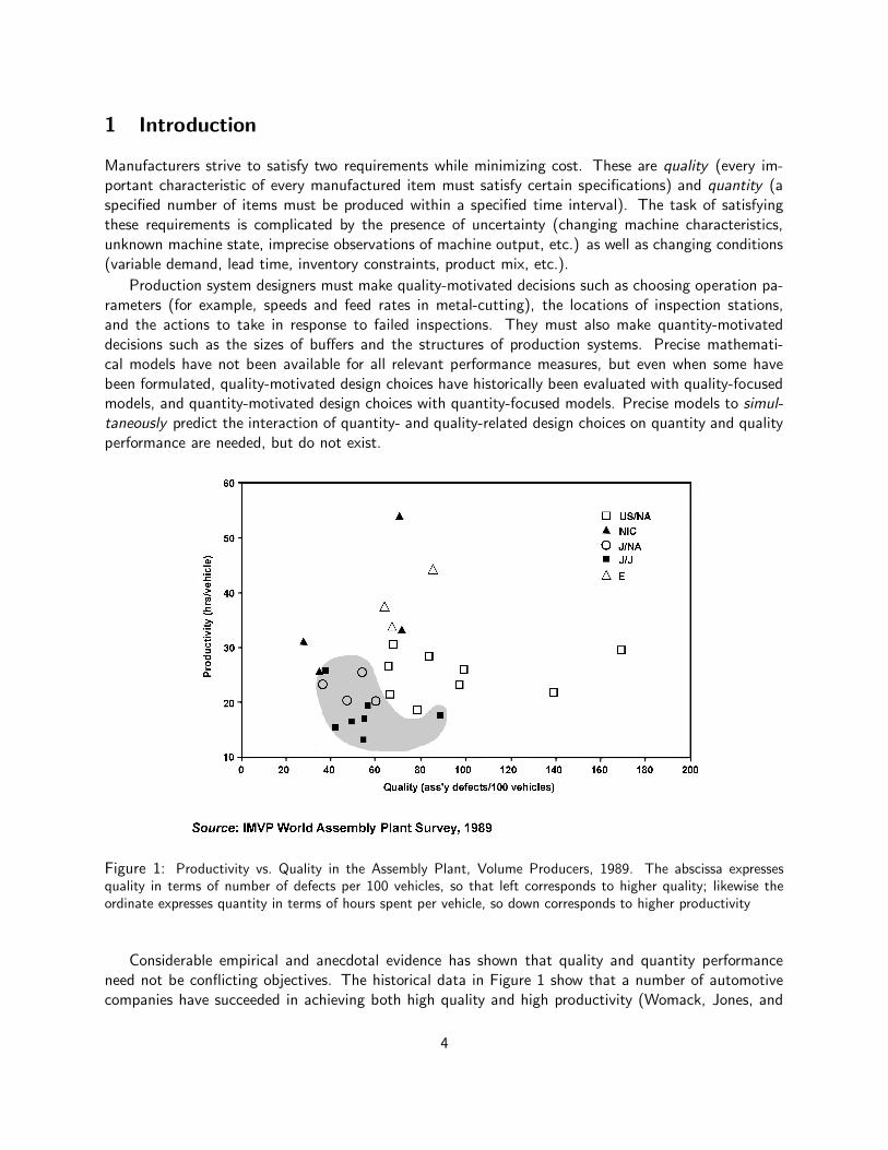
Figure 1: Productivity vs. Quality in the Assembly Plant, Volume Producers, 1989. The abscissa expressesquality in terms of number of defects per 100 vehicles, so that left corresponds to higher quality; likewise theordinate expresses quantity in terms of hours spent per vehicle, so down corresponds to higher productivity

Considerable empirical and anecdotal evidence has shown that quality and quantity performanceneed not be conflicting objectives. The historical data in Figure 1 show that a number of automotivecompanies have succeeded in achieving both high quality and high productivity (Womack, Jones, and

4

Roos 1990). Many lessons and design rules have been extracted from such studies, but predictive modelsare lacking.

During the past three decades, the success of the Toyota Production System (TPS) (Monden 1983)has spurred much research in manufacturing systems design. Numerous research papers have exploredthe relationship between production system design and productivity, so as to formulate ways of designingfactories that manufacture more products, on time, and more economically (in terms of labor, material,and space). At the same time, topics in quality research have captured the attention of practitionersand academics alike since the early 1980s. The recent popularity of Statistical Quality Control (SQC)(Woodall and Montgomery 1999), Total Quality Management (TQM) (Besterfield, Besterfield-Michna,Besterfield, and Besterfield-Sacre 2003), and Six Sigma (Pande and Holpp 2002) demonstrate theimportance given to quality by the manufacturing community.

The two issues discussed here, productivity and quality, have been extensively studied and reportedseparately, both in the manufacturing systems research literature and in the practitioner literature. How-ever, there has been little research on their relationship. The need for such work was recently describedby General Motors researchers, based upon their practical experience (Inman, Blumenfeld, Huang, andLi 2003). As this testimony demonstrates, it is necessary to satisfy both criteria simultaneously for anymanufacturer to remain competitive.

The work described here brings to bear the tools of stochastic systems, operations research, andstatistics on the problem of designing manufacturing systems that simultaneously meet high standardsof productivity and quality. Markov models are used to represent unreliable machines, Bayesian decisiontheory provides the framework for formulating optimal control policies, and both analytical and numericalmethods are employed to develop well-defined, quantitative tools for evaluating and comparing candidatedesigns, and choosing optimal policies and system parameters.

2 Modeling and Taxonomy

This section describes the components of a production system, the characteristics of quality failures,the process of quality inspection, and the actions taken as a result of inspection.

2.1 Production Systems

Consider a production system composed of a sequence of machines, possibly separated by interstagebuffers, and possibly followed by inspection stations (Figure 2).

Each machine may be operational or down. When it is operational, the machine is capable ofproducing a part, though external conditions may prevent it from doing so. If it does produce a part,then it removes an unprocessed part from the buffer immediately upstream and, having processed it,moves it to the buffer immediately downstream. The part it produces may be defective, but this is notknown until the part is inspected. When the machine is down, it is not capable of producing a part.

A machine that is operational needs an unprocessed part to work on. If such a part is temporarilyunavailable (i.e. if the buffer immediately upstream is empty), the machine is said to be starved .Similarly, a machine that is operational needs space to discharge the part it has processed. If such spaceis temporarily unavailable (i.e. if the buffer immediately downstream is full), the machine is said to beblocked . A machine that is operational only produces a part when it is neither starved nor blocked.

Interstage buffers are passive devices that accumulate parts produced by upstream machines whendownstream machines are down, and supply downstream machines with parts when upstream machines

5

M1

B1

M2

B2

M3 I

1B

3M

4 I2

M1

B1

M2

B2

M3 I

1B

3M

4 I2

Figure 2: Example of a production line: Mi are machines, Bi are interstage buffers, and Ii are inspection stations.The thin lines indicate material flow; the bold lines indicate which inspection station inspects the work of whichmachine.

are down. Buffers act to partially decouple sequences of machines, and thus increase the total productionrate. However, they accumulate in-process inventory, which may be undesirable in certain circumstances.

Finally, inspection stations test parts produced by a given set of upstream machines to detect defects;however, the test may be unreliable and thus may result in incorrect classification.

2.1.1 Machines

Each machine in a production system is modeled as a memoryless (Markovian) subsystem. It switchesamong operational and down states. When in an operational state, the machine produces parts if it isneither starved, nor blocked, though the parts it produces may be defective. When in a down state, themachine does not produce parts. During any given cycle, a machine can only switch from an operationalstate to a down state if it is working on a part.

In isolation, a machine is relatively easy to model and analyze. When embedded in a production line,however, it interacts with other components of the production line and such interactions make it difficultto formulate mathematical models that are both exact and of reasonably low dimensionality (Gershwin1987, Gershwin 1994). Consequently analytical approximations as well as simulation techniques areutilized to determine the performance of production lines composed of multiple machines, interstagebuffers, and inspection stations.

A machine may have multiple operational and down states. These states may correspond to physicalaspects of a machine, or they may be abstractions (auxiliary states) that make it possible to modelthe behavior of machines with Markov chains. To illustrate these two options, we now describe somemachine models.

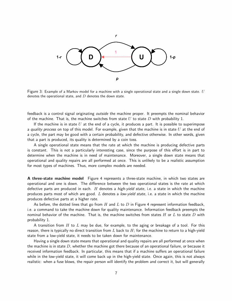
A two-state machine model A very simple machine model is illustrated in Figure 3. Here, thereare two states. The operation or cycle time is fixed. When in state U , the machine produces parts.An operational failure (e.g. a blown fuse or a burnt motor) takes the machine to state D. When instate D, the machine does not produce parts. Given that the machine is in state U , the probability pthat it switches to state D during any given cycle is the reciprocal of the Mean Time between Failures(MTBF). Given that the machine is in state D, the probability r that it switches to state U during anygiven cycle is the reciprocal of the Mean Time to Repair (MTTR).

The dotted line that goes from U to D in Figure 3 represents a command to take the machine downfor quality maintenance. As we shall see in Section 2.4.2, this is known as information feedback andcorresponds to corrective action on a machine thought to be responsible for quality defects. Information

6

UD 1-p1-r

r

p

UD 1-p1-r UD 1-p1-r

r

p

UD 1-p1-r

r

p

1

UD 1-p1-r

r

p

UD 1-p1-r UD 1-p1-r

r

p

1

Figure 3: Example of a Markov model for a machine with a single operational state and a single down state. Udenotes the operational state, and D denotes the down state.

feedback is a control signal originating outside the machine proper. It preempts the nominal behaviorof the machine. That is, the machine switches from state U to state D with probability 1.

If the machine is in state U at the end of a cycle, it produces a part. It is possible to superimposea quality process on top of this model. For example, given that the machine is in state U at the end ofa cycle, the part may be good with a certain probability, and defective otherwise. In other words, giventhat a part is produced, its quality is determined by a coin toss.

A single operational state means that the rate at which the machine is producing defective partsis constant. This is not a particularly interesting case, since the purpose of this effort is in part todetermine when the machine is in need of maintenance. Moreover, a single down state means thatoperational and quality repairs are all performed at once. This is unlikely to be a realistic assumptionfor most types of machines. Thus, more complex models are needed.

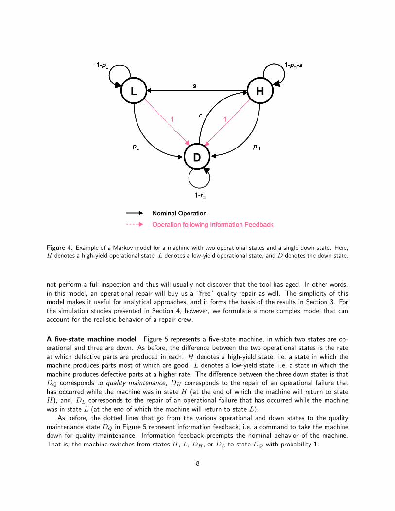
A three-state machine model Figure 4 represents a three-state machine, in which two states areoperational and one is down. The difference between the two operational states is the rate at whichdefective parts are produced in each. H denotes a high-yield state, i.e. a state in which the machineproduces parts most of which are good. L denotes a low-yield state, i.e. a state in which the machineproduces defective parts at a higher rate.

As before, the dotted lines that go from H and L to D in Figure 4 represent information feedback,i.e. a command to take the machine down for quality maintenance. Information feedback preempts thenominal behavior of the machine. That is, the machine switches from states H or L to state D withprobability 1.

A transition from H to L may be due, for example, to the aging or breakage of a tool. For thisreason, there is typically no direct transition from L back to H; for the machine to return to a high-yieldstate from a low-yield state, it needs to be taken down for maintenance.

Having a single down state means that operational and quality repairs are all performed at once whenthe machine is in state D, whether the machine got there because of an operational failure, or because itreceived information feedback. In particular, this means that if a machine suffers an operational failurewhile in the low-yield state, it will come back up in the high-yield state. Once again, this is not alwaysrealistic: when a fuse blows, the repair person will identify the problem and correct it, but will generally

7

Operation following Information Feedback

Nominal Operation

Operation following Information Feedback

Nominal Operation

L

D

H

1 - p H - s 1 - p L

r

s

1 1

p H p L

1 - r Q

L

D

H

1 - p H - s 1 - p L

r

s

1 1

p H p L

L

D

H

1 - p H - s 1 - p L

r

s

1 1

L

D

H

1 - p H - s 1 - p L

r

s

1 1

p H p L

1 - r Q

Figure 4: Example of a Markov model for a machine with two operational states and a single down state. Here,H denotes a high-yield operational state, L denotes a low-yield operational state, and D denotes the down state.

not perform a full inspection and thus will usually not discover that the tool has aged. In other words,in this model, an operational repair will buy us a “free” quality repair as well. The simplicity of thismodel makes it useful for analytical approaches, and it forms the basis of the results in Section 3. Forthe simulation studies presented in Section 4, however, we formulate a more complex model that canaccount for the realistic behavior of a repair crew.

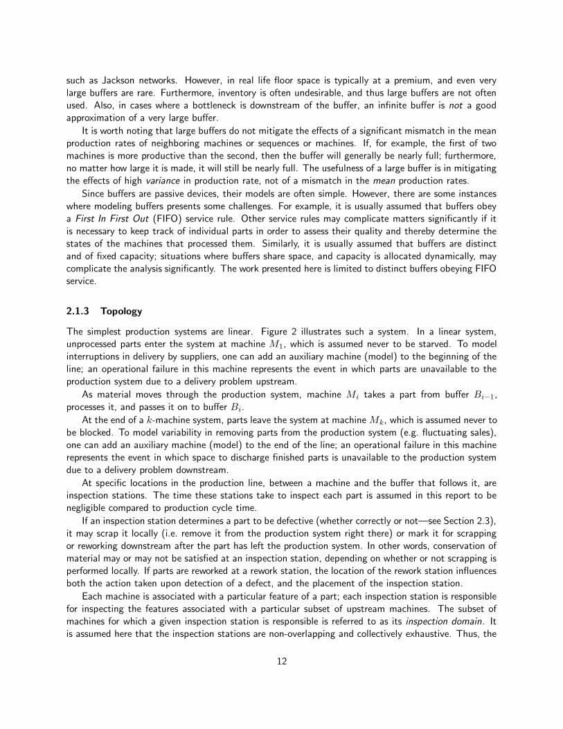
A five-state machine model Figure 5 represents a five-state machine, in which two states are op-erational and three are down. As before, the difference between the two operational states is the rateat which defective parts are produced in each. H denotes a high-yield state, i.e. a state in which themachine produces parts most of which are good. L denotes a low-yield state, i.e. a state in which themachine produces defective parts at a higher rate. The difference between the three down states is thatDQ corresponds to quality maintenance, DH corresponds to the repair of an operational failure thathas occurred while the machine was in state H (at the end of which the machine will return to stateH), and, DL corresponds to the repair of an operational failure that has occurred while the machinewas in state L (at the end of which the machine will return to state L).

As before, the dotted lines that go from the various operational and down states to the qualitymaintenance state DQ in Figure 5 represent information feedback, i.e. a command to take the machinedown for quality maintenance. Information feedback preempts the nominal behavior of the machine.That is, the machine switches from states H, L, DH , or DL to state DQ with probability 1.

8

L

DQ

DH

H

DL

1-pH-s1-pL

1-rH1-rL

1

1-rQ

rQ

rL rH

s

1 1pL pH

1

L

DQ

DH

H

DL

1-pH-s1-pL

1-rH1-rL

1

1-rQ

rQ

rL rH

s

1 1pL pH

L

DQ

DH

H

DL

1-pH-s1-pL

1-rH1-rL

1

1-rQ

rQ

rL rH

s

1 1pL pH

1

Operation following Information Feedback

Nominal Operation

Operation following Information Feedback

Nominal Operation

Figure 5: Example of a Markov model for a machine with two operational states and three down states. Here, Hdenotes a high-yield operational state, L denotes a low-yield operational state, DQ denotes quality maintenance,DH denotes an operational failure that has occurred while the machine was in state H , and DL denotes anoperational failure that has occurred while the machine was in state L.

The additional complexity of the five-state machine (as compared to the three-state machine) isoffset by the fact that now, quality repairs are not obtained “for free” when operational repairs areperformed. However, there is still a problem: if the machine is taken down for quality maintenanceduring an operational repair, the latter is cut short. This is because an immediate transition from DH

or DL to DQ is forced by the reception of information feedback, artificially shortening the time spentin the operational repair states. Thus, this time one gets a “partially free” operational repair when themachine is taken down for quality maintenance. Once again, this is not always realistic, and we finallyintroduce a model capable of properly distinguishing among operational and quality outages.

A seven-state machine model Figure 6 represents a seven-state machine, in which two states areoperational and five are down. As in the five-state machine, the difference between the two operationalstates is the rate at which defective parts are produced in each. H denotes a high-yield state, i.e. astate in which the machine produces parts most of which are good. L denotes a low-yield state, i.e. astate in which the machine produces defective parts at a higher rate. Three of the down states are alsoidentical to those in the five-state machine: DQ corresponds to quality maintenance, DH correspondsto the repair of an operational failure that has occurred while the machine was in state H (at the end ofwhich the machine will return to state H), and, DL corresponds to the repair of an operational failure

9

that has occurred while the machine was in state L (at the end of which the machine will return tostate L). In addition to these, however, there are now the two additional states D ′

H and D′

L. Thesecorrespond to operational down states after reception of information feedback . In other words, if amachine is undergoing an operational repair and receives information feedback, it continues with theoperational repair until it has been completed, and only then proceeds to quality maintenance.

L

DQ

DH′′′′

DH

H

DL

DL′′′′

1-pH-s1-pL

1-rL 1-rH

1-rH1-rL

1-rH1-rL

rH

rH

rL

rL

1-rQ

rQ

rL rH

s

1 1pL pH

L

DQ

DH′′′′

DH

H

DL

DL′′′′

1-pH-s1-pL

1-rL 1-rH

1-rH1-rL

1-rH1-rL

rH

rH

rL

rL

1-rQ

rQ

rL rH

s

1 1pL pH

Operation following Information Feedback

Nominal Operation

Operation following Information Feedback

Nominal Operation

Figure 6: Example of a Markov model for a machine with two operational states and five down states. Here, Hdenotes a high-yield operational state, L denotes a low-yield operational state, DQ denotes quality maintenance,DH denotes an operational failure that has occurred while the machine was in state H , and DL denotes anoperational failure that has occurred while the machine was in state L. The states D ′

H and D′

L respectivelydenote operational down states following reception of information feedback.

As before, the dotted lines that go from the various operational and down states to the qualitymaintenance state DQ in Figure 6 represent information feedback, i.e. a command to take the machinedown for quality maintenance. Information feedback preempts the nominal behavior of the machine.That is, the machine switches from states H or L to state DQ with probability 1. If, however, themachine is in either DH or DL when information feedback is received, then there are two possibilities:either the operational repair is completed during the current cycle (which happens with probability rH

and rL, respectively) and the machine moves on to the quality maintenance state DQ; or else theoperational repair is not completed, in which case it continues in the states D ′

H or D′

L, respectively.These states are identical to DH and DL, except that the machine moves to DQ rather than to Hor L when the operational repair is completed. Because of the memoryless property, continuing an

10

operational repair in D′

H or D′

L is indistinguishable from staying in DH or DL—except for the stateentered after the next outward transition.

In the seven-state machine model, neither operational repairs, nor quality maintenance is obtained“for free.” Rather, operational repairs and quality maintenance are performed in sequence.

Auxiliary states The states D′

H and D′

L in the seven-state machine model can be considered auxiliarystates, in that their main function is to make it possible to “remember” that information feedback hasbeen received, even though Markovian models are memoryless. There are also other cases where auxiliarystates are useful.

For example, suppose that the distribution of time spent in a particular state (say, operational repair)is not geometric. This would mean that the probability of completing the repair during any given cycleis not constant but a function of the time since the failure occurred—a realistic situation when, forinstance, it is unlikely that a repair will take a very short or a very long time. Such a system is notmemoryless, and modeling it as a Markov chain may require the addition of auxiliary states (Howard1971).

In addition to the use of auxiliary states to represent time distributions, it is also possible to constructarbitrarily complex machine models to account for phenomena such as the following:

• A variety of operational failures, each with different repair characteristics (time distribution, op-erational state reached after the repair is completed);

• The gradual aging of a machine tool and the changing characteristics of the operation and/orfailures;

• Proactive control policies in which the behavior of a machine is predicted and maintenance isscheduled before a catastrophic failure occurs.

The construction of complex Markovian models for individual machines presents no conceptualdifficulties, but factors and behaviors such as those outlined above must be taken into consideration fora model to represent accurately the properties of realistic production systems. Furthermore, the analysiscan get very complicated when machines with complex models are embedded in production systemswhere they interact with each other through buffers.

2.1.2 Buffers

Buffers are passive interstage storage locations. They provide space for parts produced by upstreammachines when a downstream machine is down, thus delaying the onset of blockage; likewise, theyprovide unprocessed parts to downstream machines when an upstream machine is down, thus delayingthe onset of starvation. In this manner, they act to partially decouple sequences of machines and thusincrease the production rate (Gershwin 1994).

However, when a machine occasionally switches to a state in which defective parts are produced,and such a switch must be detected as soon as possible, extra buffer capacity may be harmful becauseit may delay inspection—and hence, detection. The role of buffer capacity on good production rate andother performance measures under different inspection and control policies is one of the matters thatthis project has investigated, and is described in this report.

In a mathematical model of a production system, buffer capacity may be finite or infinite. Theassumption of infinite buffers totally decouples machines and makes it possible to use powerful methods

11

such as Jackson networks. However, in real life floor space is typically at a premium, and even verylarge buffers are rare. Furthermore, inventory is often undesirable, and thus large buffers are not oftenused. Also, in cases where a bottleneck is downstream of the buffer, an infinite buffer is not a goodapproximation of a very large buffer.

It is worth noting that large buffers do not mitigate the effects of a significant mismatch in the meanproduction rates of neighboring machines or sequences or machines. If, for example, the first of twomachines is more productive than the second, then the buffer will generally be nearly full; furthermore,no matter how large it is made, it will still be nearly full. The usefulness of a large buffer is in mitigatingthe effects of high variance in production rate, not of a mismatch in the mean production rates.

Since buffers are passive devices, their models are often simple. However, there are some instanceswhere modeling buffers presents some challenges. For example, it is usually assumed that buffers obeya First In First Out (FIFO) service rule. Other service rules may complicate matters significantly if itis necessary to keep track of individual parts in order to assess their quality and thereby determine thestates of the machines that processed them. Similarly, it is usually assumed that buffers are distinctand of fixed capacity; situations where buffers share space, and capacity is allocated dynamically, maycomplicate the analysis significantly. The work presented here is limited to distinct buffers obeying FIFOservice.

2.1.3 Topology

The simplest production systems are linear. Figure 2 illustrates such a system. In a linear system,unprocessed parts enter the system at machine M1, which is assumed never to be starved. To modelinterruptions in delivery by suppliers, one can add an auxiliary machine (model) to the beginning of theline; an operational failure in this machine represents the event in which parts are unavailable to theproduction system due to a delivery problem upstream.

As material moves through the production system, machine Mi takes a part from buffer Bi−1,processes it, and passes it on to buffer Bi.

At the end of a k-machine system, parts leave the system at machine Mk, which is assumed never tobe blocked. To model variability in removing parts from the production system (e.g. fluctuating sales),one can add an auxiliary machine (model) to the end of the line; an operational failure in this machinerepresents the event in which space to discharge finished parts is unavailable to the production systemdue to a delivery problem downstream.

At specific locations in the production line, between a machine and the buffer that follows it, areinspection stations. The time these stations take to inspect each part is assumed in this report to benegligible compared to production cycle time.

If an inspection station determines a part to be defective (whether correctly or not—see Section 2.3),it may scrap it locally (i.e. remove it from the production system right there) or mark it for scrappingor reworking downstream after the part has left the production system. In other words, conservation ofmaterial may or may not be satisfied at an inspection station, depending on whether or not scrapping isperformed locally. If parts are reworked at a rework station, the location of the rework station influencesboth the action taken upon detection of a defect, and the placement of the inspection station.

Each machine is associated with a particular feature of a part; each inspection station is responsiblefor inspecting the features associated with a particular subset of upstream machines. The subset ofmachines for which a given inspection station is responsible is referred to as its inspection domain. Itis assumed here that the inspection stations are non-overlapping and collectively exhaustive. Thus, the

12

M1

B1

M2

B2

M3 I

1B

3M

4 I2

M5

B5

M6

B6

M7

B7

M1

B1

M2

B2

M3 I

1B

3M

4 I2

M1

B1

M2

B2

M3 I

1B

3M

4 I2

M5

B5

M6

B6

M7

B7

M5

B5

M6

B6

M7

B7

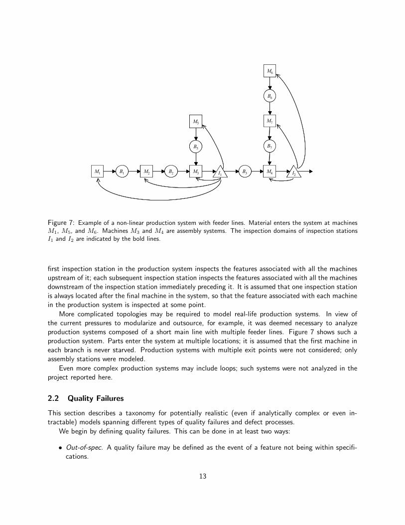
Figure 7: Example of a non-linear production system with feeder lines. Material enters the system at machinesM1, M5, and M6. Machines M3 and M4 are assembly systems. The inspection domains of inspection stationsI1 and I2 are indicated by the bold lines.

first inspection station in the production system inspects the features associated with all the machinesupstream of it; each subsequent inspection station inspects the features associated with all the machinesdownstream of the inspection station immediately preceding it. It is assumed that one inspection stationis always located after the final machine in the system, so that the feature associated with each machinein the production system is inspected at some point.

More complicated topologies may be required to model real-life production systems. In view ofthe current pressures to modularize and outsource, for example, it was deemed necessary to analyzeproduction systems composed of a short main line with multiple feeder lines. Figure 7 shows such aproduction system. Parts enter the system at multiple locations; it is assumed that the first machine ineach branch is never starved. Production systems with multiple exit points were not considered; onlyassembly stations were modeled.

Even more complex production systems may include loops; such systems were not analyzed in theproject reported here.

2.2 Quality Failures

This section describes a taxonomy for potentially realistic (even if analytically complex or even in-tractable) models spanning different types of quality failures and defect processes.

We begin by defining quality failures. This can be done in at least two ways:

• Out-of-spec. A quality failure may be defined as the event of a feature not being within specifi-cations.

13

• Quality loss function. A quality loss function may describe the influence of a given feature on theperformance characteristics of the part.

The first definition is assumed here.

2.2.1 Internal vs. External Failures

Quality failures may be due to external causes or internal causes. The latter include failures that occurat the machines inside the production line under study—e.g. a drill bit breaks or a paint nozzle getsclogged, resulting in a product that is sub-standard.

External failures occur outside the production system proper, perhaps in a supplier’s factory, orduring transportation. Examples of such failures include instances where parts delivered by the supplierare damaged, out-of-sequence, incorrect or mislabeled, or where raw material is of poor quality orincompatible with the production process.

Like delays in delivery or removal, external quality failures too can be modeled as occurring atauxiliary machines at the entry point(s) of the production system. Consequently, external quality failuresare not treated separately here. Note, however, that actions taken pursuant to the detection of externalfailures may differ significantly from actions taken after internal failures are detected.

2.2.2 Dynamic Characteristics

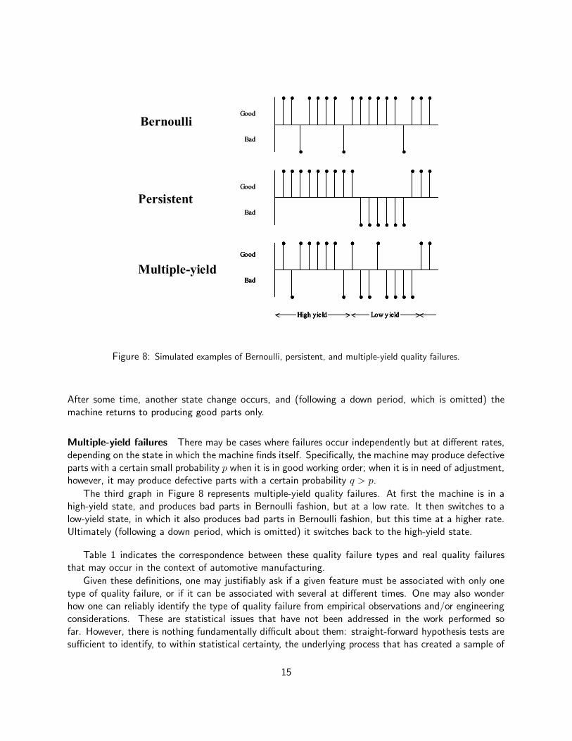
The incidence of quality failures (defects) is often reported as an aggregate measure, such as thefraction of defective parts out of the total (i.e. the yield—see Section 2.5). However, our researchhas established that the dynamic (time) characteristics of defects have a pronounced effect on systemperformance. Specifically, the dependence or independence of individual occurrences of failures acrosstime can be given precise probabilistic definitions. The following terms were coined in the course ofthe research described here, and are not traditionally used in the manufacturing literature. They areintended to convey the stochastic properties of each type of failure.

Bernoulli quality failures Quality failures that occur independently of each other are generally referredto in the traditional quality literature as “random,” “common,” or “chance” failures. The presence ofa failure in one part says nothing about the likelihood of occurrence of a failure in any other part. Forexample, a pre-existing defect in an unmachined part may cause a quality failure which is specific tothat part only. Such failures may also be associated with difficult operations or those that are based ondeveloping technology.

The first graph in Figure 8 represents Bernoulli quality failures. The horizontal axis is time. Dotsabove the line indicate good parts; dots below the line indicate bad parts. (Periods when the machineis down are suppressed.) In this graph, most of the parts produced by the machine are good, but someare bad. The occurrence of each bad part is completely independent of previous bad parts.

Persistent quality failures In some cases, a quality failure occurs when a state change takes place ina machine, e.g. a tool breaks. Such failures are generally referred to in the literature as “systematic,”“special,” “assignable,” or “unusual” failures. Once a failure occurs, every subsequent part will be baduntil the machine is repaired.

The second graph in Figure 8 represents persistent quality failures. At first, the machine onlyproduces good parts. Then a state change occurs, and the machine begins to produce bad parts only.

14

Good

Bad

Good

Bad

Good

Bad

Good

Bad

High yield Low y ield

Good

Bad

High yield Low y ield

Good

Bad

High yield Low y ieldHigh yield Low y ield

Good

Bad

Bernoulli

Persistent

Multiple-yield

Figure 8: Simulated examples of Bernoulli, persistent, and multiple-yield quality failures.

After some time, another state change occurs, and (following a down period, which is omitted) themachine returns to producing good parts only.

Multiple-yield failures There may be cases where failures occur independently but at different rates,depending on the state in which the machine finds itself. Specifically, the machine may produce defectiveparts with a certain small probability p when it is in good working order; when it is in need of adjustment,however, it may produce defective parts with a certain probability q > p.

The third graph in Figure 8 represents multiple-yield quality failures. At first the machine is in ahigh-yield state, and produces bad parts in Bernoulli fashion, but at a low rate. It then switches to alow-yield state, in which it also produces bad parts in Bernoulli fashion, but this time at a higher rate.Ultimately (following a down period, which is omitted) it switches back to the high-yield state.

Table 1 indicates the correspondence between these quality failure types and real quality failuresthat may occur in the context of automotive manufacturing.

Given these definitions, one may justifiably ask if a given feature must be associated with only onetype of quality failure, or if it can be associated with several at different times. One may also wonderhow one can reliably identify the type of quality failure from empirical observations and/or engineeringconsiderations. These are statistical issues that have not been addressed in the work performed sofar. However, there is nothing fundamentally difficult about them: straight-forward hypothesis tests aresufficient to identify, to within statistical certainty, the underlying process that has created a sample of

15

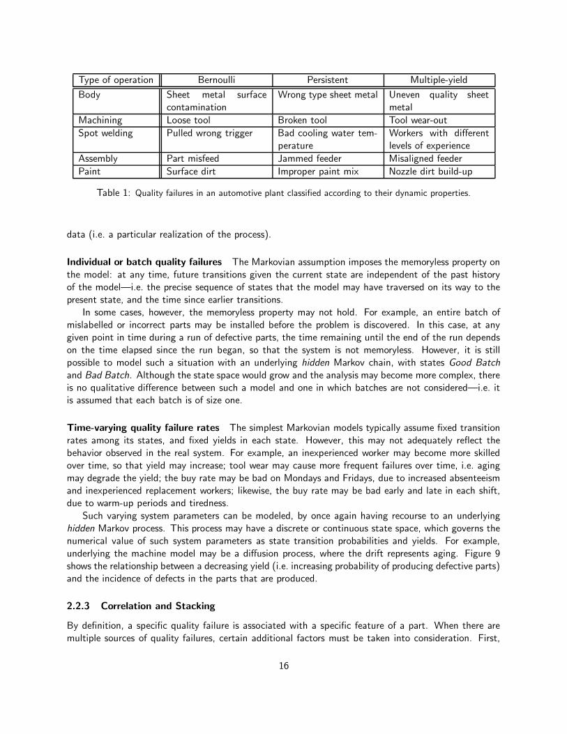
Type of operation Bernoulli Persistent Multiple-yield

Body Sheet metal surfacecontamination

Wrong type sheet metal Uneven quality sheetmetal

Machining Loose tool Broken tool Tool wear-out

Spot welding Pulled wrong trigger Bad cooling water tem-perature

Workers with differentlevels of experience

Assembly Part misfeed Jammed feeder Misaligned feeder

Paint Surface dirt Improper paint mix Nozzle dirt build-up

Table 1: Quality failures in an automotive plant classified according to their dynamic properties.

data (i.e. a particular realization of the process).

Individual or batch quality failures The Markovian assumption imposes the memoryless property onthe model: at any time, future transitions given the current state are independent of the past historyof the model—i.e. the precise sequence of states that the model may have traversed on its way to thepresent state, and the time since earlier transitions.

In some cases, however, the memoryless property may not hold. For example, an entire batch ofmislabelled or incorrect parts may be installed before the problem is discovered. In this case, at anygiven point in time during a run of defective parts, the time remaining until the end of the run dependson the time elapsed since the run began, so that the system is not memoryless. However, it is stillpossible to model such a situation with an underlying hidden Markov chain, with states Good Batchand Bad Batch. Although the state space would grow and the analysis may become more complex, thereis no qualitative difference between such a model and one in which batches are not considered—i.e. itis assumed that each batch is of size one.

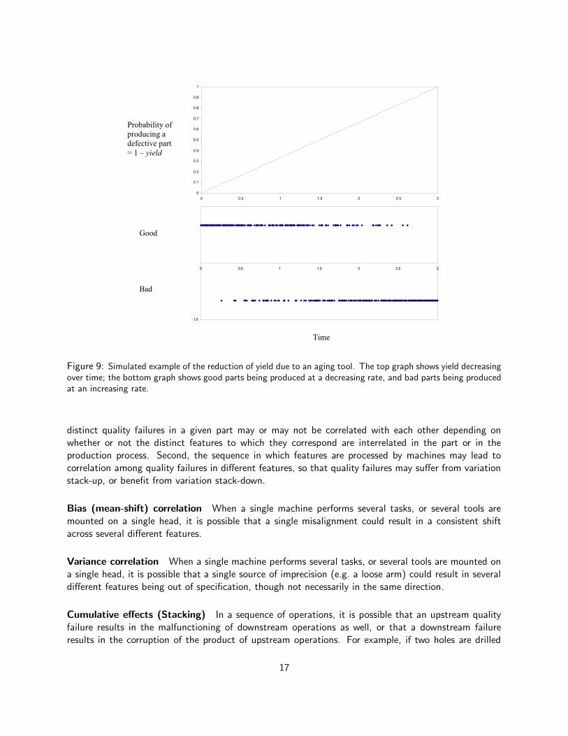
Time-varying quality failure rates The simplest Markovian models typically assume fixed transitionrates among its states, and fixed yields in each state. However, this may not adequately reflect thebehavior observed in the real system. For example, an inexperienced worker may become more skilledover time, so that yield may increase; tool wear may cause more frequent failures over time, i.e. agingmay degrade the yield; the buy rate may be bad on Mondays and Fridays, due to increased absenteeismand inexperienced replacement workers; likewise, the buy rate may be bad early and late in each shift,due to warm-up periods and tiredness.

Such varying system parameters can be modeled, by once again having recourse to an underlyinghidden Markov process. This process may have a discrete or continuous state space, which governs thenumerical value of such system parameters as state transition probabilities and yields. For example,underlying the machine model may be a diffusion process, where the drift represents aging. Figure 9shows the relationship between a decreasing yield (i.e. increasing probability of producing defective parts)and the incidence of defects in the parts that are produced.

2.2.3 Correlation and Stacking

By definition, a specific quality failure is associated with a specific feature of a part. When there aremultiple sources of quality failures, certain additional factors must be taken into consideration. First,

16

0

0.1

0.2

0.3

0.4

0.5

0.6

0.7

0.8

0.9

1

0 0.5 1 1.5 2 2.5 3

-1.5

0 0.5 1 1.5 2 2.5 3

Probability of

producing a

defective part

= 1 – yield

Good

Bad

Time

Figure 9: Simulated example of the reduction of yield due to an aging tool. The top graph shows yield decreasingover time; the bottom graph shows good parts being produced at a decreasing rate, and bad parts being producedat an increasing rate.

distinct quality failures in a given part may or may not be correlated with each other depending onwhether or not the distinct features to which they correspond are interrelated in the part or in theproduction process. Second, the sequence in which features are processed by machines may lead tocorrelation among quality failures in different features, so that quality failures may suffer from variationstack-up, or benefit from variation stack-down.

Bias (mean-shift) correlation When a single machine performs several tasks, or several tools aremounted on a single head, it is possible that a single misalignment could result in a consistent shiftacross several different features.

Variance correlation When a single machine performs several tasks, or several tools are mounted ona single head, it is possible that a single source of imprecision (e.g. a loose arm) could result in severaldifferent features being out of specification, though not necessarily in the same direction.

Cumulative effects (Stacking) In a sequence of operations, it is possible that an upstream qualityfailure results in the malfunctioning of downstream operations as well, or that a downstream failureresults in the corruption of the product of upstream operations. For example, if two holes are drilled

17

side by side, a misalignment in the first might render the second defective, and vice versa. More seriously,in a two-step process such as first drilling a coarse hole and then refining it, an error in the location of thecoarse hole could result in the breakage of the fine adjustment tool. Thus, multiple quality failures mayoccur due to a single root cause even when operations are performed by physically distinct machines.

Note that it is also possible for a downstream operation to compensate for an upstream qualityfailure and correct it. The aggravation of an upstream quality failure by a downstream quality failure iscalled stacking up. Conversely, the mitigation of an upstream quality failure by a downstream qualityfailure is called stacking down.

Defects in distinct features are assumed to be independent in the work presented here.

2.3 Inspection

Inspection stations are responsible for assessing the quality of processed parts. They are located betweenmachines and the buffers that immediately follow them.

Placing an inspection station after each and every machine (“ubiquitous inspection”) may allow theimmediate detection and isolation of quality failures, simplifying root-cause traceability and minimizingthe waste of downstream production capacity. This may be very desirable, but inspection stations areexpensive, in that they consume floor space, machinery, and labor. Therefore it is necessary to choosethe number and location of inspection stations carefully, so as to place them as sparsely as possible whilemeeting quality goals. In our analysis, therefore, we allow for fewer inspection stations than machinesin the production system. In such cases, a given inspection station may be responsible for inspectingthe work of several machines.

Inspection stations perform certain test on parts, in order to detect quality defects; these tests may,however, be inaccurate. When a defect is detected, the inspection station may cause some action to betaken on the part, and/or some action to be taken on the machine thought to be responsible for thequality defect in the part.

2.3.1 Destructive vs. Non-Destructive Testing

Testing for failures in manufactured parts can follow different strategies, depending both on the charac-teristics of the failures one is trying to detect, and on economic and other considerations. In particular,testing may or may not have a lasting effect on the part.

• Non-Destructive Testing does not have any lasting effect on the part. As a result, inspectingevery part is an alternative to consider.

• Destructive testing results in the complete loss of the part. In this case, inspecting every partwould result in zero production; thus, it is necessary to sample the parts, and only inspect thoseparts that are in the sample.

When quality failures are systematic, i.e. persistent or multiple-yield, it might be possible to makea business case for periodic destructive testing in order to detect failures reliably. When quality failuresare Bernoulli, however, destructive testing cannot be justified since the discovery of a failure in one partdoes not provide any information about the presence or absence of failures in other parts; the fractionof failures among non-destroyed parts will be identical to the fraction of failures in the population as awhole.

18

2.3.2 Domain and Frequency

Each machine is assumed to work on a particular feature or set of features of the parts; each inspectionstation is assumed to work on the features associated with a certain set of machines, called the inspectiondomain of the inspection station.

Distinct inspection stations may or may not inspect distinct features; in our work so far, we haveassumed that each machine’s work is inspected by one station only. Furthermore, inspection domainscan overlap, or they can be disjoint; in our work so far, we have assumed that inspection domainsare disjoint. What this means is that the first inspection station inspects the features associated withall machines upstream of it, and each subsequent station inspects the features associated with all themachines between the inspection station immediately upstream of it and the machine it immediatelyfollows.

It is assumed that if a production system contains any inspection stations, then one of the inspectionstations is always placed at the very end of the system. Thus, the inspection stations collectively inspectthe work of all the machines in the production system.

In our work so far, we have assumed that all parts are inspected. It is also possible to inspect onlysome parts, either randomly (at some chosen rate), or periodically (with a given period). Note that whendefects are associated with a machine state change (as in the cases of persistent or multiple-yield qualityfailures), inspecting a sample of parts instead of all parts may be reasonable, although this approachwould necessarily delay the detection of the state change and would thus degrade performance. However,when defects are independent (Bernoulli), sampling would not be a reasonable approach: when only asample of parts are inspected, defective parts that happen not to be in the sample will be missed, and ifthe defects are Bernoulli, the fraction of defective parts among those inspected will be the same as thefraction of defective parts among those not inspected. Defective parts that are not inspected cannot bescrapped or marked for reworking, and they may thus escape into the marketplace, causing customerdissatisfaction and other undesirable consequences.

2.3.3 Accuracy and Declaration of a Defective Part

The first stage in the inspection process is the detection of quality failures. Since the inspection stationis potentially unreliable, we prefer to use the term declaration rather than detection. This is becausethe latter term connotes an authoritative judgement, whereas the former is only an assessment of partquality.

Given a part, the inspection station runs a series of tests on it pertaining to the features processedby the machines in the station’s inspection domain. A separate test is run for each feature. Each testreturns one of two results: good or defective. Tests are potentially inaccurate, meaning that a goodpart may be declared to be defective or vice versa. This inaccuracy is characterized by a false positive(Type I error) probability and a false negative (Type II error) probability. Note that since each testis associated with a feature, and each feature with a machine, there are as many false negative andfalse positive probabilities as there are machines—even though the actual testing is performed at theinspection stations.

There is a trade-off between the stringency of quality testing and the cost of testing in terms ofscrapping good parts or missing bad parts. Hence, the design of an optimal testing strategy requires theachievment of a careful balance between Type I and Type II errors. Very stringent quality testing wouldcatch most or all the quality failures, but at the cost of many false positives. When the detection of afailure results in scrapping a part or stopping the production line, false positives may be very expensive.

19

On the other hand, very relaxed quality testing would seldom result in unwarranted scrapping or stoppingof the line, but this would be at the cost of many false negatives. Defective parts that are not identifiedas such consume downstream production capacity, and, if missed entirely, would result in defectiveproducts and customer dissatisfaction.

In our analysis, we keep track of the true quality characteristics of a part, in order to be able tocalculate such performance measures as the rate at which defective parts reach the marketplace or therate at which good parts are reworked or discarded. However, in reality, there is typically no directinformation as to the quality of a part outside of the results of the tests performed by the inspectionstations. (Indirect information may be obtained from customer complaints, warranty repairs, etc.) Inother words, on the factory floor, parts are treated as good or defective only on the basis of the inspectionresults.

2.3.4 Declaration of an Impaired Machine

In addition to declaring each part to be good or defective, an inspection station may also decidewhether or not a given machine in its inspection domain is in need of quality maintenance. In otherwords, the purpose of inspection is not only to catch defective parts, but also to signal that adjustmentsor corrections in the production system itself are needed, so that fewer or no defective parts will beproduced in the immediate future.

A machine is considered to be in need of quality maintenance if there is evidence that it has entered astate in which it produces a larger fraction of defective parts than is desirable. This evidence is obtainedby inspecting the parts processed by that machine, and inferring the state of the machine from theresults of inspection.

For example, the Toyota Production System philosophy of jidoka requires that a machine be takendown for maintenance as soon as a single defect has been detected. This may be a good strategy whenquality failures are persistent (or multiple-yield with a significant difference in yields) and inspection ishighly accurate, but not otherwise. (See Section 3.2.)

Alternatively, a decision rule can be formulated based on a moving window of parts, e.g. “declare themachine to be in need of maintenance if n parts have been declared defective among the most recentm inspected parts.”

When a machine is thought to need maintenance, information feedback is sent to that machine,i.e. a signal is sent that overrides the nominal behavior of the machine and takes it into the qualitymaintenance state. (See Section 2.4.2.)

2.4 Control Policies

The purpose of inspection is, of course, to trigger action. The declaration of quality defects may elicitactions in several different areas: on the part thought to be defective, on the machine thought to beresponsible for the defect, and on the workforce responsible for that section of the production system.

Decisions as to the type and timing of action must be contingent upon cost defined in the broadestpossible sense: cost of materials, cost of processing, cost of maintenance, cost of customer dissatisfac-tion, and so on. Actions can be taken reactively or pro-actively.

• Pro-active action. If inspection reveals a trend towards degrading quality, it may be possibleto schedule preventive maintenance in order to prevent further degradation and potentially a

20

catastrophic failure. This would only be possible if the system is non-stationary and the underlyingchanges can be modeled so as to allow the forecasting of performance deterioration.

• Reactive action. When a quality failure is detected, some action will be taken, ranging fromsimply noting that a failure has occurred, to stopping the production line for repair. This actionmay be immediate, or it may be delayed, depending on the type of action and the circumstancesprevailing.

2.4.1 Action on Defective Parts

When inspection station Ii declares a part to be good, the part is moved into buffer Bj. (Because ofthe imperfect accuracy of the test, the part may in truth be defective.) When inspection station I i

declares a part to be defective, the part is either scrapped immediately (i.e. never makes it into bufferBj), or it is marked as defective and moved into buffer Bj . In the latter case, it is assumed that thepart will be either scrapped or reworked after it has left the production system. (Once again, a partthat is scrapped or marked as defective may in truth be good.)

The advantage of scrapping locally is that parts believed to be defective are immediately removedfrom the system; thus, they no longer consume such resources as buffer space and machine capacity.This is especially useful when a bottleneck is present downstream, as the strain on the bottleneck issomewhat relieved by reducing the rate at which jobs arrive at it.

At the same time, scrapping locally is often not possible because material removal, storage, andtransportation equipment must be on hand to handle the part to be scrapped. If a part is marked forsubsequent scrapping downstream, the benefits of scrapping to the production line itself are no longerrealized. Even though it is marked as defective, the part will continue to move through the productionsystem, consuming resources as it goes.

Indeed, it is often highly impractical to scrap parts at all, particularly when they are expensive andrepresent a significant sunken cost in terms of raw material consumed and labor or machine capacityalready expended. In such cases, parts are marked for reworking, and may have to go through some or allthe operations again. Although this ensures that defective parts are not released into the marketplace,no savings of production line capacity are realized in this case.

The location of the rework station influences both the action taken upon detection of a defect,and the placement of the inspection station. If defective parts are scrapped locally, it is best to scrapthem as soon as possible, i.e. to locate the inspection station as close as possible to the machinewhose work it inspects. This may not always be possible, however, due the floor space constraints,availability of material handling equipment, or other factors. Likewise, if defective parts are reworkedlocally, correcting the defect may require some additional on-line operations, temporarily altering theoperation characteristics of that machine. Alternatively, corrective work may be performed off-line,with the part taken out of the production line, reworked, and re-introduced into the line at the samepoint. That does not introduce any changes into the operation characteristics of the machine. In bothcases, inspection and reworking are performed at roughly the same location, possibly imposing certainconstraints on the choice of location. In other cases, particularly when the part is large (e.g. a partiallycompleted car) and floor space is at a premium, defective parts are taken to a remote location wherethey are reprocessed. In such cases, the placement of inspection stations may not be constrained by therequirement to co-locate a reworking station.

In a line where parts are inexpensive and some amount of wasteage is acceptable, the declarationof defects may be used to compile quality statistics. In such a line, it may not be individual failures

21

that trigger action, but rather the frequency of failures. Of course this assumes that the defective partswould eventually be identified and eliminated downstream.

2.4.2 Action on Impaired Machines

When an inspection station declares a machine to be in need of quality maintenance, it sends informationfeedback to the machine. This signals to the machine or to its operators that it must be taken into thequality maintenance state. Taking a machine down for servicing is clearly not a decision that should bemade lightly: a cost will invariably be involved in making this decision, including not only the cost ofthe service call but also lost productivity due to the unscheduled outage.

Information feedback preempts the nominal operation of the machine; in other words, whatever statethe machine may have remained in or moved to were it not for information feedback, the decision to gointo quality maintenance overrides the dynamics of the machine itself.

Since inspection may take place far downstream of a machine, some time may elapse between theoccurrence of a state change in the machine, and the detection of that change by the inspection station.In the meantime, the machine may have undergone one or more state changes of its own accord. Whatexactly happens to the machine once it receives information feedback thus depends on the model of themachine: it may be taken down for maintenance immediately (at the end of the current cycle), or itmay remain in an operational repair state and only move on to the quality maintenance state after therepair has been completed. (See Section 2.1.1.)

Another issue to consider—in view of the distance between the machine and the inspection stationthat monitors its performance—is the fact that a potentially significant number of defective parts mayhave already been produced by the time the machine is taken down for quality maintenance. Forexample, suppose that there are some FIFO buffers between the machine and the inspection station,and suppose that they collectively have n parts in them at the time the machine begins to producedefective parts; barring any other machine failures, it will take n machining cycles for the first defectivepart to reach the inspection station. If the quality failure mechanism is persistent, furthermore, then then parts behind it will all be defective. This means that once information feedback has been sent to themachine, it should receive no further commands until all the parts already in the pipeline have drainedout. We call this the dead period . Experiments show that the dead period has a significant influence onthe total production rate of the machine, since the machine is not taken down for maintenance duringa dead period, and dead periods can be of significant duration; the longer or more frequent the deadperiods, the fewer the opportunities to take an operational machine down. In this respect, dead periodscompensate to some extent for decision rules that are not conservative enough. For example, taking amachine down for quality maintenance as soon as a single part is declared to be defective (jidoka) mayresult in degraded performance in some cases; dead periods may mitigate this effect, but they will doso at different rates depending on the distance between the machine and the inspection station thatmonitors it.

2.4.3 Action on People

The detection and analysis of quality failures can affect the people involved in the production line.

Traceability Factors such as line topology (especially the existence of alternate routes), location ofinspection stations, and the complexity of operations will have a significant effect on the ease or difficulty

22

with which the root causes of quality failures are isolated, diagnosed, and corrected. Ideally, the detectionand analysis of quality failures should help locate their root causes.

Motivation toward better quality The detection of quality failures provides an information feedbackloop that will help better planning, motivate process improvements, and bring about a rise in productquality.

Learning Likewise, the detection and analysis of quality failures provides an information feedback loopthat will allow personnel to develop a better understanding of the manufacturing processes. This willresult in faster diagnosis and correction over time.

2.5 Measures of System Performance

There is no single performance measure on the basis of which a complex manufacturing system canbe adequately summarized. Very diverse quantities reveal different aspects of the performance of aproduction system, and which of these aspects is the most important will often depend on externalfactors.

For example, inventory and lead time are positively correlated, so that high inventory tends to causelong lead times. If a production system manufactures off-the-shelf items, it may be desirable to havesufficient inventory available for customers to buy, even if production lead time is long as a consequence;by contrast, if a production system manufactures custom—or even partly customized—products, it maybe important to have low lead times, implying that inventory must be kept to a minimum.

Similarly, high production rates can sometimes be achieved only at the expense of high in-processinventory. A production system that manufactures products that are in great demand may chooseto tolerate a large inventory provided that a high enough production rate is achieved; by contrast, aproduction system that manufactures products that are perishable (not only in a literal sense, but alsoin the sense that new models quickly make old models obsolescent) may prefer to keep inventory levelsvery low, even if that limits the production rate.

Some important measures of production system performance are defined below.

2.5.1 Quantity and Quality

Two aspects of manufacturing that are of particular interest to this project are quantity and quality .These have been studied separately by past researchers, but the ways in which they interact is the maincontribution of the work reported here.

Quantity: Total Production Rate A measure of quantity in the performance of a production line isthe mean rate at which processed parts emerge from the end of the line, measured in parts per cycle orparts per time unit. When it is measured in parts per cycle, it is often called the efficiency of the line.One way to interpret efficiency is as the probability that a processed part emerges from the end of theline during any given cycle.

At steady-state, the average rate at which each machine produces parts is the same; this is becausemore productive machines will tend to become blocked or starved more often than less productivemachines. Thus, production rate could be measured at any machine along the line.

23

For reasons that will become clear in the next paragraph, we rename the performance measuredescribed above as the total production rate.

Quality: Good and Bad Production Rates The rate at which processed parts emerge from theproduction system does not tell the whole story. The parts produced by the line may be of good quality(i.e. up to specifications), or of bad quality (i.e. defective). Thus, we may be tempted to define thegood production rate as the rate at which good parts emerge from the production system, and the badproduction rate as the rate at which defective parts do so.

However, for workers on the factory floor, the only source of information as to the quality of producedparts is the results of inspection. Since inspection is not perfectly accurate, a part declared to be goodmay be defective, and a part declared to be defective may be good. Hence, we must tighten the abovedefinitions as follows: we define the good production rate as the rate at which good parts that areknown to be good emerge from the production system, and bad production rate as the rate at whichdefective parts known to be defective do so.

Note that this information is only available to the “omniscient analyst” and not to the workers onthe factory floor, whose knowledge is limited by the results of the inspection process. For them, it ismore appropriate to define the apparent good production rate as the rate at which parts thought to begood emerge from the production system, and the apparent bad production rate as the rate at whichparts thought to be defective do so.

Depending on the characteristics of the production system and the product, either good or badproduction rate may be the more important performance measure. If, for example, the product isinexpensive, it may be acceptable to strive for a very high good production rate even if that comes atthe expense of a high bad production rate; by contrast, if the product is very valuable and reworkingit is expensive, then it may be preferable to minimize bad production rate, even if that means that thehighest possible good production rate is not achieved.

Quality: Miss and Waste Rates Since good and bad production rates are defined on the basis ofa correct classification on the part of the inspection station(s), it is necessary to define measures thatreflect mistakes made by the inspection process.

We define the miss rate as the rate at which bad parts that were declared to be good emerge fromthe production system, and waste rate as the rate at which good parts that were declared to be bad doso.

Depending on external factors, these measures may be given different degrees of importance. Forexample, a bad part that is declared to be good will be released into the marketplace, and may causedefective products to reach the customer; this may entail waranty repairs, product recalls, ill will, andeven injured customers and ensuing litigation. Thus, it may be desired to keep the miss rate at thelowest possible level for certain key features (or components) of the product. By contrast, in the caseof expensive features that do not present significant risk, it may be desirable to minimize the waste rateeven if that is at the expense of reducing other measures of performance.

2.5.2 Inventory

Common wisdom holds that inventory is bad; advocates of lean manufacturing are especially emphaticon this count. However, some level of inventory may be desirable to achieve a particular production rate.

24

Thus, it is necessary to have a measure by which to assess the amount of inventory in the productionsystem, and to determine if that amount is justified based on the rest of the system’s performance.

The mean buffer level of a particular buffer Bi in the production system is the statistical mean (oralternatively the long-term average) number of parts in the buffer during a given cycle.

2.5.3 Production Lead Time

The amount of time elapsed between the entry of a part (or of the first component thereof to enter theproduction system) and the emergence of the finished product from the production system is referredto as the production lead time (and sometimes also cycle time; in the present report, however, thatterm is reserved for the duration of machine operations). This measure is undefined for parts that arescrapped.

Production lead time does not have a simple relationship to production rate: parts may emerge fromthe production system at a very high rate, but they may have stayed inside the production system fora very long time. Production lead time is strongly correlated with such system characteristics as cycletime and number of stages, and such performance measures as in-process inventory.

3 Analytical Results

In this section, we describe results obtained from analytical modeling of manufacturing systems. An-alytical models are those that are constructed from mathematical relations like equations. They aredesirable in that when they are solvable, they can produce numerical results quickly. In addition, theirconstruction and evaluation can provide insight into the behavior of the systems we study. Their disad-vantage is that they are often difficult or even impossible to solve. In that case, simulation models likethose described elsewhere in this report should be used.

The results reported here are a summary of those of (Kim 2004) and Kim and Gershwin (2005).

3.1 Mathematical Models

3.1.1 Single Machine Model

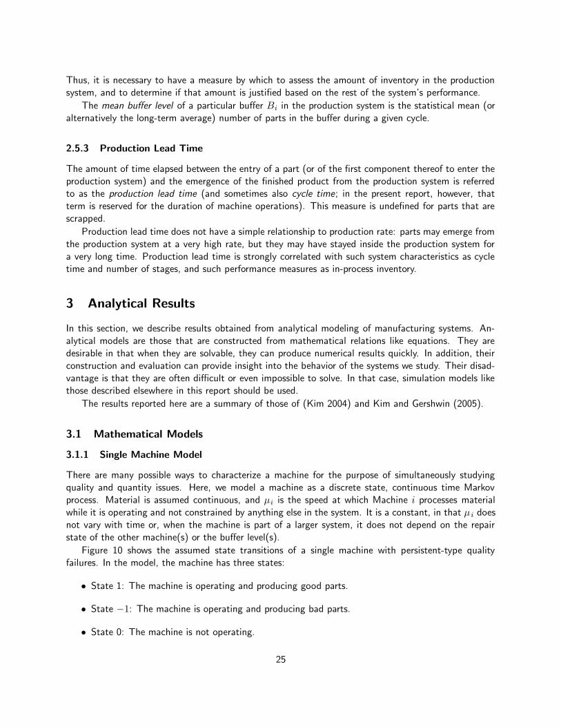
There are many possible ways to characterize a machine for the purpose of simultaneously studyingquality and quantity issues. Here, we model a machine as a discrete state, continuous time Markovprocess. Material is assumed continuous, and µi is the speed at which Machine i processes materialwhile it is operating and not constrained by anything else in the system. It is a constant, in that µ i doesnot vary with time or, when the machine is part of a larger system, it does not depend on the repairstate of the other machine(s) or the buffer level(s).

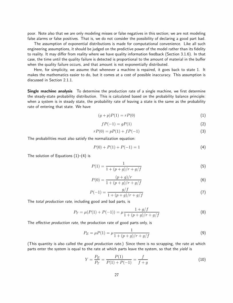
Figure 10 shows the assumed state transitions of a single machine with persistent-type qualityfailures. In the model, the machine has three states:

• State 1: The machine is operating and producing good parts.

• State −1: The machine is operating and producing bad parts.

• State 0: The machine is not operating.

25

1 −1 0

p

r

fg

Figure 10: Three-state machine model.

(Note that when the machine is in state −1, it is producing defective parts but the operator does notknow that yet; as soon as inspection reveals that defective parts are being produced, the machine istaken to state 0 for quality maintenance.)

The machine therefore has two different failure modes (i.e. transitions to failure states from state1):

• Operational failure: transition from state 1 to state 0. The machine stops producing parts due tofailures like motor burnout.

• Quality failure: transition from state 1 to state −1. The machine stops producing good parts(and starts producing bad parts) due to a failure like a sudden tool damage.

This is a simplification of the model in Figure 4.

When a machine is in state 1, it can fail due to a non-quality-related event. It goes to state 0 withtransition probability rate p, which is the reciprocal of the Mean Time to Fail (MTTF). After that anoperator fixes it, and the machine goes back to state 1 with transition rate r, the reciprocal of the MeanTime to Repair (MTTR). Sometimes, due to an assignable cause, the machine begins to produce badparts, so there is a transition from state 1 to state -1 with a probability rate g. Here g is the reciprocalof the Mean Time to Quality Failure (MTQF). A more stable operation leads to a larger MTQF and asmaller g.

The machine, when it is in state −1, can stop for two reasons: it may experience the same kindof operational failure as it does when it is in state 1; and the operator may stop it for repair when helearns that it is producing bad parts. We assume that the transition from state −1 to state 0 occursat probability rate f = p + h where h is the reciprocal of the Mean Time To Detect (MTTD). A morereliable inspection leads to a shorter MTTD and a larger f . (The detection can take place elsewhere, forexample at a remote inspection station.) Note that this implies that f > p. All the indicated transitionsare assumed to follow exponential distributions.

A larger h = f−p means that MTTD is smaller and that fewer bad parts escape detection. Thereforewe refer to inspection stations with larger h as more reliable or more accurate; and those with small h as

26

poor. Note also that we are only modeling misses or false negatives in this section; we are not modelingfalse alarms or false positives. That is, we do not consider the possibility of declaring a good part bad.

The assumption of exponential distributions is made for computational convenience. Like all suchengineering assumptions, it should be judged on the predictive power of the model rather than its fidelityto reality. It may differ from reality where we have quality information feedback (Section 3.1.6). In thatcase, the time until the quality failure is detected is proportional to the amount of material in the bufferwhen the quality failure occurs, and that amount is not exponentially distributed.

Here, for simplicity, we assume that whenever a machine is repaired, it goes back to state 1. Itmakes the mathematics easier to do, but it comes at a cost of possible inaccuracy. This assumption isdiscussed in Section 2.1.1.

Single machine analysis To determine the production rate of a single machine, we first determinethe steady-state probability distribution. This is calculated based on the probability balance principle:when a system is in steady state, the probability rate of leaving a state is the same as the probabilityrate of entering that state. We have

(g + p)P (1) = rP (0) (1)

fP (−1) = gP (1) (2)

rP (0) = pP (1) + fP (−1) (3)

The probabilities must also satisfy the normalization equation:

P (0) + P (1) + P (−1) = 1 (4)

The solution of Equations (1)–(4) is

P (1) =1

1 + (p + g)/r + g/f(5)

P (0) =(p + g)/r

1 + (p + g)/r + g/f(6)

P (−1) =g/f

1 + (p + g)/r + g/f(7)

The total production rate, including good and bad parts, is

PT = µ(P (1) + P (−1)) = µ1 + g/f

1 + (p + g)/r + g/f(8)

The effective production rate, the production rate of good parts only, is

PE = µP (1) = µ1

1 + (p + g)/r + g/f(9)

(This quantity is also called the good production rate.) Since there is no scrapping, the rate at whichparts enter the system is equal to the rate at which parts leave the system, so that the yield is

Y =PE

PT

=P (1)

P (1) + P (−1)=

f

f + g(10)

27

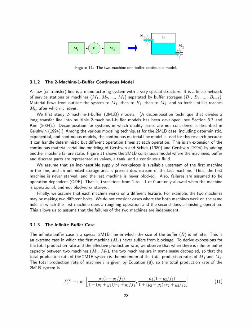
M

M

MM

B

B

1 22

1

Figure 11: The two-machine-one-buffer continuous model.

3.1.2 The 2-Machine-1-Buffer Continuous Model

A flow (or transfer) line is a manufacturing system with a very special structure. It is a linear networkof service stations or machines (M1, M2, ..., Mk) separated by buffer storages (B1, B2, ..., Bk−1).Material flows from outside the system to M1, then to B1, then to M2, and so forth until it reachesMk, after which it leaves.

We first study 2-machine-1-buffer (2M1B) models. (A decomposition technique that divides along transfer line into multiple 2-machine-1-buffer models has been developed; see Section 3.3 andKim (2004).) Decomposition for systems in which quality issues are not considered is described inGershwin (1994).) Among the various modeling techniques for the 2M1B case, including deterministic,exponential, and continuous models, the continuous material line model is used for this research becauseit can handle deterministic but different operation times at each operation. This is an extension of thecontinuous material serial line modeling of Gershwin and Schick (1980) and Gershwin (1994) by addinganother machine failure state. Figure 11 shows the 2M1B continuous model where the machines, bufferand discrete parts are represented as valves, a tank, and a continuous fluid.

We assume that an inexhaustible supply of workpieces is available upstream of the first machinein the line, and an unlimited storage area is present downstream of the last machine. Thus, the firstmachine is never starved, and the last machine is never blocked. Also, failures are assumed to beoperation dependent (ODF). That is, transitions from 1 to −1 or 0 are only allowed when the machineis operational, and not blocked or starved.

Finally, we assume that each machine works on a different feature. For example, the two machinesmay be making two different holes. We do not consider cases where the both machines work on the samehole, in which the first machine does a roughing operation and the second does a finishing operation.This allows us to assume that the failures of the two machines are independent.

3.1.3 The Infinite Buffer Case

The infinite buffer case is a special 2M1B line in which the size of the buffer (B) is infinite. This isan extreme case in which the first machine (M1) never suffers from blockage. To derive expressions forthe total production rate and the effective production rate, we observe that when there is infinite buffercapacity between two machines (M1, M2), the two machines are in some sense decoupled, so that thetotal production rate of the 2M1B system is the minimum of the total production rates of M1 and M2.The total production rate of machine i is given by Equation (8), so the total production rate of the2M1B system is

P∞

T = min

[

µ1(1 + g1/f1)

1 + (p1 + g1)/r1 + g1/f1,

µ2(1 + g2/f2)

1 + (p2 + g2)/r2 + g2/f2

]

(11)

28

The probability that machine Mi does not add defects (non-conformities) is

Yi =Pi(1)

Pi(1) + Pi(−1)=

fi

fi + gi

(12)

Since there is no scrapping or reworking in the system, the system yield is

Y = Y1Y2 =f1f2

(f1 + g1)(f2 + g2)(13)

As a result, the effective production rate is

P∞

E =f1f2

(f1 + g1)(f2 + g2)P∞

T (14)

The effective production rate evaluated from Equation (14) has been compared with a discrete-event,discrete-part simulation and has shown good agreement.

As indicated in Section 3.1.1, the detection of quality failures due to machine M1 need not occurat that machine. For example, the inspection of the feature that M1 works on could take place at aninspection station at or just after M2, and this inspection could trigger a repair of M1. (This is qualityinformation feedback. See Section 3.1.6.) In that case, the MTTD of M1 (and therefore f1) will be afunction of the amount of material in the buffer. We return to this important case in Section 3.1.6.

3.1.4 The Zero Buffer Case

In the zero buffer case, there is no buffer space between the machines. Whenever one of the machinesstops, the other one is also stopped. When both of them are working, the production rate is min[µ1, µ2].This is the other extreme case, in which blockage and starvation take place most frequently. The detailsof the analysis appear in Kim (2004) and Kim and Gershwin (2005). We summarize the results here.

We define

pbi = pi

min(µ1, µ2)

µi

, gbi = gi

min(µ1, µ2)

µi

, and f bi = fi

min(µ1, µ2)

µi

(15)

This is because we have assumed that failures are operation-dependent. As a consequence, the ratesof failure must be reduced for the faster machine. The reduction of pi to pb

i is explained in detail inGershwin (1994) and Gershwin and Schick (1980). We must reduce gi and fi for the same reasons.

The total production rate is then

P 0T =

min[µ1, µ2]

1 +f b1(p

b1 + gb

1)

r1(f b1 + gb

1)+

f b2(pb

2 + gb2)

r2(f b2 + gb

2)

(16)

and the effective production rate is

P 0E =

f b1f b

2

(f b1 + gb

1)(fb2 + gb

2)P 0

T (17)

29

3.1.5 The 2-Machine-1-Finite-Buffer Line

The two-machine line is the simplest non-trivial case of a production line. In the existing literature onthe performance evaluation of systems in which quality is not considered, two-machine lines are used indecomposition approximations of longer lines. (See Gershwin (1994).)

We analyze this system by extending the continuous material two-machine approach of Gershwinand Schick (1980). As in the earlier work, the goal of the analysis is to calculate the average productionrate and buffer level. It is more complex because first, each machine has three states rather than two,and second, there are now two different production rates: the total production rate and the productionrate of good material.

State definition The state of the 2M1B line is defined as (x, α1, α2) where

• x: the total amount of material in buffer B, 0 ≤ x ≤ N ,

• α1: the state of M1. (α1 = −1, 0, or 1),

• α2: the state of M2. (α2 = −1, 0, or 1)

The parameters of machine Mi are µi, ri, pi, fi, gi and the buffer size is N .

Model development As in Gershwin and Schick (1980), we analyze this system by finding its steady-state probability distribution. This consists of a set of density functions f(x, α1, α2) and a set ofprobability masses P (0, α1, α2) and P (N,α1, α2). Since α1 and α2 each take three values, there are 9density functions and 18 masses. We therefore derive and solve 9 differential equations (considerablymore than the 4 differential equations in the earlier work) and numerous boundary conditions .

As usual, the solution of the differential equations requires the solution of a set of simultaneouspolynomial equations. New complexity arises from the fact that the number of roots—and therefore thenumber of boundary conditions—depends on the values of the parameters.

Validation Numerous cases were compared with simulation. The average absolute value of the errorin the effective production rate was under 1% and it was under 2% for the average inventory.

3.1.6 Quality Information Feedback

Factory designers and managers know that it is ideal to have inspection after every operation, but itis often costly to do this. As a result, many factories are designed so that multiple inspections areperformed at a small number of stations. In this case, downstream inspection at can detect bad featuresmade by upstream machines. When that happens, the inspection signals that the machine that madethe bad feature should be repaired. We call this quality information feedback.

We focus here on quality information feedback in 2M1B systems when M1 produces defective featuresbut does not have inspection, and M2 has inspection that can detect bad features made by M1. In thissituation, as we demonstrate below, the yield of a line is a function of the size of the buffer. This isbecause when the buffer gets larger, more material can accumulate between an operation at M1 and theinspection of that operation at M2. All such material will be defective if a persistent quality failure takesplace. In other words, if buffer is larger, there tends to be more material in the buffer and consequently

30

more material is defective. We can approximate this phenomenon with the adjustment of the transitionprobability rate f of M1 from state −1 to state 0.

In Kim (2004) and Kim and Gershwin (2005) we describe a method for using the two-machine modeldescribed in Section 3.1.5 to analyze quality information feedback. To use that model, we approximatethe transition time from state −1 to state 0 in Machine M1 as exponentially distributed. The rate isgiven by

f1 = p1 + h1

where 1/h1 (the mean time of transitions due to the detection of a quality defect) is proportional tothe average amount of inventory in the buffer. This creates a computational problem: since the averagebuffer level is not known, it is impossible to choose h1. We solve this problem by iterating: we guessh1; then evaluate the average buffer level; then we use the average buffer level to recalculate h1; andwe repeat. Experience shows that this procedure converges reliably and rapidly.

We compared the effective production rate and the average inventory from the analytic model witha simulation. Numerous cases were evaluated and the average absolute value of the errors in PE and xestimates were about 1% and under 4%, respectively.

3.1.7 Insights From Numerical Experimentation

In this section, we perform a set of numerical experiments to provide intuitive insight into the behaviorof production lines with inspection and quality information feedback. In Figures 12–15, we comparepairs of systems that are identical except for a quality feedback loop in one of them. In both systems,only M1 can make bad parts, and M1 can inspect its own parts. M1’s failure behavior is persistent, asdescribed in Section 3.1.1. In one system of each pair (with feedback), M2 also inspects the parts; inthe other (without feedback) M2 does no inspection. In both, M1 is taken down for service when a badpart is observed.

We consider only a system with feedback in Figures 16–18.

Beneficial buffer case The system with feedback has more inspection events than the system withoutfeedback. This causes the machines to stop more frequently. As a result, the total production rate of theline is lower. However, the effective production rate can be greater since additional inspections reducethe making of defective parts. This phenomenon is shown in Figure 12. Note that the total productionrate PT without quality information feedback is consistently higher than PT with quality informationfeedback regardless of buffer size; the opposite is true for the effective production rate PE . Also, boththe total production rate and the effective production rate increase with buffer size, with or withoutquality information feedback.

Even though a larger buffer increases both total and effective production rates in this case, itdecreases yield. As explained in Section 3.1.6, the system yield is a function of the buffer size if there isquality information feedback. Figure 13 shows the system yield decreasing as the buffer size increaseswhen there is quality information feedback. This happens because when the buffer gets larger, morematerial accumulates between an operation and the inspection of that operation. All such material willbe defective when the first machine is in state −1 and the first machine does not detect the qualitydefects. This is a case in which a smaller buffer improves quality (i.e. the yield), which is widely believedto be generally true. If there is no quality information feedback, then the system yield is independentof the buffer size (and is substantially lower).

31

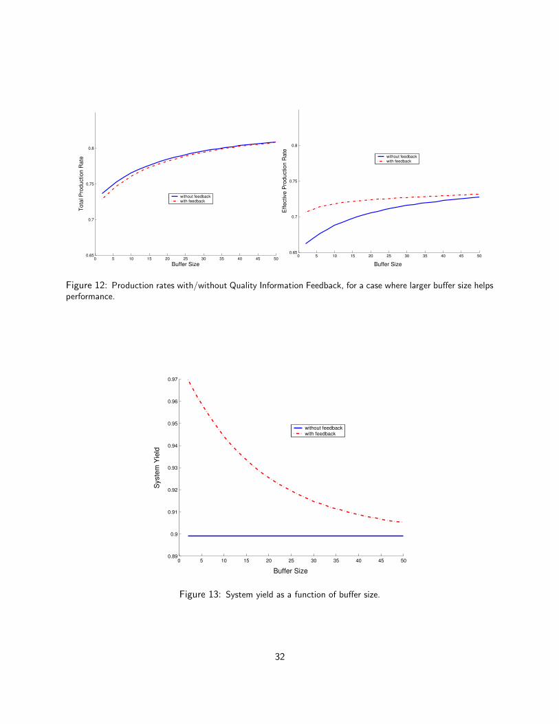
0 5 10 15 20 25 30 35 40 45 500.65

0.7

0.75

0.8

Buffer Size

Tota

l Pro

duct

ion

Rat

e

without feedbackwith feedback

0 5 10 15 20 25 30 35 40 45 500.65

0.7

0.75

0.8

Buffer Size

Effe

ctiv

e P

rodu

ctio

n R

ate

without feedbackwith feedback

Figure 12: Production rates with/without Quality Information Feedback, for a case where larger buffer size helpsperformance.

0 5 10 15 20 25 30 35 40 45 500.89

0.9

0.91

0.92

0.93

0.94

0.95

0.96

0.97

Buffer Size

Sys

tem

Yie

ld

without feedbackwith feedback

Figure 13: System yield as a function of buffer size.

32

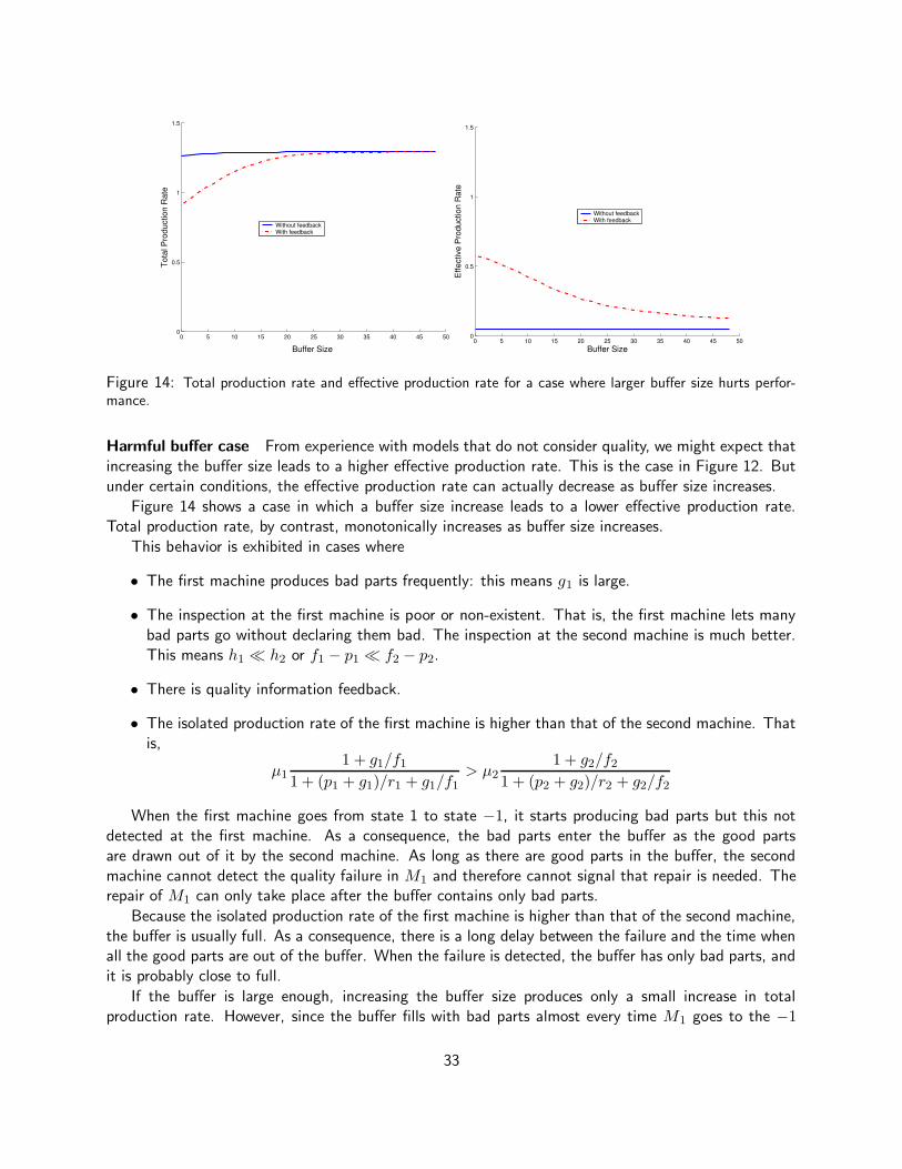
0 5 10 15 20 25 30 35 40 45 500

0.5

1

1.5

Buffer Size

Tota

l Pro

duct

ion

Rat

e

Without feedbackWith feedback

0 5 10 15 20 25 30 35 40 45 500

0.5

1

1.5

Buffer Size

Effe

ctiv

e P

rodu

ctio

n R

ate

Without feedbackWith feedback

Figure 14: Total production rate and effective production rate for a case where larger buffer size hurts perfor-mance.

Harmful buffer case From experience with models that do not consider quality, we might expect thatincreasing the buffer size leads to a higher effective production rate. This is the case in Figure 12. Butunder certain conditions, the effective production rate can actually decrease as buffer size increases.

Figure 14 shows a case in which a buffer size increase leads to a lower effective production rate.Total production rate, by contrast, monotonically increases as buffer size increases.

This behavior is exhibited in cases where

• The first machine produces bad parts frequently: this means g1 is large.

• The inspection at the first machine is poor or non-existent. That is, the first machine lets manybad parts go without declaring them bad. The inspection at the second machine is much better.This means h1 � h2 or f1 − p1 � f2 − p2.

• There is quality information feedback.

• The isolated production rate of the first machine is higher than that of the second machine. Thatis,

µ11 + g1/f1

1 + (p1 + g1)/r1 + g1/f1> µ2

1 + g2/f2

1 + (p2 + g2)/r2 + g2/f2

When the first machine goes from state 1 to state −1, it starts producing bad parts but this notdetected at the first machine. As a consequence, the bad parts enter the buffer as the good partsare drawn out of it by the second machine. As long as there are good parts in the buffer, the secondmachine cannot detect the quality failure in M1 and therefore cannot signal that repair is needed. Therepair of M1 can only take place after the buffer contains only bad parts.

Because the isolated production rate of the first machine is higher than that of the second machine,the buffer is usually full. As a consequence, there is a long delay between the failure and the time whenall the good parts are out of the buffer. When the failure is detected, the buffer has only bad parts, andit is probably close to full.

If the buffer is large enough, increasing the buffer size produces only a small increase in totalproduction rate. However, since the buffer fills with bad parts almost every time M1 goes to the −1

33

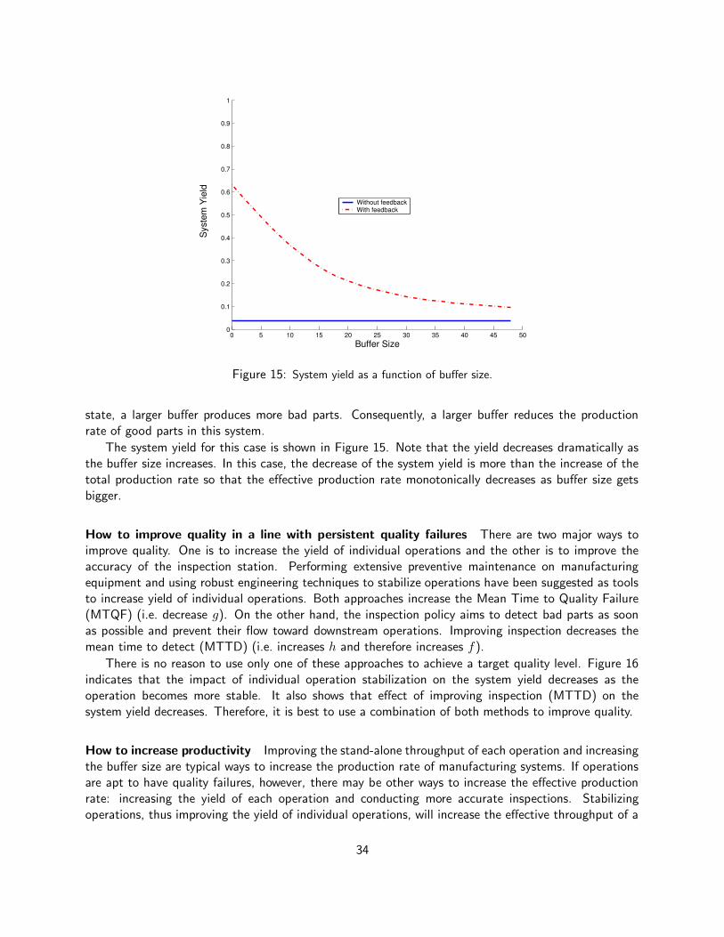
0 5 10 15 20 25 30 35 40 45 500

0.1

0.2

0.3

0.4

0.5

0.6

0.7

0.8

0.9

1

Buffer Size

Sys

tem

Yie

ldWithout feedbackWith feedback

Figure 15: System yield as a function of buffer size.

state, a larger buffer produces more bad parts. Consequently, a larger buffer reduces the productionrate of good parts in this system.

The system yield for this case is shown in Figure 15. Note that the yield decreases dramatically asthe buffer size increases. In this case, the decrease of the system yield is more than the increase of thetotal production rate so that the effective production rate monotonically decreases as buffer size getsbigger.

How to improve quality in a line with persistent quality failures There are two major ways toimprove quality. One is to increase the yield of individual operations and the other is to improve theaccuracy of the inspection station. Performing extensive preventive maintenance on manufacturingequipment and using robust engineering techniques to stabilize operations have been suggested as toolsto increase yield of individual operations. Both approaches increase the Mean Time to Quality Failure(MTQF) (i.e. decrease g). On the other hand, the inspection policy aims to detect bad parts as soonas possible and prevent their flow toward downstream operations. Improving inspection decreases themean time to detect (MTTD) (i.e. increases h and therefore increases f).

There is no reason to use only one of these approaches to achieve a target quality level. Figure 16indicates that the impact of individual operation stabilization on the system yield decreases as theoperation becomes more stable. It also shows that effect of improving inspection (MTTD) on thesystem yield decreases. Therefore, it is best to use a combination of both methods to improve quality.

How to increase productivity Improving the stand-alone throughput of each operation and increasingthe buffer size are typical ways to increase the production rate of manufacturing systems. If operationsare apt to have quality failures, however, there may be other ways to increase the effective productionrate: increasing the yield of each operation and conducting more accurate inspections. Stabilizingoperations, thus improving the yield of individual operations, will increase the effective throughput of a

34

50 100 150 200 250 300 350 400 4500

0.1

0.2

0.3

0.4

0.5

0.6

0.7

0.8

0.9

1

MTQF

Sys

tem

Yie

ld

0 0.1 0.2 0.3 0.4 0.5 0.6 0.7 0.8 0.9 10

0.1

0.2

0.3

0.4

0.5

0.6

0.7

0.8

0.9

1

f=p+h

Sys

tem

Yie

ld

Figure 16: Quality improvement by decreasing the frequency of quality errors, and by decreasing the mean timeto detect a quality failure.

manufacturing system regardless of the type of quality failure. On the other hand, reducing the MTTDwill increase the effective production rate if the quality failure is persistent but it will decrease theeffective production rate if the quality failure is Bernoulli. This is because the quality of each part isindependent of the others when the quality failure is Bernoulli. Therefore, stopping the line does notreduce the number of bad parts in the future.

In a situation in which machines produce defective parts frequently and inspection is poor, increasinginspection reliability is more effective than increasing buffer size to boost the effective production rate.Figure 17 shows this. Also, in other situations in which machines produce defective parts frequentlyand inspection is reliable, increasing machine stability is more effective than increasing buffer size toenhance effective production rate. Figure 18 shows this phenomenon.

3.2 Effectiveness of the Jidoka Stopping Policy

3.2.1 Motivation

Many tools in the Toyota Production System have been widely used in the design and operation ofmanufacturing systems in the automotive industry. Jidoka, the principle of stopping an operation assoon as a single problem is observed and preventing the production of defective items, is fundamental tothe Toyota Production System (Monden 1983). In the Toyota Production System, equipment is designedto detect abnormalities and to stop automatically and immediately whenever they occur. Operators atassembly lines are provided means of stopping the production flow (andon cords) whenever they noteanything unusual.

Experts in the Toyota Production System argue that the jidoka practice has brought several benefits.One is that it motivates kaizen (continuous improvement) since operators can clearly see the painfuloutcome of producing defects: the line stoppage. It is easier to find the root cause of a problemright after the problem takes place. Through the use of systematic ways of resolving problems (e.g.asking “Why?” five times) which are widely accepted in Toyota, operators’ learning speed accelerates(Fujimoto 1999). It has been known that operators’ learning can significantly improve productivity and

35

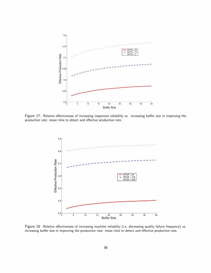
0 5 10 15 20 25 30 35 400.5

0.55

0.6

0.65

0.7

0.75

0.8

Buffer Size

Effe

ctiv

e P

rodu

ctio

n R

ate

MTTD = 20MTTD = 10MTTD = 2

Figure 17: Relative effectiveness of increasing inspection reliability vs. increasing buffer size in improving theproduction rate: mean time to detect and effective production rate.

0 5 10 15 20 25 30 35 400.3

0.4

0.5

0.6

0.7

0.8

0.9

Buffer Size

Effe

ctiv

e P

rodu

ctio

n R

ate

MTQF = 20MTQF = 100MTQF = 500

Figure 18: Relative effectiveness of increasing machine reliability (i.e. decreasing quality failure frequency) vs.increasing buffer size in improving the production rate: mean time to detect and effective production rate.

36

quality (Sandberg 1995).

The other benefit of jidoka that Toyota Production System advocates claim is that it prevents thewaste that would result from producing a series of defective items. Therefore, jidoka is considered to bea means to improve quality and increase productivity at the same time (Toyota Motor Corporation 1996,Monden 1983). It is this aspect of the jidoka policy that we investigate here. When quality failures aresuch that once a bad part is produced, all subsequent parts will be bad until the machine is repaired,and when inspection is very accurate, catching bad parts and stopping the machine as soon as possibleis the best way to maintain high quality and productivity. This is the case with breakage of thread,which caused the invention of the jidoka practice a century ago at Toyota Spinning & Weaving (Togoand Waterman 1993). On the other hand, when a defect is generated from common cause variations sothat the occurrence of a bad part implies nothing about the quality of future parts, there is no benefitto stopping a machine that has made a bad part because there is no reason to believe that future partswill be bad; thus stopping the machine would not reduce the number of bad parts in the future. In thiscase, therefore, stopping the operation does not improve quality and it reduces productivity by reducingworking time.

In reality, most machines have multiple-yield quality failures in a sense that quality failures occurindependently but at different rates depending on what state the machine is in. When a machine is ingood shape and operating without any assignable cause variations (i.e., when it is in control), it mayproduce a defective part with a very small probability, not because of any change in the machine butbecause of random perturbations. However, when a machine is operating under an assignable causevariation (i.e., it is out of control), it is likely that many of the parts that will be produced will be bad.In this situation, the optimal stopping policy is, therefore, to stop the machine only if the machine is outof control. But in many cases it is not easy to tell whether the machine is out of control or in control(in other words, whether a quality failure is from a random variation or an assignable cause variation)with a single sample. Matters get even more complicated when the inspection is not perfectly accurate.

Here, we investigate when stopping a machine after the observation of a single bad part is betterthan waiting until two consecutive bad parts are seen. We do not determine when jidoka is optimal;rather we find conditions under which it is certainly not optimal.

3.2.2 Single Machine

State definition People adopt jidoka assuming that inspection is 100% accurate and that all thedefects are from persistent quality failures. In that case, it is clear that jidoka improves quality andproductivity at the same time. But when there are Bernoulli quality failures or multiple-yield qualityfailures, there is no guarantee that subsequent parts will be defective after finding a defect. In thiscase, it may be better to stop a machine when the machine produces two defective parts in a row, forexample, since it is not likely to have two Bernoulli quality failures consecutively.

We extend the model of Section 3.1.1 to analyze jidoka. In this multiple-yield model, the stateshave the following meanings:

• State 1: The machine is in good shape and operating without any assignable cause variations.It may produce defective parts with probability 1 − π(1), which is close to 0, due to randomvariations.

• State −1: The machine is operating under an assignable cause variation and is producing badparts with probability 1 − π(−1), which is larger than 1 − π(1).

37

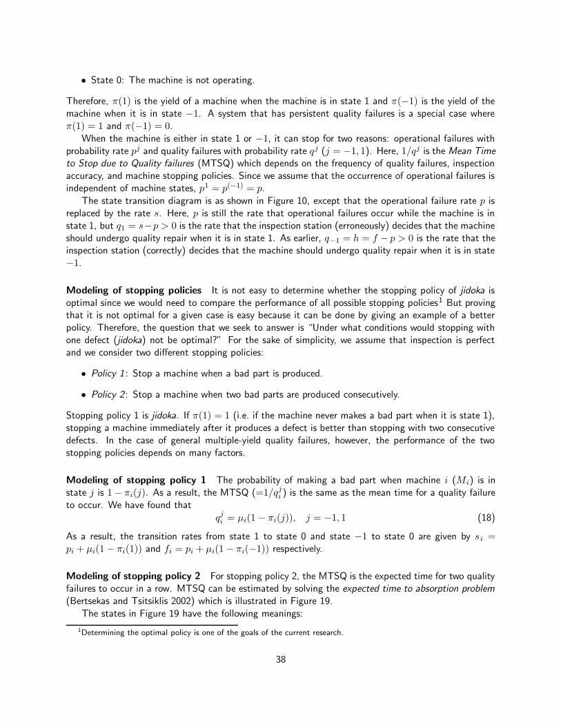
• State 0: The machine is not operating.

Therefore, π(1) is the yield of a machine when the machine is in state 1 and π(−1) is the yield of themachine when it is in state −1. A system that has persistent quality failures is a special case whereπ(1) = 1 and π(−1) = 0.

When the machine is either in state 1 or −1, it can stop for two reasons: operational failures withprobability rate pj and quality failures with probability rate qj (j = −1, 1). Here, 1/qj is the Mean Timeto Stop due to Quality failures (MTSQ) which depends on the frequency of quality failures, inspectionaccuracy, and machine stopping policies. Since we assume that the occurrence of operational failures isindependent of machine states, p1 = p(−1) = p.

The state transition diagram is as shown in Figure 10, except that the operational failure rate p isreplaced by the rate s. Here, p is still the rate that operational failures occur while the machine is instate 1, but q1 = s−p > 0 is the rate that the inspection station (erroneously) decides that the machineshould undergo quality repair when it is in state 1. As earlier, q−1 = h = f − p > 0 is the rate that theinspection station (correctly) decides that the machine should undergo quality repair when it is in state−1.

Modeling of stopping policies It is not easy to determine whether the stopping policy of jidoka isoptimal since we would need to compare the performance of all possible stopping policies1 But provingthat it is not optimal for a given case is easy because it can be done by giving an example of a betterpolicy. Therefore, the question that we seek to answer is “Under what conditions would stopping withone defect (jidoka) not be optimal?” For the sake of simplicity, we assume that inspection is perfectand we consider two different stopping policies:

• Policy 1 : Stop a machine when a bad part is produced.

• Policy 2 : Stop a machine when two bad parts are produced consecutively.

Stopping policy 1 is jidoka. If π(1) = 1 (i.e. if the machine never makes a bad part when it is state 1),stopping a machine immediately after it produces a defect is better than stopping with two consecutivedefects. In the case of general multiple-yield quality failures, however, the performance of the twostopping policies depends on many factors.

Modeling of stopping policy 1 The probability of making a bad part when machine i (Mi) is instate j is 1 − πi(j). As a result, the MTSQ (=1/qj

i ) is the same as the mean time for a quality failureto occur. We have found that

qji = µi(1 − πi(j)), j = −1, 1 (18)

As a result, the transition rates from state 1 to state 0 and state −1 to state 0 are given by si =pi + µi(1 − πi(1)) and fi = pi + µi(1 − πi(−1)) respectively.

Modeling of stopping policy 2 For stopping policy 2, the MTSQ is the expected time for two qualityfailures to occur in a row. MTSQ can be estimated by solving the expected time to absorption problem(Bertsekas and Tsitsiklis 2002) which is illustrated in Figure 19.

The states in Figure 19 have the following meanings:

1Determining the optimal policy is one of the goals of the current research.

38

Figure 19: MTSQ estimation through an expected time to absorption problem.

• State 0 : Neither of the last two parts was defective.

• State 1 : The most recent part was defective and the one before that was good.

• State 2 : Both of the last two parts were defective.

In the figure, β is the probability of producing a good part and it depends on whether the machine is instate 1 or −1. When two bad parts are produced in a row, the machine is stopped according to stoppingpolicy 2. Therefore, state 2 is an absorbing state. From the value of the mean time to reach state 2,we find

qji =

µi(1 − πi(j))2

2 − πi(j)(19)

Therefore,

si = pi +µi(1 − πi(1))

2

2−πi(1)

fi = pi +µi(1 − πi(−1))2

2−πi(−1)

(20)

To analyze a single-machine system, we use Equations (1)–(8) with these parameters. We find that theeffective production rate, the production rate of good parts, is

PE = µ[π(1)P (1) + π(−1)P (−1)] = µπ(1) + π(−1)g/f

1 + (s + g)/r + g/f(21)

A numerical analysis is described below.

3.2.3 Analysis of a Two-Machine System

The analysis of the state dynamics is exactly like that of the two-machine line of Section 3.1.2, and thetotal production rate PT is the same. The only difference is that now the effective production rate is afunction of π(1) and π(−1).

A mathematical model for the two-machine system was solved and validated through comparisonwith discrete event simulation (Kim 2004). Agreement with simulation was good.

39

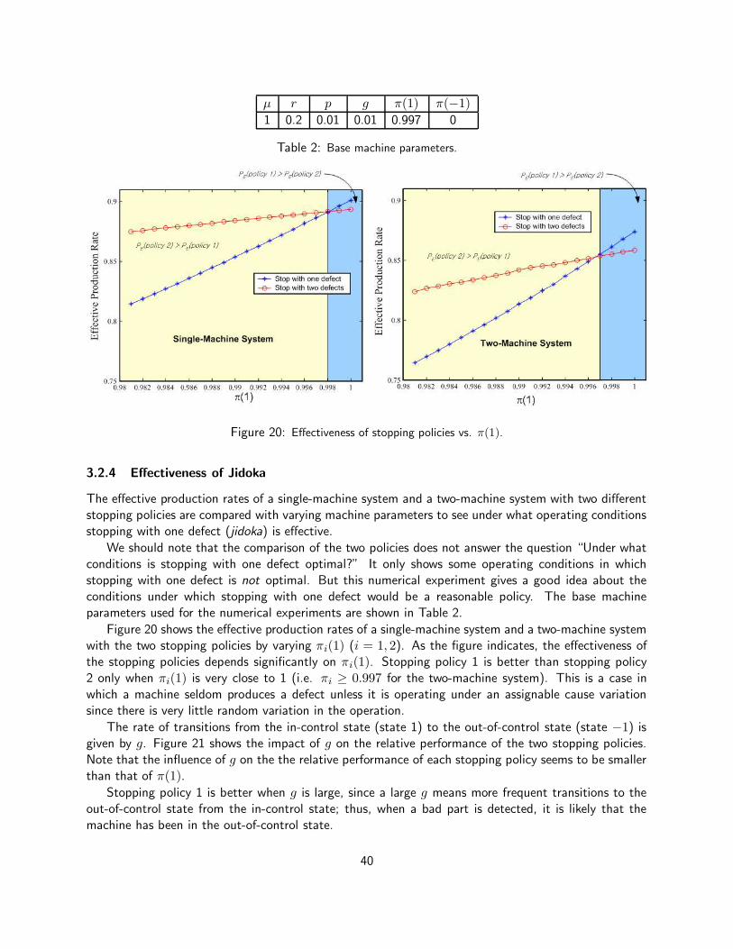
µ r p g π(1) π(−1)

1 0.2 0.01 0.01 0.997 0

Table 2: Base machine parameters.

Figure 20: Effectiveness of stopping policies vs. π(1).

3.2.4 Effectiveness of Jidoka

The effective production rates of a single-machine system and a two-machine system with two differentstopping policies are compared with varying machine parameters to see under what operating conditionsstopping with one defect (jidoka) is effective.

We should note that the comparison of the two policies does not answer the question “Under whatconditions is stopping with one defect optimal?” It only shows some operating conditions in whichstopping with one defect is not optimal. But this numerical experiment gives a good idea about theconditions under which stopping with one defect would be a reasonable policy. The base machineparameters used for the numerical experiments are shown in Table 2.

Figure 20 shows the effective production rates of a single-machine system and a two-machine systemwith the two stopping policies by varying πi(1) (i = 1, 2). As the figure indicates, the effectiveness ofthe stopping policies depends significantly on πi(1). Stopping policy 1 is better than stopping policy2 only when πi(1) is very close to 1 (i.e. πi ≥ 0.997 for the two-machine system). This is a case inwhich a machine seldom produces a defect unless it is operating under an assignable cause variationsince there is very little random variation in the operation.

The rate of transitions from the in-control state (state 1) to the out-of-control state (state −1) isgiven by g. Figure 21 shows the impact of g on the relative performance of the two stopping policies.Note that the influence of g on the the relative performance of each stopping policy seems to be smallerthan that of π(1).

Stopping policy 1 is better when g is large, since a large g means more frequent transitions to theout-of-control state from the in-control state; thus, when a bad part is detected, it is likely that themachine has been in the out-of-control state.

40

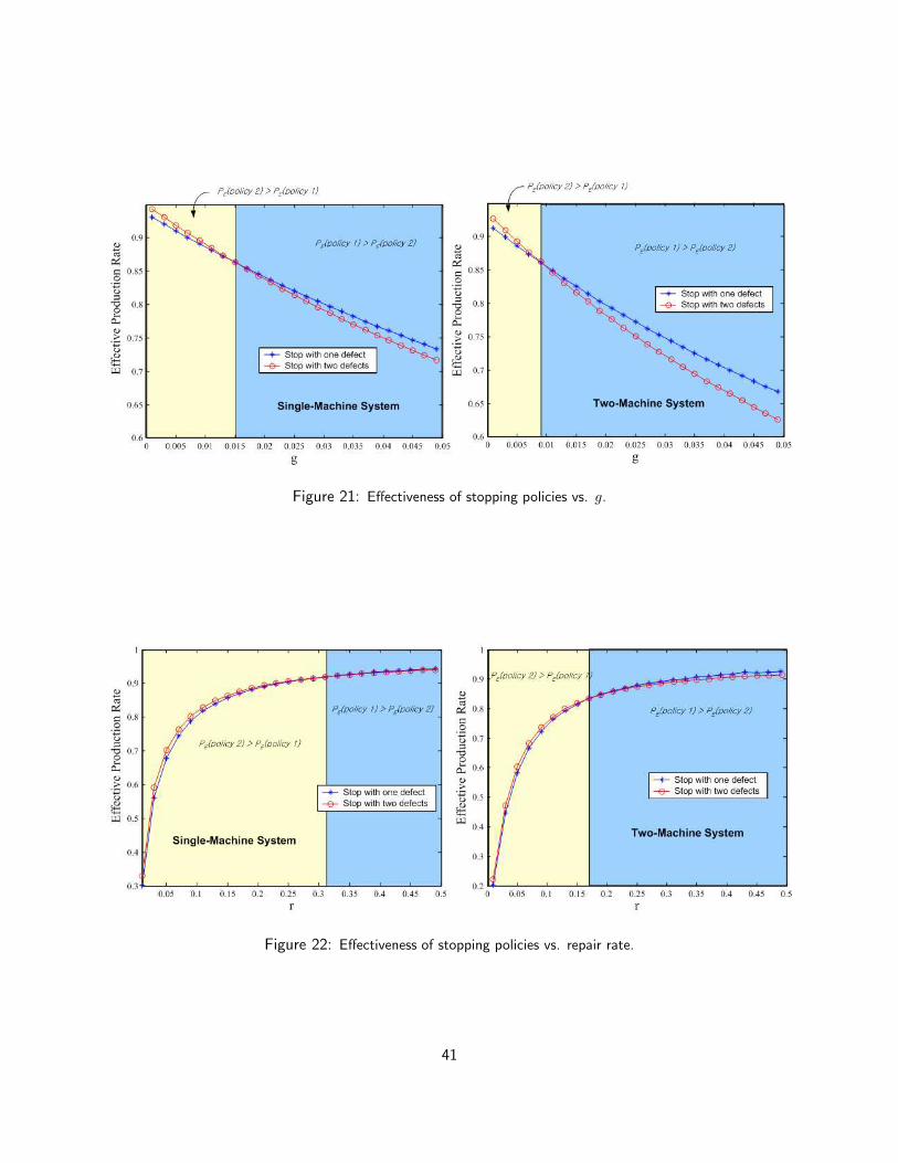
Figure 21: Effectiveness of stopping policies vs. g.

Figure 22: Effectiveness of stopping policies vs. repair rate.

41

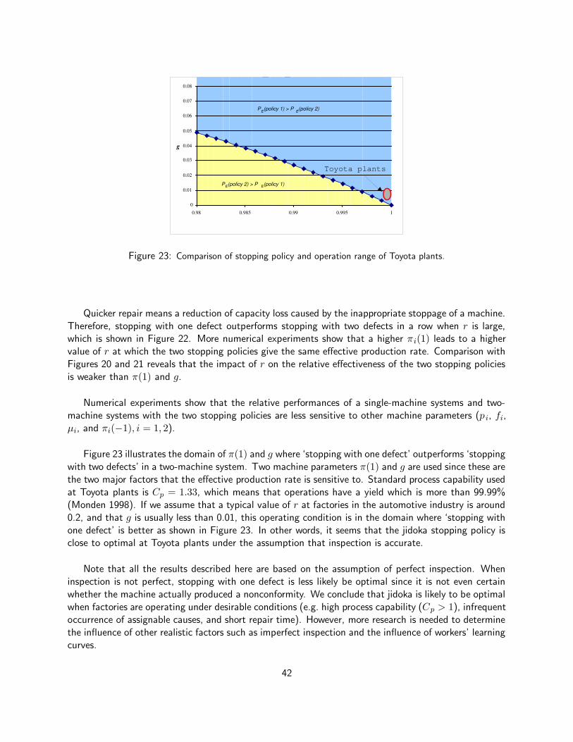
0

0.01

0.02

0.03

0.04

0.05

0.06

0.07

0.08

0.98 0.985 0.99 0.995 1

g

P E (policy 1) > P E (policy 2)

P E (policy 2) > P E (policy 1)

Toyota plants

Figure 23: Comparison of stopping policy and operation range of Toyota plants.

Quicker repair means a reduction of capacity loss caused by the inappropriate stoppage of a machine.Therefore, stopping with one defect outperforms stopping with two defects in a row when r is large,which is shown in Figure 22. More numerical experiments show that a higher πi(1) leads to a highervalue of r at which the two stopping policies give the same effective production rate. Comparison withFigures 20 and 21 reveals that the impact of r on the relative effectiveness of the two stopping policiesis weaker than π(1) and g.

Numerical experiments show that the relative performances of a single-machine systems and two-machine systems with the two stopping policies are less sensitive to other machine parameters (p i, fi,µi, and πi(−1), i = 1, 2).

Figure 23 illustrates the domain of π(1) and g where ‘stopping with one defect’ outperforms ‘stoppingwith two defects’ in a two-machine system. Two machine parameters π(1) and g are used since these arethe two major factors that the effective production rate is sensitive to. Standard process capability usedat Toyota plants is Cp = 1.33, which means that operations have a yield which is more than 99.99%(Monden 1998). If we assume that a typical value of r at factories in the automotive industry is around0.2, and that g is usually less than 0.01, this operating condition is in the domain where ‘stopping withone defect’ is better as shown in Figure 23. In other words, it seems that the jidoka stopping policy isclose to optimal at Toyota plants under the assumption that inspection is accurate.

Note that all the results described here are based on the assumption of perfect inspection. Wheninspection is not perfect, stopping with one defect is less likely be optimal since it is not even certainwhether the machine actually produced a nonconformity. We conclude that jidoka is likely to be optimalwhen factories are operating under desirable conditions (e.g. high process capability (Cp > 1), infrequentoccurrence of assignable causes, and short repair time). However, more research is needed to determinethe influence of other realistic factors such as imperfect inspection and the influence of workers’ learningcurves.

42

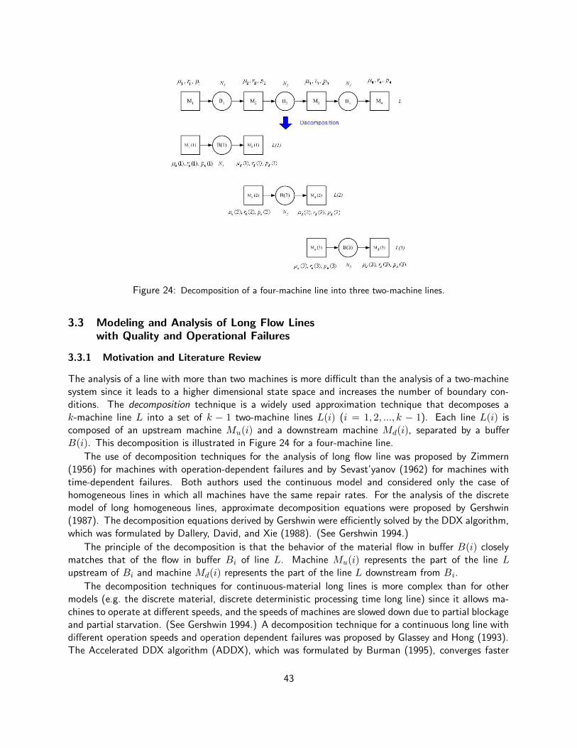
Figure 24: Decomposition of a four-machine line into three two-machine lines.

3.3 Modeling and Analysis of Long Flow Lineswith Quality and Operational Failures

3.3.1 Motivation and Literature Review

The analysis of a line with more than two machines is more difficult than the analysis of a two-machinesystem since it leads to a higher dimensional state space and increases the number of boundary con-ditions. The decomposition technique is a widely used approximation technique that decomposes ak-machine line L into a set of k − 1 two-machine lines L(i) (i = 1, 2, ..., k − 1). Each line L(i) iscomposed of an upstream machine Mu(i) and a downstream machine Md(i), separated by a bufferB(i). This decomposition is illustrated in Figure 24 for a four-machine line.

The use of decomposition techniques for the analysis of long flow line was proposed by Zimmern(1956) for machines with operation-dependent failures and by Sevast’yanov (1962) for machines withtime-dependent failures. Both authors used the continuous model and considered only the case ofhomogeneous lines in which all machines have the same repair rates. For the analysis of the discretemodel of long homogeneous lines, approximate decomposition equations were proposed by Gershwin(1987). The decomposition equations derived by Gershwin were efficiently solved by the DDX algorithm,which was formulated by Dallery, David, and Xie (1988). (See Gershwin 1994.)

The principle of the decomposition is that the behavior of the material flow in buffer B(i) closelymatches that of the flow in buffer Bi of line L. Machine Mu(i) represents the part of the line Lupstream of Bi and machine Md(i) represents the part of the line L downstream from Bi.

The decomposition techniques for continuous-material long lines is more complex than for othermodels (e.g. the discrete material, discrete deterministic processing time long line) since it allows ma-chines to operate at different speeds, and the speeds of machines are slowed down due to partial blockageand partial starvation. (See Gershwin 1994.) A decomposition technique for a continuous long line withdifferent operation speeds and operation dependent failures was proposed by Glassey and Hong (1993).The Accelerated DDX algorithm (ADDX), which was formulated by Burman (1995), converges faster

43

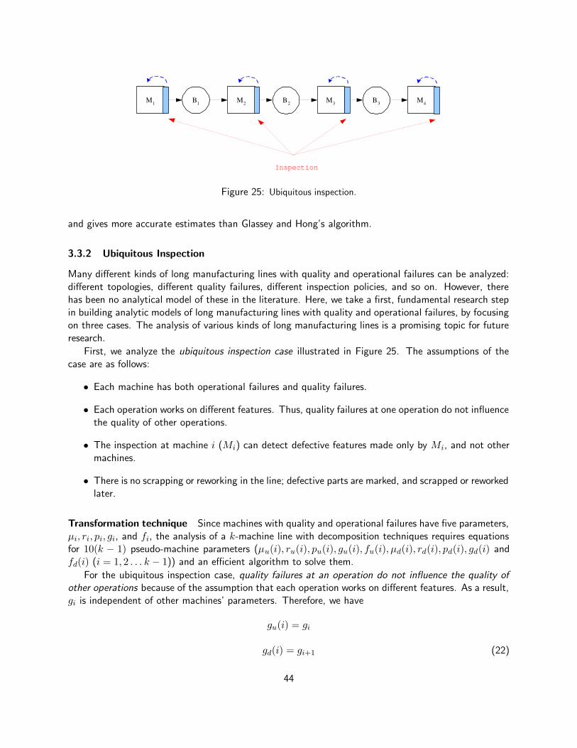
M 1 B 1 M 2 M 3 M 4 B 2 B 3

Inspection

Figure 25: Ubiquitous inspection.

and gives more accurate estimates than Glassey and Hong’s algorithm.

3.3.2 Ubiquitous Inspection

Many different kinds of long manufacturing lines with quality and operational failures can be analyzed:different topologies, different quality failures, different inspection policies, and so on. However, therehas been no analytical model of these in the literature. Here, we take a first, fundamental research stepin building analytic models of long manufacturing lines with quality and operational failures, by focusingon three cases. The analysis of various kinds of long manufacturing lines is a promising topic for futureresearch.

First, we analyze the ubiquitous inspection case illustrated in Figure 25. The assumptions of thecase are as follows:

• Each machine has both operational failures and quality failures.

• Each operation works on different features. Thus, quality failures at one operation do not influencethe quality of other operations.

• The inspection at machine i (Mi) can detect defective features made only by Mi, and not othermachines.

• There is no scrapping or reworking in the line; defective parts are marked, and scrapped or reworkedlater.

Transformation technique Since machines with quality and operational failures have five parameters,µi, ri, pi, gi, and fi, the analysis of a k-machine line with decomposition techniques requires equationsfor 10(k − 1) pseudo-machine parameters (µu(i), ru(i), pu(i), gu(i), fu(i), µd(i), rd(i), pd(i), gd(i) andfd(i) (i = 1, 2 . . . k − 1)) and an efficient algorithm to solve them.

For the ubiquitous inspection case, quality failures at an operation do not influence the quality ofother operations because of the assumption that each operation works on different features. As a result,gi is independent of other machines’ parameters. Therefore, we have

gu(i) = gi

gd(i) = gi+1 (22)

44

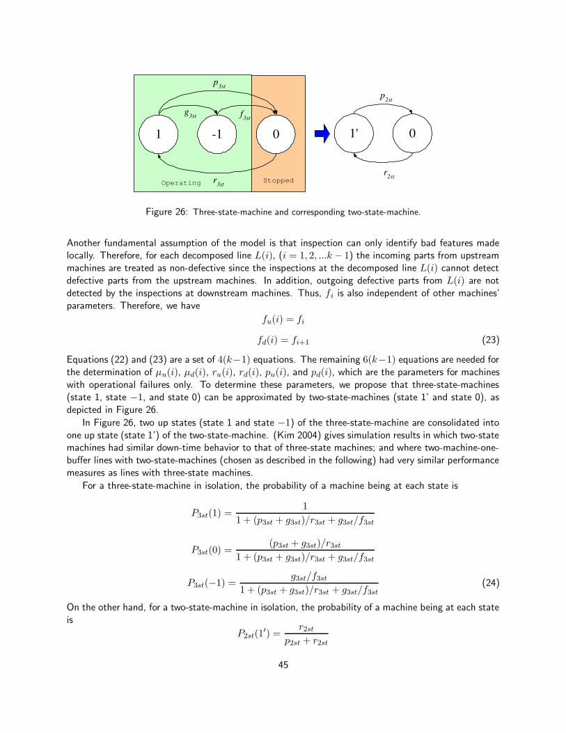
Stopped Operating

1 -1 0

p 3st

1' 0

g 3st f 3st

r 3st

p 2st

r 2st

Figure 26: Three-state-machine and corresponding two-state-machine.

Another fundamental assumption of the model is that inspection can only identify bad features madelocally. Therefore, for each decomposed line L(i), (i = 1, 2, ...k − 1) the incoming parts from upstreammachines are treated as non-defective since the inspections at the decomposed line L(i) cannot detectdefective parts from the upstream machines. In addition, outgoing defective parts from L(i) are notdetected by the inspections at downstream machines. Thus, fi is also independent of other machines’parameters. Therefore, we have

fu(i) = fi

fd(i) = fi+1 (23)

Equations (22) and (23) are a set of 4(k−1) equations. The remaining 6(k−1) equations are needed forthe determination of µu(i), µd(i), ru(i), rd(i), pu(i), and pd(i), which are the parameters for machineswith operational failures only. To determine these parameters, we propose that three-state-machines(state 1, state −1, and state 0) can be approximated by two-state-machines (state 1’ and state 0), asdepicted in Figure 26.

In Figure 26, two up states (state 1 and state −1) of the three-state-machine are consolidated intoone up state (state 1’) of the two-state-machine. (Kim 2004) gives simulation results in which two-statemachines had similar down-time behavior to that of three-state machines; and where two-machine-one-buffer lines with two-state-machines (chosen as described in the following) had very similar performancemeasures as lines with three-state machines.

For a three-state-machine in isolation, the probability of a machine being at each state is

P3st(1) =1

1 + (p3st + g3st)/r3st + g3st/f3st

P3st(0) =(p3st + g3st)/r3st

1 + (p3st + g3st)/r3st + g3st/f3st

P3st(−1) =g3st/f3st

1 + (p3st + g3st)/r3st + g3st/f3st

(24)

On the other hand, for a two-state-machine in isolation, the probability of a machine being at each stateis

P2st(1′) =

r2st

p2st + r2st

45

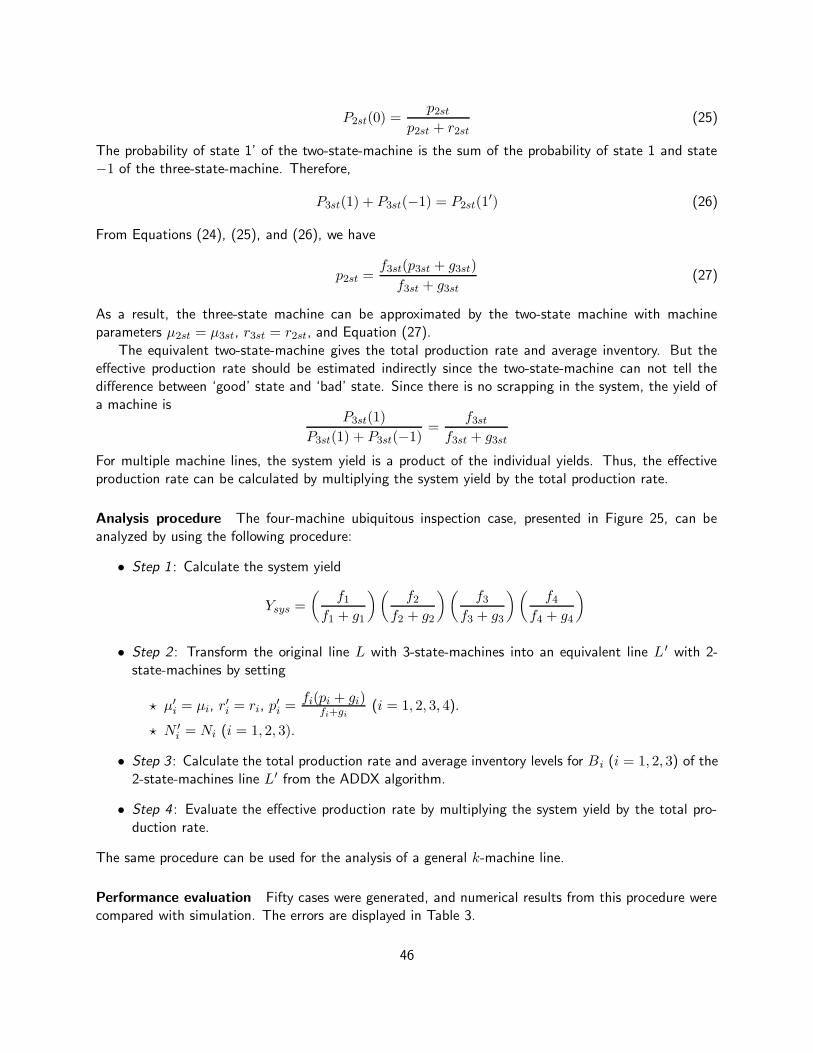
P2st(0) =p2st

p2st + r2st

(25)

The probability of state 1’ of the two-state-machine is the sum of the probability of state 1 and state−1 of the three-state-machine. Therefore,

P3st(1) + P3st(−1) = P2st(1′) (26)

From Equations (24), (25), and (26), we have

p2st =f3st(p3st + g3st)

f3st + g3st

(27)

As a result, the three-state machine can be approximated by the two-state machine with machineparameters µ2st = µ3st, r3st = r2st, and Equation (27).

The equivalent two-state-machine gives the total production rate and average inventory. But theeffective production rate should be estimated indirectly since the two-state-machine can not tell thedifference between ‘good’ state and ‘bad’ state. Since there is no scrapping in the system, the yield ofa machine is

P3st(1)

P3st(1) + P3st(−1)=

f3st

f3st + g3st

For multiple machine lines, the system yield is a product of the individual yields. Thus, the effectiveproduction rate can be calculated by multiplying the system yield by the total production rate.

Analysis procedure The four-machine ubiquitous inspection case, presented in Figure 25, can beanalyzed by using the following procedure:

• Step 1 : Calculate the system yield

Ysys =

(

f1

f1 + g1

)(

f2

f2 + g2

)(

f3

f3 + g3

)(

f4

f4 + g4

)

• Step 2 : Transform the original line L with 3-state-machines into an equivalent line L ′ with 2-state-machines by setting

? µ′

i = µi, r′i = ri, p′i =fi(pi + gi)

fi+gi(i = 1, 2, 3, 4).

? N ′

i = Ni (i = 1, 2, 3).

• Step 3 : Calculate the total production rate and average inventory levels for Bi (i = 1, 2, 3) of the2-state-machines line L′ from the ADDX algorithm.

• Step 4 : Evaluate the effective production rate by multiplying the system yield by the total pro-duction rate.

The same procedure can be used for the analysis of a general k-machine line.

Performance evaluation Fifty cases were generated, and numerical results from this procedure werecompared with simulation. The errors are displayed in Table 3.

46

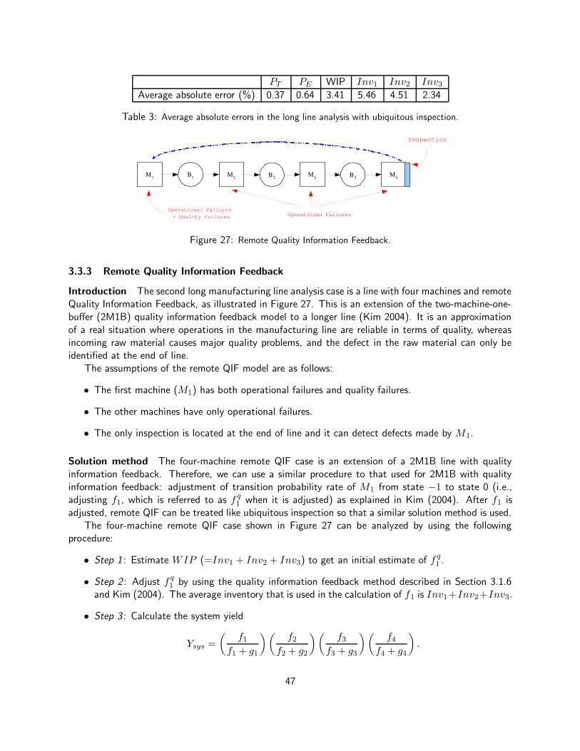
PT PE WIP Inv1 Inv2 Inv3

Average absolute error (%) 0.37 0.64 3.41 5.46 4.51 2.34

Table 3: Average absolute errors in the long line analysis with ubiquitous inspection.

Inspection

M 1 B 1 M 2 M 3 M 4 B 2 B 3

Operational Failures Operational Failures + Quality Failures

Figure 27: Remote Quality Information Feedback.

3.3.3 Remote Quality Information Feedback

Introduction The second long manufacturing line analysis case is a line with four machines and remoteQuality Information Feedback, as illustrated in Figure 27. This is an extension of the two-machine-one-buffer (2M1B) quality information feedback model to a longer line (Kim 2004). It is an approximationof a real situation where operations in the manufacturing line are reliable in terms of quality, whereasincoming raw material causes major quality problems, and the defect in the raw material can only beidentified at the end of line.

The assumptions of the remote QIF model are as follows:

• The first machine (M1) has both operational failures and quality failures.

• The other machines have only operational failures.

• The only inspection is located at the end of line and it can detect defects made by M1.

Solution method The four-machine remote QIF case is an extension of a 2M1B line with qualityinformation feedback. Therefore, we can use a similar procedure to that used for 2M1B with qualityinformation feedback: adjustment of transition probability rate of M1 from state −1 to state 0 (i.e.,adjusting f1, which is referred to as f q

1 when it is adjusted) as explained in Kim (2004). After f1 isadjusted, remote QIF can be treated like ubiquitous inspection so that a similar solution method is used.

The four-machine remote QIF case shown in Figure 27 can be analyzed by using the followingprocedure:

• Step 1 : Estimate WIP (=Inv1 + Inv2 + Inv3) to get an initial estimate of f q1 .

• Step 2 : Adjust f q1 by using the quality information feedback method described in Section 3.1.6

and Kim (2004). The average inventory that is used in the calculation of f1 is Inv1+Inv2+Inv3.

• Step 3 : Calculate the system yield

Ysys =

(

f1

f1 + g1

)(

f2

f2 + g2

)(

f3

f3 + g3

)(

f4

f4 + g4

)

.

47

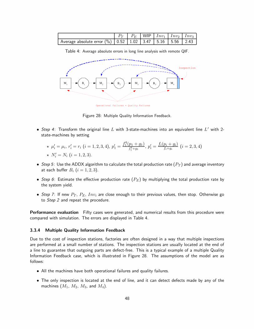
PT PE WIP Inv1 Inv2 Inv3

Average absolute error (%) 0.52 1.02 3.47 5.16 5.56 2.43

Table 4: Average absolute errors in long line analysis with remote QIF.

Inspection

M 1

B 1

M 2

M 3

M 4 B 2 B 3

Operational Failures + Quality Failures

Figure 28: Multiple Quality Information Feedback.

• Step 4 : Transform the original line L with 3-state-machines into an equivalent line L ′ with 2-state-machines by setting

? µ′

i = µi, r′i = ri (i = 1, 2, 3, 4), p′1 =f q1 (p1 + g1)

fq

1+g1

, p′i =fi(pi + gi)

fi+gi(i = 2, 3, 4)

? N ′

i = Ni (i = 1, 2, 3).

• Step 5 : Use the ADDX algorithm to calculate the total production rate (PT ) and average inventoryat each buffer Bi (i = 1, 2, 3).

• Step 6 : Estimate the effective production rate (PE) by multiplying the total production rate bythe system yield.

• Step 7 : If new PT , PE, Invi are close enough to their previous values, then stop. Otherwise goto Step 2 and repeat the procedure.

Performance evaluation Fifty cases were generated, and numerical results from this procedure werecompared with simulation. The errors are displayed in Table 4.

3.3.4 Multiple Quality Information Feedback

Due to the cost of inspection stations, factories are often designed in a way that multiple inspectionsare performed at a small number of stations. The inspection stations are usually located at the end ofa line to guarantee that outgoing parts are defect-free. This is a typical example of a multiple QualityInformation Feedback case, which is illustrated in Figure 28. The assumptions of the model are asfollows:

• All the machines have both operational failures and quality failures.

• The only inspection is located at the end of line, and it can detect defects made by any of themachines (M1, M2, M3, and M4).

48

PT PE WIP Inv1 Inv2 Inv3

Average absolute error (%) 0.55 1.95 8.62 5.97 4.75 2.76

Table 5: Average absolute errors in long line analysis with multiple QIF.

• Each operation works on different features. Quality failures at a given operation do not influencethe quality of other operations.

• There is no scrapping in the line; defective parts are marked and reworked later.

Solution method The four-machine multiple QIF case shown in Figure 28 is an extension of theremote QIF case in the sense that multiple Quality Information Feedback loops exist. Therefore, we canrepeat the same procedure that is used for the remote QIF case for each of the loop.

The four-machine multiple QIF case can be analyzed by using the following procedure:

• Step 1 : Estimate the average inventory of each buffer (Inv1, Inv2, and Inv3).

• Step 2 : Adjust f qi (i = 1, 2, 3) by using the procedure summarized in Section 3.1.6 and described

in detail in Kim (2004). In this case, f q3 is a function of Inv3; f q

2 is a function of Inv2 + Inv3;and f q

1 is a function of Inv1 + Inv2 + Inv3;

• Step 3 : Calculate the system yield

Ysys =

(

f1

f1 + g1

)(

f2

f2 + g2

)(

f3

f3 + g3

)(

f4

f4 + g4

)

.

• Step 4 : Transform the original line L with 3-state-machines into an equivalent line L ′ with 2-state-machines by setting

? µ′

i = µi, r′i = ri, p′i =f q

i (pi + gi)

f qi + gi

(i = 1, 2, 3, 4).

? N ′

i = Ni (i = 1, 2, 3).

• Step 5 : Use the ADDX algorithm to calculate the total production rate (PT ) and average inventoryat each buffer Bi (i = 1, 2, 3).

• Step 6 : Estimate the effective production rate (PE) by multiplying the total production rate bythe system yield.

• Step 7 : If the new PT , PE , Inv are close enough to their previous values, then stop. Otherwisego to Step 2 and repeat the procedure.

Performance evaluation Fifty cases were generated, and numerical results from this procedure werecompared with simulation. The errors are displayed in Table 5.

49

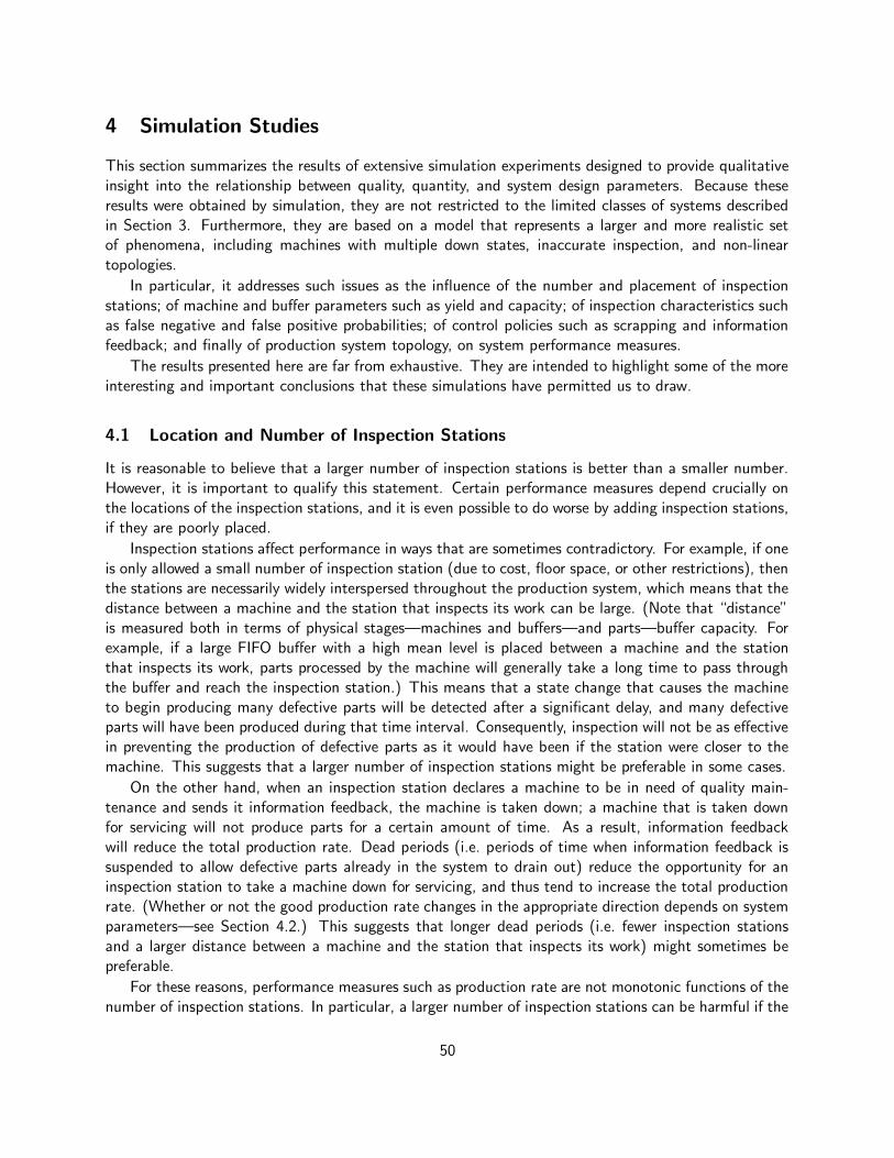
4 Simulation Studies

This section summarizes the results of extensive simulation experiments designed to provide qualitativeinsight into the relationship between quality, quantity, and system design parameters. Because theseresults were obtained by simulation, they are not restricted to the limited classes of systems describedin Section 3. Furthermore, they are based on a model that represents a larger and more realistic setof phenomena, including machines with multiple down states, inaccurate inspection, and non-lineartopologies.

In particular, it addresses such issues as the influence of the number and placement of inspectionstations; of machine and buffer parameters such as yield and capacity; of inspection characteristics suchas false negative and false positive probabilities; of control policies such as scrapping and informationfeedback; and finally of production system topology, on system performance measures.

The results presented here are far from exhaustive. They are intended to highlight some of the moreinteresting and important conclusions that these simulations have permitted us to draw.

4.1 Location and Number of Inspection Stations

It is reasonable to believe that a larger number of inspection stations is better than a smaller number.However, it is important to qualify this statement. Certain performance measures depend crucially onthe locations of the inspection stations, and it is even possible to do worse by adding inspection stations,if they are poorly placed.

Inspection stations affect performance in ways that are sometimes contradictory. For example, if oneis only allowed a small number of inspection station (due to cost, floor space, or other restrictions), thenthe stations are necessarily widely interspersed throughout the production system, which means that thedistance between a machine and the station that inspects its work can be large. (Note that “distance”is measured both in terms of physical stages—machines and buffers—and parts—buffer capacity. Forexample, if a large FIFO buffer with a high mean level is placed between a machine and the stationthat inspects its work, parts processed by the machine will generally take a long time to pass throughthe buffer and reach the inspection station.) This means that a state change that causes the machineto begin producing many defective parts will be detected after a significant delay, and many defectiveparts will have been produced during that time interval. Consequently, inspection will not be as effectivein preventing the production of defective parts as it would have been if the station were closer to themachine. This suggests that a larger number of inspection stations might be preferable in some cases.

On the other hand, when an inspection station declares a machine to be in need of quality main-tenance and sends it information feedback, the machine is taken down; a machine that is taken downfor servicing will not produce parts for a certain amount of time. As a result, information feedbackwill reduce the total production rate. Dead periods (i.e. periods of time when information feedback issuspended to allow defective parts already in the system to drain out) reduce the opportunity for aninspection station to take a machine down for servicing, and thus tend to increase the total productionrate. (Whether or not the good production rate changes in the appropriate direction depends on systemparameters—see Section 4.2.) This suggests that longer dead periods (i.e. fewer inspection stationsand a larger distance between a machine and the station that inspects its work) might sometimes bepreferable.

For these reasons, performance measures such as production rate are not monotonic functions of thenumber of inspection stations. In particular, a larger number of inspection stations can be harmful if the

50

Number of stations Number of sets of possible locations Best good production rate

0 0.1004001 1 0.2996642 14 0.3307653 91 0.3457024 364 0.3539425 1001 0.3590446 2002 0.3634037 3003 0.3656878 3432 0.3675339 3003 0.36847710 2002 0.36980011 1001 0.37076612 364 0.37197413 91 0.37205614 14 0.37243715 1 0.372901

Table 6: Number of combinations of sets of locations for each number of inspection stations, and best achievablegood production rate.

Range of Good Production Rates for Different Numbers of Inspection Stations

(15 five-state machines, 14 buffers, information feedback only)No inspection: 0.10040

0.295

0.305

0.315

0.325

0.335

0.345

0.355

0.365

0.375

0 1 2 3 4 5 6 7 8 9 10 11 12 13 14 15

Number of Inspection Stations

Go

od

Pro

du

cti

on

Rate

Best locations

Worst locations

Figure 29: Effect of the number and locations of inspection stations on the good production rate, for a productionline composed of 15 five-state machines, 14 buffers, and 1, 2, ..., 15 inspection stations.

51

stations are clustered together so that some machines are too frequently taken down for maintenancewhile others produce many defective parts before they receive information feedback. This is evidentin Figure 29, where the good production rate of a 15-machine line is plotted against the number ofinspection stations. For each number of stations, there are potentially many combinations of locationsto place them. Bearing in mind the fact that one of the inspection stations is always located after the15th machine, i.e. at the end of the production line, if there are k inspection stations altogether, thenthere are “14 choose k − 1” possible combinations of locations for the remaining k − 1. This quantityis given by:

(

14k − 1

)

=14!

(k − 1)!(15 − k)!

The number of sets of locations corresponding to each number of inspection stations appears in Table 6,together with the best achievable good production rate for that number of inspection stations. Each dotin Figure 29 represents a particular combination of locations. The dotted line at the top goes throughthe best combination of locations for each number of inspection stations, and the dotted line at thebottom goes through the worst. Although both lines would appear to be monotonically increasing, it isimportant to note that many combinations of locations for some higher numbers of inspection stationslead to worse good production rates than the best combination of locations for lower numbers. Forexample, the highest good production rate that can be achieved with 3 stations is 0.346 ppc (parts percycle). Although the highest good production rate that can be achieved with 4 stations is 0.354 ppc, for234 of the 364 combinations of locations—or 64%—the good production rate is actually lower than thebest achievable rate with 3 inspection stations. For 5 inspection stations, 279 of the 1001 combinationsof locations—or 28%—provide a good production rate below the best achievable rate with 3 inspectionstations.

Although the range between best and worst will of course change depending on machine and bufferparameters, the fact is that a higher number of inspection stations does not always give better results.The locations of inspection stations are as important as their number.

4.2 Control Policies

Two types of action (control policies) were analyzed: scrapping (which is an action on parts) andinformation feedback (which is an action on machines). Representative results for both policies arepresented below.

4.2.1 Scrapping

The principal benefit of scrapping locally is that defective parts are removed from the system, freeingup downstream machine and buffer capacity. Furthermore, lower buffer levels downstream allow fasterresponse to future quality failures—not only for the machine that made the bad parts that were scrapped,but for all downstream machines. As a result, good parts are produced at a higher rate, lead times areshorter, and buffer levels (a measure of in-process inventory) are lower.

Figure 30 illustrates the effect of local scrapping on the good production rate of a production linecomposed of 5 three-state machines. There are two inspection stations, one of which always immediatelyfollows the last machine; the other can be placed after either of the remaining four machines. Therightmost bar corresponds to no scrapping, providing a good production rate of 0.605 ppc. Countingfrom the left, the first bar corresponds to locating the free inspection station after the first machine, with

52

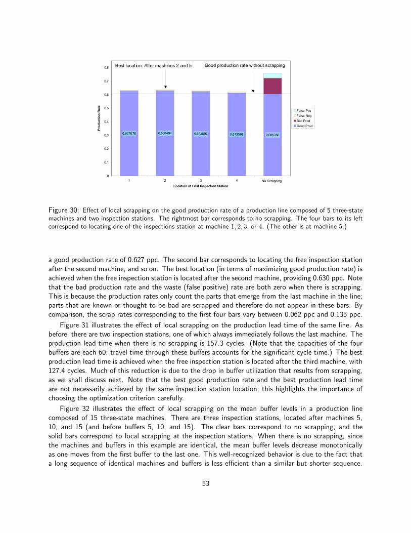
Five 3-State Machines, Two Inspection Stations

0.627078 0.630494 0.623597 0.613098 0.605356

0

0.1

0.2

0.3

0.4

0.5

0.6

0.7

0.8

1 2 3 4 5

Location of First Inspection Station

Pro

du

cti

on

Rate

False Pos

False Neg

Bad Prod

Good Prod

Best location: After machines 2 and 5 Good production rate without scrapping

No Scrapping

Figure 30: Effect of local scrapping on the good production rate of a production line composed of 5 three-statemachines and two inspection stations. The rightmost bar corresponds to no scrapping. The four bars to its leftcorrespond to locating one of the inspections station at machine 1, 2, 3, or 4. (The other is at machine 5.)

a good production rate of 0.627 ppc. The second bar corresponds to locating the free inspection stationafter the second machine, and so on. The best location (in terms of maximizing good production rate) isachieved when the free inspection station is located after the second machine, providing 0.630 ppc. Notethat the bad production rate and the waste (false positive) rate are both zero when there is scrapping.This is because the production rates only count the parts that emerge from the last machine in the line;parts that are known or thought to be bad are scrapped and therefore do not appear in these bars. Bycomparison, the scrap rates corresponding to the first four bars vary between 0.062 ppc and 0.135 ppc.

Figure 31 illustrates the effect of local scrapping on the production lead time of the same line. Asbefore, there are two inspection stations, one of which always immediately follows the last machine. Theproduction lead time when there is no scrapping is 157.3 cycles. (Note that the capacities of the fourbuffers are each 60; travel time through these buffers accounts for the significant cycle time.) The bestproduction lead time is achieved when the free inspection station is located after the third machine, with127.4 cycles. Much of this reduction is due to the drop in buffer utilization that results from scrapping,as we shall discuss next. Note that the best good production rate and the best production lead timeare not necessarily achieved by the same inspection station location; this highlights the importance ofchoosing the optimization criterion carefully.

Figure 32 illustrates the effect of local scrapping on the mean buffer levels in a production linecomposed of 15 three-state machines. There are three inspection stations, located after machines 5,10, and 15 (and before buffers 5, 10, and 15). The clear bars correspond to no scrapping, and thesolid bars correspond to local scrapping at the inspection stations. When there is no scrapping, sincethe machines and buffers in this example are identical, the mean buffer levels decrease monotonicallyas one moves from the first buffer to the last one. This well-recognized behavior is due to the fact thata long sequence of identical machines and buffers is less efficient than a similar but shorter sequence.

53

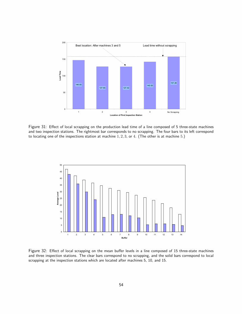
Five 3-State Machines, Two Inspection Stations

146.93

127.83 127.42

142.02

157.28

0

50

100

150

200

1 2 3 4 5

Location of First Inspection Station

Le

ad

Tim

e

Best location: After machines 3 and 5

No Scrapping

Lead time without scrapping

Figure 31: Effect of local scrapping on the production lead time of a line composed of 5 three-state machinesand two inspection stations. The rightmost bar corresponds to no scrapping. The four bars to its left correspondto locating one of the inspections station at machine 1, 2, 3, or 4. (The other is at machine 5.)

Line length 15, Buffer size 60

Average Buffer Levels (5-10-15 Scrap)

0

5

10

15

20

25

30

35

40

45

50

1 2 3 4 5 6 7 8 9 10 11 12 13 14

Buffer

Av

era

ge L

ev

el

Figure 32: Effect of local scrapping on the mean buffer levels in a line composed of 15 three-state machinesand three inspection stations. The clear bars correspond to no scrapping, and the solid bars correspond to localscrapping at the inspection stations which are located after machines 5, 10, and 15.

54

For example, the sub-line composed of machines 1–5 (and the buffers between them) is more efficientthan the sub-line of machines 1–6; by contrast, the sub-line of machines 6–15 is less efficient than thesub-line of machines 7–15. Consequently, the mean level of buffer 6 is higher than the mean level ofbuffer 7. Scrapping results in the reduction of mean buffer levels across the board, because parts arephysically removed from the line. This reduction is most pronounced in the buffer immdiately followingthe inspection station where scrapping occurs. It is interesting to note, however, that mean buffer levelsare not monotonically decreasing immediately after an inspection station. This behavior is consistentwith what we have observed in production lines without inspection where there are bottlenecks dueto cycle time (i.e. machines with longer cycle times than their neighbors). Although the intuitionunderlying it eludes us for now, the fact that both scrapping and a cycle time bottleneck result in thesame behavior is satisfying, since, from the point of view of buffers downstream of an inspection stationwhere scrapping is performed, the mean rate at which parts emerge from the station is reduced whenthe scrap rate increases.

4.2.2 Quality Information Feedback

The purpose of Quality Information Feedback is to take down for maintenance a machine that hasswitched to a state where defective parts are produced at a higher rate than usual. In the realisticsituation where a machine cannot spontaneously switch from a low-yield to a high-yield state (since, forexample, a worn tool cannot repair itself), this is the only way to ensure that good parts are producedat an acceptable rate. Indeed, if a machine has a zero-yield state, the steady-state good production ratein the absence of information feedback is exactly zero. Thus, information feedback would be essentialin that case.

In general, information feedback is most beneficial under the following conditions:

• The difference between the yield in normal performance (e.g. the high-yield state) and impairedperformance (e.g. the low-yield state) is significant. If this were not the case, there would belittle to be gained from taking the machine down for quality maintenance. Indeed, the loss inproductivity due to the forced down-time would outweigh the gain in yield achieved by the qualityrepair. By contrast, if the yield is much lower when the machine is impaired than in normaloperation, then although the loss in productivity incurred by the forced-down time would cause adrop in total production rate, the improved yield achieved in normal performance would lead to anet increase in the good production rate.

• Mean buffer levels are low. If this were not the case, then an inspection station that is not adjacentto the machine whose work it is monitoring would only receive evidence that a state change hasoccurred at the machine after a considerable delay, since the first defective part produced bythe machine would have to make its way through a large quantity of in-process inventory. As aresult of this delay, the machine would produce many defective parts before it receives informationfeedback from the inspection station and is taken down for quality maintenance. As a result, theimprovement in good production rate due to information feedback would be minimal. There aretwo reasons that cause the mean level of a buffer to be low: the buffer capacity may be low,and/or upstream machines may be less efficient than downstream machines.

To illustrate the second point, we note the well-known fact that production rate is a monotonicallyincreasing function of buffer capacity when information feedback is not present. When informationfeedback is used, however, this is not necessarily the case: good production rate sometimes decreases

55

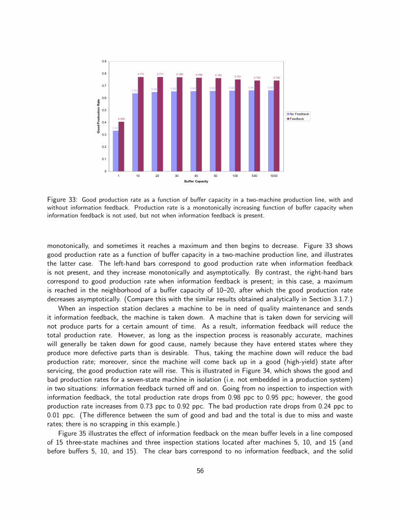
Effect of Feedback (1 in 1)

Line length 2, Number of inspection stations 1

0.331

0.6370.648 0.653 0.655 0.656 0.659 0.661 0.661

0.405

0.771 0.771 0.769 0.765 0.7620.751

0.742 0.742

0

0.1

0.2

0.3

0.4

0.5

0.6

0.7

0.8

0.9

1 10 20 30 40 50 100 500 1000

Buffer Capacity

Go

od P

rod

uc

tio

n R

ate

No Feedback

Feedback

Figure 33: Good production rate as a function of buffer capacity in a two-machine production line, with andwithout information feedback. Production rate is a monotonically increasing function of buffer capacity wheninformation feedback is not used, but not when information feedback is present.

monotonically, and sometimes it reaches a maximum and then begins to decrease. Figure 33 showsgood production rate as a function of buffer capacity in a two-machine production line, and illustratesthe latter case. The left-hand bars correspond to good production rate when information feedbackis not present, and they increase monotonically and asymptotically. By contrast, the right-hand barscorrespond to good production rate when information feedback is present; in this case, a maximumis reached in the neighborhood of a buffer capacity of 10–20, after which the good production ratedecreases asymptotically. (Compare this with the similar results obtained analytically in Section 3.1.7.)

When an inspection station declares a machine to be in need of quality maintenance and sendsit information feedback, the machine is taken down. A machine that is taken down for servicing willnot produce parts for a certain amount of time. As a result, information feedback will reduce thetotal production rate. However, as long as the inspection process is reasonably accurate, machineswill generally be taken down for good cause, namely because they have entered states where theyproduce more defective parts than is desirable. Thus, taking the machine down will reduce the badproduction rate; moreover, since the machine will come back up in a good (high-yield) state afterservicing, the good production rate will rise. This is illustrated in Figure 34, which shows the good andbad production rates for a seven-state machine in isolation (i.e. not embedded in a production system)in two situations: information feedback turned off and on. Going from no inspection to inspection withinformation feedback, the total production rate drops from 0.98 ppc to 0.95 ppc; however, the goodproduction rate increases from 0.73 ppc to 0.92 ppc. The bad production rate drops from 0.24 ppc to0.01 ppc. (The difference between the sum of good and bad and the total is due to miss and wasterates; there is no scrapping in this example.)

Figure 35 illustrates the effect of information feedback on the mean buffer levels in a line composedof 15 three-state machines and three inspection stations located after machines 5, 10, and 15 (andbefore buffers 5, 10, and 15). The clear bars correspond to no information feedback, and the solid

56

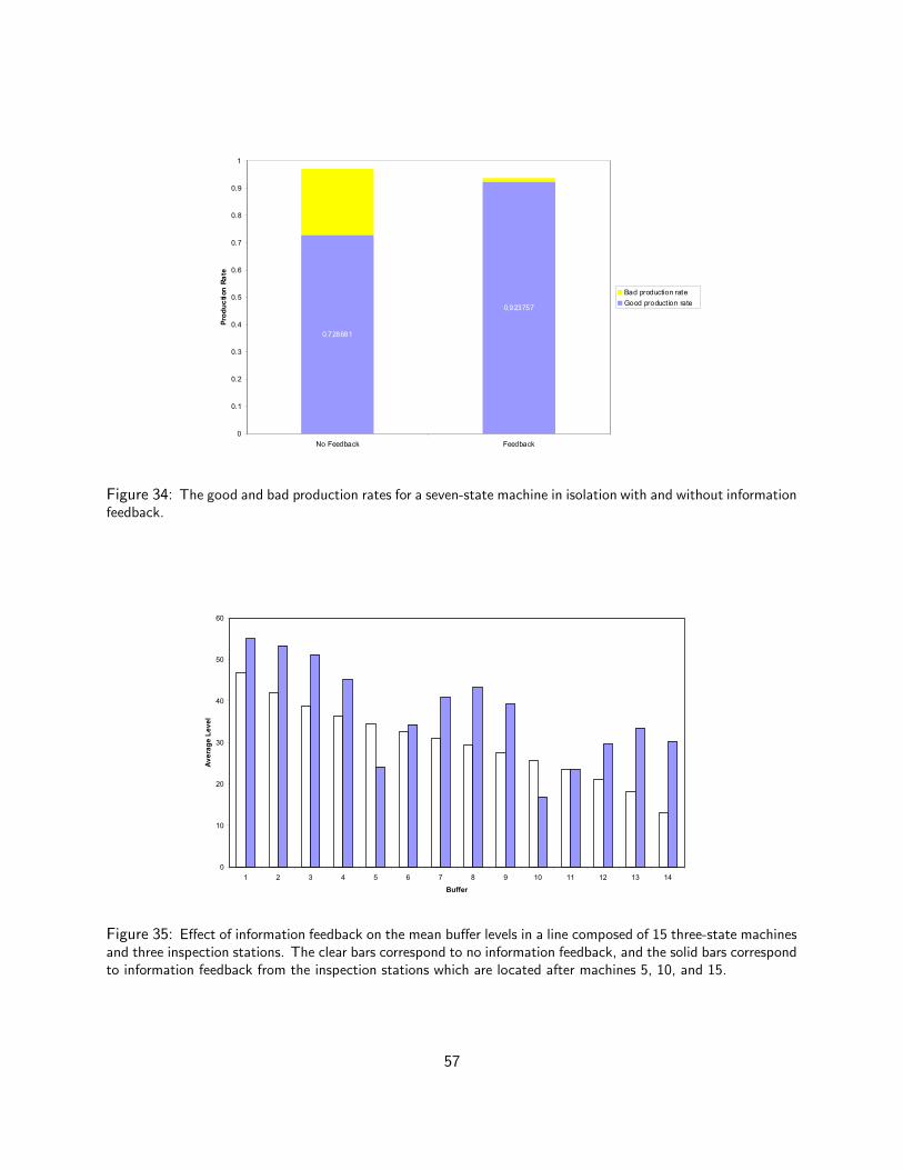
0.728681

0.923757

0

0.1

0.2

0.3

0.4

0.5

0.6

0.7

0.8

0.9

1

No Feedback Feedback

Pro

du

cti

on

R

ate

Bad production rate

Good production rate

Figure 34: The good and bad production rates for a seven-state machine in isolation with and without informationfeedback.

Line length 15, Buffer size 60

Average Buffer Levels (5-10-15 Feedback)

0

10

20

30

40

50

60

1 2 3 4 5 6 7 8 9 10 11 12 13 14

Buffer

Av

era

ge L

ev

el

Figure 35: Effect of information feedback on the mean buffer levels in a line composed of 15 three-state machinesand three inspection stations. The clear bars correspond to no information feedback, and the solid bars correspondto information feedback from the inspection stations which are located after machines 5, 10, and 15.

57

Information Feedback Rate

(One Inspection Station)

0

0.01

0.02

0.03

1 2 3 4 5 6 7 8 9 10 11 12 13 14 15

Machine

Rate

of

Info

rma

tio

n F

ee

db

ac

k

Figure 36: Rate at which information feedback is received by each machine, in a line composed of 15 three-statemachines and one inspection station at the very end.

bars correspond to information feedback. In the absence of information feedback, since the machinesand buffers in this example are identical, the mean buffer levels decrease monotonically as one movesfrom the first buffer to the last one, as seen in Figure 32. We see in Figure 35 that the main effect ofinformation feedback is to increase the mean level of most of the buffers. To explain this behavior, notefirst that even machines that are identical in every respect are not taken down for quality maintenanceat the same rate. This is because of the dead periods: all things being equal, the further a machine isfrom the inspection station that monitors its work, the longer the dead periods typically become. As aresult, machines far from an inspection station are less affected by information feedback than machinesnear the station.

Figure 36 shows the rate at which information feedback is received by each machine, measuredas signals per cycle. For clarity, there is only one inspection station, after the last machine. Theinformation feedback rate decreases monotonically with distance to the inspection station. This meansthat the performance hit (in terms of reduced production rate, not quality) taken by the machinesdecreases as they get further from the inspection station. Since this effect is not symmetrical (eachinspection station only looks at machines upstream of it), the net result is that the machines in eachinspection domain become less efficient (but higher-yield) as we move downstream within the domain.

This explains why mean buffer levels rise virtually across the board. The few buffers whose meanlevel decreases in the presence of information feedback generally immediately follow inspection stations.In these cases, the drop is due to the difference between the high rate at which the immediately upstreammachine receives information feedback from the adjacent inspection station, and the much lower rate atwhich the immediately downstream machine receives information feedback from the distant downstreaminspection station. (The examples in this section do not feature scrapping.)

58

4.3 Production System Topology

Many manufacturing systems have topologies more complex than tandem lines, particularly due tocurrent pressures to modularize and outsource. For this reason, we modeled and analyzed productionsystems composed of a short main line with multiple feeder lines.

Figures 37–40 show the specific topologies we compared. Figure 37 is a linear production system, inwhich segments that can be separated due to the ability to modularize are coded with different colors.The line segments composed of machines 1–5, 6–10, and 11-15 are each assumed to be independent ofthe others—i.e. the operations of machines 6–10 can be performed on a given part whether or not thoseof machines 1–5 have already been performed on that part, etc. It is also assumed that these segmentscan be interconnected at certain machines, namely machines 6, 11, and 16. Thus, in Figure 37, segment1–5 is connected to machine 6, segment 6–10 to machine 11, and segment 11–15 to machine 16. InFigure 38, segments 1–5 and 6–10 are both connected to machine 11, and segment 11–15 to machine16. In Figure 39, segments 1–5 and 11–15 are both connected to machine 16, while segment 6–10 isconnected to machine 11. Finally, in Figure 40, segments 1–5, 6–10, and 11–15 are all connected tomachine 16.

Figure 37: Linear topology. The potential for modularization is indicated by different colors.

1 5

6 10

11 15 16

1 5

6 10

11 15 16

Figure 38: Non-linear topology. Further potential for modularization is indicated by different colors.

It was first assumed that there are no quality failures at all. For each topology, production rate,in-process inventory, and production lead time (defined as the longest amount of time any portion of afinished part spent in the system) were compared, given the following scenarios:

• All machines and buffers are identical;

59

1 5

6 10

11 15 16

1 5

6 10

11 15 16

Figure 39: Non-linear topology. Further potential for modularization is indicated by different colors.

1 5

6 10

11 15 16

1 5

6 10

11 15 16

Figure 40: Star topology.

• All machines and buffers are identical, except for a bottleneck at machine 6;

• All machines and buffers are identical, except for a bottleneck at machine 5.

The difference between the two cases involving bottlenecks is that in the first, the bottleneck is at thebeginning of a feeder line, whereas in the second, it is at the end. In both cases, the bottleneck wassevere enough that upstream buffers were usually full and downstream buffers were usually empty.

For any given scenario, the production rate was found to be highly insensitive to topology. However,in-process inventory and production lead time were very sensitive.

No bottleneck Mean buffer levels decrease monotonically along a production line when all machinesand buffers are identical. The longer the line, the more pronounced is the decrease. Thus, for the lineartopology in Figure 37, mean buffer levels decreased by 50% from the first to the fourteenth buffer. Bycontrast, for the star topology in Figure 40, the reduction was less than 10%. Note that the contents ofdifferent buffers can have very different economic values; thus, the reduction in the value of in-processinventory may be even larger, particularly if downstream buffers contain more valuable inventory thanupstream buffers.

Production lead time is a function of both line length and in-process inventory, since in FIFO buffers,a part spends as much time in a buffer as there are parts ahead of it. In the absence of a bottleneck,and for the system parameters utilized, the influence of line length was found to be more importantthan mean buffer levels. Thus, the production lead time in the star topology was found to be 46% ofthe production lead time in the linear topology.

60

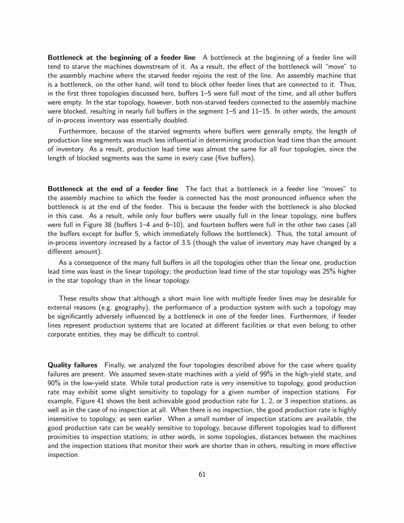
Bottleneck at the beginning of a feeder line A bottleneck at the beginning of a feeder line willtend to starve the machines downstream of it. As a result, the effect of the bottleneck will “move” tothe assembly machine where the starved feeder rejoins the rest of the line. An assembly machine thatis a bottleneck, on the other hand, will tend to block other feeder lines that are connected to it. Thus,in the first three topologies discussed here, buffers 1–5 were full most of the time, and all other bufferswere empty. In the star topology, however, both non-starved feeders connected to the assembly machinewere blocked, resulting in nearly full buffers in the segment 1–5 and 11–15. In other words, the amountof in-process inventory was essentially doubled.

Furthermore, because of the starved segments where buffers were generally empty, the length ofproduction line segments was much less influential in determining production lead time than the amountof inventory. As a result, production lead time was almost the same for all four topologies, since thelength of blocked segments was the same in every case (five buffers).

Bottleneck at the end of a feeder line The fact that a bottleneck in a feeder line “moves” tothe assembly machine to which the feeder is connected has the most pronounced influence when thebottleneck is at the end of the feeder. This is because the feeder with the bottleneck is also blockedin this case. As a result, while only four buffers were usually full in the linear topology, nine bufferswere full in Figure 38 (buffers 1–4 and 6–10), and fourteen buffers were full in the other two cases (allthe buffers except for buffer 5, which immediately follows the bottleneck). Thus, the total amount ofin-process inventory increased by a factor of 3.5 (though the value of inventory may have changed by adifferent amount).

As a consequence of the many full buffers in all the topologies other than the linear one, productionlead time was least in the linear topology; the production lead time of the star topology was 25% higherin the star topology than in the linear topology.

These results show that although a short main line with multiple feeder lines may be desirable forexternal reasons (e.g. geography), the performance of a production system with such a topology maybe significantly adversely influenced by a bottleneck in one of the feeder lines. Furthermore, if feederlines represent production systems that are located at different facilities or that even belong to othercorporate entities, they may be difficult to control.

Quality failures Finally, we analyzed the four topologies described above for the case where qualityfailures are present. We assumed seven-state machines with a yield of 99% in the high-yield state, and90% in the low-yield state. While total production rate is very insensitive to topology, good productionrate may exhibit some slight sensitivity to topology for a given number of inspection stations. Forexample, Figure 41 shows the best achievable good production rate for 1, 2, or 3 inspection stations, aswell as in the case of no inspection at all. When there is no inspection, the good production rate is highlyinsensitive to topology, as seen earlier. When a small number of inspection stations are available, thegood production rate can be weakly sensitive to topology, because different topologies lead to differentproximities to inspection stations; in other words, in some topologies, distances between the machinesand the inspection stations that monitor their work are shorter than in others, resulting in more effectiveinspection.

61

Good Production Rate by Number and Best Location of Inspection Stations

0.00

0.10

0.20

0.30

0.40

0.50

0.60

Straight Feeder 1 Feeder 2 Feeder 3

Topology

Go

od

Pro

du

cti

on

Rate

No inspection

One station

Two stations

Three stations

Figure 41: Good production rate for different topologies and different numbers of inspection stations. Theleftmost bar in each set corresponds to no inspection; other bars indicate the best achievable good productionrate for each number of inspection stations.

5 Conclusion

5.1 Summary

Although productivity and quality have each been extensively studied in the manufacturing engineeringliterature, there has been little research on how they interact. The work reported here represents afirst attempt at analyzing how production system design, quality, and productivity are inter-related inproduction networks, and developing analytical as well as numerical methods that make it possible toevaluate, compare, and optimize the performance of competing designs.

This report presents the results of work using analytical, numerical, and simulation techniques toinvestigate the effect of separating inspection from operation, as a function of machine, buffer, andinspection station parameters; control policy; production system topology, and other factors.

A taxonomy was presented for quality failures, and a class of stochastic models was described torepresent a realistic subset of those failures. Markov models were formulated for machines subject toboth operational and quality failures. Quality control mechanisms were formulated, including scrappingof defective parts as well as a quality information feedback scheme that results in taking offendingmachines down for maintenance. Pertinent performance measures were defined, including mean totalproduction rate, good production rate, yield, in-process inventory, and lead time.

Analytical results based upon a continuous-material approximation of a two-stage line were presented.These results have been validated by comparison with discrete-event simulation. Further simulationresults were presented for more complex production systems including more realistic machine models,inaccurate inspection stations, non-linear topologies, arbitrary locations of inspection stations, and otherfactors.

It was shown that total production rate and good production rate do not always behave in the same

62

manner as system parameters are varied. For example, although total production rate is known to be amonotonically increasing function of buffer capacity, good production rate is not always monotonic inbuffer capacity when quality inspection and information feedback are present.

Furthermore, while improvement in production rate may be obtained through different means—e.g.more reliable machines, more accurate inspection, larger buffers—such improvements are more sensitiveto some system parameters than to others. Thus, it is necessary to exercise care in choosing whereto invest money in order to obtain the greatest and most cost-effective marginal improvement in goodproduction rate.

It was also shown that taking a machine down for maintenance as soon as a single quality defectis detected (jidoka) is not always the optimal policy, and that system parameters must be taken intoaccount in determining the best course of action following the detection of one or more defects.

Other results presented here include the investigation of the effect of the number and placementof inspection stations, of machine and buffer parameters, of inspection policies, of control policies,and of production line topology on selected performance measures. In particular, it was shown thatperformance can be quite sensitive to the placement of inspection stations, so that a few well-placedinspection stations will result in better performance than many poorly-placed ones.

It was further shown that in-line scrapping can significantly improve performance, if economicallyjustifiable. Finally, it was shown that although production rate is not sensitive to topology, in-processinventory and production lead time are very sensitive. Thus, external factors that call for short mainlines with long feeder lines, such as modularization and outsourcing, must be weighed against systemperformance in making system design decisions.

5.2 Current Research

The research described below is currently underway, supported by General Motors.

5.2.1 Exploration of Phenomena

Analytical, numerical, and simulation techniques are being used to investigate important issues in a waythat will help us to identify important phenomena and form preliminary hypotheses about their behavior.Examples include:

• The interaction between buffers, inspection location and accuracy, and production system perfor-mance;

• The development of optimal inspection rules based on Bayes risk methods in the context of ourmodels and methods; and

• A wider variety of production topologies, including systems with rework, repair, scrap, assem-bly/disassembly, etc.

5.2.2 Validation of model assumptions

Data (time-stamped machine events and inspection verdicts) will be analyzed to validate various versionsof the multi-state quality model and its assumptions (such as the Markovian property, and distincthigh yield vs. low yield states). Transition probabilities will be deduced that fit available quality andthroughput data provided by GM.

63

General Motors will identify plant, process, and data availability, and provide available data tosupport analysis and model development.

5.2.3 GM factory case study

A model will be developed for the GM-supplied plant layout and process, to take advantage of avail-able data. That model will be applied (using simulation, if mathematically intractable) to identifyimprovement opportunities in the current process.

General Motors will identify plant, process, and data availability, and provide available data tosupport analysis and model development.

5.3 Further Research

We believe that the area that we have described is an important one, which will attract many follow-onresearch contributions. In this section, we briefly describe some areas that promise to provide practicalresults or deep insights, or that expand our framework for future research.

5.3.1 Non-Instantaneous Inspection

In all our models, we have assumed that inspection takes no time. As a consequence, time plays no rolein deciding where inspection should occur. Our conclusions may change, however if it does take time;and how they change will depend on whether inspections of different features at the same inspectionstation can occur in parallel, or whether they must be done sequentially. If they can be done in parallel,there is incentive to group them; otherwise it may be better to spread them out. This is initially asimulation task.

5.3.2 Buffer Delays and Failures

In all our models, we have assumed that the travel time in buffers is zero. That is, we assume thatparts instantaneously move from the upstream machine to the last position in the buffer queue. Asa consequence, our models overestimate production rate and underestimate lead times. In addition,they overestimate yield since the additional travel delay causes a greater lag between production anddetection of bad parts, when inspection is not ubiquitous.

We have also assumed that buffers are perfectly reliable. This is a reasonable assumption whenbuffers are simple, passive devices. However, when they include material handling equipment such asrobots, they are as prone to failure as anything else in a factory. There has been some work on unreliablebuffers (Lipset, Til, and Sengupta 1999; Burman 1995), but none on their impact on quality.

5.3.3 Analytical Models Of Scrapping

It should not be difficult to add scrapping to the two-machine, one buffer model of Section 3. At thesame time that Machine 1 makes the transition from state 1 to state −1, the buffer level instantaneouslydrops to zero. This will change the differential equations and boundary conditions of the probabilitydistribution, but they should not become much more difficult to solve because they will remain linear.

64

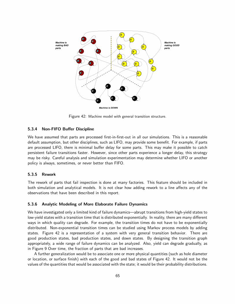
Machine is making BADparts

Machine is making GOODparts

Machine is DOWN

BB

G

G

G

G

G

G

G

G

G

BB

BB

B

D

G

G

D

DDD

D

Figure 42: Machine model with general transition structure.

5.3.4 Non-FIFO Buffer Discipline

We have assumed that parts are processed first-in-first-out in all our simulations. This is a reasonabledefault assumption, but other disciplines, such as LIFO, may provide some benefit. For example, if partsare processed LIFO, there is minimal buffer delay for some parts. This may make it possible to catchpersistent failure transitions faster. However, since other parts experience a longer delay, this strategymay be risky. Careful analysis and simulation experimentation may determine whether LIFO or anotherpolicy is always, sometimes, or never better than FIFO.

5.3.5 Rework

The rework of parts that fail inspection is done at many factories. This feature should be included inboth simulation and analytical models. It is not clear how adding rework to a line affects any of theobservations that have been described in this report.

5.3.6 Analytic Modeling of More Elaborate Failure Dynamics

We have investigated only a limited kind of failure dynamics—abrupt transitions from high-yield states tolow-yield states with a transition time that is distributed exponentially. In reality, there are many differentways in which quality can degrade. For example, the transition times do not have to be exponentiallydistributed. Non-exponential transition times can be studied using Markov process models by addingstates. Figure 42 is a representation of a system with very general transition behavior. There aregood production states, bad production states, and down states. By designing the transition graphappropriately, a wide range of failure dynamics can be analyzed. Also, yield can degrade gradually, asin Figure 9 Over time, the fraction of parts that are bad increases.

A further generalization would be to associate one or more physical quantities (such as hole diameteror location, or surface finish) with each of the good and bad states of Figure 42. It would not be thevalues of the quantities that would be associated with the state; it would be their probability distributions.

65

The measurement of these quantities, when combined with the knowledge of the failure dynamics, couldprovide a more precise and more accurate estimate of the quality state of the machine.

5.3.7 Preventive Maintenance

The more elaborate quality failure dynamics described above provides an opportunity for preventivemaintenance. The estimate of the quality state of the machine can be used to make an estimate of howmany more operations can be performed before the machine produces parts of unacceptable quality.The machine can then be scheduled for maintenance before any bad parts are actually produced (withhigh probability).

5.3.8 More General Phenomena, Including Loops, Batches, and Setups

Material flows in factories are not limited to tandem lines or even assembly trees. There are often reworkloops, reentrant loops, pallet/fixture loops, assembly following temporary disassembly, etc. In addition,items do not always travel one by one; sometimes it is preferable to create batches or lots (especiallywhen there are operations that involve chambers, such as ovens). Batches create complexities whenthey are not permanent, that is, when the same group of parts do not travel together in the wholeprocess. Setups, in which the time needed by a machine to operate on a part A after a part B is greaterthan after another part A, is another cause of scheduling and performance estimation complexity.

All of these phenomena have a bearing on both quality and quantity. They are under active inves-tigation in the quantity literature; we are not aware of any quality-related research in them.

5.3.9 Integrated Models Of Material Flow Control And Inspection

Models of loops can also be used to represent some kinds of material flow control (Frein, Mascolo,and Dallery 1994; Dallery and Liberopoulos 2000; Gershwin 2000). Thus, the analysis of quality usingmodels of material flow in some kinds of loops can be used to model quality in systems with materialflow control. This can lead to the unified modeling and design of manufacturing systems taking intoaccount a very large set of important items.

5.3.10 Decomposition Without Reducing Machine Models to Two States

We have seen that two-state machine models can sometimes be good approximations of three-statemodels (Section 3.3.2) and that this can be used to simplify the calculations associated with decompo-sition. However, this is not likely to work in all cases, especially when machine models become moreelaborate. It would be useful to extend the decomposition to deal with the full complexity hinted at inSection 5.3.6.

5.3.11 Two-Machine, One-Buffer Lines with Good and Bad PartsModeled Distinctly in the Buffer

In the models described in Section3, we do not model good and bad parts separately in the buffers. Thischoice was made to simplify the models; if good and bad are modeled separately, then the probabilitydistribution has two continuous variables, and this means that the internal transition equations arepartial differential equations. While that choice was appropriate for a first approach to the issues we arestudying, another look at the models with good and bad parts modeled explicitly may still be fruitful.

66

5.3.12 More General Inspection Strategies

We have studied only a limited range of possible inspection strategies. In particular, we have onlyconsidered 100% inspection. This is sometimes the best strategy, but sometimes it is preferable tosample, and future research should be devoted to sampling in the quality/quantity context. Second, wehave only considered systems in which each feature is inspected only once. Sometimes, certain featuresare inspected more than once, and this may have an impact on the issues we have considered. Third,we have not at all considered destructive testing. Destructive testing is appropriate sometimes, and itshould be studying within the framework we have been developing.

Acknowledgements

The authors gratefully acknowledge the stimulating discussions and valuable input of Dennis Blumenfeld,Ninja Huang, Robert Inman, Jingshan Li, Samuel Marin, and Jonathan Owen.

References

Bertsekas, D. P. and J. N. Tsitsiklis (2002). Introduction to Probability. Athena Scientific.

Besterfield, D. H., C. Besterfield-Michna, G. Besterfield, and M. Besterfield-Sacre (2003). Totalquality management. Englewood Cliffs, NJ: Prentice Hall.

Burman, M. H. (1995). New Results in Flow Line Analysis. Ph. D. thesis, Massachusetts Institute ofTechnology, Operations Research Center.

Dallery, Y., R. David, and X.-L. Xie (1988). An efficient algorithm for analysis of transfer lines withunreliable machines and finite buffers. IEEE Transactions on Automatic Control 34, 943–953.

Dallery, Y. and G. Liberopoulos (2000). Extended kanban control system: combining kanban andbase stock. IIE Transactions on Design and Manufacturing 32.

Frein, Y., M. D. Mascolo, and Y. Dallery (1994). On the design of generalized kanban control systems.International Journal of Operations and Production Management 15(9), 158–184.

Fujimoto, T. (1999). The evolution of a manufacturing systems at Toyota. Oxford University Press.

Gershwin, S. B. (1987). An efficient decomposition method for the approximate evaluation of tandemqueues with finite storage space and blocking. Operations Research 35(2), 291–305.

Gershwin, S. B. (1994). Manufacturing Systems Engineering. Englewood Cliffs, NJ: Prentice-Hall.For corrections, see http://web.mit.edu/manuf-sys/www/gershwin.errata.html.

Gershwin, S. B. (2000). Design and operation of manufacturing systems — the control-point policy.IIE Transactions 32, 891–906.

Gershwin, S. B. and I. C. Schick (1980). Continuous model of an unreliable two-machine materialflow system with a finite interstage buffer. Report LIDS-R-1039, MIT Laboratory for Informationand Decision Systems.

Glassey, C. R. and Y. Hong (1993). Analysis of behaviour of an unreliable n–stage transfer line with(n-1) interstage buffers. International Journal of Production Research 31(3), 519–530.

Howard, R. A. (1971). Dynamic Probabilistic Systems. New York: Wiley.

67

Inman, R. R., D. E. Blumenfeld, N. Huang, and J. Li (2003). Designing production systems forquality: research opportunities from and autombile industry perspective. International Journal ofProduction Research 41(9), 1953–1971.

Kim, J. (2004). Designing Production System for Quality and Quantity. Ph. D. thesis, MassachusettsInstitute of Technology.

Kim, J. and S. B. Gershwin (2005). Integrated quality and quantity modeling of a production line.OR Spectrum. to appear.

Lipset, R., R. V. Til, and S. Sengupta (1999). Steady-state performance analysis of serial transfer linessubject to machine and buffer failure. IEEE Transactions on Automatic Control 44(2), 319–325.

Toyota Motor Corporation (1996). The Toyota production system.

Monden, Y. (1983). Toyota Production System: Practical approach to production management.Atlanta: Industrial Engineering and Management Press.

Monden, Y. (1998). Toyota production system — An integrated approach to Just-In-Time. EMPBooks.

Pande, P. and L. Holpp (2002). What is six sigma? McGraw-Hill.

Sandberg, A. (1995). Enriching production. Avebury Publishing Company.

Sevast’yanov (1962). Influence of storage bin capacity on the average standstill time of a productionline. Theory of Probability Application 7, 419–438.

Togo, Y. and W. Waterman (1993). Against all odds: the story of the Toyota Motor Corporation andthe family that created it. New York: St. Martin’s.

Womack, J. P., D. T. Jones, and D. Roos (1990). The machine that changed the world: The storyof lean production. Rawson Associates.

Woodall, W. H. and D. C. Montgomery (1999). Research issues and ideas in statistical process control.Journal of Quality Technology 31(4), 376–386.

Zimmern, B. (1956). Etudes de la propagation des arrets aleatoires dans les chaines de production.Review Statististical Applications 4, 85–104.

68