Integrated calculusby Michel Helfgott

A thesis submitted in partial fulfillment of the requirements for the degree of Doctor of EducationMontana State University© Copyright by Michel Helfgott (1997)

Abstract:This research addressed the question of whether there were differences in achievement betweenstudents that followed an integrated approach to calculus that integrated mathematics and physics,compared to students that followed a non-integrated approach.

The subjects in the study were the 151 students that completed Calculus II (second semester calculusintended mainly for engineering students) at Montana State University-Bozeman during the fall of1996. There were a total of five sections with five different instructors. All the sections used theHarvard Calculus book and took common exams. Three sections were assigned to the experimentalgroup, which followed the integrated method, while two sections acted as the control group.

Both groups covered the main topics of chapters 6 -10 of the Harvard Calculus book. The instructors inthe experimental group stressed problems about applications to physics, as well as the conceptual andcomputational aspects of calculus. In addition, students in this group received enrichment notes thatsupplemented the textbook. The instructors in the control group also stressed the conceptual andcomputational aspects of calculus as well as applications to physics. However, the control group didnot delve as deeply into these applications and did not have the support of the enrichment notes.

Analysis of Covariance (ANCOVA), with Calculus I scores and SAT - math scores acting ascovariates, was the technique of choice to compare methods with regard to Calculus II and Physics Iscores. Physics I is the first semester calculus-based physics course. ANCOVAS were also used withgender as a factor, and when students take Physics I as a factor (not yet, concurrently with Calculus II,or before Calculus II). For interaction analyses, two-way analyses of variance were employed oncestudents were categorized into three groups according to their scores in Calculus I, SAT- math, andCalculus II.

Students in the integrated group did significantly better in Calculus II. Interaction was found whenPhysics I scores were analyzed, with method and SAT-math groups as factors. Students with highmathematical aptitude in the integrated group scored significantly better than students with highmathematical aptitude in the non-integrated group, when Physics I scores were analyzed. No otherinteractions were detected. Furthermore, there were no differences in Calculus II achievementaccording to when students took Physics I. No differences in achievement according to gender werefound either.

On the basis of the findings of this study, an integrated approach to the teaching of second semestercalculus is recommended. 

INTEGRATED CALCULUS

by

Michel Helfgott

A thesis submitted in partial fulfillment of the requirements for the degree

of

Doctor of Education

MONTANA STATE UNIVERSITY-BOZEMAN Bozeman, Montana

April .1997

B 3^13

ii

APPROVAL

of a thesis submitted by

Michel Helfgott

This thesis has been read by each member of the graduate committee and has been found to be satisfactory regarding content, English usage, format,, citations, bibliographic style, and consistency, and is ready for submission to the College of Graduate Studies.

Dateul % M l

tfs -U l'Aa 010^AJ!

o-Ghairperson, Graduate Committee

Co-Chairperson, Graduate ommittee

f ln u l* 3 J f f ?Date _

W / t /9 7Date Graduate Dean

iii

STATEMENT OF PERMISSION TO USE

In presenting this thesis in partial fulfillment of the requirements for a doctoral

degree at Montana State University-Bozeman, I agree that the Library shall make it

available to borrowers under rules of the Library. I further agree that copying of this

thesis is allowable only for scholarly purposes, consistent with "fair use" as prescribed in

the U.S. Copyright Law. Requests for extensive copying or reproduction of this thesis

should be referred to University Microfilms International, 300 North Zeeb Road, Ann

Arbor, Michigan 48106, to whom I have granted "the exclusive right to reproduce and

distribute my dissertation in and from microform along with the non-exclusive right to

reproduce and distribute my abstract in any format in whole or in part."

Signature

Date ~7 , ____

iv

ACKNOWLEDGMENTS

I wish to express my gratitude to the co-chairmen, Dr. Lyle Andersen and Dr.

William Hall, for their advice and encouragement. Dr. Eric Strohmeyer was a permanent

source of motivation, always ready to help me in my endeavors. I also wish to thank Dr.

Leroy Casagranda and Dr. Linda Simonsen for their assistance.

It was a pleasure and a privilege to work with Roger Griffiths and Steve Hamilton

in the experimental group. Their expertise and professionalism were important factors in

the implementation and success of the study.

I am very grateful to my wife Edith and our children Harald, Gabriela, and

Federico for their unwavering support and love.

V

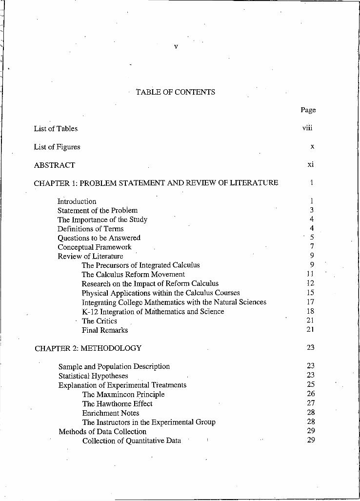
TABLE OF CONTENTS

Page

List of Tables viii

List of Figures x

ABSTRACT xi

CHAPTER I : PROBLEM STATEMENT AND REVIEW OF LITERATURE I

Introduction IStatement of the Problem 3The Importance of the Study 4Definitions of Terms 4Questions to be Answered ' 5Conceptual Framework 7Review of Literature 9

The Precursors of Integrated Calculus 9The Calculus Reform Movement 11Research on the Impact of Reform Calculus 12Physical Applications within the Calculus Courses 15Integrating College Mathematics with the Natural Sciences 17K-12 Integration of Mathematics and Science 18

■ The Critics 21Final Remarks 21

CHAPTER 2: METHODOLOGY 23

Sample and Population Description 23Statistical Hypotheses 23Explanation of Experimental Treatments 25

The Maxmincon Principle 26The Hawthorne Effect 27Enrichment Notes 28The Instructors in the Experimental Group 28

Methods of Data Collection 29Collection of Quantitative Data ' 29

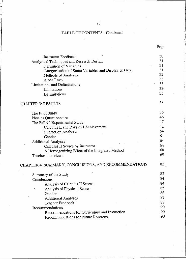
TABLE OF CONTENTS - Continued

Page

Instructor Feedback 30Analytical Techniques' and Research Design 31

Definition of Variables ‘ 31Categorization of Some Variables and Display of Data 31Methods of Analyses 32Alpha Level 33

Limitations and Delimitations 1 33Limitations 33*Delimitations 35

CHAPTER 3: RESULTS 36

The Pilot Study 36Physics Questionnaire 46The Fall 96 Experimental Study 47

Calculus II and Physics I Achievement 52Interaction Analyses 54Gender 61

Additional Analyses . 64Calculus II Scores by Instructor 64A Homogenizing Effect of the Integrated Method 68

Teacher Interviews 69

CHAPTER 4: SUMMARY, CONCLUSIONS, AND RECOMMENDATIONS 82

Summary of the Study 82Conclusions 84

Analysis of Calculus II Scores. 84Analysis of Physics I Scores 85Gender 86Additional Analyses 87Teacher Feedback - 87

Recommendations 90Recommendations for Curriculum and Instruction 90Recommendations for Future Research 90

vi

TABLE OF CONTENTS - Continued

Page

REFERENCES CITED 92

APPENDICES 96

APPENDIX A: CALCULUS II SYLLABUS AND EXAMS 97APPENDIX B: PHYSICS QUESTIONNAIRE 111APPENDIX C: RECORD OF MEETINGS OF THE EXPERIMENTAL '

GROUP 117APPENDIX D: CONCORDANCE TABLE 122APPENDIX E: A SAMPLE OF ENRICHMENT NOTES 124

Elementary Chemical Kinetics 125Wind Resistance Proportional to the Square of Velocity 129A Problem in Chemical Kinetics where Partial Fractions Are Used 130The Catenary 132Three Stages in Modeling with Differential Equations 135A Proof of the Fundamental Theorem of Calculus 138The Comparison Test for Improper Integrals 141Usual Tests in the Theory of Series 142Enzyme Kinetics 147

APPENDIX F: FURTHER DESCRIPTIVE STATISTICS 154

vii

Vlll

LIST OF TABLES

Table Page

1. Number of Students by Method and the Four Main variables 36

2. Means, Medians, and Quartiles Corresponding to the Main Variables 37

3. Ranks according to Quartiles . 3 8

4. Pearson Correlations Among the Four main Variables 38

5. Descriptive Statistics Comparing Methods 38

6. SAT and CalcI Scores in the Experimental and Control Groups 39

7. ANOVA for CalcII with Method and CalcIG as Factors 40

8. ANOVA for CalcII with Method and SATG as Factors 41

9. ANOVA for Physics with Method and CalcIG as factors 41

10. ANOVA for Physics with Method and SATG as Factors 42

11. ANOVA for Physics with Method and CalcIIG as Factors 43

12. ANCOVA for CalcII with Method as Factor 44

13. ANCOVA for Physics with Method as factor 44

14. ANCOVA for CalcII with TakePh as Factor 45

15. Students Involved in the Research by Available Information and Method 47

16. Descriptive Statistics of Scores 48

17. Categorization of Scores 48

18. Number of Students by Category and Method 48

19. Descriptive Statistics of Scores by Method 49

20. Number of Students by Method and When They Took Physics 50

LIST OF TABLES - Continued

Page

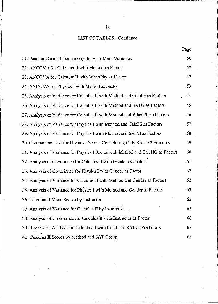
21. Pearson Correlations Among the Four Main Variables 50

22. ANCOVA for Calculus II with Method as Factor 52

23. ANCOVA for Calculus II with WhenPhy as Factor 52

24. ANCOVA for Physics I with Method as Factor 53

25. Analysis of Variance for Calculus II with Method and CalcIG as Factors . 54

26. Analysis of Variance for Calculus II with Method and SATG as Factors 55

27. Analysis of Variance for Calculus II with Method and WhenPh as Factors 56

28. Analysis of Variance for Physics I with Method and CalcIG as Factors 57

29. Analysis of Variance for Physics I with Method and SATG as Factors 58

30. Comparison Test for Physics I Scores Considering Only SATG 3 Students 59

31. Analysis of Variance for Physics I Scores with Method and CalcIIG as Factors 60

32. Analysis of Covariance for Calculus II with Gender as Factor 61

33. Analysis of Covariance for Physics I with Gender as Factor 62

34. Analysis of Variance for Calculus II with Method and Gender as Factors 62

35. Analysis of Variance for Physics I with Method and Gender as Factors 63

36. Calculus II Mean Scores by Instructor 65

37. Analysis of Variance for Calculus II by Instructor 65

38. Analysis of Covariance for Calculus II with Instructor as Factor 66

39. Regression Analysis on Calculus II with CalcI and SAT as Predictors 67

40. Calculus II Scores by Method and SAT Group 68

ix

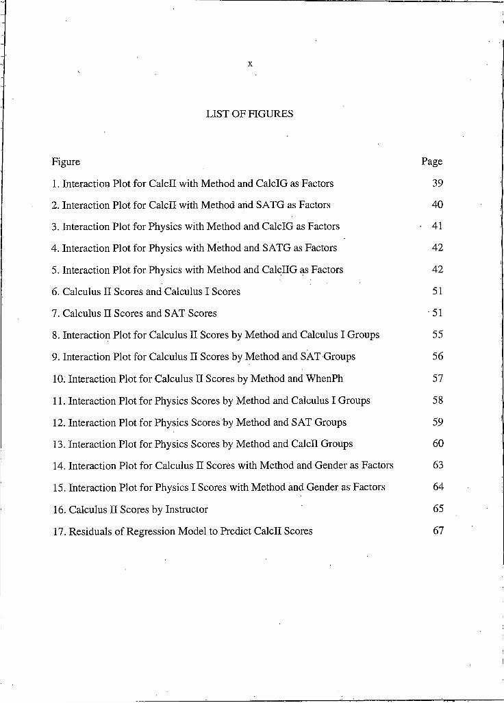
LIST OF FIGURES

1. Interaction Plot for CalcII with Method and CalcIG as Factors 39

2. Interaction Plot for CalcII with Method arid SATG as Factors 40

3. Interaction Plot for Physics with Method and CalcIG as Factors • 41

4. Interaction Plot for Physics with Method and SATG as Factors 42

5. Interaction Plot for Physics with Method and CalcIIG as Factors 42

6. Calculus II Scores and Calculus I Scores 51

7. Calculus II Scores and SAT Scores 51

8. Interaction Plot for Calculus II Scores by Method and Calculus I Groups 55

9. Interaction Plot for Calculus II Scores by Method and SAT Groups 56

10. Interaction Plot for Calculus II Scores by Method and WhenPh 57

11. Interaction Plot for Physics Scores by Method and Calculus I Groups 58

12. Interaction Plot for Physics Scores by Method and SAT Groups 5.9

13. Interaction Plot for Physics Scores by Method and CalcII Groups 60

14. Interaction Plot for Calculus II Scores with Method and Gender as Factors 63

15. Interaction Plot for Physics I Scores with Method and Gender as Factors 64

16. Calculus II Scores by Instructor 65

17. Residuals of Regression Model to Predict CalcII Scores 67

Figure Page

xi

ABSTRACT

This research addressed the question of whether there were differences in achievement between students that followed an integrated approach to calculus that integrated mathematics and physics, compared to students that followed a npn-integrated approach.

The subjects in the study were the 151 students that completed Calculus II (second semester calculus intended mainly for engineering students) at Montana State University- Bozeman during the fall of 1996. There were a total of five sections with five different instructors. All the sections used the Harvard Calculus book and took 'common exams. Three sections were assigned to the experimental group, which followed the integrated method, while two sections acted as the control group.

Both groups covered the main topics of chapters 6 -10 of the Harvard Calculus book. The instructors in the experimental group stressed problems about applications to physics, as well as the conceptual and computational aspects of calculus. In addition, students in this group received enrichment notes that supplemented the textbook. The instructors in the control group also stressed the conceptual and computational aspects of calculus as well as applications to physics. However, the control group did not delve as deeply into these applications and did not have the support of the enrichment notes.

Analysis of Covariance (ANCOVA), with Calculus I scores and SAT - math scores acting as covariates, was the technique of choice to compare methods with regard to Calculus II and Physics I scores. Physics I is the first semester calculus-based physics course. ANCOVAS were also used with gender as a factor, and when students take Physics I as a factor (not yet, concurrently with Calculus II, or before Calculus II). For interaction analyses, two-way analyses of variance were employed once students were categorized into three groups according to their scores in Calculus I, SAT- math, and Calculus II.

Students in the integrated group did significantly better in Calculus II. Interaction was found when Physics I scores were analyzed, with method and SAT-math groups as factors. Students with high mathematical aptitude in the integrated group scored significantly better than students with high mathematical aptitude in the non-integrated group, when Physics I scores were analyzed. No other interactions were detected. Furthermore, there were no differences in Calculus II achievement according to when students took Physics I. No differences in achievement according to gender were found either.

On the basis of the findings of this study, an integrated approach to the teaching of second semester calculus is recommended. .

I

CHAPTER I

PROBLEM STATEMENT AND REVIEW OF LITERATURE

Introduction

Since calculus was created in the late seventeenth century, the teaching of it has

been a matter of concern to mathematicians and educators. Probably, in no other basic

mathematical subject can one find so many pedagogical difficulties. This should not be a

surprise; for two hundred years (1670 - 1870) the best mathematicians of each generation

struggled trying to understand the underlying structure that held calculus together as a

coherent whole.

Since Newton's time, calculus has played a central role in mathematics. In its

beginnings, it was intimately linked to physics, and it remained so for a long time.

Problems in physics led to new mathematical theories that originated from calculus, for

instance, differential equations or the calculus of variations. These mathematical theories

helped to explain innumerable aspects of physics. Well into the 19th century there was

almost no gap between mathematicians and physicists; quite often, their concerns were

similar.

Euler's "Introductio in Analysin Infinitorum" (1748) can be considered to be the

first textbook on calculus in a modern sense. One way or another, every book on this

branch of mathematics published since then stems from Euler's work. The books by

Leonhard Euler epitomize a whole epoch concerned with the accelerated development of

the subject and its multiple applications.

2

At the end of the 18th century and the beginning of the 19th century,

mathematicians started to analyze with care the foundations of calculus. Joseph Lagrange,

and especially Louis Cauchy in the first decades of the past century, started a movement

towards rigorization that culminated around 1870 with the works of Karl Weierstrass.

Calculus was built around the real line, and depended solely on it.

It took a long time to put calculus on a solid foundation. No wonder that the

solution to the problem of rigorization happened to be a sophisticated structure that was

out of reach of most beginning college students. While students in Europe benefited from

the famous collection of "Cours'd' Analyse" by Cauchy, Picard, Jordan, and other great

19th century mathematicians, teaching of calculus in America lagged far behind. With

few exceptions, well into the 1950's, most calculus textbooks lacked rigor and

motivation. Applications were few and scattered across the textbooks; little or no

connection between mathematics and the real world could be found. Calculus was

presented as a series of clever tricks and procedures.

Starting in 1957, with the launching of the Sputnik, mathematics and the natural

sciences received great impetus in the United States of America. In the next two decades,

new books oh the calculus were published, stressing the theoretical aspects of the subject

but paying little attention to the links between calculus and physics or chemistry. The

pendulum swung completely in the other direction, from a lack of rigor to excessive rigor,

somehow blurring the distinction between calculus and real analysis. Quite often during

their first year in college, students had to deal with techniques that baffled them.

Moreover, applications were relegated to the end of each chapter, many times as optional

material. The net result of this way of presenting calculus was a high degree of student

failure. Voices of discontent were raised among mathematicians, natural scientists,

educators, and the community in general.

3

A conference was convened at Tulane University in 1986 to address the problem

of calculus teaching. This conference is considered to be the beginning of what is now

called "Reform Calculus." Radical steps were taken towards promoting a "lean and lively

calculus," wherein a balance could be reached between conceptual developments and

applications, and where modern technologies would be used in a pervasive way.

Several projects came to light under the inspiration of the Tulane conference. The

best known is the one started by a Consortium based at Harvard University. Montana

State University-Bozeman has adopted the Harvard Consortium textbook (Hughes-Hallet

et al. 1994) for its two semester first year calculus sequence, intended mostly for

engineering majors. This book is a radical departure from the traditional presentation

since it focuses on enhancing student's understanding, and applications are more

numerous than in the past.

It is an open question whether or not the introduction of substantial applications

from the natural sciences, within the calculus course, has a pedagogical impact (Ferrini-

Mundy and Geuther Graham 1991, p. 633). The purpose of this work is to investigate

whether there is a difference in achievement between students that follow the Harvard

Calculus textbook, and those students who, besides using the same textbook, receive

supplemental materials and study several mathematical aspects of physics related to the

course they are taking concurrently in physics.

Statement of the Problem

Is there a difference in achievement between students that follow an integrated

Harvard Calculus approach, integrating mathematics and physics, compared to students

that follow a Harvard Calculus non-integrated approach?

4

The Importance of the Study

There is ample evidence that an integrated approach to mathematics teaching,

integrating the natural sciences and mathematics, is an advisable path to follow at all

levels. However, most of this evidence is anecdotal. There is a need for carefully

conducted research to address the question of whether or not integration of academic

areas (e.g., mathematics and physics) benefits students as their proponents assert. Some

research on the subject has been done at the middle school level, but little at the high

school level and almost none at the college level. In particular, calculus is a subject taken

by more than half a million college students every year in the USA. Thus, it is important

to carefully determine whether steps toward integrating calculus with the natural sciences

is a sound option or not. This study purports to give an answer to this question.

Definitions of Terms

For the purpose of this study, the researcher used the following definitions:

Calculus II: Second semester calculus, using the Harvard Consortium book. This

course is intended primarily for engineering, mathematics, and the natural sciences

students.

Achievement in Calculus II: Achievement in Calculus II was measured by three

one-hour examinations and a comprehensive final examination.

Physics I: First semester of a three semester sequence, primarily for engineering

and physical sciences students. Covers topics in mechanics.

Achievement in Physics I: Achievement in Physics I was measured by a midterm

examination and a comprehensive final examination.

5

Calculus I: First semester calculus, using the Harvard Consortium book. Intended

primarily for engineering, mathematics, and the natural sciences students.

Previous knowledge of Calculus: Previous knowledge of calculus was measured

by three one-hour examinations and the final comprehensive examination in Calculus I

taken at Montana State University-Bozeman the previous semester.

Harvard Calculus: A reform calculus approach developed by a consortium based

at Harvard University.

Integrated Harvard Calculus Approach: This is the approach that follows the

content of the Harvard Calculus textbook, and supplements it with enrichment notes that

cover several mathematical aspects of mechanics and chemical kinetics that go beyond

the textbook. Additionally, application problems from the book are discussed thoroughly.

Non-integrated Harvard Calculus Approach: This is the approach that follows the

content of the Harvard Calculus textbook, without the enrichment notes. The non-

integrated approach does not delve as deeply into the applications.

Scholastic Aptitude in Mathematics: Scholastic aptitude was measured by the

mathematics portion of the SAT or ACT tests.

Interaction: "An interaction between two factors is said to exist if the mean

differences among levels of factor A are not constant across levels (categories) of factor

B" (Glass and Hopkins, 1996, p. 483).

Questions to be Answered

This study has attempted to answer the following questions:

I . Is there a difference in the adjusted Calculus II achievement means, between the

integrated and non-integrated groups, when statistically equated with respect to previous

knowledge of calculus and scholastic aptitude in mathematics?

6

2. In the analysis of Calculus II achievement, does method of teaching (integrated

or non-integrated) interact with previous knowledge of calculus?

3. In the analysis of Calculus II achievement, does method of teaching (integrated

or non-integrated) interact with scholastic aptitude in mathematics?

4. Is there a difference in the adjusted Calculus II achievement means, between

students that have not yet taken Physics I, are taking Physics I concurrently with Calculus

n, and took Physics I before Calculus II, when statistically equated with respect to

previous knowledge of calculus and scholastic aptitude in mathematics?

5. In the analysis of Calculus II achievement, does method of teaching (integrated

or non-integrated) interact with the time when students take Physics I (not yet,

concurrently with calculus II, or before Calculus II) ?

6. Is there a difference in the adjusted Physics I achievement means, between the

integrated and non-integrated groups, when statistically equated with respect to previous

knowledge of calculus and scholastic aptitude in mathematics?

7. In the analysis of Physics I achievement, does method of teaching (integrated or

non-integrated) interact with previous knowledge of calculus?

8. In the analysis of Physics I achievement, does method of teaching (integrated or

non-integrated) interact with scholastic aptitude in mathematics?

9. In the analysis of Physics I achievement, does method of teaching (integrated or

non-integrated) interact with achievement in Calculus II?

10. Is there a difference in the adjusted Calculus II achievement means between

female and male students, when statistically equated with respect to previous knowledge

of calculus and scholastic aptitude in mathematics?

11. Is there a difference in the adjusted Physics I achievement means between

female and male students, when statistically equated with respect to previous knowledge

of calculus and scholastic aptitude in mathematics?

7

12. In the analysis of Calculus II achievement, does method of teaching

(integrated or non-integrated) interact with gender?

13. In the analysis of Physics I achievement, does method of teaching (integrated

or non-integrated) interact with gender?

Conceptual Framework

Mathematics has been used in physics for a long time, especially since Galileo

Galilei established the basis of the scientific method at the beginning of the 17th century.

Mathematics became "the language of science," and its use, both in science research and

science instruction, steadily won ground. A natural science was considered to have

achieved full maturity once it lost a merely descriptive stage, and a mathematical

approach had been established. Chemistry followed the path of physics, and in our

century biology started to use a mathematical approach to some degree too.

In contrast, mathematics research and instruction has drifted away, little by little,

from the natural sciences. Despite the fact that physics played a very important role in the

development of mathematics (calculus is a well-known example of this assertion),

contemporary mathematicians - with few arid scattered exceptions - have become isolated

in their discipline, and have ceased to use physics in their research and instruction almost

completely. It is common knowledge that the scientific method, with its stress on

exploration, gathering of data, and prediction, is a tool that can be used with great profit

in the learning of mathematics.

When we talk about integrating mathematics and the natural sciences in the

classroom, we do not mean integration of content but of methodologies. Lynn Steen

expresses this idea very clearly, when he analyzes one of the possibilities for integrating

mathematics and science (Steen 1992, p. 8):

8

[one such possibility is to employ] mathematical methods thoroughly in science, and scientific methods thoroughly in mathematics, coordinating both subjects sufficiently to make this feasible. This is, I submit, an ideal situation. Each discipline, science and mathematics, would accrue benefits from an infusion of methods of the other, but neither would lose its identity or distinguishing features in an artificial effort at union. There are, after all, important differences between science and mathematics, both philosophical, methodological, and historical. These should not be lost in a misguided effort at homogenization.

Further on (p. 12) the same author writes:

Similarly, the compelling logic of inference and deduction can help the students experience the special power of science. Absent the rigorous logic of inference that is typical of mathematics, science instruction can easily degenerate into description, demonstration, and memorization. Without the intrinsic authority of inference, the authority found in science becomes extrinsic, hence heretical: students believe what teachers tell them, not what they have logically demonstrated from evidence.

The theoretical basis which underlies our study stems from Steen's thoughts, more

than from any other thinker's.

Teachers of mechanics use calculus pervasively. It is time that teachers of calculus

use physics and chemistry as pedagogical tools in the classroom, drawing illuminating

examples from both sciences to impress upon the students the proper idea of the close

links between mathematics and the natural sciences. There seems to be much to gain and

nothing to lose.

In consonance with the aforementioned concepts, NCTM (1991, p. 70)

recommends "connecting mathematics to other subjects and to the world outside the

classroom," while AMATYC (1995, p. 16) stresses the fact that" students must have the

opportunity to observe the inter-relatedness of scientific and mathematical

investigations."

9

Review of Literature

The Precursors of Integrated Calculus

Kline (1967) was among the first in modern times to warn of the dangers of

excessive rigor in the presentation of the calculus. He advocated an intuitive approach.

Besides, he saw the need to use physics extensively in the calculus classes:

The second essential respect in which this book differs from current ones is that the relationship of mathematics to science is taken seriously. The present trend to separate mathematics from science is tragic. There are chapters of mathematics that have value in and for themselves. However, the calculus divorced from applications is meaningless. We should also keep in mind that most of the students taking calculus will be scientists and engineers and these students must learn how to use mathematics. But the step from mathematics to its applications is not simple and straightforward and it creates difficulties for the student from the time he is called upon to solve verbal problems in algebra. The mathematics courses fail to teach students how to formulate physical problems mathematically. The science and engineering courses, on the other hand, assume that students know how to translate physical problems into mathematical language and how to make satisfactory idealizations. The gap between mathematics and science instruction must be filled, and we can do so to our own advantage because thereby we give meaning and motivation to the calculus (Kline 1967, p. vii).

The same author (Kline 1970) quite forcefully advocates an intuitive approach to

calculus teaching, with physical arguments playing an important role. This proposal is a

continuation of the criticism voiced three years earlier.

Boas (1971) called attention to the advisability of using an approach to calculus

teaching similar to the one used by scientists when they teach science. Whether in

physics, chemistry, or biology, teachers of science base many of their lectures on well-

established experiments carried out in the past. Often these experiments are difficult to

replicate or time-consuming, so scientists take them for granted in the classroom setting

10

and continue ahead. Boas maintains that proofs are to mathematics what experiments are

to the natural sciences, an analogy that can be used with great profit by teachers of

mathematics:

... I claim that the teacher of calculus would do well to follow the lead of the experimental scientist. Let him give proofs when they are easy and justify unexpected things; let him omit tedious or difficult proofs, especially those of plausible things. Let him give easy proofs under simplified assumptions rather than complicated proofs under general hypotheses. Let him by all means give correct statements, but not necessarily the most general ones that he knows (Boas 1971, p. 666).

Despite the warnings of noted teachers as Kline and Boas, the same inclination

toward rigor at the expense of understanding was followed in the seventies with regard to

calculus teaching. In fact, two trends coexisted during this decade: excessive rigor and

"watered-down" versions with no rigor at all. The latter trend had dominated calculus

teaching for most part of the first half of this century, in concordance with the belief that

the theory behind the calculus could only be understood in advanced courses on real

analysis. The pendulum started to swing to the other extreme after the launching of the

Sputnik when great changes in education were started. Both trends lacked links to physics

or to any other natural science.

In the sixties and seventies, students were failing in calculus at an alarming rate,

so several solutions to the problem were proposed. Self-pacing, discovery, collaborative

learning, computers in calculus instruction, and programmed learning were among them

(Teles 1992). However, none of them offered conclusive evidence as to their merits. In

some cases there was a small, but not significant difference when compared to traditional

calculus courses taught through the lecture format. In others it was difficult to replicate

the experiments, leaving the impression that a superb teacher could do marvels with

whatever approach he/she adopted.

11

The Calculus Reform Movement

The situation came to a crisis around 1984 when Ralston (1984) presented the

idea to put calculus on a coequal role with discrete mathematics in the first two years of

college. This would amount to downsizing calculus, a subject that for a long time had

been the center of first and second year college mathematics. The idea was hotly disputed

by many mathematicians, Daniel Kleitman and Peter D. Lax among them. Kleitman and

Lax contended that calculus should continue to be the core of first year mathematics,

since its methods and ideas are at the origin of some of the most impressive developments

in mathematics. Lax wrote: "As to calculus, mathematicians need not less, but more of it.

The real crisis is that it is badly taught, the syllabus has remained stationary, and modem

points of view, especially those having to do with the role of applications and computing

are poorly represented" (Ralston 1984, p. 380).

At the 1986 Tulane University conference there was a consensus with regard to

the need of using modern technology in the classroom, and of striking a balance between

the conceptual and computational aspects of calculus, together with significant

applications. The Mathematical Association of America published the proceedings of the

conference (Douglass 1986) and a continuation of the proceedings (Steen 1987), both of

which have become very influential.

Several reform projects were developed after the Tulane conference. The best

known, and the one that has had the greatest impact on calculus teaching, is the project

started by a consortium based at Harvard University (Hughes-Hallet et al. 1994). Two

basic principles guided their efforts:

1. Every topic should be presented geometrically, numerically, and algebraically.

2. Formal definitions and procedures evolve from the investigation of practical

problems.

12

Research on the Impact of Reform Calculus

Does research support the claims of the Harvard Consortium when compared to

traditional approaches? Ratay (1993) used a preliminary edition of the Harvard

Consortium textbook with the class of '95 at the United States Merchant Marine

Academy, while the class of '94 had used a traditional textbook. The grades of the classes

of '94 and '95 were compared for each of the three quarters of their freshman year.

Students were grouped according to their mathematics scholastic aptitude test (SAT-

math) scores into four categories (500 - 540, 550 - 590, 600 - 640, 650 - 800 ranges), and

their average grades were plotted both for the '94 and '95 classes. Results show that the

class of '95 consistently outperforms the class of '94, especially for the first quarter

among those in the 500 - 540 range. The mean difference is almost a full letter grade for

those in the lowest aptitude group. A similar result was obtained when, instead of the

SAT-math scores, the researcher used the CPT scores (CPT is an algebra examination

administered to all entering freshman at the Academy). The students were divided into

four groups according to their CPT scores (20 - 49, 50 - 69, 70 - 89, 90- 120 ranges) and

their average grade was calculated. In Summary, Ratay found that students earned higher

calculus grades using the Harvard consortium book and the benefit was larger among

those students with less preparation and aptitude in mathematics. It is to be noted that the

work under consideration is of a preliminary nature. The fact that the groups that were

compared took different examinations at different times, does diminish the validity of its

conclusions. Besides, no significance tests were conducted; the results could be due to

chance. Certain trends can be noticed from the graphs of Ratay's paper, but no conclusive

statement can be done since no statistical tests were performed.

At Brigham Young University, three calculus programs are taught simultaneously

as part of the regular curriculum (Armstrong, Garner and Wynn 1994). Two of them are

13

reform calculus (Harvard Calculus and CUM, calculus using Mathematica), and the third

is a traditional approach. The reform calculus programs are characterized as programs

where essential use of technology is made, with students learning pertinent applications in

an environment where teaching is innovative (group work, interactive teaching methods,

et cetera). Two early evaluations compared grades of students in several courses with

calculus as a prerequisite. Grades of former calculus students in courses in nine areas,

namely biology, chemical engineering, chemistry, civil engineering, electrical

engineering, electrical engineering technology, mathematics, physics, and statistics were

surveyed.

The first study concluded that Harvard Calculus students did better in six of the

nine areas, CUM students did better in mathematics, while traditional calculus students

obtained the highest grades in electrical engineering and in statistics courses. However,

only the better achievement of the CUM students in subsequent mathematics courses was

statistically significant (0.05 level). The second study comprised more students (the

authors do not specify the number of students involved in each study). Again, Harvard

Calculus students did best in the same six areas, CUM students did best in mathematics

and electrical engineering courses, while traditional calculus students did best in

statistics. None of the differences were statistically significant.

A third study was also conducted at Brigham Young University, considering

calculus grades and ACT (American College Testing) scores. Neither student selection

strategies nor instructor differences were taken into consideration. Besides, the CUM

group was very small compared to those in the other two programs. No statistical

differences in grade point averages in subsequent courses (linear algebra,

multidimensional calculus, engineering mathematics, mathematical statistics, and two

principles of physics courses) were found.

14

While these statistics were not definitive, we were happy to find that reformed calculus students did not do worse statistically than traditional students in any of the courses surveyed. This is so despite the fact that subsequent courses depend upon traditional calculus information.. Also, such surveys do not account for other factors making reformed calculus more advantageous, such as more positive student and instructor attitudes, better mastery of concepts and applications, benefits obtained through group study, and advantages to students due to their increased technological expertise (Armstrong, Garner and Wynn 1994, p. 309).

A secondary finding was reported: Students who took second semester traditional

calculus after having taken Harvard Calculus the first semester, suffered a significant

drop in grades (0.05 alpha level).

Kerry Johnson conducted a four-semester study at Oklahoma State University,

comparing Harvard calculus with traditional Calculus (Johnson 1995). Answers were

sought to the following questions:

1. Do Harvard students get better grades in calculus than traditional calculus

students?

2. Are Harvard students more likely to enroll in subsequent mathematics courses?

3. Do Harvard students perform better in subsequent mathematics courses than

other students?

4. How do students that go from Harvard Calculus I into Traditional Calculus' 2

perform?

With regard to the first question, the answer found is that a higher percentage of

the Harvard Calculus students pass the course and make a C or better in the course than

traditional calculus students (67% vs. 62% in Calculus I, 80% vs. 71% in Calculus 2.)

There was a varied response to the second question, depending on the course. For

example, among students who got a D or better in Calculus 1, 63% of Harvard Calculus

students took Calculus 2 compared to 56% of traditional calculus students that took

15

Calculus 2. Enrollments in Differentia] Equations were 36% Harvard, 33% traditional,

while in Linear Algebra it was Harvard 20%, traditional 27%. With regard to the third

question, Johnson found that the answer is no. For example, in Differential Equations,

50% of the D or better Calculus 2 students maintained or improved their grades, while

58% of the traditional calculus students maintained or improved their grades. In Linear

Algebra, the difference was Harvard 60% vs. Traditional 69%. Both Differential

Equations and Linear Algebra are traditional courses. Finally, as one might expect, it is

not advisable to go from Calculus I - Harvard Calculus into Calculus 2 - Traditional

Calculus. Only 55.3% of these students made a C or better in Calculus 2 compared to

more than 80% in the other three possible combinations (Calculus I - traditional into

calculus 2 - traditional, Calculus I - traditional into Calculus 2 - Harvard, and Calculus I

- Harvard into Calculus 2 - Harvard.) The greater emphasis on algebraic skills in

traditional calculus may explain these percentages. No statistical analysis of any kind

(besides simple percentages) is reported in the paper under consideration.

The three papers mentioned above have shortcomings which are diverse. For

instance, there are no common measures of achievement or carefully set conditions with

an experimental and a control group. Some of these difficulties are recognized by the

authors, when they write about the "preliminary nature" of their research. There has been

little published research concerning reform calculus initiatives (Becker and Pence 1994,

p.6), so the research done at the USA Merchant Marine Academy, Brigham Young

University, and Oklahoma State University, are a first step forward.

Physical Applications within the Calculus Courses

Joan Ferrini-Mundy and Karen Geuther Graham (1991) put in the forefront of

future research the idea to determine whether or not examples drawn from physics can

help in the learning of mathematical concepts related to calculus:

16

A number of mathematics education research questions arise in conjuction with the calculus effort. Several questions relate to the scope and Sequence of the mathematics content. Examples include: How does one decide which parts of the traditional curriculum can best be omitted? Is it more helpful to students to introduce the idea of limit before the idea of derivative? What are the effects of introducing substantial physical applications within the calculus course? Many questions arise that relate directly to student learning and background matters. Examples of relatively broad questions include: Does lack of algebraic facility truly hinder calculus learning? How does the experience of secondary school calculus relate to the experience of college calculus? How does student "intuition" develop? Do physical examples help in the learning of concepts?" (Ferrini-Mundy and Geuther Graham 1991, p. 633).

These research questions, and others mentioned by both authors in the same

paper, could have very important consequences since, annually, 600,000 students enroll

in some type of calculus course in four-year colleges and universities in the United States

of America. Almost half of these students are in mainstream "engineering" calculus, and

only 46% finish the year with a grade of D or higher (Ferrini-Mundy and Geuther Graham

1991, p. 627.)

A pilot project was conducted at Dutchess Community College (Poughkeepsie,

New York) by Wesley Ostertag, a mathematician, and Tony Zito, a physicist (Ostertag

and Zito 1995), fully integrating first year Harvard Calculus with first year physics. Both

of them teach this rather unique course, which blends all the topics in first year calculus

and physics. Students at Dutchess Community College can enroll in the integrated course

or enroll separately in a two semester Harvard Calculus and in a two semester

"traditional" physics course. They found that 65% of those in the integrated one-year

course obtained a grade of C or better in both semesters, while only 50% of those enrolled

in the non-integrated sequence accomplished this goal. The authors do not mention

whether or not the objectives and tests were the same. Moreover, a standardized test

designed to measure student's understanding of basic kinematics was given as a pre- and

17

post-test to students in both integrated and non-integrated sections. The mean post-test

score for the integrated section was 69% (an improvement of 22% over the pre-test mean

score), whereas the mean score for the non-integrated section was 61% (an improvement

of 15% over the pre-test mean score). The authors do not report whether these results are

significant or not.

This type of fully integrated first year calculus-physics course might be of crucial

importance for community colleges, since they offer two-year degrees, and thus cannot

afford to have first-semester calculus as a prerequisite for first-semester physics (as often

happens in four-year colleges and universities).

Integrating College Mathematics with the Natural Sciences

There has been a limited number of efforts toward integrating mathematics

teaching and the natural sciences at the college level. Among these we can mention „

Helfgott (1990), Jean and Iglesias (1990), and Helfgott (1995). The first one describes an

integrated approach to differential equations, used in the classroom setting by the author,

blending mathematics and several aspects of chemistry and physics:

Student proficiency and surveys conducted among former pupils show that an integrated approach to several aspects of the natural sciences together with differential equations is highly recommended. Students who followed the integrated approach, instead of the classical differential equations course with few examples of applications outside mathematics, found it less difficult to do the work in later courses in control theory, heat transfer, transport phenomena and chemical kinetics (Helfgott 1990, p. 1014).

The paper by Jean and Iglesias is based on a course developed by the authors,

wherein biology and mathematics are blended in a coherent whole. This is a radical

departure from traditional courses in mathematics for biology majors. The third paper

describes a first-year calculus course where history and the natural sciences (physics and

chemistry) are used extensively:

18

In teaching the calculus, it is useful to supply many examples of applications from the natural sciences. We go further than usual, developing classical examples from mechanics and chemical kinetics. The latter are particularly helpful because they are simple, require few prerequisites, and use a significant amount of readily available data. We stress the meaning of the scientific method in its different stages of building models, obtaining consequences, and contrasting them with data. Applications appear everywhere, not necessarily at the end of a section (Helfgott 1995, p. 136).

K-12 Integration of Mathematics and Science

The problem of integrating mathematics and science in the K-12 curriculum in the

United States has a long history that goes back to E.H. Moore at the turn of the century.

Moore, Professor of Mathematics at the University of Chicago, advocated teaching

mathematics in close relationship to problems in physics, chemistry, and engineering. His

idea found a great deal of support among teachers of high school mathematics and also by

teachers of the High School sciences, and eventually led to the formation of the Central

Association of Science and Mathematics Teachers, and its influential publication "School

Science and Mathematics." Breslich (1936, p. 58) wrote about the Association in the

following terms:

One of the major purposes of the association was to find and establish legitimate contacts between the mathematical subjects and the sciences. It was hoped that the constant training which the pupil derives from applying mathematics to problems in science would increase his mathematical power and that his interest in mathematics would grow with the opportunities of using it in other school subjects. Indeed, some of the leaders of the movement were advocating that algebra, geometry, and physics be organized into a coherent course. If possible, this course was to be taught by the same teacher or at least by two teachers who were in sympathy with the ideas of correlation.

What happened? The efforts toward integration have not been successful,

especially at the high school level. The trend toward specialization and the lack of proper

19

training among teachers have conspired against integration. All too often mathematics

teachers had little knowledge about science, and teachers of science had little knowledge

about mathematics.

Few steps were taken with regard to how mathematics teaching.could be

improved by using examples drawn from the natural sciences. Fortunately, in the last

decade there has been a renewed interest in the subject. Systemic initiatives have started

to foster an interdisciplinary approach to mathematics, among these the Systemic

Initiative in Montana Mathematics and Science (SIMMS) project in Montana. Its first

objective (SIMMS 1993) is to redesign the 9-12 mathematics curriculum using an

integrated approach for all students. The project is in its fifth year, and has had a marked

impact on high school education in Montana, through its workshops, the publication of

high-quality, fully integrated modules, technological support to schools, and the like.

Besides, high school teachers all over the nation are developing ways to integrate

mathematics and the natural sciences, trying to close the gap between them (Abad 1994,

Longhart and Hughes 1995).

At the elementary and middle school level some research has been done about the

effect of science and mathematics integration (Friend 1985, Kren and Huntsberger 1977).

Friend's main purpose was to determine how integrating science and mathematics in a

seventh grade physics unit affected achievement in science. Divided into 4 classes, 108

seventh graders were involved in the study. Two classes consisted of students with

standardized reading and mathematics scores at least two years above grade level (AGL),

while two classes consisted of students with standardized reading and mathematics scores

on grade level (GL). One AGL class and one GL class followed the science and

mathematics integration approach.

20

The investigation lasted 10 weeks, and students were assessed on a common test

of physics. An analysis of variance showed that only AGL students taught by the

integrated approach, demonstrated significantly greater achievement (0.01 level) than

AGL students taught by the non-integrated approach. For GL students there was no

significant difference between those in the integrated and non-integrated classes.

Moreover, analysis of variance showed that AGL students that followed the non-

integrated approach scored significantly higher (0.01 level) than GL students that

followed the integrated approach. Friend recommends, on the basis of his findings, that

science and mathematics should be integrated for AGL students.

Kren and Huntsberger investigated the effect of integrating science and

mathematics instruction on fourth and fifth-grade student achievement in two

mathematical skills (measuring and constructing angles, and interpreting and constructing

graphs). A total of 161 children from eight classrooms participated in the study. The

authors report (Kren and Huntsberger 1977, p. 558) that the treatments of the study were:

1. To present the concept in mathematics first so that the child may be able to

apply it in science at a later date.

2. To present the concept in science and mathematics concurrently so that the two

disciplines will enhance each other.

3. To present the mathematical concept in science, and follow the presentation

with a similar one in mathematics.

An analysis of variance showed that there was no significant difference among the

groups. Thus, the aforementioned mathematical skills could be taught with equal

effectiveness under any of the three approaches. The authors recommend further

investigations of ways science can be used to enhance the teaching of mathematics. The

issue of integration is actively discussed nowadays at the middle school level, both by its

21

advocates and by those that have some concerns about its implementation (George 1996,

Beane 1996).

The Critics

Reform calculus has provoked a backlash in the academic community. Some

critics adopt an emotional stance without justifying their claims that the use of

applications in calculus courses may harm the integrity of the subject (Kleinfeld 1996, p.

230) while others raise important questions with regard to calculus teaching, which have

to be addressed and discussed objectively. Hu (1996, p. 1538) quite appropriately

singularizes four main problems that seem to affect several reform calculus books:

1. Confusion between heuristics and mathematical proof.

2. Less emphasis on symbolic manipulation.

3. Use of computers as a replacement of mathematical thinking.

4. Lack of mathematical closure in the discussion of applications.

There is an ongoing discussion, a healthy development in the mathematical

community, which paid little attention to pedagogical issues in the past (Cipra 1996,

Wilson 1997). Proponents and detractors of reform calculus, and, in particular, of the .

utilization of applications as a learning device in the classroom, have laid out their

arguments. Everyone hopes that the ongoing debate will remain civil and fruitful.

Final Remarks

Should mathematics and science lose their identity in the quest of integration?

Lynn A.' Steen, former President of the Mathematical Association of America, gives a

negative answer (Steen, 1992). He would rather recommend teachers to employ

mathematical methods thoroughly in science, and scientific methods thoroughly in

I 22

mathematics. That is to say, rather than blending content, Steen advocates blending

methods. He sees mathematics and the sciences as different enterprises, one revealing

order and pattern, the other seeking to understand nature. Nonetheless, they can

contribute a lot to each other through cross-fertilization.

23

CHAPTER 2

METHODOLOGY

Sample and Population Description

The sample comprised all the students that completed second semester reform

calculus (Math 182) at Montana State University-Bozeman, during the fall semester of

1996 (Math 182 is a four credit course that meets five days per week.) Five sections with

five different instructors were scheduled at different hours. Three sections were set aside

for the experimental treatment, while two sections acted as the control group. Students

chose the sections according to their timetables and none of them knew who his or her(

instructor was going to be until the first day of classes. The students did not know which

sections were in the experimental group and which sections were in the control group. In

other words, the experimental group did not know that they were being "experimented

upon." The population under consideration is intended to simulate the students that enroll

and complete second-semester calculus in land-grant institutions of the United States.

Statistical Hypotheses

The questions to be answered by this study, stated in hypothesis form, are the

following:

I. There is no difference between the adjusted Calculus II achievement means, of

the integrated and the non-integrated groups, when statistically equated with respect to

previous knowledge of calculus and scholastic aptitude in mathematics.

24

2. Method of instruction (integrated or non-integrated) and previous knowledge of

calculus do not interact on Calculus II achievement.

3. Method of instruction (integrated or non-integrated) and scholastic aptitude in

mathematics do not interact on Calculus II achievement.

4. When statistically equated with respect to previous knowledge of calculus and

scholastic aptitude in mathematics, there is no difference in the adjusted Calculus II

achievement means between those students that have not yet taken Physics I, those

students that are concurrently taking Physics I and Calculus II, and those students that

have taken Physics I before Calculus H

5. Method of instruction (integrated or non-integrated) and when students take

Physics I (not yet, concurrently with Calculus II, or before Calculus II) do not interact on

Calculus II achievement.

6. There is no difference between the adjusted Physics I achievement means, of

the integrated and the non-integrated groups, when statistically equated with respect to

previous knowledge of calculus and scholastic aptitude in mathematics.

7. Method of instruction (integrated or non-integrated) and previous knowledge of

calculus do not interact on Physics I achievement.

8. Method of instruction (integrated or non-integrated) and scholastic aptitude in

mathematics do not interact on Physics I achievement.

9. Method of instruction (integrated or non-integrated) and achievement in

Calculus II do not interact on Physics I achievement.

10. There is no difference in the adjusted Calculus II achievement means between

female and male students, when statistically equated with respect to previous knowledge

of calculus and scholastic aptitude in mathematics.

25

11. There is no difference in the adjusted Physics I achievement means between

female and male students, when statistically equated with respect to previous knowledge

of calculus and scholastic aptitude in mathematics.

12. Method of instruction (integrated or non-integrated) and gender do not interact

on Calculus II achievement.

13. Method of instruction (integrated or non-integrated) and gender do not interact

on Physics I achievement.

Explanation of Experimental Treatments

The main objective of this study was to determine whether or not the integrated

method of instruction, which interrelates calculus and mechanics, affected performance in

calculus and physics. The three experimental sections covered the same basic materials as

the two control sections, namely chapters 6 through 10 of the Harvard Calculus textbook.

However, the experimental sections discussed in class many examples from physics.

These examples go beyond those presented in the textbook, have strong mathematical

components, and are related to topics covered in Physics I. In addition, students in the

experimental sections received enrichment notes that supplemented the textbook, a

sample of which can be found in appendix E.

The original sample of students that completed Calculus II was statistically

analyzed in order to answer hypothesis 5. This sample was smaller whenever Calculus I

achievement or SAT scores intervened as factors or covariables, because not every

student had taken Calculus I the previous semester and not all the mathematics scholastic

aptitude scores were available. Similar considerations had to be applied when Physics I

scores were analyzed, corresponding to students that took this course concurrently with

26

Calculus H. The need to obtain an unbiased score, limited the sample to those students

that took Calculus I the previous semester. In other words, the need of common

examinations to judge achievement in first semester calculus determined a smaller

sample. The latter was analyzed in order to answer several questions of this research,

namely questions 1,2,6, 7, and 10.

It should be emphasized that students that dropped out from Calculus II were not

considered in the study. They had to take all the exams, including the two-hour final, to

remain in the sample . The same applies to Physics I students wherever their scores were

analyzed. Quizzes, homework, or group work were not analyzed because of the

impossibility of obtaining a common measure acceptable to all instructors. These three

activities together determined only one sixth of the total score in Calculus I or Calculus II.

Neither are physics labs considered.

The Maxmincon Principle

The difference between the integrated and non-integrated groups was made as

large as possible, so as to maximize the systematic variance. There were constraints, due

to the fact that all sections of Calculus II had to cover the same core materials.

Nonetheless, the experimental group dealt with enrichment notes, mainly related to

several mathematical aspects of physics that are not normally covered in calculus classes.

Besides, the physics problems in the textbook were heavily stressed in the experimental

group.

There were two contaminating variables that had to be controlled: previous

knowledge of calculus and scholastic aptitude in the area of mathematics. Both were

controlled by means of an analysis of covariance. The best way to control all extraneous

variables would be through randomization (Kerlinger and Pedhazur 1973, p. 82).

27

However, in the setting of our study, random assignment to treatments could not be

accomplished since students chose the section to be in, according to their class schedules

in many different courses. It is to be noted that they did not know who their instructor was

until the first day of classes, when groups were already immutable. Thus, because of these

conditions, we can assume that there was not any systematic selection bias.

The teacher variable, always present in this type of research, was controlled by

having five different instructors; three in the experimental group, one of them the

researcher, and two in the control group. The instructors were all graduate teaching

assistants with similar backgrounds.

Minimization of error variance was accomplished through reduction of errors of

measurement. Students in all five sections of Calculus II took common examinations

simultaneously, at a certain common time in the evening especially set aside for this

purpose (outside the regular class hours). Moreover, the reliability of the graders of the

essay type questions in Calculus II was controlled carefully by establishing a common

rubric for partial credit. With regard to the physics examinations, there is confidence that

there were not any errors of measurement in grading beyond the normal standard errors

since all the exam questions were of the multiple-choice type.

The Hawthorne effect

The Hawthorne effect holds that the researcher's impact on his or her subjects may

actually affect the research results. This effect did not affect the results since students in

Calculus II did not know that a research project was under way. If students in the

experimental and control groups compared their class notes or hand-outs, they may have

noticed that there was a difference on how some topics are developed, with applications

being stressed, but they could not have noticed anything else.

Enrichment Notes

. 28

A sample of the type of additional materials — to be called "enrichment notes"—

that students in the integrated group used, can be found in appendix E. These notes

constituted a distinctive difference between the experimental and control groups. The

topics covered there went beyond the common textbook and the common syllabus used

by the five sections (experimental and control), and stressed the close links between

calculus and physics. In these notes, several models of physics problems were built from

first principles; not as accepted differential equations whose origin was unknown to the

student. Also, Some basic aspects of chemical kinetics were covered in class due to their

strong mathematical content. Mathematical closure was sought in the experimental group,

in the sense that the enrichment notes served to highlight important aspects of calculus.

These notes did not discuss isolated topics, but were fully integrated with the textbook .

Besides, the enrichment notes dealt with some proofs and techniques that cannot

be found in the Harvard Calculus book. For instance, the enrichment notes dealt with the

fundamental theorem of calculus, the criteria for comparison of improper integrals, and

the usual tests to determine the convergence of series. Even though students were not

tested on the theoretical aspects of calculus, the instructors in the experimental group

considered that it was advisable to provide proofs of some very important propositions.

The Instructors in the Experimental Group

Two instructors were invited by the researcher to participate in the experimental

group. They willingly accepted, even though they knew that the integrated method

required greater effort on the part of the teacher. A long session took place before classes

started, wherein the researcher explained the purpose and methodology of the study.

29

Thereafter, each week the three instructors met on a regular basis to discuss the

enrichment notes, practice exams, quizzes and the like. These meetings went beyond the

regular meetings of the five instructors with the course supervisor — the latter a regular

member of the faculty in the department of mathematical sciences. A careful record of

the experimental group meetings was kept, and is shown in Appendix C.

Methods of Data Collection

Collection of Quantitative Data

Achievement in Calculus II was measured by three one-hour exams and a

comprehensive final, comprising a total of 500 points, 100 for each term exam and 200

for the final. All were common examinations, taken outside the regular hours. A first

draft of each of them was made by the course supervisor, an experienced faculty member

that was not in charge of teaching a section. This draft was carefully analyzed by each

instructor, whose collective responsibility was to check for its content validity. All the

instructors got then together and discussed the final version.

With regard to grading, each instructor was assigned the job of grading one

question of all the tests. Since the questions were open-ended, of the essay type, the

grader had to adopt a consistent policy, especially concerning partial credit. This was

achieved by adopting a common rubric, which was strictly followed.

The conditions under which the study was carried out, did not allow a reliability

analysis of the test itself (test-retest technique, for example), but we may assume that

these tests are reliable due to the extensive body of knowledge accumulated on calculus

testing since reform calculus was adopted at MSU-Bozeman for the 181-182 series.

30

Physics I was taught by one member of the physics department faculty, in a large

lecture setting. Achievement in Physics I was measured by the midterm exam and a

comprehensive final, both common examinations of the multiple-choice type.

This study deals only with raw scores. Moreover, as was mentioned before, 100

points allotted in Calculus II to group work and quizzes was not considered. These were

given at the discretion of each instructor, who could adopt the policy that he/she found

best suited for the group. The very nature of the group work and quizzes did not allow a

common standard of measurement, thus determining an insurmountable barrier for

statistical analysis. For a similar reason, laboratory work in physics or chemistry was not

taken into account. The Calculus II exams taken by the students during the fall of 96 are

included in appendix A.

The SAT math scores were provided by the Office of Admissions at MSU-

Bozeman. Since some students had taken the ACT math but not the SAT math test, a

concordance table between SAT and ACT — supplied by the ACT company and shown in

appendix D - was used. The other covariate scores (Calculus I) were provided by the

instructors of first semester calculus, on the basis of three one-hour exams and a

comprehensive two-hour final (a total of 500 points).

Instructor Feedback

The researcher interviewed the two instructors that accompanied him in the

experimental group. These interviews were conducted at the end of the semester, with a

pre-established questionnaire geared toward their experiences in teaching reform calculus

with a strong applied component. The almost verbatim transcriptions of the interviews are

to be found in the next chapter.

3-1

Analytical Techniques and Research Design

Definition of Variables

The scores obtained in the one-hour exams and the final by all students in Math

182 (Fall 96) were added, constituting a number called CalcIL Similarly, their scores

obtained in their previous semester calculus (Math 181) — both in the one-hour exams

and the final — were added; this value was called CalcL Under the symbol Phy we have

scores for those students enrolled in Math 182 that were taking Physics I (Physics 211)

concurrently. These scores were obtained in the same way as in Math 181 and Math 182,

by adding the scores corresponding to the midterm exam and the final. Each student's

scholastic aptitude test in mathematics can be found under a column called SAT.

Furthermore, those students that belonged to the experimental group (three sections of

Math 182) were coded I with regard to Method, while those that belonged to the control

group (two sections of Math 182) were coded 2 with regard to Method. The variable

WhenPh had three levels (1= not yet taken Physics 211,2= taking Physics 211

concurrently with Math 182, 3= taken Physics 211 before), while female students were

coded 0 and male students were coded I .

Categorization of Some Variables and Display of Data

In order to study possible interactions, some of the variables were categorized.

With this purpose in mind, the lower and upper quart!Ies (Q1 and Q3, respectively) of

Calcl, CalcII, and SAT data were calculated to divide the students in three groups (low,

medium, and high) for each of the aforementioned variables. Thus, three new columns

were added: CalcIG, CaicIIG, and SATG. The following ten entries were the basis for all

subsequent analyses:

Method CalcI CalcII Phy SAT CalcIG CalcIIG SATG WhenPh Gender

32

Methods of Analysis

Two-way analysis of variance (ANOVA) was the statistical technique used in

order to answer questions 2, 3, 5, 7, 8, 9, 12, and 13, while analysis of covariance

(ANCOVA) with two covariates, CalcI and SAT, was the chosen statistical tool to answer

questions 1,4,6, 10, and 11.

Two-way ANOVAS , on eight different instances, were calculated:

- ANOVA for CalcII, with Method and CalcIG as factors

- ANOVA for CalcII, with Method and SATG as factors

- ANOVA for CalcII, with Method and WhenPh as factors

- ANOVA for Phy, with Method and CalcIG as factors

- ANOVA for Phy, with Method and SAT as factors

- ANOVA for Phy, with Method and CalcIIG as factors

- ANOVA for CalcII, with Method and Gender as factors

- ANOVA for Phy, with Method and Gender as factors

Five different ANCOVAS (each of them with two covariates: SAT and Calcl)

were calculated:

- ANCOVA for CalcII, with Method as factor

- ANCOVA for CalcII, with WhenPhy as factor

- ANCOVA for Phy, with Method as factor

-ANCOVA for CalcII, with Gender as factor

-ANCOVA for Phy, with Gender as factor

33

Alpha Level

An alpha level of 0.05 was set before the collection of data took place. This level

was adopted instead of a more conservative 0.01 because it is hard to imagine any harm

that could be done to the students by advocating an integrated approach to calculus even

if no measurable advantages exist. That is to say, a type I error (rejecting the null even

though it is true) could not possibly have serious negative effects. This researcher was

quite concerned about the possibility of making a type II error (failing to reject the null

even though it is false).

Limitations and Delimitations

Limitations

1. One limitation to the study is that students of Calculus II were not randomly

assigned to the experimental and control groups. They chose the section to be in

well before the beginning of the semester and according to their timetables.

Calculus II was taught in five sections, at five different times and by five different

instructors. Students did not know that there were going to be experimental and

control groups. Thus, despite lack of random assignment, one might expect that

chance was not absent from the process of selection of sections. In other words,

there is no apparent selection bias.

2. Another limitation of the study was the fact that some students enrolled in

Calculus II did not concurrently take Physics I. Only those students that

concurrently took Calculus II and Physics I were included as part of the sample

used in order to answer questions 6, 7 ,8 ,9 , 11, and 13. A smaller sample does

create problems in the realm of statistical analysis. However, the data collected

from all students enrolled in Calculus II was used to answer questions I, 2, 3, 4,

34

and IO (provided the student had taken, at MSU-Bozeman, Calculus I the previous

semester, and the student's scholastic aptitude test in mathematics was available).

Questions 5 and 12 had no restrictions, in the sense that the scores of all students

that completed Calculus II could be analyzed.

3. For one reason or another, some students dropped from courses during the

semester, reducing the size of the sample. Furthermore, some students had not '

taken Calculus I at MSU-Bozeman, or their scholastic aptitude test was not kept at

the Admissions Office. These two factors also reduced the size of the sample.

4. The background and experience of the teachers in charge of Calculus II were

not exactly the same. This fact introduces the well-known "teacher effect"

phenomenon, maybe unavoidable in educational research of this type, but

nonetheless a limitation. In order to minimize the teacher effect, three sections

followed the integrated approach: one taught by the researcher, two others by

instructors willing to participate in the experiment. The five sections used the

same textbook and followed the same syllabus, a fact that lessened the influence

of teaching styles.

5. Once classes start, the groups are immutable. Nonetheless, it can happen that a

student may want to move from an integrated group to a non-integrated group or

vice versa, for some compelling reason.

6. The course load taken by each student is an uncontrolled variable that may

affect student's achievement in Calculus II or Physics I. However, this researcher

trusts that the variability due to course load is reflected in Calculus I achievement.

A similar consideration can be applied to uncontrolled variables such as number

of hours spent on homework, or on part-time jobs. The grades in Calculus I reflect

not only mathematical aptitude - the correlation with SAT scores is rather low as

35

can be seen in the next chapter — but also the life style of the student in the

sense of how much time he/she devotes to study.

7. Some sections, following the integrated or non-integrated approaches, did

group work once per week. In one of the integrated sections, students were

encouraged to meet on weekends in order to complete the assigned group

problems. Thus, academic activities outside the classroom were an uncontrolled

variable.

Delimitations

1. The study was conducted during the 1996 fall semester, at MSU-Bozeman. It

can be assumed that this study could be replicated with a sample of students

of similar background, in land-grant institutions of the United States.

2. Another delimitation of the study is related to the fact that the study was carried

out with students enrolled in a reform calculus course. Reform calculus

welcomes applications, thus creating an atmosphere where the integrated

approach can be tried. Traditional calculus courses, offered at many institutions

(Math 170, 175, and 176 at MSU-Bozeman are an example), may not be as

receptive as reform calculus courses with regard to an integrated approach.

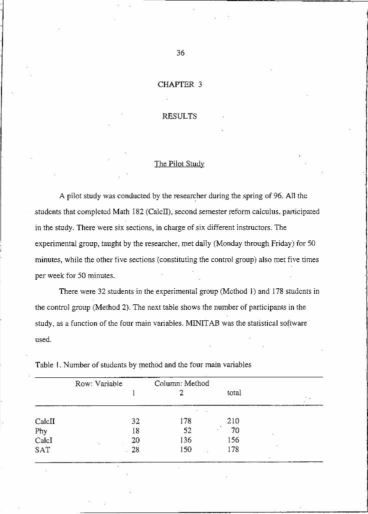
36

CHAPTER 3

RESULTS

The Pilot Study

A pilot study was conducted by the researcher during the spring of 96. All the

students that completed Math 182 (CalcII), second semester reform calculus, participated

in the study. There were six sections, in charge of six different instructors. The

experimental group, taught by the researcher, met daily (Monday through Friday) for 50

minutes, while the other five sections (constituting the control group) also met five times

per week for 50 minutes.

There were 32 students in the experimental group (Method I) and 178 students in

the control group (Method 2). The next table shows the number of participants in the

study, as a function of the four main variables. MINITAB was the statistical software

used.

Table I. Number of students by method and the four main variables

Row: VariableI

Column: Method 2 total

CalcII 32 178 210Phy 18 52 70CalcI 20 136 156SAT . 28 150 178

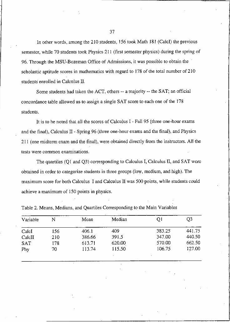
37

In other words, among the 210 students, 156 took Math 181 (CalcI) the previous

semester, while 70 students took Physics 211 (first semester physics) during the spring of

96. Through the MSU-Bozeman Office of Admissions, it was possible to obtain the

scholastic aptitude scores in mathematics with regard to 178 of the total number of 210

students enrolled in Calculus II.

Some students had taken the ACT, others - a majority - the SAT; an official

concordance table allowed us to assign a single SAT score to each one of the 178

students.

It is to be noted that all the scores of Calculus I - Fall 95 (three one-hour exams

and the final), Calculus II - Spring 96 (three one-hour exams and the final), and Physics

211 (one midterm exam and the final), were obtained directly from the instructors. All the

tests were common examinations.

The quartiles (Q1 and Q3) corresponding to Calculus I, Calculus II, and SAT were

obtained in order to categorize students in three groups (low, medium, and high). The

maximum score for both Calculus I and Calculus II was 500 points, while students could

achieve a maximum of 150 points in physics.

Table 2. Means, Medians, and Quartiles Corresponding to the Main Variables

Variable N Mean Median Ql Q3

CalcI 156 406.1 409 383.25 441.75CalcII 210 386.66 391.5 347.00 440.50SAT 178 613.71 620.00 570.00 662.50Phy 70 113.74 115.50 106.75 127.00

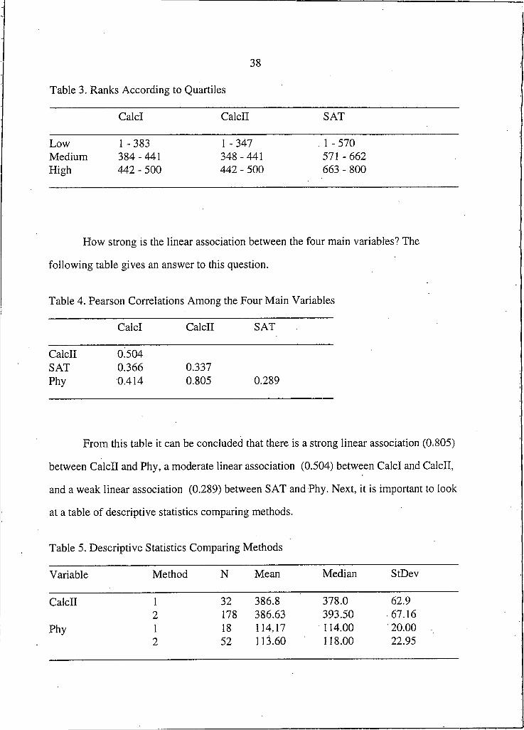
38

Table 3. Ranks According to Quartiles

CalcI CalcII SAT

Low 1-383 I -347 .1 -570Medium 384-441 348-441 571-662High 442 - 500 442 - 500 663 - 800

How strong is the linear association between the four main variables? The

following table gives an answer to this question.

Table 4. Pearson Correlations Among the Four Main Variables

CalcI CalcII SAT

CalcII 0:504SAT 0.366 0.337Phy 0.414 0.805 0.289

From this table it can be concluded that there is a strong linear association (0,805)

between CalcII and Phy, a moderate linear association (0.504) between CalcI and CalcII,

and a weak linear association (0.289) between SAT and Phy. Next, it is important to look

at a table of descriptive statistics comparing methods.

Table 5, Descriptive Statistics Comparing Methods

Variable Method N Mean Median StDev

CalcII I 32 386.8 378.0 62.92 178 386.63 393.50 • 67.16

Phy I 18 114.17 114.00 20.002 52 113.60 118.00 22.95

39

There is a striking similarity between the means in CalcII1 when method I

(integrated approach) and method 2 (non-integrated approach) are compared: 386.8 and

386.63, respectively. The means in physics are also veiy close between both methods

(114.17 and 113.60). Their medians do not differ much either. In addition, students in the

experimental and control groups were compared with regard to their SAT and CalcI

scores.

Table 6. SAT and CalcI Scores in the Experimental and Control Groups

Variable Method N Mean Median StDev

SAT I 28 620.4 650 71.82 150 612.47 620 74.23

CalcI I 20 391.1 391 46.82 136 408.19 409.50 47.68

Five different two-way ANOVAS, with their respective interaction plots, were

calculated so as to reject or retain the null hypothesis related to questions 2 ,3 ,7 ,8 , and 9.

During the pilot project the variables Gender and WhenPhy were not considered.

Figure I. Interaction Plot for CalcII Grades with Method and CalcIG as Factors

Mettiod

400 -

350 -

CALOG

40

Table 7. ANOVA for CaIcII with Method and CaIcIG as factors

Source DF Seq SS Adj SS AdjMS F P

Method I 74 1458 1458 0.46 0.498CaIcIG 2 231448 97292 48646 15.40 0.000Method*CalcIG 2 7544 7544 3772 1.19 0.306Error 150 473797 473797 3159Total 155 712863

Figure 2. Interaction Plot for CalcII with Method and SATG as Factors

Method

430 -

4 0 -

390 -

370 -

350 -

I 2 3

SATG

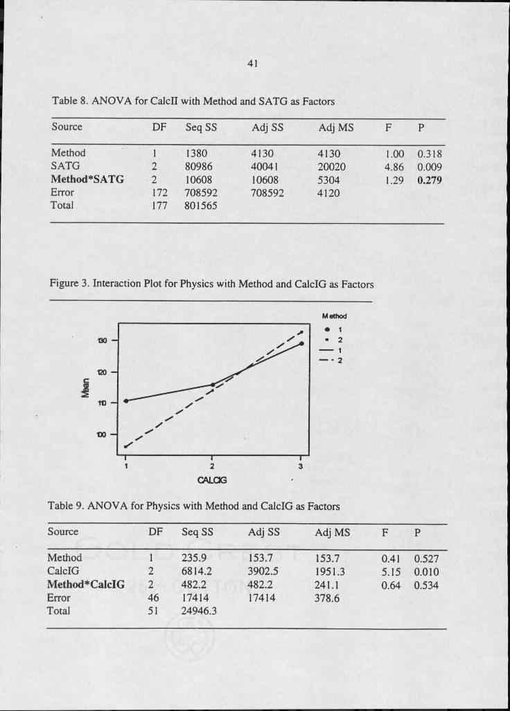
41

Table 8. ANOVA for CalcII with Method and SATG as Factors

Source DF Seq SS Adj SS Adj MS F P

Method I 1380 4130 4130 1.00 0.318SATG 2 80986 40041 20020 4.86 0.009Method*SATG 2 10608 10608 5304 1.29 0.279Error 172 708592 708592 4120Total 177 801565

Figure 3. Interaction Plot for Physics with Method and CalcIG as Factors

Method

QO -

CO -

I t) -

QO -

Table 9. ANOVA for Physics with Method and CalcIG as Factors

Source DF Seq SS Adj SS AdjMS F P

Method I 235.9 153.7 153.7 0.41 0.527CalcIG 2 6814.2 3902.5 1951.3 5.15 0.010Method*CalcIG 2 482.2 482.2 241.1 0.64 0.534Error 46 17414 17414 378.6Total 51 24946.3

42

Figure 4. Interaction Plot for Physics with Method and SATG as Factors

Method

VS -

16 —

OS -

95 -

SATC

Table 10. ANOVA for Physics with Method and SATG as Factors

Source DF Seq SS Adj SS Adj MS F P

Method I 17.1 78.5 78.5 0.16 0.693SATG 2 3485.1 3532.9 1766.4 3.54 0.035Method*SATG 2 520.0 520.0 260.0 0.52 0.597Error 58 28930.7 28930.7 498.8Total 63 32953.0

Figure 5. Interaction Plot for Physics with Method and CalcIIG as Factors

Methcxd06 —I

0 6 -

16 -

0 6 -

96 -

86 -

GMJG

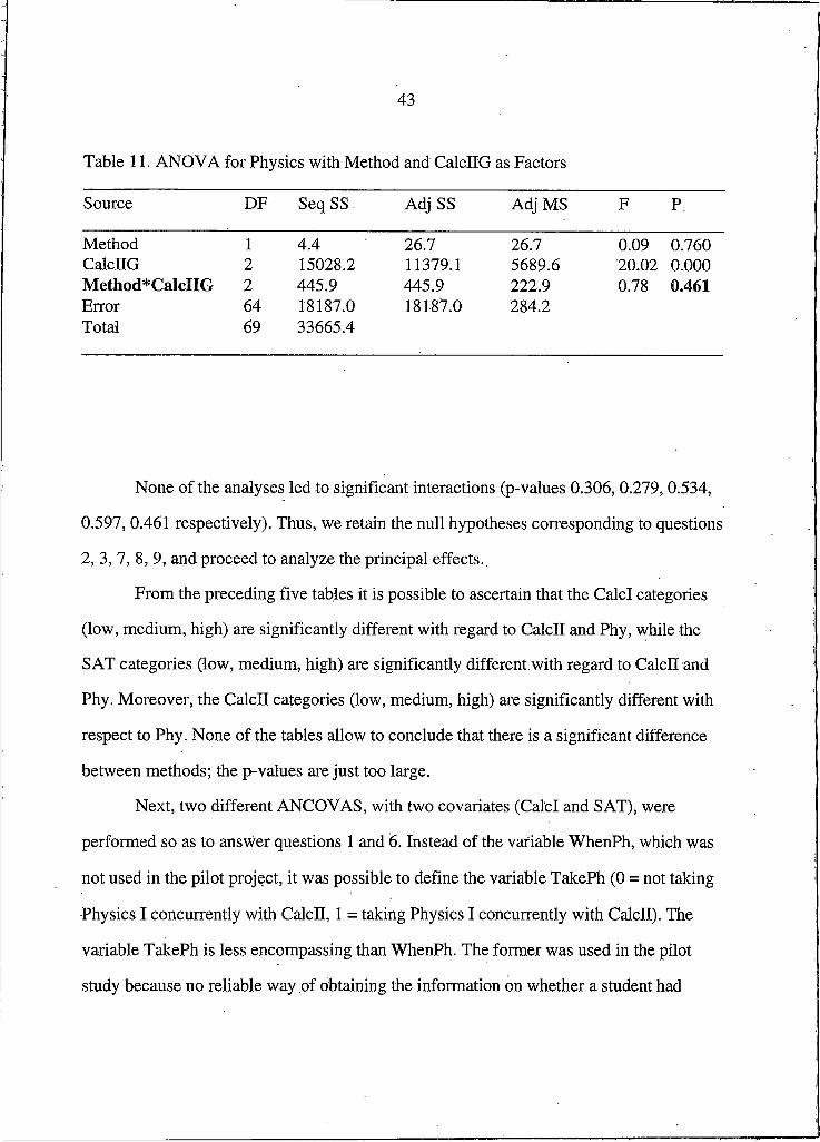
43

Table 11. ANOVA for Physics with Method and CalcIIG as Factors

Source DF Seq SS. AdjSS Adj MS F P

Method I 4.4 26.7 26.7 0.09 0.760CalcEG 2 15028.2 11379.1 5689.6 20.02 0.000Method* CaIcIIG 2 445.9 445.9 222.9 0.78 0.461Error 64 18187.0 18187.0 284.2Total 69 33665.4

None of the analyses led to significant interactions (p-values 0.306, 0.279, 0.534,

0.597, 0.461 respectively). Thus, we retain the null hypotheses corresponding to questions

2, 3, 7, 8, 9, and proceed to analyze the principal effects..

From the preceding five tables it is possible to ascertain that the CalcI categories

(low, medium, high) are significantly different with regard to CalcII and Phy, while the

SAT categories (low, medium, high) are significantly different with regard to CalcII and

Phy. Moreover, the CalcII categories (low, medium, high) are significantly different with

respect to Phy. None of the tables allow to conclude that there is a significant difference

between methods; the p-values are just too large.

Next, two different ANCOVAS, with two covariates (Calcl and SAT), were

performed so as to answer questions I and 6. Instead of the variable WhenPh, which was

not used in the pilot project, it was possible to define the variable TakePh (0 = not taking

Physics I concurrently with CalcII, I = taking Physics I concurrently with CalcII). The

variable TakePh is less encompassing than WhenPh. The former was used in the pilot

study because no reliable way of obtaining the information on whether a student had

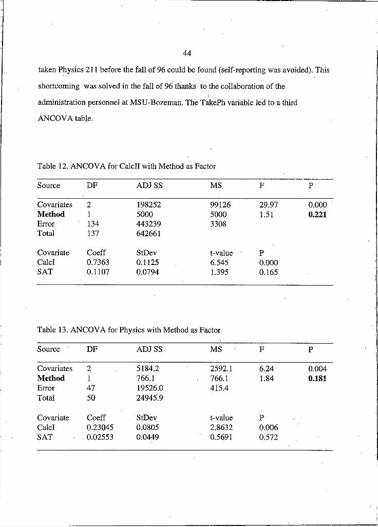
44

taken Physics 211 before the fall of 96 could be found (self-reporting was avoided). This

shortcoming was solved in the fall of 96 thanks to the collaboration of the

administration personnel at MSU-Bozeman. The TakePh variable led to a third

ANCOVA table.

Table 12. ANCOVA for CalcII with Method as Factor

Source DF ADJ SS MS F P

Covariates 2 198252 99126 29.97 0.000Method I 5000 5000 1.51 0.221Error 134 443239 3308Total 137 642661

Covariate Coeff StDev t-value PCalcI 0.7363 0.1125 6.545 0.000SAT 0.1107 0.0794 1.395 0.165

Table 13. ANCOVA for Physics with Method as Factor

Source DF ADJ SS MS ■ F P

Covariates 2 5184.2 2592.1 6.24 0.004Method I 766.1 766.1 1.84 0.181Error 47 19526.0 415.4Total 50 24945.9

Covariate Coeff StDev t-value PCalcI 0.23045 0.0805 2.8632 0.006SAT 0.02553 0.0449 0.5691 0.572

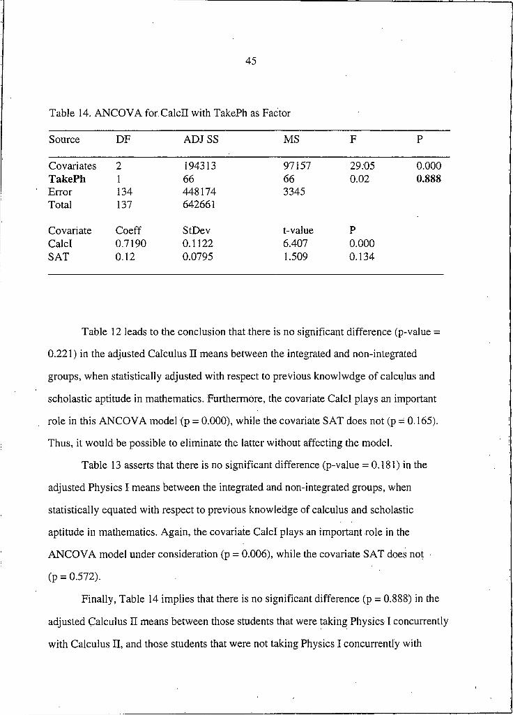
45

Table 14. ANCOVA for. CalcII with TakePh as Factor

Source DF ADJ SS MS F P

Covariates 2 194313 97157 29.05 0.000TakePh I 66 66 0.02 0.888Error 134 448174 3345Total 137 642661

Covariate Coeff StDev t-value PCalcI 0.7190 0.1122 6.407 0.000SAT 0.12 0.0795 1.509 0.134

Table 12 leads to the conclusion that there is no significant difference (p-value =

0.221) in the adjusted Calculus II means between the integrated and non-integrated

groups, when statistically adjusted with respect to previous knowlwdge of calculus and

scholastic aptitude in mathematics. Furthermore, the covariate CalcI plays an important

role in this ANCOVA model (p = 0.000), while the covariate SAT does not (p = 0.165).

Thus, it would be possible to eliminate the latter without affecting the model.

Table 13 asserts that there is no significant difference (p-value = 0.181) in the

adjusted Physics I means between the integrated and non-integrated groups, when

statistically equated with respect to previous knowledge of calculus and scholastic

aptitude in mathematics. Again, the covariate CalcI plays an important role in the

ANCOVA model under consideration (p = 0.006), while the co variate SAT does not

(p = 0.572).

Finally, Table 14 implies that there is no significant difference (p = 0.888) in the

adjusted Calculus II means between those students that were taking Physics I concurrently

with Calculus II, and those students that were not taking Physics I concurrently with

46

Calculus II, when statistically adjusted with respect to previous knowledge of calculus.

and scholastic aptitude in mathematics. The covariate CalcI exerts an important role in

this ANCOVA model too (p = 0.000), but the covariate SAT does not (p = 0.134).

The pilot study provided valuable information for the research design and the

acquisition of data procedure, as well as allowed the researcher the opportunity to write

the enrichment notes and test them in class.

Certain trends can be observed, for instance with regard to Calculus II and Physics

grades, when CalcI and SAT are categorized in three groups. Nevertheless, none of them

is significant (comparing methods) despite the fact that for low achievers the interaction

plots indicate an apparently wide difference. One explanation could be that the number of

students in the experimental group was not big enough, leading to a lack of statistical

evidence. Besides, the design was highly unbalanced, with many more students in the

control group than in the experimental group.

Physics Questionnaire

A questionnaire, based in part on the "Force Concept Inventory" test ( Hestenes,

Wells, and Swackhamer 1992) was developed. A copy is to be found in appendix B. It

was taken by 132 students enrolled in Math 182 during the spring of 96, as part of the

materials developed during the pilot project carried out in the above-mentioned period.

The purpose of the questionnaire was to find out how much physics students

learned in high school and how able they were to deal with simple physical problems

involving only high school algebra and physics. The dependent variable was achievement

in basic physics.

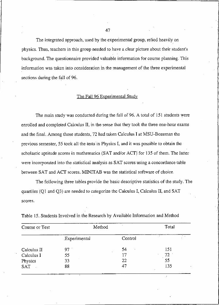
47

The integrated approach, used by the experimental group, relied heavily on

physics. Thus, teachers in this group needed to have a clear picture about their student's

background. The questionnaire provided valuable information for course planning. This

information was taken into consideration in the management of the three experimental

sections during the fall of 96.

The Fall 96 Experimental Study

The main study was conducted during the fall of 96. A total of 151 students were

enrolled and completed Calculus II, in the sense that they took the three one-hour exams

and the final. Among those students, 72 had taken Calculus I at MSU-Bozeman the

previous semester, 55 took all the tests in Physics I, and it was possible to obtain the

scholastic aptitude scores in mathematics (SAT and/or ACT) for 135 of them. The latter

were incorporated into the statistical analysis as SAT scores using a concordance table

between SAT and ACT scores. MINITAB was the statistical software of choice.

The following three tables provide the basic descriptive statistics of the study. The

quartiles (Q1 and Q3) are needed to categorize the Calculus I, Calculus II, and SAT

scores.

Table 15. Students Involved in the Research by Available Information and Method

Course or Test Method Total

.Experimental Control

Calculus II 97 54 151Calculus I 55 17 72 'Physics 33 22 55SAT - 88 47 135

48

Table 16. Descriptive Statistics of Scores

Variable N Mean Median StDev Min Max Qi Q3

SAT 135 599.70 600.00 61.51 460 740 560 640CalcII 151 333.77 ' 341.00 86.21 77. 491 282 397CalcI 72 389.24 393.00 45.93 206 470 367 415

Table 17. Categorization of Scores

Group Calculus I Calculus II SAT

Low 1-367 1-282 1-560Medium 368-415 283-397 561-640High 416-500 398-500 641-800

Table 18. Number of Students by Category and Method

Category Method Calculus I Calculus II SAT

Low I 13 15 292 5 23 9

Medium I 27 53 402 10 23 25

High I 15 29 192 2 8 13

49

Table 19. Descriptive Statistics of Scores by Method

Course or Test Method N Mean Median StDev Ql Q3

Calculus I I 55 394.93 393 40.07 369 4282 17 370.8 392 58.9 341 406

Calculus II I 97 356.99 353 71.75 320 4122 54 292.1 295 ' 94.6 236 372

SAT I 88 596.02 600 64.18 560 6402 47 606.6. 600 56.19 580 660

Physics I I 33 144.39 141 19.96 129 1602 22 132.45 132 20.83 116 148

The Calculus I and SAT medians of the students in the experimental and control

groups are remarkably similar (actually equal for the SAT), as may be inferred from the

preceding table. The corresponding Calculus I and SAT means do not differ much either.

Through an analysis of covariance it will be possible to determine whether or not the

differences among the means between the two groups are statistically significant, when

Calculus II and Physics I scores are analyzed.

The next table is related to questions 4 and 5 of this study. It provides information

about the number of students in the experimetal and control groups, according to their

status in Physics I (not yet taken Physics I, concurrently taking Physics I with Calculus II,

taken Physics I before Calculus II). It is to be noted that the sum of all the students in this

list, taking into account their status in Physics I and the two groups, has to be the total

number of students that completed Calculus II; namely 151.

50

Table 20. Number of Students by Method and When They Took Physics

Status Method Number

Not Yet I 312 20

Concurrently I 352 23

Before I 312 11

Pearson correlations can be found in Table 21. It can be seen that there is a rather

strong linear association (0.585) between Calculus I and Calculus II, and between

Calculus II and Physics I (0.583), while there is a less strong linear association between

Calculus I and Physics I (0.459). The linear association between SAT and Calculus IL

(0.293), and between SAT and Physics I (0.264), is low.

Table 21. Pearson Correlations Among The Four main variables

' SAT CalcII CalcI

CalcII 0.293CalcI 0.146 0.585Phy 0.264 0.583 0.459

Further descriptive statistics, related to students' scores in Calculus I and SAT by

instructor, are to be found in Appendix F.

51

The next two figures are highly suggestive, since they show graphically why the

linear association between Calculus I and Calculus II is much higher than the linear

association between SAT and Calculus II.

Figure 6. Calculus II Scores and Calculus I Scores

soo —

400 -

O soo -

200 -

100 -

Figure 7. Calculus II Scores and SAT Scores

soo -

400 -

o 300 —

200 -

100 -

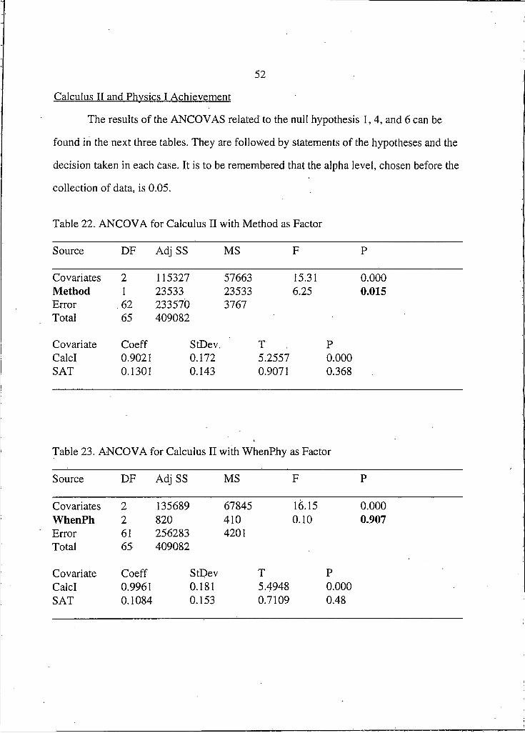
52

The results of the ANCOVAS related to the null hypothesis 1,4, and 6 can be

found in the next three tables. They are followed by statements of the hypotheses and the

decision taken in each case. It is to be remembered that the alpha level, chosen before the

collection of data, is 0.05.

Calculus II and Phvsics I Achievement

Table 22. ANCOVA for Calculus II with Method as Factor

Source DF Adj SS MS F P

Covariates 2 115327 57663 15.31 0.000Method I 23533 23533 6.25 0.015Error 62 233570 3767Total 65 409082

Covariate Coeff StDev. T PCalcI 0.9021 0.172 5.2557 0.000SAT 0.1301 0.143 0.9071 0.368

Table 23. ANCOVA for Calculus II with WhenPhy as Factor

Source DF Adj SS MS F P

Covariates 2 135689 67845 16.15 0.000WhenPh 2 820 410 0.10 0.907Error 61 256283 4201Total 65 409082

Covariate Coeff StDev T PCalcI 0.9961 0.181 5.4948 0.000SAT 0.1084 0.153 0.7109 0.48

53

Table 24. ANCOVA for Physics I with Method as Factor

Source DF AdjSS MS F P

Covariates 2 3435 1717.5 7.09 0.004Method I 507.1 507.1 2.09 0.161Error 24 5815.7 242.3Total 27 9729.2

Covariate Coeff StDev T PSAT 0.1104 0.0533 2.072 0.049CalcI 0.2343 0.0850 2.756 0.011

Hypothesis I: There is no difference between the adjusted Calculus II

achievement means, of the integrated and the non-integrated groups, when statistically

equated with respect to previous knowledege of calculus and scholastic aptitude in

mathematics.

Decision: Reject the null hypothesis. There was a statistically significant

difference between the adjusted Calculus II achievement means of both groups (p =

0. 015). The adjusted means were 343.82 (N = 50) for the experimental, group, and 298.19

(N= 16) for the control group.

Hypothesis 4: When statistically equated with respect to previous knowledge of

calculus and scholastic aptitude in mathematics, there is no difference between the

adjusted Calculus II achievement means of those students that have not yet taken Physics

1, those students that are concurrently taking Physics I and Calculus II, and those students

that have taken Physics I before Calculus II.

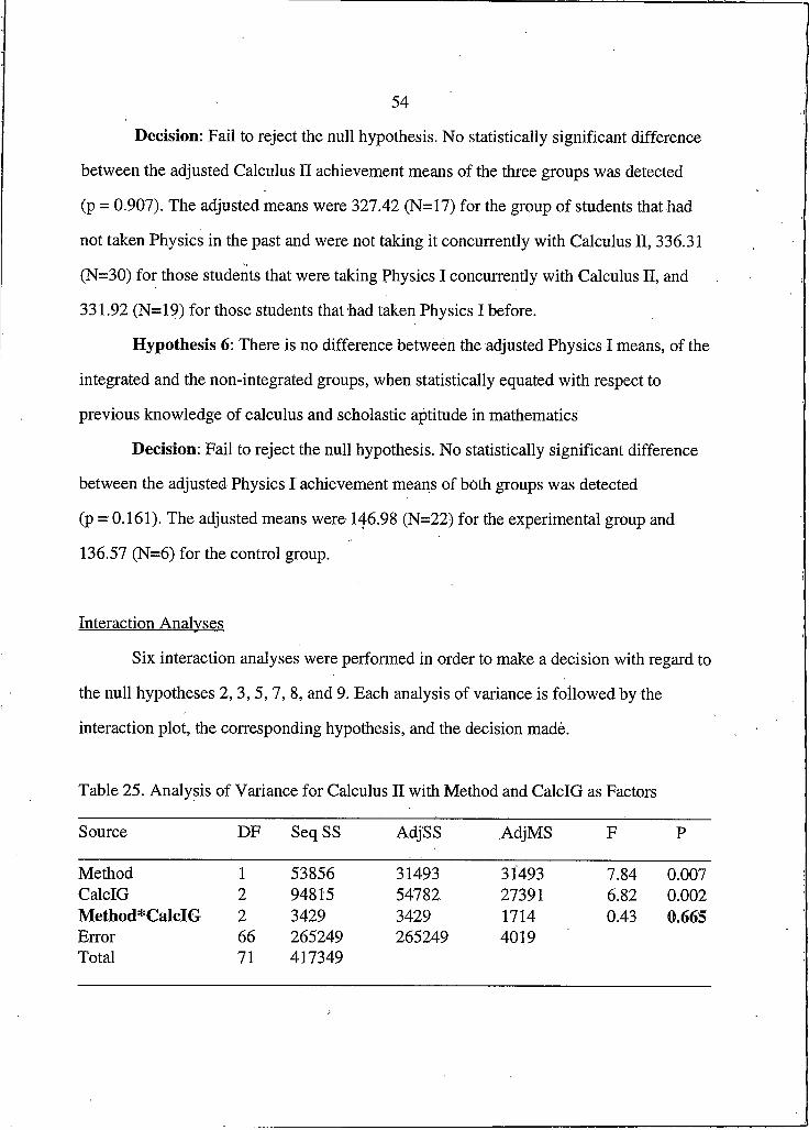
54

Decision: Fail to reject the null hypothesis. No statistically significant difference

between the adjusted Calculus II achievement means of the three groups was detected

(p = 0.907). The adjusted means were 327.42 (N= 17) for the group of students that had

not taken Physics in the past and were not taking it concurrently with Calculus II, 336.31

(N=30) for those students that were taking Physics I concurrently with Calculus II, and

331.92 (N= 19) for those students that had taken Physics I before.

Hypothesis 6: There is no difference between the adjusted Physics I means, of the

integrated and the non-integrated groups, when statistically equated with respect to

previous knowledge of calculus and scholastic aptitude in mathematics

Decision: Fail to reject the null hypothesis. No statistically significant difference

between the adjusted Physics I achievement means of both groups was detected

(p = 0.161). The adjusted means were 146.98 (N=22) for the experimental group and

136.57 (N=6) for the control group.

Interaction Analyses

Six interaction analyses were performed in order to make a decision with regard to

the null hypotheses 2 ,3 ,5 , 7, 8, and 9. Each analysis of variance is followed by the

interaction plot, the corresponding hypothesis, and the decision made.

Table 25. Analysis of Variance for Calculus II with Method and CalcIG as Factors

Source DF Seq SS AdjSS AdjMS F P

Method I 53856 31493 31493 7.84 0.007CalcIG 2 94815 54782 27391 6.82 0.002Method*CalcIG 2 3429 3429 1714 0.43 0.665Error 66 265249 265249 4019Total 71 417349

55

Figure 8. Interaction Plot for Calculus II Scores by Method and Calculus I Groups

Mefriod

400 —

350 -

300 —

250 —

CALCIG

Hypothesis 2: Method of instruction (integrated or non-integrated) and previous

knowledge of calculus do not interact on Calculus II achievement.

Decision: Fail to reject the null hypothesis. No statistically significant interaction

was detected (p = 0.655).

Table 26. Analysis of Variance for Calculus II with Method and SATG as Factors

Source DF Seq SS Adj SS AdjMS F P

Method I 136640 174382 174382 29.19 0.000SATG 2 83466 77176 38588 6.46 0.002Method*SAJG 2 19747 19747 9873 1.65 0.196Error 129 770531 770531 5973Total 134 1010383

56

Figure 9. Interaction Plot for Calculus II Scores by Method and SAT Groups

Method

400 —

350 -

300 -

250 -

SATG

Hypothesis 3: Method of instruction (integrated or non-integrated) and scholastic

aptitude in mathematics do not interact on Calculus II achievement.

Decision: Fail to reject the null hypothesis. No statistically significant interaction

was found ( p = 0.196).

Table 27. Analysis of Variance for Calculus II with Method and WhenPh as Factor

Source DF Seq SS AdjSS Adj MS F P

Method I 146180 141863 141863 22.58 0.000WhenPh 2 22651 28648 14324 2.28 0.106Method*WhenPh 2 35019 35019 17510 2.79 0.065Error 145 910955 910955 6282Total 150 1114804

57

Figure 10. Interaction Plot for Calculus II Scores by Method and WhenPh

Meffiod

360 -

<D 310 —

260 —

WhenPh

Hypothesis 5: Method of instruction (integrated or non-integrated) and when

students take Physics I (not yet, concurrently with Calculus n, or before Calculus II) do

not interact on Calculus II achievement.

Decision: Fail to reject the null hypothesis. No statistically significant interaction

was detected (p = 0.065).

Table 28. Analysis of Variance for Physics I with Method and CalcIG as Factors

Source DF Seq SS AdjSS AdjMS F P

Method I 504.3 238.8 238.8 1.26 0.272CalcIG 2 4728.2 2531.7 1265 8 6.70 0.005Method*CalcIG 2 12.7 12.7 6.3 0.03 0.967Error 24 4535.8 4535.8 189.0Total 29 9781.0

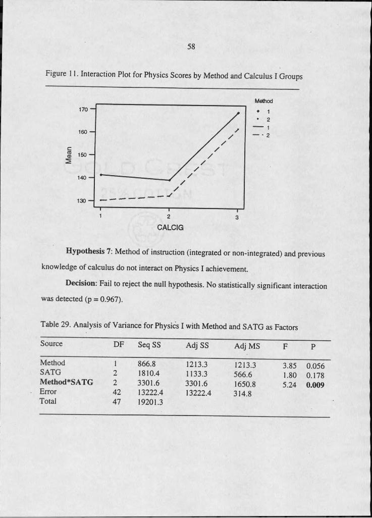
58

Figure 11. Interaction Plot for Physics Scores by Method and Calculus I Groups

Method170 ~

160 —

ISO —

140 —

130 —

CALCIG

Hypothesis 7: Method of instruction (integrated or non-integrated) and previous

knowledge of calculus do not interact on Physics I achievement.

Decision: Fail to reject the null hypothesis. No statistically significant interaction

was detected (p = 0.967).

Table 29. Analysis of Variance for Physics I with Method and SATG as Factors

Source

MethodSATGMethod*SATGErrorTotal

DF Seq SS Adj SS Adj MS F P

I 866.8 1213.3 1213.3 3.85 0.0562 1810.4 1133.3 566.6 1.80 0.17824247

3301.613222.419201.3

3301.613222.4

1650.8314.8

5.24 0.009

59

Figure 12. Interaction Plot for Physics Scores by Method and SAT groups

Method

170 —

160 —

150 —

140 —

130 —

SATG

Table 30. Comparison Test for Physics I Scores Considering Only SATG 3 Students

Method N Mean T P

I 5 171.2 3.935 0.0002 8 131.4

The program MSUSTAT was used (COMPARE subroutine, with DF = 42 and MSE = 314.8; both values come from table 29)

Hypothesis 8: Method of instruction (integrated or non-integrated) and scholastic

aptitude in mathematics do not interact on Physics I achievement.

Decision: Reject the null hypothesis. There is a statistically significant interaction

(p = 0.009). Furthermore, there is a statistically significant difference between the

experimental and control groups when the physics scores of the high scholastic aptitude

mathematics students (SATG 3) are analyzed (p < 0.001).

60

Table 3 1. Analysis of Variance for Physics I Scores with Method and CalcIIG as Factors

Source DF Seq SS Adj SS Adj MS F P

Method I 1881.6 735.9 735.9 2.55 0.116CalcIIG 2 7498.9 6157.2 3078.6 10.69 0.000Method*CalcIIG 2 247.3 247.3 123.6 0.43 0.653Error 49 14115.2 14115.2 288.1Total 54 23743.0

Figure 13. Interaction Plot for Physics Scores by Method and CalcII Groups

Method165 —

155 -

m 145 —

135 -

125 —

CaIcIIG

Hypothesis 9: Method of Instruction (integrated or non-integrated) and

achievement in Calculus II do not interact on Physics I achievement.

Decision: Fail to reject the null hypothesis. No statistically significant interaction

was detected (p = 0.653).

61

Gender

The number of female students who completed Calculus II was 25, out of a total

of 151 students who completed the course. The next four tables, followed by interaction

plots when pertinent, will help to determine whether or not to reject the last four null

hypotheses of this study (namely, hypotheses 10 - 13).

Table 32. Analysis of Covariance for Calculus II with Gender as Factor

Source DF Adj SS MS F P

Covariates 2 148289 74144 18.73 0.000Gender I -. 11624 116.24 2.94 0.092Error 62 245480 3959Total 65 409082

Covariate Coeff StDev T PSAT 0.1224 0.147 0.8330 0.408CalcI 0.9992 0.170 5.8732 0.000

Hypothesis 10: There is no difference in the adjusted Calculus II achievement

means between female, and male students, when statistically equated with respect to

previous knowledge of calculus and scholastic aptitude in mathematics.

Decision: Fail to reject the null hypothesis. No statistically significant interaction

was detected (p = 0.092), The adjusted means were 362.48 (N= 11) for female students,

and 326.81 (N = 55) for male students.

62

Table 33. Analysis of Covariance for Physics I with Gender as Factor

Source DF AdjSS MS. F P

Covariates 2 2747.6 1373.8. 5.88 0.008Gender I 715.7 715.7 3.06 0.093Error 24 5607.1 233.6Total 27 9729.2

Covariate Coeff StDev T PSAT 0.08624 0.0531 1.623 0.118CalcI 0.23006 0.0836 2.753 0.011

Hypothesis 11: There is no difference in the adjusted Physics I achievement

means between female and male students, when statistically equated with respect to

previous knowledge of calculus and scholastic aptitude in mathematics.

Decision: Fail to reject the null hypothesis. No statistically significant difference

was detected between the adjusted Physics I achievement means of female and male

students (p = 0.093). The adjusted means were 134.83 (N = 6) for female students, and

147.46 (N = 22) for male students.

Table 34. Analysis of Variance for Calculus II with Method and Gender as Factors

Source DF Seq SS AdjSS AdjMS F P

Method I 146180 110085 110085 16.89 0.000Gender I 5789 2830 2830 0.43 0.511Method*Gender I 4976 4976 4976 0.76 0.384Error 147 957860 957860 6516Total 150 1114804

63

Figure 14. Interaction Plot for Calculus II Scores with Method and Gender as Factors

380 -

320 -

300 -

Gender

Method

• I• 2

--- I-----2

0 = female

1 = male

Hypothesis 12: Method of instruction (integrated or non-integrated) and gender

do not interact on Calculus II achievement.

Decision: Fail to reject the null hypothesis. No statistically significant interaction

was detected (p = 0.384).

Table 35. Analysis o f Variance for Physics I with Method and Gender as Factors

Source DF Seq SS AdjSS AdjMS F P

Method I 1881.6 702.0 702.0 1.67 0.202Gender I 437.7 284.7 284.7 0.68 0.414Method*Gender I 8.3 8.3 8.3 0.02 0.889Error 51 21415.3 2145.3 419.9Total 54 23743.0

64

Figure 15. Interaction Plot for Physics I Scores with Method and Gender as Factors

Method

• I• 2

--- I— — — *2

0 = female

1 = male

0 IGender

Hypothesis 13: Method of instruction (integrated or non-integrated) and gender

do not interact on Physics I achievement

Decision: Fail to reject the null hypothesis. No statistically significant interaction

was detected (p = 0.889).

5 135

Additional Analyses

Calculus II Scores by Instructor

Although it is not related to any hypotheses of this study. Calculus II scores by

instructor were analyzed. The following boxplot (where horizontal segments denote

medians), and tables 36 and 37, are a first attempt in this direction. It is to be noted that

instructors 1,2,3 were in the experimental group, while the two other instructors were in

the control group.

65

Figure 16. Calculus II Scores by Instructor

soo -

o 300 -

200 -

100 -

Table 36. Calculus II Mean Scores by Instructor

Instructor Number of Students Mean StDev

I 31 353.06 75.362 30 361.80 82.473 36 356.36 59.874 19 355.58 72.005 35 257.60 87.92

Table 37. Analysis of Variance for Calculus II by Instructor

Source DF SS MS F P

Instructor 4 265586 66397 11.42 0.000Error 146 849218 5817Total 150 1114804

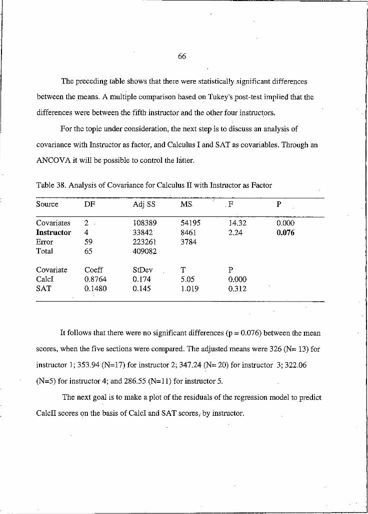
66

The preceding table shows that there were statistically significant differences

between the means. A multiple comparison based on Tukey's post-test implied that the

differences were between the fifth instructor and the other four instructors.

For the topic under consideration, the next step is to discuss an analysis of

covariance with Instructor as factor, and Calculus I and SAT as covariables. Through an

ANCOVA it will be possible to control the latter.

Table 38. Analysis of Covariance for Calculus II with Instructor as Factor

Source DF Adj SS MS F P

Covariates 2 ■ 108389 54195 14.32 0.000Instructor 4 33842 8461 2.24 0.076Error 59 223261 3784Total 65 409082

Covariate Coeff StDev T PCalcI 0.8764 0.174 5.05 0.000SAT 0.1480 0.145 1.019 0.312

It follows that there were no significant differences (p = 0.076) between the mean

scores, when the five sections were compared. The adjusted means were 326 (N= 13) for

instructor I; 353.94 (N= 17) for instructor 2; 347.24 (N= 20) for instructor 3; 322.06

(N=5) for instructor 4; and 286.55 (N=Il) for instructor 5.

The next goal is to make a plot of the residuals of the regression model to predict

CalcII scores on the basis of CalcI and SAT scores, by instructor.

67

Table 39. Regression Analysis on Calculus II with CalcI and SAT as Predictors

Predictor Coef StDev T P

Constant -129.8 102.5 -1.27 0.210CalcI 1.0137 0.1725 5.88 0.000SAT 0.1146 0.1491 0.77 0.445S = 63.88 R-Sq = 37.2% R-Sq (Adj) = 35.2%

Analysis of VarianceSource DF SS MS F PRegression 2 151979 75990 18.62 0.000Error 63 257103 4081Total 65 409082

This regression model explains about 37% of the variability of Calculus II scores.

The residuals of the regression model, by instructor, will explain how each instructor — or

some unknown factor or factors — brought the scores of Calculus II students above or

below the predicted scores on the basis of CalcI and SAT scores. The next figure shows

this phenomenon.

Figure 17. Residuals of Regression Model to Predict CalcII Scores

100 -

-100 -

-200 -

68

From the preceding figure it can be concluded that most students in the first three

sections (taught by the experimental group instructors ) did better than expected on the

basis of their CalcI and SAT scores, especially students in section 2. On the other hand,

most students in sections 4 and 5 (especially the latter) did worse than expected on the

basis of their CalcI and SAT scores.

It is to be noted that the design of this research — with several instructors in both

groups and the use of a common syllabus, a common textbook, and common exams —

lessens the "teacher effect" but cannot eliminate it completely.

A Homogenizing Effect of the Integrated Method

From figure 9 it can be seen that the integrated method "homogenizes" the

Calculus II scores of groups I and 2 according to SAT, a trend that is not observed with

regard to the non-integrated method. This homogenizing effect deserves closer attention.

Table 40. Calculus II Scores by Method and SAT Group

Method I Method 2

SATG N Mean StDev SATG N Mean StDevI 29 345.9 63 I 9 248.2 82.82 40 345.2 73.4 2 25 298.2 95.93 19 417.1 54.2 3 13 • 318.2 100.2

There is practically no difference between the means of SAT groups I and 2 in the

integrated group, while there is a marked difference between the means of SAT groups I

and 2 among students that followed the non-integrated approach. Moreover, the

69

Calculus II scores of students in the integrated group are considerably less dispersed than

the scores of their peers in the non-integrated group. A similar homogenizing effect of the

integrated method can be seen in figure 10.

Teacher Interviews

The two instructors who accompanied the researcher in the experimental group

were interviewed by the latter at the end of the semester. Ten basic questions about

calculus teaching were asked.

Question I: Do you think that applications, mainly to physics, enhance calculus

learning?

Teacher A: My answer is yes. Physicists should not try to do our job, nor should we try to do their job. But there should be enough overlap so that students can see the interrelationship between mathematics and physics, or mathematics and chemistry. Applications are good, they are fun too! It is neat to see where a new concept of calculus is used, you get to understand better the calculus and its applications.

The calculus course I took in my freshman year didn't have many applications. There were lots of practice problems in integration by parts and substitution, hundreds of them. It was only when I got to physics that I understood its relationship to what we had learned in calculus. I do like to have very many applications in calculus, it gives a better understanding of what the tool is all about.

Teacher B: What do we think we should be teaching at the level of a second semester calculus course? I think that students should walk out of there feeling that they can apply what they know. It makes them feel better. If nothing else, it helps their motivation. On the other hand, our students were not explicitly aware that they were being taught more physics examples than the sections in the control group. I am not sure what their reaction would be if it is known to them. They thought that there was the right mix of application questions. I believe that it is important for them to realize that physics is the subject that has the most readily available examples for us.

70

Question 2: Last semester, the experimental group spent more time than usual

dealing with applications. What was student's reaction, in your section about it?

Teacher A: Students' reaction to applications? In the experimental group we covered more applications than usual. This was only their second semester in calculus, so they didn't have much to compare to; To them maybe that was how a course should be taught. I received no complaints. There was an isolated case of a student wining, in the sense that he had not had any physics yet. But he had to understand that the applications we discussed in class did not presuppose any knowledge of physics or chemistry. The course was arranged in such a way that students in physics would not have an advantage.

The enrichment notes helped the best students in the class. The reality is that there are many students that don't read the book, so it is unlikely that they will read additional material. On the quizzes, sometimes I put questions related to the enrichment notes. Thus, they had to read them . However, there was a constraint. We had to prepare the students for the common exams, covering a considerable amount of material from the textbook . There wasn't much time left to discuss in detail very interesting problems like the catenary or falling bodies when the resistance of air is proportional to the square of the velocity. If there were not to be common exams, (i.e., if I could independently prepare my syllabus and teach a calculus course) I would pay more attention to the enrichment notes, absolutely. I will save those handouts for the future.

Teacher B: I didn't receive any complaints, neither personal nor written. There were some students that maintained that this was a math course and that there should be more math and less requirement on them to understand the physics. They thought that we were trying to have them understand some applied problems that should be taught in the physics class. Anyhow, some course,

' somewhere in the students' program , should put together all the ideas. Some capstone course at the end of their career. At the 182 level though, the way we teach math in the United States, we don't teach out of Apostol's books and begin proving rigorously all the results of calculus. We are trying to give them a geometric feeling and a sort of usefulness feeling for the calculus that they learn. So, any extreme is probably the wrong direction. Has reform calculus gone the wrong direction because there is less time for mathematics? I am not sure.

I think that you need examples for the students, which shows them where the mathematics is applied. Real world examples. Whether we have to spend our time trying to teach them calculus through those examples or teach them the mathematics of the calculus and then present some real world examples, I am not sure. But the examples should be there one way or the other.

Let me make some comments about the enrichment notes. Maybe the noblest endeavor that we have is to teach them to model the world with math, so I

71

think it is important that we at least present to them the information. If they would like to know where these equations came from, here is the explanation! In most of the enrichment notes that we gave to them, or presented to them, the idea was that the book picked up at step 8, and if you actually are trying to model something you need to start back a little sooner. We were not requiring them to Ieam the techniques of modeling until the end of the course when we presented differential equations. But that is maybe the whole usefulness of teaching the math to start with. So, not only shouldn't it be part of the enrichment notes, we should teach it. But then again, we do not have time for all that.

Maybe that is what reform calculus has done more than anything else, is have the courage to say we only have time to teach so many things, and these are the topics we think should be there. People may disagree on the topics, but the approach in the past has been as follows: give me a calculus book that has every single topic in i t , so that none is missed, so that my book will be sold to everyone. I think that reform calculus had the courage to knock some of those out. We might not agree about what topics should have been eliminated from first-year calculus, but then we can present our students with extra-notes . Maybe that is the right approach rather than to put all in a book and ask the student to pull out of there what you think is important. I prefer to give them a bare bones book like the ones in reform calculus.

I liked the balance that we had. Our book concentrated less on modeling in the beginning, although it tried to at the end. If I were to teach a calculus course all by myself, I would choose a book like the Harvard Calculus book, and then I would insert a few of the proofs that are easier to present, simply for the sake of presenting the idea of proof, not because any particular proof is so indispensable to calculus, and then I would try to fit in the applications.

I found it very difficult trying to integrate. I think this is my lack of experience. I had a book that was given to me to teach out of, I had your advice, and the enrichment notes, and I just picked through all these and decided what I was going to give the student. All by myself I don't know if I am qualified to decide what I am going to teach in a calculus course. I will probably have to turn to some standard, some book, someone that is telling me what should be taught, and then , maybe, I can make decisions in little chunks at a time; that I don't like this section, that this other section needs more applications. I feel woefully inadequate to do it...

Question 3: What should be the role of proofs in second-semester calculus?

Teacher A: There should be more proofs than the book provides. I know that you put in some proofs, I did as well. I like having proofs in a calculus textbook; if not in the main body of the book, at least in the appendices so that you could always refer to them . Especially the best students could look at the proofs. Calculus students should get a glimpse about what mathematics is.

72

I am not advocating e - 5 proofs. When I was an undergraduate, my calculus book had these type of proofs. They seemed a mystery to me when we ran into them for the first time. My initial reaction is no to the introduction of £- 8 proofs in first year calculus. But certain proofs can be understood by students, if not completely at least some steps of it. Memorizing and regurgitating proofs in an exam is out of the question. Rather test them in such a way that to solve a problem, some idea or ideas from a proof have to be used. If you don't make them responsible for the proofs, they probably won't even read them!

Teacher B: At some point, by the time a student has finished second semester calculus, he/she should understand the basis of mathematics. That we begin with some things that we hope to be true, and we prove results from there. I am not acquainted with all the reform calculus books, but I do not think that the Harvard Calculus book does a particularly good job presenting that idea. It does not. You have to stop and teach a student about proof, regardless what you are trying to prove. It is hard when there are not many examples in the book about proofs that the students should try to read and digest and then ask questions. Maybe there should be more proofs. But again, I think reform calculus has the right idea, something is got to go, we got to sacrifice something in order to teach the rest well.

I would like to see a treatment of the idea of proof, not necessarily many proofs. It is fine with me if we are going to tell a student that you have to believe me, if you are interested in a proof just stop by my office. Even though I would like to see more of the idea of proof, I am not adamant about which proofs should be there. It is not the omission of a particular proof I am worried about, it is the omission of the idea of proof.

Question 4: How was your experience with group work during the course?

Teacher A: We didn't do group work in my section last semester. The biggest positive result that can come out of group work is that it gets students working together outside of class. Realistically speaking, students can not finish group work in a 50 minute class period. I am skeptical about taking class-time in second semester calculus for group work. In Calculus I or precalculus I would do group work; they are starting their college studies and need support from their peers.

The situation is different in Calculus II. I believe that it is more beneficial to them to see collective work. I like to have one day per week to relax, I don't lecture on Wednesdays but stand in front of the class answering questions. I do pose questions too, and everyone has the opportunity to think about them before the smart guy in the back gets the answer!

Teacher B: In Math 1821 didn't do much group work at all. When I taught Math 1811 did a great deal of it. You have so many days a week to teach, are you going

73

to sacrifice those days to do group work? In a beginning calculus course you should, but only from a social aspect. Entering students could be immature people that will seat in class and not know the name of the person next to them; they are a little scared, they just need an excuse to talk to each other.

I think entering students need to realize the power of working together, certainly industry wants to have them work together so that they are better prepared to work as a team once they graduate from college. But I really think the group work we do in class is simply a replacement from what they should be doing outside of class. And maybe the reality is that students don't work together outside of class. We are just demanding that they do in the classroom what we wish they would do outside of the classroom. If all students were to work together outside of the classroom, there would not be a need to have them in groups in the classroom. That is a little too strong, there are some problems that are better handled with the collaboration of more than one head.

We, the instructors, are the experts, we are supposed to give the students our knowledge. However, it is true what some people say: I can't just give you what I know . You have to do it yourself, discover it on your own. But that is really the way our university system is set up . A student comes in, listens to an expert, then the expert summarizes, highlights certain topics and points out the pitfalls of the subject.

Some teachers are better on a one-to-one basis, and group work allows them to circulate around the room and see what students are doing, while some instructors are very good, excellent, lecturers. So, it should be up to each instructor. In other words, if a teacher can convey his/her knowledge and get to the student through the setting of group work, with well-crafted problems, then lecturing may not be as important.

Question 5: What is your opinion about the textbook used in Calculus II? Do

students read it?

Teacher A: There are some things that I do not like about the book and I will explain why. I think there are some fantastic problems in there. Also some very good examples, but I think that in an attempt to make it readable, they have thrown away a good deal of mathematics. I have a theory: The better a book is as a learning tool, the worst it is as a reference and vice versa. If it has too many words, it is hard to make it a good reference; if it is to be a good reference it has to be concise. When students ask me whether they should keep the textbook after the semester has come to an end, I tell them not to do so. Sell it immediately and go buy a real calculus book. By real calculus book I mean one that could serve you as a reference book. This book is a horrible reference. You can't go back in there and look for theorems.

74

In the Harvard Calculus book often the hypotheses are missing. I would like to see more theorems listed. The authors went to the other extreme when compared to books of the type theorem, proposition, lemma, corollary. In the Harvard Calculus book you find a lot of words without any good theorems you can refer to. In the past one was looking for a book that would be good for learning and reference. Harvard Calculus lacks in the latter sense. There is not a balance between readability and mathematical consistency.

I really do like the problems in the Harvard Calculus book. There you can find some hard problems. If you , as an instructor, don't think about them before going to class, you might get stuck. However, the textbook treats the whole idea of series very lightly, many important things are missing. New editions could improve some of the shortcomings.

Before calculus reform, everyone had his/her pet interests, so books started to be bigger and bigger , up to one thousand pages long. Some teachers thought that you had to cover every single topic, an evident wrong decision.

If you are a mathematics or physics major that is planning to go into graduate school, where do you start to see e - 8 proofs? Maybe you should start to see a little of them in first-year calculus. Understanding these techniques requires a long maturation process, so the sooner the better. The hardest thing in calculus is the idea of limit. In the Harvard Calculus book this idea is missed, it is gone. Then students get into real trouble when they have to deal with improper integrals, for example. You can't find in this book any list of properties of limits.In every calculus course one has to spend some time dealing with limits!

Teacher B: The Harvard Calculus text is a great book. Again, I think they had the courage to leave out some things that no one would touch before. They had the courage to leave out the e - 8 presentation of limits, something with which I agree. I think the authors did a good job, a book that could be read by students. Although some students I have talked to seemed to complain about the book and how hard it is to read.

The Harvard Calculus book is not the type of book where you have example after example and then all the problems follow the examples. The authors are trying to strive for a higher level of understanding on the part of the students, not just to apply a pattern. I really like the book. There has been support and non-support in our department by different instructors, but I think you can take the book and effectively teach with it.

They've done a great job putting a book together. Maybe the authors could seat down and agree on the philosophy that we should present the idea of proof. A preliminary section at the beginning could be a possibility. Besides, I don't think that leaving out partial fractions was a good idea; there is very little of it in the book. Trigonometric substitutions were left out, that is fine. It is a fact that the algebraic skills for those that go through Harvard Calculus are less than those that go through a traditional course.

75

I would use a reform calculus book because I could not come up with all the great problems one finds in Harvard Calculus. For the typical manipulation problems, that are also important, I could come up with problems of my own. For instance, problems that involve partial fractions. But it is more difficult to come up with the type of problems that Harvard Calculus has in abundance.

I am not really sure which one is more readable from a student's standpoint, a traditional or a reform calculus book. But I would hate for a student to get out of calculus and not have the ideas that the Harvard Calculus elaborates on. So, I think I prefer it as my resource and as a textbook for the students.

Question 6: What policies should be adopted with regard to homework and

quizzes?

Teacher A: I assign lots of problems, but do not collect them. The quizzes are based on them. Feedback from the students shows that they have a favorable opinion about this arrangement. I have had a few students that would have liked to have the homework collected and graded. However, many students are happy that I don't collect homework every day, because some days they are very busy.Let us not forget that engineering students have lots of work to do in several courses. In first-semester calculus I did grade homework, for the same reason that I had them work sometimes in groups. They were not supposed to be responsible enough at that stage of their college experience, they were just starting out.

Teacher B : We are all busy and have obligations and if I am not demanding some of their time, someone else is demanding a lot of their time. Homework is absolutely the most important aspect of the course, and quizzes function for me as a replacement for grading homework on a daily basis. It is also a good preparation for them . You can fool yourself into thinking that you have mastered a topic when you have a book by your side and you can refer to it. Quizzes are generally a good idea but if I had to choose I would pick up homework daily and mark it. The reality is that I just do not always have time to do that. I did assign homework daily, which was due the next day but I didn't collect i t . However, in each semester that I've taught, there always comes a time in the semester when they have to turn in homework for a week or two just to get them back on track.

If I am not grading the homework, on the quizzes I put problems from the assigned list. So, if you have done your homework, there is your reward. Again, somehow they should be motivated to do this on their own but you have a lot of responsibilities. So, if I can make it a reward for you on the quiz, so much the better. I am not trying to use it so much as another method of assigning you a grade, I am trying to use it as a teaching tool, I like to put things on the quizzes that will reward you for doing homework. It is just a motivational tool, and I also like to use it to ask the students questions that they might not have thought about.

76

Thus, the quizzes were mostly off the homework but maybe 20% were problems that required an extra step, to put some ideas together.

Question 7: Calculus II meets five hours per-week despite the fact that it is a four

credit course. Do you consider that this is a good policy?

Teacher A: No student has complained. In fact, occasionally I ran an extra help- session. As I mentioned before, I put aside one day per-week for an informal meeting with the students, a sort of question and answer period that proceeded quite informally. Thus, I lectured three days per week and at the end of the week I always gave them a fifty minute long quiz so as to prepare them for the exams. Taking into consideration that the amount of material to be covered in Calculus II is quite impressive, an extra hour is a positive decision taken by the department of mathematical sciences at MSU-Bozeman.

Teacher B: From the students standpoint, they are only getting four credits and have to come to class five days per week. Part of the reasoning behind why we are having students attend more days each week is the idea of a lab. For example, in a physics lab you would go for three hours and it would typically contribute one extra credit to your physics class. So, it is not always hour for hour, the credit hours are not necessarily exactly the hours that you spend in class. On the other hand, students are getting to pay for four credits and they are getting five credits of instruction. From their point of view it is a sort of trade-off, they are not getting as many credits, but they do not have to pay for them.

How many days a week you should teach calculus? I can do it in less than five. I think I could actually do it if I were not to give them quizzes. One day was completely sacrificed to the quiz, no instruction was given that day; maybe a couple of questions briefly at the beginning of the hour. If I were to grade homework every night I would not need that fifth day. It is just important to give them some feedback.

None of my students complained about the extra hour, but I am sure they talked about it. Some students are quick to complain about an "injustice". However, they didn't have to pay for the five credits, they got a deal!

• Question 8: Should Calculus I be a pre-requisite for first-semester physics?

Teacher A: I don't know how they teach physics here. Where I went to school it was a pre-requisite. Students could not take it even concurrently, unless there were special circumstances. I have the impression that the physics course there, was significantly more challenging than the one they teach here. In my college,

77

even if you had one year of high school physics and took a non-calculus based physics course the first semester, the equivalent of Physics I was tough. So, it all depends on what level first-semester physics is taught.

Teacher B: We would have to talk to the physics department. They seem to have two sequences of physics courses. One is non-calculus based, the other is calculus-based. The reality is that they cannot demand much calculus knowledge from their students because some of them are not taking calculus and those that are taking calculus have not had much integration theory until well into second semester calculus.

Calculus and physics, one helps the other. If you had physics before, it helps your calculus, and vice versa. I would really have to talk to the physics instructors and see how handicapped they feel when presenting ideas that are simple applications of the derivative or the integral. I am sure that they would like their students to have more calculus tools at their side. I think that taking physics and calculus concurrently is fine.

Question 9 : At MSU-Bozeman three different types of calculus courses have

been under way; namely, reform calculus (Math 181-Math 182), traditional calculus

(Math 175-Math 176), and honors calculus (using Spivak's book). Should it continue to

be so? Can these three approaches coexist peacefully?

Teacher A: There should be separate calculus courses for engineering majors and, say, business majors. If there were just one course, it would be slowed -down or watered-down. For engineers this is a tool they will be using all the time, so they need to know calculus really well and move at a good pace or get out from engineering school. If you cannot do well in a Math 181-2 setting (the type of courses we've been teaching), you should not be in engineering.

There is no agreement among the business departments about the need to have their students learn calculus. I believe they should take it, although at a different level than the engineering or the natural sciences students. Among the engineering people there are no doubts about the need of having their students take a strong calculus course. After all, we not only prepare their students in mathematics, but weed out the weakest students, those that are not suited to become engineers. The truth of the matter is that we weed out more engineering students than they do.

Honors calculus? Logistically it is difficult to implement. Nonetheless, it is good for Students with a strong background. But there is a drawback, we might need these students in the regular Math 181-2 classes in order to drive the whole class forward. They are an important asset for the class. So, there

78

is no easy solution. The best students need to be challenged, and an honors section might be a good way. But not having them in the regular classes is a real pity. What should be done?

Teacher B: The different series of calculus courses was originally probably a good idea, but is has gotten a little out of hand. We have a one-semester Math 170 for business students, a kind of survey of calculus. We also have the sequence 175-176. Its content is basically what we cover in Math 181-182, but from a traditional book. Maybe students in Math 181-182 are more sophisticated , but the material is not more sophisticated. Not at all. At our university, each department has a certain policy with regard to calculus. For instance, students majoring in electrical, chemical, mechanical, or civil engineering have to take Math 181-182. Students in engineering technology take math 175-176.1 think that the series 175- 176 and 181-182 should be put together, conglomerated. Anyhow, we teach only one or two sections of math 175-176; few students take it. Math 181-182 can stay just like it is if we want a reform or a non-reform book.

In our honors section, I think we should do whatever we do in Math 181- 182 and demand that they have the ability to prove many things by the time they finish first year calculus. If 181-182 follows the reform calculus approach, then honors calculus would be reform + proofs. Similarly with traditional calculus. Engineering departments who are perfectly happy to have their students omit the proof part of calculus, and just let them have the manipulative techniques and the understanding, and the ability to apply it to real world problems, would be happy with the 181-182 series. The very best engineering students or any students could still take the honors section, and we would demand that our math majors take the honors section.

Question 10: Should precalculus at MSU-Bozeman be a prerequisite for calculus?

Should more students take it?

Teacher A: The existing system -having all students take a placement exam before starting their first semester- is good. It is not perfect, but it is good enough. Those students that show a lack of algebraic expertise.have to take precalculus. I like a lot the text used in this course, by Warren Esty. Can they learn in one semester what they should have learned in High School along several years of hard study? It is difficult to give an answer .

Most of my worst students in Calculus II had not taken precalculus or had gotten a C in it. So, maybe we should raise the standards of the placement exam too. It is a pathetic situation, they don't even understand the idea of an equality sign ( i.e., if you do something to one side of the equation, you have to do it to the other side). They just don't seem to get that. A book like Esty's attempts to clear up those misunderstandings.

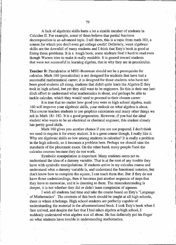
79

A lack of algebraic skills hurts a lot a sizable number of students in Calculus II. For example, some of them believe that partial fractions decomposition is an advanced topic. I tell them, this is a topic from math 103, a course for which you don't even get college credit! Definitely, weak algebraic skills are the downfall of many students and I think that Esty's book is good at fixing those problems. It is a tough book, some students find it hard to read even though Warren tries to make it really readable. It is geared toward students that were not successful in learning algebra, that is why they are in precalculus.

Teacher B: Precalculus at MSU-Bozeman should not be a prerequisite for calculus. Math 160 (precalculus) is not designed for students that have had a successful mathematical career, it is designed for those students who have not been good students all along, students that didn't quite learn the Algebra II they took in high school, but yet they still want to be engineers. So this is their one last- ditch effort to understand what mathematics is about, and perhaps be able to tackle calculus, which they would need to proceed to their chosen career.

It is true that no matter how good you were in high school algebra, math 160 will improve your algebraic skills, your outlook on what algebra is about.This course teaches students to use graphics calculators and many other things we ask in Math 181-182. It is a good preparation. However, if you had the ideal student who wants to be an electrical or chemical engineer, this student already has pretty good skills.

Math 160 gives you another chance if you are not prepared. I don't think we need to require it for every student. It is a great course though, I really like it. Why are algebraic skills so low among students in calculus? It is really a problem in the high schools, so it becomes a problem here. Perhaps we should raise the standards of the placement exam. On the other hand, many people flunk the calculus courses because they do not work.

Symbolic manipulation is important. Many students seem not to understand the idea of a dummy variable. That is at the root of any trouble they have with symbolic manipulations. If students arrive in my calculus Course and understand what a dummy variable is, and understand the functional notation, but don't know how to complete the square, I can teach them that; But if they do not have those understandings, then it becomes just another sequence of steps that they have to memorize, and it is daunting to them. The misunderstanding is deeper, it is not whether they did or didn't learn completion of squares.

I wish all students had time and take the course based on Esty's "Language of Mathematics". The contents of this book should be taught at all high schools, there is where it belongs. High school students are perfectly capable of understanding the material in the aforementioned book. I took Esty's book when I first arrived, and despite the fact that I had taken algebra at high school, I suddenly understood what algebra was all about. He has definitely put his finger on what students have trouble in understanding mathematics.

80

Question 11: What should be the role played by graphics calculators in a calculus

class?

Teacher A: I think that they are a great tool, but they are abused. Instead of using them as a tool, many students use it not even as a crutch but as a wheelchair. People will not think by themselves first and then use the tool to verify what they have come Up with. They just turn on their calculator before starting to think. Former engineering students of mine are grateful to me because I insisted that they should not just grab their calculator without a previous thought process. They have to be able to picture what some graphs look like, to visualize the generic functions, to know how to translate them. It is good that the calculators are there, but I think that they are not used the way that they should be.

I ask my students, for example, give me an upper bound of the sine function. Some of them try to use the calculator immediately, are incapable to have a mental image of the sine function! So, the use of the calculators is often abused. By not making the effort of visualizing functions, students are missing a huge facet of calculus. Calculators should be used to explore, to check a conjecture, to perform a long calculation, and the like. However, they should not replace mathematical reasoning.

If you give the student a TI-92 they may think that they do not have to learn anything. Just push a button and get an answer for an integration process.The machine will integrate it for you. Let us not forget that there are some topics students have to learn: integration by parts, substitution. These basic techniques have to be learned by hand, without calculators. It would be pretty sad if we were to ask them to find j x2 dx and they turn on their calculators. I am in favor of keeping that kind of technology out of the classroom!

Teacher B: If you always use a graphics calculator to generate a graph, then you haven't learned what we all learned in calculus and that is how to graph functions. The whole reason we learned how to find a maximum or a minimum, or how to analyze the concavity of a function, was to draw pictures. On the other hand, any technology used correctly simply allows us to see immediately whether a conjecture is true or not. Students need to explore, experiment, and then go back and determine the mathematical basis of their conjectures. So, I think that if it is used to explore it becomes a great tool.

So long as we test correctly and we ask questions that demand understanding, I don't see how a calculator can hurt. It ends up hurting because sometimes we don't ask the right questions, we don't emphasize the right things.

What should we done with calculators that do symbolic manipulations like the TI-92? A student can claim that he/she could bring a PC to class and "fire up" Maple and ask it to do their quizzes problems for them. So, just because

8 1

technological innovations lead to smaller powerful calculators doesn't make their argument, that they should use it, any more valid. We should dispel that to start with. Just because it has gotten to calculator size does not have anything to do with whether we allow it in class. Let us consider statistics. You have an introductory course in statistics at every college. What you really want students to take out of this type of course is to have them read and understand articles that claim something about statistics. You can't really get a hold on understanding statistics unless you do it yourself. If you calculate a few of the typical standard deviations, means, confidence intervals and the like, you have a feeling for what they are telling you. The same with integrals . Could you understand everything that can be understood about integrals without having done some simple integrations by pencil and paper? I doubt it. It is the same situation as with arithmetic.

Do you need to understand integral calculus? Well, if you are going to understand differential equations you certainly do. You need to know what integration is all about. Besides, you need to understand those things if nothing more because when you are in higher level classes of your major and you are told that to go from here to there one has to integrate. Whether or not you could actually do that in your head quickly is not important, but to understand what that means is important.

There is absolutely nothing wrong with any technology, but we should realize that technology cannot replace mathematical reasoning.

82

CHAPTER 4

SUMMARY, CONCLUSIONS, AND RECOMMENDATIONS

Summary of the Study

The question addressed in this study was whether there is a difference in

achievement between students that followed the Harvard Calculus textbook, and those

students who, besides using the Harvard Calculus textbook, received supplemental

materials and studied several mathematical aspects of physics that went beyond the

textbook.

The subjects in the study were the 151 students registered in Calculus II at MSU-

Bozeman during the Fall semester of 1996. In parts of the analysis the number of subjects

was smaller, namely when information for some of the variables was not available for all.

There were a total of five sections of Calculus H with different instructors. Three sections

were assigned to the experimental group (Harvard Calculus + additional materials), also

called Method I , and two sections were assigned to the control group (Harvard Calculus

alone), also called Method 2.

The main variables under study were the total scores in Calculus H ( three one-

hour exams and the final), and the total scores in Physics I (one midterm and the final) for

those students that took this course concurrently with Calculus II. The other variables

considered in the analysis were the total scores in Calculus I (for the students that took it

at MSU-Bozeman the previous semester), and the SAT-math scores (to be denoted SAT

for short). Calculus I and SAT acted as covariables. The information about the time in

83

which the students took Physics I (not yet, concurrently with Calculus II, or before, to be

represented by the variable WhenPh) was also considered, as well as gender.

Calculus I scores were obtained directly from the Spring 1996 instructors

(corresponding to three one-hour common exams and the common final), while the SAT

scores were delivered by the university's office of admissions. The latter also provided the

information with regard to the students' Physics I status. The scores in Physics I were sent

by the physics instructor to the researcher.

The statistical tools used were Analysis of Covariance, Analysis of Variance, and

Regression, accompanied by scatter-plots, box-plots, and interaction plots. The alpha

level was set at 0.05.

Despite the fact that Calculus II is a four credit course, classes met five days per-

week for fifty minutes. Four of the instructors (two in the experimental group and two in

the control group) were of similar background and experience, while the researcher —

who taught one section in the experimental group — had comparatively more teaching

experience. All of them were graduate teaching assistants at the Department of

Mathematical Sciences (MSU-Bozeman) during the time of the study.

The three instructors in the experimental group met on a weekly basis and closely

coordinated their lectures and other activities. Besides, they and the instructors in the

control group attended the regular meetings of the course. All the one-hour exams and the

final for Calculus II were common to the five sections. They were taken simultaneously

by all students, at a common time set aside in the evenings. Each instructor graded one or

more questions for every student, setting a common rubric for partial credit. A regular

faculty member, who did not teach a Calculus II class during the fall of 96, was assigned

by the Department of Mathematical Sciences as course supervisor. His main duties were

to draw a syllabus and make a first draft of every exam, as well as to verify that every

section was delivering the material on schedule.

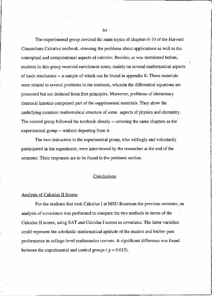
84

The experimental group covered the main topics of chapters 6-10 of the Harvard

Consortium Calculus textbook, stressing the problems about applications as well as the

conceptual and computational aspects of calculus. Besides, as was mentioned before,

students in this group received enrichment notes, mainly on several mathematical aspects

of basic mechanics — a sample of which can be found in appendix E. These materials

were related to several problems in the textbook, wherein the differential equations are

presented but not deduced from first principles. Moreover, problems of elementary

chemical kinetics comprised part of the supplemental materials. They show the

underlying common mathematical structure of some aspects of physics and chemistry.

The control group followed the textbook closely — covering the same chapters as the

experimental group — without departing from it.

The two instructors in the experimental group, who willingly and voluntarily

participated in the experiment, were interviewed by the researcher at the end of the

semester. Their responses are to be found in the pertinent section.

Conclusions

Analysis of Calculus II Scores

For the students that took Calculus I at MSU-Bozeman the previous semester, an

analysis of covariance was performed to compare the two methods in terms of the

Calculus II scores, using SAT and Calculus I scores as covariates. The latter variables

could represent the scholastic mathematical aptitude of the student and his/her past

performance in college-level mathematics courses. A significant difference was found

between the experimental and control groups ( p = 0.015).

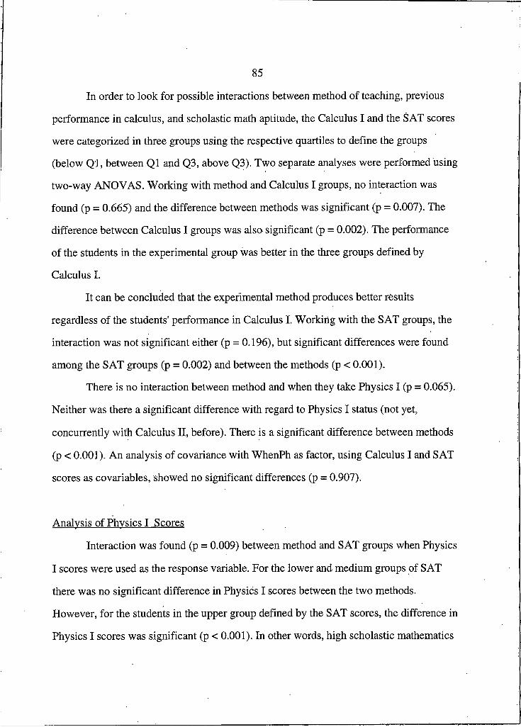
85

In order to look for possible interactions between method of teaching, previous

performance in calculus, and scholastic math aptitude, the Calculus I and the SAT scores

were categorized in three groups using the respective quartiles to define the groups

(below Q l, between Ql and Q3, above Q3). Two separate analyses were performed using

two-way ANOVAS. Working with method and Calculus I groups, no interaction was

found (p = 0.665) and the difference between methods was significant (p = 0.007). The

difference between Calculus I groups was also significant (p = 0.002). The performance

of the students in the experimental group was better in the three groups defined by

Calculus I.

It can be concluded that the experimental method produces better results

regardless of the students' performance in Calculus I. Working with the SAT groups, the

interaction was not significant either (p = 0.196), but significant differences were found

among the SAT groups (p = 0.002) and between the methods (p < 0.001).

There is no interaction between method and when they take Physics I (p = 0.065).

Neither was there a significant difference with regard to Physics I status (not yet,

concurrently with Calculus II, before). There is a significant difference between methods

(p < 0.001). An analysis of covariance with WhenPh as factor, using Calculus I and SAT

scores as covariables, showed no significant differences (p = 0.907).

Analysis of Physics I Scores

Interaction was found (p = 0.009) between method and SAT groups when Physics

I scores were used as the response variable. For the lower and medium groups of SAT

there was no significant difference in Physics I scores between the two methods.

However, for the students in the upper group defined by the SAT scores, the difference in

Physics I scores was significant (p < 0.001). In other words, high scholastic mathematics

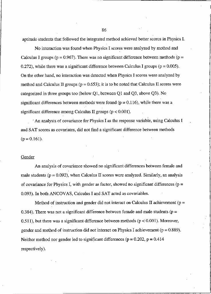
86

aptitude students that followed the integrated method achieved better scores in Physics I.

No interaction was found when Physics I scores were analyzed by method and

Calculus I groups (p = 0.967). There was no significant difference between methods (p =

0.272), while there was a significant difference between Calculus I groups (p = 0.005).

On the other hand, no interaction was detected when Physics I scores were analyzed by

method and Calculus II groups (p = 0.653); it is to be noted that Calculus II scores were

categorized in three groups too (below QI, between Ql and Q3, above Q3). No

significant differences between methods were found (p = 0.116), while there was a

significant difference among Calculus II groups (p < 0.001).

■ An analysis of covariance for Physics I as the response variable, using Calculus I

and SAT scores as covariates, did not find a significant difference between methods

(p = 0.161).

Gender

An analysis of covariance showed no significant differences between female and

male students (p = 0.092), when Calculus II scores were analyzed. Similarly, ah analysis

of covariance for Physics I, with gender as factor, showed no significant differences (p =

0.093). In both ANCOVAS, Calculus I and SAT acted as covariables.

Method of instruction and gender did not interact on Calculus II achievement (p =

0.384). There was not a significant difference between female and male students (p =

0.511), but there was a significant difference between methods (p < 0.001). Moreover,

gender and method of instruction did not interact on Physics I achievement (p = 0.889).

Neither method nor gender led to significant differences (p = 0.202, p = 0.414

respectively).

87

Additional Analyses

Calculus II scores were analyzed by instructor through an ANOVA; a significant

difference was found (p < 0.001). Sections I, 2, and 3 were in the experimental group,

while sections 4 and 5 were in the control group. The students in section 5, as a group,

got significantly lower scores than their peers in the other four sections. However, when

Calculus II scores were analyzed by instructor through an ANCOVA, with Calculus I and

SAT acting as covariables, no significant differences were found (p = 0.076).

It should come as no surprise that no significant differences were found in the

preceding ANCOVA. From comparing two groups of 50 and 16 subjects (table 22), we

ended up comparing five sections with 13, 17, 20, 5, and 11 subjects respectively.

A regression analysis on Calculus H, with Calculus I and SAT as predictors,

allowed an analysis of residuals of the regression model that led to the conclusion that

most students in sections 4 and 5 — especially the latter — did worse than expected on the

basis of their Calculus I and SAT scores (figure 17).

The integrated method exerts a "homogenizing effect" on Calculus II scores of

groups I and 2 according to S AT, a trend that is not observed with regard to the non-

integrated method. A similar effect of the integrated method is observed when Calculus II

scores are analyzed, with the variables WhenPh and Method as factors.

Teacher Feedback

Based on the teacher interviews, to be found in the preceding chapter, several

conclusions can be drawn. Instructors liked the applied emphasis of the course, and in

particular the enrichment notes used in the experimental group. They thought that a

balance had been reached between conceptual ideas, computational problems and topics

of physics and chemistry that have a high mathematical content. These topics helped to

convey mathematical ideas relevant to calculus.

88

There was the perception that the aforementioned notes helped the best students

the most. They would use them in the future, although there was always a time constraint

that limited the number of topics that could be covered in class.

There should be some proofs in the textbook, especially the good students could

profit from them . The instructors meant the treatment of the idea of proof, not

necessarily the presentation of many proofs. It was not the omission of a particular proof

what worried them, it was the omission of the idea of proof in a mathematics course.

They didn't use the group work setting. One of them chose one day per week for a

question-answer period with no lecturing. Students were encouraged to ask questions

therein. The other instructor was of the opinion that it should be up to each instructor

whether to do group work or not. Some teachers, he asserted, are excellent lecturers. So

they should lecture. Others are very good working'with groups, then they should choose

the latter alternative.

Both instructors found some weaknesses in the Harvard Calculus book, for

instance the lack of the idea of proof mentioned before. But both had a positive opinion

about the examples and problems to be found in the book. One instructor praised the

authors for having had the courage to throw out some materials from traditional books,

while the other instructor thought that the book was not a good reference. Its readability

was pointed out, but the disappearance of some aspects of the theory of limits was

regretted.

Homework was assigned but not collected in both sections. Weekly quizzes were

mainly based on the list of assigned problems. Although the importance of grading

homework was recognized, one instructor was of the opinion that graduate teaching

assistants usually did not have the time to grade it on a daily basis.

89

There was a consensus in the sense that meeting 5 days per-week was a good idea,

even though Calculus II is a 4 credit course. The extra day gave instructors the

opportunity to have the students take a 50 minutes quiz each week. No student

complained about this arrangement, adopted by the department of mathematical sciences

at MSU-Bozeman.

The instructors in the experimental group had no definite opinions on whether

Calculus I should be a prerequisite for first-semester physics. It all depended on the level

at what Physics I was taught. One instructor noted that calculus helps physics and vice

versa. He thought that it is fine to take physics and calculus concurrently.

No strong feelings were expressed about the fact that at MSU-Bozeman three

types of calculus courses are offered: traditional, reform, and honors. They are intended

for different audiences. One instructor thought that although honors calculus is a good

challenge for the best students, the regular classes suffer because of the absence of them.

Students are coming into calculus with a preoccupying lack of algebraic skills,

which is one of the main reasons for students' failure. What is even more serious, basic

ideas like dummy variables and functional notation are absent from the minds of many

students. Maybe the standards of the placement examination should be raised. On the

other hand, probably more of them should take precalculus, a highly praised college

course intended for those that want to be engineers but do not have a good background in

mathematics. These ideas were shared, one way or another, by both instructors.

Finally, the issue of technology in the calculus class drew sharp responses. The

instructors felt that quite often the use of calculators was being abused, in the sense that

they were not used for exploration but as a replacement of mathematical reasoning. One

instructor was in favor of keeping the TI-92 technology outside the calculus class

altogether, while the other instructor pointed out that what is important is to test correctly,

asking questions that demand understanding.

90

Recommendations

Recommendations for Curriculum and Instruction

On the basis of the conclusions and the experiences accumulated in the present

study, an integrated approach to second-semester calculus is a possibility that should be

considered by those instructors that are scheduled to teach the course using the Harvard

Calculus textbook. Such an approach does not cause any harm to the students. On the

contrary, it might lead to better achievement in calculus and physics. Furthermore, it is

recommended that the Harvard Calculus textbook should not be used verbatim. Each

instructor can stress what he/she considers are the strong aspects of the book while

supplementing it with enrichment notes, a sample of which can be found in Appendix E.

The enrichment notes should cover not only relevant applications, beyond those

given in the book, but also acceptable proofs of several important results such as the

fundamental theorem of calculus or the criteria for comparison of improper integrals.

Important tools, like the main properties of limits and the usual tests in the theory of

series, should also be covered in the notes.

Recommendations for Future Research

1. It is advisable to implement new studies, using large samples, comparing the

integrated and non-integrated approaches to second-semester calculus teaching. Only a

meta-analysis, based on multiple studies, could lead to a definitive answer.

2. There is a trend to be observed in figure 10, when Calculus II scores are

analyzed with the variables Method and WhenPh as factors. New research needs to be

done which looks for interaction.

91

3. A replication of this study can be done, adding more covariates. Besides CalcI

and SAT scores, one should contemplate adding, for instance, college GPA, having in

mind lessening the number of uncontrolled variables.

4. Second semester calculus-based chemistry scores should be analyzed in future

studies, provided the chosen sample includes a sufficient number of students that are

taking chemistry concurrently with Calculus H

5. Students' future academic performance, beyond their first year,, can give further

valuable information with regard to possible advantages or disadvantages of the

integrated method. Longitudinal (one or two years in length) studies, collecting data on

how well students do on courses such as control theory, physical chemistry, electrical

circuits and the like, could further substantiate an integrated approach to calculus

teaching.

6. Further studies have to be conducted with the participation of many instructors,

so as to minimize the "teacher effect" phenomenon that usually haunts educational

research of this type. Besides, random assignment of subjects to treatments is a goal to

have in mind, no matter how difficult and unattainable it is in actual practice.

7. At MSU-Bozeman, male students far outnumber female students in Calculus II.

Does this imbalance occur at bther land-grant universities in the USA? Research should

be done to find out what keeps women from enrolling in calculus courses.

8. Replicating the study with a traditional calculus textbook also needs to be done.

92

REFERENCES CITED

93

Abad, E.A. (1994). Rethinking Mathematics: Closing the gap between mathematics and science. The Science Teacher. Vol. 61, No. 8, 35-37.

Armstrong, G., Garner, L., and Wynn, J. (1994). Our experience with two reformed . calculus programs. Primus. Vol. IV, No. 4, 301-311.

Beane, J. (1996). On the Shoulders of Giants! The Case for Curriculum Integration. Middle School Journal. Vol. 28, No. I , 7-11.

Becker, J.R., and Pence, B J. (1994). The teaching and learning of college mathematics: Current status and future directions. In Kaput, J.J. and Dubinsky, E. (Editors). Research Issues in Undergraduate Mathematics Learning. Mathematical Association of America, 5-14.

Boas, R.P. (1971). Calculus as an experimental science. The American Mathematical Monthly. VolL 78, No. 6, 664-667.

Breslich, E.R. (1936). Integration of Secondary School Mathematics and Science. School Science and Mathematics. Vol. 36, No. I, 58-67,

Cipra, B. (1996). Calculus Reform Sparks a Backlash. Science. Vol. 271, No. 16, 901-902.

Douglass, R.G. (Ed.) (1986). Toward a lean and lively calculus. The Mathematical Association of America. Wasington, D.C.

Ferrini-Mundy, J. and Geuther Graham, K. (1991). An overview of the calculus reform curriculum effort. The American Mathematical Monthly. Vol. 98, No. 7, 627-634.

Friend, H. (1985). The effect of science and mathematics integration on selected 7thgrade students' attitudes toward and achievement in science. School Science and Mathematics. Vol. 85, No. 6, 453-461.

George, P.S. (1996). The Integrated Curriculum: A Reality Check. Middle School Journal. Vol. 28. No. I. 13-19.

Glass, G. and Hopkins K.D. (1996). Statistical Methods in Education and Psychology, third edition. Allyn and Bacon, Boston.

Helfgott, M. (1990). Teaching differential equations to students of chemistry andchemical engineering. International Journal of Mathematical Education in Science and Technology. Vol. 21, No. 6, 1010-1016.

94

Helfgott, M. (1995). Improved teaching of the calculus through the use of historicalmaterials. In Swetz, F. et al. (Eds.). Learn from the Masters. The Mathematical Association of America, Washington D C., 135-144.

Hestenes, D.,Wells M., and Swackhammer G. (1992). Force Concept Inventory. The Phvsics Teacher. Vol. 30, 141-158.

Hughes-Hallet, D., Gleason, A. et al. (1994). Calculus. John Wiley & Sons Inc., New York.

Jean, R., Iglesias, A. (1990). The juxtaposition vs. the integrated approach to mathematics in biology. Zentralblatt fur didaktik der Matherhatik. ZDM, M65.

Johnson, K. (1995). Harvard Calculus at Oklahoma State University. The American Mathematical Monthly. Vol. 102, No. 9, 794-797.

Kerlinger, F.N. and Pedhazur, E.J. (1973). Multiple Regression in Behavioral Research. Holt, Rinehart and Winston, New York.

Kleinfeld, M. (1996). Calculus: Reformed or Deformed? The American Mathematical Monthly. Vol. 103, No. 3, 230-232.

Kline, M. (1967). Calculus: An intuitive and physical approach. John Wiley & Sons Inc., New York.

Kline, M. (1970). Logic versus Pedagogy. The American Mathematical Monthly. Vol. 77, No. 3, 264-282.

Kren, S.R., Huntsberger, J.P. (1977). Should science be used to teach mathematical skills? Journal of Research in Science Teaching. Vol. 14, No. 6, 557-561.

Longhart, F. and Hughes, G. (1995). Integrating Mathematics and Science. Paper presented at the Montana Educational Association Convention, Missoula, Montana.

Ostertag, W. and Zito, T. (1995). An integrated calculus-phvsics sequence. Fourth conference on the teaching of mathematics, San Jose, California.

Ralston, A. (1984). Will Discrete Mathematics surpass Calculus in importance? The College Mathematics Journal. Vol. 15, No. 5, 371-382.

Ratay, G. (1993). Student performance with Calculus Reform at the United States Merchant Marine Academy. Primus. Vol. Ill, No. 1 ,107-111.

95

SIMMS (1993). Systemic Initiative for Montana Mathematics and Science. Monograph I: Philosophies. Montana State University-Bozeman, Bozeman, Montana.

Steen, LA. (Ed.) (1987). Calculus for a new century: A pump, not a filter. The Mathematical Association of America, Washington D C.

Steen, LA. (1992). Integrating School Science and mathematics: Fad or Folly?NSF/SSMA Wingspread Conference Plenary Papers. Eric Microfiche ED376-076.

Teles, E.J. (1992). Calculus Reform: What was happening before 1986? Primus. Vol. II, No. 3, 224-234. -

Wilson, R. (1997). A Decade of Teaching "Reform Calculus" Has been a Disaster, Critics Charge. The Chronicle of Higher Education. Vol. XLIII, No. 22, A l2.

Wu, H. (1996). The Mathematician and the Mathematics Education Reform. Notices of the American Mathematical Society. Vol. 43. No. 12. 1531-1537.

96

APPENDICES

97

APPENDIX A

CALCULUS II SYLLABUS AND EXAMS

98

MATH 182 FaU 1996

R e q u ire d T e x t: C a lc u lu s , H u g h e s -H a lle tt, G le a s o n , e t a l A ls o re q u ire d : A G ra p h ic C a lc u la to r

W e e k # S t a r t s o n D a y s S e c t i o n s

I Sept. 3 KTWRF 6.1, 6.2

2 Sept. 9 MTWRF 6.3, 6.4, 7.1

3 Sept. 16 MTWRF 7.1, 7.2,7.3

4 Sept. 23 MTWRF 7.3, 7.4,7.5

5 Sept. 30 MTWRF 7.5, REVIEW, TEST 1 ,7.6

6 Oct. 7 MTWRF 7.7,7.8,7.9

7 Oct. 14 MTWRF 8.1, 8.2, 8.3

8 Oct. 21 MTWRF 8.4, 8.5, 8.6

9 Oct. 28 MTWRF 8.6, REVIEW, TEST 2, 9.1

10 Nov. 4 MKWRFElection Day

9.2,9.3

11 Nov. 11 KTWRFVeteransDay

9.4,9.5, 9.6

12 Nov. 18 MTWRF 9.6, REVIEW, TEST 3,10.1

13 Nov. 25 MTWKKThanksgiving

10.1,10.2

14 Dec. 2 MTWRF 10.2,10.3

15 Dec. 9 MTWRF 10.3, REVIEW

16 Dec. 13 Finals Week

Final M onday, December 16th, 10:00-11:30 AM

Im portant Dotes to Remember;Last day to ADD: September 16 Last day to DROP: September 23 Last day to DROP with a W: October 28

Two of the most important components in order for a student to be successful in study of calculus: ADEQUATE MATHEMATICAL SKILLS IN THE PREREQUISITE TOPICS AND MASTERING THE NEW TOPICS IN A TIMELY FASHION. Each topic covemd in this class depends on the previous topics that have been covered. Mathematics Is not a spectator sp o r t

Calculators VTlllbeusedforthehomewoiic and tests. See the back side o f this sheet for recommendations.

The course grade will be based on three examinations (100 points each), quiz/homework results (100 points), and a final examination (200 points).

Students arc required to take all hour exams at the scheduled hours as they appear on the syllabus. Any exceptions must be approved by the course supervisor, and in no case will exceptions be made for two exams. In the event a hour exam is unavoidably missed for a reason approved by the course supervisor, the final comprehensive exam will count 300 points instead o f200 points. No makeup exam will be given.

99

Math 182O cto b er 8 ,1 9 9 6

Exam I

Problem I 2 3 4 T o ta lPossible 8 5 2 20 20 100S core

Name.Instructor

b. Find th e indefin ite in teg ra l J dx

2. E valuate th e fo llow ing in teg ra ls exactly . [D o n o t estim ate.]

(6PO) a) J " | - h + 7 c o s x ) dx

(IOpU) b) f lX ^ l - X 2Cbe

(IOpti) Recall: — arctan $ = __ i__.<%■ I * ?

( iip a ) d ) J l t X l n x d x

(Upu) e) d x

100

3. B elow is the g raph o f the derivative / ' W o f a function f ( x ) , w ith /(O ) = I . S ke tch the g raph o f / ( * ) . Show all c ritical po in ts and inflection po in ts giving their coord inates. [B e c lear in show ing how you calcu la te the

/ w

Z f« /

I

4 . A skier o n a p articu la r sec tio n o f th e dow nhill skiing speed tria l a t P e te 's Hill is o b se rv ed en tering the section w ith ve locity 4 0 m /s. 100 m e te rs la te r the sk ie r’s ve locity w as m easu red to be 54 nVs.A ssum ing the accele ra tio n is c o n s ta n t:a) S k e tch th e g rap h o f ve locity , v(t), versus r for th is v wsec tion o f th e c o u rse . |W"b) Label the follow ing q u an tities o n the g raph from part a).

i) d istance - 100 m ete rsii) th e accele ra tion at any point.

c ) F ind the accele ration .

t u t )

101

Math 182 Exam 2 Name.Q a o b e r 29,1 9 9 6 Show all work Instructor-

Problem I 2 3 4 5 6 T ota lPossible 15 16 15 12 22 20 100Score

N o t e : P ro b lem 2b is th e on ly p rob lem in w hich an approx im ation is acceptable.

I . At an y point x, th e c ro ss s e a ion o f a solid is a sem icircle o f radius y / f x - l ) 2 + I w here O s x s Z . Find the volum e o f the solid .

r

2. The in tegral J 1 e "l u r Z n r d r g ives the to ta l m ass M o f a c ircu lar p la te o f radius I m ete r and density

p (r ) =e "0 ,r kg /m 2.a) E xplain w hy th is in teg ra l g ives u s th e value o f M.

b) U sing th e ap p ro p ria te c a lcu la to r p rogram , evaluate Trap(SO) and Mid(SO). W hy is T rap(SO ) < Mid(SO)? A re w e go in g to have T rap (n ) < M id(n) for all n ? Justify your answ er.

3. D eterm ine w h e th er o r n o t f ~ e “ ’sin2x d x converges. I f i t co n v erg es, w ithout using th e c a lcu la to r find

num bers a an d b su ch th a t su ch th a t a s e '^ s m b c d x sfc . Explain carefully h o w you fo und a and b.

1 0 2

4. Does i: dxco n v erg e o r d iverge? I f h converges, find its value. (An ^ , u n t o o n , , no. **& **,)

For p r o b le m s 5 a n d 6 , either explain or indicate on the figures any variables you use, especially where you have placed the axis. A I s q 1 recall that the weight density o f water is 9800 Newtons per cubic meter.

w“ ^ ^ ^ ^ •*»

6. C alcu late th e w o rk to be d o n e to e m p ty the cone, h a lf full (by height) o f w ater, raising th e liquid to a height 3 m e te rs above the vertex.

103

Math 182 Exam 3 Name.N ovem ber 26, 1996 S h o w all WOrk InStTUCtOL

Problem I 2 3 4 5 6 7 T o ta lPossible 9 7 16 12 12 18 26 100Score

• I . Is y(x) = Xe ' a so lu tion to the d ifferential equation — * y - — ?dx x

2. G iven y (0 ) = A c o s (3 6 ) ♦ B sin (3 6 ) is a so lu tion o f

y (6 ) is a so lu tio n to th e Initial V alue Problem :d 6 2

£ id&2

* 9 y

* 9 y = 0 , find co n stan ts A and B su ch that

= 0 , y(0) - 2 , Y1(O) - 0 .

(a) S lope fields for 2 o f th e 3 D E s have been d raw n below . F o r each slope field, identify th e co rresponding

D E and b r ie f ly s ta te a valid reaso n fo r each cho ice.

A: ± B: ^ C : — = X 2**

i) corresponds toI M t l l t t M WI 1 M M I M M %I I I M M I M \ V 1 I M t t t M V X \ y I MMMMW^ IMlMXMW^ XXX N W S N X-v"—

■ ' / I I I I I I I / / I t I I I I I / / / M f f f f - / / / I l l t l l ' / / / I t l l l ^ / / / / / I t l

/ / / / / / / /

/ / -4* / / , -2.I I S I I I / / / s t I I I I I I t / / / - Z MMfMM/ / / - ! ! ! I i l l l i / / ' - ! I i i i l i t i i Z"4 * f M M f f f M / / -

*■ > \ ^ X X \ \ \ I \ X W \ X X M X W X t X M SXXttttt xXt t t t t t XXttlMt

, X X

it) corresponds toM M M f H M f f M J M f f f M ^ I l l l l l l l l l i r I I I I I I I I I I t y i

I I / I I I I I I / I 2 / / / / / / / / / / / /

* * ^ * * * * * * * * .

M M M M M M I I I I I I I I I I I I I I I I I I I I I I I I M M M M M M M M M M M M / / / / / / / / / / / /

• * * * * * * '* * ’* ' * * - * * * * * * ’* * ' * ' * *

* * ~ ‘? 4 - * ' * * ~ ~ 2 * ‘ * l* * * S l/ / Z Z / / / / / / / /I I / 1 I j I / i / 1 - 2M M M M M MI t i l l l t l t l l 'M M M f M M " 4I M M f f f M t f

l - '^ * ^ * ^ 2 * * * y £ * * * * A * * * * */ Z Z Z / / / / / / / /i I / I I I I I I f I i I l l l l l i i l l l l t I I I I I I I I I I t I l t i l l i l l i i i I I M f f f f M M

(b) S k e tch th e so lu tio n cu rv e passing th ro u g h th e p o in t (0 ,1 ) o n th e s lope field i)- [above to th e left]

104

4 . U se E uler's m eth o d w ith A x - 0 .2 5 to app rox im ate th e so lu tion curve to the differential eq u atio n

Q = — passing th ro u g h th e po in t ( 0 , 1) and ending a t x - I . ox y

(K eep th e ap p rox im ate function values to 3 decim al p laces.) Sum m arize your resu lts in th e tab le p rov ided . ......................... • * i. N o w o r k - N o c r e d i L

y,

(Xwy0)

(*!. y ,)

(X ^ y2)

(x ,. y ,)

(x«, y4)

5 . A five lite r tan k initially co n ta in s fresh w ater. B eginning at t ■ 0 m inutes, w a ter con ta in ing 3 g ram s o f salt p e r lite r is p um ped in to th e ta n k a t a ra te o f 0 .5 lite r p e r m inute. T he salt w a te r instan tly m ixes w ith the w a te r in th e tank . T h e excess m ix tu re is d ra ined from the tan k a t th e sam e ra te (0 J liter p e r m inute). Let s ( t) rep resen t the m ass o f salt in the tan k a t tim e t.W rite a d ifferen tia l e q u a tio n fo r th e am oun t o f salt in th e tan k (ie, — = . . . . ) .

dt

105

Math 182 Exam 3 N a m _______________________Show aO work Ingm anr

6. S u p p o se that at m idn igh t th e h ea te r in y o u r house b reaks d ow n . A t the tim e o f the h e a te r m alfunction the tem p era tu re in y o u r h ouse is 65* F and the tem pera tu re ou tside is - 35° F (m inus 35).

«»•> (a) A ssum ing th a t th e tem p era tu re T in y o u r hom e obeys N ew ton 's Law o f cooling , w r i te th e d if fe re n tia l e q u a t io n sa tis f ie d b y T .

(N ew ton 's L aw o f coo ling : R a te o f change o f tem pera tu re is p roportiona l to th e tem p era tu re d ifference. |

ro w (b ) I f you also o b se rv e th a t a t 2 A M th e tem p era tu re in your house is 50° F, so lve th e d ifferen tia l equation above, and d e te rm in e a t w hat tim e th e tem p era tu re in the house will be 32° F.

106

7 . S o N e th e follow ing D E 1S b y sep ara tio n o f variables. N ote : Y o u r so lu tion m ust be so lved fo r the dependent variable; th a t is, o f th e fo rm y (t) ■ . . . . A lso, y o u r answ ers m ust be sim plified.

am (a) = t 2e y ; y(0)=0

mm) (b) — = — ; y(0) = 2 fo r i< Idt I -I

- < = > $y ( y * 5 ) ; y (0 ) = 5 H int, using partia l f r a a io n decom position: I

y ( y * 5 )

I5 y

I5 (y + 5 )

107

Decembo 16,1996 _______ F in a l E x a m _____ Instructor,I P rob lem I I 2 3 4 5 1 6 7 8 T ota lI Possib le I 60 18 22 20 20 20 20 20 200I Score --------------r —I. Find in tegrals below . A pproxim ations are not acceptable, sh o w all steps.

(a) f i Z ta*2 +*3) * J - i 2 * x 2

(b) I x - A

x 1 + x - 6dx

(C) f * ( l - x ) ^ 4 - x 2dx

Cd) j x e ^ d x

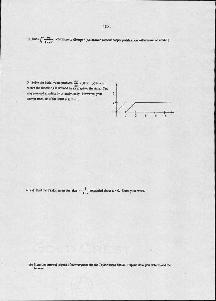
108

Z D o e s / " _ 2 L Jo l+ « 7 co n v erg e o r diverge? [An answ er w ithout p roper justification will rece ive n o credit.]

3. Solve th e initial value prob lem — = f ( x ) , y(0) = 0 ,

w here the f u n c tio n / is defined by its graph to the right. You

m ay p roceed graphically o r analytically. H ow ever, your

answ er m ust be o f th e form y(x) - . . . .

A

2'

4. (a) Find th e T ay lo r series fo r f{x) ------- expanded about x - 0 . Show yo u r w ork.I - x

(b) S ta te th e in terval (open) o f convergence for the T ay lor series above. Explain how you de term ined them tr r v f l l

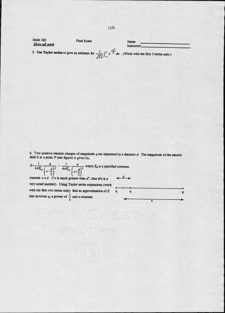
Final E xam

109

Math 182Shaw q(l tuprjr

N am eInstructor.

5. Uae Teylor aeries to give an estim ate for 1 f 1 < 2 dx . (W ork w ith the first 3 te n n s only.)

6. T w o positive e lectric charges o f m agnitude q are separa ted by a d istance d. T he m agnitude o f th e electric field £ at a poin t P (see figure) is given by,

w here E 0 is a specified constant.

4,El 4”E- [ . . $A ssum e x » < ( (“x is m uch g re a te r than <T, thus d /x is a ■*-

very sm all num ber). U sing T aylor series expansions (w o rk

w ith the first tw o term s only) find an approxim ation o f £ q

that involves q. a p o w e r o f — and a constant.P

*-x

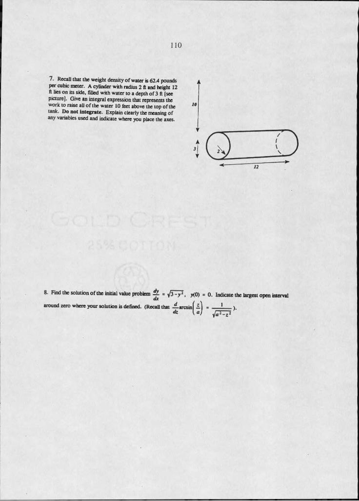
no

7 . Recall that the w eight density o f w ater is 62 .4 pounds p e r cubic m eter. A cylinder w ith radius 2 ft and height 12 ft lies o n its side, filled w ith w ater to a depth o f 3 ft [see p icture]. G ive an integral expression that represents the w ork to raise all o f the w ater 10 feet above the top o f the tank. D o n o t in te g ra te . Explain clearly the meaning o f any variables used and indicate w here you place the axes.

8. Find th e so lu tion o f th e initial value problem = y f a - y 2 , y(0) = 0 . Indicate the largest o p en interval

a round zero w here y o u r so lu tion is defined. (R ecall that — arcsin

t

12

I l l

APPENDIX B

PHYSICS QUESTIONNAIRE

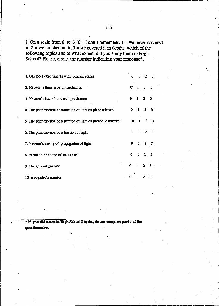
112

I. On a scale from 0 to 3(0 = 1 don’t remember, I = we never covered it, 2 = we touched on it, 3 = we covered it in depth), which of the following topics and to what extent did you study them in High School? Please, circle the number indicating your response*.

I. Galileo's experiments with inclined planes 0 I 2 3

2. Newton’s three laws of mechanics 0 I 2 3

3. Newton’s law of universal gravitation 0 I 2 3

4. The phenomenon of reflection of light on plane mirrors 0 I 2 3

5. The phenomenon of reflection of light on parabolic mirrors 0 I 2 3

6. The phenomenon of refraction of light 0 I 2 3

7. Newton’s theory of propagation of light 0 I 2 3

8. Fermat’s principle of least time 0 I 2 3

9. The general gas law 0 I 2 3

10. Avogadro’s number 0 I 2 ’ 3

* If you did not take High School Physics, do not complete part I of the questionnaire.

113

] [ DEMOGRAPHIC. DATA

1. WHAT WAS THE SIZE OF YOUR GRADUATING HIGH SCHOOL CLASS?

Less than 40 students__ Between 40 and 100 students-----More than 100 students____

2. DID YOU TAKE CALCULUS IN HIGH SCHOOL?Jsj0...................................... Last math course taken in High School_---------------------Yes...... ............................ Number of semesters_____

Did. you take the AP Calculus exam?No____Yes............................Grade obtained

3. SIMMS IS THE SYSTEMIC INITIATIVE FOR MONTANA MATHEMATICS AND SCIENCE. Were SIMMS, curricula materials used in

your mathematics classes in High School?No____Yes .........................Location of your High School-----------------------------

4. DID YOU TAKE PHYSICS COURSES IN HIGH SCHOOL?

No___Yes.... ................. .........How many years?____

Did you take the AP Physics exam?No___Yes...... ..................... Grade obtained

5. HAVE YOU TAKEN PHYSICS COURSES AT THE COLLEGE LEVEL PREVIOUS TO THIS SEMESTER?No____Yes ................................ Title of the course_-------------- --------------------- -----------6. ARE YOU TAKING A PHYSICS COURSE THIS SEMESTER ?

No__Yes...... .................................Title o f the course ----------------- --------------- .

If your answer was NO to questions 4,5, and 6, please complete only the first four questions of the next prrt^" Otherwise (that is to say, if you answered YES to either 4,5, or 6) complete the eight questions of the next section (section III).

114

IIL The following questions* do not require a knowledge o f Calculus. Please, circle the option that you consider is the correct one.

I. A heavy ba» is enached lo • suing and swung in • CiiCUlaf path m a horizontal plane as Hkistiaiad in the diagram Io the right Al Ihe point W iceed in the diagram, the string suddenly Ixeaks at the ban. It / these e v en s were observed from directly above. / indicee the path o l th e b a l after the Bring breaks. T

' - . . . . ' ( D )

(E)*

^ A stone tailing from the root o la smple eory txniding iolhe surlace ol the earth;

(A) leaches Hs maximum speed quae soon alter release and then Ials el a constant speed thereafter

(B) speeds up as It ta l l , primarily because the closer the stone gets to the earth, the stronger the gravitalional attraction.

(C) speeds up because of the eonstam gnviieuonal Ioroe acting on it(D) Ia lsbecauseo lthelnu insic tindencyolelob iectsto leltow anl Iheeanh(E) IeHs because ol a combination of the W ee ol gravity and the air pressure pushing it

3 A OOiI Dal driven down a Iarrwsy is observed to travel Ueough the air with a Uaieaory (flight path) similer IoUtalHtHte depiction below.

WtUcti know s*) to rcK i) m ore) Odtng on Ute QOlfbal during Hs enteefligrtt7

1 the Icice of gravity2 the force of th e W3. IhetorceoIoH resalance

4.

(A) Ionty(B) I a n d 2(C) 1 .2 .c n d 3

(D) I a n d 3(E) 2 an d 3

th e rocket rea ch es s o m e point c

Wtvcri path below best represents Uta path of the rodcal between D" end "C-?

.Vc rS

:1C)

-w eb . - w e o - .e - e b

f/

/(D) (()/ /

- e - e b ' '

The first four questions ccsne from the "Force Concept Inveatcry* Icet by H estates, W ells, and Swackhamcr

115

5. A ball, starting from rest at C. rolls down an inclined plane. Find its velocity at the bottom (point A ) in

terms of the height h. Friction is not to be considered. Recall that g = 32 ft/sec 2 . where g is the acceleration on

the surface of the earth due Io gravity.

(A) 32 h ft/sec (B) 32 ft/sec (C) 8 VT ft/sec

(D) 16 VT fi/sec (E) 16 ft/sec

6. Let G be the constant of universal gravitation, M the mass of the earth, and r the radius of the earth. The

relationship between G. M. r, and g is given by:

(A)g = (rG )/M (B)M = ( r 2 G ) /g (C)G = ( rg ) /M

(D)G = (r2 g) / M (E) r = (g 2 G )/M

7. One of the first tests of Newton’s law of universal gravitation had to do with the period T of the moon (T is the

time the moon takes to make one complete revolution around the earth). Assuming that the moon's orbit is circular,

and recalling that the centripetal force acting on the moon is given by the expression (m v 2) / R . where v is the

moon's velocity, and R is the distance between the center of the earth and the center of the moon, find T in terms

of r. R . and g.

(A) T = [ (2 ltR ) /r ) V R / g ( B ) T = ( I Z t t R ) V T T g (C) T = ( I tRZr) V TTg

(D) T = (2 I t R2 ) Zr g (E) T = (2 n R ) Zr g

8. Using his theory of light. Newton found the formula sin 0 = ( v, / v2 ) sin a for the phenomenon of refraction.

Fermat had reached the formula sin 0 = (V2 Zv , ) sin a on the basis of his principle of least time. It Looks like

Newton's formula, except that v, and v2 are interchanged. Who was right, Newton or Fermat? Recall that the

speed of light in air is greater than the speed of light in water.

(A) Newton (B) Fermat (C) There is not enough information to give an answer

(D) Neither Newton nor Fermat were right (E) It is an open question until todayV,

116

INSTRUMENT ANALYSIS

I. Did you find that all the questions were clearly stated?

2. Would you suggest any improvements in sections I, II, or III?

3. Do you think that the allotted time (30 minutes) was enough to complete the questionnaire in a leisurely fashion?

4. Please, make any comments you find worthwhile.

117

APPENDIX C

RECORD OF MEETINGS OF THE EXPERIMENTAL GROUP

118

The instructors in charge of the experimental group met for an hour or so on a weekly basis and planned their activities. A log of the meetings was kept by the researcher. These weekly meetings were preceded by a long encounter between the researcher and the other two instructors, wherein the former explained the purpose and methodology of the research to be conducted during the fall, 1996.

First WeekThe Fundamental Theorem of Calculus (FTC) plays an important role in the

course, so we may as well prove it. The presentation given by the textbook in section 3.4 is a heuristic argument that needs to be refined. The students are to receive an enrichment note wherein the FTC is proven along the ideas set in problem 15 p. 132. The proof is given first for increasing or decreasing continuous functions. Thereafter it is to be generalized to continuous functions that are not necessarily increasing or decreasing.

Special attention is to be paid to problem 10, p. 319. More examples are to be analyzed in class, dealing with initial value problems of the type y'(t) = f(t), y(0) = a, where a is a given number and f is sectionally continuous, i.e. continuous with a finite number of discontinuities; problem 17 on page 324 is an example of this sort. Students should realize that the solution will be continuous everywhere, but not differentiable at the points of discontinuity of the function f.

Second WeekLots of problems about motion. Problems 48-54 (section 6.4), 1-4 (section 6.5)

and 34-40 (Review of Chapter 6) are particularly interesting. Let students understand that one is dealing with differential equations of the type s"(t) = -k, where k could be g (when a body is subjected to the force of gravity) or some fixed number if one were to deal with accelerating or decelerating cars or airplanes. The importance of fixing coordinate axes. Have students solve the differential equations each time a problem is given. One of the keys to solve the application problems is to realize what the physical conditions are, and what is a mathematics derivation.

Handout on basic chemical kinetics is given to the students. This is a nice opportunity to talk about the essence of the scientific method and the role that mathematics plays in science.

Third WeekLet students understand that the underlying foundation of the method of

substitution is the chain rule and the FTC. Present a proof of the method along the lines of thought set by the book on page 350, but do it for definite integrals. Advantages and disadvantages of the algorithmic approach to substitution. Strategies to be used in substitution problems. Beware! A common mistake made by students takes place when they have to calculate a definite integral through substitution and, despite all the warnings, they forget about the proper handling of the limits of integration.

119

Have students deduce the equation given in problem 45 (page 354) from the differential equation m v'(t) = mg - k v(t). Many practice problems! Let students know that the equation presented in problem 32 (p. 359) will be deduced from first principles once we learn about the method of partial fractions.

Fourth WeekOld saying: "When you do not know what to do, apply integration by parts".

Students need to realize that there is not a unique way to solve a problem using this technique. For instance, one can "solve" I ex cos x dx in two ways. There is even a third possibility that leads to the equality 0 = 0, an unpleasant situation that shouldn't demoralize anyone. It is just a matter of trying another path!

Problem 50 on page 365 and similar ones are good for practice purposes. Completion of squares and partial fractions should be given a higher status, the book down plays both of them; this is a pity since these methodologies - especially the latter- are widely used in mathematics, physics, and chemistry. As an example, discuss in class the enrichment notes about falling objects that are subjected to air resistance proportional to the square of the velocity and chemical reactions whose solution leads to a problem in partial fractions. Have students justify items 24-31 of the short table of indefinite integrals (p. 367).

Fifth WeekExample 3 (p. 381) is particularly nice. Discuss in class similar problems, for

instance I l/(l+x3) dx between the limits 0 and I . Let the students work on most if not all the problems in section 7.6. Stress the fact that "approximating by parabolas" leads to Simpson's method (along the lines of problems 20, 21 of section 7.7).

Sixth WeekHandout on the proof of the criteria of comparison for improper integrals. Section

7.8 has a good collection of problems, including problems 29, 30. Example 5 (p. 404) is particularly well done, let students read it before coming to class. All the problems for section 7.9 look nice, especially problem 25 related to Planck's radiation law. Cover in class section 7.10, even though it is not in the syllabus; students will realize that the developments in p. 410 were covered in the first enrichment note. Many good problems in the review section for chapter seven (pp. 414-417).

Seventh WeekLots of applications! Students usually have trouble with work and water pressure

problems. With particular care discuss in class problems about cylinders full of water or gasoline, and the work to be done to empty them when the cylinder is standing on its base or lying on its side (problem 6, p. 444). The hydrostatic force on an object varies according to the shape of the submerged object and the depth of the column of water. Let students analyze triangular and circular plates.

120

Enrichment note on an alternative calculation for the escape velocity of an object on the earth's surface. This alternative approach is a good opportunity for the students; they can become acquainted with simple qualitative methods in the elementary theory of differential equations.

Show students how mathematicians used to calculate volumes of cones and spheres, before Newton and Leibniz— so as to impress upon them the power of differential and integral calculus.

Eighth WeekStudents will understand sections 8.5 and 8.6 only through the problems. Set aside

enough time to discuss in class as many problems as possible, chosen from the nice collection laid out in the book. Assign as homework several problems from the review section for chapter eight.

Ninth WeekSection 9.1 should not be a novelty, since from the very beginning of the course

we have been discussing the idea of solution of a differential equation. This section can be dealt with rather rapidly so as to concentrate on 9.2. Slope fields are something new for the students. Handout on more slope fields.

Tenth WeekHandout on the theoretical justification of Euler's method. Students need to

understand the underlying geometrical idea lying behind the method, before doing actual computations. A balance between paper and pencil computations and the use of calculators has to be reached. For the former, choose some simple problems that do not require extensive computations.

Eleventh WeekEnrichment note on the catenary, starting from basic ideas in physics. This note

explains where the equation in problem 8 (p. 482) comes from. The catenary changes into a parabola when one analyzes a suspension bridge under suitable simplifications. Enrichment note on Newton's law of cooling and radioactive decay (validation of the model, solution of the corresponding differential equation, and solution of problems that arise in actual practice).

Twelfth WeekGeneral solution of linear first order differential equations. Do cover in class the

most salient features of sections 9.10 and 9.12. These are not contemplated in the syllabus; however, students that are taking Physics I concurrently with Calculus n, have to know how to solve second order linear differential equations.

121

The book does a particularly nice job with section 9.6. Follow it closely. Enrichment note on enzyme kinetics. Simple ideas in chemistry lead to basic techniques in mathematics.

Thirteenth WeekHave students plot on their calculators different Taylor polynomials. Enrichment

note on the approximation ln(l+x) = x and its appearance in the natural sciences.

Fourteenth WeekGeometric series. Handout on series of numbers. Students need to know the main

tests (ratio, root, and integral tests). Parallelism between the theory of improper integrals and the theory of series of numbers. Taylor series as a particularly important case of series of functions. Start dealing with Taylor series, then develop the basic facts about power series.

Fifteenth WeekFollow closely section 10.3 of the book. The material is well-presented and the

problems at the end of the section are very good. Wrap up everything and separate two days for review. No quiz this week!

122

APPENDIX D

CONCORDANCE TABLE

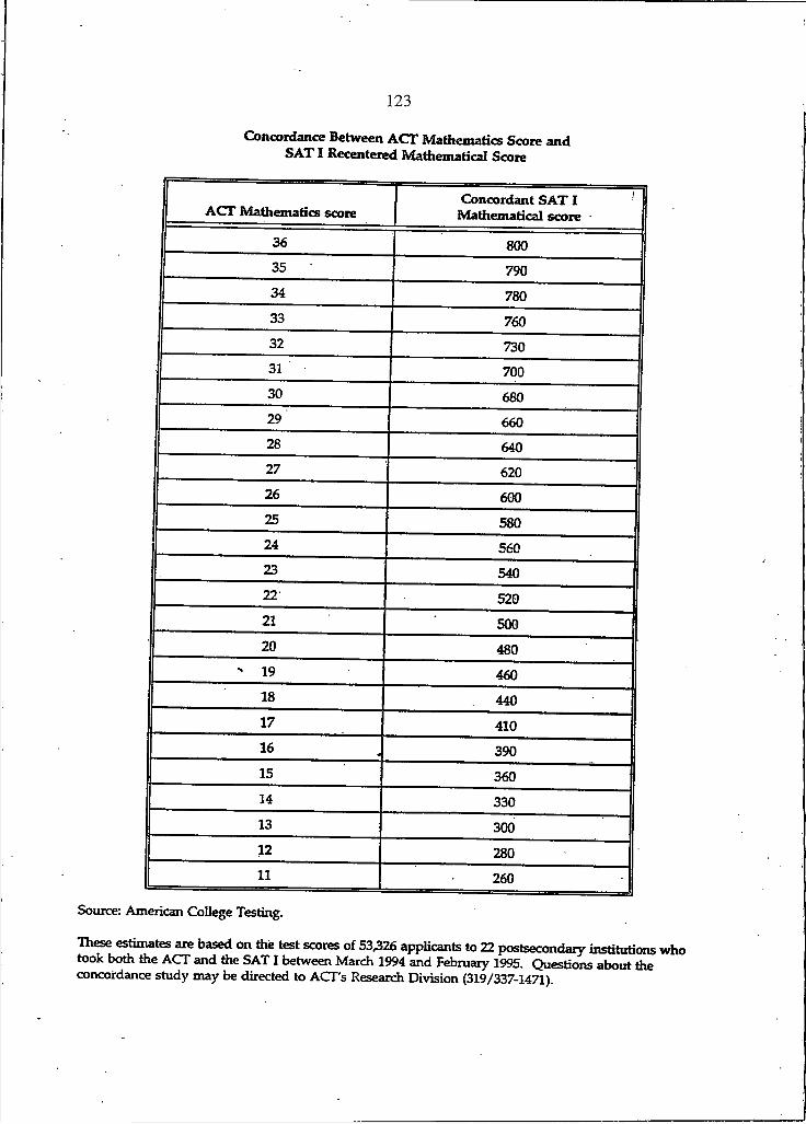
123

Concordance Between ACT M athematics Score and SAT I Recentered Mathematical Score

ACT Mathematics scoreConcordant SAT I 1

Mathematical score •

36 80035 79034 78033 76032 73031 70030 68029 66028 64027 62026 60025 58024 56023 54022 52021 50020 480

" 19 46018 44017 410

16 39015 36014 33013 30012 28011 260

Source: American College Testing.

These estimates are based on the test scores of 53,326 applicants to 22 postsecondary institutions who took both the ACT and the SAT I between March 1994 and February 1995. Questions about the concordance study may be directed to ACT's Research Division (319/337-1471).

124

APPENDIX E

A SAMPLE OF ENRICHMENT NOTES

125

Elementary Chemical Kinetics

A single reactant is put in contact with water, and its concentration c(t) is measured:

time.(hours)

concentration (moles/lt.)

0 0.1039

3.15 0.0896

4.10 0.0859

6.2 0.0776

According to basic principles of chemistry, a possible model for the reaction is the differential equation

c f ( t ) = - k c ( t )

where k is a positive parameter. If this were the case, we would have

s M . - tc ( t )

So [ t I M d s = f ' - k d sh c (s ) Jo

But ,(IncW)'=

c ( r )

for any t. Therefore:

126

[Inc(J)]'= [ - ^ ] '

Thus Inc(Z) -Inc(O) = - k t

In other words:

t c { t )

( I )

A prediction of the model is that

I l n Mt C(Z)

will remain constant for different values of t. That is to say, our model predicts that this mathematical expression is independent of t. The model

C z(Z) = -^e(Z )

will attain validity insofar as the prediction is in agreement with the data given at the beginning. Using a calculator we get the following values:

t c(0)/c(t) ln(c(0)/c(t)) (l/t)ln(c(0)/c(t))

3.15 1.15959 0.14807 0.04700

4.1 1.20954 0.19024 0.04640

6.2 1.33891 0.29186 0.04707

The last column indicates that

IlnMZ C(Z)

remains practically constant. Then we accept the model and proceed to approximate the value of k as the simple mean of the three numbers 0.04700, 0.04640, and 0.04707.

127

Notice that the validity of the model has to be checked before any attempt to approximate k. An equivalent approach, often favored by scientists, can be followed: Let us rewrite (I) as In c(t) = -k t + In c(0). This equation implies a straight line, with t on the x-axis and In c(t) on the y-axis. Using the experimental values, given in the first table, the following table is built:

t In c(t)

0 -2.26432

3.15 -2.41239

4.1 -2.45457

6.2 -2.55618

We expect that these points will be distributed in such a way that an imaginary line can be drawn passing through them. Thereafter we draw the line that best fits the four points. Its slope provides the value of k (there is a standard statistical procedure to obtain the line of “best fit” through any number of points). If the four points are arranged in a haphazard way, not suggesting the presence of a line, we reject the model because a mathematical consequence of it does not agree with the experimental values! The latter is the “supreme judge” that will determine the acceptance or rejection of the model

c ' d ) = - k e i f )

If this model is not acceptable, the next step would be to consider the model

Let us try to find a consequence of it that may be compared with a table of experimental values involving t and the corresponding c(t). We notice that

( c ( t ) ) 2

Thus

( , C 1W d s ^ f t k d s

Jo (c (s))2 Jo

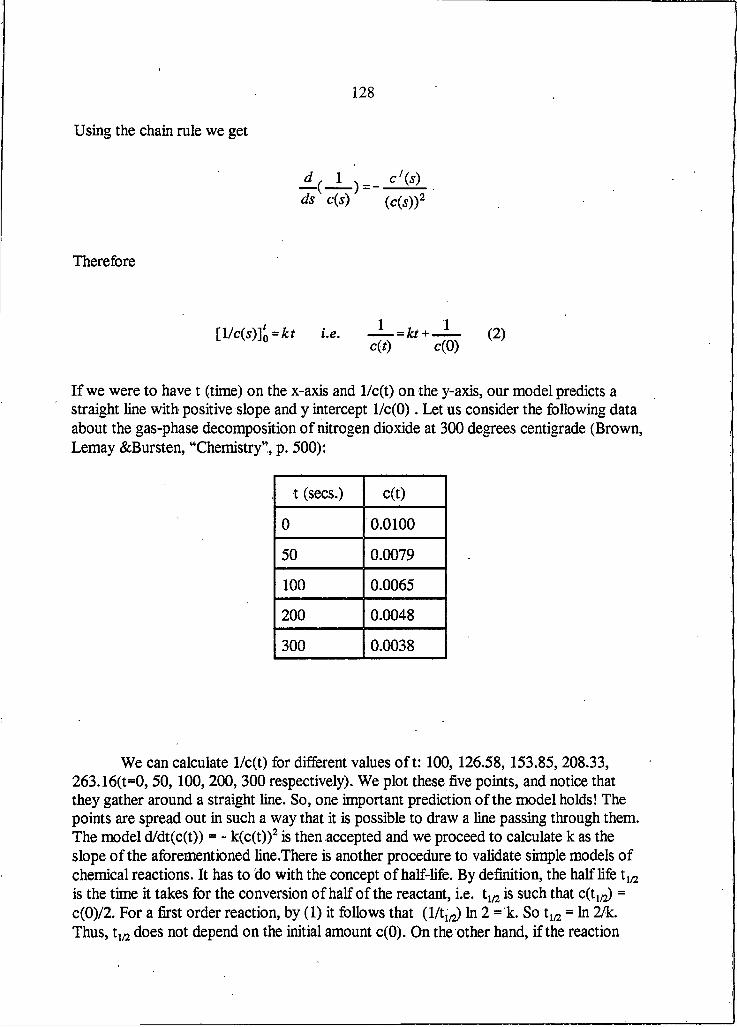
128

Using the chain rule we get

d s c{s) ( c ( s ) ) 2

Therefore

[ l / c ( s ) ] i = i.e. - l — = k t + ̂ ( 2 )° c{t) c ( 0 )

If we were to have t (time) on the x-axis and l/c(t) on the y-axis, our model predicts a straight line with positive slope and y intercept Vc(O). Let us consider the following data about the gas-phase decomposition of nitrogen dioxide at 300 degrees centigrade (Brown, Lemay &Bursten, “Chemistry”, p. 500):

t (secs.) c(t)

0 0.0100

50 0.0079

100 0.0065

200 0.0048

300 0.0038

We can calculate l/c(t) for different values oft: 100, 126.58, 153.85, 208.33, 263.16(t=0, 50, 100, 200, 300 respectively). We plot these five points, and notice that they gather around a straight line. So, one important prediction of the model holds! The points are spread out in such a way that it is possible to draw a line passing through them. The model d/dt(c(t)) = - k(c(t))2 is then accepted and we proceed to calculate k as the slope of the aforementioned line.There is another procedure to validate simple models of chemical reactions. It has to do with the concept of half-life. By definition, the half life t1/2 is the time it takes for the conversion of half of the reactant, i.e. t1/2 is such that C(Iiy2) = c(0)/2. For a first order reaction, by (I) it follows that (Vtiy2) In 2 = k. So t1/2 = In 2/k. Thus, t ly2 does not depend on the initial amount c(0). On the other hand, if the reaction

129

is of second order, from (2) we get l/(c(0)/2) = k t1Z2 +' l/c(0). Hence t 1/2 = IZkc(O). We notice that, in this case, Xm depends on c(0). Thus, a strong indication that a reaction cannot be of first order is to start with different amounts of reactant, measure the half-life, and realize that it varies. If the reaction were to be of first order, this could not happen.

Wind Resistance Proportional to the Square of Velocity

Let us make some comments about problem 32 on page 359. The book provides an expression for v(t). It looks complicated. Where does it come from? The model for a falling object of unit mass is (dZdt) v(t) = g - k (v(t))2. Then

V7CO _ !g - k ( v ( i ) ) 2

Thus

V7O) - !

By the method of partial fractions, we know that there exist numbers p and q such that

__________ I_______ - P . 9(VF+V^ v(f)) (VF - v ( t ) ) J g + y f k v ( i ) - J g - J k v i t )

The usual procedure leads to the values of p and q:

p( g1/2 - klz2 v(t)) + q(g1/2 +k1/2v(t)) = I

So p g1/2 + q g1Z2 =1 and -k1/2 p + k1Z2 q = 0. Therefore p = q = lZ(2g1/2). Using these values and integrating, we arrive to:

I r t \ ] k v Ji s ) d s _ I r t - \ f k v l{s )d s _ t

2 \ f k g 0 J g + J k v ( s ) 2 J k g J g - J k v ( s )

130

Thus

—̂ [InCy'i'+v^v^))]' [ln(yi-v^v(5))]' = t

2y[kj> 2 j k £

Then

JiiJ ^ v W , 2 ^ , y f g - y / k v ( t )

After a little bit of elementary algebra we finally arrive to

v(t) e x p j y / k g t ) -exp (-v^ r) exp(V^g t ) + exp( - y f k g t )

This is the expression we were looking for!

A Problem in Chemical Kinetics where Partial Fractions Are Used

Let us consider the chemical reaction Na2 S2O3 + CH31 — > products, with k as the parameter of the reaction. From a series of experiments we get the following data:

t (hours) Na2S2O3 CH3I (moles/lt.)

0 35,35 18.25

4.75 30.5 13.4

10 27 9.9

20 23.2 6.1

35 20.3 3.2

55 18.6 1.5

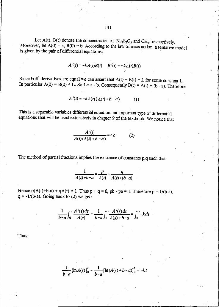
131

Let A(t), B(t) denote the concentration of Na2S2O3 and CH3I respectively. Moreover, let A(O) = a, B(O) = b. According to the law of mass action, a tentative model is given by the pair of differential equations:

A ' ( t ) = - k A ( i ) B ( f ) B \ t ) = - k A ( f ) B ( f )

Since both derivatives are equal we can assert that A(t) = B(t) + L for some constant L In particular A(O) = B(O) + L. So L= a - b. Consequently B(t) = A(t) + (b - a). Therefore

A /( t ) = - k A ( t ) ( A ( t ) + b - a ) (I)

This is a separable variables differential equation, an important type of differential equations that will be used extensively in chapter 9 of the textbook. We notice that

A \ t )

A ( t ) , ( A ( t ) + b - a )(2)

The method of partial fractions implies the existence of constants p,q such that

1 - + ____IA ( t ) + b - a A ( t ) A ( f ) + { b - a )

Hence p(A(t)+b-a) + qA(t) = I. Thus p + q = 0, pb - pa = I. Therefore p = l/(b-a), q = -l/(b-a). Going back to (2) we get:

I r t A /( s ) d s _ I /• t A ' ( s ) d s _ r t

- a Jo A ( s ) b - a Jo A ( s ) + b - a Jo- k d s

Thus

[InA(S)]' - -J_[ln(A(s) + b - a ) ] [ = - k t b - a b - a

132

Consequently

/1(f)

—-—In----- ------ = - k tb - a A ( t )+ b -a

b

i.e.

(3)( a - b ) t aB{t)

Thus, a prediction of our model is that the expression to the left of (3) will remain nearly constant through time. Using the data given above, this expression adopts the values 1.9863 x IO"3, 2 x IO"3, 1.9729 x IO"3, 1.9821 x IO 3, 1.974 x IO"3 (for t = 4.75, 10, 20, 35, and 55 respectively). So, we accept the validity of the model. Thereafter, the parameter k can be calculated in the usual way through a plot of t versus (l/(b-a))ln((bA(t)/aB(t)) on the y-axis. We will be dealing with a straight line that goes through the origin.

The CatenaryIn problem 21 (p. 436) we are given the function y = (e* + e"*)/2, and we are told

that it is called the catenary and that it represents the shape in which a cable hangs. Is that so?

Let us consider a flexible and uniform chain, suspended between its endpoints and hanging

the chain. For the time being we do not specify where the origin of the coordinate system is.

under its own weight. We draw the y-axis in such a way that itpasses through the lowest point of

^U x)

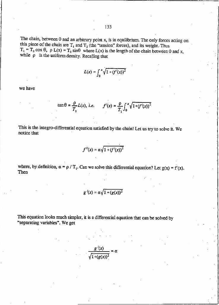
133

The chain, between O and an arbitrary point x, is in equilibrium. The only forces acting on this piece of the chain are T1 and T2 (the “tension” forces), and its weight. Thus T1 = T2 cos 0, p L(x) = T2 sin6 where L(x) is the length of the chain between 0 and x, while p is the uniform density. Recalling that

U x ) = J * -j I + ( f ' ix ) )2

we have

tan0 = ^Z(X), Le. f ' { x ) = j *

This is the integro-differential equation satisfied by the chain! Let us try to solve it. We notice that

Z zz(X) = CLsjl +Orz(X) ) 2

where, by. definition, a = p / T1. Can we solve this differential equation? Let g(x) = f (x). Then

S Z(x) = CLsjl +(g(x))2

This equation looks much simpler, it is a differential equation that can be solved by “separating variables”. We get

= ccV1+(£(*))2

134

Consequently

■ r g ^ d t ^ a r d ,

Jo J l + ( S i t ) ) 2 Jo

Formula 29 (p. 367 of our textbook) leads to the following equality:

[ln(g(0 + Vlrfe(O)2 T0 = ax

Therefore

gm^JiHgiO))2

However, g(0) = f '(0). By the way we chose the y-axis, the derivative of fat the origin has the value zero. Hence ln(g(x)+\/(l+(g(x))2) = a x. Thus

g(x) +yjl + (g(x)2 = exp(ca)

Hence

---------------- = exp(-ca)8(x) + j l + ( g ( x ) ) 2

Using the last two equalities and some elementary algebra we get:

f i x ) = g(x) exp(ax) -exp(-ax) 2

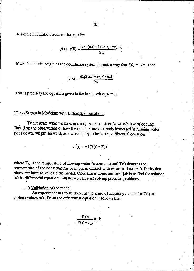
135

A simple integration leads to the equality

_ exp(ax) - 1 +exp( - ca) - 1 2a

If we choose the origin of the coordinate system in such, a way that f(0) = 1/a , then

= exp(ar) +exp(-ax)2a

This is precisely the equation given in the book, when a = I.

Three Stages in Modeling with Differential Equations

To illustrate what we have in mind, let us consider Newton’s law of cooling. Based on the observation of how the temperature of a body immersed in running water goes down, we put forward, as a working hypothesis, the differential equation

where Tm is the temperature of flowing water (a constant) and T(t) denotes the temperature of the body that has been put in contact with water at time t = 0. In the first place, we have to validate the model. Once this is done, our next job is to find the solution of the differential equation. Finally, we can start solving practical problems.

... a) Validation of the modelAn experiment has to be done, in the sense of acquiring a table for T(t) at

various values of t. From the differential equation it follows that

T'jt) _m - T M

- k

136

Therefore

r t T j(S)Cls

h T(S)-Tm

Hence

[InCr(S)-TjtX = -to

Thus

^ t ( O ) - T m

^ t ) - T m= k t (I)

A prediction of the model is that when t is on the x-axis and In { (T(O)-Tm)Z(T(I)-Tm)J is on the y-axis, the experimental values will cluster around a straight line that goes through the origin. If this happens, we accept the model and proceed to calculate k as the slope of the “line of best fit”. Thus, k is calculated once the process of data contrasting has come to an end, and the validity of the model has been accepted.

b) Finding the solution of the differential equation From (I) we get

T(O)-Tjtf

m - T M= exp(to)

Hence

T(i) = TM + (T(0)-rM)exp(-to) (2)

137

Obtaining the solution of the differential equation was pretty easy. However, in some cases it is not possible to obtain an explicit solution. Nonetheless, the process of validation, which usually precedes the search of a solution of the differential equation, can be done as was shown in the first part.

c) Solving practical problemsSuppose we wish to find the temperature at which a certain chemical reaction

takes place. For some reason, it is not possible to disturb the reaction while it is under way, i.e. we can not place a thermometer and measure the temperature of the reaction. We then bring the reaction to a stop (say, by some physical device) and the container is put in contact with a cooling system where water is circulating. Two measurements are then made: (t„ T(t,» and (t2, T(I2)). The unknown is T(O). From (2) it follows that

T (O )-T m = ( U t l) - T J e x p i k t J (3)

and

T (O ) -T m = ( U t 2) - T M)txp(k t2) (4)

Therefore

So

Once k is calculated, the value of T(O) can be found by using (3) or (4):

T(O) = Tjlf +(Tfr1) -T ^ e x p ^ )

138

A proof of the Fundamental Theorem of Calculus

Let us recall the statement of the theorem: Let f: I-*91 be a continuous function, where 9t denotes the set of real numbers. Suppose G is any antiderivative of f. Then

f bf=G(b)-G(a)J a

for any points a, b lying in the interval I.

We will first prove a lemma, following the idea given in problem 15(p. 312) of the textbook.

LemmaLet f be the function given before. Define F: I—»91 by

F(x)= [ xM d tJ a

where the lower limit of integration is any fixed point in I. Then

OX

for every x in I.

Proof

To start with, we will present a proof with the added assumption that f is increasing or decreasing. Suppose f is increasing. We notice that for any h>0

F(x+h)-F(x) = P +V - P /= P +VJ a J a J x

Since f is increasing we can assert that f(x) ̂ f(t) ^f(x+h) for every t in the interval [x, x+h]. Therefore:

139

f (x)h - J x hf{x)dt <, J xhf(t)dt < J Xfhf[x+h)dt = f(x+h)h

By looking to the graph to the right, you will notice the geometrical significance of the preceding formula.Thus:

But f is continuous at x. Consequently

linW A * -^ ) =A*)

Thus, by the “sandwich” property of limits we get

F ( x * h ) - F { x )A-O h =A*)

In a completely analogous fashion one can show that

i™ _ F ( x + h ) - F ( x )= A x )

The lemma has been proven for continuous increasing functions. The proof for decreasing functions is similar. If you are satisfied with this proof, and don’t have the time to consider the more general case when only the continuity of f is assumed, go straight to the proof of the fundamental theorem of calculus below. Otherwise, let us accept the following fact about any function p(x) defined on an interval [c,d]: If p(x) is continuous, there exists csGsd such that

I d p ( x ) d x = p ( Q ) ( d - c )

In other words, it is possible to build a rectangle whose area is equal to the area of the

140

region that lies between the curve defined by p(x) and the x-axis. It is “evident”, isn’t it? Going back to the central theme of the proof, we can assert that (for h>0)

J xJ hM d t ^ m h ) ) h

for some 0(h), where x<0(h)<x+h. Obviously

lim^0+ Q Q i) = x

(Again, we have used the sandwich” property of limits). Moreover, the continuity o ff at x assures that:

lirrw A 6(/0) = A linW # ) )

Then

l i n w \ I r m d t = linW -Ke(A)) =Alimw , 8(A)) =Ax)

Thus

Iim« -o +F ( x + h ) - F ( x )

zA x )

The limit from the left is proved in a similar way.

QED

A Proof of the FTC

Since G ' = f and F ' = f, where F is the function defined in the lemma, it follows that G ' = F '. So, for some k, G(x) = F(x) + k for every x. In particular G(a) = F(a) + k. But F(a) = 0. Sb k = G(a). Thus G(x) = F(x) + G(a) for every x in I. In particular:

141

G(b) - F(b) + G(a), i.e.

G{b) - G(a) = J bf

QED

RemarkThe lemma is discussed on pp. 409-410 of our textbook. Notice how important it is: Given any continuous function we can assert that' it has an antiderivative, precisely

F ( x ) = [ xM d tv a

This function might not be “simple”, but it exists!

The Comparison Test for Improper Integrals

Let f,g: [a,0 =) -91 be continuous functions such that 0 < f(x) < gfx) for allx^aThen: .

(0 J ” g(x) dx converges => f°°J(x) dx converges

(H) f~ fix) dx diverges - g(x)dx diverges

ProofDefine the following two functions:

F ( x ) - j f i t ) d t , G ( x ) = J x g ( t ) d t

Since f(x)^g(x), we can conclude that F(x)<G(x), x^a. Moreover, since f and g are positive functions it follows that F and G are increasing functions. Let us try to prove (i): By hypothesis, the limit of G(x) when x-~ exists. So G has to be bounded, say G(x)<M

142

for some number M and every x>a. Then F(x) < M, x ka. The function F is increasing and bounded above, so it has no alternative but to converge. In other words, Iim F(x) when x-°° exists, i.e. the integral of f(x) between a and =° converges. Furthermore, since F(x) < G(x), x£ a, and the limit of both fimctions exist when x we can assert that

/ > / : 8

The proof of (ii) is now almost immediate: it is nothing but its logical equivalent (recall that for any two statements.p and q, p -» q is equivalent to ~q =>~p, where the symbol ~ denotes the operation of negation).

QED

Usual Tests in the Theory of Series

Let a, = (1/2)" (n = 0,1,2,...) and define sn = l+(l/2)+...+(l/2)n Question: Does the limit of sn when n-°° exist? We notice that

(l/2)sn = (1/2) + (1/2)2 + ... + (l/2)n+1

So sn- (l/2)sn = I - (l/2)n+1. HenceSn = 2 - 2(l/2)n+i. But (l/2)n+1-0.Therefore sn- 2. Notice that

s n Ho(VZ)'

We have just shown that

Zm (VZ)'= 2

Another way of writing this fact is as follows:

Zm (VZ)'= 2

143

Since “i” is a “dummy” variable, we may rewrite the preceding equality as follows:

T L o (1/2)" = 2

or, as a matter of notation, we agree that

I + 1 /2+ (l/2)2+(l/2)3+ ..........= 2

The sequence (S n) is usually called the “series” determined by the sequence (aj. Quite often the series (S n) itself is denoted by the symbol

Strictly speaking, this symbol denotes a number. Nonetheless^ it is used both to denote ( S n) and its limit — when the latter exists. Beware about this double meaning! From the context of a particular problem you will be able to decide which meaning is intended.

Let us discuss another example: Determine whether the series

Y1 ” I Ln=I “ “n(n + l)

converges or not. If it converges, where does it converge to? Let

sn_ 1/1(1+1) + 1/2(2+1) + ... + l/n(n+l)

Since l/n(n+l) = 1/n - l/(n+l), we arrive to Sn = (1-1/2) + ... + (1/n - l/(n+l)), i.e.

Sn= I - l/(n+l).Thussn- I . Therefore

n ( n + l )

144

Does £ (l/n2) converge? In order to answer this question we will state a proposition, which has a striking similarity with the comparison test for improper integrals. •

Proposition ILet Can) and (bn) be sequences of non-negative terms, such that 0 < an < K bn

for some fixed constant K and all n. The following two implications are true:

(O E n -I frB c o n v e rg e s ~ Y 2 '=\ a n c o n v e rg e s

M o r e o v e r E L i a n ^ K E L i K

CO En=\ a n d iv e r g e s . V b" i-in=l d iv e rg e s

(We could weaken the hypothesis in the sense that the inequality only has to hold for all n except a finite number).

Let us use this proposition in order to determine whether or not E (l/n2)converges. We have the inequality n(n+l) < 2 n2 for n = I, 2, 3,...... Thus0 < 1/n2 < 2/n(n+l) N = 1 ,2 ,......Since E l/n(n+l) converges, we can conclude thatE 1/n2 converges. Where does it converge to? The preceding proposition does not give an answer to this question. All we can assert is that

o<EL, in(n+l)

= 2

For a long time, the “exact” value of E 1/n2 was an open question, until Leonhard Euler - probably the greatest 18th century mathematician- used a very clever technique and showed that

TT2

6

Unexpected, isn’t it? There is another result that we have to keep in mind.

145

Proposition 2 (the ratio tftstl

Let (aj be a sequence of non-zero numbers. Let

L = Iimf̂ J a nZanJ

The following two implications are true:

(0 -* £ ”=1 c o n v e r g e s

( i i ) L > I V Z, = oo -> ^"=1 a n d i v e r g e s

Using this proposition let us determine whether £ 1/n! converges. We notice that

l/(n+l)! divided by 1/n! gives n!/(n+l)!, which in turn is the quotient l/(n+l). The latter sequence obviously converges to zero. Thus £ 1/n! converges. Amazingly enough, it can be shown that:

where e is the basis of natural logarithms.

There is a deep connection between improper integrals of the type

and series of numbers, as the following proposition shows.

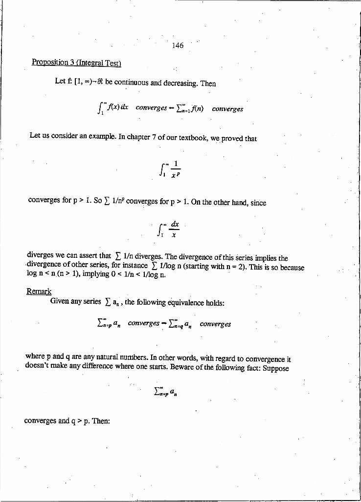
146

Proposition 3 Qntegral Tesr)

Let f: [I, be continuous and decreasing. Then

f converges •* Yjn=I Jin) converges

Let us consider an example. In chapter 7 of our textbook, we proved that

r J_J i x p

converges for p > I. So £ Vnp converges for p > I. On the other hand, since

diverges we can assert that £ 1/n diverges. The divergence of this series implies the divergence of other series, for instance £ 1/log n (starting with n = 2). This is so because log n < n (n > I), implying 0 < 1/n < 1/log n.

RemarkGiven any series £ a*, the following equivalence holds:

Yn=p an converSes ~ Y n=qan converges

where p and q are any natural numbers. In other words, with regard to convergence it doesn’t make any difference where one starts. Beware of the following fact: Suppose

Y“ Q

converges and q > p. Then:

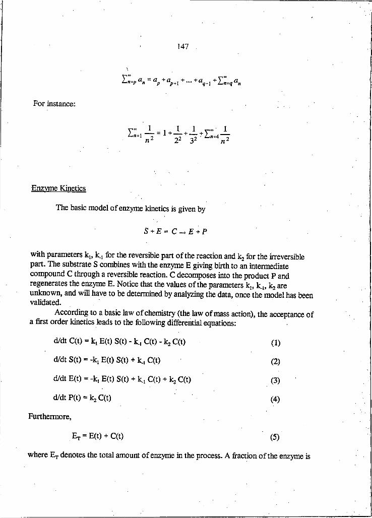
For instance:

Enzyme Kinetics

The basic model of enzyme kinetics is given by

S + E * C —* E + P

with parameters k„ k, for the reversible part of the reaction and k2 for the irreversible part. The substrate S combines with the enzyme E giving birth to an intermediate compound C through a reversible reaction. C decomposes into the product P and regenerates the enzyme E. Notice that the values of the parameters kl5 k„ k2 are unknown, and will have to be determined by analyzing the data, once the model has been validated.

According to a basic law of chemistry (the law of mass action), the acceptance of a first order kinetics leads to the following differential equations:

d/dt C(t) = kt E(t) S(t) - k, CCO - Ic2C(t)

d/dt S(t) = -k, E(t) S(t) + k, C(t)

d/dt E(t) = -k, E(t) S(t) + k , C(t) + k2 C(t)

d/dt P(t) = k2 C(t)

(3)

(2)

( I )

Furthermore,

Er = E(t) + C(t) (5)

where Et denotes the total amount of enzyme in the process. A fraction of the enzyme is

148

free ( E (t)) while the rest is bounded to the intermediate compound.The aforementioned system of differential equations looks quite complicated, and

it is complicated indeed! Around 1925 two British scientists, Briggs and Haldane, put forward a daring hypothesis: At the beginning of the experiment, substrate and enzyme combine quite rapidly giving birth to C and thereafter a “stationary state” ensues, during which the amount of C remains practically constant; the latter situation takes place because each time a molecule of P is formed by a rearrangement of C, a molecule of the enzyme is regenerated and combines rapidly with a molecule of the substrate (there is a high affinity between both of them). This mechanism lasts while there is substrate left. Thus, during considerable time one should expect that d/dt C(t) = 0.

Let us see what happens to the system of differential equations if we were to accept the stationary state hypothesis:

From (I) and (5) we have

d/dt C(t) = M E r - C(t» S(t) - k., C(t) - k2C(t)

i.e. d/dt C(t) = k, Er S(t) - (k, S(t) + k, + y C(t)

So, 0 - k, Er S(t) - (kj S(t) + k , + Ic2) C(t). Therefore

C(0 =E T S ( t )

(6)

where we define Km = (k, + k^/k,. Furthermore, using (4) and (6) we arrive to

P \ t ) =k 2 E T S ( t )

K m + S { t )(7)

But d/dt P(t) is precisely the reaction velocity v(t).The graph of v(t) corresponds to a well-known mathematical function, shown to the right. By adding more and more substrate we can increase the speed of the reaction. However, a point is reached when S becomes much bigger than Km and v cannot surpass the quantity k2 Er.

149

So, it is advisable to write Vmax = k2 Er.A little bit of elementary algebra leads to the equality - d/dt S(t) = d/dt P(t)

provided d/dt C(t) = 0. That is to say, under a stationary state scenario we arrive to the differential equation

S ' i t ) =- v .5(0K + S ( t )

(8)

called the Micaelis-Menteh equation. Let us pay a closer look at this equation. We notice that it is a separable variables differential equation! Thus we can separate variables and then integrate:

S \ t )

5(0+ S \ t ) = - V b

P- r t S X x ) d x

M 0 - S W -

Hence

Jf„[toSWfi+S(J)-S(O) = - W

Therefore

I l n M = I 5(0)-5(Q , Vmax, 3 0 r . f

This equality predicts that if (S(0)-S(t))/t is placed on the x-axis and (l/t)ln(S(0)/S(t)) on the y-axis, a straight line with negative slope will appear when we start taking into consideration the experimental values S(t). Very many experiments have been carried out.

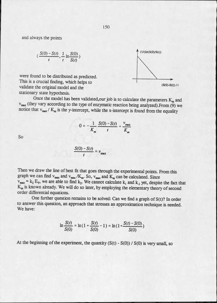
150

and always the points

(S(O)z S W l l n S(O) t t S(r)

were found to be distributed as predicted.This is a crucial finding, which helps to validate the original model and the stationary state hypothesis.

Once the model has been validated,our job is to calculate the parameters Km and Vm iu (they vary according to the type of enzymatic reaction being analyzed).From (9) we notice that Vm ix / Km is the y-intercept, while the x-intercept is found from the equality

O - _ I S(O)-SW , Vmax

So

4 (l/t)ln(S(0)/S(t))

\ \ \X

\X

(S(O)-S(I))/ t

S(O)-SW _ r# m ax

Then we draw the line of best fit that goes through the experimental points. From this graph we can find Vmix and Vmix /Km. So, Vmix and Km can be calculated. Since V m ix = k2 Er, we are able to find Ic2. We cannot calculate k, and k4 yet, despite the fact that Km is known already. We will do so later, by employing the elementary theory of second order differential equations.

One further question remains to be solved: Can we find a graph of S(t)? In order to answer this question, an approach that stresses an approximation technique is needed. We have:

InMS(O)

l n ( l + M - i ) = in(iS(O)

_ SW -S(O) S(O)

At the beginning of the experiment, the quantity (S(t) - S(O)) / S(O) is very small, so

151

, 5(f)-5(0) 5(Q-5(0)5(0) 5(0)

wherein we have used the well-known fact that ln(l+x) ~ x provided x is very small in absolute value. The aforementioned approximation, when applied to (9), leads to:

5(f) - 5(0) + K m 5(Q-5(0) 5(0)

-v t

Therefore

5(0 = 5(0) - ( 10)

Thus, at the beginning of the experiment we should have a straight line with negative slope. After a while, a lot of substrate will have been transformed into, the product. Hence S(t) will be small compared to S(0). Then ln(S(t) I S(O)) will be much bigger than I S(t)-S(0) I. The equality (9) can be written

5 (0 -S(O)+KmI n - ^ m S(O)

v t

Therefore

Consequently

5(0 = 5(0) e Km (H)

152

Thus, the curve described by S(t) behaves like a straight line with negative slope at the beginning of the experiment, and later on it becomes a negative exponential. This is another prediction of the model being discussed, which was duly corroborated by doing experiments.

All that remains to be done is find a way to calculate k* and k ,. Evidently, it is enough to calculate k, because k , = ^Km - k2. With this purpose in mind we will analyze the basic model of enzyme kinetics before the steady state, a very short period of time, at the beginning of the experiment, during which it is a good approximation to assume that S(t) is practically Sx (the total amount of substrate with which we started). It is to be noticed that, in general, ST(t) varies because the substrate is being used.

We differentiate the differential equation (4). Taking into account (I), we can assert that

= a2

where a, kt Sx + k , + Ic2, B2-Ic2 kj Ex Sx. It should be mentioned that we have used the equality E(t) = Ex - C(t) and the approximation S(t) = Sx. In front of us there is a second order linear homogeneous differential equation. Its characteristic polynomial is ^ a 1 r with roots T1 = 0 and r2 = -a,. By inspection of the differential equation it is evident that the function (a2 / a J t is a particular solution. Then, its general solution is given by

P ( t ) = C 1 + c 2 e- a t t

ta i

The initial conditions are P(O) = P0, d/dt P(O) = L2 C(O) = 0. These lead to the algebraic system

C l + C2 = P0

-a, c2 + a2 / a2 = 0

in the unknowns C1 and c2. Then

P(0 =P - _ ± + _ ± e 'V +

153

However, when t is very small we have the following approximation:

e W t ~ I + w t +w 2t 2

2

Therefore:

P i t )

2 oa 0 a 0 a < t z a ,

P c - ^ - a , ,

- I *1

Simplifying this expression we arrive to P(t) = P0+ (a2 /2)t2. Consequently P(t) - P0 = (Ic1 k2 Er STt2)/2. Thus

k i2 ( P ( t ) ~ P 0)

( 12)

In summary, the basic model of enzyme kinetics predicts that if it is possible to measure P(t) before the steady state, then the expression to the right of (12) will be constant. When around 1950 scientists developed experimental techniques to deal with very short spans of time, they could corroborate that the quantity 2(P(t)-P0) / 12 Vmu St remained practically constant. The parameter kj was obtained as the mean of these numbers at different values of t before the steady state.

The prediction that stems from (12) was a driving force in developing advanced techniques in what is now called ultrarrapid enzyme kinetics. After all, scientists wanted to know whether or not the prediction could withstand experimental verification!

Through the discussion of several aspects of enzyme kinetics we have had the opportunity to deal with some qualitative methods of approximation in the theory of elementary differential equations, as well as to realize the important role played by mathematics in the development of a scientific theory.

APPENDIX F

FURTHER DESCRIPTIVE STATISTICS

155

The following data is related to the analysis of Calculus II scores by instructor (p.

64):

Variable Ins N Mean Median StDev

Calc I I 14 396 388.5 39.72 20 399 404.5 46.93 21 389.62 384 34.154 5 379.2 400 39.45 12 367.3 392 66.6

SAT I 29 611 610 75.22 24 591.7 600 51.23 35 586.6 600 61.74 17 614.1 610 65.15 30 602.33 600 51.17

B oxplots o f C a lc l by Ins

B oxplo ts o f SA T by Ins

7 50 -

MONTANA STATE UNIVERSITY LIBRARIES

*•' ■*

3 1762 10314454 7