Embed Size (px)
Citation preview

INTEGRATION OF THE GTM T2 MODEL INTO A FULL SIZED SIMULATORFOR HUMAN-IN-THE-LOOP TESTING
BY
STEVEN T PELECH
THESIS
Submitted in partial fulfillment of the requirementsfor the degree of Master of Science in Mechanical Engineering
in the Graduate College of theUniversity of Illinois at Urbana-Champaign, 2013
Urbana, Illinois
Adviser:
Professor Naira Hovakimyan
ABSTRACT
This document presents the work to develop a human-in-the-loop flight simulator. The doc-
ument outlines the building of a Simulink library that connects with the GTM T2 dynamics
model, X-Plane, cockpit gauges, and cockpit controls. The inner workings of each block and
the computer code that handles the communication between Simulink and the environment
is also presented, in an effort to aid in expandability and adaptation beyond the current im-
plementation. The inner workings of basic cockpit gauge display are presented and detailed
to aid in future iterations. Finally, a completed system consisting of the Simulink system,
X-Plane visuals, and cockpit controls and display is shown to have more than acceptable
real-time performance for use in validation of a flight control system.
ii

To my parents, Ken Pelech and Denise Zangri, for their love and support.
iii

ACKNOWLEDGMENTS
The journey I have taken over the past two years has been a fulfilling one. New opportunities,
friends, and knowledge have greatly added to my life, and I have many people to thank for
that. Without the support of many individuals, none of this work or my experiences would
have been possible.
I would like to first thank my family and friends. The last two years has been fraught
with tests of my mental and emotional fortitude, and through all of them, they have stuck
by me and never hesitated to lend a helping hand. My parents have been supportive of
my ambitions and have worked hard to help when they could. My friends, whose list would
become a chapter on its own, I cannot thank enough for being part of the growing experience
this has been, mentally and emotionally. This work will serve as a physical reminder that
with the support of those close to you, large dreams can be accomplished.
I want to also thank my advisor Naira Hovakimyan and the individuals in the Advanced
Control Research Laboratory (ACRL) and the University of Illinois in Urbana-Champaign.
Naira welcomed me into her research group, and with that came a wealth of knowledge and
opportunities that have greatly added to my professional life. The individuals in the ACRL
have always been patient with my questions and extremely insightful; without them, I could
not have truly understood the nuances needed to fully comprehend the field of controls.
The great people at the NASA Langley Research Center, specifically Irene Gregory, Chris-
tine Belcastro and Dave Cox. Without their support, the project encompassing the work
presented here would not have been possible. I would also like to thank Ronald Carbonari
and many of the other employees at the Beckman Institute’s Illinois Simulator Laboratory
(ISL). Their facilities brought this work from inception to fruition, and their help and un-
derstanding made it happen in a timely manner.
iv

TABLE OF CONTENTS
CHAPTER 1 INTRODUCTION . . . . . . . . . . . . . . . . . . . . . . . . . . . . 1
CHAPTER 2 OUTLINING THE SYSTEM, CONNECTIONS AND GOALS . . . . 42.1 Simulink Components . . . . . . . . . . . . . . . . . . . . . . . . . . . . . . 42.2 Visual Environment . . . . . . . . . . . . . . . . . . . . . . . . . . . . . . . . 92.3 Cockpit Control and Display . . . . . . . . . . . . . . . . . . . . . . . . . . . 92.4 Completing the Loop . . . . . . . . . . . . . . . . . . . . . . . . . . . . . . . 12
CHAPTER 3 THE CNCT SIMULINK LIBRARY . . . . . . . . . . . . . . . . . . . 133.1 Cockpit Control Interpretation Blocks . . . . . . . . . . . . . . . . . . . . . . 133.2 X-Plane Communication and Graphic Driving Blocks . . . . . . . . . . . . . 243.3 Additional Library Blocks . . . . . . . . . . . . . . . . . . . . . . . . . . . . 30
CHAPTER 4 S-FUNCTION AND X-PLANE PLUGIN CODE . . . . . . . . . . . . 324.1 Frasca to Simulink Communication . . . . . . . . . . . . . . . . . . . . . . . 334.2 Simulink to Gauge Set Communication . . . . . . . . . . . . . . . . . . . . . 354.3 Simulink & X-Plane Communication . . . . . . . . . . . . . . . . . . . . . . 384.4 Xlink X-Plane Plugin . . . . . . . . . . . . . . . . . . . . . . . . . . . . . . . 41
CHAPTER 5 COCKPIT GAUGE SET . . . . . . . . . . . . . . . . . . . . . . . . . 465.1 Driving the Display Elements . . . . . . . . . . . . . . . . . . . . . . . . . . 47
CHAPTER 6 RESULTS . . . . . . . . . . . . . . . . . . . . . . . . . . . . . . . . . 556.1 Functionality . . . . . . . . . . . . . . . . . . . . . . . . . . . . . . . . . . . 55
CHAPTER 7 CONCLUSION . . . . . . . . . . . . . . . . . . . . . . . . . . . . . . 58
REFERENCES . . . . . . . . . . . . . . . . . . . . . . . . . . . . . . . . . . . . . . . 59
v

CHAPTER 1
INTRODUCTION
Verification and validation of safety critical systems are two important steps in the process
that takes any idea into its physical manifestation. End users and consumers depend on the
reassurance that the objects they use and systems that keep them safe have been rigorously
tested and will work as intended for their lifetime.
While the design process for objects and systems can be long and extensive, the validation
and testing of them can be even longer and in turn, expensive. The ‘what-ifs’ must all be
accounted for; any worst-case scenarios, even if they seem extremely unlikely, must also be
investigated. The question then becomes “how can we test for these situations, without also
putting ourselves and equipment at risk?”.
In the modern-age, the verification and validation of systems can be done through the use
of computer software. Ranging from finite element analysis of structures and components to
Monte Carlo simulations on systems, physical production and testing can some times take
a back seat. Physical verification and validation serves as supplemental information to the
data collected via computer, as well as verification of computer results.
The use of immersive simulators is an excellent example of how systems can be tested. A
simulator can provide a familiar environment to human testers, while being flexible enough
for designers to achieve their desired performance and ‘feel’ of the system. Take, for example,
a driving simulator similar to the one available at Beckman Institute’s Illinois Simulator
Laboratory[1]. The human-in-the-loop system allows for testing of various stimuli that
may occur while driving, allowing near real life data points. However, it is done in a safe
environment, where neither the human nor the equipment or test system can come into real
harm like a street-deployed system would be subjected to.
In this case, the aim is to achieve a similar result. Through the use of various software
1
packages, equipment, and coding languages, a test bed for real-time testing of flight control
laws will be achieved. Specifically, a network of Simulink[2], X-Plane[3], the classic Frasca
142 simulator cockpit, and a cockpit display built from the Qt[4] programming language.
The purpose of the construction of such a network is to aid in furthering the research and
design of the iReCoVeR flight control system. The iReCoVeR flight control system combines
flight envelope protection, fault detection isolation, and an adaptive flight controller to create
a system that works to prevent loss of control of the aircraft. Providing a localized testbed
has multiple advantages. By utilizing a local simulator, it eliminates the need for travel to a
distant facility to test iterations of the control law. Additionally, the risk and costs associated
with testing are reduced. There is no need to use a costly scale model of the aircraft, and
the consequences associated with a failed test or flawed design are nearly nonexistent while
using a simulator.
The current system has been tailored to provide plug and play compatibility with future
iterations of the iReCoVeR flight control system, and easy to adjust designs to accommo-
date changes within the test network, such as additional outputs and displays and software
changes. Due to the nature of the Simulink model and the supplied toolbox, it is also
possible to extend the simulation beyond its current working set, provided that systems
meet a set of requirements set by the quality of the simulation and restrictions on Simulink
implementation.
This document serves to provide detailed explanation of the building of the components
of the CNCT Library and their contents within that handle the communication between
machines and displays. The library and implementation currently satisfy the components
needed to run the system in ‘soft’ real-time, the utilization and design for a hard real-time
solution is left for future work as it may require dedicated hardware.
The rest of this document is divided as follows:
• Chapter 2 gives a brief introduction to structure of the model and its connections. The
chapter explains what parameters are required to provide a complete human-in-the-
loop simulation.
• Chapter 3 introduces CNCT Library and its subsystems. A thorough explanation for
2

each subsystem is provided to facilitate adaptation and accommodate ever changing
models.
• Chapter 4 presents the inner workings of the S-Functions and plugins that provide the
communication between the various simulator components.
• Chapter 5 provides explanation and design of the custom cockpit gauge set that was
built to accommodate the needs of the iReCoVeR program.
• Chapter 6 details the current results of the system as well as the steps going forward
into a more robust, real-time design.
• Chapter 7 is a short conclusion discussing the document.
3

CHAPTER 2
OUTLINING THE SYSTEM, CONNECTIONS ANDGOALS
The end result of this work is to have an immersive simulation environment that is similar
to the mapping presented in Figure 2.1 and described in the following sections.
Figure 2.1: Overview of the Immersive Simulation Loop.
2.1 Simulink Components
The Simulink component of the simulator could be considered the heart of the system. The
computer hosting this component provides the central computation power as well as the
networking and communication between the other components. The Simulink component
contains the GTM dynamics model, the simulation pace control, communication with the
X-Plane visual computers, communication with the cockpit display, communication with the
pilot controls, and the flight control block.
4

2.1.1 Subscale Dynamics Model for the GTM T2
The Generic Transport Model (GTM) T2 dynamics model was provided by the NASA Lan-
gley Research Center in Hampton, Virginia. Contained within this subsystem are multiple
subsystems that mimic the characteristics of the subscale aircraft. This includes, but is
not limited to, engine behavior, aerodynamic characteristics, sensor dynamics, and actuator
dynamics. This collection of systems allows us to test flight control laws using near-identical
behaviors we would see using actual ground flight tests of the physical aircraft. In addition,
the layout also allows us to pull various forms of data from the model, aiding in the ability to
analyze system performance as well as convey information between the pieces of the overall
network.
The dynamics model is also very flexible in terms of accommodating changes needed to
provide a robust experience as well as add additional test scenarios. The dynamics subsystem
is broken into various additional subsystems as seen in Figure 2.2.
Each of the subsystems is provided as a library block. This has some inherent advantages
and disadvantages. The disadvantages are only minor in that the blocks cannot be manipu-
lated within the model unless they are unlinked, and the current implementations lack some
flexibility in terms of a proper simulation. However, the use of library blocks aids in keeping
model iterations uniform with each other; by finalizing additions to model blocks and then
moving them into the library version, the newer blocks will be persistent in newer iterations
without effort.
The dynamics block also simulates sensor readings, which will be used in creating a cock-
pit environment as well as data collection used to quantify system performance and flight
envelope analysis.
2.1.2 Dynamics Input Generation
The input generator has two main components, which vary depending on the platform on
which testing is being done and what form of testing is occurring.
5

Figure 2.2: Overview of the GTM dynamics system and its subsystems.
Cockpit Control Interpretation
The first of the subcomponents of the Dynamics Input Generation system is the Cockpit
Control Interpretation block. The main task of this block is to receive and organize the inputs
that the system will receive from the cockpit controls. This system has two variations as
well, depending on the environment that the model is being tested in.
In the case of running tests on a single computer, such as in an office setting, the sys-
tem relies upon joystick interpretation from the flight simulator software package, in this
case, X-Plane. A plugin used in conjunction with X-Plane interprets the joystick axes and
buttons set within X-Plane and relays them to the Simulink model. These signals are then
cleaned and organized so that the flight control law can properly utilize them. This includes
separating the input signals and scaling them to standardized values for the control law to
6

easily interpret.
In the case of testing within the full scale simulator, the cockpit control interpretation is
done through user datagram protocol (UDP) communication. This communication is written
as an S-Function that the Simulink Model uses to receive and reorganize the data from the
pilot station. This method provides great flexibility in terms of communication rates as well
as new additions to the data capturing process. Through the use of UDP packets, the system
can also adapt to changes in cockpit control types. Through the use of a standardized data
packet structure, the Simulink model is capable of operating in various environments; the
only requirement is that the cockpit controls can convey the data needed for the full UDP
packet.
Flight Control System
The second component of the Dynamics Input Generation system is the flight control law.
Future iterations of the simulation system will involve the iReCoVeR Flight Control System,
however, basic stick shaping can also be used here.
A flight control law, such as the iReCoVeR model, involves multiple subsystems of its own
that work to analyze sensor data and pilot input. The subsystems work in conjunction to
identify any system faults as well as determine aircraft behavior and work to create control
signals for the aerodynamic surfaces on the aircraft. These control signals are meant to
allow the aircraft to operate in a way such that the pilot still has control, however, should
an upset onset event be detected, the control signals will operate in a way to prevent the
aircraft from progressing into what is deemed as a loss of control.
The use of basic stick shaping can be employed in scenarios in which a full flight control law
is not available, or basic testing and tuning is to be done. The idea of basic stick shaping is
simple; using the uniform inputs from the cockpit control interpretation, the control surfaces
of the aircraft are manipulated in a predetermined way. This is easily done through a one-
dimensional lookup table or a function. This allows the pilot freedom to achieve the desired
behavior from the cockpit controls, providing a good baseline for the desired response when
integrating a more complex flight controller.
7

The end result of the flight control system should be a set of signals for the various available
control surfaces corresponding to those available within the GTM dynamics model block.
2.1.3 Visual Environment Communication
The Simulink model does not provide any visual feedback to the pilot, so information regard-
ing the aircraft, such as its position and orientation and surroundings, are presented through
the use of another software package. The visual environment receives vital information from
the Simulink model such as global coordinates, Euler angles, and surface displacements,
and then displays them accordingly, filling the screens with environmental variables such as
buildings and weather.
The communication with the visual environment software is done through the use of UDP
packets and a program-specific plugin. Within Simulink, an S-Function is used to create
the UDP communication protocol between the two software packages. Depending on the
flexibility of the visual environment software that is used, additional information, such as
text displays containing simulation data, can be displayed on screen as well.
2.1.4 Cockpit Gauge Communication
In the current setup, the visual environment software package is unable to display a full set
of cockpit gauges. This is due to a limitation in the X-Plane software and its SDK. Although
X-Plane and the SDK do allow for a plugin to read the data values that drive the gauges,
plugins are not able to write to them; the associated data values are considered ‘read-only’.
Due to the ‘read-only’ nature of X-Plane’s cockpit gauges, an alternative method is needed.
A cockpit gauge display containing the basic six gauges and additional information was built
in conjunction to be used in the simulator. Similar to the way the graphics are driven, the
gauge set is also driven via UDP packets containing the sensor data associated with each
gauge. After collecting and organizing the associated sensor signals, an S-Function is utilized
to communicate over the local network to the display running the gauges.
8

2.2 Visual Environment
In this case, the simulator utilizes X-Plane Flight Simulator[3] software package to provide a
graphics environment. X-Plane was chosen because it is open source and has a community-
driven software development kit (SDK) that allows a wide range of customization, data
collection and flexibility.
The visual environment does not need to be driven by X-Plane; other graphics packages
include Microsoft R© Flight Simulator and FlightGear Flight Simulator. The software package
used only needs to allow an outside source to be able to place and position an aircraft within
the 3-D world, and preferably be able to report joystick movement and button presses. X-
Plane was chosen, rather than the other two, because of its ease of use, data manipulation
and FAA certificiation[5].
The immersion level that is aimed for in this case involves multiple displays; through the
use of three large projectors, a 180◦ field of view is achieved. The views focus on displaying
the outside world around the aircraft, giving the sense of sitting in a cockpit rather than
achieving a bird’s eye view or a chase view of the aircraft.
The level of detail presented by the visual environment is not dictated in this case. The
bare minimum will provide a good layout of the airport and surrounding area. As additional
testing is done on the effectiveness of the flight control system, additional world objects such
as other aircraft, buildings, and weather conditions can be added at the cost of additional
GPU usage.
2.3 Cockpit Control and Display
The main cockpit can be divided into two components that operate separately from one
another.
9

2.3.1 Cockpit Controls
The cockpit controls used for testing and simulation can vary from location to location. The
two focused on for these purposes are the use of a joystick and the Frasca 142 cockpit.
Joystick as Control
For basic testing, especially modifications to the communication code and iterations of the
cockpit gauge display, it is beneficial to be able to test on a singular computer. The use of a
USB joystick facilitates this. Simulink offers blocks within its Aerospace Blockset Toolbox
that will act as receivers for USB joysticks. Support will vary from joystick to joystick, so a
consistent result is not always achieved.
In order to achieve universal performance across multiple computers and joystick models,
X-Plane is used to interpret and convey joystick axes values and button presses. X-Plane
works with the device drivers that USB joysticks use, which saves the need for having to
interpret the signals sent from the joystick to the computer. Through the use of a plugin
in X-Plane, the values for the multitude of joystick axes, and button presses that have been
linked to button assignments in the plugin, are sent over UDP packet. This packet can
then be dissected and assigned to certain signals within the Simulink simulation. The use of
the raw joystick data allows a great amount of freedom inside the Simulink model. Button
presses can be linked to StateFlow charts and integrators to create logic that operates landing
gear, trim levels and other aircraft settings. The axes data can be normalized and shaped
to achieve different ‘feels’ to the control.
Frasca 142 as Control
The full simulator environment utilizes the Frasca 142 cockpit. The Frasca 142 provides a
set of controls that pilots will be familiar with, adding to the realism of the simulator. The
Frasca has been modified for a more configurable setup. Through the use of analog-to-digital
cards, the analog positions of the yoke, pedals, throttle quadrant, and buttons are available
over serial connections. A dedicated computer polls the Frasca at set intervals, creating
10
values based on the voltages of the various potentiometers that are attached to the Frasca.
Select data is then gathered into a UDP packet and then sent to the Simulink model where
it is normalized and becomes the control signals used for input generation.
Using the Frasca model provides a familiar environment for pilots as it mimics the controls
they would see in full sized aircraft. Additionally, the multitude of switches and buttons can
be reassigned for various purposes, depending on what the simulation calls for.
2.3.2 Cockpit Informational Display
The current simulation network does not allow for the flight simulator software used for the
outside environment to also handle the cockpit display, specifically the gauges. As such, a
separate application has been built to provide the necessary information about the aircraft
that mimics the displays that are typically present in aircraft.
Running alongside the Simulink model, the gauges receive UDP packets containing the
sensor data from the dynamics model. The gauge application then uses this data to adjust
the graphical displays for altitude, horizon, airspeed, vertical velocity, heading, and the
turn coordinator. Through the implementation of logic checks within the application, the
behavior of the display can also be changed, such as color changing throttle gauges.
As the gauges are not hard coded by the flight simulator software such as X-Plane, there
exists an extremely vast amount of possibilities for how much or how little data is displayed.
Outside of the basic aircraft gauges, flight information and simulation data can also be
displayed. Graphs and charts can be added to allow for a visual representation of the yoke
and pedal positions, as well real time displays of the flight envelopes.
As the gauges are UDP packet driven, they are not tied down to any specific simulator
environment or Simulink model. The main requirement is that the source of the UDP packets
be able to provide the amount of data needed for the gauges and in the correct dimensions.
This allows for playback of previous tests utilizing a stream of recorded data packets, as
well as the real time testing that will be done in the full simulator. Current implementation
is not as graphically detailed as what would be seen in most flight simulator software, but
future improvements are able to be made.
11

2.4 Completing the Loop
The pilot within the simulator will complete the loop; using the gauge display and visual
environment to determine appropriate control of the aircraft.
Testing done with the simulator will include baseline tests observing the flight envelope
during certain maneuvers as well as limitations and responsiveness of the flight control
system. The pilot is responsible for entering and maintaining the parameters of the test and
providing feedback. Their feedback will include the utility and organization of informational
displays, response of the flight control system, and indicating any quirks or flaws with the
current simulator and flight control law.
12

CHAPTER 3
THE CNCT SIMULINK LIBRARY
The CNCT Library is a Simulink library containing sets of blocks that facilitate the creation
models that work in either the simulator or on a single computer. Additionally, variations of
several of the blocks are also presented that will accommodate the different test scenarios.
The full CNCT Library can be seen in Figure 3.1.
Figure 3.1: The CNCT Simulink Library
3.1 Cockpit Control Interpretation Blocks
A total of four separate blocks are available to act as cockpit control interpretors. A set of
two blocks that are Frasca-specific and another set of two blocks that are used in conjunction
13
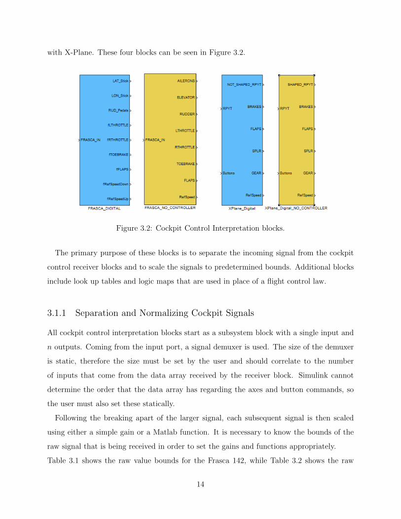
with X-Plane. These four blocks can be seen in Figure 3.2.
Figure 3.2: Cockpit Control Interpretation blocks.
The primary purpose of these blocks is to separate the incoming signal from the cockpit
control receiver blocks and to scale the signals to predetermined bounds. Additional blocks
include look up tables and logic maps that are used in place of a flight control law.
3.1.1 Separation and Normalizing Cockpit Signals
All cockpit control interpretation blocks start as a subsystem block with a single input and
n outputs. Coming from the input port, a signal demuxer is used. The size of the demuxer
is static, therefore the size must be set by the user and should correlate to the number
of inputs that come from the data array received by the receiver block. Simulink cannot
determine the order that the data array has regarding the axes and button commands, so
the user must also set these statically.
Following the breaking apart of the larger signal, each subsequent signal is then scaled
using either a simple gain or a Matlab function. It is necessary to know the bounds of the
raw signal that is being received in order to set the gains and functions appropriately.
Table 3.1 shows the raw value bounds for the Frasca 142, while Table 3.2 shows the raw
14

values for the incoming signals for X-Plane.
Table 3.1: Frasca 142 Raw Signal Bounds.
Signal Lower Bound Upper BoundLateral Stick -110 110Longitudinal Stick -66 92Pedals -95 95Left Toe Brake 0 30Right Toe Brake 0 30Left Throttle Quadrant 0 100Right Throttle Quadrant 0 100Flaps 0 100Left PTT button 0 (unpressed) 1 (pressed)Right PTT button 0 (unpressed) 1 (pressed)
Table 3.2: X-Plane Raw Signal Bounds.
Signal Lower Bound Upper BoundLateral Stick -1000 1000Longitudinal Stick -1000 1000Yaw Stick -1000 1000Throttle Quadrant -1000 1000Button [1-16] 0 (unpressed) 1 (pressed)
Given the signal bounds, mathematical operations are done on each in order to achieve
the bounds seen in Table 3.3.
Table 3.3: Normalized Input Signal Bounds.
Signal Lower Bound Upper BoundLateral Stick -1 1Longitudinal Stick -1 1Yaw -1 1Brakes 0 1Throttle Quadrant 0 100Flaps -1 1Button 0 (unpressed) 1 (pressed)
Normalizing most of the Frasca and X-Plane input values is done by using a gain block
15

defined by Equation 3.1.1.
gain =1
(upper bound of signal)(3.1.1)
For signals where the upper and lower bounds are not equal in magnitude, two different
methods of normalization can be used, with one being more straightforward than the other.
Some of the signals require a lower bound of 0, but their raw signal lower bound is nonzero,
requiring additional modification. Take, for example, a signal with a lower bound not equal
to 0, such as the Throttle Quadrant received from X-Plane. In order to normalize this, the
signal is first scaled using a gain determined by Equation 3.1.1. This results in the signal
with bounds of [-1, 1]. The signal then has 1 added to it to shift the bounds to [0, 2]. Finally,
a gain of 50 is used to bring the bounds to [0, 100]. A similar process is used to normalize the
Frasca flap signal as well as combining the left and right toe brake signals from the Frasca.
Another method of signal scaling is done through the use of a user-written Matlab function
block. For this function, the upper and lower bounds must be specified along with the
desired upper and lower bounds. These values must be coded into the function, and will
vary depending on the signal being supplied and the bounds desired. The normalized signal
is then given by Equation 3.1.2.
NormalizedSignal =(Input Signal − LBraw)
(UBraw − LBraw)∗ (UBdesired−LBdesired) +LBdesired (3.1.2)
where LB and UB are lower bound and upper bound respectively. This method is used for
the output from the Frasca longitudinal stick signal as it has asymmetrical bounds.
Following the scaling of the signals, a small dead-zone is added to the signal to accommo-
date the small ‘play’ in the controls that arise from analog signals, and reduce the sensitivity
around the center of the control. This dead-zone is not used for buttons. The use of dead-
zone blocks in Simulink brings about side effects however. The behavior of a Simulink
dead-zone block is to set the value of the signal to be 0 when it is within the specified dead-
zone bounds. The side effect is that the block will also offset the value of the signal outside
of the bounds by the value of either the upper or lower bound. As an example, consider a
16
lateral stick signal with bounds of [-1, 1]. This signal is put through a dead-zone block with
bounds of [-0.1, 0.1]. This will cause any signal between -0.1 and 0.1 to be effectively 0.0.
However, the maximum and minimum values that this signal will have now are 0.9 and -0.9,
respectively. It is important to keep this in mind when using such signals later in regards to
scheduling, as the perceived control effectiveness has been altered by the dead zone block.
Following the normalization and the application of a dead-zone, several of the signals are
multiplied by 100 and routed through global tags. These are signal routing goto tags that
have been changed from only being locally accessible to globally accessible. Several of the
signals, primarily those that account for joystick or yoke and pedal locations, brakes and the
landing gear, are given these global routing tags. These signals are used in displaying their
respective data via the cockpit gauge display that is discussed in Chapter 5, and the gain of
100 is used to aid in a smooth display of the value graphically. The use of these tags helps
to contain the amount of signal lines drawn within the model, and since they are needed in
simulations using the custom gauge display, share the same goto name as what is present in
the gauge feed block.
Key differences arise between using a USB joystick and the Frasca 142 cockpit. Current
implementation fo the Frasca does not utilize any digital buttons, whereas the joystick does.
Since the Frasca is intended to behave as a cockpit, it has the appropriate switches and
human interfaces to control an aircraft. The joystick is meant to be a universal device, used
for more than just flying aircraft, so additional work must be done to mimic a set of cockpit
controls. The digital buttons of the joystick are remapped to behave as trim adjustment,
landing gear switches, and brakes. These methods are discussed in subsection 3.1.2.
Finally, n number of output blocks are used, corresponding to the number of signals desired
from the interpretation. The size of n depends on if all signals will be fed separately, or less
than the number of input signals depending on if signals are combined in the interpretation
block. For use with the iReCoVeR flight control system, the number of outputs will equal
the number of input signals. In the cases that will be discussed in Section 3.1.2, n will be
less than the number of input signals.
17
3.1.2 Logic Maps, Digital Trim, and Scheduling
This section discusses the steps taken to create the logic maps, devices used to create trim and
scheduling the aircraft surfaces to the cockpit control signals. This allows for the simulation
to work without the iReCoVeR flight control system; the simulation will be flyable, using all
available control surfaces and can be tuned to meet the behavior the pilot desires.
Logic Mapping
Logic Mapping is used primarily in conjunction with the signals produced by button presses
as they are instantaneous and typically assigned to behave as switches. The mapping of
these buttons is done through a Stateflow[6] chart.
Stateflow is a separate environment from Simulink, but is easily integrated with Simulink
models and will work with the Simulink Coder and Embedded Coder. Using Stateflow is
similar to creating a mind map or flow chart. The chart contains several state blocks that
will dictate the value of the output. Each state block is then connected via conditional
transitions; as the set of conditions for a variable is met, the state will switch from one
block to the next block that is connected by the conditional transition. Stateflow can be
extended for use with algorithms and tables, and provides a means of creating logic without
programming a large nest of conditional blocks within Simulink.
In order to implement a landing gear toggle, a Stateflow chart was used in conjunction
with the X-Plane specific cockpit control interpretor. This is done only with X-Plane since
the USB joystick does not have any toggle switches, only buttons. The use of a Stateflow
chart in combination with a button can take on the characteristics of a toggle switch. Prior
to creating the Stateflow chart, the intended behavior of the button is described. As the
simulator will begin from an airport runway, the landing gear should start with being down.
Next, a single button press and release sequence should switch the landing gear from down
to up. A subsequent sequence should bring the gear back down.
The equivalent Stateflow map is then created as thus. Two separate state blocks are
created, one representing gear down and another for gear up. Each state contains a value
that will be the output from the Stateflow block; in this particular case gear down will be
18
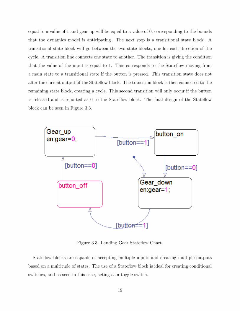
equal to a value of 1 and gear up will be equal to a value of 0, corresponding to the bounds
that the dynamics model is anticipating. The next step is a transitional state block. A
transitional state block will go between the two state blocks, one for each direction of the
cycle. A transition line connects one state to another. The transition is giving the condition
that the value of the input is equal to 1. This corresponds to the Stateflow moving from
a main state to a transitional state if the button is pressed. This transition state does not
alter the current output of the Stateflow block. The transition block is then connected to the
remaining state block, creating a cycle. This second transition will only occur if the button
is released and is reported as 0 to the Stateflow block. The final design of the Stateflow
block can be seen in Figure 3.3.
Figure 3.3: Landing Gear Stateflow Chart.
Stateflow blocks are capable of accepting multiple inputs and creating multiple outputs
based on a multitude of states. The use of a Stateflow block is ideal for creating conditional
switches, and as seen in this case, acting as a toggle switch.
19

Digital Trim
In order to maintain level flight without constant pilot interaction, the pilot needs a way to
set the trim values for yoke and rudder pedals. The trim acts to alter the value of the input
for the lateral, longitudinal and rudder pedals, without requiring the pilot to hold the yoke
or pedals at the trim position.
The Frasca 142 does not require additional components to create trim values for the
cockpit controls. As the trim wheels and trim hat are adjusted, the Frasca 142 will alter the
position of the yoke and pedals accordingly. Taking the longitudinal yoke as an example,
consider the current trim value to be set to 0, when the bounds for the signal from the
stick are [-1, 1], with the center at 0. If the trim position for the longitudinal command
corresponds to a value of 0.7, the pilot will hold the yoke at the trim point, and hold the
trim hat until there is no longer any pressure on the yoke at that point. The yoke will then
have a new ‘center’ at 0.7, and will still report a value of 0.7. In this case, there are no trim
values to report to or create within the Simulink model.
The USB joystick does not provide the same functionality as the Frasca 142, and requires
a method for the pilot to adjust the trim for each axes input. Instead of physical adjustments
to the position of the joystick, a set of two buttons will act to decrease and increase the trim
value. For ease of use, each button press will not correspond to a single incremental step,
but instead holding the button will increase or decrease the value. These digital trim values
will be created using Equations 3.1.3, and 3.1.4.
Trim Integral =
∫Trim Rate ∗ (BVincrease +BVdecrease) (3.1.3)
Trim V alue =
Boundupper if Trim V alue > Boundupper
Trim Integral if Boundlower ≤ Trim Integral ≤ Boundupper
Boundlower if Trim V alue < Boundlower
(3.1.4)
In Equation 3.1.3, BVincrease is the value of the button assigned to act as the increase to
the trim value, and BVdecrease is the value of the button assigned to act as the decrease
to the trim value. Additionally, the Trim Rate is a user-specified gain that controls the
20

rate at which the trim value is changed. In Equation 3.1.4, upper and lower bounds given
by Boundupper and Boundlower limit the value of the possible trim that can be set. The
equivalent Simulink diagram is presented in Figure 3.4.
Figure 3.4: Simulink diagram for creating trim values.
The Trim V alue is added to its accompanying signal; i.e. the yaw trim value is added to
the yaw command signal coming from the cockpit controls. This allows the pilot to let the
joystick return to its center, while still commanding the necessary amount of pitch, roll or
yaw needed to maintain level flight or a particular maneuver. The digital trimming method
can also be extended to adjusting the aircraft flaps as well as adjusting variables through
the use of momentary buttons. A similar design is used when a joystick is present to give
control of the flap position using two buttons; while using either the Frasca or joystick, the
digital trim method is used to allow the pilot to adjust a reference speed variable using two
buttons present on the controls.
Control Surface Scheduling
The lack of a full flight control presents some additional design requirements. At this point
in the construction, all of the available pilot control signals are normalized to their bounds
presented in Table 3.3. These normalized signals are useful in interacting with various flight
control laws and dynamic models, but they cannot drive the GTM dynamics model to its
full extent. In order to have full control of the aircraft surfaces, the cockpit control signals
have to be scheduled.
Scheduling in this case refers to the act of correlating the range of values that the signal
can take to the range that the control surface in question allows. Scheduling in this fashion
21
allows for full customization of the behavior the aircraft will exhibit due to the pilot input.
In this way, the sensitivity of the aircraft to control input is being adjusted. It is also
possible to change the sensitivity of various regions of the control input, creating a tailored
environment for the pilot and aircraft.
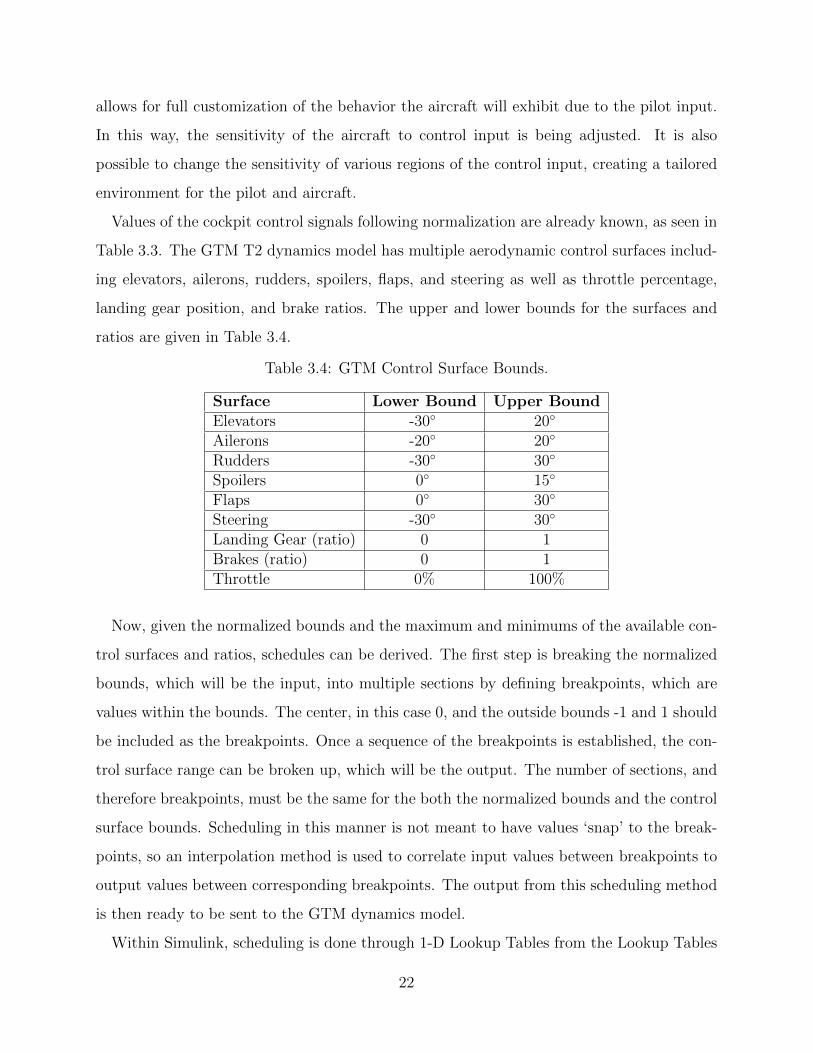
Values of the cockpit control signals following normalization are already known, as seen in
Table 3.3. The GTM T2 dynamics model has multiple aerodynamic control surfaces includ-
ing elevators, ailerons, rudders, spoilers, flaps, and steering as well as throttle percentage,
landing gear position, and brake ratios. The upper and lower bounds for the surfaces and
ratios are given in Table 3.4.
Table 3.4: GTM Control Surface Bounds.
Surface Lower Bound Upper BoundElevators -30◦ 20◦
Ailerons -20◦ 20◦
Rudders -30◦ 30◦
Spoilers 0◦ 15◦
Flaps 0◦ 30◦
Steering -30◦ 30◦
Landing Gear (ratio) 0 1Brakes (ratio) 0 1Throttle 0% 100%
Now, given the normalized bounds and the maximum and minimums of the available con-
trol surfaces and ratios, schedules can be derived. The first step is breaking the normalized
bounds, which will be the input, into multiple sections by defining breakpoints, which are
values within the bounds. The center, in this case 0, and the outside bounds -1 and 1 should
be included as the breakpoints. Once a sequence of the breakpoints is established, the con-
trol surface range can be broken up, which will be the output. The number of sections, and
therefore breakpoints, must be the same for the both the normalized bounds and the control
surface bounds. Scheduling in this manner is not meant to have values ‘snap’ to the break-
points, so an interpolation method is used to correlate input values between breakpoints to
output values between corresponding breakpoints. The output from this scheduling method
is then ready to be sent to the GTM dynamics model.
Within Simulink, scheduling is done through 1-D Lookup Tables from the Lookup Tables
22
toolbox. The input to the block is the normalized cockpit control signals, with trim added
if applicable, and the output will be the GTM control surface deflection. From the block
parameters window, on the Table and Breakpoints tab, the input value breakpoints are
entered as a vector into the Breakpoints field. The next step is to set the interpolation
method as well as the behavior of the scheduling if the input should ever exceed the bounds
on the vector in the Breakpoints field. Switching to the algorithm tab, the interpolation
method is set to ‘Linear’. The extrapolation method is then set to ‘Clip’, and then the
setting to use the last table value as values for inputs at or beyond the last breakpoint is
enabled.
An additional consideration must be made for signals that have been run through a dead-
zone block. Since the behavior of the Simulink dead zone block is to reduce the magnitude
of the signal by the upper bound when it is greater than the upper bound, and by the lower
bound when it is less than the lower bound, the breakpoints must reflect that as well. As an
example, the scheduling for the aileron displacement using the Frasca lateral stick command
will be used. The lateral stick signal has been normalized to the bounds of [-1, 1], and put
through a dead zone block with dead zone bounds of [-0.05, 0.05]. The new bounds of this
signal are effectively [-0.95, 0.95]. When establishing the breakpoints for the lookup table,
these new bounds should be used.
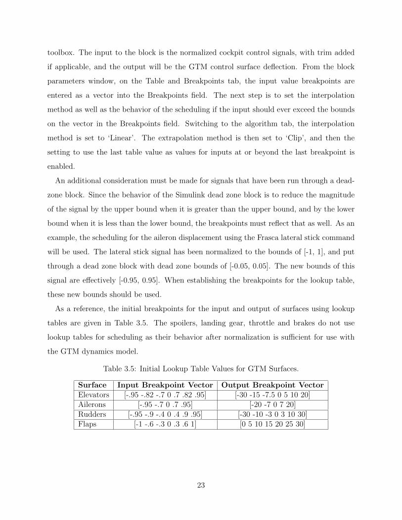
As a reference, the initial breakpoints for the input and output of surfaces using lookup
tables are given in Table 3.5. The spoilers, landing gear, throttle and brakes do not use
lookup tables for scheduling as their behavior after normalization is sufficient for use with
the GTM dynamics model.
Table 3.5: Initial Lookup Table Values for GTM Surfaces.
Surface Input Breakpoint Vector Output Breakpoint VectorElevators [-.95 -.82 -.7 0 .7 .82 .95] [-30 -15 -7.5 0 5 10 20]Ailerons [-.95 -.7 0 .7 .95] [-20 -7 0 7 20]Rudders [-.95 -.9 -.4 0 .4 .9 .95] [-30 -10 -3 0 3 10 30]Flaps [-1 -.6 -.3 0 .3 .6 1] [0 5 10 15 20 25 30]
23

3.1.3 Placeholder Input Generator
The final piece of the current cockpit control interpretation blocks is the input generator
block. This block is the housing for the flight control law, once developed. Current imple-
mentation is a placeholder block that separates the incoming control surface commands into
the multitude of components that compromise each surface category, e.g. the rudder surface
command is separated into upper and lower rudder commands. There are gains in place that
will flip signals as necessary. The aileron command that is generated from the interpretation
blocks is valid for right side ailerons, so a negative multiplier is used to change the signal for
left side aileron displacements.
This is a generic block with inputs for ailerons, elevators, rudder, flaps, throttles, brakes,
and landing gear. The output is a mux of 21 signals, comprised of the combination of
left/right, inside/outside,and upper/lower, depending on the surface. This separations are
standard and provided in the base GTM Simulink diagram.
3.2 X-Plane Communication and Graphic Driving Blocks
This section discusses the blocks developed to send and receive information for X-Plane.
These blocks provide the location and orientation of the aircraft, and receive graphic envi-
ronment variables and joystick commands if applicable.
3.2.1 Simulink to X-Plane Block
The main driving block for X-Plane communication is the Simulink to X-Plane block. This
is a masked subsystem that has three inputs and two available outputs. The first input is
the vector describing the location of the aircraft in 3-dimensional space. The second input
is the vector containing the displacements for the aircraft control surfaces. The third input
is a vector of up to a size of 6 that can be displayed in X-Plane via an overlay. If a full six
values are not provided, the remaining slots of the vector will be filled with 0. This third
input does not need to be provided for the simulator to operate correctly. The first output
is a vector of the first 16 joystick axes from X-Plane, and the second output is the vector of
24

the first 16 buttons assigned in X-Plane to the Xlink plugin. Finally, the mask allows for
a user input of a vector of strings that correspond to the labels for the overlay values that
will be used in the HUD overlay. The format for the input vectors and mask input string
are provided as reference in Table 3.6.
Table 3.6: Simulink to X-Plane Block IO Format.
Input Format(units)
Position[Latitude(degrees), Longitude(degrees),
Elevation(meters),Phi(degrees), Theta(degrees), Psi(degrees)]
Surfaces[Aileron(degrees), Elevator(degrees), Rudder(degrees),Flaps(degrees), Spoiler(degrees), Landing Gear(ratio)]
Overlay(optional,size variable)
[Value1, Value2, Value3, Value4, Value5, Value6]
HUD OverlayText (MaskInput)
{‘Text1’, ‘Text2’, ‘Text3’, ‘Text4’, ‘Text5’, ‘Text6’}
Underneath the masked subsystem are the multiple input ports and a constant block.
These input ports correspond to the block inputs, and the constant block holds the cell
array of text strings the user has specified. These inputs are fed directly to an S-Function
block. The overlay input port is muxed with a row vector of 6 zeros, with the overlay
signal populating the mux block first. The muxed signal is then demuxed into two signals
again. The first signal contains the first 6 values of the muxed signal and sent to the S-
Function block; remaining values are put in the second signal and sent to a terminator.
The S-Function block references the S-Function that has been created to communicate with
the X-Plane plugin. This function is discussed further in Section 4.3. The outputs of the
S-Function block are sent to output ports that correspond to the joystick values and button
values received from X-Plane. The third output of the S-Function block is labeled ‘Y-AGL’,
which corresponds to a X-Plane dataref. This value is the elevation of the ‘ground’ below
the aircraft in X-Plane. This value is routed through a global goto tag, and used to prevent
the aircraft from going through the ground during simulations.
25

3.2.2 X-Plane Feed Block
The X-Plane Feed block creates the two signals required by the Simulink to X-Plane block
to display the aircraft and its control surfaces in the world. This block requires no inputs,
and its outputs of ‘XP POS’ and ‘XP SURF’ correspond with the inputs on the Simulink
to X-Plane block.
This subsystem uses signal routing tags to pull the global ‘Sensors’ and ‘SurfacePos’ signals
into the block. These signals are then put into a Bus Creator block and then put into a
SelectOutputs block. Within the SelectOutputs block, certain signals are selected. The
signals selected and the correct order are provided in Table 3.7. This new signal is then sent
to a Bus Selector where it is broken into its individual components.
Table 3.7: X-Plane Signal Feed Components.
OriginatingSignal
Selected Component Signal Name
Sensors
MIDG.NAV latitude degMIDG.NAV longitude degMIDG.NAV altitude mMIDG.phi degMIDG.theta degMIDG.psi deg
SurfacePos
AILRELLOBRUDUFLAPLOBSPLLOBGEAR
Following selecting those particular signals, the latitude, longitude, elevation, phi, theta,
and psi are muxed into a single signal and sent to an output port. The aileron, elevator,
rudder, flap, spoiler and landing gear signals are muxed into a single signal and sent to
an output port as well. The signals for altitude, phi, theta, psi, flap position and spoiler
position are given global signal routing tags, as their values will be called in the Gauge Feed
block, and doing this prevents polluting the Simulink diagram. It also saves on memory at
run time as the same process to extract the signals will not have to be repeated elsewhere.
26

3.2.3 Gauge Feed Block
The Gauge Feed block operates similarly to the X-Plane Feed block. It pulls values from the
dynamics model and the cockpit control blocks, preparing them to be sent to the custom
gauge set. This block requires no inputs, and its sole output will later be fed to an S-Function
block that contains the S-Function responsible for sending the data to the gauges.
It begins by using signal routing tags to pull in the global signals ‘SurfacePos’, ‘Sensors’,
‘Engines’, and ‘RefSpeed’. These signals are fed into a Bus Creator block, and then into a
SelectOutputs block. The needed signals are selected from the list; the used signals and the
order are provided in Table 3.8.
Table 3.8: Gauge Signal Feed Components.
OriginatingSignal
Selected Component Signal Name
Sensors
AirData.altitude ftAirData.KTASMIDG.NAV Vu mpsMAG3.Ay gMAG3.Az gMAG3.p degMAG3.q degMAG3.r deg
SurfacePosTHROTLTHROTR
EnginessRPMLRPMR
RefSpeed (No subcomponents in this signal)
Unlike the X-Plane Feed block, these signals are not all in the necessary units, scale
or are used to calculate variables not directly available from the GTM dynamics model.
Additionally, signal routing tags are also used to pull in additional data. To begin, the
required data and their units that need to be provided to the custom gauge set are provided
in Table 3.9.
Next, the process of obtaining the needed output data is detailed based on the signals
available from the bus selector and signal routing tags.
The altitude output is a direct feed from the altitude data, as is the airspeed from the
27

Table 3.9: Gauge Feed Output Format.
Data UnitsAltitude feetAirspeed knotsRoll degreesPitch degreesVertical Speed 100s of feet/secondHeading degreesY-Axis Acceleration geesZ-Axis Acceleration geesZ-Axis Angular Velocity degrees/secondLeft Throttle percentageRight Throttle percentageLeft Engine RPM 1000s of rotations/minuteRight Engine RPM 1000s of rotations/minuteFlap Position degreesSpoiler Position degreesReference Speed knotsBrake ratio [0,1]Landing Gear ratio [0,1]Lateral Yoke Position ratio [-100, 100]Longitudinal Yoke Position ratio [-100,100]Rudder Pedal Position ratio [-100,100]
true airspeed data. The roll, pitch and heading outputs are derived from the conversion of
radians to degrees of the phi, theta and psi data from the navigation sensors. The vertical
speed comes from a meters/second to 100s of feet/minute conversion of the NAV Vu mps
signal. The RPM values for both engines are divided by 1000 in order to facilitate their
display. The z-axis angular velocity is derived from Equation 3.2.1
ψ̇ = q ∗ sin(φ)
cos(θ)+ r ∗ cos(φ)
cos(θ)(3.2.1)
where φ and θ are in degrees and q and r are in degrees per second. Phi and theta come
from navigation sensors, and q and r were selected from sensor data.
The remaining data in Table 3.9 not explicitly described in the previous paragraph are
direct feed through from their input counterparts, whether they be from a signal routing
tag, as in the case for yoke/pedal positions, landing gear ratio, brake ratio, flap and spoiler
28

positions and the reference speed. Once all signals are fed into a mux block in the order in
Table 3.9, they are forced to be of data type double, and then sent to the output port of the
block.
This feed block is easily adapted to new gauge sets, as additional displays and instruments
are needed. All that needs to be adjusted is the size of the mux block that combines the
data signals before the output port, and adding a source for the new data. From there,
the S-Function that drives the gauge, seen in Section 4.2, just needs to be adjusted to
accommodate the new signal size.
3.2.4 Visual Ground Elevation Block
The GTM dynamics model allows for setting a static runway altitude during the initialization
of the system. This altitude is referenced from sea level, and acts as a switch for the landing
gear calculations. If the aircraft is at or below the specified runway altitude, then the landing
gear calculations are triggered, and attempt to prevent the aircraft from going through the
ground. This static method does not work well when simulating in X-Plane. This is because
it is possible, depending on location, for the graphics for the ground to be at an elevation
different than the one specified in the initialization. This would result in either the aircraft
being displayed below the surface of the Earth, or hovering above it, rather than resting on
it at landing and takeoff.
Modifications were made to provide a more accurate graphical representation of a full
flight. First, the Simulink library for the landing gear was modified to include a signal
routing tag for the variable ‘Ground Elevation’. This tag replaces the constant block that
was referencing the static runway altitude from the initialization. This allows the the model
to dynamically change the ground elevation from elsewhere in the model.
The Visual Ground Elevation block is a masked subsystem that has no input or output
ports, and only needs to be placed in a Simulink diagram containing the Simulink to X-Plane
block and the X-Plane Feed block. These dependencies exist due to the internal workings of
the Visual Ground Elevation block. Within the masked subsystem, are two signal routing
tags, one for ‘NAVELEm’, which comes from the X-Plane Feed block, and ‘Y AGL’, which
29

comes from the Simulink to X-Plane block. Using an additional buffer value (in meters) that
will vary based on the aircraft rendering in X-Plane, these values are then converted to a
ground elevation in feet that the landing gear block can use by using Equation 3.2.2. This
value is then sent through a global signal routing tag for ‘Ground Elevation’, for use with
the GTM landing gear dynamics.
Elevationground = 3.28 ∗ (NAVELEm + buffer − Y AGL) (3.2.2)
3.3 Additional Library Blocks
Several additional blocks are included in the CNCT Simulink library. These are S-Function
blocks that have been pre-filled to facilitate the creation of new models. The contents and
operations of these S-Functions are discussed in Chapter 4. There is also a global signal
routing tag provided that is meant to be attached to a reference speed signal that will be
displayed by the gauges.
The first of these additional blocks is a block containing the S-Function that operates the
communication between the Simulink diagram and the Frasca system. This block has one
output port, and it connects to the Frasca cockpit interpretation block. The next is the
block containing the S-Function that operates the communication with the custom gauge
set. This block has only one input port, and it should be connected to the output port of the
Gauge Feed block in order to operate the gauges correctly. The last of the additional blocks
is the S-Function block that operates the communication between Simulink and the X-Plane
plugin. This block is provided as a reference, as it should not be used as a standalone. This
is identical to the S-Function block housed in the Simulink to X-Plane masked subsystem
discussed in Subsection 3.2.1. There are input ports for aircraft location, surface positions,
HUD overlay strings, and HUD overlay values, respectively. There are three output ports
corresponding to joystick axes values, button values, and the elevation of the ground being
displayed below the aircraft, respectively.
30

3.3.1 Required Blocks not in the CNCT Library
Additional blocks that are not provided by the CNCT Library are required to have the
simulation run correctly. Simulink’s default behavior is to run its solver as quickly as the
computer’s processor and available memory will allow it to. This is ideal for testing control
algorithms and systems that do not need to operate in real-time. However, such behavior
is not ideal for implementation in a simulator where the need for real-time interactions and
response are paramount.
Ideally, the dynamics and flight control system are run in real-time using a real-time com-
puter and operating system. Such an implementation requires dedicated hardware which is
not currently available to the project, so adjustments are made to achieve a similar environ-
ment. The current method is to force the Simulink solver to match its internal clock to the
clock on the computer, in a 1:1 fashion.
This matching is achieved by implementing the Simulation Pace block that is available
in the Aerospace Toolbox blockset. The Simulation Pace block has the user specify the
simulation pace, in this case 1 simulation second per clock second, and the sample time,
which is the time step used in conjunction with a fixed step solver. The user also has the
option of viewing the difference between the simulation clock and system clock, in order to
verify the validity of the soft real-time.
31

CHAPTER 4
S-FUNCTION AND X-PLANE PLUGIN CODE
The various components of the simulator are connected via a local computer network. The
communication between these various computers happens via user datagram protocol (UDP).
The Frasca sends data packets with the positions of its components, the Simulink system
receives data from the Frasca, sends and receives data from X-Plane, and sends data to the
gauges. In turn, X-Plane also sends and receives data from the Simulink system, as do the
gauges. These links are accomplished through the use of S-Functions within the Simulink
system, a plugin in X-Plane and built in communication in the gauge set. In this chapter,
the S-Functions will be covered in detail, and the X-Plane plugin, which has been provided
by NASA as part of the GTM DesignSim package, and the additions to it will be given an
overview.
S-Functions are programs written in C/C++ and compiled using Matlab’s MEX compiler
chain. There are Matlab specific functions and calls that are used in the S-Functions that
allow it access to many of Matlab’s built-in functions and provide the ability to properly
integrate into the Simulink system. For the purposes of this simulator, the coding language
of choice was C++. Many of these functions rely on the Winsock2 library, which is part
of the Windows SDK, provided for free by Microsoft[7]. In some cases, a networking li-
brary provided by XSquawkBox, PCSBSocketUDP[8], is used. PCSBSocketUDP provides
networking classes that simplify the implementation of the Winsock2 library, and extends
support to OSX and Linux as well.
For implementation as a Simulink block, the code is written as a level-2 S-Function. The
important functions of such files are as follows:
• static void mdlInitializeSizes(SimStruct *S): This function is called to set correct di-
mensions of the block e.g. number of input and output ports and their type. Further-
32
more, states of the block are also initialized in this function.
• static void mdlStart(SimStruct *S): This function is called only at the start of the
simulation, and must be defined explicitly in the source code (#define MDL START).
This function is used to initialize the UDP sockets for most of the S-Functions.
• static void mdlOutputs(SimStruct *S, int T tid): This function is called during ex-
ecution and is used to calculate the output of the block after each time step of the
simulation. This function is used to prepare data for UDP communication to X-Plane
and the cockpit display, and to prepare data received over UDP for the Simulink en-
vironment.
• static void mdlTerminate(SimStruct *S): This function is only run when the simulation
is stopped, and will be used to close and clean up the UDP sockets that are created in
the start of the simulation.
The following sections will describe the flow of each S-Function, and then provide snippets
of the source code that achieve the steps outlined.
4.1 Frasca to Simulink Communication
This function will handle the receiving of UDP packets containing the values of various
Frasca components. The current list of variables and their ranges can be seen in Table 3.1.
It will then use the data packet to create the composite signal of those values that can be
used by the cockpit interpretation blocks outlined in Section 3.1.
The C++ code begins by declaring that there are 0 inputs and 1 output for this function,
as well as including the header file that contains the local IP addresses and ports for the
Frasca and Simulink computers. The header file containing the data packet structure is also
included. This function utilizes the PCSBSocketUDP networking class, so the header file is
also included. The mdlInitializeSizes function is then populated, declaring the size of the
output port. The size of the output port is equal to the number of components of the data
structure. Finally, the size of the pointer work vectors for the function is set to 2. The
33
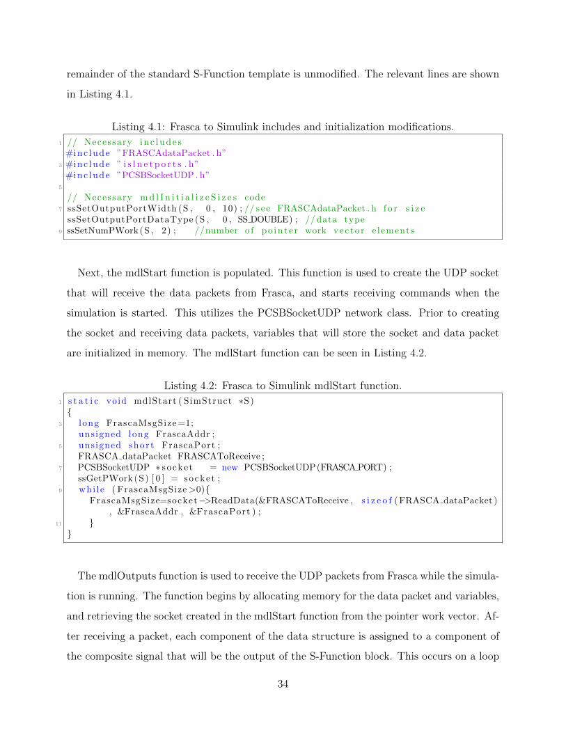
remainder of the standard S-Function template is unmodified. The relevant lines are shown
in Listing 4.1.
Listing 4.1: Frasca to Simulink includes and initialization modifications.
1 // Necessary i n c l ud e s#inc lude ”FRASCAdataPacket . h”
3 #inc lude ” i s l n e t p o r t s . h”#inc lude ”PCSBSocketUDP . h”
5
// Necessary md l I n i t i a l i z e S i z e s code7 ssSetOutputPortWidth (S , 0 , 10) ; // see FRASCAdataPacket . h f o r s i z essSetOutputPortDataType (S , 0 , SS DOUBLE) ; // data type
9 ssSetNumPWork(S , 2) ; //number o f po in t e r work vec to r e lements
Next, the mdlStart function is populated. This function is used to create the UDP socket
that will receive the data packets from Frasca, and starts receiving commands when the
simulation is started. This utilizes the PCSBSocketUDP network class. Prior to creating
the socket and receiving data packets, variables that will store the socket and data packet
are initialized in memory. The mdlStart function can be seen in Listing 4.2.
Listing 4.2: Frasca to Simulink mdlStart function.
1 s t a t i c void mdlStart ( SimStruct ∗S){
3 long FrascaMsgSize=1;unsigned long FrascaAddr ;
5 unsigned shor t FrascaPort ;FRASCA dataPacket FRASCAToReceive ;
7 PCSBSocketUDP ∗ socke t = new PCSBSocketUDP(FRASCA PORT) ;ssGetPWork (S) [ 0 ] = socke t ;
9 whi le ( FrascaMsgSize>0){FrascaMsgSize=socket−>ReadData(&FRASCAToReceive , s i z e o f (FRASCA dataPacket )
, &FrascaAddr , &FrascaPort ) ;11 }}
The mdlOutputs function is used to receive the UDP packets from Frasca while the simula-
tion is running. The function begins by allocating memory for the data packet and variables,
and retrieving the socket created in the mdlStart function from the pointer work vector. Af-
ter receiving a packet, each component of the data structure is assigned to a component of
the composite signal that will be the output of the S-Function block. This occurs on a loop
34

for as long as the simulation is running. The full mdlOutputs function can be seen in
Listing 4.3.
Listing 4.3: Frasca to Simulink mdlOutputs function.
s t a t i c void mdlOutputs ( SimStruct ∗S , int T t i d ) {2 r ea l T ∗y1 = ssGetOutputPortRealSignal (S , 0 ) ;
i n t i =0;4 long FrascaOutMsgSize=1;
unsigned long FRASCAAddr ;6 unsigned shor t FRASCAPort ;
FRASCA dataPacket FRASCAToReceive ;8 PCSBSocketUDP ∗ socke t = s t a t i c c a s t <PCSBSocketUDP∗>(ssGetPWork (S) [ 0 ] ) ;
10 // Receive FRASCA Commandswhi l e ( FrascaOutMsgSize>0){
12 FrascaOutMsgSize=socket−>ReadData(&FRASCAToReceive , s i z e o f (FRASCA dataPacket ) , &FRASCAAddr, &FRASCAPort) ;
i f ( FrascaOutMsgSize == s i z e o f (FRASCA dataPacket ) ) {14 y1 [0 ]=( double ) ( FRASCAToReceive . a i l ) ;
y1 [1 ]=( double ) ( FRASCAToReceive . e l e v ) ;16 y1 [2 ]=( double ) ( FRASCAToReceive . rudd ) ;
y1 [3 ]=( double ) ( FRASCAToReceive . l t b r ) ;18 y1 [4 ]=( double ) ( FRASCAToReceive . r tb r ) ;
y1 [5 ]=( double ) ( FRASCAToReceive . l t h r ) ;20 y1 [6 ]=( double ) ( FRASCAToReceive . r th r ) ;
y1 [7 ]=( double ) ( FRASCAToReceive . f l a p ) ;22 y1 [8 ]=( double ) ( FRASCAToReceive . PTT left ) ;
y1 [9 ]=( double ) ( FRASCAToReceive . PTT right ) ;24 }
}26 }
The last function, mdlTerminate, is used to close the UDP socket and delete it from
memory once the simulation is stopped. This is accomplished through a function in the
PCSBSocketUDP class and a delete command.
4.2 Simulink to Gauge Set Communication
This function will handle the sending of UDP packets containing the values needed for the
gauge set. The current list of variables can be seen in Table 3.9. The composite signal being
fed into the S-Function will be used to create a data packet that the gauge set can interpret
and use to update the display for the pilot.
35
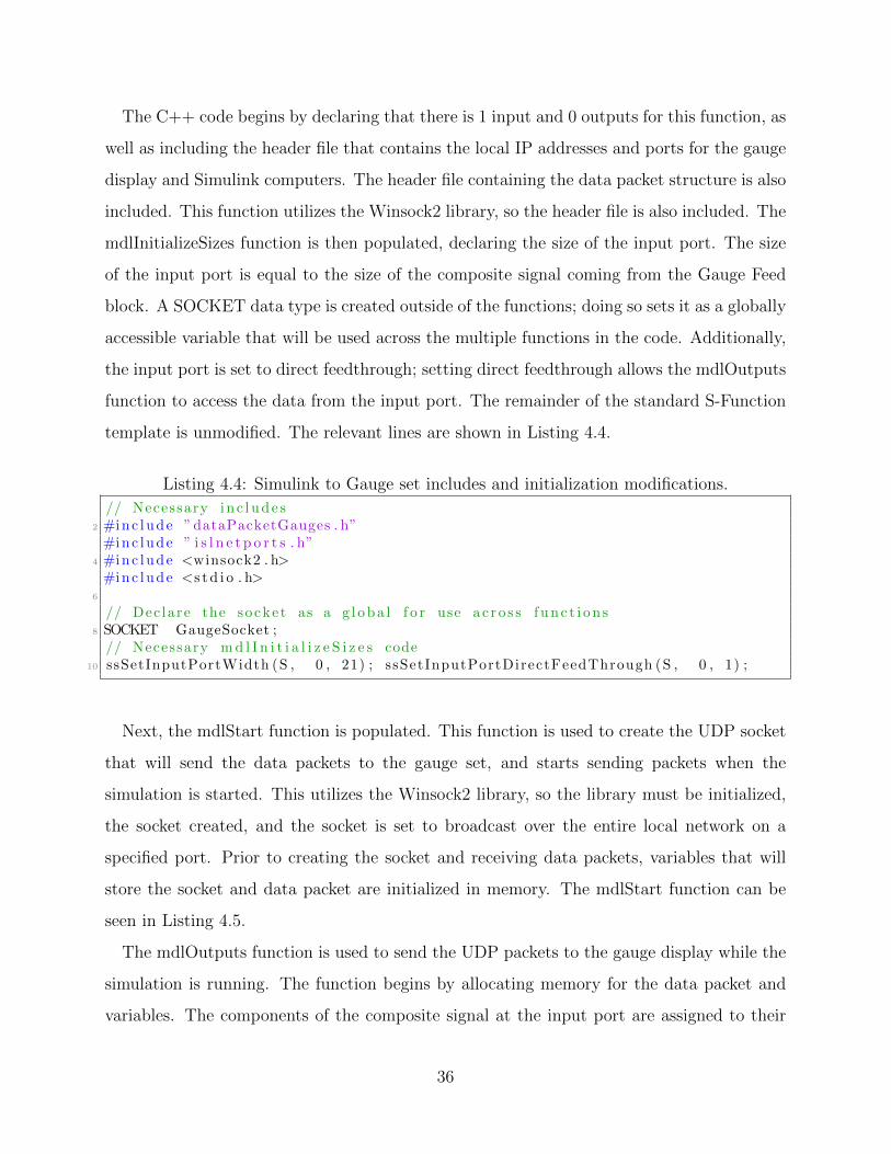
The C++ code begins by declaring that there is 1 input and 0 outputs for this function, as
well as including the header file that contains the local IP addresses and ports for the gauge
display and Simulink computers. The header file containing the data packet structure is also
included. This function utilizes the Winsock2 library, so the header file is also included. The
mdlInitializeSizes function is then populated, declaring the size of the input port. The size
of the input port is equal to the size of the composite signal coming from the Gauge Feed
block. A SOCKET data type is created outside of the functions; doing so sets it as a globally
accessible variable that will be used across the multiple functions in the code. Additionally,
the input port is set to direct feedthrough; setting direct feedthrough allows the mdlOutputs
function to access the data from the input port. The remainder of the standard S-Function
template is unmodified. The relevant lines are shown in Listing 4.4.
Listing 4.4: Simulink to Gauge set includes and initialization modifications.
// Necessary i n c l ud e s2 #inc lude ”dataPacketGauges . h”#inc lude ” i s l n e t p o r t s . h”
4 #inc lude <winsock2 . h>#inc lude <s t d i o . h>
6
// Dec lare the socke t as a g l oba l f o r use a c r o s s f unc t i on s8 SOCKET GaugeSocket ;// Necessary md l I n i t i a l i z e S i z e s code
10 ssSetInputPortWidth (S , 0 , 21) ; ssSetInputPortDirectFeedThrough (S , 0 , 1) ;
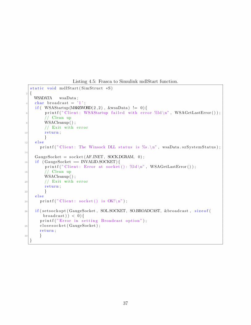
Next, the mdlStart function is populated. This function is used to create the UDP socket
that will send the data packets to the gauge set, and starts sending packets when the
simulation is started. This utilizes the Winsock2 library, so the library must be initialized,
the socket created, and the socket is set to broadcast over the entire local network on a
specified port. Prior to creating the socket and receiving data packets, variables that will
store the socket and data packet are initialized in memory. The mdlStart function can be
seen in Listing 4.5.
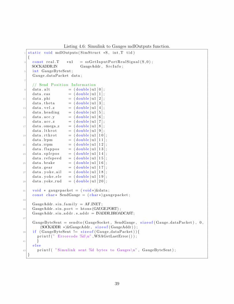
The mdlOutputs function is used to send the UDP packets to the gauge display while the
simulation is running. The function begins by allocating memory for the data packet and
variables. The components of the composite signal at the input port are assigned to their
36
Listing 4.5: Frasca to Simulink mdlStart function.
s t a t i c void mdlStart ( SimStruct ∗S)2 {
WSADATA wsaData ;4 char broadcast = ’ 1 ’ ;
i f ( WSAStartup(MAKEWORD(2 ,2 ) , &wsaData ) != 0) {6 p r i n t f ( ” C l i en t : WSAStartup f a i l e d with e r r o r %ld \n” , WSAGetLastError ( ) ) ;
// Clean up8 WSACleanup ( ) ;
// Exit with e r r o r10 re turn ;
}12 e l s e
p r i n t f ( ” C l i en t : The Winsock DLL s ta tu s i s %s .\n” , wsaData . szSystemStatus ) ;14
GaugeSocket = socket (AF INET , SOCKDGRAM, 0) ;16 i f ( GaugeSocket == INVALID SOCKET) {
p r i n t f ( ” C l i en t : Error at socke t ( ) : %ld \n” , WSAGetLastError ( ) ) ;18 // Clean up
WSACleanup ( ) ;20 // Exit with e r r o r
re turn ;22 }
e l s e24 p r i n t f ( ” C l i en t : socke t ( ) i s OK!\n” ) ;
26 i f ( s e t sockopt (GaugeSocket , SOL SOCKET, SO BROADCAST, &broadcast , s i z e o f (broadcast ) ) < 0) {
p r i n t f ( ”Error in s e t t i n g Broadcast opt ion ” ) ;28 c l o s e s o c k e t ( GaugeSocket ) ;
r e turn ;30 }}
37

respective parts of the data packet structure. The data structure is then cast into a void
pointer type then a character pointer type; this has to be done for the Winsock2 commands
to work correctly. A SOCKADDR IN data structure is then populated with the description
of the computer the packets will be sent to; this structure includes the internet protocol
version, the IP address and the port. The data packet is then sent over UDP. This occurs
on a loop for as long as the simulation is running. The mdlOutputs function can be seen in
Listing 4.6.
The last function, mdlTerminate, is used to close the UDP socket and delete it from
memory once the simulation is stopped. This is accomplished through the closesocket()
function and the WSAClean() function.
4.3 Simulink & X-Plane Communication
This function will handle the receiving and sending of UDP packets between Simulink and
X-Plane. The data that will be sent to X-Plane can be seen in Table 3.6. It will receive
a data packet containing the joystick axes and button values registered in X-Plane, as well
as the elevation of the ground below the aircraft being displayed. The data it receives will
be output 2 composite signals and a single signal. The composite signals can then either
be terminated if they are not used, as in the case of use with the Frasca, or routed to the
X-Plane cockpit interpretation blocks outlined in Section 3.1. The last signal is always used.
The C++ code begins by declaring that there are 4 inputs and 3 outputs for this function,
as well as including the header file that contains the local IP addresses and ports for the
X-Plane and Simulink computers. The header file containing the data packet structure is
also included. This function utilizes the PCSBSocketUDP networking class, so the header
file is also included. The mdlInitializeSizes function is then populated, declaring the size and
type of each output port, and the size and feedthrough setting for each input port. The sizes
of the joystick and button output ports are set to 16, since that is the amount the X-Plane
plugin will send back for each. The input port widths are 6, 6, 90 and 6; these account for
the location information, surface position information, the maximum number of characters
for the HUD overlay and the maximum number of values the HUD will display. Finally, the
38
Listing 4.6: Simulink to Gauges mdlOutputs function.
1 s t a t i c void mdlOutputs ( SimStruct ∗S , int T t i d ){
3 const r ea l T ∗u1 = ssGetInputPortRea lS igna l (S , 0 ) ;SOCKADDR IN GaugeAddr , S r c In f o ;
5 i n t GaugeByteSent ;Gauge dataPacket data ;
7
// Send Pos i t i on Informat ion9 data . a l t = ( double ) u1 [ 0 ] ;
data . eas = ( double ) u1 [ 1 ] ;11 data . phi = ( double ) u1 [ 2 ] ;
data . theta = ( double ) u1 [ 3 ] ;13 data . v e l z = ( double ) u1 [ 4 ] ;
data . heading = ( double ) u1 [ 5 ] ;15 data . acc y = ( double ) u1 [ 6 ] ;
data . a c c z = ( double ) u1 [ 7 ] ;17 data . omega z = ( double ) u1 [ 8 ] ;
data . l t h r o t = ( double ) u1 [ 9 ] ;19 data . r th r o t = ( double ) u1 [ 1 0 ] ;
data . lrpm = ( double ) u1 [ 1 1 ] ;21 data . rrpm = ( double ) u1 [ 1 2 ] ;
data . f l appo s = ( double ) u1 [ 1 3 ] ;23 data . sp l r po s = ( double ) u1 [ 1 4 ] ;
data . r e f s p e ed = ( double ) u1 [ 1 5 ] ;25 data . brake = ( double ) u1 [ 1 6 ] ;
data . gear = ( double ) u1 [ 1 7 ] ;27 data . y o k e a i l = ( double ) u1 [ 1 8 ] ;
data . yok e e l e = ( double ) u1 [ 1 9 ] ;29 data . yoke rud = ( double ) u1 [ 2 0 ] ;
31 void ∗ gaugepacket = ( void ∗)&data ;const char ∗ SendGauge = ( char ∗) gaugepacket ;
33
GaugeAddr . s i n f am i l y = AF INET ;35 GaugeAddr . s i n p o r t = htons (GAUGEPORT) ;
GaugeAddr . s i n addr . s addr = INADDRBROADCAST;37
GaugeByteSent = sendto (GaugeSocket , SendGauge , s i z e o f ( Gauge dataPacket ) , 0 ,(SOCKADDR ∗)&GaugeAddr , s i z e o f (GaugeAddr ) ) ;
39 i f ( GaugeByteSent != s i z e o f ( Gauge dataPacket ) ) {p r i n t f ( ” Errorcode %d\n” ,WSAGetLastError ( ) ) ;
41 }e l s e
43 p r i n t f ( ” Simulink sent %d bytes to Gauges\n” , GaugeByteSent ) ;}
39

size of the pointer work vectors for the function is set to 2. The remainder of the standard
S-Function template is unmodified. The relevant lines are shown in Listing 4.7.
Listing 4.7: Simulink/X-Plane IO includes and initialization modifications
// Necessary i n c l ud e s2 #inc lude ”dataPacket2 . h”#inc lude ” i s l n e t p o r t s . h”
4 #inc lude ”PCSBSocketUDP . h”
6 // Necessary md l I n i t i a l i z e S i z e s codessSetInputPortWidth (S , 0 , 6) ; // la t , lon , a l t , Rol l , Pitch ,Yaw,
8 ssSetInputPortDataType (S , 0 , SS DOUBLE) ;ssSetInputPortDirectFeedThrough (S , 0 , 1) ;
10
ssSetInputPortWidth (S , 1 , 6) ; // Sur f a c e s ( a i l , e l ev , rud , f l ap , sp l r , gear )12 ssSetInputPortDataType (S , 1 , SS DOUBLE) ;
ssSetInputPortDirectFeedThrough (S , 1 , 1) ;14
ssSetInputPortWidth (S , 2 , 90) ; // HUD Text16 ssSetInputPortDataType (S , 2 , SS UINT8) ;
ssSetInputPortDirectFeedThrough (S , 2 , 1) ;18
ssSetInputPortWidth (S , 3 , 6) ; // HUD Values20 ssSetInputPortDataType (S , 3 , SS DOUBLE) ;
ssSetInputPortDirectFeedThrough (S , 3 , 1) ;22
ssSetOutputPortWidth (S , 0 , 16) ; // Joy s t i ck Axes [max o f 16 ]24 ssSetOutputPortDataType (S , 0 , SS DOUBLE) ;
26 ssSetOutputPortWidth (S , 1 , 16) ; //Buttons [1−16]ssSetOutputPortDataType (S , 1 , SS DOUBLE) ;
28
ssSetOutputPortWidth (S , 2 , 1) ; // ground l e v e l30 ssSetOutputPortDataType (S , 2 , SS DOUBLE) ;
32 ssSetNumPWork(S , 2) ; //number o f po in t e r work vec to r e lements
Next, the mdlStart function is populated. This function is used to create the UDP socket
that will send and receive the data packets between Simulink and X-Plane, and starts receiv-
ing commands when the simulation is started. This utilizes the PCSBSocketUDP network
class. Prior to creating the socket and receiving data packets, variables that will store the
socket and data packet are initialized in memory. The mdlStart function can be seen in
Listing 4.8.
The mdlOutputs function does the work to create the data packets that will be sent to
40
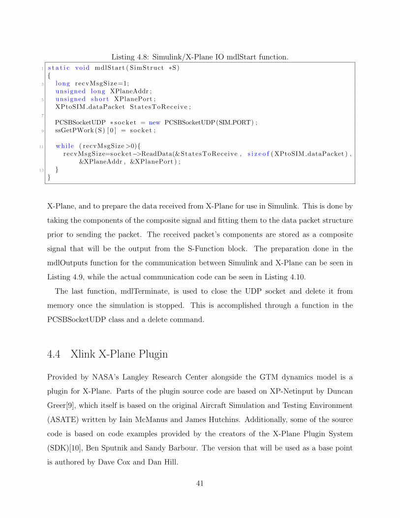
Listing 4.8: Simulink/X-Plane IO mdlStart function.
1 s t a t i c void mdlStart ( SimStruct ∗S){
3 long recvMsgSize=1;unsigned long XPlaneAddr ;
5 unsigned shor t XPlanePort ;XPtoSIM dataPacket StatesToRece ive ;
7
PCSBSocketUDP ∗ socke t = new PCSBSocketUDP(SIM PORT) ;9 ssGetPWork (S) [ 0 ] = socke t ;
11 whi le ( recvMsgSize>0){recvMsgSize=socket−>ReadData(&StatesToReceive , s i z e o f ( XPtoSIM dataPacket ) ,
&XPlaneAddr , &XPlanePort ) ;13 }}
X-Plane, and to prepare the data received from X-Plane for use in Simulink. This is done by
taking the components of the composite signal and fitting them to the data packet structure
prior to sending the packet. The received packet’s components are stored as a composite
signal that will be the output from the S-Function block. The preparation done in the
mdlOutputs function for the communication between Simulink and X-Plane can be seen in
Listing 4.9, while the actual communication code can be seen in Listing 4.10.
The last function, mdlTerminate, is used to close the UDP socket and delete it from
memory once the simulation is stopped. This is accomplished through a function in the
PCSBSocketUDP class and a delete command.
4.4 Xlink X-Plane Plugin
Provided by NASA’s Langley Research Center alongside the GTM dynamics model is a
plugin for X-Plane. Parts of the plugin source code are based on XP-Netinput by Duncan
Greer[9], which itself is based on the original Aircraft Simulation and Testing Environment
(ASATE) written by Iain McManus and James Hutchins. Additionally, some of the source
code is based on code examples provided by the creators of the X-Plane Plugin System
(SDK)[10], Ben Sputnik and Sandy Barbour. The version that will be used as a base point
is authored by Dave Cox and Dan Hill.
41

Listing 4.9: Simulink/X-Plane IO mdlOutputs function (part 1).
s t a t i c void mdlOutputs ( SimStruct ∗S , int T t i d )2 {
// de c l a r e po i n t e r s f o r the input and output por t s4 r ea l T ∗y1 = ssGetOutputPortRealSignal (S , 0 ) ;
r ea l T ∗y2 = ssGetOutputPortRealSignal (S , 1 ) ;6 r ea l T ∗y3 = ssGetOutputPortRealSignal (S , 2 ) ;
const r ea l T ∗u1 = ssGetInputPortRea lS igna l (S , 0 ) ;8 const r ea l T ∗u2 = ssGetInputPortRea lS igna l (S , 1 ) ;
const void ∗u3 = ssGetInputPortS igna l (S , 2 ) ;10 const r ea l T ∗u4 = ssGetInputPortRea lS igna l (S , 3 ) ;
i n t i =0;12 long recvMsgSize=1;
unsigned long XPlaneAddr ;14 unsigned shor t XPlanePort ;
SIMtoXP dataPacket StatesToSend ;16 XPtoSIM dataPacket StatesToRece ive ;
18 PCSBSocketUDP ∗ socke t = s t a t i c c a s t <PCSBSocketUDP∗>(ssGetPWork (S) [ 0 ] ) ;
20 StatesToSend . Lat i tude = ( double ) u1 [ 0 ] ;StatesToSend . Longitude = ( double ) u1 [ 1 ] ;
22 StatesToSend . E levat ion = ( double ) u1 [ 2 ] ;StatesToSend . Rol l = ( f l o a t ) u1 [ 3 ] ;
24 StatesToSend . Pitch = ( f l o a t ) u1 [ 4 ] ;StatesToSend .Yaw = ( f l o a t ) u1 [ 5 ] ;
26 StatesToSend . Ai l e ron = ( f l o a t ) u2 [ 0 ] ;StatesToSend . Elevator = ( f l o a t ) u2 [ 1 ] ;
28 StatesToSend . Rudder = ( f l o a t ) u2 [ 2 ] ;StatesToSend . Flap = ( f l o a t ) u2 [ 3 ] ;
30 StatesToSend . Spo i l e r = ( f l o a t ) u2 [ 4 ] ;StatesToSend .GearDown = ( i n t ) u2 [ 5 ] ;
32
memcpy( StatesToSend . HUDlabels , u3 ,90∗ s i z e o f ( char ) ) ;34 memcpy( StatesToSend . HUDvalues , u4 ,6∗ s i z e o f ( double ) ) ;
Xlink is added to X-Plane’s install folder, and becomes available through the plugins
menu. Xlink has the ability to display a flight path, view relevant X-Plane data and display
data received from Simulink. The simulator will utilize the flight path function of the plugin
for displaying the aircraft in space. Additionally, the plugin will provide information to the
Simulink system such as the elevation of the ground that is below the aircraft as well as the
joystick button and axes values.
The plugin utilizes the X-Plane SDK to access ‘datarefs’ that X-Plane uses to store values
used for display and control. ‘Datarefs’ is a term used by the SDK to describe the variables
42

Listing 4.10: Simulink/X-Plane IO mdlOutputs function (part 2).
1 // Send data to the main , l e f t , r i g h t and cente r d i sp l ay computerssocket−>WriteData(&StatesToSend , s i z e o f ( SIMtoXP dataPacket ) , ntoh l ( i n e t addr
(PLUGIN ADDR) ) , PLUGIN PORT) ;3 socket−>WriteData(&StatesToSend , s i z e o f ( SIMtoXP dataPacket ) , ntoh l ( i n e t addr
(PLUGIN ADDRL) ) , PLUGIN PORTL) ;socket−>WriteData(&StatesToSend , s i z e o f ( SIMtoXP dataPacket ) , ntoh l ( i n e t addr
(PLUGIN ADDRR) ) , PLUGIN PORTR) ;5 socket−>WriteData(&StatesToSend , s i z e o f ( SIMtoXP dataPacket ) , ntoh l ( i n e t addr
(PLUGIN ADDRC) ) , PLUGIN PORTC) ;
7 whi le ( recvMsgSize>0){recvMsgSize=socket−>ReadData(&StatesToReceive , s i z e o f ( XPtoSIM dataPacket ) ,
&XPlaneAddr , &XPlanePort ) ;9 i f ( recvMsgSize != s i z e o f ( XPtoSIM dataPacket ) ) {
p r i n t f ( ”XPlane Packet e r r o r . S i z e = %d , Error : %d\n” , recvMsgSize ,WSAGetLastError ( ) ) ;
11 }i f ( recvMsgSize == s i z e o f ( XPtoSIM dataPacket ) ) {
13 ∗y3=(double ) ( StatesToRece ive . ag l ) ; // send the th i rd part to thegraph ic ground l e v e l output
f o r ( i =0; i <16; i++){15 y1 [ i ]=( double ) ( StatesToRece ive . a x i sD e f l e c t i o n [ i ] ) ; // grab a l l 16
axesy2 [ i ]=( double ) ( ( StatesToRece ive . buttonStatus&(1<< i ) )>> i ) ; // grab a l l
16 buttons17 }
}19 }}
available in X-Plane. With the initialization of the Xlink plugin, many of these datarefs
are located in memory and assigned variables that the plugin can reference later. This is
achieved via the XPLMFindDataRef function. This function is given a string that names
the desired dataref, and returns the corresponding dataref in X-Plane memory that can be
read, written to or both. A list of the datarefs and their attributes such as read/write and
data type such as integer or float, is available on the internet[11]. The datarefs needed for
the simulator to function correctly can be seen in Table 4.1. Xlink also creates the display
overlay windows that can be enabled to show both internal data values as well as the values
and string received from the Simulink system.
X-Plane’s built-in solver needs to be disabled in order to override the aircraft location
variables and utilize the Simulink model for the aircraft dynamics. Xlink accomplishes this
43

Table 4.1: X-Plane Datarefs used with Simulink
NameDataType
X-Plane Name
Joystick AxesValues
float sim/joystick/joystick axis values
Global Longitude double sim/flightmodel/position/longitudeGlobal Latitude double sim/flightmodel/position/latitudeGlobal Elevation double sim/flightmodel/position/elevationLocal X Position double sim/flightmodel/position/local xLocal Y Position double sim/flightmodel/position/local yLocal Z Position double sim/flightmodel/position/local zPhi float sim/flightmodel/position/phiTheta float sim/flightmodel/position/thetaPsi float sim/flightmodel/position/psiGround Elevation float sim/flightmodel/position/y agl
Elevators [1-4] float
sim/flightmodel/controls/hstab1 elv1defsim/flightmodel/controls/hstab1 elv2defsim/flightmodel/controls/hstab2 elv1defsim/flightmodel/controls/hstab2 elv2def
Rudders [1-4] float
sim/flightmodel/controls/vstab1 rud1defsim/flightmodel/controls/vstab1 rud2defsim/flightmodel/controls/vstab2 rud1defsim/flightmodel/controls/vstab2 rud2def
Ailerons [1-4] float
sim/flightmodel/controls/wing1l ail1defsim/flightmodel/controls/wing3l ail2defsim/flightmodel/controls/wing1r ail1defsim/flightmodel/controls/wing3r ail2def
Flaps [1-4] float
sim/flightmodel/controls/wing1l fla1defsim/flightmodel/controls/wing2l fla1defsim/flightmodel/controls/wing1r fla1defsim/flightmodel/controls/wing2r fla1def
Spoilers [1-4] float
sim/flightmodel/controls/wing2l spo1defsim/flightmodel/controls/wing2l spo2defsim/flightmodel/controls/wing2r spo1defsim/flightmodel/controls/wing2r spo2def
Gear Down, Ratio floatsim/cockpit/switches/gear handle status
sim/aircraft/parts/acf gear deploy
by setting the override flight path dataref to on. While this override is enabled, X-Plane will
no longer change the cockpit gauge displays, as they rely on the built-in solver. The datarefs
that correspond to the various cockpit gauges are read-only, which is why an external display
44

of gauges was necessary.
The Xlink plugin receives data packets over UDP connections between itself and Simulink.
Upon receiving a correct size data packet, it writes the values it receives to the datarefs that
were stored in memory at initialization. This includes setting the aircraft orientation in
space using Euler angles, global latitude, longitude and elevation, and the equivalent local
latitude, longitude and elevation. Following the aircraft location and orientation, the aircraft
aerodynamic surface values are written. The string and overlay values sent from Simulink
are used to update the overlay windows, if enabled.
Xlink also sends data packets back to the Simulink system via UDP as well. Within
X-Plane, a user can assign joystick axes to roll, pitch, yaw and throttle. Additionally, the
joystick buttons can be assigned to functions available only to Xlink. Xlink will then retrieve
the first 16 available joystick axes, and the 16 buttons assigned to Xlink-specific functions.
It is not required that all 16 joystick axes or buttons be assigned, unassigned axes and
buttons will read 0 at all times. The elevation of the ground below the aircraft, which
represents the elevation of the ground being displayed, is also retrieved. The joystick axes
and button values, as well as the elevation are then packaged into a data packet and sent
back to Simulink.
Upon exiting or disabling the plugin, X-Plane will return to its initial state, enabling the
built-in solver, releasing the datarefs and closing the UDP socket Xlink used.
45

CHAPTER 5
COCKPIT GAUGE SET
Limitations within X-Plane prevents the simulation environment from using the detailed
cockpit displays that X-Plane provides. As such, a separate cockpit display was necessary
to utilize the Generic Transport Model (GTM) dynamics within the flight simulator. The
cockpit display implemented is based off of the QFlightInstruments[12] application available
under the GNU General Public License v3. This application includes 6 gauge displays:
• airspeed indicator in knots.
• attitude director indicator.
• altimeter in feet.
• turn coordinator with slip/skid ball.
• heading indicator.
• vertical speed indicator in hundreds of feet per second.
To provide additional information to the pilot regarding the status of the aircraft, the fol-
lowing displays and indicators were added:
• flap and spoiler positions.
• left and right engine throttle and RPM gauges.
• landing gear position indicator.
• landing gear brake indicator.
• reference speed indicator, to be utilized in the flight control law.
46

• yoke and rudder pedal location.
The final design used in the simulator environment can be seen in Figure 5.1.
Figure 5.1: Cockpit Gauge Display.
The QFlightInstruments application is written within the Qt[4] environment. Qt is a
cross-platform framework that relies heavily on the C++ programming language, and include
additional macros and a special compiler that enriches the capabilities of the Qt environment.
The Qt environment also allows for creating and editing graphical user interfaces (GUIs) from
within its development environment, greatly increasing breadth of use.
5.1 Driving the Display Elements
The cockpit display utilizes scalable vector graphics (SVGs) for the basic six displays. The
modifications to the gauges utilize many of the GUI elements available within the devel-
opment framework, such as progress bars and sliders. By using SVGs and setting layout
guidelines for the various elements, the entire display can be scaled to screen resolutions
both large and small, without a loss in visual fidelity. The GUI is operated by modifying
the positions of various parts of the gauge graphics and values of the additional elements.
47

The gauges utilize user datagram protocol (UDP) in order to receive data from the Simulink
system that in turn are used to update the various displays.
After receiving the data packet containing the values seen in Table 3.9, each display
element is updated by calculating the amount of rotation or movement needed to display
the corresponding value. Some of the display elements also change color to indicate various
regions of operation and to reduce the amount of attention the gauges demand from the
pilot.
5.1.1 Altimeter
Figure 5.2: The Altimeter Gauge.
Simulink provides the altitude in the correct units already, so the received value is used
to set the altimeter needles. The altimeter analyzes the altitude to determine the rotation
from 0◦ for the needles indicating hundreds of feet and thousands of feet, respectively. The
rotation in degrees for the needles indicating hundreds and thousands of feet are given by
Equations 5.1.1 and 5.1.2, respectively.
Rotation100s = 36 ∗ (Altitude)mod1000 (5.1.1)
Rotation1000s = 36 ∗ (Altitude)mod10000 (5.1.2)
48

5.1.2 Heading Indicator
Figure 5.3: The Heading Indicator
The heading indicator displays the Euler angle ψ of the aircraft. The value displayed by
the heading indicator is the value of ψ in degrees. The value from Simulink is converted
from radians to degrees, and then the heading indicator is rotated by that angle, with
0◦ corresponding to true north.
5.1.3 Vertical Speed Indicator
Figure 5.4: The Vertical Speed Indicator.
The vertical speed indicator uses the vertical speed in hundreds of feet from Simulink to
drive the needle. The needle has saturation points that prohibit the needle from moving
into an invalid region. Currently, the vertical speed indicator is bounded to the range [-22,
22]. The 0 mark of the dial corresponds to 180◦ on a circle. The needle is allowed to move a
maximum of 176◦ in either direction. The amount of rotation in degrees of the needle from
0◦ is given by Equation 5.1.3.
49

Rotationneedle =MaxrotationBoundupper
∗ V elocityvertical (5.1.3)
5.1.4 Airspeed Indicator
Figure 5.5: The Airspeed Indicator.
The airspeed indicator displays the airspeed of the aircraft in knots. The value received
from Simulink is already in the correct units. The amount of rotation will depend the
maximum value the indicator would display if were to use the full 360◦ to display markings.
Current implementation only shows up to 200 knots, but for calculation purposes, the gauge
could display up to 240 knots. This value was determined by doubling the value pointed
to halfway around the needle’s full rotation. The rotation of the airspeed needle is then
calculated by Equation 5.1.4.
Rotationneedle =
36 ∗ Airspeed2
(MaxDisplay
6)2
if Airspeed <MaxDisplay
6
36 ∗ AirspeedMaxDisplay
6
− 36 if Airspeed ≥ MaxDisplay
6
(5.1.4)
5.1.5 Attitude Direction Indicator
The attitude direction indicator (ADI) uses the aircraft’s pitch (θ) and roll (φ) to indicate
the aircraft’s orientation relative to the Earth’s horizon. The θ and φ received from Simulink
50

Figure 5.6: The Attitude Director Indicator.
are converted from radians to degrees prior to adjusting the display. The horizon is then
translated in the x and y directions, and then rotated. The dial surrounding the horizon is
also rotated along with the horizon. The shifting of the horizon is dictated by Equations
5.1.5, 5.1.6, 5.1.7, and 5.1.8 where r is the magnitude of maximum allowable pitch angle for
the dial, and θ and φ are in degrees. The current implementation sets r equal to 165. The
items are rotated by −φ degrees from their center.
d = r ∗ sin(−θ) (5.1.5)
dx = d ∗ sin(φ) (5.1.6)
dy = d ∗ cos(φ) (5.1.7)
[Xshift, Yshift] = [−dx,−dy] (5.1.8)
5.1.6 Turn Coordinator
The turn coordinator relays the rate of turn as well as the amount of slip or skid in the
turn. There are two separate elements to the turn coordinator: an aircraft display that
shows the turn rate, and a ball that shows the amount of slip or skid in the turn. The rate
of turn is equivalent to the rate of change in ψ. On the turn coordinator are markings that
are below level flight. These markings correspond to the standard rate turn. The standard
rate of turn will vary by aircraft, but is often equivalent to a full 360◦ turn completed in 2
minutes. Equation 5.1.9 utilizes the z-axis angular velocity, and the minutes corresponding
51

Figure 5.7: Turn Coordinator with Slip/Skid Ball.
to the aircraft’s desired standard rate to calculate the rate of turn. This is then multiplied
by a scalar value to obtain the amount of rotation the display will use. This scalar value
is equivalent to the amount of degrees from level the standard rate of turn markings are
located.
Rate of Turn =ψ̇
Minutesstandard(5.1.9)
The slip/skid is calculated using the y- and z-axis accelerations of the aircraft. The amount
of rotation in degrees from center for the slip/skid ball is given by Equation 5.1.10.
Rotationball =5 ∗ accelerationy
−accelerationz
∗ 180
π(5.1.10)
It is worth noting that the scalar value multiplying the y-axis acceleration may vary
by aircraft and should be found by comparing simulator results to baseline data from an
equivalent aircraft.
5.1.7 Throttle and RPM Indicators
The throttle and engine RPM displays utilize user interface elements not unlike a progress
bar. These displays use the throttle percentage and thousands of rotations per minute (RPM
x 1000) received from Simulink, and set the fill of the bar accordingly. The color of the bars
are set to change based on different thresholds, adding to the information provided to the
pilot. The thresholds will vary based on aircraft, as will the maximum of the RPM displays.
52

Figure 5.8: Throttle and Engine RPM Display.
5.1.8 Flap and Spoiler Position Indicators
Figure 5.9: Flap and Spoiler Position Indicators.
The flap and spoiler indicators interface elements are sliders that move based on the
angular deflection of each of these surfaces. The sliders are given bounds that match the
surface bounds seen in Table 3.4. Simulink sends the angular deflection of these surfaces as
reported by the sensor models, so no additional modification is needed.
5.1.9 Landing Gear and Brake Indicators
Figure 5.10: Landing Gear and Brake Indicators.
53
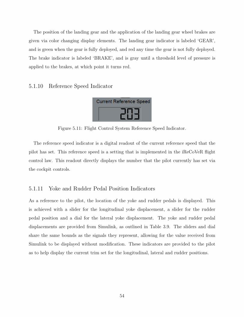
The position of the landing gear and the application of the landing gear wheel brakes are
given via color changing display elements. The landing gear indicator is labeled ‘GEAR’,
and is green when the gear is fully deployed, and red any time the gear is not fully deployed.
The brake indicator is labeled ‘BRAKE’, and is gray until a threshold level of pressure is
applied to the brakes, at which point it turns red.
5.1.10 Reference Speed Indicator
Figure 5.11: Flight Control System Reference Speed Indicator.
The reference speed indicator is a digital readout of the current reference speed that the
pilot has set. This reference speed is a setting that is implemented in the iReCoVeR flight
control law. This readout directly displays the number that the pilot currently has set via
the cockpit controls.
5.1.11 Yoke and Rudder Pedal Position Indicators
As a reference to the pilot, the location of the yoke and rudder pedals is displayed. This
is achieved with a slider for the longitudinal yoke displacement, a slider for the rudder
pedal position and a dial for the lateral yoke displacement. The yoke and rudder pedal
displacements are provided from Simulink, as outlined in Table 3.9. The sliders and dial
share the same bounds as the signals they represent, allowing for the value received from
Simulink to be displayed without modification. These indicators are provided to the pilot
as to help display the current trim set for the longitudinal, lateral and rudder positions.
54

CHAPTER 6
RESULTS
The CNCT library’s functionality and ease of use was tested using the base Generic Trans-
port Model (GTM) model that is provided by NASA’s Langley Research Center. The func-
tionality of the system was graded against smooth visual display, deviation from real-time
performance, and responsiveness of the system to pilot input. The completed simulation
environment can be seen in Figure 6.1.
Figure 6.1: Flight Simulator Environment
6.1 Functionality
The interaction and performance of the various components was graded in three main areas:
display performance, responsiveness to pilot input, and deviation from real-time. The full
55

simulator environment is run from a total of 7 computers all on the same local network. The
breakdown of the computers was as follows:
• One computer reads the voltages from the Frasca 142 and sends a data packet of the
digital equivalent to the Simulink computer.
• One computer runs the Simulink system containing the CNCT library and the GTM
dynamics model.
• One computer running the cockpit gauge display on a monitor in the Frasca cockpit.
• One computer displaying X-Plane within the control room.
• Three computers displaying X-Plane on three projectors, providing a 180◦ field of view
for the pilot.
Spanning multiple computers over a network allowed for the computational and graphic
workloads to be distributed, avoiding stress on a single computer which could slow down
the simulation. User datagram protocol (UDP) also allows extremely fast communication
between the computers, which facilitates a constant stream of data to be passed over the
network.
The display performance was benchmarked using a frames-per-second counter on each of
the X-Plane displays. With the graphics settings turned to ‘High’ levels, each display was
still able to achieve well over 120 frames per second (fps). These high frame rates allow for
extremely smooth displays and are multiple times greater than movies (24 fps), and video
games (typically 30 to 60 fps). The response was also tested using fast and drastic aircraft
movements, such as a fast roll or pitch down. Under such loads, the displays were still able
to maintain over 100 fps, satisfying the responsiveness needed for a stutter-free simulation.
Real-time deviation was measured by examining the difference between the simulation
clock and the computer clock. A positive deviation meant that the simulation clock was
ahead of the computer clock, and vice versa for a deficit. During testing, several maneuvers
were performed. The largest deviation seen was 10 millisecond difference when the simulation
was ahead of the computer clock and a 6 millisecond deficit when the simulation fell behind
56

the computer clock. The computer was capable of running the simulation for extended
periods of time without becoming sluggish or sacrificing responsiveness of the system. The
‘soft’ real-time employed in the model, along with the computer hardware, was deemed to
be more than acceptable for use in tests involving pilots in real-world simulations.
Responsiveness to pilot input was tested by examining the simulator behavior under real-
world maneuvers. Data could only be collected from simulator tests if the response to
external input, like that of the cockpit’s yoke and rudder pedals, was accurate and without
noticeable delay. The system would be considered a failure if a series of prescribed inputs
did not yield expected results. One such evaluation was done by allowing the pilot to fly
straight and level, initiate a banked right turn, and then return to straight and level flight.
To be deemed acceptable, the simulator would have to start and end the banked right turn at
nearly the same time as the pilot was commanding. Repeated testing was done alongside the
real-time deviation tests. Results of such testing deemed the responsiveness of the simulator
to be more than acceptable for flight testing and data collection using the GTM T2 dynamics
model.
The end result of testing yielded a working, valid simulation environment. The display
performance, control responsiveness and ‘soft’ real-time were deemed acceptable for flight
testing and data collection. A video of the simulator in use can be viewed on the internet[13].
57

CHAPTER 7
CONCLUSION
In this document, the development and resulting use of a human-in-the-loop flight simula-
tor has been presented. The outline of the system was developed, and each section of the
simulator environment was discussed in depth. The CNCT Simulink library and its com-
ponents were developed to meet the needs and match the GTM T2 dynamics model. The
inner workings of each component was detailed, including block components as well as S-
Functions that manage the communication between Simulink, X-Plane, the cockpit display
and cockpit controls. The development of the cockpit gauge display was also discussed in
an effort to aid in further development and refinement. Finally, the completed simulator
was presented alongside video and baseline performance data to validate its performance.
The results showed a workable human-in-the-loop flight simulator running in real time with
smooth displays and controls.
58

REFERENCES
[1] “Beckman Institute Illinois Simulator Laboratory.” [Online]. Available: http://www.isl.uiuc.edu/
[2] “Simulink.” [Online]. Available: http://www.mathworks.com/products/simulink/
[3] “X-Plane 9 Global.” [Online]. Available: http://www.x-plane.com/desktop/home/
[4] “Qt Project.” [Online]. Available: http://www.qt-project.org/
[5] D. Ernst, “Development of research platform for unmanned vehicle controllerdesign, evaluation, and implementation system: From matlab to hardware basedembedded system,” M.S. thesis, University of South Florida, 2007. [Online]. Available:http://scholarcommons.usf.edu/etd/699
[6] “State-Machine- Stateflow.” [Online]. Available: http://www.mathworks.com/products/stateflow/
[7] “Windows Sockets 2 (Windows).” [Online]. Available: http://msdn.microsoft.com/en-us/library/windows/desktop/ms740673(v=vs.85).aspx
[8] “XSquawkBox.” [Online]. Available: http://www.xsquawkbox.net/xsb/developers/
[9] “Flight Simulator Operating System.” [Online]. Available: http://sourceforge.net/projects/xfsos/
[10] “X-Plane SDK.” [Online]. Available: http://www.xsquawkbox.net/xpsdk/mediawiki/Main Page
[11] “X-Plane Datarefs.” [Online]. Available: http://www.xsquawkbox.net/xpsdk/docs/DataRefs.html
[12] “QFlightInstruments.” [Online]. Available: http://sourceforge.net/projects/qfi/
[13] “Simulator Flight Test- GTM T2 - Illinois Simulator Laboratory- UIUC.” [Online].Available: https://www.youtube.com/watch?v=fhzU1x92tH0
59