Interdependencies between flame length and firelineintensity in predicting crown fire initiationand crown scorch height

Martin E. AlexanderA,C and Miguel G. CruzB

AUniversity of Alberta, Department of Renewable Resources and Alberta School of Forest Science

and Management, Edmonton, AB, T6G 2H1, Canada.BBushfire Dynamics and Applications, CSIRO Ecosystem Sciences and Climate Adaptation

Flagship, GPO Box 1700, Canberra, ACT 2601, Australia.CCorresponding author. Email: mea2@telus.net

Abstract. This state-of-knowledge review examines some of the underlying assumptions and limitations associatedwith the inter-relationships among four widely used descriptors of surface fire behaviour and post-fire impacts in wildland

fire science and management, namely Byram’s fireline intensity, flame length, stem-bark char height and crown scorchheight. More specifically, the following topical areas are critically examined based on a comprehensive review of thepertinent literature: (i) estimating fireline intensity from flame length; (ii) substituting flame length for fireline intensity inVanWagner’s crown fire initiation model; (iii) the validity of linkages between the Rothermel surface fire behaviour and

Van Wagner’s crown scorch height models; (iv) estimating flame height from post-fire observations of stem-bark charheight; and (v) estimating fireline intensity from post-fire observations of crown scorch height. There has been anoverwhelming tendency within the wildland fire community to regard Byram’s flame length–fireline intensity and

Van Wagner’s crown scorch height–fireline intensity models as universal in nature. However, research has subsequentlyshown that such linkages among fire behaviour and post-fire impact characteristics are in fact strongly influenced byfuelbed structure, thereby necessitating consideration of fuel complex specific-type models of such relationships.

Additional keywords: fire behaviour, fire impacts, fire modelling, first-order fire effects, flame angle, flame depth,

flame-front residence time, ignition pattern, stem-bark char height, surface fire.

Received 6 January 2011, accepted 30 May 2011, published online 22 November 2011

Introduction

Fire models or modelling systems are commonly used forsimulating fire behaviour characteristics and post-fire impacts

or primary fire effects in several wildland fire and fuel man-agement applications (Burrows 1994; Reinhardt et al. 2001). Inthis regard, a recent review on assessing crown fire potential byCruz andAlexander (2010a) revealed an overwhelming need for

the users of fire modelling systems to be grounded in the theoryand proper application of such tools, including a solid under-standing of the assumptions, limitations and accuracy of the

underlying models as well as practical knowledge of the subjectphenomena.

The purpose of the present communication is to review

commonly overlooked assumptions and limitations associatedwith the inter-relationships among four widely used descriptorsof surface fire behaviour and post-fire impacts in wildland fire

science and management, namely fireline intensity, flamelength, stem-bark char height and crown scorch height(Fig. 1). The motivation behind the development of the relation-ships depicted in Fig. 1 is the focus of this paper. For the

convenience of the reader, a summary list of the variablesreferred to in the equations and text, including their symbolsand units, is given at the end of this article.

Estimating fireline intensity from flame length

Byram’s (1959) fireline intensity (IB, kWm�1) in its mostfundamental form is determined from measurements or obser-vations of fire spread rate and fuel consumption:

IB ¼ H � wa � r ð1Þ

where H is the net low heat of combustion (kJ kg�1), wa is

the fuel consumed in the active flaming front (kgm�2), and r isthe linear rate of fire spread (m s�1). This approach to determin-ing IB has been utilised around the globe in many different fuel

complexes for a variety of purposes (e.g. Van Loon 1969;Simard et al. 1982; Vasander and Lindholm 1985; Wendeland Smith 1986; Weber et al. 1987; Burrows et al. 1990; Engleand Stritzke 1995; Fernandes et al. 2000; McRae et al. 2005;

CSIRO PUBLISHING

International Journal of Wildland Fire 2012, 21, 95–113

http://dx.doi.org/10.1071/WF11001

Journal compilation � IAWF 2012 www.publish.csiro.au/journals/ijwf

Review

Gould et al. 2007; Tanskanen et al. 2007; Saglam et al. 2008;Fidelis et al. 2010). Accurate determinations of IB using Eqn 1are dependent on accurate measurements of wa and r, with the

latter quantity being subject to the greatest amount of variation.For an in-depth look at the calculation of IB on the basis of Eqn 1,readers are encouraged to consult Alexander (1982).

IB incorporates several factors of the fire environment into a

single number (Fig. 2) useful in both wildfire suppression andprescribed burning (McArthur 1962; Wilson 1988; Hirsch andMartell 1996). IB has, for example, been correlated with the

likelihood of crown fire initiation (Van Wagner 1977; Alexander

1998) and in assessing certain crown fire impacts (Van Wagner1973), in addition to serving as a direct measure of post-fire treemortality (Weber et al. 1987). IB can be calculated for any point

on the perimeter or edge of a free-burning fire (Catchpole et al.1982, 1992) and any variables related directly to it (e.g. flamezone characteristics, scorch height, crowning potential).

Byram (1959) also indicated that IB could be calculated for

fine, homogeneous fuelbeds (e.g. cured grass) using the follow-ing simple relation:

IB ¼ CR � D ð2Þ

Stem-bark charheight (hc)

Flame height(hF)

Flame angle(A)

Flame length(L)

Crown scorchheight (hs)

Firelineintensity (IB)

Criticalsurface fireintensity forinitial crown

combustion (I0)

Fig. 1. The inter-relationships involved among commonly used descriptors of surface fire behaviour

and fire impacts covered in this review. The solid arrowheads indicate primary relationships established

from field data. The hollow arrowheads represent derivations obtained from the primary relationships by

solving the equation for the independent variable or using a combination of two primary relationships.

Fire intensity – damage potential, control difficulty(Measured in kilowatts per metre, or as flame height or scorch height in metres)

Air temperature(°C)

Fine fuel quantity(kg m�2)

Rate of spread(m s�1)

Heat energy(kJ kg�1)

Slope steepness Fine fuel quantityCombustion rate of

fine fuelsWind speed,

surface instability

Chemicalproperties

Compaction, ventilation,general arrangement

Moisture content Fuel particle size

Long-termrainfall deficit

Short-termdrying conditions

Surface humidity Surface temperature

Fuel characteristics

Weather elements

Fig. 2. Schematic diagram illustrating the various elements contributing to fireline intensity and in turn flame

height and crown scorch height (after Richmond 1981).

96 Int. J. Wildland Fire M. E. Alexander and M. G. Cruz

where CR is the combustion rate (kWm�2) and D is the

horizontal flame depth (m) as illustrated in Fig. 3. D is in turnrepresented by the following formula (after Fons et al. 1963):

D ¼ r � tr ð3Þ

where tr is the flame-front residence time (s).In various US fire modelling systems, IB is calculated from

Rothermel’s (1972) reaction intensity (IR, kWm�2) as follows(Albini 1976; Andrews and Rothermel 1982):

IB ¼ IR � tr � r ð4Þ

In Eqn 4, an estimate of tr is obtained from the following

equation (Anderson 1969):

tr ¼ 189 � d ð5Þ

where d is the fuel particle diameter (cm). The Eqn 4 method ofcalculating IB yields results comparable with those obtained

from Eqn 1 if IR and tr are accurately determined. This will onlyoccur in a laboratory setting where IR is estimated from theknowledge of the rate of weight loss (Rothermel 1972). If Eqn 4

is used in a predictive approach in a field situation, theuncertainty in predicting IR and tr will lead to departures fromresults obtained with Eqn 1. The extent of the differences

between Eqns 1 and 4 is mainly a function of the fuelbedcharacteristics. It has been shown that Eqn 4 yields IB valuesconsistently lower than those produced by Eqn 1 (Cruz et al.

2004; Cruz and Alexander 2010a).

Byram (1959) established an empirical relationship between

IB and flame lengthA for surface fires that is widely applied inwildland fire science and management (from Alexander 1982):

L ¼ 0:0775 � I0:46B ð6Þ

where L is flame length (m) as illustrated in Fig. 3. In lieu ofusing Eqn 1 to determine IB, a common procedure (Rothermel

and Deeming 1980) has been to estimate IB indirectly from fieldobservations or measurements of L in many distinctly differentfuel complexes for several years now (e.g. Bevins 1976;

Woodard 1977; Chase 1984; Wyant et al. 1986; Kauffmanand Martin 1989; Zimmerman 1990; Sapsis and Kauffman1991; Smith et al. 1993; Cornett 1997; McCaw et al. 1997;Gambiza et al. 2005; Kobziar et al. 2006; Ansley and Castellano

2007). This estimation is accomplished by using the inverse orreciprocal of Eqn 6 or a similar equation (Table 1) as follows(from Alexander 1982):

IB ¼ 259:833 � L2:174 ð7Þ

Cain (1984), for example, carried out experimental fires inunthinned and thinned stands of 9-year-old loblolly pine(Pinus taeda)–shortleaf pine (Pinus echinata) in southern

Arkansas, USA. Backfires were employed on the unthinnedareas and head fires were used on the thinned plots. Althoughrate of fire spreadwasmonitored and preburn fuel load sampling

undertaken, post-burn fuel sampling was apparently not and as aresult IB was therefore not calculated using Eqn 1. Cain (1984)elected to use the relation represented by Eqn 7 and observations

of L made to the nearest 0.3m by six independent observers to

Residual or glowingcombustion phase

(actual flames are minimaland transient, smoldering)

Wind

DOB

D

A

Fuel bed

AT

hFL

Secondarycombustion phase(actual flaming isdiscontinuous)

Activecombustion phase

(solid flame zone extending from theleading fire edge to a variable

distance beyond)

Fig. 3. Cross-section of a stylised, wind-driven surface head fire on level terrain illustrating the energy or heat-release stages during and following passage of

the flame front, flame length (L), flame height (hF), flame angle (A), flame tilt angle (AT), horizontal flame depth (D), and the resulting depth of burn (DOB)

(from Alexander 1982).

AIt is worth calling attention to the fact that conversions of Byram’s (1959) original L–IB equation from imperial units to SI units, as represented here by Eqn 6,

have been incorrectly done by several authors in the past (e.g. Wilson 1980; Chandler et al. 1983; Barney et al. 1984;Windisch 1987; vanWagtendonk 2006).

Flame length and fireline intensity interdependences Int. J. Wildland Fire 97

estimate IB for both head fires (L¼ 0.9m and IB¼ 208 kWm�1)and backfires (L¼,0.6m and IB¼ 104 kWm�1).

In lieu of using Eqn 7 to directly estimate IB, some authors

(e.g. Burrows 1984) have chosen to determine L from separateobservations or measurements of flame height and flame angle(Fig. 3) using the following relation (Ryan 1981; Finney and

Martin 1992):

L ¼ hF � cos Sð Þ=sin A� Sð Þ ð8Þ

where hF is the flame height (m), A is the flame angle in degrees(8) from the horizontal, and S is the slope angle (8). L and hF canonly truly be considered equal under no-slope, no-wind (calm)conditions (Brown and DeByle 1987). It is worth noting that

some authors have chosen to relate IB to hF as opposed to L

(e.g. Luke and McArthur 1978; Marsden-Smedley andCatchpole 1995).

Both visual and photographic, including video (Adkins1995), assessments with or without specially designed standards(Britton et al. 1977) have been the most common means of

determining flame-front characteristics (Gill and Knight 1991).Ocular estimates are known to vary among observers (Johnson1982; Andrews and Sackett 1989; Jerman et al. 2004). As

Rothermel and Reinhart (1983) note, ‘It is difficult to measureflame length. The flame tip is a very unsteady reference. Youreye must average the length over a time period that is represen-tative of the fire behaviour’. Even photographic techniques can

prove challenging (Clements et al. 1983). In this respect, Adkinset al. (1994) had this to say about the interpretation of flamemeasurements:

It is important to recognise that instantaneous images of firerecorded with video (1/30 s) present a different picture offlames than human vision. When viewing a sequence of

Table 1. Listing of fireline intensity]flame length relationships presented in Fig. 4

Graph numbers are from Fig. 4. Scientific names for tree and shrub species for fuel type or fuelbed not included in the text are as follows: lodgepole pine,Pinus

contorta; Douglas-fir, Pseudotsuga menziesii; eucalypt, Eucalyptus spp.; maritime pine, Pinus pinaster; jack pine, Pinus banksiana. Variables used are IB,

fireline intensity (kW m�1); L, flame length (m). The reciprocals of the equations given below are presented in the Supplementary material (see http://www.

publish.csiro.au/?act¼view_file&file_id¼WF11001_AC.pdf)

Graph

number

Reference Fuel type or fuelbed Equation Experimental basis Range in

L (m)

Range in

IB (kW m�1)

1 Byram (1959)A Pine litter with grass understorey IB ¼ 259:833 � L2:174 Field 0.5–2.1 56–2232

2 Fons et al. (1963) Wood cribs IB ¼ 22:1 � L1:50 Laboratory 0.4–1.8 68–510

3 Thomas (1963)B Wood cribs IB ¼ 229 � L1:5 Laboratory 1.2–5 36–3600

4 Anderson et al. (1966) Lodgepole pine slash IB ¼ 54:6 � L1:54 Laboratory 1.1–2.9 781–3438

5 Anderson et al. (1966) Douglas-fir slash IB ¼ 103:4 � L1:5 Laboratory 0.8–2.2 619–4645

6 Newman (1974)C Unspecified IB ¼ 300 � L2 Rule of thumb NA NA

7 Nelson (1980) Understorey fuels IB ¼ 510:7 � L2:0 Field 0.1–1.2 21–387

8 Nelson (1980) Southern USA fuels IB ¼ 703:6 � L2:0 Field 0.1–2.1 5–3320

9 Clark (1983) Grasslands (head fire) IB ¼ 1488:7 � L1:01 Field 0.1–4.2 65–12 602

10 Clark (1983) Grasslands (backfire) IB ¼ 147:2 � L0:57 Field 0.3–1.7 41–474

11 Nelson and Adkins (1986) Litter and shrubs IB ¼ 483:3 � L2:03 Field and laboratory 0.5–2.5 98–2755

12 van Wilgen (1986) Fynbos shrublands IB ¼ 402 � L1:95 Field 1.0–4.5 194–5993

13 Burrows (1994) Eucalypt forest IB ¼ 245:1 � L1:3 Field 0.1–10 37–4368

14 Weise and Biging (1996) Excelsior IB ¼ 367:7 � L1:43 Laboratory 0.07–2.1 9–820

15 Vega et al. (1998) Shrublands IB ¼ 141:6 � L2:03 Field 1.5–6.5 294–6905

16 Catchpole et al. (1998) Shrublands IB ¼ 454:3 � L1:79 Field 0.5–18 100–77 000

17 Fernandes et al. (2000) Shrublands IB ¼ 695:0 � L2:21 Field 0.2–3.1 12–7605

18 Butler et al. (2004)D Jack pine forest (crown fire) IB ¼ 431 � L1:5 Field – –

19 Fernandes et al. (2009) Maritime pine forest (head fire) IB ¼ 302:2 � L1:84 Field 0.1–4.2 30–3527

20 Fernandes et al. (2009) Maritime pine forest (backfire) IB ¼ 133 � L1:38 Field 0.1–2.0 7–232

AContrary to Ryan’s (1981) claim that Byram’s (1959) L–IB relation represented by Eqn 6 constitutes a laboratory-derived relationship, according to

Lindenmuth and Davis (1973), it ‘was partly theoretical and partly empirical, based on some degree on longleaf and loblolly pine real-world research fires, in

whichLindenmuth collaborated’. In this regard, Byram (1959) indicates that the data contained in fig. 3.3 of his publication, illustrating the effect of wind speed

on rate of fire spread, involved small test fires carried out as part of a prescribed burning study on the Francis Marion National Forest in South Carolina, USA.

The surface fuels were considered ‘light’ with fairly uniform mixtures of grass and pine needles in rather open stands composed of longleaf pine

(Pinus palustris) and loblolly pine, weighing approximately ‘0.1 pound per square foot, or,2 tons per acre’. R. M. Nelson Jr (USDA Forest Service [retired],

pers. comm., 2010), a protege of G.M. Byram during the 60s and early 70s, suggested that perhaps a rough estimate of the experimental range in IB could be

made using the range in r given in fig. 3.3 of Byram (1959) and assuming that w¼ 0.5 kg m�2. The range in I B presented above was in fact determined in this

manner, using a value of H¼ 18 000 kJ kg�1. Then the corresponding range in L was determined using Eqn 6.BData for Thomas (1963) L–IB model was extracted from fig. 5 in Thomas (1971), using a value of H¼ 18 000 kJ kg�1.CChandler et al. (1983, p. 26) is commonly cited as the source for the SI unit version of a simple formula designed for field use as originally put forth byNewman

(1974) in imperial units. Newman (1974) limited the chart associated with his rule of thumb to an L of ,12m.DIn this case,L represents the height of the flame above the canopy top (Butler et al. 2004, fig. 1). The constant in the equationwas derived byAlbini and Stocks

(1986) on the basis of experimental crown fire 13 documented by Stocks (1987) in a 10-m tall jack pine forest where L was judged to be ,7.25m and in

IB¼ 15 790 kWm�1.

98 Int. J. Wildland Fire M. E. Alexander and M. G. Cruz

video flame images at a slow framing rate, pulsations inflame length can be seen. Flame lengths of lower intensityfires will pulsate at a higher frequency with a small variation

in flame length. High intensity fire will pulsate at a lowerfrequency with greater variation in flame lengths. In bothcases an observer will see the flames as being more or less

solid shapes with the apparent length being the maximumflame extension through the pulse cycle when viewed at thenormal rate; this is attributed to human visual persistence

integrating the apparent flame lengths.

As Rothermel (1991) so eloquently points out, ‘flame lengthis an elusive parameter that exists in the eye of the beholder. It is

a poor quantity to use in a scientific or engineering sense, but it isso readily apparent to fireline personnel and so readily conveys asense of fire intensity that it is worth featuring as a primary fire

variable’ (e.g. Murphy et al. 1991). Cheney and Sullivan (2008)have indicated that one should not expect a great degree ofprecision when it comes to estimating flame heights, suggesting

that at least for grass fires, ‘flame height estimates in steps of0.25, 0.5, 1, 2, 4 and.4m should be adequate for most purposes’.

Eqn 6 is used in several US fire modelling systems as the

means of predicting surface fire L. Albini (1976) claimed thatEqn 6 tended to give realistic results over a wide range in IB,although Byram (1959) considered it a better approximationfor low- rather than for high-intensity fires. Subsequent evalua-

tions based on experimental fires conducted in the field andlaboratory have shown both close agreement and considerabledeviation (Sneeuwjagt and Frandsen 1977; Nelson 1980; Ryan

1981; van Wilgen 1986; Nelson and Adkins 1986; Weise andBiging 1996; Anderson et al. 2006). Eqn 6 is most commonlyviewed as applicable to surface heading fires, although some

investigators, for example Nelson (1980), Clark (1983) andFernandes et al. (2009), have developed separate L–IB modelsfor backing fires.

Many research and operational users of firemodelling systems

have come toviewEqns 6 and 7 as universal in nature, probably asa result of the manner in which they are oftentimes treated in thewildland fire science and management literature (e.g. Rothermel

and Deeming 1980; Norum 1982; Simard et al. 1989; Johnsonand Miyanishi 1995; Andrews et al. 2011) and more recently oncertainwebsites such asForest EncyclopaediaNetwork (Kennard

2008a). As Nelson and Adkins (1986) point out, this is ‘despitethe fact that it was developed from a field study in a single fueltype’ (see footnote A in Table 1). However, as illustrated earlier

byAlexander (1998), at least 19 other L–IB relationships exist andtheir outputs vary widely (Fig. 4 and Table 1).

It is worth noting that Byram (1959) indicated that his L–IBrelation represented by Eqn 6 would underpredict L for ‘crown

fires becausemuch of the fuel is a considerable distance above theground’. He suggested, on the basis of visual estimates, that ‘thiscan be corrected for by adding one-half of the mean canopy

height’ to the L value obtained by Eqn 6. Rothermel (1991)suggested using Thomas’ (1963) relation to estimate L values forcrown fires from IB.More recently, Butler et al. (2004) proposed a

specific relation for calculating L of crown fires based on IB. Noneof these methods, however, seem to work consistently well basedon comparisons made against data obtained from experimentalcrown fires (Alexander 1998; Cruz and Alexander 2010b).

There are several reasons for the variation in the L–IBrelationships evident in Fig. 4, including the sample size andrange in IB sampled, themanner in which the data were collected

(e.g. visual estimates of L v. photographic documentation),assumptions made concerning the calculation of IB by Eqn 1(e.g. the method used to derive wa, value of H used), and the

interpretation of the Lmeasurement (because an internationallyrecognised standard is lacking), and differences in fuelbedstructure (Alexander 1998; Anderson et al. 2006).

With respect to the latter influence,Methven (1973)made thefollowing comments concerning two experimental fires thatexhibited nearly identical IB levels (i.e. 76 v. 78 kWm�1) carriedout at the Petawawa Forest Experiment Station (PFES), Ontario,

Canada, in a mature red pine (Pinus resinosa)–eastern whitepine (P. strobus) stand with a balsam fir (Abies balsamea)understorey:

The calculated intensities, however, reflect only the average

fire conditions and in fact the first fire resulted in someoverstorey damage due to localised but fairly widespreadpeaks of intensity. These were due to a clumped distributionof balsam fir saplings which resulted in live branches close to

the ground and a foliage bulk density great enough to carryfire upwards. Wherever these concentrations of fir occurred,therefore, flame heights were raised from less than 30 cm to

over 3m with a much increased energy output per unitground area and scorching of overstorey crowns. Theincrease in intensity was not so much a product of the

increased fuel loading which amounted to only 0.04 g cm�2,but to the rate of combustion of this fuel, which, due to itsarrangement or bulk density, burned much more rapidly thanan equivalent quantity of ground fuel.

Methven (1973) noted that the higher fuel consumption of thefirst fire compared with the second (0.589 v. 0.465 kgm�2) wasbalanced by the faster rate of spread of the second fire as a result

of lower relative humidity, drier litter fuels and a greaterin-stand wind speed.

Cheney (1990) has noted that ‘the flame characteristics

associated with a specific fire intensity are only applicable tofuel types with the same fuel structure characteristics’. Heillustrated the significance of this fact by contrasting the

physical characteristics of free-burning fires in two widelyvarying fuel types found in Australia, namely native forest andgrasslands, with each exhibiting an IB¼ 7500 kWm�1:

A grass fire y will travel at 5 kmh�1 in an average fuel of,3 t ha�1 and will have a flame length of up to 4m. Thisfire can be fought directly and there is a 90% probability that

the head fire will be stopped by a 5m wide firebreaky [A]fire y in a dry eucalypt forest has very different character-istics. Burning in a 15 t ha�1 forest fuel, the fire will travel at

,1 kmh�1 and have flames which extend up through thecrowns to a height of perhaps 10m above the tree tops andmore than 30m above the ground from the surface fire. The

fire will be throwing firebrands up to 1 km ahead of the fireand have extensive short-distance spotting and will beunstoppable by any means unless there is a change in somefactor influencing fire behaviour.

Flame length and fireline intensity interdependences Int. J. Wildland Fire 99

Cheney (1990) concluded that ‘Byram’s fireline intensity isuseful to quantify certain flame characteristics and to correlate

with fire effects but should not be used to compare fires in fueltypeswhich are structurally very different’. Thus, one should notnecessarily always expect good agreement between observed

flame lengths and predictions using Eqn 6 (Brown 1982; Smithet al. 1993).

Substituting flame length for fireline intensityin Van Wagner’s (1977) crown fire initiation model

VanWagner’s (1977) model for predicting crown fire initiationhas been implemented within many fire modelling or decisionsupport systems (Cruz and Alexander 2010a). His model can be

represented by the following composite equation:

I0 ¼ 0:010 � CBH � 460þ 25:9 � FMCð Þð Þ1:5 ð9Þ

where I0 is the critical surface fire intensity for crown

combustion (I0, kWm�1), CBH is the canopy base height (m),

and FMC is the foliar moisture content (%). The onset ofcrowning is expected to occur when the surface fire IB meetsor exceeds I0.

As first suggested by Alexander (1988), crown fire initiationcan also be expressed in terms of L instead of IB, therebypermitting a ready comparison of CBH v. L and thus a rough

guide to the likelihood of crowning (Albini 1976). Severalauthors have chosen to take this approach for their particularapplications (e.g. Graham et al. 1999; Scott and Reinhardt 2001;

Keyes and O’Hara 2002; Hummel and Agee 2003; Scott 2003;Peterson et al. 2005; Dimitrakopoulos et al. 2007; Battagliaet al. 2008;Crecente-Campo et al. 2009;Ager et al. 2010). To do

this,Wilson andBaker (1998), for example, derived a regressionequation from the data contained in a tabulation constructed byAgee (1996), in part, using Eqn 9. However, this can be donemore directly by simply combining Eqns 6 and 9, for example,

resulting in the following formulation:

L0 ¼ 0:0775 � 0:010 � CBH � 460þ 25:9 � FMCð Þð Þ0:69 ð10Þ

1086420 10864200

2000

4000

6000

8000

10 000

Fire

line

inte

nsity

(kW

m�

1 )

0

2000

4000

6000

8000

10 00011

17 12 16 151 7

11

13

20

1 6 19 18

10

8 1 914

3

5

4

2

1

Laboratory Grassland

Shrubland

Flame length (m)

1086420 1086420

Forest

Fire

line

inte

nsity

(kW

m�

1 )

Fig. 4. Graphical representation of Byram’s (1959) fireline intensity–flame length relationship (represented by curve 1) and other

models reported in the literature. Refer to Table 1 for details of each plotted relationship.

100 Int. J. Wildland Fire M. E. Alexander and M. G. Cruz

where L0 is the critical surface fire flame length for crown

combustion (m). Regardless, the formulation represented byEqn 10 should be viewed as a modelling assumption rather thanas an accepted generalisation given the manner in which Van

Wagner (1977) derived the empirical constant (0.010) given inEqn 9 on the basis of IB determined from Eqn 1 as opposed toobservations ofL (Cruz andAlexander 2010b). It is worth noting

that the flames of a surface fire don’t necessarily have to reach orextend into the lower tree crowns in order to initiate crowning(Fig. 5).

Validity of linkages between the Rothermel (1972)surface fire behaviour and Van Wagner (1973)crown scorch height models

The degree of crown scorch is reflected in the post-fire (within a

few days) browning or yellowing of needles or leaves in trees(Fig. 6) or shrubs as a result of heating to lethal temperatureduring the passage of a surface fire. Crown scorch height is

an output in some fuel treatment effectiveness simulationstudies in coniferous forests aimed at mitigating crown firepotential (e.g. Johnson 2008; Roccaforte et al. 2008). These

studies use fire modelling systems like First Order Fire EffectsModel (FOFEM) (Reinhardt et al. 1997), BehavePlus (Andrewset al. 2008), and the Fire and Fuels Extension to the ForestVegetation Simulator (FFE-FVS) (Reinhardt and Crookston

2003) that have incorporated one or all three of Van Wagner’s

(1973) modelsB for predicting the crown scorch height inconifer trees (after Alexander 1985):

hs ¼ 0:1483 � I0:667B ð11Þ

hs ¼ 4:4713 � I0:667B

TL � Tað12Þ

hs ¼ 0:74183 � I0:667B

ð0:025574 � IB þ 0:021433 � U31:2Þ0:5 � ðTL � TaÞ

ð13Þ

where hs is the crown scorch height (m), TL is the lethaltemperature for crown foliage (8C), Ta is the ambient airtemperature (8C), and U1.2 is the in-stand wind speed measured

at a height of 1.2m above ground (kmh�1) as specified muchlater on by C. E. Van Wagner (Canadian Forestry Service, pers.comm., 1984). Thus, quite understandably, Albini (1976) didn’t

specify in his publication the wind speed height or exposure inthe imperial version of Van Wagner’s (1973) hs model repre-sented by Eqn 13. As a result, some authors subsequently

assumed it was the 6.1-m open wind standard as used in firedanger rating and fire behaviour prediction purposes in the US(Crosby and Chandler 1966) as opposed to the U1.2 height andexposure standard used by VanWagner (1963, 1968) in his field

studies. Dieterich (1979), for example, on the basis of data forTa, IB and the 6.1-m open wind speed for three differentconditions (i.e. ‘high’ daytime, ‘extreme’ daytime and night)

associated with the 1973 Burnt Fire in northern Arizona, USA,computed hs values of 2.4, 4.3 and 1.5m respectively, using theimperial unit version of the Van Wagner (1973) model repre-

sented by Eqn 13 as presented in Albini (1976). Assuming awind adjustment coefficient or factor of 0.3 (Rothermel 1983),the correct computed hs values would have instead been 11.2,

19.1 and 5.6m respectively.Van Wagner’s (1973) hs models are based on 13 experimen-

tal fires carried out at PFES. Eight of these took place in a redand white pine stand (Van Wagner 1963), two in jack pine, one

in northern red oak (Quercus rubra), and two in a red pineplantation (Van Wagner 1968).

Van Wagner’s (1973) hs models include empirical constants

based on determining IB, from pre- and post-burn fuel samplingcoupled with observations of fire spread rate, much in the samemanner as in parameterising his crown fire initiation model

(Van Wagner 1977). The estimation of hs using one of VanWagner’s (1973) models that rely on Eqn 4 (e.g. FOFEM,BehavePlus and FFE-FVS) instead of Eqn 1 can potentially

lead to substantial underpredictions in hs (Fig. 7) as a result ofunderestimating tr and in turn wa, as discussed by Cruz andAlexander (2010a).

There has been very little research undertaken to evaluate the

performance of the Van Wagner (1973) hs models when imple-mentedwithin the context of the US fire modelling systems such

00

Nelson (1980); Nelson and Adkins (1986)Byram (1959)

Fernandes et al. (2009)

Thomas (1963)Bur

rows

(199

4)

2

Crit

ical

sur

face

fire

flam

e le

ngth

for

crow

n co

mbu

stio

n (m

)

4

6

Canopy base height (m)

2 4 6

Fig. 5. Critical surface fire flame length for crown combustion in a conifer

forest stand as a function of canopy base height according to various flame

length–fireline intensity models for forest fuel complexes based on Van

Wagner’s (1977) crown fire initiation model. A foliar moisture content of

100% was assumed in all cases. The dashed line represents the boundary of

exact agreement between flame length or height and canopy base height.

BIt is worth calling attention to the fact that conversions of VanWagner’s (1973) three original hs equations from old metric units to SI units presented here as

Eqns 11–13 have been incorrectly done numerous authors in the past (e.g. Chandler et al. 1983; Barney et al. 1984; Kercher and Axelrod 1984; Keane et al.

1989; Johnson 1992; Johnson and Gutsell 1993; Johnson and Miyanishi 1995; Burrows 1997; Gould et al. 1997; Dickinson and Johnson 2001).

Flame length and fireline intensity interdependences Int. J. Wildland Fire 101

as FOFEM, BehavePlus and FFE-FVS. Wade (1993) pointed

out that the validity of Van Wagner’s (1973) work for use insouthern pine stands had yet to be demonstrated and recom-mended that the BEHAVE system (Andrews and Chase 1989)

not be used in young loblolly pine stands ‘where small differ-ences in scorch height can have major consequences’.

Jakala (1995) reported a substantial discrepancy between the

observed hs (15 to 17m) in the overstoreys of red pine–easternwhite pine stands compared with predicted values of hs (0.3 to0.9m) based on the BEHAVE system associated with opera-tional prescribed fires carried out in Voyageurs National Park in

northern Minnesota, USA. The higher-than-expected scorch

heights were undoubtedly due to significant amount of torchingand subcanopy crown fire activity observed in the understorey(Methven 1973;Methven andMurray 1974; VanWagner 1977),

as shown in Fig. 8. Such episodic cases of vertical fire develop-ment are not readily accounted for in BehavePlus or any otherfire modelling system.

Knapp et al. (2006) conducted experimental fires inmasticated surface fuels at two different ponderosa pine(Pinus ponderosa) sites in northern California. They observedsubstantial crown scorch and found that the BehavePlus

0

US fire m

odelling sy

stems

US fire modelling systemsBy

ram

(195

9) a

s pe

r

Van

Wag

ner (

1973

)

Byram (1

959) as p

er

Van Wagner (1

973)

Mid-flame wind speed (km h�1)

0

5

10

(a) (b)

Cro

wn

scor

ch h

eigh

t (m

)

15

20

2 4 6 8 0 2 4

Fuel Model 2 - Timber(grass and understorey)

Fuel Model 10 - Timber(litter and understorey)

6 8

Fig. 7. Crown scorch height as per VanWagner’s (1973)model as a function ofmid-flamewind speed for twoUS

fire behaviour fuel models (Anderson 1982) based on different methods of calculating fireline intensity (i.e. Byram

1959 as per Van Wagner 1973 v. US fire modelling systems). The following environmental conditions were held

constant: slope steepness, 0%; fine dead fuel moisture, 4%; 10- and 100-h time-lag dead fuel moisture contents,

5 and 6%; live fuel moisture content, 30%; and ambient air temperature, 258C. The associated 10-m open winds

would be a function of forest structure and can be approximated by multiplying the mid-flame wind speed by

a factor varying between 2.5 (open stand) and 6.0 (dense standwith high crown ratio) (Albini and Baughman 1979).

Stem char line

Brownneedles

Green needles

Crown scorchline

Bare limbs(needles consumed)

Brown needles

Crown consumptionline

Stem charline

Charred bole

hs

hc

Wind

(a) (b)

Fig. 6. Variation in direct effects of (a) low- to (b) high-intensity surface fires on tree crowns and stem boles

(adapted from Storey and Merkel 1960).

102 Int. J. Wildland Fire M. E. Alexander and M. G. Cruz

modelling systemunderpredictedhson their ‘high’ (0.718kgm�2)

and ‘low’ (0.261 kgm�2) woody fuel load sites by factorsof approximately four and two times. Part of the under-prediction bias noted by Knapp et al. (2006) could conceivablybe attributed to the use of field observations of L to estimate IBfrom Eqn 7 and in turn to compute hs from one of the VanWagner (1973) hs models (i.e. Eqns 11–13). The higher thanexpected hs levels could also have been due to the way the

masticated fuels burned, with considerable heat being producedeven though flame length was apparently suppressed by thecompactness of the fuelbed (E. E. Knapp, USDAForest Service,

pers. comm., 2010).Albini (1976) was the first to suggest that by using Eqn 7,

L could be used in place of IB to estimate hs and accordinglyconstructed various graphical representations of Van Wagner’s

(1973)hs models for field use (e.g. Norum 1977; Reinhardt andRyan 1988). In this manner, given a value for L, the resultant IBoutput can be utilised as input in any one of the Van Wagner

(1973) hs models. Using Eqns 7 and 13, Reinhardt and Ryan

(a)

(c) (d) (e)

(b)

Fig. 8. Transitions from (a) a mild surface fire to (b–d ) intense torching and subcanopy crown fire activity, and (e) back to a low-intensity state during

prescribed burning operations in a mixed red pine and eastern white pine stand containing pockets of jack pine and understorey thickets of balsam fir,

Voyageurs National Park, northern Minnesota, USA. Photos courtesy of S. G. Jakala.

Fig. 9. Wind-driven surface fire in a Scots pine (Pinus sylvestris) stand in

central Siberia illustrating the increased flame height on the lee-side of tree

stems well above the general level of the advancing flame front in between

trees (from McRae et al. 2005).

Flame length and fireline intensity interdependences Int. J. Wildland Fire 103

(1988) prepared a nomogram for predicting hs from L and Ta,assuming U1.2¼ 8 kmh�1. Like the prediction of crown fireinitiation represented by Eqn 10, these types of decision aids

should be regarded as a modelling assumption rather than as anaccepted generalisation.

The height of crown scorch has been linked directly to hF(e.g. Cheney et al. 1992). Gould (1993), for example, derived thefollowing relationship from a graph included in McArthur’s(1962) prescribed burning guide for eucalypt forests in

Australia:

hs ¼ 5:232 � h0:756F ð14Þ

A 6-to-1 hs/hF ratio is a commonly cited rule of thumb inprescribed burning in Australia and South Africa (e.g. Van Loonand Love 1973; Byrne 1980; de Ronde 1988; de Ronde et al.

1990). This generalised guideline apparently was first intro-

duced by McArthur (1962) for eucalyptus forests and has sincebeen reinforced by the comment of Luke and McArthur (1978)that ‘Flame height has a considerable bearing on scorch height.

Broadly speaking, flames associatedwith prescribed burning arelikely to cause scorch with a zone equivalent to six times flameheight’. Subsequent evaluations have shown that there are

limitations to this appealing rule of thumb (Gould 1993; Beck1994; Burrows 1994, 1997), possibly due to excluding the effectof important factors such asTa, tr, wind speed and stand structure

characteristics, and thus it may not be appropriate for particularfuel types and geographical areas.

Estimating flame height from post-fire observationsof stem-bark char height

Another commonly used post-fire indicator of surface firebehaviour in forest fires is the height of charring or blackening

of the outer bark from exposure to flaming combustion (Fig. 6)on the lower portion of tree boles (Davis and Cooper 1963; Cain1984; Weber et al. 1987). As Burrows (1984) points out, thistechnique works best for non-fibrous-barked trees (Loomis

1973; Brown and DeByle 1987), where the bark cannot igniteand be consumed well above the height of the original flames.

Several authors (e.g. McNab 1977; Nickles et al. 1981;

Waldrop and Van Lear 1984; Hely et al. 2003) have inferredhF directly from post-fire observations of the stem-bark charheight (hc, m). In some of these studies, the authors have in turn

estimated IB using Eqn 7, assuming that hF is approximatelyequal to L; as Agee (1993) notes, ‘If the bark is flammable or hasheavy lichen cover, the height of bark char may exceed flame

heighty resulting in overestimates of fireline intensity’ such aswould be the case with many eucalypt tree species, for example(Luke and McArthur 1978; Gould et al. 2007). In taking thisapproach, one of the fundamental assumptions being made by

the authors, whether explicitly stated or not, is that there is littleor no wind effect, even though this may not actually be the case(i.e. calm conditions such that hF and L are essentially the same).

This would be a reasonably valid assumption for the firedescribed by McNab (1977) that spread at ,0.3mmin�1,reflecting very light, in-stand wind conditions.

Cain (1984) contended that there was no documentationavailable to show that hc provides an accurate estimate of eitherL or hF for thatmatter and accordingly set out to correlate L to hc.

It is unfortunate that no measurements or observations weremade of hF. Measurements of hc were made to the nearest0.03m. Cain (1984) found that hc underestimated L by 47% for

head fires (hc¼ 0.48m) and 40% for backfires (hc¼ 0.36m).Considering that the experimental fires were undertaken withopen ground level winds of 8 kmh�1 and associated spread rates

of 1.8 and 0.4mmin�1 for heading fires and backing fires, thisresult is not unexpected.

In wind-driven surface fires, bole charring will be higher onthe leeward side of a tree stem owing to the taller flame heights

(Gill 1974) as illustrated here (Fig. 9) and in Cheney andSullivan (2008, fig. 9.1) for example. As Gutsell and Johnson(1996) explain, ‘When a fire passes by a tree, its height increases

on the tree’s leeward side because of the occurrence of twoleeward vortices. The flame height increases in the vorticesbecause the turbulent mixing of fuel and air is suppressed. The

flow of gaseous fuel in the vortices becomes greater than the rateof mixing with the air, and hence there is an increased heightalong which combustion can occur’. The formation of the

leeward vortices that in turn control the height of the flames isviewed as a function of wind speed and the diameter of the stembole (Gutsell and Johnson 1996).

The measurement of hc may involve both the minimum and

maximum heights (Van Wagner 1963; Dixon et al. 1984; Helyet al. 2003), the maximum height (Cain 1984; USDI NationalPark Service 2003), or an average (Menges and Deyrup 2001;

Kennard 2008b). As wind speed increases, the ratio betweenthe leeward and windward heights will increase (Inoue 1999);this would of course be accentuated by an increase in slope

steepness. In experimental fires carried out in maritime pine inPortugal involving hF values of 0.2 to 3.5m, Fernandes (2002)found that the maximum leeward hc in heading fires was justslightly greater than the observed hF (hc¼ 1.1� hF) and for

backing fires, hFwas a little less than half the hc (hc¼ 2.5� hF).In support of Gutsell and Johnson’s (1996) theoretical analysis,Fernandes (2002) found an increase in the difference between

leeward andwindward hcwith increasing wind speeds. The ratiobetween leeward or maximum and windward or minimum hcvaried between 2.0 at low wind speeds (i.e. in-stand winds

,2 kmh�1) and 6.0–7.0 for in-stand winds of ,10 kmh�1.Van Wagner (1963) reported ratios between 2.0 and 3.0 inunderburning of red and white pine stands with in-stands winds

of ,5.0 kmh�1.A bettermethod to the general approach described above is to

simply use Eqn 8 to calculate L and, if one wishes, IB as well.This is done again by assuming that hF and hc are equivalent or

that an established ratio exists. The value of A can then beobtained directly from either ocular estimates made in the fieldor by measurements derived from photography. An estimate of

A can also be inferred from models based on hF or IB and windspeed as inputs (e.g. Albini 1981; Nelson and Adkins 1986;Alexander 1998) as undertaken for example by Hely et al.

(2003).One of the major problems with using tree stems as passive

sensors for determining hF for a fire as a whole, assuming theywere relatively uniformly distributed, is the fact that the fuels

104 Int. J. Wildland Fire M. E. Alexander and M. G. Cruz

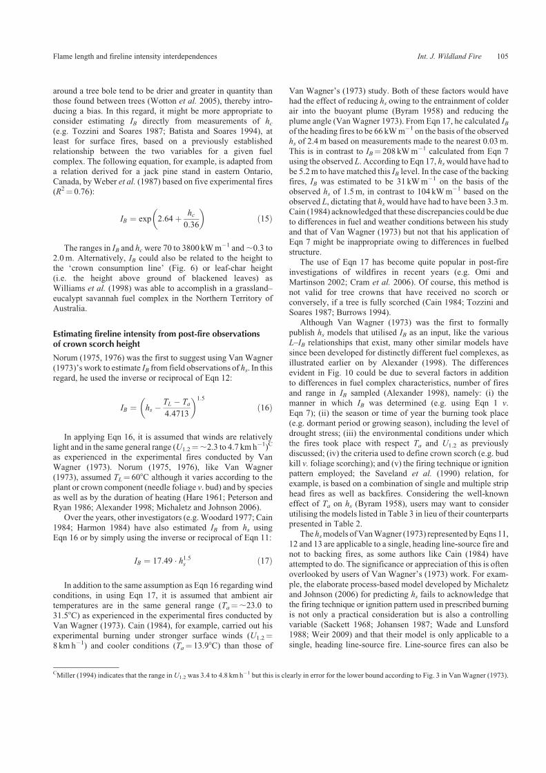
around a tree bole tend to be drier and greater in quantity thanthose found between trees (Wotton et al. 2005), thereby intro-ducing a bias. In this regard, it might be more appropriate to

consider estimating IB directly from measurements of hc(e.g. Tozzini and Soares 1987; Batista and Soares 1994), atleast for surface fires, based on a previously established

relationship between the two variables for a given fuelcomplex. The following equation, for example, is adapted froma relation derived for a jack pine stand in eastern Ontario,

Canada, byWeber et al. (1987) based on five experimental fires(R2¼ 0.76):

IB ¼ exp 2:64þ hc

0:36

� �ð15Þ

The ranges in IB and hcwere 70 to 3800 kWm�1 and,0.3 to2.0m. Alternatively, IB could also be related to the height tothe ‘crown consumption line’ (Fig. 6) or leaf-char height(i.e. the height above ground of blackened leaves) as

Williams et al. (1998) was able to accomplish in a grassland–eucalypt savannah fuel complex in the Northern Territory ofAustralia.

Estimating fireline intensity from post-fire observationsof crown scorch height

Norum (1975, 1976) was the first to suggest using Van Wagner

(1973)’s work to estimate IB from field observations of hs. In thisregard, he used the inverse or reciprocal of Eqn 12:

IB ¼ hs � TL � Ta

4:4713

� �1:5

ð16Þ

In applying Eqn 16, it is assumed that winds are relativelylight and in the same general range (U1.2¼,2.3 to 4.7 kmh�1)C

as experienced in the experimental fires conducted by Van

Wagner (1973). Norum (1975, 1976), like Van Wagner(1973), assumed TL¼ 608C although it varies according to theplant or crown component (needle foliage v. bud) and by species

as well as by the duration of heating (Hare 1961; Peterson andRyan 1986; Alexander 1998; Michaletz and Johnson 2006).

Over the years, other investigators (e.g.Woodard 1977; Cain

1984; Harmon 1984) have also estimated IB from hs usingEqn 16 or by simply using the inverse or reciprocal of Eqn 11:

IB ¼ 17:49 � h1:5s ð17Þ

In addition to the same assumption as Eqn 16 regarding windconditions, in using Eqn 17, it is assumed that ambient airtemperatures are in the same general range (Ta¼,23.0 to

31.58C) as experienced in the experimental fires conducted byVan Wagner (1973). Cain (1984), for example, carried out hisexperimental burning under stronger surface winds (U1.2¼8 kmh�1) and cooler conditions (Ta¼ 13.98C) than those of

Van Wagner’s (1973) study. Both of these factors would havehad the effect of reducing hs owing to the entrainment of colderair into the buoyant plume (Byram 1958) and reducing the

plume angle (VanWagner 1973). From Eqn 17, he calculated IBof the heading fires to be 66 kWm�1 on the basis of the observedhs of 2.4m based on measurements made to the nearest 0.03m.

This is in contrast to IB¼ 208 kWm�1 calculated from Eqn 7using the observed L. According to Eqn 17, hswould have had tobe 5.2m to have matched this IB level. In the case of the backing

fires, IB was estimated to be 31 kWm�1 on the basis of theobserved hs of 1.5m, in contrast to 104 kWm�1 based on theobserved L, dictating that hswould have had to have been 3.3m.Cain (1984) acknowledged that these discrepancies could be due

to differences in fuel and weather conditions between his studyand that of Van Wagner (1973) but not that his application ofEqn 7 might be inappropriate owing to differences in fuelbed

structure.The use of Eqn 17 has become quite popular in post-fire

investigations of wildfires in recent years (e.g. Omi and

Martinson 2002; Cram et al. 2006). Of course, this method isnot valid for tree crowns that have received no scorch orconversely, if a tree is fully scorched (Cain 1984; Tozzini and

Soares 1987; Burrows 1994).Although Van Wagner (1973) was the first to formally

publish hs models that utilised IB as an input, like the variousL–IB relationships that exist, many other similar models have

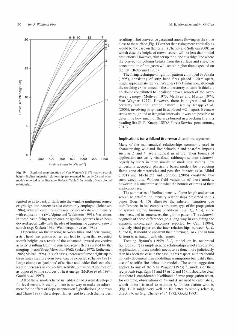
since been developed for distinctly different fuel complexes, asillustrated earlier on by Alexander (1998). The differencesevident in Fig. 10 could be due to several factors in addition

to differences in fuel complex characteristics, number of firesand range in IB sampled (Alexander 1998), namely: (i) themanner in which IB was determined (e.g. using Eqn 1 v.

Eqn 7); (ii) the season or time of year the burning took place(e.g. dormant period or growing season), including the level ofdrought stress; (iii) the environmental conditions under whichthe fires took place with respect Ta and U1.2 as previously

discussed; (iv) the criteria used to define crown scorch (e.g. budkill v. foliage scorching); and (v) the firing technique or ignitionpattern employed; the Saveland et al. (1990) relation, for

example, is based on a combination of single and multiple striphead fires as well as backfires. Considering the well-knowneffect of Ta on hs (Byram 1958), users may want to consider

utilising the models listed in Table 3 in lieu of their counterpartspresented in Table 2.

The hsmodels ofVanWagner (1973) represented byEqns 11,

12 and 13 are applicable to a single, heading line-source fire andnot to backing fires, as some authors like Cain (1984) haveattempted to do. The significance or appreciation of this is oftenoverlooked by users of Van Wagner’s (1973) work. For exam-

ple, the elaborate process-based model developed by Michaletzand Johnson (2006) for predicting hs fails to acknowledge thatthe firing technique or ignition pattern used in prescribed burning

is not only a practical consideration but is also a controllingvariable (Sackett 1968; Johansen 1987; Wade and Lunsford1988; Weir 2009) and that their model is only applicable to a

single, heading line-source fire. Line-source fires can also be

CMiller (1994) indicates that the range in U1.2 was 3.4 to 4.8 kmh�1 but this is clearly in error for the lower bound according to Fig. 3 in Van Wagner (1973).

Flame length and fireline intensity interdependences Int. J. Wildland Fire 105

ignited so as to back or flank into the wind. A multipoint source

or grid ignition pattern is also commonly employed (Johansen1984), wherein each fire increases its spread rate and intensitywith elapsed time (McAlpine and Wakimoto 1991). Variations

in these basic firing techniques or ignition patterns have beendevised specificallywith the idea of limiting the degree of crownscorch (e.g. Sackett 1969; Weatherspoon et al. 1989).

Depending on the spacing between lines and their timing,

a strip head-fire ignition pattern can lead to higher than expectedscorch heights as a result of the enhanced upward convectiveactivity resulting from the junction zone effects created by the

merging lines of fires (McArthur 1962; Sackett 1972; Rothermel1985;McRae 1996). In such cases, increased flame heights up tothree times their previous level can be expected (Cheney 1981).

Large clumps or ‘jackpots’ of surface and ladder fuels can alsolead to increases in convective activity, but as point sources of,as opposed to line sources of heat energy (McRae et al. 1994;Gould et al. 1997).

All of the hs models listed in Tables 2 and 3 were developedfor level terrain. Presently, there is no way to make an adjust-ment for the effect of slope steepness on hs predictions (Andrews

and Chase 1989). On a slope, flames tend to attach themselves,

resulting in hot convective gases and smoke flowing up the slopeclose to the surface (Fig. 11) rather than risingmore vertically aswould be the case on flat terrain (Cheney and Sullivan 2008), in

which case the height of crown scorch will be less than modelpredictions. However, ‘further up the slope at a ridge line wherethe convection column breaks from the surface and rises, the

concentration of hot gases will scorch higher than expected onthe flat’ (Rothermel 1985).

The firing technique or ignition pattern employed by Jakala

(1995), consisting of strip head fires placed ,20m apart,might approximate the VanWagner (1973) situation, althoughthe torching experienced in the understorey balsam fir thicketsno doubt contributed to localised crown scorch of the over-

storey canopy (Methven 1973; Methven and Murray 1974;Van Wagner 1977). However, there is a great deal lesscertainty with the ignition pattern used by Knapp et al.

(2006), involving strip head fires placed,2m apart. Becausestrips were ignited at irregular intervals, it was not possible todetermine how much of the area burned in a backing fire v. a

heading fire (E. E. Knapp, USDA Forest Service, pers. comm.,2010).

Implications for wildland fire research and management

Many of the mathematical relationships commonly used incharacterising wildland fire behaviour and post-fire impacts

such as L and hs are empirical in nature. Their bounds ofapplication are easily visualised (although seldom acknowl-edged) by users in their simulation modelling studies. Few

universally accepted, physically based models for predictingflame zone characteristics and post-fire impacts exist. Albini(1981) and Michaletz and Johnson (2006) constitute two

such exceptions. Without field validation of these models,however, it is uncertain as to what the bounds or limits of theirapplication are.

The summaries of fireline intensity–flame length and crown

scorch height–fireline intensity relationships presented in thispaper (Figs 4, 10) illustrate the inherent variation dueto differences in fuel complex structure, type of fire propagation

or spread regime, burning conditions (e.g. Ta, U1.2), slopesteepness, and in some cases, the ignition pattern. The acknowl-edgment of these differences go a long way in explaining the

apparent incongruent outcomes reported by Cain (1984),a widely cited paper on the inter-relationships between IB, L,hc and hs. It should be apparent that inferring hF or L and in turn

IB from hc is fraught with challenges.Treating Byram’s (1959) L–IB model or its reciprocal

(i.e. Eqns 6, 7) as simple generic relationships is not appropriate.Application of these models needs to be done more judiciously

than has been the case in the past. In this respect, authors shouldnot only document their modelling assumptions but justify theiruse of specific fire behaviour models. The same suggestion

applies to any of the Van Wagner (1973) hs models or theirreciprocals (e.g. Eqns 11 and 17 or 12 and 16). It should be clearthat there is considerable likelihood of error propagation when,

for example, observations of hF and A are used to calculate L,which in turn is used to estimate IB for correlation with hs(Fig. 1). It might very well be far better to simply relate hsdirectly to hF (e.g. Cheney et al. 1992; Gould 1993).

00

11

1

3

9245

7121086

200 400 600 800 1000

Fireline intensity (kW m�1)

1200 1400

5

10

Cro

wn

scor

ch h

eigh

t (m

)

15

20

Fig. 10. Graphical representation of Van Wagner’s (1973) crown scorch

height–fireline intensity relationship (represented by curve 2) and other

models reported in the literature. Refer to Table 2 for details of each plotted

relationship.

106 Int. J. Wildland Fire M. E. Alexander and M. G. Cruz

Closing remarks

The precautions and insights provided in this article willhopefully inspire new wildland fire behaviour-related research,thereby leading to improvements in both simulation modelling

and related field studies. This review would not be complete,however, without a word on the spatial and temporal variability infire behaviour and post-fire impacts (Van Loon and Love 1973;

Taylor et al. 2004; McRae et al. 2005). Model predictions arequite often quoted to a decimal place, implying considerableprecision in the outcome. It is easy to forget that any empiricalmodel for predicting fire behaviour and fire effects carries with it

an inherent degree of variation. This variation is further

exacerbated by the variance associated with the heterogeneity infuelbed structure and the capricious nature of surface winds, forexample. Thus, the more uniform the environmental conditions,

the more idealised the situation that can be visualised. The valueof utilising a Monte Carlo-based ensemble method to predictwildland fire behaviour has recently been demonstrated (e.g. Cruz

Table 2. Listing of crown scorch height]fireline intensity relationships presented in Fig. 10 and their reciprocals

Graph numbers are from Fig. 10. Scientific names for tree species for stand or fuel type not given in Table 1 or in the text are as follows: slash pine,

Pinus elliottii; Caribbean pine, Pinus caribaea; radiata pine, Pinus radiata; coast redwood, Sequoia sempervirens; jarrah, Eucalyptus marginata. Variables

used are hs, crown scorch height (m); IB, fireline intensity (kWm�1)

Graph

number

Reference Stand or fuel type Equation hs¼ a � IBb Equation IB¼ a � hsb Range in

hs (m)

Range in IB(kWm�1)

1 McArthur (1971)A Slash and Caribbean pine hs ¼ 0:1226 � IB0:667 IB ¼ 23:26 � hs1:5 2.1–20 50–2500

2 Van Wagner (1973) Red pine, white pine,

jack pine and

northern red oak

hs ¼ 0:1483 � IB0:667 IB ¼ 17:49 � hs1:5 2–17 67–1255

3 Cheney (1978)A Eucalypt forest hs ¼ 0:1297 � IB0:667 IB ¼ 21:38 � hs1:5 1.8–17 50–1500

4 Luke and McArthur (1978)A Eucalypt forest hs ¼ 0:1523 � IB0:667 IB ¼ 16:80 � hs1:5 ,10 ,500

5 Burrows et al. (1988)B Radiata pine thinning slash hs ¼ 0:1579 � IB0:667 IB ¼ 15:92 � hs1:5 2.5–10 26–455

6 Burrows et al. (1989) Radiata pine wildings hs ¼ 0:248 � IB0:667 � 0:41 IB ¼ 8:09 � ð0:41þ hs1:5Þ 1.5–8.8 22–225

7 Saveland et al. (1990) Ponderosa pine hs ¼ 0:063 � IB0:667 IB ¼ 63:24 � hs1:5 1–26 16–857

8 Finney and Martin (1993)C Coast redwood hs ¼ 0:228 � IB0:667 IB ¼ 9:18 � hs1:5 2.7–20.1 40–1833

9 Burrows (1994) Jarrah forest – spring hs ¼ 0:28 � IB0:58 IB ¼ 8:976 � hs1:724 1.2–8.1 45–439

10 Burrows (1994) Jarrah forest – summer hs ¼ 0:36 � IB0:59 IB ¼ 5:65 � hs1:69 1.1–24 37–1140

11 Williams et al. (1998) Grassland–eucalypt savanna hs¼ 21.2� 17.6 �exp(0.000287 � IB)

IB¼�34 843 �log(0.057 � (22.2 – hs))

3–22 100–18 000

12 Fernandes (2002) Maritime pine head fire hs ¼ 0:125 � IB0:724 IB ¼ 17:675 � hs1:38 1.8–14.1 63–1954

AThe hs–IB equations for McArthur (1971), Cheney (1978) and Luke and McArthur (1978) were derived by Alexander (1998) from the graphs presented in

these publications assuming that hs varies with the 2/3 power of IB as per VanWagner (1973). The data range in these cases reflects theminimumandmaximum

values given on the graphs.BThe hs–IB equation was derived by Alexander (1998) from the data presented in Burrows et al. (1988).CMeasurements of hF and A were used to calculate L. IB was in turn estimated from L using the IB–Lmodels of Byram (1959) and Nelson and Adkins (1986).

Steep slopeHigh

scorch

Lowscorch

Flame attachedto slope

Fig. 11. Schematic diagram illustrating conditions that lead to crown

scorch on steep slopes (from Rothermel 1985).

Table 3. Crown scorch proportionally constant (k) and experimental

range in ambient air temperatures (Ta) associated with some of the

studies listed in Table 2 that have also developed crown scorch height

(hs)]fireline intensity (IB) models of the form hs5k . IB0.667/

(602Ta) and in turn IB5 (hs2 (602Ta)/k)1.5

Reference k Range in Ta (8C)

Van Wagner (1973) 4.47 23–31

Burrows et al. (1988) 8.95A 14–20

Burrows et al. (1989) 8.74B 16–25

Saveland et al. (1990) 2.66 13–29

Finney and Martin (1993) 8.92B 16–24

Fernandes (2002) 5.05 2–20

AAs derived by Alexander (1998) from data contained in Burrows et al.

(1988).BAs estimated by Michaletz and Johnson (2006).

Flame length and fireline intensity interdependences Int. J. Wildland Fire 107

andAlexander 2009;Cruz 2010).This approachprovides for errorbounds to be established and a probabilistic output of the uncer-tainties associated with model predictions, and allows one to

capture the variability in bi-modal fire propagation systems, suchas encountered when a fire transitions back and forth betweensurface and ladder fuels or surface and understorey fuels and

overstorey crown fuels (i.e. intermittent crowning).

List of symbols, quantities and units used in equationsand text

A, flame angle (8)AT, flame tilt angle (8)CBH, canopy base height (m)CR, combustion rate (kWm�2)d, fuel particle diameter (cm)

D, horizontal flame depth (m)DOB, depth of burn (cm)FMC, foliar moisture content (%)

hc, stem-bark char height (m)hF, flame height (m)hs, crown scorch height (m)

H, low heat of combustion (kJ kg�1)IB, fireline intensity (kWm�1)I0, critical surface fire intensity for crown combustion (kWm�1)IR, reaction intensity (kWm�2)

k, crown scorch proportionally constant (dimensionless)L, flame length (m)L0, critical surface fire flame length for crown combustion (m)

r, rate of fire spread (m s�1)S, slope angle (8)tr, flame front residence time (s)

Ta, ambient air temperature (8C)TL, lethal temperature for plant material (8C)U1.2, in-stand wind speed measured at a height of 1.2m aboveground (kmh�1)

wa, fuel consumed in the active flaming front (kgm�2)

Acknowledgments

This paper is a contribution of Joint Fire Science Program Project JFSP

09-S-03–1. The comments of P. A. M. Fernandes, J. S. Gould, J. M. Varner

and D. D. Wade on earlier drafts of this paper are gratefully appreciated,

as well those made by two anonymous reviewers.

References

Adkins CW (1995) Users guide for Fire Image Analysis System –

version 5.0: a tool for measuring fire behavior characteristics. USDA

Forest Service, Southern Research Station, General Technical Report

SE-93. (Asheville, NC)

Adkins CW, Bleau CA, Duvarney RC (1994) USDA Forest Service Fire

Image Analysis System version 5.0. In ‘Proceedings of the 12th

Conference on Fire and Forest Meteorology’, 26–28 October 1993,

Jekyll Island, GA. SAF Publication 94–02, pp. 417–421. (Society of

American Foresters: Bethesda, MD)

Agee JK (1993) ‘Fire Ecology of Pacific Northwest Forests.’ (Island Press:

Washington, DC)

Agee JK (1996) The influence of forest structure on fire behavior. In

‘Proceedings of the 17th Annual Forest and Vegetation Management

Conference’, 16–18 January 1996, Redding, CA. (Ed. J Sherlock)

pp. 52–68. (Forest Vegetation Management Conference: Weed, CA)

Ager AA, Vaillant NM, Finney MA (2010) A comparison of landscape fuel

treatment strategies to mitigate wildland fire risk in the urban interface

and preserve old forest structure. Forest Ecology and Management 259,

1556–1570. doi:10.1016/J.FORECO.2010.01.032

Albini FA (1976) Estimating wildfire behavior and effects. USDA Forest

Service, Intermountain Forest and Range Experiment Station, General

Technical Report INT-30. (Ogden, UT)

Albini FA (1981) A model for the wind-blown flame from a line fire.

Combustion and Flame 43, 155–174. doi:10.1016/0010-2180(81)

90014-6

Albini FA, Baughman RG (1979) Estimating windspeeds for predicting

wildland fire behavior. USDA Forest Service, Intermountain Forest and

Range Experiment Station, Research Paper INT-221. (Ogden, UT)

Albini FA, Stocks BJ (1986) Predicted and observed rates of spread of crown

fires in immature jack pine. Combustion Science and Technology 48,

65–76. doi:10.1080/00102208608923884

Alexander ME (1982) Calculating and interpreting forest fire intensities.

Canadian Journal of Botany 60, 349–357. doi:10.1139/B82-048

Alexander ME (1985) Book reviews: fire and forestry. Forestry Chronicle

56, 119–200.

Alexander ME (1988) Help with making crown fire hazard assessments. In

‘Protecting People and Homes from Wildfire in the Interior West:

Proceedings of Symposium and Workshop’, 6–8 October 1987,

Missoula, MT. (Comps WC Fischer, SF Arno) USDA Forest Service,

Intermountain Research Station, General Technical Report INT-251,

pp. 147–156. (Ogden, UT)

Alexander ME (1998) Crown fire thresholds in exotic pine plantations of

Australasia. PhD thesis, Australian National University, Canberra.

Anderson HE (1969) Heat transfer and fire spread. USDA Forest Service,

Intermountain Forest and Range Experiment Station, Research Paper

INT-69. (Ogden, UT)

Anderson HE (1982) Aids to determining fuel models for estimating fire

behavior. USDA Forest Service, Intermountain Forest and Range

Experiment Station, General Technical Report INT-122. (Ogden, UT)

AndersonHE, BrackebuschAP,Mutch RW, Rothermel RC (1966)Mechan-

isms of fire spread research progress report 2. USDA Forest Service,

Intermountain Forest and Range Experiment Station, Research Paper

INT-28. (Ogden, UT)

Anderson W, Pastor E, Butler B, Catchpole E, Dupuy JL, Fernandes P,

Guijarro M, Mendes-Lopes JM, Ventura J (2006) Evaluating models

to estimate flame characteristics for free-burning fires using laboratory

and field data. In ‘Proceedings of 5th International Conference on

Forest Fire Research’, 27–30 November 2006, Figueira da Foz,

Portugal (Ed. DX Viegas) (CD-ROM) (Elsevier BV: Amsterdam, the

Netherlands)

Andrews PL, Chase CH (1989) BEHAVE: fire behavior prediction and fuel

modeling system – BURN subsystem, part 2. USDA Forest Service,

Intermountain Research Station, General Technical Report INT-260.

(Ogden, UT)

Andrews PL, Rothermel RC (1982) Charts for interpreting wildland fire

behavior characteristics. USDA Forest Service, Intermountain Forest

and Range Experiment Station, General Technical Report INT-131.

(Ogden, UT)

Andrews PL, Sackett SS (1989) Fire behavior observation exercises –

a valuable part of fire behavior training. Fire Management Notes

50(1), 49–52.

Andrews PL, Bevins CD, Seli RC (2008) BehavePlus fire modeling system,

version 4.0: user’s guide. USDA Forest Service, Rocky Mountain

Research Station, General Technical Report RMRS-GTR-106WWW

Revised. (Fort Collins, CO)

Andrews PL, Heinsch FA, Schelvan L (2011) How to generate and interpret

fire characteristics charts for surface and crown fire behavior. USDA

Forest Service, Rocky Mountain Research Station, General Technical

Report RMRS-GTR-253. (Fort Collins, CO)

108 Int. J. Wildland Fire M. E. Alexander and M. G. Cruz

Ansley RJ, Castellano MJ (2007) Prickly pear cactus responses to summer

and winter fires. Rangeland Ecology and Management 60, 244–252.

doi:10.2111/1551-5028(2007)60[244:PPCRTS]2.0.CO;2

Barney RJ, Fahnestock GR, Hebolsheimer WG, Miller RK, Phillips CB,

Pierovich J (1984) Section 5: fire management. In ‘Forestry Handbook’,

2nd edn. (Ed. KF Wenger) pp. 189–251. (Wiley: New York)

Batista AC, Soares RV (1994) Relationships between bark char height

and some fire behavior variables in a pine plantation prescribed

burning. In ‘Proceedings of 2nd International Conference on Forest

Fire Research, Volume II’, 21–24 November 1994, Coimbra, Portugal

(Ed. DX Viegas) pp. 867–873. (University of Coimbra: Coimbra,

Portugal)

Battaglia MA, Smith FW, ShepperdWD (2008) Can prescribed fire be used

to maintain fuel treatment effectiveness over time in Black Hills

ponderosa pine forests? Forest Ecology and Management 256,

2029–2038. doi:10.1016/J.FORECO.2008.07.026

Beck J (1994) A preliminary study of fire behaviour and short term effects in

dry sclerophyll regrowth forests in Tasmania. Forestry Tasmania, Fire

Management Branch. (Hobart, TAS)

Bevins CD (1976)An evaluation of the slash fuelmodel of the 1972National

Fire Danger Rating System. MSc thesis, University of Washington,

Seattle.

Britton CM, Karr BL, Sneva FA (1977) A technique for measuring rate of

fire spread. Journal of Range Management 30, 395–397. doi:10.2307/

3897734

Brown JK (1982) Fuel and fire behavior prediction in big sagebrush. USDA

Forest Service, Intermountain Forest and Range Experiment Station,

Research Paper INT-290. (Ogden, UT)

Brown JK, DeByle NV (1987) Fire damage, mortality, and suckering in

aspen. Canadian Journal of Forest Research 17, 1100–1109.

doi:10.1139/X87-168

Burrows ND (1984) Describing forest fires inWestern Australia: a guide for

fire managers. Forests Department of Western Australia, Technical

Paper 9. (Perth, WA)

BurrowsND (1994) Experimental development of a fire management model

for jarrah (Eucalyptus marginata Donn ex Sm.) forest. PhD thesis,

Australian National University, Canberra.

Burrows ND (1997) Predicting canopy scorch height in jarrah forests.

CALMScience 2, 267–274.

BurrowsND, Smith RH,RobinsonAD (1988) Prescribed burning slash fuels

in Pinus radiata plantations in Western Australia. Western Australia

Department of Conservation and Land Management, Technical Report

20. (Perth, WA)

Burrows ND, Woods YC, Ward BG, Robinson AD (1989) Prescribing low

intensity fire to kill wildings in Pinus radiata plantations in Western

Australia. Australian Forestry 52, 45–52.

Burrows N, Gardiner G, Ward B, Robinson A (1990) Regeneration of

Eucalyptus wandoo following fire. Australian Forestry 53, 248–258.

Butler BW, Finney MA, Andrews PL, Albini FA (2004) A radiation-driven

model of crown fire spread. Canadian Journal of Forest Research 34,

1588–1599. doi:10.1139/X04-074

Byram GM (1958) Some basic thermal processes controlling the effects of

fire on living vegetation. USDA Forest Service, Southeastern Forest

Experiment Station, Research Note 114. (Asheville, NC)

Byram GM (1959) Combustion of forest fuels. In ‘Forest Fire: Control

and Use’. (Ed. KP Davis) pp. 61–89, 554–555. (McGraw-Hill:

New York, NY)

Byrne PJ (1980) Prescribed burning in Queensland exotic pine plantations.

Queensland Department of Forestry, paper prepared for the Eleventh

Commonwealth Forestry Conference. (Brisbane, QLD)

Cain MD (1984) Height of stem-bark char underestimates flame length in

prescribed burns. Fire Management Notes 45(1), 17–21.

Catchpole EA, de Mestre NJ, Gill AM (1982) Intensity of fire at its

perimeter. Australian Forest Research 12, 47–54.

Catchpole EA, AlexanderME,Gill AM (1992) Elliptical-fire perimeter- and

area-intensity distributions. Canadian Journal of Forest Research 22,

968–972. doi:10.1139/X92-129

CatchpoleWR,BradstockRA,Choate J, FogartyLG,GellieN,McCarthyG,

McCaw WL, Marsden-Smedley JB, Pearce G (1998) Cooperative

development of equations for heathland fire behaviour. In ‘Proceedings

of 3rd International Conference on Forest Fire Research and 14th

Conference on Fire and Forest Meteorology, Volume II’, 16–20

November 1998, Luso–Coimbra, Portugal. (Ed. DX Viegas)

pp. 631–645. (University of Coimbra: Coimbra, Portugal)

Chandler C, Cheney P, Thomas P, Trabaud L, Williams D (1983) ‘Fire in

Forestry. Volume I: Forest FireBehavior and Effects.’ (Wiley: NewYork)

Chase CH (1984) Spotting distance from wind-driven surface fires –

extensions of equations for pocket calculators. USDA Forest Service,

Intermountain Forest and Range Experiment Station, Research Note

INT-346. (Ogden, UT)

Cheney NP (1978) Guidelines for fire management on forested watersheds,

based on Australian experience. In ‘Special Readings in Conservation’,

FAO Conservation Guide 4, pp. 1–37. (Food and Agriculture Organiza-

tion of the United Nations: Rome, Italy)

Cheney NP (1981) Fire behaviour. In ‘Fire and the Australian Biota’.

(EdsAMGill, RHGroves, IRNoble) pp. 151–175. (AustralianAcademy

of Science: Canberra, ACT)

Cheney NP (1990) Quantifying bushfires. Mathematical and Computer

Modelling 13(12), 9–15. doi:10.1016/0895-7177(90)90094-4

Cheney P, Sullivan A (2008) ‘Grassfires: Fuel, Weather and Fire

Behaviour.’ 2nd edn (CSIRO Publishing: Melbourne)

CheneyNP, Gould JS, Knight I (1992) A prescribed burning guide for young

regrowth forests of silvertop ash. Forestry Commission of New South

Wales, Research Division, Research Paper 16. (Sydney, NSW)

Clark RG (1983) Threshold requirements for fire spread in grassland fuels.

PhD dissertation, Texas Tech University, Lubbock.

Clements HB, Ward DE, Adkins CW (1983) Measuring fire behaviour with

photography. Photogrammetric Engineering and Remote Sensing 49,

213–217.

Cornett M (1997) Use of prescribed burning to restore jack pine

ecosystems in the Great Lakes Region. Restoration and Reclamation

Review 2(6), 1–6.

CramDS, Baker TT, Boren JC (2006)Wildland fire effects in silviculturally

treated v. untreated stands of New Mexico and Arizona. USDA Forest

Service, Rocky Mountain Research Station, Research Paper RMRS-

RP-55. (Fort Collins, CO)

Crecente-Campo F, PommereningA, Rodriguez-Soalleiro R (2009) Impacts

of thinning, on structure, growth and risk of crown fire in a

Pinus sylvestris L. plantation in northern Spain. Forest Ecology and

Management 257, 1945–1954. doi:10.1016/J.FORECO.2009.02.009

Crosby JS, Chandler CC (1966) Get the most from your windspeed

observation. Fire Control Notes 27(4), 12–13.

Cruz MG (2010) Monte Carlo-based ensemble method for prediction of

grassland fire spread. International Journal of Wildland Fire 19,

521–530. doi:10.1071/WF08195

CruzMG,AlexanderME (2009)Assessing discontinuous fire behaviour and

uncertainty associated with the onset of crowning. In ‘The ’88 Fires:

Yellowstone and Beyond’, 22–27 September 2008, Jackson Hole, WY.

(Eds RE Masters, KEM Galley, DG Despain) Tall Timbers

Research Station, Tall Timbers Miscellaneous Publication 16, p. 20.

(Tallahassee, FL)

Cruz MG, Alexander ME (2010a). Assessing crown fire potential in

coniferous forests of western North America: a critique of current

approaches and recent simulation studies. International Journal of

Wildland Fire 19, 377–398. doi:10.1071/WF08132

Cruz MG, Alexander ME (2010b) Crown fires. In ‘VI Short Course on Fire

Behaviour’, 13–14 November 2010, pp. 30–46. (Association for

the Development of Industrial Aerodynamics, Forest Fire Research

Flame length and fireline intensity interdependences Int. J. Wildland Fire 109

Centre: Coimbra, Portugal)Available at http://frames.nbii.gov/documents/

catalog/cruz_and_alexander_2010.pdf [Verified 27 December 2010]

Cruz MG, Alexander ME,Wakimoto RH (2004)Modeling the likelihood of

crown fire occurrence in conifer forest stands. Forest Science 50,

640–658. [Erratum: Forest Science 53, 99. 2007]

Davis LS, Cooper RW (1963) How prescribed burning affects wildfire

occurrence. Journal of Forestry 61, 915–917.

de Ronde C (1988) Preliminary investigations into the use of fire as a

management technique in plantation ecosystems of the Cape Province.

MSc thesis, University of Natal, Durban, South Africa.

de Ronde C, Goldammer JG,Wade DD, Soares RV (1990) Prescribed fire in

industrial pine plantations. In ‘Fire in the Tropical Biota’.

(Ed. JG Goldammer) Ecological Studies 84, pp. 216–272. (Springer-

Verlag: Berlin)

Dickinson MB, Johnson EA (2001) Fire effects on trees. In ‘Forest Fire

Behavior and Ecological Effects’. (Eds EA Johnson, K Miyanishi)

pp. 477–525. (Academic Press: New York)

Dieterich JH (1979) Recovery potential of fire-damaged south-

western ponderosa pine. USDA Forest Service, Rocky Mountain

Forest and Range Experiment Station, Research Note RM-379. (Fort

Collins, CO).

Dimitrakopoulos AP, Mitsopoulos DI, Raptis DI (2007) Nomographs for

predicting crown fire initiation in Aleppo pine (Pinus halepensis Mill.)

forests. European Journal of Forest Research 126, 555–561.

doi:10.1007/S10342-007-0176-4

Dixon WN, Corneil JA, Wilkinson RC, Foltz JL (1984) Using stem char to

predict mortality and insect infestation of fire-damaged slash pines.

Southern Journal of Applied Forestry 8, 85–88.

Engle DM, Stritzke JF (1995) Fire behavior and fire effects on eastern red

cedar in hardwood leaf-litter fires. International Journal of Wildland

Fire 5, 135–141. doi:10.1071/WF9950135

Fernandes PM (2002) Desenvolvimento de relacoes predictivas para uso no

planeamento de fogo controlado em povoamentos de Pinus pinasterAit.

[Development of predictive relationships for use in planning prescribed

fire in Pinus pinaster Ait. stands]. PhD thesis, Universidade de Tras os

Montes e Alto Douro, Vilas Real, Portugal. [In Portugese]

Fernandes PM, Catchpole WR, Rego FC (2000) Shrubland fire behaviour

modellingwithmicroplot data.Canadian Journal of Forest Research 30,

889–899. doi:10.1139/X00-012

Fernandes PM, Botelho HS, Rego FC, Loureiro C (2009) Empirical

modelling of surface fire behaviour in maritime pine stands.

International Journal of Wildland Fire 18, 698–710. doi:10.1071/

WF08023

Fidelis A, Delgado-Cartay MD, Blanco CC, Muller SC, Pillar VD,

Pfadenhauer J (2010) Fire intensity and severity in Brazilian campos

grasslands. Interciencia 35, 739–745.

FinneyMA,Martin RE (1992) Calibration and field testing of passive flame

height sensors. International Journal of Wildland Fire 2, 115–122.

doi:10.1071/WF9920115

FinneyMA,Martin RE (1993)Modeling effects of prescribed fire on young-

growth coast redwood trees. Canadian Journal of Forest Research 23,

1125–1135. doi:10.1139/X93-143

Fons WL, Clements HB, George PM (1963) Scale effects on propagation

rate of laboratory crib fires. Symposium (International) on Combustion

9, 860–866.

Gambiza J, Campbell BM, Moe SR, Frost PGH (2005) Fire behaviour in a

semi-arid Baikiaea plurijuga savannah woodland on Kalahari sands in

western Zimbabwe. South African Journal of Science 101, 239–244.

Gill AM (1974) Toward an understanding of fire-scar formation: field

observation and laboratory simulation. Forest Science 20, 198–205.

Gill AM, Knight IK (1991) Fire measurement. In ‘Conference on Bushfire

Modelling andFireDangerRating Systems’, 11–12 July 1988, Canberra,

ACT. (Eds NP Cheney, AM Gill) pp. 137–146. (CSIRO Division of

Forestry: Canberra, ACT)

Gould JS (1993) Evaluation of McArthur’s control burning guide in

regrowth Eucalyptus sieberi forest. Australian Forestry 57, 86–93.

Gould JS, Knight I, Sullivan AL (1997) Physical modelling of leaf scorch

height from prescribed fires in young Eucalyptus sieberi regrowth

forests in south-eastern Australia. International Journal of Wildland

Fire 7, 7–20. doi:10.1071/WF9970007

Gould JS,McCawWL, CheneyNP, Ellis PF, Knight IK, SullivanAL (2007)

‘Project Vesta. Fire in Dry Eucalypt Forest: Fuel Structure, Fuel

Dynamics and Fire Behaviour.’ (Ensis–CSIRO: Canberra, ACT, and

Department of Environment and Conservation: Perth, WA)

Graham RT, Harvey AE, Jain TB, Tonn JR (1999) The effects of thinning

and similar stand treatments on fire behavior in Western forests. USDA

Forest Service, Pacific Northwest Research Station, General Technical

Report PNW-GTR-463. (Portland, OR)

Gutsell SL, Johnson EA (1996) How fire scars are formed: coupling a

disturbance process to its ecological effect. Canadian Journal of Forest

Research 26, 166–174. doi:10.1139/X26-020

HareRC (1961)Heat effects on living plants.USDAForest Service, Southern

Forest Experiment Station, Occasional Paper 183. (New Orleans, LA)

Harmon ME (1984) Survival of trees after low-intensity surface fires in

Great Smoky Mountain National Park. Ecology 65, 796–802.

doi:10.2307/1938052

Hely C, FlanniganM, Bergeron Y (2003)Modeling tree mortality following

wildfire in the south-eastern Canadian mixed-wood boreal forest.Forest

Science 49, 566–576.

Hirsch KG, Martell DL (1996) A review of initial attack fire crew

productivity and effectiveness. International Journal of Wildland Fire

6, 199–215. doi:10.1071/WF9960199

Hummel S, Agee JK (2003)Western spruce budworm defoliation effects on

forest structure and potential fire behavior. Northwest Science 77,

159–169.

Inoue S (1999) A fundamental study on fire-scar of stem in a forest fire.

Estimation of wind velocity from stem-bark char by examination using

wind tunnel. Japanese Journal of Forest Environment 41, 19–24.

[In Japanese]

Jakala SG (1995) Underburning to reduce fire hazard in the southern boreal

transition forest of Voyageurs National Park, Minnesota: preliminary

results. In ‘Proceedings: Symposium on Fire in Wilderness and

Management’, 30 March–1 April 1993, Missoula, MT. (Tech Coords

JK Brown, RW Mutch, CW Spoon, RH Wakimoto) USDA Forest

Service, Intermountain Research Station, General Technical Report

INT-GTR-320, pp. 211–213. (Ogden, UT)

Jerman JL, Gould PJ, Fule PZ (2004) Slash compression treatment reduced

tree mortality from prescribed fire in south-western ponderosa pine.

Western Journal of Applied Forestry 19, 149–153.

Johansen RW (1984) Prescribed burning with spot fires in the Georgia

Coastal Plain. Georgia Forestry Commission, Research Division,

Georgia Forest Research Paper 49. (Macon, GA)

Johansen RW (1987) Ignition patterns and prescribed fire behavior in

Southern pine stands. Georgia Forestry Commission, ResearchDivision,

Georgia Forest Research Paper 72. (Macon, GA)

Johnson EA (1992) ‘Fire and Vegetation Dynamics: Studies from the

North American Boreal Forest.’ (Cambridge University Press:

Cambridge, UK)

Johnson EA, Gutsell SL (1993) Heat budget and fire behaviour associated

with the opening of serotinous cones in two Pinus species. Journal of

Vegetation Science 4, 745–750. doi:10.2307/3235610

Johnson EA, Miyanishi K (1995) The need for consideration of fire

behaviour and effects in prescribed burning. Restoration Ecology 3,

271–278. doi:10.1111/J.1526-100X.1995.TB00094.X

Johnson MC (2008) Analyzing fuel treatments and fire hazard in the Pacific

Northwest. PhD dissertation, University of Washington, Seattle.

Johnson VJ (1982) The dilemma of flame length and intensity. Fire

Management Notes 43(4), 3–7.

110 Int. J. Wildland Fire M. E. Alexander and M. G. Cruz

Kauffman JB, Martin RE (1989) Fire behaviour, fuel consumption, and

forest-floor changes following prescribed understory fires in Sierra

Nevada mixed conifer forests. Canadian Journal of Forest Research

19, 455–462. doi:10.1139/X89-071

Keane RE, Arno SF, Brown JK (1989) FIRESUM – an ecological process

model for fire succession in western conifer forests. USDA Forest

Service, Intermountain Research Station, General Technical Report

INT-266. (Ogden, UT)

KennardD (2008a) Bark chart height. In ‘Forest Encyclopedia’. Available at

http://www.forestencyclopedia.net/p/p470 [Verified 7 November 2011]

Kennard D (2008b) Relationship between flame length and fireline

intensity. In ‘Forest Encyclopedia Network’. Available at http://www.

forestencyclopedia.net/p/p492 [Verified 4 February 2010]

Kercher JR, Axelrod MC (1984) A process model of fire ecology and

succession in a mixed-conifer forest. Ecology 65, 1725–1742.

doi:10.2307/1937768

Keyes CR, O’Hara KL (2002) Quantifying stand targets for silvicultural

prevention of crown fires. Western Journal of Applied Forestry 17,

101–109.

Knapp EE, Busse MD III, Varner JM, Skinner CN, Powers RF

(2006) Behavior and short-term effects of fire in masticated fuel

beds. In ‘Proceedings of the Third International Fire Ecology and

Management Congress’, 13–17 November 2006, San Diego, CA.

Available at http://www.fs.fed.us/psw/programs/ecology_of_western_

forests/publications/publications/Knapp_AFE2006.pdf [Verified 25

May 2009]

Kobziar L, Moghaddas J, Stephens SL (2006) Tree mortality patterns

following prescribed fires in a mixed conifer forest. Canadian Journal

of Forest Research 36, 3222–3238. doi:10.1139/X06-183

Lindenmuth AW Jr, Davis JR (1973) Predicting fire spread in Arizona’s oak

chaparral. USDA Forest Service, Rocky Mountain Forest and Range

Experiment Station, Research Paper RM-101. (Fort Collins, CO)

Loomis RM (1973) Estimating fire-caused mortality and injury in oak–

hickory forests. USDA Forest Service, North Central Forest Experiment

Station, Research Paper NC-94. (St Paul, MN)

Luke RH, McArthur AG (1978) ‘Bushfires in Australia.’ (Australian

Government Publishing Service: Canberra, ACT)

Marsden-Smedley JB, Catchpole WR (1995) Fire behaviour modelling in

Tasmanian buttongrass moorlands II. Fire behaviour. International

Journal of Wildland Fire 5, 215–228. doi:10.1071/WF9950215

McAlpine RS, Wakimoto RH (1991) The acceleration of fire from point

source to equilibrium spread. Forest Science 37, 1314–1337.

McArthurAG (1962)Control burning in eucalypt forests. Commonwealth of

Australia, Forestry and Timber Bureau, Forest Research Institute,

Leaflet 80. (Canberra, ACT)

McArthur AG (1971) Aspects of fire control in the P. caribaea and

P. elliottii plantations of north-western Viti Levu, Fiji Islands.

Commonwealth of Australia, Forest and Timber Bureau, Forest

Research Institute. (Canberra, ACT)

McCawWL, Smith RH, Neal JE (1997) Prescribed burning of thinning slash

in regrowth stands of karri (Eucalyptus diversicolor) 1. Fire character-

istics, fuel consumption and tree damage. International Journal of

Wildland Fire 7, 29–40. doi:10.1071/WF9970029

McNab WH (1977) An overcrowded loblolly pine stand thinned with fire.

Southern Journal of Applied Forestry 1, 24–26.

McRae DJ (1996) Prescribed fire aerial ignition strategies. Natural

Resources Canada, Canadian Forest Service, Great Lakes Forestry

Centre, NODA/NFP Technical Report TR-33. (Sault Ste Marie, ON)

McRae DJ, Lynham TL, Frech RJ (1994) Understory prescribed burning in

red pine and white pine. Forestry Chronicle 70, 395–401.

McRae DJ, Jin J-Z, Conard SG, SukhininAI, IvanovaGA, Blake TW (2005)

Infrared characterization of fine-scale variability in behavior of boreal

forest fires. Canadian Journal of Forest Research 35, 2194–2206.

doi:10.1139/X05-096

Menges ES, Deyrup MA (2001) Post-fire survival in south Florida slash

pine: interacting effects of fire intensity, fire season, vegetation, burn

size, and bark beetles. International Journal of Wildland Fire 10, 53–63.

doi:10.1071/WF01009

Methven IR (1973) Fire, succession and community structure in a red and

white pine stand. Canadian Forestry Service, Petawawa Forest Experi-

ment Station, Information Report PS-X-43. (Chalk River, ON)

Methven IR, Murray WG (1974) Using fire to eliminate balsam fir in pine

management. Forestry Chronicle 50, 77–79.

Michaletz ST, Johnson EA (2006) A heat transfer model of crown scorch

height. Canadian Journal of Forest Research 36, 2839–2851.

doi:10.1139/X06-158

Miller M (Ed.) (1994) Fire effects guide. National Fire Equipment System,

National Wildfire Coordinating Group, Publication NFES 2394.

(Boise, ID)

Murphy PJ,Woodard PM, Quintilio D, Titus SJ (1991) Exploratory analysis

of the variables affecting initial attack hot-spotting containment rate.

Canadian Journal of Forest Research 21, 540–544.

NelsonRM Jr (1980) Flame characteristics for fires in southern fuels. USDA

Forest Service, Southeastern Forest Experiment Station, Research Paper

SE-205. (Asheville, NC)

Nelson RM Jr, Adkins CW (1986) Flame characteristics of wind-driven

surface fires. Canadian Journal of Forest Research 16, 1293–1300.

doi:10.1139/X86-229

Newman M (1974) Toward a common language for aerial delivery

mechanics. Fire Management Notes 35(1), 18–19.

Nickles JK, Tauer CG, Stritzke JF (1981) Use of prescribed fire and

hexazinone (Velpar) to thin understory shortleaf pine in an Oklahoma

pine–hardwood stand. Southern Journal of Applied Forestry 5, 124–127.

Norum RA (1975) Characteristics and effects of understory fires in western

larch–Douglas-fir stands. PhD dissertation, University of Montana,

Missoula.

Norum RA (1976) Fire-intensity–fuel reduction relationships associated

with understory burning in larch/Douglas-fir stands. In ‘Proceedings of

Tall Timbers Fire Ecology Conference Number 14 and Intermountain

Fire Research Council Fire & Land Management Symposium’, 8–10

October 1974, Missoula, MT. (Ed. EV Komarek Sr) Tall Timbers

Research Station, Proceedings Number FC14, pp. 359–372.

(Tallahassee, FL)

Norum RA (1977) Preliminary guidelines for prescribed burning under

standing timber in western larch/Douglas-fir forests. USDA Forest

Service, Intermountain Forest and Range Experiment Station, Research

Note INT-229. (Ogden, UT)

Norum RA (1982) Predicting wildfire behavior in black spruce forests in

Alaska. USDA Forest Service, Pacific Northwest Forest and Range

Experiment Station, Research Note PNW-401. (Portland, OR)

Omi PN, Martinson EJ (2002) Effect of fuels treatment on wildfire severity.

Colorado State University, Western Forest Fire Research Center, Final

Report submitted to Joint Fire Science Program Governing Board. (Fort

Collins, CO) Available at http://warnercnr.colostate.edu/frws/research/

westfire/FinalReport.pdf [Verified 7 March 2010]

PetersonDL, RyanKC (1986)Modeling post-fire conifer mortality for long-

range planning. Environmental Management 10, 797–808. doi:10.1007/

BF01867732

Peterson DL, Johnson MC, Agee JK, Jain TB, McKenzie D, Reinhardt ED

(2005) Forest structure and fire hazard in dry forests of the western

United States. USDA Forest Service, Pacific Northwest Research

Station, General Technical Report PNW-GTR-628. (Portland, OR)

Reinhardt ED, Crookston NL (Tech. Eds) (2003) The Fire and Fuels

Extension to the Forest Vegetation Simulator. USDA Forest Service,

Rocky Mountain Research Station, General Technical Report RMRS-

GTR-116. (Ogden, UT)

Reinhardt ED, Ryan KC (1988) How to estimate tree mortality resulting

from underburning. Fire Management Notes 49(4), 30–36.

Flame length and fireline intensity interdependences Int. J. Wildland Fire 111

Reinhardt ED, Keane RE, Brown JK (1997) First Order Fire Effects Model:

FOFEM 4.0, user’s guide. USDA Forest Service, Intermountain

Research Station, General Technical Report INT-GTR-344. (Ogden, UT)

Reinhardt ED, Keane RE, Brown JK (2001) Modeling fire effects. Interna-

tional Journal of Wildland Fire 10, 373–380. doi:10.1071/WF01035

Richmond R (1981) Controlled burning. In ‘Bushfires: Their Effect on

Australian Life and Landscape’. (Ed. P Standbury) pp. 74–83. (The

Macleay Museum, University of Sydney: Sydney)

Roccaforte JP, Fule PZ, CovingtonWW (2008) Landscape-scale changes in

canopy fuels and potential fire behavior following ponderosa pine

restoration treatments. International Journal of Wildland Fire 17,

293–303. doi:10.1071/WF06120

Rothermel RC (1972) A mathematical model for predicting fire spread in

wildland fuels. USDA Forest Service, Intermountain Forest and Range

Experiment Station, Research Paper INT-115. (Ogden, UT)

Rothermel RC (1983) How to predict the spread and intensity of forest and

range fires. USDA Forest Service, Intermountain Forest and Range

Experiment Station, General Technical Report INT-143. (Ogden, UT)

Rothermel RC (1985) Fire behavior considerations of aerial ignition In

‘Prescribed Fire by Aerial Ignition, Proceedings of a Workshop’, 30

October–1 November 1984, Missoula, MT. (Tech. Coord. RW Mutch)

Intermountain Fire Council, pp. 143–158. (Missoula, MT)

Rothermel RC (1991) Predicting behavior and size of crown fires in the

Northern Rocky Mountains. USDA Forest Service, Intermountain

Research Station, Research Paper INT-438. (Ogden, UT)

Rothermel RC, Deeming JE (1980)Measuring and interpreting fire behavior

for correlation with fire effects. USDA Forest Service, Intermountain

Forest and Range Experiment Station, General Technical Report

INT-93. (Ogden, UT)

Rothermel RC, Reinhart GC (1983) Field procedures for verification and

adjustment of fire behavior predictions. USDA Forest Service, Inter-

mountain Forest and Range Experiment Station, General Technical

Report INT-142. (Ogden, UT)

Ryan KC (1981) Evaluation of a passive flame-height sensor to estimate

forest fire intensity. USDA Forest Service, Pacific Northwest Forest and

Range Experiment Station, Research Note PNW-390. (Portland, OR)

Sackett SS (1968) A field trial for regulating prescribed fire intensities. Fire

Control Notes 29(3), 5–6.

Sackett SS (1969) The Chevron burn – a new prescribed firing technique for

hilly terrain. Southern Lumberman 219(2728), 147.

Sackett SS (1972) Final reports, parts I and II – optimum burning interval

study. USDA Forest Service, Southeastern Forest Experiment Station,

Southern Forest Fire Laboratory. (Macon, GA)

Saglam B, Bilgili E, Kucuk O, Durmaz BD (2008) Fire behaviour

in Mediterranean shrub species (maquis). African Journal of Biotech-

nology 7, 4122–4129.

Sapsis DB, Kauffman JB (1991) Fuel consumption and fire behavior

associated with prescribed fire in sagebrush ecosystems. Northwest

Science 65, 173–179.

Saveland JM, Bakken SR, Neuenschwander LF (1990) Predicting mortality

and scorch height from prescribed burning for ponderosa pine in

northern Idaho. University of Idaho, College of Forestry, Wildlife and

Range Sciences, Idaho Forest, Wildlife and Range Experiment Station,

Station Bulletin 53. (Moscow, ID)

Scott JH (2003) Canopy fuel treatment standards for the wildland–

urban interface. In ‘Proceedings of the Fire, Fuel Treatments, and

Ecological Restoration Conference’, 16–18 April 2002, Fort Collins,

CO. (Tech. Eds PN Omi, LN Joyce) USDA Forest Service, Rocky

Mountain Research Station, Proceedings RMRS-P-29, pp. 29–37. (Fort

Collins, CO)

Scott JH, Reinhardt ED (2001) Assessing crown fire potential by linking

models of surface and crown fire behavior. USDAForest Service, Rocky

Mountain Research Station, Research Paper RMRS-RP-29. (Fort

Collins, CO)

Simard AJ, Deacon AG, Adams KB (1982) Non-directional sampling of

wildland fire spread. Fire Technology 18, 221–228. doi:10.1007/

BF02473134

Simard AJ, Blank RW, Hobrla SL (1989) Measuring and interpreting flame

height in wildland fires. Fire Technology 25, 114–133. doi:10.1007/

BF01041421

Smith JK, LavenRD,Omi PN (1993)Microplot sampling of fire behavior on

Populus tremuloides stands in north-central Colorado. International

Journal of Wildland Fire 3, 85–94. doi:10.1071/WF9930085

Sneeuwjagt RJ, Frandsen WH (1977) Behavior of experimental grass fires

vs. predictions based on Rothermel’s fire model. Canadian Journal of

Forest Research 7, 357–367. doi:10.1139/X77-045

Stocks BJ (1987) Fire behavior in immature jack pine. Canadian Journal of

Forest Research 17, 80–86. doi:10.1139/X87-014

Storey TG, Merkel EP (1960) Mortality in a longleaf-slash pine stand

following a winter wildfire. Journal of Forestry 58, 206–210.

Tanskanen H, Granstrom A, Larjavaara M, Puttonen P (2007) Experimental

fire behaviour in managed Pinus sylvestris and Picea abies stands of

Finland. International Journal of Wildland Fire 16, 414–425.

doi:10.1071/WF05087

Taylor SW,Wotton BM, AlexanderME, Dalrymple GN (2004) Variation in

wind and crown fire behaviour in a northern jack pine–black spruce

forest. Canadian Journal of Forest Research 34, 1561–1576.

doi:10.1139/X04-116

Thomas PH (1963) The size of flames from natural fires. Symposium

(International) on Combustion 9, 844–859.

Thomas PH (1971) Rates of spread of some wind-driven fires. Forestry 44,

155–175. doi:10.1093/FORESTRY/44.2.155

Tozzini DS, Soares RV (1987) Relacoes entre comportamento do fogo e

danos causados a povoamento de Pinus taeda. [Relationship between

fire behaviour and damage caused to a Pinus taeda stand.] Revista

Floresta 17, 9–13. [In Portuguese]

USDI National Park Service (2003) Fire monitoring handbook.

National Interagency Fire Center, Fire Management Program Center.

(Boise, ID) Available at http://www.nps.gov/fire/download/fir_eco_

FEMHandbook2003.pdf [Verified 5 January 2011]

Van Loon AP (1969) Investigations into the effects of prescribed burning on

young, even-aged blackbutt. Forestry Commission of New SouthWales,

Research Note 23. (Sydney, NSW)

Van Loon AP, Love LA (1973) A prescribed burning experiment in young

slash pine. ForestryCommissionofNewSouthWales, ResearchNote 25.

(Sydney, NSW)

VanWagner CE (1963) Prescribed burning experiments: red andwhite pine.

Canada Department of Forestry, Forest Research Branch, Publication

1020. (Ottawa, ON) [Reprinted in 1965]

VanWagner CE (1968) Fire behaviour mechanisms in a red pine plantation:

field and laboratory evidence. Canada Department of Forestry and Rural

Development, Forest Research Branch, Departmental Publication 1229.

(Ottawa, ON)

Van Wagner CE (1973) Height of crown scorch in forest fires. Canadian

Journal of Forest Research 3, 373–378. doi:10.1139/X73-055

Van Wagner CE (1977) Conditions for the start and spread of crown fire.

Canadian Journal of Forest Research 7, 23–34. doi:10.1139/X77-004

van Wagtendonk JW (2006) Fire as a physical process. In ‘Fire in

California’s Ecosystems’. (Eds NG Sugihara, JW van Wagtendonk,

KE Shaffer, J Fites-Kaufman, AE Thode) pp. 38–57. (University of

California Press: Berkeley, CA)

van Wilgen BW (1986) A simple relationship for estimating the intensity of

fires in natural vegetation. South African Journal of Botany 52, 384–385.

Vasander H, Lindholm T (1985) Fire intensities and surface temperatures

during prescribed burning. Silva Fennica 19, 1–15.

Vega JA, Cuinas P, Fonturbel T, Perez-Gorostiaga P, Fernandez C (1998)

Predicting fire behaviour in Galician (NW Spain) shrubland fuel

complexes. In ‘Proceedings of 3rd International Conference on Forest

112 Int. J. Wildland Fire M. E. Alexander and M. G. Cruz

Fire Research and 14th Conference on Fire and Forest Meteorology,

Volume II’, 16–20 November 1998, Luso–Coimbra, Portugal. (Ed. DX

Viegas) pp. 713–728. (University of Coimbra: Coimbra, Portugal)

Wade DD (1993) Thinning young loblolly pine stands with fire. Interna-

tional Journal of Wildland Fire 3, 169–178. doi:10.1071/WF9930169

Wade DD, Lunsford JD (1988) A guide for prescribed fire in Southern

forests. USDA Forest Service, Southern Region, Technical Publication

R8-TP 11. (Atlanta, GA)

Waldrop TA, Van Lear DH (1984) Effect of crown scorch on survival and

growth of young loblolly pine. Southern Journal of Applied Forestry 8,

35–40.

Weatherspoon CP, Almond GA, Skinner CN (1989) Tree-centered spot

firing – a technique for prescribed burning beneath standing trees.

Western Journal of Applied Forestry 4, 29–31.

WeberMG, HummelM, VanWagner CE (1987) Selected parameters of fire

behavior and Pinus banksiana Lamb. regeneration in eastern Ontario.

Forestry Chronicle 63, 340–346.

Weir JR (2009) ‘Conducting Prescribed Fires: a Comprehensive Manual.’

(Texas A&M University Press: College Station, TX)

Weise DR, Biging GS (1996) Effects of wind velocity and slope on flame

properties. Canadian Journal of Forest Research 26, 1849–1858.

doi:10.1139/X26-210

Wendel GW, Smith HC (1986) Effects of a prescribed fire in a central

Appalachian oak–hickory stand. USDA Forest Service, Northeastern

Forest Experiment Station, Research Paper NE-RP-594. (Broomall, PA)

Williams RJ, Gill AM, Moore PHR (1998) Seasonal changes in fire

behaviour in a tropical savanna in Northern Australia. International

Journal of Wildland Fire 8, 227–239. doi:10.1071/WF9980227

Wilson JS, Baker PJ (1998) Mitigating fire risk to late-successional forest

reserves on the east slope of the Washington Cascade Range, USA.

Forest Ecology and Management 110, 59–75. doi:10.1016/S0378-1127

(98)00274-6

Wilson AAG (1988) Width of firebreak that is necessary to stop grass fires:

some field experiments. Canadian Journal of Forest Research 18,

682–687.

Wilson R (1980) Reformulation of forest fire spread equations in SI units.

USDA Forest Service, Intermountain Forest and Range Experiment

Station, Research Note INT-292. (Ogden, UT)

Windisch AG (1987) Fire intensity and stem survival in the New Jersey

plains. MSc thesis, Rutgers State University, Camden, NJ.

Woodard PM (1977) Effects of prescribed burning on two different-aged

high-elevation plant communities in eastern Washington. PhD thesis,

University of Washington, Seattle.

Wotton BM, Stocks BJ, Martell DL (2005) An index for tracking sheltered

forest floor moisture within the Canadian Forest Fire Weather Index

System. Canadian Journal of Forest Research 14, 169–182.

Wyant JG, Omi PN, Laven RD (1986) Fire induced tree mortality in a

Colorado ponderosa pine/Douglas-fir stand. Forest Science 32, 49–59.

Zimmerman GT (1990) Ecological interrelationships of dwarf mistletoe and

fire in lodgepole pine forests of Colorado. PhD dissertation, Colorado

State University, Fort Collins.

www.publish.csiro.au/journals/ijwf

Flame length and fireline intensity interdependences Int. J. Wildland Fire 113

International Journal of Wildland Fire ©IAWF 2012 doi:10.1071/WF11001_AC 

  Page 1 of 1  

Supplementary material

Interdependencies between flame length and fireline intensity in predicting crown fire initiation and crown scorch height

Martin E. AlexanderA,C and Miguel G. CruzB

AUniversity of Alberta, Department of Renewable Resources and Alberta School of Forest Science and

Management, Edmonton, AB, T6G 2H1, Canada.

BBushfire Dynamics and Applications, CSIRO Ecosystem Sciences and Climate Adaptation Flagship,

GPO Box 1700, Canberra, ACT 2601, Australia.

CCorresponding author. Email: mea2@telus.net

Estimating flame length from fireline intensity

Table 1 presents equations for calculating fireline intensity (IB, kW m-1) from flame length (L, m).

Reciprocals of these equations can be useful for estimating flame length where fireline intensity is known.

To facilitate estimation of flame length, Table S1 contains reciprocals of the equations from Table 1.

Table S1. Reciprocals of the fireline intensity–flame length equations in Table 1

Reference Equation Byram (1959) L = 0.0775·IB

0.46 Fons et al. (1963) L = 0.127·IB

0.667 Thomas (1963) L = 0.02665·IB

0.46 Anderson et al. (1966) – lodgepole pine slash L = 0.074·IB

0.651 Anderson et al. (1966) – Douglas-fir slash L = 0.0447·IB

0.67 Newman (1974) L = 0.0577·IB

0.50 Nelson (1980) – understorey fuels L = 0.04425·IB

0.50 Nelson (1980) – Southern US fuels L = 0.0377·IB

0.50 Clark (1983) – grasslands (head fire) L = 0.00015·IB

1.75 Clark (1983) – grasslands (backfire) L = 0.000722·IB

0.99 Nelson and Adkins (1986) L = 0.0475·IB

0.493 van Wilgen (1986) L = 0.0075· IB

0.46 Burrows (1994) L = 0.0147·IB

0.767 Weise and Biging (1996) L = 0.016·IB

0.7 Vega et al. (1998) L = 0.087·IB

0.493 Catchpole et al. (1998) L = 0.0325·IB

0.56 Fernandes et al. (2000) L = 0.0516·IB

0.453 Butler et al. (2004) L = 0.0175·IB

0.667

Fernandes et al. (2009) – maritime pine (head fire) L = 0.045·IB0.543

Fernandes et al. (2009) – maritime pine (backfire) L = 0.029· IB0.724