Embed Size (px)
Citation preview

Interest Rate Theory and Stochastic
Duration
by
Henrik Paulov Hammer
THESIS
for the degree of
Master of Science
Modeling and Data Analysis
(Master i Modellering og Dataanalys)
Faculty of Mathematics and Natural Sciences
University of Oslo
May 2014
Det matematisk- naturvitenskapelige fakultet
Universitetet i Oslo

Abstract
With the new regulations of Basel III and Solvency II there is a necessity to have tools
that can measure different types of financial and insurance risk in a portfolio. Stochas-
tic Duration is such a measure. This new type of measure, which is for the first time
implemented in this thesis, can be used to analyze the sensitivity of complex portfolios
of interest rate derivatives with respect to the stochastic fluctuation of the entire term
structure of interest rates or the yield surface without assuming as in the classical case
(Macaulay duration) flat or piecewise flat interest rates. It is conceivable that this con-
cept will serve as an important tool within risk management and replace the classical
Macaulay duration.
Moreover, using the concept of immunization strategies based on stochastic duration we
will be able to hedge the expected uncertainty due to the changes in the forward rate in
complex bond portfolios.
Keywords: Stochastic Duration, Immunization Strategy, HJM-modeling, Vasicek, Hull-
White, CIR.

Acknowledgements
I would like to thank my supervisor Frank Proske for giving me a challenging and inter-
esting thesis. In connection to that I would like to thank both Frank and Ph.D. student
Sindre Duedahl for the help and guidance throughout this work.
Specially I would like to thank Michael Graff, Henrik Nyhus, Anders Hovdenes, and Olav
Breivik for a lot of interesting conversations and a good student environment, as well as
of course all the others I have met during my Master at University of Oslo and Bachelor
at University of Agder.
At last, but not at least, I would like to thank my family and friends for their endless
support. A special thanks goes to my girlfriend Yaiza who has been a good discussion
partner and helped me pushing limits.
iii


Contents
Abstract iii
Acknowledgements iv
List of Figures vii
Abbreviations ix
Symbols xi
1 Introduction 1
2 Short Rate Models 3
2.1 Zero-Coupon Market . . . . . . . . . . . . . . . . . . . . . . . . . . . . . 4
2.2 Short rate models . . . . . . . . . . . . . . . . . . . . . . . . . . . . . . . 5
2.2.1 The Portfolio Setup . . . . . . . . . . . . . . . . . . . . . . . . . . 7
2.2.2 Affine Term Structure Models . . . . . . . . . . . . . . . . . . . . 11
2.2.3 Some specific short rate models . . . . . . . . . . . . . . . . . . . 13
3 A first look at the HJM-model 25
3.1 HJM no-arbitrage drift condition . . . . . . . . . . . . . . . . . . . . . . 25
3.2 The Musiela Parametrization . . . . . . . . . . . . . . . . . . . . . . . . 28
3.3 Choices of Volatility structure . . . . . . . . . . . . . . . . . . . . . . . . 29
3.3.1 Vasicek and Hull-White . . . . . . . . . . . . . . . . . . . . . . . 29
3.3.2 CIR . . . . . . . . . . . . . . . . . . . . . . . . . . . . . . . . . . 31
3.4 Calibration of the forward curve: An introduction . . . . . . . . . . . . . 32
4 Infinite Dimensional Stochastic Analysis 39
4.1 Cylindrical Brownian Motion (CBM) . . . . . . . . . . . . . . . . . . . . 40
4.2 Ito integral w.r.t. Cylindrical Brownian Motion . . . . . . . . . . . . . . 43
4.3 Infinite Dimensional Ito Integral w.r.t. CBM . . . . . . . . . . . . . . . . 49
4.4 Ito’s formula . . . . . . . . . . . . . . . . . . . . . . . . . . . . . . . . . . 51
4.5 Martingales and Martingale Representation theorem . . . . . . . . . . . . 52
4.6 Girsanov’s theorem . . . . . . . . . . . . . . . . . . . . . . . . . . . . . . 54
4.7 Stochastic Fubini . . . . . . . . . . . . . . . . . . . . . . . . . . . . . . . 55
v

Contents vi
4.8 Stochastic Differential Equations . . . . . . . . . . . . . . . . . . . . . . 56
5 Generalized HJM framework 59
5.1 The Generalized HJM framework . . . . . . . . . . . . . . . . . . . . . . 59
5.2 The Arbitrage-free Drift Condition: . . . . . . . . . . . . . . . . . . . . . 62
5.3 Generalized Bond Portfolios . . . . . . . . . . . . . . . . . . . . . . . . . 66
5.3.1 Generalized Portfolio Process . . . . . . . . . . . . . . . . . . . . 67
5.3.2 Generalized Self-Financing trading strategy . . . . . . . . . . . . 68
6 Stochastic Duration 73
6.1 Macaulay duration . . . . . . . . . . . . . . . . . . . . . . . . . . . . . . 74
6.2 Stochastic Duration . . . . . . . . . . . . . . . . . . . . . . . . . . . . . . 75
6.2.1 Generalized Portfolio . . . . . . . . . . . . . . . . . . . . . . . . . 79
6.3 Immunization Strategy . . . . . . . . . . . . . . . . . . . . . . . . . . . . 88
7 Stochastic Duration an Example 91
7.1 Principal Component Analysis . . . . . . . . . . . . . . . . . . . . . . . . 92
7.2 Stochastic Duration of the Portfolio . . . . . . . . . . . . . . . . . . . . . 94
A Mathematical Tools 99
A.1 Random Variable . . . . . . . . . . . . . . . . . . . . . . . . . . . . . . . 101
A.2 Expectation . . . . . . . . . . . . . . . . . . . . . . . . . . . . . . . . . . 102
A.3 Conditional probability and expectation . . . . . . . . . . . . . . . . . . 103
A.4 Stochastic processes . . . . . . . . . . . . . . . . . . . . . . . . . . . . . . 104
A.5 Brownian motion and Ito Integral . . . . . . . . . . . . . . . . . . . . . . 105
A.6 Ito’s Lemma . . . . . . . . . . . . . . . . . . . . . . . . . . . . . . . . . . 107
A.7 Stochastic Differential Equations . . . . . . . . . . . . . . . . . . . . . . 108
A.8 Important Financial Tools . . . . . . . . . . . . . . . . . . . . . . . . . . 109
B 113
B.1 Calculations . . . . . . . . . . . . . . . . . . . . . . . . . . . . . . . . . . 113
B.1.1 Deriving the CIR zero-coupon price . . . . . . . . . . . . . . . . . 113
B.1.2 Calculations; the Hull-White model . . . . . . . . . . . . . . . . . 115
B.1.2.1 . . . . . . . . . . . . . . . . . . . . . . . . . . . . . . . 115
B.1.2.2 . . . . . . . . . . . . . . . . . . . . . . . . . . . . . . . 115
B.1.3 Deriving the Vasicek model by means of the forward rate . . . . . 116
Bibliography 119

List of Figures
2.1 Program for one possible path of the Vasicek model . . . . . . . . . . . . 15
2.2 Program for finding the ZCB price using the Vasicek model . . . . . . . . 17
2.3 Program for finding the ZCB price using the CIR model . . . . . . . . . 19
2.4 A short-rate trajectory using the CIR model . . . . . . . . . . . . . . . . 20
2.5 Estimating the Svensson Curve . . . . . . . . . . . . . . . . . . . . . . . 23
2.6 ZCB price using the Hull-White model with the Svensson Family describingthe initial forward curve . . . . . . . . . . . . . . . . . . . . . . . . . . . 23
6.1 QVobs vs. QV-function . . . . . . . . . . . . . . . . . . . . . . . . . . . . 85
6.2 The g-function . . . . . . . . . . . . . . . . . . . . . . . . . . . . . . . . 86
6.3 The Stochastic Duration . . . . . . . . . . . . . . . . . . . . . . . . . . . 87
6.4 The Stochastic Duration . . . . . . . . . . . . . . . . . . . . . . . . . . . 88
7.1 The important components of the Yield Curve . . . . . . . . . . . . . . . 93
7.2 The Quadratic Variation function vs. the observed Quadratic Variation . 96
7.3 The volatility structure of the portfolio, g . . . . . . . . . . . . . . . . . . 96
7.4 The volatility structure of the portfolio, g . . . . . . . . . . . . . . . . . . 97
7.5 The Stochastic Duration . . . . . . . . . . . . . . . . . . . . . . . . . . . 98
vii


Abbreviations
w.r.t. with respect to,
s.t. such that
a.s. almost surley
ZCB Zero Coupon Bond
EMM Equivalent Martingale Measure
SDE Stochastic Differential Equation
SPDE Stochastic Partial Differential Equation
SSDE Semi-linear Stochastic Differential Equation
CIR Cox-Ingersoll-Ross
HJM Heath-Jarrow-Morton
YTM Yield-to-Maturity
PCA Principal Component Analysis
CG Cylindrical Gaussian Measure
CBM Cylindrical Brownian Motion
BM Brownian Motion
ONB Orthonormal Basis
ix


Symbols
Ω Sample Space
F Filtration
P Probability Measure
Q Risk Neutral Measure
P Centered Forward Rate Measure
P (t, T ) ZCB price
B(t) Normalizer
Y (t, T ) Yield Curve
˜ Normalized Value
H,K Separable Hilbert Spaces
HS(H,K) Hilbert-Schmith operators
V [0, T ] Ito Integrable Integrands w.r.t. BM
L[0,T ](H,K) Ito Integrable Integrands w.r.t. CBM
Hw Consistent Hilbert Space
Df Malliavin Derivative w.r.t. the centered forward curve f
xi

Chapter 1
Introduction
The main objective in this master thesis is the analysis and implementation of the Stochas-
tic Duration applied to bond portfolios. But in order to work with the Stochastic Duration
we need some elementary understanding of Interest Rate Theory.
Chapter 2: Short Rate Models
In this chapter we go through the most elementary tools and thoughts within interest
rate theory. The interest is in deriving prices on a ZCB, using different short rate models.
For a more thorough review [1] is recommended.
Chapter 3: A First Look at the HJM-model
Instead of modeling the short rate, an alternative, presented by Heath, Jarrow and Mer-
ton, is to model the instantaneous forward rate. With such a model we obtain that
the arbitrage free drift only depends on the volatility structure. Later on we extend the
model, using the Musiela parametrization. The parametrization exhibits some interesting
properties we want to study [2].
Further we aim at discussing a calibration procedure that we later want to use in con-
nection with a practical example. To read more about the subject [3] is recommended.
Chapter 4: Infinite Dimensional Stochastic Analysis
1

2 Interest Rate Theory and Stochastic Duration
A market observation is that there exists time-to-maturity specific risk. With a possible
infinite time-to-maturity we need infinite dimensions of noises. This part is mainly build
on [4].
Chapter 5: Generalized HJM framework
Through the generalized HJM model we include the possibility of ZCB’s having infinite
time-to-maturity. The generalized HJM model is used in the paper [5], where Stochastic
Duration is presented and constructed.
Chapter 6: Stochastic Duration
The concept of Stochastic Duration is presented in this chapter. We go through several
examples and provide a program for the stochastic duration on a simulated portfolio.
When we have calculated the stochastic duration of a portfolio we can use the immuniza-
tion strategy to hedge the interest rate risk. Read more about Stochastic Duration in [5]
and [6].
Chapter 7: Stochastic Duration an Example
In the last chapter we import data of the US Treasury yield curve and a Future contract
on a 2 year Treasury Note. The data are collected from www.quandl.com. We go through
a principal component analysis and use the estimated parameters to derive the stochastic
duration on a portfolio of a 2 year Treasury Note.
Appendix A: Mathematical Tools
The appendix goes through the most important mathematical tools used in chapter two
and three in this thesis.
Chapter 2
Short Rate Models
Our main interest in this chapter is to derive a price on a zero-coupon bond (ZCB).
Definition 2.1 (Zero-Coupon Bond [1]):
A zero-coupon bond with maturity date T , also called a T -bond, is a contract which
guarantees the holder 1 dollar to be paid on the date T . The price at time t of a bond
with maturity date T is denoted by P (t, T ).
We are going to treat the ZCB price as a derivative w.r.t. the instantaneous short rate
as the underlying process. But, as we will encounter later, we don’t necessarily need to
provide a dynamic on the short rate (also called overnight rate). We can e.g. use the
relation between the instantaneous forward rate and short rate to deduce a dynamic of
the short rate given the dynamics on the forward rate. The latter is referred to as the
HJM-framework.
In all cases we would like to have a model that creates an arbitrage free price. An arbitrage
means that with initial portfolio value at time 0 of zero we, P-a.s., have a portfolio at a
later time T that is bigger or equal than zero, with a probability bigger than 0 for the
value of the portfolio being bigger than zero. Basically a non-risky portfolio with just the
up-side.
3
4 Interest Rate Theory and Stochastic Duration
Theorem 2.2 (First Fundamental theorem [1]):
A market is arbitrage free if there exist a probability measure Q(A) that is an equivalent
Martingale measure (EMM) to P(A) s.t. the normalized asset price is a Martingale.
A proof is provided in [1]. The second fundamental theorem is about completeness in the
market. Given that we find a model of our normalized market that is arbitrage free, then
the market is complete iff the Martingale measure is unique1. The question is whether our
dynamics creates a model which is both arbitrage free and complete. In fact the question
is; yes we find a model for an arbitrage free price; but no, the market isn’t complete. This
leads us to what is called Martingale modeling.
2.1 Zero-Coupon Market
We are going to assume that there exist a ”risk less” asset referred to as the Normalizer,
and a zero-coupon bond following the assumptions
Assumption 2.3 (Regular Market):
We have the following assumption of a regular market
1. There exist a market for T -bonds for each T
2. P (t, t) = 1 for all t (if not there is an arbitrage possibility)
3. For a fixed t, the bond price P (t, T ) is differentiable w.r.t. time-of-maturity T .
Definition 2.4 (Normalizer):
The normalizer process is defined as
Bt = exp∫ t
0
rsds, (2.1)
which is the solution of the SDE dB(t) = rtB(t)dt
B(0) = 1.
1This is not the case in the infinite dimensional model.

Chapter 2. Short Rate Models 5
2.2 Short rate models
The short rate is defined as the limit, T → t, of the instantaneous forward rate.
Definition 2.5 (Instantaneous Short Rate):
Let the instantaneous forward rate with maturity T , contracted at time t be defined as
f(t, T )def= −∂ log(P (t, T ))
∂T, (2.2)
then the instantaneous short rate at time t is defined as f(t, t)
rtdef= f(t, t) = lim
T→tf(t, T ). (2.3)
By (2.2) and (2.3) we derive the following relation between the instantaneous short rate,
rt, and the ZCB price, P (t, T ),
P (t, T ) = exp−∫ T
t
rsds. (2.4)
Clearly P (t, t) = 1 for all t ∈ R+.
Still we haven’t chosen the model for rt. It might be deterministic, but this relies on the
future to be certain. Due to liquidity risk, default risk, competitive bond market where
the prices are based on supply and demand, and of course company ratings, a better
approach is to model rt on the filtered probability space (Ω,F , Ftt≥0,P). Then by the
relation (2.4) we see that the price of P (t, T ) is stochastic w.r.t. the underlying process
rt. But what is a fair price?
From a mathematical point of view the fair price is the expected arbitrage free price.
Recall the First Fundamental theorem: An arbitrage free price is equivalent with the
existence of an Equivalent Martingale measure (EMM) to P in the normalized market.
We define the normalization of the ZCB price (also commonly called the discounted ZCB
price).

6 Interest Rate Theory and Stochastic Duration
Definition 2.6 (Normalized ZCB price):
The normalized ZCB price is defined as
P (t, T ) =P (t, T )
B(t). (2.5)
By the First Fundamental theorem we would like the normalized ZCB price to be a
Martingale under the EMM Q. I.e. from the definition of the Martingale we have that
P (s, T ) = EQ[P (t, T )|Fs
], (2.6)
for t ≥ s. This leads us to the price of the ZCB
P (s, T ) = B(s)EQ[P (t, T )|Fs
]. (2.7)
Putting in for P (t, T ) yields
P (s, T ) = B(s)EQ
[exp−∫ T
0
ru du|Fs].
We can in fact derive the SDE of the ZCB. Using the Martingale representation theorem
we know that the dynamics of the normalized ZCB price is
dP (t, T ) = σtdWQt
for some function σt ∈ L2(Q)(existence of second moment). If we assume that the Gir-
sanov transform between the Equivalent Martingale measure Q and the observed proba-
bility measure P was on the form
dWQt = −λtdt+ dW P
t ,
Chapter 2. Short Rate Models 7
then by Ito’s formula we derive the dynamics of the ZCB price as
dP (t, T ) = d(B(t)P (t, T )) = P (t, T )dB(t) +B(t)dP (t, T )
= P (t, T )rtdt+ P (t, T )σtdWQ
= P (t, T )rtdt+ P (t, T )σt(−λtdt+ dW P)
= P (t, T )(rt − σtλt)dt+ P (t, T )σtdWP.
Based on the last equation we are in the ”core” of Martingale modeling. The function
λt isn’t unique in the ZCB market. This comes from the fact that we are working within
incomplete markets. Therefore it is common to define the models directly via the Q-
dynamics.
2.2.1 The Portfolio Setup
We want to model the arbitrage free ZCB price based on a short rate dynamics. Assume
that under the objective probability measure P the dynamics of rt is the solution of a
SDE of the form
drt = µ(t, rt)dt+ σ(t, rt)dWPt , (2.8)
where we recall that the dynamics of the normalizer is
dB(t) = rtB(t)dt.
The idea is to let the risk free asset B(t) be the benchmark. Then under the EMM Q
the expected return should be equal to the benchmark, B(t). Assume that the price of a
ZCB takes the form
P (t, T ) = F (t, rt;T ), (2.9)
where we assume that F is a smooth function of three variables. Since P (T, T ) = 1 we
have the obvious relation that F (T, rT ;T ) = 1 for all rT .

8 Interest Rate Theory and Stochastic Duration
We create a portfolio based on the two assets; the Normalizer and the ZCB with the
corresponding stock holding, αZCB and αB. Then the portfolio value at time t is
Vt;T = αBB(t) + αZCBP (t, T ),
and by linearity we derive the SDE
dVt;T = d[αB(t)B(t)] + d[αZCB(t)P (t, T )]
(Self-Financing) = αBdB(t) + αZCBdP (t, T )
when we assume self-financing portfolios. A self-financing portfolio is a portfolio choice
where the the stock holding doesn’t change during the portfolio time. Hence, αB(t) ≡ αB.
Let ηB and ηZCB be the weights of the portfolio. I.e.
ηB(t) =αB(t)B(t)
αB(t)B(t) + αZCB(t)P (t, T ).2 (2.10)
Then we deduce that the portfolio weights can be written as
αZCB = Vt;TηZCB(t)
P (t, T ).
Plugging into the portfolio value dynamics we derive that
dVt;T = Vt;T(ηB(t)
B(t)dB(t) +
ηZCB(t)
P (t, T )dP (t, T )
).
Earlier we assumed that P (t, T ) = F (t, rt;T ), and from the dynamics of the short rate
model we have, using the Ito’s formula, that
dP (t, T ) = dF (t, rt;T ) = [F t(t, rt;T ) + µF r(t, rt;T ) +1
2σ2F rr(t, rt;T )]dt
+σF r(t, rt;T )dW Pt ,
2Similar for the ZCB

Chapter 2. Short Rate Models 9
where e.g. F r = ∂F∂r
etc. By plugging in the portfolio process
dVt;T = Vt;T( ηBB(t)
B(t)rt +ηZBC
F (t, rt;T )[F t(t, rt;T ) + µF r(t, rt;T ) +
1
2σ2F rr(t, rt;T )]
)dt
+Vt;TηZCBσFr(t, rt;T )dW P
t .
Using Girsanov’s theorem,
dWQt = −λtdt+ dW P
t ,
we change our portfolio to be a dynamic under the risk-neutral measure Q
dVt;T = Vt;T(ηBrt +
ηZBCF (t, rt;T )
[F t(t, rt;T ) + (µ− σλ)F r(t, rt;T ) +1
2σ2F rr(t, rt;T )]
)dt
+Vt;TηZCBσFr(t, rt;T )dWQ
t .
Under the risk neutral measure Q, the drift of the ZCB portfolio must be equal to the
Benchmark(Normalizer)3. The Portfolio process holding just the Benchmark is equivalent
to having a portfolio weight of ηB(t) ≡ 1. By the property ηB(t)+ηZCB(t) = 1 ηZCB(t) ≡
0. Hence
Vt;T(ηBrt +
ηZBCF (t, rt;T )
[F t(t, rt;T ) + µF r(t, rt;T ) +1
2σ2F rr(t, rt;T )]
)dt = Vt;T rtdt,
which leads to
ηZBC [F t(t, rt;T ) + (µ− σλ)F r(t, rt;T ) +1
2σ2F rr(t, rt;T )] + F (t, rt;T )rt(ηB − 1) = 0.
Using the property, ηB + ηZCB = 1, again
F t(t, rt;T ) + (µ− σλ)F r(t, rt;T ) +1
2σ2F rr(t, rt;T )− F r(t, rt;T )rt = 0.
Recall the boundary condition F (T, rT ;T ) = 1. Then we have found what is called the
term structure equation.
3Under the risk neutral measure the Brownian motion should fluctuate around the path of the Nor-malizer (the risk free asset)
10 Interest Rate Theory and Stochastic Duration
Proposition 2.7 (Term structure equation):
In an arbitrage free market F (t, rt;T ) will satisfy the term structure equation
F t(t, rt;T ) + (µ− σλ)F r(t, rt;T ) + 12σ2F rr(t, rt;T )− F (t, rt;T )rt = 0,
F (T, rT ;T ) = 1.
We can in fact generalize this equation to all T-claims, where we have the boundary
condition F (τ, rτ , T ) = Φ(rτ ), for a contract Φ. Here we see what was meant by the view
of a ZCB price being the financial derivative w.r.t. the underlying process rt and the
contract Φ(rτ ) = 1.
We generalize the Proposition (2.7) for all T-claims and apply the Feynman-Kac stochastic
representation formula.
Proposition 2.8:
Let a T-claim be contracted as Φ(rτ ). Then in an arbitrage free market the price of the
contract at time t is
p(t; Φ) = F (t, r(t);T ),
where the functional 4 F solves the boundary condition
F t(t, rt;T ) + (µ− σλ)F r(t, rt;T ) + 12σ2F rr(t, rt;T )]− F (t, rt;T )rt = 0,
F (τ, rτ ;T ) = Φ(rτ ).
Further more by the Feynman-Kac stochastic representation, F is solved by
F (t, r;T ) = B(t)−1EQ
[B(τ)Φ(rτ )|Ft
],
where rt is Ft-adapted stochastic process with the following Q-dynamics
drt = [µ(t, rt)− λtσ(t, rt)]dt+ σ(t, rt)dWQt .
4A functional is a function of a function
Chapter 2. Short Rate Models 11
As long as we have a finite dimension of noises the normalizer (risk free asset) could in
fact be an ZCB with maturity S 6= T (see [1]).
Martingale modeling
It is common to define the rt dynamics under the Q-measure. This is in literature, [1],
referred to as Martingale modeling. This means that instead of having an representation
of the Q-dynamics in the following way
drt = [µ(t, rt)− λtσ(t, rt)]dt+ σ(t, rt)dWQt ,
we neglect5 the second term in the drift and define models through the dynamics
drt = µ(t, rt)dt+ σ(t, rt)dWQt .
2.2.2 Affine Term Structure Models
Affine term structure models are a family of models that have a certain ”nice” solution
to ZCB prices. All of the models presented in the upcoming section have an Affine Term
Structure.
Definition 2.9 (Affine Term Structure Models):
If the solution to the term structure equation (prop. 2.7) F (t, rt;T ) is on the form
F (t, rt;T ) = expA(t, T )−B(t, T )rt
, (2.11)
where A(t, T ) and B(t, T ) are deterministic functions, then the model possesses an Affine
term structure.
5More precisely neglect the procedure of going from P-dynamics to Q-dynamics
12 Interest Rate Theory and Stochastic Duration
Given an affine term structure, the term structure equation6 have the following form
At(t, T )− rtBt(t, T )− µ(t, rt)B(t, T ) +1
2σ(t, rt)
2B(t, T )2 − rt = 0. (2.12)
In order for the solution to satisfy the boundary value condition in the term structure
equation the functions A and B need to satisfy the boundary values
A(T, T ) = 0,
B(T, T ) = 0.
Assume that the drift and the volatility structure have the following form [1],
µ(t, rt) = α(t)rt + β(t),
σ(t, rt) =√γ(t)rt + δ(t),
and put them into the term structure equation (2.11). Then
At(t, T )− rtBt(t, T )− (α(t)rt + β(t))B(t, T ) +1
2
(√γ(t)rt + δ(t)
)2B(t, T )2 − rt = 0.
Because the term structure equation holds for every rt we get, by dividing the terms w.r.t.
rt-relations, following two systems to solve
At(t, T )− β(t)B(t, T ) + 12δ(t)B(t, T )2 = 0,
rt(−Bt(t, T )− α(t)B(t, T ) + 1
2γ(t)B(t, T )2
)= rt.
This leads us to the following proposition.
Proposition 2.10 (Affine Term Structure):
Assume that µ and σ are given as
µ(t, rt) = α(t)rt + β(t),
σ(t, rt) =√γ(t)rt + δ(t),
6Remember that we are using Martingale modeling
Chapter 2. Short Rate Models 13
then we have a solution of the term structure on the form
F (t, rt;T ) = expA(t, T )−B(t, T )rt
, (2.13)
where B(t, T ) and A(t, T ) are solved through the differential equations Bt(t, T ) + α(t)B(t, T )− 12γ(t)B(t, T )2 = −1
B(T, T ) = 0
and At(t, T )− β(t)B(t, T ) + 12δ(t)B(t, T )2 = 0
A(T, T ) = 0
respectively.
This type of differential equation is commonly referred to as Riccati equations.
2.2.3 Some specific short rate models
We are going to present three short rate models. The three models are well known as the
Vasicek, Cox-Ingersoll-Ross and Hull-White model [7];
Vasicek: drt = k[θ − rt]dt+ σdWQt ,
CIR: drt = k[θ − rt]dt+ σ√rtdW
Qt ,
Hull-White: drt = [θt − atrt]dt+ σtdWQt .
All models have their pros and cons. From a mathematical educational point of view,
showing the approach rather than finding the dynamics fitted perfectly in the market is
important. The Vasicek model deficiency is that it allows, with probability (or the to
high probability) bigger than zero of having negative interest rates. But in methodical
research the model is very nice because of the simple structure, and we find analytical
solution to both ZCB prices and option-prices easily.
14 Interest Rate Theory and Stochastic Duration
The CIR model is a non-negative short rate model. Its deficiency is that it doesn’t provide
a satisfying noise term, and that it is difficult to deal with, although it provides analytical
solutions to the most important derivatives7.
The Hull-White model is similar (extension) to the Vasicek model with the exception
of possible t dependence in the parameters. This improvement provides a consistency
relation with today’s term structure (or yield curve observed today).
Vasicek Model
As we defined earlier the Vasicek model have the following Q-dynamics,
drt = k[θ − rt]dt+ σdWQt . (2.14)
We can solve the SDE quite easily by using Ito’s formula on the function g(t, x) = ektx,
where the underlying process is rt. We derive
dek trt = k ek t rt dt+ ek tdrt
(The dynamics) = θ ek tdt+ ek t σ dWQt .
Solving this equation over the interval [s, t] yields
rt = e−k (t−s) rs + θ (1− e−k(t−s)) +
∫ t
s
σ e−k (t−u) dWQu . (2.15)
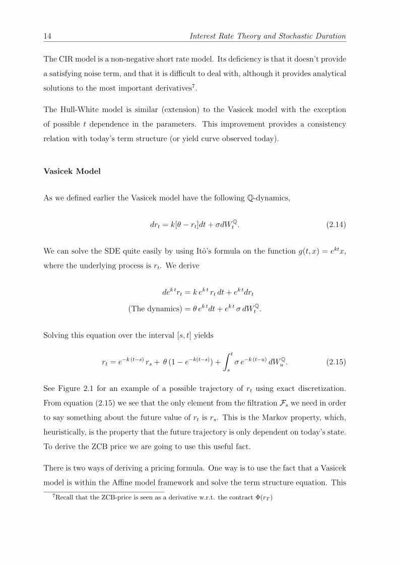
See Figure 2.1 for an example of a possible trajectory of rt using exact discretization.
From equation (2.15) we see that the only element from the filtration Fs we need in order
to say something about the future value of rt is rs. This is the Markov property, which,
heuristically, is the property that the future trajectory is only dependent on today’s state.
To derive the ZCB price we are going to use this useful fact.
There is two ways of deriving a pricing formula. One way is to use the fact that a Vasicek
model is within the Affine model framework and solve the term structure equation. This
7Recall that the ZCB-price is seen as a derivative w.r.t. the contract Φ(rT )
Chapter 2. Short Rate Models 15
T = 2; s = 0; r = 0.03; q = 0.06; k = 0.01; s = 0.04; d = 0.01;
sum@d_, T_, s_, s_D := TableBs Exp@-k tD RandomVariate@NormalDistribution@0, Sqrt@dDDD, :t, T - s
d>F ;
Accsum = Accumulate@sum@d, T, s, sDD;shortrate@T_, s_, r_, q_, k_, d_D := TableBr Exp@-k tD + q H1 - Exp@-k tDL + AccsumBB IntegerPartB t
dF FF,
8t, s + d, T, d<F;Interestratecurve = Transpose@8Table@i, 8i, 0, T, d<D, Prepend@shortrate@T, s, r, q, k, dD, rD<D;ListLinePlot@Interestratecurve, ImageSize Æ Large, PlotRange Æ 880, T<, 80, 0.07<<, LabelStyle Æ Bold,PlotStyle Æ Black, FrameStyle Æ ThickD
0.0 0.5 1.0 1.5 2.00.00
0.01
0.02
0.03
0.04
0.05
0.06
0.07
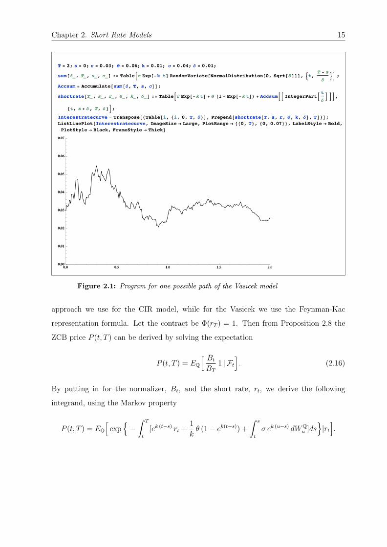
Figure 2.1: Program for one possible path of the Vasicek model
approach we use for the CIR model, while for the Vasicek we use the Feynman-Kac
representation formula. Let the contract be Φ(rT ) = 1. Then from Proposition 2.8 the
ZCB price P (t, T ) can be derived by solving the expectation
P (t, T ) = EQ
[ Bt
BT
1 | Ft]. (2.16)
By putting in for the normalizer, Bt, and the short rate, rt, we derive the following
integrand, using the Markov property
P (t, T ) = EQ
[exp
−∫ T
t
[ek (t−s) rt +1
kθ (1− ek(t−s)) +
∫ s
t
σ ek (u−s) dWQu ]ds
|rt].

16 Interest Rate Theory and Stochastic Duration
Because of the first part being Ft-measurable and deterministic we simplify the solution
to
P (t, T ) = exp−∫ T
t
ek (t−s) rt+1
kθ (1−ek(t−s))ds
EQ
[exp
−∫ T
t
∫ s
t
σ ek (u−s) dWQu ds
].
The first integral is easily solvable. We therefore approach the solution of the second
term. To find an solution we need to use the stochastic Fubini theorem and the moment
generating function for a Gaussian distributed random variable. Firstly, by the stochastic
Fubini theorem, we can rewrite the stochastic-deterministic integral as
∫ T
t
∫ s
t
σ ek (u−s) dWQu ds =
∫ T
0
∫ T
0
1[t,T ](s)1[t,s](u)σ ek (u−s) dWQu ds
(S.Fubini) =
∫ T
0
∫ T
0
1[t,T ](s)1[t,s](u)σ ek (u−s) ds dWQu ,
where we change the integrand in the following matter
1[t,T ](s)1[t,s](u) = 1[t,T ](s)1[t,s](u)1[t,T ](u) = 1[t,T ](s)1[u,∞)(s)1[t,T ](u).
Hence,
∫ T
0
∫ T
0
1[u,T ](s)1[t,T ](u)σ ek (u−s) ds dWQu =
∫ T
t
∫ T
u
σ ek (u−s) ds dWQu .
The next procedure is to use the moment generating function. The moment generating
function for a Gaussian distributed r.v. X is given by
MX(t)def= E[eXt] = etE[X]+ 1
2t2V ar[X].
Letting t = 1 and X =∫ Tt
∫ Tuσ ek (u−s) ds dWQ
u , which clearly is Gaussian distributed
due to the definition of the Ito integral and the deterministic integrand, we find the
expectation to be zero8 and variance
V arQ[−∫ T
t
∫ T
u
σ ek (u−s) ds dWQu ] =
∫ T
t
(∫ T
u
σ ek (u−s) ds)2
du.
8The expectation of a Ito integral is zero

Chapter 2. Short Rate Models 17
Rewriting the integral yields
2
∫ T
t
∫ T
u
∫ v
u
σ2 ek (u−s)ek (u−v) ds dv du = −σ2
kB(t, T )2 − σ2
k2(B(t, T )− T + t),
where B(t, T ) = 1k
(1− e−k(T−t)).
Then we have derived the price of the ZCB given the Vasicek model.
P (t, T ) = expA(t, T )−B(t, T ) rt
, (2.17)
where
A(t, T ) =(θk− σ2
2k2
)(B(t, T )− T + t)− σ2
4kB(t, T )2.
We see that the ZCB price given the Vasicek model have an Affine structure.
Example 2.1:
Let the time-interval; [t = 0.2, T = 1], interest rate at time t; rt = 0.03, the long run
interest rate; θ = 0.06, the speed of the mean reversion; k = 0.01 and the volatility be;
σ = 0.02. Then by the program in Figure 2.2 we find the price of the ZCB. P (t, T ) =
0.957893.
B@t_, T_D :=1
kH1 - Exp@-k HT - tLDL
A@t_, T_D :=q
k-s2
2 k2HB@t, TD - T + tL - s2
4 kB@t, TD2
P@t_, T_, r_D := Exp@A@t, TD - B@t, TD rDT = 1; t = 0.2; r = 0.03; q = 0.06; k = 0.01; s = 0.02;P@t, T, rD0.957893
Figure 2.2: Program for finding the ZCB price using the Vasicek model
Cox-Ingersoll-Ross model
The Q-dynamics of the CIR model is
drt = k[θ − rt]dt+ σ√rtdW
Qt .
18 Interest Rate Theory and Stochastic Duration
The model is constructed s.t. the short rate doesn’t become negative. This comes from
the fact that the CIR model is connected to a squared Ornstein-Uhlenbeck process
dXt = −αXtdt+ βdWt.
We show this fact by using Ito formula for g(t, x) =√x, with the underlying process
x = rt. Then
d√r(t) =
1
2r(t)−
12 dr(t)− 1
4r(t)−
32 (dr(t))2
=1
2r(t)−
12 ( k[θ − r(t)]dt+ σ
√r(t)dWQ
t )− 1
4r(t)−
32 σ2r(t)dt
=1
2r(t)−
12 (k θ − 1
2σ2)dt+
1
2
(− k√r(t)dt+ σdWQ
t
)(k θ =
1
2σ2) =
1
2
(− k√r(t)dt+ σdWQ
t
).
This is obvious an Ornstein-Uhlenbeck process for Xt =√rt, α = 1
2k and β = 1
2σ. Since
an Ornstein-Uhlenbeck obvious is Gaussian distributed we have that the CIR model is
some form of a non-central χ2 distributed r.v. .
Using the fact that the CIR model has an affine term structure,
α(t) = −k, β(t) = kθ, γ(t) = σ2, δ(t) = 0,
we use Proposition 2.10 to derive the ZCB price. Hence we have the following two systems
to solve
Bt(t, T )− kB(t, T )− 12σ2B(t, T )2 = −1
B(T, T ) = 0,
and
At(t, T ) = k θB(t, T )
A(T, T ) = 0.
In this case we are going to use (Mathematica) to help us. By Appendix B.1.1 we find
that
B(t, T ) =2(eh(T−t) − 1)
2h+ (k + h)(eh(T−t) − 1), (2.18)
Chapter 2. Short Rate Models 19
and
A(t, T ) =kθ(h+ k)(T − t) + 2 log[2h]− 2 log[h− k + (h+ k)eh(T−t)]
σ2. (2.19)
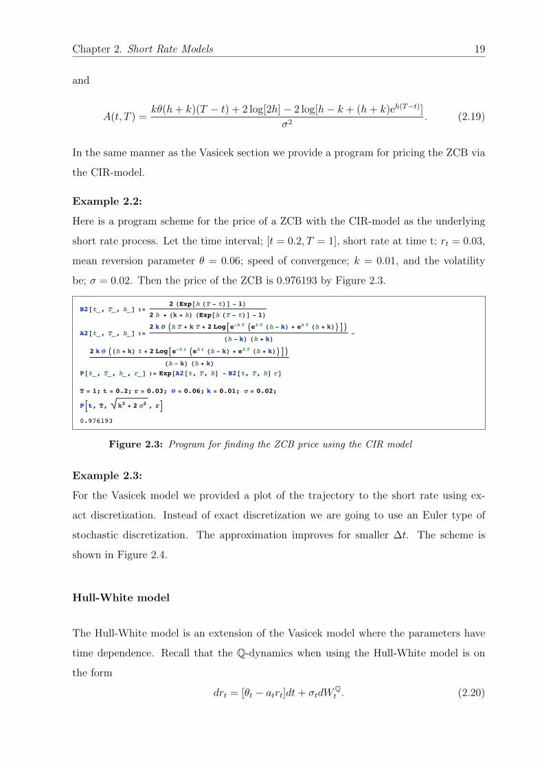
In the same manner as the Vasicek section we provide a program for pricing the ZCB via
the CIR-model.
Example 2.2:
Here is a program scheme for the price of a ZCB with the CIR-model as the underlying
short rate process. Let the time interval; [t = 0.2, T = 1], short rate at time t; rt = 0.03,
mean reversion parameter θ = 0.06; speed of convergence; k = 0.01, and the volatility
be; σ = 0.02. Then the price of the ZCB is 0.976193 by Figure 2.3.
B2@t_, T_, h_D :=2 HExp@h HT - tLD - 1L
2 h + Hk + hL HExp@h HT - tLD - 1LA2@t_, T_, h_D :=
2 k q Ih T + k T + 2 LogA„-h T I„h T Hh - kL + „h T Hh + kLMEMHh - kL Hh + kL -
2 k q IHh + kL t + 2 LogA„-h t I„h t Hh - kL + „h T Hh + kLMEMHh - kL Hh + kL
P@t_, T_, h_, r_D := Exp@A2@t, T, hD - B2@t, T, hD rDT = 1; t = 0.2; r = 0.03; q = 0.06; k = 0.01; s = 0.02;
PBt, T, k2 + 2 s2 , rF0.976193
Figure 2.3: Program for finding the ZCB price using the CIR model
Example 2.3:
For the Vasicek model we provided a plot of the trajectory to the short rate using ex-
act discretization. Instead of exact discretization we are going to use an Euler type of
stochastic discretization. The approximation improves for smaller ∆t. The scheme is
shown in Figure 2.4.
Hull-White model
The Hull-White model is an extension of the Vasicek model where the parameters have
time dependence. Recall that the Q-dynamics when using the Hull-White model is on
the form
drt = [θt − atrt]dt+ σtdWQt . (2.20)
20 Interest Rate Theory and Stochastic Duration
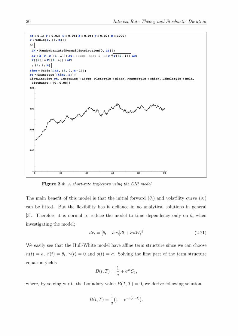
Dt = 0.1; r = 0.03; q = 0.06; k = 0.05; s = 0.02; m = 1000;r = Table@r, 8i, m<D;DoBDW = RandomVariate@NormalDistribution@0, DtDD;Dr = k Hq - r@@i - 1DDL Dt + H*Exp@-kHDt iLD*Ls r@@i - 1DD DW;r@@iDD = r@@i - 1DD + Dr;, 8i, 2, m<F
time = Table@i Dt, 8i, 0, m - 1<D;rt = Transpose@8time, r<D;ListLinePlot@rt, ImageSize Æ Large, PlotStyle Æ Black, FrameStyle Æ Thick, LabelStyle Æ Bold,PlotRange Æ 80, 0.08<D
0 20 40 60 80 100
0.02
0.04
0.06
0.08
Figure 2.4: A short-rate trajectory using the CIR model
The main benefit of this model is that the initial forward (θt) and volatility curve (σt)
can be fitted. But the flexibility has it defiance in no analytical solutions in general
[3]. Therefore it is normal to reduce the model to time dependency only on θt when
investigating the model;
drt = [θt − a rt]dt+ σdWQt (2.21)
We easily see that the Hull-White model have affine term structure since we can choose
α(t) = a, β(t) = θt, γ(t) = 0 and δ(t) = σ. Solving the first part of the term structure
equation yields
B(t, T ) =1
a+ eatC1,
where, by solving w.r.t. the boundary value B(T, T ) = 0, we derive following solution
B(t, T ) =1
a
(1− e−a(T−t)).

Chapter 2. Short Rate Models 21
To find A(t, T ) we integrate or solve the second term structure equation,
A(t, T ) =
∫ T
t
θsB(s, T )ds− 1
2σ2
∫ T
t
B(s, T )2ds. (2.22)
We want to choose θt s.t. it follows the initial forward curve. By the relation,
f(0, T ) =∂ logP (0, T )
∂T,
and knowing that the Hull-White model has an affine term structure we derive that
f(0, T ) =∂
∂T
(A(0, T )− r(0)B(0, T )
). (2.23)
Plugging in for A(0, T ) and B(0, T )
f(0, T ) =∂
∂T
( ∫ T
0
θsB(s, T )ds− 1
2σ2
∫ T
0
B(s, T )2ds− r(0)1
a
(1− e−aT
))=
∂
∂T
∫ T
0
θsB(s, T )ds− 1
2a2σ2e−2aT
(eat − 1
)2 − r(0)e−aT
(Appendix B.1.2.1) =
∫ T
0
θs∂
∂TB(s, T )ds− 1
2a2σ2e−2aT
(eat − 1
)2 − r(0)e−aT .
Define
ψ(T )def=
∫ T
0
∂
∂TθsB(s, T )ds− r0e−aT
and
h(T )def=
1
2a2σ2e−2aT
(eat − 1
)2.
Then
ψ(T ) = f(0, T ) + h(T ).
By further calculation in appendix B.1.2.2 we derive that
∂
∂Tψ(T ) = θT − aψ(T ).

22 Interest Rate Theory and Stochastic Duration
Putting in for ψ yields that
θT =∂
∂T
[(f(0, t) + h(T ))
]+ a(f(0, T ) + h(T )).
In order to calculate θT we need to fit the initial forward curve e.g. by a parametric
model, and estimate a and σ.
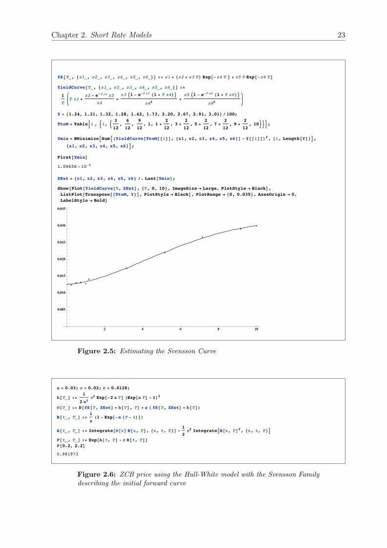
Example 2.4:
We fit the initial forward using the Svensson family. The Svensson family parametric
model is defined as [8]
fS(x, z) = z1 + (z2 + z3x)e−z4x + z5xe−z6x. (2.24)
Since we observe the yield curves, we use the defined relation
Y (t, T )def=
1
T − t
∫ T
t
f(t, s)ds,
and estimate the parameters. We see by Figure 2.5 that we get a fairly good estimate
of the parameters. Calculating θT , we derive a price for the ZCB given that a = 0.3,
σ = 0.02, t = 0.2, T = 2.2 and the short rate at time 0 is r0 = 0.0128. From Figure 2.6
we see that the price of the ZCB is 0.981973.
Chapter 2. Short Rate Models 23
fS@T_, 8z1_, z2_, z3_, z4_, z5_, z6_<D := z1 + Hz2 + z3 TL Exp@-z4 T D + z5 T Exp@-z6 TDYieldCurve@T_, 8z1_, z2_, z3_, z4_, z5_, z6_<D :=
1
TT z1 +
z2 - „-T z4 z2
z4+z3 I1 - „-T z4 H1 + T z4LM
z42+z5 I1 - „-T z6 H1 + T z6LM
z62
Y = 81.24, 1.31, 1.32, 1.28, 1.42, 1.73, 2.20, 2.67, 2.91, 3.01< ê100;TtoM = TableBi , :i, : 3
12,
6
12,
9
12, 1, 1 +
2
12, 3 +
2
12, 5 +
2
12, 7 +
2
12, 9 +
2
12, 10>>F;
Ymin = NMinimizeASumAHYieldCurve@TtoM@@iDD, 8z1, z2, z3, z4, z5, z6<D - Y@@iDDL2, 8i, Length@YD<E,8z1, z2, z3, z4, z5, z6<E;
[email protected]¥10-6
ZEst = 8z1, z2, z3, z4, z5, z6< ê. Last@YminD;Show@Plot@YieldCurve@T, ZEstD, 8T, 0, 10<, ImageSize Æ Large, PlotStyle Æ BlackD,ListPlot@Transpose@8TtoM, Y<D, PlotStyle Æ BlackD, PlotRange Æ 80, 0.035<, AxesOrigin Æ 0,LabelStyle Æ BoldD
2 4 6 8 10
0.005
0.010
0.015
0.020
0.025
0.030
0.035
Figure 2.5: Estimating the Svensson Curve
a = 0.03; s = 0.02; r = 0.0128;
h@T_D :=1
2 a2s2 Exp@-2 a TD HExp@a TD - 1L2
q@T_D := D@fS@T, ZEstD + h@TD, TD + a H fS@T, ZEstD + h@TDLB@t_, T_D :=
1
aH1 - Exp@-a HT - tLDL
A@t_, T_D := Integrate@q@sD B@s, TD, 8s, t, T<D - 1
2s2 IntegrateAB@s, TD2, 8s, t, T<E
P@t_, T_D := Exp@A@t, TD - r B@t, [email protected], 2.2D0.981973
Figure 2.6: ZCB price using the Hull-White model with the Svensson Familydescribing the initial forward curve


Chapter 3
A first look at the HJM-model
The HJM-Model describes the instantaneous forward rate rather than the short rate.
This means that the SDE have the following form under the Q-measure,
df(t, u) = α(t, u)dt+ σ(t, u)dWQt ,
or equivalent,
f(t, u) = f(0, u) +
∫ t
0
α(s, u)ds+
∫ t
0
σ(s, u)dWQs .
Definition 3.1 (Instantaneous forward rate [1]):
The instantaneous forward rate with maturity T , contracted at time t, are defined as
f(t, T )def= −∂ logP (t, T )
∂T(3.1)
3.1 HJM no-arbitrage drift condition
Using Definition 3.1 the forward rate1
P (t, T ) = exp−∫ T
t
f(t, u)du.
1Instantaneous forward rate
25

26 Interest Rate Theory and Stochastic Duration
By the First Fundamental theorem we would like the normalized ZCB price, P (t, T ), to
be a Martingale under the Q-dynamics. Plugging in for the forward rate the normalized
ZCB price have the following path
P (t, T ) = exp−( ∫ t
0
f(s, s)ds+
∫ T
t
f(t, u)du),
where f(s, s) = rs (definition 3.5). Using Fubini and Stochastic Fubini we derive that
∫ t
0
f(s, s)ds =
∫ t
0
f(0, s) +
∫ s
0
α(v, s)dv +
∫ s
0
σ(v, s)dWQv ds
(Fubini) =
∫ t
0
f(0, s)ds+
∫ T
0
∫ T
0
1[0,t](s)1[0,s](v)α(v, s) ds dv
+
∫ T
0
∫ T
0
1[0,t](s)1[0,v](u)σ(v, s)dsdWQv
=
∫ t
0
f(0, s)ds+
∫ t
0
∫ t
v
α(v, s) ds dv +
∫ t
0
∫ t
v
σ(v, s) ds dWQv ,
since
1[0,t](s)1[0,s](v) = 1[0,t](v)1[0,t](s)1[v,∞](s) = 1[0,t](v)1[v,t](s),
and
∫ T
t
f(t, u)dufub.=
∫ T
t
f(0, u)du+
∫ t
0
∫ T
t
α(v, u)dudv +
∫ t
0
∫ T
t
σ(v, u)dudWQv .
Adding the two integrals together yields
∫ T
t
f(t, u)du+
∫ t
0
f(u, u)du =
∫ T
0
f(0, u)du
+
∫ t
0
(∫ T
t
α(v, u)du+
∫ t
v
α(v, u)du)dv
+
∫ t
0
(∫ T
t
σ(v, u)du+
∫ t
v
σ(v, u)du)dWQ
v ,
which result in the equation
∫ T
0
f(0, u)du︸ ︷︷ ︸Constant
+
∫ t
0
∫ T
v
α(u, v)dudv +
∫ t
0
∫ T
v
σ(v, u)dudWQv . (3.2)
Chapter 3. A first look at the HJM-model 27
The first term is known (observed in the market), and the two last terms we define as
Xt, yielding the dynamics
dXt = αT (t, t)dt+ σT (t, t)dWQt ,
where α and σ are defined as the integrands in equation (3.2). If we take a look at the
dynamics of the normalized ZCB price,
P (t, T ) = e−(C+Xt),
we find, using Ito’s formula, that
dP (t, T ) = −P (t, T )dXt +1
2P (t, T )(dXt)
2
= −P (t, T )(αT (t, t)dt+ σT (t, t)dWQt ) +
1
2P (t, T )σT (t, t)2dt
= P (t, T )(1
2σT (t, t)2 − αT (t, t)
)dt− P (t, T )σT (t, t)dWQ
t .
By the First Fundamental theorem the normalized ZCB price need to be a Martingale
since we assume arbitrage free prices. Hence
1
2σT (t, t)2 − αT (t, t) = 0,
yielding the no arbitrage drift condition,
α(t, T ) = σ(t, T )
∫ T
t
σ(t, u)du, (3.3)
when differentiating w.r.t. T on both sides.
Theorem 3.2 (HJM no-arbitrage condition):
If we assume no arbitrage, then by the First Fundamental theorem the risk neutral dy-
namics of f(t, u) is on the form
f(t, u) = f(0, u) +
∫ t
0
α(s, u)ds+
∫ t
0
σ(s, u)dWQs , (3.4)

28 Interest Rate Theory and Stochastic Duration
where
α(t, T ) = σ(t, T )
∫ T
t
σ(t, u)du, (3.5)
referred to as the HJM no-arbitrage condition.
3.2 The Musiela Parametrization
Instead of using the parametrization time-of-maturity, T , Musiela proposed to use time-
to-maturity, x = T − t. This yield a slight difference in the forward rate dynamics.
Define
ft(x)def= f(t, t+ x) (3.6)
Because of the Musiela parametrization we get a t-dependence in the second variable.
Let ∂∂T
stand for differentiating w.r.t. to the second variable. Then formally
dft(x) = df(t, t+ x) = df(t; t+ x) +∂
∂Tf(t, t+ x)dt
= α(t, t+ x)dt+ σ(t, t+ x)dWQt +
∂
∂Tf(t, t+ x)dt.
We observe that
df(t, T ) = dft(T − t)
= dft(x)− ∂
∂xft(T − t)dt
= α(t, t+ x)dt+ σ(t, t+ x)dWQt +
∂
∂Tf(t, t+ x)dt− ∂
∂xft(T − t)dt,
which we know is equal to
α(t, t+ x)dt+ σ(t, t+ x)dWQt .
Hence,∂
∂Tf(t, t+ x)dt =
∂
∂xft(T − t)dt.
Chapter 3. A first look at the HJM-model 29
Proposition 3.3 (The Musiela Equation):
Assume that we have the forward rate dynamics under Q given as
df(t, T ) = α(t, T )dt+ σ(t, T )dWQt . (3.7)
Then by the Musiela parametrization ft(x) = f(t, t+ x) we have the following dynamic
dft(x) =[( ∂∂xft(T − t) + αt(x)
)dt+ σt(x)dWQ
t
]x=T−t
, (3.8)
commonly referred to as the Musiela equation, where
σt(x) = σ(t, t+ x),
αt(x) = σt(x)
∫ x
0
σt(u)du.
3.3 Choices of Volatility structure
In the forthcoming we are going to show some choices of volatility structure. We start
with the Vasicek and Hull-White because the choices of volatility structure are identical
in the non t-dependence case. In fact, then the Vasicek model is a specific choice of the
initial forward rate.
3.3.1 Vasicek and Hull-White
Assume that σ(t, T ) = σe−k(T−t). Then the arbitrage-free drift condition provide the
following drift
α(t, T ) = σ(t, T )
∫ T
t
σ(t, s)ds
= σe−k(T−t)∫ T
t
σe−k(s−t)ds
= −σe−k(T−t) 1
k
[σe−k(s−t)
]Ts=t
=σ2
ke−k(T−t)(1− e−k(T−t)).

30 Interest Rate Theory and Stochastic Duration
Putting into the forward rate yields
f(t, T ) = f(0, T ) +
∫ t
0
σ2
ke−k(T−s)(1− e−k(T−s))ds+
∫ t
0
e−k(T−s)σdWs
(Integrating) = f(0, T ) +σ2
k2e−kT
(e−kT2− 1− e2kt−kT
2+ ekt
)+
∫ t
0
e−k(T−s)σdWs.
Using the relation rt = f(t, t) we deduce that
rt = f(0, T ) +σ2
2k
(e−2kt − 2e−kt− 1 + 2
)+
∫ t
0
e−k(t−s)dWs
= f(0, t) +σ2
2k2
(1− e−kt
)2+
∫ t
0
e−k(t−s)σdWs.
Define φ(t)def= f(0, t) + σ2
2k2
(1− e−kt
)2and Xt =
∫ t0σeksdWs. Then
rt = φ(t) + e−ktXt.
Using Ito’s formula, with Xt as the underlying process yields
drt = (φ′(t)− kXt)dt+ e−ktdXt
= (φ′(t)− k(r(t) + φ(t))dt+ σdWt
= k(φ′(t)− kφ(t)
k− r(t)
)+ σdWt
def= k
(θ(t)− r(t)
)dt+ σdWt.
This is the Hull-White model. The Vasicek model is the specific choice of θ(t) = θ. From
earlier deductions we know that, given the specific choice of mean reversion,
rt = e−ktr0 + θ(1− e−kt) +
∫ t
0
σe−k(t−u)dWu.
Hence if we choose
f(0, t) = r0e−kt + θ(1− e−kt)− σ2
2k2
(1− e−kt
)2

Chapter 3. A first look at the HJM-model 31
we derived the Vasicek model. An another way of deriving the same initial forward rate
is provided in appendix B. There we solve the differential equation
θ(t) = θ
w.r.t. the initial forward rate.
3.3.2 CIR
Letting σ(t, T ) = e−k(T−t)√r(t)σ we derive the CIR-model when specifying the initial
forward rate structure. Using the arbitrage-free drift condition the drift in the model
becomes
α(t, T ) = σ(t, T )
∫ T
t
σ(t, u)du
= e−k(T−t)√r(t)σ
∫ t
0
e−k(u−t)√r(t)σdu
= e−k(T−t)r(t)σ2 1
k(1− e−k(T−t)).
Putting in for the the drift we find the forward rate,
f(t, T ) = f(0, T ) +
∫ t
0
e−k(T−s)rsσ2
k
(1− e−k(T−s))ds+
∫ t
0
e−k(T−s)σ√r(s)dWs,
and the short-rate,
rt = f(0, t) +
∫ t
0
e−k(t−s)rsσ2
k
(1− e−k(t−s))ds+
∫ t
0
e−k(t−s)σ√r(s)dWs.
Defining
φ(t) = f(0, t) +
∫ t
0
e−k(t−s)r(s)σ2
k
(1− e−k(t−s))ds
and letting
Xt =
∫ t
0
eksσ√r(s)dWs

32 Interest Rate Theory and Stochastic Duration
yields the same procedure as above. By Ito’s formula
dr(t) = k(θ′(t)− kθ(t)
k− r(t)
)dt+
√r(t)σdWt.
Then solving the differential equation
θ′(t)− kθ(t)k
= θ
w.r.t. the initial forward rate yields the CIR model.
3.4 Calibration of the forward curve: An introduc-
tion
In the market we observe bond prices. The first task is to derive the yield-to-maturity
(YTM) curve. The YTM is the annual return of holding a bond. To calculate the YTM
we need (in parentheses Norway)
• Maturity date
• Settlement date (trade date + 3 working days)
• Bond prices
• Face Value (100)
• Coupon rate
• Coupon interval (Annual)
• Day convention (Actual/365)
Then the YTM is the solution of
PVB =FV
(1 + Y TM)M−1
I+ n
365
+M−1∑i=0
CiFV
I(1 + Y TM)iI
+ n365
,

Chapter 3. A first look at the HJM-model 33
where PVB is the present value of the bond(observed price), FV is the face value, Ci is
the coupon rate, I is the coupon interval, M is the number of payments until maturity
and n is the number of days until the first payment. When we are solving w.r.t. Y TM ,
numerical approaches is preferable.
When the YTM is calculated we want to find the continuously compounded spot rate
defined as
Y (t, T ) = − log[P (t, T )]
(T − t),
where P (t, T ) is the ZCB price. The reason we want to find the continuously compounded
spot rate is because of the relation
Y (t, T ) =1
T − t
∫ T
t
f(t, s)ds.
When we have found the Y TM ’s we can easily calculate the related ZCB price by
PVZCB =1
(1 + Y TM)m365
,
where m is the number of days between the settlement date and maturity date. Having
the ZCB price we derive the observed continuously compounded spot rate
Y obs = − log[PVZCB]m
365
.
A first time calibration:
Recall that the forward rate is the solution
f(t, T ) = f(0, T ) +
∫ t
0
α(s, T )ds+
∫ t
0
σ(s, T )dWQs ,
where α(t, T ) follow the arbitrage-free drift condition. Because of the arbitrage drift
condition we only need to calibrate the initial forward curve f(0, T ) and the volatility
structure σ(t, T ). We calibrate the initial forward rate due to today’s forward curve, using

34 Interest Rate Theory and Stochastic Duration
e.g. smoothing splines, Svensson curve or Nelson-Siegel curve. In Norway the Svensson
curve is used [3].
Because of Girsanov’s theorem the volatility structure is equal under the objective proba-
bility measure P and under the Equivalent Martingale measure Q. Therefore the volatility
structure σ(t, T ) can be estimated through historical data. We have observed the contin-
uously compounded spot rate
Y (t, T ) =1
T − t
∫ T
t
f(t, s)ds.
Putting in for the forward rate yields
=1
T − t
∫ T
t
(f(0, s) +
∫ t
0
α(u, s)du+
∫ t
0
σ(u, s)dWu
)ds.
After calculating the continuously compounded spot rate for the time-to-maturity τk we
have a data set
xj(τk) = Y (tj, tj + τk),
for each time of observation t1, t2, . . . , tJ . Then it is two ways of estimating the volatility
structure. If the time-series xj(τk)Jj=1 have a small auto-correlation we can use the
pure observations. But if there are a clear auto-correlation, a common approach [3] is to
estimate the volatility structure w.r.t. the increments
∆xj(τk) = xj+1(τk)− xj(τk),
where tj+1 = tj + δ.
If there is a small auto-correlation we see that the volatility structure of the continuously
compounded spot rate is
V ar[Y (t, T )] =1
(T − t)2V ar[
∫ t
0
∫ T
t
σ(u, s)dWuds].

Chapter 3. A first look at the HJM-model 35
Using stochastic Fubini theorem
=1
(T − t)2V ar[
∫ t
0
∫ T
t
σ(u, s)dsdWu]
=1
(T − t)2
∫ t
0
E[( ∫ T
t
σ(u, s)ds)2]
du,
which for a deterministic volatility structure is
1
(T − t)2
∫ t
0
(∫ T
t
σ(u, s)ds)2
du.
Example 3.1:
Assume the Vasicek/Hull-White volatility structure. Then
σ(u, s) = σe−k(s−u).
Integrating the inner integral yields
∫ T
t
σ(u, s)ds = −1
kσ(
e−k(T−u) − e−k(t−u)).
By squaring the inner integral and integrating the outer integral,
∫ t
0
1
k2σ2(e−k(T−u) − ek(t−u))2du =
σ2
2k3e−2k(T+t)(e2kt − 1)(ekT − ekt)2,
we find the variance of the continuously compounding spot rate that we are estimating,
V ar[Y (t, T )] =1
(T − t)2
σ2
2k3e−2k(T+t)(e2kt − 1)(ekT − ekt)2
Note that, if we have day-to-day observations of the volatility, t = 1365
.
If there are some auto-correlation we continue estimating the volatility structure based
on the increments of the observed continuously compounded spot rate. On increment

36 Interest Rate Theory and Stochastic Duration
form the continuously compounded spot rate take the form [1]
dY (t, T ) =1
T − t
(rt dt+
∫ T
t
α(t, s)ds dt+
∫ T
t
σ(t, s)ds dWt
).
Discretizing the time-steps yields
∆xj(τ) =1
τ
(rtj∆tj +
∫ tj+τ
tj
α(tj, s)ds∆tj +
∫ tj+τ
tj
σ(tj, s)ds∆Wtj
),
where ∆tj = δ. We then find that
V ar[∆xj(τ)] = V ar[1
τ
(rtj∆tj +
∫ tj+τ
tj
α(tj, s)ds∆tj +
∫ tj+τ
tj
σ(tj, s)ds∆Wtj
)]=
1
τ 2
(∫ tj+τ
tj
σ(tj, s)ds)2
V ar[∆Wtj ]
=1
τ 2
(∫ tj+τ
tj
σ(tj, s)ds)2
∆tj,
for a deterministic volatility structure.
Estimating procedure using PCA
The estimating procedure of the volatility structure is as follows:
• Use Principal Component Analysis to find an approximation (the important com-
ponents) of time-to-maturity specific risk
• Choose and fit volatility structures for the important volatility components
A market observation is that there are time-to-maturity specific risk. In the forthcoming
chapters we are going to present models of possible infinite time-to-maturity. If we follow
the market observation we then have infinite dimension of noise. Clearly we need to reduce
the amount of dimensions, and our tool is Principal Component Analysis. Principal
Component Analysis within interest rate theory is presented in both [3] and [8]. PCA is
based on the spectral decomposition theorem.

Chapter 3. A first look at the HJM-model 37
Assume that we can decompose the vector into
X = µ+ AY = µ+∑i≥1
Yiai,
where
E[X] = µ and Cov[X] = Q = ALAT ,
E[Y ] = 0 and Cov[Y ] = L,
and ALAT is the spectral decomposition with L as the diagonal matrix of eigenvalues,
DiagMλii≥1. Estimating the covariance matrix Q based on K time-to-maturities we
have by the spectral decomposition that
Q =K∑k=1
λiaiaTi ,
where ai’s are the vector elements in matrix A. A good property of the decomposition
presented is that the total variance of X is equal to the total variation of Y
K∑k=1
V ar[Xk] =K∑k=1
V ar[Yk] = tr[L].
This means that for a d ≤ K we describe
∑dk=1 V ar[Yk]
tr[L]
amount of the total variation by the d first components. Observing that the d first com-
ponents describe more than e.g. 99% of the variance we can approximate the covariance
matrix
Q ≈ Qapprox =d∑i=1
λiaiaTi .
We estimate the volatility structure of d-th component minimizing e.g. by the least square
K∑k=1
(√λkakaTk −
1
τk
∫ tj+τk
tj
σ(tj, s)ds)2
→ minσ.

38 Interest Rate Theory and Stochastic Duration
Hence we approximate the infinite dimension of noise term by
df(t, T ) = α(t, T )dt+ σ1(t, T )dW 1t + σ2(t, T )dW 2
t + · · ·+ σd(t, T )dW dt ,
where W kt , for k = 1, . . . , d, are independent Brownian Motion. Then the arbitrage drift
condition is
α(t, T ) =d∑
k=1
σk(t, T )
∫ T
t
σ(t, s)ds.
Within interest rate theory three components is usually sufficient for an good approxi-
mation of the volatility structure. A code for the Principal Component Analysis for the
first example in [8] is presented in Chapter 7.

Chapter 4
Infinite Dimensional Stochastic
Analysis
There are two aspects concerning infinite dimensional modeling of the term structure.
The first aspect is modeling of the dynamics in time and space with time-to-maturity as
the space variable. Then we get an infinite maturity horizon. This problem we already
approached under the first view of HJM-modeling through the Musiela parametrization.
A market view is that there exists maturity specific noise. With an infinite maturity
horizon we need infinitely many sources of noise. This actually leads to the field of
infinite dimensional stochastic analysis.
The finite dimensional stochastic model has the following shortcoming from the viewpoint
of a fixed trader. From a complete market1 point of view we can by a finite dimension
of noises perfectly hedge (i.e. replicate) a, e.g., call option on a bond with x = 5 years
by means of a bond with x = 30 years. This contradicts market observations. The risk
we don’t take into account is the ”maturity specific risk”. Hence we would like to model
the maturity specific risk. The solution is a stochastic partial differential equation with
infinite dimensional noise. I.e. the instantaneous forward rate is modeled in the following
1We have an incomplete market and make it complete through using internal relations between thesame type of bonds(e.g. ZCB with its derivatives and maturities)
39
40 Interest Rate Theory and Stochastic Duration
way
dft(x) =( ∂∂xft(x) + αt(x)
)dt+
∑i∈N
σ(i)t (x)dW
(i)t , (4.1)
where W (i)t i≥1 are independent Brownian motions and each represent ”maturity specific
risk”.
4.1 Cylindrical Brownian Motion (CBM)
In this part we want to generalize infinite dimensional stochastic partial differential equa-
tions on the form
dX(t) = (drift)dt+∑i∈N
σ(i)t (x)dW
(i)t . (4.2)
E.g. choosing σ(i)t ≡ 1 the variance
V ar[X(t)] ≥ V ar[
∫ t
0
∑i∈N
σ(i)s (x)dW (i)
s ]
=∑i∈N
V ar[W it ]
=∑i∈N
t =∞.
Therefore we need to introduce a framework for the study of SPDE’s. The solution
space for SPDE’s is a separable Hilbert space, on which we are going to put additional
constraints.
Definition 4.1 (Hilbert Space):
A Hilbert space H is a vector space with an inner product
〈·, ·〉 : H ×H 7→ R,
where the inner product has the following properties
1. 〈x+ y, z〉H = 〈x, z〉H+〈y, z〉H where x, y, z ∈ H (Linearity 1)
2. 〈αx, z〉H = α〈x, z〉H where x, z ∈ H and α ∈ R (Linearity 2)
Chapter 4. Infinite Stochastic Analysis 41
3. 〈αx, z〉H = 〈αz, x〉H where x, z ∈ H,
s.t. H is complete w.r.t. the norm
‖x‖ def=√〈x, x〉.
We remark that if H is complete then for each Cauchy sequences there exists an x ∈ H
which the sequence converges too. I.e. if ‖xn − xm‖ → 0 is a Cauchy sequence there
exists an x ∈ H s.t. ‖xn − x‖ → 0 when n→∞.
Definition 4.2 (Separable Hilbert Space):
A Hilbert space H is called separable if it exists a dense countable subset y1, y2, . . . of
H s.t. for all ε > 0 and all x ∈ H there exists y ∈ y1, y2, . . . s.t. ‖y − x‖H < ε.
The choice of Hilbert space becomes clear when we define the Cylindrical Brownian
motion. The reason for adding the separability is because we would prefer the Borel
σ-algebra2, B(H)3, to be equal the σ-algebra generated by ”balls”. This property is
preferable because the σ-algebra generated by the balls simplifies some of the proves. We
are not going through those, but rather refer to [8]4.
Theorem 4.3 (ONB Representation theorem):
Let H be a Hilbert space. Then there exists an orthonormal basis (ONB) uk, k ≥ 1 of H,
i.e.
〈ui, uj〉H =
1, i = j
0, i 6= j,
s.t. for all x ∈ H we have the representation
x =∑k∈N
〈x, uk〉Huk.
2Sometimes referred as σ-field when working with random variable that is an element of R3The Borel σ-algebra is the smallest σ-algebra generated by open balls. A existence of a dense
countable subset means that we can create balls that equal the Borel σ algebra4Chapter 3
42 Interest Rate Theory and Stochastic Duration
Furthermore Parseval’s equality provides
‖x‖2H =
∑i∈N
〈x, ui〉2.
Before we use the definition of Brownian motion and Theorem (4.3) to define the Cylin-
drical Brownian motion we define the Cylindrical Gaussian measure.
Definition 4.4 (Cylindrical Gaussian Measure (CG) [4]):
Let H be a real separable Hilbert space, then the r.v. X : H 7→ L2(Ω,F ,P) on the
probability space (Ω,F ,P) is a Cylindrical Standard Gaussian if
1. The mapping X(h) is linear; i.e. X(αk + βh) = αX(k) + βX(h)
2. For an arbitrary h ∈ H, X(h) is a Gaussian r.v. with mean zero and variance ‖h‖2H
3. If h, h′ ∈ H are orthogonal, i.e. 〈h, h′〉H = 0, then the r.v.s X(h) and X(h′) are
independent.
We note that by Theorem (4.3), letting ujj≥1 be an orthonormal basis in H and h ∈ H,
we can represent X(h) as a P-a.s. convergent series (by kolmogorov three series5)
X(h) = X(∑j∈N
〈h, uj〉Huj)
=∑j∈N
〈h, uj〉HX(uj),
where in the last equality we used the linearity property in Definition (5.4).
Definition 4.5 (Cylindrical Brownian motion [4]):
A family Wtt≥0 defined on a filtered probability space (Ω,F , Ftt≥0,P) is called a
Cylindrical Brownian motion in a Hilbert space H if
1. For an arbitrary t ≥ 0 the mapping Wt : H 7→ L2(Ω,F ,P) is linear.
2. For an arbitrary h ∈ H, Wt(h) is an Ft-Brownian motion
(a) W0(h) = 0 P-a.s.
5[4]

Chapter 4. Infinite Stochastic Analysis 43
(b) For 0 ≤ t1 ≤ · · · ≤ tn = t we have that
Wt1(h),Wt2(h)−Wt1(h), . . . ,Wt(h)−Wtn−1(h)
are independent of each other.
(c) For t ≥ s we have that
Wt(h)−Ws(h)d= Wt−s(h)
are equally distributed, where Wt−s(h) ∼ CG[0, (t− s)‖h‖2
H
]3. For arbitrary h, h′ ∈ H and t ≥ 0, E[Wt(h)Wt(h
′)] = t〈h, h′〉H
Because of the linearity we can represent the Cylindrical Brownian motion as a P-a.s.
convergent series
Wt(h) =∑j∈N
〈h, uj〉HWt(uj),
where ujj≥1 is an ONB in H and W1(uj), for j ≥ 1, is a sequence of independent
standard Gaussian distributed random variables.6
In the forthcoming we are going to work with the completed filtration generated by the
Cylindrical Brownian motion. I.e.
Ft = N ∪ σWu; 0 ≤ u ≤ t,
where N stands for the P-null sets.
4.2 Ito integral w.r.t. Cylindrical Brownian Motion
Our class of function is going to be a subset of Hilbert-Schmidt operators. Therefore we
define the Hilbert-Schmidt operators first.
6‖uj‖2H = 1
44 Interest Rate Theory and Stochastic Duration
Definition 4.6 (Hilbert-Schmidt operators):
Let H and K be two Hilbert spaces. Then the operator
A : H −→ K
with the condition that∑
l≤1‖A(ul)‖2K < ∞ for an ONB ul, l ≥ 1 in H, is called a
Hilbert-Schmidt operator. The class of Hilbert-Schmidt operators from H to K is denoted
HS(H,K).
Definition 4.7:
Let L(H,K) = L[0,T ](H,K) be the class of functions f(t,ω) ∈ HS(H,K), i.e.
f(t,ω) : R+ × Ω −→ HS(H,K),
with the following properties
1. (t, w) 7→ f(t,ω) is B(R+) ⊗ F -measurable where B denotes the Borel σ-algebra and
h 7→ f(·,·)(h) is B(HS(H,K))-measurable
2. f(t,ω) is Ft-adapted
3. Existence of second moment: E[ ∫ T
0‖ft‖2
HS(H,K)dt]<∞
In the forthcoming we are going to make sense of the integral
IC [f ](ω) =
∫ T
0
f(t,ω)dWt, (4.3)
where f(t,ω) ∈ L(H,K). Firstly we construct the Ito integral w.r.t. CBM through defining
Ito integral w.r.t. CBM on elementary functions7. Then expand and show that the
elementary function can approximate the functions in L(H,K). After the procedure we
logically define the integral (4.3).
7Sometimes called elementary process
Chapter 4. Infinite Stochastic Analysis 45
An elementary function φ ∈ L(H,K) is defined as
φ(t,ω) = e0(w)10(t) +n∑j=1
ej(ω)1(tj ,tj+1](t), (4.4)
where 0 ≤ t1 ≤ · · · ≤ tn. We observe that ej must be Ftj -adapted. For an h ∈ H we
define the Ito integral w.r.t. the CBM in a Hilbert space K8 for elementary function as
(
∫ t
0
φ(t,ω)dWt)(h)def=
n∑j=1
Wtj+1∧t[ej(h)]−Wtj∧t[ej(h)].
Using this definition we derive the Ito-isometry for elementary functions.
Lemma 4.8 (Ito-isometry):
If φ(t,ω) ∈ L(H,K) is a bounded elementary function then
E[(( ∫ t
0
φsdWs
)[h])2]
=
∫ T
0
E[‖φs(h)‖2K ]ds <∞ (4.5)
Sketch of proof. Firstly we use the definition of the Ito integral w.r.t. CBM,
E[(( ∫ t
0
φsdWs
)[h])2]
= E[( n∑
j=1
Wtj+1∧t[ej(h)]−Wtj∧t[ej(h)])2]
,
and divide the summation into two parts,
E[ n∑j=1
(Wtj+1∧t[ej(h)]−Wtj∧t[ej(h)]
)2]
+ E[ n∑
(j 6=i)=1
(Wtj+1∧t[ej(h)]−Wtj∧t[ej(h)]
)(Wti+1∧t[ei(h)]−Wti∧t[ei(h)]
)].
Using the linearity property of expectation, and the property of the CBM we derive the
first expectation
E[(Wtj+1∧t[ej(h)]−Wtj∧t[ej(h)]
)2]
= (tj+1 ∧ t− tj ∧ t)E[‖ej(h)‖2
K
].
8In [4] they have been proper with the definition of CBM and the space that the CBM is defined on.This is why they need to work with adjoint operators
46 Interest Rate Theory and Stochastic Duration
When deriving the second expectation we use the rule of double expectation,
E[E[(Wtj+1∧t[ej(h)]−Wtj∧t[ej(h)]
)(Wti+1∧t[ei(h)]−Wti∧t[ei(h)]
)|Ftj∨ti
]].
Then i∧ j9-term is Ftj∨ti-measurable since i∧ j+ 1 ≤ j ∨ i when i 6= j, and the i∨ j-term
is independent of Ftj∨ti . Hence
E[E[(Wtj∨i+1∧t[ej∨i(h)]−Wtj∨i∧t[ej∨i(h)]
)]︸ ︷︷ ︸=0 by CBM
rest]
= 0.
Letting n→∞ we find that
n∑j=1
(tj+1 ∧ t− tj ∧ t)E[‖ej(h)‖2
K
]−→
∫ t
0
E[‖φ(h)‖2K ]ds,
using linearity properties of the norm.
The next step is to approximate all functions in L(H,K) by an bounded elementary
function. This is proved through a three steps proof similar to [9].
Proposition 4.9 (The function space):
If f ∈ L(H,K), then there exists a sequence of bounded elementary functions φn, n ≤ 1
approximating f in L(H,K), i.e.,
‖φn(s)− fs‖L(H,K)2 = E[ ∫ T
0
‖φn(s)− fs‖2HS(H,K)dt
]−→ 0
as n→∞.
Proof. [4]
It is possible to extend the class L(H,K) to P(H,K) where the main difference is that
instead of assuming existence of second moment we are weakening this property (def.4.7.3)
and assume
P[ ∫ T
0
‖ft‖2HS(H,K)dt <∞
]= 1.
9∧ = inf , ∨ = sup
Chapter 4. Infinite Stochastic Analysis 47
The assumption create a local Ito integral w.r.t Cylindrical Brownian motion, where
clearly the relation L ⊂ P holds. In addition we need to work with progressive measurable
stochastic process where stopping times is a necessary concept (for a stopped process we
know that the second moment exists).
Ito integral w.r.t. independent CBM
Assume that Wt is a CBM in a Hilbert Space K, and let ull≥1 ⊂ K be a sequence of
ONB in K. Then we have showed that for a k ∈ K
Wt(k) =∑l∈N
〈k, ul〉KWt(ul).
We clearly see that Wt(ul) is independent and distributed CG(0, t〈ul, ul〉) = CG(0, t)
which is identical in distribution to a Brownian motion. For simplicity we define Wt(ul) =
W lt and refer it as a Brownian motion.
Let ft ∈ L(H,K) and h ∈ H, then we know that there exists a bounded elementary
function φt s.t. ( ∫ t
0
fsdWs
)(h)
approx=
( ∫ t
0
φsdWs
)(h).
From the definition of the Ito integral w.r.t. Cylindrical Brownian motion
( ∫ t
0
φsdWs
)(h) =
n∑j=1
Wtj+1∧t[ej(h)]−Wtj∧t[ej(h)].
Since ej(h) ∈ K we use the ONB representation theorem (See 4.3) and rewrite the
elementary function for an ONB ul, l ≥ 1, as
ej(h) =∑l∈N
〈ej(h), ul〉Kul.

48 Interest Rate Theory and Stochastic Duration
Using the linearity property of the Cylindrical Brownian motion the sum is
=n∑j=1
∑l∈N
〈ej(h), ul〉K(Wtj+1∧t[ul]−Wtj∧t[ul])
=∑l∈N
n∑j=1
〈ej(h), ul〉K(W ltj+1∧t −W
ltj∧t).
Since φt ∈ L(H,K) we obviously have that 〈φt(h), ul〉K ∈ V [0, T ]. Let φlt(h)def= 〈φt(h), ul〉K .
Then φlt(h) ∈ V is an elementary function since
φlt = 〈φt(h), ul〉K = 〈e0(h)10(t)〉K +n∑j=1
〈ej(h)1(tj ,tj+1], ul〉K
(Inner product prop.) = 〈e0(h)10(t), ul〉K +n∑j=1
〈ej(h)1(tj ,tj+1](t), ul〉K
(Elementary function) = 〈e0(h), ul〉K10(t) +n∑j=1
〈ej(h), ul〉K1(tj ,tj+1](t)
def= el0(h)10(t) +
n∑j=1
elj(h)1(tj ,tj+1].
Let f lt ∈ V be approximated by φlt. Then
=∑l∈N
n∑j=1
elj(h)(W ltj+1∧t −W
ltj∧t)
(1-dim. Ito integral) =∑l∈N
∫ t
0
φls(h)dW ls
(Approx.) =∑l∈N
∫ t
0
f ls(h)dW ls.
Hence for an ft ∈ L(H,K), there exists an f lt ∈ V [0, T ] s.t.
( ∫ t
0
ftdWt
)(h) =
∑l∈N
∫ t
0
〈ft(h), ul〉KdW ls (4.6)
=∑l∈N
∫ t
0
f ls(h)dW ls. (4.7)
Chapter 4. Infinite Stochastic Analysis 49
4.3 Infinite Dimensional Ito Integral w.r.t. CBM
Let H,K be separable Hilbert spaces, ft ∈ L(H,K), Wt a CBM in the Hilbert space
K, and gjj≥1 ⊂ H be an ONB in H. Since ft ∈ L(H,K) there exists an elementary
function φt ∈ L(H, k) s.t. it approximate ft. Then
E[(∑
i∈N
∫ t
0
φsdWs(gi))2]indp=∑i∈N
E[( ∫ t
0
φsdWs(gi))2]
(Multip. with 1) =∑i∈N
E[( ∫ t
0
φsdWs(gi)〈gi, gi〉H)2]
(Scalar) =∑i∈N
E[⟨ ∫ t
0
φsdWs(gi)gi, gi⟩2
H
].
On the other hand, by the Ito isometry deduced from the Ito integrals w.r.t. CBM, we
know as well that
∑i∈N
E[( ∫ t
0
φsdWs(gi))2]
= E[ ∫ t
0
∑i∈N
‖φs(gi)‖2Kds
]= E
[ ∫ t
0
‖φs‖2HS(H,K)ds
]<∞
= ‖φs‖2L(H,K).
The latter implies that E[⟨ ∫ t
0φsdWs(gi)gi, gi
⟩2
H
]<∞. Using Parseval’s equality we have
that
E[⟨ ∫ t
0
φsdWs(gi)gi, gi⟩2
H
]= E
[∥∥ ∫ t
0
φsdWs(gi)gi∥∥2
H
].
From this point of view it is suitable to define the infinite dimensional Ito integral w.r.t.
CBM for an elementary processes as
∫ t
0
φsdWsdef=∑i∈N
( ∫ t
0
φsdWs
)(gi)gi
Clearly, by the calculations above∫ t
0φsdWs ∈ L2(P, H). We state the infinite dimensional
Ito isometry through the following proposition.

50 Interest Rate Theory and Stochastic Duration
Proposition 4.10 (Infinite Dimensional Ito Isometry):
Let φt ∈ L(H,K) be a bounded elementary function, then
‖∫ t
0
φsdWs‖L2(Ω,H) = ‖φs‖L(H,K).
Proof. The calculations above.
Recall that a function ft ∈ L(H,K) can be approximated by a bounded elementary
function φt ∈ L(H,K). Using the definition of the Ito integral w.r.t. CBM we derive
that for a bounded elementary function
∑i∈N
(
∫ t
0
φsdWs)(gi)gi =∑i∈N
n∑j=1
(Wtj+1∧t[ej(gi)]−Wtj∧t[ej(gi)]
)gi
We see that the infinite dimensional Ito integral is a linear function. Using this property
we can derive the Ito integral w.r.t. CBM. For a function ft ∈ L(H,K) and h ∈ H we
have that
( ∫ t
0
fsdWs
)(h) =
(∑i∈N
( ∫ t
0
φsdWs
)(gi)gi
)(h)
(Linearity) =⟨∑i∈N
( ∫ t
0
φsdWs
)(gi)gi, h
⟩H
=⟨∑i∈N
∑l∈N
∫ t
0
〈φs(gi), ul〉KdW ls gi, h
⟩H
(Scalar linearity) =⟨∑l∈N
∫ t
0
∑i∈N
〈φs(gi), ul〉KgidW ls, h⟩H
(Adjoint operator) =⟨∑l∈N
∫ t
0
∑i∈N
〈gi, φ∗s(ul)〉HgidW ls, h⟩H
(ONB representation thm.) =⟨∑l∈N
∫ t
0
φ∗s(ul)dWls, h⟩H
(Scalar, Linearity) =∑l∈N
∫ t
0
〈φ∗s(ul), h〉HdW ls
=∑l∈N
∫ t
0
〈φ(h), ul〉KdW ls.
Chapter 4. Infinite Stochastic Analysis 51
4.4 Ito’s formula
Here we mainly use Theorem (2.10) in [4], but we work with the Ito integral w.r.t CBM
instead of the local version.
Definition 4.11 (Infinite-dimensional Ito process):
Let H and K be separable Hilbert spaces, and Wt0≥t≥T be a K-valued Cylindrical
Brownian motion on the filtered probability space (Ω,F , Ft0≥t≥T ,P). Then the infinite-
dimensional Ito process is a stochastic process Xt on (Ω,F , F0≥t≥T ,P) of the form
Xt = X0 +
∫ t
0
U(s,ω)ds+
∫ t
0
V(s,ω)dWs,
where X0 is an F0-measurable H-valued r.v., V(s,ω) ∈ L(H,K) and U(s,ω) is an H-valued
Fs-measurable process s.t.10
P[ ∫ T
0
‖U(s,ω)‖Hds < 1]
= 1.
Given the infinite dimensional Ito process we can approach Ito’s formula.
Theorem 4.12:
Let Xt, an infinite-dimensional Ito process, be the solution to the SDE
dXt = Udt+ V dWt.
Further assume that a function F : [0, T ]× 7→ R is continuous and its partial derivatives11
Ft, Fx, Fxx are continuous and bounded on a bounded subset of [0, T ] × H. Then the
following, Ito formula, holds
F (t,Xt) = F (0, X0) +
∫ t
0
Fs(s,X(s)) + 〈Fx(s,Xs), U(s)〉H +1
2tr[Fxx(s,Xs)V (s)V (s)T ]ds
+
∫ t
0
〈Fx(s,X(s)), V (s)dWs〉H
10Bochner integrable11Frechet partial derivative

52 Interest Rate Theory and Stochastic Duration
P-a.s. for all t ∈ [0, T ].
Proof. The proof is a special case of the proof provided in [4]. Note that we are working
with V ∈ L(H,K), while the generalized proof work with V ∈ P(H,K).
4.5 Martingales and Martingale Representation the-
orem
Heuristically, if a process consist with the property that the best prediction in the future
is today’s state, the process has the Martingale property. This property is going to be
the main subject when we define Martingales in Hilbert spaces.
Definition 4.13 (Martingales in Hilbert Spaces [4]):
Let H be a separable Hilbert Space, measurable w.r.t. its Borel σ-algebra B(H). Fix
T > 0 and let (Ω,F , Ftt≤T ,P) be a filtered probability space. Let Mtt≤T be an H-
valued process adapted to the filtration Ftt≤T and E[‖Mt‖H ] <∞. Then Mt is called
a Martingale if for any 0 ≤ s ≤ t,
E[Mt|Fs] = Ms.
Let F lt = σWs(ul) : s ≤ t for an ONB ull≥1 ⊂ K be the smallest filtration generated
by the independent CBMs Ws(ul). Further define FWtdef= ∪l≥1F lt . This is the filtration
generated by all the CBMs. Using this filtration we are ready to present the Martingale
representation theorem w.r.t. CBMs.
Theorem 4.14 (Martingale Representation theorem w.r.t. CBMs):
Let K and H be a separable Hilbert space, Wt a CBM in the Hilbert Space K, and Mt a
scalar FWt -Martingale s.t. E[M20 ] < ∞ for all t ≥ 0. Then there exists a unique process
ft ∈ L(H,K) s.t.
Mt = E[M0] +( ∫ t
0
ftdWt
)(h) (4.8)
for an h ∈ H.
Chapter 4. Infinite Stochastic Analysis 53
Recall that this is equivalent with the existence of f lt(h)def= 〈ft(h), ul〉, where f lt ∈ V , s.t.
Mt = E[M0] +∑i∈N
f lt(h)dW lt . (4.9)
Sketch of proof. Because the linear span12,
span
e∫ t0 h(t)dWt(uj)− 1
2
∫ t0 h(t)dt : h ∈ L2([0, T ],R), l = 1, 2, 3, . . .
,
is dense in L2(Ω,FWt ,P) we can use the Martingale representation theorm
Mt = E[M0] +∑j∈N
∫ t
0
f ls(h)dW ls,
where
E[M2t ] = E[M0]2 + E[
∫ t
0
‖fs(h)‖2K ]ds <∞.
The latter is because of the assumption that ft ∈ L(H,K), using the Ito isometry.
Using the Martingale representation theorem w.r.t. CBM we derive the Martingale rep-
resentation theorem for Martingales in a Hilbert space H.
Theorem 4.15 (Martingale Representation theorem in a Hilbert space):
Let H and K be separable Hilbert Spaces, Wt a CBM in the Hilbert space K, and Mt an
H-valued continuous FWt -Martingale s.t. E[‖Mt‖2H ] <∞ for all t ≥ 0. Then there exists
a unique process ft ∈ L(H,K) s.t.
Mt = E[M0] +
∫ t
0
fs dWs.
Sketch of proof. Since Mt is an H-valued Martingale s.t. E[‖Mt‖2H ] <∞, we can choose
a ONB gjj≥1 ⊂ H and represent the Martingale w.r.t CBM as
〈Mt, gi〉H = E[〈M0, gi〉H ] +∑l∈N
∫ t
0
〈fs(gi), ul〉dW ls.
12[4],[9]
54 Interest Rate Theory and Stochastic Duration
Assuming that E[‖Mt‖2H ] <∞ we have by Parseval’s equality that E[
∑j≥1〈Mt, gj〉2H ] <
∞. This implies existence of an inner product and we clearly work in a Hilbert space.
Hence we can represent
Mt =∑j∈N
〈Mt, gj〉gj.
Therefore
Mt =∑j∈N
E[〈M0, gj〉Hgj] +∑j∈N
∑l∈N
∫ t
0
〈fs(gj), ul〉dW ls gj.
Since E[‖Mt‖2H ] <∞ for all t, we use the Parseval’s equality again and find that
E[∑j∈N
〈M0, gj〉Hgj] = E[M0].
The stochastic sum we have by definition
∑j∈N
∑l∈N
∫ t
0
〈fs(gj), ul〉dW lsgj =
∑j∈N
( ∫ t
0
fsdWs
)(gj)gj
=
∫ t
0
fsdWs.
Hence
Mt = E[M0] +
∫ t
0
fsdWs
for fs ∈ L(K,H).
4.6 Girsanov’s theorem
To extend Girsanov’s theorem for Cylindrical Brownian motion, we mainly extend the
Novikov condition.
Theorem 4.16 (Girsanov’s theorem w.r.t. CBM):
Let H and K be a separable Hilbert space and Wt be a CBM in the Hilbert space K. Then
Wt(ul), l ≥ 1 is a sequence of independent Brownian motions for an ONB ull≥1 ⊂ K.
Chapter 4. Infinite Stochastic Analysis 55
Further let qt ∈ HS(H,K) s.t.
E[
exp1
2
∫ t
0
‖qt‖2HS(H,K)ds
]<∞,
referred to as the extended Novikov condition. Define the probability measure
Q(A)def= E[1AZT ], A ∈ FWT ,
where for an h ∈ H the likelihood process
Zt(h)def= exp
∑l∈N
∫ t
0
qls(h)dW ls −
1
2
∫ t
0
‖qs(h)‖2Kds
.
Then the process
W lt
def= W l
t −∫ t
0
qls(h)ds
is an independent Brownian motion w.r.t. the new probability measure Q.
Proof. Because of the extended Novikov condition we know that ZT is a Martingale.
Then the rest follows from the finite dimensional Girsanov’s theorem.
4.7 Stochastic Fubini
We state the stochastic Fubini theorem for infinite dimensional Cylindrical Brownian
motion. The stochastic Fubini is used in the calculations of finding the arbitrage free
drift-condition in the generalized HJM-model.
Theorem 4.17 (Stochastic Fubini theorem):
Let Wt be an infinite dimensional CBM on a filtered probability space (Ω,F , Ftt≤T ,P).
Then if ∫G
‖Φ(·, ·, g)‖L(H,K)µ(dx) <∞
for a finite measurable space (G,G, µ), where
Φ :([0, T ]× Ω×G,B([0, T ])⊗Ft<≤T ⊗ G
)7−→ (H,B(H))

56 Interest Rate Theory and Stochastic Duration
is a measurable map, and for every g ∈ G, the process Φ(·, ·, g) is Ftt≤T -adapted,
∫G
(∫ T
0
Φ(t, ·, g)dWt
)µ(dx) =
∫ T
0
(∫G
Φ(t, ·, g)µ(dx))dWt.
Proof. Theorem (2.8) and Corollary (2.3) in [4].
4.8 Stochastic Differential Equations
Let Wt be an infinite dimensional Cylindrical Brownian motion in the separable Hilbert
space K on a filtered probability space (Ω,F , Ftt≤T ,P). We are going to study (semi-
linear) stochastic partial differential equation of the form
dXt = [AXt + F (t,Xt)]dt+B(t,Xt)dWt
X0 = x0,
where
F : Ω× [0, T ]× C([0, T ], H) 7−→ H,
B : Ω× [0, T ]× C([0, T ], H) 7−→ HS(H,K),
and A is the generator of a strongly continuous semigroup. Recall that under the Musiela
parametrization the left shift provides an extra dt term. The operator in front of ft(x),
ddx
can be shown to be the generator of the left shift operator. But in order to get an
solution we need the left shift operator holding the conditions of a strongly continuous
semigroup.
Definition 4.18 (Strongly continuous semi-group):
Consider a family of linear functions St : K 7→ K, where K is a separable Hilbert space,
s.t.
1. S0(f) = f

Chapter 4. Infinite Stochastic Analysis 57
2. Ss(St(f)) = Ss+t(f), s, t ≥ 0, f ∈ K
3. ‖St(f)− f‖Kt→0+−→ 0, f ∈ K
4. sup‖f‖K≤1‖St(f)‖K <∞, t ≥ 0
Then St,t ≥ 0 is called a strongly continuous semi-group.
A strongly continuous semi-group generate a operator A of the stochastic process Xt. We
define the generator in the following way.
Definition 4.19 (Infinitesimal generator):
Let St, t ≥ 0 be a strongly continuous semigroup on K. Define the space D ⊆ K by
Ddef=f ∈ K : lim
t→0+
St(f)− ft
<∞ w.r.t. ‖·‖K.
Then the infinitesimal generator of St is defined by
A(f)def= lim
t→0+
St(f)− ft
, f ∈ D.
If we let A be the generator of St, then the solution, X(t), of the stochastic partial
differential equation dXt = [AXt + F (t,Xt)]dt+B(t,Xt)dWt
X0 = x0,
given the conditions
P(∫ t
0
‖X(t)‖Hdt <∞)
= 1
P(∫ t
0
‖F (t,Xt)‖Hdt <∞)
= 1
E[ ∫ t
0
‖B(t,Xt)‖2HS(H,K)
]<∞,
58 Interest Rate Theory and Stochastic Duration
is called a mild solution if
X(t) = Stx0 +
∫ t
0
St−sF (s,Xs)ds+
∫ t
0
St−sB(s,Xs)dWs
Remark 4.20:
One shows that there is a unique solution to Xt if
‖F (t, x)− F (t, y)‖K + ‖B(t, x)−B(t, y)‖HS(H,K) ≤ C‖x− y‖K
for all x, y ∈ K and t ∈ [0, T ].
Chapter 5
Generalized HJM framework
We are going to present the HJM framework which follows the market observation, time-
to-maturity specific risk. Because we are assuming possible infinite time-to-maturity, we
use the framework of Cylindrical Brownian motion. Still we assume that the ZCB price
are given by
P (t, T ) = exp−∫ T
t
f(t, s)ds,
where f(t, T ) is the instantaneous forward rate. In the forthcoming we want to model
the forward curves,
x 7→ ft(x)def= f(t, t+ x),
using the following Hilbert space of functions K = Hw, profoundly specified by [2].
5.1 The Generalized HJM framework
Definition 5.1 (Consistent Hilbert space):
Let w : [0,∞) 7→ (0,∞) be increasing functions s.t.
∫ ∞0
x2
w(x)dx <∞.
Then the space Hw defined as the space of functions f : [0,∞) 7→ R with the properties
59
60 Interest Rate Theory and Stochastic Duration
1. Absolutely continuous
2.∫∞
0( ddxf(x))2w(x)dx <∞
is a Hilbert space with the inner product
〈f, g〉Hw
def= f(0)g(0) +
∫ ∞0
∂
∂x[f(x)]
∂
∂x[g(x)]w(x)dx
for function f, g ∈ Hw.
Properties 5.2 (Hw):
The space Hw has following important properties
1. The linear function (Evaluation functional) δx : Hw 7→ R is bounded. I.e.
|f(x)| ≤ C‖f‖Hw = C(f(0)2 +
∫ ∞0
(∂
∂x[f(x)])2w(x)dx
)1/2
for all f ∈ Hw; δx[f ] = f(x)
2. The linear function (Integration functional) Jx : Hw 7→ R is bounded. I.e.
|Jx[f ]| = |∫ x
0
f(s)ds| ≤ C‖f‖K
for all f ∈ Hw; Jx[f ] =∫ x
0f(s)ds.
3. The left shift operator St : Hw 7→ Hw defined by
(Stf)[x] = f(t+ x)
is a strongly continuous semigroup where the generator of St is A = ddx
.
4. f(∞)def= limx→∞ f(x) exists for all f ∈ Hw since
f(∞) = f(0) +
∫ ∞0
d
dx[f(x)]dx <∞

Chapter 5. Generalized Forward Curve 61
5. Consider the subspace H0w ⊆ Hw given by
H0w
def=f ∈ Hw : f(∞) = 0
.
Define the operation ? by
(f ? g)def= f(x)
∫ x
0
g(s)ds.
Then
‖f ? g‖Hw ≤ C‖f‖Hw‖g‖Hw
for all f, g ∈ H0w
The properties enable us to set up the following model for the forward rate ft(x) with
time-to-maturity specific risk.
Let H be a separable Hilbert space, and Wt a CBM in Hw on the filtered probability
space (Ω,F , Ftt≤T ,Q). Then we define the infinite dimensional HJM model under the
Musiela parametrization as the mild solution of the SPDE
dft = [Aft + αt(·, ft)]dt+ σt(·, ft)dWt, · ∈ Ω,
where
α : [0,∞)× Ω×Hw 7−→ H,
σ : [0,∞)× Ω×Hw 7−→ HS(H,Hw),
and A is the generator of the left shift operator St. By property (3), St being a strongly
continuous semi-group, we know that the forward rate process satisfies
ft = Stf0 +
∫ t
0
St−sαs(fs)ds+
∫ t
0
St−sσs(fs)dWs. (5.1)
62 Interest Rate Theory and Stochastic Duration
For simplicity let αsdef= αs(fs) and σs
def= σs(fs). Because of the linearity property of the
evaluation functional
δx(ft) = δx[Stf0] +
∫ t
0
δx[St−sαs]ds+
∫ t
0
δx[St−sσs]dWs
= δx[Stf0 +
∫ t
0
St−sαsds+
∫ t
0
St−sσsdWs],Q-a.s.,
not knowing what happens with the Q-null sets.
Assume that the initial forward rate is an element of Hw. Recall that by the definition
of the infinite dimensional HJM model as the mild solution of (6.1)
Q(∫ t
0
‖fs‖Hds <∞)
= 1,
Q(∫ t
0
‖αs‖Hds <∞)
= 1,
and σt ∈ L(H,Hw).
In the forthcoming we are going to work with a bond market consisting of a ZCB, priced
P (t, T ) = exp− JT−t[ft]
,
and a risk free normalizer
B(t) = exp∫ t
0
δ0(fs)ds.
5.2 The Arbitrage-free Drift Condition:
By the First Fundamental theorem the discounted bond prices are Martingales under the
risk neutral probability measure Q. Because of the existence of a Girsanov transform, we
define the HJM-model directly under the Q-measure1.
1Martingale Modeling
Chapter 5. Generalized Forward Curve 63
Fix t and time-of-maturity T. Then by the linearity property of the integration functional
− log[P (t, T )] = JT−t[Stf0] +
∫ t
0
JT−t[St−sαs]ds+
∫ t
0
JT−t[St−sσs]dWs
(JT−s = JT+s − JT−s) = JT [f0]− Jt[f0] +
∫ t
0
JT−s[αs]− Jt−s[αs]ds
+
∫ t
0
JT−s[σs]− Jt−s[σs]dWs
(Reorganize) = (JT [f0] +
∫ t
0
JT−s[αs]ds+
∫ t
0
JT−s[σs]dWs)
− (Jt[f0] +
∫ t
0
Jt−s[αs]ds+
∫ t
0
Jt−s[σs]dWs)
def= I1 − I2,
where we use the relation JT−t(Ss) = JT+s−Jt+s. Since the integration functional JT−sby the property (2) is a bounded, deterministic linear operator, JT−s(σs) ∈ HS(H,Hw).
Furthermore, knowing that σs ∈ L(H,Hw) implies IT−s(σs) ∈ L(H,Hw).
We take some extra interest in I2, since we, in fact, can show that it is equal to the
risk-free normalizer. Define u = x+ s, then
I2 = Jt[δuf0] +
∫ t
0
Jt−s[δuαs]ds+
∫ t
0
Jt−s[δuσs]dWs
(Ssδx = δu) = Jt[δuf0] +
∫ t
0
Jt−s[Ssδxαs]ds+
∫ t
0
Jt−s[Ssδxσs]dWs
(Left-shift) = Jt[δuf0] +
∫ t
0
J[s,t][δxαs]ds+
∫ t
0
J[s,t][δxσs]dWs
(Indicator) = Jt[δuf0] +
∫ t
0
Jt[δx(αs1[s,t])1[0,t](s)]ds+
∫ t
0
Jt[δx(σs1[s,t])1[0,t](s)]dWs.
From earlier we know that
1[0,t](s)1[s,t](x) = 1[0,t](x)1[x,t](s).
64 Interest Rate Theory and Stochastic Duration
Using Fubini and Stochastic Fubini
(Fubini) = Jt[δu(f0)] + Jt[∫ u
0
δxαsds] + Jt[∫ u
0
δxσsdWs]
(x = u− s) = Jt[δu(f0) +
∫ u
0
δu−sαsds+
∫ u
0
δu−sσsdWS
](Left-shift) = Jt
[δ0
(Su +
∫ t
0
Su−sαsds+
∫ u
0
Su−sσsdWs
)]= Jt[δ0(fu)] = log[B(t)].
Then we derive the logarithm of the discounted ZCB price as
log[P (t, T )] = log[P (t, T )
B(t)
]= log[P (t, T )]− log[B(t)]
= −(I1 − I2)− log[B(t)]
= −I1 + log[B(t)]− log[B(t)]
= −I1.
Using Ito’s formula on the discounted ZCB price yields
P (t, T ) = P (0, T )−∫ t
0
JT−s[αs]P (s, T )ds−∫ t
0
JT−s(σs)P (s, T )dWs
+1
2
∫ t
0
‖IT−s(σs)‖2Hw(L(H,Hw))P (s, T )ds.
By the First Fundamental theorem P (t, T ) is a Martingale under the Q-measure. Hence
JT−s(αs) =1
2‖JT−s(σs)‖2
Hw.
Differentiating on both sides, and applying property 4. and 5., we find the arbitrage free
drift condition
αs = σs ? σs = σsJx[σs].
If we in addition assume that
‖σt(f)− σt(g)‖HS(H,Hw) ≤ C‖f − g‖Hw
Chapter 5. Generalized Forward Curve 65
we have a unique, continuous solution to
dft = [Aft + αt(ft)]dt+ σt(ft)dWt
in the no-arbitrage case [8]2.
An unexpected property of this model is that the long rates never fall.
Theorem 5.3 (Long rates never fall):
Assume that we work with the framework presented above and especially consider property
4. . If we define the long rate as
`tdef= ft(∞) = lim
x→∞ft(x),
then
`s ≤ `t
for 0 ≤ s ≤ t.
Sketch of Proof. The discounted ZCB price P (t, T ) under the Musiela parametrization
has the following relation
P (t, T ) = exp−∫ t
0
fs(0)−∫ T−t
0
ft(x)dx,
where ft(x) = δxft. Consider
(P (t, T )
) 1T = exp
− 1
T
( ∫ t
0
fs(0) +
∫ T−t
0
ft(x)dx).
Letting T →∞ then
1
T
∫ t
0
fs(0)ds→ 0,
1
T
∫ T−t
0
ft(x)dx→ `t.
2(Proposition 6.2)
66 Interest Rate Theory and Stochastic Duration
Hence
limT→∞
(P (t, T ))1T = e−`t .
Then, by following the proof of [8] using the Holder’s inequality3,
E[|X||Y ||F
]≤ E[|X|p|F ]1/pE[|Y |q|F ]1/q,
for p, q ≥ 1 and 1p
+ 1q
= 1, and Fatou’s lemma
E[lim infn→∞
Xn|F ] ≤ lim infn→∞
E[Xn|F ],
where we remark that limn→∞Xn = lim infn→∞Xn = lim supn→∞Xn when the limit
exist, we derive that
e−`s ≥ e−`t .
Hence `t ≥ `s for t ≥ s.
5.3 Generalized Bond Portfolios
We are going to consider portfolios where the investor is allowed to own bonds of any
maturity. In order to define a reasonable notion of trading strategy for portfolios with
bonds of possible infinite time-to-maturity we would like to redefine the discounted bond
price to follow the Musiela parametrization. For a time-to-maturity x, using properties
that we have gone through, we can reparameterize the discounted bond price using a left
shift operator following the third property.
Definition 5.4 (Generalized model for the discounted ZCB):
Define
Pt(x)def= P (t, t+ x),
3Recall that the expectation is an integral
Chapter 5. Generalized Forward Curve 67
and let σlt(f, x) ∈ V [0, T ], l ≥ 1, f, g ∈ Hw, t, x ≥ 0, be a sequence of real valued processes
satisfying
(1)∑l∈N
‖σlt(f, x)− σlt(g, x)‖2Hw≤ C‖f − g‖2
Hw
(2) σlt(f, 0) = 0
(3)∑l∈N
|σlt(f, x)|2 ≤ C|f(x)|2.
Then in a arbitrage free market the generalized discounted bond price, Pt(x), is given by
the strictly positive, unique mild solution of the SPDE
Pt(x) = P0(x) +
∫ t
0
APs(x)ds+∑l∈N
∫ t
0
σls(Ps(x), x), dW ls,
where W lt , l ≥ 1, is a sequence of independent risk neutral CBMs, assuming that P0 ∈ Hw,
and δxPt = Pt(x).
Through the second condition we assume that the volatility of the discounted bond price
vanish at time-to-maturity x = 0, while the third condition ensures that the discounted
bond price is strictly positive. The latter comes from σlt(x, f) given condition 3. is linear
w.r.t f 4. Further the choice of the discounted bond price process being the mild solution
of the SPDE above ensures that the non-Musiela parametrization, P (t, T ), is a Martingale
w.r.t. the risk neutral measure Q.
The next step is to generalize the portfolio process, finishing with generalizing the self-
financing trading strategy.
5.3.1 Generalized Portfolio Process
Let c1, c2, . . . , cN be the stock-holding of bonds with the corresponding time-to-maturity
x1, x2, . . . , xN owned by an investor at time t. Then the portfolio value Vt(π) for the
4σlt(x, f) = σl
t(x)ft(x), which is an obvious relation when we look at discounted ZCB deduced earlier.

68 Interest Rate Theory and Stochastic Duration
strategy π = (c1, c2, . . . , cN) at a time t is
Vt(π) =N∑i=1
ciPt(xi).
This is equivalent to
Vt(π) = (N∑i=1
ciδxi)[Pt],
where δx is the evaluation functional. By the relation presented it seem reasonable to
define the generalized portfolio process for a portfolio strategy π as
Vt(π)def= πt(Pt),
where πt : Hw → R is a linear functional satisfying
sup‖f‖Hw≤1
|πt(f)| <∞,
and πt(f) is Ft-adapted for all f . By the linearity assumption we deduce that
Vt(π) = πt(Pt) = 〈πt, Pt〉Hw .
Furthermore the discounted portfolio process
Vt(π)def= B(t)Vt(π) = B(t)πt(Pt)
(Linearity) = πt(B(t)Pt)
= πt(Pt)
is equal to the portfolio strategy of the discounted ZCB price.
5.3.2 Generalized Self-Financing trading strategy
Under a self-financing strategy the portfolio strategy is decided at time 0 and invariant
w.r.t. t > 0. Therefore it is reasonable to define the Generalized Self-Financing trading
strategy as the following.

Chapter 5. Generalized Forward Curve 69
Definition 5.5 (Generalized Self-Financing strategy):
Let πt : Hw 7→ R be a portfolio strategy
Vt(π) = πt(Pt)
s.t. ∑l∈N
E[ ∫ t
0
|πs(σls(P ))|2ds]<∞.
Then πtt≥0 is Self-Financing if πt = π0def= π for all t ≥ 0.
From the definition we deduce that the discounted portfolio value at time t is the solution
Vt(π) = V0(π) +∑l∈N
∫ t
0
π[σls(Ps)]dWls (5.2)
for a V0 ∈ R, where we note that V0 = V0. If two portfolios are identical for all t and
the corresponding portfolio strategy is self-financing, we can show that the two portfolio
strategies must be equal. This leads to the theorem about uniqueness of hedging strategy.
Theorem 5.6 (Uniqueness of hedging strategy):
Assume that we are working with the framework presented. Define
H def= g ∈ Hw : g(0) = 0.
For two self-financing portfolio strategies π1t , π
2t , 0 ≤ t ≤ T , assuming that
VT (π1) = VT (π2),
then π1 = π2.
Proof. Let π1t and π2
t be two self-financing portfolio strategies and define the strategy
τTdef= π1 − π2. Assuming that VT (π1) = VT (π2) we have that
0 = VT (τ) = V0(π1)− V0(π2) +∑l∈N
∫ T
0
τ(σls(Ps))dWls (5.3)
70 Interest Rate Theory and Stochastic Duration
Since we know that the portfolio value is going to be zero, the expectation must be equal
to zero. Knowing that the expectation of an Ito integral is equal to zero we deduce that
0 = E[VT (τ)] = V0(π1)− V0(π2).
But if V0(π1)− V0(π2) = 0, then by equation (6.3)
∑l∈N
∫ T
0
τ(σls(Ps))dWls = 0.
Because W ls, l ≥ 1, is independent CBM, the Ito isometry yields
∑l∈N
E[ ∫ T
0
[τ(σls(Ps))]2ds]
= 0.
The only solution is that the integrand is equal to zero, hence
τ(σls(Ps)) = 0.
On the other hand we know by the Ito isometry that for a function g ∈ H there exists a
sequence αl, l ≥ 15, s.t.
∑l∈N
αlσlt(f) :
∑l∈N
α2l <∞, αl ∈ R, t ≤ 0, f ∈ Hw = f ∈ Hw : f(0) = 0.
Then
τ(g) = τ(∑l∈N
αlσls(Ps))
(Linearity) =∑l∈N
αl τ(σls(Ps))
=∑l∈N
αl 0 = 0,
implying that τ(g) = 0 for all g ∈ H.
5Comes from the definition of the Consistent Hilbert Space letting f(0)=0

Chapter 5. Generalized Forward Curve 71
Let f ∈ Hw and define gdef= f − f(0) ∈ H. Then
0 = τ(g) = τ(f)− τ(f(0)1)
(Linearity) = τ(f)− f(0)τ(1),
implying
τ(f) = f(0)τ1.
If we put Ps in for f we find that
0 = Vs(τ) = τ(Ps) = Ps(0)τ(1).
We deduced that τ(1) = 0 which implies that τ(f) = 0 for all f ∈ Hw. Hence τ = 0 and
we have proved that π1 = π2.
The bond market presented is incomplete even if there exists a unique risk neutral prob-
ability measure, Q. This means that we cannot replicate our possible portfolio. However
our bond market is approximately complete in the sense that for all ε > 0 there exists an
approximate trading strategy πε such that the L2-distance between the portfolio value
and the claim is smaller than ε. Hence the market have under this conditions a unique
Equivalent Martingale measure, Q. This we are going to use in the upcoming chapter;
Stochastic Duration.


Chapter 6
Stochastic Duration
Duration is a well known concept within interest rate theory [5]. Until now it is based
on deterministic interest rates. For a complex bond portfolio with options, swaps, caps,
and other interest rate derivatives, the duration deterministic based sensitivity analysis
is not satisfying since the classical duration concept (Macaulay duration) requires flat
or piecewise flat interest rates for its computation and is only applicable to portfolios
composed of rather simple interest rate derivatives as e.g. zero-coupon bonds or swaps.
In the forthcoming we are going to introduce a concept called Stochastic Duration, which
can be in contrast to the Macaulay duration used to measure the sensitivity of complex
bond portfolios with respect to stochastic fluctuations of the entire term structure of
interest rates or the yield surface. As a special case of this concept we will present the
Stochastic Duration based on the Vasicek model. Later on we will derive a numerical
estimate of the stochastic duration and provide an immunization strategy for a portfolio.
73

74 Interest Rate Theory and Stochastic Duration
6.1 Macaulay duration
For a given portfolio of one ZCB contracted with interest rate r, at time t and maturity
T , the present value is the discounted future price1
pvt = e−∫ Tt rdy = e−r(T−t).
An infinitesimal change in r yields
∂
∂rpvt = −(T − t)e−r(T−t).
Dividing on the present value we derive what is called the Macaulay Duration in contin-
uous time∂∂rpvt
pvt= −(T − t).
Note that this is the same as taking the derivative of the logarithm of the portfolio. We
see that the Macaulay Duration is the time-to-maturity. Therefore the name duration.
Because of a linearity property, the duration of the portfolio is the sum of weighted
durations of bonds in the portfolio. By this reasoning we can interpret the Macaulay
duration as the mean time-to-maturity.
Example 6.1:
Assume that we have two ZCBs in our portfolio, contracted with equal interest rate, but
different time-to-maturity, T1, T2. Further assume that the stock holding in the ZCBs is
α1 and α2 respectively. Then the present value of our portfolio is
pv = α1pv1 + α2pv2.
1Recall that by definition the future price of ZCB is equal to one

Chapter 6. Stochastic Duration 75
We derive the Macaulay duration of the portfolio
dMac1,2 =
d
d rlog[pv] =
d
d rlog[α1pv1 + α2pv2]
=1
pv[−α1pv1T1 − α2pv2T2]
= η1d1 + η2d2,
where the portfolio weight ηi is defined as
ηi =αi pvipv
and di = −Ti, for i = 1, 2.
Given that we have an portfolio with the duration −T1, and would like a portfolio with an
another, specified, duration, how can we change the portfolio s.t. we have the duration we
want? Actually, by simple algebraic operation we find a so called immunization strategy.
Example 6.2:
Assume that we want a duration of −T1,2. Then the immunization strategy would be to
find the portfolio weight of a ZCB 2 in the market s.t. the portfolio duration is −T1,2.
By simple algebraic operation we derive the portfolio weight needed
η2 =d1,2 − η1d1
d2
.
If the portfolio weight is negative we interpret the result as the portion we need to sell of
ZCB 2 in order to immunize our initial portfolio. This means that we go short in ZCB 2.
6.2 Stochastic Duration
In the forthcoming we are going to assume that the forward rate under the Musiela
parametrization is the mild solution. That is ft solves
ft = Stf0 +
∫ t
0
St−sαsds+
∫ t
0
St−sσsdWs,
76 Interest Rate Theory and Stochastic Duration
where σs is a deterministic process of Hilbert-Schmidt operators with existing inverse σ−1s
a.e., and where αs satisfies the HJM-no arbitrage condition (see Chapter 3 and 5). In
what follows we may for convenience assume that the risk premium is zero.
The concept of stochastic duration serves as a tool to measure the changes of complex
bond portfolios due to changes of the yield curve or forward curve. By the latter equation
we see what is affecting the changes in the forward rate. Using Girsanov transform
(Section 4.6) we can combine all the changes into a new Brownian Motion
dWt = dWt − αtdt,
under a probability measure P, where
αt = σ−1t (αt)
satisfies the Novikov condition in Theorem (4.16). Recall that the volatility structure
doesn’t change under the change of measure.
The centered forward curve ft is given by
ft = ft − f0 =
∫ t
0
St−sσsdWs
and a Gaussian random field under P. Then it would be suitable to define the stochastic
duration as the derivative w.r.t. f . Because of stochasticity we cannot use the standard
calculus derivative. We need to work within the framework of Malliavin Calculus w.r.t.
the centered forward curve ft. In order to be able to apply this theory (see [4]) we shall
in the sequel assume - also in view of a more general framework w.r.t. αt - that the SDE
dXt = αtdt+ dWt
has a unique strong solution.
The latter implies in connection with the properties of the left-shift operator St and the
diffusion coefficient σt that the filtrations generated by Wt and ft coincide.

Chapter 6. Stochastic Duration 77
The fundamental theorem of calculus for a Malliavin derivative w.r.t. the Brownian
motion, Wt, is
DW
∫ t
0
usdWs = us1[0,t](s) +
∫ t
s
DW (us)dWs
with adequately chosen properties on the functions and functionals [10, Chapter 3]. Using
the same theory2, presented in the paper [5] in the case of strong solutions ft, we get the
same fundamental theorem for the Malliavin derivative w.r.t. the centered forward curve
in the risk neutral world (i.e. under P):
Df
∫ t
0
usdft = us1[0,t](s) +
∫ t
s
Df (us)dfs. (6.1)
The latter is called in this master thesis the Stochastic Duration. Note the trivial fact
that for an deterministic function, us, the stochastic duration is
Df
∫ t
0
usdft(x) = us1[0,t](s).
We are going to present the theory using the Vasicek model. The volatility function for
the Vasicek is deterministic and we use the last property shown. For the CIR model we
need to take into account that it is stochastic w.r.t. the short rate.
Definition 6.1 (Stochastic Duration [5]):
Let F be a square integrable functional of the forward curve f w.r.t. the P-measure.
Assume that F is Malliavin differentiable w.r.t. f . Then the stochastic duration of F is
the stochastic process
Df F ∈ L2(Ω, F , P;H).
In the next example we need an auxiliary result.
Lemma 6.2 (Chain Rule):
Let F be Malliavin differentiable random variable w.r.t. f . Further suppose that g :
R 7→ R is continuously differentiable with bounded derivative. Then g(F ) is Malliavin
differentiable w.r.t f and
Df g(F ) = g′(F )DfF,
2Ito-Wiener Chaos Expansion, Skorohod Integral, Malliavin Calculus

78 Interest Rate Theory and Stochastic Duration
where g′ is the derivative of g.
Proof. [5]
Example 6.3:
Assume that we are going to buy a ZCB contracted at time t. What is the stochastic
duration of buying a future on the ZCB. Let the price of the ZCB at time t (future) be
denoted by Pt(x). By the definition of the instantaneous forward rates we know that the
price of a ZCB at time t is
Pt(x) = exp−∫ x
0
ft(y)dy.
First by applying the chain rule,
DfPt(x) = Pt(x)Df
∫ x
0
ft(y)dy,
and then finding the stochastic duration of the integral,
Df
∫ x
0
ft(y)dy =
∫ x
0
Dfft(y)dy
=
∫ x
0
Df (f0(y) + ft(y))dy
=
∫ x
0
(0 + 1[0,t](s))dy
= x 1[0,t](s),
we derive the stochastic duration of the future ZCB price Pt(x)
DfPt(x) = x 1[0,t](s)Pt(x).
Remark that Pt(x) is stochastic up to time t where the price is settled. This means
that the stochastic duration is stochastic. Therefore it would be suitable to talk about
expected stochastic duration. We then see that
E[DfPt(x)] = x 1[0,t](s)E[Pt(x)]

Chapter 6. Stochastic Duration 79
6.2.1 Generalized Portfolio
The stochastic duration of a portfolio of stochastic interest rate derivatives; like bond
options or swaps, is the main subject for this section. Let us assume that the bond
portfolio value at time τ is a square integrable functional of our forward curve. Then
we know (see [5]) that this portfolio value has a chaos decomposition w.r.t. ft, which
actually can be interpreted as a Taylor expansion (on some locally convex space) in
infinite dimensions.
In what follows we aim at studying the first order approximation of the chaos decompo-
sition, that is I0(f0) + I1(f1), where I0(f0) ∈ R and
I1(f1) =
∫ τ
0
gτs (Sτ−sσs)dWs
for a deterministic process gτs of (continuous) linear functionals on our Hilbert space. So
using Girsanov’s theorem we see that the portfolio value is approximately
I0(f0) +
∫ τ
0
gτs (Sτ−sαs)ds+
∫ τ
0
gτs (Sτ−sσs)dWs
under the original probability measure.
The main underlying process of the portfolio is the forward curve. Therefore we may
assume that our portfolio take the form
Zx(τ) = zv +
∫ τ
v
gτs (Sτ−sαs)ds+
∫ τ
v
gτs (Sτ−sσs)dWs.
We are watching the portfolio at time v, where x is the set of time-to-maturities in the
portfolio.
We want to work with the Vasicek model by using implicitly a 1-dimensional Brownian
motion as an approximation for Ws. The (approximated) stochastic duration of our

80 Interest Rate Theory and Stochastic Duration
portfolio is given by
DfZx(τ) = Df (I0(f) + I1(f1))
= Df (I1(f1))
= f1,
where
f1(t, x) = E[ft(x)I1(f1)]
=
∫ t
0
(St−sσs)(x) gτs (Sτ−sσs)ds
by the construction of the stochastic integral, I1(f1) (see [4]).
Approximating the g function
The function is presented in the paper [6]
We interpret the g-function as the total volatility structure of the portfolio. This structure
we approximate with series of step functions. Assume that
gτs (·) =N∑n=1
an(τ)bn(s, ·),
where ai(τ) approximate the τ -dependence in the g-function and bi(s, ·) evaluates the
variable function within g and approximate the process up to τ .
The a-function is assumed to be an integral with step functions as integrands. I.e.
an(τ) =
∫ τ
0
hn(s)ds,
where
hn(s) =M∑n=1
γn,m1(tm−1,tm](s).

Chapter 6. Stochastic Duration 81
The b-function is divided into an evaluation function and a time dependent function
bn(s, ·) =K∑k=1
bn,k(s)δxk(·),
where bn,k(s) is approximated by the step function
bn,k(s) =M∑m=1
βn,k,m1(tm−1,tm](s).
Putting in for g in the stochastic part of the portfolio process yields
∫ t
0
gτs (Sτ−sσs)dWs =N∑n=1
∫ τ
0
an(τ)bn(s, Sτ−sσs)dWs
=N∑n=1
an(τ)
∫ τ
0
bn(s, Sτ−sσs)dWs
=N∑n=1
∫ τ
0
hn(s)ds
∫ τ
0
bn(s, Sτ−sσs)dWs
=N∑n=1
∫ τ
0
bi(s, Sτ−sσs)hn(s)dWs +
∫ τ
0
∫ s
0
bn(u, Sτ−uσu(·))dWu hn(s)ds.
This means that our portfolio is decomposed as
Z(τ) = drift+N∑n=1
∫ τ
0
bi(s, Sτ−sσs)hn(s)dWs.
We also assume here that Zv = Zv(τ) is absolutely continuous w.r.t τ . If we define
θ(s)def=
N∑n=1
bi(s, Sτ−sσs)hn(s),
we see that the quadratic variation of the portfolio is
QVτdef= [Z,Z]τ =
∫ τ
0
(θ(s))2ds.

82 Interest Rate Theory and Stochastic Duration
By elementary computation the quadratic variation at τi is
QV gτi
=M−1∑m=1
N∑n,l=1
K∑k,j=1
βn,k,mβj,l,mγm,nγm,l δxjσsCσδxk
σsCσ
(λτi,tm [σs]− λτi,tm−1 [σs]
)+
N∑n,l=1
K∑k,j=1
βn,k,mβj,l,mγm,nγm,l δxjσsCσδxk
σsCσ
(λτi,τi [σs]− λτi,tM−1
[σs]),
where
λτ,t[σs] =
∫ t
0
(δτ−sσs)2ds,
and Cσ are the constants w.r.t. x in the volatility function. Note that
• M is the number of discretized time-steps approximating the time of the observations
• K is the number of different time-to-maturities in the portfolio
• N is the number of different types of a- and b-functions
At the times τi we observe the portfolio values Zobst,T (τi) and estimate the quadratic vari-
ation
QV obsτi
=i∑
j=1
(Zobst,T (τj)− Zobs
t,T (τj−1))2
.
The idea is to estimate the βn,k,m, γn,m’s by minimizing the least square of the quadratic
variation function and the observed quadratic variation. Assume that we have more than
N3 +N2 observations, then we minimize
≥N3+N2∑i=1
(QV g
τi−QV obs
τi
)2
−→ minβ,γ
.
We end this section with an simulation example.
Example 6.4:
For simplicity we assume that the volatility structure follows the Vasicek/Hull-White
model
σs(x, f) = σ exp−ax.

Chapter 6. Stochastic Duration 83
Then we derive that
λτ,t[σs] =
∫ t
0
(σ exp−a(τ − s)
)2ds
=σ2
2a(exp−2a(τ − t) − exp−2a(τ)).
By the telescope we obtain
QV gτi
=M−1∑m=1
N∑n,l=1
K∑k,j=1
βn,k,mβj,l,mγm,nγm,l e−axje−axk
(σ2
2ae−2a(τi−tm) − σ2
2ae−2a(τi−tm−1)
)+
N∑n,l=1
K∑k,j=1
βn,k,mβj,l,mγm,nγm,l e−axje−axk
[σ2
2ae−2a(τi−τi) − σ2
2ae−2a(τi−tM−1)
]=
M−1∑m=1
N∑n,l=1
K∑k,j=1
βn,k,mβj,l,mγm,nγm,lσ2
2ae−a(xj+xk+2τi)
(e2atm − e2atm−1
)+
N∑n,l=1
K∑k,j=1
βn,k,mβj,l,mγm,nγm,lσ2
2ae−a(xj+xk+2τi)
[e2aτi − e2atM−1
].
In this example we are also looking at the simulated portfolio. The main interest is in
constructing a reasonable program for calculating the stochastic duration. The program
will serve as a tool for understanding the ”non-analysis” part of the concept.
Initial Values
We need the following initial values: the standard deviation of the portfolio; σport,
the Vasicek parameters; σc and ac, the number of functions; N1, the number
of time-to-maturity in the portfolio; K, and the number of time-discretization;
M . The number of time-discretization is divided into the integer time length L and the
number of time steps between each integer, δ, yielding the time set t. This results in the
parameters; β and γ, which must be estimated. In order to estimate the parameters we
need to observe at least M × L × N1 = Length[EstPar] of the quadratic variation of
the portfolio. The observation times are τc. The last initial value need is the time-
to-maturities in the portfolio; x. For contracts that have a maturity before the ZCB

84 Interest Rate Theory and Stochastic Duration
portfolio starts (futures, options) the x’s are constants, while e.g. in the second hand
market, the x’s vary due to t.
N1 = 1; K = 2; d = 5; L = 3; M = L d; H*Creates the amount of parameters; here we can change*Lsport = 0.08; sc = 0.08; ac = 0.08; Icap = 40;H* Initial conditions: sc and ac is known from the Vasicek model,Icap is the initial capital Hportfolio value*Lb = Table@beta@i, j, lD, 8i, N1<, 8j, M<, 8l, K<D;g = Table@gamma@i, lD, 8i, N1<, 8l, M<D;EstPar = EstPar = DeleteCases@DeleteCases@Flatten@Join@b, gDD, _IntegerD, _RealD;t = TableB i
d, 8i, 0, M <F; H*Time*L
tc = TableB i
d Length@EstParD M, 8i, 0, Length@EstParD<F;x = RandomVariate@UniformDistribution@8L, L + 5<D, KDH*Table@10,8j,K1<D;*L86.02923, 7.69865<
Simulating the Portfolio
When we simulate the portfolio many choices of structures can be made. The program
provides a simple Brownian motion with the volatility structure equal to the Vasicek
model. Recall that
V ar[ ∫ τ
0
σe−axdWs
]= σ2e−2axV ar[Wτ ]
= σ2e−2axτ
When we have simulated the portfolio we easily calculate the observed quadratic variation.
SimPortfolio =Icap + Accumulate@Table@RandomVariate@NormalDistribution@0, sport Exp@-ac Htc@@i + 1DD - tc@@iDDLD DD,8i, 1, Length@EstParD<DD;
SimPortfolio = Prepend@SimPortfolio, IcapD;QVobs = AccumulateATableAHSimPortfolio@@j + 1DD - SimPortfolio@@jDDL2, 8j, 1, Length@SimPortfolioD - 1<EE;
The Quadratic Variation Function
We define the volatility structure (Vasicek) and the quadratic variation function.
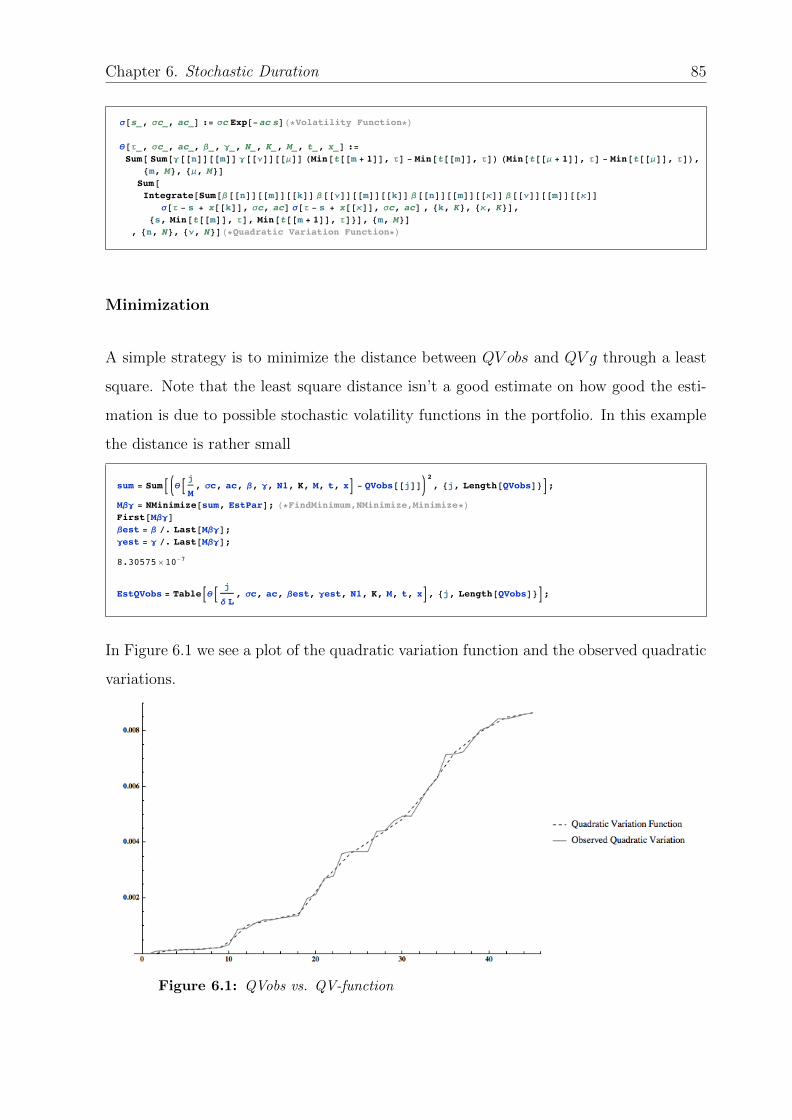
Chapter 6. Stochastic Duration 85
s@s_, sc_, ac_D := sc Exp@-ac sDH*Volatility Function*Lq@t_, sc_, ac_, b_, g_, N_, K_, M_, t_, x_D :=Sum@ Sum@g@@nDD@@mDD g@@nDD@@mDD HMin@t@@m + 1DD, tD - Min@t@@mDD, tDL HMin@t@@m + 1DD, tD - Min@t@@mDD, tDL,8m, M<, 8m, M<D
Sum@Integrate@Sum@b@@nDD@@mDD@@kDD b@@nDD@@mDD@@kDD b@@nDD@@mDD@@kDD b@@nDD@@mDD@@kDDs@t - s + x@@kDD, sc, acD s@t - s + x@@kDD, sc, acD , 8k, K<, 8k, K<D,8s, Min@t@@mDD, tD, Min@t@@m + 1DD, tD<D, 8m, M<D
, 8n, N<, 8n, N<DH*Quadratic Variation Function*L
Minimization
A simple strategy is to minimize the distance between QV obs and QV g through a least
square. Note that the least square distance isn’t a good estimate on how good the esti-
mation is due to possible stochastic volatility functions in the portfolio. In this example
the distance is rather small
sum = SumB qB jM, sc, ac, b, g, N1, K, M, t, xF - QVobs@@jDD 2
, 8j, Length@QVobsD<F;Mbg = NMinimize@sum, EstParD; H*FindMinimum,NMinimize,Minimize*LFirst@MbgDbest = b ê. Last@MbgD;gest = g ê. Last@MbgD;8.30575¥10-7
EstQVobs = TableBqB j
d L, sc, ac, best, gest, N1, K, M, t, xF, 8j, Length@QVobsD<F;
In Figure 6.1 we see a plot of the quadratic variation function and the observed quadratic
variations.
Figure 6.1: QVobs vs. QV-function
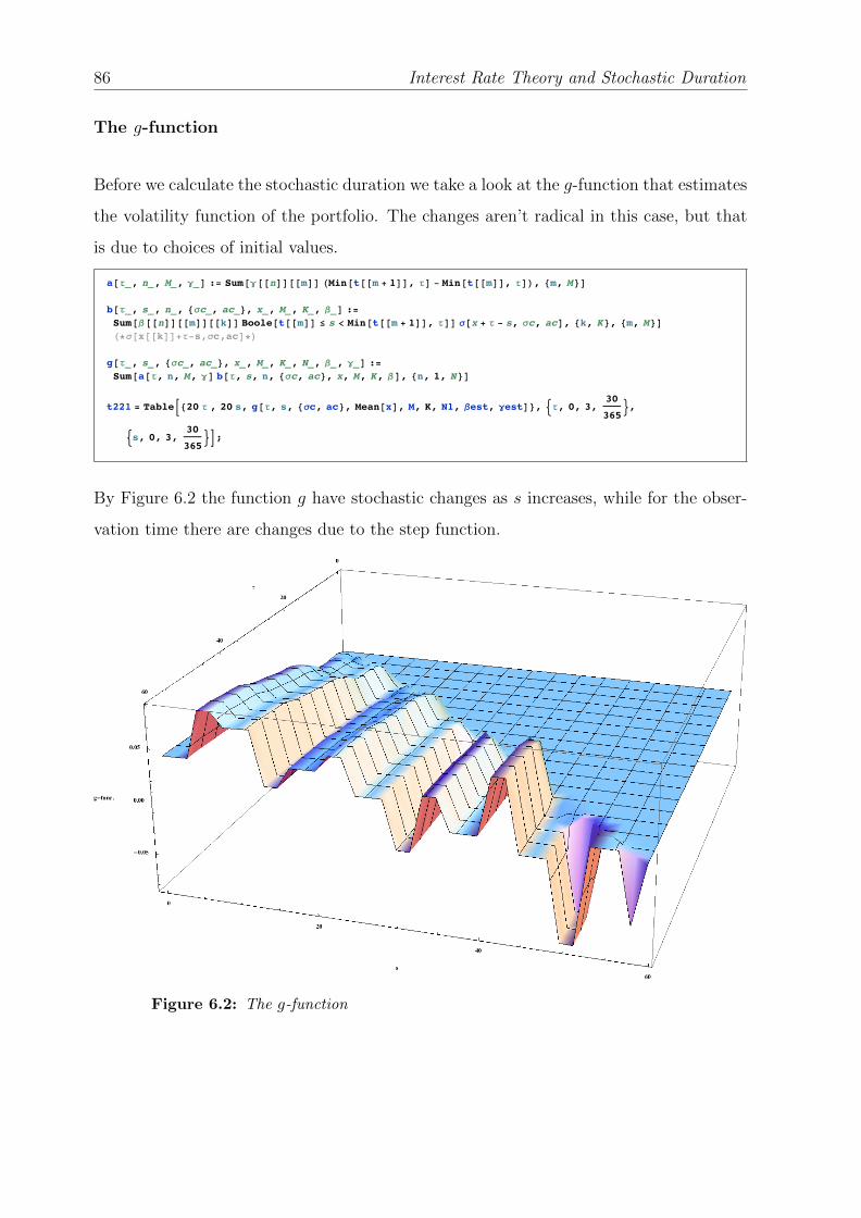
86 Interest Rate Theory and Stochastic Duration
The g-function
Before we calculate the stochastic duration we take a look at the g-function that estimates
the volatility function of the portfolio. The changes aren’t radical in this case, but that
is due to choices of initial values.
a@t_, n_, M_, g_D := Sum@g@@nDD@@mDD HMin@t@@m + 1DD, tD - Min@t@@mDD, tDL, 8m, M<Db@t_, s_, n_, 8sc_, ac_<, x_, M_, K_, b_D :=Sum@b@@nDD@@mDD@@kDD Boole@t@@mDD £ s < Min@t@@m + 1DD, tDD s@x + t - s, sc, acD, 8k, K<, 8m, M<DH*s@x@@kDD+t-s,sc,acD*L
g@t_, s_, 8sc_, ac_<, x_, M_, K_, N_, b_, g_D :=Sum@a@t, n, M, gD b@t, s, n, 8sc, ac<, x, M, K, bD, 8n, 1, N<D
t221 = TableB820 t , 20 s, g@t, s, 8sc, ac<, Mean@xD, M, K, N1, best, gestD<, :t, 0, 3,30
365>,
:s, 0, 3,30
365>F;
By Figure 6.2 the function g have stochastic changes as s increases, while for the obser-
vation time there are changes due to the step function.
Figure 6.2: The g-function
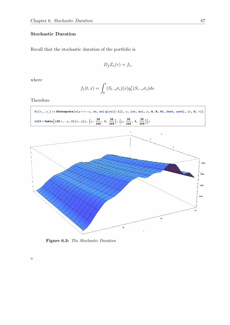
Chapter 6. Stochastic Duration 87
Stochastic Duration
Recall that the stochastic duration of the portfolio is
DfZx(τ) = f1,
where
f1(t, x) =
∫ t
0
(St−sσs)(x)gτs (Sτ−sσs)ds.
Therefore
f1@v_, y_D := NIntegrate@s@y + v - s, sc, acD g@tc@@-1DD, s, 8sc, ac<, y, M, K, N1, best, gestD, 8s, 0, v<Dt222 = TableB820 v , y, f1@v, yD<, :v, 30
365, 3,
30
365>, :y, 30
365, 3,
30
365>F;
Figure 6.3: The Stochastic Duration

88 Interest Rate Theory and Stochastic Duration
Figure 6.4: The Stochastic Duration
6.3 Immunization Strategy
The immunization strategy is based on the paper [11], where the main idea is to minimize
the stochastic duration in time and space (time-to-maturity). Assume that we have a
portfolio Vx(τ) with it’s estimated stochastic duration
DfVx(τ).
Then we want to minimize our risk using the hedging strategy Ht with the stochastic
duration
DfHx(τ).
The latter stochastic duration is ”most likely” stochastic and it will be sensible to mini-
mize the expected stochastic duration. Let, e.g., the hedging strategy be of αZCB shares
of a Future and αcall shares of a call option on a ZCB. Then the immunization strategy
would be
E[ ∫ x
0
∫ t
0
(DfVt −DfHαt )2 ds dy
]−→ min
α
w.r.t. αZCB and αcall (under some boundary conditions).
Chapter 6. Stochastic Duration 89
The stochastic duration on the future is already derived in an example. We therefore
derive the stochastic duration on a call option of a ZCB
(P (t, T )−K
)+.
Example 6.5:
Let F =(P (t, T )−K
)+then
F = 1[K,∞)
[P (t, T )
](P (t, T )−K).
Using Example 2.2 in [5] we have that
DfF = 1[K,∞)
[P (t, T )
]Df (P (t, T )−K)
= 1[K,∞)
[P (t, T )
](−(T − t)P (t, T )− 0)
= −1[K,∞)
[P (t, T )
](T − t)P (t, T ).


Chapter 7
Stochastic Duration an Example
As a major example we are going to calculate the stochastic duration for a Future portfo-
lio on a two year Treasury Note1. The data are collected from www.quandle.com, which
refer further to Chicago Mercantile Market and US Treasury From this website the fol-
lowing data collection was used; (Treasury Yield Curve Rates) and (2 Year Treasury Note
Futures, March 2013, TUH2013, CBOT).
Since we are working with a possible infinite dimensional noise, we need to reduce the
dimensions. Using PCA2 to reduce the dimension, we estimate a Vasicek model for the
total covariance of the important components. This is a strong simplification since a
better approach would be to estimate a volatility structure for each of the important
components. But for the purpose here it is well enough.
Furthermore we use the program presented in Chapter 6, using the parameters that are
estimated by means of the PCA procedure.
1A Note is equal a Bond with time-to-maturity of 2-10 years [8]2presented in Chapter 3
91
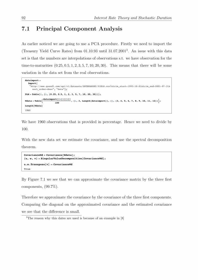
92 Interest Rate Theory and Stochastic Duration
7.1 Principal Component Analysis
As earlier noticed we are going to use a PCA procedure. Firstly we need to import the
(Treasury Yield Curve Rates) from 01.10.93 until 31.07.20013. An issue with this data
set is that the numbers are interpolations of observations s.t. we have observation for the
time-to-maturities (0.25, 0.5, 1, 2, 3, 5, 7, 10, 20, 30). This means that there will be some
variation in the data set from the real observations.
dataimport =Import@"http:êêwww.quandl.comêapiêv1êdatasetsêUSTREASURYêYIELD.csv?&trim_start=1993-10-01&trim_end=2001-07-31&
sort_order=desc", "Data"D;TtM = Table@i, 8i, 80.25, 0.5, 1, 2, 3, 5, 7, 10, 20, 30<<D;Wdata = TableB dataimport@@iDD@@jDD
100, 8i, 3, Length@dataimportD<, 8j, 83, 4, 5, 6, 7, 8, 9, 10, 11, 12<<F;
Length@WdataD1960
We have 1960 observations that is provided in percentage. Hence we need to divide by
100.
With the new data set we estimate the covariance, and use the spectral decomposition
theorem.
CovarianceWd = Covariance@WdataD;8u, w, v< = SingularValueDecomposition@CovarianceWdD;u.w.Transpose@vD ä CovarianceWd
True
By Figure 7.1 we see that we can approximate the covariance matrix by the three first
components, (99.7%).
Therefore we approximate the covariance by the covariance of the three first components.
Comparing the diagonal on the approximated covariance and the estimated covariance
we see that the difference is small.
3The reason why this dates are used is because of an example in [8]

Chapter 7. Stochastic Duration an Example 93
Figure 7.1: The important components of the Yield Curve
Sum@Diagonal@wD@@iDD Outer@Times, Transpose@vD@@iDD, Transpose@vD@@iDDD, 8i, Length@Diagonal@wDD<D äCovarianceWd
EstCov = Sum@Diagonal@wD@@iDD Outer@Times, Transpose@vD@@iDD, Transpose@vD@@iDDD, 8i, 3<D;Diagonal@EstCovDDiagonal@CovarianceWdDTrue
80.0000559628, 0.000059144, 0.0000613263, 0.0000644055, 0.0000635025,0.0000612088, 0.0000551678, 0.0000578492, 0.0000467664, 0.0000510921<
80.0000562036, 0.0000593128, 0.0000617063, 0.000064502, 0.0000635427,0.0000613593, 0.0000553911, 0.0000580185, 0.0000470086, 0.0000513019<
Performing PCA on this data set, [8], means that we are assuming the auto-correlation
to be small. Because of a simplified example, we don’t put concerns on this issue. We
recall from Example 3.1 that we need to estimate the parameters using the relation
V ar[Y (t, T )] =1
(T − t)2
σ2
2k3e−2k(T+t)(e2kt − 1)(ekT − ekt)2,
where, since we observe day-to-day changes in the volatility structure, t = 1365
. Using
least square we estimate the parameters in the Vasicek model to be σ = 0.1495 and
k = 0.00816.
VarVasicek@T_, t_, s_, k_D :=1
HT - tL2
s2
2 k3Exp@-2 k HT + tLD HExp@2 k tD - 1L HExp@k TD - Exp@k tDL2
t =1
365; TtM;
minsk = NMinimizeASumAHVarVasicek@TtM@@iDD + t, t, s, kD - Diagonal@EstCovD@@iDDL2, 8i, Length@TtMD<E, 8s, k<Eestsk = 8s, k< ê. Last@minskD;91.13759¥10-10, 8s Æ 0.149521, k Æ 0.00815519<=
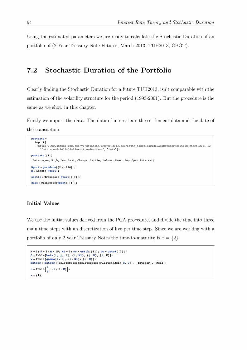
94 Interest Rate Theory and Stochastic Duration
Using the estimated parameters we are ready to calculate the Stochastic Duration of an
portfolio of (2 Year Treasury Note Futures, March 2013, TUH2013, CBOT).
7.2 Stochastic Duration of the Portfolio
Clearly finding the Stochastic Duration for a future TUH2013, isn’t comparable with the
estimation of the volatility structure for the period (1993-2001). But the procedure is the
same as we show in this chapter.
Firstly we import the data. The data of interest are the settlement data and the date of
the transaction.
portdata =Import@"http:êêwww.quandl.comêapiêv1êdatasetsêCMEêTUH2013.csv?&auth_token=LqWy2oLARYBxWdmoFX25&trim_start=2011-12-
30&trim_end=2013-03-28&sort_order=desc", "Data"D;portdata@@1DD8Date, Open, High, Low, Last, Change, Settle, Volume, Prev. Day Open Interest<Wport = portdata@@2 ;; 116DD;m = Length@WportD;settle = Transpose@WportD@@7DD;date = Transpose@WportD@@1DD;
Initial Values
We use the initial values derived from the PCA procedure, and divide the time into three
main time steps with an discretization of five per time step. Since we are working with a
portfolio of only 2 year Treasury Notes the time-to-maturity is x = 2.
K = 1; d = 5; M = 15; N1 = 1; sc = estsk@@1DD; ac = estsk@@2DD;b = Table@beta@i, j, lD, 8i, N1<, 8j, M<, 8l, K<D;g = Table@gamma@i, lD, 8i, N1<, 8l, M<D;EstPar = EstPar = DeleteCases@DeleteCases@Flatten@Join@b, gDD, _IntegerD, _RealD;t = TableB i
d, 8i, 0, M<F;
x = 82<;
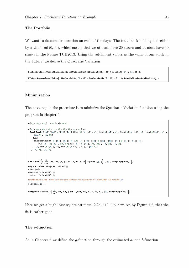
Chapter 7. Stochastic Duration an Example 95
The Portfolio
We want to do some transaction on each of the days. The total stock holding is decided
by a Uniform(20, 40), which means that we at least have 20 stocks and at most have 40
stocks in the Future TUH2013. Using the settlement values as the value of one stock in
the Future, we derive the Quadratic Variation
SimPortfolio = Table@RandomVariate@UniformDistribution@820, 40<D D settle@@-iDD, 8i, 60<D;QVobs = AccumulateATableAHSimPortfolio@@j + 1DD - SimPortfolio@@jDDL2, 8j, 1, Length@SimPortfolioD - 1<EE;
Minimization
The next step in the procedure is to minimize the Quadratic Variation function using the
program in chapter 6.
s@s_, sc_, ac_D := sc Exp@-ac sDq@t_, sc_, ac_, b_, g_, N_, K_, M_, t_, x_D :=Sum@ Sum@g@@nDD@@mDD g@@nDD@@mDD HMin@t@@m + 1DD, tD - Min@t@@mDD, tDL HMin@t@@m + 1DD, tD - Min@t@@mDD, tDL,8m, M<, 8m, M<D
Sum@Integrate@Sum@b@@nDD@@mDD@@kDD b@@nDD@@mDD@@kDD b@@nDD@@mDD@@kDD b@@nDD@@mDD@@kDDs@t - s + x@@kDD, sc, acD s@t - s + x@@kDD, sc, acD , 8k, K<, 8k, K<D,8s, Min@t@@mDD, tD, Min@t@@m + 1DD, tD<D, 8m, M<D
, 8n, N<, 8n, N<D
sum = SumB qB j
20, sc, ac, b, g, N1, K, M, t, xF - QVobs@@jDD 2
, 8j, Length@QVobsD<F;Mbg = FindMinimum@sum, EstParD;First@MbgDbest = b ê. Last@MbgD;gest = g ê. Last@MbgD;FindMinimum::cvmit : Failed to converge to the requested accuracy or precision within 100 iterations.á
2.25028¥1013
EstQVobs = TableBqB j
20, sc, ac, best, gest, N1, K, M, t, xF, 8j, Length@QVobsD<F;
Here we get a hugh least square estimate, 2.25× 10¹³, but we see by Figure 7.2, that the
fit is rather good.
The g-function
As in Chapter 6 we define the g-function through the estimated a- and b-function.
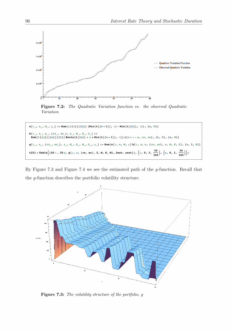
96 Interest Rate Theory and Stochastic Duration
Figure 7.2: The Quadratic Variation function vs. the observed QuadraticVariation
a@t_, n_, M_, g_D := Sum@g@@nDD@@mDD HMin@t@@m + 1DD, tD - Min@t@@mDD, tDL, 8m, M<Db@t_, s_, n_, 8sc_, ac_<, x_, M_, K_, b_D :=Sum@b@@nDD@@mDD@@kDD Boole@t@@mDD < s £ Min@t@@m + 1DD, tDD s@x + t - s, sc, acD, 8k, K<, 8m, M<D
g@t_, s_, 8sc_, ac_<, x_, M_, K_, N_, b_, g_D := Sum@a@t, n, M, gD b@t, s, n, 8sc, ac<, x, M, K, bD, 8n, 1, N<Dt221 = TableB820 t , 20 s, g@t, s, 8sc, ac<, 2, M, K, N1, best, gestD<, :t, 0, 3,
30
365>, :s, 0, 3,
30
365>F;
By Figure 7.3 and Figure 7.4 we see the estimated path of the g-function. Recall that
the g-function describes the portfolio volatility structure.
Figure 7.3: The volatility structure of the portfolio, g
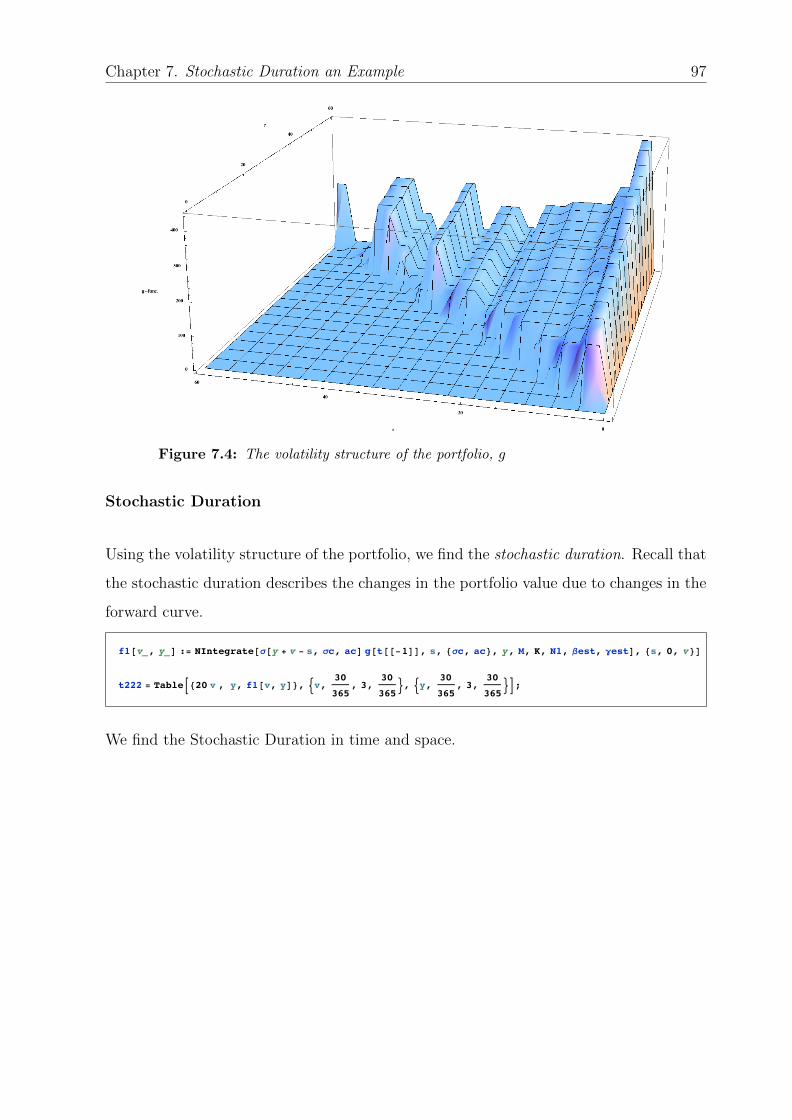
Chapter 7. Stochastic Duration an Example 97
Figure 7.4: The volatility structure of the portfolio, g
Stochastic Duration
Using the volatility structure of the portfolio, we find the stochastic duration. Recall that
the stochastic duration describes the changes in the portfolio value due to changes in the
forward curve.
f1@v_, y_D := NIntegrate@s@y + v - s, sc, acD g@t@@-1DD, s, 8sc, ac<, y, M, K, N1, best, gestD, 8s, 0, v<Dt222 = TableB820 v , y, f1@v, yD<, :v, 30
365, 3,
30
365>, :y, 30
365, 3,
30
365>F;
We find the Stochastic Duration in time and space.
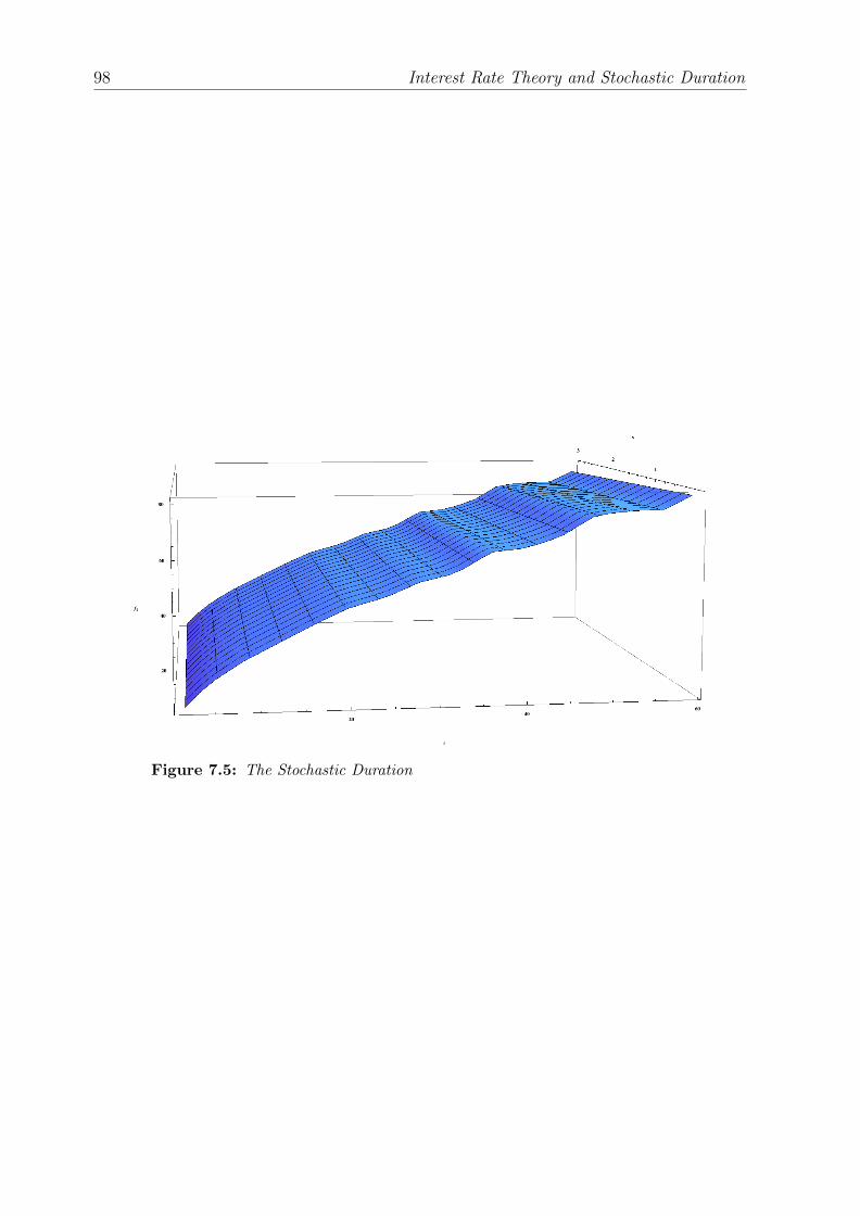
98 Interest Rate Theory and Stochastic Duration
Figure 7.5: The Stochastic Duration

Appendix A
Mathematical Tools
The short rate r is not deterministic. This means that we can’t with exact mathematical
analysis predict the path of r, which brings us into the field of probability theory. A way
to model r is to define it as an r.v. on the probability space
(Ω,F ,P),
where Ω denotes the sample space, F denotes the σ-algebra on the sample space, and P
the probability measure(distribution).
Definition A.1 (Sample space):
A set Ω 6= ∅ representing the collection of all possible outcomes of a random experiment
is called sample space.
Knowing the possible outcomes of r, Ω, we would like to figure out which family of
outcomes that are reasonable to put a probability measure on. The definition of σ-algebra
ensures some good properties of the family.
Definition A.2 (σ-algebra):
A family F of subsets of Ω is called σ-algebra on Ω if
1. ∅ ∈ F
99
100 Interest Rate Theory and Stochastic Duration
2. A ∈ F =⇒ AC ∈ F 1
3. A1, A2, · · · ∈ F =⇒ ∪i≥1 ∈ F
The last element of the probability space, the probability measure, tells us to which
degree the different measurable outcomes occur. There are several such measure (χ2,
Log-Gaussian, Pareto), but the most common within financial theory is the Gaussian
distribution. With the probability measure we get a set of working tools; moments,
characteristic function (the Fourier transform of an r.v.), etc.
Definition A.3 (Probability measure):
A function
P : F 7→ [0, 1]
is called a probability measure on (Ω,F), if
1. P(∅) = 0, P(Ω) = 1
2. A1, . . . , An, · · · ∈ F with Ai⋂Aj = ∅ 2 =⇒ P(
⋃i≥1Ai) =
∑i≥1 P(Ai)
3
Heuristically, for an event A ∈ F , P(A) is the probability that event A occurs.
Properties A.4 (Properties of the probability measure):
We have following properties of the probability measure
1. A ⊆ B =⇒ P(A) ≤ P(B)
2. P(⋃i≥1Ai) ≤
∑i≥1 P(Ai)
3. limi→∞ P(Ai) = P(A) if A =⋃i≥1Ai
In some cases an event has probability zero. This sets are referred to as the P-null sets4.
1AC def= Ω−A
2Ai and Aj is disjoint3In the literature this is called σ-additivity4Of course given that we are working with the probability measure P

Appendix A. Mathematical Tools 101
Definition A.5 (P-null sets):
An event A ∈ F s.t. P(A) = 0 is called a P-null set.
On the other side we may have some events that have probability one. In this case the
event have the P-a.s. property.
Definition A.6 (P-almost surely):
We say that an event holds P-almost surely (a.s.) if there exist a P-null set N ∈ F s.t.
the event holds for all ω ∈ NC = Ω−N .
A.1 Random Variable
Working with the outcomes isn’t always easy, especially if the events aren’t numbers.
For example could we categorize sections in companies into 1, 2, 3, 4, 5, ... instead of
the HR-section, Actuary-section, etc. By doing so we can define expectations and other
statistical tools that relay on number theory. For this type of purpose we need a mapping
function, and the mapping function is commonly referred to as the random variable or
stochastic variable.
Definition A.7 (Random Variable):
Let X be the function
X : Ω 7→ E,
where E ⊆ R. Then X is called a (E, E)-random variable (r.v.) on (Ω,F ,P), where E is
the measurability of X s.t., for an A ∈ E , the inverse image of the r.v. X−1(A) ∈ F .
Note that the Ω might be equal to E, like it is for dices. A special case of E is real valued
random variables. Then
X : Ω 7−→ R
is a r.v. on the probability space (Ω,F ,P) if the set
Adef= ω ∈ Ω : X(ω) < x
102 Interest Rate Theory and Stochastic Duration
is an event for all x ∈ R. I.e. A ∈ F . If the random variable have two or more dimension
we call it a random vector (r.v).
Definition A.8 (Random Vector):
A function
X : Ω 7→ Rn
with
X(ω) = (X1(ω), X2(ω), . . . , Xn(ω))T
is called a random vector, if X1, . . . , Xn are r.v.’s.
A.2 Expectation
The most common statistic is the expectation which is defined as the Lebesgue integral
w.r.t. the probability measure P. The reason why we are working with Lebesgue integral
is because the random variable might be discrete. In discrete case the Riemann integral
is equal to zero due to it’s definition.
Definition A.9 (Expectation w.r.t. P):
Let X ≥ 0 be a positive r.v. Then the expectation (integral) is defined as
E[X]def=
∫Ω
X(ω)P(dω).
For a general X we define
E[X]def=
∫Ω
X(ω)P(dω)def= E[X+]− E[X−],
where X+ = max(x, 0) and X− = max(−x, 0). If E[X+], E[X−] < ∞ then X is called
P-integrable.
Properties A.10 (Properties of the expectation):
Let X and Y be two r.v. and α, β ∈ R5
5R is an example of a field
Appendix A. Mathematical Tools 103
1. E[αX + βY ] = αE[X] + βE[Y ] (Linearity)
2. If X ≤ Y P-a.s. then E[X] ≤ E[Y ]
A.3 Conditional probability and expectation
In many cases there would be interesting to understand what properties a random variable
have given knowledge. E.g. for a stochastic process, defined later, it is interesting to
understand the process given knowledge about the process up to a certain time s. The
field is conditional probability and expectation.
Let X be a r.v. on the probability space (Ω,A,P), and A ⊆ A. Then the conditional
probability,
P(X|A)def=
P(1A(ω)X(ω))
E[1A(ω)],
where 1A(ω) is the indicator function
1A(ω) =
1 if ω ∈ A
0 else,
can be interpreted as the probability of X knowing that ω ∈ A, and 1A = Ω. In the same
way the conditional expectation,
E[X|A]def=
E[1A(ω)X(ω)]
E[1A(ω)]
can be interpreted as the expectation of X given that ω ∈ A. A more formal definition
of the conditional expectation is provided.
Definition A.11 (Conditional expectation w.r.t. A):
Let X be a r.v. s.t. E[|X|] < ∞. Then the expected value of X given A is the unique
r.v. Y s.t.
E[1AX] = E[1AY ]

104 Interest Rate Theory and Stochastic Duration
for all A ∈ A, and Y ≤ q ∈ A for all q ∈ R. The r.v. Y is denoted by E[X|A].
Properties A.12 (Conditional Expectation):
Let X,Y be two r.v., α, β ∈ R and A,B be two σ-algebras. Then
1. E[αX + βY |A] = αE[X|A] + βE[Y |B] (Linearity)
2. E[E[X|A]] = E[X] (Rule of double expectation)
3. E[X|A] = X, if X is independent of A
4. E[X|A] = E[X], if X is a r.v. on (Ω,A,P)
5. E[X|A] = E[E[X|B]|A] if A ⊆ B
A.4 Stochastic processes
The short rate change by time. Therefore the most general way to define the short rate
is as a stochastic process rt. But in order to define a stochastic process we need to know
the measurability for each time t. The measurability for each time t is controlled by the
filtration.
Definition A.13 (Filtration):
Let Ft0≤t≤T be a family of σ-algebras on (Ω,F ,P) s.t.
Ft1 ⊂ Ft2 ⊂ . . . | ⊂ F
for all 0 ≤ t1 < t2 ≤ ... ≤ T . Then Ft0≤t≤T is called the filtration on the probability
space (Ω,F ,P).
The smallest necessary information from the path is called a Markov process. A Markov
process have the property that the forthcoming trajectory only depends on today’s state.
This means that we can reduce the filtration Ft to today’s observation rt.
Appendix A. Mathematical Tools 105
Definition A.14 (Stochastic Process):
Let T 6= ∅ be the parameter space. Then the collection
rtt∈T
of random variables is called Stochastic Process on the filtered probability space (Ω,F , Ft,P).
Example A.1 (Parameter Space):
E.g. could the parameter space be T = [0, T ] or T = 1, 2, . . . , n.
Definition A.15 (The Markov Property; 1-dim.):
Assume that a one dimensional stochastic process rt starts at x. Then rt has the Markov
family property if
Ex[f(rt+h)|Ft] = Ert [f(rh)],
for all bounded and Borel-measurable functions f .
A.5 Brownian motion and Ito Integral
One of the most used stochastic processes is called Brownian motion. This is a process
that fluctuates due to a Gaussian distribution. With the properties of independent,
stationary increments and stochastic continuity6, Brownian motion is an element in a
broader class of stochastic processes. Namely the Levy Processes.
Definition A.16 (Brownian motion):
A stochastic process (Wt)0≤t≤T on the probability space (Ω,F , Ft0≤t≤T ,P) is called a
Brownian motion if the process has the following properties
1. W0 = 0 P-a.s.
2. Independent increments: i.e. for 0 ≤ t1 ≤ · · · ≤ tn
Wt1 ,Wt2 −Wt1 , . . . ,Wtn −Wtn−1
6Stochastic continuity is a condition that preserves jumps at fixed time. But in fact Brownian motionWt has a continuous version which means no jumps. Hence it follow the Stochastic continuity condition.

106 Interest Rate Theory and Stochastic Duration
are independent of each other
3. Stationary increments: i.e. Wt −Ws is equally distributed as Wt−s
Wt −Wsd= Wt−s
4. Gaussian distributed7: Wt−s ∼ Gaussian(0, t− s),
where the filtration Ft is the smallest σ-algebra containing the path of the process Wt up
to time t
Ftdef= σ(Wu; 0 ≤ u ≤ t)
Because of the independence8 and stationary9 property, the Brownian motion is a process
without memory. Hence a Brownian motion is a Markov process.
The stochastic integral w.r.t. a Brownian motion, Wt, also called an Ito integral, is defined
on the set of processes, f ∈ V [0, T ] as
I[f ] =
∫ t
0
fsdWs,
where the set of processes V [0, T ] have the following requirements: A function f ∈ V [0, T ]
is the mapping
f : Ω× [0, T ] 7−→ R,
where
• f is measurable w.r.t. F ⊗ B([0, T ])
• ft is Ft-adapted
• E[ ∫ T
0f 2s ds]<∞
7The Gaussian distribution is the same distribution as the well known Normal distribution8Independent on the past9The past doesn’t change the distributional properties
Appendix A. Mathematical Tools 107
The last requirement ensure the existence of the Ito-isometry
E[(
∫ T
0
fsdWs)2]
= E[ ∫ T
0
f 2s ds]
Properties A.17 (Ito integral):
The stochastic integral w.r.t. a Brownian motion have the following properties
1. (Linearity)∫ T
0αfs + βgsdWs = α
∫ T0fsdWs + β
∫ T0gsdWs
2. E[ ∫ T
0fsdWs
]= 0
3. (Ito Isometry) V ar[(∫ T
0fsdWs)
2]
= E[ ∫ T
0f 2s ds]
4. There exists a continuous version of Ytdef=∫ t
0fsdWs
By property 4. we may assume that the process Yt is continuous.
A.6 Ito’s Lemma
Assume that Xt is an Ito process, i.e. that
Xt = X0 +
∫ t
0
hsds+
∫ t
0
fsdWs,
where fs ∈ V [0, T ] and t ∈ [0, T ], and hs is Ft-adapted with the property
E[
∫ t
0
|hs|ds] <∞.
Then, which form does the function,
g(t,Xt),
take? The answer is Ito’s Lemma.

108 Interest Rate Theory and Stochastic Duration
Theorem A.18 (Ito’s Lemma):
Let Xt be an Ito process and g ∈ C2([0,∞] × R)10. Then the function g(t, x) is an Ito
process for x = Xt as the underlying process, where
g(t,Xt) = g(0, X0) +
∫ t
0
∂
∂tg(s,Xs)ds+
∫ t
0
∂
∂xg(s,Xs)dWs +
1
2
∫ t
0
∂2
∂x2g(s,Xs)(dXs)
2,
using that (dWt)2 = dt and dWt dt = dt dWt = dt dt = 0.
Note that the stochastic differential equation (SDE) of the Ito process is
dXt = ht ds+ ft dWt.
A.7 Stochastic Differential Equations
Assume we have a SDE on the form
dXt = h(t,Xt)dt+ f(t,Xt)dWs.
Then the solution is defined as the processXt, in the filtered probability space (Ω,F , Ftt≥0,P),
satisfying the equation
Xt = x0 +
∫ t
0
h(s,Xs)ds+
∫ t
0
f(s,Xs)dWs,
where h : [0, T ]× R→ R and f : [0, T ]× R→ R are given. If
|h(t, x)|+ |f(t, x)| ≤ C(1 + |x|)
and
|h(t, x)− h(t, y)|+ |f(t, x)− f(t, y)| ≤ D|x− y|10For a g ∈ C2([0,∞)× R), the function is twice differentiable on (0,∞)× R

Appendix A. Mathematical Tools 109
for all x, y ∈ R and t ∈ [0, T ], the solution Xt exist and is unique. Knowing that a
solution is unique makes us being able to do certain transformations in order to derive
an appealing solution. See the Vasicek model present earlier.
A.8 Important Financial Tools
One crucial modeling assumption is that the discounted financial market is following an
Martingale. It’s an assumption of fair price. Heuristically the Martingale property is the
model assumption that the best predicted value in the future is today’s value.
Definition A.19:
Let Xt be a stochastic process on the filtered probability space (Ω,F , Ftt≤0,P). Further
assume that E[|Xt|] <∞ for all t ∈ [0, T ] and
E[Xt|Fs] = Xs
for all s ∈ [0, t]. Then Xt is called a Ft-Martingale.
For a stochastic process following the path of a stochastic integral w.r.t. a Brownian
motion the Martingale representation theorem is an important tool in understanding the
process under arbitrage free (fair) prices.
Theorem A.20 (Martingale Representation theorem):
Let Wt be an Brownian motion, and assume that Mt ∈ L2(P) is a Ft-Martingale. Then
there exists a unique stochastic process f ∈ V [0, t] for all t ≥ 0 s.t.
Mt = E[M0] +
∫ t
0
fs dWs.
Note that assuming Mt ∈ L2(P) is the same as assuming existence of the second moment.
This condition can be relaxed. Then we are working with local Martingales, where the
main difference is that we need to work with stopping times, knowing that for a stopped
process the second moment exist.

110 Interest Rate Theory and Stochastic Duration
In most of the cases the financial process have a drift under the objective probability
measure P. But a necessity in financial modeling is that the discounted financial asset
is priced due to a Martingale. We therefore need a change of measure. Using Girsanov
transform we replace the objective probability measure by an appropriate chosen prob-
ability measure Q. The transform will remain a Brownian motion and we choose this
measure s.t. the process is a Martingale.
Theorem A.21 (Girsanov’s theorem):
Let Wt be an Ito process on the form
Wt = Wt −∫ t
0
hsds.
We define the likelihood process as
Zt(ht) = exp∫ t
0
hsdWs −1
2
∫ t
0
h2sds
for t ∈ [0, T ]. Further assume that ht satisfies the Novikov condition
E[
exp1
2
∫ t
0
h2tds]
<∞
and that the Girsanov transformation Q of the measure P is defined by the probability
measure
Q(A)def= EP[1AZT ].
Then Wt is a Brownian motion under Q.
Generally, the Brownian motion under the ”risk neutral” measure Q will be denoted WQt .
Under the risk neutral measure we are going to derive several partial differential equation
of the solution to the arbitrage free price of ZCB (also applied in deriving arbitrage
free price for an option on the underlying process of a ZCB). An auxiliary tool is the
Feynman-Kac proposition.
Appendix A. Mathematical Tools 111
Proposition A.22 (Feynman-Kac):
Let Xt be the solution of the stochastic differential equation
dXt = h(t,Xt)dt+ f(t,Xt)dWQt ,
where X0 = x0. Then for an risk free interest rate r the solution F (t, x) of the boundary
value problem
∂F
∂t(t, x) + h(t, x)
∂F
∂x(t, x) +
1
2f(t, x)2 ∂
2
∂x2(t, x)− rF (t, x) = 0
F (T, x) = φ(x)
is
F (t, x) = e−r(T−t)EQ[φ(XT )|Ft],
given that the second moment exist for the integrand in the stochastic part of F (t,Xt).
The integrability condition ensure that the stochastic integral is equal to zero. Feynman-
Kac is used in the portfolio setup, Chapter 2.
The last theorem is very often used in this thesis. The Stochastic Fubini theorem serve
in the same way as the Fubini theorem. It’s a change of inner integrands.
Theorem A.23 (Stochastic Fubini theorem):
Consider a stochastic process f(u, s) ∈ V [0, T ]. Then
∫ T
0
∫ T
0
f(u, s)dWuds =
∫ T
0
∫ T
0
f(u, s)dsdWs.
Proof. Theorem (6.2) in [3], where the assumption of f(u, s) ∈ V [0, T ] is a special case of
the proof.
For a more thorough review I refer to [9] and [1].

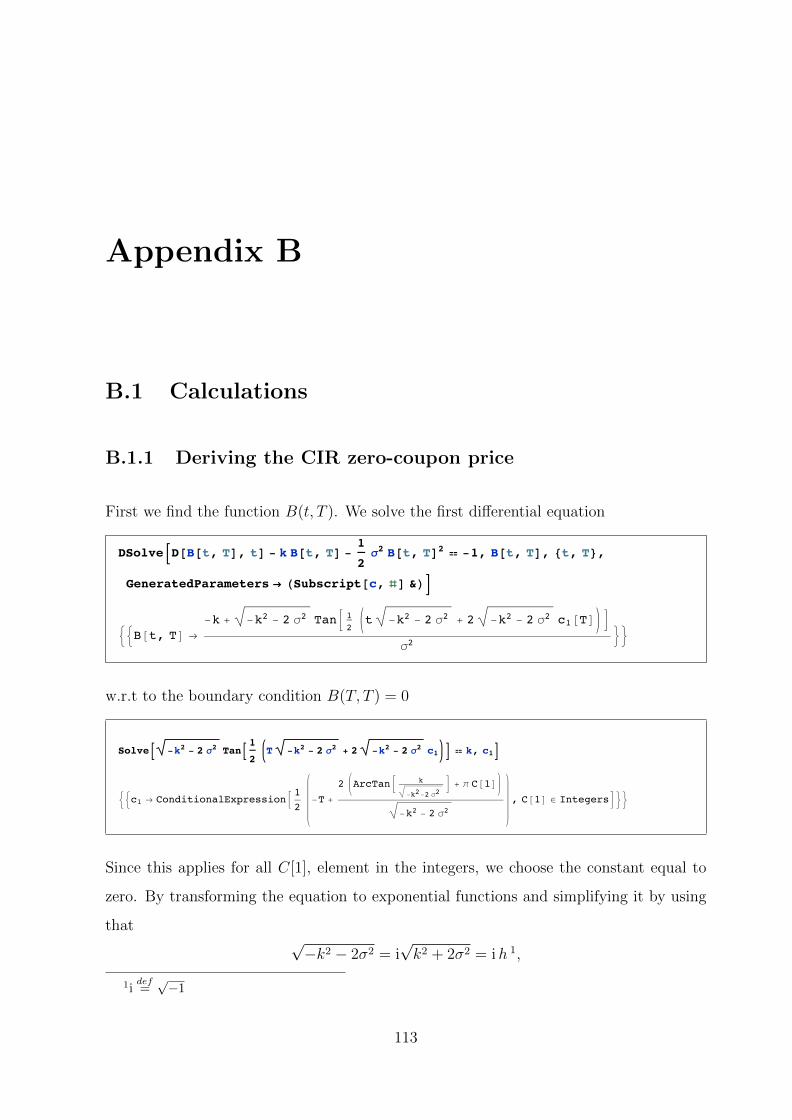
Appendix B
B.1 Calculations
B.1.1 Deriving the CIR zero-coupon price
First we find the function B(t, T ). We solve the first differential equationClear@BDDSolveBD@B@t, TD, tD - k B@t, TD - 1
2s2 B@t, TD2 ä -1, B@t, TD, 8t, T<,
GeneratedParameters Æ HSubscript@c, D &LF
::B@t, TD Æ-k + -k2 - 2 s2 TanB 1
2Kt -k2 - 2 s2 + 2 -k2 - 2 s2 c1@TDOF
s2>>
w.r.t to the boundary condition B(T, T ) = 0
SolveB -k2 - 2 s2 TanB 12
T -k2 - 2 s2 + 2 -k2 - 2 s2 c1 F ä k, c1F
::c1 Æ ConditionalExpressionB 12
-T +
2 ArcTanB k
-k2-2 s2F + p C@1D
-k2 - 2 s2, C@1D ΠIntegersF>>
Since this applies for all C[1], element in the integers, we choose the constant equal to
zero. By transforming the equation to exponential functions and simplifying it by using
that√−k2 − 2σ2 = i
√k2 + 2σ2 = ih 1,
1idef=√−1
113
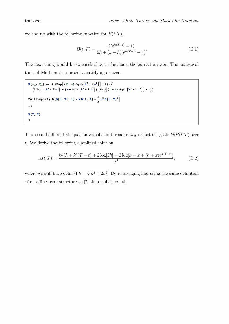
thepage Interest Rate Theory and Stochastic Duration
we end up with the following function for B(t, T ),
B(t, T ) =2(eh(T−t) − 1)
2h+ (k + h)(eh(T−t) − 1). (B.1)
The next thing would be to check if we in fact have the correct answer. The analytical
tools of Mathematica provid a satisfying answer.
B@t_, T_D := I2 IExpAHT - tL SqrtAk2 + 2 s2EE - 1MM ëI2 SqrtAk2 + 2 s2E + Ik + SqrtAk2 + 2 s2EM IExpAHT - tL SqrtAk2 + 2 s2EE - 1MM
FullSimplifyBD@B@t, TD, tD - k B@t, TD - 1
2s2 B@t, TD2F
-1
B@T, TD0
The second differential equation we solve in the same way or just integrate kθB(t, T ) over
t. We derive the following simplified solution
A(t, T ) =kθ(h+ k)(T − t) + 2 log[2h]− 2 log[h− k + (h+ k)eh(T−t)]
σ2, (B.2)
where we still have defined h =√k2 + 2σ2. By rearrenging and using the same definition
of an affine term structure as [7] the result is equal.

Appendix B. Calculations 115
B.1.2 Calculations; the Hull-White model
B.1.2.1
Recall that B(s, T ) = 1a
(1− e−a(T−s)). Then
∂
∂T
∫ T
0
θsB(s, T )ds =∂
∂T
∫ T
0
θs1
a
(1− e−a(T−s))ds
(Linearity) =∂
∂T
[ ∫ T
0
θs1
ads− e−aT
∫ T
0
θsa
e−asds]
= θT1
a− ∂
∂T
[e−aT
∫ T
0
θsa
easds]
(Product rule) =θTa
+ ae−aT∫ T
0
θsa
e−asds− e−aT1
aθT eaT
=
∫ T
0
θse−a(T−s)ds
=
∫ T
0
∂
∂Tθs
1
a
(1− e−a(T−s))ds
=
∫ T
0
∂
∂TθsB(s, T )ds.
B.1.2.2
Recall that
ψ(T ) = f(0, T ) + h(T ),
where
ψ(T )def=
∫ T
0
∂
∂TθsB(s, T )ds− r0e−aT
and
h(T )def=
1
2a2σ2e−2aT (eaT − 1)2.
From Appendix B.1.2.1
ψ(T ) =
∫ T
0
θse−a(T−s)ds.
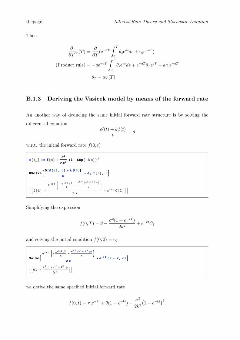
thepage Interest Rate Theory and Stochastic Duration
Then
∂
∂Tψ(T ) =
∂
∂T(e−aT
∫ T
0
θseasds+ r0e
−aT )
(Product rule) = −ae−aT∫ T
0
θseasds+ e−aT θT eaT + ar0e−aT
= θT − aψ(T )
B.1.3 Deriving the Vasicek model by means of the forward rate
An another way of deducing the same initial forward rate structure is by solving the
differential equationφ′(t) + kφ(t)
k= θ
w.r.t. the initial forward rate f(0, t)
q@t_D := f@tD + s22 k2
H1 - Exp@-k tDL2
DSolveB D@q@tD, tD + k q@tDk
ä f, f@tD, tF
::f@tD Æ
„-k t - „-k t s2
k-
„k t Js2-2 k2 fNk
2 k+ „-k t C@1D>>
Simplifying the expression
f(0, T ) = θ − σ2(1 + e−2T )
2k2+ e−ktC1
and solving the initial condition f(0, 0) = r0,
SolveB „-k 0 - „
-k 0 s2
k-„k 0 Is2-2 k2 fM
k
2 k+ „-k 0 c1 ä r, c1F
::c1 Æk2 r + s2 - k2 f
k2>>
we derive the same specified initial forward rate
f(0, t) = r0e−kt + θ(1− e−kt)− σ2
2k2
(1− e−kt
)2.

Appendix B. Calculations 117
Remark B.1:
In the program it was necessary to split between the constant and function. Therefore in
the program φ(t) = θ(t) and θ = φ.


Bibliography
[1] Tomas Bjork. Arbitrage theory in continuous time. Oxford university press, third
edition, 2009.
[2] Damir Filipovic. Consistency problems for Heath-Jarrow-Morton interest rate mod-
els. Number 1760. Springer, 2001.
[3] Damir Filipovic. Term-structure models: A graduate course, 2009.
[4] Leszek Gawarecki and Vidyadhar Mandrekar. Stochastic Differential Equations in
Infinite Dimensions: With Applications to Stochastic Partial Differential Equations.
Springer, 2010.
[5] Paul C Kettler, Frank Proske, and Mark Rubtsov. Sensitivity with respect to the
yield curve: duration in a stochastic setting. In Inspired by Finance, pages 363–385.
Springer, 2014.
[6] Sindre Duedahl. Stochastic yield curve duration and portfolio immunization strate-
gies. Working paper, 2014.
[7] Damiano Brigo and Fabio Mercurio. Interest rate models-theory and practice: with
smile, inflation and credit. Springer, second edition, 2007.
[8] Rene Carmona and Michael R Tehranchi. Interest Rate Models: an Infinite Dimen-
sional Stochastic Analysis Perspective. Springer, 2007.
[9] Bernt Øksendal. Stochastic differential equations. Springer, sixth edition, 2003.
[10] Giulia Di Nunno, Bernt Øksendal, and Frank Proske. Malliavin calculus for Levy
processes with applications to finance. Springer, 2008.
119

Bibliography Interest Rate Theory and Stochastic Duration
[11] John Hull and Alan White. The optimal hedging of interest rate sensitive securities.
University of Toronto, 1994.