Embed Size (px)
Citation preview
Intermediation in the Supply of Agricultural Products in Developing Economies
Kris Johnson Ferreira Joel Goh Ehsan Valavi
Working Paper 18-033
Working Paper 18-033
Copyright © 2017 by Kris Johnson Ferreira, Joel Goh, and Ehsan Valavi
Working papers are in draft form. This working paper is distributed for purposes of comment and discussion only. It may not be reproduced without permission of the copyright holder. Copies of working papers are available from the author.
Intermediation in the Supply of Agricultural Products in Developing Economies
Kris Johnson Ferreira Harvard Business School
Joel Goh Harvard Business School
Ehsan Valavi Harvard Business School
Intermediation in the Supply of AgriculturalProducts in Developing Economies
Kris Johnson FerreiraHarvard Business School, [email protected]
Joel GohNational University of Singapore Business School, Harvard Business School, [email protected]
Ehsan ValaviHarvard Business School, [email protected]
Problem Definition: Farmers face several challenges in agricultural supply chains in emerging economies
that contribute to extreme levels of poverty. One common challenge is that farmers only have access to one
channel, often an auction, for which to sell their crops. Recently, e-intermediaries have emerged as alternate,
technology-driven posted-price channels. We aim to develop insights into the structural drivers of farmer
and supply chain profitability in emerging markets and understand the impact of e-intermediaries.
Academic / Practical Relevance: In practice, much attention has been given to e-intermediaries and
they have often been touted as for-profit social enterprises that improve farmers’ welfare. Yet, studies in the
operations literature that systematically analyze the impact of e-intermediaries are lacking. Our work fills
this gap and answers practical questions regarding the responsible operations of e-intermediaries.
Methodology: We develop an analytical model of a supply chain that allows us to study several key features
of intermediated supply chains. We complement the model’s insights with observations from a numerical
study.
Results: In the absence of an e-intermediary, auctions cause farmers to either overproduce or underproduce
compared to their ideal production levels in a vertically integrated chain. The presence of an e-intermediary
with limited market share improves farmers’ profits; however, if the e-intermediary grows too large, it nega-
tively impacts both farmers’ and supply chain profits. Finally, as the number of farmers increases, farmers’
profits approach zero, irrespective of the e-intermediary’s presence.
Managerial Implications: Our results provide a balanced perspective on the value of e-intermediation,
compared to the generally positive views advanced by case studies. For-profit e-intermediaries that also aim
to improve farmers’ livelihoods cannot blindly operate as pure profit-maximizers, assuming that market
forces alone will ensure that farmers benefit. Even when e-intermediation benefits farmers, it is insufficient
to mitigate the negative effects of supply fragmentation, suggesting that for farmers, market power is more
important than market access.
Keywords: Developing countries, agricultural supply chains, intermediation, multiple channels, Walrasian
auction
1. Introduction
Approximately two billion people live on 475 million small farms in developing countries, where
each farm is no more than two hectares and is typically family operated (Rapsomanikis 2015). These
small farmers have a large footprint on a global scale: Studies have estimated that in aggregate,
1
Ferreira, Goh & Valavi: Intermediation in the Supply of Agricultural Products in Developing Economies2
these farmers account for approximately one third of the total food supply in the world (Wegner
and Zwart 2011). However, these farmers are often very poor, in many cases earning less than 1,000
USD per year; for example, each small cashew farm in Africa earns an average of only 500 USD per
year (Graham et al. 2012). Farmers in such settings typically face several common challenges that
make it difficult for them to improve their profits. The first challenge arises from the timing of the
farmers’ decisions. It is common for farmers to decide upon production quantities and harvest their
crops before knowing how much their crops can be sold for. This price uncertainty makes it difficult
for farmers to make optimal production and harvesting decisions. Second, farmers often have little
to no choice of where to sell their crop: some farmers only sell to traders who stop by their farm
gates, others might only sell through their local marketplace. Although these marketplaces are
usually run as auctions, evidence suggests that cheating is a common practice (see, e.g., Upton
and Fuller (2004)) that further reduces how much farmers can earn for their crop. Interestingly,
in a survey of farmers in Nigeria, farmers cite price fluctuations (coupled with the lack of price
transparency) and market failures as the top two risks that they face, and rank these factors even
above weather-related risk factors (Salimonu and Falusi (2009)).
The dire plight and vast numbers of these struggling rural farmers has gained the attention of
private charitable foundations and governments across the globe, and many have funded initiatives
to improve the income of farmers, often through social enterprises that leverage digital or mobile
technology. A recent survey conducted by researchers at the World Bank (Qiang et al. 2012)
identified “providing better market links and distribution networks” (p. vi) as one of the key
categories of functions provided by such initiatives. The implementation of this function varies
with the specific context: some implementations provide matches between buyers and sellers, as
well as support on logistics and order fulfillment, while others purchase from farmers and resell
to buyers directly. What is common among these implementations is that they provide a new,
digitally-enabled channel through which farmers can sell their product to buyers at known, posted
prices. For brevity, throughout this paper, we refer to the entity that operates this new sales
channel as an e-intermediary, where the “e-” prefix conveys the reliance on digital technology, and
the term “intermediary” is used to highlight the role played by these entities in the agricultural
supply chain. By providing price transparency and by offering an alternate sales channel for the
farmers, at least in principle, e-intermediaries alleviate some of the key challenges faced by farmers
in traditional agricultural supply chains.
One of the most well-known examples of an e-intermediary is ITC’s e-Choupal initiative in the
soybean supply chain in India, which has been the subject of several studies (e.g., Upton and
Fuller 2004, Anupindi and Sivakumar 2007, Goyal 2010, Devalkar et al. 2011). This e-intermediary
provides a computer kit to each farming village, which gives farmers in the village access to a variety
Ferreira, Goh & Valavi: Intermediation in the Supply of Agricultural Products in Developing Economies3
of information: ITC’s daily crop prices, weather forecasts, farming best practices, government news
related to farming, and a Q & A section. Another example of an e-intermediary is a company called
EasyFlower (www.easyflower.com) in the flower supply chain in China. This e-intermediary has
developed a mobile application that announces daily flower prices to the farmers. Our work was
initially motivated by several discussions with EasyFlower’s leadership team. Both ITC e-Choupal
and EasyFlower give farmers the additional option to sell their crops to the e-intermediary at a
fixed price known in advance, as opposed to the farmers being restricted to selling their crops
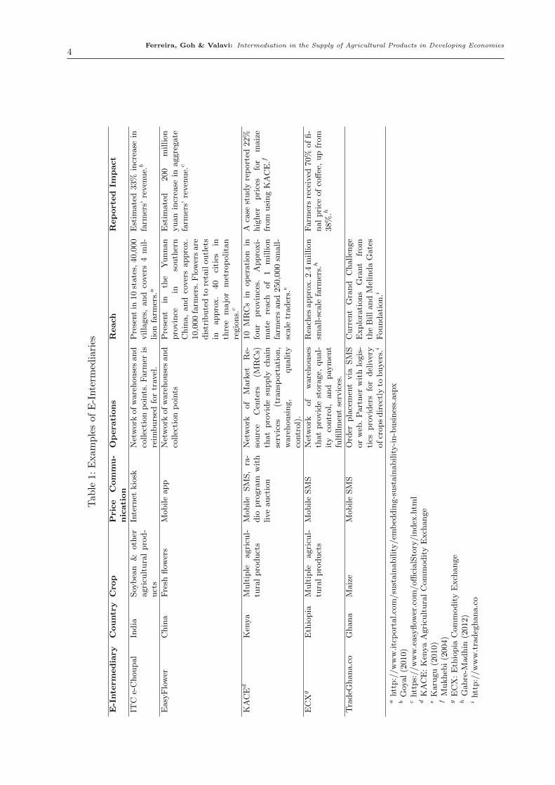
at local auctions. These and other examples of e-intermediaries are listed in Table 1. We note
that all of the examples displayed are private, for-profit organizations except for ECX, which is a
public-private partnership.
Despite the emergence of these and other similar e-intermediaries in developing economies and
some preliminary accounts of positive impact (see, e.g., Upton and Fuller 2004, Qiang et al. 2012),
we are not aware of any studies in the operations and supply chain literature that systematically
analyze the role and impact of e-intermediaries in developing markets. We argue that this gap in the
literature warrants scholarly attention for at least two reasons. First, from an academic perspective,
the study of supply chain issues in developing economies is currently a nascent field with limited,
context-specific results. Assumptions that underlie the models, theories, and insights that have
been established for supply chains in developed markets may fail to hold in developing countries.
It is therefore necessary to tailor such models to developing economies in order to obtain insights
that are relevant to the issues faced in such settings. As an example, although the literature on
supply chain contracting is large and well-developed (e.g., Taylor 2002, Cachon and Lariviere 2005),
contracts are often unenforceable in developing countries due to weak regulatory environments and
would not be a viable solution to help farmers improve their livelihood.
Second, from an applied perspective, because interventions in a supply chain may have unin-
tended consequences on other stakeholders in the chain, well-intentioned interventions such as
e-intermediation could backfire and lead to poor outcomes. Moreover, reports of social impacts on
farmers from e-intermediaries (such as those listed in Table 1) are usually anecdotal and typically
self-reported. Therefore, a rigorous study of how e-intermediaries work, as well as understanding
the extent to which farmers and supply chains benefit from their presence, can serve to guide
charitable foundations and governments in their decisions about whether and how to direct scarce
resources to support e-intermediation efforts.
In this paper, we have two primary objectives. First, we aim to develop insights into the structural
drivers of farmer and supply chain profitability in emerging market supply chains. Second, we aim
to develop an understanding of the impact of an e-intermediary on the profitability of farmers
and supply chains. To fulfill these objectives, we develop a model of a supply chain, described in
Ferreira, Goh & Valavi: Intermediation in the Supply of Agricultural Products in Developing Economies4
Tab
le1:
Exam
ple
sof
E-I
nte
rmed
iari
es
E-I
nte
rmedia
ryC
ountr
yC
rop
Pri
ce
Com
mu-
nic
ati
on
Op
era
tions
Reach
Rep
ort
ed
Impact
ITC
e-C
houpal
India
Soy
bea
n&
oth
eragri
cult
ura
lpro
d-
uct
s
Inte
rnet
kio
skN
etw
ork
of
ware
house
sand
collec
tion
poin
ts.
Farm
eris
reim
burs
edfo
rtr
avel
.
Pre
sent
in10
state
s,40,0
00
villa
ges
,and
cover
s4
mil-
lion
farm
ers.
a
Est
imate
d33%
incr
ease
infa
rmer
s’re
ven
ue.
b
Easy
Flo
wer
Chin
aF
resh
flow
ers
Mobile
app
Net
work
of
ware
house
sand
collec
tion
poin
tsP
rese
nt
inth
eY
unnan
pro
vin
cein
south
ern
Chin
a,
and
cover
sappro
x.
10,0
00
farm
ers.
Flo
wer
sare
dis
trib
ute
dto
reta
iloutl
ets
inappro
x.
40
citi
esin
thre
em
ajo
rm
etro
polita
nre
gio
ns.
c
Est
imate
d200
million
yuan
incr
ease
inaggre
gate
farm
ers’
reven
ue.
c
KA
CE
dK
enya
Mult
iple
agri
cul-
tura
lpro
duct
sM
obile
SM
S,
ra-
dio
pro
gra
mw
ith
live
auct
ion
Net
work
of
Mark
etR
e-so
urc
eC
ente
rs(M
RC
s)th
at
pro
vid
esu
pply
chain
serv
ices
(tra
nsp
ort
ati
on,
ware
housi
ng,
quality
contr
ol)
.
10
MR
Cs
inop
erati
on
info
ur
pro
vin
ces.
Appro
xi-
mate
reach
of
1m
illion
farm
ers
and
250,0
00
small-
scale
trader
s.e
Aca
sest
udy
rep
ort
ed22%
hig
her
pri
ces
for
maiz
efr
om
usi
ng
KA
CE
.f
EC
Xg
Eth
iopia
Mult
iple
agri
cul-
tura
lpro
duct
sM
obile
SM
SN
etw
ork
of
ware
house
sth
at
pro
vid
est
ora
ge,
qual-
ity
contr
ol,
and
pay
men
tfu
lfillm
ent
serv
ices
.
Rea
ches
appro
x.2.4
million
small-s
cale
farm
ers.
hF
arm
ers
rece
ived
70%
of
fi-
nal
pri
ceof
coff
ee,
up
from
38%
.h
Tra
deG
hana.c
oG
hana
Maiz
eM
obile
SM
SO
rder
pla
cem
ent
via
SM
Sor
web
.P
art
ner
wit
hlo
gis
-ti
cspro
vid
ers
for
del
iver
yofcr
ops
dir
ectl
yto
buyer
s.i
Curr
ent
Gra
nd
Challen
ge
Explo
rati
ons
Gra
nt
from
the
Bill
and
Mel
inda
Gate
sF
oundati
on.i
ahtt
p:/
/w
ww
.itc
port
al.co
m/su
stain
abilit
y/em
bed
din
g-s
ust
ain
abilit
y-i
n-b
usi
nes
s.asp
xb
Goy
al
(2010)
chtt
ps:
//w
ww
.easy
flow
er.c
om
/offi
cialS
tory
/in
dex
.htm
ld
KA
CE
:K
enya
Agri
cult
ura
lC
om
modit
yE
xch
ange
eK
aru
gu
(2010)
fM
ukheb
i(2
004)
gE
CX
:E
thio
pia
Com
modit
yE
xch
ange
hG
abre
-Madhin
(2012)
ihtt
p:/
/w
ww
.tra
deg
hana.c
o
Ferreira, Goh & Valavi: Intermediation in the Supply of Agricultural Products in Developing Economies5
§2, which captures several key features of traditional agricultural supply chains that operate in
developing economies. We analyze the model with and without an e-intermediary in §3 and §4,
respectively, and complement the insights gained with observations from a numerical study in §5.
All proofs and supporting lemmas are in the electronic companion.
One advantage of using a modeling approach is that it allows us to isolate effects of interest
that can be difficult to disentangle using other research approaches, e.g., empirical methods or case
studies. As is with ITC’s e-Choupal initiative, many real-world e-intermediaries not only provide
an alternate sales channel, but also provide additional useful information (e.g., weather forecasts)
that could help farmers make better decisions. Case studies which point to the positive impact of
e-intermediaries may be simply picking up improvements stemming from better information, rather
than providing direct evidence that a new e-intermediated channel is beneficial to farmers. In our
model, we abstract away from such information asymmetry issues and focus on what we think is
the more fundamental issue of understanding the impact of the new e-intermediated channel itself.
Our key findings are summarized below:
1. Auction mechanisms that intermediate traditional supply chains introduce sub-optimality to
the overall supply chain, in that they cause farmers to either overproduce or underproduce
compared to their ideal production levels had they been vertically integrated with the buyers.
2. The presence of an e-intermediary with limited market share tends to improve farmers’ profits
compared to the traditional supply chain. However, if the e-intermediary grows too large, it has
a negative impact on both farmers’ and total supply chain profits.
3. As the number of farmers increases, the total profits of all farmers converge to zero in the
limit, irrespective of the e-intermediary’s presence. Thus, a more impactful way to improve
the livelihood of farmers in developing economies is to consolidate farmers into larger farming
collectives to improve their market power.
1.1. Related Literature
We structure our review of related work into three groups that progressively broaden in terms of
their contextual similarity to our work. The first group comprises case studies of e-intermediaries
and empirical evaluations of specific e-intermediaries’ impact on farmers. The second group com-
prises modeling papers that fall in the broader context of agricultural supply chains in developing
economies. The third group comprises papers that may be in a different context from our work,
but share methodological similarities.
The first group of papers are case studies and empirical studies that focus specifically on e-
intermediaries operating in developing countries. As summarized in Table 1, there are numerous
examples of case studies detailing such e-intermediaries across the world. More in-depth case stud-
ies of e-intermediaries can be found for ITC e-Choupal (Upton and Fuller 2004), ECX (Alemu
Ferreira, Goh & Valavi: Intermediation in the Supply of Agricultural Products in Developing Economies6
and Meijerink 2010), and KACE (Mukhebi and Kundu 2014). While these case studies offer rich
descriptions about how these e-intermediaries operate, we caution they are also not typically peer-
reviewed. In particular, reports of positive impact on farmers from these case-studies (some of
which are summarized in Table 1) are usually obtained from the e-intermediaries themselves, who
have vested interests in what information they present. Independent, academic evaluations of the
impact of e-intermediaries on farmers are less prevalent, and we are only aware of two such stud-
ies, with mixed findings. Goyal (2010) empirically studies the impact of ITC e-Choupal when it
was first introduced as an alternate channel to the traditional auction channel that had oper-
ated for decades. Specifically, Goyal (2010) measures the e-intermediary’s impact on the auction
price, farmers’ production quantity, and farmers’ revenue, and finds that the introduction of the
e-intermediary was beneficial to farmers. In contrast, a recent study by Hernandez et al. (2017)
studies the impact of the ECX e-intermediary on coffee prices in Ethiopia; they find that the in-
troduction of ECX did not have a substantial impact on coffee prices and farmers’ profits. A result
in our paper could offer a potential explanation to these divergent empirical findings. We find that
the e-intermediary can be beneficial to farmers when its market share is small - as was likely the
case when ITC e-Choupal was first introduced. However, we also find that the reverse occurs when
the e-intermediary grows large, which reflects the setting studied by Hernandez et al. (2017).
The second group of papers share a similar context with our paper, namely, that of agricultural
supply chains in developing economies. The paper by Devalkar et al. (2011) is motivated by ITC’s
e-Choupal operations, and employs a stochastic dynamic program to characterize the firm’s optimal
operating decisions in a multi-period setting, specifically, the optimal quantities that the firm
should procure, process, and sell in each period. Whereas this paper focuses on the operations of a
single firm over multiple periods, our paper focuses on the joint decisions of multiple players in the
supply chain (e-intermediary and farmers) in order to study the impact that a two-channel setting
has on farmers, but we do not consider a multi-period model for tractability.
Two recent papers use models to study the impact of government interventions on agricultural
supply chains. Akkaya et al. (2016) study three such interventions: price support (i.e. instituting a
minimum selling price per unit), cost support (i.e. subsidizing input cost), and yield enhancement
(i.e. educating farmers on best practices). They find that in some cases, price support benefits con-
sumers more than farmers. Alizamir et al. (2015) study two potential interventions: price support
and revenue support (i.e. instituting a minimum revenue for each farmer). Their results are positive
for price support: farmer and consumer welfare are typically improved, and the intervention cost
to the government is less than that of revenue support. Our present work is distinct from these
studies of government intervention because we study the impact of for-profit intermediation.
Several papers that study interactions between for-profit firms and farmers focus on the role and
impact of supply contracts on various players. For example, both Hu et al. (2016) and Federgruen
Ferreira, Goh & Valavi: Intermediation in the Supply of Agricultural Products in Developing Economies7
et al. (2015) consider a setting where a for-profit firm offers procurement contracts to a subset
of farmers, and derive the profit-maximizing contract(s) to offer farmers. Hu et al. (2016) show
that such a contract benefits all farmers, not just those who were offered the contract. Our paper
differs from these works because we consider price-based intermediated procurement (i.e., without
contracts). As we argued in the introduction and also noted by Federgruen et al. (2015), contracting
approaches, which are common in developed economies, may not be feasible in developing countries
when the regulatory environment is weak.
Chen and Tang (2015) also study a supply chain intervention – information provision – in the
context of developing economies, but unlike the studies above who consider the objectives of the
implementor of the intervention, their study is focused primarily on understanding the mechanisms
through which farmers’ welfare is impacted by the intervention. The authors are motivated by
a growing effort by numerous organizations (including e-intermediaries like ITC e-Choupal) to
provide rural farmers with access to better market and farming information, and use a signaling
game to study the value of information on farmers’ welfare. One of their main findings is that the
provision of such “private signals” typically have a positive impact on farmers’ welfare. A similar
paper by Tang et al. (2015) studies whether farmers will act upon such information to increase
their profits and find that farmers do so in equilibrium. Similar to these papers, our paper shares
the same broad goal of understanding how farmers’ livelihood can be improved. However, it differs
because we focus on the role of a new supply chain channel as opposed to the role of information.
The third group of papers are those that share similar methodologies or modeling elements with
our paper, even though they could be motivated by firms in different industries than ours. Caldentey
and Vulcano (2007) study the relationship between an auction channel and a posted-price channel
(the e-intermediary’s pricing mechanism in our model) in the context of eBay. Consumers have
the option to buy the product in either channel, and the authors study the consumers’ optimal
channel choice and how the firm should structure the auction as a function of the posted price.
Although their model is similar to ours in that it studies a two-channel setting with similar pricing
mechanisms, a key distinction between our work and theirs is that we consider the channels’
interactions in a two-sided market with both suppliers and buyers, whereas they focus on the
channels’ interactions with only one side of the market (buyers). Our model is also tailored to
study supply chain issues (including production decisions of farmers), whereas theirs is tailored to
study purchases made in an online setting, featuring stochastically arriving customers.
Our paper also shares some modeling elements with that of Lee and Whang (2002), who consider
the impact of a secondary market formed by a network of retailers that face stochastic demands over
two periods. In the first period, retailers purchase products from a single manufacturer and face
stochastic demand; in the second period, the same retailers form a secondary market to rebalance
Ferreira, Goh & Valavi: Intermediation in the Supply of Agricultural Products in Developing Economies8
their inventories before again facing stochastic demand. Although Lee and Whang (2002) do not
explicitly note this in their paper, their model of a secondary market is a Walrasian auction, which
is also the basis of the auction mechanism used in this paper. However, there are several important
key differences between the operations of the auctions in our papers. First, demand in their model
is realized over two periods. In our model it is realized only in a single period. Second, in their
model, retailers are both sellers and buyers at the auction, and are also the same players who
face demand. In our auction model, the sellers (farmers) are distinct from the buyers (retailers),
and it is only the latter who face demand. Third, in their model, the entities (retailers) who make
procurement decisions in period 1 are also the participants in the auction in period 2; in contrast,
the entities (farmers) in our model that make production decisions in period 1 are distinct from
the buyers in the auction in period 2.
In summary, we have not found work in the literature on supply chain management that models
the interaction of farmers and buyers through a combination of an auction-based sales channel and
a posted-price intermediating channel that furthermore adds considerations that are relevant to
issues faced in developing countries (e.g., supply fragmentation). Our paper aims to fill this gap in
the literature, with an overarching objective of developing a deeper understanding of how to effect
positive change in the welfare of farmers in these settings.
2. Model Description and Preliminary Analysis
We first present our model of the traditional supply chain (without an e-intermediary) in §2.1.
Then we introduce the e-intermediary in §2.2 and outline our e-intermediated supply chain model.
Before proceeding to our main results, in §2.3 we offer some preliminary analyses and summarize
the notation that we will use throughout the rest of the paper.
2.1. Traditional Supply Chain Model
Our model of the traditional supply chain comprises two groups of players: N farmers (indexed by
i) and M retailers (indexed by j). Although we refer to the second group as “retailers”, depending
on the context and product, these retailers could in fact be disjoint groups of retailers, wholesalers,
food processors, or end-consumers; we simply use the word “retailer” for consistency. These retailers
drive stochastic demand for the product.
At a high level, the model operates as follows: farmers first make investments to each produce
some quantity of a homogenous crop. Farmers can then sell their crop to retailers through a market,
which we model as a Walrasian auction (described in detail below), who in turn sell the product
to their customers at a fixed price. We assume that all exogenous parameters to the model are
common knowledge to all parties. At the end of §2, Table 2 summarizes each of these parameters and
decision variables for both the traditional and e-intermediated supply chains for quick reference.
Ferreira, Goh & Valavi: Intermediation in the Supply of Agricultural Products in Developing Economies9
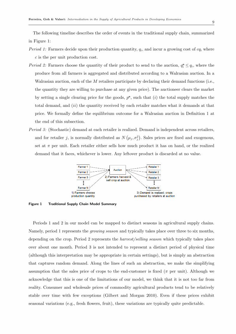
The following timeline describes the order of events in the traditional supply chain, summarized
in Figure 1:
Period 1: Farmers decide upon their production quantity, qi, and incur a growing cost of cqi where
c is the per unit production cost.
Period 2: Farmers choose the quantity of their product to send to the auction, qai ≤ qi, where the
produce from all farmers is aggregated and distributed according to a Walrasian auction. In a
Walrasian auction, each of the M retailers participate by declaring their demand functions (i.e.,
the quantity they are willing to purchase at any given price). The auctioneer clears the market
by setting a single clearing price for the goods, pa, such that (i) the total supply matches the
total demand, and (ii) the quantity received by each retailer matches what it demands at that
price. We formally define the equilibrium outcome for a Walrasian auction in Definition 1 at
the end of this subsection.
Period 3: (Stochastic) demand at each retailer is realized. Demand is independent across retailers,
and for retailer j, is normally distributed as N(µj, σ
2j
). Sales prices are fixed and exogenous,
set at π per unit. Each retailer either sells how much product it has on hand, or the realized
demand that it faces, whichever is lower. Any leftover product is discarded at no value.
Figure 1 Traditional Supply Chain Model Summary
Periods 1 and 2 in our model can be mapped to distinct seasons in agricultural supply chains.
Namely, period 1 represents the growing season and typically takes place over three to six months,
depending on the crop. Period 2 represents the harvest/selling season which typically takes place
over about one month. Period 3 is not intended to represent a distinct period of physical time
(although this interpretation may be appropriate in certain settings), but is simply an abstraction
that captures random demand. Along the lines of such an abstraction, we make the simplifying
assumption that the sales price of crops to the end-customer is fixed (π per unit). Although we
acknowledge that this is one of the limitations of our model, we think that it is not too far from
reality. Consumer and wholesale prices of commodity agricultural products tend to be relatively
stable over time with few exceptions (Gilbert and Morgan 2010). Even if these prices exhibit
seasonal variations (e.g., fresh flowers, fruit), these variations are typically quite predictable.
Ferreira, Goh & Valavi: Intermediation in the Supply of Agricultural Products in Developing Economies10
It is worth noting that in reality, farmers grow and harvest different types of crops. For the
purpose of our study, we focus on just one of those crops that they might produce and its cor-
responding supply chain structure; the per unit cost of the crop, c, can thus be interpreted as
incorporating the opportunity cost of planting a different crop instead of the crop of interest in our
study. Similarly, the farmer’s choice of production quantity in our model translates to a decision of
how many resources (e.g., land, labor, etc.) he chooses to allocate to this crop of interest relative
to a different crop. Using this interpretation, our model of each farmer’s decision is similar to what
other authors have considered in recent work (e.g., Akkaya et al. 2016).
However, primarily for analytical tractability, our model abstracts from reality by assuming that
there is no supply uncertainty (i.e., farmers can choose production quantities exactly), no capacity
limits on production, and no fixed costs or other forms of economies of scale. We believe that these
model elements would not fundamentally alter the direction of our key findings, but would add
more notation and technicalities to the paper that would likely be distracting.
Moreover, in reality, the exact auction mechanism used for many agricultural products in emerg-
ing markets are variants on first-price auctions of individual units of products. Because there are
invariably multiple units of products being sold at the auction, one option might be to directly
analyze this as a sequence of first-price auctions. Unfortunately, this turns out to be analytically
intractable. We use a Walrasian model as an approximation not only for the sake of tractability,
but also because it is an idealized model of an exchange. The latter, in particular, removes in-
efficiencies due to a sub-optimal auction implementation and allows our analysis to focus on the
impact that the supply chain’s structure has on its overall profits and the profits accrued to the
players in the chain. For an in-depth review of Walrasian auctions, we refer the reader to Joyce
(1984). The following definition describes the equilibrium outcome for the Walrasian auction.
Definition 1. Let Qa =∑N
i qai represent the total quantity available for distribution in a Wal-
rasian auction with m retailers. Suppose that yj(p) represents the demand function submitted by
retailer j. Then, the equilibrium of the Walrasian auction is (pa, x1, . . . , xm), where pa represents
the clearing price of the auction, and (x1, . . . , xm) represents the allocation of goods to retailers,
such that (i) each retailer receives what it demands at price pa, i.e., xj = yj(pa), and (ii) the market
clears with total supply matching total demand, i.e., Qa =∑m
j=1 xj.
2.2. E-Intermediated Supply Chain Model
Our model of the e-intermediated supply chain is similar to that of the traditional supply chain
except in that it allows farmers to sell their crops through an alternate channel - the e-intermediary
- as opposed to solely an auction channel. We interpret the e-intermediary as a third-party who has
access to the retailers through the use of digital technology - either on a personal computer, mobile
application, or Internet kiosk - and sells crops that it purchases from these farmers to some fraction
Ferreira, Goh & Valavi: Intermediation in the Supply of Agricultural Products in Developing Economies11
of the retailers. On the supply side, the e-intermediary chooses a fixed price per unit, pe, to procure
the crop from farmers. Using fixed pricing as an operational lever to obtain supply is broadly
consistent with what we have observed from the operations of existing e-intermediaries in emerging
markets. On the demand side, the e-intermediary also sells the crop at the exogenous price per unit
π, but captures only some portion of the overall retailer demand. Namely, m∈ {1, . . . ,M} retailers
participate in the auction in the e-intermediated supply chain, and the e-intermediary serves the
remaining retailersm+1, . . . ,M or their end-customers by taking on their total aggregated demand.
We assume that there are sufficient barriers to entry such that the e-intermediary does not have
the option to participate in the auction, and the m retailers who do participate in the auction do
not have the ability to become e-intermediaries.
There are several plausible mechanisms that motivate why this is an appropriate model, which
we describe below. Our goal in having this discussion is not to argue in favor of one mechanism
over the other, but rather to motivate that our abstract model has plausible practical roots. One
plausible mechanism is that M −m retailers decide to consolidate their sourcing operations for
the crop, and acquire or invest in technology that allows them to purchase directly from farmers
without going through the auction. A variant of this mechanism is that a government, charitable
organization, or corporate entity could be a driving force behind the development of the technology,
which is then successfully marketed to M −m of the retailers. ITC e-Choupal is an example of
an e-intermediary that fits this mechanism. Another plausible mechanism for this model is that
the e-intermediary is able to supply end-customers at lower frictions (i.e., transaction costs) than
the M −m retailers that it displaces. For example, these retailers may serve customers within a
certain geographic region and the e-intermediary might possess some geographic advantages (e.g.,
better relationships with local logistics providers), which enables it to provide a better quality
of service to customers and displace the retailers in selling the crop. EasyFlower, KACE, ECX,
and TradeGhana.co are examples of e-intermediaries that fit this mechanism. Nevertheless, in
either mechanism, our abstract model is a reasonable representation of the key economic tension
introduced by the e-intermediary, allowing us to study its impact on the supply chain. In particular,
using our model, we can compare the impact of an e-intermediary in various stages of its growth,
e.g., in its early growth phase when it captures a relatively small portion of the market (M −m is
small), or in more mature stages when it captures a larger fraction of the market (M −m is large).
On the surface, our model appears to match the operations of procurement-based e-intermediaries
(e.g., ITC e-Choupal, EasyFlower) more so than that of the e-intermediaries that operate as com-
modity exchanges (e.g., KACE, ECX, TradeGhana.co). However, we argue that this is in fact
not the case. These commodity exchanges operate by charging a transaction fee on purchases
made through their channel, which, analogous to procurement prices set by ITC e-Choupal or
Ferreira, Goh & Valavi: Intermediation in the Supply of Agricultural Products in Developing Economies12
EasyFlower, affects the quantity of crop that flows through the e-intermediary. Moreover, because
these exchanges provide transportation and/or warehousing services, they effectively bear inven-
tory risk as do ITC e-Choupal and EasyFlower. Therefore, even though the e-intermediary in our
model is described as a firm who “purchases” crops from farmers, we argue that the model and
ensuing insights are applicable for exchange-type e-intermediaries, who face similar tradeoffs.
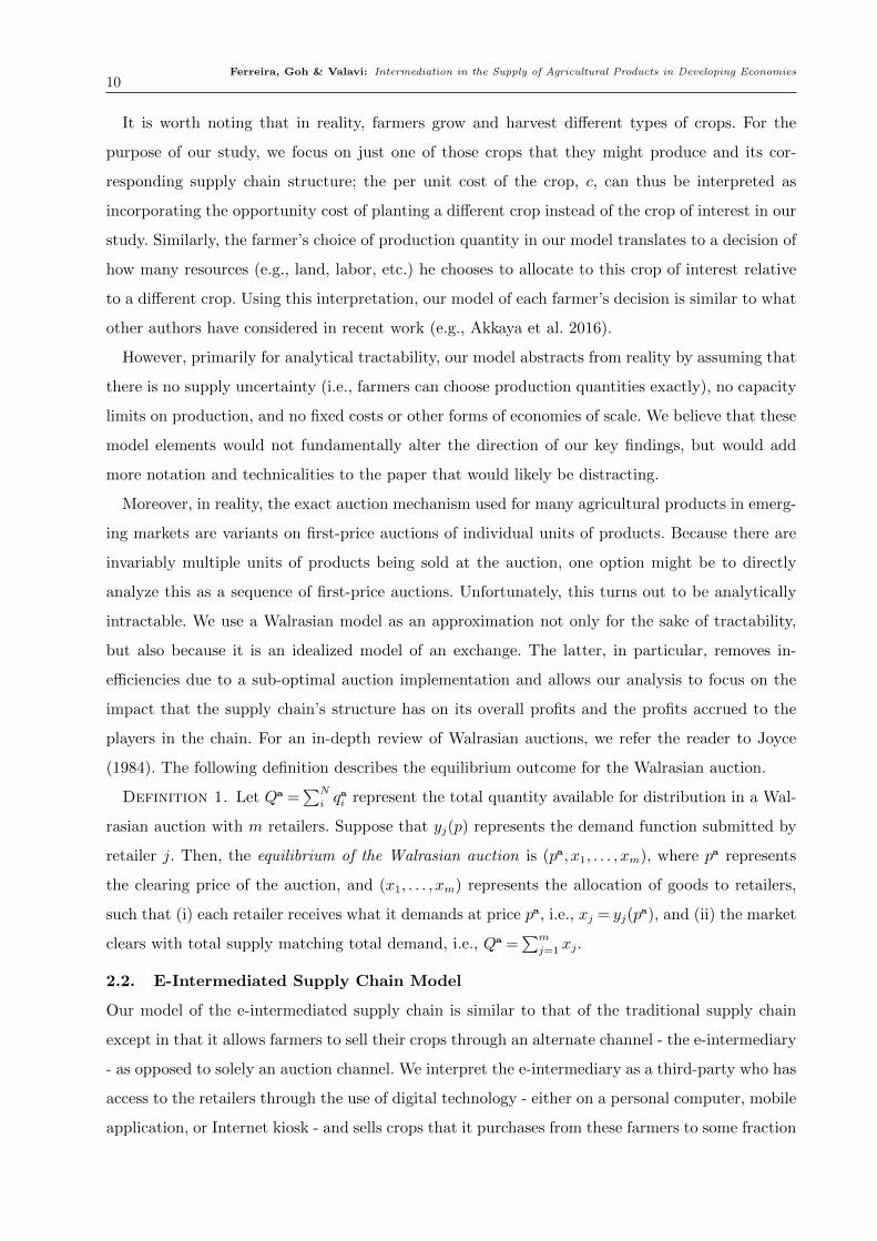
The following timeline describes the order of events in the e-intermediated supply chain, sum-
marized in Figure 2:
Period 1: As in the traditional supply chain, farmers decide upon their production quantity, qi,
and incur a growing cost of cqi.
Period 2: The e-intermediary observes the total production quantity, Q =∑N
i=1 qi, and chooses
a fixed price per unit, pe, to purchase crops from farmers. Farmers observe this price and
decide how much of their produce to sell to the e-intermediary, qei , and how much to sell at
the Walrasian auction, qai , which is run as before; clearly we must have qei + qai ≤ qi. Although
farmers do not observe pe in period 1, they rationally infer its value to inform their production
quantity decision.
Period 3: (Stochastic) demand at each retailer and the e-intermediary are realized. Demand is
independent across retailers, and for retailer j = 1, ...,m, is normally distributed as N(µj, σ
2j
),
just as in the traditional supply chain. The demand at the e-intermediary is pooled across
the M − m retailers that it represents/displaced and is normally distributed, i.e. Fe ∼
N(∑M
j=m+1 µj,∑M
j=m+1 σ2j
). As in the traditional supply chain, sales prices are fixed and ex-
ogenous at π per unit, both for the e-intermediary and all retailers participating in the auction.
Each retailer and e-intermediary either sells how much product it has on hand, or the realized
demand that it faces, whichever is lower; any leftover product is discarded at no value.
Figure 2 E-Intermediated Supply Chain Model Summary
Note that the traditional supply chain can be viewed as a special case of the e-intermediated
supply chain where m=M .
Ferreira, Goh & Valavi: Intermediation in the Supply of Agricultural Products in Developing Economies13
2.3. Preliminary Analysis
Here, we present some preliminary analyses to establish foundational results used throughout the
paper.
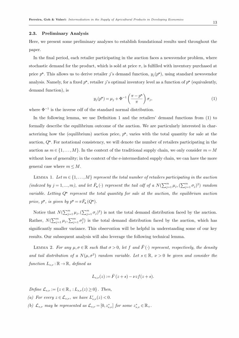
In the final period, each retailer participating in the auction faces a newsvendor problem, where
stochastic demand for the product, which is sold at price π, is fulfilled with inventory purchased at
price pa. This allows us to derive retailer j’s demand function, yj(pa), using standard newsvendor
analysis. Namely, for a fixed pa, retailer j’s optimal inventory level as a function of pa (equivalently,
demand function), is
yj(pa) = µj + Φ−1
(π− pa
π
)σj, (1)
where Φ−1 is the inverse cdf of the standard normal distribution.
In the following lemma, we use Definition 1 and the retailers’ demand functions from (1) to
formally describe the equilibrium outcome of the auction. We are particularly interested in char-
acterizing how the (equilibrium) auction price, pa, varies with the total quantity for sale at the
auction, Qa. For notational consistency, we will denote the number of retailers participating in the
auction as m∈ {1, . . . ,M}. In the context of the traditional supply chain, we only consider m=M
without loss of generality; in the context of the e-intermediated supply chain, we can have the more
general case where m≤M .
Lemma 1. Let m∈ {1, . . . ,M} represent the total number of retailers participating in the auction
(indexed by j = 1, ...,m), and let Fa (·) represent the tail cdf of a N(∑m
j=1 µj, (∑m
j=1 σj)2) random
variable. Letting Qa represent the total quantity for sale at the auction, the equilibrium auction
price, pa, is given by pa = πFa (Qa).
Notice that N(∑m
j=1 µj, (∑m
j=1 σj)2) is not the total demand distribution faced by the auction.
Rather, N(∑m
j=1 µj,∑m
j=1 σ2j ) is the total demand distribution faced by the auction, which has
significantly smaller variance. This observation will be helpful in understanding some of our key
results. Our subsequent analysis will also leverage the following technical lemma.
Lemma 2. For any µ,σ ∈R such that σ > 0, let f and F (·) represent, respectively, the density
and tail distribution of a N(µ,σ2) random variable. Let s ∈ R, ν > 0 be given and consider the
function Ls,ν :R→R, defined as
Ls,ν(z) := F (z+ s)− νzf(z+ s).
Define Ls,ν := {z ∈R+ :Ls,ν(z)≥ 0} . Then,
(a) For every z ∈Ls,ν, we have L′s,ν(z)< 0.
(b) Ls,ν may be represented as Ls,ν = [0, z∗s,ν ] for some z∗s,ν ∈R+.
Ferreira, Goh & Valavi: Intermediation in the Supply of Agricultural Products in Developing Economies14
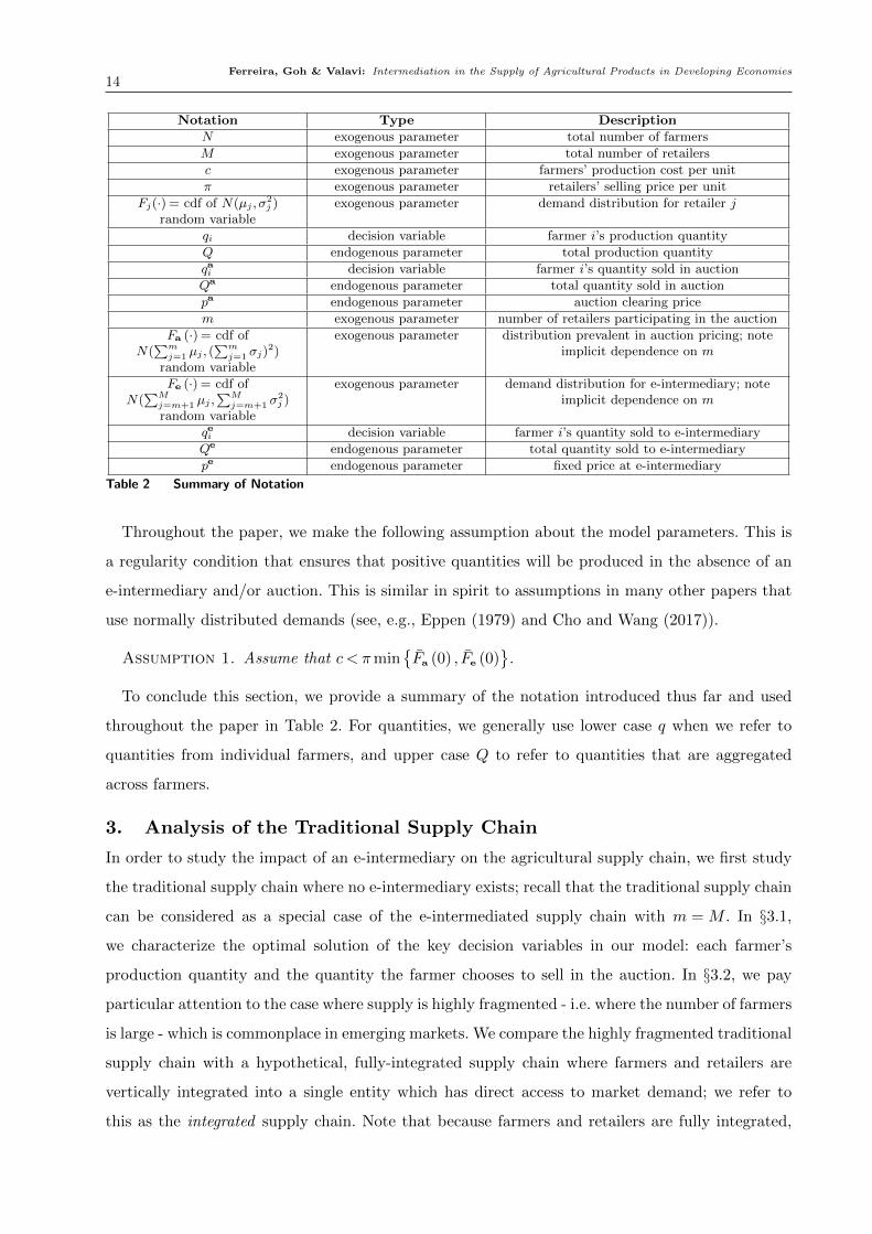
Notation Type Description
N exogenous parameter total number of farmers
M exogenous parameter total number of retailers
c exogenous parameter farmers’ production cost per unit
π exogenous parameter retailers’ selling price per unit
Fj(·) = cdf of N(µj , σ2j )
random variableexogenous parameter demand distribution for retailer j
qi decision variable farmer i’s production quantity
Q endogenous parameter total production quantity
qai decision variable farmer i’s quantity sold in auction
Qa endogenous parameter total quantity sold in auction
pa endogenous parameter auction clearing price
m exogenous parameter number of retailers participating in the auction
Fa (·) = cdf ofN(
∑mj=1 µj , (
∑mj=1 σj)
2)random variable
exogenous parameter distribution prevalent in auction pricing; noteimplicit dependence on m
Fe (·) = cdf ofN(
∑Mj=m+1 µj ,
∑Mj=m+1 σ
2j )
random variable
exogenous parameter demand distribution for e-intermediary; noteimplicit dependence on m
qei decision variable farmer i’s quantity sold to e-intermediary
Qe endogenous parameter total quantity sold to e-intermediary
pe endogenous parameter fixed price at e-intermediary
Table 2 Summary of Notation
Throughout the paper, we make the following assumption about the model parameters. This is
a regularity condition that ensures that positive quantities will be produced in the absence of an
e-intermediary and/or auction. This is similar in spirit to assumptions in many other papers that
use normally distributed demands (see, e.g., Eppen (1979) and Cho and Wang (2017)).
Assumption 1. Assume that c < πmin{Fa (0) , Fe (0)
}.
To conclude this section, we provide a summary of the notation introduced thus far and used
throughout the paper in Table 2. For quantities, we generally use lower case q when we refer to
quantities from individual farmers, and upper case Q to refer to quantities that are aggregated
across farmers.
3. Analysis of the Traditional Supply Chain
In order to study the impact of an e-intermediary on the agricultural supply chain, we first study
the traditional supply chain where no e-intermediary exists; recall that the traditional supply chain
can be considered as a special case of the e-intermediated supply chain with m = M . In §3.1,
we characterize the optimal solution of the key decision variables in our model: each farmer’s
production quantity and the quantity the farmer chooses to sell in the auction. In §3.2, we pay
particular attention to the case where supply is highly fragmented - i.e. where the number of farmers
is large - which is commonplace in emerging markets. We compare the highly fragmented traditional
supply chain with a hypothetical, fully-integrated supply chain where farmers and retailers are
vertically integrated into a single entity which has direct access to market demand; we refer to
this as the integrated supply chain. Note that because farmers and retailers are fully integrated,
Ferreira, Goh & Valavi: Intermediation in the Supply of Agricultural Products in Developing Economies15
there is no longer any auction that intermediates transactions. The integrated supply chain serves
as a best-case scenario - albeit unrealistic itself - for which to compare and better understand the
auction’s impact on production quantities and profits throughout the entire supply chain.
3.1. Farmers’ Optimal Decisions
Recall the two decisions that farmers face in the traditional supply chain: in period 1, farmers must
decide their production quantity, and in period 2, they decide how much to send to the auction.
Since farmers do not coordinate their decisions, they can be viewed as players in a noncoopera-
tive game, which we will call the traditional game. In this game, each farmer’s strategy can be
represented by a pair (qi, qai (·)), where the second element of the pair, qai (·) maps the farmer’s
production quantity to the quantity that he sends to the auction. Since farmers are homogeneous,
our analysis focuses on defining and characterizing symmetric equilibria of the game, where the
farmers’ decisions are identical. Throughout this paper, whenever we refer to “equilibria”, unless
explicitly stated otherwise, we will implicitly mean Nash equilibria that are subgame perfect. We
specify conditions for such equilibria below.
Definition 2. For a given scalar q ≥ 0 and function qa : R+ → R, consider the optimization
problem
maxq≥0
{−cq+ max
0≤qa≤q
{πqaFa (qa + (N − 1)qa(q))
}}. (2)
We call (q, qa) a symmetric equilibrium of the traditional game if the following conditions hold:
(a) qa(q) is an optimal solution to the inner problem of (2) for any q, and
(b) q is an optimal solution to the outer problem of (2).
In Definition 2, we have implicitly invoked the auction price formula from Lemma 1, and the
term (N − 1)qa(q) represents the sum of quantities that the other N − 1 farmers send to the
auction. In other words, this equilibrium definition means that each farmer plays a best response
to the decisions of all the other farmers. Using Definition 2, we can characterize the decisions made
by farmers in a symmetric equilibrium. To be precise, we characterize the equilibrium outcome
(q, qa(q)) of the game in the following proposition. Although we could, in principle, characterize
the entire equilibrium strategy (i.e., specify qa(q) for an arbitrary q), we refrain from doing so
because it would involve additional notation and technicalities that distract from the key thrust of
our analysis.
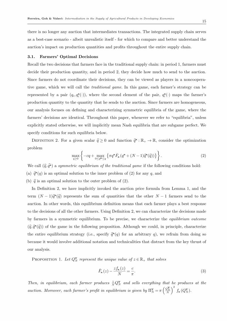
Proposition 1. Let QTN represent the unique value of z ∈R+ that solves
Fa (z)− zfa (z)
N=c
π. (3)
Then, in equilibrium, each farmer produces 1NQTN and sells everything that he produces at the
auction. Moreover, each farmer’s profit in equilibrium is given by ΠTN = π
(QT
NN
)2
fa (QTN).
Ferreira, Goh & Valavi: Intermediation in the Supply of Agricultural Products in Developing Economies16
Note that QTN refers to the total production quantity of all N farmers, where the superscript T
refers to the traditional supply chain; later in the paper, we will use superscript I to refer to the
integrated supply chain and superscript E to refer to the e-intermediated supply chain.
One implication of Proposition 1 is that in equilibrium, farmers only produce what they eventu-
ally sell. That is, there is no “wasted” production. Although this may seem obvious, the intuition
behind this is rather nuanced. In particular, if we consider the second-period subgame alone and
study the farmers’ decisions as a function of the quantity produced in the first period, it is easy to
see that in regimes where the first-period production quantity is sufficiently high, the symmetric
equilibrium of this subgame will entail wastage. It is therefore only in the equilibrium outcome of
the combined game that the “no wastage” property holds.
Having characterized the equilibrium for a fixed number of farmers, N , we now analyze how
these equilibrium quantities vary with N in the following proposition.
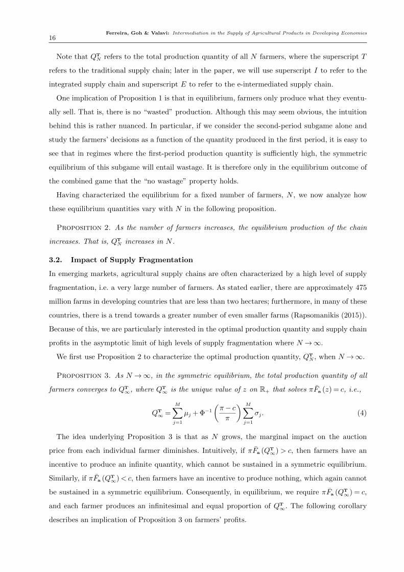
Proposition 2. As the number of farmers increases, the equilibrium production of the chain
increases. That is, QTN increases in N .
3.2. Impact of Supply Fragmentation
In emerging markets, agricultural supply chains are often characterized by a high level of supply
fragmentation, i.e. a very large number of farmers. As stated earlier, there are approximately 475
million farms in developing countries that are less than two hectares; furthermore, in many of these
countries, there is a trend towards a greater number of even smaller farms (Rapsomanikis (2015)).
Because of this, we are particularly interested in the optimal production quantity and supply chain
profits in the asymptotic limit of high levels of supply fragmentation where N →∞.
We first use Proposition 2 to characterize the optimal production quantity, QTN , when N →∞.
Proposition 3. As N →∞, in the symmetric equilibrium, the total production quantity of all
farmers converges to QT∞, where QT
∞ is the unique value of z on R+ that solves πFa (z) = c, i.e.,
QT∞ =
M∑j=1
µj + Φ−1
(π− cπ
) M∑j=1
σj. (4)
The idea underlying Proposition 3 is that as N grows, the marginal impact on the auction
price from each individual farmer diminishes. Intuitively, if πFa (QT∞) > c, then farmers have an
incentive to produce an infinite quantity, which cannot be sustained in a symmetric equilibrium.
Similarly, if πFa (QT∞)< c, then farmers have an incentive to produce nothing, which again cannot
be sustained in a symmetric equilibrium. Consequently, in equilibrium, we require πFa (QT∞) = c,
and each farmer produces an infinitesimal and equal proportion of QT∞. The following corollary
describes an implication of Proposition 3 on farmers’ profits.
Ferreira, Goh & Valavi: Intermediation in the Supply of Agricultural Products in Developing Economies17
Corollary 1. As N →∞, in the symmetric equilibrium, the total profits of all farmers converge
to zero.
This is a result of the fact that πFa (QT∞) = c, which implies that when N →∞, the farmers’
revenue per unit equals the production cost per unit; therefore, the farmers’ profit converges to
zero. This is a troubling result for agricultural supply chains in emerging economies, given their
high levels of supply fragmentation. In the remainder of this section, we study the impact of the
auction mechanism itself on the optimal production quantity and profits, given high levels of supply
fragmentation. Then in §4 and via numerical studies in §5, we will determine to what extent, if
any, the presence of an e-intermediary helps mitigate this negative impact on farmers.
Comparison with an Integrated Supply Chain
To better understand the impact that the auction has on the optimal production quantity in the
case of high levels of supply fragmentation, we compare the traditional supply chain when N →∞
with a hypothetical, fully-integrated supply chain. Specifically, we assume that farmers and retailers
are vertically integrated into a single entity (we will refer to this entity as “the firm”), which has
direct access to market demand. In particular, in the integrated firm, because farmers and retailers
are fully integrated, there is no longer any auction that intermediates transactions.
The firm faces a newsvendor problem, that is, maxQΠI(Q), where ΠI represents the profit of the
integrated chain as a function of the total quantity produced by the farmers, Q, and is defined
as ΠI(Q) := πE (DI ∧Q)− cQ, where DI ∼ N(∑M
j=1 µj,∑M
j=1 σ2j
)and can be interpreted as the
integrated firm’s total distribution. Standard newsvendor analysis gives us the optimal production
quantity of the integrated firm, outlined in the following proposition.
Proposition 4. In the integrated supply chain, the optimal production quantity of the firm is
QI, where
QI :=M∑j=1
µj + Φ−1
(π− cπ
)√√√√ M∑j=1
σ2j (5)
Note that QT∞ in Proposition 3 is identical to QI except that
∑M
j=1 σj replaces√∑M
j=1 σ2j .
Given this difference, we can see that an alternative representation of the traditional supply chain
when N →∞ is that of an integrated supply chain where the total retailer demand is DT ∼
N(∑M
j=1 µj, (∑M
j=1 σj)2)
instead of DI ∼N(∑M
j=1 µj,∑M
j=1 σ2j
), i.e. an integrated chain with larger
effective variance of retailer demand. Thus, for high levels of supply fragmentation (as N →∞),
the auction in the traditional supply chain is responsible for inflating the total retailer demand
variance that the farmers face when making their production decisions. This increase in variance
results in a sub-optimal production quantity in the highly fragmented traditional supply chain
compared to the integrated chain, as outlined in the following proposition.
Ferreira, Goh & Valavi: Intermediation in the Supply of Agricultural Products in Developing Economies18
Proposition 5. The inefficiency of total production of the highly fragmented traditional supply
chain depends on the value of c relative to π. If c < π/2, the traditional chain overproduces relative
to the integrated chain, i.e., QT∞ ≥QI. Conversely, if c > π/2, the traditional chain underproduces,
i.e., QT∞ ≤QI. Finally, if c= π/2, the traditional chain produces exactly what the integrated chain
would produce, i.e., QT∞ =QI.
Proposition 5 shows that the highly fragmented traditional supply chain, in equilibrium, gen-
erally produces a different quantity than the integrated supply chain. One interpretation of this
discrepancy in production quantity is that it is a manifestation of distorted production incentives
among farmers in the traditional supply chain. Specifically, this distortion takes on the form of
variance inflation: although the auction accurately aggregates mean total demand from retailers,
it inflates the demand variance in the traditional chain relative to the integrated chain. Farmers
produce according to this inflated variance, which is sub-optimal from the perspective of the overall
chain. It is noteworthy that the traditional supply chain may overproduce relative to the integrated
chain; other studies have found that supply chains that are intermediated typically tend to under-
produce relative to comparable integrated supply chains (see, e.g., Tang and Kouvelis 2014, Arya
and Mittendorf 2006, Gal-Or 1991, and references therein).
With a deeper understanding of how the auction impacts the optimal production quantity in the
highly fragmented traditional supply chain, we next study the impact that the auction has on the
farmers’ profit, retailers’ profit, and overall supply chain profit. In general, we expect the integrated
supply chain to have higher profits than the traditional chain. Nonetheless, it is instructive to
delve deeper to better understand the sources of inefficiency that the auction introduces in the
market. We first do so by considering a decomposition of the integrated supply chain’s profit into
parts, given a total production quantity Q. For every j = 1, . . . ,M , define Qj := µj +Φ−1(π−paπ
)σj,
where pa represents the equilibrium price from the Walrasian auction with total quantity Q, and
is calculated as pa = πFa (Q) by Lemma 1. Here, Qj represents the quantity allocated to retailer j
at the auction in the traditional supply chain, and because the auction distributes all the quantity
of goods available (Definition 1, part (ii)) , we have∑M
j=1Qj =Q. Based on this definition of Qj,
we may decompose the total supply chain profit of the integrated supply chain as
ΠI(Q) = πQFa (Q)− cQ︸ ︷︷ ︸(i)
+πM∑j=1
E (Dj ∧Qj)−πQFa (Q)︸ ︷︷ ︸(ii)
+πE (DI ∧Q)−πM∑j=1
E (Dj ∧Qj)︸ ︷︷ ︸(iii)
, (6)
where Dj ∼N(µj, σ2j ). In (6), elementary analysis reveals that each of the three terms (i), (ii), and
(iii) are nonnegative. Furthermore, term (i) represents the total farmers’ profits in the traditional
supply chain and term (ii) represents the total retailers’ profits in the traditional supply chain.
The sum of terms (i) and (ii) is thus the total supply chain profit in the traditional supply chain.
Ferreira, Goh & Valavi: Intermediation in the Supply of Agricultural Products in Developing Economies19
This leaves us with additional profit in the integrated supply chain compared to the traditional
supply chain, which is quantified in term (iii). Term (iii) can be interpreted as the profit loss in the
traditional supply chain due to retailer fragmentation; if there had only been a single retailer (i.e.,
M = 1), term (iii) would be zero. It is worth noting that such retailer fragmentation is intimately
connected to the auction, and is a prerequisite for having an auction in the first place.
Combining our preceding results with decomposition (6) enables us to analyze the impact of
supply fragmentation on the traditional supply chain’s profits, as outlined in the following theorem.
Theorem 1. As supply fragmentation (i.e., N) increases in the traditional supply chain and
farmers produce their equilibrium production quantity,
(a) the total profit of all farmers decreases,
(b) the total profit of all retailers increases,
(c) the total profit loss due to retailer fragmentation decreases if c < π/2, and
(d) the total supply chain’s profit increases if c > π/2.
One implication of part (a) of Theorem 1 is that as the number of farmers increases, individual
farmers are not only impacted by having to spread profits across more farmers, unfortunately they
are further impacted by the decrease in total farmers’ profits. In other words, not only do the
farmers have to “cut the (profit) pie” in more ways, they also face a shrinking “pie”. This means
that as supply fragmentation increases, farmers’ profits take a hit from multiple directions. In
contrast, part (b) of the theorem shows that the retailers benefit from supply fragmentation with
increased profits. When c > π2, we can further conclude from part (d) that the increase in retailers’
profits outweighs the decrease in farmers’ profits, and thus the total supply chain profits increase
with more supply fragmentation. This suggests that supply fragmentation actually helps the overall
supply chain, yet the auction allocates those additional profits in favor of the retailers instead of the
farmers. Finally, we are unable to conclude whether or not the total supply chain profit increases
with supply fragmentation when c < π2, but part (c) tells us that under this condition and as supply
fragmentation increases, the total supply chain profit of the traditional chain approaches the total
supply chain profit of the integrated chain, i.e., the negative impact of the retailer fragmentation
on total supply chain profits is mitigated by supply fragmentation when c < π2.
3.3. Discussion
Our results show that even though the idealized Walrasian auction mechanism is efficient in a
local sense, in that it finds a price for the product that perfectly matches supply and demand
between farmers and retailers, it nonetheless introduces sub-optimality to the overall supply chain.
Specifically, farmers either overproduce or underproduce in the traditional supply chain compared
to the integrated chain, which results in a sub-optimal total supply chain profit. It is striking that
this sub-optimality occurs even for such an idealized auction mechanism as an intermediary.
Ferreira, Goh & Valavi: Intermediation in the Supply of Agricultural Products in Developing Economies20
We argue that this insight is more salient than it may appear at first glance. The dominant
narrative about investments in emerging economies (particularly in the academic and popular
discourse on microfinancing) has largely revolved around the issue of developing more efficient
markets by providing liquidity to farmers (or small business owners in other settings) and reducing
transaction costs (see, e.g., Morduch 1999). Our result in Proposition 3 does not contravene this
narrative, but does provide an important caveat that a singular focus on local market creation
alone is inadequate, and that a holistic perspective of the supply chain is necessary.
Second, one might interpret this as a form of double marginalization, which has been extensively
studied in various contexts in both the operations and marketing literature (Jeuland and Shugan
1983, Pasternack 1985, Iyer 1998, Iyer et al. 2007). Generally speaking, double marginalization
refers to the phenomenon where supply chains perform sub-optimally as a consequence of interme-
diaries who optimize their operations for their own benefit. Our setting shows that a form of double
marginalization persists even when both prices and quantities are determined via an auction-based
exchange, in contrast to other settings where prices (and/or quantities) are the direct decisions
of supply chain participants. Moreover, the way that this suboptimality manifests is noteworthy.
Our results show that the supply chain distortion can manifest itself either as overproduction or
underproduction. This differs from typical findings of several variants of the classical setting where
double marginalization usually leads to underproduction (see, e.g., Tang and Kouvelis 2014, Arya
and Mittendorf 2006, Gal-Or 1991, and references therein).
4. Analysis of the E-Intermediated Supply Chain
The analysis of the traditional supply chain showed us that the auction inflates demand variance
compared to the integrated chain, which causes under/over-production and suboptimal profits. In
this section as well as the next, we study whether or not these negative effects can be mitigated
by the introduction of an e-intermediary as an alternate, fixed-price channel for which the farmers
have the option to sell their crop. Specifically, in the second period, each farmer must decide how
much product to send (a) to the auction and (b) to the e-intermediary. In §4.1, we characterize
the optimal solution of the key decision variables in our model: each farmer’s production quantity
and the quantities the farmer chooses to sell at the auction and e-intermediary, as well as the
price offered by the e-intermediary. In §4.2, we study the impact of supply fragmentation on the
e-intermediated supply chain and compare its performance to the traditional chain.
4.1. Farmers’ and E-Intermediary’s Optimal Decisions
For the auction, recall from Lemma 1 that the equilibrium auction price, pa, can be expressed as
a function of the total quantity available for distribution at the auction Qa, i.e., pa = πFa (Qa),
where Fa (·) represents the tail cdf of a N
(∑m
j=1 µj,(∑m
j=1 σj
)2)
random variable. In contrast,
Ferreira, Goh & Valavi: Intermediation in the Supply of Agricultural Products in Developing Economies21
the e-intermediary sets a price, pe, that it will purchase the product for. As described in §2.2, we
assume that the e-intermediary takes on the aggregate demand of retailers m+ 1 through M , such
that its demand is a N(∑M
j=m+1 µj,∑M
j=m+1 σ2j
)random variable. For notational brevity, we use
Fe (·) to denote the tail cdf of this random variable.
We now proceed to characterize key metrics of this e-intermediated supply chain. For ease of
reference, we will refer to the game comprising of the decisions of the farmers and the e-intermediary
in periods 1 and 2 as the e-intermediated game. Again, since farmers are homogeneous, our analysis
focuses on characterizing symmetric equilibria of the game, defined below.
Definition 3. Given a scalar q ≥ 0, functions pe : R+→ R, qa : R2+→ R, and qe : R2
+→ R, we
call (q, pe, qa, qe) a symmetric equilibrium of the e-intermediated game if the following conditions
hold simultaneously:
(a) For every given q≥ 0 and p≥ 0, qa(q, p), qe(q, p) are optimizers of the problem
Π(q, p) := maxqa≥0,qe≥0
pqe +πqaFa (qa + (N − 1)qa(q, p))
s.t. 0≤ qa + qe ≤ q. (7)
(b) For any q≥ 0, pe(Nq) is an optimizer of the problem
maxp≥0{πE (De ∧Nqe(q, p))− pNqe(q, p)} , (8)
where De ∼N(∑M
j=m+1 µj,∑M
j=m+1 σ2j
).
(c) q satisfies
q ∈ arg maxq≥0
{−cq+ Π(q, pe(q+ (N − 1)q))} , (9)
where Π(q, p) is as defined in part (a).
In Definition 3, note that we have suppressed denoting the dependence of the equilibrium quanti-
ties with model parameters (e.g., N,M,m) for notational brevity. Intuitively, part (a) requires that
each farmer allocates his products to channels optimally to maximize period 2 profits, as a best
response to the actions taken by all other farmers. Recall that qa and qe represent the quantities
allocated to the auction and e-intermediary, respectively; we have implicitly invoked Lemma 1 to
characterize the equilibrium price for the auction. Part (b) states that the price chosen by the
e-intermediary should maximize its expected profit. It turns out to be more convenient to (equiv-
alently) represent the e-intermediary’s price as a function of the total production of all farmers;
this is reflected in the notation for (b), where pe is defined as a function of Nq instead of q. Part
(c) states that each farmer chooses his first period quantity optimally.
Based on Definition 3, we can now characterize the symmetric equilibrium outcome of the e-
intermediated game. As in §3, we do not characterize off-equilibrium outcomes. We first establish
Ferreira, Goh & Valavi: Intermediation in the Supply of Agricultural Products in Developing Economies22
some preliminary definitions in order to streamline the presentation of our characterization. First,
define the function ψN :R+→R as
ψN(z) := Fa (z)− zfa (z)
N. (10)
By Lemma 2, there exists a unique value of z ≥ 0 such that ψN(z) = 0, and, for convenience, we
denote this as zN . Further, define ζN :R++→R as follows:
ζN(Q) :=
0 if ψN(0)−Qψ′N(0)≤ Fe (Q)
Q if ψN(Q)≥ Fe (0)
zN(Q)∧ zN otherwise,
(11)
where zN(Q) is the unique value of z ∈ (0,Q) that solves
ψN(z)− (Q− z)ψ′N(z) = Fe (Q− z) . (12)
It can be shown that zN , ζN are well-defined. We relegate the formal statement and verification of
technical lemmas involving these definitions to §EC.1 of the electronic companion.
The first mapping, ψN , will be used to connect the e-intermediary’s price and the total equilib-
rium quantity sent to the auction. Specifically, if z satisfies πψN(z) = p for a given p, then z will
represent the total equilibrium quantity at the auction when the e-intermediary offers price p to
farmers. The inverse mapping of ψN can thus be viewed as the impact of the e-intermediary’s price
on the total auction quantity. The second mapping, ζN , will be used to capture the impact of the
farmers’ total equilibrium production quantity on the total equilibrium quantity sent to the auc-
tion. It is important to note that our construction of ζN will implicitly capture the e-intermediary’s
optimal pricing decision.
Theorem 2. For a fixed q≥ 0, consider the optimization problem
maxq,z
(ψN(z)− c
π
)q+
z2fa (z)
N 2
s.t. z = ζN(q+ (N − 1)q)
q≥ 0.
(13)
and suppose that there is an optimal (q∗, z∗) of (13) such that q∗ = q. Then,
(a) The total amount produced by farmers is QEN :=Nq.
(b) The total quantity sent to the auction is QaN := ζN(QE
N),
(c) The total quantity sent to the e-intermediary is QeN :=QE
N −QaN .
(d) The e-intermediary chooses the purchase price pe := πψN(QaN) for the product.
In Theorem 2, problem (13) may be interpreted as the first-stage problem of farmers, who are
choosing their individual production quantity (q) as a best response to the symmetrically chosen
production quantities of the other farmers (q). We have included an auxiliary variable z to simplify
Ferreira, Goh & Valavi: Intermediation in the Supply of Agricultural Products in Developing Economies23
the presentation, which represents the total quantity sent by all farmers to the auction in the
second period. Although we do not have an explicit, closed-form characterization of the equilibrium
of this game, we can nonetheless derive certain properties about the equilibrium, which we state
in the following corollary.
Corollary 2. In a symmetric equilibrium, it is necessary that
(a) The auction price is weakly greater than the e-intermediary’s price, pe, that is, pa ≥ pe.
(b) If qe > 0, the e-intermediary’s price is weakly greater than the farmer’s marginal production cost
c, that is, pe ≥ c.
4.2. Impact of Supply Fragmentation
As described earlier, given that agricultural supply chains are often characterized by a very large
number of farmers, we pay particular attention in this section to the impact of supply fragmentation
on the e-intermediated supply chain and make comparisons to its impact on the traditional supply
chain. In the limit as N →∞, we can characterize the symmetric equilibrium of the e-intermediated
game more precisely with the following proposition.
Proposition 6. Define Qa∞ as
Qa∞ :=
m∑j=1
µj + Φ−1
(π− cπ
) m∑j=1
σj.
Furthermore, let Qe∞ represent the unique value of z that solves
Fe (z)− zfa (Qa∞) =
c
π. (14)
Then, in the limit as N →∞, the following hold in equilibrium:
(a) The e-intermediary’s purchase price converges to c.
(b) The auction price converges to c.
(c) The total quantity sent to the auction converges to Qa∞, the total quantity sent to the e-
intermediary converges to Qe∞, and the total quantity produced by all farmers converges to
QE∞ =Qa
∞+Qe∞.
Parts (a) and (b) together imply that the total farmers’ profits vanish in the limit of high supply
fragmentation, even in the e-intermediated chain. This can be viewed as an analog to Corollary 1
in the setting of a traditional chain. This result suggests a certain “hierarchy” of problems faced by
farmers in developing economies: The first-order problem is that of supply fragmentation, which
e-intermediation does not overcome. Through our numerical study in §5, we evaluate the possible
beneficial or detrimental second-order effects of e-intermediation on farmers’ profits for finite values
of N .
The following proposition presents results on the relative impact of the e-intermediary on the
overall production quantity and profits of the supply chain when supply is highly fragmented.
Ferreira, Goh & Valavi: Intermediation in the Supply of Agricultural Products in Developing Economies24
Proposition 7. Define σI, σa, σe, σT as follows:
σI :=
√√√√ M∑j=1
σ2j , σa :=
m∑j=1
σj, σe :=
√√√√ M∑j=m+1
σ2j , σT :=
M∑j=1
σj.
If c < π/2, and in addition,
M∑j=m+1
µj ≤Φ−1
(π− cπ
)(σa−
(σI−σa)(σa +σe)
σe
)and σI ≥ σa, (15)
we have QI ≤QE∞ ≤QT
∞.
Conversely, if c > π/2, and, in addition
M∑j=m+1
µj ≥Φ−1
(π− cπ
)(σa−
(σT−σa)(σa +σe)
σe
)(16)
we have QE∞ ≤QT
∞ ≤QI.
First, note that σI, σa, σe, and σT represent the standard deviation of retailer demand faced by the
integrated chain, the auction in the e-intermediated chain, the e-intermediary in the e-intermediated
chain, and the traditional supply chain, respectively. The interpretation of the proposition above
is that the impact of the e-intermediary on the supply chain’s overall profitability is mixed. When
c < π/2 and under some technical conditions, the result shows that the effect of the e-intermediary
relative to the traditional supply chain is that it pulls the total production quantity toward the
system optimal QI, which implies that supply chain profits are improved relative to the traditional
chain. The technical condition is an upper bound on the total average demand experienced by
the e-intermediary, which can be interpreted as the e-intermediary’s market share. Therefore, this
condition will tend to hold when the e-intermediary is small or in an early stage of growth. When
c > π/2, the converse holds. Under some technical conditions, the e-intermediary now pulls the
total production quantity of the chain away from the system optimal QI, diminishing the profits
of the chain. This condition tends to hold when the e-intermediary is large, or in a mature phase
of growth. The impact of the e-intermediary’s market share on the e-intermediated supply chain’s
profits, as well as on farmers’ profits, is further explored in §5.
5. Numerical Study
We conducted a numerical simulation study in order to gain further insights into how farmers’ and
supply chain profits are influenced by the e-intermediary’s presence and size, the extent of supply
fragmentation, and other parameters. Throughout our numerical analysis, we set π = 1 and fixed
total mean demand at 1000 units. We let κ represent the coefficient of variation of demand, which
we varied across simulations such that the standard deviation was 1000κ. We assumed that when
there were M retailers, these retailers were symmetric and had independent demands, so that the
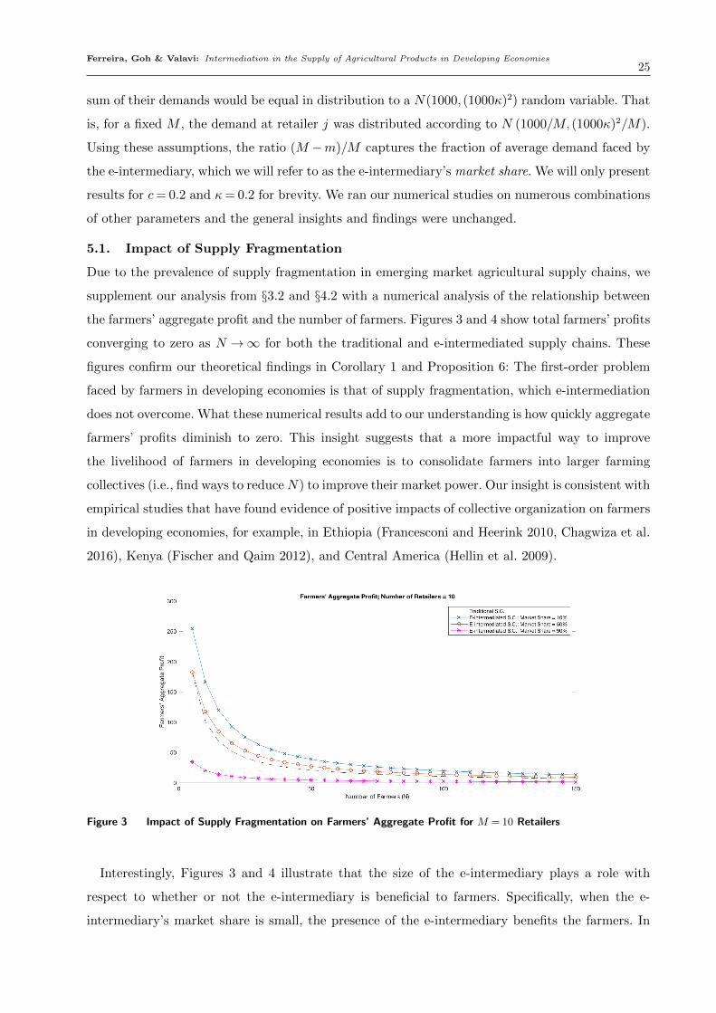
Ferreira, Goh & Valavi: Intermediation in the Supply of Agricultural Products in Developing Economies25
sum of their demands would be equal in distribution to a N(1000, (1000κ)2) random variable. That
is, for a fixed M , the demand at retailer j was distributed according to N (1000/M, (1000κ)2/M).
Using these assumptions, the ratio (M −m)/M captures the fraction of average demand faced by
the e-intermediary, which we will refer to as the e-intermediary’s market share. We will only present
results for c= 0.2 and κ= 0.2 for brevity. We ran our numerical studies on numerous combinations
of other parameters and the general insights and findings were unchanged.
5.1. Impact of Supply Fragmentation
Due to the prevalence of supply fragmentation in emerging market agricultural supply chains, we
supplement our analysis from §3.2 and §4.2 with a numerical analysis of the relationship between
the farmers’ aggregate profit and the number of farmers. Figures 3 and 4 show total farmers’ profits
converging to zero as N →∞ for both the traditional and e-intermediated supply chains. These
figures confirm our theoretical findings in Corollary 1 and Proposition 6: The first-order problem
faced by farmers in developing economies is that of supply fragmentation, which e-intermediation
does not overcome. What these numerical results add to our understanding is how quickly aggregate
farmers’ profits diminish to zero. This insight suggests that a more impactful way to improve
the livelihood of farmers in developing economies is to consolidate farmers into larger farming
collectives (i.e., find ways to reduceN) to improve their market power. Our insight is consistent with
empirical studies that have found evidence of positive impacts of collective organization on farmers
in developing economies, for example, in Ethiopia (Francesconi and Heerink 2010, Chagwiza et al.
2016), Kenya (Fischer and Qaim 2012), and Central America (Hellin et al. 2009).
Figure 3 Impact of Supply Fragmentation on Farmers’ Aggregate Profit for M = 10 Retailers
Interestingly, Figures 3 and 4 illustrate that the size of the e-intermediary plays a role with
respect to whether or not the e-intermediary is beneficial to farmers. Specifically, when the e-
intermediary’s market share is small, the presence of the e-intermediary benefits the farmers. In
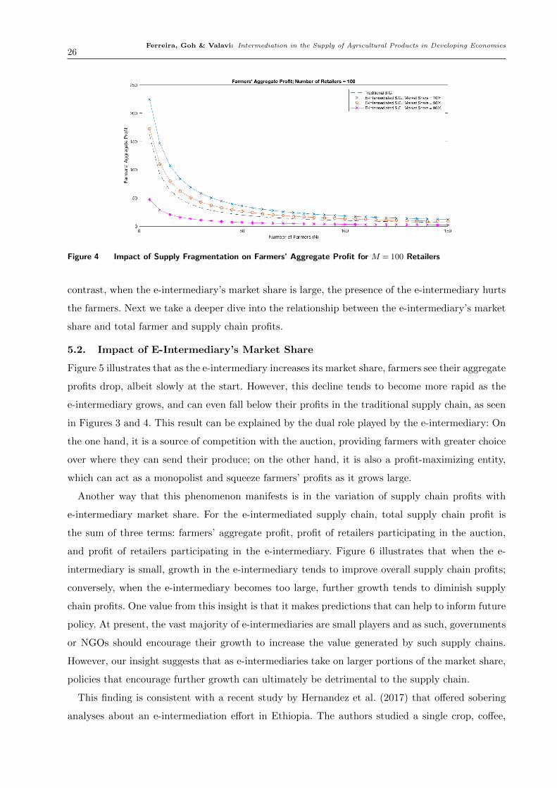
Ferreira, Goh & Valavi: Intermediation in the Supply of Agricultural Products in Developing Economies26
Figure 4 Impact of Supply Fragmentation on Farmers’ Aggregate Profit for M = 100 Retailers
contrast, when the e-intermediary’s market share is large, the presence of the e-intermediary hurts
the farmers. Next we take a deeper dive into the relationship between the e-intermediary’s market
share and total farmer and supply chain profits.
5.2. Impact of E-Intermediary’s Market Share
Figure 5 illustrates that as the e-intermediary increases its market share, farmers see their aggregate
profits drop, albeit slowly at the start. However, this decline tends to become more rapid as the
e-intermediary grows, and can even fall below their profits in the traditional supply chain, as seen
in Figures 3 and 4. This result can be explained by the dual role played by the e-intermediary: On
the one hand, it is a source of competition with the auction, providing farmers with greater choice
over where they can send their produce; on the other hand, it is also a profit-maximizing entity,
which can act as a monopolist and squeeze farmers’ profits as it grows large.
Another way that this phenomenon manifests is in the variation of supply chain profits with
e-intermediary market share. For the e-intermediated supply chain, total supply chain profit is
the sum of three terms: farmers’ aggregate profit, profit of retailers participating in the auction,
and profit of retailers participating in the e-intermediary. Figure 6 illustrates that when the e-
intermediary is small, growth in the e-intermediary tends to improve overall supply chain profits;
conversely, when the e-intermediary becomes too large, further growth tends to diminish supply
chain profits. One value from this insight is that it makes predictions that can help to inform future
policy. At present, the vast majority of e-intermediaries are small players and as such, governments
or NGOs should encourage their growth to increase the value generated by such supply chains.
However, our insight suggests that as e-intermediaries take on larger portions of the market share,
policies that encourage further growth can ultimately be detrimental to the supply chain.
This finding is consistent with a recent study by Hernandez et al. (2017) that offered sobering
analyses about an e-intermediation effort in Ethiopia. The authors studied a single crop, coffee,
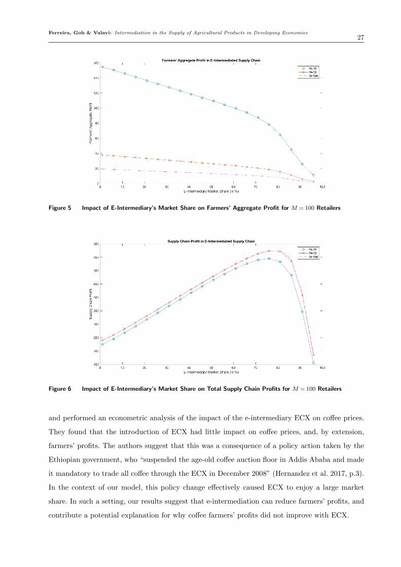
Ferreira, Goh & Valavi: Intermediation in the Supply of Agricultural Products in Developing Economies27
Figure 5 Impact of E-Intermediary’s Market Share on Farmers’ Aggregate Profit for M = 100 Retailers
Figure 6 Impact of E-Intermediary’s Market Share on Total Supply Chain Profits for M = 100 Retailers
and performed an econometric analysis of the impact of the e-intermediary ECX on coffee prices.
They found that the introduction of ECX had little impact on coffee prices, and, by extension,
farmers’ profits. The authors suggest that this was a consequence of a policy action taken by the
Ethiopian government, who “suspended the age-old coffee auction floor in Addis Ababa and made
it mandatory to trade all coffee through the ECX in December 2008” (Hernandez et al. 2017, p.3).
In the context of our model, this policy change effectively caused ECX to enjoy a large market
share. In such a setting, our results suggest that e-intermediation can reduce farmers’ profits, and
contribute a potential explanation for why coffee farmers’ profits did not improve with ECX.
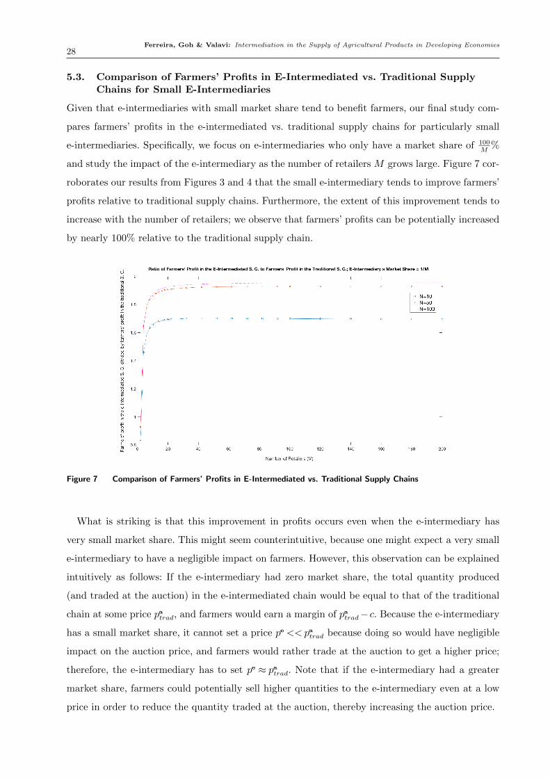
Ferreira, Goh & Valavi: Intermediation in the Supply of Agricultural Products in Developing Economies28
5.3. Comparison of Farmers’ Profits in E-Intermediated vs. Traditional SupplyChains for Small E-Intermediaries
Given that e-intermediaries with small market share tend to benefit farmers, our final study com-
pares farmers’ profits in the e-intermediated vs. traditional supply chains for particularly small
e-intermediaries. Specifically, we focus on e-intermediaries who only have a market share of 100M
%
and study the impact of the e-intermediary as the number of retailers M grows large. Figure 7 cor-
roborates our results from Figures 3 and 4 that the small e-intermediary tends to improve farmers’
profits relative to traditional supply chains. Furthermore, the extent of this improvement tends to
increase with the number of retailers; we observe that farmers’ profits can be potentially increased
by nearly 100% relative to the traditional supply chain.
Figure 7 Comparison of Farmers’ Profits in E-Intermediated vs. Traditional Supply Chains
What is striking is that this improvement in profits occurs even when the e-intermediary has
very small market share. This might seem counterintuitive, because one might expect a very small
e-intermediary to have a negligible impact on farmers. However, this observation can be explained
intuitively as follows: If the e-intermediary had zero market share, the total quantity produced
(and traded at the auction) in the e-intermediated chain would be equal to that of the traditional
chain at some price patrad, and farmers would earn a margin of patrad− c. Because the e-intermediary
has a small market share, it cannot set a price pe << patrad because doing so would have negligible
impact on the auction price, and farmers would rather trade at the auction to get a higher price;
therefore, the e-intermediary has to set pe ≈ patrad. Note that if the e-intermediary had a greater
market share, farmers could potentially sell higher quantities to the e-intermediary even at a low
price in order to reduce the quantity traded at the auction, thereby increasing the auction price.
Ferreira, Goh & Valavi: Intermediation in the Supply of Agricultural Products in Developing Economies29
Essentially, the price offered by the small e-intermediary, pe ≈ patrad, serves as a reserve price on
the auction, and the actual auction price pae−int would be higher. Since the e-intermediary purchases
a negligible amount, the quantity traded at this auction is again similar to the quantity traded
in an auction in a traditional supply chain, where the effective reserve price is c. Therefore, the
farmers’ margins in these two auctions - differing only by their effective reserve price - should
intuitively be similar, such that pae−int− patrad ≈ patrad− c. In other words, farmers’ margins in an e-
intermediated chain with a negligibly small e-intermediary should be roughly twice that of farmers’
margins in the traditional supply chain with no e-intermediary (because pae−int− c≈ 2(patrad− c)).
Since the quantity traded in both these settings is also similar, farmers’ should earn roughly twice
the profits in the e-intermediated chain relative to the traditional chain. This insight parallels
the anecdotal findings from examples summarized in Table 1 that e-intermediation efforts tend to
improve farmers’ profits.
6. Discussion and Conclusion
In our analysis of the traditional supply chain with no e-intermediary, we found that even when the
trade of produce was governed by a highly idealized model of a Walrasian auction, this nonetheless
introduced distorted incentives in the supply chain through a form of variance inflation. This can
be viewed as a manifestation of the bullwhip effect in supply chains (Lee et al. 1997). To the best of
our knowledge, this particular mechanism of generating the bullwhip effect has not been identified
in the literature before.
By analyzing an analogous supply chain with an e-intermediary, we found that e-intermediaries
with a small market share tend to increase farmers’ profits, potentially boosting their profits by a
factor of almost 2, but large e-intermediaries tend to diminish the profits of both farmers and the
supply chain. These results provide a more balanced perspective on the value of e-intermediation,
compared to the generally positive view that is advanced by case studies (see, e.g., references in
the notes of Table 1). One way to interpret this result is that for-profit e-intermediaries who also
aim to improve farmers’ livelihoods cannot blindly operate as pure profit-maximizers and assume
that the market will ensure that farmers benefit. Instead, they should also be conscious of their
social objectives, particularly as they mature and grow.
Finally, from our analyses of both the traditional and e-intermediated supply chains, we observed
that supply fragmentation seems to be the first-order issue that suppresses farmers’ profits. Even
in cases when e-intermediation has beneficial effects on farmers’ profits, it is insufficient to mitigate
the negative effects of supply fragmentation.
The broad implication of these results, viewed collectively, is a more nuanced interpretation of
how such market interventions work. Even with a casual perusal of the popular and academic
literature on developmental economics, one invariably encounters “improving market access” as
Ferreira, Goh & Valavi: Intermediation in the Supply of Agricultural Products in Developing Economies30
one of the mechanisms through which rural farmers improve their livelihood (see, e.g., Qiang et al.
2012, and references therein). Our results, however, suggest that the central issue is not market
“access” per se, but rather market “power”. After all, in our model, farmers in the traditional chain
have access to an idealized, frictionless market, but it is a lack of market power that diminishes
their profits when they are highly fragmented. Similarly, if “access” was the central issue, then
the size of the e-intermediary shouldn’t matter, since farmers have the same amount of “access”
regardless of the size (i.e., market share) of the e-intermediary. However, as the e-intermediary
grows larger, the farmers’ overall market “power” in the chain diminishes, and so do their profits.
In choosing to focus our study on these issues described above, we had to make some trade-offs
in the conception of the model to sacrifice some realism. Below, we describe the main limitations of
our model, in hopes that they can be addressed by future research. First, the two-period nature of
our model was necessary for tractability, but represents an abstraction from reality, where auctions
often take place daily over several weeks. Second, for tractability and in order to focus on broader
supply chain issues, we focus on farmers’ optimal production decisions for a single crop. Although
this is a common simplification adopted by many supply chain papers (e.g., Lee et al. (1997), Taylor
(2002), and Cachon and Lariviere (2005)), we acknowledge that this is nonetheless a simplification
from reality. Third, our model assumes no fixed costs, transaction frictions, or economies of scale
in production, all of which exist in reality. Again, these assumptions were made for tractability.
Finally, our model does not incorporate considerations of crop quality/yield; in practice, this too is
a likely driver of farmers’ profits, which may be affected positively or negatively by intermediation
efforts. Nevertheless, despite these limitations, we believe that our model broadly captures the main
tradeoffs faced by farmers, retailers, and e-intermediaries in such supply chains, and the insights
generated from the model are valuable to key stakeholders in such chains.
References
Akkaya, Duygu, Kostas Bimpikis, Hau Lee. 2016. Agricultural supply chains under government interventions.
Working Paper 3(3).
Alemu, Dawit, Gerdien Meijerink. 2010. The ethiopian commodity exchange (ECX): An overview. Tech.
rep., Wageningen University & Research.
Alizamir, Saed, Foad Iravani, Hamed Mamani. 2015. Price vs. revenue protection: An analysis of government
subsidies in the agriculture industry. Working Paper 3(3).
Anupindi, Ravi, S. Sivakumar. 2007. Supply chain re-engineering in agribusiness: A case study of ITC’s
e-choupal. Hau Lee, Chung-Yee Lee, eds., Building Supply Chain Excellence in Emerging Economies.
Springer, New York.
Arya, Anil, Brian Mittendorf. 2006. Benefits of channel discord in the sale of durable goods. Marketing
Science 25(1) 91–96.
Ferreira, Goh & Valavi: Intermediation in the Supply of Agricultural Products in Developing Economies31
Banciu, Mihai, Prakash Mirchandani. 2013. New results concerning probability distributions with increasing
generalized failure rates. Operations Research 61(4) 925–931.
Cachon, Gerard P, Martin A Lariviere. 2005. Supply chain coordination with revenue-sharing contracts:
strengths and limitations. Management science 51(1) 30–44.
Caldentey, Rene, Gustavo Vulcano. 2007. Online auction and list price revenue management. Management
Science 53(5).
Chagwiza, Clarietta, Roldan Muradian, Ruerd Ruben. 2016. Cooperative membership and dairy performance
among smallholders in ethiopia. Food Policy 59 165–173.
Chen, Ying-Ju, Christopher S Tang. 2015. The economic value of market information for farmers in devel-
oping economies. Production and Operations Management 24(9) 1441–1452.
Cho, Soo-Haeng, Xin Wang. 2017. Newsvendor mergers. Management Science 63(2).
Devalkar, Sripad, Ravi Anupindi, Amitabh Sinha. 2011. Integrated optimization of procurement, processing,
and trade of commodities. Operations Research 59(6) 1369–1381.
Eppen, Gary D. 1979. Note - effects of centralization on expected costs in a multi-location newsboy problem.
Management Science 25(5).
Federgruen, Awi, Upmanu Lall, A. Serdar Simsek. 2015. Supply chain analysis of contract farming. Working
Paper 3(3).
Fischer, Elisabeth, Matin Qaim. 2012. Linking smallholders to markets: determinants and impacts of farmer
collective action in kenya. World Development 40(6) 1255–1268.
Francesconi, Gian Nicola, Nico Heerink. 2010. Ethiopian agricultural cooperatives in an era of global com-
modity exchange: does organisational form matter? Journal of African Economies 20(1) 153–177.
Gabre-Madhin, Eleni. 2012. A market for Abdu: Creating a commodity exchange in Ethiopia. Intl Food
Policy Res Inst.
Gal-Or, Esther. 1991. Vertical restraints with incomplete information. The Journal of Industrial Economics
503–516.
Gilbert, Christopher L, C Wyn Morgan. 2010. Food price volatility. Philosophical Transactions of the Royal
Society of London B: Biological Sciences 365(1554) 3023–3034.
Gordon, Robert D. 1941. Values of mills’ ratio of area to bounding ordinate and of the normal probability
integral for large values of the argument. The Annals of Mathematical Statistics 12(3) 364–366.
Goyal, Aparajita. 2010. Information, direct access to farmers, and rural market performance in central india.
American Economic Journal: Applied Economics 2(3) 22–45.
Graham, Marine, Daria Kaboli, Malini Sridharan, Shireen Taleghani. 2012. Creating value and sustainability
in agricultural supply chains. Doctoral Dissertation Thesis in MIT Sloan School of Management .
Hellin, Jon, Mark Lundy, Madelon Meijer. 2009. Farmer organization, collective action and market access
in meso-america. Food Policy 34(1) 16–22.
Ferreira, Goh & Valavi: Intermediation in the Supply of Agricultural Products in Developing Economies32
Hernandez, Manuel A, Shahidur Rashid, Solomon Lemma, Tadesse Kuma. 2017. Market institutions and
price relationships: The case of coffee in the ethiopian commodity exchange. American Journal of
Agricultural Economics 99(3) 683–704.
Hu, Ming, Yan Liu, Wenbin Wang. 2016. Altruistic rationality: The value of strategic farmers, social en-
trepreneurs and for-profit firms in crop planting decisions. Working Paper 9(7).
Iyer, Ganesh. 1998. Coordinating channels under price and nonprice competition. Marketing Science 17(4)
338–355.
Iyer, Ganesh, Chakravarthi Narasimhan, Rakesh Niraj. 2007. Information and inventory in distribution
channels. Management Science 53(10) 1551–1561.
Jeuland, Abel P, Steven M Shugan. 1983. Managing channel profits. Marketing science 2(3) 239–272.
Joyce, Patrick. 1984. The walrasian tatonnement mechanism and information. The RAND Journal of
Economics 15(3).
Karugu, W. 2010. Kenya agricultural commodity exchange (kace): Linking small scale farmers to national
and regional markets. New York .
Lariviere, Martin A. 2006. A note on probability distributions with increasing generalized failure rates.
Operations Research 54(3) 602–604.
Lee, Hau, Seungjin Whang. 2002. The impact of the secondary market on the supply chain. Management
Science 48(6).
Lee, Hau L, Venkata Padmanabhan, Seungjin Whang. 1997. Information distortion in a supply chain: The
bullwhip effect. Management science 43(4) 546–558.
Morduch, Jonathan. 1999. The microfinance promise. Journal of economic literature 37(4) 1569–1614.
Mukhebi, Adrian. 2004. Kenya agricultural commodity exchange limited (kace). Reaching the Poor in Rural
Kenya with Market Information: A Case Study of a Market Information System 8–12.
Mukhebi, Adrian, James Kundu. 2014. Linking farmers to markets in kenya: The evolving kace model.
Cahiers Agricultures 23(4-5) 282–287.
Pasternack, Barry Alan. 1985. Optimal pricing and return policies for perishable commodities. Marketing
science 4(2) 166–176.
Qiang, Christine Zhenwei, Siou Chew Kuek, Andrew Dymond, Steve Esselaar. 2012. Mobile applications for
agriculture and rural development .
Rapsomanikis, George. 2015. The economic lives of smallholder farmers: An analysis based on household
data from nine countries. Food and Agriculture Organization of the United Nations .
Salimonu, K. K., O.A. Falusi. 2009. Sources of risk and management strategies among food crop farmers in
osun state, nigeria. African Journal of Food, Agriculture, Nutrition and Development 9(7).
Tang, Christopher S, Yulan Wang, Ming Zhao. 2015. The implications of utilizing market information
and adopting agricultural advice for farmers in developing economies. Production and Operations
Management 24(8) 1197–1215.

Ferreira, Goh & Valavi: Intermediation in the Supply of Agricultural Products in Developing Economies33
Tang, Sammi Y, Panos Kouvelis. 2014. Pay-back-revenue-sharing contract in coordinating supply chains
with random yield. Production and Operations Management 23(12) 2089–2102.
Taylor, Terry A. 2002. Supply chain coordination under channel rebates with sales effort effects. Management
science 48(8) 992–1007.
Upton, David, Virginia Fuller. 2004. The ITC echoupal initiative. Harvard Business School Case 9–604–016.
Wegner, Lucia, Gine Zwart. 2011. Who will feed the world? the production challenge. Oxfam Policy and
Practice: Agriculture, Food and Land 11(1) 1–66.
e-companion to Ferreira, Goh & Valavi: Intermediation in the Supply of Agricultural Products in Developing Economies ec1
Electronic Companion
EC.1. Statements and Proofs of Technical Lemmas for Section 4.1
Lemma EC.1. For a given Q > 0, define `N(z) := ψN(z) − (Q − z)ψ′N(z), where ψN(z) is as
defined in (10). It has the following properties:
(a) `N(z) has at most two turning points in [0,Q].
(b) If, for some s∈ (0,Q), `′N(s) = 0 and `′′N(s)≥ 0, then `′N(z)> 0 for all s < z ≤Q.
(c) If, for some s∈ (0,Q), `′N(s) = 0 and `′′N(s)≤ 0, then `′N(z)> 0 for all 0≤ z < s.
(d) If `N(0)< 1, then `′N(0)< 0.
(e) If `N(Q)> 0, then `′N(Q)< 0.
Proof. Fix Q > 0 throughout. We prove part (a) first, and begin with some preliminaries.
Throughout the proof, define µa :=∑m
j=1 µj and σa :=∑m
j=1 σj. Because
dfa (z)
dz=−z−µa
σ2a
fa (z) , (EC.1)
we can rewrite (12) as
Fa (z) +
[(Q− z)
(1 +
1
N− z(z−µa)
Nσ2a
)− z
N
]fa (z) = Fe (Q− z) . (EC.2)
Moreover, after some algebraic manipulations, we may express `′N(z) = (c4(z)− 1)fa (z), where c4
represents a quartic polynomial with a negative leading coefficient, such that the turning points of
`N may be obtained as the roots of the equation c4(z) = 1.
Note that the equation c4(z) = 1 either has 0, 2, or 4 real roots on R. In the first two cases,
(a) holds immediately. Thus, we focus on the final case where c4(z) = 1 has 4 real roots. We will
denote these roots as yj, j = 1, . . . ,4 and assume WLOG that y1 ≤ y2 ≤ y3 ≤ y4. Moreover, it is
straightforward to see that y1, y3 represent local minima of `N and y2, y4 represent local maxima.
Suppose for a contradiction that y1 ≥ 0. From basic properties of polynomials, this implies that
`′N(z)< 0 for all z < y1. Now consider the point, x1, defined as x1 := µa2−√
µ2a4
+ (N + 1)σ2a . Note
that x1 < 0≤ y1. Further, it can be easily verified that x1 is a local maximizer of ψN on R such that
ψ′N(x1) = 0 and ψ′′N(x1) ≤ 0. However, this implies that `′N(x1) = 2ψ′N(x1)− (Q− x1)ψ′′N(x1) ≥ 0,
establishing a contradiction.
Next, suppose for a contradiction that y4 ≤Q. Again, by basic polynomial properties, `′N(z)< 0
for all z > y4. In particular, this implies that `′N(Q) = ψ′N(Q)≤ 0. Using the definition of ψN and
computing its derivative, we obtain that ψ′N(Q)≤ 0 is satisfied when Q≤ µa2
+√
µ2a4
+ (N + 1)σ2a .
Now consider the point, x2, defined as x2 := µa2
+√
µ2a4
+ (N + 1)σ2a . Note that x2 ≥ Q > y4 by
construction, and it can further be verified that x2 is a local minimizer of ψN on R such that
ec2 e-companion to Ferreira, Goh & Valavi: Intermediation in the Supply of Agricultural Products in Developing Economies
ψ′N(x2) = 0 and ψ′′N(x2)≥ 0. Moreover, we have `′N(x2) = 2ψ′N(x2)−(Q−x2)ψ′′N(x2)≥ 0, establishing
a contradiction.
Hence, we have shown that when c4(z) = 1 has 4 roots, it is necessary that y1 < 0 and y4 >Q,
so that `N has at most 2 turning points in [0,Q], thus proving part (a).
To prove (b), suppose that for some s ∈ (0,Q), `′N(s) = 0 and `′′N(s) ≥ 0. Then s is a local
minimum of `N in (0,Q), i.e., s= y3. Suppose for a contradiction that for some s1 > s, `′N(s1)≤ 0.
Then there must exist some local maximum s2 of `N such that y3 < s2 ≤ s1 <Q. However, by part
(a), there is at most one local maximum of `N in (0,Q), y2 < y3, establishing a contradiction.
To prove (c), suppose that for some s ∈ (0,Q), `′N(s) = 0 and `′′N(s) ≤ 0. Then s is a local
maximum of `N in (0,Q), i.e., s= y2. Suppose for a contradiction that for some s1 < s, `′N(s1)≤ 0.
Then there must exist some local minimum s2 of `N such that 0< s2 ≤ s1 < y2. However, by part
(a), there is at most one local minimum of `N in (0,Q), y3 > y2, establishing a contradiction.
To prove (d), suppose that `N(0)< 1. This implies that
Q<NFa (0)
(N + 1)fa (0). (EC.3)
To complete the proof of (d), we use the following well-known bound that was first proven by
Gordon (1941) for the case of the standard normal distribution and adapted to our setting:
fa (z)
Fa (z)≥ z−µa
σ2a
. (EC.4)
Therefore,Fa (0)
fa (0)=Fa (2µa)
fa (2µa)≤ σ2
a
µa
. (EC.5)
By direct computation,
`′N(0) =
[Q(1 + 2
N
)µa
σ2a
− 2
(1 +
1
N
)]fa (0) .
Consider
`′N(0)/fa (0) = Q
(1 +
2
N
)µa
σ2a
− 2
(1 +
1
N
)<
(N + 2)Fa (0)
(N + 1)fa (0)
µa
σ2a
− 2
(1 +
1
N
)[By (EC.3)]
≤(
1 +1
N + 1
)− 2
(1 +
1
N
)[By (EC.5)]
< 0
To prove part (e), note that `N(Q) =ψN(Q), and the result follows from Lemma 2(a). Q.E.D.
Lemma EC.2. For a given Q > 0, define rN(z) := Fe (Q− z) and let `N(z) be as defined in
Lemma EC.1, and zN be as defined in (10). Then,
(a) If `N(0)≤ rN(0), then `N(z)≤ rN(z) for all z ∈ [0,Q].
e-companion to Ferreira, Goh & Valavi: Intermediation in the Supply of Agricultural Products in Developing Economies ec3
(b) If `N(Q)≥ rN(Q), then `N(z)≥ rN(z) for all z ∈ [0,Q].
(c) If `N(0)> rN(0) and `N(Q)< rN(Q), then there exists a unique value of z := z(Q)∈ (0,Q) such
that `N(z) = rN(z).
(d) Consider the optimization problem maxz∈[0,zN∧Q] g(z), such that g′(z) = `N(z)− rN(z). Then,
ζN(Q), as defined in (11), is optimal for this problem.
Proof. To prove (a), suppose that `N(0) ≤ rN(0). Suppose for a contradiction that for some
s ∈ [0,Q], `N(s) > rN(s). Thus, `N(0) ≤ rN(0) ≤ rN(s) < `N(s). Moreover, since rN(0) < 1,
Lemma EC.1(d) implies that `′N(0) < 0. Together, these imply that there exists some s1 ∈ (0, s)
such that s1 is a local minimum of `N . By Lemma EC.1(b), `′N(z) > 0 on (s1,Q]. This implies
that `N(Q) ≥ `N(s) > rN(0) > 0. By Lemma EC.1(e), this implies that `′N(Q) < 0, establishing a
contradiction. Therefore, `N(z)≤ rN(z) for all z ∈ [0,Q].
To prove (b), suppose that `N(Q)≥ rN(Q). Suppose for a contradiction that there exists some
s∈ [0,Q] such that `N(s)< rN(s). Thus, `N(Q)≥ rN(Q)≥ rN(s)> `N(s). Moreover, since rN(Q)>
0, Lemma EC.1(e) implies that `′N(Q) < 0. Together, these imply that there must exist some
s1 ∈ (s,Q) such that s1 is a local maximum of `N . By Lemma EC.1(c), `′N(z)> 0 on [0, s1), and
in particular, `N(0)≤ `N(s)< rN(s)< 1. However, by Lemma EC.1(d), this implies that `′N(0)< 0,
establishing a contradiction. Therefore, in this case, `N(z)≥ rN(z) for all z ∈ [0,Q].
To prove (c), suppose that `N(0)> rN(0) and `N(Q)< rN(Q). Hence, there is some z∗ ∈ (0,Q)
for which `N(z∗) = rN(z∗). We claim that in order to show that this z∗ is unique, it suffices to show
that there is some z∗∗ ≤ z∗ for which `′N(z∗∗)< 0. Suppose that this were true, and now suppose
for a contradiction that there is some other s > z∗ (WLOG) such that `N(s) = rN(s). Then, since
rN is strictly increasing, we must have `N(s) = rN(s)> rN(z∗) = `N(z∗). Since `′N(z∗∗)< 0, there
must exist some s1 ∈ (z∗∗, s) that is a local minimum of `N . By Lemma EC.1(b), this implies that
`′N(z)> 0 on (s1,Q]. In particular, this means that `′N(Q)> 0, and furthermore, `N(Q)≥ `N(s) =
rN(s) > 0. By Lemma EC.1(e), `N(Q) > 0 implies that `′N(Q) < 0, establishing a contradiction.
Hence, z∗ must be unique.
It remains to show the existence of such a point z∗∗. We consider two separate cases:
Case 1: `′N(0)< 0. Here, we can choose z∗∗ = 0.
Case 2: `′N(0) ≥ 0. We need only consider the sub-case in which `N(0) ≥ 1 since the converse
sub-case is ruled out by Lemma EC.1(d). Since `N(0)≥ 1> rN(Q)> `N(Q), there must exist some
y2 ∈ [0,Q) that is a local maximum of `N . Moreover, z∗ > y2, since `N(z)≥ 1> rN(z) for all z ≤ y2.
Hence, any point z∗∗ ∈ (y2, z∗) would satisfy z∗∗ < z∗ and `′N(z∗∗)< 0, as required.
The proof of part (d) proceeds by direct verification using parts (a)-(c). In the case where
ψN(0)−Qψ′N(0)≤ Fe (Q), part (a) implies that g is decreasing over [0,Q], and is thus maximized
at z = 0. An identical logic applies for the case of ψN(Q) ≥ Fe (0) using part (b) and is omitted
ec4 e-companion to Ferreira, Goh & Valavi: Intermediation in the Supply of Agricultural Products in Developing Economies
for brevity. In the case where ψN(0)−Qψ′N(0)> Fe (Q) and ψN(Q)< Fe (0), part (c) guarantees
that a solution zN(Q) to (12) on (0,Q) exists, and moreover that g is increasing on (0, zN(Q))
and decreasing on (zN(Q),Q). Thus, if zN < zN(Q), zN maximizes g on [0, zN ∧ Q], whereas if
zN ≥ zN(Q), then zN maximizes g on [0, zN ∧Q], as specified by the definition of ζN given in (11).
Q.E.D.
EC.2. Proofs of Main ResultsProof of Lemma 1
Proof. Combining the two conditions from Definition 1, and the retailers’ demand functions from
(1), the auction price pa satisfies
m∑j=1
(µj + Φ−1
(π− pa
π
)σj
)= qa.
Re-arranging, this gives us pa = π(
1−Φ(qa−
∑mj=1 µj∑m
j=1 σj
))= πFa (qa) . Q.E.D.
Proof of Lemma 2
Proof. To prove (a), define h(z) := f(z)/F (z). Noting that we may write Ls,ν(z) =
F (z+ s) [1− νzh(z+ s)], for any z ∈Ls,ν , we have
L′s,ν(z) =−f(z+ s) [1− νzh(z+ s)] + νF (z+ s) [−h(z+ s)− zh′(z+ s)] .
In the display above, 1−νzh(z+s)≥ 0 since z ∈Ls,ν . Also, h(z+s)> 0 and zh′(z+s)≥ 0 because
z ≥ 0 and h′(z+s)> 0 by the IFR property of the normal distribution (Lariviere 2006, Banciu and
Mirchandani 2013). Hence, L′s,ν(z)< 0 for all z ∈Ls,ν .
To prove (b), note that Ls,ν 6= ∅ since F (s)> 0, i.e., 0 ∈ Ls,ν trivially. Moreover, from part (a),
since Ls,ν(z) is strictly decreasing where it is positive, it follows that Ls,ν = [0, z∗s,ν ] for some z∗s,ν ,
where z∗s,ν is potentially infinite. We conclude the proof by showing that z∗s,ν is finite. To see this,
note that the condition Ls,ν(z) = 0 is equivalent to νh(z + s) = 1/z. It is well known (see, e.g.,
Gordon 1941) that h(z+s)→∞ as z→∞, and since 1/z→ 0 as z→∞, there exists some z∗s,ν <∞
for which h(z∗s,ν + s) = 1/z∗s,ν . Moreover, since h(z+ s) is strictly increasing in z and 1/z is strictly
decreasing in z, z∗s,ν is unique. Q.E.D.
Proof of Proposition 1
Proof. First, we show that (3) has a unique solution on R+. By Assumption 1, the LHS of (3)
exceeds the RHS at z = 0. Moreover, by Lemma 2 (for the case s = 0 and ν = 1/N), the LHS
eventually crosses zero as z→∞. By the same Lemma, in the region where the LHS is positive, it
is strictly decreasing. Hence, (3) has a unique solution on R+.
e-companion to Ferreira, Goh & Valavi: Intermediation in the Supply of Agricultural Products in Developing Economies ec5
To prove the result, let (q, qa(·)) be arbitrary. We will use the specification of a symmetric
equilibrium from Definition 2 to find necessary conditions on these quantities. Observe that each
farmer’s problem can be equivalently written as a single optimization problem
maxq≥0,0≤qa≤q
{−cq+πqaFa (qa + (N − 1)qa(q))
}.
We observe that the objective of this problem is decreasing in q, which implies that a necessary
condition for optimality is q = qa. From this condition, and writing qa = qa(q) for brevity, the
problem above simplifies to
maxqa≥0
{−cqa +πqaFa (qa + (N − 1)qa)
}(EC.6)
The derivative of the objective of (EC.6) at an arbitrary point qa ≥ 0 may be expressed as g(qa)−c,
where
g(qa) := πFa (qa + (N − 1)qa)−πqafa (qa + (N − 1)qa) . (EC.7)
We note that by Lemma 2(a), g(qa) is strictly decreasing in the region where g(qa)≥ 0. Since c > 0,
this implies that there exists a unique value of qa such that g(qa) = c, and moreover, this choice of
qa maximizes the objective of (EC.6).
By Definition 2, for qa to be an equilibrium, each farmer choosing qa = qa has to be a best
response. First, we note that qa = 0 cannot hold in equilibrium, because (EC.7) gives πFa (0)−c > 0
by Assumption 1, implying that any given farmer would have higher profits by deviating and
choosing some small qa > 0. Therefore, for qa to represent an equilibrium, it is necessary that g(qa) =
c. Changing variables such that qa = 1NQTN yields (3) as required. Uniqueness of the equilibrium
follows from the fact that (3) has a unique solution.
From this, each farmer’s profit, ΠTN , is given by ΠT
N =QT
NN
(πFa (QT
N)− c)
= π(QT
NN
)2
fa (QTN),
where the last equation is by (3). Q.E.D.
Proof of Proposition 2
Proof. Fix some N . Rewrite (3) as
1 =c
πFa (z)+
zfa (z)
NFa (z)(EC.8)
Suppose for a contradiction that QTN > QT
N+1. For notational convenience, define the functions
g,h : R+→ R as g(z) := cπFa(z)
and h(z) := zfa(z)
Fa(z). Note that g,h are strictly increasing functions;
the latter is a consequence of the IGFR property of normal distributions (Lariviere 2006, Banciu
and Mirchandani 2013). Now, (EC.8) implies that we must have
g(QTN) +
1
Nh(QT
N) = g(QTN+1) +
1
N + 1h(QT
N+1). (EC.9)
However, by our assumption that QTN > QT
N+1, we have g(QTN) > g(QT
N+1), and 1Nh(QT
N) >
1Nh(QT
N+1)> 1N+1
h(QTN+1). Together, these imply that (EC.9) cannot be satisfied, establishing the
contradiction. Q.E.D.
ec6 e-companion to Ferreira, Goh & Valavi: Intermediation in the Supply of Agricultural Products in Developing Economies
Proof of Proposition 3
Proof. This follows from (3) by observing that the function zfa (z) is bounded over all z ∈R and
by taking N →∞. Q.E.D.
Proof of Proposition 5
Proof. Consider the difference:
∆ := QT∞−QI
= Φ−1
(π− cπ
) M∑j=1
σj −
√√√√ M∑j=1
σ2j
[From (4), (5)].
First note that∑M
j=1 σj ≥√∑M
j=1 σ2j . Hence, if c < π/2, we have Φ−1
(π−cπ
)> 0, and the difference
∆≥ 0. By a similar argument, the converse result holds for c > π/2, and ∆ = 0 for c= π/2. Q.E.D.
Proof of Theorem 1
Proof. To prove parts (a) and (b), note that term (i) in (6), which represents the total farmers’
profits, decreases in Q. By Proposition 2, as N increases, in equilibrium, the total production
quantity increases, which implies that the total farmer surplus decreases. Conversely, term (ii) in
(6), which represents the total retailers’ profits, increases in Q, and by an analogous argument,
now increases as N increases.
To prove part (c), first recall that the total profit loss due to retailer fragmentation is quantified in
term (iii) of decomposition (6), and suppose that c < π/2 and fix some Q. Let FI (·) represent the tail
cdf of the integrated supply chain’s total retailer demand distribution, i.e., N(∑M
j=1 µj,∑M
j=1 σ2j
).
The derivative of term (iii) is
πFI (Q)−πM∑j=1
Fj (Qj) = πFI (Q)−πM∑j=1
Fa (Q) [Definition 1, Lemma 1]
= πFI (Q)−MπFa (Q) .
We aim to show that this expression is negative at Q = QT∞. To do so, it suffices to show that
FI (QT∞)≤ Fa (QT
∞). To this end, note that
FI (QT∞) ≤ FI (QI) [Proposition 5 and FI (·) is decreasing]
=c
π[From (5)]
= Fa (QT∞) , [From (4)]
which concludes the proof of part (c).
To prove part (d), suppose that c > π/2, and fix an arbitrary N . Note that we have
QTN ≤QT
N+1 ≤QT∞ ≤QI,
e-companion to Ferreira, Goh & Valavi: Intermediation in the Supply of Agricultural Products in Developing Economies ec7
where the last inequality above is by Proposition 5 when c > π/2 and the other inequalities are
by Proposition 2. Since ΠI(Q) is concave, it is increasing for every Q≤QI, which therefore implies
that ΠI(QTN)<ΠI(QT
N+1), concluding the proof. Q.E.D.
Proof of Theorem 2
We characterize the equilibria of this game by backward induction. First, we will characterize each
farmer’s actions in period 2 under a symmetric equilibrium. We do so by solving problem (7) for
fixed values of q and p and finding conditions on qa as a function of q, p such that farmers optimally
choose qa in a symmetric equilibrium. Note that in (7), for any q, p≥ 0, the objective is increasing
in qe, which implies that at optimality, we necessarily have qa + qe = q. This means that we can
eliminate qe in (7), and write the optimization problem equivalently as
Π(q, p) := pq+ maxqa
{−pqa +πqaFa (qa + (N − 1)qa(q, p))
}s.t. 0≤ qa ≤ q. (EC.10)
Following a similar analysis to Proposition 1, it follows that a necessary and sufficient condition
for qa(q, p) to be an equilibrium is that it satisfies
qa(q, p) :=
{0 if p≥ πFa (0)za(p)
N∧ q if p < πFa (0)
(EC.11)
where in the latter case za(p) represents the unique value of z ∈R+ that solves
Fa (z)− zfa (z)
N=p
π. (EC.12)
Therefore, in equilibrium, the second-stage profit of each farmer may be written as
Π(q, p) = pq+
(za(p)∧Nq
N
)(πFa (za(p)∧Nq)− p
). (EC.13)
We note that Lemma 2 implies that za(p) is strictly decreasing for p∈ (0, πFa (0)), and therefore
possesses an inverse. In particular, recalling the definition of zN from (10), we have z−1a (z) = πψN(z)
for all z ∈ [0, zN ].
Next, we solve the e-intermediary’s pricing problem, i.e., problem (8). Fix q ≥ 0, and define
Q = Nq for notational brevity. We now claim that if ψN(Q) ≥ 0, then it is without loss that
p≥ πψN(Q). Consider any p such that 0≤ p≤ πψN(Q). Then, for such a choice of p, by (EC.12)
and (10), we would have za(p)<Nq=Q, so that from (EC.11), we get Nqa(q, p) =Q, and therefore
Nqe(q, p) = Q −Nqa(q, p) = 0. Thus the objective of (8) at this point would be πE (De ∧ 0) for
any such p. In particular, at the boundary point, p = πψN(Q) has the same objective value of
πE (De ∧ 0). Therefore, it is without loss that p ≥ πψN(Q). By a similar logic, it is without loss
that p≤ πFa (0).
ec8 e-companion to Ferreira, Goh & Valavi: Intermediation in the Supply of Agricultural Products in Developing Economies
Now, for p such that max{πψN(Q),0} ≤ p≤ πFa (0), we may simplify (EC.11) to get
Nqa(q, p) = za(p) and Nqe(q, p) =Q− za(p). (EC.14)
Therefore, after dividing (8) by the constant π, we get
maxp≥0
{E (De ∧Nqe(q, p))− p
πNqe(q, p)
}= max
max{πψN (Q),0}≤p≤πFa(0)
{E (De ∧Nqe(q, p))− p
πNqe(q, p)
}[No loss of optimality in restriction]
= maxmax{πψN (Q),0}≤p≤πFa(0)
{E (De ∧ (Q− za(p)))− p
π(Q− za(p))
}[By (EC.14)]
= max0≤za(p)≤min{zN ,Q}
{E (De ∧ (Q− za(p)))−ψN(za(p))(Q− za(p))} [Change of optimization variable]
= max0≤z≤min{zN ,Q}
{E (De ∧ (Q− z))−ψN(z)(Q− z)} [Eliminate variable p]
Note that in the third equality, we have used the fact that πψN(za(p)) = p for any feasible p.
We also note that the final form of the optimization problem above can be verified to satisfy
the conditions of Lemma EC.2(d), and hence its optimal solution is given by ζN(Q) as defined in
(11). The e-intermediary’s optimal pricing policy is obtained by transforming the optimal value of
ζN(Q), and is expressed as pe(Q) = πψN(ζN(Q)). Furthermore, substituting this into (EC.14), we
obtain
Nqa(q, pe(Q)) = za(pe(Q)) = za(πψN(ζN(Q))) = ζN(Q), (EC.15)
which represents the quantity traded at the auction when the e-intermediary prices optimally.
Finally, we will show that problem (13) represents a given farmer’s first-stage problem of choosing
his own production quantity, q, given the symmetric production quantities q of each of the N − 1
other farmers (i.e., total production quantity is Q= q+ (N −1)q), taking into account the optimal
pricing from the e-intermediary and equilibrium decisions from all farmers in the second stage.
Using the derived expression for each farmer’s second-stage profit in (EC.13), substitute this into
(9), and also substitute the optimal pricing function of the e-intermediary, pe(Q) = πψN(ζN(Q))
and equilibrium quantity at the auction (EC.15), so that (9) simplifies to
maxq,Q
(ψN(ζN(Q))− c
π
)q+
ζN(Q)
N
(Fa (ζN(Q))−ψN(ζN(Q))
)s.t. Q= q+ (N − 1)q
Q, q≥ 0.
Using (10) to simplify the expression above, adding the auxiliary variable z = ζN(Q) and eliminating
the auxiliary variable Q yields (13).
Therefore, if supposing (z∗, q∗) is optimal in (13) such that q∗ = q, then, Nq represents the
(symmetric) equilibrium total production of all farmers, giving us part (a). From (EC.15), the
total quantity sent to the auction is ζN(Nq) and the total quantity sent to the e-intermediary is
Nq−ζN(Nq), giving us parts (b) and (c). Finally, from the optimal e-intermediary’s pricing policy,
the e-intermediary’s equilibrium price is pe = πψN(ζN(Nq)), establishing part (d). Q.E.D.
e-companion to Ferreira, Goh & Valavi: Intermediation in the Supply of Agricultural Products in Developing Economies ec9
Proof of Corollary 2
Proof. To prove (a), suppose for a contradiction that in equilibrium, each farmer sends some
qa to the auction such that the equilibrium auction price is πFa (Nqa) < pe. If qa > 0, then any
given farmer would increase his profit by reducing qa by some ε > 0 and sending this ε to the
e-intermediary. If qa = 0, since the objective of (8) is decreasing in p, then the e-intermediary can
increase his profit by deviating and reducing pe by some small amount. Therefore, πFa (Nqa)≥ pe
is necessary in equilibrium.
To prove (b), suppose for a contradiction that in equilibrium, pe < c. If qe > 0, then any farmer
i can increase his profit by simultaneously reducing both qe and q by some small ε > 0. Q.E.D.
Proof of Proposition 6
Proof. Throughout, we subscripted N to explicitly denote the dependence of various equilibrium
quantities on N . For example, we will use peN to denote the equilibrium price offered by the e-
intermediary.
We begin by proving part (a). To do so, let qN represent the equilibrium production of each
farmer as a function of N . We will first assert that
limsupN→∞
NqN <∞. (EC.16)
Suppose for a contradiction that limsupN→∞NqN =∞. We note that from Corollary 2(b), we
necessarily have limsupN→∞NqeN <∞, since either qeN = 0 or peN ≥ c > 0, and in the latter case,
the e-intermediary would make negative profit for large N . Since each farmer’s production is fully
allocated either to the e-intermediary or the auction, it is necessary that lim supN→∞NqaN =∞.
Therefore, this implies that there exists large enough N , such that the equilibrium auction price,
πFa (NqaN)< c, contradicting Corollary 2(a).
We now proceed to prove (a), that is, we claim that limN→∞ peN = c. We do so in two steps. First,
we will prove that each farmer’s equilibrium profit converges to zero. By (EC.16), we necessarily
have qN → 0. Thus, for any ε > 0, there exists large enough N such that qN < ε. Since the objective
of the optimization problem in (EC.10) is bounded above by πq, this implies that each farmer’s
equilibrium profit is bounded above by (peN − c)ε + πε for sufficiently large N . If qeN > 0, since
peN ≥ c (by Corollary 2) and peN ≤ π (obvious), and since ε is arbitrary, this means that each
farmer’s equilibrium profit converges to zero as N →∞. If qeN = 0, each farmer’s equilibrium profit
is bounded above by πε for sufficiently large N , and since ε is arbitrary, this means that each
farmer’s equilibrium profit converges to zero as N →∞.
Second, suppose for a contradiction that limsupN→∞ peN > c. Because qa = 0 is feasible in (EC.10),
each farmer’s profit is bounded from below by (peN − c)qN . Now we claim that we can establish a
profitable deviation for any given farmer, for sufficiently large N , by violating (EC.16), thereby
ec10 e-companion to Ferreira, Goh & Valavi: Intermediation in the Supply of Agricultural Products in Developing Economies
establishing a contradiction. To see this, note that there must exist a subsequence Nj such that
infj peNj> c, and define δ := infj
{peNj− c}> 0. By choosing qNj
= 1 for all Nj, each farmer’s profit
is bounded from below by δ along this entire subsequence, contradicting the assertion that each
farmer’s profit converges to zero. Therefore, part (a) must hold.
Part (b) uses the equilibrium auction price in Lemma 1 and follows from (a) and (EC.12), noting
that zfa (z) is bounded on R.
To prove (c), first define define gN :R+→R as follows:
gN(y) :=ψN(Qa∞)− yψ′N(Qa
∞)− Fe (y) .
Suppose that for a given N , a given y satisfies gN(y) = 0. Then, by (11) and (12), y is the quantity
that is sent to the e-intermediary when Qa∞ is sent to the auction when there are N farmers.
Since we know that Qa∞ is sent to the auction in the limit as N →∞, if some given Qe
∞ satisfies
limN→∞ gN(Qe∞) = 0, then Qe
∞ would represent the limiting quantity sent to the e-intermediary.
In what follows, we show that the condition limN→∞ gN(Qe∞) = 0 can be simplified to (14). For any
z ≥ 0, using the definition of ψN , we obtain limN→∞ψN(z) = Fa (z) and limN→∞ψ′N(z) =−fa (z),
such that for any y≥ 0,
limN→∞
gN(y) = Fa (Qa∞) + yfa (Qa
∞)− Fe (y) =c
π+ yfa (Qa
∞)− Fe (y) .
Hence, Qe∞ that satisfies limN→∞ gN(Qe
∞) = 0 will satisfy (14) and vice-versa.
It remains to show that (14) has a unique solution. Note that at z = 0, the LHS of (14) is
Fe (0) > c/π by Assumption 1. Moreover, as z → +∞, the LHS is strictly decreasing in z and
diverges to −∞. Hence, a unique solution to (14) exists, completing the proof. Q.E.D.
Proof of Proposition 7
Proof. We begin with several preliminaries. First, for notational brevity, throughout the proof, we
will let K := Φ−1(π−cπ
). Note that K can be positive or negative depending on whether c < π/2 or
otherwise. Second, from (14), it is easy to see that Qe∞ ≤Qe
∗, where we define µe :=∑M
j=m+1 µj, and
Qe∗ := µe +Kσe. Third, by direct computation, it is easy to see that Fe (Q) is concave for Q< µe
and convex for Q > µe. Finally, by the triangle inequality and respective definitions of σI, σa, σe,
and σT, we have, for any m= 1, . . . ,M ,
σI ≤ σa +σe ≤ σT. (EC.17)
We now prove the first part of the proposition. Suppose that c < π/2, i.e., K > 0. Then, we claim
that we necessarily have
µe ≤Qe∗
σa
σe +σa
. (EC.18)
e-companion to Ferreira, Goh & Valavi: Intermediation in the Supply of Agricultural Products in Developing Economies ec11
This is because
Qe∗
σa
σe +σa
−µe =σe
σe +σa
(Kσa−µe)≥ 0,
where the final inequality is because K > 0 and because (15) implies that µe ≤Kσa. Now, since
K > 0, we have Qe∗ > µe by definition. Hence, using a Taylor expansion for Fe (Q) in the region
µe <Q<Qe∗, we obtain
Fe (Q)−Qfa (Qa∞)≥ Fe (Qe
∗)− (Q−Qe∗)fe (Qe
∗)−Qfa (Qa∞) .
The inequality is a consequence of the convexity of Fe (Q) on Q > µe. From this inequality, the
value of Q that sets the RHS of the above inequality to c/π must therefore bound Qe∞ from below,
that is,
Qe∞ ≥Qe
∗fe (Qe
∗)
fe (Qe∗) + fa (Qa
∞)=Qe
∗σa
σe +σa
, (EC.19)
where the final equality is by direct computation using the definitions of Qe∗ and Qa
∞. Therefore,
QE∞−QI ≥ Qe
∗σa
σe +σa
−µe +K (σa−σI) [By (EC.19)]
= −µe
σe
σa +σe
+K
(σeσa
σe +σa
+σa−σI
)[By definition of Qe
∗]
≥ 0 [By (15)],
thus proving the lower bound on QE∞. To prove the upper bound, consider
QE∞−QT
∞ ≤ Qa∞+Qe
∗−QT∞ [Because Qe
∞ ≤Qe∗]
= K (σa +σe−σT)
≤ 0. [By (EC.17)]
To prove the second part of the proposition, suppose that c > π/2, i.e., K < 0. In this case, we
have Qe∗ <µe. Using a Taylor expansion for Fe (Q) in the region Qe
∗ <Q<µe, we obtain
Fe (Q)−Qfa (Qa∞)≤ Fe (Qe
∗)− (Q−Qe∗)fe (Qe
∗)−Qfa (Qa∞) ,
The inequality is a consequence of the concavity of Fe (Q) on Q < µe. From this inequality, the
value of Q that sets the RHS of the above inequality to c/π must therefore bound Qe∞ from above,
that is,
Qe∞ ≤Qe
∗fe (Qe
∗)
fe (Qe∗) + fa (Qa
∞)=Qe
∗σa
σe +σa
. (EC.20)
Hence,
QE∞−QT
∞ ≤ Qe∗
σa
σe +σa
−µe +K (σa−σT) [From (EC.20)]
= −µe
σe
σa +σe
+K
(σeσa
σe +σa
+σa−σT
)[Definition of Qe
∗]
≤ 0. [By (16)]
This completes the proof because QT∞ ≤QI has already been established in Proposition 5. Q.E.D.