Internal data, external data and consortium data for

operational risk measurement: How to pool data properly? ∗

Nicolas Baud, Antoine Frachot and Thierry Roncalli

Groupe de Recherche Operationnelle, Credit Lyonnais, France†

This version: June 01, 2002

Abstract

It is widely recognized that calibration on internal data may not suffice for computing anaccurate capital charge against operational risk. However, pooling external and internal data leadto unacceptable capital charges as external data are generally skewed toward large losses. In aprevious paper, we have developped a statistical methodology to ensure that merging both internaland external data leads to unbiased estimates of the loss distribution. This paper shows that thismethodology is applicable in real-life risk management and that it permits to pool internal andexternal data together in an appropriate way. The paper is organized as follows. We first discusshow external databases are designed and how their design may result in statistical flaws. Then wedevelop a model for the data generating process which underlies external data. In this model, thebias comes simply from the fact that external data are truncated above a specific threshold whilethis threshold may be either constant but known, or constant but unknown, or finally stochastic.We describe the rationale behind these three cases and we provide for each of them a methodologyto circumvent the related bias. In each case, numerical simulations and practical evidences aregiven. In the coming weeks, we also plan to release an Excel-based, user-friendly package in orderto pool internal and external data while avoiding over-estimation of the capital charge.

The present document reflects the methodologies, calculations, analyses andopinions of their authors and is transmitted in a strictly informative aim. Underno circumstances will the above-mentioned authors nor the Credit Lyonnaisbe liable for any lost profit, lost opportunity or any indirect, consequential,incidental or exemplary damages arising out of any use or misinterpretation ofthe present document’s content, regardless of whether the Credit Lyonnais hasbeen apprised of the likelihood of such damages.

Le present document reflete les methodologies, calculs, analyses et positions deleurs auteurs. Il est communique a titre purement informatif. En aucun casles auteurs sus-mentionnes ou le Credit Lyonnais ne pourront etre tenus pourresponsables de toute perte de profit ou d’opportunite, de toute consequence di-recte ou indirecte, ainsi que de tous dommages et interets collateraux ou exem-plaires decoulant de l’utilisation ou d’une mauvaise interpretation du contenude ce document, que le Credit Lyonnais ait ete informe ou non de l’eventualitede telles consequences.

∗We gratefully thank Maxime Pennequin, Fabienne Bieber, Catherine Duchamp and Nathalie Menkes, all of Opera-tional Risk team at Credit Lyonnais, for providing us with all the necessary informations and for stimulating discussions.We wish to thank Professor Santiago Carillo Menendez and the participants at the workshop Seminarios de MatematicaFinanciera, Instituto MEFF-RiskLab, Madrid for comments and suggestions.

†Address: Credit Lyonnais – GRO, Immeuble ZEUS, 4e etage, 90 quai de Bercy — 75613 Paris Cedex 12 — France;E-mail: nicolas.baud@creditlyonnais.fr, antoine.frachot@creditlyonnais.fr, thierry.roncalli@creditlyonnais.fr.

1

1 Introduction

According to the last proposal [1] by the Basel Committee on Banking Supervision, banks are allowedto use the Advanced Measurement Approaches (AMA) option for the computation of their capitalcharge covering operational risks (OR). Among these methods, the Loss Distribution Approach (LDA)is probably the most sophisticated one1. It is also expected to be the most risk sensitive as long asinternal data are used in the calibration process and LDA is thus supposed to be more closely relatedto the actual riskiness of each bank.

However it is now widely recognized that calibration on internal data only may not suffice toprovide accurate capital charge, especially for high severity/low frequency events. In other words,internal data should be supplemented with external data in order to improve the accuracy of capitalmeasurement. This is all the more important that high severity/low frequency events are the risktypes which contribute the most to OR capital charge (Baud, Frachot and Roncalli [2002]).Unfortunately mixing internal and external data together is likely to provide unacceptable results asexternal data are strongly biased toward extreme losses. This bias comes from the fact that externaldatabases only record the highest losses, i.e. the losses which are publicly released. Without anyrigorous statistical treatment, the estimated loss distribution is biased toward high losses and theresulting capital requirement is thus dramatically over-estimated.

As a result rigorous statistical treatments are required to make internal and external data com-parable and to ensure that merging both databases leads to unbiased estimates. A description of thestatistical treatment has been developped in a previous paper [4] (Frachot and Roncalli [2002]),at least from a theoretical point of view. The goal of our paper is to propose a practical, real-lifemethodology to pool internal and external data together in an appropriate way.

The paper is organized as follows. We first discuss how external databases are designed and howtheir design may result in statistical flaws. Then we develop a model for the data generating processwhich underlies external data. In this model, the bias simply comes from the fact that external dataare truncated above a specific threshold which may be either constant and known, or constant butunknown, or finally stochastic. We describe the rationale behind these three cases and for each ofthem we give a statistical method to circumvent the related bias. In each case, numerical simulationsand practical evidences are given.

2 Modelling external database bias

2.1 External databases

In this section, we discuss how external databases are built, which is a good starting point for assessingto what extent external databases are biased. Two types of external databases are encountered inpractice.

• The first type corresponds to databases which record publicly-released losses. In short thesedatabases are made up of losses that are far too important or emblematic to be concealed awayfrom public eyes. The first version of OpVar R© Database pioneered by PwC is a typical exampleof these first-generation external databases.

• More recent is the development of databases based on a consortium of banks. It works as anagreement among a set of banks which commit to feed a database with their own internal losses,provided that some confidentiality principles are respected. In return banks which are involvedin the project are of course allowed to use these data to supplement their own internal data.Gold of BBA (British Bankers’ Association) is an example of consortium-based data.

1see Frachot, Georges and Roncalli [2001] for an extensive presentation of this method.

2

Remark 1 The project ORX (Operational Riskdata eXchange) managed by OpVantage (administra-tive agent) and PwC Switzerland (custodian) is another example. In this case, “Participants2 deliverspecified data that meets quality assurance standards. Custodian anonymise data, clean and scale asrequired. Administrator consolidates data, performs required analysis, provides reports. Custodian[then] provides standard reports to firms after rescaling or other manipulations. Participating firms[finally] receive back data based upon the business lines and/or locations and/or events for which theyprovided data” (Peemoller [2002]).

The two types of database differ by the way losses are supposed to be truncated. In the firstcase, as only publicly-released losses are recorded, the truncation threshold is expected to be muchhigher than in the consortium-based data. For example, the OpVar R© Database declares to recordlosses greater than USD 1 million while consortium-based data pretend to record all losses greaterthan USD 25.000 for ORX database (or USD 10.000 by 2003 (Peemoller [2002])).

Furthermore public databases, as we name the firt type of external databases, and consortium-based databases differ not only by the stated threshold but also by the level of confidence one can placeon it. For example, nothing ensures that the threshold declared by a consortium-based database is theactual threshold as banks are not necessarily able to uncover all losses above this threshold even thoughthey pretend to be so3. Rather one may suspect that banks target this threshold although they do nothave always the ability to meet this requirement yet. We shall see in the next subsection how the lastremark implies a specific statistical modelling in the sense that stated threshold of consortium-baseddatabases should be considered as stochastic.

2.2 Modelling assumptions

For ease of notations, we shall consider one particular business line and one loss type. Internal losseswill be denoted by (ζi)i=1,... ,n where n is the number of recorded internal losses. In the same spirit,(ζ?

i )i=1,... ,n? represent external losses4. Let F (ζ; θ) be the parametric loss severity distribution whichinternal data are assumed to be drawn from. θ is therefore a set of parameters to be estimated. Wedenote θ0 the (unknown) true set of parameters.

We do not intend to discuss whether losses are best captured by the set of probability distributionsF (ζ; θ). Rather we shall assume that we know the true family of distributions F and that we onlyneed to uncover (estimate) the true parameter θ0. Considering for example the lognormal distributionset LN (ζ; µ, σ), think of θ = (µ, σ) as a two-dimensional parameter, i.e. the (theoretical) expectedand standard deviation of the logarithm of losses. Finally we shall denote θ an estimator of θ.

Pooling internal and external data together to improve the estimation process makes sense as longas the following assumption holds:

Assumption 1 (Fair Mixing Assumption) External data are supposed to be drawn from the samedistribution F (ζ; θ0) as internal data except that the recorded (external) data are truncated above athreshold H.

Under this assumption, external data may be viewed as “implicit internal data”, meaning that externaland internal data can be pooled together provided external data have been made comparable withinternal data. Under this condition, we could supplement internal data with these scaled externaldata in order to obtain a database with a greater number of observations. Since the accuracy of theestimators increases along with the total number of observations, one expects to estimate the lossdistribution more accurately with a pool of both internal and external data.

2The first members are (or might be) Deutsche Bank, JP Morgan Chase, ABN-AMRO, Bayerische Landesbank,BNP-Paribas, Commerzbank, Euroclear, Danske Bank, Fortis bank, HypoVereinsbank, ING and Sanpaolo IMI.

3The ORX project seems more ambitious and proposes reporting control and verification. In particular, the financialinstitution must demonstrable its capability to collect and to deliver data if it wants to be a member of the ORXconsortium.

4The superscript ? always refers to external data-based concepts.

3

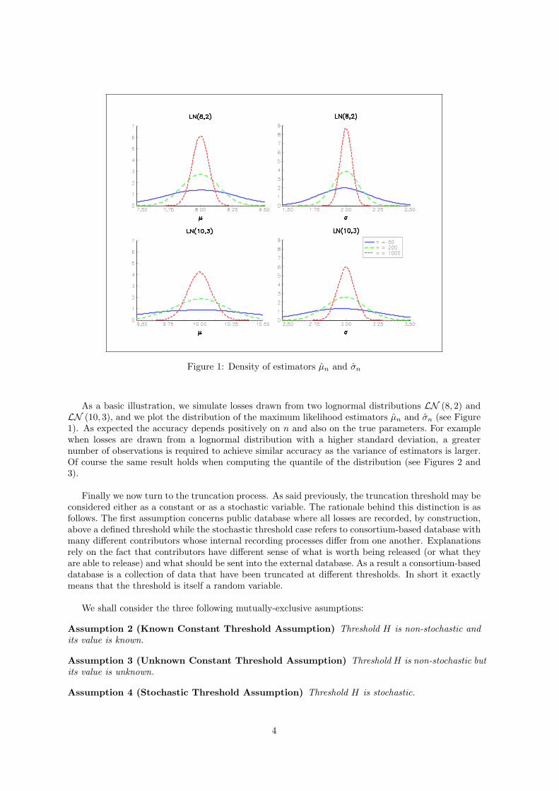
Figure 1: Density of estimators µn and σn

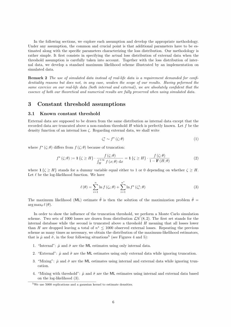
As a basic illustration, we simulate losses drawn from two lognormal distributions LN (8, 2) andLN (10, 3), and we plot the distribution of the maximum likelihood estimators µn and σn (see Figure1). As expected the accuracy depends positively on n and also on the true parameters. For examplewhen losses are drawn from a lognormal distribution with a higher standard deviation, a greaternumber of observations is required to achieve similar accuracy as the variance of estimators is larger.Of course the same result holds when computing the quantile of the distribution (see Figures 2 and3).

Finally we now turn to the truncation process. As said previously, the truncation threshold may beconsidered either as a constant or as a stochastic variable. The rationale behind this distinction is asfollows. The first assumption concerns public database where all losses are recorded, by construction,above a defined threshold while the stochastic threshold case refers to consortium-based database withmany different contributors whose internal recording processes differ from one another. Explanationsrely on the fact that contributors have different sense of what is worth being released (or what theyare able to release) and what should be sent into the external database. As a result a consortium-baseddatabase is a collection of data that have been truncated at different thresholds. In short it exactlymeans that the threshold is itself a random variable.

We shall consider the three following mutually-exclusive asumptions:

Assumption 2 (Known Constant Threshold Assumption) Threshold H is non-stochastic andits value is known.

Assumption 3 (Unknown Constant Threshold Assumption) Threshold H is non-stochastic butits value is unknown.

Assumption 4 (Stochastic Threshold Assumption) Threshold H is stochastic.

4

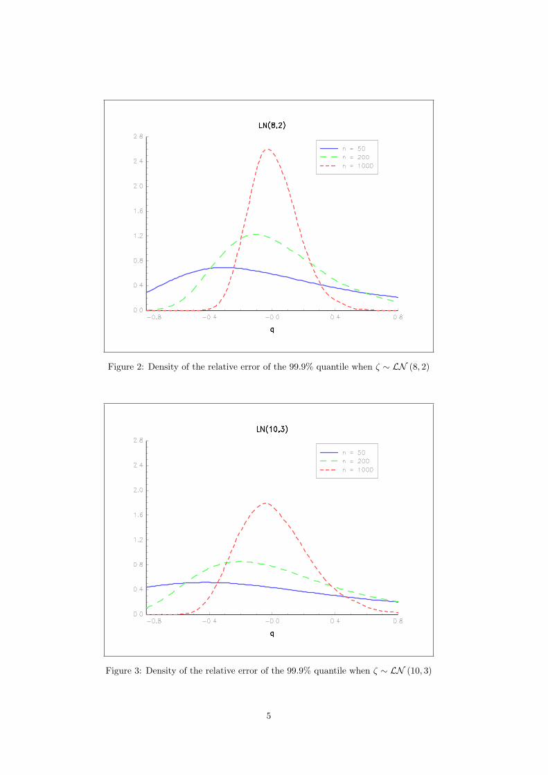
Figure 2: Density of the relative error of the 99.9% quantile when ζ ∼ LN (8, 2)

Figure 3: Density of the relative error of the 99.9% quantile when ζ ∼ LN (10, 3)

5

In the following sections, we explore each assumption and develop the appropriate methodology.Under any assumption, the common and crucial point is that additional parameters have to be es-timated along with the specific parameters characterizing the loss distribution. Our methodology israther simple. It first consists in specifying the actual loss distribution of external data when thethreshold assumption is carefully taken into account. Together with the loss distribution of inter-nal data, we develop a standard maximum likelihood scheme illustrated by an implementation onsimulated data.

Remark 2 The use of simulated data instead of real-life data is a requirement demanded for confi-dentiality reasons but does not, in any case, weaken the scope of our results. Having peformed thesame exercice on our real-life data (both internal and external), we are absolutely confident that theessence of both our theoretical and numerical results are fully preserved when using simulated data.

3 Constant threshold assumptions

3.1 Known constant threshold

External data are supposed to be drawn from the same distribution as internal data except that therecorded data are truncated above a non-random threshold H which is perfectly known. Let f be thedensity function of an internal loss ζ. Regarding external data, we shall write

ζ?i ∼ f? (ζ; θ) (1)

where f? (ζ; θ) differs from f (ζ; θ) because of truncation:

f? (ζ; θ) := 1 {ζ ≥ H} · f (ζ; θ)∫ +∞H

f (x; θ) dx= 1 {ζ ≥ H} · f (ζ; θ)

1− F (H; θ)(2)

where 1 {ζ ≥ H} stands for a dummy variable equal either to 1 or 0 depending on whether ζ ≥ H.Let ` be the log-likelihood function. We have

` (θ) =n∑

i=1

ln f (ζi; θ) +n?∑

i=1

ln f? (ζ?i ; θ) (3)

The maximum likelihood (ML) estimate θ is then the solution of the maximization problem θ =arg maxθ ` (θ).

In order to show the influence of the truncation threshold, we perform a Monte Carlo simulationscheme. Two sets of 1000 losses are drawn from distribution LN (8, 2). The first set stands for theinternal database while the second is truncated above a threshold H meaning that all losses lowerthan H are dropped leaving a total of n? ≤ 1000 observed external losses. Repeating the previousscheme as many times as necessary, we obtain the distribution of the maximum-likelihood estimators,that is µ and σ, in the four following situations5 (see Figures 4 and 5):

1. “Internal”: µ and σ are the ML estimates using only internal data.

2. “External”: µ and σ are the ML estimates using only external data while ignoring truncation.

3. “Mixing”: µ and σ are the ML estimates using internal and external data while ignoring trun-cation.

4. “Mixing with threshold”: µ and σ are the ML estimates using internal and external data basedon the log-likelihood (3).

5We use 5000 replications and a gaussian kernel to estimate densities.

6

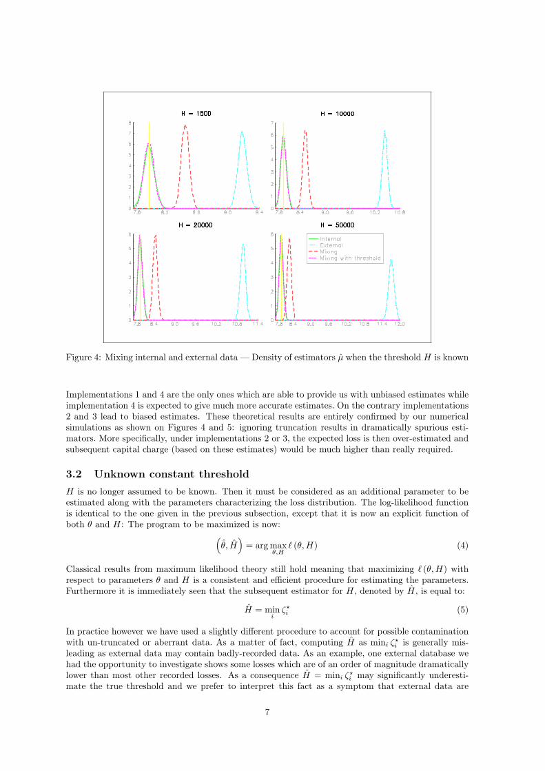
Figure 4: Mixing internal and external data — Density of estimators µ when the threshold H is known

Implementations 1 and 4 are the only ones which are able to provide us with unbiased estimates whileimplementation 4 is expected to give much more accurate estimates. On the contrary implementations2 and 3 lead to biased estimates. These theoretical results are entirely confirmed by our numericalsimulations as shown on Figures 4 and 5: ignoring truncation results in dramatically spurious esti-mators. More specifically, under implementations 2 or 3, the expected loss is then over-estimated andsubsequent capital charge (based on these estimates) would be much higher than really required.

3.2 Unknown constant threshold

H is no longer assumed to be known. Then it must be considered as an additional parameter to beestimated along with the parameters characterizing the loss distribution. The log-likelihood functionis identical to the one given in the previous subsection, except that it is now an explicit function ofboth θ and H: The program to be maximized is now:

(θ, H

)= arg max

θ,H` (θ,H) (4)

Classical results from maximum likelihood theory still hold meaning that maximizing ` (θ,H) withrespect to parameters θ and H is a consistent and efficient procedure for estimating the parameters.Furthermore it is immediately seen that the subsequent estimator for H, denoted by H, is equal to:

H = mini

ζ?i (5)

In practice however we have used a slightly different procedure to account for possible contaminationwith un-truncated or aberrant data. As a matter of fact, computing H as mini ζ?

i is generally mis-leading as external data may contain badly-recorded data. As an example, one external database wehad the opportunity to investigate shows some losses which are of an order of magnitude dramaticallylower than most other recorded losses. As a consequence H = mini ζ?

i may significantly underesti-mate the true threshold and we prefer to interpret this fact as a symptom that external data are

7

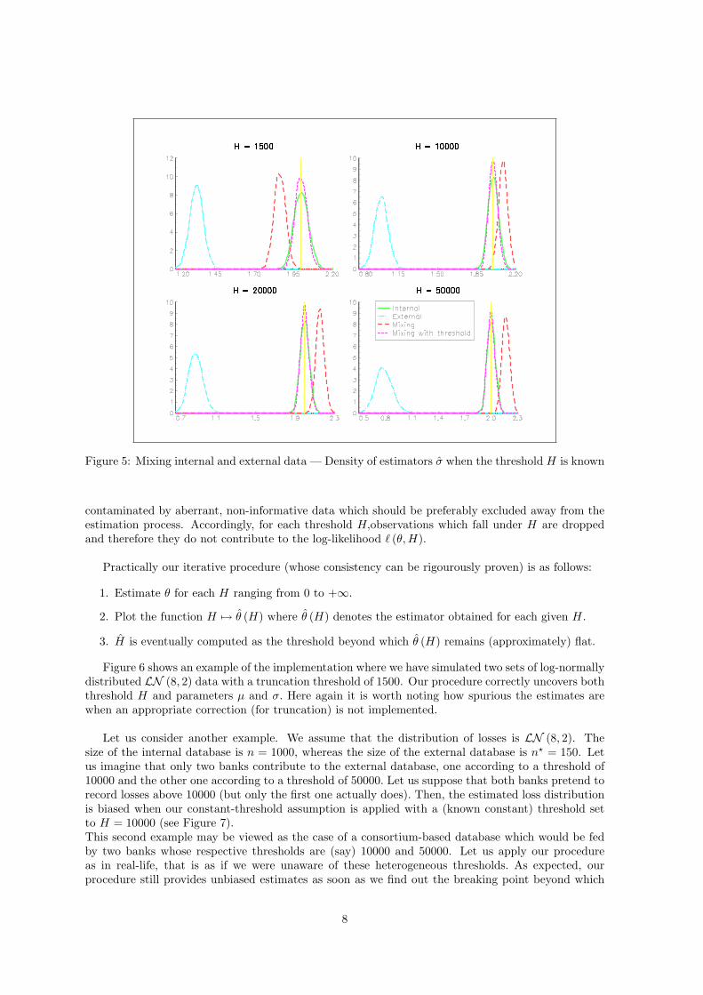
Figure 5: Mixing internal and external data — Density of estimators σ when the threshold H is known

contaminated by aberrant, non-informative data which should be preferably excluded away from theestimation process. Accordingly, for each threshold H,observations which fall under H are droppedand therefore they do not contribute to the log-likelihood ` (θ, H).

Practically our iterative procedure (whose consistency can be rigourously proven) is as follows:

1. Estimate θ for each H ranging from 0 to +∞.

2. Plot the function H 7→ θ (H) where θ (H) denotes the estimator obtained for each given H.

3. H is eventually computed as the threshold beyond which θ (H) remains (approximately) flat.

Figure 6 shows an example of the implementation where we have simulated two sets of log-normallydistributed LN (8, 2) data with a truncation threshold of 1500. Our procedure correctly uncovers boththreshold H and parameters µ and σ. Here again it is worth noting how spurious the estimates arewhen an appropriate correction (for truncation) is not implemented.

Let us consider another example. We assume that the distribution of losses is LN (8, 2). Thesize of the internal database is n = 1000, whereas the size of the external database is n? = 150. Letus imagine that only two banks contribute to the external database, one according to a threshold of10000 and the other one according to a threshold of 50000. Let us suppose that both banks pretend torecord losses above 10000 (but only the first one actually does). Then, the estimated loss distributionis biased when our constant-threshold assumption is applied with a (known constant) threshold setto H = 10000 (see Figure 7).This second example may be viewed as the case of a consortium-based database which would be fedby two banks whose respective thresholds are (say) 10000 and 50000. Let us apply our procedureas in real-life, that is as if we were unaware of these heterogeneous thresholds. As expected, ourprocedure still provides unbiased estimates as soon as we find out the breaking point beyond which

8

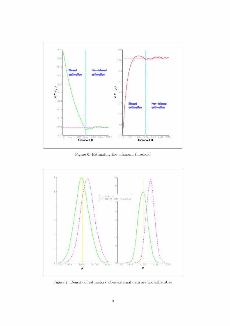
Figure 6: Estimating the unknown threshold

Figure 7: Density of estimators when external data are not exhaustive

9

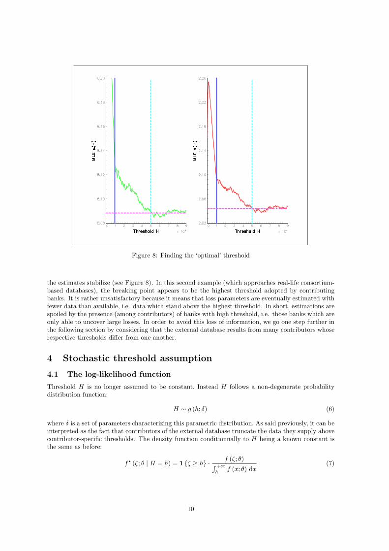
Figure 8: Finding the ‘optimal’ threshold

the estimates stabilize (see Figure 8). In this second example (which approaches real-life consortium-based databases), the breaking point appears to be the highest threshold adopted by contributingbanks. It is rather unsatisfactory because it means that loss parameters are eventually estimated withfewer data than available, i.e. data which stand above the highest threshold. In short, estimations arespoiled by the presence (among contributors) of banks with high threshold, i.e. those banks which areonly able to uncover large losses. In order to avoid this loss of information, we go one step further inthe following section by considering that the external database results from many contributors whoserespective thresholds differ from one another.

4 Stochastic threshold assumption

4.1 The log-likelihood function

Threshold H is no longer assumed to be constant. Instead H follows a non-degenerate probabilitydistribution function:

H ∼ g (h; δ) (6)

where δ is a set of parameters characterizing this parametric distribution. As said previously, it can beinterpreted as the fact that contributors of the external database truncate the data they supply abovecontributor-specific thresholds. The density function conditionnally to H being a known constant isthe same as before:

f? (ζ; θ | H = h) = 1 {ζ ≥ h} · f (ζ; θ)∫ +∞h

f (x; θ) dx(7)

10

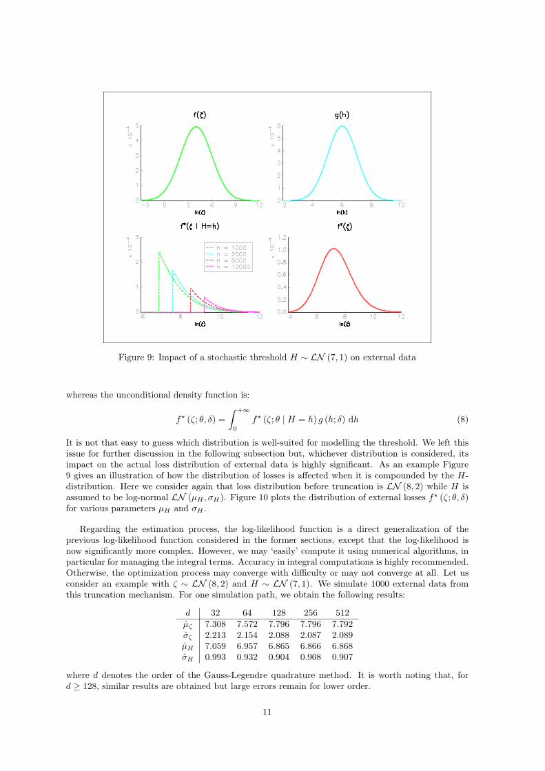
Figure 9: Impact of a stochastic threshold H ∼ LN (7, 1) on external data

whereas the unconditional density function is:

f? (ζ; θ, δ) =∫ +∞

0

f? (ζ; θ | H = h) g (h; δ) dh (8)

It is not that easy to guess which distribution is well-suited for modelling the threshold. We left thisissue for further discussion in the following subsection but, whichever distribution is considered, itsimpact on the actual loss distribution of external data is highly significant. As an example Figure9 gives an illustration of how the distribution of losses is affected when it is compounded by the H-distribution. Here we consider again that loss distribution before truncation is LN (8, 2) while H isassumed to be log-normal LN (µH , σH). Figure 10 plots the distribution of external losses f? (ζ; θ, δ)for various parameters µH and σH .

Regarding the estimation process, the log-likelihood function is a direct generalization of theprevious log-likelihood function considered in the former sections, except that the log-likelihood isnow significantly more complex. However, we may ‘easily’ compute it using numerical algorithms, inparticular for managing the integral terms. Accuracy in integral computations is highly recommended.Otherwise, the optimization process may converge with difficulty or may not converge at all. Let usconsider an example with ζ ∼ LN (8, 2) and H ∼ LN (7, 1). We simulate 1000 external data fromthis truncation mechanism. For one simulation path, we obtain the following results:

d 32 64 128 256 512µζ 7.308 7.572 7.796 7.796 7.792σζ 2.213 2.154 2.088 2.087 2.089µH 7.059 6.957 6.865 6.866 6.868σH 0.993 0.932 0.904 0.908 0.907

where d denotes the order of the Gauss-Legendre quadrature method. It is worth noting that, ford ≥ 128, similar results are obtained but large errors remain for lower order.

11

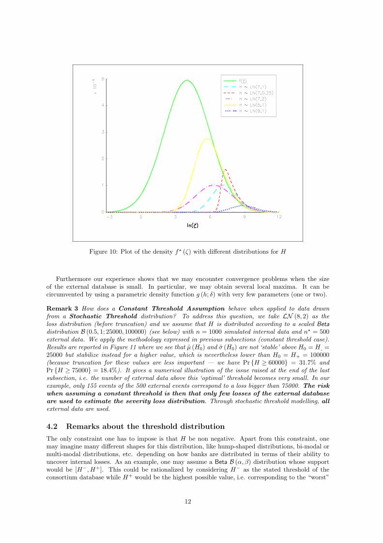
Figure 10: Plot of the density f? (ζ) with different distributions for H

Furthermore our experience shows that we may encounter convergence problems when the sizeof the external database is small. In particular, we may obtain several local maxima. It can becircumvented by using a parametric density function g (h; δ) with very few parameters (one or two).

Remark 3 How does a Constant Threshold Assumption behave when applied to data drawnfrom a Stochastic Threshold distribution? To address this question, we take LN (8, 2) as theloss distribution (before truncation) and we assume that H is distributed according to a scaled Betadistribution B (0.5, 1; 25000, 100000) (see below) with n = 1000 simulated internal data and n? = 500external data. We apply the methodology expressed in previous subsections (constant threshold case).Results are reported in Figure 11 where we see that µ (H0) and σ (H0) are not ‘stable’ above H0 = H =25000 but stabilize instead for a higher value, which is nevertheless lower than H0 = H+ = 100000(because truncation for these values are less important — we have Pr {H ≥ 60000} = 31.7% andPr {H ≥ 75000} = 18.4%). It gives a numerical illustration of the issue raised at the end of the lastsubsection, i.e. the number of external data above this ‘optimal’ threshold becomes very small. In ourexample, only 155 events of the 500 external events correspond to a loss bigger than 75000. The riskwhen assuming a constant threshold is then that only few losses of the external databaseare used to estimate the severity loss distribution. Through stochastic threshold modelling, allexternal data are used.

4.2 Remarks about the threshold distribution

The only constraint one has to impose is that H be non negative. Apart from this constraint, onemay imagine many different shapes for this distribution, like hump-shaped distributions, bi-modal ormulti-modal distributions, etc. depending on how banks are distributed in terms of their ability touncover internal losses. As an example, one may assume a Beta B (α, β) distribution whose supportwould be [H−, H+]. This could be rationalized by considering H− as the stated threshold of theconsortium database while H+ would be the highest possible value, i.e. corresponding to the “worst”

12

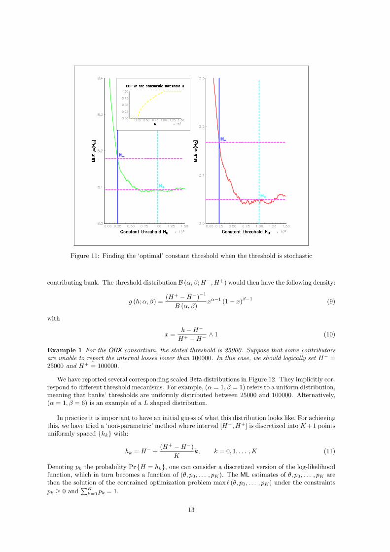
Figure 11: Finding the ‘optimal’ constant threshold when the threshold is stochastic

contributing bank. The threshold distribution B (α, β;H−, H+) would then have the following density:

g (h;α, β) =(H+ −H−)−1

B (α, β)xα−1 (1− x)β−1 (9)

with

x =h−H−

H+ −H− ∧ 1 (10)

Example 1 For the ORX consortium, the stated threshold is 25000. Suppose that some contributorsare unable to report the internal losses lower than 100000. In this case, we should logically set H− =25000 and H+ = 100000.

We have reported several corresponding scaled Beta distributions in Figure 12. They implicitly cor-respond to different threshold mecanisms. For example, (α = 1, β = 1) refers to a uniform distribution,meaning that banks’ thresholds are uniformly distributed between 25000 and 100000. Alternatively,(α = 1, β = 6) is an example of a L shaped distribution.

In practice it is important to have an initial guess of what this distribution looks like. For achievingthis, we have tried a ‘non-parametric’ method where interval [H−,H+] is discretized into K +1 pointsuniformly spaced {hk} with:

hk = H− +(H+ −H−)

Kk, k = 0, 1, . . . ,K (11)

Denoting pk the probability Pr {H = hk}, one can consider a discretized version of the log-likelihoodfunction, which in turn becomes a function of (θ, p0, . . . , pK). The ML estimates of θ, p0, . . . , pK arethen the solution of the contrained optimization problem max ` (θ, p0, . . . , pK) under the constraintspk ≥ 0 and

∑Kk=0 pk = 1.

13

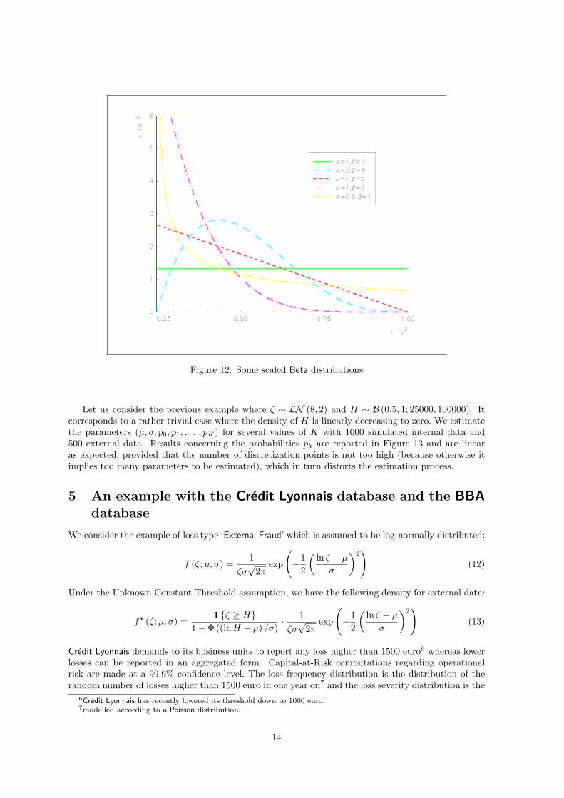
Figure 12: Some scaled Beta distributions

Let us consider the previous example where ζ ∼ LN (8, 2) and H ∼ B (0.5, 1; 25000, 100000). Itcorresponds to a rather trivial case where the density of H is linearly decreasing to zero. We estimatethe parameters (µ, σ, p0, p1, . . . , pK) for several values of K with 1000 simulated internal data and500 external data. Results concerning the probabilities pk are reported in Figure 13 and are linearas expected, provided that the number of discretization points is not too high (because otherwise itimplies too many parameters to be estimated), which in turn distorts the estimation process.

5 An example with the Credit Lyonnais database and the BBAdatabase

We consider the example of loss type ‘External Fraud’ which is assumed to be log-normally distributed:

f (ζ; µ, σ) =1

ζσ√

2πexp

(−1

2

(ln ζ − µ

σ

)2)

(12)

Under the Unknown Constant Threshold assumption, we have the following density for external data:

f? (ζ;µ, σ) =1 {ζ ≥ H}

1− Φ((ln H − µ) /σ)· 1ζσ√

2πexp

(−1

2

(ln ζ − µ

σ

)2)

(13)

Credit Lyonnais demands to its business units to report any loss higher than 1500 euro6 whereas lowerlosses can be reported in an aggregated form. Capital-at-Risk computations regarding operationalrisk are made at a 99.9% confidence level. The loss frequency distribution is the distribution of therandom number of losses higher than 1500 euro in one year on7 and the loss severity distribution is the

6Credit Lyonnais has recently lowered its threshold down to 1000 euro.7modelled according to a Poisson distribution.

14

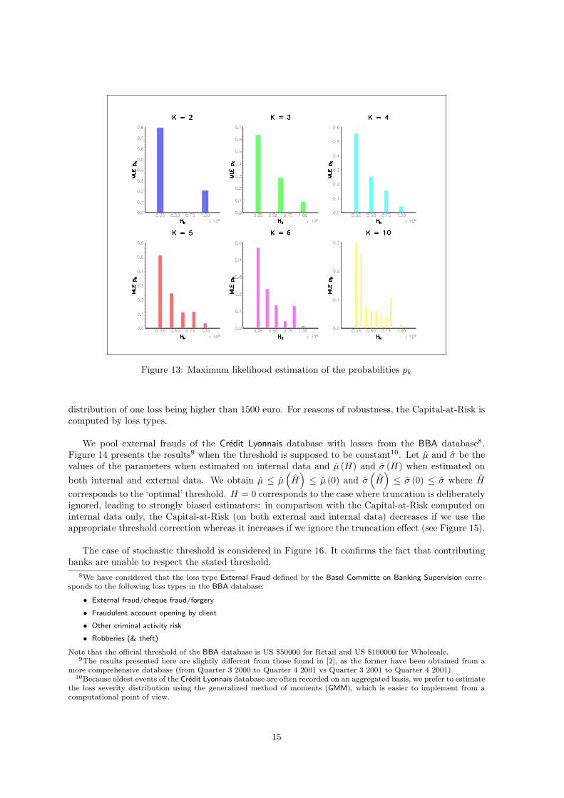
Figure 13: Maximum likelihood estimation of the probabilities pk

distribution of one loss being higher than 1500 euro. For reasons of robustness, the Capital-at-Risk iscomputed by loss types.

We pool external frauds of the Credit Lyonnais database with losses from the BBA database8.Figure 14 presents the results9 when the threshold is supposed to be constant10. Let µ and σ be thevalues of the parameters when estimated on internal data and µ (H) and σ (H) when estimated onboth internal and external data. We obtain µ ≤ µ

(H

)≤ µ (0) and σ

(H

)≤ σ (0) ≤ σ where H

corresponds to the ‘optimal’ threshold. H = 0 corresponds to the case where truncation is deliberatelyignored, leading to strongly biased estimators: in comparison with the Capital-at-Risk computed oninternal data only, the Capital-at-Risk (on both external and internal data) decreases if we use theappropriate threshold correction whereas it increases if we ignore the truncation effect (see Figure 15).

The case of stochastic threshold is considered in Figure 16. It confirms the fact that contributingbanks are unable to respect the stated threshold.

8We have considered that the loss type External Fraud defined by the Basel Committe on Banking Supervision corre-sponds to the following loss types in the BBA database:

• External fraud/cheque fraud/forgery

• Fraudulent account opening by client

• Other criminal activity risk

• Robberies (& theft)

Note that the official threshold of the BBA database is US $50000 for Retail and US $100000 for Wholesale.9The results presented here are slightly different from those found in [2], as the former have been obtained from a

more comprehensive database (from Quarter 3 2000 to Quarter 4 2001 vs Quarter 3 2001 to Quarter 4 2001).10Because oldest events of the Credit Lyonnais database are often recorded on an aggregated basis, we prefer to estimate

the loss severity distribution using the generalized method of moments (GMM), which is easier to implement from acomputational point of view.

15

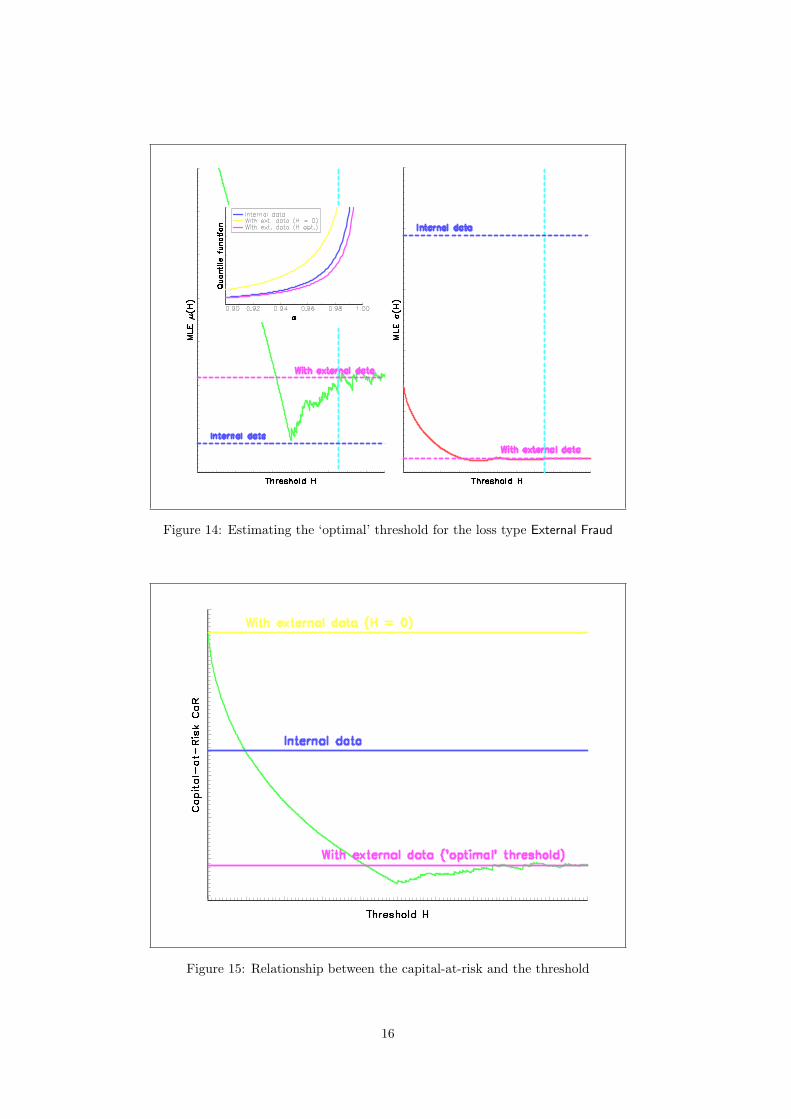
Figure 14: Estimating the ‘optimal’ threshold for the loss type External Fraud

Figure 15: Relationship between the capital-at-risk and the threshold

16

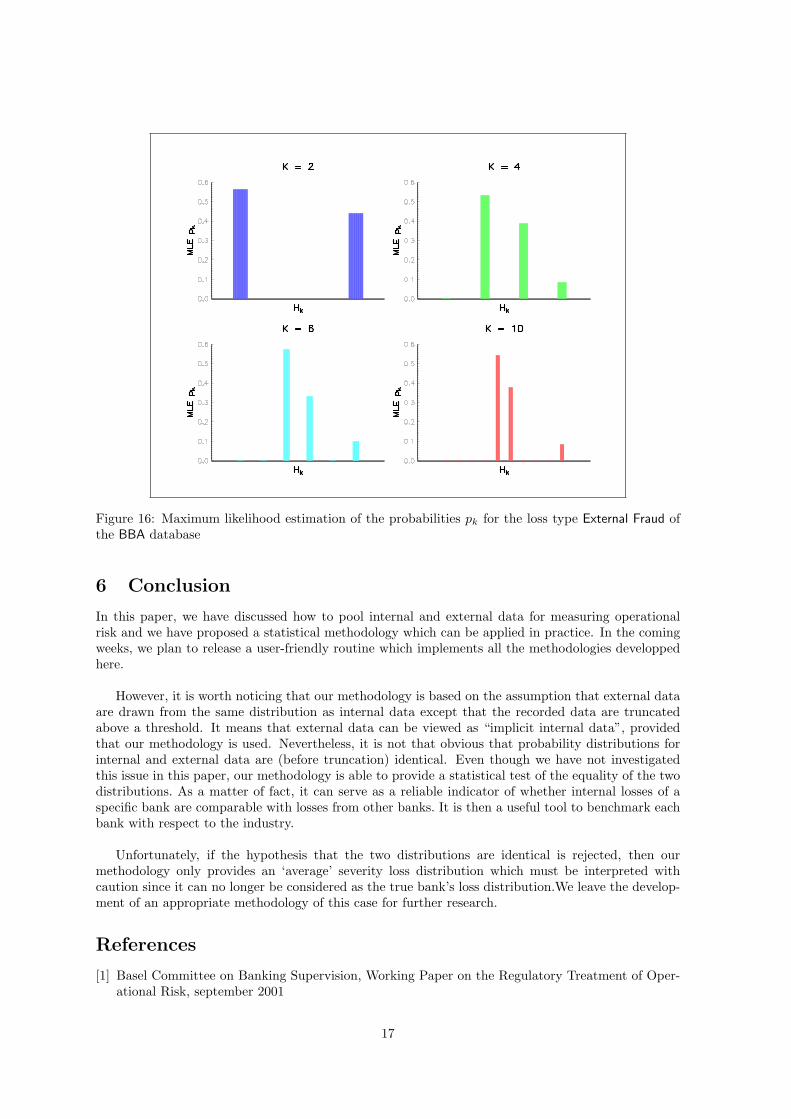
Figure 16: Maximum likelihood estimation of the probabilities pk for the loss type External Fraud ofthe BBA database

6 Conclusion

In this paper, we have discussed how to pool internal and external data for measuring operationalrisk and we have proposed a statistical methodology which can be applied in practice. In the comingweeks, we plan to release a user-friendly routine which implements all the methodologies developpedhere.

However, it is worth noticing that our methodology is based on the assumption that external dataare drawn from the same distribution as internal data except that the recorded data are truncatedabove a threshold. It means that external data can be viewed as “implicit internal data”, providedthat our methodology is used. Nevertheless, it is not that obvious that probability distributions forinternal and external data are (before truncation) identical. Even though we have not investigatedthis issue in this paper, our methodology is able to provide a statistical test of the equality of the twodistributions. As a matter of fact, it can serve as a reliable indicator of whether internal losses of aspecific bank are comparable with losses from other banks. It is then a useful tool to benchmark eachbank with respect to the industry.

Unfortunately, if the hypothesis that the two distributions are identical is rejected, then ourmethodology only provides an ‘average’ severity loss distribution which must be interpreted withcaution since it can no longer be considered as the true bank’s loss distribution.We leave the develop-ment of an appropriate methodology of this case for further research.

References

[1] Basel Committee on Banking Supervision, Working Paper on the Regulatory Treatment of Oper-ational Risk, september 2001

17

[2] Baud, N., A. Frachot, and T. Roncalli [2002], An internal model for operational risk computa-tion, Credit Lyonnais, Groupe de Recherche Operationnelle, Slides of the conference “Seminariosde Matematica Financiera”, Instituto MEFF – Risklab, Madrid

[3] Frachot, A., P. Georges and T. Roncalli [2001], Loss Distribution Approach for operationalrisk, Credit Lyonnais, Groupe de Recherche Operationnelle, Working Paper

[4] Frachot, A. and T. Roncalli [2002], Mixing internal and external data for managing operationalrisk, Credit Lyonnais, Groupe de Recherche Operationnelle, Working Paper

[5] Peemoller, F.A. [2002], Operational risk data pooling, Deutsche Bank AG, Presentation atCFSforum – Operational Risk, Frankfurt/Main

18