Embed Size (px)
Citation preview

American Economic Journal: Microeconomics 2016, 8(1): 24–56 http://dx.doi.org/10.1257/mic.20140145
24
Internal Geography, International Trade, and Regional Specialization†
By A. Kerem Cosar and Pablo D. Fajgelbaum*
We introduce an internal geography to the canonical model of international trade driven by comparative advantages to study the regional effects of external economic integration. The model features a dual-economy structure, in which locations near international gates specialize in export-oriented sectors while more distant locations do not trade with the rest of the world. The theory rationalizes patterns of specialization, employment, and relative incomes observed in developing countries that opened up to trade. We find regional specialization patterns consistent with the model in industry-level data from Chinese prefectures. (JEL F11, O18, P23, P25, P33, R12, R32)
The experience of many developing countries reveals uneven regional effects of international economic integration. For example, China’s recent globalization
process took place jointly with large movements of workers and export-oriented industries toward fast-growing coastal regions (World Bank 2009). The standard view in international trade theory interprets countries as points in space, missing this type of phenomenon. In this paper, we introduce an internal geography to the canonical model of international trade driven by comparative advantages to study the regional effects of external economic integration. The theory rationalizes patterns of specialization, employment, and relative incomes observed in developing countries that opened up to trade. A key feature of the model is that comparative-advantage industries locate closer to international gates. We find evidence consistent with this pattern in industry-level data from Chinese prefectures, and document that alterna-tive explanations based on economies of scale or location fundamentals do not fully account for it.
We model a two-sector economy where locations are arbitrarily arranged on a map and differ in trade costs to international gates such as seaports, airports, or land crossings. Within the country, trade is costly and international shipments must
* Cosar: Booth School of Business, University of Chicago 5807 South Woodlawn Avenue, Chicago, IL 60637 (e-mail: [email protected]); Fajgelbaum: Department of Economics, University of California Los Angeles, 8283 Bunche Hall, Los Angeles, CA 90095 (e-mail: [email protected]). We thank Andrew Atkeson, Ariel Burstein, Banu Demir Pakel, Chang-Tai Hsieh, Esteban Rossi-Hansberg, Gordon Hanson, Vernon Henderson, Michael Zheng Song, Ralph Ossa, Henry Overman, Stephen Redding, Daniel Yi Xu, and participants at various seminars for useful comments. Cosar thanks University of Chicago Booth School of Business for summer financial support.
† Go to http://dx.doi.org/10.1257/mic.20140145 to visit the article page for additional materials and author disclosure statement(s) or to comment in the online discussion forum.

VoL. 8 No. 1 25cosar and fajgelbaum: internal geography and international trade
cross through international gates to reach foreign markets. To produce, firms in each location use both a mobile and an immobile factor. The geographical advantage of international gates acts as an agglomeration force, but decreasing returns to scale due to immobile factors create incentives to spread economic activity across loca-tions. This structure allows us to represent all equilibrium outcomes in closed form and the model remains tractable under various extensions.
The key equilibrium feature is a dual-economy structure. Whenever the economy is not fully specialized in what it exports, two distinct regions necessarily emerge: locations near international gates specialize in export-oriented sectors, whereas more distant locations are incompletely specialized and do not trade with other regions or with the rest of the world. The first set of locations constitutes a commercially integrated coastal region with high employment density, while the second set forms an autarkic interior region where immobile factors are poorer. We examine how the interaction between internal and international trade costs determines each of these regions’ weight in national income and economic activity. International integration causes migration of mobile factors to the coastal region and an increase in the mea-sure of locations specialized in export-oriented sectors.
This specialization pattern leads to uneven regional effects of international trade. Higher openness, triggered by a reduction in either international or internal trade costs, has opposing welfare effects on immobile factors located in different points of the country. The interior region loses due to the reduced availability of mobile fac-tors who emigrate to the coastal region, while some locations in the coastal region necessarily gain. When the country is open to trade and internal trade costs are reduced from a sufficiently high level, regional inequality follows an inverted-U shape. The theory also offers a rationale for why the gains from trade may be low in the presence of poor domestic infrastructure. At the aggregate level, the gains from international trade are a weighted average of the gains accrued to each location, and can be broken down into a familiar term that captures the gains without internal geography and a term that captures domestic trade frictions. The latter depends on the size of the coastal region, so that, by reducing the measure of trading locations, domestic trade frictions hamper the aggregate gains from trade.
These qualitative results rationalize patterns of specialization, employment, and relative incomes observed in developing countries that opened up to trade. For exam-ple, economic integration led to larger employment growth in comparative-advantage industries located near borders in Mexico (Hanson 1996) and near ports in Vietnam (McCaig and Pavnick 2012). The dual-economy structure generated by the model is consistent with the coexistence of globally integrated regions and a hinterland with low international participation in large developing countries with a poor transporta-tion infrastructure (Asian Development Bank Institute 2009). The theory rational-izes these facts by introducing internal trade costs to the neoclassical trade model. Limao and Venables (2001) and Atkin and Donaldson (2014) provide evidence that such costs are sizeable in developing countries.
In the empirical analysis, we assess the key prediction of the model about regional specialization, from which its welfare and distributional implications stem: due to the interaction between national comparative advantages and internal trade costs, export-oriented industries (i.e., industries in which the economy has

26 AMEriCAN ECoNoMiC JourNAL: MiCroECoNoMiCs FEBruAry 2016
comparative advantages relative to the rest of the world) locate closer to interna-tional gates, leading to uneven regional effects of trade. We assess this prediction using industry-level data from Chinese prefectures, proxying for industries’ export orientation with national export-revenue ratios. To sidestep the concern that these ratios are endogenous to activity within China, we also rely on the argument that China’s comparative advantages lie in labor-intensive industries and use indus-try-specific labor intensities from US data as a second proxy for industry export orientation.
We find that economic activity at the industry-prefecture level is strongly cor-related with the interaction between prefecture proximity to coastlines and industry export orientation. The direct effect of distance on economic activity is sizable: moving inland by 275 miles (the median distance from the coast across prefec-tures) decreases industry employment by 17 percent for an industry with an average export-revenue ratio, and by 13 percent for an industry with average labor inten-sity. But this negative distance gradient is stronger for export-oriented industries: employment shrinks by 32 percent for an industry that has an export-revenue ratio 1 standard deviation higher than average, and by 21 percent for an industry that has labor intensity 1 standard deviation higher than average.
Finally, we examine alternative explanations that can also generate this pattern. Our approach to explaining regional specialization complements explanations within the New Economic Geography tradition of Krugman (1991). In that view, it could be that industries with higher returns to scale locate closer to international markets and are more likely to export. Following Hanson and Xiang (2004), we use prod-uct differentiation as an industry-specific measure of returns to scale to control for this home-market effect. We also control for industry-specific trade costs. While the data suggest that economies of scale may also be important in determining industry location, our main finding is not affected by this control. Our approach also comple-ments explanations based on location fundamentals such as Courant and Deardorff (1992), and on external economies of scale as in Rossi-Hansberg (2005). In those views, it could be that, closer to international gates, either endowments or external-ities drive low relative unit costs in specific industries that become export oriented. We argue that explanations of this type do not fully account for the regional special-ization pattern that we find, for they imply a positive relative-productivity gradient in favor of comparative-advantage industries toward coastlines that is not strongly present in the Chinese data.
relation to the Literature.—Few studies consider an explicit interaction between international and domestic trade costs. In a New Economic Geography context, Krugman and Livas Elizondo (1996) and Behrens et al. (2006) present models where two regions within a country trade with the rest of the world. Henderson (1982) and Rauch (1991) model systems of cities in an open economy framework. Rossi-Hansberg (2005) studies the location of industries on a continuous space with spatial externalities. These papers are based on economies of scale, whereas we focus on the interaction between heterogeneous market access within countries and comparative advantages between countries.

VoL. 8 No. 1 27cosar and fajgelbaum: internal geography and international trade
Matsuyama (1999) studies a multi-region extension of Helpman and Krugman (1985). He focuses on home-market effects under different spatial configurations, but does not include factor mobility. In neoclassical environments, Bond (1993) and Courant and Deardorff (1992) present models with regional specialization where relative factor endowments may vary across discrete regions within a country. These papers do not include heterogeneity in access to world markets. Venables and Limão (2002) study international specialization in a setup with central and peripheral loca-tions and no factor mobility.
More recently, Ramondo, Rodríguez-Clare, and Saborío-Rodríguez (2014) quan-titatively study the gains from trade and technology diffusion allowing for multiple regions within countries in the Eaton and Kortum (2003) model. Redding (2014) develops a multi-region version of the trade and labor mobility model in Helpman (1998), while Allen and Arkolakis (2014) study an Armington model extended with labor mobility and external economies. These papers do not study the effect of interna-tional trade on the pattern of industrial specialization across regions within countries.
Finally, a large empirical literature studies determinants of industry location. Holmes and Stevens (2004) offer a summary assessment of the forces that deter-mine industry location in the United States, while Hanson (1998) reviews the liter-ature on the effect of North American trade integration on the location of economic activity. Amiti and Javorcik (2008) and Lu and Tao (2009) document the determi-nants of firm and industry locations in China. Our empirical analysis complements these studies, suggesting that international trade is an important driver of industry location within China, and that it may also be so in other developing countries that are open to international trade but face high internal trade costs.
I. Model
Geography and Trade Costs.—The country consists of a set of locations arbi-trarily arranged on a map. We index locations by ℓ , and assume that only some loca-tions can trade directly with the rest of the world. Goods must cross through a port to be shipped internationally. As will be clear below, the nature of our model implies that only the distance separating each location ℓ from its nearest port matters for the equilibrium. Therefore, we assume without loss of generality that ℓ represents the distance separating each location from its nearest port, and we denote all ports by ℓ = 0 . We let
_ ℓ be the maximum distance between a location inside the country and
its nearest port.There are two industries, i ∈ { X, M } . There is an industry-specific international
iceberg trade cost such that for each unit of i shipped from ℓ = 0 , only e − τ 0 i units
arrive in the rest of the world (RoW). Within the country, iceberg trade costs are constant per unit of distance and equal τ 1 i in industry i . Therefore, for each unit of i that location ℓ ships to the RoW, only e − τ 0
i − τ 1 i ℓ units arrive.
Given this geography, we can interpret each location ℓ = 0 as a seaport, airport, or international land crossing. What is key is that not all locations have the same technology for trading with the RoW. This will drive concentration near points with good access. Internal geography vanishes when τ 1 i = 0 for i = X, M or
_ ℓ = 0 .

28 AMEriCAN ECoNoMiC JourNAL: MiCroECoNoMiCs FEBruAry 2016
Endowments.—There are two factors of production, a mobile factor and an immobile one. We refer to the mobile factor as workers, and to the immobile factor as land.1 We let λ (ℓ) be the total amount of land available in locations at distance ℓ from their nearest port and normalize units so that the national land endowment also equals one.2 Land is owned by immobile landlords who do not work. We let N be the labor endowment at the national level and n (ℓ) denote employment density in ℓ , which is to be determined in equilibrium since workers choose their location optimally.
Preferences.—Both workers and landlords spend their income locally. The indi-rect utility of a worker living in ℓ is
(1) u(ℓ) = w (ℓ) ____
E(ℓ) ,
where w(ℓ) is the wage at ℓ , and E(ℓ) is the cost-of-living index. We let p(ℓ) ≡ P X (ℓ) / P M (ℓ) be the relative price of X in ℓ . Since preferences are homo-thetic, there exists an increasing and concave function e( p(ℓ)) that depends on the relative price of X such that E(ℓ) = P M (ℓ)e( p (ℓ) ) .
For landlords, income equals rents r(ℓ) per unit of land and utility is therefore increasing in r (ℓ) / E(ℓ) . Accounting for both wages and rents, income generated by each unit of land at ℓ is y (ℓ) = w (ℓ) n (ℓ) + r (ℓ) .
Technology.—Production in each sector requires one unit of land to operate a technology with decreasing returns to scale in labor. We let n i (ℓ) be employment per unit of land in industry i at location ℓ . Profits per unit of land in sector i at ℓ are
(2) π i (ℓ) = max n i (ℓ)
{ P i (ℓ) q i [ n i (ℓ)] − w(ℓ) n i (ℓ) − r (ℓ) } .
The production technology is
(3) q i [ n i (ℓ)] = κ i n i (ℓ) 1− α i ______
a i (ℓ) ,
where a i (ℓ) is the unit cost of production in industry i in sector ℓ and κ i ≡ α i
− α i (1 − α i ) − (1− α i ) is a normalization constant that saves notation later on. Decreasing returns to scale 1 − α i measure the labor intensity in sector i , acting as a congestion force. From (3) it follows that the aggregate production function in sector i at ℓ is Cobb-Douglas with land intensity α i . To simplify the exposition, we assume that land intensity is the same across both sectors, α X = α M ≡ α , and dis-cuss the implications of differences in land intensity across sectors in Section IID.
1 Appendix A presents an extension where both labor and capital are mobile factors used in production and sec-tors can differ in labor intensity. In the empirical analysis, we use data on both employment and capital to evaluate the model’s prediction about the location of the mobile factor in different industries.
2 If the distribution of land is uniform, λ (ℓ) represents the measure of locations at distance ℓ from their nearest port.
VoL. 8 No. 1 29cosar and fajgelbaum: internal geography and international trade
Industry-specific production costs { a M (ℓ) , a X (ℓ) } may vary across locations, subject to the restriction that the relative cost of production is constant across the country:
(4) a X (ℓ) _____ a M (ℓ) = a for all ℓ ∈ [0,
_ ℓ ] .
Therefore, while some locations might be more productive than others in every industry, comparative advantages are defined at the national level. In turn, a differs across countries, creating incentives for international trade. In this way we retain the basic structure of a neoclassical model of trade, where countries are differentiated by their comparative advantages.
The solution to the firm’s problem yields labor demand per unit of land used by each sector i in location ℓ ,
(5) n i (ℓ) = 1 − α ____ α ( P i (ℓ) ________ a i (ℓ) w(ℓ)
) 1/α
for i = X, M.
Finally, we let λ i (ℓ) be the total amount of land used by sector i = X, M at ℓ .
A. Local Equilibrium
We first define and characterize a local equilibrium at each location ℓ that takes prices { P X (ℓ) , P M (ℓ) } and the real wage u ∗ as given.
DEFINITION 1: A local equilibrium at ℓ consists of population density n (ℓ) , labor demands { n i (ℓ) } i=X, M , patterns of land use { λ i (ℓ) } i=X, M , and factor prices {w (ℓ) , r(ℓ)} such that:
(i ) workers maximize utility,
(6) u(ℓ) ≤ u ∗ , = if n (ℓ) > 0;
(ii) profits are maximized,
(7) π i (ℓ) ≤ 0, = if λ i (ℓ) > 0, for i = X, M,
where π i (ℓ) is given by (2);
(iii) land and labor markets clear,
(8) ∑ i=X, M
λ i (ℓ) = λ(ℓ),
30 AMEriCAN ECoNoMiC JourNAL: MiCroECoNoMiCs FEBruAry 2016
(9) ∑ i=X, M
λ i (ℓ) ____ λ(ℓ) n i (ℓ) = n (ℓ) ; and
(iv) trade is balanced.
Conditions (ii )– (iv) from this definition constitute a small Ricardian economy where the amount of labor is given. In addition, employment density n (ℓ) at each location is determined by condition (i) .
We let p A be the autarky price in each location. By this, we mean the price pre-vailing in the absence of trade with any other location or with RoW, but when labor mobility is allowed across locations. The autarky price p A is the same and equal to a in all locations. Using (7), location ℓ must be fully specialized in X when p (ℓ) > p A , and fully specialized in M when p (ℓ) < p A . Because each location takes relative prices as given, this means that a trading location is fully specialized. Only if p (ℓ) happens to coincide with p A may a trading location be incompletely specialized. This logic also implies that an incompletely specialized location is in autarky.3
To solve for the local wage w(ℓ) we note that whenever a location is populated, the local labor supply decision (6) must be binding. Together with (5) and the market clearing conditions, this gives the equilibrium population density in each location,4
(10) n (ℓ) =
⎧
⎪
⎨ ⎪
⎩
1 − α _____ α ( 1 ______
a X (ℓ) u ∗
p (ℓ) _____
e (p (ℓ) ) ) 1/α
if p (ℓ) ≥ a,
1 − α _____ α (
1 ______ a M (ℓ) u ∗
1 _____ e (p (ℓ) ) )
1/α if p (ℓ) < a.
Expression (10) conveys the various forces that determine the location decision of workers. Agents care about the effect of prices on both income and cost of living. Since preferences are homothetic, agents employed in the industry-location pair (i, ℓ) necessarily enjoy a higher real income when the local relative price of industry i is higher in location ℓ . That is, the positive income effect from a higher relative price necessarily offsets cost-of-living effects. At the same time, there are conges-tion forces captured by the intensity of land use α , so that workers avoid places with high employment density. The larger the congestion, the smaller the population density. Naturally, agents also prefer locations with better fundamental productivity, i.e., lower a i (ℓ) .
We highlight that trade affects density through its effect on the relative price p (ℓ) . When p (ℓ) ≠ p A , locations are fully specialized and necessarily export. In this cir-cumstance n(ℓ) increases with the relative price of the exported good and decreases with the national real wage u ∗ .
3 In knife-edge cases, where p(ℓ) = p A , a location can be indifferent between autarky or trade. In that case, a location may trade and still be incompletely specialized.
4 This is a special case of the expression for density derived under more general conditions in equation (A12) in the Appendix.

VoL. 8 No. 1 31cosar and fajgelbaum: internal geography and international trade
B. General Equilibrium
We move on to the effect of market access (distance to the nearest international gate) on employment density and the specialization pattern in general equilibrium. The country is a small economy taking international prices { P X ∗ , P M ∗ } as given.5 We denote the relative price at RoW by p ∗ = P X ∗ / P M ∗ .
We also define the average international and domestic iceberg costs across sec-tors, τ j ≡ 1 _ 2 ∑ i=X, M
τ j i for j = 0, 1 . No arbitrage implies that for any pair of loca-
tions ℓ and ℓ ′ separated by distance δ ≥ 0 , relative prices in industry i satisfy
(11) P i (ℓ′ ) / P i (ℓ) ≤ e τ 1 i δ for i = X, M.
This condition binds if goods in industry i are shipped from ℓ to ℓ ′. A similar con-dition holds with respect to RoW. Since all locations ℓ = 0 can trade directly with RoW at the same relative price, (11) implies
(12) e −2 τ 0 ≤ p(0) / p ∗ ≤ e 2 τ 0 .
The first inequality is binding if the country exports X to RoW, while the second is if it imports X . Therefore, for any location ℓ, we have
(13) e −2 τ 1 ℓ ≤ p(ℓ) / p(0) ≤ e 2 τ 1 ℓ ,
where the first inequality binds if ℓ exports X to RoW, and the second does if ℓ imports X .
We are ready to define the general equilibrium of the economy:
DEFINITION 2 (General Equilibrium): An equilibrium in a small economy given international prices { P X ∗ , P M ∗ } consists of a real wage u ∗ , local outcomes
n (ℓ) , { n i (ℓ) } i=X, M , { λ i (ℓ) } i=X, M , w (ℓ) , r(ℓ) , and goods prices { P i (ℓ)} i=X, M such that:
(i) given { P i (ℓ)} i=X, M and u ∗ , local outcomes are a local equilibrium by Definition 1 for all ℓ ∈ [0,
_ ℓ ] ;
(ii) relative prices p(ℓ) satisfy the no-arbitrage conditions (12) and (13) for all ℓ, ℓ′ ∈ [0,
_ ℓ ] ; and
(iii) the real wage u ∗ adjusts such that the national labor market clears,
(14) ∫ 0 _ ℓ n (ℓ) λ (ℓ) dℓ = N .
5 It is straightforward to extend the model to a two-country general equilibrium in which the world prices are endogenously determined.
32 AMEriCAN ECoNoMiC JourNAL: MiCroECoNoMiCs FEBruAry 2016
Since Definition 1 of a local equilibrium includes trade balance for each location, trade is also balanced at the national level. To characterize the regional patterns of specialization, we first note that the no-arbitrage conditions rule out bilateral trade flows between any pair of locations within the country. Since all locations share the same relative unit costs, there are no gains from trade within the country. To see why, suppose that there is bilateral trade between two distinct locations ℓ X and ℓ M . If ℓ X is the X -exporting location of the pair, then p ( ℓ M ) ≤ p A ≤ p ( ℓ X ) . But, at the same time, the no-arbitrage condition (11) implies that the relative price of X is strictly higher in ℓ M , which is a contradiction. This implies that the country is in international autarky if and only if all locations are in autarky and incompletely specialized.6
With this in mind, we can characterize the general equilibrium. The country can be partitioned into those locations that trade with RoW and those that stay in autarky. It follows that if the country is not in international autarky there must be some boundary b ∈ [0,
_ ℓ ] , such that all locations ℓ < b are fully specialized in
the export-oriented industry. In turn, all locations ℓ > b do not trade with the RoW and stay in autarky, while locations at distance b from their nearest international gate are indifferent between trading or not with RoW.7 Therefore, an internal bound-ary b divides the country between a trading coastal region comprising all locations ℓ ∈ [0, b) whose distance to the nearest international gate is less than b and an autarkic interior region comprising the remaining locations ℓ ∈ (b,
_ ℓ ] .8
This reasoning implies that the distance separating each location from its nearest international gate is the only local fundamental that matters for specialization. This justifies our initial statement that locations may be arbitrarily arranged on a map, as well as our decision to index locations by their distance to the nearest port. In addition, any bilateral trade flow in the country either originates from ports, or is directed toward them. These features allow us to represent a two-dimensional geog-raphy on the line, leading to closed-form characterizations for aggregate equilibrium outcomes and making the model tractable for counterfactuals.
Since all locations ℓ ∈ (b, _ ℓ ] are in autarky, they are incompletely specialized
and their relative price is p A = a . Given this price in the autarkic region and the regional pattern of production, the no-arbitrage conditions (12) and (13) generate the regional price distribution as function of the internal boundary b . Henceforth, we assume that the economy is a net exporter of X , and below we provide the conditions
6 This outcome is akin to the spatial impossibility results in the tradition of Starrett (1978), whereby homoge-neous space and constant-returns-to-scale technologies lead to autarkic locations. In our setting, the only heteroge-neity across space is the distance to the port. Thus, if trade occurs, it is with the RoW. Of course, this lack of bilateral internal trade is not a feature of the data. The model could be extended with product differentiation within sectors to generate internal trade without affecting the regional specialization pattern.
7 To determine which locations belong in each set, we note that if the country is an exporter of X, then all loca-tions that trade with RoW must also export X . Therefore, all locations ℓ , such that e −2 ( τ 0 + τ 1 ℓ) p ∗ < p A , must stay in autarky, for if they specialized in X , then the relative price of X would be so low that it would induce specializa-tion in M . In the same way, all locations ℓ , such that e −2 ( τ 0 + τ 1 ℓ) p ∗ > p A , must specialize in X , for if they stayed in autarky, then the relative price of M would be so high that it would induce domestic consumers to import from abroad, violating the no-arbitrage condition (13).
8 The regional specialization pattern resembles a Von-Thünen type outcome. In the standard version of the Von-Thünen model, as featured, for example, in Chapter 3 of Fujita and Thisse (2013), the pattern of specialization across locations that trade with a central district is dictated by differences in trade costs or land intensity across goods. In our context, differences between countries lead to specialization rings within the country.
VoL. 8 No. 1 33cosar and fajgelbaum: internal geography and international trade
under which this is the case. Therefore, the distribution of local relative prices is given by
(15) p(ℓ) = p ∗ e −2 ( τ 0 + τ 1 min [ℓ, b] ) .
Using (10) in the aggregate labor-market clearing condition (14), we can solve for the real wage:
(16) u ∗ = [ 1 − α ____ α 1 __ N ∫
0 _ ℓ λ (ℓ) ( 1 _____
a X (ℓ) p(ℓ) ______ e (p(ℓ)) )
1/α
dℓ]
α
.
Since the relative price function in (15) depends on b , so does the real wage. To find the location of the boundary b , we use the continuity of the relative price function:
(17) p(b) ≥ p A , = if b < _ ℓ .
When p( _ ℓ ) > p A , then b =
_ ℓ , so that the interior region does not exist. The gen-
eral equilibrium is fully characterized by the pair { u ∗ , b} that solves (16) and (17). All other variables follow from these two outcomes.
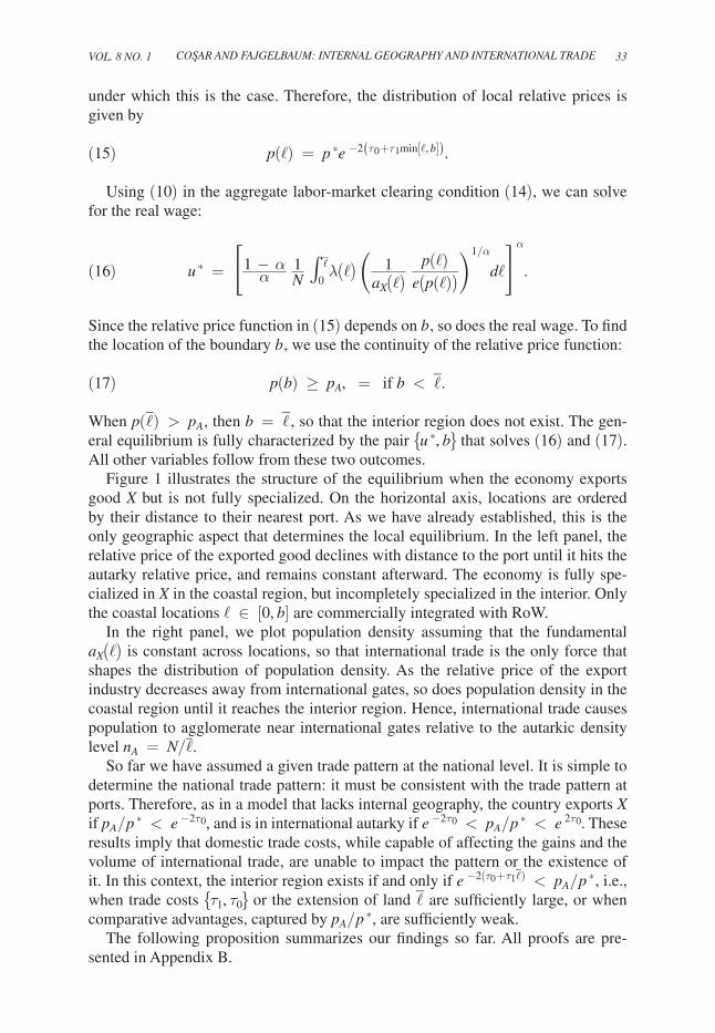
Figure 1 illustrates the structure of the equilibrium when the economy exports good X but is not fully specialized. On the horizontal axis, locations are ordered by their distance to their nearest port. As we have already established, this is the only geographic aspect that determines the local equilibrium. In the left panel, the relative price of the exported good declines with distance to the port until it hits the autarky relative price, and remains constant afterward. The economy is fully spe-cialized in X in the coastal region, but incompletely specialized in the interior. Only the coastal locations ℓ ∈ [0, b] are commercially integrated with RoW.
In the right panel, we plot population density assuming that the fundamental a X (ℓ) is constant across locations, so that international trade is the only force that shapes the distribution of population density. As the relative price of the export industry decreases away from international gates, so does population density in the coastal region until it reaches the interior region. Hence, international trade causes population to agglomerate near international gates relative to the autarkic density level n A = N/ ℓ –
.So far we have assumed a given trade pattern at the national level. It is simple to
determine the national trade pattern: it must be consistent with the trade pattern at ports. Therefore, as in a model that lacks internal geography, the country exports X if p A / p ∗ < e −2 τ 0 , and is in international autarky if e −2 τ 0 < p A / p ∗ < e 2 τ 0 . These results imply that domestic trade costs, while capable of affecting the gains and the volume of international trade, are unable to impact the pattern or the existence of it. In this context, the interior region exists if and only if e −2( τ 0 + τ 1
_ ℓ ) < p A / p ∗ , i.e.,
when trade costs { τ 1 , τ 0 } or the extension of land _ ℓ are sufficiently large, or when
comparative advantages, captured by p A / p ∗ , are sufficiently weak.The following proposition summarizes our findings so far. All proofs are pre-
sented in Appendix B.

34 AMEriCAN ECoNoMiC JourNAL: MiCroECoNoMiCs FEBruAry 2016
PROPOSITION 1 (Regional Specialization Pattern): There is a unique general equilibrium, in which:
(i) if the country trades internationally but is not fully specialized, there exists an autarkic interior region [b,
_ ℓ ] that is incompletely specialized
and a coastal region [0, b) that trades with roW and specializes in the export-oriented industry; and
(ii) the national trade pattern is determined independently from internal geography.
C. impact of international and Domestic Trade Costs
The experience of many developing countries shows that international trade inte-gration may be associated with shifts in economic concentration and industry loca-tion. In our model, population density varies across locations based on proximity to international gates and population density in the coastal region relative to the inte-rior region is endogenous. We summarize the impact of a discrete change in trade costs on these outcomes as follows.
PROPOSITION 2 (Internal Migration): A reduction in international or in domestic trade costs moves the boundary inland to b ′ > b and causes migration from region [c,
_ ℓ ] into region [0, c] for some c ∈ (b, b ′ ) . A lower τ 0 causes population at the port
n(0) to increase, but a lower τ 1 causes n(0) to decrease.
The direct impact of a reduction in trade costs is that the relative price of the exported industry increases in the coastal region, [0, b) . In the case of a reduction in τ 0 , the shift is uniform across locations, while a lower τ 1 results in a flattening of
Figure 1. Relative Prices and Population Density over Distance
Panel A: Relative price of the export industry Panel B: Population density
p(ℓ) n(ℓ)
p(0)
pA
n(0)
nA
ℓℓb ℓ
Specialized in X
Incompletely specialized
b ℓ
Specialized in X
Incompletely specialized

VoL. 8 No. 1 35cosar and fajgelbaum: internal geography and international trade
the slope of relative prices toward the interior. In both cases, the change in prices causes the relative price at b to be larger than the autarky price p A , so that locations at the boundary now find it profitable to specialize in export-oriented industries and the boundary moves inland.
What are the internal migration patterns associated with these reductions in trade costs? A natural consequence of lower trade costs is an increase in the real wage, u ∗ . Since in the autarkic interior region relative prices remain constant, labor demand shrinks. As a result, workers migrate away from locations that remain autar-kic toward the coast, and relative population density increases in the coastal region as result.
Figure 2 illustrates these effects. The solid line reproduces the initial equilib-rium from Figure 1. The dashed, double-dotted line represents a new equilibrium with lower international trade costs. The price function shifts upward and the intercept increases from p (0) to p 1 (0) , increasing population density at the port to n 1 (0) . Locations in [b, b ′ ] start trading, but the newly specialized locations [c, b ′ ] lose population. The dashed-dotted line shows the effect of a reduction in domestic trade costs. Prices at the port stay constant, but the slope flattens. As a result, population density at the port shrinks to n 2 (0) . In relative terms, locations at intermediate distances become more attractive when domestic trade costs decline. In both cases, population density is higher in [0, c] in the new equilibrium.
We move now to the impact of domestic trade costs τ 1 on the gains from interna-tional trade. We study the impact of trade costs on the real wage u ∗ , but we note that average real returns to land as well as national real income are proportional to the real wage u ∗ . Therefore trade costs have the same impact on the average real returns to both mobile and immobile factors.
We can consider two extreme cases. As τ 1 → ∞ , domestic trade becomes pro-hibitive so that b → 0 , and the country approaches international autarky. In that
Immigration Emigration
b ℓc b′
Panel A. Relative price of the export industry Panel B. Population density
Reduction in τ0
Reduction in τ1
p(ℓ) n(ℓ)
p1(0)
pA
p2(0), p(0)
n1(0)
n2(0)
n(0)
ℓ ℓ
Specialized in X
Inc. spec.
b ℓb′
Figure 2. Changes in Domestic and International Trade Costs

36 AMEriCAN ECoNoMiC JourNAL: MiCroECoNoMiCs FEBruAry 2016
case, all locations face the same relative price p (ℓ) = p A . We let u a be the real wage in that circumstance. In the other extreme, when τ 1 = 0 , then b =
_ ℓ , and all loca-
tions face the relative price p (ℓ) = p(0) . In that case, the real wage is
_ u = ( 1 − α ____ α Z __ N )
α p(0) ______ e (p(0)) ,
where
Z = ∫ 0 _ ℓ
λ (ℓ) _______
a X (ℓ) 1/α dℓ
measures the distribution of land and total productivity across locations. As in a standard neoclassical model, the real wage is increasing in the terms of trade, which are captured by p(0) . Diminishing returns to labor causes the real wage to decrease with the national labor endowment.
Using the solution for the real wage u ∗ from (16), the actual gains of moving from autarky to trade can be broken down as follows:
(18) u ∗ ___ u a = Ω (b; τ 1 ) ⋅ _ u __ u a ,
where we define the potential gains of moving from autarky to international trade as
_ u __ u a =
p (0) / e (p (0) ) __________
p A / e ( p A ) ,
and the effects of domestic trade frictions are captured by
(19) Ω (b; τ 1 ) = [ ∫ 0 _ ℓ λ (ℓ) / a X (ℓ) 1/α
___________ Z
( p (ℓ) / e (p (ℓ) )
__________ p (0) / e (p (0) ) )
1/α
dℓ]
α
.
The actual gains from trade, u ∗ / u a , equal the potential gains from trade without domestic trade costs, _ u / u a , adjusted by Ω ( τ 1 , b) . This function captures the impact of internal geography on the gains from trade. It is a weighted average of the losses caused by domestic trade costs in each location, with weights that correspond to each location’s absolute productivity level and land endowment relative to the coun-try aggregate. In turn, the location-specific losses from domestic trade costs are captured by the reduction in the terms of trade caused by distance. The total friction, Ω ( τ 1 , b) , is strictly below 1 as long as τ 1 > 0 , and it equals 1 if τ 1 = 0 .
How do the gains from trade depend on domestic trade costs? Naturally, the larger the size of the export-oriented region, the more a country should benefit from trade. Since τ 1 causes the export-oriented region to shrink, the gains from trade
VoL. 8 No. 1 37cosar and fajgelbaum: internal geography and international trade
decrease with domestic trade costs. Intuitively, a lower τ 1 makes exporting profitable for locations further away from the port, allowing economic activity to spread out and mitigate the congestion forces in dense coastal areas.
To formalize this, we define the elasticity of the consumer price index,
ε( p) = e′( p) ___ e ( p) p , and let s (ℓ) be the share of location ℓ in total employment. Given a
shock to p ∗ , τ 0 , or τ 1 , total differentiation of the labor clearing condition (14) and the condition (17) for b yield the change in the real wage:
(20) u ˆ ∗ = ∫ 0 b [1 − ε(p(ℓ))] s (ℓ) p ˆ (ℓ) dℓ,
where x ˆ represents the proportional change in variable x . This expression describes the aggregate gains from a reduction in trade costs, either domestic or interna-tional, as a function of the relative price change faced by export-oriented locations weighted by their population shares s (ℓ) . Reductions in domestic or international trade costs cause the relative price of the exported good to increase. This has a positive effect on revenues and a negative effect on the cost of living. The latter is captured by the price-index elasticity ε (p (ℓ) ) , and mitigates the total gains. In this context, (20) implies that the gains from an improvement in the terms of trade, caused by either lower τ 0 or larger p ∗ , are bounded above by the share of employ-ment in export-oriented regions.9
It follows from this reasoning that domestic and international trade costs are com-plementary, in that the gains from international trade are decreasing in domestic trade costs. Larger τ 1 causes relative export prices to decrease faster toward the interior, reducing the gains from trade:10
(21) d( u ∗ / u a ) _
d τ 1 < 0.
This aggregate effect of trade-cost reductions hides distributional effects between immobile factors located in different points of the country. The real returns to immo-bile factors at location ℓ are v (ℓ) ≡ r (ℓ) / E (ℓ) . The change in these returns at ℓ, when there are marginal changes in international or domestic trade costs, is
(22) v ˆ (ℓ) = 1 _ α [1 − ε (p (ℓ) ) ] p ˆ (ℓ) − 1 − α _ α u ˆ ∗ .
The first term measures the impact of relative price changes through both revenues and cost of living. The second part considers the economy-wide increase in real wages, which captures the emigration of mobile factors.
Consider first the interior locations ℓ ∈ (b, _ ℓ ] . In these places, p ˆ (ℓ) = 0 because
distance precludes terms of trade improvements, but mobile factors emigrate with
9 An increase in the terms of trade implies p ˆ (ℓ) = p ˆ for all ℓ ∈ [0, b] . Then, (20) gives u ˆ ∗ / p ˆ = β T ∫ 0 b [1 − ε (p (ℓ) ) ] s (ℓ) dℓ < ∫ 0 b s (ℓ) dℓ .
10 Formally, d τ 1 i > 0 implies p ˆ (ℓ) = − ℓd τ 1 i < 0 for all ℓ ∈ [0, b] so that u ˆ ∗ / d τ 1 < 0 , implying (21).

38 AMEriCAN ECoNoMiC JourNAL: MiCroECoNoMiCs FEBruAry 2016
trade reform because of the real wage increase. As a result, immobile factors in the interior (b,
_ ℓ ] region lose from lower trade costs. However, some immobile factors
located in the coastal areas ℓ ∈ [ 0, b) necessarily gain. Hence, reductions in both international and domestic trade costs generate redistribution of resources away from the interior to the coastal region.
However, outcomes for immobile resources in the coastal region are not uniformly positive. While on average the coastal region necessarily gains from improvements in international or domestic trade conditions, reductions in domestic trade costs τ 1 necessarily hurt immobile factors located at the port. In other words, coastal areas are better off if places further inside the country have poorer access to world markets.
We summarize these results as follows.
PROPOSITION 3 (Distributive Effects of Trade Across Regions): real income of immobile factors located in the interior region (b,
_ ℓ ] decreases with reductions in
international or internal trade costs, while on average the coastal locations [ 0, b) gain. There is some ε < b , such that real income of immobile factors in locations [ 0, ε ) decreases with reductions in domestic trade costs.
These distributional effects give rise to an inverted-U shape for inequality across immobile factors with internal integration. When the country is open to trade and τ 1 → ∞ , all locations other than the port are autarkic. Reducing internal trade costs leads to an initial increase in regional income inequality by expanding the coastal region, and thus benefiting newly integrated locations. But as τ 1 → 0 , inter-nal geography vanishes and outcomes are again symmetric in all locations within the country, eliminating income differences across locations.
D. Extensions
The benchmark model developed so far is purposely stylized to highlight the key forces of our analysis. In Appendix A, we characterize the local equilibrium and specialization patterns in more general model that allows for a non-tradable sector, location-specific amenities, capital as an additional (mobile) factor of production, and differences in capital and land intensity across sectors.
When the benchmark model is extended to allow for α X ≠ α M , so that land inten-sity may vary across sectors, the equilibrium features highlighted in Proposition 1 remain unchanged under a condition similar to (4). In that case, local autarky prices are the same in all locations, independent of their labor endowments, if and only if a X (ℓ) α M / a M (ℓ) α X is constant for all ℓ .11 If this condition holds, we ensure that the economy retains the dual-economy structure that we have described.12
11 From Appendix Table A1, we have that the autarky price p A (ℓ) corresponds to the unique value of p (ℓ) , such that ω X (ℓ) = ω y (ℓ) , where ω i (ℓ) is defined in (A11).
12 When α M ≠ α X , conditions ( ii )–( iv ) of the local equilibrium constitute a small Hecksher-Ohlin economy where the autarky price may in principle depend on factor endowments. However, labor mobility implies that the labor density is higher in places with more land abundance. This offsets the factor proportions effect, turning each local economy into a small Ricardian economy.

Vol. 8 No. 1 39cosar and fajgelbaum: internal geography and international trade
In turn, when the benchmark model is extended to allow for capital as an addi-tional factor of production, comparative advantages at the national level are also determined by factor endowments as in the Heckscher-Ohlin model. In Appendix A, we show that, if sector X is labor intensive, then it is the export-oriented sector if the national labor-land ratio n is sufficiently large. In the empirical analysis, we use industry labor intensity as a proxy for industry export orientation.
II. Comparative Advantage and Regional Specialization in China
The central mechanism of the model, from which its welfare and distributional implications stem, is the regional specialization pattern in export-oriented indus-tries: due to the interaction between national comparative advantages and inter-nal trade costs, export-oriented industries locate closer to international gates. This industry-location margin is not present in recent models of trade and internal geog-raphy such as Ramondo, Rodríguez-Clare, and Saborío-Rodríguez (2014); Redding (2014); or Allen and Arkolakis (2014).
We now turn to an empirical examination of this mechanism using data from China. We examine whether industries in which China has comparative advan-tages relative the rest of the world are more likely to locate in places with better access to international markets. We proxy for comparative advantages with national export-output ratios, and also rely on the argument that China’s comparative advan-tages lie on labor-intensive industries and proxy for comparative advantages using industry labor intensities from the United States.
Several factors make China a particularly suitable country for this exercise. Its rising external trade has been largely driven by its comparative advantages based on factor endowments. Before market-oriented reforms, it has been described as a closed agricultural economy with an economic structure lacking in industrial spe-cialization and agglomeration (Chan, Henderson, and Tsui 2008). After the reforms, increased industrial output and exports have been fueled by—among other fac-tors—a sustained wave of migration of workers into coastal regions (World Bank 2009).13
A. Data
Our regional data of Chinese industries is aggregated up from the firm-level Annual Survey of Industrial Production conducted by the Chinese government’s National Bureau of Statistics. The Annual Survey is a census of private firms with more than 5 million yuan (about $600,000) in revenue and all state-owned firms. It covers 338 mainland prefectures and 425 manufacturing industries in four -digit CSIS Chinese
13 China’s Household Registration System, also known as the Hukou system, was relaxed during the 1980s as part of market-oriented reforms. The current Hukou system limits the access of migrant workers to certain amenities, such as education and health, that are financed by local taxes. While the Hukou constitutes a cost to labor mobility, regional wage differentials have been sufficiently large to promote large migration flows to coastal provinces. See World Bank (2009).

40 AMEriCAN ECoNoMiC JourNAL: MiCroECoNoMiCs FEBruAry 2016
classification system between the years 1998–2007.14 Each industry-prefecture-year cell has information on employment, capital, revenue, value added, and exports by state-owned and private enterprises.15
To this data, we add the distance of each prefecture to China’s coastline. More precisely, we calculate the Euclidian distance from the administrative center of a prefecture to that of the nearest coastal prefecture. There are 53 coastal prefectures with zero distance and the median is 275 miles. An alternative distance measure using as terminal points those prefectures that host main international seaports gen-erates similar results since these facilities are scattered somewhat uniformly across the Pacific seaboard (see the map in the online Appendix). As reported below, an alternative measure based on travel times also generates similar results.
Several characteristics of China’s geography and trade suggest that distance to the coast is a good measure of foreign market access. Maritime transportation is the primary mode of shipping in external trade, while exports over land to bordering countries account for a small share ( 6.7 percent) of total exports (authors’ calcula-tion using 2006 UN Comtrade data). The share of air shipments in exports to top 20 trade partners is just 17.4 percent (Harrigan and Deng 2010). While inland rivers play an important role in freight transportation in general, their export share is lim-ited. Inland river ports, most of which are also in close proximity to the sea, consti-tute only 20 percent of port capacity (in terms of tonnage) suitable for international trade (authors’ calculation using data from Chinese Statistical Agency).
To carry out the empirical exercise, we need an industry-level measure of Chinese comparative advantages against the rest of the world. One possibility is to use prox-ies constructed from actual exports data, such as the industry export-revenue ratio. While this measure correlates with the underlying variation in relative productivity in which we are interested, to avoid endogeneity concerns it is desirable to use an industry measure that both proxies for comparative advantages and is exogenous to the Chinese environment. In what follows, we use export-revenue ratios for descrip-tive purposes, but also incorporate a second industry-specific measure, labor-capital ratio in the United States, to proxy for Chinese comparative advantages. In doing so, we draw on the notion that China has a comparative advantage in labor intensive industries.16
To construct industry-specific, labor-capital ratios in the United States, we use the publicly available NBER-CES Manufacturing Industry Database (Becker et al. 2013) and divide production worker hours by the total real capital stock for each industry.17 The NAICS 2002 classification—in which the US data is reported—can be mapped to the CSIS Chinese classification by using the official concordance between CSIS and ISIC Rev. 3 as a bridge. This reduces the number of industries
14 Prefectures are the second level of the Chinese administrative structure, contained within 31 provinces in mainland China. Due to administrative reclassifications, mostly before 2002, the number of prefectures and indus-tries varies slightly over the years.
15 The underlying firm-level data has been recently used by Hsieh and Klenow (2009) and Roberts et al. (2012). 16 In Appendix A, we develop an extension to the model where capital is also used in production. At the national
level, comparative advantages are determined as in the Heckscher-Ohlin model, so that X is the export-oriented sector if it is labor intensive and the country is sufficiently labor abundant.
17 With Cobb-Douglas technologies and common factor prices across sectors, industry labor intensities can be measured by labor-capital ratios.

VoL. 8 No. 1 41cosar and fajgelbaum: internal geography and international trade
to 120, still leaving us with enough variation to conduct our analysis. The US labor-capital ratio has a correlation coefficient of 0.6 with the Chinese labor-capital ratio, and a correlation coefficient of 0.4 with the Chinese export-revenue ratio. Table A1 in the Appendix provides further summary statistics.
B. Preliminary Analysis
As a preliminary check, we visualize the drop in regional openness toward the interior of the country. We average industry-prefecture-level observations over time and calculate export shares in prefectures’ revenues. Denoting industries by i , pre-fectures by p , and time by t , average regional export share (in logarithm) at the prefecture level is
Exportshar e p = ln ( ∑ t=1
T ( ∑ i X ipt ) ____________
T ) − ln ( ∑ t=1
T ( ∑ i r ipt ) ____________
T ) ,
where ( X ipt , r ipt ) stand for total exports and revenue at the industry-prefecture-year level. Panel A of Figure 3 plots this variable against the natural logarithm of the pre-fecture-specific distance measure introduced above. As expected, regional openness declines with distance. The elasticity is −0.73 and highly significant. The model generates this negative distance gradient for regional export shares through intensive and extensive margins. The mechanism of interest, however, is the latter, i.e., the change in industry composition against comparative-advantage industries toward the interior of the country. To preliminary assess whether declining regional export shares reflect this type of industry composition, panel B of Figure 3 plots industries’ export-revenue ratio at the national level (i.e., the share of exports in total industry revenue) against industry distance in logarithmic scale. The former variable equals
Exportshar e i = ln ( ∑ t=1
T ( ∑ p X ipt ) ____________
T ) − ln (
Σ t=1 T ( Σ p r ipt ) _
T ) .
Industry distance is defined as the employment-weighted average of prefecture distances:
Distanc e i = ∑ p
(
L ip _____ ∑ p
L ip
)
⋅ Distanc e p ,
where Distanc e p is prefecture p ’s distance and L ip is industry i ’s employment in pre-fecture p averaged over time. Therefore, the larger Distanc e i is, the farther industry i is located from the coast. If the gradient from panel A was exclusively generated by an intensive margin there would not be a definite relationship between the industry
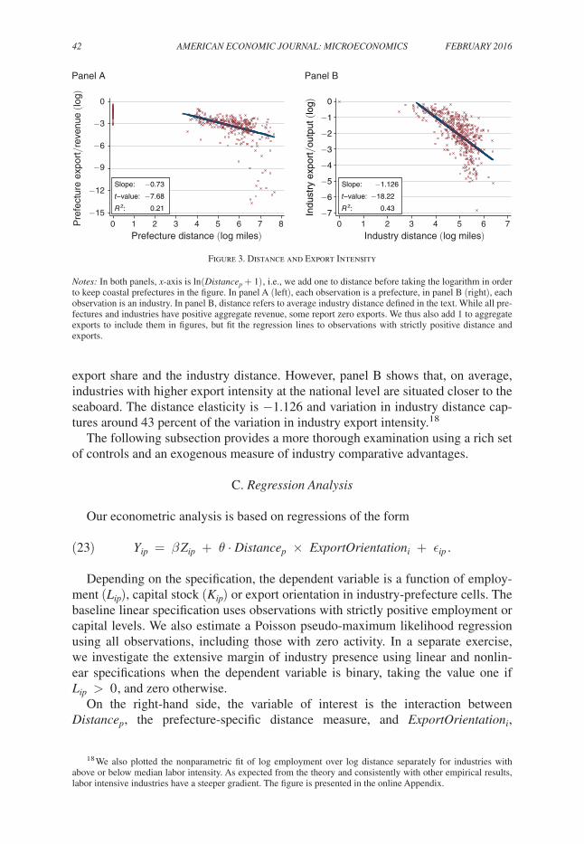
42 AMEriCAN ECoNoMiC JourNAL: MiCroECoNoMiCs FEBruAry 2016
export share and the industry distance. However, panel B shows that, on average, industries with higher export intensity at the national level are situated closer to the seaboard. The distance elasticity is −1.126 and variation in industry distance cap-tures around 43 percent of the variation in industry export intensity.18
The following subsection provides a more thorough examination using a rich set of controls and an exogenous measure of industry comparative advantages.
C. regression Analysis
Our econometric analysis is based on regressions of the form
(23) y ip = β Z ip + θ ⋅ Distanc e p × Exportorientatio n i + ϵ ip .
Depending on the specification, the dependent variable is a function of employ-ment ( L ip ), capital stock ( K ip ) or export orientation in industry-prefecture cells. The baseline linear specification uses observations with strictly positive employment or capital levels. We also estimate a Poisson pseudo-maximum likelihood regression using all observations, including those with zero activity. In a separate exercise, we investigate the extensive margin of industry presence using linear and nonlin-ear specifications when the dependent variable is binary, taking the value one if L ip > 0 , and zero otherwise.
On the right-hand side, the variable of interest is the interaction between Distanc e p , the prefecture-specific distance measure, and Exportorientatio n i ,
18 We also plotted the nonparametric fit of log employment over log distance separately for industries with above or below median labor intensity. As expected from the theory and consistently with other empirical results, labor intensive industries have a steeper gradient. The figure is presented in the online Appendix.
−15
−12
−9
−6
−3
0
Pre
fect
ure
expo
rt/r
even
ue (l
og)
0 1 2 3 4 5 6 7 8
Prefecture distance (log miles)
Slope: −0.73
t−value: −7.68
R2: 0.21 −7
−6
−5
−4
−3
−2
−1
0
Indu
stry
exp
ort/
outp
ut (l
og)
0 1 2 3 4 5 6 7
Industry distance (log miles)
Slope: −1.126
t−value: −18.22
R2: 0.43
Panel A Panel B
Figure 3. Distance and Export Intensity
Notes: In both panels, x-axis is ln (Distanc e p + 1) , i.e., we add one to distance before taking the logarithm in order to keep coastal prefectures in the figure. In panel A (left), each observation is a prefecture, in panel B (right), each observation is an industry. In panel B, distance refers to average industry distance defined in the text. While all pre-fectures and industries have positive aggregate revenue, some report zero exports. We thus also add 1 to aggregate exports to include them in figures, but fit the regression lines to observations with strictly positive distance and exports.

VoL. 8 No. 1 43cosar and fajgelbaum: internal geography and international trade
an industry-specific export orientation measure. As discussed above, we use two variables here: Chinese export-revenue ratios ( CNX r i ) and US labor-capital ratios ( usL K i ).19
Our model predicts a negative coefficient θ < 0 , i.e., export-oriented industries should be more likely to locate closer to the coast.20 Depending on the specification, the set of other covariates Z ip includes direct effects of the interacted variables or various fixed effects.
In all the regressions where usL K i is used, we only exploit the cross-sectional variation from our data by taking time averages over the period 1998–2007. The data on export-revenue ratios ( CNX r it ) allows us to investigate our model prediction on regional specialization not only in cross section but also in the panel dimension. The model predicts that, in a period of trade liberalization, industries that increase export-output ratios increase their presence closer to coastlines. In addition to the cross-sectional specifications described above, we estimate a separate panel regres-sion with industry-specific fixed effects using the export-revenue ratios.
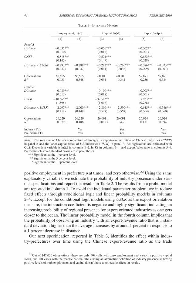
Table 1 reports the baseline cross-sectional results using time averages for all vari-ables when the dependent variable is the natural logarithm of employment (columns 1–2), capital (columns 3– 4) or the level of export-output ratio (columns 5–6), using nonzero observations. Columns 2, 4, and 6 feature industry and prefecture fixed effects. Panel A uses export-revenue ratios and panel B uses industry capital-labor ratios as proxy for industry comparative advantages. Standard errors are clustered at the prefecture level. As expected, regional employment, capital stock and export orientation decline with distance, reflecting the gradient of population density and economic activity in China. The coefficient of interest on the interaction term is negative and highly significant in all specifications.
To give a sense of the economic importance of the results, we use the interaction coefficients equal to −0.288 and −2.9 reported in the second column of panel A and B, respectively. Consider an industry with an average export-revenue ratio of 0.21. Moving inland by 275 miles, which is the median distance from the coast across prefectures, decreases regional employment by 17 percent for such an industry. The same decline is 32 percent for an industry with an export-revenue ratio one standard deviation (equal to 0.19) higher than the average. These magnitudes are 13 and 21 percent for the average and high labor-intensity industries, respectively. This is a fairly sizable impact on regional specialization.21
Given the high level of spatial and industry disaggregation in our data, it is nat-ural that not all industries will be observed in every prefecture. Approximately 58 percent of all prefecture-industry combinations in our data report zero employment. To exploit this extensive margin variation, we define the dependent variable in the estimation equation (23) as a binary variable that takes the value one if industry i has
19 As an alternative measure of export orientation, we also use the Balassa (1965) revealed comparative advan-tage ( CNrCA ) index. The correlation between CNrCA and CNXr is around 0.7, and the results are both qualita-tively and quantitatively very similar. RCA based results are available from the authors upon request.
20 In the model, the export-revenue ratio at the national level is positive for the comparative-advantage industry and zero for the import-competing industry. Adding product differentiation to the model would generate positive export-revenue ratios for both industries.
21 As Table A1 shows, the mean export-revenue ratio across all years is 0.21 with a standard deviation of 0.19. Since distance is measured in 100 miles, we multiply − 0.288 · 0.40 · 2.75 = − 0.317 .
44 AMEriCAN ECoNoMiC JourNAL: MiCroECoNoMiCs FEBruAry 2016
positive employment in prefecture p at time t , and zero otherwise.22 Using the same explanatory variables, we estimate the probability of industry presence under vari-ous specifications and report the results in Table 2. The results from a probit model are reported in column 1. To avoid the incidental parameter problem, we introduce fixed effects through conditional logit and linear probability models in columns 2–4. Except for the conditional logit models using usLK as the export orientation measure, the interaction coefficient is negative and highly significant, indicating an increasing probability of regional presence for export oriented industries as one gets closer to the ocean. The linear probability model in the fourth column implies that the probability of observing an industry with an export-revenue ratio that is 1 stan-dard deviation higher than the average increases by around 1 percent in response to a 1 percent decrease in distance.
Our next specification, reported in Table 3, identifies the effect within indus-try-prefectures over time using the Chinese export-revenue ratio as the trade
22 Out of 147,030 observations, there are only 509 cells with zero employment and a strictly positive capital stock, and 104 cases with the reverse pattern. Thus, using an alternative definition of industry presence as having positive levels of both employment and capital doesn’t have a noticeable effect on results.
Table 1—Intensive Margin
Employment, ln(L) Capital, ln(K) Export/output
(1) (2) (3) (4) (5) (6)
Panel A Distance −0.035*** −0.050*** −0.002**
(0.010) (0.012) (0.001)CNXr 0.818*** −0.521*** 0.683***
(0.145) (0.149) (0.028)Distance × CNXr −0.293*** −0.288*** −0.283*** −0.216*** −0.086*** −0.073***
(0.037) (0.037) (0.041) (0.036) (0.009) (0.007)
Observations 60,505 60,505 60,100 60,100 59,871 59,871 r
2 0.033 0.348 0.031 0.342 0.236 0.384
Panel B Distance −0.089*** −0.100*** −0.005***
(0.013) (0.018) (0.001)usLK −10.66*** −37.59*** 5.823***
(1.598) (1.696) (0.278)Distance × usLK −2.997*** −2.900*** −2.809*** −2.550*** −0.645*** −0.546***
(0.418) (0.448) (0.527) (0.569) (0.064) (0.060)
Observations 26,229 26,229 26,091 26,091 26,024 26,024 r
2 0.0796 0.486 0.0983 0.476 0.111 0.394
Industry FEs Yes Yes YesPrefecture FEs Yes Yes Yes
Notes: The measure of China’s comparative advantages is export-revenue ratios of Chinese industries (CNXr) in panel A and the labor-capital ratios of US industries (usLK) in panel B. All regressions are estimated with OLS. Dependent variable is ln(L) in columns 1–2, ln(K) in columns 3–4, and export/sales ratio in columns 5–6. Prefecture-clustered standard errors are in parentheses.
*** Significant at the 1 percent level. ** Significant at the 5 percent level. * Significant at the 10 percent level.

VoL. 8 No. 1 45cosar and fajgelbaum: internal geography and international trade
Table 3—Time Variation
ln(L)(1)
ln(L)(2)
ln(K)(3)
ln(K)(4)
Extensive margin(5)
CNXr 0.369*** 0.155 −0.005(0.140) (0.128) (0.008)
Distance × CNXr −0.206*** −0.145*** −0.176*** −0.151*** −0.005***(0.04) (0.034) (0.041) (0.04) (0.001)
Observations 361,580 361,580 362,652 362,652 1,363,315 r
2 0.818 0.841 0.800 0.817 0.732Year FEs Yes Yes YesIndustry-prefecture FEs Yes Yes Yes Yes YesIndustry-year FEs Yes YesPrefecture-year FEs Yes Yes
Notes: All panel regressions are estimated with year and industry-prefecture fixed effects. Dependent variables are the logarithm of employment L or capital K at industry-prefecture-year cells with positive observations in the first four columns. Dependent variable in the fifth column is a binary variable that takes the value one if L > 0 and zero otherwise. Prefecture-clustered standard errors are in parentheses.
*** Significant at the 1 percent level. ** Significant at the 5 percent level. * Significant at the 10 percent level.
Table 2—Extensive Margin
(1) (2) (3) (4)
Panel A Distance −0.029*** −0.035***
(0.003) (0.001)CNXr −0.175*** −0.247***
(0.026) (0.029)Distance × CNXr −0.0661*** −0.081*** −0.082*** −0.01***
(0.007) (0.007) (0.008) (0.004)
Observations 147,030 147,030 147,030 147,030 r
2 (pseudo- r 2 ) 0.088 0.111 0.027 0.434
Panel B Distance −0.034*** −0.047***
(0.003) (0.003)usLK −3.061*** −5.005***
(0.347) (0.466)Distance × usLK −0.149** −0.125 −0.118 −0.137**
(0.076) (0.186) (0.1) (0.0689)
Observations 39,884 39,884 39,412 39,884 r
2 (pseudo- r 2 ) 0.09 0.13 0.01 0.461
Regression Probit Clogit Clogit LPMIndustry FEs Yes YesPrefecture FEs Yes Yes
Notes: The measure of China’s comparative advantages is export-revenue ratios of Chinese industries (CNXr) in panel A and the labor-capital ratios of US industries (usLK) in panel B. Dependent variable equals one if there is positive industry employment in a prefecture-year, zero otherwise. Specifications: column 1 probit, columns 2–3 conditional logit, column 4 lin-ear probability model. Pseudo- r
2 values of fit are reported for probit and conditional logit models. Marginal effects reported for probit and conditional logit. Prefecture-clustered stan-dard errors are in parentheses.
*** Significant at the 1 percent level. ** Significant at the 5 percent level. * Significant at the 10 percent level.

46 AMEriCAN ECoNoMiC JourNAL: MiCroECoNoMiCs FEBruAry 2016
measure. Instead of separate industry and prefecture fixed effects, now we use industry-prefecture fixed effects in order to control for unobserved, time-invariant factors that affect economic outcomes at the industry-prefecture level. In columns 2 and 4, we also include industry-year and prefecture-year fixed effects. The interac-tion coefficient is still significantly negative, implying that the previously estimated effects are not solely due to cross-sectional variation: employment (or capital stock) in industries that have become more export-oriented at the national level during the data period increased relatively more in prefectures close to China’s seaboard.
D. Alternative Mechanisms
We now examine alternative mechanisms that could also generate this empiri-cal pattern. First, our approach to explaining regional specialization complements explanations based on location fundamentals such as Courant and Deardorff (1992) and on external economies of scale as in Rossi-Hansberg (2005). Following these views, it could be that, closer to international gates, either endowments or externali-ties drive high relative productivity in specific industries which then become export oriented.
In light of these forces, we should observe that relative productivity in export-oriented industries decreases as we move away from international gates. To inspect if this pattern is present in China we replace the dependent variable in the estimation equation (23) with measures of local industry productivity. We define value added per worker and per unit of capital as
V L ip = ValueAdde d ip _ L ip
, V K ip = ValueAdde d ip _ K ip
,
and regress the natural logarithms of these variables on the interaction variable of interest and fixed effects. The results are in Table 4. We expect a negative interaction if these alternative explanations are driving the regional specialization patterns that we find.
While there is a negative gradient for labor productivity when CNXr is used to proxy export orientation (first column of panel A), capital productivity increases toward coastal prefectures for industries with higher export orientation using either measure (second column of panel A and B). However, this is not robust to exclud-ing state-owned enterprises while constructing the regional data. Doing this ren-ders the interaction coefficient on capital productivity significant at 10 percent only (fourth column, both panels), pointing toward the existence of unproductive, capital-intensive, state-owned enterprises located in interior prefectures, operating in industries with low export orientation. These capital-intensive industries are not major exporters: the correlation between the industry-wide capital-labor ratio (in China) and industry-wide export-revenue ratio is −0.3. Therefore, interior state-owned enterprises in capital-intensive industries create the impression that coastal prefectures have higher value added per unit of capital in export-oriented industries. A likely explanation for this pattern lies in Chinese regional planning strategy in the pre-reform era, which located heavy industries in interior provinces for national

VoL. 8 No. 1 47cosar and fajgelbaum: internal geography and international trade
security purposes (see Gao 2004). Hence, while we find some association between the market-access gradient for the location of export-oriented industries and their productivity gradient, the relationship is weak once state-owned enterprises are excluded.
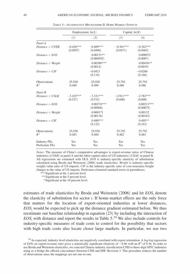
Second, our approach also complements explanations within the New Economic Geography tradition of Krugman (1991). In this view, industries with larger scale economies are more likely to locate in regions with high population density or close to gateways to large markets. Hanson and Xiang (2004) show that this mechanism is empirically relevant in international trade, i.e., more differentiated industries concentrate in large countries. Therefore, the specialization pattern that we find could result from industries with larger returns to scale situating closer to the sea-board, where many of the largest Chinese cities are historically located. Given that location, it is possible that these industries in turn become exporters to the rest of the world. Also, such industries are likely to have higher intra-industry trade, which would make the export-revenue measure less precise in capturing underlying com-parative advantages.
To control for this channel, we follow Hanson and Xiang (2004) and use indus-try elasticities of substitution as a measure of scale economies.23 We use the
23 In Krugman (1980), higher product differentiation, captured by a lower elasticity of substitution, leads to larger revenues per worker and accentuates the returns to scale. Clearly, there may be other industry-specific char-acteristics related to returns to scale, such as product differentiation on the inputs side.
Table 4—Alternative Mechanisms I: Local Productivity
ln(AVL)(1)
ln(AVK)(2)
ln(AVL)(3)
ln(AVK)(4)
Panel A Distance × CNXr −0.014 −0.078*** 0.044*** −0.0302*
(0.014) (0.017) (0.017) (0.017)
Observations 58,999 58,932 54,171 54,119 r
2 0.279 0.183 0.251 0.156
Panel B Distance × usLK −0.718** −1.086*** 0.0461 −0.541*
(0.278) (0.262) (0.238) (0.288)
Observations 25,728 25,705 23,969 23,946 r
2 0.339 0.222 0.316 0.194
Industry FEs Yes Yes Yes YesPrefecture FEs Yes Yes Yes YesOwnership All All Private Private
Notes: The measure of China’s comparative advantages is export-revenue ratios of Chinese industries (CNXr) in panel A and the labor-capital ratios of US industries (usLK) in panel B. All regressions are estimated with OLS. AVL and AVK stand for Average Value Added of Labor, and of Capital, respectively. Distance is the prefecture-specific distance measure defined in the text. The first two columns use data for all ownership types whereas the last two columns exclude state-owned enterprises. Prefecture-clustered standard errors are in parentheses.
*** Significant at the 1 percent level. ** Significant at the 5 percent level. * Significant at the 10 percent level.
48 AMEriCAN ECoNoMiC JourNAL: MiCroECoNoMiCs FEBruAry 2016
estimates of trade elasticities by Broda and Weinstein (2006) and let Eo s i denote the elasticity of substitution for sector i . If home-market effects are the only force that matters for the location of export-oriented industries at lower distances, Eo s i would be expected to pick up the distance gradient estimated before. We thus reestimate our baseline relationship in equation (23) by including the interaction of Eo s i with distance and report the results in Table 5.24 We also include controls for industry-specific measures of trade costs to control for the possibility that sectors with high trade costs also locate closer large markets. In particular, we use two
24 As expected, industry-level elasticities are negatively correlated with export orientation. A log-log regression of Eo s i on export-revenue ratio gives a statistically significant elasticity of − 0.96 with an r 2 of 0.36 . In order to use Broda and Weinstein elasticities, we concord Chinese industry classification CSIS to three-digit SITC industries using as a bridge the official concordance between CSIS and ISIC Revision 3. This procedure reduces the number of observations since the mappings are not one-to-one.
Table 5—Alternative Mechanisms II: Home Market Effects
Employment, ln(L) Capital, ln(K)
(1) (2) (3) (4)
Panel A Distance × CNXr −0.426*** −0.409*** −0.361*** −0.342***
(0.0507) (0.0496) (0.0471) (0.0465)Distance × Eos 0.00131** 0.000972
(0.000595) (0.0007)Distance × Weight 0.00380*** 0.00436**
(0.0014) (0.0019)Distance × CiF −0.0421 −0.0286
(0.116) (0.166)
Observations 25,928 25,928 25,792 25,792 r
2 0.489 0.489 0.486 0.486
Panel B Distance × usLK −3.425*** −3.331*** −2.911*** −2.782***
(0.527) (0.532) (0.600) (0.608)Distance × Eos 0.00274*** 0.00213***
(0.00068) (0.00075)Distance × Weight 0.000171 0.00132
(0.00136) (0.00181)Distance × CiF 0.480*** 0.405**
(0.122) (0.161)
Observations 25,928 25,928 25,792 25,792 r
2 0.483 0.484 0.482 0.483
Industry FEs Yes Yes Yes YesPrefecture FEs Yes Yes Yes Yes
Notes: The measure of China’s comparative advantages is export-revenue ratios of Chinese industries (CNXr) in panel A and the labor-capital ratios of US industries (usLK) in panel B. All regressions are estimated with OLS. Eos is industry-specific elasticity of substitution calculated using Broda and Weinstein (2006) trade elasticities. Weight is industry-specific weight/value ratio of US imports. CiF is the industry-specific ratio of cost-insurance-freight charges to the value of US imports. Prefecture-clustered standard errors in parentheses.
*** Significant at the 1 percent level. ** Significant at the 5 percent level. * Significant at the 10 percent level.

VoL. 8 No. 1 49cosar and fajgelbaum: internal geography and international trade
measures of trade costs: the weight/value ratio and the ratio of CIF charges to the value of imports calculated from the Census US Imports of Merchandise data.
The interaction between Eo s i is positive and typically significant, implying that more differentiated industries (lower Eo s i ) locate relatively closer to seaboards. This confirms that home market effects based on product differentiation are an important determinant of industry location in China. However, the main interaction term between distance and industry export orientation remains stable with a nega-tive sign and statistically significant.25
III. Conclusion
We developed a theory that combines a neoclassical international trade struc-ture with an internal geography. In the model, international trade creates a partition between a commercially integrated coastal region with high population density and an interior region where immobile factors are poorer. Reductions in domestic or international trade costs generate migration to the coastal region and net welfare losses for immobile factors in the interior region. Qualitatively, these outcomes are consistent with the spatial structure of economic activity in large developing countries such as China or India where coastal regions integrated with the rest of the world coexist with remote and commercially isolated corners within the country.
A key feature of the model is that comparative-advantage industries at the national level locate closer to international gates. We find evidence consistent with this pattern in industry-level data from Chinese prefectures. Previous work in economic geogra-phy and international trade highlights the importance of relative productivities and scale economies for industry location, but these channels do not fully account for the patterns that we find. A full quantitative evaluation of the relative importance of the forces in our model relative to other mechanisms in shaping industry location is out-side the scope of this paper and would be an interesting question for future research.
Appendix
A. Derivation of Equilibrium outcomes
We characterize local-equilibrium outcomes in a model that, in addition to the ingredients in the baseline model, also allows for a nontradable sector (with share 1 − β T in consumption), location-specific amenities m (ℓ) , capital as an additional factor of production (with share 1 − γ i in production per unit of land in sector i ), and differences in land intensity α i across sectors. The model in the text corresponds to the case when β T = γ i = 1, for all i , m (ℓ) = 1 for all ℓ , and α X = α M .
Utility of an agent who lives in ℓ is m (ℓ) C T (ℓ) β T C N (ℓ) 1− β T , where C T (ℓ) is a consumption basket of tradables that includes X and M , C N (ℓ) is consumption of
25 We also checked the robustness of results to using a Poisson pseudo-maximum likelihood estimator that allows us to include observations with zero employment in the estimation, to excluding autonomous interior prov-inces, coastal prefectures or state-owned enterprises, and to using as market access measures the travel time to the nearest international port. All results go through and additional insights into China’s economic geography arise. These results are presented in the online Appendix.

50 AMEriCAN ECoNoMiC JourNAL: MiCroECoNoMiCs FEBruAry 2016
nontradables, and m (ℓ) is the level of amenities at ℓ . (The preferences in equation (1) in the text are the special case when β T = m (ℓ) = 1 ).
The land endowment λ (ℓ) in each location is owned by immobile landowners that consume where they live. There are two types of mobile agents: workers (who own only labor) and capital-owners (who own only capital).
Indirect utility of a worker who lives in ℓ is u(ℓ) = m (ℓ) w (ℓ) _ E(ℓ ) , where w(ℓ ) is the
wage at ℓ , and E(ℓ ) is the cost-of-living index, which includes the (homothetic) price index for tradables E T (ℓ) and the price of nontradables P N (ℓ) :
(A1) E (ℓ) = E T ( P X (ℓ), P M (ℓ)) β T P N (ℓ) 1− β T .
We let p(ℓ) ≡ P X (ℓ)/ P M (ℓ) be the relative price in sector X , so that there exists an increasing and concave function e( p(ℓ)) satisfying E T (ℓ) = P M (ℓ) e (p (ℓ) ) . The (endogenous) real wage, common to all locations in equilibrium, is u ∗ .
Indirect utility of a capital-owner is m (ℓ) r k (ℓ) _ E(ℓ ) , where r k (ℓ) is the return to each
unit of capital. Capital owners are mobile both across locations within the country and between the country and the rest of the world, where they can obtain an outside option r k ∗ .
Demand for nontradables per unit of land in ℓ is c N (ℓ) = (1 − β T ) y (ℓ) / P N (ℓ) , where y (ℓ) is income per unit of land at ℓ . Income in each location is generated by land, capital, and labor, so that y (ℓ) = [w (ℓ) n (ℓ) + r k (ℓ) k (ℓ) + r (ℓ) ] λ (ℓ) , where k (ℓ) is the endogenous capital density.
The technology to produce output per unit of land is
q i (ℓ) = κ i _ a i (ℓ)
( ( n i (ℓ) _ γ i )
γ i
( k i (ℓ) _
1 − γ i )
1− γ i
)
1− α i
,
for i = N, M, X, where κ i = (1 − α i ) − (1− α i ) α i − α i . Land intensity in production is
α i and labor intensity per unit of land is γ i (the production technologies defined in (3) in the text are the special case when γ i → 1 ).
The local equilibrium definition is similar to Definition 1, with the following addi-tions: the nontradable market clears, the market-clearing conditions include land and labor used in the nontradable sector, there is an extra market clearing condition for capital, and real returns to capital are equalized throughout the country. Specifically, a local equilibrium at ℓ consists of population density n (ℓ) , capital density k (ℓ) , labor and capital demands { n i (ℓ) , k i (ℓ) } i=X, M , patterns of land use { λ i (ℓ) } i=X, M , and factor prices {w (ℓ) , r(ℓ), r k (ℓ) } such that
(i) workers maximize utility,
(A2) u(ℓ ) ≤ u ∗ , = if n (ℓ) > 0 ;
(ii) returns to capital are equalized
VoL. 8 No. 1 51cosar and fajgelbaum: internal geography and international trade
(A3) m (ℓ) r k (ℓ) _ E(ℓ ) ≤ r k ∗ , = if k (ℓ) > 0 ;
(iii) profits are maximized,
(A4) π i (ℓ) ≤ 0, = if λ i (ℓ) > 0, for i = X, M, N
where π i (ℓ) is given by (2);
(iv) land, labor, and capital markets clear,
(A5) ∑ i=X, M, N
λ i (ℓ) = λ(ℓ),
(A6) ∑ i=X, M, N
λ i (ℓ ) _ λ(ℓ ) n i (ℓ ) = n (ℓ) ,
(A7) ∑ i=X, M, N
λ i (ℓ ) _ λ(ℓ ) k i (ℓ ) = k (ℓ) ,
(v) nontraded sector clears, and
(vi) trade is balanced.
The profit maximization of landowners in ℓ is
(A8) π i (ℓ) = max n i (ℓ), k i (ℓ)
{ P i (ℓ) q i [ n i (ℓ)] − w(ℓ) n i (ℓ) − r k (ℓ) k i (ℓ) − r (ℓ) } .
Defining ω (ℓ) ≡ w (ℓ) /r (ℓ) as the wage-to-land rental ratio at ℓ and using the indifference conditions (A2) and (A3), the profit maximization condition (A4) can be written:
(A9) P i (ℓ) ≤ a i (ℓ) w(ℓ) _____ ω (ℓ) α i ( r k
∗ _ u ∗ ) (1− γ i ) (1− α i )
, = if λ i (ℓ) > 0
for i = X, M, N . In every populated location, (A9) binds for i = N if n (ℓ) > 0 . Using the definition of u(ℓ) together with the price for nontradables P N (ℓ) from (A9) gives the wage at ℓ that leaves workers indifferent:
(A10) w (ℓ) = E T (ℓ) ( u ∗ _ m (ℓ) )
1 __ β T ( a N (ℓ)
_ ω (ℓ) α N ) 1− β T ____ β T
( r k ∗ _ u ∗ )
(1− α N ) (1− α N ) 1− β T _ β T
.

52 AMEriCAN ECoNoMiC JourNAL: MiCroECoNoMiCs FEBruAry 2016
Using (A9), (A10), and the definition of the price index (A1) we solve for the wage-rental ratio in a location that produces in tradable sector i ∈ {X, M} ,
(A11) ω i (ℓ) = [ a i (ℓ) β T a N (ℓ) 1− β T ( E T (ℓ ) _ P i (ℓ)
) β T
( u ∗ ) 1− δ i ( r k ∗ ) δ i __________
m (ℓ) ]
1 ____________ β T α i + (1− β T ) α N
,
where δ i ≡ (1 − α N ) (1 − γ N ) (1 − β T ) + (1 − α i ) (1 − γ i ) β T .
specialization Patterns.—From (A9), if λ i (ℓ) > 0 , then ω i (ℓ) ≤ ω j (ℓ) for i, j = X, M and i ≠ j . Also, note that ω X (ℓ) is increasing in p (ℓ) and ω M (ℓ) is strictly decreasing in p (ℓ) , so that the wage-rental ratio increases with the relative price of the good exported by the location. Therefore, the local economy is fully special-ized in X when p (ℓ) > p A (ℓ) and fully specialized in M when p (ℓ) < p A (ℓ) , where p A (ℓ) is the the unique value of p (ℓ) , such that ω X (ℓ) = ω y (ℓ) . As mentioned in Section ID, this implies that if β T = m (ℓ) = 1 but α X ≠ α M , then p A (ℓ) is inde-pendent from ℓ if and only if a X (ℓ) α M / a M (ℓ) α X is independent from ℓ .
Since the local economy is incompletely specialized in autarky, p A (ℓ) must be the autarky price. When α X = α M (so that both tradable sectors use capital with the same intensity) then:
p A (ℓ) = ( u ∗ _ r k ∗ )
δ M − δ X _____ β T a X (ℓ) _ a M (ℓ) .
In this case, we have as in the main text that p A (ℓ) is the same across locations
when a X (ℓ) _ a M (ℓ) = a . In addition, comparative advantages at the national level are also
determined by factor endowments as in the Heckscher-Ohlin model. Assuming that sector X is labor intensive ( γ X > γ M , which implies δ M > δ X ) and the national labor-land ratio n is sufficiently large (so that u ∗ , and therefore the relative autarky price of X , p A , is small enough) implies that X is the export-oriented sector.
Employment Density.—To solve for population density n (ℓ) , we combine the labor and capital demand derived from (A8) with the market clearing conditions (A5) to (A7), the labor and capital mobility conditions (A2) and (A3), and the mar-ket clearing condition in the nontraded sector. When a local economy is fully spe-cialized in the production of i ∈ {X, M} and N , we can solve this system to obtain
(A12) n (ℓ) = 1 − ζ 1i − ζ 2i _ ζ 1i 1 _
ω i (ℓ) ,
VoL. 8 No. 1 53cosar and fajgelbaum: internal geography and international trade
where ω i (ℓ) is given in (A11), and where { ζ 1i , ζ 2i } are a function of the parameters.26 This condition is the generalized version of equation (10) in the text. When capital is not used in production ( γ i = 1 for i = X, M, N ) then labor density is:
(A13) n (ℓ) = 1 − _ α i _ _ α i [
z i (ℓ) _ u ∗ ( E T (ℓ) _ P i (ℓ)
) β T
]
1/ _ α i
for i = X, M ,
where _ α i ≡ β T α i + (1 − β T ) α N and z i (ℓ) ≡ m (ℓ) / ( a i (ℓ) β T a N (ℓ) 1− β T ) .
B. Proofs
The following results are shown under the assumption that α X = α M = α so that _ α i = _ α in the model from Appendix A.
PROOF OF PROPOSITION 1:For (i), we have that if the country is a net exporter of X , all locations that trade
with RoW must produce X . Condition (13) then implies that e −2 ( τ 0 + τ 1 ℓ) p ∗ ≤ p(ℓ) . Therefore, all locations, such that e −2 ( τ 0 + τ 1 ℓ) p ∗ > p A , cannot be in autarky and
must specialize in X . In turn, since the country is not fully specialized, there must be autarkic locations for which e −2 ( τ 0 + τ 1 ℓ) p ∗ < p A . Therefore, there must exist b <
_ ℓ
such that e −2 ( τ 0 + τ 1 b) p ∗ = p A . For (ii), we have that, if p A / p ∗ < e −2 τ 0 but the
country is in international autarky or exports M , then the no-arbitrage conditions (12) and (13) are violated. In that case, equilibrium condition (17) implies that b <
_ ℓ ↔ p A / p ∗ < e 2( τ 0 + τ 1
_ ℓ ) . Similar reasoning applies when the country
exports M . Finally, if e −2 τ 0 < p A / p ∗ < e 2 τ 0 but the country exports X or M then the no-arbitrage conditions (12) and (13) are violated.
PROOF OF PROPOSITION 2:From (17), it follows that b is decreasing with τ 1 or τ 0 . Therefore, b ′ > b when
either τ 1 or τ 0 decreases. Consider the case when the economy is a net exporter of X
and let p (ℓ) ′ and n (ℓ) ′ be the relative price and density in the new equilibrium with
τ 0 ′ < τ 0 or τ 1 ′ < τ 1 . Note that ∂ n (ℓ) ′ ______ ∂ ℓ < 0 and | ∂ n (ℓ) ′ ______ ∂ ℓ 1 _____
n (ℓ) ′ | ≤ | ∂ n (ℓ) _ ∂ ℓ 1 _ n (ℓ) | for all
26 These coefficients are given by
ζ 1i = α N (1 − β T ) + α i 1 − (1 − β T ) [ α N + (1 − α N ) ( γ N _____
1 − γ N ) 1− γ N
+ (1 − α i ) ( γ N _____ 1 − γ N )
− γ N ] ________________________________________________
α i + (1 − α i ) γ i − γ i (1 − γ i ) − (1− γ i )
,
ζ 2i = (1 − α i )
⎧
⎪
⎨ ⎪ ⎩ (1 − β T ) ( γ N _
1 − γ N ) − γ N
+ ( γ i _ 1 − γ i
) − γ i
1 − (1 − β T ) [ α N + (1 − α N ) ( γ N _____
1 − γ N ) 1− γ N
+ (1 − α i ) ( γ N _____ 1 − γ N )
− γ N ] ________________________________________________
α i + (1 − α i ) γ i − γ i (1 − γ i ) − (1− γ i )
⎫
⎪
⎬ ⎪ ⎭ .

54 AMEriCAN ECoNoMiC JourNAL: MiCroECoNoMiCs FEBruAry 2016
ℓ ∈ [ 0, b) . Therefore, n (b) ′ > n (b) , for otherwise ∫ 0 _ ℓ n (ℓ) ′ λ (ℓ) dℓ < N . Also note
that p (ℓ) = p (ℓ) ′ = a for all ℓ ∈ (b, _ ℓ ] and that u ∗ is higher in the new equilib-
rium. Since n (b′) ′ < n (b′) , there must be c ∈ [b, b ′ ] such that n (c) ′ = n (b) . We conclude that n (ℓ) ′ − n (ℓ) > 0 ↔ ℓ < c , so that population density increases in [0, c] . When τ 0 shrinks, n (0) ′ > n (0) , for otherwise ∫ 0
_ ℓ n (ℓ) ′ λ (ℓ) dℓ < N . In con-
trast when τ 1 shrinks then n (0) ′ < n (0) , since u ∗ is higher in the new equilibrium, but p (0) = p (0) ′ .
PROOF OF PROPOSITION 3:The real return to immobile factors at ℓ is v (ℓ) = r (ℓ) / E (ℓ) . Using (A13) and
u(ℓ) = u ∗ , we can write
v (ℓ) = _ α _ 1 − _ α n (ℓ) u ∗ ,
so that the real return to land at the national level, ∫ 0 _ ℓ v (ℓ) λ (ℓ) dℓ , equals
(A14) v = _ α _ 1 − _ α N u ∗ .
In turn, using (10), the percentage change in population density in each location in response to an arbitrary change in relative prices or in the real wage is
(A15) n ˆ (ℓ) = β T _ _ α [1 − ε T ( p (ℓ) )] p ˆ (ℓ) − 1 _ _ α u ˆ ∗ .
The percentage change in the real return to immobile factors at ℓ is given by (22) in the text. In turn, the change in relative prices in response to a change in domestic or international trade costs is
p ˆ (ℓ) = { − 2 (d τ 0 + ℓd τ 1 ) 0 if ℓ < b,
ℓ > b.
Therefore, v ˆ (ℓ) < 0 if ℓ > b . Since v ˆ > 0 from (A14), there must be some
v ˆ (ℓ) > 0 for ℓ < b . In turn, when d τ 0 = 0 > d τ 1 , then p ˆ (0) = 0 but u ˆ ∗ > 0 , implying v ˆ (0) < 0 . Since v ˆ (ℓ) > 0 for ℓ < b , there is some ε , such that v ˆ (ℓ) < 0 for all ℓ ∈ [ 0, ε ) .

VoL. 8 No. 1 55cosar and fajgelbaum: internal geography and international trade
C. Data
REFERENCES
Allen, Treb, and Costas Arkolakis. 2014. “Trade and the Topography of the Spatial Economy.” Quar-terly Journal of Economics 129 (3): 1085–1140.
Amiti, Mary, and Beata Smarzynska Javorcik. 2008. “Trade costs and location of foreign firms in China.” Journal of Development Economics 85 (1–2): 129–49.
Asian Development Bank Institute (ADBI). 2009. infrastructure for a seamless Asia. Tokyo: Asian Development Bank Institute.
Atkin, David, and Dave Donaldson. 2014. “Who’s Getting Globalized? The Size and Nature of Inter-national Trade Costs.” Unpublished.
Balassa, Bela. 1965. “Trade Liberalisation and ‘Revealed’ Comparative Advantage.” Manchester school 33 (2): 99–123.
Becker, Randy, Wayne Gray, and Jordan Marvakov. 2013. NBEr-CEs Manufacturing industry Data-base. National Bureau of Economic Research (NBER) and U.S. Census Bureau Center for Eco-nomic Studies (CES). February.
Behrens, Kristian, Carl Gaigné, Gianmarco Ottaviano, and Jacques-François Thisse. 2006. “Is Remoteness a Locational Disadvantage?” Journal of Economic Geography 6 (3): 347–68.
Bond, Eric. 1993. “Trade, Factor Mobility, and Income Distribution in a Regional Model with Com-pensating Wage Differential.” regional science and urban Economics 23 (1): 67–84.
Broda, Christian, and David Weinstein. 2006. “Globalization and the gains from variety.” Quarterly Journal of Economics 121 (2): 541–85.
Chan, Kam Wing, J. Vernon Henderson, and Kai Yuen Tsui. 2008. “Spatial Dimensions of Chinese Economic Development.” In China’s Great Economic Transformation, edited by Loren Brandt and Thomas G. Rawski, 776–828. Cambridge: Cambridge University Press.
Cosar, A. Kerem, and Pablo D. Fajgelbaum. 2016. “Internal Geography, International Trade, and Regional Specialization: Dataset.” American Economic Journal: Microeconomics. http://dx.doi.org/10.1257/mic.20140145.
Courant, Paul N., and Alan V. Deardorff. 1992. “International Trade with Lumpy Countries.” Journal of Political Economy 100 (1): 198–210.
Eaton, Jonathan, and Samuel Kortum. 2003. “Technology, Geography, and Trade.” Econometrica 70 (5): 1741–75.
Table A1—Summary Statistics
Variable Mean Median Standard deviation
industry-prefecture levelEmployment, (Lip) 969 230 3,645Capital stock, (Kip), in 1,000 USD 10,591 1,379 65,003Export-revenue ratio 0.1 0 0.22
Prefecture levelEmployment, (Lp) 173,783 91,987 261,038Capital stock, (Kp), in 1,000 USD 1,899,058 851,308 3,435,081Export-revenue ratio 0.093 0.058 0.11Distance (miles) 373 275 402
industry level Employment, (Li) 135,032 70,170 234,274 Capital stock, (Ki), in 1,000 USD 1,475,590 575,106 3,381,592 Export-revenue ratio 0.21 0.15 0.19 US labor-capital ratio 0.016 0.015 0.010
Notes: US labor-capital ratio is 1998–2007 average of production worker hours (in millions) divided by the total real capital stock (in million USD) as reported by the NBER-CES Manufacturing Industry Database. All other vari-ables are calculated from the Chinese data. Nominal amounts for the capital stock are converted to USD using the 2005 Yuan-Dollar exchange rate.
56 AMEriCAN ECoNoMiC JourNAL: MiCroECoNoMiCs FEBruAry 2016
Fujita, Masahisa, and Jacques-François Thisse. 2013. Economics of Agglomeration: Cities, industrial Location, and Globalization. Cambridge: Cambridge University Press.
Gao, Ting. 2004. “Regional Industrial Growth: Evidence from Chinese Industries.” regional science and urban Economics 34 (1): 101–24.
Hanson, Gordon H. 1996. “Economic integration, intraindustry trade, and frontier regions.” European Economic review 40 (3–5): 941–49.
Hanson, Gordon. 1998. “North American Economic Integration and Industry Location.” oxford review of Economic Policy 14 (2): 30–44.
Hanson, Gordon H., and Chong Xiang. 2004. “The Home-Market Effect and Bilateral Trade Patterns.” American Economic review 94 (4): 1108–29.
Harrigan, James, and Haiyan Deng. 2010. “China’s Local Comparative Advantage.” In China’s Grow-ing role in World Trade, edited by Robert C. Feenstra and Shang-Jin Wei, 109–33. Chicago: Uni-versity of Chicago Press.
Helpman, Elhanan. 1998. “The Size of Regions.” In Topics in Public Economics: Theoretical and Applied Analysis, edited by D. Pines, E. Sadka, and I. Zilcha. Cambridge: Cambridge University Press.
Helpman, Elhanan, and Paul Krugman. 1985. Market structure and Foreign Trade. Cambridge: MIT Press.
Henderson, J. Vernon. 1982. “Systems of Cities in Closed and Open Economies.” regional science and urban Economics 12 (3): 325–50.
Holmes, Thomas J., and John J. Stevens. 2004. “Spatial Distribution of Economic Activities in North America.” Handbook of urban and regional Economics, Vol. 4, edited by J. Vernon Henderson and Jacques-François Thisse, 2797–2843. Amsterdam: North-Holland.
Hsieh, Chang-Tai, and Peter J. Klenow. 2009. “Misallocation and Manufacturing TFP in China and India.” Quarterly Journal of Economics 124 (4): 1403–48.
Krugman, Paul. 1980. “Scale Economies, Product Differentiation, and the Pattern of Trade.” American Economic review 70 (5): 950–59.
Krugman, Paul. 1991. “Increasing Returns and Economic Geography.” Journal of Political Economy 99 (3): 483–99.
Krugman, Paul, and Raul Livas Elizondo. 1996. “Trade Policy and the Third World Metropolis.” Jour-nal of Development Economics 49 (1): 137–50.
Limão, Nuno, and Anthony J. Venables. 2001. “Infrastructure, Geographical Disadvantage, Transport Costs, and Trade.” World Bank Economic review 15 (3): 451–79.
Lu, Jiangyong, and Zhigang Tao. 2009. “Trends and determinants of China’s industrial agglomera-tion.” Journal of urban Economics 65 (2): 167–80.
Matsuyama, Kiminori. 1999. “Geography of the World Economy.” Northwestern University Center for Mathematical Studies in Economics and Management Science (CMS-EMS) Discussion Paper 1239.
McCaig, Brian, and Nina Pavnick. 2012. “Export markets and labor allocation in a poor country.” https://www.dartmouth.edu/~npavcnik/docs/mccaig_pavcnik_employment_0622.pdf.
Ramondo, Natalia, Andrés Rodríguez-Clare, and Milagro Saborío-Rodríguez. 2014. “Trade, Domes-tic Frictions, and Scale Effects.” http://eml.berkeley.edu/~arodeml/Papers/RRS_02_17_14.pdf.
Rauch, James E. 1991. “Comparative Advantage, Geographic Advantage and the Volume of Trade.” Economic Journal 101 (408): 1230–44.
Redding, Stephen J. 2014. “Goods Trade, Factor Mobility and Welfare.” National Bureau of Economic Research (NBER) Working Paper 18008.
Roberts, Mark J., Daniel Yi Xu, Xiaoyan Fan, and Shengxing Zhang. 2012. “A Structural Model of Demand, Cost, and Export Market Selection for Chinese Footwear Producers.” National Bureau of Economic Research (NBER) Working Paper 17725.
Rossi-Hansberg, Esteban. 2005. “A Spatial Theory of Trade.” American Economic review 95 (5): 1464–91.
Starrett, David. 1978. “Market Allocations of Location Choice in a Model with Free Mobility.” Jour-nal of Economic Theory 17 (1): 21–37.
Venables, Anthony J., and Nuno Limão. 2002. “Geographical Disadvantage: A Heckscher-Ohlin-von Thünen Model of International Specialization.” Journal of international Economics 58 (2): 239–63.
World Bank. 2009. World Development report: reshaping Economic Geography. Washington, DC: World Bank.