Flows completely bounded by solid surfaces are called internal flows. Internal flows may be laminar or turbulent. Some laminar flow cases may be solved analytically. In the case of turbulent flow, analytical solutions are not possible and we must rely heavily on semi-empirical theories or experimental data.

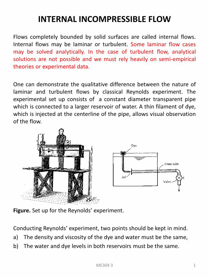
One can demonstrate the qualitative difference between the nature of laminar and turbulent flows by classical Reynolds experiment. The experimental set up consists of a constant diameter transparent pipe which is connected to a larger reservoir of water. A thin filament of dye, which is injected at the centerline of the pipe, allows visual observation of the flow.

Figure. Set up for the Reynolds’ experiment.

Conducting Reynolds’ experiment, two points should be kept in mind.

a) The density and viscosity of the dye and water must be the same,

b) The water and dye levels in both reservoirs must be the same.

INTERNAL INCOMPRESSIBLE FLOW

ME304 3 1

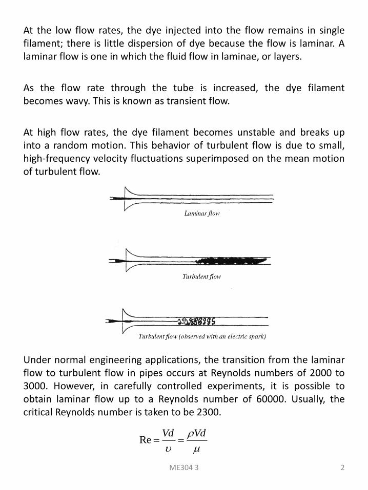
At the low flow rates, the dye injected into the flow remains in single filament; there is little dispersion of dye because the flow is laminar. A laminar flow is one in which the fluid flow in laminae, or layers.

As the flow rate through the tube is increased, the dye filament becomes wavy. This is known as transient flow.

At high flow rates, the dye filament becomes unstable and breaks up into a random motion. This behavior of turbulent flow is due to small, high-frequency velocity fluctuations superimposed on the mean motion of turbulent flow.

Under normal engineering applications, the transition from the laminar flow to turbulent flow in pipes occurs at Reynolds numbers of 2000 to 3000. However, in carefully controlled experiments, it is possible to obtain laminar flow up to a Reynolds number of 60000. Usually, the critical Reynolds number is taken to be 2300.

VdVdRe

ME304 3 2

Developing and Fully Developed Flow

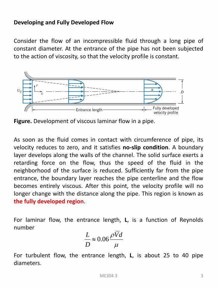
Consider the flow of an incompressible fluid through a long pipe of constant diameter. At the entrance of the pipe has not been subjected to the action of viscosity, so that the velocity profile is constant.

Figure. Development of viscous laminar flow in a pipe.

As soon as the fluid comes in contact with circumference of pipe, its velocity reduces to zero, and it satisfies no-slip condition. A boundary layer develops along the walls of the channel. The solid surface exerts a retarding force on the flow, thus the speed of the fluid in the neighborhood of the surface is reduced. Sufficiently far from the pipe entrance, the boundary layer reaches the pipe centerline and the flow becomes entirely viscous. After this point, the velocity profile will no longer change with the distance along the pipe. This region is known as the fully developed region.

For laminar flow, the entrance length, L, is a function of Reynolds number

For turbulent flow, the entrance length, L, is about 25 to 40 pipe diameters.

dV

D

L06.0

ME304 3 3

FULLY DEVELOPED LAMINAR FLOW (Chapter 8)

FULLY DEVELOPED LAMINAR FLOW BETWEEN INFINITE

PARALLEL PLATES

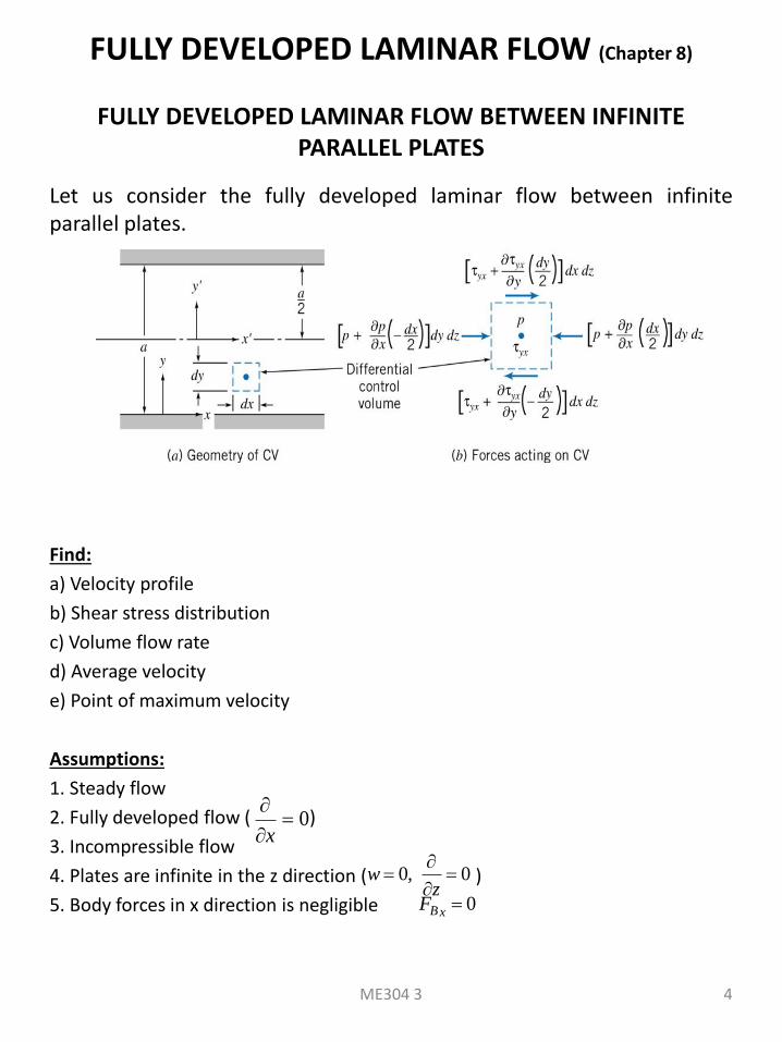
Let us consider the fully developed laminar flow between infinite parallel plates.

Find:

a) Velocity profile

b) Shear stress distribution

c) Volume flow rate

d) Average velocity

e) Point of maximum velocity

Assumptions:

1. Steady flow

2. Fully developed flow ( )

3. Incompressible flow

4. Plates are infinite in the z direction ( )

5. Body forces in x direction is negligible

0

x

0,0

zw

0xBF

ME304 3 4

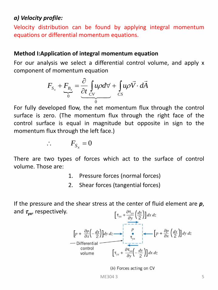
a) Velocity profile:

Velocity distribution can be found by applying integral momentum equations or differential momentum equations.

Method I:Application of integral momentum equation

For our analysis we select a differential control volume, and apply x component of momentum equation

For fully developed flow, the net momentum flux through the control surface is zero. (The momentum flux through the right face of the control surface is equal in magnitude but opposite in sign to the momentum flux through the left face.)

There are two types of forces which act to the surface of control volume. Those are:

1. Pressure forces (normal forces)

2. Shear forces (tangential forces)

If the pressure and the shear stress at the center of fluid element are p, and yx, respectively.

CSCV

BS AdVudut

FFxx

0

0

0xSF

ME304 3 5

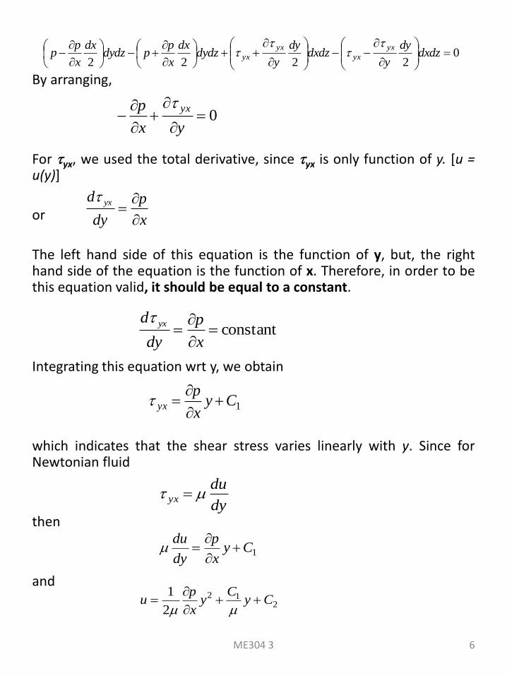
By arranging,

For yx, we used the total derivative, since yx is only function of y. [u = u(y)]

or

The left hand side of this equation is the function of y, but, the right hand side of the equation is the function of x. Therefore, in order to be this equation valid, it should be equal to a constant.

Integrating this equation wrt y, we obtain

which indicates that the shear stress varies linearly with y. Since for Newtonian fluid

then

and

02222

dxdz

yd

ydxdz

yd

ydydz

dx

x

ppdydz

dx

x

pp

yx

yx

yx

yx

0

yx

p yx

x

p

dy

d yx

constant

x

p

dy

d yx

1Cyx

pyx

dy

duyx

1Cyx

p

dy

du

212

2

1Cy

Cy

x

pu

ME304 3 6

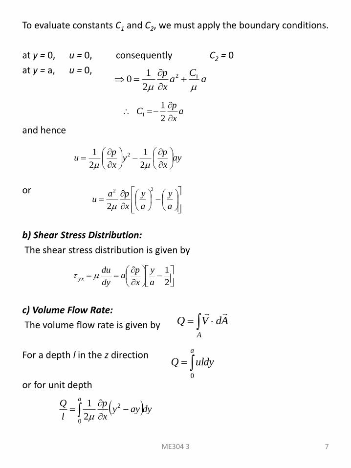
To evaluate constants C1 and C2, we must apply the boundary conditions.

at y = 0, u = 0, consequently C2 = 0

at y = a, u = 0,

and hence

or

b) Shear Stress Distribution:

The shear stress distribution is given by

c) Volume Flow Rate:

The volume flow rate is given by

For a depth l in the z direction

or for unit depth

aC

ax

p

12

2

10

ax

pC

2

11

ayx

py

x

pu

2

1

2

1 2

a

y

a

y

x

pau

22

2

2

1

a

y

x

pa

dy

duyx

A

AdVQ

a

uldyQ

0

a

dyayyx

p

l

Q

0

2

2

1

ME304 3 7

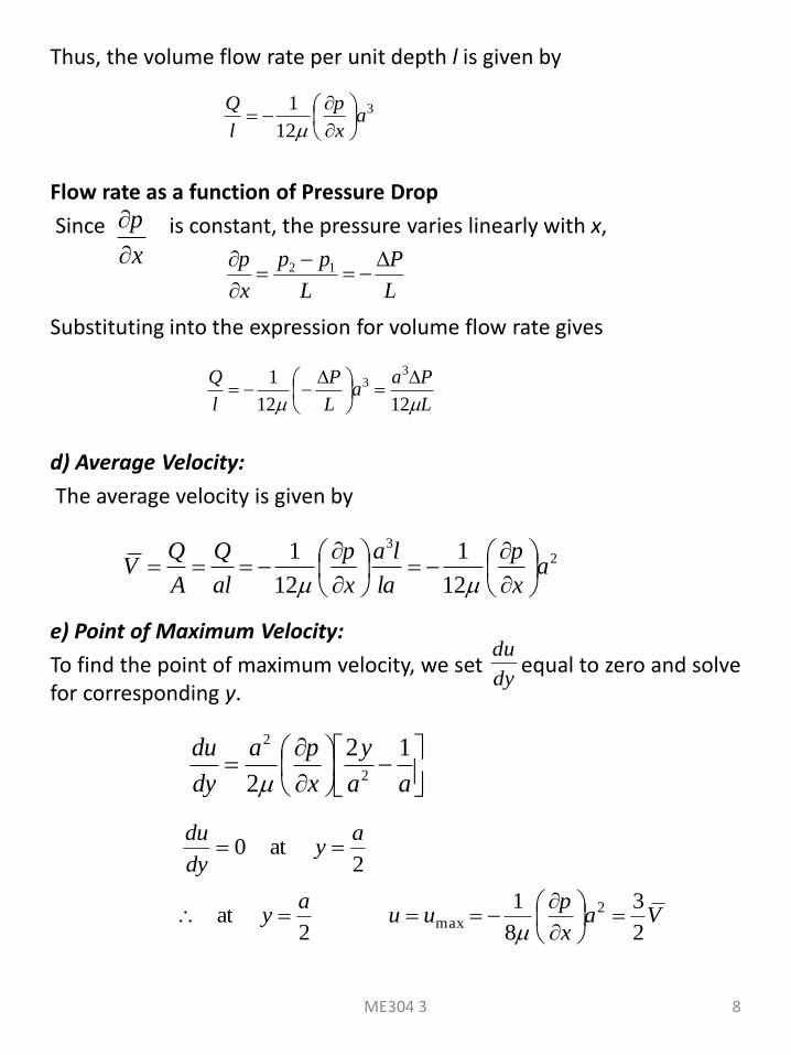
Thus, the volume flow rate per unit depth l is given by

Flow rate as a function of Pressure Drop

Since is constant, the pressure varies linearly with x,

Substituting into the expression for volume flow rate gives

d) Average Velocity:

The average velocity is given by

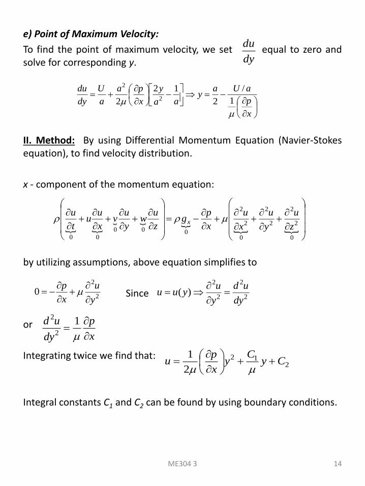
e) Point of Maximum Velocity:

To find the point of maximum velocity, we set equal to zero and solve for corresponding y.

3

12

1a

x

p

l

Q

x

p

L

P

L

pp

x

p

12

L

Paa

L

P

l

Q

1212

1 33

23

12

1

12

1a

x

p

la

la

x

p

al

Q

A

QV

dy

du

aa

y

x

pa

dy

du 12

2 2

2

2at0

ay

dy

du

Vax

puu

ay

2

3

8

1

2at 2

max

ME304 3 8

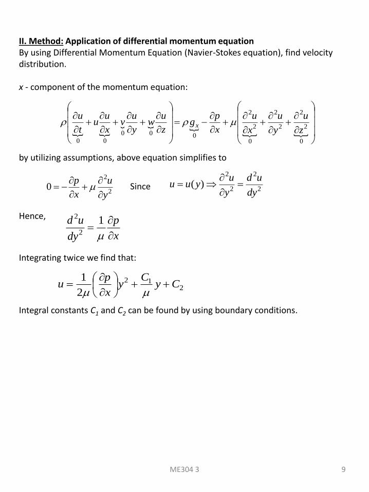
II. Method: Application of differential momentum equation By using Differential Momentum Equation (Navier-Stokes equation), find velocity distribution. x - component of the momentum equation:

by utilizing assumptions, above equation simplifies to

Since Hence, Integrating twice we find that:

Integral constants C1 and C2 can be found by using boundary conditions.

0

2

2

2

2

0

2

2

000

00

z

u

y

u

x

u

x

pg

z

uw

y

uv

x

uu

t

ux

2

2

0y

u

x

p

x

p

dy

ud

12

2

2

2

2

2

)(dy

ud

y

uyuu

212

2

1Cy

Cy

x

pu

ME304 3 9

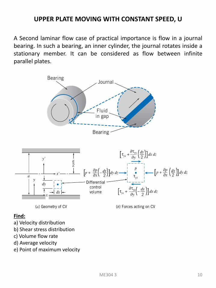
UPPER PLATE MOVING WITH CONSTANT SPEED, U

A Second laminar flow case of practical importance is flow in a journal bearing. In such a bearing, an inner cylinder, the journal rotates inside a stationary member. It can be considered as flow between infinite parallel plates.

Find: a) Velocity distribution b) Shear stress distribution c) Volume flow rate d) Average velocity e) Point of maximum velocity

ME304 3 10

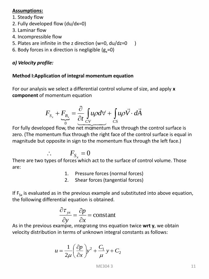
Assumptions: 1. Steady flow 2. Fully developed flow (du/dx=0) 3. Laminar flow 4. Incompressible flow 5. Plates are infinite in the z direction (w=0, du/dz=0 ) 6. Body forces in x direction is negligible (gx=0) a) Velocity profile: Method I:Application of integral momentum equation For our analysis we select a differential control volume of size, and apply x component of momentum equation For fully developed flow, the net momentum flux through the control surface is zero. (The momentum flux through the right face of the control surface is equal in magnitude but opposite in sign to the momentum flux through the left face.) There are two types of forces which act to the surface of control volume. Those are:

1. Pressure forces (normal forces) 2. Shear forces (tangential forces)

If FSx is evaluated as in the previous example and substituted into above equation, the following differential equation is obtained. As in the previous example, integrating this equation twice wrt y, we obtain velocity distribution in terms of unknown integral constants as follows:

CSCV

BS AdVudut

FFxx

0

0

0xSF

constant

x

p

y

yx

212

2

1Cy

Cy

x

pu

ME304 3 11

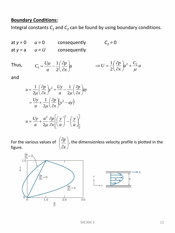
Boundary Conditions:

Integral constants C1 and C2 can be found by using boundary conditions.

at y = 0 u = 0 consequently C2 = 0

at y = a u = U consequently

Thus,

and

aC

ax

pU

12

2

1

a

x

p

a

UC

2

11

ayyx

p

a

Uy

ayx

p

a

Uyy

x

pu

2

2

2

1

2

1

2

1

a

y

a

y

x

pa

a

Uyu

22

2

For the various values of , the dimensionless velocity profile is plotted in the figure.

x

p

ME304 3 12

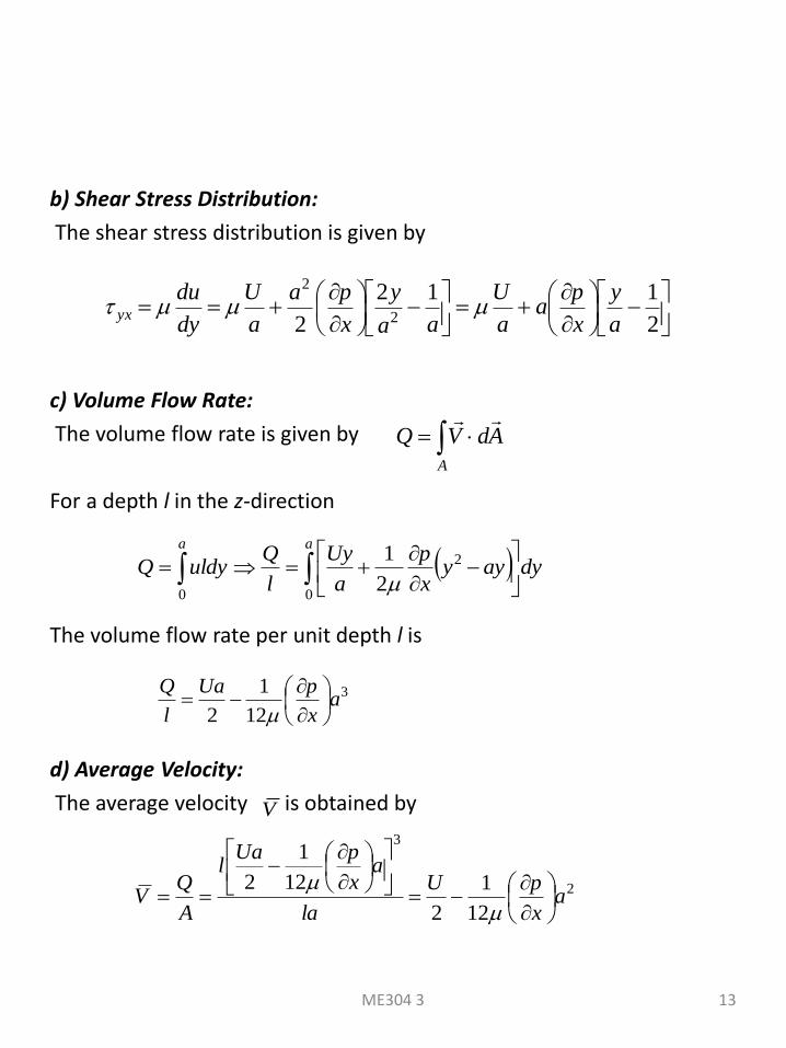
b) Shear Stress Distribution:

The shear stress distribution is given by

c) Volume Flow Rate:

The volume flow rate is given by

For a depth l in the z-direction

The volume flow rate per unit depth l is

d) Average Velocity:

The average velocity is obtained by

2

112

2 2

2

a

y

x

pa

a

U

aa

y

x

pa

a

U

dy

duyx

A

AdVQ

aa

dyayyx

p

a

Uy

l

QuldyQ

0

2

02

1

3

12

1

2a

x

pUa

l

Q

2

3

12

1

2

12

1

2a

x

pU

la

ax

pUal

A

QV

V

ME304 3 13

e) Point of Maximum Velocity:

To find the point of maximum velocity, we set equal to zero and solve for corresponding y.

II. Method: By using Differential Momentum Equation (Navier-Stokes equation), to find velocity distribution.

x - component of the momentum equation:

by utilizing assumptions, above equation simplifies to

Since

or

Integrating twice we find that:

Integral constants C1 and C2 can be found by using boundary conditions.

dy

du

x

p

aUay

aa

y

x

pa

a

U

dy

du

1

/

2

12

2 2

2

0

2

2

2

2

0

2

2

000

00

z

u

y

u

x

u

x

pg

z

uw

y

uv

x

uu

t

ux

2

2

0y

u

x

p

2

2

2

2

)(dy

ud

y

uyuu

x

p

dy

ud

12

2

212

2

1Cy

Cy

x

pu

ME304 3 14

ME304 3 15

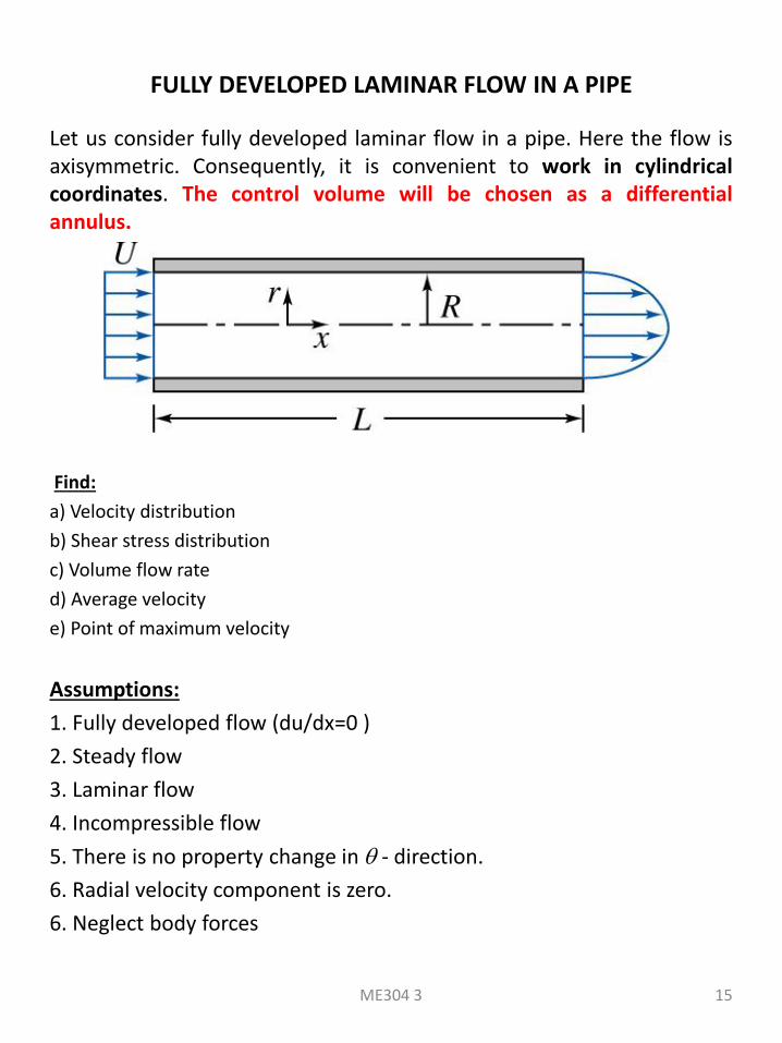
FULLY DEVELOPED LAMINAR FLOW IN A PIPE

Let us consider fully developed laminar flow in a pipe. Here the flow is axisymmetric. Consequently, it is convenient to work in cylindrical coordinates. The control volume will be chosen as a differential annulus.

Find:

a) Velocity distribution

b) Shear stress distribution

c) Volume flow rate

d) Average velocity

e) Point of maximum velocity

Assumptions:

1. Fully developed flow (du/dx=0 )

2. Steady flow

3. Laminar flow

4. Incompressible flow

5. There is no property change in - direction.

6. Radial velocity component is zero.

6. Neglect body forces

ME304 3 16

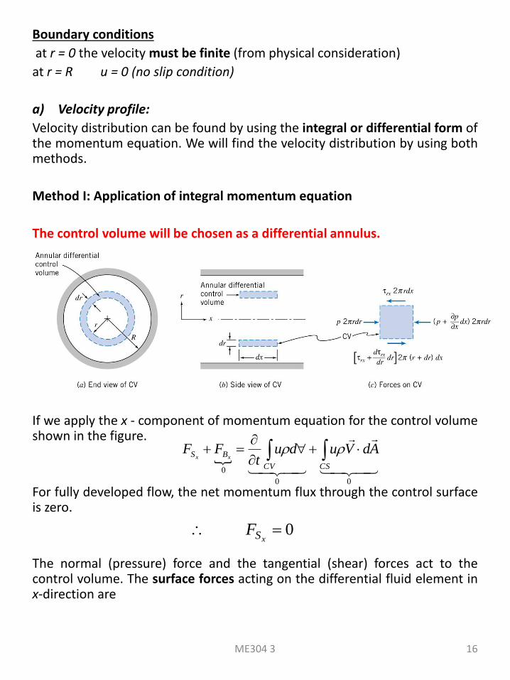
Boundary conditions

at r = 0 the velocity must be finite (from physical consideration)

at r = R u = 0 (no slip condition)

a) Velocity profile:

Velocity distribution can be found by using the integral or differential form of the momentum equation. We will find the velocity distribution by using both methods.

Method I: Application of integral momentum equation

The control volume will be chosen as a differential annulus.

If we apply the x - component of momentum equation for the control volume shown in the figure.

For fully developed flow, the net momentum flux through the control surface is zero.

The normal (pressure) force and the tangential (shear) forces act to the control volume. The surface forces acting on the differential fluid element in x-direction are

00

0

CSCV

BS AdVudut

FFxx

0xSF

ME304 3 17

To be completed in class

ME304 3 18

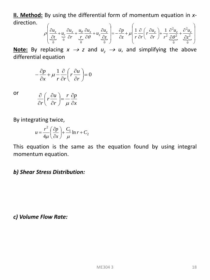
II. Method: By using the differential form of momentum equation in x-direction.

Note: By replacing x z and uz u, and simplifying the above differential equation

or

By integrating twice,

This equation is the same as the equation found by using integral momentum equation.

b) Shear Stress Distribution:

c) Volume Flow Rate:

0

2

2

0

2

2

2

000

0

11

z

uu

rr

ur

rrz

p

z

uu

u

r

u

r

uu

t

u zzzzz

zzr

z

01

r

ur

rrx

p

x

pr

r

ur

r

21

2

ln4

CrC

x

pru

ME304 3 19

d) Average Velocity:

e) Point of Maximum Velocity:

FULLY DEVELOPED TURBULENT FLOW

In turbulent flows, there is no universally acceptable relation between shear stress and velocity gradients. Therefore, the analytical solutions of turbulent flow problems are impossible, we must rely on semi-empirical data and numerical solutions.