1

International Evidence On The Oil Price-Real Output Relationship:

Does Persistence Matter?*

Richard Ashley, Virginia Tech

Kwok Ping Tsang, Virginia Tech

August 28, 2013

Abstract: The literature on the relationship between real output growth and the growth rate in

the price of oil, including an allowance for asymmetry in the impact of oil prices on output,

continues to evolve. Here we show that a new technique, which allows us to control for both this

asymmetry and also for the persistence of oil price changes, yields results implying that such

control is necessary for a statistically adequate specification of the relationship. The new

technique also yields an estimated model for the relationship which is more economically

interpretable. In particular, using quarterly data from 1976 – 2007 on each of six countries

which are essentially net oil importers, we find that changes in the growth rate of oil prices

which persist for more than four years have a large and statistically significant impact on future

output growth, whereas less persistent changes (lasting more than one year but less than four

years) have no significant impact on output growth. In contrast, ‘temporary’ fluctuations in the

oil price growth rate – persisting for only a year or less – again have a large and statistically

significant impact on output growth for most of these countries. The results for the single major

net oil producer in our sample (Norway) are distinct in an interesting way.

Keywords: oil price, frequency dependence, business cycle, nonlinearities

JEL codes: Q43, C22, E23

* Ashley: Department of Economics, Virginia Tech, Pamplin Hall (0316), Blacksburg, VA 24061-0316.

Email: ashleyr@vt.edu. Tsang (Corresponding author): Department of Economics, Virginia Tech, Pamplin Hall

(0316), Blacksburg, VA 24061-0316. Email: byront@vt.edu. The authors gratefully acknowledge the significant

contributions of Randal J. Verbrugge to both the development of the technique used here and – in Ashley, Tsang and

Verbrugge (2012) – to the exposition of it given in Section 3 below; we also thank him for numerous helpful

comments on the present paper. We also thank J. Isaac Miller and participants at the Society for Nonlinear

Dynamics and Econometrics 21st Annual Symposium for useful comments.

2

1. The Oil Price-Output Relationship

Empirical support is mixed for the impact of the price of oil on US macroeconomic variables.

Since the 1980s, there have been numerous studies on this relationship, but results are sensitive

to both the sample period and the model specification. Mixed results aside, one conclusion is

generally accepted: allowing for asymmetry in the relationship is important, and increases in oil

price are more important than decreases.

We contribute to this large empirical literature by considering the persistence of the

changes in oil price. We argue that the growth rate in output responds differently to a temporary

change in the growth rate of oil than to a relatively more persistent one. Nordhaus (2007) points

out two major channels by which the oil price can affect output. First, an increase in oil price

induces inflation; if the central bank tightens monetary policy as a response, then output drops as

a result. Second, an increase in oil price can impact consumers as a tax increase. Both of these

mechanisms are arguably stronger if the oil price change is permanent rather than transitory.

As is fairly standard in this literature, the basic specification considered in this paper is:

(1)

where is the real GDP growth rate from the current quarter to the next and is the

change in logarithm of the nominal oil price from the previous quarter to the current one; is

often allowed to differ for positive versus negative values of . We show below that it is

important to decompose the oil price change into more and less persistent components, and

that their impacts on the macroeconomy are different.

The literature on the oil price-real output relationship is too broad to be fully reviewed

here, so we focus in this section on briefly describing studies which are closely related to this

paper. (See Hamilton (2008) for a recent survey.) Hamilton (1988) provides a theoretical

framework for why the relationship between oil price and output is asymmetric: When the

growth rate of oil price goes up, durable consumption growth drops, as consumers choose to

postpone their purchases. But when the growth rate of the price of oil goes down, durable

consumption growth does not necessarily rise. Mork (1989) provides evidence that allowing for

this asymmetry – i.e. for different coefficients on price increases than on price decreases – is

important. In particular, he finds that price decreases have little impact on US real output.

3

Hooker (1996), however, finds that lagged oil price changes do not explain current output growth

after 1973, which suggests that either the relationship is unstable or, equivalently, that his model

specification is problematic. Even allowing for asymmetry in the relationship, he still finds a

poor fit using data subsequent to 1986. More recent studies focus on allowing for different

forms of nonlinearity: Hamilton (1996) suggests that an oil price increase needs to exceed a

threshold in order to have an impact; Ferderer (1996) and Jo (2012) argue that oil price volatility

matters; Lee, Ni and Ratti (1995) suggest that an oil price increase needs to be unexpected; and

Davis and Haltiwanger (2001) consider price changes sufficiently large as to make the price of

oil surpass its previous five-year average. Hamilton (2003) uses a flexible functional form and

confirms that both asymmetry and the “surprise” element are important. Finally, recent studies

by Cunado and Perez de Gracia (2003), Jiménez-Rodríguez and Sánchez (2005) and Jiménez-

Rodríguez (2009) also focus on the (asymmetric) nonlinearity in the relationship.

Kilian (2009) uses a structural VAR model to distinguish oil price movements that are

induced by structural demand or supply shocks. These two shocks are shown to have different

effects on income growth. In particular, a positive demand shock can drive up both income and

oil price. The conclusion of their paper is that, during periods when both types of shocks are

present, it is problematic to treat oil price changes as exogenous and only consider one-

directional causality from oil price to income.1

Miller and Ni (2011) model the deviations from trend – deterministic and stochastic – of

the oil price ( ) as the sum of two change series: a component (“updates to the long-term

average price”) obtained from an oil market model in levels, and a component (essentially

defined as the remainder of ) and interpreted as the “unanticipated” portion of . In

essence, one could say that they use an unobserved-components model – similar to a Beveridge-

Nelson (1981) decomposition – to extract these two updates to a latent stochastic trend in and

find that these two components have different impacts on future real GDP growth.

The present paper statistically decomposes in a new way, along a different dimension

than the decomposition considered by Kilian (2009) and Miller and Ni (2011): here the impact

1 Ordinary spectral regression yields inconsistent parameter estimates where feedback is present; the moving-

window technique used here allows for possible feedback by decomposing oil price changes using an effectively

one-sided filtering. This is described in the latter portion of Section 3.1 below.

4

on quarterly real growth is examined based on three components of , each of which

corresponds to fluctuations of a clear-cut level of persistence.2 One component contains all

sample variation in identifiable as either a smooth nonlinear trend or as stochastic

fluctuations with a persistence level corresponding to frequency components with a periodicity

larger than four years. The second component comprises all sample variation in with a

persistence level corresponding to frequency components with a periodicity greater than one year

and less than or equal to four years. And the third component comprises all sample variation in

with a persistence level of a year or less. These three components can be said to ‘partition’

the sample variation in into these three persistence levels, as they are constructed so as to

sum up to the original data on . Hence, by replacing in Equation (1) by a linear form in

these three components, it is straightforward to decompose the real-growth impact of by

persistence level.

Section 2 describes the international data used here in estimating both Equation (1) and

variations on it allowing for distinct (and asymmetric) responses to the components of ,

partitioned into the three persistence levels discussed above. Section 3 describes and motivates

the way in which this partitioning is done, based on frequency domain regression methods

developed in Ashley and Verbrugge (2007) and Ashley, Tsang and Verbrugge (2012). Results

on real GDP growth rates for the seven countries examined here are discussed in Section 4.

2. Data Description

Output growth is the quarterly growth rate of real GDP for Australia, Canada, France,

Japan, Norway, the United Kingdom and the United States; Norway is included so that the

analysis also considers a net oil exporter.3 This constitutes a representative sample of developed

countries for which ample data are available, omitting Germany due to its reunification

2 See also Wei (2012), there the focus is solely on Japan. 3 See the US Energy Information Administration website at http://www.eia.gov/countries/index.cfm?topL=exp for

net oil export data on these countries. Canada and/or the UK are considered net oil exporters by some authors – e.g.,

Jiménez-Rodríguez and Sánchez (2005) – and this is, to one degree or another, the case for portions of the sample

period considered here. In our empirical results Canada and the UK appears to ‘behave’ in the same way as do the

countries which are clearly net oil importers, whereas the results for Norway are significantly distinct. Therefore,

the grouping made at this point is used below, without substantial further comment.

5

during the period considered here.4 All growth rates series are obtained from the St. Louis

FRED database in annualized and seasonally adjusted form.

The oil price change series ( ) used here is the annualized quarterly growth rate (in

current US dollars) of the average of the of UK Brent Light, Dubai Medium and Alaska NS

Heavy spot prices, all extracted from the International Monetary Fund’s International Financial

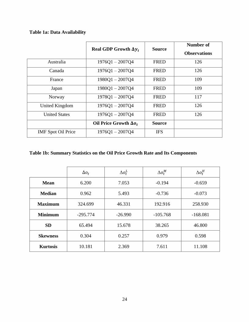
Statistics database.5 The availability of each series and the sample period used for each in the

empirical analysis are reported in Table 1a.

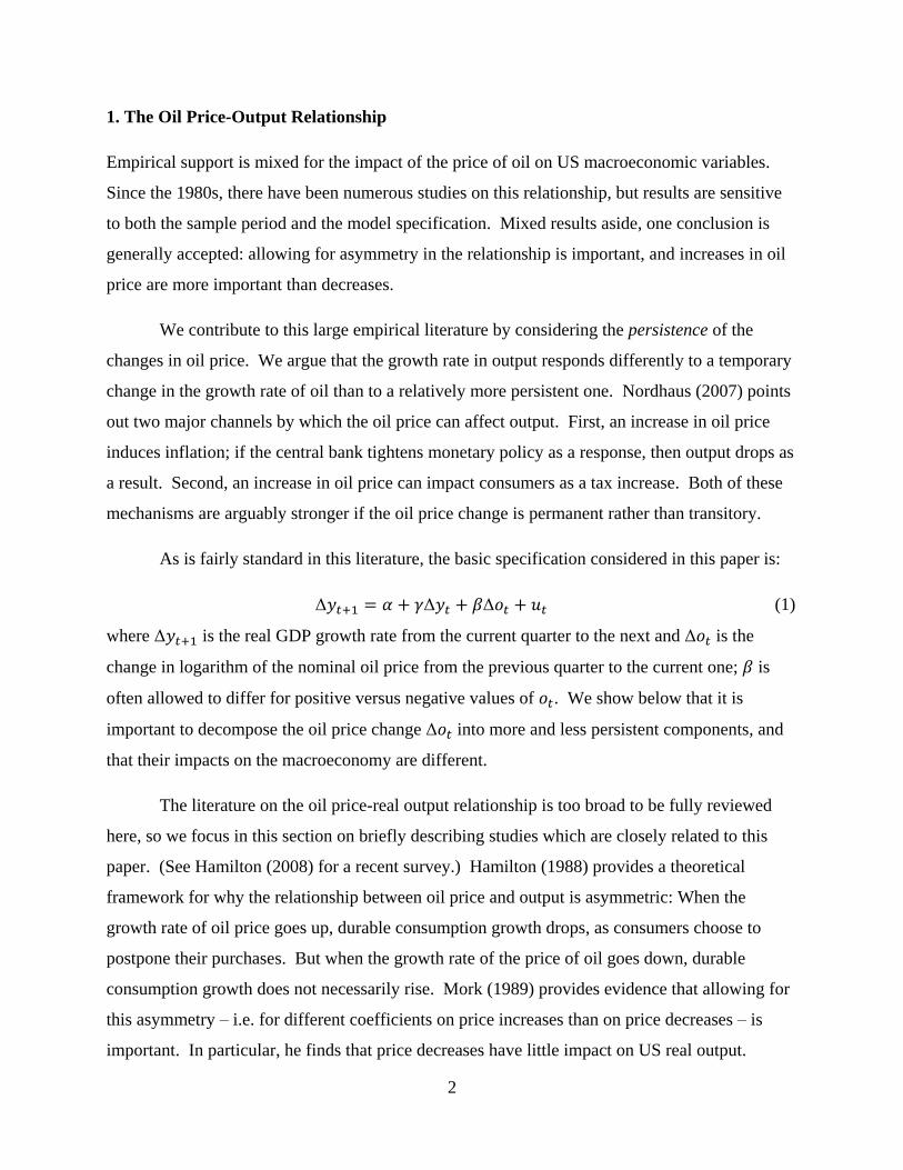
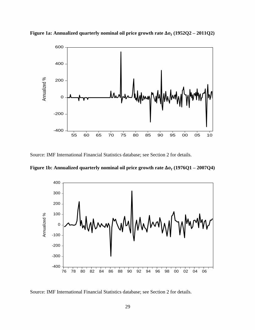
A time plot of using data from 1952Q2 to 2011Q2 is given in Figure 1a. The impact

of a number of political and economic events during this period is evident in the graph: the Arab

oil embargo in 1973, the Iran-Iraq War in 1980, and the Persian Gulf War in 1990 all coincide

with large spikes in the oil price growth rate series. Also evident is a large oil drop during

the collapse of OPEC around 1986 and an even larger drop in 2008, the latter of which clearly

corresponds to the global recession of that year. Thus, as noted in Kilian (2009), substantial

feedback (as distinct from unidirectional Granger causality) is likely present in the relationships

between and considered here.6

A prominent feature of Figure 1a is the infrequency and small size of the fluctuations in

early in the available data set. Because of this, and because of the singular nature of the

events in world oil markets in the early 1970’s, the sample actually used here is truncated to

begin in 1976Q1. Similarly, because the global macroeconomic fluctuation in 2008 so severely

impacted both world oil markets and all seven national economies, the observations subsequent

to 2007Q4 are also dropped from consideration, so as to prevent this event from having an

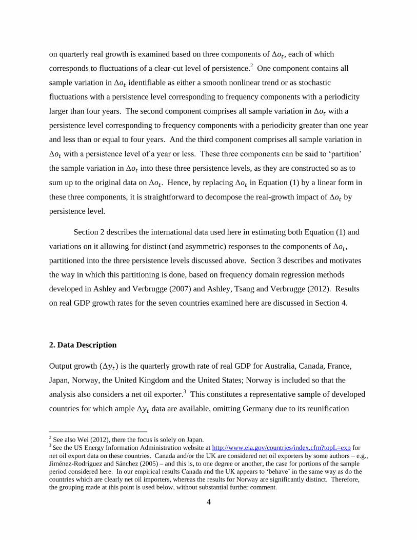
inordinate impact on our results.7 The data on for the resulting sample period (1976Q1 to

4 See Berument, Ceylan and Dogan (2010) for an analysis for the Middle Eastern and North Africa countries. 5 Using oil price in constant dollars or using the West Texas Intermediate (WTI) spot price yield almost identical

results. The oil price series are monthly, so we use the last month of each quarter to construct quarterly oil price

series; using the average oil price over all three months also yields very similar results, which are available upon

request. For simplicity (and because the analysis is in any case done entirely at a quarterly level), the windowed

frequency decomposition described in Section 3 is applied to the quarterly oil price data. 6 The possibility of feedback in a time-series relationship invalidates most frequency-domain-based regression

methods. Notably, the approach used here is not vulnerable in this regard, because it is based entirely on one-sided

filtering; this point is further discussed in Section 3 below. 7 Analogous results additionally including the later sample data are collected in an appendix available from the

authors, but are notably less interpretable: this single set of fluctuations in 2008 leads to a number of apparently-

significant coefficient estimates with perverse signs. Ordinarily, one might consider allowing for the 2008

6

2007Q4) is plotted in Figure 1b and still contains ample sample variation. Finally, note (in Table

1a) that the data for France and Japan starts later on – in 1980Q1, when their real output growth

series begin.

3. The Frequency-Dependence Approach

3.1 Description of the Method

The technique of modeling frequency dependence used here was originally developed by Tan

and Ashley (1999a and 1999b) and further developed by Ashley and Verbrugge (2009).8 The

Ashley-Verbrugge approach is uniquely well-suited to the present application because – unlike

other methods based on Fourier frequency decompositions – it is still valid in the presence of

feedback in the relationship. It also does not require any ad hoc assumptions as to which

frequencies correspond to a “business cycle” frequency band, etc.9

The remainder of this section briefly describes the procedure used here to decompose a

time series ( , in the present instance) into frequency components. To simplify the notation, in

this section the dependent variable is denoted as and the vector of explanatory variables is

denoted as . We begin with the usual multiple regression model:

(2)

where is , is and is a vector of errors.10

Now define a matrix ,

whose element is:

turbulence using dummy variables. That option is essentially infeasible here because the decomposition of into

frequency components uses 16-quarter moving windows so as to yield a one-sided filtering – see Section 3 for

details. Because these extraordinary fluctuations are so close to the end of the data set available, it seemed

preferable to present results on a truncated sample rather than replace these data artificially with interpolated values. 8 The idea of regression in the frequency domain can be traced back to Hannan (1963) and Engle (1974) – see

Ashley and Verbrugge (2009) for details. 9 The allowed frequencies are aggregated in the results presented here into three frequency bands primarily for

expositional clarity; disaggregated results are available from the authors. 10 Note that, while linear in β, Equation (2) is sufficiently general as to subsume a nonlinear (e.g. threshold

autoregressive) or a cointegrated relationship.

7

(3)

This matrix embodies what is known as the “finite Fourier transform.” It can be shown that is

orthonormal, i.e. .

Pre-multiplying the regression model in Equation (2) by yields:

(4)

While the dimensions of (y*, X

*, and u

*) are the same as those (y, X, and u), the components of

and and the rows of now correspond to frequencies (denoted by index s = 1 … T)

instead of to the time periods, t = 1 … T.11

The frequency components corresponding to the column of the X* array are

partitioned into m = 1 … M frequency bands by means of “dummy variables” ,

each of which is a vector of dimension . Each element of D*m, j

, the dummy vector for

frequency band m, is defined to be equal to the corresponding element of vector if that

11 Reference to Equation (3), however, shows that s equal to two and three both refer to the same frequency – because there is both a “cosine” and a “sine” row in A. Similarly, s equal to four and five also both refer to the same

frequency, and so forth. Thus, s runs from 1 … T and does index frequencies, but there are only T/2 distinct

frequencies. The error terms and are different from each other but they are distributed identically because is

orthonormal.

8

element corresponds to a frequency in band m; otherwise D*m, j

equals zero.12

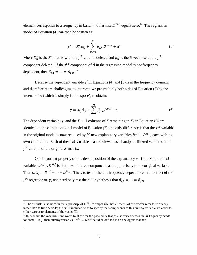
The regression

model of Equation (4) can then be written as:

(5)

where is the matrix with the column deleted and is the vector with the

component deleted. If the component of in the regression model is not frequency

dependent, then .13

Because the dependent variable y* in Equations (4) and (5) is in the frequency domain,

and therefore more challenging to interpret, we pre-multiply both sides of Equation (5) by the

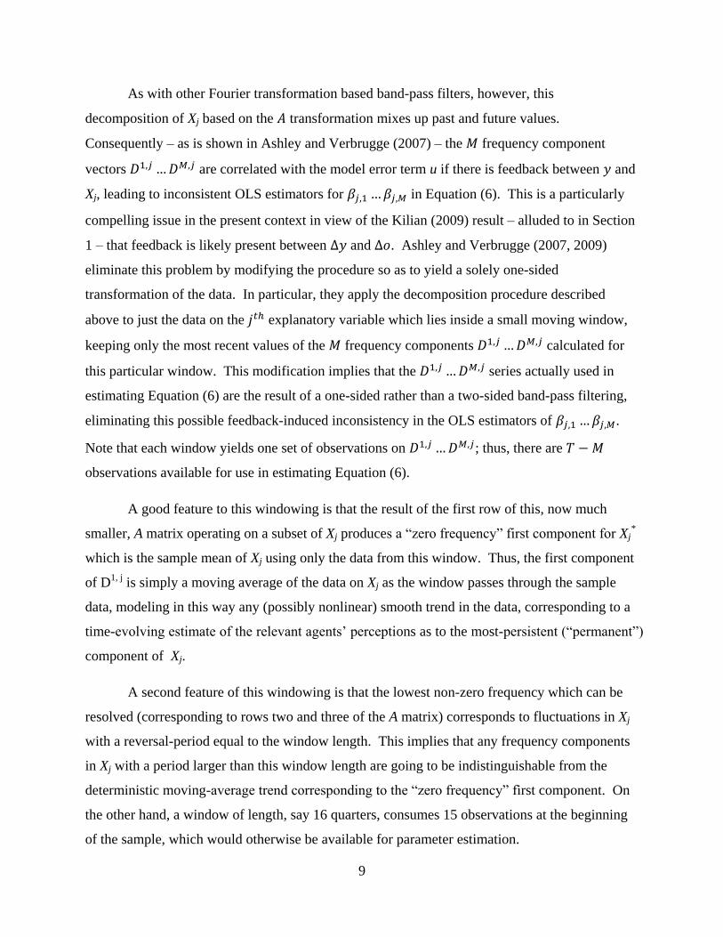
inverse of (which is simply its transpose), to obtain:

(6)

The dependent variable, and the columns of X remaining in X!j in Equation (6) are

identical to those in the original model of Equation (2); the only difference is that the variable

in the original model is now replaced by new explanatory variables , each with its

own coefficient. Each of these variables can be viewed as a bandpass-filtered version of the

column of the original matrix.

One important property of this decomposition of the explanatory variable Xj into the

variables is that these filtered components add up precisely to the original variable.

That is: . Thus, to test if there is frequency dependence in the effect of the

regressor on , one need only test the null hypothesis that .

12 The asterisk is included in the superscript of D*m, j to emphasize that elements of this vector refer to frequency

rather than to time periods; the “j” is included so as to specify that components of this dummy variable are equal to

either zero or to elements of the vector

13 If, as is not the case here, one wants to allow for the possibility that also varies across the M frequency bands

for some , then dummy variables could be defined in an analogous manner.

.

9

As with other Fourier transformation based band-pass filters, however, this

decomposition of Xj based on the transformation mixes up past and future values.

Consequently – as is shown in Ashley and Verbrugge (2007) – the frequency component

vectors are correlated with the model error term u if there is feedback between and

Xj, leading to inconsistent OLS estimators for in Equation (6). This is a particularly

compelling issue in the present context in view of the Kilian (2009) result – alluded to in Section

1 – that feedback is likely present between and . Ashley and Verbrugge (2007, 2009)

eliminate this problem by modifying the procedure so as to yield a solely one-sided

transformation of the data. In particular, they apply the decomposition procedure described

above to just the data on the explanatory variable which lies inside a small moving window,

keeping only the most recent values of the frequency components calculated for

this particular window. This modification implies that the series actually used in

estimating Equation (6) are the result of a one-sided rather than a two-sided band-pass filtering,

eliminating this possible feedback-induced inconsistency in the OLS estimators of .

Note that each window yields one set of observations on ; thus, there are

observations available for use in estimating Equation (6).

A good feature to this windowing is that the result of the first row of this, now much

smaller, A matrix operating on a subset of Xj produces a “zero frequency” first component for Xj*

which is the sample mean of Xj using only the data from this window. Thus, the first component

of D1, j

is simply a moving average of the data on Xj as the window passes through the sample

data, modeling in this way any (possibly nonlinear) smooth trend in the data, corresponding to a

time-evolving estimate of the relevant agents’ perceptions as to the most-persistent (“permanent”)

component of Xj.

A second feature of this windowing is that the lowest non-zero frequency which can be

resolved (corresponding to rows two and three of the A matrix) corresponds to fluctuations in Xj

with a reversal-period equal to the window length. This implies that any frequency components

in Xj with a period larger than this window length are going to be indistinguishable from the

deterministic moving-average trend corresponding to the “zero frequency” first component. On

the other hand, a window of length, say 16 quarters, consumes 15 observations at the beginning

of the sample, which would otherwise be available for parameter estimation.

10

In fact, the window size is chosen to be sixteen quarters in length for the present

application; this turns out to be sufficiently long that the results are not sensitive to this choice,

but one must bear this indistinguishability in mind when interpreting the results. In particular,

with the 16-quarter window used here, fluctuations with a “reversal period” in excess of four

years long are not distinguishable from the moving average trend component: both are included

in the decomposition of as part of its “zero-frequency” component. Section 3.2 below

provides more detail (and intuition) on the meaning of the frequency components in the context

of a simple example with a ten-period window.

In addition, when decomposing using fairly short windows, one must deal with the

standard problem of “edge effects” near the window endpoints. Following Dagum (1978) and

Stock and Watson (1999), this problem is resolved by augmenting the data for each window with

projections for one or two time periods. In the results quoted below, each sixteen-quarter

window uses fifteen quarters of sample data and one projected value (for the sixteenth quarter) to

produce the frequency components for the current period, i.e. for the fifteenth quarter of the

window. The projection model used here for forecasting this last (projected) value is an AR(1)

model estimated over the first fifteen sample observations in the window. (Using projections for

two quarters at the end of each window yielded essentially identical results: these were obtained

using fourteen actual sample values in each window and using an AR(1) model estimated over

these fourteen observations to project the last two values. In that case the resulting frequency

components for correspond to the fourteenth window time period.) The estimates

and inference results are generally not sensitive to either the choice of the projection length (so

long as it is small, but at least equal to one quarter), nor to the order of the projection model

used.14

14 The partitioning of Xj into frequency components as described above might appear to be a bit complicated, but it is

very easy in practice, as readily-usable Windows-based software is available from the authors which inputs the

sample data on Xj, the window length, the number of projections used in the window, and the order of the

autoregressive model used in making the projections; it outputs the M frequency components – – as a

comma delimited spreadsheet file. An ideal projection model would utilize all information available at time t, but

the AR(p) projection model specification makes the implementing software simpler and easier to use. Fortunately,

the estimates of are not very sensitive to exactly how the projections are done.

11

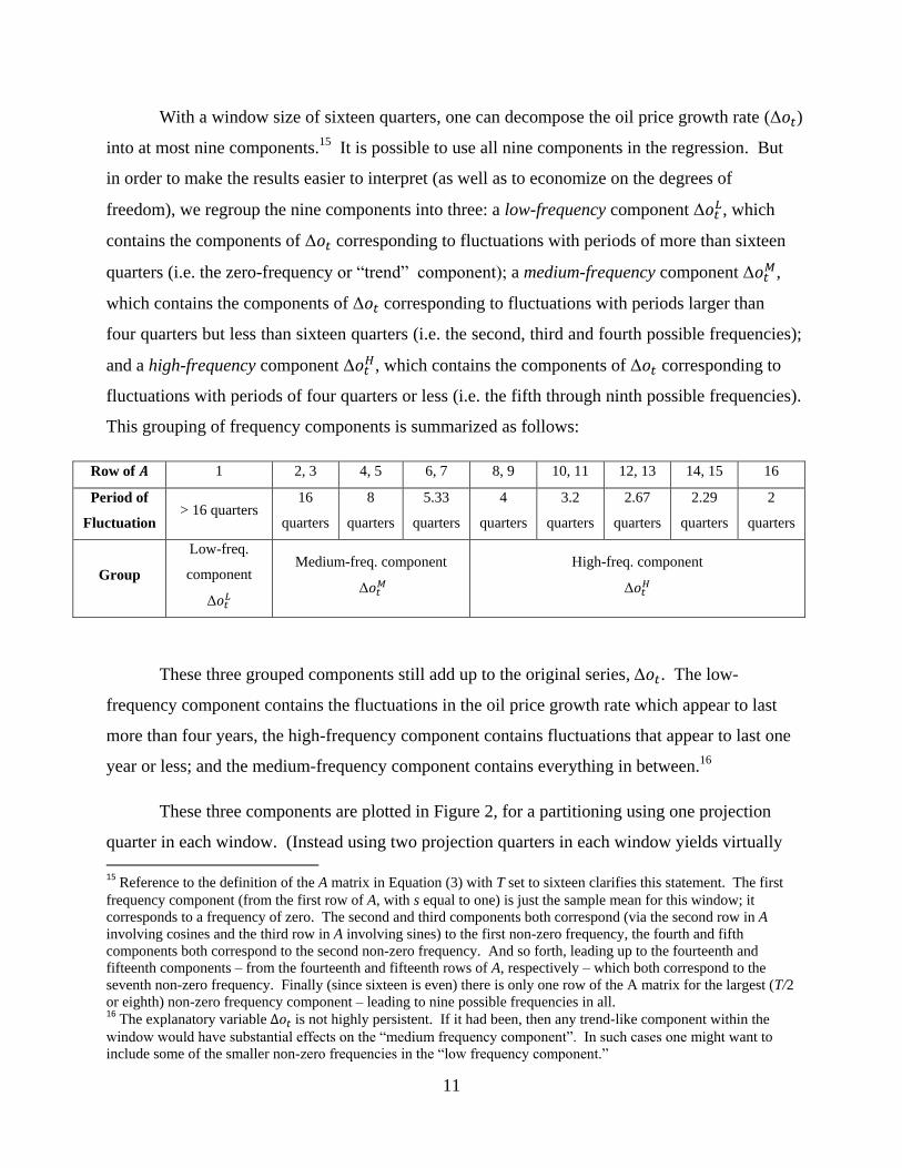
With a window size of sixteen quarters, one can decompose the oil price growth rate ( )

into at most nine components.15

It is possible to use all nine components in the regression. But

in order to make the results easier to interpret (as well as to economize on the degrees of

freedom), we regroup the nine components into three: a low-frequency component , which

contains the components of corresponding to fluctuations with periods of more than sixteen

quarters (i.e. the zero-frequency or “trend” component); a medium-frequency component ,

which contains the components of corresponding to fluctuations with periods larger than

four quarters but less than sixteen quarters (i.e. the second, third and fourth possible frequencies);

and a high-frequency component , which contains the components of corresponding to

fluctuations with periods of four quarters or less (i.e. the fifth through ninth possible frequencies).

This grouping of frequency components is summarized as follows:

Row of 1 2, 3 4, 5 6, 7 8, 9 10, 11 12, 13 14, 15 16

Period of

Fluctuation > 16 quarters

16

quarters

8

quarters

5.33

quarters

4

quarters

3.2

quarters

2.67

quarters

2.29

quarters

2

quarters

Group

Low-freq.

component

Medium-freq. component

High-freq. component

These three grouped components still add up to the original series, . The low-

frequency component contains the fluctuations in the oil price growth rate which appear to last

more than four years, the high-frequency component contains fluctuations that appear to last one

year or less; and the medium-frequency component contains everything in between.16

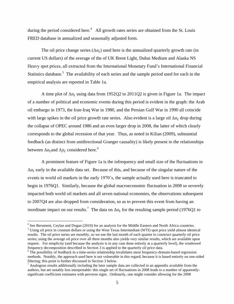
These three components are plotted in Figure 2, for a partitioning using one projection

quarter in each window. (Instead using two projection quarters in each window yields virtually

15 Reference to the definition of the A matrix in Equation (3) with T set to sixteen clarifies this statement. The first

frequency component (from the first row of A, with s equal to one) is just the sample mean for this window; it

corresponds to a frequency of zero. The second and third components both correspond (via the second row in A

involving cosines and the third row in A involving sines) to the first non-zero frequency, the fourth and fifth

components both correspond to the second non-zero frequency. And so forth, leading up to the fourteenth and

fifteenth components – from the fourteenth and fifteenth rows of A, respectively – which both correspond to the

seventh non-zero frequency. Finally (since sixteen is even) there is only one row of the A matrix for the largest (T/2

or eighth) non-zero frequency component – leading to nine possible frequencies in all. 16 The explanatory variable is not highly persistent. If it had been, then any trend-like component within the

window would have substantial effects on the “medium frequency component”. In such cases one might want to

include some of the smaller non-zero frequencies in the “low frequency component.”

12

identical plots and very similar regression results.17

) These components would be precisely

orthogonal to one another except for the use of a moving window. As explained above, this

windowing ensures that the results are not adversely impacted by any feedback which might be

present in the output versus oil-price relationship; it also allows for graceful nonlinear trend

removal (in the zero-frequency component of ) via the windowed moving average. The

sample correlations between these three components of are still quite small, however:

= 0.037,

= -0.038, and

= 0.112. Note that all

three components (as one would expect) display significant sample variation, but that the time

variation in the low-frequency component is smoother than that of the medium-frequency

component, which in turn is smoother than that of the high-frequency component.

3.2 The Appeal of this Frequency-based Approach to Disaggregation by Persistence Level

The objective of the partitioning of an explanatory variable time series – whether it is called to

be more parallel to other possible regressors or called so as to make it more specific to the

oil price model of Equation (1) – is not the band-pass filtering per se. Rather, the point of

decomposing into the components ,

, and is entirely to make it possible to

separately estimate the impact of fluctuations in of distinctly different persistence levels on

the growth rate of real output (yt) and to thereby allow inferences to be made concerning these

differential impacts.

No representation is made here that the band-pass filtering proposed above is in some

sense “optimal” – e.g., as in Koopmans (1974) or Christiano and Fitzgerald (2003). Nevertheless,

our method of decomposing a time series into frequency components has several very nice

properties, which make it overwhelmingly well-suited to the present application:

1) The frequency components which are generated from by construction partition it: that is,

these components add up precisely to the original observed data on . This makes estimation

17 The sample correlations between the components obtained using two instead of one projection quarter are 0.936,

0.999, and 0.989 for the low, medium, and high-frequency bands, respectively; this correlation (while still high) is a

bit lower for the low-frequency band because the zero-frequency component is in that case a fourteen-quarter

moving average instead of a fifteen-quarter moving average.

13

and inference with regard to frequency (or ‘persistence,’ its inverse) dependence in the

coefficient βj particularly straightforward.

2) Due to the moving windows used, this particular way of partitioning of into these

frequency components is via a set of entirely backward-looking (i.e., “one-sided”) filters. This

feature is essential to consistent OLS estimation of the coefficient βj in the – here, quite likely –

circumstance where there is bi-directional Granger-causality (feedback) between y and .

3) And, finally, this partitioning of into frequency components is not just mathematically valid

and straightforward: it is also intuitively appealing.18

The next section illustrates this with a

simple example.

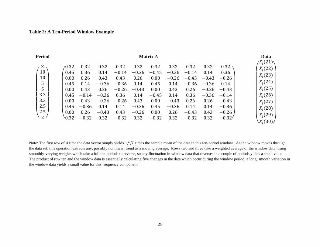
3.3 An Explicit Example with a Short Window

An example with a window ten periods in length illustrates the sense in which the

frequency components define above are extracting components of of differing levels of

persistence.19

Table 2 explicitly displays the multiplication of the matrix – whose

element is given in Equation (3) – by the ten-component sub-vector of corresponding to a

window beginning in period twenty one.

The first component of this matrix product corresponds to what one might call the “zero-

frequency” component of this subsample of . Note that the “Period” column in Table 2 is

essentially just the reciprocal of the frequency corresponding to the sine or cosine used in the

18 The Christiano-Fitzgerald (2003) bandpass filter could in principle be repeatedly applied to the data in a given

window; the filter could then be iteratively applied to the remainder from the previous repetition, only with a

different lower bound for the frequency band at each iteration. This rather unwieldy procedure would yield a

decomposition of the explanatory variable whose frequency components still add up to the original data on . Note,

however, that such a decomposition would be more complicated, less intuitively appealing, and in fact no more

“optimal” than ours. 19 A window ten periods in length is sufficiently large as to illustrate the point, while sufficiently small as to allow

Table 2 to fit onto a single page; the actual implementation in Section 4 uses a window sixteen periods in length, so

that the medium-frequency component can subsume fluctuations with a reversal period of up to four years.

14

corresponding row of the matrix. The first entry in this column of Table 2, corresponding to a

frequency of zero, is thus arbitrarily large.20

The first row of the matrix is just a constant, so the operation of this row on the ten-

vector sub-component of is in essence just calculating its sample mean over these ten

observations. Thus, the zero-frequency component of is actually just a one-sided (or “real-

time”) moving-average nonlinear trend estimate. As noted earlier, this “zero-frequency”

component is also subsuming any stochastic fluctuations in at frequencies so low

(periodicities or persistence so large) as to be invisible in a window which is only ten periods in

length.

The next two rows of (and hence the next two components of the matrix product) both

correspond to a periodicity of ten quarters because in both cases the elements of the row vary

per a sine or cosine which completes one cycle (“period”) in ten quarters. Thus, the second and

third components of will both be small for any variation in which basically reverses itself

within a few quarters, whereas these two components will be large for any variation in takes

circa ten quarters to reverse itself – i.e., for variation in which is “low-frequency.”21

In

contrast, looking at the tenth row of the matrix, it is evident that the inner product of this row

with a slowly-varying sub-vector will yield only a small value for the tenth component of ,

whereas an sub-vector which corresponds to a high-frequency fluctuation – i.e., which

reverses in just a quarter or two – will contribute significantly to the tenth component of .

Thus, the first rows of the matrix are distinguishing and extracting what are sensibly

the “low-frequency,” or “large period,” or “highly persistent” – or ‘permanent’ – components of

this ten-quarter sub-vector. And, concomitantly, the last rows of the matrix are

distinguishing and extracting what are sensibly the “high-frequency,” or “small period,” or “low

persistence” – or ‘temporary’ – components of this sub-vector.

20 Technically, the frequency is 2π divided by the period of the corresponding sine or cosine, but that detail is not

important here. 21 The first few lowest frequency components model any trend-like behavior in the data within the window.

15

4. Results and Discussion

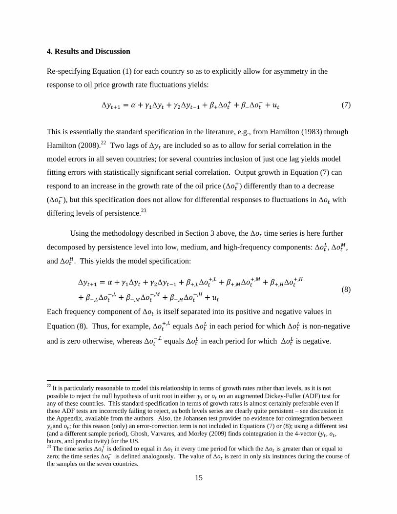
Re-specifying Equation (1) for each country so as to explicitly allow for asymmetry in the

response to oil price growth rate fluctuations yields:

(7)

This is essentially the standard specification in the literature, e.g., from Hamilton (1983) through

Hamilton (2008).22

Two lags of are included so as to allow for serial correlation in the

model errors in all seven countries; for several countries inclusion of just one lag yields model

fitting errors with statistically significant serial correlation. Output growth in Equation (7) can

respond to an increase in the growth rate of the oil price ( ) differently than to a decrease

( ), but this specification does not allow for differential responses to fluctuations in with

differing levels of persistence.23

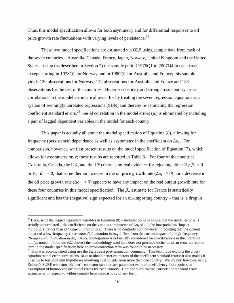
Using the methodology described in Section 3 above, the time series is here further

decomposed by persistence level into low, medium, and high-frequency components: ,

,

and . This yields the model specification:

(8)

Each frequency component of is itself separated into its positive and negative values in

Equation (8). Thus, for example,

equals in each period for which

is non-negative

and is zero otherwise, whereas

equals in each period for which

is negative.

22 It is particularly reasonable to model this relationship in terms of growth rates rather than levels, as it is not

possible to reject the null hypothesis of unit root in either or on an augmented Dickey-Fuller (ADF) test for

any of these countries. This standard specification in terms of growth rates is almost certainly preferable even if

these ADF tests are incorrectly failing to reject, as both levels series are clearly quite persistent – see discussion in

the Appendix, available from the authors. Also, the Johansen test provides no evidence for cointegration between

and ; for this reason (only) an error-correction term is not included in Equations (7) or (8); using a different test

(and a different sample period), Ghosh, Varvares, and Morley (2009) finds cointegration in the 4-vector ( , , hours, and productivity) for the US. 23 The time series

is defined to equal in in every time period for which the is greater than or equal to

zero; the time series is defined analogously. The value of is zero in only six instances during the course of

the samples on the seven countries.

16

Thus, this model specification allows for both asymmetry and for differential responses to oil

price growth rate fluctuations with varying levels of persistence.24

These two model specifications are estimated via OLS using sample data from each of

the seven countries – Australia, Canada, France, Japan, Norway, United Kingdom and the United

States – using (as described in Section 2) the sample period 1976Q1 to 2007Q4 in each case,

except starting in 1978Q1 for Norway and in 1980Q1 for Australia and France; this sample

yields 120 observations for Norway, 112 observations for Australia and France and 128

observations for the rest of the countries. Heteroscedasticity and strong cross-country cross-

correlations in the model errors are allowed for by treating the seven regression equations as a

system of seemingly unrelated regressions (SUR) and thereby re-estimating the regression

coefficient standard errors.25

Serial correlation in the model errors (ut) is eliminated by including

a pair of lagged dependent variables in the model for each country.

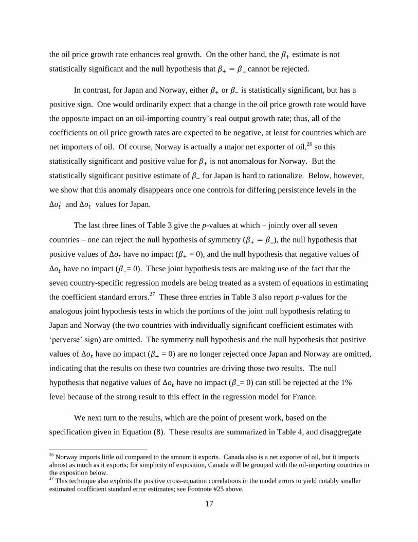
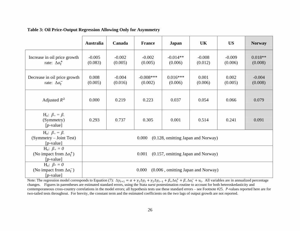
This paper is actually all about the model specification of Equation (8), allowing for

frequency (persistence) dependence as well as asymmetry in the coefficient on . For

comparison, however, we first present results on the model specification of Equation (7), which

allows for asymmetry only; these results are reported in Table 3. For four of the countries

(Australia, Canada, the UK, and the US) there is no real evidence for rejecting either Ho: β+ = 0

or Ho: = 0; that is, neither an increase in the oil price growth rate ( > 0) nor a decrease in

the oil price growth rate ( < 0) appears to have any impact on the real output growth rate for

these four countries in this model specification. The estimate for France is statistically

significant and has the (negative) sign expected for an oil-importing country – that is, a drop in

24 Because of the lagged dependent variables in Equation (8) – included so as to ensure that the model error ut is

serially uncorrelated – the coefficients on the various components of should be interpreted as ‘impact multipliers’ rather than as ‘long-run multipliers.’ There is no contradiction, however, in positing that the current

impact of a low-frequency (‘permanent’) fluctuation in differs from the current impact of a high-frequency

(‘temporary’) fluctuation in . Also, cointegration is not usually considered for specifications in this literature,

but (as noted in Footnote #22 above ) the methodology used here does not preclude inclusion of an error-correction

term in the model specification; here no error-correction term was found to be necessary. 25 This was accomplished using use the Stata suest post-estimation command. This technique exploits the cross-

equation model error correlations, so as to obtain better estimators of the coefficient standard errors; it also makes it

possible to test joint null hypotheses involving coefficients from more than one country. We are not, however, using

Zellner’s SURE estimator; Zellner’s estimator can increase parameter estimation efficiency, but requires an

assumption of homoscedastic model errors for each country. Here the suest routine corrects the standard error

estimates with respect to within-country heteroscedasticity of any form.

17

the oil price growth rate enhances real growth. On the other hand, the estimate is not

statistically significant and the null hypothesis that cannot be rejected.

In contrast, for Japan and Norway, either or is statistically significant, but has a

positive sign. One would ordinarily expect that a change in the oil price growth rate would have

the opposite impact on an oil-importing country’s real output growth rate; thus, all of the

coefficients on oil price growth rates are expected to be negative, at least for countries which are

net importers of oil. Of course, Norway is actually a major net exporter of oil,26

so this

statistically significant and positive value for is not anomalous for Norway. But the

statistically significant positive estimate of for Japan is hard to rationalize. Below, however,

we show that this anomaly disappears once one controls for differing persistence levels in the

and

values for Japan.

The last three lines of Table 3 give the p-values at which – jointly over all seven

countries – one can reject the null hypothesis of symmetry ( ), the null hypothesis that

positive values of have no impact ( = 0), and the null hypothesis that negative values of

have no impact ( = 0). These joint hypothesis tests are making use of the fact that the

seven country-specific regression models are being treated as a system of equations in estimating

the coefficient standard errors.27

These three entries in Table 3 also report p-values for the

analogous joint hypothesis tests in which the portions of the joint null hypothesis relating to

Japan and Norway (the two countries with individually significant coefficient estimates with

‘perverse’ sign) are omitted. The symmetry null hypothesis and the null hypothesis that positive

values of have no impact ( = 0) are no longer rejected once Japan and Norway are omitted,

indicating that the results on these two countries are driving those two results. The null

hypothesis that negative values of have no impact ( = 0) can still be rejected at the 1%

level because of the strong result to this effect in the regression model for France.

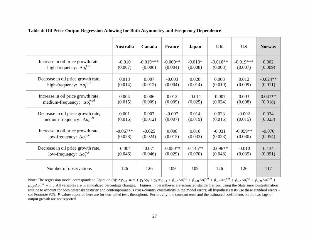
We next turn to the results, which are the point of present work, based on the

specification given in Equation (8). These results are summarized in Table 4, and disaggregate

26 Norway imports little oil compared to the amount it exports. Canada also is a net exporter of oil, but it imports

almost as much as it exports; for simplicity of exposition, Canada will be grouped with the oil-importing countries in

the exposition below. 27 This technique also exploits the positive cross-equation correlations in the model errors to yield notably smaller

estimated coefficient standard error estimates; see Footnote #25 above.

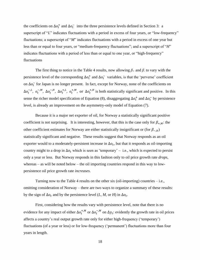
18

the coefficients on and

into the three persistence levels defined in Section 3: a

superscript of “L” indicates fluctuations with a period in excess of four years, or “low-frequency”

fluctuations; a superscript of “M” indicates fluctuations with a period in excess of one year but

less than or equal to four years, or “medium-frequency fluctuations”; and a superscript of “H”

indicates fluctuations with a period of less than or equal to one year, or “high-frequency”

fluctuations

The first thing to notice in the Table 4 results, now allowing β+ and β- to vary with the

persistence level of the corresponding and

variables, is that the ‘perverse’ coefficient

on for Japan is no longer present. In fact, except for Norway, none of the coefficients on

is both statistically significant and positive. In this

sense the richer model specification of Equation (8), disaggregating and

by persistence

level, is already an improvement on the asymmetry-only model of Equation (7).

Because it is a major net exporter of oil, for Norway a statistically significant positive

coefficient is not surprising. It is interesting, however, that this is the case only for : the

other coefficient estimates for Norway are either statistically insignificant or (for )

statistically significant and negative. These results suggest that Norway responds as an oil

exporter would to a moderately-persistent increase in , but that it responds as oil-importing

country might to a drop in which is seen as ‘temporary’ – i.e., which is expected to persist

only a year or less. But Norway responds in this fashion only to oil price growth rate drops,

whereas – as will be noted below – the oil importing countries respond in this way to low-

persistence oil price growth rate increases.

Turning now to the Table 4 results on the other six (oil-importing) countries – i.e.,

omitting consideration of Norway – there are two ways to organize a summary of these results:

by the sign of and by the persistence level (L, M, or H) in .

First, considering how the results vary with persistence level, note that there is no

evidence for any impact of either

or

on : evidently the growth rate in oil prices

affects a country’s real output growth rate only for either high-frequency (‘temporary’)

fluctuations (of a year or less) or for low-frequency (‘permanent’) fluctuations more than four

years in length.

19

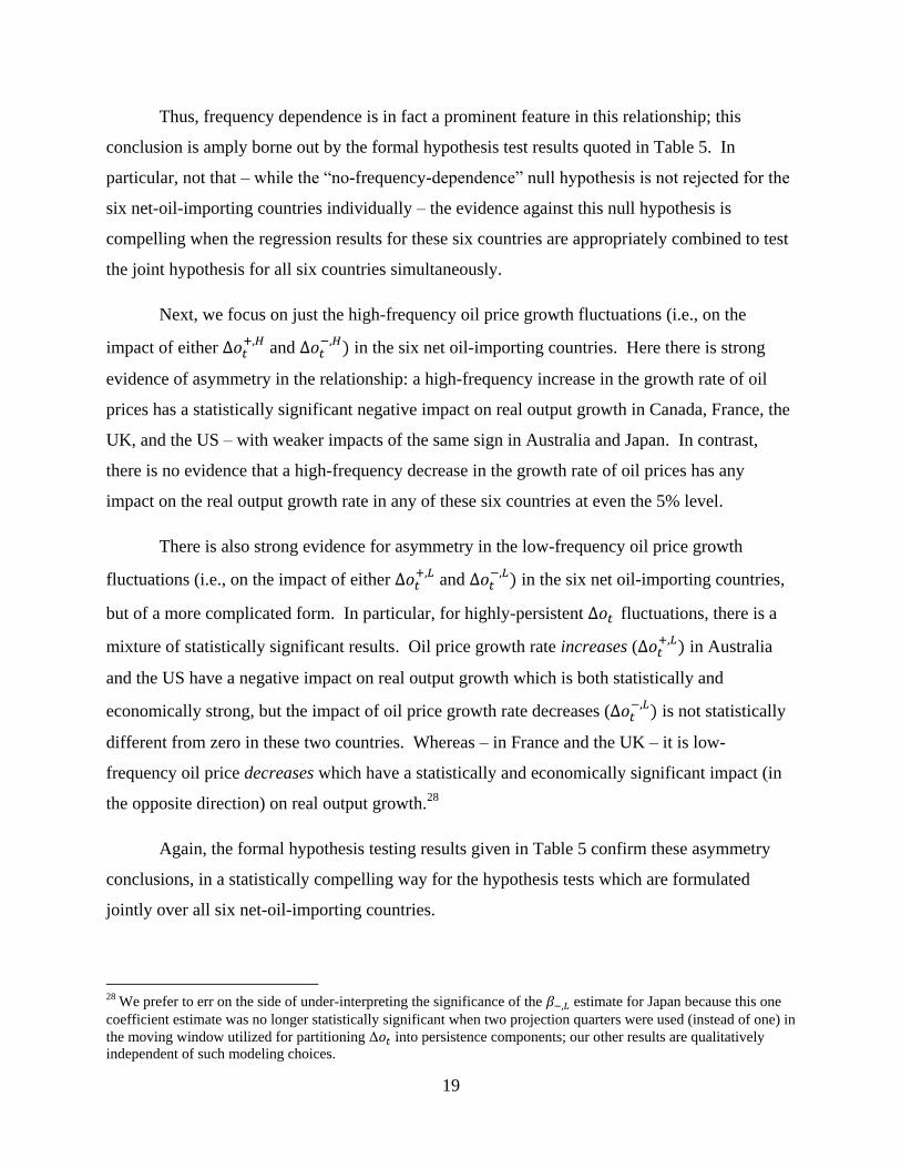
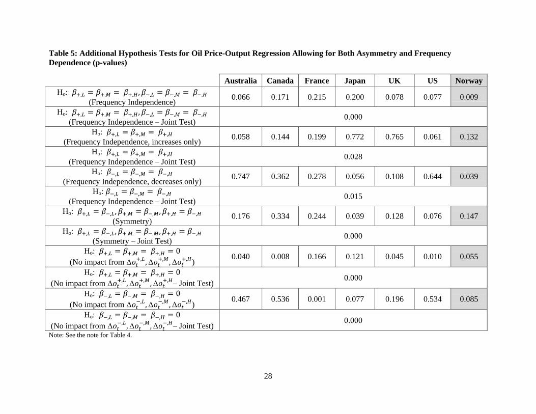
Thus, frequency dependence is in fact a prominent feature in this relationship; this

conclusion is amply borne out by the formal hypothesis test results quoted in Table 5. In

particular, not that – while the “no-frequency-dependence” null hypothesis is not rejected for the

six net-oil-importing countries individually – the evidence against this null hypothesis is

compelling when the regression results for these six countries are appropriately combined to test

the joint hypothesis for all six countries simultaneously.

Next, we focus on just the high-frequency oil price growth fluctuations (i.e., on the

impact of either

and in the six net oil-importing countries. Here there is strong

evidence of asymmetry in the relationship: a high-frequency increase in the growth rate of oil

prices has a statistically significant negative impact on real output growth in Canada, France, the

UK, and the US – with weaker impacts of the same sign in Australia and Japan. In contrast,

there is no evidence that a high-frequency decrease in the growth rate of oil prices has any

impact on the real output growth rate in any of these six countries at even the 5% level.

There is also strong evidence for asymmetry in the low-frequency oil price growth

fluctuations (i.e., on the impact of either

and in the six net oil-importing countries,

but of a more complicated form. In particular, for highly-persistent fluctuations, there is a

mixture of statistically significant results. Oil price growth rate increases ( in Australia

and the US have a negative impact on real output growth which is both statistically and

economically strong, but the impact of oil price growth rate decreases ( is not statistically

different from zero in these two countries. Whereas – in France and the UK – it is low-

frequency oil price decreases which have a statistically and economically significant impact (in

the opposite direction) on real output growth.28

Again, the formal hypothesis testing results given in Table 5 confirm these asymmetry

conclusions, in a statistically compelling way for the hypothesis tests which are formulated

jointly over all six net-oil-importing countries.

28 We prefer to err on the side of under-interpreting the significance of the estimate for Japan because this one

coefficient estimate was no longer statistically significant when two projection quarters were used (instead of one) in

the moving window utilized for partitioning into persistence components; our other results are qualitatively

independent of such modeling choices.

20

5. Concluding Remarks

We find that a model specification for the growth rate in real output allowing only for

asymmetry in the coefficient on the oil price growth rate ( ) – i.e., Equation (7) – can mislead

one into thinking that changes in have either no statistically significant impact or a perverse

effect on real output growth. For example, someone considering only the results in Table 3

might well conclude that positive values of have no impact on real output growth in

Australia, Canada, France, the UK and the US and that a negative value for has a statistically

significant impact with a perverse sign in Japan.

In contrast, our results in Table 4 show that – allowing for frequency dependence in the

real output growth rate model, i.e., for varying responses to different levels of persistence in

sample fluctuations in or

– yields results which are both statistically significant and

economically explicable. Broadly, for the six countries (Australia, Canada, France, Japan, the

UK and the US) which are not major oil exporters :

a) High-frequency (‘temporary’) increases, which typically reverse within one to four

quarters, depress real output growth rates, whereas high-frequency decreases appear

to have little impact on real output growth rates.

b) Mid-frequency changes (in either direction), which typically reverse within one to

four years, appear to have little impact on real output growth rates.

c) And low-frequency (‘permanent’) changes have statistically and economically

significant impacts – for positive changes in Australia and the US, and for negative

changes in France, Japan, and the UK.

For the major net oil-exporting country in our sample (Norway), we see a different result:

a mid-frequency increase in actually increases the real output growth rate. Note that this

result is consistent with the finding in Jiménez-Rodríguez and Sánchez (2005) that enters a

model specification like Equation (7) with a significant positive coefficient. But our result is

richer (and more nuanced) in that we find that this effect of an increase in only pertains to oil

21

price growth rate increases with a persistence in the range of more than one year but less than or

equal to four years. Additionally, we find that – unlike the net oil importing countries – Norway

responds to low-persistence decreases, rather than increases, in the oil price growth rate with a

change in the real output growth rate of the opposite sign.

Overall, then, our results demonstrate the existence of a strong (and asymmetric) impact

of oil prices on real output, once one appropriately allows for the differential impact of

fluctuations in the oil price growth rate with differing levels of persistence. Controlling for the

persistence level of oil price fluctuations not only leads to a more statistically adequate

econometric formulation of the real output versus oil price relationship, but also yields

interestingly interpretable economic results.

What are the mechanisms behind our reduced-form results? Do households and firms

respond differently to oil price changes of different levels persistence? And if so, why? Does

the central bank react differently as well? Our results point clearly to a need for a more

structural theory, leading to a model capable of addressing these new questions.

22

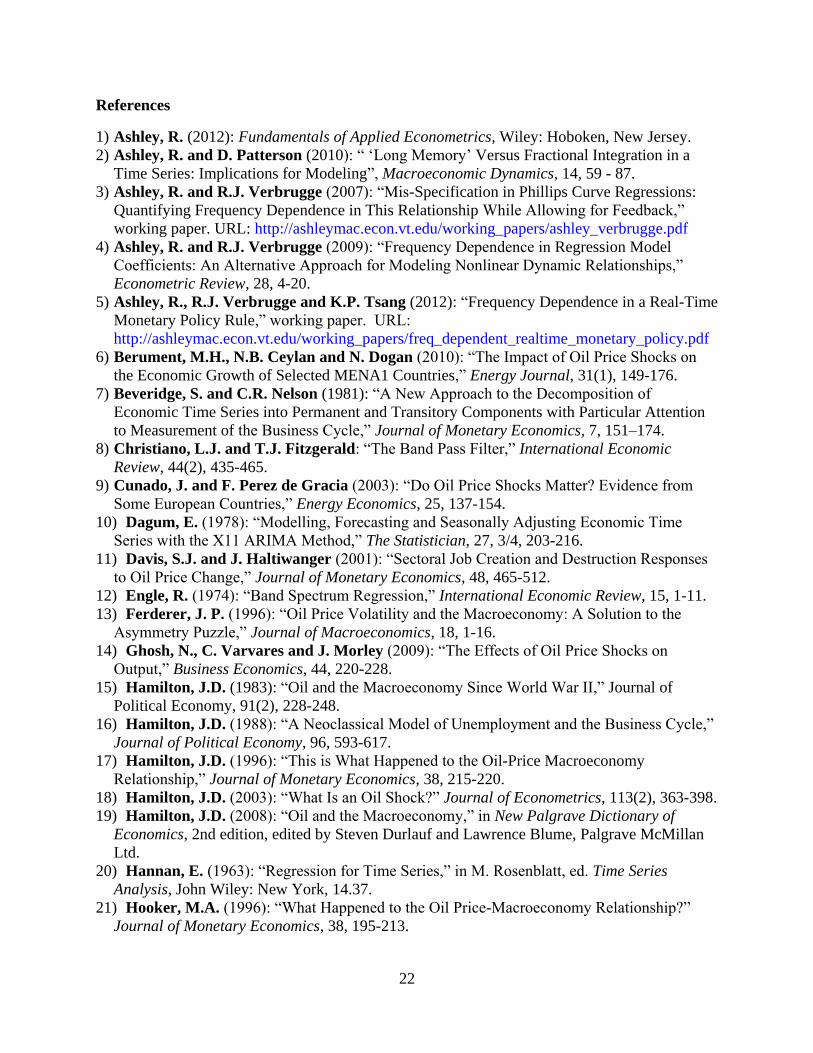
References

1) Ashley, R. (2012): Fundamentals of Applied Econometrics, Wiley: Hoboken, New Jersey.

2) Ashley, R. and D. Patterson (2010): “ ‘Long Memory’ Versus Fractional Integration in a

Time Series: Implications for Modeling”, Macroeconomic Dynamics, 14, 59 - 87.

3) Ashley, R. and R.J. Verbrugge (2007): “Mis-Specification in Phillips Curve Regressions:

Quantifying Frequency Dependence in This Relationship While Allowing for Feedback,”

working paper. URL: http://ashleymac.econ.vt.edu/working_papers/ashley_verbrugge.pdf

4) Ashley, R. and R.J. Verbrugge (2009): “Frequency Dependence in Regression Model

Coefficients: An Alternative Approach for Modeling Nonlinear Dynamic Relationships,”

Econometric Review, 28, 4-20.

5) Ashley, R., R.J. Verbrugge and K.P. Tsang (2012): “Frequency Dependence in a Real-Time

Monetary Policy Rule,” working paper. URL:

http://ashleymac.econ.vt.edu/working_papers/freq_dependent_realtime_monetary_policy.pdf

6) Berument, M.H., N.B. Ceylan and N. Dogan (2010): “The Impact of Oil Price Shocks on

the Economic Growth of Selected MENA1 Countries,” Energy Journal, 31(1), 149-176.

7) Beveridge, S. and C.R. Nelson (1981): “A New Approach to the Decomposition of

Economic Time Series into Permanent and Transitory Components with Particular Attention

to Measurement of the Business Cycle,” Journal of Monetary Economics, 7, 151–174.

8) Christiano, L.J. and T.J. Fitzgerald: “The Band Pass Filter,” International Economic

Review, 44(2), 435-465.

9) Cunado, J. and F. Perez de Gracia (2003): “Do Oil Price Shocks Matter? Evidence from

Some European Countries,” Energy Economics, 25, 137-154.

10) Dagum, E. (1978): “Modelling, Forecasting and Seasonally Adjusting Economic Time

Series with the X11 ARIMA Method,” The Statistician, 27, 3/4, 203-216.

11) Davis, S.J. and J. Haltiwanger (2001): “Sectoral Job Creation and Destruction Responses

to Oil Price Change,” Journal of Monetary Economics, 48, 465-512.

12) Engle, R. (1974): “Band Spectrum Regression,” International Economic Review, 15, 1-11.

13) Ferderer, J. P. (1996): “Oil Price Volatility and the Macroeconomy: A Solution to the

Asymmetry Puzzle,” Journal of Macroeconomics, 18, 1-16.

14) Ghosh, N., C. Varvares and J. Morley (2009): “The Effects of Oil Price Shocks on

Output,” Business Economics, 44, 220-228.

15) Hamilton, J.D. (1983): “Oil and the Macroeconomy Since World War II,” Journal of

Political Economy, 91(2), 228-248.

16) Hamilton, J.D. (1988): “A Neoclassical Model of Unemployment and the Business Cycle,”

Journal of Political Economy, 96, 593-617.

17) Hamilton, J.D. (1996): “This is What Happened to the Oil-Price Macroeconomy

Relationship,” Journal of Monetary Economics, 38, 215-220.

18) Hamilton, J.D. (2003): “What Is an Oil Shock?” Journal of Econometrics, 113(2), 363-398.

19) Hamilton, J.D. (2008): “Oil and the Macroeconomy,” in New Palgrave Dictionary of

Economics, 2nd edition, edited by Steven Durlauf and Lawrence Blume, Palgrave McMillan

Ltd.

20) Hannan, E. (1963): “Regression for Time Series,” in M. Rosenblatt, ed. Time Series

Analysis, John Wiley: New York, 14.37.

21) Hooker, M.A. (1996): “What Happened to the Oil Price-Macroeconomy Relationship?”

Journal of Monetary Economics, 38, 195-213.

23

22) Jiménez-Rodríguez, R. (2009): “Oil Price Shocks and Real GDP Growth: Testing for Non-

linearity,” Energy Journal, 30(1), 1-23.

23) Jiménez-Rodríguez, R. and M. Sánchez (2005): “Oil Price Shocks and Real GDP Growth:

Empirical Evidence for Some OECD Countries,” Applied Economics, 37(2), 201-228.

24) Jo, S. (2012): “The Effects of Oil Price Uncertainty on the Macroeconomy,” Bank of

Canada working paper 2012-40.

25) Kilian, L. (2009): “Not All Oil Price Shocks Are Alike: Disentangling Demand and Supply

Shocks in the Crude Oil Market,” American Economic Review, 99(3), 1053-1069.

26) Koopmans, L.H. (1974): The Spectral Analysis of Time Series, San Diego, CA: Academic

Press.

27) Lee, K., S. Ni and R.A. Ratti (1995): “Oil Shocks and the Macroeconomy: The Role of

Price Variability,” Energy Journal, 16, 39-56.

28) Miller, J. I. and S. Ni (2011): “Long-Term Oil Price Forecasts: A New Perspective on Oil

and the Macroeconomy,” Macroeconomic Dynamics, vol. 15(S3), 396-415.

29) Mork, K.A. B (1989): “Oil and the Macroeconomy When Prices Go Up and Down: An

Extension of Hamilton’s Results,” Journal of Political Economy, 91, 740-744.

30) Stock, J. and M. Watson (1999): “Business Cycle Fluctuations in U.S. Macroeconomic

Time Series,” in (John Taylor and Michael Woodford, eds) Handbook of Macroeconomics,

Amsterdam: Elsevier, 3-64.

31) Tan, H. B. and R. Ashley (1999a): “On the Inherent Nonlinearity of Frequency Dependent

Time Series Relationships,” in (P. Rothman, ed.) Nonlinear Time Series Analysis of Economic

and Financial Data, Kluwer Academic Publishers: Norwell, 129-142.

32) Tan, H.B. and R. Ashley (1999b): “Detection and Modeling of Regression Parameter

Variation Across Frequencies with an Application to Testing the Permanent Income

Hypothesis,” Macroeconomic Dynamics, 3, 69-83.

33) Wei, Y. (2012): “The Dynamic Relationships between Oil Prices and the Japanese Economy:

A Frequency Domain Analysis,” working paper.

24

Table 1a: Data Availability

Real GDP Growth Source Number of

Observations

Australia 1976Q1 – 2007Q4 FRED 126

Canada 1976Q1 – 2007Q4 FRED 126

France 1980Q1 – 2007Q4 FRED 109

Japan 1980Q1 – 2007Q4 FRED 109

Norway 1978Q1 – 2007Q4 FRED 117

United Kingdom 1976Q1 – 2007Q4 FRED 126

United States 1976Q1 – 2007Q4 FRED 126

Oil Price Growth Source

IMF Spot Oil Price 1976Q1 – 2007Q4 IFS

Table 1b: Summary Statistics on the Oil Price Growth Rate and Its Components

Mean 6.200 7.053 -0.194 -0.659

Median 0.962 5.493 -0.736 -0.073

Maximum 324.699 46.331 192.916 258.930

Minimum -295.774 -26.990 -105.768 -168.081

SD 65.494 15.678 38.265 46.800

Skewness 0.304 0.257 0.979 0.598

Kurtosis 10.181 2.369 7.611 11.108

25

Table 2: A Ten-Period Window Example

Period Matrix A Data

Note: The first row of time the data vector simply yields times the sample mean of the data in this ten-period window. As the window moves through

the data set, this operation extracts any, possibly nonlinear, trend as a moving average. Rows two and three take a weighted average of the window data, using

smoothly-varying weights which take a full ten periods to reverse, so any fluctuation in window data that reverses in a couple of periods yields a small value.

The product of row ten and the window data is essentially calculating five changes in the data which occur during the window period; a long, smooth variation in

the window data yields a small value for this frequency component.

26

Table 3: Oil Price-Output Regression Allowing Only for Asymmetry

Australia Canada France Japan UK US Norway

Increase in oil price growth

rate:

-0.005

(0.083)

-0.002

(0.005)

-0.002

(0.005)

-0.014**

(0.006)

-0.008

(0.012)

-0.009

(0.006)

0.018**

(0.008)

Decrease in oil price growth

rate:

0.008

(0.005)

-0.004

(0.016)

-0.008***

(0.002)

0.016***

(0.006)

0.001

(0.006)

0.002

(0.005)

-0.004

(0.008)

Adjusted 0.000 0.219 0.223 0.037 0.054 0.066 0.079

Ho: β+ = β-

(Symmetry)

-value]

0.293 0.737 0.305 0.001 0.514 0.241 0.091

Ho: β+ = β-

(Symmetry – Joint Test)

-value]

0.000 (0.128, omitting Japan and Norway)

Ho: β+ = 0

(No impact from )

-value]

0.001 (0.157, omitting Japan and Norway)

Ho: β- = 0

(No impact from )

-value]

0.000 (0.006 , omitting Japan and Norway)

Note: The regression model corresponds to Equation (7):

. All variables are in annualized percentage

changes. Figures in parentheses are estimated standard errors, using the Stata suest postestimation routine to account for both heteroskedasticity and

contemporaneous cross-country correlations in the model errors; all hypothesis tests use these standard errors – see Footnote #25. -values reported here are for

two-tailed tests throughout. For brevity, the constant term and the estimated coefficients on the two lags of output growth are not reported.

27

Table 4: Oil Price-Output Regression Allowing for Both Asymmetry and Frequency Dependence

Australia Canada France Japan UK US Norway

Increase in oil price growth rate,

high-frequency:

-0.010

(0.007)

-0.019***

(0.006)

-0.009**

(0.004)

-0.013*

(0.008)

-0.016**

(0.008)

-0.019***

(0.007)

0.002

(0.009)

Decrease in oil price growth rate,

high-frequency:

0.018

(0.014)

0.007

(0.012)

-0.003

(0.004)

0.020

(0.014)

0.003

(0.010)

0.012

(0.009)

-0.024**

(0.011)

Increase in oil price growth rate,

medium-frequency:

0.004

(0.015)

0.006

(0.009)

0.012

(0.009)

-0.011

(0.025)

-0.007

(0.024)

0.003

(0.008)

0.041**

(0.018)

Decrease in oil price growth rate,

medium-frequency:

0.001

(0.016)

0.007

(0.012)

-0.007

(0.007)

0.014

(0.019)

0.023

(0.016)

-0.002

(0.015)

0.034

(0.023)

Increase in oil price growth rate,

low-frequency:

-0.067**

(0.028)

-0.025

(0.024)

0.008

(0.015)

0.010

(0.033)

-0.031

(0.028)

-0.059**

(0.030)

-0.070

(0.054)

Decrease in oil price growth rate,

low-frequency:

-0.004

(0.046)

-0.071

(0.046)

-0.050**

(0.029)

-0.145**

(0.070)

-0.096**

(0.048)

-0.010

(0.035)

0.134

(0.091)

Number of observations 126 126 109 109 126 126 117

Note: The regression model corresponds to Equation (8):

. All variables are in annualized percentage changes. Figures in parentheses are estimated standard errors, using the Stata suest postestimation

routine to account for both heteroskedasticity and contemporaneous cross-country correlations in the model errors; all hypothesis tests use these standard errors –

see Footnote #25. P-values reported here are for two-tailed tests throughout. For brevity, the constant term and the estimated coefficients on the two lags of

output growth are not reported.

28

Table 5: Additional Hypothesis Tests for Oil Price-Output Regression Allowing for Both Asymmetry and Frequency

Dependence (p-values)

Australia Canada France Japan UK US Norway

Ho:

(Frequency Independence) 0.066 0.171 0.215 0.200 0.078 0.077 0.009

Ho:

(Frequency Independence – Joint Test) 0.000

Ho:

(Frequency Independence, increases only) 0.058 0.144 0.199 0.772 0.765 0.061 0.132

Ho:

(Frequency Independence – Joint Test) 0.028

Ho:

(Frequency Independence, decreases only) 0.747 0.362 0.278 0.056 0.108 0.644 0.039

Ho:

(Frequency Independence – Joint Test) 0.015

Ho:

(Symmetry) 0.176 0.334 0.244 0.039 0.128 0.076 0.147

Ho:

(Symmetry – Joint Test) 0.000

Ho:

(No impact from

) 0.040 0.008 0.166 0.121 0.045 0.010 0.055

Ho:

(No impact from

– Joint Test)

0.000

Ho:

(No impact from

) 0.467 0.536 0.001 0.077 0.196 0.534 0.085

Ho:

(No impact from

– Joint Test)

0.000

Note: See the note for Table 4.

29

Figure 1a: Annualized quarterly nominal oil price growth rate (1952Q2 – 2011Q2)

Source: IMF International Financial Statistics database; see Section 2 for details.

Figure 1b: Annualized quarterly nominal oil price growth rate (1976Q1 – 2007Q4)

Source: IMF International Financial Statistics database; see Section 2 for details.

-400

-200

0

200

400

600

55 60 65 70 75 80 85 90 95 00 05 10

Ann

ualiz

ed %

-400

-300

-200

-100

0

100

200

300

400

76 78 80 82 84 86 88 90 92 94 96 98 00 02 04 06

An

nu

aliz

ed

%

30

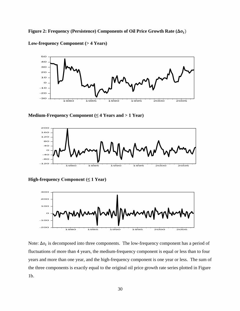
Figure 2: Frequency (Persistence) Components of Oil Price Growth Rate (

Low-frequency Component (> 4 Years)

Medium-Frequency Component (≤ 4 Years and > 1 Year)

High-frequency Component (≤ 1 Year)

Note: is decomposed into three components. The low-frequency component has a period of

fluctuations of more than 4 years, the medium-frequency component is equal or less than to four

years and more than one year, and the high-frequency component is one year or less. The sum of

the three components is exactly equal to the original oil price growth rate series plotted in Figure

1b.

-30

-20

-10

0

10

20

30

40

50

1980 1985 1990 1995 2000 2005

-120

-80

-40

0

40

80

120

160

200

1980 1985 1990 1995 2000 2005

-200

-100

0

100

200

300

1980 1985 1990 1995 2000 2005

31

Appendix: Modeling in Levels

Equation (7), as is fairly standard in this literature, specifies the relationship between real output

and oil prices in terms of their growth rates. One could instead model the relationship between

the levels (log-levels, presumably) of these time series. However, in view of the fact that both of

these time series are either integrated – i.e., I(1) – or nearly so, we view modeling this

relationship in terms of levels unwise.

The main point of this paper is that the strength (and even the sign) of the relationship

between oil prices and real output can (and does) depend on the persistence of the fluctuations in

oil prices. And we do in this paper explicitly examine the relationship between the growth rates

of real output and the oil price at various frequency components, including a component at a

frequency of zero. This zero-frequency component amounts to a moving average of recent

values of the growth rates in the oil price; this component captures any slow, smooth changes in

the mean growth rate of oil prices. In addition, we explicitly examine whether there is

cointegration between the log-level series, and find that there is not. Had evidence for such

cointegration materialized, however, the most appropriate response would have been to have

included an error-correction term in the growth rate equation, consisting of the fitting errors from

a levels model between these two series. The coefficient on that error-correction term – had it

existed – would then have quantified something different from the zero-frequency coefficient on

the growth rate in oil prices: it would have quantified the degree to which the current growth rate

in real output depends on how far real output is ‘out of kilter’ with its long-run relationship with

the price of oil, rather than quantifying the degree to which the current growth rate in real output

depends on recent (but fairly smooth) fluctuations in the price of oil. In the event, however, such

an error-correction term was not necessary, but it is important to understand the meaning which

its coefficient would have had.29

In principle, one could instead model the relationship between real output and the oil

price in levels directly, instead of using a level model only in order to find/estimate a potential

29 As shown in Ashley and Patterson (2010) the fractional integration alternative – ‘first-differencing’ both real

output and the oil price to a fractional exponent – removes any slow, smooth variation in the means of both time

series prior to the analysis. This alternative is unattractive because – in common with any high-pass bandpass

filter – it simply eliminates the low frequency variation in both time series. It also has the disadvantage of leaving

the modeling in terms of variables (fractionally differenced time series) which are difficult to interpret economically.

32

cointegrating vector. Of course, one would first remove any linear trend from each time series,

as regressing trended time series on one another is a well-known source of spurious regressions.

That de-trending inherently makes both series at least appear to be mean-reverting over the

sample period.30

Estimates of the coefficients in the level model (e.g., for the cointegrating

vector) are known to be consistent, which implies that the estimators converge in probability to

population values for arbitrarily long samples. But our actual sample – while perhaps in the

hundreds – is not at all ‘arbitrarily large.’

Indeed, there are compelling intuitive reasons for thinking that even quite large samples

are substantially smaller than one might think when the data are highly persistent. For example,

let denote the deviations of, say, observations on some highly-persistent – albeit perhaps

I(0) – time series from its trend. Because of its high persistence, a time plot of loops around

its (sample) mean value of zero only a handful of times over the course of the sample. Let j

denote the number of such loops. Effectively, then, most of the sample information on can

be summarized by 2j numbers: the value of on each maximal excursion and the time at

which each such excursion occurs. But the value of j is likely to be far, far smaller than . Thus,

if both real output and the oil price are highly persistent, then our levels-model regression

equations effectively are based on j observations rather than on observations. They are still

consistent, because j become arbitrarily large as grows unboundedly. But one can expect poor

results from such regressions in levels, even though is quite large.31

30 An I(1) time series is not actually mean-reverting, but its deviations from an estimated linear trend will necessarily

appear to be so over the sample period used in estimating the trend. A highly persistent I(0) time series is in fact

mean-reverting over all sample periods and will thus appear to be so over any sufficiently lengthy sample period,

including the one used in estimating the trend. 31 Ashley (2012, Chapter 14) takes up this topic in much greater detail. In particular, it examines the issues involved

in obtaining meaningful standard error estimates for regression coefficients estimated using highly persistent data.