International Journal of Developing and Emerging Economies

International Journal of Developing and Emerging Economies

Vol.3, No.2, pp.72-97, June 2015

___Published by European Centre for Research Training and Development UK (www.eajournals.org)

78 ISSN 2055-608X(Print), ISSN 2055-6098(Online)

EFFECT OF PUBLIC INVESTMENT ON ECONOMIC GROWTH IN

BANGLADESH: AN ECONOMETRIC ANALYSIS

Md. Mahi Uddin

Lecturer in Economics

Chibbari M. A. Motaleb College, Satkania,

Chittagong, Bangladesh

Md Niaz Murshed Chowdhury

Research Assistant, Department of Economics

South Dakota State University, USA

Samim Uddin

Department of economics,

University of Chittagong, Bangladesh

ABSTRACT: Public investment traditionally holds the main structure of any economy. We

consider annual development programme (ADP) is the main proxy for public investment in

Bangladesh and also consider the gross capital formation for more reliable results. The link

among GDP, PI and GCF are analyzed by our regression model, Ordinary Least Squares (OLS)

method was used in estimation and we apply different statistical tools in order to know different

statistical properties such as, we have used Ramsey’s RESET test for finding model

misspecification. We also used the Jarque-Bera test for normality, Breusch-Pagan-Godfrey and

White test for heteroscedasticity, the Durbin-Watson d test and the Breusch- Godfrey Serial

Correlation LM Test for correlation, and Likelihood Ratio and the Wald test as specification.

The variables were subjected to different unit root tests (ADF, PP, and KPSS) to justify

stationary status. Though variables were non-stationary, the cointegration test (Engle Granger,

CRDW, Johansen test) was conducted for long-run equilibrium as well as we use different types

of tests to find out more reliable results. In addition, we checked the Granger Causality. From

our study, we have seen that PI has positive effects on GDP in Bangladesh. According to our

result, there is a positive impact of public investment on economic development. Findings point

out that keeping the high public investment level in Bangladesh together with improvement in

institutional surroundings would be beneficial for economic growth.

KEYWORDS: Public Investment, Economic Growth, Unit Root Test, Co-Integration Test,

Jarque-Bera Test,

INTRODUCTION

Investment is one of the main components of aggregate demand. It plays an important role on

economic growth. Public investment is fully conducted by the government. By public

investment, the government can improve economic situation of the country. Currently, we

observed that public investment and private investment simultaneously plays great role to rapid

economic growth. Both the public and private investments are required to boost up real GDP

where public investment has a big share compared to private investment. Bangladesh is small

country but over populated. Its economy is rapidly improving based on market. Most of the

http://www.eajournals.org/


Vol.3, No.2, pp.72-97, June 2015



indicators of development show their positive reaction since 1971. According to Wikipedia,

Bangladesh has made significant strides in its economic sector performance since

independence in 1971. The economy has improved vastly after 1990s. Unstable political

situation is main reason behind it. The economic activity is directly related with some non-

economic factors. After 1990s, we have experienced an average growth rate above 4% per year.

Though we have improved a lot but the vicious circles of underdevelopment remain alive.

Dornbush, Fischer and Startz provide most common definition of investment. According to

them, Investment means additions to the physical stock of capital (i.e. building, machinery,

construction of factories additions to firm’s inventories). According to Mankiw, investment

consists of goods bought for future use. In the view of Eric Doviak, investment consists of

goods that firms and household purchase for future use as opposed to present use. Public

investment is defined broadly to include all government spending in the ‘core’ infrastructure

sectors which enhance the productivity of physical capital, land, transportation, power sectors,

human infrastructure or those services that raise the productivity of labour (health, education,

nutrition), rather than just capital expenditures as traditionally defined in official statistics

(Emmanual Jimenz, 1995). Public investment is one kind of government expenditure. Edward

Anderson, Paolo de Renzio and Stephanie Levy (2006) define public investment as public

expenditure that adds to the public physical capital stock. This would include the building of

roads, ports, schools, hospitals etc. This corresponds to the definition of public investment in

national accounts data, namely capital expenditure. Public investment relates to mainly

infrastructural expenditure. By the United Nations (2009) Public investment takes the form of

infrastructural outlays – for roads and rail networks, ports, bridges, energy-generating plants,

telecommunications structures, water and sanitation networks, government buildings- which

can have a productive life of several decades. Although Xiaobo Zhang and Shenggen Fan (2000)

do not define public investment directly but they describe the public investment goods are roads,

education, irrigation, electrification, rural telephones and agricultural R&D capital generated

by government investment. Sometimes public investment can mix with private investment.

Most of the time roads, water and sanitation networks and municipal swimming pools are

publicly funded and provided. Adds directly to public capital is also known as public

investment (Pantelis Kalaitzidakis and Sarantis Kalyvitisy, 2003). That kind of investment is

known as public investment which is conducted by the government for the people. Investments

undertaken by all public administrations are known as public investment. In other words,

investment in highways and roads, hydraulic infrastructures, urban structures, ports and

airports are the productive public investment (Roberto Leon Gonzalez and Daniel Montolio,

2011). On the other side, according to Eric peree and Timo Valila(2008) only investment

directly financed from budget of the government- at the central or sub-national level- qualifies

as public investment.

Public investment is the most important and fundamental potential factor of economic growth.

It can play a vital role to ameliorate the economic situation and level of economic development

of Bangladesh like other countries. Public investment influences economic growth in different

ways. Recently, the spontaneous impact of public investment is lively discussed topic because

of its positive impact on economic growth and other indicators of economic development.

Public investment can influence positively the different sectors of an economy which

aggregately augment the economic growth. Theoretically, we can say public investment

multiplier increases national income of a nation in different levels with different ways. Public

investment can reduce the evil effect of different negative factors of an economy like poverty,



Vol.3, No.2, pp.72-97, June 2015



inequality, discrimination and so on. On the other hand, public investment has a positive impact

on different positive sector of an economy such as income, private investment, infrastructure,

science, technology, savings and others. To solve the problems of basic human needs (food,

shelter, cloth, health and education) of a country, public investment can play a long term vital

role. Public investment is fully organized by government, that’s why it always on the favour of

mass population. Public investment always highlights the welfare of public that is fully absence

in private investment.

In Bangladesh perspective, the importance of public investment is relatively high compared to

other developing country. Due to low infrastructure, the return of public investment is not

satisfactory and still not clear. If we observe the developed countries, we can say the return of

public investment is much higher compare to the third world. In Bangladesh it is possible to

consider the development budget as a public investment. Generally public investment is

invested in those sectors where private investment is not effective.

The idea that public investment should have a positive effect on economic growth is intuitively

appealing. A number of prominent authors have argued that the link between public investment

and economic growth is weak or nonexistent and the question as to whether public investment

should be given preference in government budget is a controversial decision. On the other hand,

a lot of researchers conclude that there is a strong tie between public investment and economic

growth. It is very important to know whether public investment and economic growth are

related to each other especially in Bangladesh perspective or not.

In fine we can say that there is clearly a need for studying the relationship between public

investment and growth in the context of Bangladesh using the most recent data and employing

the new econometric technique.

For any economy like Bangladesh, public investment is the vital factor of the development.

Public investment can positively promote the all macroeconomic variable as well as micro. It

is important to find out the contribution of public investment in Bangladesh perspective. The

vital objective of the study is to find out the role of public investment on the overall economy

of Bangladesh. Here we can specify some objectives given below:

1 To evaluate the public investment status of Bangladesh

2 Analyze the impact of public investment on GDP

3 To find the co-integrated relationship between public investment and GDP

4 To suggest the policy maker to improve economic situation on the basis of analyzing result.

LITERATURE SURVEY

Effect of public investment on economic growth is recently a sound topic for developing

countries as well as others. Separately public investment and growth are lively discussed

economic topics. Growth mainly depends on public investment. We are going to find out the

relation between growth and public investment. In previous time, a large of consonant inquiry

has done on that theme. Here we try to eclectic delineate some of them.

William E. Cullison (1993) used a simplified version of Granger- Granger – Causility test to



Vol.3, No.2, pp.72-97, June 2015



determine that relation. He used a simulating var model to test statistically significant impacts.

Then, he draws an attention that uses past data to simulate future events. He Concluded that

the results of the study, however imply that government spending on education and labor

training and perhaps also civilian safety have statistically and numerically significant effects

on future economic growth. The VAR simulations with education, labor training and civilian

safety spending express effects so firm. Robert Kuttner (1992) argues, the economy is adhering

in a round resulting from the excesses of the 1980s with slow growth, stagnant wages,

inadequate productive investment and institutional trauma. In such an economy, reducing

government outlay as a policy of increasing investment and growth will backfire. Finally he

states a situation that the slow growth trap will not yield to an austerity cure. The proper remedy

is to restore investment by relying primarily on public expenditure. An IMF working paper

prepared by Benedict Clements, Rina Bhattacharya and Toan Que Nguyen (2003) examined

the channels through which external debt affects growth in perspective of low income countries.

Special attention is given to the indirect effects of external debt on growth via its impact on

public investment. The impact of the urbanization ratio on public investment is ambiguous.

The openness indicator is included as an explanatory variable because more open economies

often compete for foreign direct investment by among other things, trying to invest more in

infrastructure. Thus, there is likely to be a positive relationship between openness and public

investment ratio.

After discussion on external debt they finally precise it also has indirect effects on growth

through its effects on public investment. Their core findings suggest that substantial reduction

in the stock of external debt projected for highly indebted poor countries (HIPCs) would

directly increase per capita income growth by about 1 percent per annum. Reduction in external

debt service could also allow an indirect boost to growth through their effects on public

investment. Emranul Haque and Richard Kneller (2008) examine the growth effects of public

investment in the presence of corruption in developing countries and also focus on the effect

of corruption on public investment. They concluded that corruption increases public investment

but reduces its effects on economic growth. Then they suggest that the policies to deter

corruption and to increase the efficiency of public investment could give very positive impulses

to economic growth. Ejoz Ghani and Muslehud Din (2006) try to find the impact of public

investment on economic growth. They are using the vector autoregressive (VAR) approach

with the help of data (1973-2004) Pakistan. They concluded that both private investment and

public consumption positively influence output. However, public consumption turns out to be

insignificant, public investment has a negative sign, though it is insignificant. Pooloo Zainah

(2009) recently discusses the role of public investment in promoting economic growth in an

African island country Mauritius over the period 1970-2006. Dynamic econometric technique

is used, namely a vector Error correction model (VECM) to analyze the effects. The link

between public capitals and private investment is measured by transport and communication

infrastructure and economic performance that has been analyzed in a multivariate dynamic

framework allowing for feedbacks. Results from the analysis reveal that both public and private

have been important elements although not as important as the other types of capital (in the

progress of the Mauritian economy). In summary, they found that public capital has significant

contribution on economic performance more specifically on economic growth.

Alfredo M. Pereira and Maria de Fatima Pinho (2006) address the positive effect of public

investment on economic performance in Portugal. Their analysis follows a vector auto-

regressive (VAR) approach that considered various types of variables like output (Y),

employment (I) private investment (IP) and public sector investment in durable goods (ig) and



Vol.3, No.2, pp.72-97, June 2015



using data for the period of 1976- 2003. In order to determine the effects of public investment

they use the impulse functions associated to the estimated VAR models. Therefore, cuts in these

two types of public investment, would have negative long term budgetary effects as well as

negative long term budgetary effects. Clearly not all public investment is created equal. Era

Dabla-Narris, Jim Brumby, Annette Kyobe, Zac mills and chiris Papageorgiou (2011) analyze

‘investing in public investment’ under IMF, covering 71 countries including 40 low income

countries, arguments for significantly boosting in physical and social infrastructure to achieve

sustained growth rest on the high returns to investment in capital scarce environments and the

pressing deficiencies in these areas. They conclude that, The efficiency of the public investment

process is proxied by constructing indices that aggregate indicators, to reflect institutional

arrangements that can deliver the required growth benefits of scaled-up investment and also

investigate different dimensions of the investment management process.

Subarna Pal (2008) addresses on ‘does public investment boost economic growth?’ Their

findings showed that the consideration of the growth equation estimates clearly the effect of

both public investment and its square terms are significant. A comparison of the Indian

estimates with those available for the USA and the UK economies is also revealing and

highlights the role of governance on the effect of public investment. Richard H. claria (1993)

presents a neoclassical model of international capital flows, public investment and economic

growth. This model of optimal economic growth in perfect international capital mobility and

that features the sluggish convergence to the steady state evident in the data. The estimated

relationship between productivity and public capital is quite similar across countries. Finally,

he concluded that there is a structural relationship between public capital and productivity.

Eduardo Cavallo and christion Daude (2008) test empirically the linkages between public and

private investments using a dataset for a large sample of developing countries over almost three

decades and find that a strong and robust crowding out effect. That seems to be the norm rather

than the exception, both across regions and over time as well as for a variety of econometric

specifications and estimation methods. Supporting of the rationale underlying that

conditionality that public investment is not enough to crowd in private investment and thus,

money spent on public works could easily go to waste or have undesired adverse effects on the

private sector. The relationship between public and private investment has been focusing in the

literature since early 1980s and still a subject of considerable controversy. The main question

explored by researchers is whether public and private investments have a different impact on

economic growth. Assuming the aggregate production function is the economy is given by

F(k,G) where k is the private capital stock and G is public capital (e.g. infrastructure) with

standard INADA condition, implies that public capital increases the marginal productivity of

public capital. It also explained by Cobb- Douglas function. Here, they implicitly assume that

public investment is a non rival good. Analyzing data shows a negative and significant impact

of public investment on the private investment rate. Behind of this relation is that in some

countries public investment is wasteful associated with corruption, government stability,

bureaucratic quality, low and order and political conflict. But public infrastructure has a

positive effect on private investment. Finally, they conclude that public investment would still

have a positive effect on growth although it might not be the optimal use of resources from a

social welfare viewpoint and public investment in developing countries in not a blessing or a

curse, it is “mixed blessing.”



Vol.3, No.2, pp.72-97, June 2015



Syed Adnan Haider Ali shah Bukhari, Liaqat Ali and Mahpara saddaqat (2007) have been

studied to investigate whether there exists a long-term dynamic relationship between public

investment and economic growth with heterogeneous dynamic panel data from Singapore,

Taiwan and Korea. They looked into this relation empirically during the period 1971-2000, by

using Granger causality test on panel data and on individual country data as well. Wadud saad

and Kamel kalakech (2009) inquired the growth effects of government expenditure in Lebanon

over a period from 1962-2007, with a particular focus on sectorial expenditures using a

multivariate cointegration analysis. Government expenditures on education, defense, health

and agriculture are regressed in an attempt to estimate their impact on economic growth. Finally,

they suggest that, the educational sector should be favoured in order to enhance growth. Pedro

Brinca (2006) analyzes the impact of public investment in Sweden with the help of VAR

approach mainly, solo model production function and granger causality analysis. He covers the

period from 1962 to 2003, for a total of 42 observations. This econometric result suggests the

existence of an indirect of the growth rate of public investment in GDP through the growth rate

of private investment as well as a feedback mechanism between the growth rate of GDP and

private investment.

DATA AND METHODOLOGY

There are a lot of factors that impact our GDP; Public investment is one of them. In order to,

find out the probable relationship between economic growth and public investment by using

multiple regression models and other econometric method.

This study analyzes the impact of public investment with other relevant component on

economic growth of Bangladesh. We know that, the general purpose of multiple regression

method is to know more about the proper relationship between some explanatory variable and

exogenous variable and a dependent variable or endogenous variable. We also use others

econometric method such as time series analysis. The econometric tools such as unit root test,

cointegration test, Granger Causality etc will be used where possible. We use annual data for

the period from the fiscal year 1972/73 to 2010/2011. We will use secondary data that are

collected from different sources. All data are time series data. All variables are measured in

millions of us dollar in constant price.

Data are the main base for any kind of research. In the third world, data of economic indicators

are not fully reliable, available and transparent. Bangladesh is also not different from like other

developing countries. Some data are clearly vague such as same data but from different sources

are inconsistent. That’s why, careful attention was implied during self-complied period. Here,

data are to be used in this analysis will be standard and reliable because of all sources of data

are well known, recognized, widely used and accepted by government and others. So, data,

which will be used in this study, must be reliable.

The preliminary object of these empirical investigations was to find out the relation among

three variables namely annual development program, gross capital formation and gross

domestic product. Here annual development program and gross capital formation are the

determinant of gross domestic product. To do this we specify a four variable model and the

implied theoretical model is as follows-

),(ttt

GCFADPfGDP



Vol.3, No.2, pp.72-97, June 2015



Considering the above function in context of multiple regressions, the evaluation of the above

function can be done on the basis of following equation-

To complete the specification of the econometric model, we consider the form of algebraic or

linear relationship among the economic variables. In this model, GDP was depicted as a linear

function of public investment. The corresponding econometric model is

The random error e counts for the many factors which affect GDP that we have omitted from

this simple model and it also include the intrinsic and random behavior in economic activity.

Variable Definitions and Data Sources

GDP: Gross Domestic Product (GDP) at purchaser's prices is the sum of gross value added by

all resident producers in the economy plus any product taxes and minus any subsidies not

included in the value of the products. It is calculated without making deductions for

depreciation of fabricated assets or for depletion and degradation of natural resources. Data are

in constant 2000 U.S. dollars. Dollar figures for GDP are converted from domestic currencies

using 2000 official exchange rates. For a few countries where the official exchange rate does

not reflect the rate effectively applied to actual foreign exchange transactions, an alternative

conversion factor is used.

Source: World Bank national accounts data, and OECD National Accounts data files.

ADP: Actually, Annual Development Program (ADP) is considered as public investment. ADP

is an organized list of projects in various sectors. ADP is prepared on the basis of a year’s

development budget and approved by the parliament. To covert it Crore taka to us dollar we

use the average exchange rate with base year 2000/2001.

Source: Implementation Monitoring and Evaluation division, ministry of planning, government

of Bangladesh and self compiled

GCF: Gross Capital Formation (GCF) which is formerly gross domestic investment and it

consists of outlays on additions to the fixed assets of the economy plus net changes in the level

of inventories. Fixed assets include land improvements (fences, ditches, drains, and so on);

plant, machinery, and equipment purchases; and the construction of roads, railways, and the

like, including schools, offices, hospitals, private residential dwellings, and commercial and

industrial buildings. Inventories are stocks of goods held by firms to meet temporary or

unexpected fluctuations in production or sales, and "work in progress." According to the 1993

SNA, net acquisitions of valuables are also considered capital formation. Data are in constant

2000 U.S. dollars.

Source: World Bank national accounts data, and OECD National Accounts data files.

tttGCFADPGDP

210

ttttuGCFADPGDP

210



Vol.3, No.2, pp.72-97, June 2015



Expected Signs of the Estimated Coefficients

1 ; Autonomous GDP when ADP and GCF are zero though it is not very important

2 ; if ADP increase then the GDP must be increased

3 ; if GCF increase then the GDP is also increased

Empirical Analysis

Finally we consider the following model because of economic significance.

This study proceed with the OLS method.

Descriptive Statistics of All Variables

With the help of E-views, the descriptive statistics of ADP, GCF, GDP are as follows:

Table 1. Descriptive Analysis of the variables

ADP GCF GDP

Mean 2023551417.11 8029994335.12 38726349794.91

Median 1421188630.49 5115856784.60 32010406325.13

Maximum 7131782945.73 24353431450.07 88507817580.73

Minimum 99582588 498060373.68 1586254341.02

Std. Dev. 1786098874.03 6733854274.00 20478926960.04

Skewness 0.891632 0.922952 0.905424

Kurtosis 3.039959 2.661811 2.732600

Jarque-Bera 5.170143 5.722821 5.444839

Probability 0.075391 0.057188 0.065716

Sum 78918505267.34 313169779069.79 1510327642001.72

Sum Sq. Dev. 1.21E+20 1.72E+21 1.59E+22

Observations 39 39 39

All data are in US dollars

According to above table we can say that the frequency distributions of all variables are not

normal. We know Skewness is a measure of a distribution, and skewness values of all variables

are pretty much nearer to zero. The kurtosis values of all variables are closed to 3 that indicate

that the distributions of all variables are normal. Kurtosis measures the peakedness or flatness

of a distribution. Kurtosis value of ADP indicates that it is leptokurtic distribution and the other

two variables (GDP and GCF) are platy kurtic distribution.

00

01

02

ttttuGCFADPGDP

210



Vol.3, No.2, pp.72-97, June 2015



ANALYSIS OF RESULTS

Estimated results with Ordinary Least Square method has been reported in Table-2. (According

to Appendix -1)

Table 2. Regression Results

Coefficient Std. Error t-Statistic Prob.

C 14439454875.46 275460712.81 52.41929 0.0000

ADP 1.292874 0.575230 2.247576 0.0308

GCF 2.698719 0.152575 17.68781 0.0000

Table 3, shows the summary of the above model.

Table 3. Model Summary

R R Square Adjusted R

Square

Std. Error of the

Estimate

Durbin-

Watson

.891 0.997349 0.997201 1.08E+09 0.561985

From, E-views results we can say that the coefficients of all explanatory variables are positive

which make economic sense. The constant coefficient is also making an economic sense

although it is not necessary to consider statistically meaningful. The general meaning of

constant coefficient indicates that if ADP and GCF are zero then we will enjoy 14439454875.46

units GDP. It is equivalent to autonomous GDP. Coefficient of ADP and GCF indicate that the

1 unit increase of ADP and GCF ensure the GDP also increase 1.292874 and 2.698719 unit

respectively. It makes economic sense but we need to consider it statistically.

Variance Analysis Test

From Appendices -1,According to ANOVA (Analysis Of Variance) table, the value of F statistic

is 96.90957 and probability value is 0.00. It is indicate that is statistically significant.

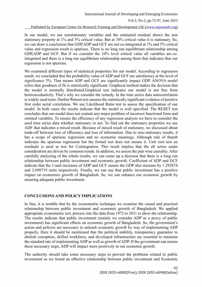
Jarque –Bera Test

We can compute Jarque-Bera test statistic using the following rule:

JB=n[S 2/6+ (K-3)2/24]

Where, n= sample size, s= skewness coefficient and k= kurtosis coefficient. If s=0 and k=3

then the value of the J-B statistic is expected to be 0. In our model, the JB value is 1.51. The

5% critical value from a chi-square distribution with 3 degrees of freedom is 7.815 and 1%

critical value is 11.345. because of 1.51< 7.815 and 1.51<11.345 so there is insufficient

evidence from residuals to conclude that the normal distribution assumption is unreasonable at

the 5% and 1% level of significance.



Vol.3, No.2, pp.72-97, June 2015



Tests for Multicollinearity

Multicollinearity is a sample phenomenon; we don’t have a unique method of testing

multicollinearity. For detecting multicollinearity in our model, we use E-VIEWS.

Correlation Matrix

Correlation matrix is one of the best techniques to detect multicollinearity. Now let’s have a

look at the following correlation matrix.

Table 4. Correlation matrix

ADP GCF GDP

ADP 1.000000 0.985260 0.987069

GCF 0.985260 1.000000 0.998487

GDP 0.987069 0.998487 1.000000

According to the Table-4, it can be seen that some variables are highly correlated with one

another. So, we can conclude from our correlation matrix the variables are highly correlated

and all values are greater than conventional level. That is multicollinearity problem exists in

this model.

So we can say, there is a high pair-wise correlation that indicates a severe collinearity problem.

Of course, remember the warning given earlier that such pair-wise correlations may be

sufficient but not a necessary condition for the existence of multicollinearity.

Tests for Heteroskedasticity

Homoskedasticity is an important property for OLS method. So it is important to find out

whether there is any heteroskedasticity problem or not. To test heteroskedasticity, we have used

the “Breusch–Pagan-Godfrey Test”.

0

1

2

3

4

5

6

7

-2.0e+09 -1.0e+09 0.00000 1.0e+09 2.0e+09

Series: Residuals

Sample 1973 2011

Observations 39

Mean -2.24e-06

Median -1.44e+08

Maximum 2.44e+09

Minimum -1.98e+09

Std. Dev. 1.05e+09

Skewness 0.435298

Kurtosis 2.579820

Jarque-Bera 1.518545

Probability 0.468007



Vol.3, No.2, pp.72-97, June 2015



Breusch–Pagan-Godfrey Test

Here the null and alternative hypotheses are;

Ho: There is no heteroskedasticity

Ha: There is heteroskedasticity problem

The formula of the Breusch-Pagan-Godfrey test shows as follows:

χ2=N*R2 ~ asy χ2 (s-1)

Where χ2 shows chi-square distribution with (s-1) degrees of freedom

Our observed χ2 = 13.32. If the computed value of χ2 exceeds the critical value of chi- square

at the chosen level of significance, we can reject the hypothesis of homoscedasticity; otherwise

does not reject it. In our model, chi-square value is 13.31590 with 2 df the 5% and 1% critical

chi square value are 5.99147 and 9.21034 which are less than computed chi-square. Therefore,

we reject the hypothesis of homoscedasticity. So, we can say that our model is not free from

heteroskedasticity and we should take steps to offset the problem. (According to appendix-5)

Remedy of Heteroscedasticity

We use white Heteroscedasticity -Consistent Standard Errors and Covariance (Appendices -2).

Now, we compare our estimation output from the uncorrected OLS regression with the

heteroscedasticity consistent covariance output. Note that in our model the coefficients are the

same but uncorrected standard error is smaller. It means that the heteroscedasticity consistent

covariance method has reduced the size of the t-statistics for the coefficients. It helps us to

avoid incorrect values for test statistics in the presence of heteroscedasticity.

Test for Autocorrelation

In order to conduct Durbin-Watson test statistic, following assumptions must be satisfied:

1) It is necessary to include a constant term in the regression.

2) The explanatory variables are non-stochastic, in repeated sampling.

3) The disturbance terms “U” are generated by the first order auto-regressive scheme.

4) The regression model does not include lagged values of the dependent variable as one

of the explanatory variables.

5) There are no missing observations in data.

6) The error term Ut is assumed to be normally distributed.

In the absence of software that computes a p-value, a test known as the bounds test, can be used

partially overcome the problem. Durbin & Watson considered two other statics dl& du whose

probability distribution do not depend on the explanatory variables.

DL < d < dU

That is, irrespective of the explanatory variables in the model under consideration will be



Vol.3, No.2, pp.72-97, June 2015



bounded by an upper bound du and 0 a lower bound dl. If d < dL, then H0 is rejected and d >du

indicates null is not rejected. Our regression model is qualified by all these assumptions. So,

we can use Durbin-Watson test. The test procedure is as follows:

(No Autocorrelation)

And, (Positive Autocorrelation)

In our model, calculated value of d=0.561985, against for n=39, k=2 and α=5%, the lower

bound =1.382 and an upper bound =1.597 at 5% level of significance. So we can reject H0

because of d< , At 1% level of significance also gives same decision. We conclude that, there

is an evidence of positive first order serial correlation. (According to Appendix-1) For reducing

this problem, we can apply “Cochrane-Orcutt” iterative procedure to estimate ρ, where, ρ is

known as the coefficient of auto-covariance. After that we can have a conclusion with the help

of EGLS technique.

Specification Test

Likelihood Ratio Test

In our model, we get the F-statistic with its p-value and a likelihood ratio test with p-value.

Both p-values are 0.00, so we reject the hypothesis that the coefficient of this variable is zero

(appendix-4).

RESET Test

Examining the model misspecification is a formal way to know whether our model is adequate

or whether we can ameliorate on it. It could be miss-specified if we have omitted important

variable, included irrelevant ones, chosen a wrong functional form or have a model that violates

the assumption of the multiple regression model. J B Ramsey (1969) has proposed a general

test of specification error called reset (Regression Specification Error Test) which is designed

to detect omitted variables and incorrect functional form. This test is proceed as follows-

We have specified and estimated the equation-

Let, (b1, b2, b3) be the LS estimates and let,

Is obtain and then consider the following artificial model-

Now, if is statistically insignificant then it can be conclude that there is no misspecification

with omitted variables and wrong functional form. Rejection of null hypothesis implies that the

original model is inadequate and can be improved when .

From our model, (appendix-5) the calculated value of F is 0.1630 and at the 5% and 1% level

0:0

pH

ld u

d

ld

ttttuGCFADPGDP

210

tttGCFbADPbbGDP

210

ttttuPDGGCFADPGDP 2

210ˆ

cricalFF



Vol.3, No.2, pp.72-97, June 2015



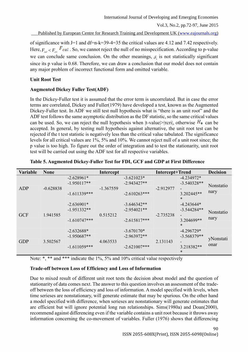
of significance with J=1 and df=n-k=39-4=35 the critical values are 4.12 and 7.42 respectively.

Here, . So, we cannot reject the null of no misspecification. According to p-value

we can conclude same conclusion. On the other meanings, is not statistically significant

since its p value is 0.68. Therefore, we can draw a conclusion that our model does not contain

any major problem of incorrect functional form and omitted variable.

Unit Root Test

Augmented Dickey Fuller Test(ADF)

In the Dickey-Fuller test it is assumed that the error term is uncorrelated. But in case the error

terms are correlated, Dickey and Fuller(1979) have developed a test, known as the Augmented

Dickey-Fuller test. In ADF we still test null hypothesis what is “there is an unit root” and the

ADF test follows the same asymptotic distribution as the DF statistic, so the same critical values

can be used. So, we can reject the null hypothesis when |t-value|>|τcri|, otherwise can be

accepted. In general, by testing null hypothesis against alternative, the unit root test can be

rejected if the t test statistic is negatively less than the critical value tabulated. The significance

levels for all critical values are 1%, 5% and 10%. We cannot reject null of a unit root since; the

p value is too high. To figure out the order of integration and to test the stationarity, unit root

test will be carried out using the ADF test for all respective variables.

Table 5. Augmented Dickey-Fuller Test for FDI, GCF and GDP at First Difference

eibairaV enoV toIVbeVnI toIVbeVnIcrbVoI nVeaiano

PDA -0.628838

-2.628961*

-1.367559

-3.621023*

-2.912977

-4.234972*

oNtansnoN

tsan

-1.950117** -2.943427** -3.540328**

-1.611339*** -2.610263***

-

3.202445**

*

FCG 1.941585

-2.636901*

0.515212

-3.646342**

-2.735238

-4.243644*

oNtansnoN

tsan

-1.951332** -2.954021** -3.544284**

-1.610747*** -2.615817***

-

3.204699**

*

FDA 3.502567

-2.632688*

4.063533

-3.670170*

2.131143

-4.296729*

noNtansno

Ntsa

-1.950687** -2.963972** -3.568379**

-1.611059*** -2.621007***

-

3.218382**

*

Note: *, ** and *** indicate the 1%, 5% and 10% critical value respectively

Trade-off between Loss of Efficiency and Loss of Information

Due to mixed result of different unit root tests the decision about model and the question of

stationarity of data comes next. The answer to this question involves an assessment of the trade-

off between the loss of efficiency and loss of information. A model specified with levels, when

time serieses are nonstationary, will generate estimate that may be spurious. On the other hand

a model specified with difference, when serieses are nonstationary will generate estimates that

are efficient but will ignore potential long run relationships. Sims(1980a) and Doan(2000),

recommend against differencing even if the variable contains a unit root because it throws away

information concerning the co-movement of variables. Fuller (1976) shows that differencing

cricalFF

1



Vol.3, No.2, pp.72-97, June 2015



produces no gain in asymptotic efficiency even if it is appropriate. Although we conduct unit

root tests and got mixed result but following Sims and Doan, the present study uses levels

rather than difference of the variables involved.

Consequences of Non Stationarity

Spurious regression results. 2. Exceptionally high r-square and t ratios, 3. No economic

meanings

Spurious Regression

The main reason why it is important to know whether a time series is stationary or nonstationary

before one embarks on a regression analysis is that there is a danger of obtaining apparently

significant regression results from unrelated data when nonstationary series are used in

regression analysis.

Such regressions are said to be spurious (lim et al). In shortly, we can say a spurious or

nonsensical relationship may be occurred when one non-stationary variable is regressed against

one or more non-stationary time series.

Rule of Thumb

According to Granger and Newbold, an R2 > d is a good rule of thumb to suspect that the

estimated regression is spurious. d stands for Durbin-Watson stat. From our result, =

0.997349 which is greater than Durbin-Watson stat =0.561985. Regression result is seems to

be spurious according to rule of thumb. So, we need formal diagnostic test to check whether

our regression is spurious or not. Co-integration test is widely use formal test for testing the

reliability of regression result.

Co-Integration Test

Unit Root Test on Residuals/ Engle Granger Test/ Augmented Engle Granger Test

If the residual series of the regression has a unit root then this regression result will spurious

where used variables are not integrated of order zero, I(0). We will operate different test for

unit root on the residuals that can be used to know cointegrating relationship. Here, we consider

ADF test only.

We can set the null and alternate hypotheses are-

: The series are not cointegrated=residuals are non-stationary.

: The series are cointegrated=residuals are stationary

Augmented Dickey-Fuller test for residual series of regression at level

Variable None Intercept Intercept+Trend Decision

Residual -1.692409

-2.632688*

-1.666872

-3.632900*

-3.739045

-4.226815* Stationary

at 10% -1.950687** -2.948404** -3.536601**

-1.611059*** -2.612874*** -3.200320***

Note: *, ** and *** indicate the 1%, 5% and 10% critical value respectively



Vol.3, No.2, pp.72-97, June 2015



In our model, we use nonstationary variables and the estimated residual shows the non

stationary property at 1% and 5% critical value. But at 10% critical value it is stationary. So,

we can draw a conclusion that GDP,ADP and GCF are not co-integrated at 1% and 5% critical

value and regression result is spurious. There is no long run equilibrium relationship among

GDP,ADP and GCF. But if we consider the 10% level critical value all variables are co-

integrated and there is a long run equilibrium relationship among them that indicates that our

regression is not spurious.

We examined different types of statistical properties for our model. According to regression

result, we concluded that the probability value of ADP and GCF are satisfactory at the level of

significance 5%. That means ADP and GCF are significantly impact GDP. ANOVA model

refers that goodness of fit is statistically significant. Graphical method makes the decision that

the model is normally distributed.Graphical test indicates our model is not free from

heteroscedasticity. That’s why we consider the remedy. In the time series data autocorrelation

is widely used term. Durbin Watson test ensures the statistically significant evidence of positive

first order serial correlation. We use Likelihood Ratio test to assess the specification of our

model. In both cases the results indicate that the model is well specified. The RESET test

concludes that our model does not contain any major problem of incorrect functional form and

omitted variables. To ensure the efficiency of any regression analysis we have to consider the

used time series data whether stationary or not. To find out the stationary properties we use

ADF that indicates a mixed result. Because of mixed result of stationary, we discussed about

trade-off between loss of efficiency and loss of information. Due to non-stationary results, it

has a scope of spurious regression and no economic meanings. Although rule of thumb

indicates the spurious regression but the formal test does not ensure it. Unit root test on

residuals is used as test for Cointegration. This result implies that the all series under

consideration are driven by common trends. In addition, we assess the pair wise causality. After

carefully analyzing of the whole results, we can come up a decision that there is a long run

relationship between public investment and economic growth. Coefficient of ADP and GCF

indicate that the 1-unit increases of ADP and GCF ensure the GDP also increase by 1.292874

and 2.698719 units respectively. Finally, we can say that public investment has a positive

impact on economics growth of Bangladesh. So, we can enhance our economic growth by

ensuring adequate public investment.

CONCLUSIONS AND POLICY IMPLICATIONS

In fine, it is notable that by the econometric technique we examine the casual and practical

relationship between public investment and economic growth of Bangladesh. We applied

appropriate econometric test, process into the data from 1972 to 2011 to show the relationship.

The results indicate that public investment (mainly we consider ADP as a proxy of public

investment) has significant effects on economic growth of Bangladesh. So, the government’s

action and policies are necessary to unleash economic growth by way of implementing ADP

properly. Here it should be mentioned that the political stability, transparency guarantee to

abolish corruption, skilled workforce, and developed infrastructure are essential to maintain

the standard rate of implementing ADP as well as growth of ADP. If the government can ensure

these necessary steps, ADP will impact more positively in our economic growth.

The authority should take some necessary steps to prevent the problems related to public

investment as we found an effective relationship between public investment and Economic



Vol.3, No.2, pp.72-97, June 2015



growth in Bangladesh. Political institutions and actors should be more compromising and

consolidate democracy with stable situation for the economic development of the country. The

administrative structure should be more accountable and transparent to achieve a good

governance system that restrains corruption. The government should enforce monitoring and

evaluation procedures in establishing the infrastructures that can ensure more implementation

status of ADP. We should also emphasize human resource development through practical

education and training programs. We believe that if government considers it then economic

growth will enhance.

The econometric model we developed for this study that may suffer from a number of

shortcomings due to lack of proper information. Therefore, some venues for future research

may be considered. They are as follows:

This study uses annual time series data, which may mask some important dynamic aspects. An

analysis based on quarterly or monthly data should certainly be more enriching. But availability

of monthly data for Bangladesh would continue to be a major stumbling block at least in the

foreseeable future. An important driving force of future research in time series analysis is the

advance in high-volume data acquisition. Further work could apply the methodologies

developed for this study to a range of other developing countries. However, the estimation

equations should be constructed to fit the specific public finance structure in each country.

Further studies using different conditions for public investment, for example, different types of

dummy could add significant insight on the effects of economic growth in our country.

Moreover, from our literature review, it is observed that public investment can crowd in and

increase private investment. Proper and accurate data will be available in future and must it be

analyzed properly and efficiently. But the special features of the data, such as large sample

sizes, heavy tails, unequally spaced observations, and mixtures of multivariate discrete and

continuous variables, can easily render existing methods inadequate. Analyses of these types

of data will certainly influence the directions of future research.



Vol.3, No.2, pp.72-97, June 2015



APPENDICES

Appendix-1

Dependent Variable: GDP

Method: Least Squares

Date: 10/04/14 Time: 21:48

Sample: 1 39

Included observations: 39


C 1.44E+10 2.75E+08 52.41929 0.0000

ADP 1.292874 0.575230 2.247576 0.0308

GCF 2.698719 0.152575 17.68781 0.0000

R-squared 0.997349 Mean dependent var 3.87E+10

Adjusted R-squared 0.997201 S.D. dependent var 2.05E+10

S.E. of regression 1.08E+09 Akaike info criterion 44.51842

Sum squared resid 4.23E+19 Schwarz criterion 44.64639

Log likelihood -865.1093 Hannan-Quinn criter. 44.56434

F-statistic 6770.731 Durbin-Watson stat 0.561985

Prob(F-statistic) 0.000000

Appendix-2

Test for Equality of Means Between Series

Date: 10/04/14 Time: 00:53

Sample: 1973 2011


Method df Value Probability

Anova F-test (2, 114) 96.90957 0.0000

Welch F-test* (2, 54.3372) 74.44398 0.0000

*Test allows for unequal cell variances

Analysis of Variance

Source of Variation df Sum of Sq. Mean Sq.

Between 2 3.02E+22 1.51E+22

Within 114 1.78E+22 1.56E+20

Total 116 4.80E+22 4.14E+20

Category Statistics

Variable Count Mean Std. Dev. of Mean

ADP 39 2.02E+09 1.79E+09 2.86E+08

GCF 39 8.03E+09 6.73E+09 1.08E+09

GDP 39 3.87E+10 2.05E+10 3.28E+09

All 117 1.63E+10 2.03E+10 1.88E+09



Vol.3, No.2, pp.72-97, June 2015



APPENDIX-3

Heteroskedasticity Test: Breusch-Pagan-Godfrey

F-statistic 9.332083 Prob. F(2,36) 0.0005

Obs*R-squared 13.31590 Prob. Chi-Square(2) 0.0013

Scaled explained SS 8.962390 Prob. Chi-Square(2) 0.0113

Test Equation:

Dependent Variable: RESID^2



C 1.33E+17 2.92E+17 0.455740 0.6513

ADP -1.16E+09 6.11E+08 -1.902183 0.0652

GCF 4.11E+08 1.62E+08 2.537673 0.0156








Appendix-4

Redundant Variables: GDP(-1)


Log likelihood ratio 82.90207 Prob. Chi-Square(1) 0.0000

Test Equation:



Sample: 2 39


Coefficie

nt Std. Error t-Statistic Prob.

C 1.44E+10 2.88E+08 50.15539 0.0000

ADP 1.293566 0.583542 2.216748 0.0332

GCF 2.698296 0.154976 17.41107 0.0000










Vol.3, No.2, pp.72-97, June 2015



Appendix-5

Ramsey RESET Test:


Log likelihood ratio 0.181296 Prob. Chi-Square(1) 0.6703

Test Equation:





C 1.44E+10 3.48E+08 41.24621 0.0000

ADP 1.276830 0.583390 2.188639 0.0354

GCF 2.758826 0.214445 12.86494 0.0000

FITTED^2 -1.92E-13 4.75E-13 -0.403833 0.6888








REFERENCES

Anderson, E., Renzio, P. de and Levy, S. (2006) “The role of public investment in poverty

reduction: Theories, evidence and methods” , Working Paper 263,Overseas Development

Institute, London SE 1 7 JD, UK

Baltagi, Badi H., Kao, Chihwa.: Nonstationary Panels, Cointegration in Panels and Dynamic

Panels: A Survey, Center for Policy Research, WorskingPaper No. 16, New York, 2000

Clements, B. , Bhattacharya, R. and Nguyen, T. Q. (2003) “External debt, Public investment

and Growth in low income countries” IMF Working Paper WP/03/249, Fiscal Affairs

Department, International Monetary Fund.

Cullision, W. E. (1993 ) “Public investment and Economic Growth” Economic Quarterly,

Volume 79/4 Fall 1993, Federal Reserve Bank of Richmond, pp. 19-33 Different reports

of Implementation Monitoring and Evaluation Division (IMED), Bangladesh

Government.

Costa, J. da Silva, R. W. Ellson, and R. C. Martin (1987) Public Capital, Regional Output and

Developments: Some Empirical Evidence. Journal of Regional Science 27:3, 419–437.

Deno, K. T. (1988) The Effect of Public Capital on U.S. Manufacturing Activity: 1970 to 1978.

Southern Economic Journal55:1, 400–411.

Doan, T. A. (2000), Rats, User’s Guide, Estima, Evanston, IL.E-views users guide i and ii.

Eberts, R. W. (1986) Estimating the Contribution of Urban Public Infrastructure to Regional

Growth. Federal Reserve Bank of Cleveland. (Working Paper No. 8610)

Fuller, W. A. (1976). Introduction to Statistical Time Series. New York: Willey.

Ghani, E. and Uddin, M. (2006) “The impact of Public investment on Economic Growth in

Pakistan” The Pakistan Development Review, 45:1 ( Spring 2006) pp. 87-98.

Gonzalez, R. L. and Montolio, D.(2011) “Growth, Convergence and Public Investment A

Bayesian Model Averaging Approach”.



Vol.3, No.2, pp.72-97, June 2015



Gujarati, Damoder N. Basic Econometrics, Fourth Edition, McGraw-Hill Higher Education.

Haque, M. E. and Kneller, R. (2008) “Public investment and Growth : the rule of corruption”

Discussion Paper Series Number 098, Centre for Growth & Business Cycle Research,

University of Manshester, Manchester.

Hsiao, Cheng: Analysis of Panel Data, Second Edition, CambridgeUniversity Press, New York,

2003

Jimenz, E. (1995) “Human and physical infrastructure: public investment and pricing polices

in developing countries” Hand book of development economics, PP.2774-2836, Volume 3

Edited by J. Behrman and T. N. Srinivasan Elsevier Science B. V 1995.

kalaitzidakis, P. and kalyvitisy, S. (2003) “Financing New public investment and or

maintenance in public capital for long run growth” Canadian Studies Program,

Department of Foreign Affairs and International Trade, Canada.

Kamps, Christophe: The Dynamic Macroeconomic Effects of Public Capital, Theory and

Evidence for OECD countries, Springer, New York, 2004.

Kappeler, A and Valila, T.(2007) “Composition of Public Investment and Fiscal Federalism:

Panel Data Evidence from Europe” economics and financial report 2007/02, European

investment bank.

Kuttner, R. (1992) “The slow growth trap and the public investment cure” The Economic Policy

Institute, Briefing Paper # 34A, USA.

Naqvi, N. H. (2002) Crowding-in or Crowding out? Modeling the Relationship between Public

and Private Fixed Capital Formation using Co-Integration Analysis, The Case of Pakistan

1964-2000. The Pakistan Development Review,41:3, 255–276.

R. Carter Hill, William e. Griffiths and Guay C. Lim, Principle of Econometrics, Fourth Edition,

John Wiley & Sons, Inc., 111 River Street, Hoboken

Sims, C. A. (1980a). “Macroeconomics and Reality” Econometrica, 48(10), pp. 1-48

Sturm, J.E.: Public Capital Expenditures inOECD Countries: The Causes and Impact of the

Decline in Public Capital Spending, Edward Elgar,Cheltenham, 1998

The Daily Ittefaq (10 April 2011), Dhaka, Bangladesh.

www.data.worldbank.com

Zhang, X. and Fan, S. (2000) “Public investment and regional inequality in rural china” EPTD

discussion paper no. 71, Washington, DC 20006 USA


Documents

International Journal of Developing and Emerging Economies