Embed Size (px)
DESCRIPTION
Topics in detail to be covered are: Smarandache multi-spaces with applications to other sciences, such as those of algebraic multi-systems, multi-metric spaces, etc.. Smarandache geometries; Differential Geometry; Geometry on manifolds; Topological graphs; Algebraic graphs; Random graphs; Combinatorial maps; Graph and map enumeration; Combinatorial designs; Combinatorial enumeration; Low Dimensional Topology; Differential Topology; Topology of Manifolds; Geometrical aspects of Mathematical Physics and Relations with Manifold Topology; Applications of Smarandache multi-spaces to theoretical physics; Applications of Combinatorics to mathematics and theoretical physics; Mathematical theory on gravitational fields; Mathematical theory on parallel universes; Other applications of Smarandache multi-space and combinatorics.
Citation preview
ISSN 1937 - 1055
VOLUME 3, 2013
INTERNATIONAL JOURNAL OF
MATHEMATICAL COMBINATORICS
EDITED BY
THE MADIS OF CHINESE ACADEMY OF SCIENCES AND
BEIJING UNIVERSITY OF CIVIL ENGINEERING AND ARCHITECTURE
September, 2013
Vol.3, 2013 ISSN 1937-1055
International Journal of
Mathematical Combinatorics
Edited By
The Madis of Chinese Academy of Sciences and
Beijing University of Civil Engineering and Architecture
September, 2013
Aims and Scope: The International J.Mathematical Combinatorics (ISSN 1937-1055)
is a fully refereed international journal, sponsored by the MADIS of Chinese Academy of Sci-
ences and published in USA quarterly comprising 100-150 pages approx. per volume, which
publishes original research papers and survey articles in all aspects of Smarandache multi-spaces,
Smarandache geometries, mathematical combinatorics, non-euclidean geometry and topology
and their applications to other sciences. Topics in detail to be covered are:
Smarandache multi-spaces with applications to other sciences, such as those of algebraic
multi-systems, multi-metric spaces,· · · , etc.. Smarandache geometries;
Differential Geometry; Geometry on manifolds;
Topological graphs; Algebraic graphs; Random graphs; Combinatorial maps; Graph and
map enumeration; Combinatorial designs; Combinatorial enumeration;
Low Dimensional Topology; Differential Topology; Topology of Manifolds;
Geometrical aspects of Mathematical Physics and Relations with Manifold Topology;
Applications of Smarandache multi-spaces to theoretical physics; Applications of Combi-
natorics to mathematics and theoretical physics;
Mathematical theory on gravitational fields; Mathematical theory on parallel universes;
Other applications of Smarandache multi-space and combinatorics.
Generally, papers on mathematics with its applications not including in above topics are
also welcome.
It is also available from the below international databases:
Serials Group/Editorial Department of EBSCO Publishing
10 Estes St. Ipswich, MA 01938-2106, USA
Tel.: (978) 356-6500, Ext. 2262 Fax: (978) 356-9371
http://www.ebsco.com/home/printsubs/priceproj.asp
and
Gale Directory of Publications and Broadcast Media, Gale, a part of Cengage Learning
27500 Drake Rd. Farmington Hills, MI 48331-3535, USA
Tel.: (248) 699-4253, ext. 1326; 1-800-347-GALE Fax: (248) 699-8075
http://www.gale.com
Indexing and Reviews: Mathematical Reviews(USA), Zentralblatt fur Mathematik(Germany),
Referativnyi Zhurnal (Russia), Mathematika (Russia), Computing Review (USA), Institute for
Scientific Information (PA, USA), Library of Congress Subject Headings (USA).
Subscription A subscription can be ordered by an email to [email protected]
or directly to
Linfan Mao
The Editor-in-Chief of International Journal of Mathematical Combinatorics
Chinese Academy of Mathematics and System Science
Beijing, 100190, P.R.China
Email: [email protected]
Price: US$48.00
Editorial Board (3nd)
Editor-in-Chief
Linfan MAO
Chinese Academy of Mathematics and System
Science, P.R.China
and
Beijing University of Civil Engineering and
Architecture, P.R.China
Email: [email protected]
Deputy Editor-in-Chief
Guohua Song
Beijing University of Civil Engineering and
Architecture, P.R.China
Email: [email protected]
Editors
S.Bhattacharya
Deakin University
Geelong Campus at Waurn Ponds
Australia
Email: [email protected]
Said Broumi
Hassan II University Mohammedia
Hay El Baraka Ben M’sik Casablanca
B.P.7951 Morocco
Junliang Cai
Beijing Normal University, P.R.China
Email: [email protected]
Yanxun Chang
Beijing Jiaotong University, P.R.China
Email: [email protected]
Jingan Cui
Beijing University of Civil Engineering and
Architecture, P.R.China
Email: [email protected]
Shaofei Du
Capital Normal University, P.R.China
Email: [email protected]
Baizhou He
Beijing University of Civil Engineering and
Architecture, P.R.China
Email: [email protected]
Xiaodong Hu
Chinese Academy of Mathematics and System
Science, P.R.China
Email: [email protected]
Yuanqiu Huang
Hunan Normal University, P.R.China
Email: [email protected]
H.Iseri
Mansfield University, USA
Email: [email protected]
Xueliang Li
Nankai University, P.R.China
Email: [email protected]
Guodong Liu
Huizhou University
Email: [email protected]
W.B.Vasantha Kandasamy
Indian Institute of Technology, India
Email: [email protected]
Ion Patrascu
Fratii Buzesti National College
Craiova Romania
Han Ren
East China Normal University, P.R.China
Email: [email protected]
Ovidiu-Ilie Sandru
Politechnica University of Bucharest
Romania
ii International Journal of Mathematical Combinatorics
Mingyao Xu
Peking University, P.R.China
Email: [email protected]
Guiying Yan
Chinese Academy of Mathematics and System
Science, P.R.China
Email: [email protected]
Y. Zhang
Department of Computer Science
Georgia State University, Atlanta, USA
Famous Words:
Do not, for one repulse, give up the purpose that you resolved to effect.
By William Shakespeare, a British dramatist.
International J.Math. Combin. Vol.3(2013), 01-15
Modular Equations for Ramanujan’s Cubic Continued Fraction
And its Evaluations
B.R.Srivatsa Kumar
(Department of Mathematics, Manipal Institute of Technology, Manipal University, Manipal-576104, India)
G.N.Rajappa
(Department of Mathematics, Adichunchanagiri Institute of Technology, Jyothi Nagar, Chikkamagalur-577102, India)
E-mail: sri−[email protected]
Abstract: In this paper, we establish certain modular equations related to Ramanujan’s
cubic continued fraction
G(q) :=q1/3
1 +
q + q2
1 +
q2 + q4
1 +..., |q| < 1.
and obtain many explicit values of G(e−π√
n), for certain values of n.
Key Words: Ramanujan cubic continued fraction, theta functions, modular equation.
AMS(2010): 33D90, 11A55
§1. Introduction
Let
G(q) :=q1/3
1 +
q + q2
1 +
q2 + q4
1 +..., (1.1)
denote the Ramanujan’s cubic continued fraction for |q| < 1. This continued fraction was
recorded by Ramanujan in his second letter to Hardy [12]. Chan [11] and Baruah [5] have
proved several elegant theorems for G(q). Berndt, Chan and Zhang [8] have proved some
general formulas for G(e−π√
n) and H(e−π√
n) where
H(q) := −G(−q)
and n is any positive rational, in terms of Ramanujan-Weber class invariant Gn and gn:
Gn := 2−1/4q−1/24(−q; q2)∞
and
gn := 2−1/4q−1/24(q; q2)∞, q = e−π√
n.
1Received June 24, 2013, Accepted July 25, 2013.
2 B.R.Srivatsa Kumar and G.N.Rajappa
For the wonderful introduction to Ramanujan’s continued fraction see [3], [6], [11] and for
some beautiful subsequent work on Ramanujan’s cubic continued fraction [1], [2], [4], [5], [14]
and [15].
In this paper, we establish certain general formulae for evaluating G(q). In section 2 of this
paper, we setup some preliminaries which are required to prove the general formulae. In section
3, we establish certain modular equations related to G(q) and in the final section, we deduce
the above stated general formulae and obtain many explicit values of G(q). We conclude this
introduction by recalling an identity for G(q) stated by Ramanujan.
1 +1
G3(q)=
ψ4(q)
qψ4(q3)(1.2)
where
ψ(q) :=
∞∑
n=0
qn(n+1)/2 =(q2; q2)∞(q; q2)∞
. (1.3)
The proof of (1.2) follows from Entry 1 (ii) and (iii) of Chapter 20 (6, p.345]).
§2. Some Preliminary Results
As usual, for any complex number a,
(a; q)0 := 1
and
(a; q)∞ :=
∞∏
n=0
(1 − aqn), |q| < 1.
A modular equation of degree n is an equation relating α and β that is induced by
n2F1
(
12 ,
12 ; 1; 1− α
)
2F1
(
12 ,
12 ; 1;α
) =2F1
(
12 ,
12 ; 1; 1− β
)
2F1
(
12 ,
12 ; 1;β
) ,
where
2F1(a, b; c;x) :=
∞∑
n=0
(a)n(b)n
(c)nn!xn, |x| < 1,
with
(a)n := a(a+ 1)(a+ 2)...(a+ n− 1).
Then, we say that β is of nth degree over α and call the ratio
m :=z1zn,
the multiplier, where z1 =2 F1
(
12 ,
12 ; 1;α
)
and zn =2 F1
(
12 ,
12 ; 1;β
)
.
Theorem 2.1 Let G(q) be as defined as in (1.1), then
G(q) +G(−q) + 2G2(−q)G2(q) = 0 (2.1)
and
G2(q) + 2G2(q2)G(q)−G(q2) = 0. (2.2)
Modular Equations for Ramanujan’s Cubic Continued Fraction and its Evaluations 3
For a proof of Theorem 2.1, see [11].
Theorem 2.2 Let β and γ be of the third and ninth degrees, respectively, with respect to α.
Let m = z1/z3 and m′ = z3/z9. Then,
(i)
(
β2
αγ
)1/4
+
(
(1 − β)2
(1 − α)(1 − γ)
)1/4
−(
β2(1 − β)2
αγ(1− α)(1 − γ)
)1/4
=−3m
m′ (2.3)
and
(ii)
(
αγ
β2
)1/4
+
(
(1− α)(1 − γ)(1− β)2
)1/4
−(
αγ(1 − α)(1 − γ)β2(1− β)2
)1/4
=m′
m. (2.4)
For a proof, see [6], Entry 3 (xii) and (xiii), pp. 352-353.
Theorem 2.3 Let α, β, γ and δ be of the first, third, fifth and fifteenth degrees respectively.
Let m denote the multiplier connecting α and β and let m′ be the multiplier relating γ and δ.
Then,
(i)
(
αδ
βγ
)1/8
+
(
(1− α)(1 − δ)(1 − β)(1− γ)
)1/8
−(
αδ(1− α)(1 − δ)βγ(1− β)(1 − γ)
)1/8
=
√
m′
m(2.5)
and
(ii)
(
βγ
αδ
)1/8
+
(
(1− β)(1 − γ)(1− α)(1 − δ)
)1/8
−(
βγ(1− β)(1 − γ)αδ(1 − α)(1 − δ)
)1/8
= −√
m
m′ . (2.6)
For a proof, see [6], Entry 11 (viii) and (ix), p. 383.
Theorem 2.4 If β, γ and δ are of degrees 3, 7 and 21 respectively, m = z1/z3 and m′ = z7/z21,
then
(i)
(
βδ
αγ
)1/4
+
(
(1 − β)(1 − δ)(1− α)(1 − γ)
)1/4
+
(
βδ(1 − β)(1 − δ)αγ(1− α)(1 − γ)
)1/4
−2
(
βδ(1 − β)(1 − δ)αγ(1− α)(1 − γ)
)1/8
1 +
(
βδ
αγ
)1/8
+
(
(1− β)(1 − δ)(1− α)(1 − γ)
)1/8
= mm′ (2.7)
and
(ii)
(
αγ
βδ
)1/4
+
(
(1− α)(1 − γ)(1− β)(1 − δ)
)1/4
+
(
αγ(1− α)(1 − γ)βδ(1− β)(1 − δ)
)1/4
−2
(
αγ(1− α)(1 − γ)βδ(1− β)(1 − δ)
)1/8
1 +
(
αγ
βδ
)1/8
+
(
(1 − α)(1 − γ)(1− β)(1 − δ)
)1/8
=9
mm′ . (2.8)
For a proof, see [6], Entry 13 (v) and (vi), pp. 400-401.
4 B.R.Srivatsa Kumar and G.N.Rajappa
§3. Modular Equations
Theorem 3.1 Let
R :=ψ(−q3)ψ(−q2)q3/8ψ(−q)ψ(−q6) and S :=
ψ(−q6)ψ(−q4)q3/4ψ(−q2)ψ(−q12)
then,(√
R
S+
√
S
R
)
(√RS +
1√RS
)
− 8 = 0. (3.1)
Proof From (1.2) and the definition of R and S, it can be seen that
B3(A3 + 1)R4 = A3(B3 + 1) (3.2)
and
C3(B3 + 1)S4 = B3(C3 + 1), (3.3)
where A = G(−q), B = G(−q2) and C = G(−q4).On changing q to q2 in (2.1), we have
G(q2) +G(−q2) + 2G2(−q2)G2(q2) = 0 (3.4)
and also change q to −q in (2.2), we have
G2(−q) + 2G2(q2)G(−q)−G(q2) = 0. (3.5)
Eliminating G(q2) between (3.4) and (3.5) using Maple,
2(AB)4 − 4(AB)3 + 3(AB)2 +AB +A3 +B3 = 0. (3.6)
Now on eliminating A between (3.2) and (3.6) using Maple, we obtain
8(BR)4 − 80(BR)3 + 63(BR)2 − 5BR+B3 − 16B3R+ 72B3R2 + 7B3R4
−22B2R+ 2B2 + 2B2R3 −B2R4 − 9BR2 +BR3 +B +R = 0. (3.7)
Changing q to q2 in (3.6),
2(BC)4 − 4(BC)3 + 3(BC)2 +BC +B3 + C3 = 0. (3.8)
Eliminating C between (3.3) and (3.8) using Maple,
8B4 + 7B3 − 16S3B3 + 72S2B3 − 80SB3 + S4B3 + 2B2S4 −B2 + 2B2S − 22S3B2
+63B2S2 − 9BS2 + SB − 5BS3 +BS4 + S3 = 0. (3.9)
Finally on eliminating B between (3.7) and (3.9) using Maple, we have
L(R,S)M(R,S) = 0,
Modular Equations for Ramanujan’s Cubic Continued Fraction and its Evaluations 5
where,
L(R,S) = 15S3R6 − 1734R4S4 + SR+ 49S2R2 − S3 − 137S4R2 + 8S4R+ 705S4R3
−137S2R4−8S2R−15S2R3 +8SR4−8SR2 +16SR3 +705S3R4−15S3R2 +16S3R−327S3R3
−120S3R5 + 705R5S4 + 15S2R5 − SR5 − S3R7 − 137R6S4 + 8R7S4 − 327R5S5 + 49R6S6
+8R4S7 −R5S8 − 15R5S6 − 8R7S6 −R8S5 − 15R6S5 + 16R7S5 − 8R6S7 + 16R5S7 +R7S7
−120S5R3 + 15S5R2 + 705S5R4 − 137S6R4 + 15S6R3 − S7R3 − S5R−R3 = 0
and
M(R,S) = R2S +RS2 − 8RS +R + S = 0.
Using the series expansion of R and S in the above we find that
L(R,S) = 223522 + 8q−15/2 − 8q−57/8 − 2q−55/8 − 56q−27/4 + 48q−13/2 − 24q−49/8 + ...
and
M(R,S) = q−15/8 + q−3/2 − 8q−9/8 + q−7/8 + q−3/4 + 2q−1/2 + ...,
where
R =1
q3/8+ q5/8 + 2q29/8 + 2q21/8 + 2q13/8 + ...
and
S =1
q3/4+ q5/4 + 2q29/4 + 2q21/4 + 2q13/4 + ....
One can see that q−1L(R,S) does not tend to 0 as q → 0 whereas q−1M(R,S) tends to 0
as q → 0. Hence, q−1M(R,S) = 0 in some neighborhood of q = 0. By analytic continuation
q−1M(R,S) = 0 in |q| < 1. Thus we have
M(R,S) = 0.
On dividing throughout by RS we have the result. 2Theorem 3.2 If
R :=ψ2(−q3)
q1/2ψ(−q)ψ(−q9) and S :=ψ2(−q6)
qψ(−q2)ψ(−q18) ,
then(
R
S
)4
+
(
S
R
)4
+
(
R
S
)2
+
(
S
R
)2
−(
RS − 3
RS
)
(
R
S
)3
+
(
S
R
)3
−3
(
RS − 3
RS
)(
R
S+S
R
)
−
(RS)2 +9
(RS)2
− 6 = 0. (3.10)
Proof Let
P :=ψ2(q3)
q1/2ψ(q)ψ(q9)and Q :=
ψ2(q6)
qψ(q2)ψ(q18).
6 B.R.Srivatsa Kumar and G.N.Rajappa
On using Entry 10 (ii)and (iii) of Chapter 17 in [6, p.122] in P and Q, we deduce
P
Q=
(
αγ
β2
)
andP 2
Q=
(
z23
z1z9
)1/2
.
Employing these in (2.3) and (2.4) it is easy to see that
(1− β)2
(1− α)(1 − γ)
1/4
=Q2(3 + P 2)
P 2(Q2 − P 2)and
(1− α)(1 − γ)(1− β)2
1/4
=P 2(P 2 − 1)
Q2 − P 2.
Multiplying these two, we arrive at
P 4 − 4P 2Q2 +Q4 + 3Q2 − P 4Q2 = 0. (3.11)
Changing q to −q in the above,
R4 − 4R2Q2 +Q4 + 3Q2 −R4Q2 = 0. (3.12)
On eliminating Q between (3.11) and (3.12), we have
P 4R4 − 5P 4 − 12P 2 + 16P 2R2 + 4P 2R4 − 11R4 − 8R6 −R8 + 12R2 + 4P 4R2
= (−4P 2 − P 4 + 4R2 +R4)√
6R4 − 24R2 + 8R6 +R8 + 9
On squaring the above and then factorizing, we have
P 4 − 2P 2R2 +R4 − P 4R2 − P 2R4 + 3P 2 + 3R2 = 0. (3.13)
Changing q to q2 in (3.13), we have
Q4 − 2Q2S2 + S4 −Q4S2 −Q2S4 + 3Q2 + 3S2 = 0. (3.14)
Eliminating Q between (3.12) and (3.14) and then on dividing throughout by (RS)4 and on
simplifying, we obtain the required result.
Theorem 3.3 If
R :=ψ(−q3)ψ(−q5)
q1/4ψ(−q)ψ(−q15) and S :=ψ(−q6)ψ(−q10)
q1/2ψ(−q2)ψ(−q30) ,
then
(
R2
S2+S2
R2
)
+
(
R
S+S
R
)
−(√
RS − 1√RS
)
√
S
R+
√
R
S+
(
R
S
)3/2
+
(
S
R
)3/2
= RS +1
RS. (3.15)
Proof Let
P :=ψ(q3)ψ(q5)
qψ(q)ψ(q15)and Q :=
ψ(q6)ψ(q10)
q2ψ(q2)ψ(q30),
Modular Equations for Ramanujan’s Cubic Continued Fraction and its Evaluations 7
On using Entry 11 (ii) and (iii) of Chapter 17 in [6, p.122] in P and Q we deduce
P
Q=
(
αδ
βγ
)1/8
andP 2
Q=
(
m′
m
)1/2
.
Employing (2.5) and (2.6) in the above, it is easy to check that
(
(1− α)(1 − δ)(1 − β)(1 − γ)
)1/8
=P (P − 1)
Q− P and
(
(1 − β)(1 − γ)(1− α)(1 − δ)
)1/8
=Q(P + 1)
P (Q− P )
Multiplying these two, we obtain
P 2 +Q2 − 2PQ− P 2Q+Q = 0. (3.16)
Changing q to −q in the above
R2 +Q2 − 2RQ−R2Q+Q = 0. (3.17)
Eliminating Q between (3.16) and (3.17), we obtain
P 2 +R2 + (P +R)(1− PR) = 0. (3.18)
On Changing q to q2 in the above
Q2 + S2 + (Q+ S)(1−QS) = 0. (3.19)
Finally, on eliminating Q between (3.17) and (3.19) and on dividing through out by (RS)2,
we have the result. 2Theorem 3.4 If
R := q2ψ(−q3)ψ(−q21)ψ(−q)ψ(−q7) and S := q4
ψ(−q6)ψ(−q42)ψ(−q2)ψ(−q14) ,
then
y8 − (4 + 6x1)y7 + (24 + 24x1 + 9x2)y6 − (148 + 12x1 + 36x2)y5 + (145 + 252x1)y4
−(648+678x1−36x2+54x3)y3+(2180+360x1+441x2−324x3)y2−(1016+2016x1−396x2−54x3)y1
+81x4 − 324x3 + 1548x2 + 1236x1 + 5250 = 0, (3.20)
where
xn = (3RS)n +1
(3RS)nand yn =
(
R
S
)n
+
(
S
R
)n
.
Proof Let
P := q2ψ(q3)ψ(q21)
ψ(q)ψ(q7)and Q := q4
ψ(q6)ψ(q42)
ψ(q2)ψ(q14),
Using Entry 11 (ii) and (iii) of Chapter 17 [6, p.122] in P and Q it is easy to deduce
P
Q=
(
αγ
βδ
)1/8
andP 2
Q=
1√mm′ .
8 B.R.Srivatsa Kumar and G.N.Rajappa
Employing (2.5) and (2.6) in the above, it is easy to check that
(P −Q)2Px
Q− PQ− P 2
2
− 4P 3Q−Q2 + 2PQ− P 2 = 0
and
(P −Q)2
Px− P −Q
2
− 4PQ− 9P 2Q2 + 18P 3Q− 9P 4 = 0.
where
x =
(
(1− β)(1 − δ)(1− α)(1 − γ)
)1/8
.
Eliminating x between these two we have
Q4 + 8Q4P 2 − 4P 3Q3 − 2P 4Q2 − 44P 4Q4 + 24Q2P 6 − 12P 7Q+ 81P 8Q4
+72P 6Q4 − 18Q2P 8 − 18Q6P 4 − 36Q5P 5 + P 8 +Q8 − 2Q6 − 12P 5Q3
−12P 3Q5 + 24Q6P 2 − 4Q5P − 36P 7Q3 − 12PQ7 = 0. (3.21)
On changing q to −q in the above
Q4 + 8Q4R2 − 4R3Q3 − 2R4Q2 − 44R4Q4 + 24Q2R6 − 12R7Q+ 81R8Q4
+72R6Q4 − 18Q2R8 − 18Q6R4 − 36Q5R5 +R8 +Q8 − 2Q6 − 12R5Q3
−12R3Q5 + 24Q6R2 − 4Q5R− 36R7Q3 − 12RQ7 = 0. (3.22)
Now on eliminating Q between (3.21) and (3.22),
R4 − 2R6 − 18P 8R2 + 144P 7R3 − 450P 6R4 + 504P 5R5 − 450P 4R6 − 12PR7
−12RP 7 + 78R2P 6 − 228R3P 5 + 226R4P 4 − 228R5P 3 + 78R6P 2 − 18R8P 2
+P 4 − 2P 6 + P 8 + 81P 8R4 +R8 + 16RP 5 − 50R2P 4
+56R3P 3 − 50R4P 2 + 16R5P + 144P 3R7 − 4RP 3 + 6P 2R2 − 4PR3
+486R6P 6 − 324R5P 7 − 324R7P 5 + 81R8P 4 = 0. (3.23)
On changing q to q2 in the above
Q4 +Q8 − 2Q6 + S4 − 2S6 + S8 − 18Q8S2 + 144Q7S3 − 450Q6S4 + 504Q5S5
−450Q4S6 − 12QS7 − 12SQ7 + 78S2Q6 − 228S3Q5 + 226S4Q4 − 228S5Q3
+78S6Q2 − 18S8Q2 + 81Q8S4 + 16SQ5 − 50S2Q4 + 56S3Q3
−50S4Q2 + 16S5Q+ 144Q3S7 − 4SQ3 + 6Q2S2 − 4QS3 + 486S6Q6
−324S5Q7 − 324S7Q5 + 81S8Q4 = 0. (3.24)
Finally, on eliminating Q between (3.22) and (3.24), on dividing throughout by (RS)8 and
then simplifying we obtain the required result. 2
Modular Equations for Ramanujan’s Cubic Continued Fraction and its Evaluations 9
Theorem 3.5 If
P =ψ(q)
q1/4ψ(q3)and Q =
ψ(q7)
q7/4ψ(q21)
then
(
2(9 + (PQ)4)
(
(
P
Q
)2
−(
Q
P
)2)
+ 3(PQ)4 + 27 = 15(PQ)2
(
(
P
Q
)2
+
(
Q
P
)2)
. (3.25)
Proof Let
Mn :=f(−q)
qn/2f(−q3n).
It is easy to see that
P =M2
2
M1and Q =
M214
M7,
which implies
M1 =M2
2
Pand M7 =
M214
Q. (3.26)
From Entry 51 of Chapter 25 [7, p.204], we have
(M1M2)2 +
9
(M1M2)2=
(
M2
M1
)6
+
(
M1
M2
)6
. (3.27)
Using (3.26) in (3.27), we deduce that
M122 =
P 8(P 4 − 9)
P 4 − 1. (3.28)
On changing q to q7 in (3.28), we have
M1214 =
Q8(Q4 − 9)
Q4 − 1.
Thus from the above and (3.28)
(
M2
M14
)12
=P 8(P 4 − 9)(Q4 − 1)
Q8(P 4 − 1)(Q4 − 9). (3.29)
From Theorem 3.1(ii) of [9], we have
LM +1
LM=
(
L
M
)3
+
(
M
L
)3
+ 4
(
L
M+M
L
)
, (3.30)
where
L =M1
M7and M =
M2
M14.
On using (3.26) in L, we obtain
L =
(
M2
M14
)2Q
Pand M =
M2
M14.
10 B.R.Srivatsa Kumar and G.N.Rajappa
Employing this in (3.30) and on dividing throughout by (PQM2/M14)3, we have
P 6 − 3
(
M2
M14
)6
P 2Q4 − 3P 4Q2 −(
M2
M14
)6
Q6 = 0. (3.31)
Finally, on eliminating M2/M14 between (3.29) and (3.31) and on dividing throughout by
(PQ)2, we have the result. 2§4. Evaluations of Ramanujan’s Cubic Continued Fraction
Lemma 4.1 For q = e−π√
n/3, let
An :=14√
3
ψ(−q)ψ(−q3) .
Then
(i) AnA1/n = 1, (4.1)
(ii) A1 = 1, (4.2)
(iii) H(q) =1
3√
3A4n + 1
. (4.3)
For a proof see [10].
Lemma 4.2
3A2nA
29n +
3
A2nA
29n
= 3 + 6A2
9n
A2n
+A4
9n
A4n
.
For a proof, see [10].
Lemma 4.3
3(AnA25n)2 +3
(AnA25n)2=
(
A25n
An
)3
−(
An
A25n
)3
+5
(
A25n
An
)2
+ 5
(
An
A25n
)2
+ 5
(
A25n
An
)
− 5
(
An
A25n
)
,
For a proof, see [10].
Theorem 4.1 If An is as defined as in Lemma 4.1, then
√
A24n
AnA16n+
√
AnA16n
A24n
(
√
A16n
An+
√
An
A16n
)
= 8. (4.4)
Proof For proof of (4.4), we use Theorem 3.1 with R(q) = A4n/An and S = A16n/A4n. 2Theorem 4.2 We have
A4 = 2 +√
3
Modular Equations for Ramanujan’s Cubic Continued Fraction and its Evaluations 11
and
A1/4 = 2−√
3.
Proof Put n = 1/4 in (4.4) and using (4.1) we obtain the result. 2Corollary 4.1 We have
H(e−π√
4/3) =1
148(292 + 168
√3)2/3(73− 42
√3)
and
H(e−π√
1/12) =1
148(292− 168
√3)2/3(73 + 42
√3).
Proof On using Theorem 4.2 in (4.3), we have result. 2Theorem 4.3 If An is as defined as in Lemma 4.1, then
(
A4nA9n
AnA36n
)4
+
(
AnA36n
A4nA9n
)4
+
(
A4nA9n
AnA36n
)2
+
(
AnA36n
A4nA9n
)2
−(
A9nA36n
AnA4n− 3
AnA4n
A9nA36n
)
×
(
A4nA9n
AnA36n
)3
+
(
AnA36n
A4nA9n
)3
− 3
(
A9nA36n
AnA4n− 3
AnA4n
A9nA36n
)(
A4nA9n
AnA36n+AnA36n
A4nA9n
)
−
(
A9nA36n
AnA4n
)2
+ 9
(
AnA4n
A9nA36n
)2
− 6 = 0. (4.5)
Proof The proof is similar to Theorem 4.1 by applying Theorem 3.2. 2Theorem 4.4 We have
A6 =4
√
6√
2− 3√
3 + 3√
6− 6 = A−11/6
and
A2/3 =1√3
4
√
6√
2 + 3√
3 + 3√
6 + 6 = A−13/2.
Proof Setting n = 1/6 in (4.5) and upon using (4.1), we find that
(
A6
A2/3
)4
+ 9
(
A2/3
A6
)4
+ 8
(
A6
A2/3
)2
− 3
(
A2/3
A6
)2
+ 2 = 0.
Since An is real and increasing in n, we have A6/A2/3 > 1. Hence
A6
A2/3=
√
3√
2− 3. (4.6)
Again on setting n = 2/3 in Lemma 4.2, we have
3(A2/3A6)2 +
3
(A2/3A6)2= 3 + 6
A26
A22/3
+A4
6
A42/3
.
12 B.R.Srivatsa Kumar and G.N.Rajappa
On using (4.6) in this, we obtain
A2/3A6 =
√
2 +√
3. (4.7)
Finally, on employing (4.6), (4.7) and (4.1) we have the result. 2Corollary 4.2 We have
H(e−π√
2) =1
(18√
2− 9√
3 + 9√
6− 17)1/3
and
H(e−π√
2/9) =1
(18√
2 + 9√
3 + 9√
6 + 19)1/3.
Proof On using Theorem 4.4 in (4.3), we have the result. 2Theorem 4.5 If An is as defined as in Lemma 4.1, then
(
A4nA25n
AnA100n
)2
+
(
AnA100n
A4nA25n
)2
+
(
A4nA25n
AnA100n+AnA100n
A4nA25n
)
−(
√
A25nA100n
AnA4n+
√
AnA4n
A25nA100n
)
(
√
A4nA25n
AnA100n+
√
AnA100n
A4nA25n+
(
A4nA25n
AnA100n
)3/2
+
(
AnA100n
A4nA25n
)3/2)
=A25nA100n
AnA4n+
AnA4n
A25nA100n.
(4.8)
Proof The proof is similar to Theorem 4.1 by using Theorem 3.3. 2Theorem 4.6 We have
A10 =
√
2 +√
10 +√
4√
10 + 10
2
4
√
a−√a2 − 36
6= A−1
1/10
and
A2/5 =
√
2 +√
10−√
4√
10 + 10
2
4
√
a−√a2 − 36
6= A−1
5/2,
where a = (18 + 4√
10)(√
4√
10 + 10) + 60 + 20√
10.
Proof Setting n = 1/10 in (4.8) and upon using (4.1), we find that
x2 +1
x2− 4
(
x+1
x
)
− 4 = 0,
where x = A10/A2/5. Since An is real and increasing in n, we have A10/A2/5 > 1. Hence we
choose
x+1
x= 2 +
√10.
On solvingA10
A2/5=
1
2
(
2 +√
10 +
√
4√
10 + 10
)
. (4.9)
Modular Equations for Ramanujan’s Cubic Continued Fraction and its Evaluations 13
Put n = 2/5 in Lemma 4.3, we have
3(A2/5A10)2 +
3
(A2/5A10)2=
(
A10
A2/5
)3
−(
A2/5
A10
)3
+5
(
A10
A2/5
)2
+
(
A2/5
A10
)2
+ 5
(
A10
A2/5− A2/5
A10
)
.
On employing (4.9) in this, we obtain
A2/5A10 =
√
a−√a2 − 36
6, (4.10)
where a = (18 + 4√
10)(√
4√
10 + 10) + 60 + 20√
10. On using (4.9) and (4.10) we have the
result. 2Theorem 4.7 If An is as defined as in Lemma 4.1, then
(
2 + 2(AnA49n)4)
[
(
An
A49n
)2
−(
A49n
An
)2]
+ 3(AnA49n)4 + 3
= 5(AnA49n)2
[
(
An
A49n
)2
+
(
A49n
An
)2]
. (4.11)
Proof The proof is similar to Theorem 4.1 by applying Theorem 3.5. 2Theorem 4.8 If An is as defined as in Lemma 4.1, then
y8 − (4 + 6x1)y7 + (24 + 24x1 + 9x2)y6 − (148 + 12x1 + 36x2)y5 + (145 + 252x1)y4
−(648+678x1−36x2+54x3)y3+(2180+360x1+441x2−324x3)y2−(1016+2016x1−396x2−54x3)y1
+81x4 − 324x3 + 1548x2 + 1236x1 + 5250 = 0, (4.12)
where
xm = (3AnA4nA49nA196n)m
+1
(3AnA4nA49nA196n)m , m = 1, 2, 3
and
ym =
(
A49nA196n
AnA4n
)m
+
(
AnA4n
A49nA196n
)m
, m = 1, 2, · · · , 8
Proof The proof is similar to Theorem 4.1 by applying Theorem 3.4. 2Theorem 4.9 We have
A14 =1
4√
34(a+
√
a2 − 14)(9 + 10√
2)1/4 = A−11/14
14 B.R.Srivatsa Kumar and G.N.Rajappa
and
A2/7 =
(
2
17
9 + 10√
2
a+√a2 − 4
)1/4
= A−17/2,
where
a =1
3(197 + 18
√113)1/3 +
13
3(197 + 18√
113)1/3+
2
3.
Proof On setting n = 1/14 in (4.12) and upon using (4.1), we find that
(
t8 +1
t8
)
− 16
(
t7 +1
t7
)
+ 90
(
t6 +1
t6
)
− 244
(
t5 +1
t5
)
+ 649
(
t4 +1
t4
)
− 2040
(
t3 +1
t3
)
+ 3134
(
t2 +1
t2
)
− 4148
(
t+1
t
)
+ 10332 = 0,
where t = (A2/7A14)2. On setting t+
1
t= x, we obtain
x8 − 16x7 + 82x6 − 132x5 + 129x4 − 1044x3 + 1332x2 + 864x+ 5184 = 0.
On solving this, we obtain
x = 6,1
3(197 + 18
√113)1/3 +
13
3(197 + 18√
113)1/3+
2
3
are the double roots and the remaining roots are imaginary. Since An is increasing in n, and
solving for (A14/A2/7)2, it is easy to see that
(
A14
A2/7
)2
=a+√a2 − 4
2,
where a is as defined earlier. On setting n = 2/7 in (4.11) and on using the above, we have the
result. 2Acknowledgement
The authors are thankful to Dr.K.R.Vasuki, Department of Studies in Mathematics, University
of Mysore, Manasagangotri, Mysore for his valuable suggestions to improve the quality of the
paper.
References
[1] C.Adiga, T.Kim, M.S.M.Naika and H.S.Madhusudan, On Ramanujan’s cubic continued
fraction and explicit evaluations of theta functions, Indian J. Pure and Appl. Math., 35
(2004), 1047-1062.
[2] C.Adiga, K.R.Vasuki and M.S.M.Naika, Some new evaluations of Ramanujan’s cubic con-
tinued fractions, New Zealand J. of Mathematics, 31 (2002), 109-117.
[3] G.E.Andrews, An introduction to Ramanujan’s ”Lost” notebook, Amer. Math. Monthly,
86 (1979), 89-108.
Modular Equations for Ramanujan’s Cubic Continued Fraction and its Evaluations 15
[4] N.D.Baruah, Modular equations for Ramanujan’s cubic continued fraction, J. Math. Anal.
Appl., 268(2002), 244-255.
[5] N.D.Baruah and Nipen Saikia, Some general theorems on the explicit evaluations of Ra-
manujan’s cubic continued fraction, J. Comp. Appl. Math., 160 (2003), 37-51.
[6] B.C.Berndt, Ramanujan’s Notebooks, Part III, Springer-Verlag, New York, 1991.
[7] B.C.Berndt, Ramanujan’s Notebooks, Part IV, Springer-Verlag, New York, 1994.
[8] B.C.Berndt, H.H.Chan, L.C.Zhang, Ramanujan’s class invariants and cubic continued frac-
tion, Acta Arith., 73, (1995), 67-85.
[9] S.Bhargava, C.Adiga, M.S.M.Naika, A new class of modular equations in Ramanujans
Alternative theory of elliptic functions of signature 4 and some new P-Q eta-function
identities, Indian J. Math., 45(1) (2003), 23-39.
[10] S.Bhargava, K.R.Vasuki and T.G.Sreeramurthy, Some evaluations of Ramanujan’s cubic
continued fraction, Indian J. Pure appl. Math., 35(8) (2004), 1003-1025.
[11] H.H.Chan, On Ramanujan’s cubic continued fraction, Acta Arith., 73 (1995), 343-345.
[12] S.Ramanujan, Notebooks (2 Volumes), Tata Instiute of Fundamental Research, Bombay,
1957.
[13] S.Ramanujan, The Lost Notebook and Other Unpublished Papers, Narosa, New Delhi 1988.
[14] K.R.Vasuki and K.Shivashankara, On Ramanujan’s continued fractions, Ganitha, 53(1)
(2002), 81-88.
[15] K.R.Vasuki and B.R.Srivatsa Kumar, Two identities for Ramanujan’s cubic continued frac-
tion, Preprint.
International J.Math. Combin. Vol.3(2013), 16-21
Semi-Symmetric Metric
Connection on a 3-Dimensional Trans-Sasakian Manifold
Kalyan Halder
(Department of Mathematics, Jadavpur University, Kolkata-700032, India)
Dipankar Debnath
(Bamanpukur High School(H.S), Bamanpukur, Sree Mayapur, Nabadwip, Nadia, Pin-741313, India)
Arindam Bhattacharyya
(Department of Mathematics, Jadavpur University, Kolkata-700032, India)
E-mail: [email protected], [email protected], [email protected]
Abstract: The object of the present paper is to study the nature of curvature tensor,
Ricci tensor, scalar curvature and Weyl conformal curvature tensors with respect to a semi-
symmetric metric connection on a 3-dimensional trans-Sasakian manifold.We have given an
example regarding it.
Key Words: α -Sasakian manifold, β-Kenmotsu manifold, cosymplectic manifold, Levi-
Civita connection, semi-symmetric connection, Weyl conformal curvature tensor.
AMS(2010): 53C25
§1. Introduction
The notion of locally ϕ-symmetric Sasakian manifold was introduced by T. Takahashi [14] in
1977. Also J.A. Oubina in 1985 introduced a new class of almost contact metric structures
which was a generalization of Sasakian [13], α-Sasakian [11], Kenmotsu [11], β-Kenmotsu [11]
and cosymplectic [11] manifolds, which was called trans-Sasakian manifold [12]. After him many
authors [4],[5],[10],[12] have studied various type of properties in trans-Sasakian manifold.
In this paper we have obtained the curvature tensor and also the first Bianchi identity with
respect to a semi-symmetric connection on a 3-dimensional trans-Sasakian manifold. We also
find out the condition of Ricci tensor to be symmetric under this connection. We have shown
that the Riemannian Weyl conformal curvature tensor is equal to the Weyl conformal curvature
tensor with respect to semi-symmetric connection and also equal to the curvature tensor with
respect to semi-symmetric connection when the Ricci tensor under this connection vanishes.
1Received April 12, 2013, Accepted August 2, 2013.
Semi-Symmetric Metric Connection on a 3-Dimensional Trans-Sasakian Manifold 17
§2. Preliminaries
Let Mn be an n-dimensional (n is odd) almost contact C∞ manifold with an almost contact
metric structure (φ, ξ, η, g) where φ is a (1, 1) tensor field, ξ is a vector field, η is a 1-form and
g is a compatible Riemannian metric.
Then the manifold satisfies the following relations ([3]):
(2.1) φ2(X) = −X + η(X)ξ, η φ = 0;
(2.2) η(X) = g(X, ξ), η(ξ) = 1;
(2.3) g(φX, φY ) = g(X,Y )− η(X)η(Y ).
Now an almost contact manifold is called trans-Sasakian manifold if it satisfies ([13]):
(2.4) (∇Xφ)Y = α[g(X,Y )ξ − η(Y )X ] + β[g(φX, Y )ξ − η(Y )φX ].
From (2.4) it follows
(2.5) (∇Xη)(Y ) = −αg(φX, Y ) + β[g(X,Y )− η(X)η(Y )], ∀ X,Y ∈ χ(M)
where α, β ∈ F (M) and ∇ be the Levi-Civita connection on Mn.
A linear connection ∇ on Mn is said to be semi-symmetric [1] if the torsion tensor T of
the connection ∇ satisfies
(2.6) T (X,Y ) = π(Y )X − π(X)Y ,
where π is a 1-form on Mn with U as associated vector field, i.e,
(2.7) π(X) = g(X,U)
for any differentiable vector field X on Mn.
A semi-symmetric connection ∇ is called semi-symmetric metric connection [2] if it further
satisfies
(2.8) ∇g = 0.
In [2] Sharfuddin and Hussain defined a semi-symmetric metric connection in an almost
contact manifold by identifying the 1-form π of [1] with the contact 1-form η i.e., by setting
(2.9) T (X,Y ) = η(Y )X − η(X)Y .
The relation between the semi-symmetric metric connection ∇ and the Levi-Civita con-
nection ∇ of (Mn, g) has been obtained by K.Yano [9], which is given by
(2.10) ∇XY = ∇XY + π(Y )X − g(X,Y )U.
Further, a relation between the curvature tensor R and R of type (1, 3) of the connections
∇ and ∇ respectively are given by [7],[8],[9]
(2.11) R(X,Y )Z = R(X,Y )Z + α(X,Z)Y − α(Y, Z)X − g(Y, Z)LX + g(X,Z)LY ,
where,
(2.12) α(Y, Z) = g(LY,Z) = (∇Y π)(Z)− π(Y )π(Z) + 12π(U)g(Y, Z).
The Weyl conformal curvature tensor of type (1, 3) of the manifold is defined by
(2.13) C(X,Y )Z = R(X,Y )Z + λ(Y, Z)X − λ(X,Z)Y + g(Y, Z)QX − g(X,Z)QY ,
18 Kalyan Halder, Dipankar Debnath and Arindam Bhattacharyya
where,
(2.14) λ(Y, Z) = g(QY,Z) = − 1n−2S(Y, Z) + r
2(n−1)(n−2)g(Y, Z),
where S and r denote respectively the (0, 2) Ricci tensor and scalar curvature of the manifold.
We shall use these results in the next sections for a 3-dimensional trans-Sasakian manifold
with semi-symmetric metric connection.
§3. Curvature tensors with Respect to the Semi-Symmetric Metric Connection
On a 3-Dimensional Trans-Sasakian Manifold
From (2.5), (2.9) and (2.12) we have
(3.1) α(Y, Z) = −αg(φY, Z)− (β + 1)η(Y )η(Z) + (β + 12 )g(Y, Z).
Using (2.12), we get from (3.1)
(3.2) LY = −αφY − (β + 1)η(Y )ξ + (β + 12 )Y.
Now using (3.1) and (3.2), we get from (2.11) after some calculations
(3.3) R(X,Y )Z = R(X,Y )Z − α[g(φX,Z)Y − g(φY, Z)X ]
−α[g(X,Z)φY − g(Y, Z)φX ] + (2β + 1)[g(X,Z)Y − g(Y, Z)X ]
−(β + 1)[η(X)η(Z)Y − η(Y )η(Z)X ]
−(β + 1)[g(X,Z)η(Y )− g(Y, Z)η(X)]ξ.
Thus we can state
Theorem 3.1 The curvature tensor with respect to ∇ on a 3-dimensional trans-Sasakian
manifold is of the form (3.3).
From (3.3) it is seen that
(3.4) R(Y,X)Z = −R(X,Y )Z.
We now define a tensor R′ of type (0, 4) by
(3.5) R′(X,Y, Z, V ) = g(R(X,Y )Z, V ).
From (3.4) and (3.5) it follows that
(3.6) R′(Y,X,Z, V ) = −R′(X,Y, Z, V ).
Combining (3.6) and (3.4) we can see that
(3.7) R′(X,Y, Z, V ) = R′(Y,X, V, Z).
Again from (3.3) exchanging X,Y, Z cyclically and adding them, we get
(3.8) R(X,Y )Z + R(Y, Z)X + R(Z,X)Y = 2α[g(φX, Y )Z + g(φY, Z)X + g(φZ,X)Y ].
This is the first Bianchi identity with respect to ∇. Thus we state
Semi-Symmetric Metric Connection on a 3-Dimensional Trans-Sasakian Manifold 19
Theorem 3.2 The first Bianchi identity with respect to ∇ on a 3-dimensional trans-Sasakian
manifold is of the form (3.8).
Let S and S denote respectively the Ricci tensor of the manifold with respect to ∇ and ∇.
From (3.3) we get by contracting X ,
(3.11) S(Y, Z) = S(Y, Z) + αg(φY, Z)− (3β + 1)g(Y, Z) + (β + 1)η(Y )η(Z).
In (3.11) we put Y = Z = ei, 1 ≤ i ≤ 3, where ei is an orthonormal basis of the tangent
space at each point of the manifold. Then summing over i, we get
(3.12) r = r − 2(4β + 1).
From (3.11), we get
(3.13) S(Y, Z)− S(Z, Y ) = α(g(φY, Z) − g(φZ, Y )) = 2αg(φY, Z).
But g(φY, Z) is not identically zero. So S(Y, Z) is not symmetric. Thus we state
Theorem 3.3 The Ricci tensor of a 3-dimensional trans-Sasakian manifold with respect to the
semi-symmetric metric connection is not symmetric.
The Weyl conformal curvature tensor of type (1, 3) of the 3-dimensional trans-sasakian
manifold with respect to the semi-symmtric metric connection ∇ is defined by
(3.14) C(X,Y )Z = R(X,Y )Z + λ(Y, Z)X − λ(X,Z)Y + g(Y, Z)QX − g(X,Z)QY ,
where,
(3.15) λ(Y, Z) = g(QY, Z) = − 12 S(Y, Z) + r
4g(Y, Z).
Putting the values of S and r from (3.11) and (3.12) respectively in (3.15) we get
(3.16) λ(Y, Z) = g(QY, Z) = λ(Y, Z)− αg(Y , Z) + 2β+12 g(Y, Z)− (β + 1)η(Y )η(Z).
and,
(3.17) QY = QY − αY + 2β+12 Y − (β + 1)η(Y )ξ.
Using (3.3),(3.16) and (3.17), we get from (3.14) after a brief calculations
(3.18) C(X,Y )Z = C(X,Y )Z.
Thus we can state
Theorem 3.4 The Weyl conformal curvature tensors of the 3-dimensional trans-sasakian man-
ifold with respect to the Levi-Civita connection and the semi-symmetric metric connection are
equal.
If in particular S = 0, then r = 0, so from (3.15) we get
(3.19) λ(Y, Z) = 0.
From (3.19) and (3.14) we get
(3.20) C(X,Y )Z = R(X,Y )Z.
From (3.18) and (3.20) we have
20 Kalyan Halder, Dipankar Debnath and Arindam Bhattacharyya
(3.21) C(X,Y )Z = R(X,Y )Z.
Corollary 3.5 If the Ricci tensor of a 3-dimensional trans-Sasakian manifold with respect to
the semi-symmetric metric connection vanishes, the Weyl conformal curvature tensor of the
manifold is equal to the curvature tensor of the manifold with respect to the semi-symmetric
metric connection.
§4. Example of a 3-Dimensional Trans-Sasakian Manifold Admitting
A Semi-Symmetric Metric Connection
Let the 3-dim. C∞ real manifold M = (x, y, z) : (x, y, z) ∈ R3, z 6= 0 with the basis
e1, e2, e3, where e1 = z ∂∂x , e2 = z ∂
∂y , e3 = z ∂∂z .
We consider the Riemannian metric g defined by
g(ei, ej) =
1, if i = j
0, if i 6= j.
Now we define a (1, 1) tensor field φ by φ(e1) = −e2, φ(e2) = e1 and φ(e3) = 0, and
choose the vector field ξ = e3 and define a 1-form η by η(X) = g(X, e3), ∀ X ∈ χ(M). Then
η(e1) = η(e2) = 0 and η(e3) = 1.
From the above construction we can easily show that
φ2(X) = −X + η(X)ξ, η φ = 0
, η(X) = g(X, ξ), η(ξ) = 1,
g(φX, φY ) = g(X,Y )− η(X)η(Y ).
Thus M is a 3-dim. almost contact C∞ manifold with the almost contact structure (φ, ξ, η, g).
We also obtain [e1, e2] = 0, [e2, e3] = −e2 and [e1, e3] = −e1. By Koszul’s formula we get
∇e1e1 = e3, ∇e2
e1 = 0, ∇e3e1 = 0,
∇e1e2 = 0, ∇e2
e2 = e3, ∇e3e2 = 0,
∇e1e3 = −e1, ∇e2
e3 = −e2, ∇e3e3 = 0.
Then it can be shown that M is a trans-Sasakian manifold of type (0,−1).
Now we define a linear connection ∇ such that
∇eiej = ∇ei
ej + η(ej)ei − g(ei, ej)e3, ∀ i, j = 1, 2, 3.
Then we get
∇e1e1 = 0, ∇e2
e1 = 0, ∇e3e1 = 0,
∇e1e2 = 0, ∇e2
e2 = 0, ∇e3e2 = 0,
∇e1e3 = 0, ∇e2
e3 = 0, ∇e3e3 = 0.
Semi-Symmetric Metric Connection on a 3-Dimensional Trans-Sasakian Manifold 21
If T is the torsion tensor of the connection ∇, then we have
T (X,Y ) = η(Y )X − η(X)Y and (∇Xg)(Y, Z) = 0,
which implies that ∇ is a semi-symmetric metric connection on M .
References
[1] A.Friedmann and J.A.Schouten, Uber die Geometric der holbsym metrischen Ubertragurgen,
Math. Zeitchr., 21(1924), 211-233.
[2] A.Sharfuddin and S.I.Hussain, Semi-symmetric metric connections in almost contact man-
ifolds, Tensor (N.S.), 30 (1976), 133-139.
[3] D.E.Blair, Contact manifolds in Riemannian geometry, Lecture Notes in Math., 509, Springer
Verlag, 1976.
[4] D.Debnath, On some type of trans-Sasakian manifold, Journal of the Tensor Society
(JTS),Vol. 5 (2011), 101-109.
[5] D.Debnath, On some type of curvature tensors on a trans-Sasakian manifold satisfying a
condition with ξ ∈ N(k), Journal of the Tensor Society (JTS),Vol. 3 (2009), 1-9.
[6] H.A.Hayden, Subspaces of space with torsion, Proc. Lon. Math. Soc., 34 (1932), 27-50.
[7] K.Yano and T.Imai, On semi-symmetric metric F -connection, Tensor (N.S.), 29 (1975),
134-138.
[8] K.Yano and T.Imai, On semi-symmetric metric φ-connection in a Sasakian manifold, Kodai
Math. Sem. Rep., 28 (1977), 150-158.
[9] K.Yano, On semi-symmetric metric connection, Revne Roumaine de Math. Pures et Ap-
pliques, 15 (1970), 1579-1586.
[10] M.Tarafdar, A.Bhattacharyya and D.Debnath, A type of pseudo projective ϕ-recurrent
trans-Sasakian manifold, Analele Stintifice Ale Universitatii”Al.I.Cuza”Iasi, Tomul LII,
S.I, Mathematica 2006 f.2 417-422.
[11] D.Janssens and L.Vanhecke, Almost contact structures and curvature tensors, Kodai Math.
J., 4(1981), 1-27.
[12] J.C.Marrero, The local structure of trans-Sasakian manifolds, Ann. Mat. Pura Appl.,(4)
162 (1992), 77-86.
[13] J.A.Oubina, New classes of almost contact metric structures, Publ. Math. Debrecen, 32
(1985), 187-195.
[14] T. Takahashi, Sasakian ϕ-symmetric spaces, Tohoku Math. J., 29 (1977), 91-113.
International J.Math. Combin. Vol.3(2013), 22-34
On Mean Graphs
R.Vasuki
(Department of Mathematics, Dr. Sivanthi Aditanar College of Engineering, Tiruchendur-628 215, Tamil Nadu, India)
S.Arockiaraj
(Mepco Schlenk Engineering College, Mepco Engineering College (PO)-626005, Sivakasi, Tamil Nadu, India)
E-mail: [email protected], sarockiaraj [email protected]
Abstract: Let G(V, E) be a graph with p vertices and q edges. For every assignment
f : V (G) → 0, 1, 2, 3, . . . , q, an induced edge labeling f∗ : E(G) → 1, 2, 3, . . . , q is
defined by
f∗(uv) =
f(u) + f(v)
2if f(u) and f(v) are of the same parity
f(u) + f(v) + 1
2otherwise
for every edge uv ∈ E(G). If f∗(E) = 1, 2, . . . , q, then we say that f is a mean labeling
of G. If a graph G admits a mean labeling, then G is called a mean graph. In this paper,
we prove that the graphs double sided step ladder graph 2S(Tm), Jelly fish graph J(m, n)
for |m − n| ≤ 2, Pn(+)Nm, (P2 ∪ kK1) + N2 for k ≥ 1, the triangular belt graph TB(α),
TBL(n, α, k, β), the edge mCn− snake, m ≥ 1, n ≥ 3 and St(B(m)(n)) are mean graphs.
Also we prove that the graph obtained by identifying an edge of two cycles Cm and Cn is a
mean graph for m, n ≥ 3.
Key Words: Smarandachely edge 2-labeling, mean graph, mean labeling, Jelly fish graph,
triangular belt graph.
AMS(2010): 05C78
§1. Introduction
Throughout this paper, by a graph we mean a finite, undirected, simple graph. Let G(V,E) be
a graph with p vertices and q edges. For notations and terminology we follow [1].
Path on n vertices is denoted by Pn and a cycle on n vertices is denoted by Cn. K1,m
is called a star and it is denoted by Sm. The bistar Bm,n is the graph obtained from K2 by
identifying the center vertices of K1,m and K1,n at the end vertices of K2 respectively. Bm,m
is often denoted by B(m). The join of two graphs G and H is the graph obtained from G ∪Hby joining each vertex of G with each vertex of H by means of an edge and it is denoted by
G + H. The edge mCn− snake is a graph obtained from m copies of Cn by identifying the
edge vk+1vk+2 in each copy of Cn, n is either 2k+ 1 or 2k with the edge v1v2 in the successive
1Received April 11, 2013, Accepted August 5, 2013.
On Mean Graphs 23
copy of Cn. The graph Pn × P2 is called a ladder. Let P2n be a path of length 2n− 1 with 2n
vertices (1, 1), (1, 2), . . . , (1, 2n) with 2n− 1 edges e1, e2, . . . , e2n−1 where ei is the edge joining
the vertices (1, i) and (1, i+ 1). On each edge ei, for i = 1, 2, . . . , n, we erect a ladder with i+ 1
steps including the edge ei and on each edge ei, for i = n + 1, n + 2, . . . , 2n − 1, we erect a
ladder with 2n+ 1 − i steps including the edge ei. The resultant graph is called double sided
step ladder graph and is denoted by 2S(Tm), where m = 2n denotes the number of vertices in
the base.
A vertex labeling of G is an assignment f : V (G) → 0, 1, 2, . . . , q. For a vertex labeling
f, the induced edge labeling f∗ is defined by
f∗(uv) =
f(u) + f(v)
2if f(u) and f(v) are of the same parity
f(u) + f(v) + 1
2otherwise
A vertex labeling f is called a mean labeling of G if its induced edge labeling f∗ : E(G) →1, 2, . . . , q is a bijection, that is, f∗(E) = 1, 2, . . . , q. If a graph G has a mean labeling,
then we say that G is a mean graph. It is clear that a mean labeling is a Smarandachely edge
2-labeling of G.
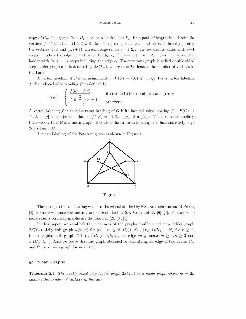
A mean labeling of the Petersen graph is shown in Figure 1.2
0
3 5
12 15
14 13
9
4
Figure 1
The concept of mean labeling was introduced and studied by S.Somasundaram and R.Ponraj
[4]. Some new families of mean graphs are studied by S.K.Vaidya et al. [6], [7]. Further some
more results on mean graphs are discussed in [2], [3], [5].
In this paper, we establish the meanness of the graphs double sided step ladder graph
2S(Tm), Jelly fish graph J(m,n) for |m − n| ≤ 2, Pn(+)Nm, (P2 ∪ kK1) + N2 for k ≥ 1,
the triangular belt graph TB(α), TBL(n, α, k, β), the edge mCn−snake m ≥ 1, n ≥ 3 and
St(B(m)(n)). Also we prove that the graph obtained by identifying an edge of two cycles Cm
and Cn is a mean graph for m,n ≥ 3.
§2. Mean Graphs
Theorem 2.1 The double sided step ladder graph 2S(Tm) is a mean graph where m = 2n
denotes the number of vertices in the base.
24 R.Vasuki and S.Arockiaraj
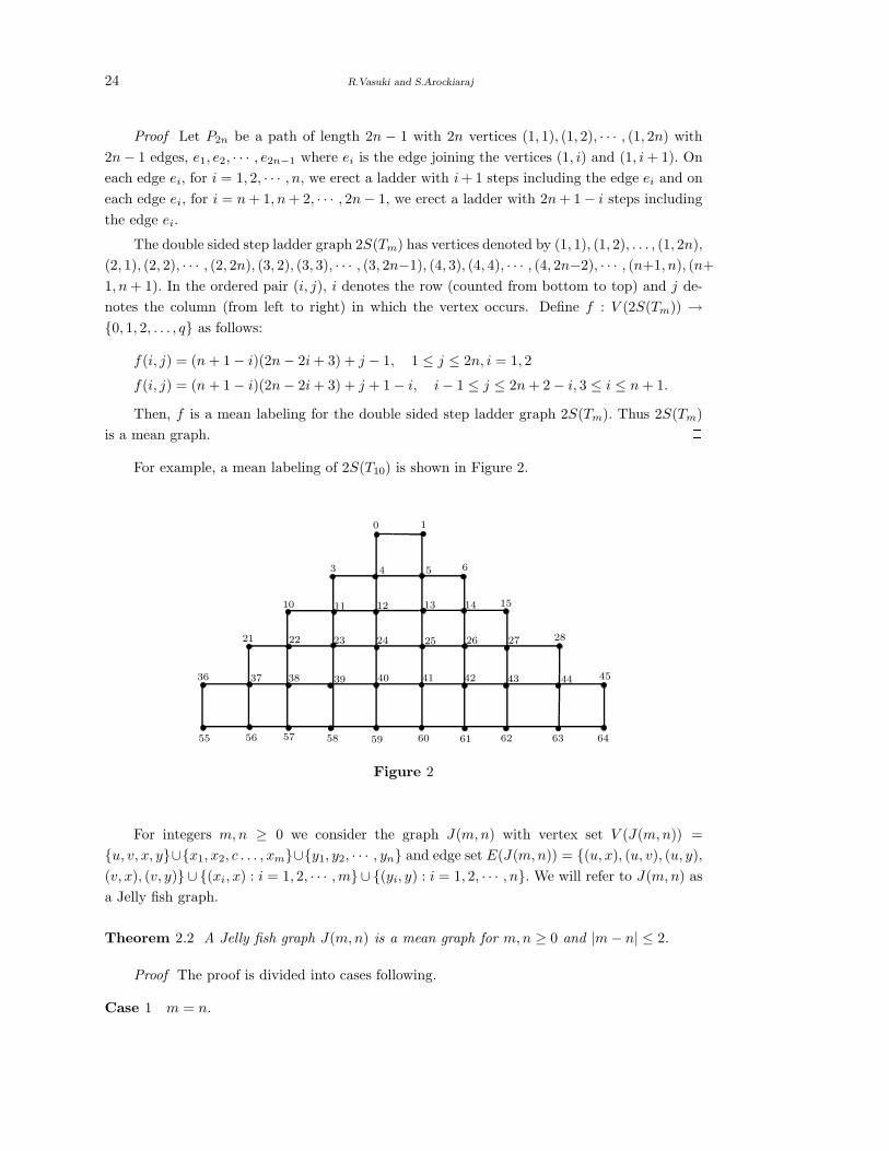
Proof Let P2n be a path of length 2n − 1 with 2n vertices (1, 1), (1, 2), · · · , (1, 2n) with
2n− 1 edges, e1, e2, · · · , e2n−1 where ei is the edge joining the vertices (1, i) and (1, i+ 1). On
each edge ei, for i = 1, 2, · · · , n, we erect a ladder with i+ 1 steps including the edge ei and on
each edge ei, for i = n+ 1, n+ 2, · · · , 2n− 1, we erect a ladder with 2n+ 1− i steps including
the edge ei.
The double sided step ladder graph 2S(Tm) has vertices denoted by (1, 1), (1, 2), . . . , (1, 2n),
(2, 1), (2, 2), · · · , (2, 2n), (3, 2), (3, 3), · · · , (3, 2n−1), (4, 3), (4, 4), · · · , (4, 2n−2), · · · , (n+1, n), (n+
1, n+ 1). In the ordered pair (i, j), i denotes the row (counted from bottom to top) and j de-
notes the column (from left to right) in which the vertex occurs. Define f : V (2S(Tm)) →0, 1, 2, . . . , q as follows:
f(i, j) = (n+ 1− i)(2n− 2i+ 3) + j − 1, 1 ≤ j ≤ 2n, i = 1, 2
f(i, j) = (n+ 1− i)(2n− 2i+ 3) + j + 1− i, i− 1 ≤ j ≤ 2n+ 2− i, 3 ≤ i ≤ n+ 1.
Then, f is a mean labeling for the double sided step ladder graph 2S(Tm). Thus 2S(Tm)
is a mean graph. 2For example, a mean labeling of 2S(T10) is shown in Figure 2.
0 1
3 4 5 6
10 11 12 13 14 15
21 22 23 24 25 26 27 28
36 37 38 39 40 41 42 43 44 45
55 56 57 58 59 60 61 62 63 64
Figure 2
For integers m,n ≥ 0 we consider the graph J(m,n) with vertex set V (J(m,n)) =
u, v, x, y∪x1, x2, c . . . , xm∪y1, y2, · · · , yn and edge set E(J(m,n)) = (u, x), (u, v), (u, y),(v, x), (v, y) ∪ (xi, x) : i = 1, 2, · · · ,m ∪ (yi, y) : i = 1, 2, · · · , n. We will refer to J(m,n) as
a Jelly fish graph.
Theorem 2.2 A Jelly fish graph J(m,n) is a mean graph for m,n ≥ 0 and |m− n| ≤ 2.
Proof The proof is divided into cases following.
Case 1 m = n.
On Mean Graphs 25
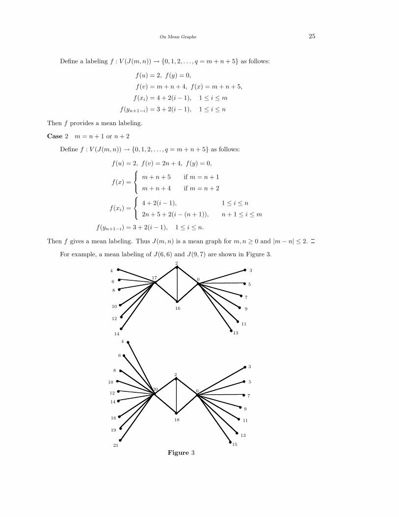
Define a labeling f : V (J(m,n))→ 0, 1, 2, . . . , q = m+ n+ 5 as follows:
f(u) = 2, f(y) = 0,
f(v) = m+ n+ 4, f(x) = m+ n+ 5,
f(xi) = 4 + 2(i− 1), 1 ≤ i ≤ mf(yn+1−i) = 3 + 2(i− 1), 1 ≤ i ≤ n
Then f provides a mean labeling.
Case 2 m = n+ 1 or n+ 2
Define f : V (J(m,n))→ 0, 1, 2, . . . , q = m+ n+ 5 as follows:
f(u) = 2, f(v) = 2n+ 4, f(y) = 0,
f(x) =
m+ n+ 5 if m = n+ 1
m+ n+ 4 if m = n+ 2
f(xi) =
4 + 2(i− 1), 1 ≤ i ≤ n2n+ 5 + 2(i− (n+ 1)), n+ 1 ≤ i ≤ m
f(yn+1−i) = 3 + 2(i− 1), 1 ≤ i ≤ n.
Then f gives a mean labeling. Thus J(m,n) is a mean graph for m,n ≥ 0 and |m− n| ≤ 2. 2For example, a mean labeling of J(6, 6) and J(9, 7) are shown in Figure 3.
2
16
17 0
4
6
8
10
12
14
3
5
7
9
11
13
2
18
0
10
12
14
16
19
21
5
7
9
11
13
15
4
6
83
20
Figure 3
26 R.Vasuki and S.Arockiaraj
Let Pn(+)Nm be the graph with p = n + m and q = 2m + n − 1. V (Pn(+)Nm) =
v1, v2, · · · , vn, y1, y2, · · · , ym, where V (Pn) = v1, v2, · · · , vn, V (Nm) = y1, y2, · · · , ym and
E(Pn(+)Nm) = E(Pn)⋃
(v1, y1), (v1, y2), · · · , (v1, ym),
(vn, y1), (vn, y2), · · · , (vn, ym).
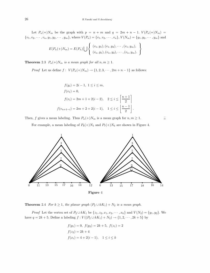
Theorem 2.3 Pn(+)Nm is a mean graph for all n,m ≥ 1.
Proof Let us define f : V (Pn(+)Nm)→ 1, 2, 3, · · · , 2m+ n− 1 as follows:
f(yi) = 2i− 1, 1 ≤ i ≤ m,f(v1) = 0,
f(vi) = 2m+ 1 + 2(i− 2), 2 ≤ i ≤⌈
n+ 1
2
⌉
f(vn+1−i) = 2m+ 2 + 2(i− 1), 1 ≤ i ≤⌊
n− 1
2
⌋
.
Then, f gives a mean labeling. Thus Pn(+)Nm is a mean graph for n,m ≥ 1. 2For example, a mean labeling of P8(+)N5 and P7(+)N6 are shown in Figure 4.
0 11 13 15 17 16 14 12
1
3
5
7
9
0 14
1
3
5
7
9
13 15 17 18 16
11
Figure 4
Theorem 2.4 For k ≥ 1, the planar graph (P2 ∪ kK1) +N2 is a mean graph.
Proof Let the vertex set of P2 ∪ kK1 be z1, z2, x1, x2, · · · , xk and V (N2) = y1, y2. We
have q = 2k + 5. Define a labeling f : V ((P2 ∪ kK1) +N2)→ 1, 2, · · · , 2k + 5 by
f(y1) = 0, f(y2) = 2k + 5, f(z1) = 2
f(z2) = 2k + 4
f(xi) = 4 + 2(i− 1), 1 ≤ i ≤ k
On Mean Graphs 27
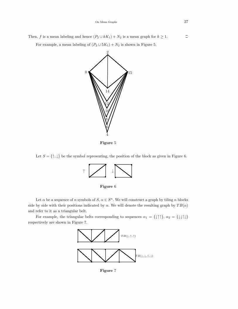
Then, f is a mean labeling and hence (P2 ∪ kK1) +N2 is a mean graph for k ≥ 1. 2For example, a mean labeling of (P2 ∪ 5K1) +N2 is shown in Figure 5.
0
2
15
14
12
10
8
6
4
Figure 5
Let S = ↑, ↓ be the symbol representing, the position of the block as given in Figure 6.
↑ ↓
Figure 6
Let α be a sequence of n symbols of S, α ∈ Sn. We will construct a graph by tiling n blocks
side by side with their positions indicated by α. We will denote the resulting graph by TB(α)
and refer to it as a triangular belt.
For example, the triangular belts corresponding to sequences α1 = ↓↑↑, α2 = ↓↓↑↓respectively are shown in Figure 7.
TB(↓, ↑, ↑)
TB(↓, ↓, ↑, ↓)
Figure 7
28 R.Vasuki and S.Arockiaraj
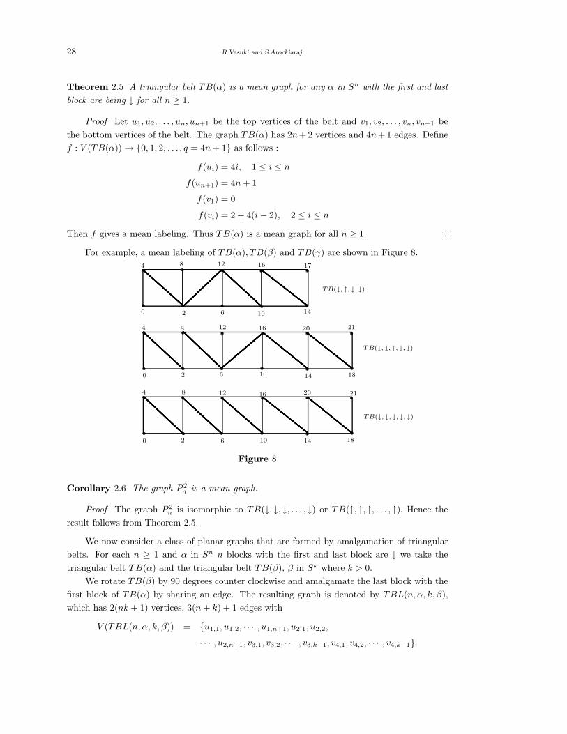
Theorem 2.5 A triangular belt TB(α) is a mean graph for any α in Sn with the first and last
block are being ↓ for all n ≥ 1.
Proof Let u1, u2, . . . , un, un+1 be the top vertices of the belt and v1, v2, . . . , vn, vn+1 be
the bottom vertices of the belt. The graph TB(α) has 2n+ 2 vertices and 4n+ 1 edges. Define
f : V (TB(α))→ 0, 1, 2, . . . , q = 4n+ 1 as follows :
f(ui) = 4i, 1 ≤ i ≤ nf(un+1) = 4n+ 1
f(v1) = 0
f(vi) = 2 + 4(i− 2), 2 ≤ i ≤ n
Then f gives a mean labeling. Thus TB(α) is a mean graph for all n ≥ 1. 2For example, a mean labeling of TB(α), TB(β) and TB(γ) are shown in Figure 8.
TB(↓, ↑, ↓, ↓)
4 8 12 16 17
0 2 6 10 14
4 8 12 16 20 21
0 2 6 10 14 18
4 8 12 16 20 21
0 2 6 10 14 18
TB(↓, ↓, ↑, ↓, ↓)
TB(↓, ↓, ↓, ↓, ↓)
Figure 8
Corollary 2.6 The graph P 2n is a mean graph.
Proof The graph P 2n is isomorphic to TB(↓, ↓, ↓, . . . , ↓) or TB(↑, ↑, ↑, . . . , ↑). Hence the
result follows from Theorem 2.5. 2We now consider a class of planar graphs that are formed by amalgamation of triangular
belts. For each n ≥ 1 and α in Sn n blocks with the first and last block are ↓ we take the
triangular belt TB(α) and the triangular belt TB(β), β in Sk where k > 0.
We rotate TB(β) by 90 degrees counter clockwise and amalgamate the last block with the
first block of TB(α) by sharing an edge. The resulting graph is denoted by TBL(n, α, k, β),
which has 2(nk + 1) vertices, 3(n+ k) + 1 edges with
V (TBL(n, α, k, β)) = u1,1, u1,2, · · · , u1,n+1, u2,1, u2,2,
· · · , u2,n+1, v3,1, v3,2, · · · , v3,k−1, v4,1, v4,2, · · · , v4,k−1.
On Mean Graphs 29
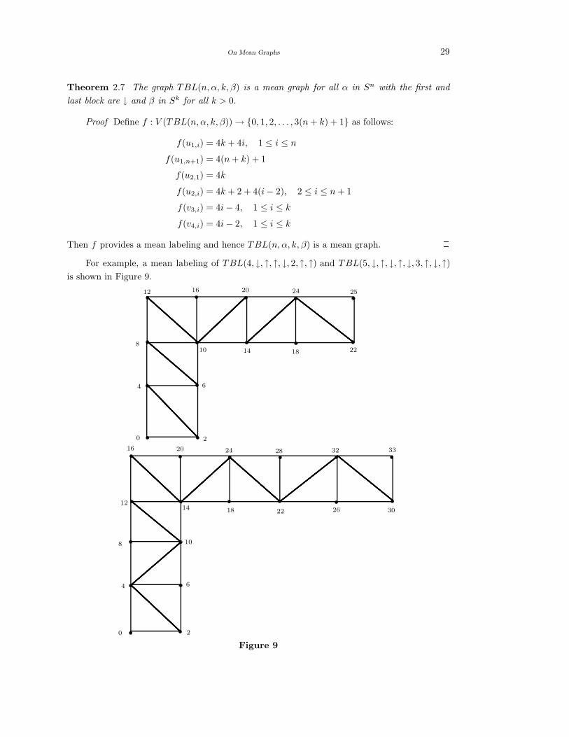
Theorem 2.7 The graph TBL(n, α, k, β) is a mean graph for all α in Sn with the first and
last block are ↓ and β in Sk for all k > 0.
Proof Define f : V (TBL(n, α, k, β))→ 0, 1, 2, . . . , 3(n+ k) + 1 as follows:
f(u1,i) = 4k + 4i, 1 ≤ i ≤ nf(u1,n+1) = 4(n+ k) + 1
f(u2,1) = 4k
f(u2,i) = 4k + 2 + 4(i− 2), 2 ≤ i ≤ n+ 1
f(v3,i) = 4i− 4, 1 ≤ i ≤ kf(v4,i) = 4i− 2, 1 ≤ i ≤ k
Then f provides a mean labeling and hence TBL(n, α, k, β) is a mean graph. 2For example, a mean labeling of TBL(4, ↓, ↑, ↑, ↓, 2, ↑, ↑) and TBL(5, ↓, ↑, ↓, ↑, ↓, 3, ↑, ↓, ↑)
is shown in Figure 9.
12 16 20 24 25
14 18 228
4
0 2
6
10
16 20 24 28 32 33
12
8
4
0 2
6
10
14 18 22 26 30
Figure 9
30 R.Vasuki and S.Arockiaraj
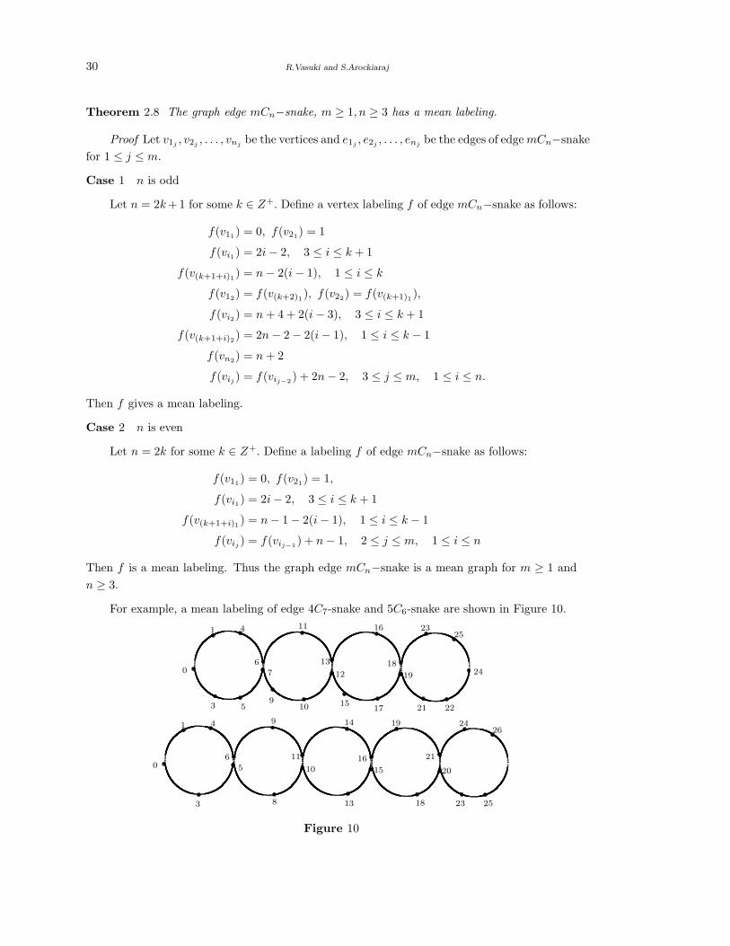
Theorem 2.8 The graph edge mCn−snake, m ≥ 1, n ≥ 3 has a mean labeling.
Proof Let v1j, v2j
, . . . , vnjbe the vertices and e1j
, e2j, . . . , enj
be the edges of edgemCn−snake
for 1 ≤ j ≤ m.
Case 1 n is odd
Let n = 2k+1 for some k ∈ Z+. Define a vertex labeling f of edge mCn−snake as follows:
f(v11) = 0, f(v21
) = 1
f(vi1) = 2i− 2, 3 ≤ i ≤ k + 1
f(v(k+1+i)1) = n− 2(i− 1), 1 ≤ i ≤ kf(v12
) = f(v(k+2)1 ), f(v22) = f(v(k+1)1 ),
f(vi2) = n+ 4 + 2(i− 3), 3 ≤ i ≤ k + 1
f(v(k+1+i)2) = 2n− 2− 2(i− 1), 1 ≤ i ≤ k − 1
f(vn2) = n+ 2
f(vij) = f(vij−2
) + 2n− 2, 3 ≤ j ≤ m, 1 ≤ i ≤ n.
Then f gives a mean labeling.
Case 2 n is even
Let n = 2k for some k ∈ Z+. Define a labeling f of edge mCn−snake as follows:
f(v11) = 0, f(v21
) = 1,
f(vi1) = 2i− 2, 3 ≤ i ≤ k + 1
f(v(k+1+i)1 ) = n− 1− 2(i− 1), 1 ≤ i ≤ k − 1
f(vij) = f(vij−1
) + n− 1, 2 ≤ j ≤ m, 1 ≤ i ≤ n
Then f is a mean labeling. Thus the graph edge mCn−snake is a mean graph for m ≥ 1 and
n ≥ 3. 2For example, a mean labeling of edge 4C7-snake and 5C6-snake are shown in Figure 10.
0
1 4
6
7
53
11
910
13
12
16
1517
18
19
2325
24
2221
0
1 4
6
5
9
8
11
10
14
13
16
15
19
18
20
2426
25233
21
Figure 10
On Mean Graphs 31
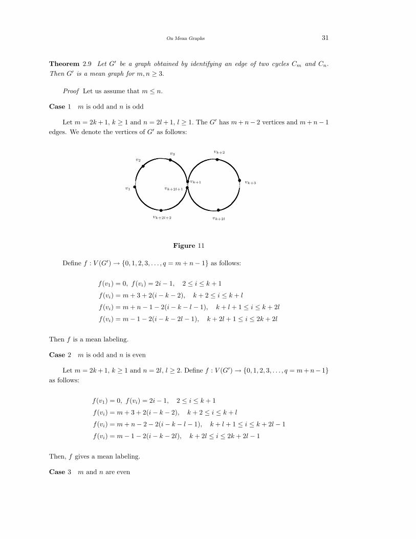
Theorem 2.9 Let G′ be a graph obtained by identifying an edge of two cycles Cm and Cn.
Then G′ is a mean graph for m,n ≥ 3.
Proof Let us assume that m ≤ n.
Case 1 m is odd and n is odd
Let m = 2k+ 1, k ≥ 1 and n = 2l+ 1, l ≥ 1. The G′ has m+ n− 2 vertices and m+ n− 1
edges. We denote the vertices of G′ as follows:
vk+1
vk+2l+1
vk+2l+2
v3
v1
vk+2
vk+2l
vk+3
v2
Figure 11
Define f : V (G′)→ 0, 1, 2, 3, . . . , q = m+ n− 1 as follows:
f(v1) = 0, f(vi) = 2i− 1, 2 ≤ i ≤ k + 1
f(vi) = m+ 3 + 2(i− k − 2), k + 2 ≤ i ≤ k + l
f(vi) = m+ n− 1− 2(i− k − l − 1), k + l + 1 ≤ i ≤ k + 2l
f(vi) = m− 1− 2(i− k − 2l− 1), k + 2l+ 1 ≤ i ≤ 2k + 2l
Then f is a mean labeling.
Case 2 m is odd and n is even
Let m = 2k+ 1, k ≥ 1 and n = 2l, l ≥ 2. Define f : V (G′)→ 0, 1, 2, 3, . . . , q = m+n− 1as follows:
f(v1) = 0, f(vi) = 2i− 1, 2 ≤ i ≤ k + 1
f(vi) = m+ 3 + 2(i− k − 2), k + 2 ≤ i ≤ k + l
f(vi) = m+ n− 2− 2(i− k − l − 1), k + l + 1 ≤ i ≤ k + 2l− 1
f(vi) = m− 1− 2(i− k − 2l), k + 2l ≤ i ≤ 2k + 2l − 1
Then, f gives a mean labeling.
Case 3 m and n are even
32 R.Vasuki and S.Arockiaraj
Let m = 2k, k ≥ 2 and n = 2l, l ≥ 2. Define f on the vertex set of G′ as follows:
f(v1) = 0, f(vi) = 2i− 2, 2 ≤ i ≤ k + 1
f(vi) = m+ 3 + 2(i− k − 2), k + 2 ≤ i ≤ k + l
f(vi) = m+ n− 2− 2(i− k − l − 1), k + l + 1 ≤ i ≤ k + 2l− 1
f(vi) = m− 1− 2(i− k − 2l), k + 2l ≤ i ≤ 2k + 2l − 2
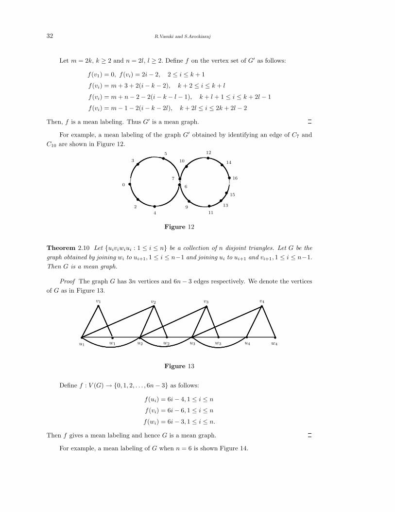
Then, f is a mean labeling. Thus G′ is a mean graph. 2For example, a mean labeling of the graph G′ obtained by identifying an edge of C7 and
C10 are shown in Figure 12.
0
3
5
7
6
4
2
10
12
14
16
15
13
119
Figure 12
Theorem 2.10 Let uiviwiui : 1 ≤ i ≤ n be a collection of n disjoint triangles. Let G be the
graph obtained by joining wi to ui+1, 1 ≤ i ≤ n−1 and joining ui to ui+1 and vi+1, 1 ≤ i ≤ n−1.
Then G is a mean graph.
Proof The graph G has 3n vertices and 6n− 3 edges respectively. We denote the vertices
of G as in Figure 13.
u1 w1 u2 w2 u3 w3 u4 w4
v1 v2 v3 v4
Figure 13
Define f : V (G)→ 0, 1, 2, . . . , 6n− 3 as follows:
f(ui) = 6i− 4, 1 ≤ i ≤ nf(vi) = 6i− 6, 1 ≤ i ≤ nf(wi) = 6i− 3, 1 ≤ i ≤ n.
Then f gives a mean labeling and hence G is a mean graph. 2For example, a mean labeling of G when n = 6 is shown Figure 14.
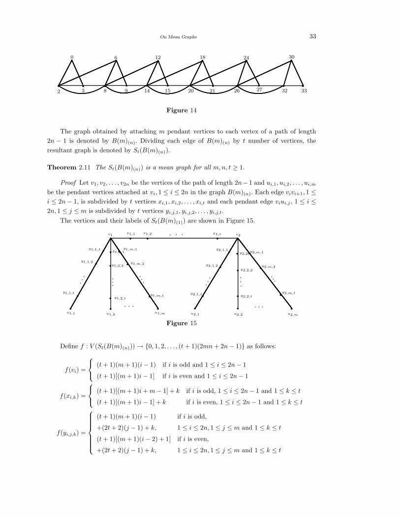
On Mean Graphs 33
2 3 8 9 14 15 20 21
0 6 12 18
26 27 32 33
3024
Figure 14
The graph obtained by attaching m pendant vertices to each vertex of a path of length
2n − 1 is denoted by B(m)(n). Dividing each edge of B(m)(n) by t number of vertices, the
resultant graph is denoted by St(B(m)(n)).
Theorem 2.11 The St(B(m)(n)) is a mean graph for all m,n, t ≥ 1.
Proof Let v1, v2, . . . , v2n be the vertices of the path of length 2n− 1 and ui,1, ui,2, . . . , ui,m
be the pendant vertices attached at vi, 1 ≤ i ≤ 2n in the graph B(m)(n). Each edge vivi+1, 1 ≤i ≤ 2n− 1, is subdivided by t vertices xi,1, xi,2, . . . , xi,t and each pendant edge viui,j , 1 ≤ i ≤2n, 1 ≤ j ≤ m is subdivided by t vertices yi,j,1, yi,j,2, . . . , yi,j,t.
The vertices and their labels of St(B(m)(1)) are shown in Figure 15.
v1x1,1 x1,2 x1,t v2
y1,1,1
y1,1,2
y1,1,t
u1,1 u1,2
y1,2,t
y1,2,2
y1,2,1
y1,m,1
y1,m,2
y1,m,t
u1,m u2,1 u2,2 u2,m
y2,1,1
y2,1,2
y2,1,t
y2,2,1
y2,2,2
y2,2,t
y2,m,1
y2,m,2
y2,m,t
Figure 15
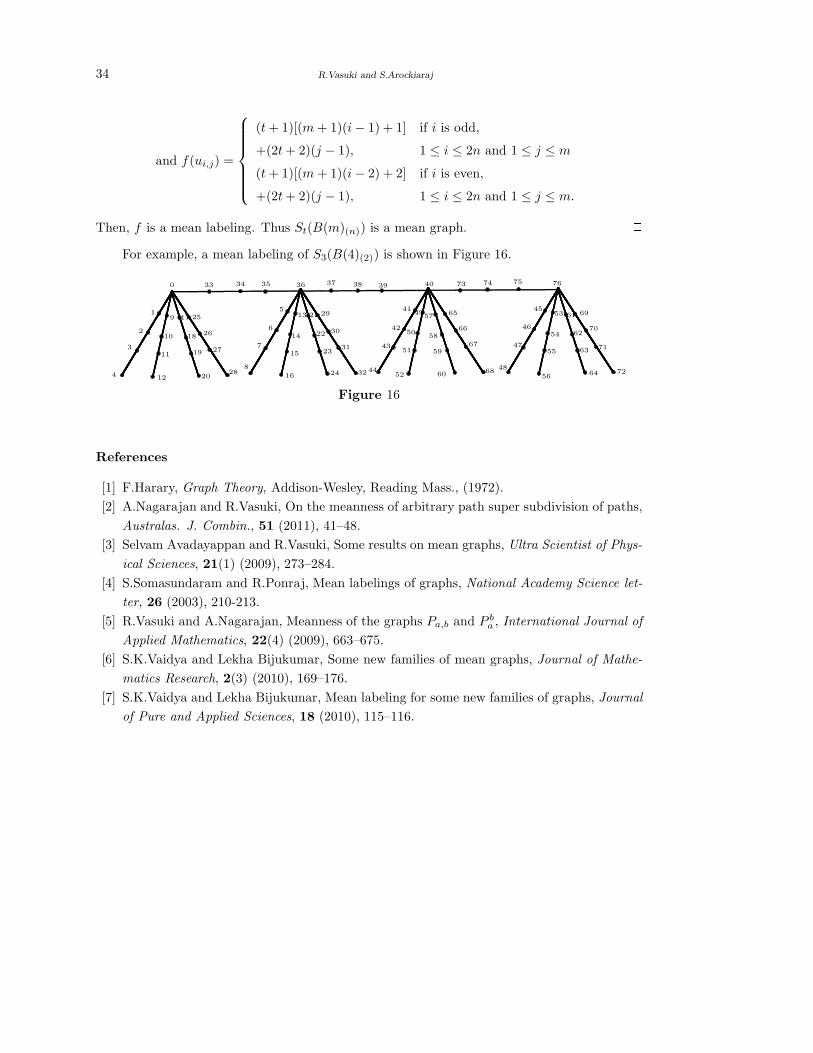
Define f : V (St(B(m)(n)))→ 0, 1, 2, . . . , (t+ 1)(2mn+ 2n− 1) as follows:
f(vi) =
(t+ 1)(m+ 1)(i− 1) if i is odd and 1 ≤ i ≤ 2n− 1
(t+ 1)[(m+ 1)i− 1] if i is even and 1 ≤ i ≤ 2n− 1
f(xi,k) =
(t+ 1)[(m+ 1)i+m− 1] + k if i is odd, 1 ≤ i ≤ 2n− 1 and 1 ≤ k ≤ t(t+ 1)[(m+ 1)i− 1] + k if i is even, 1 ≤ i ≤ 2n− 1 and 1 ≤ k ≤ t
f(yi,j,k) =
(t+ 1)(m+ 1)(i− 1) if i is odd,
+(2t+ 2)(j − 1) + k, 1 ≤ i ≤ 2n, 1 ≤ j ≤ m and 1 ≤ k ≤ t(t+ 1)[(m+ 1)(i− 2) + 1] if i is even,
+(2t+ 2)(j − 1) + k, 1 ≤ i ≤ 2n, 1 ≤ j ≤ m and 1 ≤ k ≤ t
34 R.Vasuki and S.Arockiaraj
and f(ui,j) =
(t+ 1)[(m+ 1)(i− 1) + 1] if i is odd,
+(2t+ 2)(j − 1), 1 ≤ i ≤ 2n and 1 ≤ j ≤ m(t+ 1)[(m+ 1)(i− 2) + 2] if i is even,
+(2t+ 2)(j − 1), 1 ≤ i ≤ 2n and 1 ≤ j ≤ m.
Then, f is a mean labeling. Thus St(B(m)(n)) is a mean graph. 2For example, a mean labeling of S3(B(4)(2)) is shown in Figure 16.
0
1
2
3
4
9
10
11
12
17
18
19
20
25
26
27
28
33 34 35 36
5
6
7
8
13
14
15
16
21
22
23
24
29
30
31
32
37 38 39 40
41
42
43
44
49
50
51
52
57
58
59
60
65
66
67
68
73 74 75 76
45
46
47
48
53
54
55
56
61
62
63
64
69
70
71
72
Figure 16
References
[1] F.Harary, Graph Theory, Addison-Wesley, Reading Mass., (1972).
[2] A.Nagarajan and R.Vasuki, On the meanness of arbitrary path super subdivision of paths,
Australas. J. Combin., 51 (2011), 41–48.
[3] Selvam Avadayappan and R.Vasuki, Some results on mean graphs, Ultra Scientist of Phys-
ical Sciences, 21(1) (2009), 273–284.
[4] S.Somasundaram and R.Ponraj, Mean labelings of graphs, National Academy Science let-
ter, 26 (2003), 210-213.
[5] R.Vasuki and A.Nagarajan, Meanness of the graphs Pa,b and P ba , International Journal of
Applied Mathematics, 22(4) (2009), 663–675.
[6] S.K.Vaidya and Lekha Bijukumar, Some new families of mean graphs, Journal of Mathe-
matics Research, 2(3) (2010), 169–176.
[7] S.K.Vaidya and Lekha Bijukumar, Mean labeling for some new families of graphs, Journal
of Pure and Applied Sciences, 18 (2010), 115–116.
International J.Math. Combin. Vol.3(2013), 35-43
Special Kinds of Colorable Complements in Graphs
B.Chaluvapaju
(Department of Studies and Research in Mathematics, B. H. Road, Tumkur University, Tumkur -572 103, India)
C.Nandeeshukumar and V.Chaitra
(Department of Mathematics, Bangalore University, Central College Campus, Bangalore -560 001, India)
E-mail: [email protected], [email protected], [email protected]
Abstract: Let G = (V, E) be a graph and C = C1, C2, · · · , Ck be a partition of color
classes of a vertex set V (G). Then the graph G is a k-colorable complement graph GCk (with
respect to C) if for all Ci and Cj , i 6= j, remove the edges between Ci and Cj , and add the
edges which are not in G between Ci and Cj . Similarly, the k(i)- colorable complement graph
GCk(i) of a graph G is obtained by removing the edges in 〈Ci〉 and 〈Cj〉 and adding the missing
edges in them. This paper aims at the study of Special kinds of colorable complements of a
graph and its relationship with other graph theoretic parameters are explored.
Key Words: Graph, complement, k-complement, k(i)-complement, colorable complement.
AMS(2010): 05C15, 05C70
§1. Introduction
All the graphs considered here are finite, undirected and connected with no loops and multiple
edges. As usual n = |V | and m = |E| denote the number of vertices and edges at a graph
G, respectively. For the open neighborhood of a vertex v ∈ V is N(v) = u ∈ V/uv ∈ E,the set of vertices adjacent to v. The closed neighborhood is N [v] = N(v)
⋃v. In general,
we use 〈X〉 to denote the sub graph induced by the set of vertices X . If deg(v) is the degree
of vertex v and usually, δ(G) is the minimum degree and ∆(G) is the maximum degree. The
complement Gc of a graph G defined to be graph which has V as its sets of vertices and two
vertices are adjacent in Gc if and only if they are not adjacent in G. Further, a graph G is
said to be self-complementary (s.c), if G ∼= Gc. For notation and graph theory terminology we
generally follow [3], and [5].
Let G = (V,E) be a graph and P = V1, V2, · · · , Vk be a partition of V . Then k-
complement GPk and k(i)-complement GP
k(i)(with respect to P ) are defined as follows: For all
Vi and Vj , i 6= j, remove the edges between Vi andVj , and add the edges which are not in G
between Vi and Vj . The graph GPk thus obtained is called the k-complement of a graph G with
respect to P . Similarly, the k(i)-complement of GPk(i) of a graph G is obtained by removing the
edges in 〈Vl〉 and 〈Vj〉 and adding the missing edges in them for l 6= j. This concept was first
1Received June 13, 2013, Accepted August 10, 2013.
36 B.Chaluvapaju, C.Nandeeshukumar and V.Chaitra
introduced by Sampathkumar et al. [9] and [10]. For more detail on complement graphs, we
refer [1], [2], [4], [8], [11] and [12].
A graph is said to be k-vertex colorable (or k-colorable) if it is possible to assign one color
from a set of k colors to each vertex such that no two adjacent vertices have the same color. The
set of all vertices with any one color is independent and is called a color class. An k-coloring of a
graph G uses k colors: it there by partitions V into k color classes. The chromatic number χ(G)
is defined as the minimum k for which G has an k-coloring. Hence, graph G is a k-colorable if
and only if χ(G) ≤ k, [7].
We make use of the following results in sequel [6].
Theorem 1.1 For any non-trivial graph G,
∑
xi∈V
deg(xi) = 2m.
Theorem 1.2(Konig’s [5]) In a bipartite graph G, α1(G) =β0(G). Consequently, if a graph G
has no vertex of degree 0, then α0(G) = β1(G).
§2. k-Colorable Complement
Let G = (V,E) be a graph. If there exists a k-coloring of a graph G if and only if V (G)
can be partitioned into k subsets C1, C2, · · · , Ck such that no two vertices in color classes of
Ci, i = 1, 2, · · · , k, are adjacent. Then, we have the following definitions.
Definition 2.1 The k-colorable complement graph GCk (with respect to C) of a graph G is
obtained by for every Ci and Cj, i 6= j, remove the edges between Ci and Cj in G, and add the
edges which are not in a graph G.
Definition 2.2 The graph G is k-self colorable complement graph, if G ∼= GCk .
Definition 2.3 The graph G is k-co-self colorable complement graph, if Gc∼= GC
k .
Lemma 2.1 Let G be a k-colorable graph. Then in any k-coloring of G, the subgraph induced
by the union of any two color classes is connected.
Proof If possible, let C1 and C2 be two color classes of vertex set V (G) such that the
subgraph induced by C1 ∪C2 is disconnected. Let G1 be a component of the subgraph induced
by C1∪C2. Obviously, no vertex of G1 is adjacent to a vertex in V (G)−V (G1), which is assign
the color either C1 or C2. Thus interchanging the colors of the vertices in G1 and retaining
the original colors for all other vertices, we gets a different k-coloring of a graph G, which is a
contradiction. 2Theorem 2.1 Let G be a (n,m)-graph. If for every Cl and Cj , l 6= j, and each vertex of Cl is
adjacent to each vertex of Cj , then m(GCk ) = ∅.
Proof If for every Cl and Cj , l 6= j in a (n,m)- graph with 〈Ck〉 is totally disconnected,
Special Kinds of Colorable Complements in Graphs 37
where Ck is the partition of color classes of vertex set V (G), then by the definition of k-colorable
complement, m(GCk ) = ∅ follows. Conversely, suppose the given condition is not satisfied, then
there exist at least two vertices u and v such that u ∈ Cl is not adjacent to vertex u ∈ Cj with
l 6= j. Thus by above lemma, this implies that m(GCk ) ≥ 1, which is a contradiction. 2
A graph that can be decomposed into two partite sets but not fewer is bipartite; three
sets but not fewer, tripartite; k sets but not fewer, k-partite; and an unknown number of sets,
multipartite. An 1-partite graph is the same as an independent set, or an empty graph. A 2-
partite graph is the same as a bipartite graph. A graph that can be decomposed into k partite
sets is also said to be k-colorable. That is χ(Kn) = n, but the chromatic number of complete
k- partite graph χ(Kr1,r2,r3,··· ,rk) = k < n for ri > 2, where i = 1, 2, · · · , k. By virtue of the
facts, we have following corollaries.
Corollary 2.1 Let G be a complete graph Kn; n ≥ 1 vertices and m =n(n− 1)
2edges with
χ(Kn) = n. Then m(GCn ) = ∅.
Corollary 2.2 Let G be a complete bipartite graph Kr1,r2; 1 ≤ r1 ≤ r2, with χ(Kr1,r2
) = 2 for
n = (r1 + r2)- vertices and m =(r1.r2) edges. Then m(GC2 ) = ∅.
Theorem 2.2 Let G be a path Pn with χ(Pn) = 2 ; n ≥ 2 vertices. Then
m(GC2 ) =
14 (n− 2)2 if n is even
14 (n− 1)(n− 3) if n is odd.
Proof Let G be a path Pn with χ(Pn) = 2; n ≥ 2 vertices, and C = C1, C2 be a partition
of colorable class of vertex set of Pn. We have the following cases.
Case 1 If u1, u2, · · · , ut−1, ut ∈ C1 and v1, v2, · · · , vt−1, vt ∈ C2 with v1 − vt is path of
even length. Then u1, u2, · · · , ut−1 are adjacent (t − 2)-vertices, that is deg(ui) = (t − 2) if
1 ≤ i ≤ t− 1. Similarly, v1, v2, · · · , vt are adjacent to (t− 2)- vertices that is deg(ui) = (t− 2)
if 2 ≤ i ≤ t − 1, and v1 and ut are adjacent to (t − 1)- vertices in GC2 . Thus, 2(t − 1) + (n −
2)(t − 2) = 2m(GC2 ). By Theorem 1.1, with the fact that n = 2t and m(G) = n − 1. Hence
m(GC2 ) =
1
4(n− 2)2.
Case 2 If u1, u2, · · · , ut−1, ut ∈ C1 and v1, v2, · · · , vt, vt+1 ∈ C2 with v1 − vt+1 is path
of even length. Then u1, u2, · · · , ut are adjacent (t − 1)-vertices, v2, v3, · · · , vt are adjacent to
(t− 2)- vertices and, v1 and ut−1 are adjacent to (t− 1) - vertices in GC2 . Thus, t(t− 1) + (t−
1)(t−2)+2(t−1) = 2m(GC2 ). By theorem 1.1, with the fact that n = 2t+1 and m(G) = n−1.
Hence m(GC2 ) =
1
4(n− 1)(n− 3). 2
Theorem 2.3 Let G be a cycle Cn; n ≥ 3 vertices. Then
(i) m(GC2 ) =
(n− 4)n
4, if χ(Cn) = 2 and n is even.
(ii) m(GC3 ) =
(n+ 1)(n− 3)
4, if χ(Cn) = 3 and exactly one vertex is contain in any one
colorable class of a vertex partition set of an odd cycle Cn.
38 B.Chaluvapaju, C.Nandeeshukumar and V.Chaitra
Proof The proof follows from Theorem 2.2, with even cycle of Cn and exactly one vertex
is contain in any one colorable class of a vertex partition set of an odd cycle Cn. 2Theorem 2.4 Let G be a Wheel Wn; n ≥ 4 vertices and m = 2(n− 1) edges. Then
(i) m(GC4 ) =
(n− 4)n
4, if χ(Cn) = 4 and n is even.
(ii) m(GC3 ) =
(n+ 1)(n− 3)
4, if χ(Wn) = 3 and exactly one vertex is contain in any one
colorable class of a vertex partition set of an odd cycle Cn−1 of Wn.
Proof By Theorem 2.3 and m(K1) = 0 due to the fact of Wn = K1 + Cn−1, the result
follows. 2Theorem 2.5 Let T be a nontrivial tree with χ(T ) = 2. Then
m(GC2 ) = (r1.r2)− n(T ) + 1.
Proof Let C = C1, C2 be a partition of colorable class of a tree T with n ≥ 2 vertices
and m(T ) = n(T )−1. If every vertex in C1 is adjacent to every vertex in C2, that is Kr1,r2with
m(Kr1,r2) = r1.r2. By definition of GC
k with χ(T ) = 2, we have m(GC2 ) = m(Kr1,r2
) −m(T ).
Thus the results follows. 2Theorem 2.6 For any non trivial graph G is k - self colorable complement if and only if
G ∼= P7 or 2K2.
Proof By definition of k-self colorable complement. It is clear that both G and GC2 are
isomorphic to P7 or 2K2 with χ(P7) = χ(2K2) = 2. On the other hand, suppose G is k-self
colorable complement, when G is not isomorphic with P7 or 2K2. Then there exist at least
two adjacent vertices u and v in G such that u ∈ C1 and v ∈ C2 are in disjoint color classes of
C = C1, C2 with χ(P7) = χ(2K2) = 2. This implies that, u and v are not adjacent in GC2
or they are in one color classes in GC1 , that is totally disconnected graph. Thus the graph G
and its colorable complements GCk are not isomorphic to each other, which is a contradiction.
Hence the results follows. 2Theorem 2.7 Let G be a k-self colorable complement graph. Then G has a vertex of degree at
leastn(χ(G)− 1)
2χ(G).
Proof Let G be a (n,m)- graph with G ∼= GCk and C = C1, C2, · · · , Ck be a partition
of color classes of a vertex set V (G). Suppose, if χ(G) = k and V (G) is partitioned into
k independent sets C1, C2, · · · , Ck. Thus, n = |V (G)| = |C1, C2, · · · , Ck| =∑k
i=1 |V (G)| ≤kβ(G), where β(G) is the independence number of a graph G. There fore χ(G) = k = n/β(G).
Also, suppose v ∈ Ci, where Ci is a colorable set in C with at most n/χ(G). Then the sum of
the degree of v in G and GCk is greater than
n(χ(G) − 1)
χ(G). This implies that the degree of v is
at least1
2(n− n
χ(G)). Hence the result follows. 2
Special Kinds of Colorable Complements in Graphs 39
Theorem 2.8 Let G be a k-self colorable complement graph. Then
(k − 1)(2n− k)4
≤ m(G) ≤ 2n(n− k) + k(k − 1)
4.
Proof Let G be a k-self colorable complement graph and C = C1, C2, · · · , Ck be a
partition of color classes of a vertex set V (G). If |Ct| = nt for 1 ≤ t ≤ k, then the total number
of edges between Cl and Cj in C, l 6= j, in both the graph G and its colorable complement
graph GCk is
∑
l 6=j
nlnj . Since the graph G is k-self colorable complement graph GCk , half of these
edges are not there in G. Hence m(G) ≤
n
2
−∑l 6=j
nlnj . Clearly,∑
l 6=j
nlnj is minimum, when
nt = 1 for k − 1 of the indices. Thus, we have
m(G) ≤
n
2
− 1
2[
k − 1
2
+ (k − 1)(n− k + 1)].
Hence the upper bound follow. To establish the lower bound, the graph G being k-self colorable
complement has at least∑
l 6=j
nlnj- edges. So, 12 [
k − 1
2
+ (k − 1)(n − k + 1)] ≤ m(G) and
the result follows. 2Theorem 2.9 For any non trivial graph G is k - co - self colorable complement if and only if
G ∼= Kn.
Proof On contrary, suppose given condition is not satisfied, then there exists at least three
vertices u, v and w such that v is adjacent to both u and w, and u is not adjacent to w. This
implies that an edge e = uw ∈ Gc and induced subgraph 〈u, v, w〉 in GC2 is totally disconnected.
Thus E(GC2 ) ⊂ E(Gc), which is a contradiction to the fact of Gc
∼= GCn with χ(Kn) = n.
Converse is obvious. 2§3. k(i)-Colorable Complement
Let G = (V,E) be a graph and C = C1, C2, · · · , Ck be a partition of color classes of a vertex
set V (G). Then, we have the following definitions.
Definition 3.1 The k(i) - colorable complement graph GCk(i)(with respect to C) of a graph G
is obtained by removing the edges in 〈Cl〉 and 〈Cj〉 and adding the missing edges in them for
l 6= j.
Definition 3.2 The graph G is k(i)-self colorable complement graph, if G ∼= GCk(i).
Definition 3.3 The graph G is k(i)-co-self colorable complement graph, if Gc∼= GC
k(i).
Theorem 3.1 For any graph G, m(GCk(i)) =
n(n− 1)
2if and only if the graph G is isomorphic
with complete n- partite graph Kr1,r2,r3,··· ,rnor (Kn)c.
40 B.Chaluvapaju, C.Nandeeshukumar and V.Chaitra
Proof To prove the necessity, we use the mathematical induction. Let G be a graph with
n = 1 vertex. Then χ(G) = 1 and m(GC1(i)) = ∅. Hence the result follows. Suppose the graph
G with n > 1 vertices. Then the following cases are arises.
Case 1 If the graph G is totally disconnected, that is (Kn)c, complement of a complete graph
Kn, then G has a only one color class C1 with χ((Kn)c) = 1. By the definition of GC1(i), the
induced subgraph of 〈C1〉 is complete, which form an(n− 1)
2- edges.
Case 2. If the graph G is complete n- partite graph Kr1,r2,r3,...,rn, then for every two color
classes Cl and Cj for l 6= j, and each vertex Cl adjacent to each vertex of Cj in complete n-
partite graph Kr1,r2,r3,...,rnwith m(Kr1,r2,r3,...,rn
) = r1r2r3 . . . rn. By the definition of GCn(i)
with G = Kr1,r2,r3,...,rn, we have
m(GCn(i)) =
r1
2
+
r2
2
+ . . .+
rn
2
+ r1r2r3 . . . rn,
where
rt
2
is the maximum number edges of induced subgraph 〈Ct〉 if t = 1, 2, . . . , n, which
are complete. This formsn(n− 1)
2- edges.
Conversely, suppose the graphG is not isomorphic to complete n- partite graphKr1,r2,r3,...,rn
or (Kn)c. Then there exist at least three vertices a, b, c such that at least two adjacent ver-
tices a and b are not adjacent to isolated vertex c. By the definition of GCk(i) with χ(G) = k ≥ 2,
which form a path (a− b− c) or (b−a− c) of length 2, which is not a complete, a contradiction.
This proves the sufficiency. 2Theorem 3.2 Let G be a path Pn with χ(Pn) = 2 and n ≥ 2 vertices. Then
m(GC2(i)) =
14 [n2 + 2n− 4]2 if n is even
14 (n− 1)(n+ 3) if n is odd
Proof Let G be a path Pn with χ(Pn) = 2; n ≥ 2 vertices, and C = C1, C2 be a partition
of colorable class of vertex set of Pn. We have the following cases.
Case 1 Let C = C1, C2 be a partition of colorable class of Pn. If u1, u2, · · · , ut−1, ut ∈ C1
and v1, v2, · · · , vt−1, vt ∈ C2 with v1 − ut is path of even length. Then 〈C1〉 and 〈C2〉 are
complete in GC2(i) and also v1 − ut path have (n− 1) - edges in both the graph G and its k(i)-
colorable complement graph GC2(i). Thus, m(G) + t(t − 1) = (n − 1) + n(n − 2)/4 = m(GC
2(i))
and this implies m(GC2(i)) =
1
4[n2 + 2n− 4]2.
Case 2 Let C = C1, C2 be a partition of colorable class of Pn. If u1, u2, · · · , ut−1, ut ∈ C1
and v1, v2, · · · , vt−1, vt ∈ C2 with v1 − ut+1 is path of odd length. Then 〈C1〉 and 〈C2〉 are
complete in GC2(i) and also v1−ut+1 path have (n− 1) - edges in both the graph G and its 2(i)-
colorable complement graph GC2(i). Thus, m(G) + t(t − 1)/2 + t(t + 1)/2 = (n − 1)[1 + (n −
3)/8 + (n+ 1)/8] = m(GC2(i)) and this implies m(GC
2(i)) =1
4(n− 1)(n+ 3). 2
Special Kinds of Colorable Complements in Graphs 41
Theorem 3.3 Let G be a cycle Cn; n ≥ 3 vertices. Then
(i) m(GC2(i)) =
1
4[n(n+ 2)], if χ(Cn) = 2 and n is even.
(ii) m(GC3(i)) =
1
4(n2 + 3) , if χ(Cn) = 3 and exactly one vertex is contain in any one
colorable class of a vertex partition set of an odd cycle Cn.
Proof The proof follows from Theorem 3.2, with even cycle of Cn and exactly one vertex
is contain in any one colorable class of a vertex partition set of an odd cycle Cn. 2Theorem 3.4 Let T be a nontrivial tree with χ(T ) = 2. If C = C1, C2 be a partition of
colorable class of a tree T , then
m(GC2(i)) =
1
2[r2 + s2 + n− 2],
where |C1| = r and |C2| = s.
Proof Let C = C1, C2 be a partition of colorable class of a tree T with χ(T ) = 2 and
m(T ) = n(T )− 1 = r+ s+1. Then by definition of GCk(i), we have 〈C1〉 and 〈C2〉 are complete.
There fore, m(C1) =
r
2
and m(C2) =
s
2
.
Thus, we have
m(GC2(i)) =
r
2
+
s
2
+m(T ) =1
2[r(r + 1) + s(s+ 1)− 2].
Hence the result follows. 2Theorem 3.5 For any non trivial graph G is k(i) - self colorable complement if and only if G
is isomorphic with Kn.
Proof Let G = Kn be a complete graph with χ(G) = n. Then by the definition of GCk(i),
the induced subgraph 〈Ct〉 for t = 1, 2, . . . , n are connected and |Ct| = 1 for t = 1, 2, . . . , n.
Thus GCn(i)∼= Kn and the result follows. Conversely, suppose given condition is not satisfied,
then there exists at least two non adjacent vertices u and v in a graph G such that χ(G) = 1
and m(G) = ∅. By the definition of GCk(i), we have χ(GC
1(i)) = 2 with an induced subgraph
〈u, v〉 in GC1(i) is connected. Thus m(G) < m(GC
1(i)), which is a contradiction to the fact of
G ∼= GCk(i). 2
§4. G, Gpk, G
pk(i) - Realizability
Here, we show the G,Gpk, G
pk(i) - Realizability for some graph theoretic parameter.
Let G be a graph. Then S ⊆ V (G) is a separating set if G − S has more than one
component. The connectivity κ(G) of G is the minimum size of S ⊆ V (G) such that G− S is
disconnected or a single vertex. For any k ≤ κ(G), we say that G is k-connected. Then, we
have
42 B.Chaluvapaju, C.Nandeeshukumar and V.Chaitra
Theorem 4.1 Let G be a graph with C = C1, C2 be a partition of colorable class of a
vertex set V . If 〈C1〉 and 〈C2〉 are (t − 1) -colorable with Max.χ(GCk ), χ(GC
ki) ≥ t, then
Min.k(G), k(GCk ), k(GC
ki) has at least (t− 1) -edges.
Theorem 4.2 Let G be a (n,m)- graph. Then
(i) χ(GCk ) = 1 if and only if G is isomorphic with Kn or (Kn)c or Kr1,r2,r3,··· ,rk
.
(ii) χ(GCk(i)) = n if and only if G is isomorphic with Kn or (Kn)c or Kr1,r2,r3,··· ,rk
.
Proof By the definition of GCk and Theorem 2.1, (i) follows. Also by the definition of GC
k(i)
and Theorem 3.1, (ii) follows. 2A set M of vertices in a graph G is independent if no two vertices of M are adjacent. The
number of vertices in a maximum independent set of G is denoted by β(G). Opposite to an
independent set of vertices in a graph is a clique. A clique in a graph G is a complete subgraph
of G. The order of the largest clique in a graph G and its clique number, which is denoted by
ω(G). In fact β(G) = k if and only if ω(G) = k. Then, we have
Theorem 4.3 Let G be a nontrivial (n,m)- graph. Then
(i) β(GCk(i)) ≤ β(G) ≤ β(GC
k ).
(ii) ω(GCk ) ≤ ω(G) ≤ ω(GC
ki).
Acknowledgement
Thanks are due to Prof. E.Sampathkumar for his help and valuable suggestions in the prepa-
ration of this paper.
References
[1] Acharya B.D., On Characterizing graphs switching equivalent to acyclic graphs, Indian J.
Pure Appl. Math., 12 (10)(1981), 1187-1191.
[2] Chaluvaraju B., 2-global and 2(i)-global dominating sets in graphs, Intenat. J. of Phy. Sc.
20(2)(2008)M, 481-488.
[3] Chartrand G and Lesniak L., Graphs and Digraphs, Fourth Edition, Chapman and Hall/CRC
Press 2004.
[4] Gangopadhyay T., Hebbare and Rao S. P., Paths in r-partite self-complementary graphs,
Discrete Math., 32(1980), 229-243.
[5] Harary F., Graph Theory, Addison-Wesley, Reading Mass, 1969.
[6] Harary F., Proof Techniques in Graph Theory, Academic Press, New York, 1969.
[7] Jensen T.R. and Toft B, Graph Coloring Problem, John Wiley & Sons, Inc, New York,
1995.
[8] Sampathkumar E. and Bhave V. N., Partition graphs and coloring numbers of a gra.ph,
Discrete Math., 6(1)(1976), 57-60.
Special Kinds of Colorable Complements in Graphs 43
[9] Sampathkumar E and Pushpalatha L., Complement of a graph: A generalization, Graphs
and Combinatorics, 14(4)(1998), 377-392.
[10] Sampathkumar E., Pushpalatha L., Venkatachalam C.V. and Pradeep Bhat, Generalized
complements of a graph, Indian J. Pure Appl. Math., 29 (6)(1998), 625-639.
[11] Sampathkumar E. and Venkatachalam C.V., Chromatic partition of a graph, Disc. Math.,
74 (1989), 227-239.
[12] Soner N. D., Janakiram B., and Chaluvaraju B., Domination in 2-complement (2(i)-
complement) of a graph, Advanced Studies in Contemporary Mathematics, South Korea,
7(2003), 145-154.
International J.Math. Combin. Vol.3(2013), 44-49
Vertex Graceful Labeling-Some Path Related Graphs
P.Selvaraju1, P.Balaganesan2 and J.Renuka3
1Department of Mathematics, Vel Tech Engineering College, Avadi, Chennai- 600 062, Tamil Nadu, India
2Department of Mathematics, School of Engineering, Saveetha University, Chennai- 602 105, Tamil Nadu, India
3 Departments of Mathematics, Sai Ram College of Engineering, Chennai - 600 044, India
E-mail: [email protected], [email protected]
Abstract: In this article, we show that an algorithm for VG of a caterpillar and proved
that A(mj, n) is vertex graceful if mj is monotonically increasing, 2 ≤ j ≤ n, when n is odd,
1 ≤ m2 ≤ 3 and m1 < m2, (mj , n) ∪ P3 is vertex graceful if mj is monotonically increasing,
2 ≤ j ≤ n, when n is odd, 1 ≤ m2 ≤ 3, m1 < m2 and Cn ∪ Cn+1 is vertex graceful if and
only if n ≥ 4.
Key Words: Vertex graceful graphs, vertex graceful labeling, caterpillar, actinia graphs,
Smarandachely vertex m-labeling.
AMS(2010): 05C78
§1. Introduction
A graph G with p vertices and q edges is said to be vertex graceful if a labeling f : V (G) →1, 2, 3 · · ·p exists in such a way that the induced labeling f+ : E(G) → Zq defined by
f+((u, v)) = f(u) + f(v)(mod q) is a bisection. The concept of vertex graceful (V G) was
introduced by Lee, Pan and Tsai in 2005. Generally, if replacing q by an integer m and
fS : E(G)→ Zm also is a bijection, such a labeling is called a Smarandachely vertex m-labeling.
Thus a vertex graceful labeling is in fact a Smarandachely vertex q-labeling.
All graphs in this paper are finite simple graphs with no loops or multiple edges. The
symbols V (G) and E(G) denote the vertex set and edge set of the graph G. The cardinality of
the vertex set is called the order of G. The cardinality of the edge set is called the size of G. A
graph with p vertices and q edges is called a (p, q) graph.
§2. Main Results
Algorithm 2.1
1. Let v1, v2 · · · vn be the vertices of a path in the caterpillar. (refer Figure 1).
2. Let vij be the vertices, which are adjacent to vi for 1 ≤ i ≤ n and for any j.
3. Draw the caterpillar as a bipartite graph in two partite sets denoted as Left (L) which
1Received April 10, 2013, Accepted August 15, 2013.
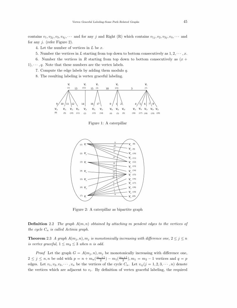
Vertex Graceful Labeling-Some Path Related Graphs 45
contains v1, v2j , v3, v4j , · · · and for any j and Right (R) which contains v1j , v2, v3j , v4, · · · and
for any j. (refer Figure 2).
4. Let the number of vertices in L be x.
5. Number the vertices in L starting from top down to bottom consecutively as 1, 2, · · · , x.6. Number the vertices in R starting from top down to bottom consecutively as (x +
1), · · · , q. Note that these numbers are the vertex labels.
7. Compute the edge labels by adding them modulo q.
8. The resulting labeling is vertex graceful labeling.
(16)
v42v41v32v21v14v12v11
(5)
v43
(6)(4)(14)(13)(9) (10) (11) (20)(2)
(1)
v1 v2
(12)
v3
(3)
v4
(15)
v5
(7)
10 11 12
v31
1714
13 15
16
51 52v 53v 54vv(17)
55v(19)(18)
18
0 19 4 5 6 7 82
3
(8)
v11
Figure 1: A caterpillar
v21
v3
v41
v42
v43
v5
v11
v12
v13
v14
v2
v31
v32
v4
v51
v52
v54
v55
v1
(3)
(2)
(1)
(4)
(5)
(6)
(7)
(8)
(9)
(10)
(11)
(12)
(13)
(14)
(15)
(17)
(18)v53
(19)
(20)
(16)
12
11
10
13
14
15
16
1718
9
0
234
1
Figure 2: A caterpillar as bipartite graph
Definition 2.2 The graph A(m,n) obtained by attaching m pendent edges to the vertices of
the cycle Cn is called Actinia graph.
Theorem 2.3 A graph A(mj , n),mj is monotonically increasing with difference one, 2 ≤ j ≤ nis vertex graceful, 1 ≤ m2 ≤ 3 when n is odd.
Proof Let the graph G = A(mj , n),mj be monotonically increasing with difference one,
2 ≤ j ≤ n, n be odd with p = n + mn(mn+12 ) −m1(
m1+12 ),m1 = m2 − 1 vertices and q = p
edges. Let v1, v2, v3, · · · , vn be the vertices of the cycle Cn. Let vij(j = 1, 2, 3, · · · , n) denote
the vertices which are adjacent to vi. By definition of vertex graceful labeling, the required
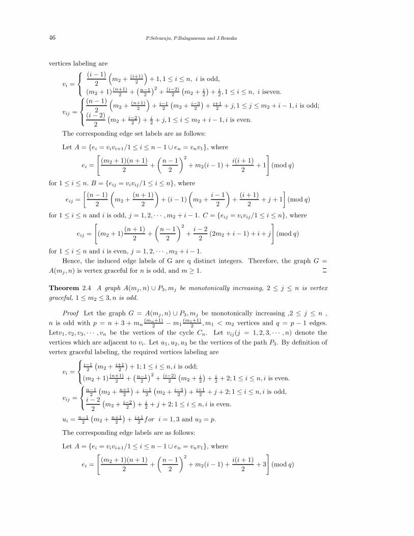
46 P.Selvaraju, P.Balaganesan and J.Renuka
vertices labeling are
vi =
(i− 1)
2
(
m2 + (i+1)2
)
+ 1, 1 ≤ i ≤ n, i is odd,
(m2 + 1) (n+1)2 +
(
n−12
)2+ (i−2)
2
(
m2 + i2
)
+ i2 , 1 ≤ i ≤ n, i iseven.
vij =
(n− 1)
2
(
m2 + (n+1)2
)
+ i−12
(
m2 + i−32
)
+ i+12 + j, 1 ≤ j ≤ m2 + i− 1, i is odd;
(i− 2)
2
(
m2 + i−22
)
+ i2 + j, 1 ≤ i ≤ m2 + i− 1, i is even.
The corresponding edge set labels are as follows:
Let A = ei = vivi+1/1 ≤ i ≤ n− 1 ∪ en = vnv1, where
ei =
[
(m2 + 1)(n+ 1)
2+
(
n− 1
2
)2
+m2(i− 1) +i(i+ 1)
2+ 1
]
(mod q)
for 1 ≤ i ≤ n. B = eij = vivij/1 ≤ i ≤ n, where
eij =
[
(n− 1)
2
(
m2 +(n+ 1)
2
)
+ (i− 1)
(
m2 +i− 1
2
)
+(i+ 1)
2+ j + 1
]
(mod q)
for 1 ≤ i ≤ n and i is odd, j = 1, 2, · · · ,m2 + i− 1. C = eij = vivij/1 ≤ i ≤ n, where
eij =
[
(m2 + 1)(n+ 1)
2+
(
n− 1
2
)2
+i− 2
2(2m2 + i− 1) + i+ j
]
(mod q)
for 1 ≤ i ≤ n and i is even, j = 1, 2, · · · ,m2 + i− 1.
Hence, the induced edge labels of G are q distinct integers. Therefore, the graph G =
A(mj , n) is vertex graceful for n is odd, and m ≥ 1. 2Theorem 2.4 A graph A(mj , n) ∪ P3,mj be monotonically increasing, 2 ≤ j ≤ n is vertex
graceful, 1 ≤ m2 ≤ 3, n is odd.
Proof Let the graph G = A(mj , n) ∪ P3,mj be monotonically increasing ,2 ≤ j ≤ n ,
n is odd with p = n + 3 + mn(mn+1)
2 − m1(m1+1)
2 ,m1 < m2 vertices and q = p − 1 edges.
Letv1, v2, v3, · · · , vn be the vertices of the cycle Cn. Let vij(j = 1, 2, 3, · · · , n) denote the
vertices which are adjacent to vi. Let u1, u2, u3 be the vertices of the path P3. By definition of
vertex graceful labeling, the required vertices labeling are
vi =
i−12
(
m2 + i+12
)
+ 1; 1 ≤ i ≤ n, i is odd;
(m2 + 1) (n+1)2 +
(
n−12
)2+ (i−2)
2
(
m2 + i2
)
+ i2 + 2; 1 ≤ i ≤ n, i is even.
vij =
n−12
(
m2 + n+12
)
+ i−12
(
m2 + i−32
)
+ i+12 + j + 2; 1 ≤ i ≤ n, i is odd,
i− 2
2
(
m2 + i−22
)
+ i2 + j + 2; 1 ≤ i ≤ n, i is even.
ui = n−12
(
m2 + n+12
)
+ i+12 for i = 1, 3 and u2 = p.
The corresponding edge labels are as follows:
Let A = ei = vivi+1/1 ≤ i ≤ n− 1 ∪ en = vnv1, where
ei =
[
(m2 + 1)(n+ 1)
2+
(
n− 1
2
)2
+m2(i− 1) +i(i+ 1)
2+ 3
]
(mod q)
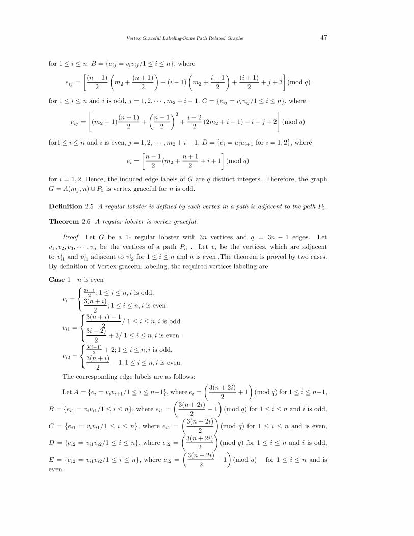
Vertex Graceful Labeling-Some Path Related Graphs 47
for 1 ≤ i ≤ n. B = eij = vivij/1 ≤ i ≤ n, where
eij =
[
(n− 1)
2
(
m2 +(n+ 1)
2
)
+ (i− 1)
(
m2 +i− 1
2
)
+(i+ 1)
2+ j + 3
]
(mod q)
for 1 ≤ i ≤ n and i is odd, j = 1, 2, · · · ,m2 + i− 1. C = eij = vivij/1 ≤ i ≤ n, where
eij =
[
(m2 + 1)(n+ 1)
2+
(
n− 1
2
)2
+i− 2
2(2m2 + i− 1) + i+ j + 2
]
(mod q)
for1 ≤ i ≤ n and i is even, j = 1, 2, · · · ,m2 + i− 1. D = ei = uiui+1 for i = 1, 2, where
ei =
[
n− 1
2(m2 +
n+ 1
2+ i+ 1
]
(mod q)
for i = 1, 2. Hence, the induced edge labels of G are q distinct integers. Therefore, the graph
G = A(mj , n) ∪ P3 is vertex graceful for n is odd. 2Definition 2.5 A regular lobster is defined by each vertex in a path is adjacent to the path P2.
Theorem 2.6 A regular lobster is vertex graceful.
Proof Let G be a 1- regular lobster with 3n vertices and q = 3n − 1 edges. Let
v1, v2, v3, · · · , vn be the vertices of a path Pn . Let vi be the vertices, which are adjacent
to vii1 and vi
i1 adjacent to vii2 for 1 ≤ i ≤ n and n is even .The theorem is proved by two cases.
By definition of Vertex graceful labeling, the required vertices labeling are
Case 1 n is even
vi =
3i−12 ; 1 ≤ i ≤ n, i is odd,
3(n+ i)
2; 1 ≤ i ≤ n, i is even.
vi1 =
3(n+ i)− 1
2/ 1 ≤ i ≤ n, i is odd
3i− 2)
2+ 3/ 1 ≤ i ≤ n, i is even.
vi2 =
3(i−1)2 + 2; 1 ≤ i ≤ n, i is odd,
3(n+ i)
2− 1; 1 ≤ i ≤ n, i is even.
The corresponding edge labels are as follows:
Let A = ei = vivi+1/1 ≤ i ≤ n−1, where ei =
(
3(n+ 2i)
2+ 1
)
(mod q) for 1 ≤ i ≤ n−1,
B = ei1 = vivi1/1 ≤ i ≤ n, where ei1 =
(
3(n+ 2i)
2− 1
)
(mod q) for 1 ≤ i ≤ n and i is odd,
C = ei1 = vivi1/1 ≤ i ≤ n, where ei1 =
(
3(n+ 2i)
2
)
(mod q) for 1 ≤ i ≤ n and is even,
D = ei2 = vi1vi2/1 ≤ i ≤ n, where ei2 =
(
3(n+ 2i)
2
)
(mod q) for 1 ≤ i ≤ n and i is odd,
E = ei2 = vi1vi2/1 ≤ i ≤ n, where ei2 =
(
3(n+ 2i)
2− 1
)
(mod q) for 1 ≤ i ≤ n and is
even.
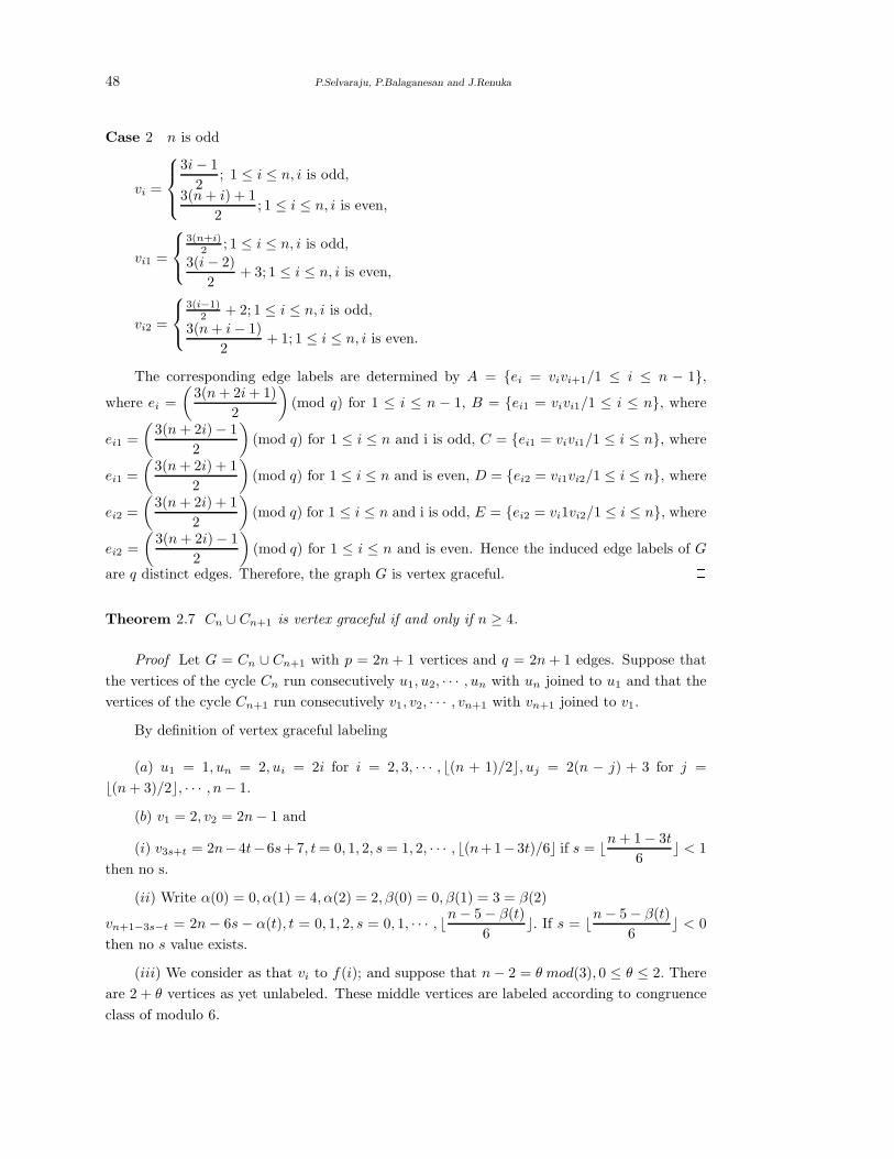
48 P.Selvaraju, P.Balaganesan and J.Renuka
Case 2 n is odd
vi =
3i− 1
2; 1 ≤ i ≤ n, i is odd,
3(n+ i) + 1
2; 1 ≤ i ≤ n, i is even,
vi1 =
3(n+i)2 ; 1 ≤ i ≤ n, i is odd,
3(i− 2)
2+ 3; 1 ≤ i ≤ n, i is even,
vi2 =
3(i−1)2 + 2; 1 ≤ i ≤ n, i is odd,
3(n+ i− 1)
2+ 1; 1 ≤ i ≤ n, i is even.
The corresponding edge labels are determined by A = ei = vivi+1/1 ≤ i ≤ n − 1,where ei =
(
3(n+ 2i+ 1)
2
)
(mod q) for 1 ≤ i ≤ n − 1, B = ei1 = vivi1/1 ≤ i ≤ n, where
ei1 =
(
3(n+ 2i)− 1
2
)
(mod q) for 1 ≤ i ≤ n and i is odd, C = ei1 = vivi1/1 ≤ i ≤ n, where
ei1 =
(
3(n+ 2i) + 1
2
)
(mod q) for 1 ≤ i ≤ n and is even, D = ei2 = vi1vi2/1 ≤ i ≤ n, where
ei2 =
(
3(n+ 2i) + 1
2
)
(mod q) for 1 ≤ i ≤ n and i is odd, E = ei2 = vi1vi2/1 ≤ i ≤ n, where
ei2 =
(
3(n+ 2i)− 1
2
)
(mod q) for 1 ≤ i ≤ n and is even. Hence the induced edge labels of G
are q distinct edges. Therefore, the graph G is vertex graceful. 2Theorem 2.7 Cn ∪ Cn+1 is vertex graceful if and only if n ≥ 4.
Proof Let G = Cn ∪ Cn+1 with p = 2n+ 1 vertices and q = 2n+ 1 edges. Suppose that
the vertices of the cycle Cn run consecutively u1, u2, · · · , un with un joined to u1 and that the
vertices of the cycle Cn+1 run consecutively v1, v2, · · · , vn+1 with vn+1 joined to v1.
By definition of vertex graceful labeling
(a) u1 = 1, un = 2, ui = 2i for i = 2, 3, · · · , ⌊(n + 1)/2⌋, uj = 2(n − j) + 3 for j =
⌊(n+ 3)/2⌋, · · · , n− 1.
(b) v1 = 2, v2 = 2n− 1 and
(i) v3s+t = 2n−4t−6s+7, t= 0, 1, 2, s = 1, 2, · · · , ⌊(n+1−3t)/6⌋ if s = ⌊n+ 1− 3t
6⌋ < 1
then no s.
(ii) Write α(0) = 0, α(1) = 4, α(2) = 2, β(0) = 0, β(1) = 3 = β(2)
vn+1−3s−t = 2n− 6s− α(t), t = 0, 1, 2, s = 0, 1, · · · , ⌊n− 5− β(t)
6⌋. If s = ⌊n− 5− β(t)
6⌋ < 0
then no s value exists.
(iii) We consider as that vi to f(i); and suppose that n− 2 = θ mod(3), 0 ≤ θ ≤ 2. There
are 2 + θ vertices as yet unlabeled. These middle vertices are labeled according to congruence
class of modulo 6.
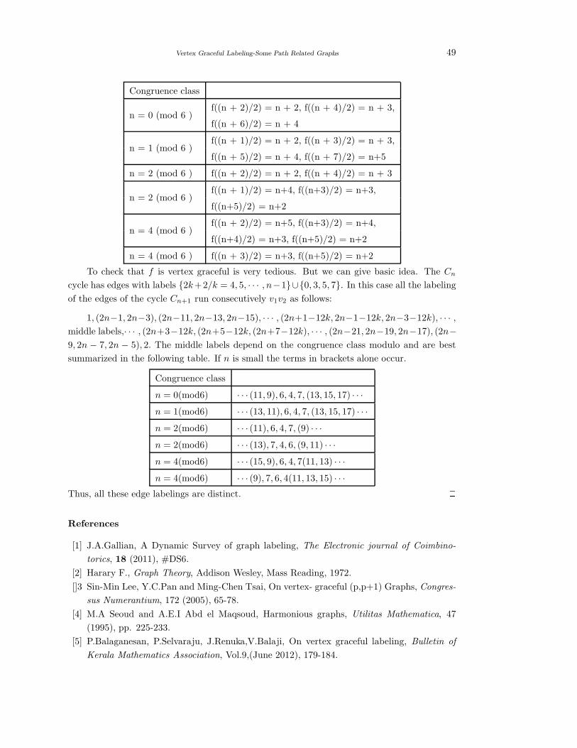
Vertex Graceful Labeling-Some Path Related Graphs 49
Congruence class
n = 0 (mod 6 )f((n + 2)/2) = n + 2, f((n + 4)/2) = n + 3,
f((n + 6)/2) = n + 4
n = 1 (mod 6 )f((n + 1)/2) = n + 2, f((n + 3)/2) = n + 3,
f((n + 5)/2) = n + 4, f((n + 7)/2) = n+5
n = 2 (mod 6 ) f((n + 2)/2) = n + 2, f((n + 4)/2) = n + 3
n = 2 (mod 6 )f((n + 1)/2) = n+4, f((n+3)/2) = n+3,
f((n+5)/2) = n+2
n = 4 (mod 6 )f((n + 2)/2) = n+5, f((n+3)/2) = n+4,
f((n+4)/2) = n+3, f((n+5)/2) = n+2
n = 4 (mod 6 ) f((n + 3)/2) = n+3, f((n+5)/2) = n+2
To check that f is vertex graceful is very tedious. But we can give basic idea. The Cn
cycle has edges with labels 2k+2/k = 4, 5, · · · , n−1∪0, 3, 5, 7. In this case all the labeling
of the edges of the cycle Cn+1 run consecutively v1v2 as follows:
1, (2n−1, 2n−3), (2n−11, 2n−13, 2n−15), · · · , (2n+1−12k, 2n−1−12k, 2n−3−12k), · · · ,middle labels,· · · , (2n+3−12k, (2n+5−12k, (2n+7−12k), · · · , (2n−21, 2n−19, 2n−17), (2n−9, 2n − 7, 2n − 5), 2. The middle labels depend on the congruence class modulo and are best
summarized in the following table. If n is small the terms in brackets alone occur.
Congruence class
n = 0(mod6) · · · (11, 9), 6, 4, 7, (13, 15, 17) · · ·n = 1(mod6) · · · (13, 11), 6, 4, 7, (13, 15, 17) · · ·n = 2(mod6) · · · (11), 6, 4, 7, (9) · · ·n = 2(mod6) · · · (13), 7, 4, 6, (9, 11) · · ·n = 4(mod6) · · · (15, 9), 6, 4, 7(11, 13) · · ·n = 4(mod6) · · · (9), 7, 6, 4(11, 13, 15) · · ·
Thus, all these edge labelings are distinct. 2References
[1] J.A.Gallian, A Dynamic Survey of graph labeling, The Electronic journal of Coimbino-
torics, 18 (2011), #DS6.
[2] Harary F., Graph Theory, Addison Wesley, Mass Reading, 1972.
[]3 Sin-Min Lee, Y.C.Pan and Ming-Chen Tsai, On vertex- graceful (p,p+1) Graphs, Congres-
sus Numerantium, 172 (2005), 65-78.
[4] M.A Seoud and A.E.I Abd el Maqsoud, Harmonious graphs, Utilitas Mathematica, 47
(1995), pp. 225-233.
[5] P.Balaganesan, P.Selvaraju, J.Renuka,V.Balaji, On vertex graceful labeling, Bulletin of
Kerala Mathematics Association, Vol.9,(June 2012), 179-184.
International J.Math. Combin. Vol.3(2013), 50-55
Total Semirelib Graph
Manjunath Prasad K B
(Sri Siddaganga College for Women, Tumkur, India)
Venkanagouda M Goudar
(Department of Mathematics, Sri Siddhartha Institute of Technology, Tumkur,Karnataka, India)
E-mail: [email protected], [email protected]
Abstract: In this paper, the concept of Total semirelib graph of a planar graph is in-
troduced. We present a characterization of those graphs whose total semirelib graphs are
planar, outer planar, Eulerian, hamiltonian with crossing number one.
Key Words: Blocks, edge degree, inner vertex number, line graph, regions Smarandachely
semirelib M -graph.
AMS(2010): 10C75, 10C10
§1. Introduction
The concept of block edge cut vertex graph was introduced by Venkanagouda M Goudar [4 ].
For the graph G(p,q), if B = u1, u2, · · · , ur : r ≥ 2 is a block of G, then we say that the vertex
ui and the block B are incident with each other. If two blocks B1 and B2 are incident with a
common cutvertex, then they are adjacent blocks.
All undefined terminology will conform with that in Harary [1]. All graphs considered here
are finite, undirected, planar and without loops or multiple edges.
The semirelib graph of a planar graph G is introduced by Venkanagouda M Goudar and
Manjunath Prasad K B [5] denoted by Rs(G) is the graph whose vertex set is the union of set
of edges, set of blocks and set of regions of G in which two vertices are adjacent if and only if
the corresponding edges of G are adjacent, the corresponding edges lies on the blocks and the
corresponding edges lies on the region. Now we define the total semirelib graph.
Let M be a maximal planar graph of a graph G. A Smarandachely semirelib M -graph
TMs (G) of M is the graph whose vertex set is the union of set of edges, set of blocks and set of
regions of M in which two vertices are adjacent if and only if the corresponding edges of M are
adjacent, the corresponding edges lies on the blocks, the corresponding edges lies on the region,
the corresponding blocks are adjacent and the graph G\M . Particularly, if G is a planar graph,
such a TMs (G) is called the total semirelib graph of G denoted, denoted by Ts(G).
The edge degree of an edge uv is the sum of the degree of the vertices of u and v. For the
planar graph G, the inner vertex number i(G) of a graph G is the minimum number of vertices
1Received March 8, 2013, Accepted August 18, 2013.
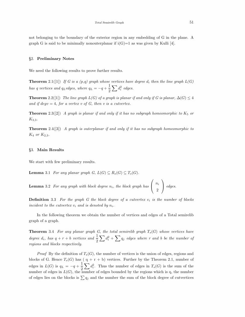
Total Semirelib Graph 51
not belonging to the boundary of the exterior region in any embedding of G in the plane. A
graph G is said to be minimally nonouterplanar if i(G)=1 as was given by Kulli [4].
§2. Preliminary Notes
We need the following results to prove further results.
Theorem 2.1([1]) If G is a (p,q) graph whose vertices have degree di then the line graph L(G)
has q vertices and qLedges, where qL = −q +1
2
∑
d2i edges.
Theorem 2.2([1]) The line graph L(G) of a graph is planar if and only if G is planar, ∆(G) ≤ 4
and if degv = 4, for a vertex v of G, then v is a cutvertex.
Theorem 2.3([2]) A graph is planar if and only if it has no subgraph homeomorphic to K5 or
K3,3.
Theorem 2.4([3]) A graph is outerplanar if and only if it has no subgraph homeomorphic to
K4 or K2,3.
§3. Main Results
We start with few preliminary results.
Lemma 3.1 For any planar graph G, L(G) ⊆ Rs(G) ⊆ Ts(G).
Lemma 3.2 For any graph with block degree ni, the block graph has
ni
2
edges.
Definition 3.3 For the graph G the block degree of a cutvertex vi is the number of blocks
incident to the cutvertex vi and is denoted by ni.
In the following theorem we obtain the number of vertices and edges of a Total semirelib
graph of a graph.
Theorem 3.4 For any planar graph G, the total semirelib graph Ts(G) whose vertices have
degree di, has q + r + b vertices and1
2
∑
d2i +
∑
qj edges where r and b be the number of
regions and blocks respectively.
Proof By the definition of Ts(G), the number of vertices is the union of edges, regions and
blocks of G. Hence Ts(G) has ( q + r + b) vertices. Further by the Theorem 2.1, number of
edges in L(G) is qL = −q +1
2
∑
d2i . Thus the number of edges in Ts(G) is the sum of the
number of edges in L(G), the number of edges bounded by the regions which is q, the number
of edges lies on the blocks is∑
qj and the number the sum of the block degree of cutvertices
52 Manjunath Prasad K B and Venkanagouda M Goudar
which is∑
(ni
2 ) by the Lemma 3.2. Hence
E[Ts(G)] = −q +1
2
∑
d2i + q +
∑
qj +∑
(ni
2 ) =1
2
∑
d2i +
∑
qj +∑
(ni
2 ). 2Theorem 3.5 For any edge in a plane graph G with edge degree ei is n, the degree of the
corresponding vertex in Ts(G) is i). n if ei is incident to a cutvertex and ii). n+1 if ei is not
incident to a cutvertex.
Proof Suppose an edge ei ∈ E(G) have degree n. By the definition of total semirelib graph,
the corresponding vertex in Ts(G) has n-1. Since edge lies on a block, we have the degree of
the vertex is n− 1 + 1 = n. Further, if ei 6= bi ∈ E(G) then by the definition of total semirelib
graph, ∀ei ∈ E(G), ei is adjacent to all vertices ej of Ts(G) which are adjacent edges of ei of
G. Also the block vertex of Ts(G) is adjacent to ei. Clearly degree of ei is n+ 1. 2Theorem 3.6 For any planar graph G with n blocks which are K2 then Ts(G) contains n
pendent vertices.
Theorem 3.7 For any graph G, Ts(G) is nonseparable.
Proof Let e1, e2, · · · , en ∈ E(G), b1 = e1, b2 = e2, · · · , bn = en be the blocks and
r1, r2, · · · , rk be the regions of G. By the definition of line graph L(G), e1, e2, · · · , en form
a subgraph without isolated vertex. By the definition of Ts(G), the region vertices are adjacent
to these vertices to form a graph without isolated vertex. Since there are n blocks which are
K2, we have each b1 = e1, b2 = e2, · · · , bn = en are adjacent to e1, e2, · · · , en. Hence semirelib
graph Rs(G) contains n pendent vertices. By the definition of total semirelib graph, the block
vertices are also adjacent. Hence Ts(G) is nonseparable. 2In the following theorem we obtain the condition for the planarity on total semirelib graph
of a graph.
Theorem 3.8 For any planar graph G, the Ts(G) is planar if and only if G is a tree such that
∆(G) ≤ 3.
Proof Suppose Rs(G) is planar. Assume that ∃vi ∈ G such that degvi ≥ 4. Suppose
degvi = 4 and e1, e2, e3, e4 are the edges incident to vi. By the definition of line graph,
e1, e2, e3, e4 form K4 as an induced subgraph. In Ts(G), the region vertex ri is adjacent with all
vertices of L(G) to form K5 as an induced subgraph. Further the corresponding block vertices
b1, b2, b3, · · · , bn−1 of of blocks B1, B2, B3, · · · , Bn in G are adjacent to vertices of K4 and the
corresponding blocks are adjacent. Clearly Ts(G) forms graph homeomorphic to K5. By the
Theorem 2.3, it is non planar, a contradiction.
Conversely, Suppose degv ≤ 3 and let e1, e2, e3 be the edges of G incident to v. By the
definition of line graph e1, e2, e3 form K3 as a subgraph. By the definition of Ts(G), the region
vertex ri is adjacent to e1, e2, e3 to form K4 as a subgraph. Further, by the Lemma 3.2, the
blocks b1, b2, b3, · · · , bn of T with n vertices such that b1 = e1, b2 = e2, · · · , bn−1 = en−1 becomes
p−1 pendant vertices.By the definition of Ts(G), these block vertices are adjacent. Hence Ts(G)
is planar. 2
Total Semirelib Graph 53
In the following theorem we obtain the condition for the outer planarity on total semirelib
graph of a graph.
Theorem 3.9 For any planar graph G, Ts(G) is outer planar if and only if G is a path P3.
Proof Suppose Ts(G) is outer planar. Assume that G is a tree with at least one vertex
v such that degv = 3. Let e1, e2, e3 be the edges of G incident to v. By the definition of line
graph e1, e2, e3 form K3 as a subgraph.In Ts(G), the region vertex ri is adjacent to e1, e2, e3 to
form K4 as induced subgraph. Further by the lemma 3.2, b1 = e1, b2 = e2, · · · , bn−1 = en−1
becomes n-1 pendant vertices in Rs(G). By the definition of Ts(G), i[Rs(G) ≥ 1], which is
non-outer planar ,a contradiction.
Conversely, Suppose G is a path P3. Let e1, e2 ∈ E(G). By the definition of line graph
L[P3](G) = P2. Further by definition of Ts(G), b1 = e1, b2 = e2 forms and the vertices of line
graph form C4 . Further the region vertex r1 is adjacent to all the vertices of Ts(G) which is
outer planar. 2In the following theorem we obtain the condition for the minimally non outer planar on
total semirelib graph of a graph.
Theorem 3.10 For any planar graph G, Ts(G) is minimally non-outer planar if and only if G
is P4.
Proof Suppose Ts(G) is minimally non-outer planar. Assume that G 6= P4.Consider the
following cases.
Case 1 Assume that G = K1,n for n ≥ 3. Then there exist at least one vertex of degree at
least 3. Suppose degv = 3 for any v ∈ G. By the definition of line graph, L[K1,3] = K3. By the
definition of Ts(G),these vertices are adjacent to a region vertex r1, which form K4. Further the
block vertices form K3 and it has e1, e2, e3 as its internal vertices. Clearly, Ts is not minimally
non-outer planar, a contradiction.
Case 2 Suppose G 6= K1,n. By the Theorem 3.9, Ts(G) is non-outer planar,a contradiction.
Case 3 Assume that G = Pn,for n ≥ 5. Suppose n = 5. By the definition of line
graph,L[P5](G) = P4 and e2, e3 are the internal vertices of L(G). By the definition of Ts,
the region vertex r1 is adjacent to all vertices of L(G) to form connected graph. Further the
block vertices are adjacent to all vertices of L(G). Clearly the vertices e2, e3 becomes the inter-
nal vertices of Ps. Clearly i[Ts] = 2, which is not minimally nonouterplanar, a contradiction.
Conversely, suppose G = P4 and let e1, e2, e3 ∈ E(G). By the definition of line graph,
L[P4] = P3. Let r1 be the region vertex in Ts(G) such that r1 is adjacent to all vertices of
L(G). Further the blocks bi are adjacent to the vertices ej for i = j. Clearly i[Ts(G)] = 1.
Hence G is minimally non-outer planar. 2In the following theorem we obtain the condition for the non Eulerian on total semirelib
graph of a graph.
Theorem 3.11 For any planar graph G, Ts(G) is always non Eulerian.
54 Manjunath Prasad K B and Venkanagouda M Goudar
Proof We consider the following cases.
Case 1 Assume that G is a tree. In a tree each edge is a block and hence b1 = e1, b2 =
e2, · · · , bn−1 = en−1∀en−1 ∈ E(G) and ∀bn−1 ∈ V [Ts(G)]. In Ts(G), the degree of a block
vertex bi is always even, but the pendent edges of G becomes the odd degree vertex in Ts(G),
which is non Eulerian.
Case 2 Assume that G is K2 -free graph. We have the following subcases of Case 2.
Subcase 1 Suppose G itself is a block with even number of edges. Clearly each edge of G is of
even degree. By the definition of Ts(G), both the region vertices and blocks have even degree.
By the Theorem 2.3, ei = bi ∈ V [Ts(G)] is of odd degree, which is non Eulerian. Further if G is
a block with odd number of edges, then by the Theorem 3.3, each ei = bi ∈ V [Ts(G)] is of even
degree. Also the block vertex and region vertex bi, ri are adjacent to these vertices. Clearly
degree of bi and ri is odd, which is non Eulerian.
Subcase 2 Suppose G is a graph such that it contains at least one cutvertex. If each edge is
even degree then by the sub case 1, it is non Eulerian. Assume that G contains at least one
edge with odd edge degree. Clearly for any ej ∈ E(G), degree of ej ∈ V [Ts(G)] is odd, which
is non Eulerian. Hence for any graph G Ts(G) is always non Eulerian. 2In the following theorem we obtain the condition for the hamiltonian on total semirelib
graph of a graph.
Theorem 3.12 For any graph G, Ts(G) is always hamiltonian.
Proof Suppose G is any graph. We have the following cases.
Case 1 Consider a graph G is a tree. In a tree, each edge is a block and hence b1 = e1, b2 =
e2, · · · , bn−1 = en−1∀en−1 ∈ E(G) and ∀bn−1 ∈ V [Ts(G)]. Since a tree T contains only ne
region r1 which is adjacent to all vertices e1, e2, · · · , en−1 of Ts(G). Also the block vertices are
adjacent to each vertex ei which corresponds to the edge of G and it is a block in G. Clearly
r1, e1, b1, b2, e2, e3, b3, · · · , r1 form a hamiltonian cycle. HenceTs(G) is hamiltonian graph.
Case 2 Suppose G is not a tree. Let e1, e2, · · · , en−1 ∈ E(G), b1, b2, · · · , bi be the blocks
and r1, r2, · · · , rk be the regions of G such that e1, e2, · · · , el ∈ V (b1), el+1, el+2, · · · , em ∈V (b2), · · · , em+1, em+2, · · · , en−1 ∈ V (bi). By the Theorem 3.3, V [Ts(G)] = e1, e2, · · · , en−1 ∪b1, b2, · · · , bi ∪ r1, r2, · · · , rk. By theorem 3.7, Ts(G) is non separable. By the definition,
b1e1, e2, · · · , el−1r1b2 · · · r2emb3 · · · ek+1, ek+2, · · · , en−1bkrkelb1 form a cycle which contains all
the vertices of Ts(G). Hence Ts(G) is hamiltonian. 2References
[1] Harary F., Graph Theory, Addition - Weseley Reading Mass, 1969.
[2] Harary F., Annals of New York Academy of Science, 1975,175 :198.
[3] Kulli V. R., On minimally non- outer planar graphs, Proceeding of the Indian National
Science Academy, Vol.41, Part A, No.3 (1975), pp 275 -280.
Total Semirelib Graph 55
[4] Y.B. Maralabhavi and Venkanagouda M. Goudar, On block edge cutvertex graph, ACTA
CIENCIA INDICA, Vol.XXXIII M.No.2, (2007), pp. 493-49.
[5] Venkanagouda M. Goudar and K B Manjunatha Prasad, Semirelib graph of a planar graph,
Applied Mathematical Sciences,vol.7, No.39(2013), pp1909 - 1915.
International J.Math. Combin. Vol.3(2013), 56-68
On Some Characterization of Ruled Surface of a Closed
Spacelike Curve with Spacelike Binormal in Dual Lorentzian Space
Ozcan BEKTAS
(Department of Mathematics, Arts and Science Faculty, Yildiz Technical University, Istanbul-Turkey)
Suleyman SENYURT
(Department of Mathematics, Arts and Science Faculty, Ordu University, Ordu-Turkey)
E-mail: [email protected], [email protected]
Abstract: In this paper, we investigate the relations between the pitch, the angle of pitch
and drall of parallel ruled surface of a closed spacelike curve with spacelike binormal in dual
Lorentzian space.
Key Words: Spacelike dual curve, ruled surface, Lorentzian space, dual numbers.
AMS(2010): 53A04, 45F10
§1. Introduction
Dual numbers were introduced by W.K. Clifford [5] as a tool for his geometrical investigations.
After him,e E.Study used dual numbers and dual vectors in his research on the geometry of
lines and kinematics [7]. The pitches and the angles of the pitches of the closed ruled surfaces
corresponding to the one parameter dual unit spherical curves and oriented lines in R3 were
calculated respectively by Hacısalihoglu [10] and Gursoy [8]. Definitions of the parallel ruled
surface were presented by Wilhelm Blaschke [6]. The integral invariants of the paralel ruled
surfaces in the 3-dimensional Euclidean space R3 corresponding to the unit dual spherical
parallel curves were calculated by Senyurt [14]. The integral invariants of ruled surface of a
timelike curve in dual Lorentzian space were calculated by Bektas and Senyurt [2]. The integral
invariants of ruled surface of a closed spacelike curve with timelike binormal in dual Lorentzian
space were calculated by Bektas and Senyurt [3].
The set D = λ = λ + ελ∗|λ, λ∗ ∈ R, ε2 = 0 is called dual numbers set, see [5].On this
set, product and addition operations are respectively
(λ+ ελ∗) + (β + εβ∗) = (λ+ β) + ε (λ∗ + β∗)
and
(λ+ ελ∗) (β + εβ∗) = λβ + ε (λβ∗ + λ∗β) .
1Received May 15, 2013, Accepted August 22, 2013.
Characterization of Ruled Surface of a Closed Spacelike Curve with Spacelike Binormal in Dual Lorentzian Space 57
The elements of the set D3 =−→A = −→a + ε−→a ∗ ∣
∣
−→a ,−→a ∗ ∈ R3
are called dual vectors. On
this set addition and scalar product operations are respectively
⊕ : D3 ×D3 → D3(−→A,−→B)
→ −→A ⊕−→B = −→a +−→b + ε
(−→a ∗ +−→b ∗)
,
⊙ : D ×D3 → D3
(
λ,−→A)
→ λ⊙−→A = (λ+ ελ∗)⊙ (−→a + ε−→a ∗) = λ−→a + ε (λ−→a ∗ + λ∗−→a )
The set(
D3,⊕)
is a module over the ring (D,+, ·), called the D −Modul .
The Lorentzian inner product of dual vectors−→A ,−→B ∈ D3 is defined by
⟨−→A,−→B⟩
=⟨−→a ,−→b
⟩
+ ε(⟨−→a ,−→b ∗
⟩
+⟨−→a ∗,
−→b⟩)
where⟨−→a ,−→b
⟩
is the following Lorentzian inner product of vectors −→a = (a1, a2, a3) and−→b =
(b1, b2, b3) ∈ R3,i.e.,
⟨−→a ,−→b⟩
= −a1b1 + a2b2 + a3b3.
The set D3 equipped with the Lorentzian inner product⟨−→A,−→B⟩
is called 3-dimensional dual
Lorentzian space and is denoted in what follows by D31 =
−→A = −→a + ε−→a ∗ ∣
∣
−→a ,−→a ∗ ∈ R31
[17].
A dual vector−→A = −→a +ε−→a ∗ ∈ D3
1 is called dual space-like vector if⟨−→A,−→A⟩
> 0 or−→A = 0,
a dual time-like vector if⟨−→A,−→A⟩
< 0, a dual null (light-like) vector if⟨−→A,−→A⟩
= 0 for−→A 6= 0
. For−→A 6= 0, the norm
∥
∥
∥
−→A∥
∥
∥ of−→A is defined by
∥
∥
∥
−→A∥
∥
∥ =
√
∣
∣
∣
⟨−→A,−→A⟩∣
∣
∣ = ‖−→a ‖+ ε〈−→a ,−→a ∗〉‖−→a ‖ , ‖−→a ‖ 6= 0.
The dual Lorentzian cross-product of−→A ,−→B ∈ D3 is defined as
−→A ∧ −→B = −→a ×−→b + ε
(−→a ×−→b ∗ +−→a ∗ ×−→b)
where −→a ×−→b is the cross-product [14] of −→a ,−→b ∈ R
3 given by
−→a ×−→b = (a3b2 − a2b3, a1b3 − a3b1, a1b2 − a2b1) .
Theorem 1.1(E. Study) The oriented lines in R3 are in one to one correspondence with the
points of the dual unit sphere ‖−→A‖ = (1, 0) where−→A 6= (
−→0 ,−→a ) ∈ D-Modul , see [9].
The dual number Φ = ϕ+ εϕ∗ is called dual angle between the unit dual vectors−→A ve
−→B
and keep in mind that
sin (ϕ+ εϕ∗) = sinϕ+ εϕ∗ cosϕ ,
cos (ϕ+ εϕ∗) = cosϕ− εϕ∗ sinϕ.
58 Ozcan BEKTAS and Suleyman SENYURT
§2. Characterization of Ruled Surface of a Closed Spacelike Curve with Spacelike
Binormal in Dual Lorentzian Space(
D31
)
Let U : I → D31 , t →
−→U (t) =
−→U 1 (t) ,
∥
∥
∥
−→U (t)
∥
∥
∥ = 1 be a differentiable spacelike curve with
spacelike binormal in the dual unit sphere. Denote by (−→U ) the closed ruled generated by this
curve.
Let−→U1,−→U2,−→U3
be the Frenet frame of the curve−→U =
−→U 1 with
−→U 1 =
−→U ,
−→U 2 =
−→U
′
/∥
∥
∥
−→U∥
∥
∥ ,−→U 3 =
−→U 1 ×
−→U 2
Definition 2.1 The closed ruled surface (−→U ) corresponding to the dual spacelike curve
−→U (t)
which makes the fixed dual angle Φ = ϕ+ εϕ∗ with−→U (t) determines
−→V = cosΦ
−→U1 + sin Φ
−→U3 (2.1)
The surface (−→V ) corresponding to the dual spacelike vector
−→V is called the parallel ruled
surface of surface (−→U ) in the dual Lorentzian space D3
1.
Now, take−→U (t) as a closed spacelike curve with curvature κ = k1 + εk∗1 and torsion
τ = k2 + εk∗2 . Recall that in the Frenet frames associated to the curve−→U1 and
−→U3 are spacelike
vectors and−→U2 is timelike vector and we have
−→U1 ×
−→U2 = −−→U3 ,
−→U2 ×
−→U3 = −−→U1 ,
−→U3 ×
−→U1 =
−→U2. (2.2)
Under these conditions, the Frenet formulas are given by ([18])
−→U1
′
= κ−→U2 ,
−→U2
′
= κ−→U1 + τ
−→U3 ,
−→U3
′
= τ−→U2. (2.3)
The Frenet instantaneous rotation vector (also called instantaneous Darboux vector) for
the spacelike curve is given by ([16])
−→Ψ = −τ−→U1 + κ
−→U3, (2.4)
Let be−→V 1 =
−→V . Differentiating of the vector
−→V1 with respect the parameter t and using
the Eq.(2.3) we get−→V1
′
= (κ cosΦ + τ sin Φ)−→U2 (2.5)
and the norm of that vector denoted by P is
P = κ cosΦ + τ sin Φ. (2.6)
Then, substituting the values of (2.5) and (2.6) into Frenet equations gives
−→V2 =
−→U2 (2.7)
For the vector−→V3,we have
−→V3 = sin Φ
−→U1 − cosΦ
−→U3 (2.8)
Characterization of Ruled Surface of a Closed Spacelike Curve with Spacelike Binormal in Dual Lorentzian Space 59
If Eq.(2.1), (2.7) and (2.8) are written matrix form, we have
−→V1
−→V2
−→V3
=
cosΦ 0 sin Φ
0 1 0
sinΦ 0 − cosΦ
·
−→U1
−→U2
−→U3
or
−→U1
−→U2
−→U3
=
cosΦ 0 sin Φ
0 1 0
sin Φ 0 − cosΦ
·
−→V1
−→V2
−→V3
The real and dual parts of−→U1,−→U2,−→U3 are
−→u 1 = cosϕ−→v 1 + sinϕ−→v 3
−→u 2 = −→v 2
−→u 3 = sinϕ−→v 1 − cosϕ−→v 3
−→u ∗1 = cosϕ−→v ∗
1 + sinϕ−→v ∗3 − ϕ∗(sinϕ−→v 1 − cosϕ−→v 3)
−→u ∗2 = −→v ∗
2
−→u ∗3 = sinϕ−→v ∗
1 − cosϕ−→v ∗3 + ϕ∗(cosϕ−→v 1 − sinϕ−→v 3)
(2.9)
Let P = p + εp∗ be the curvature and Q = q + εq∗ the torsion of curve−→V (t). Then, the
following relating holds between the vectors
−→V1,−→V2,−→V3 and
−→V1
′
,−→V2
′
,−→V3
′
[18]
−→V 1
′
= P−→V 2,
−→V 2
′
= P−→V 1 +Q
−→V 3,
−→V 3
′
= Q−→V 2
P =
√
<−→V 1
′
,−→V 1
′
>, Q = det(−→V 1,
−→V 1
′
,−→V 1
′′
)
<−→V 1
′
,−→V 1
′
>.
(2.10)
If Eq.(2.10) is separated into its real and dual parts, we get
−→v 1
′
= p−→v 2,−→v 2
′
= p−→v 1 + q−→v 3,−→v 3
′
= q−→v 2
−→v ′
1∗ = p−→v ∗
2 + p∗−→v 2,
−→v ′
2∗ = p−→v ∗
1 + p∗−→v 1 + q∗−→v 3 + q−→v 3∗,
−→v ′
3∗ = q−→v ∗
2 + q∗−→v 2
(2.11)
Now, we are ready to calculate the value of Q as function of κ and τ. Differentiating Eq.
(2.5) with respect to the curve parameter t we get
−→V
′′
1 =(+κ2 cosΦ + κτ sinΦ)−→U 1+
+ (κ cosΦ + τ sin Φ)′−→U 2 + (κτ cosΦ + τ2 sinΦ)
−→U 3
(2.12)
Using Eqs.(2.1), (2.5) and (2.12) into Eq.(2.10), we get
Q = −κ sinΦ + τ cosΦ (2.13)
60 Ozcan BEKTAS and Suleyman SENYURT
and separating Eq.(2.6) and Eq.(2.13) into its dual and real parts gives
p = k1 cosϕ+ k2 sinϕ
p∗ = k∗1 cosϕ+ k∗2 sinϕ− ϕ∗(k1 sinϕ− k2 cosϕ)
q = −k1 sinϕ+ k2 cosϕ
q∗ = −k∗1 sinϕ+ k∗2 cosϕ− ϕ∗(k1 cosϕ+ k2 sinϕ)
(2.14)
In its dual unit spherical motion the dual orthonormal system−→V1,−→V2,−→V3
at any t makes a
dual rotation motion around the instantaneous dual Darboux vector. This vector is determined
by the following equation ([16]). −→Ψ = −Q−→V1 + P
−→V3. (2.15)
For the Steiner vector of the motion, we can write
−→D =
∮ −→Ψ (2.16)
or −→D = −−→V1
∮
Qdt+−→V3
∮
Pdt (2.17)
Using the values of the vectors−→U1 and
−→U3 into Eq.(2.4), gives
−→Ψ = −τ(cosΦ−→V 1 + sinΦ
−→V 3) + κ(sinΦ
−→V 1 − cosΦ
−→V 3),
−→Ψ = −Q−→V 1 − P
−→V 3 (2.18)
Because of the equations−→D =
∮ −→Ψ for the dual Steiner vector of the motion, we may write
−→D = −−→V1
∮
Qdt−−→V3
∮
Pdt (2.19)
The real and dual parts of−→D are
−→d = −−→v 1
∮
qdt−−→v 3
∮
pdt,−→d ∗ = −−→v 1
∮
q∗dt−−→v ∗1
∮
qdt−−→v 3
∮
p∗dt−−→v ∗3
∮
pdt(2.20)
−→D = −−→U1
∮
τdt+−→U3
∮
κdt (2.21)
Eq.(2.21) can be written type of the dual and real part as follow
−→d = −−→u 1
∮
k2dt+−→u 3
∮
k1dt,−→d ∗ = −−→u ∗
1
∮
k2dt−−→u 1
∮
k∗2dt+−→u ∗
3
∮
k1dt+−→u 3
∮
k∗1dt(2.22)
If the equation (2.3) is separated into the dual and real part, we can obtain
−→u ′
1 = k1−→u 2,
−→u ′
2 = k1−→u 1 + k2
−→u 3,−→u ′
3 = k2−→u 2
−→u ′
1∗ = k∗1
−→u 2 + k1−→u ∗
2,
−→u ′
2∗ = k∗1
−→u 1 + k∗2−→u 3 + k1
−→u ∗1 + k2
−→u ∗3
−→u ′
3∗ = k∗2
−→u 2 + k2−→u ∗
2
(2.23)
Characterization of Ruled Surface of a Closed Spacelike Curve with Spacelike Binormal in Dual Lorentzian Space 61
Now, let us calculate the integral invariants of the respective closed ruled surfaces. The
pitch of the first closed surface (U1) is obtained as
Lu1
=⟨−→d ,−→u1
∗⟩
+⟨−→d ∗,−→u1
⟩
,
Lu1
= −∮
k∗2dt. (2.24)
The dual angle of the pitch of the closed surface U1 is
ΛU1= −
⟨−→D,−→U1
⟩
.
and from Eq.(2.21) we obtain
ΛU1=
∮
τdt. (2.25)
The real and dual of U1 are
λu1=
∮
k2dt , Lu1
= −∮
k∗2dt (2.26)
The drall of the closed surface (U1) is
PU1=〈d−→u1, d
−→u1∗〉
〈d−→u1, d−→u1〉
Using the values d−→u1 and d−→u1∗ given by Eq.(2.23), we get
PU1=k∗1k1
(2.27)
The pitch of the closed surface (U2) is given by
Lu2
= 0. (2.28)
The dual angle of the pitch of the closed surface (U2) is
ΛU2= −
⟨−→D,−→U2
⟩
,
ΛU2= 0. (2.29)
The drall of the closed surface (U2), we may write
PU2=〈d−→u2, d
−→u2∗〉
〈d−→u2, d−→u2〉
Using the values d−→u2 and d−→u2∗ given by Eq.(2.23), we get
PU2=k1k
∗1 + k2k
∗2
k21 + k2
2
(2.30)
The pitch of the closed surface (U3) is
Lu3=⟨−→d ,−→u3
∗⟩
+⟨−→d ∗,−→u3
⟩
,
62 Ozcan BEKTAS and Suleyman SENYURT
Lu3=
∮
k∗1dt (2.31)
The dual angle of the pitch of the closed surface (U3) is
ΛU3= −
⟨−→D,−→U3
⟩
which gives using (2.21)
ΛU3= −
∮
κdt (2.32)
The real and dual parts of ΛU3are
λu3
= −∮
k1dt , Lu3=
∮
k∗1dt (2.33)
The drall of the closed surface (U3) is
PU3=〈d−→u3, d
−→u3∗〉
〈d−→u3, d−→u3〉
Using the values of d−→u3 and d−→u3∗ given in Eq.(2.23) gives
PU3=k∗2k2. (2.34)
Let Ω (t) = ω (t)+ εω∗ (t) be the Lorentzian timelike angle between the instantaneous dual
Pfaffion vector−→Ψ and the vector
−→U3. In this case dual Pfaffion vector
−→Ψ is spacelike vector and
so,
κ =∥
∥
∥
−→Ψ∥
∥
∥ cosΩ , τ =∥
∥
∥
−→Ψ∥
∥
∥ sin Ω
then−→C = −→c + ε−→c ∗, the unit vector in the
−→Ψ direction is
−→C = − sinΩ
−→U1 + cosΩ
−→U3 (2.35)
and the real and dual parts of−→C are
−→c = − sinω−→u1 + cosω−→u3
−→c ∗ = − sinω−→u1∗ + cosω−→u3
∗ − ω∗ cosω−→u1 − ω∗ sinω−→u3
(2.36)
The pitch of the closed surface (−→C ) generated by
−→C is given by
LC =<−→d ,−→c ∗ > + <
−→d ∗,−→c >
LC = cosω
∮
k∗1dt+ sinω
∮
k∗2dt− ω∗(sinω
∮
k1dt− cosω
∮
k2dt) (2.37)
If we use Eq.(2.26) and Eq.(2.33) into Eq.(2.37) we get
LC = − sinωLu1+ cosωLu3
+ ω∗ (cosωλu1+ sinωλu3
) (2.38)
The dual angle of the pitch of that closed ruled surface (−→C ), we have
ΛC = −⟨−→D,−→C⟩
Characterization of Ruled Surface of a Closed Spacelike Curve with Spacelike Binormal in Dual Lorentzian Space 63
and from Eq.(2.21) and (2.35) it follows that
ΛU3= − < −→U1
∮
τdt+−→U3
∮
κdt,− sinΩ−→U1 + cosΩ
−→U3 >,
ΛC = − sinΩ
∮
τdt− cosΩ
∮
κdt (2.39)
Using Eg.(2.25) and (2.32) gives
ΛC = − sinΩΛU1+ cosΩΛU3
(2.40)
The drall of the closed surface (−→C ) is
PC =〈d−→c , d−→c ∗〉〈d−→c , d−→c 〉
PC =ω
′
ω∗′ − (k2 cosω − k1 sinω) [(k∗2 − k1ω∗) cosω − (k2ω
∗ + k∗1) sinω]
ω′2 − (k2 cosω − k1 sinω)2(2.41)
Now, let us calculate the integral invariants of the respective closed ruled surfaces. The
pitch of the closed (V1) surface is given by
LV1=⟨−→d ,−→v1∗
⟩
+⟨−→d ∗,−→v1
⟩
,
LV1= −
∮
q∗dt. (2.42)
Substituting by the value q∗ into Eq.(2.42)
LV1= sinϕ
∮
k∗1dt− cosϕ
∮
k∗2dt+ ϕ∗(cosϕ
∮
k1dt+ sinϕ
∮
k2dt) (2.43)
or
LV1= cosϕLu1
+ sinϕLu3+ ϕ∗ (sinϕλu1
− cosϕλu3) . (2.44)
The dual angle of the pitch of the closed ruled surface (V1) , we have
ΛV1= −
⟨−→D,−→V1
⟩
and using Eq.(2.19) we obtain
ΛV1= − < −−→V1
∮
Qdt−−→V3
∮
Pdt,−→V1 >,
ΛV1=
∮
Qdt. (2.45)
Using Eq.(2.13) into the last equation, we get
ΛV1= − sinΦ
∮
κdt+ cosΦ
∮
τdt
or
ΛV1= cosΦΛU1
+ sin ΦΛU3(2.46)
64 Ozcan BEKTAS and Suleyman SENYURT
Separating Eq.(2.46) into its real and dual parts gives
λV1= cosϕλu1
+ sinϕλu3
LV1= cosϕLu1
+ sinϕLu3+ ϕ∗ (sinϕλu1
− cosϕλu3)
(2.47)
The drall of the closed surface (V1) is
PV1=〈d−→v1 , d−→v1∗〉〈d−→v1 , d−→v1〉
which gives using the values of d−→v1 and d−→v1∗ in Eq.(2.11)
PV1=p∗
p(2.48)
and using the values of p and p∗ given by Eq.(2.14) gives
PV1=k∗1 cosϕ+ k∗2 sinϕ
k1 cosϕ+ k2 sinϕ− ϕ∗ k1 sinϕ− k2 cosϕ
k1 cosϕ+ k2 sinϕ(2.49)
Theorem 2.1 Let (V1) be the parallel surface of the surface (U1). The pitch, drall and the dual
of the pitch of the ruled surface (V1) are
1−)LV1= −
∮
q∗dt 2−)ΛV1=
∮
Qdt 3−)PV1=p∗
p
Corollary 2.1 Let (V1) be the parallel surface of the surface (U1). The pitch and the dual of
the pitch of the ruled surface (V1) related to the invariants of the surface (U1) are written as
follow
1−) LV1= cosϕLu1
+ sinϕLu3+ ϕ∗ (sinϕλu1
− cosϕλu3);
2−) ΛV1= cosΦΛU1
+ sinΦΛU3
The pitch of the closed surface (V2) is given by
LV2=⟨−→d ,−→v2∗
⟩
+⟨−→d ∗,−→v2
⟩
LV2= 0 (2.50)
The dual angle of the pitch of the closed ruled surface (V2) is
ΛV2= −
⟨−→D,−→V2
⟩
Using Eq.(2.19) we get
ΛV2= 0 (2.51)
The drall of the closed surface (V2) is
PV2=〈d−→v2 , d−→v2∗〉〈d−→v2 , d−→v2〉
Characterization of Ruled Surface of a Closed Spacelike Curve with Spacelike Binormal in Dual Lorentzian Space 65
Using the values of d−→v2 and d−→v2∗ given by Eq.(2.11) gives
PV2=pp∗ + qq∗
p2 + q2(2.52)
and with the values of p, p∗, q and q∗ given by Eq.(2.14) we get
PV2=k1k
∗1 + k2k
∗2
k21 + k2
2
(2.53)
Theorem 2.2 Let (V1) be the parallel surface of the surface (U1). The pitch, drall and the dual
of the pitch of the ruled surface (V2) are
1−)LV2= 0 2−)ΛV2
= 0 3−)PV2=pp∗ + qq∗
p2 + q2
The pitch of the closed surface (V3) is given by
LV3=⟨−→d ,−→v3∗
⟩
+⟨−→d ∗,−→v3
⟩
,
LV3= −
∮
p∗dt (2.54)
and using Eq.(2.54)
LV3= − cosϕ
∮
k∗1dt− sinϕ
∮
k∗2dt+ ϕ∗(sinϕ
∮
k1dt− cosϕ
∮
k2dt) (2.55)
or
LV3= sinϕLu1
− cosϕLu3− ϕ∗ (cosϕλu1
+ sinϕλu3) (2.56)
The dual angle of the pitch of the closed ruled surface (V3) is
ΛV3= −
⟨−→D,−→V3
⟩
Due to Eq.(2.19) we have
ΛV3= − < −→V1
∮
Qdt−−→V3
∮
Pdt,−→V3 >,
ΛV3=
∮
Pdt. (2.57)
and using Eq.(2.6) into the last equation gives
ΛV3= cosΦ
∮
κdt+ sin Φ
∮
τdt
or
ΛV3= sin ΦΛU1
− cosΦΛU3(2.58)
Separating Eq.(2.58) into its real and dual parts give
λv3= sinϕλu1
− cosϕλu3
Lv3= sinϕLu1
− cosϕLu3− ϕ∗ (cosϕλu1
+ sinϕλu3)
(2.59)
66 Ozcan BEKTAS and Suleyman SENYURT
The drall of the closed surface (V3) is
PV3=〈d−→v3 , d−→v3∗〉〈d−→v3 , d−→v3〉
Using the values of d−→v3 and d−→v3∗ given by Eq.(2.11) gives
PV3=q∗
q(2.60)
and using the values of q and q∗ given by Eq.(2.14) into the last equations, we get
PV3=−k∗1 sinϕ− k∗2 cosϕ
−k1 sinϕ+ k2 cosϕ− ϕ∗
(
k1 cosϕ+ k2 sinϕ
−k1 sinϕ+ k2 cosϕ
)
(2.61)
Theorem 2.3 Let (V1) be the parallel surface of the surface (U1). The pitch, drall and the dual
of the pitch of the ruled surface (V3) are
1−)LV3= −
∮
p∗dt 2−)ΛV3=
∮
Pdt 3−)PV3=q∗
q.
Corollary 2.2 Let (V1) be the parallel surface of the surface (U1). The pitch and the dual of
the pitch of the ruled surface (V3) related to the invariants of the surface (U1) are written as
follow
1−) LV3= sinϕLu1
− cosϕLu3− ϕ∗ (cosϕλu1
+ sinϕλu3);
2−) ΛV3= sinΦΛU1
− cosΦΛU3.
Let Θ (t) = θ (t) + εθ∗ (t) be the Lorentzian timelike angle between the instantaneous dual
Pfaffion vector−→Ψ and the vector
−→V3.
In this case dual Pfaffion vector−→Ψ is spacelike vector,
P =
∥
∥
∥
∥
−→Ψ
∥
∥
∥
∥
cosΘ, Q =
∥
∥
∥
∥
−→Ψ
∥
∥
∥
∥
sinΘ
The unit vector−→C =
−→c + ε
−→c ∗, in the
−→Ψ direction is
−→C = − sinΘ
−→V1 + cosΘ
−→V3 (2.62)
Using the values of the vectors−→V1 and
−→V3 given by Eq.(2.9) into Eq.(2.62), we get
−→C = − sinΘ
(
cosΦ−→U1 + sin Φ
−→U3
)
+ cosΘ(
sin Φ−→U1 − cosΦ
−→U3
)
−→C = sin (Θ− Φ)
−→U1 − cos (Θ− Φ)
−→U3 (2.63)
The real and dual parts of−→C are
−→c = − sin θ−→v1 + cos θ−→v3−→c ∗ = − sin θ−→v1∗ + cos θ−→v3∗ − θ∗ cos θ−→v1 − θ∗ sin θ−→v3
(2.64)
Characterization of Ruled Surface of a Closed Spacelike Curve with Spacelike Binormal in Dual Lorentzian Space 67
The pitch of the closed surface (−→C ) is given by
LC =⟨−→d ,−→c ∗⟩
+⟨−→d ∗,−→c⟩
and using the values of−→d and
−→d ∗ given by Eq.(2.22) into the last equation we get
LC = − cos θ
∮
p∗dt+ sin θ
∮
q∗dt+ θ∗(
cos θ
∮
qdt+ sin θ
∮
pdt
)
(2.65)
or
LC = − sin θLV1+ cos θLV3
+ θ∗ (cos θλV1+ sin θλV3
) (2.66)
Finally if we use Eq.(2.47) and Eq.(2.59) into Eq.(2.66), we get
LC =sin (ϕ− θ)LU1− cos (ϕ− θ)LU3
+
(ϕ∗ − θ∗) (cos(ϕ− θ)λU1) + sin (ϕ− θ)λU3
(2.67)
The dual angle of the pitch of the closed ruled surface (−→C ) , we may write
ΛC = −⟨−→D,−→C
⟩
and using Eq.(2.21) and Eq.(2.62) we get
ΛC = − < −−→V1
∮
Qdt−−→V3
∮
Pdt,− sinΘV1 + cosΘV3 >,
ΛC = − sinΘ
∮
Qdt+ cosΘ
∮
Pdt (2.68)
If we use the Eqs.(2.45) and (2.57) into the last equation, we get
ΛC = − sin ΘΛV1+ cosΘΛV3
(2.69)
If we use Eq.(2.46), we get
ΛC = − sin(Θ− Φ)ΛU1− cos(Θ− Φ)ΛU3
(2.70)
The drall of the closed surface (−→C ), we may write
PC =
⟨
d−→c , d−→c ∗⟩
⟨
d−→c , d−→c⟩
PC =θ′θ∗
′ − (q cos θ − p sin θ) [(q∗ − pθ∗) cos θ − (qθ∗ + p∗) sin θ]
θ′2 − (q cos θ − p sin θ)2 (2.71)
References
[1] Ayyildiz N., Coken A. C. and Yucesan A., On The dual Darboux rotation axis of the
spacelike dual space curve, Demonstratio Mathematica, 37(1), 197-202 (2004).
68 Ozcan BEKTAS and Suleyman SENYURT
[2] Bektas O. and Senyurt S., On some characterizations of ruled surface of a closed time-
like curve in dual Lorentzian space, Advances in Applied Clifford Algebras, Vol. 4, Issue
22(2012), pp.939-953.
[3] Bektas O., Senyurt S., On some characterizations of ruled surface of a closed spacelike curve
with timelike binormal in dual Lorentzian space V, Ankara Mathematic Days Congress, 03
- 04 June (2010).
[4] Birman G.S. and Nomizu K., Trigonometry in Lorentzian geometry, Am. Math. Mont.,
91(1984), 543-549.
[5] Clifford W.K., Preliminary sketch of biquaternions, Proceedings of London Math. Soc.,
4(1873), 361-395.
[6] Erim K., Lessons of Differential Geometry, Istanbul, 1949.
[7] Study E., Study E., Geometrie der Dynamen, Leibzig, 1903.
[8] Gursoy O., The dual angle of pitch of a closed ruled surface, Mech. and Mach. Theory,
Vol.25, No.2(1990), pp. 131-140.
[9] Hacısalihoglu H.H., Geometry of Motion and Theory of Quaternions, Publishings of Science
and Art Faculty of Gazi University, Math. No.2, Ankara, 338p (1983).
[10] Hacısalihoglu, H.H., On the pitch of a closed ruled surface, Mech. and Mach. Theory,
Vol.7, pp. 291-305 (Pargaman Press. Printed in Great Britian) (1972).
[11] Hacısalihoglu, H.H., Differential Geometry, Publishings of Science and Art Faculty of Inonu
University, Math. No.2, Malatya, 894pp (1983).
[12] Muller H. R., Lessons of Kinematic, Publishings of Science Faculty of Ankara University,
Mat.27, Ankara, 292 p (1963).
[13] Ratcliffe J. G., Foundations of Hyperbolic Manifolds, Springer-Verlag New York, Inc., New
York, 736p. (1994).
[14] Senyurt S., Paralel Regle Yuzeyler ve Bazı Karakteristik Ozellikleri, Institute of Science of
Ondokuz Mayıs University Ph. D. Thesis (1999).
[15] Turgut A., 3-Boyutlu Minkowski Uzayında Spacelike ve Timelike Regle Yuzeyler, Institute
of Science of Ankara University, Ankara Ph. D. Thesis, 96p (1995).
[16] Ugurlu H.H., On The geometry of timelike surfaces, Commun. Fac. Sci. Ank. Series A1
V.46.pp. 211-223 (1997).
[17] Ugurlu H.H. and Calıskan A., The study mapping for directed spacelike and timelike lines
in Minkowski 3-space, Math. Comp. Appl., 1(2), 142-148 (1996).
[18] Woestijne V.D.I., Minimal surfaces of the 3-dimensional Minkowski space, Proc. Congres
Geometrie differentielle et Applications, Avignon (30 May 1988), Word Scientific Publish-
ing. Singapore, 344-369 (1990).
[19] Yucesan A., Coken. A. C. and Ayyildiz N., On the dual Darboux rotation axis of the
timelike dual space curve, Balkan Journal of Geometry and Its App., Vol.7, No.2(2002),
137-142.
International J.Math. Combin. Vol.3(2013), 69-77
Some Prime Labeling Results of H-Class Graphs
L.M.Sundaram, A.Nagarajan, S.Navaneethakrishnan and A.N.Murugan
(Department of Mathematics, V.O.Chidambaram College, Tuticorin, Tamilnadu)
E-mail: [email protected], [email protected], [email protected], [email protected]
Abstract: Prime labeling originated with Entringer and was introduced by Tout, Dabboucy
and Howalla [3]. A Graph G(V, E) is said to have a prime labeling if its vertices are labeled
with distinct integers 1, 2, 3, · · · , |V (G)| such that for each edge xy the labels assigned to x
and y are relatively prime. A graph admits a prime labeling is called a prime graph. We
investigate the prime labeling of some H-class graphs.
Key Words: labeling, prime labeling, prime graph, H-class graph
AMS(2010): 05C78
§1. Introduction
A simple graph G(V,E) is said to have a prime labeling (or called prime) if its vertices are
labeled with distinct integers 1, 2, 3, . . . , |V (G)|, such that for each edge xy ∈ E(G), the labels
assigned to x and y are relatively prime [1].
We begin with listing a few definitions/notations that are used.
(1) A graph G = (V,E) is said to have order |V | and size |E|.(2) A vertex v ∈ V (G) of degree 1 is called pendant vertex.
(3) Pn is a path of length n.
(4) The H-graph is defined as the union of two paths of length n together with an edge
joining the mid points of them. That is, it is obtained from two copies of Pn with vertices
v1, v2, . . . , vn and u1, u2, . . . , un by joining the vertices v(n+1)/2 and u(n+1)/2 by means of an
edge if n is odd and the vertices v(n/2)+1 and un/2 if n is even [4].
(5) The corona G1 ⊙ G2 of two graphs G1 and G2 is defined as the graph G obtained by
taking one copy of G1 (which has p1 points) and p1 copies of G2 and then joining the ith point
of G1 to every point in the ith copy of G2 [1].
§2. Prime Labeling of H-Class Graphs
Theorem 2.1 The H-graph of a path of length n is prime.
Proof Let G = (V,E) be a H-graph of a path of length n. It is obtained from two copies
1Received April 15, 2013, Accepted August 24, 2013.
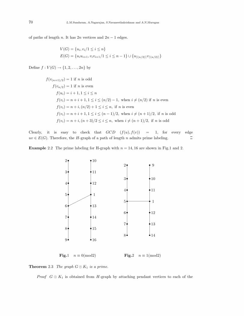
70 L.M.Sundaram, A.Nagarajan, S.Navaneethakrishnan and A.N.Murugan
of paths of length n. It has 2n vertices and 2n− 1 edges.
V (G) = ui, vi/1 ≤ i ≤ nE(G) = uiui+1, vivi+1/1 ≤ i ≤ n− 1 ∪ u⌈(n/2)⌉v⌈(n/2)⌉
Define f : V (G)→ 1, 2, . . . , 2n by
f(v(n+1)/2) = 1 if n is odd
f(vn/2) = 1 if n is even
f(ui) = i+ 1, 1 ≤ i ≤ nf(vi) = n+ i+ 1, 1 ≤ i ≤ (n/2)− 1, when i 6= (n/2) if n is even
f(vi) = n+ i, (n/2) + 1 ≤ i ≤ n, if n is even
f(vi) = n+ i+ 1, 1 ≤ i ≤ (n− 1)/2, when i 6= (n+ 1)/2, if n is odd
f(vi) = n+ i, (n+ 3)/2 ≤ i ≤ n, when i 6= (n+ 1)/2, if n is odd
Clearly, it is easy to check that GCD (f(u), f(v)) = 1, for every edge
uv ∈ E(G). Therefore, the H-graph of a path of length n admits prime labeling. 2Example 2.2 The prime labeling for H-graph with n = 14, 16 are shown in Fig.1 and 2.
2
3
4
5
6
7
8
9
10
11
12
1
13
14
15
16
2
3
4
5
6
7
8
9
10
11
1
12
13
14
Fig.1 n ≡ 0(mod2) Fig.2 n ≡ 1(mod2)
Theorem 2.3 The graph G⊙K1 is a prime.
Proof G ⊙ K1 is obtained from H-graph by attaching pendant vertices to each of the
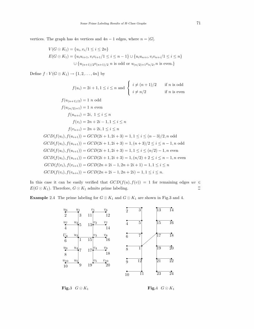
Some Prime Labeling Results of H-Class Graphs 71
vertices. The graph has 4n vertices and 4n− 1 edges, where n = |G|.
V (G⊙K1) = ui, vi/1 ≤ i ≤ 2nE(G⊙K1) = uiui+1, vivi+1/1 ≤ i ≤ n− 1 ∪ uiun+i, vivn+i/1 ≤ i ≤ n
∪ u(n+1)/2v(n+1)/2 n is odd or u(n/2)+1vn/2, n is even.
Define f : V (G⊙K1)→ 1, 2, . . . , 4n by
f(ui) = 2i+ 1, 1 ≤ i ≤ n and
i 6= (n+ 1)/2 if n is odd
i 6= n/2 if n is even
f(u(n+1)/2) = 1 n odd
f(u(n/2)+1) = 1 n even
f(un+i) = 2i, 1 ≤ i ≤ nf(vi) = 2n+ 2i− 1, 1 ≤ i ≤ n
f(vn+i) = 2n+ 2i, 1 ≤ i ≤ nGCD(f(ui), f(ui+1)) = GCD(2i+ 1, 2i+ 3) = 1, 1 ≤ i ≤ (n− 3)/2, n odd
GCD(f(ui), f(ui+1)) = GCD(2i+ 1, 2i+ 3) = 1, (n+ 3)/2 ≤ i ≤ n− 1, n odd
GCD(f(ui), f(ui+1)) = GCD(2i+ 1, 2i+ 3) = 1, 1 ≤ i ≤ (n/2)− 1, n even
GCD(f(ui), f(ui+1)) = GCD(2i+ 1, 2i+ 3) = 1, (n/2) + 2 ≤ i ≤ n− 1, n even
GCD(f(vi), f(vi+1)) = GCD(2n+ 2i− 1, 2n+ 2i+ 1) = 1, 1 ≤ i ≤ nGCD(f(vi), f(vn+i)) = GCD(2n+ 2i− 1, 2n+ 2i) = 1, 1 ≤ i ≤ n.
In this case it can be easily verified that GCD(f(u), f(v)) = 1 for remaining edges uv ∈E(G⊙K1). Therefore, G⊙K1 admits prime labeling. 2Example 2.4 The prime labeling for G⊙K1 and G⊙K1 are shown in Fig.3 and 4.
u1u6
u7
U8
u9
u10
u2
u3
u4
u5
v1
v2
v3
v4
v5
v6
v7
v8
v9
v10
2
4
6
8
10
3
5
1
7
9
11
13
15
17
19
12
14
16
18
20
2
4
6
8
9
10
3
5
1
7
12
11
13
15
17
19
21
23
14
16
18
20
22
24
Fig.3 G⊙K1 Fig.4 G⊙K1
72 L.M.Sundaram, A.Nagarajan, S.Navaneethakrishnan and A.N.Murugan
Theorem 2.5 The graph G⊙ S2 is prime.
Proof The graph G⊙ S2 has 6n vertices and 6n− 1 edges, where n = |G|.
V (G ⊙ S2) = ui, vi/1 ≤ i ≤ n ∪ u(1)i , u
(2)i , v
(1)i , v
(2)i /1 ≤ i ≤ n
E(G ⊙ S2) = uiui+1, vivi+1/1 ≤ i ≤ n− 1 ∪ uiu(1)i , uiu
(2)i , viv
(1)i , viv
(2)i /1 ≤ i ≤ n
∪ un+1/2vn+1/2 n is odd or un/2+1vn/2 n is even.
Define f : V → 1, 2, . . . , 6n by
f(un+1/2) = 1, f(u(1)(n+1)/2) = 6n− 1, f(u
(2)(n+1)/2) = 6n.
Case 1 Suppose n ≡ 1(mod 2).
Subcase 1.1 n ≡ 1(mod 4)
f(u2i−1) = 6(i− 1) + 3, 1 ≤ i ≤ (n− 1)/4
f(u2i−1) = f(u(n−1)/2) + 6 + 6[i− ((n− 1)/4) + 2],
((n− 1)/4) + 2 ≤ i ≤ ((n− 1)/2) + 1
f(u2i) = 6(i− 1) + 5, 1 ≤ i ≤ (n− 1)/4
f(u2i) = f(u(n−1)/2) + 4 + 6[i− ((n− 1)/4) + 1],
((n− 1)/4) + 1 ≤ i ≤ (n− 1)/2
f(u(1)2i−1) = f(u1)− 1 + 6(i− 1), 1 ≤ i ≤ (n− 1)/4
f(u(1)2i−1) = f(u(n−1)/2) + 7 + 6[i− ((n− 1)/4) + 2],
((n− 1)/4) + 2 ≤ i ≤ (n− 1)/2
f(u(2)2i−1) = f(u1) + 1 + 6(i− 1), 1 ≤ i ≤ (n− 1)/4
f(u(2)2i−1) = f(u(n−1)/2) + 8 + 6[i− ((n− 1)/4) + 2],
((n− 1)/4) + 2 ≤ i ≤ ((n− 1)/2) + 1
f(u(1)2i ) = f(u2) + 1 + 6(i− 1), 1 ≤ i ≤ (n− 1)/4
f(u(1)2i ) = f(u(n−1)/2) + 3 + 6[i− ((n− 1)/4 + 1],
((n− 1)/4) + 1 ≤ i ≤ (n− 1)/2
f(u(2)2i ) = f(u2) + 2 + 6(i− 1), 1 ≤ i ≤ (n− 1)/4
f(u(2)2i ) = f(u(n−1)/2) + 5 + 6[i− ((n− 1)/4) + 1],
((n− 1)/4) + 1 ≤ i ≤ (n− 1)/2
f(v1) = 3n, f(v2) = 3n+ 2
f(v2i−1) = f(v1) + 6(i− 1), 2 ≤ i ≤ (n+ 1)/2
f(v2i) = f(v2) + 6(i− 1), 2 ≤ i ≤ (n− 1)/2
f(v(1)2i−1) = f(v1)− 1 + 6(i− 1), 1 ≤ i ≤ (n+ 1)/2
Some Prime Labeling Results of H-Class Graphs 73
f(v(2)2i−1) = f(v1) + 1 + 6(i− 1), 1 ≤ i ≤ (n+ 1)/2
f(v(1)2i ) = f(v2) + 1 + 6(i− 1), 1 ≤ i ≤ (n− 1)/2
f(v(2)2i ) = f(v2) + 2 + 6(i− 1), 1 ≤ i ≤ (n− 1)/2
GCD(f(u2i−1), f(u2i)) = GCD(6i− 3, 6i− 1) = 1, 1 ≤ i ≤ (n− 1)/4
GCD(f(u2i), f(u2i+1)) = GCD(6i− 1, 6i+ 3) = 1, 1 ≤ i ≤ ((n− 1)/4)− 1
GCD(f(u2i−1), f(u2i)) = GCD(6i− 7, 6i− 3) = 1,
((n− 1)/4) + 2 ≤ i ≤ (n− 1)/2
GCD(f(u2i), f(u2i+1)) = GCD(6i− 3, 6i− 1) = 1,
((n− 1)/4) + 1 ≤ i ≤ (n− 1)/2
GCD(f(u2i−1), f(u(2)2i−1)) = GCD(6i− 7, 6i− 5) = 1,
((n− 1)/4) + 2 ≤ i ≤ ((n− 1)/2) + 1
GCD(f(u2i), f(u(2)2i )) = GCD(6i− 1, 6i+ 1) = 1, 1 ≤ i ≤ (n− 1)/4
GCD(f(u2i), f(u(2)2i )) = GCD(6i− 3, 6i− 2) = 1,
((n− 1)/4) + 1 ≤ i ≤ (n− 1)/2
GCD(f(v1), f(v2)) = GCD(3n, 3n+ 2) = 1
GCD(f(v2i−1), f(v2i)) = GCD(3n+ 6i− 6, 3n+ 6i− 4) = 1,
2 ≤ i ≤ (n− 1)/2
GCD(f(v2i), f(v2i+1)) = GCD(3n+ 6i− 4, 3n+ 6i) = 1,
1 ≤ i ≤ (n− 1)/2
GCD(f(v2i), f(v(2)2i )) = GCD(3n+ 6i− 4, 3n+ 6i− 2) = 1,
1 ≤ i ≤ (n− 1)/2.
Subcase 1.2 n ≡ 3(mod 4)
f(u2i−1) = 6(i− 1) + 3, 1 ≤ i ≤ (n+ 1)/4
f(u2i−1) = f(u(n−1)/2) + 2 + 6[i− ((n+ 1)/4) + 1],
((n+ 1)/4 + 1 ≤ i ≤ (n+ 1)/2
f(u2i) = 6(i− 1) + 5, 1 ≤ i ≤ ((n+ 1)/4)− 1
f(u2i) = f(u(n−1)/2) + 6 + 6[i− ((n+ 1)/4) + 1],
((n+ 1)/4) + 1 ≤ i ≤ ((n+ 1)/2)− 1
f(u(1)2i−1) = f(u1)− 1 + 6(i− 1), 1 ≤ i ≤ (n+ 1)/4
f(u(1)2i−1) = f(u(n−1)/2) + 3 + 6[i− ((n+ 1)/4) + 1],
((n+ 1)/4) + 1 ≤ i ≤ (n+ 1)/2
f(u(2)2i−1) = f(u1) + 1 + 6(i− 1), 1 ≤ i ≤ (n+ 1)/4
74 L.M.Sundaram, A.Nagarajan, S.Navaneethakrishnan and A.N.Murugan
f(u(2)2i−1) = f(u(n−1)/2) + 4 + 6[i− ((n+ 1)/4) + 1],
((n+ 1)/4) + 1 ≤ i ≤ (n+ 1)/2
f(u(1)2i ) = f(u2) + 1 + 6(i− 1), 1 ≤ i ≤ ((n+ 1)/4)− 1
f(u(1)2i ) = f(u(n−1)/2) + 5 + 6[i− ((n+ 1)/4) + 1],
((n+ 1)/4) + 1 ≤ i ≤ ((n+ 1)/2)− 1
f(u(2)2i ) = f(u2) + 2 + 6(i− 1), 1 ≤ i ≤ ((n+ 1)/4)− 1
f(u(2)2i ) = f(u(n−1)/2) + 7 + 6[i− ((n+ 1)/4) + 1],
((n+ 1)/4) + 1 ≤ i ≤ ((n+ 1)/2)− 1
f(v1) = 3n, f(v2) = 3n+ 2
f(v2i−1) = f(v1) + 6(i− 1), 2 ≤ i ≤ (n+ 1)/2
f(v2i) = f(v2) + 6(i− 1), 2 ≤ i ≤ ((n+ 1)/2)− 1
f(v(1)2i−1) = f(v1)− 1 + 6(i− 1), 1 ≤ i ≤ (n+ 1)/2
f(v(2)2i−1) = f(v1) + 1 + 6(i− 1), 1 ≤ i ≤ (n+ 1)/2
f(v(1)2i ) = f(v2) + 1 + 6(i− 1), 1 ≤ i ≤ ((n+ 1)/2)− 1
f(v(2)2i ) = f(v2) + 2 + 6(i− 1), 1 ≤ i ≤ ((n+ 1)/2)− 1.
As in the above case it can be verified that GCD(f(u), f(v)) = 1 for every edge uv ∈E(G⊙ S2).
Case 2. n ≡ 0(mod 2)
f(u(n/2)+1) = 1, f(u(1)(n/2)+1) = 6n− 1, f(u
(2)(n/2)+1) = 6n.
Subcase 2.1 n ≡ 0(mod 4)
f(u2i−1) = 6(i− 1) + 3, 1 ≤ i ≤ n/4f(u2i−1) = f(u(n/2)) + 6 + 6[i− (n/4) + 2], (n/4) + 2 ≤ i ≤ n/2f(u2i) = 6(i− 1) + 5, 1 ≤ i ≤ n/4f(u2i) = f(u(n/2)) + 4 + 6[i− (n/4) + 1], (n/4) + 1 ≤ i ≤ n/2
f(u(1)2i−1) = f(u1)− 1 + 6(i− 1), 1 ≤ i ≤ n/4
f(u(1)2i−1) = f(u(n/2)) + 7 + 6[i− (n/4) + 2], (n/4) + 2 ≤ i ≤ n/2
f(u(2)2i−1) = f(u1) + 1 + 6(i− 1), 1 ≤ i ≤ n/4
f(u(2)2i−1) = f(u(n/2)) + 8 + 6[i− (n/4) + 2], (n/4) + 2 ≤ i ≤ n/2
f(u(1)2i ) = f(u2) + 1 + 6(i− 1), 1 ≤ i ≤ n/4
f(u(1)2i ) = f(u(n/2)) + 3 + 6[i− (n/4) + 1], (n/4) + 1 ≤ i ≤ n/2
f(u(2)2i ) = f(u2) + 2 + 6(i− 1), 1 ≤ i ≤ n/4
f(u(2)2i ) = f(u(n/2)) + 5 + 6[i− (n/4) + 1], (n/4) + 1 ≤ i ≤ n/2
Some Prime Labeling Results of H-Class Graphs 75
f(v1) = 3n− 1, f(v2) = 3(n+ 1)
f(v2i−1) = f(v1) + 6(i− 1), 2 ≤ i ≤ n/2f(v2i) = f(v2) + 6(i− 1), 2 ≤ i ≤ n/2
f(v(1)2i−1) = f(v1) + 1 + 6(i− 1), 1 ≤ i ≤ n/2
f(v(2)2i−1) = f(v1) + 2 + 6 + (i− 1), 1 ≤ i ≤ n/2
f(v(1)2i ) = f(v2)− 1 + 6(i− 1), 1 ≤ i ≤ n/2
f(v(2)2i ) = f(v2) + 1 + 6(i− 1), 1 ≤ i ≤ n/2
Clearly GCD(f(u), f(v)) = 1 for every edge uv ∈ E(G⊙ S2).
Subcase 2.2 n ≡ 2(mod 4)
f(u2i−1) = 6(i− 1) + 3, 1 ≤ i ≤ (n+ 2)/4
f(u2i−1) = f(u(n/2)) + 2 + 6[i− ((n+ 2)/4) + 1], ((n+ 2)/4) + 1 ≤ i ≤ n/2f(u2i) = 6(i− 1) + 5, 1 ≤ i ≤ (n− 2)/4
f(u2i) = f(u(n/2)) + 6 + 6]i− ((n− 2)/4) + 2], ((n− 2)/4) + 2 ≤ i ≤ n/2
f(u(1)2i−1) = f(u1)− 1 + 6(i− 1), 1 ≤ i ≤ (n+ 2)/4
f(u(1)2i−1) = f(u(n/2)) + 3 + 6[i− ((n+ 2)/4) + 1], ((n+ 2)/4) + 1 ≤ i ≤ n/2
f(u(2)2i−1) = f(u1) + 1 + 6(i− 1), 1 ≤ i ≤ (n+ 2)/4
f(u(2)2i−1) = f(u(n/2)) + 4 + 6[i− ((n+ 2)/4) + 1], ((n+ 2)/4) + 1 ≤ i ≤ n/2
f(u(1)2i ) = f(u2) + 1 + 6(i− 1), 1 ≤ i ≤ (n− 2)/4
f(u(1)2i ) = f(u(n/2)) + 5 + 6[i− ((n− 2)/4) + 2], ((n− 2) + 2 ≤ i ≤ n/2
f(u(2)2i ) = f(u2) + 2 + 6(i− 1), 1 ≤ i ≤ (n− 2)/4
f(u(2)2i ) = f(u(n/2)) + 7 + 6[i− ((n− 2)/4) + 2], ((n− 2)/4) + 2 ≤ i ≤ n/2
f(v1) = 3n− 1, f(v2) = 3(n+ 1)
f(v2i−1) = f(v1) + 6(i− 1), 2 ≤ i ≤ n/2f(v2i) = f(v2) + 6(i− 1), 2 ≤ i ≤ n/2
f(v(1)2i−1) = f(v1) + 1 + 6(i− 1), 1 ≤ i ≤ n/2
f(v(2)2i−1) = f(v1) + 2 + 6(i− 1), 1 ≤ i ≤ n/2
f(v(1)2i ) = f(v2)− 1 + 6(i− 1), 1 ≤ i ≤ n/2
f(v(2)2i ) = f(v2) + 1 + 6(i− 1), 1 ≤ i ≤ n/2.
In this case also it is easy to check that GCD(f(u), f(v)) = 1. Therefore G ⊙ S2 admits
prime labeling. 2Example 2.6 The prime labelings for G ⊙ S2 with n ≡ 1(mod4), n ≡ 2(mod4), n ≡3(mod4), n ≡ 0(mod4) are respectively shown in Fig.5-8 following.
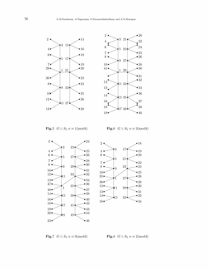
76 L.M.Sundaram, A.Nagarajan, S.Navaneethakrishnan and A.N.Murugan
2
4
6
729
30
8
10
12
13
3
5
1
9
11
15
17
21
23
27
14
16
18
1920
22
24
25
26
28
2
4
6
78
1041
12
13
14
16
18
19
3
5
9
1
11
15
17
21
23
27
29
33
35
39
20
22
24
2526
2830
3132
34
36
37
38
40
Fig.5 G⊙ S2 n ≡ 1(mod4) Fig.6 G⊙ S2 n ≡ 3(mod4)
2
46
78
1012
1347
4814
1618
1920
22
2
5
9
11
1
15
17
21
23
27
29
33
35
41
39
45
24
2526
2830
3132
3436
3738
4042
4344
46
2
46
78
1035
3612
1314
16
3
5
9
1
11
15
17
21
23
27
29
33
18
1920
2224
2526
2830
3132
34
Fig.7 G⊙ S2 n ≡ 0(mod4) Fig.8 G⊙ S2 n ≡ 2(mod4)
Some Prime Labeling Results of H-Class Graphs 77
References
[1] J.A.Gallian, A Dynamic Survey of graph labeling, The Electronic journal of Coimbino-
torics, 18 (2011), #DS6.
[2] S.M.Lee, I.Win and J.Yeh, On amalgamation of prime graphs, Bull. Malasian Math. Soci.,
(1998), 59-67.
[3] A.Tout, A.N.Dabboucy and K.Howalla, Prime labeling of graphs, Nat. Acad. Sci. Letters,
11 (1982), 365-368.
[4] R.Vasuki, A.Nagarajan, Some results on super mean graphs, International J.Math.Combin.,
3 (2009), 82-96.
International J.Math. Combin. Vol.3(2013), 78-84
On Mean Cordial Graphs
R.Ponraj
(Department of Mathematics, Sri Paramakalyani College, Alwarkurichi-627412, India)
M.Sivakumar
(Department of Mathematics, Unnamalai Institute of Technology, Kovilpatti-628502, India)
E-mail: [email protected], sivamaths.vani [email protected]
Abstract: Let f be a function from the vertex set V (G) to 0, 1, 2. For each edge uv
assign the label
⌈
f (u) + f (v)
2
⌉
. f is called a mean cordial labeling if |vf (i) − vf (j)| ≤ 1
and |ef (i) − ef (j)| ≤ 1, i, j ∈ 0, 1, 2, where vf (x) and ef (x) respectively are denote the
number of vertices and edges labeled with x (x = 0, 1, 2). A graph with a mean cordial
labeling is called a mean cordial graph. In this paper we investigate mean cordial labeling
behavior of union of some graphs, square of paths, subdivision of comb and double comb
and some more standard graphs.
Key Words: Path, star, complete graph, comb.
AMS(2010): 05C78
§1. Introduction
All graphs in this paper are finite, undirected and simple. The vertex set and edge set of a
graph G are denoted by V (G) and E (G) respectively. The union of two graphs G1 and G2 is
the graph G1 ∪ G2 with V (G1 ∪G2) = V (G1) ∪ V (G2) and E (G1 ∪G2) = E (G1) ∪ E (G2).
The corona of G with H , G ⊙H is the graph obtained by taking one copy of G and p copies
of H and joining the ith vertex of G with an edge to every vertex in the ith copy of H . The
subdivision graph S (G) of a graph G is obtained by replacing each edge uv by a path uwv.
The triangular snake Tn is obtained from the path Pn+1 by replacing each edge of the path
by the triangle C3. mG denotes the m copies of the graph G. The square G2 of a graph G
has the vertex set V(
G2)
= V (G), with u, v adjacent in G2 whenever d (u, v) ≤ 2 in G. The
powers G3, G4 . . . of G are similarly defined. Ponraj et al. defined the mean cordial labeling
of a graph in [4]. Mean cordial labeling behavior of path, cycle, star, complete graph, wheel,
comb etc have been investigated in [4]. Here we investigate the mean cordial labeling behavior
of some standard graphs. The symbol ⌈x⌉ stands for smallest integer greater than or equal to
x. Terms and definitions are not defined here are used in the sense of Harary [3].
1Received January 18, 2013, Accepted August 27, 2013.
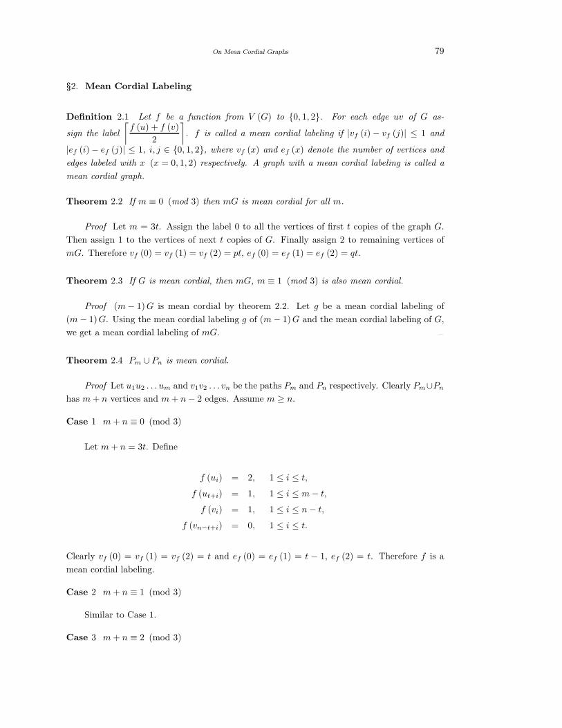
On Mean Cordial Graphs 79
§2. Mean Cordial Labeling
Definition 2.1 Let f be a function from V (G) to 0, 1, 2. For each edge uv of G as-
sign the label
⌈
f (u) + f (v)
2
⌉
. f is called a mean cordial labeling if |vf (i)− vf (j)| ≤ 1 and
|ef (i)− ef (j)| ≤ 1, i, j ∈ 0, 1, 2, where vf (x) and ef (x) denote the number of vertices and
edges labeled with x (x = 0, 1, 2) respectively. A graph with a mean cordial labeling is called a
mean cordial graph.
Theorem 2.2 If m ≡ 0 (mod 3) then mG is mean cordial for all m.
Proof Let m = 3t. Assign the label 0 to all the vertices of first t copies of the graph G.
Then assign 1 to the vertices of next t copies of G. Finally assign 2 to remaining vertices of
mG. Therefore vf (0) = vf (1) = vf (2) = pt, ef (0) = ef (1) = ef (2) = qt. 2Theorem 2.3 If G is mean cordial, then mG, m ≡ 1 (mod 3) is also mean cordial.
Proof (m− 1)G is mean cordial by theorem 2.2. Let g be a mean cordial labeling of
(m− 1)G. Using the mean cordial labeling g of (m− 1)G and the mean cordial labeling of G,
we get a mean cordial labeling of mG. 2Theorem 2.4 Pm ∪ Pn is mean cordial.
Proof Let u1u2 . . . um and v1v2 . . . vn be the paths Pm and Pn respectively. Clearly Pm∪Pn
has m+ n vertices and m+ n− 2 edges. Assume m ≥ n.
Case 1 m+ n ≡ 0 (mod 3)
Let m+ n = 3t. Define
f (ui) = 2, 1 ≤ i ≤ t,f (ut+i) = 1, 1 ≤ i ≤ m− t,f (vi) = 1, 1 ≤ i ≤ n− t,
f (vn−t+i) = 0, 1 ≤ i ≤ t.
Clearly vf (0) = vf (1) = vf (2) = t and ef (0) = ef (1) = t − 1, ef (2) = t. Therefore f is a
mean cordial labeling.
Case 2 m+ n ≡ 1 (mod 3)
Similar to Case 1.
Case 3 m+ n ≡ 2 (mod 3)
80 R.Ponraj and M.Sivakumar
Let m+ n = 3t+ 2. Define
f (ui) = 2, 1 ≤ i ≤ t,f (ut+i) = 1, 1 ≤ i ≤ m− t,f (vi) = 1, 1 ≤ i ≤ n− t− 1,
f (vn−t+i) = 0, 1 ≤ i ≤ t+ 1.
Clearly vf (0) = vf (1) = t + 1, vf (2) = t and ef (0) = t − 1, ef (1) = ef (2) = t. Therefore
Pm ∪ Pn is mean cordial. 2Theorem 2.5 Cn ∪ Pm is mean cordial if m ≥ n.
Proof Let Cn be the cycle u1u2 . . . umu1 and Pm be the path v1v2 . . . vn respectively.
Clearly Cn ∪ Pm has m+ n vertices and m+ n− 1 edges. Assume m ≥ n.
Case 1 m+ n ≡ 0 (mod 3)
Let m+ n = 3t. Define
f (ui) = 0, 1 ≤ i ≤ t,f (ut+i) = 1, 1 ≤ i ≤ n−, tf (vi) = 1, 1 ≤ i ≤ m− t,
f (vm−t+i) = 2, 1 ≤ i ≤ t.
Clearly ef (0) = t− 1, ef (1) = ef (2) = t.
Case 2 m+ n ≡ 1 (mod 3)
Let m+ n = 3t+ 1. Define
f (ui) = 0, 1 ≤ i ≤ t+ 1,
f (ut+1+i) = 1, 1 ≤ i ≤ n− t− 1,
f (vi) = 1, 1 ≤ i ≤ m− t,f (vm−t+i) = 2, 1 ≤ i ≤ t.
Clearly ef (0) = ef (1) = t− 1, ef (2) = t.
Case 3 m+ n ≡ 2 (mod 3)
Let m+ n = 3t+ 2. Define
f (ui) = 0, 1 ≤ i ≤ t+ 1,
f (ut+1+i) = 1, 1 ≤ i ≤ n− t− 1,
f (vi) = 1, 1 ≤ i ≤ m− t− 1,
f (vm−t−1+i) = 2, 1 ≤ i ≤ t.
Clearly ef (0) = ef (1) = t, ef (2) = t+ 1. Hence Cn ∪ Pm is mean cordial. 2
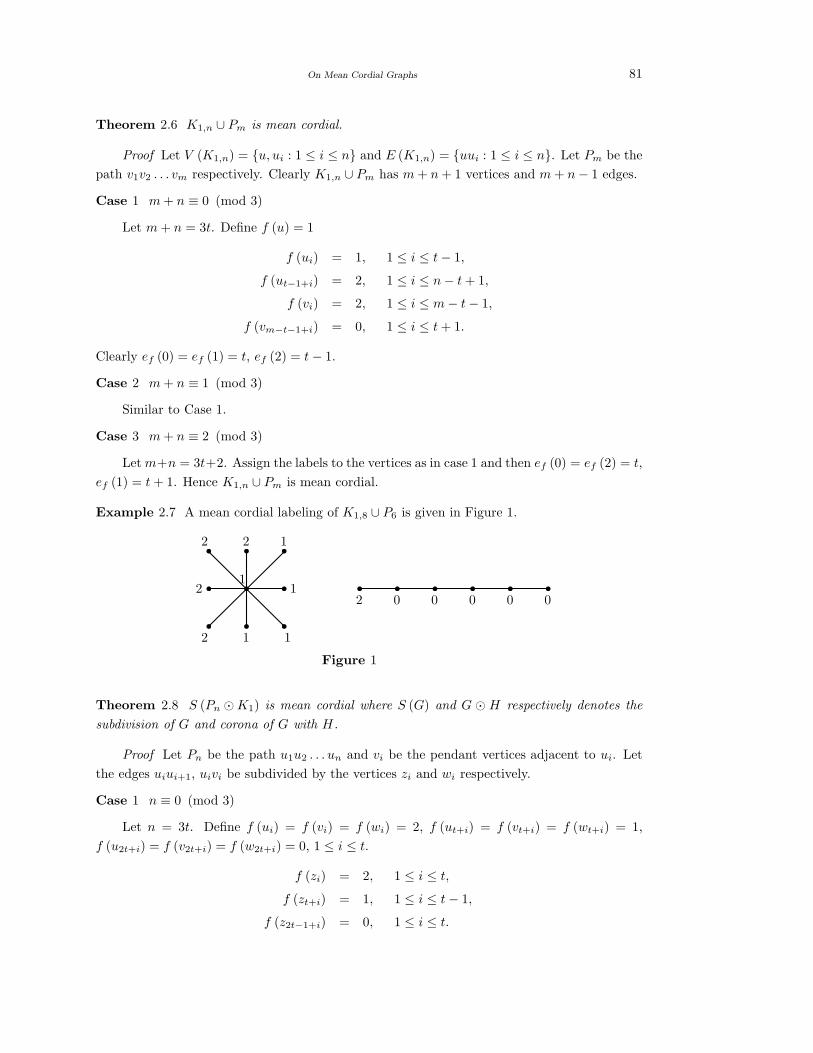
On Mean Cordial Graphs 81
Theorem 2.6 K1,n ∪ Pm is mean cordial.
Proof Let V (K1,n) = u, ui : 1 ≤ i ≤ n and E (K1,n) = uui : 1 ≤ i ≤ n. Let Pm be the
path v1v2 . . . vm respectively. Clearly K1,n ∪ Pm has m+ n+ 1 vertices and m+ n− 1 edges.
Case 1 m+ n ≡ 0 (mod 3)
Let m+ n = 3t. Define f (u) = 1
f (ui) = 1, 1 ≤ i ≤ t− 1,
f (ut−1+i) = 2, 1 ≤ i ≤ n− t+ 1,
f (vi) = 2, 1 ≤ i ≤ m− t− 1,
f (vm−t−1+i) = 0, 1 ≤ i ≤ t+ 1.
Clearly ef (0) = ef (1) = t, ef (2) = t− 1.
Case 2 m+ n ≡ 1 (mod 3)
Similar to Case 1.
Case 3 m+ n ≡ 2 (mod 3)
Letm+n = 3t+2. Assign the labels to the vertices as in case 1 and then ef (0) = ef (2) = t,
ef (1) = t+ 1. Hence K1,n ∪ Pm is mean cordial. 2Example 2.7 A mean cordial labeling of K1,8 ∪ P6 is given in Figure 1.
b b b
b b b b b b b b b
b b b
2
2
2 2
1 1
11
1
2 0 0 0 0 0
Figure 1
Theorem 2.8 S (Pn ⊙K1) is mean cordial where S (G) and G ⊙ H respectively denotes the
subdivision of G and corona of G with H.
Proof Let Pn be the path u1u2 . . . un and vi be the pendant vertices adjacent to ui. Let
the edges uiui+1, uivi be subdivided by the vertices zi and wi respectively.
Case 1 n ≡ 0 (mod 3)
Let n = 3t. Define f (ui) = f (vi) = f (wi) = 2, f (ut+i) = f (vt+i) = f (wt+i) = 1,
f (u2t+i) = f (v2t+i) = f (w2t+i) = 0, 1 ≤ i ≤ t.
f (zi) = 2, 1 ≤ i ≤ t,f (zt+i) = 1, 1 ≤ i ≤ t− 1,
f (z2t−1+i) = 0, 1 ≤ i ≤ t.
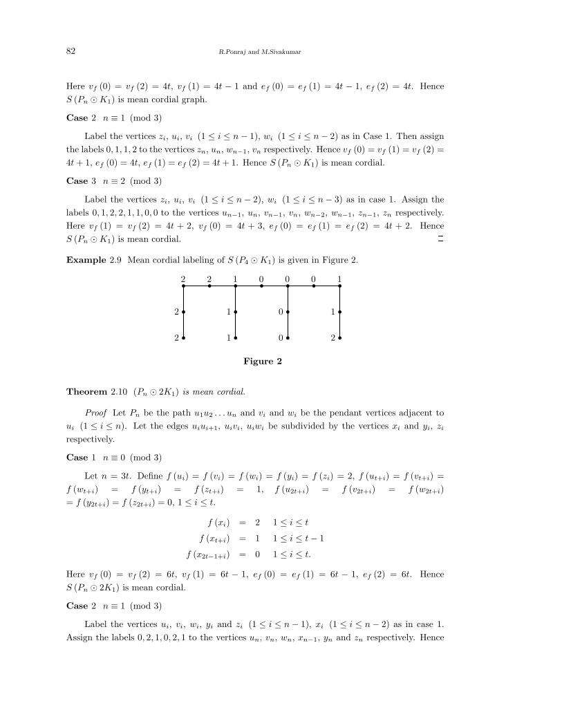
82 R.Ponraj and M.Sivakumar
Here vf (0) = vf (2) = 4t, vf (1) = 4t − 1 and ef (0) = ef (1) = 4t − 1, ef (2) = 4t. Hence
S (Pn ⊙K1) is mean cordial graph.
Case 2 n ≡ 1 (mod 3)
Label the vertices zi, ui, vi (1 ≤ i ≤ n− 1), wi (1 ≤ i ≤ n− 2) as in Case 1. Then assign
the labels 0, 1, 1, 2 to the vertices zn, un, wn−1, vn respectively. Hence vf (0) = vf (1) = vf (2) =
4t+ 1, ef (0) = 4t, ef (1) = ef (2) = 4t+ 1. Hence S (Pn ⊙K1) is mean cordial.
Case 3 n ≡ 2 (mod 3)
Label the vertices zi, ui, vi (1 ≤ i ≤ n− 2), wi (1 ≤ i ≤ n− 3) as in case 1. Assign the
labels 0, 1, 2, 2, 1, 1, 0, 0 to the vertices un−1, un, vn−1, vn, wn−2, wn−1, zn−1, zn respectively.
Here vf (1) = vf (2) = 4t + 2, vf (0) = 4t + 3, ef (0) = ef (1) = ef (2) = 4t + 2. Hence
S (Pn ⊙K1) is mean cordial. 2Example 2.9 Mean cordial labeling of S (P4 ⊙K1) is given in Figure 2.
b
b
b b
b
b
b b
b
b
b b
b
b
b
2
2
1
1
0
0
2
1
2 2 1 0 0 0 1
Figure 2
Theorem 2.10 (Pn ⊙ 2K1) is mean cordial.
Proof Let Pn be the path u1u2 . . . un and vi and wi be the pendant vertices adjacent to
ui (1 ≤ i ≤ n). Let the edges uiui+1, uivi, uiwi be subdivided by the vertices xi and yi, zi
respectively.
Case 1 n ≡ 0 (mod 3)
Let n = 3t. Define f (ui) = f (vi) = f (wi) = f (yi) = f (zi) = 2, f (ut+i) = f (vt+i) =
f (wt+i) = f (yt+i) = f (zt+i) = 1, f (u2t+i) = f (v2t+i) = f (w2t+i)
= f (y2t+i) = f (z2t+i) = 0, 1 ≤ i ≤ t.
f (xi) = 2 1 ≤ i ≤ tf (xt+i) = 1 1 ≤ i ≤ t− 1
f (x2t−1+i) = 0 1 ≤ i ≤ t.
Here vf (0) = vf (2) = 6t, vf (1) = 6t − 1, ef (0) = ef (1) = 6t − 1, ef (2) = 6t. Hence
S (Pn ⊙ 2K1) is mean cordial.
Case 2 n ≡ 1 (mod 3)
Label the vertices ui, vi, wi, yi and zi (1 ≤ i ≤ n− 1), xi (1 ≤ i ≤ n− 2) as in case 1.
Assign the labels 0, 2, 1, 0, 2, 1 to the vertices un, vn, wn, xn−1, yn and zn respectively. Hence
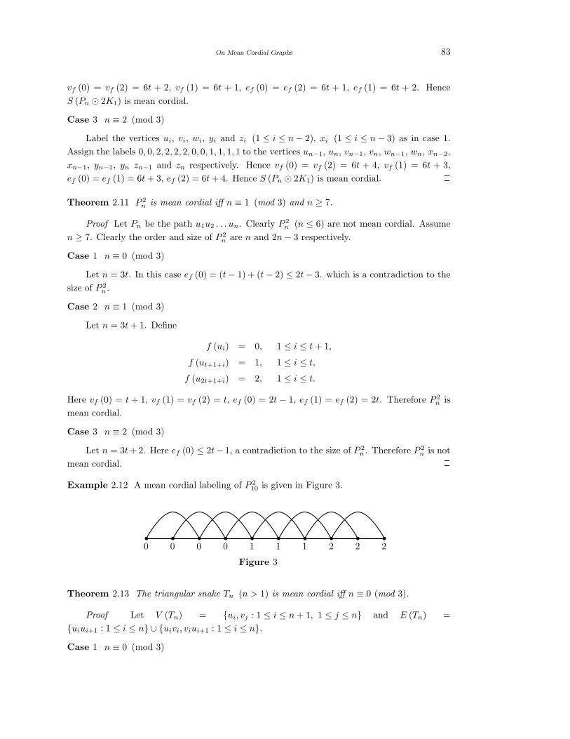
On Mean Cordial Graphs 83
vf (0) = vf (2) = 6t + 2, vf (1) = 6t + 1, ef (0) = ef (2) = 6t + 1, ef (1) = 6t + 2. Hence
S (Pn ⊙ 2K1) is mean cordial.
Case 3 n ≡ 2 (mod 3)
Label the vertices ui, vi, wi, yi and zi (1 ≤ i ≤ n− 2), xi (1 ≤ i ≤ n− 3) as in case 1.
Assign the labels 0, 0, 2, 2, 2, 2, 0, 0, 1, 1, 1, 1 to the vertices un−1, un, vn−1, vn, wn−1, wn, xn−2,
xn−1, yn−1, yn zn−1 and zn respectively. Hence vf (0) = vf (2) = 6t + 4, vf (1) = 6t + 3,
ef (0) = ef (1) = 6t+ 3, ef (2) = 6t+ 4. Hence S (Pn ⊙ 2K1) is mean cordial. 2Theorem 2.11 P 2
n is mean cordial iff n ≡ 1 (mod 3) and n ≥ 7.
Proof Let Pn be the path u1u2 . . . un. Clearly P 2n (n ≤ 6) are not mean cordial. Assume
n ≥ 7. Clearly the order and size of P 2n are n and 2n− 3 respectively.
Case 1 n ≡ 0 (mod 3)
Let n = 3t. In this case ef (0) = (t− 1) + (t− 2) ≤ 2t− 3. which is a contradiction to the
size of P 2n .
Case 2 n ≡ 1 (mod 3)
Let n = 3t+ 1. Define
f (ui) = 0, 1 ≤ i ≤ t+ 1,
f (ut+1+i) = 1, 1 ≤ i ≤ t,f (u2t+1+i) = 2, 1 ≤ i ≤ t.
Here vf (0) = t + 1, vf (1) = vf (2) = t, ef (0) = 2t− 1, ef (1) = ef (2) = 2t. Therefore P 2n is
mean cordial.
Case 3 n ≡ 2 (mod 3)
Let n = 3t+ 2. Here ef (0) ≤ 2t− 1, a contradiction to the size of P 2n . Therefore P 2
n is not
mean cordial. 2Example 2.12 A mean cordial labeling of P 2
10 is given in Figure 3.
b b b b b b b b b b
0 0 0 0 1 1 1 2 2 2
Figure 3
Theorem 2.13 The triangular snake Tn (n > 1) is mean cordial iff n ≡ 0 (mod 3).
Proof Let V (Tn) = ui, vj : 1 ≤ i ≤ n+ 1, 1 ≤ j ≤ n and E (Tn) =
uiui+1 : 1 ≤ i ≤ n ∪ uivi, viui+1 : 1 ≤ i ≤ n.
Case 1 n ≡ 0 (mod 3)
84 R.Ponraj and M.Sivakumar
Let n = 3t. Define
f (ui) = 0, 1 ≤ i ≤ t+ 1,
f (ut+1+i) = 1, 1 ≤ i ≤ t,f (u2t+1+i) = 2, 1 ≤ i ≤ t,
f (vi) = 0, 1 ≤ i ≤ m− t− 1,
f (vt+i) = 1, 1 ≤ i ≤ t,f (v2t+i) = 2, 1 ≤ i ≤ t.
Here vf (0) = t + 1, vf (1) = vf (2) = t, ef (0) = ef (1) = ef (2) = 3t. Therefore triangular
snake Tn is mean cordial.
Case 2 n ≡ 1 (mod 3)
Let n = 3t+ 1. Here vf (0) = 2t+ 1. But ef (0) ≤ 3t, a contradiction.
Case 3 n ≡ 2 (mod 3)
Let n = 3t+2. In this case vf (0) = 2t+1 or 2t+2. But ef (0) ≤ 3t+1, a contradiction.2§3. Conclusion
In this paper we have studied the mean cordial behavior of Pm ∪ Pn, Cn ∪ Pm, S (Pn ⊙K1),
S (Pn ⊙ 2K1), P2n , Tn. Mean cordial labeling behavior of join and product of given two graphs
are the open problems for future research.
References
[1] I.Cahit, Cordial Graphs: A weaker version of Graceful and Harmonious graphs, Ars com-
bin., 23(1987), 201-207.
[2] J.A.Gallian, A Dynamic survey of Graph labeling, The Electronic journal of Combinatorics,
18(2011), # DS6.
[3] F.Harary, Graph theory, Addision wesley, New Delhi, 1969.
[4] R.Ponraj, M.Sivkumar and M.Sundaram, Mean cordial labeling of Graphs, Open Journal
of Discreate Mathematics, Vol.2, No.4, 2012, 145-148.
International J.Math. Combin. Vol.3(2013), 85-90
More on p∗ Graceful Graphs
Teena Liza John and Mathew Varkey T.K
(Dept. of Mathematics, T.K.M College of Engineering, Kollam-5, Kerala, India)
E-mail: [email protected], [email protected]
Abstract: A p∗ graceful labeling of a graph G is an assignment fp of labels to the vertices
of G, that induces for each edge uv, a label f∗p = |fp(u) − fp(v)| so that the resulting edge
labels are distinct pentagonal numbers. In this paper, we investigate the p∗ graceful nature
of some graphs based on some graph theoretic operations.
Key Words: Pentagonal numbers, p∗-graceful graphs, comb graph, twig graph, banana
trees
AMS(2010): 05C78
§1. Introduction
Unless otherwise mentioned, a graph in this paper means a simple graph without isolated
vertices. For all the terminology and notations in graph theory, we follow [1] and [2] and for
the definition regarding p∗ graceful graphs, we follow [4].
A labeling f of a graph G is one-one mapping from the vertex set of G into the set of
integers. Consider a graph G with q edges. Let fp : V (G) → 0, 1, · · · , ωp(q) such that
f∗p (uv) = |fp(u)− fp(v)|. If f∗
p is a sequence of distinct consecutive pentagonal numbers, then
the function fp is said to be p∗ graceful labeling and the graph which admits the p∗ graceful
labeling is called p∗ graceful graph. Here ωp(q) =q(3q − 1)
2is the qth pentagonal number.
In [4], we proved that the paths, star graphs, comb graphs and twig graphs are p∗ graceful.
In this paper, we are having some generalizations on p∗ graceful graphs.
Theorem 1.1 S(n, 1, n) is p∗ graceful.
Proof Let G = S(n, 1, n). Let u1, u2, u3 be the vertices of P3 and u1i, u21, u3i, i = 1, 2, · · ·nbe the pendant vertices attached with the vertices of P3. Define fp : V (G)→ 0, 1, · · · , ωp(q)such that fp(u1) = 0
fp(u1i) = ωp(i), i = 1, 2, · · · , n;
fp(u2) = ωp(q), fp(u21) = fp(u2)− ωp(q − 1);
fp(u3) = fp(u2)− ωp(q − 2), fp(u3i) = fp(u3) + ωp(q − 2− i), i = 1, 2, . . . , n.
Then we can easily verify that fp generates f∗p as required. Hence the result. 2
1Received May 13, 2013, Accepted August 30, 2013.
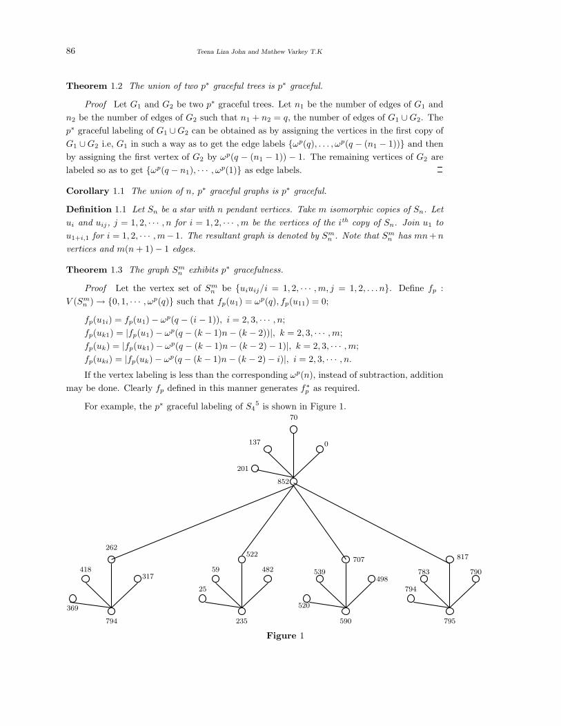
86 Teena Liza John and Mathew Varkey T.K
Theorem 1.2 The union of two p∗ graceful trees is p∗ graceful.
Proof Let G1 and G2 be two p∗ graceful trees. Let n1 be the number of edges of G1 and
n2 be the number of edges of G2 such that n1 + n2 = q, the number of edges of G1 ∪ G2. The
p∗ graceful labeling of G1 ∪G2 can be obtained as by assigning the vertices in the first copy of
G1 ∪G2 i.e, G1 in such a way as to get the edge labels ωp(q), . . . , ωp(q − (n1 − 1)) and then
by assigning the first vertex of G2 by ωp(q − (n1 − 1)) − 1. The remaining vertices of G2 are
labeled so as to get ωp(q − n1), · · · , ωp(1) as edge labels. 2Corollary 1.1 The union of n, p∗ graceful graphs is p∗ graceful.
Definition 1.1 Let Sn be a star with n pendant vertices. Take m isomorphic copies of Sn. Let
ui and uij, j = 1, 2, · · · , n for i = 1, 2, · · · ,m be the vertices of the ith copy of Sn. Join u1 to
u1+i,1 for i = 1, 2, · · · ,m− 1. The resultant graph is denoted by Smn . Note that Sm
n has mn+n
vertices and m(n+ 1)− 1 edges.
Theorem 1.3 The graph Smn exhibits p∗ gracefulness.
Proof Let the vertex set of Smn be uiuij/i = 1, 2, · · · ,m, j = 1, 2, . . . n. Define fp :
V (Smn )→ 0, 1, · · · , ωp(q) such that fp(u1) = ωp(q), fp(u11) = 0;
fp(u1i) = fp(u1)− ωp(q − (i− 1)), i = 2, 3, · · · , n;
fp(uk1) = |fp(u1)− ωp(q − (k − 1)n− (k − 2))|, k = 2, 3, · · · ,m;
fp(uk) = |fp(uk1)− ωp(q − (k − 1)n− (k − 2)− 1)|, k = 2, 3, · · · ,m;
fp(uki) = |fp(uk)− ωp(q − (k − 1)n− (k − 2)− i)|, i = 2, 3, · · · , n.
If the vertex labeling is less than the corresponding ωp(n), instead of subtraction, addition
may be done. Clearly fp defined in this manner generates f∗p as required. 2
For example, the p∗ graceful labeling of S45 is shown in Figure 1.
852
70
0137
201
794
262
317418
369
235
522
48259
25
590
707
498539
520
795
817
790783
794
Figure 1
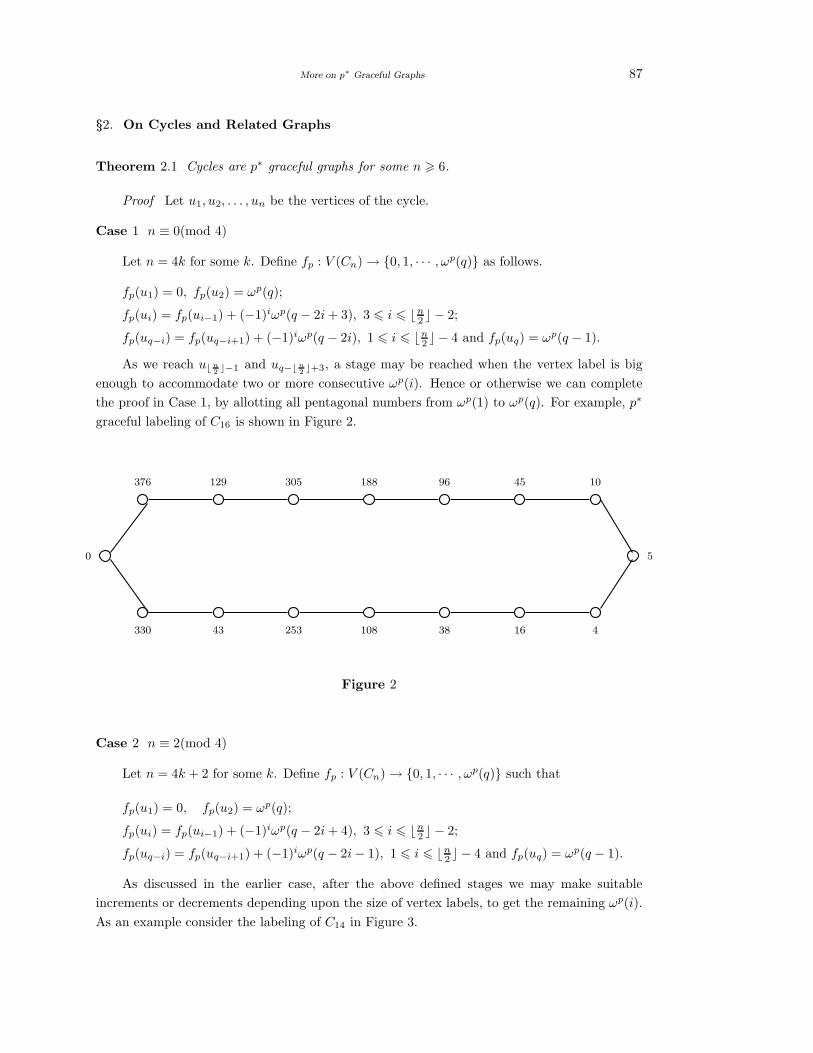
More on p∗ Graceful Graphs 87
§2. On Cycles and Related Graphs
Theorem 2.1 Cycles are p∗ graceful graphs for some n > 6.
Proof Let u1, u2, . . . , un be the vertices of the cycle.
Case 1 n ≡ 0(mod 4)
Let n = 4k for some k. Define fp : V (Cn)→ 0, 1, · · · , ωp(q) as follows.
fp(u1) = 0, fp(u2) = ωp(q);
fp(ui) = fp(ui−1) + (−1)iωp(q − 2i+ 3), 3 6 i 6 ⌊n2 ⌋ − 2;
fp(uq−i) = fp(uq−i+1) + (−1)iωp(q − 2i), 1 6 i 6 ⌊n2 ⌋ − 4 and fp(uq) = ωp(q − 1).
As we reach u⌊n2⌋−1 and uq−⌊n
2⌋+3, a stage may be reached when the vertex label is big
enough to accommodate two or more consecutive ωp(i). Hence or otherwise we can complete
the proof in Case 1, by allotting all pentagonal numbers from ωp(1) to ωp(q). For example, p∗
graceful labeling of C16 is shown in Figure 2.
129 305 188 96 45 10376
43 253 108 38 16 4330
50
Figure 2
Case 2 n ≡ 2(mod 4)
Let n = 4k + 2 for some k. Define fp : V (Cn)→ 0, 1, · · · , ωp(q) such that
fp(u1) = 0, fp(u2) = ωp(q);
fp(ui) = fp(ui−1) + (−1)iωp(q − 2i+ 4), 3 6 i 6 ⌊n2 ⌋ − 2;
fp(uq−i) = fp(uq−i+1) + (−1)iωp(q − 2i− 1), 1 6 i 6 ⌊n2 ⌋ − 4 and fp(uq) = ωp(q − 1).
As discussed in the earlier case, after the above defined stages we may make suitable
increments or decrements depending upon the size of vertex labels, to get the remaining ωp(i).
As an example consider the labeling of C14 in Figure 3.
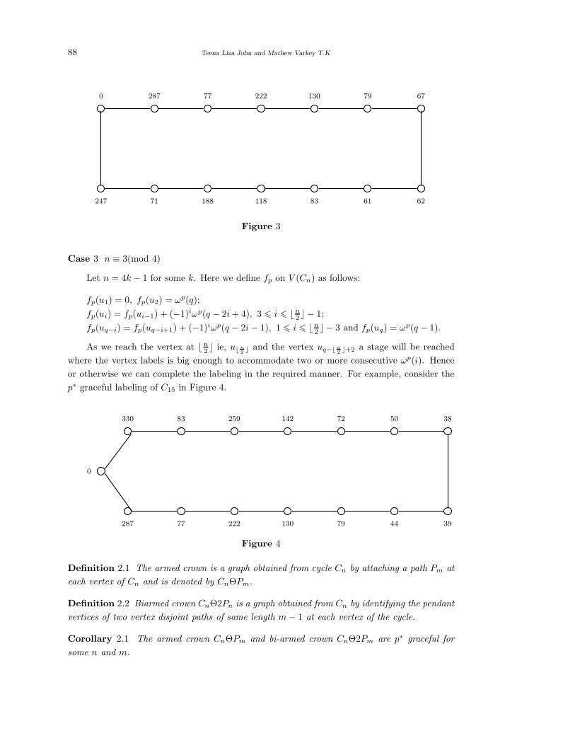
88 Teena Liza John and Mathew Varkey T.K
287 77 222 130 79 670
71 188 118 83 61 62247
Figure 3
Case 3 n ≡ 3(mod 4)
Let n = 4k − 1 for some k. Here we define fp on V (Cn) as follows:
fp(u1) = 0, fp(u2) = ωp(q);
fp(ui) = fp(ui−1) + (−1)iωp(q − 2i+ 4), 3 6 i 6 ⌊n2 ⌋ − 1;
fp(uq−i) = fp(uq−i+1) + (−1)iωp(q − 2i− 1), 1 6 i 6 ⌊n2 ⌋ − 3 and fp(uq) = ωp(q − 1).
As we reach the vertex at ⌊n2 ⌋ ie, u⌊n
2⌋ and the vertex uq−⌊n
2⌋+2 a stage will be reached
where the vertex labels is big enough to accommodate two or more consecutive ωp(i). Hence
or otherwise we can complete the labeling in the required manner. For example, consider the
p∗ graceful labeling of C15 in Figure 4.
83 259 142 72 50 38330
77 222 130 79 44 39287
0
Figure 4
Definition 2.1 The armed crown is a graph obtained from cycle Cn by attaching a path Pm at
each vertex of Cn and is denoted by CnΘPm.
Definition 2.2 Biarmed crown CnΘ2Pn is a graph obtained from Cn by identifying the pendant
vertices of two vertex disjoint paths of same length m− 1 at each vertex of the cycle.
Corollary 2.1 The armed crown CnΘPm and bi-armed crown CnΘ2Pm are p∗ graceful for
some n and m.
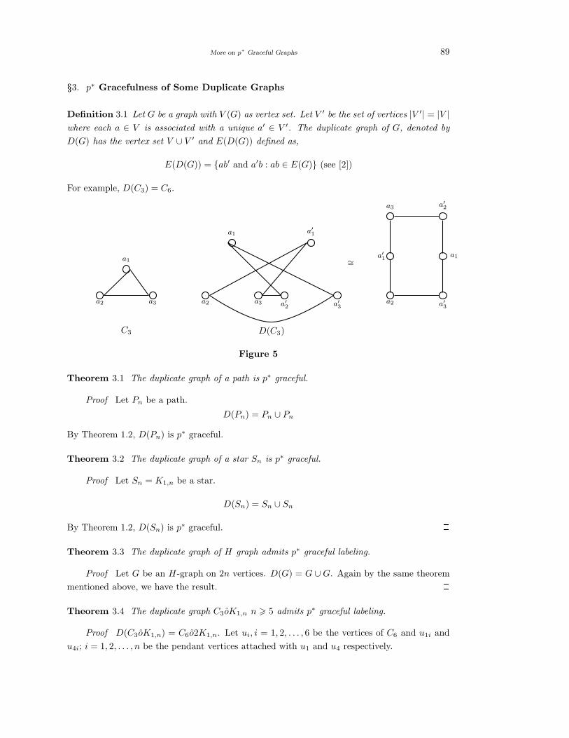
More on p∗ Graceful Graphs 89
§3. p∗ Gracefulness of Some Duplicate Graphs
Definition 3.1 Let G be a graph with V (G) as vertex set. Let V ′ be the set of vertices |V ′| = |V |where each a ∈ V is associated with a unique a′ ∈ V ′. The duplicate graph of G, denoted by
D(G) has the vertex set V ∪ V ′ and E(D(G)) defined as,
E(D(G)) = ab′ and a′b : ab ∈ E(G) (see [2])
For example, D(C3) = C6.
a′3a
′2
a3a2a3a2 a2 a′3
a1
C3 D(C3)
a1 a′1
a3 a′2
a′1
a1∼=
Figure 5
Theorem 3.1 The duplicate graph of a path is p∗ graceful.
Proof Let Pn be a path.
D(Pn) = Pn ∪ Pn
By Theorem 1.2, D(Pn) is p∗ graceful. 2Theorem 3.2 The duplicate graph of a star Sn is p∗ graceful.
Proof Let Sn = K1,n be a star.
D(Sn) = Sn ∪ Sn
By Theorem 1.2, D(Sn) is p∗ graceful. 2Theorem 3.3 The duplicate graph of H graph admits p∗ graceful labeling.
Proof Let G be an H-graph on 2n vertices. D(G) = G ∪ G. Again by the same theorem
mentioned above, we have the result. 2Theorem 3.4 The duplicate graph C3oK1,n n > 5 admits p∗ graceful labeling.
Proof D(C3oK1,n) = C6o2K1,n. Let ui, i = 1, 2, . . . , 6 be the vertices of C6 and u1i and
u4i; i = 1, 2, . . . , n be the pendant vertices attached with u1 and u4 respectively.
90 Teena Liza John and Mathew Varkey T.K
Consider the mapping fp on the vertices of G = C6o2K1,n as fp : V (G)→ 0, 1, . . . , ωp(q)such that
fp(u1) = 0, fp(u2) = ωp(6);
fp(u3) = 29, fp(u4) = 24, fp(u5) = 23, fp(u6) = 35;
fp(u1i) = ωp(6 + n+ i), i = 1, 2, . . . , n;
fp(u4i) = fp(u4) + ωp(7 + i− 1), i = 1, 2, · · · , n.
Obviously fp defined as above give rise to f∗p as required. Hence the result. 2
In general D(CmoK1,n) is p∗ graceful for some m.
Remark 3.1 D(C2n) = C2n ∪ C2n for all n is not p∗ graceful.
But D(C2n+1) = C2(2n+1) is p∗ graceful, if C2n+1 is so.
Conjecture All trees are p∗ graceful.
References
[1] F.Harary, Graph Theory, Addison-Wesley Publishing Company, 1969.
[2] Joseph A. Gallian, A dynamic survey of Graph Labeling, The Electronic Journal of Com-
binatorics, DS6 (2009), Ninth version.
[3] Mathew Varkey T.K, Some Graph Theoretic Operations Associated with Graph Labelings,
Ph.D Thesis (2000), University of Kerala, Kerala, India.
[4] Teena Liza John, Mathew Varkey T.K, p∗-graceful graphs, International J.Math.Combin.,
Vol.4, 2012, 97-102.
International J.Math. Combin. Vol.3(2013), 91-95
Symmetric Hamilton Cycle Decompositions of Complete Graphs
Plus a 1-Factor
Abolape D.Akwu
(Department of Mathematics, Federal University of Agriculture, Makurdi, Nigeria)
Deborah O.A.Ajayi
(Department of Mathematics, University of Ibadan, Ibadan, Nigeria)
E-mail: [email protected], [email protected]
Abstract: Let n ≥ 2 be an integer. The complete graph Kn with 1-factor I added has
a decomposition into Hamilton cycles if and only if n is even. We show that Kn + I has
a decomposition into Hamilton cycles which are symmetric with respect to the 1-factor I
added. We also show that the complete bipartite graph Kn,n plus a 1-factor has a symmetric
Hamilton decomposition, where n is odd.
Key Words: Complete graphs, complete bipartite graph, 1-factor, Hamilton cycle decom-
position.
AMS(2010):
§1. Introduction
By a decomposition of a nonempty graph G is meant a family of subgraphs G1, G2, · · · , Gk of G
such that their edge set form a partition of the edge set of G. Any member of the family is called
a part (of the decomposition). This decomposition is usually denoted by G = G1⊕G2⊕· · ·⊕Gk.
Let n ≥ 2 be an integer. The complete graph Kn has many Hamilton cycles and since
its vertices have degree n− 1, Kn has a decomposition into Hamilton cycles if and only if n is
odd. Suppose that n = 2m+ 1. The familiar Hamilton cycle decomposition of Kn referred to
as the Walecki decomposition in [1] is a symmetric decomposition in that each Hamilton cycle
H in the decomposition is symmetric in the following sense. Let the vertices of Kn be labeled
as 0, 1, 2, · · · ,m, 1, 2, · · · , m. Then each H is invariant under the involution i→ i, where ¯i = i;
the vertex 0 is a fixed point of this involution. A symmetric Hamilton cycle decomposition of
Kn different from Walecki’s is constructed in [1].
Let G be a graph, then G[2] is a graph whereby each vertex x is replaced by a pair of two
independent vertices x, x and each edge xy is replaced by four edges xy, xy, xy, xy.
Now suppose that n is even. Adding the edges of a 1-factor I to Kn results in a graph
1Received December 10, 2012, Accepted September 2, 2013.
92 Abolape D.Akwu and Deborah O.A.Ajayi
Kn + I each of whose vertices has even degree n. The graph Kn + I does have a decomposition
into Hamilton cycles (see [3]). The complete solution to the problem of decomposing Kn + I
into cycles of given uniform length is given in [3].
The degrees of vertices of the complete bipartite graph Kn,n equal n, and Kn,n has a
decomposition into Hamilton cycles if and only if n is even. If n is odd, adding a 1-factor I to
Kn,n results in a graph Kn,n + I with all vertices of even degree n+ 1 and Kn,n + I also has a
decomposition into Hamilton cycles.
Let n = 2m be an even integer with m ≥ 1. Consider the complete bipartite graph Kn,n
with vertex bipartition into sets 1, 2, · · · , n and 1, 2, · · · , n. By a symmetric Hamilton cycle
in Kn,n, we mean a Hamilton cycle such that ij is an edge if and only if ij is an edge. Thus a
Hamilton cycle in Kn,n is symmetric if and only if it is invariant under the involution i→ i.
A symmetric hamilton cycle decomposition of Kn,n is a partition of the edges of Kn,n
into m symmetric Hamilton cycles. Now let n = 2m + 1 be an odd integer with m ≥ 1, and
consider the 1-factor I = 1, n, 2, n− 1, · · · , n, 1 of Kn,n + I. A symmetric Hamilton
cycle decomposition of Kn,n + I is a partition of the edges of Kn,n + I into m + 1 symmetric
Hamilton cycles.
Let m > 1 be even, consider the vertex set of the complete graph K2m to be 1, 2, · · · ,m∪1, 2, · · · , m, where I = 11, 22, · · · ,mm is a 1-factor of K2m.
The edges of K2m + I are naturally partitioned into edges of Km on 1, 2, · · · ,m, the
edges of Km,m + I, and the edges of Km on 1, 2, · · · , m. We denote the complete graph on
1, 2, · · · , m by Km. We abuse terminology and write this edge partition as:
K2m + I = Km ∪ (Km,m + I) ∪ Km
By a symmetric Hamilton cycle of K2m + I we mean a Hamilton cycle such that
(1) ij is an edge in (Km) if and only if (ij) is an edge in Km and
(2) ij is an edge in (Km,m + I) if and only if ji is an edge in (Km,m + I).
Thus a Hamilton cycle of K2m + I is symmetric if and only if it is invariant under the fixed
point free involution φ of K2m + I, where φ(a) = a for all a in 1, 2, · · · ,m∪1, 2, · · · , m and
¯a = a. A symmetric Hamilton cycle decomposition of K2m + I is a decomposition of K2m + I
into m symmetric Hamilton cycles. Thus φ is a nontrivial automorphism of K2m + I, which
acts trivially on the cycles in a symmetric Hamilton cycle decomposition of K2m + I.
A double cover of K2m by Hamilton cycles is a collection C1, C2, · · · , C2m−1 of 2m − 1
Hamilton cycles such that each edge of K2m occurs as an edge of exactly two of these Hamilton
cycles. Note that the sum of the number edges in these Hamilton cycles equals
(2m− 1)2m = 2
2m
2
,
twice the number of edges of K2m, and this also equals half the number of edges of K4m − I.We use Kn + I to denote the multigraph obtained by adding the edges of a 1-factor I to
Kn, thus duplicatingn
2edges.
Symmetric Hamilton Cycle Decompositions of Complete Graphs Plus a 1-Factor 93
Let k be a positive integer and L ⊆ 1, 2, · · · , ⌊k2⌋. A circulant graph X = X(k;L) is a
graph with vertex set V (X) = u1, u2, · · · , uk and edge set E(X), where E(X) = uiui+l : i ∈Zk, l ∈ L −
k
2 ∪ uiui+k : i ∈ 1, 2, · · · , k
2 if
k
2∈ L, and E(X) = uiui+l : i ∈ Zk, l ∈ L
otherwise. An edge uiui+l, where l ∈ L is said to be of length l and L is called the edge length
set of the circulant X .
Notice that Kn is isomorphic to the circulant X(n; 1, 2, · · · , ⌊n2⌋). If n is even, Kn− I is
isomorphic to X(n; 1, 2, · · · , n2−1) and Kn +I is isomorphic to X(n; 1, 2, · · · , n
2−1,
n
2,n
2).
Let X = X(k;L) be a circulant graph with vertex set u1, u2, · · · , uk. By the rotation ρ
we mean the cyclic permutation u1, u2, · · · , uk.If P = x0x1 · · ·xp is a path,
←−P denotes the path xpxp−1 · · ·x1x0, the reverse of P .
§2. Proof of the Result
In order that Kn + I have a symmetric Hamilton cycle decomposition, it is necessary that n be
even.
Theorem 2.1 Let m ≥ 2 be an integer. There is a symmetric Hamilton cycle decomposition
of K2m + I.
Proof View the graph K2m + I as the circulant graph X(2m; 1, 2, · · · ,m−1,m,m) with
vertex set x1, x2, · · · , x2m. Let P be the zig-zag (m− 1) path
P = x1x+1x−1x+2x−2 · · ·xA
where A = 1− 2 + 3− · · ·+ (−1)m(m− 1). Thus P has edge length set Lp = 1, 2, · · · ,m− 1.It is easy to see that
C = P ∪ ρm(←−P )x1
is an 2m-cycle and ρi(C) : i = 0, 1, · · · ,m− 1 is a Hamilton cycle decomposition of K2m + I.
Next relabel the vertices of the graph K2m + I by defining a function f as follows: f :
xi → xi for 1 ≤ i ≤ m and f : xi → xi−m for m ≤ i ≤ 2m. Relabeling of the vertices of each
Hamilton cycle C2m with the new labels gives symmetric Hamilton cycle. Hence K2m + I can
be decomposed into symmetric Hamilton cycle. 2Lemma 2.2 Let m ≥ 2 be an integer, and let C be a symmetric Hamilton cycle of K2m + I.
Then
(1) If x is any vertex of K2m + I, the distance between x and x in C is odd;
(2) C is of the form x1, x2, · · · , xm, xm, xm−1, · · · , x2, x1x1 where
xi ∈ 1, 2, · · · ,m, 1, 2, · · · , m;(3) The number of edges xixi in each symmetric Hamilton cycle is 2, 1 ≤ i ≤ m.
Proof Let x be a vertex of K2m + I and let the distance between x and x in C be k. Then
there is a path x = x1, · · · , x k+1
2
, x k+1
2
, · · · , x2x1 = x in C. Since for each xi, i ∈ N we have
94 Abolape D.Akwu and Deborah O.A.Ajayi
k,k + 1
2∈ N . Suppose k is even, then
k + 1
2/∈ N .Therefore k is odd which proves (1).
Assertion (2) is now an immediate consequence. Since the cycle C is given as in (2), we
have edges x1x1 and xmxm which proves (3). 2Theorem 2.3 Let m be an even integer, then the graph Km + I[2] has a symmetric Hamilton
cycle decomposition.
Proof From the definition of the graph Km + I[2], each vertex x in Km + I is replaced by a
pair of two independent vertices x, x and each edge xy is replaced by four edges xy, xy, xy, xy.
Also note that if the graph H decomposes the graph G, then H [2] decomposes G[2].
By [3], cycle Cm decomposes Km + I, then we have
Km + I[2] = Cm[2]⊕ Cm[2]⊕ · · · ⊕ Cm[2]
Now label the vertices of each graph Cm[2] as xixi, where i = 1, 2, · · · ,m. By [2], each graph
Cm[2] decomposes into symmetric Hamilton cycle C2m. Therefore Km + I[2] decomposes into
symmetric Hamilton cycles. 2Theorem 2.4 Let m ≥ 4 be an even integer. From a symmetric Hamilton cycle decomposition
of Km + I[2] we can construct a double cover of Km + I by Hamilton cycles.
Proof By Theorem 2.3, a symmetric Hamilton cycle ofKm+I[2] is of the form x1, x2, · · · , xm,
xm, xm−1, · · · , x2, x1x1 where xi ∈ 1, 2, · · · ,m, 1, 2, · · · , m. Thus x1x2...xm is a path of length
m− 1 in Km + I[2] and xmxm−1 · · · x2x1 is its mirror image. Let
bi =
xi if xi ∈ 1, 2, · · · ,mxi if xi ∈ 1, 2, · · · , m
Then b1, b2, · · · , bm, b1 is a Hamilton cycle in Km + I, the projection of C on Km + I. Now
assume we have a symmetric Hamilton cycle decomposition of Km + I[2]. Then for each edge
xixj in Km + I, there are distinct symmetric Hamilton cycles C and C′ in our decomposition
such that xixj and xixj are edges of C and xixj and xixj are edges of C′. Hence from a
symmetric Hamilton cycle decomposition of Km + I[2], we get a double cover of Km + I from
the projections of each symmetric Hamilton cycle. 2Theorem 2.5 Let m ≥ 4 be even integer. Then K2m + I has a double cover by Hamilton
cycles.
Proof There is a Hamilton cycle C in K2m + I, and there exists disjoint 1-factor I1 and I2
whose union is the set of edges of C. The vertices of the graphs K2m + I1 and K2m − I2 have
degrees equal to the even number. The graphs K2m +I1 and K2m−I2 have decompositions into
Hamilton cycles C1, C2, · · · , Cm and D1, D2, · · · , Dm−1 respectively. Then C,C1, C2, · · · , Cm,
D1, D2, . · · · , Dm−1 is a double cover of K2m + I by Hamilton cycles . 2Theorem 2.6 For each integer m ≥ 1, there exist a symmetric Hamilton cycle decomposition
of K2m+1,2m+1 + I.
Symmetric Hamilton Cycle Decompositions of Complete Graphs Plus a 1-Factor 95
Proof Let n = 2m+ 1, we consider the complete bipartite graph Kn,n with vertex bipar-
tition 1, 2, 3, · · · , n and 1, 2, · · · , n. Let I be 1, n, 2, ¯n− 1, 3, ¯n− 2, · · · , n, 1 in
Kn,n + I.
Let the sum of edge ab be a+ b mod n. Let Sk be the set of edges whose sum is k. Let
i be an integer with 1 ≤ i ≤ m+ 1. Consider the union S2i−1 ∪ S2i, 2i is calculated modulo n.
observe that this collection of edges yields the following symmetric Hamilton cycle of Kn,n + I;
n, ¯2i− 1, 1, ¯2i− 2, 2, ¯2i− 3, 3, · · · , 2i, n
For each i, let Hi equal S2i−1 ∪ S2i. Then H1, H2, · · · , Hm+1 is a symmetric Hamilton cycle
decomposition of Kn,n + I. 2References
[1] J.Akiyama, M.Kobayashi, G.Nakamura, Symmetric Hamilton cycle decompositions of the
complete graph, J. Combin. Des., 12 (2004), 39-45.
[2] R.Laskar, Decomposition of some composite graphs into Hamiltonian cycles, in: Proc. 5th
Hungarian Coll. Keszthely, North Holland, 1978, 705-716.
[3] M.Sajna, Decomposition of the complete graph plus a 1-factor into cycles of equal length,
J. Combin. Des., 11 (2003), 170-207.
International J.Math. Combin. Vol.3(2013), 96-103
Ratio by Using Coefficients of Fibonacci Sequence
Megha Garg and Pertik Garg
(Punjab Technical University, Jalanahar, Punjab)
Ravinder Kumar
(Bhai Gurdas Group of Institution, Sangrur, Punjab)
E-mail: [email protected], [email protected], [email protected]
Abstract: In this paper, ratio by using coefficients of Fibonacci sequence has been discussed
in detail. The Fibonacci series is made from Fn+2 = Fn + Fn+1. New sequences from the
formula Fn+2 = aFn + bFn+1 by using a and b, where a and b are consecutive coefficients of
Fibonacci sequence are formed. These all new sequences have their own ratios. When find
the ratio of these ratios, it always becomes 1.6, which is known as golden ratio in Fibonacci
series.
Key Words: Fibonacci series, Fibonacci in nature, golden ratio, ratios of new sequences,
ratio of all new ratios.
AMS(2010): 05C78
§1. Introduction
The Fibonacci numbers were first discovered by a man named Leonardo Pisano. He was known
by his nickname, Fibonacci. The Fibonacci sequence is a sequence in which each term is the sum
of the 2 numbers preceding it. The first 10 Fibonacci numbers are: 1, 1, 2, 3, 5, 8, 13, 21, 34, 55
and 89. These numbers are obviously recursive. Leonardo Pisano Bogollo, (c.1170 - c.1250)
known as Leonardo of Pisa, Fibonacci was an Italian mathematician (Anderson, Frazier, &
Popendorf, 1999). He is considered as the most talented mathematician of the middle ages
(Eves, 1990). Fibonacci was first introduced to the number system we currently use with
symbols from 0 to 9 along with the Fibonacci sequence by Indian merchants when he was
in northern Africa (Anderson, Frazier, & Popendorf, 1999). He then introduced the Fibonacci
sequence and the number system we currently use to the western Europe In his book Liber Abaci
in 1202 (Singh, Acharya Hemachandra and the (so called) Fibonacci Numbers, 1986) (Singh,
The so-called Fibonacci numbers in ancient and medieval India, 1985). Fibonacci was died
around 1240 in Italy. He played an important role in reviving ancient mathematics and made
significant contributions of his own. Fibonacci numbers are important to perform a run-time
analysis of Euclid’s algorithm to Find the greatest common divisor (GCD) of two integers. A
pair of two consecutive Fibonacci numbers makes a worst case input for this algorithm (Knuth,
Art of Computer Programming, Volume 1: Fundamental Algorithms, 1997). Fibonacci numbers
1Received May 31, 2013, Accepted September 5, 2013.
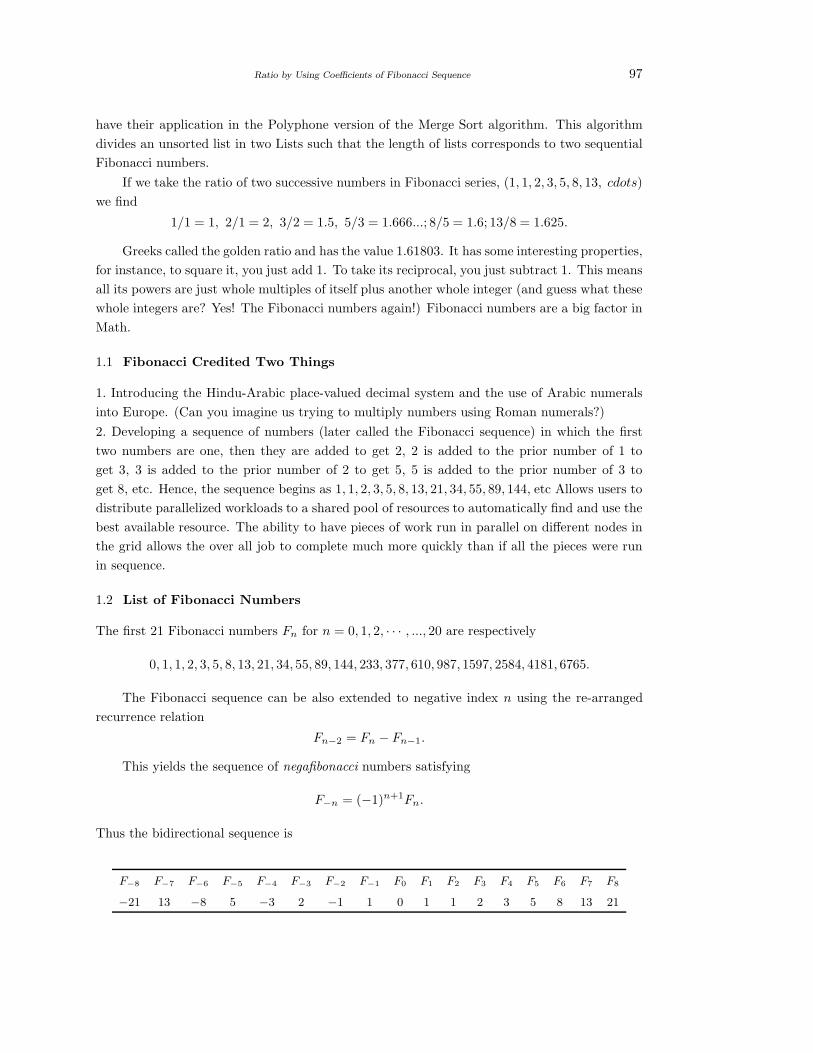
Ratio by Using Coefficients of Fibonacci Sequence 97
have their application in the Polyphone version of the Merge Sort algorithm. This algorithm
divides an unsorted list in two Lists such that the length of lists corresponds to two sequential
Fibonacci numbers.
If we take the ratio of two successive numbers in Fibonacci series, (1, 1, 2, 3, 5, 8, 13, cdots)
we find
1/1 = 1, 2/1 = 2, 3/2 = 1.5, 5/3 = 1.666...; 8/5 = 1.6; 13/8 = 1.625.
Greeks called the golden ratio and has the value 1.61803. It has some interesting properties,
for instance, to square it, you just add 1. To take its reciprocal, you just subtract 1. This means
all its powers are just whole multiples of itself plus another whole integer (and guess what these
whole integers are? Yes! The Fibonacci numbers again!) Fibonacci numbers are a big factor in
Math.
1.1 Fibonacci Credited Two Things
1. Introducing the Hindu-Arabic place-valued decimal system and the use of Arabic numerals
into Europe. (Can you imagine us trying to multiply numbers using Roman numerals?)
2. Developing a sequence of numbers (later called the Fibonacci sequence) in which the first
two numbers are one, then they are added to get 2, 2 is added to the prior number of 1 to
get 3, 3 is added to the prior number of 2 to get 5, 5 is added to the prior number of 3 to
get 8, etc. Hence, the sequence begins as 1, 1, 2, 3, 5, 8, 13, 21, 34, 55, 89, 144, etc Allows users to
distribute parallelized workloads to a shared pool of resources to automatically find and use the
best available resource. The ability to have pieces of work run in parallel on different nodes in
the grid allows the over all job to complete much more quickly than if all the pieces were run
in sequence.
1.2 List of Fibonacci Numbers
The first 21 Fibonacci numbers Fn for n = 0, 1, 2, · · · , ..., 20 are respectively
0, 1, 1, 2, 3, 5, 8, 13, 21, 34, 55, 89, 144, 233, 377, 610, 987, 1597, 2584, 4181, 6765.
The Fibonacci sequence can be also extended to negative index n using the re-arranged
recurrence relation
Fn−2 = Fn − Fn−1.
This yields the sequence of negafibonacci numbers satisfying
F−n = (−1)n+1Fn.
Thus the bidirectional sequence is
F−8 F−7 F−6 F−5 F−4 F−3 F−2 F−1 F0 F1 F2 F3 F4 F5 F6 F7 F8
−21 13 −8 5 −3 2 −1 1 0 1 1 2 3 5 8 13 21
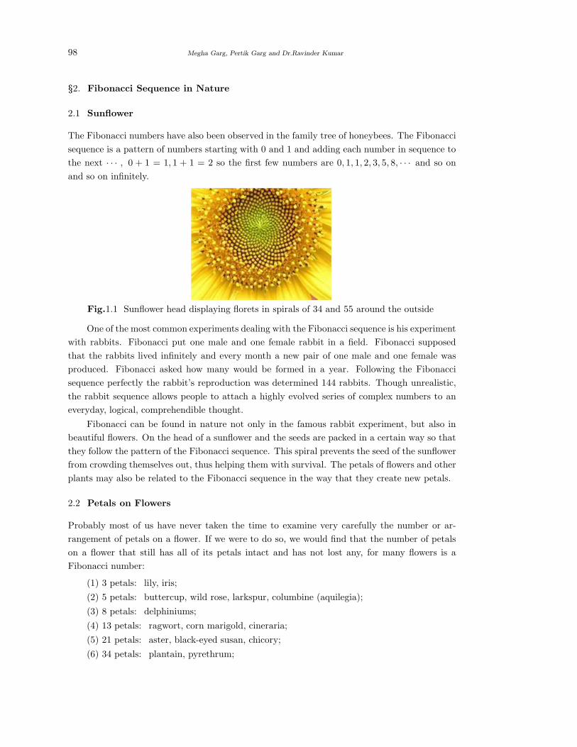
98 Megha Garg, Pertik Garg and Dr.Ravinder Kumar
§2. Fibonacci Sequence in Nature
2.1 Sunflower
The Fibonacci numbers have also been observed in the family tree of honeybees. The Fibonacci
sequence is a pattern of numbers starting with 0 and 1 and adding each number in sequence to
the next · · · , 0 + 1 = 1, 1 + 1 = 2 so the first few numbers are 0, 1, 1, 2, 3, 5, 8, · · · and so on
and so on infinitely.
Fig.1.1 Sunflower head displaying florets in spirals of 34 and 55 around the outside
One of the most common experiments dealing with the Fibonacci sequence is his experiment
with rabbits. Fibonacci put one male and one female rabbit in a field. Fibonacci supposed
that the rabbits lived infinitely and every month a new pair of one male and one female was
produced. Fibonacci asked how many would be formed in a year. Following the Fibonacci
sequence perfectly the rabbit’s reproduction was determined 144 rabbits. Though unrealistic,
the rabbit sequence allows people to attach a highly evolved series of complex numbers to an
everyday, logical, comprehendible thought.
Fibonacci can be found in nature not only in the famous rabbit experiment, but also in
beautiful flowers. On the head of a sunflower and the seeds are packed in a certain way so that
they follow the pattern of the Fibonacci sequence. This spiral prevents the seed of the sunflower
from crowding themselves out, thus helping them with survival. The petals of flowers and other
plants may also be related to the Fibonacci sequence in the way that they create new petals.
2.2 Petals on Flowers
Probably most of us have never taken the time to examine very carefully the number or ar-
rangement of petals on a flower. If we were to do so, we would find that the number of petals
on a flower that still has all of its petals intact and has not lost any, for many flowers is a
Fibonacci number:
(1) 3 petals: lily, iris;
(2) 5 petals: buttercup, wild rose, larkspur, columbine (aquilegia);
(3) 8 petals: delphiniums;
(4) 13 petals: ragwort, corn marigold, cineraria;
(5) 21 petals: aster, black-eyed susan, chicory;
(6) 34 petals: plantain, pyrethrum;
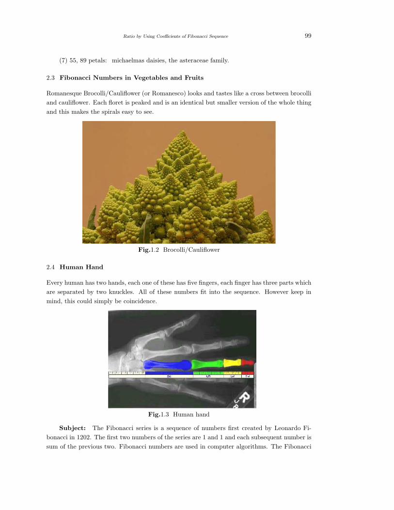
Ratio by Using Coefficients of Fibonacci Sequence 99
(7) 55, 89 petals: michaelmas daisies, the asteraceae family.
2.3 Fibonacci Numbers in Vegetables and Fruits
Romanesque Brocolli/Cauliflower (or Romanesco) looks and tastes like a cross between brocolli
and cauliflower. Each floret is peaked and is an identical but smaller version of the whole thing
and this makes the spirals easy to see.
Fig.1.2 Brocolli/Cauliflower
2.4 Human Hand
Every human has two hands, each one of these has five fingers, each finger has three parts which
are separated by two knuckles. All of these numbers fit into the sequence. However keep in
mind, this could simply be coincidence.
Fig.1.3 Human hand
Subject: The Fibonacci series is a sequence of numbers first created by Leonardo Fi-
bonacci in 1202. The first two numbers of the series are 1 and 1 and each subsequent number is
sum of the previous two. Fibonacci numbers are used in computer algorithms. The Fibonacci
100 Megha Garg, Pertik Garg and Dr.Ravinder Kumar
sequence first appears in the book Liber Abaci by Leonardo of Pisa known as Fibonacci. Fi-
bonacci considers the growth of an idealized rabbit population, assuming that a newly born
pair of rabbits, one male, one female and do the study on it. The Fibonacci series become
1, 1, 2, 3, 5, 8, 13, 21 · · · .
§3. Ratio by Using Coefficients of Fibonacci Sequence
3.1 Ratio By Using 1, 2 as Coefficients
Apply the formula by using the next two coefficients of Fibonacci series i.e. 1 for Fn+1 and 2
for Fn. So the series that becomes from this formula is Fn+2 = 2Fn + Fn+1, F1 = 1, F2 = 1,
F3 = 3, 5, 11, 21, 43, 85, 171, 341, 683, 1365, · · · . K
From this sequence, find the ratio by dividing two consecutive numbers.
F2
F1=
1
1= 1
F3
F2=
3
1= 3
F4
F3=
5
3= 1.66
F5
F4=
11
5= 2.2
F6
F5=
21
11= 1.9
F7
F6=
43
21= 2.0
F8
F7=
85
43= 1.9
F9
F8=
171
85= 2.0
From here the conclusion is that the ratio (in integer) of this series is 2.
3.2 Ratio by Using 2, 3 as Coefficients
The series that becomes by using 2, 3 as coefficients is Fn+2 = 3Fn + 2Fn+1, i.e., F1 = 1, F2 =
1, F3 = 5, 13, 41, 121, 365, 1093, 3281, 9841, · · · .From this sequence, find the ratio by dividing two consecutive numbers.
F2
F1=
1
1= 1
F3
F2=
5
1= 5
F4
F3=
13
5= 2.6
F5
F4=
41
13= 3.15
Ratio by Using Coefficients of Fibonacci Sequence 101
F6
F5=
121
41= 3.15
F7
F6=
365
121= 3.01
F8
F7=
1093
365= 2.99
F9
F8=
3281
1093= 3.01
From here the conclusion is that the ratio (in integer) of this series is 3.
3.3 Ratio by Using 3, 5 as Coefficients
The series that becomes by using 3, 5 as coefficients is Fn+2 = 5Fn + 3Fn+1, i.e., F1 = 1, F2 =
1, F3 = 8, 29, 127, 526, 2213, 9269, 38872, 162961, · · · .From this sequence, find the ratio by dividing two consecutive numbers.
F2
F1=
1
1= 1
F3
F2=
8
1= 8
F4
F3=
29
8= 3.6
F5
F4=
127
29= 4.3
F6
F5=
526
127= 4.14
F7
F6=
2213
526= 4.20
F8
F7=
9269
2213= 4.18
F9
F8=
38872
9269= 4.19
From here the conclusion is that the ratio (in integer) of this series is 4.
3.4 Ratio by Using 5, 8 as Coefficients
The series that becomes by using 5, 8 as coefficients is Fn+2 = 8Fn + 5Fn+1, i.e., F1 = 1, F2 =
1, F3 = 13, 73, 469, 2929, 18397, 115417, 724229, · · · .From this sequence , find the ratio by dividing two consecutive numbers.
F2
F1=
1
1= 1
F3
F2=
13
1= 13
F4
F3=
73
13= 5.6
102 Megha Garg, Pertik Garg and Dr.Ravinder Kumar
F5
F4=
469
73= 6.4
F6
F5=
2929
469= 6.24
F7
F6=
18397
2929= 6.28
F8
F7=
115417
18397= 6.27
F9
F8=
724229
115417= 6.27
From here the conclusion is that the ratio (in integer) of this series is 6.
Continuing in this way, find that the ratio of
Fn+2 = 13Fn + 8Fn+1 is 9 (in integer);
Fn+2 = 21Fn + 13Fn+1 is 14 (in integer);
Fn+2 = 34Fn + 21Fn+1 is 22 (in integer);
· · · · · · · · · · · · · · · · · ·
§4. Conclusion
Therefore the sequence becomes from all the ratios by using the consecutive numbers as the
coefficients of Fibonacci sequence is:
2, 3, 4, 6, 9, 14, 22, 35, 56, 90, 145, 234, 378, · · ·
Now find the ratio that on dividing consecutive integers, of this sequence is:
3/2 = 1.5, 4/3 = 1.33, 6/4 = 1.5, 14/9 = 1.6, 22/14 = 1.6, 35/22 = 1.6
and 56/35 = 1.6, 90/1.6, 145/90 = 1.6, 234/145 = 1.6 · · ·
It always become 1.6, yes it is again the golden ratio of Fibonacci sequence. So the conclusion
is that the ratio of these ratios is always become golden ratio in Fibonacci series.
References
[1] Huylebrouck Dirk, Gyllenberg Mats and Sigmund Karl (2000), The Fibonacci Chimney,
The Mathematical Intelligencer
http://www.mathsisfun.com/numbers/fibonaccisequence.html
http://www.maths.surrey.ac.uk/hostedsites/ R.Knott/Fibonacci/fib.html
http://www.maths.surrey.ac.uk/hostedsites/ R.Knott/Fibonacci/fibmaths.html
[2] The Engineer, Eden Project Gets Into Flower Power,
http://www.theengineer.co.uk/news/eden-project-gets-into-flower-power
[3] Di Carlo, Christopher (2001), Interview with Maynard James Keenan.
[4] Ingmar Lehman, Fibonacci-numbers in visual arts and literature,
http://en.wikipedia.org/wiki/Fibonacci numbers in popular culture
Ratio by Using Coefficients of Fibonacci Sequence 103
[5] Munjal Patel (2010), Fibonacci Number,
http://munjal.munpat.com/papers/fibonacci-numbers.pdf
[6] Dan Kalman and Robert Mena (2003), The Fibonacci Numbers-Exposed,
http://www.math.hmc.edu/ benjamin/papers/exposed.pdf

I want to bring out the secrets of nature and apply them for the happiness of
man. I don’t know of any better service to offer for the short time we are in the
world.
By Thomas Edison, an American inventor.
Author Information
Submission: Papers only in electronic form are considered for possible publication. Papers
prepared in formats, viz., .tex, .dvi, .pdf, or.ps may be submitted electronically to one member
of the Editorial Board for consideration in the International Journal of Mathematical
Combinatorics (ISSN 1937-1055). An effort is made to publish a paper duly recommended
by a referee within a period of 3 months. Articles received are immediately put the refer-
ees/members of the Editorial Board for their opinion who generally pass on the same in six
week’s time or less. In case of clear recommendation for publication, the paper is accommo-
dated in an issue to appear next. Each submitted paper is not returned, hence we advise the
authors to keep a copy of their submitted papers for further processing.
Abstract: Authors are requested to provide an abstract of not more than 250 words, lat-
est Mathematics Subject Classification of the American Mathematical Society, Keywords and
phrases. Statements of Lemmas, Propositions and Theorems should be set in italics and ref-
erences should be arranged in alphabetical order by the surname of the first author in the
following style:
Books
[4]Linfan Mao, Combinatorial Geometry with Applications to Field Theory, InfoQuest Press,
2009.
[12]W.S.Massey, Algebraic topology: an introduction, Springer-Verlag, New York 1977.
Research papers
[6]Linfan Mao, Combinatorial speculation and combinatorial conjecture for mathematics, In-
ternational J.Math. Combin., Vol.1, 1-19(2007).
[9]Kavita Srivastava, On singular H-closed extensions, Proc. Amer. Math. Soc. (to appear).
Figures: Figures should be drawn by TEXCAD in text directly, or as EPS file. In addition,
all figures and tables should be numbered and the appropriate space reserved in the text, with
the insertion point clearly indicated.
Copyright: It is assumed that the submitted manuscript has not been published and will not
be simultaneously submitted or published elsewhere. By submitting a manuscript, the authors
agree that the copyright for their articles is transferred to the publisher, if and when, the
paper is accepted for publication. The publisher cannot take the responsibility of any loss of
manuscript. Therefore, authors are requested to maintain a copy at their end.
Proofs: One set of galley proofs of a paper will be sent to the author submitting the paper,
unless requested otherwise, without the original manuscript, for corrections after the paper is
accepted for publication on the basis of the recommendation of referees. Corrections should be
restricted to typesetting errors. Authors are advised to check their proofs very carefully before
return.
September 2013
Contents
Modular Equations for Ramanujans Cubic Continued Fraction
And its Evaluations BY B.R.SRIVATSA KUMAR AND G.N.RAJAPPA. . . . . . . . . 01
Semi-Symeetric Metric Connection on a 3-Dimensional Trans-Sasakian
Manifold BY K.HALDER, D.DEBNATH AND A.BHATTACHARYYA . . . . . . . . . 16
On Mean Graphs BY R.VASUKI AND S.AROCKIARAJ . . . . . . . . . . . . . . . . . . . . . . . 22
Special Kinds of Colorable Complements in Graphs
BY B.CHALUVAPAJU, C.NANDEESHUKUMAR AND V.CHAITRA. . . . . . . . . . . . . . . 35
Vertex Graceful Labeling-Some Path Related Graphs
BY P.SELVARAJU, P.BALAGAMESAN AND J.RENUKA . . . . . . . . . . . . . . . . . . . . . . . . . . 44
Total Semirelib Graph
BY MANJUNATH PRASAD K B AND VENKANAGOUDA M GOUDAR . . . . . . . . . . 50
On Some Characterization of Ruled Surface of a Closed Spacelike
Curve with Spacelike Binormal in Dual Lorentzian Space
BY OZCAN BEKTAS AND SULEYMAN SENYURT . . . . . . . . . . . . . . . . . . . . . . . . . . . . . . . 56
Some Prime Labeling Results of H-Class Graphs BY L.M.SUNDARAM,
A.NAGARAJAN, S.NAVANEETHAKRISHNAN AND A.N.MURUGAN . . . . . . . . . . . . . 69
On Mean Cordial Graphs BY R.PONRAJ AND M.SIVAKUMAR . . . . . . . . . . . . 78
More on p∗ Graceful Graphs BY TEENA L.J. AND MATHEW V.T.K . . . . . . . .85
Symmetric Hamilton Cycle Decompositions of Complete Graphs
Plus a 1-Factor BY ABOLAPE D.AKWU AND DEBORAH O.A.AJAYI . . . . . . . . 91
Ratio by Using Coefficients of Fibonacci Sequence
BY MEGHA GARG, PERTIK GARG AND RAVINDER KUMAR . . . . . . . . . . . . . . . . 96
An International Journal on Mathematical Combinatorics